Nicholas J. Higham
University of Manchester
Manchester, England
Accuracy and Stability
of Numerical Algorithms
Second Edition
slam.
Society for Industrial and Applied Mathematics
Philadelphia

Copyright © 2002 by the Society for Industrial and Applied Mathematics.
1098765432 I
All rights reserved. Printed in the United States of America. No part of this book
may be reproduced, stored, or transmitted in any manner without the
written permission of the publisher. For information, write to the Society for
Industrial and Applied Mathematics, 3600 University City Science Center,
Philadelphia, PA 19104-2688.
Library of Congress Cataloging-in-Publication Data
Higham, Nicholas J., 1961-
Accuracy and stability of numerical algorithms / Nicholas J. Higham.—
2nd ed.
p. cm.
Includes bibliographical references.
ISBN 0-89871-521-0
I. Numerical analysis—Data processing.2. Computer algorithms. I.
Title.
QA297 .H53 2002
SI^^OISS'SI—dc2l
2002075848
is a registered trademark.

Dedicated to
Alan M. Turing
and
James H. Wilkinson

Contents
List of Figures xvii
List of Tables xix
Preface to Second Edition xxi
Preface to First Edition xxv
About the Dedication xxix
1 Principles of Finite Precision Computation 1
1.1 Notation and Background 2
1.2 Relative Error and Significant Digits 3
1.3 Sources of Errors 5
1.4 Precision Versus Accuracy 6
1.5 Backward and Forward Errors 6
1.6 Conditioning 8
1.7 Cancellation 9
1.8 Solving a Quadratic Equation 10
1.9 Computing the Sample Variance 11
1.10 Solving Linear Equations 12
1.10.1 GEPP Versus Cramer's Rule 13
1.11 Accumulation of Rounding Errors 14
1.12 Instability Without Cancellation 14
1.12.1 The Need for Pivoting 15
1.12.2 An Innocuous Calculation? 15
1.12.3 An Infinite Sum 16
1.13 Increasing the Precision 17
1.14 Cancellation of Rounding Errors 19
1.14.1 Computing (ex - l)/x 19
1.14.2 QR Factorization 21
1.15 Rounding Errors Can Be Beneficial 22
1.16 Stability of an Algorithm Depends on the Problem 24
1.17 Rounding Errors Are Not Random 25
1.18 Designing Stable Algorithms 26
1.19 Misconceptions 28
1.20 Rounding Errors in Numerical Analysis 28
1.21 Notes and References 28
Problems 31
vn

Vlll
Contents
2 Floating Point Arithmetic 35
2.1 Floating Point Number System 36
2.2 Model of Arithmetic 40
2.3 IEEE Arithmetic 41
2.4 Aberrant Arithmetics 43
2.5 Exact Subtraction 45
2.6 Fused Multiply-Add Operation 46
2.7 Choice of Base and Distribution of Numbers 47
2.8 Statistical Distribution of Rounding Errors 48
2.9 Alternative Number Systems 49
2.10 Elementary Functions 50
2.11 Accuracy Tests 51
2.12 Notes and References 52
Problems 57
3 Basics 61
3.1 Inner and Outer Products 62
3.2 The Purpose of Rounding Error Analysis 65
3.3 Running Error Analysis 65
3.4 Notation for Error Analysis 67
3.5 Matrix Multiplication 69
3.6 Complex Arithmetic 71
3.7 Miscellany 73
3.8 Error Analysis Demystified 74
3.9 Other Approaches 76
3.10 Notes and References 76
Problems 77
4 Summation 79
4.1 Summation Methods 80
4.2 Error Analysis 81
4.3 Compensated Summation 83
4.4 Other Summation Methods 88
4.5 Statistical Estimates of Accuracy 88
4.6 Choice of Method 89
4.7 Notes and References 90
Problems 91
5 Polynomials 93
5.1 Horner's Method 94
5.2 Evaluating Derivatives 96
5.3 The Newton Form and Polynomial Interpolation 99
5.4 Matrix Polynomials 102
5.5 Notes and References 102
Problems 104

Contents ix
6 Norms 105
6.1 Vector Norms 106
6.2 Matrix Norms 107
6.3 The Matrix p-Norm 112
6.4 Singular Value Decomposition 114
6.5 Notes and References 114
Problems 115
7 Perturbation Theory for Linear Systems 119
7.1 Normwise Analysis 120
7.2 Componentwise Analysis 122
7.3 Scaling to Minimize the Condition Number 125
7.4 The Matrix Inverse 127
7.5 Extensions 128
7.6 Numerical Stability 129
7.7 Practical Error Bounds 130
7.8 Perturbation Theory by Calculus 132
7.9 Notes and References 132
Problems 134
8 Triangular Systems 139
8.1 Backward Error Analysis 140
8.2 Forward Error Analysis 142
8.3 Bounds for the Inverse 147
8.4 A Parallel Fan-In Algorithm 149
8.5 Notes and References 151
8.5.1 LAPACK 153
Problems 153
9 LU Factorization and Linear Equations 157
9.1 Gaussian Elimination and Pivoting Strategies 158
9.2 LU Factorization 160
9.3 Error Analysis 163
9.4 The Growth Factor 166
9.5 Diagonally Dominant and Banded Matrices 170
9.6 Tridiagonal Matrices 174
9.7 More Error Bounds 176
9.8 Scaling and Choice of Pivoting Strategy 177
9.9 Variants of Gaussian Elimination 179
9.10 A Posteriori Stability Tests 180
9.11 Sensitivity of the LU Factorization 181
9.12 Rank-Revealing LU Factorizations 182
9.13 Historical Perspective 183
9.14 Notes and References 187
9.14.1 LAPACK 191
Problems 192

x Contents
10 Cholesky Factorization 195
10.1 Symmetric Positive Definite Matrices 196
10.1.1 Error Analysis 197
10.2 Sensitivity of the Cholesky Factorization 201
10.3 Positive Semidefinite Matrices 201
10.3.1 Perturbation Theory 203
10.3.2 Error Analysis 205
10.4 Matrices with Positive Definite Symmetric Part 208
10.5 Notes and References 209
10.5.1 LAPACK 210
Problems 211
11 Symmetric Indefinite and Skew-Symmetric Systems 213
11.1 Block LDLT Factorization for Symmetric Matrices 214
11.1.1 Complete Pivoting 215
11.1.2 Partial Pivoting 216
11.1.3 Rook Pivoting 219
11.1.4 Tridiagonal Matrices 221
11.2 Aasen's Method 222
11.2.1 Aasen's Method Versus Block LDLT Factorization 224
11.3 Block LDLT Factorization for Skew-Symmetric Matrices 225
11.4 Notes and References 226
11.4.1 LAPACK 228
Problems 228
12 Iterative Refinement 231
12.1 Behaviour of the Forward Error 232
12.2 Iterative Refinement Implies Stability 235
12.3 Notes and References 240
12.3.1 LAPACK 242
Problems 242
13 Block LU Factorization 245
13.1 Block Versus Partitioned LU Factorization 246
13.2 Error Analysis of Partitioned LU Factorization 249
13.3 Error Analysis of Block LU Factorization 250
13.3.1 Block Diagonal Dominance 251
13.3.2 Symmetric Positive Definite Matrices 255
13.4 Notes and References 256
13.4.1 LAPACK 257
Problems 257
14 Matrix Inversion 259
14.1 Use and Abuse of the Matrix Inverse 260
14.2 Inverting a Triangular Matrix 262
14.2.1 Unblocked Methods 262
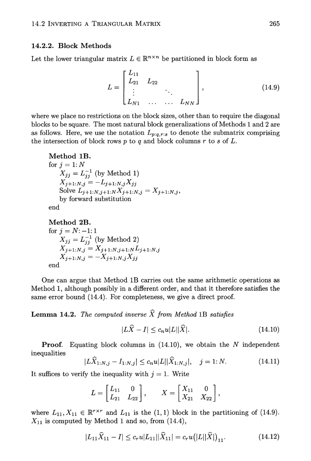
14.2.2 Block Methods 265
14.3 Inverting a Full Matrix by LU Factorization 267

Contents
XI
14.3.1 Method A 267
14.3.2 Method B 268
14.3.3 Method C 269
14.3.4 Method D 270
14.3.5 Summary 271
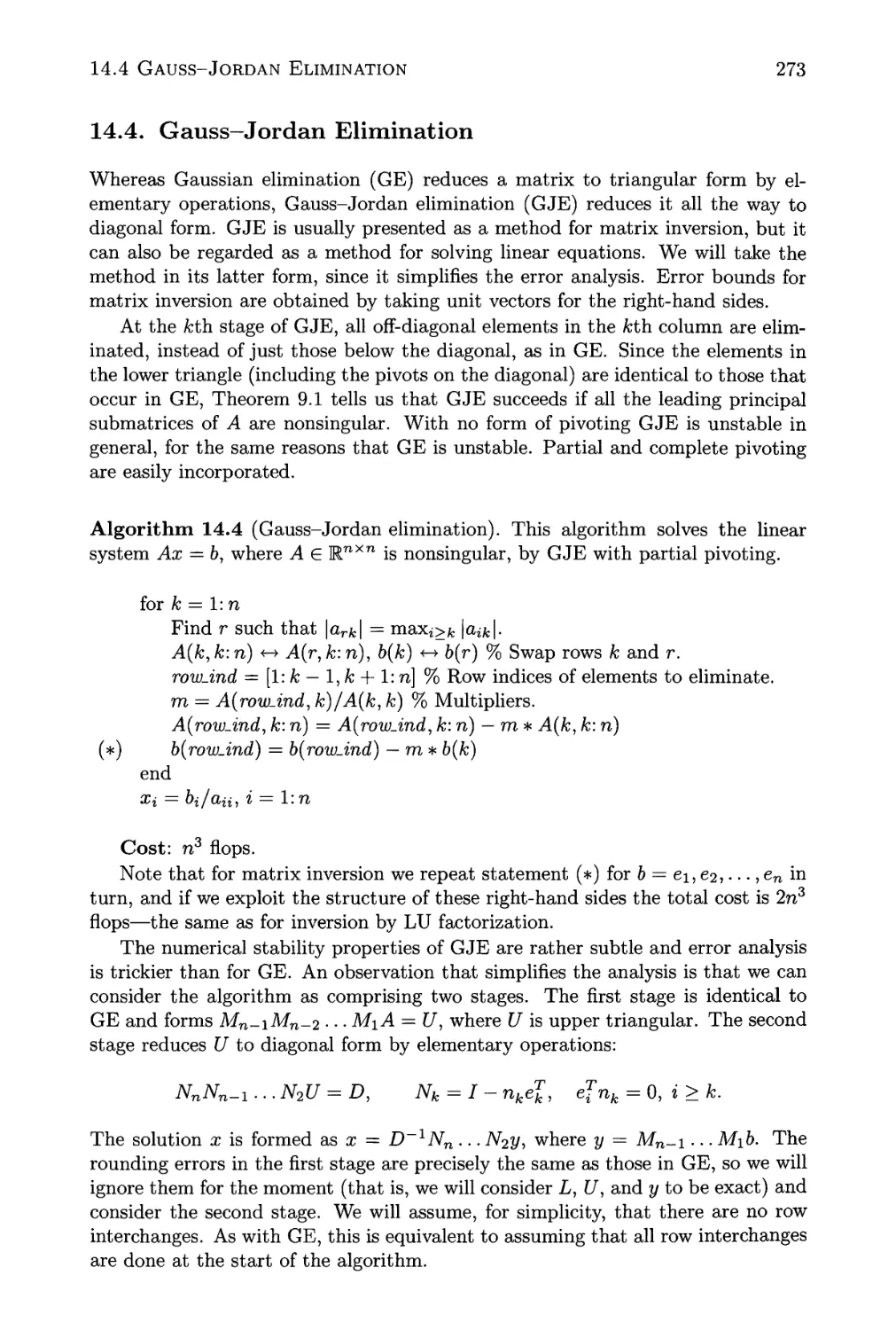
14.4 Gauss-Jordan Elimination 273
14.5 Parallel Inversion Methods 278
14.6 The Determinant 279
14.6.1 Hyman's Method 280
14.7 Notes and References 281
14.7.1 LAPACK 282
Problems 283
15 Condition Number Estimation 287
15.1 How to Estimate Componentwise Condition Numbers 288
15.2 The p-Norm Power Method 289
15.3 LAPACK 1-Norm Estimator 292
15.4 Block 1-Norm Estimator 294
15.5 Other Condition Estimators 295
15.6 Condition Numbers of Tridiagonal Matrices 299
15.7 Notes and References 301
15.7.1 LAPACK 303
Problems 303
16 The Sylvester Equation 305
16.1 Solving the Sylvester Equation 307
16.2 Backward Error 308
16.2.1 The Lyapunov Equation 311
16.3 Perturbation Result 313
16.4 Practical Error Bounds 315
16.5 Extensions 316
16.6 Notes and References 317
16.6.1 LAPACK 318
Problems 318
17 Stationary Iterative Methods 321
17.1 Survey of Error Analysis 323
17.2 Forward Error Analysis 325
17.2.1 Jacobi's Method 328
17.2.2 Successive Overrelaxation 329
17.3 Backward Error Analysis 330
17.4 Singular Systems 331
17.4.1 Theoretical Background 331
17.4.2 Forward Error Analysis 333
17.5 Stopping an Iterative Method 335
17.6 Notes and References 337
Problems 337

xii Contents
18 Matrix Powers 339
18.1 Matrix Powers in Exact Arithmetic 340
18.2 Bounds for Finite Precision Arithmetic 346
18.3 Application to Stationary Iteration 351
18.4 Notes and References 351
Problems 352
19 QR Factorization 353
19.1 Householder Transformations 354
19.2 QR Factorization 355
19.3 Error Analysis of Householder Computations 357
19.4 Pivoting and Row-Wise Stability 362
19.5 Aggregated Householder Transformations 363
19.6 Givens Rotations 365
19.7 Iterative Refinement 368
19.8 Gram-Schmidt Orthogonalization 369
19.9 Sensitivity of the QR Factorization 373
19.10 Notes and References 374
19.10.1 LAPACK 377
Problems 378
20 The Least Squares Problem 381
20.1 Perturbation Theory 382
20.2 Solution by QR Factorization 384
20.3 Solution by the Modified Gram-Schmidt Method 386
20.4 The Normal Equations 386
20.5 Iterative Refinement 388
20.6 The Seminormal Equations 391
20.7 Backward Error 392
20.8 Weighted Least Squares Problems 395
20.9 The Equality Constrained Least Squares Problem 396
20.9.1 Perturbation Theory 396
20.9.2 Methods 397
20.10 Proof of Wedin's Theorem 400
20.11 Notes and References 402
20.11.1 LAPACK 405
Problems 405
21 Under deter mined Systems 407
21.1 Solution Methods 408
21.2 Perturbation Theory and Backward Error 409
21.3 Error Analysis 411
21.4 Notes and References 413
21.4.1 LAPACK 414
Problems 414

Contents xiii
22 Vandermonde Systems 415
22.1 Matrix Inversion 416
22.2 Primal and Dual Systems 418
22.3 Stability 423
22.3.1 Forward Error 424
22.3.2 Residual 425
22.3.3 Dealing with Instability 426
22.4 Notes and References 428
Problems 430
23 Fast Matrix Multiplication 433
23.1 Methods 434
23.2 Error Analysis 438
23.2.1 Winograd's Method 439
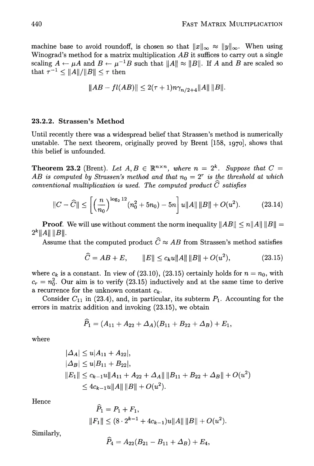
23.2.2 Strassen's Method 440
23.2.3 Bilinear Noncommutative Algorithms 443
23.2.4 The 3M Method 444
23.3 Notes and References 446
Problems 448
24 The Fast Fourier Transform and Applications 451
24.1 The Fast Fourier Transform 452
24.2 Circulant Linear Systems 454
24.3 Notes and References 456
Problems 457
25 Nonlinear Systems and Newton's Method 459
25.1 Newton's Method 460
25.2 Error Analysis 461
25.3 Special Cases and Experiments 462
25.4 Conditioning 464
25.5 Stopping an Iterative Method 467
25.6 Notes and References 468
Problems 469
26 Automatic Error Analysis 471
26.1 Exploiting Direct Search Optimization 472
26.2 Direct Search Methods 474
26.3 Examples of Direct Search 477
26.3.1 Condition Estimation 477
26.3.2 Fast Matrix Inversion 478
26.3.3 Roots of a Cubic 479
26.4 Interval Analysis 481
26.5 Other Work 484
26.6 Notes and References 486
Problems 487

xiv Contents
27 Software Issues in Floating Point Arithmetic 489
27.1 Exploiting IEEE Arithmetic 490
27.2 Subtleties of Floating Point Arithmetic 493
27.3 Cray Peculiarities 493
27.4 Compilers 494
27.5 Determining Properties of Floating Point Arithmetic 494
27.6 Testing a Floating Point Arithmetic 495
27.7 Portability 496
27.7.1 Arithmetic Parameters 496
27.7.2 2x2 Problems in LAPACK 497
27.7.3 Numerical Constants 498
27.7.4 Models of Floating Point Arithmetic 498
27.8 Avoiding Underflow and Overflow 499
27.9 Multiple Precision Arithmetic 501
27.10 Extended and Mixed Precision BLAS 503
27.11 Patriot Missile Software Problem 503
27.12 Notes and References 504
Problems 505
28 A Gallery of Test Matrices 511
28.1 The Hilbert and Cauchy Matrices 512
28.2 Random Matrices 515
28.3 "Randsvd" Matrices 517
28.4 The Pascal Matrix 518
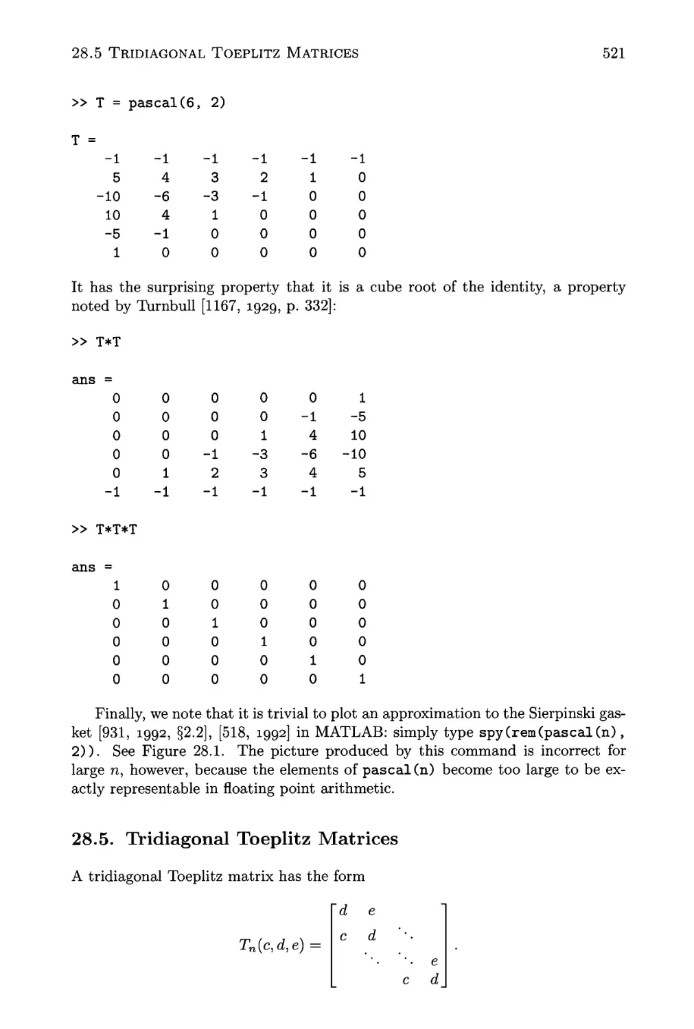
28.5 Tridiagonal Toeplitz Matrices 521
28.6 Companion Matrices 522
28.7 Notes and References 523
28.7.1 LAPACK 525
Problems 525
A Solutions to Problems 527
B Acquiring Software 573
B.l Internet 574
B.2 Netlib 574
B.3 MATLAB 575
B.4 NAG Library and NAGWare F95 Compiler 575
C Program Libraries 577
C.l Basic Linear Algebra Subprograms 578
C.2 EISPACK 579
C.3 LINPACK 579
C.4 LAPACK 579
C.4.1 Structure of LAPACK 580
D The Matrix Computation Toolbox 583
Bibliography 587

Contents xv
Name Index 657
Subject Index 667

List of Figures
1.1 Backward and forward errors for y = f(x) 7
1.2 Mixed forward-backward error for y = f(x) 8
1.3 Forward errors \\x — x||oo/IM|oo and relative residuals ||b — Ax\\oo/
(||^4||oo||^||oo) versus precision 18
1.4 Absolute error versus precision, t = — log2u, in evaluating A.8). . 19
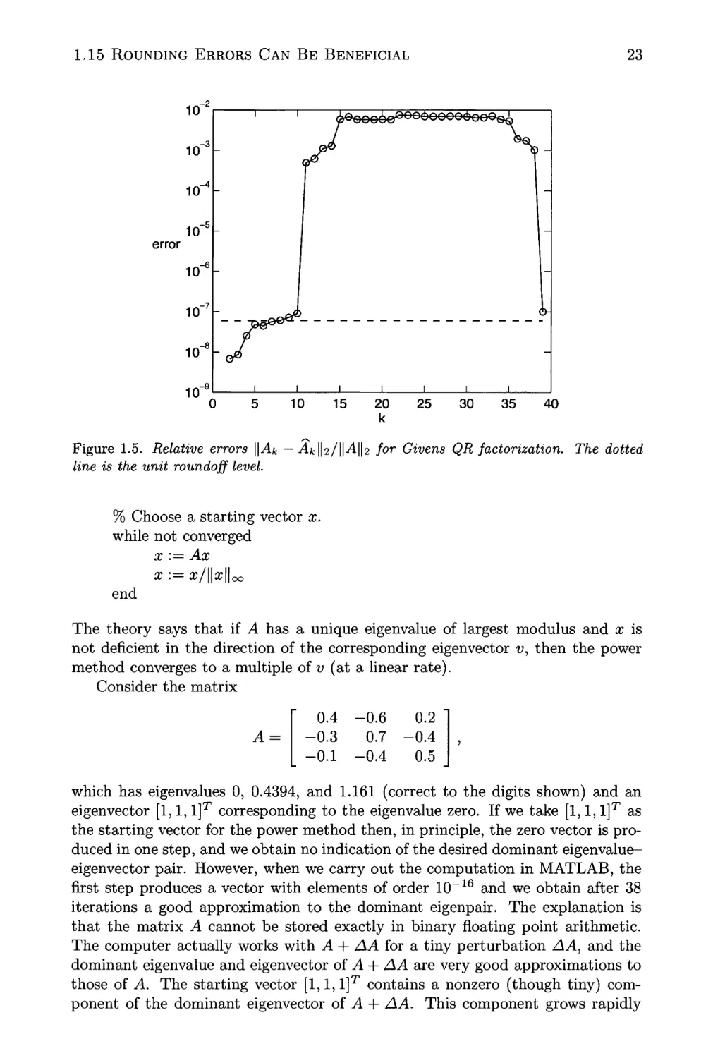
1.5 Relative errors \\Ak — ^fclta/Mlh for Givens QR factorization. . . 23
1.6 Values of rational function r(x) computed by Horner's rule 26
2.1 Relative distance from x to the next larger machine number (/? = 2,
t = 24), displaying wobbling precision 40
4.1 Recovering the rounding error 84
4.2 Errors \y(l) —yn\ for Euler's method with and without compensated
summation 87
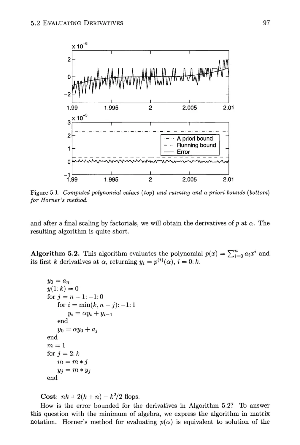
5.1 Computed polynomial values and running and a priori bounds for
Horner's method 97
6.1 Plots of p versus ||j4||p, for 1 < p < 15 113
9.1 Illustration of rook pivoting 159
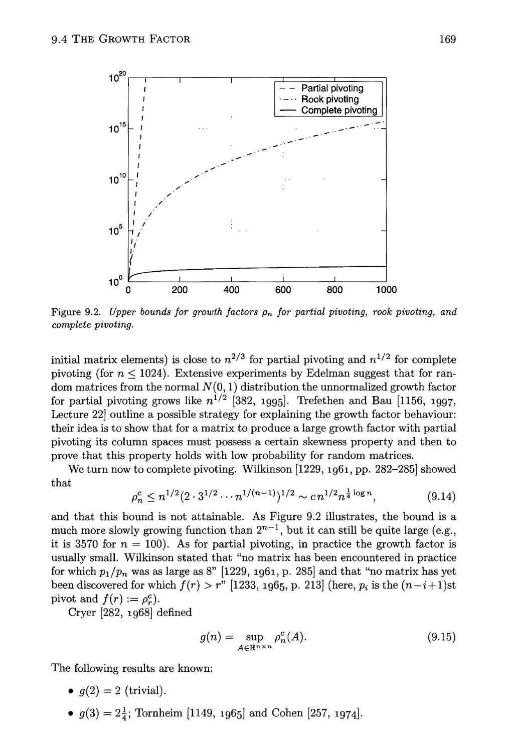
9.2 Upper bounds for growth factors pn for partial pivoting, rook
pivoting, and complete pivoting 169
9.3 Maximum growth factors and average number of comparisons for
15000 random matrices of dimension n = 100:100:1500 171
9.4 A banded matrix 173
14.1 Residuals for inverses computed by MATLAB's inv function. . . . 262
15.1 Underestimation ratio for Algorithm 15.4 for 5 x 5 matrix A@). . . 295
17.1 Forward and backward errors for SOR iteration 323
18.1 A typical hump for a convergent, nonnormal matrix 341
18.2 Diverging powers of a nilpotent matrix, Cu 341
18.3 Infinity norms of powers of 2 x 2 matrix J in A8.2) 343
18.4 Computed powers of chebspec matrices 349
18.5 Pseudospectra for chebspec matrices 350
18.6 Pseudospectrum for SOR iteration matrix 351
xvii

xviii List of Figures
19.1 Householder matrix P times vector x 355
19.2 Givens rotation, y = G(i,j,0)x 365
23.1 Exponent versus time for matrix multiplication 437
23.2 Errors for Strassen's method with two random matrices of
dimension n = 1024 444
24.1 Error in FFT followed by inverse FFT 454
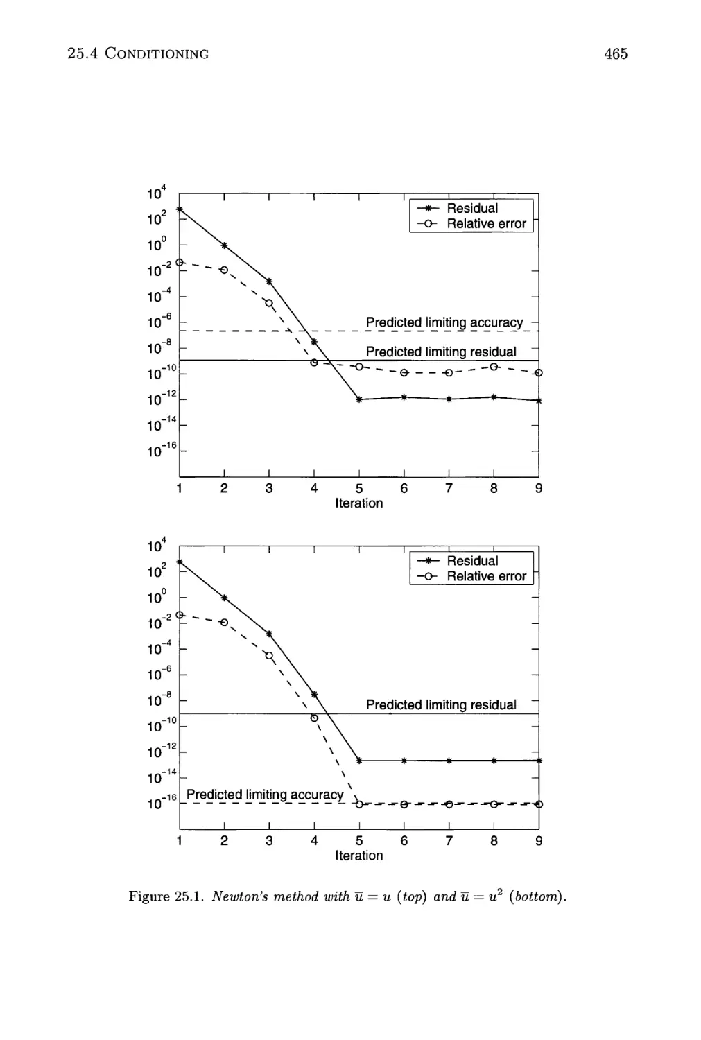
25.1 Newton's method with u = u and u = u2 465
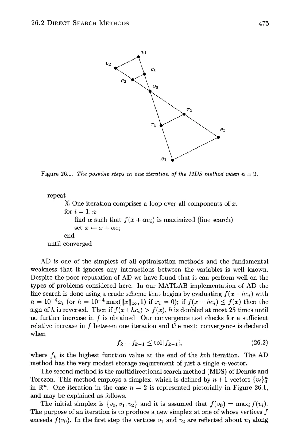
26.1 The possible steps in one iteration of the MDS method when n = 2. 475
27.1 Rational function r 491
27.2 Error in evaluating rational function r 492
28.1 spy (rem (pascal C2), 2)) 522
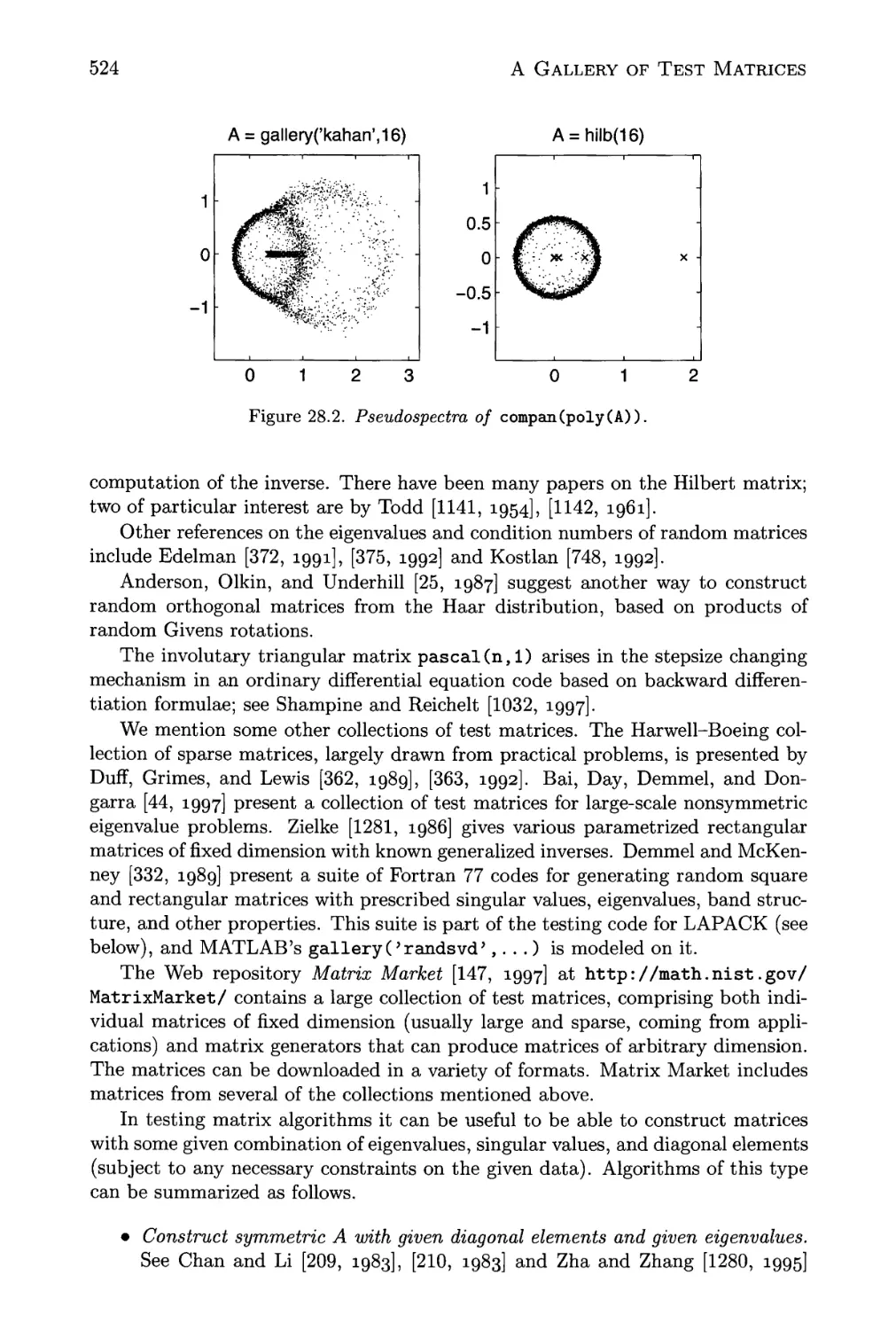
28.2 Pseudospectra of compan(poly(A)) 524
28.3 Pseudospectra of 32 x 32 pentadiagonal Toeplitz matrices 526
A.l log(l + x) evaluated using MATLAB's log and using the formula
(A.l) 529

List of Tables
1.1 Computed approximations fn = fl((l + l/n)n) to e = 2.71828.... 15
1.2 Computed values of (ex — l)/x from Algorithms 1 and 2 21
1.3 Results from GE without pivoting on an upper Hessenberg matrix. 25
2.1 Floating point arithmetic parameters 37
2.2 IEEE arithmetic exceptions and default results 42
2.3 Test arithmetics 51
2.4 Sine test 52
2.5 Exponentation test 52
4.1 Mean square errors for nonnegative X{ 89
6.1 Constants apq such that \\x\\p < <xpq\\x\\q, x G Cn 109
6.2 Constants apq such that ||A\\p < apq\\A\\q, Ae Cmxn 109
7.1 Four classes of perturbations and the corresponding condition
numbers 125
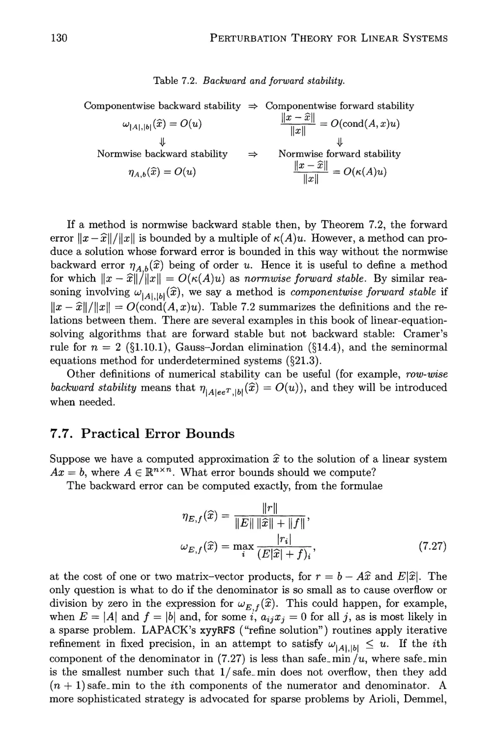
7.2 Backward and forward stability. 130
9.1 Classes of matrices for which pn = 0A) for GE without pivoting. . 166
9.2 Times for solution of a linear system of order n 185
9.3 Records for largest dense linear systems solved 191
12.1 lj,a, |6, values for A = gallery('orthog' ,25) 239
12.2
^1^1,161 values for A = gallery ('clement* ,50) 240
12.3 ^\A\\b\ values for A = gfppE0) 240
13.1 Stability of block and point LU factorization 256
14.1 Backward errors r}A h(x) for the oo-norm 260
14.2 Mflop rates for inverting a triangular matrix on a Cray 2 267
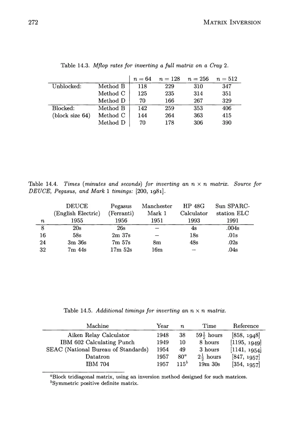
14.3 Mflop rates for inverting a full matrix on a Cray 2 272
14.4 Times (minutes and seconds) for inverting annxn matrix 272
14.5 Additional timings for inverting annxn matrix 272
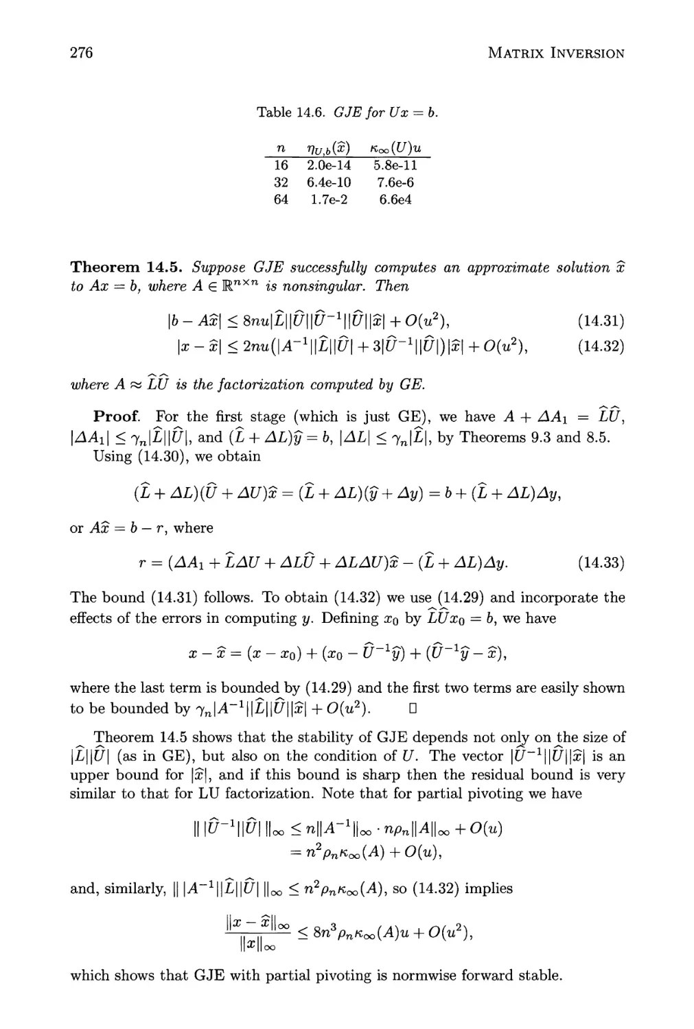
14.6 GJE for Ux = b 276
17.1 Dates of publication of selected iterative methods 322
17.2 Results for Jacobi method, a = 1/2 - S~j 328
17.3 Results for Jacobi method, a =-A/2 - 8-J') 329
xix

XX
List of Tables
19.1 Backward errors for QR factorization with no pivoting, row sorting,
and column pivoting on matrix A9.16) 363
20.1 LS backward errors and residual for Vandermonde system 394
21.1 Backward errors for underdetermined Vandermonde system 413
22.1 Bounds and estimates for K(Vn) 418
22.2 Parameters in the three-term recurrence B2.6) 422
22.3 Results for dual Chebyshev-Vandermonde-like system 427
27.1 Results from Cholesky factorization 493
27.2 Effect of extended run time on Patriot missile operation 504
28.1 MATLAB functions for generating matrices discussed in this book. 513
28.2 Condition numbers of Hilbert and Pascal matrices 514

Preface to Second Edition
We dare not lengthen this book much more,
lest it be out of moderation and should
stir up men's apathy because of its size.
— AELFRIC, schoolteacher of Cerne Abbas,
later Abbot of Eynsham (c. 995-1020)
In the nearly seven years since I finished writing the first edition of this book
research on the accuracy and stability of numerical algorithms has continued to
flourish and mature. Our understanding of algorithms has steadily improved, and
in some areas new or improved algorithms have been derived.
Three developments during this period deserve particular note. First, the
widespread adoption of electronic publication of journals and the increased
practice of posting technical reports and preprints on the Web have both made research
results more quickly available than before. Second, the inclusion of routines from
state-of-the-art numerical software libraries such as LAPACK in packages such as
MATLAB* and Maple"*" has brought the highest-quality algorithms to a very wide
audience. Third, IEEE arithmetic is now ubiquitous—indeed, it is hard to find a
computer whose arithmetic does not comply with the standard.
This new edition is a major revision of the book that brings it fully up to
date, expands the coverage, and includes numerous improvements to the original
material. The changes reflect my own experiences in using the book, as well as
suggestions received from readers.
The changes to the book can be summarized as follows.
New Chapters
• Symmetric Indefinite and Skew-Symmetric Systems (Chapter 11). A greatly
expanded treatment is given of symmetric indefinite systems (previously
contained in the chapter Cholesky Factorization) and a new section treats skew-
symmetric systems.
• Nonlinear Systems and Newton's Method (Chapter 25). Results on the
limiting accuracy and limiting residual of Newton's method are given under
general assumptions that permit the use of extended precision in calculating
residuals. The conditioning of nonlinear systems, and termination criteria
for iterative methods, are also investigated.
* MATLAB is a registered trademark of The MathWorks, Inc.
t Maple is a registered trademark of Waterloo Maple Software.
xxi

XX11
Preface to Second Edition
New Sections
• Fused Multiply-Add Operation (§2.6). The advantages of this operation,
which is included in the Intel IA-64 architecture, are discussed, along with
some subtle issues that it raises.
• Elementary Functions (§2.10). We explain why it is difficult to compute
elementary functions in a way that satisfies all the natural requirements,
and give pointers to relevant work.
• Matrix Polynomials (§5.4). How to evaluate three different matrix
generalizations of a scalar polynomial is discussed.
• More Error Bounds (§9.7). Some additional backward and forward error
bounds for Gaussian elimination (GE) without pivoting are given, leading
to the new result that GE is row-wise backward stable for row diagonally
dominant matrices.
• Variants of Gaussian Elimination (§9.9). Some lesser-known variants of GE
with partial pivoting are described.
• Rank-Revealing LU Factorizations (§9.12). This section explains why LU
factorization with an appropriate pivoting strategy leads to a factorization
that is usually rank revealing.
• Parallel Inversion Methods (§14.5). Several methods for matrix inversion on
parallel machines are described, including the Schulz iteration, which is of
wider interest.
• Block 1-Norm Estimator (§15.4). An improved version of the LAPACK
condition estimator, implemented in MATLAB's condest function, is outlined.
• Pivoting and Row-Wise Stability (§19.4). The behaviour of Householder QR
factorization for matrices whose rows are poorly scaled is examined. The
backward error result herein is the only one I know that requires a particular
choice of sign when constructing Householder matrices.
• Weighted Least Squares Problems (§20.8). Building on §19.4, an overall
rowwise backward error result is given for solution of the least squares problem
by Householder QR factorization with column pivoting.
• The Equality Constrained Least Squares Problem (§20.9). This section treats
the least squares problem subject to linear equality constraints. It gives a
perturbation result and describes three classes of methods (the method of
weighting, null space methods, and elimination methods) and their numerical
stability.
• Extended and Mixed Precision BLAS (§27.10). A brief description is given
of these important new aids to carrying out extended precision computations
in a portable way.

xxm
Other Changes
In the error analysis of QR factorization in the first edition of the book, backward
error bounds were given in normwise form and in a componentwise form that
essentially provided columnwise bounds. I now give just columnwise bounds, as
they are the natural result of the analysis and trivially imply both normwise and
componentwise bounds. The basic lemma on construction of the Householder
vector has been modified so that most of the ensuing results apply for either
choice of sign in constructing the vector. These and other results are expressed
using the error constant 7n, which replaces the more clumsy notation 7cn used in
the first edition (see §3.4).
Rook pivoting is a pivoting strategy that is applicable to both GE for general
matrices and block LDLT factorization for symmetric indefinite matrices, and it
is of pedagogical interest because it is intermediate between partial pivoting and
complete pivoting in both cost and stability. Rook pivoting is described in detail
and its merits for practical computation are explained. A thorough discussion is
given of the choice of pivoting strategy for GE and of the effects on the method of
scaling. Some new error bounds are included, as well as several other results that
help to provide a comprehensive picture of current understanding of GE.
This new edition has a more thorough treatment of block LDLT
factorization for symmetric indefinite matrices, including recent error analysis, rook
pivoting, and Bunch's pivoting strategy for tridiagonal matrices. Aasen's method and
Bunch's block LDLT factorization method for skew-symmetric matrices are also
treated.
Strengthened error analysis includes results for Gauss-Jordan elimination
(Theorem 14.5, Corollary 14.7), fast solution of Vandermonde systems (Corollary 22.7),
the fast Fourier transform (FFT) (Theorem 24.2), and solution of circulant linear
systems via the FFT (Theorem 24.3).
All the numerical experiments have been redone in the latest version, 6.1, of
MATLAB. The figures have been regenerated and their design improved, where
possible. Discussions of LAPACK reflect the current release, 3.0.
A major effort has gone into updating the bibliography, with the aim of
referring to the most recent results and ensuring that the latest editions of books
are referenced and papers are cited in their final published form. Over 190 works
published since the first edition are cited. See page 587 for a histogram that shows
the distribution of dates of publication of the works cited.
In revising the book I took the opportunity to rewrite and rearrange material,
improve the index, and fine tune the typesetting (in particular, using ideas of
Knuth [745, 1999, Chap. 33]). Several research problems from the first edition have
been solved and are now incorporated into the text, and new research problems
and general problems have been added.
In small ways the emphasis of the book has been changed. For example, when
the first edition was written IEEE arithmetic was not so prevalent, so a number of
results were stated with the proviso that a guard digit was present. Now it is
implicitly assumed throughout that the arithmetic is "well behaved" and unfortunate
consequences of lack of a guard digit are given less prominence.
A final change concerns the associated MATLAB toolbox. The Test Matrix
Toolbox from the first edition is superseded by the new Matrix Computation Tool-

XXIV
Preface to Second Edition
box, described in Appendix D. The new toolbox includes functions implementing
a number of algorithms in the book—in particular, GE with rook pivoting and
block LDLT factorization for symmetric and skew-symmetric matrices. The
toolbox should be of use for both teaching and research.
I am grateful to Bill Gragg, Beresford Parlett, Colin Percival, Siegfried Rump,
Francoise Tisseur, Nick Trefethen, and Tjalling Ypma for comments that
influenced the second edition.
It has been a pleasure working once again with the SIAM publication staff, in
particular Linda Thiel, Sara Triller Murphy, Marianne Will, and my copy editor,
Beth Gallagher.
Research leading to this book has been supported by grants from the
Engineering and Physical Sciences Research Council and by a Royal Society Leverhulme
Trust Senior Research Fellowship.
The tools used to prepare the book were the same as for the first edition, except
that for I^jX-related tasks I used Mikl^gX (http://www.miktex.org/), including
its excellent YAP previewer.
Manchester
February 2002
Nicholas J. Higham

Preface to First Edition
It has been 30 years since the publication of Wilkinson's books Rounding Errors
in Algebraic Processes [1232, 1963] and The Algebraic Eigenvalue Problem [1233,
1965]. These books provided the first thorough analysis of the effects of rounding
errors on numerical algorithms, and they rapidly became highly influential classics
in numerical analysis. Although a number of more recent books have included
analysis of rounding errors, none has treated the subject in the same depth as
Wilkinson.
This book gives a thorough, up-to-date treatment of the behaviour of
numerical algorithms in finite precision arithmetic. It combines algorithmic derivations,
perturbation theory, and rounding error analysis. Software practicalities are
emphasized throughout, with particular reference to LAPACK. The best available
error bounds, some of them new, are presented in a unified format with a minimum
of jargon. Historical perspective is given to provide insight into the development of
the subject, and further information is provided in the many quotations.
Perturbation theory is treated in detail, because of its central role in revealing problem
sensitivity and providing error bounds. The book is unique in that algorithmic
derivations and motivation are given succinctly, and implementation details
minimized, so that attention can be concentrated on accuracy and stability results.
The book was designed to be a comprehensive reference and contains extensive
citations to the research literature.
Although the book's main audience is specialists in numerical analysis, it will
be of use to all computational scientists and engineers who are concerned about
the accuracy of their results. Much of the book can be understood with only a
basic grounding in numerical analysis and linear algebra.
This first two chapters are very general. Chapter 1 describes fundamental
concepts of finite precision arithmetic, giving many examples for illustration and
dispelling some misconceptions. Chapter 2 gives a thorough treatment of floating
point arithmetic and may well be the single most useful chapter in the book. In
addition to describing models of floating point arithmetic and the IEEE standard,
it explains how to exploit "low-level" features not represented in the models and
contains a large set of informative exercises.
In the rest of the book the focus is, inevitably, on numerical linear algebra,
because it is in this area that rounding errors are most influential and have been
most extensively studied. However, I found that it was impossible to cover the
whole of numerical linear algebra in a single volume. The main omission is the area
of eigenvalue and singular value computations, which is still the subject of intensive
research and requires a book of its own to summarize algorithms, perturbation
theory, and error analysis. This book is therefore certainly not a replacement
xxv

XXVI
Preface to First Edition
for The Algebraic Eigenvalue Problem.
Two reasons why rounding error analysis can be hard to understand are that,
first, there is no standard notation and, second, error analyses are often cluttered
with re-derivations of standard results. In this book I have used notation that I
find nearly always to be the most convenient for error analysis: the key ingredient
is the symbol 7n = nu/(l — nu), explained in §3.1. I have also summarized many
basic error analysis results (for example, in Chapters 3 and 8) and made use of
them throughout the book. I like to think of these basic results as analogues of the
Fortran BLAS (Basic Linear Algebra Subprograms): once available in a standard
form they can be used as black boxes and need not be reinvented.
A number of the topics included here have not been treated in depth in
previous numerical analysis textbooks. These include floating point summation, block
LU factorization, condition number estimation, the Sylvester equation, powers of
matrices, finite precision behaviour of stationary iterative methods, Vandermonde
systems, and fast matrix multiplication, each of which has its own chapter. But
there are also some notable omissions. I would have liked to include a chapter on
Toeplitz systems, but this is an area in which stability and accuracy are
incompletely understood and where knowledge of the underlying applications is required
to guide the investigation. The important problems of updating and downdating
matrix factorizations when the matrix undergoes a "small" change have also been
omitted due to lack of time and space. A further omission is analysis of
parallel algorithms for all the problems considered in the book (though blocked and
partitioned algorithms and one particular parallel method for triangular systems
are treated). Again, there are relatively few results and this is an area of active
research.
Throughout the history of numerical linear algebra, theoretical advances have
gone hand in hand with software development. This tradition has continued with
LAPACK A987-), a project to develop a state-of-the-art Fortran package for
solving linear equations and eigenvalue problems. LAPACK has enjoyed a synergy with
research that has led to a number of important breakthroughs in the design and
analysis of algorithms, from the standpoints of both performance and accuracy.
A key feature of this book is that it provides the material needed to understand
the numerical properties of many of the algorithms in LAPACK, the exceptions
being the routines for eigenvalue and singular value problems. In particular, the
error bounds computed by the LAPACK linear equation solvers are explained, the
LAPACK condition estimator is described in detail, and some of the software
issues confronted by the LAPACK developers are highlighted. Chapter 27 examines
the influence of floating point arithmetic on general numerical software, offering
salutary stories, useful techniques, and brief descriptions of relevant codes.
This book has been written with numerical analysis courses in mind, although
it is not designed specifically as a textbook. It would be a suitable reference for
an advanced course (for example, for a graduate course on numerical linear
algebra following the syllabus recommended by the ILAS Education Committee [661,
1993]), and could be used by instructors at all levels as a supplementary text from
which to draw examples, historical perspective, statements of results, and
exercises. The exercises (actually labelled "problems") are an important part of the
book, and many of them have not, to my knowledge, appeared in textbooks before.

xxvu
Where appropriate I have indicated the source of an exercise; a name without a
citation means that the exercise came from private communication or unpublished
notes. Research problems given at the end of some sets of exercises emphasize
that most of the areas covered are still active.
In addition to surveying and unifying existing results (including some that have
not appeared in the mainstream literature) and sometimes improving upon their
presentation or proof, this book contains new results. Some of particular note are
as follows.
1. The error analysis in §5.3 for evaluation of the Newton interpolating
polynomial.
2. The forward error analysis for iterative refinement in §12.1.
3. The error analysis of Gauss-Jordan elimination in §14.4.
4. The unified componentwise error analysis of QR factorization methods in
Chapter 19, and the corresponding analysis of their use for solving the least
squares problem in Chapter 20.
5. Theorem 21.4, which shows the backward stability of the QR factorization
method for computing the minimum 2-norm solution to an underdetermined
system.
The Notes and References are an integral part of each chapter. In addition
to containing references, historical information, and further details, they include
material not covered elsewhere in the chapter, and should always be consulted, in
conjunction with the index, to obtain the complete picture.
I have included relatively few numerical examples except in the first chapter.
There are two reasons. One is to reduce the length of the book. The second reason
is because today it so easy for the reader to perform experiments in MATLAB or
some other interactive system. To this end I have made available the Test Matrix
Toolbox, which contains MATLAB M-files for many of the algorithms and special
matrices described in the book; see Appendix D.
This book has been designed to be as easy to use as possible. There are
thorough name and subject indexes, page headings show chapter and section titles
and numbers, and there is extensive cross-referencing. I have adopted the unusual
policy of giving with (nearly) every citation not only its numerical location in the
bibliography but also the names of the authors and the year of publication. This
provides as much information as possible in a citation and reduces the need for
the reader to turn to the bibliography.
A BibTJhJX database acc-stab-num-alg.bib containing all the references in
the bibliography is available over the Internet from the bibnet project (which can
be accessed via netlib, described in §B.2).
Special care has been taken to minimize the number of typographical and other
errors, but no doubt some remain. I will be happy to receive notification of errors,
as well as comments and suggestions for improvement.

XXV111
Preface to First Edition
Acknowledgements
Three books, in addition to Wilkinson's, have strongly influenced my research in
numerical linear algebra and have provided inspiration for this book: Golub and
Van Loan's Matrix Computations [509, 1996] (first edition 1983), Parlett's The
Symmetric Eigenvalue Problem [926, 1998] (first published 1980) and Stewart's
Introduction to Matrix Computations [1065, 1973]. Knuth's The Art of Computer
Programming books A973-) [743], [744], have also influenced my style and
presentation.
Jim Demmel has contributed greatly to my understanding of the subject of
this book and provided valuable technical help and suggestions. The first two
chapters owe much to the work of Velvel Kahan; I am grateful to him for giving
me access to unpublished notes and for suggesting improvements to early versions
of Chapters 2 and 27. Des Higham read various drafts of the book, offering sound
advice and finding improvements that had eluded me.
Other people who have given valuable help, suggestions, or advice are
Zhaojun Bai, Brad Baxter, Ake Bjorck, Martin Campbell-Kelly, Shiv-
kumar Chandrasekaran, Alan Edelman, Warren Ferguson, Philip Gill,
Gene Golub, George Hall, Sven Hammarling, Andrzej Kielbasinski,
Philip Knight, Beresford Parlett, David Silvester, Michael Saunders,
Ian Smith, Doron Swade, Nick Trefethen, Jack Williams, and Hongyuan
Zha.
David Carlisle provided invaluable help and advice concerning WF$$L 2s.
Working with SIAM on the publication of this book was a pleasure. Special
thanks go to Nancy Abbott (design), Susan Ciambrano (acquisition), Ed Cilurso
(production), Beth Gallagher (copy editing), Corey Gray (production), Mary Rose
Muccie (copy editing and indexing), Colleen Robishaw (design), and Sam Young
(production).
Research leading to this book has been supported by grants from the
Engineering and Physical Sciences Research Council, by a Nuffield Science Research
Fellowship from the Nuffield Foundation, and by a NATO Collaborative Research
Grant held with J. W. Demmel. I was fortunate to be able to make extensive use
of the libraries of the University of Manchester, the University of Dundee, Stanford
University, and the University of California, Berkeley.
This book was typeset in WI^i2e using the book document style. The
references were prepared in BibI^X and the index with Makelndex. It is difficult to
imagine how I could have written the book without these wonderful tools. I used
the "big" software from the emT^K distribution, running on a 486DX workstation.
I used text editors The Semware Editor (Semware Corporation) and GNU Emacs
(Free Software Foundation) and checked spelling with PC-Write (Quicksoft).
Manchester
April 1995
Nicholas J. Higham

About the Dedication
This book is dedicated to the memory of two remarkable English mathematicians,
James Hardy Wilkinson A919-1986), FRS, and Alan Mathison Turing A912-
1954), FRS, both of whom made immense contributions to scientific computation.
Turing's achievements include his paper "On Computable Numbers, with an
Application to the Entscheidungsproblem", which answered Hilbert's decidability
question using the abstract device now known as a Turing machine [1164, 1936];
his work at Bletchley Park during World War II on breaking the ciphers of the
Enigma machine; his 1945 report proposing a design for the Automatic Computing
Engine (ACE) at the National Physical Laboratory [1165, 1945]; his 1948 paper
on LU factorization and its rounding error analysis [1166, 1948]; his consideration
of fundamental questions in artificial intelligence (including his proposal of the
"Turing test"); and, during the last part of his life, spent at the University of
Manchester, his work on morphogenesis (the development of structure and form in
an organism). Turing is remembered through the Turing Award of the Association
for Computing Machinery (ACM), which has been awarded yearly since 1966 [3,
1987]. For more about Turing, read the superb biography by Hodges [631, 1983],
described by a reviewer as "one of the finest pieces of scholarship to appear in the
history of computing" [201, 1984]. Hodges maintains the Alan Turing Home Page
at http://www.turing.org.uk/turing/
Wilkinson, like Turing a Cambridge-trained mathematician, was Turing's
assistant at the National Physical Laboratory. When Turing left, Wilkinson managed
the group that built the Pilot ACE, contributing to the design and construction
of the machine and its software. Subsequently, he used the machine to develop
and study a variety of numerical methods. He developed backward error analysis
in the 1950s and 1960s, publishing the books Rounding Errors in Algebraic
Processes [1232, 1963]* (REAP) and The Algebraic Eigenvalue Problem [1233, 1965P
(AEP), both of which rapidly achieved the status of classics. (AEP was reprinted
in paperback in 1988 and, after being out of print for many years, REAP is now
also available in paperback.) The AEP was described by the late Professor Leslie
Fox as "almost certainly the most important and widely read title in numerical
analysis". Wilkinson also contributed greatly to the development of mathematical
software. The volume Handbook for Automatic Computation, Volume II: Linear
Algebra [1246, 1971], co-edited with Reinsch, contains high-quality, properly
documented software and has strongly influenced subsequent software projects such
as the NAG Library, EISPACK, LINPACK, and LAPACK.
Wilkinson received the 1970 Turing Award. In his Turing Award lecture he
*REAP has been translated into Polish [1235, 1967] and German [1237, 1969].
§AEP has been translated into Russian [1238, 1970].
XXIX

XXX
About the Dedication
described life with Turing at the National Physical Laboratory in the 1940s [1240,
i97i].
Wilkinson is remembered through SIAM's James H. Wilkinson Prize in
Numerical Analysis and Scientific Computing, awarded every 4 years; the Wilkinson Prize
for Numerical Software, awarded by Argonne National Laboratory, the National
Physical Laboratory, and the Numerical Algorithms Group; and the Wilkinson
Fellowship in Scientific Computing at Argonne National Laboratory. For more about
Wilkinson see the biographical memoir by Fox [439, 1987], Fox's article [438, 1978],
Parlett's essay [925, 1990], the prologue and epilogue of the proceedings [279, 1990]
of a conference held in honour of Wilkinson at the National Physical Laboratory
in 1987, and the tributes in [29, 1987]. Lists of Wilkinson's publications are given
in [439, 1987] and in the special volume of the journal Linear Algebra and Its
Applications (88/89, April 1987) published in his memory.

Chapter 1
Principles of Finite Precision
Computation
Numerical precision is the very soul of science.
— SIR D'ARCY WENTWORTH THOMPSON, On Growth and Form A942)
There will always be a small but steady demand for error-analysts to ...
expose bad algorithms' big errors and, more important,
supplant bad algorithms with provably good ones.
— WILLIAM M. KAHAN, Interval Arithmetic Options in the
Proposed IEEE Floating Point Arithmetic Standard A980)
Since none of the numbers which we take out from logarithmic and
trigonometric tables admit of absolute precision,
but are all to a certain extent approximate only,
the results of all calculations performed
by the aid of these numbers can only be approximately true ...
It may happen, that in special cases the
effect of the errors of the tables is so augmented that
we may be obliged to reject a method,
otherwise the best, and substitute another in its place.
— CARL FRIEDRICH GAUSS1, Theoria Motus A809)
Backward error analysis is no panacea;
it may explain errors but not excuse them.
— HEWLETT-PACKARD, HP-15C Advanced Functions Handbook A982)
1 Cited in Goldstine [500, 1977, p. 258].
1

2
Principles of Finite Precision Computation
This book is concerned with the effects of finite precision arithmetic on
numerical algorithms2, particularly those in numerical linear algebra. Central to any
understanding of high-level algorithms is an appreciation of the basic concepts of
finite precision arithmetic. This opening chapter briskly imparts the necessary
background material. Various examples are used for illustration, some of them
familiar (such as the quadratic equation) but several less well known. Common
misconceptions and myths exposed during the chapter are highlighted towards the
end, in §1.19.
This chapter has few prerequisites and few assumptions are made about the
nature of the finite precision arithmetic (for example, the base, number of digits,
or mode of rounding, or even whether it is floating point arithmetic). The second
chapter deals in detail with the specifics of floating point arithmetic.
A word of warning: some of the examples from §1.12 onward are special ones
chosen to illustrate particular phenomena. You may never see in practice the
extremes of behaviour shown here. Let the examples show you what can happen,
but do not let them destroy your confidence in finite precision arithmetic!
1.1. Notation and Background
We describe the notation used in the book and briefly set up definitions needed
for this chapter.
Generally, we use
capital letters A, B, C, A, A for matrices,
subscripted lower case letters a^-, 6^-, c^, ?^, \j for matrix elements,
lower case letters x, y, z, c, g, h for vectors,
lower case Greek letters a, /?, 7,0, ir for scalars,
following the widely used convention originally introduced by Householder [644,
1964].
The vector space of all real m x n matrices is denoted by Rmxn and the
vector space of real n-vectors by Rn. Similarly, Cmxn denotes the vector space of
complex m x n matrices. A superscript "T" denotes transpose and a superscript
"*" conjugate transpose.
Algorithms are expressed using a pseudocode based on the MATLAB language
[576, 2000], [824]. Comments begin with the % symbol.
Submatrices are specified with the colon notation, as used in MATLAB and
Fortran 90/95: A(p: q, r: s) denotes the submatrix of A formed by the intersection
of rows p to q and columns r to s. As a special case, a lone colon as the row
or column specifier means to take all entries in that row or column; thus A(:,j)
is the jth column of A, and A(i,:) the ith row. The values taken by an integer
variable are also described using the colon notation: "i — 1: n" means the same as
 = l,2,...,n".
Evaluation of an expression in floating point arithmetic is denoted fl(-), and
we assume that the basic arithmetic operations op = +,—,*, / satisfy
fl(xopy) = (a;opy)(l + *), \S\ < u. A.1)
2For the purposes of this book an algorithm is a MATLAB program; cf. Smale [1046, 1990].

1.2 Relative Error and Significant Digits
3
Here, u is the unit roundoff (or machine precision), which is typically of order
10-8 or 10-16 in single and double precision computer arithmetic, respectively,
and between 1CT10 and 10-12 on pocket calculators. For more on floating point
arithmetic see Chapter 2.
Computed quantities (and, in this chapter only, arbitrary approximations) wear
a hat. Thus x denotes the computed approximation to x.
Definitions are often (but not always) indicated by ":=" or "=:", with the colon
next to the object being defined.
We make use of the floor and ceiling functions: \_x\ is the largest integer less
than or equal to x, and \x] is the smallest integer greater than or equal to x.
The normal distribution with mean \x and variance a2 is denoted by N(/i, a2).
We measure the cost of algorithms in flops. A flop is an elementary floating
point operation: +, —, /, or *. We normally state only the highest-order terms
of flop counts. Thus, when we say that an algorithm for n x n matrices requires
2n3/3 flops, we really mean 2n3/3 + 0(n2) flops.
Other definitions and notation are introduced when needed.
Except where stated otherwise, all our numerical experiments were carried out
in MATLAB 6.1 (R12.1) [824] on a Pentium III machine under Windows 98 or
Windows ME, sometimes in conjunction with the Symbolic Math Toolbox [825].
Thus our computations were done in IEEE standard floating point arithmetic with
unit roundoff u = 2~53 « 1.1 x 10~16. Sometimes, we simulate single precision
arithmetic (u«6x 10~8) by rounding the result of every elementary operation to
single precision (using the function chop from the Matrix Computation Toolbox—
see Appendix D).
1.2. Relative Error and Significant Digits
Let x be an approximation to a real number x. The most useful measures of the
accuracy of x are its absolute error
and its relative error
Ere\(x) = , ,
\x\
(which is undefined if x = 0). An equivalent definition of relative error is ETe\(x) =
\p\, where x = x(l + p). Some authors omit the absolute values from these
definitions. When the sign is important we will simply talk about "the error x — x".
In scientific computation, where answers to problems can vary enormously in
magnitude, it is usually the relative error that is of interest, because it is scale
independent: scaling x —> ax and x —> ax leaves Ere\(x) unchanged.
Relative error is connected with the notion of correct significant digits (or
correct significant figures). The significant digits in a number are the first nonzero
digit and all succeeding digits. Thus 1.7320 has five significant digits, while 0.0491
has only three. What is meant by correct significant digits in a number that
approximates another seems intuitively clear, but a precise definition is problematic,
as we explain in a moment. First, note that for a number x with p significant

4
Principles of Finite Precision Computation
digits there are only p + 1 possible answers to the question, "How many correct
significant digits does x have?" (assuming x is not a constant such as 2.0 that is
known exactly). Therefore the number of correct significant digits is a fairly crude
measure of accuracy in comparison with the relative error. For example, in the
following two cases x agrees with x to three but not four significant digits by any
reasonable definition, yet the relative errors differ by a factor of about 44:
x = 1.00000, x = 1.00499, Erel(x) = 4.99 x 10~3,
x = 9.00000, x = 8.99899, ETel(x) = 1.12 x 10.
Here is a possible definition of correct significant digits: an approximation x
to x has p correct significant digits if x and x round to the same number to p
significant digits. Rounding is the act of replacing a given number by the nearest
p significant digit number, with some rule for breaking ties when there are two
nearest. This definition of correct significant digits is mathematically elegant and
agrees with intuition most of the time. But consider the numbers
x = 0.9949, ?=0.9951.
According to the definition x does not have two correct significant digits (x —> 0.99,
x —» 1.0), but does have one and three correct significant digits! A definition of
correct significant digits that does not suffer from the latter anomaly states that
x agrees with x to p significant digits if \x — x\ is less than half a unit in the pth
significant digit of x. However, this definition implies that 0.123 and 0.127 agree
to two significant digits, whereas many people would say that they agree to less
than two significant digits.
In summary, while the number of correct significant digits provides a useful
way in which to think about the accuracy of an approximation, the relative error
is a more precise measure (and is base independent). Whenever we give an
approximate answer to a problem we should aim to state an estimate or bound for
the relative error.
When x and x are vectors the relative error is most often defined with a norm,
as \\x — x\\/\\x\\. For the commonly used norms ||?||oo := max* \xi\, \\x\\i :=
Y^i \xi\, and ||x||2 := (xTxI^2, the inequality ||x —J||/||x|| < \ x 10~p implies that
components x\ with \xi\ « ||x|| have about p correct significant decimal digits, but
for the smaller components the inequality merely bounds the absolute error.
A relative error that puts the individual relative errors on an equal footing is
the componentwise relative error
\Xi Xj,
max —:—:—,
* Ft I
which is widely used in error analysis and perturbation analysis (see Chapter 7,
for example).
As an interesting aside we mention the "tablemaker's dilemma". Suppose you
are tabulating the values of a transcendental function such as the sine function
and a particular entry is evaluated as 0.124|500000000 correct to a few digits in
the last place shown, where the vertical bar follows the final significant digit to
be tabulated. Should the final significant digit be 4 or 5? The answer depends

1.3 Sources of Errors
5
on whether there is a nonzero trailing digit, and there is no simple bound on how
many digits we have to compute in order to answer the question.
1.3. Sources of Errors
There are three main sources of errors in numerical computation: rounding, data
uncertainty, and truncation.
Rounding errors, which are an unavoidable consequence of working in finite
precision arithmetic, are largely what this book is about. The remainder of this
chapter gives basic insight into rounding errors and their effects.
Uncertainty in the data is always a possibility when we are solving practical
problems. It may arise in several ways:
• from errors of measurement or estimation (possibly large: data in engineering
and economics [835, 1999], for example, is usually accurate to only a few
digits),
• from errors in storing the data on the computer (rounding errors—tiny),
• from the result of errors (big or small) in an earlier computation if the data
is itself the solution to another problem.
The effects of errors in the data are generally easier to understand than the effects
of rounding errors committed during a computation, because data errors can be
analysed using perturbation theory for the problem at hand, while intermediate
rounding errors require an analysis specific to the given method. This book
contains perturbation theory for most of the problems considered, for example, in
Chapters 7 (linear systems), 20 (the least squares problem), 21 (underdetermined
systems), and 25 (nonlinear systems).
Analysing truncation errors, or discretization errors, is one of the major tasks
of the numerical analyst. Many standard numerical methods (for example, the
trapezium rule for quadrature, Euler's method for differential equations, and
Newton's method for nonlinear equations) can be derived by taking finitely many terms
of a Taylor series. The terms omitted constitute the truncation error, and for many
methods the size of this error depends on a parameter (often called h, "the step-
size") whose appropriate value is a compromise between obtaining a small error
and a fast computation.
Because the emphasis of this book is on finite precision computation, with
virtually no mention of truncation errors, it would be easy for the reader to gain
the impression that the study of numerical methods is dominated by the study of
rounding errors. This is certainly not the case. Trefethen explains it well when he
discusses how to define numerical analysis [1153, 1992]:
Rounding errors and instability are important, and numerical analysts
will always be the experts in these subjects and at pains to ensure that
the unwary are not tripped up by them. But our central mission is to
compute quantities that are typically uncomputable, from an analytic
point of view, and to do it with lightning speed.

6
Principles of Finite Precision Computation
In this quotation "unconfutable" means that approximations are necessary, and
thus Trefethen's point is that developing good approximations is a more
fundamental task than analysing the effects of rounding errors on those approximations.
A possible way to avoid rounding and truncation errors (but not data
errors) is to try to solve a problem using a symbolic manipulation package, such as
Maple [815] (perhaps via MATLAB's Symbolic Math Toolbox [825]) or Mathe-
matica3 [818], [1253, 1999]. Indeed, we have used this approach to compute "exact
answers" in some of our numerical experiments. While we acknowledge the value
of symbolic manipulation as part of the toolkit of the scientific problem solver, we
do not study it in this book.
1.4. Precision Versus Accuracy
The terms accuracy and precision are often confused or used interchangeably, but
it is worth making a distinction between them. Accuracy refers to the absolute or
relative error of an approximate quantity. Precision is the accuracy with which
the basic arithmetic operations +,—,*,/ are performed, and for floating point
arithmetic is measured by the unit roundoff-u (see A.1)). Accuracy and precision
are the same for the scalar computation c = a * 6, but accuracy can be much worse
than precision in the solution of a linear system of equations, for example.
It is important to realize that accuracy is not limited by precision, at least in
theory. This may seem surprising, and may even appear to contradict many of
the results in this book. However, arithmetic of a given precision can be used
to simulate arithmetic of arbitrarily high precision, as explained in §27.9. (The
catch is that such simulation is too expensive to be of practical use for routine
computation.) In all our error analyses there is an implicit assumption that the
given arithmetic is not being used to simulate arithmetic of a higher precision.
1.5. Backward and Forward Errors
Suppose that an approximation y to y = f(x) is computed in an arithmetic of
precision u, where / is a real scalar function of a real scalar variable. How should
we measure the "quality" of y ?
In most computations we would be happy with a tiny relative error, ETe\(y) « u,
but this cannot always be achieved. Instead of focusing on the relative error of y
we can ask, "For what set of data have we actually solved our problem?", that is,
for what Ax do we have y = f(x + Ax)? In general, there may be many such Ax,
so we should ask for the smallest one. The value of \Ax\ (or min|Ar|), possibly
divided by \x\, is called the backward error. The absolute and relative errors of y
are called forward errors, to distinguish them from the backward error. Figure 1.1
illustrates these concepts.
The process of bounding the backward error of a computed solution is called
backward error analysis, and its motivation is twofold. First, it interprets
rounding errors as being equivalent to perturbations in the data. The data frequently
Mathematica is a registered trademark of Wolfram Research Inc.

1.5 Backward and Forward Errors
7
Input space Output space
x
backward error
x + Ax
y = f(x + Ax)
Figure 1.1. Backward and forward errors for y = f(x). Solid line = exact; dotted line
computed.
contains uncertainties due to measurements, previous computations, or errors
committed in storing numbers on the computer, as explained in §1.3. If the backward
error is no larger than these uncertainties then the computed solution can hardly
be criticized—it may be the solution we are seeking, for all we know. The second
attraction of backward error analysis is that it reduces the question of bounding
or estimating the forward error to perturbation theory, which for many problems
is well understood (and only has to be developed once, for the given problem, and
not for each method). We discuss perturbation theory in the next section.
A method for computing y = f(x) is called backward stable if, for any x, it
produces a computed y with a small backward error, that is, y = f(x + Ax) for
some small Ax. The definition of "small" will be context dependent. In general, a
given problem has several methods of solution, some of which are backward stable
and some not.
As an example, assumption A.1) says that the computed result of the operation
x ± y is the exact result for perturbed data x(l + 5) and y(l + 5) with |<J| < u\
thus addition and subtraction are, by assumption, backward stable operations.
Most routines for computing the cosine function do not satisfy y = cos(x + Ax)
with a relatively small Ax, but only the weaker relation y + Ay = cos(x + Ax),
with relatively small Ay and Ax. A result of the form
y + Ay = f(x + Ax), \Ay\ < e\y\, \Ax\ < n\x\ A.2)
is known as a mixed forward-backward error result and is illustrated in Figure 1.2.
Provided that e and 77 are sufficiently small, A.2) says that the computed value y
scarcely differs from the value y + Ay that would have been produced by an input
x + Ax scarcely different from the actual input x. Even more simply, y is almost
the right answer for almost the right data.
In general, an algorithm is called numerically stable if it is stable in the mixed
forward-backward error sense of A.2) (hence a backward stable algorithm can
certainly be called numerically stable). Note that this definition is specific to
problems where rounding errors are the dominant form of errors. The term stability
has different meanings in other areas of numerical analysis.

Principles of Finite Precision Computation
Input space
Output space
backward error
V = f(x)
forward error
Figure 1.2. Mixed forward-backward error for y = f(x). Solid line = exact; dotted line
= computed.
1.6. Conditioning
The relationship between forward and backward error for a problem is governed
by the conditioning of the problem, that is, the sensitivity of the solution to
perturbations in the data. Continuing the y = f(x) example of the previous
section, let an approximate solution y satisfy y = f(x + Ax), Then, assuming for
simplicity that / is twice continuously differentiate,
y-y = f(x + Ax)- f{x) = f'{x)Ax + l^*±^l(AxJ, 9 e @,1),
and we can bound or estimate the right-hand side. This expansion leads to the
notion of condition number. Since
y-y _ fxf'(x)\ Ax
y
the quantity
/(*)
c(x) =
+ 0((AxJ),
xf'(x)
fix)
measures, for small Ax, the relative change in the output for a given relative
change in the input, and it is called the (relative) condition number of /. If x or /
is a vector then the condition number is defined in a similar way using norms, and
it measures the maximum relative change, which is attained for some, but not all,
vectors Ax.
As an example, consider the function f(x) = logx. The condition number is
c(x) = |l/logx|, which is large for x « 1. This means that a small relative change
in x can produce a much larger relative change in logx for x « 1. The reason is
that a small relative change in x produces a small absolute change in f(x) = logx
(since f(x + Ax) « f(x) + ff(x)Ax = f(x) + Ax/x), and that change in logx may
be large in a relative sense.

1.7 Cancellation
9
When backward error, forward error, and the condition number are denned in
a consistent fashion we have the useful rule of thumb that
forward error < condition number x backward error,
with approximate equality possible. One way to interpret this rule of thumb is
to say that the computed solution to an ill-conditioned problem can have a large
forward error. For even if the computed solution has a small backward error, this
error can be amplified by a factor as large as the condition number when passing
to the forward error.
One further definition is useful. If a method produces answers with forward
errors of similar magnitude to those produced by a backward stable method, then
it is called forward stable. Such a method need not be backward stable itself.
Backward stability implies forward stability, but not vice versa. An example of a
method that is forward stable but not backward stable is Cramer's rule for solving
a 2 x 2 linear system, which is discussed in §1.10.1.
1.7. Cancellation
Cancellation is what happens when two nearly equal numbers are subtracted. It
is often, but not always, a bad thing. Consider the function f(x) = A — cosx)/x2.
With x = 1.2xl0-5 the value of cos a: rounded to 10 significant figures is
c = 0.9999 9999 99,
so that
1 - c = 0.0000 0000 01.
Then A - c)/x2 = 10~10/1.44 x 10~10 == 0.6944..., which is clearly wrong given
the fact that 0 < f(x) < 1/2 for all x ^ 0. A 10-significant-figure approximation
to cosx is therefore not sufficient to yield a value of f(x) with even one correct
figure. The problem is that 1 — c has only 1 significant figure. The subtraction
1 — c is exact, but this subtraction produces a result of the same size as the error in
c. In other words, the subtraction elevates the importance of the earlier error. In
this particular example it is easy to rewrite f(x) to avoid the cancellation. Since
cos a: = 1 — 2sin2(a;/2),
/(*) = o
1 /sin(>/2)
2
2 V x/2
Evaluating this second formula for f(x) with a 10-significant-figure approximation
to sin(x/2) yields f(x) = 0.5, which is correct to 10 significant figures.
To gain more insight into the cancellation phenomenon consider the subtraction
(in exact arithmetic) x = a — b, where a = a(\ + Aa) and b = b(l + Ab). The terms
Aa and Ab are relative errors or uncertainties in the data, perhaps attributable
to previous computations. With x = a — b we have
x — x
-aAa + bAb
<max(|^aU46|)M±M
\a — o\

10
Principles of Finite Precision Computation
The relative error bound for x is large when \a — b\ <C \a\ + |6|, that is, when there
is heavy cancellation in the subtraction. This analysis shows that subtractive
cancellation causes relative errors or uncertainties already present in a and b to
be magnified. In other words, subtractive cancellation brings earlier errors into
prominence.
It is important to realize that cancellation is not always a bad thing. There are
several reasons. First, the numbers being subtracted may be error free, as when
they are from initial data that is known exactly. The computation of divided
differences, for example, involves many subtractions, but half of them involve the
initial data and are harmless for suitable orderings of the points (see §5.3 and
§22.3). The second reason is that cancellation may be a symptom of intrinsic ill
conditioning of a problem, and may therefore be unavoidable. Third, the effect of
cancellation depends on the role that the result plays in the remaining
computation. For example, if x ^> y ^ z > 0 then the cancellation in the evaluation of
x + (y — z) is harmless.
1.8. Solving a Quadratic Equation
Mathematically, the problem of solving the (real) quadratic equation ax2-\-bx+c —
0 is trivial: there are two roots (if a ^ 0), given by
-b ± Vb2 - Aac
x = . A.3)
Numerically, the problem is more challenging, as neither the successful evaluation
of A.3) nor the accuracy of the computed roots can be taken for granted.
The easiest issue to deal with is the choice of formula for computing the roots.
If b2 ^> |4ac| then \/b2 — 4ac « |6|, and so for one choice of sign the formula A.3)
suffers massive cancellation. This is damaging cancellation because one of the
arguments, fl{yjb2 — 4ac), is inexact, so the subtraction brings into prominence
the earlier rounding errors. How to avoid the cancellation is well known: obtain
the larger root (in absolute value), #i, from
- (b 4- signF)\/&2 - 4ac)
X\ = - ,
2a
and the other from the equation X1X2 = c/a.
Unfortunately, there is a more pernicious source of cancellation: the subtraction
b2 — Aac. Accuracy is lost here when b2 « 4ac (the case of nearly equal roots), and
no algebraic rearrangement can avoid the cancellation. The only way to guarantee
accurate computed roots is to use extended precision (or some trick tantamount
to the use of extended precision) in the evaluation of b2 — 4ac.
Another potential difficulty is underflow and overflow. If we apply the
formula A.3) in IEEE single precision arithmetic (described in §2.3) to the equation
1020a;2 — 3 • 1020x + 2 • 1020 = 0 then overflow occurs, since the maximum floating
point number is of order 1038; the roots, however, are innocuous: x = 1 and x = 2.
Dividing through the equation by max(|a|, |6|, \c\) = 3-1020 cures the problem, but
this strategy is ineffective for the equation 10~20x2 — 3x + 2 • 1020 = 0, whose roots

1.9 Computing the Sample Variance
11
are 1020 and 2 • 1020. In the latter equation we need to scale the variable: defining
x = I020y gives 102V - 3 ¦ 1020y + 2 • 1020 = 0, which is the first equation we
considered. These ideas can be built into a general scaling strategy (see the Notes
and References), but the details are nontrivial.
As this discussion indicates, not only is it difficult to devise an accurate and
robust algorithm for solving a quadratic equation, but it is a nontrivial task to
prepare specifications that define precisely what "accurate" and "robust" mean
for a given system of floating point arithmetic.
1,9. Computing the Sample Variance
In statistics the sample variance of n numbers x\,... ,xn is defined as
i=l
where the sample mean
n
- — — V^
X — / X{.
n *-^
i=l
Computing s2 from this formula requires two passes through the data, one to
compute x and the other to accumulate the sum of squares. A two-pass computation
is undesirable for large data sets or when the sample variance is to be computed as
the data is generated. An alternative formula, found in many statistics textbooks,
uses about the same number of operations but requires only one pass through the
data:
This formula is very poor in the presence of rounding errors because it computes
the sample variance as the difference of two positive numbers, and therefore can
suffer severe cancellation that leaves the computed answer dominated by roundoff.
In fact, the computed answer can be negative, an event aptly described by Chan,
Golub, and LeVeque [214, 1983] as "a blessing in disguise since this at least alerts
the programmer that disastrous cancellation has occurred". In contrast, the
original formula A.4) always yields a very accurate (and nonnegative) answer, unless
n is large (see Problem 1.10). Surprisingly, current calculators from more than
one manufacturer (but not Hewlett-Packard) appear to use the one-pass formula,
and they list it in their manuals.
As an example, if x = [10000,10001,10002]T then, in single precision arithmetic
(u « 6 x 10-8), the sample variance is computed as 1.0 by the two-pass formula
(relative error 0) but 0.0 by the one-pass formula (relative error 1). It might
be argued that this data should be shifted by some estimate of the mean before
applying the one-pass formula (xi —> x\ — d, i = l:n, which does not change s2),
but a good estimate is not always available and there are alternative one-pass
algorithms that will always produce an acceptably accurate answer. For example,

12
Principles of Finite Precision Computation
instead of accumulating ?^ x\ and ^i x\ we can accumulate
Mfe:=-^a:; and Qfc := ^(s< - MfeJ = ^x? - - (^x,
which can be done via the updating formulae
Mi=xi, Mk = Mk-1 + Xk~^k-\ k = 2:n, A.6a)
^ n n ^ (fe-l)(xfc-Mfc,iJ
<2i =0, Qk = Qfc-i H t , k = 2:n, A.6b)
after which s^ = Qn/(n — 1). Note that the only subtractions in these recurrences
are relatively harmless ones that involve the data xi. For the numerical example
above, A.6) produces the exact answer. The updating formulae A.6) are
numerically stable, though their error bound is not as small as the one for the two-pass
formula (it is proportional to the condition number kn in Problem 1.7).
The problem of computing the sample variance illustrates well how
mathematically equivalent formulae can have different numerical stability properties.
1.10. Solving Linear Equations
For an approximate solution y to a linear system Ax = b (A ? RnXn, b E M.n)
the forward error is defined as \\x — y||/||x||, for some appropriate norm. Another
measure of the quality of y, more or less important depending on the circumstances,
is the size of the residual r = b — Ay. When the linear system comes from an
interpolation problem, for example, we are probably more interested in how closely
Ay represents b than in the accuracy of y. The residual is scale dependent: multiply
A and b by a, and r is multiplied by a. One way to obtain a scale-independent
quantity is to divide by ||.A|| \\y\\, yielding the relative residual
\\b-Ay\\
Piy) = «w
The importance of the relative residual is explained by the following result, which
was probably first proved by Wilkinson (see the Notes and References). We use
the 2-norm, defined by ||a:||2 = (xTxI^2 and ||>1||2 = maxx^0 H^lh/INh-
Lemma 1.1. With the notation above, and for the 2-norm,
p(y)=min|ilj^:(^ + 4A)y = 6}.
Proof. If (A + AA)y = b then r := b - Ay = AAy, so ||r||2 < ||ZL4||2|M|2,
giving
jAjT-Uhhh=Piy)- (L7)
On the other hand, (A + AA)y = b for AA = ryT/(yTy) and || AA||2 = IMI2/IMI2,
so the bound A.7) is attainable. ?

1.10 Solving Linear Equations
13
Lemma 1.1 says that p(y) measures how much A (but not b) must be perturbed
in order for y to be the exact solution to the perturbed system, that is, p(y) equals
a normwise relative backward error. If the data A and b are uncertain and p(y) is
no larger than this uncertainty (e.g., p(y) = 0(u)) then the approximate solution
y must be regarded as very satisfactory. For other problems the backward error
may not be as easy to compute as it is for a general linear system, as we will see for
the Sylvester equation (§16.2), the least squares problem (§20.7), and the problem
of minimum norm solution of an underdetermined system (§21.2).
To illustrate these concepts we consider two specific linear equation solvers:
Gaussian elimination with partial pivoting (GEPP) and Cramer's rule.
1.10.1. GEPP Versus Cramer's Rule
Cramer's rule says that the components of the solution to a linear system Ax = b
are given by Xi = det(Ai(b)) / det(A), where Ai(b) denotes A with its ith.
column replaced by b. These formulae are a prime example of a method that is
mathematically elegant, but useless for solving practical problems. The two flaws
in Cramer's rule are its computational expense and its numerical instability. The
computational expense needs little comment and is, fortunately, explained in most
modern linear algebra textbooks (for example, Strang [1092, 1993] cautions the
student that "it would be crazy to solve equations that way"). The numerical
instability is less well known, but not surprising. It is present even for n = 2, as a
numerical example shows.
We formed a 2x2 system Ax = b with condition number K2(A) = ||A||2||A_1||2 ~
1013, and solved the system by both Cramer's rule and GEPP in MATLAB (unit
roundoff u « 1.1 x 10-16). The results were as follows, where r = b — Ax:
Cramer's rule GEPP
x r/(P||2||<r||2)
1.0000 1.5075 x 10-7
2.0001 1.9285 x HT7
x r/(||A||2||z||2)
1.0002 -4.5689 x 10-17
2.0004 -2.1931 x 10-17
The scaled residual for GEPP is pleasantly small—of order the unit
roundoff. That for Cramer's rule is 10 orders of magnitude larger, showing that the
computed solution x from Cramer's rule does not closely satisfy the equations,
or, equivalently, does not solve a nearby system. The solutions themselves are
similar, both being accurate to three significant figures in each component but
incorrect in the fourth significant figure. This is the accuracy we would expect
from GEPP because of the rule of thumb "forward error < condition number x
backward error". That Cramer's rule is as accurate as GEPP in this example,
despite its large residual, is perhaps surprising, but it is explained by the fact that
Cramer's rule is forward stable for n = 2; see Problem 1.9. For general n, the
accuracy and stability of Cramer's rule depend on the method used to evaluate
the determinants, and satisfactory bounds are not known even for the case where
the determinants are evaluated by GEPP.
The small residual produced by GEPP in this example is typical: error analysis
shows that GEPP is guaranteed to produce a relative residual of order u when
n = 2 (see §9.3). To see how remarkable a property this is, consider the rounded

14
Principles of Finite Precision Computation
version of the exact solution: z = fl(x) = x + Ax, where || Ar||2 < w||a;||2. The
residual of z satisfies ||6 - Az\\2 = ||-AAr||2 < u||j4||2||z||2 « u||j4||2||*||2. Thus
the computed solution from GEPP has about as small a residual as the rounded
exact solution, irrespective of its accuracy.
Expressed another way, the errors in GEPP are highly correlated so as to
produce a small residual. To emphasize this point, the vector [1.0006,2.0012],
which agrees with the exact solution of the above problem to five significant figures
(and therefore is more accurate than the solution produced by GEPP), has a
relative residual HfihAMIkllfflh) of order 10~6.
1.11. Accumulation of Rounding Errors
Since the first electronic computers were developed in the 1940s, comments along
the following lines have often been made: "The enormous speed of current
machines means that in a typical problem many millions of floating point operations
are performed. This in turn means that rounding errors can potentially
accumulate in a disastrous way." This sentiment is true, but misleading. Most often,
instability is caused not by the accumulation of millions of rounding errors, but
by the insidious growth of just a few rounding errors.
As an example, let us approximate e = exp(l) by taking finite n in the definition
e := limn_^00(l -f l/n)n. Table 1,1 gives results computed in single precision
(u«6x 10"8).
The approximations are poor, degrading as n approaches the reciprocal of
the machine precision. For n a power of 10, 1/n has a nonterminating binary
expansion. When 1 + 1/n is formed for n a large power of 10, only a few significant
digits from 1/n are retained in the sum. The subsequent exponentiation to the
power n, even if done exactly, must produce an inaccurate approximation to e
(indeed, doing the exponentiation in double precision does not change any of the
numbers shown in Table 1.1). Therefore a single rounding error is responsible for
the poor results in Table 1.1.
There is a way to compute A + l/n)n more accurately, using only single
precision arithmetic; it is the subject of Problem 1.5.
Strassen's method for fast matrix multiplication provides another example of
the unpredictable relation between the number of arithmetic operations and the
error. If we evaluate fl(AB) by Strassen's method, for n x n matrices A and B,
and we look at the error as a function of the recursion threshold no < n, we find
that while the number of operations decreases as no decreases from n to 8, the
error typically increases', see §23.2.2.
1.12. Instability Without Cancellation
It is tempting to assume that calculations free from subtractive cancellation must
be accurate and stable, especially if they involve only a small number of operations.
The three examples in this section show the fallacy of this assumption.

1.12 Instability Without Cancellation
15
Table 1.1. Computed approximations fn = /J((l + l/n)n) to e = 2.71828 .
n
101
102
103
104
105
106
107
fn
2.593743
2.704811
2.717051
2.718597
2.721962
2.595227
3.293968
\e~fn\
1.25 x 10_1
1.35 x 10-2
1.23 x 10-3
3.15 x HP4
3.68 x 10~3
1.23 x 10_1
5.76 x 10
1.12.1. The Need for Pivoting
Suppose we wish to compute an LU factorization
A:
e
1
-1*
1
" 1
[hi
0"
1
«n
0
U12'
«22_
0<€< 1.
Clearly, un = e, U12 = —1, I21 = e-1, and U22 = 1 — ^21^12 = 1 -h e_1. In floating
point arithmetic, if e is sufficiently small then U22 = fl(l + e_1) evaluates to e.
Assuming Z21 is computed exactly, we then have
A-LU =
Thus the computed LU factors fail completely to reproduce A. Notice that there
is no subtraction in the formation of L and U. Furthermore, the matrix A is very
well conditioned (koo(A) = 4/A + e)). The problem, of course, is with the choice
of e as the pivot. The partial pivoting strategy would interchange the two rows of
A before factorizing it, resulting in a stable factorization.
e
1—1
1
-1"
1
' 1 0'
e 1
"e -1'
0 e~\
'0 0"
0 1_
1.12.2. An Innocuous Calculation?
For any x > 0 the following computation leaves x unchanged:
for i = 1: 60
X = y/x
end
for i
x — x
end
1:60
2
Since the computation involves no subtractions and all the intermediate numbers
lie between 1 and rr, we might expect it to return an accurate approximation to x
in floating point arithmetic.
On the HP 48G calculator, starting with x — 100 the algorithm produces
x — 1.0. In fact, for any x, the calculator computes, in place of f(x) = xy the

16
Principles of Finite Precision Computation
function
JK J [1, x> 1.
The calculator is producing a completely inaccurate approximation to f(x) in just
120 operations on nonnegative numbers. How can this happen?
The positive numbers x representable on the HP 48G satisfy 10~499 < x <
9.999 ... x 10499. If we define r(x) = x1!2 then, for any machine number x > 1,
1 < r(x) < rA0500) = 1050°/260
_ e500-2-60-logl0 < e10~15
= 1 + 105 + |-10-30 + ---,
which rounds to 1, since the HP 48G works to about 12 decimal digits. Thus
for x > 1, the repeated square roots reduce x to 1.0, which the squarings leave
unchanged.
For 0 < x < 1 we have
x < 0.99... 9
12
on a 12-digit calculator, so we would expect the square root to satisfy
v^ < A - 102I/2 = 1 - i • lO2 - | • 10-24
= 0.99...9499...987499...
12 11
This upper bound rounds to the 12-significant-digit number 0.99... 9. Hence after
the 60 square roots we have on the calculator a number x < 0.99... 9. The 60
squarings are represented by s(x) = x2 , and
s(x) < 5@.99... 9) = A - 10~12J60
= 102G0log(l-10-12)log10e
^10-26°.10-12.log10e
* 3.6 x 1000708.
Because it is smaller than the smallest positive representable number, this result
is set to zero on the calculator—a process known as underflow. (The converse
situation, in which a result exceeds the largest representable number, is called
overflow.)
The conclusion is that there is nothing wrong with the calculator. This innocuous-
looking calculation simply exhausts the precision and range of a machine with 12
digits of precision and a 3-digit exponent.
1.12.3. An Infinite Sum
It is well known that Y%Li k~2 = ^V6 = 1-6449 3406 6848.... Suppose we were
not aware of this identity and wished to approximate the sum numerically. The
most obvious strategy is to evaluate the sum for increasing k until the computed

1.13 Increasing the Precision
17
sum does not change. In single precision this yields the value 1.6447 2532, which
is first attained at k = 4096. This agrees with the exact infinite sum to just four
significant digits out of a possible nine.
The explanation for the poor accuracy is that we are summing the numbers
from largest to smallest, and the small numbers are unable to contribute to the
sum. For k = 4096 we are forming s + 4096-2 = s + 2~24, where s « 1.6. Single
precision corresponds to a 24-bit significand, so the term we are adding to s "drops
off the end" of the computer word, as do all successive terms.
The simplest cure for this inaccuracy is to sum in the opposite order: from
smallest to largest. Unfortunately, this requires knowledge of how many terms to
take before the summation begins. With 109 terms we obtain the computed sum
1.6449 3406, which is correct to eight significant digits.
For much more on summation, see Chapter 4.
1.13. Increasing the Precision
When the only source of errors is rounding, a common technique for estimating
the accuracy of an answer is to recompute it at a higher precision and to see how
many digits of the original and the (presumably) more accurate answer agree.
We would intuitively expect any desired accuracy to be achievable by computing
at a high enough precision. This is certainly the case for algorithms possessing
an error bound proportional to the precision, which includes all the algorithms
described in the subsequent chapters of this book. However, since an error bound
is not necessarily attained, there is no guarantee that a result computed in ^-digit
precision will be more accurate than one computed in s-digit precision, for a given
t > s; in particular, for a very ill conditioned problem both results could have no
correct digits.
For illustration, consider the system Ax = 6, where A is the inverse of the
5x5 Hilbert matrix and 6* = (—l)*i. (For details of the matrices used in this
experiment see Chapter 28.) We solved the system in varying precisions with unit
roundoffs u = 2~l, t = 15:40, corresponding to about 4 to 12 decimal places of
accuracy. (This was accomplished in MATLAB by using the function chop from
the Matrix Computation Toolbox to round the result of every arithmetic operation
to t bits; see Appendix D.) The algorithm used was Gaussian elimination (without
pivoting), which is perfectly stable for this symmetric positive definite matrix. The
upper plot of Figure 1.3 shows t against the relative errors \\x — ^||oc/||^||oo and
the relative residuals ||6 — ^SHoo/dl^lloollS'lloo)- The lower plot of Figure 1.3 gives
corresponding results for A = P$ + 5/, where P5 is the Pascal matrix of order
5. The condition numbers Koo(A) are 1.62 x 102 for the inverse Hilbert matrix
and 9.55 x 105 for the shifted Pascal matrix. In both cases the general trend
is that increasing the precision decreases the residual and relative error, but the
behaviour is not monotonic. The reason for the pronounced oscillating behaviour
of the relative error (but not the residual) for the inverse Hilbert matrix is not
clear.
An example in which increasing the precision by several bits does not improve

Principles of Finite Precision Computation
invhilbE)
Figure 1.3. Forward errors \\x — 2;||oo/||ff||oo ("*") and relative residuals \\b
-A^||oo/(||^4||oc||^||oo) ("o") versus precision t = —\og2u on the x axis.
the accuracy is the evaluation of
y = x -f asin(fcx), x
a=l(T8, b
->24
A.8)
Figure 1.4 plots t versus the absolute error, for precisions u = 2_t, t = 10:40. Since
asin(bx) « —8.55 x 10-9, for t less than about 20 the error is dominated by the
error in representing x = 1/7. For 22 < t < 31 the accuracy is (exactly) constant!
The plateau over the range 22 < t < 31 is caused by a fortuitous rounding error
in the addition: in the binary representation of the exact answer the 23rd to 32nd
digits are Is, and in the range of t of interest the final rounding produces a number
with a 1 in the 22nd bit and zeros beyond, yielding an unexpectedly small error
that affects only bits 33 onwards.
A more contrived example in which increasing the precision has no beneficial
effect on the accuracy is the following evaluation of z = f(x):
y = absC(x
if y = 0
z = l
else
0.5) - 0.5)/25
z -
z -
end
ey % Store to inhibit extended precision evaluation.
(z - l)/y
In exact arithmetic, z = /B/3) = 1, but in MATLAB z = fl(fB/3)) = 0.0
in both (simulated) single precision and double precision arithmetic. A further
example is provided by the "innocuous calculation" of §1.12.2, in which a step
function is computed in place of f(x) = x for a wide range of precisions.

1.14 Cancellation of Rounding Errors
19
error
10"
10"
10"
l i i i r
oooooooo
J I L
10
15
20
25
t
30 35
40
Figure 1.4. Absolute error versus precision, t = — \og2u, in evaluating A.8).
It is worth stressing that how precision is increased can greatly affect the results
obtained. Increasing the precision without preserving important properties such
as monotonicity of rounding can vitiate an otherwise reliable algorithm. Increasing
the precision without maintaining a correct relationship among the precisions in
different parts of an algorithm can also be harmful to the accuracy.
1.14. Cancellation of Rounding Errors
It is not unusual for rounding errors to cancel in stable algorithms, with the result
that the final computed answer is much more accurate than the intermediate
quantities. This phenomenon is not universally appreciated, perhaps because we
tend to look at the intermediate numbers in an algorithm only when something is
wrong, not when the computed answer is satisfactory. We describe two examples.
The first is a very short and rather unusual computation, while the second involves
a well-known algorithm for computing a standard matrix decomposition.
1.14.1. Computing (ex — l)/x
Consider the function f(x) = (ex — l)/x = Yl^o xl/(i-\-1)!, which arises in various
applications. The obvious way to evaluate / is via the algorithm
% Algorithm 1.
if x = 0
/ = 1
else
/ = (e* - l)/x
end

20
Principles of Finite Precision Computation
This algorithm suffers severe cancellation for \x\ <C 1, causing it to produce an
inaccurate answer @ instead of 1, if x is small enough). Here is an alternative:
% Algorithm 2.
y = ex
if y = l
/ = 1
else
/ = (y-i)/iogy
end
At first sight this algorithm seems perverse, since it evaluates both exp and log
instead of just exp. Some results computed in MATLAB are shown in Table 1.2.
All the results for Algorithm 2 are correct in all the significant figures shown, except
for x = 105, when the last digit should be 1. On the other hand, Algorithm 1
returns answers that become less and less accurate as x decreases.
To gain insight we look at the numbers in a particular computation with x =
9 x 10-8 and u = 24 w 6 x lO-8, for which the correct answer is 1.00000005 to
the significant digits shown. For Algorithm 1 we obtain a completely inaccurate
result, as expected:
// (^1) = fl (^209290x10-^ = L32454766.
J \ x J J \ 9.00000000 x 10- V
Algorithm 2 produces a result correct in all but the last digit:
/' (f^) - /< (IfolZTZl) = 100000006.
J \\ogex J J V1-19209282 x 10/
Here are the quantities that would be obtained by Algorithm 2 in exact arithmetic
(correct to the significant digits shown):
ex - 1 9.00000041 x 10"8 , ™„™™r
= =¦ = 1.00000005.
loge* 9.00000001 x 10"8
We see that Algorithm 2 obtains very inaccurate values of ex — 1 and log ex, but
the ratio of the two quantities it computes is very accurate. Conclusion: errors
cancel in the division in Algorithm 2.
A short error analysis explains this striking cancellation of errors. We assume
that the exp and log functions are both computed with a relative error not
exceeding the unit roundoff u. The algorithm first computes y = ex(l + 6)y \S\ < u.
If ?=1 thenex(l + <5) = 1, so
x = - log(l + S) = -S + 82/2 - 83/3 + • • •, \S\ < «,
which implies that the correctly rounded value of f(x) = 1 + x/2 + x2/6 + • • • is
1, and so / has been evaluated correctly, to the working precision. If y ^ 1 then,
using A.1),
/ = /i©-l)/log» = t^S1(l + e3). A4.)

1.14 Cancellation of Rounding Errors
21
Table 1.2. Computed values of [ex — l)/x from Algorithms 1 and 2.
X
10-5
10-6
io-7
10-8
io-9
io-10
io-u
io-12
io-13
io-14
io-15
10-16
Algorithm 1
1.000005000006965
1.000000499962184
1.000000049433680
9.999999939225290 x
1.000000082740371
1.000000082740371
1.000000082740371
1.000088900582341
9.992007221626408 x
9.992007221626408 x
1.110223024625156
0
IO
IO
io-1
Algorithm 2
1.000005000016667
1.000000500000167
1.000000050000002
1.000000005000000
1.000000000500000
1.000000000050000
1.000000000005000
1.000000000000500
1.000000000000050
1.000000000000005
1.000000000000000
1
where \ei\ < u, i = 1: 3. Thus / is a very accurate approximation to
9{y) := W
Note that y = ex(l + 6) =: ex, where x = x + S-\-0(S2). To find how g(y) compares
with g(y) = f(x) for y « 1 we write, using the series expansion of /,
g{y) - f(x) = m - f{x) = °^ + o(x- x?
= 5-+0{x-x?
« 2^(y) = ?/(*)•
From A.9) it follows that / approximates / with relative error at most about 3.5u.
The details of the analysis obscure the simplicity of the underlying explanation.
The expression (ex — l)/x cannot be accurately evaluated for a given x « 0 in
floating point arithmetic, while the expression (y — l)/\ogy can be accurately
evaluated for a given y « 1. Since these functions are slowly varying near x = 0
(y = 1), evaluating (y — l)/logy with an accurate, if inexact, approximation to
y = ex « 1 produces an accurate result.
Finally, we note that / is the divided difference of ex at x and 0: (ex — e°)/(x —
0), and Algorithm 2 rewrites / as the reciprocal of the divided difference of log at
y and 1. This example illustrates the principle that we should recognize divided
differences (which may be in disguise) and take care in their evaluation when the
arguments are close.
1.14.2. QR Factorization
Any matrix A G Emxn, ra > n, has a QR factorization A = QR, where Q e Rrnxn
has orthonormal columns and R ? Rnxn is upper trapezoidal (r^ = 0 for i > j).

22
Principles of Finite Precision Computation
One way of computing the QR factorization is to premultiply A by a sequence of
Givens rotations—orthogonal matrices G that differ from the identity matrix only
in a 2 x 2 principal submatrix, which has the form
cos 0 sin 6
— sin 6 cos 9
With A\ :— Ay a sequence of matrices Ak satisfying Ak = GkAk-i is generated.
Each Ak has one more zero than the last, so Ap = R for p = n(m — (n + l)/2).
To be specific, we will assume that the zeros are introduced in the order (n,l),
(n-1,1), ..., B,1); (n,2), ..., C,2); and so on.
For a particular 10 x 6 matrix A, Figure 1.5 plots the relative errors \\Ak —
Ak || 2/1| A || 2, where Ak denotes the matrix computed in single precision arithmetic
(u « 6 x 10~8). We see that many of the intermediate matrices are very inaccurate,
but the final computed R has an acceptably small relative error, of order u. Clearly,
there is heavy cancellation of errors on the last few stages of the computation. This
matrix A G R10x6 was specially chosen, following a suggestion of Wilkinson [1244,
1985], as a full matrix such that ||A||2 ~ 1 and A\0 has the form
110
an
0
0
ai2
1
y
,4A,3: n) 1
,4B,3: n)
AC:m,3:n)J
IMI2 « 2«.
Because y is at the roundoff level, the computed y is the result of severe subtractive
cancellation and so is dominated by rounding errors. Consequently, the computed
Givens rotations G10, •«¦, G17, whose purpose is to zero the vector y, and which
are determined by ratios involving the elements of y, bear little relation to their
exact counterparts, causing Ak to differ greatly from Ak for k = 11,12,
To shed further light on this behaviour, we note that the Givens QR
factorization is perfectly backward stable; that is, the computed R is the exact R factor
of A + AA, where ||AA||2 < cu||A||2, with c a modest constant depending on
the dimensions (Theorem 19.10). By invoking a perturbation result for the QR
factorization (namely A9.35a)) we conclude that \\R — ii||2/||i4||2 is bounded by
a multiple of k,2(A)u. Our example is constructed so that K2(A) is small (« 24),
so we know a priori that the graph in Figure 1.5 must eventually dip down to the
unit roundoff level.
We also note that \\Q — QH2 is of order u in this example, as again we can show
it must be from perturbation theory. Since Q is a product of Givens rotations,
this means that even though some of the intermediate Givens rotations are very
inaccurate, their product is highly accurate, so in the formation of Q, too, there
is extensive cancellation of rounding errors.
1.15. Rounding Errors Can Be Beneficial
An old method for computing the largest eigenvalue (in absolute value) of a matrix
A and the corresponding eigenvector is the power method, which consists of
repeatedly multiplying a given starting vector by A. With scaling to avoid underflow
and overflow, the process in its simplest form is

1.15 Rounding Errors Can Be Beneficial
23
error
Figure 1.5. Relative errors \\Ak — Ak\\2/\\A\\2 for Givens QR factorization. The dotted
line is the unit roundoff level.
% Choose a starting vector x.
while not converged
x := Ax
X \z= XJ j|X||oo
end
The theory says that if A has a unique eigenvalue of largest modulus and x is
not deficient in the direction of the corresponding eigenvector v, then the power
method converges to a multiple of v (at a linear rate).
Consider the matrix
0.4
-0.3
-0.1
-0.6
0.7
-0.4
0.2
-0.4
0.5
which has eigenvalues 0, 0.4394, and 1.161 (correct to the digits shown) and an
eigenvector [1,1,1]T corresponding to the eigenvalue zero. If we take [1,1,1]T as
the starting vector for the power method then, in principle, the zero vector is
produced in one step, and we obtain no indication of the desired dominant eigenvalue-
eigenvector pair. However, when we carry out the computation in MATLAB, the
first step produces a vector with elements of order 10~16 and we obtain after 38
iterations a good approximation to the dominant eigenpair. The explanation is
that the matrix A cannot be stored exactly in binary floating point arithmetic.
The computer actually works with A + A A for a tiny perturbation A A, and the
dominant eigenvalue and eigenvector of A + AA are very good approximations to
those of A. The starting vector [1,1,1]T contains a nonzero (though tiny)
component of the dominant eigenvector of A + A A, This component grows rapidly

24
Principles of Finite Precision Computation
under multiplication by A + A A, helped by rounding errors in the multiplication,
until convergence to the dominant eigenvector is obtained.
Perhaps an even more striking example of beneficial effects of rounding errors
is in inverse iteration, which is just the power method applied to the shifted and
inverted matrix (A — jjlI)-1 . The shift \x is usually an approximate eigenvalue. The
closer fj, is to an eigenvalue, the more nearly singular A—jiI is, and hence the larger
the error in computing y = (A — fiI)~1x (which is done by solving (A — jil)y — x).
However, it can be shown that the error lies almost entirely in the direction of the
required eigenvector, and so is harmless; see, for example, Parlett [926, 1998, §4.3]
or Golub and Van Loan [509, 1996, §7.6.1].
1-16. Stability of an Algorithm Depends on the Problem
An algorithm can be stable as a means for solving one problem but unstable when
applied to another problem. One example is the modified Gram-Schmidt method,
which is stable when used to solve the least squares problem but can give poor
results when used to compute an orthonormal basis of a matrix (see §§19.8 and
20.3).
A lesser known and much simpler example is Gaussian elimination (GE)
without pivoting for computing the determinant of an upper Hessenberg matrix. A
square matrix A is upper Hessenberg if a^ = 0 for i > j + 1. GE transforms A to
upper triangular form by n — 1 row eliminations, one for each of the boxed entries
in this 4x4 illustration:
A =
X X
\x\ x
0 \x\
0 0
X
X
X
\E\
X"
X
X
X.
'X
0
0
Lo
X
X
0
0
X
X
X
0
X
X
X
X
= u.
The determinant of A is given by the product of the diagonal elements of U. It is
easy to show that this is a stable way to evaluate det(A), even though arbitrarily
large multipliers may arise during the elimination. Note, first, that, if A^ denotes
the matrix at the start of the kth stage (A^ = A), then
_ „(*) _ „(*-!)
ukk = akk
(fc-i) (*-i)
ak,k-iak-i,k
a,
(fc-i)
*kk
a
¦fc-i,fc-i
— akk ~~
k,k-lak-l,k
(fc-1)
fc-l,fc-l
a
because the fcth row of A(k-V is the same as the kth row of A. In floating point
arithmetic the model A.1) shows that the computed aj- satisfy
Ukk = 0>kk = [ akk
*(*-!)
2fc,fc-lafc-l,fc
a
= afcfc(l + 4fc))-
<fc_D (i+«r')(i+«n)(i+«n
k-l,k-l '
a
(fc-i)
¦fc-i,fc-i
where \e\ '\ < u, i = 1:3. This equation says that the computed diagonal
elements Ukk are the exact diagonal elements corresponding not to A, but to a

1.17 Rounding Errors Are Not Random
25
Table 1.3. Results from GE without pivoting on an upper Hessenberg matrix.
Exact Computed Relative error
x:
det(A):
" 1.0000"
1.0000
1.0000
1.0000
2.0000
.3842"
1.0000
1.0000
1.0000
2.0000
1.3842
1.9209 x HP8
matrix obtained from A by changing the diagonal elements to akk(l + €3 ) and
the subdiagonal elements to ak k_1(l + e[ ')(l + e2 )(l + 4 )• In other words, the
computed u^ are exact for a matrix differing negligibly from A. The computed
determinant d, which is given by
d = fl{un ... unn) = un ... unn(l + 771)... A + r?n), \r)i\ < u,
is therefore a tiny relative perturbation of the determinant of a matrix differing
negligibly from A, so this method for evaluating det(A) is numerically stable (in
the mixed forward-backward error sense of A.2)).
However, if we use GE without pivoting to solve an upper Hessenberg linear
system then large multipliers can cause the solution process to be unstable. If we
try to extend the analysis above we find that the computed LU factors (as opposed
to just the diagonal of U) do not, as a whole, necessarily correspond to a small
perturbation of A.
A numerical example illustrates these ideas. Let
a
1
0
0
-1
1
1
0
-1
-1
1
1
-1
-1
-1
1
We took a = 10~T and b = Ae (e = [1,1,1,1]T) and used GE without pivoting in
single precision arithmetic (««6x 10~8) to solve Ax = b and compute det(A).
The computed and exact answers are shown to five significant figures in Table 1.3.
Not surprisingly, the computed determinant is very accurate. But the computed
solution to Ax = b has no correct figures in its first component. This reflects
instability of the algorithm rather than ill conditioning of the problem because
the condition number Koc(A) = 16. The source of the instability is the large first
multiplier, a2i/an — 107.
1.17. Rounding Errors Are Not Random
Rounding errors, and their accumulated effect on a computation, are not random.
This fact underlies the success of many computations, including some of those
described earlier in this chapter. The validity of statistical analysis of rounding

26
Principles of Finite Precision Computation
8.75237658077857
fl(r(x))
8.75237658077842
1
X
X
I *x
X*
j* *
X
xx
X
wjK
1 r~
x
*
x
*
X
x x
x *
X< XX
*
1
X
X
x
x
X
^^ ^x*
x"^ x** x~
X* JK XX
X
V
sr x
X
xx
|__
« X
X*
X
1 1_
—i *n q
X
X X
X
X X
X
x x
X
x*
xx y& xx
X** ?*.
It* M
*** x^ ^*r ^i
x* jg« xx< x
X* X5K j?
x^* vx *
xx x xx |
X
X
X
X
X
-^—1
X *
X * X
XK
x x
x
—1 1 J
50
100 150 200 250 300 350
k
Figure 1.6. Values of rational function r(x) computed by Horner's rule (marked as "x"),
for x = 1.606 + (k — 1J~52; solid line is the "exact" r(x).
errors is discussed in §2.8. Here we simply give a revealing numerical example (due
to W. Kahan).
Define the rational function
r(x) =
622 - sG51 - aC24 - xE9 - 4a;)))
112-a:A51-xG2-xA4-a0)) '
which is expressed in a form corresponding to evaluation of the quartic polynomials
in the numerator and denominator by Horner's rule. We evaluated r(x) by Horner's
rule in double precision arithmetic for 361 consecutive floating point numbers
starting with a = 1.606, namely x = a + (k — 1J~52, k = 1:361; the function
r(x) is virtually constant on this interval. Figure 1.6 plots the computed function
values together with a much more accurate approximation to r(x) (computed from
a continued fraction representation). The striking pattern formed by the values
computed by Horner's rule shows clearly that the rounding errors in this example
are not random.
1.18. Designing Stable Algorithms
There is no simple recipe for designing numerically stable algorithms. While this
helps to keep numerical analysts in business (even in proving each other's
algorithms to be unstable!) it is not good news for computational scientists in general.
The best advice is to be aware of the need for numerical stability when designing
an algorithm and not to concentrate solely on other issues, such as computational
cost and parallelizability.
A few guidelines can be given.

1.18 Designing Stable Algorithms
27
1. Try to avoid subtracting quantities contaminated by error (though such
subtractions may be unavoidable).
2. Minimize the size of intermediate quantities relative to the final solution. The
reason is that if intermediate quantities are very large then the final answer
may be the result of damaging subtractive cancellation. Looked at another
way, large intermediate numbers swamp the initial data, resulting in loss of
information. The classic example of an algorithm where this consideration is
important is Gaussian elimination (§9.3), but an even simpler one is recursive
summation (§4.2).
3. Look for different formulations of a computation that are mathematically
but not numerically equivalent. For example, the classical Gram-Schmidt
method is unstable, but a trivial modification produces the stable modified
Gram-Schmidt (MGS) method (§19.8). There are two ways of using the
MGS method to solve a least squares problem, the more obvious of which is
unstable (§20.3).
4. It is advantageous to express update formulae as
new.value = old.value + smalLcorrection
if the small correction can be computed with many correct significant
figures. Numerical methods are often naturally expressed in this form;
examples include methods for solving ordinary differential equations, where the
correction is proportional to a stepsize, and Newton's method for solving a
nonlinear system. A classic example of the use of this update strategy is in
iterative refinement for improving the computed solution to a linear system
Ax = 6, in which by computing residuals r = b — Ay in extended precision
and solving update equations that have the residuals as right-hand sides
a highly accurate solution can be computed; see Chapter 12. For another
example (in which the correction is not necessarily small), see Problem 2.8.
5. Use only well-conditioned transformations of the problem. In matrix
computations this amounts to multiplying by orthogonal matrices instead of
nonorthogonal, and possibly, ill-conditioned matrices, where possible. See
§6.2 for a simple explanation of this advice in terms of norms.
6. Take precautions to avoid unnecessary overflow and underflow (see §27.8).
Concerning the second point, good advice is to look at the numbers generated
during a computation. This was common practice in the early days of electronic
computing. On some machines it was unavoidable because the contents of the
store were displayed on lights or monitor tubes! Wilkinson gained much insight
into numerical stability by inspecting the progress of an algorithm, and sometimes
altering its course (for an iterative process with parameters): "Speaking for myself
I gained a great deal of experience from user participation, and it was this that
led to my own conversion to backward error analysis" [1243, 1980, pp. 112-113]
(see also [1227, 1955]). It is ironic that with the wealth of facilities we now have
for tracking the progress of numerical algorithms (multiple windows in colour,

28
Principles of Finite Precision Computation
graphical tools, fast printers) we often glean less than Wilkinson and his co-workers
did from mere paper tape and lights.
1.19. Misconceptions
Several common misconceptions and myths have been dispelled in this chapter
(none of them for the first time—see the Notes and References). We highlight
them in the following list.
1. Cancellation in the subtraction of two nearly equal numbers is always a bad
thing (§1.7).
2. Rounding errors can overwhelm a computation only if vast numbers of them
accumulate (§1.11).
3. A short computation free from cancellation, underflow, and overflow must
be accurate (§1.12).
4. Increasing the precision at which a computation is performed increases the
accuracy of the answer (§1.13).
5. The final computed answer from an algorithm cannot be more accurate than
any of the intermediate quantities; that is, errors cannot cancel (§1.14).
6. Rounding errors can only hinder, not help, the success of a computation
(§1.15).
1.20. Rounding Errors in Numerical Analysis
Inevitably, much of this book is concerned with numerical linear algebra, because
this is the area of numerical analysis in which the effects of rounding errors are most
important and have been most studied. In nonlinear problems rounding errors are
often not a major concern because other forms of error dominate. Nevertheless
the effects of rounding errors have been investigated in many areas of numerical
analysis. Throughout the book we give pointers to the general literature (usually
in the Notes and References sections), and particular topics (e.g., quadrature) can
be tracked down via the index.
1.21. Notes and References
The term "correct significant digits" is rarely defined in textbooks; it is apparently
assumed that the definition is obvious. One of the earliest books on numerical
analysis, by Scarborough [1014, 1950] (first edition 1930), is noteworthy for containing
theorems describing the relationship between correct significant digits and relative
error.
The first definition of correct significant digits in §1.2 is suggested by Hilde-
brand [627, 1974, §1.4], who notes its weaknesses.
For a formal proof and further explanation of the fact that precision does not
limit accuracy see Priest [955, 1992].

1.21 Notes and References
29
It is possible to develop formal definitions of numerical stability, either with
respect to a particular problem, as is frequently done in research papers, or for
a very general class of problems, as is done, for example, by de Jong [301, 1977].
Except in §7.6, we do not give formal definitions of stability in this book, preferring
instead to adapt informally the basic notions of backward and forward stability to
each problem, and thereby to minimize the amount of notation and abstraction.
Backward error analysis was systematically developed, exploited, and
popularized by Wilkinson in the 1950s and 1960s in his research papers and, in particular,
through his books [1232, 1963], [1233, 1965] (for more about the books see the
Notes and References for Chapter 2). Backward error ideas had earlier appeared
implicitly in papers by von Neumann and Goldstine [1200, 1947] and Turing [1166,
1948], both of which deal with the solution of linear systems, and explicitly in an
unpublished technical report of Givens [490, 1954] on the solution of the
symmetric eigenproblem by reduction to tridiagonal form followed by the use of Sturm
sequences. The concept of backward error is not limited to numerical linear
algebra. It is used, for example, in the numerical solution of differential equations; see
Coomes, Kogak, and Palmer [269, 1995], Eirola [386, 1993], Enright [390, 1989],
Sanz-Serna and Larsson [1010, 1993], and Shampine [1030, 1994, §2.2],
Conditioning of problems has been studied by numerical analysts since the
1940s, but the first general theory was developed by Rice [985, 1966]. In numerical
linear algebra, developing condition numbers is part of the subject of perturbation
theory, on which there is a large literature.
The solution of a quadratic equation is a classic problem in numerical analysis.
In 1969 Forsythe [428, 1969] pointed out "the near absence of algorithms to solve
even a quadratic equation in a satisfactory way on actually used digital computer
systems" and he presented specifications suggested by Kahan for a satisfactory
solver. Similar, but less technical, presentations are given by Forsythe [427, 1969],
Forsythe, Malcolm, and Moler [430, 1977, §2.6], and Young and Gregory [1272,
1972, §§1.2, 3.4]. Kahan [688, 1972] and Sterbenz [1062, 1974] both present
algorithms for solving a quadratic equation, accompanied by error analysis.
For more details of algorithms for computing the sample variance and their
error analysis, see Chan and Lewis [215, 1979], Chan, Golub, and LeVeque [214,
1983], Barlow [71, 1991], and the references therein. Good general references
on computational aspects of statistics are Kennedy and Gentle [723, 1980] and
Thisted [1135, 1988].
The issues of conditioning and numerical stability play a role in any
discipline in which finite precision computation is performed, but the understanding of
these issues is less well developed in some disciplines than in others. In geometric
computation, for example, there has been much interest since the late 1980s in
the accuracy and robustness of geometric algorithms; see Milenkovic [848, 1988],
Hoffmann [632, 1989], Priest [954, 1991], [955, 1992], and Shewchuk [1038, 1997].
It was after discovering Lemma 1.1 that Wilkinson began to develop backward
error analysis systematically in the 1950s. He explains that in solving eigenprob-
lems Ax = Xx by deflation, the residual of the computed solution, r := Ax — Xx
(with the normalization xTx = 1), was "always at noise level relative to ^4" [1245,
1986]. He continues, "After some years' experience of this I happened, almost by
accident, to observe that ... (A — rxT)x = Xx ... In other words A and x were

30
Principles of Finite Precision Computation
exact for a matrix A — rxT and since ||nrT||2 = IMI2, this meant that they were
exact for a matrix differing from A at the noise level of the computer." For further
details see [1245, 1986] or [1244, 1985].
The numerical stability of Cramer's rule for 2 x 2 systems has been investigated
by Moler [862, 1974] and Stummel [1095, 1981, §3.3].
The example in §1.12.2 is taken from the HP-15C Advanced Functions
Handbook [570, 1982], and a similar example is given by Kahan [690, 1980]. For
another approach to analysing this "innocuous calculation" see Problem 3.11. The
u/B/3)" example in §1.13 is also taken from [690, 1980], in which Kahan states
three "anti-theorems" that are included among our misconceptions in §1.19.
The example A.8) is adapted from an example of Sterbenz [1062, 1974, p. 220],
who devotes a section to discussing the effects of rerunning a computation at higher
precision.
The function expml := ex — 1 is provided in some floating point processors and
mathematics libraries as a more accurate alternative to forming ex and subtracting
1 [1125, 1992]. It is important in the computation of sinh and tanh, for example
(since sinh x = e~x(e2x — l)/2). Of course, it also possible to take the converse
approach and express the exponential in terms of trigonometric functions: the
expression (ex — l)/x = (ex + 1) tanh(x/2)/x provides an accurate, if generally
expensive, way to evaluate the function investigated in §1.14.1 if an accurate tanh
routine is available. Algorithm 2 in §1.14.1 is due to Kahan [690, 1980].
The instability and stability of GE without pivoting applied to an upper Hes-
senberg matrix (§1.16) was first pointed out and explained by Wilkinson [1228,
i960]; Parlett [923, 1965] also gives a lucid discussion. In the 1950s and 1960s,
prior to the development of the QR algorithm, various methods were proposed
for the nonsymmetric eigenvalue problem that involved transforming a matrix to
Hessenberg form H and then finding the zeros of the characteristic polynomial
det(H — XI). The most successful method of this type was Laguerre's iteration,
described by Parlett [922, 1964], and used in conjunction with Hyman's method
for evaluating det(H — XI). Hyman's method is described in §14.6.1.
Classic papers dispensing good advice on the dangers inherent in numerical
computation are the "pitfalls" papers by Stegun and Abramowitz [1061, 1956] and
Forsythe [429, 1970]. The book Numerical Methods That Work by Acton [4, 1970]
must also be mentioned as a fount of hard-earned practical advice on numerical
computation (look carefully and you will see that the front cover includes a faint
image of the word "Usually" before "Work"). If it is not obvious to you that the
equation x2 — lOx + 1 = 0 is best thought of as a nearly linear equation for the
smaller root, you will benefit from reading Acton (see p. 58). Everyone should
read Acton's "Interlude: What Not to Compute" (pp. 245-257). Acton's more
recent work [5, 1996] dispenses further advice.
Finally, we mention the paper "How to Get Meaningless Answers in Scientific
Computation (and What to Do About It)" by Fox [437, 1971]. Fox, a
contemporary of Wilkinson, founded the Oxford Computing Laboratory and was for many
years Professor of Numerical Analysis at Oxford. In this paper he gives
numerous examples in which incorrect answers are obtained from plausible numerical
methods (many of the examples involve truncation errors as well as rounding
errors). The section titles provide a list of reasons why you might compute worthless

Problems
31
answers:
• Your problem might be ill conditioned.
• Your method might be unstable.
• You expect too much "analysis" from the computer4.
• Your intuition fails you.
• You accept consistency too easily.
• A successful method may fail in slightly different circumstances.
• Your test examples may be too special.
Fox estimates [437, 1971, p. 296] that "about 80 per cent of all the results printed
from the computer are in error to a much greater extent than the user would
believe."
Problems
The road to wisdom?
Well, it's plain and simple to express:
Err
and err
and err again
but iess
and iess
and iess.
— PIET HEIN, Grooks A966)
1.1. In error analysis it is sometimes convenient to bound Ere\(x) = \x — x\/\x\
instead of Ere\(x) — \x — x\j\x\. Obtain inequalities between Ere\(x) and Ere\(x).
1.2. (Skeel and Keiper [1044, 1993, §1.2]) The number y = e7rV^ was evaluated
at t-digit precision for several values of ?, yielding the values shown in the following
table, which are in error by at most one unit in the least significant digit (the first
two values are padded with trailing zeros):
_t y
10 262537412600000000
15 262537412640769000
20 262537412640768744.00
25 262537412640768744.0000000
30 262537412640768743.999999999999
Does it follow that the last digit before the decimal point is 4?
1.3. Show how to rewrite the following expressions to avoid cancellation for the
indicated arguments.
4This reason refers to using an inappropriate convergence test in an iterative process.

32
Principles of Finite Precision Computation
1. >/x + l - 1, x wO.
2. sinx — siny, x « y.
3. x2 — y2, x « y.
4. A — cosx)/sinx, x « 0.
5. c=(a2+62-2afccos<9I/2, a«6, |0| < 1.
1.4. Give stable formulae for computing the square root x + iy of a complex
number a + z6.
1.5. [570, 1982] Show how to compute log(l + x) accurately for all x > —1,
including for small |x|. Assume that the log function is computed with a relative error
not exceeding u. (Hint: adapt the technique used in §1.14.1.) Hence, by writing
A + l/n)n = exp(nlog(l + 1/n)), show how to compute A + l/n)n accurately for
large n.
1.6. (Smith [1051, 1975]) Type the following numbers into your pocket calculator,
and look at them upside down (you or the calculator):
07734 The famous " world" program
38079 Object
318808 Name
35007 Adjective
57738.57734 x 1040 Exclamation on finding a bug
3331 A high-quality floating point arithmetic
a/31, 438,449 Fallen tree trunks
1.7. A condition number for the sample variance A.4), here denoted by V(x) :
Rn -> R, can be defined by
f \V(x)-V(x + Ax)\ XA .^ . . . , I
kc := hmsup^ — -r-rr-z : \Axi\ < ex* , t = l:n >.
e^o [ eV(x) J
Show that
9??=ils<-s|l*il
Kq = 2,-
(n-l)V(x) *
This condition number measures perturbations in x componentwise. A
corresponding normwise condition number is
kn := hmsup< J— r—^- : \\Ax 2 < e a; 2 ?•
:= limsup<
eV(x)
Show that
V(n - l)V(a;) V n-lV(x)y "
1.8. (Kahan, Muller, [875, 1989], Francois and Muller [442, 1991]) Consider the
recurrence
xk+i = 111 - A130 - 3000/a;fc_i)/rrfe, x0 = 11/2, xx = 61/11.

Problems
33
In exact arithmetic the Xk form a monotonically increasing sequence that converges
to 6. Implement the recurrence on your computer or pocket calculator and compare
the computed ?34 with the true value 5.998 (to four correct significant figures).
Explain what you see.
The following questions require knowledge of material from later chapters.
1.9. Cramer's rule solves a 2 x 2 system Ax = b according to
d = ana22 - a21a12,
Xl = (M22 ~ b2a12)/d,
x2 = (aii&2 ~ a>2ibi)/d.
Show that, assuming d is computed exactly (this assumption has little effect on
the final bounds), the computed solution x satisfies
"V,,*0 <73cond(^,g), ||6-ArHoo <73cond(A-1)||6||00,
Halloo
where 73 = 3u/(l — 3w), cond(A,x) — || |A_1||A||x| ||oo/||^||oo? and cond(^4) =
|| |A_1||A| I|oo. This forward error bound is as small as that for a backward stable
method (see §§7.2, 7.6), so Cramer's rule is forward stable for 2 x 2 systems.
1.10. Show that the computed sample variance V = fl(V(x)) produced by the
two-pass formula A.4) satisfies
|F~Vr| <(n + 3)u + 0(u2).
(Note that this error bound does not involve the condition numbers kc or k^
from Problem 1.7, at least in the first-order term. This is a rare instance of an
algorithm that determines the answer more accurately than the data warrants!)

Chapter 2
Floating Point Arithmetic
From 1946-1948 a great deal of quite detailed coding was done.
The subroutines for floating-point arithmetic were ...
produced by Alway and myself in 1947 ...
They were almost certainly the earliest floating-point subroutines.
J. H. WILKINSON, Turing's Work at the National Physical Laboratory ... A980)
MATLAB's creator Cleve Moler used to advise foreign visitors
not to miss the country's two most awesome spectacles:
the Grand Canyon, and meetings of IEEE p754.
— MICHAEL L. OVERTON, Numerical Computing
with IEEE Floating Point Arithmetic B001)
Arithmetic on Cray computers is interesting because it is driven by a
motivation for the highest possible floating-point performance ...
Addition on Cray computers does not have a guard digit,
and multiplication is even less accurate than addition ...
At least Cray computers serve to keep numerical analysts on their toes!
— DAVID GOLDBERG5, Computer Arithmetic A996)
It is rather conventional to obtain a "realistic" estimate
of the possible overall error due to k roundoffs,
when k is fairly large,
by replacing k by Vk in an expression for (or an estimate of)
the maximum resultant error.
— F. B. HILDEBRAND, Introduction to Numerical Analysis A974)
5In Hennessy and Patterson [562, 1996, §A.12].
35

36
Floating Point Arithmetic
2.1. Floating Point Number System
A floating point number system F C R is a subset of the real numbers whose
elements have the form
y = ±m x fit-*. B.1)
The system F is characterized by four integer parameters:
• the base C (sometimes called the radix),
• the precision t, and
• the exponent range emin < e < emax.
The significand6 m is an integer satisfying 0 < m < C* — 1. To ensure a unique
representation for each nonzero y ? F it is assumed that m > Ct_1 if y ^ 0, so that
the system is normalized. The number 0 is a special case in that it does not have
a normalized representation. The range of the nonzero floating point numbers in
F is given by f3e™'™~1 < |y| < ^emax(i _ /?-*). Values of the parameters for some
machines of historical interest are given in Table 2.1 (the unit roundoff u is defined
on page 38).
Note that an alternative (and more common) way of expressing y is
y = ^e(j + | + - + f)=±/Px.d1(fe...dt, B.2)
where each digit di satisfies 0 < di < C — 1, and d\ ^ 0 for normalized numbers.
We prefer the more concise representation B.1), which we usually find easier to
work with. This "nonpositional" representation has pedagogical advantages, being
entirely integer based and therefore simpler to grasp. In the representation B.2),
d\ is called the most significant digit and dt the least significant digit.
It is important to realize that the floating point numbers are not equally spaced.
If C = 2, t = 3, emin = — 1, and emax = 3 then the nonnegative floating point
numbers are
0, 0.25, 0.3125, 0.3750, 0.4375, 0.5, 0.625, 0.750, 0.875,
1.0, 1.25, 1.50, 1.75, 2.0, 2.5, 3.0, 3.5, 4.0, 5.0, 6.0, 7.0.
They can be represented pictorially as follows:
\ |lll|lll| I I I J 1 1 1—] 1 H 1
0 0.5 1.0 2.0 3.0 4.0 5.0 6.0 7.0
6 The significand is often called the mantissa, but strictly speaking the term mantissa should
be used only in conjunction with logarithms.

2.1 Floating Point Number System
37
Table 2.1. Floating point arithmetic parameters.
Machine and arithmetic
Cray-1 single
Cray-1 double
DEC VAX G format, double
DEC VAX D format, double
HP 28 and 48G calculators
IBM 3090 single
IBM 3090 double
IBM 3090 extended
IEEE single
IEEE double
IEEE extended (typical)
_J_
2
2
2
2
10
16
16
16
2
2
2
t
48
96
53
56
12
6
14
28
24
53
64
6min
-8192
-8192
-1023
-127
-499
-64
-64
-64
-125
-1021
-16381
6max
8191
8191
1023
127
499
63
63
63
128
1024
16384
u
4 x 105
1 x 10~29
1 x 106
1 x 10~17
5 x 102
5 x 10
1 x 10~16
2 x 103
6 x 10~8
1 x 106
5 x 100
Notice that the spacing of the floating point numbers jumps by a factor 2 at
each power of 2. The spacing can be characterized in terms of machine epsilon,
which is the distance em from 1.0 to the next larger floating point number. Clearly,
eM = /31_t, and this is the spacing of the floating point numbers between 1.0 and
/?; the spacing of the numbers between 1.0 and 1//3 is /?"* = €m/P- The spacing
at an arbitrary xGFis estimated by the following lemma.
Lemma 2.1. The spacing between a normalized floating point number x and an
adjacent normalized floating point number is at least P~1€m\x\ and at most €m\x\.
Proof. See Problem 2.2. D
The system F can be extended by including subnormal numbers (also known
as denormalized numbers), which, in the notation of B.1), are the numbers
y = ±m x /3emi"-*, 0 < m < /3*,
which have the minimum exponent and are not normalized (equivalently, in B.2)
e = €min and the most significant digit d\ =0). The subnormal numbers have fewer
digits of precision than the normalized numbers. The smallest positive normalized
floating point number is A = /?emiii_1 while the smallest positive subnormal number
is /i = /3e»iin_t = \cm- The subnormal numbers fill the gap between A and 0 and
are equally spaced, with spacing the same as that of the numbers of F between
A and /3A, namely \€m = /3emin~*. For example, in the system illustrated above
with C = 2, t = 3, emin = —1, and emax = 3, we have A = 2~2 and ji = 2-4, the
subnormal numbers are
0.0625, 0.125, 0.1875,
and the complete number system can be represented as

38
Floating Point Arithmetic
[lll|llllllll I I 1 1 1 1 1 1 1 H 1
0 0.5 1.0 2.0 3.0 4.0 5.0 6.0 7.0
Let Gel denote all real numbers of the form B.1) with no restriction on the
exponent e. If x ? R then fl(x) denotes an element of G nearest to x, and the
transformation x —» fl{x) is called rounding. There are several ways to break ties
when x is equidistant from two floating point numbers, including taking fl(x) to
be the number of larger magnitude (round away from zero) or the one with an
even last digit dt (round to even); the latter rule enjoys impeccable statistics [160,
1973]. For more on tie-breaking strategies see the Notes and References. Note
that rounding is monotonic: x > y implies fl(x) > fl(y).
Although we have defined fl as a mapping onto G, we are only interested
in the cases where it produces a result in F. We say that fl(x) overflows if
\fl(x)\ > max{ \y\ : y e F } and underflows if 0 < \fl(x)\ < min{ \y\ : 0 ^ y G F }.
When subnormal numbers are included in F, underflow is said to be gradual.
The following result shows that every real number x lying in the range of F can
be approximated by an element of F with a relative error no larger than u = §/31_t.
The quantity u is called the unit roundoff. It is the most useful quantity associated
with F and is ubiquitous in the world of rounding error analysis.
Theorem 2.2. If x E R lies in the range of F then
fl(x)=x(l + 8), \6\ <u. B.3)
Proof. We can assume that x > 0. Writing the real number x in the form
a: = px/?"-', ^~x <fi<f3\
we see that x lies between the adjacent floating point numbers y\ = [fi\/3e~l and
V2 = M/?e-i- (Strictly, if [//] = C* then the floating point representation B.1) of
7/2 is M//? • /3e_f+1.) Thus fl{x) = yi or y2 and we have
i/K*)-*i<!w^<?±
Hence
|/f(*>-«|<-jg^<y-'=1,
I x I - 11 x /3e-* ~ 2H
The last inequality is strict unless \x = /?*_1, in which case x = fl(x), and hence
the inequality of the theorem is strict. D
Theorem 2.2 says that fl(x) is equal to x multiplied by a factor very close to
1. The representation 1 + S for the factor is the standard choice, but it is not the
only possibility. For example, we could write the factor as ea, with a bound on
\a\ a little less than u (cf. the rp notation in §3.4).
The following modified version of this theorem can also be useful.

2.1 Floating Point Number System
39
Theorem 2.3. If x € R lies in the range of F then
flW = TT69 1*1 ^«-
Proof. See Problem 2.4. D
The widely used IEEE standard arithmetic (described in §2.3) has 0 = 2 and
supports two precisions. Single precision has t = 24, emin = —125, emax = 128, and
u = 2-24 « 5.96 x 10-8. Double precision has t = 53, emin = -1021, emax = 1024,
and u = 2~53 « 1.11 x 10~16. IEEE arithmetic uses round to even.
It is easy to see that
x = [ Z?'-1 + \ ) x pe
fl(x) - x
-H)
x/3e
a;
//(a:) - x
Hence, while the relative error in representing x is bounded by ^/31-t (as it must
be, by Theorem 2.2), the relative error varies with a; by as much as a factor /?.
This phenomenon is called wobbling precision and is one of the reasons why small
bases (in particular, j3 = 2) are favoured. The effect of wobbling precision is
clearly displayed in Figure 2.1, which plots machine numbers x versus the relative
distance from x to the next larger machine number, for 1 < x < 16 in IEEE
single precision arithmetic. In this plot, the relative distances range from about
2-23 « 1.19 x 10~7 just to the right of a power of 2 to about 24 « 5.96 x 10"8
just to the left of a power of 2 (see Lemma 2.1).
The notion of ulp, or "unit in last place", is sometimes used when describing
the accuracy of a floating point result. One ulp of the normalized floating point
number y — ±Ce x .did2 ...dt is ulp(y) = Ce x .00... 01 = /3e_t. If x is any real
number we can say that y and x agree to \y — x|/ulp(y) ulps in y. This measure of
accuracy "wobbles" when y changes from a power of C to the next smaller floating
point number, since ulp(y) decreases by a factor /?.
In MATLAB the permanent variable eps represents the machine epsilon, €m
(not the unit roundoff as is sometimes thought), while realmax and realmin
represent the largest positive and smallest positive normalized floating point
number, respectively. On a machine using IEEE standard double precision arithmetic
MATLAB returns
» eps
ans =
2.2204e-016
» realmax
ans =
1.7977e+308
» realmin
ans =
2.2251e-308

40
Floating Point Arithmetic
13
12
11
10
9
8
7
6
5
x10
,-8
1 2
16
Figure 2.1. Relative distance from x to the next larger machine number (C = 2, t = 24),
displaying wobbling precision.
2.2. Model of Arithmetic
To carry out rounding error analysis of an algorithm we need to make some
assumptions about the accuracy of the basic arithmetic operations. The most common
assumptions are embodied in the following model, in which x,y 6 F:
Standard model
fl{x op y) = (x op y)(l + 8), \6\ <u, op = +, -, *, /. B.4)
It is normal to assume that B.4) holds also for the square root operation.
Note that now we are using //(¦) with an argument that is an arithmetic
expression to denote the computed value of that expression. The model says that
the computed value of x op y is "as good as" the rounded exact answer, in the sense
that the relative error bound is the same in both cases. However, the model does
not require that 6 = 0 when x op y G F—a condition which obviously does hold
for the rounded exact answer—so the model does not capture all the features we
might require of floating point arithmetic. This model is valid for most computers,
and, in particular, holds for IEEE standard arithmetic. Cases in which the model
is not valid are described in §2.4.
The following modification of B.4) can also be used (cf. Theorem 2.3):

2.3 IEEE Arithmetic
41
All the error analysis in this book is carried out under the model B.4),
sometimes making use of B.5). Most results proved using the standard model remain
true with the weaker model B.6) described below, possibly subject to slight
increases in the constants. We identify problems for which the choice of model
significantly affects the results that can be proved.
2.3. IEEE Arithmetic
IEEE standard 754, published in 1985 [655, 1985], defines a binary floating point
arithmetic system. It is the result of several years' work by a working group of a
subcommittee of the IEEE Computer Society Computer Standards Committee.
Among the design principles of the standard were that it should encourage
experts to develop robust, efficient, and portable numerical programs, enable the
handling of arithmetic exceptions, and provide for the development of
transcendental functions and very high precision arithmetic.
The standard specifies floating point number formats, the results of the basic
floating point operations and comparisons, rounding modes, floating point
exceptions and their handling, and conversion between different arithmetic formats.
Square root is included as a basic operation. The standard says nothing about
exponentiation or transcendental functions such as exp and cos.
Two main floating point formats are defined:
Type
Single
Double
Size
32 bits
64 bits
Significand
23+1 bits
52+1 bits
Exponent
8 bits
11 bits
Unit roundoff
24 « 5.96 x 10"8
2~53 « 1.11 x 106
Range
10±38
10±3O8
In both formats one bit is reserved as a sign bit. Since the floating point numbers
are normalized, the most significant bit is always 1 and is not stored (except for the
denormalized numbers described below). This hidden bit accounts for the "+1" in
the table.
The standard specifies that all arithmetic operations are to be performed as if
they were first calculated to infinite precision and then rounded according to one
of four modes. The default rounding mode is to round to the nearest represent able
number, with rounding to even (zero least significant bit) in the case of a tie. With
this default mode, the model B.4) is obviously satisfied. Note that computing with
a single guard bit (see §2.4) will not always give the same answer as computing
the exact result and then rounding. But the use of a second guard bit and a third
sticky bit (the logical OR of all succeeding bits) enables the rounded exact result
to be computed. Rounding to plus or minus infinity is also supported by the
standard; this facilitates the implementation of interval arithmetic. The fourth
supported mode is rounding to zero (truncation, or chopping).
IEEE arithmetic is a closed system: every arithmetic operation produces a
result, whether it is mathematically expected or not, and exceptional operations
raise a signal. The default results are shown in Table 2.2. The default response
to an exception is to set a flag and continue, but it is also possible to take a trap
(pass control to a trap handler).
A NaN is a special bit pattern that cannot be generated in the course of
unexceptional operations because it has a reserved exponent field. Since the significand

42
Floating Point Arithmetic
Table 2.2. IEEE arithmetic exceptions and default results.
Exception type
Invalid operation
Overflow
Divide by zero
Underflow
Inexact
Example
0/0, 0XOO, y/^1
Finite nonzero/0
Whenever fl(xop
y) ^ x op y
Default result
NaN (Not a Number)
±oo
±oo
Subnormal numbers
Correctly rounded result
is arbitrary, subject to being nonzero, a NaN can have something about its
provenance encoded in it, and this information can be used for retrospective diagnostics.
A NaN is generated by operations such as 0/0, 0 x oo, oo/oo, (+oo) + (—oo), and
>/—T. One creative use of the NaN is to denote uninitialized or missing data.
Arithmetic operations involving a NaN return a NaN as the answer. A NaN
compares as unordered and unequal with everything including itself (a NaN can be
tested with the predicate x ^ x or with the IEEE recommended function isnan,
if provided).
Zero is represented by a zero exponent field and a zero significand, with the
sign bit providing distinct representations for +0 and —0. The standard defines
comparisons so that +0 = —0. Signed zeros provide an elegant way to handle
branch cuts in complex arithmetic; for details, see Kahan [694, 1987].
The infinity symbol is represented by a zero significand and the same exponent
field as a NaN; the sign bit distinguishes between ±00. The infinity symbol obeys
the usual mathematical conventions regarding infinity, such as 00 + 00 = 00,
(—1) x 00 = —00, and (finite)/oo = 0.
The standard requires subnormal numbers to be represented, instead of being
flushed to zero as in many systems. This support of gradual underflow makes it
easier to write reliable numerical software; see Demmel [308, 1984].
The standard may be implemented in hardware or software. The first hardware
implementation was the Intel 8087 floating point coprocessor, which was produced
in 1981 and implements an early draft of the standard (the 8087 very nearly
conforms to the present standard). This chip, together with its bigger and more
recent brothers the Intel 80287, 80387, 80486 and the Pentium series, is used
in IBM PC compatibles (the 80486DX and Pentiums are general-purpose chips
that incorporate a floating point coprocessor). Virtually all modern processors
implement IEEE arithmetic.
The IEEE standard defines minimum requirements for two extended number
formats: single extended and double extended. The double extended format has
at least 79 bits, with at least 63 bits in the significand and at least 15 in the
exponent; it therefore surpasses the double format in both precision and range,
having unit roundoff u < 5.42 x 10~20 and range at least 10±4932. The purpose of
the extended precision formats is not to provide for higher precision computation
per se, but to enable double precision results to be computed more reliably (by
avoiding intermediate overflow and underflow) and more accurately (by reducing
the effect of cancellation) than would otherwise be possible. In particular, extended

2.4 Aberrant Arithmetics
43
precision makes it easier to write accurate routines to evaluate the elementary
functions, as explained by Hough [640, 1981].
A double extended format of 80 bits is supported by the Intel chips mentioned
above and the Motorola 680x0 chips (used on early Apple Macintoshes); these
chips, in fact, normally do all their floating point arithmetic in 80-bit arithmetic
(even for arguments of the single or double format). However, double extended is
not supported by Sun SPARCstations or machines that use the PowerPC or DEC
Alpha chips. Furthermore, the extended format (when available) is supported
little by compilers and packages such as Mathematica and Maple. Kahan [698,
1994] notes that "What you do not use, you are destined to lose", and encourages
the development of benchmarks to measure accuracy and related attributes. He
also explains that
For now the 10-byte Extended format is a tolerable compromise
between the value of extra-precise arithmetic and the price of
implementing it to run fast; very soon two more bytes of precision will
become tolerable, and ultimately a 16-byte format ... That kind of
gradual evolution towards wider precision was already in view when
IEEE Standard 754 for Floating-Point Arithmetic was framed.
A possible side effect of the use of an extended format is the phenomenon
of double rounding, whereby a result computed "as if to infinite precision" (as
specified by the standard) is rounded first to the extended format and then to the
destination format. Double rounding (which is allowed by the standard) can give a
different result from that obtained by rounding directly to the destination format,
and so can lead to subtle differences between the results obtained with different
implementations of IEEE arithmetic (see Problem 2.9).
An IEEE Standard 854, which generalizes the binary standard 754, was
published in 1987 [656, 1987]. It is a standard for floating point arithmetic that is
independent of word length and base (although in fact only bases 2 and 10 are
provided in the standard, since the drafting committee "could find no valid
technical reason for allowing other radices, and found several reasons for not allowing
them" [251, 1988]). Base 10 IEEE 854 arithmetic is implemented in the HP-71B
calculator.
2A. Aberrant Arithmetics
In the past, not all computer floating point arithmetics adhered to the model
B.4). The most common reason for noncompliance with the model was that the
arithmetic lacked a guard digit in subtraction. The role of a guard digit is easily
explained with a simple example.
Consider a floating point arithmetic system with base E = 2 and t = 3 digits in
the significand. Subtracting from 1.0 the next smaller floating number, we have,
in binary notation,
21 x 0.100- y 21 x 0.100-
2° x 0.111 ' 21 x 0.0111
21 x 0.0001 - 2 x 0.100

44
Floating Point Arithmetic
Notice that to do the subtraction we had to line up the binary points, thereby
unnormalizing the second number and using, temporarily, a fourth digit in the
significand, known as a guard digit Some old machines did not have a guard digit.
Without a guard digit in our example we would compute as follows, assuming the
extra digits are simply discarded:
21 x 0.100- y 21 x 0.100-
2° x 0.111 y 21 x 0.011 (last digit dropped)
21 x 0.001 = 2 x 0.100
The computed answer is too big by a factor 2 and so has relative error l! For
machines without a guard digit it is not true that
fl(x±y) = (x±y)(l + 6), \6\<u,
but it is true that
fl(x ±y)= x(l + a)± y(l + /?), aC = 0, |a| + \0\ < u.
Our model of floating point arithmetic becomes
NO GUARD DIGIT MODEL
fl(x ±y) = x(l + a)± y(l + /?), |a|, |/?| < «, B.6a)
fl(x op y) = (x op y){l +8), \8\ < u, op = *,/, B.6b)
where we have stated a weaker condition on a and C that is generally easier to
work with.
Notable examples of machines that lacked guard digits are several models of
Cray computers (Cray 1, 2, X-MP, Y-MP, and C90). On these computers
subtracting any power of 2 from the next smaller floating point number gives an answer
that is either a factor of 2 too large (as in the example above—e.g., Cray X-MP
or Y-MP) or is zero (Cray 2). In 1992 Cray announced that it would produce
systems that use IEEE standard double precision arithmetic by 1995.
The lack of a guard digit is a serious drawback. It causes many algorithms
that would otherwise work perfectly to fail some of the time, including Kahan's
version of Heron's formula in the next section and compensated summation (see
§4.3). Throughout the book we assume a guard digit is used, unless otherwise
stated.
Kahan has made these interesting historical comments about guard digits [696,
1990]:
CRAYs are not the first machines to compute differences blighted by
lack of a guard digit. The earliest IBM '360s, from 1964 to 1967,
subtracted and multiplied without a hexadecimal guard digit until
SHARE, the IBM mainframe user group, discovered why the
consequential anomalies were intolerable and so compelled a guard digit to
be retrofitted. The earliest Hewlett-Packard financial calculator, the
HP-80, had a similar problem. Even now, many a calculator (but not
Hewlett-Packard's) lacks a guard digit.

2.5 Exact Subtraction
45
2.5. Exact Subtraction
It is an interesting and sometimes important fact that floating point subtraction
is exact if the numbers being subtracted are sufficiently close. The following result
about exact subtraction holds for any base /3.
Theorem 2.4 (Ferguson). If x and y are floating point numbers for which e(x —
y) < min(e(:r),e(y)O where e(x) denotes the exponent of x in its normalized
floating point representation, then fl(x—y) = x—y (assuming x—y does not underflow).
Proof. Prom the condition of the theorem the exponents of x and y differ by
at most 1. If the exponents are the same then fl(x — y) is computed exactly, so
suppose the exponents differ by 1, which can happen only when x and y have the
same sign. Scale and interchange x and y if necessary so that /?_1<2/<l<x</3,
where f3 is the base. Now x is represented in base C as x\.x2 ... xt and the exact
difference z = x — y is of the form
xi.x2. ..xt-
0.yi...yt-iyt
Zi^.-.ZtZt+x
But e(x — y) < e(y) and y < 1, so z\ = 0. The algorithm for computing z forms
z\.Z2 •.. Zt+i and then rounds to t digits; since z has at most t significant digits
this rounding introduces no error, and thus z is computed exactly. D
The next result is a corollary of the previous one but is more well known. It
is worth stating as a separate theorem because the conditions of the theorem are
so elegant and easy to check (being independent of the base), and because this
weaker theorem is sufficient for many purposes.
Theorem 2.5 (Sterbenz). If x and y are floating point numbers with y/2 < x <
2y then fl(x — y) = x — y (assuming x — y does not underflow). D
With gradual underflow, the condition "assuming x — y does not underflow"
can be removed from Theorems 2.4 and 2.5 (see Problem 2.19).
Theorem 2.5 is vital in proving that certain special algorithms work. A good
example involves Heron's formula for the area A of a triangle with sides of length
a, 6, and c:
A = y/s(s - a)(s - b)(s - c), s = (a + b + c)/2.
This formula is inaccurate for needle-shaped triangles: if a « b + c then s « a and
the term s — a suffers severe cancellation. A way around this difficulty, devised by
Kahan, is to rename a, b, and c so that a > b > c and then evaluate
A = \ J(a + (b + c))(c-(a-b))(c+(a-b)){a+(b-c)). B.7)
The parentheses are essential! Kahan has shown that this formula gives the area
with a relative error bounded by a modest multiple of the unit roundoff [496, 1991,
Thm. 3], [692, 1983], [701, 1997], [702, 2001] (see Problem 2.23). If a guard digit
is not used in subtraction, however, the computed result can be very inaccurate.

46
Floating Point Arithmetic
2,6. Fused Multiply-Add Operation
Some computers have a, fused multiply-add (FMA) operation that enables a floating
point multiplication followed by an addition or subtraction, x*y + z or x*y — z,
to be performed as though it were a single floating point operation. An FMA
operation therefore commits just one rounding error:
fl(x ±y*z) = (x±y* z){\ + 5), \8\ < u.
The Intel IA-64 architecture, as first implemented on the Intel Itanium chip,
has an FMA instruction [273, 1999], as did the IBM RISC System/6000 and IBM
Power PC before it. The Itanium's FMA instruction enables a multiply and an
addition to be performed in the same number of cycles as one multiplication or
addition, so it is advantageous for speed as well as accuracy.
An FMA is a welcome capability in that it enables the number of rounding
errors in many algorithms to be approximately halved. Indeed, by using FMAs an
inner product xTy between two n-vectors can be computed with just n rounding
errors instead of the usual 2n — 1, and any algorithm whose dominant operation
is an inner product benefits accordingly.
Opportunities to exploit an FMA are frequent. Consider, for example,
Newton's method for solving f(x) = a — 1/x = 0. The method is
f{xk) a - 1/xk
x/c+i =xk- ——- = xk =2—
f'(xk) xk2
= xk + A -xka)xk,
and its quadratic convergence can be seen from 1 — xk+ia = A — xkaJ. This
method was used on early computers to implement reciprocation in terms of
multiplication and thence division as a/b = a * A/6) [551, 1946], [1222, 1997], and
this technique is still in use [714, 1997]. Since the computation of xk+\ from xk
can be expressed as two multiply-adds, the method is attractive when an FMA is
available; an FMA also has the advantage of enabling a correctly rounded quotient
to be achieved more easily [562, 1996, §A.7]. The floating point divide algorithms
for the IA-64 architecture use this Newton-based approach [273, 1999].
An FMA makes it possible to compute an exact representation of the product
of two floating point numbers x and y: by computing a = fl{xy) and b = fl(xy—a)
with two FMAs, a + b = xy (see Problem 2.26). Furthermore, clever use of an
FMA enables highly accurate computation of, for example, the determinant of a
2x2 matrix (see Problem 2.27).
However, the presence of an FMA introduces some tricky programming
language issues [700, 1996]. If a programmer writes a*d + c*b how is this expression
to be compiled for a machine with an FMA? There are three possibilities—two
using the FMA and one without it—and they can all yield different answers. An
example of where this question is particularly important is the product of complex
numbers
(x + iy)*(x + iy) = x2 + y2 + i(xy - yx).
The product is obviously real, and the right-hand side evaluates as real in IEEE
arithmetic, but if an FMA is employed in evaluating xy — yx then a nonreal result
will generally be obtained.

2.7 Choice of Base and Distribution of Numbers
47
In the course of solving the quadratic ax2 — 2bx + c = 0 for x, the expression
y/b2 — ac must be computed. Can the discriminant under the square root evaluate
to a negative number when b2 > ac! In correctly rounded arithmetic the answer is
no: the monotonicity of rounding implies fl{b2) — fl(ac) > 0 and the floating point
subtraction of these incurs a small relative error and hence produces a nonnegative
result. However, evaluation as fl(fl(b2)—ac) using an FMA can produce a negative
result (for example, if b2 = ac and fl(b2) < b2).
In conclusion, as Kahan [700, 1996] puts it, "[FMAs] should not be used
indiscriminately". Unfortunately, compiler writers, in their efforts to obtain maximum
performance, may not give programmers the capability to inhibit FMAs in those
subexpressions where their use can have undesirable effects.
2.7. Choice of Base and Distribution of Numbers
What base /? is best for a floating point number system? Most modern computers
use base 2. Most hand-held calculators use base 10, since it makes the calculator
easier for the user to understand (how would you explain to a naive user that 0.1 is
not exactly representable on a base 2 calculator?). IBM mainframes traditionally
have used base 16. Even base 3 has been tried—in an experimental machine called
SETUN, built at Moscow State University in the late 1950s [1208, i960].
Several criteria can be used to guide the choice of base. One is the impact
of wobbling precision: as we saw at the end of §2.1, the spread of representation
errors is smallest for small bases. Another possibility is to measure the worst-
case representation error or the mean square representation error. The latter
quantity depends on the assumed distribution of the numbers that are represented.
Brent [160, 1973] shows that for the logarithmic distribution the worst-case error
and the mean square error are both minimal for (normalized) base 2, provided
that the most significant bit is not stored explicitly.
The logarithmic distribution is defined by the property that the proportion of
base 0 numbers with leading significant digit n is
log/3(n + 1) - log^ n = log^ (l + -) •
It appears that in practice real numbers are logarithmically distributed. In 1938,
Benford [102, 1938] noticed, as had Newcomb [889, 1881] before him, that the early
pages of logarithm tables showed greater signs of wear than the later ones. (He was
studying dirty books!) This prompted him to carry out a survey of 20,229 "real-
life" numbers, whose decimal representations he found matched the logarithmic
distribution closely.
The observed logarithmic distribution of leading significant digits has not been
fully explained. Some proposed explanations are based on the assumption that
the actual distribution is scale invariant, but this assumption is equivalent to
the observation to be explained [1170, 1984]. Barlow [67, 1981], [68, 1981], [70,
1988] and Turner [1169, 1982], [1170, 1984] give useful insight by showing that if
uniformly distributed numbers are multiplied together, then the resulting
distribution converges to the logarithmic one; see also Boyle [157, 1994]. Furthermore,
it is an interesting result that the leading significant digits of the numbers qk,

48
Floating Point Arithmetic
k — 0,1,2,..., are logarithmically distributed if q is positive and is not a rational
power of 10; when q = 2 and the digit is 7 this is Gelfand's problem [939, 1981,
pp. 50-51].
The nature of the logarithmic distribution is striking. For decimal numbers,
the digits 1 to 9 are not equally likely to be a leading significant digit. The
probabilities are as follows:
123456789
0.301 0.176 0.125 0.097 0.079 0.067 0.058 0.051 0.046
As an example, here is the leading significant digit distribution for the elements of
the inverse of one random 100 x 100 matrix from the normal Af@,1) distribution:
123456789
0.334 0.163 0.100 0.087 0.077 0.070 0.063 0.056 0.051
For an entertaining survey of work on the distribution of leading significant digits
see Raimi [968, 1976] (and also the popular article [967, 1969]).
2.8. Statistical Distribution of Rounding Errors
Most rounding error analyses, including all the ones in this book, are designed to
produce worst-case bounds for the error. The analyses ignore the signs of rounding
errors and are often the result of many applications of the triangle inequality and
the submultiplicative inequality. Consequently, although the bounds may well
give much insight into a method, they tend to be pessimistic if regarded as error
estimates.
Statistical statements about the effect of rounding on a numerical process
can be obtained from statistical analysis coupled with probabilistic models of the
rounding errors. For example, a well-known rule of thumb is that a more realistic
error estimate for a numerical method is obtained by replacing the dimension-
dependent constants in a rounding error bound by their square root; thus if the
bound is f(n)u, the rule of thumb says that the error is typically of order yj f{n)u
(see, for example, Wilkinson [1232, 1963, pp. 26, 102]). This rule of thumb can be
supported by assuming that the rounding errors are independent random variables
and applying the central limit theorem. Statistical analysis of rounding errors goes
back to one of the first papers on rounding error analysis, by Goldstine and von
Neumann [501, 1951].
As we noted in §1.17, rounding errors are not random. See Problem 2.10 for an
example of how two rounding errors cancel in one particular class of computations.
Forsythe [424, 1959] points out that rounding errors do not necessarily behave like
independent random variables and proposes a random form of rounding (intended
for computer testing) to which statistical analysis is applicable.
Henrici [564, 1962], [565, 1963], [566, 1964] assumes models for rounding
errors and then derives the probability distribution of the overall error, mainly in
the context of difference methods for differential equations. Hull and Swenson
[650, 1966] give an insightful discussion of probabilistic models, pointing out that
"There is no claim that ordinary rounding and chopping are random processes, or
that successive errors are independent. The question to be decided is whether or

2.9 Alternative Number Systems
49
not these particular probabilistic models of the processes will adequately describe
what actually happens" (see also the ensuing note by Henrici [567, 1966]). Kahan
[699, 1996] notes that "The fact that rounding errors are neither random nor mi-
correlated will not in itself preclude the possibility of modelling them usefully by
uncorrelated random variables. What will jeopardize the utility of such models is
their failure to mimic important properties that actual rounding errors possess."
In the last sentence Kahan is referring to results such as Theorem 2.5.
Several authors have investigated the distribution of rounding errors under the
assumption that the significands of the operands are from a logarithmic
distribution and for different modes of rounding; see Barlow and Bareiss [72, 1985] and
the references therein.
Other work concerned with statistical modelling of rounding errors includes
that of Tienari [1137, 1970] and Linnainmaa [789, 1975]; see also the discussion of
the CESTAC and PRECISE systems in §26.5.
2.9. Alternative Number Systems
The floating point format is not the only means for representing numbers in finite
precision arithmetic. Various alternatives have been proposed, though none has
achieved widespread use.
A particularly elegant system is the "level index arithmetic" of Clenshaw,
Olver, and Turner, in which a number x > 1 is represented by ? = I + /, where
/ € [0,1] and
x = ee , or / = ln(ln(... (lnx)...)),
where the exponentiation or logarithm is performed / times (/ is the "level"). If
0 < x < 1, then x is represented by the reciprocal of the representation for \/x.
An obvious feature of the level index system is that it can represent much larger
and smaller numbers than the floating point system, for similar word lengths. A
price to be paid is that as the size of the number increases the precision with
which it is represented shrinks. If I is sufficiently large then adjacent level index
numbers are so far apart that even their exponents in base 10 differ. For very
readable introductions to level index arithmetic see Clenshaw and Olver [240,
1984] and Turner [1171, 1991], and for more details see Clenshaw, Olver, and
Turner [241, 1989]. Level index arithmetic is somewhat controversial in that there
is disagreement about its advantages and disadvantages with respect to floating
point arithmetic; see Demmel [310, 1987]. A number system involving levels has
also been proposed by Matsui and Iri [826, 1981]; in their system, the number of
bits allocated to the significand and exponent is allowed to vary (within a fixed
word size).
Other number systems include those of Swartzlander and Alexopolous [1115,
1975], Matula and Kornerup [831, 1985], and Hamada [539, 1987]. For
summaries of alternatives to floating point arithmetic see the section "Alternatives to
Floating-Point—Some Candidates", in [241,1989], and Knuth [744, 1998, Chap. 4].

50
Floating Point Arithmetic
2.10. Elementary Functions
The term elementary functions refers to the base 2, e and 10 logarithms and
exponentials, and the trigonometric and hyperbolic functions and their inverses.
These functions are much harder to implement than the elementary operations
+,-,*,/ and square root and, as noted earlier, the IEEE arithmetic standard
does not have anything to say about elementary functions.
In the past, elementary function libraries were of variable quality, but with
increased demand for high-quality floating point arithmetic, the ability now to build
on IEEE standard elementary operations, and continuing research into elementary
function evaluation, the quality of algorithms and libraries is improving.
Ideally, we would like the computed value of an elementary function at a
machine number to be the correctly rounded result. The tablemaker's dilemma (see
§1.2) casts doubt on whether this goal is achievable. However, Lindemann's result
that the exponential of a nonzero algebraic number cannot be algebraic implies
that the exponential of a nonzero machine number cannot be a machine number
or half-way between two machine numbers. Therefore for a given machine number
x and precision t there is a finite m so that computing m digits of ex is sufficient
to determine ex correctly rounded to t digits. Similar arguments apply to the
other elementary functions, and so the tablemaker's dilemma does not occur in
the context of floating point arithmetic [778, 1998]. In extensive computations,
Lefevre, Muller, and Tisserand [778, 1998], [777, 2001] have determined the
maximum value of m over all double precision IEEE arithmetic numbers (t — 53) for
each of the elementary functions. They find that m is usually close to 2t = 106.
This knowledge of the worst-case m makes the goal of correctly rounded results
achievable.
Other desirable properties of computed elementary functions are preservation
of monotonicity (e.g., x < y => ex < ey), preservation of symmetries (e.g.,
sin(x) = — sin(—x)), and preservation of mathematical relations and identities
(e.g., sin(x) € [—1,1] andcos2(x)+sin2(x) = 1). Unfortunately, these requirements
can conflict. Lefevre, Muller, and Tisserand [778, 1998] note that in IEEE single
precision arithmetic the machine number closest to arctanB30) is slightly greater
than 7r/2, so a correctly rounded approximation to arctanB30) necessarily violates
the requirement that arctan(x) ? [—7r/2,7r/2].
Describing methods for evaluating elementary functions is outside the scope of
this book. Details can be found in the excellent book by Muller [876, 1997], which
is the best overall reference for this topic. Algorithms for evaluating elementary
functions in IEEE arithmetic are developed by Tang [1121, 1989], [1123, 1990],
[1125, 1992], Gal and Bachelis [451, 1991], and Ziv [1285, 1991]. Tang [1124,
1991] gives a very readable description of table lookup algorithms for evaluating
elementary functions, which are used in a number of current chips and libraries.
Algorithms for evaluating complex elementary functions that exploit
exception handling and assume the availability of algorithms for the real elementary
functions are presented by Hull, Fairgrieve, and Tang [649, 1994]. For details of
how elementary functions are evaluated on many of today's pocket calculators see
Schelin [1016, 1983], as well as Muller [876, 1997].

2.11 Accuracy Tests
51
Table 2.3. Test arithmetics.
Hardware
Casio fx-140 (« 1979)
Casio fx-992VB (« 1990)
HP 48G A993)
Sharp EL-5020 A994)
Pentium III
486DX
486DX
486DX
Software
MATLAB 6.1 B001)
WATFOR-77c V3.0 A988)
FTN 90d A993)
MS-DOS QBasic 1.1
|3x D/3 — 1) - 1| a
1 x 10-9
1 x 10~13
1 x 10~u
O.O6
2.2... x 10-16
2.2... x 10~16
2.2... x 10-16
1.1... x 10-19 e
aIntegers in the test expression are typed as real constants 3.0, etc., for the Fortran
tests.
bl x 10 ~9 if 4/3 is stored and recalled from memory.
cWATCOM Systems Inc.
dSalford Software/Numerical Algorithms Group, Version 1.2.
e2.2... x 10-16 if 4/3 is stored and recalled from a variable.
2.11. Accuracy Tests
How can you test the accuracy of the floating point arithmetic on a computer or
pocket calculator? There is no easy way, though a few software packages are
available to help with the tasks in specific programming languages (see §27.6). There
are, however, a few quick and easy tests that may reveal weaknesses. The following
list is far from comprehensive and good performance on these tests does not imply
that an arithmetic is correct. Results from the tests are given in Tables 2.4-2.5
for the selected floating point arithmetics described in Table 2.3, with incorrect
digits in boldface and underlined. Double precision was used for the compiled
languages. The last column of Table 2.3 gives an estimate of the unit roundoff
(see Problem 2.14). The estimate produced by QBasic indicates that the compiler
used extended precision in evaluating the estimate.
1. (Cody [249, 1982]) Evaluate sinB2) = -8.8513 0929 0403 8759 2169 x 10~3
(shown correct to 21 digits). This is a difficult test for the range reduction
used in the sine evaluation (which brings the argument within the range
[—7r/2,7r/2], and which necessarily uses an approximate value of 7r), since 22
is close to an integer multiple of 7r.
2. (Cody [249, 1982]) Evaluate 2.5125 = 5.5271 4787 5260 4445 6025 x 1049
(shown correct to 21 digits). One way to evaluate z = xy is as z =
exp(y\ogx). But to obtain z correct to within a few ulps it is not
sufficient to compute exp and log correct to within a few ulps; in other words,
the composition of two functions evaluated to high accuracy is not necessarily
obtained to the same accuracy. To examine this particular case, write
w := ylogx, z = exp(w).
If w —> w + Aw then z —> z + Az, where z + Az = exp(w + Aw) =

52
Floating Point Arithmetic
Table 2.4. Sine test.
Machine
Exact
Casio fx-140
Casio fx-992VB
HP48G
Sharp EL-5020
MATLAB 6.1
WATFOR-77
FTN90
QBasic
sinB2)
-8.8513 0929 0403 8759
-8.8513 62
-8.8513 0929 096
-8.8513 0929 040
-8.8513 0915 4
-8.8513 0929 0403 876
-8.8513 0929 0403 880
-8.8513 0929 0403 876
-8.8513 0929 0403 876
x 10
x 10-3
x 10~3
x 10-3
x 10
x 10
x 10-3
x 10-3
x 10~3
Table 2.5. Exponentation test. No entry for last column means same value as previous
column.
Machine
Exact
Casio fx-140
Casio fx-992VB
HP48G
Sharp EL-5020
MATLAB 6.1
WATFOR-77
FTN90
QBasic
2.5125
5.5271 4787 5260 4446
5.5271 477
5.5271 4787 526
5.5271 4787 526
5.5271 4787 3
5.5271 4787 5260 444
5.5271 4787 5260 450
5.5271 4787 5260 445
5.5271 4787 5260 444
xlO49
xlO49
xlO49
xlO49
xlO49
xlO49
xlO49
xlO49
xlO49
expA251ogB.5))
5.5271 4787 5260 4446 x 1049
5.5271 463 x 1049
5.5271 4787 377 x 1049
5.5271 4796 2 x 1049
5.5271 4787 5260 459 x 1049
5.5271 4787 5260 460 x 1049
5.5271 4787 5260 459 x 1049
exp(w) exp(Aw) « exp(it;)(l + Aw), so Az/z « Aw. In other words, the
relative error of z depends on the absolute error of w and hence on the size
of w. To obtain z correct to within a few ulps it is necessary to use extra
precision in calculating the logarithm and exponential [256, 1980, Chap. 7].
3. (Karpinski [715, 1985]) A simple test for the presence of a guard digit on a
pocket calculator is to evaluate the expressions
9/27 * 3 - 1, 9/27 * 3 - 0.5 - 0.5,
which are given in a form that can be typed directly into most four-function
calculators. If the results are equal then a guard digit is present. Otherwise
there is probably no guard digit (we cannot be completely sure from this
simple test). To test for a guard digit on a computer it is best to run one of
the diagnostic codes described in §27.5.
2.12. Notes and References
The classic reference on floating point arithmetic, and on all aspects of rounding
error analysis, is Wilkinson's Rounding Errors in Algebraic Processes (REAP) [1232,

2.12 Notes and References
53
1963]. Wilkinson was uniquely qualified to write such a book, for not only was
he the leading expert in rounding error analysis, but he was one of the architects
and builders of the Automatic Computing Engine (ACE) at the National Physical
Laboratory [1226, 1954]. The Pilot (prototype) ACE first operated in May 1950,
and an engineered version was later sold commercially as the DEUCE Computer
by the English Electric Company. Wilkinson and his colleagues were probably
the first to write subroutines for floating point arithmetic, and this enabled them
to accumulate practical experience of floating point arithmetic much earlier than
anyone else [395, 1976], [1243, 1980].
In REAP, Wilkinson gives equal consideration to fixed point and floating point
arithmetic. In fixed point arithmetic, all numbers are constrained to lie in a range
such as [—1,1], as if the exponent were frozen in the floating point representation
B.1). Preliminary analysis and the introduction of scale factors during the
computation are needed to keep numbers in the permitted range. We consider only
floating point arithmetic in this book. REAP, together with Wilkinson's second
book, The Algebraic Eigenvalue Problem (AEP) [1233, 1965], has been immensely
influential in the areas of floating point arithmetic and rounding error analysis.
Wilkinson's books were preceded by the paper "Error Analysis of Floating-
Point Computation" [1228, i960], in which he presents the model B.4) for floating
point arithmetic and applies the model to several algorithms for the eigenvalue
problem. This paper has hardly dated and is still well worth reading.
Another classic book devoted entirely to floating point arithmetic is Sterbenz's
Floating-Point Computation [1062, 1974]. It contains a thorough treatment of low-
level details of floating point arithmetic, with particular reference to IBM 360 and
IBM 7090 machines. It also contains a good chapter on rounding error analysis
and an interesting collection of exercises. R. W. Hamming has said of this book,
"Nobody should ever have to know that much about floating-point arithmetic.
But I'm afraid sometimes you might" [942, 1988]. Although Sterbenz's book is
now dated in some respects, it remains a useful reference.
A third important reference on floating point arithmetic is Knuth's Seminu-
merical Algorithms [744, 1998, Sec. 4.2], from his Art of Computer Programming
series. Knuth's lucid presentation includes historical comments and challenging
exercises (with solutions).
The first analysis of floating point arithmetic was given by Samelson and
Bauer [1009, 1953]. Later in the same decade Carr [205, 1959] gave a detailed
discussion of error bounds for the basic arithmetic operations.
An up-to-date and very readable reference on floating point arithmetic is the
survey paper by Goldberg [496, 1991], which includes a detailed discussion of IEEE
arithmetic. A less mathematical, more hardware-oriented discussion can be found
in the appendix "Computer Arithmetic" written by Goldberg that appears in the
book on computer architecture by Hennessy and Patterson [562, 1996].
A fascinating historical perspective on the development of computer floating
point arithmetics, including background to the development of the IEEE standard,
can be found in the textbook by Patterson and Hennessy [929, 1998, §4.12].
The idea of representing floating point numbers in the form B.1) is found, for
example, in the work of Forsythe [428, 1969], Matula [830, 1970], and Dekker [302,
i97i]-

54
Floating Point Arithmetic
An alternative definition of fl(x) is the nearest y € G satisfying \y\ < \x\.
This operation is called chopping, and does not satisfy our definition of rounding.
Chopped arithmetic is used in the IBM/370 floating point system.
The difference between chopping and rounding (to nearest) is highlighted by a
discrepancy in the index of the Vancouver Stock Exchange in the early 1980s [963,
19^3]- The exchange established an index in January 1982, with the initial value of
1000. By November 1983 the index had been hitting lows in the 520s, despite the
exchange apparently performing well. The index was recorded to three decimal
places and it was discovered that the computer program calculating the index
was chopping instead of rounding to produce the final value. Since the index was
recalculated thousands of times a day, each time with a nonpositive final error, the
bias introduced by chopping became significant. Upon recalculation with rounding
the index almost doubled!
When there is a tie in rounding, two possible strategies are to round to the
number with an even last digit and to round to the one with an odd last digit.
Both are stable forms of rounding in the sense that
fl{{((x + y)-y)+y)-y)=fl((x + y)-y),
as shown by Reiser and Knuth [982, 1975], [744, 1998, Sec. 4.2.2, Thm. D]. For
other rules, such as round away from zero, repeated subtraction and addition
of the same number can yield an increasing sequence, a phenomenon known as
drift. For bases 2 and 10 rounding to even is preferred to rounding to odd. After
rounding to even a subsequent rounding to one less place does not involve a tie.
Thus we have the rounding sequence 2.445, 2.44, 2.4 with round to even, but
2.445, 2.45, 2.5 with round to odd. For base 2, round to even causes computations
to produce integers more often [706, 1979] as a consequence of producing a zero
least significant bit. Rounding to even in the case of ties seems to have first been
suggested by Scarborough in the first edition A930) of [1014, 1950]. Hunt [651,
1997] notes that in the presentation of meteorological temperature measurements
round to odd is used as a tie-breaking strategy, and he comments that this may
be to avoid the temperatures 0.5°C and 32.5°F being rounding down and the
incorrect impression being given that it is freezing.
Predictions based on the growth in the size of mathematical models solved as
the memory and speed of computers increase suggest that floating point arithmetic
with unit roundoff u « 10-32 will be needed for some applications on future
supercomputers [57, 1989].
The model B.4) does not fully describe any floating point arithmetic. It is
merely a tool for error analysis—one that has been remarkably successful in view
of our current understanding of the numerical behaviour of algorithms. There
have been various attempts to devise formal models of floating point arithmetic,
by specifying sets of axioms in terms of which error analysis can be performed.
Some attempts are discussed in §27.7.4. No model yet proposed has been truly
successful. Priest [955, 1992] conjectures that the task of "encapsulating all that
we wish to know about floating point arithmetic in a single set of axioms" is
impossible, and he gives some motivation for this conjecture.
Under the model B.4), floating point arithmetic is not associative with respect
to any of the four basic operations: (a[op]b) [op]c ^ a[op|F[op]c), op = +, —, *, /,

2.12 Notes and References
55
where a [op] 6 := fl(aopb). Nevertheless, floating point arithmetic enjoys some
algebraic structure, and it is possible to carry out error analysis in the " [op]
algebra". Fortunately, it was recognized by Wilkinson and others in the 1950s
that this laboured approach is unnecessarily complicated, and that it is much
better to work with the exact equations satisfied by the computed quantities. As
Parlett [925, 1990] notes, though, "There have appeared a number of ponderous
tomes that do manage to abstract the computer's numbers into a formal structure
and burden us with more jargon."
A draft proposal of IEEE Standard 754 is defined and described in [657, 1981].
That article, together with others in the same issue of the journal Computer,
provides a very readable description of IEEE arithmetic. In particular, an excellent
discussion of gradual underflow is given by Coonen [270, 1981]. A draft proposal
of IEEE Standard 854 is presented, with discussion, in [253, 1984].
W. M. Kahan of the University of California at Berkeley received the 1989
ACM Turing Award for his contributions to computer architecture and numerical
analysis, and in particular for his work on IEEE floating point arithmetic standards
754 and 854. For interesting comments by Kahan on the development of IEEE
arithmetic and other floating point matters, see [1029, 1998], [1251, 1997],
An interesting examination of the implications of the IEEE standard for high-
level languages such as Fortran is given by Fateman [405, 1982]. Topics discussed
include trap handling and how to exploit NaNs. For an overview of hardware
implementations of IEEE arithmetic, and software support for it, see Cody [251,
1988].
Producing a fast and correct implementation of IEEE arithmetic is a difficult
task. Correctness is especially important for a microprocessor (as opposed to a
software) implementation, because of the logistical difficulties of correcting errors
when they are found. In late 1994, much publicity was generated by the discovery
of a flaw in the floating point divide instruction of Intel's Pentium chip. Because
of some missing entries in a lookup table on the chip, the FPDIV instruction could
give as few as four correct significant decimal digits for double precision floating
point arguments with certain special bit patterns [1036, 1994], [380, 1997]. The
flaw had been discovered by Intel in the summer of 1994 during ongoing testing of
the Pentium processor, but it had not been publically announced. In October 1994,
a mathematician doing research into prime numbers independently discovered the
flaw and reported it to the user community. Largely because of the way in which
Intel responded to the discovery of the flaw, the story was reported in national
newspapers (e.g., the New York Times [816, 1994]) and generated voluminous
discussion on Internet newsgroups (notably comp.sys.intel). Intel corrected
the bug in 1994 and, several weeks after the bug was first reported, offered to
replace faulty chips. For a very readable account of the Pentium FPDIV bug
story, see Moler [866, 1995]. To emphasize that bugs in implementations of floating
point arithmetic are far from rare, we mention that the Calculator application in
Microsoft Windows 3.1 evaluates //B.01 - 2.00) = 0.0.
Computer chip designs can be tested in two main ways: by software simulations
and by applying formal verification techniques. Formal verification aims to prove
mathematically that the chip design is correct, and this approach has been in use
by chip manufacturers for some time [491, 1995]. Some relevant references are

56
Floating Point Arithmetic
Barrett [79, 1989] for the Inmos T800 (or Shepherd and Wilson [1037, 1989] for
a more informal overview), and Moore, Lynch, and Kaufmann [871, 1998] and
Russinoff [1003, 1998] for AMD processors.
For low-level details of computer arithmetic several textbooks are available.
We mention only the recent and very thorough book by Parhami [921, 2000].
The floating point operation op (op = +,—,*, or /) is monotonic if fl(a op b) <
fl(copd) whenever a, 6, c, and d are floating point numbers for which a op 6 <
copd and neither fl(a op b) nor fl(cop d) overflows. IEEE arithmetic is mono-
tonic, as is any correctly rounded arithmetic. Monotonic arithmetic is important
in the bisection algorithm for finding the eigenvalues of a symmetric tridiagonal
matrix; see Demmel, Dhillon, and Ren [320, 1995], who give rigorous correctness
proofs of some bisection implementations in floating point arithmetic. Ferguson
and Bright man [410, 1991] derive conditions that ensure that an approximation
to a monotonic function preserves the monotonicity on a set of floating point
numbers.
On computers of the 1950s, (fixed point) multiplication was slower than (fixed
point) addition by up to an order of magnitude [773, 1980, Apps. 2, 3]. For
most modern computers it is a rule of thumb that a floating point addition and
multiplication take about the same amount of time, while a floating point division
is 2-10 times slower, and a square root operation (in hardware) is 1-2 times slower
than a division.
During the design of the IBM 7030, Sweeney [1116, 1965] collected statistics
on the floating point additions carried out by selected application programs on
an IBM 704. He found that 11% of all instructions traced were floating point
additions. Details were recorded of the shifting needed to align floating point
numbers prior to addition, and the results were used in the design of the shifter
on the IBM 7030.
The word bit, meaning binary digit, first appeared in print in a 1948 paper of
Claude E. Shannon, but the term was apparently coined by John W. Tukey [1160,
1984]. The word byte, meaning a group of (usually eight) bits, did not appear in
print until 1959 [173, 1981].
The earliest reference we know for Theorem 2.5 is Sterbenz [1062, 1974, Thm.
4.3.1]. Theorem 2.4 is due to Ferguson [409, 1995], who proves a more general
version of the theorem that allows for trailing zero digits in x and y. A variation
in which the condition is0<y<x<y + /3e, where e = min{j : j33 > y }, is
stated by Ziv [1285, 1991] and can be proved in a similar way.
For more on the choice of base, see Cody [255, 1973] and Kuki and Cody [754,
1-973] • Buchholz's paper Fingers or Fists? [172, 1959] on binary versus decimal
representation of numbers on a computer deserves mention for its clever title,
though the content is only of historical interest.
The model B.4) ignores the possibility of underflow and overflow. To take
underflow into account the model must be modified to
fl(x op y) = (x op y)(l + 5) + 77, op = +, -, *, /. B.8)
As before, \S\ < u. If underflow is gradual, as in IEEE arithmetic, then \q\ <
i.pemin-t _ ^ which is half the spacing between the subnormal numbers (A =
^emin-i -g foe smallest positive normalized floating point number); if underflows

Problems
57
are flushed to zero then \r]\ < A. Only one of S and r\ is nonzero: 8 if no underflow
occurs, otherwise rj. With gradual underflow the absolute error of an underflowed
result is no greater than the smallest (bound for the) absolute error that arises
from an operation fl(x op y) in which the arguments and result are normalized.
Moreover, with gradual underflow we can take r) = 0 for op = +, — (see
Problem 2.19). For more details, and a thorough discussion of how error analysis of
standard algorithms is affected by using the model B.8), see the perceptive paper
by Demmel [308, 1984]. Another relevant reference is Neumaier [884, 1985].
Hauser [553, 1996] gives a thorough and very readable treatment of exception
handling, covering underflow, overflow, indeterminate or undefined cases, and their
support in software.
An important problem not considered in this chapter is the conversion of
numbers between decimal and binary representations. These conversions are needed
whenever numbers are read into a computer or printed out. They tend to be
taken for granted, but if not done carefully they can lead to puzzling behaviour,
such as a number read in as 0.1 being printed out as 0.099... 9. To be precise,
the problems of interest are (a) convert a number represented in decimal
notation to the best binary floating point representation of a given precision, and (b)
given a binary floating point number, print a correctly rounded decimal
representation, either to a given number of significant digits or to the smallest number of
significant digits that allows the number to be re-read without loss of accuracy.
Algorithms for solving these problems are given by Clinger [247, 1990] and Steele
and White [1060, 1990]; Gay [470, 1990] gives some improvements to the
algorithms and C code implementing them. Precise requirements for binary-decimal
conversion are specified in the IEEE arithmetic standard. A program for testing
the correctness of binary-decimal conversion routines is described by Paxson [930,
1991]. Early references on base conversion are Goldberg [497, 1967] and Matula
[829, 1968], [830, 1970]. It is interesting to note that, in Fortran or C, where the
output format for a "print" statement can be precisely specified, most compilers
will, for an (in)appropriate choice of format, print a decimal string that contains
many more significant digits than are determined by the floating point number
whose value is being represented.
Other authors who have analysed various aspects of floating (and fixed) point
arithmetic include Diamond [339, 1978], Urabe [1174, 1968], and Feldstein,
Goodman, and co-authors [510, 1975], [407, 1982], [511, 1985], [408, 1986]. For a survey
of computer arithmetic up until 1976 that includes a number of references not
given here, see Garner [460, 1976].
Problems
The exercise had warmed my blood,
and I was beginning to enjoy myself amazingly.
— JOHN BUCHAN, The Thirty-Nine Steps A915)
2.1. How many normalized numbers and how many subnormal numbers are there
in the system F defined in B.1) with emin < e < emax? What are the figures for
IEEE single and double precision (base 2)?

58
Floating Point Arithmetic
2.2. Prove Lemma 2.1.
2.3. In IEEE arithmetic how many double precision numbers are there between
any two adjacent nonzero single precision numbers?
2.4. Prove Theorem 2.3.
2.5. Show that
oo
0.1 = ^Bi + 2-4i-1)
and deduce that 0.1 has the base 2 representation 0.0001100 (repeating last 4
bits). Let x = /J@.1) be the rounded version of 0.1 obtained in binary IEEE
single precision arithmetic (u = 2-24). Show that (x — x)/x = —\u.
2.6. What is the largest integer p such that all integers in the interval [—p,p] are
exactly representable in IEEE double precision arithmetic? What is the
corresponding p for IEEE single precision arithmetic?
2.7. Which of the following statements is true in IEEE arithmetic, assuming that
a and b are normalized floating point numbers and that no exception occurs in the
stated operations?
1. /Z(aop6) = fl(bopa), op = 4-,*.
2. fl{b-a) = -fl(a-b).
3. /i(a + a) = /ZB*a).
4. /Z@.5*a) = /Z(a/2).
5. /Z((a + 6) + c) = /Z(a+F + c)).
6. a < fl((a + 6)/2) < 6, given that a < 6.
2.8. Show that the inequalities a < fl((a + b)/2) < 6, where a and b are floating
point numbers with a < 6, can be violated in base 10 arithmetic. Show that
a < fl(a + (b — a)/2) < b in base ft arithmetic, for any ft.
2.9. What is the result of the computation y/l — 2~~53 in IEEE double precision
arithmetic, with and without double rounding from an extended format with a
64-bit significand?
2.10. A theorem of Kahan [496, 1991, Thm. 7] says that if ft = 2 and the
arithmetic rounds as specified in the IEEE standard, then for integers m and n with
\m\ < 2t~1 and n = 2l + 2J (some i, j), fl((m/n) * n) = m. Thus, for example,
/Z((l/3) * 3) = 1 (even though /7A/3) 7^ 1/3). The sequence of allowable n begins
1,2,3,4,5,6,8,9,10,12,16,17,18,20, so Kahan's theorem covers many common
cases. Test the theorem on your computer.
2.11. Investigate the leading significant digit distribution for numbers obtained
as follows.
1. kn, n = 0:1000 for k = 2 and 3.
2. n!, n = 1:1000.

Problems
59
3. The eigenvalues of a random symmetric matrix.
4. Physical constants from published tables.
5. From the front page of the London Times or the New York Times.
(Note that in writing a program for the first case you can form the powers of 2 or
3 in order, following each multiplication by a division by 10, as necessary, to keep
the result in the range [1,10]. Similarly for the second case.)
2.12. (Edelman [379, 1994]) Let x be a floating point number in IEEE double
precision arithmetic satisfying 1 < x < 2. Show that fl(x * (l/x)) is either 1 or
1 — e/2, where e = 2~52 (the machine epsilon).
2.13. (Edelman [379, 1994]) Consider IEEE double precision arithmetic. Find the
smallest positive integer j such that fl(x * (l/#)) ?" 1? where x = 1 + je, with
? = 2-52 (the machine epsilon).
2.14. Kahan has stated that "an (over-)estimate of u can be obtained for almost
any machine by computing |3 x D/3 — 1) — 1| using rounded floating-point for
every operation". Test this estimate against u on any machines available to you.
2.15. What is 0° in IEEE arithmetic?
2.16. Evaluate these expressions in any IEEE arithmetic environment available
to you. Are the values returned what you would expect? (None of the results is
specified by the IEEE standard.)
1. I00.
2. 2°°.
3. exp(oo), exp(—00).
4. sign(NaN), sign(-NaN).
5. NaN°.
6. oo°.
j -^NaN
8. log(oo), log(-oo), log(O).
2.17. Let rrmax denote the largest representable number in IEEE single or double
precision arithmetic. In what circumstances does 2:rmax not overflow?
2.18. Can Theorem 2.4 be strengthened to say that fl(x — y) is computed exactly
whenever the exponents of x > 0 and y > 0 differ by at most 1?
2.19. (Hauser [553, 1996]) Show that with gradual underflow, if x and y are
floating point numbers and fl(x ± y) underflows then fl(x±y) = x ± y.
2.20. Two requirements that we might ask of a routine for computing y/x in
floating point arithmetic are that the identities \fx* = \x\ and (y/xJ = \x\ be
satisfied. Which, if either, of these is a reasonable requirement?
2.21. Are there any floating point values of x and y (excepting values both 0, or
so huge or tiny as to cause overflow or underflow) for which the computed value
of x/y/x2 + y2 exceeds 1?

60
Floating Point Arithmetic
2.22. (Kahan) A natural way to compute the maximum of two numbers x and y
is with the code
% max(x,y)
if x > y then
max = x
else
max = y
end
Does this code always produce the expected answer in IEEE arithmetic?
2.23. Prove that Kahan's formula B.7) computes the area of a triangle accurately.
(Hint: you will need one invocation of Theorem 2.5.)
2.24. (Kahan) Describe the result of the computation y = (x + x) — x on a binary
machine with a guard digit and one without a guard digit.
2.25. (Kahan) Let f(x) = (((x - 0.5) + x)- 0.5) + x. Show that if / is evaluated
as shown in single or double precision binary IEEE arithmetic then f(x) =? 0 for
all floating point numbers x.
2.26. Show that if x and y are floating point numbers and a = fl(xy) and b =
fl(xy — a) are computed using fused multiply-add operations, then a + b = xy.
2.27. (Kahan) Show that with the use of a fused multiply-add operation the
algorithm
w = be
e = w — be
x = (ad — w) + e
computes x = det([" d]) with high relative accuracy.
2.28. Suppose we have an iterative algorithm for computing z = x/y. Derive a
convergence test that terminates the iteration (only) when full accuracy has been
achieved. Assume the use of IEEE arithmetic with gradual underflow (use B.8)).

3
A method of inverting the problem of round-off error is proposed
which we plan to employ in other contexts and
which suggests that it may be unwise to
separate the estimation of round-off error
from that due to observation and truncation.
— WALLACE J. GIVENS, Numerical Computation of the
Characteristic Values of a Real Symmetric Matrix A954)
The enjoyment of one's tools is an essential ingredient of successful work.
— DONALD E. KNUTH, The Art of Computer Programming,
Volume 2, Seminumerical Algorithms A998)
The subject of propagation of rounding error,
while of undisputed importance in numerical analysis,
is notorious for the difficulties which it presents when it is to be
taught in the classroom in such a manner that the student is
neither insulted by lack of mathematical content
nor bored by lack of transparence and clarity.
— PETER HENRICI, A Model for the Propagation
of Rounding Error in Floating Arithmetic A980)
The two main classes of rounding error analysis are not,
as my audience might imagine, 'backwards' and 'forwards',
but rather 'one's own' and 'other people's'.
One's own is, of course, a model of lucidity;
that of others serves only to obscure the
essential simplicity of the matter in hand.
— J. H. WILKINSON, The State of the Art in Error Analysis A985)
61

62
Basics
Having defined a model for floating point arithmetic in the last chapter, we now
apply the model to some basic matrix computations, beginning with inner
products. This first application is simple enough to permit a short analysis, yet rich
enough to illustrate the ideas of forward and backward error. It also raises the
thorny question of what is the best notation to use in an error analysis. We
introduce the n" notation, which we use widely, though not exclusively, in the
book. The inner product analysis leads immediately to results for matrix-vector
and matrix-matrix multiplication.
Also in this chapter we determine a model for rounding errors in complex
arithmetic, derive some miscellaneous results of use in later chapters, and give a
high-level overview of forward error analysis and backward error analysis.
3.1. Inner and Outer Products
Consider the inner product sn = xTy, where x,t/Gin Since the order of
evaluation of sn = Xiyi H 1-xnyn affects the analysis (but not the final error bounds),
we will assume that the evaluation is from left to right. (The effect of particular
orderings is discussed in detail in Chapter 4, which considers the special case of
summation.) In the following analysis, and throughout the book, a hat denotes a
computed quantity.
Let Si = Xiyi + • • • + XiVi denote the ith partial sum. Using the standard
model B.4), we have
«i = fl{xiyi) = xiyi(l + <$i),
?2 = fl(si + 222/2) = (Si + x2y2(l + <*2))A + h)
= (xiyi(l + *i) + x2y2(l + 62)) A + S3)
= xlVl(l + *i)(l + 5s) + x2y2(l + S2)(l + <J3), C.1)
where \Si\ <u,i — 1:3. For our purposes it is not necessary to distinguish between
the different Si terms, so to simplify the expressions let us drop the subscripts on
the Si and write 1 + Si = 1 ± S. Then
ss = fl(s2 + x3y3) = (s2 + x3y3{l ± S)) A ± S)
= (xij/iA ± SJ + x2y2(l ± SJ + x3y3(l ± 6))A ± S)
= xiyi(l ± SK + x2y2(l ± SK + x3y3(l ± SJ.
The pattern is clear. Overall, we have
sn = xiyi{l ± 5)n + x2y2(l ± S)n + x3y3(l ± SO1-1 + ¦ • • + xnyn(l ± SJ. C.2)
There are various ways to simplify this expression. A particularly elegant way is
to use the following result.

3.1 Inner and Outer Products
63
Lemma 3.1. If \8i\ < u and pi = ±1 for i = 1: n, and nu < 1, then
n
Hii + Si)* = i + en,
t=i
where Mk »«
Proof. See Problem 3.1. D
The 9n and 7n notation will be used throughout this book. Whenever we write
7n there is an implicit assumption that nu < 1, which is true in virtually any
circumstance that might arise with IEEE single or double precision arithmetic.
Applying the lemma to C.2) we obtain
sn = xlVl A + 0n) + x2jfc(l + On) + ^VsO- + 0«-i) + • • • + xnyn(l + 02). C.3)
This is a backward error result and may be interpreted as follows: the computed
inner product is the exact one for a perturbed set of data xi,...,rcn, 2/i(l +
0n), 2/2A + 0fn),..., yn(l + 62) (alternatively, we could perturb the X{ and leave the
yi alone). Each relative perturbation is certainly bounded by 7n = nu/(l — nu),
so the perturbations are tiny.
The result C.3) applies to one particular order of evaluation. It is easy to see
that for any order of evaluation we have, using vector notation,
fl(xTy) = (x 4- Axfy - xT(y + Ay), \Ax\ < 7r>|, \Ay\ < 7n|y|, C.4)
where \x\ denotes the vector with elements \xi\ and inequalities between vectors
(and, later, matrices) hold componentwise.
A forward error bound follows immediately from C.4):
n
\xTy - fl{xTy)\ < 7n ^ |x^| = ln\x\T\y\. C.5)
i=l
If y = x, so that we are forming a sum of squares xTx, this result shows that high
relative accuracy is obtained. However, in general, high relative accuracy is not
guaranteed if \xTy\ <C |x|T|t/|.
It is easy to see that precisely the same results C.3)-C.5) hold when we use the
no-guard-digit rounding error model B.6). For example, expression C.1) becomes
3*2 = ^i2/i(l + 5i)(l + ?3) + ?2y2(l + <$2)A + ?4), where ?4 has replaced a second
occurrence of ?3, but this has no effect on the error bounds.
It is worth emphasizing that the constants in the bounds above can be reduced
by focusing on particular implementations of an inner product. For example, if
n = 2m and we compute
S\ — x(l: m)Ty(l: m)
52 — x(m + 1: n)Ty(m + 1: n)
sn = si + s2

64
Basics
then |sn — ?n| < 7n/2+ilxT|M- By accumulating the inner product in two pieces
we have almost halved the error bound. This idea can be generalized by
breaking the inner product into k pieces, with each mini inner product of length n/k
being evaluated separately and the results summed. The error bound is now
7n//c+/c_1|xT||y|, which achieves its minimal value of 72x/^_ilxT||y| f°r & = v7™
(or, rather, we should take k to be the nearest integer to y/n). But it is possible
to do even better by using pairwise summation of the products xiyi (this method
is described in §4.1). With pairwise summation, the error bound becomes
\Sn-Sn\ <7riog2nl + ll*T|M-
Since many of the error analyses in this book are built upon the error analysis
of inner products, it follows that the constants in these higher-level bounds can
also be reduced by using one of these nonstandard inner product implementations.
The main significance of this observation is that we should not attach too much
significance to the precise values of the constants in error bounds.
Inner products are amenable to being calculated in extended precision. If the
working precision involves a t-digit significand then the product of two floating
point numbers has a significand of 2t — 1 or 2t digits and so can be represented
exactly with a 2t-digit significand. Some computers always form the 2t-digit
product before rounding to t digits, thus allowing an inner product to be accumulated
at 2?-digit precision at little or no extra cost, prior to a final rounding.
The extended precision computation can be expressed as fl(fle(xTy)), where
fle denotes computations with unit roundoff ue (ue < u). Defining s*n = fle (xTy),
the analysis above holds with u replaced by ue in C.3) (and with the subscripts on
the Oi reduced by 1 if the multiplications are done exactly). For the final rounding
we have
fl(fle{xTy)) = sn{l+5), \6\<u,
and so, overall,
\xTy - fl{fle{xTy))\ < u\xTy\ + -^-A + u)\x\T\y\.
1 — nue
Hence, as long as ntie|^|T|y| < w|^T2/|, the computed inner product is about as
good as the rounded exact inner product. The effect of using extended precision
inner products in an algorithm is typically to enable a factor n to be removed from
the overall error bound.
Because extended precision inner product calculations are machine dependent
it has always been difficult to write portable programs that use them, but the
widespread adoption of IEEE arithmetic and the development of the Extended
and Mixed Precision BLAS (see §27.10) make portability much easier to achieve
now. Most modern numerical codes (for example, those in EISPACK, LINPACK,
and LAPACK) do not use extended precision inner products. One process in which
these more accurate products are needed is the traditional formulation of iterative
refinement, in which the aim is to improve the accuracy of the computed solution
to a linear system (see Chapter 12).
We have seen that computation of an inner product is a backward stable
process. What can be said for an outer product A = xyT', where x,y, G Mn? The

3.2 The Purpose of Rounding Error Analysis
65
analysis is easy. We have a^ = Xiyi(l + <^), \8ij\ < u, so
A = xyT + A, \A\ < u\xyT\. C.6)
This is a satisfying result, but the computation is not backward stable. In fact,
A = (x + Ax)(y -f Ay)T does not hold for any Ax and Ay (let alone a small Ax
and Ay) because A is not in general a rank-1 matrix.
This distinction between inner and outer products illustrates a general
principle: a numerical process is more likely to be backward stable when the number of
outputs is small compared with the number of inputs, so that there is an
abundance of data onto which to "throw the backward error". An inner product has
the minimum number of outputs for its 2n scalar inputs, and an outer product
has the maximum number (among standard linear algebra operations).
3.2. The Purpose of Rounding Error Analysis
Before embarking on further error analyses, it is worthwhile to consider what a
rounding error analysis is designed to achieve. The purpose is to show the existence
of an a priori bound for some appropriate measure of the effects of rounding errors
on an algorithm. Whether a bound exists is the most important question. Ideally,
the bound is small for all choices of problem data. If not, it should reveal features of
the algorithm that characterize any potential instability and thereby suggest how
the instability can be cured or avoided. For some unstable algorithms, however,
there is no useful error bound. (For example, no bound is known for the loss of
orthogonality due to rounding error in the classical Gram-Schmidt method; see
§19.8.)
The constant terms in an error bound (those depending only on the problem
dimensions) are the least important parts of it. As discussed in §2.8, the constants
usually cause the bound to overestimate the actual error by orders of magnitude.
It is not worth spending much effort to minimize constants because the achievable
improvements are usually insignificant.
It is worth spending effort, though, to put error bounds in a concise, easily
interpreted form. Part of the secret is in the choice of notation, which we discuss
in §3.4, including the question of what symbols to choose for variables (see the
discussion in Higham [611, 1998, §3.5]).
If sharp error estimates or bounds are desired they should be computed a
posteriori, so that the actual rounding errors that occur can be taken into account.
One approach is to use running error analysis, described in the next section. Other
possibilities are to compute the backward error explicitly, as can be done for linear
equation and least squares problems (see §§7.1, 7.2, 20.7, and 21.2), or to apply
iterative refinement to obtain a correction that approximates the forward error
(see Chapter 12).
3.3. Running Error Analysis
The forward error bound C.5) is an a priori bound that does not depend on the
actual rounding errors committed. We can derive a sharper, a posteriori bound
by reworking the analysis. The inner product evaluation may be expressed as

66
Basics
50 = 0
for i = l:n
s% — ^2—i + %iy%
end
Write the computed partial sums as ?; =: Si + e% and let % := fl(xiyi). We have,
using B.5),
*i= * , r > \0i\<U =» Zi = Xifji - OiZi.
l + Oi
Similarly, A + ezMi = Si_i + Si, where \ei\ < u, or
"t t ^t t €iS% — ^z—1 i ^i —1 T" ^iyi Oi%i*
Hence e^ = ez_i — e^Si — <5zSi, which gives
|e*| < |et-i| + w|Si| + u\%\.
Since eo = 0, we have |en| < u\xn, where
fjbi = im-i + |si| + |Si|, /i0 = 0.
Algorithm 3.2. Given x,y ? Rn this algorithm computes s = fl(xTy) and a
number \x such that |s — xTy\ < jll.
5 = 0
^ = 0
for i = l:n
z = Xiyi
s = s + z
fJL = IX+\s\ + \z\
end
\x — /x* u
This type of computation, where an error bound is computed concurrently with
the solution, is called running error analysis. The underlying idea is simple: we
use the modified form B.5) of the standard rounding error model to write
\xopy- fl(xopy)\ < u\fl(xovy)\,
which gives a bound for the error in xopy that is easily computed, since fl(xopy)
is stored on the computer. Key features of a running error analysis are that few
inequalities are involved in the derivation of the bound and that the actual computed
intermediate quantities are used, enabling advantage to be taken of cancellation
and zero operands. A running error bound is, therefore, usually smaller than an
a priori one.
There are, of course, rounding errors in the computation of the running error
bound, but their effect is negligible for nu <C 1 (we do not need many correct
significant digits in an error bound).
Running error analysis is a somewhat neglected practice nowadays, but it was
widely used by Wilkinson in the early years of computing. It is applicable to
almost any numerical algorithm. Wilkinson explains [1245, 1986]:

3.4 Notation for Error Analysis 67
When doing running error analysis on the ACE at no time did I write
down these expressions. I merely took an existing program (without
any error analysis) and modified it as follows. As each arithmetic
operation was performed I added the absolute value of the computed
result (or of the dividend) into the accumulating error bound.
For more on the derivation of running error bounds see Wilkinson [1244, 1985] or
[1245, 1986]. A running error analysis for Horner's method is given in §5.1.
3.4. Notation for Error Analysis
Another way to write C.5) is
\xTy - fl(xTy)\ < nu\x\T\y\ + 0{u2). C.7)
In general, which form of bound is preferable depends on the context. The use of
first-order bounds such as C.7) can simplify the algebra in an analysis. But there
can be some doubt as to the size of the constant term concealed by the big-oh
notation. Furthermore, in vector inequalities an 0(u2) term hides the structure of
the vector it is bounding and so can make interpretation of the result difficult; for
example, the inequality \x — y\ < nu\x\ + 0(u2) does not imply that y approximates
every element of x with the same relative error (indeed the relative error could be
infinite when Xi = 0, as far as we can tell from the bound).
In more complicated analyses based on Lemma 3.1 it is necessary to manipulate
the 1 + 9k and 7fc terms. The next lemma provides the necessary rules.
Lemma 3.3. For any positive integer k let 6k denote a quantity bounded according
to \6k\ < 7fc = ku/(l — ku). The following relations hold:
(l + 0fc)(l + 0;) = l + 0k+j>
1 + flfc = [ 1 + flfe+j, j<k,
l + 0j \i + 0ah-2j, j>k,
lklj < 7min(fc,i) f°T maX0'> k)U ^ V2,
ilk < liki
lk+lj+lklj <lk+j-
Proof. See Problem 3.4. D
Concerning the second rule in Lemma 3.3, we certainly have
k , j
n(i+*)±i/n(i+*)±i=i+^'
i=l i=l
but if we are given only the expression A + 0fc)/(l + 0j) and the bounds for 6k and
0-/, we cannot do better than to replace it by 0k+2j for j > k.

68
Basics
In some error analyses it is not worth the trouble to keep precise track of the
constants in the 7fc terms. The notation
^ = T^k-u <3-8>.
is then useful, where c denotes a small integer constant whose exact value is
unimportant. Thus we can write, for example, 3jn = 7n, ra7n = n7m = 7mn, and
72+73A + 75) =7i-
Another style of writing bounds is made possible by the following lemma.
Lemma 3.4. If \Si\ < u for i — 1: n and nu < 0.01, then
n
H(l+6i) = l + r,n,
i=i
where \qn\ < l.Olnu.
Proof. We have
Kl =
fl(l+ *«)-!
2=1
< A+U)n~l.
Since 1 + x < ex for x > 0, we have A + u)n < exp(mj), and so
/, ^r, , (nuJ (raxK
/ nu /nu\2 /nu\3 \
<nu[l + Y + (Y) +(T) +-J
= nu
1 - nu/2
< nu-——; < l.Olnu. D
~ 0.995
Note that this lemma is slightly stronger than the corresponding bound we can
obtain from Lemma 3.1: \6n\ < nu/(l — nu) < raz/0.99 = 1.0101... nu.
Lemma 3.4 enables us to derive, as an alternative to C.5),
\xTy - fl(xTy)\ < 1.01ra/|z|T|y|. C.9)
A convenient device for keeping track of powers of 1 + 6 terms was introduced
by Stewart [1065, 1973, App. 3]. His relative error counter <k> denotes a product
k
<k> = J[(l+ <**)", Pi = ±l, \6i\<u. C.10)
i=l
The counters can be manipulated using the rules
<j><k> = <j + fc>,
<3> ¦ ,
ik = <J+k>-

3.5 Matrix Multiplication
69
At the end of an analysis it is necessary to bound \<k> — 1|, for which any of the
techniques described above can be used.
Wilkinson explained in [1244, 1985] that he used a similar notation in his
research, writing i\)r for a product of r factors 1 + 5i with \5{\ < u. He also derived
results for specific values of n before treating the general case—a useful trick of
the trade!
An alternative notation to //(•) to denote the rounded value of a number or
the computed value of an expression is [•], suggested by Kahan. Thus, we would
write [a + [be]] instead of fl(a + fl(bc)).
A completely different notation for error analysis was proposed by Olver [903,
1978], and subsequently used by him and several other authors. For scalars x and
y of the same sign, Olver defines the relative precision rp as follows:
y « x\ rp(a) means that y = e5x, \S\ < a.
Since e6 = 1 + 6 + 0E2), this definition implies that the relative error in x as an
approximation to y (or vice versa) is at most a + 0(a2). But, unlike the usual
definition of relative error, the relative precision possesses the properties of
symmetry: y « x; rp(a) <^=> x ~ y; rp(a),
additivity: y « x\ rp(a) and z ~ y; rp(/3) => z « x\ rp(a + /3).
Proponents of relative precision claim that the symmetry and additivity properties
make it easier to work with than the relative error.
Pryce [956, 1981] gives an excellent appraisal of relative precision, with many
examples. He uses the additional notation 1F) to mean a number 6 with 9 «
1; rpE). The 1E) notation is the analogue for relative precision of Stewart's
<k> counter for relative error. In later papers, Pryce extends the rp notation to
vectors and matrices and shows how it can be used in the error analysis of some
basic matrix computations [957, 1984], [958, 1985].
Relative precision has not achieved wide use. The important thing for an error
analyst is to settle on a comfortable notation that does not hinder the thinking
process. It does not really matter which of the notations described in this section
is used, as long as the final result is informative and expressed in a readable form.
3.5. Matrix Multiplication
Given error analysis for inner products it is straightforward to analyse matrix-
vector and matrix-matrix products. Let A G Mmxn, xGRn, and y = Ax. The
vector y can be formed as m inner products, yi — ajx^ i = 1: m, where aj is the
ith row of A. From C.4) we have
% = (a,i + Adifx, \Adi\ < 7nla*l-
This gives the backward error result
y = (A + AA)x, \AA\ < 7n|A| (A e Rmxn), C.11)

70
Basics
which implies the forward error bound
ll/-y|<7„|A||x|. C.12)
Normwise bounds readily follow (see Chapter 6 for norm definitions): we have,
\\y - y\\P < TnPUMU p = l> °°>
and for the 2-norm, using Lemma 6.6,
||t/-y||2<min(m)nI/27n||A||2||x||2.
This inner product formation of y can be expressed algorithmically as
% Sdot or inner product form.
y(l:m) = 0
for % = l:7n
for j = l:n
y(i) = y(i) + a(ij)x(j)
end
end
The two loops can be interchanged to give
% Saxpy form.
y(l:m) = 0
for j = l:n
for i = 1: m
2/@ = y@ + a(^i)^(i)
end
end
The terms "sdot" and "saxpy" come from the BLAS (see §C.l). Sdot stands for
(single precision) dot product, and saxpy for (single precision) a times x plus y.
The question of interest is whether C.11) and C.12) hold for the saxpy form. They
do: the saxpy algorithm still forms the inner products af x, but instead of forming
each one in turn it evaluates them all "in parallel", a term at a time. The key
observation is that exactly the same operations are performed, and hence exactly
the same rounding errors are committed—the only difference is the order in which
the rounding errors are created.
This "rounding error equivalence" of algorithms that are mathematically
identical but algorithmically different is one that occurs frequently in matrix
computations. The equivalence is not always as easy to see as it is for matrix-vector
products.
Now consider matrix multiplication: C = AB, where A G Rmxn and B G
RnXp. Matrix multiplication is a triple loop procedure, with six possible loop
orderings, one of which is
C(l:m,l:p)=0
for i = l:ra

3.6 Complex Arithmetic
71
for j = l:p
for k = l:n
C(i,j) = C(iJ)+A(i,k)B{kJ)
end
end
end
As for the matrix-vector product, all six versions commit the same rounding errors,
so it suffices to consider any one of them. The "jik" and "jki" orderings both
compute C a column at a time: Cj = Abj, where Cj = C(:,j) and bj = B(:,j).
From C.11),
cj = (A + AAj)bj, {AAjl^jJAl
Hence the jth computed column of C has a small backward error: itJs the exact
jth. column for slightly perturbed data. The same cannot be said for C as a whole
(see Problem 3.5 for a possibly large backward error bound). However, we have
the forward error bound
\C - C\ < jn\A\\B\ (A € Emxn, B e Rnxp), C.13)
and the corresponding normwise bounds include
\\C-C\\p<ln\\A\\p\\B\\p, p=l,oo,F.
The bound C.13) falls short of the ideal bound \C — C\< 7n|C|, which says that
each component of C is computed with high relative accuracy. Nevertheless C.13)
is the best bound we can expect, because it reflects the sensitivity of the product
to componentwise relative perturbations in the data: for any i and j we can find a
perturbation AA with \AA\ < u\A\ such that \{A + AA)B - AB\ij = u(\A\\B\)ij
(similarly for perturbations in B).
3.6. Complex Arithmetic
To carry out error analysis of algorithms in complex arithmetic we need a model for
the basic arithmetic operations. Since complex arithmetic must be implemented
using real arithmetic, the complex model is a consequence of the corresponding
real one. We will assume that for complex numbers x = a + ib and y = c 4- id we
compute
x ± y = a ± c + i(b ± d), C.14a)
xy = ac — bd-\- i(ad + be), C.14b)
, ac + bd .be — ad /rt „ A N
Lemma 3.5. For x, y ? C the basic arithmetic operations computed according to
C.14) under the standard model B.4) satisfy
fl(x±y) = (x±y)(l + S), \5\<u,
fl(xy)=xy(l + 6), \S\ < %/272,
fl(x/y) = (x/y)(l + S), \5\<V2j4.

72
Basics
Proof Throughout the proof, Si denotes a number bounded by \Si\ < u.
Addition/subtraction:
fl(x + y) = (a + c)(l + <Ji) + *(& + d)(l + <52)
= x + j/ + (a + cMi + iF + d)S2,
so
|//(z + y) - (x + y)|2 < (|a + c|2 + |6 + d\2)u2 = fls + y|uJ,
as required.
Multiplication:
/Z(xy) = (oc(l + *i) - M(l + <J2)) A + S3)
+ i(ad(l + <J4) + 6c(l + <J5))A + *e)
= ac(l + 02) - M(l + #2) + «Hl + #2) + Ml + 02"))
= xy + e,
where
as required.
Division:
|e|2<722((|oc| + |6d|J + (H + |6c|J)
<27|(a2 + 62)(c2 + d2)
= 2t| Nl2,
/Z(c2 + d2) = (c2(l + 50 + d2(l + 62))A + S3)
= c2(l + 62) + d2(l + 9'2)
= (c2 + rf2)(l + ^')-
Then
_ (ac(l + g4) + M(l + *5))(l + ft)
/((Kex/i/J- (c2 + d2)A+0«)
_ ac(l + flg') + bd{\ + fl2w)
= Rex/y + ei,
where, using Lemma 3.3,
, , ^ \ac\ + \bd\
Using the analogous formula for the error in fl(Imx/y),
2(a2 + b2)(c2+d2) 2
(c2 + d2J lA
= 1l\\xly\2,

3.7 Miscellany
73
which completes the proof. D
It is worth stressing that S in Lemma 3.5 is a complex number, so we cannot
conclude from the lemma that the real and imaginary parts of fl(x op y) are
obtained to high relative accuracy—only that they are obtained to high accuracy
relative to |xopt/|.
As explained in §27.8, the formula C.14c) is not recommended for practical
use since it is susceptible to overflow. For the alternative formula B7.1), which
avoids overflow, similar analysis to that in the proof of Lemma 3.5 shows that
fl(x/y) = (x/y)(l + 6), \5\ < y/2l7.
Bounds for the rounding errors in the basic complex arithmetic operations
are rarely given in the literature. Indeed, virtually all published error analyses
in matrix computations are for real arithmetic. However, because the bounds of
Lemma 3.5 are of the same form as for the standard model B.4) for real arithmetic,
most results for real arithmetic (including virtually all those in this book) are valid
for complex arithmetic, provided that the constants are increased appropriately.
3.7. Miscellany
In this section we give some miscellaneous results that will be needed in later
chapters. The first three results provide convenient ways to bound the effect of
perturbations in a matrix product. The first two results use norms and the third,
components.
Lemma 3.6. If Xj + AXj G Rnxn satisfies \\AXjW < SjWXjW for all j for a
consistent norm} then
m m II / m \ m
HiXj+AXj) -ux4 ^ (Hi1+si) -On ra-
j=0 j=0
¦j=0 7 j=0
Proof. The proof is a straightforward induction, which we leave as an exercise
(Problem 3.9). D
The second lemma is a variation on the first, with an analogous proof that
employs the inequality in Problem 6.5. It is useful when analysing Householder
transformations (see Chapter 19).
Lemma 3.7. If Xj + AXj e Rnxn satisfies \\AXj\\F < <yXj||2 for allj, then
771 771 || / 771 \ m
rj^+Ax^-n^j <(n(i+^)-1 )nii^iia- °
j=0 j=0 "F \?'=0 3=0
In comparing the last lemma with Lemma 3.6 for the Frobenius norm, note
that the product ||Xi||2 ... H-^felb can be much smaller than ||-X"i||f ... ||Xfc||i?; the
extreme case occurs when the Xi are orthogonal.
A componentwise result is entirely analogous.

74
Basics
Lemma 3.8. If Xj + AXj e Rnxn satisfies \AXj\ < Sj\Xj\ for all j, then
[[[{Xj + AXj)-HxA < (TJ(i + ^)-1) rj POI- a
•j=0 j=0 ' S'=0 ' j=0
The final result describes the computation of the "rank-1 update" y = (I —
abT)x, which is an operation arising in various algorithms, including the Gram-
Schmidt method and Householder QR factorization.
Lemma 3.9. Let a, 6, x G W1 and let y = (I — abT)x be computed as y = fl(x —
a{bTx)). Then y = y + Ay, where
\Ay\<ln+3(I+\a\\bT\)\x\,
so that
\\Ayh <7n+3(l + Nl2||&||2)N|2.
Proof. Consider first the computation of w = a(bTx). We have
w := (a + Aa)bT(x + Ax), \Aa\ < u\a\, \Ax\ < 7n|rc|,
= a(bTx) + a(bTAx) + AabT(x + Ax)
=: w + Aw,
where
\Aw\<(ln + u{\+ln))\a\\bT\\x\.
Finally, y = fl(x — w) satisfies
y = x-a(bTx) - Aw + Ayu \Ayi\ < u(\x\ + \w\),
and
\-Aw + AVl\< u(\x\ + |<#T|M) + A + u)Gn + «A + 7n))|a||6T||x|.
Hence y = y + Z\y, where
|4y|< [w/+Bi/ + u2+7n + 2^7n + u27n)l«l^T|]kl
<7n+3(/ + MI&Tl)l4 a
3.8. Error Analysis Demystified
The principles underlying an error analysis can easily be obscured by the details.
It is therefore instructive to examine the basic mechanism of forward and backward
error analyses. We outline a general framework that reveals the essential simplicity.
Consider the problem of computing z = f(a), where / : Rn —» Rm. Any
algorithm for computing z can be expressed as follows. Let xi = a and Xk+i =
9k{xk), k = l:p, where
r%k
%k+i =
&
&e.

3.8 Error Analysis Demystified
75
The fcth stage of the algorithm represents a single floating point operation and Xk
contains the original data together with all the intermediate quantities computed
so far. Finally, z = /?p+i, where J is comprised of a subset of the columns of
the identity matrix (so that each zi is a component of xp+i). In floating point
arithmetic we have
where Axk+i represents the rounding errors on the fcth stage and should be easy
to bound. We assume that the functions gk are continuously differentiable and
denote the Jacobian of gk at a by </&. Then, to first order,
x2 =gi(a) + Ax2,
?3 = 02(^2) + Ax3 = 02@1@) + Ax2) + Ax3
= 02@1 (o)) + J2Ax2 + Ax3l
?4 = 03(^3) + Ax4 = 03@2@1@)) + J2Ax2 + Ax3) + Ax4
= 03@2@lW)) + J3J2AX2 + J3AE3 + AxA.
The pattern is clear: for the final z = xp+\ we have
z = 7[gp(...02@1@))...) + Jp... J2Ax2 + JP... J3AX3 + • • •
+ Jp Aep + Acp+i]
Ax2
/(a)+7[Jp...J2,...,Jp,/]
Az3
Arp+i
=: f(a) + Jfc.
In a forward error analysis we bound f(a) — ?, which requires bounds for
(products of) the Jacobians Jfc. In a backward error analysis we write, again to
first order,
f(a) + Jh = z = f(a + Aa) = f(a) + JfAa,
where J/ is the Jacobian of /. So we need to solve, for Aa,
Jf Aa = J h , g = p(n+(p+l)/2)..
mxn nxl raxg qxl
In most matrix problems there are fewer outputs than inputs (m < n), so this
is an underdetermined system. For a normwise backward error analysis we want
a solution of minimum norm. For a componentwise backward error analysis, in
which we may want (for example) to minimize e subject to \Aa\ < e|a|, we can
write
Jh = JfD • D~xAa =: Be, D = diag(ot),
and then we want the solution c of minimal oo-norm.
The conclusions are that forward error analysis corresponds to bounding
derivatives and that backward error analysis corresponds to solving a large
underdetermined linear system for a solution of minimal norm. In principal, therefore, error
analysis is straightforward! Complicating factors in practice are that the Jacobians

76
Basics
Jk may be difficult to obtain explicitly, that an error bound has to be expressed
in a form that can easily be interpreted, and that we may want to keep track of
higher-order terms,
3.9. Other Approaches
In this book we do not describe all possible approaches to error analysis. Some
others are mentioned in this section.
Linearized rounding error bounds can be developed by applying equations that
describe, to first order, the propagation of absolute or relative errors in the
elementary operations +,—,*,/. The basics of this approach are given in many
textbooks (see, for example, Dahlquist and Bjorck [289, 1974, §2.2] or Stoer and
Bulirsch [1086, 1980, §1-3]), but for a thorough treatment see Stummel [1094,
1980], [1095, 1981]. Ziv [1286, 1995] shows that linearized bounds can be turned
into true bounds by increasing them by a factor that depends on the algorithm.
Rounding error analysis can be phrased in terms of graphs. This appears to
have been first suggested by McCracken and Dorn [833, 1964], who use "process
graphs" to represent a numerical computation and thereby to analyse the
propagation of rounding errors. Subsequent more detailed treatments include those
of Bauer [93, 1974], Miller [852, 1976], and Yalamov [1263, 1995]. The work on
graphs falls under the heading of automatic error analysis (for more on which see
Chapter 26) because processing of the large graphs required to represent
practical computations is impractical by hand. Linnainmaa [790, 1976] shows how
to compute the Taylor series expansion of the forward error in an algorithm in
terms of the individual rounding errors, and he presents a graph framework for
the computation.
Some authors have taken a computational complexity approach to error
analysis, by aiming to minimize the number of rounding error terms in a forward error
bound, perhaps by rearranging a computation. Because this approach ignores the
possibility of cancellation of rounding errors, the results need to be interpreted
with care. See Aggarwal and Burgmeier [7, 1979] and Tsao [1162, 1983].
3.10. Notes and References
The use of Lemma 3.1 for rounding error analysis appears to originate with the
original German edition [1085, 1972] of a book by Stoer and Bulirsch [1086, 1980].
The lemma is also used, with pi = 1, by Shampine and Allen [1031, 1973, p. 18].
The notation 7n in C.8) was suggested to the author by Beresford Parlett and
replaces the more clumsy notation 7cn used in the first edition of this book.
Lemma 3.4 is given by Forsythe and Moler [431, 1967, p. 92]. Wilkinson made
frequent use of a slightly different version of Lemma 3.4 in which the assumption
is nu < 0.1 and the bound for |r/n| is 1.06m* (see, e.g., [1233, 1965, p. 113]).
A straightforward notation for rounding errors that is subsumed by the
notation described in this chapter is suggested by Scherer and Zeller [1017, 1980].
Ziv [1284, 1982] proposes the relative error measure
d(x,y) = ||x-2/||/max(||a;||,||2/||)

Problems
77
for vectors x and y and explains some of its favourable properties for error analysis.
Wilkinson [1233, 1965, p. 447] gives error bounds for complex arithmetic;
Olver [904, 1983] does the same in the relative precision framework. Demmel [308,
1984] gives error bounds that extend those in Lemma 3.5 by taking into account
the possibility of underflow.
Henrici [568, 1980] gives a brief, easy-to-read introduction to the use of the
model B.4) for analysing the propagation of rounding errors in a general algorithm.
He uses a set notation that is another possible notation to add to those in §3.4.
The perspective on error analysis in §3.8 was suggested by J. W. Demmel.
Problems
3.1. Prove Lemma 3.1.
3.2. (Kieibasinski and Schwetlick [734, 1988], [735, 1992]) Show that if p{ = 1 in
Lemma 3.1 then the stronger bound \6n\ < nu/(l — \nu) holds for nu < 2.
3.3. One algorithm for evaluating a continued fraction
ao H
Q>n+1
is
Qn+l — Gn+1
for k = n: —1:0
qk = Q>k + bk/qk+i
end
Derive a running error bound for this algorithm.
3.4. Prove Lemma 3.3.
3.5. (Backward error result for matrix multiplication.) Let A G Rnxn and B G
Rnxn both be nonsingular. Show that fl(AB) = (A + AA)B, where \AA\ <
7n|j4||.B||.B~1|, and derive a corresponding bound in which B is perturbed.
3.6. (Backward error definition for matrix multiplication.) Let A G IRmXn and
B G Waxp be of full rank and suppose C « AB. Define the componentwise
backward error
lo = min{ 6 : C = (A + AA)(B + AB), \AA\ < eE, \AB\ < eF },
where E and F have nonnegative entries. Show that
w>max| 4/1 + ^-1 ) ,
*>* VV 9i3 )
where R = C — AB and G = EF. Explain why the definition of co makes sense only
when A and B have full rank. Define a mixed backward/forward error applicable
to the general case.

78
Basics
3.7. Give analogues of the backward error results C.4) and C.11) for complex x,
y, and A.
3.8. Which is the more accurate way to compute x2 — y2: as x2 — y2 or as (x +
y)(x — y)l (Note that this computation arises when squaring a complex number.)
3.9. Prove Lemma 3.6.
3.10. Let Au..., Ak € EnXn. Show that
\\A1...Ak-fl(Al...Ak)\\F<(kn2u + 0(u2)^
3.11. (Kahan [690, 1980]) Consider this MATLAB function, which returns the
absolute value of its first argument xGRn:
function z = absolute(x, m)
y = x.~2;
for i=l:m
y = sqrt(y);
end
z = y;
for i=l:m-l
z = z.~2;
end
Here is some output from a Pentium III workstation (which uses IEEE standard
double precision arithmetic):
» x = [.25 .5 .75 1.25 1.5 2]; z = absolute(x, 50); [x; z]
ans =
0.2500 0.5000 0.7500 1.2500 1.5000 2.0000
0.2375 0.4724 0.7316 1.1331 1.4550 1.8682
Give an error analysis to explain the results.
3.12. Consider the quadrature rule
/(/):= / f(x)dx^J2wif(xi)=: J(/),
where the weights Wi and nodes Xi are assumed to be floating point numbers.
Assuming that the sum is evaluated in left-to-right order and that
fi(f(xi)) = f(xi)(i + m), \m\<v,
obtain and interpret a bound for |/(/) — J(f)\, where J(f) = fl{J(f)).

Chapter 4
Summation
/ do hate sums.
There is no greater mistake than to call arithmetic an exact science.
There are ... hidden laws of Number
which it requires a mind like mine to perceive.
For instance, if you add a sum from the bottom up,
and then again from the top down,
the result is always different.
— MRS. LA TOUCHE7
Joseph Fourier introduced this delimited ^-notation in 1820,
and it soon took the mathematical world by storm.
— RONALD L. GRAHAM, DONALD E. KNUTH, and
OREN PATASHNIK, Concrete Mathematics A994)
One of the major difficulties in a practical [error] analysis
is that of description.
An ounce of analysis follows a pound of preparation.
BERESFORD N. PARLETT, Matrix Eigenvalue Problems A965)
7Quoted in Mathematical Gazette [819, 1924].
79

80
Summation
Sums of floating point numbers are ubiquitous in scientific computing. They occur
when evaluating inner products, means, variances, norms, and all kinds of
nonlinear functions. Although at first sight summation might appear to offer little
scope for algorithmic ingenuity, the usual "recursive summation" (with various
orderings) is just one of a variety of possible techniques. We describe several
summation methods and their error analyses in this chapter. No one method is
uniformly more accurate than the others, but some guidelines can be given on the
choice of method in particular cases.
4.1. Summation Methods
In most circumstances in scientific computing we would naturally translate a sum
5 = 0
for i = lira
S = S + Xi
end
This is known as recursive summation. Since the individual rounding errors
depend on the operands being summed, the accuracy of the computed sum s~ varies
with the ordering of the X{. (Hence Mrs. La Touche, quoted at the beginning
of the chapter, was correct if we interpret her remarks as applying to floating
point arithmetic.) Two interesting choices of ordering are the increasing order
\xi\ < \x2\ < • • - < \xn\, and the decreasing order \x\\ > \x2\ > - • • > \xn\.
Another method is pairwise summation (also known as cascade summation, or
fan-in summation), in which the x<i are summed in pairs according to
yi = x2i-\ + x2i, i = 1 : Li J (s/(n+i)/2 = xn if n is odd),
and this pairwise summation process is repeated recursively on the y^ i = 1: [(n +
1)/2J. The sum is obtained in |"log2ra] stages. For ra = 6, for example, pairwise
summation forms
^6 = ((Xi + X2) + (X3 + X4)) + (x5 + X6).
Pairwise summation is attractive for parallel computing, because each of the
|~log2ra] stages can be done in parallel [629, 1988, §5.2.2].
A third summation method is the insertion method. First, the Xi are sorted
by order of increasing magnitude (alternatively, some other ordering could be
used). Then x\ + x2 is formed, and the sum is inserted into the list x2,... ,xn,
maintaining the increasing order. The process is repeated recursively until the
final sum is obtained. In particular cases the insertion method reduces to one of
the other two. For example, if Xi — 2*-1, the insertion method is equivalent to
recursive summation, since the insertion is always to the bottom of the list:
1248 -+ 348 -> 78 -> 15.

4.2 Error Analysis
81
On the other hand, if 1 < X\ < X2 < • • • < xn < 2, every insertion is to the end of
the list, and the method is equivalent to pairwise summation if n is a power of 2;
for example, if 0 < e < 1/2,
1, 1 + e, l + 2e, 1 + 36 -> l + 2e, l + 3e, 2 + 6 -> 2 + 6, 2 + 56 -> 4 + 6e.
To choose between these methods we need error analysis, which we develop in
the next section.
4.2. Error Analysis
Error analysis can be done individually for the recursive, pairwise, and insertion
summation methods, but it is more profitable to recognize that each is a special
case of a general algorithm and to analyse that algorithm.
Algorithm 4.1. Given numbers xi,..., xn this algorithm computes Sn = Y17=i xi-
Let S = {sci,.. .,xn}.
repeat while S contains more than one element
Remove two numbers x and y from S
and add their sum x + y to <S.
end
Assign the remaining element of S to Sn.
Note that since there are n numbers to be added and hence n — 1 additions to be
performed, there must be precisely n — 1 executions of the repeat loop.
First, let us check that the previous methods are special cases of Algorithm 4.1.
Recursive summation (with any desired ordering) is obtained by taking x at each
stage to be the sum computed on the previous stage of the algorithm. Pairwise
summation is obtained by |~log2 n\ groups of executions of the repeat loop, in each
group of which the members of S are broken into pairs, each of which is summed.
Finally, the insertion method is, by definition, a special case of Algorithm 4.1.
Now for the error analysis. Express the ith execution of the repeat loop as
Ti = x^ + yix. The computed sums satisfy (using B.5))
fi = ^, \Si\ <u, t = l:n-l. D.1)
1 + di
The local error introduced in forming Ti is S^Ti. The overall error is the sum of
the local errors (since summation is a linear process), so overall we have
n-l
En:=Sn-Sn = J2Sifi. D.2)
i=l
The smallest possible error bound is therefore
n-l
\En\<uJ2\fi\. D.3)

82
Summation
(This is actually in the form of a running error bound, because it contains the
computed quantities—see §3.3.) It is easy to see that \Ti\ < Y^j=i \xj\ + 0(u) f°r
each i, and so we have also the weaker bound
n
\En\<(n-l)uJ2\xi\+0{u2). D.4)
i=l
This is a forward error bound. A backward error result showing that Sn is the
exact sum of terms Xi{l + €j) with \ei\ < 7n_i can be deduced from D.1), using
the fact that no number xi takes part in more than n — 1 additions.
The following criterion is apparent from D.2) and D.3):
In designing or choosing a summation method to achieve high
accuracy, the aim should be to minimize the absolute values of the
intermediate sums 7$.
The aim specified in this criterion is surprisingly simple to state. However, even
if we concentrate on a specific set of data the aim is difficult to achieve, because
minimizing the bound in D.3) is known to be NP-hard [708, 2000]. Some insight
can be gained by specializing to recursive summation.
For recursive summation, T^_i = Si := X)j=i xj-> and we would like to choose
the ordering of the Xi to minimize Y^=2 1^*1- This ls a combinatorial optimization
problem that is too expensive to solve in the context of summation. A reasonable
compromise is to determine the ordering sequentially by minimizing, in turn, |xi|,
1^21, • •., l&n-il- This ordering strategy, which we denote by Psum, can be
implemented with 0(n log n) comparisons. If we are willing to give up the property that
the ordering is influenced by the signs of the x\ we can instead use the increasing
ordering, which in general will lead to a larger value of J27=2 1^*1 tnan tnat ^or tne
Psum ordering. If all the Xi have the same sign then all these orderings are
equivalent. Therefore when summing nonnegative numbers by recursive summation the
increasing ordering is the best ordering, in the sense of having the smallest a priori
forward error bound.
How does the decreasing ordering fit into the picture? For the summation of
positive numbers this ordering has little to recommend it. The bound D.3) is no
smaller, and potentially much larger, than it is for the increasing ordering.
Furthermore, in a sum of positive terms that vary widely in magnitude the decreasing
ordering may not allow the smaller terms to contribute to the sum (which is why
the harmonic sum Yn=i V^ "converges" in floating point arithmetic as n —> 00).
However, consider the example with n = 4 and
x=[l, M, 2M, -3M], D.5)
where M is a floating point number so large that fl(l + M) = M (thus M > u~l).
The three orderings considered so far produce the following results:
Increasing: Sn = fl(l + M + 2M - 3M) = 0,
Psum: Sn = fl(l + M - 3M + 2M) = 0,
Decreasing: Sn = fl(-3M + 2M + M + 1) = 1.

4.3 Compensated Summation
83
Thus the decreasing ordering sustains no rounding errors and produces the exact
answer, while both the increasing and Psum orderings yield computed sums with
relative error 1. The reason why the decreasing ordering performs so well in this
example is that it adds the " after the inevitable heavy cancellation has taken
place, rather than before, and so retains the important information in this term.
If we evaluate the term /x = Y17=2 1^*1 m tne error bound D.3) for example D.5)
we find
Increasing: \i = AM, Psum: ji = 3M, Decreasing: \i = M + 1,
so D.3) "predicts" that the decreasing ordering will produce the most accurate
answer, but the bound it provides is extremely pessimistic since there are no
rounding errors in this instance.
Extrapolating from this example, we conclude that the decreasing ordering is
likely to yield greater accuracy than the increasing or Psum orderings whenever
there is heavy cancellation in the sum, that is, whenever | Y^i=i x*\ ^ S?=i \xi\-
Turning to the insertion method, a good explanation of the insertion strategy is
that it attempts to minimize, one at a time, the terms |Ti|,..., |Tn_i| in the error
bound D.3). Indeed, if the Xi are all nonnegative the insertion method minimizes
this bound over all instances of Algorithm 4.1.
Finally, we note that a stronger form of the bound D.4) holds for pairwise
summation. It can be deduced from D.3) or derived directly, as follows. Assume
for simplicity that n = 2r. Unlike in recursive summation each addend takes part
in the same number of additions, log2 n. Therefore we have a relation of the form
n log2 n
& = $> n a+40). i4°)i<«,
i=l fe=l
which leads to the bound
n
K|<7,og2nEW- D-6)
i=l
Since it is proportional to log2 n rather than n, this is a smaller bound than D.4),
which is the best bound of this form that holds in general for Algorithm 4.1.
4.3. Compensated Summation
We have left to last the compensated summation method, which is recursive
summation with a correction term cleverly designed to diminish the rounding errors.
Compensated summation is worth considering whenever an accurate sum is
required and computations are already taking place at the highest precision
supported by the hardware or the programming language in use.
In 1951 Gill [488, 1951] noticed that the rounding error in the sum of two
numbers could be estimated by subtracting one of the numbers from the sum,
and he made use of this estimate in a Runge-Kutta code in a program library
for the EDSAC computer. GilPs estimate is valid for fixed point arithmetic only.
Kahan [686, 1965] and M0ller [870, 1965] both extended the idea to floating point
arithmetic. M0ller shows how to estimate a + b — fl(a + b) in chopped arithmetic,

84
Summation
a
+ b
= 3
— a
-b
a,\
CL2
6,
62
a>\
a2 + 61
bi 0
-62 0
Figure 4.1. Recovering the rounding error.
while Kahan uses a slightly simpler estimate to derive the compensated summation
method for computing J^ILi Xi.
The estimate used by Kahan is perhaps best explained with the aid of a
diagram. Let a and b be floating point numbers with \a\ > |6|, let s* = fl(a + 6), and
consider Figure 4.1, which uses boxes to represent the significands of a and b. The
figure suggests that if we evaluate
e = - [((a + b) - a) - b] = (a - 3) + b
in floating point arithmetic, in the order indicated by the parentheses, then the
computed e will be a good estimate of the error (a -f- b) — 3*. In fact, for rounded
floating point arithmetic in base 2, we have
a + 6 = 3+e",
D.7)
that is, the computed e represents the error exactly. This result (which does not
hold for all bases) is proved by Dekker [302, 1971, Thm. 4.7], Knuth [744, 1998,
Thm. C, §4.2.2], and Linnainmaa [788, 1974, Thm. 3]. Note that there is no point
in computing fl(s + e), since ?is already the best floating point representation of
a + b! Note also that this result implies, in particular, that the error (a + b) — ?
is a floating point number; for a short proof of this fact see Problem 4.6.
Kahan's compensated summation method employs the correction e on every
step of a recursive summation. After each partial sum is formed, the correction is
computed and immediately added to the next term X{ before that term is added
to the partial sum. Thus the idea is to capture the rounding errors and feed them
back into the summation. The method may be written as follows.
Algorithm 4.2 (compensated summation). Given floating point numbers
xi,...,xn this algorithm forms the sum s = ?^=1 xi kv compensated
summation.
s = 0; e = 0
for i = 1: n
temp = s
y = Xi + e
s = temp + y
e = (temp — s) + y
end
% Evaluate in the order shown.

4.3 Compensated Summation
85
The compensated summation method has two weaknesses: e is not necessarily
the exact correction, since D.7) is based on the assumption that \a\ > |6|, and
the addition y = Xi -\- e is not performed exactly. Nevertheless, the use of the
corrections brings a benefit in the form of an improved error bound. Knuth [744,
1998, Ex. 19, §4.2.2 ] shows that the computed sum Sn satisfies
n
Sn = ^A +fJLi)xu \ih\ < 2u + 0(nu2), D.8)
i=l
which is an almost ideal backward error result (a more detailed version of Knuth's
proof is given by Goldberg [496, 1991]).
In [688, 1972] and [689, 1973] Kahan describes a variation of compensated
summation in which the final sum is also corrected (thus "s = s -f e" is appended
to the algorithm above). Kahan states in [688, 1972] and proves in [689, 1973]
that D.8) holds with the stronger bound |/z*| < 2u + 0((n- i + l)u2). The
proofs of D.8) given by Knuth and Kahan are similar; they use the model B.4)
with a subtle induction and some intricate algebraic manipulation.
The forward error bound corresponding to D.8) is
n
\En\<{2u^O{nu2))YJ\^Y D-9)
i=i
As long as nw < 1, the constant in this bound is independent of n, and so the
bound is a significant improvement over the bounds D.4) for recursive summation
and D.6) for pairwise summation. Note, however, that if J27=i \x*\ ^ I 5ZiLi xi\>
compensated summation is not guaranteed to yield a small relative error.
Another version of compensated summation has been investigated by several
authors: Jankowski, Smoktunowicz, and Wozniakowski [670, 1983], Jankowski
and Wozniakowski [672, 1985], Kielbasinski [731, 1973], Neumaier [883, 1974], and
Nickel [892, 1970]. Here, instead of immediately feeding each correction back into
the summation, the corrections are accumulated separately by recursive
summation and then the global correction is added to the computed sum. For this version
of compensated summation Kielbasinski [731, 1973] and Neumaier [883, 1974] show
that
n
Sn = J2A + lJ'i)xi' |/x»| <2u + nV, D.10)
i=l
provided nu < 0.1; this is weaker than D.8) in that the second-order term has an
extra factor n. If n2u < 0.1 then in D.10), |/x*| < 2.lu. Jankowski, Smoktunowicz,
and Wozniakowski [670, 1983] show that, by using a divide and conquer
implementation of compensated summation, the range of n for which \fii\ < cu holds in
D.10) can be extended, at the cost of a slight increase in the size of the constant c.
Neither the correction formula D.7) nor the result D.8) for compensated
summation holds under the no-guard-digit model of floating point arithmetic. Indeed,
Kahan [696, 1990] constructs an example where compensated summation fails to
achieve D.9) on certain Cray machines, but he states that such failure is extremely
rare. In [688, 1972] and [689, 1973] Kahan gives a modification of the compensated
summation algorithm in which the assignment "e = (temp — s) + y" is replaced by

86
Summation
/ = 0
if sign{temp) = sign(y), / = @.46 * s — s) + s, end
e = {{temp -f)-{s-f)) + y
Kahan shows in [689, 1973] that the modified algorithm achieves D.8) "on all North
American machines with floating hardware" and explains that "The mysterious
constant 0.46, which could perhaps be any number between 0.25 and 0.50, and the
fact that the proof requires a consideration of known machines designs, indicate
that this algorithm is not an advance in computer science."
Viten'ko [1199, 1968] shows that under the no-guard-digit model B.6) the
summation method with the optimal error bound (in a certain sense defined in
[1199, 1968]) is pairwise summation. This does not contradict Kahan's result
because Kahan uses properties of the floating point arithmetic beyond those in
the no-guard-digit model.
A good illustration of the benefits of compensated summation is provided by
Euler's method for the ordinary differential equation initial value problem y' =
/(x,y), y{a) given, which generates an approximate solution according to y&+i =
yk + hfk, 2/0 = y{o>)- We solved the equation y' = —y with y@) = 1 over [0,1]
using n steps of Euler's method {nh = 1), with n ranging from 10 to 108. With
compensated summation we replace the statements x = x + h, y = y + h*f{xiy)
by (with the initialization ex = 0, cy = 0)
dx = h + ex
new-x = x + dx
ex — {x — new-.x) + dx
x = new-X
dy = h* f{x,y) + cy
newjy = y + dy
CV = (y ~ new-y) + dy
y = new.y
Figure 4.2 shows the errors en = |y(l) — yn\, where yn is the computed
approximation to y(l). The computations were done in Fortran 90 in single precision
arithmetic on a Sun SPARCstation (ti«6x 10-8). Since Euler's method has
global error of order h, the error curve on the plot should be approximately a
straight line. For the standard implementation of Euler's method the errors en
start to increase steadily beyond n = 20000 because of the influence of
rounding errors. With compensated summation the errors en are much less affected by
rounding errors and do not grow in the range of n shown (for n = 108, en is about
10 times larger than it would be in exact arithmetic). Plots of U-shaped curves
showing total error against stepsize are common in numerical analysis textbooks
(see, e.g., Forsythe, Malcolm, and Moler [430, 1977, p. 119] and Shampine [1030,
!9945 P- 259]), but the textbooks rarely point out that the "U" can be flattened
out by compensated summation.
The cost of applying compensated summation in an ordinary differential
equation solver is almost negligible if the function / is at all expensive to evaluate.
But, of course, the benefits it brings are noticeable only when a vast number of

4.3 Compensated Summation
87
Figure 4.2. Errors \y(l) — yn\ for Euler's method with ("x") and without ("o")
compensated summation.
integration steps are taken. Very-long-term integrations are undertaken in
celestial mechanics, where roundoff can affect the ability to track planetary orbits.
Researchers in astronomy use compensated summation, and other techniques, to
combat roundoff. An example application is a 3 million year integration of the
planets in the solar system by Quinn, Tremaine, and Duncan [965, 1991]; it used
a linear multistep method of order 13 with a constant stepsize of 0.75 days and
took 65 days of machine time on a Silicon Graphics 4D-25 workstation. See also
Quinn and Tremaine [964, 1990] and Quinlan [962, 1994].
Finally, we describe an even more ingenious algorithm called doubly
compensated summation, derived by Priest [955, 1992] from a related algorithm of Kahan.
It is compensated summation with two extra applications of the correction process8
and it requires 10 instead of 4 additions per step. The algorithm is tantamount to
simulating double precision arithmetic with single precision arithmetic; it requires
that the summands first be sorted into decreasing order, which removes the need
for certain logical tests that would otherwise be necessary.
Algorithm 4.3 (doubly compensated summation). Given floating point numbers
?1,... ,xn this algorithm forms the sum sn = Yl7=i x* ^ doubly compensated
summation. All expressions should be evaluated in the order specified by the
parentheses.
Sort the Xi so that \xi\ > \x2\ > • • • > \xn\.
si = #i; ci = 0
for k — 2: n
8The algorithm should perhaps be called triply compensated summation, but we adopt Priest's
terminology.

88
Summation
Xjk = Cfc_l +Xk
uk=xk- (yk - Cfc_i)
th = Vk + 5fe_i
Vk = Vk- (tk - s/b-i)
Zfc = Ufc + Vfc
Sfc = ?fc + ^fc
ck = zk- (sk - tk)
end
Priest [955, 1992, §4.1] analyses this algorithm for t-digit base C arithmetic
that satisfies certain reasonable assumptions—ones which are all satisfied by IEEE
arithmetic. He shows that if n < /?*~3 then the computed sum 3*n satisfies
kn-Snl < 2u|sn|,
that is, the computed sum is accurate virtually to full precision.
4.4. Other Summation Methods
We mention briefly two further classes of summation algorithms. The first builds
the sum in a series of accumulators, which are themselves added to give the sum.
As originally described by Wolfe [1252, 1964] each accumulator holds a partial sum
lying in a different interval. Each term Xi is added to the lowest-level accumulator;
if that accumulator overflows it is added to the next-highest one and then reset
to zero, and this cascade continues until no overflow occurs. Modifications of
Wolfe's algorithm are presented by Malcolm [808, 1971] and Ross [993, 1965].
Malcolm [808, 1971] gives a detailed error analysis to show that his method achieves
a relative error of order u. A drawback of the algorithm is that it is strongly
machine dependent. An interesting and crucial feature of Malcolm's algorithm
is that on the final step the accumulators are summed by recursive summation
in order of decreasing absolute value, which in this particular situation precludes
severe loss of significant digits and guarantees a small relative error.
Another class of algorithms, referred to as "distillation algorithms" by Ka-
han [695, 1987], work as follows: given Xi = fl(xi), i = l:n, they iteratively
construct floating point numbers x[ \...,Xn such that Ym=ix\ = YH=\xi^
terminating when Xn * approximates Y^=i xi with relative error at most u. Ka-
han states that these algorithms appear to have average run times of order at
least nlogn. Anderson [23, 1999] gives a very readable description of a distillation
algorithm and offers comments on earlier algorithms, including those of Bohlender
[145, 1977], Leuprecht and Oberaigner [782, 1982], and Pichat [940, 1972]. See
also Kahan [695, 1987] and Priest [955, 1992, pp. 66-69] for further details and
references.
4.5. Statistical Estimates of Accuracy
The rounding error bounds presented above can be very pessimistic, because they
account for the worst-case propagation of errors. An alternative way to compare

4.6 Choice of Method
89
Table 4.1. Mean square errors for nonnegative Xi.
Distrib.
Unif @, 2fi)
ExP(m)
Increasing
0.20/x2nV
0.13/z2n3cr2
Random
0.33/x2n3cr2
0.33/i2nV
Decreasing
0.53M2n3a2
0.63/LA2n3a2
Insertion
2.6M2n2a2
2.6M2n2a2
Pairwise
2.7M2nV
4.<Vx2nV
summation methods is through statistical estimates of the error, which may be
more representative of the average case. A statistical analysis of three summation
methods has been given by Robert azzi and Schwartz [987, 1988] for the case of
nonnegative Xi. They assume that the relative errors in floating point addition are
statistically independent and have zero mean and finite variance a2. Two
distributions of nonnegative Xi are considered: the uniform distribution on [0,2/x], and
the exponential distribution with mean /i. Making various simplifying assumptions
Robert azzi and Schwartz estimate the mean square error (that is, the variance of
the absolute error) of the computed sums from recursive summation with random,
increasing, and decreasing orderings, and from insertion summation and pairwise
summation (with the increasing ordering). Their results for the summation of n
numbers are given in Table 4.1.
The results show that for recursive summation the ordering affects only the
constant in the mean square error, with the increasing ordering having the smallest
constant and the decreasing ordering the largest; since the Xi are nonnegative, this
is precisely the ranking given by the rounding error bound D.3). The insertion and
pairwise summation methods have mean square errors proportional to n2 rather
than n3 for recursive summation, and the insertion method has a smaller constant
than pairwise summation. This is also consistent with the rounding error analysis,
in which for nonnegative x\ the insertion method satisfies an error bound no larger
than pairwise summation and the latter method has an error bound with a smaller
constant than for recursive summation (log2 n versus n).
4.6. Choice of Method
There is a wide variety of summation methods to choose from. For each method
the error can vary greatly with the data, within the freedom afforded by the error
bounds; numerical experiments show that, given any two of the methods, data
can be found for which either method is more accurate than the other [600, 1993].
However, some specific advice on the choice of method can be given.
1. If high accuracy is important, consider implementing recursive summation
in higher precision; if feasible this may be less expensive (and more accurate)
than using one of the alternative methods at the working precision. What
can be said about the accuracy of the sum computed at higher precision?
If Sn = Yl7=i Xi *s computed by recursive summation at double precision
(unit roundoff u2) and then rounded to single precision, an error bound of
the form \Sn — Sn\ < u\Sn\ + nu2 JZILi \xi\ holds• Hence a relative error
of order u is guaranteed if nu^2™=1 \x{\ < \Sn\. Priest [955, 1992, pp. 62-

90
Summation
63] shows that if the x^ are sorted in decreasing order of magnitude before
being summed in double precision, then \Sn — Sn\ < 2u\Sn\ holds provided
only that n < /3t_3 for t-digit base ft arithmetic satisfying certain reasonable
assumptions. Therefore the decreasing ordering may be worth arranging if
there is a lot of cancellation in the sum. An alternative to extra precision
computation is doubly compensated summation, which is the only other
method described here that guarantees a small relative error in the computed
sum.
2. For most of the methods the errors are, in the worst case, proportional to n. If
n is very large, pairwise summation (error constant log2 n) and compensated
summation (error constant of order 1) are attractive.
3. If the Xi all have the same sign then all the methods yield a relative error
of at most nu and compensated summation guarantees perfect relative
accuracy (as long as nu < 1). For recursive summation of one-signed data,
the increasing ordering has the smallest error bound D.3) and the insertion
method minimizes this error bound over all instances of Algorithm 4.1.
4. For sums with heavy cancellation (XlILi \x*\ ^ I SLi^l)' recursive
summation with the decreasing ordering is attractive, although it cannot be
guaranteed to achieve the best accuracy.
Considerations of computational cost and the way in which the data are
generated may rule out some of the methods. Recursive summation in the natural
order, pairwise summation, and compensated summation can be implemented in
0(n) operations for general x^ but the other methods are more expensive since
they require searching or sorting. Furthermore, in an application such as the
numerical solution of ordinary differential equations, where Xk is not known until
Y^iZi xi nas been formed, sorting and searching may be impossible.
4.7. Notes and References
This chapter is based on Higham [600, 1993]. Analysis of Algorithm 4.1 can also
be found in Espelid [394, 1995].
The earliest error analysis of summation is that of Wilkinson for recursive
summation in [1228, i960], [1232, 1963].
Pairwise summation was first discussed by McCracken and Dorn [833, 1964,
pp. 61-63], Babuska [43, 1969], and Linz [792, 1970]. Caprani [203, 1971] shows
how to implement the method on a serial machine using temporary storage of size
|_log2nJ + 1 (without overwriting the Xi).
The use of compensated summation with a Runge-Kutta formula is described
by Vitasek [1198, 1969]. See also Butcher [189, 1987, pp. 118-120] and the
experiments of Linnainmaa [788, 1974]. Davis and Rabinowitz [295, 1984, §4.2.1] discuss
pairwise summation and compensated summation in the context of quadrature.
Demmel [319, 2001] analyses how much extra precision is needed in recursive
summation with the (approximately) decreasing ordering in order to guarantee a
computed result correct to working precision.

Problems
91
Problems
4.1. Define and evaluate a condition number C(x) for the summation Sn(x) =
Ya=i xi- When does the condition number take the value 1?
4.2. (Wilkinson [1232, 1963, p. 19]) Show that the bounds D.3) and D.4) are
nearly attainable for recursive summation. (Hint: assume u = 2-t, set n = 2r
(r <C ?), and define
x(l) = 1,
xB) = 1
xC:4) = 1
xE: 8) = 1
xBr-1 + l:2r) = l-2r-1"t.)
4.3. Let Sn = ]Cr=i xi De computed by recursive summation in the natural order.
Show that
Sn = On + x2)(l + 0«-i) + j^Xi(l + 0„-<+i), |0fc| < 7fc = fZ^'
and hence that En = Sn — Sn satisfies
n
\En\ < (|xi| + |a:2|On-i + ^2 \xi\ln-i+i>
t=3
Which ordering of the x^ minimizes this bound?
4.4. Let M be a floating point number so large that /ZA0 + M) = M. What are
the possible values of /lEi=1^), where {x{\\=x = {1,2,3,4, M, —M} and the
sum is evaluated by recursive summation?
4.5. The "±" method for computing Sn = J^Lix* *s defined as follows: form the
sum of the positive numbers, ?+, and the sum of the nonpositive numbers, 5_,
separately, by any method, and then form Sn = S- + S+. Discuss the pros and
cons of this method.
4.6. (Shewchuk [1038, 1997]) Consider correctly rounded binary arithmetic. Show
that if a and b are floating point numbers then err (a, b) — a + b — fl(a + b) satisfies
|err(a, 6)| < min(|a|, \b\). Hence show that, barring overflow in fl(a + 6), err(a, b)
is a floating point number.
4.7. Let {x{} be a convergent sequence with limit ?. Aitken's Z\2-method (Aitken
extrapolation) generates a transformed sequence {yi\ defined by
._ _ Qct+i - XjJ
Xi+2 - 2X;+1 +Xi
-2-',
-21-*,
- 22~\

92
Summation
Under suitable conditions (typically that {#;} is linearly convergent), the yi
converge to ? faster than the #;. Which of the following expressions should be used
to evaluate the denominator in the formula for yi?
(a) (xi+2 -2xi+i)+Xi.
(b) (xt+2 - xi+1) - (xi+i - Xi).
(c) (xi+2+Xi) -2^+i.
4.8. Analyse the accuracy of the following method for evaluating Sn = J27=i x^
n
Sn = logJ]e*'.
t=l
4.9. In numerical methods for quadrature and for solving ordinary differential
equation initial value problems it is often necessary to evaluate a function on an
equally spaced grid of points on a range [a, b]: Xi := a -f ih, i = 0:n, where
ft — (b — a)/n. Compare the accuracy of the following ways to form Xi. Assume
that a and 6, but not necessarily ft, are floating point numbers.
(a) Xi = x»_i + ft (xq = a).
(b) Xi = a + ih.
(c) Xi = a(l — i/n) + (i/n)b.
Note that (a) is typically used without comment in, for example, a Newton-
Cotes quadrature rule or a Runge-Kutta method with fixed stepsize.
4.10. (Research problem) Priest [955,1992, pp. 61-62] has proved that if \xi\ >
I#21 ^ I#31 then compensated summation computes the sum x\ + X2 -f- ?3 with a
relative error of order u (under reasonable assumptions on the arithmetic, such as
the presence of a guard digit). He also gives the example
xx = 2t+1, x2 = 2m - 2, x3=x4=xb = x6 = -B* - 1),
for which the exact sum is 2 but compensated summation computes 0 in IEEE
single precision arithmetic (t = 24). What is the smallest n for which compensated
summation applied to xi,..., xn ordered by decreasing absolute value can produce
a computed sum with large relative error?

Chapter 5
Polynomials
The polynomial (z - 1)(z - 2)... (z — 20) is not a 'difficult' polynomial per se ...
The 'difficulty' with the polynomial \[{z — i) is that of
evaluating the explicit polynomial accurately
If one already knows the roots, then the polynomial can be evaluated
without any loss of accuracy
— J. H. WILKINSON, The Perfidious Polynomial A984)
/ first used backward error analysis in connection with
simple programs for computing zeros of polynomials
soon after the PILOT ACE came into use.
— J. H. WILKINSON, The State of the Art in Error Analysis A985)
The Fundamental Theorem of Algebra asserts that
every polynomial equation over the complex field has a root.
It is almost beneath the dignity of such a majestic theorem
to mention that in fact it has precisely n roots.
— J. H. WILKINSON, The Perfidious Polynomial A984)
It can happen ... that a particular polynomial
can be evaluated accurately by nested multiplication,
whereas evaluating the same polynomial by an economical method
may produce relatively inaccurate results.
— C. T. FIKE, Computer Evaluation of Mathematical Functions A968)
93

94
Polynomials
Two common tasks associated with polynomials are evaluation and interpolation:
given the polynomial find its values at certain arguments, and given the values at
certain arguments find the polynomial. We consider Horner's rule for evaluation
and the Newton divided difference polynomial for interpolation. A third task not
considered here is finding the zeros of a polynomial. Much research was devoted
to polynomial zero finding up until the late 1960s; indeed, Wilkinson devotes a
quarter of Rounding Errors in Algebraic Processes [1232, 1963] to the topic. Since
the development of the QR algorithm for finding matrix eigenvalues there has been
less demand for polynomial zero finding, since the problem either arises as, or can
be converted to (see §28.6 and [383, 1995], [1144, 1994]), the matrix eigenvalue
problem.
5.1. Horner's Method
The standard method for evaluating a polynomial
p(x) = a0 4- aix H \- anxn E.1)
is Horner's method (also known as Horner's rule and nested multiplication), which
consists of the following recurrence:
qn{x) = an
for i = n — 1: —1: 0
qi(x) =xqi+i{x)+ai
end
P(x) = Qo(x)
The cost is 2n flops, which is n less than the more obvious method of evaluation
that explicitly forms powers of x (see Problem 5.2).
To analyse the rounding errors in Horner's method it is convenient to use the
relative error counter notation <k> (see C.10)). We have
gn_i = (xqn<l> + an_i)<l>
= xan<2> + an_i<l>,
qn-2 = (xqn-i<l> + an_2)<l>
<4> + xan_i<3> + an_2<l>.
It is easy to either guess or prove by induction that
q0 = a0<l> + aix<3> H h an-1xn~1<2n - 1> + anxn<2n>
= A + 0i)ao + A + 03)aix + • ¦ • + A + 92n-i)an-ixn~1
+ {l + e2n)anxnJ E.2)
where we have used Lemma 3.1, and where \0k\ < ku/(l — ku) =: 7fe. This result
shows that Horner's method has a small backward error: the computed qo is the
exact value at a: of a polynomial obtained by making relative perturbations of size
at most 72n to the coefficients of p(x).

5.1 Horner's Method
95
A forward error bound is easily obtained: from E.2) we have
n
\p(x) ~ & | < l2n Yl ^W = 72nP(\x\)i E-3)
2=0
where p(x) — Yl7=o \ai\x%- The relative error is bounded according to
\p(x)\ -7to|p(*)| •7toW'a*
Clearly, the factor i^(p,x) can be arbitrarily large. However, i^{p,x) = 1 if <n > 0
for all i and x > 0, or if (—lJa^ > 0 for all i and x < 0.
In a practical computation we may wish to compute an error bound along with
<fo- The bound E.3) is entirely adequate for theoretical purposes and can itself be
computed by Horner's method. However, it lacks sharpness for two reasons. First,
the bound is the result of replacing each jk by 72n. Second, and more importantly,
it is an a priori bound and so takes no account of the actual rounding errors that
occur. We can derive a sharper, a posteriori bound by a running error analysis.
For the ith. step of Horner's method we can write
A + ei)qi = xqi+i(l + Si) + Oi, |<*i|, |ct| < u, E.4)
where we have used both B.4) and B.5). Defining % =: qi + /*, we have
Qi + Si + e&i = x{Qi+i + Si+i) + xqi+i5i + a»,
or
Si = xfi+i + xQi+i$i - erfi, Sn = 0.
Hence
\Si\ < NI/t+il + ^(NI$?+il + l§il)-
Since /n = 0, we have |/i| < uiTi, where
71* = |x|7Ti+i + |z||§i+i| + |§i|, 7Tn = 0.
We can slightly reduce the cost of evaluating the majorizing sequence 7Ti by working
with \Xi := \(k% + |§i|), which satisfies the recurrence
i , ,-, 1.- .
/x» = \x\fj,i+i + \qi\, \xn = -\qn\-
We can now furnish Horner's method with a running error bound.
Algorithm 5.1. This algorithm evaluates y = SKp(x)) by Horner's method,
where p(x) = Yh=o aix*• ^ a*so evaluates a quantity jjl such that \y — p(x)\ < //.
H = l»l/2
for i = n — 1: —1:0
y = xy + a»
end
fi = uBfi- \y\)
Cost: 4n flops.

96
Polynomials
It is worth commenting on the case where one or more of the a* and x is
complex. The analysis leading to Algorithm 5.1 is still valid for complex data, but
we need to remember that the error bounds for fl(xopy) are not the same as for real
arithmetic. In view of Lemma 3.5, it suffices to replace the last line of the algorithm
by fi = \/272B/i — \y\). An increase in speed of the algorithm, with only a slight
1 /9
worsening of the bound, can be obtained by replacing \y\ = ((Ret/J + {hayJ)
by | Re 2/| + | Imy| (and, of course, \x\ should be evaluated once and for all before
entering the loop).
One use of Algorithm 5.1 is to provide a stopping criterion for a polynomial
zero-finder: if \fl(p(x))\ is of the same order as the error bound //, then further
iteration serves no purpose, for as far as we can tell, x could be an exact zero.
As a numerical example, for the expanded form of p(x) = (x + IK2 we found
in MATLAB that
/J(p(-1))=0, M = 2.4xl(T7, 72nP(M) = 1.5 x 10,
and for p(x) the Chebyshev polynomial of degree 32,
/J(p@.5)) « 0.5000, ijl = 3.3 x 100, l2np{\A) = 1-0 x 10"8.
In these two cases, the running error bound is, respectively, 62 and 31 times smaller
than the a priori one.
In another experiment we evaluated the expanded form of p(x) = (x — 2K
in simulated single precision in MATLAB (u « 6 x 10-8) for 200 equally spaced
points near x = 2. The polynomial values, the error, and the a priori and running
error bounds are all plotted in Figure 5.1. The running error bound is about seven
times smaller than the a priori one.
5.2. Evaluating Derivatives
Suppose now that we wish to evaluate derivatives of p. We could simply
differentiate E.1) as many times as necessary and apply Horner's method to each
expression, but there is a more efficient way. Observe that if we define
q(x) = Qi+q2X-\ + <?n*n"\ r = q0,
where the qi = qi(a) are generated by Horner's method for p(a), then
p(x) = (x — a)q(x) + r.
In other words, Horner's method carries out the process of synthetic division.
Clearly, p'^a) = q(a)- It is worth noting in passing that for x ^ a,
q{x) = *>(*)-P(°0
x — a
that is, q is a divided difference. If we repeat synthetic division recursively on
q(x), we will be evaluating the coefficients in the Taylor expansion
p(x) = p(a) + (x- a)p'(a) + fc^p» + ... + ^^V">(a),

5.2 Evaluating Derivatives
97
2
u
x1(T
pW
I I
in i lie
i i
i
1
1.99
1.995
2.005
2.01
x10"
-11—
1.99
— A priori bound
— Running bound
Error
j_
_L
1.995
2.005
2.01
Figure 5.1. Computed polynomial values (top) and running and a priori bounds (bottom)
for Horner's method.
and after a final scaling by factorials, we will obtain the derivatives of p at a. The
resulting algorithm is quite short.
Algorithm 5.2. This algorithm evaluates the polynomial p(x) = J27=o aixi ano^
its first k derivatives at a, returning yi = p^(a), i = 0: k.
Vo = a>n
y(l:k) = 0
for j = n — 1: —1:0
for i = min(fc, n — j): —1:1
yi = ayi + yi-i
end
yQ = ay0 + a,j
end
m = 1
for j = 2:k
m = m* j
yj=m* yj
end
Cost: nk + 2(fc + n) - k2/2 flops.
How is the error bounded for the derivatives in Algorithm 5.2? To answer
this question with the minimum of algebra, we express the algorithm in matrix
notation. Horner's method for evaluating p(a) is equivalent to solution of the

98
Polynomials
bidiagonal system
Un+iq :=
1 -a
1 -a
—a
1
Qi
.qn.
"a0n
-»nJ
=: a.
By considering E.4), we see that
(I7n+i + ^l)?= a, l^ll < «|^n+l|-
Hence
\q-q\ Kup-^WU^U + Oiu2). E.5)
The recurrence for ro = p'(a) can be expressed as Unr = q(l:n), where r =
r@:n — 1), so
(Un + A2)r = 5A:n), |42| < tx|?/n|.
Hence
f = (f/-1 - C^A^) («(!:») + (q(l:n) - q(l:n))) + 0(u2)
= r - U-1/\2r + U-\q{l-n)-q(l:n))+0(ua).
This gives, using E.5),
Ir-fl^ul^H^llrl+ul^H^llt/nll^nJI+OCti2). E.6)
Now
•1 \a\ \a\2 ... \a\n~l
1 \a\ :
1 '•• :
lO =
lOl^l
\U;Wn\\Un\ =
1 2|a| 2|a|2
1 2|a|
1
1 3|a| 5|a|2
1 3|a|
1
\a\
1
2|a|n-1
2|a|
1
Bn-l)|a|n-1
3|a|
1

5.3 The Newton Form and Polynomial Interpolation
99
By looking at the form of r and q, we find from E.6) that
n
\p'(<*)-r0\ < 2u^2k2K\\*\k-1+0(u2)
k=i
n
< 2nu^2k\ak\\a\k-1 +0(u2)
k=l
=: 2nup'(a) + 0(u2).
E.7)
This is essentially the same form of bound as for p(a) in E.3). Analogous bounds
hold for all derivatives.
5.3. The Newton Form and Polynomial Interpolation
An alternative to the monomial representation of a polynomial is the Newton form
i-l
i=0 j=0
E.8)
which is commonly used for polynomial interpolation. The interpolation problem
is to choose p so that p(ai) = /^, i = 0: n, and the numbers Ci are known as divided
differences. Assuming that the points otj are distinct, the divided differences may
be computed from a standard recurrence:
ci-i)/(<Xj-<Xj-k-i)
Cost: 3n2/2 flops.
Two questions are of interest: how accurate are the computed Cj, and what is
the effect of rounding errors on the polynomial values obtained by evaluating the
Newton form? To answer the first question we express the recurrence in matrix-
vector form:
c<°)@:n)
for k = 0:
= /@:n)
n-1
for j = n: —l:k + 1
end
end
c = c<n)
Jk)
C3~
,(o)
/, c(k+^=Lkc(k\ k = 0:n-ly
where Lk = Dk M^ is lower bidiagonal, with
Dk =diag(ones(l:fc + l),ajb+i - ao,ajb+2 - ai,... ,an - an_fc-i),
1
-1 1
Mk =
-1
-1 1

100
Polynomials
It is straightforward to show that
c<fc+1> = GkLk$k\ E.9)
where Gk = diag(ones(l: k + 1), r}k k+2,..., r\k n+1), where each r?y is of the form
Tiy = A + Si)(l + fc)(l + S3), \St\ < u. Hence'
c=(Ln-i+ALn-i)...(Lo + ALo)f, |AL«| < 73|L<|. E-10)
Prom Lemma 3.8,
|c - c\ = | (Ln_!... U - {Ln-i + ALn-i)... (Lo + 4L0))/|
<((l+73)n-l)|in-l|...|Lo||/|
= (A - 3tt)"B - l)|L„-i| • • • \Lo\\f\. E.11)
To interpret the bound, note first that merely rounding the data (/» —» /»A +
<^)> |<Ji| < w) can cause an error Ac as large as eroUnd = w|?||/|> where L =
Ln-\... Lo, so errors of at least this size are inevitable. Since |Z/n-i| • • • |Lo| >
\Ln-\... Lo | = |L|, the error in the computed divided differences can be larger than
Ground only if there is much subtractive cancellation in the product L = Ln_i... Lq.
If gjo < ot\ < • • • < an then each L* is positive on the diagonal and nonpositive on
the first subdiagonal; therefore |Ln_i| • • • \Lo\ — l-^n-i • • • A)I = |?|> and we have
the very satisfactory bound \c — c\ < (A — 3u)~n — 1)|L||/|. This same bound
holds if the a* are arranged in decreasing order.
To examine how well the computed Newton form reproduces the fa we
"unwind" the analysis above. From E.9) we have
c<fe) = LfG?*1** = (L,-1 + ALk)^k+1\ \ALk\ < J3\L^\.
By invoking Lemma 3.8 again, we obtain
|/-L-1cI<((l-3«r»-l)|Lo1|...|^il|S|. E-12)
If ao < oji < • • • < an then L > 0 for all i, and we obtain the very satisfactory
bound |/ - L_1c| < (A - 3u)~n - l)|L_1||c|. Again, the same bound holds for
points arranged in decreasing order.
In practice it is found that even when the computed divided differences are
very inaccurate, the computed interpolating polynomial may still reproduce the
original data well. The bounds E.11) and E.12) provide insight into this observed
behaviour by showing that c — c and / — L-1? can be large only when there is
much cancellation in the products Ln_i... Lo/ and Lq1 ... L'^c, respectively.
The analysis has shown that the ordering ao < ai < • • • < ctn yields "optimal"
error bounds for the divided differences and the residual, and so may be a good
choice of ordering of interpolation points. However, if the aim is to minimize
\p(x) — fl(p(x))\ for a given x ^ a^, then other orderings need to be considered.
An ordering with some theoretical support is the Leja ordering, which is defined
by the equations [975, 1990]
ao = max Ia»I, E.13a)
i
JJ \c*j - ak\ = max JJ |a* - ak\, j = 1: n - 1. E.13b)
fc=o %~3 k=o

5.3 The Newton Form and Polynomial Interpolation
101
For a given set of n + 1 points c^, the Leja ordering can be computed in n2 flops
(see Problem 5.4).
We give a numerical example to illustrate the analysis. Let n = 16 and let
ao < • • • < ®-n be equally spaced points on [—1,1]. Working in simulated single
precision with u = 2~24 « 6 x 10~8, we computed divided differences for two
different vectors /. Error statistics were computed by regarding the solutions
computed in double precision as exact. We define the ratios
(|?w-1|...|L0||/|)i (iVl-l^n-lll^Di
pi = max :—: , p2 = max
i/ii
A) For fi from the normal JV@,1) distribution the divided differences range
in magnitude from 1 to 105, and their relative errors range from 0 (the first
divided difference, /o, is always exact) to 3 x 10-7. The ratio p\ = 16.3, so E.11)
provides a reasonably sharp bound for the error in c. The relative errors when
/ is reconstructed from the computed divided differences range between 0 and
3 x 10_1 (it makes little difference whether the reconstruction is done in single or
double precision). Again, this is predicted by the analysis, in this case by E.12),
because pi = 2 x 107. For the Leja ordering, the divided differences are computed
with about the same accuracy, but / is reconstructed much more accurately, with
maximum relative error 7 x 10~6 (pi = 1 x 103, pi = 8 x 104).
B) For fi = exp(o^), the situation is reversed: we obtain inaccurate divided
differences but an accurate reconstruction of /. The divided differences range in
magnitude from 10~4 to 10_1, and their relative errors are as large as 1, but the
relative errors in the reconstructed / are all less than 10-7. Again, the error
bounds predict this behaviour: pi = 6 x 108, p<z = 1.02. The Leja ordering
performs similarly.
The natural way to evaluate the polynomial E.8) for a given x is by a
generalization of Horner's method:
for i = n — 1: — 1: 0
qi{x) = (x- Oi)qi+i{x) + c*
end
p(x) = q0(x)
A straightforward analysis shows that (cf. E.2))
Qo = Q)<1> + (x - ao)ci<4> + (x — ao)(x - ai)c2<7> H
+ (x-ao)...(x — an_2)cn_i<3n - 2>
+ (x - a0)... (x - an-i)cn<3n>.
Hence the computed qo is the exact value corresponding to a polynomial with
slightly perturbed divided differences. The corresponding forward error bound is
\p{x) - 9o| < 73n Ys \Ci\ II I* " a
i-1
i=Q i=0

102
Polynomials
5.4. Matrix Polynomials
The scalar polynomial E.1) can be generalized to a matrix polynomial in three
ways: to a matrix polynomial with scalar coefficients and matrix argument,
Pi(x) = a0I + aiX + • • • + anXn, <n € C, X € Cmxm;
to a matrix polynomial with matrix coefficients and scalar argument,
iM*) = A) + Axx + • • • + Anxn, Ai G Cmxm, xeC]
and to a matrix polynomial with matrix coefficients and matrix argument,
P3(x) = A) + AiX + • • ¦ + i4„Xn, ^ e Cmxm, X € Cmxm. E.14)
(We could also consider an analogue of P3 in which the coefficient matrices Ai
appear to the right of the powers of X.) Each type of polynomial arises in
applications: P\ in the approximation of matrix functions such as the exponential
and logarithm [868, 1978], [509, 1996, Chap. 11], [615, 2001]; P2 in the polynomial
eigenvalue problem [1139, 2001]; and P3 in quasi-birth-death processes in Markov
chains and in numerical solution of the polynomial eigenvalue problem [617, 2000].
Evaluation of P2 (or, more commonly, P2y for some vector y) is straightforward.
To evaluate Pi and P3 Horner's method can be used, but for Pi Horner's method is
not necessarily of optimal efficiency, even for a single evaluation. In fact, a method
of Paterson and Stockmeyer can evaluate Pi in a number of matrix multiplications
proportional to y/n, at the cost of extra storage proportional to m2y/n elements
[928, 1973], [509, 1996, §11.2.4]. The storage can be reduced to a small constant
multiple of n2 by a modification of Van Loan, which slightly increases the cost
[1179, 1979].
Error analysis of Horner's method and of the Paterson-Stockmeyer method for
evaluating Pi and P3 is straightforward; see Problem 5.6.
5.5. Notes and References
Backward and forward error analysis for Horner's rule was given by Wilkinson [1232,
19^3, pp. 36-37, 49-50]; our results are simply Wilkinson's presented in a
different notation. The analysis has been redone by many other authors, sometimes
without reference to Wilkinson's results. Another early reference, which gives a
forward error bound only, is McCracken and Dorn [833, 1964, §3.5],
For more on running error analysis see §3.3.
Muller [877, 1983] gives a first-order error analysis for the evaluation of the
divided difference form of a polynomial. Olver [905, 1986] derives a posteriori
error bounds for the Horner scheme with derivatives (Algorithm 5.2), phrasing
them in terms of his relative precision notation. Stewart [1063, 1971] analyses
synthetic division, using a matrix-oriented approach similar to that in §5.2.
The relative merits of the monomial and Chebyshev representations of a
polynomial are investigated, with respect to accuracy of evaluation, by Newbery [888,
1974] and Schonfelder and Razaz [1020, 1980]. Clenshaw [239, 1955] showed how
Horner's method could be extended to evaluate a polynomial expressed in the

5.5 Notes and References
103
Chebyshev form p(x) = J27=o aiTi{x), where 2* is the Chebyshev polynomial of
degree i. Error analysis of Clenshaw's method, and variations of it, are given by
Gentleman [472, 1969], Newbery [887, 1973], and Oliver [901, 1977], [902, 1979].
Clenshaw's scheme can be generalized to expansions in terms of arbitrary
orthogonal polynomials; see Smith [1050, 1965] and Algorithm 22.8.
Running error bounds for Horner's method were included in algorithms of
Kahan and Farkas [703, 1963], [704, 1963] without explanation. Adams [6, 1967]
derives the bounds and extends them to evaluation of a real polynomial at a
complex argument. Algorithm 5.1 is given in [6, 1967], and also in the classic paper
by Peters and Wilkinson [937, 1971], which describes many aspects of the solution
of polynomial equations. Wilkinson's paper "The Perfidious Polynomial" [1247,
1984] (for which he was awarded the Chauvenet Prize) is highly recommended as
a beautifully written introduction to backward error analysis in general and error
analysis for polynomials in particular.
There seems to be little work on choosing the ordering of interpolation points
to minimize the effect of rounding errors on the construction or evaluation of the
interpolating polynomial. Werner [1216, 1984] examines experimentally the effect
of different orderings on the computed value of an interpolating polynomial at a
single point, for several forms of interpolating polynomial.
The Leja ordering, which was proposed by Leja in a 1957 paper, is analysed
in detail by Reichel [975, 1990]. He shows that an appropriately defined condition
number for the Newton form of interpolating polynomial grows at a slower than
exponential rate in the degree n for Leja points, which are points taken from a
given compact set that satisfy the condition E.13). For more on the numerical
benefits of the Leja ordering see §22.3.3.
Egecioglu, Gallopoulos, and Kog [396, 1990] give a parallel algorithm, based on
the parallel prefix operation, for computing divided differences and evaluating the
interpolating polynomial and they give a rounding error analysis of the algorithm.
If a polynomial is to be evaluated many times at different arguments it may be
worthwhile to expend some effort transforming it to a form that can be evaluated
more cheaply than by a straightforward application of Horner's rule. For example,
the quartic
p(x) = a^xA + CL3X3 + CL2X2 4- a\X + ao, cla ^ 0,
can be rewritten as [744, 1998, Sec. 4.6.4]
p(x) = ((y + x + a2)y + o3)a4, y = (x + a0)x + ax,
where the coefficients a* are given by
&o = 5@3/04 - 1), P = 02/04 - 0:0@:0 + 1), Oil = fli/a4 - a0/?,
<%2 = /3 — 2ai, as = a>o/a4 — ai(ai + 0:2), 04 = 04.
Once the a* have been computed, p(x) can be evaluated in three multiplications
and five additions, as compared with the four multiplications and four additions
required by Horner's rule. If a multiplication takes longer than an addition, the
transformed polynomial should be cheaper to evaluate. For polynomials of degree

104
Polynomials
n > 4 there exist evaluation schemes that require strictly less than the 2n total
additions and multiplications required by Horner's rule; see Knuth [741, 1962], [744,
1998, Sec. 4.6.4] and Fike [412, 1967]. One application in which such schemes have
been used is in evaluating polynomial approximations in an elementary function
library [451, 1991]. Little seems to be known about the numerical stability of fast
polynomial evaluation schemes; see Problem 5.7.
Problems
5.1. Give an alternative derivation of Algorithm 5.2 by differentiating the Horner
recurrence and rescaling the iterates.
5.2. Give an error analysis for the following "beginner's" algorithm for evaluating
p(x) = a0 + aix H h anxn:
q(x) = a0; y = 1
for i = l:n
y = xy
q(x) = q(x) + aiy
end
p(x) = q(x)
5.3. Let p(x) = ao + a\x H -I- anxn and n = 2m. Then
p(x) = (ao + a2x2 + • • • + a2mrr2m) + (axx + a3x3 + • • • + a2m-ix2m~1)
= a0+ a2y-l h a2mym + x(ax + a3y + h a2m-iym_1),
where y = x2. Obtain an error bound for fl(p(x)) when p is evaluated using this
splitting (using Horner's rule on each part).
5.4. Write down an algorithm for computing the Leja ordering E.13) in n2 flops.
5.5. If the polynomial p(x) = Yl7=o aiX% nas roo^s xi> • • • 5 xn5 it can be evaluated
from the root product form p(x) = UnTl^iix — #i)« Give an error analysis for
this evaluation.
5.6. Show that the computed polynomial P3 from Horner's method applied to P3
in E.14) satisfies
||P3 - ftll < n(m + l)up3(\\X\\) + 0(u%
where ps(x) = ^7=0 ll-^-fcll^ an(^ tne norm is tne 1-norm or the oo-norm.
5.7. (Research problem) Investigate the numerical stability of fast polynomial
evaluation schemes (see the Notes and References) by both rounding error analysis
and numerical experiments. For a brief empirical study see Miller [851, 1975, §10].

Chapter 6
Norms
While it is true that all norms are equivalent theoretically,
only a homely one like the oo-norm is truly useful numerically
— J. H. WILKINSON9, Lecture at Stanford University A984)
Matrix norms are defined in many different ways in the older literature,
but the favorite was the Euclidean norm of the matrix
considered as a vector in n2-space.
Wedderburn A934) calls this the absolute value of the matrix
and traces the idea back to Peano in 1887.
— ALSTON S. HOUSEHOLDER,
The Theory of Matrices in Numerical Analysis A964)
9Quoted in Fox [439, 1987].
105

106
Norms
Norms are an indispensable tool in numerical linear algebra. Their ability to
compress the ran numbers in an m x n matrix into a single scalar measure of
size enables perturbation results and rounding error analyses to be expressed in a
concise and easily interpreted form. In problems that are badly scaled, or contain
a structure such as sparsity, it is often better to measure matrices and vectors
componentwise. But norms remain a valuable instrument for the error analyst,
and in this chapter we describe some of their most useful and interesting properties.
6.1. Vector Norms
A vector norm is a function || • || : Cn —> R satisfying the following conditions:
1. ||x|| > 0 with equality iff x = 0.
2. \\ax\\ = \a\ \\x\\ for all a (E C, x 6 Cn.
3. \\x + y\\ < \\x\\ + \\y\\ for all x,y e Cn (the triangle inequality).
The three most useful norms in error analysis and in numerical computation
are
n
||ar||i = Y^ |a?i|, "Manhattan" or "taxi cab" norm,
i=l
/ n \ 1/2
||x||2=(^|xi|2) = (x*x)l/2, Euclidean length,
Halloo = max \xi\.
l<i<n
These are all special cases of the Holder p-norm:
i/p
y n v 1/p
NIp = (EN'') - p^1-
The 2-norm has two properties that make it particularly useful for theoretical
purposes. First, it is invariant under unitary transformations, for if Q*Q = /,
then HQxIII = x*Q*Qx = x*x = ||#||2- Second, the 2-norm is differentiate for all
x, with gradient vector V||x||2 = x/||x||2.
A fundamental inequality for vectors is the Holder inequality (see, for example,
[547, 1967, App. 1])
l**vl < NWMIs, l + l = 1' F'1}
This is an equality when p,q > 1 if the vectors (|^|p) and (\yi\q) are linearly
dependent and Xiyi lies on the same ray in the complex plane for all z; equality is
also possible when p = 1 and p = 00, as is easily verified. The special case with
p = q = 2 is called the Cauchy-Schwarz inequality:
1**2/1 < IWI2IMI2.

6.2 Matrix Norms
107
For an arbitrary vector norm || • || the dual norm is defined by
\z*x\
\\x\\d =maxTT. F.2)
z^o \\z\\
It follows from the Holder inequality that the dual of the p-norm is the g-norm,
where p~l + q~x = 1. The definition of dual norm yields, trivially, the general
Holder inequality \x*y\ < \\x\\ \\y\\D- For a proof of the reassuring result that the
dual of the dual norm is the original norm (the "duality theorem") see Horn and
Johnson [636, 1985, Thm. 5.5.14].
In some analyses we need the vector z dual to y, which is defined by the
property
**» = ll*blly|| = i- F-3)
That such a vector z exists is a consequence of the duality theorem (see [636, 1985,
Cor. 5.5.15]).
How much two p-norms of a vector can differ is shown by the attainable
inequalities [462, 1983, pp. 27-28], [498, 1983, Lem. 1.1]
IM|Pa < \\x\\Pl<n{^~^\\x\\p^ Pl<p2. F.4)
The p-norms have the properties that ||a;|| depends only on the absolute value
of x, and the norm is an increasing function of the absolute values of the entries
of x. These properties are important enough to warrant a definition.
Definition 6.1. A norm on Cn is
1. monotone if \x\ < \y\ => \\x\\ < \\y\\ for all x,y ? Cn, and
2. absolute if || \x\ || = ||x|| for all x G Cn.
The following nonobvious theorem shows that these two properties are
equivalent.
Theorem 6.2 (Bauer, Stoer, and Witzgall). A norm on Cn is monotone if and
only if it is absolute.
Proof. See Horn and Johnson [636,1985, Thm. 5.5.10], or Stewart and Sun [1083,
1990, Thm. 2.1.3]. D
6.2. Matrix Norms
A matrix norm is a function || • || : Cmxn —>• M satisfying obvious analogues of the
three vector norm properties. The simplest example is the Frobenius norm
(m n v 1/2
EEl^l2 =(trace(A*A)I/2
;=i3=1 '
(which is sometimes called the Euclidean norm and denoted || • ||^).

108
Norms
A very important class of matrix norms are those subordinate to vector norms.
Given a vector norm on Cn, the corresponding subordinate matrix norm on Cmxn
is defined by
||A||=maxM F.5)
x^O \\X\\
or, equivalently,
||4| = max ||Ac||.
11*11 = 1
(Strictly speaking, this definition uses two different norms: one on Cm in the
numerator of F.5) and one on Cn in the denominator. Thus the norm used in the
definition is assumed to form a family defined on C5 for any s.)
For the 1-, 2-, and oo-vector norms it can be shown that
i — max V^ \a>u\, "max column sum",
n
oo = max >^ \o>ii\, "max row sum",
" ~ 3=1
1 /9
||A||2 = (p(A*A)) = <xmax(A)j spectral norm,
where the spectral radius
p(B) = max{ |A| : det(B - XI) = 0 },
and where crmax(^) denotes the largest singular value of A. To remember the
formulae for the 1- and oo-norms, note that 1 is a vertical symbol (for columns)
and oo is a horizontal symbol (for rows).
From the expression for the co-norm it is immediate that
PllooHII^HU, e=[l,l,...,l]T,
where \A\ = (|a;j|). This useful relation will be employed frequently in later
chapters.
A norm is consistent if it satisfies ||AB|| < ||>1|| ||B|| whenever the product AB
is defined. The Frobenius norm and all subordinate norms are consistent. An
example of a norm that is not consistent is the "max norm" ||A|| = max^- |a^|.
The best bound that holds for all A G Cmxn and B e Cnxp is \\AB\\ < n\\A\\ ||B||,
with equality when a^ = 1 and 6^ = 1.
A norm for which ||J7AV|| = ||A|| for all unitary U and V is called a unitarily
invariant norm. These norms have an interesting theory, which we will not explore
here (see [107, 1997, Chap. 4], [637, 1991, §3.5], or [1083, 1990, §2.3]). Only two
unitarily invariant norms will be needed for our analysis: the 2-norm and the
Frobenius norm. That these two norms are unitarily invariant follows easily from
the formulae above. For any unitarily invariant norm, the useful property holds
that ||A*|| = ||;4||. The 2-norm satisfies the additional relation ||AM||2 = H-AIH-
The unitary invariance of the 2- and Frobenius norms has implications for error
analysis, for it means that multiplication by unitary matrices does not magnify

6.2 Matrix Norms
109
Table 6.1. Constants apq such that \\x\\p < OLpq\\x\\q, x G Cn.
1
2
oo
1
1
1
1
2
y/n
1
1
oo
n
y/n
1
Table 6.2. Constants apq such that \\A\\P < apg||A||g, A <E CmXn. Here, \\A\\M :=
maxi,j \a,ij\ and \\A\\S := J2ij laul-
1
2
oo
F
M
S
1
1
y/n
n
yfn
1
n
yf
2
y/m
1
v7™
rank(^4)
1
y/mn rank(^4)
oo
m
y/m
1
y/m
1
m
F
y/m
1
y/n
1
1
y/mn
M
m
y/mn
n
y/mn
1
ran
5
1
1
1
1
1
1
errors. For example, if A € <Cnxn is contaminated by errors E and Q is unitary,
then
Q(A + E)Q* = QAQ* + F,
and ||-F||2 = ||Q-E'<3*||2 = \\E\\2- In contrast, if we do a general, nonsingular
similarity transformation
X(A + E)X~1 = XAX~l + G,
then ||G||2 = WXEX^h < ^{X)\\E\\2, where
k(X) = ||X||||X-1||
is the condition number of X. The condition number satisfies k(X) > 1 (k,j?(X) >
y/n) and can be arbitrarily large. Justification for calling k a condition number is
found in Theorem 6.4 below.
In perturbation theory and error analysis it is often necessary to switch
between norms. Therefore inequalities that bound one norm in terms of another
are required. It is well known that on a finite-dimensional space any two norms
differ by at most a constant that depends only on the dimension (so-called norm
equivalence). Tables 6.1 and 6.2 give attainable inequalities for the vector and
matrix norms of most interest.
The definition of subordinate matrix norm can be generalized by permitting
different norms on the input and output space:
P||^ = maxl^. F.6)

110
Norms
Note that, in general, the submultiplicative property ||AB||a>0 < ||A||a^||B||a)^
does not hold, but we do have
\\AB\\a,f, < ||A||7i/j||B||a,71 F.7)
for any third vector norm || • ||7. The choice a = 1 and /3 = oo produces the max
norm, mentioned above, ||-4||ij0o — maxij \a>ij\.
At least two important results about matrix norms hold for this mixed
subordinate norm. The first is a simple formula for the matrix condition number of a
nonsingular A G CnXn, defined by
e-,0||4i4|U.„<e||A||a,„\ CP ll/9,« /
Note that this definition uses the || • ||a,/3 norm on the data space and the || • ||/5,a
norm on the solution space, as is natural.
We need the following lemma.
Lemma 6.3. Given vector norms \\ • ||a and || • \\@ and vectors x G Cn, y G Cm
such that \\x\\a = \\y\\p = 1> there exists a matrix B G CmXn with \\B\\a^ = 1 such
that Bx = y.
Proof. Recall that the dual of the a-norm is defined by \\z\\® =
max||lu||a=i \z*w\. Let z be a vector dual to x, so that z*x = \\z\\^\\x\\a = 1, and
hence \\z\\% = 1. Let B = yz*. Then Bx = y and
\\B\UC = max \\yz*v>y = \\y\\p max \z*w\ = \\yy\\z\\S = 1,
as required. D
Theorem 6.4. For nonsingular A G Cnxn, the matrix condition number k^ q(A)
satisfies
K«AA) = WMajU^h,*- F-8)
Proof. In view of the expansion
(A + AA)~l - A-1 = -A-1 AAA-1 + Ofl| AA||2),
the result is proved if we can show that
sup \\A-1AAA-1\\p,a = \\A-1\\la. F.9)
\\AA\\Q,P<1
That F.9) holds with the equality replaced by "<" follows from two applications
of F.7). To show the opposite inequality, we have
\\A-1AAA-%ta= max U^AAA^y^^U^AAx^A'1^^ F.10)
11/3
= 1
where, for the lower bound, we have chosen y so that ||A 1y\\a — \\A 1\\p,a,
and where A~1y = ||yl_1||^)Q:a; with ||a;||a = 1. Now, from Lemma 6.3, there

6.2 Matrix Norms
111
exists a matrix AA with ||AA||Qj0 = 1 such that AAx = y. In F.10) this gives
H^-MAA!!^ > p-1^, as required. D
The next result concerns the relative distance to singularity for a matrix A e
-*nXn.
dista,p(A) := min ( ^f^}°'0 : A + AA singular X .
I \\A\\at0 J
It states that the relative distance to singularity is the reciprocal of the condition
number.
Theorem 6,5 (Gastinel, Kahan). For nonsingular A G CnXn, we have
dista,0(A) = (Pll^p-1^)-1 = Ka>0(A)-\
Proof. If A + AA is singular, then there exists x ^ 0 such that (A + AA)x = 0.
Hence
\\x\\a = WA^AAxWa < \\A-%ta\\AAx\\p < \\A-%ta\\AA\\a,p\\x\\a,
giving
\\A\\a,0 ^K«^A> ¦
To show that a suitable perturbation achieves this lower bound, let y be such that
\\y\\p = 1 and ||i4~1y||a = H-A-1!^, and write x = A~ly, By Lemma 6.3 there
exists B with ||?||a,/5 = 1 such that Bar/Ha:||a = — y. Letting AA = S/||a;||Q
we have ||Z\A||a^/||>l||a^ = Kaj3(A)~l, and A + AA is singular because (A +
AA)A~1y = 0. D
The next lemma collects some results that will be needed in later chapters.
Lemma 6.6. Let A,B e Rmxn.
(a) J/||aj||2 < \\bj\\2, 3 = 1:n> then
\\A\\F < \\B\\F, \\A\\2 < ^nk(B) ||?||2, \A\ < eeT\B\.
(b) If\A\<Bthen\\A\\2<\\B\\2.
(c) If\A\ < \B\ then \\A\\2 < ^nk(B) \\B\\2.
(d) P||2<|||A|||2<yr^n^)P||2.
Proof. The first inequality of (a) is trivial. For the second, we have, using
Table 6.2,
\\A\\2 < \\A\\F < \\B\\F < Vrank(B) ||B||2.
The third inequality follows from
Wj\ < \\ajhe < \\bjhe < \\bjhe = (eT|6i|)c = (ceT)|6i|.

112
Norms
For (b) we have
||;4||2 = max \\Ax\\2 < max || \A\\x\ ||2 < max || B\x\ ||2 = ||B||2.
Ikl|2 = l lk||2 = l lkl|2 = l
Finally, (c) is a special case of (a), and (d) is a special case of (b) and (c). ?
Note that the second inequality in (a) is sharp: there is equality if A — B has
rank 1 and in the case A = eeT, B = y/nl, in which B has full rank.
6.3. The Matrix p-Norm
The matrix p-norm is the norm subordinate to the Holder p-norm:
P|L = max^^, p>l. F.11)
*#o ||x||p
Formulae for || A||p are known only for p = 1,2, oo. For other values of p, how to
estimate or compute ||A||P is an interesting problem, the study of which, as well
as being interesting in its own right, yields insight into the properties of the 1, 2,
and oo norms.
By taking x = ej in F.11), using F.4), and using F.21) below, we can derive
the bounds, for A e CmXn,
maxPO^OII^HAII^^-^maxll^:,;)^, F.12)
3 3
maxH^OHp/^D <||A||P< m^maxHA^OIIp/b-i). F-13)
Matrix norms can be compared using the following elegant result of Schneider
and Strang [1018, 1962] (see also [636, 1985, Thm. 5.6.18]): if || • ||Q and || • \\p
denote two vector norms and the corresponding subordinate matrix norms, then
for A € Cmxn
maxfj= ( max jJ^O ( max |^Y F.14)
From F.4) and F.14), we have, when m = n,
max|^-{p- =nVmin(p1,P2) max(Pl>p2)^ (g 15)
A** \\a\\p2
Note that, unlike for vectors, px < p2 does not imply ||A||P > ||A||P . The result
F.15) implies, for example, that for all p > 1
^<\\A\\P<n1-1'>>\\A\\1, F.16)
??T7^w<||J4||P<nl1/^/2||M||2. F.17)
Upper bounds for \\A\\P that do not involve m or n can be obtained from
the interesting property that log||A||p is a convex function of l/p for p > 1

6.3 The Matrix p-Norm
113
hadamardA2)
50
40
30
on
gallery('chebspec',8)
/^~~~~
V
0 5 10 15
1/p versus log(norm(A,p))
Figure 6.1. Plots ofp versus \\A\\P, for 1 < p < 15. Fourth plot shows 1/p versus log || A\\p
for the matrices in the first three plots.
(see Figure 6.1), which is a consequence of the Riesz-Thorin theorem [548, 1952,
pp. 214, 219], [489, 1991]. The convexity implies that if f(a) = ||^||1/a, then for
0< a,/?< 1,
log/@a+ A - 9H) < 01og/(a) + A -0) log/(/?), 0 < 6 < 1.
Writing p\ = 1/a and P2 = 1/C, this inequality can be expressed as
:wip<h>Ciwi»'. p= pm
"P1"""P2 ' " (l-%!+^2'
l<Pi,P2<oo, 0 < 6> < 1.
Two interesting special cases are
iVpi
F.18)
and
\A\\V<\\A\\^\\A\\
v<\\Af^-x\\At-V\
1-1/p
OO
1 <p<2.
Note that F.19) includes the well-known inequality ||A||2 < ^/||^4||x 11^4-Noo-
Two further results that are familiar for p = 1,2,00 are
Ui-i
p q
\\A*\\v = \\A\\v
(see also Problem 6.3), and
A* 0 = max(MHp> H^ll?)-
F.19)
F.20)
F.21)

114
Norms
The bounds F.16) and F.17) imply that given the ability to compute \\A\\U
\\A\\2, and \\A\loo we can estimate ||^4||p correct to within a factor n1/4. These a
priori estimates are at their best when p is close to 1, 2, or oo, but in general
they will not provide even one correct significant digit. The bound in F.18) can
be much smaller than the other upper bounds given above, but how tight it is
depends on how nearly log \\A\\P is linear in p. Numerical methods are needed to
obtain better estimates; these are developed in Chapter 15.
6.4. Singular Value Decomposition
Any matrix A € Cmxn has a singular value decomposition (SVD)
A = UEV*, E = diag(cT!, cr2,..., ap) ? Cmxn, p = min(m,n),
where <ti > a2 > • ¦ • > av > 0 and U G Cmxm, V € Cnxn are both unitary. The
a{ are the singular values of A and the columns of U and V are the left and right
singular vectors of A, respectively.
The rank of A is equal to the number of nonzero singular values. If A is real,
U and V can be taken to be real.
For any unitarily invariant norm, \\A\\ = \\E\\, and hence
\\A\\2 = ai(A), \\A\\f = (J2°?) ¦ F-22)
The SVD is an extremely useful tool in numerical linear algebra. Aside from
exploiting these norm relations, our main use of the SVD in this book is in
Chapter 20 on the least squares problem.
6.5. Notes and References
The matrix condition number appears to have been first introduced explicitly
by Turing [1166, 1948], who defined, for example, the A/'-condition number of
A ? Rnxn as n~1N(A)N(A~1), where N(-) is Turing's notation for the Frobenius
norm. Todd [1140, 1968] gives a short survey of the matrix condition number with
many references.
Theorem 6.2 was originally proved by Bauer, Stoer, and Witzgall, in a paper
that contains many interesting results on monotonic norms [95, 1961].
Tables of constants in inequalities between different norms have been given by
various authors; see, for example, Stone [1088, 1962] and Zielke [1282, 1988].
Our development of the mixed subordinate norm || • ||a>Jg is based on that of
D. J. Higham [573, 1995].
Theorem 6.5 is proved by Kahan [687, 1966, pp. 775-776], who attributes it to
Gastinel but gives no reference. For the 2-norm, this result goes back to a paper
by Eckart and Young [370, 1936]. Theorem 6.5 is an instance of a relationship that
holds for many problems: the condition number is the reciprocal of the distance
to the nearest singular problem (one with an infinite condition number). This
relationship applies to matrix inversion, eigenvalue and eigenvector computation,

Problems
115
polynomial zero-finding, and pole assignment in linear control systems. For an
in-depth study see Demmel [309, 1987].
Schneider and Weinberger [1019, 1998] study classes of matrices for which
F.14) is attained in the case of Holder p-norms.
Direct proofs of inequality F.19) can be found in Kato [716, 1976, p. 29] and
Todd [1143, 1977, pp. 25-26]. The inequality does not seem to be well known.
For historical comments on the development of norms in numerical analysis,
see Householder [644, 1964, Chap. 2] and Stewart and Sun [1083, 1990, Chap. 2].
For more details on the SVD see Golub and Van Loan [509, 1996, §2.5.3],
Stewart and Sun [1083, 1990, pp. 30-34], and Horn and Johnson [636, 1985, §7.3],
[637, 1991, §3.1]. The history of the SVD is described by Stewart [1074, 1993] and
Horn and Johnson [637, 1991, §3.0].
Problems
Problems worthy
of attack
prove their worth
by hitting back.
— PIET HEIN, Grooks A966)
6.1. Prove the inequalities given in Tables 6.1 and 6.2. Show that each inequality
in Table 6.2 (except the one for aS2) is attainable for a matrix of the form A = xyT,
where x, y e {e, e^}, where e = [1,1,..., 1]T. Show that equality in \\A\\s <
as 21| A || 2 is attained for square real matrices A iff A is a scalar multiple of a
Hadamard matrix (see §9.4 for the definition of a Hadamard matrix), and for
square complex matrices if ar$ = expB7ri(r — l)(s — l)/n) (this is a Vandermonde
matrix based on the roots of unity).
6.2. Let x,y G Cnxn. Show that, for any subordinate matrix norm, \\xy*\\ =
Ikll llylb-
6.3. Show that a subordinate matrix norm || • || on Cnxn satisfies
Re y*Ax
max
x>v*° \\y\\D\m\
Deduce that ||A*|| = ||A||d, where the latter norm is the norm subordinate to the
vector norm || • \\d.
From ancient times until now the
study of magic squares has flourished as a kind of cult,
often with occult trappings, whose initiates range from
such eminent mathematicians as Arthur Cayiey and Oswald Veblen
to laymen such as Benjamin Franklin.
— MARTIN GARDNER, More Mathematical Puzzles and Diversions A961)
6.4. Let Mn € Mnxn denote a magic square matrix, that is, an n x n matrix
containing the integers from 1 to n2 arranged in such a way that the row and
column sums are all the same. Let jin denote the magic sum of Mn (thus, fin —
n(n2 -f l)/2). Show that ||Mn||p = /in for all 1 < p < 00. (This result is a

116
Norms
special case of an apparently little-known result of Stoer and Witzgall, which
states that the norm of a doubly stochastic matrix is 1 for any norm subordinate
to a permutation-invariant absolute vector norm [1087, 1962].)
6.5. Show that ||ABC||F < p||2||B|[F||C||2 for any A, B, and C such that the
product is defined. (This result remains true when the Frobenius norm is replaced
by any unitarily invariant norm [637, 1991, p. 211].)
6.6. Show that for any nonsingular A G CnXn,
\\M\e
maxx^o m ||
mmx^o —n—Ti—
||x||a
6.7. Show that for any A G Cnxn and any consistent matrix norm, p(A) < \\A\\,
where p is the spectral radius.
6.8. Show that for any A G Cnxn and S > 0 there is a consistent norm || • || (which
depends on A and 5) such that \\A\\ < p(A) + 5, where p is the spectral radius.
Hence show that if p(A) < 1 then there is a consistent norm || • || such that ||A|| < 1.
6.9. Let A G Cmxn. Use F.22) to obtain a bound of the form ci||A||2 < \\A\\F <
C2||^||2j where c\ and c2 are constants that depend on n. When is there equality
in the upper bound? When is there equality in the lower bound?
6.10. Show that
/ F
0 /
^+\\ni + \\n2y/^wf2^
Deduce that when HFH2 = 1, the norm is A + \/5)/2, the golden ratio.
6.11. Let AeCnxn. Prove that (a) p||i ^ = maXj \\A(:, j)\\p, and (b) ||j4||aoo =
maxillACi,:)*!^. What is ||-A||i,oo?
6.12. (Tao [1128, 1984]) Show that if A is Hermitian positive definite then
||-<4||oo,i = max{ x*Ax : ||x||oo = 1 }•
(Rohn [992, 1995] shows that the problem of computing ||.A||oo,i is NP-hard.)
6.13. Prove that if H € Rnxn is a Hadamard matrix then
\\H\\p=mzx{nl/p,n1-l/p}.
(See §9.4 for the definition of a Hadamard matrix.)
6.14. Show that if A G Rmxn has at most p nonzeros per row then
max||>l(:,j)||p < \\A\\P < ^"^max ||A(:,j)||p, F.23)
J J
while if A has at most p nonzeros per column then
max \\A(i,:)||, < \\A\\P < p1^max \\A{i, :)||„ F.24)
where p~l + q~l = 1. (These inequalities generalize F.12) and F.13).)

Problems
6.15. Show that if A e Cnxn then for any p-norm A < p < oo),
\\A\\P < II \A\ ||p < n^W-WWAW, < M\A\\P.
6.16. Define the function v : Cn -> R by
n
v(x) = ^(|Rea^| + lima;* |).
Is v a vector norm on Cn? Derive an explicit expression for
v{A) = max v(Ax)y A e Cnxn.
i/(x) = l
(For the relevance of v see §27.8.)

Chapter 7
Perturbation Theory for Linear Systems
Our hero is the intrepid, yet sensitive matrix A.
Our viiiain is E, who keeps perturbing A.
When A is perturbed he puts on a crumpled hat: A = A + E.
— G. W. STEWART and JI-GUANG SUN, Matrix Perturbation Theory A990)
The expression 'ill-conditioned' is sometimes used merely as a
term of abuse applicable to matrices or equations ...
It is characteristic of ill-conditioned sets of equations that
small percentage errors In the coefficients given may lead to
large percentage errors in the solution.
— A. M. TURING, Rounding-Off Errors in Matrix Processes A948)
119

120
Perturbation Theory for Linear Systems
In this chapter we are concerned with a linear system Ax = b, where A € Mnxn.
In the context of uncertain data or inexact arithmetic there are three important
questions:
A) How much does x change if we perturb A and 6; that is, how sensitive is
the solution to perturbations in the data?
B) How much do we have to perturb the data A and b for an approximate
solution y to be the exact solution of the perturbed system—in other words, what
is the backward error of yl
C) What bound should we compute in practice for the forward error of a given
approximate solution?
To answer these questions we need both normwise and componentwise
perturbation theory.
7.1. Normwise Analysis
First, we present some classical normwise perturbation results. We denote by
|| • || any vector norm and the corresponding subordinate matrix norm. As usual,
k(A) = \\A\\ ||A-11| is the matrix condition number. Throughout this chapter
the matrix E and the vector / are arbitrary and represent tolerances against
which the perturbations are measured (their role becomes clear when we consider
componentwise results).
Our first result makes precise the intuitive feeling that if the residual is small
then we have a "good" approximate solution.
Theorem 7.1 (Rigal and Gaches). The normwise backward error
rjEJ(y):=mm{e:(A + AA)y = b + Ab, \\AA\\ < e\\E\\, \\Ab\\ < e||/|| } G.1)
is given by
Vej{v) ' IISIIIMI +11/11' (?'2)
where r = b — Ay.
Proof. It is straightforward to show that the right-hand side of G.2) is a lower
bound for r}EJy). This lower bound is attained for the perturbations
AA . Ilfill 1MI rzr Ah . 11/11 r G3)
AA™ - \\E\\ Ibll + ll/H ' Ab™ ~ \\E\\ ||V|| + ll/H"' ^
where z is a vector dual to y (see §6.1). D
For the particular choice E = A and / = 6, nE Ay) is called the normwise
relative backward error.
The next result measures the sensitivity of the system.
Theorem 7.2. Let Ax = b and {A + AA)y = b + Ab, where \\AA\\ < e\\E\\ and
\\Ab\\ < e||/||, and assume that eWA^W \\E\\ < 1. Then
ll*-g|| < * (U-'WWfW , ||>rl|| mA G 4x

7.1 Normwise Analysis
121
and this bound is attainable to first order in e.
Proof. The bound G.4) follows easily from the equation A(y — x) — Ab —
A Ax + AA(x — y). It is attained to first order in e for A A = e\\E\\ \\x\\wvT and
Ab = -e||/||u>, where ||iy|| = 1, ||j4-1u>|| = ||A_1||, and v is a vector dual to x.
U
Associated with the way of measuring perturbations used in these two theorems
is the normwise condition number
r IIAdl
kEj(A,x) := limsupj iJ-—^ : (A + A A) (x + Ax) = b + Ab,
\\AA\\<e\\E\\, ||46|| <e||/||}.
Because the bound of Theorem 7.2 is sharp, it follows that
KE,f(A,x) = "^"j^i11711 + P_1II ll^ll- G-5)
For the choice E = A and f — b we have k(A) < kej{A,x) < 2k(A), and the
bound G.4) can be weakened slightly to yield the familiar form
||e — y\\ 2eK,(A)
1 - ck(A) '
A numerical example illustrates the above results. Let A be the 6x6 Vander-
monde matrix with (i,j) element j2^-1) and let b = e\ be the first unit vector,
so that x is the first column of A~x. We take y to be the approximate solution to
Ax — b computed by Gaussian elimination with partial pivoting. Computations
are performed in MATLAB [u « 1.1 x 1CT16). We find that r]Ah{y) = 4.16 x 100
for the oo-norm, and Kqo(A) = 1.93 x 108. This is an admirably small backward
error, but it may be uninformative for two reasons. First, the elements of A vary
over 7 orders of magnitude, so while our backward error perturbations are small
compared with the large elements of A, we may be making large perturbations
in the small elements (indeed we are in this particular example). Second, we are
perturbing the zero elements of b (as can be seen from G.3) together with the fact
that for this example the residual r has no zero entries); this is unsatisfactory if
we wish to regard y as the first column of the inverse of a perturbed matrix.
Next, let b = Ae, where e = [1,1,..., 1]T, and let z be the solution to the
perturbed system (A + AA)z = 6, where AA = tol\A\ with tol = 10~10; thus we
are perturbing each element of A by a small relative amount. We find that
llV,|Z|l°° = 1-00 x 10~10> G.6)
while the corresponding bound from G.4) with e = tol, E = A, and / = 0 is
1.97 x 10-2. Thus the normwise forward error bound is extremely pessimistic for
this special choice of perturbation.
To obtain a more satisfactory backward error measure and a sharper
perturbation bound in this example, we need componentwise analysis.

122
Perturbation Theory for Linear Systems
7.2. Componentwise Analysis
The componentwise backward error is defined as
wEJ(y)=mm{e:(A + AA)y = b + Ab, \AA\<eE, \Ab\<tf], G.7)
where E and / are now assumed to have nonnegative entries. Absolute values and
inequalities between matrices or vectors are understood to hold componentwise. In
this definition each element of a perturbation is measured relative to its individual
tolerance, so, unlike in the normwise definition, we are making full use of the n2+n
parameters in E and /.
How should E and / be chosen? There are four main choices of interest.
The most common choice of tolerances is E = \A\ and / = \b\, which yields the
componentwise relative backward error. For this choice
dij = 0 => Aaij = 0 and b\ = 0 => Abi = 0
in G.7), and so if uE Ay) is small then y solves a problem that is close to the
original one in the sense of componentwise relative perturbations and has the
same sparsity pattern. Another attractive property of the componentwise relative
backward error is that it is insensitive to the scaling of the system: if Ax = b is
scaled to (SiAS^X^1^ = Sib, where Si and 52 are diagonal, and y is scaled to
S^y, then uj remains unchanged.
The choice E = \A\eeT, f = \b\ gives a row-wise backward error. The constraint
\AA\ < eE is now \Aa,ij\ < ea*, where a; is the 1-norm of the ith. row of A, so
perturbations to the ith. row of A are being measured relative to the norm of that
row (and similarly for b). A columnwise backward error can be formulated in a
similar way, by taking E — eeT\A\ and / = ||6||ie—here, perturbations to the jth
column of A (or to b) are measured relative to the 1-norm of that column.
The fourth natural choice of tolerances is E = \\A\\eeT and / = ||fr||e, for which
uE,f(y) 1S tne same as the normwise backward error rjE Ay), up to a constant.
As for the normwise backward error in Theorem 7.1, there is a simple formula
ioruEJ{y).
Theorem 7.3 (Oettli and Prager). The componentwise backward error is
given by
w*'(y)=^(?ife' G-8)
where r = b — Ay, and ?/0 is interpreted as zero if? = 0 and infinity otherwise.
Proof. It is easy to show that the right-hand side of G.8) is a lower bound for
u;(y), and that this bound is attained for the perturbations
AA = DiED2, Ab = -Dif, G.9)
where Dx = diag(ri/(E|y| + /)*) and D2 = diag(sign(^)). D
The next result gives a forward error bound corresponding to the
componentwise backward error.

7.2 Componentwise Analysis
123
Theorem 7.4. Let Ax = b and (A + AA)y = 6 + ^&, where | AA| < eE and
|^&| < e/, awd assume that e\\ l^-1^ || < 1, where || • || is an absolute norm. Then
II*-2/11 < |||^-1|(|E|a;|+/)l|
||X|| -i-e|||>4-i|?;|| N| ' ['-lV)
and for the oo-norm this bound is attainable to first order in e.
Proof. The bound G.10) follows easily from the equation A(y — x) = Ab —
A Ax + AA(x — y). For the oo-norm the bound is attained, to first order in e, for
AA = eD\ED2 and Ab = —eD\f, where D2 = diag(sign(#;)) and D\ = diag(?j),
where ? = sign(A"%- and || lA^*! + /) |U = (lA^*! + f))k. D
Theorem 7.4 implies that the condition number
r IIArll
cond^ f(A, x) := lim sup{ "„ °° : (A + AA)(x + Ax) = b + Ab,
\AA\<eE, \Ab\<ef}
is given by
cond?;5/(A,a;) = rr— . G.11)
IFHoo
This condition number depends on x or, equivalently, on the right-hand side b. A
worst-case measure of sensitivity applicable to all x is
eonds,/(j4) = maxcond^/^rr), G.12)
X
where in practice we can take any convenient approximation to the maximum that
is correct to within a constant factor.
For the special case E = \A\ and / = \b\ we have the condition numbers
introduced by Skeel [1040, 1979]:
¦^m^i^'^y1-, G.i3)
cond(A) := cond(A,e) = || \A-l\\A\ W^ < k^A). G.14)
These differ from cond\A\y\b\(A,x) and condj^i^^A), respectively, by at most a
factor 2.
How does cond compare with k? Since cond(^4) is invariant under row scaling
Ax = b —> (DA)x = Db, where D is diagonal, it can be arbitrarily smaller than
koq(A). In fact, it is straightforward to show that
min{Koo(DA) : D diagonal} = cond(A), G-15)
where the optimal scaling Dr equilibrates the rows of A, that is, DrA has rows
of unit 1-norm (.D^l^e = e)
Chandrasekaran and Ipsen [217, 1995] note the following inequalities. First,
with Dr as just defined,
K°°^ <cond(i4)<«oo(il) G.16)
k>oo(Dr)

124
Perturbation Theory for Linear Systems
(these inequalities imply G.15)). Thus cond(^l) can be much smaller than k>oo(A)
only when the rows of A are badly scaled. Second, if Dc equilibrates the columns
of A (eT\A\Dc = eT) then
UK,
Kl(A) . \\A
7n~Tm-n
-1
\\A-
'^~ < cond(A,x) < Koo(A).
These inequalities show that cond(A,x) can be much smaller than Koo{A) only
when the columns of either A or A~l are badly scaled.
Returning to the numerical example of §7.1, we find that 0JEj(y) = 5.76x 10-15
for E = \A\ and / = \b\ or / = 0. This tells us that if we measure changes to A in
a componentwise relative sense, then for y to be the first column of the inverse of
a perturbed matrix we must make relative changes to A of just over one order of
magnitude larger than the unit roundoff. For the perturbed system, Theorem 7.4
with e = tol, E = \A\, and / = 0 gives the bound
x- z
< 4.37 x 1(T7,
which is five orders of magnitude smaller than the normwise bound from
Theorem 7.2, though still three orders of magnitude larger than the actual forward
error G.6).
An example of Kahan [687, 1966] is also instructive. Let
G.17)
where 0 < e <C 1, so that x = [e, —1,1]T. The normwise condition number Koo{A)
is 2A + e-1), so the system is very sensitive to arbitrary perturbations in A and
6. Moreover,
1
2e + l
2
1
1
-1 1
e e
€ e
, b =
A + 6)
—e
e
\A-l\\A\ =
2e
26+1
26
1 1
1 1
so cond(A) = 3 + B6)-1, which implies that the system is also very sensitive to
componentwise perturbations for some right-hand sides. However, cond(A,x) =
5/2 + 6, so for this particular b the system is very well conditioned under
componentwise perturbations.
A word is in order concerning the choice of condition number. Every
condition number for a linear system is defined with respect to a particular class of
perturbations. It is important to use the right condition number for the occasion.
For example, if x is a computed solution to Ax = b and we know its normwise
backward error r\A fc(x), then it is the condition number k(A) that appears in the
relevant forward error bound (multiplying rjAb(x)) and therefore tells us
something about the accuracy of x. The componentwise condition number cond(A, x)
is relevant only if we are dealing with the componentwise relative backward error,

7.3 Scaling to Minimize the Condition Number
125
Table 7.1. Four classes of perturbations and the corresponding condition numbers. The
terms cond(A,x) and cond(^4) are defined in G.13) and G.14).
Componentwise
relative Row-wise Columnwise Normwise
E
f
condBj(A,x)
condE,/(^4)
\A\ \A\eeT eeT\A\ UW^ee1
\b\ \b\ H&Hie ||&||ooe
cond(A,x) cond(^l)J^ \\A-^Jli^x Koo{A)
cond(A) ncond(^4) k>oo(A) k>oo(A)
^lAl 161 (^)* Looked at another way, each algorithm has an associated error analysis
that determines the condition number relevant to that algorithm.
Table 7.1 summarizes the four main classes of perturbations and the
corresponding condition numbers cond^,/^, x) and cond?5/(A). The row-wise and
columnwise condition numbers in the table (which are lower bounds that are at
most a constant factor smaller than the actual condition numbers) follow from
Problem 7.6.
7.3. Scaling to Minimize the Condition Number
In the last section we noted the invariance of cond(^4) under row scaling, which
contrasts with the strong dependence of k,^ (A) upon the row scaling. The
opportunity to scale the rows or columns of A arises in various applications, so we now
take a closer look at the effect of scaling on the normwise condition number.
First, we consider one-sided scaling, by giving a generalization of a well-known
result of van der Sluis [1176, 1969]. It shows that, for one-sided scaling in a Holder
p-norm, equilibrating the rows or columns is a nearly optimal strategy. We state
the result for rectangular matrices A, for which we define np(A) := \\A\\p\\A+\\p,
where A+ is the pseudo-inverse of A (see Problem 20.3).
Theorem 7.5 (van der Sluis). Let A G Rmxn, let Dfc C Rhfe denote the set of
nonsingular diagonal matrices, and define
Dc := dmg(\\A(:J)\\p)-\ DR := diag(M(t, :)||p)
Then
kp(ADc) < n1'1^ min kp(AD) */rank(i4) = n, G.18)
kp(DrA) < m1/p min kp(DA) i/rank(i4) = m. G.19)
Proof. For any X € Rmxn we have, from F.12),
max||A(:,i)||p < \\A\\P < n'-^max \\A(:, j)\\v. G.20)
3 3
Therefore
\\ADc\\P<n1-1^. G.21)

126 Perturbation Theory for Linear Systems
Now, for any D G Pn,
< \\AD\\p\\D-lA+\\p = kp{AD), G.22)
using the first inequality in G.20). Multiplying G.21) and G.22) and minimizing
over D, we obtain G.18). Inequality G.19) follows by noting that kp{DA) =
Kq{ATD)) where p~x + q~l = 1 (see F.21)). D
For p = oo, G.19) confirms what we already know from G.15) and G.16) for
square matrices: that in the co-norm, row equilibration is an optimal row scaling
strategy. Similarly, for p = 1, column equilibration is the best column scaling, by
G.18). Theorem 7.5 is usually stated for the 2-norm, for which it shows that row
and column equilibration produce condition numbers within factors \fm and y/n,
respectively, of the minimum 2-norm condition numbers achievable by row and
column scaling.
As a corollary of Theorem 7.5 we have the result that among two-sided
diagonal scalings of a symmetric positive definite matrix, the one that gives A a unit
diagonal is not far from optimal.
Corollary 7.6 (van der Sluis). Let A eRnXn be symmetric positive definite and
"I/O
let D* = diag(a^ / ). Then
k2{D*AD*) < n min k2(DAD). G.23)
Proof. Let A = RTR be a Cholesky factorization, note that k2(DAD) =
k2(RDJ, and apply Theorem 7.5 to RD. D
Is the scaling D* in Corollary 7.6 ever optimal? Forsythe and Straus [432,
1955] show that it is optimal if A is symmetric positive definite with property A
(that is, there exists a permutation matrix P such that PAPT can be expressed
as a block 2x2 matrix whose A,1) and B,2) blocks are diagonal). Thus, for
example, any symmetric positive definite tridiagonal matrix with unit diagonal is
optimally scaled.
We note that by using F.23) in place of G.20), the inequalities of Theorem 7.5
and Corollary 7.6 can be strengthened by replacing m and n with the maximum
number of nonzeros per column and row, respectively.
Here is an independent result for the Frobenius norm.
Theorem 7.7 (Stewart and Sun). Let A = [ai,... ,an] G Rnxn be nonsingular,
withB-.^A'1 = [&i,...,6n]T, and let Dc = di&gdWbjy/WajhI'2). Then
^2\\ajh\\bj\\2 = kf(ADc) = min kf(AD).
3

7.4 The Matrix Inverse
127
Proof. For D = diag(di) € Vn, we have, using the Cauchy-Schwarz inequality,
1/2 / N 1/2
U,JLj\\2\\Oj\\2,
/ \ 1/2 / \ 1/2
kf(AD) = (?^|M2j (XX'lMlJ > ?K-WI*i
with equality if dj||aj||2 = otd^ X\bj\2 for all j, for some a ^ 0. There is equality
for^ = ||6J-||2/||o,-||2. D
As we have seen in this and the previous section, the minimum value of k^ (DA)
is || |t4_1||A| I|oo. The next result shows that for two-sided scalings the matrix
|j4-1||j4| again features in the formula for the minimal condition number. A
matrix is irreducible if it cannot be symmetrically permuted to block triangular form.
A Perron vector of B > 0 is a nonnegative eigenvector corresponding to the
eigenvalue p(B), where p denotes the spectral radius.
Theorem 7.8 (Bauer). Let A G M.nxn be nonsingular and suppose that \A\\A~1\
and |^4-1||.A| are irreducible. Then
min Koo{DxAD2) = ^(I^HA1). G.24)
The minimum is attained for D\ = diag(#)_1 and D2 = diag(|^4_1|x); where
x > 0 is a right Perron vector o/|A||A_1| (so that |A||A_1| = /9(|^i||A_1|)x).
Proof. See Problem 7.10. D
Rump [1002, 2002] shows that G.24) holds for any nonsingular A if the
minimum on the left-hand side is replaced by an infimum.
For the Kahan example G.17),
pdA-'WAl) « 2.62 + 1.796 « 3 + B6) = || {A^Al \U
and, in fact, Koo(DAD) = 3 for D = diagF1/2,e~1//2,6~1/2), so a symmetric two-
sided scaling is nearly optimal in this case.
7.4. The Matrix Inverse
We briefly discuss componentwise perturbation theory for the matrix inverse. With
X := A-1 and X + AX := (A + AA)~l, a componentwise condition number is
"«<*> := Sa-W Ipfe: '^1? e?}s "Tk"" G'25)
In general, the inequality is strict, but there is equality when |.A_1| = DiA~xD2
for Di of the form diag(±l) [444, 1992, Thm. 1.10], [479, 1982]. Another
componentwise condition number is evaluated in Problem 7.11. We saw in Theorem 6.5
that the reciprocal of the normwise condition number for matrix inversion is the
normwise relative distance to singularity. Is the same true for an appropriate
componentwise condition number? The componentwise distance to singularity,
dE(A) := min{ e : A + AA singular, \AA\ < eE },

128
Perturbation Theory for Linear Systems
has been characterized by Rohn [990, 1989], [991, 1990] as
dE{A) = maxSuS2 p^A-iSiE)'
where the maximum is taken over all signature matrices Si = diag(±l) and where
p0(X) = max{ |A| : A is a real eigenvalue of A }.
This formula involves 4n eigenproblems and thus is computationally intractable
(in fact it has been shown to be NP-hard by Poljak and Rohn [945, 1993])-
Demmel [313, 1992] shows by complexity arguments that there can be no
simple relationship between (Ie{A) and the quantity || |^4-1|.E ||oo, which is an upper
bound for pE(A). However, (Ie{A) behaves like l/p{\A~l\E), as
' <^)<<i±2V|l, G.26)
eQA-'IE)- " '- rflA->\B)
and the upper bound is almost sharp because examples are known for which
dE(A) = n/p(\A~l\E). The lower bound was obtained by Demmel [313, 1992], and
the more difficult upper bound and the observation about its sharpness are due
to Rump [999, 1999] (see also the references therein for the history of the bound).
In the case E = \A\ these inequalities are aesthetically pleasing because d\A\{A) is
invariant under two-sided diagonal scalings of A and p(|^4-1||^4|) is the minimum
oo-norm condition number achievable by such scalings, as shown by Theorem 7.8.
7.5. Extensions
The componentwise analyses can be extended in three main ways.
A) We can use more general measures of size for the data and the solution.
Higham and Higham [575, 1992] measure AA, Ab, and Ax by
VpiKAoij/eij) (Abi/fi)]), up((Axi/gi)),
where vp(A) = (J2i j \aij\p) V-> 1 < P < °°> and the e^-, /*, and gi are tolerances.
They show that the corresponding backward error is given by the explicit formula
'Wiiii,)
where r = b — Ay1 Dj = diag(eji,..., ejn, fj)) and p_1 + q~x = 1; bounds for the
corresponding condition number are also obtained. Theorem 7.3, and Theorem 7.4
with the oo-norm, correspond to p = 00 and gi = ||#||oo- If we take p = 00 and
g = |x|, we are measuring the change in the solution in a componentwise relative
sense, as up((Axi/gi)) = max^ |Aci|/|a;i|, and the condition number is [575, 1992]
lldiagd^D-^-^BN + ^Hoo.
This latter case has also been considered by Rohn [989, 1989] and Gohberg and
Koltracht [494, 1993]. It is also possible to obtain individual bounds for |Ari|/|xi|,

7.6 Numerical Stability
129
i = 1: n, by refraining from taking norms in the analysis; see Chandrasekaran and
Ipsen [217, 1995] and Problem 7.1.
B) The backward error results and the perturbation theory can be extended to
systems with multiple right-hand sides. For the general vv measure described in
A), the backward error can be computed by rinding the minimum p-norm solutions
to n underdetermined linear systems. For details, see Higham and Higham [575,
1992].
C) Structure in A and b can be preserved in the analysis. For example, if A is
symmetric or Toeplitz then its perturbation can be forced to be symmetric or Toep-
litz too, while still using componentwise measures. References include Higham and
Higham [574, 1992] and Gohberg and Koltracht [494, 1993] for linear structure,
and Bartels and D. J. Higham [86, 1992] and Sun [1109, 1998] for Vandermonde
structure. A symmetry-preserving normwise backward error for linear systems is
explored by Bunch, Demmel, and Van Loan [180, 1989], while Smoktunowicz [1053,
1995] considers the componentwise case (see Problem 7.12). Symmetry-preserving
normwise condition numbers for the matrix inverse and linear systems are treated
by D. J. Higham [573, 1995], who shows that they cannot differ much from the
general condition numbers. Rump [997, 1998] proves the same thing for
componentwise condition numbers, and also shows that when symmetry is exploited in
the definitions the componentwise condition number and componentwise distance
to singularity can differ by an arbitrary factor.
7.6. Numerical Stability
The backward errors examined in this chapter lead to definitions of numerical
stability of algorithms for solving linear systems. Precise and formal definitions of
stability can be given, but there are so many possibilities, across different problems,
that to define and name each one tends to cloud the issues of interest. We therefore
adopt an informal approach.
A numerical method for solving a square, nonsingular linear system Ax — b is
normwise backward stable if it produces a computed solution such that r]A b(x) is of
order the unit roundoff. How large we allow r\A b(x)/u to be, while still declaring
the method backward stable, depends on the context. It is usually implicit in
this definition that r)Ab(x) = 0(u) for all A and 6, and a method that yields
rjA b(x) = 0(u) for a particular A and b is said to have performed in a normwise
backward stable manner.
The significance of normwise backward stability is that the computed solution
solves a slightly perturbed problem, and if the data A and b contain uncertainties
bounded only normwise (A —> A + A A with || AA|| = 0(u||j4||) and similarly for
6), then x may be the exact solution to the problem we wanted to solve, for all we
know.
Componentwise backward stability is denned in a similar way: we now require
the componentwise backward error u;,^, \b\(x) to be of order u. This is a more
stringent requirement than normwise backward stability. The rounding errors
incurred by a method that is componentwise backward stable are in size and effect
equivalent to the errors incurred in simply converting the data A and b to floating
point numbers before the solution process begins.

130
Perturbation Theory for Linear Systems
Table 7.2. Backward and forward stability.
Componentwise backward stability => Componentwise forward stability
"W,|6|B) = 0(u) ^p- = 0(cond(A,x)u)
Normwise backward stability =^> Normwise forward stability
rjA<b(x) = 0{u) ^p = 0(k(A)u)
If a method is normwise backward stable then, by Theorem 7.2, the forward
error \\x — x\\/\\x\\ is bounded by a multiple of k(A)u. However, a method can
produce a solution whose forward error is bounded in this way without the normwise
backward error r]Ab(x) being of order u. Hence it is useful to define a method
for which \\x — a;||/||a;|| = 0(k(A)u) as normwise forward stable. By similar
reasoning involving u;.^. iu(x)} we say a method is componentwise forward stable if
\\x — x\\/\\x\\ = 0(cond(A,x)u). Table 7.2 summarizes the definitions and the
relations between them. There are several examples in this book of linear-equation-
solving algorithms that are forward stable but not backward stable: Cramer's
rule for n = 2 (§1.10.1), Gauss-Jordan elimination (§14.4), and the seminormal
equations method for underdetermined systems (§21.3).
Other definitions of numerical stability can be useful (for example, row-wise
backward stability means that V\A\eeT ib|(^) = *^(u))> ano^ ^ne^ wm" ^e introduced
when needed.
7.7. Practical Error Bounds
Suppose we have a computed approximation x to the solution of a linear system
Ax = 6, where A € Rnxn. What error bounds should we compute?
The backward error can be computed exactly, from the formulae
llrll
\\e\\ \\x\\ + u/ir
^(?) = Tm + /v G'27)
at the cost of one or two matrix-vector products, for r = b — Ax and E\x\. The
only question is what to do if the denominator is so small as to cause overflow or
division by zero in the expression for u>Ej(x). This could happen, for example,
when E = \A\ and f = \b\ and, for some i, a^Xj = 0 for all j, as is most likely in
a sparse problem. LAPACK's xyyRFS ("refine solution") routines apply iterative
refinement in fixed precision, in an attempt to satisfy u;,^. ,6, < u. If the ith
component of the denominator in G.27) is less than safe_min/u, where safe_min
is the smallest number such that l/safe_min does not overflow, then they add
(n + l)safe_min to the zth components of the numerator and denominator. A
more sophisticated strategy is advocated for sparse problems by Arioli, Demmel,

7.7 Practical Error Bounds
131
and Duff [30, 1989]. They suggest modifying the formula G.27) for ^i^um by
replacing \bi\ in the denominator by ||A(i, :)||i||^||oo when the zth denominator is
very small. See [30, 1989] for details and justification of this strategy.
Turning to the forward error, one approach is to evaluate the forward error
bound from Theorem 7.2 or Theorem 7.4, with e equal to the corresponding
backward error. Because x in G.10) is unknown, we should use the modified bound
—jj^ji < "ej (x) jjyjj . G.28)
llxl|oo Halloo
If we have a particular E and / in mind for backward error reasons, then it is
natural to use them in G.28). However, the size of the forward error bound varies
with E and /, so it is natural to ask which choice minimizes the bound.
Lemma 7.9. The upper bound in G.28) is at least as large as the upper bound in
iFlloo Moo
and is equal to it when E\x\ + f is a multiple of \r\.
Proof. First note that r = b — Ax implies \x — x\ < |j4-1||r|, which implies
G.29). Now, for z > 0,
I^IM = (A! (zM) < max^jl^-1^,
V Zi J l \zi\
with equality if z is a multiple of r. Taking z = E\x\ + f gives
l^IM<«B,/(*)l>i-1|(^| + /)>
with equality when E\x\ + / is a multiple of |r|. The truth of this statement is
preserved when oo-norms are taken, so the result follows. Q
Since the bound G.29) is obtained by taking absolute values in the equation
x — x — A"lr, it is clearly the smallest possible such bound subject to ignoring
signs in A~l and r. It is reasonable to ask why we do not take ||^4—1r||0o/||x||00
as our error bound. (Theoretically it is an exact bound!) One reason is that we
cannot compute r or ||^4~1r||00 exactly. In place of r we compute r = fl(b — Ax),
and
r = r + Ar, \Ar\ < 7n+i(I^PI + l&l). G-30)
Therefore a strict bound, and one that should be used in practice in place of G.29),
is
ll*-S||oo < lll^-W+7n+l(M|S| + M))ll°o ,„„,
Plloo ~ Plloo " {' }
Given an LU factorization of A this bound can be cheaply estimated without
computing A~l (see Chapter 15), and this is done by LAPACK's xyyRFS routines.
Note also that if we did compute A~lr then we might as well apply a step of
iterative refinement, which could well provide a more stable and accurate solution
(see Chapter 12).
The LAPACK linear equation solvers estimate only one condition number: the
standard condition number K\{A) (or, rather, its reciprocal, referred to as rcond),
which is returned by the xyyCON routines.

132
Perturbation Theory for Linear Systems
7.8. Perturbation Theory by Calculus
The perturbation results in this book are all derived algebraically, without any use
of derivatives. Calculus can also be used to derive perturbation bounds, often in
a straightforward fashion.
As a simple example, consider a linear system A(t)x(t) = &(?), where A(t) €
Rnxn and x(t),b(i) G Rn are assumed to be continuously differentiable functions
of t. Differentiating gives
A(t)x(t) + A(t)x(t) = b(t),
or, dropping the t arguments,
x = -A~1Ax + A~~lb.
Taking norms, we obtain
— <\\A \\\\A\\ + \\A \\—-^A)^m^jlmJ. G.32)
This bound shows that k(A) is a key quantity in measuring the sensitivity of a
linear system. A componentwise bound could have been obtained just as easily.
To convert the bound G.32) to the more standard form of perturbation bound
we can choose A(t) = A + tE, b(t) =b + tf and write x(e) = x@) + ex@) + 0(e2),
which leads to a first-order version of the bound G.4).
The calculus technique is a useful addition to the armoury of the error analyst
(it is used by Golub and Van Loan [509, 1996], for example), but the algebraic
approach is preferable for deriving rigorous perturbation bounds of the standard
forms.
7.9. Notes and References
This chapter draws on the survey paper Higham [604, 1994].
Theorem 7.3 is due to Oettli and Prager [898, 1964], and predates the normwise
backward error result Theorem 7.1 of Rigal and Gaches [986, 1967]. In addition
to Theorem 7.1, Rigal and Gaches give a more general result based on norms of
blocks that includes Theorems 7.3 and 7.1 as special cases. Theorem 7.1 is also
obtained by Kovarik [749, 1976].
Theorems 7.1 and 7.3 both remain valid when A is rectangular. Componentwise
backward error for rectangular A was considered by Oettli, Prager, and
Wilkinson [899, 1965], but their results are subsumed by those of Oettli and Prager [898,
1964] and Rigal and Gaches [986, 1967].
For a linear system Ax = b subject to componentwise perturbations,
Oettli [897, 1965] shows how linear programming can be used to obtain bounds on
the components of x when all solutions of the perturbed system lie in the same
orthant. Cope and Rust [271, 1979] extend this approach by showing, in general,
how to bound all the solutions that lie in a given orthant. This type of
analysis can also be found in the book by Kuperman [758, 1971], which includes an
independent derivation of Theorem 7.3. See also Hartfiel [550, 1980].

7.9 Notes and References
133
Theorem 7.4 is a straightforward generalization of a result of Skeel [1040, 1979,
Thms. 2.1 and 2.2]. It is clear from Bauer's comments in [91, 1966] that the bound
G.10), with E = \A\ and / = |6|, was known to him, though he does not state the
bound. This is the earliest reference we know in which componentwise analysis is
used to derive forward perturbation bounds.
Theorem 7.8 is from Bauer [90, 1963]. Bauer actually states that equality
holds in G.24) for any A, but his proof of equality is valid only when |A~l \ \A\ and
|yl||>t_1| have positive Perron vectors. Businger [187, 1968] proves that a sufficient
condition for the irreducibility condition of Theorem 7.8 to hold (which, of course,
implies the positivity of the Perron vectors) is that there do not exist permutations
P and Q such that PAQ is in block triangular form.
Theorem 7.7 is from Stewart and Sun [1083, 1990, Thm. 4.3.5].
Further results on scaling to minimize the condition number k(A) are given by
Forsythe and Straus [432, 1955], Bauer [92, 1969], Golub and Varah [504, 1974],
McCarthy and Strang [832, 1974], Shapiro [1033, 1982], [1034, 1985], [1035, 1991],
and Watson [1209, 1991].
Chan and Foulser [213, 1988] introduce the idea of "effective conditioning" for
linear systems, which takes into account the projections of b onto the range space
of A. See Problem 7.5, and for an application to partial differential equations see
Christiansen and Hansen [234, 1994].
For an example of how definitions of numerical stability for linear equation
solvers can be extended to incorporate structure in the problem, see Bunch [179,
1987].
An interesting application of linear system perturbation analysis is to Markov
chains. A discrete-time Markov chain can be represented by a square matrix P,
where Pij is the probability of a transition from state i to state j. Since state i
must lead to some other state, ^2jPij = 1, and these conditions can be written in
matrix-vector form as
Pe = e. G.33)
A nonnegative matrix satisfying G.33) is called a stochastic matrix. The initial
state of the Markov chain can be defined by a vector zT, where zi denotes the
probability that the ith state of the chain is occupied. Then the state of the chain
at the next time unit is given by zTP. The steady state or stationary vector of
the chain is given by
ttt = lim zTPk.
k—KX>
An important question is the sensitivity of the individual components of the steady-
state vector to perturbations in P. This is investigated, for example, by Ipsen
and Meyer [665, 1994], who measure the perturbation matrix normwise, and by
O'Cinneide [896, 1993], who measures the perturbation matrix componentwise.
For a matrix-oriented development of Markov chain theory see Berman and Plem-
mons [106, 1994].
It is possible to develop probabilistic perturbation theory for linear systems and
other problems by making assumptions about the statistical distribution of the
perturbations. We do not consider this approach here (though see Problem 7.14),
but refer the interested reader to the papers by Fletcher [416, 1985], Stewart [1072,
199o]) and Weiss, Wasilkowski, Wozniakowski, and Shub [1214, 1986].

134
Perturbation Theory for Linear Systems
Problems
7.1. Under the conditions of Theorem 7.4, show that
\x-y\< e(I - elA-'lEy'lA-'Kf + E\x\).
Hence derive a first-order bound for \xi — Vi\/\xi\.
7.2. Let Ax = b, where A ? RnXn. Show that for any vector y and any subordinate
matrix norm,
ihi <kfyi<K(Ah imi_
W- N| - v '\\a\\\\x\\'
where the residual r = b — Ay. Interpret this result.
7.3. Prove G.16) and deduce G.15).
7.4. Let A ? Enxn be symmetric positive definite and let A = DHD, where
D = dia,g(aj ) (this is the scaling used in Corollary 7.6). Show that cond(i7) <
Koo(H) < ncond(H).
7.5. (Chan and Foulser [213, 1988]) Let A ? Rnxn have the SVD A = UEVT,
where ? = diag(c^), a\ > • - > crn, and define the projection matrix Pk := UkU?>
where Uk = U(:, n + 1 - k: n). Show that if Ax = b and A(x + Ax) = (b + Ab)
then
\\AX\\2 < ^n+l-fc II&112 ll^lb k = hn
What is the interpretation of this result?
7.6. (a) For the choice of tolerances E — |A|eeT, / = |6|, corresponding to a
row-wise backward error, show that
cond(A)|^ < condE f(A,x) < 2cond(^l)|^.
(b) For E = eeT\A\ and / = ||6||ie, corresponding to a columnwise backward
error, show that
M-i.l»lis™4.^,)S^-.|.UgMli.
Halloo Halloo
7.7. Show that
7.8. Let A ? Mrnxn and b ? Mm. Show that the normwise backward error defined
in terms of a parameter 9 > 0 by
VF(y) := min{ \\[AA, 6Ab]\\F : (A + AA)y = b+Ab}

Problems
135
is given by
/ s _ g||r||a
"^ = y/PWvM + l'
where r = b — Ay.
7.9. Let A E Mnxn be nonsingular. A componentwise condition number for the
problem of computing cTx, where Ax = 6, can be defined by
XE f(A,x) := limsupj , *} : (A + AA){x + Ax) = b + Ab,
,J e->0 I €|Ci X\
\AA\<eE, \Ab\<ef}.
Obtain an explicit formula for Xej(A,x). Show that Xej(^x) > 1 if E = \A\
or / = |6|. Derive the corresponding normwise condition number tpEf(A,x)y in
which the constraints are || AA||2 < e||J3||2 and \\Ab\\2 < ell/112-
7.10. (Bauer [90, 1963]) Let A,B,C e RnXn. (a) Prove that if B and C have
positive elements then
n min \\D1BD2\\00\\D21CD^1\\00 = p(BC),
where Vn = {diag(d;) : di > 0, i = l:n}. (Hint: consider D\ = diag(xi)-1 and
?>2 = diag(Cxi), where X\ > 0 is a right Perron vector oiBC: BCx\ = p(BC)xi.)
(b) Deduce that if \A\ and |^4-1| have positive entries, then
min kqo(D1AD2) = pQAWA'1]).
DuD2eVn
(c) Show that for any nonsingular A,
inf k00(D1AD2) < pQAWA-1]).
L>1,LJ€.V7l
(d) Strengthen (b) by showing that for any nonsingular A such that |^4||^4_1|
and |j4-1||A| are irreducible,
min Koo(D1AD2) = pQAWA-1]).
D\,LJEL>ti
(e) What can you deduce about mSx\o1^o2evri k(DiAD2) for the 1- and 2-
norms?
7.11. (Bauer [91, 1966, p. 413], Rohn [989, 1989]) We can modify the definition
of fjiE(A) in G.25) by measuring AX componentwise relative to X, giving
H'E(A) := lim sup( max ^4 : \AA\ < e? }
e->0 I i,j €\Xij\ >
(where X = A'1 and X + AX = (A + AA)'1). Show that
(\A-i\E\A-%.
V>e(A) = max J-.
13 [\A Hjy

136
Perturbation Theory for Linear Systems
7.12. Let A E MnXn be symmetric and let y be an approximate solution to Ax = b.
If y has a small backward error, so that y solves a nearby system, does it follow
that y solves a nearby symmetric system? This problem answers the question for
both the normwise and componentwise relative backward errors.
(a) (Bunch, Demmel, and Van Loan [180, 1989]) Show that if (A + G)y = b
then there exists H = HT such that (A + H)y = b with ||#||2 < ||G||2 and
\\H\\F < y/2\\G\\F. (This result does not require A = AT'.)
(b) (Smoktunowicz [1053, 1995]) Show that if A is symmetric and diagonally
dominant and (A + G)y = b with \G\ < e\A\, then there exists H = HT such that
(A + H)y — b with \H\ < Se\A\. (For a general symmetric A there may not exist
such an H, as is easily shown by a 2 x 2 example [574, 1992].)
(c) (Smoktunowicz [1053, 1995]) Show that if A is symmetric positive definite
and {A+G)y = b with \G\ < e\A\ then there exists H = HT such that (A+H)y = b
with \H\ < Bn-l)e|i4|.
7.13. Suppose that 4 G MnXn has Wi nonzeros in its ith row, i = l:n. Show that
the inequality G.31) can be replaced by
lk-?||oo< lll^Kifi + rd^ixi + ibi))^
Halloo " Plloo
where r = diagG^.+1). This bound is potentially much smaller than G.31) for
large, sparse matrices.
7.14. (D. J. Higham, after Fletcher [416, 1985]) Suppose the nonsingular, square
matrix A is perturbed to A + AA and b to b-\-Ab. Then, to first order, the solution
of Ax = b is perturbed tox + Ax, where
Ax = -A~lAAx + A~xAb.
Suppose that the perturbations have the form
where the e^ and Si are independent random variables, each having zero mean
and variance a2. (As usual, the matrix E and vector / represent fixed tolerances.)
Let ? denote the expected value.
(a) Show that
f(||^||2)=<T2||[^-1][?:][x] + [^-1][/]||1,
where square brackets denote the operation of elementwise squaring: [B]ij = bfy
(b) Hence explain why
may be regarded as an "expected condition number" for the linear system Ax — b.
(c) For the case where e^ = \\A\\2 and fj = H&H2, compare condexp(A, x) with
the "worst-case" condition number ka^A^x) for the 2-norm.

Problems
137
7.15. (Horn and Johnson [637, 1991, p. 331]) Prove that for any nonsingular
A e Rnxn,
inf k2(D1AD2)>\\AoA-t\\2,
Dl,D2?Vn
where o is the Hadamard product (A o B — (dijbij)) and Vn is defined as in
Problem 7.10. (Hint: use the inequality \\A o B\\2 < ||i4||2||B||2.) Discuss the
attainability of this bound.

Chapter 8
Triangular Systems
In the end there is left the coefficient of one unknown and the constant term.
An elimination between this equation and
one from the previous set that contains two unknowns
yields an equation with the coefficient of
another unknown and another constant term, etc.
The quotient of the constant term by the unknown
yields the value of the unknown in each case.
— JOHN V. ATANASOFF, Computing Machine for the Solution of
Large Systems of Linear Algebraic Equations A940)
The solutions of triangular systems are usually computed to high accuracy.
This fact ... cannot be proved in general, for counter examples exist.
However, it is true of many special kinds of triangular matrices and
the phenomenon has been observed in many others.
The practical consequences of this fact cannot be over-emphasized.
— G. W. STEWART, Introduction to Matrix Computations A973)
In practice one almost invariably finds that
if L is ill-conditioned, so that \\L\\ ||L_1|| > 1,
then the computed solution of Lx = b (or the computed inverse)
is far more accurate than [standard norm bounds] would suggest.
— J. H. WILKINSON, Rounding Errors in Algebraic Processes A963)
139

140
Triangular Systems
Triangular systems play a fundamental role in matrix computations. Many
methods are built on the idea of reducing a problem to the solution of one or more
triangular systems, including virtually all direct methods for solving linear systems.
On serial computers triangular systems are universally solved by the standard back
and forward substitution algorithms. For parallel computation there are several
alternative methods, one of which we analyse in §8.4.
Backward error analysis for the substitution algorithms is straightforward and
the conclusion is well known: the algorithms are extremely stable. The behaviour
of the forward error, however, is intriguing, because the forward error is often
surprisingly small—much smaller than we would predict from the normwise
condition number «, or, sometimes, even the componentwise condition number cond.
The quotes from Stewart and Wilkinson at the start of this chapter emphasize
the high accuracy that is frequently observed in practice. The analysis we give
in this chapter provides a partial explanation for the observed accuracy of the
substitution algorithms. In particular, it reveals three important but nonobvious
properties:
• the accuracy of the computed solution from substitution depends strongly
on the right-hand side;
• a triangular matrix may be much more or less ill conditioned than its
transpose; and
• the use of pivoting in LU, QR, and Cholesky factorizations can greatly
improve the conditioning of a resulting triangular system.
As well as deriving backward and forward error bounds, we show how to
compute upper and lower bounds for the inverse of a triangular matrix.
8.1. Backward Error Analysis
Recall that for an upper triangular matrix U G Enxn the system Ux = b can be
solved using the formula xi = (&f—S?=i+i uijxj)/uHi which yields the components
of x in order from last to first.
Algorithm 8.1 (back substitution). Given a nonsingular upper triangular matrix
U €RnXn this algorithm solves the system Ux = b.
%n — un/Unn
for i = n— 1: —1:1
s = bi
for j = i + l:n
O O fJi'i <i X o
end
X<i ^ S j\X%%
end
Cost: n2 flops.

8.1 Backward Error Analysis
141
We will not state the analogous algorithm for solving a lower triangular system,
forward substitution. All the results below for back substitution have obvious
analogues for forward substitution. Throughout this chapter T denotes a matrix
that can be upper or lower triangular.
To analyse the errors in substitution we need the following lemma.
Lemma 8.2. Let y = (c—^liZi aib%)/bk be evaluated in floating point arithmetic
according to
s = c
for i = 1: k — 1
s = s — aibi
end
y = s/bk
Then the computed y satisfies
fc-i
bky(l + 6k) = c-Y^ <kbi(l + 0& (8.1)
i=l
where \$i\ < 7f = iu/(l — iu).
Proof. Analysis very similar to that leading to C.2) shows that S* := fl(c —
2i=i aib%) satisfies
fc-i
5 = C(l + *i) . . . A + *fc-i) - Y, aM± + «i)(l + Si) . • • A + **-l),
2=1
where |ci|, \Si\ < u. The final division yields, using B.5), y = fl(s/bk) = S/Ffc(l +
Sk))y \$k\ < u, so that, after dividing through by A + 5\)... A + Sk-i), we have
, ^ 1 + ^fe _ v^ , l + €t
6fcy(l + *i)...(l + *fc-i)~C ^aA(l + M..-(l + ^-i)'
The result is obtained on invoking Lemma 3.1. D
Two remarks are in order. First, we chose the particular form of (8.1), in which
c is not perturbed, in order to obtain a backward error result for Ux = b in which
b is not perturbed. Second, we carefully kept track of the terms 1 + 5$ in the proof,
so as to obtain the best possible constants. Direct application of the lemma to
Algorithm 8.1 yields a backward error result.
Theorem 8.3. The computed solution x from Algorithm 8.1 satisfies
(U + AU)x = b, \AUij\ < J^-*+i|tt'i1, i=,ji U
['Y\i-j\\uijU ^3-
Theorem 8.3 holds only for the particular ordering of arithmetic operations
used in Algorithm 8.1. A result that holds for any ordering is a consequence of
the next lemma.

142
Triangular Systems
Lemma 8.4. // y = (c — J2i=i ai°i)/bk is evaluated in floating point arithmetic,
then, no matter what the order of evaluation,
k-i
i=l
where \0^\ < 7^ for all i. Ifbk = 1, so that there is no division, then \9^\ < 7fe_1
for all i.
Proof. The result is not hard to see after a little thought, but a formal proof
is tedious to write down. Note that the ordering used in Lemma 8.2 is the one
for which this lemma is least obvious! The last part of the lemma is useful when
analysing unit lower triangular systems, and in various other contexts. D
Theorem 8.5. Let the triangular system Tx = b, where T E RnXn is nonsingular,
be solved by substitution, with any ordering. Then the computed solution x satisfies
(T + AT)x = b, \AT\<ln\T\. D
In technical terms, this result says that x has a tiny componentwise relative
backward error. In other words, the backward error is about as small as we could
possibly hope.
In most of the remaining error analyses in this book, we will derive results
that, like the one in Theorem 8.5, do not depend on the ordering of the arithmetic
operations. Results of this type are more general, usually no less informative, and
easier to derive, than ones that depend on the ordering. However, it is important
to realise that the actual error does depend on the ordering, possibly strongly so
for certain data. This point is clear from Chapter 4 on summation.
8.2. Forward Error Analysis
From Theorems 8.5 and 7.4 there follows the forward error bound
lk-glloo < cond(?»7n
Moo - l-cond(rOn' K'}
where
cond(T,x) = ll|T"'ll[INIIo°, cond(T) = || \T~X\\T\ \U
Halloo
This bound can, of course, be arbitrarily smaller than the corresponding bound
involving ftoo(r) = Halloo\\T~l\\00» for the reasons explained in Chapter 7. For
further insight, note that, in terms of the traditional condition number, ft(T), ill
conditioning of a triangular matrix stems from two possible sources: variation in
the size of the diagonal elements and rows with off-diagonal elements which are
large relative to the diagonal elements. Significantly, because of its row scaling
invariance, cond(T, x) is susceptible only to the second source.

8.2 Forward Error Analysis
143
Despite its pleasing properties, cond(T, x) can be arbitrarily large. This is
illustrated by the upper triangular matrix
U(a) = (Uij), «y = {^ \Zi <8-3)
for which
We have cond(J7(o:),e) = cond(?/(a)) ~ 2an~1 as a —> oo. Therefore we cannot
assert that all triangular systems are solved to high accuracy. Nevertheless, for
any T there is always at least one system for which high accuracy is obtained: the
system Tx = e\ if T is upper triangular, or Tx = en if T is lower triangular. In
both cases cond(T, x) — 1, and the solution comprises the computation of just a
single scalar reciprocal.
To gain further insight we consider special classes of triangular matrices,
beginning with one produced by certain standard factorizations with pivoting. In all
the results below, the triangular matrices are assumed to be n x n and nonsingular,
and x is the computed solution from substitution.
Lemma 8.6. Suppose the upper triangular matrix [/ G inXn satisfies
\uu\ > \uij\ for all j > i. (8.5)
Then the unit upper triangular matrix W = |t/_1||C/| satisfies wij < 2J~* for all
j > i, and hence cond(C/) < 2n — 1.
Proof. We can write W = |V^_a11T^| where V = D~lU and D = diag(u^).
The matrix V is unit upper triangular with \vij\ < 1, and it is easy to show that
|(^~%-| < 2j-1-1 for j > i. Thus, for j > i,
*ii = ?\(v-1)ik\\vkj\<i + E 2*-*-i.i = y-i. d .
k=i k=i+l
Theorem 8.7. Under the conditions of Lemma 8.6, the computed solution x to
Ux = b obtained by substitution satisfies
\x% — %\ < 2n_2+17nmax|Sj|, i = l:n.
Proof. Prom Theorem 8.5 we have
\x - x\ = p^AUxl < 7n|f/-1||t/p|.
Using Lemma 8.6 we obtain
n n
\xi~Xi\ <7nE^I^"l ^7nmax|xj|V2J-i <2n-i+1ynm&x\xj\. D
j=i j=i

144
Triangular Systems
fl
0
L°
1
e
0
0"
e
1_
Lemma 8.6 shows that for U satisfying (8.5), cond(J7) is bounded for fixed n,
no matter how large k(U). The bounds for \xi — Xi\ in Theorem 8.7, although
large if n is large and i is small, decay exponentially with increasing i—thus, later
components of x are always computed to high accuracy relative to the elements
already computed.
Analogues of Lemma 8.6 and Theorem 8.7 hold for lower triangular L satisfying
\ki\ > \kj\ for all j <L (8.6)
Note, however, that if the upper triangular matrix T satisfies (8.5) then TT does
not necessarily satisfy (8.6). In fact, cond(TT) can be arbitrarily large, as shown
by the example
T =
cond(T) = 5, cond(rT) = 1 + -.
An important conclusion is that a triangular system Tx = b can be much more or
less ill conditioned than the system TTy = c, even if T satisfies (8.5).
Lemma 8.6 and Theorem 8.7, or their lower triangular analogues, are applicable
to
• the lower triangular matrices from Gaussian elimination with partial
pivoting, rook pivoting, and complete pivoting;
• the upper triangular matrices from Gaussian elimination with rook pivoting
and complete pivoting;
• the upper triangular matrices from the Cholesky and QR factorizations with
complete pivoting and column pivoting, respectively.
A more specialized class of upper triangular matrices than those satisfying (8.5)
is those that are row diagonally dominant, that is, U G EnXn satisfying
n
\uu\ < ^2 lwtfl> i = l:n-l.
Such matrices arise as the upper triangular matrices in the LU factorization
without pivoting of row diagonally dominant matrices, and for them a much stronger
result than Lemma 8.6 holds.
Lemma 8.8. If the upper triangular matrix U G RnXn is row diagonally dominant
then (IC/!!^!) <i+j-l and cond({7) < 2n - 1.
Proof. The proof follows that of Lemma 8.6, with D and V as defined there.
Using the fact that U, and hence V, is row diagonally dominant we find that both

8.2 Forward Error Analysis
145
V and V l have elements bounded in magnitude by 1. The bound \v)ij \ < z+ j — 1,
where W = |{/_1||[/|, is then immediate. Finally,
\\W\\00 = \\\W\e\\00 = \\\V-1\\V\e\\00
<|||F-1|[2 2 ... 2 1]T||oo
= 2n - 1. D
It follows from Lemma 8.8 and (8.2) that row diagonally dominant upper
triangular systems are solved to essentially perfect normwise relative accuracy.
Next, we consider triangular T satisfying
Ui > 0, Uj < 0 for all i ^ j.
It is easy to see that such a matrix has an inverse with nonnegative elements,
and hence is an M-matrix (for definitions of an M-matrix see the Notes and
References). Associated with any square matrix A is the comparison matrix:
M(A) = (mij), «H, = {!^|f j;j (8-7)
For any nonsingular triangular T, M(T) is an M-matrix. Furthermore, it is easy
to show that IT! < M^)'1 (see Theorem 8.12).
The following result shows that among all matrices R such that \R\ = |T|,
R = M(T) is the one that maximizes cond(i?,#).
Lemma 8.9. For any triangular T,
condG» < cond(M(T),x) = || BM{T)~1 diag(|t«|) - l)\x\ ||oo/lMloo.
Proof. The inequality follows from IT! < M^)'1, together with \T\ =
|M(T)|. Since M^)'1 > 0, we have
iMCO^IIMtT)! =M(r)-1Bdiag(|fe|) - M(T))
= 2M(T)-1diag(|^|)-7,
which yields the equality. D
If T = M(T) has unit diagonal then, using Lemma 8.9,
-1 r., ~o<T)
cond(T) = cond(T,e) = \\2T~1 - 1]]^
IK lloo
This means, for example, that the system U(l)x = b (see (8.3)), where x = e, is
about as ill conditioned with respect to componentwise relative perturbations in
GA) as it is with respect to normwise perturbations in U(l).
The next result gives a forward error bound for substitution that is proved
directly, without reference to the backward error result Theorem 8.5 (indeed, it
cannot be obtained from that result!). The bound can be very weak, because
||M(r)_1|| can be arbitrarily larger than (IT-1!! (see Problem 8.2), but it yields a
pleasing bound in the special case described in the corollary.

146
Triangular Systems
Theorem 8.10. The computed solution x obtained from substitution applied to
the triangular system Tx = b of order n satisfies
\x-x\< ((n2 + n + l)u + 0(u2))M{T)-1 \b\.
Proof. Without loss of generality, suppose T = L is lower triangular. The
proof is by induction on the components of x. The result clearly holds for the first
component. Assume that it holds for the first n — 1 components. An analogue of
Lemma 8.4 shows that
n-l
lnnxn = &n(l + 0n+i) ~ 2_^ ^rtjxj\^ + ^n+l)'
where \ff^lx\ < 7n+i for all j. Subtracting from lnnxn = bn - Y^jZi InjXj gives
n-l
n-l
*"nn\%n %n) — bn"n+i / ^ *"nj \xj xj) ' / v lnjxj"n+l->
3 = 1 3=1
so that
\%n ~ %n\ S 7n+lJ/ j" ' / v ~ i\xi ~ &i
n-l
|J„
\i.
nn\ A_* rnn|
l/j U,j
•=1 l*nn|
(8.8)
Write
M(L) =
Mn 0
—m' m„
M(L)
-l
Mn1
0
^nn^A^ll1 mj
Then the inductive assumption can be written as \x(l:n — 1) — x(l:n — 1)| <
/i„_iM{i1|6(l:n - 1)|, which implies |x(l:n - 1)| < (/xn-i + ^Mf/16A: n - 1)|.
Hence (8.8) gives
kn -xn\< 7n+i™nnlM + /in-im~^mTM1~1116A: n - 1I
+ 7n+1(/in_1 + ^m-^m^Mf^bClin - 1)|
^(Mn-l+Tn+l^n-l + l^lMlL)-1^)^
We have the recurrence \xk = A + 7fe+1)/ifc-i + 7fc+i < A + 7n+iW-i + 7n+i>
/^o = w, which yields
Mn < A + 7«+i)n« + (A + 7„+i)n - 1) < (n2 + n + l)u + 0(u2). D
Corollary 8.11. The computed solution obtained from substitution applied to the
triangular system Tx — b of order n, where T = M(T) and b>0, satisfies
-x\< ((n2 + n + l)u + 0(u2))\x\. D

8.3 Bounds for the Inverse
147
Corollary 8.11 shows that, when T is an M-matrix and the right-hand side is
nonnegative, the solution is obtained to high relative accuracy in every component.
The reason for the high accuracy is that for such a system there are no subtractions
of like-signed numbers, so that each Xi is computed as a sum of nonnegative
quantities. A consequence of the corollary is that the inverse of a triangular M-
matrix can be computed to high relative accuracy.
Triangular systems of the type in Corollary 8.11 occur in linear equations
obtained by discretizing certain elliptic partial differential equations, such as the
Poisson equation on a rectangle, with zero boundary conditions and a positive
forcing function: these problems yield symmetric positive definite M-matrices,
and the LU factors of an M-matrix are themselves M-matrices. Such systems also
occur when evaluating the bounds of the next section.
8.3. Bounds for the Inverse
In this section we describe bounds for the inverse of a triangular matrix and show
how they can be used to bound condition numbers. All the bounds in this section
have the property that they depend only on the absolute values of the elements of
the matrix. The norm estimation methods of Chapter 15, on the other hand, do
take account of the signs of the elements.
The bounds are all based on the following theorem, whose easy proof we omit.
Theorem 8.12. If U is a nonsingular upper triangular matrix then
It/! < M(U)'1 < W{U)~l < Z{U)~\
where the upper triangular matrices W(U) and Z(U) are defined as follows:
[-maxi+i^AKn \uik\, i < j,
z •¦ = Ia' i=^
ZlJ \-af3, i<j,
where a = min^ \ukk\, P = maxkj' |uij|/|uii|. D
Theorem 8.12 is a special case of results in the theory of M-matrices. For
more general results couched in terms of matrix minorants and diagonal
dominance, respectively, see Dahlquist [288, 1983] and Varga [1190, 1976]; see also
Householder [644, 1964, Exercise 15, p. 58].
An obvious implication of the theorem is that for any vector z and any absolute
norm
II icr1!!*! || < ||m{u)-'\z\ || < || w(uyl\z\ \\ < \\ z{u)-'\z\ \\.
By taking z = |t/|e, z = |t/||a:|, and z = e, respectively, we obtain upper bounds
for cond(C/), cond(U,x), and ACoo({7). The cost of computing these bounds is just
the cost of solving a triangular system with coefficient matrix M(U), W(U), or

148
Triangular Systems
Z(U), which is easily seen to be 0(n2), 0(n), and O(l) flops, respectively. By
comparison, computing any of these condition numbers exactly costs 0(ns) flops.
As an example, here is how to compute an upper bound for ||r—1 ||oo in n2
flops.
Algorithm 8.13. Given a nonsingular upper triangular matrix U E Mnxn, this
algorithm computes /x = IIM^)-1^ > ||^_1||oo-
yn = l/\unn\
for i = n — 1: —1:1
8 = 1
for j = i + l:n
s = s+ \uij\yj
end
Vi =Vi/\uu\
end
M=lltfHoo
How good are these upper bounds? We know from Problem 8.2 that the ratio
Hil^T)-1!!/!!!1-1!! can be arbitrarily large, therefore any of the upper bounds can
be arbitrarily poor. However, with suitable assumptions on T, more can be said.
It is easy to show that if T is bidiagonal then \T~l | = M(T)~X. Since a bidiag-
onal system can be solved in 0(n) flops, it follows that the three condition numbers
of interest can each be computed exactly in 0(n) flops when T is bidiagonal.
As in the previous section, triangular matrices that result from a pivoting
strategy also lead to a special result.
Theorem 8.14. Suppose the upper triangular matrix U E Rnxn satisfies
I Wit | > \uij\ for all j > i.
Then, for the 1-, 2-, and oo-norms,
1 < HJ7!! < HM^)-1!! < H^t/r1!! < ll^tO!! < -T
miiii|i*it| m\rii\Uii\
(8.9)
Proof. The left-hand inequality is trivial. The right-hand inequality follows
from the expression ||Z(C/)_1||1>00 = (/? + l)n_1/a (see Problem 8.5), together
With P||2 < VIMIlMlloo. ?
The inequalities from the second onwards in (8.9) are all equalities for the
matrix with ua = 1 and Uij = — 1 (j > i). The question arises of whether equality
is possible for the upper triangular matrices arising from QR factorization with
column pivoting, which satisfy the inequalities (see Problem 19.5)
3
^L>X^4' j = * + l:n, fc = l:n. (8.10)
i=k

8.4 A Parallel Fan-In Algorithm
149
That equality is possible is shown by the parametrized matrix of Kahan [687, 1966]
?/n(e)=dia«(l,5,...,5n-1)
1 — c —c
1 -c
—c
—c
—c
1
(8.11)
where c = cos@), s = sin@). It is easily verified that UnF) satisfies the inequalities
(8.10)—as equalities, in fact. Prom (8.4), i7n@)-1 = (/?;.,•) is given by
«!-J
*i = «l-il
i = 3,
(c+l)i-i-i, i<jt
s Jc
Thus as 0 -> 0, s^Untf)-1 -> [0,0,...,0,;r], where x = [2n-2,2n-1,...,l,l]T,
and hence, for small 0,
on-l
\\Un{Q)~ ||l,2,oo ^ 1 1 •
|^nn|
It can also be verified that the matrix UnF) = (uij) defined by Uij = {—iy~l\uij\
satisfies, for small 9, Wn^W'1 « l/|nnn|, while \\M(yn{6))\\-1 » 2n-V|unn|.
Hence the upper bounds for ||[/_1|| can all be too big by a factor of order 2n~1.
8.4. A Parallel Fan-In Algorithm
Substitution is not the only way to solve a triangular system. In this section we
describe a different approach that has been suggested for parallel computation.
Any lower triangular matrix L € Enxn can be factorized L = L1L2 •.. Ln,
where Lk differs from the identity matrix only in the fcth column:
Lk
h-i
h+i,k 1
*"nk
1
(8.12)
The solution to a linear system Lx = b may therefore be expressed as
x = L~lb = MnMn_i... M16,
(8.13)
where Mi = L~x. When evaluated in the natural right-to-left order, this formula
yields a trivial variation of a column-oriented version of substitution.
The fan-in algorithm evaluates the product (8.13) in [log(n + 1)] steps by the
fan-in operation (which is the operation used in pairwise summation: see §4.1).
For example, for n = 7 the calculation is specified by
x=((M7M6)(MbM4))((M3M2)(M1b)),

150
Triangular Systems
where all the products appearing within a particular size of parenthesis can be
evaluated in parallel. In general, the evaluation can be expressed as a binary tree
of depth |~log(n + 1)] + 1, with products Mi 6 and M;M;_i (i = 3,5,..., 2|_(n -
1)/2J + 1) at the top level and a single product yielding x at the bottom level.
This algorithm was proposed and analysed by Sameh and Brent [1008, 1977], who
show that it can be implemented in \ log2 n + O(logn) time steps on -^n3 +
0(n2) processors. The algorithm requires about n3/10 operations and thus is of
no interest for serial computation. Some pertinent comments on the practical
significance of logn terms in complexity results are given by Edelman [377, 1993].
To derive an error bound while avoiding complicated notation that obscures
the simplicity of the analysis, we take n = 7. The result we obtain is easily seen to
be valid for all n. We will not be concerned with the precise values of constants, so
we write cn for a constant depending on n. We assume that the inverses Mi = L^~
are formed exactly, because the errors in forming them affect only the constants.
Prom the error analysis of matrix-vector and matrix-matrix multiplication (§3.5),
we find that the computed solution x satisfies
X= ((M7M6 + Z\76)(M5M4 + Z\54)+^7654)((M3M2 + Zi32)(Mi+ZiiN), (8.14)
where
|A,i-i| < CnulMiWM^l + 0(u2), i = 5,7,
|^7654| < cnu(|M7M6||M5M4| + |M7M6M5M4|) + 0(u2),
\A32\ < cnu(\Ms\\M2\ + IM3M2I) + 0(u2),
\AX\ <cnu|Mx| + 0(u2).
Premultiplying (8.14) on the left by L, we find that the residual r = Lx — b is a
sum of terms of the form
L(M7 ... Mi+iJlj>...ffcMib_i... Mi6 = Li... LjAj^,.jkLk ... L7x.
All these terms share the same upper bound, which we derive for just one of them.
For j — 5, k = 4 we have
|Li... L5A54L4... L7x\ < cnu\Lx... L5\\M5\\M4\\L4 ... L7x\ + 0(u2)
= cnu\Li... Lb\\LQL7L~lLi... L4|
x \L^L7L-lL1L2L^\\LA ... L7x\ + 0{u2)
< CntxILUL^IILIIL^IILIIxl + 0{u2),
where we have used the property that, for any L € Mnxn, |Li|... \Ln\ = \L\. The
overall residual bound is therefore of the form
\b-Lx\ ^d^lLHL-^ILUL-^ILllxl + O^2), (8.15)
or, on taking norms,
\\b - Lx||oo < dnu\\ ILIIL-^ILHL^IILIIxI ||oo + 0(u2). (8.16)
By considering the binary tree associated with the fan-in algorithm, and using
the fact that the matrices at the ith level of the tree have at most 2l~l nontrivial

8.5 Notes and References
151
columns, it is easy to see that we can take dn = an log n, where a is a constant of
order 1.
It is not hard to find numerical examples where the bound in (8.16) is
approximately attained (for dn = 1) and greatly exceeds tillZ/llooHalloo) which is the
magnitude required for normwise backward stability. One way to construct such
examples is to use direct search (see Chapter 26).
The key fact revealed by (8.16) is that the fan-in algorithm is only
conditionally stable. In particular, the algorithm is normwise backward stable if L is well
conditioned. A special case in which (8.15) simplifies is when L is an M-matrix
and b > 0: Problem 8.4 shows that in this case |L_1||L||z| < Bn- l)|z|, so (8.15)
yields \Lx — b\ < Bn— lJdnu\L\\x\-{-0(u2), and we have componentwise backward
stability (to first order).
We can obtain from (8.16) the result
(L + AL)x = 6, ||ALHoo < a„t*Koo(?J||?||oo + 0(u2)y (8.17)
which was proved by Sameh and Brent [1008, 1977] (with an = ^n2logn +
0(nlogn)). However, (8.17) is a much weaker bound than (8.15) and (8.16).
In particular, a diagonal scaling Lx = b —> D1LD2 • D2~1x = D\b (where Dj is
diagonal) leaves (8.15) (and, to a lesser extent, (8.16)) essentially unchanged, but
can change the bound (8.17) by an arbitrary amount.
A forward error bound can be obtained directly from (8.14). We find that
\x-x\< d>lM7||M6|... |Mi||6| + 0{u2)
= d>M(L)->| +0(u2), (8.18)
where M(L) is the comparison matrix (a bound of the same form as that in
Theorem 8.10 for substitution—see the Notes and References and Problem 8.10),
which can be weakened to
\\x-xU < ^JM(L)-i\L\\x\U + 0{u2) {8l9)
We also have the bound
WlzM^ < dJl(|L~yNII~ + 0{u% (8.20)
which is an immediate consequence of (8.15). Either bound in (8.19) and (8.20)
can be arbitrarily larger than the other, for fixed n. An example where (8.20) is
the better bound (for large n) is provided by the matrix with lij = 1, for which
|L-1||L| has maximum element 2 and M{L)~l\L\ has maximum element 2n_1.
8.5. Notes and References
Section 8.2 is based on Higham [586, 1989]. Many of the results presented in §§8.2
and 8.3 have their origin in the work of Wilkinson. Indeed, these sections are
effectively a unification and extension of Wilkinson's results in [1229, 1961], [1232,
1963], and [1233, 1965].

152
Triangular Systems
Classic references for Theorems 8.3 and 8.5 are Wilkinson [1229, 1961, p. 294],
[1232, 1963, pp. 100-102], Forsythe and Moler [431, 1967, §21], and Stewart [1065,
1973, PP- 150, 408-410].
Analogues of Theorem 8.7 and Corollary 8.11 for matrix inversion are proved
by Wilkinson in [1229, 1961, pp. 322-323], and Corollary 8.11 itself is proved in
[1233, 1965, pp. 250-251]. Lemma 8.8 appears to have first been obtained by
Pefia [933, 1998], and it was also derived by Malyshev [811, 2000].
A matrix A G Rnxn is an M-matrix if aij < 0 for all i ^ j and all the
eigenvalues of A have nonnegative real part. This is one of many equivalent
definitions [106, 1994, Chap. 6], An M-matrix may be singular. A particularly useful
characterization of a nonsingular M-matrix is a nonsingular matrix A G Rnxn for
which ctij < 0 for alH ^ j and A~l > 0. For more information on M-matrices see
Berman and Plemmons [106, 1994] and Horn and Johnson [637, 1991, §2.5].
A result of the form of Theorem 8.10 holds for any triangular system solver that
does not rely on algebraic cancellation—in particular, for the fan-in algorithm, as
already seen in (8.18). See Problem 8.10 for a more precise formulation of this
general result.
Stewart [1079, 1997] shows that cond(C/) is small if the upper triangular
matrix U is rank-revealing in a certain sense, and he argues that the U produced
by pivoted LU, Cholesky, and QR factorizations tend to be rank-revealing. His
analysis provides further insight into why triangular systems are typically solved
to high accuracy in practice.
The bounds in §8.3 have been investigated by various authors. The unified
presentation given here is based on Higham [582, 1987]. Karasalo [710, 1974] derives
an 0{n) flops algorithm for computing \\M{T)~l \\p. Manteuffel [814, 1981] derives
the first two inequalities in Theorem 8.12, and Algorithm 8.13. A different
derivation of the equations in Algorithm 8.13 is given by Jennings [674, 1982, §9]. The
formulae given in Problem 8.5 are derived directly as upper bounds for ||T_1||iH0
by Lemeire [781, 1975].
That \\B~X Hoo can be computed in 0(n) flops when B is bidiagonal, by
exploiting the relation ||.B x||oo = ||iW(S)"~1e||00, was first pointed out by Higham [579,
1986]. Demmel and Kahan [329, 1990] derive an estimate for the smallest singular
value <7min of a bidiagonal matrix B by using the inequality a < am[n(B) < ^a,
where a = min^i?-1!!^1, ||S—1H^1) They compute a in 0(n) flops as
a = mindlMCB)-^!!-1, \\M(B)-Te\&).
Section 8.4 is adapted from Higham [605, 1995], in which error analysis is given
for several parallel methods for solving triangular systems.
The fan-in method is topical because the fan-in operation is a special case
of the parallel prefix operation and several fundamental computations in linear
algebra are amenable to a parallel prefix-based implementation, as discussed by
Demmel [315, 1992], [316, 1993]. (For a particularly clear explanation of the
parallel prefix operation see the textbook by Buchanan and Turner [171, 1992, §13.2].)
The important question of the stability of the parallel prefix implementation of
Sturm sequence evaluation for the symmetric tridiagonal eigenproblem is answered
by Mathias [822, 1995]. Mathias shows that for positive definite matrices the
relative error in a computed minor can be as large as a multiple of A~3, where An is

Problems
153
the smallest eigenvalue of the matrix; the corresponding bound for serial
evaluation involves A. The analogy with (8.20), where we also see a condition cubing
effect, is intriguing.
Higham and Pothen [622, 1994] analyse the stability of the "partitioned inverse
method" for parallel solution of sparse triangular systems with many right-hand
sides. This method has been studied by several authors in the 1990s; see Alvarado,
Pothen, and Schreiber [17, 1993] and the references therein. The idea of the
method is to factor a sparse triangular matrix L e RnXn as L = L\L2 ...Ln =
G1G2 ... Gm, where each Gi is a product of consecutive Lj terms and 1 < m < rc,
with m as small as possible subject to the Gi being sparse. Then the solution to
Lx = b is evaluated as
x = G-1G-1_1-..Gr16,
where each G^1 is formed explicitly and the product is evaluated from right to
left. The advantage of this approach is that x can be computed in m serial steps
of parallel matrix-vector multiplication.
8.5.1. LAPACK
Computational routine xTRTRS solves a triangular system with multiple right-hand
sides; xTBTRS is an analogue for banded triangular matrices. There is no driver
routine for triangular systems.
Problems
Before you start an exercise session,
make sure you have a giass of water and
a mat or towei nearby.
— MARIE HELVIN, Model Tips for a Heaithy Future A994)
8.1. Show that under the no-guard-digit model B.6), Lemma 8.2 remains true if
(8.1) is changed to
k-l
bky(l + 0k) = c - Y^ aMl + Oi+2),
t=i
and that the corresponding modification of Theorem 8.5 has
{T + AT)x = b, |AT|<7n+i|r|.
8.2. Show that for a triangular matrix T the ratio ||M(T')~1||/||T~1|| can be
arbitrarily large.
8.3. Suppose the unit upper triangular matrix U € RnXn satisfies \uij\ < 1 for j >
i. By using Theorem 8.10, show that the computed solution x from substitution
on Ux = b satisfies
\xi -Xi\< 2n~l((n2 + n + l)u + 0(u2))\\b\loo.
Compare with the result of applying Theorem 8.7.

154
Triangular Systems
8.4. Let T <E RnXn be triangular and suppose T = M(T) and Tx = b > 0. Show
that |T_1||T||a;| < Bn - l)|x|, and hence that condG» < 2n - 1. This result
shows that a triangular M-matrix system with a nonnegative right-hand side is
very well conditioned with respect to componentwise relative perturbations,
irrespective of the size of k{T) (and so leads to an alternative proof of Corollary 8.11).
8.5. Show that for a triangular T ? Rnxn, H^T)!! = (/3 + l)n_1/a for both the
1- and oo-norms (a and C are denned in Theorem 8.12).
8.6. Write detailed algorithms for efficiently computing the quantities
WMwrMU, \\w{url\z\\U
8.7. Bounds from diagonal dominance, (a) Prove the following result (Ahlberg
and Nilson [9, 1963], Varah [1188, 1975]): if A e Rnxn (not necessarily triangular)
satisfies
&i •= \o>u\ — 2^ \aij\ > 0, i = l:n
(that is, A is strictly diagonally dominant by rows), then
mini ai
(b) Hence show that (Varga [1190, 1976]) if A e Rnxn satisfies
^ := |ati|di - ^ \aij\dj > 0^ i = 1: n,
for some positive diagonal matrix D = diag(di) (that is, AD is strictly diagonally
dominant by rows), then
mini Pi
(c) Use part (b) to provide another derivation of the upper bound ||M(T)-1e||00
> Police
8.8. (a) Let A e IRnXn be nonsingular. For a given i and j, determine, if possible,
ai;j such that A -f- a^e^ej is singular. Where is the "best" place to perturb A to
make it singular?
(b) Let T = U(l) in (8.3), so that, for example,
T4
ri -1 -1 -n
1 -1 -1
1 -1
u
Show that Tn is made singular by subtracting 22 n from a certain element of Tn.
8.9. (Zha [1279, 1993]) Show that if c and s are nonnegative (with c2 + s2 = 1)
then the Kahan matrix Un{9) in (8.11) has sn~2\/l + c as its second smallest
singular value. (That there should be such an explicit formula is surprising; none
is known for the smallest singular value.)

Problems
155
8.10. Consider a method for solving triangular systems Tx = b that computes
Xi = fi(T,b) where, for all z, fi is a multivariate rational function in which the
only divisions are by diagonal elements of L and such that when T = M(T) and
b > 0 there are no subtractions in the evaluation of fi. Show that a bound holds
of the form in Theorem 8.10, namely, for T <E Mnxn,
\x-x\< (cnu + 0(u2))M{T)-l\b\. (8.21)
Give an example of a triangular system solver for which (8.21) is not satisfied.

Chapter 9
LU Factorization and Linear Equations
It appears that Gauss and Doolittle applied the method only to symmetric equations.
More recent authors, for example, Aitken, Banachiewicz, Dwyer, and Crout ...
have emphasized the use of the method, or variations of it,
in connection with non-symmetric problems ...
Banachiewicz ... saw the point ...
that the basic problem is really one of matrix factorization,
or "decomposition" as he called it.
— PAUL S. DWYER, Linear Computations A951)
Intolerable pivot-growth [with partial pivoting] is a phenomenon that happens
only to numerical analysts who are looking for that phenomenon.
— WILLIAM M. KAHAN, Numerical Linear Algebra A966)
By 1949 the major components of the
Pilot ACE were complete and undergoing trials ...
During 1951 a programme for solving simultaneous
linear algebraic equations was used for the first time.
26th June, 1951 was a landmark in the history of the machine,
for on that day it first rivalled alternative computing methods
by yielding by 3 p.m. the solution to
a set of 17 equations submitted the same morning.
— MICHAEL WOODGER, The History and Present Use of
Digital Computers at the National Physical Laboratory A958).
The closer one looks,
the more subtle and remarkable Gaussian elimination appears.
— LLOYD N. TREFETHEN, Three Mysteries of Gaussian Elimination A985)
157

158
LU Factorization and Linear Equations
9.1. Gaussian Elimination and Pivoting Strategies
We begin by giving a traditional description of Gaussian elimination (GE) for
solving a linear system Ax = 6, where A E Rnxn is nonsingular.
The strategy of GE is to reduce a problem we can't solve (a full linear system)
to one that we can (a triangular system), using elementary row operations. There
are n — 1 stages, beginning with A^ := A, b^ := b, and finishing with the upper
triangular system A^x = b^n\
At the kth stage we have converted the original system to A^x = b^k\ where
A(k)
A(k) Ak)
o 4^
with A[i € R(fe-1)x(fe_1) upper triangular. The purpose of the kth stage of the
elimination is to zero the elements below the diagonal in the kth column of A^.
This is accomplished by the operations
aij+l) = ay) ~ mikakj> i = k + 1: n, j = k + 1: n,
e^^-^e t = fc + l:n,
where the multipliers mik — a\k /akk > i = fc + l:n. At the end of the (n — l)st
stage we have the upper triangular system A^x = b^n\ which is solved by back
substitution. For an n x n matrix, GE requires 2n3/3 flops.
There are two problems with the method as described. First, there is a
breakdown with division by zero if akk = 0. Second, if we are working in finite precision
and some multiplier mik is large, then there is a possible loss of significance: in
the subtraction a\j — rnikakj\ low-order digits of a\j could be lost. Losing these
digits could correspond to making a relatively large change to the original
matrix A. The simplest example of this phenomenon is for the matrix [[\]] here,
a22 = * "" Ve> and fKa22 ) = "~ V€ if c < w, which would be the exact answer if
we changed a^2 from 1 to 0.
These observations motivate the strategy of partial pivoting. At the start of
the kth stage, the kth and rth rows are interchanged, where
i (*)» i (*0i
Partial pivoting ensures that the multipliers are nicely bounded:
\™>ik\ < 1, i = k+ l:n.
A more expensive pivoting strategy, which interchanges both rows and columns,
is complete pivoting.
At the start of the kth stage, rows k and r and columns k and s are
interchanged, where
|a?>|:= max |og}|.
Note that this requires 0(n3) comparisons in total, compared with 0(n2) for
partial pivoting. Because of the searching overhead, and because partial pivoting

9.1 Gaussian Elimination and Pivoting Strategies
159
•
lT
0
2
3
1
1
10
5
0
2
4
0
1
2
3
4
5
3
2
7I
1
2
6
4
4
8
•
9
1
3
0
5
2
4
0
1
12
Figure 9.1. Illustration of how rook pivoting searches for the first pivot for a particular
6x6 matrix (with the positive integer entries shown). Each dot denotes a putative pivot
that is tested to see if it is the largest in magnitude in both its row and its column.
works so well, complete pivoting is used only in special situations (see the Notes
and References).
Also of interest, but much less well known, is the rook pivoting strategy, which
chooses at each stage a pivot intermediate in size between the pivots that would
be chosen by partial pivoting and complete pivoting. At the start of the fcth stage,
rows k and r and columns k and s are interchanged, where
|a<*>| = max \a^\ = max |a^|;
1 rs ' k<i<n ls ' k<j<n] r° '
in other words, a pivot is chosen that is the largest in magnitude in both its column
(as for partial pivoting) and its row. The pivot search can be coded as follows:
so = k
forp= 1,2,...
rp = row index of first element of max. modulus among {cn,Sp-1}i'=k
if p > 1 and |arp,5p_J = K^^.J
take arp_liSp_1 as pivot, quit
end
sp = col. index of first element of max. modulus among {arp,j}?=/c
if \ar
end
larp,sP-il take arpySp_1 as pivot, quit, end
The rook pivoting strategy takes its name from the fact that the search for a
pivot corresponds to the moves of a rook in chess; see Figure 9.1. Note that in
the pivot search, elements previously considered can be skipped; in the following
discussion we will assume that this refinement is incorporated, though it may not
be worthwhile in practice.
Clearly, the search for a pivot in rook pivoting involves at least twice as many
comparisons as for partial pivoting, and if the whole submatrix has to be searched
then the number of comparisons is the same as for complete pivoting. Foster [435,
1997, Thm. 5] shows that if the elements {aj- }? • fc are independent identically

160
LU Factorization and Linear Equations
distributed random variables from any continuous probability distribution then
the expected number of comparisons in the pivot search for rook pivoting at stage
k is at most (n — k)e (where e = exp(l)). If this statistical assumption is satisfied
for each k then the overall number of comparisons is bounded by (n — l)ne/2,
which is of the same order as for partial pivoting ((n — l)n/2 comparisons) and an
order of magnitude less than for complete pivoting (n3/3 + 0(n/2) comparisons).
Numerical experiments show that the cost of rook pivoting is indeed usually a
small multiple of the cost of partial pivoting and significantly less than the cost
of complete pivoting (see Figure 9.3). However, rook pivoting can require 0(n3)
comparisons, as illustrated by any matrix of the form, illustrated for n = 4,
[1 02
03 04
05 06
07 J
|0il<N<---<|07|,
for which n3/4 + 0(n2) comparisons are required.
9.2. LU Factorization
Much insight into GE is obtained by expressing it in matrix notation. We can
write
^(fc+i) = MkA(k) .=
4-i
-wifc+i,fc 1
AW.
The matrix M& can be expressed compactly as Mk = I — rofce?, where e& is the
kth unit vector and ef mk = 0 for i < k. To invert M&, just flip the signs of the
multipliers: Mkl =/H-ra^e^. Overall,
Mn_iMn-2 ... M±A = A™ =: U,
and so
i4 = Mf1M2-1...M-.11J7
= (J + m^il + m2el)...(/ + mn^el^)U
n-l
= ( / + Yl mii
2 = 1
T^U
¦ 1
m2\
1
mS2
U =: LU.
.mni mn2 ... mn,n_i lj

9.2 LU Factorization
161
The conclusion is that GE computes an LU factorization of A: A = LU, where L
is unit lower triangular and U is upper triangular.
We introduce the shorthand notation Ak := A(l: k, 1: k).
Theorem 9.1. There exists a unique LU factorization of A ? Rnxn if and only
if Ak is nonsingular for k = 1: n — 1. If Ak is singular for some 1 < k < n — 1
then the factorization may exist, but if so it is not unique.
Proof. Suppose Ak is nonsingular for k — l:ra — 1. The existence of an LU
factorization can be proved by examining the steps of GE, but a more elegant
proof, which also gives uniqueness, can be obtained by an inductive bordering
construction. Suppose Ak-i has the unique LU factorization Ak-i = Lk-\Uk~\
(this supposition clearly holds for k — 1 = 1). We look for a factorization
Ak
Ak-i
a-kk
lT
' ?] [V
u
Ukk
=: LkUk.
The equations to be satisfied are Lk-iu = 6, U^_xl = c, and akk = lTu +
Ukk- The matrices Lk-i and Uk-i are nonsingular, since 0 ^ det(^4fe-i) =
det(L/c_i)det(J7/e_i), so the equations have a unique solution, completing the
induction.
We prove the converse, under the assumption that A is nonsingular; for the case
A singular see Problem 9.1. Suppose an LU factorization exists. Then Ak = LkUk
for k = 1: n, which gives
det(,4fc) = det(Uk) = un... ukk-
(9.1)
Setting fc = n we find that 0 ^ det(A) = Un...unn, and hence det(Ak) =
un • • • Ukk 7^ 0, k = 1: n - 1.
Examples that illustrate the last part of the theorem are [qq] = [J ?] [qo]»
which holds for any /, and [J J], which does not have an LU factorization. D
Visually, the condition of Theorem 9.1 is (for n = 5) that the indicated sub-
matrices must be nonsingular:
[x
X
X
X
X
x
X
X
X
X
XXX
X
X
X X X X
X
1 1
X X X X X
From (9.1) follows the expression Ukk = det(.Afc)/det(.Afc_i). In fact, all the
elements of L and U can be expressed by determinantal formulae (see, e.g., Gant-
macher [453, 1959, p. 35] or Householder [644, 1964, p. 11]):
_det(A([l:,7-M],l:j))
det(Aj)
det(A(l:»,[l:t-l,j]))
det(^i_1)
i <j.
(9.2a)
(9.2b)

162
LU Factorization and Linear Equations
The effect of partial pivoting is easily seen by considering the case n = 4. We
have
U = M3P3M2P2M1P1A, where Pk swaps rows k,r (r > fc),
= M3 ¦ P3M2P3 • P3P2M1P2P3/P3P2P1A
=: M'ZM'2M[PA,
where, for example, M{ = P3P2(I-m1e[)P2P3 = I-(P3P2m1)ef. For k = 1,2,3,
M? is the same as M& except the multipliers are interchanged. Hence, for n = 4,
GE with partial pivoting (GEPP) applied to A is equivalent to GE without pivoting
applied to the row-permuted matrix PA. This conclusion is true for any n: GEPP
computes a factorization PA = LU. Similarly, GE with rook pivoting or complete
pivoting computes a factorization PAQ = LU, where P and Q are permutation
matrices.
Exploitation of the LU factorization streamlines both the error analysis and the
practical solution of linear systems. Solution of Ax = b breaks into a factorization
phase, PA = LU for partial pivoting @(n3) flops), and a substitution phase, where
the triangular systems Ly = Pb, Ux = y are solved @(n2) flops). If more than
one system is to be solved with the same coefBcient matrix but different right-hand
sides, the factorization can be reused, with a consequent saving in work.
Computing an LU factorization A = LU is equivalent to solving the equations
min(ijf)
Q>ij = / ^ liry>rj-
r=l
If these nonlinear equations are examined in the right order, they are easily solved.
For added generality let A ? Rmxn (m > n) and consider an LU factorization with
L e Rmxn and U ? Rnxn (L is lower trapezoidal: l{j = 0 for i < j). Suppose we
know the first k — 1 columns of L and the first k — 1 rows of U. Setting Ikk = 1,
Q>kj = hiuij H 1- h,k-\Uk-\,j +1 Ukj I, j = k: n, (9.3)
Q>ik = hiuik H \-\lik kfcfc, i = k + 1:m. (9.4)
We can solve for the boxed elements in the kth row of U and then the kth column
of L. This process is called Doolittle's method.
Algorithm 9.2 (Doolittle's method). This algorithm computes an LU
factorization A — LU G Rmxn, where m > n (assuming the factorization exists), by
Doolittle's method.
for k = l:n
for j — k:n
(*) ukj = akj - ?t=i hiUij
end
for i = k-\- l:m
(**) hk = {a>ik - YljZi hjUjk)/ukk
end
end

9.3 Error Analysis
163
Cost: n2(m — ra/3) flops.
Doolittle's method is mathematically equivalent to GE without pivoting, for
we have, in (9.3),
o>kj - hiuij hsUsj = 4j+1) U > k)> (9-5)
and similarly for (9.4). Had we chosen the normalization uu = 1, we would have
obtained the Crout method. The Crout and Doolittle methods are well suited
to calculations by hand or with a desk calculator, because they obviate the need
to store the intermediate quantities aj. . They are also attractive when we can
accumulate inner products in extended precision.
It is straightforward to incorporate partial pivoting into Doolittle's method
(see, e.g., Stewart [1065, 1973, p. 138]). However, rook pivoting and complete
pivoting cannot be incorporated without changing the method.
9.3. Error Analysis
The error analysis of GE is a combination of the error analyses of inner products
and substitution. When this fact is realized, the analysis becomes
straightforward. The key observation leading to this viewpoint is that all mathematically
equivalent variants of GE satisfy a common error bound. To see why, first note
the connection between standard GE, as we have described it, and the Doolittle
method, as shown in (9.5). Whether the inner product in (9.5) is calculated as
one operation, or whether its terms are calculated many operations apart,
precisely the same rounding errors are sustained (assuming that extended precision
accumulation of inner products is not used); all that changes is the moment when
those rounding errors are committed. If we allow inner products to be reordered,
so that, for example, the summation (*) in Algorithm 9.2 is calculated with the
index i decreasing from k — 1 to 1, instead of increasing from 1 to k — 1, then the
actual rounding errors are different, but a common bound holds for all orderings.
It suffices, then, to analyse the Doolittle method. It also suffices to analyse the
method without pivoting, because GE with partial, rook, or complete pivoting is
equivalent to GE without pivoting applied to a permuted matrix.
The assignments (*) and (**) in Algorithm 9.2 are of the form y = (c —
]Ci=i aibi)/bk<> which is analysed in Lemma 8.4. Applying the lemma, we deduce
that, no matter what the ordering of the inner products, the computed matrices
L and U satisfy (with Ikk '~ 1)
fc-i
i=l
k
k
0>kj - ^2 ^^3 ~ ^kj \< Ik ^2 l'*»l l*%" I' 3 - fc'
i=i
i=l
k
at* — 2^J*j2j-fc - 7fc2Zli»jl|wjfcli *> *•
j=l
These inequalities constitute a backward error result for LU factorization.

164
LU Factorization and Linear Equations
Theorem 9.3. // GE applied to A e IRmxn (m > n) runs to completion then the
computed LU factors L G Rmxn and U G Rnxn satisfy
LU = A + AA, \AA\ < jn\L\\U\. . D (9.6)
With only a little more effort, a backward error result can be obtained for the
solution of Ax = b.
Theorem 9.4. Let A G Rnxn and suppose GE produces computed LU factors L,
U, and a computed solution x to Ax = b. Then
(A + AA)x = b, \AA\<j3n\L\\U\. (9.7)
Proof. From Theorem 9.3, LU = A +AAU \AA^ < 7n|L||I7|. By
Theorem 8.5, substitution produces y and x satisfying
(L + AL)y = b, \AL\<ln\Ll
(U + AU)x = y, \AU\<ln\U\.
Thus
b =(L + AL) (U + AU)x
= (A + AAX + LAV + ALU + ALAU)x
= (A + AA)x,
where
\AA\<CJn + ri)\L\\U\<l3n\L\\U\,
using Lemma 3.3. ?
How do we interpret Theorem 9.4? Ideally, we would like \AA\ < u\A\, which
corresponds to the uncertainty introduced by rounding the elements of A, but
because each element of A undergoes up to n arithmetic operations we cannot
expect better than a bound \AA\ < cnu\A\, where cn is a constant of order n.
Such a bound holds if L and U satisfy \L\\U\ = \LU\y which certainly holds if L
and U are nonnegative, because then (9.6) gives
\L\\U\ = \LU\ = \A + AA\<\A\+ln\L\\U\
* \ZW°\ ^ rrx-H- (9'8)
1 in
Substituting into (9.7), we obtain
(A + AA)x = b, \AA\<-^-\A\ (L,*7>0). (9.9)
This result says that x has a small componentwise relative backward error.
One class of matrices that has nonnegative LU factors is defined as follows.
A G Enxn is totally positive (nonnegative) if the determinant of every square
submatrix is positive (nonnegative). In particular, this definition requires that

9.3 Error Analysis
165
dij and det(A) be positive or nonnegative. Some examples of totally nonnegative
matrices are given in Chapter 28. If A is totally nonnegative then it has an LU
factorization A = LU in which L and U are totally nonnegative, so that L > 0
and U > 0 (see Problem 9.6); moreover, the computed factors L and U from GE
are nonnegative for sufficiently small values of the unit roundoff u [300, 1977].
Inverses of totally nonnegative matrices also have the property that \A\ — \L\^U\
(see Problem 9.8). Note that the property of a matrix or its inverse being totally
nonnegative is generally destroyed under row permutations. Hence for totally
nonnegative matrices and their inverses it is best to use Gaussian elimination
without pivoting.
One important fact that follows from (9.6) and (9.7) is that the stability of GE
is determined not by the size of the multipliers kj but by the size of the matrix
|L||{/|. This matrix can be small when the multipliers are large, and large when
the multipliers are of order 1 (as we will see in the next section).
To understand the stability of GE further we turn to norms. For GE without
pivoting, the ratio || \L\\U\ ||/||-A|| can be arbitrarily large. For example, for the
matrix [[\] the ratio is of order e_1. Assume then that partial pivoting is used.
Then \kj\ < 1 for all i>j, since the kj are the multipliers. And it is easy to show
by induction that \uij\ < 22_1 maxfc<i \a>kj\. Hence, for partial pivoting, L is small
and U is bounded relative to A,
Traditionally, backward error analysis for GE is expressed in terms of the growth
factor
1 Wi
_ maxi)J5fc|a2y|
Pn — j j~>
max^ tj I &ij 1
which involves all the elements a\j (k = l:ra) that occur during the elimination.
Using the bound \uij\ = \a[j\ < pnm&Xij |a^| we obtain the following classic
theorem.
Theorem 9.5 (Wilkinson). Let A E MnXn and suppose GE with partial pivoting
produces a computed solution x to Ax = b. Then
(A + AA)x = b, \\AA\loo <n273nPnPI|oo« ? (9.10)
We hasten to admit to using an illicit manoeuvre in the derivation of this
theorem: we have used bounds for L and U that strictly are valid only for the
exact L and U. We could instead have defined the growth factor in terms of
the computed a^ ^, but then any bounds for the growth factor would involve the
unit roundoff (similarly, we can only guarantee that \Uj\ < 1 + u). Our breach of
correctness is harmless for the purposes to which we will put the theorem.
The assumption in Theorem 9.5 that partial pivoting is used is not necessary:
|| \L\\U\ I|oo can also be bounded in terms of the growth factor for GE without
pivoting, as the next result shows.
Lemma 9.6. If A = LU G Rnxn is an LU factorization produced by GE without
pivoting then
|||i||^|||oo<(l + 2(n2-nK)||i4||0O.

166
LU Factorization and Linear Equations
Table 9.1. Classes of matrices for which pn = 0A) for GE without pivoting.
Matrix property
Totally nonnegative
Row or column diagonally dominant
Symmetric positive definite
Complex symmetric with positive definite
Hermitian and skew-Hermitian parts
Reference
§9^3
§9.5
§10.1.1
§10.4
Proof. Let lj denote the jth column of L and uj denote the ith row of U.
Then
4(*+i) = A<*> - Jfct?, fc = l:n-l,
where A^ denotes A^ with the elements in rows 1: k — 1 set to zero. Thus
\lk\\ul\ = \lkul\<\A^\ + \A^\
and hence
\L\\U\ = j^\lk\\ul\<\A\ + 2'?\AS%
Taking norms and using |a|- | < pnmaxij |a^| gives
II \L\\U\ Hoc < Plloo + 2(n - lJnpnllAHoo = A + 2(n - l)npn)P||oo. D
It is also possible to bound the growth factor above in terms of || \L\\U\ ||oo; see
Problem 9.9.
Since the normwise backward stability of GE with or without pivoting is
governed by the growth factor, we next turn our attention to analysis of the growth
factor. As a prelude, Table 9.1 summarizes classes of matrices for which the growth
factor for GE without pivoting is small, and for which it is therefore safe not to
pivot.
9.4. The Growth Factor
It is easy to show that pn < 2n_1 for partial pivoting. Wilkinson notes that this
upper bound is achieved for matrices of the form illustrated for n = 4 by
[1 0 0 1]
-1 1 0 1
-1-1 11'
[ -1 -1 -1 1 J
For these matrices, no interchanges are required by partial pivoting, and there is
exponential growth of elements in the last column of the reduced matrices. In
fact, this is just one of a nontrivial class of matrices for which partial pivoting
achieves maximal growth. When necessary in the rest of this chapter, we denote
the growth factor for partial pivoting by p% and that for complete pivoting by pcn.

9.4 The Growth Factor
167
Theorem 9.7 (Higham and Higham). Allrealnxn matrices A for which p%(A) =
2?i-i are 0j ^e form
A = DM
T : ad
0 :
where D — diag(±l), M is unit lower triangular with mij = —1 for i > j, T is an
arbitrary nonsingular upper triangular matrix of order n—I, d = A,2,4,..., 2n_1)T7
and a is a scalar such that a := |ain| = max^- |a^|.
Proof. GEPP applied to a matrix A gives a factorization B := PA = LU,
where P is a permutation matrix. It is easy to show that \uij\ < 2l~l maxr<j \brj\,
with equality for i = s only if there is equality for i = 1: s — 1. Thus pn =
2n_1 implies that the last column of J7 has the form aDdy and also that |&in| =
maxij \bij\. By considering the final column of B, and imposing the requirement
that \lij\ < 1, it is easy to show that the unit lower triangular matrix L must have
the form L = DMD. It follows that at each stage of the reduction every multiplier
is ±1; hence no interchanges are performed, that is, P = I. The only requirement
on T is that it be nonsingular, for if tu — 0 then the ith elimination stage would
be skipped because of a zero pivot column and no growth would be produced on
that stage. D
Note that by varying the elements m^- (i > j) and the vector d in Theorem 9.7
we can construct matrices for which p% achieves any desired value between 1 and
2n-l
Despite the existence of matrices for which pn is large with partial pivoting, the
growth factor is almost invariably small in practice. For example, Wilkinson says
"It is our experience that any substantial increase in size of elements of successive
Ar is extremely uncommon even with partial pivoting ... No example which has
arisen naturally has in my experience given an increase by a factor as large as
16" [1233, 1965, pp. 213-214].
Matrices that yield large growth factors and that arise, or could arise, in
practical applications, are rare. Wright [1261, 1993] has found a class of two-point
boundary value problems that, when solved by the multiple shooting method, yield
a linear system for which partial pivoting suffers exponential growth. The matrix
is block lower bidiagonal, except for a nonzero block in the top right-hand
corner. Furthermore, Foster [434, 1994] shows that a quadrature method for solving
a practically occurring Volterra integral equation gives rise to linear systems for
which partial pivoting again gives large growth factors.
There exist some well-known matrices that give unusually large, but not
exponential, growth. They can be found using the following theorem, which is
applicable whatever the strategy for interchanging rows and columns in GE.
Theorem 9.8 (Higham and Higham). Let A E Cnxn be nonsingular and set a =
maxij\a,ij\, C = ma,Xij\(A~1)..\, and 6 = {afi)~l. Then 6 < n, and for any
permutation matrices P and Q such that PAQ has an LU factorization, the growth
factor pn for GE without pivoting on PAQ satisfies pn>6.

168
LU Factorization and Linear Equations
Proof. The inequality 6 < n follows from Y^j=i aij{A x) -{ = 1- Consider an
LU factorization PAQ = LU computed by GE. We have
K2| = \eTnU-'en\ = \eZU~lL-len\ = \eTnQTA^PTen\
= \(A-1)..\ for some i, j (9.11)
Hence max*^ \a\j\ > \unn\ > /3-1, and the result follows. D
Note that 0-1 = a/3 satisfies /^(A)-1 < 0_1 < n2«00(A). Clearly, A has
to be very well conditioned for the theorem to provide a lower bound 6 near the
maximum of n.
We apply the theorem to three noncontrived matrices that appear in practical
applications.
A) The matrix
is the symmetric, orthogonal eigenvector matrix for the second difference matrix
(the tridiagonal matrix with typical row (—1, 2,-1)—see §28.5); it arises, for
example, in the analysis of time series [24, 1971, §6.5]. Theorem 9.8 gives pn{Sn) >
(n + l)/2.
B) A Hadamard matrix Hn is an n x n matrix with elements hij = ±1 and
for which the rows of Hn are mutually orthogonal. Hadamard matrices exist only
for certain n; a necessary condition for their existence if n > 2 is that n is a
multiple of 4. For more about Hadamard matrices see Hall [538, 1967, Chap. 14],
Hedayat, Sloane, and Stufken [557, 1999, Chap. 7], Wallis [1205, 1993], and Wallis,
Street, and Wallis [1206, 1972]. We have HnH^ = n/, and so H~l = n_1#J.
Theorem 9.8 gives pn ^ 71.
C) The next matrix is a complex Vandermonde matrix based on the roots of
unity, which occurs in the evaluation of Fourier transforms (see §24.1):
Vn = (exp(-27ri(r - l)(s - l)/n)Y . (9.13)
\ /r,s=l
Since V'1 = tT^V^, Theorem 9.8 gives pn(Vn) > n.
Note that each of these matrices is orthogonal or unitary (to within a row
scaling in the case of the Hadamard matrix), so it is not necessary to apply GE
to them! This may explain why growth factors of order n for these matrices have
not been reported in the literature as occurring in practice.
To summarize, although there are practically occurring matrices for which
partial pivoting yields a moderately large, or even exponentially large, growth factor,
the growth factor is almost invariably found to be small. Explaining this fact
remains one of the major unsolved problems in numerical analysis. The best attempt
to date is by Trefethen and Schreiber [1157, 1990], who develop a statistical model
of the average growth factor for partial pivoting and complete pivoting. Their
model supports their empirical findings that for various distributions of random
matrices the average growth factor (normalized by the standard deviation of the

9.4 The Growth Factor
169
.20
i i !
i
i
.j
i
i
1 / ;
1 /
(
<~~~ 1 1
1 1
— Partial pivoting
Rook pivoting
Complete pivoting |
-••-•'"*
„•:•-*'"~
i i
0 200 400 600 800 1000
Figure 9.2. Upper bounds for growth factors pn for partial pivoting, rook pivoting, and
complete pivoting.
initial matrix elements) is close to n2/3 for partial pivoting and n1/2 for complete
pivoting (for n < 1024). Extensive experiments by Edelman suggest that for
random matrices from the normal JV@,1) distribution the unnormalized growth factor
for partial pivoting grows like n1/2 [382, 1995]. Trefethen and Bau [1156, 1997,
Lecture 22] outline a possible strategy for explaining the growth factor behaviour:
their idea is to show that for a matrix to produce a large growth factor with partial
pivoting its column spaces must possess a certain skewness property and then to
prove that this property holds with low probability for random matrices.
We turn now to complete pivoting. Wilkinson [1229, 1961, pp. 282-285] showed
that
pcn < n^2B • 31/2 • • • n1/^)I/2 ~ cn1'2^ los*\ (9.14)
and that this bound is not attainable. As Figure 9.2 illustrates, the bound is a
much more slowly growing function than 2n_1, but it can still be quite large (e.g.,
it is 3570 for n = 100). As for partial pivoting, in practice the growth factor is
usually small. Wilkinson stated that "no matrix has been encountered in practice
for which pi/pn was as large as 8" [1229, 1961, p. 285] and that "no matrix has yet
been discovered for which f(r) > r" [1233, 1965, p. 213] (here, pi is the (n — z+l)st
pivot and f(r):= />?).
Cryer [282, 1968] defined
g(n)= sup pcn(A). (9.15)
AeRnxn
The following results are known:
• 0B) = 2 (trivial).
• pC) = 2\] Tornheim [1149, 1965] and Cohen [257, 1974].

170
LU Factorization and Linear Equations
• gD) = 4; Cryer [282, 1968] and Cohen [257, 1974].
• gE) < 5.005; Cohen [257, 1974].
Tornheim [1149, 1965] (see also Cryer [282, 1968]) showed that pcn(Hn) > n for
any n x n Hadamard matrix Hn (a bound which, as we saw above, holds for any
form of pivoting). For n such that a Hadamard matrix does not exist, the best
known lower bound is g(n) > Pn(Sn) = (n + l)/2 (see (9.12)).
Cryer [282, 1968] conjectured that for real matrices p^{A) < n, with equality if
and only if A is a Hadamard matrix. The conjecture Pn(A) < n became one of the
most famous open problems in numerical analysis, and has been investigated by
many mathematicians. The conjecture was finally shown to be false in 1991. Using
a package LANCELOT [263, 1992] designed for large-scale nonlinear optimization,
Gould [513, 1991] discovered a 13 x 13 matrix for which the growth factor is 13.0205
in IEEE double precision floating point arithmetic. Edelman subsequently showed,
using the symbolic manipulation packages Mathematica and Maple, that a growth
factor 13.02 can be achieved in exact arithmetic by making a small perturbation
(of relative size 10~7) to one element of Gould's matrix [374, 1992], [385, 1991]. A
more striking counterexample to the conjecture is a matrix of order 25 for which
P25 = 32.986341 [374, 1992]. Interesting problems remain, such as determining
limn_,oo g(n)/n and evaluating pcn for Hadamard matrices (see Problem 9.17).
For complex matrices the maximum growth factor is at least n for any n, since
Pn(Vn) > n (see (9.13)). The growth can exceed n, even for n = 3: Tornheim [1149,
1965] constructed the example
1 1 1
1 z z~l
1 z~l z
z = (-l + i>/8)/3,
for which p%{A) = 3.079.
Finally, we turn to rook pivoting. Foster [435, 1997] has shown that the growth
factor for rook pivoting satisfies
pn<1.5ntloen. (9.16)
This bound grows only slightly faster than that in (9.14) for complete pivoting
and is much slower growing than that for partial pivoting; see Figure 9.2.
Nothing is known about the largest attainable growth factor for rook pivoting (see
Problem 9.18).
Figure 9.3 shows the results of an experiment in which, for each dimension
n = 100:100:1500, 10 random matrices from the normal JV@,1) distribution and
10 from the uniform [0,1] distribution were factorized by LU factorization with
partial pivoting, rook pivoting, and complete pivoting. The maximum growth
factors and the number of comparisons (averaged in the case of rook pivoting) are
plotted against n.
9.5. Diagonally Dominant and Banded Matrices
For matrices with certain special properties, more can be said about the behaviour
of GE and, in particular, the size of the growth factor.

9.5 Diagonally Dominant and Banded Matrices
171
-x- Partial pivoting
• ¦*¦ Rook pivoting
-e- Complete pivoting
40
30
Pn20
10
n
I I I
X-
-X**
X
¦ *•••
Normal N@,1)
i I I
*
^X- -x^ ~*
' *X -" - X* -J
* *¦•¦*•¦¦*¦¦.*¦•¦?
& r\ nt —/> O Q—^ ^ Y
1 1 1
500
1000
1500
50
40
30
20
10
0
. , 1 1
Uniform [0,1]
1 ' i
<*^ „ - x- i
"X K ^ J
-*
^--*" 1
x— ~~x u». • • ¦"*''' "*" •••#'•¦'Ў' I
x- * *Jj q Q —o o—e—e— e -T
# | | |
500
1000
1500
10"
2io8
o
Normal @,1)
10°
10'
10"
?108
o
V)
|-106
o
O
*¦¦'*_t-x-'-?- *- * "~ -X* "*
X'
¦* ^x-
500
1000
1500
Uniform [0,1]
10' h
-x - x- - x- -x-
500
1000
1500
Figure 9.3. Maximum growth factors pn (top) and average number of comparisons
(bottom) for 15000 random matrices of dimension n = 100:100:1500.

172
LU Factorization and Linear Equations
As a first example, suppose A G Cnxn is diagonally dominant by rows,
or diagonally dominant by columns, that is, A* is diagonally dominant by rows.
Then GE without pivoting is perfectly stable.
Theorem 9.9 (Wilkinson). Let A G Cnxn be nonsingular. If A is diagonally
dominant by rows or columns then A has an LU factorization without pivoting and
the growth factor pn < 2. If A is diagonally dominant by columns then \lij\ < 1 for
all i and j in the LU factorization without pivoting (hence GEPP does not require
any row interchanges).
Proof. The result follows immediately from the more general Theorems 13.7
and 13.8 for block diagonally dominant matrices. (Note that the diagonal elements
of A are nonzero, since otherwise the diagonal dominance would imply that A has
a zero row or column, contradicting the nonsingularity of A. Therefore A3.17)
holds.) D
Note that for a matrix diagonally dominant by rows the multipliers can be
arbitrarily large but, nevertheless, pn < 2, so GE is perfectly stable. In fact, by
writing \L\\U\ = |^4.C^—x||C^| < I^HC/!!*/! and invoking Lemma 8.8 we find that
\\\L\\U\\\00<Bn-l)\\A\U (9-17)
This bound shows clearly that any large multipliers in L must be cancelled by
correspondingly small elements of [/.
A smaller bound for the growth factor also holds for an upper Hessenberg
matrix: a matrix H G CnXn for which hij = 0 for i > j + 1.
Theorem 9.10 (Wilkinson). If A e Cnxn is upper Hessenberg then p% < n.
Proof. The structure of an upper Hessenberg H means that at each stage
of GEPP we just add a multiple of the pivot row to the next row (after possibly
swapping these two rows). That p% < n is a consequence of the following claim,
which is easily proved by induction: at the start of stage k, row k + 1 of the
reduced matrix is the same as row k + 1 of the original matrix, and the pivot row
has elements of modulus at most k times the largest element of H. U
A matrix A G Cnxn has lower bandwidth p and upper bandwidth q if aij = 0 for
i > j+p and j > i + q; see Figure 9.4. It is well known that in an LU factorization
of a banded matrix the factors inherit A's band structure: L has lower bandwidth
p and U has upper bandwidth q. If partial pivoting is used then, in PA = LU,
L has at most p + 1 nonzeros per column and U has upper bandwidth p + q.
(For proofs of these properties see Golub and Van Loan [509, 1996, §4.3].) It is
not hard to see that for a banded matrix, jn in Theorem 9.3 can be replaced by
7niax<p+i,*+i) and ^3n in Theorem 9.4 can be replaced by 7max(p+M+i) + 7p+*+i-

9.5 Diagonally Dominant and Banded Matrices
173
P + l
Figure 9.4. A banded matrix.
The following result bounds the growth factor for partial pivoting on a banded
matrix.
Theorem 9.11 (Bohte). If A G CnXn has upper and lower bandwidths p then
pP < 22p~1 — (p — 1JP_2, and this bound is almost attainable when n = 2p + 1.
Proof. See Bohte [146, 1975]. An example with n
equality is almost attained is the matrix
9 and p = 4 in which
A =
1 + e
1
1
1
1
e
0
0
0
0
-1
1
-1
-1
0
-1
0
0
0
-1
0
1
-1
0
-1
-1
0
0
-1
0
0
1
0
-1
-1
-1
0
1
0
0
0
0
-1
-1
-1
-1
0
0
0
0
0
1
-1
-1
-1
0
0
0
0
0
0
1
-1
-1
0
0
0
0
0
0
0
1
-1
0
0
0
0
1
1
1
1
1
where e is an arbitrarily small positive number that ensures that rows 1 and 5
are interchanged on the first stage of the elimination, this being the only row
interchange required. Ignoring terms in e, the last column of U in PA = LU is
[1, 1, 2, 4, 8, 16, 31, 60, 116]T
and the growth factor is 116. D
A special case of Theorem 9.11 is the easily verified result that for a tridiagonal
matrix, p% < 2. Hence GEPP achieves a small normwise backward error for
tridiagonal matrices. In the next section we show that for several types of tridiagonal
matrix GE without pivoting achieves a small componentwise backward error.

174
LU Factorization and Linear Equations
9.6. Tridiagonal Matrices
Consider the nonsingular tridiagonal matrix
A =
C2
d2
e2
en-i
dr>
and assume that A has an LU factorization A = LU, where
1
h
1
U
u\ ei
U2
^2
«n J
in U
GE for computing L and U is described by the recurrence relations
(9.18)
«i = rfi;
t? — CifXii—i
Ui == O^ li&i—\
For the computed quantities, we have
i = 2:n.
(9.19)
A + €<)*,
|e»| < w,
A + 5tJ» = di - Zte»_i(l + 5i),
|0*|,|<M<«-
Hence
|c» - kui-\\ < u\Uui-i\,
\di - kci-i - ui\ < w(|Ziei_i| -f |2t|).
In matrix terms these bounds may be written as
A = LU + AA, \AA\ <u\L\\U\.
(9.20)
If the LU factorization is used to solve a system Ax = b by forward and back
substitution then it is straightforward to show that the computed solution x satisfies
(L + AL)(U + AU)x = 6, \AL\ < u\L\, \AU\ < Bu + u2)\U\. (9.21)
Combining (9.20) and (9.21) we have, overall,
(A + AA)x = 6, \AA\ < /(ti)|L||C7|, f(u) = Au + 3u2 + u3.
(9.22)
The backward error result (9.22) applies to arbitrary nonsingular tridiagonal A
having an LU factorization. We are interested in determining classes of tridiagonal
A for which a bound of the form \AA\ < g(u)\A\ holds. Such a bound will hold if
\L\\U\ = \LU\, as noted in §9.3 (see (9.8)).
Three classes of matrices for which \L\\U\ = \LU\ holds for the exact L and U
are identified in the following theorem.

9.6 Tridiagonal Matrices
175
Theorem 9.12. Let A ? MnXn be nonsingular and tridiagonal. If any of the
following conditions hold then A has an LU factorization and \L\\U\ = \LU\:
(a) A is symmetric positive definite;
(b) A is totally nonnegative, or equivalently, L > 0 and U > 0;
(c) A is an M-matrix, or equivalently, L and U have positive diagonal elements
and nonpositive off-diagonal elements;
(d) A is sign equivalent to a matrix B of type (a)-(c), that is, A = DiBD2,
where |?>i| = \D2\ =L
Proof. For (a), it is well known that a symmetric positive definite A has an
LU factorization in which U = DLT', where D is diagonal with positive diagonal
elements. Hence \L\\U\ = |L||D||LT| = \LDLT\ = \LU\, where the middle equality
requires a little thought. In (b) and (c) the equivalences, and the existence of an
LU factorization, follow from known results on totally nonnegative matrices [284,
1976] and M-matrices [106, 1994]; \L\\U\ = \LU\ is immediate from the sign
properties of L and U. (d) is trivial. D
For diagonally dominant tridiagonal matrices, |L||?7| is not equal to \LU\ = \A\,
but it cannot be much bigger.
Theorem 9.13. Suppose A € Rnxn is nonsingular, tridiagonal, and diagonally
dominant by rows or columns, and let A have the LU factorization A = LU. Then
\L\\U\<3\A\.
Proof. If \i — j\ = 1 then (|L||C/|).. = |flij|, so it suffices to consider the
diagonal elements and show that (using the notation of (9.18))
|Z<Ci_i| + |t?i| <3|di|.
The rest of the proof is for the case where A is diagonally dominant by rows; the
proof for diagonal dominance by columns is similar.
First, we claim that |e*| < \u{\ for all i. The proof is by induction. For i = 1
the result is immediate, and if it is true for i — 1 then, from (9.19),
\CA
M > \di\ - |/i||ei_i| = \di\ - 1—^—r|e*_i|
> |dt| - \ci\ > |e*|,
as required. Note that, similarly, \m\ < \di\ + |q|. Finally,
|Ztei-i| + |ui| =
Ci
Ui-l
<|ci| + (|di| + |ci|)
< 3\di\. U
+ \ui\ < \ci\ + \ui

176
LU Factorization and Linear Equations
Theorem 9.14. If the nonsingular tridiagonal matrix A is of type (a)-(d) in
Theorem 9.12, and if the unit roundoff u is sufficiently small, then GE for solving
Ax = b succeeds and the computed solution x satisfies
(A + AA)x = 6, \AA\ < h(u)\A\,
h(u)
Au + 3u2 + u3
1-u '
The same conclusion is true if A is diagonally dominant by rows or columns, with
no restriction on u, provided the bound is multiplied by 3.
Proof. If u is sufficiently small then for types (a)-(c) the diagonal elements of
U will be positive, since Ui —> Ui > 0 as u —> 0. It is easy to see that U{ > 0 for
all i ensures that \L\\U\ = \LU\. The argument is similar for type (d). The result
therefore follows from (9.22) and (9.8). The last part is trivial. D
A corollary of Theorem 9.14 is that it is not necessary to pivot for the matrices
specified in the theorem (and, indeed, pivoting could vitiate the result of the
theorem). Note that large multipliers may occur under the conditions of the
theorem, but they do not affect the stability. For example, consider the M-matrix
A =
2
e-2
0
-2 0]
2 0
-1 3
=
1 0 0
(e - 2)/2 1 0
0 -1/e lj
2-2 0
0 e 0
0 0 3
= LU,
where 0 < e < 2. The multiplier Z32 is unbounded as e —* 0, but \L\\U\ = \A\ and
GE performs very stably, as Theorem 9.14 shows it must.
9.7. More Error Bounds
Prom Theorem 9.4 it follows that the computed solution x from GE satisfies
x^x\U \\\A-i\\L\\U\\x\
-T7-7. < 73n —
Halloo ||JC||oo
and this bound can be simplified to, for example,
x-x
<73n^oo04)-
\L\\U\
Pile
Given particular information about A it is often possible to obtain much stronger
bounds. For example, if A is totally nonnegative then we know that GE produces
a small componentwise relative backward error, as shown by (9.9), and hence
||# — 2?||oo/||#||oo is bounded by a multiple of cond(v4, x)u.
Here is a line of attack that is fruitful in several situations. By Theorem 9.3
the computed LU factors satisfy LU — A + AAq, with |AAo| < 7n|L||[/|. Hence
L^iA + AAo)^-1 and
\L\\U\ < lA + AAoWU-'WUl < (\A\ +7n|L||^|)||t/-1||C/|,
which gives, since 1 — 7n|t/_:L||t/| is an M-matrix for 7n < 1,
|L||[/|<|^||[/-1||f/|(l-7n|f/-1||C/|)-1.

9.8 Scaling and Choice of Pivoting Strategy
177
Prom Theorem 9.4, (A + AA)x = b, with
\AA\ < 73nW|t/| < isJAWU-'WUKl - 7n|C/-1||f/|)-1.
It follows that GE has a row-wise backward error bounded by a multiple of
cond(U)u (see Table 7.1). Correspondingly, the forward error is easily seen to
satisfy
Halloo Halloo
< 3nucond(A)cond(!7) + 0(u2). (9.23)
In general, cond(J7) is unbounded, but from results in Chapter 8 we know that
• cond(C/) < 2n — 1 for rook pivoting and complete pivoting for general A (see
Lemma 8.6),
• cond(C/) < 2n — 1 for GE without pivoting applied to row diagonally
dominant matrices (see Lemma 8.8).
An interesting conclusion is that a small row-wise backward error and (hence) a
forward error bounded by a multiple of cond(A) are guaranteed for row diagonally
dominant matrices.
We continue the discussion of row-wise error bounds in the next section.
9.8. Scaling and Choice of Pivoting Strategy
Prior to solving a linear system Ax = b by GE we are at liberty to scale the rows
and the columns:
Ax = b -+ DXAD2 •D21x = D1b, or A'y = c, (9.24)
where Di and D2 are nonsingular diagonal matrices. We apply GE to the scaled
system A'y = c and then recover x from x — D2y. Although scaling was used in
some of the earliest published programs for GE [431, 1967], [836, 1962], how best
to choose a scaling is still not well understood, and no single scaling algorithm can
be guaranteed always to perform satisfactorily. Wilkinson's remark "We cannot
decide whether equations are ill-conditioned without examining the way in which
the coefficients were derived" [1233, 1965, p. 198] sums up the problem of scaling
rather well.
The effect of scaling in GE without pivoting is easy to describe. If the elements
of D\ and D2 are powers of the machine base /? (so that the scaling is done
without error) and GE produces L and U satisfying A + A A = LU, then GE on
Af = DXAD2 produces D^D^1 and DxdD2 satisfying A'+D1AAD2 = D^D^1-
DiUD2. In other words, the rounding errors in GE scale in the same way as A.
This is a result of Bauer [89, 1963] (see [431, 1967, Chap. 11] for a clear proof
and discussion). With partial pivoting, however, the choice of pivots is affected by
the row scaling (though not the column scaling), and in a way that is difficult to
predict.

178
LU Factorization and Linear Equations
We can take a method-independent approach to scaling, by considering any
method for solving Ax = b that yields a solution satisfying
"Tf0 < cnKoo(A)u,
with cn a constant. For the scaled system (9.24) we have
\\D^(x-x)
Halloo
< c71k00{D1AD2)u1
so it is natural to choose D\ and D2 to minimize kqo(DiAD2)- As we saw in §7.3
(Theorem 7.8) the minimum possible value is p(|A||A-1|). However, a column
scaling has the (usually) undesirable effect of changing the norm in which the
error is measured. With row scaling only, the minimum value of k^DiA) is
cond(^l) = || |A_1||A| ||oo, achieved when D\A has rows of unit 1-norm (see G.15)).
Thus row equilibration yields a cond-bounded forward error.
Specializing to GE, we can say more. If A is row-equilibrated in the 1-norm then
\A\e = e and hence, from Theorem 9.4, the backward error matrix AA satisfies
\AA\ < 73n|L||C/| < 73n|| \L\\U\ UeeT = 73n|| \L\\U\ \\oo\A\eeT.
In other words, if GE is normwise backward stable then it is row-wise backward
stable (cf. Table 7.1), as noted by Skeel [1042, 1981].
We have already seen in §9.7 that a cond-bounded forward error is guaranteed
for GE without pivoting on a row diagonally dominant matrix and for GE with
rook pivoting or complete pivoting on an arbitrary matrix, provided that cond(CZ)
is of order 1. Further possibilities exist: if we LU factorize AT instead of A (thus
effectively carrying out column operations rather than row operations on A) then
from (9.23) with the roles of L and U interchanged it follows that GEPP has a
cond-bounded forward error if cond(LT) is of order 1. With a suitable scaling it is
possible to do even better. Skeel [1040, 1979] shows that for D\ = diag(m|x|)_1,
GEPP on A is backward stable in the componentwise relative sense, and hence a
forward error bound proportional to cond(A^x) = \\ |j4-1||A||ir| ||oo/||#||oo holds;
the catch is, of course, that the scaling depends on the unknown solution x\ Row
equilibration can be regarded as approximating x by e in this "optimal" scaling.
Despite the variety of possible scalings and pivoting strategies and the catalogue
of situations in which a particular pivoting strategy may have a smaller error bound
than the usual theory predicts, in practice general linear systems are virtually
always solved by unsealed GEPP. There are three main reasons:
1. Most users of GEPP feel that it performs well in practice.
2. GEPP has a long history of use in software libraries and packages (see
page 188), and inertia makes it difficult to replace it. (For example, the
LINPACK and LAPACK LU factorization routines use partial pivoting.
LINPACK does not include scaling, while LAPACK's GEPP driver routine
xGESVX offers an initial scaling as an option.)

9.9 Variants of Gaussian Elimination
179
3. A cond(^4, z)-bounded forward error and a small componentwise relative
backward error are both achieved by following GEPP with fixed precision
iterative refinement (under mild assumptions); see §12.2.
This last point explains why scaling, rook pivoting, and complete pivoting are
not popular with numerical analysts for general linear systems. None of these
techniques, with the exception of SkeeFs optimal but implicitly defined scaling,
guarantees a small componentwise relative backward error. Yet fixed precision
refinement as a supplement to GEPP yields this ideal form of stability whenever
it can reasonably be expected to and at negligible cost.
Some programs for GEPP incorporate row scaling implicitly. They compute
row scale factors di,...,dn, but, instead of applying GEPP to diag(^)_1 x
A, they apply it to A and choose as pivot row at the kth stage a row r for
which drl^r-fe I *s maxmial- This type of scaling has the sole effect of influencing
the choice of pivots. There is little justification for using it, and the best bound
for the growth factor is 2n_1 multiplied by a product of terms di1/di2 that can be
large.
There is, however, one situation in which a form of implicit row scaling is
beneficial. Consider the pivoting strategy that selects as the kth pivot an element
a/^ f°r which
\a(k)\ \a{k)\
pWfrfcrOUoo ™T \\AW(i,k:n)\U ^^
A result of Pefia [932, 1996] shows that if there exists a permutation matrix P
such that PA has an LU factorization PA = LU with \PA\ = \L\\U\, then such
a factorization will be produced by the pivoting scheme (9.25). This means that,
unlike for partial pivoting, we can use the pivoting scheme (9.25) with impunity on
totally nonnegative matrices and their inverses, row permutations of such matrices,
and any matrix for which some row permutation has the "\PA\ = |L||C/|" property.
However, this pivoting strategy is as expensive as complete pivoting to implement,
and for general A it is not guaranteed to produce a factorization as stable as that
produced by partial pivoting.
9.9. Variants of Gaussian Elimination
Some variants of GE and partial pivoting have been proposed, mainly motivated
by parallel computing and the aim of avoiding the sequential search down a column
required by partial pivoting.
One idea is, at each element-zeroing step of GE, to interchange (if necessary)
the pivot row and the row whose first element is to be zeroed to ensure that the
multiplier is bounded by 1. In one particular algorithm, the first stage introduces
zeros into elements B,1), C,1), ..., (n, 1), in this order, and the potential row
interchanges are 1 <-» 2, 1 <-> 3, ..., 1 <-> n, instead of just one row interchange
as for partial pivoting. As well as saving on the pivot searching, this method has
the advantage of permitting eliminations to be performed in parallel. For a 6 x 6
matrix we can represent the elimination as follows, where an integer k denotes

180
LU Factorization and Linear Equations
elements that can be eliminated in parallel on the kth stage:
r x
1
2
3
4
L5
X
X
3
4
5
6
X
X
X
5
6
7
X
X
X
X
7
8
X
X
X
X
X
9
X n
X
X
X
X
X J
In general, there are 2n—3 stages in each of which up to ra/2 elements are eliminated
in parallel. This algorithm is discussed by Wilkinson [1233, 1965, pp. 236-237]
and Gallivan, Plemmons, and Sameh [452, 1990]. Sorensen [1057, 1985] derives
a backward error bound for the factorization that is proportional to 4n which,
roughly, comprises a factor 2n_1 bounding the growth factor and a factor 2n_1
bounding "L".
Another variant of GE is pairwise elimination, in which all row operations and
row interchanges are between pairs of adjacent rows only. This method is discussed
by Trefethen and Schreiber [1157, 1990] and is called Neville elimination by Gasca
and Peha [461, 1992], who apply it to totally positive matrices. An error analysis
of the method is given in [13, 1997].
Yet another idea is to avoid row interchanges altogether by adding plus or
minus the row chosen by partial pivoting to the natural pivot row, thus ensuring
that the multipliers are all bounded by 1. Mead, Renaut, and Welfert [838, 2001]
show that the growth factor for this modified form of GEPP is bounded by 3n_1,
and that this bound is nearly attainable.
9.10. A Posteriori Stability Tests
Having solved a linear system by LU factorization we can compute the
componentwise or normwise backward error at the cost of evaluating one or two matrix-vector
products (see Theorems 7.1 and 7.3). In some situations, though, we may wish to
assess the stability of a computed LU factorization before using it to solve one or
more linear systems. One possibility is to compute the growth factor by
monitoring the size of elements during the elimination, at a cost of 0(n3) comparisons.
This has been regarded as rather expensive, and more efficient ways to estimate
pn have been sought.
Businger [188, 1971] describes a way to obtain an upper bound for pn in 0(n2)
operations. This approach is generalized by Erisman and Reid [393, 1974], who
apply the Holder inequality to the equation
k
r=l
to obtain the bound
|ag+1)| < \dijl + ||(Zii,... ,i**)||p||(uij, • • •, ukj)\\q
< max \aij\ + max ||(^i,..., Jt,»-i)|Lmax \\(uljy...,Uj-ltj)\\q, (9.26)
i,3 i 3

9.11 Sensitivity of the LU Factorization
181
where p l + q x = 1. In practice, p = 1,2, oo are the values of interest. Barlow
[69, 1986] notes that application of the Holder inequality instead to
%
(fc+1)
"=fc+l
yields a sometimes sharper bound.
It is interesting to note that in light of experience with the bound (9.26), Reid
[980, 1987] recommends computing the growth factor explicitly in the context of
sparse matrices, arguing that the expense is justified because (9.26) can be a very
weak bound. See Erisman et al. [392, 1987] for some empirical results on the
quality of the bound.
Chu and George [235, 1985] observe that the co-norm of the matrix \L\\U\ can
be computed in 0(n2) operations without forming the matrix explicitly, since
\\\L\\U\\\00 = \\\L\\U\eU = \\\L\(\U\e)\\00.
Thus one can cheaply compute a bound on || AA||oo from the componentwise
backward error bounds in (9.6) and (9.7).
All the methods discussed in this section make use of an a priori error analysis
to compute bounds on the backward error. Because the bounds do not take into
account the statistical distribution of rounding errors, and because they involve
somewhat pessimistic constant terms, they cannot be expected to be very sharp.
Thus it is important not to forget that it is straightforward to compute the
backward error itself: A — LU. Exact computation costs a prohibitively expensive
0(n3) operations, but \\A — LU\\i can be estimated in 0(n2) operations using the
matrix norm estimator in Algorithm 15.4. Another possibility is to use a running
error analysis, in which an error bound is computed concurrently with the factors
(see §3.3).
9.11. Sensitivity of the LU Factorization
Although Theorem 9.3 bounds the backward error of the computed LU factors L
and U, it does not give any indication about the size of the forward errors L — L
and U — U. For most applications of the LU factorization it is the backward error
and not the forward errors that matters, but it is still of some interest to know
how big the forward errors can be. This is a question of perturbation theory and
is answered by the next result.
Theorem 9.15 (Barrlund, Sun). Let the nonsingular matrices A G Rnxn and
A + A A have LU factorizations A = LU and A + A A = (L + AL)(U + AU), and
assume that \\G\\2 < 1, where G = L~lAAU~l. Then
fll^llf \\AU\\F\ \\G\\F \\L-%\\U-%\\A\\2 \\AA\\F
\ \\L\\2 ' \\U\\2 /-l-||G||2-l-||i-1||2||f/-1||2||^||2 U\\F-
(9.27)

182
LU Factorization and Linear Equations
Moreover, if p(\G\) < I, where G = (L + AL)-XAA{U + AU)~l, then
\AL\ < \L + AL\ stril((J - IGI) |G|),
\AU\ < triu(|G|(J - IGI))!^ + AU\,
where stril(-) and triu(-) denote, respectively, the strictly lower triangular part and
the upper triangular part of their matrix arguments. U
The normwise bounds (9.27) imply that x(A) := IIL-1^!!^^^^ is an
upper bound for the condition numbers of L and U under normwise perturbations.
We have
k2(A) < x(A) < mm{K2(L),K2(U)}K2(A),
and the ratio x{A)/k2{A) can be arbitrarily large (though if partial pivoting is
used then k2(L) < n2n_1).
The componentwise bounds in Theorem 9.15 are a little unsatisfactory in that
they involve the unknown matrices AL and AU, but we can set these terms to
zero and obtain a bound correct to first order.
9.12. Rank-Revealing LU Factorizations
In many applications it is useful to have a factorization of a matrix that "reveals
the rank". In exact arithmetic, a factorization produced by GE with pivoting is
certainly rank-revealing if it has the form
V 71—r T IX — V
r
n—r
with Ln and Uu nonsingular. It is easy to see that GE without pivoting or with
partial pivoting does not in general produce such a factorization, but GE with rook
pivoting or complete pivoting does. Formulating a definition of rank-revealing LU
factorization for matrices that are not exactly rank-deficient is nontrivial, and there
are several possible approaches. We will use the general definition of Demmel et
al. [323, 1999] that a rank-revealing decomposition (RRD) of A G Rmxn is a
factorization A = XDYT, where X G Rmxr, D G Rrxr, and Y G Mnxr, with
r < min(ra,n), D diagonal and nonsingular, and X and Y well conditioned. An
RRD therefore concentrates the rank deficiency and ill condition of A into the
diagonal matrix D. The existence of an RRD is clear, because the SVD is one (see
§6.4).
Our interest here is in to what extent LU factorization with pivoting produces
an RRD. If PAQ = LU is an LU factorization with pivoting and A is nonsingular
(but possibly ill conditioned) then we can take X = L, D = diag(?7) and YT =
D~lU. With no pivoting or with partial pivoting, YT can be an arbitrary upper
triangular matrix and so an RRD is not obtained in general. With rook pivoting or
complete pivoting X and YT are both unit triangular with off-diagonal elements
bounded by 1 and hence
PAQ =
ill
-^21
0
/
Un
0
U12
0
(X),Koo(Y)<n2''

9.13 Historical Perspective
183
Moreover, in practice X and Y tend to be much better conditioned than these
bounds suggest. Therefore GE with rook pivoting or complete pivoting is a means
of computing an RRD, but with the remote possibility of failing to satisfy the
definition by factors of order 2n. This worst case is achievable. For the matrix
A{ff) = Un{6)TUn{0), where Un@) is the Kahan matrix in (8.11), for small 0 > 0
we have r = n and K2PO = ^(Y) ~ 2n_1.
Pan [914, 2000] shows the existence of a (guaranteed) RRD based on LU
factorization and gives an algorithm for computing one that begins by computing an LU
factorization with complete pivoting.
9.13. Historical Perspective
GE was the first numerical algorithm to be subjected to rounding error analysis, so
it is instructive to follow the development of the error analysis from its beginnings
in the 1940s.
In the 1940s there were three major papers giving error analyses of GE. Hotelling
[639, 1943] presented a short forward error analysis of the LU factorization stage
of GE. Under the assumptions that |a^| < 1 and \bi\ < 1 for all i and j and
that the pivots are all of modulus unity, Hotelling derives a bound containing a
factor 4n_1 for the error in the elements of the reduced upper triangular system.
Hotelling's work was quoted approvingly by Bargmann, Montgomery, and von
Neumann [64, 1946], who dismiss elimination methods for the solution of a linear
system Ax = b as being numerically unstable. Instead, they recommend
computation of A~l via the Newton-Schulz iteration described in §14.5 (which was also
discussed by Hotelling). In one paragraph they outline the alleged shortcomings
of elimination methods as follows:
In the elimination method a series of n compound operations is
performed each of which depends on the preceding. An error at any stage
affects all succeeding results and may become greatly magnified; this
explains roughly why instability should be expected. It should be
noticed that at each step a division is performed by a number whose size
cannot be estimated in advance and which might be so small that any
error in it would be greatly magnified by division. In fact such small
divisors must occur if the determinant of the matrix is small and may
occur even if it is not ... Another reason to expect instability is that
once the variable xn is obtained all the other variables are expressed
in terms of it.
As Wilkinson [1242, 1974, p. 354] notes of this paragraph, "almost every statement
in it is either wrong or misleading".
Hotelling's result led to general pessimism about the practical effectiveness of
GE for solving large systems of equations. Three papers published later in the
same decade, as well as growing practical experience with the method, helped to
restore confidence in GE.
Goldstine [499, 1972, p. 290] says of his discussions with von Neumann:
We did not feel it reasonable that so skilled a computer as Gauss would
have fallen into the trap that Hotelling thought he had noted ... Von

184
LU Factorization and Linear Equations
Neumann remarked one day that even though errors may build up
during one part of the computation, it was only relevant to ask how
effective is the numerically obtained solution, not how close were some
of the auxiliary numbers, calculated on the way to their correct
counterparts. We sensed that at least for positive definite matrices the
Gaussian procedure could be shown to be quite stable.
von Neumann and Goldstine [1200, 1947] subsequently gave a long and difficult
rigorous fixed-point error analysis for the inversion of a symmetric positive definite
matrix A via GE. They showed that the computed inverse X satisfies || AX" —J||2 <
l4.2n2UK2(A). Parlett [925, 1990] explains that "the joy of this result was getting a
polynomial in n, and the pain was obtaining 14.2, a number that reflects little more
than the exigencies of the analysis." Wilkinson [1239, 1971] gives an interesting
critique of von Neumann and Goldstine's paper and points out that the residual
bound could hardly be improved using modern error analysis techniques. In a later
paper [501, 1951], Goldstine and von Neumann gave a probabilistic analysis, which
Goldstine summarizes as showing that "under reasonable probabilistic assumptions
the error estimates of the previous paper could be reduced from a proportionality
of n2 to n" [499, 1972, p. 291].
In his 1970 Turing Award Lecture [1240, 1971], Wilkinson recounts how in
the early 1940s he solved a system of 12 linear equations on a desk calculator,
obtaining a small residual. He goes on to describe a later experience:
It happened that some time after my arrival [at the National
Physical Laboratory in 1946], a system of 18 equations arrived in
Mathematics Division and after talking around it for some time we finally
decided to abandon theorizing and to solve it ... The operation was
manned by Fox, Goodwin, Turing, and me, and we decided on Gaussian
elimination with complete pivoting ... Again the system was mildly
ill-conditioned, the last equation had a coefficient of order 10-4 (the
original coefficients being of order unity) and the residuals were again
of order 10~10, that is of the size corresponding to the exact solution
rounded to ten decimals. It is interesting that in connection with this
example we subsequently performed one or two steps of what would
now be called "iterative refinement," and this convinced us that the
first solution had had almost six correct figures.
(Fox [439, 1987] notes that the computation referred to in this quotation took
about two weeks using desk computing equipment!) In a subsequent paper, Fox,
Huskey, and Wilkinson [440, 1948] presented empirical evidence in support of GE,
commenting that "in our practical experience on matrices of orders up to the
twentieth, some of them very ill-conditioned, the errors were in fact quite small".
The experiences of Fox, Huskey, and Wilkinson prompted Turing to write a
remarkable paper "Rounding-off errors in matrix processes" [1166, 1948]. In this
paper, Turing made several important contributions. He formulated the LU
(actually, the LDU) factorization of a matrix, proving the "if" part of Theorem 9.1
and showing that GE computes an LDU factorization. He introduced the term
"condition number" and defined two matrix condition numbers, one of which is
n-1N(A)N(A-1), where N(A) = \\A\\F, the "AT-condition number of A\ He used

9.13 Historical Perspective
185
Table 9.2. Times for solution of a linear system of order n.
Machine
Logarithm tables
Desk computing equipment
Harvard Mark 1
IBM 602 Calculating Punch
Pilot ACE
Pilot ACEC
ACE
EDSAC 2
EDSAC 2 d
Year
c. 1884
c. 1946
1947
1949
1951
1954
1958
1960
1960
n
29 a
18
10
10
17
30
30
31
100
Time
7 weeks
2 weeks
45 minutes
4 hours
over 3 hours
l| mins
5 seconds
4 seconds
7 minutes
Reference
[1076, 1995]
[439, 1987]
6
[1195, 1949]
[1254, 1958]
[1254, 1958]
[1254, 1958]
[83, i960]
[83, i960]
aSymmetric positive definite system.
6[142, 1948, p. 27], [552, 1948, p. 336].
cWith magnetic drum store.
dUsing magnetic tape for auxiliary storage.
the word "preconditioning" to mean improving the condition of a system of linear
equations (a term that did not come into popular use until the 1970s). He
described iterative refinement for linear systems. He exploited backward error ideas,
for example by noting that "the triangular resolution obtained is an exact
resolution of a matrix A- S, where M(S) < e" {M(S) := maxjj I Si? |). Finally, and
perhaps most importantly, he analysed GEPP for general matrices and obtained
a bound for \\x — x||oo that contains a term proportional to {{A-1 H^. (By making
a trivial change in the analysis, namely replacing A~lb by x, Turing's bound can
be made proportional only to H^-1!!^.) Turing also showed that the factor 4n_1
in Hotelling's bound can be improved to 2n_1 and that still the bound is attained
only in exceptional cases.
In a review of Turing's paper, Bodewig [144, 1949] described the error bounds
as "impractical" and advocated computing the residual of the computed solution
and then determining "the exact correction by solving a new system." That
another researcher could miss the point of Turing's analysis emphasizes how new the
concept of rounding error analysis was in the 1940s.
Table 9.2 shows the time for solution of linear systems by GE on some early
computing devices. The performance of modern computers on two linear system
benchmarks is summarized by Dongarra [346, 2001] in a report that is regularly
updated.
Douglas [353, 1959] presented a forward error analysis for GE applied to
diagonally dominant tridiagonal systems arising in the solution of the heat equation
by finite differences. He concluded that the whole procedure of solving this
partial differential equation "is stable against round-off error". It is surprising that
Douglas' paper is little known, because irrespective of the fact that his analysis
can be simplified and clarified using modern techniques, his is one of the first truly
positive rounding error results to be published.
A major breakthrough in the error analysis of GE came with Wilkinson's
pioneering backward error analysis, in which he proved Theorem 9.5 [1229, 1961],

186 LU Factorization and Linear Equations
[1232, 1963]. Apart from its simplicity and elegance and the realistic nature of the
bounds, the main feature that distinguishes Wilkinson's analysis from the earlier
error analyses of GE is that it bounds the normwise backward error rather than
the forward error.
Wilkinson had been aware of the properties of the growth factor for partial
pivoting long before developing his backward error analysis. In a 1954 paper [1225,
1954] he noted that
After m reductions the largest element is at most 2m times as large
as the largest original coefficient. It is possible to construct sets in
which this factor is achieved but in practice an increase seldom takes
place; more frequently the coefficients become progressively smaller,
particularly if the equations are ill-conditioned.
This quote summarizes most of what we know today!
Four of the first textbooks to incorporate Wilkinson's analysis were those of Fox
[436, 1964, pp. 161-174], Isaacson and Keller [667, 1966], Wendroff [1215, 1966],
and Forsythe and Moler [431, 1967, Chap. 21]. Fox gives a simplified analysis for
fixed-point arithmetic under the assumption that the growth factor is of order 1.
Forsythe and Moler give a particularly readable backward error analysis that has
been widely quoted.
Wilkinson's 1961 result is essentially the best that can be obtained by a norm-
wise analysis. Subsequent work in error analysis for GE has mainly been concerned
with bounding the backward error componentwise, as in Theorems 9.3 and 9.4. We
note that Wilkinson could have given a componentwise bound for the backward
perturbation AA, since most of his analysis is at the element level.
Chartres and Geuder [223, 1967] analyse the Doolittle version of GE. They
derive a backward error result (A + AA)x = 6, with a componentwise bound on
AA; although they do not recognize it, their bound can be written in the form
\AA\<cnu\L\\U\.
Reid [979, 1971] shows that the assumption in Wilkinson's analysis that
partial pivoting or complete pivoting is used is unnecessary. Without making any
assumptions on the pivoting strategy, he derives for LU factorization the result
LU = A + AA, \Adij\ < 3.01min(i — 1, j)umaxfc \a\j\. Again, this is a
componentwise bound. Erisman and Reid [393, 1974] note that for a sparse matrix,
the term min(z — l,j) in Reid's bound can be replaced by m^-, where rriij is the
number of multiplications required in the calculation of Uj (i > j) or Uij (i < j).
de Boor and Pinkus [300, 1977] give the result stated in Theorem 9.4. They
refer to the original German edition [1085, 1972] of [1086, 1980] for a proof of
the result and explain several advantages to be gained by working with a
componentwise bound for A A, one of which is the strong result that ensues for totally
nonnegative matrices. A result very similar to Theorem 9.4 is proved by
Sautter [1012, 1978].
Skeel [1040, 1979] carried out a detailed componentwise error analysis of GE
with a different flavour to the analysis given in this chapter. His aim was to
understand the numerical stability of GE (in a precisely defined sense) and to determine
the proper way to scale a system by examining the behaviour of the backward
and forward errors under scaling (see §9.8). He later used this analysis to de-

9.14 Notes and References
187
rive important results about fixed precision iterative refinement (see Chapter 12).
Skeel's work popularized the use of componentwise backward error analysis and
componentwise perturbation theory.
The "|L||J7|" componentwise style of backward error analysis for GE has been
well known for some time, as evidenced by its presence in the textbooks of Conte
and de Boor [264, 1980], Golub and Van Loan [509, 1996] (also the 1983 first
edition), and Stoer and Bulirsch [1086, 1980].
Forward error analyses have also been done for GE. The analyses are more
complicated and more difficult to interpret than the backward error analyses. Olver
and Wilkinson [906, 1982] derive a posteriori forward error bounds that require the
computation of A. Further results are given in a series of papers by Stummel
[1096, 1982], [1097, 1985], [1098, 1985], [1099, 1985].
9.14. Notes and References
A variant of GE was used by the Chinese around the first century AD; the Jiu
Zhang Suanshu (Nine Chapters of the Mathematical Art) contains a worked
example for a system of five equations in five unknowns [680, 1991, pp. 156-177],
[776, 1989].
Gauss, who was a great statistician and numerical analyst, developed his
elimination method as a tool to help him prove results in linear regression theory. The
first published appearance of GE is in his Theoria Motus A809). Stewart [1076,
1995] gives a survey of Gauss's work on solving linear systems; see also the
afterword in [463, 1995].
The traditional form of GE, as given at the start of this chapter, can be
expressed algorithmically as
for k = l:n
for j = k + 1: n
for i = k + 1: n
a>ij = dij — (aik/a,kk)o>kj
end
end
end
This is identified as the kji form of GE. Altogether there are six possible or-
derings of the three loops. Doolittle's method (Algorithm 9.2) is the ijk or jik
variant of Gaussian elimination. The choice of loop ordering does not affect the
stability of the computation, but can greatly affect the efficiency of GE on a
high-performance computer. For more on the different loop orderings of GE see
Chapter 13; Dongarra, Gustavson, and Karp [344, 1984]; and the books by Don-
garra, Duff, Sorensen, and van der Vorst [349, 1998] and Golub and Van Loan [509,
1996].
This chapter draws on the survey paper by Higham [593, 1990]. Theorems 9.7
and 9.8 are from Higham and Higham [616, 1989].
Myrick Hascall Doolittle A830-1913) was a "computer of the United States
coast and geodetic survey" [402, 1987]. Crout's method was published in an
engineering journal in 1941 [281, 1941].

188
LU Factorization and Linear Equations
GE and its variants were known by various descriptive names in the early days
of computing. These include the bordering method, the escalator method (for
matrix inversion), the square root method (Cholesky factorization), and pivotal
condensation. A good source for details of these methods is Faddeeva [399, 1959].
In a confidential 1948 report that "covers the general principles of both the
design of the [Automatic Computing Engine] and the method of programming
adopted for it", Wilkinson gives a program implementing GE with partial pivoting
and iterative refinement [1224, 1948, p. 111]. This was probably the first such
program to be written—and for a machine that had not yet been built!
The terms "partial pivoting" and "complete pivoting" were introduced by
Wilkinson in [1229, 1961]. The pivoting techniques themselves were in use in
the 1940s and it is not clear who, if anyone, can be said to have invented them;
indeed, von Neumann and Goldstine [1200, 1947, §4.2] refer to complete pivoting
as the "customary procedure".
Complete pivoting is currently used in several situations where the benefits it
brings clearly outweigh the extra cost. It is used in LAPACK routine xLASY2 for
solving Sylvester equations of dimensions 1 or 2 (see §16.6.1 and the solution to
Problem 16.4) and in certain computations involving the generalized Schur
decomposition. It is also used for computing a rank-revealing decomposition (see §9.12),
for example as a first step in computing an accurate singular value decomposition;
see Demmel et al. [323, 1999].
Rook pivoting for nonsymmetric matrices was introduced by Neal and Poole
in [880, 1992]; see also [947, 2000]. Related pivoting strategies for symmetric
indefinite matrices were introduced earlier by Fletcher [415, 1976] and subsequently
by Ashcraft, Grimes, and Lewis [38, 1998]; see §11.1.3. Given the practical
effectiveness of partial pivoting it is unlikely that rook pivoting will ever gain popular
use for nonsymmetric matrices, and when the strongest possible guarantee of
stability is required complete pivoting will always be preferred. Rook pivoting may
find a niche for computing rank-revealing decompositions, since it is clearly better
than partial pivoting for this purpose and no worse than complete pivoting in the
worst case. For symmetric matrices rook pivoting-like strategies have additional
advantages that make them of great practical interest; see §11.1.3.
There is a long history of published programs for GE, beginning with Crout
routines of Forsythe [425, i960], Thacher [1134, 1961], McKeeman [836, 1962],
and Bowdler, Martin, Peters, and Wilkinson [154, 1966], all written in Algol 60
(which was the "official" language for publishing mathematical software in the
1960s and a strong competitor to Fortran for practical use at that time). The GE
routines in LAPACK are the latest in a lineage beginning with the Fortran
routines decomp and solve in Forsythe and Moler's book [431, 1967], and continuing
with routines by Moler [860, 1972], [861, 1972] (which achieve improved efficiency
in Fortran by accessing arrays by column rather than by row), Forsythe,
Malcolm, and Moler [430, 1977] (these routines incorporate condition estimation—see
Chapter 15), and LINPACK [341, 1979].
LU factorization of totally nonnegative matrices has been investigated by Cryer
[283, 1973], [284, 1976], Ando [26, 1987], and de Boor and Pinkus [300, 1977]. It
is natural to ask whether we can test for total nonnegativity without computing
all the minors. The answer is yes: for an n x n matrix total nonnegativity can be

9.14 Notes and References
189
tested in 0(n3) operations, by testing the signs of the pivots in suitable elimination
schemes, as shown by Cryer [284, 1976] and Gasca and Pena [461, 1992]. The
latter paper employs Neville (pairwise) elimination (see §9.9). Note the analogy
with positive definiteness, which holds for a symmetric matrix if and only if all the
pivots in GE are positive. For an insightful survey of totally nonnegative matrices
see Fallat [400, 2001].
The dilemma of whether to define the growth factor in terms of exact or
computed quantities is faced by all authors; most make one choice or the other, and go
on to derive, without comment, bounds that are strictly incorrect. Theorem 9.9,
for example, bounds the exact growth factor; the computed one could conceivably
violate the bound, but only by a tiny relative amount, van Veldhuizen [1184, 1977]
shows that for a variation of partial pivoting that allows either a row or column
interchange at each stage, the growth factor defined in terms of computed
quantities is at most about A + 3nuJn_1, compared with the bound 2n_1 for the exact
growth factor.
The idea of deriving error bounds for GE by analysing the equations obtained
by solving A = LU is exploited by Wilkinson [1241, 1974], who gives a general
analysis that includes Cholesky factorization. This paper gives a concise summary
of error analysis of factorization methods for linear equations and least squares
problems.
Various authors have tabulated growth factors in extensive tests with random
matrices. In tests during the development of LINPACK, the largest value observed
was pl0 = 23, occurring for a random matrix of Is, 0s, and —Is [341, 1979, p. 1.21].
Macleod [803, 1989] recorded a value pf00 = 35.1, which occurred for a symmetric
matrix with elements from the uniform distribution on [—1,1]. In one MATLAB
test of 100,000 matrices of dimension 100 from the normal iV@,1) distribution, I
found the largest growth factor to be p% = 20.12.
Gould [513, 1991] used the optimization LANCELOT [263, 1992] to maximize
the nth pivot for complete pivoting as a function of about n3/3 variables
comprising the intermediate elements a], of the elimination; constraints were included
that normalize the matrix A, describe the elimination equations, and impose the
complete pivoting conditions. Gould's package found many local maxima, and
many different starting values had to be tried in order to locate the matrix for
which P13 > 13. In an earlier attempt at maximizing the growth factor, Day and
Peterson [299, 1988] used a problem formulation in which the variables are the n2
elements of A, which makes the constraints and objective function substantially
more nonlinear than in Gould's formulation. Using the package NPSOL [484,
1986], they obtained "largest known" growth factors for 5 < n < 7.
Theoretical progress into understanding the behaviour of the growth factor for
complete pivoting has been made by Day and Peterson [299, 1988], Puschmann
and Cortes [960, 1983], Puschmann and Nordio [961, 1985], and Edelman and
Mascarenhas [382, 1995].
Probabilistic error analysis for GE is given by Barlow and Bareiss [73, 1985].
Yeung and Chan [1265, 1997] give a probabilistic analysis of GE without pivoting,
obtaining the distributions of the entries of L and U for matrices from the normal
A/r@,1) distribution.
Barlow and Zha [77, 1998] consider an alternative definition of growth factor,

190
LU Factorization and Linear Equations
pn = max*; ||A(fc)||2/||j4||2- They show that the maximum value of this growth
factor for partial pivoting is about 2n/3 and that the maximum is attained at an
orthogonal matrix.
A novel alternative to partial pivoting for stabilizing GE is proposed by
Stewart [1066, 1974]- The idea is to modify the pivot element to make it suitably large,
and undo this rank one change later using the Sherman-Morrison formula.
Stewart gives error analysis that bounds the backward error for this modified form of
GE.
Wilkinson proved Theorem 9.9 for matrices diagonally dominant by columns
[1229, 1961, pp. 288-289], Theorem 9.10 is proved in the same paper. That pn < 2
for matrices diagonally dominant by rows does not appear to be well known, but
it is proved by Wendroff [1215, 1966, pp. 122-123], for example.
In Theorem 9.9 it is assumed that A is nonsingular. It has long been known
(and frequently rediscovered) that diagonal dominance provides sufficient
conditions for nonsingularity: if a matrix is diagonally dominant with strict inequalities
in all the defining inequalities, or if it is irreducible and at least one of the
inequalities is strict, then the matrix is nonsingular [908, 1972, Thm. 6.2.6], [1190,
1976].
The results in §9.6 for tridiagonal matrices are taken from Higham [589, 1990].
Another method for solving tridiagonal systems is cyclic reduction, which was
developed in the 1960s [190, 1970]. Error analysis given by Amodio and Mazzia [18,
1994] shows that cyclic reduction is normwise backward stable for diagonally
dominant tridiagonal matrices.
The chapter "Scaling Equations and Unknowns" of Forsythe and Moler [431,
1967] is a perceptive, easy-to-understand treatment that is still well worth reading.
Early efforts at matrix scaling for GE were directed to equilibrating either just the
rows or the rows and columns simultaneously (so that all the rows and columns
have similar norms). An algorithm with the latter aim is described by Curtis and
Reid [286, 1972]. Other important references on scaling are the papers by van der
Sluis [1177, 1970] and Stewart [1069, 1977], which employ normwise analysis, and
those by Skeel [1040, 1979], [1042, 1981], which use componentwise analysis.
Much is known about the existence and stability of LU factorizations of M-
matrices and related matrices. A is an if-matrix if the comparison matrix M(A)
(defined in (8.7)) is an M-matrix. Punderlic, Neumann, and Plemmons [449, 1982]
prove the existence of an LU factorization for an if-matrix A that is generalized
diagonally dominant, that is, DA is diagonally dominant by columns for some
nonsingular diagonal matrix Z); they show that the growth factor satisfies pn <
2max* \du\/mmi \du\. Neumann and Plemmons [886, 1984] obtain a growth factor
bound for an inverse of an i^-matrix. Ahac, Buoni, and Olesky [8, 1988] describe
a novel column-pivoting scheme for which the growth factor can be bounded by n
when A is an if-matrix; for more general related work see Pena [933, 1998].
The normwise bounds in Theorem 9.15 are due to Barrlund [81, 1991] and
the componentwise ones to Sun [1103, 1992]. Similar bounds are given by
Stewart [1075, 1993] and Sun [1104, 1992]. Perturbation bounds that can be much
smaller than the normwise one in Theorem 9.15 are obtained by Chang and Paige
[218, 1998] and Stewart [1078, 1997].
Interval arithmetic techniques (see §26.4) are worth considering if high accuracy

9.14 Notes and References
191
Table 9.3. Records for largest dense linear systems solved (dimension n).
Year
1991
1992/3
1994
1995
1996
1997
1998
1999
2000
2001
n
55,296
75,264
76,800
128,600
138,240
235,000
259,200
431,344
518,096
525,000
Computer
Connection Machine CM-2
Intel iPSC/860
Connection Machine CM-5
Intel Paragon
Hitachi SR2201/1024
Intel ASCI Red
SGI T3E1200
IBM ASCI Blue
IBM ASCI White
Compaq AlphaServer SC ES45
Time
4.4 days
2§ days
4.1 days
« 1 hour
2.2 hours
1.8 hours
3.6 hours
6.9 hours
3.6 hours
6.6 hours
or guaranteed accuracy is required when solving a linear system. We mention
just two papers, those by Demmel and Kriickeberg [330, 1985] and Rump [1001,
2001], which provide very readable introductions to the subject and contain further
references.
Edelman [373, 1991], [377, 1993], [378, 1994] presents statistics and details of
applications in which large dense linear algebra problems arise. He also discusses
relevant issues such as what users expect of the computed solutions and how best
to make use of parallel computers. Table 9.3 contains "world records" for linear
systems from Edelman's surveys and based on statistics from the TOP 500
Supercomputer Sites Web site (http: //www. top500. org/ or http: //www. netlib. org/
benchmark/top500.html). A practical application in which very large systems
arise is the solution of boundary integral equations, a major application being the
analysis of radar cross sections; the resulting systems have coefficient matrices that
are complex symmetric (but not Hermitian).
9.14.1. LAPACK
Driver routines xGESV (simple) and xGESVX (expert) use LU factorization with
partial pivoting to solve a general system of linear equations with multiple right-hand
sides. The expert driver incorporates iterative refinement, condition estimation,
and backward and forward error estimation and has an option to scale the system
AX = B to (DnlADcl)DcX = D^B before solution, where DR = diagfo) =
diag(maxj |a^|) and Dc = diag(max;ri|a;j|); the scaling is done by the routine
xGEEQU. The LU factorization is computed by the routine xGETRF, which uses a
partitioned outer product algorithm. The expert driver also returns the quantity
||j4||/||{7||, where ||A|| := max^j |a^|, which is an estimate of the reciprocal of the
growth factor, l/p%. A value much less than 1 signals that the condition estimate
and forward error bound could be unreliable.
The auxiliary routine xGETC2 implements LU factorization with complete
pivoting.
For band matrices, the driver routines are xGBSV and xGBSVX, and for tridiago-
nal matrices, xGTSV and xGTSVX; they all use LU factorization with partial pivoting.

192
LU Factorization and Linear Equations
Problems
9.1. (Completion of proof of Theorem 9.1.) Show that if a singular matrix A G
RnXn has a unique LU factorization then Ak is nonsingular for k = 1: n — 1.
9.2. Define A(a) = A — al, where a eR and A G Rnxn. For how many values of
a, at most, does A(a) fail to have an LU factorization without pivoting?
9.3. Show that A G Mnxn has a unique LU factorization if 0 does not belong to
the field of values F(A) = { z*Az/{z*z) :0^zeCn}.
9.4. State analogues of Theorems 9.3 and 9.4 for LU factorization with row and
column interchanges: PAQ = LU.
9.5. Give a 2 x 2 matrix A having an LU factorization A = LU such that \L\\U\ <
c\A\ does not hold for any c, yet || \L\\U\ ||oo/||^||oo is of order 1.
9.6. Show that if A G RnXn is nonsingular and totally nonnegative it has an LU
factorization A — LU with L > 0 and U > 0. (Hint: use the inequality
det(A) < det(A(l:p,l:p)) det(A(p + l:n,p + l:n)), p = l:n- 1,
which holds for any totally nonnegative A [454, 1959, p. 100].) Deduce that the
growth factor for GE without pivoting pn = 1.
9.7. How many square submatrices, and how many rectangular submatrices, does
an n x n matrix have?
9.8. Show that if A G WlXn is nonsingular and its inverse is totally nonnegative
then it has an LU factorization A = LU with \A\ = \L\\U\. (Use the fact that
if C is totally nonnegative and nonsingular then JC~lJ is totally nonnegative,
where J = diag((—l)i+1) (this can be proved using determinantal identities; see
[26, 1987, Thm. 3.3]).)
9.9. Show that for GE without pivoting pn < 1 + n\\ \L\\U\ ||oo/PI|oo.
9.10. Suppose that GE without pivoting is applied to a linear system Ax — 6,
where A G Rnxn is nonsingular, and that all operations are performed exactly
except for the division determining a single multiplier l^ (where i > j and A =
LU), which is computed with relative error e: kj = Z^(l + e). Evaluate the
difference x — x between the exact and computed solutions. (The answer allows
us to see clearly the effect of a computational blunder, which could, for example,
be the result of the malfunction of a computer's divide operation.)
9.11. Show that 6 in Theorem 9.8 satisfies
9(B) := 6
A A
A -A
= 20(A).
Hence, for g(n) defined in (9.15) and Sn in (9.12), deduce a larger lower bound
than gBn) > pcn(S2n) = Bn + l)/2.

Problems
193
9.12. Explain the errors in the following criticism of GE with complete pivoting.
Gaussian elimination with complete pivoting maximizes the pivot at
each stage of the elimination. Since the product of the pivots is the
determinant (up to sign), which is fixed, making early pivots large forces
later ones to be small. These small pivots will have large relative errors
due to the accumulation of rounding errors during the algorithm, and
dividing by them therefore introduces larger errors.
9.13. In sparse matrix computations the choice of pivot in GE has to be made
with the aim of preserving sparsity as well as maintaining stability. In threshold
pivoting, a pivot element is chosen from among those elements in column k that
satisfy \a\^\ > rmaxm>/c |%jj.|, where r € @,1] is a parameter (see, for example,
Duff, Erisman, and Reid [360, 1986, §5.4]). Show that for threshold pivoting
max|ay| < A + r~lYj max|a^|,
i J i
where fij is the number of nonzero entries in the jth column of U. Hence obtain
a bound for pn.
9.14. Let A e RnXn be pre-pivoted for GEPP, that is, GEPP requires no row
interchanges when applied to A. Show that GEPP computes the same LU
factorization as (a) the first method described in §9.9 and (b) pairwise pivoting, with the
natural pivoting strategy that ensures the multipliers are bounded by 1, applied
to IIA, where 77 = I(n: —1:1,:) is the row reversal permutation matrix.
9.15. (Research problem) Obtain sharp bounds for the growth factor for GEPP
applied to (a) a matrix with lower bandwidth p and upper bandwidth q (thus
generalizing Theorem 9.11), and (b) a quasi-tridiagonal matrix (an nxn matrix that
is tridiagonal except for nonzero (l,n) and (n, 1) elements).
9.16. (Research problem) Explain why the growth factor for GEPP is almost
always small in practice.
9.17. (Research problem) For GE with complete pivoting what is the value of
limn^00 p(^)/^ (see (9.15))? Is pcn equal to n for Hadamard matrices?
9.18. (Research problem) Let g(n) be defined for GE with rook pivoting
analogously to (9.15). Try to obtain the exact value of g(n) for n < 4, say (cf. the
bounds for complete pivoting on page 169), and to obtain lower bounds valid for
all n. All that is currently known is the bound (9.16) and a slightly smaller
implicitly defined bound from which it is derived in [435, 1997], together with the
following lower bounds found by direct search (as in §26.1):
n
lower bound
2 3 4 5
2 (exact) 2.9 4.16 5.36

Chapter 10
Cholesky Factorization
The matrix of that equation system is negative definite—which is a
positive definite system that has been multiplied through by — 1.
For all practical geometries the common finite difference
Laplacian operator gives rise to these,
the best of all possible matrices.
Just about any standard solution method will succeed,
and many theorems are available for your pleasure.
— FORMAN S. ACTON, Numerical Methods That Work A970)
Many years ago we made out of half a dozen transformers
a simple and rather inaccurate machine for
solving simultaneous equations—the solutions being
represented as flux in the cores of the transformers.
During the course of our experiments we
set the machine to solve the equations—
X + Y + Z = 1
X + Y + Z = 2
X + Y + Z = 3
The machine reacted sharply—it blew the main fuse and put all the lights out.
— B. V. BOWDEN, The Organization of a Typical Machine A953)
There does seem to be some misunderstanding about the
purpose of an a priori backward error analysis.
All too often, too much attention is paid
to the precise error bound that has been established.
The main purpose of such an analysis is either to
establish the essential numerical stability of an algorithm or to
show why it is unstable and in doing so to
expose what sort of change is necessary to make it stable.
The precise error bound is not of great importance.
— J. H. WILKINSON, Numerical Linear Algebra on Digital Computers A974)
195

196
Cholesky Factorization
10.1. Symmetric Positive Definite Matrices
Symmetric positive definiteness is one of the highest accolades to which a matrix
can aspire. Symmetry confers major advantages and simplifications in the eigen-
problem and, as we will see in this chapter, positive definiteness permits economy
and numerical stability in the solution of linear systems.
A symmetric matrix A G IRnXn is positive definite if xTAx > 0 for all nonzero
xGin. Well-known equivalent conditions to A = AT being positive definite are
det(Ak) > 0, k = l:n,
submatrix of order k.
where Ak = A(l:k, l:k) is the leading principal
• Xk(A) > 0, k = 1: n, where A& denotes the fcth largest eigenvalue.
The first of these conditions implies that A has an LU factorization, A = LU (see
Theorem 9.1). Another characterization of positive definiteness is that the pivots
in LU factorization are positive, since Ukk = det(Ak)/ det(Ak-i). By factoring out
the diagonal of U and taking its square root, the LU factorization can be converted
into a Cholesky factorization: A = RTR, where R is upper triangular with positive
diagonal elements. This factorization is so important that it merits a direct proof.
Theorem 10.1. If A ? Enxnis symmetric positive definite then there is a unique
upper triangular R € Mnxn with positive diagonal elements such that A = RTR.
Proof. The proof is by induction. The result is clearly true for n = 1. Assume
it is true for n — 1. The leading principal submatrix An-\ = A(l:n — 1,1: n — 1)
is positive definite, so it has a unique Cholesky factorization An-\ = R^_1Rn_1.
We have a factorization
An-!
R,
n-l
T
Rn-1
0
RTR
if
Rn^r = c,
rTr + /32 = a.
A0.1)
A0.2)
A0.3)
Equation A0.2) has a unique solution since i?n-i is nonsingular. Then A0.3) gives
01 = a — rTr. It remains to check that there is a unique real, positive /3 satisfying
this equation. Prom the equation
0 < det(A) = det(i?T)det(#) = det(fln_iJ/32
we see that /?2 > 0, hence there is a unique /? > 0. D
The proof of the theorem is constructive, and provides a way to compute the
Cholesky factorization that builds R a column at a time. Alternatively, we can
work directly from the equations
^rkirkj, j > i,
k=i

10.1 Symmetric Positive Definite Matrices
197
which follow by equating (i, j) elements in A = RTR. By solving these equations in
the order A,1), A,2), B,2), A,3), B,3), C,3), ..., (rc,n), we obtain the following
algorithm.
Algorithm 10.2 (Cholesky factorization). Given a symmetric positive definite
A eRnxn this algorithm computes the Cholesky factorization A = RTR.
for j = l:n
for i = 1: j
rij = (a
end
rjj = \a33 ~
end
-1
ij ~~ l^k
" z2k=i
-1
=1 rki^kj
W
)/r.
Cost: n3/3 flops (half the cost of LU factorization).
As for Gaussian elimination (GE), there are different algorithmic forms of
Cholesky factorization. Algorithm 10.2 is the jik or "sdot" form. We describe the kij,
outer product form in §10.3.
Given the Cholesky factorization A = RTR, a linear system Ax = b can be
solved via the two triangular systems RTy = b and Rx = y.
If we define D = diag(r^) then the Cholesky factorization A = RTR can
be rewritten as A = LDLT', where L = i?Tdiag(r^)_1 is unit lower triangular.
The LDLT factorization is sometimes preferred over the Cholesky factorization
because it avoids the need to compute the n square roots that determine the r^.
The LDLT factorization is certainly preferred for solving tridiagonal systems, as
it requires n fewer divisions than Cholesky factorization in the substitution stage.
All the results for Cholesky factorization in this chapter have analogues for the
LDLT factorization. Block LDLT factorization for indefinite matrices is discussed
in §11.1.
10.1.1. Error Analysis
Error bounds for Cholesky factorization are derived in a similar way to those for
LU factorization. Consider Algorithm 10.2. Using Lemma 8.4 we have
i I i
av ~^2^kirkj\ < li Y2 IrkiWhjl A0.4)
fe=i
k=i
From a variation of Lemma 8.4 in which the division is replaced by a square root
(see Problem 10.3), we have
k=i
A backward error result is immediate.
^2r2kj <7j+i5Zr|y.
k=i
Theorem 10.3. If Cholesky factorization applied to the symmetric positive
definite matrix A €Mnxn runs to completion then the computed factor R satisfies
RTR = A + AA, |ZiA|<7n+1|JRT||.R|. D A0.5)

198
Cholesky Factorization
Theorem 10,4. Let A 6 Mnxn be symmetric positive definite and suppose Cholesky
factorization produces a computed factor R and a computed solution x to Ax = b.
Then
(A + AA)x = 6, \AA\ < 7sn+1\RT\\R\. A0.6)
Proof. The proof is analogous to the proof of Theorem 9.4. D
These results imply that Cholesky factorization enjoys perfect normwise
backward stability. The key inequality is (using Lemma 6.6)
H|Ar||«lll2 = |||ii|||i<n||ii||l = nM||2,
whose analogue for the computed R is, from A0.5),
ll|5r||5|||2<n(l-n7n+1)-1Mll2.
Thus A0.6) implies
\\AA\\2 < II \AA\ II2 < lzn+Ml - n7n+1)-1||i4||2 < 4nCn+ l)ti||A||2, A0.7)
where for the last inequality we have assumed that max(Cn + l)u,n7n+1) < 1/2.
Another indicator of stability is that the growth factor for GE is exactly 1 (see
Problem 10.4). It is important to realize that the multipliers can be arbitrarily
large (consider, for example, [ e 2] as 0 —> 0). But, remarkably, for a positive
definite matrix the size of the multipliers has no effect on stability.
Note that the perturbation A A in A0.6) is not symmetric, in general, because
the backward error matrices for the triangular solves with R and RT are not the
transposes of each other. For conditions guaranteeing that a "small" symmetric
A A can be found, see Problem 7.12.
The following rewritten version of Theorem 10.3 provides further insight into
Cholesky factorization.
Theorem 10.5 (Demmel). If Cholesky factorization applied to the symmetric
positive definite matrix A G Rnxn runs to completion then the computed factor R
satisfies
RTR = A + AA, \AA\ < A - 7„+i)-17„+idrfr,
where di — a J .
Proof. Theorem 10.3 shows that RTR = A + AA with \AA\ < 7n+i|-RT||#|.
Denoting by fi the ith column of i?, we have
so that llfilll < A — 7n+i)-la^- Then, using the Cauchy-Schwarz inequality,
\rfrj\ < \\nhWrjh < (l-7„+1)_1(ai<o«I/2,
giving
|^T||^|<(l-7n+1)-1^T A0.8)

10.1 Symmetric Positive Definite Matrices
199
and the required bound for A A. D
Standard perturbation theory applied to Theorem 10.4 yields a bound of the
form \\x — x||/||a;|| < cuuk(A) + 0(u2). However, with the aid of Theorem 10.5
we can obtain a potentially much smaller bound. The idea is to write A = DHD
where D = diag(AI/2, so that H has unit diagonal, van der Sluis's result
(Corollary 7.6) shows that
k2(H) < n min k2(FAF), A0.9)
F diagonal
so D is nearly a condition-minimizing diagonal scaling. It follows that k2(H) <
nK2(A) and that k2(H) <C k2(A) is possible if A is badly scaled. Note that
1 < II#112 < rc> since H is positive definite with ha = l.
Theorem 10.6 (Demmel, Wilkinson). Let A = DHD € Rnxn be symmetric
positive definite, where D — diag(AI/2, and suppose Cholesky factorization
successfully produces a computed solution x to Ax = b. Then the scaled error D(x — x)
satisfies
\\Dx\\2 l-K2(H)e
where e = n(l - Tn+iT^sn+i-
Proof. Straightforward analysis shows that (cf. the proof of Theorem 9.4)
(A + AA)x = 6, where
AA = AAi + AXR + RTA2 + AXA2,
with \AAX\ < (l-Tn+iJ^Tn+idd3, (by Theorem 10.5) and \AX\ < ln\RT\, \A2\ <
7n|i?|. Scaling with D, we have
(H + D~lAAD~l)Dx = D~\
and standard perturbation theory gives
\\D{x - x)h < K2(H)\\D-lAAD-%
\\Dx\\2 ~ l-K2(H)\\D-iAAD-i\\2'
But, using A0.8) and WD^ddFD~l\\2 = \\eeT\\2 = n, we have
WD^AAD-'h < 7"+* WD-'do^D-1^
1 - 7n+l
+ B7n + 72)p-i|F||^|D-1||2
<n(l-7n+1)-173n+i.
using Lemma 3.3, which yields the result. D
Care needs to be exercised when interpreting bounds that involve scaled
quantities, but in this case the interpretation is relatively easy. Suppose that H is
well conditioned and k2 (D) is large, which represents the artificial ill conditioning
that the DHD scaling is designed to clarify. The vector Dx = H~lD~lb is likely

200
Cholesky Factorization
to have components that do not vary much in magnitude. Theorem 10.6 then
guarantees that we obtain the components of Dx to good relative accuracy and
this means that the components of x (which will vary greatly in magnitude) are
obtained to good relative accuracy.
So far, our results have all contained the proviso that Cholesky factorization
runs to completion—in other words, the results assume that the argument of the
square root is always positive. Wilkinson [1236, 1968] showed that success is
guaranteed if 20n3^2K2(A)u < 1, that is, if A is not too ill conditioned. It would
be nice to replace A in this condition by H, where A = DHD. Justification for
doing so is that Algorithm 10.2 is scale invariant, in the sense that if we scale
A <— FAF, where F is diagonal, then R scales to RF; moreover, if F comprises
powers of the machine base, then even the rounding errors scale according to F.
The following theorem gives an appropriate modification of Wilkinson's condition.
Theorem 10.7 (Demmel). Let A = DHD G EnXn be symmetric positive definite,
where D = diag(^I/2. If\mm{H) > rc7n+i/(l—7n+i) ^en Cholesky factorization
applied to A succeeds (barring underflow and overflow) and produces a nonsingular
R- If Amin(iir) < — wyn+i/(l — 7n+i) ^en ^e computation is certain to fail.
Proof. The proof is by induction. Consider Algorithm 10.2. The first stage
obviously succeeds and gives fii > 0, since an > 0. Suppose the algorithm has
successfully completed k — 1 stages, producing a nonsingular i?fc_i, and consider
equations A0.1)-A0.3) with n replaced by k. The &th stage can be completed,
but may give a pure imaginary C (it will if fl(a — rTr) < 0). However, in the latter
event, the error analysis of Theorem 10.5 is still valid! Thus we obtain Rk satisfying
R*kRk = Ak + AAk, \AAk\ < A - 7*+i)-17*+idfcd?, where dk = \a\{\ ..., a]fk2]T-
Now, with Dk = diag(c?/c), we have
Anting ^ + AAh)Dtl) = Amin(tffc + D^AAhD^1)
>Xmin(Hk)-\\D^AAkD^\\2
> Amin(#fc) - , 7fc+1 lleeTH2
> Xmin(H) - fc1 7fc+1 > 0,
using the interlacing of the eigenvalues [509, 1996, Thm. 8.1.7] and the condition
of the theorem. Hence D^1(Ak + AAk)D~j^1 is positive definite, and therefore so is
the congruent matrix Ak + AAk, showing that Rk must be real and nonsingular,
as required to complete the induction.
If Cholesky succeeds, then, by Theorem 10.5, D~l(A + AA)D~l is positive
definite and so 0 < Amin(tf) + WD^AAD^h < Arain(tf) + n(l - 7n+i)_17n+i-
Hence if Amin(i7) < — n7n+1/(l — 7n+i) then the computation must fail. D
Note that, since ||#||2 > 1, the condition for success of Cholesky factorization
can be weakened slightly to «2(if)n7n+1/(l — 7n+1) < 1.

10.2 Sensitivity of the Cholesky Factorization
201
10.2. Sensitivity of the Cholesky Factorization
The Cholesky factorization has perturbation bounds that are similar to those for
LU factorization, but of a simpler form thanks to the positive definiteness (||A_1||2
replaces llf/"*1!^!!^-1!^ m the normwise bounds).
Theorem 10.8 (Sun). Let A G Rnxn be symmetric positive definite with the
Cholesky factorization A = RTR and let A A be a symmetric matrix
satisfying \\A~1AA\\2 < 1. Then A + AA has the Cholesky factorization A + AA =
(R + AR)T(R + AR), where
11^I1f<?-i/2 ^{A)e r _ \\AA\\F
Moreover, if p(\G\) < 1, where G = (R + AR)~TAA(R + AR)'1, then
\AR\ < triu(|G|G - ICI))^ + AR\,
where triu(-) denotes the upper triangular part. D
Note that the Cholesky factor of Ak = A(l:k,l:k) is Rk, and ^(^/e+i) >
K,2(Ak) by the interlacing property of the eigenvalues. Hence if Ak+i (and hence
A) is ill conditioned but Ak is well conditioned then Rk will be relatively insensitive
to perturbations in A but the remaining columns of R will be much more sensitive.
10.3. Positive Semidefinite Matrices
If A is symmetric and positive semidefinite (xTAx > 0 for all x) then a Cholesky
factorization exists, but the theory and computation are more subtle than for
positive definite A.
The questions of existence and uniqueness of a Cholesky factorization are
answered by the following result.
Theorem 10.9. Let A € RnXn be positive semidefinite of rank r. (a) There
exists at least one upper triangular R with nonnegative diagonal elements such
that A = RTR. (b) There is a permutation IT such that IITAII has a unique
Cholesky factorization, which takes the form
nTAn = rtr, r ¦¦
Rn R12
0 0
A0.11)
where Rn is r x r upper triangular with positive diagonal elements.
Proof, (a) Let the symmetric positive semidefinite square root X of A have
the QR factorization X = QR with m > 0. Then A = X2 = XTX = RTQTQR =
RTR. (b) The algorithm with pivoting described below amounts to a constructive
proof. D

202
Cholesky Factorization
Note that the factorization in part (a) is not in general unique. For example,
0 0"
0 1
0
cos#
0
sin 6

0
COS0
sin0
For practical computations a factorization of the form A0.11) is needed,
because this factorization so conveniently displays the rank deficiency. Such a
factorization can be computed using an outer product Cholesky algorithm, comprising
r = rank(^4) stages. At the fcth stage, a rank-1 matrix is subtracted from A so as
to introduce zeros into positions k: n in the kth row and column. Ignoring pivoting
for the moment, at the start of the fcth stage we have
k-l
A™ = (<%>)= A-^rrf
i=l
fe-l
n-k+1
fe-l
' 0
0
n-k+1
0
Ak
A0.12)
where rj = [0,
computing
., 0, ru,..., rin). The reduction is carried one stage further by
fkk =
rkj = akj/rkk, j = k + l:n,
lkj
a(fc+D = a(fc)
aij aij
rkiTkj, ij = fc + l:n.
Overall we have,
A = ^2nrf = RTR,
R1
[ri,...,rr
;=i
To avoid breakdown when aj^ vanishes (or is negative because of rounding
errors), pivoting is incorporated into the algorithm as follows. At the start of the
fcth stage an element a^s > 0 (s > k) is selected as pivot, and rows and columns
k and s of Ak, and the fcth and 5th elements of r;, i = 1: k — 1, are interchanged.
The overall effect is to compute the decomposition A0.11), where the permutation
II takes account of all the interchanges.
The standard form of pivoting is denned by
. r . (fc) (*) i
s = min^ j : a)/ = max a), >.
I JJ k<i<n ll J
This is equivalent to complete pivoting in GE, since Ak is positive semidefinite
so its largest element lies on the diagonal (see Problem 10.1). We note for later
reference that this pivoting strategy produces a matrix R that satisfies (cf.
Problem 19.5)
min(,7,r)
••«>
E
i=k
j = k + l:n, k = l:r.
A0.13)
It will be convenient to denote by cp(A) := UTAU the permuted matrix
obtained from the Cholesky algorithm with complete pivoting.

10.3 Positive Semidefinite Matrices
203
10.3.1. Perturbation Theory
In this section we analyse, for a positive semidefinite matrix, the effect on the
Cholesky factorization of perturbations in the matrix. This perturbation theory
will be used in the error analysis of the next section.
Throughout this section A is assumed to be an n x n positive semidefinite
matrix of rank r whose leading principal submatrix of order r is positive definite.
For k = 1: r we will write
A =
n—k
k
An
AT
n—k
Al2
A22
and other matrices will be partitioned conformally.
We have the identity
A0.14)
A =
n—k
A0.15)
RJi\rD D , ro o
RL\[Rl1' Rl2]+[o Sk(A)
where Rn is the Cholesky factor of An, R\2 = RnTAu, and
Sk(A) = A22 - A^2A^lAl2
is the Schur complement of An in A. Note that Sr(A) = 0, so that for k = r,
A0.15) is the (unique) Cholesky factorization of A. The following lemma shows
how Sk(A) changes when A is perturbed.
Lemma 10.10. Let E be symmetric and assume An + En is nonsingular. Then
Sk(A + E) = Sk(A) + E22 - (El2W + WTE12) + WTEnW + 0(||?||2), A0.16)
where W = A^lAl2.
Proof. We can expand
{An + En)-1 = Anl - AnlEnAnl + Anl EnA^ EUA^ + 0(\\E11f).
The result is obtained by substituting this expansion into Sk(A + E) = (A22 +
?22) - (An + ?i2)T(^n + E1i)~1{Ai2 + ?12), and collecting terms. D
Lemma 10.10 shows that the sensitivity of Sk{A) to perturbations in A is
governed by the matrix W = A^lAl2. The question arises of whether, for a
given A, the potential ||W||2 magnification of E indicated by A0.16) is
attainable. For the no-pivoting strategy, U = J, the answer is trivially "yes'\ since
we can take E = [Jq°0], with I7I small, to obtain \\Sk{A + E) - Sk(A)\\2 =
ll^llill^lb + 0(||?7||2). F°r complete pivoting, however, the answer is
complicated by the possibility that the sequence of pivots will be different for A + E
than for A, in which case Lemma 10.10 is not applicable. Fortunately, a mild
assumption on A is enough to rule out this technical difficulty, for small ||i?||2- In
the next lemma we redefine A := cp(^4) in order to simplify the notation.

204
Cholesky Factorization
Lemma 10.11. Let A := cp(A). Suppose that
(Si(A))n > (Si(A)) .., j = 2:n-t, t = 0:r-l A0.17)
(where S0(A) := 4). Tfeen, /or sufficiently small \\E\\2, A + E = cp(A + E). For
E = [707q]; wtth \l\ sufficiently small,
\\Sk(cp(A + E)) - Sk(A)\\2 = \\W\\1\\E\\2 + 0(\\E\\l).
Proof. Note that since A = cp(A), A0.17) simply states that there are no
ties in the pivoting strategy (since (Si(A))n = <4+ii+i m A0-12)). Lemma 10.10
shows that Si{A+E) = Si(A)+0(\\E\\2), and so, in view of A0.17), for sufficiently
small ||2?||2 we have
{Si(A + E))n>(Si(A + E))jj, j = 2:n-i, i = 0:r-l.
This shows that A+E — cp(A + E). The last part then follows from Lemma 10.10.
D
We now examine the quantity ||W||2 — II ^n1 ^12II2- We show first that ||W||2
can be bounded in terms of the square root of the condition number of -An.
Lemma 10.12. If A, partitioned as in A0.14), is symmetric positive definite and
An is positive definite then \\A^A12
II2 < y/WA^hWAtth.
Proof. Write A^A12 = A^/2A^/2A12 and use ||A~1/2||2 = H^1^72,
together with ||^4n1/2AL12||2 = IIA^^nMwII^2 - ll-^ll^2* which follows from the
fact that the Schur complement ^22 — ^i2^iiMi2 is positive semideflnite. D
Note that, by the arithmetic-geometric mean inequality y/xy < (x 4- y)/2
(x,y > 0), we also have, from Lemma 10.12, HA^A^I^ < (H^lb + P22II2V2.
The inequality of Lemma 10.12 is an equality for the positive semidefinite
matrix
ah,k h,n-k
*n—k,k & ^n—k.n—k
a > 0, A0.18)
where JP)<? is the p x q identity matrix. This example shows that ||W^||2 can be
arbitrarily large. However, for A := cp(A), ||W||2 can be bounded solely in terms
of n and k. The essence of the proof, in the next lemma, is that large elements in
A^i are countered by small elements in A\2. Hereafter we set k = r, the value of
interest in the following sections.
Lemma 10.13. Let A := cp(A) and set k = r. Then
\\A^A12\\2tF < ^(»-r)D'-l). A0.19)
There is a parametrized family of rank-r matrices AF) = cp(A@)); 9 G @, f], for
which
PnW-^WkF -> ^\{n - r)DT - 1) as 9 -> 0.

10.3 Positive Semidefinite Matrices
205
Proof. The proof is a straightforward computation. The matrix AF)
RF)TR(9), where
R{6) = diag(l,s,
nr-l\
1 —C —C
1 -C
1
-c —c
-c —c
1 —c ... — c_
A0.20)
with c = cos0, s = sin#. This is the r x n version of Kahan's matrix (8.11). R
satisfies the inequalities A0.13) (as equalities) and so A{6) = cp(A@)). D
We conclude this section with a "worst-case" example for the Cholesky
factorization with complete pivoting. Let U@) = diag(r, r — 1,..., 1)R(8)) where RF)
is given by A0.20), and define the rank-r matrix C{6) = UF)TU(e). Then CF)
satisfies the conditions of Lemma 10.11. Also,
\\w\\2 = WCniey'cMVh = \\Un(e)-lu12(e)\\2 = \\Rn(erlR12{6)\\2
-(n-r)(Ar -1) as<9-+0.
Thus, from Lemma 10.11, for E = [^q]* w^n h\ an(i ^ sufficiently small,
\\Sr{cp(CF) + E))\\2 « \{n - rW ~ l)ll^l|2.
This example can be interpreted as saying that in exact arithmetic the residual
after an r-stage Cholesky factorization of a semidefinite matrix A can overestimate
the distance of A from the rank-r semidefinite matrices by a factor as large as
(n-r)Dr-l)/3.
10.3.2. Error Analysis
In this section we present a backward error analysis for the Cholesky factorization
of a positive semidefinite matrix. An important consideration is that a matrix
of floating point numbers is very unlikely to be "exactly" positive semidefinite;
errors in forming or storing A will almost certainly render the smallest eigenvalue
nonzero, and possibly negative. Therefore error analysis for a rank-r positive
semidefinite matrix may appear, at first sight, to be of limited applicability. One
way around this difficulty is to state results for A = A + AA, where A is the
matrix stored on the computer, A is positive semidefinite of rank r, and AA is a
perturbation, which could represent the rounding errors in storing A, for example.
However, if the perturbation AA is no larger than the backward error for the
Cholesky factorization, then this extra formalism can be avoided by thinking of
AA as being included in the backward error matrix. Hence for simplicity, we frame
the error analysis for a positive semidefinite A.
The analysis makes no assumptions about the pivoting strategy, so A should
be thought of as the pre-permuted matrix JJTAn.

206
Cholesky Factorization
Theorem 10.14. Let A be an n x n symmetric positive semidefinite matrix of
floating point numbers of rank r < n. Assume that An = A(l:ry l:r) is positive
definite with
Amin(ffn) > r7r+i/(l - 7r+i)> A0.21)
where An = DuHnDn and Dn = diag(AnI/2. Then, in floating point
arithmetic, the Cholesky algorithm applied to A successfully completes r stages {barring
underflow and overflow), and the computed r x n Cholesky factor Rr satisfies
\\A - RTrRr\\2 < 2r7r+1||A||2(||W\\2 + lJ + 0{u%
A0.22)
where W = A,}A
11 ^12-
Proof. First, note that condition A0.21) guarantees successful completion of
the first r stages of the algorithm by Theorem 10.7.
Analysis very similar to that leading to Theorem 10.3 shows that
where
A + E = RFRr + A(r+1\
Rr= r[Rn R12], A^+1> =
A0.23)
r
"o
0
n—r
0
Sr+i
and
|S|<7,+l(l^ll^r| + M(r+1)|).
A0.24)
Taking norms in A0.24) and using the inequality || \B\ ||2 < ^/rankE) ||B||2 from
Lemma 6.6, we obtain
\\E\\2 < lr+l(r\\Rjh\\Rrh + V^^P(r+1)||2)
= 7r+i(r||^Rr||2 + v^^P(r+1)||2)
= 7r+1 (r\\A + E- &r+V ||2 + V^^0r+V ||2)
<7r+1(r||A||2 + r||?;||2 + n||^+1)||2),
which implies
\E\\2 <
7r+l
1 - rjr
+1
-(r||A||2+n||#'+%).
A0.25)
Our aim is to obtain an a priori bound for \\A — R^Rr\\2. It is clear from
A0.23)-A0.25) that to do this we have only to bound ||^r+1)||2. To this end, we
interpret A0.23) in such a way that the perturbation theory of §10.3.1 may be
applied. ^
Equation A0.23) shows that Sr+\ is the true Schur complement for the matrix
A + E and that An + En = R\\Rn 1S positive definite. Hence we can use
Lemma 10.10 to deduce that
||^+1)||2 = ||5r+1||2<||E22||2 + 2||?;12||2||W||2 + ||W||i||?;11||2 + 0(U2)
<||?||2(||W||2 + lJ + tV).

10.3 Positive Semidefinite Matrices
207
Substituting from A0.25) we find that
P(r+1)||2 < r7p+iP||2(||W||2 + lJ + 0(u2).
Finally, using A0.23) and A0.25), we obtain
\\A - RTrRrh < 2r7p+1||A||2(||W||2 + lJ + 0(u2). D
Theorem 10.14 is just about the best result that could have been expected,
because the bound A0.22) is essentially the same as the bound obtained on
taking norms in Lemma 10.10. In other words, A0.22) simply reflects the inherent
mathematical sensitivity of A — RTR to small perturbations in A.
We turn now to the issue of stability. Ideally, for A as defined in Theorem 10.14,
the computed Cholesky factor Rr produced after r stages of the algorithm would
satisfy
\\A-RjRr\\2<cnu\\A\\2,
where cn is a modest constant. Theorem 10.14 shows that stability depends on
the size of ||W||2 = H-An^^lta (to the extent that ||W||2 appears in a realistic
bound for the backward error).
If no form of pivoting is used then ||W||2 can be arbitrarily large for fixed n
(see A0.18)) and the Cholesky algorithm must in this case be classed as unstable.
But for complete pivoting we have from Lemma 10.13 the upper bound ||W||2 <
(|(n—r)Dr — l)I/2. Thus the Cholesky algorithm with complete pivoting is stable
if r is small, but stability cannot be guaranteed, and seems unlikely in practice, if
||W||2 (and hence, necessarily, r and n) is large.
Numerical experiments show that ||W||2 is almost always small in practice
(typically less than 10) [588, 1990]. However, it is easy to construct examples
where || W||2 is large. For example, if R is a Cholesky factor of A from complete
pivoting then let C = M(R)TM(R), where M(R) is the comparison matrix; C will
usually have a much larger value of ||W||2 than A.
An important practical issue is when to terminate the Cholesky factorization
of a semidefinite matrix. The LINPACK routine xCHDC proceeds with the
factorization until a nonpositive pivot is encountered, that is, up to and including stage
k — 1, where k is the smallest integer for which
a^KO, i = k:n. A0.26)
Usually k > r + 1, due to the effect of rounding errors.
A more sophisticated termination criterion is to stop as soon as
||Sfc|| < e||A|| or aife)<0, i = k:n, A0.27)
for some readily computed norm and a suitable tolerance e. This criterion
terminates as soon as a stable factorization is achieved, avoiding unnecessary work in
eliminating negligible elements in the computed Schur complement ?/-. Note that
||Sfc|| is indeed a reliable order-of-magnitude estimate of the true residual, since

208
Cholesky Factorization
Sk is the only nonzero block of A.W and, by A0.23) and A0.25), A-Rl^R^ =
A.™ - E with \\E\\ = 0(w)(||A|| + ||!(/c)||).
Another possible stopping criterion is
max af < ea[]>. A0.28)
k<i<n
This is related to A0.27) in that if A (pre-permuted) and Ak are positive semidef-
inite then a\± = max^j |a^| « \\A\\2, and similarly max^<i<na^ « ll^/clb- Note
that A0.28) bounds «2(i?fc-i)> since if A0.28) holds first at the fcth stage then,
using Theorem 8.14,
j(l) N1/2
«2(#ife-l) . 1^11
< I711' - 1 < c-l/2
fe-l,fe-l/
Practical experience shows that the criteria A0.27) and A0.28) with e = nu
both work well, and much more effectively than A0.26) [588, 1990]. We favour
A0.28) because of its negligible cost.
10.4. Matrices with Positive Definite Symmetric Part
Any matrix A € Rnxn can be written
A = AS + AK, As = (A + AT)/2, AK = (A-AT)/2,
where As is the symmetric part of A and As is the skew-symmetric part of A.
A number of results for symmetric positive definite matrices can be extended to
matrices with positive definite symmetric part or, equivalently, to matrices for
which xTAx > 0 for all x ^ 0; these matrices are sometimes called nonsymmetric
positive definite matrices.
A matrix with positive definite symmetric part clearly has nonsingular leading
principal submatrices, and so has an LU factorization, A = LU. It can even
be shown that pivots uu are positive. However, there is no guarantee that the
factorization is stable without pivoting, as the example [J± *] shows. The standard
error analysis for LU factorization applies (Theorems 9.3 and 9.4), and so the
question is whether \L\\U\ can be suitably bounded. Golub and Van Loan [508,
1979] show that, for the exact LU factors,
IIILIIt/l^^nll^ + ^^^lb. A0.29)
Let x(-4) = \\AS + -AkAs^kIWI^s1^ which is just k2(A) when A is
symmetric. Mathias [820, 1992] shows that || \L\\U\ \\f (involving now the computed
LU factors) is at most a factor 1 + 30un3/2x(A) times larger than the upper
bound in A0.29), and that the LU factorization (without pivoting) succeeds if
24n3/2x(A)w < 1.
These results show that it is safe not to pivot provided that the symmetric part
of A is not too ill conditioned relative to the norm of the skew-symmetric part.

10.5 Notes and References
209
If A is symmetric (Ak = 0) then we recover the results for symmetric positive
definite matrices.
For complex matrices A with positive definite Hermitian part (A + A*)/2, or
equivalently, Rex*Ax > 0 for all nonzero x € C, the results above can be extended.
A particular class of such matrices is those of the form
A = B + iC, ByC e Rnxn both symmetric positive definite. A0.30)
These matrices arise in computational electrodynamics [1183, 2001]. They are
nonsingular and have an LU factorization. George, Ikramov, and Kucherov [477,
2002] show that the growth factor pn < 3, and so LU factorization without pivoting
is perfectly normwise backward stable. An even smaller bound of about 1.28 holds
when B = /, as shown in [660, 2000].
10.5. Notes and References
Andre-Louis Cholesky A875-1918) was a French military officer involved in geodesy
and surveying in Crete and North Africa. His work was published posthumously
on his behalf by Benoit [103, 1924]. Biographies of Cholesky are given by Brezin-
ski [164, 1996] and in [28, 1922]. In some books his name is misspelled "Choleski".
Discussions about Cholesky—in particular, concerning the pronunciation of his
name!—can be found in the electronic mail magazine NA-Digest, volume 90, 1990,
issues 7, 8, 10-12, and 24.
The properties of the Cholesky factorization are intimately associated with the
properties of the Schur complement, as is apparent from some of the proofs in this
chapter. The same is true for GE in general. An excellent survey of the Schur
complement, containing historical comments, theory, and applications, is given by
Cottle [274, 1974].
For results on the Cholesky factorization in Hilbert space see Power [952, 1986].
A book by George and Liu [478, 1981] is devoted to the many practical issues in
the implementation of Cholesky factorization for the solution of sparse symmetric
positive definite systems.
There is no floating point error analysis of Cholesky factorization in Wilkinson's
books, but he gives a detailed analysis in [1236, 1968], showing that RTR = A +
E, with \\E\\2 < 2.5n3/2tz||A||2. It is unfortunate that this paper is in a rather
inaccessible proceedings, because it is a model of how to phrase and interpret an
error analysis. Meinguet [840, 1983] and Sun [1104, 1992] give componentwise
backward error bounds similar to those in Theorems 10.3 and 10.4. Kielbasinski
[733, 1987] reworks Wilkinson's analysis to improve the constant.
The fact that k>2(H) can replace the potentially much larger k,2(A) m the
forward error bound for the Cholesky method was stated informally and without
proof by Wilkinson [1236, 1968, p. 638]. Demmel [311, 1989] made this observation
precise and explored its implications; Theorems 10.5, 10.6, and 10.7 are taken
from [311, 1989].
The bounds in Theorem 10.8 are from Sun [1102, 1991], [1103, 1992]. Similar
bounds are given by Stewart [1068, 1977], [1075, 1993], Barrlund [81, 1991], and
Sun [1104, 1992]. More refined perturbation bounds are derived and explored
by Chang, Paige, and Stewart [220, 1996] and Stewart [1078, 1997]. Perturbation

210
Cholesky Factorization
results of a different flavour, including one for structured perturbations of the form
of AA in Theorem 10.5, are given by Drmac, Omladic, and Veselic [356, 1994].
The perturbation and error analysis of §10.3 for semidefinite matrices is from
Higham [588, 1990], wherein a perturbation result for the QR factorization with
column pivoting is also given. For an application in optimization that makes use
of Cholesky factorization with complete pivoting and the analysis of §10.3.1 see
Forsgren, Gill, and Murray [420, 1995]. An extension of Theorem 10.14 to Toep-
litz matrices is given by Stewart [1084, 1997], who shows that for these matrices
pivoting is not needed in order for \\W\\ to be bounded in terms of n and r only.
Fletcher and Powell [418, 1974] describe several algorithms for updating an
LDLT factorization of a symmetric positive definite A when A is modified by a
rank-1 matrix. They give detailed componentwise error analysis for some of the
methods.
An excellent way to test whether a given symmetric matrix A is positive
(semi)definite is to attempt to compute a Cholesky factorization. This test is
less expensive than computing the eigenvalues and is numerically stable. Indeed,
if the answer "yes" is obtained, it is the right answer for a nearby matrix, whereas if
the answer is "no" then A must be close to an indefinite matrix. See Higham [583,
1988] for an application of this definiteness test. An algorithm for testing the def-
initeness of a Toeplitz matrix is developed by Cybenko and Van Loan [287, 1986],
as part of a more complicated algorithm. According to Kerr [730, 1990],
misconceptions of what is a sufficient condition for a matrix to be positive (semi)definite
are rife in the engineering literature (for example, that it suffices to check the
definiteness of all 2 x 2 submatrices). See also Problem 10.8. For some results on
definiteness tests for Toeplitz matrices, see Makhoul [807, 1991].
That pivoting is not necessary for the class of complex symmetric matrices
A0.30) was first noted by Higham [610, 1998], who also investigates the behaviour
of block LDLT factorization with the Bunch-Kaufman pivoting strategy (see §11.1)
when applied to such matrices. The proof of the growth factor bound in [610, 1998]
is incorrect; the subsequent proof that pn < 3 in [477, 2002] is quite lengthy, and
obtaining a sharp bound for the growth factor is an open problem (see
Problem 10.12).
10.5.1. LAPACK
Driver routines xPOSV (simple) and xPOSVX (expert) use the Cholesky factorization
to solve a symmetric (or Hermitian) positive definite system of linear equations
with multiple right-hand sides. (There are corresponding routines for packed
storage, in which one triangle of the matrix is stored in a one-dimensional array: PP
replaces P0 in the names.) The expert driver incorporates iterative refinement,
condition estimation, and backward and forward error estimation and has an option
to scale the system AX = B to (D~lAD-l)DX = D^B, where D = diag(a*/2).
Modulo the rounding errors in computing and applying the scaling, the scaling
has no effect on the accuracy of the solution prior to iterative refinement, in view
of Theorem 10.6. The Cholesky factorization is computed by the routine xPOTRF,
which uses a partitioned algorithm that computes R a block row at a time. The
drivers xPTSV and xPTSVX for symmetric positive definite tridiagonal matrices use

Problems
211
LDLT factorization. LAPACK does not currently contain a routine for Cholesky
factorization of a positive semidefinite matrix, but there is such a routine in LIN-
PACK (xCHDC).
Problems
10.1. Show that if A G RnXn is symmetric positive definite then
\dij\ < y/audjj for all i ^ j.
What does this statement imply about max;j |a^|?
10.2. If A is a symmetric positive definite matrix, how would you compute xTA~xx?
10.3. Let y — (c — YLi=i ai^i) be evaluated in floating point arithmetic in any
order. Show that
fc-i
y2(l + 6k+1) = c - ? *Ml + 0?x),
i=l
where \0k\\ < 7fc-i for a11 h and |0fc+i| < 7fc+i-
10.4. Let A G Enxn be symmetric positive definite. Show that the reduced sub-
matrix B of order n — 1 at the end of the first stage of GE is also symmetric
positive definite. Deduce that 0 < a^ < a^fc~ < • • • < arkl* = a^k and hence
that the growth factor pn = 1.
10.5. Show that the backward error result A0.6) for the solution of a symmetric
positive definite linear system by Cholesky factorization implies
(A + AA)x = b, ||AA||M<73n+i(l-7„+i)-1||A||M>
where ||A||m = maxij |a^| (which is not a consistent matrix norm—see §6.2). The
significance of this result is that the bound for || AA||m/||-A||m contains a linear
polynomial in n, rather than the quadratic that appears for the 2-norm in A0.7).
10.6. Let A = cp(A) G RnXn be positive semidefinite of rank r and suppose it
has the Cholesky factorization A0.11) with II — L Show that Z = [W, —I]T is a
basis for the null space of A, where W = A^Al2.
10.7. Prove that A0.13) holds for the Cholesky decomposition with complete
pivoting.
10.8. Give an example of a symmetric matrix A G Mnxn for which the leading
principal submatrices Ak satisfy det(-Afc) > 0, k = lira, but A is not positive
semidefinite (recall that det(Ak) > 0, k = 1: n, implies that A is positive definite).
State a condition on the minors of A that is both necessary and sufficient for
positive semidefiniteness.
10.9. Suppose the outer product Cholesky factorization algorithm terminates at
the (fc + l)st stage (see A0.15)), with a negative pivot in the (fc + 1, fe + 1) position.
Show how to construct a direction of negative curvature for A (a vector p such
thatpTAp<0).

212
Cholesky Factorization
10.10. What is wrong with the following argument? A positive semidefinite
matrix is the limit of a positive definite one as the smallest eigenvalue tends to zero.
Theorem 10.3 shows that Cholesky factorization is stable for a positive definite
matrix, and therefore, by continuity, it must be stable for a positive semidefinite
matrix, implying that Theorem 10.14 is unnecessarily weak (since ||W||2 can be
large).
10.11. Let
An A12
A21 A22
eC71
have positive definite Hermitian part. Show that the Schur complement S =
A22 — A2iA^Al2 also has positive definite Hermitian part. In other words, show
that GE preserves positive definiteness.
10.12. (Research problem) Investigate the sharpness of the bound pn < 3 of
[477, 2002] for matrices of the form A0.30).

Chapter 11
Symmetric Indefinite and
Skew-Symmetric Systems
Unfortunately, there is no stable scheme exactly analogous to
Gaussian elimination with partial pivoting;
one cannot construct an algorithm for which
there is a bound on the element growth of the sequence A^
when at each stage only one column of
A(k)
is examined.
— JAMES R. BUNCH and LINDA KAUFMAN,
Some Stable Methods for Calculating Inertia and
Solving Symmetric Linear Systems A977)
The comparison count is much less ...
than for the complete pivoting scheme,
and in practice this fact has had a
much larger impact than originally anticipated,
sometimes cutting the execution time by about 40%.
— JAMES R. BUNCH and LINDA KAUFMAN,
Some Stable Methods for Calculating Inertia and
Solving Symmetric Linear Systems A977)
This fixed inertia property is why skew-symmetric matrices are
easier to decompose than symmetric indefinite matrices.
— JAMES R. BUNCH, A Note on the Stable Decomposition of
Skew-Symmetric Matrices A982)
213

214
Symmetric Indefinite and Skew-Symmetric Systems
A symmetric matrix A 6 Rnxn is indefinite if (xTAx)(yTAy) < 0 for some
x,y e Rn, or, equivalently, if A has both positive and negative eigenvalues.
Linear systems with symmetric indefinite coefficient matrices arise in many
applications, including least squares problems, optimization, and discretized
incompressible Navier-Stokes equations. How can we solve Ax = b efficiently?
Gaussian elimination with partial pivoting (GEPP) can be used to compute
the factorization PA = LU, but it does not take advantage of the symmetry to
reduce the cost and storage. We might try to construct a factorization A = LDLT',
where L is unit lower triangular and D is diagonal. But this factorization may not
exist, even if symmetric pivoting is allowed, and if it does exist its computation
may be unstable. For example, consider
A = PAPT=\e, 1
[1 e
There is arbitrarily large element growth for 0 < e <C 1, and the factorization does
not exist for e = 0.
For solving dense symmetric indefinite linear systems Ax = 6, two types of
factorization are used. The first is the block LDLT factorization (or symmetric
indefinite factorization)
PAPT = LDLT, A1.1)
where P is a permutation matrix, L is unit lower triangular, and D is block
diagonal with diagonal blocks of dimension 1 or 2. This factorization is essentially
a symmetric block form of GE, with symmetric pivoting. Note that by Sylvester's
inertia theorem, A and D have the same inertia10, which is easily determined from
D (see Problem 11.2).
The second factorization is that produced by Aasen's method,
PAPT = LTLT,
where P is a permutation matrix, L is unit lower triangular with first column
ei, and T is tridiagonal. Aasen's factorization is much less widely used than
block LDLT factorization, but it is mathematically interesting. We describe both
factorizations in this chapter.
A matrix A ? Rnxn is skew-symmetric if AT = —A. In the final section of
this chapter we describe a form of block LDLT factorization specialized to skew-
symmetric matrices.
11.1. Block LDLT Factorization for Symmetric Matrices
If the symmetric matrix A G Rnxn is nonzero, we can find a permutation 77 and
an integer s — 1 or 2 so that
s n—s
nAnT= s
n—s
10The inertia of a symmetric matrix is an ordered triple {?_}_, i_,2o}, where ?+ is the number of
positive eigenvalues, i_ the number of negative eigenvalues, and zo the number of zero eigenvalues.
=
1 0
1/6 1
e 0
0 e - 1/e
1 1/e
0 1
E CT
C B
A1.2)

11.1 Block LDLt Factorization for Symmetric Matrices 215
with E nonsingular. Having chosen such a 27 we can factorize
nAnT
Is 0
CE~ In-s
E 0
OB- CE~lCF
I, E-'C7
0 Ins
A1.3)
Repeating this process recursively on the (n — s) x (n — s) Schur complement
A = B-CE'1CT
yields the factorization A1.1). This factorization method is sometimes called the
diagonal pivoting method, and it costs n3/3 operations (the same cost as Cholesky
factorization of a positive definite matrix) plus the cost of determining the
permutations 77. It can be thought of as a generalization of Lagrange's method for
reducing a quadratic form to diagonal form (devised by Lagrange in 1759 and
rediscovered by Gauss in 1823) [857, 1961, p. 371].
We describe three different strategies for choosing the permutations.
11.1.1. Complete Pivoting
Bunch and Par let t [183, 1971] devised the following strategy for choosing 77. It
suffices to describe the interchanges for the first stage of the factorization.
Algorithm 11.1 (Bunch-Parlett complete pivoting strategy). This algorithm
determines the pivot for the first stage of the symmetric indefinite factorization
applied to a symmetric matrix A G Enxn using the complete pivoting strategy of
Bunch and Parlett.
a = A + vTT)/8 (« 0.64)
fio = max^ \dij\ =: \apq\ (q > p), /ii = max* \au\ =: |arr|
if /ii > a/i0
Use arr as a 1 x 1 pivot (s = 1, il swaps rows and
columns 1 and r).
else
Use I pp qp I as a 2 x 2 pivot (s = 2, 77 swaps rows and
columns 1 and p, and 2 and q, in that order),
end
Note that \i\ is the best lxl pivot under symmetric permutations and /xo is
the pivot that would be chosen by GE with complete pivoting. This strategy says
"as long as there is a diagonal pivot element not much smaller than the complete
pivot, choose it as a 1 x 1 pivot", that is, "choose a 1 x 1 pivot whenever possible".
If the strategy dictates the use of a 2 x 2 pivot then that pivot E is indefinite (see
Problem 11.2).
The parameter a is derived by minimizing a bound on the element growth. For
the following analysis we assume that the interchanges have already been done. If
s = 1 then
2tj = hj - en—cij => \&ij\ < /z0 + — < (l + — J/io-

216
Symmetric Indefinite and Skew-Symmetric Systems
Now consider the case s — 2. The (i,j) element of the Schur complement
A = B-CE~1CT is
Mj — bij
Now
ren ei2
_e2i e22
and, using the symmetry of E,
en
E~
Ci2\E~Y
1 [
det(S) [
e22
-e2i
-ei2
en
A1.4)
det(E) = eiie22 - e^ = ene22 - Mo < Mi - Mo < (^2
Assuming a G @,1), we have | det(?)| > A - a2)Mo- Tnus
l)Mo-
\E
-ii
<
A - a2)Mo
Since |c^| < Mo> we obtain from A1.4)
2A + a)jig
|o»j| < Mo +
A - a2)Mo
a 1
1 a
1 +
a
Mo-
To determine a we equate the maximum growth for two 5
for one s = 2 step:
i+iY-i+ 2
1 steps with that
which reduces to the quadratic equation 4a2 — a — 1 = 0. We require the positive
root
l + \/Tf
a =
0.64.
The analysis guarantees the growth factor bound pn < (l+a_1)n_1 = B.57)n_1,
where pn is defined in the same way as for GE. This bound is pessimistic,
however; a much more detailed analysis by Bunch [175, 1971] shows that the growth
factor is no more than 3.07(n — lH-446 times larger than the bound (9.14) for LU
factorization with complete pivoting—a very satisfactory result. Strictly speaking,
bounding the growth factor bounds only \\D\\, not ||L||. But it is easy to show
that for s = 1 and 2 no element of CE~~l exceeds max{l/a, 1/A — a)} in absolute
value, and so ||L|| is bounded independently of A
Since complete pivoting requires the whole active submatrix to be searched at
each stage, it needs up to n3/6 comparisons, and so the method is rather expensive.
11.1.2. Partial Pivoting
Bunch and Kaufman [181, 1977] devised a pivoting strategy that requires only
0(n2) comparisons. At each stage it searches at most two columns and so is
analogous to partial pivoting for LU factorization. The strategy contains several
logical tests. As before, we describe the pivoting for the first stage only. Recall
that s denotes the size of the pivot block.

11.1 Block LDLt Factorization for Symmetric Matrices 217
Algorithm 11.2 (Bunch-Kaufman partial pivoting strategy). This algorithm
determines the pivot for the first stage of the symmetric indefinite factorization
applied to a symmetric matrix A eRnXn using the partial pivoting strategy of Bunch
and Kaufman.
a = A + y/V7)/8 (« 0.64)
u\ = maximum magnitude of any subdiagonal entry in column 1.
If u)i = 0 there is nothing to do on this stage of the factorization,
if |«n I > au>i
A) Use an as a 1 x 1 pivot (s = 1, il = I).
else
r = row index of first (subdiagonal) entry of maximum
magnitude in column 1.
ojr = maximum magnitude of any off-diagonal entry in
column r.
if |an|av > oaJ\
B) Use an as a 1 x 1 pivot (s = 1, i7 = J).
else if |arr| > aujr
C) Use arr as a 1 x 1 pivot (s = 1, 77 swaps rows and
columns 1 and r).
D)
else
end
Use
an ari
rows and columns 2 and r).
as a 2 x 2 pivot (s = 2, U swaps
end
To understand the Bunch-Kaufman pivoting strategy it helps to consider the
matrix
an ... ori(a;i)
ariFt^x) ••• &rr ••¦ Gjir\UJr)
: air(ujr)
and to note that the pivot is one of a\\^ arr, and fai1 ^rll.
The parameter a is derived by element growth considerations. We consider
each of the four cases in the algorithm in turn, noting that for cases A) and B)
the elements of the Schur complement are given by11
an
Case A):
\5>ij\ < \a,ij\ + — |oij| < f 1 + - j max|oij|.
11 We commit a minor abuse of notation, in that in the rest of this section a^ should really be
ai_i,j_i (s = 1) or ai-2,j-2 (s = 2).

218
Symmetric Indefinite and Skew-Symmetric Systems
max a.
Case B): Using symmetry,
|an| a\aj *j
Case C): The original arr is now the pivot, and |arr| > acor, so
~ ;\aij\ < [1 +-)max\aij\.
I \ olJ i,j
\a>ij\ < \aij\ +
Case D): This is where we use a 2 x 2 pivot, which, after the interchanges, is
? = GI^77)(l:2,l:2) =[??]. Now
|det(??)| = \a2x — anarr\ > w\ — |an|aa;r > uj\ — ol{olu)\) — u\{\ — a2).
The elements of the Schur complement A = B — CE~lCT are given by
so
**7l
a>ij = bij — det(i?) [ an air ]
< |ft<il + (^i(l - a2)) [^i "r]
—ari
OLU)r
UJl
—ar\
an
lan|
an
Ajr
2ci;fcr(l + a) ,,,,20;,/ 2 \
max a*.
This analysis shows that the bounds for the element growth for s = 1 and 5 = 2
are the same as the respective bounds for the complete pivoting strategy. Hence,
using the same reasoning, we again choose a = A + \/l7)/8.
The growth factor for the partial pivoting strategy is bounded by B.57)n_1.
As for GEPP, large growth factors do not seem to occur in practice. But unlike for
GEPP, no example is known for which the bound is attained; see Problem 11.10.
To explain the numerical stability of partial pivoting we need the following
general result on the stability of block LDLT factorization.
Theorem 11.3. Let block LDLT factorization with any pivoting strategy be
applied to a symmetric matrix A G Rnxn to yield the computed factorization PAPT «
LDLT, where P is a permutation matrix and D has diagonal blocks of dimension
1 or 2. Let x be the computed solution to Ax = b obtained using the factorization.
Assume that for all linear systems Ey = f involving 2x2 pivots E the computed
solution x satisfies
(E + AE)y = f, \AE\<(cu + 0(u2))\E\,
where c is a constant Then
P{A + AAi)PT = LDLT,
where
A1.5)
\AAi\ < p(n)u(\A\ + PT\L\\D\\LT\P) + 0(u2),
with p a linear polynomial. D
(A + AA2)x = b,
i = l:2,

11.1 Block LDLt Factorization for Symmetric Matrices 219
For partial pivoting the condition A1.5) can be shown to hold for the two most
natural ways of solving the 2x2 systems: by GEPP and by use of the explicit
inverse (as is done in LINPACK and LAPACK); see Problem 11.5. Thus
Theorem 11.3 is applicable to partial pivoting, and the question is whether it implies
backward stability, that is, whether the matrix |L||jD||Z/T| is suitably bounded
relative to A If the elements of L were bounded by a constant then the
inequality || |L||D||LT| IIoo < ||L||00||.D||00||i/r||00 would immediately yield a satisfactory
bound. However, for partial pivoting L is unbounded, as we now show by example.
For e > 0, partial pivoting produces the factorization, with P = I,
r0 e 0"
e 0 1
0 1 1
=
1
0 1
1/e 0 1
 e
€ 0
1
 0 1/e"
1 0
1
As e —> 0, ULlloollDllooll^lloo/IIAIloo —> oo. Nevertheless, it can be shown that
for every A the matrix |L||D||LT| satisfies the bound [608, 1997]
\\\L\\D\\LT\\\M<36npn\\A\\M,
where ||-A||m = maxij |a^| and pn is the growth factor. The normwise stability of
the Bunch-Kaufman partial pivoting strategy can be summarized as follows.
Theorem 11.4. Let A GRnXn be symmetric and let x be a computed solution to
the linear system Ax = b produced by block LDLT factorization with the Bunch-
Kaufman partial pivoting strategy, where linear systems involving 2x2 pivots are
solved by GEPP or by use of the explicit inverse. Then
(A + AA)x = 6, \\AA\\M < p(n)pnu\\A\\M + 0(u2),
where p is a quadratic. U
11.1.3. Rook Pivoting
For solving linear systems, Theorem 11.4 shows that block LDLT factorization with
the Bunch-Kaufman partial pivoting strategy has satisfactory backward stability.
But for certain other applications the possibly large L factor makes the
factorization unsuitable. An example is a modified Cholesky factorization algorithm of
Cheng and Higham [228, 1998], of interest in optimization and for constructing
preconditioners. In this algorithm a block LDLT factorization of a symmetric A
is computed and then the D factor is perturbed to make it positive definite. The
perturbation of D corresponds to a perturbation of A up to ||L||2 times larger,
so it is essential in this application that ||L|| is of order 1. A small ||L|| can be
ensured by a symmetric form of rook pivoting (cf. §9.1) proposed by Ashcraft,
Grimes, and Lewis [38, 1998, §2.4]. This pivoting strategy is broadly similar to
partial pivoting, but it has an iterative phase.

220
Symmetric Indefinite and Skew-Symmetric Systems
Algorithm 11.5 (symmetric rook pivoting). This algorithm determines the pivot
for the first stage of the symmetric indefinite factorization applied to a symmetric
matrix A G RnXn using the rook pivoting strategy of Ashcraft, Grimes, and Lewis.
a = A + y/VT)/8 (« 0.64)
ui = maximum magnitude of any subdiagonal entry in column 1.
If u;i = 0 there is nothing to do on this stage of the factorization,
if kill > olu\
Use an as a 1 x 1 pivot (s = 1, 77 = I).
else
i = 1
repeat
r = row index of first (subdiagonal) entry of maximum
magnitude in column i.
u)T = maximum magnitude of any off-diagonal entry in
column r.
if |arr| > au)r
Use arr as a 1 x 1 pivot (s = 1, 77 swaps rows and
columns 1 and r).
else if Ui — ujr
da (ir
Use
*>T% lMj"p
as a 2 x 2 pivot (s = 2, II swaps
rows and columns 1 and z, and 2 and r).
else
i = r, ui = u>r
end
until a pivot is chosen
end
The repeat loop in Algorithm 11.5 searches for an element ari that is
simultaneously the largest in magnitude in the rth row and the ith column, and it uses
this element to build a 2 x 2 pivot; the search terminates prematurely if a suitable
lxl pivot is found. Note that the pivot test in case B) of the partial pivoting
strategy (Algorithm 11.2) is omitted in Algorithm 11.5—this is essential to obtain
a bounded L [38, 1998].
Since the value of a;* increases strictly from one pivot step to the next, the
search in Algorithm 11.5 takes at most n steps. The overall cost of the searching
is therefore between 0(n2) and 0(ns) comparisons. Matrices are known for which
the entire Schur complement must be searched at each step, in which case the
cost is 0(n3) comparisons. However, probabilistic results (very similar to those
for nonsymmetric rook pivoting) and experimental evidence suggest that usually
only 0(n2) comparisons are required [38, 1998].
The following properties are readily verified, using the property that any 2x2
pivot satisfies
-1-11
<
a7
1
a;r(l — a2)
1
a
1. Every entry of L is bounded by max{l/(l — a), 1/a} « 2.78.

11.1 Block LDLt Factorization for Symmetric Matrices 221
2. Every 2x2 pivot block Dti satisfies «2(At) < A + <*)/(! ~ a) ~ 4-56-
3. The growth factor for the factorization satisfies the same bound as for partial
pivoting. Also, Theorem 11.4 holds.
At the cost of a worst case 0(n3) searching overhead, the symmetric rook
pivoting strategy thus gives an L factor with elements of order 1 and produces well-
conditioned 2x2 blocks of D.
As noted by Cheng [227, 1998], we can also derive a forward error bound
analogous to (9.23) in §9.7. For any pivoting strategy satisfying the conditions of
Theorem 11.3 we have
"Til*1100 < p(n)u(cond(A,x) + || |^-1|PT|L||5||LT|P |U) + 0(u2)
Moo
< p{n)ucond(A) cond(|L>||LT|) + 0(u2). A1.7)
The term cond(|Z}||LT|) is unbounded for partial pivoting but is bounded
exponentially in n for rook pivoting, in view of properties 1 and 2 above. In theory,
then, rook pivoting seems more likely than partial pivoting to produce a cond(A)-
bounded forward error and hence to be insensitive to poor row (and hence column)
scaling of A.
11.1.4. Tridiagonal Matrices
How should we solve a symmetric tridiagonal linear system Ax — bl Most
commonly GEPP is used, which unfortunately destroys the symmetry and so does not
reveal the inertia. A factorization PA — LU is obtained, where L has at most
one nonzero below the diagonal in each column and U has upper bandwidth 2
(uij = 0 for j > i + 2). Block LDLT factorization using partial, rook, or complete
pivoting exploits the symmetry, but these pivoting strategies do not preserve the
bandwidth.
Bunch [177, 1974] suggested computing a block LDLT factorization without
interchanges, with a particular strategy for choosing the pivot size A or 2) at each
stage of the factorization. Bunch's strategy for choosing the pivot size is fully
defined by describing the choice of the first pivot.
Algorithm 11.6 (Bunch's pivoting strategy). This algorithm determines the pivot
size, 5, for the first stage of block LDLT factorization applied to a symmetric
tridiagonal matrix A € Wixn.
a = (V5-l)/2«0.62
a = max{ \a%j\ : 2,j = 1: n } (compute once, at the start of the
factorization)
if <r|an| > aali
s = 1
else
s = 2
end

222
Symmetric Indefinite and Skew-Symmetric Systems
The result is a factorization
A = LDLTy
A1.8)
where L is unit lower triangular and D is block diagonal with each diagonal block
having dimension 1 or 2. The value of a is derived in a similar way as for the
Bunch-Kaufman partial pivoting strategy, by equating growth bounds. The inertia
of A is the same as that of D, which can be read from the (block) diagonal of D,
since any 2x2 block can be shown to have one negative and one positive eigenvalue.
The numerical stability of this method is described in the next result.
Theorem 11.7. Let block LDLT factorization with the pivoting strategy of
Algorithm 11.6 be applied to a symmetric tridiagonal matrix A € Enxn to yield the
computed factorization A « LDLT, and let x be the computed solution to Ax = b
obtained using the factorization. Assume that all linear systems Ey = f involving
2x2 pivots E are solved by GEPP or by use of the explicit inverse. Then
A + AAi = LDL1
(A + AA2)x = by
where
\\AAi\\M<cu\\A\\M + 0(u2),
with c a constant. D
i = 1:2,
A1.9)
Theorem 11.7 shows that block LDLT factorization with the pivoting strategy
of Algorithm 11.6 is a perfectly normwise backward stable way to factorize a
symmetric tridiagonal matrix A and to solve a linear system Ax — b. Block LDLT
factorization therefore provides an attractive alternative to GEPP for solving such
linear systems.
11.2. Aasen's Method
Aasen's method [1, 1971] factorizes a symmetric matrix A ?
PAPT = LTLT,
where L is unit lower triangular with first column ei,
Oil Pi
Pi ol2 P2
as
Pn-
Pn-1
Oin J
is tridiagonal, and P is a permutation matrix.
To derive Aasen's method, we initially ignore interchanges and assume that
the first i — \ columns of T and the first i columns of L are known. We show how
to compute the zth column of T and the (i + l)st column of L. A key role is played
by the matrix
H = TLT, A1.10)

11.2 Aasen's Method
223
which is easily seen to be upper Hessenberg. Equating ith columns in A1.10) we
obtain
r hn
hi-i^i
fog
hi+l,i
0
L o .
= T
hi
li2
l
0
0
=
Pi-2h,i-2 + (Xi-lh,i-\ + Pi-1
0
0
A1.11)
We use an underline to denote an unknown quantity to be determined.
The first i — \ equations in A1.11) are used to compute hu, ..., /ii_i,j. The
next two equations contain two unknowns each so cannot yet be used. The (z,i)
and (i + l,i) elements of the equation A = LH give
2-1
da — y f'ijf^ji \ rig.)
i=i
0-2+1,2 — /^li+ljhji + ^2+1,2;
A1.12)
A1.13)
which we solve for ha and hi+i,*. Now we can return to the last two nontrivial
equations of A1.11) to obtain az and /?;. Finally, the zth column of the equation
A = LH yields
2+1
dki = 2__j hjhji, k = i + 2: n,
j=i
which yields the elements below the diagonal in the (i + l)st column of L:
^kA
M+i
tiki / jj — i Lkj'lji
hi
k = i + 2:n.
+ 1,2
A1.14)
The factorization has thereby been advanced by one step.
The operation count for Aasen's method is the same as for block LDLT
factorization.
To ensure that the factorization does not break down, and to improve its
numerical stability, interchanges are incorporated. Before the evaluation of A1.13)
and A1.14) we compute Vk = dki — Yl)=i hjhji, k = i + l:n, find r such that
\vr\ = max{ \vk\ • k = i+l:n}, and then swap Vi+i and vr and make corresponding
interchanges in A and L. This partial pivoting strategy ensures that \lij\ < 1 for
To solve a linear system Ax = b using the factorization PAPT = LTLT we
solve in turn
Lz = Pb, Ty = z, LTw = y, x = Pw. A1.15)

224
Symmetric Indefinite and Skew-Symmetric Systems
The system Ty = z has a symmetric tridiagonal coefficient matrix that is indefinite
in general. It is usually solved by GEPP, but the symmetry-preserving method
of §11.1.4 can be used instead. The next result gives a backward error bound for
Aasen's method; for simplicity, pivoting is ignored, that is, A is assumed to be
"pre-pivoted".
Theorem 11.8. Let A G Rnxn be symmetric and suppose Aasen's method
produces computed factors L, T and a computed solution x to Ax = b. Then
(A + AA)x = b, \AA\ < 73„+1|?||T||?T| + i2n+4\L\IIT\M\\U\\LT\,
where TIT « MU is the computed factorization produced by GEPP. Moreover,
||^||oo<(n-lJ7l5n+25imic
D
Theorem 11.8 shows that Aasen's method is a backward stable method for
solving Ax = b provided that the growth factor
Pn
IlldXj <i \I"i'i\
msxij \a,ij\
is not too large.
Using the fact that the multipliers in Aasen's method with partial pivoting are
bounded by 1, it is straightforward to show that if max^j |a^| = 1 then T has a
bound illustrated for n = 5 by
m<
1 1
1 1
2
2
4 8
8 16 32
32 64 j
Hence
4TI-2
Pn<4T
Whether this bound is attainable for n > 4 is an open question. Cheng [227,
1998] reports experiments using direct search optimization in which he obtained
growth of 7.99 for n = 4 and 14.61 for n = 5, which are to be compared with the
corresponding bounds of 16 and 64.
11.2.1. Aasen's Method Versus Block LDLT Factorization
While block LDLT of a symmetric matrix using the Bunch-Kaufman partial
pivoting strategy is implemented in all the major program libraries, the only library
we know to contain Aasen's method is the IMSL Fortran 90 library [546, 1997].
A comparison of the two methods in the mid 1970s found little difference between
them in speed [87, 1976], but no thorough comparison on modern computer
architectures has been published. See [38, 1998] for some further comments. The
greater popularity of block LDLT factorization may be due to the fact that it is
generally easier to work with a block diagonal matrix with blocks of size at most
2 than with a tridiagonal one.

11.3 Block LDLt Factorization for Skew-Symmetric Matrices 225
Note that since \kj\ < 1 for Aasen's method with pivoting, the method is
superior to block LDLT factorization with partial pivoting for applications in which
a bounded L is required.
11.3. Block LDLT Factorization for Skew-Symmetric
Matrices
Several properties follow from the definition of a skew-symmetric matrix A €
lnxn: the diagonal is zero, the eigenvalues come in pure imaginary complex
conjugate pairs, and the matrix is singular if n is odd. Because of the zero diagonal,
a skew-symmetric matrix does not usually have an LU factorization, even if
symmetric pivoting PAPT (which preserves skew-symmetry) is allowed. To obtain a
factorization that always exists and respects the skew-symmetry we must turn to
a block LDLT factorization. We consider a factorization
PAPT = LDLT,
A1.16)
where L is unit lower triangular and D is block diagonal with skew-symmetric
diagonal blocks of dimension 1 or 2.
To begin the factorization we choose a permutation 77 so that
nAnT
E -CT
C B
0,
E =
0 -e2i
e2i 0
8 = h
s = 2,
where we take s = 1 and 77 = I if the first column of A is zero, or else s = 2,
in which case 77 can be chosen so that E is nonsingular (we assume that A is
nonzero). If s = 1 there is nothing to do; otherwise we factorize
'E 0 1 \IS E^Cf1"
0 B + CE-lCT\ 0 In-S
nAUT
Is
CE~X
0
The Schur complement B + CE~XCT (note the "+") inherits skew-symmetry
from A, and so the process can be repeated recursively, yielding on completion the
factorization A1.16), with D having diagonal blocks 0 or of the form [d. ° ~ 'V'*]
with di+ij ^ 0. Bunch [178, 1982] proposed the following partial pivoting-type
pivoting strategy.
Algorithm 11.9. (Bunch's pivoting strategy) This algorithm determines the
pivot for the first stage of the block LDLT factorization of a skew-symmetric matrix
i G lnxn using the pivoting strategy of Bunch.
if ||AB:n,l)||oo = 0
Use an as a 1 x 1 pivot (s = 1, 77 = i", and no elimination required),
else
\apq\=max(\\AB: n,l)||oo, H^in^lU) (p > q)
00 as a 2 x 2 pivot (s = 2, JJ swaps rows and
Use
*>pq
0
columns 1 and q, and 2 and p, in that order),
end

226
Symmetric Indefinite and Skew-Symmetric Systems
The numerical stability of the factorization is much easier to analyse than for
the symmetric indefinite factorizations. It suffices to consider the 2x2 pivots,
since lxl pivots involve no computation. We define A := TIAIIT. Note first that
a row of CE~l has the form
[<H\ 0*2]
0 l/a21
-l/a2i 0
= [-0*2/^21 <Hi/o>2i] •
The pivoting strategy ensures that both these elements are bounded in modulus
by 1, so the same is therefore true for every element of L. Next, note that an
element of S = B + CE~lCT has the form
/'<H2\ , (a>ii\
Si-2,j-2 = a>ij - I — J flji + I — J ai2'
It follows that \sij\ < 3 |. Since the number of 2 x 2 pivots is at most
(n — 2)/2, whether n is odd or even, the growth factor for the whole elimination
satisfies
1 (*)i
V < (Vs)n'2 « A.73)n-2.
maxjj |Otj|
This bound is smaller than that for partial pivoting on a general matrix! In
practice, the growth factor is usually much smaller than this bound.
The conclusion is that block LDLT factorization with Bunch's pivoting strategy
has excellent numerical stability properties. It is, of course, possible to incorporate
rook pivoting or complete pivoting into the factorization to obtain even smaller
worst-case growth factor bounds.
This factorization is not applicable to complex skew-Hermitian matrices (A =
—A*), because they do not have zero diagonal. Bunch [178,1982] suggests applying
one of the block LDLT factorizations for Hermitian indefinite matrices to iA.
11.4. Notes and References
A major source of symmetric indefinite linear systems is the least squares problem,
because the augmented system is symmetric indefinite; see Chapter 20. Other
sources of such systems are interior methods for solving constrained optimization
problems (see Forsgren, Gill, and Shinnerl [421, 1996], S. J. Wright [1262, 1997],
and M. H. Wright [1259, 1992]) and linearly constrained optimization problems
(see Gill, Murray, Saunders, and M. H. Wright [485, 1991] and Nocedal and S. J.
Wright [894, 1999]).
The idea of using a block LDLT factorization with some form of pivoting
for symmetric indefinite matrices was first suggested by Kahan in 1965 [183,
1971]. Bunch and Parlett [183, 1971] developed the complete pivoting strategy
and Bunch [175, 1971] proved its stability. Bunch [177, 1974] discusses a rather
expensive partial pivoting strategy that requires repeated scalings. Bunch and
Kaufman [181, 1977] found the efficient partial pivoting strategy presented here,
which is the one now widely used, and Bunch, Kaufman, and Parlett [182, 1976]
give an Algol code implementing the block LDLT factorization with this pivoting
strategy. Dongarra, Duff, Sorensen, and Van der Vorst [349, 1998, §5.4.5] show

11.4 Notes and References
227
how to develop a partitioned version of the block LDLT factorization with partial
pivoting.
Liu [794, 1987] shows how to incorporate a threshold into the Bunch-Kaufman
partial pivoting strategy for sparse symmetric matrices; see also Duff et al. [361,
1991]. The partial pivoting strategy and variants of it described by Bunch and
Kaufman [181, 1977] do not preserve band structure, but the fill-in depends on the
number of 2 x 2 pivots, which is bounded by the number of negative eigenvalues
(see Problem 11.2). Jones and Patrick [676, 1993], [677, 1994] show how to exploit
this fact.
The complete and partial pivoting strategies of Bunch et al. use a fixed number
of tests to determine each pivot. Another possibility is to prescribe growth bounds
corresponding to 1 x 1 and 2x2 pivots and to search in some particular order for
a pivot satisfying the bound. Fletcher [415, 1976] uses this approach to define a
pivoting strategy that is very similar to rook pivoting and which usually requires
only 0(n2) operations. Duff, Reid, and co-workers apply the same approach to
the block LDLT factorization for sparse matrices, where sparsity considerations
also influence the choice of pivot [366, 1979], [361, 1991]; their Fortran codes
MA27 [364, 1982] and MA47 [365, 1995] implement the methods.
The backward error results Theorem 11.3 for block LDLT factorization and
Theorem 11.4 for partial pivoting are from Higham [608, 1997], who observed that
despite the widespread use of partial pivoting no proof of stability had been given.
Gill, Murray, Ponceleon, and Saunders [483, 1992] show how for sparse,
symmetric indefinite systems the block LDLT factorization can be used to construct
a (positive definite) preconditioner for an iterative method.
The work of Ashcraft, Grimes, and Lewis [38, 1998] was motivated by an
optimization problem in which solving symmetric linear systems using the Bunch-
Kaufman partial pivoting strategy led to convergence difficulties, which were traced
to the fact that ||L|| is unbounded. The theme of [38] is that pivoting strategies
such as rook pivoting that bound ||L|| lead to higher accuracy. A class of linear
systems is given in [38] where rook pivoting provides more accurate solutions than
partial pivoting, and the experimental results can be partially explained using the
bound A1.7), as shown by Cheng [227, 1998].
Theorem 11.7 is from Higham [613, 1999].
Aasen [1, 1971] states without proof a backward error bound for the
factorization produced by his method. Theorem 11.8 and a related bound for the
factorization are derived by Higham [612, 1999].
Dax and Kaniel [298, 1977] propose computing a factorization PAPT = LDLT
for symmetric indefinite matrices by an extended form of Gaussian elimination
in which extra row operations are used to "build up" a pivot element prior to
the elimination operations; here, L is unit lower triangular and D is diagonal. A
complete pivoting strategy for determining the permutation P is described in [298,
1977], and partial pivoting strategies are described in Dax [296, 1982].
Bunch [176, 1971] shows how to scale a symmetric matrix so that in every
nonzero row and column the largest magnitude of an element is 1.

228
Symmetric Indefinite and Skew-Symmetric Systems
11.4.1. LAPACK
Driver routines xSYSV (simple) and xSYSVX (expert) use block LDLT factorization
with partial pivoting to solve a symmetric indefinite system of linear equations
with multiple right-hand sides. For Hermitian matrices the corresponding routines
are xHESV (simple) and xHESVX (expert). (Variants of these routines for packed
storage have names in which SP replaces SY and HP replaces HE.) The expert
drivers incorporate iterative refinement, condition estimation, and backward and
forward error estimation. The factorization is computed by the routine xSYTRF or
xHETRF.
Problems
11.1. Explain why if A is nonzero a nonsingular pivot E in A1.2) can be found.
11.2. Consider block LDLT factorization applied to a symmetric matrix. Show
that with the symmetric partial pivoting, rook pivoting, or complete pivoting
strategies any 2x2 pivot is indefinite. Hence give a formula for the inertia in
terms of the block sizes of the block diagonal factor. Show how to avoid overflow
in computing the inverse of a 2 x 2 pivot.
11.3. Describe the effect of applying the block LDLT factorization with partial
pivoting to a 2 x 2 symmetric matrix.
11.4. What factorization is computed if the block LDLT factorization with partial
pivoting is applied to a symmetric positive definite matrix?
11.5. (Higham [608, 1997]) Show that the condition A1.5) is satisfied for the
2x2 pivots from partial pivoting if the system is solved by GEPP or by use of
the explicit inverse.
11.6. Show that for matrices of the form generated by the MATLAB code
A = zeros(n);
A(n,l) = 2;
for i = 2:n-l
A(i+l,i) = n-i+2;
end
A = A + A';
AB,2) = n;
rook pivoting (Algorithm 11.5) requires the maximum number of comparisons on
each stage of the factorization [38, 1998].
11.7. (Sorensen and Van Loan; see [349, 1998, §5.3.2]) Suppose the partial
pivoting strategy in Algorithm 11.2 is modified by redefining
u;r = ||i4(:,r)||oo
(thus "u>?ew = max(u;?ld, |orr|)"). Show that the same growth factor bound holds
as before and that for a positive definite matrix no interchanges are done and only
lxl pivots are used.

Problems
229
11.8. For the matrix A in A1.6) what are the factorizations produced by block
LDLT with rook pivoting and complete pivoting?
11.9. A matrix of the form
B -G
where H G Rnxn and G G Rmxm are symmetric positive definite, has been called
a symmetric quasidefinite matrix by Vanderbei [1186, 1995]. Show that (a) A is
nonsingular, (b) for any permutation 77, IITATI has an LU factorization, (c) AS
is nonsymmetric positive definite, where S = diagG, — I). (This last property
reduces the question of the stability of an LDLT factorization of A to that of the
stability of the LU factorization of a nonsymmetric positive definite matrix, for
which see §10.4. This reduction is pointed out and exploited by Gill, Saunders,
and Shinnerl [487, 1996].)
11.10. (Research problem) Investigate the attainability of the growth factor
bounds for block LDLT factorization with
(a) partial pivoting,
(b) rook pivoting,
(c) Bunch's partial pivoting strategy for skew-symmetric matrices.
Similarly, investigate the attainability of the growth factor bound for Aasen's
method.

Chapter 12
Iterative Refinement
The ILLIAC's memory is sufficient to accommodate a system of 39 equations
when used with Routine 51.
The additional length of Routine 100 restricts to 37
the number of equations that it can handle.
With 37 equations the operation time of Routine 100 is about
4 minutes per iteration.
— JAMES N. SNYDER, On the Improvement of the Solutions to a Set of
Simultaneous Linear Equations Using the IL LI AC A955)
In a short mantissa computing environment
the presence of an iterative improvement routine can
significantly widen the class of solvable Ax = b problems.
— GENE H. GOLUB and CHARLES F. VAN LOAN,
Matrix Computations A996)
Most problems involve inexact input data and
obtaining a highly accurate solution to an
imprecise problem may not be justified.
— J. J. DONGARRA, J. R. BUNCH, C. B. MOLER, and G. W. STEWART,
LINPACK Users' Guide A979)
It is shown that even a single iteration of
iterative refinement in single precision is enough to
make Gaussian elimination stable in a very strong sense.
— ROBERT D. SKEEL, Iterative Refinement Implies Numerical Stability
for Gaussian Elimination A980)
231

232
Iterative Refinement
Iterative refinement is an established technique for improving a computed solution
x to a linear system Ax = b. The process consists of three steps:
1. Compute r = b — Ax.
2. Solve Ad = r.
3. Update y = x + d.
(Repeat from step 1 if necessary, with x replaced by y,)
If there were no rounding errors in the computation of r, d, and y, then y would be
the exact solution to the system. The idea behind iterative refinement is that if r
and d are computed accurately enough then some improvement in the accuracy of
the solution will be obtained. The economics of iterative refinement are favourable
for solvers based on a factorization of A, because the factorization used to compute
x can be reused in the second step of the refinement.
Traditionally, iterative refinement is used with Gaussian elimination (GE), and
r is computed in extended precision before being rounded to working precision.
Iterative refinement for GE was used in the 1940s on desk calculators, but the
first thorough analysis of the method was given by Wilkinson in 1963 [1232, 1963].
The behaviour of iterative refinement for GE is usually summarized as follows: if
double the working precision is used in the computation of r, and A is not too
ill conditioned, then the iteration produces a solution correct to working precision
and the rate of convergence depends on the condition number of A. In the next
section we give a componentwise analysis of iterative refinement that confirms this
summary and provides some further insight.
Iterative refinement is of interest not just for improving the accuracy or stability
of an already stable linear system solver, but also for ameliorating instability in
a less reliable solver. Examples of this usage are in Li and Demmel [786, 1998]
and Dongarra, Eijkhout, and Luszczek [345, 2000], where sparse GE is performed
without pivoting, for speed, and iterative refinement is used to regain stability.
12.1. Behaviour of the Forward Error
Let A ? Rnxn be nonsingular and let x be a computed solution to Ax = b. Define
X\ = x and consider the following iterative refinement process: r* = b — Axi
(precision u), solve Ad{ = r* (precision w), Xi+i = Xi+di (precision u), i — 1,2,
For traditional iterative refinement, u = u2. Note that in this chapter subscripts
specify members of a vector sequence, not vector elements.
We henceforth define r«, d;, and Xi to be the computed quantities (to avoid a
profusion of hats). The only assumption we will make on the solver is that the
computed solution y to a system Ay = c satisfies
(A + AA)x = 6, \AA\ < uW, A2.1)
where W is a nonnegative matrix depending on A, n, and u (but not on b). Thus
the solver need not be LU factorization or even a factorization method.
The page or so of analysis that follows is straightforward but tedious. The
reader is invited to jump straight to A2.5), at least on first reading.

12.1 Behaviour of the Forward Error 233
Consider first the computation of r^. There are two stages. First, Si = fl(b ~
Axi) = b — Axi + Asi is formed in the (possibly) extended precision u, so that
\Asi\ < 7ynjrl(\b\Jt\A\\xi\) (cf. C.11)), where7fe < ku/(l—ku). Second, the residual
is rounded to the working precision: Ti — fl(si) = Si + fo, where \fi\ <u\s{\. Hence
ri = b-Axi + Aru \An\ < u\b - Ax{\ + A + uOn+1(|6| + \A\\xi\)-
By writing x\ = x + (xi — x), we obtain the bound
\Ari\<[u+{l+u)in+1]\A\\x- xi|+2(l + t*On+1|A||a;|. A2.2)
For the second step we have, by A2.1), (A + AAi)di = riy where \AAi\ < uW.
Now write
(A + AAi)-1 = (A(I + A-'AAi))'1 =: (I + Fi)A~\
where
1^1 <u\A-l\W + 0{u2). A2.3)
Hence
(k = {I + F^A^n = (J + Fi){x - Xi + A~lAri). A2.4)
For the last step,
Xi+i = Xi + di + Axi,
\Axi\ < u\xi + d{\ < u(\x — Xi\ + |a;| + \di\).
Using A2.4) we have
xi+1 -x = Ft(x - Xi) + (J + F^A^An + Ax^
Hence
\xi+i -x\< \Fi\\x - Xi\ + (/ + iFiDIA)!^! + u\x - Xi\ + u|z| + w|d*|
< I^Hx - Xi\ + (I + I^DI^-^Zinl + u|z - a;i| + u\x\
+ n(/+|F,|)(|x-^| + |A-1||Z\ri|)
= (A + ti)|*;| + 2ul)\x - Xi\ + A + u){I + IFil)^-1!!^! + u\x\.
Substituting the bound for \Avi\ from A2.2) gives
\xi+i-x\ < ({1 + u)\Fi\ + 2ul)\x - Xi\
+ (l + u)(ti+(l + txOn+i)(/+|Fi|)|A-1||i4||x-a;<|
+ 2(l + WJ7n+1(/+|Fi|)|A-1||^||x|+^|
=:Gi|x-Xi|+^. A2.5)
Using A2.3), we estimate
Gi » |F4| + (n + 7n+i)(/+ iFiDM-1!^
<u\A-l\W + {u + ^n+1){I + u\A-l\W)\A-l\\A\,
gi*2in+1(I+\Fi\)\A-1\\A\\x\ + u\x\
<2jn+1(I + u\A-1\W)\A-1\\A\\x\+u\x\.

234
Iterative Refinement
As long as A is not too ill conditioned and the solver is not too unstable, we
have 11 Gi||oo < 1, which means that the error contracts until we reach a point at
which the gi term becomes significant. The limiting normwise accuracy, that is, the
minimum size of ||x — ^||oo/||^||cxd5 is roughly ||#i||oo/|f#||oo ~ 2raZcond(A,?) + u.
Moreover, if 2nti(/+ii|yl_1|W/)|A-1||A||x| < fiu\x\ for some ju, then we can expect
to obtain a componentwise relative error of order //w, that is, min^ \x — xi\ <
/^u|rr|. Note that G{ is essentially independent of u, which suggests that the rate
of convergence of mixed and fixed precision iterative refinement will be similar; it
is only the limiting accuracy that differs.
In the traditional use of iterative refinement, u = i/2, and one way to summarize
our findings is as follows.
Theorem 12.1 (mixed precision iterative refinement). Let iterative refinement be
applied to the nonsingular linear system Ax = b, using a solver satisfying A2.1)
and with residuals computed in double the working precision. Let 77 = u\\ |A_1|(|A|+
W) ||oo. Then, provided rj is sufficiently less than 1, iterative refinement reduces the
forward error by a factor approximately rj at each stage, until \\x—?i||oo/||^||oo ~ u.
D
For LU factorization, Theorem 9.4 shows that we can take
uW = l3n\L\\U\, A2.6)
where L and U are the computed LU factors. In this case Theorem 12.1 is stronger
than the standard results in the literature, which have ^(A^ in place of 77 ~
u\\ \A~1\(\A\ + 3n|L||J7|) ||oo. We can have 77 <C Koo(A)u, since 77 is independent of
the row scaling of A (as long as the scaling does not cause changes in the pivot
sequence). For example, if |L||i7| ~ \A\ then 77 « 3ncond(A)u, and cond(A) can
be arbitrarily smaller than Koq(A).
Consider now the case where u = u, which is called fixed precision iterative
refinement. We have an analogue of Theorem 12.1.
Theorem 12.2 (fixed precision iterative refinement). Let iterative refinement in
fixed precision be applied to the nonsingular linear system Ax = b of order n,
using a solver satisfying A2.1). Let 77 = w|| |A_1|(|^4| + W) ||oo. Then, provided rj
is sufficiently less than 1, iterative refinement reduces the forward error by a factor
approximately 77 at each stage, until \\x — Xi||oo/IMIoo ~ 2ncond(A,x)u. D
The key difference between mixed and fixed precision iterative refinement is
that in the latter case a relative error of order u is no longer ensured. But we do
have a relative error bound of order cond(^4, x)u. This is a stronger bound than
holds for the original computed solution x, for which we can say only that
l|a-?||oo ^ Jl^-Wkllloo
Nloo ~ Moo
In fact, a relative error bound of order cond(A, x)u is the best we can possibly
expect if we do not use higher precision, because it corresponds to the uncertainty
introduced by making componentwise relative perturbations to A of size u (see

12.2 Iterative Refinement Implies Stability
235
Theorem 7.4); this level of uncertainty is usually present, because of errors in
computing A or in rounding its elements to floating point form.
The gist of this discussion is that iterative refinement is beneficial even if
residuals are computed only at the working precision. This fact became widely
appreciated only after the publication of Skeel's 1980 paper [1041, 1980]. One reason for
the delayed appreciation may be that comments such as that made by Forsythe and
Moler, "It is absolutely essential that the residuals r^ be computed with a higher
precision than that of the rest of the computation" [431, 1967, p. 49], were
incorrectly read to mean that without the use of higher precision no advantage at all
could be obtained from iterative refinement. In the next section we will see that
fixed precision iterative refinement does more than just produce a cond(A, x)u-
bounded forward error for LU factorization—it brings componentwise backward
stability as well.
12.2. Iterative Refinement Implies Stability
We saw in the last section that fixed precision iterative refinement can improve
the accuracy of a computed solution to Ax = b. The question arises of what the
refinement process does to the backward error. To answer this question we give a
general backward error analysis that is applicable to a wide class of linear equation
solvers. Throughout this section, "iterative refinement" means fixed precision
iterative refinement.
We assume that the computed solution x to Ax = b satisfies
\b - Ax\ < u(g(A, b)\x\ + h(A, b)), A2.7)
where g : R*x(»+i) _> R"x" and h . Rnx(n+i) _^ Rn have nonnegative entries.
The functions g and h may depend on n and u as well as on the data A and b. We
also assume that the residual r = b — Ax is computed in such a way that
\r-r\ <ut(A,b,x), A2.8)
where t : RnX(n+2) —> Rn is nonnegative. If r is computed in the conventional
way, then we can take
t(A,b,x) = ^(\A\\x\ + \b\). A2.9)
u
First we give an asymptotic result that does not make any further assumptions
on the linear equation solver.
Theorem 12.3. Let A ? Rnxn be nonsingular. Suppose the linear system Ax = b
is solved in floating point arithmetic using a solver S together with one step of
iterative refinement. Assume that the computed solution x produced by S satisfies
A2.7) and that the computed residual r satisfies A2.8). Then the corrected solution
y satisfies
\b-Ay\<u(h(A,r) + t(A,b,y) + \A\\y\)+uq, A2.10)
where q = 0{u) if t(A,b,x) -t(A,b,y) = 0(\\x-y\\oo)-

236
Iterative Refinement
Proof. The residual r = b — Ax of the original computed solution x satisfies
\r\ < u(g(A,b)\x\ + h(A,b)). A2.11)
The computed residual is 9 = r + Ar, where \Ar\ < ut(A,b,x). The computed
correction d satisfies
Ad = r + fu |A|<W(<K,4,r)|3| + /i(Af)). A2.12)
Finally, for the corrected solution we have
y = fl(x + d)=x + d + f2, \f2\<u(\x\ + \d\). A2.13)
Collecting together the above results we obtain
b - Ay = b - Ax - Ad- Af2=r-Ar- Ad- Af2 = -/i -At- Af2.
Hence
|6-Ay|<^E(A,f)|^ + /i(Ar))+^(A,6^) + ^|(|J| + H^ A2.14)
= u(h(A,r) + t(A,b,y) + \A\\y\) + uq,
where
q = t(A,b,x) - t(A,b,y) + g(A,r)\d\ + \A\(\x\ - \y\ + \d\).
The claim about the order of q follows since x — y, \x\ — \y\, and d are all of order
Theorem 12.3 shows that, to first order, the componentwise relative backward
error a;.^. ,6. will be small after one step of iterative refinement as long as h(A^)
and t(A,6,y) are bounded by a modest scalar multiple of \A\\y\ + |6|. This is true
for t if the residual is computed in the conventional way (see A2.9)), and in some
cases we may take h = 0, as shown below. Note that the function g of A2.7)
does not appear in the first-order term of A2.10). This is the essential reason
why iterative refinement improves stability: potential instability manifested in g
is suppressed by the refinement stage.
A weakness of Theorem 12.3 is that the bound A2.10) is asymptotic. Since
a strict bound for q is not given, it is difficult to draw firm conclusions about
the size of u;,A, ,6,. The next result overcomes this drawback, at the cost of some
specialization (and a rather long proof).
We introduce a measure of ill scaling of the vector |?||x|,
/o „\ maxi(|B||x|)i
cr\r>,x) —
mmi(\B\\x\)i '
Theorem 12.4. Under the conditions of Theorem 12.3, suppose that g(A, b) =
G\A\ and h(A,b) = H\b\, where G,H G Enxn have nonnegative entries, and that
the residual is computed in the conventional manner. Then there is a function
f(tut2) * (t2(ti + n + lVcond^) + 2(ti + n + 2JA + ut2J)/(n + 1)

12.2 Iterative Refinement Implies Stability
237
such that if
cond(A-V(A») < (/(IIGIUIItflU)*)
then
)b-Ay\<2ln+1\A\\y\.
Proof. As with the analysis in the previous section, this proof can be skipped
without any real loss of understanding. Prom A2.14) in the proof of Theorem 12.3,
using the formula A2.9) for t, we have
\b - Ay\ < uH\r\ + 7n+1|6| + Gn+1 + u)\A\\x\ + u(I + G)\A\\d\. A2.15)
The inequality A2.11) implies
\b\ - \A\\x\ <\b- Ax\ < u{G\A\\x\ + H\b\),
or (I-uH)\b\ < (I + uG)\A\\x\. If u\\H||oo < 1/2 (say) then I-uH is nonsingular
with a nonnegative inverse satisfying ||(J — uH)'1^ < 2 and we can solve for
|6| to obtain |6| < (/ — uif)_1G -h wG)|i4||x|. It follows from this relation and
consideration of the rest of the proof that the simplifying step of replacing b by
0 in the analysis has little effect on the bounds—it merely produces unimportant
perturbations in / in the statement of the theorem. Making this replacement in
A2.15) and approximating 7n+1 + u « 7n+1, we have
\b - Ay\ < uH\r\ + 7n+il^PI + u(* + G)\A\\d\. A2.16)
Our task is now to bound |-A||2c|, |f|, and |i4||d| in terms of \y\. By manipulating
A2.13) we obtain the inequality
|x| < A - u)-1 (\y\ + A + u)[d\) « |y| + \d\. A2.17)
Also, we can bound \r\ by
|f| < \r\ + \Ar\ < u{G\A\\x\ + H\b\) + ln+1(\A\\x\ + \b\),
and dropping the |6| terms and using A2.17) gives
|r| < (uG + 7n+iJ)|^||x| < (uG + 7„+1I)|^|(|y| + \d\). A2.18)
Substituting from A2.17) and A2.18) into A2.16) we find
\b-Ay\ < (ln+1I + uH(uG + ln+lI))\A\\y\
+{ln+1I + u(I + G) + uH(uG + ln+1I))\A\\d\
=: Gn+17 + Mx)|A||y| + M2\A\\d\, A2.19)
where
l|Afi||oo<«||/r||oo(«||G||00+7n+l).
||M2||oo < 7„+2 + «l|G||oo +«||ff||oo(«||G||00 +7„+i).

238
Iterative Refinement
Now from A2.12), making use of A2.18),
|d| < |JA-1|(|F| +uC?|^4||^|
< |>1-1|((J + uH)(uG + in+1I)\A\(\y\ + \d\) + uG\A\\d\).
After premultiplying by \A\ this may be rearranged as
(I - «Af3)|A||d| < u\A\\A~1\Ma |i4||y|, A2.20)
where
M3 = \A\\A-l\{{I + uH){G + Gn+i/«)J) + G),
M4 = (I + uH)(G + (ln+1/u)I).
Using Jn+i/u < (n -f 1)/A — (n + l)w) ~ n + 1, we have the bounds
||M3||oo < cond^-^dlGHoo + n + 1)B + u||fT||oo),
||M4||00<(||G||00 + n+l)(l + ^||i/||00).
If uHMalloo < 1/2 (say) then (I - uMs)'1 > 0 with \\(I - uMs)'1]]^ < 2 and we
can rewrite A2.20) as
|A||d| < u(I - uMsY^AWA-^ M4 |A||y|. A2.21)
Substituting this bound into A2.19) we obtain
\b-Ay\ < (ln+1I + M1^uM2(I-uM3y1\A\\A-1\M4)\A\\y\ A2.22)
=:(-yn+1I + Mt)\A\\y\
< G„+i + l|M5||oo^(il,y))|i4||y|
(see Problem 12.1). Finally, we bound Hindoo. Writing g = ||G||oo, h = ||#||oo,
we have
||Af5||oo < u2gh + liking + 2uGn+2 + ug + u2#/i + u/i7n+i)
x cond(A_1)(^ + n + 1)A + wft)
and this expression is approximately bounded byu2(/i(#-f-n + l) + 2(<7+n-i-2J(l +
uhJ cond(^4-1)). Requiring ||M5||oo0"C4j2/) not to exceed 7n+1 leads to the result.
D
Theorem 12.4 says that as long as A is not too ill conditioned, \A\\y\ is not
too badly scaled (cond(A~1)a(A1y) is not too large), and the solver is not too
unstable (/(||G||ooj ||#||oo) is not too large), then cu,A, ,6. < 27n+1 after one step
of iterative refinement. Note that the term 7n+i|^4||y| in A2.22) comes from the
error bound for evaluation of the residual, so this bound for u is about the smallest
we could expect to prove.
Let us apply Theorem 12.4 to GE with or without pivoting. If there is pivoting,
assume (without loss of generality) that no interchanges are required. Theorem 9.4
shows that we can take
g(A,b)*3n\L\\Ul /i(A,6) = 0,

12.2 Iterative Refinement Implies Stability
239
Table 12.1. ^i^ijbi values for A = galleryOorthog' ,25).
cond(A~l)o-(A,x) = 3.0el
cond(A) = 2.1el, Koo(A) = 2.lei
GEPP GE QR
3.5e-16 4.4e-7 3.4e-16
2.2e-16 7.2e-14 2.1e-16
1.6e-16
where^ L, U are the computed LU factors of A. To apply Theorem 12.4 we use
A « LU and write
g(A,b) « ?>n\L\\L-1A\ < ^n\L\\L'l\\Al
which shows that we can take
G = Zn\L\\L-l\, /(IIGHoo, \\H\U « 18n|| \L\\L-l\ |&.
Without pivoting the growth factor-type term || |L||L_1| ||oo is unbounded, but
with partial pivoting it cannot exceed 2n and is typically 0(n) [1157, 1990].
We can conclude that, for GE with partial pivoting (GEPP), one step of
iterative refinement will usually be enough to yield a small componentwise relative
backward error as long as A is not too ill conditioned and \A\\y\ is not too badly
scaled. Without pivoting the same holds true with the added proviso that the
computation of the original x must not be too unstable.
One interesting problem remains: to reconcile Theorem 12.4 with Theorem 12.2.
Under the conditions of Theorem 12.4 the componentwise relative backward error
is small after one step of iterative refinement, so the forward error is certainly
bounded by a multiple of cond(A, x)u. How can this be shown (for GE) using the
analysis of §12.1? An explanation is nontrivial—see Problem 12.2.
We will see applications of Theorems 12.3 and 12.4 to other types of linear
equation solver in Chapters 19, 20, and 22.
Tables 12.1-12.3 show the performance of fixed precision iterative refinement
for GE without pivoting, GEPP, and Householder QR factorization (see §19.7).
The matrices are as follows: gallery ('clement >) is tridiagonal with zero
diagonal entries, gallery(,orthog>) is a symmetric and orthogonal matrix, and gfpp
(from the Matrix Computation Toolbox) is a matrix for which the growth factor
for GEPP is maximal. In each case the right-hand side b was chosen as a random
vector from the uniform distribution on [0,1]. We report the componentwise
relative backward errors for the initial solution and the refined iterates (refinement
was terminated when u;,^, \b\{y) < 2u). GEPP performs as predicted by both our
and Skeel's analyses. In fact, iterative refinement converges in one step even when
9(A, x) := cond(A~1)a(A,x) exceeds u~l in the examples reported and in most
others we have tried. GE also achieves a small componentwise relative backward
error, but can require more than one refinement step, even when 6(A, x) is small.

240
Iterative Refinement
Table 12.2. ^u|,|6| values for A = gallery(' clement' ,50).
cond(A_1)a(A5x) = 1.2el5
cond(A) = 1.4e6, Koo(A) = 3.5e7
GEPP GE QR
1.0e-16 Fail 4.9e-9
1.7e-16
Table 12.3. ^|ai,|6| values for A = gfppE0).
cond^)^^,^) = 4.9e2
cond(A) = 50, Koo(A) = 50
GEPP GE QR
1.7e-3 1.8e-3 1.8e-15
5.5e-17 5.5e-17 7.0e-17
12.3. Notes and References
Wilkinson [1232, 1963] gave a detailed analysis of iterative refinement in a kind
of scaled fixed point arithmetic called block-floating arithmetic. Moler [859, 1967]
extended the analysis to floating point arithmetic. Very readable analyses of
iterative refinement are given in the books by Forsythe and Moler [431, 1967, §22]
and Stewart [1065, 1973, §4.5].
As we mentioned in §9.14, as early as 1948 Wilkinson had written a program
for the ACE to do GEPP and iterative refinement. Other early implementations
of iterative refinement are in a code for the University of Illinois' ILLIAC by
Snyder [1055, 1955], the Algol code of McKeeman [836, 1962], and the Algol codes
in the Handbook [154, 1966], [817, 1966]. Some of the machines for which these
codes were intended could accumulate inner products in extended precision, and
so were well suited to mixed precision iterative refinement.
Interest in fixed precision iterative refinement was sparked by two papers that
appeared in the late 1970s. Jankowski and Wozniakowski [671, 1977] proved that
an arbitrary linear equation solver is made normwise backward stable by the use
of fixed precision iterative refinement, as long as the solver is not too unstable
to begin with and A is not too ill conditioned. Skeel [1041, 1980] analysed
iterative refinement for GEPP and showed that one step of refinement yields a small
componentwise relative backward error, as long as cond(A~1)a(A,x) is not too
large.
The analysis in §12.1 is from Higham [607, 1997] and that in §12.2 is from
Higham [596, 1991].
The results for GE in §12.2 are very similar to those of Skeel [1041, 1980]. The
main differences are that Skeel's analysis covers an arbitrary number of refinement
steps with residuals computed at working or double the working precision, his
analysis is specific to GE, and his results involve <j(A,x) rather than a(A,y).
The most general backward error results for iterative refinement are those of

12.3 Notes and References
241
Higham [607, 1997], which apply to an arbitrary solver over an arbitrary number
of refinement steps with residuals computed at working or extended precision. The
analysis in [607] suggests that, as for the forward error, the rate of reduction of the
componentwise relative backward error is approximately the same for both fixed
and mixed precision refinement.
The quantity a(A,x) appearing in Theorem 12.4 can be interpreted as follows.
Consider a linear system Ax = b for which (|A||a?|)i = 0 for some i. While the
componentwise relative backward error UtA, ,hi (x) of the exact solution x is zero, an
arbitrarily small change to a component Xj where a%j ^ 0 yields u^Ai *b,(x + Ax) >
1. Therefore solving Ax = b to achieve a small componentwise relative backward
error can be regarded as an ill-posed problem when \A\\x\ has a zero component.
The quantity a(A,x) reflects this ill-posedness because it is large when \A\\x\ has
a relatively small component.
For a lucid survey of both fixed and mixed precision iterative refinement and
their applications, see Bjorck [123, 1990]. For particular applications of fixed
precision iterative refinement see Govaerts [515, 2000], Govaerts and Pryce [514,
1990], and Jankowski and Wozniakowski [672, 1985].
By increasing the precision from one refinement iteration to the next it is
possible to compute solutions to arbitrarily high accuracy, an idea first suggested by
Stewart in an exercise [1065, 1973, pp. 206-207]. For algorithms, see Kielbasinski
[732, 1981] and Smoktunowicz and Sokolnicka [1054, 1984].
In the past, mixed precision iterative refinement could not be implemented
in a portable way when the working precision was already the highest precision
supported by a compiler. This is the main reason why iterative refinement is
not supported in LINPACK. (The LINPACK manual lists a subroutine that
implements mixed precision iterative refinement for single precision data, but it is
not part of LINPACK [341, 1979, pp. 1.8-1.10].) However, with the release of
the Extended and Mixed Precision BLAS (see §27.10) and the portable reference
implementation for IEEE arithmetic, and with the ubiquity of IEEE arithmetic,
portable mixed precision iterative refinement is now achievable.
Two important practical issues when implementing iterative refinement
concern storage and convergence. For either form of refinement, a copy of the matrix
A needs to be kept in order to form the residual, and this necessitates an extra
n2 elements of storage. A test for terminating the refinement is needed. In
addition to revealing when convergence has been achieved, it must signal lack of
(sufficiently fast) convergence, which may certainly be experienced when A is very
ill conditioned. In the LAPACK driver xGESVX for LU factorization with partial
pivoting, fixed precision iterative refinement is terminated if the componentwise
relative backward error oj = u,A, \b\(xi) satisfies
1. to <uy
2. uj has not decreased by a factor of at least 2 during the current iteration, or
3. five iterations have been performed.
These criteria were chosen to be robust in the face of different BLAS
implementations and machine arithmetics. In an implementation of mixed precision iterative
refinement it is more natural to test for convergence of the sequence {?*}, with a

242
Iterative Refinement
test such as \\xi — #i-i||oo/||?t||oo < w (see, e.g., Forsythe and Moler [431, 1967,
p. 65]). However, if A is so ill conditioned that Theorem 12.1 is not applicable, the
sequence xi could converge to a vector other than the solution. This behaviour
is very unlikely, and Kahan [687, 1966] quotes a "prominent figure in the world
of error-analysis" as saying "Anyone unlucky enough to encounter this sort of
calamity has probably already been run over by a truck."
A by-product of extended precision iterative refinement is an estimate of the
condition^number. Since the error decreases by a factor approximately r? =
w|||>l~1||L||[/|||00on each iteration for LU factorization (Theorem 12.1), the
relative change in x on the first iteration should be about 77, that is, ||^ij|00/11*^1100 ^
77 « «oo(A)w. Now that reliable and inexpensive condition estimators are available
(Chapter 15) this rough estimate is less important.
An unusual application of iterative refinement is to fault-tolerant computing.
Boley et al. [148, 1994] propose solving Ax = b by GEPP or QR factorization,
performing one step of fixed precision iterative refinement and then testing whether
the a priori residual bound in Theorem 12.4 is satisfied. If the bound is violated
then a hardware fault may have occurred and special action is taken.
12.3.1. LAPACK
Iterative refinement is carried out by routines whose names end -RFS, and these
routines are called by the expert drivers (name ending -SVX). Iterative refinement
is available for all the standard matrix types except triangular matrices, for which
the original computed solution already has a componentwise relative backward
error of order u. As an example, the expert driver xGESVX uses LU factorization
with partial pivoting and fixed precision iterative refinement to solve a general
system of linear equations with multiple right-hand sides, and the refinement is
actually carried out by the routine xGERFS.
Problems
12.1. Show that for A G RmXn and x G Mn, \A\\x\ < 0-||4||oo|:r|, where a =
max; \xi\/mini \xi\.
12.2. Use the analysis of §12.1 to show that, under the conditions of Theorem 12.4,
||# — ^Hoo/IMloo is bounded by a multiple of cond(A,x)u for GEPP after one step
of fixed precision iterative refinement.
12.3. Investigate empirically the size of || |L||L-1| ||oo for L from GEPP.
12.4. (Demmel and Higham [324, 1992]) Suppose GEPP with fixed precision
iterative refinement is applied to the multiple right-hand side system AX = B,
and that refinement of the columns of X is done "in parallel": R = B — AX,
AD = R,Y = X -f D. What can be said about the stability of the process if R is
computed by conventional multiplication but the second step is done using a fast
multiplication technique for which only A3.4) holds?
12.5. (Research problem [607, 1997]) Is one step of fixed precision iterative
refinement sufficient to produce a componentwise relative backward error of order u

Problems
243
for Cholesky factorization applied to a symmetric positive definite system Ax = 6,
assuming cond(A~1)a(A,x) is not too large? Answer the same question for the
diagonal pivoting method with partial pivoting applied to a symmetric system
Ax = b.

Chapter 13
Block LU Factorization
Block algorithms are advantageous for at least two important reasons.
First, they work with blocks of data having b2 elements,
performing 0(b3) operations.
The 0(b) ratio of work to storage means that
processing elements with an 0(b) ratio of
computing speed to input/output bandwidth can be tolerated.
Second, these algorithms are usually rich in matrix multiplication.
This is an advantage because
nearly every modern parallel machine is good at matrix multiplication.
— ROBERT S. SCHREIBER, Block Algorithms for Parallel Machines A988)
It should be realized that, with partial pivoting,
any matrix has a triangular factorization.
DECOMP actually works faster when zero pivots occur because they mean that
the corresponding column is already in triangular form.
— GEORGE E. FORSYTHE, MICHAEL A. MALCOLM, and CLEVE B. MOLER,
Computer Methods for Mathematical Computations A977)
It was quite usual when dealing with very large matrices to
perform an iterative process as follows:
the original matrix would be read from cards and the reduced matrix punched
without more than a single row of the original matrix
being kept in store at any one time;
then the output hopper of the punch would be
transferred to the card reader and the iteration repeated.
— MARTIN CAMPBELL-KELLY, Programming the Pilot ACE A981)
245

246
Block LU Factorization
13.1. Block Versus Partitioned LU Factorization
As we noted in Chapter 9 (Notes and References), Gaussian elimination (GE)
comprises three nested loops that can be ordered in six ways, each yielding a different
algorithmic variant of the method. These variants involve different computational
kernels: inner product and saxpy operations (level-1 BLAS), or outer product and
gaxpy operations (level-2 BLAS). To introduce matrix-matrix operations (level-3
BLAS), which are beneficial for high-performance computing, further
manipulation beyond loop reordering is needed. We will use the following terminology,
which emphasises an important distinction.
A partitioned algorithm is a scalar (or point) algorithm in which the operations
have been grouped and reordered into matrix operations.
A block algorithm is a generalization of a scalar algorithm in which the basic
scalar operations become matrix operations (a + /?, a/3, and a/ft become A + B,
AB, and AB~l), and a matrix property based on the nonzero structure becomes
the corresponding property blockwise (in particular, the scalars 0 and 1 become
the zero matrix and the identity matrix, respectively). A block factorization is
defined in a similar way and is usually what a block algorithm computes.
A partitioned version of the outer product form of LU factorization may be
developed as follows. For A G Rnxn and a given block size r, write
Mn Al2
[A21 A22
where An is r x r.
Algorithm 13.1 (partitioned LU factorization). This algorithm computes an LU
factorization A = LU G Enxn using a partitioned outer product implementation,
using block size r and the notation A3.1).
1. Factor An = Lnt/11.
2. Solve LnUu = A12 for U\2.
3. Solve L21U11 — A21 for Z^i-
4. Form S = A22 - L21Ui2.
5. Repeat steps 1-4 on S to obtain L22 and 1722-
Note that in step 4, S = A22 — A21 AnA12 is the Schur complement of An in
A. Steps 2 and 3 require the solution of the multiple right-hand side triangular
systems, so steps 2-4 are all level-3 BLAS operations. This partitioned algorithm
does precisely the same arithmetic operations as any other variant of GE, but
it does the operations in an order that permits them to be expressed as matrix
operations.
A genuine block algorithm computes a block LU factorization, which is a
factorization A = LU G Mnxn, where L and U are block triangular and L has identity
matrices on the diagonal:
~Un U\2 ... J7im 1
U22 : I
Um—1,771 I
11
21
0
*n—r
'Ir
0
0"
s
Uu
0
U12
¦Ln—r
A3.1)
L =
->2\
Li'ml ••• Lmm— 1 ij
u =

13.1 Block Versus Partitioned LU Factorization
247
In general, the blocks can be of different dimensions. Note that this factorization is
not the same as a standard LU factorization, because U is not triangular. However,
the standard and block LU factorizations are related as follows: if A = LU is a
block LU factorization and each Uu has an LU factorization Uu = Lull a, then
A = Ldiag(L^) • dia,g(Uu)U is an LU factorization. Conditions for the existence
of a block LU factorization are easy to state.
Theorem 13.2. The matrix A = (A^).™=1 G EnXn has a unique block LU
factorization if and only if the first m — 1 leading principal block submatrices of A are
nonsingular.
Proof. The proof is entirely analogous to the proof of Theorem 9.1. D
This theorem makes clear that a block LU factorization may exist when an LU
factorization does not.
li An G Rrxr is nonsingular we can write
'An A12
A21 A22
=
" / 0'
L21 /.
'An An~
_ 0 S _
which describes one block step of an outer-product-based algorithm for computing
a block LU factorization. Here, S is again the Schur complement of An in A. If
the A,1) block of S of appropriate dimension is nonsingular then we can factorize
5 in a similar manner, and this process can be continued recursively to obtain
the complete block LU factorization. The overall algorithm can be expressed as
follows.
Algorithm 13.3 (block LU factorization). This algorithm computes a block LU
factorization A = LU G Rnxn, using the notation A3.2).
1. Un = A1U U12 = A12.
2. Solve L21A11 = A21 for Z^i-
3. S = A22 — L21A12.
4. Compute the block LU factorization of 5, recursively.
Given a block LU factorization of A, the solution to a system Ax = b can
be obtained by solving Ly = b by forward substitution (since L is triangular)
and solving Ux = y by block back substitution. There is freedom in how step 2
of Algorithm 13.3 is accomplished, and how the linear systems with coefficient
matrices Uu that arise in the block back substitution are solved. The two main
possibilities are as follows.
Implementation 1: An is factorized by GEPP. Step 2 and the solution of linear
systems with Uu are accomplished by substitution with the LU factors of An.
Implementation 2: A^ is computed explicitly, so that step 2 becomes a matrix
multiplication and Ux = y is solved entirely by matrix-vector multiplications.
This approach is attractive for parallel machines.
A particular case of partitioned LU factorization is recursively partitioned L U
factorization. Assuming, for simplicity, that n is even, we write
\An A12
I ^21 -^22
ill
L21
ln/2
in/2
Un
0
U12
In/2]
A3.3)

248
Block LU Factorization
where each block is n/2 x n/2. The algorithm is as follows.
Algorithm 13.4 (recursively partitioned LU factorization). This algorithm
computes an LU factorization A = LU GlnXn using a recursive partitioning, using
the notation A3.3).
1. Recursively factorize
in
?21
Ui
ii-
An
A21_
2. Solve L11U12 = A12 for J712.
3. Form S = A22 - L21U12.
4. Recursively factorize S = L22U22.
In contrast with Algorithm 13.1, this recursive algorithm does not require a
block size to be chosen. Intuitively, the recursive algorithm maximizes the
dimensions of the matrices that are multiplied in step 3: at the top level of the recursion
two n/2 x n/2 matrices are multiplied, at the next level two n/4 x n/4 matrices,
and so on. Toledo [1145, 1997] shows that Algorithm 13.4 transfers fewer words
of data between primary and secondary computer memory than Algorithm 13.1
and shows that it outperforms Algorithm 13.1 on a range of computers. He also
shows that the large matrix multiplications in Algorithm 13.4 enable it to benefit
particularly well from the use of Strassen's fast matrix multiplication method (see
§23.1).
What can be said about the numerical stability of partitioned and block LU
factorization? Because the partitioned algorithms are just rearrangements of
standard GE, the standard error analysis applies if the matrix operations are computed
in the conventional way. However, if fast matrix multiplication techniques are used
(for example, Strassen's method), the standard results are not applicable.
Standard results are, in any case, not applicable to block LU factorization; its stability
can be very different from that of LU factorization. Therefore we need error
analysis for both partitioned and block LU factorization based on general assumptions
that permit the use of fast matrix multiplication.
Unless otherwise stated, in this chapter an unsubscripted norm denotes \\A\\ :=
m&Xij \a,ij\. We make two assumptions about the underlying level-3 BLAS (matrix-
matrix operations).
A) If A G Rmxn and B <E Rnxp then the computed approximation C to
C = AB satisfies
6 = AB + AC, \\AC\\ < ci(m,n,p)u\\A\\ \\B\\ + 0{u2), A3.4)
where ci(ra, n,p) denotes a constant depending on m, n, and p.
B) The computed solution X to the triangular systems TX = B, where T e
Rmxm and B e Rmxp^ satisfies
TX = B + AB, \\AB\\ < c2(m,p)u\\T\\ \\X\\ + 0(u2). A3.5)
For conventional multiplication and substitution, conditions A3.4) and A3.5)
hold with ci(m,n,p) = n2 and c2(m,p) = m2. For implementations based on
Strassen's method, A3.4) and A3.5) hold with c\ and c2 rather complicated
functions of the dimensions m, n, p, and the threshold no that determines the level of
recursion (see Theorem 23.2 and [592, 1990]).

13.2 Error Analysis of Partitioned LU Factorization
249
13.2. Error Analysis of Partitioned LU Factorization
An error analysis for partitioned LU factorization must answer two questions.
The first is whether partitioned LU factorization becomes unstable in some
fundamental way when fast matrix multiplication is used. The second is whether the
constants in A3.4) and A3.5) are propagated stably into the final error bound
(exponential growth of the constants would be disastrous).
We will analyse Algorithm 13.1 and will assume that the block level LU
factorization is done in such a way that the computed LU factors of An GlrXr satisfy
LnUn = An + AA1U \\AA11\\ < C3(rM|Ln|| ||tfn|| + 0(u2). A3.6)
Theorem 13.5 (Demmel and Higham). Under the assumptions A3.4)-A3.6), the
LU factors of A G Mnxn computed using the partitioned outer product form of LU
factorization with block size r satisfy LU = A + AA, where
\\AA\\<uF(n,r)\\A\\+0(n,r)\\L\\\\U\\)+O(u2), A3.7)
and where
5(n, r) = 1 + S(n — r,r), 5(r, r) = 0,
9(n,r) — max{c3(r),C2(r, n — r), 1 + c\(n — r,r,n — r) + 5{n — r,r)
-f-0(n-r,r)}, 0(r,r) = cs(r).
Proof. The proof is essentially inductive. To save clutter we will omit "+0(t/2)"
from each bound. For n — r, the result holds trivially. Consider the first block
stage of the factorization, with the partitioning A3.1). The assumptions imply
that
LnU12 = A12 + AA12, \\AA12\\ < c2(r,n - r)u\\Ln\\ ||1712||, A3.8)
L2iUn=A21+AA2u \\AA21 \\ < c2(r,n - r)u\\L21\\ \\Un\l A3.9)
To obtain S — A22 — L2±Ui2 we first compute C — L2\U\2, obtaining
C = L21U12 + AC, \\AC\\ < Cl(n -r,r,n- r)u\\L21\\ \\U12\\,
and then subtract from A22, obtaining
S = A22 - C + F, ||F|| < «(P22|| + ||C||). A3.10)
It follows that
S = A22 - L2lU12 + AS, A3.11a)
\\AS\\ < u(\\A22\\ + ||L21|| \\U12\\ + Cl(n -r,r,n- r)\\L21\\ \\U12\\). A3.11b)
The remainder of the algorithm consists of the computation of the LU factorization
of S, and by our inductive assumption A3.7), the computed LU factors satisfy
L22U22 = S + AS, A3.12a)
\\AS\\ < S(n - r,r)u\\S\\ + 6{n - r,r)u\\L22\\ \\U22\\. A3.12b)

250
Block LU Factorization
Combining A3.11) and A3.12), and bounding ||5|| using A3.10), we obtain
L21U12 + L22U22 — ^22 4- AA22,
\\AA22W < ^([1 + 5(n - r,r)]||i422|| + [1 + ci(n - r,r,n - r) + 6(n - r,r)]
x||L21||||f/12||+^(n-r,r)||L22||||C/22||). A3.13)
Collecting A3.6), A3.8), A3.9), and A3.13) we have LU = A + AA, where bounds
on ||Z\i4ij|| are given in the equations just mentioned. These bounds for the blocks
of AA can be weakened slightly and expressed together in the more succinct form
A3.7). D
These recurrences for 6(n, r) and Q(n,r) show that the basic error constants in
assumptions A3.4)-A3.6) combine additively at worst. Thus, the backward error
analysis for the LU factorization is commensurate with the error analysis for the
particular implementation of the BLAS3 employed in the partitioned factorization.
In the case of the conventional BLAS3 we obtain a Wilkinson-style result for GE
without pivoting, with 8(n,r) = 0(n3) (the growth factor is hidden in L and U).
Although the above analysis is phrased in terms of the partitioned outer
product form of LU factorization, the same result holds for other "ijk" partitioned
forms (with slightly different constants), for example, the gaxpy or sdot forms and
the recursive factorization (Algorithm 13.4). There is no difficulty in extending
the analysis to cover partial pivoting and solution of Ax = b using the computed
LU factorization (see Problem 13.6).
13.3. Error Analysis of Block LU Factorization
Now we turn to block LU factorization. We assume that the computed matrices
L21 from step 2 of Algorithm 13.3 satisfy
?21 An = A2i + E21, \\E21W < c4(n,rH|L211| ||An|| + 0{u2). A3.14)
We also assume that when a system UuXi = di of order r is solved, the computed
solution Xi satisfies
(Uu + AUa)xi - (k, \\AUuW < C5(r)u||E/«|| + 0(u2). A3.15)
The assumptions A3.14) and A3.15) are satisfied for Implementation 1 of
Algorithm 13.3 and are sufficient to prove the following result.
Theorem 13.6 (Demmel, Higham, and Schreiber). LetL andU be the computed
block LU factors of A ? Rnxn from Algorithm 13,3 (with Implementation I), and
let x be the computed solution to Ax = b. Under the assumptions A3.4), A3.14),
and A3.15),
LU = A + AAl9 (A + AA2)x = 6,
\\AAiW < dnu(\\A\\ + ||Z|| ||ftII) + 0(n2), i = l:2, A3.16)
where the constant dn is commensurate with those in the assumptions.

13.3 Error Analysis of Block LU Factorization
251
Proof. We omit the proof (see Demmel, Higham, and Schreiber [326, 1995]
for details). It is similar to the proof of Theorem 13.5. ?
The bounds in Theorem 13.6 are valid also for other versions of block LU
factorization obtained by "block loop reordering", such as a block gaxpy based
algorithm.
Theorem 13.6 shows that the stability of block LU factorization is determined
by the ratio ||L|| ||?/||/||A|| (numerical experiments show that the bounds are, in
fact, reasonably sharp). If this ratio is bounded by a modest function of n, then
L and U are the true factors of a matrix close to A, and x solves a slightly
perturbed system. However, ||L|| \\U\\ can exceed \\A\\ by an arbitrary factor, even
if A is symmetric positive definite or diagonally dominant by rows. Indeed, ||L|| >
11^211| — 11^21-^n1 H> usmS the- partitioning A3.2), and this lower bound for ||L|| can
be arbitrarily large. In the following two subsections we investigate this instability
more closely and show that ||L|| \\U\\ can be bounded in a useful way for particular
classes of A. Without further comment we make the reasonable assumption that
||L|| \\U\\ « \\L\\ ||?71|, so that these bounds may be used in Theorem 13.6.
What can be said for Implementation 2? Suppose, for simplicity, that the
inverses A^ (which are used in step 2 of Algorithm 13.3 and in the block back
substitution) are computed exactly. Then the best bounds of the forms A3.14)
and A3.15) are
L2lAn = A21 + AA21, \\AA21W < C4(n,r)ix«(i4ii)||A2i|| +0(u2),
(Uu + AU^Xi = du \\AUuW < c5(r)n«(l7«)||%|| + 0(u2).
Working from these results, we find that Theorem 13.6 still holds provided the
first-order terms in the bounds in A3.16) are multiplied by max;ft(E/u). This
suggests that Implementation 2 of Algorithm 13.3 can be much less stable than
Implementation 1 when the diagonal blocks of U are ill conditioned, and this is
confirmed by numerical experiments.
13.3.1. Block Diagonal Dominance
One class of matrices for which block LU factorization has long been known to be
stable is block tridiagonal matrices that are diagonally dominant in an appropriate
block sense. A general matrix A E Mnxn is block diagonally dominant by columns
with respect to a given partitioning A = (Aij) and a given norm if, for all j,
ll^r-ElMMI^^O. A3.17)
This definition implicitly requires that the diagonal blocks Ajj are all nonsingu-
lar. A is block diagonally dominant by rows if AT is block diagonally dominant
by columns. For the block size 1, the usual property of point diagonal
dominance is obtained. Note that for the 1- and co-norms diagonal dominance does
not imply block diagonal dominance, nor does the reverse implication hold (see
Problem 13.2). Throughout our analysis of block diagonal dominance we take the
norm to be an arbitrary subordinate matrix norm.

252
Block LU Factorization
First, we show that for block diagonally dominant matrices a block LU
factorization exists, using the key property that block diagonal dominance is inherited by
the Schur complements obtained in the course of the factorization. In the analysis
we assume that A has m block rows and columns.
Theorem 13.7 (Demmel, Higham, and Schreiber). Suppose A € Rnxn is non-
singular and block diagonally dominant by rows or columns with respect to a
subordinate matrix norm in A3.17). Then A has a block LU factorization, and all
the Schur complements arising in Algorithm 13.3 have the same kind of diagonal
dominance as A.
Proof. This proof is a generalization of Wilkinson's proof of the corresponding
result for point diagonally dominant matrices [1229, 1961, pp. 288-289], [509,
1996, Thm. 3.4.3] (as is the proof of Theorem 13.8 below). We consider the case of
block diagonal dominance by columns; the proof for row-wise diagonal dominance
is analogous.
The first step of Algorithm 13.3 succeeds, since An is nonsingular, producing
a matrix that we can write as
0 S
AB)
For j = 2: m we have
m m
i=1 i-2
m m
II + Pi,-II || IlLlMdl
1=2 t=2
m
< ? ll^ll + ||Ay|| H^lKPri1!!-1 " ll^ill). "sing A3.17),
i=2
m
= Sll^ll + l^yll-Pyllll^nllll^ill
i = 2
< \\AjlW'1 - ||Ay|| HAH1!! Piill, using A3.17),
= rxiin ||^^rt:|| - H^i^H H^r/ll ll^ill
||s||=i
^^J(AM-AJiAiiAij)x\\
lis =1
4B)
= min \\A)j}x\\. A3.18)
11x11 = 1 - 33
Now if Af) is singular it follows that ??L2>Mi ||A^2)|| = 0; therefore A&\ and
hence also A, is singular, which is a contradiction. Thus A^- is nonsingular, and

13.3 Error Analysis of Block LU Factorization
253
A3.18) can be rewritten
Eii^HPir1!!-1'
i=2
i*3
showing that A^ is block diagonally dominant by columns. The result follows by
induction. D
The next result allows us to bound \\U\\ for a block diagonally dominant matrix.
Theorem 13.8 (Demmel, Higham, and Schreiber). Let A satisfy the conditions
of Theorem 13.7. // A^ denotes the matrix obtained after k — 1 steps of
Algorithm 13.3, then
max P^ll <2 max P^.
k<i,j<m J l<i>i3<rn
Proof. Let A be block diagonally dominant by columns (the proof for row
diagonal dominance is similar). Then
E ||4B)|l _V^ 114.. _ A A-lA II
i=2 i=2
m m
< ^ 11^,11 +\\Ali\\ ii^u ?11^11
i=2 i=2
m
< ?11^11,
i=l
using A3.17). By induction, using Theorem 13.7, it follows that YJHk IIA^II ^
YZA^jl This yields
m m
max \\A{$\\< max Vp^ll^ max V||^-||.
i=k i=l
From A3.17), ?^. ||4y|| < \\Ajfl\-1 < \\Ajjl so
max P^}||<2 max ||A«|| < 2 max ||A,j||=2 max \\Ai:i\\. D
k<i,j<m J k<j<m l^j^ro l<i,j<m
The implications of Theorems 13.7 and 13.8 for stability are as follows. Suppose
A is block diagonally dominant by columns. Also, assume for the moment that
the (subordinate) norm has the property that
nu*||,4y||<PII<?ll^jll. A3.19)
which holds for any p-norm, for example. The subdiagonal blocks in the first
block column of L are given by Ln = AnA^ and so ||[-Z^2i, - • • >?mi]T|| < 1, by
A3.17) and A3.19). From Theorem 13.7 it follows that ||[Lj+i,i>... ,I^]T|| < 1

254
Block LU Factorization
for j = 2:ra. Since Uij = A*f) for j > i, Theorem 13.8 shows that \\Uij\\ < 2\\A\\
for each block of U (and \\Uu\\ < \\A\\). Therefore ||L|| < m and \\U\\ < m2\\A\\,
and so ||L|| \\U\\ < m3||A||. For particular norms the bounds on the blocks of L
and U yield a smaller bound for ||L|| and ||C/||. For example, for the 1-norm we
have ||L||i||C/||i < 2m||A||i and for the oo-norm ||L||oo||^||oo < 2ra2||A||00. We
conclude that block LU factorization is stable if A is block diagonally dominant
by columns with respect to any subordinate matrix norm satisfying A3.19).
Unfortunately, block LU factorization can be unstable when A is block
diagonally dominant by rows, for although Theorem 13.8 guarantees that \\Uij \\ < 2||A||,
||L|| can be arbitrarily large. This can be seen from the example
LU,
where A is block diagonally dominant by rows in any subordinate norm for any
nonsingular matrix An. It is easy to confirm numerically that block LU
factorization can be unstable on matrices of this form.
Next, we bound ||L|| \\U\\ for a general matrix and then specialize to point
:= max; ,• la*J. We
'An
Ai
0
I
I
. 2Jni
0
I
Au
0
0
J
diagonal dominance. From this point on we use the norm
partition A according to
t,j i^tji
A =
An A12
Mi A22
An <e:
A3.20)
and denote by pn the growth factor for GE without pivoting. We assume that GE
applied to A succeeds.
To bound ||L||, we note that, under the partitioning A3.20), for the first
block stage of Algorithm 13.3 we have HL21II = ll^i^ii1!! ^ npnK(A) (see
Problem 13.4). Since the algorithm works recursively with the Schur complement 5,
and since every Schur complement satisfies k(S) < pnK>(A) (see Problem 13.4),
each subsequently computed subdiagonal block of L has norm at most np^K(A).
Since U is composed of elements of A together with elements of Schur complements
of A,
\\U\\<pn\\A\l A3.21)
Overall, then, for a general matrix A eWnxn1
\\L\\ \\U\\ < np2nK(A) . pn\\A\\ = nplK{A)\\A\\.
A3.22)
Thus, block LU factorization is stable for a general matrix A as long as GE is
stable for A (that is, pn is of order 1) and A is well conditioned.
If A is point diagonally dominant by columns then, since every Schur
complement enjoys the same property, we have \\Lij\\ < 1 for i > j, by Problem 13.5.
Hence ||L|| = 1. Furthermore, pn < 2 (Theorem 9.9 or Theorem 13.8), giving
\\U\\ < 2\\A\\ by A3.21), and so
!JWI|<2||A||.
Thus block LU factorization is perfectly stable for a matrix point diagonally
dominant by columns.

13.3 Error Analysis of Block LU Factorization
255
If A is point diagonally dominant by rows then the best we can do is to take
pn < 2 in A3.22), obtaining
||L||||^||<8nK(i4)||i4||. A3.23)
Hence for point row diagonally dominant matrices, stability is guaranteed if A
is well conditioned. This in turn is guaranteed if the row diagonal dominance
amounts jj in the analogue of A3.17) for point row diagonal dominance are
sufficiently large relative to ||A||, because HA-1^ < (min^ 7j)_1 (see Problem 8.7(a)).
13.3.2. Symmetric Positive Definite Matrices
Further useful results about the stability of block LU factorization can be derived
for symmetric positive definite matrices. First, note that the existence of a block
LU factorization is immediate for such matrices, since all their leading
principal submatrices are nonsingular. Let A be a symmetric positive definite matrix,
partitioned as
~An A^'
A =
^21 ^22
Au e
The definiteness implies certain relations among the submatrices Aij that can be
used to obtain a stronger bound for ||I/||2 than can be deduced for a general matrix
(cf. Problem 13.4).
Lemma 13.9. If A is symmetric positive definite then H^i^iiNk < ^(AI/2.
Proof. This lemma is a corollary of Lemma 10.12, but we give a separate
proof. Let A have the Cholesky factorization
A =
R? °t
¦^12 -^22
R\l i?i2
0 i?22
i?ll€
Then ^21^11 = -^12*^11 * ^11 -*Mi — -^12-^11 > ^
The following lemma is proved in a way similar to the second inequality in
Problem 13.4.
Lemma 13.10. If A is symmetric positive definite then the Schur complement
S = A22 — A2iAn1A2i satisfies k2(S) < k2(A).
Using the same reasoning as in the last subsection, we deduce from these
two lemmas that each subdiagonal block of L is bounded in 2-norm by /^(AI/2.
Therefore ||L||2 < 1-f ra/^AI/2, where there are m block stages in the algorithm.
Also, it can be shown that \\U\\2 < v^ll^lb- Hence
||i||2||J7||2 < Vm(l + mK2(^I/2)P||2. A3.24)

256
Block LU Factorization
Table 13.1. Stability of block and point LU factorization. pn is the growth factor for GE
without pivoting.
Matrix property
Symmetric positive definite
Block column diagonally dominant
Point column diagonally dominant
Block row diagonally dominant
Point row diagonally dominant
Arbitrary
Block LU
k(^I/2
1
1
pU(A)
k(A)
pIk(A)
Point LU
1
Pn
1
Pn
1
Pn
It follows from Theorem 13.6 that when Algorithm 13.3 is applied to a symmetric
positive definite matrix A, the backward errors for the LU factorization and the
subsequent solution of a linear system are both bounded by
Cny/mu\\A\\2B + mK2(iI/2) + 0(u2). A3.25)
Any resulting bound for \\x — a?||2/||#||2 will be proportional to K2(AK/2, rather
than K2(A) as for a stable method. This suggests that block LU factorization
can lose up to 50% more digits of accuracy in x than a stable method for solving
symmetric positive definite linear systems. The positive conclusion to be drawn,
however, is that block LU factorization is guaranteed to be stable for a symmetric
positive definite matrix that is well conditioned.
The stability results for block LU factorization are summarized in Table 13.1,
which tabulates a bound for \\A — LU\\/{cnu\\A\\) for block and point LU
factorization for the matrix properties considered in this chapter. The constant cn
incorporates any constants in the bound that depend polynomially on the dimension,
so a value of 1 in the table indicates unconditional stability.
13.4. Notes and References
The distinction between a partitioned algorithm and a block algorithm is rarely
made in the literature (exceptions include the papers by Schreiber [1021, 1988] and
Demmel, Higham, and Schreiber [326, 1995]); the term "block algorithm" is
frequently used to describe both types of algorithm. A partitioned algorithm might
also be called a "blocked algorithm" (as is done by Dongarra, Duff, Sorensen,
and van der Vorst [349, 1998]), but the similarity of this term to "block
algorithm" can cause confusion and so we do not recommend this terminology. Note
that in the particular case of matrix multiplication, partitioned and block
algorithms are equivalent. Our treatment of partitioned LU factorization has focused
on the stability aspects; for further details, particularly concerning
implementation on high-performance computers, see Dongarra, Duff, Sorensen, and van der
Vorst [349, 1998] and Golub and Van Loan [509, 1996].
Recursive LU factorization is now regarded as the most efficient way in which
to implement LU factorization on machines with hierarchical memories [535, 1997],
[1145, 1997], but it has not yet been incorporated into LAPACK.

Problems
257
Block LU factorization appears to have first been proposed for block tridi-
agonal matrices, which frequently arise in the discretization of partial differential
equations. References relevant to this application include Isaacson and Keller [667,
1966, p. 59], Varah [1187, 1972], Bank and Rose [62, 1977], Mattheij [827, 1984],
[828, 1984], and Concus, Golub, and Meurant [262, 1985].
For an application of block LU factorization to linear programming, see Elder-
sveld and Saunders [388, 1992].
Theorem 13.5 is from Demmel and Higham [324, 1992]. The results in §13.3 are
from Demmel, Higham, and Schreiber [326, 1995], which extends earlier analysis
of block LU factorization by Demmel and Higham [324, 1992].
Block diagonal dominance was introduced by Feingold and Varga [406, 1962],
and has been used mainly in generalizations of the Gershgorin circle theorem.
Varah [1187, 1972] obtained bounds on ||L|| and \\U\\ for block diagonally dominant
block tridiagonal matrices; see Problem 13.1.
Theorem 13.7 is obtained in the case of block diagonal dominance by rows
with minj 7^ > 0 by Polman [946, 1987]; the proof in [946, 1987] makes use of the
corresponding result for point diagonal dominance and thus differs from the proof
we have given.
At the cost of a much more difficult proof, Lemma 13.9 can be strengthened
to the attainable bound H^i^n.1 II2 < M^I/2 - k2(^)-1/2)/2, as shown by
Demmel [307, 1983, Thm. 4], but the weaker bound is sufficient for our purposes.
13.4.1. LAPACK
LAPACK does not implement block LU factorization, but its LU factorization
(and related) routines for full matrices employ partitioned LU factorization in
order to exploit the level-3 BLAS and thereby to be efficient on high-performance
machines.
Problems
13.1. (Varah [1187, 1972]) Suppose A is block tridiagonal and has the block LU
factorization A = LU (so that L and U are block bidiagonal and Ui^i = Ai^i).
Show that if A is block diagonally dominant by columns then
while if A is block diagonally dominant by rows then
I^M-ill < ||i4<1i-i||/||j4i_1,i||, \\UuW < \\AU\\ + HAi-ill-
What can be deduced about the stability of the factorization for these two classes
of matrices?
13.2. Show that for the 1- and co-norms diagonal dominance does not imply block
diagonal dominance, and vice versa.
13.3. If A ? Mnxn is symmetric, has positive diagonal elements, and is block
diagonally dominant by rows, must it be positive definite?

258
Block LU Factorization
13.4. Let A ? :
be partitioned
A
An A12
A21 A22
An e
A3.26)
with An nonsingular. Let ||A|| := max;j |a^|. Show that H^i^n1!! ^ npnK,(A),
where pn is the growth factor for GE without pivoting on A. Show that the Schur
complement 5 = A22 — A21A^A12 satisfies k(S) < pnK,(A).
13.5. Let A G Rnxn be partitioned as in A3.26), with An nonsingular, and
suppose that A is point diagonally dominant by columns. Show that \\A21
1.
13.6. Show that under the conditions of Theorem 13.5 the computed solution to
Ax = b satisfies
(A + AA)x = b, \\AA\\ < CnuiWAW + \\L\\ \\U\\) + 0(u%
and the computed solution to the multiple right-hand side system AX = B (where
A3.5) is assumed to hold for the multiple right-hand side triangular solves) satisfies
\\AX - B\\ < cnu(\\A\\ + \\L\\ ||tf ||) \\X\\ + 0(u2).
In both cases, cn is a constant depending on n and the block size.
13.7. Let X=[^]e Rnxn, where A is square and nonsingular. Show that
det(X) = det(.4)det(?> - CA~XB).
Assuming A,B,C,D are all m x m, give a condition under which det(X) =
det(AD - CB).
13.8. By using a block LU factorization show that
.-1-1
A B
C D
A-x + A-lBS-lCA-1 -A-XBS-1
-S-lCA~l S~x
where A is assumed to be nonsingular and S = D — CA XB.
13.9. Let A e Rnxm, B G Rmxn. Derive the expression
(I - AB)-1 =I + A(I- BA)~1B
by considering block LU and block UL factorizations of \B T ]. Deduce the Sherman-
Morrison-Woodbury formula
(T-UW-1VTy1 =T~l +T~1U(W -VTT-1U)-1VTT-1,
where T 6 RnXn, U € Rnxr, W ? Rrxr, V € Wxn.

Chapter 14
Matrix Inversion
It is amusing to remark that we were so involved with
matrix inversion that we probably talked of nothing else for months.
Just in this period Mrs. von Neumann acquired a big,
rather wild but gentle Irish Setter puppy,
which she called Inverse in honor of our work!
— HERMAN H. GOLDSTINE, The Computer: From Pascal to von Neumann A972)
The most computationally intensive portion of the tasks assigned to the processors is
integrating the KKR matrix inverse over the first Brillouin zone.
To evaluate the integral,
hundreds or possibly thousands of complex double precision matrices
of order between 80 and 300 must be formed and inverted.
Each matrix corresponds to a different vertex of the tetrahedrons
into which the Brillouin zone has been subdivided.
— M. T. HEATH, G. A. GEIST, and J. B. DRAKE,
Superconductivity Computations,
in Early Experience with the Intel iPSC/860
at Oak Ridge National Laboratory A990)
Press \)-/x) to invert the matrix.
Note that matrix inversion can produce erroneous results
if you are using ill-conditioned matrices.
— HEWLETT-PACKARD, HP 48G Series User's Guide A993)
Almost anything you can do with A'1 can be done without it.
— GEORGE E. FORSYTHE and CLEVE B. MOLER,
Computer Solution of Linear Algebraic Systems A967)
259

260
Matrix Inversion
14.1. Use and Abuse of the Matrix Inverse
To most numerical analysts, matrix inversion is a sin. Forsythe, Malcolm, and
Moler put it well when they say [430, 1977, p. 31] "In the vast majority of practical
computational problems, it is unnecessary and inadvisable to actually compute
A-1." The best example of a problem in which the matrix inverse should not
be computed is the linear equations problem Ax = b. Computing the solution as
x = A'1 x b requires 2n3 flops, assuming A-1 is computed by Gaussian elimination
with partial pivoting (GEPP), whereas GEPP applied directly to the system costs
only 2n3/3 flops.
Not only is the inversion approach three times more expensive, but it is much
less stable. Suppose X = A~l is formed exactly-, and that the only rounding errors
are in forming x = fl(Xb). Then x = {X + AX)b, where \AX\ < jn\X\, by C.11).
So Ax = A(X + AX)b = (I + AAX)b, and the best possible residual bound is
\b-M\<ln\A\\A^\\b\.
For GEPP, Theorem 9.4 yields
\b-Ax\<l3n\L\\U\\x\.
Since it is usually true that || \L\\U\ ||oo ~ Halloo for GEPP, we see that the matrix
inversion approach is likely to give a much larger residual than GEPP if A is ill
conditioned and if ||#||oo < || lA^H&l ||oo. For example, we solved fifty 25 x 25
systems Ax = b in MATLAB, where the elements of x are taken from the normal
JV@,1) distribution and A is random with «2(A) = W1/2 « 9 x 107. As Table 14.1
shows, the inversion approach provided much larger backward errors than GEPP
in this experiment.
Given the inexpedience of matrix inversion, why devote a chapter to it? The
answer is twofold. First, there are situations in which a matrix inverse must
be computed. Examples are in statistics [63, 1974, §7.5], [806, 1984, §2.3], [834,
1989, p. 342 ffj, where the inverse can convey important statistical information,
in certain matrix iterations arising in eigenvalue-related problems [47, 1997], [193,
1987], [621, 1994], in the computation of matrix functions such as the square root
[609, 1997] and the logarithm [231, 2001], and in numerical integrations arising in
superconductivity computations [555, 1990] (see the quotation at the start of the
chapter). Second, methods for matrix inversion display a wide variety of stability
properties, making for instructive and challenging error analysis. (Indeed, the
first major rounding error analysis to be published, that of von Neumann and
Goldstine, was for matrix inversion—see §9.13).
Table 14.1. Backward errors r)Ah(x) for the oo-norm.
x = A 1 x b
GEPP
min max
6.66e-12 1.69e-10
3.44e-18 7.56e-17

14.1 Use and Abuse of the Matrix Inverse
261
Matrix inversion can be done in many different ways—in fact, there are more
computationally distinct possibilities than for any other basic matrix computation.
For example, in triangular matrix inversion different loop orderings are possible
and either triangular matrix-vector multiplication, solution of a triangular system,
or a rank-1 update of a rectangular matrix can be employed inside the outer loop.
More generally, given a factorization PA = LU', two ways to evaluate A~l are as
A-1 = U'1 x L~l x P, and as the solution to UA'1 = L~l x P. These methods
generally achieve different levels of efficiency on high-performance computers, and
they propagate rounding errors in different ways. We concentrate in this chapter
on the numerical stability, but comment briefly on performance issues.
The quality of an approximation Y « A~x can be assessed by looking at the
right and left residuals, AY — J and YA — 7, and the forward error, Y — A~1.
Suppose we perturb A —» A + A A with \AA\ < e\A\\ thus, we are making relative
perturbations of size at most e to the elements of A. If Y = (A + AA)~l then
(A + AA)Y = Y{A + AA) = 7, so that
\AY -I\ = \AAY\ < e\A\\Y\, A4.1)
\YA - 7| = \YAA\ < e\Y\\A\, A4.2)
and, since {A + AA)~l = A - A'1 AAA'1 + 0(e2),
l^ ~Y\< elA^WAWA-1] + 0(e2). A4.3)
(Note that A4.3) can also be derived from A4.1) or A4.2).) The bounds A4.1)-
A4.3) represent "ideal" bounds for a computed approximation Y to A-1, if we
regard e as a small multiple of the unit roundoff u. We will show that, for triangular
matrix inversion, appropriate methods do indeed achieve A4.1) or A4.2) (but not
both) and A4.3).
It is important to note that neither A4.1), A4.2), nor A4.3) implies that
Y + AY = {A + AA)'1 with HAAIloo < c||A||oo and ||4y||oo < ^FIU that
is, Y need not be close to the inverse of a matrix near to Ay even in the norm
sense. Indeed, such a result would imply that both the left and right residuals are
bounded in norm by Be + e2)|| A||oo Halloo? and this is not the case for any of the
methods we will consider.
To illustrate the latter point we give a numerical example. Define the matrix
An G Enxn as triu(qr(vand(n))), in MATLAB notation (vand is a routine from
the Matrix Computation Toolbox—see Appendix D); in other words, An is the
upper triangular QR factor of the nxn Vandermonde matrix based on equispaced
points on [0,1]. We inverted An, for n = 5:80, using MATLAB's inv function,
which uses GEPP. The left and right normwise relative residuals
\\XA-lWv, ||Ay-J||e,
resL = -^ —, resR = ^—,
IMIooPHoo PIUMloo
are plotted in Figure 14.1. We see that while the left residual is always less than
the unit roundoff, the right residual becomes large as n increases. These matrices
are very ill conditioned (singular to working precision for n > 20), yet it is still
reasonable to expect a small residual, and we will prove in §14.3.2 that the left
residual must be small, independent of the condition number.

262
Matrix Inversion
.-5
1 1 1
Right residual
Unit roundoff
10 20 30 40 50 60 70 80
Figure 14.1. Residuals for inverses computed by MATLAB's inv function.
In most of this chapter we are not concerned with the precise values of constants
(§14.4 is the exception); thus cn denotes a constant of order n. To simplify the
presentation we introduce a special notation. Let Ai ? MmiXTli, i = l:k, be
matrices such that the product A\ A2... Ak is defined and let
fc-i
Then A(Ai,A2,..., Ak) ? Rmi Xnk denotes a matrix bounded according to
\A(AuA2j..., Ak)\ < cvu\Al\\A2\... \Ak\.
This notation is chosen so that if C = fl(AiA2 . ..Ak), with the product evaluated
in any order, then
C = AXA2 ...Ak + A(A1, A2i •. •, Ak).
14.2. Inverting a Triangular Matrix
We consider the inversion of a lower triangular matrix L ? ]Rnxn, treating
unblocked and blocked methods separately. We do not make a distinction between
partitioned and block methods in this section. All the results in this and the next
section are from Du Croz and Higham [357, 1992].
14.2.1. Unblocked Methods
We focus our attention on two ujn methods that compute L~l a column at a time.
Analogous "z" and "fc" methods exist, which compute L-1 row-wise or use outer
products, respectively, and we comment on them at the end of the section.
IU
10
10
10
10
10
4ri
f10
r18
r20
r25
f30
-35

14.2 Inverting a Triangular Matrix
263
The first method computes each column of X = L~l independently, using
forward substitution. We write it as follows, to facilitate comparison with the
second method.
Method 1.
for j = l:n
x -r1
X33 — Ljj
X{j + 1: nj) = -XjjLU + 1: nj)
Solve L{j + l:nj + l:n)X(j + l:nj) = X(j + l:n, j),
by forward substitution,
end
In BLAS terminology, this method is dominated by n calls to the level-2 BLAS
routine xTRSV (TRiangular SolVe).
The second method computes the columns in the reverse order. On the jth
step it multiplies by the previously computed inverse L(j +1: n, j -f1: n)~l instead
of solving a system with coefficient matrix L(j + 1: n, j + 1: n).
Method 2.
for j — n: —1:1
x- =rx
^33 l3J
X(j + hnj) = X{j + l:nj + l:n)L(j + l:n, j)
X(j + l:n, j) = -XjjX(j + l:n, j)
end
Method 2 uses n calls to the level-2 BLAS routine xTRMV (TRiangular Matrix
times Vector). On most high-performance machines xTRMV can be implemented to
run faster than xTRSV, so Method 2 is generally preferable to Method 1 from the
point of view of efficiency (see the performance figures at the end of §14.2.2). We
now compare the stability of the two methods. ^
Theorem 8.5 shows that the jth column of the computed X from Method 1
satisfies
(L + ALj)xj = ej, lALjl < cnit|L|.
It follows that we have the componentwise residual bound
\LX - I\ < cnu\L\\X\ A4.4)
and the componentwise forward error bound
\X-L-l\<cnu\L~l\\L\\X\. A4.5)
Since X = L-1 + O(w), A4.5) can be written as
\X - L~l\ < c^lL^IILHL-1! + 0{u2), A4.6)
which is invariant under row and column scaling of L. If we take norms we obtain
normwise relative error bounds that are either row or column scaling independent:
from A4.6) we have
HX"L ^-KcnUCondiL-^+Oiu2), A4.7)
]L-M

264
Matrix Inversion
and the same bound holds with cond(L *) replaced by cond(L).
Notice that A4.4) is a bound for the right residual, LX — I. This is because
Method 1 is derived by solving LX = J. Conversely, Method 2 can be derived
by solving XL = /, which suggests that we should look for a bound on the left
residual for this method.
Lemma 14.1. The computed inverse X from Method 2 satisfies
\XL-I\<cnu\X\\L\.
A4.8)
Proof. The proof is by induction on n, the case n = 1 being trivial. Assume
the result is true for n — 1 and write
a 0
y M
X = L~X =
C 0
z N
where a,/? G R, y,z € Rn_\ and M,N e r(«-i)x(*-i). Method 2 computes the
first column of X by solving XL = I according to
p = a~l, z = -CNy.
In floating point arithmetic we obtain
)8 = a-1(l + «), |*| <u,
2=-0Ny + A@,N,y).
Thus
/3a = 1 + <5,
za + Ny = -8Ny + aZ\(/3, AT, y).
This may be written as
^ u
\XL - I\(l:n, 1) < [u]fiM + ^^ + u)\fiM
<c'nu{\X\\L\)(l:n,l).
By assumption, the corresponding inequality holds for the B: n, 2: n) submatrices
and so the result is proved. D
Lemma 14.1 shows that Method 2 has a left residual analogue of the right
residual bound A4.4) for Method 1. Since there is, in general, no reason to choose
between a small right residual and a small left residual, our conclusion is that
Methods 1 and 2 have equally good numerical stability properties.
More generally, it can be shown that all three i, j, and k inversion variants
that can be derived from the equations LX = I produce identical rounding errors
under suitable implementations, and all satisfy the same right residual bound;
likewise, the three variants corresponding to the equation XL = I all satisfy the
same left residual bound. The LINPACK routine xTRDI uses a k variant derived
from XL = J; the LINPACK routines xGEDI and xPODI contain analogous code
for inverting an upper triangular matrix (but the LINPACK Users' Guide [341,
1979, Chaps. 1 and 3] describes a different variant from the one used in the code).

14.2 Inverting a Triangular Matrix
265
14.2.2. Block Methods
Let the lower triangular matrix L G
be partitioned in block form as
L =
'NN-*
A4.9)
where we place no restrictions on the block sizes, other than to require the diagonal
blocks to be square. The most natural block generalizations of Methods 1 and 2 are
as follows. Here, we use the notation Lp:q^r:s to denote the submatrix comprising
the intersection of block rows p to q and block columns r to s of L.
Method IB.
for j = l:N
Xjj = L (by Method 1)
Xj+l:Nj — ~Lj+i:NjXjj
Solve Lj+l-.Nj+l-.NXj+l-.Nj = ^0+l:7V,j,
by forward substitution
end
Method 2B.
for j = N: -1:1
Xjj = Ljj1 (by Method 2)
Xj + \:N,j = Xj+I-.Nj+I'.nLj+i-.nj
Xj + l:N,j = -Xj + l:N,jXjj
end
One can argue that Method IB carries out the same arithmetic operations as
Method 1, although possibly in a different order, and that it therefore satisfies the
same error bound A4.4). For completeness, we give a direct proof.
Lemma 14.2. The computed inverse X from Method IB satisfies
\LX - I\ < cnu\L\\X\.
A4.10)
Proof. Equating block columns in A4.10), we obtain the N independent
inequalities
\LX1:NJ - Il:NJ\ < Cnu\L\\X1:Nij\, j = 1:N. A4.11)
It suffices to verify the inequality with j = 1. Write
L =
?11 0
?21 ?22
X
Xn 0
^21 ^22
where Lu,Xu G Krxr and Ln is the A,1) block in the partitioning of A4.9).
Xn is computed by Method 1 and so, from A4.4),
liiiXn - /| < c^lLnllXnl = crti(|L||X|)n.
A4.12)

266
Matrix Inversion
X2i is computed by forming T = — L2iXn and solving L22X2\ = T. The
computed X21 satisfies
^22^21 + A(L22jX2i) = —•?'21^11 + A(L2i,Xn).
Hence
|i2iXn +L22X21| < cnu(\L2l\\Xn\ + IL22IIX21I)
= cn^(|L||X|Jr A4.13)
Together, inequalities A4.12) and A4.13) are equivalent to A4.11) with j = 1, as
required. ?
We can attempt a similar analysis for Method 2B. With the same notation as
above, X2\ is computed as X2\ = —X22L2\X\\. Thus
X21 = -X22L21Xn + A(X22,L21,Xn). A4.14)
To bound the left residual we have to postmultiply by Ln and use the fact that
Xn is computed by Method 2:
X2iLn + X22L2i{I + A(Xn,Lii)) = A(X22,L2i,Xn)Ln.
This leads to a bound of the form
\X21Ln +X22L2l\ < c^l^H^iHXnllLnl,
which would be of the desired form in A4.8) were it not for the factor |Xn||I/n|.
This analysis suggests that the left residual is not guaranteed to be small.
Numerical experiments confirm that the left and right residuals can be large
simultaneously for Method 2B, although examples are quite hard to find [357, 1992];
therefore the method must be regarded as unstable when the block size exceeds 1.
The reason for the instability is that there are two plausible block
generalizations of Method 2 and we have chosen an unstable one that does not carry out the
same arithmetic operations as Method 2. If we perform a solve with Ljj instead of
multiplying by Xjj we obtain the second variation, which is used by LAPACK's
xTRTRI.
Method 2C.
for j = N:-1:1
Xjj = LJ31 (by Method 2)
Xj+i-.Nj = Xj+i:Nij+i:NLj+i:jsfij
Solve Xj+i:NjLjj = —Xj+i:N,j by back substitution,
end
For this method, the analogue of A4.14) is
^21^11 + A(X2i,Ln) = —X22L2i -f A(X22jL2i),
which yields
\X21Ln + ?22^21! < cnu(\X21\\Ln\ + \X22\\L21\).
Hence Method 2C enjoys a very satisfactory residual bound.

14.3 Inverting a Full Matrix by LU Factorization
267
Table 14.2. Mflop rates for inverting a triangular matrix on a Cray 2.
Unblocked:
Blocked:
(block size
64)
Method 1
Method 2
k variant
Method IB
Method 2C
k variant
n = 128
95
114
114
125
129
148
n = 256
162
211
157
246
269
263
n = 512
231
289
178
348
378
344
n = 1024
283
330
191
405
428
383
Lemma 14.3. The computed inverse X from Method 2C satisfies
\XL-I\ <cnu\X\\L\. D
In summary, block versions of Methods 1 and 2 are available that have the same
residual bounds as the point methods. However, in general, there is no guarantee
that stability properties remain unchanged when we convert a point method to
block form, as shown by Method 2B.
In Table 14.2 we present some performance figures for inversion of a lower
triangular matrix on a Cray 2. These clearly illustrate the possible gains in efficiency
from using block methods, and also the advantage of Method 2 over Method 1.
For comparison, the performance of a k variant is also shown (both k variants run
at the same rate). The performance characteristics of the i variants are similar to
those of the j variants, except that since they are row oriented rather than
column oriented, they are liable to be slowed down by memory-bank conflicts, page
thrashing, or cache missing.
14.3. Inverting a Full Matrix by LU Factorization
Next, we consider four methods for inverting a full matrix A ? lRnxn, given an
LU factorization computed by GEPP. We assume, without loss of generality, that
there are no row interchanges. We write the computed LU factors as L and U.
Recall that A + AA = LU, with \AA\ < cnu\L\\U\ (Theorem 9.3).
14.3.1. Method A
Perhaps the most frequently described method for computing X = A~l is the
following one.
Method A.
for j = hn
Solve Axj = ej.
end
Compared with the methods to be described below, Method A has the
disadvantages of requiring more temporary storage and of not having a convenient

268
Matrix Inversion
partitioned version. However, it is simple to analyse. Prom Theorem 9.4 we have
(A + AAj)xj=eh \AAjl <c>|L||[/|, . A4.15)
and so
\AX-I\<c'nu\L\\U\\X\. A4.16)
This bound departs from the form A4.1) only in that \A\ is replaced by its upper
bound \L\\U\ + 0(u). The forward error bound corresponding to A4.16) is
\X - A~l\ < c'nUlA^WLWUWXl A4.17)
Note that A4.15) says that Xj is the jth column of the inverse of a matrix close
to A, but it is a different perturbation AAj for each column. It is not true that
X itself is the inverse of a matrix close to A, unless A is well conditioned.
14.3.2. Method B
Next, we consider the method used by LINPACK's xGEDI, LAPACK's xGETRI,
and MATLAB's inv function.
Method B.
Compute U~l and then solve for X the equation XL = U~l.
To analyse this method we will assume that U~l is computed by an analogue
of Method 2 or 2C for upper triangular matrices that obtains the columns of U~l
in the order 1 to n. Then the computed inverse X\j « U~x will satisfy the residual
bound
\XuU - I\ < cnu\Xu\\Ul
We also assume that the triangular solve from the^ right with L te done by back
substitution. The computed X therefore satisfies XL = X\j + A(X,L) and so
X(A + AA) = XLU = XVU + A{X, L)U.
This leads to the residual bound
|XA-/|<cn^(|C/-1||C/|+2|X||L||t/|)
<c>|X||L||[/|, A4.18)
which is the left residual analogue of A4.16). Prom A4.18) we obtain the forward
error bound
\X-A^\<c'nu\X\\L\\U\\A-l\.
Note that Methods A and B are equivalent, in the sense that Method A solves
for X the equation LUX = I while Method B solves XLU = /. Thus the two
methods carry out analogous operations but in different orders. It follows that the
methods must satisfy analogous residual bounds, and so A4.18) can be deduced
from A4.16).
We mention in passing that^ the LINPACK majQual states that for Method B
a bound holds of the form \\AX - I\\ < dnu\\A\\ \\X\\ [341, 1979, p. 1.20]. This is
incorrect, although counterexamples are rare; it is the left residual that is bounded
this way, as follows from A4.18).

14.3 Inverting a Full Matrix by LU Factorization
269
14.3.3. Method C
The next method that we consider is from Du Croz and Higham [357, 1992]. It
solves the equation UXL = I, computing X a partial row and column at a time.
To derive the method partition
uu u{21
0 U22\>
where the A,1) blocks are scalars, and assume that the trailing submatrix X22 is
already known. Then the rest of X is computed according to
#21 = —-^22^21 >
x\2 = ~uf2X22/u1U
xn = 1/un -x[2l21.
The method can also be derived by forming the product X = U_1 x L_1 using
the representation of L and U as a product of elementary matrices (and diagonal
matrices in the case of U). In detail the method is as follows.
Method C.
for k = n: —1:1
X(k + 1: n, k) = -X(k + 1: n, k + 1: n)L(k + 1: n, k)
X(k, k + 1: n) = -U(k, k + 1: n)X(k + 1: n, k + 1: n)/ukk
Xkk = 1/wfcfc — X(k, k + 1: n)L(k + 1: n, k)
end
The method can be implemented so that X overwrites L and [/, with the aid
of a work vector of length n (or a work array to hold a block row or column in
the partitioned case). Because most of the work is performed by matrix-vector
(or matrix-matrix) multiplication, Method C is likely to be the fastest of those
considered in this section on many machines. (Some performance figures are given
at the end of the section.)
A straightforward error analysis of Method C shows that the computed X
satisfies
\UXL -I\< cnu\U\\X\\L\. A4.19)
We will refer to UXL — I as a "mixed residual". From A4.19) we can obtain
bounds on the left and right residual that are weaker than those in A4.18) and
A4.16) by a factor |C>^ x111^| on the left or |L||L_1| on the right, respectively. We
also obtain from A4.19) the forward error bound
\X -A~l\< cnu|C/-1||t/||X||L||L-1|,
which is A4.17) with \A~l\ replaced by its upper bound It/^! + 0(u) and
the factors reordered.
The LINPACK routine xSIDI uses a special case of Method C in
conjunction with block LDLT factorization with partial pivoting to invert a symmetric
indefinite matrix; see Du Croz and Higham [357, 1992] for details.
X =
xn
Z21 X:
^12
22
L =
1
hi
0
?22
u

270
Matrix Inversion
14.3.4. Method D
The next method is based on another natural way to form A-1 and is used by
LAPACK's xPOTRI, which inverts a symmetric positive definite matrix.
Method D.
Compute I/-1 and U~x and then form A = U~l x L_1.
The advantage of this method is that no extra workspace is needed; U~l and
L_1 can overwrite U and L, and can then be overwritten by their product.
However, Method D is significantly slower on some machines than Methods B or C,
because it uses a smaller average vector length for vector operations.
To analyse Method D we will assume initially that L~l is computed by Method 2
(or Method 2C) and, as for Method B above, that U~l is computed by an analogue
of Method 2 or 2C for upper triangular matrices. We have
X = XuXL + A{XUyXL). A4.20)
Since A = LU - AA,
XA = XVXLLU - XVXLAA + A{Xu,XL)A. A4.21)
Rewriting the first term of the right-hand side using X^L = I + A(Xl, L), and
similarly for U, we obtain
XA~I = A(XUy U) + XuA(XL, L)U - XVXLAA + A(XV, XL)A, A4.22)
and so
\XA -I\< c'nu(\U-l\\U\ + 2|<7-1||L-1||L||t/| + It/-1^-1^!)
<c>|C/-1||L-1||L||t/|. A4.23)
This bound is weaker than A4.18), since \X\ < \U~1\\L~1\ + 0(u). Note, however,
that the term A(Xu,Xl)A in the residual A4.22) is an unavoidable consequence
of forming XuXl, and so the bound A4.23) is essentially the best possible.
The analysis above assumes that Xl and Xjj both have small left residuals. If
they both have small right residuals, as when they are computed using Method 1,
then it is easy to see that a bound analogous to A4.23) holds for the right residual
AX — I. If Xl has a small left residual and X\j has a small right residual (or
vice versa) then it does not seem possible to derive a bound of the form A4.23).
However, we have
\XLL -I\ = \L-\LXL - I)L\ < IL-'WLXl - I\\L\, A4.24)
and since L is unit lower triangular with |/^| < 1, we have |(L_1)^| < 2n-1,
which places a bound on how much the left and right residuals of Xl can
differ. Furthermore, since the matrices L from GEPP tend to be well conditioned
(koo(L) <C n2n~1), and since our numerical experience is that large residuals tend
to occur only for ill-conditioned matrices, we would expect the left and right
residuals of Xl almost always to be of similar size. We conclude that even in the

14.3 Inverting a Full Matrix by LU Factorization
271
"conflicting residuals" case, Method D will, in practice, usually satisfy A4.23) or
its right residual counterpart, according to whether Xjj has a small left or right
residual respectively. Similar comments apply to Method B when U~l is computed
by a method yielding a small right residual.
These considerations are particularly pertinent when we consider Method D
specialized to symmetric positive definite matrices and the Cholesky factorization
A = RTR. Now A~l is obtained by computing Xr = R~l and then forming
A~l = XrXr; this is the method used in the LINPACK routine xPODI [341,
1979, Chap. 3]. If Xr has a small right residual then Xr has a small left residual,
so in this application we naturally encounter conflicting residuals. Fortunately,
the symmetry and definiteness of the problem help us to obtain a satisfactory
residual bound. The analysis parallels the derivation of A4.23), so it suffices to
show how to treat the term XRX^RTR (cf. A4.21)), where R now denotes the
computed Cholesky factor. Assuming RXr = I + A(R,Xr), and using A4.24)
with L replaced by i?, we have
XRXlRTR = Xr(I + A(R, Xr)t)R
= i + f + xra(r,Xr)tr, \f\<\r-1\\a(r,xr)\\r\,
and
|G| < cttd/l^ll/Illir1^! + \R-l\\ErT\\RT\\R\).
From the inequality || \B\ ||2 < Vn||B||2 for B G Rnxn (see Lemma 6.6), together
with p||2 = ||i2||i + 0(u), it follows that
\\G\\2<2n2cnu\\A\\2\\A-%,
and thus overall we have a bound of the form
||^-7||2<d„uP||2||X||2.
Since X and A are symmetric the same bound holds for the right residual.
14.3.5. Summary
In terms of the error bounds, there is little to choose between Methods A, B, C,
and D. Numerical results reported in [357, 1992] show good agreement with the
bounds. Therefore the choice of method can be based on other criteria, such as
performance and the use of working storage. Table 14.3 gives some performance
figures for a Cray 2, covering both blocked (partitioned) and unblocked forms of
Methods B, C, and D.
On a historical note, Tables 14.4 and 14.5 give timings for matrix inversion on
some early computing devices; times for two more modern machines are given for
comparison. The inversion methods used for the timings on the early computers
in Table 14.4 are not known, but are probably methods from this section or the
next.

272
Matrix Inversion
Table 14.3.
Unblocked:
Blocked:
(block size
64)
Mflop rates for inverting
1 n = 64
Method B
Method C
Method D
Method B
Method C
Method D
118
125
70
142
144
70
a full matrix on a
n = 12S n = 256
229
235
166
259
264
178
310
314
267
353
363
306
Cray 2.
n = 512
347
351
329
406
415
390
Table 14.4. Times (minutes and seconds) for inverting an n x n matrix. Source for
DEUCE, Pegasus, and Mark 1 timings: [200, 1981].
n
8
16
24
32
DEUCE
(English Electric)
1955
20s
58s
3m 36s
7m 44s
Pegasus
(Ferranti)
1956
26s
2m 37s
7m 57s
17m 52s
Manchester
Mark 1
1951
-
—
8m
16m
HP48G
Calculator
1993
4s
18s
48s
—
Sun SPARC-
station ELC
1991
.004s
.01s
.02s
.04s
Table 14.5. Additional timings for inverting an n x n matrix.
Machine
Year
Time
Reference
Aiken Relay Calculator
IBM 602 Calculating Punch
SEAC (National Bureau of Standards)
Datatron
IBM 704
1948
1949
1954
1957
1957
38
10
49
80a
1156
59 \ hours
8 hours
3 hours
2\ hours
19m 30s
[858, 1948]
[1195, 1949]
[1141, 1954]
[847, 1957]
[354, 1957]
aBlock tridiagonal matrix, using an inversion method designed for such matrices.
^Symmetric positive definite matrix.

14.4 Gauss-Jordan Elimination
273
14.4. Gauss-Jordan Elimination
Whereas Gaussian elimination (GE) reduces a matrix to triangular form by
elementary operations, Gauss-Jordan elimination (GJE) reduces it all the way to
diagonal form. GJE is usually presented as a method for matrix inversion, but it
can also be regarded as a method for solving linear equations. We will take the
method in its latter form, since it simplifies the error analysis. Error bounds for
matrix inversion are obtained by taking unit vectors for the right-hand sides.
At the kth stage of GJE, all off-diagonal elements in the fcth column are
eliminated, instead of just those below the diagonal, as in GE. Since the elements in
the lower triangle (including the pivots on the diagonal) are identical to those that
occur in GE, Theorem 9.1 tells us that GJE succeeds if all the leading principal
submatrices of A are nonsingular. With no form of pivoting GJE is unstable in
general, for the same reasons that GE is unstable. Partial and complete pivoting
are easily incorporated.
Algorithm 14.4 (Gauss-Jordan elimination). This algorithm solves the linear
system Ax = 6, where A G Rnxn is nonsingular, by GJE with partial pivoting.
for k = 1: n
Find r such that \ark\ = maxi>/- \dik\.
A(k, k: n) <-> A(r, k: n), b(k) <-> b(r) % Swap rows k and r.
rowJnd = [1: k — 1, k -f 1: n] % Row indices of elements to eliminate.
m = A(row-ind,k)/A(k,k) % Multipliers.
A(rowJnd, k: n) = A(row-ind, k: n) — m* A(k, k: n)
(*) b(rowJnd) = b(row-ind) — m * b(k)
end
Xi = bi/aa, i = l:n
Cost: n3 flops.
Note that for matrix inversion we repeat statement (*) for b = ei, e2, •. •, en in
turn, and if we exploit the structure of these right-hand sides the total cost is 2n3
flops—the same as for inversion by LU factorization.
The numerical stability properties of GJE are rather subtle and error analysis
is trickier than for GE. An observation that simplifies the analysis is that we can
consider the algorithm as comprising two stages. The first stage is identical to
GE and forms Mn_iMn_2 ... M\A — U, where U is upper triangular. The second
stage reduces U to diagonal form by elementary operations:
JVnJVn-i. ..N2U = D, Nk = I- nkel, efnk = 0, i > k.
The solution x is formed as x = JD_1iVn ... N2IJ, where y — Mn_i... Mib. The
rounding errors in the first stage are precisely the same as those in GE, so we will
ignore them for the moment (that is, we will consider L, ?/, and y to be exact) and
consider the second stage. We will assume, for simplicity, that there are no row
interchanges. As with GE, this is equivalent to assuming that all row interchanges
are done at the start of the algorithm.

274
Matrix Inversion
Define E/fc+i = Nk . •. N2U (so U2 = f/) and note that A/^ and ?/* have the
forms
J7fc =
Nk =
Dk-! [vk Wk]
0 Zk
h-i [nk 0]
0 In-k+l
, Dfe-! € r(*-i)x(*-i), diagonal,
where nk = [—Uik/ukk,...,—uk-i,k/ukk}T. The computed matrices obviously
satisfy
"Ofe-i Z\W
0 0n_fc+i
Ak =
, |4b|<73|JW*l
A4.25a)
A4.25b)
(to be precise, TV/- is defined as Nk but with (Nk)ik = —Uik/ukk). Similarly, with
Xfc+i = JVfc ... AT2y, we have
?fc+1 = Nkx + fk, e[fk = Q,i>k, IAI < 73l^ll^l- A4-26)
Because of the structure of Nk, Ak, and fk, we have the useful property that
NiAj = Ajy i>j, Nifj = fj, i>j-
Without loss of generality, we now assume that the final diagonal matrix D is the
identity (i.e., the pivots are all 1); this simplifies the analysis a little and has a
negligible effect on the final bounds. Thus A4.25) and A4.26) yield
I = Un+1=Nn...N2U + J2Ak>
k=2
n
x = ?n+i = Nn ... N2y + ^2 fk'
A4.27)
A4.28)
k=2
Now
\Ak\ < -yz\Nk\\Uk\ < 73|iVfc||iVfc-iC/fc-i + 4b-i|
<7s(l + 73)\Nk\\Nh-i\Uk-i\
<--<73(l+73)fc-2|^l^.|^2||C/|,
and, similarly,
l/fe|<73(l + 73)fe~2l^l---l^2||y|.
But defining n^ = [nj. 0]T 6 En, we have
\Nk\ ...\N2\ = I+ \nk\el + ¦¦¦ + |n2|4
<\Nn\...\N2\ = \Nn...N2\=:\X\,

14.4 Gauss-Jordan Elimination
275
where X = U~x + 0(u) (by A4.27)). Hence
X>fc|<(n-lO3(l + 73)n-2|*l|f|,
k=2
?lM<(n-lO3(l+73)n-2™-
k=2
Combining A4.27) and A4.28) we have, for the solution of Ux = y,
^ k=2 ' k=2 ^ fc=2 ' /c=2
which gives the componentwise forward error bound
\x - x\ < (n - 1O3A +73)n_2|^l(l^lkl + \V\)- A4-29)
This is an excellent forward error bound: it says that the error in x is no larger
than the error we would expect for an approximate solution with a tiny
componentwise relative backward error. In other words, the forward error is bounded in
the same way as for substitution. However, we have not, and indeed cannot, show
that the method is backward stable. The best we can do is to derive from A4.27)
and A4.28) the result
(U + AU)x = y + Ay, A4.30a)
\AU\ < (n - 1O3A + 73)n-2|tfil*ll^l, A4.30b)
\Ay\ <(n- 1O3A + js)n-2\U\\X\\yl A4.30c)
using iV^T1... TV = U + 0(u). These bounds show that, with respect to the
system Ux = y, x has a normwise backward error bounded approximately by
Koc{U)(n—1O3- Hence the backward error can be guaranteed to be small only if U
is well conditioned. This agrees with the comments of Peters and Wilkinson [938,
1975] that "the residuals corresponding to the Gauss-Jordan solution are often
larger than those corresponding to back-substitution by a factor of order «."
A numerical example helps to illustrate the results. We take U to be the
upper triangular matrix with Is on the diagonal and —Is everywhere above the
diagonal (U = U(l) from (8.3)). This matrix has condition number k^^U) =
n2n_1. Table 14.6 reports the normwise relative backward error r)Ub(x) = ||?/x—
6||oo/(||C/||ooP||oo + ll&lloo) (see G.2)) for b = Ux, where x = e/3.' Clearly, GJE
is backward unstable for these matrices—the backward errors show a dependence
on Koo{U). However, the relative distance between x and the computed solution
from substitution (not shown in the table) is less than k,oo{U)u, which shows that
the forward error is bounded by Koo(U)u, confirming A4.29).
By bringing in the error analysis for the reduction to upper triangular form,
we obtain an overall result for GJE.

276
Matrix Inversion
Table 14.6. GJE for Ux = b.
n Vutb(%) ^oq{U)u
16 2.0e-14 5.8e-ll
32 6.4e-10 7.6e-6
64 1.7e-2 6.6e4
Theorem 14.5. Suppose GJE successfully computes an approximate solution x
to Ax = b, where A eRnxn is nonsingular. Then
\b - Ax\ < SHLHC/II^HC/pi + 0{u2), A4.31)
\x-x\< 2nu{\A-1\\L\\U\ + ^U^WU^ + 0(u2), A4.32)
where A « LU is the factorization computed by GE.
Proof. For the first stage (which is just GE), we have A + AA\ = LU,
|AAi| < 7n|L||f/|, and (L + AL)y = b, \AL\ < 7n|L|, by Theorems 9.3 and 8.5.
Using A4.30), we obtain
(L + AL)(U + AU)x = (L + AL) {y + Ay) = b + (L + AL)Ay,
or Ax = b — r, where
r = (ZL4i + LAU + Z\L!7 + AL/lt/)* - (L + AL)Ziy. A4.33)
The bound A4.31) follows. To obtain A4.32) we use A4.29) and incorporate the
effects of the errors in computing y. Defining xo by LUxq = 6, we have
x - x = (x - xq) + (xq - U~xy) + {U~ly - x),
where the last term is bounded by A4.29) and the first two terms are easily shown
to be bounded by 7n|A-1||L||?/p| + 0(u2). D
Theorem 14.5 shows that the stability of GJE depends not only onjbhe size of
\L\\U\ (as in GE), but also on the condition of U. The vector |f7_1||t/||x| is an
upper bound for \x\, and if this bound is sharp then the residual bound is very
similar to that for LU factorization. Note that for partial pivoting we have
II l^!!^ Hoc < nWA-'Woo . npnPHoo + 0(u)
= n2pnKoo(A)-{-0(u),
and, similarly, || |A_1||L||J7| ||oo < n2pnK,oo(A), so A4.32) implies
l|X„~„*l|o° < SnSpnKooWu + 0{u2),
IfIIoo
which shows that GJE with partial pivoting is normwise forward stable.

14.4 Gauss-Jordan Elimination
277
The bounds in Theorem 14.5 have the pleasing property that they are invariant
under row or column scaling of A, though of course if we are using partial pivoting
then row scaling can change the pivots and alter the bound.
As mentioned earlier, to obtain bounds for matrix inversion we simply take b
to be each of the unit vectors in turn. For example, the residual bound becomes
\AX -I\< 8nu|L||^||C/-1||[/||X| + 0{u2).
The question arises of whether there is a significant class of matrices for which
GJE is backward stable. The next result proves that GJE without pivoting is
forward stable for symmetric positive definite matrices and provides a smaller
residual bound than might be expected from Theorem 14.5. We make the natural
assumption that symmetry is exploited in the elimination.
Corollary 14.6. Suppose GJE successfully computes an approximate solution x
to Ax = b, where A G Rnxn is symmetric positive definite. Then, provided the
computed pivots are positive,
\\b - Ax\\2 < %n*uK2{A)l!2\\A\\2\\x\\2 + 0(u2),
x\\2
<8n5/2UK2(A) + 0(u2),
\\X\\2
where A « LU is the factorization computed by symmetric GE.
Proof. By Theorem 9.3 we have A + AA = LU, where AA is symmetric
and satisfies \AA\ < in\L\\U\. Defining D = diag(f/I/2 we have, by symmetry,
A + AA = LD • D~lU = RTR. Hence
\\\U-1\\U\\\2 = \\\R-1D-1\\DR\\\2
= \\\R-1\\R\h
< nn2(R) = uk2(A + AAI/2
= nK2(A)lf2+0{u).
Furthermore, it is straightforward to show that || \L\\U\ \\2 = \\ \RT\\R\ \\2 < n(l —
nln)_1 II^4II2- The required bounds follow (note that the first term on the right-
hand side of A4.32) dominates). D
Our final result shows that if A is row diagonally dominant then GJE without
pivoting is both forward stable and row-wise backward stable (see Table 7.1).
Corollary 14.7. If GJE successfully computes an approximate solution x to Ax =
b, where i G Inxn is row diagonally dominant, then
\b - Ax\ < 32n2u\A\eeT\x\ + 0(u2),
l|x~rllo° < 4n3n(/ioo(^) + 3) + 0(u2).
Proof. The bounds follow from Theorem 14.5 on noting that U is row
diagonally dominant and using Lemma 8.8 to bound cond(U) and (9.17) to bound
IIWIIIoo. D

278
Matrix Inversion
14.5. Parallel Inversion Methods
Vavasis [1192, 1989] shows that GEPP is P-complete, a complexity result whose
implication is that GEPP cannot be efficiently implemented on a highly parallel
computer with a large number of processors. This result provides motivation for
looking for non-GE-based methods for solving linear systems on massively parallel
machines. In this section we briefly describe some matrix inversion methods whose
computational complexity makes them contenders for linear system solution on
parallel, and perhaps other, machines.
Csanky [285, 1976] gives a method for inverting annxn matrix (and thereby
solving a linear system) in 0(log2 n) time on 0(n4) processors. This method has
optimal computational complexity amongst known methods for massively
parallel machines, but it involves the use of the characteristic polynomial and it has
abysmal numerical stability properties (as can be seen empirically by applying the
method to 37, for example!).
A more practical method is Newton's method for A~l, which is known as the
Schulz iteration [1027, 1933]:
Xfc+1 = XkBI - AXk) = B1 - XkA)Xk.
It is known that Xk converges to A~x (or, more generally, to the pseudo-inverse
if A is rectangular) if X0 = a0AT and 0 < a0 < 2/||A\\% [1056, 1974]. The Schulz
iteration is attractive because it involves only matrix multiplication—an operation
that can be implemented very efficiently on high-performance computers. The rate
of convergence is quadratic, since if Ek = I — AXk or Ek = I — Xk A then
^fc+1 — &k — ' ' ' — &0
Like Csanky's method, the Schulz iteration has polylogarithmic complexity, but,
unlike Csanky's method, it is numerically stable [1056, 1974]- Unfortunately, for
scalar a > 0,
0 < xk < a-1 => Xfc+i = 2xk - xkaxk < 2xk,
and since xk —> a-1, convergence can initially be slow. Overall, about 21og2 «2(A)
iterations are required for convergence in floating point arithmetic. Pan and
Schreiber [919, 1991] show how to accelerate the convergence by at least a
factor 2 via scaling parameters and how to use the iteration to carry out rank and
projection calculations. For an interesting application of the Schulz iteration to a
sparse matrix possessing a sparse inverse, see [14, 1993], and for its adaptation to
Toeplitz-like (low displacement rank) matrices see [917, 2001, Chap. 6] and [918,
1999]-
For inverting triangular matrices a divide and conquer method with
polylogarithmic complexity is readily derived. See Higham [605, 1995] for details and error
analysis.
Another inversion method is one of Strassen, which makes use of his fast matrix
multiplication method: see Problem 23.8 and §26.3.2.

14.6 The Determinant
279
14.6. The Determinant
It may be too optimistic to hope that determinants will
fade out of the mathematicai picture in a generation;
their notation alone is a thing of beauty
to those who can appreciate that sort of beauty.
— E. T. BELL, Review of "Contributions to the History of Determinants,
1900-1920", by Sir Thomas Muir A931)
Like the matrix inverse, the determinant is a quantity that rarely needs to
be computed. The common fallacy that the determinant is a measure of ill
conditioning is displayed by the observation that if Q G Mnxn is orthogonal then
det(a:<2) = andet(Q) = ±an, which can be made arbitrarily small or large
despite the fact that cxQ is perfectly conditioned. Of course, we could normalize the
matrix before taking its determinant and define, for example,
¦M - 5E=13) - 5$ff- »-««m.--)l».
where D~lA has rows of unit 2-norm. This function ip is called the Hadamard
condition number by Birkhoff [112, 1975], because Hadamard's determinantal
inequality (see Problem 14.11) implies that ip(A) > 1, with equality if and only
if A has mutually orthogonal rows. Unless A is already row equilibrated (see
Problem 14.13), i/)(A) does not relate to the conditioning of linear systems in any
straightforward way.
As good a way as any to compute the determinant of a general matrix A € Mnxn
is via GEPP. If PA = LU then
det(A) = det(P)-1 det(U) = (-l)run ... unn, A4.34)
where r is the number of row interchanges during the elimination. If we use A4.34)
then, barring underflow and overflow, the computed determinant d = /Z(det(i4))
satisfies
d = det(tf)(l + 0„),
where \6n\ < 7n, so we have a tiny relative perturbation of the exact determinant of
a perturbed matrix A+AA, where AA is bounded in Theorem 9.3. In other words,
we have almost the right determinant for a slightly perturbed matrix (assuming
the growth factor is small).
However, underflow and overflow in computing the determinant are quite likely,
and the determinant itself may not be a represent able number. One possibility is to
compute log | det(A)| = Y^i=i l°g \uu\i as pointed out by Forsythe and Moler [431,
1967, p. 55], however, the computed sum may be inaccurate due to cancellation.
Another approach, used in LINPACK, is to compute and represent det(A) in the
form y x 10e, where 1 < |y| < 10 and e is an integer exponent.

280
Matrix Inversion
14.6.1. Hyman's Method
In §1.16 we analysed the evaluation of the determinant of a Hessenberg matrix H
by GE. Another method for computing det(H) is Hyman's method [652, 1957],
which is superficially similar to GE but algorithmically different. Hyman's method
has an easy derivation in terms of LU factorization that leads to a very short error
analysis. Let H G IRnxn be an unreduced upper Hessenberg matrix (/i;+i,; / 0 for
all i) and write
H =
hT 7/
T y
H! =
T
hT
h,ye
1O1— 1
7/G
The matrix H\ is H with the first row cyclically permuted to the bottom, so
det(Hi) = (-l)n_1 det(iJ). Since T is a nonsingular upper triangular matrix, we
have the LU factorization
#i
I
T
0 r]
y
hTT~\
= LU,
from which we obtain det(#i) = det(T)(r? - hTT~ly). Therefore
det(tf) = (-l)n_1 det(T)fa - hTT-ly).
A4.35)
A4.36)
Hyman's method consists of evaluating A4.36) in the natural way: by solving the
triangular system Tx = y by back substitution, then forming 77 — hTx and its
product with det(T) = /121/132 • • • ^n,n-i-
For the error analysis we assume that no underflows or overflows occur. From
the backward error analysis for substitution (Theorem 8.5) and for an inner
product (see C.4)) we have immediately, on defining fi :— 77 — hTT~ly,
(l=(rj-(h + Ahf(T + ATy'y) A + 5),
where
l^l<7„-iW, |AT|<7B-iin 1*1 <«.
The computed determinant therefore satisfies
d := fl{det{H)) = A + $n) det(T)G7 - (h + Ah)T{T + AT)-^),
where \6n\ < 7n. This is not a backward error result, because only one of the
two Ts in this expression is perturbed. However, we can write det(T) = det(T +
AT){l + 9{n_1J), so that
d = det(T + AT)G,A + 0n2_n+1) - (h + Ah)T(T + AT)~ly{l + 0n,_n+1)).
We conclude that the computed determinant is the exact determinant of a
perturbed Hessenberg matrix in which each element has undergone a relative
perturbation not exceeding 7n2_n+1 « n2u, which is a very satisfactory result. In fact,
the constant 7n2_n+1 can be reduced to 72n-i by a slightly modified analysis; see
Problem 14.14.

14.7 Notes and References
281
14.7. Notes and References
Classic references on matrix inversion are Wilkinson's paper Error Analysis of
Direct Methods of Matrix Inversion [1229, 1961] and his book Rounding Errors
in Algebraic Processes [1232, 1963]. In discussing Method 1 of §14.2.1, Wilkinson
says " The residual of X as a left-hand inverse may be larger than the residual as a
right-hand inverse by a factor as great as \\L\\ ||I/_:L|| ... We are asserting that the
computed X is almost invariably of such a nature that XL — I is equally small"
[1232, 1963, p. 107]. Our experience concurs with the latter statement. Triangular
matrix inversion provides a good example of the value of rounding error analysis:
it helps us identify potential instabilities, even if they are rarely manifested in
practice, and it shows us what kind of stability is guaranteed to hold.
In [1229, 1961] Wilkinson identifies various circumstances in which triangular
matrix inverses are obtained to much higher accuracy than the bounds of this
chapter suggest. The results of §8.2 provide some insight. For example, if T is a
triangular M-matrix then, as noted after Corollary 8.11, its inverse is computed
to high relative accuracy, no matter how ill conditioned L may be.
Sections 14.2 and 14.3 are based closely on Du Croz and Higham [357, 1992].
Method D in §14.3.4 is used by the Hewlett-Packard HP-15C calculator, for
which the method's lack of need for extra storage is an important property [570,
1982].
GJE is an old method. It was discovered independently by the geodesist Wil-
helm Jordan A842-1899) (not the mathematician Camille Jordan A838-1922))
and B.-I. Clasen [16, 1987].
An Algol routine for inverting positive definite matrices by GJE was published
in the Handbook for Automatic Computation by Bauer and Reinsch [94, 1971].
As a means of solving a single linear system, GJE is 50% more expensive than
GE when cost is measured in flops; the reason is that GJE takes 0(n3) flops to
solve the upper triangular system that GE solves in n2 flops. However, GJE has
attracted interest for vector computing because it maintains full vector lengths
throughout the algorithm. Hoffmann [633, 1987] found that it was faster than
GE on the CDC Cyber 205, a now-defunct machine with a relatively large vector
startup overhead.
Turing [1166, 1948] gives a simplified analysis of the propagation of errors in
GJE, obtaining a forward error bound proportional to k(A). Bauer [91, 1966] does
a componentwise forward error analysis of GJE for matrix inversion and obtains
a relative error bound proportional to Koo(A) for symmetric positive definite A.
Bauer's paper is in German and his analysis is not easy to follow. A summary of
Bauer's analysis (in English) is given by Meinguet [839, 1969].
The first thorough analysis of the stability of GJE was by Peters and
Wilkinson [938, 1975]. Their paper is a paragon of rounding error analysis. Peters and
Wilkinson observe the connection with GE, then devote their attention to the
"second stage" of GJE, in which Ux = y is solved. They show that each component
of x is obtained by solving a lower triangular system, and they deduce that, for
each i, (U + AUi)x& = y + Ayu where \AUi\ < jn\U\ and \Ayi\ < 7n|y|, and
where the ith component of a; W is the ith component of x. They then show that x
has relative error bounded by 2nK00(U)u-\-0(u2)y but that x does not necessarily

282
Matrix Inversion
have a small backward error. The more direct approach used in our analysis is
similar to that of Dekker and Hoffmann [303, 1989], who give a normwise analysis
of a variant of GJE that uses row pivoting (elimination across rows) and column
interchanges.
Peters and Wilkinson [938, 1975] state that "it is well known that Gauss-
Jordan is stable" for a diagonally dominant matrix. In the first edition of this
book we posed proving this statement as a research problem. In answer to this
question, Malyshev [811, 2000] shows that normwise backward stability is easily
proved using Theorem 14.5, as shown in Corollary 14.7. Our observation that
row-wise backward stability holds is new. Malyshev also shows that GJE without
pivoting is backward unstable for matrices diagonally dominant by columns.
Goodnight [512, 1979] describes the use of GJE in statistics for solving least
squares problems. Parallel implementation of GJE is discussed by Quint ana, Quin-
tana, Sun, and van de Geijn [966, 2001].
Demmel [316, 1993] points out the numerical instability of Csanky's method.
For discussion of the numerical properties of Csanky's method and the Schulz
iteration from a computational complexity viewpoint see Codenotti, Leoncini and
Preparata [248, 2001].
For an application of the Hadamard condition number see Burdakov [184,
1997]-
Error analysis of Hyman's method is given by Wilkinson [1228, i960], [1232,
1963, pp. 147-154], [1233, 1965, pp. 426-431]. Although it dates from the 1950s,
Hyman's method is not obsolete: it has found use in methods designed for high-
performance computers; see Ward [1207, 1976], Li and Zeng [784, 1992], and
Dubrulle and Golub [359, 1994].
Some fundamental problems in computational geometry can be reduced to
testing the sign of the determinant of a matrix, so the question arises of how to be
sure that the sign is determined correctly in floating point arithmetic. For work
on this problem see Pan and Yu [920, 2001] and the references therein.
Intimately related to the matrix inverse is the adjugate matrix,
adj(i4) = ((-l)i+'det(^4).
where A^ denotes the submatrix of A obtained by deleting row i and column j.
Thus the adjugate is the transpose of the matrix of cofactors of A, and for non-
singular A, A~l = &d)(A) / det(A). Stewart [1081, 1998] shows that the adjugate
can be well conditioned even when A is ill conditioned, and he shows how adj(-A)
can be computed in a numerically stable way from a rank revealing decomposition
of A
14.7.1. LAPACK
LAPACK contains computational routines, but not high-level drivers, for matrix
inversion. Routine xGETRI computes the inverse of a general square matrix by
Method B using an LU factorization computed by xGETRF. The corresponding
routine for a symmetric positive definite matrix is xPOTRI, which uses Method D,
with a Cholesky factorization computed by xPOTRF. Inversion of a symmetric
indefinite matrix is done by xSYTRI. Triangular matrix inversion is done by xTRTRI,

Problems
283
which uses Method 2C. None of the LAPACK routines computes the determinant,
but it is easy for the user to evaluate it after computing an LU factorization.
Problems
14.1. Reflect on this cautionary tale told by Acton [4, 1970, p. 246].
It was 1949 in Southern California. Our computer was a very new CPC
(model 1, number 1)—a 1-second-per-arithmetic-operation clunker that
was holding the computational fort while an early electronic monster was
being coaxed to life in an adjacent room. Prom a nearby aircraft
company there arrived one day a 16 x 16 matrix of 10-digit numbers whose
inverse was desired ... We labored for two days and, after the usual
number of glitches that accompany any strange procedure involving repeated
handling of intermediate decks of data cards, we were possessed of an
inverse matrix. During the checking operations ... it was noted that,
to eight significant figures, the inverse was the transpose of the original
matrix! A hurried visit to the aircraft company to explore the source of
the matrix revealed that each element had been laboriously hand
computed from some rather simple combinations of sines and cosines of a
common angle. It took about 10 minutes to prove that the matrix was,
indeed, orthogonal!
14.2. Rework the analysis of the methods of §14.2.2 using the assumptions A3.4)
and A3.5), thus catering for possible use of fast matrix multiplication techniques.
14.3. Show that for any nonsingular matrix A,
K{A) ~ maX \ \\XA - I\\'\\AX - I\\ J '
This inequality shows that the left and right residuals of X as an approximation
to A-1 can differ greatly only if A is ill conditioned.
14.4. (Mendelsohn [841, 1956]) Find parametrized 2x2 matrices A and X such
that the ratio \\AX — I\\/\\XA — I\\ can be made arbitrarily large.
14.5. Let X and Y be approximate inverses of A e Rnxn that satisfy
\AX -I\< u\A\\X\ and \YA - I\ < u\Y\\A\,
and let x = fl(Xb) and y = fl(Yb). Show that
\Ax-b\<ln+1\A\\X\\b\ and \Ay-b\<ln+l\A\\Y\\A\\x\.
Derive forward error bounds for x and y. Interpret all these bounds.
14.6. What is the inverse of the matrix on the front cover of the LAPACK Users'
Guide [20, 1999]? (The first two editions gave the inverse on the back cover.)
Answer the same question for the UNPACK Users' Guide [341, 1979].

284
Matrix Inversion
14.7. Show that for any matrix having a row or column of Is, the elements of the
inverse sum to 1.
14.8. Let X = A + iB G Cnxn be nonsingular, where A and B are real. Show
that X-1 can be expressed in terms of the inverse of the real matrix of order 2n,
A -B
B A
Show that if X is Hermitian positive definite then Y is symmetric positive definite.
Compare the economics of real versus complex inversion.
14.9. For a given nonsingular A e WlXn and X ^ A-1, it is interesting to ask
what is the smallest e such that X + AX = (A + AA)~l with ||Z\X|| < e||X|| and
\\AA\\ < c\\A\\. We require (A + AA)(X + AX) = /, or
AAX + AAX + AAAX = I - AX,
It is reasonable to drop the second-order term, leaving a generalized Sylvester
equation that can be solved using singular value decompositions of A and X (cf.
§16.2). Investigate this approach computationally for a variety of A and methods
of inversion.
14.10. For a nonsingular A e RnXn and given integers % and j, under what
conditions is det(A) independent of a^? What does this imply about the suitability
of det(A) for measuring conditioning?
14.11. Prove Hadamard's inequality for A G Cnxn:
n
|det(A)|<IjKll2,
k=l
where a^ = A(:, k). When is there equality? (Hint: use the QR factorization.)
14.12. (a) Show that if AT = QR is a QR factorization then the Hadamard
condition number i/j(A) = Yl^i Pi/\ru\, where pi — \\R(: ,i)||2- (b) Evaluate ip{A)
for A = ?7A) (see (8.3)) and for the Pei matrix A = (a - 1I + eeT.
14.13. (Guggenheimer, Edelman, and Johnson [530, 1995]) (a) Prove that for a
nonsingular A eM.nXn,
"«<»»(*)" (i4-37»
(Hint: apply the arithmetic-geometric mean inequality to the n numbers af/2,
af/2, a\, ..., &n-ii where the Oi are the singular values of A) (b) Deduce that
if A has rows of unit 2-norm then
where ij) is the Hadamard condition number. For more on this type of bound see
[842, 1997], and for a derivation of A4.37) from a different perspective see [336,
1993]-

Problems
285
14.14. Show that Hyman's method for computing det(H), where H ?
unreduced upper Hessenberg matrix, computes the exact determinant of H + AH
where \AH\ < 72n_il-ff|, barring underflow and overflow. What is the effect on
the error bound of a diagonal similarity transformation H —> D~lHD, where
D = diag(di), dk ^ 0?
14.15. (Godunov, Antonov, Kiriljuk, and Kostin [493, 1993]) Show that if A €
Rnxn and K2(A)||Z\A||2/m||2 < 1 then
\det(A + AA)_-det(A)\ < 2lj||A||2
det^ -1-nW^

Chapter 15
Condition Number Estimation
Most of LAPACK's condition numbers and error bounds are based on
estimated condition numbers ...
The price one pays for using an estimated
rather than an exact condition number is
occasional (but very rare) underestimates of the true error;
years of experience attest to the reliability of our estimators,
although examples where they badly underestimate the error can be constructed.
— E. ANDERSON et al.f LAPACK Users' Guide A999)
The importance of the counter-examples is that they make clear that
any effort toward proving that the algorithms
always produce useful estimations is fruitless.
It may be possible to prove that the algorithms
produce useful estimations in certain situations, however,
and this should be pursued.
An effort simply to construct more complex algorithms is dangerous.
— A. K. CLINE and R. K. REW, A Set of Counter-Examples
to Three Condition Number Estimators A983)
Singularity is almost invariably a clue.
— SIR ARTHUR CONAN DOYLE, The Boscombe Valley Mystery A892)
287

288
Condition Number Estimation
Condition number estimation is the process of computing an inexpensive estimate
of a condition number, where "inexpensive" usually means that the cost is an
order of magnitude less than would be required to compute the condition number
exactly. Condition estimates are required when evaluating forward error bounds
for computed solutions to many types of linear algebra problems. An estimate of
the condition number that is correct to within a factor 10 is usually acceptable,
because it is the magnitude of an error bound that is of interest, not its precise
value. In this chapter we are concerned with condition numbers involving A,
where A is a given nonsingular n x n matrix; these arise in linear systems Ax — b
but also more generally in, for example, least squares problems and eigenvalue
problems.
An important question for any condition estimator is whether there exists a
"counterexample": a parametrized matrix for which the quotient "estimate divided
by true condition number" can be made arbitrarily small (or large, depending on
whether the estimate is a lower bound or an upper bound) by varying a parameter.
Intuitively, it might be expected that any condition estimator has counterexamples
or, equivalently, that estimating a condition number to within a constant factor
independent of the matrix A must cost as much, asymptotically, as computing
A-1. This property was conjectured by Demmel [314, 1992] and strong evidence
for it is provided by Demmel, Diament, and Malajovich [321, 2001]. In the latter
paper it is shown that the cost of computing an estimate of ||A_1|| of guaranteed
quality is at least the cost of testing whether the product of two nxn matrices is
zero, and performing this test is conjectured to cost as much as actually computing
the product [185, 1997, Problem 16.3].
15.1. How to Estimate Componentwise Condition
Numbers
In the perturbation theory of Chapter 7 for linear equations we obtained
perturbation bounds that involve the condition numbers
KEj{A,x)
condE,f(Ayx)
and their variants. To compute these condition numbers exactly we need to
compute A-1, which requires 0(n3) operations, even if we are given a factorization
of A. Is it possible to produce reliable estimates of both condition numbers in
0(n2) operations? The answer is yes, but to see why we first need to rewrite
the expression for condE,f(Ay x). Consider the general expression || ^"^dHoo,
where d is a given nonnegative vector (thus, d = f + E\x\ for condJBj/(A, x)); note
that the practical error bound G.31) is of this form. Writing D = diag(d) and
e = [1,1,..., 1]T, we have
|| lA-'ld |U = || \A-l\De Hoc = II \A~xD\e 1^ = || \A~1D\ |U = U^DU.
A5.1)
i-1!,
II3-
1-1
+ ||A-1||||?||,
\A-'\{\E\x\+f)\

15.2 The p-Norm Power Method
289
Hence the problem is equivalent to that of estimating ||S||oo := ||^_1^||oo- If we
can estimate this quantity then we can estimate any of the condition numbers or
perturbation bounds for a linear system. There is an algorithm, described in §15.3,
that produces reliable order-of-magnitude estimates of ||B||i, for an arbitrary B, by
computing just a few matrix-vector products Bx and BTy for carefully selected
vectors x and y and then approximating ||B||i ~ ||Bx||i/||x||i. If we assume
that we have a factorization of A (say, PA = LU or A — Qi?), then we can
form the required matrix-vector products for B = A~lD in 0(n2) flops. Since
||jB||i = ||jBt||oo, it follows that we can use the algorithm to estimate || l^l^!!^
in 0(n2) flops.
Before presenting the 1-norm condition estimation algorithm, we describe a
more general method that estimates \\B\\P for any p € [l,oo]. This more general
method is of interest in its own right and provides insight into the special case
p = l.
15.2. The p-Norm Power Method
An iterative "power method" for computing \\A\\P was proposed by Boyd in 1974
[155, 1974]. When p = 2 it reduces to the usual power method applied to ATA. We
use the notation dualp(x) to denote any vector y of unit g-norm such that equality
holds in the Holder inequality xTy < ||x||p||y||g (this normalization is different
from the one we used in F.3), but is more convenient for our present purposes).
Throughout this section, p > 1 and q is defined by p~l + q~l = 1.
Algorithm 15.1 (p-norm power method). Given A G Rmxn and xq G Rn, this
algorithm computes 7 and x such that 7 < ||j4||p and || Ae||p = 7||x||p.
ar = xo/||z0||p
repeat
y = Ax
z = ATdualp(y)
if ||2||g < zTx
7=IIvIIp
quit
end
x = dualgB:)
end
Cost: 4rmn flops (for r iterations).
There are several ways to derive Algorithm 15.1. Perhaps the most natural
way is to examine the optimality conditions for maximization of
IMIp
First, we note that the subdifferential (that is, the set of subgradients) of an
arbitrary vector norm || • || is given by [417, 1987, p. 379]
a||rr|| = {A:AT:c=||x||, ||A||D<1}.

290
Condition Number Estimation
If x 7^ 0 then XTx = \\x\\ => ||A||d > 1> from the Holder inequality, and so, if x ^ 0,
3||z|| = {\:\Tx=\\x\\, \\X\\d = 1}
=: {dual(#)}.
It can also be shown that if A has full rank,
d\\Ax\\ = {AT dual(Ac)}. A5.2)
We assume now that A has full rank, 1 < p < co, and x =^ 0. Then it is easy
to see that there is a unique vector dualp(x), so <9||#||p has just one element, that
is, ||x||p is differentiate. Hence we have
v7Z7/^_ ATdualp(Ax) Px||pdualp(x)
VF(X)" mp iNii ' ( }
The first-order Kuhn-Tucker condition for a local maximum of F is therefore
4Tdualp(Ar) = ^^dualp(z).
Since dualg(dualp(x)) = x/||a;||p if p ^ 1, oo, this equation can be written
x
|2
x = JL_!!?- duaL(AT dusL(Ax)). A5.4)
The power method is simply functional iteration applied to this transformed set of
Kuhn-Tucker equations (the scale factor ||x||p/||Ax||p is irrelevant since F(ax) =
F(x)).
For the 1- and oo-norms, which are not everywhere differentiable, a different
derivation can be given. The problem can be phrased as one of maximizing the
convex function F(x) := ||Ar||p over the convex set S := {x : ||x||p < 1}. The
convexity of F and S ensures that, for any u G ?, at least one vector g exists such
that
F(v) > F(u) + gT(v - u) for all v G S. A5.5)
Vectors g satisfying A5.5) are called subgradients of F (see, for example, [417,
1987, p. 364]). Inequality A5.5) suggests the strategy of choosing a subgradient g
and moving from u to a point v* G 5 that maximizes gT(v — u), that is, a vector
that maximizes gTv. Clearly, v* = dualg(^). Since, from A5.2), g has the form
j4Tdualp(Ar), this completes the derivation of the iteration.
For all values of p the power method has the desirable property of generating
an increasing sequence of norm approximations.
Lemma 15.2. In Algorithm 15.1, the vectors from the kth iteration satisfy
(a) zkTxk = ||yfc||p, and
(b)||yfc||p<lkfc||fl<||tf*+1||p<||i4||p.
The first inequality in (b) is strict if convergence is not obtained on the kth
iteration.

15.2 The p-Norm Power Method
291
Proof. zkTxk = dualp{yk)TAxk = dualp(yk)Tyk = \\yk\\p. Then
||yfc ||p = zkTxk
< ll«fc||,l|a;fc||p = 11**11, = zkT*k+1 = dua\p(yk)TAxh+1
<||dualp(yfe)||g||^fc+1||p=||yfe+1||p
< \\A\\P.
For the last part, note that, in view of (a), the convergence test "||zfc||g < zk xkv
can be written as "\\zk\\q < ||yfe||p". D
It is clear from Lemma 15.2 (or directly from the Holder inequality) that the
convergence test "\\z\\q < zTx" in Algorithm 15.1 is equivalent to "||z||g = zTx"
and, since \\x\\p = 1, this is equivalent to x = dual^z). Thus, although the
convergence test compares two scalars, it is actually testing for equality in the
vector equation A5.4).
The convergence properties of Algorithm 15.1 merit a careful description. First,
in view of Lemma 15.2, the scalars 7& = \\yk\\p form an increasing and convergent
sequence. This does not necessarily imply that Algorithm 15.1 converges, since the
algorithm tests for convergence of the xk, and these vectors could fail to converge.
However, a subsequence of the xk must converge to a limit, x say. Boyd [155,
1974] shows that if x is a strong local maximum of F with no zero components,
then xk —> x linearly.
If Algorithm 15.1 converges, it converges to a stationary point of F(x) when
1 < p < 00. Thus, instead of the desired global maximum ||A||P, we may obtain
only a local maximum or even a saddle point. When p = 1 or 00, if the algorithm
converges to a point at which F is not differentiable, that point need not even be
a stationary point. On the other hand, for p = 1 or 00 Algorithm 15.1 terminates
in at most n 4- 1 iterations (assuming that when dualp or dualg is not unique an
extreme point of the unit ball is taken), since the algorithm moves between the
vertices e; of the unit ball in the 1-norm, increasing F on each stage (x = ±e*
for p = 1, and dualp(y) = ±e* for p = 00). An example where n iterations are
required for p = 1 is given in Problem 15.3.
For two special types of matrix, more can be said about Algorithm 15.1.
A) If A = xyT (rank 1), the algorithm converges on the second step with
7 = ll^llp = IHUyll?, whatever x0.
B) Boyd [155, 1974] shows that if A has nonnegative elements, ATA is
irreducible, 1 < p < 00, and xo has positive elements, then the xk converge and
ik - piiP.
For values of p strictly between 1 and 00 the convergence behaviour of
Algorithm 15.1 is typical of a linearly convergent method: exact convergence is not
usually obtained in a finite number of steps and arbitrarily many steps can be
required for convergence, as is well known for the 2-norm power method.
Fortunately, there is a method for choosing a good starting vector that can be combined
with Algorithm 15.1 to produce a reliable norm estimator; see the Notes and
References and Problem 15.2.
We now turn our attention to the extreme values of p: 1 and 00.

292
Condition Number Estimation
15.3. LAPACK 1-Norm Estimator
Algorithm 15.1 has two remarkable properties when p = 1: it almost always
converges within four iterations (when xq = [1,1,..., 1]T, say) and it frequently
yields ||A||i exactly. This rapid, finite termination is also obtained for p = oo and
is related to the fact that Algorithm 15.1 moves among the finite set of extreme
points of the unit ball. Numerical experiments suggest that the accuracy is about
the same for both norms but that slightly more iterations are required on average
for p = co. Hence we will confine our attention to the 1-norm.
The 1-norm version of Algorithm 15.1 was derived independently of the general
algorithm by Hager [536, 1984] and can be expressed as follows. The notation
? = sign(y) means that & = 1 or — 1 according as yi > 0 or yi < 0. We now
specialize to square matrices.
Algorithm 15.3 A-norm power method). Given A ? Rnxn this algorithm
computes 7 and x such that 7 < ||^4||i and ||Ar||i = 7||x||i.
x = n~1e
repeat
y = Ax
f = sign(y)
if Halloo < zTx
7= bill
quit
end
x = ej, where \zj\ = ||^||oo (smallest such j)
end
Numerical experiments show that the estimates produced by Algorithm
15.3 are frequently exact G = ||j4||i), usually "acceptable" G > ||^4||i/10), and
sometimes poor G < ||A||i/10).
A general class of counterexamples for Algorithm 15.3 is given by the matrices
A = I + 0C,
where Ce = CTe = 0 (there are many possible choices for C). For any such
matrix, Algorithm 15.3 computes y = n-1e,? = e, 2 = e, and hence the algorithm
terminates at the end of the first iteration with
The problem is that the algorithm stops at a local maximum that can differ from
the global one by an arbitrarily large factor.
A more reliable and more robust algorithm is produced by the following
modifications of Higham [585, 1988].
Definition of estimate. To overcome most of the poor estimates, 7 is redefined
as
7 = max{||y||1>|!!l},

15.3 LAPACK 1-Norm Estimator
293
where
c=Ab, bi={-i)i+i(i+^±y
The vector b is considered likely to "pick out" any large elements of A in those
cases where such elements fail to propagate through to y.
Convergence test The algorithm is limited to a minimum of two and a
maximum of five iterations. Further, convergence is declared after computing ? if the
new ? is parallel to the previous one12; this event signals that convergence will be
obtained on the current iteration and that the next (and final) multiplication AT?
is unnecessary. Convergence is also declared if the new \\y\\i is no larger than the
previous one. This nonincrease of the norm can happen only in finite precision
arithmetic and signals the possibility of a vertex ej being revisited—the onset of
"cycling".
The improved algorithm is as follows. This algorithm is the basis of all the
condition number estimation in LAPACK.
Algorithm 15.4 (LAPACK norm estimator). Given A e Rnxn this algorithm
computes 7 and v = Aw such that 7 < ||A||i with |M|i/N||i = 7 (w is not
returned).
v = A(n~1e)
if n = 1, quit with 7 = \v\\y end
1 = Nli
? = sign(v)
x = AT?
k = 2
repeat
j = min{z:|xi| = ||ar||oo }
v — Aej
7 = 7
7= Nil
if sign(v) = ±f or 7 < 7, goto (*), end
? = sign(v)
x = AT?
k = k + l
until (||#||oo = Xj or k > 5)
(*) Xi = (-1)^A + ^), i = l:n
x — Ax
if 2||z||i/Cn) > 7 then
v = x
7 = 2||x||1/Cn)
end
Algorithm 15.4 can still be "defeated": it returns an estimate 1 for matrices
AF) of the form
A(9) = I + eP, where P = PT, Pe = 0, Pex = 0, Pb = 0. A5.6)
12In [585, 1988] and in the algorithm used in LAPACK, only equality of the new and old ? is
tested, due to an oversight.

294
Condition Number Estimation
(P can be constructed as I — Q, where Q is the orthogonal projection onto
span{e,ei,&}.) Indeed, the existence of counterexamples is intuitively obvious
since Algorithm 15.4 samples the behaviour of A on fewer than n vectors in Mn.
Numerical counterexamples (not parametrized) can be constructed automatically
by direct search, as described in §26.3.1. Despite these weaknesses, practical
experience with Algorithm 15.4 shows that it is very rare for the estimate to be more
than three times smaller than the actual norm, independent of the dimension n.
Therefore Algorithm 15.4 is, in practice, a very reliable norm estimator. The
number of matrix-vector products required is at least 4 and at most 11, and averages
between 4 and 5.
There is an analogue of Algorithm 15.3 for complex matrices, in which & is
defined as yi/\yi\ if y% ^ 0 and 1 otherwise. In the corresponding version of
Algorithm 15.4 the test for parallel consecutive ? vectors is removed, because ?
now has noninteger, complex components and so is unlikely to "repeat".
MATLAB has a built-in function rcond that implements Algorithm 15.4.
It is interesting to look at a performance profile of Algorithm 15.4. A
performance profile is a plot of some measure of the performance of an algorithm versus
a problem parameter (the idea originates in quadrature—see [800, 1976]). In this
case, the natural measure of performance is the underestimation ratio, 7/||.A||i.
Figure 15.1 shows the performance profile for a 5 x 5 matrix A@) of the form
A5.6), with P constructed as described above (because of rounding errors in
constructing A{6) and within the algorithm, the computed norm estimates differ from
those that would be produced in exact arithmetic). The jagged nature of the
performance curve is typical for algorithms that contain logical tests and branches.
Small changes in the parameter 0, which themselves result in different rounding
errors, can cause the algorithm to visit different vertices in this example.
15.4. Block 1-Norm Estimator
Algorithm 15.4 has two limitations. First, it offers the user no way to control or
improve the accuracy of the estimate. Therefore it is not well suited to applications
in which an estimate with one or more correct digits is required. Second, it is based
on level-2 BLAS operations, which implies less than optimal efficiency on modern
computers.
Higham and Tisseur [624, 2000] derive a block version of the 1-norm power
method that iterates with annxt matrix, where t > 1 is a parameter; for t = 1,
Algorithm 15.3 is recovered. They develop this method into a practical algorithm
generalizing Algorithm 15.4. The algorithm has several key features.
• The accuracy and reliability of the estimates it produces generally increase
with t, leading quickly to estimates with one or more correct digits.
• The number of iterations varies little with t, so the fast convergence for t = 1
is maintained.
• The computational kernels are level-3 BLAS operations for t > 1.
• The first column of the starting matrix is n~1e (as in Algorithm 15.4) and
the last t—1 columns are chosen randomly, giving the algorithm a statistical

15.5 Other Condition Estimators
295
:'
1
s
1
1
1
if ;
' 0 0.5 1 1.5
e
Figure 15.1. Underestimation ratio for Algorithm 15.4 for 5x5 matrix A@) of A5.6)
with 200 equally spaced values of 0 € [0,1.5].
flavour. Hence if the algorithm is applied repeatedly to a given matrix it
may not give the same estimate each time. The randomness lessens the
importance of counterexamples, since any counterexample will be valid only
for particular starting matrices.
• Working with t > 1 columns in the iteration matrix can lead to a vector from
the current iteration being parallel to one from the current iteration or an
earlier iteration, which results in redundant computation. This redundancy
is largely avoided by detecting parallel vectors within the current iteration
and the previous one and replacing them by random vectors.
• As for Algorithm 15.4, the algorithm is applicable to both real and complex
matrices.
Details of the block algorithm can be found in [624, 2000], and serial and
parallel Fortran implementations are described by Cheng and Higham [229, 2001],
[230, 2001]. The algorithm is available in MATLAB as function normestl, which
is invoked by the condition estimation function condest (the default is t = 2).
15.5. Other Condition Estimators
The first condition estimator to be widely used is the one employed in LINPACK.
It was developed by Cline, Moler, Stewart, and Wilkinson [243, 1979]. The idea
behind this condition estimator originates with Gragg and Stewart [516, 1976], who
were interested in computing an approximate null vector rather than estimating
the condition number itself.

296
Condition Number Estimation
We will describe the algorithm as it applies to a triangular matrix T G Rnxn.
There are three steps:
1. Choose a vector d such that ||y|| is as large as possible relative to ||d||, where
TTy = d.
2. Solve Tx = y.
3. Estimate lir^ll^lWI/IMI^IIT-1!!).
In LINPACK the norm is the 1-norm, but the algorithm can also be used for
the 2-norm or the oo-norm. The motivation for step 2 is based on a singular value
decomposition analysis. Roughly, if ||2/||/||d|| (« ||^~T||) is large then ||z||/||y||
(« ||T_1||) will almost certainly be at least as large, and it could be a much better
estimate. Notice that TTTx = d, so the algorithm is related to the power method
on the matrix {TTT)~l with the specially chosen starting vector d.
To examine step 1 more closely, suppose that T = UT is lower triangular and
note that the equation Uy = d can be solved by the following column-oriented
(saxpy) form of substitution:
p(hn) = 0
for j = n: —1:1
Vj = (dj-Pj)/ujj
(*) p(l:j - 1) = p(l:j - 1) + 17A: j - IJ)y(j)
end
The idea is to choose the elements of the right-hand side vector d adaptively as the
solution proceeds, with dj = ±1. At the jth stage of the algorithm dn,..., dj+i
have been chosen and yni..., yJ+i are known. The next element dj € {+1,-1} is
chosen so as to maximize a weighted sum of dj —pj and the partial sums pi,..., pj,
which would be computed during the next execution of statement (*) above. Hence
the algorithm looks ahead, trying to gauge the effect of the choice of dj on future
solution components. This heuristic algorithm for choosing d is expressed in detail
as follows.
Algorithm 15.5 (LINPACK condition estimator). Given a nonsingular upper
triangular matrix U € Rnxn and a set of nonnegative weights {wi}, this algorithm
computes a vector y such that Uy = d, where the elements dj = ±1 are chosen to
make \\y\\ large.
p(l:n) =0
for j = n: —1:1
yj = (-1-Pj)/uJj
p+(l: j - 1) = p(l:j - 1) + U(l:j - lj)y+(j)
p-(l:j - 1) =p(l:j - 1) + U(l:j - lj)y-(j)
if wj\i -pj\ + ELi1 wi\pt\ ^ wj\1 +pj\ + ELi1 wi\p7\
Vj ~ y~t
p(l:j-l)=p+(l:j-l)

15.5 Other Condition Estimators
297
else
yj = yj
p(l:j-l)=p-(l:j-l)
end
end
Cost: An2 flops.
LINPACK takes the weights Wj = 1, though another possible (but more
expensive) choice would be Wj = 1/\ujj\, which corresponds to how pj is weighted
in the expression yj = (dj — Pj)/v,jj.
To estimate ||^4_1||i for a full matrix A, the LINPACK estimator makes use
of an LU factorization of A. Given PA — LU, the equations solved are UTz = d,
LTy = z, and Ax = PTy, where for the first system d is constructed by the
analogue of Algorithm 15.5 for lower triangular matrices; the estimate is ||#||i/||y||i ~
|| A-1 ||i. Since d is chosen without reference to L, there is an underlying
assumption that any ill condition in A is reflected in U. This assumption may not be
true; see Problem 15.4.
In contrast to the LAPACK norm estimator, the LINPACK estimator requires
explicit access to the elements of the matrix. Hence the estimator cannot be used
to estimate componentwise condition numbers. Furthermore, separate code has
to be written for each different type of matrix and factorization. Consequently,
while LAPACK has just a single norm estimation routine, which is called by many
other routines, LINPACK has multiple versions of its algorithm, each tailored to
the specific matrix or factorization.
Several years after the LINPACK condition estimator was developed, several
parametrized counterexamples were found by Cline and Rew [244, 1983].
Numerical counterexamples can also be constructed by direct search, as shown in §26.3.1.
Despite the existence of these counterexamples the LINPACK estimator has been
widely used and is regarded as being almost certain to produce an estimate correct
to within a factor 10 in practice.
A 2-norm condition estimator was developed by Cline, Conn, and Van Loan [245,
1982, Algorithm 1]; see also Van Loan [1181, 1987] for another explanation. The
algorithm builds on the ideas underlying the LINPACK estimator by using "look-
behind" as well as look-ahead. It estimates <rm\n{R) = ll^-1!!^1 or crma,x(R) =
\\RW2 for a triangular matrix R, where <jmin and <Jmax denote the smallest and
largest singular values, respectively. Full matrices can be treated if a factorization
A = QR is available (Q orthogonal, R upper triangular), since R and A have the
same singular values. The estimator performs extremely well in numerical tests,
often producing an estimate that has some correct digits [245, 1982], [582, 1987].
No counterexamples to the estimator were known until Bischof [115, 1990]
obtained counterexamples as a by-product of the analysis of a different but related
method, mentioned at the end of this section.
We now describe some methods with intrinsic randomness, for which the output
of the method depends on the particular random numbers chosen. A natural idea
along these lines is to apply the power method to the matrix {AAT)~l with a
randomly chosen starting vector. If a factorization of A is available, the power
method vectors can be computed inexpensively by solving linear systems with A
and AT. Analysis based on the singular value decomposition suggests that there

298
Condition Number Estimation
is a high probability that a good estimate of \\A x H2 will be obtained. This notion
is made precise by Dixon [340, 1983], who proves the following result.
Theorem 15.6 (Dixon). Let A G RnXn be nonsingular and let 0 > 1 be a
constant If x G M.n is a random vector from the uniform distribution on the unit
sphere Sn = {y G Rn : yTy = 1}, then the inequality
(xT(AAT)-kxI/2k < \\A-% < e(xT(AAT)-kxI/2k A5.7)
holds with probability at least 1 - O.S6-k/2n^2 (fc > 1). D
Note that the left-hand inequality in A5.7) always holds; it is only the right-
hand inequality that is in question.
For k = 1, A5.7) can be written as
WA-'xh^WA-'h^ewA-'xh,
which suggests the simple estimate ||A_1||2 ~ ||A_1x||2, where x is chosen
randomly from the uniform distribution on Sn. Such vectors x can be generated from
the formula
Xi = Zi/\\z\\2,
where z\,..., zn are independent random variables from the normal 7V@,1)
distribution [744, 1998, §3.4.1, EF)]. If, for example, n = 100 and 6 has the rather
large value 6400 then inequality A5.7) holds with probability at least 0.9.
In order to take a smaller constant 0, for fixed n and a desired probability, we
can use larger values oik. If k = 2j is even then we can simplify A5.7), obtaining
\\(AAT)-ix\\y2j < \\A~% < OWiAA^xWl^, A5.8)
and the minimum probability stated by the theorem is 1 — O.SO'^n1^2. Taking
j = 3, for the same value n = 100 as before, we find that A5.8) holds with
probability at least 0.9 for the considerably smaller value 9 = 4.31.
Probabilistic condition estimation has not yet been adopted in any major
software packages, perhaps because the other techniques work so well. For more on the
probabilistic power method approach see Dixon [340, 1983], Higham [582, 1987],
and Kuczynski and Wozniakowski [753, 1992] (who also analyse the more powerful
Lanczos method with a random starting vector). For a probabilistic condition
estimation method of very general applicability see Kenney and Laub [728, 1994] and
Gudmundsson, Kenney, and Laub [529, 1995], and for applications see Kenney,
Laub, and Reese [726, 1998], [727, 1998].
The condition estimators described above assume that a single estimate is
required for a matrix given in its entirety. Condition estimators have also been
developed for more specialized situations. Bischof [115, 1990] develops a method
for estimating the smallest singular value of a triangular matrix that processes
the matrix a row or a column at a time. This "incremental condition
estimation" method can be used to monitor the condition of a triangular matrix as it
is generated, and so is useful in the context of matrix factorizations such as the
QR factorization with column pivoting. The estimator is generalized to sparse

15.6 Condition Numbers of Tridiagonal Matrices
299
matrices by Bischof, Lewis, and Pierce [116, 1990]. Barlow and Vemulapati [76,
1992] develop a 1-norm incremental condition estimator with look-ahead for sparse
matrices.
Condition estimates are also required in applications where a matrix
factorization is repeatedly updated as a matrix undergoes low rank changes. Algorithms
designed for a recursive least squares problem and employing the Lanczos method
are described by Ferng, Golub, and Plemmons [411, 1991]. Pierce and Plem-
mons [941, 1992] describe an algorithm for use with the Cholesky factorization as
the factorization is updated, while Shroff and Bischof [1039, 1992] treat the QR
factorization.
15.6. Condition Numbers of Tridiagonal Matrices
For a bidiagonal matrix ?, \B~1\ = M(B)~1 (see §8.3), so the condition numbers
kej and cond^j can be computed exactly with an order of magnitude less work
than is required to compute B~l explicitly. This property holds more generally for
several types of tridiagonal matrix, as a consequence of the following result. Recall
that the LU factors of a tridiagonal matrix are bidiagonal and may be computed
using the formulae (9.19).
Theorem 15.7. // the nonsingular tridiagonal matrix A € Rnxn has the LU
factorization A = LU and \L\\U\ = \A\, then p^WL'1] = {A'1].
Proof. Using the notation of (9.18), |L||f7| = \A\ = \LU\ if and only if, for
all i,
\kei-i + Ui\ — |Z;||e*_i| + \ui\j
that is, if
Using the formulae
signr^i')=1. A5.9)
A5.10)
j-i
i-l
(L~% = IK-W), i>3,
P-J
we have
k=ma,x(i,j)
fc-1 / \ fc-1
n 1 fc—1 i v fc —1
- e ^n ^ )n<-v«>
fc=raax(i,j) p=i x y ' V-3
maxB,j) —1 . v max(i,j) —1
- n (=*)• n <-',«)

300
Condition Number Estimation
n 1 k—1 / i
x V^ _ TT ffpfp±l
k—max.(i,j) p=ma,x(i,j)
max.(i,j) — l . v max(i,j) —1
n ^)• n <-'«)
., n k—1
e n
^p^p+1
«max(tj) fe=max(ij)p=max(i,j) V UP+1
Thus, in view of A5.9), it is clear that IC-1!,^ = (l?/-1!^!).., as required.
D "
Since L and U are bidiagonal, |?/_1| = M(C/)_1 and |L_1| = M{L)~l. Hence,
if |4| = \L\\U\, then, from Theorem 15.7,
l^_1|y = It/!^-1!?/ = Miuy^iLyiy. A5.11)
It follows that we can compute any of the condition numbers or forward error
bounds of interest exactly by solving two bidiagonal systems. The cost is 0(n)
flops, as opposed to the 0(n2) flops needed to compute the inverse of a tridiagonal
matrix.
When does the condition \A\ = \L\\U\ hold? Theorem 9.12 shows that it holds
if the tridiagonal matrix A is symmetric positive definite, totally positive, or an
M-matrix. So for these types of matrix we have a very satisfactory way to compute
the condition number.
If A is tridiagonal and diagonally dominant by rows, then we can compute in
0(n) flops an upper bound for the condition number that is not more than a factor
2n — 1 too large.
Theorem 15.8. Suppose the nonsingular, row diagonally dominant tridiagonal
matrix A G Rnxn has the LU factorization A = LU. Then, ify>0,
|||t/-1||L-1|y||oo<Bn-l)|||A-1|2/||00.
Proof. We have L_1 = UA'1, so
\U-l\\L-l\y<\U-l\\U\\A-l\y,
and the result follows on taking norms and applying Lemma 8.8. D
In fact, it is possible to compute |A_1|y exactly in 0(n) operations for any
tridiagonal matrix. This is a consequence of the special form of the inverse of a
tridiagonal matrix.
Theorem 15.9 (Ikebe). Let A e RnXn be tridiagonal and irreducible (that is,
fli+i,* and ai,i+i are nonzero for all i). Then there are vectors x, y, p, and q such
that
(A-% = lXiVj' {-J' D

15.7 Notes and References
301
This result says that the inverse of an irreducible tridiagonal matrix is the
upper triangular part of a rank-1 matrix joined along the diagonal to the lower
triangular part of another rank-1 matrix. If A is reducible then it has the block
form [j^1 a° ] (or its transpose), and this blocking can be applied recursively until
the diagonal blocks are all irreducible, at which point the theorem can be applied
to the diagonal blocks.
The vectors x, y, p, and q in Theorem 15.9 can all be computed in 0{n)
flops, and this enables the condition numbers and forward error bounds to be
computed also in 0(n) flops (see Problem 15.6). Unfortunately, the vectors x,
t/, p, and q can have a huge dynamic range, causing the computation to break
down because of overflow or underflow. For example, for the diagonally dominant
tridiagonal matrix with an = 4, di+ij = a^+i = 1, we have (xi = 1) \xn\ « 0n_1,
IJ/iI ~ 0-1> and \lJn\ ~ 0~n> where 6 = 2 + y/3 « 3.73. An ingenious way of
exploiting triangular factorizations to compute «i (A) without explicitly computing
the vectors x, y, p, and g, and techniques for avoiding overflow and underflow in
these computations, are developed by Dhillon [338, 1998].
15.7. Notes and References
The clever trick A5.1) for converting the norm || |^4-1|d ||oo into the norm of a
matrix with which products are easily formed is due to Arioli, Demmel, and Duff [30,
1989].
The p-norm power method was first derived and analysed by Boyd [155, 1974]
and was later investigated by Tao [1127, 1984]. Tao applies the method to an
arbitrary mixed subordinate norm ||-A||aj0 (see F.6)), while Boyd takes the a- and
/3-norms to be p-norms (possibly different). Algorithm 15.1 can be converted to
estimate ||^4.||a,/? by making straightforward modifications to the norm-dependent
terms. An algorithm that estimates ||-A||P using the power method with a
specially chosen starting vector is developed by Higham [598, 1992]; the method for
obtaining the starting vector is outlined in Problem 15.2. The estimate produced
by this algorithm is always within a factor n1-1/p of ||-A||P and the cost is about
70n2 flops. A MATLAB M-file pnorm implementing this method is part of the
Matrix Computation Toolbox (see Appendix D).
The finite convergence of the power method for p = 1 and p = 00 holds more
generally: if the power method is applied to the norm || • ||0jJg and one of the a-
and /?-norms is polyhedral (that is, its unit ball has a finite number of extreme
points), then the iteration converges in a finite number of steps. Moreover, under
a reasonable assumption, this number of steps can be bounded in terms of the
number of extreme points of the unit balls in the a-norm and the dual of the
/3-norm. See Bartels [85, 1991] and Tao [1127, 1984] for further details.
Hager [536, 1984] gave a derivation of the 1-norm estimator based on subgradi-
ents and used the method to estimate «i(A). That the method is of wide
applicability because it accesses A only through matrix-vector products was recognized by
Higham, who developed Algorithm 15.4 and its complex analogue and wrote
Fortran 77 implementations, which use a reverse communication interface [585, 1988],
[591, 1990]. These codes are used in LAPACK, the NAG library, and various
other program libraries. Algorithm 15.4 is implemented in ROM on the Hewlett-

302
Condition Number Estimation
Packard HP 48G and HP 48GX calculators (along with several other LAPACK
routines), in a form that estimates ki(A). The Hewlett-Packard implementation
is instructive because it shows that condition estimation can be efficient even for
small dimensions: on a standard HP 48G, inverting A and estimating its condition
number (without being given a factorization of A in either case) both take about
5 seconds for n = 10, while for n = 20 inversion takes 30 seconds and condition
estimation only 20 seconds.
Moler [863, 1978] describes an early version of the LINPACK condition
estimator and raises the question of the existence of counterexamples. An early version
without look-ahead was incorporated in the Fortran code decomp in the book of
Forsythe, Malcolm, and Moler [430, 1977].
Matrices for which condition estimators perform poorly can be very hard to
find theoretically or with random testing, but for all the estimators described in
this chapter they can be found quite easily by applying direct search optimization
to the under- or overestimation ratio; see §26.3.1.
Both LINPACK and LAPACK return estimates of the reciprocal of the
condition number, in a variable rcond < 1. Overflow for a very ill conditioned matrix
is thereby avoided, and rcond is simply set to zero when singularity is detected.
A simple modification to the LINPACK estimator that can produce a larger
estimate is suggested by O'Leary [900, 1980]. For sparse matrices, Grimes and
Lewis [526, 1981] suggest a way to reduce the cost of the scaling strategy used in
LINPACK to avoid overflow in the condition estimation. Zlatev, Wasniewski, and
Schaumburg [1287, 1986] describe their experience in implementing the LINPACK
condition estimation algorithm in a software package for sparse matrices.
Stewart [1070, 1980] describes an efficient way to generate random matrices of
a given condition number and singular value distribution (see §28.3) and tests the
LINPACK estimator on such random matrices.
Condition estimators specialized to the (generalized) Sylvester equation have
been developed by Byers [191, 1984], Kagstrom and Westin [685, 1989], and
Kagstrom and Poromaa [682, 1992].
A survey of condition estimators up to 1987, which includes counterexamples
and the results of extensive numerical tests, is given by Higham [582, 1987].
Theorems 15.7 and 15.8 are from Higham [589, 1990]. That H^"!!^ can be
computed in 0(n) flops for symmetric positive definite tridiagonal A was first
shown in Higham [579, 1986].
Theorem 15.9 has a long history, having been discovered independently in
various forms by different authors. The earliest reference we know for the result
as stated is Ikebe [658, 1979], where a more general result for Hessenberg matrices
is proved. A version of Theorem 15.9 for symmetric tridiagonal matrices was
proved by Bukhberger and Emel'yanenko [174, 1973]. The culmination of the
many papers on inverses of tridiagonal and Hessenberg matrices is a result of Cao
and Stewart on the form of the inverse of a block matrix (Aij) with Aij = 0 for
i > j + s [202, 1986]; despite the generality of this result, the proof is short and
elegant. Any banded matrix has an inverse with a special "low rank" structure;
the earliest reference on the inverse of a general band matrix is Asplund [40, 1959].
For a recent survey on the inverses of symmetric tridiagonal and block tridiagonal
matrices see Meurant [845, 1992].

Problems
303
For symmetric positive definite tridiagonal A the standard way to solve Ax = b
is by using a Cholesky or LDLT factorization, rather than an LU factorization. The
LINPACK routine SPTSL uses a "twisted" factorization [927, 2000] resulting from
the BABE ("burn at both ends") algorithm, which eliminates from the middle of
the matrix to the top and bottom simultaneously (see [341, 1979, Chap. 7] and
Higham [579, 1986]). The results of §15.6 are applicable to all these factorizations,
with minor modifications.
15.7.1. LAPACK
Algorithm 15.4 is implemented in routine xLACON, which has a reverse
communication interface. The LAPACK routines xPTCON and xPTRFS for symmetric
positive definite tridiagonal matrices compute condition numbers using A5.11); the
LAPACK routines xGTCON and xGTRFS for general tridiagonal matrices use
Algorithm 15.4. LINPACK's tridiagonal matrix routines do not incorporate condition
estimation.
Problems
15.1. Show how to rewrite and approximate || |A||i4_1||A| ||oo so that it can be
estimated using the LAPACK norm estimator (Algorithm 15.4).
15.2. (Higham [598, 1992]) The purpose of this problem is to develop a non-
iterative method for choosing a starting vector for Algorithm 15.1. The idea is
to choose the components of x in the order xi, X2, ..., xn in an attempt to
maximize ||Ax||p/||x||p. Suppose xi,...,Xk-i satisfying ||x(l:A; - l)||p = 1 have
been determined and let 7^-1 = \\A(:, 1: fc — l)a:(l: k — l)||p. We now try to choose
Xk, and at the same time revise x(l: k~ 1), to give the next partial product a larger
norm. Defining
p(A,/x) = ||AA(:,l:fe-l)a:(l:fc-l) + /Xi4(:,fc)||p
we set
xh = /A x(l: k - 1) <- \*x(l: k - 1), .
where
g(\*,fjf) = max| g(\,ii) :
Then ||x(l:fc)||p = 1 and
7fc = ||A(:,l:fcMl:fc)||p>7fe-i.
Develop this outline into a practical algorithm. What can you prove about the
quality of the estimate ||Ax||p/||x||p that it produces?
15.3. (Higham [591, 1990]) Let the n x n symmetric tridiagonal matrix Tn(a) =
(tij) be defined by
B, i = 1,
tu = <i, 2<i<n-l,
[ -*n,n-l + Ot, i = U,
-4

304
Condition Number Estimation
f-((i + l)/2-a) if i is odd,
*m+i - \ -i/2 if i is even.
For example, T$(a) is given by
r 2 -(l-a)
-A-a) 2 -1
-1 3 -B-a)
-B - a) 4 -2
-2 5
L -C-a)
-C-a
3
Note that, for all a, ||Tn(a)en_i||i = ||Tn(a)||i. Show that if Algorithm 15.3 is
applied to Tn(a) with 0 < a < 1 then x = e^_i on the ith iteration, for i = 2,..., n,
with convergence on the rzth iteration. Algorithm 15.4, however, terminates after
five iterations with y5 = Tn{a)e^ and
l|y5||i 8-a
— -» 0 as n —> oo.
||Tn(a)||i 2n-2-a
Show that the extra estimate saves the day, so that Algorithm 15.4 returns a final
estimate that is within a factor 3 of the true norm, for any a < 1.
15.4. Let PA = LU be an LU factorization with partial pivoting of A ? Rnxn.
Show that
^IIC^ILo^nllA-1!
P-1!
2n-l — N~ "°° —
15.5. Investigate the behaviour of Algorithms 15.3 and 15.4 for
(a) (Higham [585, 1988]) the Pei matrix, A = al + eeT (a > 0), and for the
upper bidiagonal matrix with Is on the diagonal and the first superdiagonal,
and
(b) (Dhillon [338, 1998]) the inverse of the tridiagonal matrix with zero diagonal
and ones on the sub- and superdiagonals.
15.6. (Ikebe [658, 1979], Higham [579, 1986]) Let A e Rnxn be nonsingular,
tridiagonal, and irreducible. By equating the last columns in AA~X = I and the
first rows in A-1 A = /, show how to compute the vectors x and y in Theorem 15.9
in 0(n) flops. Hence obtain an 0(n) flops algorithm for computing || |A_1|d||oo>
where d > 0.
15.7. The representation of Theorem 15.9 for the inverse of nonsingular,
tridiagonal, and irreducible A ? Enxn involves 4n parameters, yet A depends only on
3n — 2 parameters. Obtain an alternative representation that involves only 3n — 2
parameters. (Hint: symmetrize the matrix.)
15.8. (Research problem) Let A ? Rnxn be diagonally dominant by rows, let
A = LU be an LU factorization, and let y > 0. What is the maximum size of
|| |C/_1||L_1|y Hoo/11^4-1yHoo? This is an open problem raised in [589, 1990]. In a
small number of numerical experiments with full random matrices the ratio has
been found to be less than 2 [589, 1990], [885, 1986].

Chapter 16
The Sylvester Equation
We must commence, not with a square,
but with an oblong arrangement of terms consisting, suppose,
of m lines and n columns.
This will not in itself represent a determinant,
but is, as it were, a Matrix out of which we may form
various systems of determinants by fixing upon a number p,
and selecting at will p lines and p columns,
the squares corresponding to which may be termed
determinants of the pth order.
— J. J. SYLVESTER, Additions to the Articles, "On a New Class
of Theorems," and "On Pascal's Theorem" A850)
/ have in previous papers defined a "Matrix" as a rectangular array of terms,
out of which different systems of determinants may be engendered,
as from the womb of a common parent;
these cognate determinants being
by no means isolated in their relations to one another,
but subject to certain simple laws of
mutual dependence and simultaneous deperition.
— J. J. SYLVESTER, On the Relation Between the Minor
Determinants of Linearly Equivalent Quadratic Functions A851)
305

306
The Sylvester Equation
The linear matrix equation
AX - XB = C, A6.1)
where A e Rmxm, B e Mnxn, and C G Mmxn are given and X € Mmxn is to be
determined, is called the Sylvester equation. It is of pedagogical interest because
it includes as special cases several important linear equation problems:
1. linear system: Ax = c,
2. multiple right-hand side linear system: AX = C,
3. matrix inversion: AX = J,
4. eigenvector corresponding to given eigenvalue b: (A — bl)x — 0,
5. commuting matrices: AX — XA = 0.
The Sylvester equation arises in its full generality in various applications. For
example, the equations
A AX-XB-C
0 B
show that block-diagonalizing a block triangular matrix is equivalent to solving a
Sylvester equation. The Sylvester equation can also be produced from finite
difference discretization of a separable elliptic boundary value problem on a rectangular
domain, where A and B represent application of a difference operator in the "y"
and "x" directions, respectively [1059, 1991].
That A6.1) is merely a linear system is emphasized by writing it in the form
"/ -X'
0 I
'A -C
0 B
I X'
0 I
=
{In®A-BT® Im) vec(X) = vec(C),
A6.2)
where A (8) B := (aijB) is a Kronecker product and the vec operator stacks the
columns of a matrix into one long vector. For future reference, we note the useful
relation
vec(AXB) = (BT 0 A) vec(X).
(See Horn and Johnson [637, 1991, Chap. 4] for a detailed presentation of
properties of the Kronecker product and the vec operator.) The mn x ran coefficient
matrix in A6.2) has a very special structure, illustrated for n = 3 by
A~bnI -b2J -hil
—612/ A — 622^ —b^I
—&I3J —&23J ^ — ^33^
In dealing with the Sylvester equation it is vital to consider this structure and not
treat A6.2) as a general linear system.
Since the ran eigenvalues of In (8) A — BT <g> Jm are given by
Xij(In ®A-BT®Im) = Xi(A) - Xj(B), i = 1: ra, j = 1: n,
A6.3)
the Sylvester equation is nonsingular precisely when A and B have no eigenvalues
in common.

16.1 Solving the Sylvester Equation
307
In this chapter we briefly discuss the Schur method for solving the Sylvester
equation and summarize its rounding error analysis. Then we determine the
backward error for the Sylvester equation, investigate its relationship with the residual,
and derive a condition number. All these results respect the structure of the
Sylvester equation and are relevant to any solution method. We also consider the
special case of the Lyapunov equation and mention how the results extend to
generalizations of the Sylvester equation.
16.1. Solving the Sylvester Equation
One way to solve the Sylvester equation is to apply Gaussian elimination with
partial pivoting (GEPP) to the "big" system A6.2), but the structure of the
coefficient matrix cannot be exploited and the cost is a prohibitive 0(msn3) flops.
A more efficient method, requiring 0(ra3 + n3) flops, is obtained with the aid of
Schur decompositions of A and B. Let A and B have the real Schur decompositions
A = URUT, B = VSVT, A6.4)
where U and V are orthogonal and R and S are quasi-triangular, that is, block
triangular with 1 x 1 or 2 x 2 diagonal blocks, and with any 2x2 diagonal blocks
having complex conjugate eigenvalues. (See Golub and Van Loan [509, 1996,
§7.4.1] for more details of the real Schur decomposition.)
With the decompositions A6.4), the Sylvester equation transforms to
RZ-ZS = D (Z = UTXV, D = UTCV), A6.5)
or, equivalently, Pz = d, where P = In<g>R — 5T<8)/m, z = vec(Z) and d = vec(D).
If R and S are both triangular then P is block triangular with triangular diagonal
blocks, so Pz = d can be solved by substitution. Expressed in the notation
of A6.5), the solution process take the form of n substitutions: if S is upper
triangular then
(R-SjjI)Z(:J) = D(:J) + Z(:,l:j - 1MA: j - 1,j), j = l:n.
Suppose now that R and S are quasi-triangular, and for definiteness assume
that they are both upper quasi-triangular. Partitioning Z = (Zy) conformally
with R = (Rij) and S = (Sij) we have
m j-i
RaZij — ZijSjj = Dij — y ^ RikZkj + / v ZjkSkj. A6.6)
k=i+l k-l
These equations can be used to determine the blocks of Z working up the block
columns from first to last. Since Ru and Sjj are both of order 1 or 2, each system
A6.6) is a linear system of order 1, 2, or 4 for Z^\ in the latter two cases it is
usually solved by GEPP (or even Gaussian elimination with complete pivoting—
see Problem 16.4).
This Schur decomposition method for solving the Sylvester equation is due to
Bartels and Stewart [84, 1972]. What can be said about its numerical stability?
In the case where R and S are both triangular, Theorem 8.5 shows that
(P + AP)z = d, IAP| < Cmtnu\Pl A6.7)

308
The Sylvester Equation
where cm,n denotes a constant depending on the dimensions m and n (in fact, we
can take cm?n « ran). Thus \d — P5\ < c^^PHS], which implies the weaker
inequality
\D - {RZ - ZS)\ < cm,nu(\R\\Z\ + |Z||5|). A6.8)
If R or S is quasi-triangular then the error analysis depends on how the systems
of dimension 2 or 4 are solved. If GEPP followed by fixed precision iterative
refinement is used for each of these systems "Pz = d", and if for each system P
is not too ill conditioned and the vector |P||^| is not too badly scaled, then A6.7)
and A6.8) remain valid (see §12.2). Otherwise, we have only a normwise bound
||D - (RZ - ZS)\\F < c'^nu{\\R\\F + \\S\\F)\\Z\\F.
Because the transformation of a matrix to Schur form (by the QR algorithm) is a
backward stable process13 it is true overall that
||C - (AX - XB)\\P < CMWMf + \\B\\F)\\X\\F. A6.9)
Thus the relative residual is guaranteed to be bounded by a modest multiple of
the unit roundoff u.
Golub, Nash, and Van Loan [503, 1979] suggested a modification of the Bartels-
Stewart algorithm in which A is reduced only to upper Hessenberg form: A =
UHUT. The reduced system HZ - ZS = D can be solved by solving n systems
that are either upper Hessenberg or differ from upper Hessenberg form by the
addition of an extra subdiagonal. As shown in [503, 1979], the Hessenberg-Schur
algorithm has a smaller flop count than the Bartels-Stewart algorithm, with the
improvement depending on the relative sizes of m and n. The computed solution
X again satisfies A6.9).
The use of iterative methods to solve the Sylvester equation has attracted
attention recently for applications where A and B are large and sparse [628, 1995],
[645, 1992], [1059, 1991], [1202, 1988]. The iterations are usually terminated when
an inequality of the form A6.9) holds, so here the size of the relative residual is
known a priori (assuming the method converges).
16.2. Backward Error
We saw in the last section that standard methods for solving the Sylvester equation
are guaranteed to produce a small relative residual. Does a small relative residual
imply a small backward error? The answer to this question for a general linear
system is yes (Theorem 7.1). But for the highly structured Sylvester equation the
answer must be no, because for the special case of matrix inversion we know that
a small residual does not imply a small backward error (§14.1). In this section we
investigate the relationship between residual and backward error for the Sylvester
equation.
13See Golub and Van Loan [509, 1996, §7.5.6], A proof is outside the scope of this book, but
the necessary tools are Lemmas 19.3 and 19.9 about Householder and Givens rotations.

16.2 Backward Error
309
The normwise backward error of an approximate solution Y to A6.1) is defined
by
77(F) = min{ e:(A + AA)Y - Y(B 4- AB) = C + AC, \\AA\\F < ea,
\\AB\\F<eC, \\AC\\F<e1}. A6.10)
The tolerances a, /?, and 7 provide some freedom in how we measure the
perturbations. Of most interest is the choice a = \\A\\F, C = ||-B||f> 7 = ||C||f,
for which we will call 7? the normwise relative backward error. The equation
(A + AA)Y - Y(B + AB) = C + AC may be written
AAY - YAB -AC = R, A6.11)
where the residual R = C — (AY — YB). A small backward error implies a small
relative residual since, using the optimal perturbations from A6.10) in A6.11), we
have
||i?||F = \\AAY - YAB - AC\\F < ((a + 0)\\Y\\F + j)V(Y). A6.12)
To explore the converse question of what the residual implies about the
backward error we begin by transforming A6.11) using the SVD of Y (see §6.4),
Y = UZVT, where U € Emxm and V € Rnxn are orthogonal and E = diag(af) €
Rmxn. The numbers a\ > a2 > • • ¦ > cmin(m,n) > 0 are the singular values of Y
and we define, in addition, amin(m,n)+i = • • • = <Tmax(m?n) = 0. Equation A6.11)
transforms to
AAE - EAB -AC = R, A6.13)
where
AA = UTAAU, AB = VTABV, AC = UT ACV, R = UTRV.
This is an underdetermined system, with ran equations in m2jrn2+mn unknowns.
We can write it in the uncoupled form14
• aaj -pen • —^- -7 ~=rij, i = l:m, j = l:n. A6.14)
a p 7
For each i and j it is straightforward to show that the minimum of (a~1AaijJ +
(p^AbijJ + G2c^J subject to A6.14) is attained for
Adij
a
Ab^
0
Adj
aaj
a2a]+C2af
-fai
a2a] + /32a2
"T
+ 72
+ 72
~
riJ->
Vljl
a2a2+/32a2+12 %r
14 For notational convenience we extend A A (if m < n) or AB (if m > n) to dimension ra x n;
the "fictitious" elements will be set to zero by the minimization.

310
The Sylvester Equation
These matrices minimize
AA AB AC
a /3 7
AA
a
+
AB
P
+
AC
7
1/2
Since t)(Y) is the minimum value of max{ HoT1 AA||F, P AB||F, ||7-MC||f },
it follows that
^ < V(Y) < S, A6-15)
where
Z:=mm{\\ [a-1 AA C~lAB 7"MC]||f}
, m n ~2 x 1/2
=iJ=iaS2 + /?2^2 + ^2
A6.16)
This expression shows that the backward error is approximately equal not to the
normwise relative residual ^^/((a + /3)||X||F + 7), but to a componentwise
residual corresponding to the diagonalized equation A6.13).
From A6.15) and A6.16) we deduce that
V(Y) < tx
\\R\U
(a+myy+y
where
ix :=
(a + /3)||Y||F + 7
A6.17)
A6.18)
(a^ + ^ + T2I'2-
The scalar fj, > 1 is an amplification factor that measures by how much, at worst,
the backward error can exceed the normwise relative residual. We now examine
[i more closely, concentrating on the normwise relative backward error, for which
a = \\A\\F, 13 = \\B\\F, and 7 = ||C7||jr.
First, note that if n = 1 and B = 0, so that the Sylvester equation reduces
to a linear system Ay = c, then <Ti = \\y\\2 and Gk = 0 for k > 1, so jjl =
(||A||F||y||2 + ||c||2)/(P||J.||y||l + ||c||lI/2. Clearly, 1 < /x < x/2, and so we recover
Theorem 7.1 (for the 2-norm) from A6.12) and A6.17), to within a constant factor.
If m = n then
ju
(||Al|F + ||B||F)||y|lF + HC||F
((PI|2F + II^H2FVmin(FJ + ||C||2F)V2-
We see that /x is large only when
\\Y\\F »^mi„(r) and \\Y\\F2>
\\C\\i
+ \\B\\
A6.19)
A6.20)
that is, when Y is ill conditioned and Y is a large-normed solution to the Sylvester
equation. In the general case, with m ^ n, one of cr^ and <72 is always zero and
hence \i can be large for a third reason: A (if m < n) or B (if to > n) greatly
exceeds the rest of the data in norm; in these cases the Sylvester equation is badly

16.2 Backward Error
311
scaled. However, if we set a = C = \\A\\f + ||#||f» which corresponds to regarding
A and B as comprising a single set of data, then bad scaling does not affect fx.
If we allow only A and B to be perturbed in A6.10) (as may be desirable
if the right-hand side C is known exactly), then 7 = 0 and A6.19) and A6.20)
remain valid with \\C\\f replaced by zero. In this case [x > ||y||F||F+||2 ~ k^QO
(for any m and n), so \i is large whenever Y is ill conditioned (and included in
this case is matrix inversion). Conditions involving controllability which guarantee
that the solution to the Sylvester equation with m = n is nonsingular are given
by Hearon [554, 1977], while Datta [292, 1988] gives a determinantal condition
for nonsingularity. It is an open problem to derive conditions for the Sylvester
equation to have a well-conditioned solution (see Problem 16.5).
The following numerical example illustrates the above analysis. This particular
example was carefully chosen so that the entries of A and B are of a simple form,
but equally effective examples are easily generated using random, ill-conditioned
A and B of dimension m, n > 2. Let
A-[l -1
Define C by the property that vec(C) is the singular vector corresponding to the
smallest singular value of In 0 A — BT <g) 7m. With a = 10-6, we solved the
Sylvester equation in MATLAB by the Bartels-Stewart algorithm and found that
the computed solution X satisfies
^t = 2.82 x 107, a(X) = {2x 1018,5 x 105},
(\\A\\F + \\B\\F)\\X\\F + \\C\\F
rf(X) « ? = 2.21 x 10"8, 11 = 5.66 x 1012.
Although X has a very acceptable residual (as it must in view of A6.9)), its
backward error is eight orders of magnitude larger than is necessary to achieve
backward stability. We solved the same Sylvester equation using GEPP on the
system A6.2). The relative residual was again less than u, but the backward error
was appreciably larger: rj(X) w 1.53 x 10-5.
One conclusion we can draw from the analysis is that standard methods for
solving the Sylvester equation are at best conditionally backward stable^siuce there
exist rounding errors such that rm>n is the only nonzero element of R, and then
A6.17) is an approximate equality, with jj, possibly large.
16.2.1. The Lyapunov Equation
If we put B = —AT in the Sylvester equation we obtain
AX + XAT = C,
which is called the Lyapunov equation. This equation plays a major role in control
and systems theory and it can be solved using the same techniques as for the
Sylvester equation.
B = A
a
1 + a
0

312
The Sylvester Equation
If C = CT then C = AX + XAT = XTAT + AXT = CT, so X and XT are
both solutions to the Lyapunov equation. If the Lyapunov equation is nonsingular
(equivalently, \i(A) + \j(A) ^ 0 for all i and j, by A6.3)) it therefore has a unique
symmetric solution.
We assume that C is symmetric and that Y is a symmetric approximate
solution. The definition of backward error is now
7](Y) = min{ e : {A + AA)Y + Y(A + AA)T = C + AC, \\AA\\F < ea,
AC = ACT, \\AC\\F<e^}.
The analogue of A6.11) is AAY + YAAT - AC = R := C - AY - YAT. Let
Y = UAUT be a spectral decomposition, with A = diag(Ai). Then the residual
equation transforms to
AAA + AAA -AC = R,
where AA = UTAAU, AC = UTACU, and R = UTRU. This system can be
written in uncoupled form as
^.a\j+a\i.^-1-^=rij, i,j = l:n. A6.21)
a a 7
We can obtain the minimum value of || [a-1Z\A j_1AC] \\p by minimizing
(a-1 AaijJ + (a-'AajiJ + 2GZ^J
subject to A6.21), for i, j = l:n. The solution is
Adij _ 2aXj _ Acij _ — 7 _
~V = 2a2(A2 + A2)+72riJ' "T" = 2a2(A2 + A2)+72r^'
(Note that Z\C is symmetric since R is.) It follows that ?/\/2 < 77(y) < ?, where
? ^ B«2(A? + A2) + 72J - .^ B«2(Af + A2) + 72)'
where the last inequality is usually a good approximation. Comparing with A6.16)
we see that respecting the extra structure of the Lyapunov equation has essentially
no effect on the backward error.
Finally, the analogue of A6.17) and A6.18) is
rj(Y) < a mF a ¦= ^<*WY\\F+l)
m >-^2a\\Y\\F+i' M- Da2A2+72I/2 '
where A» = mini \Xt\.

16.3 Perturbation Result
313
16.3. Perturbation Result
To derive a perturbation result we consider the perturbed Sylvester equation
(A + AA)(X + AX) - (X + AX){B + AB) = C + AC,
which, on dropping second-order terms, becomes
AAX - AXB = AC- AAX + XAB.
This system may be written in the form
P vec(AX) = - [ XT ® Im -In®X -Imn ]
vec(AA)
vec(AB)
vec(zAC)
A6.22)
where P = In ® A — BT (g> Im. If we measure the perturbations normwise by
\F \\AB\\F \\ACy
max
{^
P 7
where a, /?, and 7 are tolerances as in A6.10), then
^W^ < v^e A6.23)
IIaIIf
is a sharp bound (to first order in e), where
9=\\p-1[a(XT®Im) -C(In®X) -7Jmn] ||2/||X||F A6.24)
is the corresponding condition number for the Sylvester equation. The bound
A6.23) can be weakened to
llAXllF < VZ<Pe, A6.25)
II*IIf
where
* „P-i,i (q + j9)||X||F + 7
\\x\\f
If ||P_1 ||2(q; + j3)e < 1/2 then twice the upper bound in A6.25) can be shown to
be a strict bound for the error. The perturbation bound A6.25) with a = \\A\\f,
/3 = ||B||f•> and 7 = ||C||f is the one that is usually quoted in the literature
for the Sylvester equation (see [503, 1979] and [569, 1988], for example), and
corresponds to applying standard perturbation theory for Ax — b to A6.2). Note
that IIP-1!^ = sep(A, B)~l, where sep is the separation of A and B,
sep(;4,B) = min ^"f^K A6.26)
The sep function is an important tool for measuring invariant subspace sensitivity
[509, 1996, §7.2.4], [1064, 1973], [1189, 1979].

314
The Sylvester Equation
For the Lyapunov equation, a similar derivation to the one above shows that
the condition number is
\\(In®A + A®In)-1[a((XT®In) + (In®X)IIT), -7/na]||2/||X||P, A6.27)
where 77 is the vec-permutation matrix, which is defined by the property that
vec(AT) = IIvec(A).
How much can the bounds A6.23) and A6.25) differ? The answer is by an
arbitrary factor. To show this we consider the case where B is normal (or equiv-
alently, A is normal if we transpose the Sylvester equation). We can assume
B is in Schur form, thus B = diag(/Xj) (with the \i3- possibly complex). Then
P = diag(^4 — fj,jjlm), and it is straightforward to show that if X = [x\,..., xn],
and if we approximate the 2-norms in the definitions of & and $ by Probenius
norms, then
V j=l 3=1
+ 72Ell(A-Wi/m)-1||J.)/||X||^J
3 = 1 J
while
^^^II^-^^-^I^^ + ^ + i/II^IIfJ.
3 = 1
These formulae show that in general $? and $ will be of similar magnitude, and
we know that & < <P from the definitions. However, & can be much smaller than
<?. For example, suppose that 7 = 0 and
\\(A - Vnnlm^WF » max ||(j4 - lAjjIm)-1^.
3^n
Then if
\\Xn\\z ^i J 11(^4 — Mnn^m)" X\\f ^ \\ ( a t \-1m
VOf VQf -Pnnlm) IIf,
we have \P <C $. Such examples are easily constructed. To illustrate, let A =
diagB,2,..., 2,1) and B = diag(l/2,1/2,..., 1/2,1 - e), with e > 0, so that
A - Unnlm, = diag(l + e, 1 + e,..., 1 + e, e), and let X = (A - /irm/m)F, where
Y = [y,y,...,y,0] with \\(A - finnIm)y\\2 = \\A - finnIm\\2 and ||y||2 = 1. Then,
if 7 = 0F),
# = 0(a2 + /?2), # » e~\a2 + /?2).
To summarize, the "traditional" perturbation bound A6.25) for the Sylvester
equation can severely overestimate the effect of a perturbation on the data when
only A and B are perturbed, because it does not take account of the special
structure of the problem. In contrast, the perturbation bound A6.23) does respect
the Kronecker structure, and consequently is attainable for any given A, B, and C.

16.4 Practical Error Bounds
315
To obtain an a posteriori error bound for ji computed solution X := X + AX
we can set AA = 0, AB = 0, and AC = AX - XB - C = R in A6.22), which
leads to ^
^^<\\r-%mr- A6-28)
\\X\\F \\X\\F
A similar but potentially much smaller bound is described in the next section.
16.4. Practical Error Bounds
For the Sylvester equation we can obtain an analogue of the practical error bound
G.31) by identifying Ax = b with A6.2). For the computed residual of a computed
solution X we have
R = fKC - (fl(AX) - fl(XB))) = R + AR,
\AR\ < u\C\ +lm+2\A\\X\ +7n+2WI =: ft*.
Therefore the bound is
ll*-*ll < IHP^KIvec^l+vec^))!!
11*11 ~ \\X\\
where ||X|| := max^-\xij\. After transformation by the technique illustrated
in A5.1), this bound can be estimated by the LAPACK norm estimator
(Algorithm 15.4) at the cost of solving a few linear systems with coefficient matrices
In 0 A - BT <g> Im and its transpose—in other words, solving a few Sylvester
equations AX - XB = C and ATX - XBT = D. If the Bartels-Stewart
algorithm is used, these solutions can be computed with the aid of the previously
computed Schur decompositions of A and B. The condition number ^ in A6.24)
and sep(A, B) = Hi3-1!!^ can both be estimated in much the same way;
alternatively, the power method can be used (see Ghavimi and Laub [480, 1995]). Other
algorithms for efficiently estimating sep(A, B) given Schur decompositions of A
and B are given by Byers [191, 1984] and Kagstrom and Poromaa [682, 1992].
The attraction of A6.29) is that large elements in the jfth column of P-1
may be countered by a small jth element of vec(i?) + vec(Ru), making the bound
much smaller than A6.28). In this sense A6.29) has better scaling properties than
A6.28), although A6.29) is not actually invariant under diagonal scalings of the
Sylvester equation.
We give a numerical example to illustrate the advantage of A6.29) over A6.28).
Let
i4 = J3@), ? = J3A0-3), q, = 1,
where Jn(X) denotes a Jordan block of size n with eigenvalue A. Solving the
Sylvester equation by the Bartels-Stewart algorithm we found that the bounds
are
A6.28) : 8.00 x 10, A6.29) : 6.36 x 105
(where in evaluating A6.28) we replaced R by \R\ + Ru, as in A6.29)). Here,
sep(i4,?) = 1.67 x 10~16, and the bound A6.29) is small because relatively large

316
The Sylvester Equation
columns of P l are nullified by relatively small elements of | vec(i?)| + vec(Ru)
For this example, with a = \\A\\f, P = ||-B||f> 1 ~ I|C||f> we have
& = 7.00 x 109, ? = 1.70 x 1016,
confirming that the usual perturbation bound A6.25) for the Sylvester equation
can be very pessimistic. Furthermore,
mF =7.02xl0-24,
(\\A\\F + \\B\\F)\\X\\F + \\C\\F
a(X) = {6x 1015, 5 x 108, 3 x 102},
r)(X) « f = 1.00 x 109, /x = 2.26 x 1013,
so we have an example where the backward error is small despite a large \x.
16.5. Extensions
The Sylvester equation can be generalized in two main ways. One retains the
linearity but adds extra coefficient matrices, yielding the generalized Sylvester
equations
AXB + CXD = E A6.30)
and
AX - YB = C, DX - YE = F. A6.31)
These two forms are equivalent, under conditions on the coefficient matrices [236,
1987]; for example, defining Z := XB and W := — CX, A6.30) becomes AZ —
WD = Ey CZ + WB = 0. Applications of generalized Sylvester equations include
the computation of stable eigendecompositions of matrix pencils [327, 1987], [328,
1988], [683, 1996], [684, 1996] and the implementation of numerical methods for
solving implicit ordinary differential equations [391, 1980].
The second generalization incorporates a quadratic term, yielding the algebraic
Riccati equation
AX + XB- XFX + G = 0. A6.32)
This general Riccati equation and its symmetric counterpart with B = AT and F
and G symmetric are widely used in control theory.
The backward error results and perturbation theory of this chapter can be
generalized in a straightforward way to A6.31) and A6.32). See Kagstrom [681,
1994] for A6.31) and Ghavimi and Laub [480, 1995] for A6.32). The backward
error derivations do not extend to A6.30), because in this equation the coefficient
matrices appear nonlinearly.
A variation of the Lyapunov equation called the discrete-time Lyapunov
equation has the form
X - FTXF = Q,
where F,Q G RnXn. As in A6.30), the data appears nonlinearly. Ghavimi and
Laub [481, 1995] show how to derive an approximation to the backward error
by linearizing an equation characterizing the optimal perturbations. Generalized

16.6 Notes and References
317
versions of the Lyapunov equation and the discrete-time Lyapunov equation are
considered by Penzl [934, 1998].
Another generalization of the Sylvester equation, mainly of theoretical interest,
is
k
YJAiXBi = C,
i=l
where A{ e Rmx™ and B* G Mnxn, i = l:fc. See Lancaster [764, 1970] for
associated theory.
16.6. Notes and References
This chapter is based on Higham [602, 1993]. The backward error derivations
make use of ideas of Ghavimi and Laub [480, 1995].
The Sylvester equation is so named because Sylvester considered the
homogeneous version of the equation [1119, 1884].
Bhatia and Rosenthal [109, 1997] give a survey of theoretical results for the
Sylvester equation in both finite- and infinite-dimensional spaces.
For details of the role of the Sylvester equation in the eigenproblem see Bai,
Demmel, and McKenney [46, 1993], [49, 1993] and the references therein.
Iterative methods that make use of matrix inversion to solve the Sylvester
equation are described by Miller [849, 1988] and Roberts [988, 1980].
Hammarling [540, 1982] gives a method for solving the Lyapunov equation
AX + XAT = — C in the case where A has eigenvalues with negative real parts
and C is positive semidefinite; his method directly computes the Cholesky factor
of the solution (which is indeed symmetric positive definite—see Problem 16.2).
A survey of the vec operator, the Kronecker product, and the vec-permuta-
tion matrix is given together with historical comments by Henderson and Searle
[561, 1981]. Historical research by Henderson, Pukelsheim, and Searle [560, 1983]
indicates that the Kronecker product should be called the Zehfuss product, in
recognition of an 1858 paper by Zehfuss that gives a determinantal result involving
the product.
The vec-permutation matrix 77 (which appears in A6.27)) is given explicitly
by
n
and has the property that (A ® B)II — II(B <g> A). It is also known as the
commutation matrix [804, 1979], [805, 1979],
Applications of the Lyapunov equation in control theory, including special
situations where an approximate solution of low rank is required, are discussed by
Hodel [630, 1992]. A much older reference to applications is Barnett and Storey [78,
1968].
Algorithms and software for solving A6.30) are developed by Gardiner, Wette,
Laub, Amato, and Moler [457, 1992], [458, 1992].

318
The Sylvester Equation
Perturbation theory for Lyapunov and Riccati equations can be found in the
work of Byers [192, 1985], Hewer and Kenney [569, 1988], [724, 1990], and Gahinet,
Laub, Kenney, and Hewer [450, 1990].
Chu [236, 1987] determines conditions for the existence of unique solutions to
the generalized Sylvester equations A6.30) and A6.31). The appropriate
conditions for A6.30) are that the pencils A + AC and D + XB are regular and the
spectra of the pencils have an empty intersection, which neatly generalizes the
conditions for the Sylvester equation to have a unique solution; the conditions for
A6.31) are analogous.
There is much work on algorithms and software for solving the algebraic
Riccati equation. For a sampling, see Laub [771, 1979], Arnold and Laub [37, 1984],
Byers [193, 1987], Gardiner, and Laub [456, 1991], and Kenney, Laub, and Pa-
padopoulos [729, 1992].
An algorithm for estimating a generalization of sep that occurs in perturbation
theory for the generalized Sylvester equation A6.31) is developed by Kagstrom
and Westin [685, 1989].
Another generalization of the Sylvester equation is to take just one equation
from A6.31), AX - YB = C (A6.13) is of this form). This equation can be
underdetermined or overdetermined, depending on the dimensions of the coefficient
matrices. Conditions involving generalized inverses that are both necessary and
sufficient for the existence of a solution are given by Baksalary and Kala [58, 1979].
Zi§tak examines the inconsistent case [1283, 1985] for one choice of dimensions
giving an overdetermined system. Stewart [1073, 1992] shows how to compute a
minimum Probenius norm least squares solution. The even more general equation
AXB + CYD = E has also been analysed by Baksalary and Kala [59, 1980], who
again give necessary and sufficient conditions for the existence of a solution.
16.6.1. LAPACK
The computations discussed in this chapter can all be done using LAPACK. The
Bartels-Stewart algorithm can be implemented by calling xGEES to compute the
Schur decomposition, using the level-3 BLAS routine xGEMM to transform the right-
hand side C, calling xTRSYL to solve the (quasi-) triangular Sylvester equation, and
using xGEMM to transform back to the solution X. The error bound A6.29) can be
estimated using xLACON in conjunction with the above routines.
Routine xLASY2 solves a real Sylvester equation AX ± XB = aC in which A
and B have dimension 1 or 2 and a is a scale factor. It is called by xTRSYL.
LAPACK also contains a code xTGSYL for solving A6.31), for the case where the
coefficient matrices are in (quasi-) triangular form. See Kagstrom and Poromaa
[684, 1996] for a description of the underlying algorithm.
Problems
16.1. Show that the Sylvester equation AX — XA — I has no solution.
16.2. (Bellman [101, 1970, §10.18]) Show that if the expression
/»oo
X = - I eMCeBt dt
Jo

Problems
319
exists for all C it represents the unique solution of the Sylvester equation AX +
XB — C. (Hint: consider the matrix differential equation dZ/dt = AZ(t) +
Z(t)B, Z@) = C.) Deduce that the Lyapunov equation AX + XAT = -C has a
symmetric positive definite solution if A has eigenvalues with negative real parts
and C is symmetric positive definite.
16.3. (Byers and Nash [195, 1987]) Let A <E Rnxn and consider
sep(A A ) - mm ^^
Show that there exists a minimizer X that is either symmetric or skew-symmetric.
16.4. How would you solve a Sylvester equation AX — XB = C in which A and B
are of dimension 1 or 2? Compare your method with the one used in the LAPACK
routine xLASY2.
16.5. (Research problem) Derive conditions for the Sylvester equation to have
a well-conditioned solution.

Chapter 17
Stationary Iterative Methods
/ recommend this method to you for imitation.
You will hardly ever again eliminate directly,
at least not when you have more than 2 unknowns.
The indirect [iterative] procedure can be done while half asleep,
or while thinking about other things.16
— CARL FRIEDRICH GAUSS, Letter to C. L. Gerling A823)
The iterative method is commonly called the "Seidel process,"
or the "Gauss-Seidel process."
But, as Ostrowski A952) points out,
Seidel A874) mentions the process but advocates not using it.
Gauss nowhere mentions it.
— GEORGE E. FORSYTHE,
Solving Linear Algebraic Equations Can Be Interesting A953)
The spurious contributions in null(A)
grow at worst linearly and
if the rounding errors are small the scheme can be quite effective.
— HERBERT B. KELLER,
On the Solution of Singular and Semidefinite Linear Systems by Iteration A965)
15 Gauss refers here to his relaxation method for solving the normal equations. The translation
is taken from Forsythe [422, 1951].
321

Stationary Iterative Methods
Dates of publication of selected iterative methods. Based on Young [1271,
1845 Jacobi Jacobi method
1874 Seidel Gauss-Seidel method
1910 Richardson Richardson's method
1938-1939 Temple Method of steepest descent
1940s Various (analysis by Successive overrelaxation
Young and Frankel) (SOR) method
1952 Hestenes and Stiefel Conjugate gradient method
Iterative methods for solving linear systems have a long history, going back at
least to Gauss. Table 17.1 shows the dates of publication of selected methods. It
is perhaps surprising, then, that rounding error analysis for iterative methods is not
well developed. There are two main reasons for the paucity of error analysis. One
is that in many applications accuracy requirements are modest and are satisfied
without difficulty, resulting in little demand for error analysis. Certainly there is
no point in computing an answer to greater accuracy than that determined by
the data, and in scientific and engineering applications the data often has only a
few correct digits. The second reason is that rounding error analysis for iterative
methods is inherently more difficult than for direct methods, and the bounds that
are obtained are harder to interpret.
In this chapter we consider a simple but important class of iterative methods,
stationary iterative methods, for which a reasonably comprehensive error analysis
can be given. The basic question that our analysis attempts to answer is, "What
is the limiting accuracy of a method in floating point arithmetic?" Specifically,
"How small can we guarantee that the backward or forward error will be over all
iterations k = 1,2,...?" Without an answer to this question we cannot be sure
that a convergence test of the form ||6 — Axk\\ < e (say) will ever be satisfied, for
any given value of e < \\b — Axo\\l
As an indication of the potentially devastating effects of rounding errors we
present an example constructed and discussed by Hammarling and Wilkinson [541,
1976]. Here, A is the 100 x 100 lower bidiagonal matrix with an = 1.5 and
a^-i = 1, and bi = 2.5. The successive overrelaxation (SOR) method is applied in
MATLAB with parameter u = 1.5, starting with the rounded version of the exact
solution x, given by Xi = 1 — (—2/3)*. The forward errors \\xk — #||oc/||#||oo and the
oo-norm backward errors r]A b(xk) are plotted in Figure 17.1. The SOR method
converges in exact arithmetic, since the iteration matrix has spectral radius 1/2,
but in the presence of rounding errors it diverges. The iterate #238 has a largest
element of order 1013, xk+2 = xk for k > 238, and for k > 100, xkF0:100) «
(—l)fcxiooF0:100). The divergence is not a result of ill conditioning of A, since
k00(A) « 5. The reason for the initial rapid growth of the errors in this example
is that the iteration matrix is far from normal; this allows the norms of its powers
to become very large before they ultimately decay by a factor « 1/2 with each
successive power. The effect of rounding errors is to cause the forward error curve
in Figure 17.1 to level off near k = 100, instead of decaying to zero as it would
322
Table 17.1.
1989].

17.1 Survey of Error Analysis 323
10°
 50 100 150 200 250
Iteration number
Figure 17.1. SOR iteration.
in exact arithmetic. More insight into the initial behaviour of the errors can be
obtained using the notion of pseudo-eigenvalues; see §18.3.
17.1. Survey of Error Analysis
Before analysing stationary iterative methods, we briefly survey the published
error analysis for iterative methods. For symmetric positive definite systems,
Golub [507, 1962] derives both statistical and nonstatistical bounds for the forward
error and residual of the Richardson method. Benschop and Ratz [104, 1971] give
a statistical analysis of the effect of rounding errors on stationary iteration, under
the assumption that the rounding errors are independent random variables with
zero mean. Lynn [802, 1964] presents a statistical analysis for the SOR method
with a symmetric positive definite matrix.
Hammarling and Wilkinson [541, 1976] give a normwise error analysis for the
SOR method. With the aid of numerical examples, they emphasize that while it is
the spectral radius of the iteration matrix M~lN that determines the asymptotic
rate of convergence, it is the norms of the powers of this matrix that govern the
behaviour of the iteration in the early stages. This point is also explained by
Trefethen [1154, 1992], using the tool of pseudospectra.
Dennis and Walker [335, 1984] obtain bounds for \\x — Xfc+i||/||a; — Xk\\ for
stationary iteration as a special case of error analysis of quasi-Newton methods
for nonlinear systems. The bounds in [335, 1984] do not readily yield information
about normwise or componentwise forward stability.
Bollen [149, 1984] analyses the class of "descent methods" for solving Ax =
6, where A is required to be symmetric positive definite; these are obtained by
iteratively using exact line searches to minimize the quadratic function F(x) =

324
Stationary Iterative Methods
(A~1b — x)TA(A~1b — x). The choice of search direction Pk — b — Axk =: r^ yields
the steepest descent method, while pk = Cj (unit vector), where \rk\j = Halloo,
gives the Gauss-Southwell method. Bollen shows that both methods are normwise
backward stable as long as a condition of the form cuk{A)u < 1 holds. If the Pk
are cyclically chosen to be the unit vectors e\, e<i,..., en then the Gauss-Seidel
method results, but unfortunately no results specific to this method are given
in [149, 1984].
Wozniakowski [1256, 1977] shows that the Chebyshev semi-iterative method is
normwise forward stable but not normwise backward stable, and in [1257, 1978]
he gives a normwise error analysis of stationary iterative methods. Some of the
assumptions in [1257, 1978] are difficult to justify, as explained by Higham and
Knight [618, 1993].
In [1258, 1980] Wozniakowski analyses a class of conjugate gradient algorithms
(which does not include the usual conjugate gradient method). He obtains a
forward error bound proportional to k(AK/2 and a residual bound proportional to
k(A), from which neither backward nor forward normwise stability can be
deduced. We note that as part of the analysis in [1258, 1980] Wozniakowski obtains
a residual bound for the steepest descent method that is proportional to «(A), and
is therefore much weaker than the bound obtained by Bollen [149, 1984].
Zawilski [1277, 1991] shows that the cyclic Richardson method for symmetric
positive definite systems is normwise forward stable provided the parameters are
suitably ordered. He also derives a sharp bound for the residual that includes a
factor k(A), and which therefore shows that the method is not normwise backward
stable.
Arioli and Romani [36, 1992] give a statistical error analysis of stationary
iterative methods. They investigate the relations between a statistically defined
asymptotic stability factor, ill conditioning of M~1Ay where A = M — N is the
splitting, and the rate of convergence.
Greenbaum [519, 1989] presents a detailed error analysis of the conjugate
gradient method, but her concern is with the rate of convergence rather than the
attainable accuracy. An excellent survey of work concerned with the effects of
rounding error on the conjugate gradient method (and the Lanczos method) is
given by Greenbaum and Strakos in the introduction of [523, 1992]; see also
Greenbaum [520, 1994]. Notay [895, 1993] analyses how rounding errors influence the
convergence rate of the conjugate gradient method for matrices with isolated
eigenvalues at the ends of the spectrum. Van der Vorst [1201, 1990] examines the effect
of rounding errors on preconditioned conjugate gradient methods with incomplete
Cholesky preconditioners. Greenbaum [521, 1997] analyses the limiting backward
error for a general class of iterative methods that compute the residual b — Axk
by an updating formula rather than explicitly; this class includes the conjugate
gradient method and several more recent methods. Numerical stability of the GM-
RES method is analysed in [355, 1995], while error analysis of Krylov solvers for
symmetric indefinite systems is treated in [1045, 2000].
The analysis given in the remainder of this chapter is from Higham and Knight
[618, 1993], [619, 1993], wherein more details are given. Error analysis of Kacz-
marz's row-action method is given by Knight [739, 1993]-

17.2 Forward Error Analysis
325
17.2. Forward Error Analysis
A stationary iterative method has the form
Mxk+i = Nxk + 6,
where A = M — N EMnxn is nonsingular and M is nonsingular. We assume that
the spectral radius p(M~1N) < 1, so that in exact arithmetic the iteration
converges for any starting vector Xq. We are not concerned with the size of constants
in this analysis, so we denote by cn a constant of order n.
The computed vectors xk satisfy an equality of the form
(M + 4Mfc+i)?k+i = Nxk + b + /*,
which we write as
Mxk+1=Nxk + b-?k, A7.1)
where
?fc = AM/-+1 Xk+i - /fc.
We will assume that M is triangular (as is the case for the Jacobi, Gauss-Seidel,
SOR, and Richardson iterations), so that |AMfc+i| < c^tt|M| and fk accounts
solely for the errors in forming Nxk + b. Hence
|&| < Cnu{\M\\xM\ + \N\\xk\ + |6|) =: /xfc. A7.2)
Solving the recurrence A7.1) we obtain
m
xm+1 = CT^xo + ]T GkM~\b - U-k), A7-3)
k=0
where G = M~lN. Since the iteration is stationary at x,
m
x = Gm+1x + Y^ GkM~\ A7.4)
fc=0
and so the error em+i := x — xm+i satisfies
m
em+1 = G™+1e0 + X) GkM-xU-k- A7.5)
fc=0
We have
m
|em+i| < IG-^eol + ^IG^f-^m-fc, A7.6)
fc=0
where //& is the bound for ?& denned in A7.2). The first term, |Gm+1eo|, is the
error of the iteration in exact arithmetic and is negligible for large m. The accuracy
that can be guaranteed by the analysis is therefore determined by the last term in
A7.6), and it is this term on which the rest of the analysis focuses.

326
Stationary Iterative Methods
At this point we can proceed by using further componentwise inequalities or
by using norms. First we consider the norm approach. By taking norms in A7.6)
and defining
W^k oo /-, n n\
Ix = sup , A7.7)
k Moo
we obtain
m
||em+i||oo<||Gm+1e0||oo+ max U^Uoo V U^M^
0<fc<ro ^—-'
fe=0
< ||Gm+1eo||oo + cnu(l + 7x)(||M||oo + ||W||oo)IMIoo
oo
^HG'M-^loo, A7.8)
OO
X
k=0
where the existence of the sum is assured by the result of Problem 17.1.
If ||G||oo = HM-^Hoo = q<\ then A7.8) yields
||em+i||oo < ||Gm+1eo||oo+cn^(l+7x)(||M||00+ 11^11^I^" l|M
oo .,
1-q
Thus if q is not too close to 1 (q < 0.9, say), and jx and ||M-1||oo are not too
large, a small forward error is guaranteed for sufficiently large m.
Of more interest is the following componentwise development of A7.6).
Defining
6X = sup max ( ™ ) , A7.9)
k l<i<n \ \Xi\ )
so that |2cfc| < Qx\x\ for all k, we have from A7.2),
|/xfc| < Cnu(l + 9X)(\M\ + \N\)\x\. A7.10)
Hence A7.6) yields
|em+i| < |Gm+1e0| + cnu{\ + 6X) (f^ ^M'1]) (\M\ + \N\)\x\, A7.11)
vfc=0
where, again, the existence of the sum is assured by the result of Problem 17.1.
Since A = M - N = M(I - M~lN) we have
a-1 = nTfM^AO^Ar1.
The sum in A7.11) is clearly an upper bound for \A |. Defining c(A) > 1 by
c(A)=minl er^KM-^M! < e ^(M^A^M = e^l I,
A7.12)

17.2 Forward Error Analysis
327
we have our final bound
|em+i| < IG^^eol+CnttCl + ^MAJIil^KlMI+ 1^1Ix1- A7.13)
An interesting feature of stationary iteration methods is that if the elements
of M and N are multiples of the elements in the corresponding positions of A,
then any scaling of the form Ax = b —> D1AD2 • D^lx = D\b (Di diagonal) leaves
the eigenvalues of M_1N unchanged; hence the asymptotic convergence rate is
independent of row and column scaling. This scale independence applies to the
Jacobi and SOR iterations, but not, for example, to the stationary Richardson
iteration, for which M — I. One of the benefits of doing a componentwise analysis
is that under the above assumptions on M and N the bound A7.13) largely shares
the scale independence. In A7.13) the scalar c(A) is independent of the row and
column scaling of A, and the term |A_1|(|M| 4- |AT|)|a;| scales in the same way as
x. Furthermore, 0X can be expected to depend only mildly on the row and column
scaling, because the bound in A7.2) for the rounding error terms has the correct
scaling properties.
What can be said about c{A)l In general, it can be arbitrarily large. Indeed,
c(A) is infinite for the Jacobi and Gauss-Seidel iterations for any n > 3 if A is the
symmetric positive definite matrix with a^- = min(z,j), because A~l is tridiagonal
and (Af-1JVr)fcM is not.
If M~l and M~lN both have nonnegative elements then c(A) = 1; as we will
see in the next section, this condition holds in some important instances.
Some further insight into c(A) can be obtained by examining the case where
M~lN e Cnxn is diagonal with eigenvalues A;. It is easy to show that c(A) =
max; |1 — Ai|/A — |A;|), so c(A) can be large only if p(M~lN) is close to 1. Although
M~lN cannot be diagonal for the Jacobi or Gauss-Seidel methods, this formula
can be taken as being indicative of the size of c(A) when M~lN is diagonalizable
with a well-conditioned matrix of eigenvectors. We therefore have the heuristic
inequality, for general A,
c(A) > max ^—^j, A, = A^M AT). A7.14)
* 1-|A;|
In practical problems where stationary iteration is used, we would expect c(A)
to be of modest size @(n), say) for two reasons. First, to achieve a reasonable
convergence rate, p{M~lN) has to be safely less than 1, which implies that the
heuristic lower bound A7.14) for c(A) is not too large. Second, even if A is sparse,
A~l will usually be full, and so there are unlikely to be zeros on the right-hand
side of A7.12). (Such zeros are dangerous because they can make c(A) infinite.)
Note that in A7.13) the only terms that depend on the history of the iteration
are |Gm+1eo| and 9X. In using this bound we can redefine xo to be any iterate Xk,
thereby possibly reducing 6X. This is a circular argument if used to obtain a priori
bounds, but it does suggest that the potentially large 6X term will generally be
innocuous. Note that if xi = 0 for some i then 6X is infinite unless (xk)i = 0 for all
k. This difficulty with zero components of x can usually be overcome by redefining
((|M| + |iVi)|gfcl),
vx = sup max -7——¦ ¦—,,, |V ,
fl<i<n ((\M\ + \N\)\X\).'

328
Stationary Iterative Methods
3
3
3
3
3
= 1
= 2
= 3
= 4
= 5
Table 17.2. Jacobi method,
p{M~lN)
0.75
0.97
0.996
1.00
1.00
Iters.
90
352
1974
11226
55412
cond(^4,
3.40
4.76
4.97
5.00
5.00
x)_
a = 1/2 - 8~3
minjt <t>{xk)
2.22e-16
1.78e-15
1.42e-14
1.14e-13
9.10e-13
mmkr)Aib(xk)
1.27e-16
9.02e-16
7.12e-15
5.69e-14
4.55e-13
for which the above bounds remain valid if 6X is replaced by 26x.
Finally, we note that A7.13) implies
||^m+l ||oo < ||Gm+1e0||oo + cnu(l + ex)c(A)\\ lA-^QM] + \N\)\x\ \U A7-15)
If 9xc(A) = O(l) and \M\ + \N\ < a\A\, with a = 0A), this bound is of the form
cn cond(A, x)u as m —> oo, and we have componentwise forward stability.
Now we specialize the forward error bound A7.15) to the Jacobi, Gauss-Seidel,
and SOR iterations.
17.2.1. Jacobi's Method
For the Jacobi iteration, M = D = diag(A) and N = diag(A) — A. Hence
\M\ + \N\ = \M-N\ = \A\, and so A7.15) yields
llCm+llloo < ll^^eolloo + CnUil + e^ciA^lA^Ullx
A7.16)
If A is an M-matrix then M > 0 and M_17V > 0, so c{A) = 1. Hence in
this case we have componentwise forward stability as m —> oo if 6X is suitably
bounded.
Wozniakowski [1257, 1978, Ex. 4.1] cites the symmetric positive definite matrix
1 a a
a 1 a
a a 1
0<a<l, «2(>4) = l±??> p{M-iN) = 2a,
Z 1 — a
as a matrix for which the Jacobi method can be unstable, in the sense that there
exist rounding errors such that no iterate has a relative error bounded by cnKoo{A)u.
Let us see what our analysis predicts for this example. Straightforward
manipulation shows that if a = 1/2 — e (e > 0), then c(A) « Ce)-1, so c(A) —> 00
as e —> 0. (The heuristic lower bound A7.14) is approximately 3Be)-1 in this
case.) Therefore A7.16) suggests that the Jacobi iteration can be unstable for this
matrix. To confirm the instability we applied the Jacobi method to the problem
with x = [1,1,1]T and a = 1/2 — 8_J, j = 1:5. We took a random xq with
II? — Xq \\2 = 10~10, and the iteration was terminated when there was no decrease
in the norm of the residual for 50 consecutive iterations. Table 17.2 reports the
smallest value of <j)(xk) = \\% — ^Jfe 1100/Halloo over aU iterations, for each j; the
number of iterations is shown in the column "Iters."

17.2 Forward Error Analysis
329
Table 17.3. Jacobi method, a = -A/2 - 8~~j).
j = l
7 = 2
i = 3
i = 4
J =5
p(M_1iV)
0.75
0.97
0.996
1.00
1.00
Iters.
39
273
1662
9051
38294
cond(A, x)
7\00
6.30el
5.11e2
4.09e3
3.28e4
minfc0(xfc)
4.44e-16
4.88e-15
4.22e-14
3.41e-13
2.73e-12
mmkr)Ab(xk)
5.55e-17
7.63e-17
8.24e-17
8.32e-17
8.33e-17
The ratio minfc <f>(xk)j+i/ mink <t>{%k)j takes the values 8.02, 7.98, 8.02, 7.98 for
j = 1:4, showing excellent agreement with the behaviour predicted by A7.16),
since c(A) « 8J'/3. Moreover, 6X « 1 in these tests and setting cn « 1 the bound
A7.16) is at most a factor 13.3 larger than the observed error, for each j.
If -1/2 < a < 0 then A is an M-matrix and c(A) = 1. The bound A7.16)
shows that if we set a = —A/2 — S~j) and repeat the above experiment then the
Jacobi method will perform in a componentwise forward stable manner (clearly,
03 « 1 is to be expected). We carried out the modified experiment, obtaining the
results shown in Table 17.3. All the min^ (j)(xk)j values are less than cond(^4, x)u,
so the Jacobi iteration is indeed componentwise forward stable in this case. Note
that since p{M~lN) and ||M_17V"||2 take the same values for a and —a, the usual
rate of convergence measures cannot distinguish between these two examples.
17.2.2. Successive Overrelaxation
The SOR method can be written in the form Mxk+i = Nxk + 6, where
M = -{D + wL), N=-{A- lj)D - uU),
and where A = D + L + [/, with L and U strictly lower triangular and upper
triangular, respectively. The matrix \M\ + |iV| agrees with \A\ everywhere except,
possibly, on the diagonal, and the best possible componentwise inequality between
these two matrices is
\M\ + \N\ < 1 + |1~"Vl = f(u)\A\. A7.17)
Note that f(u) = 1 for 1 < u) < 2, and f(u) —> oo as u —> 0. Prom A7.15) we
have
||^m+l ||oo
< ||Gm+1e0||oo +Cnu(l + 0x)c(A)f(u>)\\ \A 1 ||>l||rE;| ||oo-
If A is an M-matrix and 0 < uj < 1 then M_1 > 0 and M~lN > 0, so c(A) = 1.
The Gauss-Seidel method corresponds to cv = 1, and it is interesting to note that
for this method the forward error bound has exactly the same form as that for the
Jacobi method (though c(A) and 6X are, of course, different for the two methods).

330
Stationary Iterative Methods
17.3. Backward Error Analysis
We now turn our attention to bounding the residual vector, rk = b — Ax^.
From A7.3) and A7.4) we find that
ro
rm+1 = AG™+l{x - x0) + '?AGkM-1trn-k.
k=0
It is easy to show that AGk = HkA, where H := ATM (recall that G = M^N).
Therefore
'm+1 —
k=0
Taking norms and using A7.2) gives, similarly to A7.8),
||rm+i||oo < ||ffm+1ro||oo+Cnw(l + 7*)(l|M||oo +
where
A7.18)
A7.19)
a =
J2\Hk(I-H)\
k=0
The following bound shows that a is small if||flr||00 = ^<l, with q not too close
to 1:
a<ii/-^i|00f;iiH|^ = M^!s.
k=o q
A potentially much smaller bound can be obtained under the assumption that H
is diagonalizable. If H = XDX~l, with D = diag(A*), then
a =
<
J2\X(Dk-Dk+1)X~1\
k=0
^(Jdiagdl-AillAfDJIX!
^k=0
< Koo(X) max
1 — Ai|
* 1-W
A7.20)
Note that X{ = Xi(H) = Xi(NM~l) = Xi(M~lN), so we see the reappearance of
the term in the heuristic bound A7.14). The bound A7.20) is of modest size if
the eigenproblem for H is well conditioned (^{X) is small) and p(H) is not too
close to 1. Note that real eigenvalues of H near +1 do not affect the bound for a,
even though they may cause slow convergence.
To summarize, A7.19) shows that, for large m, the normwise backward error
rjA b(xm) for the oo-norm is certainly no larger than
cnu(l + 7a:)(
UMlU + llivilc
Plloc
-.y

17.4 Singular Systems
331
Note that ||M||oo + Halloo < 2ll^l|oo for the Jacobi and Gauss-Seidel methods,
and also for the SOR method if u > 1.
A componentwise residual bound can also be obtained, but it does not lead to
any identifiable classes of matrix or iteration for which the componentwise relative
backward error is small.
To conclude, we return to our numerical examples. For the SOR example at
the start of the chapter, c(A) = OA045) and a = OA030), so our error bounds for
this problem are all extremely large. In this problem max^ |1 — A»|/(l — |Ai|) = 3,
where A* = Ai(M_1AT), so A7.14) is very weak; A7.20) is not applicable since
M~XN is defective.
For the first numerical example in §17.2.1, Table 17.2 reports the minimum
oo-norm backward errors rjA b(xk)- For this problem it is straightforward to show
that a = A—e)/e = 8JA—8~J"). The ratios of backward errors for successive values
of j are 7.10, 7.89, 7.99, 8.00, so we see excellent agreement with the behaviour
predicted by the bounds. Table 17.3 reports the normwise backward errors for
the second numerical example in §17.2.1. The backward errors are all less than w,
which again is close to what the bounds predict, since it can be shown that a < 5
for —1/2 < a < 0. In both of the examples of §17.2.1 the componentwise backward
error u,At \b\(xk) ~ ^bO^fe)? ano^ m our practical experience this behaviour is
typical for the Jacobi and SOR iterations.
17.4. Singular Systems
Singular linear systems occur in a variety of applications, including the
computation of the stationary distribution vector in a Markov chain [106, 1994], [717, 1983]
and the solution of a Neumann boundary value problem by finite difference
methods [943, 1976]. Because of the structure and the possibly large dimension of the
coefficient matrices in these applications, iterative solution methods are frequently
used. An important question is how the rather delicate convergence properties of
the iterative methods are affected by rounding errors. In this section we extend
the analysis of stationary iteration to singular systems.
17.4.1. Theoretical Background
A useful tool in analysing the behaviour of stationary iteration for a singular
system is the Drazin inverse. This can be defined, for A G Mnxn, as the unique
matrix AD such that
ADAAD=AD, AAD = ADA, and AMAD=Ak,
where k = index(A). The index of A is the smallest nonnegative integer k such
that rank(Afc) = rank(^4fc+1); it is characterized as the dimension of the largest
Jordan block of A with eigenvalue zero. If index(A) — 1 then AD is also known as
the group inverse of A and is denoted by A&. The Drazin inverse is an "equation-
solving inverse" precisely when index(^4) < 1, for then AADA = A, and so if
Ax = b is a consistent system then ADb is a solution. As we will see, however, the
Drazin inverse of the coefficient matrix A itself plays no role in the analysis. The

332
Stationary Iterative Methods
Drazin inverse can be represented explicitly as follows. If
A = P
B 0
0 N
where P and B are nonsingular and N has only zero eigenvalues, then
AD = P
B-1
0
p-K
Further details of the Drazin inverse can be found in Campbell and Meyer's
excellent treatise [199, 1979, Chap. 7].
Let A G tnxn be a singular matrix and consider solving Ax = b by stationary
iteration with a splitting A = M — AT, where M is nonsingular. First, we examine
the convergence of the iteration in exact arithmetic. Since any limit point x of the
sequence {#&} must satisfy Mx = Nx + 6, or Ax = 6, we restrict our attention
to consistent linear systems. (For a thorough analysis of stationary iteration for
inconsistent systems see Dax [297, 1990].) As in the nonsingular case we have the
relation (cf. A7.4)):
a+1=Gm+1x0 + ^GiM6'
A7.21)
i=0
where G = M~lN. Since A is singular, G has an eigenvalue 1, so Gm does not tend
to zero as m —> 00, that is, G is not convergent. If the iteration is to converge for
all xq then lim™-^ Gm must exist. Following Meyer and Plemmons [846, 1977],
we call a matrix B for which limm_>oo Bm exists semiconvergent
We assume from this point on that G is semiconvergent. It is easy to see [106,
1994, Lem. 6.9] that G must have the form
G = P
I 0
0 r
?-i
A7.22)
where P is nonsingular and p(f) < 1. Hence
lim Grn = P
m—»oo
1 0
0 0
j-i
To rewrite this limit in terms of G, we note that
I-G = P
and, since I — T is nonsingular,
(I -G)D = P
Hence
0 0
0 I-T
P~\
0 0
0 (/-r)-1
3-1
lim Gm = I-{I-G)D{I-G).
A7.23)
A7.24)
A7.25)

17.4 Singular Systems
333
To evaluate the limit of the second term in A7.21) we note that, since the system
is consistent, M~xb = M~xAx = (I — G)x, and so
m m
^GlM-lb = ^Gi{I-G)x
2=0 2=0
= G-Gm+1)x
-+ (/ - G)D{I - G)x = {I- G)DM-lb.
We note in passing that the condition that G is semiconvergent is equivalent to
I — G having index 1, in view of A7.23), but that this condition does not imply
that A = M(I -G) has index 1.
The conclusion is that if G is semiconvergent, stationary iteration converges to
a solution of Ax = b that depends on x$:
lim xm = {I - (I - G)D(I - G))x0 + (I- G)DM~lb. A7.26)
ra—»oo
The first term in this limit is in null(/ — G) and the second term is in rangeG — G).
To obtain the unique solution in range (I — G) we should take for xo any vector in
range(J — G) (xo = 0, say).
17.4.2. Forward Error Analysis
We wish to bound em+i = x — ?m+i5 where x is the limit in A7.26) corresponding
to the given starting vector xq. The analysis proceeds as in the nonsingular case,
up to the derivation of equation A7.5):
m
em+1 = G™+1e0 + Yl G'M^U-i-
2=0
As before, the first term, Gm+1eo, is negligible for large ra, because it is the
error after ra + 1 stages of the exact iteration and this error tends to zero. To
obtain a useful bound for the second term, we cannot simply take norms or
absolute values, because Y^ILo G% grows unboundedly with m (recall that G has an
eigenvalue 1). Our approach is to split the vectors'& according to ?* = Ql +Q ,
where M'1^ e rangeG - G) and M^2} e null(/ - G); this is a well-defined
splitting because rangeG — G) and null(J — G) are complementary subspaces (since
index(i" — G) = 1, or equivalently, G is semiconvergent). Using the properties of
the splitting the error can be written as
em+1 = G™+1e0 + ? ffM^ + ? ^M^
2=0 2=0
771 ra
2=0 2=0
We achieve the required splitting for & via the formulae

334
Stationary Iterative Methods
where
E = (I-G)D(I-G).
Hence the error can be written as
m m
em+1 = Gm+1e0 + '?fGiEM-1Zm-i + (I ~ E)M~lJ2U-i- A7.27)
i=0
i=0
Clearly, as m —> oo the final term in this expression can become unbounded,
but since it grows only linearly in the number of iterations it is unlikely to have
a significant effect in applications where stationary iteration converges quickly
enough to be of practical use.
Now we bound the term
S7n = J2GiEM~1Z™-i- A7'28)
Using inequality A7.2) and the definition of ^x in A7.7) and 0X in A7.9), we have
m
< cnu(l + 7x)(l|M||00 + IIJVllooJIIsclloo Y^ \\GlEM 1||00,
i=0
m
\Sm\ Kcnuil + ej^&EM-^QMl + lNMx]. A7.29)
i=0
The convergence of the two infinite sums is assured by the result of Problem 17.1,
since by A7.22)-A7.24),
GiE = Gi{I-G)D(I-G)
p
p
0'
o ri
' 0 0
o r\
p-i.p
' 0 0
o (i-ry1 _
p-i
p-1 = {gey (i > i),
¦ p
' 0 0
o (i-r)
p-1
A7.30)
where p(r) < 1.
We conclude that we have the normwise error bound
|^m+l ||oo < ||Gm+1eo||oc + cnu(l + 7x)(||M||0O + ||JV|| coy ||^ II oo
oo
x[J2\\GiEM-1\\00 + (m+l)\\(I-E)M~1\\00}. A7.31)
i=0
On setting E = I we recover the result A7.8) for the nonsingular case. If we
assume that r is diagonal, so that P in A7.30) is a matrix of eigenvectors of G,
then
oo
^WG'EM-1^ < Koo^HM^Iloo——-.
^ l"/>@
This bound shows that a small forward error is guaranteed if ft(P)||M-1|| = 0A)
and the second largest eigenvalue of G is not too close to 1. (It is this subdominant
eigenvalue that determines the asymptotic rate of convergence of the iteration.)

17.5 Stopping an Iterative Method
335
Turning to the componentwise case, we see from A7.24) and A7.30) that
oo
Y,GiE = (I-G)D.
Because of the form of the sum in A7.29), this prompts us to define the scalar
c(A) > 1 by
c(A) = minje : jjT \GlEM~l\ < e\(I - G^M^A,
in terms of which we have the componentwise error bound
|<Wi| < \Grn+1eo\^cnu(l + 6x){c{A)\{I-G)DM-1\
+ (m + 1)|(I - E)M~1\}(\M\ + \N\)\x\. A7.32)
Again, as a special case we have the result for nonsingular A, A7.13).
To what should we compare this bound? A perturbation result for Ax = b is
given in [619, 1993]that projects the perturbations of A and b into range(J—G) and
thus can be thought of as gauging the effect of perturbations to the "nonsingular
part of the system". For perturbations of order e it gives an expression
Ax = (I- G)DM~1{Ab - AAx) + 0(e2).
Hence we can deduce conditions on a stationary iterative method that ensure it is
componentwise forward stable, in the sense of yielding a solution whose error is no
larger than the uncertainty in x caused by rounding the data. The constants 6X
and c(A) should be bounded by dny where dn denotes a slowly growing function of
n; the inequality \M\ + \N\ < d'n\A\ should hold, as it does for the Jacobi method
and for the SOR method when u> G [/?, 2], where 0 is positive and not too close
to zero; and the "exact error" Gm+1eo must decay quickly enough to ensure that
the term (m + 1)|(J — E)M~1\ does not grow too large before the iteration is
terminated.
Numerical results given in [619, 1993] show that the analysis can correctly
predict forward and backward stability, and that for certain problems linear growth
of the component of the error in null (A) can indeed cause an otherwise convergent
iteration to diverge, even when starting very close to a solution.
17.5. Stopping an Iterative Method
What convergence test should be used to stop an iterative linear equation solver?
In this section we explain how backward errors and condition numbers help answer
this question. Note first that most iterative methods for solving Ax = b compute
all or part of a matrix-vector product w = Av on each iteration, and in floating
point arithmetic we have
w = (A + AA)v, \AA\<<ym\A\,

336 Stationary Iterative Methods
where m is the maximum number of nonzeros per row of A. The method therefore
cannot distinguish between A and A + A A where \AA\ < 7m|^4|, and so there is
no point in trying to achieve a componentwise relative backward error less than
7m. Of course, instability of a method (or simply lack of convergence) may pose
further restrictions on how small a backward error can be achieved.
It is worth keeping in mind throughout this discussion that in practical
applications accuracy and stability requirements are often quite modest because of
large errors or uncertainties in the data, or because the iteration is an "inner step"
of some "outer" iterative process. Indeed, one of the advantages of iterative
methods is that the slacker the convergence tolerance the less computational effort is
required, though the relation between tolerance and work depends very much on
the method.
Natural stopping criteria for an iterative method are that some measure of
backward error or forward error does not exceed a tolerance, e. We will assume
that the residual r = b — Ay is available for each iterate y, and that norms of
y, r, and A can be computed or estimated. If r is not computed directly, but is
recurred by the method, as, for example, in the conjugate gradient method, then
the norm of the computed residual may differ from that of the true residual by
several orders of magnitude; clearly, this affects the way that the stopping tests
are interpreted.
Prom Theorem 7.1 we have the following equivalences, for any subordinate
matrix norm:
||r||<e||6|| ^ Ay = b + Ab, \\Ab\\ < e\\b\\, A7.33a)
||r|| < 6||4| ||y|| <=> (A + AA)y = b, \\AA\\ < e\\A\\, A7.33b)
IH|<6(P|||M| + ||6||) ^ (A + AA)y = b + Ab,
\\AA\\<e\\A\\, ||ZU>||<e||6||. A7.33c)
These inequalities remain true with norms replaced by absolute values
(Theorem 7.3), but then to evaluate A7.33b) and A7.33c) a matrix-vector product
\A\\y\ must be computed, which is a nontrivial expense in an iterative method.
Of these tests, A7.33c) is preferred in general, assuming it is acceptable to
perturb both A and b. Note the importance of including both \\A\\ and \\y\\ in
the test on ||r||; a test ||r|| < e||A||, though scale independent, does not bound
any relative backward error. Test A7.33a) is commonly used in existing codes,
but may be very stringent, and possibly unsatisfiable. To see why, note that the
residual of the rounded exact solution fl(x) = x 4- Ax, \Ax\ < u\x\, satisfies, for
any absolute norm,
\\r\\ = \\b-A(x + Ax)\\<u\\A\\\\x\\,
and
II4II Hrll
Ujf<W<MIW.
If A is ill conditioned and x is a large-normed solution (that is, ||rr|| « ||^4-1|| \\b\\),
so that ||6|| is close to its lower bound, then A7.33a) is much harder to satisfy than
A7.33c).

17.6 Notes and References
337
If the forward error is to be bounded, then, for a nonsingular problem, tests
can be derived involving the residual and A-1: the equality x — y — A~xr leads
to normwise and componentwise forward error bounds, such as ||jc — y||/||y|| <
ll^-1|| Ikll/ll^ll (°f- Problem 7.2). Since these bounds involve A-1, they are non-
trivial to compute. Some iterative methods automatically produce estimates of the
extremal eigenvalues, and hence of K2(A) = \max(A)/\min(A). For large, sparse
symmetric positive definite matrices ||A_1||2 can be cheaply estimated using the
Lanczos method. Another possibility is to use condition estimation techniques
(Chapter 15).
The discussion in this section has inevitably been very general. Other
considerations in practice include detecting nonconvergence of a method (due to rounding
errors or otherwise), adapting the tests to accommodate a preconditioner (the
residual r provided by the method may now be that for the preconditioned
system), and using a norm that corresponds to a quantity being minimized by the
method (a norm that may be nontrivial to compute). Moreover, it may be
possible to design a stopping criterion that relates to the error or residual for the
original problem that lead to the linear system; how to do this for the conjugate
gradient method applied to linear systems produced by the finite element method
is explained by Arioli [34, 2000].
17.6. Notes and References
The Gauss-Seidel method was chosen by Wilkinson [1224, 1948] as an "example
of coding" for the ACE. Speaking of his experience at that time at the National
Physical Laboratory, he explained that "In general, direct methods have been
used on those equations which did not yield readily to relaxation, and hence those
solved by direct methods have nearly always been of an ill-conditioned type".
Stationary iterative methods are relatively easy to program, although there are
many issues to consider when complicated data structures or parallel machines are
used. A good source of straightforward C, Fortran, and MATLAB implementations
of the Jacobi, Gauss-Seidel, and SOR methods, and other nonstationary iterative
methods, is the book Templates for the Solution of Linear Systems [80, 1994]; the
software is available from netlib. The book contains theoretical discussions of the
methods, together with practical advice on topics such as data structures and the
choice of a stopping criterion. The choice of stopping criteria for iterative methods
is also discussed by Arioli, Duff, and Ruiz [35, 1992].
Recent textbooks on iterative methods include those by Axelsson [42, 1994]
and Greenbaum [522, 1997]. Numerical linear algebra textbooks that have good
coverage of iterative methods include Demmel [317, 1997] and Trefethen and Bau
[1156, 1997].
Problems
17.1. Show that if B e Rnxn and p(B) < 1, then the series J2T=o \Bk\ and
XlfcLo 11-^*11 are b°th convergent, where || ¦ || is any norm.

Chapter 18
Matrix Powers
Unfortunately, the roundoff errors in the mth power of a matrix, say B™,
are usually small relative to \\B\\7n rather than ||Bm||.
— CLEVE B. MOLER and CHARLES F. VAN LOAN,
Nineteen Dubious Ways to Compute the Exponential of a Matrix A978)
It is the size of the hump that matters:
the behavior of \\p(AAt)n\\ = \\p(AAt)t/At\\ for small but nonzero t.
The eigenvalues and the norm, by contrast, give sharp information
only about the limits t —> oo or t —> 0.
— DESMOND J. HIGHAM and LLOYD N. TREFETHEN,
Stiffness of ODEs A993)
Many people will go through life powering matrices
and never see anything as dramatic as J2@.99)fc. 16
— G. W. STEWART, Matrix Algorithms. Volume II: Eigensystems B001)
^2(o.99)=r090j9].
339

340
Matrix Powers
Powers of matrices occur in many areas of numerical analysis. One approach to
proving convergence of multistep methods for solving differential equations is to
show that a certain parameter-dependent matrix is uniformly "power bounded" [537,
1991, §V.7], [974, 1992]. Stationary iterative methods for solving linear equations
converge precisely when the powers of the iteration matrix converge to zero. And
the power method for computing the largest eigenvalue of a matrix computes the
action of powers of the matrix on a vector. It is therefore important to understand
the behaviour of matrix powers, in both exact and finite precision arithmetic.
It is well known that the powers Ak of A G CnXn tend to zero as k —> 00 if
p(A) < 1, where p is the spectral radius. However, this simple statement does
not tell the whole story. Figure 18.1 plots the 2-norms of the first 30 powers
of a certain 3x3 matrix with p(A) = 0.75. The powers do eventually decay,
but initially they grow rapidly. (In this and other similar plots, k on the a;-axis is
plotted against ||//(Afc)||2 on the y-axis, and the norm values are joined by straight
lines for plotting purposes.) Figure 18.2 plots the 2-norms of the first 250 powers
of a 14 x 14 nilpotent matrix Cu discussed by Trefethen and Trummer [1158, 1987]
(see §18.2 for details). The plot illustrates the statement of these authors that the
matrix is not power bounded in floating point arithmetic, even though its 14th
power should be zero.
These examples suggest two important questions.
• For a matrix with p(A) < 1, how does the sequence {||-Afc||} behave? In
particular, what is the size of the "hump" max*; ||-Afc||?
• What conditions on A ensure that fl(Ak) —> 0 as k —> 00?
We examine these questions in the next two sections.
18.1. Matrix Powers in Exact Arithmetic
In exact arithmetic the limiting behaviour of the powers of A ? Cnxn is determined
by A's eigenvalues. As already noted, if p(A) < 1 then Ak —» 0 as k —> 00; if
p(A) > 1, \\Ak\\ —>• 00 as k —* 00. In the remaining case of p(A) = 1, ||-Afe|| —> 00 if
A has a defective eigenvalue A such that |A| = 1; Ak does not converge if A has a
nondefective eigenvalue A 7^ 1 such that |A| = 1 (although the norms of the powers
may converge); otherwise, the only eigenvalue of modulus 1 is the nondefective
eigenvalue 1 and Ak converges to a nonzero matrix. These statements are easily
proved using the Jordan canonical form
A = XJX~1 <ECnxn, A8.1a)
where X is nonsingular and
J = diag(Ji, J2,.. •, J8), Ji
Xi 1
Xi
A8.1b)
where n\ + 712 H \-ns =n. We will call a matrix for which Ak —> 0 as k —> 00
(or equivalently, p(A) < 1) a convergent matrix.

18.1 Matrix Powers in Exact Arithmetic
341
0 5 10 15 20 25 30
Figure 18.1. A typical hump for a convergent, nonnormal matrix.
0 50 100 150 200 250
Figure 18.2. Diverging powers of a nilpotent matrix, Ci4-

342
Matrix Powers
The norm of a convergent matrix can be arbitrarily large, as is shown trivially
by the scaled Jordan block
'1 a
J = X
0 1
A8.2)
with |A| < 1 and a > 1. While the spectral radius determines the asymptotic rate
of growth of matrix powers, the norm influences the initial behaviour of the powers.
The interesting result that p(A) = limfc—oo HA*^1/* for any norm (see Horn and
Johnson [636, 1985, p. 299], for example) confirms the asymptotic role of the
spectral radius. This formula for p(A) has actually been considered as a means for
computing it; see Wilkinson [1233, 1965, pp. 615-617] and Friedland [445, 1991].
An important quantity is the "hump" max*- ||Afc||, which can be arbitrarily
large for a convergent matrix. Figure 18.1 shows the hump for the 3x3 upper
triangular matrix with diagonal entries 3/4 and off-diagonal entries 2; this matrix
has 2-norm 3.57. The shape of the plot is typical of that for a convergent matrix
with norm bigger than 1. Note that if A is normal (so that in A8.1a) J is diagonal
and X can be taken to be unitary) we have ||Afc||2 = || diag(A*)||2 = H-AH* = p{A)k,
so the problem of bounding ||Afc|| is of interest only for nonnormal matrices. The
hump phenomenon arises in various areas of numerical analysis. For example, it
is discussed for matrix powers in the context of stiff differential equations by D. J.
Higham and Trefethen [577, 1993], and by Moler and Van Loan [868, 1978] for the
matrix exponential eAt with t —> 00.
More insight into the behaviour of matrix powers can be gained by considering
the 2 x 2 matrix A8.2) with 0 < A < 1 and a > 0. We have
and
1 ka
0 1
tt^t=A i+fca * H1+*)for large *¦ A8-3)
Hence
IUfc+1||oo<IUfc|U if fc^V^a1-
It follows that the norms of the powers can increase for arbitrarily many steps
until they ultimately decrease. Moreover, because A:-1 tends to zero quite slowly
as k —* 00, the rate of convergence of || Jfe||oo to zero can be much slower than
the convergence of \k to zero (see A8.3)) when A is close to 1. In other words,
nontrivial Jordan blocks retard the convergence to zero.
For this 2x2 matrix, the hump max/. || Jfc||oo is easily shown to be
approximately
1/a-l/loK.p a
logep'
where p — A-1 > 1, this value being attained for k « (loge p)_1 —a-1. Figure 18.3
displays the norms of the first 400 powers of the matrices with A = 0.99 and a =
0,0.001,0.01,0.1,1. The size and location of the hump are complicated expressions
even in this simple case. When we generalize to direct sums of larger Jordan

18.1 Matrix Powers in Exact Arithmetic
343
Figure 18.3. Infinity norms of powers of 2x2 matrix J in A8.2), for X ¦
(bottom line) and a = 10~fc, k = 0:3.
400
0.99 and a = 0
blocks and incorporate a similarity transformation, giving A8.1a), the qualitative
behaviour of the powers becomes too difficult to describe precisely.
In the rest of this section we briefly survey bounds for \\Ak\\, where || • || is a
consistent norm. First, however, we comment on the condition number k(X) =
\\X\\ ||X_1|| that appears in various bounds in this chapter. The matrix X in the
Jordan form A8.1a) is by no means unique [453, 1959, pp. 220-221], [506, 1976]:
if A has distinct eigenvalues (hence J is diagonal) then X can be replaced by XD,
for any nonsingular diagonal D, while if A has repeated eigenvalues then X can be
replaced by XT, where T is a block matrix with block structure conformal with
that of J and which contains some arbitrary upper trapezoidal Toeplitz blocks.
We adopt the convention that k(X) denotes the minimum possible value of k(X)
over all possible choices of X. This minimum value is not known for general
A, and the best we can hope is to obtain a good estimate of it. However, if
A has distinct eigenvalues then the results in Theorems 7.5 and 7.7 on diagonal
scalings are applicable and enable us to determine (an approximation to) the
minimal condition number. Explicit expressions can be given for the minimal
2-norm condition number for n = 2; see Young [1270, 1971, §3.8].
A trivial bound is ||j4fc|| < ||j4||fe. A sharper bound can be derived in terms of
the numerical radius
r(A) = max <
z*Az
z*z
:0y?ze
:n},
which is the point of largest modulus in the field of values of A. It is not hard to
show that PH2/2 < r(A) < \\A\\2 [636, 1985, p. 331]. The (nontrivial) inequality
r(Ak) < r(A)k [636, 1985, p. 333] leads to the bound
\\A%<2r(A)k.

344
Matrix Powers
If A is diagonalizable then, from A8.1a), we have the bound
\\Ak\\p < Kp(X)p(A)k, A8.4)
for any p-norm. (Since p(A) < \\A\\ for any consistent norm (Problem 6.7), we
also have the lower bound p(A)k < ||Afc||p.) This bound is unsatisfactory for
two reasons. First, by choosing A to have well-conditioned large eigenvalues and
ill-conditioned small eigenvalues we can make the bound arbitrarily pessimistic
(see Problem 18-1). Second, it models norms of powers of convergent matrices as
monotonically decreasing sequences, which is qualitatively incorrect if there is a
large hump.
The Jordan canonical form can also be used to bound the norms of the powers
of a defective matrix. If XJX-1 is the Jordan canonical form of 5_1 A then
\\Ak\\p<Kp(X)(p(A) + 5)k, A8.5)
for all S > 0. This is a special case of a result of Ostrowski [909, 1973, Thm. 20.1]
and the proof is straightforward: We can write S~l A = X(S~1D + M)X_1, where
D = diag(Ai) and M is the off-diagonal part of the Jordan form. Then A =
X(D + 5M)X~1, and A8.5) follows by powering and taking norms. An alternative
way of writing this bound is
\\A%<kp(X)kp(D)(P(A) + 6)\
where A = XJX'1 and D = diagEn_1,5n-2,..., 1). Note that this is not the
same X as in A8.5): multiplying A by a scalar changes k(X) when A is not
diagonalizable. Both bounds suffer from the same problems as the bound A8.4)
for diagonalizable matrices.
Another bound in terms of the Jordan canonical form A8.1) of A is given by
Gautschi [469, 1953]. For convergent matrices, it can be written in the form
Pfe||F < cF-V(A)*, A8.6)
where p = max{n^ : A^ ^ 0} and c is a constant depending only on A (c is not
defined explicitly in [469, 1953]). The factor kp~1 makes this bound somewhat
more effective at predicting the shapes of the actual curve than A8.5), but again
c can be unsuitably large.
Since the norm estimation problem is trivial for normal matrices, it is natural
to look for bounds that involve a measure of nonnormality. Consider the Schur
decomposition Q*AQ = D + AT, where N is strictly upper triangular, and let
S represent the set of all such N. The nonnormality of A can be measured by
Henrici's departure from normality [563, 1962]
A(A,\\-\\) = A(A) = mm\\N\\.
For the Frobenius norm, Henrici shows that ||JV||/r is independent of the particular
Schur form and that
^^)=(ii^-Ei^i01/a^(nFiI/V^-^iiya.
i

18.1 Matrix Powers in Exact Arithmetic
345
Laszlo [770, 1994] has recently shown that Ap(A) is within a constant factor of
the distance from A to the nearest normal matrix:
^P- < u(A) < AF(A),
where v{A) = min{ \\E\\f : A + E is normal}. Henrici uses the departure from
normality to derive the 2-norm bounds
WjW)fc-M2(,4)\ P(A)>0,
||<A*||2<< S W- ' ' A8.7)
[ A2{A)k, p(A) = 0 and k < n.
Empirical evidence suggests that the first bound in A8.7) can be very pessimistic.
However, for normal matrices both the bounds are equalities.
Another bound involving nonnormality is given by Golub and Van Loan [509,
1996, Lem. 7.3.2]. They show that, in the above notation,
n^ii2<(i+^-i(^)+4^);
for any 0 > 0. This bound is an analogue of A8.5) with the Schur form replacing
the Jordan form. Again, there is equality when A is normal (if we set 6 = 0).
To compare bounds based on the Schur form with ones based on the Jordan
form we need to compare A(A) with k(X). If A is diagonalizable then [795, 1969,
Thm. 4]
it can be shown by a 2 x 2 example that minx «2(-X") can exceed ^f(-4)/||-A||f by
an arbitrary factor [224, 1993, §4.2.7], [208, 1996, §9.1.1].
Another tool that can be used to bound the norms of powers is the pseudo-
spectrum of a matrix, popularized by Trefethen [389], [1154, 1992], [1155, 1999].
The e-pseudospectrum of A G Cnxn is defined, for a given e > 0, to be the set
Ae(A) = { z : z is an eigenvalue of A + E for some E with \\E\\2 < e },
and it can also be represented, in terms of the resolvent (zl — A)-1, as
MA) = {z:\\(zI-A)-%>€-1}.
As Trefethen notes [1154, 1992], by using the Cauchy integral representation of
Ak (which involves a contour integral of the resolvent) one can show that
Pfe||2 < ?-VM)fc+1, A8-8)
where the e-pseudospectral radius
p€(A) = max{ \z\:ze A€(A) }. A8.9)

346
Matrix Powers
This bound is very similar in flavour to A8.5). The difficulty is transferred from
estimating k(X) to choosing e and estimating p€(A).
Bai, Demmel, and Gu [48, 1997] consider A with p(A) < 1 and manipulate the
Cauchy integral representation of Ak in a slightly different way from Trefethen to
produce a bound in terms of the distance to the nearest unstable matrix,
d(A) = min{ || AAH2 : A -f AA has an eigenvalue of modulus 1}
= min{e:p€(A) = 1}.
Their bound is
I..*,, <U*m(l-d(A)r, m>(l-d(A))/d(AI
11  " \l/d(A), m < A - d(A))/d(A),
where e < am := A + l/ra)m+1 < 4. Note that d(A) < 1 when p(A) < 1, as
is easily seen from the Schur decomposition. The distance d(A) is not easy to
compute. One approach is a bisection technique of Byers [194, 1988].
Finally, we mention that the Kreiss matrix theorem provides a good estimate
of supfc>0 \\Ak\\ for a general A E Cnxn, albeit in terms of an expression that
involves the resolvent and is not easy to compute:
4>(A) <sup||A*||2 <ne<t){A),
k>0
where <f>(A) = sup{ (\z\ - l)\\(zl - A)_1||2 : \z\ > 1} and e = exp(l). Details and
references are given by Wegert and Trefethen [1212, 1994].
18.2, Bounds for Finite Precision Arithmetic
The formulae A- Ak or Ak A can be implemented in several ways, corresponding to
different loop orderings in each individual product, but as long as each product is
formed using the standard formula (AB)ij — J^fc dikbkj, all these variations satisfy
the same rounding error bounds. We do not analyse here the use of the binary
powering technique, where, for example, A9 is formed as A((A2JJ; alternate
multiplication on the left and right (fl(Ak) = fl(Afl{Ak~2)A))\ or fast matrix
multiplication techniques such as Strassen's method. None of these methods is
equivalent to repeated multiplication in finite precision arithmetic.
We suppose, without loss of generality, that the columns of Am are computed
one at a time, the jth as fl(A(A(... (Aej)...))), where ej is the jth unit vector.
The error analysis for matrix-vector multiplication shows that the jth. computed
column of A171 satisfies
fl(Amej) = {A + AAX){A + AA2)... (A + ZiAm)ej, A8.10)
where, for both real and complex matrices, we have (Problem 3.7)
\AAi\<ln+2\A\. A8.11)
It follows that
1/1(^I <(l+7„+2H4mej,

18.2 Bounds for Finite Precision Arithmetic
347
and so a sufficient condition for convergence of the computed powers is that
1 "I" 7n+2
This result is useful in certain special cases: /o(|A|) = p(A) if A is triangular or has
a checkerboard sign pattern (since then \A\ = DAD-1 where D = diag(±l)); if A
is normal then p(|A|) < y/np(A) (this bound being attained for a Hadamard
matrix); and in Markov processes, where the a^ are transition probabilities, \A\ = A.
However, in general p(|A|) can exceed p(A) by an arbitrary factor (see
Problem 18.2).
To obtain sharper and more informative results it is necessary to use more
information about the matrix. In the following theorem we give a sufficient
condition, based on the Jordan canonical form, for the computed powers of a matrix
to converge to zero. Although the Jordan form is usually eschewed by numerical
analysts because of its sensitivity to perturbations, it is convenient to work with
in this application and leads to an informative result.
Theorem 18.1 (Higham and Knight). LetAe Cnxn with the Jordan form A8.1)
have spectral radius p(A) < 1. A sufficient condition for fl(Am) —> 0 asm->oo
is
4«7„+2«oo(-X')ll^lloo < A -P(A))\ A8.13)
where t = max* n^.
Proof. It is easy to see that if we can find a nonsingular matrix S such that
HS^ASHoo + «oo(^H^^lloo < 1 A8.14)
for all i, then the product
{A + AAx)... (A + AAm) = SiS^AS + S^AArf)... {S'1AS + S-1AAmS)S'1
tends to 0 as m —^ oo. In the rest of the proof we construct such a matrix S for
the AAi in A8.10).
Let P(e) = diag(Pi(c),..., P8(e)) where 0 < e < 1 - p(A) and
PiF) = diag((l-|Ai|-6I-^,(l-|Ai|-6J-%...,l)GE^x^.
Now consider the matrix P(e)_1 JP{e). Its ith diagonal block is of the form \I +
A — |Ai| — e)iV, where the only nonzeros in N are Is on the first superdiagonal,
and so
\\P{e)-lX-1AXP{e)\\00 = HP(c)-1 JP(e)||oo < max(|Ai| + 1 - |A*| - e) = 1 - e.
i
Defining S = XP(e), we have ||5_1yi5||oo < 1 - e and
«ooE) < Koo(P(e))KooP0 < A - P(A) - e^-'KooW- A8.15)

348
Matrix Powers
Now we set e = 0A — p(A)) where 0 < 6 < 1 and we determine 6 so that A8.14)
is satisfied, that is, so that /^(SJHAAiHoo < e for all i. From A8.11) and A8.15)
we have
Koo(S)||^||oo < 7„+2(l - ^I_t(l - P(^)I_*«oo WPIloo-
Therefore A8.14) is satisfied if
7n+2(l - 0)l-\l - p^J^'kooWHAHoo < 0A - p(A)),
that is, if
7„+2«oo WPHoo < A - ^"^(l - /»M))'.
If the integer t is greater than 1 then the function f@) = A — 6)t~16 has a
maximum on [0,1] at<9* = ?~x and/((9*) = {t-l)~l {l-t'1I satisfies D(t-l))~1 <
/(#*) < e. We conclude that for all integers 1 < t < n,
7„+2«ooWP||00<l(l-p(A))t
is sufficient to ensure that A8.14) holds. D
If A is normal then ||j4||2 = p(A) < 1, t = 1, and k2{X) = 1, so A8.13) can be
written in the form
«A) < TT^?
where cn is a constant depending on n. This condition is also easily derived by
taking 2-norms in A8.10) and A8.11).
We can show the sharpness of the condition in Theorem 18.1 by using the
Chebyshev spectral differentiation matrix Cn eRnXn described by Trefethen and
Trummer [1158, 1987]. The matrix Cn arises from degree n — 1 polynomial
interpolation of n arbitrary data values at n Chebyshev points, including a boundary
condition at 1. It is nilpotent and is similar to a single Jordan block of
dimension n. We generate Cn in MATLAB using gallery('chebspec' ,n). Figure 18.4
shows the norms of the powers of four variants of the Cn matrix.
The powers of C$ converge to zero, while the powers of 15Cs diverge. Using
a technique for estimating k2(X) described in [620, 1995], it can be shown that
twc2(X)||C8||2 ^ 1-08 x 10~9, which is safely less than 1, so that Theorem 18.1
predicts convergence. For 15Cg we have tt«2(-X") II 15Cs ||2 ^ 2.7, so the theorem
correctly does not predict convergence.
Next, for the matrix A = C13 + 0.367, whose powers diverge, we have UK2{X) x
||A||2/A - p(A)I3 « 13.05, and for A = C13 + 0.017, whose powers converge,
u«2(-X")||j4||2/A — p(A))ls « 0.01, so again the theorem is reasonably sharp.
The plots reveal interesting scalloping patterns in the curves of the norms. For
Cg and 15Cg the dips are every eight powers, but the point of first dip and the
dipping intervals are altered by adding different multiples of the identity matrix,
as shown by the C13 examples. Explaining this behaviour is an open problem (see
Problem 18.3).
We saw in the last section that the powers of A can be bounded in terms of
the pseudospectral radius. Can the pseudospectrum provide information about

18.2 Bounds for Finite Precision Arithmetic
349
chebspec(8)
0 50 100
chebspecA3) + 0.01 *eyeA3)
10"
10,!
10"
105
10°
15*chebspec(8)
mmm
0 50 100
chebspecA3) + 0.36*eyeA3)
100
Figure 18.4. Computed powers of chebspec matrices.
the behaviour of the computed powers? Figure 18.5 shows approximations to the
e-pseudospectra for the matrices used in Figure 18.4, where e = n\\ A\\2U; the
(computed) eigenvalues are plotted as crosses "x". We see that the pseudospectrum
lies inside the unit disc precisely when the powers converge to zero.
A heuristic argument based on A8.10) and A8.11) suggests that, if for
randomly chosen perturbations AAi with || AAi|| < cnti||A||, most of the eigenvalues
of the perturbed matrices lie outside the unit disc, then we can expect a high
percentage of the terms A + AAi in A8.10) to have spectral radius bigger than
1 and hence we can expect the product to diverge. On the other hand, if the
cnti||A11-pseudospectrum is wholly contained within the unit disc, each A + AAi
will have spectral radius less than 1 and the product can be expected to converge.
(Note, however, that if p(A) < 1 and p{B) < 1 it is not necessarily the case that
p(AB) < 1.) To make this heuristic precise, we need an analogue of Theorem 18.1
phrased in terms of the pseudospectrum rather than the Jordan form.
Theorem 18.2 (Higham and Knight). Suppose that A G Cnxn is diagonalizable
with A = X diag(Ai)X-1 and has a unique eigenvalue Ai of largest modulus.
Suppose that \\X\\i = YJi=i \xiA and ||^r_1||oo = YJj=i Is/ijl* where X~X = (%)- Jf
pe(A) < 1 for e = cnw||i4||2, where cn is a constant depending only on n, then,
provided that a certain 0(e2) term can be ignored, limm^oc fl(Am) = 0.
Proof. It can be shown (see [620, 1995]) that the conditions on ||X||i and
llX^Hoo imply there is a perturbation A = A + AA of A with ||Z\A||2 = e such
that
p(A)>P(A) + ^ + 0(e*).

350
Matrix Powers
chebspec(8)
-1 0 1
chebspecA3) + 0.01*eyeA3)
1
15*chebspec(8)
-1 0 1
chebspecA3) + 0.36*eyeA3)
1
Figure 18.5. Pseudospectra for chebspec matrices.
Hence, if pe(A) < 1 then p(A) + K2(X)e/n2 < 1 + 0(e2). Ignoring the 0(e2) term
and rearranging gives
cnuK2(X)\\A\\2/n2 <1- p(A).
Using Theorem 18.1 we have the required result for cn = 4n2(n -f 2), since t = 1.
D
Suppose we compute the eigenvalues of A by a backward stable algorithm, that
is, one that yields the exact eigenvalues of A + E, where ||i?||2 < Cn^ll^lh, with cn
a modest constant. (An example of such an algorithm is the QR algorithm [509,
1996, §7.5]). Then the computed spectral radius p satisfies p < PCnUiMii2(^)- In
view of Theorem 18.2 we can formulate a rule of thumb—one that bears a pleasing
symmetry with the theoretical condition for convergence:
The computed powers of A can be expected to converge to 0 if the
spectral radius computed via a backward stable eigensolver is less
than 1.
This rule of thumb has also been discussed by Trefethen and Trummer [1158, 1987]
and Reichel and Trefethen [978, 1992]. In our experience the rule of thumb is fairly
reliable when p is not too close to 1. For the matrices used in our examples we
have, using MATLAB's eig function,
p(C8) = 0.067, pA5C8) = 0.98, p(d4) = 1.004,
p(C13 + 0.01/) = 0.72, p(C13 + 0.36/) = 1.05,
and we observed convergence of the computed powers for Cg and C13 + 0.01/ and
divergence for the other matrices.

18.3 Application to Stationary Iteration 351
0.8
0.6
0.4
0.2
0
-0.2
-0.4
-0.6
-0.8
-1.5 -1 -0.5
Figure 18.6. Pseudospectrum for SOR iteration matrix.
18.3. Application to Stationary Iteration
As we saw in the previous chapter, the errors in stationary iteration satisfy e& =
(M~1N)keo, so convergence of the iteration depends on the convergence of (M~1N)
to zero as k —» oo. While the errors in stationary iteration are not precisely
modelled by the errors in matrix powering, because matrix powers are not formed
explicitly, the behaviour of the computed powers //((M-1^)^) can be expected
to give some insight into the behaviour of stationary iteration.
For the successive overrelaxation (SOR) example at the start of Chapter 17,
the matrix G = M~1N is lower triangular with g^ = 0.5(—1)*~J". The computed
powers of G in MATLAB reach a maximum norm of « 1028 at k = 99 and then
decay to zero; the eventual convergence is inevitable in view of the condition
A8.12), which clearly is satisfied for this triangular G. An approximation to the
w||G||2-pseudospectrum is plotted in Figure 18.6, and we see clearly that part of
the pseudospectrum lies outside the unit disk. These facts are consistent with the
nonconvergence of the SOR iteration (see Figure 17.1).
That the pseudospectrum of G gives insight into the behaviour of stationary
iteration has also been observed by Trefethen [1152, 1990], [1154, 1992] and Chatelin
and Fraysse [226, 1992], but no rigorous results about the connection are available.
18.4. Notes and References
This chapter is based closely on Higham and Knight [620, 1995].
The analysis for the powers of the matrix A8.2) is modelled on that of
Stewart [1077, 1997], who uses the matrix to construct a Markov chain whose second
i r

352
Matrix Powers
largest eigenvalue does not correctly predict the decay of the transient.
For some results on the asymptotic behaviour of the powers of a nonnegative
matrix, see Friedland and Schneider [446, 1980].
Another application of matrix powering is in the scaling and squaring method
for computing the matrix exponential, which uses the identity eA = (eA/m)m
together with a Taylor or Pade approximation to eA/m; see Moler and Van Loan
[868, 1978].
Problems
18.1. Let A e Cnxn be diagonalizable: A = XAX~l, A = diag(A»). Construct
a parametrized example to show that the bound ||Afc||2 < K2(X)p(A)k can be
arbitrarily weak.
18.2. Show that p(\A\)/p(A) can be arbitrarily large for A € RnXn.
18.3. (Research problem) Explain the scalloping patterns in the curves of
norms of powers of a matrix, as seen, for example, in Figure 18.4. (Consider
exact arithmetic, as the phenomenon is not rounding error dependent.)
18.4. (Research problem) Obtain a sharp sufficient condition for fl{Ak) —> 0
in terms of the Schur decomposition of A € Cnxn with p(A) < 1.

Chapter 19
QR Factorization
Any orthogonal matrix can be written as the product of reflector matrices.
Thus the class of reflections is rich enough for all occasions
and yet each member is characterized by a single vector
which serves to describe its mirror.
— BERESFORD N. PARLETT, The Symmetric Eigenvalue Problem A998)
A key observation for understanding the numerical properties of the
modified Gram-Schmidt algorithm is that it can be interpreted as
Householder QR factorization applied to the matrix A
augmented with a square matrix of zero elements on top.
These two algorithms are not only mathematically ...
but also numerically equivalent.
This key observation, apparently by Charles Sheffield,
was relayed to the author in 1968 by Gene Golub.
— AKE BJORCK, Numerics of Gram-Schmidt Orthogonalization A994)
The great stability of unitary transformations in numerical analysis
springs from the fact that both the ll^-norm
and the Frobenius norm are unitarily Invariant.
This means in practice that even when rounding errors are made,
no substantial growth takes place in the
norms of the successive transformed matrices.
— J. H. WILKINSON,
Error Analysis of Transformations Based on the
Use of Matrices of the Form I - 2wwH A965)
353

354
QR Factorization
The QR factorization is a versatile computational tool that finds use in linear
equation, least squares and eigenvalue problems. It can be computed in three main
ways. The Gram-Schmidt process, which sequentially orthogonalizes the columns
of A, is the oldest method and is described in most linear algebra textbooks.
Givens transformations are preferred when A has a special sparsity structure, such
as band or Hessenberg structure. Householder transformations provide the most
generally useful way to compute the QR factorization. We explore the numerical
properties of all three methods in this chapter. We also examine the use of iterative
refinement on a linear system solved with a QR factorization and consider the
inherent sensitivity of the QR factorization.
19.1. Householder Transformations
A Householder matrix (also known as a Householder transformation, or
Householder reflector) is a matrix of the form
P = I--^vvT, O^veW1.
V1 V
It enjoys the properties of symmetry and orthogonality, and, consequently, is in-
volutary (P2 = I). The application of P to a vector yields
BvTx
Px = x - ^
\ V1 V
Figure 19.1 illustrates this formula and makes it clear why P is sometimes called
a Householder reflector: it reflects x about the hyperplane span(t?)±.
Householder matrices are powerful tools for introducing zeros into vectors.
Consider the question, "Given x and y can we find a Householder matrix P such
that Px = yV Since P is orthogonal we clearly require that ||x||2 = ||2/||2- Now
_ ^/vTx\
Px = y <*=> x - 2 -=- )v = y,
\viv J
and this last equation has the form av = x — y for some a. But P is independent
of the scaling of v, so we can set a = 1.
With v — x — y we have
vTv = xTx + yTy — 2xTy,
and, since xTx = yTy,
T
v x
Therefore
as required. We conclude that, provided ||x||2 = \\y\\2i we can find a Householder
matrix P such that Px = y. (Strictly speaking, we have to exclude the case x = y,
which would require v = 0, making P undefined.)
h
r-p rp X rp
x x — y x = -v v.
y 2
Px — x — v

19.2 QR Factorization
355
x span^I"
Figure 19.1. Householder matrix P times vector x.
Normally we choose y to have a special pattern of zeros. The usual choice is
y — aei where a = ±||a;||2, which yields the maximum number of zeros in y. Then
v = x — y = x — aei.
Most textbooks recommend using this formula with the sign chosen to avoid
cancellation in the computation of v\ = Xi — a:
-sign(xi)||x||2,
v = x — aei.
A9.1)
This is the approach used by the QR factorization routines in LINPACK [341,
1979] and LAPACK [20, 1999]. The prominence of the sign A9.1) has led to the
myth that the other choice of sign is unsuitable. In fact, the other sign is perfectly
satisfactory provided that the formula for Vi is rearranged as follows [924, 1971],
[291, 1976], [926, 1998, §6.3.1]:
a = sign(xi)\\x\\2.
vi = x\ — a =
x.
-{xl + --* + xl)
xi + a xi +a
For both choices of sign it is easy to show that P = I — f3vvT with
2 __ 1
jTv avi'
P
A9.2a)
A9.2b)
19.2, QR Factorization
A QR factorization of A G Rmxn with m > n is a factorization
A = QR=[Q1 Q2]
Ri
0
= QiRii
where Q e Rmxm is orthogonal and Ri G Rnxn is upper triangular. The matrix
R is called upper trapezoidal, since the term triangular applies only to square

356
QR Factorization
matrices. Depending on the context, either the full factorization A = QR or the
"economy size" version A = Q\R\ can be called a QR factorization. A quick
existence proof of the QR factorization is provided by the Cholesky factorization:
if A has full rank and ATA — RTR is a Cholesky factorization, then A = AR • R
is a QR factorization. The QR factorization is unique if A has full rank and we
require R to have positive diagonal elements (A = QD • DR is a QR factorization
for any D = diag(±l)).
The QR factorization can be computed by premultiplying the given matrix by
a suitably chosen sequence of Householder matrices. The process is illustrated for
a generic 4x3 matrix as follows:
A =
X
X
X
X
X
0
0
0
XXX
X
X
X
~0~
0
XXX
X
X
X
X
X
Pl)
Pz)
X
~0~
0
_ 0
X
0
0
0
X
X
X
X
X
X
0
0
X
X
X
X
X
X
X
0
Pi
R.
The general process is adequately described by the kth stage of the reduction
to triangular form. With A\ — A we have, at the start of the fcth stage,
Ak =
Rk-l
0
Zk
%k
Bk
Ck
ifc_i G r(*-i>x<*-i), Xk G R^-fc+\ A9.3)
where Rk-i is upper triangular. Choose a Householder matrix Pk such that
Pkxk = aei and embed Pk into an m x m matrix
A =
4-i
o
0
Pk
A9.4)
Then let Ak+1 = PkAk. Overall, we obtain R = PnPn-i • • • Pi A =: QT A (Pn = I
if m = n).
The Householder matrices P{ are never formed in practice; storage and
computations use solely the Householder vector v. For example, to compute Ak+i we
need to form PCk. We can write
PkCk = (I - PwT)Ck = Ck- Cv(vTCk), 0 = 2/{vTv),
which shows that the matrix product can be formed as a matrix-vector product
followed by an outer product. This approach is much more efficient than forming
Pk explicitly and doing a matrix multiplication.
By taking a nonnegative and switching between the formulae A9.1) and A9.2)
according as X\ is nonpositive and positive, respectively, we can obtain an R factor
with nonnegative diagonal elements; this is done in [509, 1996, Algs. 5.1.1, 5.2.1],
for example. However, this approach is not recommended for badly row scaled
matrices, for reasons explained in §19.4.

19.3 Error Analysis of Householder Computations
357
The overall cost of the Householder reduction to triangular form is 2n2(m—n/3)
flops. Explicit formation of Q = P\P<i • • • Pn can be done in two ways: from left
to right or from right to left. The right to left evaluation is the more efficient,
because the effective dimension of the intermediate products grows from ra — n
to ra, whereas with the left to right order it is m at each stage. The right to left
evaluation requires 4(m2n-mn2+n3/3) flops, or 2n2(m —n/3) flops (the same as
for the reduction to triangular form) if only the first n columns of Q are formed.
For most applications (such as solving the least squares problem) it suffices to
leave Q in factored form.
19.3. Error Analysis of Householder Computations
It is well known that computations with Householder matrices are very stable.
Wilkinson showed that the computation of a Householder vector, and the
application of a Householder matrix to a given matrix, are both normwise stable, in
the sense that the computed Householder vector is very close to the exact one
and the computed update is the exact update of a tiny normwise perturbation of
the original matrix [1233, 1965, pp. 153-162, 236], [1234, 1965]. Wilkinson also
showed that the Householder QR factorization algorithm is normwise backward
stable [1233, p. 236]. In this section we give a columnwise error analysis of
Householder matrix computations. The columnwise bounds provide extra information
over the normwise ones that is essential in certain applications (for example, the
analysis of iterative refinement).
In the following analysis it is not worthwhile to evaluate the integer constants
in the bounds explicitly, so we make frequent use of the notation
cku
Ik
1 — cku
introduced in C.8), where c denotes a small integer constant.
Lemma 19.1. Let x G W1. Consider the following two constructions of C ? M
and v ? M.n such that Px = ae\, where P — I — CvvT is a Householder matrix
with/3 = 2/(vTv):
% "Usual" choice of sign, A9.1): % Alternative choice of sign, A9.2):
% sign(cr) = -sign(zi). % sign(a) = sign(xi).
V = X V — X
s = signal)||x||2 % o~ =-s s = sign(a?i)||x||2 % a = s
Vi = vi + s Compute vi from A9.2)
0 = l/(«vi) P = l/(wi)
In floating point arithmetic the computed /3 and v from both constructions satisfy
vB: n) = v{2: n) and
? = /?(l + fl„), vi=vi(l + 0n),
where \6n\ < 7 .

358
QR Factorization
Proof. We sketch the proof for the first construction. Each occurrence of S
denotes a different number bounded by |<5| < u. We compute fl(xTx) = A +
6n)xTx, and then /Z(||x||2) = A + *)A + 0nI/2(zT*I/2 = A + ^+i)||x||2 (the
latter term 1-f 6n+i is suboptimal, but our main aim is to keep the analysis simple).
Hence ?= A + 6n+i)s.
For notational convenience, define w = v\ + s. We have w = (v\ + 3)A -f S) =
w(l + 0n+2) (essentially because there is no cancellation in the sum). Hence
P = fl(l/(sw))= A + <5J
A+*J
(l + 04n+s)/?.
(i + e2n+z)sw
The proof for the second construction is similar. D
For convenience we will henceforth write Householder matrices in the form
I—vvT, which requires ||t;||2 = y/2 and amounts to redefining v :— y/fiv and ft := I
in the representation of Lemma 19.1. We can then write, using Lemma 19.1,
v = v + Av, \Av\<jm\v\ (veR™, ||v||2 = V2), A9.5)
where, as required for the next two results, the dimension is now m.
The next result describes the application of a Householder matrix to a vector,
and is the basis of all the subsequent analysis. In the applications of interest P
is defined as in Lemma 19.1, but we will allow P to be an arbitrary Householder
matrix. Thus v is an arbitrary, normalized vector, and the only assumption we
make is that the computed v satisfies A9.5).
Lemma 19.2. Let b G M™ and consider the computation ofy = Pb = (I—vvT)b =
b — v(vTb), where v G Rm satisfies A9.5). The computed y satisfies
y = (P + AP)b, \\AP\\F<jm,
where P = I — vvT.
Proof. (Cf. the proof of Lemma 3.9.) We have
w := fl(v(vTb)) = (v + Av)(vT(b + Ab)),
where \Av\ < u\v\ and \Ab\ < jm\b\. Hence
w = (v 4- Av + Av)(v + Av)T(b + Ab) =: v(vTb) + Aw,
where \Aw\ < 7m|v||fT||6|. Then
y = fl(b-w) = b-v(vTb) -Aw + Ayu \Ayi\ < u\b-w\.
We have
\-Aw + Ayx\ < u\b\ + 7mlvllvT|l6l-
Hence y = Pb + Ay, where \\Ay\\2 < 7m||6||2. But then y = (P + APN, where
AP = AybT/bTb satisfies \\AP\\F = ||^y||2/||6||2 < ym. U

19.3 Error Analysis of Householder Computations
359
Next, we consider a sequence of Householder transformations applied to a
matrix. Again, each Householder matrix is arbitrary and need have no connection to
the matrix to which it is being applied. In the cases of interest, the Householder
matrices Pk have the form A9.4), and so are of ever-decreasing effective dimension,
but to exploit this property would not lead to any significant improvement in the
bounds. Since the Pj are applied to the columns of A, columnwise error bounds
are to be expected, and these are provided by the next lemma.
We will assume that
nm < 2> A9-6)
where r is the number of Householder transformations. We will write the jth
columns of A and A A as a,j and Adj, respectively.
Lemma 19.3. Consider the sequence of transformations
Ak+1=PkAk, fc = l:r,
where A\ = A € Rmxn and Pk = I — vkv^ E Rmxm is a Householder matrix.
Assume that the transformations are performed using computed Householder vectors
vk ~ Vk that satisfy A9.5). The computed matrix Ar+\ satisfies
Ar+1=QT(A + AA), A9.7)
where QT = PrPr-\... Pi and
H^ajl|2<r7m||aj||2, j = hn. A9.8)
In the special case n — 1, so that A = a, we have a^r+1^ = (Q + AQ)Ta with
WAQWf < rim.
Proof. The jth. column of A undergoes the transformations of = Pr... P\dj.
By Lemma 19.2 we have
af+1) = {Pr + APr)... (Pi + APifa, A9.9)
where each APk depends on j and satisfies ||APfc||ir < 7m. Using Lemma 3.7 we
obtain
s(r+l) = QT{a. + Aaj)^
n*
\\Aaj\\2 < (A + 7m)r - 1)IIM2 < -^-Ho^lla = r^K-lfe, A9-10)
using Lemma 3.1 and assumption A9.6). Finally, if n = 1, so that A is a column
vector, then (as in the proof of Lemma 19.2) we can rewrite A9.7) as a^r+1^ =
(Q + AQ)Ta, where AQT = {QTAa)aT/aTa and \\AQ\\F = ||Ai||2/||a||2 < rjm.
D
Recall that columnwise error bounds are easily converted into normwise ones
(Lemma 6.6). For example, A9.8) implies ||AA||j? < r7m||^4||F.
Lemma 19.3 yields the standard backward error result for Householder QR
factorization.

360
QR Factorization
Theorem 19.4. Let R G Rmxn be the computed upper trapezoidal QR factor of
A G Rmxn (m > n) obtained via the Householder QR algorithm {with either choice
of sign, A9.1) or A9.2)). Then there exists an orthogonal Q G Mmxm such that
A + AA = QR,
where
Poill2<7mnlMl2, j = l:n. A9.11)
The matrix Q is given explicitly as Q — (PnPn_i... P\)T, where Pk is the
Householder matrix that corresponds to the exact application of the kth step of the
algorithm to Ak.
Proof. This is virtually a direct application of Lemma 19.3, with Pk defined as
the Householder matrix that produces zeros below the diagonal in the fcth column
of the computed matrix Ak. One subtlety is that we do not explicitly compute the
lower triangular elements of R, but rather set them to zero explicitly. However, it
is easy to see that the conclusions of Lemmas 19.2 and 19.3 are still valid in these
circumstances; the essential reason is that the elements of APb in Lemma 19.2
that correspond to elements that are zeroed by the Householder matrix P are
forced to be zero, and hence we can set the corresponding rows of AP to zero too,
without compromising the bound on || AP||/?. D
We note that for Householder QR factorization APk = 0 for k > j in A9.9),
and consequently the factor 7mn in A9.11) can be reduced to 7 •.
Theorem 19.4 is often stated in the weaker form Hzi-AH^ < 7mn||-A||F that
is implied by A9.11) (see, e.g., [509, 1996, §5.2.1]). For a matrix whose columns
vary widely in norm this normwise bound on A A is much weaker than A9.11). For
an alternative way to express this backward error result define B by A = BDc,
where Dc = diag(||^4(:,i)||2); then the result states that there exists an orthogonal
q ? Rmxm guch that
(B + AB)DC = QR, \\AB(:, j)\\2 < 7™, A9.12)
so that ||AB||2/||B||2 = O(t0.
Note that the matrix Q in Theorem 19.4 is not computed by the QR
factorization algorithm and is of purely theoretical interest. It is the fact that Q is
exactly orthogonal that makes the result so useful. When Q is explicitly formed,
two questions arise:
1. How close is the computed Q to being orthonormal?
2. How large is A - QR?
Both questions are easily answered using the analysis above.
We suppose that Q = P1P2 • •. Pn is evaluated in the more efficient right to left
order. Lemma 19.3 gives (with A\ = 7m)
Q = Q(Im + AI), ||^/(:,j)||2<7mn, J = l:n-
Hence
\\Q-Q\\f <^Jmn, A9-13)

19.3 Error Analysis of Householder Computations
361
showing that Q is very close to an orthonormal matrix. Moreover, using
Theorem 19.4,
\\{A - QR)(:J)h = \\(A - QR)(:J) + ((Q - Q)R)(:J)h
<7mnK'll2 + ||0-Q||F||S(:,i)||2
Thus if Q is replaced by Q in Theorem 19.4, so that A + AA = QR, then the
backward error bound remains true with an appropriate increase in the constant.
Finally, we consider use of the QR factorization to solve a linear system. Given
a QR factorization of a nonsingular matrix A G Rnxn, a linear system Ax = b can
be solved bv forming QTb and then solving Rx = QTb. From Theorem 19.4, the
computed R is guaranteed to be nonsingular if K2(A)n1^2;yrnn < 1.
Theorem 19.5. Let A G Mnxn be nonsingular. Suppose we solve the system
Ax = b with the aid of a QR factorization computed by the Householder algorithm.
The computed x satisfies
(A + AA)x = b + Ab,
where
\\A*jh < 7„2||aj||2, 3 = l:n, ll^lb < 7n*IN2.
Proof. By Theorem 19.4, the computed upper triangular factor R satisfies A+
AA = QR with ||Axj||2 < 7n2||%||2- By Lemma 19.3, the computed transformed
right-hand side satisfies c = QT{b + Ab), with ||46||2 ? 7n2||&||2- Importantly, the
same orthogonal matrix Q appears in the equations involving R and <?.
By Theorem 8.5, the computed solution x to the triangular system Rx = d
satisfies
(R + AR)x = c, |^JR|<7n|JR|.
Premultiplying by Q yields
(A + AA + QAR) x = b + Ab,
that is, (A + ~AA)x = b + Ab, where ~AA = A A + QAR. Using R = QT(A + A A)
we have
||35j||2< H^OjIb +7nll0ll2
= Il^ajll2+7nll^+^ll2
<7„2Kll2. ?
The proof of Theorem 19.5 naturally leads to a result in which b is perturbed.
However, we can easily modify the proof so that only A is perturbed: the trick is
to use the last part of Lemma 19.3 to write c= {Q + AQ)Tb, where ||/1<2||f < 7n2,
and to premultiply by (Q + AQ)~T instead of Q in the middle of the proof. This
leads to the result
(A + AA)x = b, \\Aaj\\2 < 7n2|K||2, j = l:n. A9.14)
An interesting application of Theorem 19.5 is to iterative refinement, as
explained in §19.7.

362
QR Factorization
19.4- Pivoting and Row-Wise Stability
It is natural to ask whether a small row-wise backward error bound holds for
Householder QR factorization, since matrices A for which the rows vary widely in
norm occur commonly in weighted least squares problems (see §20.8). In general,
the answer is no. However, if column pivoting is used together with row pivoting or
row sorting, and the choice of sign A9.1) is used in constructing the Householder
vectors, then such a bound does hold. The column pivoting strategy exchanges
columns at the start of the kth stage of the factorization to ensure that
||4fc)(fe:m)||2=max||af>(A;:m)||2. A9.15)
In other words, it maximizes the norm of the active part of the pivot column.
Theorem 19.6 (Powell and Reid; Cox and Higham). Let R G RmXn be the
computed upper trapezoidal QR factor of A ? IRmxn (m > n) obtained via the
Householder QR algorithm with column pivoting, with the choice of sign A9.1). Then
there exists an orthogonal Q G RmXm such that
(A + AA)n = QR,
where II is a permutation matrix that describes the overall effect of the column
interchanges and
\A<Hj\ < j2jmai max |ai5|,
where
maxj \a,ij\
- <Jkh
and Ak = (a\j ). The matrix Q is defined as in Theorem 19.4. D
Problem 19.6 indicates the first part of a proof of Theorem 19.6 and gives
insight into why column pivoting is necessary to obtain such a result.
Theorem 19.6 shows that the row-wise backward error is bounded by a multiple
of max^ ai. In general, the row-wise growth factors a* can be arbitrarily large. The
size of the a* is limited by row pivoting and row sorting. With row pivoting, after
the column interchange has taken place at the start of the kth stage we interchange
rows to ensure that
i>k
The alternative strategy of row sorting reorders the rows prior to carrying out the
factorization so that
p^OHoo = max||A(j,:)||00, i = l:m.
Note that row interchanges before or during Householder QR factorization have no
mathematical effect on the result, because they can be absorbed into the Q factor
and the QR factorization is essentially unique. The effect of row interchanges is to
change the intermediate numbers that arise during the factorization, and hence to

19.5 Aggregated Householder Transformations
363
Table 19.1. Backward errors for QR factorization with no pivoting, row sorting, and
column pivoting on matrix A9.16).
Pivoting:
Normwise (n)
Row-wise (rjR)
maxi OLi
None
Row Column Row and column
2.9e-16 4.2e-16 3.2e-16 1.9e-16
2.0e-4 2.7e-4 2.0e-4 4.0-16
1.4el2 1.0el2 1.4el2 2.0e0
alter the effects of rounding errors. If row pivoting or row sorting is used it can be
shown that a* < y/m(l + y/2)n~l for all i [275, 1998], [951, 1969], and experience
shows that the cti are usually small in practice. Therefore the a* are somewhat
analogous to the growth factor for GEPP. For the alternative choice of sign A9.2)
in the Householder vectors, the o^ are unbounded even if row pivoting or row
sorting is used and so row-wise stability is lost; see [275, 1998] for an illustrative
example.
We give an example to illustrate the results. The matrix, from [1180, 1985], is
A =
rl
1
1
1
v
ifi
1
3
-1
1
V
V
1
1
1
1
M
-A
A9.16)
We applied Householder QR factorization in MATLAB with fi = 1012, using both
no pivoting and combinations of row sorting and column pivoting. The normwise
and row-wise backward errors
r)
\\AII - QR\\2
77H = max
\\(An-QR)(i,:)h
||A(i,:)||2
are shown in Table 19.1; here, Q denotes the computed product of the Householder
transformations. As expected, the computation is normwise backward stable in
every case, but row-wise stability prevails only when both row sorting and column
pivoting are used, with the size of the 0^ being a good predictor of stability.
19.5. Aggregated Householder Transformations
In Chapter 13 we noted that LU factorization algorithms can be partitioned so
as to express the bulk of the computation as matrix-matrix operations (level-3
BLAS). For computations with Householder transformations the same goal can
be achieved by aggregating the transformations. This technique is widely used in
LAPACK.
One form of aggregation is the "WY" representation of Bischof and Van Loan
[117, 1987]. This involves representing the product Qr = PrPr-i... Pi of r
Householder transformations Pi = I — v%vj 6 Rmxm (where vjvi = 2) in the form
Qr=I + WrY?
wryYre:

364
QR Factorization
This can be done using the recurrence
Wx = -Vl, Yi = vu Wi = [Wi_i - V& Yi = K_! Q^t/J. A9.17)
Using the WY representation, a partitioned QR factorization can be developed
as follows. Partition A e Rmxn (m > n) as
A=[AX B], 4Glmxr, A9.18)
and compute the Householder QR factorization of A\,
PrPr.1...P1A1 =
Pi
0
Qi:=J+[Wi_i -Vi]
= Qi-i-vifl(vfQi_1).
The product PrPr_i... Pi = I + WrY^F is accumulated using A9.17), as the P*
are generated, and then B is updated according to
b <- (j + vrrrrT)p - 5 + wr(yrT?)>
which involves only level-3 BLAS operations. The process is now repeated on the
last m — r rows of B.
When considering numerical stability, two aspects of the WY representation
need investigating: ^its construction and its application. For the construction, we
need to show that Qr := I + WrY? satisfies
HQrQjT - /||2 < diu, A9.19)
\\Wr\\2<d2, ||yr||2<d3, A9-20)
for modest constants di, d2, and d$. Now
But this last equation is essentially a standard multiplication by a Householder
matrix, Qi = (I — vivJ)Qi-i^ albeit with less opportunity for rounding errors. It
follows from Lemma 19.3 that the near orthogonality of Qi~\ is inherited by Qi\
the condition on Yr in A9.20) follows similarly and that on Wr is trivial. Note
that the condition A9.19) implies that
Qr = Ur + AUr, UjUr = I, \\AUr\\2 < dm, A9.21)
that is, Q is close to an exactly orthogonal matrix (see Problem 19.14).
Next we consider the application of Qr. Suppose we form C = QrB — (I +
WrY^B for the B in A9.18), so that
d = fl{B + fl(Wr(YrTB))).
Analysing this level-3 BLAS-based computation using A9.21) and the very general
assumption A3.4) on matrix multiplication (for the 2-norm), it is straightforward
to show that
6 = UrB + AC = Ur(B + UjAC),
\\AC\\2 < [l + di+d2d3(l + ci(r,m,n-r)
+ ci(m,r,n- r))]u||S||2 + Q(u2). A9.22)

19.6 Givens Rotations
365
' Xi
Xj
' Vi
[vA
c
—s
s
c
Xi
[Xj\
Figure 19.2. Givens rotation, y = G(i,j,6)x.
This result shows that the computed update is an exact orthogonal update of a
perturbation of B, where the norm of the perturbation is bounded in terms of the
error constants for the level-3 BLAS.
Two conclusions can be drawn. First, algorithms that employ the WY
representation with conventional level-3 BLAS are as stable as the corresponding point
algorithms. Second, the use of fast BLAS3 for applying the updates affects stability
only through the constants in the backward error bounds. The same conclusions
apply to the more storage-efficient compact WY representation of Schreiber and
Van Loan [1024, 1989], and the variation of Puglisi [959, 1992].
19.6. Givens Rotations
Another way to compute the QR factorization is with Givens rotations. A Givens
rotation (or plane rotation) G(i, j, 6) G Enxn is equal to the identity matrix except
that
c s
G([i, j},[i, j})
—s
where c — cos 6 and s = sin0. The multiplication y = G(i,j,8)x rotates x through
6 radians clockwise in the (i, j) plane; see Figure 19.2. Algebraically,
Vk
and so yj = 0 if
s =
sjA+x]
c =
v^
A9.23)
+ xj
Givens rotations are therefore useful for introducing zeros into a vector one at a
time. Note that there is no need to work out the angle 9, since c and s in A9.23)
are all that are needed to apply the rotation. In practice, we would scale the
computation to avoid overflow (cf. §27.8).

366
QR Factorization
To compute the QR factorization, Givens rotations are used to eliminate the
elements below the diagonal in a systematic fashion. Various choices and orderings
of rotations can be used; a natural one is illustrated as follows for a generic 4x3
matrix:
A =
XXX
XXX
XXX
XXX
G34
XXX
XXX
XXX
0 x x
G23
XXX
XXX
0 x x
0 x x
r x
ho"
0
L °
X
X
X
X
X
X
X
X
G34
X
"
0
0
X
X
X
0
X
X
X
X
G23
X
0
0
0
X
X
"
0
X "
X j
X j
x 1
G34
XXX
0 x x
0 0 x
0 0 0
R.
The operation count for Givens QR factorization of a general m x n matrix
(m > n) is 3n2(ra — n/3) flops, which is 50% more than that for Householder
QR factorization. The main use of Givens rotations is to operate on structured
matrices—for example, to compute the QR factorization of a tridiagonal or Hessen-
berg matrix, or to carry out delicate zeroing in updating or downdating problems
[509, 1996, §12.5].
Error analysis for Givens rotations is similar to that for Householder matrices—
but a little easier. We omit the (straightforward) proof of the first result.
Lemma 19.7, Let a Givens rotation G(i,j,6) be constructed according to A9.23).
The computed c and ? satisfy
where \94\A^\ < 1a-
c = c(l + 04), 5 = s(l + 6^),
D
A9.24)
Lemma 19.8. Let x e Rm and consider the computation ofy = GijXy where Gij
is a computed Givens rotation in the (i,j) plane for which c and ? satisfy A9.24).
The computed y satisfies
y = (Gij + AGij)x, \\AGhWf < V27e,
where Gij is an exact Givens rotation based on c and s in A9.24). All the rows of
AGij except the ith and jth are zero.
Proof. The vector y differs from x only in elements i and j. We have
Vi = fl{cXi + 'sXj) = CXi(l + 0q) + SXj(l + 0?),
where |06|> I #61 ^ 76> an(^ similarly for jjj. Hence
\y-Gijx\ <-Y6\Gij\\x\,

19.6 Givens Rotations
367
so that \\y — Gijx\\2 < V2^6\\x\\2. We take AGij = (y- Gijx)xT/xTx. D
For the next result we need the notion of disjoint Givens rotations. Rotations
<2ii,ji, • • •, Girjr are disjoint if the integers is, js, iu and jt are distinct for s ^ t.
Disjoint rotations are "nonconflicting" and therefore commute; it matters neither
mathematically nor numerically in which order the rotations are applied. (Disjoint
rotations can therefore be applied in parallel, though that is not our interest here.)
Our approach is to take a given sequence of rotations and reorder them into groups
of disjoint rotations. The reordered algorithm is numerically equivalent to the
original one, but allows a simpler error analysis.
As an example of a rotation sequence already ordered into disjoint groups,
consider the following sequence and ordering illustrated for a 6 x 5 matrix:
" X
1
2
3
4
_5
X
X
3
4
5
6
X
X
X
5
6
7
X
X
X
X
7
8
x"
x
X
X
X
9.
Here, an integer k in position (i,j) denotes that the (i, j) element is eliminated on
the kth step by a rotation in the (j, i) plane, and all rotations on the fcth step are
disjoint. For an m x n matrix with m > n there are r = m + n — 2 stages, and
the Givens QR factorization can be written as WrWr_i... W\A — i?, where each
Wi is a product of at most n disjoint rotations. It is easy to see that an analogous
grouping into disjoint rotations can be done for the scheme illustrated at the start
of this section.
Lemma 19.9. Consider the sequence of transformations
Ak+1 = WkAk, fc = l:r,
where A\ = A G Rmxn and each Wk is a product of disjoint Givens rotations.
Assume that the individual Givens rotations are performed using computed sine
and cosine values related to the exact values defining the Wk by A9.24). Then the
computed matrix Ar+i satisfies
Ar+X=QT{A + AA),
where QT = WrWr-i... W\ and
\\Aaj\\2 <7rK'll2, j = l:n.
In the special case n = 1, so that A — a, we have a^r+1^ = (Q 4- AQ)Ta with
\\AQ\\F<%.
Proof. The proof is analogous to that of Lemma 19.3, so we offer only a sketch.
First, we consider the jth column of A, a^, which undergoes the transformations
aj = ^r '' * Wia.r By Lemma 19.8 and the disjointness of the rotations, we
have
a$r+1) = (Wr + AWr)... (Wi + AWJclj,

368
QR Factorization
where each AWk depends on j and satisfies ||4Wfc||2 < V2j6. Using Lemma 3.6
we obtain
s(r+l) = QT(a. + Aa ,);
\\Aajh < (A + y/hsY - l)l|ajl|2 = %h}h- A9-25)
The result for n = 1 is proved as in Lemma 19.3. D
We are now suitably equipped to give a result for Givens QR factorization.
Theorem 19.10. Let R G Rmxn be the computed upper trapezoidal QR factor of
A G ]RmXn (m > n) obtained via the Givens QR algorithm, with any standard
choice and ordering of rotations. Then there exists an orthogonal Q G Rmxm such
that
A + AA = QR, ||^-||2 <7m+n-2Kll2, j = 1: n.
(The matrix Q is a product of Givens rotations, the kth of which corresponds to
the exact application of the kth step of the algorithm to Ak-) ?
It is interesting that the error bounds for QR factorization with Givens
rotations are a factor n smaller than those for Householder QR factorization. This
appears to be an artefact of the analysis, and we are not aware of any difference
in accuracy in practice.
19.7. Iterative Refinement
Consider a nonsingular linear system Ax = b, where A eM.nxn. Suppose we solve
the system using a QR factorization A = QR computed using Householder or
Givens transformations (thus, x is obtained by solving Rx = QTb). Theorem 19.5,
and its obvious analogue for Givens rotations, imply a small columnwise relative
backward error but not a small componentwise relative backward error. In fact,
we know of no nontrivial class of matrices for which Householder or Givens QR
factorization is guaranteed to yield a small componentwise relative backward error.
Suppose that we carry out a step of fixed precision iterative refinement, to
obtain y. In order to invoke Theorem 12.4 we need to express the backward error
bounds for x in the form
\b-A?\<u(G\A\\x\+H\b\),
for suitable nonnegative matrices G and H. For our columnwise backward error
bounds this can be done with the aid of Lemma 6.6: A9.14) yields
\b-Ax\<\AA\\x\<%2eeT\A\\x\.
Theorem 12.4 can now be invoked with G « n2eeT and H = 0, giving the
conclusion that the componentwise relative backward error u;.A, i6. (y) after one step of
iterative refinement will be small provided that A is not too ill conditioned and
\A\\y\ is not too badly scaled. This conclusion is similar to that for GEPP, except
that for GEPP there is the added requirement that the LU factorization does not
suffer large element growth.

19.8 Gram-Schmidt Orthogonalization
369
The limiting forward error can be bounded by Theorems 12.1 and 12.2, for
which rj « n2uKoo(A).
The performance of QR factorization with fixed precision iterative refinement
is illustrated in Tables 12.1-12.3 in §12.2. The performance is as predicted by the
analysis. Notice that the initial componentwise relative backward error is large
in Table 12.2 but that iterative refinement successfully reduces it to the roundoff
level (despite cond(A~1)a(A,x) being huge). It is worth stressing that the QR
factorization yielded a small normwise relative backward error in each example
(r]A b(x) < u, in fact), as we know it must.
19.8. Gram—Schmidt Orthogonalization
The oldest method for computing a QR factorization is the Gram-Schmidt
orthogonalization method. It can be derived directly from the equation A = QR,
where A, Q G RmXn and R G Rnxn (Gram-Schmidt does not compute the m x m
matrix Q in the full QR factorization and hence does not provide a basis for the
orthogonal complement of range (A).) Denoting by a,j and qj the jth columns of
A and Q, respectively, we have
3
Q>j =^2rkjqk.
fe=i
Premultiplying by q[ yields, since Q has orthonormal columns, qfaj = r\j, i =
1: j — 1. Further,
Qj=Qj/rjji
where
j-i
dj = a3 ~ S rk3qk' rJ3 = IIq,3 II2*
fc=l
Hence we can compute Q and R a column at a time. To ensure that rjj > 0 we
require that A has full rank.
Algorithm 19.11 (classical Gram-Schmidt). Given A e RmXn of rank n this
algorithm computes the QR factorization A = QR, where Q is m x n and R is
n x n, by the Gram-Schmidt method.
for j = l:n
for i = l:j — 1
Tij = qfdj
end
Qj = <*j ~ ECi rkjQk
r;;HI*Jll2
Qj = Qj/rJJ
end
Cost: 2mn2 flops Bn3/3 flops more than Householder QR factorization with
Q left in factored form).

370
QR Factorization
In the classical Gram-Schmidt method (CGS), a7 appears in the computation
only at the jth stage. The method can be rearranged so that as soon as qj is
computed, all the remaining vectors are orthogonalized against qj. This gives the
modified Gram-Schmidt method (MGS).
Algorithm 19.12 (modified Gram-Schmidt). Given A <E Emxn of rank n this
algorithm computes the QR factorization A = QR, where Q is m x n and R is
n x n, by the MGS method.
,«-
= at, k = l:n
*fc>
k =
Tkk
Qk
for
= l:n
= Ha?)||2
= 4fc)A*k
j = k + \:n
t (fe)
rkj=%a)
(fc+i) (fe)
end
end
^fcj^fe
Cost: 2ran2 flops.
It is worth noting that there are two differences between the CGS and MGS
methods. The first is the order in which the calculations are performed: in the
modified method each remaining vector is updated once on each step instead of
having all its updates done together on one step. This is purely a matter of the
order in which the operations are performed. Second, and more crucially in finite
precision computation, two different (but mathematically equivalent) formulae for
Tkj are used: in the classical method, r^ = q^aj, which involves the original
vector ctj, whereas in the modified method ctj is replaced in this formula by the
partially orthogonalized vector aS '. Another way to view the difference between
the two Gram-Schmidt methods is via representations of an orthogonal projection;
see Problem 19.8.
The MGS procedure can be expressed in matrix terms by defining A^ —
[<?i,... ,qk-\,a\. \... ,dn ]• MGS transforms A\ = A into An+i = Q by the
sequence of transformations Ak = Ak+\Rk, where Rk is equal to the identity
except in the /cth row, where it agrees with the final R. For example, if n = 4 and
k = 3,
As=[qi 92 43) 43)] = [gi q2 qs a[4)]
10 0 0
0 10 0
0 0 r33 r34
0 0 0 1
= A4R3.
Thus R = Rn...R1.
The Gram-Schmidt methods produce Q explicitly, unlike the Householder and
Givens methods, which hold Q in factored form. While this is a benefit, in that no
extra work is required to form Q, it is^also a weakness, because there is nothing in
the methods to force the computed Q to be orthonormal in the face of roundoff.

19.8 Gram-Schmidt Orthogonalization
371
Orthonormality of Q is a consequence of orthogonality relations that are implicit
in the methods, and these relations may be vitiated by rounding errors.
Some insight is provided by the case n = 2, for which the CGS and MGS
methods are identical. Given a\,a2 € Rm we compute qi = ai/||ai||2, which
we will suppose is done exactly, and then we form the unnormalized vector q2 =
a2 — (o[a2)Qi' The computed vector satisfies
where
Hence
$2 = «2 - Qifa + Aa2)qi + Aq2,
\Aa2\ <7mla2|, \Aq2\ < u\a2\ + ^qj(a2 + Aa^Wqx
q2 = q2 + Aq2, \Aq2\ < TmkflHkil + u|a2| + 72(! + TrJkilNkil,
and so the normalized inner product satisfies
t Q2
Qi
Q2\\2
<
(m + 2)u
l|a2|h
(m + 2)u
\q2\\2 sinZ(ai,a2)'
A9.26)
where Z(ai,a2) is the angle between a\ and a2. But k2(A) > cot/.(ai,a2), where
A = [ai, a2] (Problem 19.9). Hence, for n = 2, the loss of orthogonality can be
bounded in terms of k2(A). The same is true in general for the MGS method, as
proved by Bjorck [119, 1967]. A direct proof is quite long and complicated, but a
recent approach of Bjorck and Paige [131, 1992] enables a much shorter derivation;
we take this approach here.
The observation that simplifies the error analysis of the MGS method is that
the method is equivalent, both mathematically and numerically, to Householder
QR factorization of the padded matrix [°»] e R(m+n)xri. To understand this
equivalence, consider the Householder QR factorization
On
A
P„...P2Pi.
A9.27)
Let qi,..., qn G Em be the vectors obtained by applying the MGS method to A.
Then it is easy to see that
P±=I- v1v1 , vi
Qi
v'[v1 = 2
and that the multiplication A2 = Pi[°?] carries out the first step of the MGS
method on A, producing the first row of R and a^ ,
B).
Ao = n-1
ni r12
0 0
0
.B)
n.n
0
B)
a
The argument continues in the same way, and we find that
Pk = I -vkvl, vk =
-ek
Qk
vkvk = 2, k = 2:n.
A9.28)

372
QR Factorization
With the Householder-MGS connection established, we are ready to derive error
bounds for the MGS method by making use of our existing error analysis for the
Householder method.
Theorem 19.13. Suppose the MGS methodjs applied to A e Mmxn of rank n,
yielding computed matrices Q e Rmxn and R G Mnxn. Then there are constants
d = Ci(m,n) such that
A + AAX = QR, \\AAX||2 < clU\\A\\2, A9.29)
\\QTQ - /||2 < c2uk2(A) + 0({uk2{A)J), A9.30)
and there exists an orthonormal matrix Q such that
A + AA2 = QR, \\AA2(:J)\\2 < c3u||a,-||2, j = 1: n. A9.31)
Proof. To prove A9.29) we use the matrix form of the MGS method. For the
computed matrices we have
Ak = Ak+xRk + Ak, \Ak\ < u\Ak+i\\Rk\-
Expanding this recurrence, we obtain
A = QR + Ai#n-1 . . . Ri + Zin-l^n-2 . . . ?1 + • ¦ • + A2RX + AX.
Hence
\A - QR\ < u(\An^\\Rn\... 1^1 + ... + |23||i?2||?i| + \A2\\Ri\), A9-32)
and a typical term has the form
|Afc||flfc_i|...|5i| = |[§i ... qk-ia{kk) ... aW]|5fc_i, A9.33)
where Sk-i agrees with \R\ in its first k — 1 rows and the identity in its last n — fc + 1
rows. Assume for simplicity that ||§i||2 = 1 (this does not affect the final result).
We have a^ ' = (/ — qkqk)a, , and Lemma 3.9 shows that the computed vector
satisfies
-(fc+i)
.(*),
sri;ii2<(i+27m+3)iisrii2
- fl(ZT~(k)\
which implies ||-A/c+iH.P < A + 27m+3) ||A||.p and, from rkj = fl{qkaK- ;), we have
||^||f < y/n(l +7m)A + 27m+3)n-1P||F. Using A9.32) and exploiting the form
of A9.33) we find, after a little working, that
\\A-QR\\F<4n2u\\A\\F,
provided that A + 7m)(l + 27m+3)—1 < 2.
To prove the last two parts of the theorem we exploit the Householder-MGS
connection. By applying Theorem 19.4 to A9.27) we find that there is an
orthogonal P such that _
AA3
+ AA4_
= P
R
0
'-Pnl
.P21.
R,
A9.34)

19.9 Sensitivity of the QR Factorization
373
with
ZL44(:,j)
<7mnllajll2, j = l:n.
2
This does not directly yield A9.31), since P2\ is not orthonormal. However, it can
be shown that if we define Q to be the nearest orthonormal matrix to P21 in the
Frobenius norm, then A9.31) holds with C3 = (y/m + 1H4 (see Problem 19.12).
Now A9.29) and A9.31) yield Q-Q = (AAX - AA2)R~\ so
IIQ-QII2 < (ci + V^c^uUhWR-'h <
_! ^ C5UK2(A)
1 - ^C^UK2(A)'
where C5 = c\ + y/nc$ and we have used A9.31) to bound \\R l\\2. This bound
implies A9.30) with c2 = 2c5 (use the first inequality in Problem 19.14). D
We note that A9.30) can be strengthened by replacing n2{A) in the bound by
the minimum over positive diagonal matrices D of k2(AD). This follows from the
observation that in the MGS method the computed Q is invariant under scalings
A <— AD, at least if D comprises powers of the machine base. As a check, note
that the bound in A9.26) for the case n = 2 is independent of the column scaling,
since sm/L(ai,a2) is.
Theorem 19.13 tells us three things. First, the computed QR factors from the
MGS method have a small residual. Second, the departure from orthonormality
of Q is bounded by a multiple of k2(A)u, so that Q is guaranteed to be nearly
orthonormal if A is well conditioned. Finally, R is the exact triangular QR factor
of a matrix near to A in a columnwise sense, so it is as good an i?-factor as that
produced by Householder QR factorization applied to A. In terms of the error
analysis, the MGS method is weaker than Householder QR factorization only in
that Q is not guaranteed to be nearly orthonormal.
For the CGS method the residual bound A9.29) still holds, but no bound of
the form A9.30) holds for n > 2 (see Problem 19.10).
Here is a numerical example to illustrate the behaviour of the Gram-Schmidt
methods. We take the 25 x 15 Vandermonde matrix A = (p/_1), where the pi are
equally spaced on [0,1]. The condition number k2(A) = 1.5 x 109. We have
CGS : \\A - QR\\2 = 5.0 x 106, ||QTQ - I\\2 = 5.2,
MGS : \\A - QR\\2 = 1.0 x 105, ||QTQ - I\\2 = 9.5 x 10"9.
Both methods produce a small residual for the QR factorization. While CGS
produces a Q showing no semblance of orthogonality, for MGS we have \\QTQ —
/||2«k2(j4)w/17.
19.9. Sensitivity of the QR Factorization
How do the QR factors of a matrix behave under small perturbations of the matrix?
This question was first considered by Stewart [1068, 1977]. He showed that if
A e Rmxn has rank n and
A = QR and A + AA = (Q + AQ){R + AR)

374
QR Factorization
are QR factorizations, then, for sufficiently small A A,
\\AQ\\F<CnKF(A)\y^, A9.35b)
where cn is a constant. Here, and throughout this section, we use the "economy
size" QR factorization with R a square matrix normalized to have nonnegative
diagonal elements. Similar normwise bounds are given by Stewart [1075, 1993]
and Sun [1102, 1991], and, for AQ only, by Bhatia and Mukherjea [108, 1994] and
Sun [1106, 1995].
Columnwise sensitivity analyses have been given by Zha [1278, 1993] and
Sun [1103, 1992], [1104, 1992]. Zha's bounds can be summarized as follows, with
the same assumptions and notation as for Stewart's result above. Let \AA\ <
eG|A|, where G is nonnegative with ||G||2 = 1- Then, for sufficiently small e,
^^ < cm,necondOR) +0(e2),
11^112
\\AQ\\2 < Cm^econdiR-1) +0(e2), A9.36)
where cm?n is a constant depending on m and n. The quantity (j)(A) = cond(#-1) =
|| \R\ |i?_1| H2 can therefore be thought of as a condition number for the QR
factorization under the columnwise class of perturbations considered. Note that (f> is
independent of the column scaling of A.
^^As an application of these bounds, consider a computed QR factorization A «
QR obtained via the Householder algorithm, where Q is the computed product
of the computed Householder matrices, and let Q be the exact ^-factor of A.
Theorem 19.4 shows that A-\-AA = QR for an exactly orthogonal Q, with \AA\ <
7mneeT|A| (cf. §19.7). Moreover, we know from A9.13) that ||Q-Q||f < V^7mn-
Now Q — Q = (Q - Q) + (Q - Q) and hence applying A9.36) to the first term we
obtain
\\Q - Qh < Crn,nU(i>(A) + 0(u2). A9.37)
In cases where a large kf (A) is caused by poor column scaling, we can improve
the bounds A9.35) by undoing the poor scaling to leave a well-conditioned matrix;
the virtue of the columnwise analysis is that it does not require a judicious scaling
in order to yield useful results.
19.10. Notes and References
The earliest appearance of Householder matrices is in the book by Turnbull and
Aitken [1168, 1932, pp. 102-105]. These authors show that if ||x||2 = IMI2 (x ^
—y) then a unitary matrix of the form R = azz* — I (in their notation) can
be constructed so that Rx = y. They use this result to prove the existence
of the Schur decomposition. The first systematic use of Householder matrices
for computational purposes was by Householder [643, 1958], who used them to
construct the QR factorization. Householder's motivation was to compute the QR

19.10 Notes and References
375
factorization with fewer arithmetic operations (in particular, fewer square roots)
than are required by the use of Givens rotations.
A detailed analysis of different algorithms for constructing a Householder
matrix P such that Px = ae\ is given by Parlett [924, 1971].
Tsao [1161, 1975] describes an alternative way to form the product of a
Householder matrix with a vector and gives an error analysis. There is no major
advantage over the usual approach.
As for Householder matrices, normwise error analysis for Givens rotations was
given by Wilkinson [1231, 1963], [1233, 1965, pp. 131-139]. Wilkinson analysed
QR factorization by Givens rotations for square matrices [1233, 1965, pp. 240-
241], and his analysis was extended to rectangular matrices by Gentleman [474,
1973]. The idea of exploiting disjoint rotations in the error analysis was developed
by Gentleman [475, 1975], who gave a normwise analysis that is simpler and
produces smaller bounds than Wilkinson's (our normwise bound in Theorem 19.10 is
essentially the same as Gentleman's).
For more details of algorithmic and other aspects of Householder and Givens
QR factorization, see Golub and Van Loan [509, 1996, §5].
The error analysis in §19.3 is a refined and improved version of analysis that
appeared in the technical report [594, 1990] and was quoted without proof in
Higham [596, 1991]. The analysis has been reworked for this edition of the book
to emphasize the columnwise nature of the backward error bounds.
The need for row and column pivoting in Householder QR factorization for
badly row scaled matrices was established by Powell and Reid [951, 1969] and was
reported in Lawson and Hanson's 1974 book [775, pp. 103-106, 149]. Theorem 19.6
was originally proved under some additional assumptions by Powell and Reid [951,
1969]. The result as stated is proved by Cox and Higham [275, 1998]; it also follows
from a more general result of Higham [614, 2000] that includes Theorems 19.4 and
19.6 as special cases. Bjorck [128, 1996, p. 169] conjectures that "there is no need
to perform row pivoting in Householder QR, provided that the rows are sorted after
decreasing row norm before the factorization". This conjecture was proved by Cox
and Higham [275, 1998], who also pointed out that row-wise backward stability is
obtained for only one of the two possible choices of sign in the Householder vector.
The WY representation for a product of Householder transformations should
not be confused with a genuine block Householder transformation. Schreiber and
Parlett [1023, 1988] define, for a given Z e Mmxn (m > n), the "block reflector
that reverses the range of Z" as
H = Im- ZWZT, W = 2(ZTZ)+ e Rnxn.
If n = 1 this is just a standard Householder transformation. A basic task is as
follows: given E ? M.mxn (m > n) find a block reflector H such that
HE = K , F € Enxn.
Schreiber and Parlett develop theory and algorithms for block reflectors, in both
of which the polar decomposition plays a key role.

376
QR Factorization
Sun and Bischof [1111, 1995] show that any orthogonal matrix can be expressed
in the form Q = I—YSYT, even with S triangular, and they explore the properties
of this representation.
Another important use of Householder matrices, besides computation of the QR
factorization, is to reduce a matrix to a simpler form prior to iterative
computation of eigenvalues (Hessenberg or tridiagonal form) or singular values (bidiagonal
form). For these two-sided transformations an analogue of Lemma 19.3 holds with
normwise bounds (only) on the perturbation. Error analyses of two-sided
application of Householder transformations is given by Ortega [907, 1963] and Wilkinson
[1230, 1962], [1233, 1965, Chap. 6].
Mixed precision iterative refinement for solution of linear systems by
Householder QR factorization is discussed by Wilkinson [1234, 1965, §10], who notes
that convergence is obtained as long as a condition of the form cnK2(A)u < 1
holds.
Fast Givens rotations can be applied to a matrix with half the number of
multiplications of conventional Givens rotations, and they do not involve square
roots. They were developed by Gentleman [474, 1973] and Hammarling [542, 1974].
Fast Givens rotations are as stable as conventional ones—see the error analysis
by Parlett in [926, 1998, §6.8.3], for example—but, for the original formulations,
careful monitoring is required to avoid overflow. Rath [973, 1982] investigates the
use of fast Givens rotations for performing similarity transformations in solving
the eigenproblem. Barlow and Ipsen [74, 1987] propose a class of scaled Givens
rotations suitable for implementation on systolic arrays, and they give a detailed
error analysis. Anda and Park [19, 1994] develop fast rotation algorithms that use
dynamic scaling to avoid overflow.
Rice [984, 1966] was the first to point out that the MGS method produces a
more nearly orthonormal matrix than the CGS method in the presence of rounding
errors. Bjorck [119, 1967] gives a detailed error analysis, proving A9.29) and
A9.30) but not A9.31), which is an extension of the corresponding normwise result
of Bjorck and Paige [131, 1992]. Bjorck and Paige give a detailed assessment of
fylGS versus Householder QR factorization.
The difference between the CGS and MGS methods is indeed subtle. Wilkinson
[1239, 1971] admitted that "I used the modified process for many years without
even noticing explicitly that I was not performing the classical algorithm."
The orthonormality of the matrix Q from Gram-Schmidt can be improved
by reorthogonalization, in which the orthogonalization step of the classical or
modified method is iterated. Analyses of Gram-Schmidt with reorthogonalization
are given by Abdelmalek [2, 1971], Ruhe [996, 1983], and Hoffmann [634, 1989].
Daniel, Gragg, Kaufman, and Stewart [290, 1976] analyse the use of classical
Gram-Schmidt with reorthogonalization for updating a QR factorization after a
rank one change to the matrix.
The mathematical and numerical equivalence of the MGS method with
Householder QR factorization of the matrix [°^] was known in the 1960s (see the
Bjorck quotation at the start of the chapter) and the mathematical equivalence
was pointed out by Lawson and Hanson [775, 1995, Ex. 19.39].
A block Gram-Schmidt method is developed by Jalby and Philippe [668, 1991]
and error analysis given. See also Bjorck [127, 1994], who gives an up-to-date

19.10 Notes and References
377
survey of numerical aspects of the Gram-Schmidt method.
For more on Gram-Schmidt methods, including historical comments, see Bjorck
[128, 1996].
More refined (and substantially more complicated) perturbation bounds for
the QR factorization than those in §19.9 are given by Chang, Paige and Stewart
[221, 1997] and Chang and Paige [219, 2001].
One use of the QR factorization is to orthogonalize a matrix that, because of
rounding or truncation errors, has lost its orthogonality; thus we compute A = QR
and replace A by Q. An alternative approach is to replace A G RmXn (m >
n) by the nearest orthonormal matrix, that is, the matrix Q that solves {||^4 —
Q|| : QTQ = 1} = min. For the 2- and Frobenius norms, the optimal Q is the
orthonormal polar factor U of A, where A = UH is a polar decomposition: U G
Rmxn has orthonormal columns and H G Enxn is symmetric positive semidefinite.
If m = n, U is the nearest orthogonal matrix to A in any unitarily invariant norm,
as shown by Fan and Hoffman [401, 1955]. Chandrasekaran and Ipsen [216, 1994]
show that the QR and polar factors satisfy \\A — Q\\2,f < 5y/n\\A — ?/||2, under
the assumptions that A has full rank and columns of unit 2-norm and that R
has positive diagonal elements. Sun [1105, 1995] proves a similar result and also
obtains a bound for ||Q — U\\f in terms of ||AT.A — I\\p. Algorithms for maintaining
orthogonality in long products of orthogonal matrices, which arise, for example,
in subspace tracking problems in signal processing, are analysed by Edelman and
Stewart [384, 1993] and Mathias [823, 1996].
Various iterative methods are available for computing the orthonormal polar
factor U, and they can be competitive in cost with computation of a QR
factorization. For more details on the theory and numerical methods, see Higham [578,
1986], [587, 1989], Higham and Papadimitriou [621, 1994], and the references
therein.
A notable omission from this chapter is a treatment of rank-revealing QR
factorizations—ones in which the rank of A can readily be determined from R.
This topic is not one where rounding errors play a major role, and hence it is
outside the scope of this book. Pointers to the literature include Golub and Van
Loan [509, 1996, §5.4], Chan and Hansen [212, 1992], and Bjorck [128, 1996].
Column pivoting in the QR factorization ensures that if A has rank r then only
the first r rows of R are nonzero (see Problem 19.5). A perturbation theorem for
the QR factorization with column pivoting is given by Higham [588, 1990]; it is
closely related to the perturbation theory in §10.3.1 for the Cholesky factorization
of a positive semidefinite matrix.
19.10.1. LAPACK
LAPACK contains a rich selection of routines for computing and manipulating the
QR factorization and its variants. Routine xGEQRF computes the QR factorization
A = QR of an m x n matrix A by the Householder QR algorithm. If m < n (which
we ruled out in our analysis, merely to simplify the notation), the factorization
takes the form A = Q[R\ R2], where i?i is m x m upper triangular. The matrix
Q is represented as a product of Householder transformations and is not formed
explicitly. A routine xORGQR (or xUNGQR in the complex case) is provided to form

378
QR Factorization
all or part of Q, and routine xORMQR (or xUNMQR) will pre- or postmultiply a matrix
by Q or its (conjugate) transpose.
Routine xGEQPF computes the QR factorization with column pivoting.
An LQ factorization is computed by xGELQF. When A is m x n with m < n it
takes the form A=[L 0]Q. It is essentially the same as a QR factorization of AT
and hence can be used to find the minimum 2-norm solution to an underdetermined
system (see §21.1).
LAPACK also computes two nonstandard factorizations ofanmxnA:
xGEQLF : A = Q
where L is lower trapezoidal and R upper trapezoidal.
Problems
19.1. Find the eigenvalues of a Householder matrix and a Givens matrix.
19.2. Let P = I — j3vvT', where j3 ajid j; are the computed quantities described in
Lemma 19.1. Derive a bound for ||PTP — I\\2-
19.3. A complex Householder matrix has the form
P = I -j3vv\
where 0 ^ v G Cn and C = 2/v*v. For given x,y eCn, show how to determine, if
possible, P so that Px = y,
19.4. (Wilkinson [1233, 1965, p. 242]) Let x G Rn and let P be a Householder
matrix such that Px = ±||o;||2^i- Let Gi,2,..., Gn_i)n be Givens rotations such
that Qx := G\^ • •. Gn-\,nx = ±||a:||2ei. True or false: P = Q?
19.5. Show that the R factor produced by QR factorization with column pivoting
(see A9.15)) satisfies
3
rlk>^2r^, j = k + l:n, k = l:n,
i=k
so that, in particular, |rn| > |r22| > • * • > VnnV (These are the same equations as
A0.13), which hold for the Cholesky factorization with complete pivoting—why?)
19.6. (Higham [614, 2000]) Show that in Householder QR factorization applied to
A G WnXn the Householder vector Vk from the &th stage constructed according to
A9.1) satisfies
v^||ajjf°(ft:m)||2 < K||2 < 2\\a{kk)(k:m)\\2. A9.38)
Consider now the computation of a^ = fl(Pkaj ) for j > k, where Pk =
I — /3kvkv? and % satisfies
Vk=Vk + Avk, \Avk\ < 7m-fe|Vfe|,
J, m>n, xGERQF : A = [0 R) Q, m < n,

Problems
379
where
Pk = I- Pkvkvl
is the Householder matrix corresponding to the exact application of the fcth stage
of the algorithm to the computed matrix A^k\ Show that
a3
= Pkaf)+f)k\ A9.39)
where f{jk)(l:k-l)=0 and
|/j 1 <^K- ;l+7m-fc fe) Kl- A9-40)
Ha* (fcm)||2
Explain the significance of this result for badly row-scaled problems.
19.7. Let W G u^x™ ke a pro(iuct of disjoint Givens rotations. Show that
II \W\ \\2 < >ft.
19.8. The CGS method and the MGS method applied to A e Rmxn (m > n)
compute a QR factorization A = QR, Q G Emxn. Define the orthogonal projection
Pi = QiQfi where qi = Q(:, i). Show that
(i-pj)(i-pj_1)...(i-p1) = i-pj pl
Show that the CGS method corresponds to the operations
Q>j <- (/ - Pj A)aj, 3 = 1: n,
while MGS corresponds to
aj^(I-Pj){I-Pj-1)...(I-Pl)aji j = l:n.
19.9. Let A = [ai, 02] G Rmx2 and denote the angle between ai and a2 by 0,
0 < 9 < tt/2. (Thus, cos0 := |«^a,2|/(||«iH21|<^2lb)-) Show that
K /4w max(|la1||2,l|a2||2) fl
mm(||ai||2,||a2||2)
19.10. (Bjorck [119, 1967]) Let
A =
which is a matrix of the form discussed by Lauchli [772, 1961]. Assuming that
//A-f e2) = 1, evaluate the Q matrices produced by the CGS and MGS methods
and assess their orthonormality.
rl
e
0
Lo
1
0
€
0
11
0
0
eJ

380
QR Factorization
19.11. Show that the matrix P in A9.27) has the form
P
On QT
Q I-QQT
where Q is the matrix obtained from the MGS method applied to A.
19.12. (Bjorck and Paige [131, 1992]) For any matrices satisfying
AAi
A-\-AA2
P11
P21
R,
A 1^11 + ^21^21 — I>
where both Pn and P21 have at least as many rows as columns, show that there
exists an orthonormal Q such that A + AA — QR, where
AA = FAA1+AA2,
\F\\2 < 1.
(Hint: use the CS decomposition Pn = UCWT, P2i = VSWT, where U and V
have orthonormal columns, W is orthogonal, and C and S are square, nonnegative
diagonal matrices with C2 + S2 = I. Let Q = VWT. Note, incidentally, that
p21 = VWT • WSWT, so Q = VWT is the orthonormal polar factor of P2i and
hence is the nearest orthonormal matrix to P21 in the 2- and Frobenius norms.
For details of the CS decomposition see Golub and Van Loan [509, 1996, §§2.6.4,
8.7.3] and Paige and Wei [913, 1994].)
19.13. We know that Householder QR factorization of [A] is equivalent to the
MGS method applied to A, and Problem 19.11 shows that the orthonormal matrix
Q from MGS is a submatrix of the orthogonal matrix P from the Householder
method. Since Householder's method produces a nearly orthogonal P, does it not
follow that MGS must also produce a nearly orthonormal Q?
19.14. (Higham [603, 1994]) Let A G
A = UH. Show that
(m > n) have the polar decomposition
UTA - Ih < ¦¦ A m , WA - Ifo
This result shows that the two measures of orthonormality \\ATA — IW2 and \\A —
f/||2 are essentially equivalent (cf. A9.30)).

Chapter 20
The Least Squares Problem
For some time it has been believed that orthogonalizing methods
did not suffer this squaring of the condition number ...
It caused something of a shock, therefore,
when in 1966 Golub and Wilkinson ... asserted that
already the multiplications QA and Qb may produce errors in the solution
containing a factor ^{A).
— A. VAN DER SLUIS,
Stability of the Solutions of Linear Least Squares Problems A975)
Most packaged regression problems do compute a cross-products matrix
and solve the normal equations using a matrix inversion subroutine.
All the programs ... that disagreed
{and some of those that agreed) with the unperturbed solution
tried to solve the normal equations.
— ALBERT E. BEATON, DONALD B. RUBIN, and JOHN L. BARONE,
The Acceptability of Regression Solutions:
Another Look at Computational Accuracy A976)
On January 1, 1801 Giuseppe Piazzi discovered the asteroid Ceres.
Ceres was only visible for forty days
before it was lost to view behind the sun ...
Gauss, using three observations, extensive analysis,
and the method of least squares, was able to
determine the orbit with such accuracy that Ceres was
easily found when it reappeared in late 1801.
— DAVID K. KAHANER, CLEVE B. MOLER, and STEPHEN G. NASH,
Numerical Methods and Software A989)
381

382
The Least Squares Problem
In this chapter we consider the least squares (LS) problem min^ ||6 — Ax||2, where
A ? fl?mxn (m > ri) has full rank. We begin by examining the sensitivity of the LS
problem to perturbations. Then we examine the stability of methods for solving
the LS problem, covering QR factorization methods, the normal equations and
seminormal equations methods, and iterative refinement. Finally, we show how to
compute the backward error of an approximate LS solution.
We do not develop the basic theory of the LS problem, which can be found
in standard textbooks (see, for example, Golub and Van Loan [509, 1996, §5.3]).
However, we recall the fundamental result that any solution of the LS problem
satisfies the normal equations ATAx = ATb (see Problem 20.1). Therefore if A
has full rank there is a unique LS solution. More generally, whatever the rank
of A the vector Xls = A+b is an LS solution, and it is the solution of minimal
2-norm. Here, A+ is the pseudo-inverse of A (given by A+ — (ATA)~1AT when
A has full rank); see Problem 20.3. (For more on the pseudo-inverse see Stewart
and Sun [1083, 1990, §3.1].)
20.1. Perturbation Theory
Perturbation theory for the LS problem is, not surprisingly, more complicated than
for linear systems, and there are several forms in which bounds can be stated. We
begin with a normwise perturbation theorem that is a restatement of a result of
Wedin [1211, 1973, Thm. 5.1]. For an arbitrary rectangular matrix A we define the
condition number k2(A) = ||A||2||A+||2. If A has r = rank(A) nonzero singular
values, a 1 > • • • > ay, then k2{A) = a\jar.
Theorem 20.1 (Wedin). Let A e RmXn (m > n) and A + AA both be of full
rank, and let
\\b — Ax\\2 = min, r = b — Ax,
||F + Ab) - (A + AA)y\\2 = min, s = 6 + Ab - (A + AA)y,
\\AA\\2 < e||A||2, \\Ab\\2 < e\\b\\2.
Then, provided that K2(A)e < 1,
t^vk < ^i)L_ B+{K2(A) + D-JMO, B0.i)
NI2 l-K2(A)e V IMW&lk/
fci!!i<(l + 2«2(J4)N. B0.2)
These bounds are approximately attainable.
Proof. We defer a proof until §20.10, since the techniques used in the proof
are not needed elsewhere in this chapter. D
The bound B0.1) is usually interpreted as saying that the sensitivity of the LS
problem is measured by k2(A) when the residual is small or zero and by k2(AJ
otherwise. This means that the sensitivity of the LS problem depends strongly on
b as well as A, unlike for a square linear system.

20.1 Perturbation Theory
383
Here is a simple example where the ^{AJ effect is seen:
A = I 0 * I , AA-.

0
0
0"
s
0
 0 "
0 0
0 6/2
, b =
"ll
0
lj
Z\6 = 0.
It is a simple exercise to verify that
"l"
0
, r =
"
0
1
, y =
' i "
2
L 56 J
, S =
" ° 1
2
4*
. 5 J
Since k2(A) = 1/6,
\\x-yh 2 < /^v
lk-*ll2_ i < ,,*
25'
1
2*
Surprisingly, it is easier to derive componentwise perturbation bounds than
normwise ones for the LS problem. The key idea is to express the LS solution and
its residual as the solution of the augmented system
B0.3)
which is simply another way of writing the normal equations, ATAx = ATb. This
is a square nonsingular system, so standard techniques can be applied. The
perturbed system of interest is
" / A'
r
X
=
'b~
0
J A + AA
(A + AA)T 0
where we assume that
\AA\ < eE,
From B0.3) and B0.4) we obtain
b + Ab
0
AT
A
0
s — r
y-x
\Ab\ < e/.
Ab- A Ay
-AATs
B0.4)
B0.5)
Premultiplying by the inverse of the matrix on the left (obtainable from
Problem 13.8) gives
s — r
y-x
I-AA+
A+
(A+)T
-{ATA)'\
Ab- A Ay
-AATs
B0.6)
Looking at the individual block components we obtain
\s-r\< e{\I - A+A\(f + E\y\) + \A+\TET\s\), B0.7)
\y-x\< e(\A+\(f + E\y\) + ^A)-1]^^). B0.8)
(Note that \\I — AA+\\2 = min{l,m — n}, as is easily proved using the SVD.) On
taking norms we obtain the desired perturbation result.

384
The Least Squares Problem
Theorem 20.2. Let A <E Mmxn (m > n) and A + AA be of full rank. For the
perturbed LS problem described by B0.4) and B0.5) we have
llx
1
\\r
— 2/11
x\\
~s\\
<c\\\A+\(f + E\y\)\\ + \\\(ATA)-i\ET\s\
<€¦
\I-AA+\(f + E\y\)\\ + \\\A+\TET\8\
B0.9)
B0.10)
for any absolute norm. These bounds are approximately attainable. D
For a square system, we have 5 = 0, and we essentially recover Theorem 7.4.
Note, however, that the bounds contain the perturbed vectors y and s. For
theoretical analysis it may be preferable to use alternative bounds in which x and r
replace y and s and there is an extra factor
\I-AA+\ \A+\T
|,4+| \(ATA)-i\
0 E
ET 0
where the term in parentheses is assumed to be positive. For practical computation
B0.9) is unsatisfactory because we do not know s = b + Ab — {A + AA)y. However,
as Stewart and Sun observe [1083, 1990, p. 159], r = b — Ay is computable and
\s\<\r\+e(f + E\y\),
and using this bound in B0.9) makes only a second-order change.
The componentwise bounds enjoy better scaling properties than the normwise
ones. If E = \A\ and / = |6| then the bounds B0.7) and B0.8), and to a lesser
extent B0.9) and B0.10), are invariant under column scalings b — Ax —> b — AD •
D~lx (D diagonal). Row scaling does affect the componentwise bounds, since it
changes the LS solution, but the componentwise bounds are less sensitive to the
row scaling than the normwise bounds, in a way that is difficult to make precise.
20.2. Solution by QR Factorization
Let A G Rmxn, with m>n and rank(A) = n. If A has the QR factorization
QTA =
then
II Ar - b||I = \\QTAx - QTbg =:
= ||Jir-c||! + ||d||!.
Rx — c
-d
It follows that the unique LS solution is x = R~lc, and the residual ||6 — Ax\\2 =
||d||2. Thus the LS problem can be solved with relatively little extra work beyond
the computation of a QR factorization. Note that Q is not required explicitly;

20.2 Solution by QR Factorization
385
we just need the ability to apply QT to a vector. The cost of the solution is
2n2(m — n/3) flops if we use Householder QR factorization.
It is well known that the Givens and Householder QR factorization algorithms
provide a normwise backward stable way to solve the LS problem. The next
result expresses this fact for the Householder method and also provides columnwise
backward error bounds (essentially the same result holds for the Givens method).
Theorem 20.3. Let A € Mrnxn (m > n) have full rank and suppose the LS
problem mmx \\b — Ax\\2 is solved using the Householder QR factorization method.
The computed solution x is the exact LS solution to
min ||F + Ab) -(A + AA)x\\2,
X
where
\\Aajh < 7m„Kll2, 3 = l:n, \\Ab\\2 < jmn\\b\\2.
Proof. The proof is a straightforward generalization of the proof of
Theorem 19.5 and is left as an exercise (Problem 20.2). D
As for Theorem 19.5 (see A9.14)), Theorem 20.3 remains true if we set Ab = 0,
but in general there is no advantage to restricting the perturbations to A.
Theorem 20.3 is a strong result, but it does not bound the residual of the
computed solution, which, after all, is what we are trying to minimize. How close,
then, is ||6 - Ax\\2 to minx ||b — Ar||2? We can answer this question using the
perturbation theory of §20.1. With f := b + Ab — (A + AA)x, x := xls, and
r :=b- Ax, B0.6) yields
f _ r = (j _ AA+)(Ab - AAx) - {A+)TAATr,
so that
(b-Ax)-r = -AA+(Ab - AAx) - {A+)T AATr.
Substituting the bounds for AA and Ab from Theorem 20.3, written in the form
\AA\ < 7mneeT|A|, \Ab\ < 7mneeT|6|, and noting that ||AA+||2 = 1, we obtain
||F _ AS) - r\\2 < 7mn(||eeT(|6| + |A||*|)||2 + || |A+f |^|eeT|r| lb) + 0(u2)
< m7ron(|| |b| + |A||*| ||2 + cond2(AT)||r||2) +0(u2),
where cond2(A) := || |A+||A| ||2. Hence
||b - Ax\\2 < m7mn|| |6| + \A\\x\ ||2 + (l + mjmncond2(AT))||r||2 + 0(u2).
This bound contains two parts. The term m7mn|| \b\ + \A\\x\ \\2 is a multiple of
the bound for the error in evaluating fl(b — Ax), and so is to be expected. The
factor 1 -f ra7mncond2(AT) will be less than 1.1 (say) provided that cond2(-AT) is
not too large. Note that cond2(AT) < nn2(A) and cond2(AT) is invariant under
column scaling of A (A <— Adiag(d;), di ^ 0). The conclusion is that, unless A
is very ill conditioned, the residual b — Ax will not exceed the larger of the true
residual r = b — Ax and a constant multiple of the error in evaluating fl(r)—a
very satisfactory result.

386
The Least Squares Problem
20.3. Solution by the Modified Gram-Schmidt Method
The modified Gram-Schmidt (MGS) method can be used to solve the LS
problem. However, we must not compute x from x — R~~x(QTb), because the lack of
orthonormality of the computed Q would adversely affect the stability. Instead we
apply MGS to the augmented matrix [A b]:
[A b} = \Q1 qn+1]
R z
0 p
We have
Ax- 6= [A b]
x
-1
= [Ql tfn+l]
Rx — z
= Qi(Rx-z) -pqn+i.
Since qn+i is orthogonal to the columns of Qi, ||& — Ax\\% = \\Rx — z\\\ + p2, so
the LS solution is x = R~xz. Of course, z = Qjb, but z is now computed as part
of the MGS procedure instead of as a product between QT and 6.
Bjorck [119, 1967] showed that this algorithm is forward stable, in the sense
that the forward error \\x — x\\2/\\x\\2 is as small as that for a normwise backward
stable method. It was subsequently shown by Bjorck and Paige [131, 1992] that the
algorithm is, in fact, normwise backward stable (see also Bjorck [127, 1994]), that
is, a normwise result of the form in Theorem 20.3 holds. Moreover, a columnwise
result of the form in Theorem 20.3 holds too—see Problem 20.5. Hence the possible
lack of orthonormality of Q does not impair the stability of the MGS method as
a means for solving the LS problem.
20.4. The Normal Equations
The oldest method of solving the LS problem is to form and solve the normal
equations, ATAx = ATb. Assuming that A has full rank, we can use the following
procedure:
Form C = ATA and c = ATb.
Compute the Cholesky factorization C = RTR.
Solve RTy = c, Rx = y.
Cost: n2(m + n/3) flops.
If m ^> n, the normal equations method requires about half as many flops as
the Householder QR factorization approach (or the MGS method). However, it has
less satisfactory numerical stability properties. There are two problems. The first
is that information may be lost when C = fl(ATA) is formed—essentially because
forming the cross product is a squaring operation that increases the dynamic range
of the data. A simple example is the matrix
A =
1 1
€ 0
0 < € < y/u,

20.4 The Normal Equations
387
for which
ATA =
1 + e2
1
fl(ATA) =
Even though A is distance approximately e from a rank-deficient matrix, and hence
unambiguously full rank if e « y/u/2, the computed cross product is singular. In
general, whenever k2(A) > u~1/2 we can expect C to be singular or indefinite, in
which case Cholesky factorization is likely to break down (Theorem 10.7).
The second weakness of the normal equations method is more subtle and is
explained by a rounding error analysis. In place of C = ATA and c = ATb we
compute
C
c
ATb + Ac,
\AC,\ < 7m\AT\\A\t
\Ac\ < jm\AT\\b\.
By Theorems 10.3 and 10.4, the computed Cholesky factor R and solution x satisfy
B0.11)
RTR = C + AC2,
F + AC3)x = c,
\AC2\ < jn+1\RT\\R\,
l^3| < lSn+l\RT\\R\-
Overall,
{ATA + AA)x = ATb + Ac,
\AA\ < lm\AT\\A\ + j3n+1\RT\\Rl \Ac\ < lm\AT\\b\.
By bounding || \RT\\R\ ||2 with the aid of B0.11), we find that
\\AA\\2 < {run + 3n2 + n)u\\A\\22 + 0(<x2),
||^c||2<mn1/2u||A||2||6||2+0(tx2).
B0.12)
B0.13a)
B0.13b)
These bounds show that we have solved the normal equations in a backward stable
way, as long as ||A||2||&||2 ~ ||Ar6||2. But if we try to translate this result into a
backward error result for the LS problem itself, we find that the best backward
error bound contains a factor n2{A) [623, 1987]. The best forward error bound we
can expect, in view of B0.13), is of the form
¦* 2
<
* 2
Cm,nK>2(AJU
B0.14)
(since K2(ATA) = k2(AJ). Now we know from Theorem 20.1 that the sensitivity
of the LS problem is measured by k2(^4J if the residual is large, but by k>2(A) if
the residual is small. It follows that the normal equations method has a forward
error bound that can be much larger than that possessed by a backward stable
method.
A mitigating factor for the normal equations method is that, in view of
Theorem 10.6, we can replace B0.14) by the (not entirely rigorous) bound
,, <cm,n/,2(?)u,

388
The Least Squares Problem
where A = BD, with D — diag(|| A(:, Olb), so that B has columns of unit 2-norm.
Van der Sluis's result (Theorem 7.5) shows that
k>2(B) < \fn min K2(AF).
F diagonal
Hence the normal equations method is, to some extent, insensitive to poor column
scaling of A.
Although numerical analysts almost invariably solve the full rank LS problem
by QR factorization, statisticians frequently use the normal equations (though
perhaps less frequently than they used to, thanks to the influence of numerical
analysts). The normal equations do have a useful role to play. In many statistical
problems the regression matrix is contaminated by errors of measurement that are
very large relative to the roundoff level; the effects of rounding errors are then
likely to be insignificant compared with the effects of the measurement errors,
especially if IEEE double precision (as opposed to single precision) arithmetic is
used.
The normal equations (NE) versus (Householder) QR factorization debate can
be summed up as follows.
• The two methods have a similar computational cost if m « n, but the NE
method is up to twice as fast for m ^> n. (This statement assumes that A
and b are dense; for details of the storage requirements and computational
cost of each method for sparse matrices, see, for example, Bjorck [128, 1996]
and Heath [556, 1984].)
• The QR method is always backward stable. The NE method is guaranteed
to be backward stable only if A is well conditioned.
• The forward error from the NE method can be expected to exceed that for
the QR method when A is ill conditioned and the residual of the LS problem
is small.
• The QR method lends itself to iterative refinement, as described in the next
section. Iterative refinement can be applied to the NE method, but the rate
of convergence inevitably depends on K2(AJ instead of ^{A).
20.5. Iterative Refinement
As for square linear systems, iterative refinement can be used to improve the
accuracy and stability of an approximate LS solution. However, for the LS problem
there is more than one way to construct an iterative refinement scheme.
By direct analogy with the square system case, we might consider the scheme
1. Compute r = b — Ax.
2. Solve the LS problem min^ \\Ad — r||2.
3. Update y = x + d.
(Repeat from step 1 if necessary, with x replaced by y.)

20.5 Iterative Refinement
389
This scheme is certainly efficient—a computed QR factorization (for example) of
A can be reused at each step 2. Golub and Wilkinson [505, 1966] investigated this
scheme and found that it works well only for nearly consistent systems.
An alternative approach suggested by Bjorck [118, 1967] is to apply iterative
refinement to the augmented system B0.3), so that both x and r are refined
simultaneously. Since this is a square, nonsingular system, existing results on the
convergence and stability of iterative refinement can be applied, and we would
expect the scheme to work well. To make precise statements we need to examine
the augmented system method in detail.
For the refinement steps we need to consider an augmented system with an
arbitrary right-hand side:
r + Ax = /,
ATr = g.
B0.15a)
B0.15b)
If A has the QR factorization
A = Q
where R € Mnxn, then B0.15) transforms to
QTr
x = QTf,
[RT 0}QTr = g
This system can be solved as follows:
h = R~Tg,
d = QTf =
di
d2
r = Q
h
d2
x = R~1(di -h).
The next result describes the effect of rounding errors on the solution process.
The bounds are columnwise, but we state them as componentwise inequalities for
convenience.
Theorem 20.4. Let A € RTOXn be of full rank n <m end suppose the augmented
system B0.15) is solved using a Householder QR factorization of A as described
above. The computed x and f satisfy
(A + AA?I
A + AAt
0
f + Af
9 + Ag
where
\AAi\ <mnjmG\A\, t = 1:2,
\Ag\ < my2n7m\AT\Hz\r\,

390
The Least Squares Problem
with \\G\\F = 1, \\Hi\\F = 1, i = 1:3.
Proof. The proof does not involve any new ideas and is rather tedious, so we
omit it. D
Consider first fixed precision iterative refinement. Theorem 20.4 implies that
the computed solution (rT,xT)T to B0.15) satisfies
17"
-
" / A'
AT 0
f 1
x\
< mn^v
H2 G\A\
\AT\{GT + HZ) 0
+
Hi 0
0 0
l/l
Isl
Unfortunately, this bound is not of a form that allows us to invoke Theorem 12.4.
However, we can apply Theorem 12.3, which tells us that the corrected solution
(sT,yT)T obtained after one step of iterative refinement satisfies
AT
A
0
< mn%
Hi
0
+ u
I
\AT\
+lm+n+l
+ 0(u2).
I
\AT\
\A\
0
\y\
+
\A\
0
>l
0
\s\
B0.16)
Here, (rf, r$) denotes the residual of the augmented system corresponding to
the original computed solution. We will make two simplifications to the bound
B0.16). First, since (rf, r;f )T = 0(u), the first term in the bound may be included
in the 0(u2) term. Second, B0.16) yields \b - "s — Ay\ = 0(u) and so \s\ <
\A\\y\ + \b\ + 0(u). With these two simplifications, B0.16) may be written
\b'
[o
-
" / A
AT 0
*1
.y\
^ < 27m+n+2
0 |A|
\AT\ 0
PI
\y\
+
0
+ 0(u2).
In view of the Oettli-Prager result (Theorem 7.3) this inequality tells us that,
asymptotically, the solution y produced after one step of fixed precision iterative
refinement has a small componentwise relative backward error with respect to the
augmented system. However, this backward error allows the two occurrences of A
in the augmented system coefficient matrix to be perturbed differently, and thus
is not a true componentwise backward error for the LS problem. Nevertheless, the
result tells us that iterative refinement can be expected to produce some
improvement in stability. Note that the bound in Theorem 20.2 continues to hold if we
perturb the two occurrences of A in the augmented system differently. Therefore
the bound is applicable to iterative refinement (with E = \A\, f = \b\), and so
we can expect iterative refinement to mitigate the effects of poor row and column
scaling of A. Numerical experiments show that these predictions are borne out in
practice [596, 1991].
Turning to mixed precision iterative refinement, we would like to apply the
analysis of §12.1, with "Ax — 6" again identified with the augmented system.
However, the analysis of §12.1 requires a backward error result in which only the

20.6 The Seminormal Equations
391
coefficient matrix is perturbed (see A2.1)). This causes no difficulties because
from Theorem 20.4 we can deduce a normwise result (cf. Problem 7.7):
/ A
AT 0
+ A
\Ah ^ Cm,nU
I A
AT 0
The theory of §12.1 then tells us that mixed precision iterative refinement will
converge as long as the condition number of the augmented system matrix is not
too large and that the rate of convergence depends on this condition number. How
does the condition number of the augmented system relate to that of A? Consider
the matrix that results from the scaling A <^- a~1A (a> 0):
C(a) =
al A
AT 0
B0.17)
Bjorck [118, 1967] shows that the eigenvalues of C(a) are
1/2
X(C(a)) = {
2 It+Gv ' t= '
a,
m~n times,
where a^ i = 1: n, are the singular values of A, and that
V2k2(A) < min/c2(C(a)) < 2«2(A), max^2(C(a)) > k2{AJ,
B0.18)
B0.19)
with minaK2(C(a)) being achieved for a = crn/\/2 (see Problem 20.7). Hence
C(a) may be much more ill conditioned than A. However, in our analysis we are
at liberty to take mina «2(C(a)) as the condition number, because scaling the LS
problem according to b — Ax <— (b — Ax) /a does not change the computed solution
or the rounding errors in any way (at least not if a is a power of the machine
base). Therefore it is ^(A) that governs the behaviour of mixed precision
iterative refinement, irrespective of the size of the LS residual. As Bjorck [123, 1990]
explains, this means that "in a sense iterative refinement is even more
satisfactory for large residual least-squares problems." He goes on to explain that "When
residuals to the augmented system are accumulated in precision /3~t2, ?2 > 2ti,
this scheme gives solutions to full single-precision accuracy even though the initial
solution may have no correct significant figures"
Iterative refinement can be applied with the MGS method. Bjorck [118, 1967]
gives the details and shows that mixed precision refinement works just as well as
it does for Householder's method.
20.6. The Seminormal Equations
When we use a QR factorization to solve an LS problem minx ||6 — Ar||2, the
solution x is determined from the equation Rx — QTb (or via a similar expression
involving Q for the MGS method). But if we need to solve for several right-hand
sides that are not all available when the QR factorization is computed, we need
to store Q before applying it to the right-hand sides. If A is large and sparse it is

392
The Least Squares Problem
undesirable to store Q, as it can be much more dense than A We can, however,
rewrite the normal equations as
RTRx = ATb,
which are called the seminormal equations. The solution x can be determined
from these equations without the use of Q. Since the cross product matrix ATA is
not formed explicitly and R is determined stably via a QR factorization, we might
expect this approach to be more stable than the normal equations method.
Bjorck [122, 1987] has done a detailed error analysis of the seminormal
equations (SNE) method, under the assumption that R is computed by a backward
stable method. His forward error bound for the SNE method is of the same form
as that for the normal equations method, involving a factor k2(AJ. Thus the SNE
method is not backward stable. Bjorck considers applying one step of fixed
precision iterative refinement to the SNE method, and he calls the resulting process
the corrected seminormal equations (CSNE) method:
RTRx = ATb
r = b — Ax
RTRw = ATr
y = x + w
It is important that the normal equations residual be computed as shown, as
AT(b — Ax), and not as ATb — ATAx. Bjorck derives a forward error bound for
the CSNE method that is roughly of the form
Il*-yll2 < r (K (A. K Mv2fl (, , IHI2 \ , ^{AJu\\r\\2\
—[7-7] < Cm?n K2(A)U • K,2{A) U 11 + + „ „ „ ,, .
IMI2 V V PII2NI2/ H^lhNh /
Hence, if k2(AJu < 1, the CSNE method has a forward error bound similar to
that for a backward stable method, and the bound is actually smaller than that
for the QR method if k2(AJu <^C 1 and r is small. However, the CSNE method is
not backward stable for all A.
20.7. Backward Error
Although it has been known since the 1960s that a particular method for solving
the LS problem, namely the Householder QR factorization method, yields a small
normwise backward error (see §20.2), it was for a long time an open problem
to obtain a formula for the backward error of an arbitrary approximate solution.
Little progress had been made towards solving this problem until Walden, Karlson,
and Sun [1203, 1995] found an extremely elegant solution. We will denote by Amin
and <7min the smallest eigenvalue of a symmetric matrix and the smallest singular
value of a general matrix, respectively.
Theorem 20.5 (Walden, Karlson, and Sun). Let A G Emxn (m >n),be Rm,
0 ^ y G Rn, and r = b — Ay. The normwise backward error
rjF(y) := min{ ||[ZL4, 6Ab]\\F :\\(A + AA)y - (b + Ab)\\2 = min} B0.20)

20.7 Backward Error
393
is given by
Vf(v) = {
ink
II1/II2
2
I \\\y\\f + K
Vm> a* > °>
1/2
, A* < 0,
where
A* — Amin I AA — fi
rrx
fl2lly|ll
i + *2IMIi'
The backward error B0.20) is not a direct generalization of the usual norm-
wise backward error for square linear systems, because it minimizes ||[AA, 0zA6]||i?
instead of max{||zL4||2/||i?||2, ll^&lb/H/lh}- However, the parameter 9 allows us
some flexibility: taking the limit 6 —> 00 forces Ab = 0, giving the case where only
A is perturbed.
Theorem 20.5 can be interpreted as saying that if A* > 0 then the backward
error is the same as that given in Problem 7.8 for a consistent linear system. If
A* < 0, however, the nearest perturbed system of which y is the LS solution is
inconsistent. A sufficient condition for A* < 0 is b # range(A) (assuming /z ^ 0),
that is, the original system is inconsistent.
The formulae given in Theorem 20.5 are unsuitable for computation because
they can suffer from catastrophic cancellation when A* < 0. Instead, the following
alternative formula derived in [1203, 1995] should be used (see Problem 20.9):
r]F(y) =min{0, amin([A </>(! - rr+)]) }, <f> = y/ji
IIII2
lly||2*
B0.21)
To illustrate Theorem 20.5, we consider an LS problem with a 25 x 15 Vandermonde
matrix A — (p}_1), where the Pi are equally spaced on [0,1], and b = Ax with
Xi = i (giving a zero residual problem). The condition number K2(A) = 1.47 x
109. We solved the LS problem in MATLAB in four different ways: by using
the NE with Cholesky factorization, via Householder QR factorization, and via
the MGS method, using both the stable approach described in §20.3 and the
unstable approach in which QTb is formed as a matrix-vector product (denoted
MGS (bad)). The results, including the norms of the residuals r = b — Ax, are
shown in Table 20.1. As would be expected from the analysis in this chapter,
the QR and stable MGS methods produce backward stable solutions, but the NE
method and the unstable MGS approach do not.
As we saw in the analysis of iterative refinement, sometimes we need to consider
the augmented system with different perturbations to A and AT. The next result
shows that from the point of view of normwise perturbations and columnwise
perturbations the lack of "symmetry" in the perturbations has little effect on the
backward error of y.
Lemma 20.6 (Kielbasinski and Schwetlick). Let A
sider the perturbed augmented system
(A + AA2O
A + AA1
0
(m > n) and con-

394
The Least Squares Problem
Table 20.1. LS backward errors and residual for Vandermonde system.
NE
QR
MGS
MGS(bad)
71F (A-U
\\[Ab]\\F [U l)
3.1 x 101
4.7 x 108
5.6 x 10-18
2.0 x HP11
iffc<'-~>
8.6 x 1(T10
1.3 x 106
1.6 x 10-16
5.5 x 100
l|r||2
2.4 x 10-7
3.4 x 104
4.0 x 10~14
4.4 x 10-7
There is a vector ? and a perturbation AA with
AA = G1AA1 + G2AA2, Gj = d = G\, d + G2
such that
B0.22)
(A + AA)T 0 J [y
that is, y solves the LS problem minx ||(A 4- AA)x — b\[2.
Proof. If s = b - (A 4- AAi)y = 0 we take AA = AA\. Otherwise, we set
AA := PAA2 + (J - P)AAX =: AA1 + PH,
where P = ssT/sTs and H = AA2 - AA1. We have
s := b - (A + AA)y = b-(A + AAx)y - PHy = 0s,
where /3 = 1 — sTHy/sTs. Then
{A + AA)Ts = (A + AA2 + (P - /)#)T/?s
= 0((A + ^42)Ts + tfT(P - /)*) =0. D
Note that B0.22) implies a bound stronger than just ||ZL4||2 < ||AAi||2 +
ll^42||2:
llAA^KillAA^l + llAA^/^ p = 2,F.
Turning to componentwise backward error, the simplest approach is to
apply the componentwise backward error wEf(y) to the augmented system B0.3),
setting
0 EA
ETA 0
so as not to perturb the diagonal blocks J and 0 of the augmented system
coefficient matrix. However, this approach allows A and AT to undergo different
perturbations AA\ and AA2 with AA\ ^ AAl^ and thus does not give a true
backward error, and Lemma 20.6 is of no help. This problem can be overcome by
using a structured componentwise backward error to force symmetry of the
perturbations; see Higham and Higham [574, 1992] for details. One problem remains: as
far as the backward error of y is concerned, the vector r in the augmented system

20.8 Weighted Least Squares Problems
395
is a vector of free parameters, so to obtain the true componentwise backward error
we have to minimize the structure-preserving componentwise backward error over
all r. This is a nonlinear optimization problem to which no closed-form solution
is known. Experiments show that when y is a computed LS solution, r = b ~ Ay
is often a good approximation to the minimizing r [574, 1992], [596, 1991].
20.8. Weighted Least Squares Problems
In many applications of the LS problem the rows of A have widely varying norms
(with corresponding variation in the size of the elements of 6), typically because
in the underlying model some observations have been given greater weight than
others. Such weighted LS problems also arise when the method of weighting is used
to approximate the solution to the linearly constrained LS problem; see §20.9.2.
As we saw in §19.4, Householder QR factorization needs to be implemented
with column pivoting together with row pivoting or row sorting, and with the
correct choice of sign in the Householder vectors, if a row-wise backward stable
QR factorization is to be obtained. The following result describes the row-wise
stability of Householder QR factorization for solving the LS problem.
Theorem 20.7 (Powell and Reid; Cox and Higham). Suppose the LS problem
mhxc ||6 — Ar||2, where A G Rmxn is of full rank n, is solved using Householder
QR factorization with column pivoting, with the choice of sign A9.1). Then the
computed solution x is the exact solution to
min ||F + Ab) - (A + ZL4)z||2,
X
where the perturbations satisfy
\Aa>ij\ < j2ymai max\ais\, \Abi\ < n27m$max(</>max|ais|, |6;|),
s s
where
maxjfi \a>ij \ max(^max^ \a\y\, |6* |)
max^la^l ' % max(<^maxj \dij\, \bi\)
|l6(*>(fc:m)||2
<p = maxfc —ttt . U
||4fc)(fc:m)||2
The theorem shows that row-wise backward stability holds if ma,Xi{ai,0i} and
(f> are of order 1. With row pivoting or row sorting, maxi{a^, /%} < ^Jrn(l+^/2)n~l.
The scalar (f> is easily seen to be independent of the row ordering and so is beyond
our control.
No formula for the row-wise backward error of an approximate LS solution is
known (see Problem 20.13).
For a treatment of the weighted LS problem from a forward error perspective
see Hough and Vavasis [642, 1997].

396
The Least Squares Problem
20.9. The Equality Constrained Least Squares Problem
We now consider the LS problem with linear equality constraints
LSE: min ||6 - Ax\\2, B0.23)
Bx=d
where A e Rmxn and B ? Wxn, with m + p > n > p. Note that the condition
m>n—p ensures that the LSE problem is over determined. We will assume that
rank(?) = p, null(A) n null(S) = {0}. B0.24)
The assumption that B is of full rank ensures that the system Bx = d is consistent
and hence that the LSE problem has a solution. The second condition in B0.24),
which is equivalent to the condition that the matrix [AT, BT]T has full rank n,
then guarantees that there is a unique solution.
The LSE problem arises in various applications, including the analysis of large-
scale structures [66, 1988], [669, 1997], and the solution of the inequality
constrained least squares problem [775, 1995, Chap. 23].
20.9.1. Perturbation Theory
We begin with a perturbation result for the LSE problem.
Theorem 20.8 (Elden; Cox and Higham). Consider the LSE problem as defined
above and a perturbed problem defined by A + AA, b + Ab, B + AB, and d + Ad
with solution y, where
fll^llF \\Mh \\AB\\f \\M\\2\
maX\ \\A\\F ' ||6||2 ' HBII, ' \\d\\2 J-6'
Assume that the condition B0.24) is satisfied by both problems. Then
l|Ar||2
* 2
<e
-^^ki+1+^{i?h+i
+ «M)»({ifc«"JI. + i)-tk
+ 0(e2), B0.25)
IWMMI2J
where
kb(A) = ||,4|H|(^P)+||2, ka(B) = ||?||H|B}||2,
and
P = I- B+B, B+ = {I- {AP)+A)B+. D
As a check, we can recover the perturbation bound B0.1) to first order by
setting B = 0 and d = 0 (see Problem 20.11).
The bound B0.25) shows that if the residual r is small or zero, the sensitivity
is governed by ka{B) and kb(A), otherwise by ka(B) and Ks(ylJ||i?||i?||AB^||2/
I\A\\p- A sufficient condition for the LSE problem to be well conditioned is that
B and AP are both well conditioned.
An analogous bound can be derived for Ar that has no direct dependence on
ka{B) and in which kb(A) appears only to the first power.

20.9 The Equality Constrained Least Squares Problem
397
20.9.2. Methods
We describe three classes of methods for solving the LSE problem. The method of
weighting is based on the observation that the solution to the LSE problem B0.23)
is the limit of the solution of the unconstrained problem
mm
A
jjlB
x —
b
fid
B0.26)
as the weight ji tends to infinity. Therefore the LSE solution can be approximated
by solving B0.26) for a suitably large weight. For insightful analysis of how to
choose the weight see Stewart [1080, 1998, pp. 317-320]. Van Loan [1180, 1985]
describes an algorithm that solves B0.26) for a single weight and uses a refinement
procedure to approximate the required limit. The algorithm is analysed further
by Barlow and Vemulapati [70, 1988], [75, 1992].
Two further classes of methods for solving the LSE problem are null space
methods and elimination methods, with each class having more than one variation.
A basic difference between the classes is that the latter QR factorizes the constraint
matrix B while the former QR factorizes BT.
We first describe the null space methods, so-called because they employ an
orthogonal basis for the null space of the constraint matrix. We begin with a version
based on the generalized QR factorization. The generalized QR factorization was
introduced by Hammarling [543, 1987] and Paige [912, 1990] and further analysed
by Anderson, Bai, and Dongarra [21, 1992] and is of interest in its own right.
Theorem 20.9 (generalized QR factorization). Let A e '.
with m + p > n > p. There are orthogonal matrices Q ?
such that
rxn and B e Wxn
lnxn and U G Rmx™
UTAQ
m—n+p
n~p
p n—p
in 0 "
?21 ?22
p n—p
BQ = P [S 0 ], B0.27)
where L22 and S are lower triangular. More precisely, we have
UTAQ = {
m—n
n
if m>n,
B0.28)
n—m m
[m [ X L] if m < n,
where L is lower triangular. The assumptions B0.24) are equivalent to S and L22
being nonsingular.
Proof. Let
Q'B1 =
0
be a QR factorization of BT. We can determine an orthogonal U so that UT(AQ)
has the form B0.28), where L is lower triangular (for example, we can construct

398
The Least Squares Problem
U as a product of suitably chosen Householder transformations). Clearly, B has
full rank if and only if S is nonsingular. Partition Q = [Q\ Q2] conformably with
[S 0] and assume S is nonsingular. Then, clearly, null(B) = range(Q2)- We can
write
~Ln 0
A[Q! Q2] = [U1 U2]
L>2\
^22
so that AQ2 = U2L22. It follows that null(i4) n null(B)
being nonsingular. D
{0} is equivalent to L22
While B0.28) is needed to define the generalized QR factorization precisely,
the partitioning of UTAQ in B0.27) enables us to explain the application to the
LSE problem without treating the cases m>n and m <n separately.
Using B0.27) the constraint Bx — d may be written
Syi = [S 0]
: d, y = QTx.
Hence the constraint determines y\ € MP as the solution of the triangular system
Syi = d and leaves y2 € Rn~p arbitrary. Since
\\b-Ax\\2 = \\c-UTAQy\\2,
we see that we have to find
mm
2/2
in 0
?21 ?22
"yil
.2/2 J
= min
II2 y2 III
c = UTb,
ci - inj/i
(c2 — L2iyi) - L22y2
Therefore y2 is the solution to the triangular system L22y2 = c2 — L2\y\. The
solution x is recovered from x = Qy. We refer to this solution process as the GQR
method. It is the method used by the LAPACK driver routine xGGLSE [20, 1999].
The operation count for the method is a complicated function of m, n, and p\ for
m > n » p it is approximately 2ran2 flops.
The stability of the GQR method is summarized by the following result.
Theorem 20.10 (Cox and Higham). Suppose the LSE problem B0.23) is solved
using the GQR method, where the generalized QR factorization is computed using
Householder transformations, and let the assumptions B0.24) be satisfied. Let x
denote the computed solution.
(a) x — x + Ax, where x solves
min{ ||b + Ab - (A + AA)x\\2 : (B + AB)x = d},
where
\\Ax\\2 <7nplMl2,
ll^4||F<7mnPllF,
Il^ll2<7mnl|6||2,
\AB\\F<ynp\\B\\F.

20.9 The Equality Constrained Least Squares Problem
399
(b) x solves
min{ ||ft + Ab - (A + AA)x\\2 : (B + AB)x = d + Ad],
where
\\Ab\\2 < lmnPh + 7„pI|A||fP||2, IIAA||f < imn\\A\\F,
\\AB\\F < inp\\B\\F, ||Ai||2 < 7„Pl|B||F||x||2. D
The first part of the theorem says that x is very close to the exact solution of a
slightly different LSE problem; this is a mixed form of stability. The second part
says that x exactly solves a perturbed LSE problem in which the perturbations
to A and B are tiny but those to ft and d can be relatively large when x is large-
normed. It is an open problem whether genuine backward stability holds. In any
case, the stability of the GQR method can be regarded as quite satisfactory.
The GQR method can be modified to reduce the amount of computation and
the modified versions have the same stability properties [276, 1999].
The final class of methods for solving the LSE problem is based on elimination.
First, we use QR factorization with column pivoting to factorize
Bn = Q[Ri R2], Ri€ MPXp upper triangular, nonsingular. B0.29)
Note that column pivoting is essential here in order to obtain a nonsingular Ri.
Then, partitioning IJTx = [xf, xJ]T, X\ E MP and substituting the factorization
B0.29) into the constraints yields
RlXi = QTd - i?2^2-
By solving for x\ and partitioning All = [Ai, A2], A\ G ]Rmxp we reduce the LSE
problem to the unconstrained problem
min ||A2 - A1R{1R2)X2 - (b - A1R^1QTd)\\2.
Solving this unconstrained problem by QR factorization completes the elimination
method as originally presented by Bjorck and Golub [130, 1967] (see also Lawson
and Hanson [775, 1995, Chap. 21]). It is instructive to think of the method in
terms of transformations on the matrix "B-over-A":
p n—p
Bi B2
Ai A2
-
¦51 ^2
Ai A2_
where R3 € R("~p)x (n-p) is upper triangular. Note that the penultimate
transformation is simply the annihilation of A\ by Gaussian elimination. The B-over-^4
matrix also arises in the method of weighting; see B0.26).
B
A
Ri
0
R2
A2 - A1RiLR
->
R\ R2
0 R3\
0 0
B0.30)

400
The Least Squares Problem
Another elimination method that also produces the factorization B0.30) was
derived by Cox and Higham [278, 1999] and independently by Reid [981, 2000].
A row-wise backward error result is available for both elimination methods
[278, 1999]. The computed solution exactly solves a perturbed LSE problem for
which row-wise backward error bounds involving row-wise growth factors hold for
both the objective function and the constraints. If row sorting or row pivoting is
used (separately on A and B) then the growth factors have similar behaviour to
the Oii in Theorem 19.6.
20.10. Proof of Wedin's Theorem
In this section we give a proof of Theorem 20.1. We define PA := AA+, the
orthogonal projection onto range(^4).
Lemma 20.11. Let A,B e Rmxn. If mnk(A) = rank(?) and r? = P+||2P -
B\\2 < 1; then
l|5+||2<j4^M+||2.
Proof. Let r — rank(A). A standard result on the perturbation of singular
values gives
ar(B)>ar(A)-\\A-B\\2,
that is,
\\B+\\^>\\A+\\^-\\A-B\\2>0,
which gives the result on rearranging. D
Lemma 20.12. Let A,B e Rmxn. //rank(A) = rank(?) then
\\Pa(I ~ Ps)h = \\PbV - Pa)\\2 < U - B\\2 min{ ||A+||2, ||B+||2 }.
Proof. We have
\\Pb(I-Pa)\\2 = \\(Pb(I-Pa))T\\2
= \\(I-Pa)Pb\\2
= \\(I-AA+)BB+\\2
= \\{I-AA+){A + {B-A))B+\\2
= \\(I-AA+)(B-A)B+\\2
<\\A-B\\2\\B+\\2.
The result then follows from the (nontrivial) equality \\Pa(I ~ Pb)\U = \\Pb(I ~
Pa)\W' see> f°r example, Stewart [1067, 1977, Thm. 2.3] or Stewart and Sun [1083,
1990, Lem. 3.3.5], where proofs that use the CS decomposition are given. D

20.10 Proof of Wedin's Theorem
401
Proof of Theorem 20.1. Let B := A + AA. We have, with r = b- Ax,
y-x = B+{b + Ab)-x = B+(r + Ax + Ab) - x
= ?+(r + Bx - AAx + Ab) - x
= B+(r - AAx + Ab) -(I- B+B)x
= B+(r - AAx + Ab), B0.31)
since B has full rank. Now
B+r = B+{BB+)r = B+PBr = B+PB{I - PA)r. B0.32)
Applying Lemmas 20.11 and 20.12, we obtain
||B+r||2<||B+||2(||B-A||2p+||2)||r||2
^{Afe ||r||2
\-K2{A)e\\A\W
Similarly,
\\B+(-AAx + Ab)\\2 < llAPJ2 e(\\A\\2\\x\\2 + \\b\\2)
B0.33)
l-n2(A)e\ \\A\\2\\x\\2
<^^B+Jl^W Bo.34)
The bound for ||a; — j/||2/||a;||2 is obtained by using inequalities B0.33) and B0.34)
in B0.31).
Turning to the residual, using B0.31) we find that
s - r = Ab + B(x -y)- AAx
= Ab- BB+(r - AAx + Ab) - AAx
= (I - BB+){Ab - AAx) - BB+r.
Since \\I - BB+\\2 = min{l,m-n},
\\r - s\\2 < \\Ab\\2 + \\AAx\\2 + \\BB+r\\2 < e(||6||2 + ||A||2||x||2) + ||BB+r||2.
Using B0.32), Lemma 20.12, and ||BB+||2 = 1, we obtain
||BB+r||2 = \\BB+PB(I-PA)r\\2 < ||ZU||2||,4+||2||r||2 < K2{A)e\\r\\2.
Hence
Ik - sh < e L + Mjyxb + K2{A)kk) < eA + 2K2{A)).
Ph

402
The Least Squares Problem
For the attainability, see Wedin [1211, 1973, §6]. D
Note that, as the proof has shown, Wedin's theorem actually holds without any
restriction on m and n, provided we define x = A+b and y = (A + AA)+(b + Ab)
when m < n (in which case r = 0). We consider underdetermined systems in
detail in the next chapter. The original version of Wedin's theorem also requires
only rank(A) = rank(^4 + AA) and not that A have full rank.
20.11. Notes and References
The most comprehensive and up-to-date treatment of the LS problem is the book
by Bjorck [128, 1996], which is an updated and expanded version of [124, 1990].
It treats many aspects not considered here, including rank-deficient and modified
problems. An early book devoted to numerical aspects of the LS problem was
written by Lawson and Hanson [775, 1995] (originally published in 1974), who,
together with Stewart [1065, 1973], were the first to present error analysis for the
LS problem in textbook form.
The history of the LS problem is described in the statistically oriented book
by Farebrother [403, 1988].
The pseudo-inverse A+ underlies the theory of the LS problem, since the LS
solution can be expressed as x = A+b. An excellent reference for perturbation
theory of the pseudo-inverse is Stewart and Sun [1083, 1990, §3.3]. The literature
on pseudo-inverses is vast, as evidenced by the annotated bibliography of Nashed
and Rail [879, 1976], which contains 1,776 references published up to 1976.
Normwise perturbation theory for the LS problem was developed by various
authors in the 1960s and 1970s. The earliest analysis was by Golub and
Wilkinson [505, 1966], who gave a first-order bound and were the first to recognize the
potential K2{AJ sensitivity. A nonasymptotic perturbation bound was given by
Bjorck [119, 1967], who worked from the augmented system.
An early set of numerical experiments on the Householder, Gram-Schmidt,
and normal equations methods for solving the LS problem was presented by
Jordan [679, 1968]; this paper illustrates the incomplete understanding of
perturbation theory and error analysis for the LS problem at that time.
van der Sluis [1178, 1975] presents a geometric approach to LS perturbation
theory and gives lower bounds for the effect of worst-case perturbations. Golub
and Van Loan [509, 1996, Thm. 5.3.1] give a first-order analogue of Theorem 20.1
expressed in terms of the angle 0 between b and range(A) instead of the residual r.
Wei [1213, 1990] gives a normwise perturbation result for the LS problem with
a rank-deficient A that allows rank(A + A A) > rank(A).
Componentwise perturbation bounds of the form in Theorem 20.2 were first
derived by Bjorck in 1988 and variations have been given by Arioli, Duff, and de
Rijk [31, 1989], Bjorck [125, 1991], and Higham [590, 1990].
Higham [590, 1990] examined the famous test problem from Longley [796,
1967]—a regression problem which has a notoriously ill-conditioned 16 x 7
coefficient matrix with K2(A) « 5x 109. The inequality B0.8) was found to give
tight bounds for the effect of random componentwise relative perturbations of the
problem generated in experiments of Beaton, Rubin, and Barone [97, 1976]. Thus

20.11 Notes and References
403
componentwise perturbation bounds are potentially useful in regression analysis
as an alternative to the existing statistically based techniques.
The tools required to prove Theorem 20.3 are developed in Wilkinson's book
The Algebraic Eigenvalue Problem [1233, 1965]. Normwise (rather than
columnwise) results of this form were derived informally by Golub and Wilkinson
(assuming the use of extended precision inner products) [505, 1966], stated by
Wilkinson [1234, 1965, p. 93] and Stewart [1065, 1973], and proved by Lawson and
Hanson [775, 1995, Chap. 16].
The idea of using QR factorization to solve the LS problem was mentioned
in passing by Householder [643, 1958]. Golub [502, 1965] worked out the details,
using Householder QR factorization, and this method is sometimes called "Golub's
method". In the same paper, Golub suggested the form of iterative refinement
described at the start of §20.5 (which is implemented in a procedure by Businger
and Golub [186, 1965]), and showed how to use QR factorization to solve the LSE
problem B0.23).
Higham and Stewart [623, 1987] compare the normal equations method with
the QR factorization method, with emphasis on aspects relevant to regression
problems in statistics.
Foster [433, 1991] proposes a class of methods for solving the LS problem that
are intermediate between the normal equations method and the MGS method, and
that can be viewed as block MGS algorithms.
The most general analysis of QR factorization methods for solving the LS and
related problems is by Bjorck and Paige [132, 1994], who consider an augmented
system with an arbitrary right-hand side (see Problem 21.1) and prove a number
of subtle stability results.
Error analysis for solution of the LS problem by the classical Gram-Schmidt
method with reorthogonalization is given by Abdelmalek [2, 1971], who obtains a
forward error bound as good as that for a backward stable method.
It was Bjorck [118, 1967] who first recognized that iterative refinement should
be applied to the augmented system for best results, and he gave a detailed
rounding error analysis for the use of a QR factorization computed by the Householder
or MGS methods. Bjorck and Golub [130, 1967] show how to compute and
refine the solution to the LSE problem using Householder transformations, while
Bjorck [120, 1968] gives a similar approach based on the Gram-Schmidt method.
In [121, 1978], Bjorck dispels some misconceptions of statisticians about (mixed
precision) iterative refinement for the LS problem; he discusses standard
refinement together with two versions of refinement based on the seminormal equations.
Theorem 20.4 and the following analysis are from Higham [596, 1991].
Arioli, Duff, and de Rijk [31, 1989] investigate the application of fixed precision
iterative refinement to large, sparse LS problems, taking the basic solver to be the
block LDLT factorization code MA27 [364, 1982] from the Harwell Subroutine
Library (applied to the augmented system); in particular, they use scaling of the
form B0.17). Bjorck [126, 1992] determines, via an error analysis for solution of
the augmented system by block LDLT factorization, a choice of a in B0.17) that
minimizes a bound on the forward error.
The idea of implementing iterative refinement with a precision that increases
on each iteration (see the Notes and References to Chapter 12) can be applied to

404
The Least Squares Problem
the LS problem; see Gluchowska and Smoktunowicz [492, 1990].
The use of the seminormal equations was first suggested by Kahan, in the
context of iterative refinement, as explained by Golub and Wilkinson [505, 1966].
Stewart [1069, 1977] discusses the problem of finding the normwise backward
error for the LS problem and offers some backward perturbations that are
candidates for being of minimal norm. The problem is also discussed by Higham [590,
1990]. Componentwise backward error for the LS problem has been investigated
by Arioli, Duff, and de Rijk [31, 1989], Bjorck [125, 1991], and Higham [590, 1990].
As noted by Gu [527, 1998], the formula B0.21) has the disadvantage that
the matrix [A </>(I — rr+)] has badly scaled columns when <$> is large, which can
cause standard methods for computing the SVD to return an inaccurate computed
smallest singular value. However, SVD methods developed in [323, 1999], [614,
2000] do not suffer from this difficulty as they are insensitive to the column scaling.
The formula B0.21) requires computation of the SVD of an m x (n + m) matrix,
which can be prohibitively expensive for large problems. Karlson and Walden
[713, 1997] derive upper and lower bounds for the quantity r}F(y)\e=QO in which
only A is perturbed. Their bounds can be computed in 0(mri) operations but the
bounds can differ by an arbitrary factor. Gu [527, 1998] derives an approximation
t° Vf^vI0=00 that differs from it by a factor less than 2 and can be computed in
0(mn2) operations. For large, sparse A, Malyshev and Sadkane [813, 2002] show
how to use Lanczos bidiagonalization to compute an upper bound for VF(y)\e=oo-
Theorem 20.5 has been extended to the multiple right-hand side LS problem
by Sun [1107, 1996]. In [1108, 1997], Sun shows that adding the requirement in
B0.20) that y is the solution of minimum 2-norm does not change the backward
error if y and b are both nonzero (a result that is, of course, immediate if A + A A
has full rank at the minimum).
Lemma 20.6 is from a book by Kielbasihski and Schwetlick, which has been
published in German [734, 1988] and Polish [735, 1992] editions, but not in English.
The lemma is their Lemma 8.2.11, and can be shown to be equivalent to a result
of Stewart [1067, 1977, Thm. 5.3].
Other methods for solving the LS problem not considered in this chapter
include those of Peters and Wilkinson [936, 1970], Cline [242, 1973], and Plemmons
[944, 1974], all of which begin by computing an LU factorization of the rectangular
matrix A. Error bounds for these methods can be derived using results from this
chapter and Chapters 9 and 19.
A result similar to Theorem 20.7 was originally proved under some additional
assumptions by Powell and Reid [951, 1969]. The result as stated is proved by Cox
and Higham [278, 1999, Thm. 4.1], and originally appeared in a slightly weaker
form in [275, 1998].
Theorem 20.8 is from Cox and Higham [276, 1999] and is essentially the same
perturbation result as that obtained by Elden [387, 1980], differing only in the
assumptions on the perturbations. The bound B0.25) does not yield a condition
number for the LSE problem, since it is not attainable. A sharp bound involving
Kronecker products is obtained in [276, 1999], but it is more difficult to interpret.
That the null space method for solving the LSE problem can be conveniently
expressed in terms of the generalized QR factorization was pointed out by Paige [912,
1990] and Anderson, Bai, and Dongarra [21, 1992].

Problems
405
Perturbation bounds for the generalized QR factorization are given by Bar-
rlund [82, 1994].
No analogue of Theorem 20.5 is known for the LSE problem, but upper bounds
on the normwise backward error of an approximate LSE solution are derived by
Cox and Higham [277, 1999], where they are shown by experiment to be of practical
use. A backward error formula for the problem of least squares minimization over
a sphere, min||x||2<a ||6 — Ax\\2, is given by Malyshev [812, 2001].
Theorem 20.10 is from Cox and Higham [276, 1999].
The use of a weighted QR factorization for solving weighted and/or linearly
constrained LS problems is proposed and investigated by Gulliksson and Wedin [533,
1992], [531, 1994], [532, 1995].
In this chapter we have not treated LS problems with linear inequality
constraints or quadratic constraints, or generalized LS problems. For coverage of
these, see Bjorck [128, 1996, Chap. 5] and Golub and Van Loan [509, 1996, §§5-6.3,
12.1] and the references therein.
20.11.1. LAPACK
Driver routine xGELS solves the full rank LS problem by Householder QR
factorization. It caters for multiple right-hand sides, each of which defines a separate LS
problem. Thus, xGELS solves min{ ||B - AX\\F : X G Rnxp }, where A G Rmxn
(m > n) and B G Mmxp. This routine does not return any error bounds, but
code for computing an error bound (essentially B0.1)) is given in [20, 1999, §4-5].
Iterative refinement is not supported for LS problems in LAPACK.
Driver routines xGELSY and xGELSS, xGELSD solve the rank-deficient LS problem
with multiple right-hand sides, using, respectively, a complete orthogonal
factorization (computed via QR factorization with column pivoting), the SVD, and a
divide and conquer implementation of the SVD.
LAPACK also contains routines for solving the LSE problem (xGGLSE, which
uses the GQR method) and a generalized form of weighted LS problem (xGGGLM).
Code for computing an error bound (essentially B0.25)) is given in [20, 1999, §4.6].
Problems
20.1. Show that any solution to the LS problem minx ||6 — Ax\\2 satisfies the
normal equations ATAx = ATb. What is the geometrical interpretation of these
equations?
20.2. Prove Theorem 20.3.
20.3. The pseudo-inverse X G Rnxm of A G Rmxn can be defined as the unique
matrix satisfying the four Moore-Penrose conditions
(i) AXA = A, (ii) XAX = X,
(iii) AX = (AX)T, (iv) XA=(XA)T.
Let A = UEVT be an SVD, with E = diagfo) and let r = rank(A). Show that
X = Vdiag(<rf1,... jCr^jO,... ,0)UT satisfies (i)-(iv) and hence is the pseudo-
inverse of A. Show that (A+)+ = A.

406
The Least Squares Problem
20.4. Show that the pseudo-inverse A+ of A G Rmxn solves the problem
min \\AX-Im\\F.
X€MnXm
Is the solution unique?
20.5. Prove a result analogous to Theorem 20.3 for the MGS method, as described
in §20.3.
20.6. Consider the LS problem min* ||6 - Ar||2, where A G Rmxn. Let x be the
computed LS solution obtained from the normal equations method and x the exact
solution, and define ?=b — Ax, r = b — Ax. Using B0.12) and B0.13) show that
a bound holds of the form
\rrr _?t^ < CrnnU][][X _ ?||2||A||2(||A||2||?||2 + ||6||2) + 0(u2).
20.7. Prove B0.18) and B0.19).
20.8. (Walden, Karlson, and Sun [1203, 1995]) Partially complete the gap in
Theorem 20.5 by evaluating ryF@) for the case  = 00", that is, Ab = 0.
20.9. Prove B0.21).
20.10. Show that x solves the LSE problem B0.23) if and only if
AT{b-Ax) = BT\,
Bx = d,
where A G MP is a vector of Lagrange multipliers. These are the normal equations
for the LSE problem.
20.11. Show that for the unconstrained LS problem B0.25) reduces to a first-order
approximation of B0.1).
20.12. (Research problem) For the unconstrained least squares problem Gu [527,
199§] proves that mixed stability implies backward stability. Can this result be
extended to the LSE problem?
20.13. (Research problem) Derive a computable expression for the row-wise
backward error of an approximate LS solution.

Chapter 21
Underdetermined Systems
I'm thinking of two numbers.
Their average is 3.
What are the numbers?
— CLEVE B. MOLER, The World's Simplest Impossible Problem A990)
This problem arises in important algorithms used in mathematical programming ...
In these cases, B is usually very large and sparse and,
because of storage difficulties,
it is often uneconomical to store and access Qi ...
Sometimes it has been thought that [the seminormal equations method]
could be disastrously worse than [the Q method] ...
It is the purpose of this note to show that such algorithms are
numerically quite satisfactory
— C. C. PAIGE, An Error Analysis of a Method for Solving Matrix Equations A973)
407

408
Underdetermined Systems
Having considered well-determined and overdetermined linear systems, we now
turn to the remaining class of linear systems: those that are underdetermined.
21.1. Solution Methods
Consider the underdetermined system Ax — b, where A G RmXn with m < n. The
system can be analysed using a QR factorization
AT = Q
B1.1)
where Q G IRnxn is orthogonal and R G Mrnxrn is upper triangular. (We could,
alternatively, use an LQ factorization of A, but we will keep to the standard
notation.) We have
b = Ax = [RT 0}QTx = RTyu B1.2)
where
y
Vi
V2
QTx, y1 G
If A has full rank then y\ = R Tb is uniquely determined and all solutions of
Ax = b are given by
x = Q
V2 e'.
arbitrary.
The unique solution xls that minimizes ||x||2 is obtained by setting y2 = 0. We
have
xls = Q
= Q
R'Tb
0
R-iR-fb = Q
(H'Ry'b
B1.3)
B1.4)
= AT(AAT)-lb
= A+b,
where A+ = AT(AAT)~1 is the pseudo-inverse of A. Hence xls can be
characterized as xls = ATy, where y solves the normal equations AATy = b.
Equation B1.3) defines one way to compute xls- We will refer to this method
as the "Q method". When A is large and sparse it is desirable to avoid storing and
accessing Q, which can be expensive. An alternative method with this property
uses the QR factorization B1.1) but computes xls as xls = ATyy where
RTRy = b
B1.5)
(cf. B1.4)). These latter equations are called the seminormal equations (SNE).
As the "semi" denotes, however, this method does not explicitly form AAT, which
would be undesirable from the standpoint of numerical stability. Note that
equations B1.5) are different from the equations RTRx = ATb for an overdetermined
least squares (LS) problem, where A = Q[RT 0]T G
also called seminormal equations (see §20.6).
with m^n, which are

21.2 Perturbation Theory and Backward Error
409
21.2. Perturbation Theory and Backward Error
A componentwise perturbation result for the minimum 2-norm solution to an un-
derdetermined system is readily obtained.
Theorem 21.1 (Demmel and Higham). Let A G RmXn (m < n) be of full rank
andO^beR™. Suppose \\A+AA\\2 < 1 and
\AA\ < eE, \Ab\ < ef.
If x and y are the minimum 2-norm solutions to Ax = b and (A-\-AA)y ~ b + Ab,
respectively, then, for any absolute norm.
ll*-y||
< (|| |/ - A+A\ ¦ ET ¦ \A+Tx\ || + || \A+\ • (/ + E\x\) ||) ^ + 0(e2).
IFII v > IFII
B1.6)
For any Holder p-norm, the bound is attainable to within a constant factor
depending on n.
Proof. The perturbed matrix A + A A = A(I + A+AA) has full rank, so we
can manipulate the equation
y = (A + AAf ((A + AA) (A + AA)T)~\b + Ab)
to obtain
y - x = (I - A+A)AAT{AAT)~lb + A+{Ab - AAx) + 0(e2)
= (I - A+A)AATA+Tx + A+(Ab - AAx) + <9(e2). B1.7)
The required bound follows on using absolute value inequalities and taking norms.
That the bound is attained to within a constant factor depending on n for Holder
p-norms is a consequence of the fact that the two vectors on the right-hand side
of B1.7) are orthogonal. D
Two special cases are worth noting, for later use. We will use the equality
|| J — -A+A||2 = min{l, n — ra}, which can be derived by consideration of the QR
factorization B1.1), for example. If E = \A\H, where If is a given nonnegative
matrix, and / = \b\, then we can put B1.6) in the form
"* ~ ^ < min{3, n - m + 2} max{ ||tf ||2,1}cond2(A)e + 0(e2), B1.8)
Il*ll2
where
cond2(A) = || \A+\\A\
Note that cond2(A) is independent of the row scaling of A (cond2(DA) = cond2(A)
for nonsingular diagonal D). If E = ||A||2eme^ and / = ||&||2em, where em denotes
the m-dimensional vector of Is, then
ll^~„yl12 < mm{3, n - m + 2}(mn)^2K2(A)e + 0(e2). B1.9)
\\x\\2

410
Underdetermined Systems
The following analogue of Lemma 20.6 will be needed for the error analysis in
the next section. It says that if we perturb the two occurrences of A in the normal
equations AATx — b differently, then the solution of the perturbed system is the
solution of normal equations in which there is only one perturbation of A and,
moreover, this single perturbation is no larger, in the normwise or row-wise sense,
than the two perturbations we started with.
Lemma 21.2 (Kielbasiriski and Schwetlick). Let A G Emxn (m < n) be of full
rank and suppose
(A + AAi)x = b, x = (A + AA2)Ty.
Assume that 3max(||j4+/L4i||2, ||^4~h^X^4.2II2) < 1- Then there is a vector y and a
perturbation AA with
AA = AAYGX + AA2G2, G\ = Gx = G\, d + G2 = /,
such that
(A + AA)x = b, x = (A + AAfy,
that is, x is the minimum 2-norm solution to (A + AA)x = b.
Proof. The proof is similar to that of Lemma 20.6, but differs in some details.
If x = (A + AA2)Ty = 0we take AA = AA2. Otherwise, we set
AA := AAXP + AA2{I - P) =: AA2 + HP,
where P = x~xT/xTx and H = AA\ — AA2. We have
(A + AAfy = (A + AA2 + HP)Ty = px,
where /? = 1 + xTHTy/xTx, which shows that we need to set y — C~ly. To check
that (A + AA)x = 6, we evaluate
(A + AA)x = (A + AAX + H(P - I))x
= (A + AAi)x = b,
as required. The vector y is undefined if C = 0. But
^ xTHTy = 1 | xTHT(A + AA2)+Tx
XTX XTX
>1-\\(A + AA2)+H\\2
^-i-u*HXh (if|l^2»2<1)
(\\A+AA1\\2 + \\A+AA2\\2)
1 - ||i4+^A2||2
which is positive if 3max(p+^L4i||2, P+/\A2||2) < 1. ?

21.3 Error Analysis
411
Note that in Lemma 21.2 we have the normwise bound
\\AA\\p<{\\AA1\\l + \\^A2fpI/2, p = 2,F.
A normwise backward error formula for an arbitrary approximate minimum
2-norm solution is given by the following result.
Theorem 21.3 (Sun and Sun). Let A G Rmxn (m < n), b <E Rm, andr = b-Ay.
The normwise backward error
rjF(y) := min{ ||[AA, 0^46] H/p : y is the minimum 2-norm solution to
(A + AA)y = b + Ab}
is given by r}F@) = 0\\b\\2 and, for y ^0,
Note that if m — n then Gm(^4(J — yy+)) = 0 and the formula in the theorem
reduces to the formula in Problem 7.8 for linear systems.
21.3. Error Analysis
We now consider the stability of the Q method and the SNE method. For both
methods we assume that the QR factorization is computed using Householder or
Givens transformations.
Before presenting the results we define a measure of stability. The row-wise
backward error for a minimum-norm underdetermined system Ax = b is defined
as
wR(y) := min{ e : 3 AA G Emxn, Ab G Rm with
||/L4(v)||2 < e||i4(»,:)||2 and \Abi\ < e|^|, i = l:n,
s.t. y is the min. norm solution to (A + AA)y = b + Ab }.
Note the requirement in this definition that y be the minimum norm solution;
the usual row-wise backward error W\A\eer 151B/) (see G.7)) is a generally smaller
quantity. Let us say that a method is row-wise backward stable if it produces a
computed solution x for which the row-wise backward error uR(x) is of order u.
Theorem 21.4. Let A e Rmxn with rank(A) = m < n, and assume that a
condition of the form coT\d2{A)mn/yn < 1 holds. Suppose the underdetermined
system Ax = b is solved in the minimum 2-norm sense using the Q method. Then
the computed solution x is the minimum 2-norm solution to (A-\-AA)x = b, where
||A4(v)||2<7mJ|A(i,:)||2, i = l:m.

412
Underdetermined Systems
Proof. The Q method solves the triangular system RTyi = b and then forms
x = Q[yi , 0]T. Assuming the use of Householder QR factorization, from
Theorem 19.4 we have that
(A + AA0)T = Q
for some orthogonal matrix Q, where ||AAo(i, :)||2 < 7mn||j4(z, :)||2, i = l:m. The
computed y\ satisfies
(R + ARfui=b, \AR\<lm\R\.
Prom Lemma 19.3, the computed solution x satisfies
x = (Q + AQ)
Vi
0
\\AQ\\f < ™7„-
B1.10)
We now rewrite the latter two equations in such a way that we can apply Lemma 21.2:
(A + AA1)x:= [{R + AR)T 0] (Q + AQ)'1 ¦ (Q + AQ)
= 6,
x = (Q + AQ)
It is straightforward to show that
RTlyi=:{A + AA2)TV.
\\AAk(i,:)h<7mJA(i,:)\\2, i = l:m, fc = l:2.
The result follows on invocation of Lemma 21.2. D
Theorem 21.4 says that the Q method is row-wise backward stable. This
is not altogether surprising, since (Householder or Givens) QR factorization for
the LS problem enjoys an analogous backward stability result (Theorem 20.3),
albeit without the restriction of a minimum norm solution. Applying B1.8) to
Theorem 21.4 with H = eeT we obtain the forward error bound
F-s||2
ll*||2
<n7mncond2(^)+0(u2).
B1.11)
The same form of forward error bound B1.11) can be derived for the SNE
method [325, 1993]. However, it is not possible to obtain a result analogous to
Theorem 21.4, nor even to obtain a residual bound of the form ||6 — Ax\\2 <
cmjnu||j4||2||?||2 (which would imply that x solved a nearby system, though x
would not necessarily be the minimum norm solution). The method of solution
guarantees only that the seminormal equations themselves have a small residual.
Thus, as in the context of over determined LS problems, the SNE method is not
backward stable. A possible way to improve the stability is by iterative refinement,
as shown in [325, 1993].
Note that the forward error bound B1.11) is independent of the row scaling of
Ay since cond2(.A) is. The bound is therefore potentially much smaller than the
bound
¦* 2
Fib
< CminUK2(A)-\-0(u2I

21.4 Notes and References
413
Table 21.1. Backward errors for underdetermined Vandermonde system.
Householder QR
MGS with x:=Qy
MGS with x formed stably (see text)
SNE method (using Householder QR)
lF @ = 1)
\\[A,b]\\F
1.6 x 10-17
1.8 x 10-3
3.4 x 10~17
4.7 x KT14
obtained by Paige [911, 1973] for the SNE method and by Jennings and
Osborne [675, 1974] and Arioli and Laratta [32, 1985, Thm. 4] for the Q method.
Finally, we mention an alternative version of the Q method that is based on the
modified Gram-Schmidt (MGS) method. The obvious approach is to compute the
QR factorization AT = QR using MGS (Q <E Mnxm, R e Rmxm), solve RTy = 6,
and then form x = Qy. Since Q is provided explicitly by the MGS method,
the final stage is a full matrix-vector multiplication, unlike for the Householder
method. However, because the computed Q may depart from orthonormality, this
method is unstable in the form described. The formation of x = Qy should instead
be done as follows:
xM = 0
for k = n: — 1:1
ak = q?xW
end
x = aj(°)
The recurrence can be written as x^k~^ = x^ + ykqk — (g^x^)^, and the
last term is zero in exact arithmetic if the q^ are mutually orthogonal. In finite
precision arithmetic this correction term has the "magical" effect of making the
algorithm stable, in the sense that it satisfies essentially the same result as the Q
method in Theorem 21.4; see Bjorck and Paige [132, 1994].
A numerical example is instructive. Take the 20 x 30 Vandermonde matrix
A = (p/_1), where the pi are equally spaced on [0,1], and let b have elements
equally spaced on [0,1]. The condition number cond2(A) = 7.6 x 1012. The
backward error from Theorem 21.3 is shown in Table 21.1. For AT, the Q supplied
by MGS satisfies \\QTQ - I\\2 = 9 x 10~3, which explains the instability of the
"obvious" MGS solver.
21.4. Notes and References
The seminormal equations method was suggested by Gill and Murray [482, 1973]
and Saunders [1011, 1972]. Other methods for obtaining minimal 2-norm solutions
of underdetermined systems are surveyed by Cline and Plemmons [246, 1976].
Theorem 21.1 is from Demmel and Higham [325, 1993]. The bound B1.9) is
well known; it follows from Wedin's original version of our Theorem 20.1, which

414
Underdetermined Systems
applies to minimum 2-norm underdetermined problems as well as LS problems.
Theorem 21.3 is from Sun and Sun [1110, 1997] and solves a research problem
posed in the first edition of this book.
Theorem 21.4 first appeared in the first edition of this book. Demmel and
Higham [325, 1993] prove the weaker result that x from the Q method is very
close to a vector x that satisfies the criterion for row-wise backward stability,
and Lawson and Hanson [775, 1995, Thm. 16.18] give a corresponding result in
which x satisfies the criterion for general normwise backward stability. The key
to showing actual backward stability is the use of Kielbasinski and Schwetlick's
lemma, which is a modification of Lemma 8.2.11 in [734, 1988] and [735, 1992]
(our Lemma 20.6). Demmel and Higham [325, 1993] also give error analysis for
the seminormal equations method.
The new MGS algorithm for solving the minimum norm problem was first
suggested by Bjorck and Paige [131, 1992]; see also Bjorck [127, 1994].
Arioli and Laratta [33, 1986] give error analysis of QR factorization methods
for solving the general problem min{ ||x — c||2 : Ax = 6}, where A € fl?mxn with
m <n.
21.4.1. LAPACK
The same routines that solve the (overdetermined) LS problem also solve under-
determined systems for the solution of minimal 2-norm. Thus, xGELS solves a full
rank underdetermined system with multiple right-hand sides by the Q method.
Routines xGELSY and xGELSS solve rank-deficient problems with multiple right-
hand sides, using, respectively, a complete orthogonal factorization (computed via
QR factorization with column pivoting) and the singular value decomposition.
Problems
21.1. (Bjorck [126, 1992]) Show that the system
" I A'
_AT 0
y
X
=
b
c
characterizes the solution to the following generalizations of the LS problem and
the problem of finding the minimum norm solution to an underdetermined system:
minx ||6 - Ax\\% + 2cTx, B1.13)
miny \\y — 6||2 subject to ATy = c. B1.14)

Chapter 22
Vandermonde Systems
We began, 25 years ago, to take up [the conditioning of]
the class of Vandermonde matrices.
The original motivation came from unpleasant experiences with the
computation of Gauss type quadrature rules from the
moments of the underlying weight function.
— WALTER GAUTSCHI, How (Unstable Are Vandermonde Systems? A990)
Extreme ill-conditioning of the [Vandermonde] linear systems
will eventually manifest itself as n increases by yielding
an error curve which is not sufficiently levelled on the current reference ...
or more seriously fails to have the correct number of sign changes.
— M. ALMACANY, C. B. DUNHAM, and J. WILLIAMS,
Discrete Chebyshev Approximation by Interpolating Rationals A984)
415

416
Vandermonde Systems
A Vandermonde matrix is defined in terms of scalars gjq, c*i, ..., an ? C by
V = V(a0,au...,an) =
1 1
Lafl a?
1
a"
G (p(n+1)x(n+1)
Vandermonde matrices play an important role in various problems, such as in
polynomial interpolation. Suppose we wish to find the polynomial pn(x) = anxn +
H----H-Oo that interpolates to the data (c^,/i)™=0, for distinct points
an-ix
n-l
a*, that is, pn(&i) = fi, i — 0:n. Then the desired coefficient vector a
[oq, oi,..., an]T is the solution of the dual Vandermonde system
The primal system
VTa = / (dual).
Vx = b (primal)
represents a moment problem, which arises, for example, when determining the
weights for a quadrature rule: given moments bi find weights X{ such that
Y?j=oxjaj =bu i = 0:n.
Because a Vandermonde matrix depends on only n + 1 parameters and has
a great deal of structure, it is possible to perform standard computations with
reduced complexity. The easiest algorithm to derive is for matrix inversion.
22.1. Matrix Inversion
Assume that V is nonsingular and let V~l =W = (u;^)^ -=0. The zth row of the
equation WV = I may be written
^2wija3k = 6ik, k = 0:
j=o
n.
These equations specify a fundamental interpolation problem that is solved by the
Lagrange basis polynomial:
j=o
k=0
52wijXf = J] (%r^7) =•¦ h(x).
B2.1)
The inversion problem is now reduced to finding the coefficients of k(x). It is clear
from B2.1) that V is nonsingular iff the o^ are distinct. It also follows from B2.1)
that V~l is given explicitly by
w<
'v
(-l)n Vn-j(q0,... ,a^i,am,...,Q!n)
n '
1] (oti - ak)
fc=0
B2.2)

22.1 Matrix Inversion 417
where (Jk(yi, • • • ? Un) denotes the sum of all distinct products of k of the arguments
2/i,..., yn (that is, a^ is the fcth elementary symmetric function). An efficient way
to find the Wij is first to form the master polynomial
n n+1
<t>{x) = J\(x - ak) =: ^2,aix\
k=0 i-0
and then to recover each Lagrange polynomial by synthetic division:
qi(x) = 4>(x)/{x-ai),
k{x) = qi(x)/qi(ai).
The scalars g*(a;) can be computed by Horner's rule as the coefficients of qi are
formed.
Algorithm 22.1. Given distinct scalars ao, ai, ..., an G C this algorithm
computes W = (wij)?j=Q = V(a0> ai,..., a^).
% Stage 1: Construct the master polynomial.
a0 = -ao; a\ — 1
for k = l:n
for j = k: —1:1
end
a0 = — a^ao
end
% Stage 2: Synthetic division,
for i = 0: n
Itfin = 1; s = 1
for j = n— 1: —1:0
w^ = aj+i + aity^j+i
5 = aiS -f w^-
end
w(v) = w(i,:)/s
end
Cost: 6n2 flops.
The 0(n2) complexity is optimal, since the algorithm has n2 output values,
each of which must partake in at least one operation.
Vandermonde matrices have the deserved reputation of being ill conditioned.
The ill conditioning is a consequence of the monomials being a poor basis for the
polynomials on the real line. A variety of bounds for the condition number of a
Vandermonde matrix have been derived. Let Vn — V(ao, ai,..., an_i) € Cnxn.
For arbitrary distinct points a*,
nmax(l, |a7-|) llT, i M tt 1 + laJ ,__ nX
, V '' , < \\V~l\\oo < maxTT ^L, B2.3)
o \ai — aj\ t ±¦* \oti — qlj\

418
Vandermonde Systems
Table 22.1. Bounds and estimates for K,(Vn).
(VI):
(V2):
(V3):
(V4):
(V5):
(V6):
(V7):
Oi_
1
arbitrary real
ai >0
equispaced [0,1]
equispaced [—1,1]
Chebyshev nodes [—1,1]
roots of unity
Bound or estimate
Koo(K) > n"+1
«2(K)>DrI/2(i + V2r-
K2(K)>57^T[(l + v^Jn
+ A + V2)-2
Koo(K)~D7r)-1N/2 8n
KooO^WV4^!)"
«oo(V„) ~ 2^1A + V2)n
k2(K) = 1
Reference
[468, 1990]
_1 [98, 2000]
n] [98, 2000]
[468, 1990]
[465, 1975]
[465, 1975]
well known
with equality on the right when aj = \oij\ete for all j with a fixed 0 (in
particular, when aj > 0 for all j) [464, 1962], [466, 1978]. Note that the upper and
lower bounds differ by at most a factor 2n_1. More specific bounds are given in
Table 22.1, on which we now comment.
Bound (VI) and estimate (V4) follow from B2.3). The condition number for
the harmonic points l/(i + 1) grows faster than n!; by contrast, the condition
numbers of the notoriously ill-conditioned Hilbert and Pascal matrices grow only
exponentially (see §§28.1 and 28.4). For any choice of real points the rate of
growth is at least exponential (V2), and this rate is achieved for points equally
spaced on [0,1]. For points equally spaced on [—1,1] the condition number grows
at a slower exponential rate than that for [0,1], and the growth rate is slower still
for the zeros of the nth degree Chebyshev polynomial (V6). For one set of points
the Vandermonde matrix is perfectly conditioned: the roots of unity, for which
Vn/y/n is unitary.
22.2. Primal and Dual Systems
The standard Vandermonde matrix can be generalized in at least two ways: by
allowing confluency of the points a* and by replacing the monomials by other
polynomials. An example of a confluent Vandermonde matrix is
B2.4)
Lc4 4ag 12ag a\ 4afJ
The second, third, and fifth columns are obtained by "differentiating" the previous
column. The transpose of a confluent Vandermonde matrix arises in Hermite
interpolation; it is nonsingular if the points corresponding to the "nonconfluent
columns" are distinct.
A Vandermonde-like matrix is defined by P = (Pi(«j))^J=0, where pi is a
polynomial of degree i. The case of practical interest is where the pi satisfy a three-
1
OtQ
a'?,
<*o
0
1
2a0
Za20
0
0
2
6a0
1
ai
«?
a?
0 1
1
2c*!
3a?

22.2 Primal and Dual Systems
419
term recurrence relation. In the rest of this chapter we will assume that the pi do
satisfy a three-term recurrence relation. A particular application is the solution
of certain discrete Chebyshev approximation problems [12, 1984]. Incorporating
confluency, we obtain a confluent Vandermonde-like matrix, defined by
P = P(a0,ai,...,an) = \q0(cxo), gifo), ..., qn(an)} € C<"+1>x<n+1>,
where the ai are ordered so that equal points are contiguous, that is,
a.i = aj (i<j) => ai = ai+1 = -•¦ = olj, B2.5)
and the vectors qj (x) are defined recursively by
{[po(s)> Pi(z), ...,pn(^)]T, if j = 0oraj ^a^-i,
—qj-i^x), otherwise.
ax
For all polynomials and points, P is nonsingular; this follows from the derivation of
the algorithms below. One reason for the interest in Vandermonde-like matrices is
that for certain polynomials they tend to be better conditioned than Vandermonde
matrices (see, for example, Problem 22.5). Gautschi [467, 1983] derives bounds
for the condition numbers of Vandermonde-like matrices.
Fast algorithms for solving the confluent Vandermonde-like primal and dual
systems Px = b and PTa = f can be derived under the assumption that the Pj(x)
satisfy the three-term recurrence relation
Pj+i(x) = 9j{x - Pj)pj(x) - 7^_i(x), j > 1, B2.6a)
po(x) = 1, Pl{x) = 60(x - Po)p0{x), B2.6b)
where 0j ^ 0 for all j. Note that in this chapter 7* denotes a constant in the
recurrence relation and not iu/(l — iu) as elsewhere in the book. The latter
notation is not used in this chapter.
The algorithms exploit the connection with interpolation. Denote by r(i) > 0
the smallest integer for which ar^ = ar(^)+i = ••¦ = o^. Considering first the
dual system PTa = /, we note that
n
1>(x) = '$2aipi(x) B2.7)
satisfies
^*-rW)(ai) = /i, i = 0:n.
Thus ip is a Hermite interpolating polynomial for the data {o^,/*}, and our task
is to obtain its representation in terms of the basis {Pi{x)}^=0. As a first step we
construct the divided difference form of ip,
n i—1
#*) = !> IIC*-**)• B2-8)
i=0 j=0

420
Vandermonde Systems
The (confluent) divided differences Ci = /[ao><*i> • • • ,<**] niay be generated using
the recurrence relation
f /[c*j_fc,...,aj] -/[aj-_A._i,...,aj_i]
/[aj./c-i,...,^-] = <
a,- - a7_fe-i
/r(j)+fc+l
I (* + l)! '
, aj^OLj-k-i,
a3 = OLj-k-1-
B2.9)
Now we need to generate the a^ in B2.7) from the d in B2.8). The idea is to
expand B2.8) using nested multiplication and use the recurrence relations B2.6)
to express the results as a linear combination of the pj. Define
Qn[X) — Cni
qk{x) = (x - ak)qk+i(x) + ck, k = n - 1: —1:0,
from which qo(x) = ij)(x). Let
n—k
Qk(x) = ^2a{kkljpj(x).
B2.10)
B2.11)
B2.12)
j=o
To obtain recurrences for the coefficients aS ' we expand the right-hand side of
B2.11), giving
n—k — l
qk(x) = (x- ak) ]T at+jiiPAx) + ck-
3=0
Using the relations, from B2.6),
xpo(x) = t-Pi(x)+A),
xPj(x) = Z"fe+i(x) +W-iW) +PjPj{x)i 3 > 1,
we obtain, for k = 0: n — 2,
qk(x) = a^ f _Pl(o;) +^oJ
n—k—l , ~ \
n—k—l
-<*k J2 ai+5+ift-(a?)+c*
. /^ v (fc+1) . 7l (fc+1)
= Cfe + (A) - afc)a^+1 + g-alk+2
n-k-2
+ E ^
i=i
0,-_i
«X) + (ft - «*)««& + ^<0]«(*)

22.2 Primal and Dual Systems
421
\Vn-k-2 J
(x)
+ -J—a?+%n-k(x), B2.13)
Vn-k-1
in which the empty summation is denned to be zero. For the special case k = n — 1
we have
qn-i{x) = cn_! + (/?o - an_i)<4n) + -j-a^pxix). B2.14)
Recurrences for the coefficients dj\j = k:n, in terms of a^ + \ j = k + l:rc,
follow immediately by comparing B2.12) with B2.13) and B2.14).
In the following algorithm, stage I computes the confluent divided differences
and stage II implements the recurrences derived above.
Algorithm 22.2 (dual, PTa = /). Given parameters {#j,/?j,7j}!po , a vector /,
and points a@: n) G Cn+1 satisfying B2.5), this algorithm solves the dual confluent
Vandermonde-like system PTa = /.
% Stage I:
Set c = /
for k = 0: n — 1
clast = Ck
for j = k + l:n
if OLj = oij-k-i then
Cj = Cj/(fc + l)
else
temp = Cj
Cj = (cj — clast)/(a j — otj-k-i)
clast = temp
end
end
end
% Stage II:
Set a = c
On-i = an-i + (A) ~ an_i)an
for fe = n-2:-l:0
afc = ak + (A) - afcW+i + Gi/#i W+2
for j = 1: n — k — 2
ak+j = ak+j/0j-i + (/3j - a^)afc+j+i + Gj+i/0j+i)ajfe+j+2
end
an_i = an-i/9n-k-2 + (Ai-fc-i - ttfc)an
&n — G"n/6n-k-l
end
Assuming that the values 7j/#j are given (note that jj appears only in the
terms 7j/#j), the computational cost of Algorithm 22.2 is at most 9n2/2 flops.

422
Vandermonde Systems
Table 22.2. Parameters in the three-term recurrence B2.6).
Polynomial Oj 0j 7?
Monomials 10 0
Chebyshev 2* 0 1 *<90 - 1
Legendre* V±± 0 ^ *Pj(l) = 1
Hermite 2 0 2j
Laguerre --^ 2j + 1 j^
The vectors c and a have been used for clarity; in fact both can be replaced by
/, so that the right-hand side is transformed into the solution without using any
extra storage.
Values of 6j, /3j, 7^ for some polynomials of interest are collected in Table 22.2.
The key to deriving a corresponding algorithm for solving the primal system
is to recognize that Algorithm 22.2 implicitly computes a factorization of P~~T
into the product of 2n triangular matrices. In the rest of this chapter we adopt
the convention that the subscripts of all vectors and matrices run from 0 to n. In
stage I, letting c^ denote the vector c at the start of the kth iteration of the outer
loop, we have
c@) = ^ C(fc+D = LkC{k)^ fc = 0:n - 1. B2.15)
The matrix Lk is lower triangular and agrees with the identity matrix in rows 0
to k. The remaining rows can be described, for k + 1 < j < n, by
*V
n _ fej/(fc+l), if olj =aj_fc_i,
k \ (ej — ej)/(aj — aj_fc-i), some s < j, otherwise,
where ej is column j of the identity matrix. Similarly, stage II can be expressed
as
(n) = c(n), a{k) = Uka{k+l\ k = n - 1: -1: 0. B2.16)
The matrix Uk is upper triangular, it agrees with the identity matrix in rows 0
to k — 1, and it has zeros everywhere above the first two superdiagonals.
From B2.15) and B2.16) we see that the overall effect of Algorithm 22.2 is to
evaluate, step-by-step, the product
a = U0... ?/n-iin-i.. • L0f = P"T/. B2.17)
Taking the transpose of this product we obtain a representation of P_1, from
which it is easy to write down an algorithm for computing x = P~lb.
Algorithm 22.3 (primal, Px = b). Given parameters {Oj^j^jYjZo > a vector 6,
and points a@:n) € Cn+1 satisfying B2.5), this algorithm solves the primal
confluent Vandermonde-like system Px — b.
% Stage I:
Set d = b

22.3 Stability
423
for k = 0: n - 2
for j = n — h: —1:2
dfc+j = {lj-i/9j~i)dk+j-2 + (/?j-i - ^fe)^fc+i-i + dk+j/0j-i
end
d/b+i = (A) - ^fc)rffc + dk+i/60
end
dn = (A) - <*n_i)dn_i + dn/#0
% Stage II:
Set x = d
for k = n — 1: —1:0
x/asi = 0
for j = n: — 1: k + 1
if aj = ctj-k-i then
Xj = Xj/(k + 1)
else
iemj? = Xj/(otj — aj_fc_i)
rcj = temp — xlast
xlast = temp
end
end
Xk = Xk — xlast
end
Algorithm 22.3 has, by construction, the same operation count as Algorithm 22.2.
22.3. Stability
Algorithms 22.2 and 22.3 have interesting stability properties. Depending on the
problem parameters, the algorithms can range from being very stable (in either a
backward or forward sense) to very unstable.
When the pi are the monomials and the points a» are distinct, the algorithms
reduce to those of Bjorck and Pereyra [133, 1970]. Bjorck and Pereyra found that
for the system Vx = b with ai = \/(i + 3), 6; = 2~\ n = 9, and on a computer
with u « 106,
Kaoiy) = 9 x 1013, max'Vi = 5w-
* \Xi\
Thus the computed solution has a tiny componentwise relative error, despite the
extreme ill condition of V. Bjorck and Pereyra comment "It seems as if at least
some problems connected with Vandermonde systems, which traditionally have
been considered too ill-conditioned to be attacked, actually can be solved with
good precision." This high accuracy can be explained with the aid of the error
analysis below.
The analysis can be kept quite short by exploiting the interpretation of the
algorithms in terms of matrix-vector products. Because of the inherent duality
between Algorithms 22.2 and 22.3, any result for one has an analogue for the other,
so we will consider only Algorithm 22.2.

424
Vandermonde Systems
22.3.1. Forward Error
Theorem 22.4. If no underflows or overflows are encountered then Algorithm 22.2
runs to completion and the computed solution a satisfies
\a-a\< c(n,u) \U0\... |tf„_i||L„_i|... |L0||/|,
where c(n, u) := A + uOn — 1 = Inu + 0(u2).
B2.18)
Proof. First, note that Algorithm 22.2 must succeed in the absence of
underflow and overflow, because division by zero cannot occur.
The analysis of the computation of the c^ vectors is exactly the same as that
for the nonconfluent divided differences in §5.3 (see E.9) and E.10)). However,
we obtain a slightly cleaner error bound by dropping the jk notation and instead
writing
c<fc+1) = (Lk + ALk)$k\ \ALk\ < [A + uf - 1] |Lfc|.
B2.19)
Turning to the equations B2.16), we can regard the multiplication a^ =
Uk0^kJrl^ as comprising a sequence of three-term inner products. Analysing these
in standard fashion we arrive at the equation
o<*> = (Uk + AUk)aSk+l\ \AUk\ < [A + uf - l] \Uk\, B2.20)
where we have taken into account the rounding errors in forming u\ /+1 = Cj — ak
and U.-J+2 = 7j + l/^+l (* = * + j)>
Since c<°) = /, and a = aP\ B2.19) and B2.20) imply that
a=(U0 + AU0).. . (J7„_i + AUn-MLn-! + ALn_x)... (L0 + AL0)f. B2.21)
Applying Lemma 3.8 to B2.21) and using B2.17), we obtain the desired bound
for the forward error. D
The product \Uq\ ... |f/n_i||Ln_i|... |Lo| in B2.18) is an upper bound for
\Uo ... C/n_iLn_i... I/q| = \P~T\ and is equal to it when there is no subtractive
cancellation in the latter product. To gain insight, suppose the points are distinct
and consider the case n = 3. We have
P~T = UoU1U2L2L1Lo
-1
X
<
A
rl

0
0
0
J -
'o1
0 0
1 0
1
1
-l
C*2— Oio
0
Pi -a0
'r1
o ¦
0
00 -012
o ¦
72 /02
02 -«0
6»Jl J
-1 0
1
-1
0 1
0 0
n n
V0 J LU V
1
a2 — oto
-1
_J
1
-l
0:3—0:0
0
0o-<
Oo1
1
03 — ocq
21
0
7i/*i
Pi -OLi
o-1
03—01

22.3 Stability
425
1
-l l
ai-ao ai—ao
o -=l-
o o
a2—oci ot2~Oii
-1
B2.22)
0:3— C*2 CX3 — Ot-2 "*
There is no subtractive cancellation in this product as long as each matrix has the
alternating (checkerboard) sign pattern defined, for A = (a^), by (—1)*+J'a^- >
0. This sign pattern holds for the matrices Li if the points a; are arranged in
increasing order. The matrices Ui have the required sign pattern provided that
(in general)
0i > 0, 7i > 0 for all z, and /3; — ak < 0 for all i + k < n — 1.
In view of Table 22.2 we have the following result.
Corollary 22.5. If 0 < a0 < ai < • • • < an then for the monomials, or the
Chebyshev, Legendre, or Hermite polynomials,
\a-a\<c(n,u)\p-T\\f\. D
Corollary 22.5 explains the high accuracy observed by Bjorck and Pereyra.
Note that if
|P-T||/|<tn|F-T/|=tn|a|
then, under the conditions of the corollary, \a — a\ < c(n,u)tn\a\, which shows
that the componentwise relative error is bounded by c(n,u)tn. For the problem of
Bjorck and Pereyra it can be shown that tn « n4/24. Another factor contributing
to the high accuracy in this problem is that many of the subtractions otj — aj-k-i =
l/(j -h 3) — l/(j — k + 2) are performed exactly, in view of Theorem 2.5.
Note that under the conditions of the corollary P~T has the alternating sign
pattern, since each of its factors does. Thus if (—l)lfi > 0 then tn = 1, and the
corollary implies that a is accurate essentially to full machine precision,
independent of the condition number /^(P). In particular, taking / to be a column of
the identity matrix shows that we can compute the inverse of P to high relative
accuracy, independent of its condition number.
22.3.2. Residual
Next we look at the residual, r = f — PTa. Rewriting B2.21),
/ = (L0 + AL0)~l... (Ln_! + ALn^y^Un-r + AUn^y1... (U0 + AU^a.
B2.23)
From the proof of Theorem 22.4 and the relation E.9) it is easy to show that
[Lk + ALk)-1=Lll + Ek, \Ek\< [(l-u)-3-!]^-1!.
Strictly, an analogous bound for (Uk + AUk)'1 does not hold, since AUk cannot be
expressed in the form of a diagonal matrix times Uk. However, it seems reasonable
to make a simplifying assumption that such a bound is valid, say
{Uk + AUk)-1 = f/fe + Fk, \Fk\ < c{n,u)\Uk-X\- B2.24)

426
Vandermonde Systems
Then, writing B2.23) as
f = (Lo1+Eo)...(L^1 + En,1){U^1+Fn^1)...(Uo\+Fo)a
and invoking Lemma 3.8, we obtain the following result.
Theorem 22.6. Under the assumption B2.24), the residual of the computed
solution a from Algorithm 22.2 is bounded by
\f - PTa\ < d(n,ti) ILo1! ... IL-^WU-l.l... \U^\\a\, B2.25)
where d(n,u) := A + c(n,u))n(l - u)~Sn - 1 = n(c{n,u) + 3u) + 0{u2). D
We now specialize to the monomials, for which Li and Ui are bidiagonal.
Assumption B2.24) can be shown to hold with c(n, u) = (n + l)u + 0(u2); see
Problem 22.8. For distinct, nonnegative points arranged in increasing order the inverses
of Li and Ui have nonnegative elements and, since PT = Lq1 ... L~]_1U~^l... Uq1,
we obtain from B2.25) the following pleasing result, which guarantees a tiny
componentwise relative backward error.
Corollary 22.7. Let 0 < ao < ai < • • • < an, and consider Algorithm 22.2 for
the monomials. The computed solution a satisfies
\f - PTa\ < (n(n + 4)« + 0(u2)) \PT\\a\. D
22.3.3. Dealing with Instability
The potential instability of Algorithm 22.2 is illustrated by the following example.
Take the Chebyshev polynomials Ti with the points a; = QOs{irc/n) (the extrema of
Tn), and define the right-hand side by /; = (—1)*. The exact solution to PTa = f
is the last column of the identity matrix. Relative errors and residuals are shown
in Table 22.3 (u w 1(T16). Even though k2(P) < 2 for all n (see Problem 22.7),
the forward errors and relative residuals are large and grow with n. The reason for
the instability is that there are large intermediate numbers in the algorithm (at
the start of stage II for n = 40, ||c||oo is of order 1015); hence severe cancellation
is necessary to produce the final answer of order 1. Looked at another way, the
factorization of PT used by the algorithm is unstable because it is very sensitive
to perturbations in the factors.
How can we overcome this instability? There are two possibilities: prevention
and cure. The only means at our disposal for preventing instability is to reorder
the points a*. The ordering is arbitrary subject to condition B2.5) being satisfied.
Recall that the algorithms construct an LU factorization of PT in factored form,
and note that permuting the rows of PT is equivalent to reordering the points
ai. A reasonable approach is therefore to take whatever ordering of the points
would be produced by GEPP applied to PT. Since the diagonal elements of U in
PT = LU have the form
i-l
u>u = hi Y[{ai - aj), i = 0:n,
j=Q

22.3 Stability
427
Table 22.3. Results for dual Chebyshev-Vandermonde-like system.
n
||a-a||oo
Halloo
||/-PT3||oo
||P||oo||3||oo + ||/||oo
10 20 30 40
2.5 x 10-12 6.3 x 10-7 4.7 x 10-2 1.8 x 103
6.0 x 10-13 1.1 x 10 5.3 x 10-3 8.3 x 10-2
where hi depends only on the 9i, and since partial pivoting maximizes the pivot at
each stage, this ordering of the a* can be computed at the start of the algorithm
in n2 flops (see Problem 22.9). This ordering is essentially the Leja ordering E.13)
(the difference is that partial pivoting leaves ao unchanged).
To attempt to cure observed instability we can use iterative refinement in
fixed precision. Ordinarily, residual computation for linear equations is trivial,
but in this context the coefficient matrix is not given explicitly and computing the
residual turns out to be conceptually almost as difficult, and computationally as
expensive, as solving the linear system!
To compute the residual for the dual system we need a means for evaluating
i{j(t) in B2.7) and its first k <n derivatives, where k = max;(i — r(i)) is the order
of confluency. Since the polynomials pj satisfy a three-term recurrence relation
we can use an extension of the Clenshaw recurrence formula (which evaluates
ijj but not its derivatives). The following algorithm implements the appropriate
recurrences, which are given by Smith [1050, 1965] (see Problem 22.10).
Algorithm 22.8 (extended Clenshaw recurrence). This algorithm computes the
k -f 1 values yj = ijjti\x), 0 < j < k, where V> is given by B2.7) and k < n. It
uses a work vector z of order k.
Set y@: k) = z@: k) = 0
for j = n — 1: —1:0
temp = yo
yo = 0j(x - pj)y0 - 7j+i^o + a>j
zq = temp
for i = 1: min(fc, n — j)
temp = yi
yi = 0j((x - Cj)yi + Zi-i) - lj+iZi
zi = temp
end
end
m = 1
for i = 2: k
m = m*i
yi = m*yi
end

428
Vandermonde Systems
Computing the residual using Algorithm 22.8 costs between 3n2 flops (for full
confluency) and 6n2 flops (for the nonconfluent case); recall that Algorithm 22.2
costs at most 9n2/2 flops!
The use of iterative refinement can be justified with the aid of Theorem 12.3.
For (confluent) Vandermonde matrices, the residuals are formed using Horner's
rule and A2.9) holds in view of E.3) and E.7). Hence for standard Vandermonde
matrices, Theorem 12.3 leads to an asymptotic componentwise backward stability
result. A complete error analysis of Algorithm 22.8 is not available for (confluent)
Vandermonde-like matrices, but it is easy to see that A2.9) will not always hold.
Nevertheless it is clear that a normwise bound can be obtained (see Oliver [901,
1977] for the special case of the Chebyshev polynomials) and hence an
asymptotic normwise stability result can be deduced from Theorem 12.3. Thus there is
theoretical backing for the use of iterative refinement with Algorithm 22.8.
Numerical experiments using Algorithm 22.8 in conjunction with the partial
pivoting reordering and fixed precision iterative refinement show that both
techniques are effective means for stabilizing the algorithms, but that iterative
refinement is likely to fail once the instability is sufficiently severe. Because of its lower
cost, the reordering approach is preferable.
Two heuristics are worth noting. Consider a (confluent) Vandermonde-like
system Px = b. Heuristic 1: it is systems with a large normed solution (||a;|| ~
||jF*_1|| ll&ll) that are solved to high accuracy by the fast algorithms. To produce a
large solution the algorithms must sustain little cancellation, and the error
analysis shows that cancellation is the main cause of instability. Heuristic 2: GEPP is
unable to solve accurately Vandermonde systems with a very large normed
solution (||x|| > u~l||6||/||P||). The pivots for GEPP will tend to satisfy \uu\ > u\\P\\,
so that the computed solution will tend to satisfy ||x|| < w_1||6||/||P||. A
consequence of these two heuristics is that for Vandermonde (-like) systems with a
very large-normed solution the fast algorithms will be much more accurate (but
no more backward stable) than GEPP. However, we should be suspicious of any
framework in which such systems arise; although the solution vector may be
obtained accurately (barring overflow), subsequent computations with numbers of
such a wide dynamic range will probably themselves be unstable.
22.4. Notes and References
The formulae B2.1) and B2.2), and inversion methods based on these
formulae, have been discovered independently by many authors. Traub [1150, 1966,
§14] gives a short historical survey, his earliest reference being a 1932 book by
Kowalewski. There does not appear to be any published error analysis for
Algorithm 22.1 (see Problem 22.3). There is little justification for using the output
of the algorithm to solve the primal or dual linear system, as is done in [953,
1992, §2.8]; Algorithms 22.2 and 22.3 are more efficient and almost certainly
at least as stable. Calvetti and Reichel [198, 1993] generalize Algorithm 22.1
to Vandermonde-like matrices, but they do not present any error analysis. Go-
hberg and Olshevsky [495, 1994] give another 0(n2) flops algorithm for inverting
a Chebyshev-Vandermonde matrix.
The standard condition number k(V) is not an appropriate measure of sensi-

22.4 Notes and References
429
tivity when only the points oii are perturbed, because it does not reflect the special
structure of the perturbations. Appropriate condition numbers were first derived
by Higham [581, 1987] and are comprehensively investigated by Bartels and D. J.
Higham [86, 1992]; see Problem 22.11.
Structured backward errors for Vandermonde systems are defined and
investigated by Sun [1109, 1998], who obtains upper and lower bounds.
Methods for solving the dual and primal Vandermonde systems have an
interesting history. The earliest algorithm was derived by Lyness and Moler [801,
1966] via Neville interpolation; it solves the dual system in 0(ns) flops. The first
0(n2) algorithm was obtained by Ballester and Pereyra [61, 1967]; it computes
the LU factors of the Vandermonde matrix and requires 0(n2) elements of
storage. Bjorck and Pereyra [133, 1970] derived the specialization of Algorithms 22.2
and 22.3 to nonconfluent Vandermonde matrices; these algorithms require no
storage other than that for the problem data. The algorithms of Bjorck and Pereyra
were generalized by Bjorck and Elfving to confluent systems [129, 1973], and by
Higham to Vandermonde-like systems [584, 1988] and confluent Vandermonde-like
systems [595, 1990]. The error analysis in this chapter is based on [595, 1990].
Tang and Golub [1126, 1981] give a block algorithm that requires only real
arithmetic to solve a Vandermonde system in which all the points appear in complex
conjugate pairs.
Other 0(n2) algorithms for solving Chebyshev-Vandermonde systems are given
by Reichel and Opfer [977, 1991] and Calvetti and Reichel [197, 1992]. The former
algorithms are progressive, in that they allow the solution to be updated when
a new point a* is added; they generalize progressive algorithms of Bjorck and
Pereyra [133, 1970]. Boros, Kailath, and Olshevsky [151, 1994] use the concept
of displacement structure to derive further 0(n2) algorithms for solving
Vandermonde and Chebyshev-Vandermonde systems. No error analysis is given in [151,
1994], [197, 1992], or [977, 1991].
The 0(n2) complexity of the algorithms mentioned above for solving
Vandermonde-like systems is not optimal. Lu [797, 1994], [798, 1995], [799, 1996]
derives 0(n logn logp) flops algorithms, where p is the number of distinct points.
The numerical stability and practical efficiency of the algorithms remain to be
determined. Bini and Pan [111, 1994] give an 0(nlog2 n) algorithm for solving
a dual Vandermonde system that involves solving related Toeplitz and Hankel
systems.
Since Vandermonde systems can be solved in less than 0(n3) flops it is natural
to ask whether the 0(mn2) complexity of QR factorization of an m x n matrix
can be bettered for a Vandermonde matrix. QR factorization algorithms with
0(mn) flop counts have been derived by Demeure [305, 1989], [306, 1990], and for
Vandermonde-like matrices where the polynomials satisfy a three-term recurrence
by Reichel [976, 1991]. No error analysis has been published for these algorithms.
Demeure's algorithms are likely to be unstable, because they form the normal
equations matrix VTV.

430
Vandermonde Systems
Problems
22.1. Derive a modified version of Algorithm 22.1 in which the scale factor $ =
qi(cti) is computed directly as
n
Y[{ai-ak).
k=0
What is the flop count for this version?
22.2. (Calvetti and Reichel [198, 1993]) Generalize Algorithm 22.1 to the inversion
of a Vandermonde-like matrix for polynomials that satisfy a three-term recurrence
relation.
22.3. Investigate the stability of Algorithm 22.1 and the modified version of
Problem 22.1. (a) Evaluate the left and right residuals of the computed inverses;
compare the results with those for GEPP. (b) Show that Algorithm 22.1 always
performs subtractions of like-signed numbers and explain the implications for stability.
(Does Algorithm 22.1 share the high accuracy properties discussed at the end of
§22.3.1?) (c) (Research problem) Derive and explore forward error bounds
and residual bounds for both algorithms. Extend the analysis to the algorithms
of Calvetti and Reichel [198, 1993].
22.4. By summing B2.1) for i = 0: n, show that Y17=o wij ~ ^'O* What does this
imply about the sign pattern of V~x? What is the sum of all the elements of V~ll
22.5. Let T = T(ao,ai,... ,an) = (Ti(aj))™j=Q be a Chebyshev-Vandermonde
matrix (Tj is the Chebyshev polynomial of degree j), with T_1 = (uij).
Analogously to B2.1) we have YTj=o uijTj(x) = k(x). Hence ?j=0 WijX* = ?j=o uijTj(%),
where V-1 = V(ao, ai,... ,an)_1 = (wij). Show that
n n
j=0 j=0
and hence that
(Hint: show that T = LV for a lower triangular matrix L and use the fact that
22.6. Show that for a nonconfluent Vandermonde-like matrix P = (-Pi(cKj))^=o>
where the pi satisfy B2.6),
det(P) = n^-in(oi-ai).
i=0 i>j
(Hint: study the structure of B2.22).)
22.7. Show that for the Chebyshev-Vandermonde-like matrix T = T(ao,
ai,...,a„),

Problems
431
1. K2(T) = y/2, for Oii = cos((z + \)ir/(n + 1)) (zeros of Tn+1).
2. K2(T) < 2, for ai = cos(iir/n) (extrema of Tn).
(Hint: use the discrete orthogonality properties of the Chebyshev polynomials;
see, e.g., Hamming [545, 1973, pp. 472-473].)
22.8. Let U ? Rnxn be upper bidiagonal and let AU be a perturbation such that
Auij = SijUij. Show that
Interpret this equality. Deduce that for Uk + AUk in B2.24) we have
(Uk + AUk)-> = tV1 + Fk, \Fk\ < J?jty±-\Uj;l\.
22.9. Derive an 0(n2) flops algorithm that reorders the distinct points ao, ai, ...,
an € C according to the same permutation that would be produced by GEPP
applied to PT(a05 ai,..., an). (Cf. Problem 5.4.) Can your algorithm ever produce
the increasing ordering?
22.10. Derive Algorithm 22.8 by differentiating repeatedly the original Clenshaw
recurrence (which is Algorithm 22.8 with k = 0) and rescaling so as to consign
factorial terms to a cleanup loop at the end. Derive an algorithm for computing
the residual for the primal system in a similar way, using recurrences obtained by
differentiating B2.6).
22.11. (Higham [581, 1987]) A structured condition number for the primal Vander-
monde system Vx = 6, where V = T^(ao, ai,..., an), can be defined by
cond(V) := limsup^ " „ °° : V(a0 + Aa0, ...,<*„ + Aan){x + Ax) = 6,
e^O I €||x||oo
\Aai\ < e\ai\, i = 0:n >.
Show that
cond{V) = lll^-1diag@,l,2,...,n)F|N ^
Hoc
and derive a corresponding condition number for the dual system VTa = /.

Chapter 23
Fast Matrix Multiplication
A simple but extremely valuable bit of equipment in matrix multiplication
consists of two plain cards,
with a re-entrant right angle cut out of one or both of them
if symmetric matrices are to be multiplied.
In getting the element of the ith row and jth column of the product,
the ith row of the first factor and the jth column of the second
should be marked by a card beside, above, or below it.
— HAROLD HOTELLING, Some New Methods in Matrix Calculation A943)
It was found that multiplication of matrices using punched card storage
could be a highly efficient process on the Pilot ACE,
due to the relative speeds of the Hollerith card reader used for input
(one number per 16 ms.) and the automatic multiplier B ms.).
While a few rows of one matrix were held in the machine
the matrix to be multiplied by it was passed through the card reader.
The actual computing and selection of numbers from store
occupied most of the time between the passage of
successive rows of the cards through the reader,
so that the overall time was but little longer
than it would have been if the machine had
been able to accommodate both matrices.
— MICHAEL WOODGER, The History and Present Use of
Digital Computers at the National Physical Laboratory A958)
433

434
Fast Matrix Multiplication
23.1. Methods
A fast matrix multiplication method forms the product of two n x n matrices
in 0(nu) arithmetic operations, where u < 3. Such a method is more efficient
asymptotically than direct use of the definition
n
(AB)ij=Y,a^b*J> B31)
k=\
which requires 0(n3) operations. For over a century after the development of
matrix algebra in the 1850s by Cayley, Sylvester, and others, this definition provided
the only known method for multiplying matrices. In 1967, however, to the surprise
of many, Winograd found a way to exchange half the multiplications for additions
in the basic formula [1249, 1968]. The method rests on the identity, for vectors of
even dimension n,
n/2 n/2 n/2
i=l i=l i=l
When this identity is applied to a matrix product AB, with x a row of A and y
a column of ??, the second and third summations are found to be common to the
other inner products involving that row or column, so they can be computed once
and reused. Winograd's paper generated immediate practical interest because
on the computers of the 1960s floating point multiplication was typically two or
three times slower than floating point addition. (On today's machines these two
operations are usually similar in cost.)
Shortly after Winograd's discovery, Strassen astounded the computer science
community by finding an 0(nlog2 7) operations method for matrix multiplication
(log27 « 2.807). A variant of this technique can be used to compute A~l (see
Problem 23.8) and thereby to solve Ax = 6, both in O(nlog2 7) operations. Hence
the title of Strassen's 1969 paper [1093, 1969], which refers to the question of
whether Gaussian elimination is asymptotically optimal for solving linear systems.
Strassen's method is based on a circuitous way to form the product of a pair
of 2 x 2 matrices in 7 multiplications and 18 additions, instead of the usual 8
multiplications and 4 additions. As a means of multiplying 2x2 matrices the
formulae have nothing to recommend them, but they are valid more generally for
block 2x2 matrices. Let A and B be matrices of dimensions m x n and n x p
respectively, where all the dimensions are even, and partition each of A, B, and
C = AB into four equally sized blocks:
Cn C12
I C21 C22
An A12
A.2\ A22
B\\ B12
B21 B22
B3.3)

23.1 Methods
435
Strassen's formulae are
Pi = (A11+A22){Bi1+B22),
P2 = (A21 + A22)Biu
P3 = An(Bi2 - B22),
P4 = A22(B2i — Bn),
P5 = (Au + A12)B22,
Pe = {A21 - An)(Bn + B12), B3.4)
Pi = (Au - A22)(B2i + B22),
Cn = P1 + PA-P6 + Pr,
C12 = Pz + P5,
C2\ — P2 + P±,
C22 = Pi-\- P$ — P2 + -Pe-
Counting the additions (A) and multiplications (M) we find that while conventional
multiplication requires
mnpM + m(n — l)pA,
Strassen's algorithm, using conventional multiplication at the block level, requires
7 w /^ , rtX 5 5 8 \ A
-mnpM -f I -m(n — 2)p+ -mn+ -np+ -mpjA.
Thus, if m, n, and p are large, Strassen's algorithm reduces the arithmetic by a
factor of about 7/8. The same idea can be used recursively on the multiplications
associated with the Pi. In practice, recursion is only performed down to the
"crossover" level at which any savings in floating point operations are outweighed
by the overheads of a computer implementation.
To state a complete operation count, we suppose that m = n = p = 2k and that
recursion is terminated when the matrices are of dimension no = 2r, at which point
conventional multiplication is used. The number of multiplications and additions
can be shown to be
M(k) = 7fc"r8r, A(k) = 4rBr + 5Ofc"r - 6 • 4*. B3.5)
The sum M(k) + A(k) is minimized over all integers r by r = 3; interestingly, this
value is independent of k. The total operation count for the "optimal" no = 8 is
less than
4 • 7k = 4 • 2log2 ?k = 4Bfc)loS2 7 = 4nlog2 7 = An2'807'".
Hence, in addition to having a lower exponent, Strassen's method has a reasonable
constant.
Winograd found a variant of Strassen's formulae that requires the same number
of multiplications but only 15 additions (instead of 18). This variant therefore has
slightly smaller constants in the operation count for n x n matrices. For the product

436
Fast Matrix Multiplication
B3.3) the formulae are
Si-
S2:
s3
S4:
s5-
S6:
s7-
S8:
= ^21+^22,
= 51-^11,
= An-A2i,
= Ai2 - S2,
= B\i — Bn,
= -622 - S5,
= B22 - B12,
= Sq — B21,
Mi
M2
M3
Mi
M5
M6
M7
= S2S6,
= AnBn
= A12B21
= 5357,
= S1S5,
= S4B22,
= A22S&,
Until the late 1980s there was a widespread view that Strassen's method was
of theoretical interest only, because of its supposed large overheads for dimensions
of practical interest (see, for example, [1028, 1988] and [953, 1992]). However,
in 1970 Brent implemented Strassen's algorithm in Algol-W on an IBM 360/67
and concluded that in this environment, and with just one level of recursion, the
method runs faster than the conventional method for n > 110 [158, 1970]. In 1988,
Bailey compared his Fortran implementation of Strassen's algorithm for the Cray-
2 with the Cray library routine for matrix multiplication and observed speedup
factors ranging from 1.45 for n = 128 to 2.01 for n = 2048 (although 35% of
these speedups were due to Cray-specific techniques) [52, 1988]. These empirical
results, together with more recent experience of various researchers, show that
Strassen's algorithm is of practical interest, even for n in the hundreds. Indeed,
Fortran codes for (Winograd's variant of) Strassen's method have been supplied
with IBM's ESSL library [653, 1988] and Cray's UNICOS library [662, 1989] since
the late 1980s.
Strassen's paper raised the question, "What is the minimum exponent u such
that multiplication of n x n matrices can be done in 0{nu) operations?" Clearly,
uj > 2, since each element of each matrix must partake in at least one operation.
It was 10 years before the exponent was reduced below Strassen's log2 7. A flurry
of publications, beginning in 1978 with Pan and his exponent 2.795 [915, 1978],
resulted in reduction of the exponent to the current record 2.376, obtained by
Coppersmith and Winograd in 1987 [272, 1987]. Figure 23.1 plots exponent versus
time of publication (not all publications are represented in the graph); in principle,
the graph should extend back to 1850!
Some of the fast multiplication methods are based on a generalization of
Strassen's idea to bilinear forms. Let A, B € Rhxh. A bilinear noncommuta-
tive algorithm over R for multiplying A and B with t "nonscalar multiplications"
forms the product C = AB according to
t
CH = J2 wh(i-i)+j,kpki B3.7a)
k=i
k = (E uife)^) (E w«%). * =1: *. B3-7b)
Ti =Mi + M2,
T2 = Ti + M4,
C11 = M2 + M3,
C12 = Ti + M5 + M6,
C21 = T2 - M7,
C22 = T2 + M5.
B3.6)

23.1 Methods
437
j i i I
1965 1970 1975 1980 1985 1990
Figure 23.1. Exponent versus time for matrix multiplication.
where the elements of the matrices W, U^k\ and V^ are constants. This
algorithm can be used to multiply n x n matrices A and 5, where n = hk, as follows:
partition A, B, and C into h2 blocks Aij, Bij, and Cij of size ftfe_1, then compute
C = AB by the bilinear algorithm, with the scalars a^-, 6^-, and Cij replaced by
the corresponding matrix blocks. (The algorithm is applicable to matrices since,
by assumption, the underlying formulae do not depend on commutativity.) To
form the t products Pk of (n/h) x (n/h) matrices, partition them into h2 blocks of
dimension n/h2 and apply the algorithm recursively. The total number of scalar
multiplications required for the multiplication is tk = na, where a = log^ t.
Strassen's method has h = 2 and t = 7. For 3x3 multiplication (h = 3), the
smallest t obtained so far is 23 [760, 1976]; since log3 23 « 2.854 > log2 7, this does
not yield any improvement over Strassen's method. The method described in Pan's
paper [915, 1978] has h = 70 and t = 143,640, which yields a = log70 143,640 =
2.795....
In the methods that achieve exponents lower than 2.775, various intricate
techniques are used. Laderman, Pan, and Sha [761, 1992] explain that for these
methods "very large overhead constants are hidden in the '0' notation", and that the
methods "improve on Strassen's (and even the classical) algorithm only for
immense numbers AT".
A further method that is appropriate to discuss in the context of fast
multiplication methods, even though it does not reduce the exponent, is a method for
efficient multiplication of complex matrices. The clever formula
(a + ib)(c + id) = ac-bd + i[(a + b)(c + d)-ac- bd] B3.8)
computes the product of two complex numbers using three real multiplications
instead of the usual four. Since the formula does not rely on commutativity it
extends to matrices. Let A = A1 + iA2 and B = Bx+ iB2, where Aj,Bj € Rnxn1
3
2.8
2.6
2.4
2.2

438
Fast Matrix Multiplication
and define C = C\ + iC2 = AB. Then C can be formed using three real matrix
multiplications as
T1=A1BU T2 = A2B2j
Ci=T1-T2j B3.9)
C2 = (Ai + A2)(Bl + B2) - Ti - T2,
which we will refer to as the M method". This computation involves 3n3 scalar
multiplications and 3n3 + 2n2 scalar additions. Straightforward evaluation of the
conventional formula C — A\B\ — A2B2 + i(AiB2 + A2Bi) requires 4n3
multiplications and 4n3 — 2n2 additions. Thus, the 3M method requires strictly fewer
arithmetic operations than the conventional means of multiplying complex
matrices for n > 3, and it achieves a saving of about 25% for n > 30 (say). Similar
savings occur in the important special case where A or B is triangular. This kind
of clear-cut computational saving is rare in matrix computations!
IBM's ESSL library and Cray's UNICOS library both contain routines for
complex matrix multiplication that apply the 3M method and use Strassen's method
to evaluate the resulting three real matrix products.
23.2. Error Analysis
To be of practical use, a fast matrix multiplication method needs to be faster than
conventional multiplication for reasonable dimensions without sacrificing
numerical stability. The stability properties of a fast matrix multiplication method are
much harder to predict than its practical efficiency and need careful investigation.
The forward error bound C.13) for conventional computation of C = AB,
where A, B € Mnxn, can be written
\C-C\< nu|j4||B| + 0{u2). B3.10)
Miller [850, 1975] shows that any polynomial algorithm for multiplying n x n
matrices that satisfies a bound of the form B3.10) (perhaps with a different
constant) must perform at least n3 multiplications. (A polynomial algorithm is
essentially one that uses only scalar addition, subtraction, and multiplication.) Hence
Strassen's method, and all other polynomial algorithms with an exponent less than
3, cannot satisfy B3.10). Miller also states, without proof, that any polynomial
algorithm in which the multiplications are all of the form (J2i,j uij aij) {^ij vij b%j)
must satisfy a bound of the form
\C-d\<fnu\\A\\\\B\\+0(u2). B3.11)
It follows that any algorithm based on recursive application of a bilinear noncom-
mutative algorithm satisfies B3.11); however, the all-important constant fn is not
specified. These general results are useful because they show us what types of
results we can and cannot prove and thereby help to focus our efforts.
In the subsections below we analyse particular methods.
Throughout the rest of this chapter an unsubscripted matrix norm denotes
\\A\\ :— max|aij|.

23.2 Error Analysis
439
As noted in §6.2, this is not a consistent matrix norm, but we do have the bound
||AB|| < n\\A\\ \\B\\ for n x n matrices.
23.2.1. Winograd's Method
Winograd's method does not satisfy the conditions required for the bound B3.11),
since it involves multiplications with operands of the form a^ + brs. However, it
is straightforward to derive an error bound.
Theorem 23.1 (Brent). Let x,y € Rnxn; where n is even. The inner product
computed by Winograd's method satisfies
\xTy - fl(xTy)\ < n7n/2+4(IM|oo + ||</||ooJ. B3.12)
Proof. A straightforward adaptation of the inner product error analysis in
§3.1 produces the following analogue of C.3):
n/2
fl(xTy) = ^2(x2i-i + y2i){x2i + 2/2<-i)(l + et)
i=l
n/2 n/2
- ^2x2i-lX2i(l + OLi) ~ 5^y2i-iy2t(l +/?t),
i=\ i=l
where the e*, q;^, and & are all bounded in modulus by 7n/2+4- Hence
n/2
\XTV - fl(xTy)\ < 7n/2+4 ^2{\x2i-l + V2i\\X2i + V2i-l\
i=l
+ \x2i-lX2i\ + \y2i-lV2i\)
< 7„/2+4(n/2) ((Halloo + lll/llooJ + Nl^ + Hvll^o)
<^7n/2+4(lklloo + ||y||ooJ. ?
The analogue of B3.12) for matrix multiplication is \\AB—fl(AB) || < rc7n/2+4 x
(\\A\\ + \\B\\y.
Conventional evaluation of xTy yields the bound (see C.5))
\xTy - fl(xTy)\ < ln\x\T\y\ < ^7nlklloc||y||oo. B3.13)
The bound B3.12) for Winograd's method exceeds the bound B3.13) by a factor
approximately ||aj||oo/||y||oo + ||2/||oo/||^||oo- Therefore Winograd's method is stable
if ||x||oo and ||y||oo nave similar magnitude, but potentially unstable if they differ
widely in magnitude. The underlying reason for the instability is that Winograd's
method relies on cancellation of terms X2i-\X2i and y2z-i2/2i that can be much
larger (\\xWIq and ||y||^o) than the final answer (\xTy\ < ||^||oo||y||i); therefore the
intermediate rounding errors can swamp the desired inner product.
A simple way to avoid the instability is to scale x <— \xx and y <— {i~xy before
applying Winograd's method, where //, which in practice might be a power of the

440
Fast Matrix Multiplication
machine base to avoid roundoff, is chosen so that ||x||oo ~ 112/1 loo- When using
Winograd's method for a matrix multiplication AB it suffices to carry out a single
scaling A <— \xA and B <— fi~1B such that ||j4|| « ||P||. If A and B are scaled so
that r < P||/||B|| < r then
||ilJ5 - fl(AB)\\ < 2(r + l)n7n/2+4P|| ||B||.
23.2.2. Strassen's Method
Until recently there was a widespread belief that Strassen's method is numerically
unstable. The next theorem, originally proved by Brent [158, 1970], shows that
this belief is unfounded.
Theorem 23.2 (Brent). Let A,B € Rnxn, where n = 2k. Suppose that C =
AB is computed by Strassen's method and that no = 2r is the threshold at which
conventional multiplication is used. The computed product C satisfies
l|C-C||< (-) (n20 + 5n0)-5n
u\\A\\\\B\\ +0(u2). B3.14)
Proof. We will use without comment the norm inequality || AB \ \ < n\\A\\ \\B\\ =
2"\\A\\\\B\\.
Assume that the computed product C « AB from Strassen's method satisfies
C = AB + E, \\E\\ < cku\\A\\ \\B\\ + 0(u2), B3.15)
where ck is a constant. In view of B3.10), B3.15) certainly holds for n = no, with
cr = Uq. Our aim is to verify B3.15) inductively and at the same time to derive
a recurrence for the unknown constant Ck •
Consider C\\ in B3.4), and, in particular, its subterm Pi. Accounting for the
errors in matrix addition and invoking B3.15), we obtain
where
Pi = (An + A22 + AA){Bn + B22 + AB) + Eu
\Aa\ <u\A11+A22\,
\Ab\ <u\B11+B22\,
\\EiII < cfc_i«||i4n + A22 + AA\\ \\Bn + B22 + AB\\ + 0(u2)
<4c,_^P||||P||+0(u2).
Hence
ll^ill < (8 • 2* + 4ck^)u\\M \\B\\ + 0(u2).
Similarly,
P4 = A22{B21 - Bn + AB) + E4,

23.2 Error Analysis
441
where
\Ab\<u\B2i-Bu\,
\\EA\\ < cfc_iu||A22|| ||S2i - 5n + AB\\ + 0(u2),
which gives
P4 = P4 + F4,
||*4|| < B . 2k~x + 2ck^)u\\A\\ ||P|| + 0(u2).
Now
Cii=//(Pi+P4-P5 + ^),
where P^ =: P5 + P5 and P7 =: P7 + F7 satisfy exactly the same error bounds as
P4 and Pi, respectively. Assuming that these four matrices are added in the order
indicated, we have
C11 = C\\ + AC\u
H^C'iill < ^C11^!!! +3||P4|| + 2||P5|| + ll^rll) + ll^i + -^4-^5 + ^V|| +0(tx2)
< 26 • 2k~lu\\A\\ ||P|| + 4E • 2* + 3c*_i)u||j4|| ||B|| + 0{u2)
= D6 • 2k~l + 12cfc_i)ii||i4|| \\B\\ + 0{u2),
Clearly, the same bound holds for the other three ||Z\Cij|| terms. Thus, overall,
C = AB + AC, \\AC\\ < D6 • 2k~l + 12cfc_i)u||i4|| ||P|| + 0{u2).
A comparison with B3.15) shows that we need to define the ck by
cfc = 12cfe_i + 46 • 2*, k > r, cr = 4r, B3.16)
where cr = Uq. Solving this recurrence we obtain
ck = 12fc"r4r + 46 • 2k~xF j,)
/ n \ loS212 9 46 n / / n \ loS2 6 \
= U n° + T2(t) -1)
/ n \iog2i2
< ( — ) (no + 5no) - 5n,
\n0/
which gives B3.14). D
The forward error bound for Strassen's method is not of the componentwise
form B3.10) that holds for conventional multiplication, which we know it cannot
be by Miller's result. One unfortunate consequence is that while the scaling AB —>
(AD)(D~1B), where D is diagonal, leaves B3.10) unchanged, it can alter B3.14)
by an arbitrary amount.
The reason for the scale dependence is that Strassen's method adds together
elements of A matrix-wide (and similarly for B)\ for example, in B3.4) An is added
to A22, A12, and A21. This intermingling of elements is particularly undesirable
when A or B has elements of widely differing magnitudes because it allows large

442
Fast Matrix Multiplication
errors to contaminate small components of the product. This phenomenon is well
illustrated by the example
 0'
0 1
1 e"
_e e2.
which is evaluated exactly in floating point arithmetic if we use conventional
multiplication. However, Strassen's method computes
c22 = 2A + e2) + (€ - e2) - 1 - A + e).
Because C22 involves subterms of order unity, the error C22 — C22 wm* ^e °f order u.
Thus the relative error |c22 — C22I/IC22I = 0(u/e2), which is much larger than u if
e is small. This is an example where Strassen's method does not satisfy the bound
B3.10). For another example, consider the product X = PS2E, where Pn is the
n x n Pascal matrix (see §28.4) and e^ = 1/3. With just one level of recursion
in Strassen's method we find in MATLAB that max^ \x{j — Xij\/\xij\ is of order
10~5, so that, again, some elements of the computed product have high relative
error.
It is instructive to compare the bound B3.14) for Strassen's method with the
weakened, normwise version of B3.10) for conventional multiplication:
\\C - C\\ < n2u\\A\\ \\B\\ + 0{u2), B3.17)
The bounds B3.14) and B3.17) differ only in the constant term. For Strassen's
method, the greater the depth of recursion the bigger the constant in B3.14): if we
use just one level of recursion (no = n/2) then the constant is 3n2 + 25n, whereas
with full recursion (no = 1) the constant is 6nlog212 — 5n « 6n3,585 — 5n. It is also
interesting to note that the bound for Strassen's method (minimal for no = n) is
not correlated with the operation count (minimal for no = 8).
Our conclusion is that Strassen's method has less favourable stability properties
than conventional multiplication in two respects: it satisfies a weaker error bound
(normwise rather than componentwise) and it has a larger constant in the bound
(how much larger depending on no).
Another interesting property of Strassen's method is that it always involves
some genuine subtractions (assuming that all additions are of nonzero terms).
This is easily deduced from the formulae B3.4). This makes Strassen's method
unattractive in applications where all the elements of A and B are nonnegative (for
example, in Markov processes). Here, conventional multiplication yields low
componentwise relative error because, in B3.10), |-A||JB| = \AB\ = |C|, yet comparable
accuracy cannot be guaranteed for Strassen's method.
An analogue of Theorem 23.2 holds for Winograd's variant of Strassen's method.
Theorem 23.3. Let A,B G Rnxn, where n = 2fc. Suppose that C = AB is
computed by Winograd's variant B3.6) of Strassen's method and that uq = 2r is
the threshold at which conventional multiplication is used. The computed product
C satisfies
u\\A\\\\B\\+0(u2). B3.18)
\\c-c\\<
( n \ loS2 is
( —) (ri2+6n0)
\no/
6n\

23.2 Error Analysis
443
Proof. The proof is analogous to that of Theorem 23.2, but more tedious. It
suffices to analyse the computation of C12, and the recurrence corresponding to
B3.16) is
ck = 18cfc_i + 89 • 2fc"\ k > r, cr = 4r. D
Note that the bound for the Winograd-Strassen method has exponent log2 18 ~
4.170 in place of log2 12 « 3.585 for Strassen's method, suggesting that the price
to be paid for a reduction in the number of additions is an increased rate of error
growth. All the comments above about Strassen's method apply to the Winograd
variant.
Two further questions are suggested by the error analysis:
• How do the actual errors compare with the bounds?
• Which formulae are the more accurate in practice, Strassen's or Winograd's
variant?
To give some insight we quote results obtained with a single precision Fortran 90
implementation (u«6x 10~8) of the two methods (the code is easy to write
if we exploit the language's dynamic arrays and recursive procedures). We take
random n x n matrices A and B and look at \\AB - /Z(AB)||/(||j4|| ||S||) for
no = 1,2,..., 2k = n (note that this is not the relative error, since the denominator
is || A|| ||B || instead of ||AB||, and note that no = n corresponds to conventional
multiplication). Figure 23.2 plots the results for one random matrix of order 1024
from the uniform [0,1] distribution and another matrix of the same size from the
uniform [—1,1] distribution. The error bound B3.14) for Strassen's method is also
plotted. Two observations can be made.
• Winograd's variant can be more accurate than Strassen's formulae, for all
no, despite its larger error bound.
• The error bound overestimates the actual error by a factor up to 1.8 x 106
for n = 1024, but the variation of the errors with no is roughly as predicted
by the bound.
23.2.3. Bilinear Noncommutative Algorithms
Bini and Lotti [110, 1980] have analysed the stability of bilinear noncommutative
algorithms in general. They prove the following result.
Theorem 23.4 (Bini and Lotti). Let A,B e Rnxn (n = hk) and let the product
C = AB be formed by a recursive application of the bilinear noncommutative
algorithm B3.7), which multiplies hxh matrices using t nonscalar multiplications.
The computed product C satisfies
\\C-C\\ < annlog^log^nP|| ||B|| +0(w2), B3.19)
where a and C are constants that depend on the number of nonzero terms in the
matrices U, V, and W that define the algorithm. D

444
Fast Matrix Multiplication
Uniform [0,1]
Figure 23.2. Errors for Strassen's method with two random matrices of dimension
n = 1024. Strassen's formulae: "x", Winograd's variant: "o". X-axis contains log2
of recursion threshold no, 1 < no < n. Dot-dash line is error bound for Strassen's
formulae.
The precise definition of a and ft is given in [110, 1980]. If we take k = 1,
so that h = n, and if the basic algorithm B3.7) is chosen to be conventional
multiplication, then it turns out that a = n — 1 and K = n, so the bound of
the theorem becomes (n — l)nu||.A|| ||S|| + 0(u2), which is essentially the same
as B3.17). For Strassen's method, h = 2 and t = 7, and a = 5, C = 12, so the
theorem produces the bound 5unlog212log2n||A|| ||S|| + 0(u2), which is a factor
log2 n larger than B3.14) (with no = 1). This extra weakness of the bound is not
surprising given the generality of Theorem 23.4.
Bini and Lotti consider the set of all bilinear noncommutative algorithms that
form 2x2 products in 7 multiplications and that employ integer constants of the
form ±22, where i is an integer (this set breaks into 26 equivalence classes). They
show that Strassen's method has the minimum exponent /3 in its error bound
in this class (namely, /? = 12). In particular, Winograd's variant of Strassen's
method has /3 = 18, so Bini and Lotti's bound has the same exponent log2 18 as
in Theorem 23.3.
23.2.4. The 3M Method
A simple example reveals a fundamental weakness of the 3M method. Consider
the computation of the scalar
z = x + iy = @ + i/6J = 62 - 1/62 + 2%.
In floating point arithmetic, if y is computed in the usual way, as y = 0A/8) +
A/0H, then no cancellation occurs and the computed ?/has high relative accuracy:

23.2 Error Analysis
445
\y — y\/\y\ — 0{u). The 3M method computes
,_(,+j)(.+i)-,-?.
If \9\ is large this formula expresses a number of order 1 as the difference of large
numbers. The computed y will almost certainly be contaminated by rounding
errors of order u62, in which case the relative error is large: \y — y\/\y\ = O(u02).
However, if we measure the error in y relative to z, then it is acceptably small:
\y — y\/\z\ = 0(u). This example suggests that the 3M method may be stable, but
in a weaker sense than for conventional multiplication.
To analyse the general case, consider the product C\ + iC2 = (A\ + iA2)(Bi +
iB2), where Ak, Bk, Ck G Rnxn, k = 1: 2. Using B3.10) we find that the computed
product from conventional multiplication,
C = fl(A1B1-A2B2+i(A1B2 + A2B1)I
satisfies
|Ci - Cil < (n + l)«(|i4i||Bi| + \A2\\B2\) + 0(u2), B3.20)
\C2-C2\ < (n + \)u{\Ai\\B2\ + \A2\\B!\) +0(u2). B3.21)
For the 3M method C\ is computed in the conventional way, and so B3.20)
holds. It is straightforward to show that C2 satisfies
\C2-C2\ < (n+4)u[(|/l1| + |A2|)(|B1| + |B2|)+|^1||B1|+|A2||JB2|]+C»(U2). B3.22)
Two notable features of the bound B3.22) are as follows. First, it is of a
different and weaker form than B3.21); in fact, it exceeds the sum of the bounds
B3.20) and B3.21). Second and more pleasing, it retains the property of B3.20)
and B3.21) of being invariant under diagonal scalings
C = AB -> ?>iAD2 • D^BDs = DXCD^ Dj diagonal,
in the sense that the upper bound AC2 in B3.22) scales also according to D\ AC2D$.
(The "hidden" second-order terms in B3.20)-B3.22) are invariant under these
diagonal scalings.)
The disparity between B3.21) and B3.22) is, in part, a consequence of the
differing numerical cancellation properties of the two methods. It is easy to show that
there are always subtractions of like-signed numbers in the 3M method, whereas
if j4i, A2, Bi, and B2 have nonnegative elements (for example) then no numerical
cancellation takes place in conventional multiplication.
We can define a measure of stability with respect to which the 3M method
matches conventional multiplication by taking norms in B3.21) and B3.22). We
obtain the weaker bounds
IIC2-C2IU <2(n+lH|A||0O||B||0O + 0(U2), B3.23)
||C2 - C2||oo < 4(n + ^ttllAHoollSIJoo + 0(t*2) B3.24)

446
Fast Matrix Multiplication
(having used || \Ai\ + \A2\ ||oo < \/2||^4i + ^blloo)- Combining these with an
analogous weakening of B3.20), we find that for both conventional multiplication
and the 3M method the computed complex matrix C satisfies
\\C-d\\0O<cnu\\A\\oo\\B\\oo+0(u'2),
where cn = 0(n).
The conclusion is that the 3M method produces a computed product C whose
imaginary part may be contaminated by relative errors much larger than those for
conventional multiplication (or, equivalently, much larger than can be accounted
for by small componentwise perturbations in the data A and B). However, if
the errors are measured relative to \\A\\ ||jE?||, which is a natural quantity to use
for comparison when employing matrix norms, then they are just as small as for
conventional multiplication.
It is straightforward to show that if the 3M method is implemented using
Strassen's method to form the real matrix products, then the computed complex
product C satisfies the same bound B3.14) as for Strassen's method itself, but
with an extra constant multiplier of 6 and with 4 added to the expression inside
the square brackets.
23.3. Notes and References
A good introduction to the construction of fast matrix multiplication methods
is provided by the papers of Pan [916, 1984] and Laderman, Pan, and Sha [761,
1992]-
Harter [549, 1972] shows that Winograd's formula B3.2) is the best of its kind,
in a certain precise sense.
How does one derive formulae such as those of Winograd and Strassen, or
that in the 3M method? Inspiration and ingenuity seem to be the key. A fairly
straightforward, but still not obvious, derivation of Strassen's method is given
by Yuval [1276, 1978]. Gustafson and Aluru [534, 1996] develop algorithms that
systematically search for fast algorithms, taking advantage of a parallel computer.
In an exhaustive search taking 21 hours of computation time on a 256 processor
nCUBE 2, they were able to find 12 methods for multiplying 2 complex numbers
in 3 multiplications and 5 additions; they could not find a method with fewer
additions, thus proving that such a method does not exist. However, they estimate
that a search for Strassen's method on a 1024 processor nCUBE 2 would take
many centuries, even using aggressive pruning rules, so human ingenuity is not yet
redundant!
To obtain a useful implementation of Strassen's method a number of issues
have to be addressed, including how to program the recursion, how best to
handle rectangular matrices of arbitrary dimension (since the basic method is defined
only for square matrices of dimension a power of 2), and how to cater for the
extra storage required by the method. These issues are discussed by Bailey [52,
1988], Bailey, Lee, and Simon [56, 1991], Fischer [414, 1974], Higham [592, 1990],
Kreczmar [750, 1976], and Spiefi [1058, 1976], among others. Douglas, Heroux,
Slishman, and Smith [351, 1994] present a portable Fortran implementation of

23.3 Notes and References
447
Winograd's variant of Strassen's method for real and complex matrices, with a
level-3 BLAS interface; they take care to use a minimal amount of extra storage
(about 2n3/3 elements of extra storage is required when multiplying n xn
matrices).
Higham [592, 1990] shows how Strassen's method can be used to produce
algorithms for all the level-3 BLAS operations that are asymptotically faster than the
conventional algorithms. Most of the standard algorithms in numerical linear
algebra remain stable (in an appropriately weakened sense) when fast level-3 BLAS
are used. See, for example, Chapter 13, §19.5, and Problems 12.4 and 14.2.
Knight [740, 1995] shows how to choose the recursion threshold to minimize
the operation count of Strassen's method for rectangular matrices. He also shows
how to use Strassen's method to compute the QR factorization of an m x n matrix
in 0(mn1838) operations instead of the usual 0(mn2).
Bailey, Lee, and Simon [56, 1991] substituted their Strassen's method code for
a conventionally coded BLAS3 subroutine SGEMM and tested LAPACK's LU
factorization subroutine SGETRF on a Cray Y-MP. They obtained speed improvements
for matrix dimensions 1024 and larger.
Kaporin [709, 1999] investigates a fast matrix multiplication formula of Pan
from 1972 and shows that it can be implemented so as to be competitive with
Strassen's method in terms of both practical efficiency and numerical accuracy.
This method deserves further investigation.
The Fortran 95 standard includes an intrinsic function MATMUL that returns
the product of its two matrix arguments. The standard does not specify which
method is to be used for the multiplication. An IBM compiler supports the use
of Winograd's variant of Strassen's method, via an optional third argument to
MATMUL (an extension to Fortran 95) [352, 1994].
Not only multiplication but also division of complex numbers can be done with
fewer real multiplications and divisions than by the obvious formulae. The division
(a + ib)/(c+id) can be done with six real multiplications and divisions (see B7.1))
and l/(c -f id) and a/(c + id) can both be done in four real multiplications and
divisions. These operation counts, and that for B3.8), are optimal, as shown by
Alt and van Leeuwen [15, 1981] and Lickteig [787, 1987].
Brent was the first to point out the possible instability of Winograd's method
[159, 1970]. He presented a full error analysis (including Theorem 23.1) and showed
that scaling ensures stability.
An error analysis of Strassen's method was given by Brent in 1970 in an
unpublished technical report that has not been widely cited [158, 1970]. Section 23.2.2
is based on Higham [592, 1990].
When AB is to be formed by Strassen's method and the elements of A and B
vary widely in magnitude Dumitrescu [367, 1998] suggests computing Di(D± lA •
BD21)D2, where the diagonal matrices D\ and D2 are chosen to equilibrate the
rows of A and the columns of B; he shows that this scaling can improve the
accuracy of the result.
According to Knuth, the 3M formula was suggested by P. Ungar in 1963 [744,
1998, p. 706]. It is analogous to a formula of Karatsuba and Ofman [711, 1963]
for squaring a 2n-digit number using three squarings of n-digit numbers. That
three multiplications (or divisions) are necessary for evaluating the product of two

448
Fast Matrix Multiplication
complex numbers was proved by Winograd [1250, 1971].
Section 23.2.4 is based on Higham [599, 1992].
The answer to the question, "What method should we use to multiply complex
matrices?" depends on the desired accuracy and speed. In a Fortran environment
an important factor affecting the speed is the relative efficiency of real and complex
arithmetic, which depends on the compiler and the computer (complex arithmetic
is automatically converted by the compiler into real arithmetic). For a discussion
and some statistics see [599, 1992].
The efficiency of Winograd's method is very machine dependent. Bj0rstad,
Manne, S0revik, and Vajtersic [134, 1992] found the method useful on the MasPar
MP-1 parallel machine, on which floating point multiplication takes about three
times as long as floating point addition at 64-bit precision. They also implemented
Strassen's method on the MP-1 (using Winograd's method at the bottom level of
recursion) and obtained significant speedups over conventional multiplication for
dimensions as small as 256.
As noted in §23.1, Strassen [1093, 1969] gave not only a method for multiplying
n x n matrices in 0(nlog2 7) operations, but also a method for inverting annxn
matrix with the same asymptotic cost. The method is described in Problem 23.8.
For more on Strassen's inversion method see §26.3.2, Bailey and Ferguson [50,
1988], and Balle, Hansen, and Higham [60, 1993].
Problems
23.1. (Knight [740, 1995]) Suppose we have a method for multiplying n x n
matrices in 0(na) operations, where 2 < a < 3. Show that if A is m x n and B
isnxp then the product AB can be formed in 0(n^~2ri2ns) operations, where
n\ = min(ra,n,p) and n2 and ris are the other two dimensions.
23.2. Work out the operation count for Winograd's method applied tonxn
matrices.
23.3. Let Sn(no) denote the operation count (additions plus multiplications) for
Strassen's method applied tonxn matrices, with recursion down to the level of
no x no matrices. Assume that n and no are powers of 2. For large n, estimate
Sn{8)/Sn(n) and 5n(l)/5n(8) and explain the significance of these ratios (use
B3.5)).
23.4. (Knight [740, 1995]) Suppose that Strassen's method is used to multiply an
m x n matrix by an n x p matrix, where m = a2-?, n = 62J, p = c2J, and that
conventional multiplication is used once any dimension is 2r or less. Show that
the operation count is olV + /34J, where
(8\r 5
- j + - (ah + be + ac)
C = --Ea6 + 56c + 8ac).
o
Show that by setting r = 0 and a = 1 a special case of the result of Problem 23.1
is obtained.

Problems
449
23.5. Compare and contrast Winograd's inner product formula for n
imaginary part of the 3M formula B3.8).
2 with the
23.6. Prove the error bound described at the end of §23.2.4 for the combination
of the 3M method and Strassen's method.
23.7. Two fast ways to multiply complex matrices are (a) to apply the 3M method
to the original matrices and to use Strassen's method to form the three real matrix
products, and (b) to use Strassen's method with the 3M method applied at the
bottom level of recursion. Investigate the merits of the two approaches with respect
to speed and storage.
23.8. Strassen [1093, 1969] gives a method for inverting an n x n matrix in
O(nlog2 7) operations. Assume that n is even and write
An An
A21 A22
Aij E
n ¦
2m.
The inversion method is based on the following formulae:
Pi = An\
Ps = P1A12,
Pb = Pa — A22,
P2 = A21P1,
Pa = A21P3,
3-1
Pi — P3P6P2
PeP2
— M 5
P3P6
-Pe
The matrix multiplications are done by Strassen's method and the inversions
determining Pi and Pq are done by recursive invocations of the method itself, (a)
Verify these formulae, using a block LU factorization of A, and show that they
permit the claimed O(nlog27) complexity, (b) Show that if A is upper triangular,
Strassen's method is equivalent to (the unstable) Method 2B of §14.2.2.
(For a numerical investigation into the stability of Strassen's inversion method,
see §26.3.2.)
23.9. Find the inverse of the block upper triangular matrix
I A 0
0 I B
0 0 I
Deduce that matrix multiplication can be reduced to matrix inversion.
23.10. (Research problem) Carry out extensive numerical experiments to test
the accuracy of Strassen's method and Winograd's variant (cf. the results at the
end of §23.2.2).

Chapter 24
The Fast Fourier Transform and
Applications
Once the [FFT] method was established
it became clear that it had a long and interesting prehistory
going back as far as Gauss.
But until the advent of computing machines
it was a solution looking for a problem.
— T. W. KORNER, Fourier Analysis A988)
Life as we know it would be very different without the FFT.
— CHARLES F. VAN LOAN, Computational
Frameworks for the Fast Fourier Transform A992)
451

452
The Fast Fourier Transform and Applications
24.1. The Fast Fourier Transform
The matrix-vector product y = Fnx, where
Fn = (exp(-27ri(r - l)(s - l)/n)Y ,
is the key computation in the numerical evaluation of Fourier transforms. If the
product is formed in the obvious way then 0(n2) operations are required. The
fast Fourier transform (FFT) is a way to compute y in just 0(n log n) operations.
This represents a dramatic reduction in complexity.
The FFT is best understood (at least by a numerical analyst!) by interpreting
it as the application of a clever factorization of the discrete Fourier transform
(DFT) matrix Fn.
Theorem 24.1 (Cooley-Tukey radix 2 factorization). If n = 2l then the DFT
matrix Fn may be factorized as
Fn = At...A1Pn, B4.1)
where Pn is a permutation matrix and
Ak = I2t-k 0 B2k
32fc =
Qr = c
J. <p u uy
Iiag(l,u;fc,.
7
, r = 2k~\
.., urk~~l), uik = exp(-2ni/2
Proof. See Van Loan [1182, 1992, Thm. 1.3.3]. D
The theorem shows that we can write y = Fnx as
y = At...A1Pnx,
which is formed as a sequence of matrix-vector products. It is the sparsity of the
Ak (two nonzeros per row) that yields the 0(n log n) operation count.
We will not consider the implementation of the FFT, and therefore we do not
need to define the "bit reversing" permutation matrix Pn in B4.1). However,
the way in which the weights u3k are computed does affect the accuracy. We will
assume that computed weights u)Jk are used that satisfy, for all j and k,
"i=4 + *kr tay|</i. B4.2)
Among the many methods for computing the weights are ones for which we can
take /j, = cu, fi — cidogj, and jjl = cuj, where c is a constant that depends on the
method; see Van Loan [1182, 1992, §1.4].
We are now ready to prove an error bound.

24.1 The Fast Fourier Transform
453
Theorem 24.2. Let y = fl(Fnx), where n = 2l, be computed using the Cooley-
Tukey radix 2 FFT, and assume that B4.2) holds. Then
\\y-yh
<
tv
r/:=^ + 74(^/2 + M)-
llylb ~ i-W
Proof. Note first that ||Ajfc||2 = \\B2k\\2 = V2 and
= 2 = V2||i4fc||2.
\Ak\\\2 = || |B2*Nl2 =
J" /
I I
B4.3)
Denote by Ak the matrix defined in terms of the computed 03k. Then
y = fl(At...A1Pnx),
= (At + AAt) ...(Ai + AM)Pnx,
where, using the fact that each Ak has only two nonzeros per row, and recalling
that we are using complex arithmetic, |A/lfc| < 74|Afc|, and hence
||^fc||2<|||ZL4fc|||2<74lll^|||2.
In view of B4.2),
Ak = Ak + AAk, \\AAk\\2<V2n = ti\\Akh-
Hence, using B4.3) and B4.4),
|||Afc|||2<|||Afc|||2 + |||^fc|||2<(v^ + A*)||Afc||2.
Overall, then,
B4.4)
y = (At + Et)...(A1+Ei)Pnx,
\\Ek\\2 < (M + 74(^ +1*))Ukh = vUkh.
Invoking Lemma 3.6 we find that
\\V - V\\2 < [A + V)' - 1] Uth ¦ ¦ ¦ ll>4l||2||Pn||2|k||2
<
trj
1-tT)
-2</2||d|
B4.5)
using Lemma 3.1 for the second inequality. Finally, because Fn is y/n times a
unitary matrix (Fn*Fn = nl\ \\x\\2 = n-^2\\y\\2 = 2-t/2||y||2. ?
Theorem 24.2 says that the Cooley-Tukey radix 2 FFT yields a tiny forward
error, provided that the weights are computed stably. It follows immediately that
the computation is backward stable, since y — y + Ay = Fnx + Ay implies y =
Fn(x + Ax) with ||Ar||2/||z||2 = ||^y||2/||2/||2. If we form y = Fnx by conventional
multiplication using the exact Fn, then (Problem 3.7) \y — y\ < 7n+2l-Fn|M> so
\\y — y\\2 < nl^27n+2ll2/ll2- Hence when fi is of order u, the FFT has an error bound

454
The Fast Fourier Transform and Applications
10
10
10
10
;
r16
r16
-17
:
/
/
/
/
/
s
y
^
_L
^
-
•*"
T^
_L
„
-
-
-*
_|
r~
i
„
_
r^
_ - - -1
»-o o g>
-J
i I
10
«og2n
15
20
Figure 24.1. Error in FFT followed by inverse FFT ("o"). Dashed line is error bound.
smaller than that for conventional multiplication by a factor even greater than the
reduction in complexity of the method. To sum up, the FFT is perfectly stable.
The inverse transform x = F~xy = n~1F*y can again be computed in 0(n log n)
operations using the Cooley-Tukey radix 2 factorization, and ||x — #||2/||#||2
satisfies the same bound as in Theorem 24.2. (Strictly, we should replace t by t + 1
in the bound to account for the rounding error in dividing by n.)
For other variations of the FFT, based on different radices or different
factorizations of Fn, results analogous to Theorem 24.2 hold.
A simple way to test the error bounds is to compute the FFT followed by the
inverse transform, x = fl(F~lfl(Fnx)), and to evaluate en = ||x — ?||2/||#||2- Our
analysis gives the bound en < 2log2nr} + 0(r}2). Figure 24.1 plots en and the
approximate error bound 21og2nu for n = 2fc, k = 0: 21, with random x from the
normal iV@,1) distribution (the FFTs were computed using MATLAB's f f t and
if ft functions). The errors grow at roughly the same rate as the bound and are
on average about a factor of 10 smaller than the bound.
24.2. Circulant Linear Systems
A circulant matrix (or circulant, for short) is a special Toeplitz matrix in which
the diagonals wrap around:
C = C(c) =
Cl
C2
cn
Cn
Cl
c2
C2]
Cn
Cl J
eC"

24.2 Circulant Linear Systems
455
Circulant matrices have the important property that they are diagonalized by the
DFT matrix Fn:
FnCF-1 = D = dizg(di).
Moreover, the eigenvalues are given by d = Fnc, where c = [ci, c2, ¦. ¦, cn]T. Hence
a linear system Cx = b can be solved in O(nlogn) operations with the aid of the
FFT as follows:
A) d = Fnc,
B) g = Fnb,
C) h = D-'g,
D) x = F-'h.
The computation involves two FFTs, a diagonal scaling, and an inverse FFT. We
now analyse the effect of rounding errors. It is convenient to write the result of
Theorem 24.2 in the equivalent form (from B4.5))
y = (Fn + AFn)x, \\AFn\\2 < n1/2-^- =: /(n,u). B4.6)
1 — IT]
Steps A) and B) yield
d = (Fn + Ax)c, ||^!||2 < /(n,«), B4.7)
g={Fn + A2)b, \\A2W2 < f(n,u).
For steps C) and D) we have, using Lemma 3.5,
h = {I + E)D-l% \E\ < V274/,
x = {F-l+A3)h, ||Z\3||2 < n^ffau).
Putting these equations together we have
x = (F-1 + A3)(I + E)b-\Fn + A2)b
= (I + AsF^F-1 ¦ (I + E)D-X ¦ Fn(I + F~1A2)b,
or
F~lD{I + E)-lFn - (/ + AsF^-'x = (I + F~1A2)b. B4.8)
Note that F~lD(I -f E)~1Fn is a circulant, since D(I + E)~x is diagonal. Hence
B4.8) can be written as the circulant system
C(c + Ac)(x + Ax) = b + Ab,
where
I n-1
max < " " , "^„lH > < _
f^6||2 \\Ax\\2\^ n-Wffau)
I II
and, working to first order,
\ ||6||2 ' p||2 /-l-n-i/V(n,n)
c + Ac = F-1{I + E)-1d
= F-1(I + E)-1(Fn + A1)c
^c + F-1{A1-EFn)c,

456
The Fast Fourier Transform and Applications
so that
Pc||2 < n-l'\f{n,u) + V274V^)||c||2.
We summarize our findings as follows.
Theorem 24.3 (Yalamov). Let C G CnXn be a circulant and suppose the system
Cx = b is solved by the FFT process described above, where the FFT satisfies
B4.6). Then the computed solution x satisfies C{c + Ac)(x+ Ax) = b + Ab, where
I ||c||2 H&II2 M2 J
The conclusion is that the computed solution from the FFT method for
solving a circulant system is very close to the exact solution of a slightly perturbed
circulant system. This is a structured mixed forward-backward error result. The
computed solution x does not, in general, itself solve a nearby circulant system, as
can be verified experimentally by computing the "circulant backward error" using
techniques from [574, 1992]. The basic reason for the lack of this stronger form of
stability is that there are too few parameters in the matrix onto which to throw
the backward error.
A forward error bound can be obtained by applying standard perturbation
theory to Theorem 24.3: the forward error is bounded by a multiple of K2{C)u.
That the forward error can be as large as K2(C)u is clear from the analysis above,
because B4.7) shows that the computed eigenvalue min^ \di\ is contaminated by
an error of order umax* \di\.
24.3- Notes and References
For a unified treatment of the many different versions of the FFT, including
implementation details, see Van Loan [1182, 1992].
For a comprehensive survey of the discrete Fourier transform see Briggs and
Henson [165, 1995].
The Cooley-Tukey radix 2 FFT was presented in [267, 1965], which is one of
the most cited mathematics papers of all time [611, 1998, p. 217].
The history of the FFT is discussed by Cooley [265, 1990], [266, 1994] and
Cooley and Tukey [268, 1993]. Cooley [265, 1990] states that the earliest known
reference to the FFT is an obscure 1866 paper of Gauss in neoclassic Latin, and
he recommends that researchers not publish papers in neoclassic Latin!
Theorem 24.2 is not new, but the proof is more concise than most in the
literature. In the first edition of this book the bound of Theorem 24.2 had an
extra factor y/n, owing to a less sharp analysis. Early references that derive error
bounds using the matrix factorization formulation of the FFT are Gentleman and
Sande [473, 1966] and Ramos [971, 1971]. A full list of references for error analysis
of the FFT up to 1992 is given by Van Loan [1182, 1992, §1.4]. Schatzman [1015,
1996] and Tasche and Zeuner [1129, 2001] discuss the effect of errors in the weights
on the computed FFT.
Linzer [793, 1992] showed that the FFT-based circulant solver is forward stable
and posed the question of whether or not the solver is backward stable. Backward

Problems
457
error analysis given in the first edition of this book answered this question
positively. Yalamov [1264, 2000] shows that the solver is actually structured mixed
forward-backward stable, and Theorem 24.3 incorporates this stronger result.
One application of circulant linear systems is in the preconditioned conjugate
gradient method for solving Toeplitz systems. The idea of using a circulant pre-
conditioner was suggested by Strang [1091, 1986], and the theory and practice of
this technique is now well developed. For more details see Chan and Ng [211, 1996]
and the references therein. A good source of results about circulant matrices is
the book by Davis [294, 1979].
Highly efficient implementations of the FFT are available in the FFTW
software (the "fastest Fourier transform in the west") [447, 1998]; see http://www.
fftw.org/. This software provides automatically optimized C routines for the
FFT in one or more dimensions.
Problems
24.1. (Bailey [53, 1993], Percival [935, 2002]) In high-precision multiplication we
have two integer n-vectors x and y representing high-precision numbers and we
wish to form the terms Zk — Ylj=ixjVk+i-j, k — l:n. By padding the vectors
with n zeros, these products can be expressed in the form Zk = S?=i ZjVk+i-j,
where k + 1 — j is interpreted as k + 1 — j + n if k + 1 — j is negative. These
products represent a convolution: a matrix-vector product involving a circulant
matrix. Analogously to the linear system solution in §24.2, this product can be
evaluated in terms of discrete Fourier transforms as z = F~l(Fnx-Fny), where the
dot denotes componentwise multiplication of two vectors. Since x and y are integer
vectors, the Zi should also be integers, but in practice they will be contaminated
by rounding errors. Obtain a bound on z — z~ and deduce a sufficient condition for
the nearest integer vector to z to be the exact z.

Chapter 25
Nonlinear Systems and Newton's Method
Not a single student showed up for Newton's second lecture,
and throughout almost every lecture for the next seventeen years ...
Newton talked to an empty room.
— MICHAEL WHITE, Isaac Newton: The Last Sorcerer A997)
[On Newton's method]
If we start with an approximation to a zero which is
appreciably more accurate than the
limiting accuracy which we have just described,
a single iteration will usually spoil this very good approximation
and produce one with an error which is typical of the limiting accuracy
— J. H. WILKINSON, Rounding Errors in Algebraic Processes A963)
459

460
Nonlinear Systems and Newton's Method
25.1. Newton's Method
Newton's method is a key tool in scientific computing for solving nonlinear
equations and optimization problems. Our interest in this chapter is in Newton's
method for solving algebraic systems of nonlinear equations.
Let F : W1 —> W1 be continuously differentiate and denote by J its Jacobian
matrix (dFi/dxj). Given a starting vector xq, Newton's method for finding a
solution of F(x) = 0 generates a sequence {xi} defined by
J(xi)(xi+i - x^ = -F(xi), i > 0. B5.1)
The attraction of the method stems from the fact that, under appropriate
conditions, it converges rapidly to a solution from any starting vector xo sufficiently
close to that solution. In particular, if the Jacobian is nonsingular at the solution
then the rate of convergence is quadratic [333, 1983, Thm. 5.2.1].
Computationally, Newton's method is implemented as
solve J(xi)di = —F(xi),
x^-j-i = X{ -p &%•
In practical computation rounding and other errors are introduced, so the
computed iterates xi actually satisfy
xi+l =$i- (J(xi) + Ei)'1 (F(xi) + a) + eu B5.2)
where
• ei is the error made when computing the residual F(xi),
• Ei is the error incurred in forming J(xi) and solving the linear system for
di, and
• Si is the error made when adding the correction di to Xi.
Note that the term Ei in B5.2) enables the model to cover modified Newton
methods, in which the Jacobian is held constant for several iterations in order to
reduce the cost of the method.
The question of interest in this chapter is how the various errors in B5.2) affect
the convergence of Newton's method. In particular, it is important to know the
limiting accuracy and limiting residual, that is, how small ||x* — Xi\\ and ||F(x;)||
are guaranteed to become as n increases, where x* is the solution to which the
iteration would converge in the absence of errors. One might begin an analysis by
arguing that (sufficiently small) errors made on a particular iteration are damped
out by Newton's method, since the method is locally convergent. However, we are
concerned in B5.2) with systematic errors, possibly much larger than the working
precision, and how the errors from different iterations interact is not obvious.
In the next section we give general error analysis results for Newton's method in
floating point arithmetic that cater for a wide variety of situations: they allow for
extended precision in computation of the residual and the use of possibly unstable
linear system solvers.

25.2 Error Analysis
461
25.2. Error Analysis
We assume that F(xi) is computed in the possibly extended precision u < u before
rounding back to working precision w, and that di and Xi are computed at precision
u. Hence we assume that there exists a function ^ depending on F, Xi, and u such
that
INI <u\\F{xi)\\+i;(F,xuu). B5.3)
The norm in this chapter denotes any absolute vector norm and the corresponding
subordinate matrix norm. Note that standard error analysis shows that ||ei|| <
w||F(xi)|| is the best we can obtain in practice for both mixed and fixed precision.
We assume that the error Ei satisfies
\\Ei\\ < ucj)(F,xun,u), B5.4)
for some function (f> that reflects both the instability of the linear system solver and
the error made when approximating or forming J(xi). In practice, we certainly
have (f)(F,Xi,n,u) > \\J(xi)\\. For the error S{, we have
INI < u(||xi|| + 11*11).
Finally, we assume that J is Lipschitz continuous with constant /3, that is,
\\J(v) - J{w)\\ < C\\v - w\\ for all v,w e Rn.
The first result bounds the limiting accuracy.
Theorem 25.1 (Tisseur). Assume that there is an x* such that F(x*) = 0 and
J* = J(x*) is nonsingular with
uk(J*) < -. B5.5)
Assume also that for <fi in B5.4),
uWJ^i^W^F.Xi.n.u) < - for alii. B5.6)
Then, for all xq such that
P\\J;1\\\\x0-x4<l, B5.7)
Newton's method in floating point arithmetic generates a sequence {xi} whose
normwise relative error decreases until the first i for which
\\xi+i-x4 _. P^W^p^rf+u. B5.8)
Ik* II \\x*\\
Proof. See Tisseur [1138, 2001, §2.2]. D
As a check, we note that in the absence of errors w, ip(F, v,u), and (p(F, v, n, u)
are all zero and thus Theorem 25.1 implies local convergence of Newton's method.

462
Nonlinear Systems and Newton's Method
In words, Theorem 25.1 says that if J(x*) is not too ill conditioned, the Ja-
cobian evaluation and the solver are not too inaccurate, the Lipschitz constant C
is not too large, and the initial guess xq is not too far from x*, then the limiting
accuracy is proportional to the condition of the Jacobian at the solution and the
accuracy with which the residual is evaluated. Note that the term (j> does not
appear in B5.8), which shows that errors in evaluating J and solving the linear
system do not affect the limiting accuracy, provided they are not too large. The
details of the analysis in [1138, 2001] show that these latter errors do affect the
rate of convergence and that this rate is essentially independent of u.
The next result bounds the limiting residual.
Theorem 25.2 (Tisseur). Assume that there is an x* such that F(x*) = 0, that
J* = J(x*) is nonsingular, that B5.5) and B5.6) are satisfied, and that the limiting
accuracy g « \\J~l\\il?(F,x*,u) + u||x*|| satisfies Cg\\J~1\\ < 1/8. Then, for all
xq such that B5.7) holds, the sequence {\\F(xi)\\} of residual norms generated by
Newton's method in floating point arithmetic decreases until
IIF^+iJII^^^^uJ+ullJ^OIMI^II. B5.9)
Proof. See Tisseur [1138, 2001, §2.3]. D
Theorem 25.2 shows that, under very similar conditions to those in
Theorem 25.1, the limiting residual is at the level of the error made in computing the
residual plus the term u||J(xi)|| ||xi||. This latter term is inevitable: from the
Taylor series
F(x* + Ax*) = F(x*) + J(x*)Ar* + 0(|| Ar*||2),
we see that merely rounding the exact solution to x* = x* -f Z\x*, || Ar*|| < u||x*||
gives
iiF^)ii^ii^oii 11^.11 <«iiJr(*.)iiik.n-
As for the limiting accuracy, the limiting residual does not depend on the errors
in evaluating J or in solving the linear systems, and the analysis in [1138, 2001]
shows that the rate of decrease of the residual does not depend on u.
Theorems 25.1 and 25.2 confirm the folklore that Newton's method must be
provided with good function values if it is to work well in practice.
25.3. Special Cases and Experiments
A particularly simple but important special case of Newton's method is iterative
refinement of linear systems. Iterative refinement, described in Chapter 12, is
equivalent to Newton's method with F(x) = b — Ax : Rn —> Mn, for which J(x) =
A, and thus we can take the Lipschitz constant /? = 0.
If the residual r = F(x) is computed at precision u (for example, using the
Extended and Mixed Precision BLAS described in §27.10 when u < u), then for
ijj in B5.3) we can take
^{F,x,u) = ln+l{\\A\\\\x\\ + \\b\\\

25.3 Special Cases and Experiments
463
where _
_ nu
1 — nu
Theorem 25.1 then shows that if uk(A) is sufficiently less than 1 and if the linear
system solver is not too unstable then iterative refinement reduces the relative
forward error until
ifc?l«tt + «(^OB+1.
If u = u2 then the relative error is of order u provided that nn(A)u < 1.
Under the same assumptions, Theorem 25.2 shows further that the norm of
the residual r = b — Ax decreases until
||f,||«maxGn+1^)(||A||P|| + ||6||),
so that, exploiting the connection between the residual and the backward error
in Theorem 7.1, iterative refinement yields a normwise backward error n(x) «
maxGn+1,w). These conclusions agree with those in §§12.1 and 12.2, modulo the
use of normwise analysis in this chapter rather than componentwise analysis. This
analysis of Newton's method therefore loses little by its generality.
To illustrate the analysis numerically we consider the eigenvalue problem Ax =
Ax, which can be posed as the nonlinear system F(v) = 0, where
F(v) =
(A - XI)x
eTx — 1
v =
B5.10)
The last component of F serves to normalize the eigenvector, and here 5 is some
fixed integer. The Jacobian is
J(v) =
A-XI -x
eT 0
for which we can take the Lipschitz constant to be 2||j4||. The eigenvalue A of
interest is assumed to be simple, which implies that J(v) is nonsingular at the
solution. For the evaluation of F at Vi = [xi Xi)T we have
^(F,vi,ii)=7„+i(||i4||H-|Ai|)||xi||.
In a MATLAB experiment we used Newton's method to compute the smallest
eigenvalue and corresponding eigenvector of the 10 x 10 Frank matrix. The Frank
matrix [443, 1958] (MATLAB's gallery ('frank')) is an upper Hessenberg
matrix with integer entries and its eigenvalues are notoriously ill conditioned. We
obtained the exact eigenpair using 50 digit arithmetic with MATLAB's Symbolic
Math Toolbox. For the starting vector vo we used the exact eigenpair rounded to
2 binary digits and we took 5 = 4. We implemented the iteration with the residual
computed both at the working precision (u = u) and at twice the working precision
(u = u2), the latter using the Symbolic Math Toolbox; linear systems were solved
by GEPP. The 2-norm relative errors \\v — ^l^/IMh and residuals ||F(^)||2 are
shown in Figure 25.1. With u = u, Newton's method is able to provide a solution
with relative error of order 10~10, but with u = u2 full accuracy is obtained. The

464
Nonlinear Systems and Newton's Method
predictions from the analysis are a little pessimistic, but correctly indicate that
doubling the precision will not improve the residual (because || J(v)\\ \\v\\ ~ 106 at
the solution, and so the second term in B5.9) dominates), but will achieve a fully
accurate solution. For comparison, the eigenpair computed by MATLAB's eig
command has relative error 3 x 10~8 and residual 5 x 10~10.
25.4. Conditioning
In order to determine the sensitivity of the solution of a nonlinear system to
perturbations in the data it is first necessary to decide what is the data. The
problem formulation, F(x) — 0, does not explicitly specify the data and hence
does not enable us to identify the allowable perturbations of F. We will assume
that F depends parametrically on a vector d of data:
F(x) = F(x;d), deRm.
In many cases it is clear what are the problem parameters and hence how to define
d. For a linear system, F(x) = b — Ax, d naturally comprises the elements of A
and/or 6, while for the eigenproblem B5.10) we can take d = vec(A). In other
cases the choice of d should be guided by the source of errors. For example, if
F(x) = x — cos(x) G R then we can assume that
fl(F(x)) = A + S3){x - A + S2) cos(x(l + *i))), \Si\ < 7i, % = 1:3,
under a reasonable assumption on the cosine evaluation (cf. the discussion on
page 7). A suitable choice of d is then
F(x; d) — x — d\ cos x.
The reasoning is that the multiplicative factor 1 + ^3 can have little influence
when solving F(x) = 0, while the 1 + 6\ factor can safely be absorbed into the
perturbation in the solution space.
Suppose now that F(x*;d) = 0, that F is a sufficiently smooth function of x
and d, and that Fx(x*;d) is nonsingular, where we write
For \\Ad\\ sufficiently small the implicit function theorem tells us that there is a
unique Ax such that F(x* + Ax; d + Ad) = 0. A Taylor series expansion about
(x*,d) gives
F(x* + Ax; d + Ad) = Fx(x*; d)Ax + Fd(x*; d)Ad + 0(max(|| Ac||, ||Zid||J),
and so
Ax = -Fx(x+; d)-lFd(x*; d)Ad + 0(||ZW||2),
which expresses the perturbation in the solution in terms of the perturbation in
the data. It is then clear that the condition number defined by
cond(F,x*;d) :=limsup{ \ X °° : F(x* + Ax; d + Ad) - 0, \\Ad\\ < e\\d\\ \

25.4 Conditioning
465
-*- Residual
-o- Relative error
104k
10"
5 6
Iteration
1(f
102
10°
10"
10"
10"
10_i
10"
10"
10"
10" h
I I I I I
_ \ \
\ \
\ \
\ \ Predict
i i . i
-*- Residual
-o- Relative error H
2d limiting residual |
© \ I
\ \
- \ \ J
_ \ J
Predicted limiting accuracy \ I
-o- ——e- — — -e— -—o- — — -©
i i i i i i i I
4 5 6
Iteration
Figure 25.1. Newton's method with u — u (top) and u — u2 (bottom).

466
Nonlinear Systems and Newton's Method
is given by
cond(F,z*;d) = \\Fx(x*;d) 1Fd(x*;d)\\
\\d\\
IM"
B5.11)
For the special case of a linear system, F(x) = b — Ax, taking d = vec(A) and
the Frobenius norm, we find
cond(F,z*;d) = \\A l [x\I x2I
XnI]
,I3l = \\a-i\\f\\a\\f,
FI2
which agrees (modulo the nonsubordinate choice of norm) with the condition
number ka,o{A,x) in G.5) for linear systems.
A natural question is how to reconcile the condition number B5.11) with
the limiting accuracy B5.8) of Newton's method, since the latter bears no
simple relationship with the former. In particular, is it possible that || </(#*)_1 II =
||Fx(x*;d)||_1 be large yet cond(F,?*;d) small, in which case Newton's method is
potentially unstable? Wozniakowski [1255, 1977] has shown that, under a
moderately strong assumption on the errors in the evaluation of F relative to a given
set of parameters d, Newton's method does achieve a forward error bounded, to
first order, by a multiple of cond(F, ?*; d)u. This result does not imply any
weakness in Theorem 25.1, because Theorem 25.1 makes a much weaker assumption on
the errors in the evaluation of F and does not involve a parameter vector d. For
illustration we consider the example, from [1255, 1977],
F(x) =
X\ — X2
x\ + \xx\ — \i
M>0,
B5.12)
which has the solution v = (///(l + /i)I/2[l 1]T. We regard fi as fixed and consider
how to parametrize F in a way that reflects the rounding errors in its evaluation.
It is straightforward to show that
//(F(x)) = diag(l + «i,l + «2)
where |#i|, |#2| < u, \6s\ < 73. Hence we take
F(x;d)
x\ - x2
A + 63)(xl + iix%) - 11
B5.13)
X\ — X2
d{x\ + fjixl) — fi
where d = 1 is the parameter value of interest. Since
1-1
F^iy'F^i)
it follows that, for any norm,
1 -1
2l7i 2fJ,V2
0
1
= 2V>
cond(F, v; 1) = - for all jjl.
Thus the problem is very well conditioned, yet the Jacobian J(v) = Fx(v\ 1)
becomes singular as \x —> 0 or /x —> 00.

25.5 Stopping an Iterative Method
467
We applied Newton's method to B5.12) in MATLAB with x0 = [1 2]T and
\x — 108 and found that the limiting residual was of order 10~8, which is as
predicted by Theorem 25.2, since || J(t>)|| = ||Fx(^; 1)|| ~ 108. It is easy to check
that for this problem
ip(F,x*,u) « u^kil ~ u^ ~ ^ll-FO^*)!!?
so the limiting accuracy B5.8) is roughly /c(J*)u, which is of order 10~8. However,
the actual limiting accuracy was approximately u, which reflects the conditioning
of the problem rather than the conditioning of the Jacobian J = Fx at the solution.
The reason B5.8) overestimates the limiting accuracy is that it does not take
account of the nature of the errors in evaluating F (displayed in B5.13)).
Rheinboldt [983, 1976] argues that an appropriate condition number for F(x) =
0 on a closed set S is
_ max^s \\F(u) - F(v)\\/\\u •
mmu,veS\\F(u)-F(v)\\/\\u-vW
This quantity directly generalizes the matrix condition number k{A) (see
Problem 6.6). If F is smooth and we let S shrink around a solution ?* then C(F,S)
tends to «(J(a;*)). Rheinboldt's analysis leads him to conclude that
"asymptotically near z the conditioning of the nonlinear mapping F and its derivative F'(z)
are the same". There is no contradiction with the analysis above: the condition
number cond in B5.11) is a structured condition number whereas C(F,S)
corresponds to allowing arbitrary perturbations to F. The example B5.12) shows the
importance of exploiting structure in the problem when it is present.
25.5. Stopping an Iterative Method
How to terminate an iteration from a nonlinear equation solver is an important
question to which there is no simple answer. Reliable termination is more difficult
than in the linear equation case discussed in §17.5, since there is no concept of
backward error for a nonlinear equation and the notion of "scale" (how to normalize
F) is less clear.
Stopping tests can be based on the norm of the residual, || F(xi) ||, or the relative
error. In a small neighborhood of a solution the residual and relative error can
be related, because F is well approximated by a linear function there. If y is
sufficiently close to a solution x* then a Taylor series gives
F(y) « F(x*) + J(x*)(y - z*) = J(x*)(y - a;*).
It follows that
\\7?(oA\\
ll^-yll^ll^O-'llimtf)!!,
II^OII ~"'
which are familiar inequalities in the case of linear equations (see Problem 7.2).
For ||x* — y\\ sufficiently small these inequalities are rigorous if the lower bound is
multiplied by 1/2 and the upper bound by 2 [721, 1995, Lem. 4.3.1]. We conclude
that the ratio of the relative error and the residual is bounded in terms of the
conditioning of the Jacobian at the solution.

468
Nonlinear Systems and Newton's Method
In stopping tests the relative error ||x;+i — #*||/||#*|| is typically approximated
by the relative difference ||#;+i —Xi||/||xi+i|| between two successive iterates. The
latter quantity is actually approximating \\xi — x*\\/\\x*\\ rather than \\xi+i —
x*\\/\\x*\\. For
and for sufficiently fast convergence ||a?i+i — x*\\ <C \\xi — x*\\ and hence the two
terms on the right-hand side are of roughly equal magnitude and opposite signs.
To be more precise, consider Newton's method. Quadratic convergence guarantees
that
||?;+1 - Z*|| < c\\Xi - ?*||2 B5.14)
close to convergence, where c is a constant. Now
\\Xi - X* || < \\Xi - Xi+i || + ||xi+i - ?* ||
< \\xi -Xi+i\\ +c\\xi - x*\\2.
"Solving" for \\xi — x*\\ and substituting in B5.14) gives
lki+i-^ll \2
1 - c\\Xi - X*\\ J
< 2c\\xi+1 -Xi\\2,
for small enough ||#i — #*||, so the error in Xi+i is bounded in terms of the square
Of ||Xi+i -Xi\\.
25.6, Notes and References
This chapter is based on Tisseur [1138, 2001, §2.2], who gives the first
comprehensive analysis of the limiting accuracy and limiting residual of Newton's method
in floating point arithmetic. Earlier work on the subject includes that of
Lancaster [763, 1966], Wozniakowski [1255, 1977], Ypma [1273, 1983], and Dennis and
Walker [335, 1984].
Related to the results in this chapter is work on inexact Newton methods [304,
1982], which solve the Newton equations J(xi)di = —F(xi) approximately—by
an iterative method, for example. These methods are usually analyzed in terms
of a forcing sequence r]i such that the computed Xi satisfy \\J(xi)di + ^(a^H <
77j|F(:ri)||. The theory of inexact Newton methods does not distinguish the
different sources of error and is concerned with the rate of convergence rather than
with the limiting accuracy or residual in the presence of persistent rounding errors.
For more details of inexact Newton methods see Kelley [721, 1995, Chap. 6] or
Nocedal and Wright [894, 1999] and the references therein.
For historical background on Newton's method see Ypma [1275, 1995].
Phrasing the eigenproblem as a nonlinear system and solving it by Newton's
method is an old idea. For a detailed discussion see Tisseur [1138, 2001], which
contains references to the earlier literature.
Section 25.4 is based on Wozniakowski [1255, 1977]. Related issues are
discussed by Chaitin-Chatelin and Fraysse [208, 1996]. The literature contains
relatively little on the conditioning of the general nonlinear equations problem and
the condition number B5.11) does not seem to be well known.
F*+i
<c

Problems
469
Problems
25.1. (Descloux [337, 1963]) Consider the iterative process
xk+i = G(xk) + efc, xQ given,
where G : Rn -> Rn satisfies
\\G(x) - a\\ < 0\\x - a\\ for all x € Rn, B5.15)
for some 0 G @,1), and where ||efc|| < a for all k. Note that a must satisfy
G(a) = a.
(a) Show that
ii\\xk-a\\<- then \\xk+i - a\\ <
1-P ^x M^+1 "" " 1-/35
ex,
if \\xk - a\\ > _ then \\xk+i - a\\ < \\xk - a\\ .
(b) Show that the sequence {xk} is bounded and its points of accumulation x
satisfy
\\x — all <
1-13'
(c) Explain the practical relevance of the result of (b).
25.2. (Research problem) Extend the results reported in this chapter to
problems for which the Jacobian is singular at the solution. Useful references are
Griewank [525, 1985] and Ypma [1274, 1983].

Chapter 26
Automatic Error Analysis
Given the pace of technology,
I propose we leave math to the machines and go play outside.
— CALVIN, Calvin and Hobbes by Bill Watterson A992)
To analyse a given numerical algorithm we proceed as follows.
A number which measures the effect of roundoff error
is assigned to each set of data.
"Hill-climbing" procedures are then applied to search for
values large enough to signal instability.
— WEBB MILLER, Software for Roundoff Analysis A975)
The prospects for effective use of interval arithmetic look very good,
so efforts should be made to increase its availability
and to make it as user-friendly as possible.
— DONALD E. KNUTH, The Art of Computer Programming,
Volume 2, Seminumerical Algorithms A998)
Despite its wide use,
until quite recently the Nelder-Mead method and its ilk have been
deprecated, scorned, or ignored
by almost all of the mainstream optimization community
— MARGARET H. WRIGHT, Direct Search
Methods: Once Scorned, Now Respectable A996)
471

472
Automatic Error Analysis
Automatic error analysis is any process in which we use the computer to help us
analyse the accuracy or stability of a numerical computation. The idea of
automatic error analysis goes back to the dawn of scientific computing. For example,
running error analysis, described in §3.3, is a form of automatic error analysis; it
was used extensively by Wilkinson on the ACE machine. Various forms of
automatic error analysis have been developed. In this chapter we describe in detail
the use of direct search optimization for investigating questions about the stability
and accuracy of algorithms. We also describe interval analysis and survey other
forms of automatic error analysis.
26.1. Exploiting Direct Search Optimization
Is Algorithm X numerically stable? How large can the growth factor be for
Gaussian elimination (GE) with pivoting strategy P? By how much can condition
estimator C underestimate the condition number of a matrix? These types of
questions are common, as we have seen in this book. Usually, we attempt to
answer such questions by a combination of theoretical analysis and numerical
experiments with random and nonrandom data. But a third approach can be a valuable
supplement to the first two: phrase the question as an optimization problem and
apply a direct search method.
A direct search method for the problem
max/Or), / : W1 -+ R B6.1)
is a numerical method that attempts to locate a maximizing point using function
values only and does not use or approximate derivatives of /. Such methods are
usually based on heuristics that do not involve assumptions about the function /.
Various direct search methods have been developed; for surveys see Powell [948,
1970], [950, 1998], Swann [1112, 1972], [1113, 1974], Lewis, Torczon, and Trossett
[783, 2000], and Wright [1260, 1996]. Most of the methods were developed in the
1960s, in the early years of numerical optimization. For problems in which / is
smooth, direct search methods have largely been supplanted by more sophisticated
optimization methods that use derivatives (such as quasi-Newton methods and
conjugate gradient methods), but they continue to find use in applications where
/ is not differentiate, or even not continuous. These applications range from
chemical analysis [994, 1977], where direct search methods have found considerable
use, to the determination of drug doses in the treatment of cancer [105, 1991]; in
both applications the evaluation of / is affected by experimental errors. Lack of
smoothness of /, and the difficulty of obtaining derivatives when they exist, are
characteristic of the optimization problems we consider here.
The use of direct search can be illustrated with the example of the growth
factor for GE on A e Mnxn,
maxij \oij\
where the a\-} are the intermediate elements generated during the elimination.

26.1 Exploiting Direct Search Optimization
473
We know from §9.3 that the growth factor governs the stability of GE, so for a
given pivoting strategy we would like to know how big pn(A) can be.
To obtain an optimization problem of the form B6.1) we let x = vec(A) G Rn ,
and we define f(x) := pn{A). Then we wish to determine
max f(x)
rr€En2
max
A€MnXn
Pn(A).
1.7846
3.3848
0.2760
0.2760
-0.2760
0.7240
-0.2760
-0.2760
-0.2760
-0.3492
1.4311
-0.2760
-0.2760
-0.2760
-0.2760
0.7240
Suppose, first, that no pivoting is done. Then / is defined and continuous at all
points where the elimination does not break down, and it is differentiable except at
points where there is a tie for the maximum in the numerator or denominator of the
expression defining pn{A). We took n — 4 and applied the direct search maximizer
MDS (described in §26.2) to /(#), starting with the identity matrix A = J4. After
11 iterations and 433 function evaluations, the maximizer converged17, having
located the matrix18
B =
for which /04(B) = 1.23 x 105. (The large growth is a consequence of the submatrix
B(l: 3,1:3) being ill conditioned; B itself is well conditioned.) Thus the optimizer
readily shows that pn(A) can be very large for GE without pivoting.
Next, consider GE with partial pivoting (GEPP). Because the elimination
cannot break down, / is now defined everywhere, but it is usually discontinuous
when there is a tie in the choice of pivot element, because then an arbitrarily
small change in A can alter the pivot sequence. We applied the maximizer MDS
to /, this time starting with the 4x4 instance of the orthogonal matrix19 A with
Oij = B/V2n + 1) sinBzj7r/Bn + l)) (cf. (9.12)), for which p4(A) = 2.32. After 29
iterations and 1169 function evaluations the maximizer converged to a matrix B
with Pa(B) = 5.86. We used this matrix to start the maximizer AD (described in
§26.2); it took 5 iterations and 403 function evaluations to converge to the matrix
C =
0.7248 0.7510 0.5241 0.7510
0.7317 0.1889 0.0227 -0.7510
0.7298 -0.3756 0.1150 0.7511
-0.6993 -0.7444 0.6647 -0.7500
for which /04(C) = 7.939. This is one of the matrices described in Theorem 9.7,
modulo the convergence tolerance.
These examples, and others presented below, illustrate the following
attractions of using direct search methods to investigate the stability of a numerical
computation.
17In the optimizations of this section we used the convergence tests described in §26.2 with
tol = 10-3. There is no guarantee that when convergence is achieved it is to a local maximum;
see §26.2.
18 All numbers quoted are rounded to the number of significant figures shown.
19This matrix is MATLAB's gallery Oorthog' ,n,2).

474
Automatic Error Analysis
A) The simplest possible formulation of optimization problem is often sufficient
to yield useful results. Derivatives are not needed, and direct search methods tend
to be insensitive to lack of smoothness in the objective function /. Unboundedness
of / is a favourable property—direct search methods usually quickly locate large
values of /.
B) Good progress can often be made from simple starting values, such as an
identity matrix. However, prior knowledge of the problem may provide a good
starting value that can be substantially improved (as in the partial pivoting
example).
C) Usually it is the global maximum of / in B6.1) that is desired (although
it is often sufficient to know that / can exceed a specified value). When a direct
search method converges it will, in general, at best have located a local maximum—
and in practice the maximizer may simply have stagnated, particularly if a slack
convergence tolerance is used. However, further progress can often be made by
restarting the same (or a different) maximizer, as in the partial pivoting example.
This is because for methods that employ a simplex (such as the MDS method),
the behaviour of the method starting at xq is determined not just by xq but also
by the n + 1 vectors in the initial simplex constructed at x$.
D) The numerical information revealed by direct search provides a starting
point for further theoretical analysis. For example, the GE experiments above
strongly suggest the (well-known) results that pn(A) is unbounded without
pivoting and bounded by 2n~1 for partial pivoting, and inspection of the numerical
data suggests the methods of proof.
When applied to smooth problems the main disadvantages of direct search
methods are that they have at best a linear rate of convergence and they are unable
to determine the nature of the point at which they terminate (since derivatives
are not calculated). These disadvantages are less significant for the problems we
consider, where it is not necessary to locate a maximum to high accuracy and
objective functions are usually nonsmooth. (Note that these disadvantages are
not necessarily shared by methods that implicitly or explicitly estimate derivatives
using function values, such as methods based on conjugate directions, for which
see Powell [948, 1970], [949, 1975]; however, these are not normally regarded as
direct search methods.)
A final attraction of direct search is that it can be used to test the correctness of
an implementation of a stable algorithm. The software in question can be used in
its original form and does not have to be translated into some other representation.
26.2. Direct Search Methods
For several years I have been using MATLAB implementations of three direct
search methods. The first is the alternating directions (AD) method (also known
as the coordinate search method). Given a starting value x it attempts to solve the
problem B6.1) by repeatedly maximizing over each coordinate direction in turn:

26.2 Direct Search Methods
475
Figure 26.1. The possible steps in one iteration of the MDS method when n = 2.
repeat
% One iteration comprises a loop over all components of x.
for i = l:n
find a such that f(x + aei) is maximized (line search)
set x <— x + cxci
end
until converged
AD is one of the simplest of all optimization methods and the fundamental
weakness that it ignores any interactions between the variables is well known.
Despite the poor reputation of AD we have found that it can perform well on the
types of problems considered here. In our MATLAB implementation of AD the
line search is done using a crude scheme that begins by evaluating f(x + hei) with
h = 10~4Xi (or h = 10_4max(||a;||oo, 1) if Xi — 0); if f(x -f hei) < f(x) then the
sign of h is reversed. Then if f{xJrhei) > /(#), h is doubled at most 25 times until
no further increase in / is obtained. Our convergence test checks for a sufficient
relative increase in / between one iteration and the next: convergence is declared
when
/fc-A-i<tol|/*_i|, B6.2)
where /*. is the highest function value at the end of the kth iteration. The AD
method has the very modest storage requirement of just a single n-vector.
The second method is the multidirectional search method (MDS) of Dennis and
Torczon. This method employs a simplex, which is defined by n + 1 vectors {vi}o
in Mn. One iteration in the case n = 2 is represented pictorially in Figure 26.1,
and may be explained as follows.
The initial simplex is {^0,^1,^2} and it is assumed that f(vo) = max;/(t^).
The purpose of an iteration is to produce a new simplex at one of whose vertices /
exceeds f(vo). In the first step the vertices v\ and V2 are reflected about vq along

476
Automatic Error Analysis
the lines joining them to i?o, yielding r\ and r2 and the reflected simplex {vq, ^1,^2}.
If this reflection step is successful, that is, if maxi/(ri) > /(^o)* then the edges
from vq to ri are doubled in length to give an expanded simplex {vo^i^}. The
original simplex is then replaced by {^0^1 ^2} if max^/(e*) > maxj/(r^), and
otherwise by {^o, ri, r2}. If the reflection step is unsuccessful then the edges vq — Vi
of the original simplex are shrunk to half their length to give the contracted simplex
{^o,Ci,C2}. This becomes the new simplex if max;/(c;) > max;/^), in which
case the current iteration is complete; otherwise the algorithm jumps back to the
reflection step, now working with the contracted simplex. For further details of
the MDS method see Dennis and Torczon [334, 1991], Kelley [722, 1999, §8.2], and
Torczon [1146, 1989], [1147, 1991].
The MDS method requires at least 2n independent function evaluations per
iteration, which makes it very suitable for parallel implementation.
Generalizations of the MDS method that are even more suitable for parallel computation are
described in [334, 1991]. The MDS method requires 0(n2) elements of storage for
the simplices, but this can be reduced to 0(n) (at the cost of extra bookkeeping)
if an appropriate choice of initial simplex is made [334, 1991].
Our implementation of the MDS method provides two possible starting
simplices, both of which include the starting point Xq: a regular one (all sides of equal
length) and a right-angled one based on the coordinate axes, both as described
by Torczon in [1146, 1989]. The scaling is such that each edge of the regular
simplex, or each edge of the right-angled simplex that is joined to Xq, has length
max(Halloo, !)• Also as in [1146, 1989], the main termination test halts the
computation when the relative size of the simplex is no larger than a tolerance tol,
that is, when
7—-—n—r max lb; — v0\\i < tol. B6.3)
max(l, ||v0||i) i<i<nu U||i - v }
Unless otherwise stated, we used tol = 10 in B6.2) and B6.3) in all our
experiments.
The AD and MDS methods are both examples of pattern search methods.
Torczon [1148, 1997] shows that for any pattern search method if the level set
of / at the starting vector is compact and / is continuously differentiable on a
neighborhood of this level set then every limit point of the sequence of iterates is
a stationary point (subject to certain technical conditions on the definition of the
method). For additional results specific to the MDS method see Torczon [1147,
i99i]-
The third method that we have used is the Nelder-Mead direct search method
[881, 1965], [722, 1999, §8.1], which also employs a simplex but which is
fundamentally different from the MDS method. We omit a description since the method
is described in textbooks (see, for example, Gill, Murray, and Wright [486, 1981,
§4.2.2], or Press, Teukolsky, Vetterling, and Flannery [953, 1992, §10.4]). Our
practical experience of the Nelder-Mead method is that while it can sometimes
outperform the MDS method, the MDS method is generally superior for our
purposes. No convergence results of the form described above for pattern search
methods are available for the Nelder-Mead method, and such results cannot exist
in view of an example of McKinnon [837, 1998]; see [762, 1998] for what is known.

26.3 Examples of Direct Search
477
It is interesting to note that the MDS method, the Nelder-Mead method, and
our particular implementation of the AD method do not exploit the numerical
values of /: their only use of / is to compare two function values to see which is
the larger!
Our MATLAB implementations of the AD, MDS, and Nelder-Mead direct
search methods are in the Matrix Computation Toolbox, described in Appendix D.
26.3. Examples of Direct Search
In this section we give examples of the use of direct search to investigate the
behaviour of numerical algorithms.
26.3.1. Condition Estimation
MATLAB's function rcond uses the LAPACK condition number estimator,
described in Algorithm 15.4, to produce a lower bound est (A) for «i(j4), where
A E Rnxn. We are interested here in automatically generating counterexamples
to rcond.
To put the problem in the form of B6.1), we define x — vec(A) and
/(*) =
tti(A)
est(A)
> 1.
We note that, since the algorithm underlying rcond contains tests and branches,
there are matrices A for which an arbitrarily small change in A can completely
change the condition estimate; hence / has points of discontinuity.
We applied the MDS maximizer to rcond starting at the 5x5 version of the nxn
matrix with a^ = cos((z — l)(j — l)ir/(n — 1)) (this is a Chebyshev-Vandermonde
matrix, as used in §22.3.3, and is gallery('orthog* ,n,-l) in MATLAB). With
tol = 10-6, after 59 iterations and 3326 function evaluations the maximizer had
located the (well-scaled) matrix
A =
1.1377 1.1653 0.8503
1.1377 0.7964 0.3155
1.1377 -0.2186 -0.8608
1.1377 -0.7683 -2.6908
1.1377 0.5523 0.5631
for which
kx(A) = 8.6 x 106, est(A) = 3.4 x 101,
3.3805 1.1377 "
-0.5736 -0.7518
0.1404 1.4912
1.5626 -1.1289
-0.8623 1.4928 .
, ^4l=2.5x
5
106
est(A)
With relatively little effort on our part (most of the effort was spent
experimenting with different starting matrices), the maximizer has discovered an
example where the condition estimator fails to achieve its objective of producing
an estimate correct to within an order of magnitude. The value of direct search
maximization in this context is clear: it can readily demonstrate the fallibility of

478
Automatic Error Analysis
a condition estimator—a task that can be extremely difficult to accomplish using
theoretical analysis or tests with random matrices. Moreover, the numerical
examples obtained from direct search may provide a starting point for the construction
of parametrized theoretical ones, or for the improvement of a condition estimation
algorithm.
In addition to measuring the quality of a single algorithm, direct search can be
used to compare two competing algorithms to investigate whether one algorithm
performs uniformly better than the other. We applied the MDS maximizer to the
function
_ estC(A)
J{ } eatR(AY
where estR(A) is the condition estimate from rcond and estC(A) is the condition
estimate from MATLAB's condest, which implements a block 1-norm estimator
(see §15.4). If f(x) > 1 then condest has produced a larger lower bound for
Ki (A) than rcond. Starting with the same 5x5 starting matrix as above, the MDS
maximizer with tol = 10-6 produced after 1426 function evaluations a matrix A for
which estC(A) = kx{A) = 2.5x 106 and f(x) = 5.0x 105. With / defined as f(x) =
estR(A) / estC(A) we tried several different starting matrices but were unable to
drive / higher than 2. This experiment confirms what we would expect: that the
block estimator (iterating with n x 2 matrices—the default in condest) provides
condition estimates that can be much better than those from rcond (which iterates
with vectors) and are rarely much worse.
26.3.2. Fast Matrix Inversion
We recall Strassen's inversion method from Problem 23.8: for
A =
An
A2i
Au
A22
Aij G
2m,
it uses the formulae
Pi = An,
Ps = PiAi2,
P5 = Pa- A22
A~x =
A21P1,
A21P3,
5
¦Pi — P3P6P2 P3P6
P6P2 — P&
P2
Pa
P6
Pr1
where each of the matrix products is formed using Strassen's fast matrix
multiplication method. Strassen's inversion method is clearly unstable for general A,
because the method breaks down if An is singular. Indeed Strassen's inversion
method has been implemented on a Cray-2 by Bailey and Ferguson [50, 1988]
and tested for n < 2048, and these authors observe empirically that the method
has poor numerical stability. Direct search can be used to gain insight into the
numerical stability.
With x = vec(^4) E 3Rn , define the stability measure
/(*)
min{||AY-f|U||X^-J||00}
NUIXlloo
B6.4)

26.3 Examples of Direct Search
479
where X is the inverse of A computed using Strassen's inversion method. This
definition of / is appropriate because, as shown in Chapter 14, for most
conventional matrix inversion methods either the left residual XA — I or the right residual
AX — I is guaranteed to have norm of order u\\X\\ \\A\\. To treat Strassen's
inversion method as favourably as possible we use just one level of recursion; thus Pi
and Pq are computed using GEPP but the multiplications are done with Strassen's
method. We applied the MDS maximizer, with tol = 10~9 in B6.3), starting with
the 4x4 Vandermonde matrix whose (i, j) element is ((j — l)/3J. After 34
iterations the maximizer had converged with / = 0.838, which represents complete
instability. The corresponding matrix A is well conditioned, with K2(A) = 82.4.
For comparison, the value of / when A is inverted using Strassen's method with
conventional multiplication is / = 6.90 x 10~2; this confirms that the instability is
not due to the use of fast multiplication techniques—it is inherent in the inversion
formulae.
If A is a symmetric positive definite matrix then its leading principal submatri-
ces are no more ill conditioned than the matrix itself, so we might expect Strassen's
inversion method to be stable for such matrices. To investigate this possibility we
carried out the same maximization as before, except we enforced positive defl-
niteness as follows: when the maximizer generates a vector x = vec(.B), A in
B6.4) is defined as A = BTB. Starting with a 4 x 4 random matrix A with
k2(A) = 6.71 x 107, the maximization yielded the value / = 3.32 x 10~8 after
15 iterations, and the corresponding value of / when conventional multiplication
is used is / = 6.61 x 10-11 (the "maximizing" matrix A has condition number
«2(,4) = 3.58xl09).
The conclusion from these experiments is that Strassen's inversion method
cannot be guaranteed to produce a small left or right residual even when A is
symmetric positive definite and conventional multiplication is used. Hence the
method must be regarded as being fundamentally unstable.
26.3.3. Roots of a Cubic
Explicit formulae can be obtained for the roots of a cubic equation using techniques
associated with the 16th century mathematicians del Ferro, Cardano, Tartaglia,
and Vieta [156, 1989], [368, 1990], [882, 1998]. The following development is based
on Birkhoff and Mac Lane [114, 1977, §5.5].
Any nondegenerate cubic equation can be put in the form x3 + ax2 + bx + c = 0
by dividing through by the leading coefficient. We will assume that the coefficients
are real. The change of variable x = y — a/3 eliminates the quadratic term:
o ^ a2 2 o ab
y +py + q = 0, P=-y+&, 9=27° 3"+c"
Then Vieta's substitution y = w — p/{3w) yields
v3
27w3
and hence a quadratic equation in w3: (w3J + qw3 — p3/27 = 0. Hence

480
Automatic Error Analysis
For either choice of sign, the three cube roots for w yield the roots of the original
cubic, on transforming back from w to y to x.
Are these formulae for solving a cubic numerically stable? Direct search
provides an easy way to investigate. The variables are the three coefficients a, 6, c and
for the objective function we take an approximation to the relative error of the
computed roots ? G M3. We compute the "exact" roots z using MATLAB's roots
function (which uses the QR algorithm to compute the eigenvalues of the
companion matrix20) and then our relative error measure is min^ \\z — 77?||oo/||<2:||oo5
where we minimize over all six permutations 77.
First, we arbitrarily take the "+" square root in B6.5). With almost any
starting vector of coefficients, the MDS maximizer rapidly identifies coefficients
for which the computed roots are very inaccurate. For example, starting with
[1,1,1]T we are led to the vector
[a b
[1.732 1 1.2704]1
for which the computed and "exact" roots are
-1.5999e+0
-6.6066e-2 - 8.8557e-li
-6.6066e-2 + 8.8557e-H
z =
-1.6026e+0
-6.4678e-2 + 8.8798e-H
-6.4678e-2 - 8.8798e-lz
When the cubic is evaluated at the computed roots ?the results are of order 10~2,
whereas they are of order 10~15 for z. Since the roots are well separated the
problem of computing them is not ill conditioned, so we can be sure that z is an
accurate approximation to the exact roots. The conclusion is that the formulae,
as programmed, are numerically unstable.
Recalling the discussion for a quadratic equation in §1.8, a likely reason for
the observed instability is cancellation in B6.5). Instead of always taking the "+"
sign, we therefore take
w =-?-agnte)\/:T +
27'
B6.6)
When the argument of the square root is nonnegative, this formula suffers no
cancellation in the subtraction; the same is true when the argument of the square
root is negative, because then the square root is pure imaginary. With the use of
B6.6), we were unable to locate instability using the objective function described
above. However, an alternative objective function can be derived as follows. It is
reasonable to ask that the computed roots be the exact roots of a slightly perturbed
cubic. Thus each computed root % should be a root of
A -I- Ad)x3 + (a + Aa)x2 + (b + Ab)x + c + Ac = 0,
where max(|Z\a|, \Ab\, \Ac\, |ZW|)/max(|a|, |6|, |c|, 1) is of the order of the unit
roundoff. Notice that we are allowing the leading coefficient of unity to be
perturbed. Denoting the unperturbed cubic by /, we find that this condition implies
20Edelman and Murakami [383, 1995] and Toh and Trefethen [1144, 1994] analyse the stability
of this method of finding polynomial roots; the method is stable.

26.4 Interval Analysis
481
that ^
max ^^ = r- B6.7)
* max(H,|6|,|c|,l)E,3=0|2fl
is of order u. We therefore take the quantity in B6.7) as the function to be
maximized. On applying the MDS maximizer with starting vector [1,1,1]T, we
obtain after 10 iterations an objective function value of 1.2 x 10-11. The cubic
coefficient vector is (to three significant figures)
[a b c]T = [-5.89 x 102 3.15 x 102 -1.36 xlO1],
and the computed roots are (ignoring tiny, spurious imaginary parts)
zT = [4.75 x 10 4.87 x 1CT1 5.89 x 102].
The value of the objective function corresponding to the "exact" roots (computed
as described above) is of order 10-16 (and the value of the previous relative error
objective function for the computed roots is of order 10~14).
The conclusion is that even using B6.6) the formulae for the roots are
numerically unstable. However, further theoretical analysis is needed to understand the
stability fully; see Problem 26.3.
26.4. Interval Analysis
Interval analysis has been an area of extensive research since the 1960s, and it had
been considered earlier by Turing and Wilkinson in the 1940s [1243, 1980, p. 104].
As the name suggests, the idea is to perform arithmetic on intervals [a, b] (b > a).
The aim is to provide as the solution to a problem an interval in which the desired
result is guaranteed to lie, which may be particularly appropriate if the initial data
is uncertain (and hence can be thought of as an interval).
For the elementary operations, arithmetic on intervals is defined by
[a, 6] op [c, d] = { x op y : x G [a, b], y e [c, d) },
and the results are given directly by the formulae
[a, b] + [c, d] = [a + c, b + d],
[a, b] — [c, d] = [a — d, b — c],
[a, b] * [c, d] = [min (ac, a6,6c, 6d),max (ac, a6, be, bd)],
[a,6]/[c,d] = [a,6]*[l/d,l/c], 0?[c,d].
We will use the notation [x] for an interval [?1,0:2] and we define width(x) :=
x2 - x\.
In floating point arithmetic, an interval containing fl([x] op [y]) is obtained
by rounding computations on the left endpoint to —00 and those on the right
endpoint to +00 (both these rounding modes are supported in IEEE arithmetic).
The success of an interval analysis depends on whether an answer is produced
at all (an interval algorithm will break down with division by zero if it attempts

482
Automatic Error Analysis
to divide by an interval containing zero), and on the width of the interval answer.
A one-line program that prints "[-co, oo]" would be correct, robust, and fast, but
useless. Interval analysis is controversial because, in general, narrow intervals
cannot be guaranteed. One reason is that when dependencies occur in a calculation,
in the sense that a variable appears more than once, final interval lengths can be
pessimistic. For example, if [x] = [1,2] then
[*]-[*] = [-1,1], [x]/[x] = [1/2,2],
whereas the optimal intervals for these calculations are, respectively, [0,0] and
[1,1]. These calculations can be interpreted as saying that there is no additive or
multiplicative inverse in interval arithmetic. Another source of overestimation is
the wrapping effect: the result of an interval computation in 2 or more dimensions
is a rectangular box with sides parallel to the coordinate axes, yet it may enclose
an image set oriented at an angle to the axes and of much smaller area than the
box.
Successful interval computation usually requires algorithms designed for the
purpose [1001, 2001]. An example of an algorithm for which interval arithmetic
can be ineffective is GEPP, which in general gives very pessimistic error bounds
and is unstable in interval arithmetic even for a well-conditioned matrix [893, 1977].
The basic problem is that the interval sizes grow exponentially. For example, in
the 2x2 reduction
 Ml
.! \v\.
-
f1 M 1
.0 M-N_
if [x] « [y] then
width([y] - [x]) « widthfls] - [x]) = 2 widthflx]).
This type of growth is very likely to happen, unlike the superficially similar
phenomenon of element growth in standard GEPP. The poor interval bounds are
entirely analogous to the pessimistic results returned by early forward error
analyses of GEPP (see §9.13). Nickel [893, 1977] states that "The interval Gauss
elimination method is one of the most unfavourable cases of interval computation
... Nearly all other numerical methods give much better results if transformed to
interval methods". Interval GE is effective, however, for certain special classes of
matrices, such as M-matrices.
As already mentioned, there is a large body of literature on interval arithmetic,
though, as Skeel notes (in an article that advocates interval arithmetic),
"elaborate formalisms and abstruse notation make much of the literature impenetrable
to all but the most determined outsiders" [1043, 1989]. Despite the inscrutable
nature of much of the interval literature, interval arithmetic is becoming more
popular, partly because interval arithmetic software is now more widely available
(see below). In fact, interval arithmetic is now quite widely used in science and
engineering, for example in computational geometry [751, 2001]. A particular
application is in computer-assisted proofs of mathematical results; see Frommer [448,
2001] for an excellent survey and Tucker [1163, 2002] for a recent result concerning
the Lorenz at tract or.
One of the perceived drawbacks of interval arithmetic has been the difficulty of
exploiting high-performance computers when implementing it. Rump [998, 1999]

26.4 Interval Analysis
483
shows that by using a representation of intervals by the midpoint and radius,
interval arithmetic can be implemented entirely using BLAS of all three levels,
with major benefits for efficiency.
Good sources of information include various conference proceedings and the
journal Computing. The earliest book is by Moore [872, 1966], whose later book
[873, 1979] is one of the best references on the subject. Nickel [893, 1977] gives an
easy-to-read summary of research up to the mid 1970s. A more recent reference is
Alefeld and Herzberger [11, 1983]. A short, very readable introduction to interval
computations is given by Kearfott [719, 1996].
Yohe [1268, 1979] describes a Fortran 66 package for performing interval
arithmetic in which machine-specific features are confined to a few modules. It is
designed to work with a precompiler for Fortran called Augment [280, 1979], which
allows the user to write programs as though Fortran had extended data types—in
this case an INTERVAL type. A version of the package that allows arbitrary
precision interval arithmetic by incorporating Brent's multiple precision arithmetic
package (see §27.9) is described in [1269, 1980]. In [1267, 1979], Yohe describes
general principles of implementing nonstandard arithmetic in software, with
particular reference to interval arithmetic. Kearfott [718, 1996] presents a Fortran 90
module for interval arithmetic.
Kulisch and Miranker have proposed endowing a computer arithmetic with a
super-accurate inner product, that is, a facility to compute an exactly rounded
inner product for any two vectors of numbers at the working precision [755, 1981],
[756, 1983], [757, 1986]. This idea was implemented in the package ACRITH
from IBM, which employs interval arithmetic [139, 1985]. Anomalies in early
versions of ACRITH are described by Kahan and LeBlanc [705, 1985] and Jansen
and Weidner [673, 1986]. For a readable discussion of interval arithmetic and
the super-accurate inner product, see Rail [970, 1991]. Cogent arguments against
adopting a super-accurate inner product are given by Demmel [312, 1991].
Fortran and Pascal compilers (Fortran SC and Pascal-XSC) and a C++ class
library that support a super-accurate inner product and interval arithmetic have
been developed jointly by researchers at IBM and the University of Karlsruhe [140,
19^7]> [737, 1993], [738, 1992]. A toolbox of routines written in Pascal-XSC for
solving basic numerical problems and verifying the results is presented in [544,
1993]-
Rump [1000, 1999] has produced a MATLAB toolbox INTLAB that permits
interval computations to be carried out elegantly and efficiently in MATLAB.
Multiple precision interval arithmetic can be done using the MPFR-based package
described in §27.9.
A proposal for a set of interval BLAS is contained in an appendix to the BLAS
Technical Forum Standard document (see §C.l) [88, 2002].
Finally, we explain why any attempt to compute highly accurate answers using
interval arithmetic of a fixed precision (possibly combined with a super-accurate
inner product) cannot always succeed. Suppose we have a sequence of problems
to solve, where the output of one is the input to the next: Xi+\ = fi(xi), i =
l:n, for smooth functions fa : R —> R. Suppose X\ is known exactly (interval
width zero). Working in finite precision interval arithmetic, we obtain an interval
[x2 — OL2,X2 + ^2] containing #2- This is used as input to the computation of fi-

484
Automatic Error Analysis
Even under the favourable assumption of no rounding errors in the evaluation of
/2, we obtain an interval answer whose width must be of order
1/2(^2) - /2(*2 ± 62)| > |/2>2)|e2, e2 = min(|a2|, |/J2|)
(the interval could be much bigger than /2(#2) — /2OE2 ±?2)? depending on the
algorithm used to evaluate /2). In other words, the width of the interval containing
X3 is roughly proportional to the condition number of /2. When the output of the
ji computation is fed into jz the interval width is multiplied by /^. The width of
the final interval containing xn+\ is proportional to the product of the condition
numbers of all the functions fc and if there are enough functions, or if they are
conditioned badly enough, the final interval will provide no useful information.
The only way to avoid such a failure is to use variable precision arithmetic or to
reformulate the problem to escape the product of the condition numbers of the /;.
26.5. Other Work
In this section we outline other work on automatic error analysis.
First, we describe a linearized forward error expression that underlies
several of the methods. Suppose that the function / is evaluated at the data D =
[rfi,..., dn}T by an algorithm g using intermediate variables dn+i,..., d/v, where
for simplicity / and all the di are assumed to be real scalars. Each dk (k > n)
is assumed to be the result of an elementary operation, +,—,*,/ or square root;
denote by^ 8 k the associated rounding error. Then, to first order, the computed
solution djsf satisfies
N ~
dN-f(dU...,dn)= J2 ddT^D'S)Sk' B6'8)
k=n+l k
Langlois [766, 2001] presents a method called CENA which computes the
linearization B6.8) of the error and adds this quantity to the computed solution in
order to correct it (to first order). The derivatives are computed by automatic
differentiation, and the rounding errors 8 k are computed exactly (for addition,
subtraction, and multiplication) or closely approximated (for division and square
root), using techniques such as that in §4.3 for addition. The method provides a
bound for the errors in evaluating the sum in B6.8), making use of running error
analysis. For a certain class of "linear algorithms" constructively defined in [766,
2001], which includes the substitution algorithm for solving triangular systems,
the relation B6.8) is exact and the CENA method provides a corrected solution
with a strict error bound.
In the 1970s, Miller and his co-authors developed methods and software for
automatically searching for numerical instability in algebraic processes [851, 1975],
[854, 1978], [856, 1980]. In [851, 1975] Miller defines a quantity a(d) that bounds,
to first order, the sensitivity of an algorithm to perturbations in the data d and
in the intermediate quantities that the algorithm generates; a(d) is essentially the
result of applying the triangular inequality to B6.8) and using \8k\ < u. He then

26.5 Other Work
485
defines the forward stability measure p(d) = a(d)/K,(d), where K,(d) is a condition
number for the problem under consideration. The algorithms to be analysed are
required to contain no loops or conditional branches and are presented to Miller's
Fortran software in a special numeric encoding. The software automatically
computes the partial derivatives needed to evaluate p(d), and attempts to maximize
p using the method of alternating directions. Miller gives several examples
illustrating the scope of his software; he shows, for example, that it can identify
the instability of the classical Gram-Schmidt method for orthogonalizing a set of
vectors.
In [854, 1978], [855, 1978] Miller and Spooner extend the work in [851, 1975] in
several ways. The algorithm to be analysed is expressed in a Fortran-like language
that allows for-loops but not logical tests. The definition of p is generalized and a
method of computing it is developed that involves solving a generalized eigenvalue
problem. The book by Miller and Wrathall [856, 1980] gives a thorough
development of the work of [854, 1978], including a description of the graph theory
techniques used to compute the partial derivatives, and it provides further
examples of the use of the software. The potential of Miller and Spooner's software for
exposing numerical instability is clearly demonstrated by the case studies in these
references, yet the software has apparently not been widely used. This is
probably largely due to the inability of the software to analyse algorithms expressed in
Fortran, or any other standard language.
A different approach to algorithm analysis is taken by Larson and Sameh [768,
1978], [769, 1980] and implemented in software by Larson, Pasternak, and Wis-
niewski [767, 1983]. Here, errors are measured in a relative rather than an absolute
sense, and the stability is analysed at fixed data instead of attempting to maximize
instability over all data; however, the analysis is still linearized.
The idea of applying automatic differentiation to a computational graph to
obtain estimates for the forward error in an algorithm is found not only in the
references cited above, but also in the automatic differentiation literature; see Rail
[969, 1981], Iri [666, 1991], and Kubota [752, 1991], for example.
Hull [646, 1979] discusses the possibility of applying program verification
techniques to computations that are subject to rounding errors, with the aim of
proving a program "correct". Difficulties include deciding what "correct" means and
formulating appropriate assertions. Although he reports some progress, Hull
concludes that "there is not a great deal to be gained by trying to apply the techniques
of program verification to programs for numerical calculations".
Bliss, Brunet, and Gallopoulos [141, 1992] develop Fortran preprocessor tools
for implementing the local relative error approach of Larson and Sameh. Their
tools also implement a statistical technique of Brunet and Chatelin [169, 1989],
[225, 1990] in which the result of every floating point operation is randomly
perturbed and statistical methods are used to measure the effect on the output of the
algorithm.
Rowan [995, 1990] develops another way to search for numerical instability.
For an algorithm with data d he maximizes S(d) = e(d)/K,(d) using a direct search
maximizer he has developed called the subplex method (which is based on the
Nelder-Mead simplex method). Here, e(d) = yacc — y is an approximation to the
forward error in the computed solution y, where yacc is a more accurate estimate

486
Automatic Error Analysis
of the true solution than y, and the condition number n(d) is estimated using
finite difference approximations. The quantity S(d) is a lower bound on the
backward error of the algorithm at d. Fortran software given in [995, 1990] implements
this "functional stability analysis". The software takes as input two user-supplied
Fortran subprograms; one implements the algorithm to be tested in single
precision, and the other provides a more accurate solution, typically by executing
the same algorithm in double precision. The examples in [995, 1990] show that
Rowan's software is capable of detecting numerical instability in a wide variety of
numerical algorithms.
A technique called "significance arithmetic" was studied by Ashenhurst,
Metropolis, and others in the 1960s. It involves performing arithmetic on unnormal-
ized numbers in such a way that the number of significant digits in the answers
provides estimates of the accuracy of those answers. Significance arithmetic is
therefore a form of automatic error analysis. For more details see, for example,
Ashenhurst and Metropolis [39, 1965], [844, 1977] and Sterbenz [1062, 1974, §7.2];
Sterbenz explains several drawbacks of the technique.
Stoutemyer [1089, 1977] describes the use of the symbolic manipulation package
REDUCE to analyse the propagation of data and rounding errors in numerical
algorithms.
The CESTAC (permutation-perturbation) method of La Porte and Vignes [170,
1986], [759, 1974], [1196, 1986] takes a statistical approach. It assumes that
rounding errors can be modelled by independent random variables and that the global
error in a computation can be well approximated by the sum of the local errors.
It runs the algorithm in question 2 or 3 times, making a random perturbation of
the last bit of the result of each elementary operation, computes the mean M of
the final results, and estimates the number of M's correct digits using a Student
test. This approach is therefore forward error oriented. Chaitin-Chatelin and her
co-workers have developed a backward error oriented method called PRECISE. It
makes random perturbations in the original data and examines the effect on the
residual and the error divided by the residual, producing statistical estimates of
various indicators of backward error, forward error, and conditioning. See Brunet
[169, 1989], Chatelin and Brunet [225, 1990], and Chaitin-Chatelin and Fraysse
[208, 1996]. PRECISE was designed as a tool to explore the behaviour of numerical
algorithms as a function of parameters such as mesh size, time step, nonnormality,
and nearness to singularity.
Finally, we note that running error analysis (see §3.3) is a form of automatic
error analysis and is an attractive alternative to interval arithmetic as a means of
computing a posteriori error bounds for almost any numerical algorithm.
26.6. Notes and References
Sections 26.1-26.3.2 and §26.5 are based on Higham [601, 1993]-
Another way to solve a cubic is to use Newton's method to find a real zero,
and then to find the other two zeros by solving a quadratic equation. In a detailed
investigation, Kahan [693, 1986] finds this iterative method to be preferable to
(sophisticated) use of the explicit formulae. Other useful references on the
numerical computation of roots of a cubic are Acton [5, 1996, pp. 29-32], Lanczos [765,

Problems
487
1956, Chap. 1], Press, Teukolsky, Vetterling, and Flannery [953, 1992, §5-6], and
Uspensky [1175, 1948].
Problems
26.1. Let A G M4x4 and let Qcgs and Qmgs be the computed orthogonal QR
factors produced by the classical and modified Gram-Schmidt methods, respectively.
Use direct search to maximize the functions
h{A) = \\QTCGSQCGS-Ih,
f2(A) = \\QTMGSQMGS-I\\2,
MA) = MA)/h(A).
In order to keep K2(A) small, try maximizing fi{A) — 0max(ft2(^4) — M,0), where
6 is a large positive constant and fi is an upper bound on the acceptable condition
numbers.
26.2. It is well known that if A G Rnxn is nonsingular and vTA~1u ^ -1 then
/A T\— 1 ,4—1 -<* ^^ **
(A + uvT) l=A 1- .
l + ^A^u
This is known as the Sherman-Morrison formula (cf. Problem 13.9). For a history
and generalizations see Henderson and Searle [559, 1981]. A natural question is
whether this formula provides a stable way to solve a rank-1 perturbed linear
system. That is, is the following algorithm stable?
% Solve Cx: =(A + uvT)x = b.
Solve Ay = b for y.
Solve Az = u for z.
x = y — (vTy)(l + vTz)~1z
(a) Investigate the stability using direct search. Let both linear systems with
coefficient matrix A be solved by GEPP. Take A, u, and v as the data and let the
function to be maximized be the normwise backward error rjc b in the co-norm.
(b) (Research problem) Obtain backward and forward error bounds for the
method (for some existing analysis see Yip [1266, 1986]).
26.3. (Research problem) Investigate the stability of the formulae of §26.3.3
for computing the roots of a cubic.
26.4. (Research problem) Use direct search to try to make progress on some
of the research problems in Chapters 9, 10, 11, and 15.

Chapter 27
Software Issues in Floating Point
Arithmetic
The first American Venus probe was lost due to a
program fault caused by the
inadvertent substitution of a statement of the form
DO 3 I = 1.3 for one of the form DO 3 I = 1,3.
— JIM HORNING, Note on Program Reliability21 A979)
Numerical subroutines should deliver results that satisfy simple,
useful mathematical laws whenever possible.
— DONALD E. KNUTH, The Art of Computer Programming,
Volume 2, Seminumerical Algorithms A998)
No method of solving a computational problem is
really available to a user until it is
completely described in an algebraic computing language
and made completely reliable.
Before that, there are indeterminate aspects in any algorithm.
— GEORGE E. FORSYTHE,
Today's Computational Methods of Linear Algebra A967)
The extended precision calculation of pi has substantial application as a
test of the "global integrity" of a supercomputer ...
Such calculations ... are apparently now used routinely
to check supercomputers before they leave the factory.
A large-scale calculation of pi is entirely unforgiving;
it soaks into all parts of the machine and a
single bit awry leaves detectable consequences.
— J. M. BORWEIN, P. B. BORWEIN, and D. H. BAILEY,
Ramanujan, Modular Equations, and Approximations to Pi
or How to Compute One Billion Digits of Pi A989)
21Quoted, with further details, in Tropp [1159, 1984].
489

490
Software Issues in Floating Point Arithmetic
In this chapter we discuss some miscellaneous aspects of floating point arithmetic
that have an impact on software development.
27.1. Exploiting IEEE Arithmetic
IEEE standard 754 and 854 arithmetic can be exploited in several ways in
numerical software, provided that proper access to the arithmetic's features is available
in the programming environment. Unfortunately, although virtually all modern
floating point processors conform to the IEEE standards, language standards and
compilers generally provide poor support (exceptions include the Standard Apple
Numerics Environment (SANE) [260, 1988], Apple's PowerPC numerics
environment [261, 1994], and Sun's SPARCstation compilers [1101, 1992], [1100, 1992]).
We give four examples to show the benefits of IEEE arithmetic on software.
Suppose we wish to evaluate the dual of the vector p-norm A < p < 00), that
is, the #-norm, where p~l + q~x = 1. In MATLAB notation we simply write
norm(x,l/(l-l/p)), and the extreme cases p = 1 and 00 correctly yield q =
1/A — 1/p) = 00 and 1 in IEEE arithmetic. (Note that the formula q = p/(p — 1)
would not work, because inf /inf evaluates to a NaN.)
The following code finds the biggest element in an array a(l: n), and elegantly
solves the problem of choosing a "sufficiently negative number" with which to
initialize the variable max:
max = ¦
for j =
if cij
-inf
l:n
> max
max = cij
end
end
Any unknown or missing elements of the array could be assigned NaNs (a (j) = NaN)
and the code would (presumably) still work, since a NaN compares as unordered
with everything.
Consider the following continued fraction [691, 1981]:
r(x) = 7 ,
10
x-7 +
x-2-
x-3
which is plotted over the range [0,4] in Figure 27.1. Another way to write the
rational function r(x) is in the form
_ ((Gs - 101):r + 54Q)x - 1204K? + 958
rW- (((x - U)x + 72)x - lbl)x + 112 '
in which the polynomials in the numerator and denominator are written in the
form in which they would be evaluated by Horner's rule. Examining these two

27.1 Exploiting IEEE Arithmetic
491
j i i i i i i I
0 0.5 1 1.5 2 2.5 3 3.5 4
Figure 27.1. Rational function r.
representations of r, we see that the continued fraction requires fewer arithmetic
operations to evaluate (assuming it is evaluated in the obvious "bottom up"
fashion) but it incurs division by zero at the four points x = 1:4, even though r
is well behaved at these points. However, in IEEE arithmetic r evaluates
correctly at these points because of the rules of infinity arithmetic. For x = 1077,
the rational form suffers overflow, while the continued fraction evaluates correctly
to 7.0; indeed, in IEEE arithmetic the continued fraction is immune to overflow.
Figure 27.2 shows the relative errors made in evaluating r in double precision on
an equally spaced grid of points on the range [0,4] (many of the errors for the
continued fraction are zero, hence the gaps in the error curve); clearly, the
continued fraction produces the more accurate function values. The conclusion is that
in IEEE arithmetic the continued fraction representation is the preferred one for
evaluating r.
The exception handling provided by IEEE arithmetic can be used to simplify
and speed up certain types of software, provided that the programming
environment properly supports these facilities. Recall that the exceptional operations
underflow, overflow, divide by zero, invalid operation, and inexact deliver a result,
set a flag, and continue. The flags (one for each type of exception) are "sticky",
remaining set until explicitly cleared, and implementations of the IEEE standard are
required to provide a means to read and write the flags. Unfortunately, compiler
writers have been slow to make exception handling, and some of IEEE arithmetic's
other unusual features, available to the programmer. Kahan has commented that
"the fault lies partly with the IEEE standard, which neglected to spell out
standard names for the exceptions, their flags, or even oo."
As an example of how exception handling can be exploited, consider the use of
the LAPACK norm estimator (Algorithm 15.4) to estimate ||^4_1||i. The algorithm
11
10
9
8
7
6
5
4

492
Software Issues in Floating Point Arithmetic
10"
10"
10"
10"
— Rational form
x Continued fraction
p xxxx-
0 0.5 1 1.5 2 2.5 3 3.5 4
Figure 27.2. Error in evaluating rational function r.
requires the solution of linear systems of the form Ax = b and ATy = c, which
is typically done with the aid of an LU factorization PA — LU'. Solution of
the resulting triangular systems is prone to both overflow and division by zero.
In LAPACK, triangular systems are solved in this context not with the level-
2 Basic Linear Algebra Subprograms (BLAS) routine xTRSV but with a routine
xLATRS that contains elaborate tests and scalings to avoid overflow and division
by zero [22, 1991]. In an IEEE arithmetic environment a simpler and potentially
faster approach is possible: solve the triangular systems with xTRSV and after
computing each solution check the flags to see whether any exceptions occurred.
Provided that some tests are added to take into account overflow due solely to
11A ||i being tiny, the occurrence of an exception allows the conclusion that A is
singular to working precision; see Demmel and Li [331, 1994] for the details.
For the condition estimator that uses exception handling to be uniformly faster
than the code with scaling it is necessary that arithmetic with NaNs, infinities, and
subnormal numbers be performed at the same speed as conventional arithmetic.
While this requirement is often satisfied, there are machines for which arithmetic
on NaNs, infinities, and subnormal numbers is between one and three orders of
magnitude slower than conventional arithmetic [331, 1994, Table 2]. Demmel and
Li compared the LAPACK condition estimation routines xxxCON with modified
versions containing exception handling and found the latter to be up to 6 times
faster and up to 13 times slower, depending on the machine and the matrix.
Appendices to the IEEE standards 754 and 854 recommend 10 auxiliary
functions and predicates to support portability of programs across different IEEE
systems. These include nextafter(z, y), which returns the next floating point number
to x in the direction of y, and scalb(z, n), which returns x x f3n without explicitly
computing /3n, where n is an integer and 0 the base. Not all implementations of
IEEE arithmetic support these functions. In MATLAB, scalb(rr,n) for C = 2 is

27.2 Subtleties of Floating Point Arithmetic
493
Table 27.1. Results from Cholesky factorization.
Bits
"T28~
64
64
64
64
64
u
le-29
le-17
le-16
le-16
le-15
le-15
Computer
Cray 2
IBM 3090
Convex 220
IRIS
Cray 2
Cray Y-MP
Displacement
.447440341
.447440344
.447440339
.447440339
.447440303
.447436106
available as pow2(x,n). Portable C versions of six of the functions are presented
by Cody and Coonen [254, 1993].
27.2. Subtleties of Floating Point Arithmetic
On some computers of the past, the difference x — y of two machine numbers could
evaluate to zero even when x ^ y, because of underflow. This made a test such
as
iix^y
f = f/(x-y)
end
unreliable. However, in a system that supports gradual underflow (such as IEEE
arithmetic) x — y always evaluates as nonzero when x ^ y (see Problem 2.19).
On several models of Cray computer (Cray 1, 2, X-MP, Y-MP, and C90) this
code could fail for another reason: they compute f/(x — y) as / * (l/(x — y)) and
l/(x — y) could overflow.
It is a general principle that one should not test two floating point numbers for
equality, but rather use a test such as \x — y\ < tol (there are exceptions, such as
Algorithm 2 in §1.14.1). Of course, skill may be required to choose an appropriate
value for tol. A test of this form would correctly avoid the division in the example
above when underflow occurs.
27.3. Cray Peculiarities
Carter [206, 1991] describes how a Cray computer at the NASA Ames Laboratories
produced puzzling results that were eventually traced to properties of its floating
point arithmetic. Carter used Cholesky factorization on a Cray Y-MP to solve
a sparse symmetric positive definite system of order 16146 resulting from a finite
element model of the National Aerospace Plane. The results obtained for several
computers are shown in Table 27.1, where "Displacement" denotes the largest
component of the solution and incorrect digits are set in boldface and underlined.
Since the coefficient matrix has a condition number of order 1011, the errors in the
displacements are consistent with the error bounds for Cholesky factorization.

494
Software Issues in Floating Point Arithmetic
Given that both the Cray 2 and the Cray Y-MP lack guard digits, it is not
surprising that they give a less accurate answer than the other machines with a
similar unit roundoff. What is surprising is that, even though both machines use
64-bit binary arithmetic with a 48-bit significand, the result from the Cray Y-MP
is much less accurate than that from the Cray 2. The explanation (diagnosed over
the telephone to Carter by Kahan, as he scratched on the back of an envelope)
lies in the fact that the Cray 2 implementation of subtraction without a guard
digit produces more nearly unbiased results (average error zero), while the Cray
Y-MP implementation produces biased results, causing fl(x — y) to be too big if
x > y > 0. Since the inner loop of the Cholesky algorithm contains an operation
of the form the errors in the diagonal elements reinforce as the
factorization proceeds on the Cray Y-MP, producing a Cholesky factor with a
diagonal that is systematically too large. Similarly, since Carter's matrix has off-
diagonal elements that are mostly negative or zero, the Cray Y-MP produces a
Cholesky factor with off-diagonal elements that are systematically too large and
negative. For the large value of n used by Carter, these two effects in concert are
large enough to cause the loss of a further two digits in the answer.
An inexpensive way to improve the stability of the computed solution is to use
iterative refinement in fixed precision (see Chapter 12). This was tried by Carter.
He found that after one step of refinement the Cray Y-MP solution was almost as
accurate as that from the Cray 2 without refinement.
27.4. Compilers
Some of the pitfalls a compiler writer should avoid when implementing floating
point arithmetic are discussed by Farnum [404, 1988]. The theme of his paper is
that programmers must be able to predict the floating point operations that will be
performed when their codes are compiled; this may require, for example, that the
compiler writer forgoes certain "optimizations". In particular, compilers should
not change groupings specified by parentheses. For example, the two expressions
A.0E-30 + 1.0E+30) - 1.0E+30
1.0E-30 + A.0E+30 - 1.0E+30)
will produce different answers on many machines. Farnum explains that
Compiler texts and classes rarely address the peculiar problems of
floating-point computation, and research literature on the topic is
generally confined to journals read by numerical analysts, not compiler
writers. Many production-quality compilers that are excellent in other
respects make basic mistakes in their compilation of floating-point,
resulting in programs that produce patently absurd results, or worse,
reasonable but inaccurate results.
27.5. Determining Properties of Floating Point Arithmetic
Clever algorithms have been devised that attempt to reveal the properties and
parameters of a floating point arithmetic. The first algorithms were published by

27.6 Testing a Floating Point Arithmetic
495
Malcolm [809, 1972] (see Problem 27.3). These have been improved and extended
by other authors. Kahan's paranoia code carries out detailed investigations of
a computer's floating point arithmetic; there are Basic, C, Modula, Pascal, and
Fortran versions, all available from netlib. In addition to computing the arithmetic
parameters, paranoia tries to determine how well the arithmetic has been
implemented (so it can be regarded as a program to test a floating point arithmetic—see
the next section). Karpinski [715, 1985] gives an introduction to paranoia for the
layman, but the best documentation for the code is the output it produces.
Cody has a Fortran routine machar for determining 13 parameters associated
with a floating point arithmetic system [250, 1988] (an earlier version was published
in the book by Cody and Waite [256, 1980]). Cody notes some strange behaviour
of compilers and says that he was unable to make his code run correctly on the
Cyber 205. A routine based on machar is given in Numerical Recipes [953, 1992,
§20.1].
LAPACK contains a routine xLAMCH for determining machine parameters.
Because of the difficulty of handling the existing variety of machine arithmetics it
is over 850 lines long (including comments and the subprograms it calls).
Programs such as machar, paranoia, and xLAMCH are difficult to write; for example,
xLAMCH tries to determine the overflow threshold without invoking overflow. The
Fortran version of paranoia handles overflow by requiring the user to restart the
program, after which checkpointing information previously written to a file is read
to determine how to continue.
Fortran 95 contains environmental inquiry functions, which for REAL
arguments return the precision (PRECISION22), exponent range (RANGE), machine ep-
silon (EPSIL0N), largest number (HUGE), and so on, corresponding to that
argument [843, 1999]. The values of these parameters are chosen by the implementor to
best fit a model of the machine arithmetic due to Brown [167, 1981] (see §27.7.4).
Fortran 95 also contains functions for manipulating floating point numbers: for
example, to set or return the exponent or fractional part (EXPONENT, FRACTION,
SET_EXP0NENT) and to return the spacing of the numbers having the same
exponent as the argument (SPACING).
27.6. Testing a Floating Point Arithmetic
How can we test whether a particular implementation of floating point arithmetic
is correct? It is impractical to test a floating point operation with all possible
arguments because there are so many of them—about 1019 in IEEE double
precision arithmetic, for example (see Problem 2.1)! Special techniques are therefore
needed that test with a limited number of arguments.
A package FPV [878, 1986] from NAG Ltd. attempts to verify experimentally
that a floating point arithmetic has been correctly implemented according to its
specification. FPV must be supplied by the user with the arithmetic parameters
/?, t, emin, emax> and with the rounding rule; it then attempts to verify that the
arithmetic conforms to these parameters by probing for errors. The tests cover
the basic arithmetic operations (including square root) but not the elementary
Intrinsic function names are shown in parentheses.

496
Software Issues in Floating Point Arithmetic
functions. FPV, which is available in both Fortran 77 and Pascal versions, adopts
an approach used in an earlier program FPTST [1025, 1981], [1026, 1984] by
Schryer of AT&T Bell Laboratories: it tests arithmetic operations with a limited
set of operands that are regarded as being most likely to reveal errors. This
approach is based on the premise that errors are most likely to occur as "edge
effects", induced by operands close to a discontinuity or boundary of the floating
point number system (such as a power of the base /?).
FPV and FPTST have both revealed implementation errors in floating point
arithmetics on commercial computers. Errors detected include multiplication and
negation producing unnormalized results, x * y differing from (—x) * (—J/), and
the product of two numbers greater than 1 being less than 1! Wichmann [1221,
1992] suggests that it was probably revelations such as these that led the UK
Ministry of Defence to issue an interim standard prohibiting the use of floating
point arithmetic in safety-critical systems.
Verdonk, Cuyt, and Verschaeren [1193, 2001], [1194, 2001] present a tool for
testing compliance of a base 2 floating point arithmetic with the principles of the
IEEE standard. The tool comprises a driver program and a large set of test vectors
and it works for any specified precision and exponent range.
A Fortran package ELEFUNT by Cody and Waite contains programs to test
the elementary functions [249, 1982], [256, 1980]; the package is available from
netlib. It checks identities such as cos(x) = cos(:r/3)Dcos2(:r/3) — 1), taking
care to choose arguments x for which the errors in evaluating the identities are
negligible. A package CELEFUNT serves the same purpose for the complex
elementary functions [252, 1993]. Tang [1122, 1990] develops table-driven techniques
for testing the functions exp and log.
27.7. Portability
Software is portable if it can be made to run on different systems with just a few
straightforward changes (ideally, we would like to have to make no changes, but
this level of portability is often impossible to achieve). Sometimes the word
"transportable" is used to describe software that requires certain well-defined changes
to run on different machines. For example, Demmel, Dongarra, and Kahan [322,
1992] describe LAPACK as "a transportable way to achieve high efficiency on
diverse modern machines", noting that to achieve high efficiency the BLAS need
to be optimized for each machine. A good example of a portable collection of
Fortran codes is LINPACK. It contains no machine-dependent constants and uses
the PFORT subset of Fortran 77; it uses the level-1 BLAS, so, ideally, optimized
BLAS would be used on each machine.
27.7.1. Arithmetic Parameters
Differences between floating point arithmetics cause portability problems. First,
what is meant by REAL and DOUBLE PRECISION in Fortran varies greatly between
machines, as shown by the following table:

27.7 Portability
497
IBM
Cray
u (REAL) u (DOUBLE PRECISION) u (EXTENDED)
i i0 «i06 «10-31
: 10-15 « 108
Second, for a given level of precision, u, the various arithmetic parameters such
as base, unit roundoff, largest and smallest machine numbers, and the type of
rounding, can all vary. Some possible ways for a code to acquire these parameters
are as follows.
A) The parameters are evaluated and embedded in the program in PARAMETER
and DATA statements. This is conceptually the simplest approach, but it is not
portable.
B) Functions are provided that return the machine parameters. Bell
Laboratories' PORT library [441, 1978] has three functions:
RlMACH(k) 1 < k < 5 real parameters,
DlMACH(k) 1 < k < 5 double precision parameters,
IlMACH(k) 1 < k < 16 integer parameters.
R1MACH returns the underflow and overflow thresholds, the smallest and largest
relative spacing (/?"*, /?1_t respectively), and log10/3, where C is the base and t
the number of digits in the significand. IIMACH returns standard input, output, and
error units and further floating point information, such as /3, t, and the minimum
and maximum exponents emin and emax. These functions do not carry out any
computation; they contain DATA statements with the parameters for most common
machines in comment lines, and the relevant statements have to be uncommented
for a particular machine. This approach is more sensible for a library than the
previous one, because only these three routines have to be edited, instead of every
routine in the library.
The NAG Library takes a similar approach to PORT. Each of the 18 routines
in its X02 chapter returns a different machine constant. For example, X02AJF
returns the unit roundoff and X02ALF returns the largest positive floating point
number. These values are determined once and for all when the NAG library is
implemented on a particular platform using a routine similar to paranoia and
machar, and they are hard coded into the Chapter X02 routines.
C) The information is computed at run-time, using algorithms such as those
described in §27.5.
On a parallel computer system in which not all processors share precisely the
same floating point arithmetic (a possible example is a network of workstations
from different manufacturers) the arithmetic parameters can be different for
different processors. For a detailed discussion of the problems that can arise in such
heterogeneous computing environments and their resolution see [136, 1997].
27.7.2. 2x2 Problems in LAPACK
LAPACK contains 10 or so auxiliary routines for solving linear equation and
eigenvalue problems of dimension 2. For example, SLASV2 computes the singular value
decomposition of a 2 x 2 triangular matrix (see [45, 1993] for a discussion of this
routine), SLAEV2 computes the eigenvalues and eigenvectors of a 2 x 2 symmetric
matrix, and SLASY2 solves a Sylvester equation AX — XB = C where A and B

498
Software Issues in Floating Point Arithmetic
have order 1 or 2. These routines need to be reliable and robust because they
are called repeatedly by higher-level solvers. Because LAPACK makes minimal
assumptions about the underlying floating point arithmetic, the 2x2 routines are
nontrivial to write and are surprisingly long: the counts of executable statements
are 118 for SLASV2, 75 for SLAEV2, and 235 for SLASY2. If the availability of
extended precision arithmetic (possibly simulated using the working precision) or
IEEE arithmetic can be assumed, the codes can be simplified significantly.
Complicated and less efficient code for these 2x2 problem solvers is a price to be paid
for portability across a wide range of floating point arithmetics.
27.7.3. Numerical Constants
How should numerical constants be specified, e.g., for a Gauss quadrature rule or a
Runge-Kutta method? Some compilers limit the number of significant digits that
can be specified in a DATA statement or an assignment statement. One possibility
is to use rational approximations, but again the number of digits required to cater
for all precisions may be too large for some compilers. Another scheme is to store
a carefully designed table of leading and trailing parts of constants. A constant
such as 7r is best computed via a statement such as pi = 4.0*atanA.0), if you
trust your language's mathematics library.
27.7.4. Models of Floating Point Arithmetic
The model B.4) of floating point arithmetic contains only one parameter, the unit
roundoff. Other more detailed models of floating point arithmetic have been
proposed, with the intention of promoting the development of portable mathematical
software. A program developed under a model and proved correct for that model
has the attraction that it necessarily performs correctly on any machine for which
the model is valid.
The first detailed model was proposed by van Wijngaarden [1185, 1966]; it
contained 32 axioms and was unsuccessful because it was "mathematically
intimidating" and did not cover the CDC 600, an important high-performance computer
of that time [697, 1991]. A more recent model is that of Brown [167, 1981]. Brown's
model contains four parameters: the base /3, the precision t, and the minimum and
maximum exponents emin and emax, together with a number of axioms describing
the behaviour of the floating point arithmetic. Aberrant arithmetics are
accommodated in the model by penalizing their parameters (for example, reducing t
by 1 from its actual machine value if there is no guard digit). Brown builds a
substantial theory on the model and gives an example program to compute the
2-norm of a vector, which is accompanied by a correctness proof for the model.
Brown's model is intended to cater to diverse computer arithmetics. In fact,
"any behaviour permitted by the axioms of the model is actually exhibited by at
least one commercially important computer" [167, 1981, p. 457]. This broadness
is a weakness. It means that there are important properties shared by many (but
not all) machines that the model cannot reflect, such as the exactness of fl(x — y)
described in Theorem 2.4. As Kahan[691, 1981] notes, "Programming for the
[IEEE] standard is like programming for one of a family of well-known machines,
whereas programming for a model is like programming for a horde of obscure and

27.8 Avoiding Underflow and Overflow
499
ill-understood machines all at once." Although Brown's model was used in the
Ada language to provide a detailed specification of floating point arithmetic, the
model is still somewhat controversial.
Wichmann [1220, 1989] gives a formal specification of floating point arithmetic
in the VDM specification language based on a modification of Brown's model
The most recent model is the Language Independent Arithmetic (LIA-1) [654,
1994]. The LIA-1 specifies floating point arithmetic far more tightly than Brown's
model. It, too, is controversial; an explanation of flaws in an earlier version (known
then as the Language Compatible Arithmetic Standard) was published by Ka-
han [697, 1991].
For a more detailed critique of models of floating point arithmetic see Priest [955,
1992].
27.8. Avoiding Underflow and Overflow
The radius of the observable universe it estimated as 1026 meters. The radius of
a proton is about 8 x 10~16 meters. The range 10±308 provided by IEEE double
precision arithmetic might therefore seem more than adequate to avoid underflow
and overflow in practical computations. Unfortunately, it is not: intermediate
quantities occurring in the computation of representable quantities can overflow
or underflow. A simple indication of the problem is the fact that for about half of
all machine numbers a:, x2 either underflows or overflows.
A classic example showing how care is needed to avoid underflow and overflow
is the evaluation of a vector 2-norm, \\x\\2 = {J2i \xi\2I^2- Overflow is avoided by
the following algorithm:
*=Woo
S = 0
for i = \:n
s = s + (x(i)/tJ
end
\\x\\2=ty/5
The trouble with this algorithm is that it requires n divisions and two passes over
the data (the first to evaluate ||aj||oo)> so it is slow. (It also involves more rounding
errors than the unsealed evaluation, which could be obviated by scaling by a power
of the machine base.) Blue [143, 1978] develops a one-pass algorithm that avoids
both overflow and underflow and requires between 0 and n divisions, depending
on the data, and he gives an error analysis to show that the algorithm produces an
accurate answer. The idea behind the algorithm is simple. The sum of squares is
collected in three accumulators, one each for small, medium, and large numbers.
After the summation, various logical tests are used to decide how to combine the
accumulators to obtain the final answer.
The original, portable implementation of the level-1 BLAS routine xNRM2 (listed
in [341, 1979]) was written by C. L. Lawson in 1978 and, according to Lawson,
Hanson, Kincaid, and Krogh [774, 1979], makes use of Blue's ideas. However, xNRM2 is
not a direct coding of Blue's algorithm and is extremely difficult to understand—a
classic piece of "Fortran spaghetti"! Nevertheless, the routine clearly works and

500
Software Issues in Floating Point Arithmetic
is reliable, because it has been very widely used without any reported problems.
Lawson's version of xNRM2 has now been superseded in the LAPACK distribution
by a concise and elegant version by S. J. Hammarling, which implements a one-
pass algorithm; see Problem 27.5.
A special case of the vector 2-norm is the Pythagorean sum, y/a2 + 62, which
occurs in many numerical computations. One way to compute it is by a
beautiful cubically convergent, square-root-free iteration devised by Moler and Morri-
son [867, 1983]; see Problem 27.6. LAPACK has a routine xLAPY2 that computes
\Jx\ + x\ and another routine xLAPY3 that computes \Jx\ + x2 + x\\ both
routines avoid overflow by using the algorithm listed at the start of this section with
n — 2 or 3.
Pythagorean sums arise in computing the 1-norm of a complex vector:
n
Nil = J2 V^Jtea^ + CIma*J, x e ?n-
The level-1 BLAS routine xCASUM does not compute the 1-norm, but the more
easily computed quantity
n
4=1
The reason given by the BLAS developers is that it was assumed that users would
expect xCASUM to compute a less expensive measure of size than the 2-norm [774,
1979]. This reasoning is sound, but many users have been confused not to receive
the true 1-norm. In the BLAS Technical Forum Standard both the true 1- and co-
norms and the "real" versions employing | Re xi | + | Im X\ are included [88, 2002],
[137, 2001]. See Problem 6.16 for more on this pseudo 1-norm.
Another example where underflow and overflow can create problems is in
complex division. If we use the formula
a + ib ac + bd .be — ad
c + id c2 +d2 c2 + d2 '
then overflow will occur whenever cord exceeds the square root of the overflow
threshold, even if the quotient (a + ib)/(c -f- id) does not overflow. Certain Cray
and NEC machines implement complex division in this way [322, 1992]; on these
machines the exponent range is effectively halved from the point of view of the
writer of robust software. Smith [1052, 1962] suggests a simple way to avoid
overflow: if \c\ > \d\ use the following formula, obtained by multiplying the numerators
and denominators by c_1,
a + ib _ a-\-b(dc~1) .6 — a(dc~l)
TTid " c + didc-1) + 'c + didc-1I { }
and if \d\ > \c\ use the analogous formula involving d_1. Stewart [1071, 1985]
points out that underflow is still possible in these formulae and suggests a more
complicated algorithm that avoids both underflow and overflow.

27.9 Multiple Precision Arithmetic
501
Demmel [308, 1984] discusses in detail the effects of underflow on numerical
software and analyses different ways of implementing underflows, the main two of
which are flush to zero and gradual underflow (as used in IEEE standard
arithmetic). Cody [250, 1988] makes the following observations:
The variety in the treatment of underflow is wondrous. There exist
machines in which the exponent wraps around and underflow results
in a large floating-point number, perhaps with an accompanying sign
change. There are also machines on which underflow is replaced by
the smallest in magnitude nonzero number, machines on which small
positive numbers vanish when added to themselves, and machines on
which such small numbers vanish when multiplied by 1.0. Finally, on
IEEE-style machines, underflow may be graceful.
27.9. Multiple Precision Arithmetic
If we wish to work at a precision beyond that provided by a Fortran compiler's
DOUBLE PRECISION (or the quadruple precision supported as an extension by some
compilers) there are two basic approaches. The first is to implement higher
precision arithmetic using arrays of double precision variables, where the unevaluated
sum of the elements of an array represents a high-precision variable. Arithmetic
can be implemented in this system using techniques such as those of Dekker [302,
1971] (cf. compensated summation, described in §4.3), as refined by Linnain-
maa [791, 1981] and Priest [954, 1991], [955, 1992]. These techniques require a
"well-behaved" floating point arithmetic, such as IEEE standard arithmetic, and
are not straightforward to apply.
A particular case of this first approach is the "double-double" format, in which
two double precision variables are used to represent a variable of twice the
precision, the first representing the leading digits and the second the trailing digits.
A 16-byte double-double format can be implemented port ably in IEEE arithmetic
[785, 2000], [1038, 1997]. The execution of double-double arithmetic is speeded
up by the use of a fused multiply-add (FMA) operation (see §2.6). Quad-double
arithmetic, based on four double precision numbers, has also been developed [572,
2001].
The second approach to achieving high precision is to use arrays to represent
numbers in "standard" floating point form with a large base and a long significand
spread across the elements of an array. All the remaining software described in
this section is of the second type.
The first major piece of multiple precision Fortran software was Brent's
package [161, 1978], [162, 1978]. This is a portable collection of Fortran 66
subroutines with wide capabilities, including the evaluation of special functions. Brent's
package represents multiple precision numbers as arrays of integers and operates
on them with integer arithmetic. An interface between Brent's package and the
Fortran precompiler Augment [280, 1979] is described by Brent, Hooper, and
Yohe [163, 1980]; it makes Brent's package much easier to use.
More recent is Bailey's multiple precision arithmetic package MPFUN [53,
1993], which consists of about 10,000 lines of Fortran 77 code in 87 subprograms.

502
Software Issues in Floating Point Arithmetic
In MPFUN, a multiprecision (MP) number is a vector of single precision floating
point numbers; it represents a number in base 224 (for IEEE arithmetic). Complex
multiprecision numbers are also supported.
MPFUN routines are available to perform the basic arithmetic operations,
evaluate nth roots and transcendental functions, compare MP numbers, produce
a random MP number, solve polynomial equations, and perform other operations.
For many of these routines both simple and advanced algorithms are provided; the
advanced algorithms are intended for computations at precision levels above 1000
digits. One advanced algorithm is a fast Fourier transform technique for evaluating
the convolution involved in a multiplication (see Problem 24.1). Another is used
for division: x/y is evaluated as x * A/y), where 1/y is evaluated by Newton's
method (see §2.6), which involves only multiplications. An interesting aspect of
Newton's method in this context is that it can be implemented with a precision
level that doubles at each stage, since the iteration damps out any errors. Another
interesting feature of a variable precision environment is that numerical instability
can be tackled simply by increasing the precision. As an example, MPFUN does
complex multiplication using the 3M method
(a + ib)(c + id) = ac — bd + i[(a + b)(c + d) — ac- bd],
which uses three real multiplications instead of the usual four. As we saw in
§23.2.4, the 3M method produces a computed imaginary part that can have large
relative error, but this instability is not a serious obstacle to its use in MPFUN.
Bailey provides a translator that takes Fortran 77 source containing directives
in comments that specify the precision level and which variables are to be treated
as multiprecision, and produces a Fortran 77 program containing the
appropriate multiprecision subroutine calls. He also provides a Fortran 90 version of the
package that employs derived data types and operator extensions [54, 1995]. This
Fortran 90 version is a powerful and easy-to-use tool for doing high-precision
numerical computations.
Bailey's own use of the packages includes high-precision computation of
constants such as 7r [51, 1988] and Euler's constant 7. A practical application to a
fluid flow problem is described by Bailey, Krasny, and Pelz [55, 1993]. They found
that converting an existing code to use MPFUN routines increased execution times
by a factor of about 400 at 56 decimal digit precision, and they comment that this
magnitude of increase is fairly typical for multiple precision computation.
Smith [1048, 1991], [1049, 1998] provides Fortran 77 programs for multiple
precision real and complex arithmetic that are functionally quite similar to Bailey's
MPFUN.
Fortran routines for high-precision computation can also be found in Numerical
Recipes [953, 1992, §20.6], and high-precision numerical computation is supported
by many symbolic manipulation packages, including Maple [222, 1991] and Math-
ematica [1253, 1999].
GNU MP is a free, portable C library for arbitrary precision arithmetic,
operating on integers and rationals as well as floating point numbers. For details see
http://www.swox.com/gmp/. The MPFR library, developed in France, is a C
library for multiprecision floating point computations and is based on the GNU MP
library. It provides the four IEEE rounding modes and provides some elementary

27.10 Extended and Mixed Precision BLAS
503
functions, all correctly rounded. MPFR is intended to replace GNU MP's existing
floating point class (called MPF) in future releases. A multiple precision interval
arithmetic library built on MPFR is also available. For details concerning MPFR
see http://www.mpfr.org/.
A Pascal-like programming language called Turing [635, 1988] developed at
the University of Toronto in the 1980s is the basis of an extension called
Numerical Turing, developed by Hull and his co-workers [648, 1985]. Numerical Turing
includes decimal floating point arithmetic whose precision can be dynamically
varied throughout the course of a program, a feature argued for in [647, 1982] and
implemented in hardware in [259, 1983].
27.10. Extended and Mixed Precision BLAS
As part of a major effort by the BLAS Technical Forum to develop a new BLAS
standard [88, 2002], a set of Extended and Mixed Precision BLAS has been defined
[785, 2000]. (See Appendix C for details of the original BLAS.) These BLAS
use extended precision internally, defined to mean a precision at least 1.5 times
as accurate as double precision and wider than 80 bits. The input and output
arguments remain single or double precision variables, but some arguments can be
of mixed type (real or complex) as well as mixed precision (single or double). These
BLAS provide extended and mixed precision counterparts of selected existing level
1,2, and 3 BLAS, and the main visible difference is an extra input argument that
specifies the precision at which internal computations are to be performed.
A reference implementation is provided that employs the double-double format
described in the previous section, giving an extended precision of about 106 bits.
For full details of the Extended and Mixed Precision BLAS, including interesting
historical background and the approach taken to the tricky issue of testing an
implementation, see [785, 2000].
Earlier, an extended precision extension to the level-2 BLAS had been proposed
in [347, 1988, App. B].
27.11. Patriot Missile Software Problem
A report from the United States General Accounting Office begins, "On February
25, 1991, a Patriot missile defense system operating at Dhahran, Saudi Arabia,
during Operation Desert Storm failed to track and intercept an incoming Scud.
This Scud subsequently hit an Army barracks, killing 28 Americans" [1173, 1992].
The report finds that the failure to track the Scud missile was caused by a precision
problem in the software.
The computer used to control the Patriot missile was based on a 1970s design
and uses 24-bit arithmetic. The Patriot system tracks its targets by measuring the
time it takes for radar pulses to bounce back from them. Time is recorded by the
system clock in tenths of a second, but is stored as an integer. To enable tracking
calculations the time is converted to a 24-bit floating point number. Rounding
errors in the time conversions cause shifts in the system's "range gate", which is
used to track the target.

504
Software Issues in Floating Point Arithmetic
Table 27.2. Effect of extended run time on Patriot missile operation.
Hours
0~~
1
8
20°
48
72
1006
Seconds
0~~"
3600
28800
72000
172800
259200
360000
Calculated time
(seconds)
0
3599.9966
28799.9725
71999.9313
172799.8352
259199.7528
359999.6567c
Inaccuracy
(seconds)
6
.0034
.0275
.0687
.1648
.2472
.3433
Approximate shift in
range gate (meters)
0
7
55
137
330
494
687
aFor continuous operation exceeding 20 hours target is outside range gate.
bAlpha battery ran continuously for about 100 hours.
cCorrected value.
On February 11, 1991 the Patriot Project Office received field data identifying
a 20% shift in the Patriot system's range gate after the system had been running
continuously for 8 hours. This data implied that after 20 consecutive hours of
use the system would fail to track and intercept a Scud. Modified software that
compensated for the inaccurate time calculations was released on February 16 by
army officials. On February 25, Alpha Battery, which was protecting the Dhahran
Air Base, had been in continuous operation for over 100 hours. The inaccurate
time calculations caused the range gate to shift so much that the system could not
track the incoming Scud. On February 26, the next day, the modified software
arrived in Dhahran. Table 27.2, taken from [1173, 1992], shows clearly how, with
increasing time of operation, the Patriot lost track of its target. Note that the
numbers in Table 27.2 are consistent with a relative error of 2~20 in the computer's
representation of 0.1, this constant being used to convert from the system clock's
tenths of a second to seconds B~20 is the relative error introduced by chopping
0.1 to 23 bits after the binary point).
27.12. Notes and References
The issues discussed in this chapter are rarely treated in textbooks. One book
that is worth consulting is Miller's Engineering of Numerical Software [853, 1984],
which is concerned with the designing of reliable numerical software and presents
practical examples.
Kahan's paper [688, 1972] is not, as the title suggests, a survey of error
analysis, but treats in detail some specific problems, including solution of a quadratic
equation and summation, giving error analysis, programs illustrating foibles of
Fortran compilers, and ingenious workarounds.
The collection of papers Improving Floating-Point Programming [1204, 1990]
contains, in addition to an introduction to floating point arithmetic and Brown's
model, descriptions of recent work on embedding interval arithmetic with a super-
accurate inner product in Pascal and ADA (see §26.4).

Problems
505
There are several algorithms for evaluating a continued fraction; see, for
example, Blanch [138, 1964] and Press, Teukolsky, Vetterling, and Flannery [953,
1992, §5.2]. Rounding error analysis for the "bottom up" algorithm is given by
Jones and Thron [678, 1974].
A standard set of names and definitions of machine parameters was proposed
by the IFIP Working Group on Numerical Software (WG 2.5) [419, 1978], though
these do not appear to have been widely adopted.
The use of high-precision computations to investigate the Riemann hypothesis
and other mathematical problems and conjectures is described by Varga [1191,
1990], who has made use of Brent's package [161, 1978], [162, 1978].
Problems
27.1. (a) The following MATLAB code attempts to compute
fi := min{ floating point x : //(l + x) > 1 },
under the assumption that the base /3 = 2.
function x = mu
x = 1;
xpl = x + 1;
while xpl > 1
x = x/2;
xpl = x + 1;
end
x = 2*x;
On my workstation, running this code gives
» mu
ans =
2.2204e-016
Try this code, or a translation of it into another language, on any machines
available to you. Are the answers what you expected?
(b) Under what circumstances might the code in (a) fail to compute fi? (Hint:
consider optimizing compilers.)
(c) What is the value of /i in terms of the arithmetic parameters /3 and t?
Note: the answer depends subtly on how rounding is performed, and in particular
on whether double rounding is in effect; see Higham [597, 1991] and Moler [865,
1990]. On a workstation with an Intel 486DX chip (in which double rounding does
occur), the following behaviour is observed in MATLAB 4.2:
» format hex; format compact °/0 Hexadecimal format.
» x = 2^(-53) + 2^(-64) + 2~(-105); y = [1+x 1 x]
y =
3ff0000000000001 3ff0000000000000 3ca0020000000001

506
Software Issues in Floating Point Arithmetic
» x = T (-53) + 2*(-64) + 2"(-106); y = [1+x 1 x]
y =
3ff0000000000000 3ff0000000000000 3ca0020000000000
27.2. Show that Smith's formulae B7.1) can be derived by applying Gaussian
elimination with partial pivoting to the 2x2 linear system obtained from (c +
id)(x + iy) = a + ib.
27.3. The following MATLAB function implements an algorithm of Malcolm [809,
1972] for determining the floating point arithmetic parameters C and t.
function [beta, t] = param(x)
a = 1;
while (a+1) - a == 1
a = 2*a;
end
b = 1;
while (a+b) == a
b = 2*b;
end
beta = (a+b) - a;
t = 1;
a = beta;
while (a+1) - a == 1
t = t+1;
a = a*beta;
end
Run this code, or a translation into another language, on any machines available
to you. Explain how the code works. (Hint: consider the integers that can be
represented exactly as floating point numbers.) Under what circumstances might
it fail to produce the desired results?
27.4. Hough [641, 1989] formed a 512 x 512 matrix using the following Fortran
random number generator:
subroutine matgen(a,Ida,n,b,norma)
REAL a(lda,l),b(l),norma
c
init = 1325
norma =0.0
do 30 j = l,n
do 20 i = l,n
init = modC125*init,65536)
a(i,j) = (init - 32768.0)/16384.0
norma = max(a(i,j), norma)
20 continue
30 continue
He then solved a linear system using this matrix, on a workstation that uses IEEE
single precision arithmetic. He found that the program took an inordinate amount
of time to run and tracked the problem to underflows. On the system in question

Problems
507
underflows are trapped and the correct result recomputed very slowly in software.
Hough picks up the story:
I started printing out the pivots in the program. They started out as
normal numbers like 1 or —10, then suddenly dropped to about le-7,
then later to le-14, and then:
k 82 pivot
k 83 pivot
k 84 pivot
k 85 pivot
k 86 pivot
k 87 pivot
k 88 pivot
k 89 pivot
k 90 pivot
k 91 pivot
k 92 pivot
k 93 pivot
k 94 pivot
k 95 pivot
k 96 pivot
k 97 pivot
-1.8666e-20
-2.96595e-14
2.46156e-14
2.40541e-14
-4.99053e-14
1.7579e-14
1.69295e-14
-1.56396e-14
1.37869e-14
-3.10221e-14
2.35206e-14
1.32175e-14
-7.77593e-15
1.34815e-14
-1.025896-21
4.27131e-22
k
k
k
k
k
k
k
k
k
k
k
k
k
k
k
k
k
98 ]
pivot J
99 pivot -
100
101
102
103
104
105
106
107
108
109
110
111
112
113
114
pivot
pivot
pivot
pivot
pivot
pivot
pivot
pivot
pivot
pivot
pivot
pivot
pivot
pivot
pivot
L.22101e-21
-7.12407e-22
-1.75579e-21
3.13343e-21
-6.99946e-22
3.82048e-22
8.05538e-22
-1.18164e-21
-6.349e-22
-2.48245e-21
-8.89452e-22
-8.23235e-22
4.40549e-21
1.12387e-21
-4.78853e-22
4.38739e-22
7.3868e-28
SIGFPE 8: numerical exception, CHK, or TRAP
stopped at daxpy+0xl8c: movl a4@@xel0),a3@
Explain this behaviour.
27.5. The version of the level-1 BLAS routine xNRM2 that is distributed with
LAPACK implements the following algorithm for computing ||x||2> x G W1:
t = 0
5 = 1
for i = l:n
if \xi\ > t
5 = 1 + 5 (t/XiJ
t = Ir-I
else
s = s + (xi/tJ
end
end
|M|2 =ty/s
Prove that the algorithm works and describe its properties.
27.6. (Moler and Morrison [867, 1983], Dubrulle [358, 1983]) This MATLAB
M-file computes the Pythagorean sum yja2 + b2 using an algorithm of Moler and
Morrison.

508
Software Issues in Floating Point Arithmetic
function p = pythag(a,b)
7oPYTHAG Pythagorean sum.
p = max(abs(a), abs(b));
q = min(abs(a), abs(b));
while 1
r = (q/p)~2;
if r+4 — 4, return, end
s = r/D+r);
p = p+2*s*p;
q = s*q;
fprintfOp = °/019.15e, q = °/,19.15e\n>, p, q)
end
The algorithm is immune to underflow and overflow (unless the result overflows),
is very accurate, and converges in at most three iterations, assuming the unit
roundoff u > lO0.
Example:
» p = pythagC,4); (p-5)/5
p = 4.986301369863014e+000, q = 3.698630136986301e-001
p = 4.999999974188253e+000, q = 5.080526329415358e-004
p = 5.000000000000001e+000, q = 1.311372652397091e-012
ans =
1.7764e-016
The purpose of this problem is to show that pythag is Halley's method applied
to a certain equation. Halley's method for solving f(x) = 0 is the iteration
n i-|/n/^/(/;J'
where /n, f'n, and f% denote the values of / and its first two derivatives at xn.
(a) For given xq and yo such that 0 < yo < xo, the Pythagorean sum p =
Vxo + Vo *s a root °f the equation f(x) = x2 — p2 = 0. Show that Halley's
method applied to this equation gives
/ nrp- — x2
xn+1 = »„ 1 + 2 - - n-
'p2 + 3xl/
Show that if 0 < xo < p = V*o+l/o *^en xn < xn+i < p for all n. Deduce that
yn := \Jp2 — x\ is defined and that
yn+1-4xl+yl
Confirm that pythag implements a scaled version of these equations.

Problems
509
(b) Show that
_ (p ~ Xnf
P2 + 3x1
which displays the cubic convergence of the iteration.
27.7. (Incertis [664, 1985]) (a) Given a skew-symmetric matrix Y G M.nxn with
||y||2 < 1, show that there is a real, symmetric X satisfying X2 = I + Y2 such
that X + Y is orthogonal.
(b) Consider the following iteration, for P0,<2o G Mnxn with ||P0||2 > HQ0II2,
which generalizes to matrices the "pythag" iteration in Problem 27.6.
for k = 1: 00
Sk = RkDI + Rk)-1
Pfc+i = Pk + 1SkPk
Qk+i = SkQk
end
Show that this iteration can be used to compute X in part (a).
(c) Investigate the convergence of the iteration in (b) for general P0 and Qo-
27.8. Why might we prefer the expression y/\x\/V3 to >/|x|/3 in an algorithm
intended to be robust in floating point arithmetic?

Chapter 28
A Gallery of Test Matrices
Many tricks or treats associated with the Hiibert matrix
may seem rather frightening or fascinating.
MAN-DUEN CHOI, Tricks or Treats with the Hiibert Matrix A983)
/ start by looking at a 2 by 2 matrix.
Sometimes i took at a 4 by 4 matrix.
That's when things get out of control and too hard.
Usually 2 by 2 or 3 by 3 is enough, and / look at them,
and I compute with them, and I try to guess the facts.
First, think of a question.
Second, I look at examples, and then third,
guess the facts.
— PAUL R. HALMOS23 A991)
When people look down on matrices,
remind them of great mathematicians such as
Frobenius, Schur, C. L. Siegel, Ostrowski, Motzkin, Kac, etc.,
who made important contributions to the subject.
OLGA TAUSSKY, How I Became a Torchbearer for Matrix Theory A988)
23From interviews by Albers in [10, 1991]-
511

512
A Gallery of Test Matrices
Ever since the first computer programs for matrix computations were written in
the 1940s, researchers have been devising matrices suitable for test purposes and
investigating the properties of these matrices. In the 1950s and 1960s it was
common for a whole paper to be devoted to a particular test matrix: typically its
inverse or eigenvalues would be obtained in closed form.
Early collections of test matrices include those of Newman and Todd [891, 1958]
and Rutishauser [1006, 1968]; most of Rutishauser's matrices come from continued
fractions or moment problems. Two well-known books present collections of test
matrices. Gregory and Karney [524, 1969] deal exclusively with the topic, while
West lake [1217, 1968] gives an appendix of test matrices.
In this chapter we present a gallery of matrices. We describe their properties
and explain why they are useful (or not so useful, as the case may be) for test
purposes. The coverage is limited, and all the matrices we consider are available
in MATLAB. A comprehensive, well-documented collection of parametrized test
matrices is contained in MATLAB's gallery function (see help gallery), and
MATLAB has several other special matrices that can be used for test purposes
(see help elmat).
In addition to the matrices discussed in this chapter, interesting matrices
discussed elsewhere in this book include magic squares (Problem 6.4), the Kahan
matrix (equation (8.11)), Hadamard matrices (§9.4), and Vandermonde matrices
(Chapter 22).
Table 28.1 lists MATLAB functions that can be used to generate many of the
test matrices considered in this book.
The matrices described here can be modified in various ways while still
preserving some or all of their interesting properties. Among the many ways of
constructing new test matrices from old are
• similarity transformations A <— X~lAX,
• unitary transformations A <— UAV, where U*U = V*V = I,
• Kronecker products A <r- A<g>B or B® A (for which MATLAB has a function
kron),
• powers A <— Ak.
28.1. The Hilbert and Cauchy Matrices
The Hilbert matrix Hn € Rnxn, with elements hij = l/(i + j — 1), is perhaps
the most famous of all test matrices. It was widely used in the 1950s and 1960s
for testing inversion algorithms and linear equation solvers. Its attractions were
threefold: it is very ill conditioned for even moderate values of n, formulae are
known for the elements of the inverse, and the matrix arises in a practical problem:
least squares fitting by a polynomial expressed in the monomial basis.
Despite its past popularity and notoriety, the Hilbert matrix is not a good test
matrix. It is too special. Not only is it symmetric positive definite, but it is totally
positive. This means, for example, that Gaussian elimination without pivoting
is guaranteed to produce a small componentwise relative backward error (as is

28.1 The Hilbert and Cauchy Matrices
513
Table 28.1. MATLAB functions for generating matrices discussed in this book.
compan
frank
gallery
gallery('chebspec',...)
gallery(*clement',...)
gallery('kalian',. ..)
gallery('orthog',...)
gallery('pei',...)
gallery('randsvd',...)
gallery('toeppen',...)
gallery('tridiag',...)
hadamard
hilb
invhilb
magic
pascal
rand
randn
toeplitz
vander
Companion matrix
Frank matrix—ill-conditioned eigenvalues
Large collection of test matrices
Chebyshev spectral differentiation matrix
Clement matrix—tridiagonal with zero diagonal
entries
Kahan matrix—upper trapezoidal
Orthogonal and nearly orthogonal matrices
Pei matrix
Random matrix with preassigned singular values
and specified bandwidth
Pentadiagonal Toeplitz matrix
Tridiagonal matrix
Hadamard matrix
Hilbert matrix
Inverse Hilbert matrix
Magic square
Pascal matrix
Matrix of uniformly distributed random numbers
Matrix of normally distributed random numbers
Toeplitz matrix
Vandermonde matrix
Cholesky factorization). Thus the Hilbert matrix is not a typical ill-conditioned
matrix.
The (i,j) element of the inverse of the Hilbert matrix Hn is the integer
and
frm.i-gg-i:-1!'.?-.^
B8.2)
A!2! ...Bn-l)!)
There are many ways to rewrite the formula B8.1). These formulae are best
obtained as special cases of those for the Cauchy matrix below.
The Cholesky factor Rn of the inverse of the Hilbert matrix is known explicitly,
as is Rl1:
V2i^l[(j-l)\}
3 >*.
v (i+j-mj-ir
(R-% = (-l)i+i^2T=l
1
i-1
j > i.
B8.3)
B8.4)
One interesting application of these formulae is to compute the eigenvalues of Hn
as the squares of the singular values of Rn; if Rn is evaluated from B8.3) and

514
A Gallery of Test Matrices
Table 28.2. Condition numbers of Hilbert and Pascal matrices.
n
~2~
3
4
5
6
7
8
9
10
11
12
13
14
15
16
K2(Hn)
1.9281el
5.2406e2
1.5514e4
4.7661e5
1.4951e7
4.7537e8
1.5258el0
4.9315ell
1.6026el3
5.2307el4
1.7132el6
5.6279el7
1.8534el9
6.1166e20
2.0223e22
K2(Pn)
6.8541e0
6.1984el
6.9194e2
8.5175e3
1.1079e5
1.4934e6
2.0645e7
2.9078e8
4.1552e9
6.0064el0
8.7639ell
1.2888el3
1.9076el4
2.8396el5
4.2476el6
the one-sided Jacobi algorithm is used to compute the singular values then high
relative accuracy is obtained for every eigenvalue, as shown by Mathias [821, 1995].
The condition number of the Hilbert matrix grows at an exponential rate:
K2(Hn) ~ expC.5n) [1141, 1954]. See Table 28.2 for the first few condition
numbers (these were obtained by computing the inverse exactly using MATLAB's
Symbolic Math Toolbox [825] and then computing the norm of the numeric
representation of the inverse; the numbers given are correct to the figures shown).
It is an interesting fact that the matrix Hn = (l/(i + j)) E Mnxn (a submatrix
of Hn+i) satisfies \in := ||ffn||2 = tt + 0A/logn) as n —> 00, as proved by
Taussky [1131, 1949]. The convergence to -k is very slow: ^200 = 2.01, /X300 = 2.08,
AMoo = 2.12.
That H~l is known explicitly is not as useful a property for testing an inversion
algorithm as it might appear, because Hn cannot be stored exactly in floating point
arithmetic. This means that when we attempt to invert Hn we at best invert
Hn + AH (the matrix actually stored on the computer), where \AH\ < uHn, and
(Hn + Aff) can differ greatly from H~x, in view of the ill conditioning. A
possible way round this difficulty is to start with the integer matrix H~x, but its
entries are so large that they are exactly representable in IEEE double precision
arithmetic only for n less than 13.
The Hilbert matrix is a special case of a Cauchy matrix Cn G RnXn, whose
elements are Cij = l/(xi + yj), where x,y E Rn are given n-vectors (take xt =
Vi — i — 0.5 for the Hilbert matrix). The following formulae give the inverse and
determinant of Cn, and therefore generalize those for the Hilbert matrix. The

28.2 Random Matrices
515
(iyj) element of Cn x is
JJ (xj + yk){xk + Vi)
Kk<n
(«i+y%) n fa ~x^ n &_ ^)
l<fc<n l<fc<n
k^j k^i
and
II (x3 - xi)(Vj - Vi)
l<i<j<n
det(C„) =
n (x'+%')
l<z,j<n
the latter formula having been published by Cauchy in 1841 [207, 1841, pp. 151-
159]. The LU factors of Cn were found explicitly by Cho [232, 1968]:
Xi + Vi *Ji [Xi + yk){Xj - xk)
t 1 TTJXi-XkKVj-Vk) i<i<j<n.
13 Xi + Vj ?J[ (Xk + Vj)(Xi + Vk) '
11 a —
It is known that Cn is totally positive if 0 < X\ < • • • < xn and 0 < y\ < - • • < yn
(as is true for the Hilbert matrix) [1133, 1962, p. 295]. Interestingly, the sum of all
the elements of C~l is J27=i(Xi+Vi) [743> 1997, Ex. 44, §1.2.3]. By exploiting their
structure, singular value decompositions of Cauchy matrices can be computed to
high accuracy; see Demmel [318, 1999].
28.2. Random Matrices
Random matrices are widely used for test purposes. Perhaps the earliest use of
random matrices in numerical analysis was by von Neumann and Goldstine [1200,
1947], [501, 1951], who estimated the size of their error bounds for matrix inversion
(see §9.13) for the case of random matrices; to do this, they had to estimate the
condition number of a random matrix.
Intuitively, one might expect random matrices to be good at revealing
programming errors and unusual behaviour of algorithms, but this expectation is
not necessarily correct. For example, Miller [853, 1984, pp. 96-97] describes a
mutation experiment involving Fortran codes for Gaussian elimination without
pivoting, Gaussian elimination with partial pivoting, and Gauss-Jordan
elimination with partial pivoting. For each code, all possible mutants were generated,
where a mutant is obtained by making a single typographical change to the source
code. All the mutants were tested on a single random linear system Ax = 6, with
known solution, where a^ was chosen from the uniform [—1,1] distribution. Many
mutants were detected by their failure to pass the test of producing a solution
with forward error less than a tolerance. However, some mutants passed this test,
including all those that solve a system correctly in exact arithmetic; mutants in

516
A Gallery of Test Matrices
the latter class include those that select an incorrect pivot row and thus
implement a numerically unstable algorithm. A conclusion to be drawn from Miller's
experiment is that random test data can reveal some programming errors, but will
not reveal all.
A good example of a problem for which random test matrices are very poor
at revealing algorithmic weaknesses is matrix condition number estimation. The
popular condition estimation algorithms can yield poor estimates but, in practice,
never produce them for a random matrix (see Chapter 15). The role of random
matrices here is to indicate the average quality of the estimates.
Edelman [376, 1993] summarizes the properties of random matrices well when
he says that
What is a mistake is to psychologically link a random matrix with the
intuitive notion of a "typical" matrix or the vague concept of "any old
matrix." In contrast, we argue that "random matrices" are very special
matrices. The larger the size of the matrices the more predictable they
are because of the central limit theorem.
Various results are known about the behaviour of matrices with elements from
the normal 7V@,1) distribution. Matrices of this type are generated by MATLAB's
randn function. Let An denote a full n x n matrix, Tn a triangular matrix, and
Tn a unit triangular matrix, all with elements from this distribution, and let E(-)
be the expectation operator. Then, in the appropriate probabilistic sense, the
following results hold as n —> 00:
E(log(K2(^n))) * logn +1.537
E(log(K2(An))) » logn +0.982
\\An\\2 » 2V^
\\Anh « 2V2VH
p{An) « y/n
K2(Tn)l/n « 2
K2(TnI/n « 1-306
(real data),
(complex data),
(real data),
(complex data),
(real or complex data),
(real data),
(real data).
B8.5)
B8.6)
B8.7)
B8.8)
B8.9)
B8.10)
B8.11)
For details of B8.5)-B8.8) see Edelman [371, 1988], and for B8.10), B8.11) see
Viswanath and Trefethen [1197, 1998]. Edelman conjectures that the condition
number results are true for any distribution with mean 0—in particular, the
uniform [-1,1] distribution used by MATLAB's rand. The results B8.5) and B8.6)
show that random matrices from the normal 7V@,1) distribution tend to be very
well conditioned.
The spectral radius result B8.9) has been proved as an upper bound on p(An)
by Geman [471, 1986] for independent identically distributed random variables
a^ with zero mean and unit variance, and computer experiments suggest the
approximate equality for the standard normal distribution [471, 1986].
A question of interest in eigenvalue applications is how many eigenvalues of a
random real matrix are real. The answer has been given by Edelman, Kostlan,
and Shub [381, 1994]: denoting by En the expected number of real eigenvalues of
an n x n matrix from the normal iV@,1) distribution,
lim -? = \ -.

28.3 "Randsvd" Matrices
517
Thus the proportion of real eigenvalues, En/n, tends to zero as n —> oo. Exact
formulae for En for finite n are also given in [381, 1994].
As a final, and more straightforward, example of the special nature of random
matrices, note that a square matrix from the uniform [0,1] distribution has all
positive entries with probability 1, and therefore has a real and positive dominant
eigenvalue, by the Perron-Frobenius theory [636, 1985, Chap. 8]. The remaining
eigenvalues tend to be of much smaller magnitude than the dominant one [27,
1990].
28.3. "Randsvd" Matrices
By randsvd24 we mean a matrix A G Rmxn formed as A = UEVT', where U G
Rmxm and V G Rnxn are random orthogonal matrices and E = diag(aj) (a* > 0)
is a given matrix of singular values. This type of matrix has a predetermined
singular value distribution (and 2-norm condition number), but is, nevertheless,
random.
Randsvd matrices have been widely used as test matrices, for example for
condition estimators [582, 1987], [1070, 1980], and in the LAPACK testing software.
Singular value distributions of interest include, with a := K2(A) > 1 a parameter,
1. one large singular value: o~\ — 1, o% = a-1, i = 2:n;
2. one small singular value: Oi = 1, i — 1: n — 1, an = a-1;
3. geometrically distributed singular values: o~i = fil~l, i — l:n, where /3 =
al/(n-l).
4. arithmetically distributed singular values: G{ — 1 — A — a~l){i — l)/(n — 1),
i — l:n.
To be precise about what we mean by "random orthogonal matrix" we specify
matrices from the Haar distribution, which is a natural distribution over the space
of orthogonal matrices, defined in terms of a measure called the Haar measure [874,
1982, §2.1.4]. IfAe Rnxn has elements from the normal 7V@, a2) distribution and
A has the QR factorization A = QR, with the factorization normalized so that the
diagonal elements of R are positive, then Q is from the Haar distribution, for any
variance a2 [113, 1979], [1070, 1980]. If we compute Q from this prescription, the
cost is 2n3 flops. For our randsvd application, a more efficient approach is based
on the following result of Stewart [1070, 1980].
Theorem 28.1 (Stewart). Let the independent vectors Xi G W have elements
from the normal AT@,1) distribution for i — l:n — 1. Let Pi = diag(/n_i,Pi),
where Pi is the Householder transformation that reduces Xi to rae\. Then the
product Q = DP\P<i... Pn-i is a random orthogonal matrix from the Haar
distribution, where D = diag(sign(r^)). D
24In MATLAB matrices of this type are generated by gallery ('randsvd',...).

518
A Gallery of Test Matrices
This result allows us to compute a product form representation of a random
nxn orthogonal matrix from the Haar distribution in 0(n2) flops. If we implicitly
compute U e RrnXrn and V G lRnXn using the construction in Theorem 28.1, and
then form A = UEVT, exploiting the structure, the cost is m3 + n3 flops. The
alternative, which involves obtaining U and V from the QR factorization of random
matrices A, is about twice as expensive.
Note that forming UEVT with U and V single Householder matrices, as is
sometimes done in the literature, is not recommended, as it produces matrices of
a very special form: diagonal plus a rank-2 correction.
The construction of randsvd matrices is, of course, easily adapted to produce
random symmetric matrices A = QAQT with given eigenvalues.
28.4. The Pascal Matrix
The numbers in Pascal's triangle satisfy, practically speaking,
infinitely many identities.
— RONALD L. GRAHAM, DONALD E. KNUTH, and OREN PATASHNIK,
Concrete Mathematics A994)
A particularly entertaining test matrix is the Pascal matrix Pn e Rnxn, defined
by
(i + j-2)! _(i + j-2\
Pij (t-l)!(j-l)! \ j-1 J'
The rows of Pascal's triangle appear as anti-diagonals of Pn:
» P = pascalF)
P =
1 1
1 2
1 3
1 4
1 5
1 6
1
3
6
10
15
21
1
4
10
20
35
56
1
5
15
35
70
126
1
6
21
56
126
252
The earliest references to the Pascal matrix appear to be in 1958 by Newman
and Todd [891, 1958] and by Rutishauser [1007, 1958] (see also Newman [890,
1962, pp. 240-241]); Newman and Todd say that the matrix was introduced to
them by Rutishauser. The matrix was independently suggested as a test matrix
byCaffney [196, 1963].
Rutishauser [1006, 1968, §8] notes that Pn belongs to the class of moment
matrices M whose elements are contour integrals
Jc
z)% w(z)dz.
All moment matrices corresponding to a positive weight function w(z) on a contour
C are Hermitian positive definite (as is easily verified by considering the quadratic
form y*My). The choice C = [0,1], with weight function w(z) = 1, yields the

28.4 The Pascal Matrix
519
Hilbert matrix. The Pascal matrix is obtained for C the circle {z : \z — 1| = 1}
and w(z) = Bni(z - l)) (not w(z) = B7r)~1 as stated in [1006, 1968]); the
change of variable z = 1 + exp(i#) yields a moment integral with a positive weight
function.
Remarkably, the Cholesky factor of the Pascal matrix again contains the rows
of Pascal's triangle, now arranged columnwise:
» R = chol(P)
R =
111111
0 12 3 4 5
0 0 1 3 6 10
0 0 0 1 4 10
0 0 0 0 15
0 0 0 0 0 1
The scaled and transposed Cholesky factor S = RT diag(l, —1,1, —1,..., (—l)n+1)
is returned by pascal(n,l):
» S = pascalF, 1)
S =
1 0
1 -1
1 -2
1 -3
1 -4
1 -5
0
0
1
3
6
10
0
0
0
-1
-4
-10
0
0
0
0
1
5
0
0
0
0
0
-1
It is involutary: S2 = I. This special property leads us to several more properties
of P = Pn. First, since P = SST, P~l = S~TS~l = STS, and so P~l has integer
entries (as is also clear from the fact that det(P) = det(i?J = 1). Moreover,
P = SST = 5ET5M = SP^S-1,
so P and P~l are similar and hence have the same eigenvalues. In other words,
the eigenvalues appear in reciprocal pairs. In fact, the characteristic polynomial
7rn has a palindromic coefficient vector, which implies the reciprocal eigenvalues
property, since 7rn(A) = An7rn(l/A). This is illustrated as follows (making use of
MATLAB's Symbolic Math Toolbox):
» charpoly(P)
ans =
l-351*x+6084*x~2-13869*x~3+6084*x~4-351*x~5+x~6
» eig(P)
ans =

520
A Gallery of Test Matrices
0.0030
0.0643
0.4893
2.0436
15.5535
332.8463
Since P is symmetric, its eigenvalues are its singular values and so we also have
t ||P||2 = ||p-i||2 and ||P||F = \\P-1\\f- Now
Pun < \\P\\2 < (ll^lllll^llooI72 = {^^)pnn,
where for the last equality we used a binomial coefficient summation identity from
[517, 1994, §5.1]. Hence, using Stirling's approximation (n! ~ v/27ra(n/e)n),
(n!J/ wk '
Thus Pn is exponentially ill conditioned as n —> 00.
It is worth pointing out that it is not hard to generate symmetric positive
definite matrices with determinant 1 and the reciprocal root property. Let X =
ZDZ~l where Z is nonsingular and D = diag(±l) ^ ±1. Then X2 = I and the
matrix A = XTX has the desired properties. If we choose Z lower triangular then
X is the Cholesky factor of A up to a column scaling by diag(±l).
The inverse of the Pascal matrix was found explicitly by Cohen [258, 1975]:
the (i,j) element is
^'gCT'X::::;)- -••
The Pascal matrix can be made singular simply by subtracting 1 from the
(n, n) element. To see this, note that
P - eneTn = SST - eneTn = S(I - (Sen)(Sen)T)ST
= Sdiag(l,l,...,l,0)ST.
This perturbation, AP = — ene^, is far from being the smallest one that makes
P singular, which is APopt = ~^nvnvn^ where An is the smallest eigenvalue of P
and vn is the corresponding unit eigenvector, for ||AP0pt||2 = An = H-P!^1 1S °f
order (n!J/Bn)! ~ 4-ny/n7r, as we saw above.
A more subtle property of the Pascal matrix is that it is totally positive. Karlin
[712, 1968, p. 137] shows that the matrix with elements (i+jrl) (ij = 0,1,...)
is totally positive; the Pascal matrix is a submatrix of this one and hence is also
totally positive. From the total positivity it follows that the Pascal matrix has
distinct eigenvalues, which (as we already know from the positive definiteness) are
real and positive, and that its ith eigenvector (corresponding to the ith largest
eigenvalue) has exactly i — 1 sign changes [454, 1959, Thm. 13, p. 105].
T = pascal(n,2) is obtained by rotating S clockwise through 90 degrees and
multiplying by —1 if n is even:

28.5 Tridiagonal Toeplitz Matrices
521
» T = pascalF, 2)
T =
-1
5
-10
10
-5
1
-1
4
-6
4
-1
0
-1
3
-3
1
0
0
-1
2
-1
0
0
0
-1
1
0
0
0
0
-1
0
0
0
0
0
It has the surprising property that it is a cube root of the identity, a property
noted by Turnbull [1167, 1929, p. 332]:
» T*T
ans =
0
0
0
0
0
-1
» T*T*T
ans =
1
0
0
0
0
0
0
0
0
0
1
-1
0
1
0
0
0
0
0
0
0
-1
2
-1
0
0
1
0
0
0
0
0
1
-3
3
-1
0
0
0
1
0
0
0
-1
4
-6
4
-1
0
0
0
0
1
0
1
-5
10
-10
5
-1
0
0
0
0
0
1
Finally, we note that it is trivial to plot an approximation to the Sierpinski
gasket [931, 1992, §2.2], [518, 1992] in MATLAB: simply type spy (rem (pascal (n),
2)). See Figure 28.1. The picture produced by this command is incorrect for
large n, however, because the elements of pascal (n) become too large to be
exactly representable in floating point arithmetic.
28.5. Tridiagonal Toeplitz Matrices
A tridiagonal Toeplitz matrix has the form
Tn(c,d,e)
d e
c d
'. e
c d

522
A Gallery of Test Matrices
0
5
10
15
20
25
30
(
••••!•••
-••••
-• <
-•
-• i
)
» •
• 1
•
•
» •
•
I
5
•
•
rt77
ZZTT.
i • i
»•
i
10
§
i
15
nz =
>••:•«••:•••«:•« i
i i i i i i
••
•
••
• • •
••
• • •
• • •
20 25 30
243
Figure 28.1. spy (rem (pascal C2) ,2)).
Such matrices arise, for example, when discretizing partial differential equations
or boundary value problems for ordinary differential equations. The eigenvalues
are known explicitly [1004, 1947], [1005, 1952], [1143, 1977, pp. 155-156]:
d + 2(ceI/2 cos(fc7r/(n + 1)),
k = l:n.
The eigenvalues are also known for certain variations of the symmetric matrix
Tn(c,d,c) in which the A,1) and (n,n) elements are modified; see Gregory and
Karney [524, 1969].
The matrix Tn(—1,2,-1) is minus the well-known second difference matrix,
which arises in applying central differences to a second derivative operator. Its
inverse has (i, j) element —i(n — j + l)/(ra + 1) (cf. Theorem 15.9). The condition
number satisfies «2(Tn) ~ D/7r2)n2.
One interesting property of Tn(c, d, e) is that the diagonals of its LU
factorization converge as n —> 00 when Tn is symmetric and diagonally dominant, and
this allows some savings in the computation of the LU factorization, as shown by
Malcolm and Palmer [810, 1974]. Similar properties hold for cyclic reduction; see
Bondeli and Gander [150, 1994].
28.6. Companion Matrices
The companion matrix associated with the characteristic polynomial
det(A - A7) = (-l)n(An - ^-iA71 a0)

28.7 Notes and References
523
of A e
nxn is the matrix
C =
«n-l
1
0
0
Gn-2 • •
0
1
• 0
1
GO
0
0
0
0
In MATLAB C can be computed from A via C = compan(poly(A)). It is easy
to check that C has the same characteristic polynomial as A, and that if A is an
eigenvalue of C then [An_1, An_2,..., A, 1]T is a corresponding eigenvector. Since
C — XI has rank at least n — 1 for any A, C is nonderogatory, that is, in the Jordan
form no eigenvalue appears in more than one Jordan block. It follows that A is
similar to C only if A is nonderogatory.
There are no explicit formulae for the eigenvalues of C, but, perhaps
surprisingly, the singular values have simple representations, as found by Kenney and
Laub [725, 1988] (see also Kittaneh [736, 1995]):
a\ — 1, i = 2:n — 1,
°"= 2 (a~ Va2-4ao)'
where a = 1 + a§ + • • • + Q>n-i- These formulae generalize to block companion
matrices, as shown by Higham and Tisseur [625, 2001].
The compan function is a useful means for generating new test matrices from
old. For any A G Cnxn, compan (poly (A)) is a nonnormal matrix with the same
eigenvalues as A (to be precise, compan (poly (A)) is normal if and only if clq = 1
and di = 0 for i > 0).
Companion matrices tend to have interesting pseudospectra, as illustrated in
Figure 28.2. For more information on the pseudospectra of companion matrices
see Toh and Trefethen [1144, 1994].
28.7. Notes and References
The earliest reference to the Hilbert matrix appears to be [626, 1894], wherein
Hilbert obtains the formula B8.2) for det(Hn).
The formula B8.1) for H'1 is taken from Choi [233, 1983], who describes
various interesting properties of the Hilbert matrix and its infinite analogue. An
excellent reference for the derivation of formulae for the inverse of the Cauchy
and Hilbert matrices is Knuth [743, 1997, pp. 37-38]. Another reference for the
Cauchy matrix is Tyrtyshnikov [1172, 1991]. The formulae B8.3) and B8.4) for
the Cholesky factor and its inverse are from Choi [233, 1983] and Todd [1141,
1954]-
Forsythe and Moler [431, 1967] have a chapter devoted to the Hilbert matrix,
in which they describe the underlying least squares problem and discuss numerical

524
A Gallery of Test Matrices
A = gallery('kahan\16)
A = hilbA6)
Figure 28.2. Pseudospectra of compan(poly(A)).
computation of the inverse. There have been many papers on the Hilbert matrix;
two of particular interest are by Todd [1141, 1954], [1142, 1961].
Other references on the eigenvalues and condition numbers of random matrices
include Edelman [372, 1991], [375, 1992] and Kostlan [748, 1992].
Anderson, Olkin, and Underhill [25, 1987] suggest another way to construct
random orthogonal matrices from the Haar distribution, based on products of
random Givens rotations.
The involutary triangular matrix pascal(n,l) arises in the stepsize changing
mechanism in an ordinary differential equation code based on backward
differentiation formulae; see Shampine and Reichelt [1032, 1997].
We mention some other collections of test matrices. The Harwell-Boeing
collection of sparse matrices, largely drawn from practical problems, is presented by
Duff, Grimes, and Lewis [362, 1989], [363, 1992]. Bai, Day, Demmel, and Don-
garra [44, 1997] present a collection of test matrices for large-scale nonsymmetric
eigenvalue problems. Zielke [1281, 1986] gives various parametrized rectangular
matrices of fixed dimension with known generalized inverses. Demmel and McKen-
ney [332, 1989] present a suite of Fortran 77 codes for generating random square
and rectangular matrices with prescribed singular values, eigenvalues, band
structure, and other properties. This suite is part of the testing code for LAPACK (see
below), and MATLAB's galleryOrandsvd',. . . ) is modeled on it.
The Web repository Matrix Market [147, 1997] at http://math.nist.gov/
MatrixMarket/ contains a large collection of test matrices, comprising both
individual matrices of fixed dimension (usually large and sparse, coming from
applications) and matrix generators that can produce matrices of arbitrary dimension.
The matrices can be downloaded in a variety of formats. Matrix Market includes
matrices from several of the collections mentioned above.
In testing matrix algorithms it can be useful to be able to construct matrices
with some given combination of eigenvalues, singular values, and diagonal elements
(subject to any necessary constraints on the given data). Algorithms of this type
can be summarized as follows.
Construct symmetric A with given diagonal elements and given eigenvalues.
See Chan and Li [209, 1983], [210, 1983] and Zha and Zhang [1280, 1995]

Problems
525
(see also Ikramov [659, 1998]). A special case is the generation of random
correlation matrices with specified eigenvalues (a correlation matrix is a
symmetric positive semidefinite matrix with ones on the diagonal); see Davies
and Higham [293, 2000] and the references therein.
• Construct A with given eigenvalues and given singular values. See Chu [238,
2000], and see Kosowski and Smoktunowicz [747, 2000] for the case of
triangular matrices with unit diagonal (the latter paper solves a research problem
posed in the first edition of this book).
• Construct A with given singular values and given diagonal elements. See
Chu [237, 1999].
Note that not all these algorithms come with a guarantee that the construction is
numerically stable: caveat emptor!
28.7.1. LAPACK
The LAPACK distribution contains a suite of routines for generating test
matrices, located in the directory LAPACK/TESTING/MATGEN (in Unix notation). These
routines (whose names are of the form xLAzzz) are used for testing when LAPACK
is installed and are not described in the LAPACK Users' Guide [20, 1999].
Problems
28.1. Investigate the spectral and pseudospectral properties of pentadiagonal Toep-
litz matrices. See Figure 28.3. MATLAB's gallery('toeppen',...) generates
matrices of this type. References are Beam and Warming [96, 1993] and Reichel
and Trefethen [978, 1992].
28.2. (Research problem) Two methods for generating a real orthogonal
matrix from the Haar distribution are Stewart's method (Theorem 28.1), based on
Householder transformations, and a method of Anderson, Olkin, and Underhill [25,
1987], based on Givens rotations. Compare the efficiency of these two methods
when used to generate randsvd matrices. Investigate the use of the Givens
rotations approach to construct random banded matrices with given singular values
and random symmetric banded matrices with given eigenvalues, and compare with
the technique of generating a full matrix and then using band reduction (as
implemented in MATLAB's gallery('randsvd',...)).

526
A Gallery of Test Matrices
@,1/2,0,0,1)
@,1,1,0,1/4), Inverse matrix
0 1
@,1/2,1,1,1)
1
0.5
0
¦0.5
-1
v^*.
r xv^
mjfr"
0 1 2
@,1,0,0,1/4)
0 1
-0.5 0 0.5 1 1.5
Figure 28.3. Pseudospectra of 32 x 32 pentadiagonal Toeplitz matrices,
gallery(,toeppen, ,32,a,b,c,d,e). Shown are the parameters (a,b,c,d,e).

Appendix A
Solutions to Problems
1.1. Since Eie\(x) = Etei(x)\x\/\x\ and x = x(l ± Ere\(x)), we have
l + Ele1(x)-^el(X)Sl-Etei(xY
Hence if Ere\(x) < 0.01, say, then there is no difference between ETe\ and Ere\ for practical
purposes.
1.2. Nothing can be concluded about the last digit before the decimal point. Evaluating
y to higher precision yields
* y
35 262537412640768743.99999999999925007
40 262537412640768743.9999999999992500725972
This shows that the required digit is, in fact, 3. The interesting fact that y is so close
to an integer was pointed out by Lehmer [779, 1943], who explains its connection with
number theory. It is known that y is irrational [1090, 1991].
1.3. 1. x/(V5TT+i).
2. 2sin^cos^.
3. (x — y)(x + y). Cancellation has not been avoided, but it is now harmless if x and
y are known exactly (see also Problem 3.8).
4. sin#/(l + cos re).
5. c = ((a - bJ + a&Bsin0/2JI/2.
1.4. a+ib = (x+iyJ = x2-y2+2ixy, sob = 2xy and a = x2 — y2, giving x2 — b2/Da:2) =
a, or 4z4 — 4ax2 — b2 — 0. Hence
2_ 4a ± VWa2 + 1662 _ a ± yV + b2
X 8 2
If a > 0 we use this formula with the plus sign, since x2 > 0. If a < 0 this formula is
potentially unstable, so we use the rewritten form
x
2(-a + \/a2 + b2)'
In either case we get two values for x and recover y from y = b/Bx). Note that there
are other issues to consider here, such as scaling to avoid overflow.
527

528
Solutions to Problems
1.5. A straightforward evaluation of log(l + x) is not sufficient, since the addition 1 + x
loses significant digits of x when x is small. The following method is effective (for another
approach, see Hull, Fairgrieve, and Tang [649, 1994]): calculate w — 1 + x and then
compute
!x w — 1
xlogw ' (A.l)
w — 1
The explanation of why this method works is similar to that for the method in §1.14.1.
We have w = (l + x)(l + 5), \S\ < u, and if w = 1 then |x| < u + u2-\-u3 H , so from the
Taylor series f(x) = x(l — x/2 + x2/3 — • • •) we see that f(x) = x is a correctly rounded
result. If w / 1 then
~ (^log^)(l + ei)(l + e2)n , u\<„
Defining W =: 1 + 2,
9(w) := -^—- = = 1 - z/2 + z /3 ,
w — 1 z
so if w ~ w ~ 1 (thus x « 0) then
, N ,^N w — w A + x)<5 J g(w)S
g(w)-g(w) » -T- = —2— « - « -y-.
Thus, with 1 + 0 := A + ei)(l + c2)(l + ca)^ + e4),
/ = xp(t??)(l + 6) « xp(iy)(l + 0) = /(x)(l + 0),
showing that / is an accurate approximation to f(x) = log(l + x). Figure A.l shows
MATLAB plots of log(l + x), using MATLAB's built-in log function, and loglp, an
M-file of Cleve Moler that implements (A.l). Close to the origin the lack of smoothness
of the curve for the log evaluation is clear.
1.7. From A.4) we have
n n 2
(n - l)V(x + Ax) = ^2(xi + Axi -x- n_1 ^ Ax A
n n
= (n- l)V(x) + 2 53(a;* - x) (Axi - n ^2 Axj)
i=l j=l
n n 2
+ 'E,(Axi-n-1Y,A*j)
n
= (n - l)^(x) + 2 ^(Xi - x)Axi
3=1
n n
This yields the following inequality, which is attainable to first order:
n n n „
(n - l)|V(ar) - V(x + Ax)\ <2eJ^ \xt - x\\Xi\ + e2 ? (|a;<| + n ? |x,|) .
i=l 2=1 j=l

Solutions to Problems
529
5e-15h
-5e-15
5e-15
-5e-15
-4e-15 -2e-15
2e-15 4e-15
Figure A.l. log(l + x) evaluated using MATLAB's log (top) and using the formula (A.l)
(bottom).
Dividing by e(n — 1)V(x) and taking the limit as e —> 0 gives the expression for kc- The
result for kn follows from
n | j n \ 1/2
?(*< - x)AxA < ( ?(*, ~ x? ) cll^Ha = €(n - l)l/2V(x)l/2\\x\\2,
j = l I M = l '
where the inequality is attainable (Cauchy-Schwarz), together with the relation (n —
l)V(x) = ||x||2 — naf2. That «jv" > nc is easily verified.
1.8. The general solution to the recurrence is
100fc+1a + 6fc+16 + 5fe+1c
Xk
100ka + 6kb + 5kc
where a, 6, and c are arbitrary constants. The particular starting values chosen yield
a = 0, b = c = 1, so that
6fc+i + 5fc+i
**= 6* + 5* = 6~
1
1 + F/5)k
Rounding errors in the evaluation (and in the representation of xi on a binary machine)
cause a nonzero "a" term to be introduced, and the computed values are approximately
of the form
^ _ 100fc+1T7 + 6fc+1+5fc+1
Xk ~ 100fcr/ + 6fc + 5*
for a constant rj of order the unit roundoff. Hence the computed iterates rapidly converge
to 100. Note that resorting to higher precision merely delays the inevitable convergence
to 100. Priest [955, 1992, pp. 54-56] gives some interesting observations on the stability
of the evaluation of the recurrence.

530
Solutions to Problems
1.9. Writing
we have
C := adj(A) =
«22 — CL12
—a2i an
x = fl
(H
= J(C + 4CN, |4C|<73|C|,
So
a
\\x-x\\oo . IMA!
< 73-
< 73cond(A, x).
Halloo ||X||oc
Also, r = b — Ax = —(l/d)A.<dC&, so |r| < 73|A||A_1||6|, which implies the normwise
residual bound. Note that the residual bound shows that |H|oo/(||A|| 00 \\X 00
) will be
small if x is a large-normed solution (||x||oo ~ ||^1 ^ |]001|^>||00)-
1.10. Let ra = fl(x). For any standard summation method we have (see §4.2)
n
m = n_1 ^T Xi(l + 8i), \Si\ < 7n_i,
n
= m-\-Am, Am := n y] Xjdj.
i=l
Then, since fl((xi - inJ) — (xi - mJ(l + onJ(l + /?;), |a*|, \/3i\ < it, V satisfies
n
(n - 1)V" = ^(Xi ~ rhJ(l + c<), |e<| < 7n+3
n
= S [(Xi "" mJ "" 2Am(xi - m) + 4m2] A + e*)
n
= (n-l)V + ?(ai-roJe«
n
-f ^(-2Z\m(^i - m) + Z\m2)(l + €*).
2 = 1
Hence, defining ju := n_1 ?]?_¦[_ l^l* so tnat l^ml < 7n-iM>
n
(n - 1)|V - V"| < 7n+s(n - 1)V + ]T | - 2Z\m(^ - m)ei + Am2(l + Ci)|
that is,
< 7n+3(n - 1)V + 27n_17n+3^V/™(™ - 1)V + 7n-lM^(l + 7n+3),
|VryV| < 7n+3 + 2(97n-l7n+3 + ^7n-l(l + 7n+3)
= (n + 3)tt-f 0(u2),
where

Solutions to Problems
531
2.1. There are 1 + 2(emax — cmin + \){p - l)/3t_1 normalized numbers (the " is for
zero), and 2(f3t~1 — 1) subnormal numbers. For IEEE arithmetic we therefore have
Single precision
Double precision
Normalized Subnormal
4.3 x 109 1.7 x 107
1.8 x 1019 9 x 1015
2.2. Without loss of generality suppose x > 0. We can write x — m x f3e t, where
j3l~l < m < fi1. The next larger floating point number is x + Ax, where Ax = Ce~l, and
0~1*m\x\ = p~l\x\ < M = \Ax\ < Ce-\l51-tm) = eM\x\.
m
The same upper bound clearly holds for the "next smaller" case, and the lower bound in
this case is also easy to see.
2.3. The answer is the same for all adjacent nonzero pairs of single precision numbers.
Suppose the numbers are 1 and 1 + €m (single) = 1 + 23. The spacing of the double
precision numbers on [1,2] is 2~52, so the answer is 229 — 1 « 5.4 x 108.
2.4. Inspecting the proof of Theorem 2.2 we see that \yi\ > /?e_1, i = 1, 2, and so we also
have \fl(x) — x\/\fl(x)\ < u, that is, fl(x) = x/(l + E), |?| < u. Note that this is not the
same 8 as in Theorem 2.2, although it has the same bound, and unlike in Theorem 2.2
there can be equality in this bound for 8.
2.5. The first part is trivial. Since, in binary notation,
x = 0.1100 1100 1100 1100 1100 1100 | 1100... x 2,
we have, rounding to 24 bits,
x = 0.1100 1100 1100 1100 1100 1101 x 2-3.
Thus
x-x = @.001 - 0.000TT00J x 2~21 x 2-3
- (l-—\ x 24 - — x 2~24
"U 10JX2 0X2 '
and so (x — x)/x = — \ x 2~24 = —\u.
2.6. Since the double precision significand contains 53 bits, p = 253 = 9007199254740992 «
9.01 x 1015. For single precision, p = 224 = 16777216 w 1.68 x 107.
2.7.
1. True, since in IEEE arithmetic fl(a op 6) is defined to be the rounded value of
a op 6, round(a op 6), which is the same as roundF op a).
2. True for round to nearest (the default) and round to zero, but false for round to
±oo.
3. True, because fl(a + a) := round(a + a) = roundB * a) =: /ZB * a).
4. True: similar to 3.
5. False, in general.

532
Solutions to Problems
6. True for binary arithmetic. Since the division by 2 is exact, the inequality is
equivalent to 2a < fl{a + b) < 26. But a + b < 26, so, by the monotonicity of
rounding, fl(a + 6) = round(a + b) < roundB6) = 26. The lower bound is verified
similarly.
2.8. Examples in 3-digit decimal arithmetic are /Z(E.01 + 5.02)/2) = f 1A0.0/2) = 5.0
and /J(E.02 + 5.04)/2) = //A0.1/2) = 5.05.
The left-hand inequality is immediate, since fl((b — a)/2) > 0. The right-hand
inequality can possibly be violated only if a and b are close (otherwise (a + 6)/2 is safely
less than 6, so the inequality will hold). But then, by Theorem 2.5, fl(b — a) is obtained
exactly, and the result will have several zero low-order digits in the significand because of
cancellation. Consequently, if the base is even the division is done exactly, and the right-
hand inequality follows by the monotonicity of rounding. Alternatively, and even more
simply, for any base we can argue that fl((b — a)/2) < 6 —a, so that a + fl((b — a)/2) < 6
and, again, the result follows by the monotonicity of rounding.
2.9.
J\ - 2-53 = i _ I . 23 - - . 206
v 2 8
= 0.11... 1011... 1 Oil... (binary).
53 54
Rounded directly to 53 bits this yields 1 — 2-53. But rounded first to 64 bits it yields
0.11... 1100... 0,
53 10
and when this number is rounded to 53 bits using the round to even rule it yields 1.0.
2.12. The spacing between the floating point numbers in the interval A/2,1] is e/2 (cf.
Lemma 2.1), so \l/x — fl(l/x)\ < e/4, which implies that |1 - xfl(l/x)\ < ex/A < e/2.
Thus
l-e/2<xfl(l/x) < l + e/2.
Since the spacing of the floating point numbers just to the right of 1 is e, xfl(l/x) must
round to either 1 — e/2 or 1.
2.13. If there is no double rounding the answer is 257, 736,490. For a proof that combines
mathematical analysis with computer searching, see Edelman [379, 1994].
2.15. The IEEE standard does not define the results of exponentiation. The choice
0° = 1 can be justified in several ways. For example, if p(x) = Y^j=oaJxJ tnen P@) =
ao = 00 x 0°, and the binomial expansion (x + y)n = ]C?_.0 (!k)xkyn~k yields 1 = 0°
for x — 0, y = 1. For more detailed discussions see Goldberg [496, 1991, p. 32] and
Knuth [742, 1992, pp. 406-408].
2.17. If the rounding mode is round to zero or round to —00 then flBxma,x) = xma,K.
2.18. No. A counterexample in 2-digit base 10 arithmetic is /JB.0 - 0.91) = /JA.09) =
1.1.
2.19. Every floating point number (whether normalized or unnormalized) is a multiple
of ji = /?emi"_t (although the converse is not true), therefore x±y is also a multiple of fi.
The subnormal numbers are equally spaced between \x and /3emin_1, the smallest positive
normalized floating point number. But since fl(x±y) underflows, |x±j/| < j3emin~li and
therefore x ± y is exactly representable as a subnormal number. Thus fl(x±y) = x ± y.

Solutions to Problems
533
2.20. The function fl(y/x) maps the set of positive floating point numbers onto a set
of floating point numbers with about half as many elements. Hence there exist two
distinct floating point numbers x having the same value of fl(y/x), and so the condition
(y/xJ = \x\ cannot always be satisfied in floating point arithmetic. The requirement
y/x2 = \x\ is reasonable for base 2, however, and is satisfied in IEEE arithmetic, as we
now show.
Without loss of generality, we can assume that 1 < x < 2, since scaling a: by a power
of 2 does not alter x/fl(Va?). By definition, fl(y/a?) is the nearest floating point number
to \/fl(x2) = y/x2(l + 5), \S\ < u, and
y/fl&) = |S|A + SI/2 = \x\ (l + ^=—^ = M + °-
Now the spacing of the floating point numbers between 1 and 2 is cm = 2u, so
|0|<B-2tO-=JL—.
Vl — u-\-1
Hence |0| < u if u < 1/4 (say), and then \x\ is the nearest floating point number to
y/ft(&), so that fl{yffl(rf)) = \x\.
In base 10 floating point arithmetic, the condition Vx2 = \x\ can be violated.
For example, working to 5 significant decimal digits, if* = 3.1625 then fl(x2) =
//A0.0014 0625) = 10.001, and //(VTOOOI) = //C.1624 3577...) = 3.1624 < x.
2.21. On a Cray Y-MP the answer is yes, but in base 2 IEEE arithmetic the answer is
no. It suffices to demonstrate that fl(x/y/a?) = sign(#) (x / 0), which is shown by the
proof of Problem 2.20.
2.22. The test "x > y" returns false if x or y is a NaN, so the code computes max(NaN, 5) =
5 and maxE,NaN) = NaN, which violates the obvious requirement that max(x,2/) =
max(y,rr). Since the test x ^ x identifies a NaN, the following code implements a
reasonable definition of max(x,y):
% max(*, y)
if x ^ x then
max = y
else if y ^ y then
max = x
else if y > x then
max = y
else
max = x
end
end
end
A further refinement is to ensure that max(—0, +0) = +0, which is not satisfied by the
code above since —0 and +0 compare as equal; this requires bit-level programming.
2.23. We give an informal proof; the details are obtained by using the model fl(xopy) =
(x op y)(l + 5), but they obscure the argument.
Since a, 6, and c are nonnegative, a + (b + c) is computed accurately. Since c < b < a,
c + (a — 6) and a + F — c) are the sums of two positive numbers and so are computed

534
Solutions to Problems
accurately. Since a, 6, and c are the lengths of sides of a triangle, a < 6 + c; hence, using
c<b<a,
&<a<6 + c<26,
which implies that a — b is computed exactly, by Theorem 2.5. Hence c — (a — b) is
the difference of two exactly represented numbers and so is computed accurately. Thus
fl(A) = fl(\Vx), where x is an accurate approximation to the desired argument x of
the square root. It follows that fl(A) is accurate.
2.24. For a machine with a guard digit, y = x, by Theorem 2.5 (assuming 2x does not
overflow). If the machine lacks a guard digit then the subtraction produces x if the last
bit of x is zero, otherwise it produces an adjacent floating point number with a zero last
bit; in either case the result has a zero last bit. Gu, Demmel, and Dhillon [528, 1994]
apply this bit zeroing technique to numbers d\, &i,..., dn arising in a divide and conquer
bidiagonal SVD algorithm, their motivation being that the differences di — dj can then
be computed accurately even on machines without a guard digit.
2.25. The function f(x) = 3x — 1 has the single root x = 1/3. We can have fl(f(x)) = 0
only for x « 1/3. For x « 1/3 the evaluation can be summarized as follows:
s-0.5«-i,
6+X 6'
1-0.5.-1,
6 3'
The first, second, and fourth subtractions are done exactly, by Theorem 2.5. The result
of the first subtraction has a zero least-significant bit and the result of the second has two
zero least-significant bits; consequently the third subtraction suffers no loss of trailing
bits and is done exactly. Therefore f(x) is computed exactly for x = fl(x) near 1/3. But
fl(x) can never equal 1/3 on a binary machine, so fl(f(x)) ^ 0 for all x.
2.26. If x and y are t-digit floating point numbers then xy has 2t — 1 or 2t significant
digits. Since the error fl(xy)—xy is less than one ulp in xy (i.e., beyond the tth significant
digit), the difference xy — fl(xy) is exactly representable in t digits, and it follows from
the definition of FMA that the difference is computed exactly.
2.27. We have
w = bc(l + ?1),
e = (w-bc)(l + 62),
A + 6a)x = {ad - w)(l + S3) + e,
where \5i\ < u, i = 1:4. Hence
A + ?4)? = (ad -be- bcSi){l + S3) + bcSi(l + S2) = x + xS3 - bcSifa - &),
so that
\x-x\< u(\x\ + |x|) + 2u2\bc\,
which implies high relative accuracy unless u\bc\ ^> |x|. For comparison, the bound for
standard evaluation of fl(ad — be) is \x — x\ < 72(|ad| + |6c|).

Solutions to Problems
535
2.28. We would like B.8) to be satisfied, that is, we want z = fl(x/y) to satisfy
z = (x/y)(l + 6) + ri, \6\<u, \v\ < At*. (A.2)
This implies that
\zy -x\ — \x5 + r)y\ < u\x\ + \u\y\.
In place of r = zy — x we have to use f = fl(zy — x) = %A + e) — x, where \e\ < u, and
where we can assume the subtraction is exact, since the case of interest is where 'zy « x
(see Theorem 2.5). Thus \r\ = \r -f 'zye] < \r\ + u|z||y|, and bounding \?\\y\ using (A.2)
we obtain
\r\ < \r\ + u(l + u)\x\ + \u2\y\ « \r\ + u|a?|.
Therefore the convergence test is
\r\ < 2u\x\ + \u\y\.
Since Xu underflows to zero it cannot be precomputed, and we should instead compute
\(u\y\).
3.1. The proof is by induction. Inductive step: for pn = +1,
n
]J(l + Si) = A + Sn)(l + On-l) = l + 6n,
i=l
0n=5n + (l+SnHn-U
(n — l)u
\On\<U+(l+u)z
1 - (n - l)u
_ u(l - (n - l)u) + A4- u)(n - l)u
l-(n-l)u
_ nu
1 — (n — l)u
For pn = — 1 we find, similarly, that
1 — nu + (n — l)ii2
3.2. This result can be proved by a modification of the proof of Lemma 3.1. But it
follows immediately from the penultimate line of the proof of Lemma 3.4.
3.3. The computed iterates qk satisfy
A -\-Sk)qk =afc + ^—A + €fc), |<$fc|,|efc| < u.
Qk+i
Defining qk = qk + ek, we have
qk + 6fc + ?fc$fc = CLk +
= «fc +
This gives
(\Qk+i\ - \ek+i\)\qk+i\ \Qk+i\
The running error bound [x can therefore be computed along with the continued fraction
as follows:
bk
qk+i + efc+i
bk
qk+i qk+i
\bk\\ek+i\
bk^k
Qk+i
bkek+i
(qk+i +efc+i)
i „
, IM
bkCk
Qk+l

536
Solutions to Problems
Qn-\-i — an+i
/n+1 = 0
for k = n: — 1:0
rk — bk/qk+i
qk = a>k+ rk
fk = \qk\ + |rfc| + |6fc|/fc+i/((|gfc+i| - ufk+i\)\qk+i\)
end
A* = «/o
The error bound is valid provided that \qk+i\ — u/fc+i > 0 for all fc. Otherwise a more
sophisticated approach is necessary (for example, to handle the case where qk+i = 0,
qk = oo, and qk-\ is finite).
3.4. We prove just the division result and the last result. Let A + 0k)/(l + 6j) = 1 + a.
Then a = Fk - 0^/A + 0j)i so
¦ | < T=tl + TZ^i (fc + j)u - 2kju2
|a|" 1-t^ ~ (l-2ju)(l-ku)
_ (fe + j)u - 2/cjn2 (fc +j)u <
~ 1 - Bj + &)u + 2jlfeu2 - 1 - Bj + fc)u ~ 7fc+2j'*
However, it is easy to verify that, in fact,
(k + j)u — 2kju2 (k + j)u
<
A - 2ju)(l -ku) ~ 1 - (k + j)u
if j < fc.
For the last result,
ku{\ — ju) + ju(l — ku) + Hi/2
7fc+7j+7*7j = —
(l-fai)(l-jti)
(fe + j)u — fcju2
I — (k + j)u + kju2
(k + j>
< l-(fc + j)tt-7fc+^
3.5. We have fl(AB) = AB + AC = (A + ZiCB-1)^ =: (A + ZL4)?, where ZU =
ACB~\ and |Z\C| < 7n|A||J5| by C.13). Similarly, //(AB) = A(B + AB), \AB\ <
7n|A||A||B|.
3.6. We have
which implies
\R\ = | A4? + ZU? + ZL4Z\?| < 2e?F + e2EF,
e2gij + 2epij - |r»j| > 0 for all i, j.
Solving these inequalities for e gives the required lower bound.
The definition is flawed in general as can be seen from rank considerations. For
example if A and B are vectors and rank(C) ^ 1, then no perturbations A A and AB
exist to satisfy C = (A + AA)(B + AB)\ Thus we have to use a mixed forward/backward
stability definition in which we perturb C by at most e as well as A and B.

Solutions to Problems
537
3.7. Lemma 3.5 shows that C.2) holds provided that each A + 5)k product is replaced
by A + e)(l + ?)fc~\ where |e| < V272, where the 1 + e corresponds to a multiplication
Xiyi. Thus we have
n
Sn = ^2 xiVi(l + a0> where 1 + a* = A + fl^Xl + a).
It is easy to show that \cti\ < 7^+2? so the only change required in C.4) is to replace 7n
by 7n+2- The complex analogue of C.11) is y = (A + AA)x, \AA\ < 7n+2|^l-
3.8. We have fl((x + y)(x - y)) = (x + y)(x - y)(l + 03), \03\ < 7s = 3«/(l - 3u), so
the computed result has small relative error. Moreover, ify/2 < x < y then x — y is
computed exactly, by Theorem 2.5, hence fl((x + y)(x — y)) = (x + y)(x — y)(l -f #2).
However, //(x2 - y2) = z2(l + 02) - y2(l + 02), so that
i/K*2 -y2) - (x2 -y2) I _ \x262 - y2Q'2 I
x2 — y2
x2 — y2
<72
x2+y2
\x2-y2V
and we cannot guarantee a small relative error.
If I a; I ^> \y\ then fl(x2—y2) suffers only two rounding errors, since the error in forming
fl(y2) will not affect the final result, while fl((x+y)(x — y)) suffers three rounding errors;
in this case fl(x2 — y2) is likely to be the more accurate result.
3.9. Assume the result is true for m — 1. Now
TO TO—1
Y[(Xj + AXj) = (Xm + AXm) J] {Xj + AXj),
j=o
3=0
so
fliXj + AX^-flx,
3=0
i=o
X-n
Y[(Xi+AXi)-l[X1
3=0 j=0
TO—1
+ AXm YliXj+AXj)
i=o
<iixmii(n(i+^)-i) nnx
3=0
3=0
+^TOiixm||2n(ii^ii(i+^))
3=0
to v to
j=o ' j=o
3.10. Without loss of generality we can suppose that the columns of the product are
computed one at a time. With x3-, = A\ ... Akej we have, using C.11),
fl(Xi) = (Ax + AA1)... (Afc + AAk)eh ||4*||2 < v^7nll^l|2,
and so, by Lemma 3.6,
\\*i ~ MXi)h < [A + ^ln)h - 1] II^Ha • • • ||Afc||2.
Squaring these inequalities and summing over j yields
||Ai ... Afc - fl(Ai... Ak)\\F < y/H[(l + ^7n)k - 1] P1II2 • • • \\Ak\\2,
which gives the result.

538
Solutions to Problems
3.11. The computations can be expressed as
Vi =x2
Vi+i = y/yi, i — l\m
z\ = ym+i
Zi+i = zf, i = l:m- 1
We have
yi =x2(l + 6o)
z\ = ym+i
Zi+i = z?{l + u), i = l:m-l
where |<5»|, |e»| < u. Solving these recurrences, we find that
ym+1 = A + *ra)(l + <5m-01/2(l + <5m-2I/4 • • • A + 60I/2myl/2m.
It follows that
A - ufyf" < ym+1 < A + ufyf*,
which shows that ym+i differs negligibly from ym+i- For the repeated squarings, however,
we find that
Zm = A + €m-l)(l + em-2J(l + em-3L . . . A + CiJ"*^2
= A + 0a«-iJ?m = A + ^m+i)|x|,
where we have used Lemma 3.1. Hence the squarings introduce a relative error that can
be approximately as large as 2mu. Since u = 2~53, this relative error is of order 0.1 for
m = 50, which explains the observed results for m = 50.
3.12. The analysis is just a slight extension of that for an inner product. The analogue
of C.3) is
J(f) = tl>l/(*l)(l + »?l)(l + #n) + W2f(x2)(l + lfc)(l + On)
+W3f(x3)(l + 7?3)A + On-l) + • • • + Wnf(xn)(l + r?n)(l + 02).
Hence
|/(/)-J(/)l<(»? + 7»+»?7»)EWI/(xi)|.
Z=l
Setting M = max{ |/(x)| : a < x < b}, we have
n
|/(/) - Af)\ < M(n + 7„ + in») E M- (A-3)
Any reasonable quadrature rule designed for polynomic / has Y^7=i Wi ~ & ~~ a"> so one
implication of (A.3) is that it is best not to have weights of large magnitude and varying
sign; ideally, w% > 0 for all i (as for Gaussian integration rules, for example), so that
4.1. A condition number is
: \Ax\ < e\x\ \ .
It is easy to show that
°w-\sn(x)\- iEr.^*r
The condition number is 1 if the Xi all have the same sign.
C(x) = max <
Sn(x) - Sn(x + Ax)
tSn(x)

Solutions to Problems
539
4.2. In the (i — l)st floating point addition the fc_t" portion of Xi does not propagate
into the sum (assuming that the floating point arithmetic uses round to nearest with ties
broken by rounding to an even last bit or rounding away from zero), thus there is an
error of 2k~l and Si = i. The total error is
2-*(i + 22 + 24 + • • • + 22(r-x)) = 2"*^^,
while the upper bound of D.4) is
n
(n - l)u]T \xi\ + 0(u2) < 2r2"t2r + 0B~2t) « 2_t4r,
i-l
which agrees with the actual error to within a factor 3; thus the smaller upper bound
of D.3) is also correct to within this factor. The example just quoted is, of course, a
very special one, and as Wilkinson [1232, 1963, p. 20] explains, "in order to approach the
upper bound as closely as this, not only must each error take its maximum value, but all
the terms must be almost equal."
4.3. With Sk = ?*=i Xi, we have
Sk = fl(Sk-i + xk) = (Sk-i + xfc)(l + Sk), \6k\<u, k = 2:n.
By repeated use of this relation it follows that
to n n
5„ = (si+xa)rj(l+*fc)+5>irj(l + *b).
fe=2 2=3 k—i
which yields the required expression for Sn- The bound on \En\ is immediate.
The bound is minimized if the Xi are in increasing order of absolute value. This
observation is common in the literature and it is sometimes used to conclude that the
increasing ordering is the best one to use. This reasoning is fallacious, because minimizing
an error bound is not the same as minimizing the error itself. As D.3) shows, if we know
nothing about the signs of the rounding errors then the "best" ordering to choose is one
that minimizes the partial sums.
4.4. Any integer between 0 and 10 inclusive can be produced. For example, //(l + 2 +
3 + 4 + M-M) = 0, fl(M-M+ 1 + 2 + 3 + 4) = 10, and j7B + 3 + M-M + l + 4) = 5.
4.5. This method is sometimes promoted on the basis of the argument that it minimizes
the amount of cancellation in the computation of Sn. This is incorrect: the "±" method
does not reduce the amount of cancellation—it simply concentrates all the cancellation
into one step. Moreover, cancellation is not a bad thing per se, as explained in §1.7.
The "±" method is an instance of Algorithm 4.1 (assuming that 5+ and S~ are
computed using Algorithm 4.1) and it is easy to see that it maximizes max* |T»| over
all methods of this form (where, as in §4.2, T» is the sum computed at the ith stage).
Moreover, when J27=i 1^*1 ^ I ^27=i Xi\ *ne vame °f max* \Ti\ tends to be much larger for
the "±" method than for the other methods we have considered.
4.6. Suppose, without loss of generality, that \a\ > \b\. By definition, fl(a + b) solves
min I (a + 6) — x\ over all floating point numbers x. Since a is a floating point number,
err(a,6) < |(a + 6) - a\ = |6|,
which gives the first part. Now the least significant nonzero bit of err (a, b) is no smaller
than 1 ulp in b (cf. Figure 4.1), and by the first part, |err(a, b)\ < \b\. Hence the significand
of err(a, 6) is no longer than that of 6, which means that it is representable as a floating
point number in the absence of overflow.

540
Solutions to Problems
4.7. The main concern is to evaluate the denominator accurately when the xi are close
to convergence. The bound D.3) tells us to minimize the partial sums; these are,
approximately, for Xi « ?, (a) —?, 0, (b) 0, 0, (c) 2?, 0. Hence the error analysis of summation
suggests that (b) is the best expression, with (a) a distant second. That (b) is the best
choice is confirmed by Theorem 2.5, which shows there will be only one rounding error
when the x% are close to convergence. A further reason to prefer (b) is that it is less
prone to overflow than (a) and (c).
4.8. This is, of course, not a practical method, not least because it is very prone to
overflow and underflow. However, its error analysis is interesting. Ignoring the error in
the log evaluation, and assuming that exp is evaluated with relative error bounded by w,
we have, with \&i\ <uiox all z, and for some fen
Sn = log(eXl ... eXnA + Si)... A + fen-i))
= lQg(cai...eX»(l + *2nJn-1)
= xi + • • • + xn + Bn - 1) log(l + fen)
« xi H h xn + Bn - l)fen.
Hence the best relative error bound we can obtain is |5n — Sn\/\Sn\ ^ Bn — l)u/|5n|.
Clearly, this method of evaluation guarantees a small absolute error, but not a small
relative error when |5n| <C 1.
4.9. Method (a) is recursive summation of a, h, h,..., h. From D.3) we have \a+ih—Xi\ <
[ia + \i(i + l)h]u + 0(u2). Hence, since h = h(l + e), \e\ < u,
\xi — Xi\ < \ih — ih\ + \a + ih — Xi\ < ihu + i(\a\ + |(i + l)h)u + 0(u2)
= i(\a\ + ±(i + 3)h)u + 0{u2).
For (b), using the relative error counter notation C.10), x% — (a + ih<l>)<l> =
a<l> + i/i<3>. Hence
\xi —Xi\< u\a\ +73i/i.
For (c), Xi = a(l - <l>i/n)<2> + (i/n)b<3>, hence
\xi -Xi\ < 72|a| + 73|a|i/n + 73|6|i/n < 73(|a|(l + i/n) + \b\i/n).
The error bound for (b) is about a factor i smaller than that for (a). Note that
method (c) is the only one guaranteed to yield xn = b (assuming fl(n/n) = 1, as holds
in IEEE arithmetic), which may be important when integrating a differential equation
to a given end-point.
If a > 0 then the bounds imply
(a) : \xi - Xi\ <iu\xi\,
(b) : \xi -Xi\ < 73|a;i|,
(c) : \xi — Xi\ < 73(a + i/n(a + b)) = 73(a + i/n(b - a + 2a))
= 73(a + ih + 2ai/n) < 3*y3\xi\.
Thus (b) and (c) provide high relative accuracy for all z, while the relative accuracy of
(a) can be expected to degrade as i increases.

Solutions to Problems
541
5.1. By differentiating the Horner recurrence q\ = xqi+i + a*, qn — an, we obtain
<?;' = a?"+i + 2<7-+1, g? = ^_! = 0, q'n-2 = 2an,
qi = xqi+1 + <%+1, qn = gn-i = gn_2 - U, gn-3 = oan.
The factors 2, 3, ..., can be removed by redefining r\ ) = q\ '/k\. Then r\ = xr\^ -f
r(*-D r(fc) _a
ri+l ' rn-fc — an-
5.2. Analysis similar to that for Horner's rule shows that
fl(p(x)) = ao<n> + a\x<n + 1> -\ f- anxn<n + 1>.
The total number of rounding errors is the same as for Horner's algorithm, but they
are distributed more equally among the terms of the polynomial. Horner's rule can
be expected to be more accurate when the terms \aiXz\ decrease rapidly with i, such
as when p(x) is the truncation of a rapidly convergent power series. Of course, this
algorithm requires twice as many multiplications as Horner's method.
5.3. Accounting for the error in forming y, we have, using the relative error counter
notation C.10),
fl(p(x)) = [a0<l> + a2x2<4> -\ h an_2/<3m - 2> + anxn<3m>
+ z<l>(ai<l> + a3?2<4> + • • • + a2n-ix2n~1<3m - 3>)] <1>
= X>**A +fl&+1), |C+ll < 73m+l.
7 = 0
Thus the relative backward perturbations are bounded by Cra/2 -f l)u instead of 2nu for
Horner's rule.
5.4. Here is a MATLAB M-file to perform the task.
function [a, perm] = leja(a)
V.LEJA LEJA ordering.
7, [A, PERM] = LEJA(A) reorders the points A by the
% Leja ordering and returns the permutation vector that
% effects the ordering in PERM.
n = max(size(a));
perm = A:n)';
% a(l) = max(abs(a)).
[t, i] = max(abs(a));
if i -- 1
a([l i]) = a([i 1]);
perm([l i]) = perm([i 1]);
end
p = ones(n,l);
for k=2:n-l
for i=k:n

542
Solutions to Problems
p(i) = p(i)*(a(i)-a(k-l));
end
[t, i] = max(abs(p(k:n)));
i = i+k-1;
if i -- k
a([k i]) - a([i k]);
p([k i]) = p([i k]);
perm([k i]) = perm([i k]);
end
end
5.5. It is easy to show that the computed p satisfies p — p(#)(l+02n+i), |#2n+i| < 72n+i-
Thus p has a tiny relative error. Of course, this assumes that the roots Xi are known
exactly!
6.1. For a5J, if A € CmXn then, using the Cauchy-Schwarz inequality,
UWs = (? |ay |)* < mn\\A\\2F < mnr*ii\n{A)\\A\\l.
The first inequality is an equality iff \a,ij\ = a, and the second inequality is an equality
iff A is a multiple of a matrix with orthonormal columns. If A is real and square, these
requirements are equivalent to A being a scalar multiple of a Hadamard matrix. If A is
complex and square, the requirements are satisfied by the given Vandermonde matrix,
which is y/n times a unitary matrix.
6.2. \\xy*\\ = maxM==1 \\xy*z\\ = ||x|| maxw==i \y*z\ = ||a:|| \\y\\D.
6.3. By the Holder inequality,
Rey*Ax < \y*Ax\ < \\y\\D\\A\\ \\x\\. (A.4)
We now show that equality is possible throughout (A.4). Let x satisfy ||A|| = ||j4a?||/||a;||
and let y be dual to Ax. Then
Rey*Ax = y*Ax = ||y||D||Ac|| = ||y||c||A|| ||x||,
as required. The last part follows by applying this equality to A* and using the fact that
the dual of the dual vector norm is the original norm.
6.4. Prom F.19) we have ||Mn||P < Mn jui" p = l^n- But by taking x in the definition
F.11) to be the vector of all ones, we see that ||Mn||P > Hn-
6.5. If A = PDQ* is an SVD then
\\AB\\F = \\PDQ*B\\F = \\DQ*B\\F
< ||diag(maxai)Q*i?||F = (max.<7i)\\Q*B\\F
= \\Ah\\B\\F.
Similarly, ||BC||f < II^I|f||C||2, and these two inequalities together imply the required
one.

Solutions to Problems
543
6.6. By F.6) and F.8) it suffices to show that ||A_1 H^ = (min^o H^H/j/NI**). We
have
\\A 1\\p,a = max
iia-^iu
x^O \\X\\C
y*o \\Ay\\p
(y = A^x)
= (mm\\Ax\y/\\x\\a)-\
6.7. Let A be an eigenvalue of A and x the corresponding eigenvector, and form the
matrix X = [x,x,...,s] € Cnxn. Then AX = AX, so |A|||X|| = \\AX\\ < \\A\\ \\X\\t
showing that |A| < ||A||. For a subordinate norm it suffices to take norms in the equation
Ax = \x.
6.8. The following proof is much simpler than the usual proof based on diagonal scaling
to make the off-diagonal of the Jordan matrix small (see, e.g., Horn and Johnson [636,
1985, Lem. 5.6.10]). The proof is from Ostrowski [909, 1973, Thm. 19.3].
Let 6~XA have the Jordan canonical form 8~XA = XJX'1. We can write J = 6~lD-\-
Nj where D = diag(A*) and the A* are the eigenvalues of A. Then A = X(D + EAT)X-1,
so
||A|| := II*-1 AY||oo = ||?> + 6N\\oo < p(A) + 6.
Note that we actually have ||A|| = p(A)+S if the largest eigenvalue occurs in a Jordan
block of size greater than 1. If A is diagonalizable then with 6 = 0 we get ||A|| = p(A).
The last part of the result is trivial.
6.9. We have ||A||2 < \\A\\f < y^ll^lh (in fact, we can replace y/n by y/r, where
r = rank(A)). There is equality on the left when <t2 = • • • = an = 0, that is, when A has
rank 1 (A = xy*) or A = 0. There is equality on the right when <j\ — ¦ • • = an — a, that
is, when A — aQ where Q has orthonormal columns, a ? C.
6.10. Let F = PEQ* be an SVD. Then
\\I F]
\[o i\
II2 1
\P 0"
[0 Q
I E'
0 I
P* 0 1
0 Q*\
I2 1
\I E]\
[0 l\\
But [0 ^] can De permuted into the form diag(Di), where Di = [* **]. It is easy to find
the singular values of Di, and the maximum value is attained for <7\ = \\F\\2.
6.11. (a)
\\Axh = VxjA(:,i)| < max 11^0,7I1/, V|^ |,
II ^ H/3 3 *-?
3 3
with equality for x = efc, where the maximum is attained for j = k.
(b)
||AarlU = max \A(i,: )x\ < max(||A(»,: )*||?||*||«) = ||x||a max ||A(t,: )* ||?.
Equality is attained for an x that gives equality in the Holder inequality involving the
kth row of A, where the maximum is attained for i = k. Finally, from either formula,
||A||1>00 =maxi,j \aij\.

544
Solutions to Problems
6.12. Using the Cholesky factorization A = R*R,
Plloo,! = max M^ = max{ y*Ax : W^ = 1, ||2/||oo = 1}
a^O ||x||oo
= max{ (Ry)*Rx : ||o:||oo = 1, \\y\\oo = 1}
= max{ (Rx)*Rx : ||x||oo = 1}
= max{:r*Ar : ||x||oo = 1 }¦
6.13. HT is also a Hadamard matrix, so by the duality result F.21) it suffices to show
that \\H\\P = n1/p for 1 < p < 2. Since \hij\ = 1, F.12) gives ||#||p > n1/p. Since
|| JJ||i = n and ||#||2 = n1/2, F.20) gives ||iJ||p < n1/p, and so \\H\\P = n1/p for 1 < p < 2,
as required.
6.14. We prove the lower bound in F.23) and the upper bound in F.24); the other
bounds follow on using \\AT\\P = \\A\\q. The lower bound in F.23) is just F.12). Now
assume that A has at most \x nonzeros per column. Define
Di = diag(Sii, . . . , Sin), 5y = I Q' **' _ Q'
and note that
We have
\\Ax\\* = J2 \A(i, :)x\P = ? \A(U 0Ax|"
-i i
<?P(v)CTA*ii?
i
<max||A(i,:)||;^;||Aar||?
i
<max||A(i,:)||;AiWJ,
which gives the upper bound in F.24).
6.15. The lower bound follows from ||Ar||p/||x||p < || \A\\x\ \\v/\\ \x\ ||p. From F.12) we
have
|| \A\ ||p < n1-1^max || |^|e,||p = nl~1/pma^WAe^ < n1-1/p||A||p.
3 3
By F.21), we also have || \A\ ||p = || |^T| ||9 < nl-1/q\\AT\\q = n1/p||A||p and the result
follows.
6.16. The function v is not a vector norm because v(ax) ^ H^ar) does not hold for all
a E C, x e Cn. However, v(ax) < v{a)v{x), and the other two norm conditions hold, so
it makes sense to define the "subordinate norm". We have
u(Ax) = p{^XjA{'. J)) < X vfaAi: J))
3 3
< X "(xjMM:J)) < maxz/(A(:, j)) ^ K*i)
3 3
= max^(A(: ,j))v(x).
3
There is equality for Xj an appropriate unit vector ej. Hence v{A) = maxj v{A(\ ,j)).

Solutions to Problems
545
7.1. It is straightforward to obtain from A(y — x) = Ab — AAx-\-AA(x — y) the inequality
(I - e\A~l\E)\x - y\ < e\A~l\{f -f E\x\). In general, if B > 0 and p(B) < 1 then
I — B is nonsingular. Since p(e\A~1\E) < e\\\A~1\E\\ < 1, we can premultiply by
(I — e\A~1\E)~1 > 0 to obtain the bound for \x — y\. For the last part,
|*<-»i| ^(\A-l\U + E\x\))i |(?(;2)
\Xi\ \Xi\
7.2. Take norms in r = A(x — y) and x — y — A~1r. The result says that the normwise
relative error is at least as large as the normwise relative residual and possibly k(A) times
as large. Since the upper bound is attainable, the relative residual is not a good predictor
of the relative error unless A is very well conditioned.
7.3. Let Dr equilibrate the rows of A, so that B = DrA satisfies \B\e = e. Then
cond(B) - IIIB-'UBIelloo = H^MIco - Halloo = ««»(?).
Hence Koc(DrA) — cond(DRA) = cond(A), which implies Koo(A) < Koo(DR)cond(A).
The inequality cond(A) < Koo(A) is trivial, and the deduction of G.15) is immediate.
7.4. The first inequality is trivial. For the second, since tin = 1 and \hij\ < 1 we have
\H\ > I and ||tf ||oc < n. Hence
|| IH-'WH] Hoo > || li/! Hoo = Utf-ioo > llH-'llJ^ = «?&!.
7.5. We have Ax = A~lAb, which yields ||Ar||2 < cr ||zA6||2- Now
" (ufbJ
i=l
(ufbJ
\\x\\l = \\V?-lUTb\\2 = J2 ^T- ("i = U(:, i))
i=n+l—fc
\\PkHl
°n+l-fc i=n+i_fc an+l-k
which yields the result.
If we take k = n we obtain the bound that would be obtained by applying standard
perturbation theory (Theorem 7.2). The gist of this result is that the full K2{A)
magnification of the perturbation will not be felt if 6 contains a significant component in the
subspace span(C7fc) for a k such that (jn+i_fc « an. This latter condition says that x must
be a large-normed solution: ||x||2 ~ ||j4~1||2||&||2.
7.6. (a) Use || lA^^ ||oo = ||x||i|| \A-*\\A\e ||oo = N|i|| lA^ ||oo. For the upper
bound, use / < |A||a:|.
(b) Use || \A~l\E\x\ Hoc = || \A-l\eeT\A\\x\ ||oo = P^IUH \A\\x\ ||i.
7.7. We will prove the result for cj; the proof for 77 is entirely analogous. The lower
bound is trivial. Let e = W\A\ \b\(y) and r = b — Ay. Then \r\ < e(\A\\y\ + \b\) and
(A + AA)y = b+Ab with \AA\<e\A\ and \Ab\ < e\b\. Hence \b\ = |(A + AA)y - Ab\ <
A + e)\A\\y\ + c|6|, yielding |6| < A - e)"^! + e)\A\\y\. Thus
\r\ <ei 1 +
which implies the result, by Theorem 7.3
\^)\A\\y\ = ^-e\A\\y\,

546
Solutions to Problems
7.8. The constraint on A A and Ab can be written
y
r,
[AA OAb]
and so
l|r||2 < (IMIi + 9-2I/2\\[aa, eAb]\\2 < e-'^WyWl + iI/2\\[aa, eAb]\\F,
which gives a lower bound on r)F(y). The bound is attained for the rank-1 perturbation
[AA, OAb] = r [yT, -0~l]T/Ml + 0~2).
7.9. We have Ax = A-x(Ab - AAx) + 0(e2). Therefore cTAx = cTA_1(Z\6 - AAx) +
0(e2), and so
|cTAc| Ic^^KZ + Elxl)
e|cTx| S |cTa:| + W'
this inequality being sharp. Hence
The lower bound for X\A\,\b\(A,x) follows from the inequalities \cTx\ = |cTA_1 • Ax\ <
|cTu4_1| \A\ \x\ and \cTx\ — |cTA_16| < |cT^_1||6|. A slight modification to the derivation
oi\Bj{A,x) yields
Vej\A,x) -\\c A \\2 r^j .
7.10. (a) For any D\,D2 6 Pn we have
p(BC) = piD.BCD^1) < HABCDr'lloo < PiBDallooll^'CDr'lloo. (A.5)
The rest of the proof shows that equality can be attained in this inequality.
Let xi > 0 be a right Perron vector of BC, so that BCx\ = 7rxi, where tt = p(BC) >
0. Define
x2 = Cxu (A.6)
so that #2 > 0 and
Bx2=nxi. (A.7)
(We note, incidentally, that ?2 is a right Perron vector of CB: CBx2 = irx2.)
Now define
Di = diag(xi)-1, D2 = diag(x2). (A.8)
Then, with e = [1,1,..., 1]T, (A.7) can be written BD2e = 7r?>f xe, or D\BD2e = 7re.
Since D\BD2 > 0, this gives HD1BD2II00 = fl". Similarly, (A.6) can be written Z^e =
CD^e, or D^CD^e = e, which gives HD^CD^Hoo = 1. Hence for ?>i and ?>2
defined by (A.8) we have \\D1BD2\\oo\\D2-1CD-1\\00 = ?r = pEC), as required.
Note that for the optimal D\ and D2, D\BD2 and D21CD^1 both have the property
that all their rows sums are equal.
(b) Take B = \A\ and C = |A_1|, and note that k00{D1AD2) = ||?>i|-A|L>2||oo x
WD^lA-^D^Woo. Now apply (a).
(c) We can choose Fi > 0 and F2 > 0 so that |A| + iFi > 0 and |A_1| + tF2 > 0 for
all t > 0. Hence, using (a),
inf Koo(DiAD2) < inf \\D1(\A\+tF1)D2\\00\\D21(\A-1\+tF2)DT1\\oo
= P((\A\ + tF1)(\A-1\+tF2)).

Solutions to Problems
547
Taking the limit as t —> 0 yields the result, using continuity of eigenvalues.
(d) A nonnegative irreducible matrix has a positive Perron vector, from standard
Perron-Probenius theory (see, e.g., Horn and Johnson [636, 1985, Chap. 8]). Therefore
the result follows by noting that in the proof of (a) all we need is for D± and D2 in (A.8)
to be defined and nonsingular, that is, for x\ and X2 to be positive vectors. This is the
case if BC and CB are irreducible (since ?2 is a Perron vector of CB)
(e) Using k\(A) = Koo(AT), p(A) = p(AT), and p(AB) = p(BA), it is easy to show
that the results of (a)-(d) remain true with the oo-norm replaced by the 1-norm. Prom
\\A\\2 < (P||iP||ooI/2 it then follows that inf^,z>2ei>„ k2{DiAD2) < p(\A\ {A'1]). In
fact, the result in (a) holds for any p-norm, though the optimal D\ and D2 depend on
the norm; see Bauer [90, 1963, Lem. l(i)].
7.11. That p!e{A) cannot exceed the claimed expression follows by taking absolute values
in the expression AX = — (A-1 AAA-1 + A-1 A A AX). To show it can equal it we need
to show that if the maximum is attained for (i, j) = (r, s) then
\Axr.\=e{\A-1\E\A-1\)r3
can be attained, to first order in e. Equality is attained for A A = D1ED2, where
Di = diag(sign(^_1)ri), D2 = diag(sign(A_1)is).
7.12. (a) We need to find a symmetric H satisfying Hy
factorization
?11 ?12
b — Ay =: r. Consider the QR
QT[y
0 t22
0 0
The constraint can be rewritten QTHQ • QTy = QTr, and it is satisfied by QTHQ :=
diagE, On-2) if we can find H 6 R2x2 such that
Ht-u, H = HT, where t
tn
0
tl2
?22
We can take H := (IMh/H^W-P, where P G R2x2 is either a suitably chosen Householder
matrix, or the identity if t is a positive multiple of u. Then
ii# 112 = ii#ii2 = 1M2/M2
= l|r||2/||»||2 = l|Gy||2/||y||2 < ||G||3>
and ||Jf||F = \\H\\F < y/2\\H\\3 < V2||G||2 < V2\\G\\F.
(b) We can assume, without loss of generality, that
IVi|<|jfc|<-"<|lfe|.
(A.9)
Define the off-diagonal of H by hij = hji = gij for j > i, and let hn = gn. The ith
equation of the constraint Hy = Gy will be satisfied if
huyi = guyi + 2j(?«j ~ 9ji)Vj-
If yi = 0 set ha = 0; then (A. 10) holds by (A.9). Otherwise, set
(A.10)
hu = gu + 22(gij - 9ji)—,
(A.11)

548
Solutions to Problems
which yields
i-l
\hu\ <€|aii| + 2e^|aij| < 3e|a^|7
3=1
by the diagonal dominance. _
(c) Let D = diag(aV2) and A =: DAD.JThen an = 1 and \dij\ < 1 for i ^ j. The
given condition can be written (A + G)y = 6, \G\ < e\A\, where y = Dy and b = D~1b.
Defining H as in the proof of (b), we find from (A.11) that \hu\ < c+2e(i — 1) < Bn —l)e,
so that \H\ < Bn - 1)\A\. With H := DHD, we find that H = HT, (A + H)y = 6, and
\H\ <Bn-l)e|A|.
7.13. By examining the error analysis for an inner product (§3.1), it is easy to see that
for any x e Rn,
\fl(Ax)-Ax\<diag(-fWi)\A\\x\.
Hence r = fl(b — Ax) satisfies
r = r + Ar, \Ar\ < r(\A\\x\ + \b\), (A.12)
which is used in place of G.30) to obtain the desired bound.
7.14. (a) Writing A*1 = (a%j), we have
n n n
Axi = - JZ aij zJ e3ke3kXk + z2 aiJ^fi-
j = l fc=l j = l
By the independence of the e^ and Si,
?(Ar?) = a2 (? ? a2,^ + ? 4/j) = -2 (t^-'l^lN + [^H/l), ¦
\j = l k = l j = l J
Hence
? (||Ar||!) = ??(Ar2) = a2|| [A]^*] + [A]!/] Hl
t = l
(b) A traditional condition number would be based on the maximum of || Arl^/O^H^Ih)
over all "perturbations to the data of relative size <j". The expression condexp(^4,6) uses
the "expected perturbation" V^GI^IID/MMh) rather than the worst case.
(c) For dj = ||A||2 and fi = \\b\\2 we have
[A-l][E][x] + [A^lf] = {\\A\\l\\x\\l + \\bf2)[A-
m
i
But
^.6(A,ar)=^||A||2 + gjijp-1||2.
Hence
2~1/2ka,&(^4,#) < condexp(yl, rr) < v/^«A,b(^.,^).
This inequality shows that when perturbations are measured normwise there is little
difference between the average and worst-case condition numbers.

Solutions to Problems
549
7.15. We have
Po^-T||2 = \\DiAD2oDi1A-TDZ% = \\(D!AD2)o (D1AD2yT\\2
< \\DiAD2\\2\\(DiAD2)-Th = n2(D!AD2).
Note that this result gives a lower bound for the optimal condition number, while Bauer's
result in Problem 7.10(c) gives an upper bound. There is equality for diagonal A, trivially.
For triangular A we have \\A o A~l ||2 = 1 = p(|j4||j4_1|) and so there is equality in view
of Problem 7.10(e).
8.1. Straightforward.
8.2. Let
T(A)
1 1
A A
0 A
Then
T(A)-1 =
A -A2
0
A -A2
0 0
, M{T(\)YX =
A A2 2A3
0 A A2
0 0 A2
As A -+ oo, ||M(T(A))||/||T(A)|| ~ A. This 3x3 example can be extended to an
n x n one by padding with an identity matrix.
8.3. The bound follows from Theorem 8.10, since (M(C/)-1).. < 2j~i~1 (j > i). Using
H&lloo < HallooINloo < n||x||oo we get a similar result to that given by Theorem 8.7.
8.4. Assume T is upper triangular, and write T — D — U, where D = diag(t^) > 0 and
U > 0 is strictly upper triangular. Then, using the fact that (D_1C/)n = 0,
\T~l\\T\ = (I~ D-1U)-1D~1 -(D + U)
n-l
= ^{D-luy ¦ (i + d~1u)
i=Q
n-l
n-l
= ,?(D-1u)i + ,?(D-1u)i
i=0 i=l
Now 0 < b = Tx = (D - U)x, so Dx > Ux, that is, x > D~lUx. Hence
n — 1 n —1
\T~l\\T\x = J2(D~luYx + ^(P-Iuyx <(n + n- l)x,
i=0 i=l
which gives the result, since x — T~lb > 0.
8.5. Use (8.4).
8.7. (a) Write
\\A ^loo = max
\\A-lx\\
'^0 \\x\\c
"' llylloo'
where Ab = y. Let |6fc| =
From
ctkkbk = Vk — 2_^ akjbj
3*k

550
Solutions to Problems
it follows that
\akk\\bk\ < \\y\\oo + J2\ak^b\\°°'
and hence that ||&||oo/|M|oo < l/«fc < l/(miniai).
(b) Apply the result of (a) to AD and use the inequality ||^_1 ||oo < \\(AD)~X ||oo ||?>||oo.
(c) If A is triangular then we can achieve any diagonal dominance factors Pi we like,
by appropriate column scaling. In particular, we can take Ci = 1 in (b), which requires
M(A)d = e, where d = De. Then ||Z>||oo = ||d||oo = (^(A)"^^, so the bound is
||^_1||oo < ||M(A)~1e||0o, as required.
8.8. (a) Using the formula detG + xyT) = 1 + yTx we have det(A + ae^ej) = det(A(J +
aA~1eieJ)) = det(A)(l + aejA~1ei). Hence we take a^ = —(ejA~1ei)~l if ejA~xei ^
0; otherwise there is no a^ that makes A + a^ejej singular.
It follows that the "best" place to perturb A to make it singular (the place that gives
the smallest a^) is in the (s,r) position, where the element of largest absolute value of
A~l is in the (r,$) position.
(b) The off-diagonal elements of T~l are given by (T^1)^ = 2*~t~1. Hence, using
part (a), Tn + aenef is singular, where a = —22-n. In fact, Tn is also made singular by
subtracting 21-n from all the elements in the first column.
8.9. Here is Zha's proof. If s = 1 the result is obvious, so assume 5 < 1. Define the
n-vectors
T
V =
and
T
u
-0. r-
o, - - + c ~s
2 V2(l + c)
and let a — sn~2y/l + c. It is easy to check that
Un@)v = CTU, Un@)TU = (TV,
which shows that a is a singular value of Un@). With Ui denoting the ith largest singular
value,
Now we prove by induction that an-i(Un@)) = a. For n = 2 it is easy to check by direct
computation that a\A/2@)) = y/1 + c. Using the interlacing property of the singular
values [509, 1996, §8.6.1] and the inductive assumption, we have
<Tn-2(Un@)) > <7„-2(^n-l (*)) = S^* VlT~C > V.
Therefore on-i(Un@)) = o.
8.10. For a solver of this form, it is not difficult to see that
\fl(fi(T,b)) - fi(T,b)\ < CnuJtiMiT), \b\) + 0(u2),
where fi denotes fi with all its coefficients replaced by their absolute values, and where
f{(M(T)y \b\) is a rational expression consisting entirely of nonnegative terms. This is the
required bound expressed in a different notation. An example (admittedly, a contrived
one) of a solver that does not satisfy (8.21) is, for a 2 x 2 lower triangular system Lx = 6,
Xi = 6l/Zll, X2 = (F2 - 6l)(Jll + hi) + Wn - W2l)/(/ll*22).

Solutions to Problems
551
9.1. The proof is by induction. Assume the result is true for matrices of order n -
suppose
a
b
a
C
1
I
0 "
M
a
0
T 1
a
V _
1, and
is a unique LU factorization. Then MV = C — laT has a unique LU factorization, and
so by the inductive hypothesis has nonsingular leading principal submatrices of order 1
to n — 2. Thus vu ^ 0, i = l:n — 2. If a = 0 then 6 = 0 and I is arbitrary subject
to C — laT having an LU factorization. But C — (I + Al)aT has nonsingular leading
principal submatrices of order 1 to n — 2 for sufficiently small Al (irrespective of a), so
has an LU factorization for sufficiently small Al. Thus if a = 0 we have a contradiction
to the uniqueness of the factorization. Hence a ^ 0, which completes the proof.
9.2. A(a) fails to have an LU factorization without pivoting only if one of its leading
principal submatrices is singular, that is, if a G \(A(a)(l: k, 1: fc)), for k e {1, 2,..., n —
1}. There are thus l + 2 + --- + (ra — l) = |(n — l)n "danger" values of a, which may
not all be distinct.
9.3. If 0 ^ F{A) then all the principal submatrices of A must be nonsingular, so the
result follows by Theorem 9.1. Note that A may have a unique LU factorization even
when 0 is in the field of values, as shown by the matrices
A =
1 1
1 0
(z = e2) and A ¦
'1
1
1
1
0
0
1"
0
1
(z = e2),
so the implication is only one way. Note also that 0 ^ F(A) iff e%e A has positive definite
Hermitian part for some real 9 (Horn and Johnson [637, 1991, Thm. 1.3.5]).
9.4. The changes are minor. Denoting by P and Q the computed permutations, the
result of Theorem 9.3 becomes
LU = PAQ + AA, \AA\ < -yn\L\\U\,
and that of Theorem 9.4 becomes
(A + AA)x = 6, \AA\ < l3nPT\L\\U\QT.
9.5.
A =
 1'
1 0
 0"
1 1

0
r
-1
= Lt/; |L||tf| =
1 1
1 2
9.6. Since A is nonsingular and every submatrix has a nonnegative determinant, the de-
terminantal inequality shows that det(^4(l:p, l:p)) > 0forp = 1: n — 1, which guarantees
the existence of an LU factorization (Theorem 9.1). That the elements of L and U are
nonnegative follows from (9.2).
GE computes a^+ '
a,
(fc)
.(fc) - „(fc) .
.(!)
J2)
7 / (*0
¦hkUkj < a2y,
i:j - mika"ky = aiy - kkUkj S Q>ij\ since Uk,Ukj > 0. Thus
> a$ > • • • > a^, r = mm(ij). For i > j, a™ > a™ = "'= ^
for j > i, a\y = • • • =
But pn > 1, so pn = 1.
(n)
: Ui
> 0. Thus 0 < a\j < a,ij for all i, j, k and hence pn < 1.

552
Solutions to Problems
9.7. The number of square submatrices is
2
g @ = AJ ^ ^ §5'1])
Bn)!
(n!)*
A/27rBn) Bn/eJn /CT , ,
— ~2- (Stirling s approximation)
(v/27m(n/e)n)
2n
1 /2n/eVn 4
V^n \ n/e
The number of rectangular submatrices is
\2n An
) ~v* = °{4n)-
2
which, interestingly, is not many more than the number of square submatrices.
9.8. The given fact implies that JAJ is totally nonnegative. Hence it has an LU
factorization JAJ = LU with L > 0 and U > 0. This means that A = (JLJ)(JUJ) = LU is
an LU factorization, and |L||C/| = LU = JAJ = \A\.
9.9. With lj the jih column of L and u[ the zth row of ?/, we have
A(k) =A- hu( h-iul-i =A- ?,(:, 1: fc - 1I/A: k - 1,:),
hence
|A<*>| < |A| + |L(:, 1:* - 1)||^A:* - 1, :)| < \A\ + \L\\U\.
Equating (i, j) elements gives
l<4fl<M + |l|L||C|||oc,
from which the result follows on dividing by maxij \a%j\.
9.10. By inspecting the equations in Algorithm 9.2 we see that the computed LU factors
satisfy
A — LU — ehjUjjeiej .
Since LUx = 6, we have, writing a = ekjUjj and using the Sherman-Morrison formula
(Problem 26.2),
3 = (A - ae^Y'b = (V + ^f^ )b = x ¦ ^'"^
1 - aejA-le- J 1 - aejA^e,
So
^v C fc i 1 Lb'j i JL -i
-A-'hi)
l-elijujjA-1(j1i)
The error x — ir is a rational function of e and is zero if Xj =0, but it will typically be
of order c«oo(i4)||a?||oo.
9.11. a(B) = a(A), and B'1 = \[*l\ J^i], so /?(?) = \C(A). Hence (9(B) =
(a(BH(B))~l = 20(A). Taking 4 - Sn, gBn) > pc2n(B) > 0(B) = 20(Sn) = n + 1.

Solutions to Problems
553
9.12. First, the size or accuracy of the pivots is not the fundamental issue. The error
analysis shows that instability corresponds to large elements in the intermediate matrices
or in L or U. Second, in PAQ — LU, u~^ is an element of A-1 (see (9.11)), so it is
not necessarily true that the pivoting strategy can force unn to be small. Third, from
a practical point of view it is good to obtain small final pivots because they reveal near
singularity of the matrix.
9.13. Because the rows of U are the pivot rows, jjlj is the maximum number of times any
element in the jth. column of A was modified during the reduction. Since the multipliers
are bounded by r~x, the bound for max* \a\^\ follows easily. Thus
10.1. Observe that if x = aei — ejy where e; is the zth unit vector, then for any a we
have, using the symmetry of A,
0 < x1 Ax = a2 an — 2aa,ij + cljj.
Since the right-hand side is a quadratic in a, the discriminant must be negative, that is,
Aa2j — Aandjj < 0, which yields the desired result. This result can also be proved using
the Cholesky decomposition and the Cauchy-Schwarz inequality: A = RTR => 0,%$ =
rfrj < llnlhll^jlh = (clucljjI^2 (there is strict inequality for i ^ j, since n ^ cxtj). The
inequality implies that \a.ij\ < max(aii,ajj), which shows that max^j \a%j\ = max^a^,
that is, the largest element of A lies on the diagonal.
10.2. Compute the Cholesky factorization A = RTR, solve RTy = x, then compute yTy.
In addition to being more efficient than forming A-1 explicitly, this approach guarantees
a nonnegative result.
10.3. Let s = c - Y^iZi aibi' BY Lemma 8.4,
fc-i
Then y = fl(\/f) = Vf(l + 6), \6\ < u. Hence
as required.
10.4. A = [* al\ => AB) = [I al], where B = C - aaT/a. Let y = [l,0z]T. Then
0 < yrAy = 02zTCz-\-26zTa + a for all 0 and so the discriminant 4(zTaJ -4azTCz < 0
if z ^ 0, that is, zTBz = zTCz - ^(zTaJ > 0 (since a = an > 0). This shows that B
is positive definite.
By induction, the elimination succeeds (i.e., all pivots are nonzero) and all the reduced
submatrices are positive definite. Hence a!w > 0 for all r. Therefore
(r) (rJ
n(r+l) _ (r) _ <hcr_Ar) _ (r) _ <Vfc < „(r)
ukk — ukk (r) urk ~ ukk (r) — akk ¦
a>TT Urr
Thus akk — ttfefc > • • • > arkk > 0. Since the largest element of a positive definite matrix
lies on the diagonal (Problem 10.1), for any i,j, k there exists r such that
l<#>|<a?><.••<<&>=» _ ..
which shows that the growth factor pn = 1 (since pn > 1).

554
Solutions to Problems
10.5. From A0.8),
\RT\\R\ < A - 7n+i)(aJ/Vf) < A - Tn+irVaxa;,),
\RT\\R\\\M<{l--yn+1)-l\\A\\M,
as required.
10.6. W = A~^Ai2 = R11R12, so RZ = 0 and hence AZ
n x (n — r) and of full rank, so it spans null(A).
0. Z is of dimension
10.7. The inequalities A0.13) follow from the easily verified fact that, for j > k,
„(*> =
min( j,r)
i=k
10.8. Examples of indefinite matrices with nonnegative leading principal minors are
0 0
0 -1
and

o
1
0
0
0
1—1
o:
oj
A necessary and sufficient condition for definiteness is that all the principal minors of A
(of which there are 2n_1) be nonnegative (not just the leading principal minors); see, e.g.,
Horn and Johnson [636, 1985, p. 405] or Mirsky [857, 1961, p. 405] (same page number
in both books!).
10.9. For the matrix Z = [-(RTiRi2)T, if € RnX(n-V we have, from A0.15), ZTAZ =
Sk(A) and so we can take p = Zei, the first column of Z.
10.10. Theorem 10.3 is applicable only if Cholesky succeeds, which can be guaranteed
only if the (suitably scaled) matrix A is not too ill conditioned (Theorem 10.7). Therefore
the standard analysis is not applicable to positive semidefinite matrices that are very
close to being singular. Theorem 10.14 provides a bound on the residual after rank(^4)
stages and, in particular, on the computed Schur complement, which would be zero in
exact arithmetic. The condition of Theorem 10.7 ensures that all the computed Schur
complements are positive definite, so that even if magnification of errors by a factor \\W\\%
occurs, it is absorbed by the next part of the Cholesky factor. The proposed appeal to
continuity is simply not valid.
10.11. For any nonzero x 6 Cn we have
0<Re[xt xl\
Putting xi = —A^Ai2X2 we obtain
0<Re[x! X2]
An
A21
A12
A22
0
-AliA^ A12X2 + A22X2
which shows that S is positive definite.
= Rea;2(^22 - AI1A11 Al2)x2,
11.1. If a nonsingular pivot matrix E of dimension 1 or 2 cannot be found, then all 1 x 1
and 2x2 principal submatrices of the symmetric matrix A are singular, and this is easily
seen to imply that A is the zero matrix.

Solutions to Problems
555
11.2. The analysis in §11.1 shows that for a 2 x 2 pivot E, det(E) < (a2 - l)f4 for
complete pivoting and det(E) < (a2 — 1)lj2 for partial pivoting (r = 1) and rook pivoting.
Now a2 — 1 < 0 and /xo and ur are nonzero if a 2 x 2 pivot is needed. Hence det(E) < 0,
which means that E has one positive and one negative eigenvalue. Note that if A is
positive definite it follows that all pivots are lxl.
If the block diagonal factor has p+ positive lxl diagonal blocks, p- negative lxl
diagonal blocks, po zero lxl diagonal blocks, and q 2 x 2 diagonal blocks, then the
inertia is (+,-,0) = (p+ + q,P- +<7,Po)-
Denote a 2 x 2 pivot by
a b]
b
and consider partial pivoting. We know det(?") = ac—b2 < 0 and |b| > |a|, so the formula
det(E) = [(a/b)c — b]b minimizes the risk of overflow. Similarly, the formula
E =
E~l =
b[(a/b)(c/b)-l]
c/b -1
-1 a/b
helps to avoid overflow; this is the formula used in LINPACK's xSIDI and LAPACK's
xSYTRI. The same formulae are suitable for rook pivoting and complete pivoting because
then |6| > max( |o|, \c\).
11.3. The partial pivoting strategy simplifies as follows: if \au\ > a\a,2i\ use a 1 x 1 pivot
an, if |a22| > o:|oi2| use a 1 x 1 pivot 022, else use a 2 x 2 pivot, that is, do nothing.
11.4. There may be interchanges, because the tests |an| > aa;i and au>2 < \au\ur can
both fail, for example for A = [J 2^2] with 0 > a~l. But there can be no 2 x 2 pivots, as
they would be indefinite (Problem 11.2). Therefore the factorization is PAPT = LDLT
for a diagonal D with positive diagonal entries.
11.7. That the growth factor bound is unchanged is straightforward to check. No 2x2
pivots are used for a positive definite matrix because, as before (Problem 11.2), any
2x2 pivot is indefinite. To show that no interchanges are required for a positive definite
matrix we show that the second test, auj\ < |an|u;r, is always passed. The submatrix
[a11 a^1] *s positive definite, so a\\arv — a2i > 0. Hence
|aii|u;r > anarr > arl = u)\ > ac^i,
as required.
11.8. Complete pivoting and rook pivoting both yield
'1
PAP1
'1 1 0"
1 0 €
0 e 1
=
1
1 1
-€ 1
-1
l + ea
Unlike for partial pivoting, ||L||oo is bounded independently of e as e —> 0.
11.9. (a) The nonsingularity of A follows from the factorization
H BT
B -G
I
BH'1
H
0
BT
-{G + BH~lBT)
since G -f BH 1BT is symmetric positive definite.

556
Solutions to Problems
(b) It suffices to show that the first n -f m — 1 leading principal submatrices of nTAIJ
are nonsingular for any permutation matrix 77. But these submatrices are of the form
77 Ap77, where Ap is a principal submatrix of A and 77 is a permutation matrix. Any
such Ap is of the form
J\p —
77p Bp
Bp —Gp
where Hp and Gp are principal submatrices of 77 and G, respectively, and so are positive
definite. Thus Ap is symmetric quasidefinite and hence nonsingular by (a), as required,
(c)
AS_\n -bt
** ~ [ B G
so (AS + (AS)T)/2 = diag(/f, G), which is symmetric positive definite.
12.1.
|A||X| < HAIUIHIooC < 11/MloolWloo-^L = HAIU^iMlxl.
mini \Xi\ mini \Xi\
12.2. The inequality A2.5) yields, with xo := 0, and dropping the subscripts on the gi
and Gi,
\x - x2\ < G\x - Si| + g < G2\x -x0\ + Gg + g = G2\x\ + (G + I)g.
Now G « \F\ < 2-yn\A-l\\L\\U\ < 2-fn\A~1\B\A\, where B = I^IL-1! can be assumed to
have a modest co-norm. Now, using Problem 12.1,
G2\x\ < 2n2u2\A-1\(B\A\\A-1\B)\A\\x\
< 2nV|| B\A\\A~l\B lloo^A^IA-'llAllxl
< 2n2\\B\\2OQ • ucondiA-^aiA.x) ¦ u^^AWx]
<2n2\\B\\l0-u\A-l\\A\\xl
under the conditions of Theorem 12.4. The term Gg can be bounded in a similar way.
The required bound for 11 x — xi \ | oo /11 x \ | oo follows.
13.1. The equations for the blocks of L and U are Un = An and
Li
Ua — An Liiyi—\A.i—\^i J
First, consider the case where A is block diagonally dominant by columns. We prove by
induction that
l|Afc,fc-illll^"-i,k-ill<l. k>2.
which implies both the required bounds. This inequality clearly holds for k = 2; suppose
it holds for k — i. We have
Uu = Au(I - A^Lm-iA^x.O =: Au(I - P),
where
iipii < pr/iKPi.i-iii i^r-i.i-iiDPi-Liii
^II^^IIIAi-LiH
^l-IIAifllllAi+MH,

Solutions to Problems 557
using the block diagonal dominance for the last inequality. Hence
ujj-lu < \\Aii 11 < 1
as required.
The proof for A block diagonally dominant by rows is similar. The inductive
hypothesis is that
II^-ViIIII^-mII^i.
and with P defined as before, we have
IIPII^II^iip^xiiii^.^iiii^-!,,!!
<i-K-/||||AM+1||,
giving WU'^W < IIAi.i+iH, as required.
For block diagonal dominance by columns in the oo-norm we have ||L||oo < 2 and
Halloo < 3||i4||oo, so block LU factorization is stable. If A is block diagonally dominant
by rows, stability is assured if ||^4;,i-i||/||Ai_i,i|| is suitably bounded for all i.
13.2. The block 2x2 matrix
e
2
1
0
2
e
0
1
1
0
e
2
0 1
1
2
e J
is block diagonally dominant by rows and columns in the 1- and oo-norms for e = 1/2,
but is not point diagonally dominant by rows or columns. The block 2x2 matrix
' 2
1
1
0
1
1
0
0
1
0
2
1
0 "
0
1
1
is point diagonally dominant by rows and columns but not block diagonally dominant by
rows or columns in the oo-norm or 1-norm.
13.3. No. A counterexample is the first matrix in the solution to Problem 13.2, with
e = 1/2, which is clearly not positive definite because the largest element does not lie on
the diagonal.
13.4. Prom A3.2) it can be seen that (A_1Ji = —S~1A2iA^, where the Schur
complement S = A22 — A2iAiiAi2- Hence
WA^W^nWSWMA-^WKnWSWWA-'W,
where the factor n comes from the fact that this norm is not consistent—see §6.2. S is the
trailing submatrix that would be obtained after r — 1 steps of GE. It follows immediately
that ||S||</*n||A||.
For the last part, note that ||5_1|| < ||A_1||, because 5_1 is the B,2) block of A'1,
as is easily seen from A3.2).

558
Solutions to Problems
13.5. The proof is similar to that of Problem 8.7(a). We will show that ||j4nTj42i ||oo < 1.
Let y — A^f A?\x and let \yk\ = \\y\\<x>- The fcth equation of A[xy = A^x gives
n r
Q>kkyk = 2_^ aikXi-r ~ ^ Ciikyi-
i=r+\
i^k
Hence
\yk\<\\x\\oo ? g + llvll~?
i^k
Q>ik
Q>kk
which yields ||y||oo < Halloo in view of the column diagonal dominance, as required.
13.7. We have the block LU factorization
X
A B
C D
I 0
CA~l I
A B
0 D-CA~lB
so that
det(X) = det(A) det(D - CA~lB).
Hence det(X) = det(A?> — ACA~1B), which equals det(AD - CB) if C commutes with
A.
13.8. The result is obtained by inverting
13.9. We have
7 A
B I
A B
C D
I 0
B I
I 0
CA-1 I
I A
0 I-BA
A B
0 S
I A
0 I
I-AB 0
B I
Inverting both factorizations and equating A,1) blocks gives the required relation. The
Sherman-Morrison-Woodbury formula is obtained by setting A = T~lU and B =
W~lVT.
14.2. The new bounds have norms in place of absolute values and the constants are
different.
14.3. Immediate from AX - I = A(XA - I)A'1.
14A. With 0 < e < 1, let
1
A= I 1 e J, X =
€
i-1
1-C+-
e
1 1
2-e+ =¦
e e2
-2-e
-l-c+-
Then
while
AX =
XA
0(e'2) Oie-1)
0(e) 0(e)
1 + c -e
e 1-e
Hence \\AX — I\\/\\XA — I\\ —» oo as e —> 0. Note that in this example every element of
AX — I is large.

Solutions to Problems
559
14.5. We have x = fl(Xb) = Xb + fu where |/i| < 7nl*ll&l- Hence Ax = AXb + Aft =
6 + n, where |n| < ti|A||X||6| + 7n|A||X||6| < 7n+1|A||X||6|. Similarly,
y = fl(Yb) = Yb + fr, |/2| < <yn\Y\\b\. (A.13)
Hence Ay = AYb + Af2 = A(YA)x + -4/2 = & + r2, where
|r2| < tt|A||y||i4||x| +7n|A||y||6| < 7n+i WI?PN.
Clearly,
\x-x\< (n + l)ti|i4_1||i4||A-1||fc| + 0(«2).
From (A.13), y = YAx + /2, so
\y-y\< u\Y\\A\\x\ + in\Y\\b\ < (n + l^^-1!^!^! + 0(u2).
The first conclusion is that the approximate left inverse yields the smaller residual bound,
while the approximate right inverse yields the smaller forward error bound. Therefore
which inverse is "better" depends on whether a small backward error or a small forward
error is desired. The second conclusion is that neither approximate inverse yields a
componentwise backward stable algorithm, despite the favourable assumptions on X
and y. Multiplying by an explicit inverse is simply not a good way to solve a linear
system.
14.6. Here is a hint: notice that the matrix on the front cover of the LAPACK Users'
Guide has the form
1
1
1
1
1
-1
1
-1
1
1 1
1 -1
diag(L,A,P,A,C,JO.
14.7. If the ith row of A contains all Is then simply sum the elements in the zth row of
the equation AA~x = I.
14.8. (A + iB)(P + iQ)=I is equivalent to AP - BQ = I and AQ + BP = 0, or
The definiteness result follows
'A -B'
B A
' P'
Q.
=
r
0
so X x is obtainable from the first n columns of Y x.
from
(x + iy)*(A + iB)(x + iy) = xT(Ax - By) + yT(Ay + Bx)
+ i[xT(Ay + Bx) - yT(Ax - By)]
y
-B
A
where we have used the fact that A = AT and B — —BT. Doubling the dimension (from
X to Y) multiplies the number of flops by a factor of 8, since the flop count for inversion
is cubic in the dimension. Yet complex operations should, in theory, cost between about
two and eight times as much as real ones (the extremes being for addition and division).
The actual relative costs of inverting X and Y depend on the machine and the compiler,
so it is not possible to draw any firm conclusions. Note also that Y requires twice the
storage of X.

560
Solutions to Problems
14.10. As in the solution to Problem 8.8, we have
det(A + aeiej) = det(A)(l + aejA~lei).
If (A~1)ji = 0, this expression is independent of a, and hence det(A) is independent
of dij. (This result is clearly correct for a triangular matrix.) That det(A) can be
independent of ctij shows that det(A), or even a scaling of it, is an arbitrarily poor
measure of conditioning, for A + ae^ej approaches a multiple of a rank-1 matrix as
a —> oo.
14.11. That Hadamard's inequality can be deduced from QR factorization was noted by
Householder [643, 1958, p. 341]. From A = QR we have q^A = e^R, so that
kfcfel = \qk*k\ < IMI2.
Hadamard's inequality follows since | det(A)| = | det(R)\ = |m ... rnn\. There is equality
when \q^ak\ = ||ofc||2 for k = l:n, that is, when ak — ctkqk, k = l:n, for some scalars
afc. In other words, there is equality when R in the QR factorization is diagonal.
14.12. (a) Straightforward, (b) For A = ?7A), ip(A) = y/n\. For the Pei matrix,
<0(A) = (a2+n- l)n/2/((n + a - I) (a - l)n_1).
14.13. (a) The geometric mean of a\/2, a\/2, o\, ..., on_1 is
(i^l...aLi)Vn= (i^i...^I/B= QK2(A)|det(A)|J/B.
Since the geometric mean does not exceed the arithmetic mean,
(^(A)\deb(A)\) n<I(a? + ...+cr»_1)<i(«7? + ... + 0 = -PllF.
\Z J n n n
which gives the required bound, (b) is trivial.
14.14. The key observation is that for a triangular system Tx = fr, T ? EnXn, the
computed solution from substitution satisfies
(T + AT)x = b + Ab, |4T|<7n|T|, diag(T)=0, \Ab\ < 7n|6|. (A.14)
This result holds for any order of evaluation and is proved (for any particular order
of evaluation) using a variation on the proof of Lemma 8.2 in which we do not divide
through by the product of 1 + Si terms. Using (A.14) we have
d = A + On) det(T)G7 - (h + Ah)r(T + AT)-\y + Ay)),
where \0n\ < 7„, \Ay\ < 7n_i|y|, and \Ah\ < 7n_i|/i|. But, since diag(AT) = 0,
det(T) = det(T + AT), hence
d = det(T + AT)(r?(l + 6n) -(h + Ah)T(T + AT)~l{y + 4y)),
where \Ah\ < 72n-i|^l- The conclusion is that d = det(# + AH), where |A?f| <
l2n-l\H\.
If / = fl{det{D~lHD)) then
/ = det(D~1ifD + A), \A\ < l2n_l\D~lHD\ = 72n-i|?-1||#|^|.
Thus
/ = det(?>_1(# + DAD'^D) = det(H + DAD-1), I^AD! < 72n_i|#|.
A diagonal similarity therefore has no effect on the error bound and so there is no point
in scaling H before applying Hyman's method.

Solutions to Problems
561
14.15. We use the fact that det(A) — Yli=i ai(A), where ai(A) is the ith. largest singular
value of A. We have
det(A + AA) - det(A) _ A <n(A + AA)
-1.
det(A) Al o-.(A)
Now, using standard singular value inequalities [509, 1996, §8.6],
at(A + AA) < ai(A)+a1(AA) < 1 + a.jAA) = x + ^{A) \\AA\\2
<n(A)
ffi(A)
and
Hence
ai(A + AA) > ai(A)-a1(AA) > 1
CTn(A)
ai(AA)
= 1-K2(A)
<Ti(A) ~ ai(A) ~ an(A) "v ' ||A||2
ll^lla
n^7#1-1 = nA + ^-1' l«*l<«2(A)J
i=l v 7 i=l
and the result follows from Lemma 3.1.
\\A\U
, i = l:n,
15.1. We have
|A||A-1||A|||0e = |||A||A-1||A|e||oo
= \\\A\\A-1\D1e\\co, Di = diag(|A|e)
= |||^p-1|D1||00
^lll^p-1^!!!
= ||D1|A-TPT|||
= ||D1|A-'r|D2||oc
= HDiA-^Dalloe,
D2 = diag(|AT|e)
where « means "within a factor n of".
15.4. Straightforward, since L is unit lower triangular with \kj\ < 1.
15.7. Let D = diag(dj), where d\ = 1 and
3-1
n
Qfc,fc+i
j = 2:n.
Then T = DA is tridiagonal, symmetric and irreducible. By applying Theorem 15.9 and
using symmetry, we find that
(A-lh
There is one degree of freedom in the vectors x and y, which can be expended by setting
xi = 1, say.
16.1. The equation would imply, on taking traces, 0 — trace(J), which is false.

562
Solutions to Problems
16.2. It is easily checked that the differential equation given in the hint has the solution
Z(t) = eAtCeBt. Integrating the differential equation between 0 and oo gives, assuming
that lim?^oo Z(t) = 0,
-C = A
( f°°z(tyj <tt+( rz{t)dt\ b.
Hence — /0°° Z(t) dt = — /0°° eAtCeBt dt satisfies the Sylvester equation. For the Lya-
punov equation, the integral — /0°° eAt(—C)eA l dt exists under the assumption on A,
and the corresponding quadratic form is easily seen to be positive.
16.3. Since
\\AX + XAT \\F = \\(AX + XAT)
T\T\
F = \\AXT + XTA7
f,
XT is a minimizer if X is. If X + XT = 0 then X is a skew-symmetric minimizer.
Otherwise, note that the minimization problem is equivalent to finding the right singular
vector corresponding to the smallest singular value crmin of P = I ® A + A<g> I. Since
vec(X) and vec(XT) (suitably normalized) are both singular vectors corresponding to
0"min, so is their sum, vec(X -f XT) ^ 0. Thus the symmetric matrix X + XT is a
minimizer.
Byers and Nash [195, 1987] investigate conditions under which a symmetric minimizer
exists.
16.4. xLASY2 uses Gaussian elimination with complete pivoting to solve the 2 x 2 or
4x4 linear system that arises on converting to the Kronecker product form A6.2). For
complete pivoting on a 4 x 4 matrix the growth factor is bounded by 4 (§9.4), versus 8
for partial pivoting. The reasons for using complete pivoting rather than partial pivoting
are that, first, the small increase in cost is regarded as worthwhile for a reduction in the
error bound by a factor of 2 and, second, complete pivoting reveals the rank better than
partial pivoting, enabling better handling of ill-conditioned systems [46, 1993, p. 78].
17.1. Since p(B)
consistent norm I
< 1, a standard result (Problem 6.8) guarantees the existence of a
for which \\B\\P < 1. The series ??L0 \\Bk\\p < ?°
A — ||P||p)-1 is clearly convergent, and so, by the equivalence of norms, ^
convergent for any norm.
Since (|Pfe|)^ < ||Pfe||oo, the
XXo \Bk\. (The convergence of ??°=c
canonical form.)
fc=0 I
IS
convergence of J2T=o ll-^ll00 ensures tnat of
\Bk\ can also be proved directly using the Jordan
18.1. Let Xn be the n x n version of the upper triangular matrix
1 -6 -0 -6
1 -/ !>-'. *>°>
1
where D = diag(i/l + (j - 1H2), so that \\Xn(:,j)\\2 = 1, j = l:n. From (8.4), X~l is
the obvious n x n analogue of
D
1 6 9@ + 1) 6@ -hiJ
1 0 0@ + 1)
1 0
1

Solutions to Problems
563
Let A = diag@,..., 0, A), with |A| < 1. Then
\\Ak\\2 = \\XnAkX;l\\2 = \\\k\\XnenelX^\\2
= |A|fc||Xn(:ln)||2||X-1(n,:)||2 = \\\k y/T+b^TjP.
But
K2(Xn)p(A)k > |A|fcmax|a^|max|(X-%| > \\\k0n-\
Therefore K2(Xn)p(A)k/\\Ak\\2 —> oo as 6 —> oo. There is still the question of whether
Xn is optimally scaled. We can perturb the zero eigenvalues of A to distinct, sufficiently
small numbers so that ||^4fc H2 is essentially unchanged and so that the only freedom in Xn
is a diagonal scaling. Since Xn has columns of unit 2-norm, minF=diag(^.) K2(XnF) >
n-i/2K2(Xn) (Theorem 7.5), so even for the optimally scaled Xn the bound can be
arbitrarily poor.
18.2. A simple example is
1 2 2
2 12
a —a 1
A:
for which X(A) = {-1,1,3} and A(|A|) = {-1,2 ± Da + 1I/2}, so p(\A\)/p(A) -> 00 as
19.1. For the Householder matrix / — B/vTv)vvT there is an eigenvalue —1 with
eigenvector v1 and there are n — 1 eigenvalues 1, with eigenvectors any basis for span(i;)-L. A
Givens matrix G(i,j>6) has eigenvalues e±z0, together with n — 2 eigenvalues 1.
19.2. Straightforward manipulation shows that a bound holds of the form cnu + 0(u2),
where c is a constant of order 10.
19.3. We must have x*Px = x*y, so x*y must be real. Also, we need x*x = y*y and
x 7^ y. Then, with v = x — y, v*v = 2v*x, so Px = y.
LAPACK uses modified Householder matrices P = I — rvv* that are unitary but not
Hermitian (r is not real). The benefit of this approach is that such a P can always be
chosen so that Px = ae\, with a real (for this equation to hold for a genuine Householder
matrix P it would be necessary that xi be real). For more details see Lehoucq [780, 1996].
19.4. False. det(P) = —1 for any Householder matrix and det(G) = 1 for any Givens
matrix, so det(Q) = 1. Moreover, whereas P is generally a full, symmetric matrix, Q has
some zero entries and is generally nonsymmetric.
19.5. The inequalities follow from the fact that, in the notation of A9.3), ||xfc||2 — \fkk\
and ||ca;(: , j)||! = Y^l=krij^ tne ^atter equality being a consequence of the invariance
of the 2-norm under orthogonal transformations. The last part follows because QR
factorization with column pivoting on A is essentially equivalent to Cholesky factorization
with complete pivoting applied to ATA.
19.6. The second inequality in A9.38) follows from A9.1) and the first from
vlvk = \2ak(ak - akk>)\ > 2a\ = 2\\akk)(k: m)\\l
Prom the proof of Lemma 19.2 we see that A9.39) holds with /j A: k — 1) = 0 and
|/jfc)| < u\af | +^m.k(\Ck\\vk\T\af)\)\vk\.

564
Solutions to Problems
Now
(\/3k\\vk\T\af\)\vk\ = 2
<2
~~ii—ill—Vfc
IK HI
\\af\k:m)\\2
IK(fcm)||2 '
Vk\
^||gf>(fc:m)||2|
< v2—tit; Kb
\\akk\k:m)\W
using A9.38), and A9.40) follows. Consider a badly row-scaled problem and k = 1, and
assume that v\ has the same scaling as a^ (which row pivoting or row sorting both
ensure). Then the bound A9.40) shows that the error will scale in the same way as long
as \\aj A: wi)||2/||ai A: ra)||2 is not too large; column pivoting guarantees that this ratio
is bounded by 1. For the full development of this argument see Higham [614, 2000].
19.7. If y = \W\x and W comprises r disjoint rotations then, in a rather loose notation,
<
E
fc=i
It
Ck Sk
— Sk Ck
l^Jk
+ E ¦
k-2r+l
<2?4+ E 4<2|N
k=\ k=2r+\
19.8. Straightforward. This problem shows that the CGS and MGS methods correspond
to two different ways of representing the orthogonal projection onto span{gi,..., qj}.
19.9. Assume, without loss of generality, that ||ai||2 < H02II2. If E is any matrix such
that A + E is rank deficient then
0 = <Tmin(A + E) > <7min(A) - \\E\\2
Ormiu(A) < \\E\\2.
We take E = [ei, 0], where e\ is chosen so that e[ai — 0 and a\ + ei = aa2, for some a.
Prom Pythagoras's theorem we have that ||ei||2 = tan0 ||ai||2, and so
(Jmin(A) < tan0||ai||2 = tan0 min(||ai||2, ||a2||2).
Together with the trivial bound crmax(A) = \\A\\2 > max(||ai||2, ||c*2II2), this yields the
result.
19.10. We find that
QcGS =
0
l_
J*
0
0
1
5
0
1
V2
Qa
0
1
V2
0 0
0
1_
For Qmgs, \qjqj\ < e/V% for i / j, but for Qcgs, \q2qs\ = 1/2. It is easy to see
that fl(l + e2) = 1 implies e < yfu and that k2(A) — e_1V3 + e2. Hence for Qmgs,
\?Tqj\ ~ K,2(A)u/y/&, showing, as expected, that the loss of orthogonality for MGS is
bounded in terms of k2(A)u.

Solutions to Problems
565
19.11. P is the product Pn...P\, where Pk is defined in A9.28). Since vkrvk_1 =
ele/e-i + QkQk-i = 0, we have
PkPk-l = (I ~ VkVk)(I - Vk-lVk-i) = I - Vkvl - Vfc-iVfcll-
Hence
n n
fc=i fe=i
This is of the required form, with Q = [qii...,qn] the matrix from the MGS method
applied to A.
19.12. With Q defined as in the hint,
AA = QR - A = (Q - P21)R + AA2
= (VWT -P21)R + AA2
= V(I-S)WTR+AA2
= V(I + Sy1C2WTR + AA2
= V(I + 5)_1 WT - WCUT • UCWT • R + AA2
= V(I + 5) WT • PnPuH + Z\^2
= V(/ + 5)"VT • P&AAi + ^A2,
and the result follows.
19.13. To produce the Householder method's P we have to explicitly form the product
of the individual Householder transformations. As long as this is done in a stable way the
computed P is guaranteed to be nearly orthogonal. MGS's Q is formed in an algebraically
different way, and the rounding errors in its formation are different from those in the
formation of P; in other words, Q is not a submatrix of P. Consequently, there is no
reason to expect Q to be nearly orthonormal. Further insight can be gained by a detailed
look at the structure of the computed P; see Bjorck and Paige [131, 1992, §4].
19.14. It is straightforward to show that ATA — I = (A — U)T(A + U). Taking norms
gives the lower bound. Since A + U = U(H + /) we have, from the previous relation,
(A - U)TU = (ATA - I)(H + J)"\
Hence
IIA - U\\2 = \\(A- UfUh < \\ATA - I\\2\\(H + I)~% < ^—Ik,
since the eigenvalues of H are the singular values of A. In fact, the result holds for any
unitarily invariant norm (but the denominators must be left unchanged).
20.1. One approach is to let x be a solution and y an arbitrary vector, and consider
f(a) = \\A(x -f ay) — b\\2. By expanding this expression it can be seen that if the
normal equations are not satisfied then a and y can be chosen so that /(a) < /@).
Alternatively, note that for f(x) = F — Ax)T(b — Ax) = xTATAx — 2bTAx + bTb we have
V/(x) = 2(ATAx - ATb) and V2/(x) = 2ATA, so any solution of the normal equations
is a local minimum of /, and hence a global minimum since / is quadratic. The normal
equations can be written as F — Ax)TA = 0, which shows that the residual b — Ax is
orthogonal to range(A).
-q^l
-Wk
qkql

566
Solutions to Problems
20.2. A = Q[*]. The computed upper triangular QR factor R satisfies A + AA = Q[*]
with ||^aj||2 < Tmnllojlh, by Theorem 19.4. By Lemma 19.3, the computed transformed
right-hand side satisfies c — QT(b + Ab), with \\Ab\\2 < 7mnl|&l|2.
By Theorem 8.5, the computed solution x to the triangular system Rx = c satisfies
(R + AR)x = c, \AR\<yn\R\.
So x exactly solves the LS problem
R+AR
0
which is equivalent to the LS problem, on premultiplying by Q,
(A + AA)x :=[A + AA + Q
AR
0
x « b + Ab.
We have
||Z5i||2<||^Oi||2+7n||fil|2
= H^-112 +7n||aj+^Oj||2
<7mn||Ojl|2. ?
20.3. A straightforward verification.
20.4. Notice that
m
\\AX - Im\\l = \\A[xi,...,xro] - [ei,... ,em]||| = ^ \\Axi - a\&
i=l
which is minimized if || Axi — e% ||2 is minimized for i = 1: m. Thus we have m independent
LS problems. The solution is Xi = A+ay i = l:m, that is, X = A+Im = A+. This is the
unique solution only if A has full rank, but it is always the unique minimum Probenius
norm solution.
20.5. By Theorem 19.13 there is an orthonormal matrix [Wu wn+i] G RmX(n+1) such
that ^
[A + AA b + Ab] = {W! w»+i][j t\
where ||^Oj||2 < Cm,nw||oj||2 and \\Ab\\2 < Cm,nu\\b\\2. The computed solution x to
Rx — z satisfies
(R + AR)x = z, \AR\ <<yn\R\.
Therefore x exactly solves the LS problem
'R + AR
0
x «
2
,P_
which, on premultiplying by [W±, wn+i], is equivalent to the LS problem
Wi(R + AR)x « W{z + wn+ip,
or
We have
(A + AA)x := (A + AA + WiAR)x ^b+Ab.
||^Oi||2<||^Oi||2+7n||rj||2<
Cm,nU\\Cij \\2'

Solutions to Problems
567
20.6. Subtracting rTr = bTr — xTATr from rTr = rT6, we have
rTr — rTr = bT(r — f) + xTATr
= bTA(x -x) + xT(ATb - ATAx)
= xTATA(x -x) + xT(ATb - ATAx)
= (x-x)T(ATAx~ATb)
= (x- x)T(Ac - A Ax) by B0.12).
Taking norms gives the result.
20.7. By constructing a block LU factorization it is straightforward to show that
det (C(a) - XI) = (a - A)m"n det(ATA + A(a - A)/).
Hence the eigenvalues of C(a) are A — a (m — n times) together with the solutions of
\(a -X) = -a}, namely, A = a/2 ± (a2/4 + a2I/2, i = 1: n.
Now
a-min(C(a)) = minj a, (^ + a^j ~ f }'
so the minimum condition number must occur when a = (a2/A + a2I/2 - a/2. This
gives a = Cn
/y/21 for which
K2(C(a)) = l + (\+2K2(AfI/2.
The lower bound for the maximum is achieved for a = ai/\/2-
20.8. Let y = 0 and \\(A + AA)y-b\\2 = min. If b = 0 then we can take Z\A = 0.
Otherwise, the normal equations tell us that (A + AA)Tb = 0, so ||AA||2 > ||AT&||2/||6||2. This
lower bound is achieved, and the normal equations satisfied, for AAT = —(ATb)bT/bTb.
Hence, for 0 = oo,
n„@) = i UTbhl\n^ MO,
IFK } \0, 6 = 0.
20.9. For the case A* < 0 we have
112 , „JT x \ 1/2
" mmr + "llvlll" \\r\\V )
1/2
20.10. This is a standard result that can be derived by considering the first- and second-
order optimality conditions in the theory of constrained optimization.
20.11. Setting B = 0 and d = 0 and using ||6||2 < ||r||2 + ||^||f||x||2 we obtain
WM\2^^IA,(n , ,~tA, , ,, ||r||3
^^B + (^ + 1)ra)+°(?2)-
IWI2 - v ;V v v " '\\A\\F\\xh,
where 7z(A) = ||^4||f||^+||2, which is a first-order approximation of B0.1).

568
Solutions to Problems
21.1. Setting the gradient of B1.13) to zero gives ATAx — ATb + c = 0, which can
be written as y = b — Ax, ATy = c, which is B1.12). The Lagrangian for B1.14)
is L(y,x) = \{y — b)T(y - b) + xT(ATy - c). We have VyL(y,x) = y — b + Ax and
VxL(y,x) = ATy — c. Setting the gradients to zero gives the system B1.12).
22.1. The modified version has the same flop count as the original version.
22.4. The summation gives
n n n
Y, x3 Y2 wio = Y **(*) = 1>
j=0 i=0 i=0
which implies the desired equality. It follows that all columns of V-1 except the first
must have both positive and negative entries. In particular, V~x > 0 is not possible.
The elements of V-1 sum to 1, independently of the points a* (see also Problem 14.7).
22.5. We have U(% : )T(a0, ...,<*„) = W(i,: )V(a0,..., an). But T =
the form illustrated for n = 5 by
LV, where L has
1
0
-3
0
and Le = e, so U(i,: )L = W(it:), or U(i,: )T = L~J W(i,: Y . But L~l > 0 by the
given xn formula, so ||ZrT||i = HlT^co = ll^elloo = ||e||oo = 1, hence \\U(i,:)\\i <
ll^(v)lli.
As an aside, we can evaluate ||L||oo as
llilloc = \Tn(V=l)\ = |[A + >/2)» + A - V2)B],
after a little trigonometric algebra.
22.7. Denote the matrix by C. For the zeros of Tn+i we have
CCT = (n + l)diag(l,i,i|...,i).
It follows that ||C||1 = v/rT+T, ||C-1||2 = 2/y/rT+T, giving the result.
Extrema of Tn: we have
CDCT
\€T\
D = diag^,l,l,...,l,0.
k2(DI/2 = >/2. Then
Hence ? = CZI/2 satisfies ??T = f D-1, and so k2(?)
«2(C) < k2(^1/2)«2(B) = 2.
22.8. The first expression follows from the formula A5.10) for the inverse of an upper
bidiagonal matrix. The expression shows that a small componentwise relative change in
a bidiagonal matrix causes only a small componentwise relative change in the inverse.
For the second part^we note that in Algorithm 22.2, for the monomials, we have Uk +
AUk = diag(l + ti)Uk, |e»| < u, where Uk agrees with Uk everywhere except in certain
superdiagonal elements, where (Uk)i,i+i = (Uk)i,i+i(l + &,t+i), |&,i+i| < u. The result
now follows by applying the first part (and noting that Uk is of dimension n + 1).

Solutions to Problems
569
22.9. The increasing ordering is never produced, since the algorithm must choose ai to
maximize |ai — ao|.
22.11. The dual condition number is
|||V-T||VrTdiag@,l,2,...Jn)a|||oo
See Higham [581, 1987] for proofs.
23.1. Consider the case where m < min(n,p), and suppose n = jm and p — km for some
integers j and k. Then the multiplication of the two matrices can be split into ra x m
blocks:
#11 ... B\k
AB = [Ai A2 ... Aj]1
iBji
¦>ik
which involves a total of jk multiplications ofmxm matrices, each involving 0(ma)
operations. Thus the total number of operations is 0(jkma), or 0(ma~2np), as required,
and we can show similar results for the cases when n and p are the smallest dimensions.
23.2. \r? + n2 multiplications and |n3 + 2n(n — 1) additions.
23.3. For large n = 2fc, Sn(S)/Sn(n) « 1.96 x G/8)fe and Sn(l)/Sn{8) « 1.79. The ratio
Sn(S)/Sn(n) measures the best possible reduction in the amount of arithmetic by using
Strassen's method in place of conventional multiplication. The ratio 6'n(l)/5n(8)
measures how much more arithmetic is used by recurring down to the scalar level instead of
stopping once the optimal dimension no is reached. Of course, the efficiency of a practical
code for Strassen's method also depends on the various non-floating point operations.
23.5. Apart from the differences in stability, the key difference is that Winograd's formula
relies on commutativity and so cannot be generalized to matrices.
23.7. Some brief comments are given by Douglas, Heroux, Slishman, and Smith [351,
1994]-
23.9. The inverse is
"/ -A AB
0 I -B
0 0 7
Hence we can form AB by inverting a matrix of thrice the dimension. This result is not
of practical value, but it is useful for computational complexity analysis.
25.1. (a) We have
Ijajfe+i - a|| - \\G(xk) - a + efc|| < 0\\xk - a\\ + a. (A.15)
If \\xk - a\\ < a/(l - 0) then
||a*+i - a|| < 0-
+ a:
a
1-0 1-0-
If \\xk — o|| > oi/(l — /?), so that 0\\xk — a\\ < \\xk - a\\ — a, then, using (A.15),
||a?fc+i - a|| < (||xfc - a|| - a) + a = \\xk - a||.

570
Solutions to Problems
(b) We break the proof into two cases. First, suppose that \\xm — a\\ < a/(l — /3)
for some m. By part (a), the same inequality holds for all k > m and we are finished.
Otherwise, \\xk — a\\ > a/(l — 0) for all k. By part (a) the positive sequence \\xk — a\\ is
monotone decreasing and therefore it converges to a limit I. Suppose that / = a/(l—0)+S,
where S > 0. Since 0 < 1, for some k we must have
.1 M Ol S
By (A.15),
\\xk+i-a\\<^+S + a=T^+5 = l,
which is a contradiction. Hence I = a/(l — 0), as required.
(c) The vectors eit can be regarded as representing the rounding errors on the fcth
iteration. The bound in (b) tells us that provided the error vectors are bounded by a,
we can expect to achieve a relative error no larger than a/(l — f3). In other words, the
result gives us an upper bound on the achievable accuracy. When this result is applied
to stationary iteration, /? is a norm of the iteration matrix; to make 0 less than 1 we may
have to use a scaled norm of the form ||j4|| := ||X.AX_1||.
26.2. With n = 3 and almost any starting data, the backward error can easily be made of
order 1, showing that the method is unstable. However, the backward error is found to be
roughly of order Koo(A)u, so the method may have a backward error bound proportional
to Koo(A) (this is an open question).
27.1. (b) An optimizing compiler might convert the test xpl > 1 to x+1 > 1 and then to
x > 0. (For a way to stop this conversion in Fortran, see the solution to Problem 27.3.)
Then the code would compute a number of order 2emin instead of a number of order 2""*.
27.3. The algorithm is based on the fact that the positive integers that can be exactly
represented are 1,2,..., 01 and
0* +0,0' + 20,0l + 3/?,... ,0t+\0t+1 + 0\ .. •.
In the interval [0t,0t+l] the floating point numbers are spaced 0 apart. This interval
must contain a power of 2, a = 2k. The first while loop finds such an a (or, rather, the
floating point representation of such an a) by testing successive powers 2* to see if both
2* and 2l +1 are represent able. The next while loop adds successive powers of 2 until the
next floating point number is found; on subtracting a the base 0 is produced. Finally t
is determined as the smallest power of 0 for which the distance to the next floating point
number exceeds 1.
The routine can fail for at least two reasons. First, an optimizing compiler might
simplify the test while (a+1) - a == 1 to while 1 == 1, thus altering the meaning of
the program. Second, in the same test the result (a+1) might be held in an extra length
register and the subtraction done in extra precision. The computation would then reflect
this higher precision and not the intended one. We could try to overcome this problem by
saving the result a+1 in a variable, but an optimizing compiler might undo this effort by
dispensing with the variable and storing the result in a register. In Fortran, the compiler's
unwanted efforts can be nullified by a test of the form while f oo(a+l) - a ¦= 1, where
f oo is a function that simply returns its argument. The problems caused by the use of
extra length registers were discussed by Gentleman and Marovich [476, 1974]; see also
Miller [853, 1984, §2.2].

Solutions to Problems
571
27.4. (This description is based on Schreiber [1022, 1989].) The random number
generator in matgen repeats after 16384 numbers [744, 1998, §3.2.1.2, Thm. B]. The dimension
n = 512 divides the period of the generator A6384 = 512 x 32), with the effect that the
first 32 columns of the matrix are repeated 16 times E12 = 32 x 16), so the matrix has
this structure:
B = randE12,32);
A = [B, B, B, B, B, B, B, B, B, B, B, B, B, B, B, B] ;
Now consider the first 32 steps of Gaussian elimination. We apply 32 transformations to
A that have the effect, in exact arithmetic, of making B upper trapezoidal. In floating
point arithmetic, they leave a residue of small numbers (about u « 10-7 in size) in rows
33 onward. Because of the structure of the matrix, identical small numbers occur in each
of the 15 blocks of A to the right of the first. Thus, the remaining E12 - 32) x E12 - 32)
submatrix has the same block structure as A (but with 15 block columns). Hence this
process repeats every 32 steps:
after 32 steps the elements drop to « 10~7;
after 64 steps the elements drop to « 104;
after 96 steps the elements drop to « 10~21;
after 128 steps the elements drop to « 10~28;
after 160 steps the elements drop to « 10-35;
after 192 steps the elements would drop to « 10~42,
but that is less than the underflow threshold. The actual pivots do not exactly match the
analysis, which is probably due to rank deficiency of one of the submatrices generated.
Also, underflow occurs earlier than predicted, apparently because two small numbers
(both 0AO-21)) are multiplied in a saxpy operation.
27.5. Let Si and U denote the values of s and t at the start of the ith stage of the
algorithm. Then
t-i
5>2 = tfo. (A.16)
fc=i
If \xi\ > U then the algorithm uses the relation
i
^2 Xl = ^Si + xi = X<i ((t/XiJSi + l) ,
fc=l
so with Si+i = (U/xiJSi + 1 and t»+i = |<Ci|, (A.16) continues to hold for the next value
of i. The same is true trivially in the case \xi\ < U.
This is a one-pass algorithm using n divisions that avoids overflow except, possibly,
on the final stage in forming ty/s, which can overflow only if ||rc||2 does.
27.7. (a) The matrix A := I + Y2 = I — YTY is symmetric positive semidefinite since
||Y||2 < 1, hence it has a (unique) symmetric positive semidefinite square root X
satisfying X2 = A = I + Y2. The square root X is a polynomial in A (see, for example,
Higham [580, 1987]) and hence a polynomial in V; therefore X and Y commute, which
implies that (X + Y)T(X + Y) = (X-Y)(X+ Y) = X2 -Y2 = I, as required.
27.8. |x|/3 could underflow to zero, or become unnormalized, when y/\x\/y/3 does not.

Appendix B
Acquiring Software
Caveat receptor ...
Anything free comes with no guarantee!
— JACK DONGARRA and ERIC GROSSE, Netlib mail header
573

574
Acquiring Software
In this appendix we provide information on how to acquire software mentioned in
the book. First, we describe some basic aspects of the Internet.
B.l. Internet
A huge variety of information and software is available over the Internet, the
worldwide combination of interconnected computer networks. The location of
a particular object is specified by a URL, which stands for "Uniform Resource
Locator". Examples of URLs are
http://www.netlib.org/index.html
ftp://ftp.netlib.org
The first example specifies a World Wide Web server (http = hypertext transfer
protocol) together with a file in hypertext format (html = hypertext markup
language), while the second specifies an anonymous ftp site. In any URL, the site
address may, optionally, be followed by a filename that specifies a particular file.
For more details about the Internet see on-line information, or one of the many
books on the subject.
B.2. Netlib
Netlib is a repository of freely available mathematical software, documents, and
databases of interest to the scientific computing community [350, 1987], [168, 1994].
It includes
• research codes,
• golden oldies (classic programs that are not available in standard libraries),
• the collected algorithms of the ACM,
• program libraries such as EISPACK, LINPACK, LAPACK, and MINPACK.
• back issues of NA-Digest, a weekly digest for the numerical analysis
community,
• databases of conferences and performance data for a wide variety of
machines.
Netlib also enables the user to download technical reports from certain institutions,
to download software and errata for textbooks, and to search a "white pages"
database.
Netlib can be accessed in several ways.
• Over the World Wide Web: http://www.netlib.org
• By anonymous ftp: f tp: //f tp. netlib. org

B.3 MATLAB
575
• By electronic mail. For an introduction and master index, send a one-line
email message as follows:
mail netlib@netlib.org
send index
Netlib is mirrored at various sites throughout the world.
B.3. MATLAB
MATLAB is a commercial program sold by The Math Works, Inc. It runs on a
variety of platforms. The Math Works maintains a collection of user-contributed
M-files, which is accessible over the Internet.
For information contact
The MathWorks, Inc.
3 Apple Hill Drive
Natick, MA 01760-2098
USA
Tel: +508-647-7000
Fax: +508-647-7001
Web: www.mathworks.com
Newsgroup: comp.soft-sys.matlab
FTP: ftp.mathworks.com
E-mail: info@mathworks.com
B.4. NAG Library and NAGWare F95 Compiler
The Numerical Algorithms Group (NAG) produces a variety of software products.
Relevant to this book are the f95 compiler and the NAG Library, a large numerical
program library available in several programming languages.
For information contact
NAG Ltd.
Wilkinson House
Jordan Hill Road
Oxford, OX2 8DR
UK
Tel: 4-44 1865 511245
Fax: +44 1865 310139
email: sales@nag.co.uk
Web: http://www.nag.co.uk
NAG has subsidiaries and distributors, whose addresses can be obtained from
the above sources.

Appendix C
Program Libraries
Since the programming is likely to be the
main bottleneck in the use of an electronic computer
we have given a good deal of thought to the
preparation of standard routines of considerable generality for the
more important processes involved in computation.
By this means we hope to reduce the time
taken to code up large-scale computing problems,
by building them up, as it were,
from prefabricated units.
— J. H. WILKINSON, The Automatic Computing Engine at the
National Physical Laboratory A948)
In spite of the self-contained nature of the linear algebra field,
experience has shown that even here
the preparation of a fully tested set of algorithms
is a far greater task than had been anticipated.
— J. H. WILKINSON and C. REINSCH, Handbook for
Automatic Computation: Linear Algebra A971)
577

578
Program Libraries
In this appendix we briefly describe some of the freely available program libraries
that have been mentioned in this book. These packages are all available from
netlib (see §B.2).
C.l. Basic Linear Algebra Subprograms
The Basic Linear Algebra Subprograms (BLAS) are sets of Fortran primitives
for matrix and vector operations. They cover all the common operations in linear
algebra. There are three levels, corresponding to the types of object operated upon.
In the examples below, x and y are vectors, A, B, C are rectangular matrices, and
T is a square triangular matrix. Names of BLAS routines are given in parentheses.
The leading "x" denotes the Fortran data type, whose possible values are some or
all of
S real
D double precision
C complex
Z complex*16, or double complex
Level 1: [774, 1979] Vector operations. Inner product: xTy (xdot); y <— ax + y
(xAXPY); vector 2-norm (yTyI^2 (xNRM2); swap vectors x <-+ y (xSWAP); scale
a vector x <^ ax (xSCAL); and other operations.
Level 2: [347, 1988], [348, 1988] Matrix-vector operations. Matrix times vector
(gaxpy): y <— a Ax + 0y (xGEMV); rank-1 update: A <- A + axyT (xGER);
triangular solve: x <— T~xx (xTRSV); and variations on these.
Level 3: [342, 1990], [343, 1990] Matrix-matrix operations. Matrix
multiplication: C <— aAB + f3C (xGEMM); multiple right-hand side triangular solve:
A <— aT~xA (xTRSM); rank-r and rank-2r updates of a symmetric matrix
(xSYRK, xSYR2K); and variations on these.
The BLAS are intended to be called in innermost loops of linear algebra codes.
Usually, most of the computation in a code that uses BLAS calls is done
inside these calls. LINPACK [341, 1979] uses the level-1 BLAS throughout (model
Fortran implementations of the level-1 BLAS are listed in [341, 1979, App. D]).
LAPACK [20, 1999] exploits all three levels, using the highest possible level at all
times.
Each set of BLAS comprises a set of subprogram specifications only. The
specifications define the parameters to each routine and state what the routine must
do, but not how it must do it. Thus the implementor has freedom over the precise
implementation details (loop orderings, block algorithms, special code for special
cases) and even the method (fast versus conventional matrix multiply), but the
implementation is required to be numerically stable, and code that tests the
numerical stability is provided with the model implementations [343, 1990], [348,
1988].
For more details on the BLAS and the advantages of using them, see the
defining papers listed above, or, for example, [349, 1998] or [509, 1996, Chap. 1].

C.2 EISPACK
579
Automated techniques for producing BLAS tuned to particular machines have
been developed in the ATLAS project [1218, 2001].
More recently, a BLAS Technical Forum Standard has been produced that
extends the functionality of the original level-1, -2, and -3 BLAS, adding BLAS
to handle sparse and banded matrices, further dense matrix computations (many
based on LAPACK auxiliary routines), and extended and mixed precision
computations [88, 2002], [137, 2001]. It provides bindings for Fortran 95, Fortran 77, and
C. For more on the Extended and Mixed Precision BLAS see §27.10. The Web site
of the BLAS Technical Forum is http://www.netlib.org/blas/blast-forum/
C.2. EISPACK
EISPACK is a collection of Fortran 66 subroutines for computing eigenvalues and
eigenvectors of matrices [1047, 1976], [455, 1977]- It contains 58 subroutines and
13 drivers. The subroutines are the basic building blocks for eigensystem
computations; they perform such tasks as reduction to Hessenberg form, computation
of some or all of the eigenvalues/vectors, and back transformations, for various
types of matrix (real, complex, symmetric, banded, etc.). The driver subroutines
provide easy access to many of EISPACK's capabilities; they call from one to five
other EISPACK subroutines to do the computations.
EISPACK is primarily based on Algol 60 procedures developed in the 1960s
by 19 different authors and published in the journal Numerische Mathematik. An
edited collection of these papers was published in the Handbook for Automatic
Computation [1246, 1971].
C.3. LINPACK
LINPACK is a collection of Fortran 66 subroutines that analyse and solve linear
equations and linear least squares problems [341, 1979]. The package solves
linear systems whose matrices are general, banded, symmetric indefinite, symmetric
positive definite, triangular, or tridiagonal. In addition, the package computes the
QR and singular value decompositions and applies them to least squares problems.
All the LINPACK routines use calls to the level-1 BLAS in the innermost loops;
thus most of the floating point arithmetic in LINPACK is done within the level-1
BLAS.
C.4. LAPACK
LAPACK [20, 1999] was released on February 29, 1992. As the announcement
stated, "LAPACK is a transportable library of Fortran 77 subroutines for
solving the most common problems in numerical linear algebra: systems of linear
equations, linear least squares problems, eigenvalue problems, and singular value
problems. It has been designed to be efficient on a wide range of modern high-
performance computers."
LAPACK has been developed since 1987 by a worldwide team of numerical
analysts. It can be regarded as a successor to LINPACK and EISPACK, as it

580
Program Libraries
has virtually all their capabilities and much more besides. LAPACK improves on
LINPACK and EISPACK in four main respects: speed, accuracy, robustness, and
functionality. It was designed at the outset to exploit the level-3 BLAS.
Interfaces from LAPACK (or translations of LAPACK) to other languages
are available for Fortran 95 [65, 2001], C, C++, and Java; see the links on the
LAPACK home page at http: //www. netlib. org/lapack/
A related project ScaLAPACK has produced a subset of LAPACK routines
redesigned for distributed memory parallel machines [135, 1997].
Other work includes developing codes that take advantage of the careful
rounding and exception handling of IEEE arithmetic [331, 1994]. For more details of all
these topics see [20, 1999].
LAPACK undergoes regular updates, which are announced on the electronic
newsletter NA-Digest. At the time of writing, the current release is version 3.0,
last updated May 31, 2000, and the package contains over 1000 routines and over
735,000 lines of Fortran 77 code, including testing and timing code.
Mark 16 onward of the NAG Fortran 77 Library contains much of LAPACK
in Chapters F07 and F08.
C.4.1. Structure of LAPACK
The LAPACK routines can be divided into three classes.
The drivers solve a complete problem. The simple drivers have a minimal
specification, while the expert drivers have additional capabilities of interest to the
sophisticated user. The computational routines perform individual tasks such as
computing a factorization or reducing a matrix to condensed form; they are called
by the drivers. The auxiliary routines perform relatively low-level operations such
as unblocked factorizations, estimating or computing matrix norms, and solving a
triangular system with scaling to prevent overflow.
The driver and computational routines have names of the form xyyzzz. The
first letter specifies the data type, which is one of S, D, C, and Z. The second two
letters refer to the type of matrix. A partial list of types is as follows (there are
27 types in all):
BD bidiagonal
GB general band
GE general
GT general tridiagonal
HS upper Hessenberg
OR (real) orthogonal
PO symmetric or Hermitian positive definite
PT symmetric or Hermitian positive definite tridiagonal
SB (real) symmetric band
ST (real) symmetric tridiagonal
SY symmetric
TR triangular (or quasi-triangular)
The last three characters specify the computation performed.

C.4 LAPACK
581
TRF factorize
TRS solve a (multiple right-hand side) linear system using
the factorization
CON estimate l/«i(A) (or compute it exactly when A is
tridiagonal and symmetric positive definite or Her-
mitian positive definite)
RFS apply fixed precision iterative refinement and
compute the componentwise relative backward error and
a forward error bound
TRI use the factorization to compute A-1
EQU compute factors to equilibrate the matrix
The auxiliary routines follow a similar naming convention, with most of them
having yy = LA.

Appendix D
The Matrix Computation Toolbox
The Matrix Computation Toolbox is a collection of MATLAB M-files containing
functions for constructing test matrices, computing matrix factorizations,
visualizing matrices, and carrying out direct search optimization. Various other
miscellaneous functions are also included.
This toolbox supersedes the Test Matrix Toolbox [606, 1995] that was described
in the first edition of this book. Most of the test matrices in that toolbox have
been incorporated into MATLAB in the gallery function. The new toolbox
incorporates some of the other routines in the Test Matrix Toolbox and adds
several new ones.
Of particular relevance to this book are functions for
• Cholesky factorization with complete pivoting for a symmetric positive semidef-
inite matrix: cholp;
• rounding matrix elements to a specified number of bits—useful for simulating
lower precision in experiments: chop;
• GE with one of four optional pivoting strategies: no pivoting, partial
pivoting, rook pivoting, and complete pivoting: gep;
• Gauss-Jordan elimination with no pivoting or partial pivoting for solving a
linear system: gj;
• generalized QR factorization: gqr;
• the classical and modified Gram-Schmidt methods for QR factorization:
gs_c, gs-m;
• block LDLT factorization of symmetric matrices with partial pivoting or rook
pivoting: ldlt_symm;
• block LDLT factorization of symmetric tridiagonal matrices with Bunch's
pivoting strategy: ldlt_sytr;
• block LDLT factorization of skew-symmetric matrices with Bunch's partial
pivoting strategy: ldlt_skew;
• solving the equality constrained least squares problem: lse;
• two- and three-dimensional views of pseudospectra: ps, pscont;
583

584
The Matrix Computation Toolbox
• direct search optimization by the alternating directions method, ad, the
multidirectional search method, mds, and the Nelder-Mead simplex method, nms;
• the p-norm of a matrix: pnorm;
• Strassen's method for matrix multiplication and Winograd's variant: strassen,
strassenw;
• converting between a triangular matrix and the nontrivial elements of its vec
(useful in direct search optimization): treshape;
• the vec-permutation matrix: vecperm.
The Matrix Computation Toolbox is available from
http://www.ma.man.ac.uk/~higham/mctoolbox
We summarize the contents of the toolbox in the following tables, which list
the M-files by category, with short descriptions.
| Demonstration |
I mctdemo Demonstration of Matrix Computation Toolbox. J
Test Matrices
augment
gfpp
makej cf
rschur
vand
vecperm
Augmented system matrix.
Matrix giving maximal growth factor for Gaussian elimination
with partial pivoting.
A matrix with specified Jordan canonical form.
An upper quasi-triangular matrix.
Vandermonde matrix.
Vec-permutation matrix.
Factorizations and Decompositions
Cholesky factorization with complete pivoting of a positive
semidefinite matrix.
Complete orthogonal decomposition.
Gaussian elimination with pivoting: none, complete, partial,
or rook.
Gauss-Jordan elimination with no pivoting or partial pivoting
to solve Ax = b.
Generalized QR factorization.
Classical Gram-Schmidt QR factorization.
Modified Gram-Schmidt QR factorization.
Block LDLT factorization for a skew-symmetric matrix.
Block LDLT factorization with partial pivoting or rook
pivoting for a symmetric indefinite matrix.
Block LDLT factorization for a symmetric tridiagonal matrix.
Matrix sign function of a triangular matrix.
Polar decomposition.
Matrix sign decomposition.
Unitary reduction of trapezoidal matrix to triangular form.
cholp
cod
gep
gj
gqr
gs_c
gs-m
ldlt_skew
ldlt_symm
ldlt-sytr
matsignt
poldec
signm
trap2tri

The Matrix Computation Toolbox
585
Visualization
fv
gersh
ps
pscont
see
Field of values (or numerical range).
Gershgorin disks.
Dot plot of a pseudospectrum.
Contours and colour pictures of pseudospectra.
Pictures of a matrix.
Direct Search Optimization
adsmax Alternating directions method,
mdsmax Multidirectional search method,
mmsmax Nelder-Mead simplex method.
Miscellaneous
Round matrix elements.
Determine suitable axis for plot of complex vector.
Dual vector with respect to Holder p-norm.
Solve the equality constrained least squares problem.
Matrix Computation Toolbox information and matrix access
by number.
Estimate of matrix p-norm A < p < oo).
Pth root of a matrix.
Sequence of points related to Chebyshev polynomials.
Multiplicative sequence.
Display signs of matrix elements.
Skew-symmetric (skew-Hermitian) part.
Randomly set matrix elements to zero.
Strassen's fast matrix multiplication algorithm.
Strassen's fast matrix multiplication algorithm (Winograd
variant).
Principal submatrix.
Symmetric (Hermitian) part.
Reshape vector to or from (unit) triangular matrix.
chop
cpltaxes
dual
lse
matrix
pnorm
rootm
seqcheb
seqm
show
skewpart
sparsify
strassen
strassenw
sub
symmpart
treshape

Bibliography
80-
70-
60~
03
o
o
§50-
o
P
^40-
o
CD
-Q „„
E 30-
=>
Z
20-
10-
0J
J _J I I I I
n
j] U
II rVi-i 1:
1 I
[hi
JklMlMlfll
1 1
71
j
¦
! j r~
fl n il
rrfi i r-
In
j : h~
n U
i
illili L
1930 1940 1950 1960 1970 1980 1990 2000
• The distribution of the year of publication of the references in this
bibliography is shown in the graph above.
• Many of the unpublished references are available on the Web and can be
found by using Google (www.google.com) to search on author and title.
For the more difficult-to-obtain unpublished references a URL is given when
known.
• Many of the author's papers are available from
http://www.ma.man,ac.uk/~higham/
• Many of Kahan's manuscripts are available from
http://http.cs.berkeley.edu/~wkahan.
• NA Digest is a weekly electronic mail magazine available at
http://www.netlib.org/na-digest-html
587

588
Bibliography
[1] Jan Ole Aasen. On the reduction of a symmetric matrix to tridiagonal form. BIT,
11:233-242, 1971.
[2] Nabih N. Abdelmalek. Round off error analysis for Gram-Schmidt method and
solution of linear least squares problems. BIT, 11:345-368, 1971.
[3] ACM Turing Award Lectures: The First Twenty Years, 1966-1985.
Addison-Wesley, Reading, MA, USA, 1987. xviii+483 pp. ISBN 0-201-54885-2.
[4] Forman S. Acton. Numerical Methods That Work. Harper and Row, New York,
1970. xviii+541 pp. Reprinted by Mathematical Association of America,
Washington, D.C., with new preface and additional problems, 1990. ISBN 0-88385-450-3.
[5] Forman S. Acton. Real Computing Made Real: Preventing Errors in Scientific
and Engineering Calculations. Princeton University Press, Princeton, NJ, USA,
1996. xv+259 pp. ISBN 0-691-03663-2.
[6] Duane A. Adams. A stopping criterion for polynomial root finding. Comm. ACM,
10:655-658, 1967.
[7] Vijay B. Aggarwal and James W. Burgmeier. A round-off error model with
applications to arithmetic expressions. SIAM J. Com/put., 8(l):60-72, 1979.
[8] Alan A. Ahac, John J. Buoni, and D. D. Olesky. Stable LU factorization of
./^-matrices. Linear Algebra Appl, 99:97-110, 1988.
[9] J. H. Ahlberg and E. N. Nilson. Convergence properties of the spline fit. J. Soc.
Indust. Appl. Math., 11A):95-104, 1963.
[10] Paul Halmos by parts (interviews by Donald J. Albers). In Paul Halmos:
Celebrating 50 Years of Mathematics, John H. Ewing and F. W. Gehring, editors,
Springer-Verlag, Berlin, 1991, pages 3-32.
[11] Goltz Alefeld and Jiirgen Herzberger. Introduction to Interval Computations.
Academic Press, New York, 1983. xviii+333 pp. ISBN 0-12-049820-0.
[12] M. Almacany, C. B. Dunham, and J. Williams. Discrete Chebyshev approximation
by interpolating rationals. IMA J. Numer. Anal., 4:467-477, 1984.
[13] P. Alonso, M. Gasca, and J. M. Pena. Backward error analysis of Neville
elimination. Appl. Numer. Math., 23:193-204, 1997.
[14] B. Alpert, G. Beylkin, R. Coifman, and V. Rokhlin. Wavelet-like bases for the fast
solution of second-kind integral equations. SIAM J. Sci. Comput., 14A): 159-184,
1993.
[15] H. Alt and J. van Leeuwen. The complexity of basic complex operations.
Computing, 27:205-215, 1981.
[16] Steven C. Althoen and Renate Mclaughlin. Gauss-Jordan reduction: A brief
history. Amer. Math. Monthly, 94B): 130-142, 1987.
[17] Fernando L. Alvarado, Alex Pothen, and Robert S. Schreiber. Highly parallel
sparse triangular solution. In Graph Theory and Sparse Matrix Computations,
J. Alan George, John R. Gilbert, and Joseph W. H. Liu, editors, volume 56 of
IMA Volumes in Mathematics and Its Applications, Springer-Verlag, New York,
1993, pages 141-158.
[18] Pierluigi Amodio and Francesca Mazzia. Backward error analysis of cyclic
reduction for the solution of tridiagonal systems. Math. Comp., 62B06) :601-617,
1994.
[19] Andrew A. Anda and Haesun Park. Fast plane rotations with dynamic scaling.
SIAM J. Matrix Anal Appl, 15A):162-174, 1994.

Bibliography
589
[20] E. Anderson, Z. Bai, C. H. Bischof, S. Blackford, J. W. Demmel, J. J.
Dongarra, J. J. Du Croz, A. Greenbaum, S. J. Hammarling, A. McKenney, and D. C.
Sorensen. LAPACK Users' Guide. Third edition, Society for Industrial and
Applied Mathematics, Philadelphia, PA, USA, 1999. xxvi+407 pp. ISBN 0-89871-
447-8.
[21] E. Anderson, Z. Bai, and J. Dongarra. Generalized QR factorization and its
applications. Linear Algebra Appl, 162-164:243-271, 1992.
[22] Edward Anderson. Robust triangular solves for use in condition estimation.
Technical Report CS-91-142, Department of Computer Science, University of
Tennessee, Knoxville, TN, USA, August 1991. 35 pp. LAPACK Working Note 36.
[23] I. J. Anderson. A distillation algorithm for floating-point summation. SI AM J.
Sci. Comput, 20E):1797-1806, 1999.
[24] T. W. Anderson. The Statistical Analysis of Time Series. Wiley, New York, 1971.
xiv+704 pp. ISBN 0-471-02900-9.
[25] T. W. Anderson, I. Olkin, and L. G. UnderhilL Generation of random orthogonal
matrices. SI AM J. Sci. Statist. Comput., 8D):625-629, 1987.
[26] T. Ando. Totally positive matrices. Linear Algebra Appl, 90:165-219, 1987.
[27] Alan L. Andrew. Eigenvalues and singular values of certain random matrices. J.
Comput. Appl Math., 30:165-171, 1990.
[28] Anonymous. Le Commandant Cholesky. Bulletin Geodesique, pages 159-161,
1922. Translation by Richard W. Cottle ("Major Cholesky") appears in [806,
Appendix] and in NA Digest, Volume 90, Issue 7, 1990.
[29] Anonymous. James Wilkinson A919-1986). Annals of the History of Computing,
9B):205-210, 1987. Prom the introduction: "A series of lightly edited extracts
from messages that were sent over various computer networks during the period
October 5, 1986-February 13, 1987".
[30] M. Arioli, J. W. Demmel, and I. S. Duff. Solving sparse linear systems with sparse
backward error. SIAM J. Matrix Anal. Appl, 10B):165-190, 1989.
[31] M. Arioli, I. S. Duff, and P. P. M. de Rijk. On the augmented system approach
to sparse least-squares problems. Numer. Math., 55:667-684, 1989.
[32] M. Arioli and A. Laratta. Error analysis of an algorithm for solving an underde-
termined linear system. Numer. Math., 46:255-268, 1985.
[33] M. Arioli and A. Laratta. Error analysis of algorithms for computing the
projection of a point onto a linear manifold. Linear Algebra Appl., 82:1-26, 1986.
[34] Mario Arioli. A stopping criterion for the conjugate gradient algorithm in a finite
element method framework. Technical Report 1179, Istituto di Analisi Numerica
- C.N.R., Pavia, Italy, 2000. 12 pp.
[35] Mario Arioli, Iain S. Duff, and Daniel Ruiz. Stopping criteria for iterative solvers.
SIAM J. Matrix Anal Appl, 13A):138-144, 1992.
[36] Mario Arioli and Francesco Romani. Stability, convergence, and conditioning of
stationary iterative methods of the form x^+1^ = Px^ + q for the solution of
linear systems. IMA J. Numer. Anal, 12:21-30, 1992.
[37] William F. Arnold and Alan J. Laub. Generalized eigenproblem algorithms and
software for algebraic Riccati equations. Proc. IEEE, 72A2):1746-1754, 1984.
[38] Cleve Ashcraft, Roger G. Grimes, and John G. Lewis. Accurate symmetric
indefinite linear equation solvers. SIAM J. Matrix Anal Appl, 20B)-.513-561, 1998.

590
Bibliography
R. L. Ashenhurst and N. Metropolis. Error estimation in computer calculation.
Amer. Math. Monthly, 72B):47-58, 1965.
Edgar Asplund. Inverses of matrices {a^} which satisfy a,ij = 0 for j > i + p.
Math. Scand., 7:57-60, 1959.
John V. Atanasoff. Computing machine for the solution of large systems of linear
algebraic equations. Unpublished manuscript, Iowa State College, Ames, IA, USA,
August 1940. Reprinted in [972, pp. 315-335].
Owe Axelsson. Iterative Solution Methods. Cambridge University Press, 1994.
xiii+654 pp. ISBN 0-521-44524-8.
Ivo Babuska. Numerical stability in mathematical analysis. In Proc. IFIP
Congress, Information Processing 68, North-Holland, Amsterdam, The
Netherlands, 1969, pages 11-23.
Zhaojun Bai, David Day, James Demmel, and Jack Dongarra. A test matrix
collection for non-Hermitian eigenvalue problems (release 1.0). Technical Report
CS-97-355, Department of Computer Science, University of Tennessee, Knoxville,
TN, USA, March 1997. 45 pp. LAPACK Working Note 123.
Zhaojun Bai and James W. Demmel. Computing the generalized singular value
decomposition. SI AM J. Sci. Comput., 14F): 1464-1486, 1993.
Zhaojun Bai and James W. Demmel. On swapping diagonal blocks in real Schur
form. Linear Algebra Appl, 186:73-95, 1993.
Zhaojun Bai, James W. Demmel, Jack J. Dongarra, Antoine Petitet, Howard
Robinson, and K. Stanley. The spectral decomposition of nonsymmetric matrices
on distributed memory parallel computers. SI AM J. Sci. Compute 18E): 1446-
1461, 1997.
Zhaojun Bai, James W. Demmel, and Ming Gu. Inverse free parallel spectral
divide and conquer algorithms for nonsymmetric eigenproblems. Numer. Math.,
76:279-308, 1997.
Zhaojun Bai, James W. Demmel, and Alan McKenney. On computing condition
numbers for the nonsymmetric eigenproblem. ACM Trans. Math. Software, 19B):
202-223, 1993.
D. H. Bailey and H. R. P. Ferguson. A Strassen-Newton algorithm for
highspeed parallelizable matrix inversion. In Proceedings of Supercomputing '88, IEEE
Computer Society Press, New York, 1988, pages 419-424.
David H. Bailey. The computation of it to 29,360,000 decimal digits using Bor-
weins' quartically convergent algorithm. Math. Comp., 50A81):283-296, 1988.
David H. Bailey. Extra high speed matrix multiplication on the Cray-2. SI AM J.
Sci. Statist. Comput, 9C):603-607, 1988.
David H. Bailey. Algorithm 719: Multiprecision translation and execution of
FORTRAN programs. ACM Trans. Math. Software, 19C):288-319, 1993.
David H. Bailey. A Fortran 90-based multiprecision system. ACM Trans. Math.
Software, 21D):379-387, 1995.
David H. Bailey, Robert Krasny, and Richard Pelz. Multiple precision, multiple
processor vortex sheet roll-up computation. In Proceedings of the Sixth SI AM
Conference on Parallel Processing for Scientific Computing, Volume I, Richard F.
Sincovec, David E. Keyes, Michael R. Leuze, Linda R. Petzold, and Daniel A.
Reed, editors, Society for Industrial and Applied Mathematics, Philadelphia, PA,
USA, 1993, pages 52-56.

Bibliography 591
[56
[58;
[59;
[60]
[61
[62]
[63]
[64
[65]
[66
[67]
[68;
[69;
[70;
[71
[72;
[73;
David H. Bailey, King Lee, and Horst D. Simon. Using Strassen's algorithm to
accelerate the solution of linear systems. J. Super computing, 4:357-371, 1991.
David H. Bailey, Horst D. Simon, John T. Barton, and Martin J. Fouts. Floating
point arithmetic in future supercomputers. Internal. J. Supercomputer AppL, 3
C):86-90, 1989.
J. K. Baksalary and R. Kala. The matrix equation AX — YB = C. Linear Algebra
AppL, 25:41-43, 1979.
J. K. Baksalary and R. Kala. The matrix equation AXB + CYD = E. Linear
Algebra AppL, 30:141-147, 1980.
Susanne M. Balle, Per Christian Hansen, and Nicholas J. Higham. A Strassen-
type matrix inversion algorithm for the Connection Machine. Technical Report
CNC/1993/028, Centre for Novel Computing, University of Manchester,
Manchester, England, October 1993. 29 pp.
C. Ballester and V. Pereyra. On the construction of discrete approximations to
linear differential expressions. Math. Comp., 21:297-302, 1967.
Randolph E. Bank and Donald J. Rose. Marching algorithms for elliptic boundary
value problems. I: The constant coefficient case. SI AM J. Numer. Anal, 14E):
792-829, 1977.
Yonathan Bard. Nonlinear Parameter Estimation. Academic Press, New York,
1974. x+341 pp. ISBN 0-12-078250-2.
V. Bargmann, D. Montgomery, and J. von Neumann. Solution of linear systems
of high order. Report prepared for Navy Bureau of Ordnance, 1946. Reprinted in
[1130, pp. 421-477].
V. A. Barker, L. S. Blackford, J. J. Dongarra, J. J. Du Croz, S. J. Hammarling,
M. Marinova, J. Wasniewski, and P. Yalamov. LAPACK95 Users7 Guide. Society
for Industrial and Applied Mathematics, Philadelphia, PA, USA, 2001. xviii+258
pp. ISBN 0-89871-504-0.
J. L. Barlow, N. K. Nichols, and R. J. Plemmons. Iterative methods for equality-
constrained least squares problems. SI AM J. Sci. Statist. Comput., 9E):892-906,
1988.
Jesse L. Barlow. On the distribution of accumulated roundoff error in floating
point arithmetic. In Proc. 5th IEEE Symposium on Computer Arithmetic, Ann
Arbor, Michigan, 1981, pages 100-105.
Jesse L. Barlow. Probabilistic Error Analysis of Floating Point and CRD
Arithmetics. PhD thesis, Northwestern University, Evanston, IL, USA, June 1981.
Jesse L. Barlow. A note on monitoring the stability of triangular decomposition
of sparse matrices. SI AM J. Sci. Statist. Comput., 7A):166-168, 1986.
Jesse L. Barlow. Error analysis and implementation aspects of deferred correction
for equality constrained least squares problems. SI AM J. Numer. Anal, 25F):
1340-1358, 1988.
Jesse L. Barlow. Error analysis of a pairwise summation algorithm to compute
the sample variance. Numer. Math., 58:583-590, 1991.
Jesse L. Barlow and E. H. Bareiss. On roundoff error distributions in floating
point and logarithmic arithmetic. Computing, 34:325-347, 1985.
Jesse L. Barlow and E. H. Bareiss. Probabilistic error analysis of Gaussian
elimination in floating point and logarithmic arithmetic. Computing, 34:349-364, 1985.

592
Bibliography
Jesse L. Barlow and Use C. F. Ipsen. Scaled Givens rotations for the solution of
linear least squares problems on systolic arrays. SI AM J. Sci. Statist. Compute 8
E):716-7333 1987.
Jesse L. Barlow and Udaya B. Vemulapati. A note on deferred correction for
equality constrained least squares problems. SI AM J. Numer. Anal, 29A) :249-
256, 1992.
Jesse L. Barlow and Udaya B. Vemulapati. Rank detection methods for sparse
matrices. SI AM J. Matrix Anal AppL, 13D):1279-1297, 1992.
Jesse L. Barlow and Hongyuan Zha. Growth in Gaussian elimination, orthogonal
matrices, and the 2-norm. SIAM J. Matrix Anal AppL, 19C):807-815, 1998.
S. Barnett and C. Storey. Some applications of the Lyapunov matrix equation. J.
Inst Maths. Applies., 4:33-42, 1968.
Geoff Barrett. Formal methods applied to a floating-point number system. IEEE
Trans. Software Engrg., 15E):611-621, 1989.
Richard Barrett, Michael Berry, Tony F. Chan, James Demmel, June Donato,
Jack Dongarra, Victor Eijkhout, Roldan Pozo, Charles Romine, and Henk van der
Vorst. Templates for the Solution of Linear Systems: Building Blocks for Iterative
Methods. Society for Industrial and Applied Mathematics, Philadelphia, PA, USA,
1994. xiii+112 pp. ISBN 0-89871-328-5.
Anders Barrlund. Perturbation bounds for the LDLH and LU decompositions.
BIT, 31:358-363, 1991.
Anders Barrlund. Perturbation bounds for the generalized QR factorization.
Linear Algebra AppL, 207:251-271, 1994.
D. W. Barron and H. P. F. Swinnerton-Dyer. Solution of simultaneous linear
equations using a magnetic-tape store. Comput. J., 3(l):28-33, 1960.
R. H. Bartels and G. W. Stewart. Algorithm 432: Solution of the matrix equation
AX + XB = C. Comm. ACM, 15(9):820-826, 1972.
Sven G. Bartels. Two topics in matrix analysis: Structured sensitivity for
Vandermonde-like systems and a subgradient method for matrix norm estimation.
M.Sc. Thesis, Department of Mathematics and Computer Science, University of
Dundee, Dundee, Scotland, September 1991.
Sven G. Bartels and Desmond J. Higham. The structured sensitivity of
Vandermonde-like systems. Numer. Math., 62:17-33, 1992.
Victor Barwell and Alan George. A comparison of algorithms for solving
symmetric indefinite systems of linear equations. A CM Trans. Math. Software, 2C):
242-251, 1976.
Basic Linear Algebra Subprograms Technical (BLAST) Forum Standard. Int. J.
High Performance Applications and Super computing, 2002. To appear.
F. L. Bauer. Optimal scaling of matrices and the importance of the minimal
condition. In Proc. IFIP Congress 1962, Cicely M. Popplewell, editor, Information
Processing 62, North-Holland, Amsterdam, The Netherlands, 1963, pages 198-
201.
F. L. Bauer. Optimally scaled matrices. Numer. Math., 5:73-87, 1963.
F. L. Bauer. Genauigkeitsfragen bei der Losung linearer Gleichungssysteme. Z.
Angew. Math. Mech., 46G):409-421, 1966.
[92] F. L. Bauer. Remarks on optimally scaled matrices. Numer. Math., 13:1-3, 1969.

Bibliography 593
[93
[94
[95
[96
[97]
[98
[99
[100
[101
[102
[103;
[104;
[105;
[io6;
[107;
[108;
[109;
F. L. Bauer. Computational graphs and rounding errors. SI AM J. Numer. Anal,
ll(l):87-96, 1974.
F. L. Bauer and C. Reinsch. Inversion of positive definite matrices by the Gauss-
Jordan method. In Linear Algebra, J. H. Wilkinson and C. Reinsch, editors,
volume II of Handbook for Automatic Computation, Springer-Verlag, Berlin, 1971,
pages 45-49. Contribution 1/3.
F. L. Bauer, J. Stoer, and C. Witzgall. Absolute and monotonic norms. Numer.
Math., 3:257-264, 1961.
Richard M. Beam and Robert F. Warming. The asymptotic spectra of banded
Toeplitz and quasi-Toeplitz matrices. SI AM J. Sci. Comput, 14D):971-1006,
1993.
Albert E. Beaton, Donald B. Rubin, and John L. Barone. The acceptability of
regression solutions: Another look at computational accuracy. J. Amer. Statist.
Assoc, 71 C53): 158-168, 1976.
Bernhard Beckermann. The condition number of real Vandermonde, Krylov and
positive definite Hankel matrices. Numer. Math., 85:553-577, 2000.
C. Gordon Bell and Allen Newell. Computer Structures: Readings and Examples.
McGraw-Hill, New York, 1971. xix+668 pp. ISBN 07-004357-4.
E. T. Bell. Review of "Contributions to the History of Determinants, 1900-1920",
by Sir Thomas Muir. Amer. Math. Monthly, 38:161-164, 1931. Reprinted in [397].
Richard Bellman. Introduction to Matrix Analysis. Second edition, McGraw-Hill,
New York, 1970. xxiii+403 pp. Reprinted by Society for Industrial and Applied
Mathematics, Philadelphia, PA, USA, 1997. ISBN 0-89871-399-4.
Frank Benford. The law of anomalous numbers. Proceedings of the American
Philosophical Society, 78D):551-572, 1938.
Commandant Benoit. Note sur une methode de resolution des equations nor-
males provenant de 1'application de la methode des moindres carres a un systeme
d'equations lineaires en nombre inferieur a celui des inconnues. Application de
la methode a la resolution d'un systeme defini d'equations lineaires (Procede du
Commandant Cholesky). Bulletin Geodesique (Toulouse), 2:67-77, 1924. Cited in
[28, Cottle's translation].
N. F. Benschop and H. C. Ratz. A mean square estimate of the generated roundoff
error in constant matrix iterative processes. J. Assoc. Comput. Mach., 18A):48-
62, 1971.
M. C. Berenbaum. Direct search methods in the optimisation of cancer
chemotherapy. Br. J. Cancer, 61:101-109, 1991.
Abraham Berman and Robert J. Plemmons. Nonnegative Matrices in the
Mathematical Sciences. Society for Industrial and Applied Mathematics, Philadelphia,
PA, USA, 1994. xx+340 pp. Corrected republication, with supplement, of work
first published in 1979 by Academic Press. ISBN 0-89871-321-8.
Rajendra Bhatia. Matrix Analysis. Springer-Verlag, New York, 1997. xi+347 pp.
ISBN 0-387-94846-5.
Rajendra Bhatia and Kalyan Mukherjea. Variation of the unitary part of a matrix.
SIAM J. Matrix Anal. Appl, 15C):1007-1014, 1994.
Rajendra Bhatia and Peter Rosenthal. How and why to solve the operator
equation AX - XB = Y. Bull. London Math. Soc, 29:1-21, 1997.

594
Bibliography
[110] Dario Bini and Grazia Lotti. Stability of fast algorithms for matrix multiplication.
Numer. Math., 36:63-72, 1980.
[Ill] Dario Bini and Victor Y. Pan. Polynomial and Matrix Computations. Volume
1: Fundamental Algorithms. Birkhauser, Boston, MA, USA, 1994. xvi+415 pp.
ISBN 0-8176-3786-9.
[112] Garrett Birkhoff. Two Hadamard numbers for matrices. Coram. ACM, 18A):
25-29, 1975.
[113] Garrett Birkhoff and Surender Gulati. Isotropic distributions of test matrices. J.
Appl. Math. Phys. (ZAMP), 30:148-158, 1979.
[114] Garrett Birkhoff and Saunders Mac Lane. A Survey of Modern Algebra. Fourth
edition, Macmillan, New York, 1977. xi+500 pp. ISBN 0-02-310070-2.
[115] Christian H. Bischof. Incremental condition estimation. SIAM J. Matrix Anal.
Appl, llB):312-322, 1990.
[116] Christian H. Bischof, John G. Lewis, and Daniel J. Pierce. Incremental condition
estimation for sparse matrices. SIAM J. Matrix Anal Appl, 11 D):644-659, 1990.
[117] Christian H. Bischof and Charles F. Van Loan. The WY representation for
products of Householder matrices. SIAM J. Sci. Statist. Comput., 8(l):s2-sl3, 1987.
[118] Ake Bjorck. Iterative refinement of linear least squares solutions I. BIT, 7:257-278,
1967.
[119] Ake Bjorck. Solving linear least squares problems by Gram-Schmidt orthogonal-
ization. BIT, 7:1-21, 1967.
[120] Ake Bjorck. Iterative refinement of linear least squares solutions II. BIT, 8:8-30,
1968.
[121] Ake Bjorck. Comment on the iterative refinement of least-squares solutions. J.
Amer. Statist Assoc, 73C61):161-166, 1978.
[122] Ake Bjorck. Stability analysis of the method of seminormal equations for linear
least squares problems. Linear Algebra Appl, 88/89:31-48, 1987.
[123] Ake Bjorck. Iterative refinement and reliable computing. In Reliable Numerical
Computation, M. G. Cox and S. J. Hammarling, editors, Oxford University Press,
1990, pages 249-266.
[124] Ake Bjorck. Least squares methods. In Handbook of Numerical Analysis, P. G.
Ciarlet and J. L. Lions, editors, volume I: Finite Difference Methods—Solution of
Equations in IRn, Elsevier/North-Holland, Amsterdam, The Netherlands, 1990.
[125] Ake Bjorck. Component-wise perturbation analysis and error bounds for linear
least squares solutions. BIT, 31:238-244, 1991.
[126] Ake Bjorck. Pivoting and stability in the augmented system method. In Numerical
Analysis 1991, Proceedings of the 14th Dundee Conference, D. F. Griffiths and
G. A. Watson, editors, volume 260 of Pitman Research Notes in Mathematics,
Longman Scientific and Technical, Essex, UK, 1992, pages 1-16.
[127] Ake Bjorck. Numerics of Gram-Schmidt orthogonalization. Linear Algebra Appl,
197/198:297-316, 1994.
[128] Ake Bjorck. Numerical Methods for Least Squares Problems. Society for Industrial
and Applied Mathematics, Philadelphia, PA, USA, 1996. xvii+408 pp. ISBN 0-
89871-360-9.
[129] Ake Bjorck and Tommy Elfving. Algorithms for confluent Vandermonde systems.
Numer. Math., 21:130-137, 1973.

Bibliography
595
[130] Ake Bjorck and Gene H. Golub. Iterative refinement of linear least squares
solutions by Householder transformation. BIT, 7:322-337, 1967.
[131] Ake Bjorck and C. C. Paige. Loss and recapture of orthogonality in the modified
Gram-Schmidt algorithm. SIAM J. Matrix Anal Appl, 13A):176-190, 1992.
[132] Ake Bjorck and C. C. Paige. Solution of augmented linear systems using
orthogonal factorizations. BIT, 34:1-24, 1994.
[133] Ake Bjorck and Victor Pereyra. Solution of Vandermonde systems of equations.
Math. Comp., 24A12):893-903, 1970.
[134] P. Bj0rstad, F. Manne, T. S0revik, and M. Vajtersic. Efficient matrix
multiplication on SIMD computers. SIAM J. Matrix Anal AppL, 13A):386-401, 1992.
[135] L. S. Blackford, J. Choi, A. Cleary, E. D'Azevedo, J. Demmel, I. Dhillon, J. Don-
garra, S. Hammarling, G. Henry, A. Petitet, K. Stanley, D. Walker, and R. C.
Whaley. ScaLAPACK Users' Guide. Society for Industrial and Applied
Mathematics, Philadelphia, PA, USA, 1997. xxvi+325 pp. ISBN 0-89871-397-8.
[136] L. S. Blackford, A. Cleary, A. Petitet, R. C. Whaley, J. Demmel, I. Dhillon,
H. Ren, K. Stanley, J. Dongarra, and S. Hammarling. Practical experience in the
numerical dangers of heterogeneous computing. ACM Trans. Math. Software, 23
B): 133-147, 1997.
[137] L. S. Blackford, J. Demmel, J. Dongarra, I. Duff, S. Hammarling, G. Henry,
M. Heroux, L. Kaufman, A. Lumsdaine, A. Petitet, R. Pozo, K. Remington, and
R. C. Whaley. An updated set of Basic Linear Algebra Subprograms (BLAS),
February 2001. Submitted to ACM Trans. Math. Software. 20 pp.
[138] G. Blanch. Numerical evaluation of continued fractions. SIAM Rev., 6D):383-421,
1964.
[139] J. H. Bleher, A. E. Roeder, and S. M. Rump. ACRITH: High-accuracy arithmetic.
An advanced tool for numerical computation. In Proceedings of the 1th Symposium
on Computer Arithmetic, Kai Hwang, editor, IEEE Computer Society Press, Silver
Spring, MD, USA, 1985, pages 318-321.
[140] J. H. Bleher, S. M. Rump, U. Kulisch, M. Metzger, Ch. Ullrich, and W. Walter.
A study of a FORTRAN extension for engineering/scientific computation with
access to ACRITH. Computing, 39:93-110, 1987.
[141] B. Bliss, M.-C. Brunet, and E. Gallopoulos. Automatic program
instrumentation with applications in performance and error analysis. In Expert Systems for
Scientific Computing, E. N. Houstis, J. R. Rice, and R. Vichnevetsky, editors,
North-Holland, Amsterdam, The Netherlands, 1992, pages 235-260.
[142] Richard M. Bloch. Mark I calculator. In [552], pages 23-30.
[143] James L. Blue. A portable Fortran program to find the Euclidean norm of a
vector. ACM Trans. Math. Software, 4(l):15-23, 1978.
[144] E. Bodewig. Review of "Rounding-Off Errors in Matrix Processes" by A. M.
Turing. Math. Rev., 10:405, 1949.
[145] Gerd Bohlender. Floating-point computation of functions with maximum
accuracy. IEEE Trans. Comput., C-26G):621-632, 1977.
[146] Z. Bohte. Bounds for rounding errors in the Gaussian elimination for band
systems. J. Inst. Maths. Applies., 16:133-142, 1975.

596
Bibliography
147] Ronald F. Boisvert, Roldan Pozo, Karin Remington, Richard F. Barrett, and
Jack J. Dongarra. Matrix Market: A Web resource for test matrix collections.
In Quality of Numerical Software: Assessment and Enhancement, Ronald F.
Boisvert, editor, Chapman and Hall, London, 1997, pages 125-136.
148] Daniel Boley, Gene H. Golub, Samy Makar, Nirmal Saxena, and Edward J. Mc-
Cluskey. Floating point fault tolerance with backward error assertions. IEEE
Trans. Comput., 44B):302-311, 1994.
149] Jo A. M. Bollen. Numerical stability of descent methods for solving linear
equations. Numer. Math., 43:361-377, 1984.
150] S. Bondeli and W. Gander. Cyclic reduction for special tridiagonal systems. SI AM
J. Matrix Anal Appl, 15(l):321-330, 1994.
151] T. Boros, T. Kailath, and V. Olshevsky. Fast algorithms for solving Vandermonde
and Chebyshev-Vandermonde systems. Manuscript, 1994. 22 pp.
[152] J. M. Borwein, P. B. Borwein, and D. H. Bailey. Ramanujan, modular equations,
and approximations to Pi or how to compute one billion digits of Pi. Amer. Math.
Monthly, 96C):201-219, 1989.
[153] B. V. Bowden. The organization of a typical machine. In Faster than Thought:
A Symposium on Digital Computing Machines, B. V. Bowden, editor, Pitman,
London, 1953, pages 67-77.
[154] H. J. Bowdler, R. S. Martin, G. Peters, and J. H. Wilkinson. Solution of real
and complex systems of linear equations. Numer. Math., 8:217-234, 1966. Also
in [1246, pp. 93-110], Contribution 1/7.
155] David W. Boyd. The power method for ?p norms. Linear Algebra Appl, 9:95-101,
1974.
[156] Carl B. Boyer. A History of Mathematics. Second edition, Wiley, New York, 1989.
xviii+762 pp. Revised by Uta C. Merzbach. ISBN 0-471-50357-6.
[157] Jeff Boyle. An application of Fourier series to the most significant digit problem.
Amer. Math. Monthly, 101(ll):879-886, 1994.
[158] R. P. Brent. Algorithms for matrix multiplication. Technical Report CS 157,
Department of Computer Science, Stanford University, Stanford, CA, USA, March
1970. ii+52 pp.
[159] R. P. Brent. Error analysis of algorithms for matrix multiplication and triangular
decomposition using Winograd's identity. Numer. Math., 16:145-156, 1970.
[160] Richard P. Brent. On the precision attainable with various floating-point number
systems. IEEE Trans. Comput., C-22F):601-607, 1973.
[161] Richard P. Brent. A Fortran multiple-precision arithmetic package. ACM Trans.
Math. Software, 4(l):57-70, 1978.
[162] Richard P. Brent. ALGORITHM 524 MP, a Fortran multiple-precision arithmetic
package. ACM Trans. Math. Software, 4A):71-81, 1978.
[163] Richard P. Brent, Judith A. Hooper, and J. Michael Yohe. An AUGMENT
interface for Brent's multiple precision arithmetic package. ACM Trans. Math.
Software, 6B): 146-149, 1980.
[164] Claude Brezinski. Andre Louis Cholesky. In A Numerical Analysis Conference in
Honour of Jean Meinguet, 1996, pages 45-50. Published as a supplement to the
Bulletin of the Belgian Mathematical Society. Also available as Publication ANO-
347, Laboratoire d'Analyse Numerique et d'Optimisation, Universite des Sciences
et Technologies de Lille, Nov. 1995, http://ano.univ-lillel.fr.

Bibliography 597
165
166
167!
168;
169]
1701
171
172
173;
174;
175]
176]
177]
178]
179]
180]
181
182
William L. Briggs and Van Emden Henson. The DFT: An Owner's Manual for
the Discrete Fourier Transform. Society for Industrial and Applied Mathematics,
Philadelphia, PA, USA, 1995. xv+434 pp. ISBN 0-89871-342-0.
J. L. Britton, editor. Collected Works of A. M. Turing: Pure Mathematics. North-
Holland, Amsterdam, The Netherlands, 1992. xxii+287 pp. ISBN 0-444-88059-3.
W. S. Brown. A simple but realistic model of floating-point arithmetic. ACM
Trans. Math. Software, 7D):445-480, 1981.
Shirley V. Browne, Jack J. Dongarra, Stan C. Green, Keith Moore, Thomas H.
Rowan, and Reed C. Wade. Netlib services and resources. Report ORNL/TM-
12680, Oak Ridge National Laboratory, Oak Ridge, TN, USA, April 1994. 42
pp.
Marie-Christine Brunet. Contribution a la Fiabilite de Logiciels Numeriques et a
L 'analyse de Leur Comportement: Une Approche Statistique. PhD thesis, Univer-
site de Paris IX Dauphine, U.E.R. Mathematiques de la Decision, January 1989.
viii+214 pp.
Marie-Christine Brunet and Prangoise Chatelin. CESTAC, a tool for a stochastic
round-off error analysis in scientific computing. In Numerical Mathematics and
Applications, R. Vichnevetsky and J. Vignes, editors, Elsevier Science Publishers
B.V. (North-Holland), Amsterdam, The Netherlands, 1986, pages 11-20.
James L. Buchanan and Peter R. Turner. Numerical Methods and Analysis.
McGraw-Hill, New York, 1992. xv+751 pp. ISBN 0-07-008717-2, 0-07-112922-7
(international paperback edition).
W. Buchholz. Fingers or fists? (The choice of decimal or binary representation).
Comm. ACM, 2A2):3-11, 1959.
W. Buchholz. Origin of the word byte. Annals of the History of Computing, 3A):
72, 1981.
B. Bukhberger and G. A. Emel'yanenko. Methods of inverting tridiagonal
matrices. U.S.S.R. Computational Math, and Math. Phys., 13:10-20, 1973.
James R. Bunch. Analysis of the diagonal pivoting method. SIAM J. Numer.
Anal., 8D):656-680, 1971.
James R. Bunch. Equilibration of symmetric matrices in the max-norm. J. Assoc.
Comput. Mach., 18D):566-572, 1971.
James R. Bunch. Partial pivoting strategies for symmetric matrices. SIAM J.
Numer. Anal, llC):521-528, 1974.
James R. Bunch. A note on the stable decomposition of skew-symmetric matrices.
Math. Comp., 38A58):475-479, 1982.
James R. Bunch. The weak and strong stability of algorithms in numerical linear
algebra. Linear Algebra Appl, 88/89:49-66, 1987.
James R. Bunch, James W. Demmel, and Charles F. Van Loan. The strong
stability of algorithms for solving symmetric linear systems. SIAM J. Matrix
Anal. Appl., 10D):494-499, 1989.
James R. Bunch and Linda Kaufman. Some stable methods for calculating inertia
and solving symmetric linear systems. Math. Comp., 31 A37): 163-179, 1977.
James R. Bunch, Linda Kaufman, and Beresford N. Parlett. Decomposition of a
symmetric matrix. Numer. Math., 27:95-109, 1976.

598 Bibliography
[183] James R. Bunch and Beresford N. Parlett. Direct methods for solving symmetric
indefinite systems of linear equations. SI AM J. Numer. Anal, 8D):639-655, 1971.
[184] Oleg Burdakov. A greedy algorithm for the optimal basis problem. BIT, 37C):
591-599, 1997.
[185] Peter Biirgisser, Michael Clausen, and M. Amin ShokroUahi. Algebraic Complexity
Theory. Springer-Verlag, Berlin, 1997. xxiii+618 pp. ISBN 0-540-60582-7.
[186] P. Businger and G. H. Golub. Linear least squares solutions by Householder
transformations. Numer. Math., 7:269-276, 1965. Also in [1246, pp. 111-118],
Contribution 1/8.
[187] P. A. Businger. Matrices which can be optimally scaled. Numer. Math., 12:
346-348, 1968.
[188] P. A. Businger. Monitoring the numerical stability of Gaussian elimination.
Numer. Math., 16:360-361, 1971.
[189] J. C. Butcher. The Numerical Analysis of Ordinary Differential Equations:
Runge-Kutta and General Linear Methods. Wiley, Chichester, UK, 1987. xv+512
pp. ISBN 0-471-91046-5.
[190] B. L. Buzbee, G. H. Golub, and C. W. Nielson. On direct methods for solving
Poisson's equations. SI AM J. Numer. Anal, 7D):627-656, 1970.
[191] Ralph Byers. A LINPACK-style condition estimator for the equation AX —
XBT = C. IEEE Trans. Automat. Control, AC-29A0):926-928, 1984.
[192] Ralph Byers. Numerical condition of the algebraic Riccati equation. In Linear
Algebra and Its Role in Systems Theory, B. N. Datta, editor, volume 47 of
Contemporary Math., American Mathematical Society, Providence, RI, USA, 1985,
pages 35-49.
[193] Ralph Byers. Solving the algebraic Riccati equation with the matrix sign function.
Linear Algebra Appl, 85:267-279, 1987.
[194] Ralph Byers. A bisection method for measuring the distance of a stable matrix
to the unstable matrices. SI AM J. Sci. Statist Comput., 9E):875-881, 1988.
[195] Ralph Byers and Stephen Nash. On the singular "vectors" of the Lyapunov
operator. SI AM J. Alg. Discrete Methods, 8(l):59-66, 1987.
[196] John Caffhey. Another test matrix for determinants and inverses. Comm. ACM,
6F):310, 1963.
[197] D. Calvetti and L. Reichel. A Chebychev-Vandermonde solver. Linear Algebra
Appl., 172:219-229, 1992.
[198] D. Calvetti and L. Reichel. Fast inversion of Vandermonde-like matrices involving
orthogonal polynomials. BIT, 33:473-484, 1993.
[199] S. L. Campbell and C. D. Meyer, Jr. Generalized Inverses of Linear
Transformations. Pitman, London, 1979. xi+272 pp. Reprinted by Dover, New York, 1991.
ISBN 0-486-66693-X.
[200] Martin Campbell-Kelly. Programming the Pilot ACE: Early programming activity
at the National Physical Laboratory. Annals of the History of Computing, 3B):
133-162, 1981.
[201] Martin Campbell-Kelly. Review of "Alan Turing: The Enigma", by Andrew
Hodges. Annals of the History of Computing, 6B):176-178, 1984.
[202] Wei-Lu Cao and William J. Stewart. A note on inverses of Hessenberg-like
matrices. Linear Algebra Appl., 76:233-240, 1986.

Bibliography 599
[203] Ole Caprani. Implementation of a low round-off summation method. BIT, 11:
271-275, 1971.
[204] B. E. Carpenter and R. W. Doran, editors. A. M. Turing's ACE Report of 1946
and Other Papers, volume 10 of Charles Babbage Institute Reprint Series for the
History of Computing. MIT Press, Cambridge, MA, USA, 1986. vii+141 pp. ISBN
0-262-03114-0.
[205] John W. Carr III. Error analysis in floating point arithmetic. Comm. ACM, 2E):
10-15, 1959.
[206] Russell Carter. Y-MP floating point and Cholesky factorization. Int. J. High
Speed Computing, 3C/4):215-222, 1991.
[207] A. Cauchy. Exercices d'Analyse et de Phys. Math., volume 2. Paris, 1841. Cited
in [1013].
[208] Frangoise Chaitin-Chatelin and Valerie Praysse. Lectures on Finite Precision
Computations. Society for Industrial and Applied Mathematics, Philadelphia, PA,
USA, 1996. xv+235 pp. ISBN 0-89871-358-7.
[209] N. N. Chan and Kim-Hung Li. Algorithm 115: A FORTRAN subroutine for
finding a real symmetric matrix with prescribed diagonal elements and eigenvalues.
Comput. J., 26B):184-186, 1983.
[210] N. N. Chan and Kim-Hung Li. Diagonal elements and eigenvalues of a real
symmetric matrix. J. Math. Anal AppL, 91:562-566, 1983.
[211] Raymond H. Chan and Michael K. Ng. Conjugate gradient methods for Toeplitz
systems. SI AM Rev., 38C):427-482, 1996.
[212] T. F. Chan and P. C. Hansen. Some applications of the rank revealing QR
factorization. SIAM J. Sci. Statist Comput, 13C):727-741, 1992.
[213] Tony F. Chan and David E. Foulser. Effectively well-conditioned linear systems.
SIAM J. Sci. Statist. Comput, 9F):963-969, 1988.
[214] Tony F. Chan, Gene H. Golub, and Randall J. LeVeque. Algorithms for computing
the sample variance: Analysis and recommendations. The American Statistician,
37C):242-247, 1983.
[215] Tony F. Chan and John Gregg Lewis. Computing standard deivations: Accuracy.
Comm. ACM, 22(9):526-531, 1979.
[216] Shivkumar Chandrasekaran and Use C. F. Ipsen. Backward errors for eigenvalue
and singular value decompositions. Numer. Math., 68:215-223, 1994.
[217] Shivkumar Chandrasekaran and Use C. F. Ipsen. On the sensitivity of solution
components in linear systems of equations. SIAM J. Matrix Anal. AppL, 16A):
93-112, 1995.
[218] Xiao-Wen Chang and Christopher C. Paige. On the sensitivity of the LU
factorization. BIT, 38C):486-501, 1998.
[219] Xiao-Wen Chang and Christopher C. Paige. Componentwise perturbation
analyses for the QR factorization. Numer. Math., 88:319-345, 2001.
[220] Xiao-Wen Chang, Christopher C. Paige, and G. W. Stewart. New perturbation
analyses for the Cholesky factorization. IMA J. Numer. Anal., 16D):457-484,
1996.
[221] Xiao-Wen Chang, Christopher C. Paige, and G. W. Stewart. Perturbation
analyses for the QR factorization. SIAM J. Matrix Anal Appl, 18C):775-791, 1997.

600 Bibliography
[222] Bruce W. Char, Keith O. Geddes, Gaston H. Gonnet, Benton L. Leong, Michael B.
Monagan, and Stephen M. Watt. Maple V Library Reference Manual. Springer-
Verlag, Berlin, 1991. xxv+698 pp. ISBN 3-540-97592-6.
[223] Bruce A. Chartres and James C. Geuder. Computable error bounds for direct
solution of linear equations. J. Assoc. Comput Mach., 14A):63-71, 1967.
[224] Frangoise Chatelin. Eigenvalues of Matrices. Wiley, Chichester, UK, 1993.
xviii+382 pp. ISBN 0-471-93538-7.
[225] Frangoise Chatelin and Marie-Christine Brunet. A probabilistic round-off error
propagation model. Application to the eigenvalue problem. In Reliable Numerical
Computation, M. G. Cox and S. J. Hammarling, editors, Oxford University Press,
1990, pages 139-160.
[226] Frangoise Chatelin and Valerie Fraysse. Elements of a condition theory for the
computational analysis of algorithms. In Iterative Methods in Linear Algebra,
R. Beauwens and P. de Groen, editors, Elsevier Science Publishers B.V. (North-
Holland), Amsterdam, The Netherlands, 1992, pages 15-25.
[227] Sheung Hun Cheng. Symmetric Indefinite Matrices: Linear System Solvers and
Modified Inertia Problems. PhD thesis, University of Manchester, Manchester,
England, January 1998. 150 pp.
[228] Sheung Hun Cheng and Nicholas J. Higham. A modified Cholesky algorithm
based on a symmetric indefinite factorization. SI AM J. Matrix Anal. Appl, 19
D):1097-1110, 1998.
[229] Sheung Hun Cheng and Nicholas J. Higham. Implementation for LAPACK of a
block algorithm for matrix 1-norm estimation. Numerical Analysis Report No.
393, Manchester Centre for Computational Mathematics, Manchester, England,
August 2001. 19 pp. LAPACK Working Note 152.
[230] Sheung Hun Cheng and Nicholas J. Higham. Parallel implementation of a block
algorithm for matrix 1-norm estimation. In Euro-Par 2001, Parallel Processing,
Rizos Sakellariou, John Keane, John Gurd, and Len Freeman, editors, volume
2150 of Lecture Notes in Computer Science, Springer-Verlag, Berlin, 2001, pages
568-577.
[231] Sheung Hun Cheng, Nicholas J. Higham, Charles S. Kenney, and Alan J. Laub.
Approximating the logarithm of a matrix to specified accuracy. SI AM J. Matrix
Anal. Appl., 22D):1112-1125, 2001.
[232] Choong Yun Cho. On the triangular decomposition of Cauchy matrices. Math.
Comp., 2A04):819-825, 1968.
[233] Man-Duen Choi. Tricks or treats with the Hilbert matrix. Amer. Math. Monthly,
90:301-312, 1983.
[234] S0ren Christiansen and Per Christian Hansen. The effective condition number
applied to error analysis of certain boundary collocation methods. J. Comput.
Appl Math., 54:15-36, 1994.
[235] Eleanor Chu and Alan George. A note on estimating the error in Gaussian
elimination without pivoting. ACM SIGNUM Newsletter, 20B):2-7, 1985.
[236] King-wah Eric Chu. The solution of the matrix equations AXB — CXD = E and
(YA - DZ, YC - BZ) = (E, F). Linear Algebra Appl, 93:93-105, 1987.
[237] Moody T. Chu. On constructing matrices with prescribed singular values and
diagonal elements. Linear Algebra Appl, 288:11-22, 1999.

Bibliography
601
[238] Moody T. Chu. A fast recursive algorithm for constructing matrices with
prescribed eigenvalues and singular values. SIAM J. Numer. Anal, 37C): 1004-1020,
2000.
[239] C. W. Clenshaw. A note on the summation of Chebyshev series. M.T.A.C., 9
E1):118-120, 1955.
[240] C. W. Clenshaw and F. W. J. Olver. Beyond floating point. J. Assoc. Comput
Mach., 31B):319-328, 1984.
[241] C. W. Clenshaw, F. W. J. Olver, and P. R. Turner. Level-index arithmetic: An
introductory survey. In Numerical Analysis and Parallel Processing, Lancaster
1987, Peter R. Turner, editor, volume 1397 of Lecture Notes in Mathematics,
Springer-Verlag, Berlin, 1989, pages 95-168.
[242] A. K. Cline. An elimination method for the solution of linear least squares
problems. SIAM J. Numer. Anal, 10B):283-289, 1973.
[243] A. K. Cline, C. B. Moler, G. W. Stewart, and J. H. Wilkinson. An estimate for
the condition number of a matrix. SIAM J. Numer. Anal, 16B):368-375, 1979.
[244] A. K. Cline and R. K. Rew. A set of counter-examples to three condition number
estimators. SIAM J. Sci. Statist. Comput, 4D):602-611, 1983.
[245] Alan K. Cline, Andrew R. Conn, and Charles F. Van Loan. Generalizing the
LINPACK condition estimator. In Numerical Analysis, Mexico 1981, J. P. Hen-
nart, editor, volume 909 of Lecture Notes in Mathematics, Springer-Verlag, Berlin,
1982, pages 73-83.
[246] R. E. Cline and R. J. Plemmons. ^-solutions to underdetermined linear systems.
SIAM Rev., 18A):92-106, 1976.
[247] William D. Clinger. How to read floating point numbers accurately. SIGPLAN
Notices, 25F):92-101, 1990.
[248] B. Codenotti, M. Leoncini, and F. P. Preparata. The role of arithmetic in fast
parallel matrix inversion. Algorithmica, 30D):685-707, 2001.
[249] W. J. Cody. Implementation and testing of function software. In Problems
and Methodologies in Mathematical Software Production, Paul C. Messina and
Almerico Murli, editors, volume 142 of Lecture Notes in Computer Science,
Springer-Verlag, Berlin, 1982, pages 24-47.
[250] W. J. Cody. ALGORITHM 665 MACHAR: A subroutine to dynamically
determine machine parameters. ACM Trans. Math. Software, 14D):303-311, 1988.
[251] W. J. Cody. Floating-point standards—Theory and practice. In Reliability in
Computing: The Role of Interval Methods in Scientific Computing, Ramon E.
Moore, editor, Academic Press, Boston, MA, USA, 1988, pages 99-107.
[252] W. J. Cody. Algorithm 714. CELEFUNT: A portable test package for complex
elementary functions. ACM Trans. Math. Software, 19A):121, 1993.
[253] W. J. Cody, J. T. Coonen, D. M. Gay, K. Hanson, D. Hough, W. Kahan,
R. Karpinski, J. Palmer, F. N. Ris, and D. Stevenson. A proposed radix- and
word-length-independent standard for floating-point arithmetic. IEEE Micro, 4
D):86-100, 1984.
[254] W. J. Cody and Jerome T. Coonen. ALGORITHM 722: Functions to support the
IEEE standard for binary floating-point arithmetic. A CM Trans. Math. Software,
19D):443-451, 1993.

602 Bibliography
[255] William J. Cody, Jr. Static and dynamic numerical characteristics of floating-point
arithmetic. IEEE Trans. Comput., C-22F):598-601, 1973.
[256] William J. Cody, Jr. and William Waite. Software Manual for the Elementary
Functions. Prentice-Hall, Englewood Cliffs, NJ, USA, 1980. x+269 pp. ISBN
0-13-822064-6.
[257] A. M. Cohen. A note on pivot size in Gaussian elimination. Linear Algebra Appl,
8:361-368, 1974.
[258] A. M. Cohen. The inverse of a Pascal matrix. Mathematical Gazette, 59D08):
111-112, 1975.
[259] Marty S. Cohen, T. E. Hull, and V. Carl Hamacher. CADAC: A controlled-
precision decimal arithmetic unit. IEEE Trans. Comput, C-32D):370-377, 1983.
[260] Apple Computer. Apple Numerics Manual Second edition, Addison-Wesley,
Reading, MA, USA, 1988.
[261] Apple Computer. Inside Macintosh: PowerPC Numerics. Addison-Wesley,
Reading, MA, USA, 1994. ISBN 0-201-40728-0.
[262] P. Concus, G. H. Golub, and G. Meurant. Block preconditioning for the conjugate
gradient method. SIAM J. Sci. Statist. Comput, 6(l):220-252, 1985.
[263] Andrew R. Conn, Nicholas I. M. Gould, and Philippe L. Toint. LANCELOT: A
Fortran Package for Large-Scale Nonlinear Optimization (Release A). Springer-
Verlag, Berlin, 1992. xviii+330 pp. ISBN 0-387-55470-X.
[264] Samuel D. Conte and Carl de Boor. Elementary Numerical Analysis: An
Algorithmic Approach. Third edition, McGraw-Hill, Tokyo, 1980. xii+432 pp. ISBN
0-07-066228-2.
[265] James W. Cooley. How the FFT gained acceptance. In A History of Scientific
Computing, Stephen G. Nash, editor, Addison-Wesley, Reading, MA, USA, 1990,
pages 133-140.
[266] James W. Cooley. Lanczos and the FFT: A discovery before its time. In
Proceedings of the Cornelius Lanczos International Centenary Conference, J. David
Brown, Moody T. Chu, Donald C. Ellison, and Robert J. Plemmons, editors,
Society for Industrial and Applied Mathematics, Philadelphia, PA, USA, 1994,
pages 3-9.
[267] James W. Cooley and John W. Tukey. An algorithm for the machine calculation
of complex Fourier series. Math. Comp., 19(90):297-301, 1965.
[268] James W. Cooley and John W. Tukey. On the origin and publication of the FFT
paper. Current Contents, E1-52) :8-9, 1993.
[269] Brian A. Coomes, Hiiseyin Kogak, and Kenneth J. Palmer. Rigorous
computational shadowing of orbits of ordinary differential equations. Numer. Math., 69
D):401-421, 1995.
[270] Jerome T. Coonen. Underflow and the denormalized numbers. Computer, 14:
75-87, 1981.
[271] J. E. Cope and B. W. Rust. Bounds on solutions of linear systems with inaccurate
data. SIAM J. Numer. Anal., 16F):950-963, 1979.
[272] Don Coppersmith and Shmuel Winograd. Matrix multiplication via arithmetic
progressions. In Proceedings of the Nineteenth Annual ACM Symposium on Theory
of Computing, ACM Press, New York, 1987, pages 1-6.

Bibliography
603
[273] Marius Cornea-Hasegan and Bob Norin. IA-64 floating-point operations and the
IEEE standard for binary floating-point arithmetic. Intel Technology Journal, Q4,
1999. http://developer.intel.com/technology/itj/.
[274] Richard W. Cottle. Manifestations of the Schur complement. Linear Algebra
AppL, 8:189-211, 1974.
[275] Anthony J. Cox and Nicholas J. Higham. Stability of Householder QR
factorization for weighted least squares problems. In Numerical Analysis 1997, Proceedings
of the 17th Dundee Biennial Conference, D. F. Griffiths, D. J. Higham, and G. A.
Watson, editors, volume 380 of Pitman Research Notes in Mathematics, Addison
Wesley Longman, Harlow, Essex, UK, 1998, pages 57-73.
[276] Anthony J. Cox and Nicholas J. Higham. Accuracy and stability of the null space
method for solving the equality constrained least squares problem. BIT, 39A):
34-50, 1999.
[277] Anthony J. Cox and Nicholas J. Higham. Backward error bounds for constrained
least squares problems. BIT, 39B):210-227, 1999.
[278] Anthony J. Cox and Nicholas J. Higham. Row-wise backward stable elimination
methods for the equality constrained least squares problem. SIAM J. Matrix Anal.
AppL, 21(l):313-326, 1999.
[279] M. G. Cox and S. J. Hammarling, editors. Reliable Numerical Computation.
Oxford University Press, 1990. xvi+339 pp. ISBN 0-19-853564-3.
[280] Fred D. Crary. A versatile precompiler for nonstandard arithmetics. ACM Trans.
Math. Software, 5B):204-217, 1979.
[281] Prescott D. Crout. A short method for evaluating determinants and solving
systems of linear equations with real or complex coefficients. Trans. Amer. Inst. Elec.
Eng., 60:1235-1241, 1941.
[282] Colin W. Cryer. Pivot size in Gaussian elimination. Numer. Math., 12:335-345,
1968.
[283] Colin W. Cryer. The L/7-factorization of totally positive matrices. Linear Algebra
AppL, 7:83-92, 1973.
[284] Colin W. Cryer. Some properties of totally positive matrices. Linear Algebra
AppL, 15:1-25, 1976.
[285] L. Csanky. Fast parallel matrix inversion algorithms. SIAM J. Comput., 5D):
618-623, 1976.
[286] A. R. Curtis and J. K. Reid. On the automatic scaling of matrices for Gaussian
elimination. J. Inst. Maths. Applies., 10:118-124, 1972.
[287] George Cybenko and Charles F. Van Loan. Computing the minimum eigenvalue
of a symmetric positive definite Toeplitz matrix. SIAM J. Sci. Statist. Comput,
7A):123-131, 1986.
[288] G. Dahlquist. On matrix majorants and minorants, with applications to
differential equations. Linear Algebra AppL, 52/53:199-216, 1983.
[289] Germund Dahlquist and Ake Bjorck. Numerical Methods. Prentice-Hall, Engle-
wood Cliffs, NJ, USA, 1974. xviii+573 pp. Translated by Ned Anderson. ISBN
0-13-627315-7.
[290] J. W. Daniel, W. B. Gragg, L. Kaufman, and G. W. Stewart. Reorthogonalization
and stable algorithms for updating the Gram-Schmidt QR factorization. Math.
Comp., 30A36):772-795, 1976.

604 Bibliography
[291] B. Danloy. On the choice of signs for Householder's matrices. J. Comput. Appl.
Math., 2(l):67-69, 1976.
[292] Karabi Datta. The matrix equation XA — BX = R and its applications. Linear
Algebra Appl, 109:91-105, 1988.
[293] Philip I. Davies and Nicholas J. Higham. Numerically stable generation of
correlation matrices and their factors. BIT, 40D):640-651, 2000.
[294] Philip J. Davis. Circulant Matrices. Wiley, New York, 1979. xv+250 pp. ISBN
0-471-05771-1.
[295] Philip J. Davis and Philip Rabinowitz. Methods of Numerical Integration. Second
edition, Academic Press, London, 1984. xiv+612 pp. ISBN 0-12-206360-0.
[296] Achiya Dax. Partial pivoting strategies for symmetric Gaussian elimination. Math.
Programming, 22:288-303, 1982.
[297] Achiya Dax. The convergence of linear stationary iterative processes for solving
singular unstructured systems of linear equations. SI AM Rev., 32D) :611-635,
1990.
[298] Achiya Dax and S. Kaniel. Pivoting techniques for symmetric Gaussian
elimination. Numer. Math., 28:221-241, 1977.
[299] Jane M. Day and Brian Peterson. Growth in Gaussian elimination. Amer. Math.
Monthly, 95F):489-513, 1988.
[300] Carl de Boor and Allan Pinkus. Backward error analysis for totally positive linear
systems. Numer. Math., 27:485-490, 1977.
[301] Lieuwe Sytse de Jong. Towards a formal definition of numerical stability. Numer.
Math., 28:211-219, 1977.
[302] T. J. Dekker. A floating-point technique for extending the available precision.
Numer. Math., 18:224-242, 1971.
[303] T. J. Dekker and W. Hoffmann. Rehabilitation of the Gauss-Jordan algorithm.
Numer. Math., 54:591-599, 1989.
[304] Ron S. Dembo, Stanley C. Eisenstat, and Trond Steihaug. Inexact Newton
methods. SIAM J. Numer. Anal, 19B):400-408, 1982.
[305] Cedric J. Demeure. Fast QR factorization of Vandermonde matrices. Linear
Algebra Appl, 122/3/4:165-194, 1989.
[306] Cedric J. Demeure. QR factorization of confluent Vandermonde matrices. IEEE
Trans. Acoust, Speech, Signal Processing, 38A0) :1799-1802, 1990.
[307] James W. Demmel. The condition number of equivalence transformations that
block diagonalize matrix pencils. SIAM J. Numer. Anal, 20C):599-610, 1983.
[308] James W. Demmel. Underflow and the reliability of numerical software. SIAM J.
Sci. Statist. Comput, 5D):887-919, 1984.
[309] James W. Demmel. On condition numbers and the distance to the nearest ill-
posed problem. Numer. Math., 51:251-289, 1987.
[310] James W. Demmel. On error analysis in arithmetic with varying relative
precision. In Proceedings of the Eighth Symposium on Computer Arithmetic, Como,
Italy, Mary Jane Irwin and Renato Stefanelli, editors, IEEE Computer Society,
Washington, D.C., 1987, pages 148-152.
[311] James W. Demmel. On floating point errors in Cholesky. Technical Report CS-
89-87, Department of Computer Science, University of Tennessee, Knoxville, TN,
USA, October 1989. 6 pp. LAPACK Working Note 14.

Bibliography
605
[312] James W. Demmel. On the odor of IEEE arithmetic. NA Digest, Volume 91,
Issue 39, 1991. (Response to a message "IEEE Arithmetic Stinks" in Volume 91,
Issue 33.)
[313] James W. Demmel. The componentwise distance to the nearest singular matrix.
SIAM J. Matrix Anal. Appl., 13A):10-19, 1992.
[314] James W. Demmel. Open problems in numerical linear algebra. IMA Preprint
Series #961, Institute for Mathematics and Its Applications, University of
Minnesota, Minneapolis, MN, USA, April 1992. 21 pp. LAPACK Working Note
47.
[315] James W. Demmel. A specification for floating point parallel prefix. Technical
Report CS-92-167, Department of Computer Science, University of Tennessee,
Knoxville, TN, USA, July 1992. 8 pp. LAPACK Working Note 49.
[316] James W. Demmel. Trading off parallelism and numerical stability. In Linear
Algebra for Large Scale and Real-Time Applications, Marc S. Moonen, Gene H.
Golub, and Bart L. De Moor, editors, volume 232 of NATO ASI Series E, Kluwer
Academic Publishers, Dordrecht, The Netherlands, 1993, pages 49-68.
[317] James W. Demmel. Applied Numerical Linear Algebra. Society for Industrial and
Applied Mathematics, Philadelphia, PA, USA, 1997. xi+419 pp. ISBN 0-89871-
389-7.
[318] James W. Demmel. Accurate singular value decompositions of structured
matrices. SIAM J. Matrix Anal. Appl, 21B):562-580, 1999.
[319] James W. Demmel. A note on accurate floating point summation. Manuscript,
2001. 5 pp.
[320] James W. Demmel, Inderjit Dhillon, and Huan Ren. On the correctness of some
bisection-like parallel eigenvalue algorithms in floating point arithmetic. Electron.
Trans. Numer. Anal, 3:116-149, 1995.
[321] James W. Demmel, Benjamin Diament, and Gregorio Malajovich. On the
complexity of computing error bounds. Found. Comput. Math., 1A):101-125, 2001.
[322] James W. Demmel, J. J. Dongarra, and W. Kahan. On designing portable high
performance numerical libraries. In Numerical Analysis 1991, Proceedings of the
14th Dundee Conference, D. F. Griffiths and G. A. Watson, editors, volume 260 of
Pitman Research Notes in Mathematics, Longman Scientific and Technical, Essex,
UK, 1992, pages 69-84.
[323] James W. Demmel, Ming Gu, Stanley Eisenstat, Ivan Slapnicar, Kresimir Veselic,
and Zlatko Drmac. Computing the singular value decomposition with high relative
accuracy. Linear Algebra Appl, 299:21-80, 1999.
[324] James W. Demmel and Nicholas J. Higham. Stability of block algorithms with
fast level-3 BLAS. ACM Trans. Math. Software, 18C):274-291, 1992.
[325] James W. Demmel and Nicholas J. Higham. Improved error bounds for underde-
termined system solvers. SIAM J. Matrix Anal. Appl, 14A):1-14, 1993.
[326] James W. Demmel, Nicholas J. Higham, and Robert S. Schreiber. Stability of
block LU factorization. Numerical Linear Algebra with Applications, 2B): 173-
190, 1995.
[327] James W. Demmel and Bo Kagstrom. Computing stable eigendecompositions of
matrix pencils. Linear Algebra Appl., 88/89:139-186, 1987.
[328] James W. Demmel and Bo Kagstrom. Accurate solutions of ill-posed problems in
control theory. SIAM J. Matrix Anal. Appl., 9A):126-145, 1988.

606 Bibliography
[329] James W. Demmel and W. Kahan. Accurate singular values of bidiagonal
matrices. SIAM J. Sci. Statist Corn-put, 11E):873-912, 1990.
[330] James W. Demmel and F. Kriickeberg. An interval algorithm for solving systems
of linear equations to prespecified accuracy. Computing, 34:117-129, 1985.
[331] James W. Demmel and Xiaoye Li. Faster numerical algorithms via exception
handling. IEEE Trans. Comput, 43(8):983-992, 1994.
[332] James W. Demmel and A. McKenney. A test matrix generation suite. Preprint
MCS-P69-0389, Mathematics and Computer Science Division, Argonne National
Laboratory, Argonne, IL, USA, March 1989. 16 pp. LAPACK Working Note 9.
[333] John E. Dennis, Jr. and Robert B. Schnabel. Numerical Methods for
Unconstrained Optimization and Nonlinear Equations. Prentice-Hall, Englewood Cliffs,
NJ, USA, 1983. xiii+378 pp. Reprinted by Society for Industrial and Applied
Mathematics, Philadelphia, PA, USA, 1996. ISBN 0-13-627216-9 (original), 0-
89871-364-1 (reprint).
[334] John E. Dennis, Jr. and Virginia Torczon. Direct search methods on parallel
machines. SIAM J. Optim., lD):448-474, 1991.
[335] John E. Dennis, Jr. and Homer F. Walker. Inaccuracy in quasi-Newton methods:
Local improvement theorems. Math. Prog. Study, 22:70-85, 1984.
[336] John E. Dennis, Jr. and Henry Wolkowicz. Sizing and least-change secant
methods. SIAM J. Numer. Anal, 30E):1291-1314, 1993.
[337] J. Descloux. Note on the round-off errors in iterative processes. Math. Comp., 17:
18-27, 1963.
[338] Inderjit Dhillon. Reliable computation of the condition number of a tridiagonal
matrix in 0(n) time. SIAM J. Matrix Anal. Appl, 19C):776-796, 1998.
[339] Harold G. Diamond. Stability of rounded off inverses under iteration. Math.
Comp., 32A41):227-232, 1978.
[340] John D. Dixon. Estimating extremal eigenvalues and condition numbers of
matrices. SIAM J. Numer. Anal, 20D):812-814, 1983.
[341] J. J. Dongarra, J. R. Bunch, C. B. Moler, and G. W. Stewart. UNPACK Users7
Guide. Society for Industrial and Applied Mathematics, Philadelphia, PA, USA,
1979. ISBN 0-89871-172-X.
[342] J. J. Dongarra, J. J. Du Croz, I. S. Duff, and S. J. Hammarling. A set of Level 3
basic linear algebra subprograms. ACM Trans. Math. Software, 16:1-17, 1990.
[343] J. J. Dongarra, J. J. Du Croz, I. S. Duff, and S. J. Hammarling. Algorithm 679. A
set of Level 3 basic linear algebra subprograms: Model implementation and test
programs. ACM Trans. Math. Software, 16:18-28, 1990.
[344] J. J. Dongarra, F. G. Gustavson, and A. Karp. Implementing linear algebra
algorithms for dense matrices on a vector pipeline machine. SIAM Rev., 26A):
91-112, 1984.
[345] Jack Dongarra, Victor Eijkhout, and Piotr Luszczek. Recursive approach in sparse
matrix LU factorization. In Proceedings of the 1st SGI Users Conference, Cracow,
Poland, October 2000, pages 409-418. ACC Cyfronet UMM.
[346] Jack J. Dongarra. Performance of various computers using standard linear
equations software. Technical Report CS-89-85, Department of Computer Science,
University of Tennessee, Knoxville, TN, USA, August 2001. 58 pp.

Bibliography
607
Jack J. Dongarra, Jeremy J. Du Croz, Sven J. Hammarling, and Richard J.
Hanson. An extended set of Fortran basic linear algebra subprograms. ACM Trans.
Math. Software, 14A):1-17, 1988.
Jack J. Dongarra, Jeremy J. Du Croz, Sven J. Hammarling, and Richard J.
Hanson. Algorithm 656. An extended set of Fortran basic linear algebra subprograms:
Model implementation and test programs. ACM Trans. Math. Software, 14A):
18-32, 1988.
Jack J. Dongarra, Iain S. Duff, Danny C. Sorensen, and Henk A. van der Vorst.
Numerical Linear Algebra for High-Performance Computers. Society for Industrial
and Applied Mathematics, Philadelphia, PA, USA, 1998. xviii+342 pp. ISBN 0-
89871-428-1.
Jack J. Dongarra and Eric Grosse. Distribution of mathematical software via
electronic mail. Comm. ACM, 30E):403-407, 1987.
Craig C. Douglas, Michael Heroux, Gordon Slishman, and Roger M. Smith.
GEMMW: A portable level 3 BLAS Winograd variant of Strassen's matrix-matrix
multiply algorithm. J. Comput. Phys., 110:1-10, 1994.
Craig C. Douglas and Gordon Slishman. Variants of matrix-matrix multiplication
for Fortran-90. ACM SIGNUM Newsletter, 29:4-6, 1994.
Jim Douglas, Jr. Round-off error in the numerical solution of the heat equation.
J. Assoc. Comput. Mach., 6:48-58, 1959.
Thomas C. Doyle. Inversion of symmetric coefficient matrix of positive-definite
quadratic form. M.T.A.C, 11:55-58, 1957.
J. Drkosova, A. Greenbaum, M. Rozloznik, and Z. Strakos. Numerical stability
of GMRES. BIT, 35:309-330, 1995.
Zlatko Drmac, Matjaz Omladic, and Kresimir Veselic. On the perturbation of the
Cholesky factorization. SIAM J. Matrix Anal. AppL, 15D):1319-1332, 1994.
Jeremy J. Du Croz and Nicholas J. Higham. Stability of methods for matrix
inversion. IMA J. Numer. Anal, 12:1-19, 1992.
Augustin A. Dubrulle. A class of numerical methods for the computation of
Pythagorean sums. IBM J. Res. Develop., 27F):582-589, 1983.
Augustin A. Dubrulle and Gene H. Golub. A multishift QR iteration without
computation of the shifts. Numerical Algorithms, 7:173-181, 1994.
I. S. Duff, A. M. Erisman, and J. K. Reid. Direct Methods for Sparse Matrices.
Oxford University Press, 1986. xiii+341 pp. ISBN 0-19-853408-6.
I. S. Duff, N. I. M. Gould, J. K. Reid, J. A. Scott, and K. Turner. The factorization
of sparse symmetric indefinite matrices. IMA J. Numer. Anal, 11:181-204, 1991.
Iain S. Duff, Roger G. Grimes, and John G. Lewis. Sparse matrix test problems.
ACM Trans. Math. Software, 15A):1-14, 1989.
Iain S. Duff, Roger G. Grimes, and John G. Lewis. Users' guide for the Harwell-
Boeing sparse matrix collection (release 1). Report RAL-92-086, Atlas Centre,
Rutherford Appleton Laboratory, Didcot, Oxon, UK, December 1992. 84 pp.
Iain S. Duff and John K. Reid. MA27—A set of Fortran subroutines for solving
sparse symmetric sets of linear equations. Technical Report AERE R10533, AERE
Harwell Laboratory, July 1982. Published by Her Majesty's Stationary Office,
London.

608
Bibliography
Iain S. Duff and John K. Reid. MA47, a Fortran code for direct solution of
indefinite sparse symmetric linear systems. Report RAL-95-001, Atlas Centre,
Rutherford Appleton Laboratory, Didcot, Oxon, UK, January 1995. 63 pp.
Iain S. Duff, John K. Reid, Neils Munskgaard, and Hans B. Nielsen. Direct
solution of sets of linear equations whose matrix is sparse, symmetric and indefinite.
J. Inst. Maths. Applies., 23:235-250, 1979.
Bogdan Dumitrescu. Improving and estimating the accuracy of Strassen's
algorithm. Numer. Math., 79:485-499, 1998.
William Dunham. Journey Through Genius: The Great Theorems of Mathematics.
Penguin, New York, 1990. xiii+300 pp. ISBN 0-14-014739-X.
Paul S. Dwyer. Linear Computations. Wiley, New York, 1951. xi-|-344 pp.
Carl Eckart and Gale Young. The approximation of one matrix by another of
lower rank. Psychometrika, 1C):211-218, 1936.
Alan Edelman. Eigenvalues and condition numbers of random matrices. SI AM J.
Matrix Anal. Appl, 9D):543-560, 1988.
Alan Edelman. The distribution and moments of the smallest eigenvalue of a
random matrix of Wishart type. Linear Algebra Appl., 159:55-80, 1991.
Alan Edelman. The first annual large dense linear system survey. ACM SIGNUM
Newsletter, 26:6-12, 1991.
Alan Edelman. The complete pivoting conjecture for Gaussian elimination is false.
The Mathematica Journal, 2:58-61, 1992.
Alan Edelman. On the distribution of a scaled condition number. Math. Comp.,
58A97):185-190, 1992.
Alan Edelman. Eigenvalue roulette and random test matrices. In Linear Algebra
for Large Scale and Real-Time Applications, Marc S. Moonen, Gene H. Golub, and
Bart L. De Moor, editors, volume 232 of NATO ASI Series E, Kluwer Academic
Publishers, Dordrecht, The Netherlands, 1993, pages 365-368.
Alan Edelman. Large dense numerical linear algebra in 1993: The parallel
computing influence. Intemat. J. Supercomputer Appl, 7B):113-128, 1993.
Alan Edelman. Scalable dense numerical linear algebra in 1994: The
multicomputer influence. In Proceedings of the Fifth SIAM Conference on Applied Linear
Algebra, John G. Lewis, editor, Society for Industrial and Applied Mathematics,
Philadelphia, PA, USA, 1994, pages 344-348.
Alan Edelman. When is x * A/x) ^ 1? Manuscript, 1994.
Alan Edelman. The mathematics of the Pentium division bug. SIAM Rev., 39A):
54-67, 1997.
Alan Edelman, Eric Kostlan, and Michael Shub. How many eigenvalues of a
random matrix are real? J. Amer. Math. Soc, 7(l):247-267, 1994.
Alan Edelman and Walter Mascarenhas. On the complete pivoting conjecture for
a Hadamard matrix of order 12. Linear and Multilinear Algebra, 38C):181-188,
1995.
Alan Edelman and H. Murakami. Polynomial roots from companion matrix
eigenvalues. Math. Comp., 64B10):763-776, 1995.
Alan Edelman and G. W. Stewart. Scaling for orthogonality. IEEE Trans. Signal
Processing, 41 D): 1676-1677, 1993.

Bibliography 609
[385
[386
[387]
[388
[389
[390;
[391
[392
[393
[394
[395;
[396^
[397;
[398;
[399;
[400]
[401
[402
[403]
[404;
[405]
Editor's note. SIAM J. Matrix Anal AppL, 12C), 1991.
Timo Eirola. Aspects of backward error analysis of numerical ODEs. J. Comput
AppL Math., 45(l-2):65-73, 1993.
Lars Elden. Perturbation theory for the least squares problem with linear equality
constraints. SIAM J. Numer. Anal, 17C):338-350, 1980.
Samuel K. Eldersveld and Michael A. Saunders. A block-L?7 update for large-scale
linear programming. SIAM J. Matrix Anal AppL, 13A): 191-201, 1992.
Mark Embree and Lloyd N. Trefethen. Pseudospectra gateway. http://www.
comlab.ox.ac.uk/pseudospectra/.
W. H. Enright. A new error-control for initial value solvers. AppL Math. Comput.,
31:288-301, 1989.
Michael A. Epton. Methods for the solution of AXD — BXC = E and its
application in the numerical solution of implicit ordinary differential equations. BIT,
20:341-345, 1980.
A. M. Erisman, R. G. Grimes, J. G. Lewis, W. G. Poole, and H. D. Simon.
Evaluation of orderings for unsymmetric sparse matrices. SIAM J. Sci. Statist
Comput, 8D):600-624, 1987.
A. M. Erisman and J. K. Reid. Monitoring the stability of the triangular
factorization of a sparse matrix. Numer. Math., 22:183-186, 1974.
Terje O. Espelid. On floating-point summation. SIAM Rev., 37D):603~607, 1995.
Christopher Evans. Interview with J. H. Wilkinson. Number 10 in Pioneers of
Computing, 60-Minute Recordings of Interviews. Science Museum, London, 1976.
Omer Egecioglu, E. Gallopoulos, and Q. K. Kog. A parallel method for fast and
practical high-order Newton interpolation. BIT, 30:268-288, 1990.
John Ewing, editor. A Century of Mathematics Through the Eyes of the Monthly.
Mathematical Association of America, Washington, D.C., 1994. xi+323 pp. ISBN
0-88385-459-7.
John H. Ewing and F. W. Gehring, editors. Paul Halmos: Celebrating 50 Years of
Mathematics. Springer-Verlag, New York, 1991. viii+320 pp. ISBN 3-540-97509-8.
V. N. Faddeeva. Computational Methods of Linear Algebra. Dover, New York,
1959. x+252 pp. ISBN 0-486-60424-1.
Shaun M. Fallat. Bidiagonal factorizations of totally nonnegative matrices. Amer.
Math. Monthly, 108(8) :697-712, 2001.
Ky Fan and A. J. Hoffman. Some metric inequalities in the space of matrices.
Proc. Amer. Math. Soc, 6:111-116, 1955.
R. W. Farebrother. A memoir of the life of M. H. Doolittle. IMA Bulletin, 23
F/7):102, 1987.
R. W. Farebrother. Linear Least Squares Computations. Marcel Dekker, New
York, 1988. xiii+293 pp. ISBN 0-8247-7661-5.
Charles Farnum. Compiler support for floating-point computation. Software—
Practice and Experience, 18G):701-709, 1988.
Richard J. Fateman. High-level language implications of the proposed IEEE
floating-point standard. ACM Trans. Program. Lang. Syst, 4B):239-257, 1982.

610
Bibliography
David G. Feingold and Richard S. Varga. Block diagonally dominant matrices and
generalizations of the Gerschgorin circle theorem. Pacific J. Math., 12:1241-1250,
1962.
Alan Feldstein and Richard Goodman. Loss of significance in floating point
subtraction and addition. IEEE Trans. Comput, C-31D):328-335, 1982.
Alan Feldstein and Peter Turner. Overflow, underflow, and severe loss of
significance in floating-point addition and subtraction. IMA J. Numer. Anal, 6:
241-251, 1986.
Warren E. Ferguson, Jr. Exact computation of a sum or difference with
applications to argument reduction. In Proc. 12th IEEE Symposium on Computer
Arithmetic, Bath, England, Simon Knowles and William H. McAllister, editors,
IEEE Computer Society Press, Los Alamitos, CA, USA, 1995, pages 216-221.
Warren E. Ferguson, Jr. and Tom Brightman. Accurate and monotone
approximations of some transcendental functions. In Proc. 10th IEEE Symposium on
Computer Arithmetic, Peter Kornerup and David W. Matula, editors, IEEE Computer
Society Press, Los Alamitos, CA, USA, 1991, pages 237-244.
William R. Ferng, Gene H. Golub, and Robert J. Plemmons. Adaptive Lanczos
methods for recursive condition estimation. Numerical Algorithms, 1A): 1-19,
1991.
C. T. Fike. Methods of evaluating polynomial approximations in function
evaluation routines. Comm. ACM, 10C):175-178, 1967.
C. T. Fike. Computer Evaluation of Mathematical Functions. Prentice-Hall, En-
glewood Cliffs, NJ, USA, 1968. xii+227 pp.
Patrick C. Fischer. Further schemes for combining matrix algorithms. In
Automata, Languages and Programming, Jacques Loeckx, editor, volume 14 of Lec-
ture Notes in Computer Science, Springer-Verlag, Berlin, 1974, pages 428-436.
R. Fletcher. Factorizing symmetric indefinite matrices. Linear Algebra AppL, 14:
257-272, 1976.
R. Fletcher. Expected conditioning. IMA J. Numer. Anal, 5:247-273, 1985.
R. Fletcher. Practical Methods of Optimization. Second edition, Wiley, Chichester,
UK, 1987. xiv+436 pp. ISBN 0-471-91547-5.
R. Fletcher and M. J. D. Powell. On the modification of LDLT factorizations.
Math. Comp., 28A28):1067-1087, 1974.
Brian Ford. Parameterization of the environment for transportable numerical
software. ACM Trans. Math. Software, 4B):100-103, 1978.
Anders Forsgren, Philip E. Gill, and Walter Murray. Computing modified Newton
directions using a partial Cholesky factorization. SI AM J. Sci. Comput., 16A):
139-150, 1995.
Anders Forsgren, Philip E. Gill, and Joseph R. Shinnerl. Stability of symmetric
ill-conditioned systems arising in interior methods for constrained optimization.
SI AM J. Matrix Anal Appl, 17A):187-211, 1996.
George E. Forsythe. Gauss to Gerling on relaxation. Mathematical Tables and
Other Aids to Computation, 5:255-258, 1951.
George E. Forsythe. Solving linear algebraic equations can be interesting. Bull
Amer. Math. Soc, 59D):299-329, 1953.

Bibliography 611
[424] George E. Forsythe. Reprint of a note on rounding-ofF errors. SI AM Rev., 1A):
66-67, 1959.
[425] George E. Forsythe. Algorithm 16: Crout with pivoting. Comm. ACM, 3(9):
507-508, 1960.
[426] George E. Forsythe. Today's computational methods of linear algebra. SI AM
Rev., 9:489-515, 1967.
[427] George E. Forsythe. Solving a quadratic equation on a computer. In The
Mathematical Sciences: A Collection of Essays, National Research Council's Committee
on Support of Research in the Mathematical Sciences, editor, MIT Press,
Cambridge, MA, USA, 1969, pages 138-152.
[428] George E. Forsythe. What is a satisfactory quadratic equation solver? In
Constructive Aspects of the Fundamental Theorem of Algebra, Bruno Dejon and Peter
Henrici, editors, Wiley-Interscience, London, 1969, pages 53-61.
[429] George E. Forsythe. Pitfalls in computation, or why a math book isn't enough.
Amer. Math. Monthly, 77:931-956, 1970.
[430] George E. Forsythe, Michael A. Malcolm, and Cleve B. Moler. Computer Methods
for Mathematical Computations. Prentice-Hall, Englewood Cliffs, NJ, USA, 1977.
xi+259 pp. ISBN 0-13-165332-6.
[431] George E. Forsythe and Cleve B. Moler. Computer Solution of Linear Algebraic
Systems. Prentice-Hall, Englewood Cliffs, NJ, USA, 1967. xi+148 pp.
[432] George E. Forsythe and E. G. Straus. On best conditioned matrices. Proc. Amer.
Math. Soc, 6:340-345, 1955.
[433] Leslie Foster. Modifications of the normal equations method that are numerically
stable. In Numerical Linear Algebra, Digital Signal Processing and Parallel
Algorithms, G. H. Golub and P. M. Van Dooren, editors, volume F70 of NATO ASI
Series, Springer-Verlag, Berlin, 1991, pages 501-512.
[434] Leslie V. Foster. Gaussian elimination with partial pivoting can fail in practice.
SI AM J. Matrix Anal. Appl., 15D):1354-1362, 1994.
[435] Leslie V. Foster. The growth factor and efficiency of Gaussian elimination with
rook pivoting. J. Comput. Appl Math., 86:177-194, 1997. Corrigendum in J.
Comput. Appl. Math., 98:177, 1998.
[436] L. Fox. An Introduction to Numerical Linear Algebra. Oxford University Press,
1964. xi+328 pp.
[437] L. Fox. How to get meaningless answers in scientific computation (and what to
do about it). IMA Bulletin, 7A0):296-302, 1971.
[438] L. Fox. All about Jim Wilkinson, with a commemorative snippet on backward
error analysis. In The Contribution of Dr. J. H. Wilkinson to Numerical
Analysis, Symposium Proceedings Series No. 19, The Institute of Mathematics and Its
Applications, Southend-On-Sea, Essex, UK, 1978, pages 1-20.
[439] L. Fox. James Hardy Wilkinson, 1919-1986. Biographical Memoirs of Fellows of
the Royal Society, 33:671-708, 1987.
[440] L. Fox, H. D. Huskey, and J. H. Wilkinson. Notes on the solution of algebraic
linear simultaneous equations. Quart. J. Mech. Appl. Math., 1:149-173, 1948.
[441] P. A. Fox, A. D. Hall, and N. L. Schryer. The PORT mathematical subroutine
library. ACM Trans. Math. Software, 4B): 104-126, 1978.

612
Bibliography
Philippe Francois and Jean-Michel Muller. The SCALP perturbation method.
In Proceedings of IMACS '91, 13th World Congress on Computation and Applied
Mathematics, Dublin, Volume 1, 1991, pages 59-60.
Werner L. Prank. Computing eigenvalues of complex matrices by determinant
evaluation and by methods of Danilewski and Wielandt. J. Soc. Indust. AppL
Math., 6:378-392, 1958.
V. Fraysse. Reliability of Computer Solutions. PhD thesis, L'Institut National
Polytechnique de Toulouse, Toulouse, Prance, July 1992. CERFACS Report
TH/PA/92/11.
Shmuel Friedland. Revisiting matrix squaring. Linear Algebra AppL, 154-156:
59-63, 1991.
Shmuel Friedland and Hans Schneider. The growth of powers of a nonnegative
matrix. SI AM J. Alg. Discrete Methods, 1B): 185-200, 1980.
Matteo Frigo and Steven G. Johnson. FFTW: An adaptive software architecture
for the FFT. In Proceedings of International Conference on Acoustics, Speech and
Signal Processing, Volume 3, 1998, pages 1381+.
Andreas Frommer. Proving conjectures by use of interval arithmetic. In
Perspectives on Enclosure Methods, A. Facius, U. Kulisch, and R. Lohner, editors,
Springer-Verlag, New York, 2001, pages 1-13.
R. E. Funderlic, M. Neumann, and R. J. Plemmons. LU decompositions of
generalized diagonally dominant matrices. Numer. Math., 40:57-69, 1982.
Pascal M. Gahinet, Alan J. Laub, Charles S. Kenney, and Gary A. Hewer.
Sensitivity of the stable discrete-time Lyapunov equation. IEEE Trans. Automat.
Control, AC-35A1):1209-1217, 1990.
Shmuel Gal and Boris Bachelis. An accurate elementary mathematical library
for the IEEE floating point standard. ACM Trans. Math. Software, 17(l):26-45,
1991.
K. A. Gallivan, R. J. Plemmons, and A. H. Sameh. Parallel algorithms for dense
linear algebra computations. SIAM Rev., 32A):54-135, 1990.
F. R. Gantmacher. The Theory of Matrices, volume one. Chelsea, New York,
1959. x+374 pp. ISBN 0-8284-0131-4.
F. R. Gantmacher. The Theory of Matrices, volume two. Chelsea, New York,
1959. ix+276 pp. ISBN 0-8284-0133-0.
B. S. Garbow, J. M. Boyle, J. J. Dongarra, and C. B. Moler. Matrix Eigensystem
Routines—EISPACK Guide Extension, volume 51 of Lecture Notes in Computer
Science. Springer-Verlag, Berlin, 1977. viii+343 pp. ISBN 3-540-08254-9.
Judith D. Gardiner and Alan J. Laub. Parallel algorithms for algebraic Riccati
equations. Intemat. J. Control, 54F): 1317-1333, 1991.
Judith D. Gardiner, Alan J. Laub, James J. Amato, and Cleve B. Moler. Solution
of the Sylvester matrix equation AXBT + CXDT — E. ACM Trans. Math.
Software, 18B):223-231, 1992.
[458] Judith D. Gardiner, Matthew R. Wette, Alan J. Laub, James J. Amato, and
Cleve B. Moler. Algorithm 705: A FORTRAN-77 software package for solving
the Sylvester matrix equation AXBT+CXDT = E. ACM Trans. Math. Software,
18B):232-238, 1992.

Bibliography 613
[459
[460;
[461
[462;
[463;
[464;
[465;
[466;
[467;
[468;
[469;
[470;
[471;
[472;
[473;
[474;
[475]
[476;
[477]
Martin Gardner. More Mathematical Puzzles and Diversions. Penguin, New York,
1961. 187 pp. ISBN 0-14-020748-1.
Harvey L. Garner. A survey of some recent contributions to computer arithmetic.
IEEE Trans. Comput., C-25A2):1277-1282, 1976.
M. Gasca and J. M. Pefia. Total positivity and Neville elimination. Linear Algebra
Appl., 165:25-44, 1992.
Noel Gastinel. Linear Numerical Analysis. Kershaw Publishing, London, 1983.
ix+341 pp. First published in English by Academic Press, London, 1970. ISBN
0-901665-16-9.
Carl Friedrich Gauss. Theory of the Combination of Observations Least Subject
to Errors. Part One, Part Two, Supplement. Society for Industrial and Applied
Mathematics, Philadelphia, PA, USA, 1995. xi+241 pp. Translated from the
Latin by G. W. Stewart. ISBN 0-89871-347-1.
Walter Gautschi. On inverses of Vandermonde and confluent Vandermonde
matrices. Numer. Math., 4:117-123, 1962.
Walter Gautschi. Norm estimates for inverses of Vandermonde matrices. Numer.
Math., 23:337-347, 1975.
Walter Gautschi. On inverses of Vandermonde and confluent Vandermonde
matrices III. Numer. Math., 29:445-450, 1978.
Walter Gautschi. The condition of Vandermonde-like matrices involving
orthogonal polynomials. Linear Algebra Appl, 52/53:293-300, 1983.
Walter Gautschi. How (un)stable are Vandermonde systems? In Asymptotic
and Computational Analysis, R. Wong, editor, volume 124 of Lecture Notes in
Pure and Applied Mathematics, Marcel Dekker, New York and Basel, 1990, pages
193-210.
Werner Gautschi. The asymptotic behaviour of powers of matrices. Duke Math.
J., 20:127-140, 1953.
David M. Gay. Correctly rounded binary-decimal and decimal-binary conversions.
Numerical Analysis Manuscript 90-10, AT&T Bell Laboratories, Murray Hill, NJ,
USA, November 1990. 16 pp.
Stuart Geman. The spectral radius of large random matrices. Ann. Probab., 14
D):1318-1328, 1986.
W. M. Gentleman. An error analysis of Goertzel's (Watt's) method for computing
Fourier coefficients. Comput. J., 12:160-165, 1969.
W. M. Gentleman and G. Sande. Fast Fourier transforms—for fun and profit.
In Fall Joint Computer Conference, volume 29 of AFIPS Conference Proceedings,
Spartan Books, Washington, D.C., 1966, pages 563-578.
W. Morven Gentleman. Least squares computations by Givens transformations
without square roots. J. Inst. Maths. Applies., 12:329-336, 1973.
W. Morven Gentleman. Error analysis of QR decompositions by Givens
transformations. Linear Algebra Appl, 10:189-197, 1975.
W. Morven Gentleman and Scott B. Marovich. More on algorithms that reveal
properties of floating point arithmetic units. Comm. ACM, 17E):276-277, 1974.
Alan George, Khakim D. Ikramov, and Andrey B. Kucherov. On the growth
factor in Gaussian elimination for generalized Higham matrices. Numerical Linear
Algebra with Applications, 9:107-114, 2002.

614
Bibliography
[478] Alan George and Joseph W-H Liu. Computer Solution of Large Sparse Positive
Definite Systems. Prentice-Hall, Englewood Cliffs, NJ, USA, 1981. xii+324 pp.
ISBN 0-13-165274-5.
[479] A. J. Geurts. A contribution to the theory of condition. Numer. Math., 39:85-96,
1982.
[480] Ali R. Ghavimi and Alan J. Laub. Backward error, sensitivity, and refinement of
computed solutions of algebraic Riccati equations. Numerical Linear Algebra with
Applications, 2(l):29-49, 1995.
[481] Ali R. Ghavimi and Alan J. Laub. Residual bounds for discrete-time Lyapunov
equations. IEEE Trans. Automat. Control, 40G): 1244-1249, 1995.
[482] P. E. Gill and W. Murray. A numerically stable form of the simplex algorithm.
Linear Algebra Appl, 7:99-138, 1973.
[483] Philip E. Gill, Walter Murray, Dulce B. Ponceleon, and Michael A. Saunders.
Preconditioners for indefinite systems arising in optimization. SI AM J. Matrix
Anal. Appl, 13A):292-311, 1992.
[484] Philip E. Gill, Walter Murray, Michael A. Saunders, and Margaret H. Wright.
User's guide for NPSOL (version 4.0): A Fortran package for nonlinear
programming. Technical Report SOL 86-2, Department of Operations Research, Stanford
University, Stanford, CA, USA, January 1986. 53 pp.
[485] Philip E. Gill, Walter Murray, Michael A. Saunders, and Margaret H. Wright.
Inertia-controlling methods for general quadratic programming. SI AM Rev., 33
(l):l-36, 1991.
[486] Philip E. Gill, Walter Murray, and Margaret H. Wright. Practical Optimization.
Academic Press, London, 1981. xvi+401 pp. ISBN 0-12-283952-8.
[487] Philip E. Gill, Michael A. Saunders, and Joseph R. Shinned. On the stability
of Cholesky factorization for symmetric quasidefinite systems. SI AM J. Matrix
Anal. Appl., 17(l):35-46, 1996.
[488] S. Gill. A process for the step-by-step integration of differential equations in an
automatic digital computing machine. Proc. Cambridge Phil. Soc, 47:96-108,
1951.
[489] T. A. Gillespie. Noncommutative variations on theorems of Marcel Riesz and
others. In Paul Halmos: Celebrating 50 Years of Mathematics, John H. Ewing
and F. W. Gehring, editors, Springer-Verlag, Berlin, 1991, pages 221-236.
[490] Wallace J. Givens. Numerical computation of the characteristic values of a real
symmetric matrix. Technical Report ORNL-1574, Oak Ridge National
Laboratory, Oak Ridge, TN, USA, 1954. 107 pp.
[491] James Glanz. Mathematical logic flushes out the bugs in chip designs. Science,
267:332-333, 1995. 20 January.
[492] J. Gluchowska and A. Smoktunowicz. Solving the linear least squares problem
with very high relative accuracy. Computing, 45:345-354, 1990.
[493] S. K. Godunov, A. G. Antonov, O. P. Kiriljuk, and V. I. Kostin. Guaranteed
Accuracy in Numerical Linear Algebra. Kluwer Academic Publishers, Dordrecht,
The Netherlands, 1993. xi+535 pp. ISBN 0-7923-2352-1.
[494] I. Gohberg and I. Koltracht. Mixed, componentwise, and structured condition
numbers. SI AM J. Matrix Anal. Appl, 14C):688-704, 1993.

Bibliography 615
495;
496;
497;
498;
499;
500;
501
502
503]
504
505
506
507
508]
509]
510
511
512;
513
514'
I. Gohberg and V. Olshevsky. Fast inversion of Chebyshev-Vandermonde
matrices. Numer. Math., 67(l):71-92, 1994.
David Goldberg. What every computer scientist should know about floating-point
arithmetic. ACM Computing Surveys, 23(l):5-48, 1991.
I. Bennett Goldberg. 27 bits are not enough for 8-digit accuracy. Comm. ACM,
10B):105-106, 1967.
Moshe Goldberg and E. G. Straus. Multiplicativity of lp norms for matrices.
Linear Algebra Appl, 52/53:351-360, 1983.
Herman H. Goldstine. The Computer: From Pascal to von Neumann. Princeton
University Press, Princeton, NJ, USA, 1972. xii+378 pp. 1993 printing with new
preface. ISBN 0-691-02367-0.
Herman H. Goldstine. A History of Numerical Analysis from the 16th through the
19th Century. Springer-Verlag, New York, 1977. xiv+348pp. ISBN 0-387-90277-5.
Herman H. Goldstine and John von Neumann. Numerical inverting of matrices
of high order II. Proc. Amer. Math. Soc, 2:188-202, 1951. Reprinted in [1130,
pp. 558-572].
G. H. Golub. Numerical methods for solving linear least squares problems. Numer.
Math., 7:206-216, 1965.
G. H. Golub, S. Nash, and C. F. Van Loan. A Hessenberg-Schur method for
the problem AX + XB = C. IEEE Trans. Automat. Control, AC-24F):909-913,
1979.
G. H. Golub and J. M. Varah. On a characterization of the best ^2-scaling of a
matrix. SI AM J. Numer. Anal, llC):472-479, 1974.
G. H. Golub and J. H. Wilkinson. Note on the iterative refinement of least squares
solution. Numer. Math., 9:139-148, 1966.
G. H. Golub and J. H. Wilkinson. Ill-conditioned eigensystems and the
computation of the Jordan canonical form. SIAM Rev., 18D):578-619, 1976.
Gene H. Golub. Bounds for the round-off errors in the Richardson second order
method. BIT, 2:212-223, 1962.
Gene H. Golub and Charles F. Van Loan. Unsymmetric positive definite linear
systems. Linear Algebra Appl, 28:85-97, 1979.
Gene H. Golub and Charles F. Van Loan. Matrix Computations. Third edition,
Johns Hopkins University Press, Baltimore, MD, USA, 1996. xxvii+694 pp. ISBN
0-8018-5413-X (hardback), 0-8018-5414-8 (paperback).
R. Goodman and A. Feldstein. Round-off error in products. Computing, 15:
263-273, 1975.
R. H. Goodman, A. Feldstein, and J. Bustoz. Relative error in floating-point
multiplication. Computing, 35:127-139, 1985.
James H. Goodnight. A tutorial on the SWEEP operator. The American
Statistician, 33C): 149-158, 1979.
N. L M. Gould. On growth in Gaussian elimination with complete pivoting. SIAM
J. Matrix Anal Appl., 12B):354-361, 1991.
W. Govaerts and J. D. Pryce. Block elimination with one iterative refinement
solves bordered linear systems accurately. BIT, 30:490-507, 1990.

616
Bibliography
Willy J. F. Govaerts. Numerical Methods for Bifurcations of Dynamical Equi-
ilibria. Society for Industrial and Applied Mathematics, Philadelphia, PA, USA,
2000. xxii+362 pp. ISBN 0-89871-442-7.
W. B. Gragg and G. W. Stewart. A stable variant of the secant method for solving
nonlinear equations. SIAM J. Numer. Anal, 13F):889-903, 1976.
Ronald L. Graham, Donald E. Knuth, and Oren Patashnik. Concrete
Mathematics: A Foundation for Computer Science. Second edition, Addison-Wesley,
Reading, MA, USA, 1994. xiii+657 pp. ISBN 0-201-55802-5.
Andrew Granville. Zaphod Beeblebrox's brain and the fifty-ninth row of Pascal's
triangle. Amer. Math. Monthly, 99:318-331, 1992.
Anne Greenbaum. Behavior of slightly perturbed Lanczos and conjugate-gradient
recurrences. Linear Algebra Appl., 113:7-63, 1989.
Anne Greenbaum. The Lanczos and conjugate gradient algorithms in finite
precision arithmetic. In Proceedings of the Cornelius Lanczos International Centenary
Conference, J. David Brown, Moody T. Chu, Donald C. Ellison, and Robert J.
Plemmons, editors, Society for Industrial and Applied Mathematics, Philadelphia,
PA, USA, 1994, pages 49-60.
Anne Greenbaum. Estimating the attainable accuracy of recursively computed
residual methods. SIAM J. Matrix Anal. Appl., 18C):535-551, 1997.
Anne Greenbaum. Iterative Methods for Solving Linear Systems. Society for
Industrial and Applied Mathematics, Philadelphia, PA, USA, 1997. xiii+220 pp.
ISBN 0-89871-396-X.
Anne Greenbaum and Zdenek Strakos. Predicting the behavior of finite precision
Lanczos and conjugate gradient computations. SIAM J. Matrix Anal. Appl., 13
A):121-137, 1992.
Robert T. Gregory and David L. Karney. A Collection of Matrices for Testing
Computational Algorithms. Wiley, New York, 1969. ix+154 pp. Reprinted with
corrections by Robert E. Krieger, Huntington, New York, 1978. ISBN 0-88275-
649-4.
Andreas Griewank. On solving nonlinear equations with simple singularities or
nearly singular solutions. SIAM Rev., 27D):537-563, 1985.
Roger G. Grimes and John G. Lewis. Condition number estimation for sparse
matrices. SIAM J. Sci. Statist. Comput., 2D):384-388, 1981.
Ming Gu. Backward perturbation bounds for linear least squares problems. SIAM
J. Matrix Anal. Appl, 20B):363-372, 1998.
Ming Gu, James W. Demmel, and Inderjit Dhillon. Efficient computation of the
singular value decomposition with applications to least squares problems.
Technical Report CS-94-257, Department of Computer Science, University of Tennessee,
Knoxville, TN, USA, October 1994. 19 pp. LAPACK Working Note 88.
Thorkell Gudmundsson, Charles S. Kenney, and Alan J. Laub. Small-sample
statistical estimates for matrix norms. SIAM J. Matrix Anal. Appl, 16C):776-
792, 1995.
Heinrich W. Guggenheimer, Alan S. Edelman, and Charles R. Johnson. A simple
estimate of the condition number of a linear system. College Mathematics Journal,
26(l):2-5, 1995.
Marten Gulliksson. Iterative refinement for constrained and weighted linear least
squares. BIT, 34:239-253, 1994.

Bibliography 617
[532;
[533;
[534
[535;
[536
[537
[538;
[539
[540;
[541
[542;
[543;
[544;
[545;
[546;
[547;
[548;
Marten Gulliksson. Backward error analysis for the constrained and weighted
linear least squares problem when using the weighted QR factorization. SIAM J.
Matrix Anal Appi, 16B):675-687, 1995.
Marten Gulliksson and Per-Ake Wedin. Modifying the QR-decomposition to
constrained and weighted linear least squares. SIAM J. Matrix Anal. Appi, 13D):
1298-1313, 1992.
John L. Gustafson and Srinivas Aluru. Massively parallel searching for better
algorithms or, how to do a cross product with five multiplications. Scientific
Programming, pages 203-213, 1996.
F. G. Gustavson. Recursion leads to automatic variable blocking for dense linear-
algebra algorithms. IBM Journal of Research and Development, 41 F):737-755,
1997.
William W. Hager. Condition estimates. SIAM J. Sci. Statist. Comput, 5B):
311-316, 1984.
E. Hairer and G. Wanner. Solving Ordinary Differential Equations II. Springer-
Verlag, Berlin, 1991. xv+601 pp. ISBN 3-540-53775-9.
Marshall Hall, Jr. Combinatorial Theory. Blaisdell, Waltham, MA, USA, 1967.
x-f-310 pp.
Hozumi Hamada. A new real number representation and its operation. In
Proceedings of the Eighth Symposium on Computer Arithmetic, Como, Italy, Mary Jane
Irwin and Renato Stefanelli, editors, IEEE Computer Society, Washington, D.C.,
1987, pages 153-157.
S. J. Hammarling. Numerical solution of the stable, non-negative definite Lya-
punov equation. IMA J. Numer. Anal, 2:303-323, 1982.
S. J. Hammarling and J. H. Wilkinson. The practical behaviour of linear iterative
methods with particular reference to S.O.R. Report NAC 69, National Physical
Laboratory, Teddington, UK, September 1976. 19 pp.
Sven Hammarling. A note on modifications to the Givens plane rotation. J. Inst
Maths. Applies., 13:215-218, 1974.
Sven J. Hammarling. The numerical solution of the general Gauss-Markov linear
model. In Mathematics in Signal Processing, T. S. Durrani, J. B. Abbiss, and
J. E. Hudson, editors, Oxford University Press, 1987, pages 451-456.
Rolf Hammer, Matthias Hocks, Ulrich Kulisch, and Dietmar Ratz. Numerical
Toolbox for Verified Computing I. Basic Numerical Problems: Theory, Algorithms,
and Pascal-XSC Programs. Springer-Verlag, Berlin, 1993. xiii+337 pp. ISBN 3-
540-57118-3.
R. W. Hamming. Numerical Methods for Scientists and Engineers. Second edition,
McGraw-Hill, New York, 1973. ix+721 pp. ISBN 0-07-025887-2.
Richard J. Hanson. Aasen's method for linear systems with self-adjoint
matrices. Visual Numerics, Inc., http://www.vni.com/books/whitepapers/Aasen.
html, July 1997.
G. H. Hardy. A Course of Pure Mathematics. Tenth edition, Cambridge University
Press, 1967. xii+509 pp. ISBN 0-521-09227-2.
G. H. Hardy, J. E. Littlewood, and G. Polya. Inequalities. Second edition,
Cambridge University Press, 1952. xii+324 pp.

618
Bibliography
[549] Richard Harter. The optimality of Winograd's formula. Coram. ACM, 15E):352,
1972.
[550] D. J. Hartfiel. Concerning the solution set of Ax = b where P < A < Q and
p<b<q. Numer. Math., 35:355-359, 1980.
[551] A Manual of Operation for the Automatic Sequence Controlled Calculator.
Harvard University Press, Cambridge, MA, USA, 1946. Reprinted, with new foreword
and introduction, Volume 8 in the Charles Babbage Institute Reprint Series for
the History of Computing, MIT Press, Cambridge, MA, USA, 1985. xxxii+561
pp. ISBN 0-262-01084-4.
[552] Proceedings of a Symposium on Large-Scale Digital Calculating Machinery,
volume 16 of The Annals of the Computation Laboratory of Harvard University.
Harvard University Press, Cambridge, MA, USA, 1948. Reprinted, with a new
introduction by William Aspray, Volume 7 in the Charles Babbage Institute Reprint
Series for the History of Computing, MIT Press, Cambridge, MA, USA, 1985.
xxix+302 pp. ISBN 0-262-08152-0.
[553] John R. Hauser. Handling floating-point exceptions in numeric programs. ACM
Trans. Program. Lang. SysL, 18B):139-174, 1996.
[554] John Z. Hearon. Nonsingular solutions of TA — BT = C. Linear Algebra Appl,
16:57-63, 1977.
[555] M. T. Heath, G. A. Geist, and J. B. Drake. Early experience with the Intel
iPSC/860 at Oak Ridge National Laboratory. Report ORNL/TM-11655, Oak
Ridge National Laboratory, Oak Ridge, TN, USA, September 1990. 26 pp.
[556] Michael T. Heath. Numerical methods for large sparse linear least squares
problems. SIAM J. Sci. Statist. Comput., 5C):497-513, 1984.
[557] A. S. Hedayat, N. J. A. Sloane, and John Stufken. Orthogonal Arrays: Theory
and Applications. Springer-Verlag, New York, 1999. xxiii+416 pp. ISBN 0-387-
98766-5.
[558] Piet Hein. Grooks. Number 85 in Borgens Pocketbooks. Second edition, Borgens
Forlag, Copenhagen, Denmark, 1992. 53 pp. First published in 1966. ISBN
87-418-1079-1.
[559] H. V. Henderson and S. R. Searle. On deriving the inverse of a sum of matrices.
SIAM Rev., 23(l):53-60, 1981.
[560] Harold V. Henderson, Friedrich Pukelsheim, and Shayle R. Searle. On the history
of the Kronecker product. Linear and Multilinear Algebra, 14:113-120, 1983.
[561] Harold V. Henderson and S. R. Searle. The vec-permutation matrix, the vec
operator and Kronecker products: A review. Linear and Multilinear Algebra, 9:
271-288, 1981.
[562] John L. Hennessy and David A. Patterson. Computer Architecture: A
Quantitative Approach. Second edition, Morgan Kaufmann, San Francisco, CA, USA,
1996. xxiii+760+appendices pp. ISBN 1-55860-329-8.
[563] Peter Henrici. Bounds for iterates, inverses, spectral variation and fields of values
of non-normal matrices. Numer. Math., 4:24-40, 1962.
[564] Peter Henrici. Discrete Variable Methods in Ordinary Differential Equations. John
Wiley, New York, 1962. xi+407 pp.
[565] Peter Henrici. Error Propagation for Difference Methods. John Wiley, New York,
1963. vi+73 pp.

Bibliography 619
[566
[567;
[568
[569;
[570;
[571
[572;
[573;
[574
[575;
[576;
[577]
[578
[579
[580;
[581
[582
[583
[584
[585
Peter Henrici. Elements of Numerical Analysis. Wiley, New York, 1964. xv+328
pp.
Peter Henrici. Test of probabilistic models for the propagation of roundoff errors.
Comm. ACM, 9F):409-410, 1966.
Peter Henrici. A model for the propagation of rounding error in floating
arithmetic. In Interval Mathematics 1980, Karl L. E. Nickel, editor, Academic Press,
New York, 1980, pages 49-73.
Gary Hewer and Charles Kenney. The sensitivity of the stable Lyapunov equation.
SIAM J. Control Optim., 26B):321-344, 1988.
HP-15C Advanced Functions Handbook. Hewlett-Packard, Portable Computer
Division, Corvallis, OR, USA, 1982. 221 pp. Part number 00015-90011 Rev. C.
HP 4SG Series User's Guide. Hewlett-Packard, Corvallis Division, Corvallis, OR,
USA, 1993. Part number 00048-90126, Edition 3.
Yozo Hida, Xiaoye S. Li, and David H. Bailey. Algorithms for quad-double
precision floating point arithmetic. In Proc. 15th IEEE Symposium on Computer
Arithmetic, IEEE Computer Society Press, Los Alamitos, CA, USA, 2001, pages
155-162.
Desmond J. Higham. Condition numbers and their condition numbers. Linear
Algebra Appl, 214:193-213, 1995.
Desmond J. Higham and Nicholas J. Higham. Backward error and condition of
structured linear systems. SIAM J. Matrix Anal. Appl, 13A):162-175, 1992.
Desmond J. Higham and Nicholas J. Higham. Componentwise perturbation theory
for linear systems with multiple right-hand sides. Linear Algebra Appl, 174:111-
129, 1992.
Desmond J. Higham and Nicholas J. Higham. MATLAB Guide. Society for
Industrial and Applied Mathematics, Philadelphia, PA, USA, 2000. xxii+283 pp.
ISBN 0-89871-516-4.
Desmond J. Higham and Lloyd N. Trefethen. Stiffness of ODEs. BIT, 33:285-303,
1993.
Nicholas J. Higham. Computing the polar decomposition—with applications.
SIAM J. Sci. Statist CompuL, 7D): 1160-1174, 1986.
Nicholas J. Higham. Efficient algorithms for computing the condition number of
a tridiagonal matrix. SIAM J. Sci. Statist. Comput., 7A):150-165, 1986.
Nicholas J. Higham. Computing real square roots of a real matrix. Linear Algebra
Appl, 88/89:405-430, 1987.
Nicholas J. Higham. Error analysis of the Bjorck-Pereyra algorithms for solving
Vandermonde systems. Numer. Math., 50E):613-632, 1987.
Nicholas J. Higham. A survey of condition number estimation for triangular
matrices. SIAM Rev., 29D):575-596, 1987.
Nicholas J. Higham. Computing a nearest symmetric positive semidefinite matrix.
Linear Algebra Appl, 103:103-118, 1988.
Nicholas J. Higham. Fast solution of Vandermonde-like systems involving
orthogonal polynomials. IMA J. Numer. Anal, 8:473-486, 1988.
Nicholas J. Higham. FORTRAN codes for estimating the one-norm of a real or
complex matrix, with applications to condition estimation (Algorithm 674). ACM
Trans. Math. Software, 14D):381-396, 1988.

620
Bibliography
[586] Nicholas J. Higham. The accuracy of solutions to triangular systems. SIAM J.
Numer. Anal, 26E): 1252-1265, 1989.
[587] Nicholas J. Higham. Matrix nearness problems and applications. In Applications
of Matrix Theory, M. J. C. Gover and S. Barnett, editors, Oxford University Press,
1989, pages 1-27.
[588] Nicholas J. Higham. Analysis of the Cholesky decomposition of a semi-definite
matrix. In Reliable Numerical Computation, M. G. Cox and S. J. Hammarling,
editors, Oxford University Press, 1990, pages 161-185.
[589] Nicholas J. Higham. Bounding the error in Gaussian elimination for tridiagonal
systems. SIAM J. Matrix Anal Appl, llD):521-530, 1990.
[590] Nicholas J. Higham. Computing error bounds for regression problems. In
Statistical Analysis of Measurement Error Models and Applications, Contemporary
Mathematics 112, Philip J. Brown and Wayne A. Fuller, editors, American
Mathematical Society, Providence, RI, USA, 1990, pages 195-208.
[591] Nicholas J. Higham. Experience with a matrix norm estimator. SIAM J. Sci.
Statist Comput, 11 D):804-809, 1990.
[592] Nicholas J. Higham. Exploiting fast matrix multiplication within the level 3 BLAS.
ACM Trans. Math. Software, 16D):352-368, 1990.
[593] Nicholas J. Higham. How accurate is Gaussian elimination? In Numerical
Analysis 1989, Proceedings of the IZth Dundee Conference, D. F. Griffiths and G. A.
Watson, editors, volume 228 of Pitman Research Notes in Mathematics, Longman
Scientific and Technical, Essex, UK, 1990, pages 137-154.
[594] Nicholas J. Higham. Iterative refinement enhances the stability of QR
factorization methods for solving linear equations. Numerical Analysis Report No. 182,
University of Manchester, Manchester, England, April 1990.
[595] Nicholas J. Higham. Stability analysis of algorithms for solving confluent
Vandermonde-like systems. SIAM J. Matrix Anal Appl, 11A):23-41, 1990.
[596] Nicholas J. Higham. Iterative refinement enhances the stability of QR
factorization methods for solving linear equations. BIT, 31:447-468, 1991.
[597] Nicholas J. Higham. Three measures of precision in floating point arithmetic. NA
Digest, Volume 91, Issue 16, 1991. Electronic mail magazine: na. help@na-net.
ornl.gov.
[598] Nicholas J. Higham. Estimating the matrix p-norm. Numer. Math., 62:539-555,
1992.
[599] Nicholas J. Higham. Stability of a method for multiplying complex matrices with
three real matrix multiplications. SIAM J. Matrix Anal Appl, 13C):681-687,
1992.
[600] Nicholas J. Higham. The accuracy of floating point summation. SIAM J. Sci.
Comput, 14D):783-799, 1993.
[601] Nicholas J. Higham. Optimization by direct search in matrix computations. SIAM
J. Matrix Anal Appl, 14B):317-333, 1993.
[602] Nicholas J. Higham. Perturbation theory and backward error for AX — XB — C.
BIT, 33:124-136, 1993.
[603] Nicholas J. Higham. The matrix sign decomposition and its relation to the polar
decomposition. Linear Algebra Appl, 212/213:3-20, 1994.

Bibliography
621
[604] Nicholas J. Higham. A survey of componentwise perturbation theory in numerical
linear algebra. In Mathematics of Computation 1943-1993: A Half Century of
Computational Mathematics, Walter Gautschi, editor, volume 48 of Proceedings of
Symposia in Applied Mathematics, American Mathematical Society, Providence,
RI, USA, 1994, pages 49-77.
[605] Nicholas J. Higham. Stability of parallel triangular system solvers. SI AM J. Sci.
Compute 16B):400-413, 1995.
[606] Nicholas J. Higham. The Test Matrix Toolbox for MATLAB (version 3.0).
Numerical Analysis Report No. 276, Manchester Centre for Computational Mathematics,
Manchester, England, September 1995. 70 pp.
[607] Nicholas J. Higham. Iterative refinement for linear systems and LAPACK. IMA
J. Numer. Anal, 17D):495-509, 1997.
[608] Nicholas J. Higham. Stability of the diagonal pivoting method with partial
pivoting. SIAM J. Matrix Anal Appl, 18(l):52-65, 1997.
[609] Nicholas J. Higham. Stable iterations for the matrix square root. Numerical
Algorithms, 15B):227-242, 1997.
[610] Nicholas J. Higham. Factorizing complex symmetric matrices with positive
definite real and imaginary parts. Math. Comp., 67B24):1591-1599, 1998.
[611] Nicholas J. Higham. Handbook of Writing for the Mathematical Sciences. Second
edition, Society for Industrial and Applied Mathematics, Philadelphia, PA, USA,
1998. xvi+302 pp. ISBN 0-89871-420-6.
[612] Nicholas J. Higham. Notes on accuracy and stability of algorithms in numerical
linear algebra. In The Graduate Student's Guide to Numerical Analysis '98, Mark
Ainsworth, Jeremy Levesley, and Marco Marietta, editors, Springer-Verlag, Berlin,
1999, pages 48-82.
[613] Nicholas J. Higham. Stability of block LDLT factorization of a symmetric tridi-
agonal matrix. Linear Algebra Appl, 287:181-189, 1999.
[614] Nicholas J. Higham. QR factorization with complete pivoting and accurate
computation of the SVD. Linear Algebra Appl, 309:153-174, 2000.
[615] Nicholas J. Higham. Evaluating Pade approximants of the matrix logarithm.
SIAM J. Matrix Anal Appl, 22D):1126-1135, 2001.
[616] Nicholas J. Higham and Desmond J. Higham. Large growth factors in Gaussian
elimination with pivoting. SIAM J. Matrix Anal. Appl, 10B): 155-164, 1989.
[617] Nicholas J. Higham and Hyun-Min Kim. Numerical analysis of a quadratic matrix
equation. IMA J. Numer. Anal, 20D):499-519, 2000.
[618] Nicholas J. Higham and Philip A. Knight. Componentwise error analysis for
stationary iterative methods. In Linear Algebra, Markov Chains, and Queueing
Models, Carl D. Meyer and Robert J. Plemmons, editors, volume 48 of IMA
Volumes in Mathematics and Its Applications, Springer-Verlag, New York, 1993,
pages 29-46.
[619] Nicholas J. Higham and Philip A. Knight. Finite precision behavior of stationary
iteration for solving singular systems. Linear Algebra Appl, 192:165-186, 1993.
[620] Nicholas J. Higham and Philip A. Knight. Matrix powers in finite precision
arithmetic. SIAM J. Matrix Anal. Appl, 16B):343-358, 1995.
[621] Nicholas J. Higham and Pythagoras Papadimitriou. A parallel algorithm for
computing the polar decomposition. Parallel Comput., 20(8):1161-1173, 1994.

622 Bibliography
[622] Nicholas J. Higham and Alex Pothen. Stability of the partitioned inverse method
for parallel solution of sparse triangular systems. SI AM J. Sci. Comput., 15A):
139-148, 1994.
[623] Nicholas J. Higham and G. W. Stewart. Numerical linear algebra in statistical
computing. In The State of the Art in Numerical Analysis, A. Iserles and M. J. D.
Powell, editors, Oxford University Press, 1987, pages 41-57.
[624] Nicholas J. Higham and Franchise Tisseur. A block algorithm for matrix 1-norm
estimation, with an application to 1-norm pseudospectra. SI AM J. Matrix Anal.
Appl, 21 D): 1185-1201, 2000.
[625] Nicholas J. Higham and Frangoise Tisseur. Bounds for eigenvalues of matrix
polynomials. Numerical Analysis Report 371, Manchester Centre for Computational
Mathematics, Manchester, England, January 2001. 16 pp. To appear in Linear
Algebra Appl.
[626] David Hilbert. Ein Beitrag zur Theorie des Legendre'schen Polynoms. Acta
Mathematical 18:155-159, 1894.
[627] F. B. Hildebrand. Introduction to Numerical Analysis. Second edition, McGraw-
Hill, New York, 1974. xiii+669 pp. Reprinted by Dover, New York, 1987. ISBN
0-486-65363-3.
[628] Marlis Hochbruck and Gerhard Starke. Preconditioned Krylov subspace methods
for Lyapunov matrix equations. SI AM J. Matrix Anal. Appl, 16A): 156-171, 1995.
[629] R. W. Hockney and C. R. Jesshope. Parallel Computers 2: Architecture,
Programming and Algorithms. Adam Hilger, Bristol, 1988. xv+625 pp. ISBN 0-
85274-812-4.
[630] A. Scottedward Hodel. Recent applications of the Lyapunov equation in control
theory. In Iterative Methods in Linear Algebra, R. Beauwens and P. de Groen,
editors, Elsevier Science Publishers B.V. (North-Holland), Amsterdam, The
Netherlands, 1992, pages 217-227.
[631] Andrew Hodges. Alan Turing: The Enigma. Burnett Books, London, 1983.
xix+586 pp. 1992 edition with preface, Vintage, London. ISBN 0-09-911641-3.
[632] Christoph M. Hoffmann. The problems of accuracy and robustness in geometric
computation. Computer, March:31-41, 1989.
[633] W. Hoffmann. Solving linear systems on a vector computer. J. Comput. Appl.
Math., 18:353-367, 1987.
[634] W. Hoffmann. Iterative algorithms for Gram-Schmidt orthogonalization.
Computing, 41:335-348, 1989.
[635] R. C. Holt and J. R. Cordy. The Turing programming language. Comm. ACM,
31A2):1410-1423, 1988.
[636] Roger A. Horn and Charles R. Johnson. Matrix Analysis. Cambridge University
Press, 1985. xiii+561 pp. ISBN 0-521-30586-1.
[637] Roger A. Horn and Charles R. Johnson. Topics in Matrix Analysis. Cambridge
University Press, 1991. viii+607 pp. ISBN 0-521-30587-X.
[638] Jim Horning. Note on program reliability. ACM SIGSOFT Software Engineering
Notes, 4D) :6, 1979. Cited in [1159].
[639] Harold Hotelling. Some new methods in matrix calculation. Ann. Math. Statist.,
14A): 1-34, 1943.

Bibliography
623
[640] David Hough. Applications of the proposed IEEE 754 standard for floating-point
arithmetic. Computer, 14:70-74, 1981.
David Hough. Random story. NA Digest, Volume 89, Issue 1, 1989.
Patricia D. Hough and Stephen A. Vavasis. Complete orthogonal decomposition
for weighted least squares. SI AM J. Matrix Anal Appi, 18B):369-392, 1997.
Alston S. Householder. Unitary triangularization of a nonsymmetric matrix. J.
Assoc. Comput. Mack., 5:339-342, 1958.
Alston S. Householder. The Theory of Matrices in Numerical Analysis. Blaisdell,
New York, 1964. xi+257 pp. Reprinted by Dover, New York, 1975. ISBN 0-486-
61781-5.
D. Y. Hu and L. Reichel. Krylov subspace methods for the Sylvester equation.
Linear Algebra Appi, 172:283-313, 1992.
T. E. Hull. Correctness of numerical software. In Performance Evaluation of
Numerical Software, Lloyd D. Fosdick, editor, North-Holland, Amsterdam, The
Netherlands, 1979, pages 3-15.
T. E. Hull. Precision control, exception handling and a choice of numerical
algorithms. In Numerical Analysis Proceedings, Dundee 1981, G. A. Watson, editor,
volume 912 of Lecture Notes in Mathematics, Springer-Verlag, Berlin, 1982, pages
169-178.
T. E. Hull, A. Abraham, M. S. Cohen, A. F. X. Curley, C. B. Hall, D. A. Penny,
and J. T. M. Sawchuk. Numerical TURING. ACM SIGNUM Newsletter, 20C):
26-34, 1985.
T. E. Hull, Thomas F. Fairgrieve, and Ping Tak Peter Tang. Implementing
complex elementary functions using exception handling. ACM Trans. Math. Software,
20B):215-244, 1994.
T. E. Hull and J. R. Swenson. Tests of probabilistic models for propagation of
roundoff errors. Comm. ACM, 9B):108-113, 1966.
Julian Hunt. Rounding and other approximations for measurements, records and
targets. Mathematics Today, 33:73-77, 1997.
M. A. Hyman. Eigenvalues and eigenvectors of general matrices. Presented at
the 12th National Meeting of the Association for Computing Machinery, Houston,
Texas, 1957. Cited in [1232].
IBM. Engineering and Scientific Subroutine Library, Guide and Reference, Release
3. Fourth Edition (Program Number 5668-863), 1988.
ISO/IEC 10967-1 A994-12): Information Technology—Language Independent
Arithmetic—Part 1: Integer and Floating Point Arithmetic. International Elec-
trotechnical Commission, Geneva, Switzerland, 1994. 92 pp.
IEEE Standard for Binary Floating-Point Arithmetic, ANSI/IEEE Standard 754-
1985. Institute of Electrical and Electronics Engineers, New York, 1985. Reprinted
in SIGPLAN Notices, 22B):9-25, 1987.
A Radix-Independent Standard for Floating-Point Arithmetic, IEEE Standard
854-1987. IEEE Computer Society, New York, 1987.
IEEE Computer Society Microprocessor Standards Committee, Floating-Point
Working Group. A proposed standard for binary floating-point arithmetic, Draft
8.0 of IEEE Task P754 (with introductory comments by David Stevenson).
Computer, 14:51-62, 1981.

624 Bibliography
[658] Yasuhiko Ikebe. On inverses of Hessenberg matrices. Linear Algebra Appl, 24:
93-97, 1979.
[659] Khakim D. Ikramov. A remark on "A note on constructing a symmetric matrix
with specified diagonal entries and eigenvalues". BIT, 38D):807, 1998.
[660] Khakim D. Ikramov and Andrey B. Kucherov. Bounding the growth factor in
Gaussian elimination for Buckley's class of complex symmetric matrices.
Numerical Linear Algebra with Applications, 7E):269-274, 2000.
[661] ILAS Education Committee. Report on graduate linear algebra courses.
Manuscript from the International Linear Algebra Society, November 1993. http:
//gauss.technion.ac.il/iic/GRAD-ED.SYLLABI. 4 pp.
[662] Cray Research Inc. UNICOS Math and Scientific Library Reference Manual.
Number SR-2081, Version 5.0, Eagan, MN, USA, 1989.
[663] D. C. Ince, editor. Collected Works of A. M. Turing: Mechanical Intelligence.
North-Holland, Amsterdam, The Netherlands, 1992. xix+227 pp. ISBN 0-444-
88058-5.
[664] F. Incertis. A faster method of computing matrix Pythagorean sums. IEEE Trans.
Automat. Control, AC-30C):273-275, 1985.
[665] Use C. F. Ipsen and Carl D. Meyer. Uniform stability of Markov chains. SIAM J.
Matrix Anal Appl, 15D): 1061-1074, 1994.
[666] Masao Iri. History of automatic differentiation and rounding error estimation. In
Automatic Differentiation of Algorithms: Theory, Implementation, and
Application, Andreas Griewank and George F. Corliss, editors, Society for Industrial and
Applied Mathematics, Philadelphia, PA, USA, 1991, pages 3-16.
[667] Eugene Isaacson and Herbert Bishop Keller. Analysis of Numerical Methods.
Wiley, New York, 1966. xv+541 pp. Reprinted by Dover, New York, 1994. ISBN
0-486-68029-0.
[668] William Jalby and Bernard Philippe. Stability analysis and improvement of the
block Gram-Schmidt algorithm. SIAM J. Sci. Statist. Comput., 12E):1058-1073,
1991.
[669] Ho-Jong Jang. A constrained least-squares approach to the rapid reanalysis of
structures. Linear Algebra Appl, 265:185-202, 1997.
[670] M. Jankowski, A. Smoktunowicz, and H. Wozniakowski. A note on floating-point
summation of very many terms. J. Information Processing and Cybernetics-EIK,
19(9):435-440, 1983.
[671] M. Jankowski and H. Wozniakowski. Iterative refinement implies numerical
stability. BIT, 17:303-311, 1977.
[672] M. Jankowski and H. Wozniakowski. The accurate solution of certain continuous
problems using only single precision arithmetic. BIT, 25:635-651, 1985.
[673] Paul Jansen and Peter Weidner. High-accuracy arithmetic software—some tests
of the ACRITH problem-solving routines. ACM Trans. Math. Software, 12A):
62-70, 1986.
[674] A. Jennings. Bounds for the singular values of a matrix. IMA J. Numer. Anal.,
2:459-474, 1982.
[675] L. S. Jennings and M. R. Osborne. A direct error analysis for least squares.
Numer. Math., 22:325-332, 1974.

Bibliography 625
[676
[677
[678
[679
[680]
[681
[682
[683
[684
[685
[686;
[687;
[688;
[689;
[690;
[691
[692;
[693;
Mark T. Jones and Merrell L. Patrick. Bunch-Kaufman factorization for real
symmetric indefinite banded matrices. SIAM J. Matrix Anal. Appl, 14B):553-
559, 1993.
Mark T. Jones and Merrell L. Patrick. Factoring symmetric indefinite matrices
on high-performance architectures. SIAM J. Matrix Anal. Appl., 15(l):273-283,
1994.
William B. Jones and W. J. Thron. Numerical stability in evaluating continued
fractions. Math. Comp., 28A27):795-810, 1974.
T. L. Jordan. Experiments on error growth associated with some linear least-
squares procedures. Math. Comp., 22:579-588, 1968.
George Gheverghese Joseph. The Crest of the Peacock: Non-European Roots of
Mathematics. Penguin, London, 1991. xv+371 pp. ISBN 0-14-012529-9.
Bo Kagstrom. A perturbation analysis of the generalized Sylvester equation (AR—
LB,DR-LE) = (C,F). SIAM J. Matrix Anal. Appl., 15D): 1045-1060, 1994.
Bo Kagstrom and Peter Poromaa. Distributed and shared memory block
algorithms for the triangular Sylvester equation with sep-1 estimators. SIAM J.
Matrix Anal. Appl, 13A):90-101, 1992.
Bo Kagstrom and Peter Poromaa. Computing eigenspaces with specified
eigenvalues of a regular matrix pair (A, B) and condition estimation: Theory, algorithms
and software. Numerical Algorithms, 12:369-407, 1996.
Bo Kagstrom and Peter Poromaa. LAPACK-style algorithms and software for
solving the generalized Sylvester equation and estimating the separation between
regular matrix pairs. ACM Trans. Math. Software, 22A):78-103, 1996.
Bo Kagstrom and Lars Westin. Generalized Schur methods with condition
estimators for solving the generalized Sylvester equation. IEEE Trans. Automat.
Control, AC-34G):745-751, 1989.
W. Kahan. Further remarks on reducing truncation errors. Comm. ACM, 8A):
40, 1965.
W. Kahan. Numerical linear algebra. Canadian Math. Bulletin, 9:757-801, 1966.
W. Kahan. A survey of error analysis. In Proc. IFIP Congress, Ljubljana,
Information Processing 71, North-Holland, Amsterdam, The Netherlands, 1972, pages
1214-1239.
W. Kahan. Implementation of algorithms (lecture notes by W. S. Haugeland and
D. Hough). Technical Report 20, Department of Computer Science, University of
California, Berkeley, CA, USA, 1973.
W. Kahan. Interval arithmetic options in the proposed IEEE floating point
arithmetic standard. In Interval Mathematics 1980, Karl L. E. Nickel, editor, Academic
Press, New York, 1980, pages 99-128.
W. Kahan. Why do we need a floating-point arithmetic standard? Technical
report, University of California, Berkeley, CA, USA, February 1981. 41 pp.
W. Kahan. Mathematics written in sand—the HP-15C, Intel 8087, etc. In
Statistical Computing Section, Proceedings of the American Statistical Association,
Toronto, 1983, pages 12-26.
W. Kahan. To solve a real cubic equation. Technical Report PAM-352, Center
for Pure and Applied Mathmatics, University of California, Berkeley, CA, USA,
November 1986. 20 pp.

626
Bibliography
[694] W. Kahan. Branch cuts for complex elementary functions or much ado about
nothing's sign bit. In The State of the Art in Numerical Analysis, A. Iserles and
M. J. D. Powell, editors, Oxford University Press, 1987, pages 165-211.
[695] W. Kahan. Doubled-precision IEEE standard 754 floating-point arithmetic.
Manuscript, February 1987.
[696] W. Kahan. How Cray's arithmetic hurts scientific computation (and what might
be done about it). Manuscript prepared for the Cray User Group meeting in
Toronto, June 1990. 42 pp.
[697] W. Kahan. Analysis and refutation of the LCAS. ACM SIGNUM Newsletter, 26
C):2-15, 1991.
[698] W. Kahan. Computer benchmarks versus accuracy. Draft manuscript, June 1994.
[699] W. Kahan. The improbability of probabilistic error analyses for numerical
computations. Manuscript, March 1996. 34 pp.
[700] W. Kahan. Lecture notes on the status of IEEE Standard 754 for binary
floatingpoint arithmetic. Manuscript, May 1996. 30 pp.
[701] W. Kahan. Miscalculating area and angles of a needle-like triangle. Manuscript,
July 1997. 20 pp.
[702] W. Kahan. What has the volume of a tetrahedron to do with computer
programming languages? Manuscript, April 2001. 31 pp.
[703] W. Kahan and I. Farkas. Algorithm 168: Newton interpolation with backward
divided differences. Comm. ACM, 6D):165, 1963.
[704] W. Kahan and I. Farkas. Algorithm 169: Newton interpolation with forward
divided differences. Comm. ACM, 6D): 165, 1963.
[705] W. Kahan and E. LeBlanc. Anomalies in the IBM ACRITH package. In
Proceedings of the 7th Symposium on Computer Arithmetic, Kai Hwang, editor, IEEE
Computer Society Press, Silver Spring, MD, USA, 1985, pages 322-331.
[706] W. Kahan and J. Palmer. On a proposed floating-point standard. ACM SIGNUM
Newsletter, 14:13-21, 1979.
[707] David K. Kahaner, Cleve B. Moler, and Stephen G. Nash. Numerical Methods
and Software. Prentice-Hall, Englewood Cliffs, NJ, USA, 1989. xii+495 pp. ISBN
0-13-627258-4.
[708] Ming-Yang Kao and Jie Wang. Linear-time approximation algorithms for
computing numerical summation with provably small errors. SI AM J. Comput., 29
E): 1568-1576, 2000.
[709] Igor Kaporin. A practical algorithm for faster matrix multiplication. Numerical
Linear Algebra with Applications, 6:687-700, 1999.
[710] Ilkka Karasalo. A criterion for truncation of the Q.R-decomposition algorithm for
the singular linear least squares problem. BIT, 14:156-166, 1974.
[711] A. Karatsuba and Yu. Ofman. Multiplication of multidigit numbers on automata.
Soviet Physics—Doklady, 7G):595-596, 1963.
[712] Samuel Karlin. Total Positivity, volume 1. Stanford University Press, Stanford,
CA, USA, 1968.
[713] Rune Karlson and Bertil Walden. Estimation of optimal backward perturbation
bounds for the linear least squares problem. BIT, 37D):862-869, 1997.

Bibliography
627
[714] Alan H. Karp and Peter Markstein. High-precision division and square root. ACM
Trans. Math. Software, 23D):561-589, 1997.
[715] Richard Karpinski. Paranoia: A floating-point benchmark. BYTE, 10B):223-235,
1985.
[716] Tosio Kato. Perturbation Theory for Linear Operators. Second edition, Springer-
Verlag, Berlin, 1976. xxi+619 pp. ISBN 3-540-97588-5.
[717] Linda Kaufman. Matrix methods for queuing problems. SI AM J. Sci. Statist.
Comput, 4C):525-552, 1983.
[718] R. Baker Kearfott. Algorithm 763: INTERVAL_ARITHMETIC: A Fortran 90
module for an interval data type. ACM Trans. Math. Software, 22D):385-392,
1996.
[719] R. Baker Kearfott. Interval computations: Introduction, uses, and
resources. Euromath Bulletin, 2A):95-112, 1996. http://interval.louisiana.
edu/preprints.html.
[720] Herbert B. Keller. On the solution of singular and semidefmite linear systems by
iteration. SI AM J. Numer. Anal, 2B):281-290, 1965.
[721] C. T. Kelley. Iterative Methods for Linear and Nonlinear Equations. Society for
Industrial and Applied Mathematics, Philadelphia, PA, USA, 1995. xiii+165 pp.
ISBN 0-89871-352-8.
[722] C. T. Kelley. Iterative Methods for Optimization. Society for Industrial and
Applied Mathematics, Philadelphia, PA, USA, 1999. xv+180 pp. ISBN 0-89871-
433-8.
[723] William J. Kennedy, Jr. and James E. Gentle. Statistical Computing. Marcel
Dekker, New York, 1980. xi+591 pp. ISBN 0-8247-6898-1.
[724] Charles Kenney and Gary Hewer. The sensitivity of the algebraic and differential
Riccati equations. SIAM J. Control Optim., 28(l):50-69, 1990.
[725] Charles Kenney and Alan J. Laub. Controllability and stability radii for
companion form systems. Math. Control Signals Systems, 1:239-256, 1988.
[726] Charles Kenney, Alan J. Laub, and M. S. Reese. Statistical condition estimation
for linear least squares. SIAM J. Matrix Anal. AppL, 19D):906-923, 1998.
[727] Charles Kenney, Alan J. Laub, and M. S. Reese. Statistical condition estimation
for linear systems. SIAM J. Sci. Comput, 19B):566-583, 1998.
[728] Charles S. Kenney and Alan J. Laub. Small-sample statistical condition estimates
for general matrix functions. SIAM J. Sci. Comput, 15A):36-61, 1994.
[729] Charles S. Kenney, Alan J. Laub, and Philip M. Papadopoulos. Matrix-sign
algorithms for Riccati equations. IMA J. Math. Control Inform., 9:331-344, 1992.
[730] Thomas H. Kerr. Fallacies in computational testing of matrix positive definite-
ness/semidefiniteness. IEEE Trans. Aerospace and Electronic Systems, 26B):415-
421, 1990.
[731] Andrzej Kielbasinski. Summation algorithm with corrections and some of its
applications. Math. Stos., 1:22-41, 1973. (In Polish, cited in [670] and [672].)
[732] Andrzej Kielbasinski. Iterative refinement for linear systems in variable-precision
arithmetic. BIT, 21:97-103, 1981.
[733] Andrzej Kielbasinski. A note on rounding-error analysis of Cholesky factorization.
Linear Algebra AppL, 88/89:487-494, 1987.

628
Bibliography
Andrzej Kielbasinski and Hubert Schwetlick. Numerische Lineare Algebra: Eine
Computerorientierte Einfuhrung. VEB Deutscher, Berlin, 1988. 472 pp. ISBN
3-87144-999-7.
Andrzej Kielbasinski and Hubert Schwetlick. Numeryczna Algebra Liniowa:
Wprowadzenie do Obliczen Zautomatyzowanych. Wydawnictwa Naukowo-
Techniczne, Warszawa, 1992. 502 pp. ISBN 83-204-1260-9.
Fuad Kittaneh. Singular values of companion matrices and bounds on zeros of
polynomials. SIAM J. Matrix Anal AppL, 16(l):333-340, 1995.
R. Klatte, U. W. Kulisch, C. Lawo, M. Rauch, and A. Wiethoff. C-XSC: A C+ +
Class Library for Extended Scientific Computing. Springer-Verlag, Berlin, 1993.
ISBN 0-387-56328-8.
R. Klatte, U. W. Kulisch, M. Neaga, D. Ratz, and Ch. Ullrich. PASCAL-XSC—
Language Reference with Examples. Springer-Verlag, Berlin, 1992.
Philip A. Knight. Error Analysis of Stationary Iteration and Associated Problems.
PhD thesis, University of Manchester, Manchester, England, September 1993. 135
pp.
Philip A. Knight. Fast rectangular matrix multiplication and QR decomposition.
Linear Algebra AppL, 221:69-81, 1995.
Donald E. Knuth. Evaluation of polynomials by computer. Comm. ACM, 5A2):
595-599, 1962.
Donald E. Knuth. Two notes on notation. Amer. Math. Monthly, 99E):403-422,
1992.
Donald E. Knuth. The Art of Computer Programming, Volume 1, Fundamental
Algorithms. Third edition, Addison-Wesley, Reading, MA, USA, 1997. xix+650
pp. ISBN 0-201-89683-4.
Donald E. Knuth. The Art of Computer Programming, Volume 2, Seminumerical
Algorithms. Third edition, Addison-Wesley, Reading, MA, USA, 1998. xiii+762
pp. ISBN 0-201-89684-2.
Donald E. Knuth. Digital Typography. CSLI Lecture Notes Number 78. Center
for the Study of Language and Information, Stanford University, Stanford, CA,
USA, 1999. xv+685 pp. ISBN 0-57586-010-4.
T. W. Korner. Fourier Analysis. Cambridge University Press, Cambridge, UK,
1988. xii+591 pp. ISBN 0-521-38991-7.
Przemyslaw Kosowski and Alicja Smoktunowicz. On constructing unit triangular
matrices with prescribed singular values. Computing, 64:279-285, 2000.
Eric Kostlan. On the spectra of Gaussian matrices. Linear Algebra AppL, 162-164:
385-388, 1992.
Z. V. Kovarik. Compatibility of approximate solutions of inaccurate linear
equations. Linear Algebra AppL, 15:217-225, 1976.
Antoni Kreczmar. On memory requirements of Strassen's algorithms, volume 45 of
Lecture Notes in Computer Science, Springer-Verlag, Berlin, 1976, pages 404-407.
Shankar Krishnan, Mark Foskey, Tim Culver, John Keyser, and Dinesh Manocha.
PRECISE: Efficient multiprecision evaluation of algebraic roots and predicates
for reliable geometric computation. In Proc. ACM Symposium on Computational
Geometry, David Eppstein, Dan Halperin, and Dinesh Manocha, editors, ACM
Press, 2001, pages 274-283.

Bibliography 629
[752
[753
[754
[755
[756;
[757
[758;
[759;
[760;
[761
[762;
[763;
[764
[765;
[766
[76T
[768]
[769]
[770]
Koichi Kubota. PADRE2, a Fortran precompiler yielding error estimates and
second derivatives. In Automatic Differentiation of Algorithms: Theory,
Implementation, and Application, Andreas Griewank and George F. Corliss, editors,
Society for Industrial and Applied Mathematics, Philadelphia, PA, USA, 1991,
pages 251-262.
J. Kuczyriski and H. Wozniakowski. Estimating the largest eigenvalue by the
power and Lanczos algorithms with a random start. SI AM J. Matrix Anal. Appl,
13D):1094-1122, 1992.
H. Kuki and W. J. Cody. A statistical study of the accuracy of floating point
number systems. Comm. ACM, 16D):223-230, 1973.
Ulrich W. Kulisch and Willard L. Miranker. Computer Arithmetic in Theory and
in Practice. Academic Press, New York, 1981. xiii+249 pp. ISBN 0-12-428650-X.
Ulrich W. Kulisch and Willard L. Miranker, editors. A New Approach to Scientific
Computation. Academic Press, New York, 1983. xv+384 pp. ISBN 0-12-428660-7.
Ulrich W. Kulisch and Willard L. Miranker. The arithmetic of the digital
computer: A new approach. SI AM Rev., 28(l):l-40, 1986.
I. B. Kuperman. Approximate Linear Algebraic Equations. Van Nostrand Rein-
hold, London, 1971. xi+225 pp. ISBN 0-442-04546-8.
M. La Porte and J. Vignes. Etude statistique des erreurs dans l'arithmetique
des ordinateurs; application au controle des resultats d'algorithmes numeriques.
Numer. Math., 23:63-72, 1974.
J. D. Laderman. A noncommutative algorithm for multiplying 3x3 matrices
using 23 multiplications. Bull Amer. Math. Soc, 82A):126-128, 1976.
Julian Laderman, Victor Pan, and Xuan-He Sha. On practical algorithms for
accelerated matrix multiplication. Linear Algebra Appl., 162-164:557-588, 1992.
Jeffrey C. Lagarias, James A. Reeds, Margaret H. Wright, and Paul E. Wright.
Convergence properties of the Nelder-Mead simplex method in low dimensions.
SI AM J. Optim., 9A):112-147, 1998.
Peter Lancaster. Error analysis for the Newton-Raphson method. Numer. Math.,
9:55-68, 1966.
Peter Lancaster. Explicit solutions of linear matrix equations. SI AM Rev., 12D):
544-566, 1970.
Cornelius Lanczos. Applied Analysis. Prentice-Hall, Englewood Cliffs, NJ, USA,
1956. xx+539 pp. Reprinted by Dover, New York, 1988. ISBN 0-486-65656-X.
Philippe Langlois. Automatic linear correction of rounding errors. BIT, 41C):
515-539, 2001.
John L. Larson, Mary E. Pasternak, and John A. Wisniewski. Algorithm 594:
Software for relative error analysis. ACM Trans. Math. Software, 9A): 125-130,
1983.
John L. Larson and Ahmed H. Sameh. Efficient calculation of the effects of
roundoff errors. ACM Trans. Math. Software, 4C):228-236, 1978. Errata 5C):372,
1979.
John L. Larson and Ahmed H. Sameh. Algorithms for roundoff error analysis—A
relative error approach. Computing, 24:275-297, 1980.
Lajos Laszlo. An attainable lower bound for the best normal approximation.
SIAM J. Matrix Anal. Appl, 15C): 1035-1043, 1994.

630 Bibliography
[771] Alan J. Laub. A Schur method for solving algebraic Riccati equations. IEEE
Trans. Automat Control, AC-24F):913-921, 1979.
[772] Peter Lauchli. Jordan-Elimination und Ausgleichung nach kleinsten Quadraten.
Numer. Math., 3:226-240, 1961.
[773] Simon Lavington. Early British Computers: The Story of Vintage Computers and
the People Who Built Them. Manchester University Press, 1980. 139 pp. ISBN
0-7190-0803-4.
[774] C. L. Lawson, R. J. Hanson, D. R. Kincaid, and F. T. Krogh. Basic linear algebra
subprograms for Fortran usage. ACM Trans. Math. Software, 5C):308-323, 1979.
[775] Charles L. Lawson and Richard J. Hanson. Solving Least Squares Problems.
Society for Industrial and Applied Mathematics, Philadelphia, PA, USA, 1995.
xii-f-337 pp. Revised republication of work first published in 1974 by Prentice-
Hall. ISBN 0-89871-356-0.
[776] Lam Lay-Yong and Shen Kangshen. Methods of solving linear equations in
traditional China. Historia Mathematica, 16B): 107-122, 1989.
[777] Vincent Lefevre and Jean-Michel Muller. Worst cases for correct rounding of
the elementary functions in double precision. In Proc. 15th IEEE Symposium on
Computer Arithmetic, IEEE Computer Society Press, Los Alamitos, CA, USA,
2001.
[778] Vincent Lefevre, Jean-Michel Muller, and Arnaud Tisserand. Toward correctly
rounded transcendentals. IEEE Trans. Comput., 47A1):1235-1243, 1998.
[779] D. H. Lehmer. Tables to many places of decimals. Mathematical Tables and Other
Aids to Computation, 1A):30-31, 1943.
[780] R. B. Lehoucq. The computation of elementary unitary matrices. A CM Trans.
Math. Software, 22D):393-400, 1996.
[781] Frans Lemeire. Bounds for condition numbers of triangular and trapezoid
matrices. BIT, 15:58-64, 1975.
[782] H. Leuprecht and W. Oberaigner. Parallel algorithms for the rounding exact
summation of floating point numbers. Computing, 28:89-104, 1982.
[783] Robert Michael Lewis, Virginia J. Torczon, and Michael W. Trossett. Direct
search methods: Then and now. J. Comput. Appl. Math., 124:191-207, 2000.
[784] T. Y. Li and Zhonggang Zeng. Homotopy-determinant algorithm for solving non-
symmetric eigenvalue problems. Math. Comp., 59B00):483-502, 1992.
[785] X. S. Li, J. W. Demmel, D. H. Bailey, G. Henry, Y. Hida, J. Iskandar, W. Kahan,
A. Kapur, M. C. Martin, T. Tung, and D. J. Yoo. Design, implementation and
testing of Extended and Mixed Precision BLAS. Technical Report CS-00-451,
Department of Computer Science, University of Tennessee, Knoxville, TN, USA,
October 2000. 61 pp. LAPACK Working Note 149.
[786] Xiaoye S. Li and James W. Demmel. Making sparse Gaussian elimination scalable
by static pivoting. In Proceedings of SC98: High Performance Networking and
Computing Conference, Orlando, Florida, 1998. CD ROM.
[787] Thomas Lickteig. The computational complexity of division in quadratic extension
fields. SI AM J. Comput, 16B):278-311, 1987.
[788] Seppo Linnainmaa. Analysis of some known methods of improving the accuracy
of floating-point sums. BIT, 14:167-202, 1974.

Bibliography 631
[789]
[790;
[791
[792;
[793;
[794]
[795;
[796
[797]
[798]
[799]
[800]
[801
[802
[803]
[804
[805]
[806]
[807
[808]
[809]
[810]
Seppo Linnainmaa. Towards accurate statistical estimation of rounding errors in
floating-point computations. BIT, 15:165-173, 1975.
Seppo Linnainmaa. Taylor expansion of the accumulated rounding error. BIT,
16:146-160, 1976.
Seppo Linnainmaa. Software for doubled-precision floating-point computations.
ACM Trans. Math. Software, 7C):272-283, 1981.
Peter Linz. Accurate floating-point summation. Comm. ACM, 13F):361-362,
1970.
Elliot Linzer. On the stability of transform-based circular deconvolution. SI AM
J. Numer. Anal, 29E): 1482-1492, 1992.
Joseph W. H. Liu. A partial pivoting strategy for sparse symmetric matrix
decomposition. ACM Trans. Math. Software, 13B):173-182, 1987.
Georghios Loizou. Nonnormality and Jordan condition numbers of matrices. J.
Assoc. Comput. Mach., 16D):580-584, 1969.
J. W. Longley. An appraisal of least squares programs for the electronic computer
from the point of view of the user. J. Amer. Statist. Assoc., 62:819-841, 1967.
Hao Lu. Fast solution of confluent Vandermonde linear systems. SI AM J. Matrix
Anal. Appl, 15D): 1277-1289, 1994.
Hao Lu. Fast algorithms for confluent Vandermonde linear systems and
generalized Trummer's problem. SI AM J. Matrix Anal. Appl, 16B):655-674, 1995.
Hao Lu. Solution of Vandermonde-like systems and confluent Vandermonde-like
systems. SIAM J. Matrix Anal. Appl, 17A):127-138, 1996.
J. N. Lyness and J. J. Kaganove. Comments on the nature of automatic quadrature
routines. ACM Trans. Math. Software, 2A):65-81, 1976.
J. N. Lyness and C. B. Moler. Van der Monde systems and numerical
differentiation. Numer. Math., 8:458-464, 1966.
M. Stuart Lynn. On the round-off error in the method of successive over-
relaxation. Math. Comp., 18(85) :36-49, 1964.
Allan J. Macleod. Some statistics on Gaussian elimination with partial pivoting.
ACM SIGNUM Newsletter, 24B/3):10-14, 1989.
Jan R. Magnus and Heinz Neudecker. The commutation matrix: Some properties
and applications. Ann. Statist, 7B):381-394, 1979.
Jan R. Magnus and Heinz Neudecker. Matrix Differential Calculus with
Applications in Statistics and Econometrics. Revised edition, Wiley, Chichester, UK,
1999. xviii+395 pp. ISBN 0-471-98633-X.
J. H. Maindonald. Statistical Computation. Wiley, New York, 1984. xviii+370
pp. ISBN 0-471-86452-8.
John Makhoul. Toeplitz determinants and positive semidefiniteness. IEEE Trans.
Signal Processing, 39C):743-746, 1991.
Michael A. Malcolm. On accurate floating-point summation. Comm. ACM, 14
(ll):731-736, 1971.
Michael A. Malcolm. Algorithms to reveal properties of floating-point arithmetic.
Comm. ACM, 15A1):949-951, 1972.
Michael A. Malcolm and John Palmer. A fast method for solving a class of
tridiagonal linear systems. Comm. ACM, 17A): 14-17, 1974.

632
Bibliography
[811] Alexander N. Malyshev. A note on the stability of Gauss-Jordan elimination for
diagonally dominant matrices. Computing, 65C):281-284, 2000.
[812] Alexander N. Malyshev. Optimal backward perturbation bounds for the LSS
problem. BIT, 41B):430-432, 2001.
[813] Alexander N. Malyshev and Miloud Sadkane. Computation of optimal backward
perturbation bounds for large sparse linear least squares problems. BIT, 41D):
739-747, 2002.
[814] Thomas A. Manteuffel. An interval analysis approach to rank determination in
linear least squares problems. SIAM J. Sci. Statist. Comput, 2C):335-348, 1981.
[815] Maple. Waterloo Maple Inc., Waterloo, Ontario, Canada. http://www.
maplesoft.com.
[816] John Markoff. Circuit flaw causes Pentium chip to miscalculate, Intel admits.
New York Times, 1994. 24 November.
[817] R. S. Martin, G. Peters, and J. H. Wilkinson. Iterative refinement of the solution
of a positive definite system of equations. Numer. Math., 8:203-216, 1966. Also
in [1246, pp. 31-44], Contribution 1/2.
[818] Mathematica. Wolfram Research, Inc., Champaign, IL, USA. http://www.
wolfram.com.
[819] Gleanings far and near. Mathematical Gazette, 22A70):95, 1924.
[820] Roy Mathias. Matrices with positive definite Hermitian part: Inequalities and
linear systems. SIAM J. Matrix Anal. AppL, 13B):640-654, 1992.
[821] Roy Mathias. Accurate eigensystem computations by Jacobi methods. SIAM J.
Matrix Anal. AppL, 16C):977-1003, 1995.
[822] Roy Mathias. The instability of parallel prefix matrix multiplication. SIAM J.
Sci. Comput, 16D):956-973, 1995.
[823] Roy Mathias. Analysis of algorithms for orthogonalizing products of unitary
matrices. Numerical Linear Algebra with Applications, 3B): 125-145, 1996.
[824] MATLAB. The MathWorks, Inc., Natick, MA, USA. http://www.mathworks.
com.
[825] Symbolic Math Toolbox Version 2: User's Guide. The MathWorks, Inc., Natick,
MA, USA. Online version.
[826] Shouichi Matsui and Masao Iri. An overflow/underflow-free floating-point
representation of numbers. J. Information Processing, 4C): 123-133, 1981.
[827] R. M. M. Mattheij. Stability of block //{/-decompositions of matrices arising from
BVP. SIAM J. Alg. Discrete Methods, 5C):314-331, 1984.
[828] R. M. M. Mattheij. The stability of LU-decompositions of block tridiagonal
matrices. Bull. Austral. Math. Soc, 29:177-205, 1984.
[829] David W. Matula. In-and-out conversions. Comm. ACM, ll(l):47-50, 1968.
[830] David W. Matula. A formalization of floating-point numeric base conversion.
IEEE Trans. Comput, C-19(8):681-692, 1970.
[831] David W. Matula and Peter Kornerup. Finite precision rational arithmetic: Slash
number systems. IEEE Trans. Comput, C-34(l):3-18, 1985.
[832] Charles McCarthy and Gilbert Strang. Optimal conditioning of matrices. SIAM
J. Numer. Anal, 10B):370-388, 1974.

Bibliography 633
[833] Daniel D. McCracken and William S. Dorn. Numerical Methods and Fortran
Programming: With Applications in Science and Engineering. Wiley, New York,
1964. xii+457 pp.
[834] P. McCullagh and J. A. Nelder. Generalized Linear Models. Second edition,
Chapman and Hall, London, 1989. xix+511 pp. ISBN 0-412-31760-5.
[835] B. D. McCullough and H. D. Vinod. The numerical reliability of econometric
software. Journal of Economic Literature, 37:633-665, 1999.
[836] William Marshall McKeeman. Algorithm 135: Crout with equilibration and
iteration. Comm. ACM, 5:553-555, 1962.
[837] K. I. M. McKinnon. Convergence of the Nelder-Mead simplex method to a non-
stationary point. SI AM J. Optim., 9A):148-158, 1998.
[838] J. L. Mead, R. E. Renaut, and B. D. Welfert. Stability of a pivoting strategy for
parallel Gaussian elimination. BIT, 41C):633-639, 2001.
[839] Jean Meinguet. On the estimation of significance. In Topics in Interval Analysis,
Elden Hansen, editor, Oxford University Press, 1969, pages 47-64.
[840] Jean Meinguet. Refined error analyses of Cholesky factorization. SI AM J. Numer.
Anal, 20F): 1243-1250, 1983.
[841] N. S. Mendelsohn. Some elementary properties of ill conditioned matrices and
linear equations. Amer. Math. Monthly, 63E):285-295, 1956.
[842] Jorma Kaarlo Merikoski, Uoti Arpala, Ari Virtanen, Tin-Yau Tarn, and Prank
Uhlig. A best upper bound for the 2-norm condition number of a matrix. Linear
Algebra Appl, 254:355-365, 1997.
[843] Michael Metcalf and John K. Reid. Fortran 90/95 Explained. Second edition,
Oxford University Press, 1999. 358 pp. ISBN 0-19-850558-2.
[844] N. Metropolis. Methods of significance arithmetic. In The State of the Art in
Numerical Analysis, David A. H. Jacobs, editor, Academic Press, London, 1977,
pages 179-192.
[845] Gerard Meurant. A review on the inverse of symmetric tridiagonal and block
tridiagonal matrices. SIAM J. Matrix Anal. Appl, 13C):707-728, 1992.
[846] Carl D. Meyer, Jr. and R. J. Plemmons. Convergent powers of a matrix with
applications to iterative methods for singular linear systems. SIAM J. Numer.
Anal, 14D):699-705, 1977.
[847] H. I. Meyer and B. J. Hollingsworth. A method of inverting large matrices of
special form. M.T.A.C., 11:94-97, 1957.
[848] Victor J. Milenkovic. Verifiable implementations of geometric algorithms using
finite precision arithmetic. Artificial Intelligence, 37:377-401, 1988.
[849] D. F. Miller. The iterative solution of the matrix equation XA + BX + C = 0.
Linear Algebra Appl, 105:131-137, 1988.
[850] Webb Miller. Computational complexity and numerical stability. SIAM J. Corn-
put, 4B):97-107, 1975.
[851] Webb Miller. Software for roundoff analysis. ACM Trans. Math. Software, 1B):
108-128, 1975.
[852] Webb Miller. Graph transformations for roundoff analysis. SIAM J. Comput., 5
B):204-216, 1976.

634 Bibliography
[853] Webb Miller. The Engineering of Numerical Software. Prentice-Hall, Englewood
Cliffs, NJ, USA, 1984. viii+167 pp. ISBN 0-13-279043-2.
[854] Webb Miller and David Spooner. Software for roundoff analysis, II. A CM Trans.
Math. Software, 4D):369-387, 1978.
[855] Webb Miller and David Spooner. Algorithm 532: Software for roundoff analysis.
ACM Trans. Math. Software, 4D):388-390, 1978.
[856] Webb Miller and Celia Wrathall. Software for Roundoff Analysis of Matrix
Algorithms. Academic Press, New York, 1980. x+151 pp. ISBN 0-12-497250-0.
[857] L. Mirsky. An Introduction to Linear Algebra. Oxford University Press, 1961.
viii+440 pp. Reprinted by Dover, New York, 1990. ISBN 0-486-66434-1.
[858] Herbert F. Mitchell, Jr. Inversion of a matrix of order 38. M.T.A.C., 3:161-166,
1948.
[859] Cleve B. Moler. Iterative refinement in floating point. J. Assoc. Comput. Mach.,
14B):316-321, 1967.
[860] Cleve B. Moler. Matrix computations with Fortran and paging. Comm. ACM, 15
D):268-270, 1972.
[861] Cleve B. Moler. Algorithm 423: Linear equation solver. Comm. ACM, 15D):274,
1972.
[862] Cleve B. Moler. Cramer's rule on 2-by-2 systems. ACM SIGNUM Newsletter, 9
D):13-14, 1974.
[863] Cleve B. Moler. Three research problems in numerical linear algebra. In Numerical
Analysis, G. H. Golub and J. Oliger, editors, volume 22 of Proceedings of Symposia
in Applied Mathematics, American Mathematical Society, Providence, RI, USA,
1978, pages 1-18.
[864] Cleve B. Moler. Cleve's corner: The world's simplest impossible problem. The
MathWorks Newsletter, 4B):6-7, 1990.
[865] Cleve B. Moler. Technical note: Double-rounding and implications for numeric
computations. The MathWorks Newsletter, 4:6, 1990.
[866] Cleve B. Moler. A tale of two numbers. SIAM News, 28:1,16, 1995. Also in
MATLAB News and Notes, Winter 1995, 10-12.
[867] Cleve B. Moler and Donald Morrison. Replacing square roots by Pythagorean
sums. IBM J. Res. Develop., 27F):577-581, 1983.
[868] Cleve B. Moler and Charles F. Van Loan. Nineteen dubious ways to compute the
exponential of a matrix. SIAM Rev., 20D):801-836, 1978.
[869] Ole M0ller. Note on quasi double-precision. BIT, 5:251-255, 1965.
[870] Ole M0ller. Quasi double-precision in floating point addition. BIT, 5:37-50, 1965.
See also [869] for remarks on this article.
[871] J. Strother Moore, Thomas W. Lynch, and Matt Kaufmann. A mechanically
checked proof of the AMD5k86 floating-point division program. IEEE Trans.
Comput, 47(9):913-926, 1998.
[872] Ramon E. Moore. Interval Analysis. Prentice-Hall, Englewood Cliffs, NJ, USA,
1966. xi+145 pp.
[873] Ramon E. Moore. Methods and Applications of Interval Analysis. Society for
Industrial and Applied Mathematics, Philadelphia, PA, USA, 1979. xi+190 pp.
ISBN 0-89871-161-4.

Bibliography
635
Robb J. Muirhead. Aspects of Multivariate Statistical Theory. Wiley, New York,
1982. xix+673 pp. ISBN 0-471-09442-0.
Jean-Michel Muller. Arithmetique des Ordinateurs. Masson, Paris, 1989. 214 pp.
In French. Cited in [442]. ISBN 2-225-81689-1.
Jean-Michel Muller. Elementary Functions: Algorithms and Implementation.
Birkhauser, Boston, MA, USA, 1997. xv+204 pp. ISBN 0-8176-3990-X.
K. H. Muller. Rounding error analysis of Horner's scheme. Computing, 30:285-
303, 1983.
FPV: A floating-point validation package. Release I. User's guide. Technical
Report NP 1201, NAG Ltd., Oxford, May 1986.
M. Zuhair Nashed and L. B. Rail. Annotated bibliography on generalized inverses
and applications. In Generalized Inverses and Applications, M. Zuhair Nashed,
editor, Academic Press, New York, 1976, pages 771-1041.
Larry Neal and George Poole. A geometric analysis of Gaussian elimination. II.
Linear Algebra Appl, 173:239-264, 1992.
J. A. Nelder and R. Mead. A simplex method for function minimization. Comput.
J., 7:308-313, 1965.
David Nelson, editor. The Penguin Dictionary of Mathematics. Second edition,
Penguin, London, 1998. 461 pp. ISBN 0-14-051342-6.
A. Neumaier. Rundungsfehleranalyse einiger Verfahren zur Summation endlicher
Summen. Z. Angew. Math. Mech., 54:39-51, 1974.
A. Neumaier. Inner product rounding error analysis in the presence of underflow.
Computing, 34:365-373, 1985.
A. Neumaier. On the comparison of if-matrices with M-matrices. Linear Algebra
Appl, 83:135-141, 1986.
M. Neumann and R. J. Plemmons. Backward error analysis for linear systems
associated with inverses of if-matrices. BIT, 24:102-112, 1984.
A. C. R. Newbery. Error analysis for Fourier series evaluation. Math. Comp., 27
A23):639-644, 1973.
A. C. R. Newbery. Error analysis for polynomial evaluation. Math. Comp., 28
A27):789-793, 1974.
Simon Newcomb. Note on the frequency of use of the different digits in natural
numbers. Amer. J. Math., 4:39-40, 1881.
Morris Newman. Matrix computations. In Survey of Numerical Analysis, John
Todd, editor, McGraw-Hill, New York, 1962, pages 222-254.
Morris Newman and John Todd. The evaluation of matrix inversion programs. J.
Soc. Indust Appl. Math., 6D):466-476, 1958.
K. Nickel. Das Kahan-Babuskasche Summierungsverfahren in Triplex-ALGOL 60.
Z. Angew. Math. Mech., 50:369-373, 1970.
Karl Nickel. Interval-analysis. In The State of the Art in Numerical Analysis,
David A. H. Jacobs, editor, Academic Press, London, 1977, pages 193-225.
Jorge Nocedal and Stephen J. Wright. Numerical Optimization. Springer-Verlag,
New York, 1999. xx+636 pp. ISBN 0-387-98793-2.
Yvan Not ay. On the convergence rate of the conjugate gradients in presence of
rounding errors. Numer. Math., 65:301-317, 1993.

636
Bibliography
Colm Art O'Cinneide. Entry wise perturbation theory and error analysis for
Markov chains. Numer. Math., 65:109-120, 1993.
W. Oettli. On the solution set of a linear system with inaccurate coefficients.
SIAM J. Numer. Anal, 2A):115-118, 1965.
W. Oettli and W. Prager. Compatibility of approximate solution of linear
equations with given error bounds for coefficients and right-hand sides. Numer. Math.,
6:405-409, 1964.
W. Oettli, W. Prager, and J. H. Wilkinson. Admissible solutions of linear systems
with not sharply defined coefficients. SIAM J. Numer. Anal, 2B):291-299, 1965.
Dianne Prost O'Leary. Estimating matrix condition numbers. SIAM J. Sci.
Statist. Comput, lB):205-209, 1980.
J. Oliver. An error analysis of the modified Clenshaw method for evaluating
Chebyshev and Fourier series. J. Inst. Maths. Applies., 20:379-391, 1977.
J. Oliver. Rounding error propagation in polynomial evaluation schemes. J.
Comput Appl Math., 5B):85-97, 1979.
F. W. J. Olver. A new approach to error arithmetic. SIAM J. Numer. Anal, 15
B):368-393, 1978.
F. W. J. Olver. Error analysis of complex arithmetic. In Computational Aspects
of Complex Analysis, volume 102 of NATO Advanced Study Institute Series C, D.
Reidel, Dordrecht, Holland, 1983, pages 279-292.
F. W. J. Olver. Error bounds for polynomial evaluation and complex arithmetic.
IMA J. Numer. Anal, 6:373-379, 1986.
F. W. J. Olver and J. H. Wilkinson. A posteriori error bounds for Gaussian
elimination. IMA J. Numer. Anal, 2:377-406, 1982.
James M. Ortega. An error analysis of Householder's method for the symmetric
eigenvalue problem. Numer. Math., 5:211-225, 1963.
James M. Ortega. Numerical Analysis: A Second Course. Academic Press, New
York, 1972. xiii+201 pp. Republished by Society for Industrial and Applied
Mathematics, Philadelphia, PA, USA, 1990. ISBN 0-89871-250-5 (original), 0-
89871-250-5 (SIAM).
A. M. Ostrowski. Solution of Equations in Euclidean and Banach Spaces.
Academic Press, New York, 1973. xx+412 pp. Third edition of Solution of Equations
and Systems of Equations. ISBN 0-12530260-6.
Michael L. Overton. Numerical Computing with IEEE Floating Point Arithmetic:
Including One Theorem, One Rule of Thumb, and One Hundred and One
Exercises. Society for Industrial and Applied Mathematics, Philadelphia, PA, USA,
2001. xiv+104 pp. ISBN 0-89871-482-6.
C. C. Paige. An error analysis of a method for solving matrix equations. Math.
Comp., 27A22):355-359, 1973.
C. C. Paige. Some aspects of generalized QR factorizations. In Reliable Numerical
Computation, M. G. Cox and S. J. Hammarling, editors, Oxford University Press,
1990, pages 73-91.
C. C. Paige and M. Wei. History and generality of the CS decomposition. Linear
Algebra Appl, 208/209:303-326, 1994.
C.-T. Pan. On the existence and computation of rank-revealing LU factorizations.
Linear Algebra Appl, 316:199-222, 2000.

Bibliography
637
[915] Victor Y. Pan. Strassen algorithm is not optimal. Trilinear technique of
aggregating, uniting and canceling for constructing fast algorithms for matrix
multiplication. In Proc. 19th Annual Symposium on the Foundations of Computer Science,
Ann Arbor, MI, USA, 1978, pages 166-176.
Victor Y. Pan. How can we speed up matrix multiplication? SI AM Rev., 26C):
393-415, 1984.
Victor Y. Pan. Structured Matrices and Polynomials: Unified Superfast
Algorithms. Birkhauser, Boston, MA, USA, 2001. xxiv+278 pp. ISBN 0-8176-4240-4.
Victor Y. Pan, Sheryl Branham, Rhys E. Rosholt, and Ai-Long Zheng. Newton's
iteration for structured matrices. In Fast Reliable Algorithms for Matrices with
Structure, Thomas Kailath and Ali H. Sayed, editors, Society for Industrial and
Applied Mathematics, Philadelphia, PA, USA, 1999, pages 189-210.
Victor Y. Pan and Robert Schreiber. An improved Newton iteration for the
generalized inverse of a matrix, with applications. SI AM J. Sci. Statist. Comput.,
12E):1109-1130, 1991.
Victor Y. Pan and Y. Yu. Certification of numerical computation of the sign of
the determinant of a matrix. Algorithmica, 30D):708-724, 2001.
Behrooz Parhami. Computer Arithmetic: Algorithms and Hardware Designs.
Oxford University Press, New York, 2000. xx+490 pp. ISBN 0-19-512583-5.
Beresford N. Parlett. Laguerre's method applied to the matrix eigenvalue problem.
Math. Comp., 18:464-485, 1964.
Beresford N. Parlett. Matrix eigenvalue problems. Amer. Math. Monthly, 72B):
59-66, 1965.
Beresford N. Parlett. Analysis of algorithms for reflections in bisectors. SI AM
Rev., 13B):197-208, 1971.
Beresford N. Parlett. The contribution of J. H. Wilkinson to numerical analysis.
In A History of Scientific Computing, Stephen G. Nash, editor, Addison-Wesley,
Reading, MA, USA, 1990, pages 17-30.
Beresford N. Parlett. The Symmetric Eigenvalue Problem. Society for
Industrial and Applied Mathematics, Philadelphia, PA, USA, 1998. xxiv+398 pp.
Unabridged, amended version of book first published by Prentice-Hall in 1980.
ISBN 0-89871-402-8.
Beresford N. Parlett and Inderjit S. Dhillon. Relatively robust representations of
symmetric tridiagonals. Linear Algebra Appl, 309:121-151, 2000.
Michael S. Paterson and Larry J. Stockmeyer. On the number of nonscalar
multiplications necessary to evaluate polynomials. SI AM J. Comput, 2(l):60-66,
1973.
David A. Patterson and John L. Hennessy. Computer Organization and Design:
The Hardware/Software Interface. Second edition, Morgan Kaufmann, San
Francisco, CA, USA, 1998. xxix+759+appendices pp. ISBN 1-55860-428-6.
Vern Paxson. A program for testing IEEE decimal-binary conversion. Manuscript.
ftp://ftp.ee.lbl.gOv/testbase-report.ps.Z, May 1991. 40 pp.
Heinz-Otto Peitgen, Hartmut Jiirgens, and Dietmar Saupe. Fractals for the
Classroom. Part One: Introduction to Fractals and Chaos. Springer-Verlag, New York,
1992. xiv+450 pp. ISBN 0-387-97041-X.

638
Bibliography
J. M. Pena. Pivoting strategies leading to small bounds of the errors for certain
linear systems. IMA J. Numer. Anal, 16B):141-153, 1996.
J. M. Peiia. Pivoting strategies leading to diagonal dominance by rows. Numer.
Math., 81:293-304, 1998.
Thilo Penzl. Numerical solution of generalized Lyapunov equations. Adv. in
Comput. Math., 8:33-48, 1998.
Colin Percival. Rapid multiplication modulo the sum and difference of highly
composite numbers. Math. Comp., 2002. To appear.
G. Peters and J. H. Wilkinson. The least squares problem and pseudo-inverses.
Comput. J., 13C):309-316, 1970.
G. Peters and J. H. Wilkinson. Practical problems arising in the solution of
polynomial equations. J. Inst. Maths. Applies., 8:16-35, 1971.
G. Peters and J. H. Wilkinson. On the stability of Gauss-Jordan elimination with
pivoting. Comm. ACM, 18(l):20-24, 1975.
Karl Petersen. Ergodic Theory. Cambridge University Press, Cambridge, UK,
1981. xi+329 pp. ISBN 0-521-23632-0.
M. Pichat. Correction d'une somme en arithmetique a virgule flottante. Numer.
Math., 19:400-406, 1972.
Daniel J. Pierce and Robert J. Plemmons. Fast adaptive condition estimation.
SIAM J. Matrix Anal Appl, 13A):274-291, 1992.
P. J. Plauger. Properties of floating-point arithmetic. Computer Language, 5C):
17-22, 1988.
R. J. Plemmons. Regular splittings and the discrete Neumann problem. Numer.
Math., 25:153-161, 1976.
Robert J. Plemmons. Linear least squares by elimination and MGS. J. Assoc.
Comput. Mach., 21D):581-585, 1974.
Svatopluk Poljak and Jiff Rohn. Checking robust nonsingularity is NP-hard.
Math. Control Signals Systems, 6:1-9, 1993.
Ben Polman. Incomplete blockwise factorizations of (block) //-matrices. Linear
Algebra Appl, 90:119-132, 1987.
George Poole and Larry Neal. The rook's pivoting strategy. J. Comput. Appl
Math., 123:353-369, 2000.
M. J. D. Powell. A survey of numerical methods for unconstrained optimization.
SIAM Rev., 12(l):79-97, 1970.
M. J. D. Powell. A view of unconstrained minimization algorithms that do not
require derivatives. ACM Trans. Math. Software, 1B):97-107, 1975.
M. J. D. Powell. Direct search algorithms for optimization calculations. Acta
Numerica, 7:287-336, 1998.
M. J. D. Powell and J. K. Reid. On applying Householder transformations to linear
least squares problems. In Proc. IFIP Congress 1968, North-Holland, Amsterdam,
The Netherlands, 1969, pages 122-126.
Stephen Power. The Cholesky decomposition in Hilbert space. IMA Bulletin, 22
A1/12):186-187, 1986.

Bibliography 639
[953
[954
[955
[956
[957]
[958
[959;
[960;
[961
[962;
[963;
[964;
[965
[966;
[967
[968;
[969
[970
[971
William H. Press, Saul A. Teukolsky, William T. Vetterling, and Brian P. Flan-
nery. Numerical Recipes in FORTRAN: The Art of Scientific Computing. Second
edition, Cambridge University Press, 1992. xxvi+963 pp. ISBN 0-521-43064-X.
Douglas M. Priest. Algorithms for arbitrary precision floating point arithmetic.
In Proc. 10th IEEE Symposium on Computer Arithmetic, Peter Kornerup and
David W. Matula, editors, IEEE Computer Society Press, Los Alamitos, CA,
USA, 1991, pages 132-143.
Douglas M. Priest. On Properties of Floating Point Arithmetics: Numerical
Stability and the Cost of Accurate Computations. PhD thesis, Mathematics
Department, University of California, Berkeley, CA, USA, November 1992. 126 pp.
ftp://ftp.icsi.berkeley.edu/pub/theory/priest-thesis.ps.Z.
J. D. Pryce. Round-off error analysis with fewer tears. IMA Bulletin, 17:40-47,
1981.
J. D. Pryce. A new measure of relative error for vectors. SI AM J. Numer. Anal.,
21A):202-215, 1984.
J. D. Pryce. Multiplicative error analysis of matrix transformation algorithms.
IMA J. Numer. Anal, 5:437-445, 1985.
Chiara Puglisi. Modification of the Householder method based on the compact
WY representation. SIAM J. ScL Statist. Comput., 13C):723-726, 1992.
Heinrich Puschmann and Joaquin Cortes. The coordinex problem and its relation
to the conjecture of Wilkinson. Numer. Math., 42:291-297, 1983.
Heinrich Puschmann and Marcelo Nordio. Zwei Unzalassige Verstarkungen der
Vermutung von Wilkinson. Linear Algebra Appi, 72:167-176, 1985. In German.
Gerald D. Quinlan. Round-off error in long-term orbital integrations using multi-
step methods. Celestial Mechanics and Dynamical Astronomy, 58:339-351, 1994.
Kevin Quinn. Ever had problems rounding off figures? This stock exchange has.
Wall Street Journal, 1983. 8 November.
Thomas Quinn and Scott Tremaine. Roundoff error in long-term planetary orbit
integrations. Astron. J., 99C):1016-1023, 1990.
Thomas R. Quinn, Scott Tremaine, and Martin Duncan. A three million year
integration of the earth's orbit. Astron. J., 101F):2287-2305, 1991.
Enrique S. Quintana, Gregorio Quint ana, Xiaobai Sun, and Robert van de Geijn.
A note on parallel matrix inversion. SIAM J. Sci. Comput, 22E): 1762-1771,
2001.
Ralph A. Raimi. The peculiar distribution of first digits. Scientific American, 221
F):109-120, 1969.
Ralph A. Raimi. The first digit problem. Amer. Math. Monthly, 83:521-538, 1976.
Louis B. Rail. Automatic Differentiation: Techniques and Applications, volume
120 of Lecture Notes in Computer Science. Springer-Verlag, Berlin, 1981. viii+165
pp.
Louis B. Rail. Tools for mathematical computation. In Computer Aided Proofs
in Analysis, Kenneth R. Meyer and Dieter S. Schmidt, editors, volume 28 of IMA
Volumes in Mathematics and Its Applications, Springer-Verlag, New York, 1991,
pages 217-228.
George U. Ramos. Roundoff error analysis of the fast Fourier transform. Math.
Comp., 25A16):757-768, 1971.

640
Bibliography
[972] Brian Randell, editor. The Origins of Digital Computers: Selected Papers. Third
edition, Springer-Verlag, Berlin, 1975. xvi+580 pp. ISBN 3-540-11319-3.
[973] Wolfgang Rath. Fast Givens rotations for orthogonal similarity transformations.
Numer. Math., 40:47-56, 1982.
[974] Satish C. Reddy and Lloyd N. Trefethen. Stability of the method of lines. Numer.
Math., 62:235-267, 1992.
[975] Lothar Reichel. Newton interpolation at Leja points. BIT, 30:332-346, 1990.
[976] Lothar Reichel. Fast QR decomposition of Vandermonde-like matrices and
polynomial least squares approximation. SI AM J. Matrix Anal. Appl, 12C):552-564,
1991.
[977] Lothar Reichel and Gerhard Opfer. Chebyshev-Vandermonde systems. Math.
Comp., 57A96):703-721, 1991.
[978] Lothar Reichel and Lloyd N. Trefethen. Eigenvalues and pseudo-eigenvalues of
Toeplitz matrices. Linear Algebra Appl., 162-164:153-185, 1992.
[979] J. K. Reid. A note on the stability of Gaussian elimination. J. Inst. Maths.
Applies., 8:374-375, 1971.
[980] J. K. Reid. Sparse matrices. In The State of the Art in Numerical Analysis,
A. Iserles and M. J. D. Powell, editors, Oxford University Press, 1987, pages
59-85.
[981] J. K. Reid. Implicit scaling of linear least squares problems. BIT, 40A): 146-157,
2000.
[982] John F. Reiser and Donald E. Knuth. Evading the drift in floating-point addition.
Inform. Process. Lett, 3C):84-87, 1975.
[983] Werner C. Rheinboldt. On measures of ill-conditioning for nonlinear equations.
Math. Comp., 30A33):104-111, 1976.
[984] John R. Rice. Experiments on Gram-Schmidt orthogonalization. Math. Comp.,
20:325-328, 1966.
[985] John R. Rice. A theory of condition. SIAM J. Numer. Anal, 3B):287-310, 1966.
[986] J. L. Rigal and J. Gaches. On the compatibility of a given solution with the data
of a linear system. J. Assoc. Comput. Mach., 14C):543-548, 1967.
[987] T. G. Robertazzi and S. C. Schwartz. Best "ordering" for floating-point addition.
ACM Trans. Math. Software, 14A):101-110, 1988.
[988] J. D. Roberts. Linear model reduction and solution of the algebraic Riccati
equation by use of the sign function. Intemat. J. Control, 32D):677-687, 1980. First
issued as report CUED/B-Control/TR13, Department of Engineering, University
of Cambridge, 1971.
[989] Jiff Rohn. New condition numbers for matrices and linear systems. Computing,
41:167-169, 1989.
[990] Jiff Rohn. Systems of linear interval equations. Linear Algebra Appl, 126:39-78,
1989.
[991] Jiff Rohn. Nonsingularity under data rounding. Linear Algebra Appl., 139:171-
174, 1990.
[992] Jiff Rohn. NP-hardness results for some linear and quadratic problems. Technical
Report No. 619, Institute of Computer Science, Academy of Sciences of the Czech
Reupublic, Prague, January 1995. 11 pp.

Bibliography 641
[993
[994
[995
[996
[997]
[998
[999;
IOOO;
1001
1002
1003]
1004]
1005]
1006
1007]
1008;
1009;
1010
1011
D. R. Ross. Reducing truncation errors using cascading accumulators. Coram.
ACM, 8(l):32-33, 1965.
M. W. Routh, P. A. Swartz, and M. B. Denton. Performance of the super modified
simplex. Analytical Chemistry, 49(9): 1422-1428, 1977.
Thomas Harvey Rowan. Functional Stability Analysis of Numerical Algorithms.
PhD thesis, University of Texas at Austin, Austin, TX, USA, May 1990. xii+205
pp.
Axel Ruhe. Numerical aspects of Gram-Schmidt orthogonalization of vectors.
Linear Algebra Appl, 52/53:591-601, 1983.
Siegfried M. Rump. Structured perturbations and symmetric matrices. Linear
Algebra Appl, 278:121-132, 1998.
Siegfried M. Rump. Fast and parallel interval arithmetic. BIT, 39C):534-554,
1999.
Siegfried M. Rump. Ill-conditioned matrices are componentwise near to
singularity. SIAM Rev., 41A):102-112, 1999.
Siegfried M. Rump. INTLAB—INTerval LABoratory. In Developments in Reliable
Computing, Tibor Csendes, editor, Kluwer Academic Publishers, Dordrecht, The
Netherlands, 1999, pages 77-104.
Siegfried M. Rump. Self-validating methods. Linear Algebra Appl, 324:3-13,
2001.
Siegfried M. Rump. Optimal scaling for P-norms and componentwise distance to
singularity. IMA J. Numer. Anal, 2002. To appear.
David M. Russinofl. A mechanically checked proof of IEEE compliance of the
floating point multiplication, division and square root algorithms of the AMD-K7
processor. LMS J. Computer Math., 1:148-200, 1998.
D. E. Rutherford. Some continuant determinants arising in physics and chemistry.
Proc. Royal Soc. Edin., 62,A:229-236, 1947.
D. E. Rutherford. Some continuant determinants arising in physics and
chemistry—II. Proc. Royal Soc. Edin., 63,A:232-241, 1952.
H. Rutishauser. On test matrices. In Programmation en Mathematiques
Numeriques, Besangon, 1966, volume 7 (no. 165) of Editions Centre Nat.
Recherche Sci., Paris, 1968, pages 349-365.
Heinz Rutishauser. Solution of eigenvalue problems with the LR-transformation.
In Further Contributions to the Solution of Simultaneous Linear Equations and
the Determination of Eigenvalues, number 49 in Applied Mathematics Series,
National Bureau of Standards, United States Department of Commerce, Washington,
D. C, 1958, pages 47-81.
Ahmed H. Sameh and Richard P. Brent. Solving triangular systems on a parallel
computer. SIAM J. Numer. Anal, 14F):1101-1113, 1977.
Klaus Samelson and Friedrich L. Bauer. Optimale Rechengenauigkeit bei
Rechenanlagen mit gleitendem Komma. Z. Angew. Math. Phys., 4:312-316, 1953.
J. M. Sanz-Serna and S. Larsson. Shadows, chaos, and saddles. Appl. Numer.
Math., 13:181-190, 1993.
M. A. Saunders. Large-scale linear programming using the Cholesky factorization.
Report CS 252, Department of Computer Science, Stanford University, January
1972.

642
Bibliography
1012] Werner Sautter. Error analysis of Gauss elimination for the best least squares
problem. Numer. Math., 30:165-184, 1978.
1013] I. Richard Savage and Eugene Lukacs. Tables of inverse of finite segments of the
Hilbert matrix. In Contributions to the Solution of Systems of Linear Equations
and the Determination of Eigenvalues, Olga Taussky, editor, number 39 in Applied
Mathematics Series, National Bureau of Standards, United States Department of
Commerce, Washington, D. C, 1954, pages 105-108.
1014] James B. Scarborough. Numerical Mathematical Analysis. Second edition, Johns
Hopkins University Press, Baltimore, MD, USA, 1950. xviii+511 pp.
1015] James C. Schatzman. Accuracy of the discrete Fourier transform and the fast
Fourier transform. SI AM J. Sci. Comput., 17E):1150-1166, 1996.
1016] Charles W. Schelin. Calculator function approximation. Amer. Math. Monthly,
90E):317-325, 1983.
1017] R. Scherer and K. Zeller. Shorthand notation for rounding errors. Computing,
Suppl. 2:165-168, 1980.
1018] Hans Schneider and W. Gilbert Strang. Comparison theorems for supremum
norms. Numer. Math., 4:15-20, 1962.
1019] Hans Schneider and Hans F. Weinberger. On matrices for which norm bounds are
attained. Linear Algebra Appl, 275-276:563-577, 1998.
1020] J. L. Schonfelder and M. Razaz. Error control with polynomial approximations.
IMA J. Numer. Anal., 1:105-114, 1980.
1021] Robert S. Schreiber. Block algorithms for parallel machines. In Numerical
Algorithms for Modern Parallel Computer Architectures, M. H. Schultz, editor,
number 13 in IMA Volumes In Mathematics and Its Applications, Springer-Verlag,
Berlin, 1988, pages 197-207.
1022] Robert S. Schreiber. Hough's random story explained. NA Digest, Volume 89,
Issue 3, 1989.
1023] Robert S. Schreiber and Beresford N. Parlett. Block reflectors: Theory and
computation. SIAM J. Numer. Anal., 25(l):189-205, 1988.
1024] Robert S. Schreiber and Charles F. Van Loan. A storage efficient WY
representation for products of Householder transformations. SIAM J. Sci. Statist. Comput.,
10:53-57, 1989.
1025] N. L. Schryer. A test of a computer's floating-point arithmetic unit. Computing
Science Technical Report No. 89, AT&T Bell Laboratories, Murray Hill, NJ, USA,
1981.
1026] N. L. Schryer. Determination of correct floating-point model parameters. In
Sources and Development of Mathematical Software, Wayne R. Cowell, editor,
Prentice-Hall, Englewood Cliffs, NJ, USA, 1984, pages 360-366.
1027] Giinther Schulz. Iterative Berechnung der reziproken Matrix. Z. Angew. Math.
Mech., 13:57-59, 1933.
1028] Robert Sedgewick. Algorithms. Second edition, Addison-Wesley, Reading, MA,
USA, 1988. xii+657 pp. ISBN 0-201-06673-4.
1029] Charles Severance. An interview with the old man of floating-point. Reminiscences
elicited from William Kahan by Charles Severance, February 1998. http://www.
cs.berkeley.edu/~wkahan/ieee754status/754story.html. A shortened version
appears in Computer, 31 C): 114-115, March 1998.

Bibliography
643
1030] Lawrence F. Shampine. Numerical Solution of Ordinary Differential Equations.
Chapman and Hall, New York, 1994. x+484 pp. ISBN 0-412-05151-6.
1031] Lawrence F. Shampine and Richard C. Allen, Jr. Numerical Computing: An
Introduction. W. B. Saunders, Philadelphia, PA, USA, 1973. vii+258 pp. ISBN
0-7216-8150-6.
1032] Lawrence F. Shampine and Mark W. Reichelt. The MATLAB ODE suite. SIAM
J. Sci. Comput., 18(l):l-22, 1997.
1033] Alexander Shapiro. Optimally scaled matrices, necessary and sufficient conditions.
Numer. Math., 39:239-245, 1982.
1034] Alexander Shapiro. Optimal block diagonal ^-scaling of matrices. SIAM J.
Numer. Anal, 22(l):81-94, 1985.
1035] Alexander Shapiro. Upper bounds for nearly optimal diagonal scaling of matrices.
Linear and Multilinear Algebra, 29:147-147, 1991.
1036] H. P. Sharangpani and M. L. Barton. Statistical analysis of floating point flaw
in the Pentium processor A994). Technical report, Intel Corporation, November
1994. 31 pp.
1037] David Shepherd and Greg Wilson. Making chips that work. New Scientist, pages
61-64, 1989. 13 May.
1038] Jonathan Richard Shewchuk. Adaptive precision floating-point arithmetic and
fast robust geometric predicates. Discrete and Computational Geometry, 18C):
305-363, 1997.
1039] Gautam M. Shroff and Christian H. Bischof. Adaptive condition estimation for
rank-one updates of QR factorizations. SIAM J. Matrix Anal. Appi, 13D): 1264-
1278, 1992.
1040] Robert D. Skeel. Scaling for numerical stability in Gaussian elimination. J. Assoc.
Comput. Mach., 26C):494-526, 1979.
1041] Robert D. Skeel. Iterative refinement implies numerical stability for Gaussian
elimination. Math. Comp., 35A51):817-832, 1980.
1042] Robert D. Skeel. Effect of equilibration on residual size for partial pivoting. SIAM
J. Numer. Anal., 18C):449-454, 1981.
1043] Robert D. Skeel. Safety in numbers: The boundless errors of numerical
computation. Working Document 89-3, Department of Computer Science, University of
Illinois, Urbana, IL, USA, 1989. 9 pp.
1044] Robert D. Skeel and Jerry B. Keiper. Elementary Numerical Computing with
Mathematica. McGraw-Hill, New York, 1993. xiv+434 pp. ISBN 0-07-057820-6.
1045] Gerard L. G. Sleijpen, Henk A. Van der Vorst, and Jan Modersitzki. Differences
in the effects of rounding errors in Krylov solvers for symmetric indefinite linear
systems. SIAM J. Matrix Anal. Appl, 22C):726-751, 2000.
1046] Steve Smale. Some remarks on the foundations of numerical analysis. SIAM Rev.,
32B):211-220, 1990.
1047] B. T. Smith, J. M. Boyle, J. J. Dongarra, B. S. Garbow, Y. Ikebe, V. C. Klema,
and C. B. Moler. Matrix Eigensystem Routines—EISPACK Guide, volume 6 of
Lecture Notes in Computer Science. Second edition, Springer-Verlag, Berlin, 1976.
vii+551 pp. ISBN 3-540-06710-8.
[1048] David M. Smith. Algorithm 693: A FORTRAN package for floating-point
multiple-precision arithmetic. ACM Trans. Math. Software, 17B):273-283, 1991.

644
Bibliography
[1049] David M. Smith. Algorithm 786: Multiple-precision complex arithmetic and
functions. ACM Trans. Math. Software, 24D):359-367, 1998.
[1050] Francis J. Smith. An algorithm for summing orthogonal polynomial series and
their derivatives with applications to curve-fitting and interpolation. Math.
Comp., 19:33-36, 1965.
[1051] Jon M. Smith. Scientific Analysis on the Pocket Calculator. Wiley, New York,
1975. xii+380 pp. ISBN 0-471-79997-1.
[1052] Robert L. Smith. Algorithm 116: Complex division. Comm. ACM, 5(8):435, 1962.
[1053] Alicja Smoktunowicz. A note on the strong componentwise stability of algorithms
for solving symmetric linear systems. Demonstratio Mathematica, 28B):443-448,
1995.
[1054] Alicja Smoktunowicz and Jolanta Sokolnicka. Binary cascades iterative refinement
in doubled-mantissa arithmetics. BIT, 24:123-127, 1984.
[1055] James N. Snyder. On the improvement of the solutions to a set of
simultaneous linear equations using the ILLIAC. Mathematical Tables and Other Aids to
Computation, 9:177-184, 1955.
[1056] Torsten Soderstrom and G. W. Stewart. On the numerical properties of an
iterative method for computing the Moore-Penrose generalized inverse. SIAM J.
Numer. Anal., ll(l):61-74, 1974.
[1057] D. C. Sorensen. Analysis of pairwise pivoting in Gaussian elimination. IEEE
Trans. Comput., 0-34:274-278, 1985.
[1058] J. Spiefi. Untersuchungen des Zeitgewinns durch neue Algorithmen zur Matrix-
Mult iplikation. Computing, 17:23-36, 1976.
[1059] Gerhard Starke and Wilhelm Niethammer. SOR for AX - XB = C. Linear
Algebra Appl, 154-156:355-375, 1991.
[1060] Guy L. Steele, Jr. and Jon L. White. How to print floating-point numbers
accurately. SIGPLAN Notices, 25F):112-126, 1990.
[1061] Irene A. Stegun and Milton Abramowitz. Pitfalls in computation. J. Soc. Indust.
Appl. Math., 4D):207-219, 1956.
[1062] Pat H. Sterbenz. Floating-Point Computation. Prentice-Hall, Englewood Cliffs,
NJ, USA, 1974. xiv+316 pp. ISBN 0-13-322495-3.
[1063] G. W. Stewart. Error analysis of the algorithm for shifting the zeros of a
polynomial by synthetic division. Math. Comp., 25A13):135-139, 1971.
[1064] G. W. Stewart. Error and perturbation bounds for subspaces associated with
certain eigenvalue problems. SIAM Rev., 15D):727-764, 1973.
[1065] G. W. Stewart. Introduction to Matrix Computations. Academic Press, New York,
1973. xiii-h441 pp. ISBN 0-12-670350-7.
[1066] G. W. Stewart. Modifying pivot elements in Gaussian elimination. Math. Comp.,
28A26):537-542, 1974.
[1067] G. W. Stewart. On the perturbation of pseudo-inverses, projections and linear
least squares problems. SIAM Rev., 19D):634-662, 1977.
[1068] G. W. Stewart. Perturbation bounds for the QR factorization of a matrix. SIAM
J. Numer. Anal, 14C):509-518, 1977.
[1069] G. W. Stewart. Research, development, and LINPACK. In Mathematical Software
HI, John R. Rice, editor, Academic Press, New York, 1977, pages 1-14.

Bibliography 645
1070;
1071
1072
1073!
1074;
1075
1076]
10771
1078]
1079;
1080;
1081
1082;
1083;
1084
1085
1086;
1087]
1088
1089
1090
1091
G. W. Stewart. The efficient generation of random orthogonal matrices with an
application to condition estimators. SI AM J. Numer. Anal, 17C): 403-409, 1980.
G. W. Stewart. A note on complex division. ACM Trans. Math. Software, 11C):
238-241, 1985.
G. W. Stewart. Stochastic perturbation theory. SI AM Rev., 32D):579-610, 1990.
G. W. Stewart. Note on a generalized Sylvester equation. IMA Preprint Series
#985, Institute for Mathematics and Its Applications, University of Minnesota,
Minneapolis, MN, USA, May 1992. 3 pp.
G. W. Stewart. On the early history of the singular value decomposition. SI AM
Rev., 35D):551-566, 1993.
G. W. Stewart. On the perturbation of LU, Cholesky, and QR factorizations.
SI AM J. Matrix Anal. Appl, 14D): 1141-1145, 1993.
G. W. Stewart. Gauss, statistics, and Gaussian elimination. Journal of
Computational and Graphical Statistics, 4A): 1-11, 1995.
G. W. Stewart. On Markov chains with sluggish transients. Communication in
Statistics, Stochastic Models, 13:85-95, 1997.
G. W. Stewart. On the perturbation of LU and Cholesky factors. IMA J. Numer.
Anal, 17(l):l-6, 1997.
G. W. Stewart. The triangular matrices of Gaussian elimination and related
decompositions. IMA J. Numer. Anal, 17A):7-16, 1997.
G. W. Stewart. Matrix Algorithms. Volume I: Basic Decompositions. Society for
Industrial and Applied Mathematics, Philadelphia, PA, USA, 1998. xx+458 pp.
ISBN 0-89871-414-1.
G. W. Stewart. On the adjugate matrix. Linear Algebra Appl, 283:151-164, 1998.
G. W. Stewart. Matrix Algorithms. Volume II: Eigensystems. Society for
Industrial and Applied Mathematics, Philadelphia, PA, USA, 2001. xix+469 pp. ISBN
0-89871-503-2.
G. W. Stewart and Ji-guang Sun. Matrix Perturbation Theory. Academic Press,
London, 1990. xv+365 pp. ISBN 0-12-670230-6.
Michael Stewart. Cholesky factorization of semidefinite Toeplitz matrices. Linear
Algebra Appl, 254:497-525, 1997.
Josef Stoer. Einfilhrung in die Numerische Mathematik I. Springer-Verlag, Berlin,
1972. ix+250 pp. ISBN 0-387-05750-1.
Josef Stoer and R. Bulirsch. Introduction to Numerical Analysis. Springer-Verlag,
New York, 1980. ix+609 pp. ISBN 0-387-90420-4.
Josef Stoer and C. Witzgall. Transformations by diagonal matrices in a normed
space. Numer. Math., 4:158-171, 1962.
Betty Jane Stone. Best possible ratios of certain matrix norms. Numer. Math.,
4:114-116, 1962.
David R. Stoutemyer. Automatic error analysis using computer algebraic
manipulation. ACM Trans. Math. Software, 3(l):26-43, 1977.
David R. Stoutemyer. Crimes and misdemeanours in the computer algebra trade.
Notices Amer. Math. Soc, 38G):778-785, 1991.
Gilbert Strang. A proposal for Toeplitz matrix calculations. Studies in Applied
Mathematics, 74:171-176, 1986.

646 Bibliography
[1092] Gilbert Strang. Introduction to Linear Algebra. Wellesley-Cambridge Press,
Wellesley, MA, USA, 1993. viii+472 pp. ISBN 0-9614088-5-5.
[1093] V. Strassen. Gaussian elimination is not optimal. Numer. Math., 13:354-356,
1969.
[1094] F. Stummel. Rounding error analysis of elementary numerical algorithms.
Computing, Suppl. 2:169-195, 1980.
[1095] F. Stummel. Perturbation theory for evaluation algorithms of arithmetic
expressions. Math. Comp., 37A56):435-473, 1981.
[1096] F. Stummel. Optimal error estimates for Gaussian elimination in floating-point
arithmetic. Z. Angew. Math. Mech., 62:T355-T357, 1982.
[1097] F. Stummel. Strict optimal error estimates for Gaussian elimination. Z. Angew.
Math. Mech., 65:T405-T407, 1985.
[1098] Friedrich Stummel. Forward error analysis of Gaussian elimination, Part I: Error
and residual estimates. Numer. Math., 46:365-395, 1985.
[1099] Friedrich Stummel. Forward error analysis of Gaussian elimination, Part II:
Stability theorems. Numer. Math., 46:397-415, 1985.
[1100] SPARCompiler FORTRAN: Numerical Computation Guide. Sun Microsystems,
Inc., Mountain View, CA, USA, October 1992. Part No. 800-7097-11, Revision
A.
[1101] SPARCompiler FORTRAN 2.0.1: User's Guide. Sun Microsystems, Inc.,
Mountain View, CA, USA, October 1992. Part No. 800-6552-11, Revision A.
[1102] Ji-guang Sun. Perturbation bounds for the Cholesky and QR factorizations. BIT,
31:341-352, 1991.
[1103] Ji-guang Sun. Componentwise perturbation bounds for some matrix
decompositions. BIT, 32D):702-714, 1992.
[1104] Ji-guang Sun. Rounding-error and perturbation bounds for the Cholesky and
LDLT factorizations. Linear Algebra Appl., 173:77-97, 1992.
[1105] Ji-guang Sun. A note on backward perturbations for the Hermitian eigenvalue
problem. BIT, 35:385-393, 1995.
[1106] Ji-guang Sun. On perturbation bounds for the QR factorization. Linear Algebra
Appl, 215:95-111, 1995.
[1107] Ji-guang Sun. Optimal backward perturbation bounds for the linear least-squares
problem with multiple right-hand sides. IMA J. Numer. Anal, 16A):1—11, 1996.
[1108] Ji-guang Sun. On optimal backward perturbation bounds for the linear least
squares problem. BIT, 37A): 179-188, 1997.
[1109] Ji-guang Sun. Bounds for the structured backward errors of Vandermonde
systems. SIAM J. Matrix Anal. Appl, 20(l):45-59, 1998.
[1110] Ji-guang Sun and Zheng Sun. Optimal backward perturbation bounds for under-
determined systems. SIAM J. Matrix Anal. Appl, 18B):393-402, 1997.
[1111] Xiaobai Sun and Christian H. Bischof. A basis-kernel representation of orthogonal
matrices. SIAM J. Matrix Anal. Appl, 16D):1184-1196, 1995.
[1112] W. H. Swann. Direct search methods. In Numerical Methods for Unconstrained
Optimization, W. Murray, editor, Academic Press, London, 1972, pages 13-28.

Bibliography 647
1113;
1114;
1115;
1116;
1117
ins;
1119]
11201
1121
1122;
1123;
1124
1125
1126
1127
1128
1129
1130
W. H. Swann. Constrained optimization by direct search. In Numerical Methods
for Constrained Optimization, P. E. Gill and W. Murray, editors, Academic Press,
London, 1974, pages 191-217.
Earl E. Swartzlander, Jr., editor. Computer Arithmetic, volume 21 of Benchmark
Papers in Electrical Engineering and Computer Science. Dowden, Hutchinson and
Ross, Stroudsburg, PA, USA, 1980.
Earl E. Swartzlander, Jr. and Aristides G. Alexopolous. The sign/logarithm
number system. IEEE Trans. Comput, C-24A2):1238-1242, 1975.
D. W. Sweeney. An analysis of floating-point addition. IBM Systems Journal, 4:
31-42, 1965. Reprinted in [1114, pp. 317-328].
J. J. Sylvester. Additions to the articles, "On a New Class of Theorems," and
"On Pascal's Theorem". Philosophical Magazine, 37:363-370, 1850. Reprinted in
[1120, pp. 1451-151].
J.J. Sylvester. On the relation between the minor determinants of linearly
equivalent quadratic functions. Philosophical Magazine, (Fourth Series) 1:295-305, 1851.
Reprinted in [1120, pp. 241-250].
J. J. Sylvester. Sur I'equation en matrices px — xq. Comptes Rendus de VAcademic
des Sciences, pages 67-71 and 115-116, 1884.
The Collected Mathematical Papers of James Joseph Sylvester, volume 1 A837-
1853). Cambridge University Press, 1904. xii+650 pp.
Ping Tak Peter Tang. Table-driven implementation of the exponential function
in IEEE floating-point arithmetic. ACM Trans. Math. Software, 15B): 144-157,
1989.
Ping Tak Peter Tang. Accurate and efficient testing of the exponential and
logarithm functions. ACM Trans. Math. Software, 16C): 185-200, 1990.
Ping Tak Peter Tang. Table-driven implementation of the logarithm function
in IEEE floating-point arithmetic. ACM Trans. Math. Software, 16C):378-400,
1990.
Ping Tak Peter Tang. Table-lookup algorithms for elementary functions and their
error analysis. In Proc. 10th IEEE Symposium on Computer Arithmetic, Peter
Kornerup and David W. Matula, editors, IEEE Computer Society Press, Los
Alamitos, CA, USA, 1991, pages 232-236.
Ping Tak Peter Tang. Table-driven implementation of the expml function in IEEE
floating-point arithmetic. ACM Trans. Math. Software, 18B):211-222, 1992.
W. P. Tang and G. H. Golub. The block decomposition of a Vandermonde matrix
and its applications. BIT, 21:505-517, 1981.
Pham Dinh Tao. Convergence of a subgradient method for computing the bound
norm of matrices. Linear Algebra Appl., 62:163-182, 1984. In French.
Pham Dinh Tao. Some methods for computing the maximum of quadratic form
on the unit ball of the maximum norm. Numer. Math., 45:377-401, 1984. In
French.
Manfred Tasche and Hansmartin Zeuner. Worst and average case roundoff error
analysis for FFT. BIT, 41C):563-581, 2001.
A. H. Taub, editor. John von Neumann Collected Works, volume V, Design of
Computers, Theory of Automata and Numerical Analysis. Pergamon, Oxford,
1963. ix+784 pp.

648
Bibliography
[1131] Olga Taussky. A remark concerning the characteristic roots of the finite segments
of the Hilbert matrix. Quarterly Journal of Mathematics, 20:80-83, 1949.
[1132] Olga Taussky. How I became a torchbearer for matrix theory. Amer. Math.
Monthly, 95(9):801-812, 1988.
[1133] Olga Taussky and Marvin Marcus. Eigenvalues of finite matrices. In Survey
of Numerical Analysis, John Todd, editor, McGraw-Hill, New York, 1962, pages
279-313.
[1134] Henry C. Thacher, Jr. Algorithm 43: Crout with pivoting II. Comm. ACM, 4D):
176-177, 1961.
[1135] Ronald A. Thisted. Elements of Statistical Computing: Numerical Computation.
Chapman and Hall, New York, 1988. xx+427 pp. ISBN 0-412-01371-1.
[1136] D'Arcy Wentworth Thompson. On Growth and Form. The Complete Revised
Edition. Cambridge University Press, 1942. viii+1116 pp. Reprinted by Dover,
New York, 1992. ISBN 0-486-67135-6.
[1137] Martti Tienari. A statistical model of roundoff error for varying length
floatingpoint arithmetic. BIT, 10:355-365, 1970.
[1138] Franchise Tisseur. Newton's method in floating point arithmetic and iterative
refinement of generalized eigenvalue problems. SIAM J. Matrix Anal. Appl., 22
D):1038-1057, 2001.
[1139] Franchise Tisseur and Karl Meerbergen. The quadratic eigenvalue problem. SIAM
Rev., 43B):235-286, 2001.
[1140] J. Todd. On condition numbers. In Programmation en Mathematiques
Numeriques, Besangon, 1966, volume 7 (no. 165) of Editions Centre Nat.
Recherche Sci., Paris, 1968, pages 141-159.
[1141] John Todd. The condition of the finite segments of the Hilbert matrix. In
Contributions to the Solution of Systems of Linear Equations and the Determination
of Eigenvalues, Olga Taussky, editor, number 39 in Applied Mathematics Series,
National Bureau of Standards, United States Department of Commerce,
Washington, D. C, 1954, pages 109-116.
[1142] John Todd. Computational problems concerning the Hilbert matrix. J. Res. Nat.
Bur. Standards-B, 65(l):19-22, 1961.
1143] John Todd. Basic Numerical Mathematics, Vol. 2: Numerical Algebra.
Birkhauser, Basel, and Academic Press, New York, 1977. 216 pp. ISBN 0-12-
692402-3.
1144] Kim-Chuan Toh and Lloyd N. Trefethen. Pseudozeros of polynomials and pseu-
dospectra of companion matrices. Numer. Math., 68C):403-425, 1994.
1145] Sivan Toledo. Locality of reference in LU decomposition with partial pivoting.
SIAM J. Matrix Anal. Appl, 18D):1065-1081, 1997.
1146] Virginia J. Torczon. Multi-Directional Search: A Direct Search Algorithm for
Parallel Machines. PhD thesis, Rice University, Houston, TX, USA, May 1989.
vii+85 pp.
1147] Virginia J. Torczon. On the convergence of the multidirectional search algorithm.
SIAM J. Optim., 1A):123-145, 1991.
1148] Virginia J. Torczon. On the convergence of pattern search algorithms. SIAM J.
Optim., 7(l):l-25, 1997.

Bibliography 649
1149]
11501
1151
1152
1153;
1154
1155
1156
1157
1158;
1159;
1160"
1161
1162
1163
1164
1165
1166
1167
L. Tornheim. Maximum third pivot for Gaussian reduction. Technical report,
Calif. Research Corp., Richmond, CA, 1965. Cited in [282].
J. F. Traub. Associated polynomials and uniform methods for the solution of
linear problems. SI AM Rev., 8C):277-301, 1966.
Lloyd N. Trefethen. Three mysteries of Gaussian elimination. A CM SIGNUM
Newsletter, 20:2-5, 1985.
Lloyd N. Trefethen. Approximation theory and numerical linear algebra. In
Algorithms for Approximation II, J. C Mason and M. G. Cox, editors, Chapman
and Hall, London, 1990, pages 336-360.
Lloyd N. Trefethen. The definition of numerical analysis. SI AM News, 25:6 and
22, 1992. Reprinted in IMA Bulletin, 29 C/4), pp. 47-49, 1993.
Lloyd N. Trefethen. Pseudospectra of matrices. In Numerical Analysis 1991,
Proceedings of the 14th Dundee Conference, D. F. Griffiths and G. A. Watson,
editors, volume 260 of Pitman Research Notes in Mathematics, Longman Scientific
and Technical, Essex, UK, 1992, pages 234-266.
Lloyd N. Trefethen. Spectra and pseudospectra. In The Graduate Student's Guide
to Numerical Analysis '98, Mark Ainsworth, Jeremy Levesley, and Marco
Marietta, editors, Springer-Verlag, Berlin, 1999, pages 217-250.
Lloyd N. Trefethen and David Bau III. Numerical Linear Algebra. Society for
Industrial and Applied Mathematics, Philadelphia, PA, USA, 1997. xii+361 pp.
ISBN 0-89871-361-7.
Lloyd N. Trefethen and Robert S. Schreiber. Average-case stability of Gaussian
elimination. SIAM J. Matrix Anal Appi, 11 C):335-360, 1990.
Lloyd N. Trefethen and Manfred R. Trummer. An instability phenomenon in
spectral methods. SIAM J. Numer. Anal, 24E):1008-1023, 1987.
Henry S. Tropp. FORTRAN anecdotes. Annals of the History of Computing, 6
(l):59-64, 1984.
Henry S. Tropp. Origin of the term bit. Annals of the History of Computing, 6
B):152-155, 1984.
Nai-kuan Tsao. A note on implementing the Householder transformation. SIAM
J. Numer. Anal, 12(l):53-58, 1975.
Nai-kuan Tsao. A simple approach to the error analysis of division-free numerical
algorithms. IEEE Trans. Comput, C-32D):343-351, 1983.
Warwick Tucker. A rigorous ODE solver and Smale's 14th problem. Found.
Comput. Math., 2A):53-117, 2002.
A. M. Turing. On computable numbers, with an application to the Entschei-
dungsproblem. Proc. London Math. Soc, 42:230-265, 1936.
A. M. Turing. Proposal for development in the Mathematics Division of an
Automatic Computing Engine (ACE). Report E.882, Executive Committee, National
Physical Laboratory, Teddington, UK, 1945. Reprinted in [204, pp. 20-105] and
[663, pp. 1-86].
A. M. Turing. Rounding-off errors in matrix processes. Quart. J. Mech. Appl.
Math., 1:287-308, 1948. Reprinted in [166] with summary and notes (including
corrections).
H. W. Turnbull. The Theory of Determinants, Matrices, and Invariants. Blackie,
London and Glasgow, 1929. xvi+338 pp.

650
Bibliography
[1168] H. W. Turnbull and A. C. Aitken. An Introduction to the Theory of Canonical
Matrices. Blackie, London and Glasgow, 1932. xiii+200 pp. Reprinted with
appendix, 1952.
[1169] Peter R. Turner. The distribution of leading significant digits. IMA J. Numer.
Anal, 2:407-412, 1982.
[1170] Peter R. Turner. Further revelations on L.S.D. IMA J. Numer. Anal, 4:225-231,
1984.
[1171] Peter R. Turner. Will the "real" real arithmetic please stand up? Notices Amer.
Math. Soc, 38D):298-304, 1991.
[1172] Evgenij E. Tyrtyshnikov. Cauchy-Toeplitz matrices and some applications. Linear
Algebra Appl, 149:1-18, 1991.
[1173] Patriot missile defense: Software problem led to system failure at Dhahran, Saudi
Arabia. Report GAO/IMTEC-92-26, Information Management and Technology
Division, United States General Accounting Office, Washington, D.C., February
1992. 16 pp.
[1174] Minoru Urabe. Roundoff error distribution in fixed-point multiplication and a
remark about the rounding rule. SIAM J. Numer. Anal, 5B):202-210, 1968.
[1175] J. V. Uspensky. Theory of Equations. McGraw-Hill, New York, 1948. vii+353 pp.
[1176] A. van der Sluis. Condition numbers and equilibration of matrices. Numer. Math.,
14:14-23, 1969.
[1177] A. van der Sluis. Condition, equilibration and pivoting in linear algebraic systems.
Numer. Math., 15:74-86, 1970.
[1178] A. van der Sluis. Stability of the solutions of linear least squares problems. Numer.
Math., 23:241-254, 1975.
[1179] Charles F. Van Loan. A note on the evaluation of matrix polynomials. IEEE
Trans. Automat Control, AC-24B):320-321, 1979.
[1180] Charles F. Van Loan. On the method of weighting for equality-constrained least-
squares problems. SIAM J. Numer. Anal, 22E):851-864, 1985.
[1181] Charles F. Van Loan. On estimating the condition of eigenvalues and eigenvectors.
Linear Algebra Appl, 88/89:715-732, 1987.
182] Charles F. Van Loan. Computational Frameworks for the Fast Fourier Transform.
Society for Industrial and Applied Mathematics, Philadelphia, PA, USA, 1992.
xiii+273 pp. ISBN 0-89871-285-8.
[1183] Ursula van Rienen. Numerical Methods in Computational Electrodynamics: Linear
Systems in Practical Applications. Number 12 in Lecture Notes in Computational
Science and Engineering. Springer-Verlag, Berlin, 2001. xiii-f-375 pp. ISBN 3-540-
67629-5.
[1184] M. van Veldhuizen. A note on partial pivoting and Gaussian elimination. Numer.
Math., 29:1-10, 1977.
1185] A. van Wijngaarden. Numerical analysis as an independent science. BIT, 6:66-81,
1966.
1186] Robert J. Vanderbei. Symmetric quasi-definite matrices. SIAM J. Optim., 5A):
100-113, 1995.
1187] J. M. Varah. On the solution of block-tridiagonal systems arising from certain
finite-difference equations. Math. Comp., 26A20):859-868, 1972.

Bibliography 651
1188;
1189;
1190;
1191
1192
1193]
1194
1195]
1196;
1197
1198
1199;
12001
1201
1202;
1203;
1204"
J. M. Varah. A lower bound for the smallest singular value of a matrix. Linear
Algebra Appl, 11:3-5, 1975.
J. M. Varah. On the separation of two matrices. SI AM J. Numer. Anal, 16B):
216-222, 1979.
Richard S. Varga. On diagonal dominance arguments for bounding ||A_1||oo-
Linear Algebra Appl, 14:211-217, 1976.
Richard S. Varga. Scientific Computation on Mathematical Problems and
Conjectures. Society for Industrial and Applied Mathematics, Philadelphia, PA, USA,
1990. vi+122 pp. ISBN 0-89871-257-2.
S. A. Vavasis. Gaussian elimination with partial pivoting is P-complete. SIAM J.
Disc. Math., 2:413-423, 1989.
Brigitte Verdonk, Annie Cuyt, and Dennis Verschaeren. A precision and range
independent tool for testing floating-point arithmetic I: Basic operations, square
root and remainder. ACM Trans. Math. Software, 27A):92-118, 2001.
Brigitte Verdonk, Annie Cuyt, and Dennis Verschaeren. A precision and range
independent tool for testing floating-point arithmetic II: Conversions. ACM Trans.
Math. Software, 27A):119-140, 2001.
Prank M. Verzuh. The solution of simultaneous linear equations with the aid of
the 602 calculating punch. M.T.A.C., 3:453-462, 1949.
J. Vignes and R. Alt. An efficient stochastic method for round-off error analysis.
In Accurate Scientific Computations, Proceedings, 1985, Willard L. Miranker and
Richard A. Toupin, editors, volume 235 of Lecture Notes in Computer Science,
Springer-Verlag, Berlin, 1986, pages 183-205.
D. Viswanath and L. N. Trefethen. Condition numbers of random triangular
matrices. SIAM J. Matrix Anal. Appl, 19B):564-581, 1998.
Emil Vitasek. The numerical stability in solution of differential equations. In
Conference on the Numerical Solution of Differential Equations, J. LI. Morris,
editor, volume 109 of Lecture Notes in Mathematics, Springer-Verlag, Berlin, 1969,
pages 87-111.
I. V. Viten'ko. Optimum algorithms for adding and multiplying on computers with
a floating point. U.S.S.R. Computational Math, and Math. Phys., 8E): 183-195,
1968.
John von Neumann and Herman H. Goldstine. Numerical inverting of matrices
of high order. Bull Amer. Math. Soc, 53:1021-1099, 1947. Reprinted in [1130,
pp. 479-557].
H. A. Van Der Vorst. The convergence behaviour of preconditioned CG and CG-S
in the presence of rounding errors. In Preconditioned Conjugate Gradient Methods,
Owe Axelsson and Lily Yu. Kolotilina, editors, volume 1457 of Lecture Notes in
Mathematics, Springer-Verlag, Berlin, 1990, pages 126-136.
Eugene L. Wachpress. Iterative solution of the Lyapunov matrix equation. Appl.
Math. Lett, l(l):87-90, 1988.
Bertil Walden, Rune Karlson, and Ji-guang Sun. Optimal backward
perturbation bounds for the linear least squares problem. Numerical Linear Algebra with
Applications, 2C):271-286, 1995.
Peter J. L. Wallis, editor. Improving Floating-Point Programming. Wiley, London,
1990. xvi+191 pp. ISBN 0-471-92437-7.

652
Bibliography
[1205] W. D. Wallis. Hadamard matrices. In Combinatorial and Graph-Theoretical
Problems in Linear Algebra, Richard A. Brualdi, Shmuel Friedland, and Victor Klee,
editors, volume 50 of IMA Volumes in Mathematics and Its Applications,
Springer-Verlag, New York, 1993, pages 235-243.
[1206] W. D. Wallis, Anne Penfold Street, and Jennifer Seberry Wallis. Combinatorics:
Room Squares, Sum-Free Sets, Hadamard Matrices, volume 292 of Lecture Notes
in Mathematics. Springer-Verlag, Berlin, 1972. 508 pp. ISBN 3-540-06035-9.
[1207] Robert C. Ward. The QR algorithm and Hyman's method on vector computers.
Math. Comp., 30A33):132-142, 1976.
[1208] Willis H. Ware, editor. Soviet computer technology—1959. Comm. ACM, 3C):
131-166, 1960.
[1209] G. A. Watson. An algorithm for optimal li scaling of matrices. IMA J. Numer.
Anal, 11:481-492, 1991.
[1210] J. H. M. Wedderburn. Lectures on Matrices, volume 17 of American Mathematical
Society Colloquium Publications. American Mathematical Society, Providence, RI,
USA, 1934. vii+205 pp.
[1211] Per-Ake Wedin. Perturbation theory for pseudo-inverses. BIT, 13:217-232, 1973.
[1212] Elias Wegert and Lloyd N. Trefethen. Prom the Buffon needle problem to the
Kreiss matrix theorem. Amer. Math. Monthly, 101B):132-139, 1994.
[1213] Musheng Wei. Perturbation of the least squares problem. Linear Algebra AppL,
141:177-182, 1990.
[1214] N. Weiss, G. W. Wasilkowski, H. Wozniakowski, and M. Shub. Average condition
number for solving linear equations. Linear Algebra AppL, 83:79-102, 1986.
[1215] Burton Wendroff. Theoretical Numerical Analysis. Academic Press, New York,
1966. xi+239 pp.
[1216] Wilhelm Werner. Polynomial interpolation: Lagrange versus Newton. Math.
Comp., 43A67):205-217, 1984.
[1217] Joan R. Westlake. A Handbook of Numerical Matrix Inversion and Solution of
Linear Equations. Wiley, New York, 1968.
[1218] R. Clint Whaley, Antoine Petitet, and Jack J. Dongarra. Automated empirical
optimization of software and the ATLAS project. Parallel Comput, 27(l-2):3-25,
2001.
[1219] Michael White. Isaac Newton: The Last Sorcerer. Fourth Estate, London, 1997.
402 pp. ISBN 1-85702-706-X.
[1220] B. A. Wichmann. Towards a formal specification of floating point. Comput. J.,
32:432-436, 1989.
[1221] B. A. Wichmann. A note on the use of floating point in critical systems. Comput.
J., 35(l):41-44, 1992.
[1222] M. V. Wilkes. Arithmetic on the EDSAC. IEEE Annals of the History of
Computing, 19A):13-15, 1997.
[1223] J. H. Wilkinson. The Automatic Computing Engine at the National Physical
Laboratory. Proc. Roy. Soc. London Ser. A, 195:285-286, 1948.
[1224] J. H. Wilkinson. Progress report on the Automatic Computing Engine. Report
MA/17/1024, Mathematics Division, Department of Scientific and Industrial
Research, National Physical Laboratory, Teddington, UK, April 1948. 127 pp.

Bibliography
653
[1225] J. H. Wilkinson. Linear algebra on the Pilot ACE. In Automatic Digital
Computation, Her Majesty's Stationery Office, London, 1954. Reprinted in [1248,
pp. 337-344].
[1226] J. H. Wilkinson. The Pilot ACE. In Automatic Digital Computation, Her
Majesty's Stationery Office, London, 1954, pages 5-14. Reprinted in [99, pp. 193-
199] and [1248, pp. 219-228].
[1227] J. H. Wilkinson. The use of iterative methods for finding the latent roots and
vectors of matrices. Mathematical Tables and Other Aids to Computation, 9:184-
191, 1955.
[1228] J. H. Wilkinson. Error analysis of floating-point computation. Numer. Math., 2:
319-340, 1960.
[1229] J. H. Wilkinson. Error analysis of direct methods of matrix inversion. J. Assoc.
Comput. Mach., 8:281-330, 1961.
[1230] J. H. Wilkinson. Error analysis of eigenvalue techniques based on orthogonal
transformations. J. Soc. Indust. Appl. Math., 10A):162-195, 1962.
[1231] J. H. Wilkinson. Plane-rotations in floating-point arithmetic. In Experimental
Arithmetic, High Speed Computing and Mathematics, volume 15 of Proceedings of
Symposia in Applied Mathematics, American Mathematical Society, Providence,
RI, USA, 1963, pages 185-198.
[1232] J. H. Wilkinson. Rounding Errors in Algebraic Processes. Notes on Applied
Science No. 32, Her Majesty's Stationery Office, London, 1963. vi+161 pp. Also
published by Prentice-Hall, Englewood Cliffs, NJ, USA. Reprinted by Dover, New
York, 1994. ISBN 0-486-67999-3.
[1233] J. H. Wilkinson. The Algebraic Eigenvalue Problem. Oxford University Press,
1965. xviii+662 pp. ISBN 0-19-853403-5 (hardback), 0-19-853418-3 (paperback).
[1234] J. H. Wilkinson. Error analysis of transformations based on the use of matrices
of the form J — 2wwH. In Error in Digital Computation, Louis B. Rail, editor,
volume 2, Wiley, New York, 1965, pages 77-101.
[1235] J. H. Wilkinson. Bledy Zaokraglen w Procesach Algebraicznych. PWW, Warszawa,
1967. Polish translation of [1232].
[1236] J. H. Wilkinson. A priori error analysis of algebraic processes. In Proc.
International Congress of Mathematicians, Moscow 1966, I. G. Petrovsky, editor, Mir
Publishers, Moscow, 1968, pages 629-640.
[1237] J. H. Wilkinson. Rundungsfehler. Springer-Verlag, Berlin, 1969. German
translation of [1232].
[1238] J. H. Wilkinson. The Algebraic Eigenvalue Problem. Nauka, U.S.S.R. Academy
of Sciences, 1970. 564 pp. Russian translation of [1233].
[1239] J. H. Wilkinson. Modern error analysis. SI AM Rev., 13D):548-568, 1971.
[1240] J. H. Wilkinson. Some comments from a numerical analyst. J. Assoc. Comput
Mach., 18B):137-147, 1971. Reprinted in [3].
[1241] J. H. Wilkinson. The classical error analyses for the solution of linear systems.
IMA Bulletin, 10E/6): 175-180, 1974.
[1242] J. H. Wilkinson. Numerical linear algebra on digital computers. IMA Bulletin,
10(9/10):354-356, 1974.

654
Bibliography
[1243] J. H. Wilkinson. Turing's work at the National Physical Laboratory and the
construction of Pilot ACE, DEUCE, and ACE. In A History of Computing in
the Twentieth Century: A Collection of Essays, N. Metropolis, J. Howlett, and
Gian-Carlo Rota, editors, Academic Press, New York, 1980, pages 101-114.
[1244] J. H. Wilkinson. The state of the art in error analysis. In NAG Newsletter 2/85,
Numerical Algorithms Group, Oxford, UK, November 1985, pages 5-28.
12451 J- H. Wilkinson. Error analysis revisited. IMA Bulletin, 22(ll/12):192-200, 1986.
12461 J. H. Wilkinson and C. Reinsch, editors. Linear Algebra, volume II of Handbook
for Automatic Computation. Springer-Verlag, Berlin, 1971. ix+439 pp. ISBN
3-540-05414-6.
1247] James H. Wilkinson. The perfidious polynomial. In Studies in Numerical
Analysis, G. H. Golub, editor, volume 24 of Studies in Mathematics, Mathematical
Association of America, Washington, D.C., 1984, pages 1-28.
12481 M. R. Williams and Martin Campbell-Kelly, editors. The Early British Computer
Conferences, volume 14 of Charles Babbage Institute Reprint Series for the History
of Computing. MIT Press, Cambridge, MA, USA, 1989. xvi+508 pp. ISBN 0-
262-23136-0.
S. Winograd. A new algorithm for inner product. IEEE Trans. Comput., C-18:
693-694, 1968.
1249
1250!
1251
1252
1253
1254;
1255'
1256
1257
1258]
1259;
1260
S. Winograd. On multiplication of 2 x 2 matrices. Linear Algebra Appl, 4:381-388,
1971.
Jack Woehr. A conversation with William Kahan. Dr. Dobb's Journal, 271:18-32,
1997.
Jack M. Wolfe. Reducing truncation errors by programming. Comm. ACM, 7F):
355-356, 1964.
Stephen Wolfram. The Mathematica Book. Fourth edition, Wolfram Media,
Champaign, IL, USA and Cambridge University Press, Cambridge, UK, 1999.
xxvi+1470 pp. ISBN 1-57955-004-5 (Wolfram), 0-521-64314-7 (Cambridge).
Michael Woodger. The history and present use of digital computers at the
National Physical Laboratory. Process Control and Automation, pages 437-442, 1958.
Reprinted in [204, pp. 125-140].
H. Wozniakowski. Numerical stability for solving nonlinear equations. Numer.
Math., 27:373-390, 1977.
H. Wozniakowski. Numerical stability of the Chebyshev method for the solution
of large linear systems. Numer. Math., 28:191-209, 1977.
H. Wozniakowski. Roundoff-error analysis of iterations for large linear systems.
Numer. Math., 30:301-314, 1978.
H. Wozniakowski. Roundoff-error analysis of a new class of conjugate-gradient
algorithms. Linear Algebra Appl, 29:507-529, 1980.
Margaret H. Wright. Interior methods for constrained optimization. Acta Numer-
ica, pages 341-407, 1992.
Margaret H. Wright. Direct search methods: Once scorned, now respectable.
In Numerical Analysis 1995, Proceedings of the 16th Dundee Conference, D. F.
Griffiths and G. A. Watson, editors, volume 344 of Pitman Research Notes in
Mathematics, Addison Wesley Longman, Harlow, Essex, UK, 1996, pages 191-
208.

Bibliography
655
[1261] Stephen J. Wright. A collection of problems for which Gaussian elimination with
partial pivoting is unstable. SIAM J. Sci. Statist CompuL, 14(l):231-238, 1993.
[1262] Stephen J. Wright. Primal-Dual Interior-Point Methods. Society for Industrial
and Applied Mathematics, Philadelphia, PA, USA, 1997. xx+289 pp. ISBN 0-
89871-382-X.
[1263] P. Y. Yalamov. Graphs and stability of algorithms. Preprint N27, University of
Rousse, Bulgaria, February 1995. 17 pp.
[1264] Plamen Y. Yalamov. On the almost strong stability of the circular deconvolution
algorithm. SIAM J. Matrix Anal Appi, 22B):358-363, 2000.
[1265] Man-Chung Yeung and Tony. F. Chan. Probabilistic analysis of Gaussian
elimination without pivoting. SIAM J. Matrix Anal. Appl, 18B):499-517, 1997.
[1266] E. L. Yip. A note on the stability of solving a rank-p modification of a linear system
by the Sherman-Morrison-Woodbury formula. SIAM J. Sci. Statist. Comput, 7
C):507-513, 1986.
[1267] J. M. Yohe. Implementing nonstandard arithmetics. SIAM Rev., 21(l):34-56,
1979.
[1268] J. M. Yohe. Software for interval arithmetic: A reasonably portable package.
ACM Trans. Math. Software, 5(l):50-63, 1979.
[1269] J. M. Yohe. Portable software for interval arithmetic. Computing, Suppl. 2:211-
229, 1980.
[1270] David M. Young. Iterative Solution of Large Linear Systems. Academic Press,
New York, 1971. xxiv+570 pp. ISBN 0-12-773050-8.
[1271] David M. Young. A historical overview of iterative methods. Computer Physics
Communications, 53:1-17, 1989.
[1272] David M. Young and Robert T. Gregory. A Survey of Numerical Mathematics,
volume 1. Addison-Wesley, Reading, MA, USA, 1972. x+492+appendices pp.
Reprinted by Dover, New York, 1988. ISBN 0-486-65691-8.
[1273] Tjalling J. Ypma. The effect of rounding errors on Newton-like methods. IMA J.
Numer. Anal, 3:109-118, 1983.
[1274] Tjalling J. Ypma. Finding a multiple zero by transformations and Newton-like
methods. SIAM Rev., 25C):365-378, 1983.
[1275] Tjalling J. Ypma. Historical development of the Newton-Raphson method. SIAM
Rev., 37D):531-551, 1995.
[1276] Gideon Yuval. A simple proof of Strassen's result. Inform. Process. Lett, 7F):
285-286, 1978.
[1277] Adam T. Zawilski. Numerical stability of the cyclic Richardson iteration. Numer.
Math., 60:251-290, 1991.
[1278] Hongyuan Zha. A componentwise perturbation analysis of the QR decomposition.
SIAM J. Matrix Anal. Appl, 14D):1124-1131, 1993.
[1279] Hongyuan Zha. Problem 10312. Amer. Math. Monthly, 100E):499, 1993.
[1280] Hongyuan Zha and Zhenyue Zhang. A note on constructing a symmetric matrix
with specified diagonal entries and eigenvalues. BIT, 35:448-452, 1995.
[1281] G. Zielke. Report on test matrices for generalized inverses. Computing, 36:105-
162, 1986.

656 Bibliography
[1282] Gerhard Zielke. Some remarks on matrix norms, condition numbers, and error
estimates for linear equations. Linear Algebra Appl, 110:29-41, 1988.
[1283] K. Zi§tak. On a particular case of the inconsistent linear matrix equation AX +
YB = C. Linear Algebra Appl, 66:249-258, 1985.
[1284] Abraham Ziv. Relative distance—An error measure in round-off error analysis.
Math. Comp., 39A60):563-569, 1982.
[1285] Abraham Ziv. Fast evaluation of elementary mathematical functions with
correctly rounded last bit. ACM Trans. Math. Software, 17C):410-423, 1991.
[1286] Abraham Ziv. Converting approximate error bounds into exact ones. Math.
Comp., 64B09):265-277, 1995.
[1287] Zahari Zlatev, Jerzy Wasniewski, and Kjeld Schaumburg. Condition number
estimators in a sparse matrix software. SI AM J. Sci. Statist. Comput., 7D): 1175-
1189, 1986.

Name Index
Science is organized knowledge.
— HERBERT SPENCER, Essays On Education A861)
A suffix "t" after a page number denotes a table, "f" a figure, "n" a footnote, and "q" a
quotation.
Aasen, Jan Ole, 214, 222, 224, 227
Abdelmalek, Nabih N., 376, 403
Abramowitz, Milton, 30
Acton, Forman S., 30, 195 q, 283 q, 486
Adams, Duane A., 103
Aelfric, xxiq
Aggarwal, Vijay B., 76
Ahac, Alan A., 190
Ahlberg, J. H., 154
Aitken, Alexander Craig, 91, 374
Albers, Donald J., 511 n
Alefeld, Goltz, 483
Alexopolous, Aristides G., 49
Allen, Jr., Richard C, 76
Almacany, Mont aha, 415 q
Alt, H., 447
Aluru, Srinivas, 446
Alvarado, Fernando L., 153
Amato, James J., 317
Amodio, Pierluigi, 190
Anda, Andrew A., 376
Anderson, Edward, 287 q, 397, 404
Anderson, Iain J., 88
Anderson, T. W., 524, 525
Ando, T., 188
Antonov, A. G., 285
Arioli, Mario, 130, 301, 324, 337, 402-
404, 413, 414
Arnold, William F., 318
Ashcraft, Cleve, 188, 219, 227
Ashenhurst, R. L., 486
Asplund, Edgar, 302
Atanasoff, John V., 139 q
Axelsson, Owe, 337
Babuska, Ivo, 90
Bachelis, Boris, 50
Bai, Zhaojun, 317, 346, 397, 404, 524
Bailey, David H., 436, 446-448, 457, 478,
489 q, 501, 502
Baksalary, J. K., 318
Balle, Susanne M., 448
Ballester, C., 429
Bank, Randolph E., 257
Bareiss, E. H., 49, 189
Bargmann, V., 183
Barlow, Jesse L., 29, 47, 49, 181, 189,
299, 376, 397
Barnett, S., 317
Barone, John L., 381 q, 402
Barrett, Geoff, 56
Barrlund, Anders, 181, 190, 209, 405
Bartels, R. H., 307
Bartels, Sven G., 129, 301, 429
Bau III, David, 169, 337
Bauer, F. L., 53, 76, 107, 114, 127, 133,
135, 177, 281, 547
Beam, Richard M., 525
Beaton, Albert E., 381 q, 402
Bell, E. T., 279 q
Bellman, Richard, 318
Benford, Frank, 47
Benoit, Commandant, 209
Benschop, N. F., 323
Berman, Abraham, 133, 152
Bhatia, Rajendra, 317, 374
Bini, Dario, 429, 443, 444
Birkhoff, Garrett, 279, 479
Bischof, Christian H., 297-299, 363, 376
657

658
Name Index
Bjorck, Ake, 76, 241, 353 q, 371, 375-
377, 379, 380, 386, 388, 389,
391, 391 q, 392, 399, 402-405,
413, 414, 423, 423 q, 425, 429,
565
Bj0rstad, Petter, 448
Blanch, G., 505
Bliss, B., 485
Blue, James L., 499
Bodewig, E., 185
Bohlender, Gerd, 88
Bohte, Z., 173
Boley, Daniel, 242
Bollen, Jo A. M., 323
Bondeli, S., 522
Boros, T., 429
Borwein, J. M., 489 q
Borwein, P. B., 489q
Bowden, B. V., 195q
Bowdler, H. J., 188
Boyd, David W., 289, 291, 301
Boyle, Jeff, 47
Brent, Richard P., 47, 150, 151, 436,
439, 440, 447, 483, 501, 505
Brezinski, Claude, 209
Briggs, William L., 456
Brightman, Tom, 56
Brown, W. S., 495, 498, 498q
Brunet, Marie-Christine, 485, 486
Buchan, John, 57 q
Buchanan, James L., 152
Buchholz, W., 56
Bukhberger, B., 302
Bulirsch, R., 76, 187
Bunch, James R., 129, 133, 136, 213q,
215, 216, 221, 225-227, 231 q
Buoni, John J., 190
Burdakov, Oleg, 282
Burgmeier, James W., 76
Businger, Peter A., 133, 180, 403
Butcher, J. C, 90
Byers, Ralph, 302, 315, 318, 319, 346,
562
Caffney, John, 518
Calvetti, D., 428-430
Calvin (and Hobbes), 471 q
Campbell, S. L., 332
Campbell-Kelly, Martin, 245 q
Cao, Wei-Lu, 302
Caprani, Ole, 90
Cardano, Geronimo, 479
Carr III, John W., 53
Carter, Russell, 493, 494
Cauchy, August in-Louis, 515
Cayley, Arthur, 434
Chaitin-Chatelin, Francoise, 351, 468, 485,
486
Chan, N. N., 524
Chan, Raymond H., 457
Chan, Tony F., 11 q, 29, 133, 134, 189,
377
Chandrasekaran, Shivkumar, 123, 129,
377
Chang, Xiao-Wen, 190, 209, 377
Chartres, Bruce A., 186
Chatelin, Francoise, see Chaitin-Chatelin,
Frangoise
Cheng, Sheung Hun, 219, 221, 224, 227,
295
Cho, Choong Yun, 515
Choi, Man-Duen, 511 q, 523
Cholesky, Andre-Louis, 209
Christiansen, S0ren, 133
Chu, Eleanor, 181
Chu, King-wah Eric, 318
Chu, Moody T., 525
Clasen, B.-L, 281
Clenshaw, C. W., 49, 102
Cline, Alan K., 287 q, 295, 297, 404
Cline, R. E., 413
Clinger, William D., 57
Codenotti, B., 282
Cody, Jr., William J., 51, 55, 56, 493,
495, 496, 501 q
Cohen, A. M., 169, 170, 520
Concus, P., 257
Conn, Andrew R., 297
Conte, Samuel D., 187
Cooley, James W., 456
Coomes, Brian A., 29
Coonen, Jerome T., 55, 493
Cope, J. E., 132
Coppersmith, Don, 436
Cortes, Joaquin, 189
Cottle, Richard W., 209
Cox, Anthony J., 362, 375, 395, 396,
398, 400, 404, 405
Crout, Prescott D., 187
Cryer, Colin W., 169, 170, 188, 189
Csanky, L., 278
Curtis, A. R., 190
Cuyt, Annie, 496

Name Index
659
Cybenko, George, 210
Dahlquist, Germund, 76, 147
Daniel, J. W., 376
Datta, Karabi, 311
Davies, Philip L, 525
Davis, Philip J., 90, 457
Dax, Achiya, 227, 332
Day, David, 524
Day, Jane M., 189
de Boor, Carl, 186-188
de Jong, Lieuwe Sytse, 29
de Rijk, P. P. M., 402-404
Dekker, T. J., 53, 84, 282, 501
del Ferro, Scipione, 479
Demeure, Cedric J., 429
Demmel, James W., 42, 49, 56, 57, 77,
90,115, 128-130, 136, 152, 182,
188, 191, 198-200, 209, 232,
242, 249-253, 256, 257, 282,
288, 301, 317, 337, 346, 409,
413, 414, 483, 492, 496, 501,
515, 524, 534
Dennis, Jr., John E., 323, 468, 475, 476
Descloux, J., 469
Dhillon, Inderjit S., 56, 301, 304, 534
Diament, Benjamin, 288
Diamond, Harold G., 57
Dixon, John D., 298
Dongarra, Jack J., 185, 187, 226, 231 q,
232, 256, 397, 404, 496, 524,
573 q
Doolittle, Myrick Hascall, 187
Dorn, William S., 76, 90, 102
Douglas, Craig C, 446, 569
Douglas, Jr., Jim, 185
Doyle, Sir Arthur Conan, 287 q
Drake, J. B., 259q
Drmac, Zlatko, 210
Du Croz, Jeremy J., 262, 269, 281
Dubrulle, Augustin A., 282, 507
Duff, Iain S., 131, 187, 193, 226, 227,
256, 301, 337, 402-404, 524
Dumitrescu, Bogdan, 447
Duncan, Martin, 87
Dunham, C. B., 415 q
Dwyer, Paul S., 157q
Eckart, Carl, 114
Edelman, Alan, 59, 150, 169, 170, 189,
191, 284, 377, 480 n, 516, 516 q,
524, 532
Egecioglu, Omer, 103
Eijkhout, Victor, 232
Eirola, Timo, 29
Elden, Lars, 396, 404
Eldersveld, Samuel K., 257
Elfving, Tommy, 429
Emel'yanenko, G. A., 302
Enright, Wayne H., 29
Erisman, A. M., 180, 181, 186, 193
Espelid, Terje O., 90
Faddeeva, V. N., 188
Fairgrieve, Thomas F., 50, 528
Fallat, Shaun M., 189
Fan, Ky, 377
Farebrother, R. W., 402
Farkas, I., 103
Farnum, Charles, 494, 494 q
Fateman, Richard J., 55
Feingold, David G., 257
Feldstein, A., 57
Ferguson, H. R. P., 448, 478
Ferguson, Jr., Warren E., 45, 56
Ferng, William R., 299
Fike, C. T., 93 q, 104
Fischer, Patrick C, 446
Flannery, Brian P., 476, 487, 505
Fletcher, Roger, 133, 136, 188, 210, 227
Forsgren, Anders, 210, 226
Forsythe, George E., 29, 29q, 30, 48,
53, 76, 86, 126, 133, 152, 186,
188, 190, 235, 240, 242, 245 q,
259 q, 260, 279, 302, 321 q, 489 q,
523
Foster, Leslie V., 159, 167, 170, 403
Foulser, David E., 133, 134
Fox, L., xxixq, xxx, 30, 31 q, 105 n, 184,
186
Francois, Philippe, 32
Fraysse, Valerie, 351, 468, 486
Friedland, Shmuel, 342, 352
Frommer, Andreas, 482
Funderlic, R. E., 190
Gaches, J., 120, 132
Gahinet, Pascal M., 318
Gal, Shmuel, 50
Gallivan, K. A., 180
Gallopoulos, E., 103, 485
Gander, Walter, 522
Gantmacher, F. R., 161
Gardiner, Judith D., 317, 318

660
Name Index
Gardner, Martin, 115 q
Garner, Harvey L., 57
Gasca, M., 180, 189
Gastinel, Noel, 111, 114
Gauss, Carl Friedrich, 1 q, 187, 215, 321 q,
381, 456
Gautschi, Walter, 415 q, 419
Gautschi, Werner, 344
Gay, David M., 57
Geist, G. A., 259q
Geman, Stuart, 516
Gentle, James E., 29
Gentleman, W. Morven, 103, 375, 376,
456, 570
George, Alan, 181, 209
Geuder, James C., 186
Ghavimi, Ali R., 315-317
Gill, Philip E., 210, 226, 227, 229, 413,
476
Gill, S., 83
Givens, Wallace J., 29, 61 q
Gluchowska, J., 404
Godunov, S. K., 285
Gohberg, L, 128, 129, 428
Goldberg, David, 35 q, 53, 85, 532
Goldberg, I. Bennett, 57
Goldstine, Herman H., In, 29, 48, 183,
184, 188, 259q, 260, 515
Golub, Gene H., xxviii, 11 q, 24, 29, 115,
132, 133, 172, 187, 208, 231 q,
256, 257, 282, 299, 307, 308,
308 n, 323, 345, 375, 377, 380-
382, 389, 399, 402-405, 429
Goodman, R., 57
Goodnight, James H., 282
Gould, Nicholas I. M., 170, 189
Govaerts, Willy J. F., 241
Gragg, W. B., 295, 376
Graham, Ronald L., 79 q, 518 q
Greenbaum, Anne, 324, 337
Gregory, Robert T., 29, 512, 522
Griewank, Andreas, 469
Grimes, Roger G., 188, 219, 227, 302,
524
Grosse, Eric, 573 q
Gu, Ming, 346, 404, 406, 534
Gudmundsson, Thorkell, 298
Guggenheimer, Heinrich W., 284
Gulliksson, Marten, 405
Gustafson, John L., 446
Gustavson, F. G., 187
Hager, William W., 292, 301
Hall, Jr., Marshall, 168
Halmos, Paul R., 511 q
Hamada, Hozumi, 49
Hammarling, Sven J., 317, 322, 323, 376,
397, 500
Hamming, R. W., 53, 431
Hansen, Per Christian, 133, 377, 448
Hanson, Richard J., 375, 376, 399, 402,
403, 414, 499
Harter, Richard, 446
Hartfiel, D. J., 132
Hauser, John R., 57, 59
Hearon, John Z., 311
Heath, Michael T., 259 q, 388
Hedayat, A. S., 168
Hein, Piet, 31 q, 115 q
Helvin, Marie, 153 q
Henderson, Harold V., 317, 487
Hennessy, John L., 35 n, 53
Henrici, Peter, 48, 49, 61 q, 77, 344
Henson, Van Emden, 456
Heroux, Michael, 446, 569
Herzberger, Jiirgen, 483
Hewer, Gary, 318
Higham, Desmond J., 114, 128, 129, 136,
167, 187, 339 q, 342, 394, 429
Higham, Nicholas J., 65, 90, 128, 129,
132, 151-153, 167, 187, 190,
210, 219, 227, 228, 240-242,
249-253, 256, 257, 262, 269,
278, 281, 292, 294, 295, 298,
301-304, 317, 324, 347, 349,
351, 362, 375, 377, 378, 380,
394-396, 398, 400, 402-405, 409,
413, 414, 429, 431, 446-448,
486, 505, 523, 525, 564, 569,
571
Hilbert, David, 523
Hildebrand, F. B., 28, 35 q
Hodel, A. Scottedward, 317
Hodges, Andrew, xxix
Hoffman, A. J., 377
Hoffmann, Christoph M., 29
Hoffmann, W., 281, 282, 376
Hooper, Judith A., 501
Horn, Roger A., 107, 115, 137, 152, 306,
342, 543, 547, 551, 554
Horning, Jim, 489 q
Hotelling, Harold, 183, 433 q
Hough, David, 43, 506, 507

Name Index
661
Hough, Patricia D., 395
Householder, Alston S., 2, 105q, 115,
147, 161, 374, 403, 560
Hull, T. E., 48, 50, 485, 485q, 503, 528
Hunt, Julian, 54
Huskey, H. D., 184
Hyman, M. A., 280
Ikebe, Yasuhiko, 300, 302, 304
Ikramov, Khakim D., 209, 525
Incertis, F., 509
Ipsen, Use C. F., 123, 129, 133, 376, 377
Iri, Masao, 49, 485
Isaacson, Eugene, 186, 257
Jalby, William, 376
Jankowski, M., 85, 240, 241
Jansen, Paul, 483
Jennings, A., 152
Jennings, L. S., 413
Johnson, Charles R., 107, 115, 137, 152,
284, 306, 342, 543, 547, 551,
554
Johnson, Samuel, 667
Jones, Mark T., 227
Jones, William B., 505
Jordan, Camille, 281
Jordan, T. L., 402
Jordan, Wilhelm, 281
Kagstrom, Bo, 302, 315, 316, 318
Kahan, William M. (Velvel), lq, 26, 29,
30, 32, 42, 43 q, 44 q, 45, 47q,
49, 55, 58, 59 q, 60, 69, 78, 83-
86, 88, 103, 111, 114, 124, 149,
152, 157 q, 226, 242, 404, 483,
486, 491 q, 494-496, 498 q, 499,
504
Kahaner, David K., 381 q
Kailath, T., 429
Kala, R., 318
Kaniel, S., 227
Kaporin, Igor, 447
Karasalo, Ilkka, 152
Karatsuba, A., 447
Karlin, Samuel, 520
Karlson, Rune, 392, 404, 406
Karney, David L., 512, 522
Karp, A., 187
Karpinski, Richard, 52, 495
Kato, Tosio, 115
Kaufman, Linda, 213 q, 216, 226, 227,
376
Kaufmann, Matt, 56
Kearfott, R. Baker, 483
Keiper, Jerry B., 31
Keller, Herbert Bishop, 186, 257, 321 q
Kelley, C. T., 468, 476
Kennedy, Jr., William J., 29
Kenney, Charles S., 298, 318, 523
Kerr, Thomas H., 210
Kielbasihski, Andrzej, 77, 85, 209, 241,
393, 404, 410, 414
Kincaid, D. R., 499
Kiriljuk, O. P., 285
Kittaneh, Fuad, 523
Knight, Philip A., 324, 347, 349, 351,
447, 448
Knuth, Donald E., xxiii, xxviii, 49, 53,
54, 61 q, 79 q, 84, 85, 104,447,
471 q, 489 q, 518 q, 523, 532
Koq, Q K., 103
Kocak, Hiiseyin, 29
Koltracht, L, 128, 129
Korner, T. W., 451 q
Kornerup, Peter, 49
Kosowski, Przemyslaw, 525
Kostin, V. I., 285
Kostlan, Eric, 516, 524
Kovarik, Z. V., 132
Kowalewski, G., 428
Krasny, Robert, 502
Kreczmar, Antoni, 446
Krogh, F. T., 499
Kriickeberg, F., 191
Kubota, Koichi, 485
Kucherov, Andrey B., 209
Kuczyriski, J., 298
Kuki, H., 56
Kulisch, Ulrich W., 483
Kuperman, I. B., 132
La Porte, M., 486
La Touche, Mrs., 79q, 80
Laderman, Julian, 437, 446
Lagrange, Joseph Louis, 215
Lancaster, Peter, 317, 468
Lanczos, Cornelius, 486
Langlois, Philippe, 484
Laratta, A., 413, 414
Larson, John L., 485
Larsson, S., 29
Laszlo, Lajos, 345

662
Name Index
Laub, Alan J., 298, 315-318, 523
Lauchli, Peter, 379
Lawson, Charles L., 375, 376, 399, 402,
403, 414, 499
LeBlanc, E., 483
Lee, King, 446, 447
Lefevre, Vincent, 50
Lehmer, D. H., 527
Lehoucq, Richard B., 563
Lemeire, Prans, 152
Leoncini, M., 282
Leuprecht, H., 88
LeVeque, Randall J., 11 q, 29
Lewis, John G., 29, 188, 219, 227, 299,
302, 524
Lewis, Robert Michael, 472
Li, Kim-Hung, 524
Li, T. Y., 282
Li, Xiaoye S., 232, 492
Lickteig, Thomas, 447
Linnainmaa, Seppo, 49, 76, 84, 90, 501
Linz, Peter, 90
Linzer, Elliot, 456
Liu, Joseph W. H., 209, 227
Longley, James W., 402
Lotti, Grazia, 443, 444
Lu, Hao, 429
Luszczek, Piotr, 232
Lynch, Thomas W., 56
Lyness, J. N., 429
Lynn, M. Stuart, 323
Mac Lane, Saunders, 479
Macleod, Allan J., 189
Makhoul, John, 210
Malajovich, Gregorio, 288
Malcolm, Michael A., 29, 86, 88, 188,
245 q, 260, 302,495, 506, 522
Malyshev, Alexander N., 152, 282, 404,
405
Manne, F., 448
Manteuffel, Thomas A., 152
Marovich, Scott B., 570
Martin, R. S., 188
Mascarenhas, Walter, 189
Mathias, Roy, 152, 208, 377, 514
Matsui, Shouichi, 49
Mattheij, R. M. M., 257
Matula, David W., 49, 53, 57
Mazzia, Francesca, 190
McCarthy, Charles, 133
McCracken, Daniel D., 76, 90, 102
McKeeman, William Marshall, 188, 240
McKenney, Alan, 317, 524
McKinnon, K. I. M., 476
Mead, J. L., 180
Meinguet, Jean, 209, 281
Mendelsohn, N. S., 283
Metropolis, N., 486
Meurant, Gerard, 257, 302
Meyer, Jr., Carl D., 133, 332
Milenkovic, Victor J., 29
Miller, D. F., 317
Miller, Webb, 76, 104, 438, 441, 471 q,
484, 485, 504, 515, 570
Miranker, Willard L., 483
Mirsky, L., 554
Moler, Cleve B., 29, 30, 55, 76, 86, 152,
186, 188, 190, 231 q, 235, 240,
242, 245 q, 259q, 260, 279, 295,
302, 317, 339 q, 342, 352, 381 q,
407q, 429, 500, 505, 507, 523
M0ller, Ole, 83
Montgomery, D., 183
Moore, J. Strother, 56
Moore, Ramon E., 483
Morrison, Donald, 500, 507
Mukherjea, Kalyan, 374
Muller, Jean-Michel, 32, 50
Muller, K. H., 102
Murakami, H., 480 n
Murray, Walter, 210, 226, 227, 413, 476
Nash, Stephen G., 308, 319, 381 q, 562
Nashed, M. Zuhair, 402
Neal, Larry, 188
Neumaier, A., 57, 85
Neumann, M., 190
Newbery, A. C. R., 102, 103
Newcomb, Simon, 47
Newman, Morris, 512, 518
Ng, Michael K., 457
Nickel, Karl, 85, 482 q, 483
Nilson, E. N., 154
Nocedal, Jorge, 226, 468
Nordio, Marcelo, 189
Notay, Yvan, 324
Oberaigner, W., 88
O'Cinneide, Colm Art, 133
Oettli, W., 122, 132
Ofman, Yu., 447
O'Leary, Dianne Prost, 302
Olesky, D. D., 190

Name Index
663
Oliver, J., 103, 428
Olkin, Ingram, 524, 525
Olshevsky, V., 428, 429
Olver, F. W. J., 49, 69, 77, 102, 187
Omladic, Matjaz, 210
Opfer, Gerhard, 429
Ortega, James M., 376
Osborne, M. R., 413
Ostrowski, A. M., 344, 543
Overton, Michael L., 35 q
Paige, Christopher C, 190, 209, 371,
376, 377, 380, 386, 397, 403,
404, 407q, 413, 414, 565
Palmer, John, 522
Palmer, Kenneth J., 29
Pan, Ching-Tsuan, 183
Pan, Victor Y., 278, 282, 429, 436, 437,
446
Papadimitriou, Pythagoras, 377
Papadopoulos, Philip M., 318
Parhami, Behrooz, 56
Park, Haesun, 376
Parlett, Beresford N., xxviii, xxx, 24,
30, 55, 76, 79 q, 184, 215, 226,
353 q, 375, 376
Pasternak, Mary E., 485
Patashnik, Oren, 79 q, 518 q
Paterson, Michael S., 102
Patrick, Merrell L., 227
Patterson, David A., 35n, 53
Paxson, Vern, 57
Pelz, Richard, 502
Pena, J. M., 152, 179, 180, 189, 190
Penzl, Thilo, 317
Percival, Colin, 457
Pereyra, Victor, 423, 423 q, 425, 429
Peters, G., 103, 188, 275, 281, 282, 404
Peterson, Brian, 189
Philippe, Bernard, 376
Pichat, M., 88
Pierce, Daniel J., 299
Pinkus, Allan, 186, 188
Plemmons, Robert J., 133, 152, 180, 190,
299, 332, 404, 413
Poljak, Svatopluk, 128
Polman, Ben, 257
Ponceleon, Dulce B., 227
Poole, George, 188
Poromaa, Peter, 302, 315, 318
Pothen, Alex, 153
Powell, M. J. D., 210, 362, 375, 395, 404,
472, 474
Power, Stephen, 209
Prager, W., 122, 132
Preparata, F. P., 282
Press, William H., 476, 487, 505
Priest, Douglas M., 28, 29, 54, 87-89,
92, 499, 501, 529
Pryce, J. D., 69, 241
Puglisi, Chiara, 365
Pukelsheim, Friedrich, 317
Puschmann, Heinrich, 189
Quinlan, Gerald D., 87
Quinn, Thomas R., 87
Quintana, Enrique S., 282
Quintana, Gregorio, 282
Rabinowitz, Philip, 90
Raimi, Ralph A., 48
Rail, Louis B., 402, 483, 485
Ramos, George U., 456
Rath, Wolfgang, 376
Ratz, H. C., 323
Razaz, M., 102
Reese, M. S., 298
Reichel, Lothar, 103, 350, 428-430, 525
Reichelt, Mark W., 524
Reid, John K., 180, 181, 186, 190, 193,
227, 362, 375, 395, 400, 404
Reinsch, C, xxix, 281, 577q
Reiser, John F., 54
Ren, Huan, 56
Renaut, R. E., 180
Rew, R. K., 287 q, 297
Rheinboldt, Werner C, 467, 467 q
Rice, John R., 29, 376
Rigal, J. L., 120, 132
Robertazzi, T. G., 89
Roberts, J. D., 317
Rohn, Jiff, 116, 128, 135
Romani, Francesco, 324
Rose, Donald J., 257
Rosenthal, Peter, 317
Ross, D. R., 88
Rowan, Thomas Harvey, 485, 486
Rubin, Donald B., 381 q, 402
Ruhe, Axel, 376
Ruiz, Daniel, 337
Rump, Siegfried M., 127-129, 191, 482,
483
RussinofT, David M., 56

664
Name Index
Rust, B. W., 132
Rutishauser, Heinz, 512, 518
Sadkane, Miloud, 404
Sameh, Ahmed H., 150, 151, 180, 485
Samelson, Klaus, 53
Sande, G., 456
Sanz-Serna, J. M., 29
Saunders, Michael A., 226, 227, 229, 257,
413
Sautter, Werner, 186
Scarborough, James B., 28, 54
Schatzman, James C, 456
Schaumburg, Kjeld, 302
Schelin, Charles W., 50
Scherer, R., 76
Schneider, Hans, 112, 115, 352
Schonfelder, J. L., 102
Schreiber, Robert S., 153, 168, 180, 245 q,
250-253, 256, 257, 278, 365,
375, 571
Schryer, N. L., 496
Schulz, Giinther, 183, 278
Schwartz, S. C, 89
Schwetlick, Hubert, 77, 393, 404, 410,
414
Searle, Shayle R., 317, 487
Sha, Xuan-He, 437, 446
Shampine, Lawrence F., 29, 76, 86, 524
Shannon, Claude E., 56
Shapiro, Alexander, 133
Shepherd, David, 56
Shewchuk, Jonathan Richard, 29, 91
Shinnerl, Joseph R., 226, 229
Shroff, Gautam M., 299
Shub, Michael, 133, 516
Simon, Horst D., 446, 447
Skeel, Robert D., 31, 123, 133, 178, 186,
187, 190, 231 q, 235, 240, 482 q
Slishman, Gordon, 446, 569
Sloane, N. J. A., 168
Smale, Steve, 2n
Smith, David M., 502
Smith, Francis J., 103, 427
Smith, Jon M., 32
Smith, Robert L., 500, 506
Smith, Roger M., 446, 569
Smoktunowicz, Alicja, 85, 129, 136, 241,
404, 525
Snyder, James N., 231 q, 240
Sokolnicka, Jolanta, 241
Sorensen, Danny C, 180, 187, 226, 228,
256
S0revik, T., 448
Spencer, Herbert, 657
Spiefi, J., 446
Spooner, David, 485
Steele, Jr., Guy L., 57
Stegun, Irene A., 30
Sterbenz, Pat H., 29, 30, 45, 53, 56, 486
Stewart, G. W. (Pete), xxviii, 68, 102,
107, 115, 119 q, 126, 133, 139 q,
152, 163, 187, 190, 209, 231 q,
240, 241, 282, 295, 302, 307,
318, 339 q, 351, 373, 374, 376,
377, 382, 384, 397, 400, 402-
404, 500, 517, 525
Stewart, Michael, 210
Stewart, William J., 302
Stockmeyer, Larry J., 102
Stoer, Josef, 76, 107, 114, 116, 187
Stone, Betty Jane, 114
Storey, C, 317
Stoutemyer, David R., 486
Strakos, Zdenek, 324
Strang, Gilbert, 13 q, 112, 133, 457
Strassen, Volker, 278, 434, 448, 449
Straus, E. G., 126, 133
Street, Anne Penfold, 168
Stufken, John, 168
Stummel, Friedrich, 30, 76, 187
Sun, Ji-guang, 107, 115, 119 q, 126, 129,
133, 181, 190, 201, 209, 374,
377, 382, 384, 392, 400, 402,
404, 406, 411, 414, 429
Sun, Xiaobai, 282, 376
Sun, Zheng, 411, 414
Swann, W. H., 472
Swartzlander, Jr., Earl E., 49
Sweeney, D. W., 56
Swenson, J. R., 48
Sylvester, James Joseph, 305 q, 317, 434
Tang, Ping Tak Peter, 50, 496, 528
Tang, W. P., 429
Tao, Pham Dinh, 116, 301
Tartaglia, Niccolo, 479
Tasche, Manfred, 456
Taussky, Olga, 511 q, 514
Teukolsky, Saul A., 476, 487, 505
Thacher, Jr., Henry C, 188
Thisted, Ronald A., 29
Thompson, Sir D'arcy Wentworth, lq

Name Index
665
Thron, W. J., 505
Tienari, Martti, 49
Tisserand, Arnaud, 50
Tisseur, Franchise, 294, 461, 462, 468,
523
Todd, John, 114, 115, 512, 518, 523, 524
Toh, Kim-Chuan, 480 n, 523
Toledo, Sivan, 248
Torczon, Virginia J., 472, 475, 476
Tornheim, L., 169, 170
Traub, J. F., 428
Trefethen, Lloyd N., 5q, 157q, 168, 169,
180, 323, 337, 339 q, 340, 342,
345, 346, 348, 350, 351, 480 n,
516, 523, 525
Tremaine, Scott, 87
Tropp, Henry S., 489 n
Trossett, Michael W., 472
Trummer, Manfred R., 340, 348, 350
Tsao, Nai-kuan, 76, 375
Tucker, Warwick, 482
Tukey, John W., 56, 456
Turing, Alan Mathison, xxix, xxx, 29,
114, 119 q, 184, 185, 281,481
contributions in 1948 paper "Rounding-
off errors...", 184-185, 281
Turnbull, H. W., 374, 521
Turner, Peter R., 47, 49, 152
Tyrtyshnikov, Evgenij E., 523
Underhill, L. G., 524, 525
Ungar, Peter, 447
Urabe, Minoru, 57
Uspensky, J. V., 487
Vajtersic, M., 448
van de Geijn, Robert, 282
van der Sluis, A., 125, 126, 190, 199,
381 q, 402
Van der Vorst, Henk A., 187, 226, 256,
324
van Leeuwen, J., 447
Van Loan, Charles F., xxviii, 24, 102,
115, 129, 132, 136, 172, 187,
208, 210, 228, 231 q, 256, 297,
307, 308, 308 n, 339 q, 342, 345,
352, 363, 365, 375, 377, 380,
382, 397, 402, 405, 451 q, 452,
456
van Veldhuizen, M., 189
van Wijngaarden, A., 498
Vanderbei, Robert J., 229
Varah, James M., 133, 154, 257
Varga, Richard S., 147, 154, 257, 505
Vavasis, Stephen A., 278, 395
Vemulapati, Udaya B., 299, 397
Verdonk, Brigitte, 496
Verschaeren, Dennis, 496
Veselic, Kresimir, 210
Vetterling, William T., 476, 487, 505
Viet a, Franciscus, 479
Vignes, J., 486
Viswanath, D., 516
Vitasek, Emil, 90
Viten'ko, I. V., 86
von Neumann, John, 29, 48, 183, 184,
188, 260, 515
Waite, William, 495, 496
Walden, Bertil, 392, 404, 406
Walker, Homer F., 323, 468
Wallis, Jennifer Seberry, 168
Wallis, W. D., 168
Ward, Robert C, 282
Warming, Robert F., 525
Wasilkowski, G. W., 133
Wasniewski, Jerzy, 302
Watson, G. A., 133
Watterson, Bill, 471
Wedderburn, J. H. M., 105q
Wedin, Per-Ake, 382, 400, 402, 405, 413
Wegert, Elias, 346
Wei, Musheng, 380, 402
Weidner, Peter, 483
Weinberger, Hans F., 115
Weiss, N., 133
Welfert, B. D., 180
WendrofT, Burton, 186, 190
Werner, Wilhelm, 103
Westin, Lars, 302, 318
Westlake, Joan R., 512
Wette, Matthew R., 317
White, Jon L., 57
White, Michael, 459 q
Wichmann, B. A., 496, 499
Wilkinson, J. H., xxv, xxviii-xxx, 12,
22, 27 q, 29, 29 q, 30, 35 q, 48,
52, 53, 55, 61 q, 66, 67, 67 q,
69, 76, 77, 90, 91, 93 q, 94,
102, 103, 105 q, 132, 139 q, 151,
152, 165, 167, 169, 172, 177 q,
180, 183-190, 195 q, 199, 200,
209, 232, 240, 252, 275, 281,
282, 295, 322, 323, 337 q, 342,

666
353 q, 357, 375, 376, 376 q, 378,
381, 389, 402-404, 459 q, 472,
481, 539, 577 q
first program for Gaussian
elimination, 188
on the purpose of a priori error
analysis, 195 q
solving linear systems on desk
calculator in 1940s, 184
user participation in a computation,
27
Williams, Jack, 415 q
Wilson, Greg, 56
Winograd, Shmuel, 434-436, 448
Wisniewski, John A., 485
Witzgall, C., 107, 114, 116
Wolfe, Jack M., 88
Woodger, Michael, 157 q, 433 q
Wozniakowski, H., 85, 133, 240, 241, 298,
324, 328, 466, 468
Wrathall, Celia, 485
Wright, Margaret H., 226, 471 q, 472,
476
Wright, Stephen J., 167, 226, 468
Yalamov, Plamen Y., 76, 456, 457
Yeung, Man-Chung, 189
Yip, E. L., 487
Yohe, J. Michael, 483, 501
Young, David M., 29, 3221, 343
Young, Gale, 114
Ypma, Tjalling Y., 468, 469
Yu, Y., 282
Yuval, Gideon, 446
Zawilski, Adam T., 324
Zehfuss, Johann Georg, 317
Zeller, K., 76
Zeng, Z., 282
Zeuner, Hansmartin, 456
Zha, Hongyuan, 154, 189, 374, 524
Zhang, Zhenyue, 524
Zielke, Gerhard, 114, 524
Zietak, K., 318
Ziv, Abraham, 50, 56, 76
Zlatev, Zahari, 302

Subject Index
Knowledge is of two kinds.
We know a subject ourselves,
or we know where we can find information upon it.
— SAMUEL JOHNSON, Boswell's Life of Johnson A775)
A suffix "t" after a page number denotes a table, "f" a figure, "n" a footnote, and "q" a
quotation. Mathematical symbols and Greek letters are indexed as if they were spelled
out. The solution to a problem is not indexed if the problem itself is indexed under the
same term.
Aasen's method, 222-225
growth factor, 224
absolute error, 3
absolute norm, 107
accuracy versus precision, 6, 28
ACRITH, 483
adjugate matrix, 282
Aitken extrapolation, 91
alternating directions method, 474-475
ATLAS, 579
Augment precompiler, 483, 501
augmented system, 383
iterative refinement on, 389
scaling and conditioning, 391
Automatic Computing Engine (ACE),
53, 1851, 188, 337
automatic differentiation, 485
automatic error analysis, 471-487, see
also interval analysis; running
error analysis
condition estimation, 477-478
roots of a cubic, 479-481
Strassen's inversion method, 478-
479
using direct search optimization, 472-
474
back substitution, 140
backward error, 6-7
columnwise, 122
componentwise, 122, 128
evaluating, 130
componentwise relative, 122
definition, 6
least squares problem, 392-395, 406
linear system
Oettli-Prager theorem, 122
Rigal-Gaches theorem, 12, 120
Lyapunov equation, 311-312
mixed forward-backward error, 7,
456
normwise, 120
normwise relative, 120
preserving symmetric structure, 394-
395
row-wise, 122
structured, 129
Sylvester equation, 308-311
symmetric structure, preserving, 136
underdetermined system, 411
backward error analysis
development by Wilkinson, 29-30,
185-186
in differential equations, 29
motivation, 6
not a panacea, 1 q
purpose, 65, 195 q
backward stability
componentwise, 129
definition, 7
667

668
Subject Index
normwise, 129
row-wise, 130
banded matrix, growth factor, 173
Bartels-Stewart method, 307-308
base, of floating point arithmetic, 36
Bauer's scaling theorem, 127, 133
bilinear noncommutative matrix
multiplication algorithm, 436-437
error analysis, 443-444
binary-decimal conversion, 57
bit, 56
BLAS (Basic Linear Algebra Subprograms),
578
Extended and Mixed Precision, 64,
241, 462, 503, 579
fast level 3, 447
Technical Forum Standard, 503, 579
xNRM2 B-norm), 499-500, 507
block algorithm
advantages of, 245 q
definition, 246
block diagonal dominance, 251-255, 257
and block LU factorization, 252-
255
definition, 251
block LDLT factorization (of symmetric
matrix), 214-222
complete pivoting and its stability,
215-216
for tridiagonal matrix, 221-222
growth factor
complete pivoting, 216
partial pivoting, 218
rook pivoting, 221
partial pivoting and its stability, 216-
219
rook pivoting and its stability, 219-
221
block LDLl factorization (of
skew-symmetric matrix), 225-226
growth factor, 226
block LU factorization, 246, 247
computation, 247
error analysis, 250-256
existence and uniqueness, 247
stability
for (point) diagonally dominant
matrix, 254-255
for block diagonally dominant
matrix, 251-255
for block tridiagonal matrix, 257
for symmetric positive definite
matrix, 255-256
Bunch-Kaufman partial pivoting
strategy, 216-219
Bunch-Parlett complete pivoting
strategy, 215-216
byte, 56
calculator, displaying words on, 32
cancellation, 9-10, 27
in summation, 83, 539
not a bad thing, 10
of rounding errors, 19-22
Cauchy matrix, 514-515
determinant, 515
inverse, 515
LU factors, 515
Cauchy-Schwarz inequality, 106
CELEFUNT package, 496
CESTAC, 486
Chebyshev spectral differentiation
matrix, 340, 348
Cholesky factorization, 196
computation of, 197
conditions for success in floating point,
200
error analysis, 197-200
existence and uniqueness, 196
perturbation bounds, 201
semidefinite matrix
complete pivoting, 202
computation of, 202
error analysis, 205-208
existence and uniqueness, 201
perturbation theory, 203-205
termination criteria, 207-208
chopping, 54
circulant matrix, 454
circulant system, error analysis for
solution by FFT, 454-456
colon notation, 2
commutation matrix, 317
companion matrix, 522-523
singular values, 523
comparison matrix, 145
compensated summation, 83-88
complete pivoting, 158
early use of, 188
fallacious criticism of, 193
for symmetric indefinite matrices,
215-216
growth factor, 169-170, 189

Subject Index
conjecture proved false, 170
use of, in practice, 188, 562
complex arithmetic, error analysis, 71-
73, 77
complex number
division without overflow, 500, 506
square root of, 32
componentwise relative error, 4
condition number
distance to singularity and, 111, 114,
127
estimation, 287-304
asymptotic cost, 288
block 1-norm estimator, 294-295
counterexamples, 287 q, 288, 292-
294, 297, 302
counterexamples by direct search,
477-478
for tridiagonal matrices, 299-301
incremental, 298
LAPACK estimator, 292-294, 477-
478
LINPACK estimator, 295-297
probabilistic methods, 297-298
general theory, 29
Hadamard, 279, 282, 284
minimizing by scaling, 123, 125-
127, 133
of function, 8
of linear system
componentwise, 123
normwise, 121
of matrix (rectangular), 382
of matrix (square), 109, 110, 114
of nonlinear system, 464-467
of summation, 91
Skeel's, 123
conjugate gradient method, 324, 336
circulant preconditioner, 457
continued fraction
algorithms and error analysis, 505
evaluating in IEEE arithmetic, 490-
491
running error bound, 77
convergent matrix, 332, 340
conversion, binary-decimal, 57
correct significant digits, 3-4, 28
correlation matrix, 525
Cramer's rule, (in)stability of, 13-14, 30,
33
Cray computers
669
adoption of IEEE arithmetic, 44
arithmetic on, 35 q, 493
puzzling results from Cray Y-MP
and Cray 2, 493-494
UNICOS library, 436, 438
Crout's method, 163
CS decomposition, 380, 400
cubic equation
Newton's method, 486-487
stability of explicit formulae for roots,
479-481
cyclic reduction, 190
denormalized numbers, see subnormal
numbers
departure from normality (Henrici's), 344-
345
determinant, 279-280
computation of, 279-280
of upper Hessenberg matrix, 24-25
perturbation bound, 285
testing sign of, 282
diagonal dominance, 172, see also block
diagonal dominance
diagonally dominant matrix
and block LU factorization, 254-
255
Gaussian elimination, error bounds
for, 177
growth factor, bound for, 172
inverse, bound for, 154
inverse by Gauss-Jordan
elimination, error bound for, 277
nonsingularity of, 190
triangular, bound for cond, 144
tridiagonal
bound for inverse, 300
bound for LU factors, 175
differential equations, see ordinary
differential equations
direct search optimization methods, 474-
477
discretization error, 5
distance to singularity
componentwise, 127
normwise, 111
divided differences, 21, 99-101
confluent, 419-420
Doolittle's method, 162-163, 187
double rounding, 43, 58
Drazin inverse, 331-332
drift, in floating point arithmetic, 54

670
Subject Index
dual norm, 107
dual vector, 107
effective conditioning, 133
EISPACK, 579
ELEFUNT package, 496
elementary functions, 50
equilibration, 123, 126, 178
error
absolute, 3
backward, see backward error
forward, see forward error
mixed forward-backward error, 7,
456
relative, 3, 4
sources of, 5-6
error analysis, see rounding error
analysis
ESSL library (IBM), 436, 438
Euler's method, with compensated
summation, 86
expml function (ex — 1), 30
fan-in algorithm, 152
for summation, 80
for triangular system solution, 149-
151
fast Fourier transform, 451-457
Cooley-Tukey factorization of DFT
matrix, 452
error bound, 453
for solving circulant systems, 454-
456
inverse transform, 454
fast matrix multiplication, 433-449
bilinear noncommutative algorithm,
436-437
deriving methods, 446
error analysis, 438-446
in the level-3 BLAS, 447
Miller's error results, 438
record exponent, 436
Strassen's method, 434-436
Winograd's variant, 435-436, 442-
443
3M method for complex
multiplication, 437-438
Winograd's method, 434
FFT, see fast Fourier transform
FFTW, 457
fixed point arithmetic, 53
fl operator (rounding), 38
floating point arithmetic, 35-60
alternatives to, 49
banned from safety-critical systems,
496
base, 36
choice of, 47, 56
binary-decimal conversion, 57
chopping, 54
compiler optimization, dangers of,
494
complex arithmetic, error analysis,
71-73
determining properties of, 494-495
drift in, 54
earliest subroutines, 35 q
elementary functions, 50
formal [op] algebra, 54-55
fused multiply-add operation, 46-
47, 60
gradual underflow, see gradual
underflow
guard digit, see guard digit
IEEE arithmetic, see IEEE
arithmetic
Language Independent Arithmetic
(LIA-1), 499
mantissa, 36 n
model, 54, 498-499
Brown's, 495, 498-499
complex arithmetic, 71
standard, 40
with underflow, 56-57
without guard digit, 44
monotonic, 56
multiple precision, 501-503
parameters for selected machines,
37t
parameters in software, specifying,
496-497
representation error, 47
rounding, see rounding; double
rounding
significand, 36
software issues, 489-509
speed of operations (relative), 56
subnormal numbers, 37, 42, 492
subtraction done exactly, 45
testing accuracy of, 51-52
testing correctness of, 495-496
unit roundoff, 3, 38
wobbling precision, 39, 47

Subject Index
671
floating point coprocessors, 42
floating point numbers
characterization, 36
normalized, 36
spacing between, 37
subnormal, 37, 42
testing for equality, 493
flop, 3
Fortran 95
environmental inquiry functions, 495
matnml, 447
forward error, 6-7
definition, 6
for linear system, 12
linearized expression for, 484
mixed forward-backward error, 7,
456
forward stability
componentwise, 130
definition, 9
normwise, 130
forward substitution, 141
Fourier matrix, 168
FPV (floating point verification)
package, 495-496
Frank matrix, 463
Frobenius norm, 107
fused multiply-add operation, 46-47, 60
7n (error constant)
definition, 63
properties, 67
7n (error constant), 68
Gauss-Jordan elimination, 273-277, 281-
282
algorithm, 273
error analysis, 273-277
Gauss-Seidel method, 321 q, 329
Gaussian elimination, 158-163, see also
LU factorization
a posteriori stability tests, 180-181
complete pivoting, 158, see also
complete pivoting
computer programs
first, 188
history of, 188
connection with LU factorization,
161
error analysis, 163-166
history of, 183-187
growth factor, 165-173, see also growth
factor
in ancient China, 187
loop orderings, 187
need for pivoting, 158
on diagonally dominant matrix, 170-
172
on Hessenberg matrix, 24-25
on tridiagonal matrix, 174
pairwise elimination, 180, 189
parallel variants of, 179-180
partial pivoting, 158, 162, see also
partial pivoting
pessimism of its accuracy in 1940s,
183
pivoting strategy, choice of, 178-
179
rook pivoting, 159, see also rook
pivoting
row-wise error bounds, 177
scaling, row and column, 177-179
threshold pivoting, 193
use by Gauss, 187
versus Cramer's rule, 13-14
without pivoting, instability of, 15
GE, see Gaussian elimination
Gelfand's problem, 48
generalized QR factorization, 397-398
geometric computation, accuracy of
algorithms in, 29
GEPP, see Gaussian elimination, partial
pivoting
Givens rotation, 365
disjoint rotations, 367-368, 379
fast, 376
GNU MP library, 502
gradual underflow, 38, 42, 45, 56
Gram-Schmidt method, 369-373
classical, 369
error analysis, 371, 373
modified, 370
connection with Householder QR
factorization, 353 q, 371-372,
376
error analysis, 371-373
error analysis for application to
LS problem, 386
stability, 24
reorthogonalization, 376
group inverse, 331
growth factor, 165-173
a posteriori estimates for, 180-181
define using exact or computed quan-

672
Subject Index
tities?, 165, 189
for banded matrix, 173
for block LDLT factorization, 216,
218, 221, 226
for complete pivoting, 169-170
for diagonally dominant matrix, 172
for partial pivoting, 166-173
large growth in practical
problems, 167
for random matrices, 189
for rook pivoting, 170
for tridiagonal matrix, 173
for upper Hessenberg matrix, 172
lower bound for, 167
maximization by direct search, 472-
473
numerical maximization for complete
pivoting, 170, 189
statistical model of, 168
guard digit, 44
test for, 52
Haar distribution, random orthogonal
matrix from, 517-518
Hadamard condition number, 279, 282,
284
Hadamard matrix, 116, 168, 170, 193
Hadamard's inequality, 284
Halley's method, 508
Harwell-Boeing sparse matrix collection,
524
Heron's formula, 45
Hessenberg matrix
determinant of, 24-25, 30, 280
Gaussian elimination, 24-25, 30
growth factor for, 172
Hewlett-Packard HP 48G calculator
condition estimator, 302
exhausting its range and precision,
15-16
hidden bit, 41
Hilbert matrix, 512-515, 523-524
Cholesky factor, 513
determinant, 513
inverse, 513
Holder inequality, 106, 107
Horner's method, 94-104
for derivatives, 96-99
for rational function, 26
running error bound, 95-96, 103
Hough's underflow story, 506-507
Householder transformation, 354-355
aggregated (WY representation), 363-
365
block, 375
choice of sign in, 355
error analysis, 357-363
history of, 374-375
in QR factorization, 355-357
Hyman's method, 30, 280, 285
IBM, ESSL library, 436, 438
IEEE arithmetic, 39, 41-43
double rounding, 43, 58
exception handling, 41, 491-492
exceptions, 41-42
exploiting in software, 490-493
extended formats, 42
gradual underflow, 42
implementation using formal
methods, 55-56
oo, 42, 490, 492
NaN, 41-42, 490, 492
parameters, 371, 41
recommended auxiliary functions,
492-493
rounding modes, 41
signed zeros, 42
Standard 754, 41
Standard 854, 43
subnormal numbers, 42, 492
index of a matrix, 331
inertia, 214 n
oo (IEEE arithmetic), 42, 490, 492
inner product
error analysis, 62-65
in extended precision, 64
reducing constant in error bound,
63
Intel
Itanium chip, 46
Pentium chip, division bug, 55
Internet, 574
interval analysis, 41, 190, 481-484
dependencies, 482
fallibility, 483-484
Gaussian elimination, 482
super-accurate inner product, 483
interval arithmetic, see interval analysis
INTLAB, 483
inverse iteration, 24
inverse matrix, 259-285
bound using diagonal dominance,
154

Subject Index
673
Csanky's method for, 278
error analysis
for Gauss-Jordan elimination, 273-
277
for LU factorization, 267-271
for triangular matrix, 262-267
high-accuracy computation of, 281
in solving Ax = 6, stability, 260
left and right residuals, 261
Newton's method for, 278
perturbation theory, 127-128
Schulz iteration, 278
Strassen's method for, 448-449, 478-
479
times for computation on early
computers, 2721
triangular
bounds for, 147-149
methods for, 262-267
why not to compute, 260
involutary matrix, 519
irreducible matrix, 127
Itanium chip, 46
iterative methods, see also stationary
iterative methods
dates of publication, 3221
error analysis, 325-335
survey of, 323-324
stopping criteria, 335-337, 467-468
iterative refinement
backward error analysis, 235-239,
463
condition number estimate from, 242
for least squares problem, 388-391,
403
for square linear system, 27, 184,
231-243, 462-463
with QR factorization, 368-369
for Vandermonde system, 427-428
forward error analysis, 232-235, 463
in fixed precision, 179, 234, 494
in mixed precision, 234
LAPACK convergence test, 241
practical issues, 241-242
Jacobi method, forward error analysis,
328-329
Jordan canonical form, 340
Kahan matrix, 149, 205
second smallest singular value, 154
Kreiss matrix theorem, 346
Kronecker product, 306, 317
LANCELOT, 170, 189
LAPACK, 579-581
block LDLT factorization (of
symmetric matrix), 228
block and partitioned LU
factorization, 257
Cholesky factorization, 210-211
condition number estimation, 292-
294, 303
forward error bound for linear
systems, 131
iterative refinement, 241-242
least squares problem, 405
linear system, 191
LU factorization, 178, 191-192, 257
matrix 1-norm estimator, 292-294,
477-478
matrix inversion, 282-283
QR factorization, 377-378
Sylvester equation, 318
test matrix generation, 525
triangular systems, 153
2x2 problems, solving, 497-498
underdetermined system, 414
xLAMCH for determining machine
parameters, 495
Latin, neoclassic, publishing papers in,
456
LDLT factorization, 197
least significant digit, 36
least squares problem, 382
augmented system, 383
scaling and conditioning of, 391
backward error, 392-395, 406
iterative refinement, 388-391, 403
linear equality constrained, 396-400
backward error, 405
elimination method, 399-400
method of weighting, 397
null space method, 397-399
perturbation theory, 396
linear inequality constrained, 405
Longley test problem, 402
modified Gram-Schmidt, error
analysis, 386
normal equations, 382, 405
error analysis, 386-388
versus QR factorization, 388
perturbation theory, 382-384

674
Subject Index
QR factorization, error analysis, 384-
385
quadratic constrained, 405
seminormal equations, 391-392
weighted, 395
Leja ordering, 100, 101, 103, 104, 427
level index arithmetic, 49
linear system
large dense, in applications, 191
perturbation theory, 119-137
practical forward error bounds, 131
records for largest solved, 1911
scaling before Gaussian elimination,
177-179, 190
times for solution on early
computers, 1851
LINPACK, 579
Cholesky factorization of semidefi-
nite matrix, 207
condition estimator, 295-297, 302
iterative refinement, 241
LU factorization, 178
matrix inversion, 264, 268, 269, 271
tridiagonal system solution, 303
log(l + x), accurate evaluation, 32
logarithmic distribution of numbers, 47,
49
Longley test problem, 402
LU factorization, 161, see also Gaussian
elimination
a posteriori stability tests, 180-181
block, see block LU factorization
complete pivoting, 158, see also
complete pivoting
Crout's method, 163
determinantal formulae for factors,
161
Doolittle's method, 162-163
error analysis, 163-166
history of, 183-187
existence and uniqueness, 161
for nonsymmetric positive definite
matrix, 208-209
growth factor, 165-173, see also growth
factor
loop orderings, 187
of diagonally dominant matrix, 170-
172
of Hessenberg matrix, 24-25
of tridiagonal matrix, 174
parallel variants of, 179-180
partial pivoting, 158, 162, see also
partial pivoting
partitioned, 246
error analysis of, 249-250
perturbation bounds, 181-182
pivoting strategy, choice of, 178-
179
rank-revealing, 182-183
recursively partitioned, 248
rook pivoting, 159, see also rook
pivoting
scaling, row and column, 177-179
stability for M-matrix, 190
threshold pivoting, 193
versus Cramer's rule, 13-14
without pivoting, instability of, 15
Lyapunov equation, 311
backward error, 311-312
discrete-time, 316-317
M-matrix, 145, 152
stability of LU factorization, 190
triangular, 145-147
machar code, 495
machine epsilon, 37
magic square matrix, p norm of, 115
mantissa, 36 n
Maple, 6, 170, 502
Markov chain, perturbation analysis for,
133
Mathematica, 6, 170, 502
MATLAB, 3, 575
compan, 5131, 523
condest, xxii, 295
eig, 464
eps, 39
f ft, 454
frank, 5131
gallery, 512, 5131, 583
gallery('chebspec',...), 348, 5131
gallery('clement',...), 239, 5131
gallery('frank',...), 463
gallery ('kalian',...), 5131
gallery('orthog',...), 239, 473n,
477, 5131
galleryCpei',...), 513t
gallery('randsvd',...), 5131, 517n,
524, 525
galleryCtoeppen',...), 5131, 525
galleryCtridiag',.. .), 5131
hadamard, 5131
hilb, 513t

Subject Index
675
ifft, 454
invhilb, 513t
inv, 261, 268
magic, 513t
normestl, 295
pascal, 5131, 524
pow2, 493
rand, 513t, 516
randn, 5131, 516
rcond, 294
realmax, 39
realmin, 39
roots, 480
toeplitz, 513t
vander, 513t
Matrix Computation Toolbox, 583-
585
Symbolic Math Toolbox, 3, 6, 463,
514, 519
matrix
adjugate, 282
block diagonally dominant, 251
Cauchy, 514-515
circulant, 454
commutation, 317
companion, 522-523
comparison, 145
condition number, 109, 110, 114,
382
confluent Vandermonde-like, 419
convergent, 332, 340
correlation, 525
diagonally dominant, 172
distance to singularity, 111, 127
Drazin inverse, 331-332
Fourier, 168
Frank, 463
group inverse, 331
Hadamard, 116, 168, 170, 193
Hilbert, 512-515, 523-524
inversion, 259-285, see also inverse
matrix
involutary, 519
irreducible, 127
Kahan, 149, 154, 205
M-matrix, 145, 152
magic square, 115
moment, 518
nonsymmetric positive definite, 208
Pascal, 518-521
Pei, 284, 304
polynomials, 102
powers of, 339-352, see also powers
of a matrix
pseudo-inverse, 382, 402, 405, 408
random, 515-518
randsvd, 517-518, 525
second difference, 522
semiconvergent, 332
skew-symmetric, 214, 225
submatrices, number of, 192
Sylvester's introduction of term, 305
symmetric indefinite, 214
symmetric positive definite, 196
symmetric positive semidefinite, 201
symmetric quasidefinite, 229
test, 511-525
totally nonnegative, 164
tridiagonal, 174-176
Toeplitz, 521-522
Vandermonde, 416
Vandermonde-like, 418
vec-permutation, 314, 317
Matrix Market, 524
matrix multiplication
backward error, 77
error analysis, 69-71, 78
fast methods, 433-449
matrix norm, see norm
meaningless answers, why you might get
them, 30-31
misconceptions, of floating point
arithmetic, 28
mixed forward-backward error, 7, 456
modified Gram-Schmidt method, see Gram-
Schmidt method, modified
moment matrix, 518
monotone norm, 107
monotonicity
of floating point arithmetic, 56
of rounding, 38
Moore-Penrose conditions, 405
most significant digit, 36
multidirectional search method, 475-477
multiple precision arithmetic, 501-503
Bailey's package MPFUN, 501-502
Brent's package, 483, 501
GNU MP library, 502
mutation testing, 515-516
NAG Library, 575
LAPACK in, 580
machine constants, 497

676
Subject Index
NaN (not a number), 41-42, 490, 492
Nelder-Mead simplex method, 476-477
netlib, 574-575
Neville elimination, 180, 189
Newton's method, 460
for eigenproblem, 463-464
for matrix inverse, 278
for reciprocation, 46
inexact, 468
limiting accuracy, 461
limiting residual, 462
sources of error in, 460
stopping criteria, 467-468
Newton-Schulz iteration, 183
nonsymmetric positive definite matrix,
208
LU factorization, stability of, 208-
209
norm, 105-117
|| • \\a,p, explicit formulae for, 116
absolute, 107
consistent, 108
dual, 107
Probenius, 107
Holder inequality, 106
matrix, 107-112
norm equivalence constants, 1091
matrix p-norm, 112-114
of magic square matrix, 115
monotone, 107
subordinate matrix, 108, 109
2-norm, evaluation without overflow,
499-500
unitarily invariant, 108
vector, 106-107
norm equivalence constants, 1091
normal distribution, 3
normal equations, 382, 405
error analysis, 386-388
notation, explanation of, 2-3, 67-69
0°, definition, 59
NPSOL, 189
numerical analysis, definition, 5-6
numerical radius, 343
numerical stability
definition, 7, 29
for linear equation solvers, 129-130
Oettli-Prager backward error theorem,
122
ordinary differential equations
accuracy of mesh point formation,
92
backward error in, 29
Euler's method with compensated
summation, 86
outer product, error analysis, 64-65
overflow, 16, 38
avoiding, 499-501
p-norm power method, 289-291, 301-
302
pairwise (fan-in) summation, 80
pair wise elimination, 180, 189
parallel prefix operation, 103, 152
paranoia code, 495
partial pivoting, 158, 162
early use of, 188
for skew-symmetric matrices, 225
for symmetric indefinite matrices,
216-219
growth factor, 166-173
large growth in practical
problems, 167
threshold pivoting, 193
partitioned algorithm, definition, 246
partitioned LU factorization, 246
error analysis, 249-250
Pascal matrix, 518-521
Cholesky factor, 519
eigenvalue reciprocity, 519
inverse, 520
total positivity, 520
Patriot missile software problem, 503-
504
Pei matrix, 284, 304
Pentium chip, division bug, 55
performance profile, for LAPACK norm
estimator, 294
perturbation theory
by calculus, 132
linear systems, 119-137
statistical, 133, 136
Sylvester equation, 313-315
pi Gr), high-precision calculation as
computer test, 489 q
polar decomposition, 377, 380
polynomials, 93-104, see also Horner's
method
divided differences, 99-101
fast evaluation schemes, 103-104
matrix, evaluation of, 102
Newton form, 99-101

Subject Index
677
PORT library, machine constants, 497
portability of software, 496-499
positive definite matrix, see nonsymmet-
ric positive definite matrix;
symmetric positive definite matrix
power method, 22
for matrix 1-norm estimation, 292-
295
for matrix p-norm estimation, 289-
291, 301-302
powers of a matrix, 339-352
behaviour of stationary iteration,
351
departure from normality, 344-345
hump, 342-343
in exact arithmetic, 340-346
in finite precision arithmetic, 346-
350
pseudospectrum, 345-346, 349-350
role of spectral radius, 340-342
PRECISE, 486
precision
effect of increasing, 17-19
versus accuracy, 6, 28
program verification, applied to error
analysis, 485
pseudo-inverse, 382, 402, 405, 408
pseudospectral radius, 345
pseudospectrum, 345-346, 349-350
of companion matrix, 523
Pythagorean sum, 500, 507-509
QR factorization, 355
column pivoting, 362, 378
generalized, 397-398
Givens, 365-366
cancellation of errors in, 21-22
error analysis, 366-368
Householder, 355-357
error analysis, 359-363
error analysis for application to
LS problem, 384-385
error analysis for partitioned (WY
representation), 363-365
iterative refinement for linear
system, 368-369
perturbation theory, 373-374
rank-revealing, 377
row pivoting, 362
row sorting, 362
quadratic equation, solving, 10-11, 29
quadrature
accuracy of grid formation, 92
error bound for evaluation of rule,
78
quasidefinite matrix, see symmetric qua-
sidefinite matrix
random matrices, 515-518
condition number of, 516
correlation matrices, 525
expected number of real
eigenvalues, 516-517
orthogonal, 517, 524
spectral radius of, 516
tend to be well conditioned, 516
2-norm of, 516
with given singular values, 517-518
randsvd matrix, 517-518, 524, 525
range reduction, 51
RCOND condition estimator (LAPACK,
LINPACK, MATLAB), 302, 477-
478
recursively partitioned LU factorization,
248
relative error, 3, 4
componentwise, 4
relative error counter, </c>, 68
relative precision, 69
relative residual, 12
research problems, 92, 104, 193, 212, 229,
242, 304, 319, 352, 406, 430,
449, 469, 487, 525
residual, relative, 12
Riccati equation, algebraic, 316
Rigal-Gaches backward error theorem,
120
rook pivoting, 159-160, 188
average number of comparisons, 160,
220
for symmetric indefinite matrices,
219-221
growth factor, 170
rounding, 4, 38
dealing with ties, 38, 54
modes in IEEE arithmetic, 41
monotonicity of, 38
to even versus to odd, 54
rounding error analysis
automatic, 471-487
demystified, 74-76
graphs in, 76
model
standard, 40

678
Subject Index
with underflow, 56-57
without guard digit, 44
notation, 67-69
ordering of operations, effect of, 70,
141, 142
purpose of, 65, 195 q
statistical approach, 48-49
rounding errors
accumulation of, 14
are not random, 25-26, 48
beneficial effects of, 22-24
cancellation of, 19-22
in subtraction, 45
statistical assumptions on, 48-49
rules of thumb
condition for computed powers of
matrix to converge to zero, 350
forward error related to backward
error and condition number, 9
relative speed of floating point
operations, 56
square root of constants in error
bound, 48
Runge-Kutta method, 83, 90
running error analysis, 66, 486
for continued fraction, 77
for Horner's method, 95-96, 103
for inner product, 65-67
sample variance, see variance
ScaLAPACK, 580
scaling a linear system before Gaussian
elimination, 177-179, 190
scaling to minimize the condition
number, 123, 125-127, 178
Schulz iteration, 183, 278
Schur complement, 203, 209, 215, 246,
252
perturbation bounds for symmetric
positive semidefinite matrix, 203-
208
second difference matrix, 522
semiconvergent matrix, 332
seminormal equations
for least squares problem, 391-392
for under determined system, 408
separation (sep), of two matrices, 313
Sherman-Morrison formula, 190, 487
Sherman-Morrison-Woodbury formula,
258, 558
Sierpinski gasket, 521
significance arithmetic, 486
significand, 36
significant digits
correct, 3-4, 28
least and most significant, 36
singular value decomposition (SVD), 114-
115
skew-symmetric matrix, 214, 225
software
avoiding underflow and overflow, 499-
501
effects of underflow, 501
issues in floating point arithmetic,
489-509
portability, 496-499
specifying arithmetic parameters, 496-
497
specifying numerical constants, 498
SOR method, forward error analysis, 329
square root, of complex number, 32
stability, see backward stability; forward
stability
stable algorithms, designing, 26-28
stationary iterative methods, 321-337
and powers of a matrix, 351
backward error analysis, 330-331
forward error analysis, 325-329
singular systems, 333-335
Jacobi method, 328-329
scale independence, 327
singular systems, theory for, 331-
333
SOR method, 329
stopping criteria, 335-337
statistics, see also variance
computational references, 29
sticky bit, 41
Strassen's method, 434-436
accuracy compared with conventional
multiplication, 441-442
error analysis, 440-443
error versus operation count, 14
for inversion, 448-449, 478-479
implementation issues, 446-447
Winograd's variant, 435-436, 442-
443
subdifferential, of a vector norm, 289
subgradient, 290
subnormal numbers, 37, 42, 492
substitution, back and forward, 140-141
subtraction, exactness in floating point
arithmetic, 45

Subject Index
679
successive overrelaxation method, see SOR
method
summation, 79-92
choice of method: summary, 89-90
compensated and applications, 83-
88
condition number, 91
criterion for minimizing error, 82
distillation algorithms, 88
doubly compensated, 87-88
error analysis, 81-83
insertion method, 80
pairwise (fan-in), 80
recursive, 80
ordering in, 17, 82-83
statistical error estimates, 88-89
SVD (singular value decomposition), 114-
115
Sylvester equation, 306
backward error, 308-311
Bartels-Stewart method, 307-308
generalizations, 316-318
perturbation theory, 313-315
practical error bounds, 315-316
solution methods, 307-308
symbolic manipulation package, 6
Symbolic Math Toolbox, 3, 6, 463, 514,
519
symmetric indefinite factorization, see block
LDLT factorization (of
symmetric matrix)
symmetric indefinite matrix, 214
symmetric positive definite matrix, 196
and block LU factorization, 255-
256
practical test for, 210
symmetric positive semidefinite matrix,
201
determinantal conditions for, 211
symmetric quasidefinite matrix, 229
synthetic division, 96
tablemaker's dilemma, 4, 50
test
for accuracy of floating point
arithmetic, 51-52
for guard digit, 52
test matrices, 511-525, see also MAT-
LAB; matrix; random
matrices
Matrix Computation Toolbox, 583-
585
Harwell-Boeing collection, 524
Matrix Market, 524
3M method, 437-438, 447-448, 502
error analysis, 444-446
threshold pivoting, 193
Toeplitz matrix
pseudospectra, 525, 526 f
tridiagonal, 521-522
totally nonnegative matrix, 164, 520
LU factorization, 164-165, 188
row scaling in, 179
test for, 188
transformations, well conditioned, 27
triangular matrix
bounds for inverse, 147-149
condition numbers, 142-143
inversion methods
blocked, 265-267
unblocked, 262-264
M-matrix, 145-147
triangular systems, 139-155
accurate solution of, 139 q, 143, 144,
147
conditioning, 144-145
fan-in algorithm, 149-151
partitioned inverse method, 153
substitution
backward error analysis, 140-142
forward error analysis, 142-147
tridiagonal matrix, 174-176
condition number estimation, 299-
301
growth factor, 173
LU factorization, 174
error analysis of, 174-176
structure of inverse, 300-302
Toeplitz, 521-522
truncation error, 5
Turing Award of the ACM, xxix, 55
Turing programming language, 503
Numerical Turing, 503
twisted factorization, 303
2x2 problems, reliable solution of, 497-
498
ulp (unit in last place), 39
uncertainty, in data, 5
under determined system, 408
backward error
normwise, 411
row-wise, 411
modified Gram-Schmidt, 413

680
Subject Index
perturbation theory, 409-411
Q method (QR factorization), 408
error analysis, 411-413
seminormal equations, 408
error analysis, 412
underflow, 16, 38
avoiding, 499-501
effects on software, 501
gradual, 38, 42, 45, 56
model for error analysis, 56-57
UNICOS library (Cray), 436, 438
unit roundoff, 3, 38
update formula, involving small
correction, 27
van der Sluis's theorem, 125
Vancouver Stock Exchange, inaccurate
index, 54
Vandermonde matrix
bounds and estimates for condition
number, 417-418
definition, 416
inverse, 416-418
inversion algorithm, 417
LU factorization in factored form,
422
QR factorization, 429
structured condition number, 428-
429
Vandermonde system, 415-431
accuracy independent of condition
number, 425
algorithm
for dual, 421
for primal, 422-423
for residual of confluent system,
427
backward error analysis, 425-426
complexity results, 429
curing instability, 427-428
forward error analysis, 424-425
history of solution methods, 429
preventing instability, 426-427
structured backward error, 429
Vandermonde-like matrix
confluent, definition, 419
definition, 418
determinant, 430
variance
algorithms for computing, 11-12, 29
condition numbers for, 32
error bound for two-pass formula,
33
vec operator, 306
vec-permutation matrix, 314, 317, 584
Venus probe, loss due to program bug,
489 q
Wedin's least squares perturbation
theorem, 382
proof, 400-402
Winograd's method, 434, 448
error analysis, 439-440
scaling for stability, 439-440
wobbling precision, 39, 47
WY representation of product of
Householder matrices, 363-365
0°, definition, 59