Introduction to Algorithms
Second Edition

Thomas H. Cormen
Charles E. Leiserson
Ronald L. Rivest
Clifford Stein
Introduction to Algorithms
Second Edition
The MIT Press
Cambridge, Massachusetts London, England
McGraw-Hill Book Company
Boston Burr Ridge, IL Dubuque, IA Madison, WI
New York San Francisco St. Louis Montreal Toronto

This book is one of a series of texts written by faculty of the Electrical Engineering and Computer Science
Department at the Massachusetts Institute of Technology. It was edited and produced by The МГГ Press under a
joint production-distribution agreement with the McGraw-Hill Book Company.
Ordering Information:
North America
Text orders should be addressed to the McGraw-Hill Book Company. All other orders should be addressed to The
MIT Press.
Outside North America
All orders should be addressed to The МГГ Press or its local distributor.
Fourth printing, 2003
© 2001 by The Massachusetts Institute of Technology
First edition 1990
All rights reserved. No part of this book may be reproduced in any form or by any electronic or mechanical means
(including photocopying, recording, or information storage and retrieval) without permission in writing from the
publisher.
This book was printed and bound in the United States of America.
Library of Congress Cataloging-in-Publication Data
Introduction to algorithms / Thomas H. Cormen... [et al.].—2nd ed.
p. cm.
Includes bibliographical references and index.
ISBN 0-262-03293-7 (he.: alk. paper, MIT Press).—ISBN 0-07-013151-1 (McGraw-Hill)
1. Computer programming. 2. Computer algorithms. I. Title:
Algorithms. П. Cormen, Thomas H.
QA76.615858 2001
005.1—dc21
2001031277

Contents
Preface xtii
I Foundations
Introduction 3
The Role of Algorithms in Computing 5
1.1 Algorithms 5
1.2 Algorithms as a technology 10
Getting Started 25
2.1 Insertion sort 75
2.2 Analyzing algorithms 21
2.3 Designing algorithms 27
Growth of Functions 41
3.1 Asymptotic notation 41
3.2 Standard notations and common functions 57
Recurrences 62
4.1 The substitution method 63
4.2 The recursion-tree method 67
4.3 The master method 73
4.4 Proof of the master theorem 76
91
Probabilistic Analysis and Randomized Algorithms
5.1 The hiring problem 91
5.2 Indicator random variables 94
5.3 Randomized algorithms 99
5.4 Probabilistic analysis and further uses of indicator random variables
706

vi Contents
II Sorting and Order Statistics
Introduction 123
Heapsort 127
6.1 Heaps 127
6.2 Maintaining the heap property 130
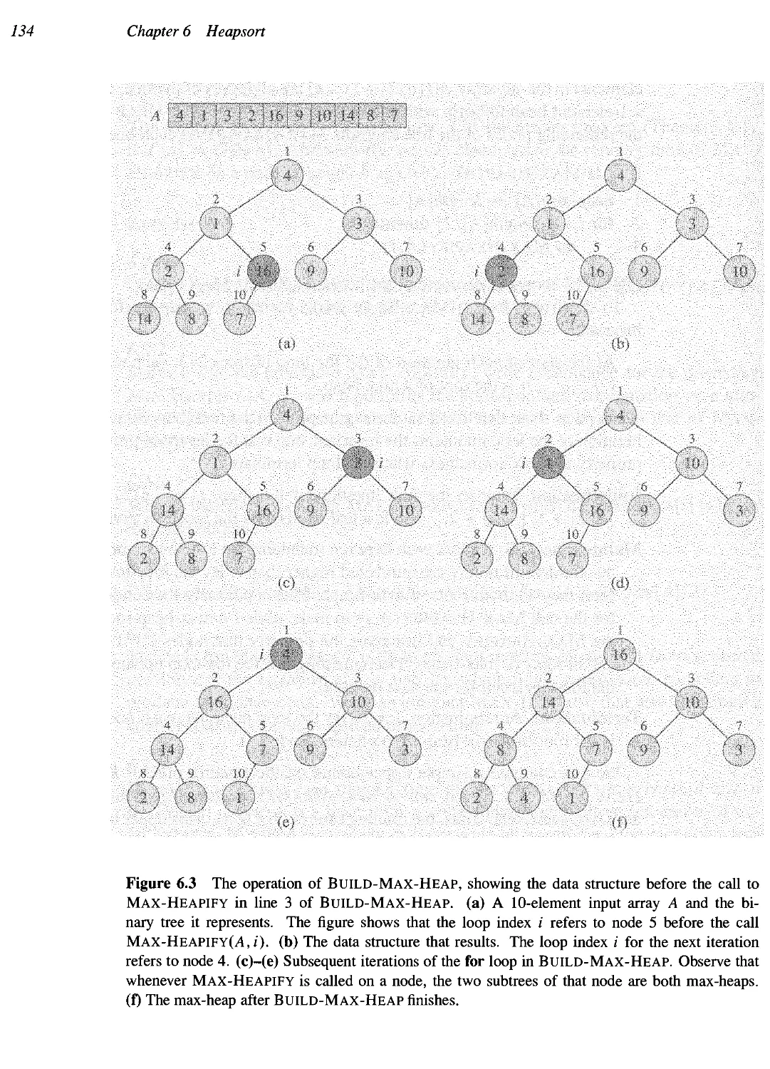
6.3 Bmlding a heap 132
6.4 The heapsort algorithm 135
6.5 Priority queues 138
Quicksort 145
7.1 Description of quicksort 145
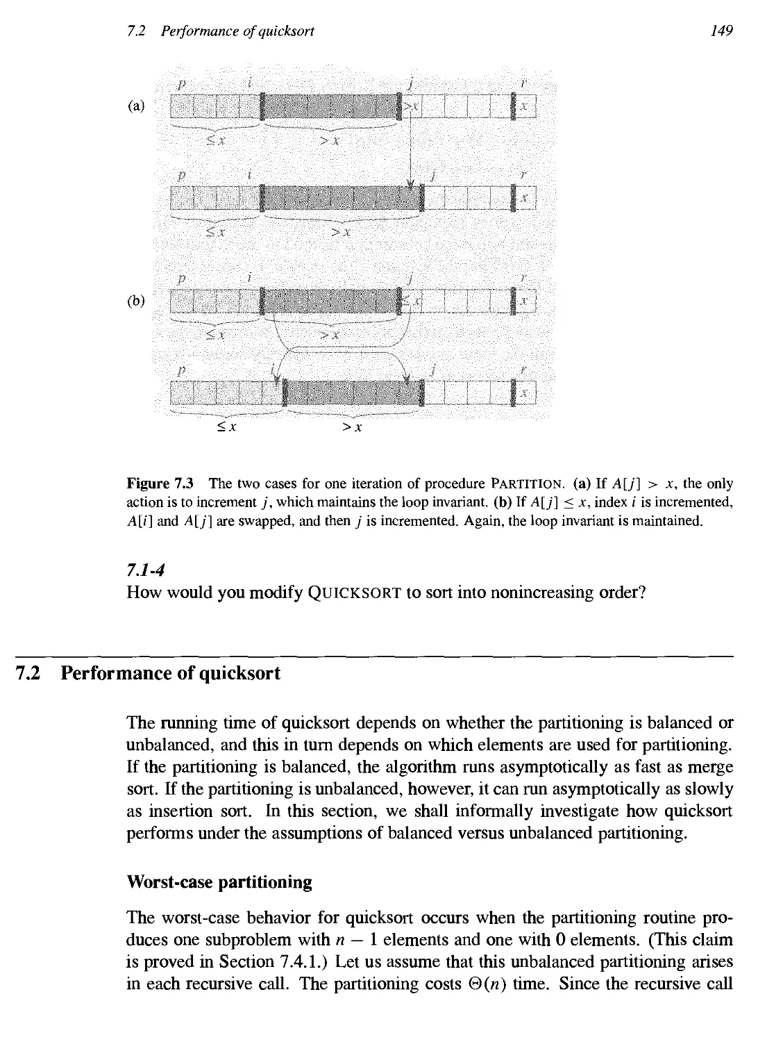
7.2 Performance of quicksort 149
7.3 A randomized version of quicksort 153
7.4 Analysis of quicksort 155
Sorting in Linear Time 165
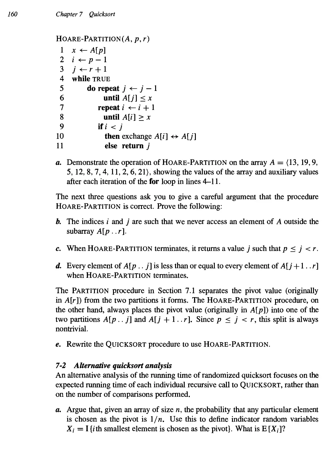
8.1 Lower bounds for sorting 165
8.2 Counting sort 168
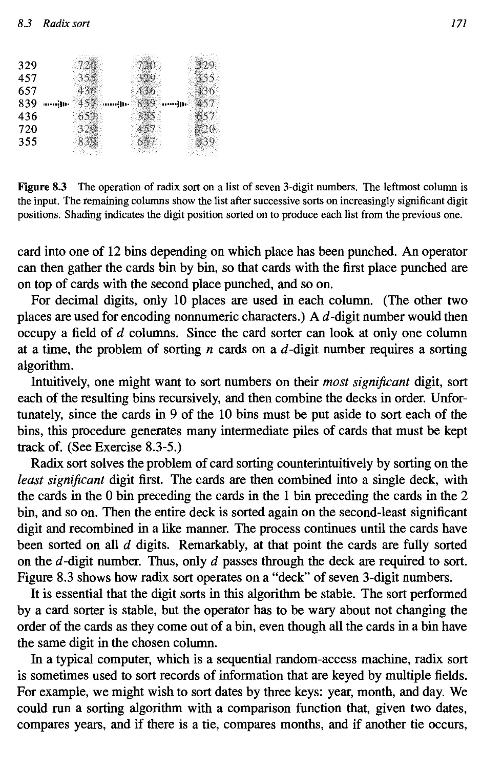
8.3 Radix sort 770
8.4 Bucket sort 774
Medians and Order Statistics 183
9.1 Minimum and maximum 184
9.2 Selection in expected linear time 185
9.3 Selection in worst-case linear time 189
III Data Structures
Introduction 197
10 Elementary Data Structures 200
10.1 Stacks and queues 200
10.2 Linked lists 204
10.3 Implementing pointers and objects 209
10.4 Representing rooted trees 214
11 Hash Tables 221
11.1 Direct-address tables 222
11.2 Hash tables 224
11.3 Hash functions 229
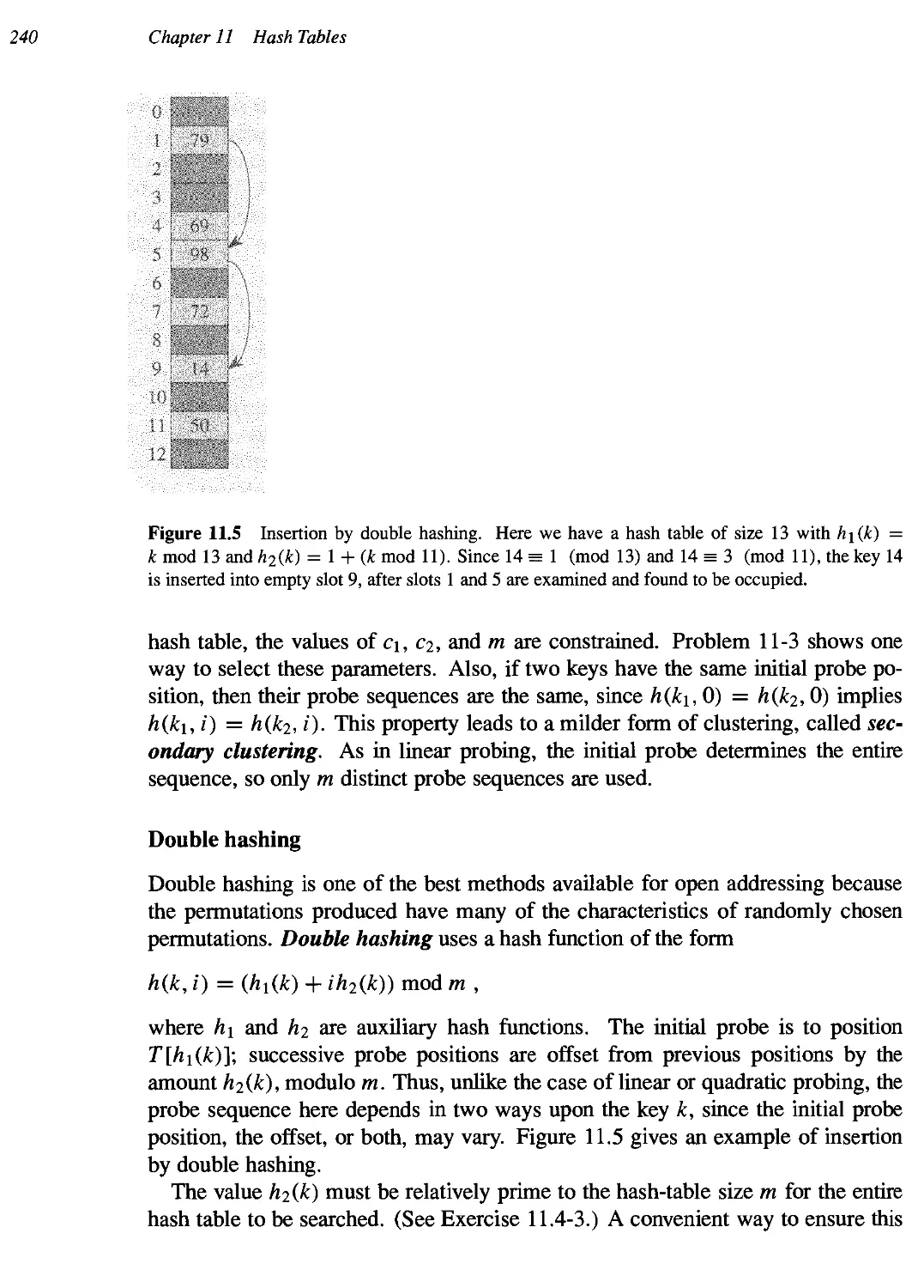
11.4 Open addressing 237
• 11.5 Perfect hashing 245

Contents
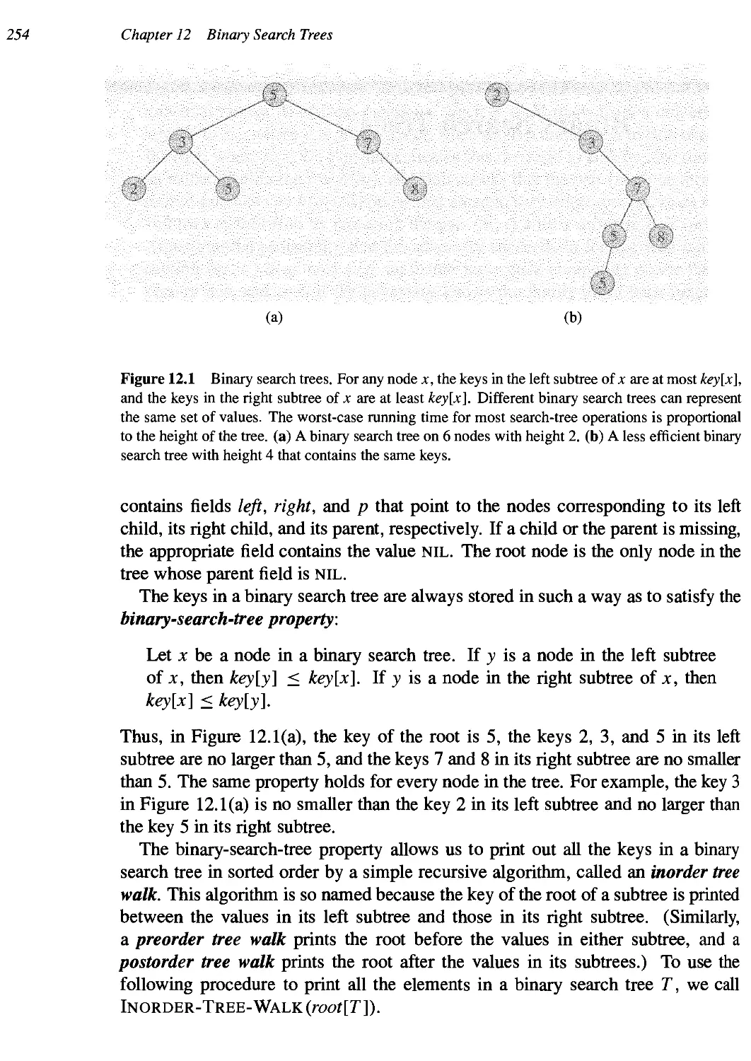
12 Binary Search Trees 253
12.1 What is a binary search tree? 253
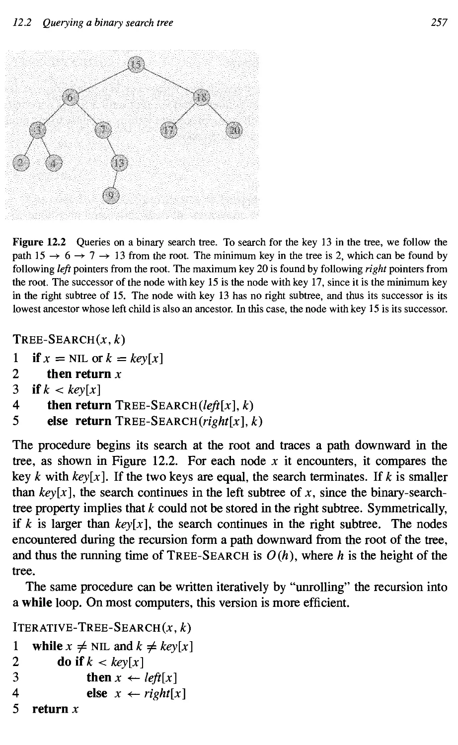
12.2 Querying a binary search tree 256
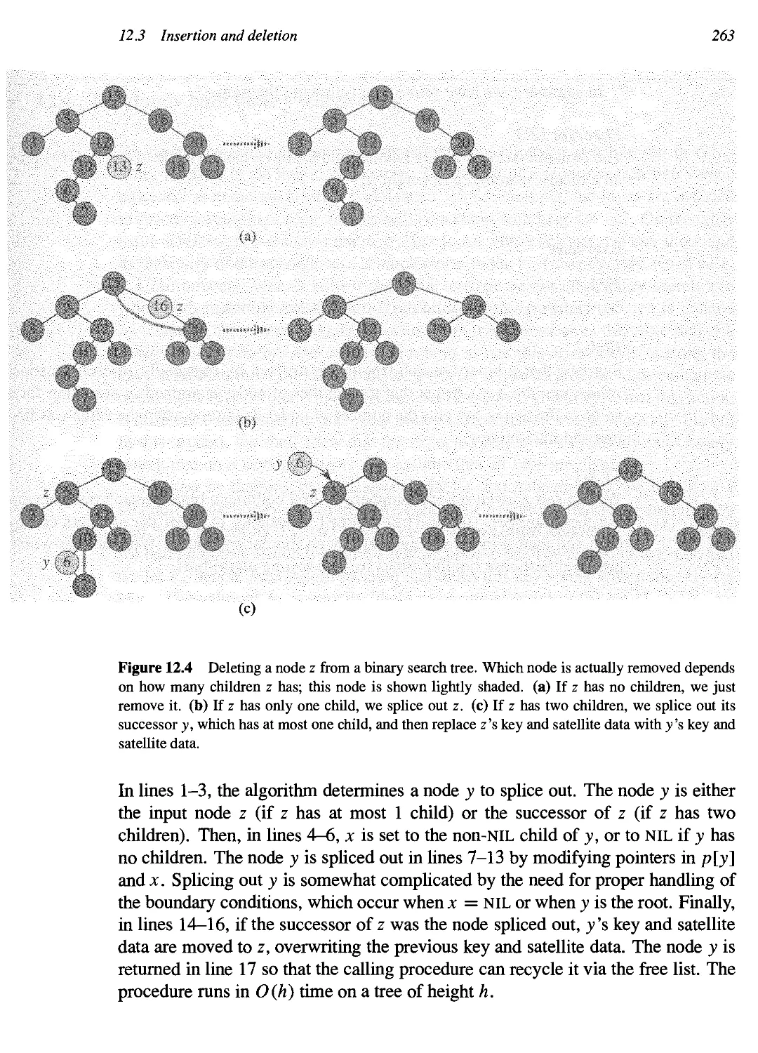
12.3 Insertion and deletion 267
* 12.4 Randomly built binary search trees 265
13 Red-Black Trees 273
13.1 Properties of red-black trees 273
13.2 Rotations 277
13.3 Insertion 280
13.4 Deletion 288
14 Augmenting Data Structures 302
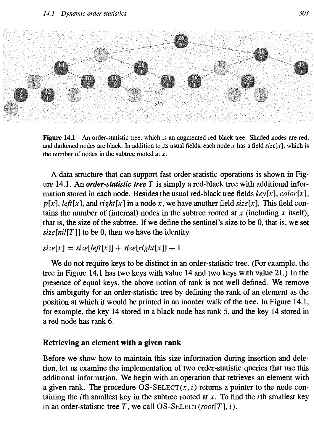
14.1 Dynamic order statistics 302
14.2 How to augment a data structure 50S
14.3 Interval trees 311
IV Advanced Design and Analysis Techniques
Introduction 321
15 Dynamic Programming 323
15.1 Assembly-line scheduling 324
15.2 Matrix-chain multiplication 331
15.3 Elements of dynamic programming 339
15.4 Longest common subsequence 350
15.5 Optimal binary search trees 356
16 Greedy Algorithms 370
16.1 An activity-selection problem 371
16.2 Elements of the greedy strategy 379
16.3 Huffman codes 5S5
• 16.4 Theoretical foundations for greedy methods 393
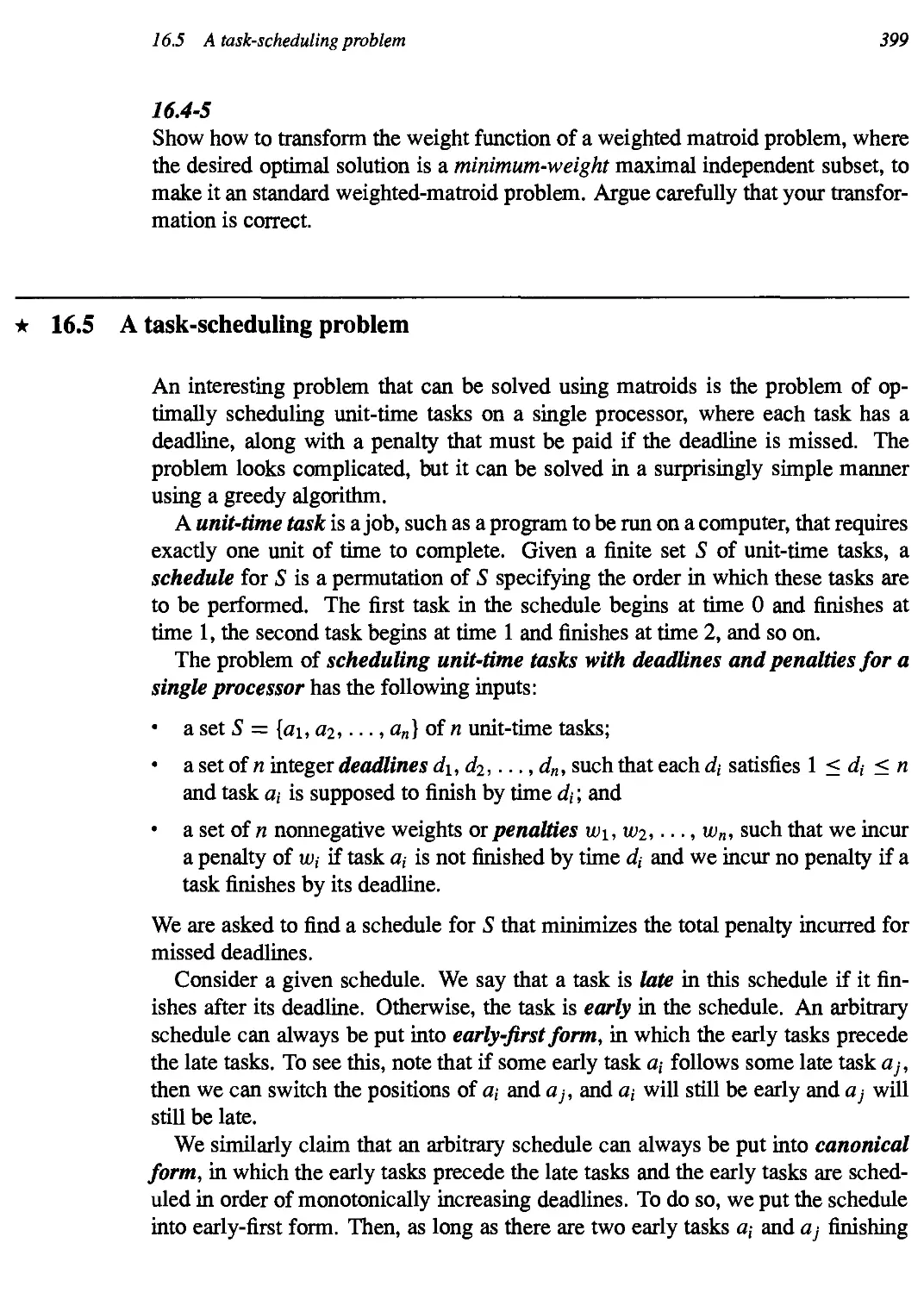
• 16.5 A task-scheduling problem 399
17 Amortized Analysis 405
17.1 Aggregate analysis 406
17.2 The accounting method 410
17.3 The potential method 412
11A Dynamic tables 416

Contents
V Advanced Data Structures
Introduction 431
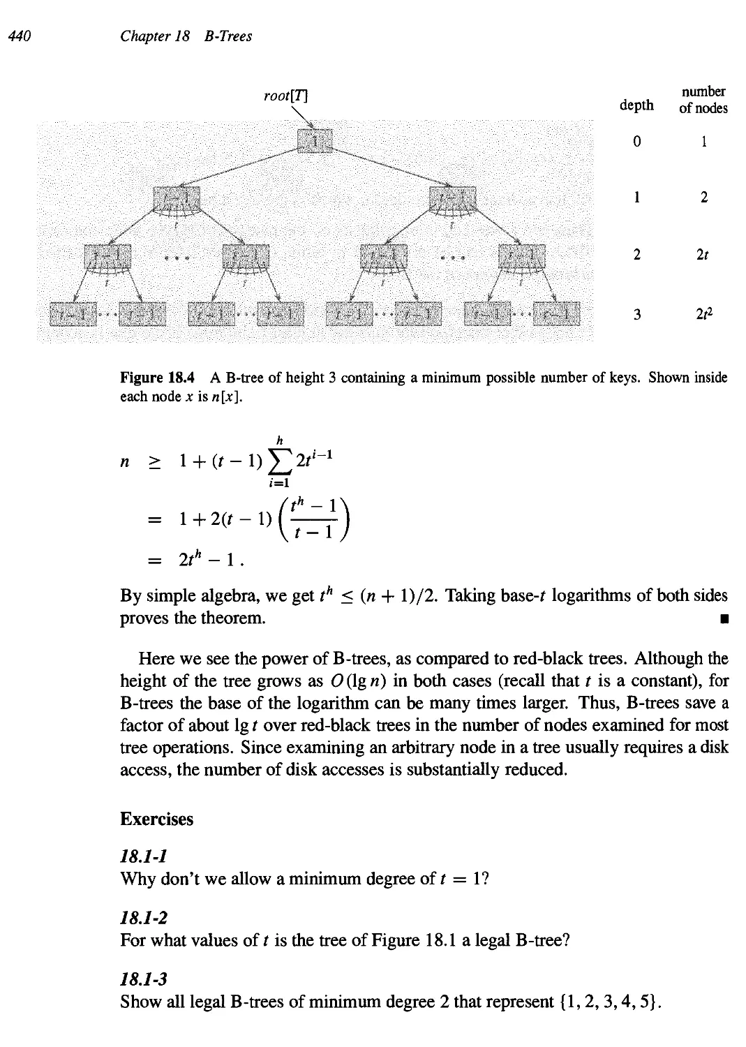
18 B-Trees 434
18.1 Definition of B-trees 438
18.2 Basic operations on B-trees 441
18.3 Deleting a key from a B-tree 449
19 Binomial Heaps 455
19.1 Binomial trees and binomial heaps 457
19.2 Operations on binomial heaps 461
20 Fibonacci Heaps 476
20.1 Structure of Fibonacci heaps 477
20.2 Mergeable-heap operations 479
20.3 Decreasing a key and deleting a node 489
20.4 Bounding the maximum degree 493
21 Data Structures for Disjoint Sets 498
21.1 Disjoint-set operations 49S
21.2 Linked-list representation of disjoint sets 507
21.3 Disjoint-set forests 505
•k 21.4 Analysis of union by rank with path compression 509
VI Graph Algorithms
Introduction 525
22 Elementary Graph Algorithms 527
22 A Representations of graphs 527
22.2 Breadth-first search 531
22.3 Depth-first search 540
22.4 Topological sort 549
22.5 Strongly connected components 552
23 Minimum Spanning Trees 561
23.1 Growing a minimum spanning tree 562
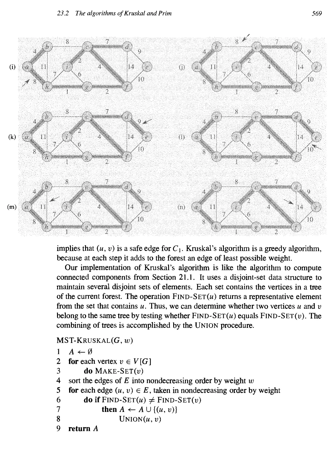
23.2 The algorithms of Kraskal and Prim 567
24 Single-Source Shortest Paths 580
24.1 The Bellman-Ford algorithm 588
24.2 Single-source shortest paths in directed acyclic graphs 592
24.3 Dijkstra's algorithm 595
24.4 Difference constraints and shortest paths 607
24.5 Proofs of shortest-paths properties 607

Contents ix
25 All-Pairs Shortest Paths 620
25.1 Shortest paths and matrix multiplication 622
25.2 The Floyd-Warshall algorithm 629
25.3 Johnson's algorithm for sparse graphs 636
26 Maximum Flow 643
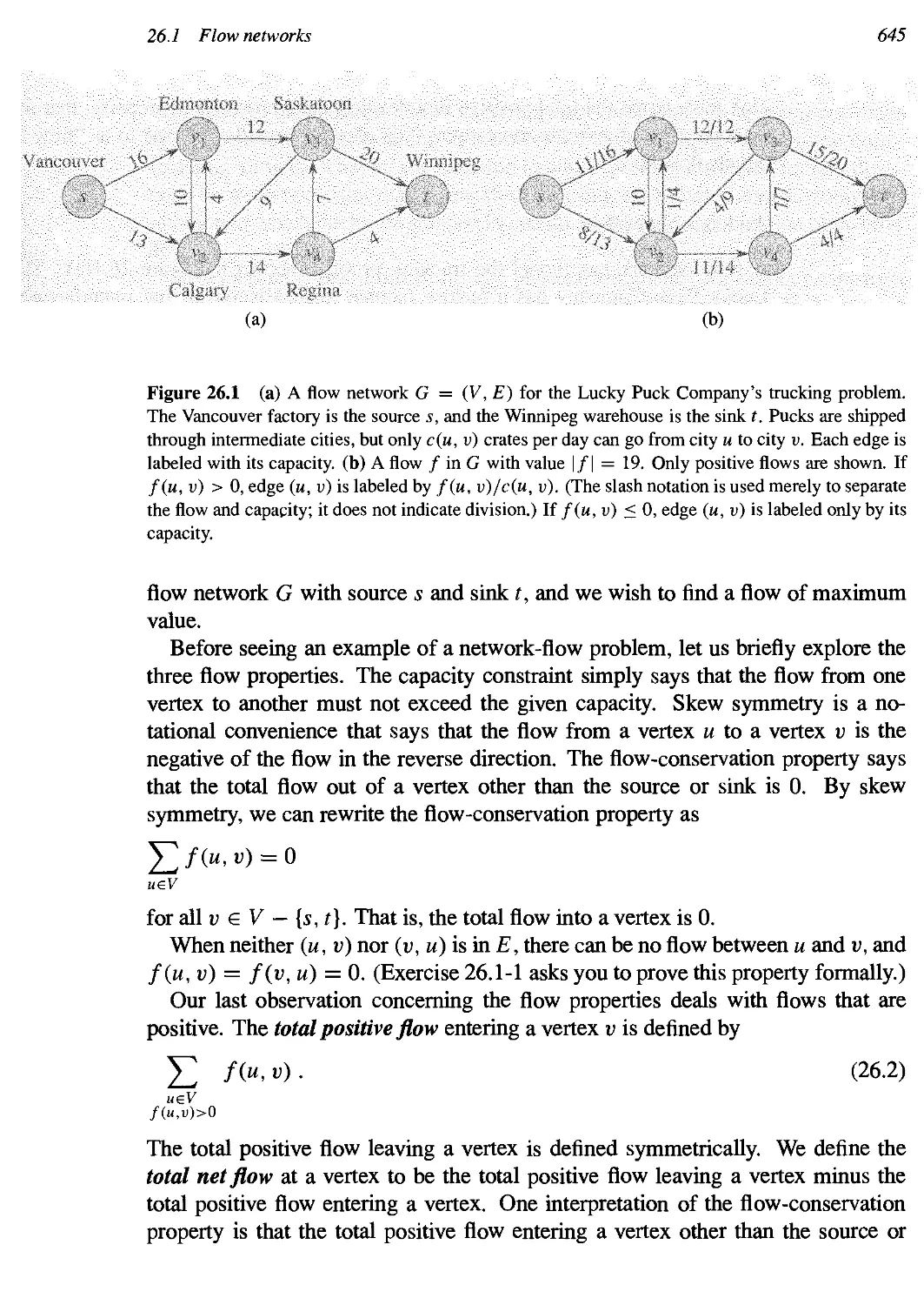
26.1 Flow networks 644
26.2 The Ford-Fulkerson method 651
26.3 Maximum bipartite matching 664
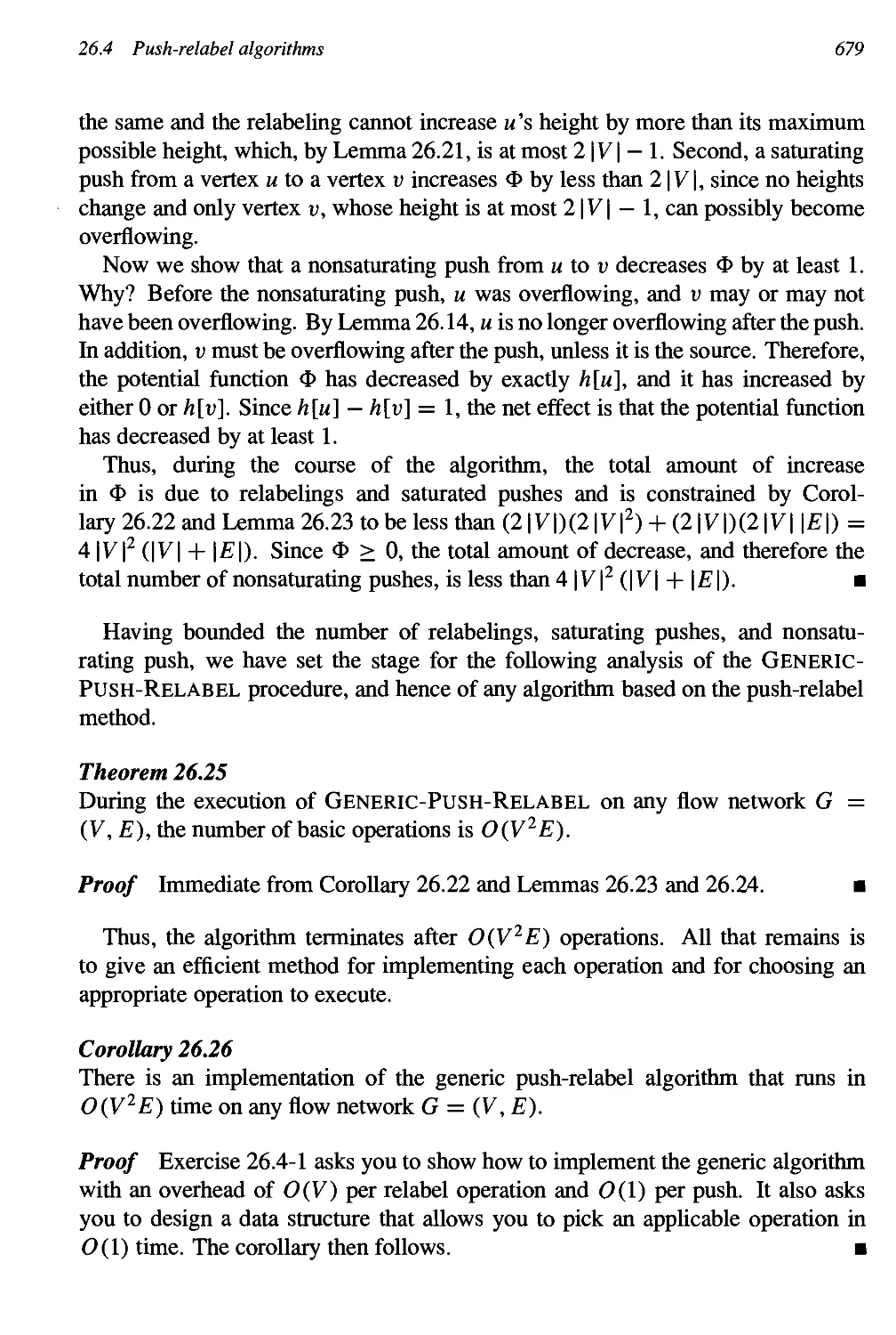
• 26.4 Push-relabel algorithms 669
• 26.5 The relabel-to-front algorithm 681
VII Selected Topics
Introduction 701
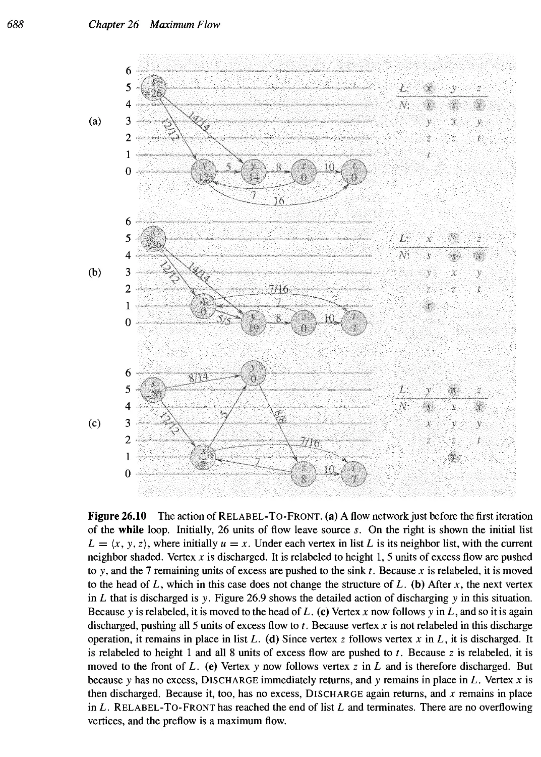
27 Sorting Networks 704
27..1 Comparison networks 704
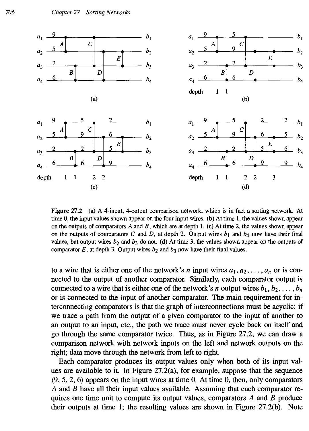
27.2 The zero-one principle 709
21.3 A bitonic sorting network 712
21A A merging network 716
27.5 A sorting network 719
28 Matrix Operations 725
28.1 Properties of matrices 725
28.2 Strassen's algorithm for matrix multiplication 735
28.3 Solving systems of linear equations 742
28.4 Inverting matrices 755
28.5 Symmetric positive-definite matrices and least-squares approximation
760
29 Linear Programming 770
29.1 Standard and slack forms 777
29.2 Formulating problems as linear programs 785
29.3 The simplex algorithm 790
29.4 Duality 804
29.5 The initial basic feasible solution 811
30 Polynomials and the FFT 822
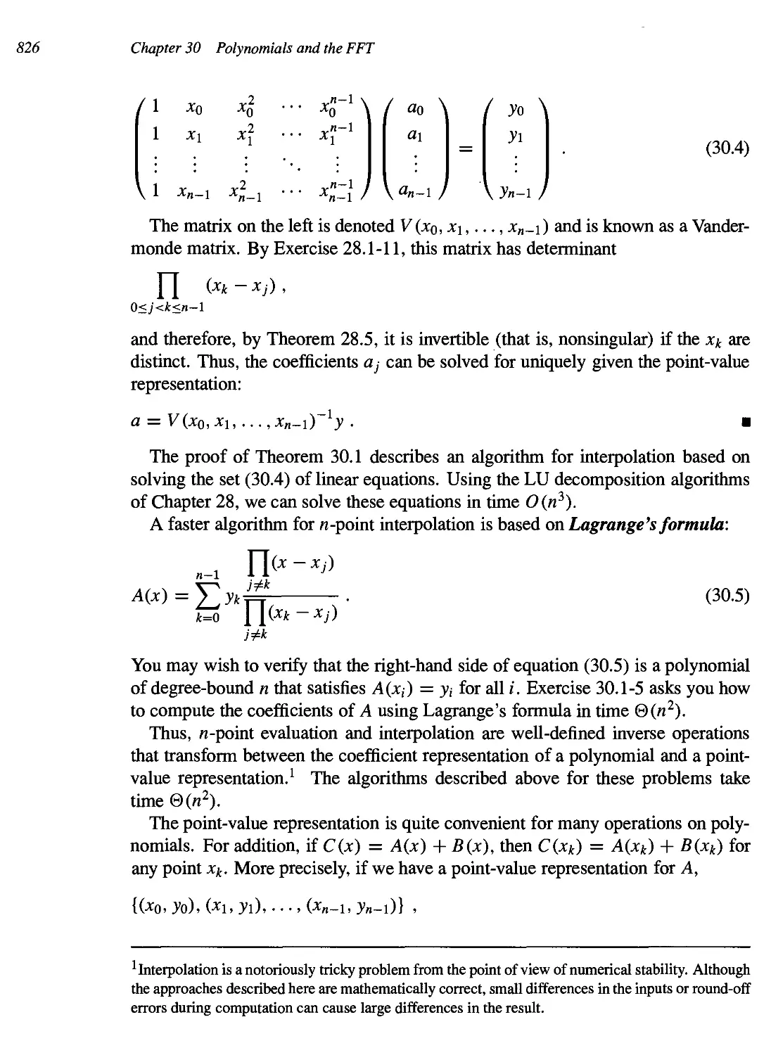
30.1 Representation of polynomials 824
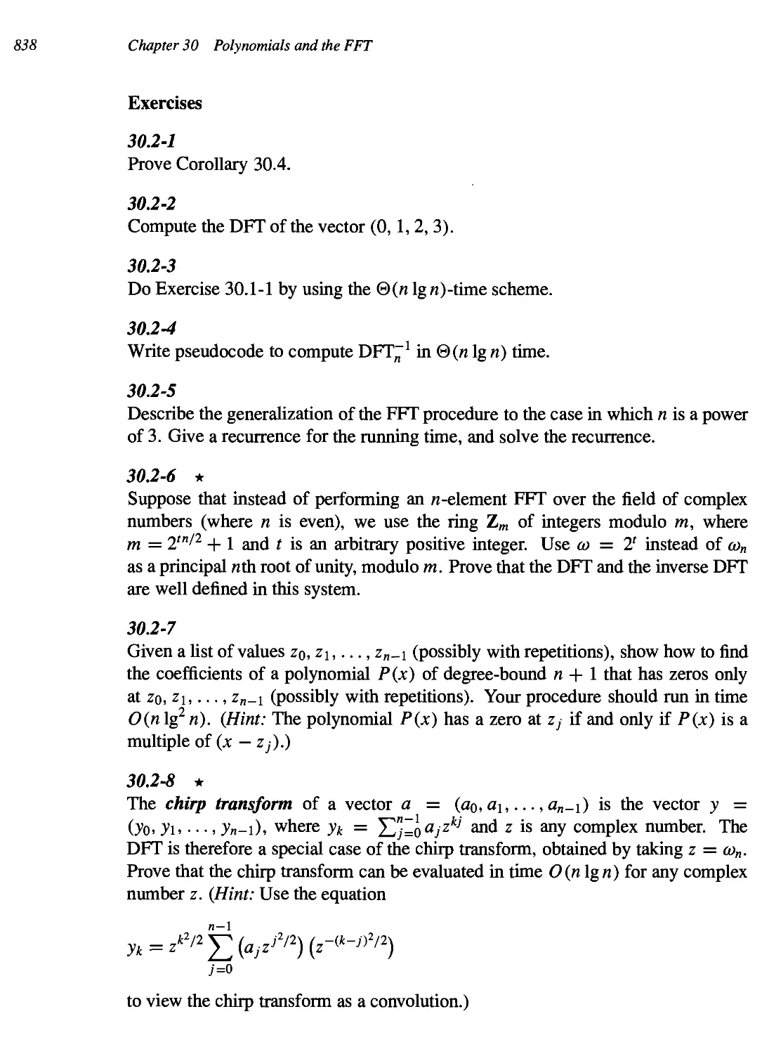
30.2 The DFT and FFT 830
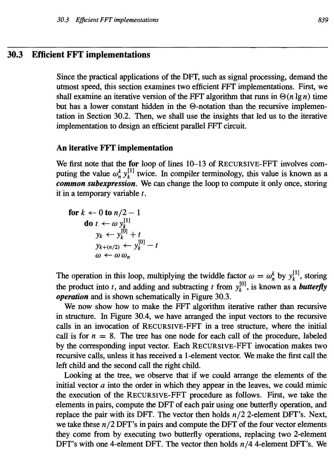
30.3 Efficient FFT implementations 839

•
•
31.2
31.3
31.4
31.5
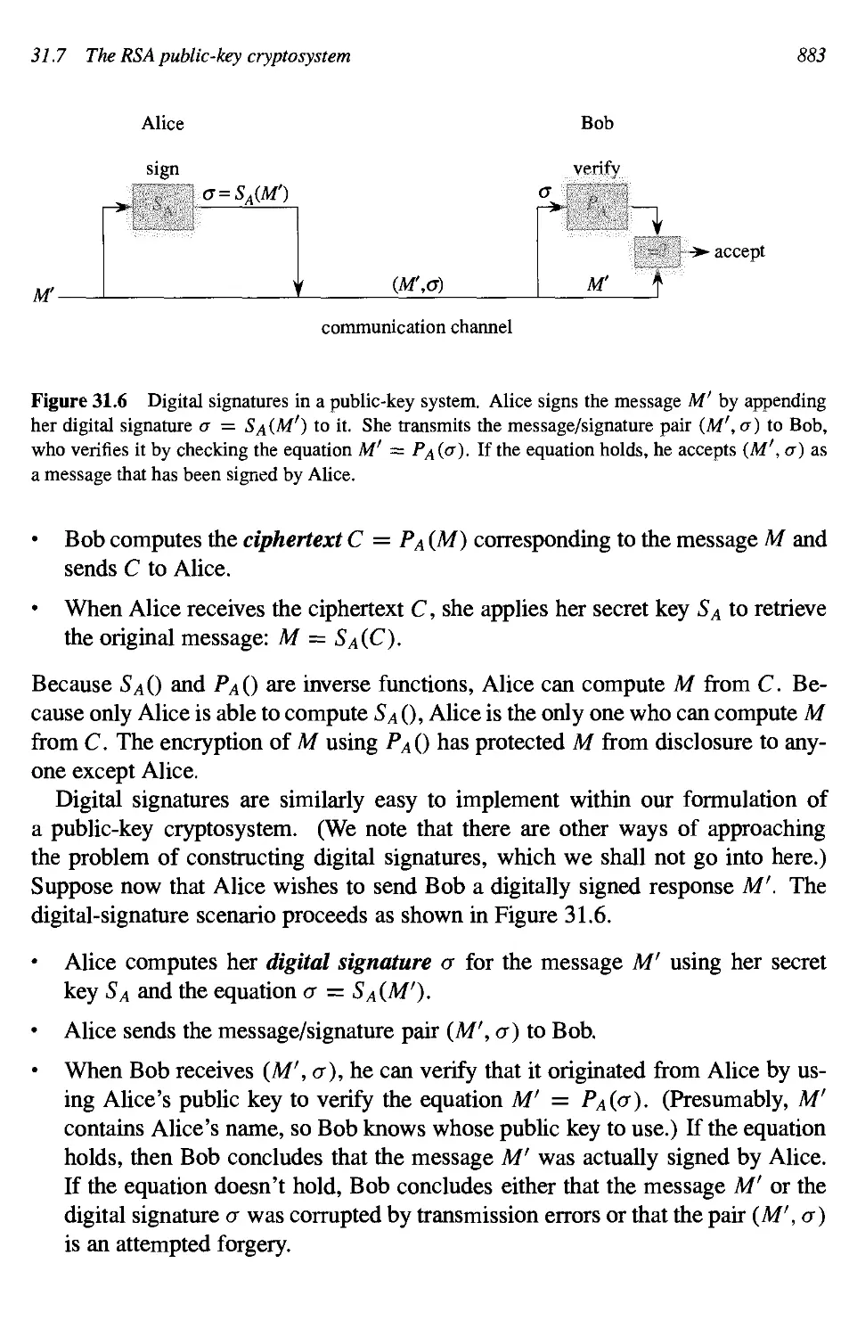
31.6
31.7
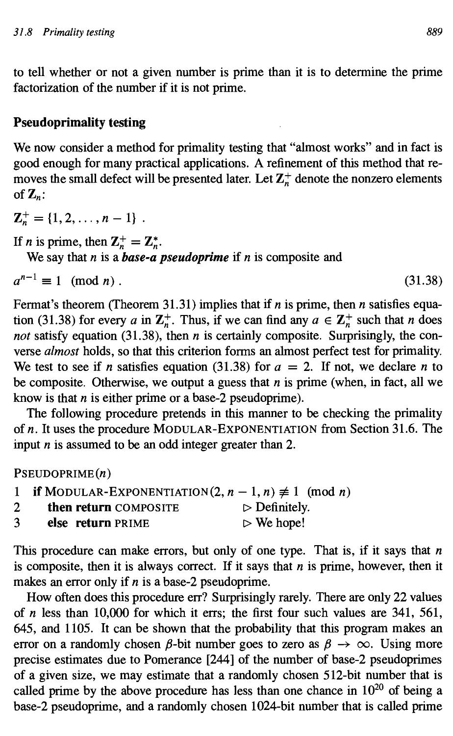
31.8
31.9
Contents
31 Number-Theoretic Algorithms 849
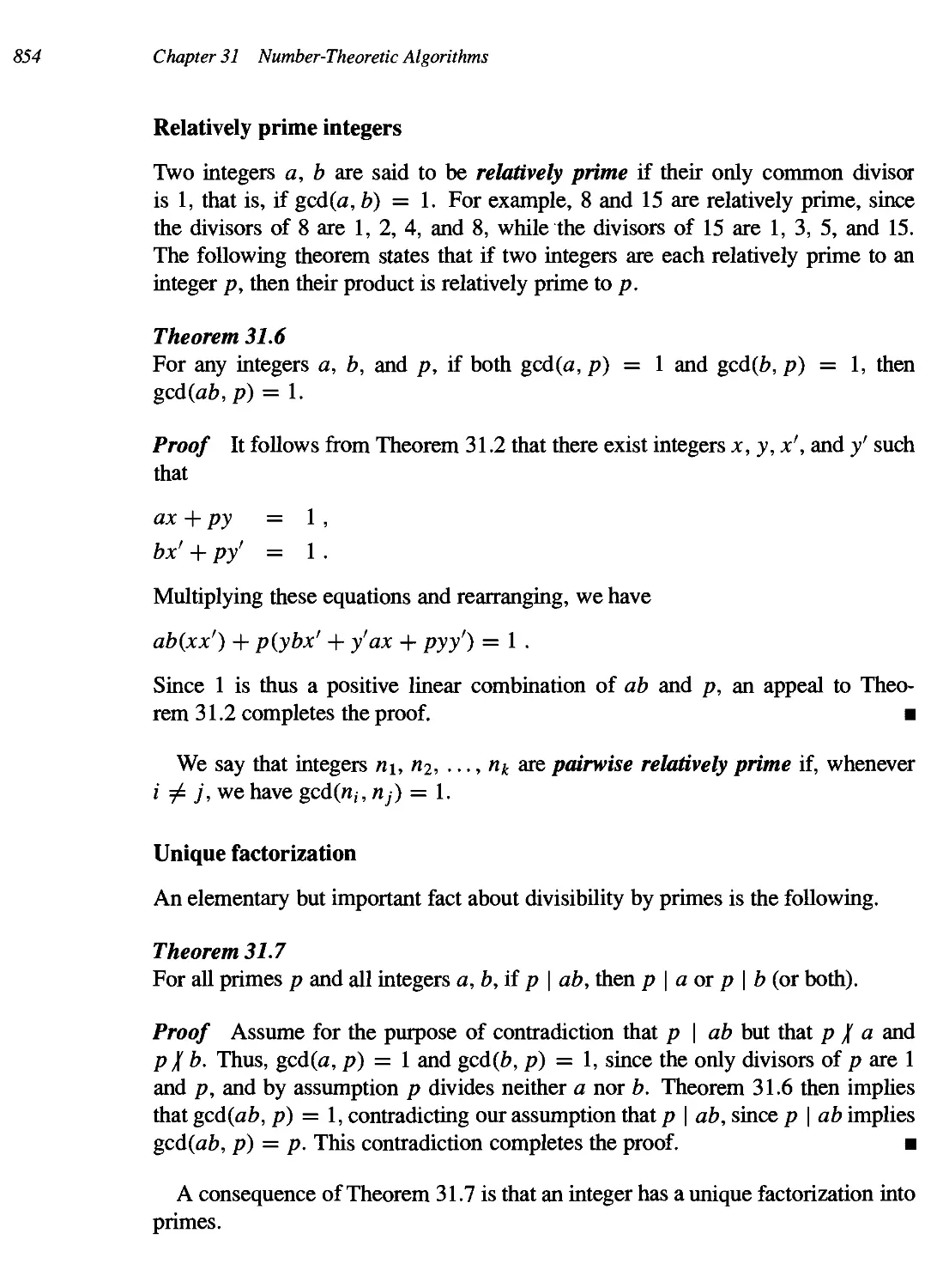
31.1 Elementary number-theoretic notions 850
Greatest common divisor 856
Modular arithmetic 862
Solving modular linear equations 869
The Chinese remainder theorem 873
Powers of an element 876
The RSA public-key cryptosystem 881
Primality testing 887
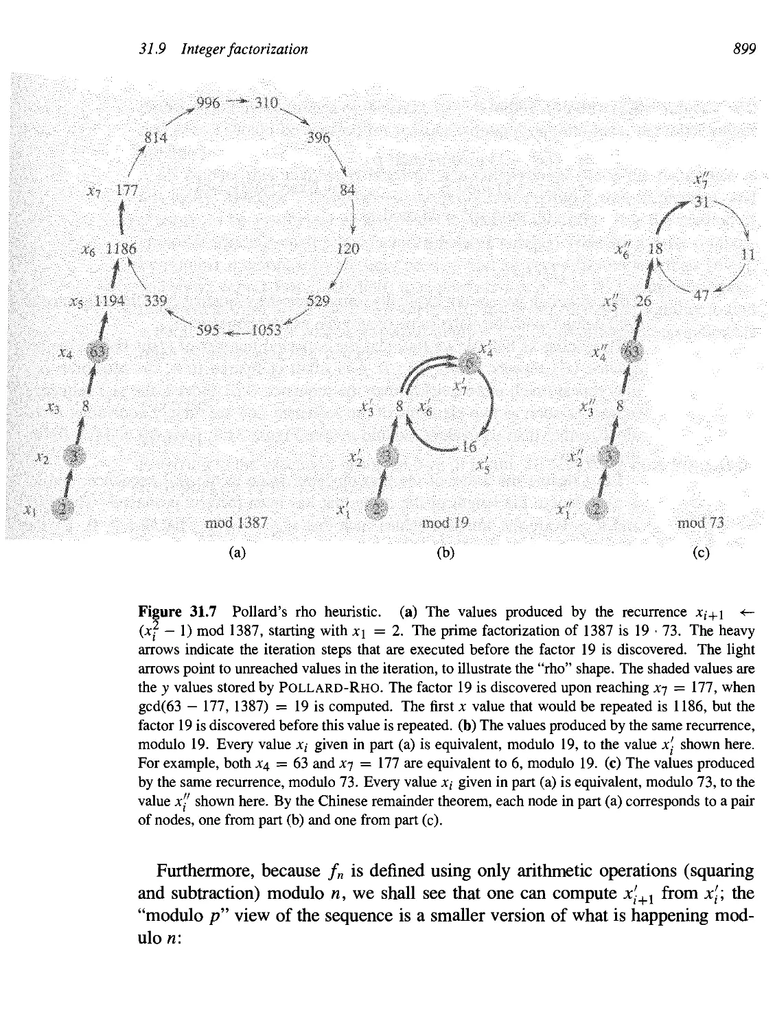
Integer factorization 896
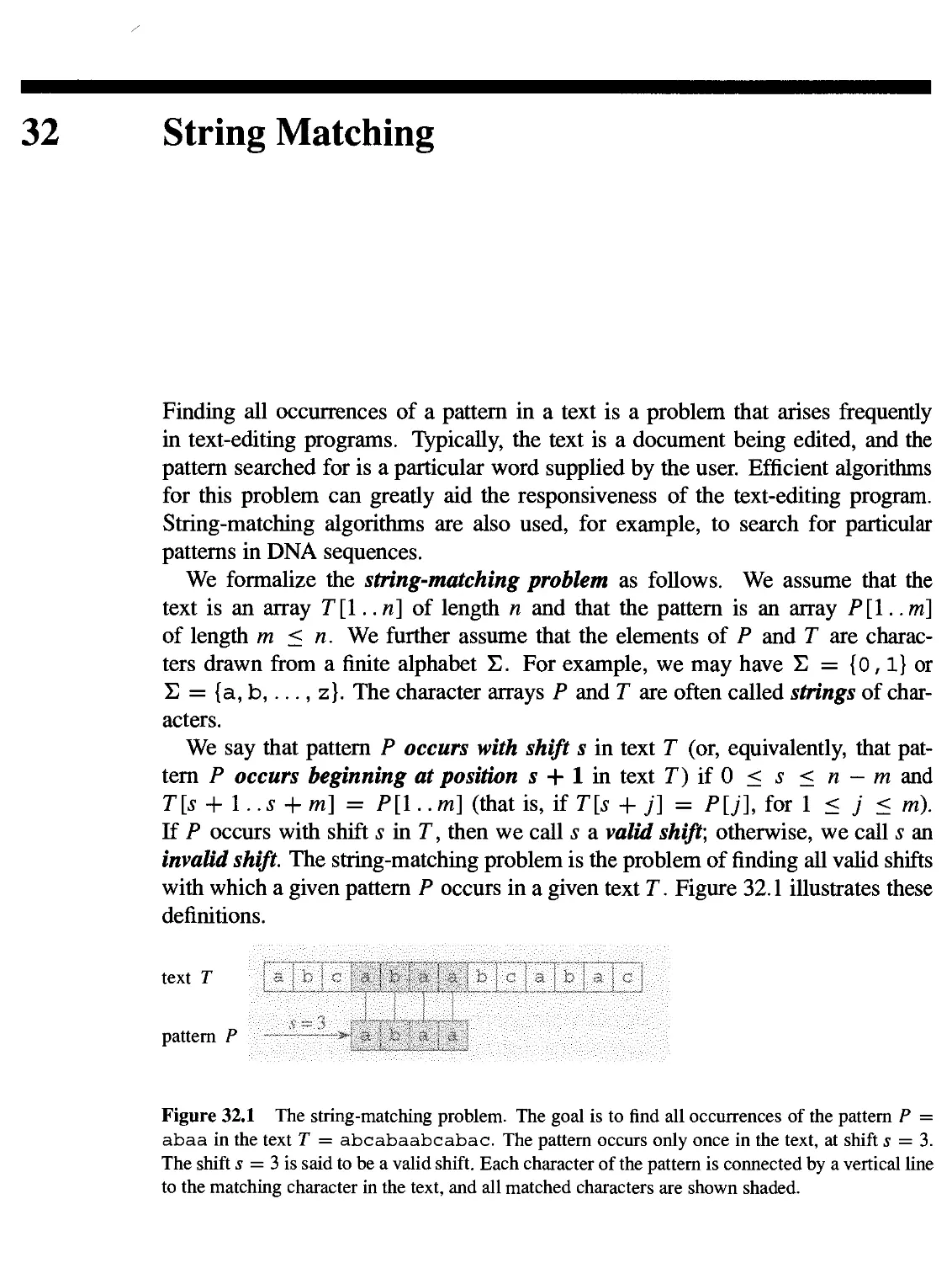
32 String Matching 906
32.1 The naive string-matching algorithm 909
32.2 The Rabin-Karp algorithm 977
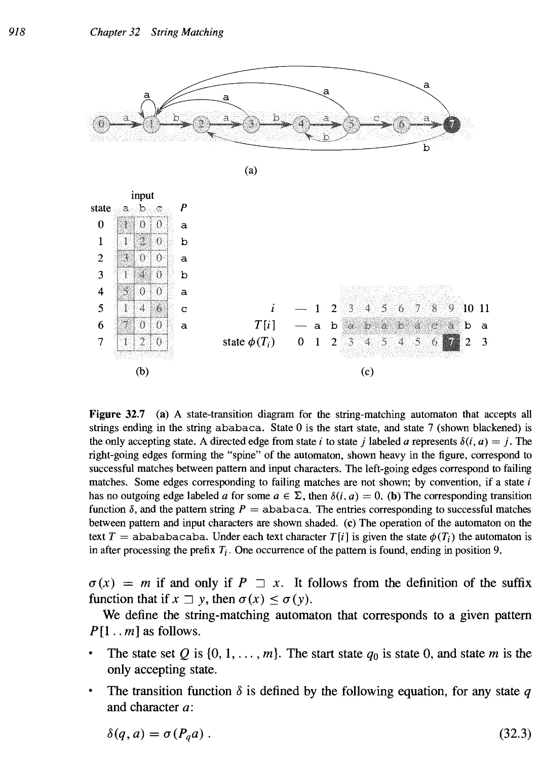
32.3 String matching with finite automata 976
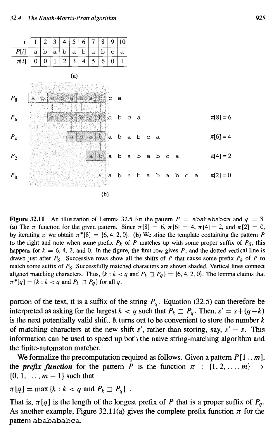
• 32.4 The Knuth-Morris-Pratt algorithm 923
33 Computational Geometry 933
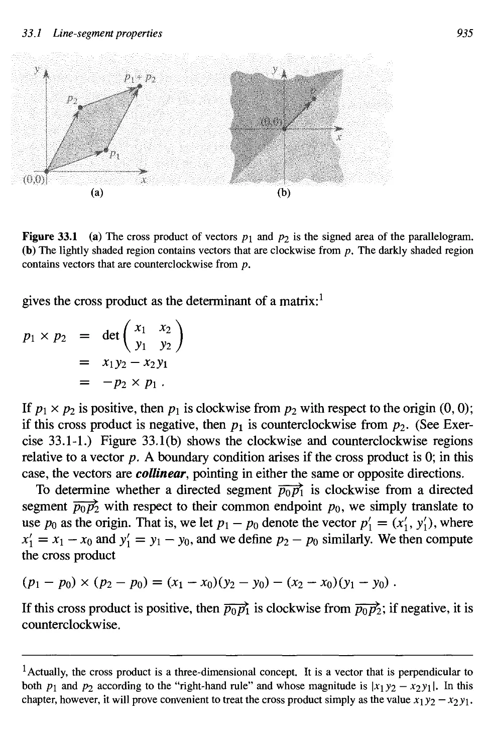
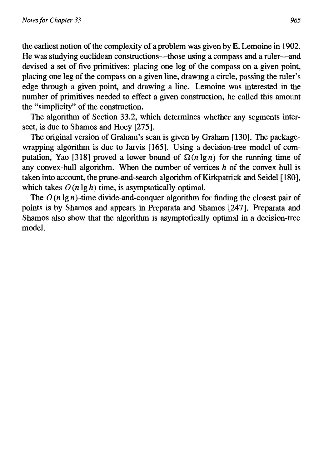
33.1 Line-segment properties 934
33.2 Determining whether any pair of segments intersects 940
33.3 Finding the convex hull 947
33.4 Finding the closest pair of points 957
34 NP-Completeness 966
34.1 Polynomial time 977
34.2 Polynomial-time verification 979
34.3 NP-completeness and reducibility 984
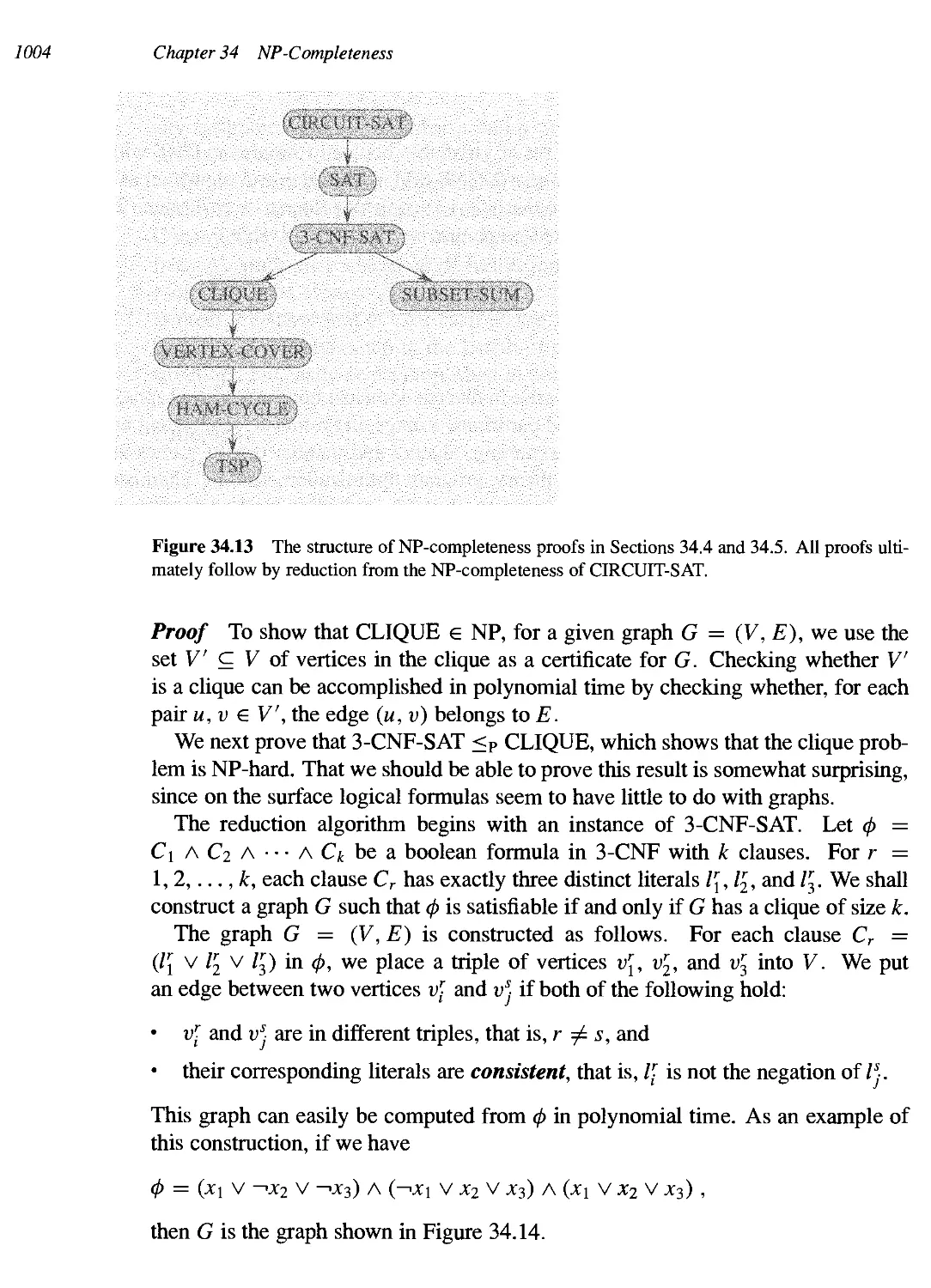
34.4 NP-completeness proofs 995
34.5 NP-complete problems 1003
35 Approximation Algorithms 1022
35.1 The vertex-cover problem 1024
35.2 The traveling-salesman problem 7027
35.3 The set-covering problem 1033
35.4 Randomization and linear programming 1039
35.5 The subset-sum problem 1043
VIII Appendix: Mathematical Background
Introduction 1057
A Summations 1058
A.I Summation formulas and properties 1058
A.2 Bounding summations 7062

Contents xi
В Sets, Etc. 1070
B.I Sets 7070
В .2 Relations 1075
B.3 Functions 1077
B.4 Graphs 1080
B.5 Trees 1085
С Counting and Probability 1094
C.I Counting 1094
C.2 Probability 1100
C.3 Discrete random variables 1106
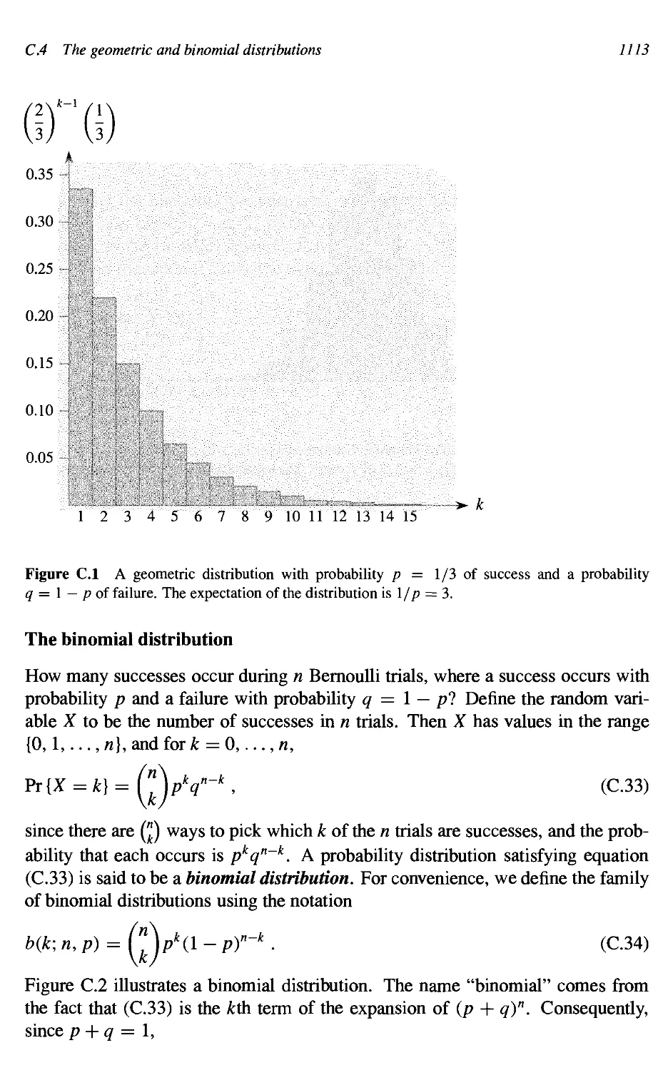
СЛ The geometric and binomial distributions 1112
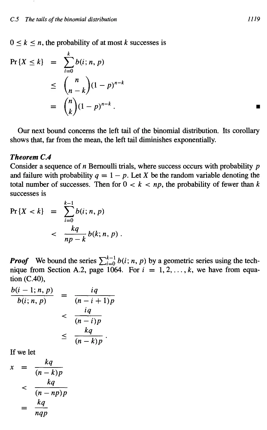
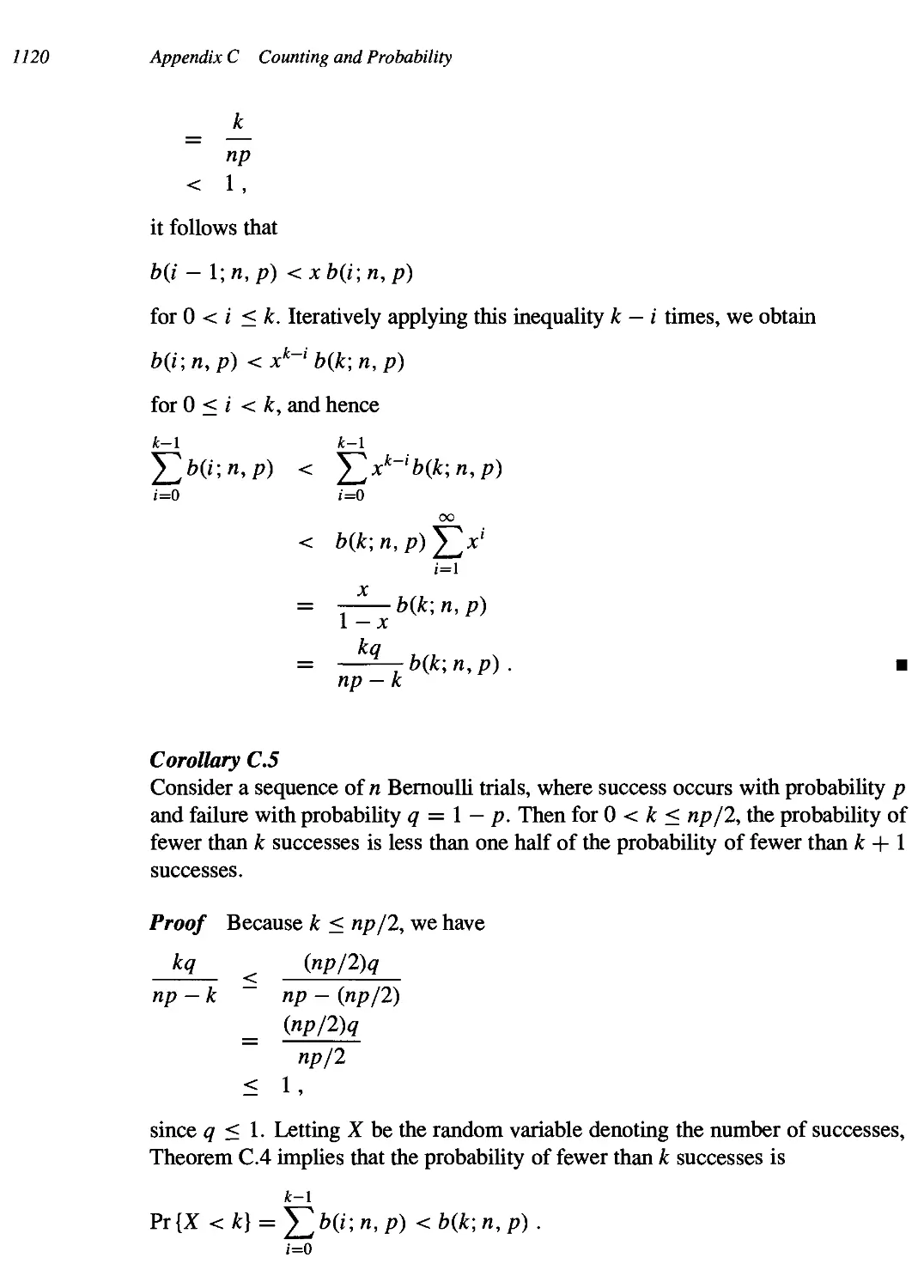
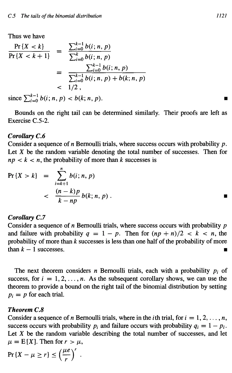
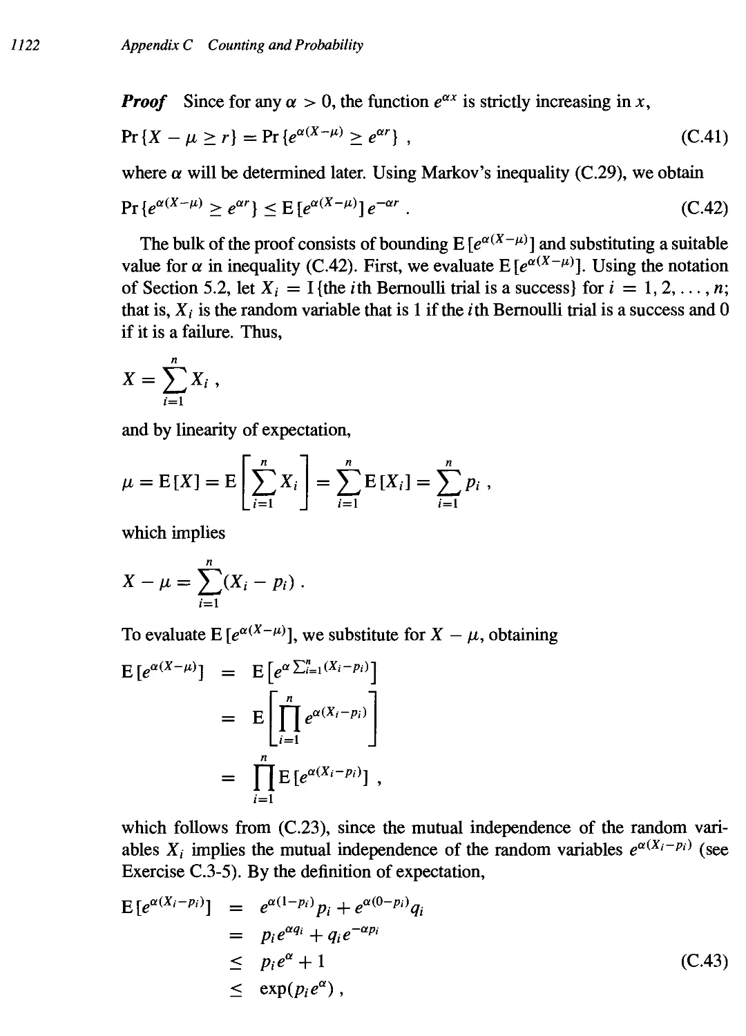
• C.5 The tails of the binomial distribution 1118
Bibliography 1127
Index 1145

Preface
This book provides a comprehensive introduction to the modern study of computer
algorithms. It presents many algorithms and covers them in considerable depth, yet
makes their design and analysis accessible to all levels of readers. We have tried to
keep explanations elementary without sacrificing depth of coverage or mathemati-
mathematical rigor.
Each chapter presents an algorithm, a design technique, an application area, or a
related topic. Algorithms are described in English and in a "pseudocode" designed
to be readable by anyone who has done a little programming. The book contains
over 230 figures illustrating how the algorithms work. Since we emphasize effi-
efficiency as a design criterion, we include careful analyses of the running times of all
our algorithms.
The text is intended primarily for use in undergraduate or graduate courses in
algorithms or data structures. Because it discusses engineering issues in algorithm
design, as well as mathematical aspects, it is equally well suited for self-study by
technical professionals.
In this, the second edition, we have updated the entire book. The changes range
from the addition of new chapters to the rewriting of individual sentences.
To the teacher
This book is designed to be both versatile and complete. You will find it useful for
a variety of courses, from an undergraduate course in data structures up through
a graduate course in algorithms. Because we have provided considerably more
material than can fit in a typical one-term course, you should think of the book as
a "buffet" or "smorgasbord" from which you can pick and choose the material that
best supports the course you wish to teach.
You should find it easy to organize your course around just the chapters you
need. We have made chapters relatively self-contained, so that you need not worry
about an unexpected and unnecessary dependence of one chapter on another. Each
chapter presents the easier material first and the more difficult material later, with

xiv Preface
section boundaries marking natural stopping points. In an undergraduate course,
you might use only the earlier sections from a chapter; in a graduate course, you
might cover the entire chapter.
We have included over 920 exercises and over 140 problems. Each section ends
with exercises, and each chapter ends with problems. The exercises are generally
short questions that test basic mastery of the material. Some are simple self-check
thought exercises, whereas others are more substantial and are suitable as assigned
homework. The problems are more elaborate case studies that often introduce new
material; they typically consist of several questions that lead the student through
the steps required to arrive at a solution.
We have starred (*) the sections and exercises that are more suitable for graduate
students than for undergraduates. A starred section is not necessarily more diffi-
difficult than an unstarred one, but it may require an understanding of more advanced
mathematics. Likewise, starred exercises may require an advanced background or
more than average creativity.
To the student
We hope that this textbook provides you with an enjoyable introduction to the
field of algorithms. We have attempted to make every algorithm accessible and
interesting. To help you when you encounter unfamiliar or difficult algorithms, we
describe each one in a step-by-step manner. We also provide careful explanations
of the mathematics needed to understand the analysis of the algorithms. If you
already have some familiarity with a topic, you will find the chapters organized so
that you can skim introductory sections and proceed quickly to the more advanced
material.
This is a large book, and your class will probably cover only a portion of its
material. We have tried, however, to make this a book that will be useful to you
now as a course textbook and also later in your career as a mathematical desk
reference or an engineering handbook.
What are the prerequisites for reading this book?
• You should have some programming experience. In particular, you should un-
understand recursive procedures and simple data structures such as arrays and
linked lists.
• You should have some facility with proofs by mathematical induction. A few
portions of the book rely on some knowledge of elementary calculus. Beyond
that, Parts I and VIII of this book teach you all the mathematical techniques you
will need.

Preface xv
To the professional
The wide range of topics in this book makes it an excellent handbook on algo-
algorithms. Because each chapter is relatively self-contained, you can focus in on the
topics that most interest you.
Most of the algorithms we discuss have great practical utility. We therefore
address implementation concerns and other engineering issues. We often provide
practical alternatives to the few algorithms that are primarily of theoretical interest.
If you wish to implement any of the algorithms, you will find the translation of
our pseudocode into your favorite programming language a fairly straightforward
task. The pseudocode is designed to present each algorithm clearly and succinctly.
Consequently, we do not address error-handling and other software-engineering is-
issues that require specific assumptions about your programming environment. We
attempt to present each algorithm simply and directly without allowing the idiosyn-
idiosyncrasies of a particular programming language to obscure its essence.
To our colleagues
We have supplied an extensive bibliography and pointers to the current literature.
Each chapter ends with a set of "chapter notes" that give historical details and
references. The chapter notes do not provide a complete reference to the whole
field of algorithms, however. Though it may be hard to believe for a book of this
size, many interesting algorithms could not be included due to lack of space.
Despite myriad requests from students for solutions to problems and exercises,
we have chosen as a matter of policy not to supply references for problems and
exercises, to remove the temptation for students to look up a solution rather than to
find it themselves.
Changes for the second edition
What has changed between the first and second editions of this book? Depending
on how you look at it, either not much or quite a bit.
A quick look at the table of contents shows that most of the first-edition chapters
and sections appear in the second edition. We removed two chapters and a handful
of sections, but we have added three new chapters and four new sections apart from
these new chapters. If you were to judge the scope of the changes by the table of
contents, you would likely conclude that the changes were modest.
The changes go far beyond what shows up in the table of contents, however.
In no particular order, here is a summary of the most significant changes for the
second edition:

Preface
• Cliff Stein was added as a coauthor.
• Errors have been corrected. How many errors? Let's just say several.
• There are three new chapters:
• Chapter 1 discusses the role of algorithms in computing.
• Chapter 5 covers probabilistic analysis and randomized algorithms. As in
the first edition, these topics appear throughout the book.
• Chapter 29 is devoted to linear programming.
• Within chapters that were carried over from the first edition, there are new sec-
sections on the following topics:
• perfect hashing (Section 11.5),
• two applications of dynamic programming (Sections 15.1 and 15.5), and
• approximation algorithms that use randomization and linear programming
(Section 35.4).
• To allow more algorithms to appear earlier in the book, three of the chapters on
mathematical background have been moved from Part I to the Appendix, which
is Part VIII.
• There are over 40 new problems and over 185 new exercises.
• We have made explicit the use of loop invariants for proving correctness. Our
first loop invariant appears in Chapter 2, and we use them a couple of dozen
times throughout the book.
• Many of the probabilistic analyses have been rewritten. In particular, we use in
a dozen places the technique of "indicator random variables," which simplify
probabilistic analyses, especially when random variables are dependent.
• We have expanded and updated the chapter notes and bibliography. The bibli-
bibliography has grown by over 50%, and we have mentioned many new algorithmic
results that have appeared subsequent to the printing of the first edition.
We have also made the following changes:
• The chapter on solving recurrences no longer contains the iteration method. In-
Instead, in Section 4.2, we have "promoted" recursion trees to constitute a method
in their own right. We have found that drawing out recursion trees is less error-
prone than iterating recurrences. We do point out, however, that recursion trees
are best used as a way to generate guesses that are then verified via the substi-
substitution method.

Preface xvii
• The partitioning method used for quicksort (Section 7.1) and the expected
linear-time order-statistic algorithm (Section 9.2) is different. We now use the
method developed by Lomuto, which, along with indicator random variables,
allows for a somewhat simpler analysis. The method from the first edition, due
to Hoare, appears as a problem in Chapter 7.
• We have modified the discussion of universal hashing in Section 11.3.3 so that
it integrates into the presentation of perfect hashing.
• There is a much simpler analysis of the height of a randomly built binary search
tree in Section 12.4.
• The discussions on the elements of dynamic programming (Section 15.3) and
the elements of greedy algorithms (Section 16.2) are significantly expanded.
The exploration of the activity-selection problem, which starts off the greedy-
algorithms chapter, helps to clarify the relationship between dynamic program-
programming and greedy algorithms.
• We have replaced the proof of the running time of the disjoint-set-union data
structure in Section 21.4 with a proof that uses the potential method to derive a
tight bound.
• The proof of correctness of the algorithm for strongly connected components
in Section 22.5 is simpler, clearer, and more direct.
• Chapter 24, on single-source shortest paths, has been reorganized to move
proofs of the essential properties to their own section. The new organization
allows us to focus earlier on algorithms.
• Section 34.5 contains an expanded overview of NP-completeness as well as new
NP-completeness proofs for the hamiltonian-cycle and subset-sum problems.
Finally, virtually every section has been edited to correct, simplify, and clarify
explanations and proofs.
Web site
Another change from the first edition is that this book now has its own web site:
http: //mitpress .mit. edu/algorithms/. You can use the web site to
report errors, obtain a list of known errors, or make suggestions; we would like to
hear from you. We particularly welcome ideas for new exercises and problems, but
please include solutions.
We regret that we cannot personally respond to all comments.

Preface
Acknowledgments for the first edition
Many friends and colleagues have contributed greatly to the quality of this book.
We thank all of you for your help and constructive criticisms.
MIT's Laboratory for Computer Science has provided an ideal working environ-
environment. Our colleagues in the laboratory's Theory of Computation Group have been
particularly supportive and tolerant of our incessant requests for critical appraisal of
chapters. We specifically thank Baruch Awerbuch, Shafi Goldwasser, Leo Guibas,
Tom Leighton, Albert Meyer, David Shmoys, and Eva Tardos. Thanks to William
Ang, Sally Bemus, Ray Hirschfeld, and Mark Reinhold for keeping our machines
(DEC Microvaxes, Apple Macintoshes, and Sun Sparcstations) running and for re-
recompiling TeX whenever we exceeded a compile-time limit. Thinking Machines
Corporation provided partial support for Charles Leiserson to work on this book
during a leave of absence from MIT.
Many colleagues have used drafts of this text in courses at other schools. They
have suggested numerous corrections and revisions. We particularly wish to thank
Richard Beigel, Andrew Goldberg, Joan Lucas, Mark Overmars, Alan Sherman,
and Diane Souvaine.
Many teaching assistants in our courses have made significant contributions to
the development of this material. We especially thank Alan Baratz, Bonnie Berger,
Aditi Dhagat, Burt Kaliski, Arthur Lent, Andrew Moulton, Marios Papaefthymiou,
Cindy Phillips, Mark Reinhold, Phil Rogaway, Flavio Rose, Arie Rudich, Alan
Sherman, Cliff Stein, Susmita Sur, Gregory Troxel, and Margaret Tuttle.
Additional valuable technical assistance was provided by many individuals.
Denise Sergent spent many hours in the МГГ libraries researching bibliographic
references. Maria Sensale, the librarian of our reading room, was always cheerful
and helpful. Access to Albert Meyer's personal library saved many hours of li-
library time in preparing the chapter notes. Shlomo Kipnis, Bill Niehaus, and David
Wilson proofread old exercises, developed new ones, and wrote notes on their so-
solutions. Marios Papaefthymiou and Gregory Troxel contributed to the indexing.
Over the years, our secretaries Inna Radzihovsky, Denise Sergent, Gayle Sherman,
and especially Be Blackburn provided endless support in this project, for which we
thank them.
Many errors in the early drafts were reported by students. We particularly
thank Bobby Blumofe, Bonnie Eisenberg, Raymond Johnson, John Keen, Richard
Lethin, Mark Lillibridge, John Pezaris, Steve Ponzio, and Margaret Tuttle for their
careful readings.
Colleagues have also provided critical reviews of specific chapters, or informa-
information on specific algorithms, for which we are grateful. We especially thank Bill
Aiello, Alok Aggarwal, Eric Bach, Vasek Chvutal, Richard Cole, Johan Hastad,
Alex Ishii, David Johnson, Joe Kilian, Dina Kravets, Bruce Maggs, Jim Orlin,
James Park, Thane Plambeck, Hershel Safer, Jeff Shallit, Cliff Stein, Gil Strang,

Preface xix
Bob Tarjan, and Paul Wang. Several of our colleagues also graciously supplied
us with problems; we particularly thank Andrew Goldberg, Danny Sleator, and
Umesh Vazirani.
It has been a pleasure working with The МГГ Press and McGraw-Hill in the
development of this text. We especially thank Frank Satlow, Terry Ehling, Larry
Cohen, and Lorrie Lejeune of The МГГ Press and David Shapiro of McGraw-Hill
for their encouragement, support, and patience. We are particularly grateful to
Larry Cohen for his outstanding copyediting.
Acknowledgments for the second edition
When we asked Julie Sussman, P.P.A., to serve as a technical copyeditor for the
second edition, we did not know what a good deal we were getting. In addition
to copyediting the technical content, Julie enthusiastically edited our prose. It is
humbling to think of how many errors Julie found in our earlier drafts, though
considering how many errors she found in the first edition (after it was printed,
unfortunately), it is not surprising. Moreover, Julie sacrificed her own schedule
to accommodate ours—she even brought chapters with her on a trip to the Virgin
Islands! Julie, we cannot thank you enough for the amazing job you did.
The work for the second edition was done while the authors were members of
the Department of Computer Science at Dartmouth College and the Laboratory for
Computer Science at MIT. Both were stimulating environments in which to work,
and we thank our colleagues for their support.
Friends and colleagues all over the world have provided suggestions and opin-
opinions that guided our writing. Many thanks to Sanjeev Arora, Javed Aslam, Guy
Blelloch, Avrim Blum, Scot Drysdale, Hany Farid, Hal Gabow, Andrew Goldberg,
David Johnson, Yanlin Liu, Nicolas Schabanel, Alexander Schrijver, Sasha Shen,
David Shmoys, Dan Spielman, Gerald Jay Sussman, Bob Tarjan, Mikkel Thorup,
and Vijay Vazirani.
Many teachers and colleagues have taught us a great deal about algorithms. We
particularly acknowledge our teachers Jon L. Bentley, Bob Floyd, Don Knuth,
Harold Kuhn, H. T. Kung, Richard Lipton, Arnold Ross, Larry Snyder, Michael I.
Shamos, David Shmoys, Ken Steiglitz, Tom Szymanski, Eva Tardos, Bob Tarjan,
and Jeffrey Ullman.
We acknowledge the work of the many teaching assistants for the algorithms
courses at МГГ and Dartmouth, including Joseph Adler, Craig Barrack, Bobby
Blumofe, Roberto De Prisco, Matteo Frigo, Igal Galperin, David Gupta, Raj D.
Iyer, Nabil Kahale, Sarfraz Khurshid, Stavros Kolliopoulos, Alain Leblanc, Yuan
Ma, Maria Minkoff, Dimitris Mitsouras, Alin Popescu, Harald Prokop, Sudipta
Sengupta, Donna Slonim, Joshua A. Tauber, Sivan Toledo, Elisheva Werner-Reiss,
Lea Wittie, Qiang Wu, and Michael Zhang.

Preface
Computer support was provided by William Ang, Scott Blomquist, and Greg
Shomo at MIT and by Wayne Cripps, John Konkle, and Tim Tregubov at Dart-
Dartmouth. Thanks also to Be Blackburn, Don Dailey, Leigh Deacon, Irene Sebeda,
and Cheryl Patton Wu at МГГ and to Phyllis Bellmore, Kelly Clark, Delia Mauceli,
Sammie Travis, Deb Whiting, and Beth Young at Dartmouth for administrative
support. Michael Fromberger, Brian Campbell, Amanda Eubanks, Sung Hoon
Kim, and Neha Narula also provided timely support at Dartmouth.
Many people were kind enough to report errors in the first edition. We thank
the following people, each of whom was the first to report an error from the first
edition: Len Adleman, Selim Akl, Richard Anderson, Juan Andrade-Cetto, Gre-
Gregory Bachelis, David Barrington, Paul Beame, Richard Beigel, Margrit Betke, Alex
Blakemore, Bobby Blumofe, Alexander Brown, Xavier Cazin, Jack Chan, Richard
Chang, Chienhua Chen, len Cheng, Hoon Choi, Drue Coles, Christian Collberg,
George Collins, Eric Conrad, Peter Csaszar, Paul Dietz, Martin Dietzfelbinger,
Scot Drysdale, Patricia Ealy, Yaakov Eisenberg, Michael Ernst, Michael For-
mann, Nedim Fresko, Hal Gabow, Marek Galecki, Igal Galperin, Luisa Gargano,
John Gately, Rosario Genario, Mihaly Gereb, Ronald Greenberg, Jerry Gross-
Grossman, Stephen Guattery, Alexander Hartemik, Anthony Hill, Thomas Hofmeister,
Mathew Hostetter, Yih-Chun Hu, Dick Johnsonbaugh, Marcin Jurdzinki, Nabil
Kahale, Fumiaki Kamiya, Anand Kanagala, Mark Kantrowitz, Scott Karlin, Dean
Kelley, Sanjay Khanna, Haluk Konuk, Dina Kravets, Jon Kroger, Bradley Kusz-
maul, Tim Lambert, Hang Lau, Thomas Lengauer, George Madrid, Brace Maggs,
Victor Miller, Joseph Muskat, Tung Nguyen, Michael Orlov, James Park, Seongbin
Park, Ioannis Paschalidis, Boaz Patt-Shamir, Leonid Peshkin, Patricio Poblete, Ira
Pohl, Stephen Ponzio, Kjell Post, Todd Poynor, Colin Prepscius, Sholom Rosen,
Dale Russell, Hershel Safer, Karen Seidel, Joel Seiferas, Erik Seligman, Stanley
Selkow, Jeffrey Shallit, Greg Shannon, Micha Sharir, Sasha Shen, Norman Shul-
man, Andrew Singer, Daniel Sleator, Bob Sloan, Michael Sofka, Volker Strumpen,
Lon Sunshine, Julie Sussman, Asterio Tanaka, Clark Thomborson, Nils Thomme-
sen, Homer Tilton, Martin Tompa, Andrei Toom, Felzer Torsten, Hirendu Vaishnav,
M. Veldhorst, Luca Venuti, Jian Wang, Michael Welhnan, Gerry Wiener, Ronald
Williams, David Wolfe, Jeff Wong, Richard Woundy, Neal Young, Huaiyuan Yu,
Tian Yuxing, Joe Zachary, Steve Zhang, Florian Zschoke, and Uri Zwick.
Many of our colleagues provided thoughtful reviews or filled out a long sur-
survey. We thank reviewers Nancy Amato, Jim Aspnes, Kevin Compton, William
Evans, Peter Gacs, Michael Goldwasser, Andrzej Proskurowski, Vijaya Ramachan-
dran, and John Reif. We also thank the following people for sending back the
survey: James Abello, Josh Benaloh, Bryan Beresford-Smith, Kenneth Blaha,
Hans Bodlaender, Richard Borie, Ted Brown, Domenico Cantone, M. Chen,
Robert Cimikowski, William Clocksin, Paul Cull, Rick Decker, Matthew Dick-
erson, Robert Douglas, Margaret Fleck, Michael Goodrich, Susanne Hambrasch,

Preface xxi
Dean Hendrix, Richard Johnsonbaugh, Kyriakos Kalorkoti, Srinivas Kankanahalli,
Hikyoo Koh, Steven Lindell, Errol Lloyd, Andy Lopez, Dian Rae Lopez, George
Lucker, David Maier, Charles Martel, Xiannong Meng, David Mount, Alberto Poli-
criti, Andrzej Proskurowski, Kirk Prahs, Yves Robert, Guna Seetharaman, Stanley
Selkow, Robert Sloan, Charles Steele, Gerard Tel, Murali Varanasi, Bernd Walter,
and Alden Wright. We wish we could have carried out all your suggestions. The
only problem is that if we had, the second edition would have been about 3000
pages long!
The second edition was produced in ИГеХ 2£. Michael Downes converted the
ИГеХ macros from "classic" ИЩХ to ИЩХ 2£, and he converted the text files to
use these new macros. David Jones also provided ИЩХ 2£ support. Figures for the
second edition were produced by the authors using MacDraw Pro. As in the first
edition, the index was compiled using Windex, а С program written by the authors,
and the bibliography was prepared using BibTeX. Ayorkor Mills-Tettey and Rob
Leathern helped convert the figures to MacDraw Pro, and Ayorkor also checked
our bibliography.
As it was in the first edition, working with The MIT Press and McGraw-Hill
has been a delight. Our editors, Bob Prior of The MIT Press and Betsy Jones of
McGraw-Hill, put up with our antics and kept us going with carrots and sticks.
Finally, we thank our wives—Nicole Cormen, Gail Rivest, and Rebecca Ivry—
our children—Ricky, William, and Debby Leiserson; Alex and Christopher Rivest;
and Molly, Noah, and Benjamin Stein—and our parents—Renee and Perry
Cormen, Jean and Mark Leiserson, Shirley and Lloyd Rivest, and Irene and Ira
Stein—for their love and support during the writing of this book. The patience
and encouragement of our families made this project possible. We affectionately
dedicate this book to them.
THOMAS H. CORMEN Hanover, New Hampshire
CHARLES E. LEISERSON Cambridge, Massachusetts
Ronald L. Rivest Cambridge, Massachusetts
Clifford Stein Hanover, New Hampshire
May 2001

Introduction to Algorithms
Second Edition

/ Foundations

Introduction
This part will get you started in thinking about designing and analyzing algorithms.
It is intended to be a gentle introduction to how we specify algorithms, some of the
design strategies we will use throughout this book, and many of the fundamental
ideas used in algorithm analysis. Later parts of this book will build upon this base.
Chapter 1 is an overview of algorithms and their place in modern computing
systems. This chapter defines what an algorithm is and lists some examples. It also
makes a case that algorithms are a technology, just as are fast hardware, graphical
user interfaces, object-oriented systems, and networks.
In Chapter 2, we see our first algorithms, which solve the problem of sorting
a sequence of n numbers. They are written in a pseudocode which, although not
directly translatable to any conventional programming language, conveys the struc-
structure of the algorithm clearly enough that a competent programmer can implement
it in the language of his choice. The sorting algorithms we examine are insertion
sort, which uses an incremental approach, and merge sort, which uses a recursive
technique known as "divide and conquer." Although the time each requires in-
increases with the value of и, the rate of increase differs between the two algorithms.
We determine these running times in Chapter 2, and we develop a useful notation
to express them.
Chapter 3 precisely defines this notation, which we call asymptotic notation. It
starts by defining several asymptotic notations, which we use for bounding algo-
algorithm running times from above and/or below. The rest of Chapter 3 is primarily a
presentation of mathematical notation. Its purpose is more to ensure that your use
of notation matches that in this book than to teach you new mathematical concepts.

Part I Foundations
Chapter 4 delves further into the divide-and-conquer method introduced in
Chapter 2. In particular, Chapter 4 contains methods for solving recurrences, which
are useful for describing the running times of recursive algorithms. One powerful
technique is the "master method," which can be used to solve recurrences that arise
from divide-and-conquer algorithms. Much of Chapter 4 is devoted to proving the
correctness of the master method, though this proof may be skipped without harm.
Chapter 5 introduces probabilistic analysis and randomized algorithms. We typ-
typically use probabilistic analysis to determine the running time of an algorithm in
cases in which, due to the presence of an inherent probability distribution, the
running time may differ on different inputs of the same size. In some cases, we
assume that the inputs conform to a known probability distribution, so that we are
averaging the running time over all possible inputs. In other cases, the probability
distribution comes not from the inputs but from random choices made during the
course of the algorithm. An algorithm whose behavior is determined not only by its
input but by the values produced by a random-number generator is a randomized
algorithm. We can use randomized algorithms to enforce a probability distribution
on the inputs—thereby ensuring that no particular input always causes poor perfor-
performance—or even to bound the error rate of algorithms that are allowed to produce
incorrect results on a limited basis.
Appendices A-C contain other mathematical material that you will find helpful
as you read this book. You are likely to have seen much of the material in the
appendix chapters before having read this book (although the specific notational
conventions we use may differ in some cases from what you have seen in the past),
and so you should think of the Appendices as reference material. On the other
hand, you probably have not already seen most of the material in Part I. All the
chapters in Part I and the Appendices are written with a tutorial flavor.

The Role of Algorithms in Computing
What are algorithms? Why is the study of algorithms worthwhile? What is the role
of algorithms relative to other technologies used in computers? In this chapter, we
will answer these questions.
1.1 Algorithms
Informally, an algorithm is any well-defined computational procedure that takes
some value, or set of values, as input and produces some value, or set of values, as
output. An algorithm is thus a sequence of computational steps that transform the
input into the output.
We can also view an algorithm as a tool for solving a well-specified computa-
computational problem. The statement of the problem specifies in general terms the desired
input/output relationship. The algorithm describes a specific computational proce-
procedure for achieving that input/output relationship.
For example, one might need to sort a sequence of numbers into nondecreasing
order. This problem arises frequently in practice and provides fertile ground for
introducing many standard design techniques and analysis tools. Here is how we
formally define the sorting problem:
Input: A sequence of и numbers (a\, a2, ■.., an).
Output: A permutation (reordering) (a[, a'2, ..., a'n) of the input sequence such
thataj < a'2 < ■■ ■ < a'n.
For example, given the input sequence C1,41, 59, 26,41, 58), a sorting algorithm
returns as output the sequence B6, 31, 41, 41, 58, 59). Such an input sequence is
called an instance of the sorting problem. In general, an instance of a problem
consists of the input (satisfying whatever constraints are imposed in the problem
statement) needed to compute a solution to the problem.
Sorting is a fundamental operation in computer science (many programs use it
as an intermediate step), and as a result a large number of good sorting algorithms

Chapter 1 The Role of Algorithms in Computing
have been developed. Which algorithm is best for a given application depends
on—among other factors—the number of items to be sorted, the extent to which
the items are already somewhat sorted, possible restrictions on the item values, and
the kind of storage device to be used: main memory, disks, or tapes.
An algorithm is said to be correct if, for every input instance, it halts with the
correct output. We say that a correct algorithm solves the given computational
problem. An incorrect algorithm might not halt at all on some input instances, or it
might halt with an answer other than the desired one. Contrary to what one might
expect, incorrect algorithms can sometimes be useful, if their error rate can be
controlled. We shall see an example of this in Chapter 31 when we study algorithms
for finding large prime numbers. Ordinarily, however, we shall be concerned only
with correct algorithms.
An algorithm can be specified in English, as a computer program, or even as
a hardware design. The only requirement is that the specification must provide a
precise description of the computational procedure to be followed.
What kinds of problems are solved by algorithms?
Sorting is by no means the only computational problem for which algorithms have
been developed. (You probably suspected as much when you saw the size of this
book.) Practical applications of algorithms are ubiquitous and include the follow-
following examples:
• The Human Genome Project has the goals of identifying all the 100,000 genes
in human DNA, determining the sequences of the 3 billion chemical base pairs
that make up human DNA, storing this information in databases, and devel-
developing tools for data analysis. Each of these steps requires sophisticated algo-
algorithms. While the solutions to the various problems involved are beyond the
scope of this book, ideas from many of the chapters in this book are used in the
solution of these biological problems, thereby enabling scientists to accomplish
tasks while using resources efficiently. The savings are in time, both human and
machine, and in money, as more information can be extracted from laboratory
techniques.
• The Internet enables people all around the world to quickly access and retrieve
large amounts of information. In order to do so, clever algorithms are employed
to manage and manipulate this large volume of data. Examples of problems
which must be solved include finding good routes on which the data will travel
(techniques for solving such problems appear in Chapter 24), and using a search
engine to quickly find pages on which particular information resides (related
techniques are in Chapters 11 and 32).

/ .1 Algorithms 7
• Electronic commerce enables goods and services to be negotiated and ex-
exchanged electronically. The ability to keep information such as credit card num-
numbers, passwords, and bank statements private is essential if electronic commerce
is to be used widely. Public-key cryptography and digital signatures (covered in
Chapter 31) are among the core technologies used and are based on numerical
algorithms and number theory.
• In manufacturing and other commercial settings, it is often important to allo-
allocate scarce resources in the most beneficial way. An oil company may wish
to know where to place its wells in order to maximize its expected profit. A
candidate for the presidency of the United States may want to determine where
to spend money buying campaign advertising in order to maximize the chances
of winning an election. An airline may wish to assign crews to flights in the
least expensive way possible, making sure that each flight is covered and that
government regulations regarding crew scheduling are met. An Internet service
provider may wish to determine where to place additional resources in order to
serve its customers more effectively. All of these are examples of problems that
can be solved using linear programming, which we shall study in Chapter 29.
While some of the details of these examples are beyond the scope of this book,
we do give underlying techniques that apply to these problems and problem areas.
We also show how to solve many concrete problems in this book, including the
following:
• We are given a road map on which the distance between each pair of adjacent
intersections is marked, and our goal is to determine the shortest route from
one intersection to another. The number of possible routes can be huge, even if
we disallow routes that cross over themselves. How do we choose which of all
possible routes is the shortest? Here, we model the road map (which is itself a
model of the actual roads) as a graph (which we will meet in Chapter 10 and
Appendix B), and we wish to find the shortest path from one vertex to another
in the graph. We shall see how to solve this problem efficiently in Chapter 24.
• We are given a sequence {A\, A2,..., An) of n matrices, and we wish to deter-
determine their product A\ A2 ■ ■ ■ An. Because matrix multiplication is associative,
there are several legal multiplication orders. For example, if и = 4, we could
perform the matrix multiplications as if the product were parenthesized in any
of the following orders: (AX(A2(A3A4))), (A1((A2A3)AA)), ((AXA2)(A3AA)),
((A\(A2A3))AA), or (((A\A2)A3)AA). If these matrices are all square (and
hence the same size), the multiplication order will not affect how long the ma-
matrix multiplications take. If, however, these matrices are of differing sizes (yet
their sizes are compatible for matrix multiplication), then the multiplication
order can make a very big difference. The number of possible multiplication

Chapter 1 The Role of Algorithms in Computing
orders is exponential in n, and so trying all possible orders may take a very
long time. We shall see in Chapter 15 how to use a general technique known as
dynamic programming to solve this problem much more efficiently.
• We are given an equation ax = b (mod и), where a, b, and n are integers,
and we wish to find all the integers x, modulo n, that satisfy the equation.
There may be zero, one, or more than one such solution. We can simply try
x = 0, 1,..., n — 1 in order, but Chapter 31 shows a more efficient method.
• We are given n points in the plane, and we wish to find the convex hull of
these points. The convex hull is the smallest convex polygon containing the
points. Intuitively, we can think of each point as being represented by a nail
sticking out from a board. The convex hull would be represented by a tight
rubber band that surrounds all the nails. Each nail around which the rubber
band makes a turn is a vertex of the convex hull. (See Figure 33.6 on page 948
for an example.) Any of the 2" subsets of the points might be the vertices
of the convex hull. Knowing which points are vertices of the convex hull is
not quite enough, either, since we also need to know the order in which they
appear. There are many choices, therefore, for the vertices of the convex hull.
Chapter 33 gives two good methods for finding the convex hull.
These lists are far from exhaustive (as you again have probably surmised from
this book's heft), but exhibit two characteristics that are common to many interest-
interesting algorithms.
1. There are many candidate solutions, most of which are not what we want. Find-
Finding one that we do want can present quite a challenge.
2. There are practical applications. Of the problems in the above list, shortest
paths provides the easiest examples. A transportation firm, such as a trucking
or railroad company, has a financial interest in finding shortest paths through
a road or rail network because taking shorter paths results in lower labor and
fuel costs. Or a routing node on the Internet may need to find the shortest path
through the network in order to route a message quickly.
Data structures
This book also contains several data structures. A data structure is a way to store
and organize data in order to facilitate access and modifications. No single data
structure works well for all purposes, and so it is important to know the strengths
and limitations of several of them.

1.1 Algorithms 9
Technique
Although you can use this book as a "cookbook" for algorithms, you may someday
encounter a problem for which you cannot readily find a published algorithm (many
of the exercises and problems in this book, for example!). This book will teach you
techniques of algorithm design and analysis so that you can develop algorithms on
your own, show that they give the correct answer, and understand their efficiency.
Hard problems
Most of this book is about efficient algorithms. Our usual measure of efficiency
is speed, i.e., how long an algorithm takes to produce its result. There are some
problems, however, for which no efficient solution is known. Chapter 34 studies
an interesting subset of these problems, which are known as NP-complete.
Why are NP-complete problems interesting? First, although no efficient algo-
algorithm for an NP-complete problem has ever been found, nobody has ever proven
that an efficient algorithm for one cannot exist. In other words, it is unknown
whether or not efficient algorithms exist for NP-complete problems. Second, the
set of NP-complete problems has the remarkable property that if an efficient al-
algorithm exists for any one of them, then efficient algorithms exist for all of them.
This relationship among the NP-complete problems makes the lack of efficient so-
solutions all the more tantalizing. Third, several NP-complete problems are similar,
but not identical, to problems for which we do know of efficient algorithms. A
small change to the problem statement can cause a big change to the efficiency of
the best known algorithm.
It is valuable to know about NP-complete problems because some of them arise
surprisingly often in real applications. If you are called upon to produce an efficient
algorithm for an NP-complete problem, you are likely to spend a lot of time in a
fruitless search. If you can show that the problem is NP-complete, you can instead
spend your time developing an efficient algorithm that gives a good, but not the
best possible, solution.
As a concrete example, consider a trucking company with a central warehouse.
Each day, it loads up the truck at the warehouse and sends it around to several lo-
locations to make deliveries. At the end of the day, the truck must end up back at
the warehouse so that it is ready to be loaded for the next day. To reduce costs, the
company wants to select an order of delivery stops that yields the lowest overall
distance traveled by the truck. This problem is the well-known "traveling-salesman
problem," and it is NP-complete. It has no known efficient algorithm. Under cer-
certain assumptions, however, there are efficient algorithms that give an overall dis-
distance that is not too far above the smallest possible. Chapter 35 discusses such
"approximation algorithms."

10 Chapter 1 The Role of Algorithms in Computing
Exercises
1.1-1
Give a real-world example in which one of the following computational problems
appears: sorting, determining the best order for multiplying matrices, or finding
the convex hull.
1.1-2
Other than speed, what other measures of efficiency might one use in a real-world
setting?
1.1-3
Select a data structure that you have seen previously, and discuss its strengths and
limitations.
1.1-4
How are the shortest-path and traveling-salesman problems given above similar?
How are they different?
1.1-5
Come up with a real-world problem in which only the best solution will do. Then
come up with one in which a solution that is "approximately" the best is good
enough.
1.2 Algorithms as a technology
Suppose computers were infinitely fast and computer memory was free. Would
you have any reason to study algorithms? The answer is yes, if for no other reason
than that you would still like to demonstrate that your solution method terminates
and does so with the correct answer.
If computers were infinitely fast, any correct method for solving a problem
would do. You would probably want your implementation to be within the bounds
of good software engineering practice (i.e., well designed and documented), but
you would most often use whichever method was the easiest to implement.
Of course, computers may be fast, but they are not infinitely fast. And memory
may be cheap, but it is not free. Computing time is therefore a bounded resource,
and so is space in memory. These resources should be used wisely, and algorithms
that are efficient in terms of time or space will help you do so.

1.2 Algorithms as a technology 11
Efficiency
Algorithms devised to solve the same problem often differ dramatically in their
efficiency. These differences can be much more significant than differences due to
hardware and software.
As an example, in Chapter 2, we will see two algorithms for sorting. The first,
known as insertion sort, takes time roughly equal to С\пг to sort n items, where c\
is a constant that does not depend on n. That is, it takes time roughly proportional
to n2. The second, merge sort, takes time roughly equal to c2n lgw, where lgw
stands for log2 n and c2 is another constant that also does not depend on n. Insertion
sort usually has a smaller constant factor than merge sort, so that c\ < c2. We shall
see that the constant factors can be far less significant in the running time than the
dependence on the input size n. Where merge sort has a factor of lg n in its running
time, insertion sort has a factor of и, which is much larger. Although insertion sort
is usually faster than merge sort for small input sizes, once the input size n becomes
large enough, merge sort's advantage of lg n vs. n will more than compensate for
the difference in constant factors. No matter how much smaller c\ is than c2, there
will always be a crossover point beyond which merge sort is faster.
For a concrete example, let us pit a faster computer (computer A) running inser-
insertion sort against a slower computer (computer B) running merge sort. They each
must sort an array of one million numbers. Suppose that computer A executes one
billion instructions per second and computer В executes only ten million instruc-
instructions per second, so that computer A is 100 times faster than computer В in raw
computing power. To make the difference even more dramatic, suppose that the
world's craftiest programmer codes insertion sort in machine language for com-
computer A, and the resulting code requires 2w2 instructions to sort n numbers. (Here,
c\ = 2.) Merge sort, on the other hand, is programmed for computer В by an aver-
average programmer using a high-level language with an inefficient compiler, with the
resulting code taking 50w lg n instructions (so that c2 = 50). To sort one million
numbers, computer A takes
2 • A06J instructions
—~—— = 2000 seconds ,
10y instructions/second
while computer В takes
50 • 106 lg 106 instructions
« 100 seconds .
10' instructions/second
By using an algorithm whose running time grows more slowly, even with a poor
compiler, computer В runs 20 times faster than computer A! The advantage of
merge sort is even more pronounced when we sort ten million numbers: where
insertion sort takes approximately 2.3 days, merge sort takes under 20 minutes. In
general, as the problem size increases, so does the relative advantage of merge sort.

12 Chapter 1 The Role of Algorithms in Computing
Algorithms and other technologies
The example above shows that algorithms, like computer hardware, are a technol-
technology. Total system performance depends on choosing efficient algorithms as much
as on choosing fast hardware. Just as rapid advances are being made in other com-
computer technologies, they are being made in algorithms as well.
You might wonder whether algorithms are truly that important on contemporary
computers in light of other advanced technologies, such as
• hardware with high clock rates, pipelining, and superscalar architectures,
• easy-to-use, intuitive graphical user interfaces (GUIs),
• object-oriented systems, and
• local-area and wide-area networking.
The answer is yes. Although there are some applications that do not explicitly
require algorithmic content at the application level (e.g., some simple web-based
applications), most also require a degree of algorithmic content on their own. For
example, consider a web-based service that determines how to travel from one
location to another. (Several such services existed at the time of this writing.) Its
implementation would rely on fast hardware, a graphical user interface, wide-area
networking, and also possibly on object orientation. However, it would also require
algorithms for certain operations, such as finding routes (probably using a shortest-
path algorithm), rendering maps, and interpolating addresses.
Moreover, even an application that does not require algorithmic content at the
application level relies heavily upon algorithms. Does the application rely on fast
hardware? The hardware design used algorithms. Does the application rely on
graphical user interfaces? The design of any GUI relies on algorithms. Does the
application rely on networking? Routing in networks relies heavily on algorithms.
Was the application written in a language other than machine code? Then it was
processed by a compiler, interpreter, or assembler, all of which make extensive use
of algorithms. Algorithms are at the core of most technologies used in contempo-
contemporary computers.
Furthermore, with the ever-increasing capacities of computers, we use them to
solve larger problems than ever before. As we saw in the above comparison be-
between insertion sort and merge sort, it is at larger problem sizes that the differences
in efficiencies between algorithms become particularly prominent.
Having a solid base of algorithmic knowledge and technique is one characteristic
that separates the truly skilled programmers from the novices. With modern com-
computing technology, you can accomplish some tasks without knowing much about
algorithms, but with a good background in algorithms, you can do much, much
more.

Problems for Chapter 1
13
Exercises
1.2-1
Give an example of an application that requires algorithmic content at the applica-
application level, and discuss the function of the algorithms involved.
1.2-2
Suppose we are comparing implementations of insertion sort and merge sort on the
same machine. For inputs of size n, insertion sort runs in 8w2 steps, while merge
sort runs in 64w lg n steps. For which values of n does insertion sort beat merge
sort?
1.2-3
What is the smallest value of n such that an algorithm whose running time is 100w2
runs faster than an algorithm whose running time is 2" on the same machine?
Problems
1-1 Comparison of running times
For each function /(и) and time t in the following table, determine the largest size
и of a problem that can be solved in time t, assuming that the algorithm to solve
the problem takes f(n) microseconds.
lg"
>
n
nlgn
n2
«3
2"
и!
1
second
1
minute
1
hour
1
day
1
month
1
year
1
century

14 Chapter 1 The Role of Algorithms in Computing
Chapter notes
There are many excellent texts on the general topic of algorithms, including those
by Aho, Hopcroft, and Ullman [5, 6], Baase and Van Gelder [26], Brassard
and Bratley [46, 47], Goodrich and Tamassia [128], Horowitz, Sahni, and Ra-
jasekaran [158], Kingston [179], Knuth [182, 183, 185], Kozen [193], Manber
[210], Mehlhorn [217, 218, 219], Purdom and Brown [252], Reingold, Nievergelt,
and Deo [257], Sedgewick [269], Skiena [280], and Wilf [315]. Some of the more
practical aspects of algorithm design are discussed by Bentley [39,40] and Gonnet
[126]. Surveys of the field of algorithms can also be found in the Handbook of
Theoretical Computer Science, Volume A [302] and the CRC Handbook on Al-
Algorithms and Theory of Computation [24]. Overviews of the algorithms used in
computational biology can be found in textbooks by Gusfield [136], Pevzner [240],
Setubal and Meidanis [272], and Waterman [309].

Getting Started
This chapter will familiarize you with the framework we shall use throughout the
book to think about the design and analysis of algorithms. It is self-contained, but
it does include several references to material that will be introduced in Chapters
3 and 4. (It also contains several summations, which Appendix A shows how to
solve.)
We begin by examining the insertion sort algorithm to solve the sorting problem
introduced in Chapter 1. We define a "pseudocode" that should be familiar to read-
readers who have done computer programming and use it to show how we shall specify
our algorithms. Having specified the algorithm, we then argue that it correctly sorts
and we analyze its running time. The analysis introduces a notation that focuses
on how that time increases with the number of items to be sorted. Following our
discussion of insertion sort, we introduce the divide-and-conquer approach to the
design of algorithms and use it to develop an algorithm called merge sort. We end
with an analysis of merge sort's running time.
2.1 Insertion sort
Our first algorithm, insertion sort, solves the sorting problem introduced in Chap-
Chapter 1:
Input: A sequence of и numbers (a\, a2,..., an).
Output: A permutation (reordering) (a[, a'2, ... ,a'n) of the input sequence such
thata'j <a'2 <••• <a'n.
The numbers that we wish to sort are also known as the keys.
In this book, we shall typically describe algorithms as programs written in a
pseudocode that is similar in many respects to C, Pascal, or Java. If you have been
introduced to any of these languages, you should have little trouble reading our al-
algorithms. What separates pseudocode from "real" code is that in pseudocode, we

16 Chapter 2 Getting Started
>
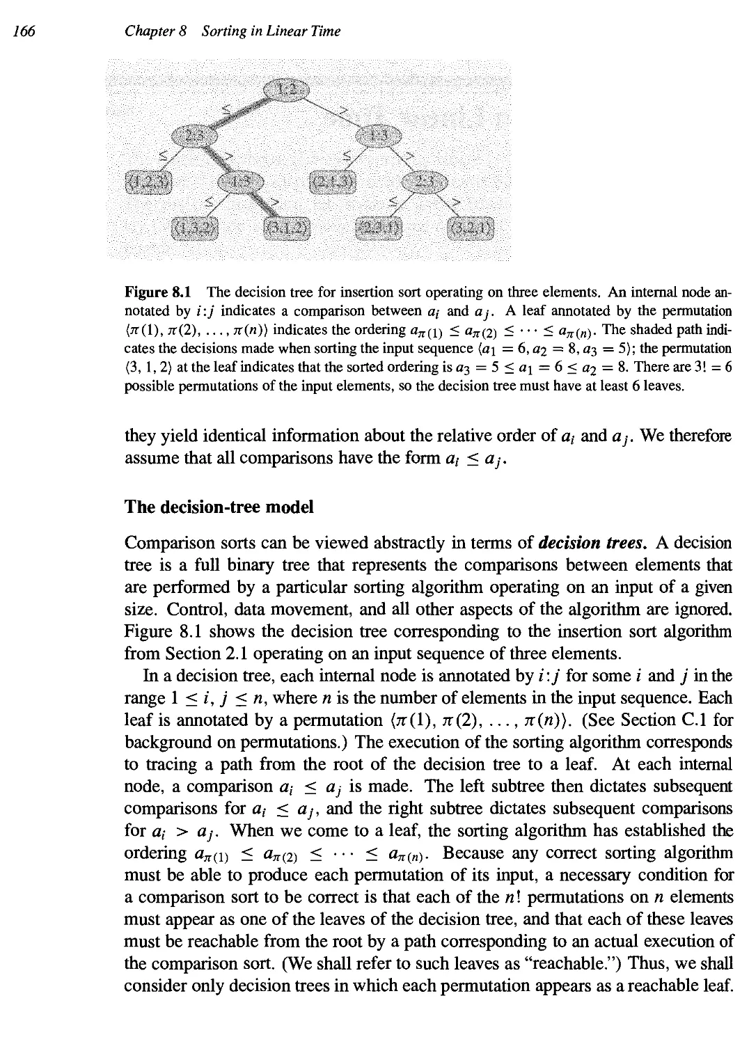
Figure 2.1 Sorting a hand of cards using insertion sort.
employ whatever expressive method is most clear and concise to specify a given al-
algorithm. Sometimes, the clearest method is English, so do not be surprised if you
come across an English phrase or sentence embedded within a section of "real"
code. Another difference between pseudocode and real code is that pseudocode
is not typically concerned with issues of software engineering. Issues of data ab-
abstraction, modularity, and error handling are often ignored in order to convey the
essence of the algorithm more concisely.
We start with insertion sort, which is an efficient algorithm for sorting a small
number of elements. Insertion sort works the way many people sort a hand of
playing cards. We start with an empty left hand and the cards face down on the
table. We then remove one card at a time from the table and insert it into the
correct position in the left hand. To find the correct position for a card, we compare
it with each of the cards already in the hand, from right to left, as illustrated in
Figure 2.1. At all times, the cards held in the left hand are sorted, and these cards
were originally the top cards of the pile on the table.
Our pseudocode for insertion sort is presented as a procedure called Insertion-
SORT, which takes as a parameter an array A[l.. n] containing a sequence of
length n that is to be sorted. (In the code, the number n of elements in Л is denoted
by length[A].) The input numbers are sorted in place: the numbers are rearranged
within the array A, with at most a constant number of them stored outside the
array at any time. The input array A contains the sorted output sequence when
Insertion-Sort is finished.

2.1 Insertion sort
(a)
(d) . : ' i 5 , .-> Di ' ' ! :; ■ 4 " n
Figure 2.2 The operation of Insertion-Sort on the array A = E, 2, 4, 6, 1, 3). Array indices
appear above the rectangles, and values stored in the array positions appear within the rectangles,
(a)-(e) The iterations of the for loop of lines 1-8. In each iteration, the black rectangle holds the
key taken from A[j], which is compared with the values in shaded rectangles to its left in the test of
line 5. Shaded arrows show array values moved one position to the right in line 6, and black arrows
indicate where the key is moved to in line 8. (f) The final sorted array.
Insertion-Sort (A)
1 for j <r- 2 to length[A]
2 do key «- A[j]
3 > Insert A [j] into the sorted sequence A[l.. j — 1].
4 ,•<_/_ l
5 while i > 0 and A[i] > key
6 do A[i + 1] <- A[i]
7 i <- i - 1
8 A[i + 1] <- key
Loop invariants and the correctness of insertion sort
Figure 2.2 shows how this algorithm works for A = E, 2, 4, 6, 1, 3). The in-
index j indicates the "current card" being inserted into the hand. At the beginning
of each iteration of the "outer" for loop, which is indexed by j, the subarray con-
consisting of elements A[l.. j — I] constitute the currently sorted hand, and elements
A[j + 1.. n] correspond to the pile of cards still on the table. In fact, elements
A[l.. j' — 1] are the elements originally in positions 1 through j — I, but now in
sorted order. We state these properties of A[l.. j' — 1] formally as a loop invariant:
At the start of each iteration of the for loop of lines 1-8, the subarray
A[l.. j — I] consists of the elements originally in A [1.. j; — 1] but in sorted
order.
We use loop invariants to help us understand why an algorithm is correct. We
must show three things about a loop invariant:

18 Chapter 2 Getting Started
Initialization: It is true prior to the first iteration of the loop.
Maintenance: If it is true before an iteration of the loop, it remains true before the
next iteration.
Termination: When the loop terminates, the invariant gives us a useful property
that helps show that the algorithm is correct.
When the first two properties hold, the loop invariant is true prior to every iteration
of the loop. Note the similarity to mathematical induction, where to prove that a
property holds, you prove a base case and an inductive step. Here, showing that
the invariant holds before the first iteration is like the base case, and showing that
the invariant holds from iteration to iteration is like the inductive step.
The third property is perhaps the most important one, since we are using the loop
invariant to show correctness. It also differs from the usual use of mathematical in-
induction, in which the inductive step is used infinitely; here, we stop the "induction"
when the loop terminates.
Let us see how these properties hold for insertion sort.
Initialization: We start by showing that the loop invariant holds before the first
loop iteration, when j = 2.1 The subarray A[l.. j — 1], therefore, consists
of just the single element A[l], which is in fact the original element in A[l].
Moreover, this subarray is sorted (trivially, of course), which shows that the
loop invariant holds prior to the first iteration of the loop.
Maintenance: Next, we tackle the second property: showing that each iteration
maintains the loop invariant. Informally, the body of the outer for loop works
by moving A[j — 1], A[j — 2], A[j — 3], and so on by one position to the right
until the proper position for A[j] is found (lines 4—7), at which point the value
of A [j] is inserted (line 8). A more formal treatment of the second property
would require us to state and show a loop invariant for the "inner" while loop.
At this point, however, we prefer not to get bogged down in such formalism,
and so we rely on our informal analysis to show that the second property holds
for the outer loop.
Termination: Finally, we examine what happens when the loop terminates. For
insertion sort, the outer for loop ends when j exceeds n, i.e., when j = n + 1.
Substituting n + 1 for j in the wording of loop invariant, we have that the
subarray A[l..n] consists of the elements originally in A [1.. и], but in sorted
1 When the loop is a for loop, the moment at which we check the loop invariant just prior to the first
iteration is immediately after the initial assignment to the loop-counter variable and just before the
first test in the loop header. In the case of INSERTION-SORT, this time is after assigning 2 to the
variable j but before the first test of whether j < length[A].

2.1 Insertion sort 19
order. But the subarray A[\.. n] is the entire array! Hence, the entire array is
sorted, which means that the algorithm is correct.
We shall use this method of loop invariants to show correctness later in this
chapter and in other chapters as well.
Pseudocode conventions
We use the following conventions in our pseudocode.
1. Indentation indicates block structure. For example, the body of the for loop
that begins on line 1 consists of lines 2-8, and the body of the while loop that
begins on line 5 contains lines 6-7 but not line 8. Our indentation style applies
to if-then-else statements as well. Using indentation instead of conventional
indicators of block structure, such as begin and end statements, greatly reduces
clutter while preserving, or even enhancing, clarity.2
2. The looping constructs while, for, and repeat and the conditional constructs
if, then, and else have interpretations similar to those in Pascal.3 There is one
subtle difference with respect to for loops, however: in Pascal, the value of the
loop-counter variable is undefined upon exiting the loop, but in this book, the
loop counter retains its value after exiting the loop. Thus, immediately after a
for loop, the loop counter's value is the value that first exceeded the for loop
bound. We used this property in our correctness argument for insertion sort.
The for loop header in line 1 is for j <— 2 to length[A], and so when this loop
terminates, j = length[A]+l (or, equivalently, j = n+l, since л = length[A]).
3. The symbol ">" indicates that the remainder of the line is a comment.
4. A multiple assignment of the form i <— j <— e assigns to both variables i and j
the value of expression e; it should be treated as equivalent to the assignment
j <— e followed by the assignment i <- j.
5. Variables (such as /, j, and key) are local to the given procedure. We shall not
use global variables without explicit indication.
6. Array elements are accessed by specifying the array name followed by the in-
index in square brackets. For example, A[i] indicates the /th element of the ar-
array A. The notation ".." is used to indicate a range of values within an ar-
2In real programming languages, it is generally not advisable to use indentation alone to indicate
block structure, since levels of indentation are hard to determine when code is split across pages.
3Most block-structured languages have equivalent constructs, though the exact syntax may differ
from that of Pascal.

20 Chapter 2 Getting Started
ray. Thus, A[\.. j] indicates the subarray of A consisting of the j elements
], A[2],...,
7. Compound data are typically organized into objects, which are composed of
attributes or fields. A particular field is accessed using the field name followed
by the name of its object in square brackets. For example, we treat an array as
an object with the attribute length indicating how many elements it contains. To
specify the number of elements in an array A, we write length[A]. Although we
use square brackets for both array indexing and object attributes, it will usually
be clear from the context which interpretation is intended.
A variable representing an array or object is treated as a pointer to the data
representing the array or object. For all fields / of an object x, setting у <— x
causes f[y] = f[x]. Moreover, if we now set f[x] <— 3, then afterward not
only is f[x] = 3, but f[y] = 3 as well. In other words, x and у point to the
same object after the assignment у <— x.
Sometimes, a pointer will refer to no object at all. In this case, we give it the
special value nil.
8. Parameters are passed to a procedure by value: the called procedure receives
its own copy of the parameters, and if it assigns a value to a parameter, the
change is not seen by the calling procedure. When objects are passed, the
pointer to the data representing the object is copied, but the object's fields are
not. For example, if л is a parameter of a called procedure, the assignment
x <— у within the called procedure is not visible to the calling procedure. The
assignment f[x] <— 3, however, is visible.
9. The boolean operators "and" and "or" are short circuiting. That is, when we
evaluate the expression "x and y" we first evaluate x. If x evaluates to FALSE,
then the entire expression cannot evaluate to TRUE, and so we do not evaluate y.
If, on the other hand, x evaluates to TRUE, we must evaluate у to determine the
value of the entire expression. Similarly, in the expression "x or y" we evaluate
the expression у only if x evaluates to FALSE. Short-circuiting operators allow
us to write boolean expressions such as "x Ф NIL and f[x] = y" without
worrying about what happens when we try to evaluate f[x] when x is NIL.
Exercises
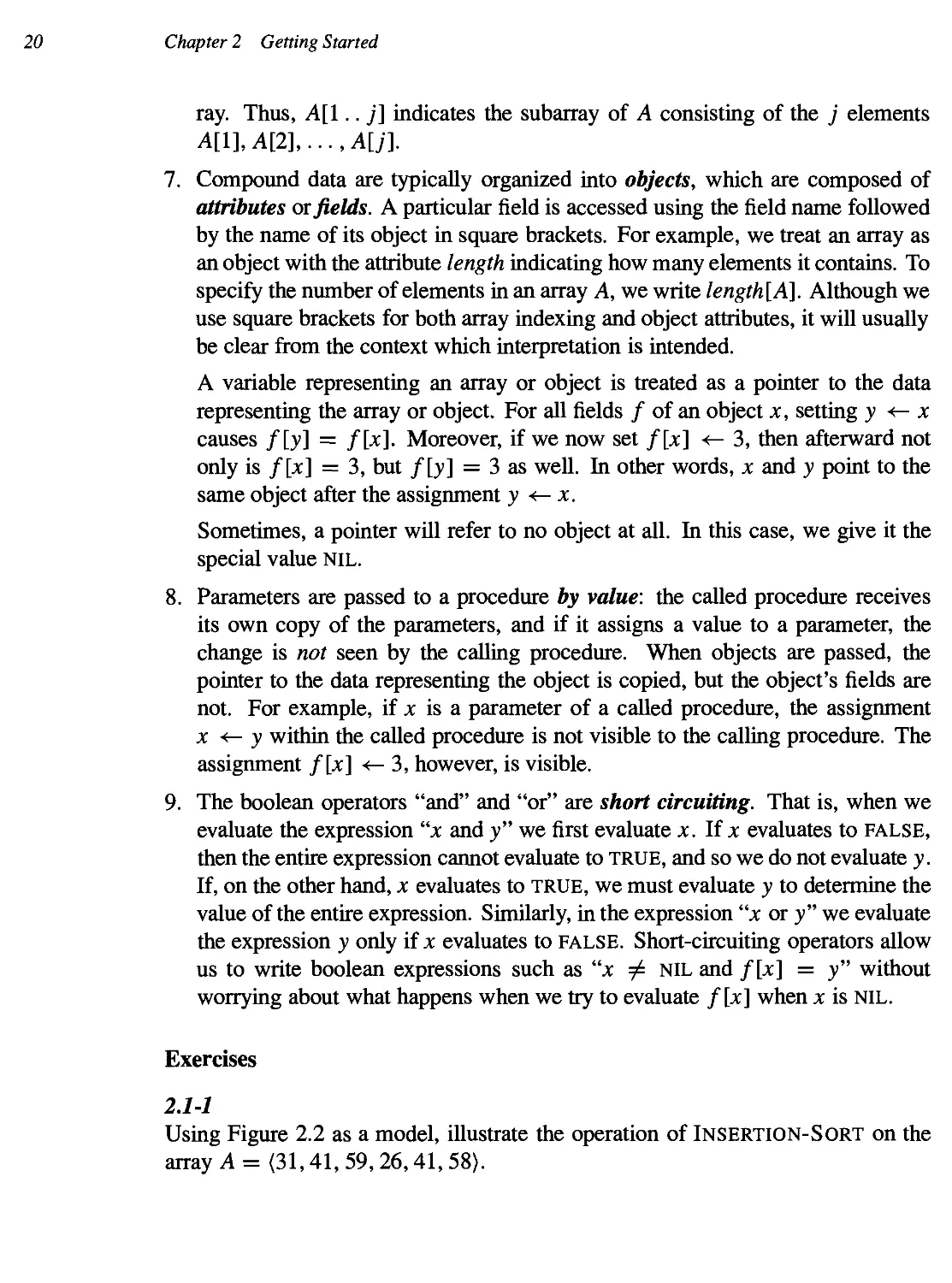
2.1-1
Using Figure 2.2 as a model, illustrate the operation of INSERTION-SORT on the
array A = C1,41, 59,26,41,58).

2.2 Analyzing algorithms 21
2.1-2
Rewrite the Insertion-Sort procedure to sort into nonincreasing instead of non-
decreasing order.
2.1-3
Consider the searching problem:
Input: A sequence of л numbers A = (a\, аг,..., an) and a value v.
Output: An index i such that v = A[i] or the special value NIL if v does not
appear in A.
Write pseudocode for linear search, which scans through the sequence, looking
for v. Using a loop invariant, prove that your algorithm is correct. Make sure that
your loop invariant fulfills the three necessary properties.
2.1-4
Consider the problem of adding two л-bit binary integers, stored in two л-element
arrays A and В. The sum of the two integers should be stored in binary form in
an (n + 1)-element array C. State the problem formally and write pseudocode for
adding the two integers.
2.2 Analyzing algorithms
Analyzing an algorithm has come to mean predicting the resources that the algo-
algorithm requires. Occasionally, resources such as memory, communication band-
bandwidth, or computer hardware are of primary concern, but most often it is compu-
computational time that we want to measure. Generally, by analyzing several candidate
algorithms for a problem, a most efficient one can be easily identified. Such anal-
analysis may indicate more than one viable candidate, but several inferior algorithms
are usually discarded in the process.
Before we can analyze an algorithm, we must have a model of the implemen-
implementation technology that will be used, including a model for the resources of that
technology and their costs. For most of this book, we shall assume a generic one-
processor, random-access machine (RAM) model of computation as our imple-
implementation technology and understand that our algorithms will be implemented as
computer programs. In the RAM model, instructions are executed one after an-
another, with no concurrent operations. In later chapters, however, we shall have
occasion to investigate models for digital hardware.
Strictly speaking, one should precisely define the instructions of the RAM model
and their costs. To do so, however, would be tedious and would yield little insight
into algorithm design and analysis. Yet we must be careful not to abuse the RAM

22 Chapter 2 Getting Started
model. For example, what if a RAM had an instruction that sorts? Then we could
sort in just one instruction. Such a RAM would be unrealistic, since real comput-
computers do not have such instructions. Our guide, therefore, is how real computers are
designed. The RAM model contains instructions commonly found in real com-
computers: arithmetic (add, subtract, multiply, divide, remainder, floor, ceiling), data
movement (load, store, copy), and control (conditional and unconditional branch,
subroutine call and return). Each such instruction takes a constant amount of time.
The data types in the RAM model are integer and floating point. Although we
typically do not concern ourselves with precision in this book, in some applications
precision is crucial. We also assume a limit on the size of each word of data. For
example, when working with inputs of size n, we typically assume that integers are
represented by clg n bits for some constant с > 1. We require с > 1 so that each
word can hold the value of n, enabling us to index the individual input elements,
and we restrict с to be a constant so that the word size does not grow arbitrarily. (If
the word size could grow arbitrarily, we could store huge amounts of data in one
word and operate on it all in constant time—clearly an unrealistic scenario.)
Real computers contain instructions not listed above, and such instructions rep-
represent a gray area in the RAM model. For example, is exponentiation a constant-
time instruction? In the general case, no; it takes several instructions to compute xy
when x and у are real numbers. In restricted situations, however, exponentiation is
a constant-time operation. Many computers have a "shift left" instruction, which
in constant time shifts the bits of an integer by к positions to the left. In most
computers, shifting the bits of an integer by one position to the left is equivalent to
multiplication by 2. Shifting the bits by к positions to the left is equivalent to mul-
multiplication by 2*. Therefore, such computers can compute 2* in one constant-time
instruction by shifting the integer 1 by A: positions to the left, as long as к is no more
than the number of bits in a computer word. We will endeavor to avoid such gray
areas in the RAM model, but we will treat computation of 2* as a constant-time
operation when к is a small enough positive integer.
In the RAM model, we do not attempt to model the memory hierarchy that is
common in contemporary computers. That is, we do not model caches or virtual
memory (which is most often implemented with demand paging). Several compu-
computational models attempt to account for memory-hierarchy effects, which are some-
sometimes significant in real programs on real machines. A handful of problems in this
book examine memory-hierarchy effects, but for the most part, the analyses in this
book will not consider them. Models that include the memory hierarchy are quite a
bit more complex than the RAM model, so that they can be difficult to work with.
Moreover, RAM-model analyses are usually excellent predictors of performance
on actual machines.
Analyzing even a simple algorithm in the RAM model can be a challenge. The
mathematical tools required may include combinatorics, probability theory, alge-

2.2 Analyzing algorithms 23
braic dexterity, and the ability to identify the most significant terms in a formula.
Because the behavior of an algorithm may be different for each possible input, we
need a means for summarizing that behavior in simple, easily understood formulas.
Even though we typically select only one machine model to analyze a given al-
algorithm, we still face many choices in deciding how to express our analysis. We
would like a way that is simple to write and manipulate, shows the important char-
characteristics of an algorithm's resource requirements, and suppresses tedious details.
Analysis of insertion sort
The time taken by the Insertion-Sort procedure depends on the input: sorting a
thousand numbers takes longer than sorting three numbers. Moreover, INSERTION-
SORT can take different amounts of time to sort two input sequences of the same
size depending on how nearly sorted they already are. In general, the time taken
by an algorithm grows with the size of the input, so it is traditional to describe the
running time of a program as a function of the size of its input. To do so, we need
to define the terms "running time" and "size of input" more carefully.
The best notion for input size depends on the problem being studied. For many
problems, such as sorting or computing discrete Fourier transforms, the most nat-
natural measure is the number of items in the input—for example, the array size n
for sorting. For many other problems, such as multiplying two integers, the best
measure of input size is the total number of bits needed to represent the input in
ordinary binary notation. Sometimes, it is more appropriate to describe the size of
the input with two numbers rather than one. For instance, if the input to an algo-
algorithm is a graph, the input size can be described by the numbers of vertices and
edges in the graph. We shall indicate which input size measure is being used with
each problem we study.
The running time of an algorithm on a particular input is the number of primitive
operations or "steps" executed. It is convenient to define the notion of step so
that it is as machine-independent as possible. For the moment, let us adopt the
following view. A constant amount of time is required to execute each line of our
pseudocode. One line may take a different amount of time than another line, but
we shall assume that each execution of the /th line takes time c,-, where c; is a
constant. This viewpoint is in keeping with the RAM model, and it also reflects
how the pseudocode would be implemented on most actual computers.4
4There are some subtleties here. Computational steps that we specify in English are often variants
of a procedure that requires more than just a constant amount of time. For example, later in this
book we might say "sort the points by x-coordinate," which, as we shall see, takes more than a
constant amount of time. Also, note that a statement that calls a subroutine takes constant time,
though the subroutine, once invoked, may take more. That is, we separate the process of calling the
subroutine—passing parameters to it, etc.—from the process of executing the subroutine.

24 Chapter 2 Getting Started
In the following discussion, our expression for the running time of Insertion-
Sort will evolve from a messy formula that uses all the statement costs c,- to a
much simpler notation that is more concise and more easily manipulated. This
simpler notation will also make it easy to determine whether one algorithm is more
efficient than another.
We start by presenting the INSERTION-SORT procedure with the time "cost"
of each statement and the number of times each statement is executed. For each
j = 2, 3,..., n, where n = length[A], we let tj be the number of times the while
loop test in line 5 is executed for that value of j. When a for or while loop exits in
the usual way (i.e., due to the test in the loop header), the test is executed one time
more than the loop body. We assume that comments are not executable statements,
and so they take no time.
Insertion-Sort (A) cost times
1 for j <— 2 to length[A] c\ n
2 do key <— A[j] сг п — \
3 > Insert A[j] into the sorted
sequence A[l.. j — 1]. 0 n — 1
4 i <- j — I c\ n — \
5 while i > 0 and A[i] > key C5 J2"j=2 h
6 do A[i + 1] <- A[i] c6 £5=2@-1)
7 i<-i-1 c7 £5=2@-1)
8 A[i + 1] «- key c8 n - 1
The running time of the algorithm is the sum of running times for each statement
executed; a statement that takes c,- steps to execute and is executed n times will
contribute ctn to the total running time.5 To compute T(n), the running time of
Insertion-Sort, we sum the products of the cost and times columns, obtaining
T(n) =
j=2 7=2
7=2
Even for inputs of a given size, an algorithm's running time may depend on
which input of that size is given. For example, in INSERTION-SORT, the best
5 This characteristic does not necessarily hold for a resource such as memory. A statement that
references m words of memory and is executed n times does not necessarily consume mn words of
memory in total.

2.2 Analyzing algorithms 25
case occurs if the array is already sorted. For each j = 2, 3,..., n, we then find
that A[i] < key in line 5 when / has its initial value of j — 1. Thus tj = 1 for
j =2,3,... ,n, and the best-case running time is
T(n) = сщ + c2(n - 1) + cA(n - 1) + c5(n - 1) + cs(n - 1)
- (C2 + CA + C5+ Cg) .
This running time can be expressed as an + b for constants a and Ь that depend on
the statement costs c,; it is thus a linear function of л.
If the array is in reverse sorted order—that is, in decreasing order—the worst
case results. We must compare each element A[j] with each element in the entire
sorted subarray A[l.. j — 1], and so tj = j for j =2,3,... ,n. Noting that
+ 1)
1
and
7=2 Z
(see Appendix A for a review of how to solve these summations), we find that in
the worst case, the running time of Insertion-Sort is
T(n) = сщ + c2(n - 1) + cA{n -
- 1J
C5 C6 C7
l+^ + C4 + y-y-T +
- (Q + c4 + c5 + c8) .
This worst-case running time can be expressed as an2 + bn + с for constants a, b,
and с that again depend on the statement costs c,; it is thus a quadratic function
of n.
Typically, as in insertion sort, the running time of an algorithm is fixed for a
given input, although in later chapters we shall see some interesting "randomized"
algorithms whose behavior can vary even for a fixed input.
Worst-case and average-case analysis
In our analysis of insertion sort, we looked at both the best case, in which the input
array was already sorted, and the worst case, in which the input array was reverse
sorted. For the remainder of this book, though, we shall usually concentrate on

26 Chapter 2 Getting Started
finding only the worst-case running time, that is, the longest running time for any
input of size n. We give three reasons for this orientation.
• The worst-case running time of an algorithm is an upper bound on the running
time for any input. Knowing it gives us a guarantee that the algorithm will never
take any longer. We need not make some educated guess about the running time
and hope that it never gets much worse.
• For some algorithms, the worst case occurs fairly often. For example, in search-
searching a database for a particular piece of information, the searching algorithm's
worst case will often occur when the information is not present in the database.
In some searching applications, searches for absent information may be fre-
frequent.
• The "average case" is often roughly as bad as the worst case. Suppose that we
randomly choose n numbers and apply insertion sort. How long does it take to
determine where in subarray A[\.. j — 1] to insert element A[j]l On average,
half the elements in A[l.. j — 1] are less than A[j], and half the elements are
greater. On average, therefore, we check half of the subarray A[l.. j — 1],
so tj is about j/2. The resulting average-case running time turns out to be a
quadratic function of the input size, just like the worst-case running time.
In some particular cases, we shall be interested in the average-case or expected
running time of an algorithm; in Chapter 5, we shall see the technique of prob-
probabilistic analysis, by which we determine expected running times. One problem
with performing an average-case analysis, however, is that it may not be apparent
what constitutes an "average" input for a particular problem. Often, we shall as-
assume that all inputs of a given size are equally likely. In practice, this assumption
may be violated, but we can sometimes use a randomized algorithm, which makes
random choices, to allow a probabilistic analysis.
Order of growth
We used some simplifying abstractions to ease our analysis of the INSERTION-
Sort procedure. First, we ignored the actual cost of each statement, using the
constants c,- to represent these costs. Then, we observed that even these constants
give us more detail than we really need: the worst-case running time is an2+bn+c
for some constants a, b, and с that depend on the statement costs c,-. We thus
ignored not only the actual statement costs, but also the abstract costs c,-.
We shall now make one more simplifying abstraction. It is the rate of growth,
or order of growth, of the running time that really interests us. We therefore con-
consider only the leading term of a formula (e.g., an2), since the lower-order terms
are relatively insignificant for large n. We also ignore the leading term's constant
coefficient, since constant factors are less significant than the rate of growth in

2.3 Designing algorithms 27
determining computational efficiency for large inputs. Thus, we write that inser-
insertion sort, for example, has a worst-case running time of ®(n2) (pronounced "theta
of л-squared"). We shall use 0-notation informally in this chapter; it will be de-
defined precisely in Chapter 3.
We usually consider one algorithm to be more efficient than another if its worst-
case running time has a lower order of growth. Due to constant factors and lower-
order terms, this evaluation may be in error for small inputs. But for large enough
inputs, a ®(n2) algorithm, for example, will run more quickly in the worst case
than a 0(л3) algorithm.
Exercises
2.2-1
Express the function л3/Ю00 - 100л2 - 100л + 3 in terms of 0-notation.
2.2-2
Consider sorting л numbers stored in array A by first finding the smallest element
of A and exchanging it with the element in A[l]. Then find the second smallest
element of A, and exchange it with A[2]. Continue in this manner for the first л — 1
elements of A. Write pseudocode for this algorithm, which is known as selection
sort. What loop invariant does this algorithm maintain? Why does it need to run
for only the first л — 1 elements, rather than for all л elements? Give the best-case
and worst-case running times of selection sort in 0-notation.
2.2-3
Consider linear search again (see Exercise 2.1-3). How many elements of the in-
input sequence need to be checked on the average, assuming that the element being
searched for is equally likely to be any element in the array? How about in the
worst case? What are the average-case and worst-case running times of linear
search in 0-notation? Justify your answers.
2.2-4
How can we modify almost any algorithm to have a good best-case running time?
2.3 Designing algorithms
There are many ways to design algorithms. Insertion sort uses an incremental ap-
approach: having sorted the subarray A[\.. j — 1], we insert the single element A[j]
into its proper place, yielding the sorted subarray A[l.. j].

28 Chapter 2 Getting Started
In this section, we examine an alternative design approach, known as "divide-
and-conquer." We shall use divide-and-conquer to design a sorting algorithm
whose worst-case running time is much less than that of insertion sort. One advan-
advantage of divide-and-conquer algorithms is that their running times are often easily
determined using techniques that will be introduced in Chapter 4.
2.3.1 The divide-and-conquer approach
Many useful algorithms are recursive in structure: to solve a given problem, they
call themselves recursively one or more times to deal with closely related sub-
problems. These algorithms typically follow a divide-and-conquer approach: they
break the problem into several subproblems that are similar to the original prob-
problem but smaller in size, solve the subproblems recursively, and then combine these
solutions to create a solution to the original problem.
The divide-and-conquer paradigm involves three steps at each level of the recur-
recursion:
Divide the problem into a number of subproblems.
Conquer the subproblems by solving them recursively. If the subproblem sizes
are small enough, however, just solve the subproblems in a straightforward
manner.
Combine the solutions to the subproblems into the solution for the original prob-
problem.
The merge sort algorithm closely follows the divide-and-conquer paradigm. In-
Intuitively, it operates as follows.
Divide: Divide the л-element sequence to be sorted into two subsequences of я/2
elements each.
Conquer: Sort the two subsequences recursively using merge sort.
Combine: Merge the two sorted subsequences to produce the sorted answer.
The recursion "bottoms out" when the sequence to be sorted has length 1, in which
case there is no work to be done, since every sequence of length 1 is already in
sorted order.
The key operation of the merge sort algorithm is the merging of two sorted se-
sequences in the "combine" step. To perform the merging, we use an auxiliary pro-
procedure MERGE(A, p, q, r), where Л is an array and p, q, and r are indices num-
numbering elements of the array such that p < q < r. The procedure assumes that the
subarrays A[p .. q] and A[q + 1.. r] are in sorted order. It merges them to form a
single sorted subarray that replaces the current subarray A[p .. r].
Our MERGE procedure takes time ®(n), where n = r — p + 1 is the number
of elements being merged, and it works as follows. Returning to our card-playing

2.3 Designing algorithms 29
motif, suppose we have two piles of cards face up on a table. Each pile is sorted,
with the smallest cards on top. We wish to merge the two piles into a single sorted
output pile, which is to be face down on the table. Our basic step consists of
choosing the smaller of the two cards on top of the face-up piles, removing it
from its pile (which exposes a new top card), and placing this card face down onto
the output pile. We repeat this step until one input pile is empty, at which time
we just take the remaining input pile and place it face down onto the output pile.
Computationally, each basic step takes constant time, since we are checking just
two top cards. Since we perform at most n basic steps, merging takes в (л) time.
The following pseudocode implements the above idea, but with an additional
twist that avoids having to check whether either pile is empty in each basic step.
The idea is to put on the bottom of each pile a sentinel card, which contains a
special value that we use to simplify our code. Here, we use oo as the sentinel
value, so that whenever a card with oo is exposed, it cannot be the smaller card
unless both piles have their sentinel cards exposed. But once that happens, all the
nonsentinel cards have already been placed onto the output pile. Since we know in
advance that exactly r — p + 1 cards will be placed onto the output pile, we can
stop once we have performed that many basic steps.
MERGE(A,p, q,r)
1 щ <-q — p + 1
2 n2<-r -q
3 create arrays L[\ ..щ + l] and R[l.. пг + 1]
4 for i <— 1 to Щ
5 do L[z] «-A[p + i - 1]
6 for j <— 1 tO «2
7 Ao R[j] ^ A[q + j]
8 L[ni + l]^oo
9 R[n2 + 1] <- oo
10 i «- 1
И У<-1
12 for к <r- p to r
13 do if L[i] < R[j]
14 then A[k] ^ L[i]
15 i «- i + 1
16 else A[k] «- R[j]
17 j <- j + 1
In detail, the MERGE procedure works as follows. Line 1 computes the length n\
of the subarray A[p..q], and line 2 computes the length пг of the subarray
A[q + l..r]. We create arrays L and R ("left" and "right"), of lengths гц + 1
and «2 + 1. respectively, in line 3. The for loop of lines 4-5 copies the subar-

30
Chapter 2 Getting Started
> W И Г I •' ' i ч
! ;,4! 5:1 7 П
i 2 4
Г:^;
)..,"
тГГаТзТ
/ • 2 i 4
(c)
(d)
Figure 2.3 The operation of lines 10-17 in the call Merge(A,9, 12, 16), when the subarray
A[9.. 16] contains the sequence B, 4, 5, 7, 1, 2, 3, 6). After copying and inserting sentinels, the
array L contains B, 4, 5, 7, oo), and the array R contains A, 2, 3, 6, oo). Lightly shaded positions
in A contain their final values, and lightly shaded positions in L and R contain values that have yet
to be copied back into A. Taken together, the lightly shaded positions always comprise the values
originally in A[9 .. 16], along with the two sentinels. Heavily shaded positions in A contain values
that will be copied over, and heavily shaded positions in L and R contain values that have already
been copied back into A. (a)-(h) The arrays A, L, and R, and their respective indices k,i, and j
prior to each iteration of the loop of lines 12-17. (i) The arrays and indices at termination. At this
point, the subarray in A [9.. 16] is sorted, and the two sentinels in L and R are the only two elements
in these arrays that have not been copied into A.
ray A[p .. q\ into L[l.. n{\, and the for loop of lines 6-7 copies the subarray
A[q + 1.. r] into R[l.. n2]. Lines 8-9 put the sentinels at the ends of the arrays L
and R. Lines 10-17, illustrated in Figure 2.3, perform the r — p + 1 basic steps by
maintaining the following loop invariant:
At the start of each iteration of the for loop of lines 12-17, the subarray
A[p .. к — 1] contains the к — p smallest elements of L[l.. n\ + 1] and
R[l.. n2 + 1], in sorted order. Moreover, L[i] and R[j] are the smallest
elements of their arrays that have not been copied back into A.
We must show that this loop invariant holds prior to the first iteration of the for
loop of lines 12-17, that each iteration of the loop maintains the invariant, and
that the invariant provides a useful property to show correctness when the loop
terminates.
Initialization: Prior to the first iteration of the loop, we have к = р, so that the
subarray A[p .. к — 1] is empty. This empty subarray contains the к — p = 0

2.3 Designing algorithms
31
A .. 1 ' 2 "l : *. '' t~F3 Гз'Г
4 ; 2 '• з; 6 .
/,■2.4.5
к • I : 2 I 3 ! о
И 2 j j : с
•; i i ,4 ,•, (.,
t 1 l .' И : 4 > , r. !
R ' '!,] 2 i 3 b
■4!5 i v
.2T4T5T7-
f 2 3!
(i)
smallest elements of L and R, and since i = j = I, both L[/] and /?|j] are the
smallest elements of their arrays that have not been copied back into A.
Maintenance: To see that each iteration maintains the loop invariant, let us first
suppose that L[i] < R[j]. Then L[i] is the smallest element not yet copied
back into A. Because A[p .. к — 1] contains the к — p smallest elements, after
line 14 copies L[i] into A[k], the subarray A[p .. k] will contain the к — p + 1
smallest elements. Incrementing к (in the for loop update) and i (in line 15)
reestablishes the loop invariant for the next iteration. If instead L[i] > R[j],
then lines 16-17 perform the appropriate action to maintain the loop invariant.
Termination: At termination, к = r + 1. By the loop invariant, the subarray
A[p .. к — 1], which is A[p .. r], contains the £ — p = r — p + I smallest
elements of L[l.. n\ + 1] and R[\.. пг + 1], in sorted order. The arrays L
and R together contain n\ + пг + 2 = r — p + Ъ elements. All but the two
largest have been copied back into A, and these two largest elements are the
sentinels.
To see that the Merge procedure runs in ©(и) time, where n = r — p + 1,
observe that each of lines 1-3 and 8-11 takes constant time, the for loops of

32 Chapter 2 Getting Started
lines 4-7 take ®(n\ + ni) = ©(л) time,6 and there are n iterations of the for
loop of lines 12-17, each of which takes constant time.
We can now use the MERGE procedure as a subroutine in the merge sort al-
algorithm. The procedure Merge-Sort(A, p, r) sorts the elements in the subar-
ray A[p ../•]. If p > r, the subarray has at most one element and is therefore
already sorted. Otherwise, the divide step simply computes an index q that par-
partitions A[p .. r] into two subarrays: A[p .. q], containing \n/2~\ elements, and
A[q + 1.. /•], containing [n/2\ elements.7
Merge-Sort(A, p, r)
1 if p < r
2 then q «- L(P + r)/2J
3 MERGE-SORT(A, p, q)
4 MERGE-SORT(A, q + 1, r)
5 MEKGE(A, p,q,r)
To sort the entire sequence A = (A[l], A[2], ..., A[n]), we make the initial call
MERGE-SORT(A, 1, length[A]), where once again length[A] = n. Figure 2.4 il-
illustrates the operation of the procedure bottom-up when л is a power of 2. The
algorithm consists of merging pairs of 1-item sequences to form sorted sequences
of length 2, merging pairs of sequences of length 2 to form sorted sequences of
length 4, and so on, until two sequences of length n/2 are merged to form the final
sorted sequence of length n.
2.3.2 Analyzing divide-and-conquer algorithms
When an algorithm contains a recursive call to itself, its running time can often
be described by a recurrence equation or recurrence, which describes the overall
running time on a problem of size n in terms of the running time on smaller inputs.
We can then use mathematical tools to solve the recurrence and provide bounds on
the performance of the algorithm.
A recurrence for the running time of a divide-and-conquer algorithm is based
on the three steps of the basic paradigm. As before, we let T(n) be the running
time on a problem of size n. If the problem size is small enough, say n < с
6We shall see in Chapter 3 how to formally interpret equations containing ©-notation.
7The expression |"*1 denotes the least integer greater than or equal to x, and |_*J denotes the greatest
integer less than or equal to x. These notations are denned in Chapter 3. The easiest way to verify
that setting q to |_(p + r)/2J yields subarrays A[p.. q] and A[q + 1.. r] of sizes ln/2] and |_«/2J,
respectively, is to examine the four cases that arise depending on whether each of p and r is odd or
even.

2.3 Designing algorithms 33
sorted sequence
llilliai sequence
Figure 2.4 The operation of merge sort on the array A = E, 2, 4, 7, 1, 3, 2, 6). The lengths of the
sorted sequences being merged increase as the algorithm progresses from bottom to top.
for some constant c, the straightforward solution takes constant time, which we
write as 0A). Suppose that our division of the problem yields a subproblems,
each of which is \/b the size of the original. (For merge sort, both a and b are 2,
but we shall see many divide-and-conquer algorithms in which а ф b.) If we
take D{n) time to divide the problem into subproblems and C{n) time to combine
the solutions to the subproblems into the solution to the original problem, we get
the recurrence
\ ifn<c,
\aT(n/b) + D(n) + С (л) otherwise .
In Chapter 4, we shall see how to solve common recurrences of this form.
Analysis of merge sort
Although the pseudocode for MERGE-SORT works correctly when the number of
elements is not even, our recurrence-based analysis is simplified if we assume that
the original problem size is a power of 2. Each divide step then yields two subse-
subsequences of size exactly и/2. In Chapter 4, we shall see that this assumption does
not affect the order of growth of the solution to the recurrence.

34 Chapter 2 Getting Started
We reason as follows to set up the recurrence for Г (л), the worst-case running
time of merge sort on л numbers. Merge sort on just one element takes constant
time. When we have л > 1 elements, we break down the running time as follows.
Divide: The divide step just computes the middle of the subarray, which takes
constant time. Thus, D(n) = ©A).
Conquer: We recursively solve two subproblems, each of size л/2, which con-
contributes 2Г (л/2) to the running time.
Combine: We have already noted that the MERGE procedure on an л-element
subarray takes time ©(л), so С (л) = ©(л).
When we add the functions D(n) and С (л) for the merge sort analysis, we are
adding a function that is ©(л) and a function that is ©A). This sum is a linear
function of л, that is, ©(л). Adding it to the 2Г(л/2) term from the "conquer"
step gives the recurrence for the worst-case running time T (л) of merge sort:
(©A) ifn = l,
1 W ~ }2Г(л/2) + ©(л) if л > 1 . K '
In Chapter 4, we shall see the "master theorem," which we can use to show that
Г (л) is ®(n\gri), where Ign stands for log2n. Because the logarithm function
grows more slowly than any linear function, for large enough inputs, merge sort,
with its ®(nlgn) running time, outperforms insertion sort, whose running time
is ©(л2), in the worst case.
We do not need the master theorem to intuitively understand why the solution to
the recurrence B.1) is T(n) = ©(л lg л). Let us rewrite recurrence B.1) as
iin= 1 ,
+ cn
where the constant с represents the time required to solve problems of size 1 as
well as the time per array element of the divide and combine steps.8
Figure 2.5 shows how we can solve the recurrence B.2). For convenience, we
assume that л is an exact power of 2. Part (a) of the figure shows Г (л), which
in part (b) has been expanded into an equivalent tree representing the recurrence.
The en term is the root (the cost at the top level of recursion), and the two subtrees
8It is unlikely that the same constant exactly represents both the time to solve problems of size 1
and the time per array element of the divide and combine steps. We can get around this problem by
letting с be the larger of these times and understanding that our recurrence gives an upper bound on
the running time, or by letting с be the lesser of these times and understanding that our recurrence
gives a lower bound on the running time. Both bounds will be on the order of я lg я and, taken
together, give a ®(n lgn) running time.

2.3 Designing algorithms
35
Цп)
cn/2
cn/2
T(n/2) T(n/2)
T(n/4) T(n/4) T(n/4) T(n/4)
(a) (b) (c)
lgn
■■in- СП
■■in- en
cn/4 cn/4 cn/4 cn/4 in- en
cn/2
cn/2
■■!!"■ en
(d)
Total: cn\gn + en
Figure 2.5 The construction of a recursion tree for the recurrence T(n) = 2T(n/2) + en.
Part (a) shows T(n), which is progressively expanded in (b)—(d) to form the recursion tree. The
fully expanded tree in part (d) has lg n + 1 levels (i.e., it has height lg n, as indicated), and each level
contributes a total cost of en. The total cost, therefore, is cnlgn + en, which is ®{n lg n).

36 Chapter 2 Getting Started
of the root are the two smaller recurrences T(л/2). Part (c) shows this process car-
carried one step further by expanding Г (л/2). The cost for each of the two subnodes
at the second level of recursion is сл/2. We continue expanding each node in the
tree by breaking it into its constituent parts as determined by the recurrence, until
the problem sizes get down to 1, each with a cost of c. Part (d) shows the resulting
tree.
Next, we add the costs across each level of the tree. The top level has total
cost en, the next level down has total cost с(л/2) + с(л/2) = en, the level after
that has total cost с(л/4) + с(л/4) + с(л/4) + с(л/4) = en, and so on. In general,
the level / below the top has 2' nodes, each contributing a cost of с(л/2'), so that
the /th level below the top has total cost 2' с(л/2') = ел. At the bottom level, there
are л nodes, each contributing a cost of c, for a total cost of en.
The total number of levels of the "recursion tree" in Figure 2.5 is lg л + 1. This
fact is easily seen by an informal inductive argument. The base case occurs when
л = 1, in which case there is only one level. Since lg 1 = 0, we have that lg л + 1
gives the correct number of levels. Now assume as an inductive hypothesis that the
number of levels of a recursion tree for 2' nodes is lg 2' + 1 = i + 1 (since for
any value of /, we have that lg 2' = i). Because we are assuming that the original
input size is a power of 2, the next input size to consider is 2'+1. A tree with 2'+1
nodes has one more level than a tree of 2' nodes, and so the total number of levels
is (i + 1) -h 1 =lg2'+1 + l.
To compute the total cost represented by the recurrence B.2), we simply add up
the costs of all the levels. There are lg л + 1 levels, each costing en, for a total cost
of cn(lgn + 1) = cnlgn + en. Ignoring the low-order term and the constant с
gives the desired result of ©(л lg л).
Exercises
2.3-1
Using Figure 2.4 as a model, illustrate the operation of merge sort on the array
A = C,41,52,26, 38, 57,9,49).
2.3-2
Rewrite the MERGE procedure so that it does not use sentinels, instead stopping
once either array L or R has had all its elements copied back to A and then copying
the remainder of the other array back into A.
2.3-3
Use mathematical induction to show that when л is an exact power of 2, the solution
of the recurrence

Problems for Chapter 2 37
T( [2 ifn = 2,
W \2T (л/2) + л if n = 2k, for к > 1
is Г (я) = nig л.
3
Insertion sort can be expressed as a recursive procedure as follows. In order to sort
A[l.. я], we recursively sort A[l.. я — 1] and then insert A[n] into the sorted array
A[l.. л — 1]. Write a recurrence for the running time of this recursive version of
insertion sort.
2.3-5
Referring back to the searching problem (see Exercise 2.1-3), observe that if the
sequence A is sorted, we can check the midpoint of the sequence against v and
eliminate half of the sequence from further consideration. Binary search is an
algorithm that repeats this procedure, halving the size of the remaining portion of
the sequence each time. Write pseudocode, either iterative or recursive, for binary
search. Argue that the worst-case running time of binary search is ©(lg я).
2.3-6
Observe that the while loop of lines 5 - 7 of the INSERTION-SORT procedure in
Section 2.1 uses a linear search to scan (backward) through the sorted subarray
A[l.. j — 1]. Can we use a binary search (see Exercise 2.3-5) instead to improve
the overall worst-case running time of insertion sort to ©(л lg л)?
2.3-7 *
Describe а ©(л lg л)-йте algorithm that, given a set S of л integers and another
integer x, determines whether or not there exist two elements in S whose sum is
exactly x.
Problems
2-1 Insertion sort on small arrays in merge sort
Although merge sort runs in ®(nlgn) worst-case time and insertion sort runs
in ©(л2) worst-case time, the constant factors in insertion sort make it faster for
small л. Thus, it makes sense to use insertion sort within merge sort when subprob-
lems become sufficiently small. Consider a modification to merge sort in which
n/k sublists of length к are sorted using insertion sort and then merged using the
standard merging mechanism, where к is a value to be determined.
a. Show that the n/k sublists, each of length k, can be sorted by insertion sort in
®(nk) worst-case time.

38 Chapter 2 Getting Started
b. Show that the sublists can be merged in ©(я lg(n/k)) worst-case time.
c. Given that the modified algorithm runs in ®(nk + n lg(n/k)) worst-case time,
what is the largest asymptotic (©-notation) value of k as a function of n for
which the modified algorithm has the same asymptotic running time as standard
merge sort?
d. How should к be chosen in practice?
2-2 Correctness ofbubblesort
Bubblesort is a popular sorting algorithm. It works by repeatedly swapping adja-
adjacent elements that are out of order.
Bubblesort (A)
1 for i <- 1 to length[A]
2 do for j ■<- length[A] downto i + 1
3 doifA[j]<A[j-l]
4 then exchange A[j] о A[j — 1]
a. Let A' denote the output of Bubblesort(A). To prove that BUBBLESORT is
correct, we need to prove that it terminates and that
A'[l] < A'[2] < < A'[n] , B.3)
where n = length[A]. What else must be proved to show that BUBBLESORT
actually sorts?
The next two parts will prove inequality B.3).
b. State precisely a loop invariant for the for loop in lines 2-4, and prove that this
loop invariant holds. Your proof should use the structure of the loop invariant
proof presented in this chapter.
c. Using the termination condition of the loop invariant proved in part (b), state
a loop invariant for the for loop in lines 1-4 that will allow you to prove in-
inequality B.3). Your proof should use the structure of the loop invariant proof
presented in this chapter.
d. What is the worst-case running time of bubblesort? How does it compare to the
running time of insertion sort?

Problems for Chapter 2 39
2-3 Correctness of Homer's rule
The following code fragment implements Homer's rule for evaluating a polynomial
P(x) =
= ao+x(ai +x{a2-\
given the coefficients ao,a\,... ,an and a value for x:
1 у <-0
2 i ^n
3 while i > 0
4 do у •«— a, + x • у
5 i «- i - 1
a. What is the asymptotic running time of this code fragment for Homer's rule?
b. Write pseudocode to implement the naive polynomial-evaluation algorithm that
computes each term of the polynomial from scratch. What is the running time
of this algorithm? How does it compare to Homer's rule?
c. Prove that the following is a loop invariant for the while loop in lines 3 —5.
At the start of each iteration of the while loop of lines 3-5,
n-O'+l)
Interpret a summation with no terms as equaling 0. Your proof should follow
the structure of the loop invariant proof presented in this chapter and should
show that, at termination, у = Yll=o akXk.
d. Conclude by arguing that the given code fragment correctly evaluates a poly-
polynomial characterized by the coefficients oq, a\,..., an.
2-4 Inversions
Let Л[1.. n] be an array of n distinct numbers. If i < j and A[i] > A[j], then the
pair (i, j) is called an inversion of A.
a. List the five inversions of the array B, 3, 8, 6,1).
b. What array with elements from the set {1,2,..., n] has the most inversions?
How many does it have?

40 Chapter 2 Getting Started
c. What is the relationship between the running time of insertion sort and the
number of inversions in the input array? Justify your answer.
d. Give an algorithm that determines the number of inversions in any permutation
on n elements in &(n lgn) worst-case time. (Hint: Modify merge sort.)
Chapter notes
In 1968, Knuth published the first of three volumes with the general title The Art of
Computer Programming [182, 183, 185]. The first volume ushered in the modern
study of computer algorithms with a focus on the analysis of running time, and the
full series remains an engaging and worthwhile reference for many of the topics
presented here. According to Knuth, the word "algorithm" is derived from the
name "al-Khowarizmi," a ninth-century Persian mathematician.
Aho, Hopcroft, and Ullman [5] advocated the asymptotic analysis of algorithms
as a means of comparing relative performance. They also popularized the use of
recurrence relations to describe the running times of recursive algorithms.
Knuth [185] provides an encyclopedic treatment of many sorting algorithms. His
comparison of sorting algorithms (page 381) includes exact step-counting analyses,
like the one we performed here for insertion sort. Knuth's discussion of insertion
sort encompasses several variations of the algorithm. The most important of these
is Shell's sort, introduced by D. L. Shell, which uses insertion sort on periodic
subsequences of the input to produce a faster sorting algorithm.
Merge sort is also described by Knuth. He mentions that a mechanical colla-
collator capable of merging two decks of punched cards in a single pass was invented
in 1938. J. von Neumann, one of the pioneers of computer science, apparently
wrote a program for merge sort on the EDVAC computer in 1945.
The early history of proving programs correct is described by Giles [133], who
credits P. Naur with the first article in this field. Giles attributes loop invariants to
R. W. Floyd. The textbook by Mitchell [222] describes more recent progress in
proving programs correct.

Growth of Functions
The order of growth of the running time of an algorithm, denned in Chapter 2,
gives a simple characterization of the algorithm's efficiency and also allows us to
compare the relative performance of alternative algorithms. Once the input size n
becomes large enough, merge sort, with its 0(nlgn) worst-case running time,
beats insertion sort, whose worst-case running time is 0(n2). Although we can
sometimes determine the exact running time of an algorithm, as we did for insertion
sort in Chapter 2, the extra precision is not usually worth the effort of computing
it. For large enough inputs, the multiplicative constants and lower-order terms of
an exact running time are dominated by the effects of the input size itself.
When we look at input sizes large enough to make only the order of growth of
the running time relevant, we are studying the asymptotic efficiency of algorithms.
That is, we are concerned with how the running time of an algorithm increases with
the size of the input in the limit, as the size of the input increases without bound.
Usually, an algorithm that is asymptotically more efficient will be the best choice
for all but very small inputs.
This chapter gives several standard methods for simplifying the asymptotic anal-
analysis of algorithms. The next section begins by denning several types of "asymptotic
notation," of which we have already seen an example in ©-notation. Several no-
tational conventions used throughout this book are then presented, and finally we
review the behavior of functions that commonly arise in the analysis of algorithms.
3.1 Asymptotic notation
The notations we use to describe the asymptotic running time of an algorithm
are denned in terms of functions whose domains are the set of natural numbers
N = {0, 1, 2,...}. Such notations are convenient for describing the worst-case
running-time function T(n), which is usually denned only on integer input sizes.
It is sometimes convenient, however, to abuse asymptotic notation in a variety of

42 Chapter 3 Growth of Functions
ways. For example, the notation is easily extended to the domain of real numbers
or, alternatively, restricted to a subset of the natural numbers. It is important, how-
however, to understand the precise meaning of the notation so that when it is abused, it
is not misused. This section defines the basic asymptotic notations and also intro-
introduces some common abuses.
0-notation
In Chapter 2, we found that the worst-case running time of insertion sort is
T{ri) = &(n2). Let us define what this notation means. For a given function g(n),
we denote by ®(g(n)) the set of functions
®(g(n)) = {/(«) : there exist positive constants c\, сг, and щ such that
0 < cig{n) < fin) < c2g(n) for all n > n0] -1
A function f(n) belongs to the set ®(g(n)) if there exist positive constants c\
and C2 such that it can be "sandwiched" between c\g(n) and C2g(n), for suffi-
sufficiently large n. Because ®(g(n)) is a set, we could write "/(") e ©CgOO)"
to indicate that f(n) is a member of 0(g(n)). Instead, we will usually write
"f(n) = ®(g(n))" to express the same notion. This abuse of equality to denote
set membership may at first appear confusing, but we shall see later in this section
that it has advantages.
Figure 3.1(a) gives an intuitive picture of functions f(n) and g(n), where we
have that f(n) = ®(g(n)). For all values of n to the right of щ, the value of f(n)
lies at or above c\g(ri) and at or below C2g(n). In other words, for all n > щ, the
function f{n) is equal to g(n) to within a constant factor. We say that g(n) is an
asymptotically tight bound for f(n).
The definition of ®(g(n)) requires that every member f(n) e ®(g(n)) be
asymptotically nonnegative, that is, that f(n) be nonnegative whenever n is suf-
sufficiently large. (An asymptotically positive function is one that is positive for all
sufficiently large n.) Consequently, the function g(n) itself must be asymptotically
nonnegative, or else the set ®(g(n)) is empty. We shall therefore assume that every
function used within 0-notation is asymptotically nonnegative. This assumption
holds for the other asymptotic notations defined in this chapter as well.
In Chapter 2, we introduced an informal notion of 0-notation that amounted
to throwing away lower-order terms and ignoring the leading coefficient of the
highest-order term. Let us briefly justify this intuition by using the formal def-
definition to show that \n2 — Ъп = ®(n2). To do so, we must determine positive
constants c\, C2, and no such that
1 Within set notation, a colon should be read as "such that."

3.1 Asymptotic notation
43
cgin)
/(и) = e(g(n))
(a)
/(и) = 0(*(и))
(b)
Figure 3.1 Graphic examples of the 0, О, and Й notations. In each part, the value of /iq shown is
the minimum possible value; any greater value would also work, (a) ©-notation bounds a function to
within constant factors. We write fin) = ®(g(n)) if there exist positive constants no, c\, and ci such
that to the right of щ, the value of fin) always lies between c\g(ri) and C2g(n) inclusive, (b) O-
notation gives an upper bound for a function to within a constant factor. We write fin) = O(g(n))
if there are positive constants no and с such that to the right of no, the value of /(n) always lies on
or below cgin). (c) й-notation gives a lower bound for a function to within a constant factor. We
write fin) = tligin)) if there are positive constants no and с such that to the right of no, the value
of fin) always lies on or above cgin).
СЩ2 < -n2 - Ъп < С2П2
for all n > «o- Dividing by n2 yields
1 3
c\ < - - - < c2 .
2 n
The right-hand inequality can be made to hold for any value of n > 1 by choosing
C2 > 1/2- Likewise, the left-hand inequality can be made to hold for any value
of и > 7 by choosing c\ < 1/14. Thus, by choosing c\ = 1/14, ci = 1/2, and
n0 = 7, we can verify that ^n2 — Ъп = 0(n2). Certainly, other choices for the
constants exist, but the important thing is that some choice exists. Note that these
constants depend on the function ^n2 — Ъп; a different function belonging to 0(n2)
would usually require different constants.
We can also use the formal definition to verify that 6n3 ф 0(n2). Suppose for
the purpose of contradiction that сг and щ exist such that 6n3 < сгп2 for all n > no-
But then n < C2/6, which cannot possibly hold for arbitrarily large n, since сг is
constant.
Intuitively, the lower-order terms of an asymptotically positive function can be
ignored in determining asymptotically tight bounds because they are insignificant
for large n. A tiny fraction of the highest-order term is enough to dominate the

44 Chapter 3 Growth of Functions
lower-order terms. Thus, setting c\ to a value that is slightly smaller than the co-
coefficient of the highest-order term and setting сг to a value that is slightly larger
permits the inequalities in the definition of ©-notation to be satisfied. The coef-
coefficient of the highest-order term can likewise be ignored, since it only changes c\
and сг by a constant factor equal to the coefficient.
As an example, consider any quadratic function f(n) = an2 + bn + c, where
a, b, and с are constants and a > 0. Throwing away the lower-order terms and
ignoring the constant yields f{n) = 0(n2). Formally, to show the same thing, we
take the constants c\ = a/A, сг = la/A, and щ = 2-max((|&| /a), V(H /a))- The
reader may verify that 0 < c\n2 < an2 + bn + c < сгп2 for all n > щ. In general,
for any polynomial p{ri) = Yl1=o a'n'' wnere me a\ WQ constants and ad > 0, we
have p(n) = &(nd) (see Problem 3-1).
Since any constant is a degree-0 polynomial, we can express any constant func-
function as 0(n°), or 0A). This latter notation is a minor abuse, however, because it is
not clear what variable is tending to infinity.2 We shall often use the notation 0A)
to mean either a constant or a constant function with respect to some variable.
О-notation
The 0-notation asymptotically bounds a function from above and below. When
we have only an asymptotic upper bound, we use О -notation. For a given func-
function g(n), we denote by O(g(n)) (pronounced "big-oh of g of n" or sometimes just
"oh of g of n") the set of functions
O(g(n)) = {/(«) : there exist positive constants с and щ such that
0 < f(n) < cg(n) for all n > щ] ■
We use О -notation to give an upper bound on a function, to within a constant
factor. Figure 3.1 (b) shows the intuition behind О -notation. For all values n to the
right of щ, the value of the function f{n) is on or below cg{n).
We write f(n) = O(g(n)) to indicate that a function f(n) is a member of
the set O(g(n)). Note that f(n) = &(g(n)) implies f(n) = O(g(n)), since 0-
notation is a stronger notion than О -notation. Written set-theoretically, we have
®(g(n)) Я O(g(n)). Thus, our proof that any quadratic function an2 + bn + c,
where a > 0, is in 0(n2) also shows that any such quadratic function is in 0{n2).
What may be more surprising is that any linear function an + b is in О (и2), which
is easily verified by taking с = a + \b\ and щ = 1.
The real problem is that our ordinary notation for functions does not distinguish functions from
values. In Я-calculus, the parameters to a function are clearly specified: the function n2 could be
written as kn.n2, or even Xr.r2. Adopting a more rigorous notation, however, would complicate
algebraic manipulations, and so we choose to tolerate the abuse.

3.1 Asymptotic notation 45
Some readers who have seen О -notation before may find it strange that we
should write, for example, n = O(n2). In the literature, О-notation is sometimes
used informally to describe asymptotically tight bounds, that is, what we have de-
defined using ©-notation. In this book, however, when we write f(n) = O(g(n)),
we are merely claiming that some constant multiple of g(n) is an asymptotic upper
bound on /(«), with no claim about how tight an upper bound it is. Distinguish-
Distinguishing asymptotic upper bounds from asymptotically tight bounds has now become
standard in the algorithms literature.
Using О -notation, we can often describe the running time of an algorithm
merely by inspecting the algorithm's overall structure. For example, the doubly
nested loop structure of the insertion sort algorithm from Chapter 2 immediately
yields an О (и2) upper bound on the worst-case running time: the cost of each it-
iteration of the inner loop is bounded from above by 0A) (constant), the indices i
and j are both at most n, and the inner loop is executed at most once for each of
the n2 pairs of values for i and j.
Since О -notation describes an upper bound, when we use it to bound the worst-
case running time of an algorithm, we have a bound on the running time of the
algorithm on every input. Thus, the О (и2) bound on worst-case running time of
insertion sort also applies to its running time on every input. The 0(n2) bound
on the worst-case running time of insertion sort, however, does not imply a 0 (n2)
bound on the running time of insertion sort on every input. For example, we saw
in Chapter 2 that when the input is already sorted, insertion sort runs in 0(n) time.
Technically, it is an abuse to say that the running time of insertion sort is 0(n2),
since for a given n, the actual running time varies, depending on the particular
input of size n. When we say "the running time is 0(n2)" we mean that there is a
function f(n) that is 0{n2) such that for any value of n, no matter what particular
input of size n is chosen, the running time on that input is bounded from above by
the value f(n). Equivalently, we mean that the worst-case running time is 0{n2).
ft-notation
Just as (9-notation provides an asymptotic upper bound on a function, fi-notation
provides an asymptotic lower bound. For a given function g(n), we denote by
& (g(n)) (pronounced "big-omega of g of n" or sometimes just "omega of g of n")
the set of functions
fi(g(n)) = {/(n) : there exist positive constants с and щ such that
0 < cg(n) < f(n) for all n > n0} •
The intuition behind fi-notation is shown in Figure 3.1(c). For all values n to the
right of щ, the value of f(n) is on or above cg{n).
From the definitions of the asymptotic notations we have seen thus far, it is easy
to prove the following important theorem (see Exercise 3.1-5).

46 Chapter 3 Growth of Functions
Theorem 3.1
For any two functions f(n) and g(n), we have f(n) = 0(g(n)) if and only if
/(л) = O(g(n)) and /(л) =
As an example of the application of this theorem, our proof that an2 + bn + c =
0(n2) for any constants a, b, and c, where a > 0, immediately implies that
an2 + bn + с = fi (n2) and an2 + bn + с = 0{n2). In practice, rather than using
Theorem 3.1 to obtain asymptotic upper and lower bounds from asymptotically
tight bounds, as we did for this example, we usually use it to prove asymptotically
tight bounds from asymptotic upper and lower bounds.
Since fi-notation describes a lower bound, when we use it to bound the best-case
running time of an algorithm, by implication we also bound the running time of the
algorithm on arbitrary inputs as well. For example, the best-case running time of
insertion sort is п (и), which implies that the running time of insertion sort is fi (n).
The running time of insertion sort therefore falls between fi(n) and 0{n2), since
it falls anywhere between a linear function of n and a quadratic function of n.
Moreover, these bounds are asymptotically as tight as possible: for instance, the
running time of insertion sort is not Q{n2), since there exists an input for which
insertion sort runs in 0(n) time (e.g., when the input is already sorted). It is not
contradictory, however, to say that the worst-case running time of insertion sort
is fi(n2), since there exists an input that causes the algorithm to take Q(n2) time.
When we say that the running time (no modifier) of an algorithm is fi(g(n)), we
mean that no matter what particular input of size n is chosen for each value of n,
the running time on that input is at least a constant times g{n), for sufficiently
large n.
Asymptotic notation in equations and inequalities
We have already seen how asymptotic notation can be used within mathematical
formulas. For example, in introducing О -notation, we wrote "n = O(n2)." We
might also write 2n2 + Ъп + 1 = 2n2 + ®(n). How do we interpret such formulas?
When the asymptotic notation stands alone on the right-hand side of an equation
(or inequality), as in n = О (и2), we have already denned the equal sign to mean set
membership: n e 0{n2). In general, however, when asymptotic notation appears
in a formula, we interpret it as standing for some anonymous function that we do
not care to name. For example, the formula 2n2 + Ъп + 1 = 2n2 + 0(n) means
that 2n2 + Ъп + 1 = 2n2 + f(n), where f(n) is some function in the set 0(n). In
this case, f{n) = Ъп + 1, which indeed is in 0(n).
Using asymptotic notation in this manner can help eliminate inessential detail
and clutter in an equation. For example, in Chapter 2 we expressed the worst-case
running time of merge sort as the recurrence

3.1 Asymptotic notation 47
If we are interested only in the asymptotic behavior of T(n), there is no point in
specifying all the lower-order terms exactly; they are all understood to be included
in the anonymous function denoted by the term ®(n).
The number of anonymous functions in an expression is understood to be equal
to the number of times the asymptotic notation appears. For example, in the ex-
expression
there is only a single anonymous function (a function of i). This expression is thus
not the same as 0A) + 0B) + • • • + O(n), which doesn't really have a clean
interpretation.
In some cases, asymptotic notation appears on the left-hand side of an equation,
as in
We interpret such equations using the following rule: No matter how the anony-
anonymous functions are chosen on the left of the equal sign, there is a way to choose
the anonymous functions on the right of the equal sign to make the equation valid.
Thus, the meaning of our example is that for any function f(n) e ®(n), there
is some function g(n) e ®(n2) such that 2n2 + f(n) = g(n) for all n. In other
words, the right-hand side of an equation provides a coarser level of detail than the
left-hand side.
A number of such relationships can be chained together, as in
2n2 + Ъп + 1 = 2n2 + ®(n)
We can interpret each equation separately by the rule above. The first equation says
that there is some function f(n) e ®(n) such that 2n2 + Ъп + 1 = 2n2 + f(n) for
all n. The second equation says that for any function g(n) e ®(n) (such as the f(n)
just mentioned), there is some function h(n) e ®(n2) such that 2n2 + g(n) = h(n)
for all n. Note that this interpretation implies that 2n2 + Ъп + 1 = ®(n2), which is
what the chaining of equations intuitively gives us.
0-notation
The asymptotic upper bound provided by О -notation may or may not be asymp-
asymptotically tight. The bound 2n2 = O(n2) is asymptotically tight, but the bound
2n = О (n2) is not. We use o-notation to denote an upper bound that is not asymp-
asymptotically tight. We formally define o(g(n)) ("little-oh of g of n") as the set

48 Chapter 3 Growth of Functions
o(g(n)) = {/(«) : for any positive constant с > 0, there exists a constant
«o > 0 such that 0 < f(n) < cg(n) for all n > no} •
For example, 2n = o(n2), but 2n2 ^ o(n2).
The definitions of О -notation and o-notation are similar. The main difference is
that in f(n) = O(g(n)), the bound 0 < f(n) < cg(n) holds for some constant
с > 0, but in f(n) = o(g(n)), the bound 0 < f(n) < cg(n) holds for all con-
constants с > 0. Intuitively, in the o-notation, the function f(n) becomes insignificant
relative to g(n) as n approaches infinity; that is,
limM = 0. C.1)
n^oo g(n)
Some authors use this limit as a definition of the o-notation; the definition in this
book also restricts the anonymous functions to be asymptotically nonnegative.
«-notation
By analogy, «-notation is to fi-notation as o-notation is to (9-notation. We use
«-notation to denote a lower bound that is not asymptotically tight. One way to
define it is by
f(n) e co(g(n)) if and only if g(n) e o(f(n)).
Formally, however, we define a>(g(n)) ("little-omega of g of n") as the set
origin)) = {/(«) : for any positive constant с > 0, there exists a constant
«o > 0 such that 0 < cg(n) < f(n) for all n > щ} •
For example, «2/2 = co(n), but и2/2 ф со(п2). The relation f(n) = (o(g(n))
implies that
,. fin)
Inn ——- = oo ,
n^o g(n)
if the limit exists. That is, f(n) becomes arbitrarily large relative to g(n) as n
approaches infinity.
Comparison of functions
Many of the relational properties of real numbers apply to asymptotic comparisons
as well. For the following, assume that f(n) and g(n) are asymptotically positive.

3.1 Asymptotic notation
49
Transitivity:
fin) = ®(g(n)) and gin)
fin) = Oigin)) and gin)
fin) = U(g(n)) and g(n)
fin) = o(g(n)) and g(n)
fin) = co(g(n)) and gin)
®(h(n)) imply fin) = S(h(n)),
0{h(n)) imply f{n) = 0{h{n)),
П(п(п)) imply f(n) = n(h(n)),
o(h(n)) imply f(n) = o(h(n)) ,
(x)(h(ri)) imply f(n) = a>(h(n)) .
Reflexivity:
f{n) =
f{n) = Oifin)),
fin) = П(/(л)).
Symmetry:
fin) = Sigin)) if and only if gin) = Sifin)) .
Transpose symmetry:
f(n) = Oigin)) if and only if gin) = Uifin)),
fin) = oigin)) if and only if gin) = coif in)).
Because these properties hold for asymptotic notations, one can draw an analogy
between the asymptotic comparison of two functions / and g and the comparison
of two real numbers a and b:
fin) = Oigin)) я
fin) = fi(g(n)) -
/(л) = eigin)) s
/(л) = o(g(n)) s
/(Л) = <В(«(Л)) S
« a <b,
« a >b,
« a = b,
« a <b ,
« a > b .
We say that fin) is asymptotically smaller than gin) if fin) = oigin)), and fin)
is asymptotically larger than gin) if fin) = coigin)).
One property of real numbers, however, does not carry over to asymptotic nota-
notation:
Trichotomy: For any two real numbers a and b, exactly one of the following must
hold: a < b, a = b, or a > b.

50 Chapter 3 Growth of Functions
Although any two real numbers can be compared, not all functions are asymptoti-
asymptotically comparable. That is, for two functions f(n) and g(n), it may be the case that
neither f(n) = O(g(n)) nor f(n) = fi(g(n)) holds. For example, the functions n
and n1+sm" cannot be compared using asymptotic notation, since the value of the
exponent in n1+sm" oscillates between 0 and 2, taking on all values in between.
Exercises
3.1-1
Let f{n) and g(n) be asymptotically nonnegative functions. Using the basic defi-
definition of ©-notation, prove that max(/(n), g(n)) = ©(/(«) + g(n)).
3.1-2
Show that for any real constants a and b, where b > 0,
(n + a)b = S(nb). C.2)
3.1-3
Explain why the statement, "The running time of algorithm A is at least O(n2)," is
meaningless.
3.1-4
Is 2n+1 = 0B")? Is 22n = 0B")?
3.1-5
Prove Theorem 3.1.
3.1-6
Prove that the running time of an algorithm is ®(g(n)) if and only if its worst-case
running time is O(g(n)) and its best-case running time is fi (g(n)).
3.1-7
Prove that o(g(n)) П a>(g(n)) is the empty set.
3.1-8
We can extend our notation to the case of two parameters n and m that can go to
infinity independently at different rates. For a given function g(n, m), we denote
by 0(g(n,m)) the set of functions
O(g(n, m)) = {f(n, m) : there exist positive constants с, щ, and mo
such that 0 < f(n, m) < cg(n, m)
for all n > «o and m > mo).
Give corresponding definitions for Q(g(n, m)) and ®(g(n,m)).

3.2 Standard notations and common functions 51
3.2 Standard notations and common functions
This section reviews some standard mathematical functions and notations and ex-
explores the relationships among them. It also illustrates the use of the asymptotic
notations.
Monotonicity
A function f{ri) is monotonically increasing if m < n implies f(m) < f(n).
Similarly, it is monotonically decreasing if m < n implies f{m) > f{n). A
function f{n) is strictly increasing if m < n implies f(m) < f(n) and strictly
decreasing if m < n implies f{m) > f{ri).
Floors and ceilings
For any real number x, we denote the greatest integer less than or equal to x by |_*J
(read "the floor of x") and the least integer greater than or equal to x by \x~\ (read
"the ceiling of x"). For all real x,
x - 1 < L*J < x < [jcl < x + 1 . C.3)
For any integer n,
Гл/21 + L«/2J = n ,
and for any real number n > 0 and integers a, b > 0,
Un/d] /Ы = \n/ab\ , C.4)
VVn/a\/b\ = [n/abj , C.5)
\a/b\ < (a + (b-l))/b, C.6)
la/b} > (a-(b-l))/b. C.7)
The floor function f(x) = [jcJ is monotonically increasing, as is the ceiling func-
function f{x) = M.
Modular arithmetic
For any integer a and any positive integer n, the value a mod n is the remainder
(or residue) of the quotient a/n:
a mod n = a — \_a/n\ n . C.8)
Given a well-defined notion of the remainder of one integer when divided by an-
another, it is convenient to provide special notation to indicate equality of remainders.

52 Chapter 3 Growth of Functions
If (a mod n) = (b mod n), we write a = b (mod n) and say that a is equivalent
to b, modulo n. In other words, a = b (mod n) if a and & have the same remainder
when divided by n. Equivalently, a = b (mod n) if and only if и is a divisor of
b — a. We write а ф b (mod n) if a is not equivalent to b, modulo n.
Polynomials
Given a nonnegative integer d, a polynomial in n of degree d is a function p(n) of
the form
p(n) = yjtf;ft' ,
;=o
where the constants ao, a\,... ,ad are the coefficients of the polynomial and
ad ф 0. A polynomial is asymptotically positive if and only if ад > 0. For an
asymptotically positive polynomial p{n) of degree d, we have p(n) = ®(nd). For
any real constant a > 0, the function na is monotonically increasing, and for any
real constant a < 0, the function na is monotonically decreasing. We say that a
function f(n) ispolynomially bounded if /(n) = <2(nfc) for some constant k.
Exponentials
For all real a > 0, m, and n, we have the following identities:
a° = 1,
a = I/a,
(am)" = am" ,
(am)n = (an)m ,
aman = am+n .
For all n and a > 1, the function a" is monotonically increasing in n. When
convenient, we shall assume 0° = 1.
The rates of growth of polynomials and exponentials can be related by the fol-
following fact. For all real constants a and b such that a > 1,
nb
lim — = 0 , C.9)
a"
from which we can conclude that
nb = o(an) .
Thus, any exponential function with a base strictly greater than 1 grows faster than
any polynomial function.

3.2 Standard notations and common functions 53
Using e to denote 2.71828..., the base of the natural logarithm function, we
have for all real x,
Y2 3 oo i
L. J. ,=0 I.
where "!" denotes the factorial function denned later in this section. For all real x,
we have the inequality
e*>l+x, C.11)
where equality holds only when x = 0. When |jc| < 1, we have the approximation
l+x<ex<l+x+x2. C.12)
When x —*■ 0, the approximation of ex by 1 + x is quite good:
e* = l+x + 0(x2) .
(In this equation, the asymptotic notation is used to describe the limiting behavior
as x -> 0 rather than as x -> oo.) We have for all x,
lim A + -)" = e* . C.13)
n-s-oo V n'
Logarithms
We shall use the following notations:
lg n = log2 n (binary logarithm) ,
Inn = logen (natural logarithm) ,
lgfcn = (lgn)fc (exponentiation) ,
lglgn = lg(lgn) (composition) .
An important notational convention we shall adopt is that logarithm functions will
apply only to the next term in the formula, so that lg n + к will mean (lg n) + к and
not lg(n + k). If we hold b > 1 constant, then for n > 0, the function logft n is
strictly increasing.
For all real a > 0, b > 0, с > 0, and n,
a = blos»a ,
logc(ab) = logc a + logc b ,
logft a" = n logft a ,
>ogsa . ££.

54 Chapter 3 Growth of Functions
logft(l/a) = -logfta,
1
,a =
tog,,-
where, in each equation above, logarithm bases are not 1.
By equation C.14), changing the base of a logarithm from one constant to an-
another only changes the value of the logarithm by a constant factor, and so we shall
often use the notation "lg n" when we don't care about constant factors, such as in
О -notation. Computer scientists find 2 to be the most natural base for logarithms
because so many algorithms and data structures involve splitting a problem into
two parts.
There is a simple series expansion for ln(l + x) when |x| < 1:
x2 x3 x4 x5
)++
We also have the following inequalities for x > — 1:
< ln(l+x) < x, C.16)
l+x
where equality holds only for x = 0.
We say that a function f(n) is polylogarithmically bounded if /(«) = O(lgfc n)
for some constant k. We can relate the growth of polynomials and poly logarithms
by substituting lgn for n and 2" for a in equation C.9), yielding
lim ——:— = lim = 0 .
n-s-oo Bayg" n->oo na
From this limit, we can conclude that
for any constant a > 0. Thus, any positive polynomial function grows faster than
any polylogarithmic function.
Factorials
The notation n\ (read "n factorial") is denned for integers n > 0 as
if и = 0,
•(л-l)! ifn>0.
Thus, и! = 1-2 -3-й.

3.2 Standard notations and common functions 55
A weak upper bound on the factorial function is n! < n", since each of the n
terms in the factorial product is at most n. Stirling's approximation,
C.17)
where e is the base of the natural logarithm, gives us a tighter upper bound, and a
lower bound as well. One can prove (see Exercise 3.2-3)
n\ = o(nn) ,
n\ = coBn),
lg(n!) = 0(nlgn), C.18)
where Stirling's approximation is helpful in proving equation C.18). The following
equation also holds for all n > 1:
n\ = V2^(-)V" C.19)
where
1 - < an < -L . C.20)
-1 12n
Functional iteration
We use the notation /(l)(«) to denote the function f(n) iteratively applied i times
to an initial value of n. Formally, let f{n) be a function over the reals. For non-
negative integers i, we recursively define
f(i)(n\-ln ifi=0,
7 W ~ \f(f(i-l)(n)) ifi>0.
For example, if f(n) = In, then /@(n) = 2'n.
The iterated logarithm function
We use the notation lg* n (read "log star of n") to denote the iterated logarithm,
which is denned as follows. Let lg(l) n be as denned above, with f(n) = lgn.
Because the logarithm of a nonpositive number is undefined, lg(l) n is denned only
if lg('~!) n > 0. Be sure to distinguish lg(l) n (the logarithm function applied i
times in succession, starting with argument n) from lg' n (the logarithm of и raised
to the j'th power). The iterated logarithm function is denned as
j >0:lg(On < 1} .

56 Chapter 3 Growth of Functions
The iterated logarithm is a very slowly growing function:
lg*2 = 1,
lg*4 = 2,
lg*16 = 3,
lg* 65536 = 4,
lg*B65536) = 5.
Since the number of atoms in the observable universe is estimated to be about 1080,
which is much less than 265536, we rarely encounter an input size n such that
lg*n>5.
Fibonacci numbers
The Fibonacci numbers are denned by the following recurrence:
Fo = 0,
Fi = 1, C.21)
Ft = F,_i + F,_2 for i > 2 .
Thus, each Fibonacci number is the sum of the two previous ones, yielding the
sequence
0, 1, 1, 2, 3, 5, 8, 13, 21, 34, 55, ....
Fibonacci numbers are related to the golden ratio ф and to its conjugate ф, which
are given by the following formulas:
Ф = Щ^ C.22)
= 1.61803... ,
- 1-V5
Ф = —Г-
= -.61803... .
Specifically, we have
Fi = ^f- , C.23)
which can be proved by induction (Exercise 3.2-6). Since \ф\ < 1, we have
I0M/V5 < 1/V5 < 1/2, so that the ith Fibonacci number F; is equal to ф'/*/5
rounded to the nearest integer. Thus, Fibonacci numbers grow exponentially.

Problems for Chapter 3 57
Exercises
3.2-1
Show that if f(n) and g(n) are monotonically increasing functions, then so are the
functions f(n) + g(n) and f(g(n)), and if f{n) and g(n) are in addition nonneg-
ative, then f(n) • g(n) is monotonically increasing.
3.2-2
Prove equation C.15).
3.2-3
Prove equation C.18). Also prove that n! = a>B") and n! = o(nn).
3.2-4 •
Is the function fign\! polynomially bounded? Is the function figlgri\! polynomi-
ally bounded?
3.2-5 •
Which is asymptotically larger: lg(lg* n) or lg*(lg n)?
3.2-6
Prove by induction that the ith Fibonacci number satisfies the equality
where ф is the golden ratio and ф is its conjugate.
3.2-7
Prove that for i > 0, the (i + 2)nd Fibonacci number satisfies Fi+2 > ф'.
Problems
3-1 Asymptotic behavior of polynomials
Let
d
i=0
where ad > 0, be a degree-d polynomial in n, and let к be a constant. Use the
definitions of the asymptotic notations to prove the following properties.
a. Ifk> d, then p(n) = O(nk).

Chapter 3 Growth of Functions
b. lfk< d, then p(n) = S2(nk).
с lfk = d, then p(n) = ®(nk).
d. Ifk> d, then p(n) = o(nk).
e. If к < d, then p(n) = a>(nk).
3-2 Relative asymptotic growths
Indicate, for each pair of expressions (Л, В) in the table below, whether A is О, о,
Q, со, or © of B. Assume that к > 1, e > 0, and с > 1 are constants. Your answer
should be in the form of the table with "yes" or "no" written in each box.
a.
b.
с.
d.
e.
f.
A
\gn
nk
y/n
2"
nlgc
lg(n!)
В
n€
c"
„sinn
2n/2
clg"
lg(n")
0
0
Q
(X)
0
3-3 Ordering by asymptotic growth rates
a. Rank the following functions by order of growth; that is, find an arrangement
g\, 82, ■ ■., 8зо of the functions satisfying gi = fi(g2), gi = П(g3),..., g29 =
£2(g3o)- Partition your list into equivalence classes such that f(n) and g(n) are
in the same class if and only if f(n) = ®(g(n)).
(lgn)!
lg(lg*n)
(I)"
In Inn
2lg"
lg*(lgn)
2lg*"
n3
lg*«
(lgn)lg«
2л№
(V2)lgn
lg2n
n-2"
en
n
n2
lg(n!)
nlglg"
4ign
2"
n!
22"
Inn
(n + 1)!
nlgn
22"+1
b. Give an example of a single nonnegative function /(n) such that for all func-
functions g;(n) in part (a), f(n) is neither O(g,(n)) nor

Problems for Chapter 3 59
3-4 Asymptotic notation properties
Let f(n) and g(n) be asymptotically positive functions. Prove or disprove each of
the following conjectures.
a. f(n) = O(g(n)) implies g(n) = O(f(n)).
b. f(n) + g(n) =
с f(n) = O(g(n)) implies lg(/(«)) = O(lg(g(n))), where lg(g(n)) > 1 and
f(n) > 1 for all sufficiently large n.
d. /(л) = O(g(n)) implies 2^n) = О B«(n)).
e. f(n) = O((f(n)J).
f. f(n) = O(g(n)) implies g(n) = U(f(n)).
g. f(n) = @(f(n/2)).
h. f(n)+o(f(n)) =
3-5 Variations on О and Q
Some authors define Q in a slightly different way than we do; let's use Q (read
"omega infinity") for this alternative definition. We say that f(n) = &(g(n)) if
there exists a positive constant с such that f(n) > cg(n) > 0 for infinitely many
integers n.
a. Show that for any two functions f(n) and g(n) that are asymptotically nonneg-
00
ative, either f(n) = О (g(и)) or f(n) = Q(g(n)) or both, whereas this is not
true if we use £2 in place of £2.
00
b. Describe the potential advantages and disadvantages of using Q instead of Q to
characterize the running times of programs.
Some authors also define О in a slightly different manner; let's use O' for the alter-
alternative definition. We say that f(n) = 0'{g{n)) if and only if \f(n)\ = O(g(n)).
с What happens to each direction of the "if and only if" in Theorem 3.1 if we
substitute O' for О but still use W.
Some authors define О (read "soft-oh") to mean О with logarithmic factors ig-
ignored:
O(g(n)) = {/(и) : there exist positive constants с, к, and ио such that
0 < f(n) < cg(n) lgk(n) for all n > n0] ■

60
Chapter 3 Growth of Functions
d. Define Q and в in a similar manner. Prove the corresponding analog to Theo-
Theorem 3.1.
3-6 Iterated functions
The iteration operator * used in the lg* function can be applied to any monotoni-
cally increasing function f(n) over the reals. For a given constant с е R, we define
the iterated function f* by
fc*(n)=min{i>O:f{i)(n)<c) ,
which need not be well-defined in all cases. In other words, the quantity f*(n) is
the number of iterated applications of the function / required to reduce its argu-
argument down to с or less.
For each of the following functions f(n) and constants c, give as tight a bound
as possible on f*(n).
a.
b.
с.
d.
e.
g-
h.
n- 1
Ign
nil
nil
^J ft
^J ft
n1/3
n/lgn
с
0
1
1
2
2
1
2
2
/Л")
Chapter notes
Knuth [182] traces the origin of the О-notation to a number-theory text by P. Bach-
mann in 1892. The o-notation was invented by E. Landau in 1909 for his discussion
of the distribution of prime numbers. The £2 and в notations were advocated by
Knuth [186] to correct the popular, but technically sloppy, practice in the litera-
literature of using О-notation for both upper and lower bounds. Many people continue
to use the О-notation where the в-notation is more technically precise. Further
discussion of the history and development of asymptotic notations can be found in
Knuth [182,186] and Brassard and Bratley [46].
Not all authors define the asymptotic notations in the same way, although the
various definitions agree in most common situations. Some of the alternative def-

Notes for Chapter 3 61
initions encompass functions that are not asymptotically nonnegative, as long as
their absolute values are appropriately bounded.
Equation C.19) is due to Robbins [260]. Other properties of elementary math-
mathematical functions can be found in any good mathematical reference, such as
Abramowitz and Stegun [1] or Zwillinger [320], or in a calculus book, such as
Apostol [18] or Thomas and Finney [296]. Knuth [182] and Graham, Knuth, and
Patashnik [132] contain a wealth of material on discrete mathematics as used in
computer science.

Recurrences
As noted in Section 2.3.2, when an algorithm contains a recursive call to itself, its
running time can often be described by a recurrence. A recurrence is an equation
or inequality that describes a function in terms of its value on smaller inputs. For
example, we saw in Section 2.3.2 that the worst-case running time T(n) of the
Merge-Sort procedure could be described by the recurrence
J if л =
\2T(n/2) + ®(n) if n >
whose solution was claimed to be T(и) = ®(nlgn).
This chapter offers three methods for solving recurrences—that is, for obtain-
obtaining asymptotic "в" or " bounds on the solution. In the substitution method, we
guess a bound and then use mathematical induction to prove our guess correct. The
recursion-tree method converts the recurrence into a tree whose nodes represent
the costs incurred at various levels of the recursion; we use techniques for bound-
bounding summations to solve the recurrence. The master method provides bounds for
recurrences of the form
T(n) = aT(n/b) + f(n),
where a > 1, b > 1, and f(n) is a given function; it requires memorization of
three cases, but once you do that, determining asymptotic bounds for many simple
recurrences is easy.
Technicalities
In practice, we neglect certain technical details when we state and solve recur-
recurrences. A good example of a detail that is often glossed over is the assumption of
integer arguments to functions. Normally, the running time T (n) of an algorithm is
only defined when и is an integer, since for most algorithms, the size of the input is
always an integer. For example, the recurrence describing the worst-case running
time of Merge-Sort is really

4.1 The substitution method 63
Boundary conditions represent another class of details that we typically ignore.
Since the running time of an algorithm on a constant-sized input is a constant,
the recurrences that arise from the running times of algorithms generally have
T (n) = 6A) for sufficiently small n. Consequently, for convenience, we shall
generally omit statements of the boundary conditions of recurrences and assume
that T(n) is constant for small n. For example, we normally state recurrence D.1)
as
Г(л)=2Г(л/2) + в(л), D.3)
without explicitly giving values for small n. The reason is that although changing
the value of T(l) changes the solution to the recurrence, the solution typically
doesn't change by more than a constant factor, so the order of growth is unchanged.
When we state and solve recurrences, we often omit floors, ceilings, and bound-
boundary conditions. We forge ahead without these details and later determine whether
or not they matter. They usually don't, but it is important to know when they do.
Experience helps, and so do some theorems stating that these details don't affect
the asymptotic bounds of many recurrences encountered in the analysis of algo-
algorithms (see Theorem 4.1). In this chapter, however, we shall address some of these
details to show the fine points of recurrence solution methods.
4.1 The substitution method
The substitution method for solving recurrences entails two steps:
1. Guess the form of the solution.
2. Use mathematical induction to find the constants and show that the solution
works.
The name comes from the substitution of the guessed answer for the function when
the inductive hypothesis is applied to smaller values. This method is powerful, but
it obviously can be applied only in cases when it is easy to guess the form of the
answer.
The substitution method can be used to establish either upper or lower bounds
on a recurrence. As an example, let us determine an upper bound on the recurrence
Т(п) = 2ТЦп/2\) + п, D.4)
which is similar to recurrences D.2) and D.3). We guess that the solution is T (n) =
О (n lg n). Our method is to prove that T (n) <cnlgn for an appropriate choice of

64 Chapter 4 Recurrences
the constant с > 0. We start by assuming that this bound holds for In/2], that is,
that T([n/2j) < с \n/2\ lg(Ln/2J). Substituting into the recurrence yields
T(n) < 2(cL«/2Jlg(L«/2J))+n
< cnlg(n/2) + n
= cnlgn — cnlg2 + n
= cnlgn — en + n
< cnlgn ,
where the last step holds as long as с > 1.
Mathematical induction now requires us to show that our solution holds for the
boundary conditions. Typically, we do so by showing that the boundary condi-
conditions are suitable as base cases for the inductive proof. For the recurrence D.4),
we must show that we can choose the constant с large enough so that the bound
T(n) < cnlgn works for the boundary conditions as well. This requirement
can sometimes lead to problems. Let us assume, for the sake of argument, that
T(l) = 1 is the sole boundary condition of the recurrence. Then for n = 1, the
bound T(n) < cnlgn yields T(l) < cl lg 1 = 0, which is at odds with T(l) = 1.
Consequently, the base case of our inductive proof fails to hold.
This difficulty in proving an inductive hypothesis for a specific boundary condi-
condition can be easily overcome. For example, in the recurrence D.4), we take advan-
advantage of asymptotic notation only requiring us to prove T(n) < cnlgn for n > щ,
where no is a constant of our choosing. The idea is to remove the difficult bound-
boundary condition T(l) = 1 from consideration in the inductive proof. Observe that
for n > 3, the recurrence does not depend directly on T(l). Thus, we can replace
T(l) by Г B) and TC) as the base cases in the inductive proof, letting щ = 2.
Note that we make a distinction between the base case of the recurrence (n = 1)
and the base cases of the inductive proof (n = 2 and n = 3). We derive from the
recurrence that ГB) = 4 and TC) = 5. The inductive proof that T(n) < cnlgn
for some constant с > 1 can now be completed by choosing с large enough so that
T B) < c2 lg 2 and T C) < c3 lg 3. As it turns out, any choice of с > 2 suffices for
the base cases of n = 2 and n = 3 to hold. For most of the recurrences we shall
examine, it is straightforward to extend boundary conditions to make the inductive
assumption work for small n.
Making a good guess
Unfortunately, there is no general way to guess the correct solutions to recurrences.
Guessing a solution takes experience and, occasionally, creativity. Fortunately,
though, there are some heuristics that can help you become a good guesser. You
can also use recursion trees, which we shall see in Section 4.2, to generate good
guesses.

4.1 The substitution method 65
If a recurrence is similar to one you have seen before, then guessing a similar
solution is reasonable. As an example, consider the recurrence
T(n)=2T{\n/2\+\l) + n,
which looks difficult because of the added 7" in the argument to T on the right-
hand side. Intuitively, however, this additional term cannot substantially affect the
solution to the recurrence. When n is large, the difference between T{\n/2\) and
T (L«/2J +17) is not that large: both cut n nearly evenly in half. Consequently, we
make the guess that T(n) = O(n Ign), which you can verify as correct by using
the substitution method (see Exercise 4.1-5).
Another way to make a good guess is to prove loose upper and lower bounds
on the recurrence and then reduce the range of uncertainty. For example, we might
start with a lower bound of T (n) = Q(n) for the recurrence D.4), since we have the
term и in the recurrence, and we can prove an initial upper bound of T (n) = O(n2).
Then, we can gradually lower the upper bound and raise the lower bound until we
converge on the correct, asymptotically tight solution of T(n) = в (и Ign).
Subtleties
There are times when you can correctly guess at an asymptotic bound on the so-
solution of a recurrence, but somehow the math doesn't seem to work out in the in-
induction. Usually, the problem is that the inductive assumption isn't strong enough
to prove the detailed bound. When you hit such a snag, revising the guess by
subtracting a lower-order term often permits the math to go through.
Consider the recurrence
We guess that the solution is O(n), and we try to show that T(n) < en for an
appropriate choice of the constant c. Substituting our guess in the recurrence, we
obtain
T(n) < с \n/2\ + с Гл/21 + 1
= en + 1 ,
which does not imply T(n) < en for any choice of с It's tempting to try a larger
guess, say T(n) = O(n2), which can be made to work, but in fact, our guess that
the solution is T(n) = O(n) is correct. In order to show this, however, we must
make a stronger inductive hypothesis.
Intuitively, our guess is nearly right: we're only off by the constant 1, a lower-
order term. Nevertheless, mathematical induction doesn't work unless we prove the
exact form of the inductive hypothesis. We overcome our difficulty by subtracting
a lower-order term from our previous guess. Our new guess is T(n) < en — b,

66 Chapter 4 Recurrences
where b > 0 is constant. We now have
T(n) < (c L«/2J - fe) + (с Гл/21 - ft) + 1
= си - 2fo + 1
< en —b ,
as long as fo > 1. As before, the constant с must be chosen large enough to handle
the boundary conditions.
Most people find the idea of subtracting a lower-order term counterintuitive. Af-
After all, if the math doesn't work out, shouldn't we be increasing our guess? The key
to understanding this step is to remember that we are using mathematical induc-
induction: we can prove something stronger for a given value by assuming something
stronger for smaller values.
Avoiding pitfalls
It is easy to err in the use of asymptotic notation. For example, in the recur-
recurrence D.4) we can falsely "prove" T(n) = O(n) by guessing T(n) < en and
then arguing
T(n) < 2(cln/2\)+n
< en + n
= O(n) , ■$= wrong!!
since с is a constant. The error is that we haven't proved the exact form of the
inductive hypothesis, that is, that T(n) < en.
Changing variables
Sometimes, a little algebraic manipulation can make an unknown recurrence simi-
similar to one you have seen before. As an example, consider the recurrence
which looks difficult. We can simplify this recurrence, though, with a change of
variables. For convenience, we shall not worry about rounding off values, such
as л/й, to be integers. Renaming m = Ign yields
TBm) = 2TBm/2) + m.
We can now rename S(m) = TBm) to produce the new recurrence
S(m) = 2S(m/2) + m,
which is very much like recurrence D.4). Indeed, this new recurrence has the
same solution: S(m) = O(m lgm). Changing back from S(m) to T(n), we obtain
T(n) = TBm) = S(m) = O(mlgm) = O(lgnlglgn).

4.2 The recursion-tree method 67
Exercises
4.1-1
Show that the solution of T(n) = T{\n/2\) + 1 is O(lgn).
4.1-2
We saw that the solution of T(n) = 2T([n/2]) + n is О (п lg n). Show that the so-
solution of this recurrence is also £l(n Ign). Conclude that the solution is &(n Ign).
4.1-3
Show that by making a different inductive hypothesis, we can overcome the dif-
difficulty with the boundary condition 7A) = 1 for the recurrence D.4) without
adjusting the boundary conditions for the inductive proof.
4.1-4
Show that @(n Ign) is the solution to the "exact" recurrence D.2) for merge sort.
4.1-5
Show that the solution to T(n) = 2T{[n/2\ + 17) + n is O(n Ign).
4.1-6
Solve the recurrence T(n) = 2T(^/n) + 1 by making a change of variables. Your
solution should be asymptotically tight. Do not worry about whether values are
integral.
4.2 The recursion-tree method
Although the substitution method can provide a succinct proof that a solution to
a recurrence is correct, it is sometimes difficult to come up with a good guess.
Drawing out a recursion tree, as we did in our analysis of the merge sort recurrence
in Section 2.3.2, is a straightforward way to devise a good guess. In a recursion
tree, each node represents the cost of a single subproblem somewhere in the set of
recursive function invocations. We sum the costs within each level of the tree to
obtain a set of per-level costs, and then we sum all the per-level costs to determine
the total cost of all levels of the recursion. Recursion trees are particularly useful
when the recurrence describes the running time of a divide-and-conquer algorithm.
A recursion tree is best used to generate a good guess, which is then verified
by the substitution method. When using a recursion tree to generate a good guess,
you can often tolerate a small amount of "sloppiness," since you will be verifying
your guess later on. If you are very careful when drawing out a recursion tree and
summing the costs, however, you can use a recursion tree as a direct proof of a

68 Chapter 4 Recurrences
solution to a recurrence. In this section, we will use recursion trees to generate
good guesses, and in Section 4.4, we will use recursion trees directly to prove the
theorem that forms the basis of the master method.
For example, let us see how a recursion tree would provide a good guess for
the recurrence T(n) = ЗГ(|_я/4_|) + в (и2). We start by focusing on finding an
upper bound for the solution. Because we know that floors and ceilings are usually
insubstantial in solving recurrences (here's an example of sloppiness that we can
tolerate), we create a recursion tree for the recurrence T(n) = 3T(n/4) + en2,
having written out the implied constant coefficient с > 0.
Figure 4.1 shows the derivation of the recursion tree for T(n) = 3T(n/4)+cn2.
For convenience, we assume that и is an exact power of 4 (another example of
tolerable sloppiness). Part (a) of the figure shows T(n), which is expanded in
part (b) into an equivalent tree representing the recurrence. The en2 term at the
root represents the cost at the top level of recursion, and the three subtrees of the
root represent the costs incurred by the subproblems of size и/4. Part (c) shows
this process carried one step further by expanding each node with cost T(n/4)
from part (b). The cost for each of the three children of the root is c(n/4J. We
continue expanding each node in the tree by breaking it into its constituent parts as
determined by the recurrence.
Because subproblem sizes decrease as we get further from the root, we eventu-
eventually must reach a boundary condition. How far from the root do we reach one? The
subproblem size for a node at depth i is n /A1. Thus, the subproblem size hits n = 1
when n I A1 = 1 or, equivalently, when i = log4n. Thus, the tree has log4n + 1
levels @,1,2, ...,log4n).
Next we determine the cost at each level of the tree. Each level has three times
more nodes than the level above, and so the number of nodes at depth i is 3l.
Because subproblem sizes reduce by a factor of 4 for each level we go down
from the root, each node at depth i, for i = 0, 1, 2,..., log4 n — 1, has a cost
of c(n/41J. Multiplying, we see that the total cost over all nodes at depth i,
for i = 0, 1,2,... ,log4n - 1, is Ус{п/А1J = (З/ХбУсп2. The last level, at
depth log4 n, has 3log"" = nlog*3 nodes, each contributing cost T A), for a total cost
of и1о&*3ТA), which is @(nlog*3).
Now we add up the costs over all levels to determine the cost for the entire tree:
Iog4 П—1
/=0
C/i6) -i cnl

4.2 The recursion-tree method
69
(a)
en
r(j) г ф
(b)
(с)
Iog4«
сп'
„lOg43
(d)
Total: O(n2)
Figure 4.1 The construction of a recursion tree for the recurrence T(n) = 3T(n/4) + en .
Part (a) shows T(n), which is progressively expanded in (b)-(d) to form the recursion tree. The
fully expanded tree in part (d) has height Iog4 n (it has Iog4 n + 1 levels).

70 Chapter 4 Recurrences
This last formula looks somewhat messy until we realize that we can again take
advantage of small amounts of sloppiness and use an infinite decreasing geometric
series as an upper bound. Backing up one step and applying equation (A.6), we
have
Iog4« —1 /ON
= У (-
4^ \16
l
cn
1 - C/16)
= ^с„2 + в
= O(n2).
Thus, we have derived a guess of T (n) = O(n2) for our original recurrence T (n) =
ЗГ(|_я/4_|) + в(и2). In this example, the coefficients of cn2 form a decreasing
geometric series and, by equation (A.6), the sum of these coefficients is bounded
from above by the constant 16/13. Since the root's contribution to the total cost
is cn2, the root contributes a constant fraction of the total cost. In other words, the
total cost of the tree is dominated by the cost of the root.
In fact, if О (и2) is indeed an upper bound for the recurrence (as we shall verify in
a moment), then it must be a tight bound. Why? The first recursive call contributes
a cost of в (и2), and so Q (и2) must be a lower bound for the recurrence.
Now we can use the substitution method to verify that our guess was correct, that
is, T(n) = О (и2) is an upper bound for the recurrence T (n) = ЗГ([я/4_|)+в(я2).
We want to show that T(n) < dn2 for some constant d > 0. Using the same
constant с > 0 as before, we have
T{n) < 3T(ln/4]) + cn2
< 3d[n/4]2 + cn2
< 3d(n/4J + cn2
= —dn2 + cn2
16
< dn2 ,
where the last step holds as long as d > A6/13) с
As another, more intricate example, Figure 4.2 shows the recursion tree for
T(n) = Tin/3) + TBn/3) + О in) .
(Again, we omit floor and ceiling functions for simplicity.) As before, we let с
represent the constant factor in the О (и) term. When we add the values across the

4.2 The recursion-tree method
71
en
C(§)
,2n
C(f) in- СП
\
\
а- сп
Total: O(nlgn)
Figure 4.2 A recursion tree for the recurrence T(n) = T(n/3) + TBn/3) + en.
levels of the recursion tree, we get a value of en for every level. The longest path
from the root to a leaf is n -» B/3)и -» B/3Jи -> ► 1. Since B/3)kn = 1
when £ = log3/2 и, the height of the tree is log3/2 n.
Intuitively, we expect the solution to the recurrence to be at most the number
of levels times the cost of each level, or О {en log3/2n) = 0(n Ign). The total
cost is evenly distributed throughout the levels of the recursion tree. There is a
complication here: we have yet to consider the cost of the leaves. If this recursion
tree were a complete binary tree of height log3/2 n, there would be 2log3/2" = nlog3/2 2
leaves. Since the cost of each leaf is a constant, the total cost of all leaves would
then be 0(nlog3/2 2), which is co(n lg ri). This recursion tree is not a complete binary
tree, however, and so it has fewer than «lo&/22 leaves. Moreover, as we go down
from the root, more and more internal nodes are absent. Consequently, not all
levels contribute a cost of exactly en; levels toward the bottom contribute less. We
could work out an accurate accounting of all costs, but remember that we are just
trying to come up with a guess to use in the substitution method. Let us tolerate
the sloppiness and attempt to show that a guess of О (n lg ri) for the upper bound is
correct.
Indeed, we can use the substitution method to verify that О (и Ign) is an upper
bound for the solution to the recurrence. We show that T(n) <dnlgn, where d is
a suitable positive constant. We have

72 Chapter 4 Recurrences
T(n) < T(n/3) + TBn/3) + cn
< d(n/3) lg(n/3) + dBn/3) lgBn/3) + en
= (d(n/3)lgn -d(n/3)lg3)
+ (dBn/3) Ign- dBn/3) lgC/2)) + en
= dnlgn- d((n/3)lg3 + Bn/3)lgC/2)) + en
= dnlgn- d((n/3) lg 3 + Bи/3) lg 3 - Bи/3) lg 2) + en
= dnlgn -dn(lg3-2/3) + en
< dnlgn ,
as long as d > c/(lg 3 — B/3)). Thus, we did not have to perform a more accurate
accounting of costs in the recursion tree.
Exercises
4.2-1
Use a recursion tree to determine a good asymptotic upper bound on the recurrence
T(n) = 3T(\n/2\) + n. Use the substitution method to verify your answer.
4.2-2
Argue that the solution to the recurrence T(n) = T(n/3) + TBn/3) + cn, where с
is a constant, is Q (n lg n) by appealing to a recursion tree.
4.2-3
Draw the recursion tree for T (n) = AT (\_n/2\ )+cn, where с is a constant, and pro-
provide a tight asymptotic bound on its solution. Verify your bound by the substitution
method.
4.2-4
Use a recursion tree to give an asymptotically tight solution to the recurrence
T(n) = T(n — a) + T(a) + en, where a > 1 and с > 0 are constants.
4.2-5
Use a recursion tree to give an asymptotically tight solution to the recurrence
T(n) = T(an) + T((l — a)n) + en, where a is a constant in the range 0 < a < 1
and с > 0 is also a constant.

4.3 The master method 73
4.3 The master method
The master method provides a "cookbook" method for solving recurrences of the
form
= aT(n/b) + f(n), D.5)
where a > 1 and b > 1 are constants and f(n) is an asymptotically positive
function. The master method requires memorization of three cases, but then the
solution of many recurrences can be determined quite easily, often without pencil
and paper.
The recurrence D.5) describes the running time of an algorithm that divides a
problem of size n into a subproblems, each of size n/b, where a and b are pos-
positive constants. The a subproblems are solved recursively, each in time T(n/b).
The cost of dividing the problem and combining the results of the subproblems
is described by the function f(n). (That is, using the notation from Section 2.3.2,
f(n) = D(n)+C(n).) For example, the recurrence arising from the Merge-Sort
procedure has a = 2, b = 2, and f(n) = в (и).
As a matter of technical correctness, the recurrence isn't actually well defined
because n/b might not be an integer. Replacing each of the a terms T(n/b) with
either T{\n/b\) or T{\n/b~\) doesn't affect the asymptotic behavior of the recur-
recurrence, however. (We'll prove this in the next section.) We normally find it conve-
convenient, therefore, to omit the floor and ceiling functions when writing divide-and-
conquer recurrences of this form.
The master theorem
The master method depends on the following theorem.
Theorem 4.1 (Master theorem)
Let a > 1 and b > 1 be constants, let f(n) be a function, and let T(n) be defined
on the nonnegative integers by the recurrence
T(n)=aT(n/b) + f(n),
where we interpret n/b to mean either \n/b\ or \n/b~\. Then T{n) can be bounded
asymptotically as follows.
1. If f(n) = O(nloSbu-€) for some constant e > 0, then T(n) = в(и1о&а).
2. If f(n) = ®(nlos"a), then T(n) = ®(nlo&>a Ign).
3. If f(n) = £l(nlos>>a+€) for some constant e > 0, and if af (n/b) < cf(n) for
some constant с < 1 and all sufficiently large n, then T(n) = ®(f(n)). m

74 Chapter 4 Recurrences
Before applying the master theorem to some examples, let's spend a moment
trying to understand what it says. In each of the three cases, we are comparing the
function f(n) with the function nloeb". Intuitively, the solution to the recurrence is
determined by the larger of the two functions. If, as in case 1, the function nlo$b" is
the larger, then the solution is T(n) = ®(nloeb"). If, as in case 3, the function f(n)
is the larger, then the solution is T(n) = ®(f(n)). If, as in case 2, the two func-
functions are the same size, we multiply by a logarithmic factor, and the solution is
T(n) = ®(nlo&>algn) = @(f(n)lgn).
Beyond this intuition, there are some technicalities that must be understood. In
the first case, not only must f(n) be smaller than nloeb", it must bepolynomially
smaller. That is, f(n) must be asymptotically smaller than nloeb" by a factor of n€
for some constant e > 0. In the third case, not only must f(n) be larger than nx°ua,
it must be polynomially larger and in addition satisfy the "regularity" condition that
af(n/b) < cf(n). This condition is satisfied by most of the polynomially bounded
functions that we shall encounter.
It is important to realize that the three cases do not cover all the possibilities
for /(«)• There is a gap between cases 1 and 2 when f(n) is smaller than nloeb"
but not polynomially smaller. Similarly, there is a gap between cases 2 and 3
when f(n) is larger than nx°ua but not polynomially larger. If the function f(n)
falls into one of these gaps, or if the regularity condition in case 3 fails to hold, the
master method cannot be used to solve the recurrence.
Using the master method
To use the master method, we simply determine which case (if any) of the master
theorem applies and write down the answer.
As a first example, consider
T(n) = 9T(n/3)+n.
For this recurrence, we have a = 9, b = 3, f(n) = n, and thus we have that
„lofoa _ „log39 _ @(„2) Smce ди) _ 0(и1о8з9-е^ whefe e = ^ we can apply
case 1 of the master theorem and conclude that the solution is T(n) = ®(n2).
Now consider
Г(л) = ГBл/3) + 1,
in which a = 1, b = 3/2, f(n) = 1, and nl°s"a = л10*/*1 = и0 = 1. Case 2
applies, since f(n) = в(и1о&а) = вA), and thus the solution to the recurrence is
T(n) = @(lgn).
For the recurrence
T(n) = 3T(n/4) + nlgn,
we have a = 3, b = 4, f(n) = nlgn, and nlo^a = «log = О (и0793). Since
f(n) = £2 (nlog4 3+e), where e « 0.2, case 3 applies if we can show that the regular-

4.3 The master method 75
ity condition holds for f(n). For sufficiently large n, af(n/b) = 3(n/4) lg(n/4) <
C/4)nlgn = cf(n) for с = 3/4. Consequently, by case 3, the solution to the
recurrence is T(n) = ®(n Ign).
The master method does not apply to the recurrence
T(n) = 2T(n/2) + nlgn,
even though it has the proper form: a = 2, b = 2, fin) = и Ign, and nloeb" = n.
It might seem that case 3 should apply, since fin) = и Ign is asymptotically
larger than nXo?*a = n. The problem is that it is not polynomially larger. The ratio
/(и)/и1о&а = (nlgn)/n = Ign is asymptotically less than n€ for any positive
constant €. Consequently, the recurrence falls into the gap between case 2 and
case 3. (See Exercise 4.4-2 for a solution.)
Exercises
4.3-1
Use the master method to give tight asymptotic bounds for the following recur-
recurrences.
a. T(n)=4T(n/2) + n.
b. T(n) = 4T(n/2) + n2.
e. T(n)
4.3-2
The recurrence T(n) = 7Г (я/2)+я2 describes the running time of an algorithm A.
A competing algorithm A' has a running time of T'(n) = aT'(n/4) + и2. What is
the largest integer value for a such that A' is asymptotically faster than Л?
4.3-3
Use the master method to show that the solution to the binary-search recurrence
T(n) = T{n/2) + G(l) is Tin) = @ilgn). (See Exercise 2.3-5 for a description
of binary search.)
4.3-4
Can the master method be applied to the recurrence Tin) = AT in/2) + и2 Ign?
Why or why not? Give an asymptotic upper bound for this recurrence.
4.3-5 •
Consider the regularity condition afin/b) < с fin) for some constant с < 1, which
is part of case 3 of the master theorem. Give an example of constants a > 1
and b > 1 and a function fin) that satisfies all the conditions in case 3 of the
master theorem except the regularity condition.

76 Chapter 4 Recurrences
• 4.4 Proof of the master theorem
This section contains a proof of the master theorem (Theorem 4.1). The proof need
not be understood in order to apply the theorem.
The proof is in two parts. The first part analyzes the "master" recurrence D.5),
under the simplifying assumption that T(n) is defined only on exact powers
of b > 1, that is, for n = \,b, b2, This part gives all the intuition needed to
understand why the master theorem is true. The second part shows how the analy-
analysis can be extended to all positive integers n and is merely mathematical technique
applied to the problem of handling floors and ceilings.
In this section, we shall sometimes abuse our asymptotic notation slightly by
using it to describe the behavior of functions that are defined only over exact pow-
powers of b. Recall that the definitions of asymptotic notations require that bounds be
proved for all sufficiently large numbers, not just those that are powers of b. Since
we could make new asymptotic notations that apply to the set {bl : i = 0, 1,...},
instead of the nonnegative integers, this abuse is minor.
Nevertheless, we must always be on guard when we are using asymptotic no-
notation over a limited domain so that we do not draw improper conclusions. For
example, proving that T(n) = O(n) when и is an exact power of 2 does not guar-
guarantee that T(n) = O(n). The function T(n) could be defined as
T{n) = \\ ^ = J.2,4,8,...,
[пг otherwise ,
in which case the best upper bound that can be proved is T(n) = O(n2). Because
of this sort of drastic consequence, we shall never use asymptotic notation over
a limited domain without making it absolutely clear from the context that we are
doing so.
4.4.1 The proof for exact powers
The first part of the proof of the master theorem analyzes the recurrence D.5)
T(n) = aT(n/b) + f(n),
for the master method, under the assumption that и is an exact power of b > 1,
where b need not be an integer. The analysis is broken into three lemmas. The first
reduces the problem of solving the master recurrence to the problem of evaluating
an expression that contains a summation. The second determines bounds on this
summation. The third lemma puts the first two together to prove a version of the
master theorem for the case in which и is an exact power of b.

4.4 Proof of the master theorem
f(n/b) ■
-in- af(n/b)
f(n/b) f(n/b)
... Ж Ж
f(n/b2)f(n/b2}f(n/b2) f(n/b2)f(n/b2}f(n/b2) f(n/b2)f(n/b2}f(n/b2) • a2f(n/b2)
a\ J a
a\ J a
a\ J a
0A) 0A) 0A) 0A) 0A) 0A) 0A) 0A) 0A) 0A)
0A) 0A) 0A) Hi- 0(nlogba)
logj,n-l
Total: 0(nlog"a)+ J2 aJf(n/bj)
Figure 4.3 The recursion tree generated by T(n) = aT(n/b) + f{ri). The tree is a complete a-ary
tree with nlog* " leaves and height logfe n. The cost of each level is shown at the right, and their sum
is given in equation D.6).
Lemma 4.2
Let a > 1 and b > 1 be constants, and let f(n) be a nonnegative function defined
on exact powers of b. Define T(n) on exact powers of b by the recurrence
(
K> \aT(n/b) + f(n) if n=bl,
where i is a positive integer. Then
ajf(n/bj).
D.6)
j=o
Proof We use the recursion tree in Figure 4.3. The root of the tree has cost /(и),
and it has a children, each with cost f(n/b). (It is convenient to think of a as being
an integer, especially when visualizing the recursion tree, but the mathematics does
not require it.) Each of these children has a children with cost f(n/b2), and thus
there are a2 nodes that are distance 2 from the root. In general, there are aj nodes

78 Chapter 4 Recurrences
that are distance j from the root, and each has cost f(n/bJ). The cost of each leaf
is T(l) = 6A), and each leaf is at depth logfe n, since п/Ь1оёьП = 1. There are
aioSbn _ n\ogba ieaves jn the tree.
We can obtain equation D.6) by summing the costs of each level of the tree, as
shown in the figure. The cost for a level j of internal nodes is a; /(п/Ы), and so
the total of all internal node levels is
log(,n-l
In the underlying divide-and-conquer algorithm, this sum represents the costs of
dividing problems into subproblems and then recombining the subproblems. The
cost of all the leaves, which is the cost of doing all nloeb" subproblems of size 1,
is @(л1о&а). ■
In terms of the recursion tree, the three cases of the master theorem correspond
to cases in which the total cost of the tree is A) dominated by the costs in the
leaves, B) evenly distributed across the levels of the tree, or C) dominated by the
cost of the root.
The summation in equation D.6) describes the cost of the dividing and combin-
combining steps in the underlying divide-and-conquer algorithm. The next lemma pro-
provides asymptotic bounds on the summation's growth.
Lemma 4.3
Let a > 1 and b > 1 be constants, and let /(и) be a nonnegative function defined
on exact powers of b. A function g(n) defined over exact powers of b by
lOg(,n-l
g(n)= £ aif(n/bi) D-7)
can then be bounded asymptotically for exact powers of b as follows.
1. If f(n) = O(n{oSba-€) for some constant e > 0, then g(n) = O(nloSba).
2. If f(n) = @(п1о*ь"), then g(n) = ®(nl0&algn).
3. If af(n/b) < cf(n) for some constant с < 1 and for all n > b, then g(n) =
©(/(л)).
Proof For case 1, we have f(n) = O(nlog*a~e), which implies that f(n/bj) =
O((n/bj)l°Zba-€). Substituting into equation D.7) yields

4.4 Proof of the master theorem 79
We bound the summation within the О-notation by factoring out terms and simpli-
simplifying, which leaves an increasing geometric series:
logi,n-l
Since b and e are constants, we can rewrite the last expression as nloet>a~eO(ne) =
O(nloeb"). Substituting this expression for the summation in equation D.8) yields
g(n) = 0{nl0^a) ,
and case 1 is proved.
Under the assumption that /(и) = Э(и1о&>а) for case 2, we have that f{n/bj) =
®{{п/Ъ]')ъ%ьа). Substituting into equation D.7) yields
We bound the summation within the Э as in case 1, but this time we do not obtain
a geometric series. Instead, we discover that every term of the summation is the
same:
j=o
= nloe»alogbn.
Substituting this expression for the summation in equation D.9) yields
g(n) =
and case 2 is proved.

80 Chapter 4 Recurrences
Case 3 is proved similarly. Since /(и) appears in the definition D.7) of g(n)
and all terms of g(n) are nonnegative, we can conclude that g(n) = £2(/(n))
for exact powers of b. Under our assumption that af{n/b) < cf{n) for some
constant с < 1 and all n > b, we have f{n/b) < {c/a)f{n). Iterating j times, we
have f(n/bj) < (c/a)j f(n) or, equivalently, aj f(n/bJ) < cj f(n). Substituting
into equation D.7) and simplifying yields a geometric series, but unlike the series
in case 1, this one has decreasing terms:
ajf(n/bj)
cjf(n)
00
= Ыт-)
= 0{f{n)),
since с is constant. Thus, we can conclude that g(n) = Э(/(и)) for exact powers
of b. Case 3 is proved, which completes the proof of the lemma. ■
We can now prove a version of the master theorem for the case in which и is an
exact power of b.
Lemma 4.4
Let a > 1 and b > 1 be constants, and let /(и) be a nonnegative function defined
on exact powers of b. Define T (и) on exact powers of b by the recurrence
ifn = l,
\aT{n/b) + f{n) if n = bl,
where / is a positive integer. Then T{n) can be bounded asymptotically for exact
powers of b as follows.
1. If /(и) = O{nXogba'e) for some constant e > 0, then T{n) = 0(nlog»a).
2. If/(и) = 0(nlo&>a),then7» = 0(nlo^algn).
3. If /(и) = u(nl°z>>a+f) for some constant e > 0, and if af{n/b) < cf{n) for
some constant с < 1 and all sufficiently large n, then T {n) = Э(/(и)).

4.4 Proof of the master theorem 81
Proof We use the bounds in Lemma 4.3 to evaluate the summation D.6) from
Lemma 4.2. For case 1, we have
Г (л) = 0(nlogfca) + O{nXog»a)
= ®(п1оё»а),
and for case 2,
T{n) = Э (nlogfc a) + Э (nlogfc a lg n)
For case 3,
7» =
= ©(/(«)),
because f(n) = U (n
4.4.2 Floors and ceilings
To complete the proof of the master theorem, we must now extend our analysis to
the situation in which floors and ceilings are used in the master recurrence, so that
the recurrence is defined for all integers, not just exact powers of b. Obtaining a
lower bound on
T{n)=aT{\n/b\) + f{n) D.10)
and an upper bound on
T{n)=aT{\n/b\) + f{n) D.11)
is routine, since the bound \n/b~\ > n/b can be pushed through in the first case
to yield the desired result, and the bound [n/bj < n/b can be pushed through in
the second case. Lower bounding the recurrence D.11) requires much the same
technique as upper bounding the recurrence D.10), so we shall present only this
latter bound.
We modify the recursion tree of Figure 4.3 to produce the recursion tree in Fig-
Figure 4.4. As we go down in the recursion tree, we obtain a sequence of recursive
invocations on the arguments
n ,
\n/b\ ,
\\nlb\IV\ ,
\\\п1ЪЛ1ЪЛ1ЪЛ ,

82
Chapter 4 Recurrences
fin)
••in.-
f(ni)
Ж
Llogb«j / | \
f(n2) f(n2) - f(n2)
f(ni)
Ж
f(ni)
Ж
■■ii- af(ni)
f(n2) f(n2) - f(n2) f(n2) f(n2) - f(n2)
a2f(n2)
a\ 1 a\ la
aV a
aV a
V 0A) 0A) 0A) 0A) 0A) 0A) 0A) 0A) 0A) 0A) ... 0A) 0A) 0A).»»..- @(nl0&>a)
Llog6nJ-l
Total: ©(и108»") + J^ ajf(nj)
Figure4.4 The recursion tree generated by T (n) = аГ(Г«
is given by equation D.12).
. The recursive argument «у
Let us denote the jth element in the sequence by rij, where
%j-x/b\ if У > 0 .
D.12)
Our first goal is to determine the depth к such that щ is a constant. Using the
inequality \x\ < x + 1, we obtain
n0 < n,
n 1 л
n 1 1

4.4 Proof of the master theorem 83
In general,
n ti, 1
bj+hb'
n_ b
~Ы+ b-\ '
Letting j = [log6 n\, we obtain
n b
and thus we see that at depth |_log6 n\, the problem size is at most a constant.
From Figure 4.4, we see that
Ll0g),>lJ-l
T(n) = ®W°^a)+ J] ajf(nj), D.13)
y=o
which is much the same as equation D.6), except that и is an arbitrary integer and
not restricted to be an exact power of b.
We can now evaluate the summation
g(n)= Y, «'/(«;) D-14)
from D.13) in a manner analogous to the proof of Lemma 4.3. Beginning with
case 3, if af\\n/b~[) < cf{n) for и > b + b/{b — 1), where с < 1 is a constant,
then it follows that a* f{rij) < c* f{ri). Therefore, the sum in equation D.14) can
be evaluated just as in Lemma 4.3. For case 2, we have /(и) = ®{nlogbu). If we
can show that /(и,) = O(nlogfca/aJ) = 0{{п/У)х°&ьа), then the proof for case 2
of Lemma 4.3 will go through. Observe that j < Llog^wJ implies У /n < 1. The
bound /(и) = O(nlogba) implies that there exists a constant с > 0 such that for all

84 Chapter 4 Recurrences
sufficiently large n3,
since c(l + 6/F — l))l0&a is a constant. Thus, case 2 is proved. The proof of
case 1 is almost identical. The key is to prove the bound f{rij) = О(п1о&>а~е),
which is similar to the corresponding proof of case 2, though the algebra is more
intricate.
We have now proved the upper bounds in the master theorem for all integers n.
The proof of the lower bounds is similar.
Exercises
4.4-1 *
Give a simple and exact expression for tij in equation D.12) for the case in which b
is a positive integer instead of an arbitrary real number.
4.4-2 *
Show that if /(и) = Э(и1о&>а lg* и), where к > 0, then the master recurrence has
solution T{ri) = 0(nlog(>alg*+1 n). For simplicity, confine your analysis to exact
powers of b.
4.4-3 *
Show that case 3 of the master theorem is overstated, in the sense that the regularity
condition af{n/b) < cf{n) for some constant с < 1 implies that there exists a
constant e > 0 such that /(и) = u(nlo&>a+<;).

Problems for Chapter 4 85
Problems
4-1 Recurrence examples
Give asymptotic upper and lower bounds for T (и) in each of the following recur-
recurrences. Assume that T(n) is constant for n < 2. Make your bounds as tight as
possible, and justify your answers.
a. Т{п) = 2Т{п/2) +
b. T(n) = T(9n/W)
c. Т{п) = 16T(n/4)
d. Т{п) = 1Т{п/Ъ) +
e. T{n) = lT{n/2) +
f. T(n) = 2T(n/A) +
g. T{n) = T{n-\)
h.
4-2 Finding the missing integer
An array A[l.. n] contains all the integers from 0 to и except one. It would be easy
to determine the missing integer in О (и) time by using an auxiliary array В [0.. n]
to record which numbers appear in A. In this problem, however, we cannot access
an entire integer in A with a single operation. The elements of A are represented
in binary, and the only operation we can use to access them is "fetch the jth bit
of A[i]" which takes constant time.
Show that if we use only this operation, we can still determine the missing inte-
integer in О (и) time.
4-3 Parameter-passing costs
Throughout this book, we assume that parameter passing during procedure calls
takes constant time, even if an N -element array is being passed. This assumption
is valid in most systems because a pointer to the array is passed, not the array itself.
This problem examines the implications of three parameter-passing strategies:

86 Chapter 4 Recurrences
1. An array is passed by pointer. Time = ЭA).
2. An array is passed by copying. Time = @(N), where N is the size of the array.
3. An array is passed by copying only the subrange that might be accessed by the
called procedure. Time = ®{q — p + \) if the subarray A[p .. q] is passed.
a. Consider the recursive binary search algorithm for finding a number in a sorted
array (see Exercise 2.3-5). Give recurrences for the worst-case running times
of binary search when arrays are passed using each of the three methods above,
and give good upper bounds on the solutions of the recurrences. Let N be the
size of the original problem and и be the size of a subproblem.
b. Redo part (a) for the MERGE-SORT algorithm from Section 2.3.1.
4-4 More recurrence examples
Give asymptotic upper and lower bounds for T{n) in each of the following recur-
recurrences. Assume that T{ri) is constant for sufficiently small n. Make your bounds
as tight as possible, and justify your answers.
a. T{n) = 3T(n/2)+nlgn.
b. T{n) = 5T{n/5)
с
d. T (л) = ЗТ (и/3 + 5) + и/2.
e. T(n) = 2T(n/2)+n/lgn.
f. T {n) = T{n/2) + Т(и/4) + Т(и/8)+и.
g. Г(л) = Г(л-1) + 1/л.
h. T(n) = T(n-l) + lgn.
i. Т(и) = Т(и-2)+21ёи.
j. T(n) = V^
4-5 Fibonacci numbers
This problem develops properties of the Fibonacci numbers, which are defined
by recurrence C.21). We shall use the technique of generating functions to solve

Problems for Chapter 4 87
the Fibonacci recurrence. Define the generating function (or formal power se-
series) !F as
i=0
= 0 + z + z2 + 2z3 + 3z4 + 5z5 + 8z6 + 13z7 + 21z8 + • ■ ■ ,
where F,- is the /th Fibonacci number.
a. Showthat ^(z) = z 2
b. Show that
1 - z - z2
z
where
= 1.61803...
2
and
~ * ~ = -0.61803....
2
c. Show that
ОС j
rf. Prove that F,- = </»' /V5 for / > 0, rounded to the nearest integer. {Hint: Observe
that |0| < 1.)
e. Prove that Fi+2 > Ф' for / > 0.
4-6 VLSI chip testing
Professor Diogenes has n supposedly identical VLSI1 chips that in principle are
capable of testing each other. The professor's test jig accommodates two chips at
1 VLSI stands for "very large scale integration," which is the integrated-circuit chip technology used
to fabricate most microprocessors today.

Chapter 4 Recurrences
a time. When the jig is loaded, each chip tests the other and reports whether it is
good or bad. A good chip always reports accurately whether the other chip is good
or bad, but the answer of a bad chip cannot be trusted. Thus, the four possible
outcomes of a test are as follows:
Chip A says
В is good
В is good
В is bad
В is bad
Chip В says
A is good
A is bad
A is good
A is bad
Conclusion
both are good, or both are bad
at least one is bad
at least one is bad
at least one is bad
a. Show that if more than n/2 chips are bad, the professor cannot necessarily de-
determine which chips are good using any strategy based on this kind of pairwise
test. Assume that the bad chips can conspire to fool the professor.
b. Consider the problem of finding a single good chip from among n chips, as-
assuming that more than n/2 of the chips are good. Show that ln/2} pairwise
tests are sufficient to reduce the problem to one of nearly half the size.
c. Show that the good chips can be identified with Э(и) pairwise tests, assuming
that more than n/2 of the chips are good. Give and solve the recurrence that
describes the number of tests.
4-7 Monge arrays
An m x n array A of real numbers is a Monge array if for all /, j, k, and / such
that I < i < к < т and 1 < j < I < n, we have
In other words, whenever we pick two rows and two columns of a Monge array
and consider the four elements at the intersections of the rows and the columns,
the sum of the upper-left and lower-right elements is less or equal to the sum of the
lower-left and upper-right elements. For example, the following array is Monge:
10 17 13 28 23
17 22 16 29 23
24 28 22 34 24
11 13 6 17 7
45 44 32 37 23
36 33 19 21 6
75 66 51 53 34
a. Prove that an array is Monge if and only if for all / = 1,2,..., m — 1 and
j = 1,2,..., n — 1, we have

Notes for Chapter 4 89
(Hint: For the "if" part, use induction separately on rows and columns.)
b. The following array is not Monge. Change one element in order to make it
Monge. (Hint: Use part (a).)
37 23 22 32
21 6 7 10
53 34 30 31
32 13 9 6
43 21 15 8
c. Let /(/) be the index of the column containing the leftmost minimum element
of row /. Prove that /A) < /B) < • • • < f(m) for any m x n Monge array.
d. Here is a description of a divide-and-conquer algorithm that computes the left-
leftmost minimum element in each row of an m x n Monge array A:
Construct a submatrix A' of A consisting of the even-numbered rows of A.
Recursively determine the leftmost minimum for each row of A'. Then
compute the leftmost minimum in the odd-numbered rows of A.
Explain how to compute the leftmost minimum in the odd-numbered rows of A
(given that the leftmost minimum of the even-numbered rows is known) in
О (т + n) time.
e. Write the recurrence describing the running time of the algorithm described in
part (d). Show that its solution is О {m + n log m).
Chapter notes
Recurrences were studied as early as 1202 by L. Fibonacci, for whom the Fibonacci
numbers are named. A. De Moivre introduced the method of generating functions
(see Problem 4-5) for solving recurrences. The master method is adapted from
Bentley, Haken, and Saxe [41], which provides the extended method justified by
Exercise 4.4-2. Knuth [182] and Liu [205] show how to solve linear recurrences
using the method of generating functions. Purdom and Brown [252] and Graham,
Knuth, and Patashnik [132] contain extended discussions of recurrence solving.
Several researchers, including Акта and Bazzi [13], Roura [262], and Verma
[306], have given methods for solving more general divide-and-conquer recur-
recurrences than are solved by the master method. We describe the result of Акта and
Bazzi here, which works for recurrences of the form

90
Chapter 4 Recurrences
D.15)
where к > 1; all coefficients a, are positive and sum to at least 1; all bt are
greater than 1; /(и) is bounded, positive, and nondecreasing; and for all con-
constants с > 1, there exist constants no,d > 0 such that /(и/с) > df{ri)
for all n > n0. This method would work on a recurrence such as T{ri) =
T(|_w/3J) + T(|_2n/3J) + 0{ri), for which the master method does not apply. To
solve the recurrence D.15), we first find the value of p such that Y^t=\ aiKP = 1-
(Such a p always exists, and it is unique and positive.) The solution to the recur-
recurrence is then
T{n) = 0(n") + 0
(n" £
for n' a sufficiently large constant. The Akra-Bazzi method can be somewhat diffi-
difficult to use, but it serves in solving recurrences that model division of the problem
into substantially unequally sized subproblems. The master method is simpler to
use, but it applies only when subproblem sizes are equal.

Probabilistic Analysis and Randomized
Algorithms
This chapter introduces probabilistic analysis and randomized algorithms. If you
are unfamiliar with the basics of probability theory, you should read Appendix C,
which reviews this material. Probabilistic analysis and randomized algorithms will
be revisited several times throughout this book.
5.1 The hiring problem
Suppose that you need to hire a new office assistant. Your previous attempts at
hiring have been unsuccessful, and you decide to use an employment agency. The
employment agency will send you one candidate each day. You will interview
that person and then decide to either hire that person or not. You must pay the
employment agency a small fee to interview an applicant. To actually hire an
applicant is more costly, however, since you must fire your current office assistant
and pay a large hiring fee to the employment agency. You are committed to having,
at all times, the best possible person for the job. Therefore, you decide that, after
interviewing each applicant, if that applicant is better qualified than the current
office assistant, you will fire the current office assistant and hire the new applicant.
You are willing to pay the resulting price of this strategy, but you wish to estimate
what that price will be.
The procedure Hire-Assistant, given below, expresses this strategy for hiring
in pseudocode. It assumes that the candidates for the office assistant job are num-
numbered 1 through n. The procedure assumes that you are able to, after interviewing
candidate /, determine if candidate / is the best candidate you have seen so far.
To initialize, the procedure creates a dummy candidate, numbered 0, who is less
qualified than each of the other candidates.

92 Chapter 5 Probabilistic Analysis and Randomized Algorithms
Hire-Assistant (и)
1 best •«— 0 > candidate 0 is a least-qualified dummy candidate
2 for i «- 1 to n
3 do interview candidate i
4 if candidate / is better than candidate best
5 then best <- i
6 hire candidate i
The cost model for this problem differs from the model described in Chapter 2.
We are not concerned with the running time of Hire-Assistant, but instead with
the cost incurred by interviewing and hiring. On the surface, analyzing the cost of
this algorithm may seem very different from analyzing the running time of, say,
merge sort. The analytical techniques used, however, are identical whether we are
analyzing cost or running time. In either case, we are counting the number of times
certain basic operations are executed.
Interviewing has a low cost, say c,, whereas hiring is expensive, costing ch.
Let m be the number of people hired. Then the total cost associated with this
algorithm is O(nc/ +mch). No matter how many people we hire, we always inter-
interview n candidates and thus always incur the cost nc, associated with interviewing.
We therefore concentrate on analyzing mcf,, the hiring cost. This quantity varies
with each run of the algorithm.
This scenario serves as a model for a common computational paradigm. It is
often the case that we need to find the maximum or minimum value in a sequence
by examining each element of the sequence and maintaining a current "winner."
The hiring problem models how often we update our notion of which element is
currently winning.
Worst-case analysis
In the worst case, we actually hire every candidate that we interview. This situation
occurs if the candidates come in increasing order of quality, in which case we hire n
times, for a total hiring cost of 0{nch).
It might be reasonable to expect, however, that the candidates do not always
come in increasing order of quality. In fact, we have no idea about the order in
which they arrive, nor do we have any control over this order. Therefore, it is
natural to ask what we expect to happen in a typical or average case.
Probabilistic analysis
Probabilistic analysis is the use of probability in the analysis of problems. Most
commonly, we use probabilistic analysis to analyze the running time of an algo-
algorithm. Sometimes, we use it to analyze other quantities, such as the hiring cost in

5.1 The hiring problem 93
procedure Hire-Assistant. In order to perform a probabilistic analysis, we must
use knowledge of, or make assumptions about, the distribution of the inputs. Then
we analyze our algorithm, computing an expected running time. The expectation is
taken over the distribution of the possible inputs. Thus we are, in effect, averaging
the running time over all possible inputs.
We must be very careful in deciding on the distribution of inputs. For some
problems, it is reasonable to assume something about the set of all possible inputs,
and we can use probabilistic analysis as a technique for designing an efficient al-
algorithm and as a means for gaining insight into a problem. For other problems, we
cannot describe a reasonable input distribution, and in these cases we cannot use
probabilistic analysis.
For the hiring problem, we can assume that the applicants come in a random
order. What does that mean for this problem? We assume that we can compare
any two candidates and decide which one is better qualified; that is, there is a
total order on the candidates. (See Appendix В for the definition of a total order.)
We can therefore rank each candidate with a unique number from 1 through n,
using rank{i) to denote the rank of applicant i, and adopt the convention that a
higher rank corresponds to a better qualified applicant. The ordered Ust (rank(l),
rankB), ..., rank{ri)) is a permutation of the list A,2, ..., n). Saying that the
applicants come in a random order is equivalent to saying that this Ust of ranks is
equally likely to be any one of the n\ permutations of the numbers 1 through n.
Alternatively, we say that the ranks form a uniform random permutation; that is,
each of the possible n! permutations appears with equal probability.
Section 5.2 contains a probabilistic analysis of the hiring problem.
Randomized algorithms
In order to use probabilistic analysis, we need to know something about the dis-
distribution on the inputs. In many cases, we know very Uttle about the input distri-
distribution. Even if we do know something about the distribution, we may not be able
to model this knowledge computationally. Yet we often can use probabiUty and
randomness as a tool for algorithm design and analysis, by making the behavior of
part of the algorithm random.
In the hiring problem, it may seem as if the candidates are being presented to
us in a random order, but we have no way of knowing whether or not they reaUy
are. Thus, in order to develop a randomized algorithm for the hiring problem, we
must have greater control over the order in which we interview the candidates. We
will, therefore, change the model sUghtly. We wiU say that the employment agency
has n candidates, and they send us a list of the candidates in advance. On each day,
we choose, randomly, which candidate to interview. Although we know nothing
about the candidates (besides their names), we have made a significant change.

94 Chapter 5 Probabilistic Analysis and Randomized Algorithms
Instead of relying on a guess that the candidates will come to us in a random order,
we have instead gained control of the process and enforced a random order.
More generally, we call an algorithm randomized if its behavior is determined
not only by its input but also by values produced by a random-number gener-
generator. We shall assume that we have at our disposal a random-number generator
Random. A call to Random (a, b) returns an integer between a and b, inclu-
inclusive, with each such integer being equally likely. For example, Random@, 1)
produces 0 with probability 1/2, and it produces 1 with probability 1/2. A call to
RandomC, 7) returns either 3, 4, 5, 6 or 7, each with probability 1/5. Each inte-
integer returned by Random is independent of the integers returned on previous calls.
You may imagine Random as rolling a {b — a + l)-sided die to obtain its out-
output. (In practice, most programming environments offer a pseudorandom-number
generator, a deterministic algorithm returning numbers that "look" statistically
random.)
Exercises
5.1-1
Show that the assumption that we are always able to determine which candidate is
best in line 4 of procedure Hire-Assistant implies that we know a total order
on the ranks of the candidates.
5.1-2 *
Describe an implementation of the procedure Random(o, b) that only makes calls
to Random@, 1). What is the expected running time of your procedure, as a
function of a and ft?
5.1-3 *
Suppose that you want to output 0 with probability 1/2 and 1 with probability 1/2.
At your disposal is a procedure Biased-Random, that outputs either 0 or 1. It
outputs 1 with some probability p and 0 with probability 1 — p, where 0 < p < 1,
but you do not know what p is. Give an algorithm that uses Biased-Random
as a subroutine, and returns an unbiased answer, returning 0 with probability 1/2
and 1 with probability 1/2. What is the expected running time of your algorithm
as a function of pi
5.2 Indicator random variables
In order to analyze many algorithms, including the hiring problem, we will use in-
indicator random variables. Indicator random variables provide a convenient method

52 Indicator random variables 95
for converting between probabilities and expectations. Suppose we are given a
sample space 5 and an event A. Then the indicator random variable I {A} associ-
associated with event A is defined as
■is
ЦЛ}=Г ifAoccurs' E
10 if Л does not occur .
As a simple example, let us determine the expected number of heads that we
obtain when flipping a fair coin. Our sample space is 5 = {H, Т}, with Pr {#} =
Pr{T} = 1/2. We can then define an indicator random variable Хн, associated
with the coin coming up heads, which is the event H. This variable counts the
number of heads obtained in this flip, and it is 1 if the coin comes up heads and 0
otherwise. We write
1 if Я occurs ,
0 if T occurs .
The expected number of heads obtained in one flip of the coin is simply the ex-
expected value of our indicator variable XH:
E[XH] =
= 1Рг{Я} + 0Рг{Т}
= 1.A/2)+ 0.A/2)
= 1/2.
Thus the expected number of heads obtained by one flip of a fair coin is 1/2. As
the following lemma shows, the expected value of an indicator random variable
associated with an event A is equal to the probability that A occurs.
Lemma 5.1
Given a sample space 5 and an event Л in the sample space 5, let Xa = 1{A}.
ThE[X] P{A}
Proof By the definition of an indicator random variable from equation E.1) and
the definition of expected value, we have
E[XA] =
= l-Pr{A}
where A denotes 5 — A, the complement of A. m
Although indicator random variables may seem cumbersome for an application
such as counting the expected number of heads on a flip of a single coin, they are

96 Chapters Probabilistic Analysis and Randomized Algorithms
useful for analyzing situations in which we perform repeated random trials. For
example, indicator random variables give us a simple way to arrive at the result
of equation (C.36). In this equation, we compute the number of heads in n coin
flips by considering separately the probability of obtaining 0 heads, 1 heads, 2
heads, etc. However, the simpler method proposed in equation (C.37) actually
implicitly uses indicator random variables. Making this argument more explicit,
we can let X, be the indicator random variable associated with the event in which
the j'th flip comes up heads: X, = I {the /th flip results in the event H}. Let X be
the random variable denoting the total number of heads in the n coin flips, so that
We wish to compute the expected number of heads, so we take the expectation of
both sides of the above equation to obtain
E[X] =
The left side of the above equation is the expectation of the sum of n random vari-
variables . By Lemma 5.1, we can easily compute the expectation of each of the random
variables. By equation (C.20)—linearity of expectation—it is easy to compute the
expectation of the sum: it equals the sum of the expectations of the n random
variables. Linearity of expectation makes the use of indicator random variables a
powerful analytical technique; it applies even when there is dependence among the
random variables. We now can easily compute the expected number of heads:
E[X] =
= E £
(=1
= л/2.
Thus, compared to the method used in equation (C.36), indicator random variables
greatly simplify the calculation. We shall use indicator random variables through-
throughout this book.

5.2 Indicator random variables 97
Analysis of the hiring problem using indicator random variables
Returning to the hiring problem, we now wish to compute the expected number of
times that we hire a new office assistant. In order to use a probabihstic analysis, we
assume that the candidates arrive in a random order, as discussed in the previous
section. (We shall see in Section 5.3 how to remove this assumption.) Let X be the
random variable whose value equals the number of times we hire a new office as-
assistant. We could then apply the definition of expected value from equation (C.19)
to obtain
=x} ,
x=\
but this calculation would be cumbersome. We shall instead use indicator random
variables to greatly simplify the calculation.
To use indicator random variables, instead of computing E [X] by defining one
variable associated with the number of times we hire a new office assistant, we
define n variables related to whether or not each particular candidate is hired. In
particular, we let X, be the indicator random variable associated with the event in
which the ith candidate is hired. Thus,
v те .•,,.■ ,■ ,, fl if candidate / is hired ,
X, = I {candidate г is hired} = {„ .. ... .. ... E.2)
' 10 if candidate г is not hired, v
and
X = Xx + X2 + ■ ■ ■ + Хя . E.3)
By Lemma 5.1, we have that
E [X(] = Pr {candidate i is hired} ,
and we must therefore compute the probability that lines 5-6 of Hire-Assistant
are executed.
Candidate i is hired, in line 5, exactly when candidate i is better than each of
candidates 1 through i — 1. Because we have assumed that the candidates arrive in
a random order, the first i candidates have appeared in a random order. Any one of
these first i candidates is equally likely to be the best-qualified so far. Candidate i
has a probability of \/i of being better qualified than candidates 1 through i — 1
and thus a probability of l/г of being hired. By Lemma 5.1, we conclude that
= l/i. E.4)
Now we can compute E [X]:

98 Chapter 5 Probabilistic Analysis and Randomized Algorithms
E[X] = E
и
(by equation E.3)) E.5)
1=1
E [Xi] (by linearity of expectation)
1// (by equation E.4))
= Inn+ 0A) (by equation (A.7)) . E.6)
Even though we interview n people, we only actually hire approximately hi и of
them, on average. We summarize this result in the following lemma.
Lemma 5.2
Assuming that the candidates are presented in a random order, algorithm HlRE-
ASSISTANT has a total hiring cost of 0{Ch mn).
Proof The bound follows immediately from our definition of the hiring cost and
equation E.6). ■
The expected hiring cost is a significant improvement over the worst-case hiring
cost of 0{nch).
Exercises
5.2-1
In Hire-Assistant, assuming that the candidates are presented in a random or-
order, what is the probability that you will hire exactly one time? What is the proba-
probability that you will hire exactly n times?
5.2-2
In Hire-Assistant, assuming that the candidates are presented in a random or-
order, what is the probability that you will hire exactly twice?
5.2-3
Use indicator random variables to compute the expected value of the sum of и dice.
5.2-4
Use indicator random variables to solve the following problem, which is known as
the hat-check problem. Each of n customers gives a hat to a hat-check person at a
restaurant. The hat-check person gives the hats back to the customers in a random
order. What is the expected number of customers that get back their own hat?

5.3 Randomized algorithms 99
5.2-5
Let A[l.. n] be an array of n distinct numbers. If i < j and A[i] > A[j], then
the pair (/, j) is called an inversion of A. (See Problem 2-4 for more on inver-
inversions.) Suppose that the elements of A form a uniform random permutation of
{1,2,... ,n). Use indicator random variables to compute the expected number of
inversions.
5.3 Randomized algorithms
In the previous section, we showed how knowing a distribution on the inputs can
help us to analyze the average-case behavior of an algorithm. Many times, we do
not have such knowledge and no average-case analysis is possible. As mentioned
in Section 5.1, we may be able to use a randomized algorithm.
For a problem such as the hiring problem, in which it is helpful to assume that
all permutations of the input are equally likely, a probabilistic analysis will guide
the development of a randomized algorithm. Instead of assuming a distribution
of inputs, we impose a distribution. In particular, before running the algorithm,
we randomly permute the candidates in order to enforce the property that every
permutation is equally likely. This modification does not change our expectation
of hiring a new office assistant roughly In n times. It means, however, that for any
input we expect this to be the case, rather than for inputs drawn from a particular
distribution.
We now explore the distinction between probabilistic analysis and randomized
algorithms further. In Section 5.2, we claimed that, assuming that the candidates
are presented in a random order, the expected number of times we hire a new
office assistant is about In л. Note that the algorithm here is deterministic; for any
particular input, the number of times a new office assistant is hired will always
be the same. Furthermore, the number of times we hire a new office assistant
differs for different inputs, and it depends on the ranks of the various candidates.
Since this number depends only on the ranks of the candidates, we can represent
a particular input by listing, in order, the ranks of the candidates, i.e., {rank{\),
rankB), ..., rank{n)). Given the rank list Ax = A, 2, 3, 4, 5, 6, 7, 8, 9, 10), a
new office assistant will always be hired 10 times, since each successive candidate
is better than the previous one, and lines 5-6 will be executed in each iteration of
the algorithm. Given the list of ranks A2 = A0, 9, 8, 7, 6, 5, 4, 3, 2, 1), a new
office assistant will be hired only once, in the first iteration. Given a list of ranks
Лз = E, 2, 1, 8, 4, 7, 10, 9, 3, 6), a new office assistant will be hired three times,
upon interviewing the candidates with ranks 5, 8, and 10. Recalling that the cost of
our algorithm is dependent on how many times we hire a new office assistant, we

700 Chapter 5 Probabilistic Analysis and Randomized Algorithms
see that there are expensive inputs, such as A\, inexpensive inputs, such as A2, and
moderately expensive inputs, such as A3.
Consider, on the other hand, the randomized algorithm that first permutes the
candidates and then determines the best candidate. In this case, the randomization
is in the algorithm, not in the input distribution. Given a particular input, say A3
above, we cannot say how many times the maximum will be updated, because
this quantity differs with each run of the algorithm. The first time we run the
algorithm on A3, it may produce the permutation A\ and perform 10 updates, while
the second time we run the algorithm, we may produce the permutation A2 and
perform only one update. The third time we run it, we may perform some other
number of updates. Each time we run the algorithm, the execution depends on
the random choices made and is likely to differ from the previous execution of the
algorithm. For this algorithm and many other randomized algorithms, no particular
input elicits its worst-case behavior. Even your worst enemy cannot produce a
bad input array, since the random permutation makes the input order irrelevant.
The randomized algorithm performs badly only if the random-number generator
produces an "unlucky" permutation.
For the hiring problem, the only change needed in the code is to randomly per-
permute the array.
Randomized-Hire- Assistant (л)
1 randomly permute the list of candidates
2 best 4-0 > candidate 0 is a least-qualified dummy candidate
3 for / 4- 1 to n
4 do interview candidate i
5 if candidate / is better than candidate best
6 then best «- i
7 hire candidate i
With this simple change, we have created a randomized algorithm whose perfor-
performance matches that obtained by assuming that the candidates were presented in a
random order.
Lemma 5.3
The expected hiring cost of the procedure Randomized-Hire-Assistant is
O(chlnn).
Proof After permuting the input array, we have achieved a situation identical to
that of the probabilistic analysis of Hire-ASSISTANT. ■
The comparison between Lemmas 5.2 and 5.3 captures the difference between
probabilistic analysis and randomized algorithms. In Lemma 5.2, we make an

5.3 Randomized algorithms 101
assumption about the input. In Lemma 5.3, we make no such assumption, although
randomizing the input takes some additional time. In the remainder of this section,
we discuss some issues involved in randomly permuting inputs.
Randomly permuting arrays
Many randomized algorithms randomize the input by permuting the given input
array. (There are other ways to use randomization.) Here, we shall discuss two
methods for doing so. We assume that we are given an array A which, without loss
of generality, contains the elements 1 through я. Our goal is to produce a random
permutation of the array.
One common method is to assign each element A[i] of the array a random pri-
priority P[i], and then sort the elements of A according to these priorities. For ex-
example if our initial array is Л = A, 2, 3, 4) and we choose random priorities
P = C6, 3, 97, 19), we would produce an array В = B,4, 1, 3), since the second
priority is the smallest, followed by the fourth, then the first, and finally the third.
We call this procedure Permute-By-Sorting:
Permute-By-Sorting (A)
1 n <- length[A]
2 for / «- 1 to л
3 do P[i] = RANDOMA, л3)
4 sort A, using P as sort keys
5 return A
Line 3 chooses a random number between 1 and л3. We use a range of 1 to л3
to make it likely that all the priorities in P are unique. (Exercise 5.3-5 asks you
to prove that the probability that all entries are unique is at least 1 — l/л, and
Exercise 5.3-6 asks how to implement the algorithm even if two or more priorities
are identical.) Let us assume that all the priorities are unique.
The time-consuming step in this procedure is the sorting in line 4. As we shall
see in Chapter 8, if we use a comparison sort, sorting takes £2 (я lg л) time. We
can achieve this lower bound, since we have seen that merge sort takes ® (л lg л)
time. (We shall see other comparison sorts that take ®(nlgn) time in Part II.)
After sorting, if P[i] is the y'th smallest priority, then A[i] will be in position j of
the output. In this manner we obtain a permutation. It remains to prove that the
procedure produces a uniform random permutation, that is, that every permutation
of the numbers 1 through л is equally likely to be produced.
Lemma 5.4
Procedure Permute-by-Sorting produces a uniform random permutation of the
input, assuming that all priorities are distinct.

102 Chapter 5 Probabilistic Analysis and Randomized Algorithms
Proof We start by considering the particular permutation in which each ele-
element A[i] receives the /th smallest priority. We shall show that this permutation
occurs with probability exactly l/я!. For / = 1, 2,..., я, let X, be the event
that element A[i] receives the /th smallest priority. Then we wish to compute the
probability that for all /, event X,- occurs, which is
3n---nxn_i nxn} .
Using Exercise C.2-6, this probability is equal to
Pr{Xi}-Pr{X2 |Xi}Pr{X3 |X2nXi}-Pr{X4 |
|xi_,nxi_2n--.nx1}---Pr{xn
We have that Pr {Xi} = l/я because it is the probability that one priority chosen
randomly out of a set of я is the smallest. Next, we observe that Pr{X2 | Xi} =
1/(я - 1) because given that element A[l] has the smallest priority, each of the re-
remaining я — 1 elements has an equal chance of having the second smallest priority.
In general, for / = 2, 3,..., л, we have that Pr {X,- | X,_i П Х,_2 П • • • П Xi} =
1/(л - i + 1), since, given that elements A[l] through A[i — 1] have the i - 1
smallest priorities (in order), each of the remaining я — (/ — 1) elements has an
equal chance of having the /th smallest priority. Thus, we have
рг{х,пх2пх,п...пх„_1пх„) = (I) (_!_)...(I) (I)
and we have shown that the probability of obtaining the identity permutation
is l/л!.
We can extend this proof to work for any permutation of priorities. Consider
any fixed permutation a = (c(l), cB),..., o{ri)) of the set {1,2,..., л}. Let us
denote by r, the rank of the priority assigned to element A[i], where the element
with the jth smallest priority has rank j. If we define X, as the event in which
element A[i] receives the <r(/)th smallest priority, or r, = cr(i), the same proof
still applies. Therefore, if we calculate the probability of obtaining any particular
permutation, the calculation is identical to the one above, so that the probability of
obtaining this permutation is also l/л!. ■
One might think that to prove that a permutation is a uniform random permuta-
permutation it suffices to show that, for each element A[i], the probability that it winds up
in position j is l/л. Exercise 5.3-4 shows that this weaker condition is, in fact,
insufficient.
A better method for generating a random permutation is to permute the given
array in place. The procedure Randomize-In-Place does so in O(n) time.

5.3 Randomized algorithms 103
In iteration /, the element A[i] is chosen randomly from among elements A[i]
through A[n]. Subsequent to iteration i, A[i] is never altered.
Randomize-In-Place (A)
1 я «- length[A]
2 for / 4- 1 to л
3 do swap A[i] о A[RANDOM(/, л)]
We will use a loop invariant to show that procedure Randomize-In-Place
produces a uniform random permutation. Given a set of я elements, a k-
permutation is a sequence containing к of the я elements. (See Appendix C.) There
are я!/(я — k)l such possible ^-permutations.
Lemma 5.5
Procedure Randomize-In-Place computes a uniform random permutation.
Proof We use the following loop invariant:
Just prior to the /th iteration of the for loop of lines 2-3, for each possi-
possible (/ — 1)-permutation, the subarray A[l.. i — 1] contains this (/ — 1)-
permutation with probability (я — / + 1)!/я!.
We need to show that this invariant is true prior to the first loop iteration, that each
iteration of the loop maintains the invariant, and that the invariant provides a useful
property to show correctness when the loop terminates.
Initialization: Consider the situation just before the first loop iteration, so that
/ = 1. The loop invariant says that for each possible O-permutation, the sub-
array A[l.. 0] contains this O-permutation with probability (я — / + 1)!/я! =
л!/л! = 1. The subarray A[l.. 0] is an empty subarray, and a O-permutation
has no elements. Thus, A[l.. 0] contains any O-permutation with probability 1,
and the loop invariant holds prior to the first iteration.
Maintenance: We assume that just before the /th iteration, each possible
(/ — l)-permutation appears in the subarray A[l.. i — 1] with probability
(л —i + 1)!/я!, and we will show that after the /th iteration, each possible
/-permutation appears in the subarray A[l../] with probability (л — /)!/л!.
Incrementing / for the next iteration will then maintain the loop invariant.
Let us examine the /th iteration. Consider a particular /-permutation, and de-
denote the elements in it by {x\, x2, ..., x,). This permutation consists of an
(/ - 1)-permutation {x\,..., x,_i) followed by the value x, that the algorithm
places in A[i]. Let E\ denote the event in which the first / — 1 iterations have
created the particular (/ — 1)-permutation (xi,..., x,_i) in A[\.. i — 1]. By the

104 Chapter 5 Probabilistic Analysis and Randomized Algorithms
loop invariant, Pr {E\} = (я - i + l)\/n\. Let £2 be the event that /th iteration
puts x, in position A[i]. The /-permutation (xi, ..., x,) is formed in A[l.. i]
precisely when both E\ and £2 occur, and so we wish to compute Pr {E2 П E\}.
Using equation (C.14), we have
The probability Pr {£2 I E1} equals 1 / (n—i +1) because in line 3 the algorithm
chooses x, randomly from the n — i + 1 values in positions A[i.. n]. Thus, we
have
Рг{£2П£,} =
1 (л-1 + l)!
~ n-i + l n\
(n - /)!
n\ '
Termination: At termination, i = n + 1, and we have that the subarray A[l.. n]
is a given л-permutation with probability (n — n)\/n\ = \/n\.
Thus, Randomize-In-Place produces a uniform random permutation. ■
A randomized algorithm is often the simplest and most efficient way to solve a
problem. We shall use randomized algorithms occasionally throughout this book.
Exercises
5.3-7
Professor Marceau objects to the loop invariant used in the proof of Lemma 5.5.
He questions whether it is true prior to the first iteration. His reasoning is that
one could just as easily declare that an empty subarray contains no O-permutations.
Therefore, the probability that an empty subarray contains a O-permutation should
be 0, thus invalidating the loop invariant prior to the first iteration. Rewrite the
procedure Randomize-In-Place so that its associated loop invariant applies to
a nonempty subarray prior to the first iteration, and modify the proof of Lemma 5.5
for your procedure.
5.3-2
Professor Kelp decides to write a procedure that will produce at random any per-
permutation besides the identity permutation. He proposes the following procedure:
Permute-Without-Identity (A)
1 n 4- length[A]
2 for / 4- 1 to n - 1
3 do swap A[/] о A[Random(/ + 1, л)]

5.4 Probabilistic analysis and further uses of indicator random variables 105
Does this code do what Professor Kelp intends?
5.3-3
Suppose that instead of swapping element A[i] with a random element from the
subarray A[i.. я], we swapped it with a random element from anywhere in the
array:
Permute- With- All(A)
1 я 4- length[A]
2 for / 4- 1 to л
3 do swap A[i] о A[RandomA, л)]
Does this code produce a uniform random permutation? Why or why not?
5.3-4
Professor Armstrong suggests the following procedure for generating a uniform
random permutation:
Permute-By-Cyclic (A)
1 л 4- length[A]
2 offset 4- RandomA, л)
3 for / 4- 1 to л
4 do dest «- i + offset
5 if dest > я
6 then dest •*- dest —n
1 B[dest] 4- A[i]
8 return В
Show that each element A[i] has a l/л probability of winding up in any particular
position in B. Then show that Professor Armstrong is mistaken by showing that
the resulting permutation is not uniformly random.
5.3-5 •
Prove that in the array P in procedure Permute-By-Sorting, the probability
that all elements are unique is at least 1 — 1/л.
5.3-6
Explain how to implement the algorithm Permute-By-Sorting to handle the
case in which two or more priorities are identical. That is, your algorithm should
produce a uniform random permutation, even if two or more priorities are identical.

106 Chapter 5 Probabilistic Analysis and Randomized Algorithms
• 5.4 Probabilistic analysis and further uses of indicator random variables
This advanced section further illustrates probabilistic analysis by way of four ex-
examples. The first determines the probability that in a room of к people, some pair
shares the same birthday. The second example examines the random tossing of
balls into bins. The third investigates "streaks" of consecutive heads in coin flip-
flipping. The final example analyzes a variant of the hiring problem in which you have
to make decisions without actually interviewing all the candidates.
5.4.1 The birthday paradox
Our first example is the birthday paradox. How many people must there be in a
room before there is a 50% chance that two of them were born on the same day of
the year? The answer is surprisingly few. The paradox is that it is in fact far fewer
than the number of days in a year, or even half the number of days in a year, as we
shall see.
To answer this question, we index the people in the room with the integers
1, 2,... ,k, where к is the number of people in the room. We ignore the issue
of leap years and assume that all years have n = 365 days. For i = 1,2,... ,k,
let ft, be the day of the year on which person i 's birthday falls, where 1 < ft,- < n.
We also assume that birthdays are uniformly distributed across the n days of the
year, so that Pr {ft, = r} = l/n for i = 1, 2,..., к and r = 1,2,... ,n.
The probability that two given people, say i and j, have matching birthdays
depends on whether the random selection of birthdays is independent. We assume
from now on that birthdays are independent, so that the probability that i 's birthday
and y's birthday both fall on day r is
Pr {Ь{ = r and bj = r} = Pr {ft, = r} Pr {bj = r}
= l/n2.
Thus, the probability that they both fall on the same day is
n
Pr{ft, = bj} = ^Pr{ft;; = r andbj = r}
= l/n. E.7)
More intuitively, once ft, is chosen, the probability that ft; is chosen to be the same
day is l/n. Thus, the probability that i and j have the same birthday is the same
as the probability that the birthday of one of them falls on a given day. Notice,

5.4 Probabilistic analysis and further uses of indicator random variables 107
however, that this coincidence depends on the assumption that the birthdays are
independent.
We can analyze the probability of at least 2 out of к people having matching
birthdays by looking at the complementary event. The probability that at least two
of the birthdays match is 1 minus the probability that all the birthdays are different.
The event that к people have distinct birthdays is
where A,- is the event that person i's birthday is different from person j's for
all j < i. Since we can write 5* = Ak<~\ Bn,we obtain from equation (C.I6) the
recurrence
Pr {Bk} = Pr №_,} Pr {A* | Bt_i} , E.8)
where we take Pr{Bi} = Pr{Ai} = 1 as an initial condition. In other words,
the probability that b\,b2, ■ ■ ■ ,bk are distinct birthdays is the probability that
b\, &2, • • •, Ьк-i are distinct birthdays times the probability that bk Ф b{ for
i = 1, 2,... ,k — 1, given that b\, b2,.. ■, bk-\ are distinct.
If b\, b-i, ■ ■ ■, bk-i are distinct, the conditional probability that bk ф b{ for
i = 1, 2,... ,k — 1 is Pr{A^ | Bk-\) = (n — к + \)/n, since out of the n days,
there are n — (к — 1) that are not taken. We iteratively apply the recurrence E.8)
to obtain
Pi{Bk} =
Inequality C.11), 1 + x < ex, gives us
_ е-к(к-1)/2п
< 1/2
when -к(к - l)/2n < ln(l/2). The probability that all к birthdays are distinct
is at most 1/2 when к(к — 1) > 2л In 2 or, solving the quadratic equation, when

108 Chapter 5 Probabilistic Analysis and Randomized Algorithms
к > A + VI + (81п2)л)/2. For л = 365, we must have к > 23. Thus, if at
least 23 people are in a room, the probability is at least 1/2 that at least two people
have the same birthday. On Mars, a year is 669 Martian days long; it therefore
takes 31 Martians to get the same effect.
An analysis using indicator random variables
We can use indicator random variables to provide a simpler but approximate anal-
analysis of the birthday paradox. For each pair (/, j) of the к people in the room, we
define the indicator random variable X,;, for 1 < i < j < k, by
Xjj = I {person / and person j have the same birthday}
1 if person i and person j have the same birthday ,
[0 otherwise .
By equation E.7), the probability that two people have matching birthdays is 1/л,
and thus by Lemma 5.1, we have
E [X{j] = Pr {person i and person j have the same birthday}
= 1/л.
Letting X be the random variable that counts the number of pairs of individuals
having the same birthday, we have
Taking expectations of both sides and applying linearity of expectation, we obtain
к к
E[X] =
= ЕЕ
= \'Y
k(k - 1)
2л
When k(k — I) > 2n, therefore, the expected number of pairs of people with the
same birthday is at least 1. Thus, if we have at least \/2л +1 individuals in a room,
we can expect at least two to have the same birthday. For n = 365, if к = 28, the
expected number of pairs with the same birthday is B8 • 27)/B • 365) « 1.0356.

5.4 Probabilistic analysis and further uses of indicator random variables 109
Thus, with at least 28 people, we expect to find at least one matching pair of birth-
birthdays. On Mars, where a year is 669 Martian days long, we need at least 38 Mar-
Martians.
The first analysis, which used only probabilities, determined the number of peo-
people required for the probability to exceed 1/2 that a matching pair of birthdays
exists, and the second analysis, which used indicator random variables, determined
the number such that the expected number of matching birthdays is 1. Although
the exact numbers of people differ for the two situations, they are the same asymp-
asymptotically: &
5.4.2 Balls and bins
Consider the process of randomly tossing identical balls into b bins, numbered
1,2,... ,b. The tosses are independent, and on each toss the ball is equally likely
to end up in any bin. The probability that a tossed ball lands in any given bin is \/b.
Thus, the ball-tossing process is a sequence of Bernoulli trials (see Appendix C.4)
with a probability \/b of success, where success means that the ball falls in the
given bin. This model is particularly useful for analyzing hashing (see Chapter 11),
and we can answer a variety of interesting questions about the ball-tossing process.
(Problem C-l asks additional questions about balls and bins.)
How many balls fall in a given bin? The number of balls that fall in a given bin
follows the binomial distribution b(k; n, l/b). If л balls are tossed, equation (C.36)
tells us that the expected number of balls that fall in the given bin is n /b.
How many balls must one toss, on the average, until a given bin contains a ball?
The number of tosses until the given bin receives a ball follows the geometric
distribution with probability l/b and, by equation (C.31), the expected number of
tosses until success is l/(l/b) = b.
How many balls must one toss until every bin contains at least one ball? Let
us call a toss in which a ball falls into an empty bin a "hit." We want to know the
expected number n of tosses required to get b hits.
The hits can be used to partition the n tosses into stages. The /th stage consists
of the tosses after the (/ — l)st hit until the /th hit. The first stage consists of the first
toss, since we are guaranteed to have a hit when all bins are empty. For each toss
during the /th stage, there are i — 1 bins that contain balls and b — i + l empty bins.
Thus, for each toss in the /th stage, the probability of obtaining a hit is (b—i + l)/b.
Let л, denote the number of tosses in the /th stage. Thus, the number of tosses
required to get b hits is n = X^=i ni- Each random variable щ has a geometric
distribution with probability of success (b — i + \)/b and, by equation (C.31),
Е[л,-]= Ь .
b -i + 1

110 Chapter 5 Probabilistic Analysis and Randomized Algorithms
By linearity of expectation,
ь
= b(lnb
The last line follows from the bound (A.7) on the harmonic series. It therefore takes
approximately blab tosses before we can expect that every bin has a ball. This
problem is also known as the coupon collector's problem, and says that a person
trying to collect each of b different coupons must acquire approximately blab
randomly obtained coupons in order to succeed.
5.4.3 Streaks
Suppose you flip a fair coin n times. What is the longest streak of consecutive
heads that you expect to see? The answer is ®(lg/i), as the following analysis
shows.
We first prove that the expected length of the longest streak of heads is О (lg л).
The probability that each coin flip is a head is 1/2. Let Aik be the event that a
streak of heads of length at least к begins with the /th coin flip or, more precisely,
the event that the к consecutive coin flips i, i + 1,..., i + к — 1 yield only heads,
where 1 < к < n and I <i < n—k+l. Since coin flips are mutually independent,
for any given event Aik, the probability that all к flips are heads is
Pr{Aik} = l/2k. E.9)
For£ = 2flg«l,
Pr{A,-,2rignl} =
< l/221g"
= 1/л2,
and thus the probability that a streak of heads of length at least 2 fig л 1 begins in
position i is quite small. There are at most n — 2 fig ri\ + 1 positions where such

5.4 Probabilistic analysis and further uses of indicator random variables 111
a streak can begin. The probability that a streak of heads of length at least 2 fig ri\
begins anywhere is therefore
n-2rignl+l I n-2rignl+l
| E
|n2rign
U 4-2pg»i| < E
= 1/л, E.10)
since by Boole's inequality (C.I8), the probability of a union of events is at most
the sum of the probabilities of the individual events. (Note that Boole's inequality
holds even for events such as these that are not independent.)
We now use inequality E.10) to bound the length of the longest streak. For
j = 0, 1, 2,..., n, let Lji be the event that the longest streak of heads has length
exactly j, and let L be the length of the longest streak. By the definition of expected
value,
£ • E-11)
We could try to evaluate this sum using upper bounds on each Pr{L;} similar
to those computed in inequality E.10). Unfortunately, this method would yield
weak bounds. We can use some intuition gained by the above analysis to ob-
obtain a good bound, however. Informally, we observe that for no individual term
in the summation in equation E.11) are both the factors j and Pr{L;} large.
Why? When j >2\\gri\, then Pr{Lj} is very small, and when j < 2 [lgn~\,
then j is fairly small. More formally, we note that the events Lj for j =
0, 1,..., n are disjoint, and so the probability that a streak of heads of length
at least 2 |~lg«l begins anywhere is 5D"=2[igni Pr^j}- ВУ inequality E.10), we
have l]"=2[ignl Pr{^;} < l/л- Also, noting that I]"=0Pr{L;} = 1, we have that
2bl < 1. Thus, we obtain
n
E[L] = ^ j Pi {Lj}
2[Tgnl-l
n
E j
j=0 j=2\lgn\
2[lgnl-l
E B Tig Л1
;=2[ignl

112 Chapter 5 Probabilistic Analysis and Randomized Algorithms
2flgnl-l
J2
j=0 ;=2[lgnl
< 2[lgn\-l+n-(l/n)
= OQgn).
The chances that a streak of heads exceeds r fig n\ flips diminish quickly with r.
For r > 1, the probability that a streak of r fign\ heads starts in position i is
Pr{A1>rlgnl} =
< l/nr .
Thus, the probability is at most n/rf = l/nr~l that the longest streak is at
least r fig ri\, or equivalently, the probability is at least 1 — \/nr~x that the longest
streak has length less than r fig ri\.
As an example, for n = 1000 coin flips, the probability of having a streak of at
least 2 fig ri\ = 20 heads is at most \/n = 1/1000. The chances of having a streak
longer than 3 \\gn\ = 30 heads is at most l/л2 = 1/1,000,000.
We now prove a complementary lower bound: the expected length of the longest
streak of heads in n coin flips is SI (lg ri). To prove this bound, we look for streaks
of length s by partitioning the n flips into approximately n/s groups of s flips each.
If we choose s = l(lgn)/2\, we can show that it is likely that at least one of
these groups comes up all heads, and hence it is likely that the longest streak has
length at least s = £2 (lg ri). We will then show that the longest streak has expected
length fi(lg л).
We partition the n coin flips into at least \n/ |_(lg«)/2JJ groups of |_(lg«)/2J
consecutive flips, and we bound the probability that no group comes up all heads.
By equation E.9), the probability that the group starting in position i comes up all
heads is
Pr{AU(lgn)/2J} =
The probability that a streak of heads of length at least [(lg n)/2\ does not begin
in position i is therefore at most 1 — \/^fn. Since the \n/ L(lg")/2JJ groups are
formed from mutually exclusive, independent coin flips, the probability that every
one of these groups fails to be a streak of length |_(lg n)/2\ is at most
< A -

5.4 Probabilistic analysis and further uses of indicator random variables 113
For this argument, we used inequality C.11), 1 + x < ex, and the fact, which you
might want to verify, that Bл/ lg n — V)/*fn > lg n for sufficiently large n.
Thus, the probability that the longest streak exceeds [(lg n)/2\ is
n
Y Pr{Lj}>l-O(l/n). E.12)
;=L(lgn)/2J+l
We can now calculate a lower bound on the expected length of the longest streak,
beginning with equation E.11) and proceeding in a manner similar to our analysis
of the upper bound:
E[L]
= E./Pr{L;}
L(lg«)/2J
= y yprU'./H
L0g«)/2J
> Y O-Pt{Lj}
L0g«)/2J
= 0- У^ Pr{L,}
> 0+Ldgn)/2J(l-
n
;=L0gn)/2J+l
n
+ y
yPr{Ly}
L(lgn)/2JPr{L;}
; = L(lgn)/2J+l
+ L(lg«)/2J
-O(l/n))
n
;=L(lgn)/2J+l
(by inequality E.12))
As with the birthday paradox, we can obtain a simpler but approximate analysis
using indicator random variables. We let X,£ = I{A,t} be the indicator random
variable associated with a streak of heads of length at least к beginning with the /th
coin flip. To count the total number of such streaks, we define
n-k+l
Taking expectations and using linearity of expectation, we have
[n-k+l
Y Xi
n-k+l
n-k+l

114 Chapter 5 Probabilistic Analysis and Randomized Algorithms
n-k+l
= E
1=1
n-k
1/2*
+ 1
2k
By plugging in various values for k, we can calculate the expected number of
streaks of length k. If this number is large (much greater than 1), then many streaks
of length к are expected to occur and the probability that one occurs is high. If this
number is small (much less than 1), then very few streaks of length к are expected
to occur and the probability that one occurs is low. If к = с lg л, for some positive
constant c, we obtain
E[X] = n_-clgn + l
n -c\gn + 1
nc
1 (c\gn-l)/n
nc~l nc~l
If с is large, the expected number of streaks of length с lg л is very small, and we
conclude that they are unlikely to occur. On the other hand, if с < 1/2, then we
obtain E[X] = ©(l/n1/2) = ®(л1/2), and we expect that there will be a large
number of streaks of length A/2) lg л. Therefore, one streak of such a length is
very likely to occur. From these rough estimates alone, we can conclude that the
expected length of the longest streak is ®(lgn).
5.4.4 The on-line hiring problem
As a final example, we consider a variant of the hiring problem. Suppose now that
we do not wish to interview all the candidates in order to find the best one. We
also do not wish to hire and fire as we find better and better applicants. Instead, we
are willing to settle for a candidate who is close to the best, in exchange for hiring
exactly once. We must obey one company requirement: after each interview we
must either immediately offer the position to the applicant or must tell them that
they will not receive the job. What is the trade-off between minimizing the amount
of interviewing and maximizing the quality of the candidate hired?
We can model this problem in the following way. After meeting an applicant,
we are able to give each one a score; let score(i) denote the score given to the z'th
applicant, and assume that no two applicants receive the same score. After we
have seen j applicants, we know which of the j has the highest score, but we do
not know if any of the remaining n — j applicants will have a higher score. We
decide to adopt the strategy of selecting a positive integer к < n, interviewing and

5.4 Probabilistic analysis and further uses of indicator random variables 115
then rejecting the first к applicants, and hiring the first applicant thereafter who has
a higher score than all preceding applicants. If it turns out that the best-qualified
applicant was among the first к interviewed, then we will hire the nth applicant.
This strategy is formalized in the procedure On-Line-Maximum(£, л), which
appears below. Procedure On-Line-Maximum returns the index of the candidate
we wish to hire.
On-Line- Maximum (k, n)
1 bestscore < oo
2 for /: <- 1 to к
3 do if score (/') > bestscore
4 then bestscore <- score(i)
5 for /' «- к + 1 to n
6 do if score(i) > bestscore
7 then return /'
8 return n
We wish to determine, for each possible value of k, the probability that we
hire the most qualified applicant. We will then choose the best possible k, and
implement the strategy with that value. For the moment, assume that к is fixed.
Let M(j) = maxi<,<; {score(i)} denote the maximum score among applicants 1
through j. Let S be the event that we succeed in choosing the best-qualified
applicant, and let S, be the event that we succeed when the best-qualified appli-
applicant is the z'th one interviewed. Since the various S, are disjoint, we have that
Pr {S} = 5Z"=i Pr{5,-}. Noting that we never succeed when the best-qualified ap-
applicant is one of the first k, we have that Pr {S,•} = 0 for /' = 1, 2,... ,k. Thus, we
obtain
Pr{S}= J2 Pr{St} . E.13)
i=k+l
We now compute Pr {S,}. In order to succeed when the best-qualified applicant
is the z'th one, two things must happen. First, the best-qualified applicant must be
in position /, an event which we denote by Bt. Second, the algorithm must not
select any of the applicants in positions к +1 through /' - 1, which happens only if,
for each j such that k+l<j<i — l,v/e find that score(j) < bestscore in line 6.
(Because scores are unique, we can ignore the possibility of score(j) = bestscore.)
In other words, it must be the case that all of the values score (k + 1) through
score(i — 1) are less than M(k); if any are greater than M{k) we will instead return
the index of the first one that is greater. We use 0, to denote the event that none
of the applicants in position к + 1 through i — 1 are chosen. Fortunately, the
two events Bt and 0, are independent. The event 0, depends only on the relative

116 Chapter 5 Probabilistic Analysis and Randomized Algorithms
ordering of the values in positions 1 through / — 1, whereas Bt depends only on
whether the value in position /' is greater than the values in all other positions. The
ordering of the values in positions 1 through /' — 1 does not affect whether the
value in position /' is greater than all of them, and the value in position /' does not
affect the ordering of the values in positions 1 through /' — 1. Thus we can apply
equation (C.15) to obtain
Pr{S,} = Pr{B, П 0,} = Pr{B,}Pr{0,} .
The probability Pr{B,} is clearly l/л, since the maximum is equally likely to be
in any one of the л positions. For event 0, to occur, the maximum value in po-
positions 1 through /' — 1 must be in one of the first к positions, and it is equally
likely to be in any of these /' - 1 positions. Consequently, Pr {0,} = k/(i — 1) and
Pr {Si} = k/(n(i — 1)). Using equation E.13), we have
n
Pr{S} = J2 *№
i=k+\
к
n—1 i
я 1—f i
i=k
We approximate by integrals to bound this summation from above and below. By
the inequalities (A. 12), we have
Г 1 J ^\ 1 Г 1 J
/ -dx < > -</ -dx .
Jk x j^ki Л-i x
Evaluating these definite integrals gives us the bounds
к к
-Aпл - Ink) < Pr{S} < -Aп(л - 1) - ln(k - 1)) ,
л л
which provide a rather tight bound for Pr {S}. Because we wish to maximize our
probability of success, let us focus on choosing the value of к that maximizes the
lower bound on Pr {S}. (Besides, the lower-bound expression is easier to maximize
than the upper-bound expression.) Differentiating the expression (k/n)Qnn — ]nk)
with respect to k, we obtain
1

5.4 Probabilistic analysis and further uses of indicator random variables 117
Setting this derivative equal to 0, we see that the lower bound on the probability
is maximized when 1п£ = 1пл-1 = 1п(л/е) or, equivalently, when к = n/e.
Thus, if we implement our strategy with к = n/e, we will succeed in hiring our
best-qualified applicant with probability at least l/e.
Exercises
5.4-1
How many people must there be in a room before the probability that someone
has the same birthday as you do is at least 1/2? How many people must there be
before the probability that at least two people have a birthday on July 4 is greater
than 1/2?
5.4-2
Suppose that balls are tossed into b bins. Each toss is independent, and each ball
is equally likely to end up in any bin. What is the expected number of ball tosses
before at least one of the bins contains two balls?
5.4-3 •
For the analysis of the birthday paradox, is it important that the birthdays be mutu-
mutually independent, or is pairwise independence sufficient? Justify your answer.
5.4-4 •
How many people should be invited to a party in order to make it likely that there
are three people with the same birthday?
5.4-5 •
What is the probability that a ^-string over a set of size n is actually a k-
permutation? How does this question relate to the birthday paradox?
5.4-6 *
Suppose that n balls are tossed into n bins, where each toss is independent and the
ball is equally likely to end up in any bin. What is the expected number of empty
bins? What is the expected number of bins with exactly one ball?
5.4-7 *
Sharpen the lower bound on streak length by showing that in n flips of a fair coin,
the probability is less than 1 /n that no streak longer than lg n — 2 lg lg n consecutive
heads occurs.

118 Chapter 5 Probabilistic Analysis and Randomized Algorithms
Problems
5-7 Probabilistic counting
With a ft-bit counter, we can ordinarily only count up to 2b — 1. With R. Morris's
probabilistic counting, we can count up to a much larger value at the expense of
some loss of precision.
We let a counter value of i represent a count of л, for / =0, 1,..., 2b — 1, where
the я,- form an increasing sequence of nonnegative values. We assume that the
initial value of the counter is 0, representing a count of ло = 0. The Increment
operation works on a counter containing the value / in a probabilistic manner. If
i = 2b — I, then an overflow error is reported. Otherwise, the counter is increased
by 1 with probability 1/(я,+1 — я,), and it remains unchanged with probability
1 - 1/(л,+1 -л,).
If we select я, = / for all / > 0, then the counter is an ordinary one. More
interesting situations arise if we select, say, я, = 2' for / > 0 or я, = F, (the /th
Fibonacci number—see Section 3.2).
For this problem, assume that я2*_1 is large enough that the probability of an
overflow error is negligible.
a. Show that the expected value represented by the counter after я INCREMENT
operations have been performed is exactly я.
b. The analysis of the variance of the count represented by the counter depends on
the sequence of the я,. Let us consider a simple case: я, = 100/ for all i > 0.
Estimate the variance in the value represented by the register after я Incre-
Increment operations have been performed.
5-2 Searching an unsorted array
This problem examines three algorithms for searching for a value x in an unsorted
array A consisting of я elements.
Consider the following randomized strategy: pick a random index i into A. If
A[i] = x, then we terminate; otherwise, we continue the search by picking a new
random index into A. We continue picking random indices into A until we find an
index j such that A[j] = x or until we have checked every element of A. Note that
we pick from the whole set of indices each time, so that we may examine a given
element more than once.
a. Write pseudocode for a procedure RANDOM-SEARCH to implement the strat-
strategy above. Be sure that your algorithm terminates when all indices into A have
been picked.

Problems for Chapter 5 119
b. Suppose that there is exactly one index / such that A[i] = x. What is the
expected number of indices into A that must be picked before x is found and
Random-Search terminates?
c. Generalizing your solution to part (b), suppose that there are к > 1 indices i
such that A[i] = x. What is the expected number of indices into A that must
be picked before x is found and Random-Search terminates? Your answer
should be a function of n and k.
d. Suppose that there are no indices / such that A[i] = x. What is the expected
number of indices into A that must be picked before all elements of A have
been checked and Random-Search terminates?
Now consider a deterministic linear search algorithm, which we refer to as
Deterministic-Search. Specifically, the algorithm searches A for x in order,
considering A[l], A[2], A[3],..., A[n] until either A[i] = x is found or the end
of the array is reached. Assume that all possible permutations of the input array
are equally likely.
e. Suppose that there is exactly one index / such that A[i] = x. What is the
expected running time of Deterministic-Search? What is the worst-case
running time of Deterministic-Search?
/. Generalizing your solution to part (e), suppose that there are к > 1 indices i
such that A[i] = x. What is the expected running time of DETERMINISTIC-
Search? What is the worst-case running time of Deterministic-Search?
Your answer should be a function of n and к.
g. Suppose that there are no indices / such that A[i] = x. What is the expected
running time of Deterministic-Search? What is the worst-case running
time of Deterministic-Search?
Finally, consider a randomized algorithm Scramble-Search that works by
first randomly permuting the input array and then running the deterministic lin-
linear search given above on the resulting permuted array.
h. Letting к be the number of indices / such that A[i] = x, give the worst-case and
expected running times of Scramble-Search for the cases in which к = 0
and к = 1. Generalize your solution to handle the case in which к > 1.
i. Which of the three searching algorithms would you use? Explain your answer.

120 Chapter 5 Probabilistic Analysis and Randomized Algorithms
Chapter notes
Bollobas [44], Hofri [151], and Spencer [283] contain a wealth of advanced prob-
probabilistic techniques. The advantages of randomized algorithms are discussed and
surveyed by Karp [174] and Rabin [253]. The textbook by Motwani and Raghavan
[228] gives an extensive treatment of randomized algorithms.
Several variants of the hiring problem have been widely studied. These problems
are more commonly referred to as "secretary problems." An example of work in
this area is the paper by Ajtai, Meggido, and Waarts [12].

// Sorting and Order Statistics

Introduction
This part presents several algorithms that solve the following sorting problem:
Input: A sequence of и numbers (ai,a2,... ,an).
Output: A permutation (reordering) (a[, a'2, ..., a'n) of the input sequence such
thataj < a'2 < ■■■ < a'n.
The input sequence is usually an я-element array, although it may be represented
in some other fashion, such as a linked list.
The structure of the data
In practice, the numbers to be sorted are rarely isolated values. Each is usually
part of a collection of data called a record. Each record contains a key, which
is the value to be sorted, and the remainder of the record consists of satellite data,
which are usually carried around with the key. In practice, when a sorting algorithm
permutes the keys, it must permute the satellite data as well. If each record includes
a large amount of satellite data, we often permute an array of pointers to the records
rather than the records themselves in order to minimize data movement.
In a sense, it is these implementation details that distinguish an algorithm from a
full-blown program. Whether we sort individual numbers or large records that con-
contain numbers is irrelevant to the method by which a sorting procedure determines
the sorted order. Thus, when focusing on the problem of sorting, we typically as-
assume that the input consists only of numbers. The translation of an algorithm for
sorting numbers into a program for sorting records is conceptually straightforward,
although in a given engineering situation there may be other subtleties that make
the actual programming task a challenge.

124 Part II Sorting and Order Statistics
Why sorting?
Many computer scientists consider sorting to be the most fundamental problem in
the study of algorithms. There are several reasons:
• Sometimes the need to sort information is inherent in an application. For ex-
example, in order to prepare customer statements, banks need to sort checks by
check number.
• Algorithms often use sorting as a key subroutine. For example, a program
that renders graphical objects that are layered on top of each other might have
to sort the objects according to an "above" relation so that it can draw these
objects from bottom to top. We shall see numerous algorithms in this text that
use sorting as a subroutine.
• There is a wide variety of sorting algorithms, and they use a rich set of tech-
techniques. In fact, many important techniques used throughout algorithm design
are represented in the body of sorting algorithms that have been developed over
the years. In this way, sorting is also a problem of historical interest.
• Sorting is a problem for which we can prove a nontrivial lower bound (as we
shall do in Chapter 8). Our best upper bounds match the lower bound asymptot-
asymptotically, and so we know that our sorting algorithms are asymptotically optimal.
Moreover, we can use the lower bound for sorting to prove lower bounds for
certain other problems.
• Many engineering issues come to the fore when implementing sorting algo-
algorithms. The fastest sorting program for a particular situation may depend on
many factors, such as prior knowledge about the keys and satellite data, the
memory hierarchy (caches and virtual memory) of the host computer, and the
software environment. Many of these issues are best dealt with at the algorith-
algorithmic level, rather than by "tweaking" the code.
Sorting algorithms
We introduced two algorithms that sort n real numbers in Chapter 2. Insertion sort
takes 0(n2) time in the worst case. Because its inner loops are tight, however,
it is a fast in-place sorting algorithm for small input sizes. (Recall that a sorting
algorithm sorts in place if only a constant number of elements of the input ar-
array are ever stored outside the array.) Merge sort has a better asymptotic running
time, 0(n lg n), but the MERGE procedure it uses does not operate in place.
In this part, we shall introduce two more algorithms that sort arbitrary real num-
numbers. Heapsort, presented in Chapter 6, sorts n numbers in place in O(n lg л) time.
It uses an important data structure, called a heap, with which we can also imple-
implement a priority queue.

Part 11 Sorting and Order Statistics 125
Quicksort, in Chapter 7, also sorts n numbers in place, but its worst-case running
time is 0(n2). Its average-case running time is 0(n lgn), though, and it generally
outperforms heapsort in practice. Like insertion sort, quicksort has tight code, so
the hidden constant factor in its running time is small. It is a popular algorithm for
sorting large input arrays.
Insertion sort, merge sort, heapsort, and quicksort are all comparison sorts: they
determine the sorted order of an input array by comparing elements. Chapter 8 be-
begins by introducing the decision-tree model in order to study the performance limi-
limitations of comparison sorts. Using this model, we prove a lower bound of Q (n lg n)
on the worst-case running time of any comparison sort on n inputs, thus showing
that heapsort and merge sort are asymptotically optimal comparison sorts.
Chapter 8 then goes on to show that we can beat this lower bound of Q (n lg n) if
we can gather information about the sorted order of the input by means other than
comparing elements. The counting sort algorithm, for example, assumes that the
input numbers are in the set {1, 2,... ,k}. By using array indexing as a tool for de-
determining relative order, counting sort can sort n numbers in ©(к + n) time. Thus,
when к = O(n), counting sort runs in time that is linear in the size of the input
array. A related algorithm, radix sort, can be used to extend the range of count-
counting sort. If there are n integers to sort, each integer has d digits, and each digit is
in the set {1,2,..., к}, then radix sort can sort the numbers in @(d(n + к)) time.
When d is a constant and к is O(n), radix sort runs in linear time. A third algo-
algorithm, bucket sort, requires knowledge of the probabilistic distribution of numbers
in the input array. It can sort n real numbers uniformly distributed in the half-open
interval [0, 1) in average-case O(n) time.
Order statistics
The /th order statistic of a set of n numbers is the /th smallest number in the set.
One can, of course, select the /th order statistic by sorting the input and indexing
the /th element of the output. With no assumptions about the input distribution,
this method runs in Q. (n lg n) time, as the lower bound proved in Chapter 8 shows.
In Chapter 9, we show that we can find the /th smallest element in O(n) time,
even when the elements are arbitrary real numbers. We present an algorithm with
tight pseudocode that runs in 0(n2) time in the worst case, but linear time on
average. We also give a more complicated algorithm that runs in O(n) worst-case
time.
Background
Although most of this part does not rely on difficult mathematics, some sections
do require mathematical sophistication. In particular, the average-case analyses
of quicksort, bucket sort, and the order-statistic algorithm use probability, which is

126 Part 11 Sorting and Order Statistics
reviewed in Appendix C, and the material on probabilistic analysis and randomized
algorithms in Chapter 5. The analysis of the worst-case linear-time algorithm for
order statistics involves somewhat more sophisticated mathematics than the other
worst-case analyses in this part.

Heapsort
In this chapter, we introduce another sorting algorithm. Like merge sort, but unlike
insertion sort, heapsort's running time is 0(n lgn). Like insertion sort, but unlike
merge sort, heapsort sorts in place: only a constant number of array elements are
stored outside the input array at any time. Thus, heapsort combines the better
attributes of the two sorting algorithms we have already discussed.
Heapsort also introduces another algorithm design technique: the use of a data
structure, in this case one we call a "heap," to manage information during the exe-
execution of the algorithm. Not only is the heap data structure useful for heapsort, but
it also makes an efficient priority queue. The heap data structure will reappear in
algorithms in later chapters.
We note that the term "heap" was originally coined in the context of heapsort, but
it has since come to refer to "garbage-collected storage," such as the programming
languages Lisp and Java provide. Our heap data structure is not garbage-collected
storage, and whenever we refer to heaps in this book, we shall mean the structure
defined in this chapter.
6.1 Heaps
The (binary) heap data structure is an array object that can be viewed as a nearly
complete binary tree (see Section B.5.3), as shown in Figure 6.1. Each node
of the tree corresponds to an element of the array that stores the value in the
node. The tree is completely filled on all levels except possibly the lowest, which
is filled from the left up to a point. An array A that represents a heap is an
object with two attributes: length[A], which is the number of elements in the
array, and heap-size[A], the number of elements in the heap stored within ar-
array A. That is, although Л[1.. length[A]] may contain valid numbers, no element
past A[heap-size[A]], where heap-size[A] < length[A], is an element of the heap.

128 Chapter 6 Heapsort
'■ , • ,; tHv!4, 10;
Л , !
Figure 6.1 A max-heap viewed as (a) a binary tree and (b) an array. The number within the circle
at each node in the tree is the value stored at that node. The number above a node is the corresponding
index in the array. Above and below the array are lines showing parent-child relationships; parents
are always to the left of their children. The tree has height three; the node at index 4 (with value 8)
has height one.
The root of the tree is A[l], and given the index / of a node, the indices of its parent
PARENT(/), left child Left(/), and right child RlGHT(/) can be computed simply:
PARENT @
return L//2J
Left@
return 2/
RlGHT(/)
return 2/ + 1
On most computers, the Left procedure can compute 2i in one instruction by sim-
simply shifting the binary representation of г left one bit position. Similarly, the RIGHT
procedure can quickly compute 2/ +1 by shifting the binary representation of/ left
one bit position and adding in a 1 as the low-order bit. The PARENT procedure
can compute [i/2j by shifting / right one bit position. In a good implementation
of heapsort, these three procedures are often implemented as "macros" or "in-line"
procedures.
There are two kinds of binary heaps: max-heaps and min-heaps. In both kinds,
the values in the nodes satisfy a heap property, the specifics of which depend on
the kind of heap. In a max-heap, the max-heap property is that for every node /
other than the root,
A [PARENT (/)] >

6.1 Heaps 129
that is, the value of a node is at most the value of its parent. Thus, the largest
element in a max-heap is stored at the root, and the subtree rooted at a node contains
values no larger than that contained at the node itself. A min-heap is organized in
the opposite way; the min-heap property is that for every node i other than the
root,
A [Parent (/)] < A[i].
The smallest element in a min-heap is at the root.
For the heapsort algorithm, we use max-heaps. Min-heaps are commonly used
in priority queues, which we discuss in Section 6.5. We shall be precise in spec-
specifying whether we need a max-heap or a min-heap for any particular application,
and when properties apply to either max-heaps or min-heaps, we just use the term
"heap."
Viewing a heap as a tree, we define the height of a node in a heap to be the
number of edges on the longest simple downward path from the node to a leaf, and
we define the height of the heap to be the height of its root. Since a heap of n ele-
elements is based on a complete binary tree, its height is 0(lgn) (see Exercise 6.1-2).
We shall see that the basic operations on heaps run in time at most proportional
to the height of the tree and thus take О (lg n) time. The remainder of this chapter
presents some basic procedures and shows how they are used in a sorting algorithm
and a priority-queue data structure.
• The M AX-HEAPIFY procedure, which runs in О (lg и) time, is the key to main-
maintaining the max-heap property.
• The Build-Max-Heap procedure, which runs in linear time, produces a max-
heap from an unordered input array.
• The Heapsort procedure, which runs in О (nig и) time, sorts an array in
place.
• The Max-Heap-Insert, Heap-Extract-Max, Heap-Increase-Key,
and Heap-Maximum procedures, which run in O(lgn) time, allow the heap
data structure to be used as a priority queue.
Exercises
6.1-1
What are the minimum and maximum numbers of elements in a heap of height hi
6.1-2
Show that an n-element heap has height |_lg n\.

130 Chapter 6 Heapsort
6.1-3
Show that in any subtree of a max-heap, the root of the subtree contains the largest
value occurring anywhere in that subtree.
6.1-4
Where in a max-heap might the smallest element reside, assuming that all elements
are distinct?
6.1-5
Is an array that is in sorted order a min-heap?
6.1-6
Is the sequence B3,17, 14, 6, 13, 10, 1, 5, 7, 12) a max-heap?
6.1-7
Show that, with the array representation for storing an и-element heap, the leaves
are the nodes indexed by \n/2\ + 1, \n/2\ + 2,..., n.
6.2 Maintaining the heap property
MAX-HEAPIFY is an important subroutine for manipulating max-heaps. Its inputs
are an array A and an index i into the array. When Max-Heapify is called, it is
assumed that the binary trees rooted at Left(/) and Right (/) are max-heaps, but
that A[i] may be smaller than its children, thus violating the max-heap property.
The function of Max-Heapify is to let the value at A[i] "float down" in the max-
heap so that the subtree rooted at index i becomes a max-heap.
Max-Heapify (A, i)
1 / <- Left@
2 r <- Right (/)
3 if / < heap-size[A] and A[l] > A[i]
4 then largest <- /
5 else largest <- i
6 if r < heap-size[A] and A[r] > A[largest]
7 then largest <- r
8 if largest ф1
9 then exchange A[i] о A[largest]
10 Max-Heapify (A, largest)
Figure 6.2 illustrates the action of Max-Heapify. At each step, the largest of
the elements A[i], A[Left(/)], and A[RlGHT(/)] is determined, and its index is

6.2 Maintaining the heap property
131
U>
if!
., !4
Figure 6.2 The action of Max-HeapifyG4, 2), where heap-size[A] = 10. (a) The initial con-
configuration, with Л [2] at node i = 2 violating the max-heap property since it is not larger than
both children. The max-heap property is restored for node 2 in (b) by exchanging Л [2] with Л [4],
which destroys the max-heap property for node 4. The recursive call Мах-Неар1РУ(Л, 4) now
has i = 4. After swapping Л [4] with Л [9], as shown in (c), node 4 is fixed up, and the recursive call
Мах-Неар1РУ(Л , 9) yields no further change to the data structure.
stored in largest. If A[i] is largest, then the subtree rooted at node i is a max-heap
and the procedure terminates. Otherwise, one of the two children has the largest
element, and A[i] is swapped with A[largest], which causes node i and its children
to satisfy the max-heap property. The node indexed by largest, however, now has
the original value A[i], and thus the subtree rooted at largest may violate the max-
heap property. Consequently, Max-Heapify must be called recursively on that
subtree.
The running time of Max-Heapify on a subtree of size n rooted at given node i
is the 0A) time to fix up the relationships among the elements A[i], A[Left(/)],
and A[Right(/)], plus the time to run Max-Heapify on a subtree rooted at one
of the children of node i. The children's subtrees each have size at most 2n/3—the
worst case occurs when the last row of the tree is exactly half full—and the running
time of Max-Heapify can therefore be described by the recurrence

132 Chapter 6 Heapsort
T(n)<TBn/3)
The solution to this recurrence, by case 2 of the master theorem (Theorem 4.1),
is Г (и) = O(lgn). Alternatively, we can characterize the running time of Max-
He APIFY on a node of height h as О (h).
Exercises
6.2-1
Using Figure 6.2 as a model, illustrate the operation of Max-Heapify(A, 3) on
the array A = B7,17, 3,16, 13,10, 1,5,7,12,4, 8,9, 0).
6.2-2
Starting with the procedure Max-Heapify, write pseudocode for the procedure
Min-Heapify(A, i), which performs the corresponding manipulation on a min-
heap. How does the running time of Min-Heapify compare to that of Max-
Heapify?
6.2-3
What is the effect of calling Max-Heapify(A, /) when the element A[i] is larger
than its children?
6.2-4
What is the effect of calling Max-Heapify(A, /) for i > heap-size[A]/21
6.2-5
The code for Max-Heapify is quite efficient in terms of constant factors, except
possibly for the recursive call in line 10, which might cause some compilers to
produce inefficient code. Write an efficient Max-Heapify that uses an iterative
control construct (a loop) instead of recursion.
6.2-6
Show that the worst-case running time of MAX-HEAPIFY on a heap of size n
is fi(lgn). (Hint: For a heap with n nodes, give node values that cause Max-
Heapify to be called recursively at every node on a path from the root down to a
leaf.)
6.3 Building a heap
We can use the procedure Max-Heapify in a bottom-up manner to convert an
array A[l.. n], where n = length[A], into a max-heap. By Exercise 6.1-7, the

6.3 Building a heap 133
elements in the subarray A[( |_n/2J +1).. n] are all leaves of the tree, and so each is
a 1-element heap to begin with. The procedure Build-Max-Heap goes through
the remaining nodes of the tree and runs Max-Heapify on each one.
Build-Max-Heap (A)
1 heap-size[A] •«- length[A]
2 for i «- llength[A]/2\ downto 1
3 do Max-Heapify (A, i)
Figure 6.3 shows an example of the action of Build-Max-Heap.
To show why Build-Max-Heap works correctly, we use the following loop
invariant:
At the start of each iteration of the for loop of lines 2-3, each node i + 1,
/ + 2,..., n is the root of a max-heap.
We need to show that this invariant is true prior to the first loop iteration, that each
iteration of the loop maintains the invariant, and that the invariant provides a useful
property to show correctness when the loop terminates.
Initialization: Prior to the first iteration of the loop, i = ln/2]. Each node
|_n/2J + 1, |_w/2J + 2,..., n is a leaf and is thus the root of a trivial max-heap.
Maintenance: To see that each iteration maintains the loop invariant, observe that
the children of node i are numbered higher than /. By the loop invariant, there-
therefore, they are both roots of max-heaps. This is precisely the condition required
for the call Max-Heapify(A, i) to make node i a max-heap root. Moreover,
the Max-Heapify call preserves the property that nodes i + 1, i + 2,..., n
are all roots of max-heaps. Decrementing / in the for loop update reestablishes
the loop invariant for the next iteration.
Termination: At termination, / = 0. By the loop invariant, each node 1, 2,..., n
is the root of a max-heap. In particular, node 1 is.
We can compute a simple upper bound on the running time of Build-Max-
Heap as follows. Each call to Max-Heapify costs O(lgn) time, and there
are O(n) such calls. Thus, the running time is О (п lg n). This upper bound, though
correct, is not asymptotically tight.
We can derive a tighter bound by observing that the time for Max-Heapify to
run at a node varies with the height of the node in the tree, and the heights of most
nodes are small. Our tighter analysis relies on the properties that an n-element heap
has height [lgnj (see Exercise 6.1-2) and at most |"w/2A+1l nodes of any height h
(see Exercise 6.3-3).
The time required by Max-Heapify when called on a node of height h is O(h),
so we can express the total cost of BUILD-MAX-HEAP as being bounded from
above by

134
Chapter 6 Heapsort
\ 4
)fv
I j,
14
14 ■ л
H ? i
' 4
I I
D ■
)■• '
Figure 6.3 The operation of Build-Max-Heap, showing the data structure before the call to
Max-Heapify in line 3 of Build-Max-Heap. (a) A 10-element input array A and the bi-
binary tree it represents. The figure shows that the loop index / refers to node 5 before the call
Max-Heapify(A, /). (b) The data structure that results. The loop index / for the next iteration
refers to node 4. (c)-(e) Subsequent iterations of the for loop in Build-Max-Heap. Observe that
whenever Max-Heapify is called on a node, the two subtrees of that node are both max-heaps.
(f) The max-heap after Build-Max-Heap finishes.

6.4 The heapsort algorithm 135
LlgnJ
E
A=0
The last summation can be evaluated by substituting x = 1/2 in the formula (A.8),
which yields
V2
h=0 _ A - 1/2J
= 2.
Thus, the running time of Build-Max-Heap can be bounded as
^ h \ ( ^ h
A=0 Z / \ A=0
Hence, we can build a max-heap from an unordered array in linear time.
We can build a min-heap by the procedure BuilD-Min-Heap, which is the
same as Build-Max-Heap but with the call to Max-Heapify in line 3 replaced
by a call to Min-Heapify (see Exercise 6.2-2). Build-Min-Heap produces a
min-heap from an unordered linear array in linear time.
Exercises
6.3-1
Using Figure 6.3 as a model, illustrate the operation of BUILD-MAX-HEAP on the
array A = E, 3,17,10, 84,19, 6, 22, 9).
6.3-2
Why do we want the loop index / in line 2 of Build-Max-Heap to decrease from
[length[A]/2] to 1 rather than increase from 1 to llength[A]/2\ ?
6.3-3
Show that there are at most |"w/2A+1l nodes of height h in any я-element heap.
6.4 The heapsort algorithm
The heapsort algorithm starts by using Build-Max-Heap to build a max-heap
on the input array A[l.. n], where n = length[A]. Since the maximum element
of the array is stored at the root A[l], it can be put into its correct final position

136 Chapter 6 Heapsort
by exchanging it with A[n]. If we now "discard" node л from the heap (by decre-
decrementing heap-size[A\), we observe that A[\.. (л — 1)] can easily be made into a
max-heap. The children of the root remain max-heaps, but the new root element
may violate the max-heap property. All that is needed to restore the max-heap
property, however, is one call to Max-Heapify(A, 1), which leaves a max-heap
in Л[1.. (л — 1)]. The heapsort algorithm then repeats this process for the max-
heap of size л — 1 down to a heap of size 2. (See Exercise 6.4-2 for a precise loop
invariant.)
Heapsort (A)
1 Build-Max-Heap (Л)
2 for i <r- length[A] downto 2
3 do exchange A[l] о A[i]
4 heap-size[A] •«- heap-size[A] — 1
5 Max-Heapify(A, 1)
Figure 6.4 shows an example of the operation of heapsort after the max-heap is
initially built. Each max-heap is shown at the beginning of an iteration of the for
loop of lines 2-5.
The Heapsort procedure takes time O(n lgn), since the call to Build-Max-
Heap takes time 0{n) and each of the л — 1 calls to Max-Heapify takes
time O(lgn).
Exercises
6.4-1
Using Figure 6.4 as a model, illustrate the operation of Heapsort on the array
Л = E, 13,2,25,7, 17,20,8,4).
6.4-2
Argue the correctness of HEAPSORT using the following loop invariant:
At the start of each iteration of the for loop of lines 2-5, the subarray
Л[1.. i] is a max-heap containing the / smallest elements of Л[1.. л], and
the subarray A[i + 1.. n] contains the л — i largest elements of Л[1.. л],
sorted.
6.4-3
What is the running time of heapsort on an array A of length л that is already sorted
in increasing order? What about decreasing order?
6.4-4
Show that the worst-case running time of heapsort is £2 (л lg л).

6.4 The heapsort algorithm 137
L' |П K' ' 10 ' N'' "'*
■ X ■ '7.4. Л 4 . : 7 i) . ' ;< 4 . 7 ' ! 'i ' 3'
2 4 Г 2 , S '16' / 2 .14. '.16,
Oil I 111 i.-'I
u S 7
8 ' ',3 .?;' ' .< ■ 4; з
'4.' ■ 7 , I ' 2 . 4 ! ■ / '9; 1 *2 8' / ■.'<>'
'to'; ;L' .16; ,10; 14, '.t6< 10. 1,4. -.16;
nil " " ' нч ' ;C(
4 л, '2
1 2 '' 3 2 ■ ■' 1 I ' ■' 3,' /
., !'' i-f; H\, \f- i : :,7; ■'» >' ('4; :7; '8; '9'
;i'cr .'M' :'ш (т ы, w \Ъ- :1л ш_
B . 3 '■
Л 1 . 2 ; ^ 4 ' ? ' S ' 4 W !4 16
D-. 7: S; :?; '" '
■;J(|' '14; /ife
(j) (k)
Figure 6.4 The operation of Heapsort. (a) The max-heap data structure just after it has been
built by Build-Max-Heap, (b)-(j) The max-heap just after each call of Max-Heapify in line 5.
The value of / at that time is shown. Only lightly shaded nodes remain in the heap, (k) The resulting
sorted array A.

138 Chapter 6 Heapsort
6.4-5 *
Show that when all elements are distinct, the best-case running time of heapsort
is fi(nlgn).
6.5 Priority queues
Heapsort is an excellent algorithm, but a good implementation of quicksort, pre-
presented in Chapter 7, usually beats it in practice. Nevertheless, the heap data struc-
structure itself has enormous utility. In this section, we present one of the most popular
applications of a heap: its use as an efficient priority queue. As with heaps, there
are two kinds of priority queues: max-priority queues and min-priority queues. We
will focus here on how to implement max-priority queues, which are in turn based
on max-heaps; Exercise 6.5-3 asks you to write the procedures for min-priority
queues.
A priority queue is a data structure for maintaining a set 5 of elements, each
with an associated value called a key. A max-priority queue supports the following
operations.
InsertE, x) inserts the element x into the set 5. This operation could be written
as 5 <r- S U {x}.
Maximum(S) returns the element of S with the largest key.
Extract-MaxE) removes and returns the element of 5 with the largest key.
Increase-Key E, x, k) increases the value of element x's key to the new value k,
which is assumed to be at least as large as x's current key value.
One application of max-priority queues is to schedule jobs on a shared computer.
The max-priority queue keeps track of the jobs to be performed and their relative
priorities. When a job is finished or interrupted, the highest-priority job is selected
from those pending using Extract-Max. A new job can be added to the queue
at any time using Insert.
Alternatively, a min-priority queue supports the operations Insert, Minimum,
Extract-Min, and Decrease-Key. A min-priority queue can be used in an
event-driven simulator. The items in the queue are events to be simulated, each
with an associated time of occurrence that serves as its key. The events must be
simulated in order of their time of occurrence, because the simulation of an event
can cause other events to be simulated in the future. The simulation program uses
Extract-Min at each step to choose the next event to simulate. As new events are
produced, they are inserted into the min-priority queue using Insert. We shall see
other uses for min-priority queues, highlighting the Decrease-Key operation, in
Chapters 23 and 24.

6.5 Priority queues 139
Not surprisingly, we can use a heap to implement a priority queue. In a given ap-
application, such as job scheduling or event-driven simulation, elements of a priority
queue correspond to objects in the application. It is often necessary to determine
which application object corresponds to a given priority-queue element, and vice-
versa. When a heap is used to implement a priority queue, therefore, we often need
to store a handle to the corresponding application object in each heap element. The
exact makeup of the handle (i.e., a pointer, an integer, etc.) depends on the applica-
application. Similarly, we need to store a handle to the corresponding heap element in each
application object. Here, the handle would typically be an array index. Because
heap elements change locations within the array during heap operations, an actual
implementation, upon relocating a heap element, would also have to update the ar-
array index in the corresponding application object. Because the details of accessing
application objects depend heavily on the application and its implementation, we
shall not pursue them here, other than noting that in practice, these handles do need
to be correctly maintained.
Now we discuss how to implement the operations of a max-priority queue. The
procedure Heap-Maximum implements the Maximum operation in 0A) time.
Heap-Maximum (A)
1 return
The procedure Heap-Extract-Max implements the Extract-Max opera-
operation. It is similar to the for loop body (lines 3-5) of the Heapsort procedure.
Heap-Extract-Max (A)
1 if heap-size[A] < 1
2 then error "heap underflow"
3 max <— A[l]
4 A[l] «- A[heap-size[A]]
5 heap-size[A] •<- heap-size[A] — 1
6 Max-Heapify(A, 1)
7 return max
The running time of Heap-Extract-Max is O(lgn), since it performs only a
constant amount of work on top of the O(lg n) time for Max-Heapify.
The procedure Heap-Increase-Key implements the Increase-Key opera-
operation. The priority-queue element whose key is to be increased is identified by an
index i into the array. The procedure first updates the key of element A[i] to its
new value. Because increasing the key of A[i] may violate the max-heap prop-
property, the procedure then, in a manner reminiscent of the insertion loop (lines 5-7)
of INSERTION-SORT from Section 2.1, traverses a path from this node toward the

140 Chapter 6 Heapsort
root to find a proper place for the newly increased key. During this traversal, it re-
repeatedly compares an element to its parent, exchanging their keys and continuing
if the element's key is larger, and terminating if the element's key is smaller, since
the max-heap property now holds. (See Exercise 6.5-5 for a precise loop invariant.)
Heap-Increase-Key (A, i, key)
1 if key < A[i]
2 then error "new key is smaller than current key"
3 A[i] <- key
4 while i > 1 and A [Parent (i)] < A[i]
5 do exchange A[i] о A [Parent (/)]
6 i ■«- ParentO)
Figure 6.5 shows an example of a Heap-Increase-Key operation. The running
time of Heap-Increase-Key on an «-element heap is O(lgn), since the path
traced from the node updated in line 3 to the root has length O(lg n).
The procedure Max-Heap-Insert implements the INSERT operation. It takes
as an input the key of the new element to be inserted into max-heap A. The proce-
procedure first expands the max-heap by adding to the tree a new leaf whose key is — oo.
Then it calls Heap-Increase-Key to set the key of this new node to its correct
value and maintain the max-heap property.
Max-Heap-Insert(A, key)
1 heap-size[A] <— heap-size[A] + 1
2 A[heap-size[A]] < oo
3 Heap-Increase-Key (A, heap-size[A], key)
The running time of Max-Heap-Insert on an «-element heap is O(lgn).
In summary, a heap can support any priority-queue operation on a set of size n
in O(lgn) time.
Exercises
6.5-1
Illustrate the operation of Heap-Extract-Max on the heap A = A5, 13, 9, 5,
12,8,7,4,0,6,2,1).
6.5-2
Illustrate the operation of Max-Heap-Insert(A, 10) on the heap A = A5, 13,
9, 5, 12, 8, 7, 4, 0, 6, 2, 1). Use the heap of Figure 6.5 as a model for the Heap-
INCREASE-KEY call.

6.5 Priority queues
141
4;
15 1 !
• In
\x
15 '
(c)
(d)
Figure 6.5 The operation of Heap-Increase-Key, (a) The max-heap of Figure 6.4(a) with a
node whose index is i heavily shaded, (b) This node has its key increased to 15. (c) After one
iteration of the while loop of lines 4-6, the node and its parent have exchanged keys, and the index (
moves up to the parent, (d) The max-heap after one more iteration of the while loop. At this point,
A[Parent((')] > A[i]. The max-heap property now holds and the procedure terminates.
6.5-3
Write pseudocode for the procedures Heap-Minimum, Heap-Extract-Min,
Heap-Decrease-Key, and Min-Heap-Insert that implement a min-priority
queue with a min-heap.
6.5-4
Why do we bother setting the key of the inserted node to — oo in line 2 of Max-
Heap-Insert when the next thing we do is increase its key to the desired value?

142 Chapter 6 Heapsort
6.5-5
Argue the correctness of Heap-Increase-Key using the following loop invari-
invariant:
At the start of each iteration of the while loop of lines 4—6, the array
A[l.. heap-size[A\] satisfies the max-heap property, except that there may
be one violation: A[i] may be larger than A[Parent(O].
6.5-6
Show how to implement a first-in, first-out queue with a priority queue. Show
how to implement a stack with a priority queue. (Queues and stacks are defined in
Section 10.1.)
6.5-7
The operation Heap-Delete(A, i) deletes the item in node i from heap A. Give
an implementation of Heap-Delete that runs in O(lgn) time for an «-element
max-heap.
6.5-8
Give an О (nig A:)-time algorithm to merge к sorted lists into one sorted list,
where n is the total number of elements in all the input lists. {Hint: Use a min-
heap for £-way merging.)
Problems
6-1 Building a heap using insertion
The procedure Build-Max-Heap in Section 6.3 can be implemented by repeat-
repeatedly using Max-Heap-Insert to insert the elements into the heap. Consider the
following implementation:
Build-Max-Heap' (A)
1 heap-size[A] •<- 1
2 for i <- 2 to length[A]
3 do Max-Heap-Insert(A, A[i])
a. Do the procedures Build-Max-Heap and Build-Max-Heap' always create
the same heap when run on the same input array? Prove that they do, or provide
a counterexample.
b. Show that in the worst case, Build-Max-Heap' requires 0(nlgn) time to
build an «-element heap.

Problems for Chapter 6 143
6-2 Analysis ofd-ary heaps
A d-ary heap is like a binary heap, but (with one possible exception) non-leaf
nodes have d children instead of 2 children.
a. How would you represent a d-ary heap in an array?
b. What is the height of a d-агу heap of n elements in terms of n and dl
c. Give an efficient implementation of Extract-Max in a d-ary max-heap. An-
Analyze its running time in terms of d and n.
d. Give an efficient implementation of Insert in a d-ary max-heap. Analyze its
running time in terms of d and n.
e. Give an efficient implementation of Increase-Key(A, i, k), which first sets
A[i] <- max (А [г], к) and then updates the d-ary max-heap structure appropri-
appropriately. Analyze its running time in terms of d and n.
6-3 Young tdbleaus
An m x n Young tableau is an m x n matrix such that the entries of each row are
in sorted order from left to right and the entries of each column are in sorted order
from top to bottom. Some of the entries of a Young tableau may be oo, which we
treat as nonexistent elements. Thus, a Young tableau can be used to hold r < mn
finite numbers.
a. Draw a 4x4 Young tableau containing the elements {9, 16, 3, 2, 4, 8,5, 14, 12}.
b. Argue that апшхи Young tableau Y is empty if Y[l, 1] = oo. Argue that Y
is full (contains mn elements) if Y[m, n] < oo.
c. Give an algorithm to implement Extract- Min on a nonempty m x n Young
tableau that runs m O(m + n) time. Your algorithm should use a recur-
recursive subroutine that solves an m x n problem by recursively solving either
an (m — 1) x n or an m x (n — 1) subproblem. (Hint: Think about Max-
Heapify.) Define T(p), where p = m + n, to be the maximum running time
of Extract-Min on any m x n Young tableau. Give and solve a recurrence
for T(p) that yields the O(m + n) time bound.
d. Show how to insert a new element into a nonfull m x n Young tableau in
O(m + «) time.
e. Using no other sorting method as a subroutine, show how to use an n x n Young
tableau to sort n2 numbers in O(n3) time.

144 Chapter 6 Heapsort
f. Give an О (т+n) -time algorithm to determine whether a given number is stored
in a given m x n Young tableau.
Chapter notes
The heapsort algorithm was invented by Williams [316], who also described how
to implement a priority queue with a heap. The Build-Max-Heap procedure
was suggested by Floyd [90].
We use min-heaps to implement min-priority queues in Chapters 16, 23, and 24.
We also give an implementation with improved time bounds for certain operations
in Chapters 19 and 20.
Faster implementations of priority queues are possible for integer data. A data
structure invented by van Emde Boas [301] supports the operations Minimum,
Maximum, Insert, Delete, Search, Extract-Min, Extract-Max, Pre-
Predecessor, and SUCCESSOR in worst-case time O(lglgC), subject to the restric-
restriction that the universe of keys is the set {1, 2,..., C}. If the data are й-bit in-
integers, and the computer memory consists of addressable 6-bit words, Fredman
and Willard [99] showed how to implement Minimum in 0A) time and Insert
and Extract-Min in O(y/lgn) time. Thorup [299] has improved the O(,/lgn)
bound to О ((lg lg nJ) time. This bound uses an amount of space unbounded in n,
but it can be implemented in linear space by using randomized hashing.
An important special case of priority queues occurs when the sequence of
Extract-Min operations is monotone, that is, the values returned by succes-
successive Extract-Min operations are monotonically increasing over time. This case
arises in several important applications, such as Dijkstra's single-source shortest-
paths algorithm, which is discussed in Chapter 24, and in discrete-event simulation.
For Dijkstra's algorithm it is particularly important that the DECREASE-KEY oper-
operation be implemented efficiently. For the monotone case, if the data are integers in
the range 1, 2,..., C, Ahuja, Melhorn, Orlin, and Tarjan [8] describe how to im-
implement Extract-Min and Insert in O(lgC) amortized time (see Chapter 17
for more on amortized analysis) and DECREASE-KEY in 0A) time, using a data
structure called a radix heap. The О (lg C) bound can be improved to О (д/lgC) us-
using Fibonacci heaps (see Chapter 20) in conjunction with radix heaps. The bound
was further improved to O(lg1/3+e C) expected time by Cherkassky, Goldberg, and
Silverstein [58], who combine the multilevel bucketing structure of Denardo and
Fox [72] with the heap of Thorup mentioned above. Raman [256] further improved
these results to obtain a bound of 0(min(lg1/4+e C, lg1/3+e«)), for any fixed e > 0.
More detailed discussions of these results can be found in papers by Raman [256]
and Thorup [299].

Quicksort
Quicksort is a sorting algorithm whose worst-case running time is 0(«2) on an
input array of n numbers. In spite of this slow worst-case running time, quicksort
is often the best practical choice for sorting because it is remarkably efficient on
the average: its expected running time is 0(n lgn), and the constant factors hidden
in the 0(« lgn) notation are quite small. It also has the advantage of sorting in
place (see page 16), and it works well even in virtual memory environments.
Section 7.1 describes the algorithm and an important subroutine used by quick-
quicksort for partitioning. Because the behavior of quicksort is complex, we start with
an intuitive discussion of its performance in Section 7.2 and postpone its precise
analysis to the end of the chapter. Section 7.3 presents a version of quicksort that
uses random sampling. This algorithm has a good average-case running time, and
no particular input elicits its worst-case behavior. The randomized algorithm is
analyzed in Section 7.4, where it is shown to run in 0(n2) time in the worst case
and, assuming distinct elements, in O(n lgn) time on average.
7.1 Description of quicksort
Quicksort, like merge sort, is based on the divide-and-conquer paradigm introduced
in Section 2.3.1. Here is the three-step divide-and-conquer process for sorting a
typical subarray A[p .. r].
Divide: Partition (rearrange) the array A[p .. r] into two (possibly empty) subar-
rays A[p .. q — 1] and A[q + 1.. r] such that each element of A[p .. «7 — 1] is
less than or equal to A[q], which is, in turn, less than or equal to each element
of A[q + 1.. r]. Compute the index q as part of this partitioning procedure.
Conquer: Sort the two subarrays A[p .. q — 1] and A[q +1.. r] by recursive calls
to quicksort.
Combine: Since the subarrays are sorted in place, no work is needed to combine
them: the entire array A[p .. r] is now sorted.

146 Chapter 7 Quicksort
The following procedure implements quicksort.
QUICKSORT^, p, r)
1 if p < r
2 then q «- Partition(A, p, r)
3 Quicksort^, p, q - 1)
4 Quicksort(A, q + l, r)
To sort an entire array A, the initial call is QuiCKSORT(A, 1, length[A\).
Partitioning the array
The key to the algorithm is the Partition procedure, which rearranges the subar-
ray A[p . . r] in place.
Partition(A, p, r)
1 x 4- A[r]
2 i «- p - 1
3 for j <- p to r - 1
4 doifA[/]<x
5 then г «- г + 1
6 exchange Л [г] о A[j]
7 exchange Л[г + 1] о А[г]
8 return г + 1
Figure 7.1 shows the operation of Partition on an 8-element array. Partition
always selects an element x = A[r] as a pivot element around which to partition
the subarray A[p. .r]. As the procedure runs, the array is partitioned into four
(possibly empty) regions. At the start of each iteration of the for loop in lines 3-6,
each region satisfies certain properties, which we can state as a loop invariant:
At the beginning of each iteration of the loop of lines 3-6, for any array
index k,
1. If p < к < i, then A[k] < x.
2.1fi + l<k<j-l, then A[k] > x.
3. \fk = r,thenA[k]=x.
Figure 7.2 summarizes this structure. The indices between j and r — 1 are not
covered by any of the three cases, and the values in these entries have no particular
relationship to the pivot x.
We need to show that this loop invariant is true prior to the first iteration, that
each iteration of the loop maintains the invariant, and that the invariant provides a
useful property to show correctness when the loop terminates.

7.1 Description of quicksort 147
(a)
(d)
(e)
(h) : '•">. '■ «J'sf ? iYfhJ-;
Figure 7.1 The operation of PARTITION on a sample array. Lightly shaded array elements are all in
the first partition with values no greater than x. Heavily shaded elements are in the second partition
with values greater than x. The unshaded elements have not yet been put in one of the first two
partitions, and the final white element is the pivot, (a) The initial array and variable settings. None of
the elements have been placed in either of the first two partitions, (b) The value 2 is "swapped with
itself" and put in the partition of smaller values, (c)-(d) The values 8 and 7 are added to the partition
of larger values, (e) The values 1 and 8 are swapped, and the smaller partition grows, (f) The values
3 and 7 are swapped, and the smaller partition grows, (g)-(h) The larger partition grows to include
5 and 6 and the loop terminates, (i) In lines 7-8, the pivot element is swapped so that it lies between
the two partitions.
Initialization: Prior to the first iteration of the loop, i = p — 1, and j = p. There
are no values between p and i, and no values between i + 1 and j — 1, so the
first two conditions of the loop invariant are trivially satisfied. The assignment
in line 1 satisfies the third condition.
Maintenance: As Figure 7.3 shows, there are two cases to consider, depending
on the outcome of the test in line 4. Figure 7.3(a) shows what happens when

148 Chapter 7 Quicksort
<x >x unrestricted
Figure 7.2 The four regions maintained by the procedure PARTITION on a subarray A[p.. r]. The
values in A[p .. i] are all less than or equal to x, the values in A[i + 1.. j — 1 ] are all greater than x,
and A[r] = x. The values in A[j .. r — 1] can take on any values.
> x; the only action in the loop is to increment j. After j is incre-
incremented, condition 2 holds for A[j — 1] and all other entries remain unchanged.
Figure 7.3(b) shows what happens when A[j] < x; i is incremented, A[i]
and A[j] are swapped, and then j is incremented. Because of the swap, we
now have that A[i] < x, and condition 1 is satisfied. Similarly, we also have
that A[j — 1] > x, since the item that was swapped into A[j — 1] is, by the
loop invariant, greater than x.
Termination: At termination, j = r. Therefore, every entry in the array is in one
of the three sets described by the invariant, and we have partitioned the values
in the array into three sets: those less than or equal to x, those greater than x,
and a singleton set containing x.
The final two lines of Partition move the pivot element into its place in the
middle of the array by swapping it with the leftmost element that is greater than x.
The output of Partition now satisfies the specifications given for the divide step.
The running time of Partition on the subarray A[p..r] is 0(«), where
n = r — p + 1 (see Exercise 7.1-3).
Exercises
7.1-1
Using Figure 7.1 as a model, illustrate the operation of Partition on the array
A = A3, 19, 9, 5, 12, 8, 7,4,11, 2, 6, 21).
7.1-2
What value of q does Partition return when all elements in the array A[p .. r]
have the same value? Modify Partition so that q = (p+r)/2 when all elements
in the array A[p .. r] have the same value.
7.1-3
Give a brief argument that the running time of Partition on a subarray of size n
is ®(n).

72 Performance of quicksort 149
(a)
(b)
,-¥ц - ,-■ Ч -Ш
<x >x
Figure 7.3 The two cases for one iteration of procedure Partition, (a) If A[j] > x, the only
action is to increment j, which maintains the loop invariant, (b) If A[j] < x, index i is incremented,
A[i] and A[j] are swapped, and then j is incremented. Again, the loop invariant is maintained.
7.1-4
How would you modify Quicksort to sort into nonincreasing order?
7.2 Performance of quicksort
The running time of quicksort depends on whether the partitioning is balanced or
unbalanced, and this in turn depends on which elements are used for partitioning.
If the partitioning is balanced, the algorithm rans asymptotically as fast as merge
sort. If the partitioning is unbalanced, however, it can ran asymptotically as slowly
as insertion sort. In this section, we shall informally investigate how quicksort
performs under the assumptions of balanced versus unbalanced partitioning.
Worst-case partitioning
The worst-case behavior for quicksort occurs when the partitioning routine pro-
produces one subproblem with и — 1 elements and one with 0 elements. (This claim
is proved in Section 7.4.1.) Let us assume that this unbalanced partitioning arises
in each recursive call. The partitioning costs в (и) time. Since the recursive call

150 Chapter 7 Quicksort
on an array of size 0 just returns, T@) = вA), and the recurrence for the running
time is
T(n) = Г(л-1) + Г@) + 6(л)
= Г(л-1) + 6(л).
Intuitively, if we sum the costs incurred at each level of the recursion, we get
an arithmetic series (equation (A.2)), which evaluates to в (л2). Indeed, it is
straightforward to use the substitution method to prove that the recurrence T (л) =
Г(л - 1) + 6 (л) has the solution Г (л) = в (л2). (See Exercise 7.2-1.)
Thus, if the partitioning is maximally unbalanced at every recursive level of the
algorithm, the running time is в (л2). Therefore the worst-case running time of
quicksort is no better than that of insertion sort. Moreover, the в (л2) running time
occurs when the input array is already completely sorted—a common situation in
which insertion sort runs in О (л) time.
Best-case partitioning
In the most even possible split, Partition produces two subproblems, each of
size no more than л/2, since one is of size [n/2j and one of size [«/21 — 1. In this
case, quicksort runs much faster. The recurrence for the running time is then
Г (л) <2Г(л/2) + в(л),
which by case 2 of the master theorem (Theorem 4.1) has the solution Г (л) =
О (л lg л). Thus, the equal balancing of the two sides of the partition at every level
of the recursion produces an asymptotically faster algorithm.
Balanced partitioning
The average-case running time of quicksort is much closer to the best case than to
the worst case, as the analyses in Section 7.4 will show. The key to understand-
understanding why is to understand how the balance of the partitioning is reflected in the
recurrence that describes the running time.
Suppose, for example, that the partitioning algorithm always produces a 9-to-l
proportional split, which at first blush seems quite unbalanced. We then obtain the
recurrence
Г (л) < Г (9л/10) + Т (л/10) + сп
on the running time of quicksort, where we have explicitly included the constant с
hidden in the в (л) term. Figure 7.4 shows the recursion tree for this recurrence.
Notice that every level of the tree has cost en, until a boundary condition is reached
at depth log10n = в(Ь*л), and then the levels have cost at most en. The re-
recursion terminates at depth Iog10/9n = в(^л). The total cost of quicksort is

7.2 Performance of quicksort
151
log10/9n
1 in- < en
О (nig и)
Figure 7.4 A recursion tree for QUICKSORT in which PARTITION always produces a 9-to-l split,
yielding a running time of 0{n lgn). Nodes show subproblem sizes, with per-level costs on the right.
The per-level costs include the constant с implicit in the в (n) term.
therefore 0{n\gn). Thus, with a 9-to-l proportional split at every level of re-
recursion, which intuitively seems quite unbalanced, quicksort runs in O(n\gn)
time—asymptotically the same as if the split were right down the middle. In fact,
even a 99-to-l split yields an О (л lg n) running time. The reason is that any split
of constant proportionality yields a recursion tree of depth в (lg n), where the cost
at each level is O(n). The running time is therefore O(n lg n) whenever the split
has constant proportionality.
Intuition for the average case
To develop a clear notion of the average case for quicksort, we must make an
assumption about how frequently we expect to encounter the various inputs. The
behavior of quicksort is determined by the relative ordering of the values in the
array elements given as the input, and not by the particular values in the array. As
in our probabilistic analysis of the hiring problem in Section 5.2, we will assume
for now that all permutations of the input numbers are equally likely.
When we run quicksort on a random input array, it is unlikely that the partition-
partitioning always happens in the same way at every level, as our informal analysis has
assumed. We expect that some of the splits will be reasonably well balanced and
that some will be fairly unbalanced. For example, Exercise 7.2-6 asks you to show

152 Chapter 7 Quicksort
&(n) и -»■•".-....... —п.- 0(n)
(a) (b)
Figure 7.5 (a) Two levels of a recursion tree for quicksort. The partitioning at the root costs n
and produces a "bad" split: two subarrays of sizes 0 and я — 1. The partitioning of the subarray of
size я — 1 costs я — 1 and produces a "good" split: subarrays of size (n — l)/2 — 1 and (n — l)/2.
(b) A single level of a recursion tree that is very well balanced. In both parts, the partitioning cost for
the subproblems shown with elliptical shading is О (я). Yet the subproblems remaining to be solved
in (a), shown with square shading, are no larger than the corresponding subproblems remaining to be
solved in (b).
that about 80 percent of the time Partition produces a split that is more balanced
than 9 to 1, and about 20 percent of the time it produces a split that is less balanced
than 9 to 1.
In the average case, Partition produces a mix of "good" and "bad" splits. In a
recursion tree for an average-case execution of Partition, the good and bad splits
are distributed randomly throughout the tree. Suppose for the sake of intuition,
however, that the good and bad splits alternate levels in the tree, and that the good
splits are best-case splits and the bad splits are worst-case splits. Figure 7.5(a)
shows the splits at two consecutive levels in the recursion tree. At the root of the
tree, the cost is n for partitioning, and the subarrays produced have sizes n — 1
and 0: the worst case. At the next level, the subarray of size n — 1 is best-case
partitioned into subarrays of size {n — l)/2 — 1 and (л — 1)/2. Let's assume that
the boundary-condition cost is 1 for the subarray of size 0.
The combination of the bad split followed by the good split produces three sub-
subarrays of sizes 0, (n — l)/2 — 1, and (л — 1)/2 at a combined partitioning cost
of 0(n) + 0(n — 1) = 0(л). Certainly, this situation is no worse than that in
Figure 7.5(b), namely a single level of partitioning that produces two subarrays of
size {n — l)/2, at a cost of 0(л). Yet this latter situation is balanced! Intuitively,
the 0(n — 1) cost of the bad split can be absorbed into the 0(л) cost of the good
split, and the resulting split is good. Thus, the running time of quicksort, when lev-
levels alternate between good and bad splits, is like the running time for good splits
alone: still O{n lg n), but with a slightly larger constant hidden by the О-notation.
We shall give a rigorous analysis of the average case of a randomized version of
quicksort in Section 7.4.2.

7.3 A randomized version of quicksort 153
Exercises
7.2-1
Use the substitution method to prove that the recurrence T (n) = T (n — 1) + в (л)
has the solution T{ri) = в (л2), as claimed at the beginning of Section 7.2.
7.2-2
What is the running time of QUICKSORT when all elements of array A have the
same value?
7.2-3
Show that the running time of QUICKSORT is в (л2) when the array A contains
distinct elements and is sorted in decreasing order.
7.2-4
Banks often record transactions on an account in order of the times of the transac-
transactions, but many people like to receive their bank statements with checks listed in
order by check number. People usually write checks in order by check number, and
merchants usually cash them with reasonable dispatch. The problem of converting
time-of-transaction ordering to check-number ordering is therefore the problem of
sorting almost-sorted input. Argue that the procedure Insertion-Sort would
tend to beat the procedure Quicksort on this problem.
7.2-5
Suppose that the splits at every level of quicksort are in the proportion 1 — a to a,
where 0 < a < 1/2 is a constant. Show that the minimum depth of a leaf in the re-
recursion tree is approximately — lg n/ lg a and the maximum depth is approximately
— lg n/ lg(l — a). (Don't worry about integer round-off.)
7.2-6 •
Argue that for any constant 0 < a < 1/2, the probability is approximately 1 — 2a
that on a random input array, Partition produces a split more balanced than 1 —a
to a.
7.3 A randomized version of quicksort
In exploring the average-case behavior of quicksort, we have made an assumption
that all permutations of the input numbers are equally likely. In an engineering
situation, however, we cannot always expect it to hold. (See Exercise 7.2-4.) As we
saw in Section 5.3, we can sometimes add randomization to an algorithm in order
to obtain good average-case performance over all inputs. Many people regard the

154 Chapter 7 Quicksort
resulting randomized version of quicksort as the sorting algorithm of choice for
large enough inputs.
In Section 5.3, we randomized our algorithm by explicitly permuting the input.
We could do so for quicksort also, but a different randomization technique, called
random sampling, yields a simpler analysis. Instead of always using A[r] as the
pivot, we will use a randomly chosen element from the subarray A[p .. r]. We do
so by exchanging element A[r] with an element chosen at random from A[p.. r].
This modification, in which we randomly sample the range p,... ,r, ensures that
the pivot element x = A[r] is equally likely to be any of the r — p + 1 elements in
the subarray. Because the pivot element is randomly chosen, we expect the split of
the input array to be reasonably well balanced on average.
The changes to Partition and Quicksort are small. In the new partition
procedure, we simply implement the swap before actually partitioning:
Randomized-Partition(A, p, r)
1 i <- Random^, r)
2 exchange A[r] ■*» A[i]
3 return Partition(A, p, r)
The new quicksort calls Randomized-Partition in place of Partition:
Randomized-Quicksort(A, p, r)
1 if p<r
2 then q <- Randomized-Partition(A, p, r)
3 Randomized-Quicksort(A, p, q - 1)
4 Randomized-Quicksort(A, q + 1, r)
We analyze this algorithm in the next section.
Exercises
7.3-1
Why do we analyze the average-case performance of a randomized algorithm and
not its worst-case performance?
7.3-2
During the running of the procedure Randomized-Quicksort, how many calls
are made to the random-number generator Random in the worst case? How about
in the best case? Give your answer in terms of 6-notation.

7.4 Analysis of quicksort 155
7.4 Analysis of quicksort
Section 7.2 gave some intuition for the worst-case behavior of quicksort and for
why we expect it to run quickly. In this section, we analyze the behavior of quick-
quicksort more rigorously. We begin with a worst-case analysis, which applies to either
Quicksort or Randomized-Quicksort, and conclude with an average-case
analysis of Randomized-Quicksort.
7.4.1 Worst-case analysis
We saw in Section 7.2 that a worst-case split at every level of recursion in quicksort
produces а в (л2) running time, which, intuitively, is the worst-case running time
of the algorithm. We now prove this assertion.
Using the substitution method (see Section 4.1), we can show that the running
time of quicksort is О (л2). Let Г (л) be the worst-case time for the procedure
Quicksort on an input of size n. We have the recurrence
T(n)= max (T(.q) + T(n-q-l)) + @(n), G.1)
0<l
where the parameter q ranges from 0 to n — 1 because the procedure Partition
produces two subproblems with total size n — 1. We guess that T{ri) < en2 for
some constant c. Substituting this guess into recurrence G.1), we obtain
T{n) < max (cq2 + c{n-q - IJ) + 6 (л)
0<q<n-l
= с-max (q2 + (л -q - IJ) + в(л).
0<q<n-l
The expression q2 + (л—q — IJ achieves a maximum over the parameter's range
0 < q < n — lat either endpoint, as can be seen since the second derivative of
the expression with respect to q is positive (see Exercise 7.4-3). This observation
gives us the bound maxo<9<n_i(<?2 + (n — q — IJ) < (л — IJ = n2 — In + 1.
Continuing with our bounding of Г (л), we obtain
Г (л) < сл2-сBл-1) + в(л)
< ел2,
since we can pick the constant с large enough so that the с Bл — 1) term dom-
dominates the в (л) term. Thus, Г (л) = О (л2). We saw in Section 7.2 a specific
case in which quicksort takes £2 (л2) time: when partitioning is unbalanced. Al-
Alternatively, Exercise 7.4-1 asks you to show that recurrence G.1) has a solution of
Г (л) = £2 (л2). Thus, the (worst-case) running time of quicksort is в (л2).

156 Chapter 7 Quicksort
7.4.2 Expected running time
We have already given an intuitive argument why the average-case running time of
Randomized-Quicksort is 0{n lg n): if, in each level of recursion, the split in-
induced by Randomized-Partition puts any constant fraction of the elements on
one side of the partition, then the recursion tree has depth в (lg n), and О (n) work
is performed at each level. Even if we add new levels with the most unbalanced
split possible between these levels, the total time remains O(nlgn). We can an-
analyze the expected running time of Randomized-Quicksort precisely by first
understanding how the partitioning procedure operates and then using this under-
understanding to derive an О (л lg n) bound on the expected running time (assuming that
the values of the elements are distinct). This upper bound on the expected running
time, combined with the в (л lg n) best-case bound we saw in Section 7.2, yields a
в (л lg n) expected running time.
Running time and comparisons
The running time of Quicksort is dominated by the time spent in the Parti-
Partition procedure. Each time the Partition procedure is called, a pivot element is
selected, and this element is never included in any future recursive calls to QUICK-
QUICKSORT and Partition. Thus, there can be at most n calls to Partition over the
entire execution of the quicksort algorithm. One call to Partition takes 0A)
time plus an amount of time that is proportional to the number of iterations of the
for loop in lines 3-6. Each iteration of this for loop performs a comparison in
line 4, comparing the pivot element to another element of the array A. Therefore,
if we can count the total number of times that line 4 is executed, we can bound the
total time spent in the for loop during the entire execution of Quicksort.
Lemma 7.1
Let X be the number of comparisons performed in line 4 of Partition over the
entire execution of Quicksort on an л-element array. Then the running time of
Quicksort is 0{n + X).
Proof By the discussion above, there are n calls to Partition, each of which
does a constant amount of work and then executes the for loop some number of
times. Each iteration of the for loop executes line 4. ■
Our goal, therefore is to compute X, the total number of comparisons performed
in all calls to Partition. We will not attempt to analyze how many comparisons
are made in each call to Partition. Rather, we will derive an overall bound on the
total number of comparisons. To do so, we must understand when the algorithm
compares two elements of the array and when it does not. For ease of analysis, we
rename the elements of the array A as z\, Z2,..., zn, with z, being the ith smallest

7.4 Analysis of quicksort 157
element. We also define the set Zi; = {z,, z,-+i,..., z;} to be the set of elements
between z, and zj, inclusive.
When does the algorithm compare z, and zp. To answer this question, we first
observe that each pair of elements is compared at most once. Why? Elements
are compared only to the pivot element and, after a particular call of Partition
finishes, the pivot element used in that call is never again compared to any other
elements.
Our analysis uses indicator random variables (see Section 5.2). We define
Хц = I {z, is compared to z;} ,
where we are considering whether the comparison takes place at any time during
the execution of the algorithm, not just during one iteration or one call of Parti-
Partition. Since each pair is compared at most once, we can easily characterize the
total number of comparisons performed by the algorithm:
И —1 «
,-=1 j=i+\
Taking expectations of both sides, and then using linearity of expectation and
Lemma 5.1, we obtain
"и-1
E[X] = E J2
J
и—1
= £
(=1 j=i+\
n—\ n
= ^ X! Prfo is comparedtOz;} • G-2)
(=1 j=i+l
It remains to compute Pr {z, is compared to z;}. Our analysis assumes that each
pivot is chosen randomly and independently.
It is useful to think about when two items are not compared. Consider an input
to quicksort of the numbers 1 through 10 (in any order), and assume that the first
pivot element is 7. Then the first call to Partition separates the numbers into two
sets: {1, 2, 3,4, 5, 6} and {8, 9, 10}. In doing so, the pivot element 7 is compared
to all other elements, but no number from the first set (e.g., 2) is or ever will be
compared to any number from the second set (e.g., 9).
In general, because we assume that element values are distinct, once a pivot x
is chosen with z, < x < zj, we know that z, and z; cannot be compared at any
subsequent time. If, on the other hand, z, is chosen as a pivot before any other item
in Z(j, then z, will be compared to each item in Zi;, except for itself. Similarly, if
Zj is chosen as a pivot before any other item in Zy, then z; will be compared to

158 Chapter 7 Quicksort
each item in Zy, except for itself. In our example, the values 7 and 9 are compared
because 7 is the first item from Z79 to be chosen as a pivot. In contrast, 2 and 9
will never be compared because the first pivot element chosen from Z2,9 is 7. Thus,
z, and Zj are compared if and only if the first element to be chosen as a pivot from
Zjj is either z,- or Zj.
We now compute the probability that this event occurs. Prior to the point at
which an element from Zy has been chosen as a pivot, the whole set Zy is together
in the same partition. Therefore, any element of Zy is equally likely to be the first
one chosen as a pivot. Because the set Zy has j—i + l elements, and because pivots
are chosen randomly and independently, the probability that any given element is
the first one chosen as a pivot is \/{j — i + 1). Thus, we have
Pr {z, is compared to z;} = Pr {z, or zj is first pivot chosen from Zy}
= Pr {z, is first pivot chosen from Zy}
+ Pr {zj is first pivot chosen from Zy}
1 1
G.3)
The second line follows because the two events are mutually exclusive. Combining
equations G.2) and G.3), we get that
2
We can evaluate this sum using a change of variables (к = j —i) and the bound on
the harmonic series in equation (A.7):
n—1 n л
n—1 n—(
к 2
,=1 H
И —1 П
(=1 *=1
И-1
(=1
= O(/ilg/i). G.4)
Thus we conclude that, using Randomized-Partition, the expected running
time of quicksort is О (п lg n) when element values are distinct.

Problems for Chapter 7 159
Exercises
7.4-1
Show that in the recurrence
T(n)= max (T(q) + T(n-q-l))
0<q<n-l
7.4-2
Show that quicksort's best-case running time is Q. (n lg n).
7.4-3
Show that q2 + (n — q — IJ achieves a maximum over q =0,1,... ,n — 1 when
q = 0 or q = n — 1.
Show that RANDOMlZED-QuiCKSORT's expected running time is £l(n lg/г).
7.4-5
The running time of quicksort can be improved in practice by taking advantage
of the fast running time of insertion sort when its input is "nearly" sorted. When
quicksort is called on a subarray with fewer than к elements, let it simply return
without sorting the subarray. After the top-level call to quicksort returns, run in-
insertion sort on the entire array to finish the sorting process. Argue that this sorting
algorithm runs in О (nk + n lg(n/k)) expected time. How should к be picked, both
in theory and in practice?
7.4-6 *
Consider modifying the Partition procedure by randomly picking three elements
from array A and partitioning about their median (the middle value of the three
elements). Approximate the probability of getting at worst an a-to-(l — a) split,
as a function of a in the range 0 < a < 1.
Problems
7-1 Hoare partition correctness
The version of Partition given in this chapter is not the original partitioning
algorithm. Here is the original partition algorithm, which is due to C. A. R. Hoare:

160 Chapter 7 Quicksort
Hoare-Partition (A, p, r)
1 x <- A[p]
2 i■. ^ p - 1
3 ;<-r + l
4 while true
5 do repeat j «- 7 — 1
6 until A[y] < л:
7 repeat / «- / + 1
8 until A[i] > x
9 if/ < j
10 then exchange A[/] -е- Л[7]
11 else return j
a. Demonstrate the operation of Hoare-Partition on the array A = A3, 19,9,
5, 12, 8, 7, 4, 11, 2, 6, 21), showing the values of the array and auxiliary values
after each iteration of the for loop in lines 4-11.
The next three questions ask you to give a careful argument that the procedure
Hoare-Partition is correct. Prove the following:
b. The indices i and j are such that we never access an element of A outside the
subarray A[p. . r].
с When Hoare-Partition terminates, it returns a value j such that p < j < r.
d. Every element of A[p .. j] is less than or equal to every element of A[j +1.. r]
when Hoare-Partition terminates.
The Partition procedure in Section 7.1 separates the pivot value (originally
in A[r]) from the two partitions it forms. The Hoare-Partition procedure, on
the other hand, always places the pivot value (originally in A[p]) into one of the
two partitions A[p .. j] and A[j + 1.. r]. Since p < j < r, this split is always
nontrivial.
e. Rewrite the QUICKSORT procedure to use Hoare-Partition.
7-2 Alternative quicksort analysis
An alternative analysis of the running time of randomized quicksort focuses on the
expected running time of each individual recursive call to QUICKSORT, rather than
on the number of comparisons performed.
a. Argue that, given an array of size n, the probability that any particular element
is chosen as the pivot is \/n. Use this to define indicator random variables
X{ = I {/th smallest element is chosen as the pivot}. What is E [X,-]?

Problems for Chapter 7 161
b. Let T (и) be a random variable denoting the running time of quicksort on an
array of size n. Argue that
Е[Г(л)] =
л
Xq(T(q- \) + T(n->
lq=\
G-5)
c. Show that equation G.5) can be rewritten as
n Л—1
G.6)
d. Show that
X2\2 G.7)
*=2 L б
{Hint: Split the summation into two parts, one for к = 2, 3,..., \n/Z\ — 1 and
one for к = \n/2\ ,... ,n — I.)
e. Using the bound from equation G.7), show that the recurrence in equation G.6)
has the solution E[T(n)] = @(nlgn). (Hint: Show, by substitution, that
E [T(n)] < an lg n for sufficiently large n and for some positive constant a.)
7-3 Stooge sort
Professors Howard, Fine, and Howard have proposed the following "elegant" sort-
sorting algorithm:
STOOGE-SORT(A, i, j)
1 if A[i]>A[j]
2 then exchange A[i] -** A[j]
3 ifi + l>;
4 then return
5 к <r- l(j - i + 1)/3J О Round down.
6 Stooge-Sort(A, i, j -k) > First two-thirds.
7 Stooge-Sort(A, i + k, j) > Last two-thirds.
8 STOOGE-SORT(A, i, j -к) О First two-thirds again.
a. Argue that, if n = length[A], then Stooge-Sort(A, 1, length[A]) correctly
sorts the input array A[l.. n].
b. Give a recurrence for the worst-case running time of Stooge-Sort and a tight
asymptotic (©-notation) bound on the worst-case running time.

162 Chapter 7 Quicksort
с. Compare the worst-case running time of Stooge-Sort with that of insertion
sort, merge sort, heapsort, and quicksort. Do the professors deserve tenure?
7-4 Stack depth for quicksort
The QUICKSORT algorithm of Section 7.1 contains two recursive calls to itself.
After the call to Partition, the left subarray is recursively sorted and then the
right subarray is recursively sorted. The second recursive call in QUICKSORT
is not really necessary; it can be avoided by using an iterative control structure.
This technique, called tail recursion, is provided automatically by good compil-
compilers. Consider the following version of quicksort, which simulates tail recursion.
QuiCKSORT'(A,p,r)
1 while p < r
2 do О Partition and sort left subarray.
3 q -«-Partition(A,p,r)
4 Quicksort'(A, p, q - 1)
5 P^q + l
a. Argue that Quicksort'(A, 1, length[A\) correctly sorts the array A.
Compilers usually execute recursive procedures by using a stack that contains per-
pertinent information, including the parameter values, for each recursive call. The
information for the most recent call is at the top of the stack, and the information
for the initial call is at the bottom. When a procedure is invoked, its information
is pushed onto the stack; when it terminates, its information is popped. Since
we assume that array parameters are represented by pointers, the information for
each procedure call on the stack requires 0A) stack space. The stack depth is the
maximum amount of stack space used at any time during a computation.
b. Describe a scenario in which the stack depth of Quicksort' is 0(и) on an
и-element input array.
c. Modify the code for Quicksort' so that the worst-case stack depth is 0(lg h).
Maintain the О (п lg n) expected running time of the algorithm.
7-5 Median-of-3 partition
One way to improve the RANDOMIZED-QUICKSORT procedure is to partition
around a pivot that is chosen more carefully than by picking a random element
from the subarray. One common approach is the median-of-3 method: choose
the pivot as the median (middle element) of a set of 3 elements randomly selected
from the subarray. (See Exercise 7.4-6.) For this problem, let us assume that the
elements in the input array A[\.. n] are distinct and that n > 3. We denote the

Problems for Chapter 7 163
sorted output array by A'[I.. n]. Using the median-of-3 method to choose the
pivot element x, define pi = Pr [x = A'[i]}.
a. Give an exact formula for pi as a function of n and i for i = 2, 3,..., n — 1.
(Note that p\ = pn = 0.)
b. By what amount have we increased the likelihood of choosing the pivot as
x = А'[Цп + 1)/2J], the median of A[l.. n], compared to the ordinary im-
implementation? Assume that n -> oo, and give the limiting ratio of these proba-
probabilities.
c. If we define a "good" split to mean choosing the pivot as x = A'[i], where
и/3 < i < 2n/3, by what amount have we increased the likelihood of getting a
good split compared to the ordinary implementation? (Hint: Approximate the
sum by an integral.)
d. Argue that in the £2 (n lg n) running time of quicksort, the median-of-3 method
affects only the constant factor.
7-6 Fuzzy sorting of intervals
Consider a sorting problem in which the numbers are not known exactly. Instead,
for each number, we know an interval on the real line to which it belongs. That is,
we are given n closed intervals of the form [a,-, bj], where a,- < b{. The goal is to
fuzzy-sort these intervals, i.e., produce a permutation (i" i, ii, ■ ■ ■, in} of the intervals
such that there exist cj e \_щр 6,v] satisfying c\ < C2 < • • • < cn.
a. Design an algorithm for fuzzy-sorting n intervals. Your algorithm should have
the general structure of an algorithm that quicksorts the left endpoints (the a,- 's),
but it should take advantage of overlapping intervals to improve the running
time. (As the intervals overlap more and more, the problem of fuzzy-sorting
the intervals gets easier and easier. Your algorithm should take advantage of
such overlapping, to the extent that it exists.)
b. Argue that your algorithm runs in expected time 0(и lg n) in general, but runs
in expected time ®(n) when all of the intervals overlap (i.e., when there exists a
value x such that x e [a{, bf\ for all /)• Your algorithm should not be checking
for this case explicitly; rather, its performance should naturally improve as the
amount of overlap increases.

164 Chapter 7 Quicksort
Chapter notes
The quicksort procedure was invented by Hoare [147]; Hoare's version appears in
Problem 7-1. The Partition procedure given in Section 7.1 is due to N. Lomuto.
The analysis in Section 7.4 is due to Avrim Blum. Sedgewick [268] and Bent-
ley [40] provide a good reference on the details of implementation and how they
matter.
Mcllroy [216] showed how to engineer a "killer adversary" that produces an
array on which virtually any implementation of quicksort takes 0 (и2) time. If the
implementation is randomized, the adversary produces the array after seeing the
random choices of the quicksort algorithm.

8 Sorting in Linear Time
We have now introduced several algorithms that can sort n numbers in О (nig n)
time. Merge sort and heapsort achieve this upper bound in the worst case; quicksort
achieves it on average. Moreover, for each of these algorithms, we can produce a
sequence of n input numbers that causes the algorithm to run in £1 (n lg n) time.
These algorithms share an interesting property: the sorted order they determine
is based only on comparisons between the input elements. We call such sorting
algorithms comparison sorts. All the sorting algorithms introduced thus far are
comparison sorts.
In Section 8.1, we shall prove that any comparison sort must make Q(nlgn)
comparisons in the worst case to sort n elements. Thus, merge sort and heapsort
are asymptotically optimal, and no comparison sort exists that is faster by more
than a constant factor.
Sections 8.2, 8.3, and 8.4 examine three sorting algorithms—counting sort, radix
sort, and bucket sort—that run in linear time. Needless to say, these algorithms use
operations other than comparisons to determine the sorted order. Consequently, the
£2 (n lg n) lower bound does not apply to them.
8.1 Lower bounds for sorting
In a comparison sort, we use only comparisons between elements to gain order
information about an input sequence {a\, ai,..., an). That is, given two elements
a,- and aj, we perform one of the tests at < uj, at < ay, a,- = ay, at > ay, or
at > ay to determine their relative order. We may not inspect the values of the
elements or gain order information about them in any other way.
In this section, we assume without loss of generality that all of the input elements
are distinct. Given this assumption, comparisons of the form a,- = ay are useless,
so we can assume that no comparisons of this form are made. We also note that
the comparisons a, < ay, a,- > ay, a,- > ay, and a,- < ay are all equivalent in that

166 Chapter 8 Sorting in Linear Time
X -■
'(-•■'.<)''
<
Figure 8.1 The decision tree for insertion sort operating on three elements. An internal node an-
annotated by i:j indicates a comparison between a,- and aj. A leaf annotated by the permutation
(тгA), 7гB), ..., л(п)) indicates the ordering ал(\) < anB) < • • • < an(n). The shaded path indi-
indicates the decisions made when sorting the input sequence (a\ = 6, ai = 8,03 =5); the permutation
C, 1,2) at the leaf indicates that the sorted ordering is 03 = 5 < a\ = 6 < at = 8. There are 3! = 6
possible permutations of the input elements, so the decision tree must have at least 6 leaves.
they yield identical information about the relative order of щ and a}. We therefore
assume that all comparisons have the form щ < aj.
The decision-tree model
Comparison sorts can be viewed abstractly in terms of decision trees. A decision
tree is a full binary tree that represents the comparisons between elements that
are performed by a particular sorting algorithm operating on an input of a given
size. Control, data movement, and all other aspects of the algorithm are ignored.
Figure 8.1 shows the decision tree corresponding to the insertion sort algorithm
from Section 2.1 operating on an input sequence of three elements.
In a decision tree, each internal node is annotated by i:j for some i and j in the
range 1 <i,j < n, where n is the number of elements in the input sequence. Each
leaf is annotated by a permutation Gr(l), 7rB), ..., n(n)). (See Section C.I for
background on permutations.) The execution of the sorting algorithm corresponds
to tracing a path from the root of the decision tree to a leaf. At each internal
node, a comparison щ < aj is made. The left subtree then dictates subsequent
comparisons for at < ctj, and the right subtree dictates subsequent comparisons
for a; > aj. When we come to a leaf, the sorting algorithm has established the
ordering аж^ < аЛB) < • • < й^(п)- Because any correct sorting algorithm
must be able to produce each permutation of its input, a necessary condition for
a comparison sort to be correct is that each of the n! permutations on n elements
must appear as one of the leaves of the decision tree, and that each of these leaves
must be reachable from the root by a path corresponding to an actual execution of
the comparison sort. (We shall refer to such leaves as "reachable.") Thus, we shall
consider only decision trees in which each permutation appears as a reachable leaf.

8.1 Lower bounds for sorting 167
A lower bound for the worst case
The length of the longest path from the root of a decision tree to any of its reachable
leaves represents the worst-case number of comparisons that the corresponding
sorting algorithm performs. Consequently, the worst-case number of comparisons
for a given comparison sort algorithm equals the height of its decision tree. A lower
bound on the heights of all decision trees in which each permutation appears as a
reachable leaf is therefore a lower bound on the running time of any comparison
sort algorithm. The following theorem establishes such a lower bound.
Theorem 8.1
Any comparison sort algorithm requires Q (n lg n) comparisons in the worst case.
Proof From the preceding discussion, it suffices to determine the height of a
decision tree in which each permutation appears as a reachable leaf. Consider a
decision tree of height h with / reachable leaves corresponding to a comparison
sort on n elements. Because each of the и! permutations of the input appears as
some leaf, we have n\ < I. Since a binary tree of height h has no more than 2A
leaves, we have
n\ < I < 2h ,
which, by taking logarithms, implies
h > lg(n!) (since the lg function is monotonically increasing)
= £2(nigи) (by equation C.18)) . ■
Corollary 8.2
Heapsort and merge sort are asymptotically optimal comparison sorts.
Proof The О (n lg n) upper bounds on the running times for heapsort and merge
sort match the Q (n lg n) worst-case lower bound from Theorem 8.1. ■
Exercises
8.1-1
What is the smallest possible depth of a leaf in a decision tree for a comparison
sort?
8.1-2
Obtain asymptotically tight bounds on lg(n!) without using Stirling's approxi-
approximation. Instead, evaluate the summation Yll=i lg^ usmg techniques from Sec-
Section A.2.

168 Chapter 8 Sorting in Linear Time
8.1-3
Show that there is no comparison sort whose running time is linear for at least half
of the n\ inputs of length n. What about a fraction of 1/и of the inputs of length nl
What about a fraction 1/2"?
8.1-4
You are given a sequence of и elements to sort. The input sequence consists ofn/k
subsequences, each containing к elements. The elements in a given subsequence
are all smaller than the elements in the succeeding subsequence and larger than the
elements in the preceding subsequence. Thus, all that is needed to sort the whole
sequence of length n is to sort the к elements in each of the n/k subsequences.
Show an £2 (n lg k) lower bound on the number of comparisons needed to solve
this variant of the sorting problem. (Hint: It is not rigorous to simply combine the
lower bounds for the individual subsequences.)
8.2 Counting sort
Counting sort assumes that each of the n input elements is an integer in the range
0 to k, for some integer k. When к = O(ri), the sort runs in 0(и) time.
The basic idea of counting sort is to determine, for each input element x, the
number of elements less than x. This information can be used to place element x
directly into its position in the output array. For example, if there are 17 elements
less than x, then x belongs in output position 18. This scheme must be modified
slightly to handle the situation in which several elements have the same value, since
we don't want to put them all in the same position.
In the code for counting sort, we assume that the input is an array A[\.. n], and
thus length[A] = n. We require two other arrays: the array B[\.. ri\ holds the
sorted output, and the array C[0.. k] provides temporary working storage.
Counting-Sort (А, В, к)
1
2
3
4
5
6
7
8
9
10
for i «-
do
for 7 «-
do
О С [i]
for i «-
do
О С [i]
for 7 «-
do
-Otoifc
cm <- о
- 1 to length[A]
C[A[j]] <- C[A[j]] + 1
now contains the number of elements equal to i.
-I to к
cm«- cm+c[i — i]
now contains the number of elements less than or equal to i.
- length[A] downto 1
B[C[A[j]]] <- Am

8.2 Counting sort
169
: 1 i 5 ' 3 ' о ; 2 "- • о
?',я ' 2 i,n i
i : 3
s 0
7 X
(d)
(e)
(f)
Figure 8.2 The operation of COUNTING-SORT on an input array A[\.. 8], where each element
of Л is a nonnegative integer no larger than k = 5. (a) The array A and the auxiliary array С after
line 4. (b) The array С after line 7. (c)-(e) The output array В and the auxiliary array С after one,
two, and three iterations of the loop in lines 9-11, respectively. Only the lightly shaded elements of
array В have been filled in. (f) The final sorted output array В.
Figure 8.2 illustrates counting sort. After the initialization in the for loop of
lines 1-2, we inspect each input element in the for loop of lines 3-4. If the value of
an input element is i, we increment C[i]. Thus, after line 4, C[i] holds the number
of input elements equal to i for each integer i = 0, 1,... ,k. In lines 6-7, we de-
determine for each i = 0,1,... ,k, how many input elements are less than or equal
to i by keeping a running sum of the array C.
Finally, in the for loop of lines 9-11, we place each element A[j] in its correct
sorted position in the output array B. If all n elements are distinct, then when
we first enter line 9, for each A[j], the value C[A[j]] is the correct final position
of A[j] in the output array, since there are C[A[/]] elements less than or equal
to A[j]. Because the elements might not be distinct, we decrement C[A[j]] each
time we place a value A[j] into the В array. Decrementing C[A[j]] causes the
next input element with a value equal to A[j], if one exists, to go to the position
immediately before A[j] in the output array.
How much time does counting sort require? The for loop of lines 1-2 takes
time ®(k), the for loop of lines 3^- takes time 0(n), the for loop of lines 6-7
takes time ®(k), and the for loop of lines 9-11 takes time ®(n). Thus, the overall
time is ®(k+n). In practice, we usually use counting sort when we have к = O(n),
in which case the running time is ®(n).
Counting sort beats the lower bound of £1 (n lg n) proved in Section 8.1 because
it is not a comparison sort. In fact, no comparisons between input elements occur

170 Chapter 8 Sorting in Linear Time
anywhere in the code. Instead, counting sort uses the actual values of the elements
to index into an array. The £2 {n lg n) lower bound for sorting does not apply when
we depart from the comparison-sort model.
An important property of counting sort is that it is stable: numbers with the same
value appear in the output array in the same order as they do in the input array. That
is, ties between two numbers are broken by the rule that whichever number appears
first in the input array appears first in the output array. Normally, the property of
stability is important only when satellite data are carried around with the element
being sorted. Counting sort's stability is important for another reason: counting
sort is often used as a subroutine in radix sort. As we shall see in the next section,
counting sort's stability is crucial to radix sort's correctness.
Exercises
8.2-1
Using Figure 8.2 as a model, illustrate the operation of COUNTING-SORT on the
array A = F,0, 2, 0, 1, 3,4, 6, 1, 3, 2).
8.2-2
Prove that COUNTING-SORT is stable.
8.2-3
Suppose that the for loop header in line 9 of the COUNTING-SORT procedure is
rewritten as
9 for j <- 1 to length[A]
Show that the algorithm still works properly. Is the modified algorithm stable?
8.2-4
Describe an algorithm that, given n integers in the range 0 to k, preprocesses its
input and then answers any query about how many of the n integers fall into a
range [a.. b] in 0A) time. Your algorithm should use ®(n + k) preprocessing
time.
8.3 Radix sort
Radix sort is the algorithm used by the card-sorting machines you now find only
in computer museums. The cards are organized into 80 columns, and in each col-
column a hole can be punched in one of 12 places. The sorter can be mechanically
"programmed" to examine a given column of each card in a deck and distribute the

8.3 Radix sort 171
329
457
657
839
436
720
355
Figure 8.3 The operation of radix sort on a list of seven 3-digit numbers. The leftmost column is
the input. The remaining columns show the list after successive sorts on increasingly significant digit
positions. Shading indicates the digit position sorted on to produce each list from the previous one.
card into one of 12 bins depending on which place has been punched. An operator
can then gather the cards bin by bin, so that cards with the first place punched are
on top of cards with the second place punched, and so on.
For decimal digits, only 10 places are used in each column. (The other two
places are used for encoding nonnumeric characters.) A d-digit number would then
occupy a field of d columns. Since the card sorter can look at only one column
at a time, the problem of sorting n cards on a rf-digit number requires a sorting
algorithm.
Intuitively, one might want to sort numbers on their most significant digit, sort
each of the resulting bins recursively, and then combine the decks in order. Unfor-
Unfortunately, since the cards in 9 of the 10 bins must be put aside to sort each of the
bins, this procedure generates many intermediate piles of cards that must be kept
track of. (See Exercise 8.3-5.)
Radix sort solves the problem of card sorting counterintuitively by sorting on the
least significant digit first. The cards are then combined into a single deck, with
the cards in the 0 bin preceding the cards in the 1 bin preceding the cards in the 2
bin, and so on. Then the entire deck is sorted again on the second-least significant
digit and recombined in a like manner. The process continues until the cards have
been sorted on all d digits. Remarkably, at that point the cards are fully sorted
on the rf-digit number. Thus, only d passes through the deck are required to sort.
Figure 8.3 shows how radix sort operates on a "deck" of seven 3-digit numbers.
It is essential that the digit sorts in this algorithm be stable. The sort performed
by a card sorter is stable, but the operator has to be wary about not changing the
order of the cards as they come out of a bin, even though all the cards in a bin have
the same digit in the chosen column.
In a typical computer, which is a sequential random-access machine, radix sort
is sometimes used to sort records of information that are keyed by multiple fields.
For example, we might wish to sort dates by three keys: year, month, and day. We
could run a sorting algorithm with a comparison function that, given two dates,
compares years, and if there is a tie, compares months, and if another tie occurs,

172 Chapter 8 Sorting in Linear Time
compares days. Alternatively, we could sort the information three times with a
stable sort: first on day, next on month, and finally on year.
The code for radix sort is straightforward. The following procedure assumes that
each element in the и-element array A has d digits, where digit 1 is the lowest-order
digit and digit d is the highest-order digit.
RADIX-SORT(A, d)
1 for i <- 1 to d
2 do use a stable sort to sort array A on digit i
Lemma 8.3
Given n d-digit numbers in which each digit can take on up to k possible values,
RADIX-SORT correctly sorts these numbers in ®(d(n + к)) time.
Proof The correctness of radix sort follows by induction on the column being
sorted (see Exercise 8.3-3). The analysis of the running time depends on the stable
sort used as the intermediate sorting algorithm. When each digit is in the range 0
to k—1 (so that it can take on k possible values), and k is not too large, counting sort
is the obvious choice. Each pass over n d-digit numbers then takes time ®(n + к).
There are d passes, so the total time for radix sort is ®(d{n +k)). m
When d is constant and k = О (п), radix sort runs in linear time. More generally,
we have some flexibility in how to break each key into digits.
Lemma 8.4
Given n 6-bit numbers and any positive integer r < b, RADIX-SORT correctly
sorts these numbers in ®((b/r)(n + 2r)) time.
Proof For a value r < b, we view each key as having d = \b/r~\ digits of r bits
each. Each digit is an integer in the range 0 to T — 1, so that we can use counting
sort with к = 2r — 1. (For example, we can view a 32-bit word as having 4 8-bit
digits, so that b = 32, r = S,k = 2r - 1 = 255, and d = b/r = 4.) Each pass of
counting sort takes time ®(n + k) = ®(n + 2r) and there are d passes, for a total
running time of ®(d(n + 2r)) = ®((b/r)(n + 2r)). и
For given values of n and b, we wish to choose the value of r, with r < b,
that minimizes the expression (b/r)(n + 2r). If b < [lgn\, then for any value
of r < b, we have that (n + 2r) = ®(n). Thus, choosing r = b yields a running
time of (b/b)(n + 2b) = ®(n), which is asymptotically optimal. If b > [lgn\,
then choosing r = [lg «J gives the best time to within a constant factor, which
we can see as follows. Choosing r = [Ignj yields a running time of ®(bn/lgn).
As we increase r above UgwJ, the 2r term in the numerator increases faster than

8.3 Radix sort 173
the r term in the denominator, and so increasing r above \\gn\ yields a running
time of Sl{bn/\gn). If instead we were to decrease r below \\gn\, then the b/r
term increases and the n + 2r term remains at 0(и).
Is radix sort preferable to a comparison-based sorting algorithm, such as quick-
quicksort? If b = О(lg n), as is often the case, and we choose r « lg n, then radix sort's
running time is 0(и), which appears to be better than quicksort's average-case time
of 0(и Ign). The constant factors hidden in the 0-notation differ, however. Al-
Although radix sort may make fewer passes than quicksort over the n keys, each pass
of radix sort may take significantly longer. Which sorting algorithm is preferable
depends on the characteristics of the implementations, of the underlying machine
(e.g., quicksort often uses hardware caches more effectively than radix sort), and
of the input data. Moreover, the version of radix sort that uses counting sort as the
intermediate stable sort does not sort in place, which many of the 0(и Ign)-time
comparison sorts do. Thus, when primary memory storage is at a premium, an
in-place algorithm such as quicksort may be preferable.
Exercises
8.3-1
Using Figure 8.3 as a model, illustrate the operation of RADIX-SORT on the fol-
following list of English words: COW, DOG, SEA, RUG, ROW, MOB, BOX, TAB,
BAR, EAR, TAR, DIG, BIG, TEA, NOW, FOX.
8.3-2
Which of the following sorting algorithms are stable: insertion sort, merge sort,
heapsort, and quicksort? Give a simple scheme that makes any sorting algorithm
stable. How much additional time and space does your scheme entail?
8.3-3
Use induction to prove that radix sort works. Where does your proof need the
assumption that the intermediate sort is stable?
8.3-4
Show how to sort n integers in the range 0 to n2 — 1 in О (п) time.
8.3-5 *
In the first card-sorting algorithm in this section, exactly how many sorting passes
are needed to sort d-digit decimal numbers in the worst case? How many piles of
cards would an operator need to keep track of in the worst case?

174 Chapter 8 Sorting in Linear Time
8.4 Bucket sort
Bucket sort runs in linear expected time when the input is drawn from a uniform
distribution. Like counting sort, bucket sort is fast because it assumes something
about the input. Whereas counting sort assumes that the input consists of integers in
a small range, bucket sort assumes that the input is generated by a random process
that distributes elements uniformly over the interval [0, 1). (See Section C.2 for a
definition of uniform distribution.)
The idea of bucket sort is to divide the interval [0, 1) into n equal-sized subin-
tervals, or buckets, and then distribute the n input numbers into the buckets. Since
the inputs are uniformly distributed over [0, 1), we don't expect many numbers to
fall into each bucket. To produce the output, we simply sort the numbers in each
bucket and then go through the buckets in order, listing the elements in each.
Our code for bucket sort assumes that the input is an и-element array A and
that each element A[i] in the array satisfies 0 < A[i] < 1. The code requires an
auxiliary array B[0.. n — 1] of linked lists (buckets) and assumes that there is a
mechanism for maintaining such lists. (Section 10.2 describes how to implement
basic operations on linked lists.)
BUCKET-SORT(A)
1 n <- length[A]
2 for i <- 1 to n
3 do insert A[i] into list B[l_nA[i]J]
4 for i <r- 0 to n - 1
5 do sort list В [i] with insertion sort
6 concatenate the lists B[0], В [I],..., B[n — 1] together in order
Figure 8.4 shows the operation of bucket sort on an input array of 10 numbers.
To see that this algorithm works, consider two elements A[i] and A[j]. As-
Assume without loss of generality that A[i] < A[j]. Since [n^t'U < L«^D1J>
element A[i] is placed either into the same bucket as A[j] or into a bucket with a
lower index. If A[i] and A[j] are placed into the same bucket, then the for loop of
lines 4-5 puts them into the proper order. If A[i] and A[j] are placed into different
buckets, then hne 6 puts them into the proper order. Therefore, bucket sort works
correctly.
To analyze the running time, observe that all lines except line 5 take O(n) time in
the worst case. It remains to balance the total time taken by the n calls to insertion
sort in line 5.
To analyze the cost of the calls to insertion sort, let n,- be the random variable
denoting the number of elements placed in bucket fl[i]. Since insertion sort runs
in quadratic time (see Section 2.2), the running time of bucket sort is

8.4
• и
Bucket sort
74,' '',''.
I ' ' , ''
>-.2l! *■• *-:.:}
175
lb\
hi ьп
(a)
им/
(b)
Figure 8.4 The operation of Bucket-Sort, (a) The input array A[\.. 10]. (b) The array В [0. .9]
of sorted lists (buckets) after line 5 of the algorithm. Bucket i holds values in the half-open
interval [г/10, (i + l)/10). The sorted output consists of a concatenation in order of the lists
Л-1
1=0
Taking expectations of both sides and using linearity of expectation, we have
Е[Г(л)] =
= Е Э(л) + ]Г0(л?)
L i=0 J
n-\
= 0 (и) + ^ E [ О (л f) ] (by linearity of expectation)
1=0
n-l
']) (by equation (C.21)) .
1=0
We claim that
Е[л?] = 2-1/л
(8.1)
(8.2)
for i = 0,1,..., n — 1. It is no surprise that each bucket / has the same value of
E [n?], since each value in the input array A is equally likely to fall in any bucket.
To prove equation (8.2), we define indicator random variables
Xtj = I [A[j] falls in bucket /}
for i = 0,1,..., n — 1 and j = 1, 2,..., n. Thus,

176
Chapter 8 Sorting in Linear Time
To compute E [n?], we expand the square and regroup terms:
E Гп?1 = E
[(§'•)]
;=i k=\
= E
E
(8.3)
where the last line follows by linearity of expectation. We evaluate the two sum-
summations separately. Indicator random variable Xij is 1 with probability \/n and 0
otherwise, and therefore
г 1 ~\ A _.
When к ф j, the variables Xtj and X,-* are independent, and hence
B[XuXik] =
1
Substituting these two expected values in equation (8.3), we obtain
?] = Ё;+ £
1
= n ■ -
n
= 1 + -
— 1) • -г
nz
2--,

8.4 Bucket sort 177
which proves equation (8.2).
Using this expected value in equation (8.1), we conclude that the expected time
for bucket sort is ®(n) + n ■ 0B — \/ri) = ®(n). Thus, the entire bucket sort
algorithm runs in linear expected time.
Even if the input is not drawn from a uniform distribution, bucket sort may still
run in linear time. As long as the input has the property that the sum of the squares
of the bucket sizes is linear in the total number of elements, equation (8.1) tells us
that bucket sort will run in linear time.
Exercises
8.4-1
Using Figure 8.4 as a model, illustrate the operation of BUCKET-SORT on the array
A = {.19, .13, .16, .64, .39, .20, .89, .53, .71, .42).
8.4-2
What is the worst-case running time for the bucket-sort algorithm? What simple
change to the algorithm preserves its linear expected running time and makes its
worst-case running time O(n lgn)?
8.4-3
Let X be a random variable that is equal to the number of heads in two flips of a
fair coin. What is E [X2]? What is E2 [X]?
8.4-4 *
We are given n points in the unit circle, pi = (*,-, j,), such that 0 < xf + yf < 1
for г = 1,2,..., п. Suppose that the points are uniformly distributed; that is,
the probability of finding a point in any region of the circle is proportional to the
area of that region. Design а 0(и) expected-time algorithm to sort the n points by
their distances di = Jxf + yf from the origin. (Hint: Design the bucket sizes in
Bucket-Sort to reflect the uniform distribution of the points in the unit circle.)
8.4-5 *
A probability distribution function P(x) for a random variable X is defined by
P(x) = Pr{X < x}. Suppose that a list of n random variables Xb X2,..., Xn
is drawn from a continuous probability distribution function P that is computable
in 0A) time. Show how to sort these numbers in linear expected time.

178 Chapter 8 Sorting in Linear Time
Problems
8-1 Average-case lower bounds on comparison sorting
In this problem, we prove an £2 (n lg n) lower bound on the expected running time
of any deterministic or randomized comparison sort on n distinct input elements.
We begin by examining a deterministic comparison sort A with decision tree 7д.
We assume that every permutation of A's inputs is equally likely.
a. Suppose that each leaf of T& is labeled with the probability that it is reached
given a random input. Prove that exactly и! leaves are labeled \/n\ and that the
rest are labeled 0.
b. Let D(T) denote the external path length of a decision tree T; that is, D(T)
is the sum of the depths of all the leaves of T. Let Г be a decision tree with
к > 1 leaves, and let LT and RT be the left and right subtrees of T. Show that
D(T) = D(LT) + D(RT) + к.
c. Let d(k) be the minimum value of D(T) over all decision trees T with к > 1
leaves. Show that d(k) = mini<,<*_i {d(i) + d(k — i) + k}. (Hint: Consider a
decision tree T with к leaves that achieves the minimum. Let i0 be the number
of leaves in LT and к — io the number of leaves in RT.)
d. Prove that for a given value of к > 1 and / in the range 1 < i < к — 1,
the function ilgi + (k — /) lg(£ — i) is minimized at i = к/2. Conclude that
= Q(klgk).
e. Prove that D (Та) = £2 (n! lg(n!)), and conclude that the expected time to sort n
elements is £2 (n lg n).
Now, consider a randomized comparison sort B. We can extend the decision-tree
model to handle randomization by incorporating two kinds of nodes: ordinary com-
comparison nodes and "randomization" nodes. A randomization node models a random
choice of the form RandomA, r) made by algorithm B; the node has r children,
each of which is equally likely to be chosen during an execution of the algorithm.
/. Show that for any randomized comparison sort В, there exists a deterministic
comparison sort A that makes no more comparisons on the average than В does.
8-2 Sorting in place in linear time
Suppose that we have an array of n data records to sort and that the key of each
record has the value 0 or 1. An algorithm for sorting such a set of records might
possess some subset of the following three desirable characteristics:

Problems for Chapter 8 179
1. The algorithm runs in О (п) time.
2. The algorithm is stable.
3. The algorithm sorts in place, using no more than a constant amount of storage
space in addition to the original array.
a. Give an algorithm that satisfies criteria 1 and 2 above.
b. Give an algorithm that satisfies criteria 1 and 3 above.
c. Give an algorithm that satisfies criteria 2 and 3 above.
d. Can any of your sorting algorithms from parts (a)-(c) be used to sort n records
with Ь-bit keys using radix sort in О (bn) time? Explain how or why not.
e. Suppose that the n records have keys in the range from 1 to k. Show how to
modify counting sort so that the records can be sorted in place in О (n + к)
time. You may use О (к) storage outside the input array. Is your algorithm
stable? (Hint: How would you do it for к = 3?)
8-3 Sorting variable-length items
a. You are given an array of integers, where different integers may have different
numbers of digits, but the total number of digits over all the integers in the array
is n. Show how to sort the array in О (п) time.
b. You are given an array of strings, where different strings may have different
numbers of characters, but the total number of characters over all the strings
is n. Show how to sort the strings in О (п) time.
(Note that the desired order here is the standard alphabetical order; for example,
a < ab < b.)
8-4 Water jugs
Suppose that you are given n red and n blue water jugs, all of different shapes and
sizes. All red jugs hold different amounts of water, as do the blue ones. Moreover,
for every red jug, there is a blue jug that holds the same amount of water, and vice
versa.
It is your task to find a grouping of the jugs into pairs of red and blue jugs that
hold the same amount of water. To do so, you may perform the following operation:
pick a pair of jugs in which one is red and one is blue, fill the red jug with water,
and then pour the water into the blue jug. This operation will tell you whether the
red or the blue jug can hold more water, or if they are of the same volume. Assume
that such a comparison takes one time unit. Your goal is to find an algorithm that

180 Chapter 8 Sorting in Linear Time
makes a minimum number of comparisons to determine the grouping. Remember
that you may not directly compare two red jugs or two blue jugs.
a. Describe a deterministic algorithm that uses Э («2) comparisons to group the
jugs into pairs.
b. Prove a lower bound of fi (« lg «) for the number of comparisons an algorithm
solving this problem must make.
c. Give a randomized algorithm whose expected number of comparisons is
О (« lg w), and prove that this bound is correct. What is the worst-case num-
number of comparisons for your algorithm?
8-5 Average sorting
Suppose that, instead of sorting an array, we just require that the elements in-
increase on average. More precisely, we call an «-element array A k-sorted if, for all
i = 1,2,... ,n — к, the following holds:
к - к
a. What does it mean for an array to be 1-sorted?
b. Give a permutation of the numbers 1, 2,..., 10 that is 2-sorted, but not sorted.
c. Prove that an «-element array is ^-sorted if and only if A[i] < A[i + k] for all
i = 1, 2,..., n - k.
d. Give an algorithm that £-sorts an «-element array in О (п \g(n/k)) time.
We can also show a lower bound on the time to produce a it-sorted array, when к is
a constant.
e. Show that a ^-sorted array of length n can be sorted in О (n lg k) time. {Hint:
Use the solution to Exercise 6.5-8. )
/. Show that when к is a constant, it requires £2 (n lg n) time to it-sort an «-element
array. {Hint: Use the solution to the previous part along with the lower bound
on comparison sorts.)
8-6 Lower bound on merging sorted lists
The problem of merging two sorted lists arises frequently. It is used as a subroutine
of Merge-Sort, and the procedure to merge two sorted lists is given as Merge
in Section 2.3.1. In this problem, we will show that there is a lower bound of 2« — 1

Notes for Chapter 8 181
on the worst-case number of comparisons required to merge two sorted lists, each
containing n items.
First we will show a lower bound of 2n — o{ri) comparisons by using a decision
tree.
a. Show that, given 2n numbers, there are Bn") possible ways to divide them into
two sorted lists, each with n numbers.
b. Using a decision tree, show that any algorithm that correctly merges two sorted
lists uses at least In — o(n) comparisons.
Now we will show a slightly tighter In — 1 bound.
c. Show that if two elements are consecutive in the sorted order and from opposite
lists, then they must be compared.
d. Use your answer to the previous part to show a lower bound of 2n — 1 compar-
comparisons for merging two sorted lists.
Chapter notes
The decision-tree model for studying comparison sorts was introduced by Ford and
Johnson [94]. Knuth's comprehensive treatise on sorting [185] covers many vari-
variations on the sorting problem, including the information-theoretic lower bound on
the complexity of sorting given here. Lower bounds for sorting using generaliza-
generalizations of the decision-tree model were studied comprehensively by Ben-Or [36].
Knuth credits H. H. Seward with inventing counting sort in 1954, and also with
the idea of combining counting sort with radix sort. Radix sorting starting with the
least significant digit appears to be a folk algorithm widely used by operators of
mechanical card-sorting machines. According to Knuth, the first published refer-
reference to the method is a 1929 document by L. J. Comrie describing punched-card
equipment. Bucket sorting has been in use since 1956, when the basic idea was
proposed by E. J. Isaac and R. С Singleton.
Munro and Raman [229] give a stable sorting algorithm that performs O(n1+e)
comparisons in the worst case, where 0 < e < 1 is any fixed constant. Although
any of the O(n lgn)-time algorithms make fewer comparisons, the algorithm by
Munro and Raman moves data only O(n) times and operates in place.
The case of sorting n Ь-bit integers in o(nlgn) time has been considered by
many researchers. Several positive results have been obtained, each under slightly
different assumptions about the model of computation and the restrictions placed
on the algorithm. All the results assume that the computer memory is divided into

182 Chapter 8 Sorting in Linear Time
addressable Ь-bit words. Fredman and Willard [99] introduced the fusion tree data
structure and used it to sort n integers in О (nig n/ lg lg n) time. This bound was
later improved to O(n^/\gn) time by Andersson [16]. These algorithms require
the use of multiplication and several precomputed constants. Andersson, Hagerup,
Nilsson, and Raman [17] have shown how to sort n integers in O(nlglgn) time
without using multiplication, but their method requires storage that can be un-
unbounded in terms of n. Using multiplicative hashing, one can reduce the stor-
storage needed to O(n), but the O(nlglgn) worst-case bound on the running time
becomes an expected-time bound. Generalizing the exponential search trees of
Andersson [16], Thorup [297] gave an O(n(lglgnJ)-time sorting algorithm that
does not use multiplication or randomization, and uses linear space. Combining
these techniques with some new ideas, Han [137] improved the bound for sorting
to О (n lg lg n lg lg lg n) time. Although these algorithms are important theoretical
breakthroughs, they are all fairly complicated and at the present time seem unlikely
to compete with existing sorting algorithms in practice.

Medians and Order Statistics
The i'th order statistic of a set of n elements is the /th smallest element. For ex-
example, the minimum of a set of elements is the first order statistic (i = 1), and the
maximum is the nth order statistic (i = n). A median, informally, is the "halfway
point" of the set. When n is odd, the median is unique, occurring at i = (n + l)/2.
When n is even, there are two medians, occurring at i = n/2 and i = n/2 + 1.
Thus, regardless of the parity of n, medians occur at i = \Jji + 1)/2J (the lower
median) and i = \{n + l)/2] (the upper median). For simplicity in this text,
however, we consistently use the phrase "the median" to refer to the lower median.
This chapter addresses the problem of selecting the i th order statistic from a set
of n distinct numbers. We assume for convenience that the set contains distinct
numbers, although virtually everything that we do extends to the situation in which
a set contains repeated values. The selection problem can be specified formally as
follows:
Input: A set A of n (distinct) numbers and a number i, with 1 < i < n.
Output: The element x e A that is larger than exactly i — 1 other elements of A.
The selection problem can be solved in О (п lg n) time, since we can sort the num-
numbers using heapsort or merge sort and then simply index the /th element in the
output array. There are faster algorithms, however.
In Section 9.1, we examine the problem of selecting the minimum and maximum
of a set of elements. More interesting is the general selection problem, which
is investigated in the subsequent two sections. Section 9.2 analyzes a practical
algorithm that achieves an О (п) bound on the running time in the average case,
assuming distinct elements. Section 9.3 contains an algorithm of more theoretical
interest that achieves the О (п) running time in the worst case.

184 Chapter 9 Medians and Order Statistics
9.1 Minimum and maximum
How many comparisons are necessary to determine the minimum of a set of n
elements? We can easily obtain an upper bound of n — 1 comparisons: examine
each element of the set in turn and keep track of the smallest element seen so
far. In the following procedure, we assume that the set resides in array A, where
length[A] = n.
Minimum (A)
1 min *- A[l]
2 for i «- 2 to length[A]
3 do if min > A[i]
4 then min «- A[i]
5 return min
Finding the maximum can, of course, be accomplished with и — 1 comparisons as
well.
Is this the best we can do? Yes, since we can obtain a lower bound of n — 1
comparisons for the problem of determining the minimum. Think of any algorithm
that determines the minimum as a tournament among the elements. Each compar-
comparison is a match in the tournament in which the smaller of the two elements wins.
The key observation is that every element except the winner must lose at least one
match. Hence, n — 1 comparisons are necessary to determine the minimum, and
the algorithm Minimum is optimal with respect to the number of comparisons
performed.
Simultaneous minimum and maximum
In some applications, we must find both the minimum and the maximum of a set
of n elements. For example, a graphics program may need to scale a set of (x, y)
data to fit onto a rectangular display screen or other graphical output device. To do
so, the program must first determine the minimum and maximum of each coordi-
coordinate.
It is not difficult to devise an algorithm that can find both the minimum and the
maximum of n elements using Э (n) comparisons, which is asymptotically optimal.
Simply find the minimum and maximum independently, using n — 1 comparisons
for each, for a total of 2n — 2 comparisons.
In fact, at most 3 In/2} comparisons are sufficient to find both the minimum and
the maximum. The strategy is to maintain the minimum and maximum elements
seen thus far. Rather than processing each element of the input by comparing it
against the current minimum and maximum, at a cost of 2 comparisons per element,

9.2 Selection in expected linear time 185
we process elements in pairs. We compare pairs of elements from the input first
with each other, and then we compare the smaller to the current minimum and the
larger to the current maximum, at a cost of 3 comparisons for every 2 elements.
Setting up initial values for the current minimum and maximum depends on
whether n is odd or even. If n is odd, we set both the minimum and maximum
to the value of the first element, and then we process the rest of the elements in
pairs. If n is even, we perform 1 comparison on the first 2 elements to determine
the initial values of the minimum and maximum, and then process the rest of the
elements in pairs as in the case for odd n.
Let us analyze the total number of comparisons. If n is odd, then we perform
3 \n/2\ comparisons. If n is even, we perform 1 initial comparison followed by
3(n — 2)/2 comparisons, for a total of 3n/2 — 2. Thus, in either case, the total
number of comparisons is at most 3 \n/2\.
Exercises
9.1-1
Show that the second smallest of n elements can be found with n + \\gri\ — 2
comparisons in the worst case. {Hint: Also find the smallest element.)
9.1-2 *
Show that \Ъп/2~\ — 2 comparisons are necessary in the worst case to find both the
maximum and minimum of n numbers. {Hint: Consider how many numbers are
potentially either the maximum or minimum, and investigate how a comparison
affects these counts.)
9.2 Selection in expected linear time
The general selection problem appears more difficult than the simple problem of
finding a minimum. Yet, surprisingly, the asymptotic running time for both prob-
problems is the same: &{n). In this section, we present a divide-and-conquer algorithm
for the selection problem. The algorithm Randomized-S elect is modeled af-
after the quicksort algorithm of Chapter 7. As in quicksort, the idea is to partition
the input array recursively. But unlike quicksort, which recursively processes both
sides of the partition, Randomized-Select only works on one side of the parti-
partition. This difference shows up in the analysis: whereas quicksort has an expected
running time of 0(nlgn), the expected time of Randomized-Select is ®{n),
assuming that the elements are distinct.
Randomized-Select uses the procedure Randomized-Partition intro-
introduced in Section 7.3. Thus, like Randomized-Quicksort, it is a randomized al-
algorithm, since its behavior is determined in part by the output of a random-number

186 Chapter 9 Medians and Order Statistics
generator. The following code for Randomized-Select returns the ith smallest
element of the array A[p .. r].
Randomized-Select (A, p, r, i)
1 if p = r
2 then return A[p]
3 q -«-RANDOMIZED-PARTITION(A,p, r)
4 к <^q- p + l
5 if i = к > the pivot value is the answer
6 then return A[q]
7 elseif i < к
8 then return Randomized-Select (A, p, q — 1, i)
9 else return Randomized-Select(A, q + 1, r, i — k)
After Randomized-Partition is executed in line 3 of the algorithm, the ar-
array A[p .. r] is partitioned into two (possibly empty) subarrays A[p .. q — 1] and
A[q + 1.. r] such that each element of A[p .. q — 1] is less than or equal to A[q],
which in turn is less than each element of A[q + 1.. r]. As in quicksort, we will
refer to A[q] as the pivot element. Line 4 of Randomized-Select computes the
number к of elements in the subarray A[p .. q], that is, the number of elements in
the low side of the partition, plus one for the pivot element. Line 5 then checks
whether A[q] is the ith smallest element. If it is, then A[q] is returned. Other-
Otherwise, the algorithm determines in which of the two subarrays A[p .. q — 1] and
A[q + 1.. r] the ith smallest element lies. If i < k, then the desired element lies
on the low side of the partition, and it is recursively selected from the subarray
in line 8. If г > к, however, then the desired element lies on the high side of
the partition. Since we already know к values that are smaller than the /th small-
smallest element of A[p .. r]—namely, the elements of A[p .. q]—the desired element
is the (i — k)th smallest element of A[q + 1.. r], which is found recursively in
line 9. The code appears to allow recursive calls to subarrays with 0 elements, but
Exercise 9.2-1 asks you to show that this situation cannot happen.
The worst-case running time for Randomized-Select is &(n2), even to find
the minimum, because we could be extremely unlucky and always partition around
the largest remaining element, and partitioning takes ®(n) time. The algorithm
works well in the average case, though, and because it is randomized, no particular
input elicits the worst-case behavior.
The time required by Randomized-Select on an input array A[p .. r] of n
elements is a random variable that we denote by T(n), and we obtain an upper
bound on E[T(n)] as follows. Procedure Randomized-Partition is equally
likely to return any element as the pivot. Therefore, for each к such that 1 < к < n,
the subarray A[p.. q] has к elements (all less than or equal to the pivot) with

9.2 Selection in expected linear time 187
probability \/n. For к = 1, 2,..., n, we define indicator random variables Xk
where
Xk = 1 {the subarray A[p .. q] has exactly к elements} ,
and so, assuming that the elements are distinct, we have
E[Xk] = l/n. (9.1)
When we call Randomized-Select and choose A[q] as the pivot element,
we do not know, a priori, if we will terminate immediately with the correct answer,
recurse on the subarray A[p .. q — 1], or recurse on the subarray A[q + 1.. r].
This decision depends on where the /th smallest element falls relative to A[q].
Assuming that T(n) is monotonically increasing, we can bound the time needed for
the recursive call by the time needed for the recursive call on the largest possible
input. In other words, we assume, to obtain an upper bound, that the ith element
is always on the side of the partition with the greater number of elements. For
a given call of Randomized-Select, the indicator random variable Xk has the
value 1 for exactly one value of k, and it is 0 for all other k. When Xk = 1, the two
subarrays on which we might recurse have sizes к — 1 and n — k. Hence, we have
the recurrence
T(n) <
k=l
n
k=l
Taking expected values, we have
E[T(n)]
= ^ E [Xk • T (max(l - 1, n - к))] + О (п) (by linearity of expectation)
n
= J^ E [Xt] • E [Г (max(ifc - 1, и - it))] + О (п) (by equation (C.23))
k=l
" 1
"^ - • E [T (max(£ - 1, n - к))] + О (n) (by equation (9.1)) .
In order to apply equation (C.23), we rely on Xk and T(max(k — 1, n — к)) being
independent random variables. Exercise 9.2-2 asks you to justify this assertion.
Let us consider the expression max(£ — 1, n — k). We have

188 Chapter 9 Medians and Order Statistics
-1 if* > [л/21
max(A: .,„ «.,-,.. u if*<fn/21
If n is even, each term from T(\n/2~\) up to Г(и — 1) appears exactly twice in
the summation, and if n is odd, all these terms appear twice and T(\n/2\) appears
once. Thus, we have
E[T(n)]<- J^ E[T(k)] + O(n) .
П k=Yn/2\
We solve the recurrence by substitution. Assume that T(ri) < en for some
constant с that satisfies the initial conditions of the recurrence. We assume that
T(n) = 0A) for n less than some constant; we shall pick this constant later. We
also pick a constant a such that the function described by the O(n) term above
(which describes the non-recursive component of the running time of the algo-
algorithm) is bounded from above by an for all n > 0. Using this inductive hypothesis,
we have
r\ Л —1
E[T(n)] < - Y* ck + an
n *=L«/2J
2c Пп-1)п (L»/2J-l)Ln/2J\ |
2c }(n-\)n (n/2-2)(n/2-\)
2
2/
2c/n2-n n2/4-3n/2 + 2\
Ъп1
Ъсп с
- ~ + 2+аП
(СП С
In order to complete the proof, we need to show that for sufficiently large n, this
last expression is at most en or, equivalently, that en/A — c/2 — an > 0. If we
add c/2 to both sides and factor out n, we get n(c/A — a) > c/2. As long as we

9.3 Selection in worst-case linear time 189
choose the constant с so that c/4 — a > 0, i.e., с > 4a, we can divide both sides
by c/4 — a, giving
c/2 2c
n > — = .
c/4 — а с — 4a
Thus, if we assume that T(n) = 0A) for n < 2c/(c - 4a), we have E [T(n)] =
O(n). We conclude that any order statistic, and in particular the median, can be
determined on average in linear time, assuming that the elements are distinct.
Exercises
9.2-1
Show that in Randomized-Select, no recursive call is ever made to a O-length
array.
9.2-2
Argue that the indicator random variable Xk and the value T(max(£ — 1, n — k))
are independent.
9.2-3
Write an iterative version of Randomized-Select.
9.2-4
Suppose we use Randomized-Select to select the minimum element of the
array A = C, 2,9,0,7,5,4, 8,6,1). Describe a sequence of partitions that results
in a worst-case performance of Randomized-Select.
9.3 Selection in worst-case linear time
We now examine a selection algorithm whose running time is О (п) in the worst
case. Like Randomized-Select, the algorithm Select finds the desired ele-
element by recursively partitioning the input array. The idea behind the algorithm,
however, is to guarantee a good split when the array is partitioned. Select
uses the deterministic partitioning algorithm Partition from quicksort (see Sec-
Section 7.1), modified to take the element to partition around as an input parameter.
The Select algorithm determines the ith smallest of an input array of n > 1
elements by executing the following steps. (If n = 1, then Select merely returns
its only input value as the /th smallest.)
1. Divide the n elements of the input array into \n/5\ groups of 5 elements each
and at most one group made up of the remaining n mod 5 elements.

190 Chapter 9 Medians and Order Statistics
f f p f p
If ;? If >_ jf f
*k ik h '■ }k 4t '|
:; n ! /i !
Figure 9.1 Analysis of the algorithm SELECT. The n elements are represented by small circles,
and each group occupies a column. The medians of the groups are whitened, and the median-of-
medians x is labeled. (When rinding the median of an even number of elements, we use the lower
median.) Arrows are drawn from larger elements to smaller, from which it can be seen that 3 out
of every full group of 5 elements to the right of x are greater than x, and 3 out of every group
of 5 elements to the left of x are less than x. The elements greater than x are shown on a shaded
background.
2. Find the median of each of the [n/5] groups by first insertion sorting the ele-
elements of each group (of which there are at most 5) and then picking the median
from the sorted list of group elements.
3. Use Select recursively to find the median x of the \n/5~\ medians found in
step 2. (If there are an even number of medians, then by our convention, x is
the lower median.)
4. Partition the input array around the median-of-medians x using the modified
version of Partition. Let к be one more than the number of elements on the
low side of the partition, so that x is the £th smallest element and there are n — k
elements on the high side of the partition.
5. If i = k, then return x. Otherwise, use Select recursively to find the ith
smallest element on the low side if i < k, or the (i — k)th smallest element on
the high side if i > k.
To analyze the running time of Select, we first determine a lower bound on
the number of elements that are greater than the partitioning element x. Figure 9.1
is helpful in visualizing this bookkeeping. At least half of the medians found in
step 2 are greater than or equal to the median-of-medians x.1 Thus, at least half of
1 Because of our assumption that the numbers are distinct, all medians except x are either greater
than or less than x.

9.3 Selection in worst-case linear time 191
the \n/5~\ groups contribute 3 elements that are greater than x, except for the one
group that has fewer than 5 elements if 5 does not divide n exactly, and the one
group containing x itself. Discounting these two groups, it follows that the number
of elements greater than x is at least
Similarly, the number of elements that are less than x is at least 3n/10 — 6. Thus,
in the worst case, Select is called recursively on at most 7n/10 + 6 elements in
step 5.
We can now develop a recurrence for the worst-case running time T(n) of the
algorithm Select. Steps 1, 2, and 4 take O(n) time. (Step 2 consists of O(n)
calls of insertion sort on sets of size О A).) Step 3 takes time T(\n/5~\), and step 5
takes time at most ГGи/10 + 6), assuming that T is monotonically increasing.
We make the assumption, which seems unmotivated at first, that any input of fewer
than 140 elements requires 0A) time; the origin of the magic constant 140 will be
clear shortly. We can therefore obtain the recurrence
ifn<140,
if и > 140.
We show that the running time is linear by substitution. More specifically, we will
show that T(n) < en for some suitably large constant с and all n > 0. We begin
by assuming that T{n) < en for some suitably large constant с and all n < 140;
this assumption holds if с is large enough. We also pick a constant a such that
the function described by the О (п) term above (which describes the non-recursive
component of the running time of the algorithm) is bounded above by an for all
n > 0. Substituting this inductive hypothesis into the right-hand side of the recur-
recurrence yields
T(n) < c[n/5] +cGn/W + 6) + an
= 9cn/\0
= cn + (-cn/10
which is at most en if
-cn/W + 7c + an <0. (9.2)
Inequality (9.2) is equivalent to the inequality с > Wa(n/(n — 70)) when n > 70.
Because we assume that n > 140, we have n/(n — 70) < 2, and so choosing
с > 20a will satisfy inequality (9.2). (Note that there is nothing special about the
constant 140; we could replace it by any integer strictly greater than 70 and then
choose с accordingly.) The worst-case running time of Select is therefore linear.

192 Chapter 9 Medians and Order Statistics
As in a comparison sort (see Section 8.1), Select and Randomized-Select
determine information about the relative order of elements only by comparing ele-
elements. Recall from Chapter 8 that sorting requires £2 (n lg n) time in the compari-
comparison model, even on average (see Problem 8-1). The linear-time sorting algorithms
in Chapter 8 make assumptions about the input. In contrast, the linear-time se-
selection algorithms in this chapter do not require any assumptions about the input.
They are not subject to the £2 (n lg n) lower bound because they manage to solve
the selection problem without sorting.
Thus, the running time is linear because these algorithms do not sort; the linear-
time behavior is not a result of assumptions about the input, as was the case for the
sorting algorithms in Chapter 8. Sorting requires £2 (n lg n) time in the comparison
model, even on average (see Problem 8-1), and thus the method of sorting and
indexing presented in the introduction to this chapter is asymptotically inefficient.
Exercises
9.3-1
In the algorithm Select, the input elements are divided into groups of 5. Will
the algorithm work in linear time if they are divided into groups of 7? Argue that
Select does not run in linear time if groups of 3 are used.
9.3-2
Analyze Select to show that if n > 140, then at least \n/4~\ elements are greater
than the median-of-medians x and at least |"«/41 elements are less than x.
9.3-3
Show how quicksort can be made to run in О (п lg n) time in the worst case, as-
assuming that all elements are distinct.
9.3-4 *
Suppose that an algorithm uses only comparisons to find the г'ш smallest element
in a set of n elements. Show that it can also find the i — 1 smaller elements and
the n — i larger elements without performing any additional comparisons.
9.3-5
Suppose that you have a "black-box" worst-case linear-time median subroutine.
Give a simple, linear-time algorithm that solves the selection problem for an arbi-
arbitrary order statistic.
9.3-6
The kth quantiles of an «-element set are the к — 1 order statistics that divide the
sorted set into к equal-sized sets (to within 1). Give an О (п lg £)-time algorithm to
list the £th quantiles of a set.

9.3 Selection in worst-case linear time
193
Figure 9.2 Professor Olay needs to determine the position of the east-west oil pipeline that mini-
minimizes the total length of the north-south spurs.
9.3-7
Describe an О (n)-time algorithm that, given a set S of n distinct numbers and a
positive integer к < n, determines the к numbers in S that are closest to the median
ofS.
9.3-8
Let X[l.. n] and Y[1.. n] be two arrays, each containing n numbers already in
sorted order. Give an О (lg n)-time algorithm to find the median of all 2n elements
in arrays X and Y.
9.3-9
Professor Olay is consulting for an oil company, which is planning a large pipeline
running east to west through an oil field of n wells. From each well, a spur pipeline
is to be connected directly to the main pipeline along a shortest path (either north
or south), as shown in Figure 9.2. Given x- and у -coordinates of the wells, how
should the professor pick the optimal location of the main pipeline (the one that
minimizes the total length of the spurs)? Show that the optimal location can be
determined in linear time.

194 Chapter 9 Medians and Order Statistics
Problems
9-1 Largest i numbers in sorted order
Given a set of n numbers, we wish to find the i largest in sorted order using a
comparison-based algorithm. Find the algorithm that implements each of the fol-
following methods with the best asymptotic worst-case running time, and analyze the
running times of the algorithms in terms of n and i.
a. Sort the numbers, and list the i largest.
b. Build a max-priority queue from the numbers, and call Extract-Max i times.
c. Use an order-statistic algorithm to find the г'ш largest number, partition around
that number, and sort the i largest numbers.
9-2 Weighted median
For n distinct elements x\, x2 xn with positive weights w\, w2 wn such
that YH=i ">! = 1> the weighted (lower) median is the element xk satisfying
Xi<Xk
and
' - 2 •
Xi >Xk
a. Argue that the median of x\, x2, ■ ■ ■, xn is the weighted median of the x,- with
weights wt = \/n fori = 1,2,... ,n.
b. Show how to compute the weighted median of n elements in О (n lg n) worst-
case time using sorting.
с Show how to compute the weighted median in в (n) worst-case time using a
linear-time median algorithm such as Select from Section 9.3.
The post-office location problem is defined as follows. We are given n points
P\, P2 Pn with associated weights w\, w2 wn. We wish to find a point p
(not necessarily one of the input points) that minimizes the sum YL1=\ wi d(p, Pi),
where d(a, b) is the distance between points a and b.
d. Argue that the weighted median is a best solution for the 1-dimensional post-
office location problem, in which points are simply real numbers and the dis-
distance between points a and b is d(a, b) = \a — b\.

Notes for Chapter 9 195
e. Find the best solution for the 2-dimensional post-office location problem, in
which the points are (x, y) coordinate pairs and the distance between points
a = (xi, yi) and b = (x2, y{) is the Manhattan distance given by d(a, b) =
9-3 Small order statistics
The worst-case number T(n) of comparisons used by Select to select the ith
order statistic from n numbers was shown to satisfy T (n) = G (n), but the constant
hidden by the G-notation is rather large. When i is small relative to n, we can
implement a different procedure that uses Select as a subroutine but makes fewer
comparisons in the worst case.
a. Describe an algorithm that uses [/,• (n) comparisons to find the ith smallest of n
elements, where
U-ln) -\
1 v' ~ \ \n/2\ + Ui({n/2]) + TBi) otherwise .
(Hint: Begin with ln/2\ disjoint pairwise comparisons, and recurse on the set
containing the smaller element from each pair.)
b. Show that, if i < n/2, then £/,-(«) = n + О (TBi) lg(n/i)).
с Show that if г is a constant less than n/2, then [/,- (n) = n + О (lg n).
d. Show that if i = n/k for k > 2, then Ut(n) = n + O(TBn/k)lgk).
Chapter notes
The worst-case linear-time median-finding algorithm was devised by Blum, Floyd,
Pratt, Rivest, and Tarjan [43]. The fast average-time version is due to Hoare [146].
Floyd and Rivest [92] have developed an improved average-time version that parti-
partitions around an element recursively selected from a small sample of the elements.
It is still unknown exactly how many comparisons are needed to determine the
median. A lower bound of 2n comparisons for median finding was given by Bent
and John [38]. An upper bound of 3n was given by Schonhage, Paterson, and
Pippenger [265]. Dor and Zwick [79] have improved on both of these bounds;
their upper bound is slightly less than 2.95n and the lower bound is slightly more
than 2n. Paterson [239] describes these results along with other related work.

/// Data Structures

Introduction
Sets are as fundamental to computer science as they are to mathematics. Whereas
mathematical sets are unchanging, the sets manipulated by algorithms can grow,
shrink, or otherwise change over time. We call such sets dynamic. The next five
chapters present some basic techniques for representing finite dynamic sets and
manipulating them on a computer.
Algorithms may require several different types of operations to be performed on
sets. For example, many algorithms need only the ability to insert elements into,
delete elements from, and test membership in a set. A dynamic set that supports
these operations is called a dictionary. Other algorithms require more complicated
operations. For example, min-priority queues, which were introduced in Chap-
Chapter 6 in the context of the heap data structure, support the operations of inserting
an element into and extracting the smallest element from a set. The best way to
implement a dynamic set depends upon the operations that must be supported.
Elements of a dynamic set
In a typical implementation of a dynamic set, each element is represented by an
object whose fields can be examined and manipulated if we have a pointer to the
object. (Section 10.3 discusses the implementation of objects and pointers in pro-
programming environments that do not contain them as basic data types.) Some kinds
of dynamic sets assume that one of the object's fields is an identifying key field.
If the keys are all different, we can think of the dynamic set as being a set of key
values. The object may contain satellite data, which are carried around in other
object fields but are otherwise unused by the set implementation. It may also have

198 Part III Data Structures
fields that are manipulated by the set operations; these fields may contain data or
pointers to other objects in the set.
Some dynamic sets presuppose that the keys are drawn from a totally ordered set,
such as the real numbers, or the set of all words under the usual alphabetic ordering.
(A totally ordered set satisfies the trichotomy property, defined on page 49.) A total
ordering allows us to define the minimum element of the set, for example, or speak
of the next element larger than a given element in a set.
Operations on dynamic sets
Operations on a dynamic set can be grouped into two categories: queries, which
simply return information about the set, and modifying operations, which change
the set. Here is a list of typical operations. Any specific application will usually
require only a few of these to be implemented.
Search(S, k)
A query that, given a set S and a key value к, returns a pointer x to an element
in S such that кеу[х] = k, or nil if no such element belongs to S.
Insert (S,x)
A modifying operation that augments the set S with the element pointed to by x.
We usually assume that any fields in element x needed by the set implementa-
implementation have already been initialized.
Delete (S,x)
A modifying operation that, given a pointer x to an element in the set S, re-
removes x from S. (Note that this operation uses a pointer to an element x, not a
key value.)
MlNIMUM(S)
A query on a totally ordered set S that returns a pointer to the element of S with
the smallest key.
Maximum(S)
A query on a totally ordered set S that returns a pointer to the element of S with
the largest key.
Successor^, x)
A query that, given an element x whose key is from a totally ordered set S,
returns a pointer to the next larger element in S, or nil if x is the maximum
element.
Predecessor(S,x)
A query that, given an element x whose key is from a totally ordered set S,
returns a pointer to the next smaller element in S, or nil if x is the minimum
element.

Part III Data Structures 199
The queries SUCCESSOR and PREDECESSOR are often extended to sets with non-
distinct keys. For a set on n keys, the normal presumption is that a call to MINI-
MINIMUM followed by n — 1 calls to SUCCESSOR enumerates the elements in the set in
sorted order.
The time taken to execute a set operation is usually measured in terms of the size
of the set given as one of its arguments. For example, Chapter 13 describes a data
structure that can support any of the operations listed above on a set of size n in
time O(lg«).
Overview of Part Ш
Chapters 10-14 describe several data structures that can be used to implement dy-
dynamic sets; many of these will be used later to construct efficient algorithms for
a variety of problems. Another important data structure—the heap—has already
been introduced in Chapter 6.
Chapter 10 presents the essentials of working with simple data structures such
as stacks, queues, linked lists, and rooted trees. It also shows how objects and
pointers can be implemented in programming environments that do not support
them as primitives. Much of this material should be familiar to anyone who has
taken an introductory programming course.
Chapter 11 introduces hash tables, which support the dictionary operations In-
Insert, Delete, and Search. In the worst case, hashing requires 0 (и) time to per-
perform a Search operation, but the expected time for hash-table operations is О A).
The analysis of hashing relies on probability, but most of the chapter requires no
background in the subject.
Binary search trees, which are covered in Chapter 12, support all the dynamic-
set operations listed above. In the worst case, each operation takes 0 (и) time on a
tree with n elements, but on a randomly built binary search tree, the expected time
for each operation is О (lg и). Binary search trees serve as the basis for many other
data structures.
Red-black trees, a variant of binary search trees, are introduced in Chapter 13.
Unlike ordinary binary search trees, red-black trees are guaranteed to perform well:
operations take О (lg n) time in the worst case. A red-black tree is a balanced
search tree; Chapter 18 presents another kind of balanced search tree, called a B-
tree. Although the mechanics of red-black trees are somewhat intricate, you can
glean most of their properties from the chapter without studying the mechanics in
detail. Nevertheless, walking through the code can be quite instructive.
In Chapter 14, we show how to augment red-black trees to support operations
other than the basic ones listed above. First, we augment them so that we can
dynamically maintain order statistics for a set of keys. Then, we augment them in
a different way to maintain intervals of real numbers.

10 Elementary Data Structures
In this chapter, we examine the representation of dynamic sets by simple data struc-
structures that use pointers. Although many complex data structures can be fashioned
using pointers, we present only the rudimentary ones: stacks, queues, linked lists,
and rooted trees. We also discuss a method by which objects and pointers can be
synthesized from arrays.
10.1 Stacks and queues
Stacks and queues are dynamic sets in which the element removed from the set
by the Delete operation is prespecified. In a stack, the element deleted from
the set is the one most recently inserted: the stack implements a last-in, first-out,
or LIFO, policy. Similarly, in a queue, the element deleted is always the one that
has been in the set for the longest time: the queue implements afirst-in, first-out,
or FIFO, policy. There are several efficient ways to implement stacks and queues
on a computer. In this section we show how to use a simple array to implement
each.
Stacks
The Insert operation on a stack is often called Push, and the Delete opera-
operation, which does not take an element argument, is often called POP. These names
are allusions to physical stacks, such as the spring-loaded stacks of plates used
in cafeterias. The order in which plates are popped from the stack is the reverse
of the order in which they were pushed onto the stack, since only the top plate is
accessible.
As shown in Figure 10.1, we can implement a stack of at most n elements with
an array 5[1.. и]. The array has an attribute top[S] that indexes the most recently
inserted element. The stack consists of elements 5[1.. top[S]], where 5[1] is the
element at the bottom of the stack and S[top[S]] is the element at the top.

10.1 Stacks and queues 201
12 3 4 5 6 7
s
t
top[S] = 4
(a)
12 3 4 5
s -
top
(b)
6
t
'[S]
7
= 6
12 3 4
s | _ •
top\
(c)
5
t
[S]
6 7
= 5
Figure 10.1 An array implementation of a stack S. Stack elements appear only in the lightly shaded
positions, (a) Stack S has 4 elements. The top element is 9. (b) Stack S after the calls PUSH(,S, 17)
and PUSH(S, 3). (c) Stack S after the call POP(S) has returned the element 3, which is the one most
recently pushed. Although element 3 still appears in the array, it is no longer in the stack; the top is
element 17.
When top[S] = 0, the stack contains no elements and is empty. The stack can
be tested for emptiness by the query operation Stack-Empty. If an empty stack
is popped, we say the stack underflows, which is normally an error. If top[S] ex-
exceeds n, the stack overflows. (In our pseudocode implementation, we don't worry
about stack overflow.)
The stack operations can each be implemented with a few lines of code.
Stack-Empty E)
2 then return true
3 else return false
PushE,x)
1 top[S] <- top[S] + 1
2 S[top[S]] «- x
POP(S)
1 if Stack-EmptyE)
2 then error "underflow"
3 else top[S] «- top[S] - 1
4 return S[top[S] + 1]
Figure 10.1 shows the effects of the modifying operations PUSH and POP. Each of
the three stack operations takes 0A) time.
Queues
We call the Insert operation on a queue Enqueue, and we call the Delete
operation Dequeue; like the stack operation Pop, Dequeue takes no element

202
Chapter 10 Elementary Data Structures
1 2 3 4 5 6 7 8 9 10 11 12
(а) б j j ! ! ■ !\ v, Ч л ', ,
Г '" "t
head[Q\ = l tail[Q]= 12
(b)
1 2 3 4 5 6 7 8 9 10 11 12
t t
tail[Q] = 3 head[Q] = 7
1 2 3 4 5 6 7 8 9 10 11 12
(c) Q ■) • x |f t '
t t
= 3 head[Q] = 8
Figure 10.2 A queue implemented using an array Q[\ .. 12]. Queue elements appear only in the
lightly shaded positions, (a) The queue has 5 elements, in locations Q[l ..11]. (b) The configuration
of the queue after the calls ENQUEUE(g, 17), ENQUEUE(g, 3), and ENQUEUE(g, 5). (c) The
configuration of the queue after the call DequeueB) returns the key value 15 formerly at the head
of the queue. The new head has key 6.
argument. The FIFO property of a queue causes it to operate like a line of people
in the registrar's office. The queue has a head and a tail. When an element is
enqueued, it takes its place at the tail of the queue, just as a newly arriving student
takes a place at the end of the line. The element dequeued is always the one at
the head of the queue, like the student at the head of the line who has waited the
longest. (Fortunately, we don't have to worry about computational elements cutting
into line.)
Figure 10.2 shows one way to implement a queue of at most n — 1 elements us-
using an array Q[\.. и]. The queue has an attribute head[Q] that indexes, or points
to, its head. The attribute tail[Q] indexes the next location at which a newly ar-
arriving element will be inserted into the queue. The elements in the queue are in
locations head[Q], head[Q] +1,..., tail[Q] — 1, where we "wrap around" in the
sense that location 1 immediately follows location и in a circular order. When
head[Q] = tail[Q], the queue is empty. Initially, we have head[Q] = tail[Q] = 1.
When the queue is empty, an attempt to dequeue an element causes the queue to
underflow. When head[Q] = tail[Q] + 1, the queue is full, and an attempt to
enqueue an element causes the queue to overflow.

10.1 Stacks and queues 203
In our procedures Enqueue and Dequeue, the error checking for underflow
and overflow has been omitted. (Exercise 10.1-4 asks you to supply code that
checks for these two error conditions.)
Enqueue (Q, x)
1 QitailiQ]] <-x
2 if tail[Q] = length[Q]
3 then tail[Q] <- 1
4 else tail[Q] <- tail[Q] + 1
Dequeue(Q)
1 x <- Q[head[Q]]
2 if head[Q] = length[Q]
3 then head[Q] «- 1
4 else head[Q] <- head[Q] + 1
5 return x
Figure 10.2 shows the effects of the Enqueue and Dequeue operations. Each
operation takes 0A) time.
Exercises
10.1-1
Using Figure 10.1 as a model, illustrate the result of each operation in the sequence
PUSHE,4), PUSHE, 1), PUSHE,3), POP(S), PushE, 8), and POP(S) on an
initially empty stack 5 stored in array 5[1.. 6].
10.1-2
Explain how to implement two stacks in one array A[l.. n] in such a way that
neither stack overflows unless the total number of elements in both stacks together
is n. The PUSH and Pop operations should run in 0A) time.
10.1-3
Using Figure 10.2 as a model, illustrate the result of each operation in the
sequence Enqueue(£>, 4), Enqueue(£>, 1), Enqueue(£>,3), Dequeue(£>),
Enqueue(<2, 8), and Dequeue(<2) on an initially empty queue Q stored in array
GE1.-6].
10.1-4
Rewrite Enqueue and Dequeue to detect underflow and overflow of a queue.

204 Chapter 10 Elementary Data Structures
10.1-5
Whereas a stack allows insertion and deletion of elements at only one end, and a
queue allows insertion at one end and deletion at the other end, a deque (double-
ended queue) allows insertion and deletion at both ends. Write four O(l)-time
procedures to insert elements into and delete elements from both ends of a deque
constructed from an array.
10.1-6
Show how to implement a queue using two stacks. Analyze the running time of the
queue operations.
10.1-7
Show how to implement a stack using two queues. Analyze the running time of the
stack operations.
10.2 Linked lists
A linked list is a data structure in which the objects are arranged in a linear order.
Unlike an array, though, in which the linear order is determined by the array in-
indices, the order in a linked list is determined by a pointer in each object. Linked
lists provide a simple, flexible representation for dynamic sets, supporting (though
not necessarily efficiently) all the operations listed on page 198.
As shown in Figure 10.3, each element of a doubly linked list L is an object
with a key field and two other pointer fields: next and prev. The object may also
contain other satellite data. Given an element x in the list, next[x] points to its
successor in the linked list, andprev[x] points to its predecessor. If prev[x] = nil,
the element x has no predecessor and is therefore the first element, or head, of the
list. If next[x] = nil, the element x has no successor and is therefore the last
element, or tail, of the list. An attribute head[L] points to the first element of the
list. If head[L] = nil, the list is empty.
A list may have one of several forms. It may be either singly linked or doubly
linked, it may be sorted or not, and it may be circular or not. If a list is singly
linked, we omit the prev pointer in each element. If a list is sorted, the linear order
of the list corresponds to the linear order of keys stored in elements of the list; the
minimum element is the head of the list, and the maximum element is the tail. If
the list is unsorted, the elements can appear in any order. In a circular list, the prev
pointer of the head of the list points to the tail, and the next pointer of the tail of
the list points to the head. The list may thus be viewed as a ring of elements. In the
remainder of this section, we assume that the lists with which we are working are
unsorted and doubly linked.

10.2 Linked lists 205
prev key next
\ I /
(a) head[L] *■: / ' ч [
(b) head[L] » • S
(c) head\L\ ^y'lSi
Figure 10.3 (a) A doubly linked list L representing the dynamic set {1, 4, 9, 16}. Each element in
the list is an object with fields for the key and pointers (shown by arrows) to the next and previous
objects. The next field of the tail and the prev field of the head are NIL, indicated by a diagonal slash.
The attribute head[L] points to the head, (b) Following the execution of List-Insert(L , x), where
£ey[x] = 25, the linked list has a new object with key 25 as the new head. This new object points to
the old head with key 9. (c) The result of the subsequent call List-Delete(L , x), where x points to
the object with key 4.
Searching a linked list
The procedure List-Search(L, k) finds the first element with key k in list L
by a simple linear search, returning a pointer to this element. If no object with
key k appears in the list, then nil is returned. For the linked list in Figure 10.3(a),
the call List-Search(L, 4) returns a pointer to the third element, and the call
List-Search(L, 7) returns nil.
List-Search (L, k)
1 x <— head[L]
2 while x ф nil and кеу[х] ф к
3 do x •<- next[x]
4 return x
To search a list of n objects, the List-Search procedure takes &(n) time in the
worst case, since it may have to search the entire list.
Inserting into a linked list
Given an element x whose key field has already been set, the List-Insert proce-
procedure "splices" x onto the front of the linked list, as shown in Figure 10.3(b).

206 Chapter 10 Elementary Data Structures
List-Insert (L,x)
1 next[x] «- head[L]
2 if head[L] ф nil
3 thenprev[head[L]] ■<—x
4 head[L] <- x
5 prev[x] «- nil
The running time for List-Insert on a list of n elements is 0A).
Deleting from a linked list
The procedure List-Delete removes an element x from a linked list L. It must
be given a pointer to x, and it then "splices" x out of the list by updating pointers.
If we wish to delete an element with a given key, we must first call List-Search
to retrieve a pointer to the element.
List-Delete (L,x)
1 if prev[x] ф nil
2 then next[prev[x]] •<- next[x]
3 else head[L] «- next[x]
4 if next[x] ф nil
5 thenprev[we;tf[x]] •<— prev[x]
Figure 10.3(c) shows how an element is deleted from a linked list. List-Delete
runs in О A) time, but if we wish to delete an element with a given key, &(n) time
is required in the worst case because we must first call List-Search.
Sentinels
The code for List-Delete would be simpler if we could ignore the boundary
conditions at the head and tail of the list.
List-Delete' (L,x)
1 next[prev[x]] <— next[x]
2 prev[next[x]] <—prev[x]
A sentinel is a dummy object that allows us to simplify boundary conditions. For
example, suppose that we provide with list L an object nil[L] that represents nil
but has all the fields of the other list elements. Wherever we have a reference
to nil in list code, we replace it by a reference to the sentinel nil[L]. As shown
in Figure 10.4, this turns a regular doubly linked list into a circular, doubly linked
list with a sentinel, in which the sentinel nil[L] is placed between the head and

10.2 Linked lists 207
(a) nil[L]
(b)
(c) nil[L] Я1,.,' • ..."!■**'--
(d)
Figure 10.4 A circular, doubly linked list with a sentinel. The sentinel nil[L] appears between the
head and tail. The attribute head[L] is no longer needed, since we can access the head of the list
by next[nil[LJ]. (a) An empty list, (b) The linked list from Figure 10.3(a), with key 9 at the head
and key 1 at the tail, (c) The list after executing List-InSERt'(L, x), where key[x] = 25. The new
object becomes the head of the list, (d) The list after deleting the object with key 1. The new tail is
the object with key 4.
tail; the field next[nil[L]] points to the head of the list, and prev[nil[L]] points to
the tail. Similarly, both the next field of the tail and the prev field of the head
point to nil[L]. Since next[nil[L]] points to the head, we can eliminate the attribute
head[L] altogether, replacing references to it by references to next[nil[L]]. An
empty list consists of just the sentinel, since both next[nil[L]] and prev[nil[L]] can
be set to nil[L].
The code for List-Search remains the same as before, but with the references
to nil and head[L] changed as specified above.
List-Search'(L,£)
1 x <— next[nil[L]]
2 while x ф nil[L] and key[x] ф к
3 do x <- next[x]
4 return x
We use the two-line procedure List-DELETE' to delete an element from the list.
We use the following procedure to insert an element into the list.
List- Insert' (L,x)
1 next[x] ■<— next[nil[L]]
2 prev[next[nil[L]]] <— x
3 next[nil[L]] ■<— x
4 prev[x] <— nil[L]

208 Chapter 10 Elementary Data Structures
Figure 10.4 shows the effects of List-Insert' and List-Delete' on a sample list.
Sentinels rarely reduce the asymptotic time bounds of data structure operations,
but they can reduce constant factors. The gain from using sentinels within loops
is usually a matter of clarity of code rather than speed; the linked list code, for
example, is simplified by the use of sentinels, but we save only 0A) time in the
List-Insert' and List-Delete' procedures. In other situations, however, the
use of sentinels helps to tighten the code in a loop, thus reducing the coefficient of,
say, n or n2 in the running time.
Sentinels should not be used indiscriminately. If there are many small lists, the
extra storage used by their sentinels can represent significant wasted memory. In
this book, we use sentinels only when they truly simplify the code.
Exercises
10.2-1
Can the dynamic-set operation Insert be implemented on a singly linked list
in 0A) time? How about Delete?
10.2-2
Implement a stack using a singly linked list L. The operations PUSH and POP
should still take 0A) time.
10.2-3
Implement a queue by a singly linked list L. The operations ENQUEUE and De-
Dequeue should still take 0A) time.
10.2-4
As written, each loop iteration in the List-Search' procedure requires two tests:
one for x ф nil[L] and one for key[x] ф к. Show how to eliminate the test for
x ф nil[L] in each iteration.
10.2-5
Implement the dictionary operations Insert, Delete, and Search using singly
linked, circular lists. What are the running times of your procedures?
10.2-6
The dynamic-set operation Union takes two disjoint sets 5i and 52 as input, and
it returns a set 5 = 5i U 52 consisting of all the elements of 5i and 5г. The
sets 5i and 52 are usually destroyed by the operation. Show how to support UNION
in 0A) time using a suitable list data structure.

10.3 Implementing pointers and objects 209
10.2-7
Give a 0 (и)-time nonrecursive procedure that reverses a singly linked list of n
elements. The procedure should use no more than constant storage beyond that
needed for the list itself.
10.2-8 *
Explain how to implement doubly linked lists using only one pointer value np[x]
per item instead of the usual two (next and prev). Assume that all pointer
values can be interpreted as &-bit integers, and define np[x] to be np[x] =
next[x] XORprev[x], the &-bit "exclusive-or" of next[x] andprev[x]. (The value
nil is represented by 0.) Be sure to describe what information is needed to access
the head of the list. Show how to implement the SEARCH, Insert, and DELETE
operations on such a list. Also show how to reverse such a list in 0A) time.
10.3 Implementing pointers and objects
How do we implement pointers and objects in languages, such as Fortran, that do
not provide them? In this section, we shall see two ways of implementing linked
data structures without an explicit pointer data type. We shall synthesize objects
and pointers from arrays and array indices.
A multiple-array representation of objects
We can represent a collection of objects that have the same fields by using an array
for each field. As an example, Figure 10.5 shows how we can implement the linked
list of Figure 10.3(a) with three arrays. The array key holds the values of the keys
currently in the dynamic set, and the pointers are stored in the arrays next and prev.
For a given array index x, key[x], next[x], and prev[x] represent an object in the
linked list. Under this interpretation, a pointer x is simply a common index into the
key, next, and prev arrays.
In Figure 10.3(a), the object with key 4 follows the object with key 16 in the
linked list. In Figure 10.5, key 4 appears in key[2], and key 16 appears in key[5],
so we have next[5] = 2 andprev[2] = 5. Although the constant nil appears in
the next field of the tail and the prev field of the head, we usually use an integer
(such as 0 or —1) that cannot possibly represent an actual index into the arrays. A
variable L holds the index of the head of the list.
In our pseudocode, we have been using square brackets to denote both the in-
indexing of an array and the selection of a field (attribute) of an object. Either way,
the meanings of key[x], next[x], and prev[x] are consistent with implementation
practice.

210 Chapter 10 Elementary Data Structures
Figure 10.5 The linked list of Figure 10.3(a) represented by the arrays key, next, and prev. Each
vertical slice of the arrays represents a single object. Stored pointers correspond to the array indices
shown at the top; the arrows show how to interpret them. Lightly shaded object positions contain list
elements. The variable L keeps the index of the head.
A single-array representation of objects
The words in a computer memory are typically addressed by integers from 0
to M — 1, where M is a suitably large integer. In many programming languages, an
object occupies a contiguous set of locations in the computer memory. A pointer
is simply the address of the first memory location of the object, and other memory
locations within the object can be indexed by adding an offset to the pointer.
We can use the same strategy for implementing objects in programming envi-
environments that do not provide explicit pointer data types. For example, Figure 10.6
shows how a single array A can be used to store the linked list from Figures 10.3(a)
and 10.5. An object occupies a contiguous subarray A[j .. k]. Each field of the ob-
object corresponds to an offset in the range from 0 to к — j, and a pointer to the object
is the index j. In Figure 10.6, the offsets corresponding to key, next, and prev are
0, 1, and 2, respectively. To read the value of prev[i], given a pointer i, we add the
value i of the pointer to the offset 2, thus reading A[i + 2].
The single-array representation is flexible in that it permits objects of different
lengths to be stored in the same array. The problem of managing such a hetero-
heterogeneous collection of objects is more difficult than the problem of managing a
homogeneous collection, where all objects have the same fields. Since most of the
data structures we shall consider are composed of homogeneous elements, it will
be sufficient for our purposes to use the multiple-array representation of objects.
Allocating and freeing objects
To insert a key into a dynamic set represented by a doubly linked list, we must al-
allocate a pointer to a currently unused object in the linked-list representation. Thus,
it is useful to manage the storage of objects not currently used in the linked-list
representation so that one can be allocated. In some systems, a garbage collec-
collector is responsible for determining which objects are unused. Many applications,

10.3 Implementing pointers and objects 211
prev
next
Figure 10.6 The linked list of Figures 10.3(a) and 10.5 represented in a single array A. Each list
element is an object that occupies a contiguous subarray of length 3 within the array. The three
fields key, next, and prev correspond to the offsets 0, 1, and 2, respectively. A pointer to an object is
an index of the first element of the object. Objects containing list elements are lightly shaded, and
arrows show the list ordering.
however, are simple enough that they can bear responsibility for returning an un-
unused object to a storage manager. We shall now explore the problem of allocating
and freeing (or deallocating) homogeneous objects using the example of a doubly
linked list represented by multiple arrays.
Suppose that the arrays in the multiple-array representation have length m and
that at some moment the dynamic set contains n < m elements. Then n objects
represent elements currently in the dynamic set, and the remaining m—n objects are
free; the free objects can be used to represent elements inserted into the dynamic
set in the future.
We keep the free objects in a singly linked list, which we call the free list. The
free list uses only the next array, which stores the next pointers within the list.
The head of the free list is held in the global variable free. When the dynamic
set represented by linked list L is nonempty, the free list may be intertwined with
list L, as shown in Figure 10.7. Note that each object in the representation is either
in list L or in the free list, but not in both.
The free list is a stack: the next object allocated is the last one freed. We can
use a list implementation of the stack operations PUSH and POP to implement the
procedures for allocating and freeing objects, respectively. We assume that the
global variable free used in the following procedures points to the first element of
the free list.
ALLOCATE-OBJECT()
1 if free = NIL
2 then error "out of space"
3 else x <— free
4 free <- next[x]
5 return x

212
Chapter 10 Elementary Data Structures
I, : 7
l
псм
kn
pi ex
/
4
5
/
1
2
X
♦ 1
■л
2
16
7
''
1 *
'I
5
9
/
4
. t
/. ' 4
- t, i >■
;/■:■;;' 14 ^[.,-
i _• з
(c)
Figure 10.7 The effect of the Allocate-Object and Free-Object procedures, (a) The list
of Figure 10.5 (lightly shaded) and a free list (heavily shaded). Arrows show the free-list structure,
(b) The result of calling ALLOCATE-OBJECT() (which returns index 4), setting key[A] to 25, and
calling LlST-lNSERT(L, 4). The new free-list head is object 8, which had been next[4] on the free
list, (c) After executing List-Delete(L, 5), we call Free-ObjectE). Object 5 becomes the new
free-list head, with object 8 following it on the free list.
Free-Object (x)
1 next[x] <-free
2 free <- x
The free list initially contains all n unallocated objects. When the free list has been
exhausted, the Allocate-Object procedure signals an error. It is common to
use a single free list to service several linked lists. Figure 10.8 shows two linked
lists and a free list intertwined through key, next, and prev arrays.
The two procedures run in 0A) time, which makes them quite practical. They
can be modified to work for any homogeneous collection of objects by letting any
one of the fields in the object act like a next field in the free list.
Exercises
10.3-1
Draw a picture of the sequence A3, 4, 8, 19, 5, 11) stored as a doubly linked list
using the multiple-array representation. Do the same for the single-array represen-
representation.

10.3 Implementing pointers and objects 213
free Щ 123456789 10
-. next
Ll '■ key
L[ prev
Figure 10.8 Two linked lists, L \ (lightly shaded) and Lj (heavily shaded), and a free list (darkened)
intertwined.
10.3-2
Write the procedures Allocate-Object and Free-Object for a homogeneous
collection of objects implemented by the single-array representation.
10.3-3
Why don't we need to set or reset the prev fields of objects in the implementation
of the Allocate-Object and Free-Object procedures?
10.3-4
It is often desirable to keep all elements of a doubly linked list compact in storage,
using, for example, the first m index locations in the multiple-array representation.
(This is the case in a paged, virtual-memory computing environment.) Explain
how the procedures Allocate-Object and Free-Object can be implemented
so that the representation is compact. Assume that there are no pointers to elements
of the linked list outside the list itself. {Hint: Use the array implementation of a
stack.)
10.3-5
Let L be a doubly linked list of length m stored in arrays key, prev, and next of
length n. Suppose that these arrays are managed by Allocate-Object and
Free-Object procedures that keep a doubly linked free list F. Suppose further
that of the n items, exactly m are on list L and n—m are on the free list. Write a pro-
procedure Compactify-List(L, F) that, given the list L and the free list F, moves
the items in L so that they occupy array positions 1,2,... ,m and adjusts the free
list F so that it remains correct, occupying array positions m + \,m +2,... ,n.
The running time of your procedure should be <d(m), and it should use only a con-
constant amount of extra space. Give a careful argument for the correctness of your
procedure.

214 Chapter 10 Elementary Data Structures
10.4 Representing rooted trees
The methods for representing lists given in the previous section extend to any ho-
homogeneous data structure. In this section, we look specifically at the problem of
representing rooted trees by linked data structures. We first look at binary trees,
and then we present a method for rooted trees in which nodes can have an arbitrary
number of children.
We represent each node of a tree by an object. As with linked lists, we assume
that each node contains a key field. The remaining fields of interest are pointers to
other nodes, and they vary according to the type of tree.
Binary trees
As shown in Figure 10.9, we use the fields p, left, and right to store pointers to the
parent, left child, and right child of each node in a binary tree T. If p[x] = NIL,
then x is the root. If node x has no left child, then left[x] = nil, and similarly for
the right child. The root of the entire tree T is pointed to by the attribute root[T].
If root[T] = NIL, then the tree is empty.
Rooted trees with unbounded branching
The scheme for representing a binary tree can be extended to any class of trees in
which the number of children of each node is at most some constant k: we replace
the left and right fields by child\, child2,..., childk. This scheme no longer works
when the number of children of a node is unbounded, since we do not know how
many fields (arrays in the multiple-array representation) to allocate in advance.
Moreover, even if the number of children k is bounded by a large constant but most
nodes have a small number of children, we may waste a lot of memory.
Fortunately, there is a clever scheme for using binary trees to represent trees with
arbitrary numbers of children. It has the advantage of using only О («) space for
any «-node rooted tree. The left-child, right-sibling representation is shown in
Figure 10.10. As before, each node contains a parent pointer p, and root[T] points
to the root of tree T. Instead of having a pointer to each of its children, however,
each node x has only two pointers:
1. left-child\x\ points to the leftmost child of node x, and
2. right-sibling[x] points to the sibling of x immediately to the right.
If node x has no children, then left-child[x] = NIL, and if node x is the rightmost
child of its parent, then right-sibling[x] = NIL.

10.4 Representing rooted trees
215
Figure 10.9 The representation of a binary tree T. Each node x has the fields p[x] (top), left[x]
(lower left), and right[x] (lower right). The key fields are not shown.
/i" v
П
.■: 4
Figure 10.10 The left-child, right-sibling representation of a tree T. Each node x has fields p[x]
(top), left-child[x] (lower left), and right-sibling[x] (lower right). Keys are not shown.

216 Chapter 10 Elementary Data Structures
Other tree representations
We sometimes represent rooted trees in other ways. In Chapter 6, for example, we
represented a heap, which is based on a complete binary tree, by a single array plus
an index. The trees that appear in Chapter 21 are traversed only toward the root, so
only the parent pointers are present; there are no pointers to children. Many other
schemes are possible. Which scheme is best depends on the application.
Exercises
10.4-1
Draw the binary tree rooted at index 6 that is represented by the following fields.
index key left right
1
2
3
4
5
6
7
8
9
10
12
15
4
10
2
18
7
14
21
5
7
8
10
5
NIL
1
NIL
6
NIL
NIL
3
NIL
NIL
9
NIL
4
NIL
2
NIL
NIL
10.4-2
Write an O(w)-time recursive procedure that, given an w-node binary tree, prints
out the key of each node in the tree.
10.4-3
Write an О (w) -time nonrecursive procedure that, given an w-node binary tree,
prints out the key of each node in the tree. Use a stack as an auxiliary data structure.
10.4-4
Write an О (и)-time procedure that prints all the keys of an arbitrary rooted tree
with n nodes, where the tree is stored using the left-child, right-sibling representa-
representation.
10.4-5 *
Write an O(w)-time nonrecursive procedure that, given an w-node binary tree,
prints out the key of each node. Use no more than constant extra space outside
of the tree itself and do not modify the tree, even temporarily, during the proce-
procedure.

Problems for Chapter 10
217
10.4-6 *
The left-child, right-sibling representation of an arbitrary rooted tree uses three
pointers in each node: left-child, right-sibling, and parent. From any node, its
parent can be reached and identified in constant time and all its children can be
reached and identified in time linear in the number of children. Show how to use
only two pointers and one boolean value in each node so that the parent of a node
or all of its children can be reached and identified in time linear in the number of
children.
Problems
10-1 Comparisons among lists
For each of the four types of lists in the following table, what is the asymptotic
worst-case running time for each dynamic-set operation listed?
Search(L,£)
lNSERT(L,Jt)
Delete(L,x)
SUCCESSOR(L,Jt)
Predecessor(L , x)
MlNIMUM(L)
Maximum(L)
unsorted,
singly
linked
sorted,
singly
linked
unsorted,
doubly
linked
sorted,
doubly
linked
10-2 Mergeable heaps using linked lists
A mergeable heap supports the following operations: Make-Heap (which creates
an empty mergeable heap), Insert, Minimum, Extract-Min, and Union.1
Show how to implement mergeable heaps using linked lists in each of the following
cases. Try to make each operation as efficient as possible. Analyze the running
time of each operation in terms of the size of the dynamic set(s) being operated on.
a. Lists are sorted.
because we have defined a mergeable heap to support MINIMUM and ExTRACT-MlN, we can also
refer to it as a mergeable min-heap. Alternatively, if it supported MAXIMUM and Extract-Max,
it would be a mergeable max-heap.

218 Chapter 10 Elementary Data Structures
b. Lists are unsorted.
c. Lists are unsorted, and dynamic sets to be merged are disjoint.
10-3 Searching a sorted compact list
Exercise 10.3-4 asked how we might maintain an w-element list compactly in the
first n positions of an array. We shall assume that all keys are distinct and that the
compact list is also sorted, that is, key[i] < key[next[i]] for all / = 1,2,..., n such
that next[i] ф NIL. Under these assumptions, you will show that the following
randomized algorithm can be used to search the list in O{-Jn) expected time.
Compact-List-Search (L, n, k)
1 i «- head[L]
2 while i ф NIL and key[i] < к
3 do j <- RandomA, n)
4 if key[i] < key[j] and key[j] < к
5 then i <- j
6 if key[i] = к
1 then return i
8 i ■*- next[i]
9 iff = NIL or key[i] > к
10 then return nil
11 else return i
If we ignore lines 3-7 of the procedure, we have an ordinary algorithm for
searching a sorted linked list, in which index i points to each position of the list in
turn. The search terminates once the index i "falls off" the end of the list or once
key[i] > k. In the latter case, if key[i] = k, clearly we have found a key with the
value k. If, however, key[i] > k, then we will never find a key with the value k,
and so terminating the search was the right thing to do.
Lines 3-7 attempt to skip ahead to a randomly chosen position j. Such a skip
is beneficial if key[j] is larger than key[i] and no larger than k; in such a case, j
marks a position in the list that i would have to reach during an ordinary list search.
Because the list is compact, we know that any choice of j between 1 and n indexes
some object in the list rather than a slot on the free list.
Instead of analyzing the performance of Compact-List-Search directly, we
shall analyze a related algorithm, COMPACT-List-Search', which executes two
separate loops. This algorithm takes an additional parameter t which determines
an upper bound on the number of iterations of the first loop.

Problems for Chapter 10 219
Compact-List-Search' (L, n, k, t)
1 / «- head[L]
2
3
4
5
6
7
8
9
10
11
12
for q <r
do
while /
do
- Hot
j «- RandomA
if &ey[z] < key[j]
then i •<- y
if key[i] =
,n)
and/
■k
then return /
Ф NIL and ^;ey[/]
i ■*- next[i]
if/ = nil or key[i] > &
then
else
return nil
return i
<k
To compare the execution of the algorithms COMPACT-List-Search(L ,k) and
Compact-List-Search'(L Д, t), assume that the sequence of integers returned
by the calls of RandomA, и) is the same for both algorithms.
a. Suppose that Compact-List-Search(L,lc) takes t iterations of the while
loop of lines 2-8. Argue that Compact-List-Search'(£, £, t) returns the
same answer and that the total number of iterations of both the for and while
loops within Compact-List-Search' is at least t.
In the call Compact-List-Search'(L ,k, t), let X, be the random variable that
describes the distance in the linked list (that is, through the chain of next pointers)
from position i to the desired key к after t iterations of the for loop of lines 2-7
have occurred.
b. Argue that the expected running time of COMPACT-List-Search'(L Д, t) is
O(t+E[Xt]).
с Show that E [Xt] < £"=1 A - г/и)'. (Hint: Use equation (C.24).)
d. Show that J2"Zo r' < nt+1/(t + 1).
e. Prove that E [X,] < n/(t + 1).
/. Show that Compact-List-Search'(L Д, t) runs in O(t+n/t) expected time.
g. Conclude that Compact-List-Search runs in О (y/n) expected time.
h. Why do we assume that all keys are distinct in Compact-List-Search? Ar-
Argue that random skips do not necessarily help asymptotically when the list con-
contains repeated key values.

220 Chapter 10 Elementary Data Structures
Chapter notes
Aho, Hopcroft, and Ullman [6] and Knuth [182] are excellent references for ele-
elementary data structures. Many other texts cover both basic data structures and their
implementation in a particular programming language. Examples of these types of
textbooks include Goodrich and Tamassia [128], Main [209], Shaffer [273], and
Weiss [310, 312, 313]. Gonnet [126] provides experimental data on the perfor-
performance of many data structure operations.
The origin of stacks and queues as data structures in computer science is un-
unclear, since corresponding notions already existed in mathematics and paper-based
business practices before the introduction of digital computers. Knuth [182] cites
A. M. Turing for the development of stacks for subroutine linkage in 1947.
Pointer-based data structures also seem to be a folk invention. According to
Knuth, pointers were apparently used in early computers with drum memories. The
A-l language developed by G. M. Hopper in 1951 represented algebraic formulas
as binary trees. Knuth credits the IPL-П language, developed in 1956 by A. Newell,
J. С Shaw, and H. A. Simon, for recognizing the importance and promoting the
use of pointers. Their IPL-Ш language, developed in 1957, included explicit stack
operations.

Hash Tables
Many applications require a dynamic set that supports only the dictionary opera-
operations Insert, Search, and Delete. For example, a compiler for a computer
language maintains a symbol table, in which the keys of elements are arbitrary
character strings that correspond to identifiers in the language. A hash table is an
effective data structure for implementing dictionaries. Although searching for an
element in a hash table can take as long as searching for an element in a linked
list—<Э(л) time in the worst case—in practice, hashing performs extremely well.
Under reasonable assumptions, the expected time to search for an element in a hash
table is 0A).
A hash table is a generalization of the simpler notion of an ordinary array. Di-
Directly addressing into an ordinary array makes effective use of our ability to ex-
examine an arbitrary position in an array in 0A) time. Section 11.1 discusses direct
addressing in more detail. Direct addressing is applicable when we can afford to
allocate an array that has one position for every possible key.
When the number of keys actually stored is small relative to the total number of
possible keys, hash tables become an effective alternative to directly addressing an
array, since a hash table typically uses an array of size proportional to the number
of keys actually stored. Instead of using the key as an array index directly, the array
index is computed from the key. Section 11.2 presents the main ideas, focusing on
"chaining" as a way to handle "collisions" in which more than one key maps to the
same array index. Section 11.3 describes how array indices can be computed from
keys using hash functions. We present and analyze several variations on the basic
theme. Section 11.4 looks at "open addressing," which is another way to deal with
collisions. The bottom line is that hashing is an extremely effective and practical
technique: the basic dictionary operations require only 0A) time on the average.
Section 11.5 explains how "perfect hashing" can support searches in 0A) worst-
case time, when the set of keys being stored is static (that is, when the set of keys
never changes once stored).

222 Chapter 11 Hash Tables
11.1 Direct-address tables
Direct addressing is a simple technique that works well when the universe U of
keys is reasonably small. Suppose that an application needs a dynamic set in which
each element has a key drawn from the universe U = {0, 1,..., m — 1}, where m
is not too large. We shall assume that no two elements have the same key.
To represent the dynamic set, we use an array, or direct-address table, denoted
by T[0.. m — 1], in which each position, or slot, corresponds to a key in the uni-
universe U. Figure 11.1 illustrates the approach; slot k points to an element in the set
with key k. If the set contains no element with key k, then T [k] = NIL.
The dictionary operations are trivial to implement.
Direct-Address-SearchG\ k)
return T[k]
Direct-Address-Insert (Г, x)
T[key[x]] <- x
Direct-Address-Delete (T, x)
T[key[x]] <- nil
Each of these operations is fast: only 0A) time is required.
For some applications, the elements in the dynamic set can be stored in the
direct-address table itself. That is, rather than storing an element's key and satellite
data in an object external to the direct-address table, with a pointer from a slot in
the table to the object, we can store the object in the slot itself, thus saving space.
Moreover, it is often unnecessary to store the key field of the object, since if we
have the index of an object in the table, we have its key. If keys are not stored,
however, we must have some way to tell if the slot is empty.
Exercises
11.1-1
Suppose that a dynamic set S is represented by a direct-address table T of length m.
Describe a procedure that finds the maximum element of S. What is the worst-case
performance of your procedure?
11.1-2
A bit vector is simply an array of bits @'s and l's). A bit vector of length m takes
much less space than an array of m pointers. Describe how to use a bit vector

11.1 Direct-address tables 223
0
key satellite data
i \ /
Figure 11.1 Implementing a dynamic set by a direct-address table T. Each key in the universe
U = {0, 1,..., 9} corresponds to an index in the table. The set К = {2, 3, 5, 8} of actual keys
determines the slots in the table that contain pointers to elements. The other slots, heavily shaded,
contain NIL.
to represent a dynamic set of distinct elements with no satellite data. Dictionary
operations should run in 0A) time.
11.1-3
Suggest how to implement a direct-address table in which the keys of stored el-
elements do not need to be distinct and the elements can have satellite data. All
three dictionary operations (Insert, Delete, and Search) should run in 0A)
time. (Don't forget that Delete takes as an argument a pointer to an object to be
deleted, not a key.)
11.1-4 *
We wish to implement a dictionary by using direct addressing on a huge array. At
the start, the array entries may contain garbage, and initializing the entire array
is impractical because of its size. Describe a scheme for implementing a direct-
address dictionary on a huge array. Each stored object should use 0A) space; the
operations Search, Insert, and Delete should take 0A) time each; and the
initialization of the data structure should take 0A) time. (Hint: Use an additional
stack, whose size is the number of keys actually stored in the dictionary, to help
determine whether a given entry in the huge array is valid or not.)

224 Chapter 11 Hash Tables
11.2 Hash tables
The difficulty with direct addressing is obvious: if the universe U is large, storing
a table T of size \U\ may be impractical, or even impossible, given the memory
available on a typical computer. Furthermore, the set К of keys actually stored
may be so small relative to U that most of the space allocated for T would be
wasted.
When the set К of keys stored in a dictionary is much smaller than the uni-
universe U of all possible keys, a hash table requires much less storage than a direct-
address table. Specifically, the storage requirements can be reduced to @(|/sT|)
while we maintain the benefit that searching for an element in the hash table still
requires only 0A) time. The only catch is that this bound is for the average time,
whereas for direct addressing it holds for the worst-case time.
With direct addressing, an element with key k is stored in slot k. With hashing,
this element is stored in slot h(k); that is, we use a hash function h to compute the
slot from the key k. Here h maps the universe U of keys into the slots of a hash
table T[0..m-l]:
h :U ^ {0, 1,...,ot-1} .
We say that an element with key к hashes to slot h(k); we also say that h(k)
is the hash value of key k. Figure 11.2 illustrates the basic idea. The point of
the hash function is to reduce the range of array indices that need to be handled.
Instead of \U\ values, we need to handle only m values. Storage requirements are
correspondingly reduced.
There is one hitch: two keys may hash to the same slot. We call this situation
a collision. Fortunately, there are effective techniques for resolving the conflict
created by collisions.
Of course, the ideal solution would be to avoid collisions altogether. We might
try to achieve this goal by choosing a suitable hash function h. One idea is to
make h appear to be "random," thus avoiding collisions or at least minimizing
their number. The very term "to hash," evoking images of random mixing and
chopping, captures the spirit of this approach. (Of course, a hash function h must be
deterministic in that a given input к should always produce the same output h(k).)
Since \U\ > m, however, there must be at least two keys that have the same hash
value; avoiding collisions altogether is therefore impossible. Thus, while a well-
designed, "random"-looking hash function can minimize the number of collisions,
we still need a method for resolving the collisions that do occur.
The remainder of this section presents the simplest collision resolution tech-
technique, called chaining. Section 11.4 introduces an alternative method for resolving
collisions, called open addressing.

11.2 Hash tables
225
0
Kk4)
h(k2) = h(k5)
7И-1
Figure 11.2 Using a hash function h to map keys to hash-table slots. Keys k^ and £5 map to the
same slot, so they collide.
Л-,,
■ I- .'
"■Jj:
/
Figure 11.3 Collision resolution by chaining. Each hash-table slot T[j] contains a linked list of all
the keys whose hash value is j. For example, h{k\) = h{k^) and h(k^) = hfa) = h(kj).
Collision resolution by chaining
In chaining, we put all the elements that hash to the same slot in a linked list, as
shown in Figure 11.3. Slot j contains a pointer to the head of the list of all stored
elements that hash to j; if there are no such elements, slot j contains nil.
The dictionary operations on a hash table T are easy to implement when colli-
collisions are resolved by chaining.

226 Chapter 11 Hash Tables
CHAINED-HASH-lNSERT(r, x)
insert x at the head of list T[h(key[x])]
Chained-Hash-SearchG\ k)
search for an element with key к in list T [h(k)]
Chained-Hash-DeleteG\ x)
delete x from the list T[h(key[x])]
The worst-case running time for insertion is 0A). The insertion procedure is fast
in part because it assumes that the element x being inserted is not already present
in the table; this assumption can be checked if necessary (at additional cost) by
performing a search before insertion. For searching, the worst-case running time is
proportional to the length of the list; we shall analyze this operation more closely
below. Deletion of an element x can be accomplished in 0A) time if the lists are
doubly linked. (Note that Chained-Hash-Delete takes as input an element x
and not its key k, so we don't have to search for x first. If the lists were singly
linked, it would not be of great help to take as input the element x rather than the
key k. We would still have to find x in the list T[h(key[x])], so that the next link
of x 's predecessor could be properly set to splice x out. In this case, deletion and
searching would have essentially the same running time.)
Analysis of hashing with chaining
How well does hashing with chaining perform? In particular, how long does it take
to search for an element with a given key?
Given a hash table T with m slots that stores n elements, we define the load
factor a for T as n/m, that is, the average number of elements stored in a chain.
Our analysis will be in terms of a, which can be less than, equal to, or greater
than 1.
The worst-case behavior of hashing with chaining is terrible: all и keys hash
to the same slot, creating a list of length n. The worst-case time for searching
is thus <Э(и) plus the time to compute the hash function—no better than if we
used one linked list for all the elements. Clearly, hash tables are not used for their
worst-case performance. (Perfect hashing, described in Section 11.5, does however
provide good worst-case performance when the set of keys is static.)
The average performance of hashing depends on how well the hash function h
distributes the set of keys to be stored among the m slots, on the average. Sec-
Section 11.3 discusses these issues, but for now we shall assume that any given el-
element is equally likely to hash into any of the m slots, independently of where
any other element has hashed to. We call this the assumption of simple uniform
hashing.

11.2 Hash tables 227
For j = 0,1,..., m — 1, let us denote the length of the list T [j ] by nj, so that
n = no + nl-\ hnm_i, A1.1)
and the average value of nj is E [nj] = a = n/m.
We assume that the hash value h{k) can be computed in 0A) time, so that
the time required to search for an element with key к depends linearly on the
length пщ) of the list T[h(k)]. Setting aside the 0A) time required to compute
the hash function and to access slot h{k), let us consider the expected number of
elements examined by the search algorithm, that is, the number of elements in the
list T[h(k)] that are checked to see if their keys are equal to k. We shall consider
two cases. In the first, the search is unsuccessful: no element in the table has key k.
In the second, the search successfully finds an element with key k.
Theorem 11.1
In a hash table in which collisions are resolved by chaining, an unsuccessful search
takes expected time 0A + a), under the assumption of simple uniform hashing.
Proof Under the assumption of simple uniform hashing, any key к not already
stored in the table is equally likely to hash to any of the m slots. The expected time
to search unsuccessfully for a key к is the expected time to search to the end of
list T[h(k)], which has expected length E [лщ)] = a. Thus, the expected number
of elements examined in an unsuccessful search is a, and the total time required
(including the time for computing h(k)) is 0A + a). ■
The situation for a successful search is slightly different, since each list is not
equally likely to be searched. Instead, the probability that a list is searched is pro-
proportional to the number of elements it contains. Nonetheless, the expected search
time is still 0A + a).
Theorem 11.2
In a hash table in which collisions are resolved by chaining, a successful search
takes time 0A + a), on the average, under the assumption of simple uniform
hashing.
Proof We assume that the element being searched for is equally likely to be any
of the n elements stored in the table. The number of elements examined during
a successful search for an element x is 1 more than the number of elements that
appear before x in x's list. Elements before x in the list were all inserted after x
was inserted, because new elements are placed at the front of the list. To find
the expected number of elements examined, we take the average, over the n ele-
elements x in the table, of 1 plus the expected number of elements added to x's list
after x was added to the list. Let x,- denote the ith element inserted into the ta-

228 Chapter 11 Hash Tables
ble, for г = 1,2,... ,n, and let £,• = key[xi]. For keys £,• and kj, we define the
indicator random variable X,y = I {&(&,) = h(kj)}. Under the assumption of sim-
simple uniform hashing, we have Pr {&(£,) = h(k/)} = \/m, and so by Lemma 5.1,
E [Xtj] = \/m. Thus, the expected number of elements examined in a successful
search is
^У lmearity °f expectation)
1 / 2 л(Л+1)\
= 14 I n I (by equation (A. 1
nm \ 2 )
1 +
1))
n-1
2m
a a
Thus, the total time required for a successful search (including the time for com-
computing the hash function) is 0B + a/2 - a/2n) = 0A + a). ■
What does this analysis mean? If the number of hash-table slots is at least pro-
proportional to the number of elements in the table, we have n = 0(m) and, con-
consequently, a = n/m = O(m)/m = 0A). Thus, searching takes constant time
on average. Since insertion takes 0A) worst-case time and deletion takes 0A)
worst-case time when the lists are doubly linked, all dictionary operations can be
supported in 0A) time on average.
Exercises
11.2-1
Suppose we use a hash function h to hash n distinct keys into an array T of
length m. Assuming simple uniform hashing, what is the expected number of

11.3 Hash functions 229
collisions? More precisely, what is the expected cardinality of {{k, 1} : к ф1 and
h(k) =
11.2-2
Demonstrate the insertion of the keys 5, 28, 19, 15, 20,33,12,17, 10 into a hash
table with collisions resolved by chaining. Let the table have 9 slots, and let the
hash function be h(k) = k mod 9.
11.2-3
Professor Marley hypothesizes that substantial performance gains can be obtained
if we modify the chaining scheme so that each list is kept in sorted order. How
does the professor's modification affect the running time for successful searches,
unsuccessful searches, insertions, and deletions?
11.2-4
Suggest how storage for elements can be allocated and deallocated within the hash
table itself by Unking all unused slots into a free list. Assume that one slot can
store a flag and either one element plus a pointer or two pointers. All dictionary
and free-list operations should run in 0A) expected time. Does the free list need
to be doubly linked, or does a singly linked free list suffice?
11.2-5
Show that if \U\ > nm, there is a subset of U of size n consisting of keys that
all hash to the same slot, so that the worst-case searching time for hashing with
chaining is 0(n).
11.3 Hash functions
In this section, we discuss some issues regarding the design of good hash functions
and then present three schemes for their creation. Two of the schemes, hashing by
division and hashing by multiplication, are heuristic in nature, whereas the third
scheme, universal hashing, uses randomization to provide provably good perfor-
performance.
What makes a good hash function?
A good hash function satisfies (approximately) the assumption of simple uniform
hashing: each key is equally likely to hash to any of the m slots, independently of
where any other key has hashed to. Unfortunately, it is typically not possible to
check this condition, since one rarely knows the probability distribution according
to which the keys are drawn, and the keys may not be drawn independently.

230 Chapter 11 Hash Tables
Occasionally we do know the distribution. For example, if the keys are known
to be random real numbers к independently and uniformly distributed in the range
0 < k < 1, the hash function
h(k) = [km}
satisfies the condition of simple uniform hashing.
In practice, heuristic techniques can often be used to create a hash function that
performs well. Qualitative information about distribution of keys may be useful
in this design process. For example, consider a compiler's symbol table, in which
the keys are character strings representing identifiers in a program. Closely related
symbols, such as pt and pts, often occur in the same program. A good hash
function would minimize the chance that such variants hash to the same slot.
A good approach is to derive the hash value in a way that is expected to be
independent of any patterns that might exist in the data. For example, the "division
method" (discussed in Section 11.3.1) computes the hash value as the remainder
when the key is divided by a specified prime number. This method frequently
gives good results, assuming that the prime number is chosen to be unrelated to
any patterns in the distribution of keys.
Finally, we note that some applications of hash functions might require stronger
properties than are provided by simple uniform hashing. For example, we might
want keys that are "close" in some sense to yield hash values that are far apart.
(This property is especially desirable when we are using linear probing, defined in
Section 11.4.) Universal hashing, described in Section 11.3.3, often provides the
desired properties.
Interpreting keys as natural numbers
Most hash functions assume that the universe of keys is the set N = {0, 1, 2,...}
of natural numbers. Thus, if the keys are not natural numbers, a way is found to in-
interpret them as natural numbers. For example, a character string can be interpreted
as an integer expressed in suitable radix notation. Thus, the identifier pt might be
interpreted as the pair of decimal integers A12, 116), since p = 112 and t = 116
in the ASCII character set; then, expressed as a radix-128 integer, pt becomes
A12-128) + 116 = 14452. It is usually straightforward in an application to devise
some such method for interpreting each key as a (possibly large) natural number.
In what follows, we assume that the keys are natural numbers.
11.3.1 The division method
In the division method for creating hash functions, we map a key к into one of m
slots by taking the remainder of к divided by m. That is, the hash function is
h{k) = к mod m .

11.3 Hash functions 231
For example, if the hash table has size m = 12 and the key is к = 100, then
h{k) = 4. Since it requires only a single division operation, hashing by division is
quite fast.
When using the division method, we usually avoid certain values of m. For
example, m should not be a power of 2, since if m = 2P, then h{k) is just the p
lowest-order bits of k. Unless it is known that all low-order p-bit patterns are
equally likely, it is better to make the hash function depend on all the bits of the
key. As Exercise 11.3-3 asks you to show, choosing m = 2P — 1 when к is a
character string interpreted in radix 2P may be a poor choice, because permuting
the characters of к does not change its hash value.
A prime not too close to an exact power of 2 is often a good choice for m. For
example, suppose we wish to allocate a hash table, with collisions resolved by
chaining, to hold roughly n = 2000 character strings, where a character has 8 bits.
We don't mind examining an average of 3 elements in an unsuccessful search, so
we allocate a hash table of size m = 701. The number 701 is chosen because it is a
prime near 2000/3 but not near any power of 2. Treating each key к as an integer,
our hash function would be
11.3.2 The multiplication method
The multiplication method for creating hash functions operates in two steps. First,
we multiply the key к by a constant Л in the range 0 < A < 1 and extract the
fractional part of к A. Then, we multiply this value by m and take the floor of the
result. In short, the hash function is
h(k) = \m(kA mod 1)J ,
where "к A mod 1" means the fractional part of к A, that is, к A — 1кА\.
An advantage of the multiplication method is that the value of m is not critical.
We typically choose it to be a power of 2 {m = 2P for some integer p) since we can
then easily implement the function on most computers as follows. Suppose that the
word size of the machine is w bits and that к fits into a single word. We restrict A
to be a fraction of the form s/2w, where s is an integer in the range 0 < s < 2W.
Referring to Figure 11.4, we first multiply к by the u>-bit integer s = A • 2W. The
result is a 2u>-bit value r\2w + r0, where r\ is the high-order word of the product
and r0 is the low-order word of the product. The desired p-bit hash value consists
of the p most significant bits of r^.
Although this method works with any value of the constant A, it works better
with some values than with others. The optimal choice depends on the character-
characteristics of the data being hashed. Knuth [185] suggests that

232 Chapter 11 Hash Tables
w bits
к
-, д . 2'1
к'\1г;а:] ;.• bits
Figure 11.4 The multiplication method of hashing. The m-bit representation of the key k is multi-
multiplied by the m-bit value s = A -2W. The p highest-order bits of the lower iw-bit half of the product
form the desired hash value h(k).
- l)/2 = 0.6180339887... A1.2)
is likely to work reasonably well.
As an example, suppose we have k = 123456, p = 14, m = 214 = 16384,
and w = 32. Adapting Knuth's suggestion, we choose A to be the fraction of
the form s/232 that is closest to (V5 - l)/2, so that A = 2654435769/232. Then
k ■ s = 327706022297664 = G6300 ■ 232) + 17612864, and so rx = 76300
and r0 = 17612864. The 14 most significant bits of r0 yield the value h(k) = 67.
• 11.3.3 Universal hashing
If a malicious adversary chooses the keys to be hashed by some fixed hash func-
function, then he can choose n keys that all hash to the same slot, yielding an average
retrieval time of 0(n). Any fixed hash function is vulnerable to such terrible worst-
case behavior; the only effective way to improve the situation is to choose the hash
function randomly in a way that is independent of the keys that are actually going
to be stored. This approach, called universal hashing, can yield provably good
performance on average, no matter what keys are chosen by the adversary.
The main idea behind universal hashing is to select the hash function at random
from a carefully designed class of functions at the beginning of execution. As in
the case of quicksort, randomization guarantees that no single input will always
evoke worst-case behavior. Because of the randomization, the algorithm can be-
behave differently on each execution, even for the same input, guaranteeing good
average-case performance for any input. Returning to the example of a compiler's
symbol table, we find that the programmer's choice of identifiers cannot now cause
consistently poor hashing performance. Poor performance occurs only when the
compiler chooses a random hash function that causes the set of identifiers to hash

11.3 Hash functions 233
poorly, but the probability of this situation occurring is small and is the same for
any set of identifiers of the same size.
Let M be a finite collection of hash functions that map a given universe U of
keys into the range {0,1,... ,m — I]. Such a collection is said to be universal
if for each pair of distinct keys k, I e U, the number of hash functions h e M
for which h{k) = h{l) is at most \M\ /m. In other words, with a hash function
randomly chosen from M, the chance of a collision between distinct keys к and /
is no more than the chance l/m of a collision if h{k) and h{l) were randomly and
independently chosen from the set {0, 1,..., m — 1}.
The following theorem shows that a universal class of hash functions gives good
average-case behavior. Recall that n, denotes the length of list T[i].
Theorem 11.3
Suppose that a hash function h is chosen from a universal collection of hash func-
functions and is used to hash n keys into a table T of size m, using chaining to resolve
collisions. If key к is not in the table, then the expected length E [пцк)] of the
list that key к hashes to is at most a. If key к is in the table, then the expected
length E \rih(k)\ of the list containing key к is at most 1 + a.
Proof We note that the expectations here are over the choice of the hash func-
function, and do not depend on any assumptions about the distribution of the keys.
For each pair к and / of distinct keys, define the indicator random variable
Xki = I [h{k) = h{l)}. Since by definition, a single pair of keys collides with prob-
probability at most l/m, we have Pr [h{k) = h{l)} < l/m, and so Lemma 5.1 implies
that E[X#/] < l/m.
Next we define, for each key k, the random variable Yk that equals the number
of keys other than к that hash to the same slot as к, so that
Yk =
/еГ
¥*
Thus we have
ЕИ = E
/еГ
Цфк
(by linearity of expectation)
leT
< E1-
The remainder of the proof depends on whether key к is in table T.

234 Chapter 11 Hash Tables
If jfc #T, then nHk) = Yk and |{/ : / e T and / ф к}\ = n. Thus Е[пцк)] =
Е[У*] <п/т =а.
If к е 7\ then because key к appears in list T[h(k)] and the count Yk does not
include key k, we have пцк) = Yk +1 and |{/ : / e T and / Ф k}\ = n — 1. Thus
= Е[У*] + 1 < (л - l)/in + 1 = 1 +a - l/m < 1 +a. m
The following corollary says universal hashing provides the desired payoff: it is
now impossible for an adversary to pick a sequence of operations that forces the
worst-case running time. By cleverly randomizing the choice of hash function at
run time, we guarantee that every sequence of operations can be handled with good
expected running time.
Corollary 11.4
Using universal hashing and collision resolution by chaining in a table with m
slots, it takes expected time 0(n) to handle any sequence of n Insert, Search
and DELETE operations containing 0{m) INSERT operations.
Proof Since the number of insertions is 0{m), we have n = 0{m) and so
a = 0A). The Insert and Delete operations take constant time and, by The-
Theorem 11.3, the expected time for each SEARCH operation is 0A). By linearity
of expectation, therefore, the expected time for the entire sequence of operations
is 0{n). и
Designing a universal class of hash functions
It is quite easy to design a universal class of hash functions, as a little number
theory will help us prove. You may wish to consult Chapter 31 first if you are
unfamiliar with number theory.
We begin by choosing a prime number p large enough so that every possible
key к is in the range 0 to p — 1, inclusive. Let Zp denote the set {0, 1,..., p — 1},
and let Z* denote the set {1, 2,..., p — 1}. Since p is prime, we can solve equa-
equations modulo p with the methods given in Chapter 31. Because we assume that the
size of the universe of keys is greater than the number of slots in the hash table, we
have p > m.
We now define the hash function ha<b for any a e Z* and any b e Ър using a
linear transformation followed by reductions modulo p and then modulo m:
ha,bik) = @* + b) mod P) mod m ■ C1 !-3)
For example, with p = 17 and m = 6, we have /13,4(8) = 5. The family of all such
hash functions is
3ip,m = [ha,b :aeZ*pmdbeZp} . A1.4)

11.3 Hash functions 235
Each hash function haj, maps Zp to Zm. This class of hash functions has the nice
property that the size m of the output range is arbitrary—not necessarily prime—a
feature which we shall use in Section 11.5. Since there are p — 1 choices for a and
there are p choices for b, there are p(p — 1) hash functions in Mp<m.
Theorem 11.5
The class Жр<т of hash functions denned by equations A1.3) and A1.4) is univer-
universal.
Proof Consider two distinct keys k and / from Zp, so that к Ф I. For a given hash
function hab we let
r = {ak + b) mod p ,
s = {al + b) mod p .
We first note that г ф s. Why? Observe that
r — s = a{k — I) (mod p) .
It follows that г Ф s because p is prime and both a and (к — I) are nonzero
modulo p, and so their product must also be nonzero modulo p by Theorem 31.6.
Therefore, during the computation of any Aa>fc in Mp<m, distinct inputs k and / map
to distinct values r and s modulo p; there are no collisions yet at the "mod p
level." Moreover, each of the possible p(p — 1) choices for the pair (a, b) with
а ф 0 yields a different resulting pair (r, s) with г ф s, since we can solve for a
and b given r ands:
a = ((r — s)((lc — I)'1 mod p)) mod p ,
b = (r — ak) mod p ,
where ((£ — I)'1 mod p) denotes the unique multiplicative inverse, modulo p,
of k — /. Since there are only p(p — 1) possible pairs (r, s) with г ф s, there
is a one-to-one correspondence between pairs (a, b) with a ^ 0 and pairs (r, 5)
with г ф s. Thus, for any given pair of inputs к and /, if we pick {a, b) uniformly
at random from Z* x Zp, the resulting pair (r, s) is equally likely to be any pair of
distinct values modulo p.
It then follows that the probability that distinct keys k and / collide is equal to
the probability that r = s (mod m) when r and s are randomly chosen as distinct
values modulo p. For a given value of r, of the p — 1 possible remaining values
for s, the number of values s such that s ф r and s = r (mod ти) is at most
\p/m\ - 1 < ((p + ти - 1)/ти) - 1 (by inequality C.6))
= (p-l)/m.
The probability that 5 collides with r when reduced modulo ти is at most
((p - l)/m)/(p - 1) = 1/m.

236 Chapter 11 Hash Tables
Therefore, for any pair of distinct values k, I e Zp,
so that Жр<т is indeed universal.
Exercises
11.3-1
Suppose we wish to search a linked list of length n, where each element contains a
key к along with a hash value h(k). Each key is a long character string. How might
we take advantage of the hash values when searching the list for an element with a
given key?
11.3-2
Suppose that a string of r characters is hashed into m slots by treating it as a
radix-128 number and then using the division method. The number m is easily
represented as a 32-bit computer word, but the string of r characters, treated as a
radix-128 number, takes many words. How can we apply the division method to
compute the hash value of the character string without using more than a constant
number of words of storage outside the string itself?
11.3-3
Consider a version of the division method in which h(k) = к mod m, where
m = 2P — 1 and к is a character string interpreted in radix 2P. Show that if string x
can be derived from string у by permuting its characters, then x and у hash to the
same value. Give an example of an application in which this property would be
undesirable in a hash function.
11.3-4
Consider a hash table of size m = 1000 and a corresponding hash function h{k) =
\m {k A mod 1)J for A = (y/5 — l)/2. Compute the locations to which the keys
61, 62, 63, 64, and 65 are mapped.
11.3-5 •
Define a family M of hash functions from a finite set U to a finite set В to be
e-universal if for all pairs of distinct elements к and / in U,
where the probability is taken over the drawing of hash function h at random from
the family M. Show that an e-universal family of hash functions must have
1 1
€-Jb\~W\'

11.4 Open addressing 237
11.3-6 •
Let U be the set of n-tuples of values drawn from Zp, and let В = Zp, where p
is prime. Define the hash function h/, : U -*■ В for b e Zp on an input n-tuple
(ao,ai,...,an-i) from U as
n-l
7=0
and let Ж = {hb ■ b e Zp]. Argue that <# is ((n — l)/p)-universal according to
the definition of e-universal in Exercise 11.3-5. (Hint: See Exercise 31.4-4.)
11.4 Open addressing
In open addressing, all elements are stored in the hash table itself. That is, each
table entry contains either an element of the dynamic set or nil. When searching
for an element, we systematically examine table slots until the desired element is
found or it is clear that the element is not in the table. There are no lists and no
elements stored outside the table, as there are in chaining. Thus, in open address-
addressing, the hash table can "fill up" so that no further insertions can be made; the load
factor a can never exceed 1.
Of course, we could store the linked lists for chaining inside the hash table, in
the otherwise unused hash-table slots (see Exercise 11.2-4), but the advantage of
open addressing is that it avoids pointers altogether. Instead of following pointers,
we compute the sequence of slots to be examined. The extra memory freed by not
storing pointers provides the hash table with a larger number of slots for the same
amount of memory, potentially yielding fewer collisions and faster retrieval.
To perform insertion using open addressing, we successively examine, or probe,
the hash table until we find an empty slot in which to put the key. Instead of being
fixed in the order 0,1,..., m — 1 (which requires 0(n) search time), the sequence
of positions probed depends upon the key being inserted. To determine which slots
to probe, we extend the hash function to include the probe number (starting from 0)
as a second input. Thus, the hash function becomes
h : U x {0, 1 m - 1} -» {0, 1 m - 1} .
With open addressing, we require that for every key k, the probe sequence
),... ,h(k,m - 1))
be a permutation of @,1,..., m — 1), so that every hash-table position is eventually
considered as a slot for a new key as the table fills up. In the following pseudocode,

238 Chapter 11 Hash Tables
we assume that the elements in the hash table T are keys with no satellite infor-
information; the key к is identical to the element containing key k. Each slot contains
either a key or nil (if the slot is empty).
HASH-lNSERTG, k)
1 i «-0
2 repeat
3 if
4 then T[j] «- к
5 return j
6 else i «- i + 1
7 until i = /n
8 error "hash table overflow"
The algorithm for searching for key к probes the same sequence of slots that the
insertion algorithm examined when key к was inserted. Therefore, the search can
terminate (unsuccessfully) when it finds an empty slot, since к would have been
inserted there and not later in its probe sequence. (This argument assumes that
keys are not deleted from the hash table.) The procedure Hash-Search takes as
input a hash table T and a key к, returning j if slot j is found to contain key к, or
NIL if key к is not present in table T.
Hash-SearchG, k)
1
2
3
4
5
6
7
i ^0
repeat
until
return
j <-
ifT\
- h(k, i)
[П = к
then return j
i •«-
T[j
NIL
i + l
] = nil or i = m
Deletion from an open-address hash table is difficult. When we delete a key from
slot i, we cannot simply mark that slot as empty by storing nil in it. Doing so
might make it impossible to retrieve any key к during whose insertion we had
probed slot i and found it occupied. One solution is to mark the slot by storing
in it the special value DELETED instead of nil. We would then modify the proce-
procedure Hash-Insert to treat such a slot as if it were empty so that a new key can
be inserted. No modification of Hash-Search is needed, since it will pass over
DELETED values while searching. When we use the special value DELETED, how-
however, search times are no longer dependent on the load factor a, and for this reason
chaining is more commonly selected as a collision resolution technique when keys
must be deleted.

11.4 Open addressing 239
In our analysis, we make the assumption of uniform hashing: we assume that
each key is equally likely to have any of the ml permutations of @, 1,..., m — 1)
as its probe sequence. Uniform hashing generalizes the notion of simple uniform
hashing defined earlier to the situation in which the hash function produces not just
a single number, but a whole probe sequence. True uniform hashing is difficult
to implement, however, and in practice suitable approximations (such as double
hashing, defined below) are used.
Three techniques are commonly used to compute the probe sequences required
for open addressing: linear probing, quadratic probing, and double hashing. These
techniques all guarantee that {h(k, 0), h(k, 1), ..., h(k, m — 1)) is a permutation
of @, 1,..., m — 1) for each key k. None of these techniques fulfills the assump-
assumption of uniform hashing, however, since none of them is capable of generating
more than m2 different probe sequences (instead of the m! that uniform hashing
requires). Double hashing has the greatest number of probe sequences and, as one
might expect, seems to give the best results.
Linear probing
Given an ordinary hash function h' : U —>■ {0,1,..., m — 1}, which we refer to as
an auxiliary hash function, the method of linear probing uses the hash function
h(k, i) = (h'(k) + /) mod m
for i = 0, 1,..., m — 1. Given key k, the first slot probed is T[h'(k)], i.e., the
slot given by the auxiliary hash function. We next probe slot T[h'(k) + 1], and
so on up to slot T[m — 1]. Then we wrap around to slots T[0], T[l],..., until
we finally probe slot T[h'(k) — 1]. Because the initial probe determines the entire
probe sequence, there are only m distinct probe sequences.
Linear probing is easy to implement, but it suffers from a problem known as
primary clustering. Long runs of occupied slots build up, increasing the average
search time. Clusters arise since an empty slot preceded by i full slots gets filled
next with probability (/ + \)/m. Long runs of occupied slots tend to get longer,
and the average search time increases.
Quadratic probing
Quadratic probing uses a hash function of the form
h(k, i) = (h'(k) + cxi + c2i2) mod m , A1.5)
where h' is an auxiliary hash function, c\ and c2 ф 0 are auxiliary constants, and
i = 0, 1,..., m — 1. The initial position probed is T[h'(k)]; later positions probed
are offset by amounts that depend in a quadratic manner on the probe number i.
This method works much better than linear probing, but to make full use of the

240 Chapter 11 Hash Tables
Figure 11.5 Insertion by double hashing. Here we have a hash table of size 13 with h\{k) =
к mod 13 and h2(k) = 1 + (k mod 11). Since 14 = 1 (mod 13) and 14 = 3 (mod 11), the key 14
is inserted into empty slot 9, after slots 1 and 5 are examined and found to be occupied.
hash table, the values of c\, c2, and m are constrained. Problem 11-3 shows one
way to select these parameters. Also, if two keys have the same initial probe po-
position, then their probe sequences are the same, since h(k\, 0) = h(k2,0) implies
h(k\, i) = h(k2, i). This property leads to a milder form of clustering, called sec-
secondary clustering. As in linear probing, the initial probe determines the entire
sequence, so only m distinct probe sequences are used.
Double hashing
Double hashing is one of the best methods available for open addressing because
the permutations produced have many of the characteristics of randomly chosen
permutations. Double hashing uses a hash function of the form
h(k, i) = (hi(k) + ih2(k)) mod m ,
where h\ and h2 are auxiliary hash functions. The initial probe is to position
T[hi(k)]; successive probe positions are offset from previous positions by the
amount h2{k), modulo m. Thus, unlike the case of linear or quadratic probing, the
probe sequence here depends in two ways upon the key k, since the initial probe
position, the offset, or both, may vary. Figure 11.5 gives an example of insertion
by double hashing.
The value h2(k) must be relatively prime to the hash-table size m for the entire
hash table to be searched. (See Exercise 11.4-3.) A convenient way to ensure this

11.4 Open addressing 241
condition is to let m be a power of 2 and to design h2 so that it always produces an
odd number. Another way is to let m be prime and to design h2 so that it always
returns a positive integer less than m. For example, we could choose m prime and
let
h\{k) = к mod m ,
h2(k) = l + (k mod m'),
where m' is chosen to be slightly less than m (say, m — 1). For example, if
к = 123456, m = 701, and m' = 700, we have hi(k) = 80 and h2(k) = 257,
so the first probe is to position 80, and then every 257th slot (modulo m) is exam-
examined until the key is found or every slot is examined.
Double hashing improves over linear or quadratic probing in that &(m2) probe
sequences are used, rather than &(m), since each possible (h\{k), h2(k)) pah-
yields a distinct probe sequence. As a result, the performance of double hash-
hashing appears to be very close to the performance of the "ideal" scheme of uniform
hashing.
Analysis of open-address hashing
Our analysis of open addressing, like our analysis of chaining, is expressed in terms
of the load factor a = n/m of the hash table, as n and m go to infinity. Of course,
with open addressing, we have at most one element per slot, and thus n < m, which
implies a < 1.
We assume that uniform hashing is used. In this idealized scheme, the probe
sequence {h(k, 0), h(k, 1),..., h(k, m — 1)) used to insert or search for each key к
is equally likely to be any permutation of @,1,..., m — 1). Of course, a given key
has a unique fixed probe sequence associated with it; what is meant here is that,
considering the probability distribution on the space of keys and the operation of
the hash function on the keys, each possible probe sequence is equally likely.
We now analyze the expected number of probes for hashing with open address-
addressing under the assumption of uniform hashing, beginning with an analysis of the
number of probes made in an unsuccessful search.
Theorem 11.6
Given an open-address hash table with load factor a = n/m < 1, the expected
number of probes in an unsuccessful search is at most 1 / A — a), assuming uniform
hashing.
Proof In an unsuccessful search, every probe but the last accesses an occupied
slot that does not contain the desired key, and the last slot probed is empty. Let us
define the random variable X to be the number of probes made in an unsuccessful
search, and let us also define the event A,, for / = 1, 2,..., to be the event that

242 Chapter 11 Hash Tables
there is an /th probe and it is to an occupied slot. Then the event {X > i] is the
intersection of events A\ П A2 П • • • П A,_i. We will bound Pr {X > i} by bounding
Pr {Ai П A2 П • • • П A,_i}. By Exercise C.2-6,
nA2n---nA,_i} =Pr{Ai}-Pr{A2 I Ai}-Pr{A3 \ At П A2] ■ ■ ■
Pr{A,-_! I At П А2 П • • • П A,_2} .
Since there are n elements and m slots, Pr{Ai} = n/m. For j > 1, the probability
that there is a /th probe and it is to an occupied slot, given that the first j — 1
probes were to occupied slots, is (n — j + l)/(w — j +1). This probability follows
because we would be finding one of the remaining (n — (j — 1)) elements in one
of the (m — (j — 1)) unexamined slots, and by the assumption of uniform hashing,
the probability is the ratio of these quantities. Observing that n < m implies that
(n — j)/(m — j) < n/m for all j such that 0 < j < m, we have for all / such that
Pl{x>n = l
m m — 1 m — 2 m — i +2
= a1-1
Now we use equation (C.24) to bound the expected number of probes:
E[X] =
00
<
1=1
00
= £«'
1=0
1
The above bound of 1+а+а2+а3Н— has an intuitive interpretation. One probe
is always made. With probability approximately a, the first probe finds an occupied
slot so that a second probe is necessary. With probability approximately a2, the first
two slots are occupied so that a third probe is necessary, and so on.
If a is a constant, Theorem 11.6 predicts that an unsuccessful search runs
in 0A) time. For example, if the hash table is half full, the average number of
probes in an unsuccessful search is at most 1/A — .5) = 2. If it is 90 percent full,
the average number of probes is at most 1/A — .9) = 10.

11.4 Open addressing 243
Theorem 11.6 gives us the performance of the Hash-Insert procedure almost
immediately.
Corollary 11.7
Inserting an element into an open-address hash table with load factor a requires at
most 1/A — a) probes on average, assuming uniform hashing.
Proof An element is inserted only if there is room in the table, and thus a < 1.
Inserting a key requires an unsuccessful search followed by placement of the key
in the first empty slot found. Thus, the expected number of probes is at most
1/A-a). ■
Computing the expected number of probes for a successful search requires a
little more work.
Theorem 11.8
Given an open-address hash table with load factor a < 1, the expected number of
probes in a successful search is at most
a 1 — a
assuming uniform hashing and assuming that each key in the table is equally likely
to be searched for.
Proof A search for a key к follows the same probe sequence as was followed
when the element with key к was inserted. By Corollary 11.7, if к was the (i + l)st
key inserted into the hash table, the expected number of probes made in a search
for к is at most 1/A — i/m) = m/(m — i). Averaging over all n keys in the hash
table gives us the average number of probes in a successful search:
f V л £\ fit 9f f V л £\ fit 9f
= l-(Hm-Hmn)
a
where #, = Yl'j=i ^/J is me 'th harmonic number (as defined in equation (A.7)).
Using the technique of bounding a summation by an integral, as described in Sec-
Section A.2, we obtain

244 Chapter 11 Hash Tables
1 1 m
— (Hm — Hm-n) = — /
<* <* k=m_n+l
< - (l/x)dx (by inequality (A. 12))
1 m
= —In
a m — n
a \-a
for a bound on the expected number of probes in a successful search. ■
If the hash table is half full, the expected number of probes in a successful search
is less than 1.387. If the hash table is 90 percent full, the expected number of probes
is less than 2.559.
Exercises
11.4-1
Consider inserting the keys 10, 22, 31,4,15, 28,17, 88,59 into a hash table of
length m = 11 using open addressing with the auxiliary hash function h'(k) =
к mod m. Illustrate the result of inserting these keys using linear probing, us-
using quadratic probing with ci = 1 and c2 = 3, and using double hashing with
h2(k) = \ + (k mod (m - 1)).
11.4-2
Write pseudocode for Hash-Delete as outlined in the text, and modify Hash-
Insert to handle the special value deleted.
11.4-3 *
Suppose that we use double hashing to resolve collisions; that is, we use the hash
function h(k, i) = (h\(k)+ih2(k)) mod m. Show that if m and h2(k) have greatest
common divisor d > 1 for some key k, then an unsuccessful search for key к
examines (l/flf)th of the hash table before returning to slot h\(k). Thus, when
d = 1, so that m and h2(k) are relatively prime, the search may examine the entire
hash table. (Hint: See Chapter 31.)
11.4-4
Consider an open-address hash table with uniform hashing. Give upper bounds
on the expected number of probes in an unsuccessful search and on the expected
number of probes in a successful search when the load factor is 3/4 and when it
is 7/8.

11.5 Perfect hashing 245
11.4-5 *
Consider an open-address hash table with a load factor a. Find the nonzero value a
for which the expected number of probes in an unsuccessful search equals twice
the expected number of probes in a successful search. Use the upper bounds given
by Theorems 11.6 and 11.8 for these expected numbers of probes.
• 11.5 Perfect hashing
Although hashing is most often used for its excellent expected performance, hash-
hashing can be used to obtain excellent worst-case performance when the set of keys is
static, once the keys are stored in the table, the set of keys never changes. Some
applications naturally have static sets of keys: consider the set of reserved words in
a programming language, or the set of file names on a CD-ROM. We call a hashing
technique perfect hashing if the worst-case number of memory accesses required
to perform a search is 0A).
The basic idea to create a perfect hashing scheme is simple. We use a two-level
hashing scheme with universal hashing at each level. Figure 11.6 illustrates the
approach.
The first level is essentially the same as for hashing with chaining: the n keys
are hashed into m slots using a hash function h carefully selected from a family of
universal hash functions.
Instead of making a list of the keys hashing to slot j, however, we use a small
secondary hash table 5; with an associated hash function hr By choosing the
hash functions hj carefully, we can guarantee that there are no collisions at the
secondary level.
In order to guarantee that there are no collisions at the secondary level, however,
we will need to let the size ms of hash table 5; be the square of the number n;
of keys hashing to slot j. While having such a quadratic dependence of ms on ns
may seem likely to cause the overall storage requirements to be excessive, we shall
show that by choosing the first level hash function well, the expected total amount
of space used is still 0(n).
We use hash functions chosen from the universal classes of hash functions of
Section 11.3.3. The first-level hash function is chosen from the class Mp,m, where
as in Section 11.3.3, p is a prime number greater than any key value. Those keys

246 Chapter 11 Hash Tables
» ! in 0 | 1П
'! -■ 4 :H!,l«fii!!;"'~;
[V,
Figure 11.6 Using perfect hashing to store the set К = {10, 22, 37, 40, 60, 70, 75}. The outer
hash function is h(k) = ((ak + b) mod p) mod m, where a = 3, b = 42, p — 101, and m = 9.
For example, A G5) = 2, so key 75 hashes to slot 2 of table T. A secondary hash table Sj stores
all keys hashing to slot j. The size of hash table Sj is rrij, and the associated hash function is
hj(k) = ((ajk + bj) mod p) mod my. Since Й2G5) = 1, key 75 is stored in slot 1 of secondary
hash table S2- There are no collisions in any of the secondary hash tables, and so searching takes
constant time in the worst case.
hashing to slot j are re-hashed into a secondary hash table Sj of size rrij using a
hash function hj chosen from the class 3tp,mj}
We shall proceed in two steps. First, we shall determine how to ensure that
the secondary tables have no collisions. Second, we shall show that the expected
amount of memory used overall—for the primary hash table and all the secondary
hash tables—is O(n).
Theorem 11.9
If we store n keys in a hash table of size m = n2 using a hash function h randomly
chosen from a universal class of hash functions, then the probability of there being
any collisions is less than 1/2.
Proof There are (") pairs of keys that may collide; each pair collides with prob-
probability \/m if h is chosen at random from a universal family M of hash functions.
Let X be a random variable that counts the number of collisions. When m = n2,
the expected number of collisions is
1When tij = rrij = 1, we don't really need a hash function for slot j; when we choose a hash
function haf,{k) = ((ak + b) mod p) mod rrij for such a slot, we just use a = b = 0.

11.5 Perfect hashing 247
E[X] =
n2-n J_
2 ' n2
< 1/2.
(Note that this analysis is similar to the analysis of the birthday paradox in Sec-
Section 5.4.1.) Applying Markov's inequality (C.29), Pr{X >t}< E[X]/t, with
t = 1 completes the proof. ■
In the situation described in Theorem 11.9, where m = n2, it follows that a hash
function h chosen at random from M is more likely than not to have no collisions.
Given the set К of n keys to be hashed (remember that К is static), it is thus easy
to find a collision-free hash function h with a few random trials.
When n is large, however, a hash table of size m = n2 is excessive. Therefore,
we adopt the two-level hashing approach, and we use the approach of Theorem 11.9
only to hash the entries within each slot. An outer, or first-level, hash function h
is used to hash the keys into m = n slots. Then, if nj keys hash to slot j, a
secondary hash table Sj of size mj = n2 is used to provide collision-free constant-
time lookup.
We now turn to the issue of ensuring that the overall memory used is О (и). Since
the size my of the jth secondary hash table grows quadratically with the number «y
of keys stored, there is a risk that the overall amount of storage could be excessive.
If the first-level table size is m = n, then the amount of memory used is O(n)
for the primary hash table, for the storage of the sizes mj of the secondary hash
tables, and for the storage of the parameters ay and by defining the secondary hash
functions hj drawn from the class 3ip,mj of Section 11.3.3 (except when «y = 1
and we use a = b = 0). The following theorem and a corollary provide a bound on
the expected combined sizes of all the secondary hash tables. A second corollary
bounds the probability that the combined size of all the secondary hash tables is
superlinear.
Theorem 11.10
If we store n keys in a hash table of size m = n using a hash function h randomly
chosen from a universal class of hash functions, then
~m-l 
J=Q J
< In ,
where n; is the number of keys hashing to slot j.
Proof We start with the following identity, which holds for any nonnegative inte-
integer a:

248
Chapter 11 Hash Tables
A1.6)
(by equation A1.6))
(by linearity of expectation)
(by equation A1.1))
(since n is not a random variable)
To evaluate the summation YHj=o ()' we observe that it is just the total number
of collisions. By the properties of universal hashing, the expected value of this
summation is at most
/n\ 1 _ n(n
\2jm~~2
- 1) n-\
2m
since m = n. Thus,
< n + 2
= 2л-1
< 2л.
и-1
Corollary 11.11
If we store и keys in a hash table of size m = n using a hash function h randomly
chosen from a universal class of hash functions and we set the size of each sec-
secondary hash table to nij = n2- for j = 0,1,..., m — 1, then the expected amount
of storage required for all secondary hash tables in a perfect hashing scheme is less
than2n.
Proof Since nij = nj for j = 0, 1,..., m — 1, Theorem 11.10 gives

Problems for Chapter 11
249
"m-1 "I Гт-l "I
Effl. =E Г„2
J=Q J L;=o J
which completes the proof.
A1.7)
Corollary 11.12
If we store n keys in a hash table of size m = n using a hash function h randomly
chosen from a universal class of hash functions and we set the size of each sec-
secondary hash table to ntj = я2- for j = 0, 1,..., m — 1, then the probability that the
total storage used for secondary hash tables exceeds An is less than 1/2.
Proof Again we apply Markov's inequality (C.29), Pr{X > t] < E[X]/t, this
time to inequality A1.7), with X = 517=0 mJ an(^t = ^n:
In
< An
= 1/2. .
From Corollary 11.12, we see that testing a few randomly chosen hash functions
from the universal family will quickly yield one that uses a reasonable amount of
storage.
Exercises
11.5-1 *
Suppose that we insert n keys into a hash table of size m using open addressing and
uniform hashing. Let p(и, m) be the probability that no collisions occur. Show that
p{n, m) < g-nf"-!)/2»1. {Hint: See equation C.11).) Argue that when n exceeds
, the probability of avoiding collisions goes rapidly to zero.
Problems
11-1 Longest-probe bound for hashing
A hash table of size m is used to store n items, with n < m/2. Open addressing is
used for collision resolution.
a. Assuming uniform hashing, show that for i = 1,2,... ,n, the probability that
the i th insertion requires strictly more than k probes is at most 2~k.

250 Chapter 11 Hash Tables
b. Show that for i = 1,2,... ,n, the probability that the /th insertion requires
more than 2 lg n probes is at most l/n2.
Let the random variable X, denote the number of probes required by the i th inser-
insertion. You have shown in part (b) that Pr{X, > 21gn} < l/n2. Let the random
variable X = maxi<,<n X, denote the maximum number of probes required by any
of the n insertions.
с Show that Pr [X > 2 lg n} < l/n.
d. Show that the expected length E [X] of the longest probe sequence is О (lg и).
11-2 Slot-size bound for chaining
Suppose that we have a hash table with n slots, with collisions resolved by chain-
chaining, and suppose that n keys are inserted into the table. Each key is equally likely
to be hashed to each slot. Let M be the maximum number of keys in any slot after
all the keys have been inserted. Your mission is to prove an O(lg n/ lg lg n) upper
bound on E [M], the expected value of M.
a. Argue that the probability Qk that exactly k keys hash to a particular slot is
given by
n-k
о-
b. Let Pk be the probability that M = k, that is, the probability that the slot
containing the most keys contains k keys. Show that Pk <nQk-
c. Use Stirling's approximation, equation C.17), to show that Qk < ек/кк.
d. Show that there exists a constant с > 1 such that Q^ < l/n3 for k0 =
с lg n/ lg lg n. Conclude that Pk < l/n2 for k > &o = c lg n/ lg lg и.
e. Argue that
lglgn
Conclude that E [M] = <9(lg n/ lg lg и).
11-3 Quadratic probing
Suppose that we are given a key к to search for in a hash table with positions
0,1,... ,m — 1, and suppose that we have a hash function h mapping the key
space into the set {0, 1,..., m — 1}. The search scheme is as follows.

Problems for Chapter 11 251
1. Compute the value i <— h{k), and set j ■<— 0.
2. Probe in position i for the desired key k. If you find it, or if this position is
empty, terminate the search.
3. Set j «- (j + 1) mod m and i «- (i + ;) mod m, and return to step 2.
Assume that m is a power of 2.
a. Show that this scheme is an instance of the general "quadratic probing" scheme
by exhibiting the appropriate constants c\ and C2 for equation A1.5).
b. Prove that this algorithm examines every table position in the worst case.
11-4 k-universal hashing and authentication
Let M be a class of hash functions in which each hash function h e M maps
the universe U of keys to {0, 1,..., m — 1}. We say that M is k-universal if, for
every fixed sequence of к distinct keys (xA), xB),..., Jt(t)) and for any h chosen at
random from M, the sequence (h(xm), h{x{2)),..., /г(хда)) is equally likely to be
any of the mk sequences of length к with elements drawn from {0, 1,..., m — 1}.
a. Show that if the family H of hash functions is 2-universal, then it is universal.
b. Suppose that the universe U is the set of и-tuples of values drawn from
Ър = {0, 1,..., p — 1}, where p is prime. Consider an element x =
(x0, xi, ..., xn-i) e U. For any n-tuple a = (ao, a\,..., an_i) e U, define the
hash function ha by
Let 3t = {ha}. Show that 3t is universal, but not 2-universal. (Hint: Find a key
for which all hash functions in H produce the same value.)
c. Suppose that we modify 3t slightly from part (b): for any a e U and for any
b e Ър, define
b I mod P
and 3i' = {h'ab}. Argue that 3i' is 2-universal. (Hint: Consider fixed x e U
and у e U, with x,- ф yt for some /. What happens to h'ab(x) and h'ab(y) as
at and b range over Zp?)

252 Chapter 11 Hash Tables
d. Suppose that Alice and Bob secretly agree on a hash function h from a 2-
universal family H of hash functions. Each h e H maps from a universe of
keys U to Zp, where p is prime. Later, Alice sends a message m to Bob over the
Internet, where met/. She authenticates this message to Bob by also sending
an authentication tag t = h{m), and Bob checks that the pair (m, t) he receives
indeed satisfies t = h{m). Suppose that an adversary intercepts (m, t) en route
and tries to fool Bob by replacing the pair (m, t) with a different pair {m1, t').
Argue that the probability that the adversary succeeds in fooling Bob into ac-
accepting (m', t') is at most l/p, no matter how much computing power the ad-
adversary has, and even if the adversary knows the family 3t of hash functions
used.
Chapter notes
Knuth [185] and Gonnet [126] are excellent references for the analysis of hash-
hashing algorithms. Knuth credits H. P. Luhn A953) for inventing hash tables, along
with the chaining method for resolving collisions. At about the same time, G. M.
Amdahl originated the idea of open addressing.
Carter and Wegman introduced the notion of universal classes of hash functions
in 1979 [52].
Fredman, Komlos, and Szemeredi [96] developed the perfect hashing scheme
for static sets presented in Section 11.5. An extension of their method to dynamic
sets, handling insertions and deletions in amortized expected time 0A), has been
given by Dietzfelbinger et al. [73].

12 Binary Search Trees
Search trees are data structures that support many dynamic-set operations, includ-
including Search, Minimum, Maximum, Predecessor, Successor, Insert, and
Delete. Thus, a search tree can be used both as a dictionary and as a priority
queue.
Basic operations on a binary search tree take time proportional to the height of
the tree. For a complete binary tree with n nodes, such operations run in 0(lg n)
worst-case time. If the tree is a linear chain of n nodes, however, the same oper-
operations take 0(n) worst-case time. We shall see in Section 12.4 that the expected
height of a randomly built binary search tree is O(lgn), so that basic dynamic-set
operations on such a tree take 0(lg n) time on average.
In practice, we can't always guarantee that binary search trees are built ran-
randomly, but there are variations of binary search trees whose worst-case perfor-
performance on basic operations can be guaranteed to be good. Chapter 13 presents one
such variation, red-black trees, which have height O(lgn). Chapter 18 introduces
B-trees, which are particularly good for maintaining databases on random-access,
secondary (disk) storage.
After presenting the basic properties of binary search trees, the following sec-
sections show how to walk a binary search tree to print its values in sorted order, how
to search for a value in a binary search tree, how to find the minimum or maximum
element, how to find the predecessor or successor of an element, and how to insert
into or delete from a binary search tree. The basic mathematical properties of trees
appear in Appendix B.
12.1 What is a binary search tree?
A binary search tree is organized, as the name suggests, in a binary tree, as shown
in Figure 12.1. Such a tree can be represented by a linked data structure in which
each node is an object. In addition to a key field and satellite data, each node

254 Chapter 12 Binary Search Trees
(a) (b)
Figure 12.1 Binary search trees. For any node x, the keys in the left subtree of л: are at most key[x],
and the keys in the right subtree of x are at least key[x]. Different binary search trees can represent
the same set of values. The worst-case running time for most search-tree operations is proportional
to the height of the tree, (a) A binary search tree on 6 nodes with height 2. (b) A less efficient binary
search tree with height 4 that contains the same keys.
contains fields left, right, and p that point to the nodes corresponding to its left
child, its right child, and its parent, respectively. If a child or the parent is missing,
the appropriate field contains the value nil. The root node is the only node in the
tree whose parent field is nil.
The keys in a binary search tree are always stored in such a way as to satisfy the
binary-search-tree property:
Let x be a node in a binary search tree. If у is a node in the left subtree
of x, then key[y] < &ey[x]. If у is a node in the right subtree of x, then
key[x] <
Thus, in Figure 12.1(a), the key of the root is 5, the keys 2, 3, and 5 in its left
subtree are no larger than 5, and the keys 7 and 8 in its right subtree are no smaller
than 5. The same property holds for every node in the tree. For example, the key 3
in Figure 12.1 (a) is no smaller than the key 2 in its left subtree and no larger than
the key 5 in its right subtree.
The binary-search-tree property allows us to print out all the keys in a binary
search tree in sorted order by a simple recursive algorithm, called an inorder tree
walk. This algorithm is so named because the key of the root of a subtree is printed
between the values in its left subtree and those in its right subtree. (Similarly,
a preorder tree walk prints the root before the values in either subtree, and a
postorder tree walk prints the root after the values in its subtrees.) To use the
following procedure to print all the elements in a binary search tree T, we call
Inorder-Tree-Walk (mot[T]).

12.1 What is a binary search tree? 255
Inorder-Tree- Walk (x)
1 if x ф nil
2 then Inorder-Tree-Walk (left[x])
3 print key[x]
4 Inorder-Tree- Walk (right[x])
As an example, the inorder tree walk prints the keys in each of the two binary
search trees from Figure 12.1 in the order 2, 3, 5, 5, 7, 8. The correctness of the
algorithm follows by induction directly from the binary-search-tree property.
It takes 0(n) time to walk an и-node binary search tree, since after the ini-
initial call, the procedure is called recursively exactly twice for each node in the
tree—once for its left child and once for its right child. The following theorem
gives a more formal proof that it takes linear time to perform an inorder tree walk.
Theorem 12.1
If x is the root of an n-node subtree, then the call Inorder-Tree-Walk (x)
takes 0(n) time.
Proof Let T(n) denote the time taken by Inorder-Tree-Walk when it is
called on the root of an я-node subtree. Inorder-Tree-Walk takes a small, con-
constant amount of time on an empty subtree (for the test x ф nil), and so Г @) = с
for some positive constant c.
For n > 0, suppose that Inorder-Tree-Walk is called on a node x whose
left subtree has к nodes and whose right subtree has n — к — 1 nodes. The time to
perform Inorder-Tree-Walk (x) is T (и) = Т (к) + T (n - к - 1) + d for some
positive constant d that reflects the time to execute Inorder-Tree-Walk(x),
exclusive of the time spent in recursive calls.
We use the substitution method to show that T{n) = ®(n) by proving that
T{n) = (c + d)n + с For n = 0, we have (c + d)-0 + c = c = 7@). For n > 0,
we have
T(n) = T(k)+T(n-k-l)+d
= {c + d)n+c-{c
= (c + d)n + c ,
which completes the proof.

Chapter 12 Binary Search Trees
Exercises
12.1-1
For the set of keys {1,4,5, 10, 16, 17, 21}, draw binary search trees of height
2, 3,4, 5, and 6.
12.1-2
What is the difference between the binary-search-tree property and the min-heap
property (see page 129)? Can the min-heap property be used to print out the keys
of an n-node tree in sorted order in О (и) time? Explain how or why not.
12.1-3
Give a nonrecursive algorithm that performs an inorder tree walk. (Hint: There is
an easy solution that uses a stack as an auxiliary data structure and a more compli-
complicated but elegant solution that uses no stack but assumes that two pointers can be
tested for equality.)
12.1-4
Give recursive algorithms that perform preorder and postorder tree walks in G(n)
time on a tree of n nodes.
12.1-5
Argue that since sorting n elements takes Q(nlgn) time in the worst case in
the comparison model, any comparison-based algorithm for constructing a binary
search tree from an arbitrary list of n elements takes Q(n lg n) time in the worst
case.
12.2 Querying a binary search tree
A common operation performed on a binary search tree is searching for a key
stored in the tree. Besides the SEARCH operation, binary search trees can support
such queries as Minimum, Maximum, Successor, and Predecessor. In this
section, we shall examine these operations and show that each can be supported in
time O(h) on a binary search tree of height h.
Searching
We use the following procedure to search for a node with a given key in a binary
search tree. Given a pointer to the root of the tree and a key k, Tree-Search
returns a pointer to a node with key k if one exists; otherwise, it returns nil.

12.2 Querying a binary search tree 257
Figure 12.2 Queries on a binary search tree. To search for the key 13 in the tree, we follow the
path 15 —»■ 6 —*■ 7 —>■ 13 from the root. The minimum key in the tree is 2, which can be found by
following left pointers from the root. The maximum key 20 is found by following right pointers from
the root. The successor of the node with key 15 is the node with key 17, since it is the minimum key
in the right subtree of 15. The node with key 13 has no right subtree, and thus its successor is its
lowest ancestor whose left child is also an ancestor. In this case, the node with key 15 is its successor.
Tree-Search (хД)
1 ifx =NlLor£ = key[x]
2 then return x
3 if к < key[x]
4 then return Tree-Search(left[x], k)
5 else return Tree-Search(right[x],k)
The procedure begins its search at the root and traces a path downward in the
tree, as shown in Figure 12.2. For each node x it encounters, it compares the
key к with key[x]. If the two keys are equal, the search terminates. If к is smaller
than key[x], the search continues in the left subtree of x, since the binary-search-
tree property implies that к could not be stored in the right subtree. Symmetrically,
if к is larger than key[x], the search continues in the right subtree. The nodes
encountered during the recursion form a path downward from the root of the tree,
and thus the running time of Tree-Search is О (h), where h is the height of the
tree.
The same procedure can be written iteratively by "unrolling" the recursion into
a while loop. On most computers, this version is more efficient.
Iterative-Tree-Search(x, k)
1 while x ф nil and к ф кеу[х]
2 doif*<fey[jc]
3 then x <- left[x]
4 else x «- right[x]
5 return x

258 Chapter 12 Binary Search Trees
Minimum and maximum
An element in a binary search tree whose key is a minimum can always be found
by following left child pointers from the root until a nil is encountered, as shown
in Figure 12.2. The following procedure returns a pointer to the minimum element
in the subtree rooted at a given node x.
Tree-Minimum (x)
1 while left[x] ф nil
2 do x <- left[x]
3 return x
The binary-search-tree property guarantees that Tree-Minimum is correct. If a
node x has no left subtree, then since every key in the right subtree of x is at least
as large as key[x], the minimum key in the subtree rooted at x is key[x]. If node x
has a left subtree, then since no key in the right subtree is smaller than key[x] and
every key in the left subtree is not larger than key[x], the minimum key in the
subtree rooted at x can be found in the subtree rooted at left[x].
The pseudocode for Tree-Maximum is symmetric.
Tree-Maximum (x)
1 while right[x] ф nil
2 do x •<- right[x]
3 return x
Both of these procedures run in О (h) time on a tree of height h since, as in Tree-
Search, the sequence of nodes encountered forms a path downward from the
root.
Successor and predecessor
Given a node in a binary search tree, it is sometimes important to be able to find
its successor in the sorted order determined by an inorder tree walk. If all keys
are distinct, the successor of a node x is the node with the smallest key greater
than key[x]. The structure of a binary search tree allows us to determine the suc-
successor of a node without ever comparing keys. The following procedure returns the
successor of a node x in a binary search tree if it exists, and nil if x has the largest
key in the tree.

12.2 Querying a binary search tree 259
Tree-Successor(x)
1 if right[x] Ф nil
2 then return TREE-MlNlMUM(ng/tf[x])
3 y<-p[x]
4 while у ф NIL and x = right[y]
5 do x «- у
6 у <- ply]
7 return у
The code for Tree-Successor is broken into two cases. If the right subtree
of node x is nonempty, then the successor of x is just the leftmost node in the
right subtree, which is found in line 2 by calling TREE-MlNlMUM(ng/tf[x]). For
example, the successor of the node with key 15 in Figure 12.2 is the node with
key 17.
On the other hand, as Exercise 12.2-6 asks you to show, if the right subtree of
node x is empty and x has a successor y, then у is the lowest ancestor of x whose
left child is also an ancestor of x. In Figure 12.2, the successor of the node with
key 13 is the node with key 15. To find y, we simply go up the tree from x until
we encounter a node that is the left child of its parent; this is accomplished by
lines 3-7 of Tree-Successor.
The running time of Tree-Successor on a tree of height h is O(h), since
we either follow a path up the tree or follow a path down the tree. The proce-
procedure Tree-Predecessor, which is symmetric to Tree-Successor, also runs
in time O(h).
Even if keys are not distinct, we define the successor and predecessor of any
node x as the node returned by calls made to Tree-Successor(jc) and Tree-
Predecessor(x), respectively.
In summary, we have proved the following theorem.
Theorem 12.2
The dynamic-set operations Search, Minimum, Maximum, Successor, and
Predecessor can be made to run in О (Л) time on a binary search tree of
height h. ■
Exercises
12.2-1
Suppose that we have numbers between 1 and 1000 in a binary search tree and
want to search for the number 363. Which of the following sequences could not be
the sequence of nodes examined?
a. 2, 252, 401, 398, 330, 344, 397, 363.
b. 924, 220, 911, 244, 898, 258, 362, 363.

260 Chapter 12 Binary Search Trees
с 925,202,911,240,912,245,363.
d. 2, 399, 387, 219, 266, 382, 381, 278, 363.
e. 935, 278, 347, 621, 299, 392, 358, 363.
12.2-2
Write recursive versions of the Tree-Minimum and Tree-Maximum proce-
procedures.
12.2-3
Write the Tree-Predecessor procedure.
12.2-4
Professor Bunyan thinks he has discovered a remarkable property of binary search
trees. Suppose that the search for key к in a binary search tree ends up in a leaf.
Consider three sets: A, the keys to the left of the search path; B, the keys on the
search path; and C, the keys to the right of the search path. Professor Bunyan
claims that any three keys a e A, b e B, and с € С must satisfy a < b < с Give
a smallest possible counterexample to the professor's claim.
12.2-5
Show that if a node in a binary search tree has two children, then its successor has
no left child and its predecessor has no right child.
12.2-6
Consider a binary search tree T whose keys are distinct. Show that if the right
subtree of a node x in T is empty and x has a successor y, then у is the lowest
ancestor of x whose left child is also an ancestor of x. (Recall that every node is
its own ancestor.)
12.2-7
An inorder tree walk of an и-node binary search tree can be implemented by finding
the minimum element in the tree with Tree-Minimum and then making n — 1 calls
to Tree-Successor. Prove that this algorithm runs in &(n) time.
12.2-8
Prove that no matter what node we start at in a height-/? binary search tree, к suc-
successive calls to Tree-Successor take О (к + К) time.
12.2-9
Let Г be a binary search tree whose keys are distinct, let x be a leaf node, and let у
be its parent. Show that key[y] is either the smallest key in T larger than key[x] or
the largest key in T smaller than

12.3 Insertion and deletion 261
12.3 Insertion and deletion
The operations of insertion and deletion cause the dynamic set represented by a
binary search tree to change. The data structure must be modified to reflect this
change, but in such a way that the binary-search-tree property continues to hold.
As we shall see, modifying the tree to insert a new element is relatively straight-
straightforward, but handling deletion is somewhat more intricate.
Insertion
To insert a new value v into a binary search tree T, we use the procedure Tree-
Insert. The procedure is passed a node z for which key[z] = v, left[z] = nil,
and right[z] = NIL. It modifies T and some of the fields of z in such a way that z
is inserted into an appropriate position in the tree.
Tree-Insert G\z)
1
2
3
4
5
6
7
8
9
10
11
12
13
у <- NIL
x «- root[T]
while x Ф nil
do у «-jc
if key[z] < key[x]
then x <r- leftix]
else x «- right[x]
p[z] <- у
lfy = NIL
then root[T] «- z
else if key[z] < key[y]
then left[y] «- z
else ngAf[y] «- z
О Tree T was empty
Figure 12.3 shows how Tree-Insert works. Just like the procedures Tree-
Search and Iterative-Tree-Search, Tree-Insert begins at the root of the
tree and traces a path downward. The pointer x traces the path, and the pointer у
is maintained as the parent of x. After initialization, the while loop in lines 3-7
causes these two pointers to move down the tree, going left or right depending on
the comparison of key[z] with key[x], until x is set to NIL. This NIL occupies the
position where we wish to place the input item z. Lines 8-13 set the pointers that
cause z to be inserted.
Like the other primitive operations on search trees, the procedure Tree-Insert
runs in О (h) time on a tree of height h.

262 Chapter 12 Binary Search Trees
■'13> '17 ■
Figure 12.3 Inserting an item with key 13 into a binary search tree. Lightly shaded nodes indicate
the path from the root down to the position where the item is inserted. The dashed line indicates the
link in the tree that is added to insert the item.
Deletion
The procedure for deleting a given node z from a binary search tree takes as an
argument a pointer to z. The procedure considers the three cases shown in Fig-
Figure 12.4. If z has no children, we modify its parent p[z] to replace z with NIL as its
child. If the node has only a single child, we "splice out" z by making a new link
between its child and its parent. Finally, if the node has two children, we splice
out z's successor y, which has no left child (see Exercise 12.2-5) and replace z's
key and satellite data with y's key and satellite data.
The code for Tree-Delete organizes these three cases a little differently.
Tree-Delete G\ z)
1
2
3
4
5
6
7
8
9
10
11
12
13
14
15
16
17
if left[z] = nil or right[z] = NIL
then j<-z
else у <- Tree-Successor(z)
if leftly] #nil
then x «- leftly]
else x «- rightly]
if X ф NIL
then plx] <- ply]
if ply] = nil
then rootlT] «- x
else if у = leftlply]]
then leftlply]] ^x
else rightlply]] <-x
ify^z
then keylz] «- keyly]
copy y's satellite data into z
return у

12.3 Insertion and deletion 263
''?'
Ш] '23 i№ -"hf '23:
\;ri/
A0' ;
"Гу\
'.'П
% Ш, Л 5,
•щ -■■•
1
(c)
Figure 12.4 Deleting a node z from a binary search tree. Which node is actually removed depends
on how many children z has; this node is shown lightly shaded, (a) If z has no children, we just
remove it. (b) If z has only one child, we splice out z. (c) If z has two children, we splice out its
successor y, which has at most one child, and then replace z's key and satellite data with y's key and
satellite data.
In lines 1-3, the algorithm determines a node у to splice out. The node у is either
the input node z (if z has at most 1 child) or the successor of z (if z has two
children). Then, in lines 4—6, x is set to the non-NIL child of y, or to NIL if у has
no children. The node у is spliced out in lines 7-13 by modifying pointers in p[y]
and x. Splicing out у is somewhat complicated by the need for proper handling of
the boundary conditions, which occur when x = NIL or when у is the root. Finally,
in lines 14—16, if the successor of z was the node spliced out, j's key and satellite
data are moved to z, overwriting the previous key and satellite data. The node у is
returned in line 17 so that the calling procedure can recycle it via the free list. The
procedure runs in О (A) time on a tree of height h.

264 Chapter 12 Binary Search Trees
In summary, we have proved the following theorem.
Theorem 12.3
The dynamic-set operations Insert and Delete can be made to run in О (h) time
on a binary search tree of height h. ■
Exercises
12.3-1
Give a recursive version of the Tree-Insert procedure.
12.3-2
Suppose that a binary search tree is constructed by repeatedly inserting distinct
values into the tree. Argue that the number of nodes examined in searching for a
value in the tree is one plus the number of nodes examined when the value was first
inserted into the tree.
12.3-3
We can sort a given set of n numbers by first building a binary search tree contain-
containing these numbers (using Tree-Insert repeatedly to insert the numbers one by
one) and then printing the numbers by an inorder tree walk. What are the worst-
case and best-case running times for this sorting algorithm?
12.3-4
Suppose that another data structure contains a pointer to a node у in a binary search
tree, and suppose that y's predecessor z is deleted from the tree by the procedure
Tree-Delete. What problem can arise? How can Tree-Delete be rewritten to
solve this problem?
12.3-5
Is the operation of deletion "commutative" in the sense that deleting x and then у
from a binary search tree leaves the same tree as deleting у and then x? Argue why
it is or give a counterexample.
12.3-6
When node z in Tree-Delete has two children, we could splice out its predeces-
predecessor rather than its successor. Some have argued that a fair strategy, giving equal
priority to predecessor and successor, yields better empirical performance. How
might Tree-Delete be changed to implement such a fair strategy?

12.4 Randomly built binary search trees 265
* 12.4 Randomly built binary search trees
We have shown that all the basic operations on a binary search tree run in О (h)
time, where h is the height of the tree. The height of a binary search tree varies,
however, as items are inserted and deleted. If, for example, the items are inserted
in strictly increasing order, the tree will be a chain with height n — 1. On the other
hand, Exercise B.5-4 shows that h > UgwJ. As with quicksort, we can show that
the behavior of the average case is much closer to the best case than the worst case.
Unfortunately, little is known about the average height of a binary search tree
when both insertion and deletion are used to create it. When the tree is created
by insertion alone, the analysis becomes more tractable. Let us therefore define a
randomly built binary search tree on n keys as one that arises from inserting the
keys in random order into an initially empty tree, where each of the n! permutations
of the input keys is equally likely. (Exercise 12.4-3 asks you to show that this notion
is different from assuming that every binary search tree on n keys is equally likely.)
In this section, we shall show that the expected height of a randomly built binary
search tree on n keys is O(lgn). We assume that all keys are distinct.
We start by denning three random variables that help measure the height of a
randomly built binary search tree. We denote the height of a randomly built binary
search on n keys by Xn, and we define the exponential height Yn = 2X". When
we build a binary search tree on n keys, we choose one key as that of the root, and
we let Rn denote the random variable that holds this key's rank within the set of n
keys. The value of Rn is equally likely to be any element of the set {1,2,..., n}.
If Rn = *', then the left subtree of the root is a randomly built binary search tree
on i — 1 keys, and the right subtree is a randomly built binary search tree on n — i
keys. Because the height of a binary tree is one more than the larger of the heights
of the two subtrees of the root, the exponential height of a binary tree is twice the
larger of the exponential heights of the two subtrees of the root. If we know that
Rn = i, we therefore have that
As base cases, we have Y\ = 1, because the exponential height of a tree with 1
node is 2° = 1 and, for convenience, we define Yq = 0.
Next we define indicator random variables Zn>i, Zn,2,..., Zn>n, where
Zn,t=l{Rn = i} .
Because Rn is equally likely to be any element of {1,2,..., n}, we have that
Pr {Rn = i] = \/n for г = 1,2,..., n, and hence, by Lemma 5.1,
E[Zn>,] = l/n, A2.1)
for г = 1,2,..., п. Because exactly one value of Znj is 1 and all others are 0, we
also have

266 Chapter 12 Binary Search Trees
Yn = L Z«.< B • max(r'-b Yn-d) ■
We will show that E [Yn] is polynomial in n, which will ultimately imply that
E[Xn] = O(lgn).
The indicator random variable Znj = l{Rn = i} is independent of the values
of Yi-i and Fn_,-. Having chosen Rn = i, the left subtree, whose exponential
height is F,-_i, is randomly built on the i — 1 keys whose ranks are less than i. This
subtree is just like any other randomly built binary search tree on i — 1 keys. Other
than the number of keys it contains, this subtree's structure is not affected at all by
the choice of Rn = i; hence the random variables F,_i and Zni are independent.
Likewise, the right subtree, whose exponential height is Fn_,-, is randomly built on
the n — i keys whose ranks are greater than i. Its structure is independent of the
value of Rn, and so the random variables Fn_,- and Znj are independent. Hence,
E \Zni B • max(F,_i, Fn_,))] (by linearity of expectation)
= ^E [ZnJ] E [2 • max(F,_i, Г„_,)] (by independence)
Е[Г„] = E
i=i
- • E [2 • тах(Г,_!, Г„_,)] (by equation A2.1))
n
= -УЕ[тах(У,_ьУ„_,)] (by equation (C.21))
2 "
< - V(E [F,_i] + E [Г„_,]) (by Exercise C.3-4) .
Each term E [Yo], E [Yi],..., E [Fn_i] appears twice in the last summation, once
as E [F,_i] and once as E [Г„_,], and so we have the recurrence
Е[Г„]<-У]Е[Г,] . A2.2)
Using the substitution method, we will show that for all positive integers n, the
recurrence A2.2) has the solution
In doing so, we will use the identity

12.4 Randomly built binary search trees 267
scn-cn-
(Exercise 12.4-1 asks you to prove this identity.)
For the base case, we verify that the bound
holds. For the substitution, we have that
< - > - ( „ ) (by the inductive hypothesis)
nUA 3 /
= -I + I
(by equation A2.3))
n 4! (n - 1)!
We have bounded E[Fn], but our ultimate goal is to bound Е[Х„]. As Exer-
Exercise 12.4-4 asks you to show, the function f(x) = 2X is convex (see page 1109).
Therefore, we can apply Jensen's inequality (C.25), which says that
to derive that
3)(и + 2)(и
4 6
и3 +6и2 + Пи+ 6
= 24 '
Taking logarithms of both sides gives E [Х„] = O(lgw). Thus, we have proven the
following:

268 Chapter 12 Binary Search Trees
Theorem 12.4
The expected height of a randomly built binary search tree on n keys is О (lg ri).
Exercises
12.4-1
Prove equation A2.3).
12.4-2
Describe a binary search tree on n nodes such that the average depth of a node in
the tree is 0(lgw) but the height of the tree is &>(lgw). Give an asymptotic upper
bound on the height of an и-node binary search tree in which the average depth of
anode is 0(lgw).
12.4-3
Show that the notion of a randomly chosen binary search tree on n keys, where
each binary search tree of n keys is equally likely to be chosen, is different from
the notion of a randomly built binary search tree given in this section. {Hint: List
the possibilities when n = 3.)
12.4-4
Show that the function f{x) = 2X is convex.
12.4-5 *
Consider RANDOMIZED-QUICKSORT operating on a sequence of n distinct input
numbers. Prove that for any constant k > 0, all but 0{\/nk) of the n\ input
permutations yield an О (и lgw) running time.
Problems
12-1 Binary search trees with equal keys
Equal keys pose a problem for the implementation of binary search trees.
a. What is the asymptotic performance of Tree-Insert when used to insert n
items with identical keys into an initially empty binary search tree?
We propose to improve Tree-Insert by testing before line 5 whether or not
key[z] = key[x] and by testing before line 11 whether or not key[z] = key[y].
If equality holds, we implement one of the following strategies. For each strategy,
find the asymptotic performance of inserting n items with identical keys into an
initially empty binary search tree. (The strategies are described for line 5, in which

Problems for Chapter 12 269
, on', , You .
- ion
Figure 12.5 A radix tree storing the bit strings 1011, 10, 011, 100, and 0. Each node's key can be
determined by traversing the path from the root to that node. There is no need, therefore, to store the
keys in the nodes; the keys are shown here for illustrative purposes only. Nodes are heavily shaded
if the keys corresponding to them are not in the tree; such nodes are present only to establish a path
to other nodes.
we compare the keys of z and x. Substitute у for x to arrive at the strategies for
line 11.)
b. Keep a boolean flag b[x] at node x, and set x to either left[x] or right[x] based
on the value of b[x], which alternates between FALSE and true each time x is
visited during insertion of a node with the same key as x.
с Keep a list of nodes with equal keys at x, and insert z into the list.
d. Randomly set x to either left[x] or right[x]. (Give the worst-case performance
and informally derive the average-case performance.)
12-2 Radix trees
Given two strings a = а^а\... ap and b = Ьф\... bq, where each a, and each bj
is in some ordered set of characters, we say that string a is lexicographically less
than string b if either
1. there exists an integer j, where 0 < j < min(p, q), such that щ = bt for all
i = 0,1,..., j' — 1 and aj < bj, or
2. p < q and a, = bt for all i = 0,1,..., p.
For example, if a and b are bit strings, then 10100 < 10110 by rule 1 (letting
j = 3) and 10100 < 101000 by rule 2. This is similar to the ordering used in
English-language dictionaries.
The radix tree data structure shown in Figure 12.5 stores the bit strings 1011,
10, 011, 100, and 0. When searching for a key a = aoai... ap, we go left at a node

270 Chapter 12 Binary Search Trees
of depth i if a,- =0 and right if a,- = 1. Let 5 be a set of distinct binary strings
whose lengths sum to n. Show how to use a radix tree to sort 5 lexicographically
in &(n) time. For the example in Figure 12.5, the output of the sort should be the
sequence 0, Oil, 10,100, 1011.
12-3 Average node depth in a randomly built binary search tree
In this problem, we prove that the average depth of a node in a randomly built
binary search tree with n nodes is О (lg n). Although this result is weaker than that
of Theorem 12.4, the technique we shall use reveals a surprising similarity between
the building of a binary search tree and the running of Randomized-Quicksort
from Section 7.3.
We define the total path length P(T) of a binary tree T as the sum, over all
nodes x in T, of the depth of node x, which we denote by d(x, T).
a. Argue that the average depth of a node in Г is
-Td(x,T) = -P(T).
n7£ n
Thus, we wish to show that the expected value of P(T) is O(n lg«).
b. Let Ti and Tr denote the left and right subtrees of tree T, respectively. Argue
that if T has n nodes, then
с. Let P (n) denote the average total path length of a randomly built binary search
tree with n nodes. Show that
1 Л-1
P(n) = -
n 1=0
d. Show that P (n) can be rewritten as
e. Recalling the alternative analysis of the randomized version of quicksort given
in Problem 7-2, conclude that P(n) = O(n Ign).
At each recursive invocation of quicksort, we choose a random pivot element to
partition the set of elements being sorted. Each node of a binary search tree parti-
partitions the set of elements that fall into the subtree rooted at that node.

Problems for Chapter 12 271
f. Describe an implementation of quicksort in which the comparisons to sort a set
of elements are exactly the same as the comparisons to insert the elements into
a binary search tree. (The order in which comparisons are made may differ, but
the same comparisons must be made.)
12-4 Number of different binary trees
Let bn denote the number of different binary trees with n nodes. In this problem,
you will find a formula for bn, as well as an asymptotic estimate.
a. Show that ^o = 1 and that, for n > 1,
Л-1
bn =
k=0
b. Referring to Problem 4-5 for the definition of a generating function, let В (х) be
the generating function
oo
n=0
J
Show that В (x) = xB(xJ + 1, and hence one way to express В (х) in closed
form is
The Taylor expansion of f(x) around the point x = a is given by
where /(t) (x) is the kth derivative of / evaluated at x.
c. Show that
1
(the nth Catalan number) by using the Taylor expansion of Vl —4л around
x = 0. (If you wish, instead of using the Taylor expansion, you may use
the generalization of the binomial expansion (C.4) to nonintegral exponents n,
where for any real number n and for any integer к, we interpret (£) to be
n(n-l)---(n-k+ l)/kl if к > 0, and 0 otherwise.)

272 Chapter 12 Binary Search Trees
d. Show that
4"
Chapter notes
Knuth [185] contains a good discussion of simple binary search trees as well as
many variations. Binary search trees seem to have been independently discovered
by a number of people in the late 1950's. Radix trees are often called tries, which
comes from the middle letters in the word retrieval. They are also discussed by
Knuth [185].
Section 15.5 will show how to construct an optimal binary search tree when
search frequencies are known prior to constructing the tree. That is, given the
frequencies of searching for each key and the frequencies of searching for values
that fall between keys in the tree, we construct a binary search tree for which a
set of searches that follows these frequencies examines the minimum number of
nodes.
The proof in Section 12.4 that bounds the expected height of a randomly built
binary search tree is due to Aslam [23]. Martinez and Roura [211] give randomized
algorithms for insertion into and deletion from binary search trees in which the
result of either operation is a random binary search tree. Their definition of a
random binary search tree differs slightly from that of a randomly built binary
search tree in this chapter, however.

13 Red-Black Trees
Chapter 12 showed that a binary search tree of height h can implement any of the
basic dynamic-set operations—such as Search, Predecessor, Successor,
Minimum, Maximum, Insert, and Delete—in O(h) time. Thus, the set op-
operations are fast if the height of the search tree is small; but if its height is large,
their performance may be no better than with a linked list. Red-black trees are one
of many search-tree schemes that are "balanced" in order to guarantee that basic
dynamic-set operations take O(lgw) time in the worst case.
13.1 Properties of red-black trees
A red-black tree is a binary search tree with one extra bit of storage per node: its
color, which can be either red or BLACK. By constraining the way nodes can be
colored on any path from the root to a leaf, red-black trees ensure that no such path
is more than twice as long as any other, so that the tree is approximately balanced.
Each node of the tree now contains the fields color, key, left, right, and p. If
a child or the parent of a node does not exist, the corresponding pointer field of
the node contains the value NIL. We shall regard these nil's as being pointers to
external nodes (leaves) of the binary search tree and the normal, key-bearing nodes
as being internal nodes of the tree.
A binary search tree is a red-black tree if it satisfies the following red-black
properties:
1. Every node is either red or black.
2. The root is black.
3. Every leaf (NIL) is black.
4. If a node is red, then both its children are black.
5. For each node, all paths from the node to descendant leaves contain the same
number of black nodes.

274 Chapter 13 Red-Black Trees
Figure 13.1 (a) shows an example of a red-black tree.
As a matter of convenience in dealing with boundary conditions in red-black
tree code, we use a single sentinel to represent NIL (see page 206). For a red-black
tree T, the sentinel nil[T] is an object with the same fields as an ordinary node in
the tree. Its color field is BLACK, and its other fields—p, left, right, and key—can
be set to arbitrary values. As Figure 13.1(b) shows, all pointers to NIL are replaced
by pointers to the sentinel nil[T].
We use the sentinel so that we can treat a NIL child of a node x as an ordinary
node whose parent is x. Although we instead could add a distinct sentinel node for
each NIL in the tree, so that the parent of each NIL is well defined, that approach
would waste space. Instead, we use the one sentinel nil[T] to represent all the
nil's—all leaves and the root's parent. The values of the fields p, left, right,
and key of the sentinel are immaterial, although we may set them during the course
of a procedure for our convenience.
We generally confine our interest to the internal nodes of a red-black tree, since
they hold the key values. In the remainder of this chapter, we omit the leaves when
we draw red-black trees, as shown in Figure 13.1(c).
We call the number of black nodes on any path from, but not including, a node x
down to a leaf the black-height of the node, denoted bh(x). By property 5, the
notion of black-height is well defined, since all descending paths from the node
have the same number of black nodes. We define the black-height of a red-black
tree to be the black-height of its root.
The following lemma shows why red-black trees make good search trees.
Lemma 13.1
A red-black tree with n internal nodes has height at most 2 lg(w + 1).
Proof We start by showing that the subtree rooted at any node x contains at least
2bh« _ i internal nodes. We prove this claim by induction on the height of x. If
the height of x is 0, then x must be a leaf (nil[T]), and the subtree rooted at x
indeed contains at least 2bhW — 1=2° — 1=0 internal nodes. For the inductive
step, consider a node x that has positive height and is an internal node with two
children. Each child has a black-height of either bh(x) or bh(x) — 1, depending on
whether its color is red or black, respectively. Since the height of a child of x is
less than the height of x itself, we can apply the inductive hypothesis to conclude
that each child has at least 2ъь^х)~1 — 1 internal nodes. Thus, the subtree rooted atx
contains at least (г^Ы - 1) + ^M - 1) + 1 = 2bhw - 1 internal nodes,
which proves the claim.
To complete the proof of the lemma, let h be the height of the tree. According
to property 4, at least half the nodes on any simple path from the root to a leaf, not

13.1 Properties of red-black trees
275
о
о
■4 ' IB
IB
Ф
о
о
' '^' fill ШШ '■; -<(
23 в! 8!l ^B
о
о
о
i .'(I
О
о
20
М-
о
О
1С)
о е
20
О
34 '
о
Figure 13.1 A red-black tree with black nodes darkened and red nodes shaded. Every node in a
red-black tree is either red or black, the children of a red node are both black, and every simple path
from a node to a descendant leaf contains the same number of black nodes, (a) Every leaf, shown
as a NIL, is black. Each поп-nil node is marked with its black-height; nil's have black-height 0.
(b) The same red-black tree but with each NIL replaced by the single sentinel nil[T], which is always
black, and with black-heights omitted. The root's parent is also the sentinel, (c) The same red-black
tree but with leaves and the root's parent omitted entirely. We shall use this drawing style in the
remainder of this chapter.

276 Chapter 13 Red-Black Trees
including the root, must be black. Consequently, the black-height of the root must
be at least A/2; thus,
n > 2A/2 - 1 .
Moving the 1 to the left-hand side and taking logarithms on both sides yields
rA <21g(n + l). ■
An immediate consequence of this lemma is that the dynamic-set operations
Search, Minimum, Maximum, Successor, and Predecessor can be imple-
implemented in O(lgw) time on red-black trees, since they can be made to run in O(h)
time on a search tree of height h (as shown in Chapter 12) and any red-black tree
on n nodes is a search tree with height O(lgw). (Of course, references to nil in
the algorithms of Chapter 12 would have to be replaced by nil[T].) Although the
algorithms Tree-Insert and Tree-Delete from Chapter 12 run in 0(lg«) time
when given a red-black tree as input, they do not directly support the dynamic-set
operations Insert and Delete, since they do not guarantee that the modified bi-
binary search tree will be a red-black tree. We shall see in Sections 13.3 and 13.4,
however, that these two operations can indeed be supported in О (lg n) time.
Exercises
13.1-1
In the style of Figure 13.1 (a), draw the complete binary search tree of height 3 on
the keys {1, 2,..., 15}. Add the nil leaves and color the nodes in three different
ways such that the black-heights of the resulting red-black trees are 2, 3, and 4.
13.1-2
Draw the red-black tree that results after Tree-Insert is called on the tree in
Figure 13.1 with key 36. If the inserted node is colored red, is the resulting tree a
red-black tree? What if it is colored black?
13.1-3
Let us define a relaxed red-black tree as a binary search tree that satisfies red-
black properties 1, 3, 4, and 5. In other words, the root may be either red or black.
Consider a relaxed red-black tree T whose root is red. If we color the root of T
black but make no other changes to T, is the resulting tree a red-black tree?
13.1-4
Suppose that we "absorb" every red node in a red-black tree into its black parent,
so that the children of the red node become children of the black parent. (Ignore
what happens to the keys.) What are the possible degrees of a black node after all
its red children are absorbed? What can you say about the depths of the leaves of
the resulting tree?

13.2 Rotations 277
13.1-5
Show that the longest simple path from a node x in a red-black tree to a descendant
leaf has length at most twice that of the shortest simple path from node x to a
descendant leaf.
13.1-6
What is the largest possible number of internal nodes in a red-black tree with black-
height kl What is the smallest possible number?
13.1-7
Describe a red-black tree on n keys that realizes the largest possible ratio of red in-
internal nodes to black internal nodes. What is this ratio? What tree has the smallest
possible ratio, and what is the ratio?
13.2 Rotations
The search-tree operations Tree-Insert and Tree-Delete, when run on a red-
black tree with n keys, take O(lgw) time. Because they modify the tree, the result
may violate the red-black properties enumerated in Section 13.1. To restore these
properties, we must change the colors of some of the nodes in the tree and also
change the pointer structure.
We change the pointer structure through rotation, which is a local operation in
a search tree that preserves the binary-search-tree property. Figure 13.2 shows the
two kinds of rotations: left rotations and right rotations. When we do a left rotation
on a node x, we assume that its right child v is not nil[T]; x may be any node in
the tree whose right child is not nil[T]. The left rotation "pivots" around the link
from x to y. It makes у the new root of the subtree, with x as j's left child and j's
left child as x's right child.
The pseudocode for Left-Rotate assumes that right[x] ф nil[T] and that the
root's parent is nil[T].

278 Chapter 13 Red-Black Trees
i.i.M.R... ч,</ ■•
// V
Figure 13.2 The rotation operations on a binary search tree. The operation Left-RotateG\ x)
transforms the configuration of the two nodes on the left into the configuration on the right by chang-
changing a constant number of pointers. The configuration on the right can be transformed into the config-
configuration on the left by the inverse operation RlGHT-ROTATEG\ y). The letters a, /8, and у represent
arbitrary subtrees. A rotation operation preserves the binary-search-tree property: the keys in a
precede fceyM> which precedes the keys in fi, which precede fceyty]. which precedes the keys in у.
Left-Rotate (Г, х)
1
2
3
4
5
6
7
8
9
10
11
12
у <r- rightlx] >
right[x]
if leftly
then
ply] +-
if Plx]
then
else
leftly] «
Plx] «-
<- leftly] >
] Ф nillT]
Plleftly]] «- x
■ Plx] >
= nil[T]
rootlT] «- у
if x = leftlplx]]
then leftlplx]]
Set у
Turn
Link
<- У
else rightlplx]] «-
t-x >
■y
Put*
/s
x's
У
on
left subtree into x 's right subtree.
parent to y.
j'sleft.
Figure 13.3 shows how Left-Rotate operates. The code for Right-Rotate
is symmetric. Both Left-Rotate and Right-Rotate run in 0A) time. Only
pointers are changed by a rotation; all other fields in a node remain the same.
Exercises
13.2-1
Write pseudocode for Right-Rotate.
13.2-2
Argue that in every и-node binary search tree, there are exactly n — 1 possible
rotations.

13.2 Rotations 279
,• ! 1 .X ,'
•*• >-v,i ■" ''
., '',,'' lii -v,
1 ' >- „.--Г,"
■ 41'/ < • '
■ 14 ,
12 '
Figure 13.3 An example of how the procedure Left-RotateG\ x) modifies a binary search tree.
Inorder tree walks of the input tree and the modified tree produce the same listing of key values.
13.2-3
Let a, b, and с be arbitrary nodes in subtrees a, fi, and y, respectively, in the left
tree of Figure 13.2. How do the depths of a, b, and с change when a left rotation is
performed on node x in the figure?
13.2-4
Show that any arbitrary и-node binary search tree can be transformed into any other
arbitrary w-node binary search tree using O(n) rotations. (Hint: First show that at
most и — 1 right rotations suffice to transform the tree into a right-going chain.)
13.2-5 •
We say that a binary search tree T\ can be right-converted to binary search tree T%
if it is possible to obtain T2 from T\ via a series of calls to Right-Rotate. Give
an example of two trees T\ and T2 such that T\ cannot be right-converted to T2.
Then show that if a tree T\ can be right-converted to T2, it can be right-converted
using O(n2) calls to Right-Rotate.

Chapter 13 Red-Black Trees
13.3 Insertion
Insertion of a node into an и-node red-black tree can be accomplished in O(lgw)
time. We use a slightly modified version of the Tree-Insert procedure (Sec-
(Section 12.3) to insert node z into the tree T as if it were an ordinary binary search
tree, and then we color z red. To guarantee that the red-black properties are pre-
preserved, we then call an auxiliary procedure RB-Insert-Fixup to recolor nodes
and perform rotations. The call RB-Insert(T, z) inserts node z, whose key field
is assumed to have already been filled in, into the red-black tree T.
RB-Insert (T,z)
1
2
3
4
5
6
7
8
9
10
11
12
13
14
15
16
17
v «- nil[T]
x <r- root[T]
while x ф nil[T]
do v ■«- x
if key[z] < key[x]
then x *- left[x]
else x ■«- right[x]
p[z] <- v
if v = nil[T]
then root[T] <- z
else if key[z] < key[y]
then left[y] ■«- z
else right[y] «- z
fc#[z] <- иг/[Г]
rigAr[z] -<- иг/[Г]
color[z] ■«- RED
RB-lNSERT-FlXUP(T, z)
There are four differences between the procedures Tree-Insert and RB-
Insert. First, all instances of nil in Tree-Insert are replaced by nil[T]. Sec-
Second, we set left[z] and right[z] to nil[T] in hnes 14-15 of RB-Insert, in order
to maintain the proper tree structure. Third, we color z red in line 16. Fourth,
because coloring z red may cause a violation of one of the red-black properties,
we call RB-Insert-Fixup(T, z) in line 17 of RB-Insert to restore the red-black
properties.

13.3 Insertion 281
RB-lNSERT-FlXUP(T, z)
1
2
3
4
5
6
7
8
9
10
11
12
13
14
15
16
while color[p[z]] = red
do it р[г] = 1ф[р[рШ
then у <- right[p[p[z]]]
if color [y] = RED
then color[p[z]] 4- BLACK
color[y] <- BLACK
Cohr[p[p[z]]] •*- RED
z <- p[p[z]]
else if z = n'g/tf [p[z]]
then z ■«- p[z]
Left-Rotate (T, z)
co/or[p[z]] «- BLACK
color[p[p[z]]] •*- red
Right-Rotate (Г, p[p[z]])
else (same as then clause
with "right" and "left" exchanged)
color[root[T]] «- BLACK
> Case 1
> Case 1
> Case 1
> Case 1
> Case 2
> Case 2
> Case 3
> Case 3
> Case 3
To understand how RB-Insert-Fixup works, we shall break our examination
of the code into three major steps. First, we shall determine what violations of
the red-black properties are introduced in RB-Insert when the node z is inserted
and colored red. Second, we shall examine the overall goal of the while loop in
lines 1-15. Finally, we shall explore each of the three cases1 into which the while
loop is broken and see how they accomplish the goal. Figure 13.4 shows how
RB-Insert-Fixup operates on a sample red-black tree.
Which of the red-black properties can be violated upon the call to RB-Insert-
Fixup? Property 1 certainly continues to hold, as does property 3, since both
children of the newly inserted red node are the sentinel nil[T]. Property 5, which
says that the number of black nodes is the same on every path from a given node, is
satisfied as well, because node z replaces the (black) sentinel, and node z is red with
sentinel children. Thus, the only properties that might be violated are property 2,
which requires the root to be black, and property 4, which says that a red node
cannot have a red child. Both possible violations are due to z being colored red.
Property 2 is violated if z is the root, and property 4 is violated if z's parent is red.
Figure 13.4(a) shows a violation of property 4 after the node z has been inserted.
The while loop in lines 1-15 maintains the following three-part invariant:
'Case 2 falls through into case 3, and so these two cases are not mutually exclusive.

282 Chapter 13 Red-Black Trees
2 ' |tl
(а) ф ф
, 8 ■
о
• © ©
. 4 : C:tse 2
(с)
(d)
О
у ,
О
О
о
о
ф
о
©
о
I:
: S5
Figure 13.4 The operation of RB-lNSERT-FlXUP. (a) A node z after insertion. Since z and its
parent p[z] are both red, a violation of property 4 occurs. Since z's uncle у is red, case 1 in the
code can be applied. Nodes are recolored and the pointer z is moved up the tree, resulting in the tree
shown in (b). Once again, z and its parent are both red, but z's uncle у is black. Since z is the right
child of p[z], case 2 can be applied. A left rotation is performed, and the tree that results is shown
in (c). Now z is the left child of its parent, and case 3 can be applied. A right rotation yields the tree
in (d), which is a legal red-black tree.

13.3 Insertion 283
At the start of each iteration of the loop,
a. Node z is red.
b. If p[z] is the root, then p[z] is black.
с If there is a violation of the red-black properties, there is at most one
violation, and it is of either property 2 or property 4. If there is a violation
of property 2, it occurs because z is the root and is red. If there is a
violation of property 4, it occurs because both z and p[z] are red.
Part (c), which deals with violations of red-black properties, is more central to
showing that RB-Insert-Fixup restores the red-black properties than parts (a)
and (b), which we use along the way to understand situations in the code. Because
we will be focusing on node z and nodes near it in the tree, it is helpful to know
from part (a) that z is red. We shall use part (b) to show that the node p[p[z]] exists
when we reference it in lines 2, 3, 7, 8, 13, and 14.
Recall that we need to show that a loop invariant is true prior to the first itera-
iteration of the loop, that each iteration maintains the loop invariant, and that the loop
invariant gives us a useful property at loop termination.
We start with the initialization and termination arguments. Then, as we examine
how the body of the loop works in more detail, we shall argue that the loop main-
maintains the invariant upon each iteration. Along the way, we will also demonstrate
that there are two possible outcomes of each iteration of the loop: the pointer z
moves up the tree, or some rotations are performed and the loop terminates.
Initialization: Prior to the first iteration of the loop, we started with a red-black
tree with no violations, and we added a red node z. We show that each part of
the invariant holds at the time RB-Insert-Fixup is called:
a. When RB-Insert-Fixup is called, z is the red node that was added.
b. If p[z] is the root, then p[z] started out black and did not change prior to the
call of RB-lNSERT-FlXUP.
с We have already seen that properties 1, 3, and 5 hold when RB-Insert-
Fixup is called.
If there is a violation of property 2, then the red root must be the newly added
node z, which is the only internal node in the tree. Because the parent and
both children of z are the sentinel, which is black, there is not also a violation
of property 4. Thus, this violation of property 2 is the only violation of red-
black properties in the entire tree.
If there is a violation of property 4, then because the children of node z are
black sentinels and the tree had no other violations prior to z being added,
the violation must be because both z and p[z] are red. Moreover, there are
no other violations of red-black properties.

284 Chapter 13 Red-Black Trees
Termination: When the loop terminates, it does so because p[z] is black. (If z
is the root, then p[z] is the sentinel nil[T], which is black.) Thus, there is
no violation of property 4 at loop termination. By the loop invariant, the only
property that might fail to hold is property 2. Line 16 restores this property, too,
so that when RB-Insert-Fixup terminates, all the red-black properties hold.
Maintenance: There are actually six cases to consider in the while loop, but three
of them are symmetric to the other three, depending on whether z 's parent p[z]
is a left child or a right child of z's grandparent p[p[z]], which is determined
in line 2. We have given the code only for the situation in which p[z] is a left
child. The node p[p[z]] exists, since by part (b) of the loop invariant, if p[z] is
the root, then p\z\ is black. Since we enter a loop iteration only if p\z\ is red,
we know that p[z] cannot be the root. Hence, p[p[z]] exists.
Case 1 is distinguished from cases 2 and 3 by the color of z's parent's sibling, or
"uncle." Line 3 makes у point to z's uncle right[p[p[z]]], and a test is made in
line 4. If у is red, then case 1 is executed. Otherwise, control passes to cases 2
and 3. In all three cases, z's grandparent p[p[z]] is black, since its parent p[z]
is red, and property 4 is violated only between z and p[z].
Case 1: z's uncle у is red
Figure 13.5 shows the situation for case 1 (lines 5-8). Case 1 is executed
when both p[z] and у are red. Since p[p[z]] is black, we can color both p[z\
and у black, thereby fixing the problem of z and p[z] both being red, and
color p[p[z]] red, thereby maintaining property 5. We then repeat the while
loop with p[p[z]] as the new node z. The pointer z moves up two levels in the
tree.
Now we show that case 1 maintains the loop invariant at the start of the next
iteration. We use z to denote node z in the current iteration, and z' = p[p[z]]
to denote the node z at the test in line 1 upon the next iteration.
a. Because this iteration colors p[p[z]] red, node z' is red at the start of the next
iteration.
b. The node p[zf] is />[/>[/>[z]]] in this iteration, and the color of this node does
not change. If this node is the root, it was black prior to this iteration, and it
remains black at the start of the next iteration.
с We have already argued that case 1 maintains property 5, and it clearly does
not introduce a violation of properties 1 or 3.
If node z' is the root at the start of the next iteration, then case 1 corrected
the lone violation of property 4 in this iteration. Since z' is red and it is the
root, property 2 becomes the only one that is violated, and this violation is
due to z'.

13.3 Insertion 285
121
(Ь) !,< ' /• ' ЦЦ 111
г ,4 / 4» ,<• /4 ;■ ^
ар ар
Figure 13.5 Case I of the procedure RB-lNSERT. Property 4 is violated, since z and its parent p[z]
are both red. The same action is taken whether (a) z is a right child or (b) z is a left child. Each of
the subtrees a, jS, y, S, and e has a black root, and each has the same black-height. The code for
case 1 changes the colors of some nodes, preserving property 5: all downward paths from a node to
a leaf have the same number of blacks. The while loop continues with node z's grandparent p[p[z]]
as the new z. Any violation of property 4 can now occur only between the new z, which is red, and
its parent, if it is red as well.
If node z' is not the root at the start of the next iteration, then case 1 has
not created a violation of property 2. Case 1 corrected the lone violation
of property 4 that existed at the start of this iteration. It then made z' red
and left p[z'] alone. If p[z'] was black, there is no violation of property 4.
If p[z'] was red, coloring z' red created one violation of property 4 between z'
andp[z'].
Case 2: z's uncle у is black and z is a right child
Case 3: z's uncle у is black and z is a left child
In cases 2 and 3, the color of z's uncle у is black. The two cases are distin-
distinguished by whether z is a right or left child of p[z]. Lines 10-11 constitute
case 2, which is shown in Figure 13.6 together with case 3. In case 2, node z
is a right child of its parent. We immediately use a left rotation to transform
the situation into case 3 (lines 12-14), in which node z is a left child. Because
both z and p[z] are red, the rotation affects neither the black-height of nodes
nor property 5. Whether we enter case 3 directly or through case 2, z's uncle у
is black, since otherwise we would have executed case 1. Additionally, the
node p[p[z]] exists, since we have argued that this node existed at the time that

286 Chapter 13 Red-Black Trees
& !\ . 9 ; О
a , в ^ > : a ' : c:
f> ' . : ' Л у и /i v
0 Y ар
Case 2 Case 3
Figure 13.6 Cases 2 and 3 of the procedure RB-Insert. As in case 1, property 4 is violated in
either case 2 or case 3 because z and its parent p[z] are both red. Each of the subtrees a, fi,y, and 8
has a black root (a, /8, and у from property 4, and 8 because otherwise we would be in case 1), and
each has the same black-height. Case 2 is transformed into case 3 by a left rotation, which preserves
property 5: all downward paths from a node to a leaf have the same number of blacks. Case 3
causes some color changes and a right rotation, which also preserve property 5. The while loop then
terminates, because property 4 is satisfied: there are no longer two red nodes in a row.
lines 2 and 3 were executed, and after moving z up one level in line 10 and then
down one level in line 11, the identity of p[p[z]] remains unchanged. In case 3,
we execute some color changes and a right rotation, which preserve property 5,
and then, since we no longer have two red nodes in a row, we are done. The
body of the while loop is not executed another time, since p[z] is now black.
Now we show that cases 2 and 3 maintain the loop invariant. (As we have just
argued, p[z] will be black upon the next test in line 1, and the loop body will
not execute again.)
a. Case 2 makes z point to p[z], which is red. No further change to z or its
color occurs in cases 2 and 3.
b. Case 3 makes p[z] black, so that if p[z] is the root at the start of the next
iteration, it is black.
с As in case 1, properties 1, 3, and 5 are maintained in cases 2 and 3.
Since node z is not the root in cases 2 and 3, we know that there is no viola-
violation of property 2. Cases 2 and 3 do not introduce a violation of property 2,
since the only node that is made red becomes a child of a black node by the
rotation in case 3.
Cases 2 and 3 correct the lone violation of property 4, and they do not intro-
introduce another violation.
Having shown that each iteration of the loop maintains the invariant, we have
shown that RB-Insert-Fixup correctly restores the red-black properties.

13.3 Insertion 287
Analysis
What is the running time of RB -Insert? Since the height of a red-black tree on n
nodes is O(lgn), lines 1-16 of RB-Insert take O(lgn) time. In RB-Insert-
Fixup, the while loop repeats only if case 1 is executed, and then the pointer z
moves two levels up the tree. The total number of times the while loop can be
executed is therefore O(lgn). Thus, RB-Insert takes a total of O(lgn) time.
Interestingly, it never performs more than two rotations, since the while loop ter-
terminates if case 2 or case 3 is executed.
Exercises
13.3-1
In line 16 of RB-Insert, we set the color of the newly inserted node z to red.
Notice that if we had chosen to set z 's color to black, then property 4 of a red-black
tree would not be violated. Why didn't we choose to set z's color to black?
13.3-2
Show the red-black trees that result after successively inserting the keys 41, 38, 31,
12, 19, 8 into an initially empty red-black tree.
13.3-3
Suppose that the black-height of each of the subtrees a, fi, y, S, s in Figures 13.5
and 13.6 is k. Label each node in each figure with its black-height to verify that
property 5 is preserved by the indicated transformation.
13.3-4
Professor Teach is concerned that RB-Insert-Fixup might set color[nil[T]] to
RED, in which case the test in line 1 would not cause the loop to terminate when z
is the root. Show that the professor's concern is unfounded by arguing that RB-
Insert-Fixup never sets color[nil[T]] to RED.
13.3-5
Consider a red-black tree formed by inserting n nodes with RB-Insert. Argue
that if n > 1, the tree has at least one red node.
13.3-6
Suggest how to implement RB-Insert efficiently if the representation for red-
black trees includes no storage for parent pointers.

288 Chapter 13 Red-Black Trees
13.4 Deletion
Like the other basic operations on an n-node red-black tree, deletion of a node
takes time O(lgn). Deleting a node from a red-black tree is only slightly more
complicated than inserting a node.
The procedure RB-Delete is a minor modification of the Tree-Delete pro-
procedure (Section 12.3). After splicing out a node, it calls an auxiliary procedure
RB-Delete-Fixup that changes colors and performs rotations to restore the red-
black properties.
RB-Delete (T, z)
1
2
3
4
5
6
7
8
9
10
11
12
13
14
15
16
17
18
if left[z] = nil[T] or right[z] = nil[T]
then у *- z
else у *- Tree-Successor(z)
iflefty] фпИ[Т]
then x <- left[y]
else x +- right[y]
p[x] <- p[y]
if p[y] = nil[T]
then root[T] <- x
else if у = left[p[y]]
then left[p[y]] <- x
else right[p[y]] *- x
ify^z
then key[z] <- key[y]
copy y's satellite data into z
if color[y] = BLACK
then RB-Delete-Fixup(T, x)
return у
There are three differences between the procedures Tree-Delete and RB-
Delete. First, all references to nil in Tree-Delete are replaced by references
to the sentinel nil[T] in RB -Delete. Second, the test for whether x is nil in line 7
of Tree-Delete is removed, and the assignment p[x] <- p[y] is performed
unconditionally in line 7 of RB-Delete. Thus, if x is the sentinel nil[T], its
parent pointer points to the parent of the spliced-out node y. Third, a call to RB-
Delete-Fixup is made in lines 16-17 if у is black. If у is red, the red-black
properties still hold when у is spliced out, for the following reasons:
• no black-heights in the tree have changed,
• no red nodes have been made adjacent, and

13.4 Deletion 289
• since у could not have been the root if it was red, the root remains black.
The node x passed to RB-Delete-Fixup is one of two nodes: either the node
that was y's sole child before у was spliced out if у had a child that was not the
sentinel nil[T], or, if у had no children, x is the sentinel nil[T]. In the latter case,
the unconditional assignment in line 7 guarantees that x's parent is now the node
that was previously y's parent, whether x is a key-bearing internal node or the
sentinel nil[T].
We can now examine how the procedure RB-Delete-Fixup restores the red-
black properties to the search tree.
RB-Delete-Fixup (T, x)
1 while x ф root[T] and color[x] = BLACK
2
3
4
5
6
7
8
9
10
И
12
13
14
15
16
17
18
19
20
21
22
23 cole
doifx = left[p[x]]
then w <- right[p[x]]
if color[w] = RED
then color[w] «- black
СО/<ЗГ[/?[х]] «- RED
Left-Rotate (T, p[x])
w <- right[p[x]]
if color[left[w]\ = BLACK and color[right[w]
then color[w] «- red
else if color[right[w]] = black
then color[left[w]] «- black
color[w] «- RED
RlGHT-ROTATE(T, w)
ш <- right[p[x]]
color[w] <- color[p[x]]
C0hr[p[x]] •«— BLACK
co/or[ngAf [w]] •«- black
Left-Rotate (T, p [x])
x <— root[T]
> Case 1
> Case 1
> Case 1
> Case 1
]= BLACK
> Case 2
> Case 2
> Case 3
> Case 3
> Case 3
> Case 3
> Case 4
> Case 4
> Case 4
> Case 4
> Case 4
else (same as then clause with "right" and "left" exchanged)
»гГх1 <- black
If the spliced-out node у in RB-Delete is black, three problems may arise.
First, if у had been the root and a red child of у becomes the new root, we have
violated property 2. Second, if both x and p[y] (which is now also p[x]) were
red, then we have violated property 4. Third, y's removal causes any path that
previously contained у to have one fewer black node. Thus, property 5 is now
violated by any ancestor of у in the tree. We can correct this problem by saying

290 Chapter 13 Red-Black Trees
that node x has an "extra" black. That is, if we add 1 to the count of black nodes on
any path that contains x, then under this interpretation, property 5 holds. When we
splice out the black node y, we "push" its blackness onto its child. The problem
is that now node x is neither red nor black, thereby violating property 1. Instead,
node x is either "doubly black" or "red-and-black," and it contributes either 2 or 1,
respectively, to the count of black nodes on paths containing x. The color attribute
of x will still be either red (if x is red-and-black) or BLACK (if x is doubly black).
In other words, the extra black on a node is reflected in x's pointing to the node
rather than in the color attribute.
The procedure RB-Delete-Fixup restores properties 1, 2, and 4. Exercises
13.4-1 and 13.4-2 ask you to show that the procedure restores properties 2 and 4,
and so in the remainder of this section, we shall focus on property 1. The goal of
the while loop in lines 1-22 is to move the extra black up the tree until
1. x points to a red-and-black node, in which case we color x (singly) black in
line 23,
2. x points to the root, in which case the extra black can be simply "removed," or
3. suitable rotations and recolorings can be performed.
Within the while loop, x always points to a nonroot doubly black node. We
determine in line 2 whether x is a left child or a right child of its parent p[x]. (We
have given the code for the situation in which x is a left child; the situation in
which x is a right child—line 22—is symmetric.) We maintain a pointer w to the
sibling of x. Since node x is doubly black, node w cannot be nil[T]; otherwise,
the number of blacks on the path from p[x] to the (singly black) leaf w would be
smaller than the number on the path from p[x] to x.
The four cases2 in the code are illustrated in Figure 13.7. Before examining each
case in detail, let's look more generally at how we can verify that the transforma-
transformation in each of the cases preserves property 5. The key idea is that in each case the
number of black nodes (including x's extra black) from (and including) the root of
the subtree shown to each of the subtrees a, fi,..., f is preserved by the transfor-
transformation. Thus, if property 5 holds prior to the transformation, it continues to hold
afterward. For example, in Figure 13.7(a), which illustrates case 1, the number of
black nodes from the root to either subtree a or fi is 3, both before and after the
transformation. (Again, remember that node x adds an extra black.) Similarly, the
number of black nodes from the root to any of y, S, e, and f is 2, both before and
after the transformation. In Figure 13.7(b), the counting must involve the value с
of the color attribute of the root of the subtree shown, which can be either red
or black. If we define count(RED) = 0 and count(BLACK) = 1, then the num-
2 As in RB-lNSERT-FlXUP, the cases in RB-DELETE-FlXUP are not mutually exclusive.

13.4 Deletion 291
Ц. ^sej н ц
(а) ll|J| ■'■Ь1 :■-■.■ {,'#''' в!
Case 2
t> ;)>.•« \ В
(ь) ^ ЩЗ! С2Р11 «V °"
О О
Case3
b* ,, <•• I) ,,
(c) x mm wk1' ' ^v' lSSll
lk4V::
О
Case 4
»■ /) ,,
(d) * в ' в"'
и ji С >' {'£'' ШЪ С •' /- Г
у д е С, a ft у 5 new x = root[T\
Figure 13.7 The cases in the while loop of the procedure RB-Delete-Fixup. Darkened nodes
have color attributes BLACK, heavily shaded nodes have color attributes RED, and lightly shaded
nodes have color attributes represented by с and c', which may be either RED or BLACK. The letters
a,f},...,$ represent arbitrary subtrees. In each case, the configuration on the left is transformed
into the configuration on the right by changing some colors and/or performing a rotation. Any node
pointed to by x has an extra black and is either doubly black or red-and-black. The only case that
causes the loop to repeat is case 2. (a) Case 1 is transformed to case 2, 3, or 4 by exchanging the
colors of nodes В and D and performing a left rotation, (b) In case 2, the extra black represented by
the pointer x is moved up the tree by coloring node D red and setting x to point to node B. If we
enter case 2 through case 1, the while loop terminates because the new node x is red-and-black, and
therefore the value с of its color attribute is RED. (c) Case 3 is transformed to case 4 by exchanging
the colors of nodes С and D and performing a right rotation, (d) In case 4, the extra black represented
by x can be removed by changing some colors and performing a left rotation (without violating the
red-black properties), and the loop terminates.

292 Chapter 13 Red-Black Trees
ber of black nodes from the root to a is 2 + count (c), both before and after the
transformation. In this case, after the transformation, the new node x has color at-
attribute c, but this node is really either red-and-black (if с = RED) or doubly black
(if с = black). The other cases can be verified similarly (see Exercise 13.4-5).
Case 1: x's sibling w is red
Case 1 (lines 5-8 of RB-Delete-Fixup and Figure 13.7(a)) occurs when node w,
the sibling of node x, is red. Since w must have black children, we can switch the
colors of w and p[x] and then perform a left-rotation on p[x] without violating
any of the red-black properties. The new sibling of x, which is one of w's children
prior to the rotation, is now black, and thus we have converted case 1 into case 2,
3, or 4.
Cases 2, 3, and 4 occur when node w is black; they are distinguished by the
colors of w's children.
Case 2: x's sibling w is black, and both ofw's children are black
In case 2 (lines 10-11 of RB-Delete-Fixup and Figure 13.7(b)), both of w's
children are black. Since w is also black, we take one black off both x and w,
leaving x with only one black and leaving w red. To compensate for removing
one black from x and w, we would like to add an extra black to p[x], which was
originally either red or black. We do so by repeating the while loop with p[x] as
the new node x. Observe that if we enter case 2 through case 1, the new node x
is red-and-black, since the original p[x] was red. Hence, the value с of the color
attribute of the new node x is red, and the loop terminates when it tests the loop
condition. The new node x is then colored (singly) black in line 23.
Case 3: x's sibling w is black, w's left child is red, and w's right child is black
Case 3 (lines 13-16 and Figure 13.7(c)) occurs when w is black, its left child
is red, and its right child is black. We can switch the colors of w and its left
child left[w] and then perform a right rotation on w without violating any of the
red-black properties. The new sibling w of x is now a black node with a red right
child, and thus we have transformed case 3 into case 4.
Case 4: x's sibling w is black, and w's right child is red
Case 4 (lines 17-21 and Figure 13.7(d)) occurs when node x's sibling w is black
and w's right child is red. By making some color changes and performing a left
rotation on p[x], we can remove the extra black on x, making it singly black,
without violating any of the red-black properties. Setting x to be the root causes
the while loop to terminate when it tests the loop condition.

13.4 Deletion 293
Analysis
What is the running time of RB -Delete? Since the height of a red-black tree of n
nodes is O(lgn), the total cost of the procedure without the call to RB-Delete-
Fixup takes O(lgn) time. Within RB-Delete-Fixup, cases 1, 3, and 4 each
terminate after performing a constant number of color changes and at most three
rotations. Case 2 is the only case in which the while loop can be repeated, and
then the pointer x moves up the tree at most O(lgn) times and no rotations are
performed. Thus, the procedure RB-Delete-Fixup takes O(lgn) time and per-
performs at most three rotations, and the overall time for RB-Delete is therefore
also O(lgn).
Exercises
13.4-1
Argue that after executing RB-Delete-Fixup, the root of the tree must be black.
13.4-2
Argue that if in RB-Delete both x and p[y] are red, then property 4 is restored
by the call RB-Delete-FixupG\ x).
13.4-3
In Exercise 13.3-2, you found the red-black tree that results from successively
inserting the keys 41, 38, 31,12, 19, 8 into an initially empty tree. Now show the
red-black trees that result from the successive deletion of the keys in the order
8,12,19,31,38,41.
13.4-4
In which lines of the code for RB-Delete-Fixup might we examine or modify
the sentinel nil[T]7
13.4-5
In each of the cases of Figure 13.7, give the count of black nodes from the root of
the subtree shown to each of the subtrees a, fi,..., f, and verify that each count
remains the same after the transformation. When a node has a color attribute с
or c', use the notation count(c) or count(c') symbolically in your count.
13.4-6
Professors Skelton and Baron are concerned that at the start of case 1 of RB-
Delete-Fixup, the node p[x] might not be black. If the professors are correct,
then lines 5-6 are wrong. Show that p[x] must be black at the start of case 1, so
that the professors have nothing to worry about.

294 Chapter 13 Red-Black Trees
13.4-7
Suppose that a node x is inserted into a red-black tree with RB-Insert and then
immediately deleted with RB-Delete. Is the resulting red-black tree the same as
the initial red-black tree? Justify your answer.
Problems
13-1 Persistent dynamic sets
During the course of an algorithm, we sometimes find that we need to maintain past
versions of a dynamic set as it is updated. Such a set is called persistent. One way
to implement a persistent set is to copy the entire set whenever it is modified, but
this approach can slow down a program and also consume much space. Sometimes,
we can do much better.
Consider a persistent set 5 with the operations Insert, Delete, and Search,
which we implement using binary search trees as shown in Figure 13.8(a). We
maintain a separate root for every version of the set. In order to insert the key 5
into the set, we create a new node with key 5. This node becomes the left child
of a new node with key 7, since we cannot modify the existing node with key 7.
Similarly, the new node with key 7 becomes the left child of a new node with
key 8 whose right child is the existing node with key 10. The new node with key 8
becomes, in turn, the right child of a new root r' with key 4 whose left child is the
existing node with key 3. We thus copy only part of the tree and share some of the
nodes with the original tree, as shown in Figure 13.8(b).
Assume that each tree node has the fields key, left, and right but no parent field.
(See also Exercise 13.3-6.)
a. For a general persistent binary search tree, identify the nodes that need to be
changed to insert a key к or delete a node y.
b. Write a procedure Persistent-Tree-Insert that, given a persistent tree T
and a key к to insert, returns a new persistent tree T' that is the result of insert-
inserting к into T.
с If the height of the persistent binary search tree T is h, what are the time and
space requirements of your implementation of Persistent-Tree-Insert?
(The space requirement is proportional to the number of new nodes allocated.)
d. Suppose that we had included the parent field in each node. In this case,
Persistent-Tree-Insert would need to perform additional copying. Prove
that Persistent-Tree-Insert would then require Q(n) time and space,
where n is the number of nodes in the tree.

Problems for Chapter 13 295
я .'■,','8, ;
(a) (b)
Figure 13.8 (a) A binary search tree with keys 2, 3, 4, 7, 8, 10. (b) The persistent binary search
tree that results from the insertion of key 5. The most recent version of the set consists of the nodes
reachable from the root r', and the previous version consists of the nodes reachable from r. Heavily
shaded nodes are added when key 5 is inserted.
e. Show how to use red-black trees to guarantee that the worst-case running time
and space are O(lgn) per insertion or deletion.
13-2 Join operation on red-black trees
The join operation takes two dynamic sets 5i and S2 and an element x such that
for any X! e 5i and x2 € S2, we have fe?y|>:i] < key[x] < key[x2]. It returns a
set 5 = 5i U {x} U 5г. In this problem, we investigate how to implement the join
operation on red-black trees.
a. Given a red-black tree T, we store its black-height as the field bh[T]. Argue that
this field can be maintained by RB-Insert and RB-Delete without requiring
extra storage in the nodes of the tree and without increasing the asymptotic
running times. Show that while descending through T, we can determine the
black-height of each node we visit in 0A) time per node visited.
We wish to implement the operation RB-JoiN(Tb x, T2), which destroys T\ and T2
and returns a red-black tree T = 7\ U {x} U T2. Let n be the total number of nodes
in 7\ and T2.
b. Assume that bh[Ti\ > bh[T2]. Describe an 0(lgn)-time algorithm that finds a
black node у in 7\ with the largest key from among those nodes whose black-
height is bh[T2].

296 Chapter 13 Red-Black Trees
c. Let Ty be the subtree rooted at y. Describe how Ty U {x} U T2 can replace Ty
in 0A) time without destroying the binary-search-tree property.
d. What color should we make x so that red-black properties 1,3, and 5 are main-
maintained? Describe how properties 2 and 4 can be enforced in O(lg n) time.
e. Argue that no generality is lost by making the assumption in part (b). Describe
the symmetric situation that arises when bh[T\\ < bh[T2].
f. Argue that the running time of RB - JOIN is О (lg n).
13-3 AVL trees
An AVL tree is a binary search tree that is height balanced: for each node x, the
heights of the left and right subtrees of x differ by at most 1. To implement an AVL
tree, we maintain an extra field in each node: h[x] is the height of node x. As for
any other binary search tree T, we assume that root[T] points to the root node.
a. Prove that an AVL tree with n nodes has height О (lg ri). {Hint: Prove that in an
AVL tree of height h, there are at least F/, nodes, where F/, is the /ith Fibonacci
number.)
b. To insert into an AVL tree, a node is first placed in the appropriate place in
binary search tree order. After this insertion, the tree may no longer be height
balanced. Specifically, the heights of the left and right children of some node
may differ by 2. Describe a procedure BALANCE(x), which takes a subtree
rooted at x whose left and right children are height balanced and have heights
that differ by at most 2, i.e., \h [right[x]] - h [left[x]] \ < 2, and alters the subtree
rooted at x to be height balanced. (Hint: Use rotations.)
c. Using part (b), describe a recursive procedure AVL-lNSERT(x, z), which takes
a node x within an AVL tree and a newly created node z (whose key has al-
already been filled in), and adds z to the subtree rooted at x, maintaining the
property that x is the root of an AVL tree. As in Tree-Insert from Sec-
Section 12.3, assume that key[z] has already been filled in and that left[z] = NIL
and right[z] = nil; also assume that h[z] = 0. Thus, to insert the node z into
the AVL tree T, we call AVL-lNSERT(ro<tf[T], z).
d. Show that AVL-Insert, run on an n-node AVL tree, takes O(lgn) time and
performs 0A) rotations.
13-4 Treaps
If we insert a set of n items into a binary search tree, the resulting tree may be horri-
horribly unbalanced, leading to long search times. As we saw in Section 12.4, however,

Problems for Chapter 13 297
■ (i: 4
- *■'' '*..-..
H: 7 ~ '//: 5' •
.. .* 4... 4.
■!■. Ш. ' f-: 2^ ■■ A'.
'/:
Figure 13.9 A treap. Each node x is labeled with key[x] : priority[x]. For example, the root has
key G and priority 4.
randomly built binary search trees tend to be balanced. Therefore, a strategy that,
on average, builds a balanced tree for a fixed set of items is to randomly permute
the items and then insert them in that order into the tree.
What if we do not have all the items at once? If we receive the items one at a
time, can we still randomly build a binary search tree out of them?
We will examine a data structure that answers this question in the affirmative. A
treap is a binary search tree with a modified way of ordering the nodes. Figure 13.9
shows an example. As usual, each node x in the tree has a key value key[x]. In
addition, we assign priority[x\, which is a random number chosen independently
for each node. We assume that all priorities are distinct and also that all keys are
distinct. The nodes of the treap are ordered so that the keys obey the binary-search-
tree property and the priorities obey the min-heap order property:
• If v is a left child of u, then key[v] < key[u\.
• If v is a right child of u, then key[v] > key[u\.
• If v is a child of u, then priority[v] > priority[u].
(This combination of properties is why the tree is called a "treap;" it has features
of both a binary search tree and a heap.)
It helps to think of treaps in the following way. Suppose that we insert nodes
X\,X2, ■ ■ ■, xn, with associated keys, into a treap. Then the resulting treap is the
tree that would have been formed if the nodes had been inserted into a normal
binary search tree in the order given by their (randomly chosen) priorities, i.e.,
priority[Xi\ < priority[Xj] means that jc,- was inserted before Xj.
a. Show that given a set of nodes x\, хг,..., xn, with associated keys and priorities
(all distinct), there is a unique treap associated with these nodes.

298 Chapter 13 Red-Black Trees
b. Show that the expected height of a treap is 0 (lg n), and hence the time to search
for a value in the treap is 0(lgn).
Let us see how to insert a new node into an existing treap. The first thing we do
is assign to the new node a random priority. Then we call the insertion algorithm,
which we call Treap-Insert, whose operation is illustrated in Figure 13.10.
c. Explain how Treap-Insert works. Explain the idea in English and give pseu-
pseudocode. (Hint: Execute the usual binary-search-tree insertion procedure and
then perform rotations to restore the min-heap order property.)
d. Show that the expected running time of Treap-Insert is 0 (lg n).
Treap-Insert performs a search and then a sequence of rotations. Although
these two operations have the same expected running time, they have different
costs in practice. A search reads information from the treap without modifying it.
In contrast, a rotation changes parent and child pointers within the treap. On most
computers, read operations are much faster than write operations. Thus we would
like Treap-Insert to perform few rotations. We will show that the expected
number of rotations performed is bounded by a constant.
In order to do so, we will need some definitions, which are illustrated in Fig-
Figure 13.11. The left spine of a binary search tree T is the path from the root to the
node with the smallest key. In other words, the left spine is the path from the root
that consists of only left edges. Symmetrically, the right spine of T is the path
from the root consisting of only right edges. The length of a spine is the number
of nodes it contains.
e. Consider the treap T immediately after x is inserted using Treap-Insert.
Let С be the length of the right spine of the left subtree of x. Let D be the
length of the left spine of the right subtree of x. Prove that the total number of
rotations that were performed during the insertion of x is equal to С + D.
We will now calculate the expected values of С and D. Without loss of generality,
we assume that the keys are 1,2,... ,n, since we are comparing them only to one
another.
For nodes x and y, where у Ф x, let к = key[x] and / = key[y]. We define
indicator random variables
Xitk = I {y is in the right spine of the left subtree of x (in T)} .
f. Show that Xitk = 1 if and only if priority[y] > priority[x], key[y] < key[x],
and, for every z such that key[y] < key[z] < key[x], we have priority[y] <
priority [z].

Problems for Chapter 13
299
Ji
(•': 4 ■
Л; I"
ii: ':'•'■
'■'•: !(">',
Ч
. A'1 «o
/. '■?,
, r '• .!'- '
ii.'i
B:
it 5 •'
A: tc
//; ^
4.
K:
. /
i): '<•'
i.': -1
A
к-
4..
л'-05
(e)
(f)
h '"?•
Figure 13.10 The operation of Treap-Insert. (a) The original treap, prior to insertion, (b) The
treap after inserting a node with key С and priority 25. (c)-(d) Intermediate stages when inserting a
node with key D and priority 9. (e) The treap after the insertion of parts (c) and (d) is done. @ The
treap after inserting a node with key F and priority 2.

300
Chapter 13 Red-Black Trees
■% -
,'' IS
V-
( iis :
4.
'hi
Figure 13.11 Spines of a binary search tree. The left spine is shaded in (a), and the right spine is
shaded in (b).
e. Show that
(k-i + 1)! (k-i + l)(k - i)
A. Show that
t-l
i. Use a symmetry argument to show that
1
E[D] = 1-
n-k + l
j. Conclude that the expected number of rotations performed when inserting a
node into a treap is less than 2.
Chapter notes
The idea of balancing a search tree is due to Adel'son-Verskii and Landis [2], who
introduced a class of balanced search trees called "AVL trees" in 1962, described
in Problem 13-3. Another class of search trees, called -3 trees," was introduced
by J. E. Hopcroft (unpublished) in 1970. Balance is maintained in a 2-3 tree by ma-
manipulating the degrees of nodes in the tree. A generalization of 2-3 trees introduced
by Bayer and McCreight [32], called B-trees, is the topic of Chapter 18.
Red-black trees were invented by Bayer [31] under the name "symmetric binary
B-trees." Guibas and Sedgewick [135] studied their properties at length and in-
introduced the red/black color convention. Andersson [15] gives a simpler-to-code

Notes for Chapter 13 301
variant of red-black trees. Weiss [311] calls this variant AA-trees. An AA-tree is
similar to a red-black tree except that left children may never be red.
Treaps were proposed by Seidel and Aragon [271]. They are the default imple-
implementation of a dictionary in LEDA, which is a well-implemented collection of data
structures and algorithms.
There are many other variations on balanced binary trees, including weight-
balanced trees [230], ^-neighbor trees [213], and scapegoat trees [108]. Perhaps
the most intriguing are the "splay trees" introduced by Sleator and Tarjan [281],
which are "self-adjusting." (A good description of splay trees is given by Tarjan
[292].) Splay trees maintain balance without any explicit balance condition such as
color. Instead, "splay operations" (which involve rotations) are performed within
the tree every time an access is made. The amortized cost (see Chapter 17) of each
operation on an n-node tree is О (lg n).
Skip lists [251] are an alternative to balanced binary trees. A skip list is a linked
list that is augmented with a number of additional pointers. Each dictionary oper-
operation runs in expected time О (lg n) on a skip list of n items.

14 Augmenting Data Structures
There are some engineering situations that require no more than a "textbook" data
structure—such as a doubly linked list, a hash table, or a binary search tree—but
many others require a dash of creativity. Only in rare situations will you need to
create an entirely new type of data structure, though. More often, it will suffice to
augment a textbook data structure by storing additional information in it. You can
then program new operations for the data structure to support the desired applica-
application. Augmenting a data structure is not always straightforward, however, since the
added information must be updated and maintained by the ordinary operations on
the data structure.
This chapter discusses two data structures that are constructed by augmenting
red-black trees. Section 14.1 describes a data structure that supports general order-
statistic operations on a dynamic set. We can then quickly find the ith smallest
number in a set or the rank of a given element in the total ordering of the set.
Section 14.2 abstracts the process of augmenting a data structure and provides a
theorem that can simplify the augmentation of red-black trees. Section 14.3 uses
this theorem to help design a data structure for maintaining a dynamic set of inter-
intervals, such as time intervals. Given a query interval, we can then quickly find an
interval in the set that overlaps it.
14.1 Dynamic order statistics
Chapter 9 introduced the notion of an order statistic. Specifically, the ith order
statistic of a set of n elements, where i 6 {1,2,..., n}, is simply the element in
the set with the ith smallest key. We saw that any order statistic could be retrieved
in О (п) time from an unordered set. In this section, we shall see how red-black
trees can be modified so that any order statistic can be determined in О (lg h) time.
We shall also see how the rank of an element—its position in the linear order of
the set—can likewise be determined in O(lg n) time.

14.1 Dynamic order statistics 303
И'
Figure 14.1 Ал order-statistic tree, which is an augmented red-black tree. Shaded nodes are red,
and darkened nodes are black. In addition to its usual fields, each node x has a field size[x], which is
the number of nodes in the subtree rooted at x.
A data structure that can support fast order-statistic operations is shown in Fig-
Figure 14.1. An order-statistic tree T is simply a red-black tree with additional infor-
information stored in each node. Besides the usual red-black tree fields key[x], color[x],
p[x], left[x], and right[x] in anode x, we have another field size[x]. This field con-
contains the number of (internal) nodes in the subtree rooted at x (including x itself),
that is, the size of the subtree. If we define the sentinel's size to be 0, that is, we set
size[nil[T]] to be 0, then we have the identity
size[x] = size[left[x]] + size[right[x]] + 1 .
We do not require keys to be distinct in an order-statistic tree. (For example, the
tree in Figure 14.1 has two keys with value 14 and two keys with value 21.) In the
presence of equal keys, the above notion of rank is not well defined. We remove
this ambiguity for an order-statistic tree by defining the rank of an element as the
position at which it would be printed in an inorder walk of the tree. In Figure 14.1,
for example, the key 14 stored in a black node has rank 5, and the key 14 stored in
a red node has rank 6.
Retrieving an element with a given rank
Before we show how to maintain this size information during insertion and dele-
deletion, let us examine the implementation of two order-statistic queries that use this
additional information. We begin with an operation that retrieves an element with
a given rank. The procedure OS-Select(x, i) returns a pointer to the node con-
containing the ith smallest key in the subtree rooted at x. To find the ?th smallest key
in an order-statistic tree T, we call OS-SELECT(raof[T], i).

304 Chapter 14 Augmenting Data Structures
OS-Select(x, i)
1 r <- size[left[x]]+l
2 if t = г
3 then return x
4 elseif i < r
5 then return OS-SELECT(/e/?[jc],i)
6 else return OS-SELECT(right[x], i - r)
The idea behind OS-SELECT is similar to that of the selection algorithms in Chap-
Chapter 9. The value of size[left[x]] is the number of nodes that come before x in an
inorder tree walk of the subtree rooted at x. Thus, size[left[x]] + 1 is the rank of x
within the subtree rooted at x.
In line 1 of OS-SELECT, we compute r, the rank of node x within the subtree
rooted at x. If i = r, then node x is the ith smallest element, so we return x in
line 3. If г < r, then the ith smallest element is in x's left subtree, so we recurse
on left[x] in line 5. If i > r, then the ith smallest element is in x's right subtree.
Since there are r elements in the subtree rooted at x that come before x's right
subtree in an inorder tree walk, the г th smallest element in the subtree rooted at x
is the (i — r)th smallest element in the subtree rooted at right[x]. This element is
determined recursively in line 6.
To see how OS-SELECT operates, consider a search for the 17th smallest ele-
element in the order-statistic tree of Figure 14.1. We begin with x as the root, whose
key is 26, and with г = 17. Since the size of 26's left subtree is 12, its rank is 13.
Thus, we know that the node with rank 17 is the 17 — 13 = 4th smallest element
in 26's right subtree. After the recursive call, x is the node with key 41, and i = 4.
Since the size of 41's left subtree is 5, its rank within its subtree is 6. Thus, we
know that the node with rank 4 is the 4th smallest element in 41's left subtree.
After the recursive call, x is the node with key 30, and its rank within its subtree
is 2. Thus, we recurse once again to find the 4 — 2 = 2nd smallest element in the
subtree rooted at the node with key 38. We now find that its left subtree has size 1,
which means it is the second smallest element. Thus, a pointer to the node with
key 38 is returned by the procedure.
Because each recursive call goes down one level in the order-statistic tree, the
total time for OS-SELECT is at worst proportional to the height of the tree. Since
the tree is a red-black tree, its height is O(lgn), where n is the number of nodes.
Thus, the running time of OS-SELECT is О (lg n) for a dynamic set of n elements.
Determining the rank of an element
Given a pointer to a node x in an order-statistic tree T, the procedure OS-RANK
returns the position of x in the linear order determined by an inorder tree walk of T.

14.1 Dynamic order statistics 305
OS-Rank(T,x)
1 r «- size[left[x]] + 1
2 у 4-х
3 while у ф root[T]
4 do if у = right[p[y]]
5 then r +-r + size[left[p[y]]] + 1
6 J «- p[j]
7 return r
The procedure works as follows. The rank of x can be viewed as the number of
nodes preceding x in an inorder tree walk, plus 1 for x itself. OS-Rank maintains
the following loop invariant:
At the start of each iteration of the while loop of lines 3-6, r is the rank of
key[x] in the subtree rooted at node y.
We use this loop invariant to show that OS-Rank works correctly as follows:
Initialization: Prior to the first iteration, line 1 sets r to be the rank of key[x]
within the subtree rooted at x. Setting у ■*- x in line 2 makes the invariant true
the first time the test in line 3 executes.
Maintenance: At the end of each iteration of the while loop, we set у •<- p[y].
Thus we must show that if r is the rank of key [x] in the subtree rooted at у at the
start of the loop body, then r is the rank of key[x] in the subtree rooted at p[y]
at the end of the loop body. In each iteration of the while loop, we consider
the subtree rooted at p[y]. We have already counted the number of nodes in
the subtree rooted at node у that precede x in an inorder walk, so we must add
the nodes in the subtree rooted at y's sibling that precede x in an inorder walk,
plus 1 for p[y] if it, too, precedes x. If у is a left child, then neither p[y] nor
any node in p[y]'s right subtree precedes x, so we leave r alone. Otherwise, у
is a right child and all the nodes in p[y]'s left subtree precede x, as does p[y]
itself. Thus, in line 5, we add size[left[p[y]]] + 1 to the current value of r.
Termination: The loop terminates when у = root[T], so that the subtree rooted
at у is the entire tree. Thus, the value of r is the rank of key [x] in the entire tree.
As an example, when we run OS-Rank on the order-statistic tree of Figure 14.1
to find the rank of the node with key 38, we get the following sequence of values
of key[y] and r at the top of the while loop:
iteration key[y] r
1
2
3
4
38
30
41
26
2
4
4
17

306 Chapter 14 Augmenting Data Structures
Left-RotateCT, x)
»■■
•il:
RlGHT-ROTATE(r, y)
Figure 14.2 Updating subtree sizes during rotations. The link around which the rotation is per-
performed is incident on the two nodes whose size fields need to be updated. The updates are local,
requiring only the size information stored in x, y, and the roots of the subtrees shown as triangles.
The rank 17 is returned.
Since each iteration of the while loop takes 0A) time, and у goes up one level in
the tree with each iteration, the running time of OS-Rank is at worst proportional
to the height of the tree: O(lgn) on an и-node order-statistic tree.
Maintaining subtree sizes
Given the size field in each node, OS -SELECT and OS -Rank can quickly compute
order-statistic information. But unless these fields can be efficiently maintained by
the basic modifying operations on red-black trees, our work will have been for
naught. We shall now show that subtree sizes can be maintained for both insertion
and deletion without affecting the asymptotic running time of either operation.
We noted in Section 13.3 that insertion into a red-black tree consists of two
phases. The first phase goes down the tree from the root, inserting the new node
as a child of an existing node. The second phase goes up the tree, changing colors
and ultimately performing rotations to maintain the red-black properties.
To maintain the subtree sizes in the first phase, we simply increment 5ize[x] for
each node x on the path traversed from the root down toward the leaves. The new
node added gets a size of 1. Since there are 0(\%n) nodes on the traversed path,
the additional cost of maintaining the size fields is O(lgn).
In the second phase, the only structural changes to the underlying red-black tree
are caused by rotations, of which there are at most two. Moreover, a rotation is a
local operation: only two nodes have their size fields invalidated. The link around
which the rotation is performed is incident on these two nodes. Referring to the
code for Left-Rotate(T, x) in Section 13.2, we add the following lines:
13 size[y] 4- size[x]
14 size[x] 4- size[left[x]] + size[right[x]] + 1
Figure 14.2 illustrates how the fields are updated. The change to Right-Rotate
is symmetric.

14.1 Dynamic order statistics 307
Since at most two rotations are performed during insertion into a red-black tree,
only 0A) additional time is spent updating size fields in the second phase. Thus,
the total time for insertion into an и-node order-statistic tree is O(lgn), which is
asymptotically the same as for an ordinary red-black tree.
Deletion from a red-black tree also consists of two phases: the first operates
on the underlying search tree, and the second causes at most three rotations and
otherwise performs no structural changes. (See Section 13.4.) The first phase
splices out one node y. To update the subtree sizes, we simply traverse a path
from node у up to the root, decrementing the size field of each node on the path.
Since this path has length O(lgn) in an и-node red-black tree, the additional time
spent maintaining size fields in the first phase is O(lgn). The 0A) rotations in
the second phase of deletion can be handled in the same manner as for insertion.
Thus, both insertion and deletion, including the maintenance of the size fields,
take O(lg n) time for an n-node order-statistic tree.
Exercises
14.1-1
Show how OS-SELECT(raof[T], 10) operates on the red-black tree T of Fig-
Figure 14.1.
14.1-2
Show how OS-Rank(T, x) operates on the red-black tree T of Figure 14.1 and
the node x with key[x] = 35.
14.1-3
Write a nonrecursive version of OS-SELECT.
14.1-4
Write a recursive procedure OS-Key-Rank(T, k) that takes as input an order-
statistic tree T and a key к and returns the rank of к in the dynamic set represented
by T. Assume that the keys of Г are distinct.
14.1-5
Given an element x in an и-node order-statistic tree and a natural number i, how
can the i th successor of x in the linear order of the tree be determined in О (lg n)
time?
14.1-6
Observe that whenever the size field of a node is referenced in either OS-SELECT
or OS-Rank, it is used only to compute the rank of the node in the subtree rooted
at that node. Accordingly, suppose we store in each node its rank in the subtree of

308 Chapter 14 Augmenting Data Structures
which it is the root. Show how this information can be maintained during insertion
and deletion. (Remember that these two operations can cause rotations.)
14.1-7
Show how to use an order-statistic tree to count the number of inversions (see
Problem 2-4) in an array of size n in time О (п lg n).
14.1-8 •
Consider n chords on a circle, each defined by its endpoints. Describe an O(n lgn)-
time algorithm for determining the number of pairs of chords that intersect inside
the circle. (For example, if the и chords are all diameters that meet at the center,
then the correct answer is (!j).) Assume that no two chords share an endpoint.
14.2 How to augment a data structure
The process of augmenting a basic data structure to support additional functionality
occurs quite frequently in algorithm design. It will be used again in the next section
to design a data structure that supports operations on intervals. In this section,
we shall examine the steps involved in such augmentation. We shall also prove a
theorem that allows us to augment red-black trees easily in many cases.
Augmenting a data structure can be broken into four steps:
1. choosing an underlying data structure,
2. determining additional information to be maintained in the underlying data
structure,
3. verifying that the additional information can be maintained for the basic modi-
modifying operations on the underlying data structure, and
4. developing new operations.
As with any prescriptive design method, you should not blindly follow the steps
in the order given. Most design work contains an element of trial and error, and
progress on all steps usually proceeds in parallel. There is no point, for example, in
determining additional information and developing new operations (steps 2 and 4)
if we will not be able to maintain the additional information efficiently. Neverthe-
Nevertheless, this four-step method provides a good focus for your efforts in augmenting
a data structure, and it is also a good way to organize the documentation of an
augmented data structure.
We followed these steps in Section 14.1 to design our order-statistic trees. For
step 1, we chose red-black trees as the underlying data structure. A clue to the
suitability of red-black trees comes from their efficient support of other dynamic-

14.2 How to augment a data structure 309
set operations on a total order, such as Minimum, Maximum, Successor, and
Predecessor.
For step 2, we provided the size field, in which each node x stores the size of the
subtree rooted at x. Generally, the additional information makes operations more
efficient. For example, we could have implemented OS-Select and OS-Rank
using just the keys stored in the tree, but they would not have run in О (lg n) time.
Sometimes, the additional information is pointer information rather than data, as
in Exercise 14.2-1.
For step 3, we ensured that insertion and deletion could maintain the size fields
while still running in O(lgn) time. Ideally, only a few elements of the data struc-
structure should need to be updated in order to maintain the additional information. For
example, if we simply stored in each node its rank in the tree, the OS-Select
and OS-Rank procedures would run quickly, but inserting a new minimum ele-
element would cause a change to this information in every node of the tree. When we
store subtree sizes instead, inserting a new element causes information to change
in only O(lg n) nodes.
For step 4, we developed the operations OS-Select and OS-Rank. After all,
the need for new operations is why we bother to augment a data structure in the first
place. Occasionally, rather than developing new operations, we use the additional
information to expedite existing ones, as in Exercise 14.2-1.
Augmenting red-black trees
When red-black trees underlie an augmented data structure, we can prove that cer-
certain kinds of additional information can always be efficiently maintained by inser-
insertion and deletion, thereby making step 3 very easy. The proof of the following
theorem is similar to the argument from Section 14.1 that the size field can be
maintained for order-statistic trees.
Theorem 14.1 (Augmenting a red-black tree)
Let / be a field that augments a red-black tree T of n nodes, and suppose that
the contents of / for a node x can be computed using only the information in
nodes x, left[x], and right[x], including f[left[x]] and f[right[x]]. Then, we can
maintain the values of / in all nodes of T during insertion and deletion without
asymptotically affecting the O(lgn) performance of these operations.
Proof The main idea of the proof is that a change to an / field in a node x propa-
propagates only to ancestors of x in the tree. That is, changing f[x] may require /[/?[x]]
to be updated, but nothing else; updating /[/?[x]] may require /[p[p[x]]] to be
updated, but nothing else; and so on up the tree. When f[root[T]] is updated, no
other node depends on the new value, so the process terminates. Since the height

310 Chapter 14 Augmenting Data Structures
of a red-black tree is O(lgn), changing an / field in a node costs O(lgn) time in
updating nodes dependent on the change.
Insertion of a node x into T consists of two phases. (See Section 13.3.) Dur-
During the first phase, x is inserted as a child of an existing node p[x]. The value
for f[x] can be computed in 0A) time since, by supposition, it depends only on
information in the other fields of x itself and the information in x 's children, but x 's
children are both the sentinel nil[T]. Once f[x] is computed, the change propa-
propagates up the tree. Thus, the total time for the first phase of insertion is O(lgn).
During the second phase, the only structural changes to the tree come from rota-
rotations. Since only two nodes change in a rotation, the total time for updating the /
fields is O(lg n) per rotation. Since the number of rotations during insertion is at
most two, the total time for insertion is O(lgn).
Like insertion, deletion has two phases. (See Section 13.4.) In the first phase,
changes to the tree occur if the deleted node is replaced by its successor, and when
either the deleted node or its successor is spliced out. Propagating the updates to /
caused by these changes costs at most O(lgn) since the changes modify the tree
locally. Fixing up the red-black tree during the second phase requires at most three
rotations, and each rotation requires at most O(lg n) time to propagate the updates
to /. Thus, like insertion, the total time for deletion is O(lgn). ■
In many cases, such as maintenance of the size fields in order-statistic trees, the
cost of updating after a rotation is 0A), rather than the O(lgn) derived in the
proof of Theorem 14.1. Exercise 14.2-4 gives an example.
Exercises
14.2-1
Show how the dynamic-set queries Minimum, Maximum, Successor, and
Predecessor can each be supported in 0A) worst-case time on an augmented
order-statistic tree. The asymptotic performance of other operations on order-
statistic trees should not be affected. {Hint: Add pointers to nodes.)
14.2-2
Can the black-heights of nodes in a red-black tree be maintained as fields in the
nodes of the tree without affecting the asymptotic performance of any of the red-
black tree operations? Show how, or argue why not.
14.2-3
Can the depths of nodes in a red-black tree be efficiently maintained as fields in the
nodes of the tree? Show how, or argue why not.

14.3 Interval trees 311
14.2-4 •
Let ® be an associative binary operator, and let a be a field maintained in each node
of a red-black tree. Suppose that we want to include in each node x an additional
field / such that f[x] = a[x\] <8> a[x2] <8> • • • <8> a[xm], where x\, X2,..., xm is the
inorder listing of nodes in the subtree rooted at x. Show that the / fields can be
properly updated in 0A) time after a rotation. Modify your argument slightly to
show that the size fields in order-statistic trees can be maintained in 0A) time per
rotation.
14.2-5 •
We wish to augment red-black trees with an operation RB-Enumerate (x, a, b)
that outputs all the keys к such that a < к < b in a red-black tree rooted at x.
Describe how RB -Enumerate can be implemented in в (m +lg n) time, where m
is the number of keys that are output and n is the number of internal nodes in the
tree. (Hint: There is no need to add new fields to the red-black tree.)
14.3 Interval trees
In this section, we shall augment red-black trees to support operations on dynamic
sets of intervals. A closed interval is an ordered pair of real numbers [?i, t2], with
h < h- The interval [h, t2] represents the set {t e R : tx < t < t2}. Open and half-
open intervals omit both or one of the endpoints from the set, respectively. In this
section, we shall assume that intervals are closed; extending the results to open and
half-open intervals is conceptually straightforward.
Intervals are convenient for representing events that each occupy a continuous
period of time. We might, for example, wish to query a database of time intervals
to find out what events occurred during a given interval. The data structure in this
section provides an efficient means for maintaining such an interval database.
We can represent an interval [fi, t2] as an object i, with fields low[i] = t\ (the
low endpoint) and high[i] = t2 (the high endpoint). We say that intervals i and i'
overlap if i D V ф 0, that is, if low[i] < high[i'] and low[i'] < high[i]. Any
two intervals i and i' satisfy the interval trichotomy; that is, exactly one of the
following three properties holds:
a. i and i' overlap,
b. i is to the left of i' (i.e., high[i] < low[i']),
с i is to the right of i' (i.e., high[i'] < low[i]).
Figure 14.3 shows the three possibilities.

312 Chapter 14 Augmenting Data Structures
(a)
(b) (c)
Figure 14.3 The interval trichotomy for two closed intervals i and i'. (a) If i and i' overlap, there
are four situations; in each, low[i] < high[i'] and low[i'] < high[i]. (b) The intervals do not overlap,
and high[i] < low[i']. (c) The intervals do not overlap, and high[i'] < low[i].
An interval tree is a red-black tree that maintains a dynamic set of elements, with
each element x containing an interval int[x]. Interval trees support the following
operations.
Interval-Insert(T, x) adds the element x, whose int field is assumed to contain
an interval, to the interval tree T.
Interval-Delete (T, x) removes the element x from the interval tree T.
Interval-Search(T, i) returns a pointer to an element x in the interval tree T
such that int[x] overlaps interval i, or the sentinel nil[T] if no such element is in
the set.
Figure 14.4 shows how an interval tree represents a set of intervals. We shall track
the four-step method from Section 14.2 as we review the design of an interval tree
and the operations that run on it.
Step 1: Underlying data structure
We choose a red-black tree in which each node x contains an interval int[x] and
the key of x is the low endpoint, low[int[x]], of the interval. Thus, an inorder tree
walk of the data structure lists the intervals in sorted order by low endpoint.
Step 2: Additional information
In addition to the intervals themselves, each node x contains a value max[x], which
is the maximum value of any interval endpoint stored in the subtree rooted at x.

14.3 Interval trees
313
26 И 26
251
19H20
171 119
161 121
151 123
6h
HO
10
15
(a)
20
25
30
25. 'M)\
16,1OJ
Figure 14.4 An interval tree, (a) A set of 10 intervals, shown sorted bottom to top by left endpoint.
(b) The interval tree that represents them. An inorder tree walk of the tree lists the nodes in sorted
order by left endpoint.
Step 3: Maintaining the information
We must verify that insertion and deletion can be performed in O(lg n) time on an
interval tree of n nodes. We can determine max[x] given interval int[x] and the
max values of node x's children:
max[x] = max(high[int[x]], max[left[x]], max[right[x]]) .
Thus, by Theorem 14.1, insertion and deletion run in O(lg n) time. In fact, updat-
updating the max fields after a rotation can be accomplished in 0A) time, as is shown
in Exercises 14.2-4 and 14.3-1.

314 Chapter 14 Augmenting Data Structures
Step 4: Developing new operations
The only new operation we need is Interval-Search(T, i), which finds a node
in tree T whose interval overlaps interval i. If there is no interval that overlaps i in
the tree, a pointer to the sentinel nil[T] is returned.
Interval-Search (T, i)
1 x <- root[T]
2 while x ф nil[T] and i does not overlap int[x]
3 do if left\x\ ф nil[T] and max[left[x]] > low[i]
4 then x <r- left\x\
5 else x «- right[x]
6 return x
The search for an interval that overlaps i starts with x at the root of the tree and
proceeds downward. It terminates when either an overlapping interval is found
or x points to the sentinel nil[T]. Since each iteration of the basic loop takes 0A)
time, and since the height of an и-node red-black tree is O(lg n), the Interval-
Search procedure takes O(lg n) time.
Before we see why Interval-Search is correct, let's examine how it works
on the interval tree in Figure 14.4. Suppose we wish to find an interval that overlaps
the interval i = [22,25]. We begin with x as the root, which contains [16,21] and
does not overlap i. Since max[left[x]] = 23 is greater than low[i] = 22, the loop
continues with x as the left child of the root—the node containing [8,9], which
also does not overlap i. This time, max[left[x]] = 10 is less than low[i] = 22,
so the loop continues with the right child of x as the new x. The interval [15,23]
stored in this node overlaps i, so the procedure returns this node.
As an example of an unsuccessful search, suppose we wish to find an interval
that overlaps i = [11,14] in the interval tree of Figure 14.4. We once again begin
with x as the root. Since the root's interval [16, 21] does not overlap i, and since
max[left[x]] = 23 is greater than low[i] = 11, we go left to the node contain-
containing [8,9]. Interval [8,9] does not overlap i, and max[left[x]] = 10 is less than
low[i] = 11, so we go right. (Note that no interval in the left subtree overlaps i.)
Interval [15,23] does not overlap i, and its left child is nil[T], so we go right, the
loop terminates, and the sentinel nil[T] is returned.
To see why Interval-Search is correct, we must understand why it suffices
to examine a single path from the root. The basic idea is that at any node x, if int[x]
does not overlap i, the search always proceeds in a safe direction: an overlapping
interval will definitely be found if there is one in the tree. The following theorem
states this property more precisely.

14.3 Interval trees 315
(a) (b)
Figure 14.5 Intervals in the proof of Theorem 14.2. The value of max[left[x]] is shown in each case
as a dashed line, (a) The search goes right. No interval i' in x's left subtree can overlap i. (b) The
search goes left. The left subtree of x contains an interval that overlaps i (situation not shown), or
there is an interval i' in x's left subtree such that high[i'] = max[lefi[x]]. Since i does not overlap /',
neither does it overlap any interval i" in x's right subtree, since low[i'] < low[i"].
Theorem 14.2
Any execution of Interval-Search (T, i) either returns a node whose interval
overlaps i, or it returns nil[T] and the tree T contains no node whose interval
overlaps i.
Proof The while loop of lines 2-5 terminates either when x = nil[T] or i over-
overlaps int[x]. In the latter case, it is certainly correct to return x. Therefore, we focus
on the former case, in which the while loop terminates because x = nil[T].
We use the following invariant for the while loop of lines 2-5:
If tree T contains an interval that overlaps i, then there is such an interval in
the subtree rooted at x.
We use this loop invariant as follows:
Initialization: Prior to the first iteration, line 1 sets x to be the root of T, so that
the invariant holds.
Maintenance: In each iteration of the while loop, either line 4 or line 5 is exe-
executed. We shall show that the loop invariant is maintained in either case.
If line 5 is executed, then because of the branch condition in line 3, we have
left\x\ = nil[T], or max[left[x]] < low[i]. If left[x] = nil[T], the subtree
rooted at left[x] clearly contains no interval that overlaps i, and so setting x
to right[x] maintains the invariant. Suppose, therefore, that left[x] ф nil[T]
and max[left[x]] < low[i]. As Figure 14.5(a) shows, for each interval V in x's
left subtree, we have
high[i'] < max[left[x]]

316 Chapter 14 Augmenting Data Structures
By the interval trichotomy, therefore, V and i do not overlap. Thus, the left
subtree of x contains no intervals that overlap /, so that setting x to right[x]
maintains the invariant.
If, on the other hand, line 4 is executed, then we will show that the contraposi-
tive of the loop invariant holds. That is, if there is no interval overlapping i in
the subtree rooted at left[x], then there is no interval overlapping i anywhere in
the tree. Since line 4 is executed, then because of the branch condition in line 3,
we have max[left[x]] > low[i]. Moreover, by definition of the max field, there
must be some interval V in x's left subtree such that
high[i'] = max[left[x]]
(Figure 14.5(b) illustrates the situation.) Since i and V do not overlap, and since
it is not true that high[i'] < low[i], it follows by the interval trichotomy that
high[i] < low[i']. Interval trees are keyed on the low endpoints of intervals,
and thus the search-tree property implies that for any interval i" in x's right
subtree,
high[i] <
By the interval trichotomy, i and i" do not overlap. We conclude that whether
or not any interval in x's left subtree overlaps i, setting x to left[x] maintains
the invariant.
Termination: If the loop terminates when x = nil[T], there is no interval over-
overlapping i in the subtree rooted at x. The contrapositive of the loop invariant
implies that T contains no interval that overlaps i. Hence it is correct to return
x = nil[T]. и
Thus, the Interval-Search procedure works correctly.
Exercises
14.3-1
Write pseudocode for Left-Rotate that operates on nodes in an interval tree and
updates the max fields in 0A) time.
14.3-2
Rewrite the code for Interval-Search so that it works properly when all inter-
intervals are assumed to be open.

14.3 Interval trees 317
14.3-3
Describe an efficient algorithm that, given an interval i, returns an interval overlap-
overlapping i that has the minimum low endpoint, or nil[T] if no such interval exists.
14.3-4
Given an interval tree T and an interval i, describe how all intervals in T that
overlap i can be listed in О (min(n, k lg n)) time, where k is the number of intervals
in the output list. {Optional: Find a solution that does not modify the tree.)
14.3-5
Suggest modifications to the interval-tree procedures to support the new operation
Interval-Search-ExactlyG\ i), which returns a pointer to a node x in inter-
interval tree T such that low[int[x]] = low[i] and high[int[x]] = high[i], or nil[T] if T
contains no such node. All operations, including Interval-Search-Exactly,
should run in 0(lg n) time on an n-node tree.
14.3-6
Show how to maintain a dynamic set Q of numbers that supports the operation
Min-Gap, which gives the magnitude of the difference of the two closest num-
numbers in Q. For example, if Q = {1, 5, 9,15,18, 22}, then MlN-GAP(g) returns
18 — 15 = 3, since 15 and 18 are the two closest numbers in Q. Make the op-
operations Insert, Delete, Search, and Min-Gap as efficient as ppssible, and
analyze their running times.
14.3-7 •
VLSI databases commonly represent an integrated circuit as a list of rectan-
rectangles. Assume that each rectangle is rectilinearly oriented (sides parallel to the
x- and y-axis), so that a representation of a rectangle consists of its minimum
and maximum x- and ^-coordinates. Give an О (n lg n)-time algorithm to decide
whether or not a set of rectangles so represented contains two rectangles that over-
overlap. Your algorithm need not report all intersecting pairs, but it must report that an
overlap exists if one rectangle entirely covers another, even if the boundary lines
do not intersect. (Hint: Move a "sweep" line across the set of rectangles.)

318
Chapter 14 Augmenting Data Structures
Problems
14-1 Point of maximum overlap
Suppose that we wish to keep track of a point of maximum overlap in a set of in-
intervals—a point that has the largest number of intervals in the database overlapping
it.
a. Show that there will always be a point of maximum overlap which is an end-
point of one of the segments.
b. Design a data structure that efficiently supports the operations Interval-
Insert, Interval-Delete, and Find-POM, which returns a point of max-
maximum overlap. (Hint: Keep a red-black tree of all the endpoints. Associate
a value of +1 with each left endpoint, and associate a value of —1 with each
right endpoint. Augment each node of the tree with some extra information to
maintain the point of maximum overlap.)
14-2 Josephus permutation
The Josephus problem is defined as follows. Suppose that n people are arranged in
a circle and that we are given a positive integer m < n. Beginning with a designated
first person, we proceed around the circle, removing every mth person. After each
person is removed, counting continues around the circle that remains. This process
continues until all n people have been removed. The order in which the people are
removed from the circle defines the (и, m)-Josephus permutation of the integers
1, 2,..., n. For example, the G, 3)-Josephus permutation is C, 6,2,7, 5,1,4).
a. Suppose that m is a constant. Describe an 0(n)-time algorithm that, given an
integer n, outputs the (n, m)-Josephus permutation.
b. Suppose that m is not a constant. Describe an O(nlgn)-time algorithm that,
given integers n and m, outputs the (n, m)-Josephus permutation.
Chapter notes
In their book, Preparata and Shamos [247] describe several of the interval trees
that appear in the literature, citing work by H. Edelsbrunner A980) and E. M. Mc-
Creight A981). The book details an interval tree for which, given a static database
of n intervals, all к intervals that overlap a given query interval can be enumerated
in O(k + lgn) time.

IV Advanced Design and Analysis Techniques

Introduction
This part covers three important techniques for the design and analysis of efficient
algorithms: dynamic programming (Chapter 15), greedy algorithms (Chapter 16),
and amortized analysis (Chapter 17). Earlier parts have presented other widely
applicable techniques, such as divide-and-conquer, randomization, and the solution
of recurrences. The new techniques are somewhat more sophisticated, but they
are useful for effectively attacking many computational problems. The themes
introduced in this part will recur later in the book.
Dynamic programming typically applies to optimization problems in which a
set of choices must be made in order to arrive at an optimal solution. As choices
are made, subproblems of the same form often arise. Dynamic programming is
effective when a given subproblem may arise from more than one partial set of
choices; the key technique is to store the solution to each such subproblem in case it
should reappear. Chapter 15 shows how this simple idea can sometimes transform
exponential-time algorithms into polynomial-time algorithms.
Like dynamic-programming algorithms, greedy algorithms typically apply to
optimization problems in which a set of choices must be made in order to arrive
at an optimal solution. The idea of a greedy algorithm is to make each choice in
a locally optimal manner. A simple example is coin-changing: to minimize the
number of U.S. coins needed to make change for a given amount, it suffices to se-
select repeatedly the largest-denomination coin that is not larger than the amount still
owed. There are many such problems for which a greedy approach provides an op-
optimal solution much more quickly than would a dynamic-programming approach.
It is not always easy to tell whether a greedy approach will be effective, however.
Chapter 16 reviews matroid theory, which can often be helpful in making such a
determination.

322 PartlV Advanced Design and Analysis Techniques
Amortized analysis is a tool for analyzing algorithms that perform a sequence of
similar operations. Instead of bounding the cost of the sequence of operations by
bounding the actual cost of each operation separately, an amortized analysis can
be used to provide a bound on the actual cost of the entire sequence. One reason
this idea can be effective is that it may be impossible in a sequence of operations
for all of the individual operations to run in their known worst-case time bounds.
While some operations are expensive, many others might be cheap. Amortized
analysis is not just an analysis tool, however; it is also a way of thinking about
the design of algorithms, since the design of an algorithm and the analysis of its
running time are often closely intertwined. Chapter 17 introduces three ways to
perform an amortized analysis of an algorithm.

15 Dynamic Programming
Dynamic programming, like the divide-and-conquer method, solves problems by
combining the solutions to subproblems. ("Programming" in this context refers to
a tabular method, not to writing computer code.) As we saw in Chapter 2, divide-
and-conquer algorithms partition the problem into independent subproblems, solve
the subproblems recursively, and then combine their solutions to solve the original
problem. In contrast, dynamic programming is applicable when the subproblems
are not independent, that is, when subproblems share subsubproblems. In this con-
context, a divide-and-conquer algorithm does more work than necessary, repeatedly
solving the common subsubproblems. A dynamic-programming algorithm solves
every subsubproblem just once and then saves its answer in a table, thereby avoid-
avoiding the work of recomputing the answer every time the subsubproblem is encoun-
encountered.
Dynamic programming is typically applied to optimization problems. In such
problems there can be many possible solutions. Each solution has a value, and
we wish to find a solution with the optimal (minimum or maximum) value. We
call such a solution an optimal solution to the problem, as opposed to the optimal
solution, since there may be several solutions that achieve the optimal value.
The development of a dynamic-programming algorithm can be broken into a
sequence of four steps.
1. Characterize the structure of an optimal solution.
2. Recursively define the value of an optimal solution.
3. Compute the value of an optimal solution in a bottom-up fashion.
4. Construct an optimal solution from computed information.
Steps 1-3 form the basis of a dynamic-programming solution to a problem. Step 4
can be omitted if only the value of an optimal solution is required. When we do
perform step 4, we sometimes maintain additional information during the compu-
computation in step 3 to ease the construction of an optimal solution.

324 Chapter 15 Dynamic Programming
The sections that follow use the dynamic-programming method to solve some
optimization problems. Section 15.1 examines a problem in scheduling two auto-
automobile assembly lines, where after each station, the auto under construction can
stay on the same line or move to the other. Section 15.2 asks how we can multiply
a chain of matrices so that the fewest total scalar multiplications are performed.
Given these examples of dynamic programming, Section 15.3 discusses two key
characteristics that a problem must have for dynamic programming to be a viable
solution technique. Section 15.4 then shows how to find the longest common sub-
subsequence of two sequences. Finally, Section 15.5 uses dynamic programming to
construct binary search trees that are optimal, given a known distribution of keys
to be looked up.
15.1 Assembly-line scheduling
Our first example of dynamic programming solves a manufacturing problem. The
Colonel Motors Corporation produces automobiles in a factory that has two assem-
assembly lines, shown in Figure 15.1. An automobile chassis enters each assembly line,
has parts added to it at a number of stations, and a finished auto exits at the end of
the line. Each assembly line has n stations, numbered j = 1, 2,..., n. We denote
the jih station on line i (where i is 1 or 2) by S,j. The jih station on line 1 (Sij)
performs the same function as the jih station on line 2 ($2,Д The stations were
built at different times and with different technologies, however, so that the time
required at each station varies, even between stations at the same position on the
two different lines. We denote the assembly time required at station 5,-,у by ац.
As Figure 15.1 shows, a chassis enters station 1 of one of the assembly lines, and
it progresses from each station to the next. There is also an entry time e; for the
chassis to enter assembly line i and an exit time x,- for the completed auto to exit
assembly line i.
Normally, once a chassis enters an assembly line, it passes through that line
only. The time to go from one station to the next within the same assembly line
is negligible. Occasionally a special rush order comes in, and the customer wants
the automobile to be manufactured as quickly as possible. For rush orders, the
chassis still passes through the n stations in order, but the factory manager may
switch the partially-completed auto from one assembly line to the other after any
station. The time to transfer a chassis away from assembly line i after having gone
through station Sij is t;j, where i = 1,2 and j = 1, 2,..., n — 1 (since after
the nth station, assembly is complete). The problem is to determine which stations
to choose from line 1 and which to choose from line 2 in order to minimize the
total time through the factory for one auto. In the example of Figure 15.2(a), the

75.7 Assembly-line scheduling
325
-, ^,w , _, /fc^' -f > ; ',
completed
auto
t..;
4 ,■
л .
Figure 15.1 A manufacturing problem to find the fastest way through a factory. There are two
assembly lines, each with n stations; the 7'th station on line i is denoted S,-j and the assembly time
at that station is ajj. An automobile chassis enters the factory, and goes onto line i (where i = 1
or 2), taking e,- time. After going through the 7th station on a line, the chassis goes on to the G + l)st
station on either line. There is no transfer cost if it stays on the same line, but it takes time t{j to
transfer to the other line after station Sjj. After exiting the nth station on a line, it takes Xf time for
the completed auto to exit the factory. The problem is to determine which stations to choose from
line 1 and which to choose from line 2 in order to minimize the total time through the factory for one
auto.
fastest total time comes from choosing stations 1,3, and 6 from line 1 and stations
2,4, and 5 from line 2.
The obvious, "brute force" way of minimizing the time through the factory is
infeasible when there are many stations. If we are given a list of which stations
to use in line 1 and which to use in line 2, it is easy to compute in ®(n) time
how long it takes a chassis to pass through the factory. Unfortunately, there are 2"
possible ways to choose stations, which we see by viewing the set of stations used
in line 1 as a subset of {1, 2,...,«} and noting that there are 2" such subsets. Thus,
determining the fastest way through the factory by enumerating all possible ways
and computing how long each takes would require £2B") time, which is infeasible
when n is large.
Step 1: The structure of the fastest way through the factory
The first step of the dynamic-programming paradigm is to characterize the struc-
structure of an optimal solution. For the assembly-line scheduling problem, we can
perform this step as follows. Let us consider the fastest possible way for a chassis
to get from the starting point through station S\j. If j = 1, there is only one way
that the chassis could have gone, and so it is easy to determine how long it takes
to get through station S\j. For j = 2,3,...,«, however, there are two choices:

326 Chapter 15 Dynamic Programming
vn!'>!\ ',,''.■ i •' " #■-' ^ ', ■ '*»•! Л — ■ >', '
», , ,/' "" ' ■";" ' ' Л ' ' ■'/ **\ completed
lVV''!" '"' V '/ "x \ / auto
:• \ . i" \ ': \ 2 ' ' Г' f exits
• г,"?;, г,
". j.. .".,:..■'.• , ,v :-:"-. -":/* =
(b)
Figure 15.2 (a) An instance of the assembly-line problem with costs ev, au j, t^ у, and x,- indicated.
The heavily shaded path indicates the fastest way through the factory, (b) The values of /,[;]> /*.
/,■ [j], and /* for the instance in part (a).
the chassis could have come from station S\j-\ and then directly to station S\j,
the time for going from station j — 1 to station j on the same line being negligi-
negligible. Alternatively, the chassis could have come from station S2J-1 and then been
transferred to station S\j, the transfer time being t2j-\. We shall consider these
two possibilities separately, though we will see that they have much in common.
First, let us suppose that the fastest way through station S\j is through sta-
station Sij-i. The key observation is that the chassis must have taken a fastest way
from the starting point through station S\j-\. Why? If there were a faster way to
get through station Si,/-i, we could substitute this faster way to yield a faster way
through station S\j: a contradiction.
Similarly, let us now suppose that the fastest way through station Si,у is through
station S2J-1. Now we observe that the chassis must have taken a fastest way from
the starting point through station S2j-\. The reasoning is the same: if there were a
faster way to get through station S2,/-i> we could substitute this faster way to yield
a faster way through station S\j, which would be a contradiction.

15.1 Assembly-line scheduling 327
Put more generally, we can say that for assembly-line scheduling, an optimal
solution to a problem (finding the fastest way through station 5,-,y) contains within
it an optimal solution to subproblems (finding the fastest way through either Si,/-i
or S2,y_i). We refer to this property as optimal substructure, and it is one of
the hallmarks of the applicability of dynamic programming, as we shall see in
Section 15.3.
We use optimal substructure to show that we can construct an optimal solution to
a problem from optimal solutions to subproblems. For assembly-line scheduling,
we reason as follows. If we look at a fastest way through station S\j, it must go
through station j — I on either line 1 or line 2. Thus, the fastest way through
station Si,у is either
• the fastest way through station Si,/-i and then directly through station Sij, or
• the fastest way through station 5г,у-ь a transfer from line 2 to line 1, and then
through station 5i?y.
Using symmetric reasoning, the fastest way through station S2,; is either
• the fastest way through station S2J-1 and then directly through station S2J, or
• the fastest way through station 5i,y_i, a transfer from line 1 to line 2, and then
through station 5г, у.
To solve the problem of finding the fastest way through station j of either line, we
solve the subproblems of finding the fastest ways through station j — 1 on both
lines.
Thus, we can build an optimal solution to an instance of the assembly-line
scheduling problem by building on optimal solutions to subproblems.
Step 2: A recursive solution
The second step of the dynamic-programming paradigm is to define the value of an
optimal solution recursively in terms of the optimal solutions to subproblems. For
the assembly-line scheduling problem, we pick as our subproblems the problems
of finding the fastest way through station j on both lines, for j = 1,2,... ,n.
Let fi[j] denote the fastest possible time to get a chassis from the starting point
through station S,y.
Our ultimate goal is to determine the fastest time to get a chassis all the way
through the factory, which we denote by /*. The chassis has to get all the way
through station n on either line 1 or line 2 and then to the factory exit. Since the
faster of these ways is the fastest way through the entire factory, we have
/* = min(/i[/i] +*i, /2[/i] +x2) . A5.1)

328 Chapter 15 Dynamic Programming
It is also easy to reason about /i[l] and /г[1]. To get through station 1 on either
line, a chassis just goes directly to that station. Thus,
= ei+fli,i, A5.2)
f2[l] = е2 + а2Л. A5.3)
Now let us consider how to compute fi[j] for j = 2,3,... ,n (and i = 1,2).
Focusing on f\[j], we recall that the fastest way through station S\j is either the
fastest way through station Sij-i and then directly through station S1;, or the
fastest way through station S2j-\, a transfer from line 2 to line 1, and then through
station Sij. In the first case, we have fdj] = fdj — 1] + a^j, and in the latter
case, /i[;"] = f2[j - 1] + '2,7-1 + a\j- Thus,
/i[;] = min(/,[j - 1] + aUj, f2[j - 1] + /^ + au) A5.4)
for j = 2,3,... ,n. Symmetrically, we have
МП = min(/f2[; - 1] + a2J, fdj - 1] + *i,,_i + a2J) A5.5)
for j = 2,3,... ,n. Combining equations A5.2)-A5.5), we obtain the recursive
equations
71Ш Jmin(/i[; - 1] + au /2[; - 1] + t2J-i + aUj) if ; > 2
Figure 15.2(b) shows the /)[;] values for the example of part (a), as computed by
equations A5.6) and A5.7), along with the value of /*.
The fi[j] values give the values of optimal solutions to subproblems. To help
us keep track of how to construct an optimal solution, let us define /,-[;"] to be
the line number, 1 or 2, whose station у — 1 is used in a fastest way through
station Sij. Here, i = 1,2 and j = 2,3,... ,n. (We avoid defining /,-[1] because
no station precedes station 1 on either line.) We also define /* to be the line whose
station n is used in a fastest way through the entire factory. The /,-[;"] values help
us trace a fastest way. Using the values of/* and /,•[;"] shown in Figure 15.2(b), we
would trace a fastest way through the factory shown in part (a) as follows. Starting
with /* = 1, we use station Si6. Now we look at /i[6], which is 2, and so we
use station 52,5. Continuing, we look at /2[5] = 2 (use station 52,4), h [4] = 1
(station 5i,3), /i[3] = 2 (station S2j2), and /2[2] = 1 (station Su).
Step 3: Computing the fastest times
At this point, it would be a simple matter to write a recursive algorithm based on
equation A5.1) and the recurrences A5.6) and A5.7) to compute the fastest way

15.1 Assembly-line scheduling 329
through the factory. There is a problem with such a recursive algorithm: its running
time is exponential in n. To see why, let /•,•(_/) be the number of references made
to filj] m a recursive algorithm. From equation A5.1), we have
l. A5.8)
From the recurrences A5.6) and A5.7), we have
riij) = riij) = n(j + 1) + r2(j + 1) A5.9)
for у = 1, 2,..., n — 1. As Exercise 15.1-2 asks you to show, /•,•(_/) = 2"~;.
Thus, /i[l] alone is referenced 2" times! As Exercise 15.1-3 asks you to show,
the total number of references to all fj[j] values is GB").
We can do much better if we compute the fj[j] values in a different order from
the recursive way. Observe that for j > 2, each value of ft[j] depends only on
the values of f\[j — 1] and f2[j — 1]. By computing the fi[j] values in order of
increasing station numbers j—left to right in Figure 15.2(b)—we can compute the
fastest way through the factory, and the time it takes, in G(n) time. The Fastest-
Way procedure takes as input the values a,y, ttj, e,-, and jc,, as well as n, the
number of stations in each assembly line.
Fastest-Way (a, t, e, x, n)
2
3 for j «- 2 to n
4 do if /i [y - 1] + aij < f2[j - 1] + t2j-i +
5
6
7
8
9
10
11
12
13
14 i
15
16
17
18
then/it/] «-/iU-1]
Ш1 «- l
else МЛ <- Ш - 1]
/j [y] «_ 2
if/2[;-l]+a2,;</i[;
then f2[j] <- h\j - 1]
ЫЛ <r- 2
else /2[;]<-/i[;-l]
/2[y] ^ i
if /l [«] + JCi < /2[«] + Jf2
then /* = fi [ri\ + x\
I* = 1
else /* = /2[n] + x2
I* = 2
+ ^2,y-l + a\,j
- 1] + ?i,y-i +a2j
+ a2,j
+ hj-\ +a2j
Fastest-WAY works as follows. Lines 1-2 compute /i[l] and /2[1] using equa-
equations A5.2) and A5.3). Then the for loop of lines 3-13 computes f{[j] and /,[;]

330 Chapter 15 Dynamic Programming
for / = 1, 2 and j = 2, 3,..., n. Lines 4—8 compute f\[j] and l\[j] using equa-
equation A5.4), and lines 9-13 compute f2[j] and fety] using equation A5.5). Finally,
lines 14—18 compute /* and /* using equation A5.1). Because lines 1-2 and 14-18
take constant time and each of the n — 1 iterations of the for loop of lines 3-13
takes constant time, the entire procedure takes G(n) time.
One way to view the process of computing the values of f;[j] and /,-[_/] is that
we are filling in table entries. Referring to Figure 15.2(b), we fill tables containing
values ft [j] and l;[j] from left to right (and top to bottom within each column). To
fill in an entry fdj], we need the values of f\[j — 1] and /2[у — 1] and, knowing
that we have already computed and stored them, we determine these values simply
by looking them up in the table.
Step 4: Constructing the fastest way through the factory
Having computed the values of /}[y], /*, /,-[_/], and /*, we need to construct the
sequence of stations used in the fastest way through the factory. We discussed
above how to do so in the example of Figure 15.2.
The following procedure prints out the stations used, in decreasing order of sta-
station number. Exercise 15.1-1 asks you to modify it to print them in increasing order
of station number.
Print-Stations (/, n)
1 1 «- /•
2 print "line " / ", station " n
3 for j <- n downto 2
4 do/ <-/,[;]
5 print "line " i ", station " у - 1
In the example of Figure 15.2, PRINT-STATIONS would produce the output
line 1, station 6
line 2, station 5
line 2, station 4
line 1, station 3
line 2, station 2
line 1, station 1
Exercises
15.1-1
Show how to modify the PRINT-STATIONS procedure to print out the stations in
increasing order of station number. (Hint: Use recursion.)

15.2 Matrix-chain multiplication 331
15.1-2
Use equations A5.8) and A5.9) and the substitution method to show that r;(j), the
number of references made to fi[j] in a recursive algorithm, equals 2"~-'.
15.1-3
Using the result of Exercise 15.1-2, show that the total number of references to
all МД values, or £f=1 Z%i n(j), is exactly 2"+1 - 2.
15.1-4
Together, the tables containing ft[j] and /,•[_/'] values contain a total of An — 2
entries. Show how to reduce the space requirements to a total of In + 2 entries,
while still computing /* and still being able to print all the stations on a fastest
way through the factory.
15.1-5
Professor Canty conjectures that there might exist some ei, aij, and ttj values for
which Fastest-Way produces lt[j] values such that h[j] = 2 and I2[j] = 1 for
some station number j. Assuming that all transfer costs t-u-} are nonnegative, show
that the professor is wrong.
15.2 Matrix-chain multiplication
Our next example of dynamic programming is an algorithm that solves the problem
of matrix-chain multiplication. We are given a sequence (chain) (Ль Аг, ...,А„)
of n matrices to be multiplied, and we wish to compute the product
AiA2---AB. A5.10)
We can evaluate the expression A5.10) using the standard algorithm for multiply-
multiplying pairs of matrices as a subroutine once we have parenthesized it to resolve all
ambiguities in how the matrices are multiplied together. A product of matrices
is fully parenthesized if it is either a single matrix or the product of two fully
parenthesized matrix products, surrounded by parentheses. Matrix multiplication
is associative, and so all parenthesizations yield the same product. For example',
if the chain of matrices is {A\, A2, A3, A4), the product A1A2A3A4 can be fully
parenthesized in five distinct ways:
(Ai(A2(A3A4))),
(Ai((A2A3)A4)),
((A1A2XA3A4)) ,
((Ai(A2A3))A4) ,
(((AiA2)A3)A4).

332 Chapter 15 Dynamic Programming
The way we parenthesize a chain of matrices can have a dramatic impact on the
cost of evaluating the product. Consider first the cost of multiplying two matrices.
The standard algorithm is given by the following pseudocode. The attributes rows
and columns are the numbers of rows and columns in a matrix.
Matrix-Multiply (A, B)
1 if columns[A] ф rows[B]
2 then error "incompatible dimensions"
3 else for / «- 1 to row.y[A]
4 do for j «- 1 to columns[B]
5 do С [i, Л «- О
6 for k ■*- 1 to columns[A]
i do cu, j] <- c[/, ;l+ ар, *] • в [к, л
8 return С
We can multiply two matrices A and В only if they are compatible: the number of
columns of A must equal the number of rows offi.IfAisapx# matrix and В is
&q xr matrix, the resulting matrix Cisapxr matrix. The time to compute С is
dominated by the number of scalar multiplications in line 7, which is pqr. In what
follows, we shall express costs in terms of the number of scalar multiplications.
To illustrate the different costs incurred by different parenthesizations of a matrix
product, consider the problem of a chain {A\, Аг, A?) of three matrices. Suppose
that the dimensions of the matrices are 10 x 100, 100 x 5, and 5 x 50, respec-
respectively. If we multiply according to the parenthesization ((A 1A2M3), we perform
10 • 100-5 = 5000 scalar multiplications to compute the 10 x 5 matrix prod-
product А\Аг, plus another 10 • 5 • 50 = 2500 scalar multiplications to multiply this
matrix by A3, for a total of 7500 scalar multiplications. If instead we multiply
according to the parenthesization (А^АгАз)), we perform 100 • 5 • 50 = 25,000
scalar multiplications to compute the 100 x 50 matrix product A2A3, plus another
10 • 100 • 50 = 50,000 scalar multiplications to multiply A\ by this matrix, for a
total of 75,000 scalar multiplications. Thus, computing the product according to
the first parenthesization is 10 times faster.
The matrix-chain multiplication problem can be stated as follows: given a chain
(A\, Ai,..., An) of n matrices, where for/ = 1,2,... ,n, matrix A, has dimension
Pi-\ x p^ fully parenthesize the product A\ Аг • • • An in a way that minimizes the
number of scalar multiplications.
Note that in the matrix-chain multiplication problem, we are not actually multi-
multiplying matrices. Our goal is only to determine an order for multiplying matrices
that has the lowest cost. Typically, the time invested in determining this optimal
order is more than paid for by the time saved later on when actually performing the
matrix multiplications (such as performing only 7500 scalar multiplications instead
of 75,000).

15.2 Matrix-chain multiplication 333
Counting the number of parenthesizations
Before solving the matrix-chain multiplication problem by dynamic programming,
let us convince ourselves that exhaustively checking all possible parenthesizations
does not yield an efficient algorithm. Denote the number of alternative parenthe-
parenthesizations of a sequence of n matrices by P (n). When n = 1, there is just one matrix
and therefore only one way to fully parenthesize the matrix product. When n > 2,
a fully parenthesized matrix product is the product of two fully parenthesized ma-
matrix subproducts, and the split between the two subproducts may occur between
the kth and (k + l)st matrices for any к = 1, 2,..., n — 1. Thus, we obtain the
recurrence
P(n) =
1 ifn=l,
A5.11)
(n-k) if л
k=l
Problem 12-4 asked you to show that the solution to a similar recurrence is the se-
sequence of Catalan numbers, which grows as fiD"/«3/2). A simpler exercise (see
Exercise 15.2-3) is to show that the solution to the recurrence A5.11) is Q B"). The
number of solutions is thus exponential in n, and the brute-force method of exhaus-
exhaustive search is therefore a poor strategy for determining the optimal parenthesization
of a matrix chain.
Step 1: The structure of an optimal parenthesization
Our first step in the dynamic-programming paradigm is to find the optimal sub-
substructure and then use it to construct an optimal solution to the problem from op-
optimal solutions to subproblems. For the matrix-chain multiplication problem, we
can perform this step as follows. For convenience, let us adopt the notation Ai.j,
where i < j, for the matrix that results from evaluating the product A,-A,+i ■■■ Aj.
Observe that if the problem is nontrivial, i.e., / < j, then any parenthesization of
the product A,; A,-+i • • • Aj must split the product between Ak and Ak+i for some
integer к in the range i < к < j. That is, for some value of k, we first compute
the matrices A,-..* and Ak+i.j and then multiply them together to produce the final
product Aj.j. The cost of this parenthesization is thus the cost of computing the
matrix Д.ь plus the cost of computing Ak+i.j, plus the cost of multiplying them
together.
The optimal substructure of this problem is as follows. Suppose that an op-
optimal parenthesization of A, \A,+i • • ■ Aj splits the product between Ak and At+i-
Then the parenthesization of the "prefix" subchain ДA,+i ■ • • Ak within this op-
optimal parenthesization of ДД+i • • • Aj must be an optimal parenthesization of
At Ai+\ ■■■ Ak. Why? If there were a less costly way to parenthesize At Д+i ■■• Ak,
substituting that parenthesization in the optimal parenthesization of Д Д+i • • • Aj

334 Chapter 15 Dynamic Programming
would produce another parenthesization of A, At+i • • • Aj whose cost was lower
than the optimum: a contradiction. A similar observation holds for the paren-
parenthesization of the subchain Ak+iAk+2 ••• Aj in the optimal parenthesization of
A{Ai+i • • • Aj'. it must be an optimal parenthesization of Ak+\ Ak+2 ••• Aj.
Now we use our optimal substructure to show that we can construct an optimal
solution to the problem from optimal solutions to subproblems. We have seen that
any solution to a nontrivial instance of the matrix-chain multiplication problem
requires us to split the product, and that any optimal solution contains within it op-
optimal solutions to subproblem instances. Thus, we can build an optimal solution to
an instance of the matrix-chain multiplication problem by splitting the problem into
two subproblems (optimally parenthesizing ДAI+i • • • Ak and At+i At+2 • • • Aj),
finding optimal solutions to subproblem instances, and then combining these op-
optimal subproblem solutions. We must ensure that when we search for the correct
place to split the product, we have considered all possible places so that we are
sure of having examined the optimal one.
Step 2: A recursive solution
Next, we define the cost of an optimal solution recursively in terms of the optimal
solutions to subproblems. For the matrix-chain multiplication problem, we pick as
our subproblems the problems of determining the minimum cost of a parenthesiza-
parenthesization of A{A{+\ ••■ Aj for 1 < i < j < n. Let m[i, j] be the minimum number of
scalar multiplications needed to compute the matrix Л,..;; for the full problem, the
cost of a cheapest way to compute A\,M would thus be m[\, n].
We can define m[i, j] recursively as follows. If i = j, the problem is trivial;
the chain consists of just one matrix Л,., = At, so that no scalar multiplications
are necessary to compute the product. Thus, m[i, i] = 0 for i = 1,2,... ,n. To
compute m[i, j] when i < j, we take advantage of the structure of an optimal
solution from step 1. Let us assume that the optimal parenthesization splits the
product A{Ai+i ■ ■ ■ Aj between Ak and Ak+i, where i < к < j. Then, m[i, j] is
equal to the minimum cost for computing the subproducts At,.к and Ak+i.j, plus
the cost of multiplying these two matrices together. Recalling that each matrix A,
is pj-i x p^ we see that computing the matrix product A,-..* At+i..y takes pt-.\pkPj
scalar multiplications. Thus, we obtain
m[i, j] = m[i, k] + m[k + 1, j] + pt-ipkPj ■
This recursive equation assumes that we know the value of k, which we do not.
There are only j — i possible values for k, however, namely к = i, i +1,..., j — 1.
Since the optimal parenthesization must use one of these values for k, we need only
check them all to find the best. Thus, our recursive definition for the minimum cost
of parenthesizing the product Д Ai+\ ■ ■ ■ Aj becomes

15.2 Matrix-chain multiplication 335
[0 ifi=y,
тЬ>Л = \ min {m[i,k\+m[k + \,n + p^pkpj] if/ < j . A5Л2)
The m[i, j] values give the costs of optimal solutions to subproblems. To help
us keep track of how to construct an optimal solution, let us define s[i, j] to
be a value of к at which we can split the product A,;A,+i ■■■ Aj to obtain an
optimal parenthesization. That is, s[i, j] equals a value к such that m[i, j] =
i, к] + т[к + 1, j] + p
Step 3: Computing the optimal costs
At this point, it is a simple matter to write a recursive algorithm based on recur-
recurrence A5.12) to compute the minimum cost m[l, n] for multiplying A\ Аг • ■ • An.
As we shall see in Section 15.3, however, this algorithm takes exponential time,
which is no better than the brute-force method of checking each way of parenthe-
parenthesizing the product.
The important observation that we can make at this point is that we have rel-
relatively few subproblems: one problem for each choice of i and j satisfying
1 < i < j < n, or Q) + n = @(n2) in all. A recursive algorithm may encounter
each subproblem many times in different branches of its recursion tree. This prop-
property of overlapping subproblems is the second hallmark of the applicability of dy-
dynamic programming (the first hallmark being optimal substructure).
Instead of computing the solution to recurrence A5.12) recursively, we perform
the third step of the dynamic-programming paradigm and compute the optimal
cost by using a tabular, bottom-up approach. The following pseudocode assumes
that matrix A, has dimensions p,_i x p, for / = 1,2,..., n. The input is a se-
sequence p = (po, P\, . ■ ■, pn), where length[p] = n + 1. The procedure uses
an auxiliary table m[\.. n, 1.. n] for storing the m[i, j] costs and an auxiliary
table s[l ..n,l..n] that records which index of к achieved the optimal cost in
computing m[i, j]. We will use the table s to construct an optimal solution.
In order to correctly implement the bottom-up approach, we must determine
which entries of the table are used in computing m[i, j]. Equation A5.12) shows
that the cost m[i, j] of computing a matrix-chain product of j — / + 1 matri-
matrices depends only on the costs of computing matrix-chain products of fewer than
j — i + 1 matrices. That is, for к = i, i + 1,..., j — 1, the matrix A,.^ is a
product of к — i + 1 < j — i + 1 matrices and the matrix Ак+i..j is a product of
j — к < j — i + 1 matrices. Thus, the algorithm should fill in the table m in a
manner that corresponds to solving the parenthesization problem on matrix chains
of increasing length.

336 Chapter 15 Dynamic Programming
Matrix-Chain-Order (p)
1
2
3
4
5
6
7
8
9
10
11
12
13
n ч- length[p]
for / ч- 1 to n
dom[/,/]
for / 4- 2 to n
do for / 4-
do
return m and 5
- 1
4-0
>
- 1 to n -
У 4- / +
m[/, у] ч-
for A: 4-
do<?
if
/ is the chain length.
-/ + 1
/- 1
- 00
/ to У - 1
ч- m[i,k] + m[k +
q<m[i,j]
then m[i, j] ч- ^
^[/, y] 4- A:
Л
The algorithm first computes m[i,i] ч- 0 for / = 1,2,..., n (the minimum
costs for chains of length 1) in lines 2-3. It then uses recurrence A5.12) to compute
m[i, i + 1] for / = 1,2,..., n — 1 (the minimum costs for chains of length 1 = 2)
during the first execution of the loop in lines 4-12. The second time through the
loop, it computes m [/, / + 2] for i = 1,2,... ,n —2 (the minimum costs for chains
of length / = 3), and so forth. At each step, the m[i, j] cost computed in lines 9-12
depends only on table entries m[i, k] and m[k + 1, j] already computed.
Figure 15.3 illustrates this procedure on a chain of n = 6 matrices. Since we
have defined m[i, j] only for i < j, only the portion of the table m strictly above
the main diagonal is used. The figure shows the table rotated to make the main
diagonal run horizontally. The matrix chain is listed along the bottom. Using
this layout, the minimum cost m[i, j] for multiplying a subchain AtAi+\ ■■■Aj
of matrices can be found at the intersection of lines running northeast from A,
and northwest from Aj. Each horizontal row in the table contains the entries for
matrix chains of the same length. MATRIX-CHAIN-ORDER computes the rows
from bottom to top and from left to right within each row. An entry m[i, j] is
computed using the products pi-ipkPj for к = i, i + 1,..., j — 1 and all entries
southwest and southeast from m[i, j].
A simple inspection of the nested loop structure of Matrix-Chain-Order
yields a running time of 0(n3) for the algorithm. The loops are nested three deep,;
and each loop index (/, /, and k) takes on at most n — 1 values. Exercise 15.2-4 asks j
you to show that the running time of this algorithm is in fact also fi(n3). The al-1
gorithm requires G(n2) space to store the m and s tables. Thus, Matrix-Chain-
Order is much more efficient than the exponential-time method of enumerating ;
all possible parenthesizations and checking each one.

15.2 Matrix-chain multiplication 337
. i I K.'5 '.0..S')'! .
; 4 V 5 ."',1 '.5 ■ \; ?"■"<
"»'ЛГ5\ V'^ -• 2.500,- чом.,>
3A - 2,ft2S ■ "^'i V !.<l(!0 >, >
Figure 15.3 The m and .s tables computed by MATRlX-CHAlN-ORDERfor n = 6 and the following
matrix dimensions:
matrix
A\
A2
л3
Aa
A5
A*
dimension
30x35
35 x 15
15 x 5
5x 10
10x20
20x25
The tables are rotated so that the main diagonal runs horizontally. Only the main diagonal and upper
triangle are used in the m table, and only the upper triangle is used in the .s table. The minimum
number of scalar multiplications to multiply the 6 matrices is m[l,6] = 15,125. Of the darker
entries, the pairs that have the same shading are taken together in line 9 when computing
m[2, 2] + m[3, 5] + р\ргръ = 0 + 2500 + 35-15-20 = 13000 ,
m[2, 5] = min \ m[2, 3] + m[4, 5] + р\ргрь = 2625 + 1000 + 35 • 5 • 20 = 7125 ,
m[2,4] + m[5,5] + piPAP5 =4375 + 0+35- 10-20 = 11375
= 7125 .
Step 4: Constructing an optimal solution
Although Matrix-Chain-Order determines the optimal number of scalar mul-
multiplications needed to compute a matrix-chain product, it does not directly show
how to multiply the matrices. It is not difficult to construct an optimal solution from
the computed information stored in the table s[l.. n, I.. n]. Each entry s[i, j]
records the value of к such that the optimal parenthesization of A, A,+i • • • Ay-
splits the product between A* and A*+i. Thus, we know that the final matrix
multiplication in computing Ai..n optimally is A\,.*[1,П]А^[1;П]+1..П. The earlier ma-
matrix multiplications can be computed recursively, since j[1,j[1,/i]] determines

338 Chapter 15 Dynamic Programming
the last matrix multiplication in computing A\,,s[\^, and s[s[l, n] + 1, n] deter-
determines the last matrix multiplication in computing As[\,n]+\..n- The following re-
recursive procedure prints an optimal parenthesization of (At, Ai+\,..., Aj), given
the s table computed by Matrix-Chain-Order and the indices i and j. The
initial call Print-Optimal-PaRENSO, \,ri) prints an optimal parenthesization
of {A\,A2,..., An).
Print-Optimal-Parens (s, i, j)
1 if / = y
2 then print "A",-
3 else print"("
4 Print-Optimal-Parens (s, i, s[i, j])
5 Print-Optimal-Parens (s, s[i, j] + 1, j)
6 print")"
In the example of Figure 15.3, the call Print-Optimal-Parens (s, 1, 6) prints
the parenthesization ((А^Аг^зЖСА^Мб))-
Exercises
15.2-1
Find an optimal parenthesization of a matrix-chain product whose sequence of
dimensions is E, 10, 3,12,5,50,6).
15.2-2
Give a recursive algorithm Matrix-Chain-Multiply(A,.s,/, j) that actually
performs the optimal matrix-chain multiplication, given the sequence of matrices
(Ль А2,..., An), the s table computed by Matrix-Chain-ORDER, and the in-
indices i and j. (The initial call would be Matrix-Chain-Multiply(A, s, 1, n).)
15.2-3
Use the substitution method to show that the solution to the recurrence A5.11)
is ПB").
15.2-4
Let R(i, j) be the number of times that table entry m[i, j] is referenced while
computing other table entries in a call of Matrix-Chain-Order. Show that the
total number of references for the entire table is
» » пъ-п
1=1 j=i
{Hint: You may find equation (A.3) useful.)

15.3 Elements of dynamic programming 339
15.2-5
Show that a full parenthesization of an «-element expression has exactly n — 1 pairs
of parentheses.
15.3 Elements of dynamic programming
Although we have just worked through two examples of the dynamic-programming
method, you might still be wondering just when the method applies. From an engi-
engineering perspective, when should we look for a dynamic-programming solution to
a problem? In this section, we examine the two key ingredients that an optimiza-
optimization problem must have in order for dynamic programming to be applicable: opti-
optimal substructure and overlapping subproblems. We also look at a variant method,
called memoization,1 for taking advantage of the overlapping-subproblems prop-
property.
Optimal substructure
The first step in solving an optimization problem by dynamic programming is to
characterize the structure of an optimal solution. Recall that a problem exhibits
optimal substructure if an optimal solution to the problem contains within it opti-
optimal solutions to subproblems. Whenever a problem exhibits optimal substructure,
it is a good clue that dynamic programming might apply. (It also might mean that
a greedy strategy applies, however. See Chapter 16.) In dynamic programming,
we build an optimal solution to the problem from optimal solutions to subprob-
subproblems. Consequently, we must take care to ensure that the range of subproblems we
consider includes those used in an optimal solution.
We discovered optimal substructure in both of the problems we have exam-
examined in this chapter so far. In Section 15.1, we observed that the fastest way
through station j of either line contained within it the fastest way through sta-
station j — 1 on one line. In Section 15.2, we observed that an optimal parenthe-
parenthesization of А{А{+\ ■ ■ • Aj that splits the product between Ak and Ak+\ contains
within it optimal solutions to the problems of parenthesizing A{Ai+\ • ■ ■ A^ and
At+iAt+2 ••• Aj.
You will find yourself following a common pattern in discovering optimal sub-
substructure:
This is not a misspelling. The word really is memoization, not memorization. Memoization comes
from memo, since the technique consists of recording a value so that we can look it up later.

340 Chapter 15 Dynamic Programming
1. You show that a solution to the problem consists of making a choice, such as
choosing a preceding assembly-line station or choosing an index at which to
split the matrix chain. Making this choice leaves one or more subproblems to
be solved.
2. You suppose that for a given problem, you are given the choice that leads to an
optimal solution. You do not concern yourself yet with how to determine this
choice. You just assume that it has been given to you.
3. Given this choice, you determine which subproblems ensue and how to best
characterize the resulting space of subproblems.
4. You show that the solutions to the subproblems used within the optimal so-
solution to the problem must themselves be optimal by using a "cut-and-paste"
technique. You do so by supposing that each of the subproblem solutions is not
optimal and then deriving a contradiction. In particular, by "cutting out" the
nonoptimal subproblem solution and "pasting in" the optimal one, you show
that you can get a better solution to the original problem, thus contradicting
your supposition that you already had an optimal solution. If there is more than
one subproblem, they are typically so similar that the cut-and-paste argument
for one can be modified for the others with little effort.
To characterize the space of subproblems, a good rule of thumb is to try to keep
the space as simple as possible, and then to expand it as necessary. For example,
the space of subproblems that we considered for assembly-line scheduling was
the fastest way from entry into the factory through stations Sij and Sz,j- This
subproblem space worked well, and there was no need to try a more general space
of subproblems.
Conversely, suppose that we had tried to constrain our subproblem space for
matrix-chain multiplication to matrix products of the form A1A2 ■ ■ ■ Aj. As before,
an optimal parenthesization must split this product between Ak and Ak+\ for some
1 < к < j. Unless we could guarantee that к always equals / - 1, we would
find that we had subproblems of the form A1A2 ■ ■ ■ A^ and A^iAk+2 ■ • ■ Aj, and
that the latter subproblem is not of the form A1A2 ■ ■ ■ Aj. For this problem, it was
necessary to allow our subproblems to vary at "both ends," that is, to allow both i
and j to vary in the subproblem AiAi+\ ■ ■ ■ Aj.
Optimal substructure varies across problem domains in two ways:
1. how many subproblems are used in an optimal solution to the original problem,
and
2. how many choices we have in determining which subproblem(s) to use in an
optimal solution.
In assembly-line scheduling, an optimal solution uses just one subproblem, but
we must consider two choices in order to determine an optimal solution. To find

15.3 Elements of dynamic programming 341
the fastest way through station 5;,y, we use either the fastest way through S\j-\
or the fastest way through S2J-1; whichever we use represents the one sub-
problem that we must optimally solve. Matrix-chain multiplication for the sub-
chain AiA[+\ • ■ ■ Aj serves as an example with two subproblems and j — i choices.
For a given matrix Ak at which we split the product, we have two subprob-
subproblems—parenthesizing A,\A,+1 ••• Ak and parenthesizing Дн-i At+2 • • • Aj—and we
must solve both of them optimally. Once we determine the optimal solutions to
subproblems, we choose from among j — i candidates for the index k.
Informally, the running time of a dynamic-programming algorithm depends on
the product of two factors: the number of subproblems overall and how many
choices we look at for each subproblem. In assembly-line scheduling, we had & (n)
subproblems overall, and only two choices to examine for each, yielding a &(n)
running time. For matrix-chain multiplication, there were @(n2) subproblems
overall, and in each we had at most n — 1 choices, giving an О (и3) running time.
Dynamic programming uses optimal substructure in a bottom-up fashion. That
is, we first find optimal solutions to subproblems and, having solved the subprob-
subproblems, we find an optimal solution to the problem. Finding an optimal solution to
the problem entails making a choice among subproblems as to which we will use
in solving the problem. The cost of the problem solution is usually the subproblem
costs plus a cost that is directly attributable to the choice itself. In assembly-line
scheduling, for example, first we solved the subproblems of finding the fastest
way through stations Si,y_i and S2J-1, and then we chose one of these stations
as the one preceding station Stj. The cost attributable to the choice itself de-
depends on whether we switch lines between stations j — 1 and j; this cost is atj
if we stay on the same line, and it is ti>j-i + aij, where /' ф i, if we switch. In
matrix-chain multiplication, we determined optimal parenthesizations of subchains
of AtAi+i ■ ■ ■ Aj, and then we chose the matrix Ak at which to split the product.
The cost attributable to the choice itself is the term pt-ipkPj.
In Chapter 16, we shall examine "greedy algorithms," which have many similar-
similarities to dynamic programming. In particular, problems to which greedy algorithms
apply have optimal substructure. One salient difference between greedy algorithms
and dynamic programming is that in greedy algorithms, we use optimal substruc-
substructure in a top-down fashion. Instead of first finding optimal solutions to subproblems
and then making a choice, greedy algorithms first make a choice—the choice that
looks best at the time—and then solve a resulting subproblem.
Subtleties
One should be careful not to assume that optimal substructure applies when it does
not. Consider the following two problems in which we are given a directed graph
G = (V, E) and vertices u, v e V.

342 Chapter 15 Dynamic Programming
Unweighted shortest path:2 Find a path from и to v consisting of the fewest
edges. Such a path must be simple, since removing a cycle from a path pro-
produces a path with fewer edges.
Unweighted longest simple path: Find a simple path from и to v consisting of
the most edges. We need to include the requirement of simplicity because other-
otherwise we can traverse a cycle as many times as we like to create paths with an
arbitrarily large number of edges.
The unweighted shortest-path problem exhibits optimal substructure, as follows.
Suppose that и ф v, so that the problem is nontrivial. Then any path p from и to v
must contain an intermediate vertex, say w. (Note that w may be и or v.) Thus we
can decompose the path и "&■ v into subpaths и Д w Д v. Clearly, the number
of edges in p is equal to the sum of the number of edges in p\ and the number of
edges in рг- We claim that if p is an optimal (i.e., shortest) path from и to v, then p\
must be a shortest path from и to w. Why? We use a "cut-and-paste" argument:
if there were another path, say p[, from и to w with fewer edges than p\, then we
could cut out p\ and paste in p[ to produce a path и ~* w Д v with fewer edges
than p, thus contradicting p's optimality. Symmetrically, p% must be a shortest
path from w to v. Thus, we can find a shortest path from и to v by considering
all intermediate vertices w, finding a shortest path from и to w and a shortest path
from w tov, and choosing an intermediate vertex w that yields the overall shortest
path. In Section 25.2, we use a variant of this observation of optimal substructure
to find a shortest path between every pair of vertices on a weighted, directed graph.
It is tempting to assume that the problem of finding an unweighted longest sim-
simple path exhibits optimal substructure as well. After all, if we decompose a longest
simple path и "&■ v into subpaths uQ w Q v, then mustn't p\ be a longest simple
path from и tow, and mustn't рг be a longest simple path from w to u? The answer
is no! Figure 15.4 gives an example. Consider the path q -* r -*■ t, which is a
longest simple path from q to t. Is q -*■ r a longest simple path from q to r? No,
for the path ^-^-.y-^-^risa simple path that is longer. Is r -*■ t a longest
simple path from r to tl No again, for the path r -+ q -+ s -+ t isa simple path
that is longer.
This example shows that for longest simple paths, not only is optimal substruc-
substructure lacking, but we cannot necessarily assemble a "legal" solution to the problem
from solutions to subproblems. If we combine the longest simple paths q —► s -*■
t -*■ r and r —> q —*■ s —*■ t, we get the path q-^-s-^-t-^-r-^-q-^-s-^-t,
We use the term "unweighted" to distinguish this problem from that of finding shortest paths with
weighted edges, which we shall see in Chapters 24 and 25. We can use the breadth-first search
technique of Chapter 22 to solve the unweighted problem.

15.3 Elements of dynamic programming 343
¥ if
Figure 15.4 A directed graph showing that the problem of finding a longest simple path in an
unweighted directed graph does not have optimal substructure. The path q -*■ r —► t is a longest
simple path from q to t, but the subpath q —► r is not a longest simple path from q lor, nor is the
subpath r-»(a longest simple path from r to t.
which is not simple. Indeed, the problem of finding an unweighted longest sim-
simple path does not appear to have any sort of optimal substructure. No efficient
dynamic-programming algorithm for this problem has ever been found. In fact,
this problem is NP-complete, which—as we shall see in Chapter 34—means that
it is unlikely that it can be solved in polynomial time.
What is it about the substructure of a longest simple path that is so different
from that of a shortest path? Although two subproblems are used in a solution to a
problem for both longest and shortest paths, the subproblems in finding the longest
simple path are not independent, whereas for shortest paths they are. What do
we mean by subproblems being independent? We mean that the solution to one
subproblem does not affect the solution to another subproblem of the same prob-
problem. For the example of Figure 15.4, we have the problem of finding a longest
simple path from q to t with two subproblems: finding longest simple paths from
q to r and from r to t. For the first of these subproblems, we choose the path
q -*■ s -*■ t -> r, and so we have also used the vertices s and t. We can no longer
use these vertices in the second subproblem, since the combination of the two solu-
solutions to subproblems would yield a path that is not simple. If we cannot use vertex t
in the second problem, then we cannot solve it all, since t is required to be on the
path that we find, and it is not the vertex at which we are "splicing" together the
subproblem solutions (that vertex being r). Our use of vertices s and t in one sub-
subproblem solution prevents them from being used in the other subproblem solution.
We must use at least one of them to solve the other subproblem, however, and we
must use both of them to solve it optimally. Thus we say that these subproblems
are not independent. Looked at another way, our use of resources in solving one
subproblem (those resources being vertices) has rendered them unavailable for the
other subproblem.
Why, then, are the subproblems independent for finding a shortest path? The
answer is that by nature, the subproblems do not share resources. We claim that
if a vertex w is on a shortest path p from «tou, then we can splice together any
shortest path uQ w and any shortest path w Q v to produce a shortest path from и
to v. We are assured that, other than w, no vertex can appear in both paths p\

344 Chapter 15 Dynamic Programming
and p2. Why? Suppose that some vertex x Ф w appears in both p\ and рг, so that
we can decompose p\ as и %% x ~~> w and рг as w ~> x %% v. By the optimal
substructure of this problem, path p has as many edges as p\ and рг together; let's
say that p has e edges. Now let us construct a path и ~S x ~? v from м to v. This
path has at most e — 2 edges, which contradicts the assumption that p is a shortest
path. Thus, we are assured that the subproblems for the shortest-path problem are
independent.
Both problems examined in Sections 15.1 and 15.2 have independent subprob-
subproblems. In matrix-chain multiplication, the subproblems are multiplying subchains
A{Ai+\ ■ • ■ Ak and Дн-i At+2 • • ■ Aj. These subchains are disjoint, so that no ma-
matrix could possibly be included in both of them. In assembly-line scheduling, to
determine the fastest way through station 5,-j, we look at the fastest ways through
stations Sij-i and Szj-i- Because our solution to the fastest way through sta-
station Sij will include just one of these subproblem solutions, that subproblem is
automatically independent of all others used in the solution.
Overlapping subproblems
The second ingredient that an optimization problem must have for dynamic pro-
programming to be applicable is that the space of subproblems must be "small" in
the sense that a recursive algorithm for the problem solves the same subproblems
over and over, rather than always generating new subproblems. Typically, the total
number of distinct subproblems is a polynomial in the input size. When a recursive
algorithm revisits the same problem over and over again, we say that the optimiza-
optimization problem has overlapping subproblems.3 In contrast, a problem for which a
divide-and-conquer approach is suitable usually generates brand-new problems at
each step of the recursion. Dynamic-programming algorithms typically take ad-
advantage of overlapping subproblems by solving each subproblem once and then
storing the solution in a table where it can be looked up when needed, using con-
constant time per lookup.
In Section 15.1, we briefly examined how a recursive solution to assembly-line
scheduling makes 2n~-> references to ft[j] for j = 1, 2,..., n. Our tabular solution
takes an exponential-time recursive algorithm down to linear time.
To illustrate the overlapping-subproblems property in greater detail, let us re-
examine the matrix-chain multiplication problem. Referring back to Figure 15.3,
3It may seem strange that dynamic programming relies on subproblems being both independent
and overlapping. Although these requirements may sound contradictory, they describe two different
notions, rather than two points on the same axis. Two subproblems of the same problem are inde-
independent if they do not share resources. Two subproblems are overlapping if they are really the same
subproblem that occurs as a subproblem of different problems.

15.3 Elements of dynamic programming
345
1..4
1..3 4.4
2.2 3..4 2.Л 4,,4 !,.! 2..3 3,3 4..4 1.,! 2..3 j,.2 3,3
3..3 4..4 2,.2 3.3
2.2 3.3 LI 2. .2
Figure 15.5 The recursion tree for the computation of Recursive-Matrix-Chain(/?, 1,4).
Each node contains the parameters i and j. The computations performed in a shaded subtree are
replaced by a single table lookup in Memoized-Matrix-Chain(/?, 1,4).
observe that Matrix-Chain-Order repeatedly looks up the solution to subprob-
lems in lower rows when solving subproblems in higher rows. For example, en-
entry m[3,4] is referenced 4 times: during the computations of m[2,4], m[l,4],
m[3, 5], and m[3,6]. If m[3,4] were recomputed each time, rather than just being
looked up, the increase in running time would be dramatic. To see this, consider
the following (inefficient) recursive procedure that determines m[i, j], the mini-
minimum number of scalar multiplications needed to compute the matrix-chain product
Aj__j = AtAi+\ ■ ■ ■ Aj. The procedure is based directly on the recurrence A5.12).
RECURSIVE-MATRIX-CHAIN(/7, i, j)
1
2
3
4
5
6
7
8
ifi = j
then
m[i, j]
fork <r
do
return
return 0
<— oo
- i to j — 1
^ <r- Recursive-Matrix-Chain(p, i, k)
+ Recursive-Matrix-Chain (p, k+\, j)
+ Pi-lPkPj
ifq <m[i,j]
then m[i, j] <— q
m[i, j]
Figure 15.5 shows the recursion tree produced by the call ReCURSIVE-Matrix-
Chain(/7, 1,4). Each node is labeled by the values of the parameters i and j.
Observe that some pairs of values occur many times.
In fact, we can show that the time to compute m[\, n] by this recursive proce-
procedure is at least exponential in n. Let T{n) denote the time taken by Recursive-

346 Chapter 15 Dynamic Programming
Matrix-Chain to compute an optimal parenthesization of a chain of n matrices.
If we assume that the execution of lines 1-2 and of lines 6-7 each take at least unit
time, then inspection of the procedure yields the recurrence
л-1
Tin) > 1 + У~дГ(&) + Tin — к) + 1) for и > 1 .
Noting that for i = 1, 2,..., n — 1, each term T (i) appears once as T ik) and once
as Tin — к), and collecting the n — 1 l's in the summation together with the 1 out
front, we can rewrite the recurrence as
n-l
Г(О + л. A5.13)
We shall prove that Tin) = QBn) using the substitution method. Specifi-
Specifically, we shall show that Tin) > 2"-1 for all n > 1. The basis is easy, since
ГA) > 1 = 2°. Inductively, for n > 2 we have
Tin) > 2
n-2
1=0
= 2B"~1 - 1) + n
= B" - 2) + n
> 2"-\
which completes the proof. Thus, the total amount of work performed by the call
Recursive-Matrix-Chain(/?, l, n) is at least exponential in n.
Compare this top-down, recursive algorithm with the bottom-up, dynamic-
programming algorithm. The latter is more efficient because it takes advantage
of the overlapping-subproblems property. There are only @(n2) different subprob-
lems, and the dynamic-programming algorithm solves each exactly once. The re-
recursive algorithm, on the other hand, must repeatedly resolve each subproblem
each time it reappears in the recursion tree. Whenever a recursion tree for the
natural recursive solution to a problem contains the same subproblem repeatedly,
and the total number of different subproblems is small, it is a good idea to see if
dynamic programming can be made to work.
Reconstructing an optimal solution
As a practical matter, we often store which choice we made in each subproblem
in a table so that we do not have to reconstruct this information from the costs

15.3 Elements of dynamic programming 347
that we stored. In assembly-line scheduling, we stored in /,[,/] the station pre-
preceding Sij in a fastest way through S,-j. Alternatively, having filled in the en-
entire fi[j] table, we could determine which station precedes S\j in a fastest way
through Sij with a little extra work. If fi[j] = f\[j — 1] + aij, men station Sij-i
precedes Sij in a fastest way through S\j. Otherwise, it must be the case mat
fdj] = h\j - 1] + h,j-i + fli.y» and so S2i;_i precedes Si,;. For assembly-
line scheduling, reconstructing the predecessor stations takes only 0A) time per
station, even without the /,-[,/] table.
For matrix-chain multiplication, however, the table s[i, j] saves us a significant
amount of work when reconstructing an optimal solution. Suppose that we did not
maintain the s[i, j] table, having filled in only the table m[i, j] containing optimal
subproblem costs. There are j —i choices in determining which subproblems to use
in an optimal solution to parenthesizing AiAl+\ ■ ■ ■ Aj, and j — i is not a constant.
Therefore, it would take ®(j — i) = co(\) time to reconstruct which subproblems
we chose for a solution to a given problem. By storing in s[i, j] the index of the
matrix at which we split the product M Al+i ■ ■ ■ Aj, we can reconstruct each choice
in 0A) time.
Memoization
There is a variation of dynamic programming that often offers the efficiency of the
usual dynamic-programming approach while maintaining a top-down strategy. The
idea is to memoize the natural, but inefficient, recursive algorithm. As in ordinary
dynamic programming, we maintain a table with subproblem solutions, but the
control structure for filling in the table is more like the recursive algorithm.
A memoized recursive algorithm maintains an entry in a table for the solution to
each subproblem. Each table entry initially contains a special value to indicate that
the entry has yet to be filled in. When the subproblem is first encountered during
the execution of the recursive algorithm, its solution is computed and then stored
in the table. Each subsequent time that the subproblem is encountered, the value
stored in the table is simply looked up and returned.4
Here is a memoized version of Recursive-Matrix-Chain:
4This approach presupposes that the set of all possible subproblem parameters is known and that the
relation between table positions and subproblems is established. Another approach is to memoize by
using hashing with the subproblem parameters as keys.

348 Chapter 15 Dynamic Programming
Memoized-Matrix-Ch ain (p)
1 n <r- length[p] — 1
2 for / «- 1 to л
3 do for j 4— i to n
4 do m[i, j] <— oo
5 return Lookup-Chain(p, 1, ri)
Lookup-Chain (p, i, j)
1 if m[i, j] < oo
2 then return m[i, j]
3 ifi = j
4 then m[i, j] «- 0
5 else for к <— i to j — 1
6 do <? «- Lookup-Chain(p, i, Л:)
+ Lookup-Chain(p, к + 1,;) + pi-
7 if ^ < m[/, y]
8 thenm[/, Я «- ^
9 return m[/, j ]
Memoized-Matrix-Chain, like Matrix-Chain-Order, maintains a table
ти[1..л,1..л] of computed values of m[i, j], the minimum number of scalar mul-
multiplications needed to compute the matrix ALj. Each table entry initially con-
contains the value oo to indicate that the entry has yet to be filled in. When the
call Lookup-Chain(/7, i, j) is executed, if m[i, j] < oo in line 1, the proce-
procedure simply returns the previously computed cost m[i, j] (line 2). Otherwise, the
cost is computed as in Recursive-Matrix-Chain, stored in m[i, j], and re-
returned. (The value oo is convenient to use for an unfilled table entry since it is the
value used to initialize m[i, j] in line 3 of Recursive-Matrix-Chain.) Thus,
Lookup-Chain{p, i, j) always returns the value of m[i, j], but it computes it
only if this is the first time that Lookup-Chain has been called with the parame-
parameters i and j.
Figure 15.5 illustrates how Memoized-Matrix-Chain saves time compared
to Recursive-Matrix-Chain. Shaded subtrees represent values that are looked
up rather than computed.
Like the dynamic-programming algorithm Matrix-Chain-Order, the pro-
procedure Memoized-Matrix-Chain runs in О (л3) time. Each of @(л2) table
entries is initialized once in line 4 of Memoized-Matrix-Chain. We can cate-
categorize the calls of Lookup-Chain into two types:
1. calls in which m[i, j] = oo, so that lines 3-9 are executed, and
2. calls in which m[i, j] < oo, so that Lookup-Chain simply returns in line 2.

15.3 Elements of dynamic programming 349
There are @(n2) calls of the first type, one per table entry. All calls of the sec-
second type are made as recursive calls by calls of the first type. Whenever a given
call of Lookup-Chain makes recursive calls, it makes 0{ri) of them. There-
Therefore, there are О (и3) calls of the second type in all. Each call of the second type
takes 0A) time, and each call of the first type takes 0{n) time plus the time spent
in its recursive calls. The total time, therefore, is О (и3). Memoization thus turns
an nB")-time algorithm into an 0(n3)-time algorithm.
In summary, the matrix-chain multiplication problem can be solved by either a
top-down, memoized algorithm or a bottom-up, dynamic-programming algorithm
in О (и3) time. Both methods take advantage of the overlapping-subproblems prop-
property. There are only ®(n2) different subproblems in total, and either of these meth-
methods computes the solution to each subproblem once. Without memoization, the
natural recursive algorithm runs in exponential time, since solved subproblems are
repeatedly solved.
In general practice, if all subproblems must be solved at least once, a bottom-
up dynamic-programming algorithm usually outperforms a top-down memoized
algorithm by a constant factor, because there is no overhead for recursion and less
overhead for maintaining the table. Moreover, there are some problems for which
the regular pattern of table accesses in the dynamic-programming algorithm can be
exploited to reduce time or space requirements even further. Alternatively, if some
subproblems in the subproblem space need not be solved at all, the memoized
solution has the advantage of solving only those subproblems that are definitely
required.
Exercises
15.3-1
Which is a more efficient way to determine the optimal number of multiplications
in a matrix-chain multiplication problem: enumerating all the ways of parenthesiz-
parenthesizing the product and computing the number of multiplications for each, or running
Recursive-Matrix-Chain? Justify your answer.
15.3-2
Draw the recursion tree for the Merge-Sort procedure from Section 2.3.1 on an
array of 16 elements. Explain why memoization is ineffective in speeding up a
good divide-and-conquef algorithm such as Merge-Sort.
15.3-3
Consider a variant of the matrix-chain multiplication problem in which the goal is
to parenthesize the sequence of matrices so as to maximize, rather than minimize,
the number of scalar multiplications. Does this problem exhibit optimal substruc-
substructure?

350 Chapter 15 Dynamic Programming
15.3-4
Describe how assembly-line scheduling has overlapping subproblems.
15.3-5
As stated, in dynamic programming we first solve the subproblems and then choose
which of them to use in an optimal solution to the problem. Professor Capulet
claims that it is not always necessary to solve all the subproblems in order to find
an optimal solution. She suggests that an optimal solution to the matrix-chain mul-
multiplication problem can be found by always choosing the matrix A^ at which to split
the subproduct ЛЛ+i • • • Aj (by selecting к to minimize the quantity pt-\PkPj)
before solving the subproblems. Find an instance of the matrix-chain multiplica-
multiplication problem for which this greedy approach yields a suboptimal solution.
15.4 Longest common subsequence
In biological applications, we often want to compare the DNA of two (or more)
different organisms. A strand of DNA consists of a string of molecules called
bases, where the possible bases are adenine, guanine, cytosine, and thymine.
Representing each of these bases by their initial letters, a strand of DNA can
be expressed as a string over the finite set {A, C, G, T}. (See Appendix С for
a definition of a string.) For example, the DNA of one organism may be
Si = ACCGGTCGAGTGCGCGGAAGCCGGCCGAA, while the DNA of another or-
organism may be Si = GTCGTTCGGAATGCCGTTGCTCTGTAAA. One goal of com-
comparing two strands of DNA is to determine how "similar" the two strands are, as
some measure of how closely related the two organisms are. Similarity can be and
is defined in many different ways. For example, we can say that two DNA strands
are similar if one is a substring of the other. (Chapter 32 explores algorithms to
solve this problem.) In our example, neither Si nor S2 is a substring of the other.
Alternatively, we could say that two strands are similar if the number of changes
needed to turn one into the other is small. (Problem 15-3 looks at this notion.) Yet
another way to measure the similarity of strands Si and S2 is by finding a third
strand S3 in which the bases in S3 appear in each of Si and S2; these bases must ap-
appear in the same order, but not necessarily consecutively. The longer the strand S3
we can find, the more similar Si and S2 are. In our example, the longest strand S3
is GTCGTCGGAAGCCGGCCGAA.
We formalize this last notion of similarity as the longest-common-subsequence
problem. A subsequence of a given sequence is just the given sequence with zero or
more elements left out. Formally, given a sequence X = (x\, X2,... ,xm), another
sequence Z = (z\, 22, ..., z^) is a subsequence of X if there exists a strictly
increasing sequence (t'i, «2. • • • ,h) of indices of X such that for all j = 1, 2,..., k,

15.4 Longest common subsequence 351
we have x-4 = Zj. For example, Z = (B, C, D, B) is a subsequence of X =
(A, B, C, B, D, A, B) with corresponding index sequence B, 3, 5,7).
Given two sequences X and Y, we say that a sequence Z is a common sub-
subsequence of X and Y if Z is a subsequence of both X and У. For example, if
X = (A, B, C, B, D, A, B) and Y = (B, D, С, А, В, A), the sequence (В, С, A)
is a common subsequence of both X and Y. The sequence (В, С, А) is not a longest
common subsequence (LCS) of X and У, however, since it has length 3 and the se-
sequence (В, С, В, A), which is also common to both X and Y, has length 4. The
sequence (B, C, B, A) is an LCS of X and Y, as is the sequence (B, D, A, B),
since there is no common subsequence of length 5 or greater.
In the longest-common-subsequence problem, we are given two sequences X =
{x\, X2, ..., xm) and Y = (yi, yi, • • •, yn) and wish to find a maximum-length
common subsequence of X and Y. This section shows that the LCS problem can
be solved efficiently using dynamic programming.
Step 1: Characterizing a longest common subsequence
A brute-force approach to solving the LCS problem is to enumerate all subse-
subsequences of X and check each subsequence to see if it is also a subsequence of Y,
keeping track of the longest subsequence found. Each subsequence of X corre-
corresponds to a subset of the indices {1, 2,..., m) of X. There are 2m subsequences
of X, so this approach requires exponential time, making it impractical for long
sequences.
The LCS problem has an optimal-substructure property, however, as the follow-
following theorem shows. As we shall see, the natural classes of subproblems corre-
correspond to pairs of "prefixes" of the two input sequences. To be precise, given a
sequence X = (хь хг,..., xm), we define the ithprefix of X, for i = 0, 1,..., m,
as X{ = (xi,x2,..., Xi). For example, if X = (A, B, C, B, D, A, B), then
X4 = (А, В, С, В) and Xo is the empty sequence.
Theorem 15.1 (Optimal substructure of an LCS)
Let X = {x\, X2, .. •, xm) and Y = {y\, yi, ..., у„) be sequences, and let Z =
(zi, Z2,..., Zfc) be any LCS of X and Y.
1. If xm = yn, then Zk = xm = yn and Z^ is an LCS of Xm_i and Yn-\.
2. If хтфуп, then Zk Ф xm implies that Z is an LCS of Xm_i and Y.
3. If xm ф yn, then zk ф yn implies that Z is an LCS of X and Yn_x.
Proof A) If Zk ф xm, then we could append xm = yn to Z to obtain a common
subsequence of X and Y of length к + 1, contradicting the supposition that Z is
a longest common subsequence of X and Y. Thus, we must have zk = xm = yn.

352 Chapter 15 Dynamic Programming
Now, the prefix Z^_i is a length-(/: — 1) common subsequence of Xm_i and У„_1.
We wish to show that it is an LCS. Suppose for the purpose of contradiction that
there is a common subsequence W of Xm_i and У„_1 with length greater than k—1.
Then, appending xm = yn to W produces a common subsequence of X and У
whose length is greater than к, which is a contradiction.
B) If Z£ ф xm, then Z is a common subsequence of Xm_\ and Y. If there were a
common subsequence W of Xm_i and У with length greater than к, then W would
also be a common subsequence of Xm and Y, contradicting the assumption that Z
is an LCS of X and Y.
C) The proof is symmetric to B). ■
The characterization of Theorem 15.1 shows that an LCS of two sequences con-
contains within it an LCS of prefixes of the two sequences. Thus, the LCS problem has
an optimal-substructure property. A recursive solution also has the overlapping-
subproblems property, as we shall see in a moment.
Step 2: A recursive solution
Theorem 15.1 implies that there are either one or two subproblems to examine
when finding an LCS of X = (xu x2, ..., xm) and Y = (yu y2, ..., у„). If
xm = yn, we must find an LCS of Xm_i and У„_1. Appending xm = yn to this
LCS yields an LCS of X and У. If xm Ф yn, then we must solve two subproblems:
finding an LCS of Xm_\ and У and finding an LCS of X and Ул_1. Whichever of
these two LCS's is longer is an LCS of X and У. Because these cases exhaust all
possibilities, we know that one of the optimal subproblem solutions must be used
within an LCS of X and У.
We can readily see the overlapping-subproblems property in the LCS problem.
To find an LCS of X and У, we may need to find the LCS's of X and У„_1 and
of Xm_i and У. But each of these subproblems has the subsubproblem of finding
the LCS of Xm_\ and У„_1. Many other subproblems share subsubproblems.
As in the matrix-chain multiplication problem, our recursive solution to the LCS
problem involves establishing a recurrence for the value of an optimal solution.
Let us define c[i, j] to be the length of an LCS of the sequences X, and Yj. If
either / = 0 or j = 0, one of the sequences has length 0, so the LCS has length 0.
The optimal substructure of the LCS problem gives the recursive formula
10 if i = 0 or j = 0 ,
c[i - 1, ; - 1] + 1 if i, j > 0 and x, = yj , A5.14)
max(c[/, j - 1], c[i - 1, ;]) if'. ; > 0 and xt ф у, .
Observe that in this recursive formulation, a condition in the problem restricts!
which subproblems we may consider. When x,- = yj, we can and should con-
consider the subproblem of finding the LCS of X,_i and У/_1. Otherwise, we in- \

15.4 Longest common subsequence 353
stead consider the two subproblems of rinding the LCS of X, and Yj~\ and of
X,_i and Yj. In the previous dynamic-programming algorithms we have exam-
examined—for assembly-line scheduling and matrix-chain multiplication—no subprob-
subproblems were ruled out due to conditions in the problem. Finding the LCS is not the
only dynamic-programming algorithm that rules out subproblems based on condi-
conditions in the problem. For example, the edit-distance problem (see Problem 15-3)
has this characteristic.
Step 3: Computing the length of an LCS
Based on equation A5.14), we could easily write an exponential-time recursive
algorithm to compute the length of an LCS of two sequences. Since there are
only &{mn) distinct subproblems, however, we can use dynamic programming to
compute the solutions bottom up.
Procedure LCS-Length takes two sequences X = (x\, хг, ..., xm) and Y =
(yi, У2, ■■■, Уп) as inputs. It stores the c[i, j] values in a table c[0. .m,0..n]
whose entries are computed in row-major order. (That is, the first row of с is
filled in from left to right, then the second row, and so on.) It also maintains the
table b[\.. m, 1.. n] to simplify construction of an optimal solution. Intuitively,
b[i, j] points to the table entry corresponding to the optimal subproblem solution
chosen when computing c[i, j]. The procedure returns the b and с tables; c[m, n]
contains the length of an LCS of X and Y.
LCS-Length(X, Y)
1
2
3
4
5
6
7
8
9
10
11
12
13
14
15
16
17
m <r- length[X]
n <r- length[Y]
for i <r- 1 to m
do c[i, 0] <r- 0
for у <— 0 to и
do c[0, У] <
for / <— 1 to m
do for у <—
-0
lton
do if x,- = jy-
return с and 6
then c[i, j] •
b[i, j] ■
else if c[i —
then
else
(- c[i -
<-«v
1,Л>
c[/, У] <■
ь[/, у] ^
c[/, j] +
b[i, j] <r
1, У - И +
c[/, У - И
-c[/ - l,y]
- c[/, У — 1]

354 Chapter 15 Dynamic Programming
j 0 1 2 3 4 5 6
i
I
о
1
2
3
4
5
6
7
Figure 15.6 The с and b tables computed by LCS-Length on the sequences X = (А, В, С, В,
D,A,B) andF = {B, D,C, A, B, A). The square in row г and column; contains the value of с [г, ;]
and the appropriate arrow for the value of b[i, j]. The entry 4 in c[7, 6]—the lower right-hand corner
of the table—is the length of an LCS (B, C, B, A) of X and Y. For i, j > 0, entry c[i, j] depends
only on whether x\ = yy and the values in entries c[i — 1, j], c[i, j — 1], and c[i — 1, j — 1],
which are computed before c[i, j]. To reconstruct the elements of an LCS, follow the b[i, j] arrows
from the lower right-hand corner; the path is shaded. Each "\" on the path corresponds to an entry
(highlighted) for which xj = yj is a member of an LCS.
Figure 15.6 shows the tables produced by LCS-Length on the sequences X =
{A, B, C, B, D, A, B) and Y = {B, D, С, А, В, A). The running time of the
procedure is 0(mn), since each table entry takes 0A) time to compute.
Step 4: Constructing an LCS
The b table returned by LCS-Length can be used to quickly construct an LCS
of X = (xi, x2, .. ■, xm) and Y = (jb y2, ..., yn). We simply begin at b[m, n]
and trace through the table following the arrows. Whenever we encounter a "\"
in entry b[i, j], it implies that x, = yj is an element of the LCS. The elements of
the LCS are encountered in reverse order by this method. The following recursive
procedure prints out an LCS of X and Y in the proper, forward order. The initial
invocation is Print-LCSF, X, length[X], length[Y]).

15.4 Longest common subsequence 355
Print-LCS (fc, X,i, j)
1 ift=Oor;=0
2 then return
3 if b[i,j] = "\"
4 then PRINT-LCS(fe, X, i - I, j - 1)
5 print Xi
6 elseiffc[i,;] = "t"
7 then Print-LCS(b,X,i -l,j)
8 else Print-LCS (b, X, i, j - 1)
For the b table in Figure 15.6, this procedure prints "ВСВ A." The procedure takes
time O(m + n), since at least one of i and j is decremented in each stage of the
recursion.
Improving the code
Once you have developed an algorithm, you will often find that you can improve
on the time or space it uses. This is especially true of straightforward dynamic-
programming algorithms. Some changes can simplify the code and improve con-
constant factors but otherwise yield no asymptotic improvement in performance. Oth-
Others can yield substantial asymptotic savings in time and space.
For example, we can eliminate the b table altogether. Each c[i, j] entry depends
on only three other с table entries: c[i — 1, j — 1], c[i — 1, j], and c[i, j — 1]. Given
the value of c[i, j], we can determine in О A) time which of these three values was
used to compute c[i, j], without inspecting table b. Thus, we can reconstruct an
LCS in O(m + и) time using a procedure similar to Print-LCS. (Exercise 15.4-2
asks you to give the pseudocode.) Although we save &{mn) space by this method,
the auxiliary space requirement for computing an LCS does not asymptotically
decrease, since we need ®(mn) space for the с table anyway.
We can, however, reduce the asymptotic space requirements for LCS-Length,
since it needs only two rows of table с at a time: the row being computed and the
previous row. (In fact, we can use only slightly more than the space for one row
of с to compute the length of an LCS. See Exercise 15.4-4.) This improvement
works if we need only the length of an LCS; if we need to reconstruct the elements
of an LCS, the smaller table does not keep enough information to retrace our steps
in O(m + n) time.
Exercises
15.4-1
Determine an LCS of A, 0, 0, 1,0, 1, 0, 1) and @, 1, 0, 1, 1, 0, 1, 1, 0).

356 Chapter 15 Dynamic Programming
15.4-2
Show how to reconstruct an LCS from the completed с table and the original se-
sequences X = (xi,X2,... ,xm) and У = (уi, y2,..., yn) in O(m + n) time, without
using the b table.
15.4-3
Give a memoized version of LCS-Length that runs in О (тп) time.
15.4-4
Show how to compute the length of an LCS using only 2 ■ min(m, n) entries in
the с table plus 0A) additional space. Then show how to do this using min(m, n)
entries plus 0A) additional space.
15.4-5
Give an 0(n2)-time algorithm to find the longest monotonically increasing subse-
subsequence of a sequence of n numbers.
15.4-6 *
Give an 0(n lg n)-time algorithm to find the longest monotonically increasing sub-
subsequence of a sequence of n numbers. (Hint: Observe that the last element of a
candidate subsequence of length i is at least as large as the last element of a can-
candidate subsequence of length i — 1. Maintain candidate subsequences by linking
them through the input sequence.)
15.5 Optimal binary search trees
Suppose that we are designing a program to translate text from English to French.
For each occurrence of each English word in the text, we need to look up its French
equivalent. One way to perform these lookup operations is to build a binary search
tree with n English words as keys and French equivalents as satellite data. Because
we will search the tree for each individual word in the text, we want the total time
spent searching to be as low as possible. We could ensure an O(lg n) search time
per occurrence by using a red-black tree or any other balanced binary search tree.
Words appear with different frequencies, however, and it may be the case that a
frequently used word such as "the" appears far from the root while a rarely used
word such as "mycophagist" appears near the root. Such an organization would
slow down the translation, since the number of nodes visited when searching for a
key in a binary search tree is one plus the depth of the node containing the key. We

15.5 Optimal binary search trees 357
(a) (b)
Figure 15.7 Two binary search trees for a set of n = 5 keys with the following probabilities:
0 12 3 4 5
Pi
0.15 0.10 0.05 0.10 0.20
0.05 0.10 0.05 0.05 0.05 0.10
(a) A binary search tree with expected search cost 2.80. (b) A binary search tree with expected search
cost 2.75. This tree is optimal.
want words that occur frequently in the text to be placed nearer the root.5 Moreover,
there may be words in the text for which there is no French translation, and such
words might not appear in the binary search tree at all. How do we organize a
binary search tree so as to minimize the number of nodes visited in all searches,
given that we know how often each word occurs?
What we need is known as an optimal binary search tree. Formally, we are
given a sequence К = (ki, кг, ■.., кп) of n distinct keys in sorted order (so
that к\ < кг < ■ ■ ■ < kn), and we wish to build a binary search tree from these
keys. For each key ki, we have a probability pi that a search will be for ki. Some
searches may be for values not in K, and so we also have n + 1 "dummy keys"
do, d\, йг,..., dn representing values not in K. In particular, do represents all val-
values less than k\, dn represents all values greater than kn, and for i = 1, 2,..., n — 1,
the dummy key di represents all values between ki and ki+\. For each dummy
key di, we have a probability qt that a search will correspond to dt. Figure 15.7
shows two binary search trees for a set of n = 5 keys. Each key ki is an internal
node, and each dummy key dt is a leaf. Every search is either successful (finding
some key k{) or unsuccessful (finding some dummy key d;), and so we have
If the subject of the text is edible mushrooms, we might want "mycophagist" to appear near the
root.

358 Chapter 15 Dynamic Programming
= 1- A5-15)
/=i /=o
Because we have probabilities of searches for each key and each dummy key,
we can determine the expected cost of a search in a given binary search tree T. Let
us assume that the actual cost of a search is the number of nodes examined, i.e.,
the depth of the node found by the search in T, plus 1. Then the expected cost of a
search in Г is
E [search cost in T] = ^(depthr(/:,) + 1) • pi + ^(depthr((i;) + 1) • qt
1=1 ;=o
n n
= 1 + ]T depthr (*,-) -Pi + J2 depthr (dt) ■ q; , A5.16)
i=0
where depthr denotes a node's depth in the tree T. The last equality follows from
equation A5.15). In Figure 15.7(a), we can calculate the expected search cost node
by node:
node
h
k2
*3
*4
*5
do
dx
d2
d3
d4
d5
depth
1
0
2
1
2
2
2
3
3
3
3
probability
0.15
0.10
0.05
0.10
0.20
0.05
0.10
0.05
0.05
0.05
0.10
contribution
0.30
0.10
0.15
0.20
0.60
0.15
0.30
0.20
0.20
0.20
0.40
Total 2.80
For a given set of probabilities, our goal is to construct a binary search tree whose
expected search cost is smallest. We call such a tree an optimal binary search tree.
Figure 15.7(b) shows an optimal binary search tree for the probabilities given in
the figure caption; its expected cost is 2.75. This example shows that an optimal
binary search tree is not necessarily a tree whose overall height is smallest. Nor
can we necessarily construct an optimal binary search tree by always putting the
key with the greatest probability at the root. Here, key &5 has the greatest search
probability of any key, yet the root of the optimal binary search tree shown is k2.
(The lowest expected cost of any binary search tree with k.5 at the root is 2.85.)
As with matrix-chain multiplication, exhaustive checking of all possibilities fails
to yield an efficient algorithm. We can label the nodes of any и-node binary tree
with the keys k\, k2,..., kn to construct a binary search tree, and then add in the
dummy keys as leaves. In Problem 12-4, we saw that the number of binary trees

75.5 Optimal binary search trees 359
with n nodes is £2D"/и3/2), and so there are an exponential number of binary
search trees that we would have to examine in an exhaustive search. Not surpris-
surprisingly, we will solve this problem with dynamic programming.
Step 1: The structure of an optimal binary search tree
To characterize the optimal substructure of optimal binary search trees, we start
with an observation about subtrees. Consider any subtree of a binary search tree.
It must contain keys in a contiguous range ki,..., kj, for some 1 < i < j < n.
In addition, a subtree that contains keys &,,..., kj must also have as its leaves the
dummy keys d,-_i,..., dj.
Now we can state the optimal substructure: if an optimal binary search tree T has
a subtree T' containing keys k{,... ,kj, then this subtree T must be optimal as well
for the subproblem with keys ki,..., kj and dummy keys d,-_i,..., dj. The usual
cut-and-paste argument applies. If there were a subtree T" whose expected cost is
lower than that of T', then we could cut T' out of T and paste in T", resulting in a
binary search tree of lower expected cost than T, thus contradicting the optimality
ofT.
We need to use the optimal substructure to show that we can construct an op-
optimal solution to the problem from optimal solutions to subproblems. Given keys
k{,... ,kj, one of these keys, say kr (i < r < j), will be the root of an optimal
subtree containing these keys. The left subtree of the root kr will contain the keys
ki,..., kr-\ (and dummy keys d,-_i,..., dr-\), and the right subtree will contain
the keys kr+\, ...,kj (and dummy keys dr,...,dj). As long as we examine all
candidate roots kr, where i < r < j, and we determine all optimal binary search
trees containing ki,... ,kr-i and those containing &r+1,... ,kj, we are guaranteed
that we will find an optimal binary search tree.
There is one detail worth noting about "empty" subtrees. Suppose that in a
subtree with keys ki,... ,kj, we select ki as the root. By the above argument, Vs
left subtree contains the keys ki,..., &,_i. It is natural to interpret this sequence as
containing no keys. Bear in mind, however, that subtrees also contain dummy keys.
We adopt the convention that a subtree containing keys kt,... ,ki-\ has no actual
keys but does contain the single dummy key di-\. Symmetrically, if we select kj
as the root, then kj's right subtree contains the keys &,+1 ,...,&,; this right subtree
contains no actual keys, but it does contain the dummy key dj.
Step 2: A recursive solution
We are ready to define the value of an optimal solution recursively. We pick our
subproblem domain as finding an optimal binary search tree containing the keys
ki,..., kj, where i > 1, j < n, and j > i — 1. (It is when j = i — 1 that there
are no actual keys; we have just the dummy key d,-_i.) Let us define e[i, j] as

360 Chapter 15 Dynamic Programming
the expected cost of searching an optimal binary search tree containing the keys
ki,... ,kj. Ultimately, we wish to compute e[l, n].
The easy case occurs when j = i — 1. Then we have just the dummy key dt-\.
The expected search cost is e[i, i — 1] = qi-\.
When j > i, we need to select a root kr from among k{,..., kj and then make
an optimal binary search tree with keys k{,... ,kr-\ its left subtree and an optimal
binary search tree with keys kr+\,.. .,kj its right subtree. What happens to the
expected search cost of a subtree when it becomes a subtree of a node? The depth
of each node in the subtree increases by 1. By equation A5.16), the expected search
cost of this subtree increases by the sum of all the probabilities in the subtree. For
a subtree with keys kt,.. .,kj, let us denote this sum of probabilities as
• A5-17)
Thus, if kr is the root of an optimal subtree containing keys &,-,... ,kj, we have
e[i, j] = pr + (e[i, r - 1] + w(i, r - 1)) + (e[r + 1, Л + w{r + 1, j)) .
Noting that
w(i, j) = w(i, r - 1) + pr + w(r + 1, j) ,
we rewrite e[i, j] as
e[i, j] = e[i, r-l] + e[r + 1, Л + w{i, j) . A5.18)
The recursive equation A5.18) assumes that we know which node kr to use as
the root. We choose the root that gives the lowest expected search cost, giving us
our final recursive formulation:
Iqi-\ if j = i — 1,
min [e[i, r-l] + e[r + 1, /] + w{i, j)} if i < j . A5Л9)
i<r<j
The e[i, j] values give the expected search costs in optimal binary search trees.
To help us keep track of the structure of optimal binary search trees, we define
root[i, j], for 1 < i < j < n, to be the index r for which kr is the root of an
optimal binary search tree containing keys k{, ...,kj. Although we will see how
to compute the values of root[i, j], we leave the construction of the optimal binary
search tree from these values as Exercise 15.5-1.
Step 3: Computing the expected search cost of an optimal binary search tree
At this point, you may have noticed some similarities between our characterizations
of optimal binary search trees and matrix-chain multiplication. For both problem

75.5 Optimal binary search trees 361
domains, our subproblems consist of contiguous index subranges. A direct, recur-
recursive implementation of equation A5.19) would be as inefficient as a direct, recur-
recursive matrix-chain multiplication algorithm. Instead, we store the e[i, j] values in a
table е[1..л + 1,0..л]. The first index needs to run to л +1 rather than л because
in order to have a subtree containing only the dummy key dn, we will need to com-
compute and store e[n + l,n]. The second index needs to start from 0 because in order
to have a subtree containing only the dummy key do, we will need to compute and
store e[l, 0]. We will use only the entries e[i, j] for which j > i — 1. We also use
a table root[i, j], for recording the root of the subtree containing keys &,,... ,kj.
This table uses only the entries for which 1 < i < j < n.
We will need one other table for efficiency. Rather than compute the value
of w(i, j) from scratch every time we are computing e[i, j]—which would take
®(j — i) additions—we store these values in a table w[l..n + 1,0..и]. For the
base case, we compute w[i, i — 1] = qi-\ for 1 < i < n. For j > i, we compute
w[i, j] = w[i, j - 1] + pj + qj . A5.20)
Thus, we can compute the 9(и2) values of w[i, j] in 9A) time each.
The pseudocode that follows takes as inputs the probabilities p\,..., pn and
qo,... ,qn and the size n, and it returns the tables e and root.
OPTIMAL-BST(p, q, n)
1 for i «- 1 to n + 1
2 Aoe[i,i - 1] <-q{-i
3 w[i, i - 1] <- qi-\
4 for / «- 1 to n
5 do for i «- 1 to л - / + 1
6 do j «- i + / - 1
7 e[i, j] <- oo
8 w[i, j] «- w[i, j - 1] + pj + qj
9 for r «- i to ;
10 do t <e- e[i, r-l] + e[r + 1, j] + w[i, j]
11 if t<e[i,j]
12 then e[i, j] <- t
13 root[i, j] -«- r
14 return e and root
From the description above and the similarity to the Matrix-Chain-Order pro-
procedure in Section 15.2, the operation of this procedure should be fairly straightfor-
straightforward. The for loop of lines 1-3 initializes the values of e[i, i — 1] and w[i, i — 1].
The for loop of lines 4-13 then uses the recurrences A5.19) and A5.20) to com-
compute e[i, j] and w[i, j] for all 1 <i < j < n. In the first iteration, when / = 1, the
loop computes e[i, i] and w[i,i] for г = 1, 2,..., л. The second iteration, with

362 Chapter 15 Dynamic Programming
4 • 2.75 , ?
1
2
,' {'
0.45
4
l5>'
Vn
5
'l
.70
" -, i
.00.
i.SO:
"■>■ ts.
^ обо'.
3O'.^'O,5
; ... 1,75 \2-00,,-, ^
> < 1 25'- 1,20''''!.,30 , .
, ,-'СЬ.)Гр.' 0 70 /О 6()'%-. Ь,*И) • с
■;O,*J5'''/o, Ri.>-''ri,fM'> i).(i5v'0.O5>'b.|i.) - b,054-'b.H)N i)h5/\)ХЪ •- 0.A5 '.''O.IO'
5 ■ 1
4 4 2 , 2
2 Vs' 4 \
2 v 2 ;.<Y>.V\, A
, i >. 2 V 4 V 5 V <
I '*' 2 ■ i '>. 4 '"•.' 5 ;
Figure 15.8 The tables e[i, j], w[i, j], and root[i, j] computed by Optimal-BST on the key
distribution shown in Figure 15.7. The tables are rotated so that the diagonals run horizontally.
/ = 2, computes e[i, i +1] and w[i, i +1] for i = 1,2,... ,n — 1, and so forth. The
innermost for loop, in lines 9-13, tries each candidate index r to determine which
key kr to use as the root of an optimal binary search tree containing keys к,;,... ,kj.
This for loop saves the current value of the index r in root[i, j] whenever it finds a
better key to use as the root.
Figure 15.8 shows the tables e[i, j], w[i, j], and root[i, j] computed by the
procedure Optimal-BST on the key distribution shown in Figure 15.7. As in the
matrix-chain multiplication example, the tables are rotated to make the diagonals
run horizontally. Optimal-BST computes the rows from bottom to top and from
left to right within each row.
The Optimal-BST procedure takes 9(и3) time, just like Matrix-Chain-
Order. It is easy to see that the running time is О (и3), since its for loops are
nested three deep and each loop index takes on at most n values. The loop indices in
Optimal-BST do not have exactly the same bounds as those in Matrix-Chain-
Order, but they are within at most 1 in all directions. Thus, like Matrix-Chain-
Order, the Optimal-BST procedure takes £2(л3) time.

75.5 Optimal binary search trees 363
Exercises
15.5-1
Write pseudocode for the procedure CONSTRUCT-OpTlMAL-BST(rooO which,
given the table root, outputs the structure of an optimal binary search tree. For the
example in Figure 15.8, your procedure should print out the structure
кг is the root
k\ is the left child of кг
do is the left child of k\
d\ is the right child of k\
&5 is the right child of кг
&4 is the left child of £5
&з is the left child of £4
йг is the left child of £3
d?, is the right child of £3
di, is the right child of £4
^5 is the right child of £5
corresponding to the optimal binary search tree shown in Figure 15.7(b).
15.5-2
Determine the cost and structure of an optimal binary search tree for a set of n = 7
keys with the following probabilities:
i
Pi
4i
0
0.06
1
0.04
0.06
2
0.06
0.06
3
0.08
0.06
4
0.02
0.05
5
0.10
0.05
6
0.12
0.05
7
0.14
0.05
15.5-3
Suppose that instead of maintaining the table w[i, j], we computed the value
of w(i, j) directly from equation A5.17) in line 8 of Optimal-BST and used this
computed value in line 10. How would this change affect the asymptotic running
time of Optimal-BST?
15.5-4 *
Knuth [184] has shown that there are always roots of optimal subtrees such that
root[i, j — 1] < root[i, j] < root[i + 1, j] for all 1 < i < j < n. Use this fact to
modify the Optimal-BST procedure to run in 9(и2) time.

364 Chapter 15 Dynamic Programming
Problems
15-1 Bitonic euclidean traveling-salesman problem
The euclidean traveling-salesman problem is the problem of determining the
shortest closed tour that connects a given set of и points in the plane. Figure 15.9(a)
shows the solution to a 7-point problem. The general problem is NP-complete, and
its solution is therefore believed to require more than polynomial time (see Chap-
Chapter 34).
J. L. Bentley has suggested that we simplify the problem by restricting our at-
attention to bitonic tours, that is, tours that start at the leftmost point, go strictly left
to right to the rightmost point, and then go strictly right to left back to the starting
point. Figure 15.9(b) shows the shortest bitonic tour of the same 7 points. In this
case, a polynomial-time algorithm is possible.
Describe an 0(/i2)-time algorithm for determining an optimal bitonic tour. You
may assume that no two points have the same x -coordinate. {Hint: Scan left to
right, maintaining optimal possibilities for the two parts of the tour.)
15-2 Printing neatly
Consider the problem of neatly printing a paragraph on a printer. The input text is
a sequence of n words of lengths /1; /2,..., ln, measured in characters. We want
to print this paragraph neatly on a number of lines that hold a maximum of M
characters each. Our criterion of "neatness" is as follows. If a given line contains
words i through j, where i < j, and we leave exactly one space between words,
the number of extra space characters at the end of the line is M — j + i — J2i=i h,
which must be nonnegative so that the words fit on the line. We wish to minimize
the sum, over all lines except the last, of the cubes of the numbers of extra space
characters at the ends of lines. Give a dynamic-programming algorithm to print
a paragraph of n words neatly on a printer. Analyze the running time and space
requirements of your algorithm.
15-3 Edit distance
In order to transform one source string of text x[l.. m] to a target string у [I.. и],
we can perform various transformation operations. Our goal is, given x and y, to
produce a series of transformations that change x to y. We use an array z—assumed
to be large enough to hold all the characters it will need—to hold the intermediate
results. Initially, z is empty, and at termination, we should have z[j] = y[j] for
j = 1, 2,..., n. We maintain current indices i into x and j into z, and the opera-
operations are allowed to alter z and these indices. Initially, i = j = 1. We are required

Problems for Chapter 15
365
(a)
(b)
Figure 15.9 Seven points in the plane, shown on a unit grid, (a) The shortest closed tour, with
length approximately 24.89. This tour is not bitonic. (b) The shortest bitonic tour for the same set of
points. Its length is approximately 25.58.
to examine every character in x during the transformation, which means that at the
end of the sequence of transformation operations, we must have i = m + 1.
There are six transformation operations:
x[i] and then incrementing both i
c, and then
Copy a character from x to z by setting z[j]
and j. This operation examines x[i].
Replace a character from x by another character c, by setting z[j]
incrementing both i and j. This operation examines x[i].
Delete a character from x by incrementing i but leaving j alone. This operation
examines x[i].
Insert the character с into z by setting z[j] «- с and then incrementing j, but
leaving i alone. This operation examines no characters of x.
Twiddle (i.e., exchange) the next two characters by copying them from x to z but
in the opposite order; we do so by setting z[j] <- x[i + 1] and z[j + 1] «- x[i]
and then setting i <- i + 2 and j ч- j + 2. This operation examines x[i]
andx[i + 1].
Kill the remainder of x by setting i <- m + 1. This operation examines all char-
characters in x that have not yet been examined. If this operation is performed, it
must be the final operation.
As an example, one way to transform the source string algorithm to the target
string altruistic is to use the following sequence of operations, where the
underlined characters are x[i] and z[j] after the operation:

366
Chapter 15 Dynamic Programming
algorithm
algorithm
algorithm
algorithm
algorithm
algorithm
algorithm
algorithm
algorithm
algorithm
algorithm
algorithm_
a_
al_
alt_
alt_
altr_
altru_
altrui_
altruis_
altruisti_
altruistic
altruistic
Operation
initial strings
copy
copy
replace by t
delete
copy
insert u
insert i
insert s
twiddle
insert с
kill
Note that there are several other sequences of transformation operations that trans-
transform algorithm to altruistic.
Each of the transformation operations has an associated cost. The cost of an
operation depends on the specific application, but we assume that each operation's
cost is a constant that is known to us. We also assume that the individual costs of
the copy and replace operations are less than the combined costs of the delete and
insert operations; otherwise, the copy and replace operations would not be used.
The cost of a given sequence of transformation operations is the sum of the costs
of the individual operations in the sequence. For the sequence above, the cost of
transforming algorithm to altruistic is
C • cost(copy)) + cost(replace) + cost(delete) + D • cost(insert))
+ cost(twiddle) + cost(kill).
a. Given two sequences x[l..m] and y[l.. n] and set of transformation-operation
costs, the edit distance from x to у is the cost of the least expensive operation
sequence that transforms x to y. Describe a dynamic-programming algorithm
that finds the edit distance from jc[1 .. иг] to y[l.. и] and prints an optimal
operation sequence. Analyze the running time and space requirements of your
algorithm.
The edit-distance problem is a generalization of the problem of aligning two DNA
sequences (see, for example, Setubal and Meidanis [272, Section 3.2]). There are
several methods for measuring the similarity of two DNA sequences by aligning
them. One such method to align two sequences x and у consists of inserting spaces
at arbitrary locations in the two sequences (including at either end) so that the
resulting sequences x' and y' have the same length but do not have a space in the
same position (i.e., for no position j are both x'[j] and y'[j] a space.) Then we
assign a "score" to each position. Position j receives a score as follows:

Problems for Chapter 15 367
• +1 if x'[j] = y'[j] and neither is a space,
• —1 if x'[j] ф y'[j] and neither is a space,
• — 2 if either x'[j] or у'[j] is a space.
The score for the alignment is the sum of the scores of the individual positions. For
example, given the sequences x = GATCGGCAT and у = CAATGTGAATC, one
alignment is
G ATCG GCAT
CAAT GTGAATC
A + under a position indicates a score of+1 for that position, a - indicates a score
of —1, and a * indicates a score of —2, so that this alignment has a total score of
6 • 1 - 2 • 1 - 4 • 2 = -4.
b. Explain how to cast the problem of finding an optimal alignment as an edit
distance problem using a subset of the transformation operations copy, replace,
delete, insert, twiddle, and kill.
15-4 Planning a company party
Professor Stewart is consulting for the president of a corporation that is planning
a company party. The company has a hierarchical structure; that is, the supervisor
relation forms a tree rooted at the president. The personnel office has ranked each
employee with a conviviality rating, which is a real number. In order to make the
party fun for all attendees, the president does not want both an employee and his
or her immediate supervisor to attend.
Professor Stewart is given the tree that describes the structure of the corporation,
using the left-child, right-sibling representation described in Section 10.4. Each
node of the tree holds, in addition to the pointers, the name of an employee and
that employee's conviviality ranking. Describe an algorithm to make up a guest
list that maximizes the sum of the conviviality ratings of the guests. Analyze the
running time of your algorithm.
15-5 VUerbi algorithm
We can use dynamic programming on a directed graph G = (V, E) for speech
recognition. Each edge (м, v) e E is labeled with a sound a{u, v) from a fi-
finite set £ of sounds. The labeled graph is a formal model of a person speaking
a restricted language. Each path in the graph starting from a distinguished ver-
vertex vq € V corresponds to a possible sequence of sounds produced by the model.
The label of a directed path is defined to be the concatenation of the labels of the
edges on that path.

368 Chapter 15 Dynamic Programming
a. Describe an efficient algorithm that, given an edge-labeled graph G with dis-
distinguished vertex vo and a sequence s = (o\, 02,..., a*) of characters from E,
returns a path in G that begins at vq and has s as its label, if any such path exists.
Otherwise, the algorithm should return NO-SUCH-PATH. Analyze the running
time of your algorithm. (Hint: You may find concepts from Chapter 22 useful.)
Now, suppose that every edge (u, v) e E has also been given an associated non-
negative probability p{u,v) of traversing the edge (u, v) from vertex и and thus
producing the corresponding sound. The sum of the probabilities of the edges leav-
leaving any vertex equals 1. The probability of a path is denned to be the product of
the probabilities of its edges. We can view the probability of a path beginning at щ
as the probability that a "random walk" beginning at vo will follow the specified
path, where the choice of which edge to take at a vertex и is made probabilistically
according to the probabilities of the available edges leaving u.
b. Extend your answer to part (a) so that if a path is returned, it is a most prob-
probable path starting at vo and having label s. Analyze the running time of your
algorithm.
15-6 Moving on a checkerboard
Suppose that you are given an n x n checkerboard and a checker. You must move
the checker from the bottom edge of the board to the top edge of the board accord-
according to the following rule. At each step you may move the checker to one of three
squares:
1. the square immediately above,
2. the square that is one up and one to the left (but only if the checker is not already
in the leftmost column),
3. the square that is one up and one to the right (but only if the checker is not
already in the rightmost column).
Each time you move from square x to square y, you receive p{x, y) dollars. You
are given p{x, y) for all pairs (x, y) for which a move from x to у is legal. Do not
assume that p{x, y) is positive.
Give an algorithm that figures out the set of moves that will move the checker
from somewhere along the bottom edge to somewhere along the top edge while
gathering as many dollars as possible. Your algorithm is free to pick any square
along the bottom edge as a starting point and any square along the top edge as a
destination in order to maximize the number of dollars gathered along the way.
What is the running time of your algorithm?

Notes for Chapter 15 369
15-7 Scheduling to maximize profit
Suppose you have one machine and a set of n jobs a\, ai,. ■ ■, an to process on that
machine. Each job ay has a processing time tj, a profit pj, and a deadline dj. The
machine can process only one job at a time, and job ay must ran uninterruptedly
for tj consecutive time units. If job ay is completed by its deadline dj, you receive
a profit Pj, but if it is completed after its deadline, you receive a profit of 0. Give
an algorithm to find the schedule that obtains the maximum amount of profit, as-
assuming that all processing times are integers between 1 and n. What is the running
time of your algorithm?
Chapter notes
R. Bellman began the systematic study of dynamic programming in 1955. The
word "programming," both here and in linear programming, refers to the use of a
tabular solution method. Although optimization techniques incorporating elements
of dynamic programming were known earlier, Bellman provided the area with a
solid mathematical basis [34].
Hu and Shing [159, 160] give an 0{n lg n)-time algorithm for the matrix-chain
multiplication problem.
The 0(mn)-time algorithm for the longest-common-subsequence problem ap-
appears to be a folk algorithm. Knuth [63] posed the question of whether subquadratic
algorithms for the LCS problem exist. Masek and Paterson [212] answered this
question in the affirmative by giving an algorithm that runs in 0{mn/ lg n) time,
where n < m and the sequences are drawn from a set of bounded size. For the
special case in which no element appears more than once in an input sequence,
Szymanski [288] shows that the problem can be solved in 0{{n + m) lg(n + m))
time. Many of these results extend to the problem of computing string edit dis-
distances (Problem 15-3).
An early paper on variable-length binary encodings by Gilbert and Moore [114]
had applications to constructing optimal binary search trees for the case in which all
probabilities p, are 0; this paper contains an О (и3)-time algorithm. Aho, Hopcroft,
and Ullman [5] present the algorithm from Section 15.5. Exercise 15.5-4 is due to
Knuth [184]. Hu and Tucker [161] devised an algorithm for the case in which all
probabilities p, are 0 that uses O(n2) time and O(n) space; subsequently, Knuth
[185] reduced the time to O(n lg n).

16 Greedy Algorithms
Algorithms for optimization problems typically go through a sequence of steps,
with a set of choices at each step. For many optimization problems, using dynamic
programming to determine the best choices is overkill; simpler, more efficient al-
algorithms will do. A greedy algorithm always makes the choice that looks best
at the moment. That is, it makes a locally optimal choice in the hope that this
choice will lead to a globally optimal solution. This chapter explores optimization
problems that are solvable by greedy algorithms. Before reading this chapter, you
should read about dynamic programming in Chapter 15, particularly Section 15.3.
Greedy algorithms do not always yield optimal solutions, but for many prob-
problems they do. We shall first examine in Section 16.1 a simple but nontrivial prob-
problem, the activity-selection problem, for which a greedy algorithm efficiently com-
computes a solution. We shall arrive at the greedy algorithm by first considering a
dynamic-programming solution and then showing that we can always make greedy
choices to arrive at an optimal solution. Section 16.2 reviews the basic elements
of the greedy approach, giving a more direct approach to proving greedy algo-
algorithms correct than the dynamic-programming-based process of Section 16.1. Sec-
Section 16.3 presents an important application of greedy techniques: the design of
data-compression (Huffman) codes. In Section 16.4, we investigate some of the
theory underlying combinatorial structures called "matroids" for which a greedy
algorithm always produces an optimal solution. Finally, Section 16.5 illustrates
the application of matroids using a problem of scheduling unit-time tasks with
deadlines and penalties.
The greedy method is quite powerful and works well for a wide range of prob-
problems. Later chapters will present many algorithms that can be viewed as applica-
applications of the greedy method, including minimum-spanning-tree algorithms (Chap-
(Chapter 23), Dijkstra's algorithm for shortest paths from a single source (Chapter 24),
and Chvatal's greedy set-covering heuristic (Chapter 35). Minimum-spanning-tree
algorithms are a classic example of the greedy method. Although this chapter and
Chapter 23 can be read independently of each other, you may find it useful to read
them together.

16.1 An activity-selection problem 371
16.1 An activity-selection problem
Our first example is the problem of scheduling several competing activities that re-
require exclusive use of a common resource, with a goal of selecting a maximum-size
set of mutually compatible activities. Suppose we have a set 5 = {аь аг,..., an}
of n proposed activities that wish to use a resource, such as a lecture hall, which
can be used by only one activity at a time. Each activity a,- has a start time s,- and a
finish time /,, where 0 < s, < fj < oo. If selected, activity a,- takes place during
the half-open time interval [s,, /;). Activities a,- and a} are compatible if the inter-
intervals [si, fi) and [sj, fj) do not overlap (i.e., a,- and ay are compatible if s, > /y
or Sj > fi). The activity-selection problem is to select a maximum-size subset
of mutually compatible activities. For example, consider the following set 5 of
activities, which we have sorted in monotonically increasing order of finish time:
I
fi
1
1
4
2
3
5
3
0
6
4
5
7
5
3
8
6
5
9
7
6
10
8
8
11
9
8
12
10
2
13
11
12
14
(We shall see shortly why it is advantageous to consider activities in sorted order.)
For this example, the subset {аз, ад, аи} consists of mutually compatible activities.
It is not a maximal subset, however, since the subset {ai, a*, a%, an} is larger. In
fact, [a\, a4, a%,an) is a largest subset of mutually compatible activities; another
largest subset is {аг, а$, ад, ац}.
We shall solve this problem in several steps. We start by formulating a dynamic-
programming solution to this problem in which we combine optimal solutions to
two subproblems to form an optimal solution to the original problem. We consider
several choices when determining which subproblems to use in an optimal solu-
solution. We shall then observe that we need only consider one choice—the greedy
choice—and that when we make the greedy choice, one of the subproblems is
guaranteed to be empty, so that only one nonempty subproblem remains. Based
on these observations, we shall develop a recursive greedy algorithm to solve the
activity-scheduling problem. We shall complete the process of developing a greedy
solution by converting the recursive algorithm to an iterative one. Although the
steps we shall go through in this section are more involved than is typical for the
development of a greedy algorithm, they illustrate the relationship of greedy algo-
algorithms and dynamic programming.
The optimal substructure of the activity-selection problem
As mentioned above, we start by developing a dynamic-programming solution to
the activity-selection problem. As in Chapter 15, our first step is to find the optimal

372 Chapter 16 Greedy Algorithms
substructure and then use it to construct an optimal solution to the problem from
optimal solutions to subproblems.
We saw in Chapter 15 that we need to define an appropriate space of subprob-
subproblems. Let us start by defining sets
5,7 = {akeS : fi <sk < fk< Sj} ,
so that 5,y is the subset of activities in 5 that can start after activity a, finishes
and finish before activity ay starts. In fact, 5,7 consists of all activities that are
compatible with a, and ay and are also compatible with all activities that finish no
later than a, finishes and all activities that start no earlier than ay starts. In order
to represent the entire problem, we add fictitious activities ao and an+\ and adopt
the conventions that /0 = 0 and sn+\ = 00. Then 5 = 5o,n+i, and the ranges for i
and j are given by 0 < i, j < n + 1.
We can further restrict the ranges of i and j as follows. Let us assume that the
activities are sorted in monotonically increasing order of finish time:
/0 < /1 < /2 <•••</»< /»+i • A6.1)
We claim that 5,y = 0 whenever i > j. Why? Suppose that there exists an activity
ak € 5y for some i > j, so that a, follows ay in the sorted order. Then we would
have fi < Sk < fk < sj < fj. Thus, fi < /y, which contradicts our assumption
that a, follows ay in the sorted order. We can conclude that, assuming that we have
sorted the activities in monotonically increasing order of finish time, our space of
subproblems is to select a maximum-size subset of mutually compatible activities
from 5,7, for 0 < i < j < n + 1, knowing that all other 5,7 are empty.
To see the substructure of the activity-selection problem, consider some non-
nonempty subproblem Sy,1 and suppose that a solution to 5,7 includes some activity a^,
so that fi < Sk < fk < Sj. Using activity a^ generates two subproblems, 5,-*
(activities that start after a, finishes and finish before a^ starts) and Skj (activities
that start after a^ finishes and finish before ay starts), each of which consists of a
subset of the activities in 5,7. Our solution to 5,y is the union of the solutions to 5,-*
and Stj, along with the activity a*. Thus, the number of activities in our solution
to 5,y is the size of our solution to 5,-*, plus the size of our solution to Skj, plus one
(for ak).
The optimal substructure of this problem is as follows. Suppose now that an
optimal solution A,y to 5,y includes activity a*. Then the solutions A,-* to 5,-* and
Akj to Skj used within this optimal solution to 5,y must be optimal as well. The
usual cut-and-paste argument applies. If we had a solution A'ik to 5,-* that included
1 We will sometimes speak of the sets S,y as subproblems rather than just sets of activities. It will al-
always be clear from the context whether we are referring to S,y as a set of activities or the subproblem
whose input is that set.

16.1 An activity-selection problem 373
more activities than A,-*, we could cut out A,-* from Ay and paste in A'ik, thus pro-
producing another solution to 5y with more activities than Ay. Because we assumed
that Ay is an optimal solution, we have derived a contradiction. Similarly, if we
had a solution A'k- to 5ty with more activities than Ay, we could replace Ащ by
A'kj to produce a solution to 5y with more activities than Ay.
Now we use our optimal substructure to show that we can construct an optimal
solution to the problem from optimal solutions to subproblems. We have seen that
any solution to a nonempty subproblem 5y includes some activity a^, and that
any optimal solution contains within it optimal solutions to subproblem instances
5,-t and Skj. Thus, we can build a maximum-size subset of mutually compatible
activities in 5y by splitting the problem into two subproblems (finding maximum-
size subsets of mutually compatible activities in 5,t and 5t/), finding maximum-
size subsets Aft and Ащ of mutually compatible activities for these subproblems,
and forming our maximum-size subset Ay of mutually compatible activities as
Ay = Aik U {ak} U Akj . A6.2)
An optimal solution to the entire problem is a solution to 5o,n+i-
A recursive solution
The second step in developing a dynamic-programming solution is to recursively
define the value of an optimal solution. For the activity-selection problem, we
let c[i, j] be the number of activities in a maximum-size subset of mutually com-
compatible activities in 5y. We have c[i, j] = 0 whenever 5y = 0; in particular,
c[i, j] = 0 for i > j.
Now consider a nonempty subset 5y. As we have seen, if at is used in a max-
maximum-size subset of mutually compatible activities of 5y, we also use maximum-
size subsets of mutually compatible activities for the subproblems 5,t and 5t/.
Using equation A6.2), we have the recurrence
c[i,j] = c[i,k] + c[k,j] + l .
This recursive equation assumes that we know the value of k, which we do not.
There are j — i — 1 possible values for k, namely к = i + 1,..., j — 1. Since the
maximum-size subset of 5y must use one of these values for k, we check them all
to find the best. Thus, our full recursive definition of c[i, j] becomes
10 if5y=0,
max {c[i, k] + c[k, j] + 1} if 5y ф 0 . A6.3)
i<k<j
Converting a dynamic-programming solution to a greedy solution
At this point, it would be a straightforward exercise to write a tabular, bottom-
up, dynamic-programming algorithm based on recurrence A6.3). In fact, Exer-

374 Chapter 16 Greedy Algorithms
cise 16.1-1 asks you to do just that. There are two key observations, however, that
allow us to simplify our solution.
Theorem 16.1
Consider any nonempty subproblem Sy, and let am be the activity in Sy with the
earliest finish time:
fm =min{//t :ak e S,7} .
Then
1. Activity am is used in some maximum-size subset of mutually compatible ac-
activities of Sij.
2. The subproblem S,m is empty, so that choosing am leaves the subproblem Smj
as the only one that may be nonempty.
Proof We shall prove the second part first, since it's a bit simpler. Suppose
that Sim is nonempty, so that there is some activity a* such that /, < Sk < fk <
sm < fm- Then ak is also in Sy and it has an earlier finish time than am, which
contradicts our choice of am. We conclude that S,m is empty.
To prove the first part, we suppose that Ay is a maximum-size subset of mutually
compatible activities of Sy, and let us order the activities in Ay in monotonically
increasing order of finish time. Let a* be the first activity in Ay. If a* = am, we
are done, since we have shown that am is used in some maximum-size subset of
mutually compatible activities of Sy. If а* Ф am, we construct the subset A!i} =
Aij — {a*} U {am}- The activities in A^ are disjoint, since the activities in Ay are,
ak is the first activity in Ay to finish, and fm < /*. Noting that A!i} has the same
number of activities as Ay, we see that А„ is a maximum-size subset of mutually
compatible activities of 5,y that includes am. и
Why is Theorem 16.1 so valuable? Recall from Section 15.3 that optimal sub-
substructure varies in how many subproblems are used in an optimal solution to the
original problem and in how many choices we have in determining which subprob-
subproblems to use. In our dynamic-programming solution, two subproblems are used in
an optimal solution, and there are j—i — l choices when solving the subproblem 5y.
Theorem 16.1 reduces both of these quantities significantly: only one subproblem
is used in an optimal solution (the other subproblem is guaranteed to be empty),
and when solving the subproblem Sy, we need consider only one choice: the one
with the earliest finish time in Sy. Fortunately, we can easily determine which
activity this is.
In addition to reducing the number of subproblems and the number of choices,
Theorem 16.1 yields another benefit: we can solve each subproblem in a top-down

16.1 An activity-selection problem 375
fashion, rather than the bottom-up manner typically used in dynamic programming.
To solve the subproblem Sy, we choose the activity am in Sy with the earliest finish
time and add to this solution the set of activities used in an optimal solution to the
subproblem Smj. Because we know that, having chosen am, we will certainly be
using a solution to Smj in our optimal solution to Sy, we do not need to solve Smj
before solving Sy. To solve Sy, we can first choose am as the activity in 5y with
the earliest finish time and then solve Smj.
Note also that there is a pattern to the subproblems that we solve. Our original
problem is 5 = So,n+i. Suppose that we choose amx as the activity in 50>n+i with the
earliest finish time. (Since we have sorted activities by monotonically increasing
finish times and /o = 0, we must have m\ = 1.) Our next subproblem is Smi,n+i.
Now suppose that we choose ami as the activity in Smi>n+i with the earliest finish
time. (It is not necessarily the case that тг = 2.) Our next subproblem is 5m2>n+i.
Continuing, we see that each subproblem will be of the form SM,,n+i for some
activity number m{. In other words, each subproblem consists of the last activities
to finish, and the number of such activities varies from subproblem to subproblem.
There is also a pattern to the activities that we choose. Because we always
choose the activity with the earliest finish time in Sm,,n+i> the finish times of the
activities chosen over all subproblems will be strictly increasing over time. More-
Moreover, we can consider each activity just once overall, in monotonically increasing
order of finish times.
The activity am that we choose when solving a subproblem is always the one
with the earliest finish time that can be legally scheduled. The activity picked is
thus a "greedy" choice in the sense that, intuitively, it leaves as much opportunity
as possible for the remaining activities to be scheduled. That is, the greedy choice
is the one that maximizes the amount of unscheduled time remaining.
A recursive greedy algorithm
Now that we have seen how to streamline our dynamic-programming solution, and
how to treat it as a top-down method, we are ready to see an algorithm that works
in a purely greedy, top-down fashion. We give a straightforward, recursive solution
as the procedure Recursive-Activity-Selector. It takes the start and finish
times of the activities, represented as arrays s and /, as well as the indices i and n
that define the subproblem 5,,n+i it is to solve. (The parameter n indexes the last
actual activity an in the subproblem, and not the fictitious activity а„+ь which is
also in the subproblem.) It returns a maximum-size set of mutually compatible
activities in 5,,n+i. We assume that the n input activities are ordered by mono-
monotonically increasing finish time, according to equation A6.1). If not, we can sort
them into this order in 0{n lgn) time, breaking ties arbitrarily. The initial call is
Recursive-Activity-Selector(s, f, 0, n).

376 Chapter 16 Greedy Algorithms
RECURSIVE-ACTIVITY-SELECT0RE, /, /, n)
1 m <r- i + 1
2 while m < n and sm < /, > Find the first activity in 5,n+i.
3 do m 4- m + 1
4 if яг < n
5 then return {am} и Recursive-Activity-Selector(s, /, яг, n)
6 else return 0
Figure 16.1 shows the operation of the algorithm. In a given recursive call
Recursive-Activity-SelectorE, /, i, n), the while loop of lines 2-3 looks
for the first activity in 5,n+i. The loop examines a,-+1, a,+2, • • -,an, until it finds
the first activity am that is compatible with a,; such an activity has sm > ft. If
the loop terminates because it finds such an activity, the procedure returns in line 5
the union of [am} and the maximum-size subset of 5mn+i returned by the recursive
call Recursive-Activity-SelectorE, f,m,n). Alternatively, the loop may
terminate because m > n, in which case we have examined all activities without
finding one that is compatible with a,. In this case, 5,n+i = 0, and so the procedure
returns 0 in line 6.
Assuming that the activities have already been sorted by finish times, the running
time of the call Recursive-Activity-SelectorE, /, 0, n) is 0(n), which we
can see as follows. Over all recursive calls, each activity is examined exactly once
in the while loop test of line 2. In particular, activity a^ is examined in the last call
made in which i < k.
An iterative greedy algorithm
We easily can convert our recursive procedure to an iterative one. The procedure
Recursive-Activity-Selector is almost "tail recursive" (see Problem 7-4):
it ends with a recursive call to itself followed by a union operation. It is usu-
usually a straightforward task to transform a tail-recursive procedure to an iterative
form; in fact, some compilers for certain programming languages perform this task
automatically. As written, Recursive-Activity-Selector works for subprob-
lems 5,,n+i, i.e., subproblems that consist of the last activities to finish.
The procedure Greedy-Activity-Selector is an iterative version of the pro-
procedure Recursive-Activity-Selector. It also assumes that the input activi-
activities are ordered by monotonically increasing finish time. It collects selected activ-
activities into a set A and returns this set when it is done.

16.1 An activity-selection problem
377
0-0
1 1 4
2 3 5
3 0
4 5 7
5 3
6 5 9
7 6 10
8 8 11
ai
m = \
Recursive-Activity-SelectorC?,/,
0,11)
ReCURSIVE-AcTIVITY-SeLECTORCs, /,
1,11)
Recursive-Activity-SelectorC?,/,
4,11)
9 8 12
10 2 13
11 12 14
12
Recursive-Activity-SelectorC?,/, 8,11) I**--—,
Recursive-Activity-SelectorE,/, 11,11) i
0 12 3 4 5 6 7
9 10 11 12 13 14
time
Figure 16.1 The operation of RECURSIVE-ACTIVITY-SELECTOR on the 11 activities given earlier.
Activities considered in each recursive call appear between horizontal lines. The fictitious activity oq
finishes at time 0, and in the initial call, RECURSIVE-ACTlviTY-SELECTOR(s, /, 0, 11), activity aj
is selected. In each recursive call, the activities that have already been selected are shaded, and
the activity shown in white is being considered. If the starting time of an activity occurs before
the finish time of the most recently added activity (the arrow between them points left), it is re-
rejected. Otherwise (the arrow points directly up or to the right), it is selected. The last recursive call,
Recursive-Activity-SelectorE, /, 11,11), returns 0. The resulting set of selected activities
is{aba4, a%,an}.

378 Chapter 16 Greedy Algorithms
Greedy-Activity-Selector E, /)
1
2
3
4
5
6
7
8
n «- length[s]
A «- {fll}
1 «- 1
for иг ч- 2 to n
doifsm >
then
return A
1
ft
A+-AU{am)
i «- иг
The procedure works as follows. The variable i indexes the most recent addition
to A, corresponding to the activity a, in the recursive version. Since the activities
are considered in order of monotonically increasing finish time, /, is always the
maximum finish time of any activity in A. That is,
/, = maxf/fc : ak e A) . A6.4)
Lines 2-3 select activity a\, initialize A to contain just this activity, and initialize i
to index this activity. The for loop of lines 4-7 finds the earliest activity to finish
in 5,n+i. The loop considers each activity am in turn and adds am to A if it is
compatible with all previously selected activities; such an activity is the earliest
to finish in 5,,n+i. To see if activity am is compatible with every activity currently
in A, it suffices by equation A6.4) to check (line 5) that its start time sm is not earlier
than the finish time fi of the activity most recently added to A. If activity am is
compatible, then lines 6-7 add activity am to A and set i to m. The set A returned
by the call Greedy-Activity-SelectorE, /) is precisely the set returned by
the call Recursive-Activity-SelectorE, /, 0, n).
Like the recursive version, Greedy-Activity-Selector schedules a set of и
activities in 0(n) time, assuming that the activities were already sorted initially by
their finish times.
Exercises
16.1-1
Give a dynamic-programming algorithm for the activity-selection problem, based
on the recurrence A6.3). Have your algorithm compute the sizes c[i, j] as denned
above and also produce the maximum-size subset A of activities. Assume that the
inputs have been sorted as in equation A6.1). Compare the running time of your
solution to the running time of Greedy-Activity-Selector.
16.1-2
Suppose that instead of always selecting the first activity to finish, we instead select
the last activity to start that is compatible with all previously selected activities. De-

16.2 Elements of the greedy strategy 379
scribe how this approach is a greedy algorithm, and prove that it yields an optimal
solution.
16.1-3
Suppose that we have a set of activities to schedule among a large number of lecture
halls. We wish to schedule all the activities using as few lecture halls as possible.
Give an efficient greedy algorithm to determine which activity should use which
lecture hall.
(This is also known as the interval-graph coloring problem. We can create
an interval graph whose vertices are the given activities and whose edges connect
incompatible activities. The smallest number of colors required to color every
vertex so that no two adjacent vertices are given the same color corresponds to
finding the fewest lecture halls needed to schedule all of the given activities.)
16.1-4
Not just any greedy approach to the activity-selection problem produces a maxi-
maximum-size set of mutually compatible activities. Give an example to show that the
approach of selecting the activity of least duration from those that are compatible
with previously selected activities does not work. Do the same for the approaches
of always selecting the compatible activity that overlaps the fewest other remaining
activities and always selecting the compatible remaining activity with the earliest
start time.
16.2 Elements of the greedy strategy
A greedy algorithm obtains an optimal solution to a problem by making a sequence
of choices. For each decision point in the algorithm, the choice that seems best at
the moment is chosen. This heuristic strategy does not always produce an optimal
solution, but as we saw in the activity-selection problem, sometimes it does. This
section discusses some of the general properties of greedy methods.
The process that we followed in Section 16.1 to develop a greedy algorithm was
a bit more involved than is typical. We went through the following steps:
1. Determine the optimal substructure of the problem.
2. Develop a recursive solution.
3. Prove that at any stage of the recursion, one of the optimal choices is the greedy
choice. Thus, it is always safe to make the greedy choice.
4. Show that all but one of the subproblems induced by having made the greedy
choice are empty.

380 Chapter 16 Greedy Algorithms
5. Develop a recursive algorithm that implements the greedy strategy.
6. Convert the recursive algorithm to an iterative algorithm.
In going through these steps, we saw in great detail the dynamic-programming
underpinnings of a greedy algorithm. In practice, however, we usually streamline
the above steps when designing a greedy algorithm. We develop our substructure
with an eye toward making a greedy choice that leaves just one subproblem to
solve optimally. For example, in the activity-selection problem, we first defined
the subproblems S,y, where both i and j varied. We then found that if we always
made the greedy choice, we could restrict the subproblems to be of the form Sj,n+i.
Alternatively, we could have fashioned our optimal substructure with a greedy
choice in mind. That is, we could have dropped the second subscript and defined
subproblems of the form 5,- = {aj 6 S : /; < ij}, Then, we could have proven
that a greedy choice (the first activity am to finish in 5;), combined with an optimal
solution to the remaining set Sm of compatible activities, yields an optimal solution
to St. More generally, we design greedy algorithms according to the following
sequence of steps:
1. Cast the optimization problem as one in which we make a choice and are left
with one subproblem to solve.
2. Prove that there is always an optimal solution to the original problem that makes
the greedy choice, so that the greedy choice is always safe.
3. Demonstrate that, having made the greedy choice, what remains is a subprob-
subproblem with the property that if we combine an optimal solution to the subproblem
with the greedy choice we have made, we arrive at an optimal solution to the
original problem.
We shall use this more direct process in later sections of this chapter. Neverthe-
Nevertheless, beneath every greedy algorithm, there is almost always a more cumbersome
dynamic-programming solution. f''"''
How can one tell if a greedy algorithm will solve a particular optimization prob-
problem? There is no way in general, but the greedy-choice property and optimal sub-
substructure are the two key ingredients. If we can demonstrate that the problem has
these properties, then we are well on the way to developing a greedy algorithm
for it.
Greedy-choice property
The first key ingredient is the greedy-choice property: a globally optimal solution
can be arrived at by making a locally optimal (greedy) choice. In other words,
when we are considering which choice to make, we make the choice that looks
best in the current problem, without considering results from subproblems.

16.2 Elements of the greedy strategy 381
Here is where greedy algorithms differ from dynamic programming. In dynamic
programming, we make a choice at each step, but the choice usually depends on the
solutions to subproblems. Consequently, we typically solve dynamic-programming
problems in a bottom-up manner, progressing from smaller subproblems to larger
subproblems. In a greedy algorithm, we make whatever choice seems best at the
moment and then solve the subproblem arising after the choice is made. The choice
made by a greedy algorithm may depend on choices so far, but it cannot depend
on any future choices or on the solutions to subproblems. Thus, unlike dynamic
programming, which solves the subproblems bottom up, a greedy strategy usually
progresses in a top-down fashion, making one greedy choice after another, reducing
each given problem instance to a smaller one.
Of course, we must prove that a greedy choice at each step yields a globally
optimal solution, and this is where cleverness may be required. Typically, as in
the case of Theorem 16.1, the proof examines a globally optimal solution to some
subproblem. It then shows that the solution can be modified to use the greedy
choice, resulting in one similar but smaller subproblem.
The greedy-choice property often gains us some efficiency in making our choice
in a subproblem. For example, in the activity-selection problem, assuming that we
had already sorted the activities in monotonically increasing order of finish times,
we needed to examine each activity just once. It is frequently the case that by
preprocessing the input or by using an appropriate data structure (often a priority
queue), we can make greedy choices quickly, thus yielding an efficient algorithm.
Optimal substructure
A problem exhibits optimal substructure if an optimal solution to the problem
contains within it optimal solutions to subproblems. This property is a key in-
ingredient of assessing the applicability of dynamic programming as well as greedy
algorithms. As an example of optimal substructure, recall how we demonstrated in
Section 16.1 that if an optimal solution to subproblem 5,;- includes an activity a^,
then it must also contain optimal solutions to the subproblems Sik and Sy ■ Given
this optimal substructure, we argued that if we knew which activity to use as a^, we
could construct an optimal solution to S;; by selecting щ along with all activities
in optimal solutions to the subproblems Sik and Sy. Based on this observation of
optimal substructure, we were able to devise the recurrence A6.3) that described
the value of an optimal solution.
We usually use a more direct approach regarding optimal substructure when
applying it to greedy algorithms. As mentioned above, we have the luxury of
assuming that we arrived at a subproblem by having made the greedy choice in
the original problem. All we really need to~do is argue that an optimal solution to
the subproblem, combined with the greedy choice already made, yields an optimal

382 Chapter 16 Greedy Algorithms
solution to the original problem. This scheme implicitly uses induction on the
subproblems to prove that making the greedy choice at every step produces an
optimal solution.
Greedy versus dynamic programming
Because the optimal-substructure property is exploited by both the greedy and
dynamic-programming strategies, one might be tempted to generate a dynamic-
programming solution to a problem when a greedy solution suffices, or one
might mistakenly think that a greedy solution works when in fact a dynamic-
programming solution is required. To illustrate the subtleties between the two
techniques, let us investigate two variants of a classical optimization problem.
The 0-1 knapsack problem is posed as follows. A thief robbing a store finds n
items; the i th item is worth u,- dollars and weighs w, pounds, where vt and w* are
integers. He wants to take as valuable a load as possible, but he can carry at most W
pounds in his knapsack for some integer W. Which items should he take? (This
is called the 0-1 knapsack problem because each item must either be taken or left
behind; the thief cannot take a fractional amount of an item or take an item more
than once.)
In the fractional knapsack problem, the setup is the same, but the thief can take
fractions of items, rather than having to make a binary @-1) choice for each item.
You can think of an item in the 0-1 knapsack problem as being like a gold ingot,
while an item in the fractional knapsack problem is more like gold dust.
Both knapsack problems exhibit the optimal-substructure property. For the 0-1
problem, consider the most valuable load that weighs at most W pounds. If we
remove item j from this load, the remaining load must be the most valuable load
weighing at most W — Wj that the thief can take from the n — 1 original items
excluding j. For the comparable fractional problem, consider that if we remove
a weight w of one item j from the optimal load, the remaining load must be the
most valuable load weighing at most W — w that the thief can take from the n - 1
original items plus Wj — w pounds of item j.
Although the problems are similar, the fractional knapsack problem is solvable
by a greedy strategy, whereas the 0-1 problem is not. To solve the fractional prob-
problem, we first compute the value per pound и;/ш, for each item. Obeying a greedy
strategy, the thief begins by taking as much as possible of the item with the greatest
value per pound. If the supply of that item is exhausted and he can still carry more,
he takes as much as possible of the item with the next greatest value per pound,
and so forth until he can't carry any more. Thus, by sorting the items by value per
pound, the greedy algorithm runs in O(n lgn) time. The proof that the fractional
knapsack problem has the greedy-choice property is left as Exercise 16.2-1.

16.2 Elements of the greedy strategy
383
ittlii I
i20i
arm ''
, 301
,•'■'
50"
$60 $100 $120 knapsack
(a)
30
20
"•> 1 20
f
Sin»
V
20
10
4
_>;
30
—,
It)
= $220
= $160
(b)
= $180
20
Id
$80
S100
$60
= $240
(c)
Figure 16.2 The greedy strategy does not work for the 0-1 knapsack problem, (a) The thief must
select a subset of the three items shown whose weight must not exceed 50 pounds, (b) The optimal
subset includes items 2 and 3. Any solution with item 1 is suboptimal, even though item 1 has
the greatest value per pound, (c) For the fractional knapsack problem, taking the items in order of
greatest value per pound yields an optimal solution.
To see that this greedy strategy does not work for the 0-1 knapsack problem,
consider the problem instance illustrated in Figure 16.2(a). There are 3 items, and
the knapsack can hold 50 pounds. Item 1 weighs 10 pounds and is worth 60 dollars.
Item 2 weighs 20 pounds and is worth 100 dollars. Item 3 weighs 30 pounds and
is worth 120 dollars. Thus, the value per pound of item 1 is 6 dollars per pound,
which is greater than the value per pound of either item 2 E dollars per pound)
or item 3 D dollars per pound). The greedy strategy, therefore, would take item 1
first. As can be seen from the case analysis in Figure 16.2(b), however, the optimal
solution takes items 2 and 3, leaving 1 behind. The two possible solutions that
involve item 1 are both suboptimal.
For the comparable fractional problem, however, the greedy strategy, which
takes item 1 first, does yield an optimal solution, as shown in Figure 16.2(c). Tak-
Taking item 1 doesn't work in the 0-1 problem because the thief is unable to fill his
knapsack to capacity, and the empty space lowers the effective value per pound
of his load. In the 0-1 problem, when we consider an item for inclusion in the
knapsack, we must compare the solution to the subproblem in which the item is in-
included with the solution to the subproblem in which the item is excluded before we
can make the choice. The problem formulated in this way gives rise to many over-
overlapping subproblems—a hallmark of dynamic programming, and indeed, dynamic
programming can be used to solve the 0-1 problem. (See Exercise 16.2-2.)

384 Chapter 16 Greedy Algorithms
Exercises
16.2-1
Prove that the fractional knapsack problem has the greedy-choice property.
16.2-2
Give a dynamic-programming solution to the 0-1 knapsack problem that runs in
О (n W) time, where n is number of items and W is the maximum weight of items
that the thief can put in his knapsack.
16.2-3
Suppose that in a 0-1 knapsack problem, the order of the items when sorted by
increasing weight is the same as their order when sorted by decreasing value. Give
an efficient algorithm to find an optimal solution to this variant of the knapsack
problem, and argue that your algorithm is correct.
16.2-4
Professor Midas drives an automobile from Newark to Reno along Interstate 80.
His car's gas tank, when full, holds enough gas to travel n miles, and his map gives
the distances between gas stations on his route. The professor wishes to make
as few gas stops as possible along the way. Give an efficient method by which
Professor Midas can determine at which gas stations he should stop, and prove that
your strategy yields an optimal solution.
16.2-5
Describe an efficient algorithm that, given a set {xb x2,..., х„} of points on the
real line, determines the smallest set of unit-length closed intervals that contains
all of the given points. Argue that your algorithm is correct.
16.2-6 *
Show how to solve the fractional knapsack problem in О (и) time.
16.2-7
Suppose you are given two sets A and B, each containing n positive integers. You
can choose to reorder each set however you like. After reordering, let щ be the ith
element of set A, and let Ъг be the ith element of set B. You then receive a payoff
of Y\1=i aibi • Give an algorithm that will maximize your payoff. Prove that your
algorithm maximizes the payoff, and state its running time.

16.3 Huffman codes 385
16.3 Huffman codes
Huffman codes are a widely used and very effective technique for compressing
data; savings of 20% to 90% are typical, depending on the characteristics of the
data being compressed. We consider the data to be a sequence of characters. Huff-
Huffman's greedy algorithm uses a table of the frequencies of occurrence of the char-
characters to build up an optimal way of representing each character as a binary string.
Suppose we have a 100,000-character data file that we wish to store compactly.
We observe that the characters in the file occur with the frequencies given by Fig-
Figure 16.3. That is, only six different characters appear, and the character a occurs
45,000 times.
There are many ways to represent such a file of information. We consider the
problem of designing a binary character code (or code for short) wherein each
character is represented by a unique binary string. If we use a fixed-length code,
we need 3 bits to represent six characters: a = 000, b = 001, ..., f = 101. This
method requires 300,000 bits to code the entire file. Can we do better?
A variable-length code can do considerably better than a fixed-length code, by
giving frequent characters short codewords and infrequent characters long code-
codewords. Figure 16.3 shows such a code; here the 1-bit string 0 represents a, and the
4-bit string 1100 represents f. This code requires
D5-1 + 13 • 3 + 12 • 3 + 16 • 3 + 9 • 4 + 5 • 4) • 1,000 = 224,000 bits
to represent the file, a savings of approximately 25%. In fact, this is an optimal
character code for this file, as we shall see.
Prefix codes
We consider here only codes in which no codeword is also a prefix of some other
codeword. Such codes are called prefix codes? It is possible to show (although
we won't do so here) that the optimal data compression achievable by a character
code can always be achieved with a prefix code, so there is no loss of generality in
restricting attention to prefix codes.
Encoding is always simple for any binary character code; we just concatenate the
codewords representing each character of the file. For example, with the variable-
length prefix code of Figure 16.3, we code the 3-character file abc as 0-101 • 100 =
0101100, where we use "•" to denote concatenation.
Perhaps "prefix-free codes" would be a better name, but the term "prefix codes" is standard in the
literature.

386 Chapter 16 Greedy Algorithms
45
000
0
13
001
101
12
010
100
16
on
111
9
100
1101
5
101
1100
Frequency (in thousands)
Fixed-length codeword
Variable-length codeword
Figure 16.3 A character-coding problem. A data file of 100,000 characters contains only the char-
characters a-f, with the frequencies indicated. If each character is assigned a 3-bit codeword, the file
can be encoded in 300,000 bits. Using the variable-length code shown, the file can be encoded in
224,000 bits.
Prefix codes are desirable because they simplify decoding. Since no codeword
is a prefix of any other, the codeword that begins an encoded file is unambiguous.
We can simply identify the initial codeword, translate it back to the original char-
character, and repeat the decoding process on the remainder of the encoded file. In our
example, the string 001011101 parses uniquely as 0 • 0 • 101 • 1101, which decodes
to aabe.
The decoding process needs a convenient representation for the prefix code so
that the initial codeword can be easily picked off. A binary tree whose leaves
are the given characters provides one such representation. We interpret the binary
codeword for a character as the path from the root to that character, where 0 means
"go to the left child" and 1 means "go to the right child." Figure 16.4 shows the
trees for the two codes of our example. Note that these are not binary search trees,
since the leaves need not appear in sorted order and internal nodes do not contain
character keys.
An optimal code for a file is always represented by a. full binary tree, in which
every nonleaf node has two children (see Exercise 16.3-1). The fixed-length code
in our example is not optimal since its tree, shown in Figure 16.4(a), is not a full
binary tree: there are codewords beginning 10..., but none beginning 11 Since
we can now restrict our attention to full binary trees, we can say that if С is the
alphabet from which the characters are drawn and all character frequencies are
positive, then the tree for an optimal prefix code has exactly \C\ leaves, one for
each letter of the alphabet, and exactly \C\ — 1 internal nodes (see Exercise B.5-3).
Given a tree T corresponding to a prefix code, it is a simple matter to compute
the number of bits required to encode a file. For each character с in the alphabet C,
let f(c) denote the frequency of с in the file and let dT (c) denote the depth of c's
leaf in the tree. Note that dT(c) is also the length of the codeword for character с
The number of bits required to encode a file is thus
ceC
which we define as the cost of the tree T.

16.3
«)/
Huffman codes
■ i I'/ ' I
,ln»;
u
387
■ 25 .' Ч'
Ъ,45-
(a) (b)
Figure 16.4 Trees corresponding to the coding schemes in Figure 16.3. Each leaf is labeled with
a character and its frequency of occurrence. Each internal node is labeled with the sum of the fre-
frequencies of the leaves in its subtree, (a) The tree corresponding to the fixed-length code a = 000,
f = 101. (b) The tree corresponding to the optimal prefix code a = 0, b = 101,..., f = 1100.
Constructing a Huffman code
Huffman invented a greedy algorithm that constructs an optimal prefix code called
a Huffman code. Keeping in line with our observations in Section 16.2, its proof of
correctness relies on the greedy-choice property and optimal substructure. Rather
than demonstrating that these properties hold and then developing pseudocode, we
present the pseudocode first. Doing so will help clarify how the algorithm makes
greedy choices.
In the pseudocode that follows, we assume that С is a set of n characters and that
each character с б С is an object with a defined frequency f[c]. The algorithm
builds the tree T corresponding to the optimal code in a bottom-up manner. It
begins with a set of \C\ leaves and performs a sequence of \C\ — 1 "merging"
operations to create the final tree. A min-priority queue Q, keyed on /, is used to
identify the two least-frequent objects to merge together. The result of the merger
of two objects is a new object whose frequency is the sum of the frequencies of the
two objects that were merged.

388 Chapter 16 Greedy Algorithms
HUFFMAN(C)
2 Q^C
3 for i 4- 1 to n - 1
4 do allocate a new node z
5 /e#[z] «- x «- EXTRACT-MINB)
6 n'g/tf[z] «-)>-<- ExTRACT-MlNB)
7 /[z] 4- /[x] + f[y]
8 Insert B, z)
9 return ExTRACT-MlNB) > Return the root of the tree.
For our example, Huffman's algorithm proceeds as shown in Figure 16.5. Since
there are 6 letters in the alphabet, the initial queue size is n = 6, and 5 merge steps
are required to build the tree. The final tree represents the optimal prefix code. The
codeword for a letter is the sequence of edge labels on the path from the root to the
letter.
Line 2 initializes the min-priority queue Q with the characters in C. The for
loop in lines 3-8 repeatedly extracts the two nodes x and у of lowest frequency
from the queue, and replaces them in the queue with a new node z representing
their merger. The frequency of z is computed as the sum of the frequencies of x
and у in line 7. The node z has x as its left child and у as its right child. (This
order is arbitrary; switching the left and right child of any node yields a different
code of the same cost.) After и — 1 mergers, the one node left in the queue—the
root of the code tree—is returned in line 9.
The analysis of the running time of Huffman's algorithm assumes that Q is im-
implemented as a binary min-heap (see Chapter 6). For a set С of и characters, the
initialization of Q in line 2 can be performed in O(n) time using the Build-Min-
HEAP procedure in Section 6.3. The for loop in lines 3-8 is executed exactly и -1
times, and since each heap operation requires time O(lgn), the loop contributes
О (п lg n) to the running time. Thus, the total running time of HUFFMAN on a set
of n characters is 0{n\gn).
Correctness of Huffman's algorithm
To prove that the greedy algorithm Huffman is correct, we show that the prob-
problem of determining an optimal prefix code exhibits the greedy-choice and optimal-
substructure properties. The next lemma shows that the greedy-choice property
holds.
Lemma 16.2
Let С be an alphabet in which each character с е С has frequency f[c]. Let*
and у be two characters in С having the lowest frequencies. Then there exists an

16.3 Huffman codes
389
(a)
! ' i
(c)
(e)
s _ r •. :■
Figure 16.5 The steps of Huffman's algorithm for the frequencies given in Figure 16.3. Each part
shows the contents of the queue sorted into increasing order by frequency. At each step, the two trees
with lowest frequencies are merged. Leaves are shown as rectangles containing a character and its
frequency. Internal nodes are shown as circles containing the sum of the frequencies of its children.
An edge connecting an internal node with its children is labeled 0 if it is an edge to a left child and 1
if it is an edge to a right child. The codeword for a letter is the sequence of labels on the edges
connecting the root to the leaf for that letter, (a) The initial set of n = 6 nodes, one for each letter,
(b)-(e) Intermediate stages, (f) The final tree.
optimal prefix code for С in which the codewords for x and у have the same length
and differ only in the last bit.
Proof The idea of the proof is to take the tree T representing an arbitrary optimal
prefix code and modify it to make a tree representing another optimal prefix code
such that the characters x and у appear as sibling leaves of maximum depth in the
new tree. If we can do this, then their codewords will have the same length and
differ only in the last bit.

390 Chapter 16 Greedy Algorithms
i ■' - r:
\ "'•!•>• ; X ' ; V :
Figure 16.6 An illustration of the key step in the proof of Lemma 16.2. In the optimal tree Г,
leaves a and b are two of the deepest leaves and are siblings. Leaves x and у are the two leaves that
Huffman's algorithm merges together first; they appear in arbitrary positions in T. Leaves a and x
are swapped to obtain tree T'. Then, leaves b and у are swapped to obtain tree T". Since each swap
does not increase the cost, the resulting tree T" is also an optimal tree.
Let a and b be two characters that are sibling leaves of maximum depth in T.
Without loss of generality, we assume that f[a] < f[b] and f[x] < f[y]. Since
f[x] and f[y] are the two lowest leaf frequencies, in order, and f[a] and f[b]
are two arbitrary frequencies, in order, we have f[x] < f[a] and f[y] < f[b].
As shown in Figure 16.6, we exchange the positions in Г of a and x to produce a
tree T, and then we exchange the positions in T' of b and у to produce a tree T".
By equation A6.5), the difference in cost between T and T is
B(T)-B(T') =
ceC ceC
= fMdT(x) + f[a]dT(a) - f[x]dr(x) - f[a]dr(a)
= f[x]dT (x) + f[a\dT (a) - f[x]dT (a) - f[a]dT (x)
= (f[a]-f[xmdT(a)-dT(x))
> 0,
because both f[a] — f[x] and dr(a) — dr(x) are nonnegative. More specifi-
specifically, f[a] — f[x] is nonnegative because x is a minimum-frequency leaf, and
dT{a) — dr(x) is nonnegative because a is a leaf of maximum depth in T. Sim-
Similarly, exchanging у and b does not increase the cost, and so B(T') — B(T") is
nonnegative. Therefore, B(T") < B(T), and since T is optimal, B(T) < B(T"),
which implies B(T") = B(T). Thus, T" is an optimal tree in which x and у appear
as sibling leaves of maximum depth, from which the lemma follows. ■
Lemma 16.2 implies that the process of building up an optimal tree by mergers
can, without loss of generality, begin with the greedy choice of merging together
those two characters of lowest frequency. Why is this a greedy choice? We can
view the cost of a single merger as being the sum of the frequencies of the two items
being merged. Exercise 16.3-3 shows that the total cost of the tree constructed is
the sum of the costs of its mergers. Of all possible mergers at each step, Huffman
chooses the one that incurs the least cost.

16.3 Huffman codes 391
The next lemma shows that the problem of constructing optimal prefix codes has
the optimal-substructure property.
Lemma 16.3
Let С be a given alphabet with frequency f[c] defined for each character с € С.
Let x and у be two characters in С with minimum frequency. Let С be the
alphabet С with characters x, у removed and (new) character z added, so that
С = С - {x, у} U {z}; define / for С as for C, except that /[z] = f[x] + f[y].
Let T be any tree representing an optimal prefix code for the alphabet C". Then
the tree T, obtained from T by replacing the leaf node for z with an internal node
having x and у as children, represents an optimal prefix code for the alphabet С
Proof We first show that the cost В (T) of tree T can be expressed in terms of the
cost B(T') of tree T by considering the component costs in equation A6.5). For
each с € С — {x, у], we have dr(c) = dr>(c), and hence f[c]dr(c) = f[c]dr>(c).
Since dr (x) = dj (y) = dr(z) + 1, we have
f[x]dT(x) + f[y]dT(y) =
from which we conclude that
or, equivalently,
B(T') = B(T) - f[x] - f[y] .
We now prove the lemma by contradiction. Suppose that T does not represent
an optimal prefix code for С Then there exists a tree T" such that B(T") < B(T).
Without loss of generality (by Lemma 16.2), T" has x and у as siblings. Let T" be
the tree T" with the common parent of x and у replaced by a leaf z with frequency
f[z] = fix] + f[y]. Then
B(T"') = B(T")-f[x]-f[y]
< B(T)-f[x]-f[y]
= B(T') ,
yielding a contradiction to the assumption that T represents an optimal prefix code
for С Thus, T must represent an optimal prefix code for the alphabet С. ш
Theorem 16.4
Procedure Huffman produces an optimal prefix code.
Proof Immediate from Lemmas 16.2 and 16.3. ■

392 Chapter 16 Greedy Algorithms
Exercises
16.3-1
Prove that a binary tree that is not full cannot correspond to an optimal prefix code.
16.3-2
What is an optimal Huffman code for the following set of frequencies, based on
the first 8 Fibonacci numbers?
a:l b:l c:2 d:3 e:5 f:8 g:13 h:21
Can you generalize your answer to find the optimal code when the frequencies are
the first n Fibonacci numbers?
16.3-3
Prove that the total cost of a tree for a code can also be computed as the sum, over
all internal nodes, of the combined frequencies of the two children of the node.
16.3-4
Prove that if we order the characters in an alphabet so that their frequencies
are monotonically decreasing, then there exists an optimal code whose codeword
lengths are monotonically increasing.
16.3-5
Suppose we have an optimal prefix code on a set С = {0, 1,..., n — 1} of charac-
characters and we wish to transmit this code using as few bits as possible. Show how to
represent any optimal prefix code on С using only 2n — 1 + n fig n~\ bits. (Hint:
Use 2n — 1 bits to specify the structure of the tree, as discovered by a walk of the
tree.)
16.3-6
Generalize Huffman's algorithm to ternary codewords (i.e., codewords using the
symbols 0, 1, and 2), and prove that it yields optimal ternary codes.
16.3-7
Suppose a data file contains a sequence of 8-bit characters such that all 256 charac-
characters are about as common: the maximum character frequency is less than twice the
minimum character frequency. Prove that Huffman coding in this case is no more
efficient than using an ordinary 8-bit fixed-length code.
16.3-8
Show that no compression scheme can expect to compress a file of randomly cho-
chosen 8-bit characters by even a single bit. (Hint: Compare the number of files with
the number of possible encoded files.)

16.4 Theoretical foundations for greedy methods 393
• 16.4 Theoretical foundations for greedy methods
There is a beautiful theory about greedy algorithms, which we sketch in this sec-
section. This theory is useful in determining when the greedy method yields optimal
solutions. It involves combinatorial structures known as "matroids." Although this
theory does not cover all cases for which a greedy method applies (for example,
it does not cover the activity-selection problem of Section 16.1 or the Huffman
coding problem of Section 16.3), it does cover many cases of practical interest.
Furthermore, this theory is being rapidly developed and extended to cover many
more applications; see the notes at the end of this chapter for references.
Matroids
A matroid is an ordered pair M = E, i) satisfying the following conditions.
1. 5 is a finite set.
2. 1 is a nonempty family of subsets of 5, called the independent subsets of 5,
such that if В e 1 and А с В, then A e 1. We say that 1 is hereditary if it
satisfies this property. Note that the empty set 0 is necessarily a member of 1.
3. If A e 1, В € 1, and \A\ < \B\, then there is some element x e В — A such
that AUfjt} e i. We say that M satisfies the exchange property.
The word "matroid" is due to Hassler Whitney. He was studying matric ma-
matroids, in which the elements of 5 are the rows of a given matrix and a set of rows
is independent if they are linearly independent in the usual sense. It is easy to show
that this structure defines a matroid (see Exercise 16.4-2).
As another example of matroids, consider the graphic matroid Mq = (Sg, io)
denned in terms of a given undirected graph G = (V, E) as follows.
• The set So is denned to be E, the set of edges of G.
• If A is a subset of E, then A e Iq if and only if A is acyclic. That is, a set of
edges A is independent if and only if the subgraph Ga = (V, A) forms a forest.
The graphic matroid Mq is closely related to the minimum-spanning-tree problem,
which is covered in detail in Chapter 23.
Theorem 16.5
If G = (V, E) is an undirected graph, then Mq = (Sg, &g) is a matroid.
Proof Clearly, Sg = E is a finite set. Furthermore, 1q is hereditary, since a
subset of a forest is a forest. Putting it another way, removing edges from an
acyclic set of edges cannot create cycles.

394 Chapter 16 Greedy Algorithms
Thus, it remains to show that Mq satisfies the exchange property. Suppose that
GA = (V, A) and GB = (V, B) are forests of G and that \B\ > \A\. That is, A
and В are acyclic sets of edges, and В contains more edges than A does.
It follows from Theorem B.2 that a forest having к edges contains exactly | V \ —k
trees. (To prove this another way, begin with | V | trees, each consisting of a single
vertex, and no edges. Then, each edge that is added to the forest reduces the number
of trees by one.) Thus, forest Ga contains \V\ - \A\ trees, and forest Gb contains
|V|-|B| trees.
Since forest Gb has fewer trees than forest Ga does, forest Gb must contain
some tree T whose vertices are in two different trees in forest Ga- Moreover,
since T is connected, it must contain an edge (и, и) such that vertices и and и
are in different trees in forest Ga- Since the edge (и, v) connects vertices in two
different trees in forest Ga, the edge (и, v) can be added to forest Ga without
creating a cycle. Therefore, Mq satisfies the exchange property, completing the
proof that Mq is a matroid. i
Given a matroid M = E, i), we call an element x $ A an extension of A e 1
if x can be added to A while preserving independence; that is, л: is an extension
of A if A U {x} € 1. As an example, consider a graphic matroid Mg- If A is an
independent set of edges, then edge e is an extension of A if and only if e is not
in A and the addition of e to A does not create a cycle.
If A is an independent subset in a matroid M, we say that A is maximal if it has
no extensions. That is, A is maximal if it is not contained in any larger independent
subset of M. The following property is often useful.
Theorem 16.6
All maximal independent subsets in a matroid have the same size.
Proof Suppose to the contrary that A is a maximal independent subset of M
and there exists another larger maximal independent subset В of M. Then, the
exchange property implies that A is extendible to a larger independent set AU{j(}
for some x € В — A, contradicting the assumption that A is maximal. ■
As an illustration of this theorem, consider a graphic matroid MG for a con-
connected, undirected graph G. Every maximal independent subset of Mq must be a
free tree with exactly | V | — 1 edges that connects all the vertices of G. Such a tree
is called a spanning tree of G.
We say that a matroid M = E,1) is weighted if there is an associated weight
function w that assigns a strictly positive weight w(x) to each element x e 5. The
weight function w extends to subsets of 5 by summation:
w(A) =

16.4 Theoretical foundations for greedy methods 395
for any A c. S. For example, if we let w(e) denote the length of an edge e in a
graphic matroid MG, then w(A) is the total length of the edges in edge set A.
Greedy algorithms on a weighted matroid
Many problems for which a greedy approach provides optimal solutions can be for-
formulated in terms of finding a maximum-weight independent subset in a weighted
matroid. That is, we are given a weighted matroid M = E, i), and we wish to
find an independent set A e 1 such that w(A) is maximized. We call such a subset
that is independent and has maximum possible weight an optimal subset of the ma-
matroid. Because the weight w(x) of any element x € 5 is positive, an optimal subset
is always a maximal independent subset—it always helps to make A as large as
possible.
For example, in the minimum-spanning-tree problem, we are given a connected
undirected graph G = (V, E) and a length function w such that w(e) is the (posi-
(positive) length of edge e. (We use the term "length" here to refer to the original edge
weights for the graph, reserving the term "weight" to refer to the weights in the
associated matroid.) We are asked to find a subset of the edges that connects all
of the vertices together and has minimum total length. To view this as a problem
of finding an optimal subset of a matroid, consider the weighted matroid Mq with
weight function u/, where w'(e) = wq — w(e) and u>0 is larger than the maximum
length of any edge. In this weighted matroid, all weights are positive and an opti-
optimal subset is a spanning tree of minimum total length in the original graph. More
specifically, each maximal independent subset A corresponds to a spanning tree,
and since
for any maximal independent subset A, an independent subset that maximizes the
quantity w'(A) must minimize w(A). Thus, any algorithm that can find an optimal
subset A in an arbitrary matroid can solve the minimum-spanning-tree problem.
Chapter 23 gives algorithms for the minimum-spanning-tree problem, but here
we give a greedy algorithm that works for any weighted matroid. The algorithm
takes as input a weighted matroid M = E, i) with an associated positive weight
function w, and it returns an optimal subset A. In our pseudocode, we denote the
components of M by S[M] and 1[M] and the weight function by w. The algorithm
is greedy because it considers each element x e 5 in turn in order of monotonically
decreasing weight and immediately adds it to the set A being accumulated if
is independent.

396 Chapter 16 Greedy Algorithms
GREEDY(M, w)
1 A «-0
2 sort S[M] into monotonically decreasing order by weight w
3 for each x e S[M], taken in monotonically decreasing order by weight w{x)
4 do if A U Wei[M]
5 then Af-4UD
6 return A
The elements of 5 are considered in turn, in order of monotonically decreasing
weight. If the element x being considered can be added to A while maintaining A's
independence, it is. Otherwise, x is discarded. Since the empty set is independent
by the definition of a matroid, and since x is added to A only if A U {x} is inde-
independent, the subset A is always independent, by induction. Therefore, GREEDY
always returns an independent subset A. We shall see in a moment that A is a
subset of maximum possible weight, so that A is an optimal subset.
The running time of Greedy is easy to analyze. Let n denote |5|. The sorting
phase of GREEDY takes time O(n Ign). Line 4 is executed exactly n times, once
for each element of 5. Each execution of line 4 requires a check on whether or not
the set A U {x} is independent. If each such check takes time О(/(«)), the entire
algorithm runs in time О (n lg n + nf(n)).
We now prove that GREEDY returns an optimal subset.
Lemma 16.7 (Matroids exhibit the greedy-choice property)
Suppose that M = E, i) is a weighted matroid with weight function w and that 5
is sorted into monotonically decreasing order by weight. Let x be the first element
of 5 such that {x} is independent, if any such x exists. If x exists, then there exists
an optimal subset A of 5 that contains x.
Proof If no such x exists, then the only independent subset is the empty set and
we're done. Otherwise, let В be any nonempty optimal subset. Assume that x ф В;
otherwise, we let A = В and we're done.
No element of В has weight greater than w{x). To see this, observe that у е В
implies that {y} is independent, since В e 1 and 1 is hereditary. Our choice of x
therefore ensures that w(x) > w(y) for any у е В.
Construct the set A as follows. Begin with A = {x}. By the choice of x, A is
independent. Using the exchange property, repeatedly find a new element of В that
can be added to A until \A\ = \B\ while preserving the independence of A. Then,
A = В — {у} U {x} for some у е В, and so
W(A) = W(B) - W(y) + W(X) ;
> w(B) .

16.4 Theoretical foundations for greedy methods 397
Because В is optimal, A must also be optimal, and because x e A, the lemma is
proven. ■
We next show that if an element is not an option initially, then it cannot be an
option later.
Lemma 16.8
Let M = (S, 1) be any matroid. If x is an element of 5 that is an extension of some
independent subset A of 5, then x is also an extension of 0.
Proof Since x is an extension of A, we have that A U {x} is independent. Since 1
is hereditary, {x} must be independent. Thus, x is an extension of 0. ■
Corollary 16.9
Let M = E, i) be any matroid. If x is an element of 5 such that x is not an
extension of 0, then x is not an extension of any independent subset A of 5.
Proof This corollary is simply the contrapositive of Lemma 16.8. ■
Corollary 16.9 says that any element that cannot be used immediately can never
be used. Therefore, Greedy cannot make an error by passing over any initial
elements in 5 that are not an extension of 0, since they can never be used.
Lemma 16.10 (Matroids exhibit the optimal-substructure property)
Let x be the first element of 5 chosen by GREEDY for the weighted matroid
M = E, i). The remaining problem of finding a maximum-weight independent
subset containing x reduces to finding a maximum-weight independent subset of
the weighted matroid M' = (S', 1'), where
5' = {yeS:{x,y}el} ,
Г = {В с 5 - {x} : В U {x} e 1} , and
the weight function for M' is the weight function for M, restricted to 5'. (We
call M' the contraction of M by the element x.)
Proof If A is any maximum-weight independent subset of M containing x, then
A' = A — {x} is an independent subset of M'. Conversely, any independent sub-
subset A' of M' yields an independent subset A = A'U{x}of M. Since we have in both
cases that w(A) = w(A') + w(x), a maximum-weight solution in M containing x
yields a maximum-weight solution in M', and vice versa. ■

398 Chapter 16 Greedy Algorithms
Theorem 16.11 (Correctness of the greedy algorithm on matroids)
If M = E, i) is a weighted matroid with weight function w, then Greedy(M, w)
returns an optimal subset.
Proof By Corollary 16.9, any elements that are passed over initially because they
are not extensions of 0 can be forgotten about, since they can never be useful.
Once the first element x is selected, Lemma 16.7 implies that GREEDY does not
err by adding x to A, since there exists an optimal subset containing x. Finally,
Lemma 16.10 implies that the remaining problem is one of finding an optimal
subset in the matroid M' that is the contraction of M by x. After the procedure
Greedy sets A to {x}, all of its remaining steps can be interpreted as acting in the
matroid M' = (S\ I1), because В is independent in M1 if and only if В U {x} is
independent in M, for all sets В e I'. Thus, the subsequent operation of GREEDY
will find a maximum-weight independent subset for M', and the overall operation
of Greedy will find a maximum-weight independent subset for M. i
Exercises
16.4-1
Show that E, i*) is a matroid, where 5 is any finite set and i* is the set of all
subsets of 5 of size at most k, where к < \S\.
16.4-2 *
Given апт x n matrix T over some field (such as the reals), show that (S, i) is a
matroid, where 5 is the set of columns of T and A e 1 if and only if the columns
in A are linearly independent.
16.4-3 *
Show that if E, i) is a matroid, then E,1') is a matroid, where
1' = {A' : S — A' contains some maximal A e 1} .
That is, the maximal independent sets of E,1') are just the complements of the
maximal independent sets of E, i).
16.4-4 *
Let 5 be a finite set and let Si, 5г,..., S* be a partition of 5 into nonempty disjoint
subsets. Define the structure E, i) by the condition that 1 = {A : \A П 5,| < 1
for i = 1, 2,..., k]. Show that E, i) is a matroid. That is, the set of all sets A
that contain at most one member in each block of the partition determines the
independent sets of a matroid.

16.5 A task-scheduling problem 399
16.4-5
Show how to transform the weight function of a weighted matroid problem, where
the desired optimal solution is a minimum-weight maximal independent subset, to
make it an standard weighted-matroid problem. Argue carefully that your transfor-
transformation is correct.
• 16.5 A task-scheduling problem
An interesting problem that can be solved using matroids is the problem of op-
optimally scheduling unit-time tasks on a single processor, where each task has a
deadline, along with a penalty that must be paid if the deadline is missed. The
problem looks complicated, but it can be solved in a surprisingly simple manner
using a greedy algorithm.
A unit-time task is a job, such as a program to be run on a computer, that requires
exactly one unit of time to complete. Given a finite set 5 of unit-time tasks, a
schedule for 5 is a permutation of 5 specifying the order in which these tasks are
to be performed. The first task in the schedule begins at time 0 and finishes at
time 1, the second task begins at time 1 and finishes at time 2, and so on.
The problem of scheduling unit-time tasks with deadlines and penalties for a
single processor has the following inputs:
• a set 5 = {ai, аг,... ,an} of n unit-time tasks;
• a set of n integer deadlines d\, di,..., dn, such that each di satisfies 1 < dt < n
and task щ is supposed to finish by time d[\ and
• a set of n nonnegative weights от penalties w\, W2, ■ ■ ■, wn, such that we incur
a penalty of tu, if task a, is not finished by time dj and we incur no penalty if a
task finishes by its deadline.
We are asked to find a schedule for 5 that minimizes the total penalty incurred for
missed deadlines.
Consider a given schedule. We say that a task is late in this schedule if it fin-
finishes after its deadline. Otherwise, the task is early in the schedule. An arbitrary
schedule can always be put into early-first form, in which the early tasks precede
the late tasks. To see this, note that if some early task щ follows some late task aj,
then we can switch the positions of a; and aj, and a; will still be early and aj will
still be late.
We similarly claim that an arbitrary schedule can always be put into canonical
form, in which the early tasks precede the late tasks and the early tasks are sched-
scheduled in order of monotonically increasing deadlines. To do so, we put the schedule
into early-first form. Then, as long as there are two early tasks щ and aj finishing

400 Chapter 16 Greedy Algorithms
at respective times к and к 4- 1 in the schedule such that dj < ф, we swap the
positions of щ and a-3. Since a-3 is early before the swap, к + 1 < dj. Therefore,
к + 1 < d{, and so a; is still early after the swap. Task aj is moved earlier in the
schedule, so it also is still early after the swap.
The search for an optimal schedule thus reduces to finding a set A of tasks that
are to be early in the optimal schedule. Once A is determined, we can create the
actual schedule by listing the elements of Л in order of monotonically increasing
deadline, then listing the late tasks (i.e., 5 — Л) in any order, producing a canonical
ordering of the optimal schedule.
We say that a set A of tasks is independent if there exists a schedule for these
tasks such that no tasks are late. Clearly, the set of early tasks for a schedule forms
an independent set of tasks. Let 1 denote the set of all independent sets of tasks.
Consider the problem of determining whether a given set A of tasks is indepen-
independent. For t = 0, 1, 2,..., n, let Nt (A) denote the number of tasks in A whose
deadline is t or earlier. Note that N0(A) = 0 for any set A.
Lemma 16.12
For any set of tasks Л, the following statements are equivalent.
1. The set A is independent.
2. For t = 0, 1, 2 n, we have N, {A) < t.
3. If the tasks in A are scheduled in order of monotonically increasing deadlines,
then no task is late.
Proof Clearly, if N, (A) > t for some t, then there is no way to make a schedule
with no late tasks for set Л, because there are more than t tasks to finish before
time t. Therefore, A) implies B). If B) holds, then C) must follow: there is no
way to "get stuck" when scheduling the tasks in order of monotonically increasing
deadlines, since B) implies that the /th largest deadline is at most /. Finally, C)
trivially implies A). ■
Using property 2 of Lemma 16.12, we can easily compute whether or not a given
set of tasks is independent (see Exercise 16.5-2).
The problem of minimizing the sum of the penalties of the late tasks is the same
as the problem of maximizing the sum of the penalties of the early tasks. The
following theorem thus ensures that we can use the greedy algorithm to find an
independent set A of tasks with the maximum total penalty.
Theorem 16.13
If 5 is a set of unit-time tasks with deadlines, and 1 is the set of all independent
sets of tasks, then the corresponding system E,1) is a matroid.

16.5 A task-scheduling problem 401
Task
Щ
Wi
1
4
70
2
2
60
3
4
50
4
3
40
5
1
30
6
4
20
7
6
10
Figure 16.7 An instance of the problem of scheduling unit-time tasks with deadlines and penalties
for a single processor.
Proof Every subset of an independent set of tasks is certainly independent. To
prove the exchange property, suppose that В and A are independent sets of tasks
and that |fi| > |A|. Let к be the largest t such that N,(B) < Nt(A). (Such a value
of t exists, since N0(A) = N0(B) = 0.) Since Nn(B) = \B\ and Nn(A) = |A|, but
\B\ > | A|, we must have that к < n and that Nj(B) > Nj(A) for all j in the range
к + 1 < j < n. Therefore, В contains more tasks with deadline к + 1 than A does.
Let щ be a task in В — A with deadline к+l. Let A' = A U {a,}.
We now show that A' must be independent by using property 2 of Lemma 16.12.
For 0 < t < k, we have Nt(A') = Nt(A) < t, since A is independent. For
к < t < n, we have Nt(A') < Nt(B) < t, since В is independent. Therefore, A' is
independent, completing our proof that E,1) is a matroid. ■
By Theorem 16.11, we can use a greedy algorithm to find a maximum-weight
independent set of tasks A. We can then create an optimal schedule having the
tasks in A as its early tasks. This method is an efficient algorithm for scheduling
unit-time tasks with deadlines and penalties for a single processor. The running
time is О (и2) using GREEDY, since each of the О (и) independence checks made
by that algorithm takes time O{n) (see Exercise 16.5-2). A faster implementation
is given in Problem 16-4.
Figure 16.7 gives an example of a problem of scheduling unit-time tasks with
deadlines and penalties for a single processor. In this example, the greedy algo-
algorithm selects tasks аи аг, аз, and «4, then rejects a5 and a^, and finally accepts a7.
The final optimal schedule is
(a2,«4,«l, «3, «7. «5, «б) >
which has a total penalty incurred of W5 + w^ = 50.
Exercises
16.5-1
Solve the instance of the scheduling problem given in Figure 16.7, but with each
penalty Wi replaced by 80 — tu;.

402 Chapter 16 Greedy Algorithms
16.5-2
Show how to use property 2 of Lemma 16.12 to determine in time 0(|A|) whether
or not a given set A of tasks is independent.
Problems
16-1 Coin changing
Consider the problem of making change for n cents using the fewest number of
coins. Assume that each coin's value is an integer.
a. Describe a greedy algorithm to make change consisting of quarters, dimes,
nickels, and pennies. Prove that your algorithm yields an optimal solution.
b. Suppose that the available coins are in the denominations that are powers of c,
i.e., the denominations are c°, c1,..., ck for some integers с > 1 and к > 1.
Show that the greedy algorithm always yields an optimal solution.
с Give a set of coin denominations for which the greedy algorithm does not yield
an optimal solution. Your set should include a penny so that there is a solution
for every value of и.
d. Give an О (nfc)-time algorithm that makes change for any set of к different coin
denominations, assuming that one of the coins is a penny.
16-2 Scheduling to minimize average completion time
Suppose you are given a set S = {a\, аг, ■ ■ ■, an} of tasks, where task a, requires pt
units of processing time to complete, once it has started. You have one computer on
which to run these tasks, and the computer can run only one task at a time. Let c,
be the completion time of task a,-, that is, the time at which task a, completes pro-
processing. Your goal is to minimize the average completion time, that is, to minimize
A/и) J21=i ci- For example, suppose there are two tasks, a\ and аг, with р\=Ъ
and p2 = 5, and consider the schedule in which a2 runs first, followed by a\. Then
C2 = 5, Ci = 8, and the average completion time is E + 8)/2 = 6.5.
a. Give an algorithm that schedules the tasks so as to minimize the average com-
completion time. Each task must run non-preemptively, that is, once task a, is
started, it must run continuously for pt units of time. Prove that your algorithm
minimizes the average completion time, and state the running time of your al-
algorithm.

Problems for Chapter 16 403
b. Suppose now that the tasks are not all available at once. That is, each task
has a release time r; before which it is not available to be processed. Suppose
also that we allow preemption, so that a task can be suspended and restarted
at a later time. For example, a task щ with processing time pi = 6 may start
running at time 1 and be preempted at time 4. It can then resume at time 10 but
be preempted at time 11 and finally resume at time 13 and complete at time 15.
Task a, has run for a total of 6 time units, but its running time has been divided
into three pieces. We say that the completion time of a; is 15. Give an algorithm
that schedules the tasks so as to minimize the average completion time in this
new scenario. Prove that your algorithm minimizes the average completion
time, and state the running time of your algorithm.
16-3 Acyclic subgraphs
a. Let G = (V, E) be an. undirected graph. Using the definition of a matroid,
show that (E, 1) is a matroid, where A e 1 if and only if Л is an acyclic subset
of£.
b. The incidence matrix for an undirected graph G = (V, E) is a |V| x \E\ ma-
matrix M such that Mve = 1 if edge e is incident on vertex v, and Mve = 0 other-
otherwise. Argue that a set of columns of M is linearly independent over the field
of integers modulo 2 if and only if the corresponding set of edges is acyclic.
Then, use the result of Exercise 16.4-2 to provide an alternate proof that {E, 1)
of part (a) is matroid.
c. Suppose that a nonnegative weight w{e) is associated with each edge in an
undirected graph G = (V, E). Give an efficient algorithm to find an acyclic
subset of E of maximum total weight.
d. Let G(V, E) be an arbitrary directed graph, and let {E, 1) be defined so that
A € 1 if and only if A does not contain any directed cycles. Give an example
of a directed graph G such that the associated system {E, 1) is not a matroid.
Specify which defining condition for a matroid fails to hold.
e. The incidence matrix for a directed graph G = (V, E) is a |V | x \E | matrix M
such that Mve = — 1 if edge e leaves vertex v, Mve = 1 if edge e enters ver-
vertex v, and Mve = 0 otherwise. Argue that if a set of columns of M is linearly
independent, then the corresponding set of edges does not contain a directed
cycle.
/. Exercise 16.4-2 tells us that the set of linearly independent sets of columns of
any matrix M forms a matroid. Explain carefully why the results of parts (d)
and (e) are not contradictory. How can there fail to be a perfect correspon-

404 Chapter 16 Greedy Algorithms
dence between the notion of a set of edges being acyclic and the notion of the
associated set of columns of the incidence matrix being linearly independent?
16-4 Scheduling variations
Consider the following algorithm for the problem from Section 16.5 of scheduling
unit-time tasks with deadlines and penalties. Let all n time slots be initially empty,
where time slot / is the unit-length slot of time that finishes at time /. We consider
the tasks in order of monotonically decreasing penalty. When considering tasko/,
if there exists a time slot at or before cij 's deadline dj that is still empty, assign a;
to the latest such slot, filling it. If there is no such slot, assign task cij to the latest
of the as yet unfilled slots.
a. Argue that this algorithm always gives an optimal answer.
b. Use the fast disjoint-set forest presented in Section 21.3 to implement the algo-
algorithm efficiently. Assume that the set of input tasks has already been sorted into
monotonically decreasing order by penalty. Analyze the running time of your
implementation.
Chapter notes
Much more material on greedy algorithms and matroids can be found in Lawler
[196] and Papadimitriou and Steiglitz [237].
The greedy algorithm first appeared in the combinatorial optimization literature
in a 1971 article by Edmonds [85], though the theory of matroids dates back to
a 1935 article by Whitney [314].
Our proof of the correctness of the greedy algorithm for the activity-selection
problem is based on that of Gavril [112]. The task-scheduling problem is studied
in Lawler [196], Horowitz and Sahni [157], and Brassard and Bratley [47].
Huffman codes were invented in 1952 [162]; Lelewer and Hirschberg [200] sur-
surveys data-compression techniques known as of 1987.
An extension of matroid theory to greedoid theory was pioneered by Korte and
Lovasz [189, 190, 191, 192], who greatly generalize the theory presented here.

17 Amortized Analysis
In an amortized analysis, the time required to perform a sequence of data-structure
operations is averaged over all the operations performed. Amortized analysis can
be used to show that the average cost of an operation is small, if one averages over
a sequence of operations, even though a single operation within the sequence might
be expensive. Amortized analysis differs from average-case analysis in that prob-
probability is not involved; an amortized analysis guarantees the average performance
of each operation in the worst case.
The first three sections of this chapter cover the three most common techniques
used in amortized analysis. Section 17.1 starts with aggregate analysis, in which
we determine an upper bound T{ri) on the total cost of a sequence of n operations.
The average cost per operation is then T{n)/n. We take the average cost as the
amortized cost of each operation, so that all operations have the same amortized
cost.
Section 17.2 covers the accounting method, in which we determine an amortized
cost of each operation. When there is more than one type of operation, each type of
operation may have a different amortized cost. The accounting method overcharges
some operations early in the sequence, storing the overcharge as "prepaid credit"
on specific objects in the data structure. The credit is used later in the sequence to
pay for operations that are charged less than they actually cost.
Section 17.3 discusses the potential method, which is like the accounting method
in that we determine the amortized cost of each operation and may overcharge op-
operations early on to compensate for undercharges later. The potential method main-
maintains the credit as the "potential energy" of the data structure as a whole instead of
associating the credit with individual objects within the data structure.
We shall use two examples to examine these three methods. One is a stack
with the additional operation MultipOP, which pops several objects at once. The
other is a binary counter that counts up from 0 by means of the single operation
Increment.
While reading this chapter, bear in mind that the charges assigned during an
amortized analysis are for analysis purposes only. They need not and should not

406 Chapter 17 Amortized Analysis
appear in the code. If, for example, a credit is assigned to an object x when using
the accounting method, there is no need to assign an appropriate amount to some
attribute credit[x] in the code.
The insight into a particular data structure gained by performing an amortized
analysis can help in optimizing the design. In Section 17.4, for example, we shall
use the potential method to analyze a dynamically expanding and contracting table.
17.1 Aggregate analysis
In aggregate analysis, we show that for all n, a sequence of n operations takes
worst-case time T{n) in total. In the worst case, the average cost, or amortized
cost, per operation is therefore T{ri)/n. Note that this amortized cost applies to
each operation, even when there are several types of operations in the sequence.
The other two methods we shall study in this chapter, the accounting method and
the potential method, may assign different amortized costs to different types of
operations.
Stack operations
In our first example of aggregate analysis, we analyze stacks that have been aug-
augmented with a new operation. Section 10.1 presented the two fundamental stack
operations, each of which takes 0A) time:
PushE, x) pushes object x onto stack 5.
POP(S) pops the top of stack 5 and returns the popped object.
Since each of these operations runs in 0A) time, let us consider the cost of each
to be 1. The total cost of a sequence of n PUSH and POP operations is therefore n,
and the actual running time for n operations is therefore ©(и).
Now we add the stack operation MultipopE, fc),v which removes the к top
objects of stack 5, or pops the entire stack if it contains fewer than к objects. In
the following pseudocode, the operation Stack-Empty returns TRUE if there are
no objects currently on the stack, and FALSE otherwise.
MULTIPOP(S,fc)
1 while not Stack-Empty E) and к ф О
2 do Pop(S)
3 к+-к-1
Figure 17.1 shows an example of MULTIPOP.

17.1 Aggregate analysis 407
top
23
17
6
39
10
47
top -»-
10
47
(a) (b) (c)
Figure 17.1 The action of MULTIPOP on a stack S, shown initially in (a). The top 4 objects are
popped by MultipopE, 4), whose result is shown in (b). The next operation is MultipopE, 7),
which empties the stack—shown in (c)—since there were fewer than 7 objects remaining.
What is the running time of MultipopE, k) on a stack of s objects? The actual
running time is linear in the number of Pop operations actually executed, and thus
it suffices to analyze MULTIPOP in terms of the abstract costs of 1 each for PUSH
and Pop. The number of iterations of the while loop is the number min(s, k) of
objects popped off the stack. For each iteration of the loop, one call is made to Pop
in line 2. Thus, the total cost of MULTIPOP is min(s, k), and the actual running time
is a linear function of this cost.
Let us analyze a sequence of и PUSH, Pop, and MULTIPOP operations on an ini-
initially empty stack. The worst-case cost of a MULTIPOP operation in the sequence
is 0{n), since the stack size is at most n. The worst-case time of any stack opera-
operation is therefore V{n), and hence a sequence of и operations costs О (и2), since we
may have 0{n) MULTIPOP operations costing 0{n) each. Although this analysis
is correct, the 0{n2) result, obtained by considering the worst-case cost of each
operation individually, is not tight.
Using aggregate analysis, we can obtain a better upper bound that considers the
entire sequence of n operations. In fact, although a single MULTIPOP operation
can be expensive, any sequence of n PUSH, Pop, and MULTIPOP operations on
an initially empty stack can cost at most 0{n). Why? Each object can be popped
at most once for each time it is pushed. Therefore, the number of times that POP
can be called on a nonempty stack, including calls within MULTIPOP, is at most
the number of PUSH operations, which is at most n. For any value of n, any
sequence of и PUSH, Pop, and MULTIPOP operations takes a total of 0{n) time.
The average cost of an operation is 0{n)/n = 0A). In aggregate analysis, we
assign the amortized cost of each operation to be the average cost. In this example,
therefore, all three stack operations have an amortized cost of 0A).
We emphasize again that although we have just shown that the average cost, and
hence running time, of a stack operation is 0A), no probabilistic reasoning was
involved. We actually showed a worst-case bound of 0{n) on a sequence of n

408 Chapter 17 Amortized Analysis
operations. Dividing this total cost by n yielded the average cost per operation, or
the amortized cost.
Incrementing a binary counter
As another example of aggregate analysis, consider the problem of implementing
a fc-bit binary counter that counts upward from 0. We use an array A[0.. к - 1] of
bits, where length[A] = k, as the counter. A binary number x that is stored in the
counter has its lowest-order bit in A[0] and its highest-order bit in A[k — 1], so that
x = Х^Го A[i] • 2'. Initially, x = 0, and thus A[i] = 0 for i = 0,1,... ,k - 1. To
add 1 (modulo 2k) to the value in the counter, we use the following procedure.
Increment (A)
1 i <-0
2 while / < length[A] and A[i] = 1
3 do A[i] +- 0
4 /«-/ +1
5 if i < length[A]
6 then A[i] «- 1
Figure 17.2 shows what happens to a binary counter as it is incremented 16 times,
starting with the initial value 0 and ending with the value 16. At the start of
each iteration of the while loop in lines 2-4, we wish to add a 1 into position i.
If A[i] = 1, then adding 1 flips the bit to 0 in position / and yields a carry of 1,
to be added into position / + 1 on the next iteration of the loop. Otherwise, the
loop ends, and then, if / < k, we know that A[i] = 0, so that adding a 1 into posi-
position /, flipping the 0 to a 1, is taken care of in line 6. The cost of each INCREMENT
operation is linear in the number of bits flipped.
As with the stack example, a cursory analysis yields a bound that is correct but
not tight. A single execution of INCREMENT takes time ®(k) in the worst case, in
which array A contains all l's. Thus, a sequence of n INCREMENT operations on
an initially zero counter takes time О (пк) in the worst case.
We can tighten our analysis to yield a worst-case cost of O(n) for a sequence
of n Increment's by observing that not all bits flip each time Increment is
called. As Figure 17.2 shows, A[0] does flip each time INCREMENT is called.
The next-highest-order bit, A[l], flips only every other time: a sequence of и IN-
INCREMENT operations on an initially zero counter causes A[l] to flip \n/2\ times.
Similarly, bit A[2] flips only every fourth time, or \n/A\ times in a sequence of n
Increment's. In general, for / = 0,1,... ,k - 1, bit A[i] flips [п/2'\ times in
a sequence of n INCREMENT operations on an initially zero counter. For / > k,

17.1 Aggregate analysis 409
Counter , , , Total
value cost
0 - - ■ - а о
1 :...,.!,•.;>! 1
2 ' ;• .. '! 3
3 с i •- ■■ ч d i i 4
4 ■;,■■..,!.<! 7
5 • .. и ■ <' . 0 t 8
6 " '■ ■■ f 'i , , i. 10
7 ■» ■- ■■ ■) ',< ! ; 1 11
8 " '■ .' •■■ ' -•• i. f 15
9 •' ■; '> •, ••; () : 16
10 ■,:,:.!< '.'• 18
11 .• • \- : ( •',' i г 19
12 i: ■! <■ «' : • ■■> i, 22
13 w ii ■• ■' . ! J I 23
14 • " .'■ ' I »i 25
15 •■ .-■■:• i i f ; 26
16 '..<,:, ,, ', n 3i
Figure 17.2 An 8-bit binary counter as its value goes from 0 to 16 by a sequence of 16 INCREMENT
operations. Bits that flip to achieve the next value are shaded. The running cost for flipping bits is
shown at the right. Notice that the total cost is never more than twice the total number of Increment
operations.
bit A[i] never flips at all. The total number of flips in the sequence is thus
k-l oo .
= 2л,
by equation (A.6). The worst-case time for a sequence of n Increment operations
on an initially zero counter is therefore O(n). The average cost of each operation,
and therefore the amortized cost per operation, is О(п)/п = 0A).
Exercises
17.1-1
If the set of stack operations included a MULTIPUSH operation, which pushes к
items onto the stack, would the 0A) bound on the amortized cost of stack opera-
operations continue to hold?
17.1-2
Show that if a Decrement operation were included in the £-bit counter example,
n operations could cost as much as ®(nk) time.

410 Chapter 17 Amortized Analysis
17.1-3
A sequence of n operations is performed on a data structure. The /th operation
costs / if / is an exact power of 2, and 1 otherwise. Use aggregate analysis to
determine the amortized cost per operation.
17.2 The accounting method
In the accounting method of amortized analysis, we assign differing charges to
different operations, with some operations charged more or less than they actually
cost. The amount we charge an operation is called its amortized cost. When an
operation's amortized cost exceeds its actual cost, the difference is assigned to
specific objects in the data structure as credit. Credit can be used later on to help
pay for operations whose amortized cost is less than their actual cost. Thus, one
can view the amortized cost of an operation as'being split between its actual cost
and credit that is either deposited or used up. This method is very different from
aggregate analysis, in which all operations have the same amortized cost.
One must choose the amortized costs of operations carefully. If we want analysis
with amortized costs to show that in the worst case the average cost per operation
is small, the total amortized cost of a sequence of operations must be an upper
bound on the total actual cost of the sequence. Moreover, as in aggregate analysis,
this relationship must hold for all sequences of operations. If we denote the actual
cost of the /th operation by c, and the amortized cost of the /th operation by cj, we
require
1=1 1=1
for all sequences of n operations. The total credit stored in the data structure is the
difference between the total amortized cost and the total actual cost, or X^"=1 cj -
J2l=i ci- By inequality A7.1), the total credit associated with the data structure
must be nonnegative at all times. If the total credit were ever allowed to become
negative (the result of undercharging early operations with the promise of repaying
the account later on), then the total amortized costs incurred at that time would be
below the total actual costs incurred; for the sequence of operations up to that time,
the total amortized cost would not be an upper bound on the total actual cost. Thus,
we must take care that the total credit in the data structure never becomes negative.
Stack operations
To illustrate the accounting method of amortized analysis, let us return to the stack
example. Recall that the actual costs of the operations were

17.2 The accounting method 411
Push 1,
Pop 1,
MULTIPOP min(£, s) ,
where к is the argument supplied to MULTIPOP and s is the stack size when it is
called. Let us assign the following amortized costs:
Push 2,
Pop 0,
multipop 0.
Note that the amortized cost of MULTIPOP is a constant @), whereas the actual
cost is variable. Here, all three amortized costs are 0A), although in general the
amortized costs of the operations under consideration may differ asymptotically.
We shall now show that we can pay for any sequence of stack operations by
charging the amortized costs. Suppose we use a dollar bill to represent each unit
of cost. We start with an empty stack. Recall the analogy of Section 10.1 between
the stack data structure and a stack of plates in a cafeteria. When we push a plate
on the stack, we use 1 dollar to pay the actual cost of the push and are left with a
credit of 1 dollar (out of the 2 dollars charged), which we put on top of the plate.
At any point in time, every plate on the stack has a dollar of credit on it.
The dollar stored on the plate is prepayment for the cost of popping it from the
stack. When we execute a POP operation, we charge the operation nothing and pay
its actual cost using the credit stored in the stack. To pop a plate, we take the dollar
of credit off the plate and use it to pay the actual cost of the operation. Thus, by
charging the PUSH operation a little bit more, we needn't charge the Pop operation
anything.
Moreover, we needn't charge MULTIPOP operations anything either. To pop the
first plate, we take the dollar of credit off the plate and use it to pay the actual cost of
a Pop operation. To pop a second plate, we again have a dollar of credit on the plate
to pay for the POP operation, and so on. Thus, we have always charged enough up
front to pay for MULTIPOP operations. In other words, since each plate on the
stack has 1 dollar of credit on it, and the stack always has a nonnegative number of
plates, we have ensured that the amount of credit is always nonnegative. Thus, for
any sequence of n PUSH, POP, and MULTIPOP operations, the total amortized cost
is an upper bound on the total actual cost. Since the total amortized cost is O(n),
so is the total actual cost.
Incrementing a binary counter
As another illustration of the accounting method, we analyze the Increment op-
operation on a binary counter that starts at zero. As we observed earlier, the running
time of this operation is proportional to the number of bits flipped, which we shall

412 Chapter 17 Amortized Analysis
use as our cost for this example. Let us once again use a dollar bill to represent
each unit of cost (the flipping of a bit in this example).
For the amortized analysis, let us charge an amortized cost of 2 dollars to set a
bit to 1. When a bit is set, we use 1 dollar (out of the 2 dollars charged) to pay
for the actual setting of the bit, and we place the other dollar on the bit as credit to
be used later when we flip the bit back to 0. At any point in time, every 1 in the
counter has a dollar of credit on it, and thus we needn't charge anything to reset a
bit to 0; we just pay for the reset with the dollar bill on the bit.
The amortized cost of Increment can now be determined. The cost of resetting
the bits within the while loop is paid for by the dollars on the bits that are reset.
At most one bit is set, in line 6 of Increment, and therefore the amortized cost
of an Increment operation is at most 2 dollars. The number of 1 's in the counter
is never negative, and thus the amount of credit is always nonnegative. Thus, for n
Increment operations, the total amortized cost is O(n), which bounds the total
actual cost.
Exercises
17.2-1
A sequence of stack operations is performed on a stack whose size never exceeds k.
After every k operations, a copy of the entire stack is made for backup purposes.
Show that the cost of n stack operations, including copying the stack, is О (и) by
assigning suitable amortized costs to the various stack operations.
17.2-2
Redo Exercise 17.1-3 using an accounting method of analysis.
17.2-3
Suppose we wish not only to increment a counter but also to reset it to zero (i.e.,
make all bits in it 0). Show how to implement a counter as an array of bits so
that any sequence of n Increment and Reset operations takes time O(n) on an
initially zero counter. (Hint: Keep a pointer to the high-order 1.)
17.3 The potential method
Instead of representing prepaid work as credit stored with specific objects in the
data structure, the potential method of amortized analysis represents the prepaid
work as "potential energy," or just "potential," that can be released to pay for future
operations. The potential is associated with the data structure as a whole rather than
with specific objects within the data structure.

17.3 The potential method 413
The potential method works as follows. We start with an initial data structure До
on which n operations are performed. For each i = 1, 2,..., л, we let c, be
the actual cost of the z'th operation and Д be the data structure that results after
applying the z'th operation to data structure Д-ь A potential function Ф maps
each data structure Д to a real number Ф(Д), which is the potential associated
with data structure Д. The amortized cosfcj of the z'th operation with respect to
potential function Ф is defined by
cj = a■+ Ф(Д) - Ф(Д-1). A7.2)
The amortized cost of each operation is therefore its actual cost plus the increase in
potential due to the operation. By equation A7.2), the total amortized cost of the n
operations is
n
>>■+
A7.3)
The second equality follows from equation (A.9), since the Ф(Д) terms telescope.
If we can define a potential function Ф so that Ф(Д) > Ф(До), then the total
amortized cost X7=i Q is an upper bound on the total actual cost J21=i ct-Ь1 Prac-
tice, we do not always know how many operations might be performed. Therefore,
if we require that Ф(Д) > Ф(Дэ) for all z, then we guarantee, as in the accounting
method, that we pay in advance. It is often convenient to define Ф(До) to be 0 and
then to show that Ф(Д) > О for all i. (See Exercise 17.3-1 for an easy way to
handle cases in which Ф(Д>) ф 0.)
Intuitively, if the potential difference Ф(Д) — Ф(Д_0 of the z'th operation is
positive, then the amortized cost cj represents an overcharge to the z'th operation,
and the potential of the data structure increases. If the potential difference is neg-
negative, then the amortized cost represents an undercharge to the z'th operation, and
the actual cost of the operation is paid by the decrease in the potential.
The amortized costs defined by equations A7.2) and A7.3) depend on the choice
of the potential function Ф. Different potential functions may yield different amor-
amortized costs yet still be upper bounds on the actual costs. There are often trade-offs
that can be made in choosing a potential function; the best potential function to use
depends on the desired time bounds.
Stack operations
To illustrate the potential method, we return once again to the example of the stack
operations PUSH, Pop, and MULTIPOP. We define the potential function Ф on a
stack to be the number of objects in the stack. For the empty stack До with which

414 Chapter 17 Amortized Analysis
we start, we have Ф(А>) = О. Since the number of objects in the stack is never
negative, the stack Д that results after the /th operation has nonnegative potential,
and thus
Ф(Д-) > 0
The total amortized cost of n operations with respect to Ф therefore represents an
upper bound on the actual cost.
Let us now compute the amortized costs of the various stack operations. If the /th
operation on a stack containing s objects is a PUSH operation, then the potential
difference is
Ф(Д)-Ф(Д_!) = (S + I) -S
= 1.
By equation A7.2), the amortized cost of this PUSH operation is
cj = с,+Ф(А)-Ф(Д_1)
= l + l
= 2.
Suppose that the /th operation on the stack is Multipop(S, k) and that к' =
min(£, s) objects are popped off the stack. The actual cost of the operation is kf,
and the potential difference is
Ф(Д) - Ф(Д_1) = -к'.
Thus, the amortized cost of the MULTIPOP operation is
ci = С; + Ф(Д)-Ф(Д_1)
= к'-к'
= 0.
Similarly, the amortized cost of an ordinary POP operation is 0.
The amortized cost of each of the three operations is 0A), and thus the total
amortized cost of a sequence of n operations is O(ri). Since we have already argued
that Ф(Д) > Ф(Аз), the total amortized cost of n operations is an upper bound
on the total actual cost. The worst-case cost of n operations is therefore O(n).
Incrementing a binary counter
As another example of the potential method, we again look at incrementing a binary
counter. This time, we define the potential of the counter after the /th Increment
operation to be 6,-, the number of l's in the counter after the /th operation.

17.3 The potential method 415
Let us compute the amortized cost of an Increment operation. Suppose that
the /th Increment operation resets Ц bits. The actual cost of the operation is
therefore at most Ц + 1, since in addition to resetting Ц bits, it sets at most one bit
to 1. If bt = 0, then the /th operation resets all к bits, and so 6,_i = Ц = k. If
bi > 0, then b{ = bt-i —ti + l. In either case, bt < bt-i — Ц +1, and the potential
difference is
Ф(А)-Ф(А_!) < (*>,_! - M + 1) - bt-i
= 1-й.
The amortized cost is therefore
Ъ = С,:+ Ф(Д-) - Ф(Д_1)
< fo + l) + (l-f,)
= 2.
If the counter starts at zero, then Ф(Д>) = 0. Since Ф(А) > 0 for all /, the total
amortized cost of a sequence of n Increment operations is an upper bound on the
total actual cost, and so the worst-case cost of n INCREMENT operations is O(n).
The potential method gives us an easy way to analyze the counter even when it
does not start at zero. There are initially bo l's, and after n Increment operations
there are bn l's, where 0 < bo, bn < k. (Recall that к is the number of bits in the
counter.) We can rewrite equation A7.3) as
A7.4)
We have q < 2 for all 1 < / < n. Since Фф0) = bo and Фф„) = bn, the total
actual cost of n INCREMENT operations is
1=1 i=i
= 2n-bn+b0 .
Note in particular that since bo < k, as long as к = O(n), the total actual cost
is O(n). In other words, if we execute at least n = Q(k) Increment operations,
the total actual cost is О (л), no matter what initial value the counter contains.
Exercises
17.3-1
Suppose we have a potential function Ф such that Ф(Д) > Ффо) f°r ^l i, but
Ффо) Ф 0. Show that there exists a potential function Ф' such that Ф'фо) = О,
Ф'(А) > 0 for all / > 1, and the amortized costs using Ф' are the same as the
amortized costs using Ф.

416 Chapter 17 Amortized Analysis
17.3-2
Redo Exercise 17.1-3 using a potential method of analysis.
17.3-3
Consider an ordinary binary min-heap data structure with n elements that supports
the instructions INSERT and EXTRACT-MlN in O(lgn) worst-case time. Give a
potential function Ф such that the amortized cost of Insert is О (lg n) and the
amortized cost of EXTRACT-MlN is 0A), and show that it works.
17.3-4
What is the total cost of executing n of the stack operations PUSH, Pop, and MuL-
TIPOP, assuming that the stack begins with sq objects and finishes with sn objects?
17.3-5
Suppose that a counter begins at a number with b l's in its binary representa-
representation, rather than at 0. Show that the cost of performing n INCREMENT operations
is О (и) if n = Q(b). (Do not assume that b is constant.)
17.3-6
Show how to implement a queue with two ordinary stacks (Exercise 10.1-6) so that
the amortized cost of each Enqueue and each Dequeue operation is 0A).
17.3-7
Design a data structure to support the following two operations for a set S of inte-
integers:
lNSERT(S, x) inserts x into set S.
Delete-Larger-Half(S) deletes the largest \\S\ /21 elements from S.
Explain how to implement this data structure so that any sequence of m operations
runs in O(m) time.
17.4 Dynamic tables
In some applications, we do not know in advance how many objects will be stored
in a table. We might allocate space for a table, only to find out later that it is
not enough. The table must then be reallocated with a larger size, and all objects
stored in the original table must be copied over into the new, larger table. Similarly,
if many objects have been deleted from the table, it may be worthwhile to reallocate
the table with a smaller size. In this section, we study this problem of dynamically
expanding and contracting a table. Using amortized analysis, we shall show that the

17.4 Dynamic tables 417
amortized cost of insertion and deletion is only 0A), even though the actual cost of
an operation is large when it triggers an expansion or a contraction. Moreover, we
shall see how to guarantee that the unused space in a dynamic table never exceeds
a constant fraction of the total space.
We assume that the dynamic table supports the operations Table-Insert and
Table-Delete. Table-Insert inserts into the table an item that occupies a
single slot, that is, a space for one item. Likewise, Table-Delete can be thought
of as removing an item from the table, thereby freeing a slot. The details of the
data-structuring method used to organize the table are unimportant; we might use
a stack (Section 10.1), a heap (Chapter 6), or a hash table (Chapter 11). We might
also use an array or collection of arrays to implement object storage, as we did in
Section 10.3.
We shall find it convenient to use a concept introduced in our analysis of hashing
(Chapter 11). We define the load factor a(T) of a nonempty table T to be the
number of items stored in the table divided by the size (number of slots) of the
table. We assign an empty table (one with no items) size 0, and we define its load
factor to be 1. If the load factor of a dynamic table is bounded below by a constant,
the unused space in the table is never more than a constant fraction of the total
amount of space.
We start by analyzing a dynamic table in which only insertions are performed.
We then consider the more general case in which both insertions and deletions are
allowed.
17.4.1 Table expansion
Let us assume that storage for a table is allocated as an array of slots. A table
fills up when all slots have been used or, equivalently, when its load factor is I.1 In
some software environments, if an attempt is made to insert an item into a full table,
there is no alternative but to abort with an error. We shall assume, however, that our
software environment, like many modern ones, provides a memory-management
system that can allocate and free blocks of storage on request. Thus, when an item
is inserted into a full table, we can expand the table by allocating a new table with
more slots than the old table had. Because we always need the table to reside in
contiguous memory, we must allocate a new array for the larger table and then copy
items from the old table into the new table.
A common heuristic is to allocate a new table that has twice as many slots as
the old one. If only insertions are performed, the load factor of a table is always at
'in some situations, such as an open-address hash table, we may wish to consider a table to be full if
its load factor equals some constant strictly less than 1. (See Exercise 17.4-1.)

418 Chapter 17 Amortized Analysis
least 1/2, and thus the amount of wasted space never exceeds half the total space
in the table.
In the following pseudocode, we assume that T is an object representing the
table. The field table[T] contains a pointer to the block of storage representing
the table. The field num[T] contains the number of items in the table, and the
field size[T] is the total number of slots in the table. Initially, the table is empty:
num[T] = size[T] = 0.
Table-Insert (T,x)
1 ifsize[T]=0
2 then allocate table[T] with 1 slot
3 size[T] «- 1
4 if num[T] =size[T] {
5 then allocate new-table with 2 • size[T] slots
6 insert all items in table[T] into new-table
7 free table[T]
8 table[T] «- new-table
9 size[T] «- 2 • size[T]
10 insert x into table[T]
11 num[T] <- num[T] + 1
Notice that we have two "insertion" procedures here: the Table-Insert proce-
procedure itself and the elementary insertion into a table in lines 6 and 10. We can
analyze the running time of Table-Insert in terms of the number of elementary
insertions by assigning a cost of 1 to each elementary insertion. We assume that
the actual running time of Table-Insert is linear in the time to insert individual
items, so that the overhead for allocating an initial table in line 2 is constant and
the overhead for allocating and freeing storage in lines 5 and 7 is dominated by the
cost of transferring items in line 6. We call the event in which the then clause in
lines 5-9 is executed an expansion.
Let us analyze a sequence of n Table-Insert operations on an initially empty
table. What is the cost c, of the /th operation? If there is room in the current
table (or if this is the first operation), then c, = 1, since we need only perform the
one elementary insertion in line 10. If the current table is full, however, and an
expansion occurs, then c, = /: the cost is 1 for the elementary insertion in line 10
plus / — 1 for the items that must be copied from the old table to the new table in
line 6. If n operations are performed, the worst-case cost of an operation is O(n),
which leads to an upper bound of O(n2) on the total running time for n operations.
This bound is not tight, because the cost of expanding the table is not borne often
in the course of n Table-Insert operations. Specifically, the /th operation causes
an expansion only when / — 1 is an exact power of 2. The amortized cost of an

17.4 Dynamic tables 419
operation is in fact 0A), as we can show using aggregate analysis. The cost of
the /th operation is
— 1 is an exact power of 2 ,
{/ if i — 1 is ш
1 otherwise.
The total cost of n Table-Insert operations is therefore
LlgnJ
2>
(=1 7=0
< n + 2n
= 3n,
since there are at most n operations that cost 1 and the costs of the remaining oper-
operations form a geometric series. Since the total cost of n Table-Insert operations
is Зи, the amortized cost of a single operation is 3.
By using the accounting method, we can gain some feeling for why the amor-
amortized cost of a Table-Insert operation should be 3. Intuitively, each item pays
for 3 elementary insertions: inserting itself in the current table, moving itself when
the table is expanded, and moving another item that has already been moved once
when the table is expanded. For example, suppose that the size of the table is m
immediately after an expansion. Then, the number of items in the table is m/2, and
the table contains no credit. We charge 3 dollars for each insertion. The elementary
insertion that occurs immediately costs 1 dollar. Another dollar is placed as credit
on the item inserted. The third dollar is placed as credit on one of the m/2 items
already in the table. Filling the table requires m/2 — 1 additional insertions, and
thus, by the time the table contains m items and is full, each item has a dollar to
pay for its reinsertion during the expansion.
The potential method can also be used to analyze a sequence of n Table-
Insert operations, and we shall use it in Section 17.4.2 to design a Table-
Delete operation that has 0A) amortized cost as well. We start by denning a
potential function Ф that is 0 immediately after an expansion but builds to the table
size by the time the table is full, so that the next expansion can be paid for by the
potential. The function
Ф(Г) = 2.ииот[Г]-як[Г] A7.5)
is one possibility. Immediately after an expansion, we have num[T] = size[T]/2,
and thus Ф(Г) = О, as desired. Immediately before an expansion, we have
num[T] = size[T], and thus Ф(Т) = num[T], as desired. The initial value of the
potential is 0, and since the table is always at least half full, num[T] > size[T]/2,
which implies that Ф(Г) is always nonnegative. Thus, the sum of the amortized
costs of n Table-Insert operations is an upper bound on the sum of the actual
costs.

420 Chapter 17 Amortized Analysis
To analyze the amortized cost of the /th Table-Insert operation, we let nunti
denote the number of items stored in the table after the i th operation, sizet denote
the total size of the table after the /th operation, and Ф,- denote the potential after
the /th operation. Initially, we have nunto = 0, sizeo = 0, and Фо = О.
If the /th Table-Insert operation does not trigger an expansion, then we have
sizei = sizei-i and the amortized cost of the operation is
q = ct + Ф,- - Ф,_1
= 1 + B • nunti — size^ — B • ии/и,_1 — size{-\)
= 1 + B • nunti — sizet) — B(ии/и,- —1) — sizei)
= 3.
If the /th operation does trigger an expansion, then we have size{ = 2 ■ sizet-\ and
sizet-i = nunti-i = nunti —1, which implies that size{ = 2 ■ {nunti —1). Thus, the
amortized cost of the operation is
Q = C{ + Ф; - Ф,_1
= nunti +B • nunti — sizei) — B • ии/и,_1 — 5/ze,_i)
= nuntj +B • nuntj —2 ■ (nuntj —1)) — B(nunti — 1) — (nunti —1))
= nunti +2 — (пит{ —1)
= 3.
Figure 17.3 plots the values of им/и,, sizex, and Ф, against /. Notice how the poten-
potential builds to pay for the expansion of the table.
17.4.2 Table expansion and contraction
To implement a Table-Delete operation, it is simple enough to remove the spec-
specified item from the table. It is often desirable, however, to contract the table when
the load factor of the table becomes too small, so that the wasted space is not ex-
exorbitant. Table contraction is analogous to table expansion: when the number of
items in the table drops too low, we allocate a new, smaller table and then copy the
items from the old table into the new one. The storage for the old table can then be
freed by returning it to the memory-management system. Ideally, we would like to
preserve two properties:
• the load factor of the dynamic table is bounded below by a constant, and
• the amortized cost of a table operation is bounded above by a constant.
We assume that cost can be measured in terms of elementary insertions and dele-
deletions.
A natural strategy for expansion and contraction is to double the table size when
an item is inserted into a full table and halve the size when a deletion would cause

17.4 Dynamic tables
421
32
24
16
/
i
\/
\/
V V
size;
I
!
A
\
r
w
V
num-t
/
J
/
/
/
/
/
16
24
32
Figure 17.3 The effect of a sequence of n Table-Insert operations on the number nuntj of items
in the table, the number size; of slots in the table, and the potential Ф,- = 2 • пит, — sizei, each being
measured after the i th operation. The thin line shows пит,, the dashed line shows size;, and the thick
line shows Ф,-. Notice that immediately before an expansion, the potential has built up to the number
of items in the table, and therefore it can pay for moving all the items to the new table. Afterwards,
the potential drops to 0, but it is immediately increased by 2 when the item that caused the expansion
is inserted.
the table to become less than half full. This strategy guarantees that the load factor
of the table never drops below 1/2, but unfortunately, it can cause the amortized
cost of an operation to be quite large. Consider the following scenario. We per-
perform n operations on a table T, where и is an exact power of 2. The first n/2
operations are insertions, which by our previous analysis cost a total of Э(и). At
the end of this sequence of insertions, nwn[T] = size[T] = n/2. For the sec-
second n/2 operations, we perform the following sequence:
I, D, D, I, I, D, D, I, I,... ,
where I stands for an insertion and D stands for a deletion. The first insertion causes
an expansion of the table to size n. The two following deletions cause a contraction
of the table back to size n/2. Two further insertions cause another expansion, and
so forth. The cost of each expansion and contraction is Э(и), and there are 0(и)
of them. Thus, the total cost of the n operations is Э(и2), and the amortized cost
of an operation is Э(и).
The difficulty with this strategy is obvious: after an expansion, we do not per-
perform enough deletions to pay for a contraction. Likewise, after a contraction, we
do not perform enough insertions to pay for an expansion.

422 Chapter 17 Amortized Analysis
We can improve upon this strategy by allowing the load factor of the table to
drop below 1/2. Specifically, we continue to double the table size when an item
is inserted into a full table, but we halve the table size when a deletion causes the
table to become less than 1/4 full, rather than 1/2 full as before. The load factor of
the table is therefore bounded below by the constant 1/4. The idea is that after an
expansion, the load factor of the table is 1/2. Thus, half the items in the table must
be deleted before a contraction can occur, since contraction does not occur unless
the load factor would fall below 1/4. Likewise, after a contraction, the load factor
of the table is also 1/2. Thus, the number of items in the table must be doubled
by insertions before an expansion can occur, since expansion occurs only when the
load factor would exceed 1.
We omit the code for Table-Delete, since it is analogous to Table-Insert.
It is convenient to assume for analysis, however, that if the number of items in the
table drops to 0, the storage for the table is freed. That is, if num[T] = 0, then
size[T] = 0.
We can now use the potential method to analyze the cost of a sequence of и
Table-Insert and Table-Delete operations. We start by denning a potential
function Ф that is 0 immediately after an expansion or contraction and builds as
the load factor increases to 1 or decreases to 1/4. Let us denote the load factor
of a nonempty table T by a(T) = num[T]/ size[T]. Since for an empty table,
nwn[T] = size[T] = 0 and a[T] = 1, we always have num[T] = ce(T) • size[T],
whether the table is empty or not. We shall use as our potential function
\2 • num[T] - size[T] if a(T)> 1/2
=l2
[sizi
[size[T]/2 - num[T] if a(T) < 1/2 . v '
Observe that the potential of an empty table is 0 and that the potential is never
negative. Thus, the total amortized cost of a sequence of operations with respect
to Ф is an upper bound on the actual cost of the sequence.
Before proceeding with a precise analysis, we pause to observe some proper-
properties of the potential function. Notice that when the load factor is 1/2, the poten-
potential is 0. When the load factor is 1, we have size[T] = nwn[T], which implies
Ф(Т) = num[T], and thus the potential can pay for an expansion if an item is in-
inserted. When the load factor is 1/4, we have size[T] = 4 • num[T], which implies
ф(Г) = num[T], and thus the potential can pay for a contraction if an item is
deleted. Figure 17.4 illustrates how the potential behaves for a sequence of opera-
operations.
To analyze a sequence of и Table-Insert and Table-Delete operations,
we let ct denote the actual cost of the /th operation, q denote its amortized cost
with respect to Ф, ии/и,- denote the number of items stored in the table after the /th
operation, sizet denote the total size of the table after the /th operation, or,- denote
the load factor of the table after the /th operation, and Ф,- denote the potential after
the /th operation. Initially, им/no = 0, sizeo = 0, oro = 1, and Фо = О.

17.4 Dynamic tables
423
16
24
32
40
48
Figure 17.4 The effect of a sequence of n Table-Insert and Table-Delete operations on the
number nuntj of items in the table, the number sizej of slots in the table, and the potential
Ф,=
{2 • nuntj —sizej if a,- > 1/2 ,
sizej /2 - nuntj if a; < 1/2 ,
each being measured after the jth operation. The thin line shows пи/я;, the dashed line shows sizej,
and the thick line shows Ф,-. Notice that immediately before an expansion, the potential has built up
to the number of items in the table, and therefore it can pay for moving all the items to the new table.
Likewise, immediately before a contraction, the potential has built up to the number of items in the
table.
We start with the case in which the ith operation is TABLE-INSERT. The analysis
is identical to that for table expansion in Section 17.4.1 if or,_i > 1/2. Whether
the table expands or not, the amortized cost q of the operation is at most 3. If
or,_i < 1/2, the table cannot expand as a result of the operation, since expansion
occurs only when a(_\ = 1. If a,- < 1/2 as well, then the amortized cost of the /th
operation is
Q = Cj + Ф; - Ф,_1
= 1 + (size; /2 — nuntj) — (sizej-i /2 — пит(-{)
= 1 + {sizej /2 — nuntj) — (sizej /2 — (nuntj —1))
= 0.
Ifa,_i < 1/2 but a,- > 1/2, then

424 Chapter 17 Amortized Analysis
Ci + Ф; - Ф,_1
1 + B • num{ — sizei) — {sizet-\ /2 — nunii-\)
1 + B(ш/и,-_1 +1) — sizei-i) — (sizet-i /2 — nM/n,_i)
= 3 • ш/и,_1 — - sizei-i +3
3
= 3a,_i sizei-i — - sizet-y +3
3 3 „
< - sizei-i — - sizei-\ +3
= 3.
Thus, the amortized cost of a Table-Insert operation is at most 3.
We now turn to the case in which the /th operation is Table-Delete. In this
case, пит, = nunij-\ —1. If or,-_i < 1/2, then we must consider whether the
operation causes a contraction. If it does not, then size, = sizei-i and the amortized
cost of the operation is
q = ct + Ф, - Ф,_1
= 1 + (size{ /2 — nunti) — (sizet_i /2 — nunti-\)
= 1 + (sizei /2 — nunti) — (size, /2 — (им/и,- +1))
= 2.
If a,_i < 1/2 and the /th operation does trigger a contraction, then the actual cost
of the operation is с,- = им/и,- +1, since we delete one item and move nunij items.
We have sizei /2 = sizej-i /4 = пит^\ = numt +1, and the amortized cost of the
operation is
ti +1) + {sizet /2 — nunti) — {sizei_x /2 — nunti-\)
= {nunti +1) + {{nunti +1) - nunti) — (B • nunti +2) - (ии/и, +1))
= 1.
When the г th operation is a Table-Delete and a,_i > 1/2, the amortized cost is
also bounded above by a constant. The analysis is left as Exercise 17.4-2.
In summary, since the amortized cost of each operation is bounded above by
a constant, the actual time for any sequence of и operations on a dynamic table
is 0{n).
Exercises
17.4-1
Suppose that we wish to implement a dynamic, open-address hash table. Why
might we consider the table to be full when its load factor reaches some value a

Problems for Chapter 17 425
that is strictly less than 1? Describe briefly how to make insertion into a dynamic,
open-address hash table run in such a way that the expected value of the amortized
cost per insertion is 0A). Why is the expected value of the actual cost per insertion
not necessarily 0A) for all insertions?
17.4-2
Show that if or,_i > 1/2 and the ith operation on a dynamic table is Table-
Delete, then the amortized cost of the operation with respect to the potential
function A7.6) is bounded above by a constant.
17.4-3
Suppose that instead of contracting a table by halving its size when its load factor
drops below 1/4, we contract it by multiplying its size by 2/3 when its load factor
drops below 1/3. Using the potential function
Ф(Г) = |2 • num[T] - size[T]\ ,
show that the amortized cost of a Table-Delete that uses this strategy is bounded
above by a constant.
Problems
17-1 Bit-reversed binary counter
Chapter 30 examines an important algorithm called the Fast Fourier Transform,
or FFT. The first step of the FFT algorithm performs a bit-reversal permutation on
an input array A[0.. n — 1] whose length is n = 2k for some nonnegative integer k.
This permutation swaps elements whose indices have binary representations that
are the reverse of each other.
We can express each index a as a &-bit sequence (a*_i, a*_2, ..., ao), where
° = Еы)в*2'. We define
к-\,Ок-2, ...,Я0/) =
thus,
k-\
i=0
For example, if n = 16 (or, equivalently, к = 4), then rev*C) = 12, since the 4-bit
representation of 3 is ООП, which when reversed gives 1100, the 4-bit representa-
representation of 12.

426 Chapter 17 Amortized Analysis
a. Given a function rev^ that runs in 0 (k) time, write an algorithm to perform the
bit-reversal permutation on an array of length n = 2k in О {п k) time.
We can use an algorithm based on an amortized analysis to improve the running
time of the bit-reversal permutation. We maintain a "bit-reversed counter" and a
procedure Bit-Reversed-Increment that, when given a bit-reversed-counter
value a, produces rev^(revt(a) + 1). If A: = 4, for example, and the bit-reversed
counter starts at 0, then successive calls to Bit-Reversed-Increment produce
the sequence
0000,1000,0100,1100, 0010,1010,... = 0, 8,4,12, 2,10,... .
b. Assume that the words in your computer store A:-bit values and that in unit time,
your computer can manipulate the binary values with operations such as shifting
left or right by arbitrary amounts, bitwise-AND, bitwise-OR, etc. Describe
an implementation of the Bit-Reversed-Increment procedure that allows
the bit-reversal permutation on an и-element array to be performed in a total
of О (и) time.
c. Suppose that you can shift a word left or right by only one bit in unit time. Is it
still possible to implement an O(n)-time bit-reversal permutation?
17-2 Making binary search dynamic
Binary search of a sorted array takes logarithmic search time, but the time to insert
a new element is linear in the size of the array. We can improve the time for
insertion by keeping several sorted arrays.
Specifically, suppose that we wish to support Search and Insert on a set
of n elements. Let к = \\g(n + 1)], and let the binary representation of и be
(«fc-i, nk_2, •• ■, «o>- We have к sorted arrays Ao, A\,..., A*_i, where for i =
0,1,..., к — 1, the length of array A,- is 2'. Each array is either full or empty,
depending on whether щ = 1 or щ = 0, respectively. The total number of elements
held in all & arrays is therefore Yl'iZo ni^' = n- Although each individual array is
sorted, there is no particular relationship between elements in different arrays.
a. Describe how to perform the SEARCH operation for this data structure. Analyze
its worst-case running time.
b. Describe how to insert a new element into this data structure. Analyze its worst-
case and amortized running times.
c. Discuss how to implement DELETE.

Problems for Chapter 17 427
17-3 Amortized weight-balanced trees
Consider an ordinary binary search tree augmented by adding to each node x the
field size[x] giving the number of keys stored in the subtree rooted at x. Let a be a
constant in the range 1/2 < a < 1. We say that a given node x is a-balanced if
size[left[x]] < a ■ size[x]
and
size[right[x]] < a • size[x] .
The tree as a whole is a-balanced if every node in the tree is a-balanced. The
following amortized approach to maintaining weight-balanced trees was suggested
by G. Varghese.
a. A 1/2-balanced tree is, in a sense, as balanced as it can be. Given a node x in
an arbitrary binary search tree, show how to rebuild the subtree rooted at x so
that it becomes 1/2-balanced. Your algorithm should run in time ®(size[x]),
and it can use O(size[x]) auxiliary storage.
b. Show that performing a search in an и-node a-balanced binary search tree
takes O(lgn) worst-case time.
For the remainder of this problem, assume that the constant a is strictly greater
than 1/2. Suppose that Insert and Delete are implemented as usual for an n-
node binary search tree, except that after every such operation, if any node in the
tree is no longer a-balanced, then the subtree rooted at the highest such node in the
tree is "rebuilt" so that it becomes 1/2-balanced.
We shall analyze this rebuilding scheme using the potential method. For a node x
in a binary search tree T, we define
A(x) = \size[left[x]] — size[right[x]]\ ,
and we define the potential of T as
= с
xeT:A(x)>2
where с is a sufficiently large constant that depends on a.
c. Argue that any binary search tree has nonnegative potential and that a 1/2-
balanced tree has potential 0.
d. Suppose that m units of potential can pay for rebuilding an m-node subtree.
How large must с be in terms of a in order for it to take 0A) amortized time
to rebuild a subtree that is not a-balanced?
e. Show that inserting a node into or deleting a node from an и-node a-balanced
tree costs O(lgn) amortized time.

428 Chapter 17 Amortized Analysis
17-4 The cost of restructuring red-black trees
There are four basic operations on red-black trees that perform structural modi-
modifications: node insertions, node deletions, rotations, and color modifications. We
have seen that RB-Insert and RB-Delete use only 0A) rotations, node inser-
insertions, and node deletions to maintain the red-black properties, but they may make
many more color modifications.
a. Describe a legal red-black tree with n nodes such that calling RB-INSERT to
add the (n + l)st node causes fi(lg«) color modifications. Then describe a
legal red-black tree with n nodes for which calling RB-Delete on a particular
node causes Q{\gn) color modifications.
Although the worst-case number of color modifications per operation can be log-
logarithmic, we shall prove that any sequence of m RB-Insert and RB-Delete
operations on an initially empty red-black tree causes 0(m) structural modifica-
modifications in the worst case.
b. Some of the cases handled by the main loop of the code of both RB-Insert-
Fixup and RB-Delete-Fixup are terminating: once encountered, they cause
the loop to terminate after a constant number of additional operations. For each
of the cases of RB-Insert-Fixup and RB-Delete-Fixup, specify which are
terminating and which are not. (Hint: Look at Figures 13.5, 13.6, and 13.7.)
We shall first analyze the structural modifications when only insertions are per-
performed. Let Г be a red-black tree, and define Ф (T) to be the number of red nodes
in T. Assume that 1 unit of potential can pay for the structural modifications per-
performed by any of the three cases of RB-Insert-Fixup.
с Let T' be the result of applying Case 1 of RB-INSERT-FIXUP to T. Argue that
Ф(Г) = Ф(Г) - 1.
d. Node insertion into a red-black tree using RB -INSERT can be broken down into
three parts. List the structural modifications and potential changes resulting
from lines 1-16 of RB-lNSERT, from nonterminating cases of RB-lNSERT-
Fixup, and from terminating cases of RB-INSERT-FIXUP.
e. Using part (d), argue that the amortized number of structural modifications per-
performed by any call of RB-Insert is 0A).
We now wish to prove that there are 0(m) structural modifications when there are
both insertions and deletions. Let us define, for each node x,
0 if x is red,
1 if x is black and has no red children ,
0 if x is black and has one red child ,
2 if x is black and has two red children .

Notes for Chapter 17 429
Now we redefine the potential of a red-black tree T as
Ф(Г) =
xeT
and let Г' be the tree that results from applying any nonterminating case of RB-
INSERT-FIXUP ОГ RB-DELETE-FlXUP to T.
f. Show that Ф(Г') < Ф(Г) - 1 for all nonterminating cases of RB-Insert-
Fixup. Argue that the amortized number of structural modifications performed
by any call of RB-Insert-Fixup is 0A).
g. Show that ФG") < Ф(Т) - 1 for all nonterminating cases of RB-Delete-
Fixup. Argue that the amortized number of structural modifications performed
by any call of RB-Delete-Fixup is 0A).
h. Complete the proof that in the worst case, any sequence of m RB-Insert and
RB-Delete operations performs О (m) structural modifications.
Chapter notes
Aggregate analysis was used by Aho, Hopcroft, and Ullman [5]. Tarjan [293]
surveys the accounting and potential methods of amortized analysis and presents
several applications. He attributes the accounting method to several authors, in-
including M. R. Brown, R. E. Tarjan, S. Huddleston, and K. Mehlhorn. He attributes
the potential method to D. D. Sleator. The term "amortized" is due to D. D. Sleator
and R. E. Tarjan.
Potential functions are also useful for proving lower bounds for certain types of
problems. For each configuration of the problem, we define a potential function
that maps the configuration to a real number. Then we determine the potential Ф;п;(
of the initial configuration, the potential Ф^а of the final configuration, and the
maximum change in potential ДФщах due to any step. The number of steps must
therefore be at least |Фйпа1 — Фши1 / |АФтах|. Examples of the use of potential
functions for proving lower bounds in I/O complexity appear in works by Cormen
[71], Floyd [91], and Aggarwal and Vitter [4]. Krumme, Cybenko, and Venkatara-
man [194] applied potential functions to prove lower bounds on gossiping: com-
communicating a unique item from each vertex in a graph to every other vertex.

V Advanced Data Structures

Introduction
This part returns to the examination of data structures that support operations on
dynamic sets but at a more advanced level than Part III. Two of the chapters,
for example, make extensive use of the amortized analysis techniques we saw in
Chapter 17.
Chapter 18 presents B-trees, which are balanced search trees specifically de-
designed to be stored on magnetic disks. Because magnetic disks operate much more
slowly than random-access memory, we measure the performance of B-trees not
only by how much computing time the dynamic-set operations consume but also
by how many disk accesses are performed. For each B-tree operation, the number
of disk accesses increases with the height of the B-tree, which is kept low by the
B-tree operations.
Chapters 19 and 20 give implementations of mergeable heaps, which support
the operations Insert, Minimum, Extract-Min, and Union.2 The Union
operation unites, or merges, two heaps. The data structures in these chapters also
| support the operations Delete and Decrease-Key.
Binomial heaps, which appear in Chapter 19, support each of these operations
in O(lgn) worst-case time, where n is the total number of elements in the input
heap (or in the two input heaps together in the case of Union). When the Union
operation must be supported, binomial heaps are superior to the binary heaps in-
2As in Problem 10-2, we have defined a mergeable heap to support Minimum and Extract-Min,
and so we can also refer to it as a mergeable min-heap. Alternatively, if it supported MAXIMUM
and Extract-Max, it would be a mergeable max-heap. Unless we specify otherwise, mergeable
heaps will be by default mergeable min-heaps.

432 Part V Advanced Data Structures
traduced in Chapter 6, because it takes &(n) time to unite two binary heaps in the
worst case.
Fibonacci heaps, in Chapter 20, improve upon binomial heaps, at least in a the-
theoretical sense. We use amortized time bounds to measure the performance of Fi-
Fibonacci heaps. The operations Insert, Minimum, and Union take only 0A)
actual and amortized time on Fibonacci heaps, and the operations Extract-Min
and Delete take O(lgn) amortized time. The most significant advantage of Fi-
Fibonacci heaps, however, is that Decrease-Key takes only 0A) amortized time.
The low amortized time of the Decrease-Key operation is why Fibonacci heaps
are key components of some of the asymptotically fastest algorithms to date for
graph problems.
Finally, Chapter 21 presents data structures for disjoint sets. We have a universe
of n elements that are grouped into dynamic sets. Initially, each element belongs to
its own singleton set. The operation Union unites two sets, and the query Find-
Set identifies the set that a given element is in at the moment. By representing each
set by a simple rooted tree, we obtain surprisingly fast operations: a sequence of
m operations runs in О (т а (и)) time, where а (и) is an incredibly slowly growing
function—or (и) is at most 4 in any conceivable application. The amortized analysis
that proves this time bound is as complex as the data structure is simple.
The topics covered in this part are by no means the only examples of "advanced"
data structures. Other advanced data structures include the following:
• Dynamic trees, introduced by Sleator and Tarjan [281] and discussed by Tarjan
[292], maintain a forest of disjoint rooted trees. Each edge in each tree has
a real-valued cost. Dynamic trees support queries to find parents, roots, edge
costs, and the minimum edge cost on a path from a node up to a root. Trees
may be manipulated by cutting edges, updating all edge costs on a path from a
node up to a root, linking a root into another tree, and making a node the root
of the tree it appears in. One implementation of dynamic trees gives an О (lg n)
amortized time bound for each operation; a more complicated implementation
yields 0(lgn) worst-case time bounds. Dynamic trees are used in some of the
asymptotically fastest network-flow algorithms.
• Splay trees, developed by Sleator and Tarjan [282] and discussed by Tarjan
[292], are a form of binary search tree on which the standard search-tree oper-
operations run in O(lgn) amortized time. One application of splay trees simplifies
dynamic trees.
• Persistent data structures allow queries, and sometimes updates as well, on past
versions of a data structure. Driscoll, Sarnak, Sleator, and Tarjan [82] present
techniques for making linked data structures persistent with only a small time
and space cost. Problem 13-1 gives a simple example of a persistent dynamic
set.

Part V Advanced Data Structures 433
• Several data structures allow a faster implementation of dictionary operations
(Insert, Delete, and Search) for a restricted universe of keys. By tak-
taking advantage of these restrictions, they are able to achieve better worst-case
asymptotic running times than comparison-based data structures. A data struc-
structure invented by van Emde Boas [301] supports the operations Minimum,
Maximum, Insert, Delete, Search, Extract-Min, Extract-Max,
Predecessor, and Successor in worst-case time <9(lglg«), subject to the
restriction that the universe of keys is the set {1,2,..., n}. Fredman and Willard
introduced fusion trees [99], which were the first data structure to allow faster
dictionary operations when the universe is restricted to integers. They showed
how to implement these operations in О (lg n/ lg lg n) time. Several subsequent
data structures, including exponential search trees [16], have also given im-
improved bounds on some or all of the dictionary operations and are mentioned in
the chapter notes throughout this book.
• Dynamic graph data structures support various queries while allowing the
structure of a graph to change through operations that insert or delete vertices
or edges. Examples of the queries that are supported include vertex connec-
connectivity [144], edge connectivity, minimum spanning trees [143], biconnectivity,
and transitive closure [142].
Chapter notes throughout this book mention additional data structures.

18 B-Trees
B-trees are balanced search trees designed to work well on magnetic disks or other
direct-access secondary storage devices. B-trees are similar to red-black trees
(Chapter 13), but they are better at minimizing disk I/O operations. Many database
systems use B-trees, or variants of B-trees, to store information.
B-trees differ from red-black trees in that B-tree nodes may have many children,
from a handful to thousands. That is, the "branching factor" of a B-tree can be quite
large, although it is usually determined by characteristics of the disk unit used. B-
trees are similar to red-black trees in that every и-node B-tree has height O(lgn),
although the height of a B-tree can be considerably less than that of a red-black
tree because its branching factor can be much larger. Therefore, B-trees can also
be used to implement many dynamic-set operations in time O(lgn).
B-trees generalize binary search trees in a natural manner. Figure 18.1 shows a
simple B-tree. If an internal B-tree node x contains n[x] keys, then x has n[x] + 1
children. The keys in node x are used as dividing points separating the range of
keys handled by x into n[x] + 1 subranges, each handled by one child of x. When
searching for a key in a B-tree, we make an (и[х] + l)-way decision based on
comparisons with the n[x] keys stored at node x. The structure of leaf nodes differs
from that of internal nodes; we will examine these differences in Section 18.1.
Section 18.1 gives a precise definition of B-trees and proves that the height of
a B-tree grows only logarithmically with the number of nodes it contains. Sec-
Section 18.2 describes how to search for a key and insert a key into a B-tree, and
Section 18.3 discusses deletion. Before proceeding, however, we need to ask why
data structures designed to work on a magnetic disk are evaluated differently than
data structures designed to work in main random-access memory.
Data structures on secondary storage
There are many different technologies available for providing memory capacity in
a computer system. The primary memory (or main memory) of a computer system
normally consists of silicon memory chips. This technology is typically two orders

Chapter 18 B-Trees 435
root[T]
6 H j ,Q T V :
c?
Figure 18.1 A B-tree whose keys are the consonants of English. An internal node x containing
n[x] keys has n[x] + 1 children. All leaves are at the same depth in the tree. The lightly shaded
nodes are examined in a search for the letter R.
of magnitude more expensive per bit stored than magnetic storage technology, such
as tapes or disks. Most computer systems also have secondary storage based on
magnetic disks; the amount of such secondary storage often exceeds the amount of
primary memory by at least two orders of magnitude.
Figure 18.2(a) shows a typical disk drive. The drive consists of several platters,
which rotate at a constant speed around a common spindle. The surface of each
platter is covered with a magnetizable material. Each platter is read or written by a
head at the end of an arm. The arms are physically attached, or "ganged" together,
and they can move their heads toward or away from the spindle. When a given head
is stationary, the surface that passes underneath it is called a track. The read/write
heads are vertically aligned at all times, and therefore the set of tracks underneath
them are accessed simultaneously. Figure 18.2(b) shows such a set of tracks, which
is known as a cylinder.
Although disks are cheaper and have higher capacity than main memory, they
are much, much slower because they have moving parts. There are two components
to the mechanical motion: platter rotation and arm movement. As of this writing,
commodity disks rotate at speeds of 5400-15,000 revolutions per minute (RPM),
with 7200 RPM being the most common. Although 7200 RPM may seem fast, one
rotation takes 8.33 milliseconds, which is almost 5 orders of magnitude longer than
the 100 nanosecond access times commonly found for silicon memory. In other
words, if we have to wait a full rotation for a particular item to come under the
read/write head, we could access main memory almost 100,000 times during that
span! On average we have to wait for only half a rotation, but still, the difference
in access times for silicon memory vs. disks is enormous. Moving the arms also
takes some time. As of this writing, average access times for commodity disks are
in the range of 3 to 9 milliseconds.
In order to amortize the time spent waiting for mechanical movements, disks
access not just one item but several at a time. Information is divided into a number

436 Chapter 18 B-Trees
:. Л-
, ' Ч.
>ч_
i
4
Д ' Г'
I
(a) (b)
Figure 18.2 (a) A typical disk drive. It is composed of several platters that rotate around a spindle.
Each platter is read and written with a head at the end of an arm. The arms are ganged together so
that they move their heads in unison. Here, the arms rotate around a common pivot axis. A track is
the surface that passes beneath the read/write head when it is stationary, (b) A cylinder consists of a
set of covertical tracks.
of equal-sized pages of bits that appear consecutively within cylinders, and each
disk read or write is of one or more entire pages. For a typical disk, a page might be
211 to 214 bytes in length. Once the read/write head is positioned correctly and the
disk has rotated to the beginning of the desired page, reading or writing a magnetic
disk is entirely electronic (aside from the rotation of the disk), and large amounts
of data can be read or written quickly.
Often, it takes more time to access a page of information and read it from a
disk than it takes for the computer to examine all the information read. For this
reason, in this chapter we shall look separately at the two principal components of
the running time:
• the number of disk accesses, and
• the CPU (computing) time.
The number of disk accesses is measured in terms of the number of pages of infor-
information that need to be read from or written to the disk. We note that disk access
time is not constant—it depends on the distance between the current track and the
desired track and also on the initial rotational state of the disk. We shall nonethe-
nonetheless use the number of pages read or written as a first-order approximation of the
total time spent accessing the disk.

Chapter 18 B-Trees 437
In a typical В-tree application, the amount of data handled is so large that all
the data do not fit into main memory at once. The В-tree algorithms copy selected
pages from disk into main memory as needed and write back onto disk the pages
that have changed. В-tree algorithms are designed so that only a constant number
of pages are in main memory at any time; thus, the size of main memory does not
limit the size of B-trees that can be handled.
We model disk operations in our pseudocode as follows. Let x be a pointer to an
object. If the object is currently in the computer's main memory, then we can refer
to the fields of the object as usual: £ey[x], for example. If the object referred to by x
resides on disk, however, then we must perform the operation Disk-Read (x) to
read object x into main memory before we can refer to its fields. (We assume that if
x is already in main memory, then DISK-Read (x) requires no disk accesses; it is
a "no-op.") Similarly, the operation Disk-Write(x) is used to save any changes
that have been made to the fields of object x. That is, the typical pattern for working
with an object is as follows:
x -<- a pointer to some object
Disk-Read (x)
operations that access and/or modify the fields of x
Disk-Write(x) > Omitted if no fields of x were changed.
other operations that access but do not modify fields of x
The system can keep only a limited number of pages in main memory at any one
time. We shall assume that pages no longer in use are flushed from main memory
by the system; our B-tree algorithms will ignore this issue.
Since in most systems the running time of a B-tree algorithm is determined
mainly by the number of DISK-READ and DlSK-WRITE operations it performs,
it is sensible to use these operations efficiently by having them read or write as
much information as possible. Thus, a B-tree node is usually as large as a whole
disk page. The number of children a B-tree node can have is therefore limited by
the size of a disk page.
For a large B-tree stored on a disk, branching factors between 50 and 2000 are
often used, depending on the size of a key relative to the size of a page. A large
branching factor dramatically reduces both the height of the tree and the number of
disk accesses required to find any key. Figure 18.3 shows a B-tree with a branching
factor of 1001 and height 2 that can store over one billion keys; nevertheless, since
the root node can be kept permanently in main memory, only two disk accesses at
most are required to find any key in this tree!

438
Chapter 18 B-Trees
!ОчО
1 node,
1000 keys
icOi'i 1001 nodes,
": | '•;: 1,001,000 keys
1,002,001 nodes,
1,002,001,000 keys
Figure 18.3 A B-tree of height 2 containing over one billion keys. Each internal node and leaf
contains 1000 keys. There are 1001 nodes at depth 1 and over one million leaves at depth 2. Shown
inside each node x is n[x], the number of keys in x.
18.1 Definition of B-trees
To keep things simple, we assume, as we have for binary search trees and red-black
trees, that any "satellite information" associated with a key is stored in the same
node as the key. In practice, one might actually store with each key just a pointer to
another disk page containing the satellite information for that key. The pseudocode
in this chapter implicitly assumes that the satellite information associated with a
key, or the pointer to such satellite information, travels with the key whenever the
key is moved from node to node. A common variant on a B-tree, known as a B+-
tree, stores all the satellite information in the leaves and stores only keys and child
pointers in the internal nodes, thus maximizing the branching factor of the internal
nodes.
A B-tree Г is a rooted tree (whose root is root[T]) having the following proper-
properties:
1. Every node x has the following fields:
a. n[x], the number of keys currently stored in node x,
b. the n[x] keys themselves, stored in nondecreasing order, so that key^x] <
key2[x] < ... <keyn[x][x],
c. leaf[x], a boolean value that is TRUE if x is a leaf and FALSE if x is an
internal node.
2. Each internal node x also contains n [x] +1 pointers c\ [x], c2 [x],..., cnW+i [x]
to its children. Leaf nodes have no children, so their c, fields are undefined.

18.1 Definition ofB-trees 439
3. The keys keyx [x] separate the ranges of keys stored in each subtree: if &,■ is any
key stored in the subtree with root c,-[jc], then
h < keyt[x] <k2< key2[x] <■■■ < keyn[x][x] < kn[x]+1 .
4. All leaves have the same depth, which is the tree's height h.
5. There are lower and upper bounds on the number of keys a node can contain.
These bounds can be expressed in terms of a fixed integer t > 2 called the
minimum degree of the B-tree:
a. Every node other than the root must have at least t — \ keys. Every internal
node other than the root thus has at least t children. If the tree is nonempty,
the root must have at least one key.
b. Every node can contain at most 2t — 1 keys. Therefore, an internal node can
have at most 2t children. We say that a node is full if it contains exactly
It - 1 keys.1
The simplest B-tree occurs when t = 2. Every internal node then has either 2, 3,
or 4 children, and we have a 2-3-4 tree. In practice, however, much larger values
of t are typically used.
The height of a B-tree
The number of disk accesses required for most operations on a B-tree is propor-
proportional to the height of the B-tree. We now analyze the worst-case height of a B-tree.
Theorem 18.1
If n > 1, then for any n-key B-tree T of height h and minimum degree t > 2,
, , и + 1
h < log, —r- .
Proof If a B-tree has height h, the root contains at least one key and all other
nodes contain at least t — 1 keys. Thus, there are at least 2 nodes at depth 1, at
least 2t nodes at depth 2, at least 2t2 nodes at depth 3, and so on, until at depth h
there are at least 2th~l nodes. Figure 18.4 illustrates such a tree for h = 3. Thus,
the number n of keys satisfies the inequality
1 Another common variant on a B-tree, known as a B*-tree, requires each internal node to be at least
2/3 full, rather than at least half full, as a B-tree requires.

440 Chapter 18 B-Trees
root[T] , . number
^ depth of nodes
-A - . ..<*- *. . -
/ • ! ' r ! ... ■•- '. 2 2?
l 4'
- J A
r -<-•••- i ' 3 2f2
Figure 18.4 A B-tree of height 3 containing a minimum possible number of keys. Shown inside
each node x is n[x].
1=1
'th-\
t- 1
= 2th-\.
By simple algebra, we get th < (n + l)/2. Taking base-/ logarithms of both sides
proves the theorem. ■
Here we see the power of B-trees, as compared to red-black trees. Although the
height of the tree grows as О (lg n) in both cases (recall that t is a constant), for
B-trees the base of the logarithm can be many times larger. Thus, B-trees save a
factor of about lg t over red-black trees in the number of nodes examined for most
tree operations. Since examining an arbitrary node in a tree usually requires a disk
access, the number of disk accesses is substantially reduced.
Exercises
18.1-1
Why don't we allow a minimum degree of t = 1?
18.1-2
For what values of t is the tree of Figure 18.1a legal B-tree?
18.1-3
Show all legal B-trees of minimum degree 2 that represent {1,2, 3,4,5}.

18.2 Basic operations on B-trees 441
18.1-4
As a function of the minimum degree t, what is the maximum number of keys that
can be stored in a B-tree of height Л?
18.1-5
Describe the data structure that would result if each black node in a red-black tree
were to absorb its red children, incorporating their children with its own.
18.2 Basic operations on B-trees
In this section, we present the details of the operations B-Tree-Search, B-
Tree-Create, and В-Tree-Insert. In these procedures, we adopt two con-
conventions:
• The root of the B-tree is always in main memory, so that a Disk-Read on
the root is never required; a Disk-Write of the root is required, however,
whenever the root node is changed.
• Any nodes that are passed as parameters must already have had a Disk-Read
operation performed on them.
The procedures we present are all "one-pass" algorithms that proceed downward
from the root of the tree, without having to back up.
Searching a B-tree
Searching a B-tree is much like searching a binary search tree, except that instead
of making a binary, or "two-way," branching decision at each node, we make a
multiway branching decision according to the number of the node's children. More
precisely, at each internal node x, we make an (n[x] + l)-way branching decision.
B-Tree-Search is a straightforward generalization of the Tree-Search pro-
procedure defined for binary search trees. B-Tree-Search takes as input a pointer
to the root node x of a subtree and a key it to be searched for in that subtree. The
top-level call is thus of the form B-Tree-Search(too/[T], k). If A: is in the B-
tree, B-Tree-Search returns the ordered pair (y, i) consisting of a node у and
an index i such that keyt[y] = k. Otherwise, the value NIL is returned.

442 Chapter 18 B-Trees
B-Tree-Search(.x, k)
1 i *- 1
2 while i < n[x] and к > key([x]
3 do i 4- i + 1
4 if i < n[x] and & = fcey,-[jt]
5 then return (x, i)
6 if leaf [x]
7 then return nil
8 else Disk-Read (q [x])
9 return B-Tree-Search(c,U],k)
Using a linear-search procedure, lines 1-3 find the smallest index i such that
к < key([x], or else they set i to n[x] + 1. Lines 4-5 check to see if we have
now discovered the key, returning if we have. Lines 6-9 either terminate the search
unsuccessfully (if л; is a leaf) or recurse to search the appropriate subtree of x, after
performing the necessary Disk-Read on that child.
Figure 18.1 illustrates the operation of B-Tree-Search; the lightly shaded
nodes are examined during a search for the key R.
As in the Tree-Search procedure for binary search trees, the nodes en-
encountered during the recursion form a path downward from the root of the
tree. The number of disk pages accessed by B-Tree-Search is therefore
O(h) = О (log, n), where h is the height of the B-tree and n is the number of
keys in the B-tree. Since n[x] < 2t, the time taken by the while loop of lines 2-3
within each node is О (t), and the total CPU time is О (th) = O(t log, n).
Creating an empty B-tree
To build a B-tree T, we first use B-Tree-Create to create an empty root node
and then call B-Tree-Insert to add new keys. Both of these procedures use an
auxiliary procedure ALLOCATE-NODE, which allocates one disk page to be used
as a new node in 0A) time. We can assume that a node created by ALLOCATE-
Node requires no Disk-Read, since there is as yet no useful information stored
on the disk for that node.
В -Tree-Create (T)
1 x 4- Allocate-Node()
2 leaf[x] 4- true
3 n[x] 4- 0
4 Disk-Write (x)
5 root[T] 4- x
В-Tree-Create requires 0A) disk operations and 0A) CPU time.

18.2 Basic operations on B-trees 443
Inserting a key into a B-tree
Inserting a key into a B-tree is significantly more complicated than inserting a key
into a binary search tree. As with binary search trees, we search for the leaf position
at which to insert the new key. With a B-tree, however, we cannot simply create
a new leaf node and insert it, as the resulting tree would fail to be a valid B-tree.
Instead, we insert the new key into an existing leaf node. Since we cannot insert a
key into a leaf node that is full, we introduce an operation that splits a full node у
(having 2t - 1 keys) around its median key keyt[y] into two nodes having t — 1
keys each. The median key moves up into y's parent to identify the dividing point
between the two new trees. But if y's parent is also full, it must be split before the
new key can be inserted, and thus this need to split full nodes can propagate all the
way up the tree.
As with a binary search tree, we can insert a key into a B-tree in a single pass
down the tree from the root to a leaf. To do so, we do not wait to find out whether
we will actually need to split a full node in order to do the insertion. Instead, as we
travel down the tree searching for the position where the new key belongs, we split
each full node we come to along the way (including the leaf itself). Thus whenever
we want to split a full node y, we are assured that its parent is not full.
Splitting a node in a B-tree
The procedure B-Tree-Split-Child takes as input a nonfull internal node x (as-
(assumed to be in main memory), an index i, and a node у (also assumed to be in
main memory) such that у = Ci[x] is a full child of x. The procedure then splits
this child in two and adjusts x so that it has an additional child. (To split a full root,
we will first make the root a child of a new empty root node, so that we can use
B-Tree-Split-Child. The tree thus grows in height by one; splitting is the only
means by which the tree grows.)
Figure 18.5 illustrates this process. The full node у is split about its median
key S, which is moved up into y's parent node x. Those keys in у that are greater
than the median key are placed in a new node z, which is made a new child of x.

444 Chapter 18 B-Trees
У = с,W | у = с[х\ У \ z = с,+, [х]
liiTViTi iiii 1111
Тх Т2 Тъ Г4 Г5 Т6 Т7 Г8 Г, Г2 Г3 7 Г5 Т6 Т7 Г8
Figure 18.5 Splitting a node with t = 4. Node j is split into two nodes, у and z, and the median
key S of j is moved up into j's parent.
B-Tree-Split-Child(x, i, y)
1
2
3
4
5
6
7
8
9
10
11
12
13
14
15
16
17
18
19
Z <г- ALLOCATE-NODE()
leaf[z] <- leaf [у]
n[z] ч- / - 1
for у ^ 1 to / - 1
do keyj[z] <— fey7-+f[y]
if not leaf[y]
then for у <- 1 to /
do cj[z] <-cJ+t[y]
n[y] 4- / - 1
for у <- n[x] + 1 downto i + 1
docj+i[x] ■<- Cj[x]
Q+iM •<- z
for у <- n[x] downto /
do keyj+l[x] <^keyj[x]
keyj[x] *- keyt[y]
n[x] <r- n[x] + 1
Disk- Write (y)
Disk-Write (z)
Disk- Write (x)
B-Tree-Split-Child works by straightforward "cutting and pasting." Here, у
is the /th child of x and is the node being split. Node у originally has 2t children
Bt — 1 keys) but is reduced to t children (t — 1 keys) by this operation. Node z
"adopts" the t largest children (f — 1 keys) of y, and z becomes a new child of x,
positioned just after у in x 's table of children. The median key of у moves up to
become the key in x that separates у and z.

18.2 Basic operations on B-trees 445
Lines 1-8 create node z and give it the larger t — 1 keys and corresponding t
children of y. Line 9 adjusts the key count for y. Finally, lines 10-16 insert z as
a child of x, move the median key from у up to x in order to separate у from z,
and adjust x's key count. Lines 17-19 write out all modified disk pages. The
CPU time used by B-Tree-Split-Child is ©(/), due to the loops on lines 4-5
and 7-8. (The other loops ran for 0@ iterations.) The procedure performs 0A)
disk operations.
Inserting a key into a B-tree in a single pass down the tree
We insert a key к into a B-tree T of height Л in a single pass down the tree, re-
requiring 0(h) disk accesses. The CPU time required is O(th) = 0(t log, n). The
B-Tree-Insert procedure uses B-Tree-Split-Child to guarantee that the re-
recursion never descends to a full node.
В-Tree-Insert G\ k)
1 r <- root[T]
2 ifn[r]=2/-l
3 thens <- Allocate-Node()
4 root[T] <- s
5 leaf[s] <- FALSE
6 /its] «- 0
7 с^]<-г
8 B-Tree-Split-Child(s, l,r)
9 B-Tree-Insert-Nonfull(s, k)
10 else B-TREE-lNSERT-NONFULL(r, k)
Lines 3-9 handle the case in which the root node r is full: the root is split and a new
node s (having two children) becomes the root. Splitting the root is the only way
to increase the height of a B-tree. Figure 18.6 illustrates this case. Unlike a binary
search tree, a B-tree increases in height at the top instead of at the bottom. The
procedure finishes by calling B-Tree-Insert-Nonfull to perform the insertion
of key A: in the tree rooted at the nonfull root node. B-Tree-Insert-Nonfull
recurses as necessary down the tree, at all times guaranteeing that the node to which
it recurses is not full by calling B-Tree-Split-Child as necessary.
The auxiliary recursive procedure B-Tree-Insert-Nonfull inserts key к into
node x, which is assumed to be nonfull when the procedure is called. The operation
of B-Tree-Insert and the recursive operation of B-Tree-Insert-Nonfull
guarantee that this assumption is true.

446 Chapter 18 B-Trees
root[T\
\
root[T]
ШШ11 I II I I I I I
тх т2 т3 тА т5 т6 т7 г8 т, т2 г3 г4 г5 т6 т7 ts
Figure 18.6 Splitting the root with t = 4. Root node r is split in two, and a new root node s is
created. The new root contains the median key of r and has the two halves of r as children. The
B-tree grows in height by one when the root is split.
B-Tree-Insert-Nonfull(x, k)
1 / <- n[x]
2 if leaf [x]
3 then while i > 1 and к < keyt[x]
4 do keyi+l[x] ^ key;[x]
5 i <r- i - 1
6 keyi+i ix] <- к
7 n[x] <- n[x] + 1
8 Disk- Write (x)
9 else while i > 1 and к < keyi [x]
10 do i <- i - 1
11 i <-i + 1
12 Disk-Read (c,[x])
13 if n[ci[x]] = 2t - 1
14 then B-Tree-Split-Child(x, i, c,[x])
15 if к > key;[x]
16 then/ <- i + 1
17 B-Tree-Insert-Nonfull(c,|X|, A:)
The B-Tree-Insert-Nonfull procedure works as follows. Lines 3-8 handle
the case in which x is a leaf node by inserting key к into x. If x is not a leaf
node, then we must insert к into the appropriate leaf node in the subtree rooted
at internal node x. In this case, lines 9-11 determine the child of x to which the
recursion descends. Line 13 detects whether the recursion would descend to a full
child, in which case line 14 uses B-Tree-Split-Child to split that child into two
nonfull children, and lines 15-16 determine which of the two children is now the
correct one to descend to. (Note that there is no need for a Disk-Read (c,[x])

18.2 Basic operations on B-trees 447
after line 16 increments i, since the recursion will descend in this case to a child
that was just created by B-Tree-Split-Child.) The net effect of lines 13-16 is
thus to guarantee that the procedure never recurses to a full node. Line 17 then
recurses to insert к into the appropriate subtree. Figure 18.7 illustrates the various
cases of inserting into a B-tree.
The number of disk accesses performed by B-Tree-Insert is O(h) for a B-
tree of height h, since only 0A) Disk-Read and Disk-Write operations are
performed between calls to B-Tree-Insert-Nonfull. The total CPU time used
is O(th) = O{t\o%tn). Since B-Tree-Insert-Nonfull is tail-recursive, it can
be alternatively implemented as a while loop, demonstrating that the number of
pages that need to be in main memory at any time is 0 A).
Exercises
18.2-1
Show the results of inserting the keys
F, S, Q, K,C,L, H, T, V, W, M, R, N, P, A, B, X, Y, D, Z, E
in order into an empty B-tree with minimum degree 2. Only draw the configura-
configurations of the tree just before some node must split, and also draw the final configu-
configuration.
18.2-2
Explain under what circumstances, if any, redundant Disk-Read or DlSK-WRITE
operations are performed during the course of executing a call to B-Tree-Insert.
(A redundant Disk-Read is a Disk-Read for a page that is already in memory.
A redundant Disk-Write writes to disk a page of information that is identical to
what is already stored there.)
18.2-3
Explain how to find the minimum key stored in a B-tree and how to find the prede-
predecessor of a given key stored in a B-tree.
18.2-4 *
Suppose that the keys {1, 2,..., n} are inserted into an empty B-tree with minimum
degree 2. How many nodes does the final B-tree have?
18.2-5
Since leaf nodes require no pointers to children, they could conceivably use a dif-
different (larger) t value than internal nodes for the same disk page size. Show how
to modify the procedures for creating and inserting into a B-tree to handle this
variation.

448 Chapter 18 B-Trees
и '!Ui;.!i' ir-.v ;„ О ,М Р ,Х .,
л,-.;Г . - 4-,,' • .. , -'::*, ..,.;." ■-.=».
А С' £>, Е J ■ К ! I Л' О , Л S Г V Л' < 'i £ ,•
л ft г /) /■ ; ./ А : ■' .V О ! i Н S Г t- V • ' У I
;, ".mprw : c; w ,u / x
л # с л fc"! '< ■./ f. ■ ' /V о ; ■ о ?? > ■ < i ; y г .
Л В С 1) В } '■ J h I '> N О ■ \ Q M S ■ U V '■ I ¥ Z
. '.' с; Д/ ' ;, T X ■
n к h '. \ j к t, [ ■ ал q ; ■ о % i":; : (/ 'У
Figure 18.7 Inserting keys into a B-tree. The minimum degree t for this B-tree is 3, so a node can
hold at most 5 keys. Nodes that are modified by the insertion process are lightly shaded, (a) The
initial tree for this example, (b) The result of inserting В into the initial tree; this is a simple insertion
into a leaf node, (c) The result of inserting Q into the previous tree. The node RSTUV is split into
two nodes containing RS and UV, the key T is moved up to the root, and Q is inserted in the
leftmost of the two halves (the RS node), (d) The result of inserting L into the previous tree. The
root is split right away, since it is full, and the B-tree grows in height by one. Then L is inserted into
the leaf containing JK. (e) The result of inserting F into the previous tree. The node ABCDE is
split before F is inserted into the rightmost of the two halves (the DE node).

18.3 Deleting a key from a B-tree 449
18.2-6
Suppose that В-Tree-Search is implemented to use binary search rather than
linear search within each node. Show that this change makes the CPU time required
O(lgn), independently of how t might be chosen as a function of n.
18.2-7
Suppose that disk hardware allows us to choose the size of a disk page arbitrarily,
but that the time it takes to read the disk page is a + bt, where a and b are specified
constants and t is the minimum degree for a B-tree using pages of the selected size.
Describe how to choose t so as to minimize (approximately) the B-tree search time.
Suggest an optimal value of t for the case in which a = 5 milliseconds and 6=10
microseconds.
18.3 Deleting a key from a B-tree
Deletion from a B-tree is analogous to insertion but a little more complicated, be-
because a key may be deleted from any node—not just a leaf—and deletion from an
internal node requires that the node's children be rearranged. As in insertion, we
must guard against deletion producing a tree whose structure violates the B-tree
properties. Just as we had to ensure that a node didn't get too big due to insertion,
we must ensure that a node doesn't get too small during deletion (except that the
root is allowed to have fewer than the minimum number t — 1 of keys, though it
is not allowed to have more than the maximum number 2t — 1 of keys). Just as a
simple insertion algorithm might have to back up if a node on the path to where the
key was to be inserted was full, a simple approach to deletion might have to back
up if a node (other than the root) along the path to where the key is to be deleted
has the minimum number of keys.
Assume that procedure B-Tree-Delete is asked to delete the key к from the
subtree rooted at x. This procedure is structured to guarantee that whenever B-
Tree-Delete is called recursively on a node x, the number of keys in л: is at
least the minimum degree t. Note that this condition requires one more key than
the minimum required by the usual B-tree conditions, so that sometimes a key may
have to be moved into a child node before recursion descends to that child. This
strengthened condition allows us to delete a key from the tree in one downward
pass without having to "back up" (with one exception, which we'll explain). The
following specification for deletion from a B-tree should be interpreted with the
understanding that if it ever happens that the root node x becomes an internal node
having no keys (this situation can occur in cases 2c and 3b, below), then x is deleted
and x's only child c\ [x] becomes the new root of the tree, decreasing the height of

450 Chapter 18 B-Trees
•;: s.-,.!,.:! i'-ч'
Г ' '
Л." / - „ -- - V ,-'..' Л , . . . . A'- ,, ' A. -
! 4 ■ В ' ■// .V /■ ' ,/ 'A' L ! Л' О , Q R Я ' <.> V . ; } /
Л ; -'• /. , ./ Л" I ; ; A' 0 , ' Q R S ; V V ' , > ?.'
,....*..._> - > _. ,.;»., .. , л'' _•» ..*. , -
л в ; d е ' < к ' ' л/ «') ; о л- \% ' v v у 7
Я S ' ; ?' V ! i К ' 7
Figure 18.8 Deleting keys from a B-tree. The minimum degree for this B-tree is t = 3, so a node
(other than the root) cannot have fewer than 2 keys. Nodes that are modified are lightly shaded,
(a) The B-tree of Figure 18.7(e). (b) Deletion of F. This is case 1: simple deletion from a leaf.
(c) Deletion of M. This is case 2a: the predecessor L of M is moved up to take M's position.
(d) Deletion of G. This is case 2c: G is pushed down to make node DEGJK, and then G is deleted
from this leaf (case 1). (e) Deletion of D. This is case 3b: the recursion can't descend to node CL
because it has only 2 keys, so P is pushed down and merged with CL and TX to form CLPTX;
then, D is deleted from a leaf (case 1). (e') After (d), the root is deleted and the tree shrinks in height
by one. (f) Deletion of В. This is case За: С is moved to fill В 's position and E is moved to fill С 's
position.

18.3 Deleting a key from a B-tree 451
,4 ■«■ л i л , ,v Г/ ■ • o; ff
» : lt; '/ Л* ' I V O'1 QM
I I
the tree by one and preserving the property that the root of the tree contains at least
one key (unless the tree is empty).
We sketch how deletion works instead of presenting the pseudocode. Figure 18.8
illustrates the various cases of deleting keys from а В-tree.
1. If the key к is in node x and л: is a leaf, delete the key к from x.
2. If the key к is in node x and л: is an internal node, do the following.
a. If the child у that precedes к in node x has at least t keys, then find the
predecessor к' of к in the subtree rooted at y. Recursively delete к', and
replace к by к' in x. (Finding к' and deleting it can be performed in a single
downward pass.)
b. Symmetrically, if the child z that follows к in node x has at least t keys, then
find the successor к' of к in the subtree rooted at z. Recursively delete к',
and replace к by к' in x. (Finding к' and deleting it can be performed in a
single downward pass.)
с Otherwise, if both у and z have only t — 1 keys, merge к and all of z into y,
so that x loses both к and the pointer to z, and у now contains It — 1 keys.
Then, free z and recursively delete к from y.
3. If the key к is not present in internal node x, determine the root ct[x] of the
appropriate subtree that must contain к, if к is in the tree at all. If c, [x] has only
t — 1 keys, execute step 3a or 3b as necessary to guarantee that we descend to
a node containing at least t keys. Then, finish by recursing on the appropriate
child of*.

452 Chapter 18 B-Trees
a. If a [x] has only t — 1 keys but has an immediate sibling with at least t keys,
give Cj[x] an extra key by moving a key from x down into Cj[x], moving a
key from q[jc]'s immediate left or right sibling up into x, and moving the
appropriate child pointer from the sibling into Cj[x].
b. If a[x] and both of c,-[jc]'s immediate siblings have t — 1 keys, merge Ci[x]
with one sibling, which involves moving a key from x down into the new
merged node to become the median key for that node.
Since most of the keys in a B-tree are in the leaves, we may expect that in
practice, deletion operations are most often used to delete keys from leaves. The B-
Tree-Delete procedure then acts in one downward pass through the tree, without
having to back up. When deleting a key in an internal node, however, the procedure
makes a downward pass through the tree but may have to return to the node from
which the key was deleted to replace the key with its predecessor or successor
(cases 2a and 2b).
Although this procedure seems complicated, it involves only O(h) disk oper-
operations for a B-tree of height h, since only 0A) calls to Disk-Read and Disk-
Write are made between recursive invocations of the procedure. The CPU time
required is 0{th) = O(t log, n).
Exercises
18.3-1
Show the results of deleting C, P, and V, in order, from the tree of Figure 18.8(f).
18.3-2
Write pseudocode for B-Tree-Delete.
Problems
18-1 Stacks on secondary storage
Consider implementing a stack in a computer that has a relatively small amount
of fast primary memory and a relatively large amount of slower disk storage. The
operations Push and Pop are supported on single-word values. The stack we wish
to support can grow to be much larger than can fit in memory, and thus most of it
must be stored on disk.
A simple, but inefficient, stack implementation keeps the entire stack on disk.
We maintain in memory a stack pointer, which is the disk address of the top element
on the stack. If the pointer has value p, the top element is the (p mod /n)th word
on page lp/m\ of the disk, where m is the number of words per page.

Problems for Chapter 18 453
To implement the Push operation, we increment the stack pointer, read the ap-
appropriate page into memory from disk, copy the element to be pushed to the ap-
appropriate word on the page, and write the page back to disk. A POP operation is
similar. We decrement the stack pointer, read in the appropriate page from disk,
and return the top of the stack. We need not write back the page, since it was not
modified.
Because disk operations are relatively expensive, we count two costs for any
implementation: the total number of disk accesses and the total CPU time. Any
disk access to a page of m words incurs charges of one disk access and в (т) CPU
time.
a. Asymptotically, what is the worst-case number of disk accesses for n stack
operations using this simple implementation? What is the CPU time for n stack
operations? (Express your answer in terms of m and n for this and subsequent
parts.)
Now consider a stack implementation in which we keep one page of the stack in
memory. (We also maintain a small amount of memory to keep track of which page
is currently in memory.) We can perform a stack operation only if the relevant disk
page resides in memory. If necessary, the page currently in memory can be written
to the disk and the new page read in from the disk to memory. If the relevant disk
page is already in memory, then no disk accesses are required.
b. What is the worst-case number of disk accesses required for n Push opera-
operations? What is the CPU time?
c. What is the worst-case number of disk accesses required for n stack operations?
What is the CPU time?
Suppose that we now implement the stack by keeping two pages in memory (in
addition to a small number of words for bookkeeping).
d. Describe how to manage the stack pages so that the amortized number of disk
accesses for any stack operation is 0{\/m) and the amortized CPU time for
any stack operation is 0A).
18-2 Joining and splitting 2-3-4 trees
The join operation takes two dynamic sets S' and S" and an element x such that
for any x' e S' and x" e S", we have &еу[У] < key[x] < key[x"]. It returns
a set S = S' U {x} U S". The split operation is like an "inverse" join: given a
dynamic set S and an element x e S, it creates a set S' consisting of all elements
in S — {x} whose keys are less than key[x] and a set S" consisting of all elements
in S — {x} whose keys are greater than key[x]. In this problem, we investigate

454 Chapter 18 B-Trees
how to implement these operations on 2-3-4 trees. We assume for convenience that
elements consist only of keys and that all key values are distinct.
a. Show how to maintain, for every node л: of a 2-3-4 tree, the height of the subtree
rooted at jc as a field height[x]. Make sure that your implementation does not
affect the asymptotic running times of searching, insertion, and deletion.
b. Show how to implement the join operation. Given two 2-3-4 trees T and T"
and a key k, the join should run in 0A + \h' — h"\) time, where h' and h" are
the heights of T' and T", respectively.
c. Consider the path p from the root of a 2-3-4 tree Г to a given key k, the set S'
of keys in T that are less than k, and the set S" of keys in T that are greater
than k. Show that p breaks S' into a set of trees {Го\ T[,..., 7^} and a set of
keys {k[, k'2,..., k'm}, where, for / = 1,2,..., m, we have у < k\ < z for any
keys у e T(_x and z e T(. What is the relationship between the heights of T[_x
and 7V? Describe how p breaks S" into sets of trees and keys.
d. Show how to implement the split operation on T. Use the join operation to
assemble the keys in S' into a single 2-3-4 tree T and the keys in S" into a
single 2-3-4 tree T". The running time of the split operation should be O(lgn),
where n is the number of keys in T. (Hint: The costs for joining should tele-
telescope.)
Chapter notes
Knuth [185], Aho, Hopcroft, and Ullman [5], and Sedgewick [269] give further
discussions of balanced-tree schemes and B-trees. Comer [66] provides a compre-
comprehensive survey of B-trees. Guibas and Sedgewick [135] discuss the relationships
among various kinds of balanced-tree schemes, including red-black trees and 2-3-4
trees.
In 1970, J. E. Hopcroft invented 2-3 trees, a precursor to B-trees and 2-3-4 trees,
in which every internal node has either two or three children. B-trees were intro-
introduced by Bayer and McCreight in 1972 [32]; they did not explain their choice of
name.
Bender, Demaine, and Farach-Colton [37] studied how to make B-trees perform
well in the presence of memory-hierarchy effects. Their cache-oblivious algo-
algorithms work efficiently without explicitly knowing the data transfer sizes within
the memory hierarchy.

19 Binomial Heaps
This chapter and Chapter 20 present data structures known as mergeable heaps,
which support the following five operations.
Make-Heap () creates and returns a new heap containing no elements.
Insert(#, x) inserts node x, whose key field has already been filled in, into
heap Я.
Minimum(#) returns a pointer to the node in heap Я whose key is minimum.
Extract-Min(#) deletes the node from heap Я whose key is minimum, return-
returning a pointer to the node.
UNION (Яь Hi) creates and returns a new heap that contains all the nodes of heaps
H\ and Яг. Heaps H\ and Яг are "destroyed" by this operation.
In addition, the data structures in these chapters also support the following two
operations.
Decrease-Key (Я, x, к) assigns to node x within heap Я the new key value к,
which is assumed to be no greater than its current key value.1
Delete^, x) deletes node x from heap Я.
As the table in Figure 19.1 shows, if we don't need the UNION operation, ordi-
ordinary binary heaps, as used in heapsort (Chapter 6), work well. Operations other
than UNION run in worst-case time O(lgn) (or better) on a binary heap. If the
UNION operation must be supported, however, binary heaps perform poorly. By
concatenating the two arrays that hold the binary heaps to be merged and then run-
running Min-Heapify (see Exercise 6.2-2), the UNION operation takes ®(n) time in
the worst case.
As mentioned in the introduction to Part V, our default mergeable heaps are mergeable min-
heaps, and so the operations MINIMUM, ExTRACT-MlN, and DECREASE-KEY apply. Alterna-
Alternatively, we could define a mergeable max-heap with the operations Maximum, Extract-Max,
and Increase-Key.

456
Chapter 19 Binomial Heaps
Binary heap Binomial heap Fibonacci heap
Procedure
Make-Heap
Insert
Minimum
Extract-Min
Union
Decrease-Key
Delete
(worst-case)
0A)
0(lg«)
0A)
0(lg/i)
®(n)
©(lgn)
0(lg«)
(worst-case)
0A)
O(lgn)
O(lgn)
@(lgn)
O(lgn)
®(lgn)
@(lgn)
(amortized)
0A)
0A)
0A)
O(lgn)
0A)
0A)
O(lgn)
Figure 19.1 Running times for operations on three implementations of mergeable heaps. The
number of items in the heap(s) at the time of an operation is denoted by n.
In this chapter, we examine "binomial heaps," whose worst-case time bounds are
also shown in Figure 19.1. In particular, the UNION operation takes only O(lgn)
time to merge two binomial heaps with a total of n elements.
In Chapter 20, we shall explore Fibonacci heaps, which have even better time
bounds for some operations. Note, however, that the running times for Fibonacci
heaps in Figure 19.1 are amortized time bounds, not worst-case per-operation time
bounds.
This chapter ignores issues of allocating nodes prior to insertion and freeing
nodes following deletion. We assume that the code that calls the heap procedures
deals with these details.
Binary heaps, binomial heaps, and Fibonacci heaps are all inefficient in their
support of the operation Search; it can take a while to find a node with a given
key. For this reason, operations such as Decrease-Key and Delete that refer
to a given node require a pointer to that node as part of their input. As in our
discussion of priority queues in Section 6.5, when we use a mergeable heap in
an application, we often store a handle to the corresponding application object
in each mergeable-heap element, as well as a handle to corresponding mergeable-
heap element in each application object. The exact nature of these handles depends
on the application and its implementation.
Section 19.1 defines binomial heaps after first defining their constituent binomial
trees. It also introduces a particular representation of binomial heaps. Section 19.2
shows how we can implement operations on binomial heaps in the time bounds
given in Figure 19.1.

19.1 Binomial trees and binomial heaps 457
19.1 Binomial trees and binomial heaps
A binomial heap is a collection of binomial trees, so this section starts by defining
binomial trees and proving some key properties. We then define binomial heaps
and show how they can be represented.
19.1.1 Binomial trees
The binomial tree Bk is an ordered tree (see Section B.5.2) defined recursively.
As shown in Figure 19.2(a), the binomial tree Bo consists of a single node. The
binomial tree Bk consists of two binomial trees Bk-\ that are linked together: the
root of one is the leftmost child of the root of the other. Figure 19.2(b) shows the
binomial trees Bq through B4.
Some properties of binomial trees are given by the following lemma.
Lemma 19.1 (Properties of binomial trees)
For the binomial tree Bk,
1. there are 2k nodes,
2. the height of the tree is k,
3. there are exactly (k) nodes at depth / for / = 0, 1,... ,k, and
4. the root has degree k, which is greater than that of any other node; moreover if
the children of the root are numbered from left to right by к — 1 ,k — 2,..., 0,
child i is the root of a subtree fi,.
Proof The proof is by induction on k. For each property, the basis is the binomial
tree Bo. Verifying that each property holds for Bo is trivial.
For the inductive step, we assume that the lemma holds for Б*_ь
1. Binomial tree Bk consists of two copies of Bk-\, and so Bk has 2k~l +2k~1 = 2k
nodes.
2. Because of the way in which the two copies of Bk-\ are linked to form Bk, the
maximum depth of a node in Bk is one greater than the maximum depth in Bk-\ ■
By the inductive hypothesis, this maximum depth is (k — 1) + 1 = k.
3. Let D(k, /) be the number of nodes at depth / of binomial tree Bk. Since Bk
is composed of two copies of Bk-\ linked together, a node at depth /' in Bk-\
appears in Bk once at depth /' and once at depth / + 1. In other words, the
number of nodes at depth / in Bk is the number of nodes at depth i in Bk_\ plus

458 Chapter 19 Binomial Heaps
(a)
depth
0
!
2
3
4
(c) "- v • ... ■
A.
if,
Bt
Figure 19.2 (a) The recursive definition of the binomial tree B^. Triangles represent rooted sub-
subtrees, (b) The binomial trees Bq through B4. Node depths in B4 are shown, (c) Another way of
looking at the binomial tree B^.
the number of nodes at depth i — 1 in Bk-\. Thus,
D(k,i) = D(k — l,i) + D(k — l,i — l) (by the inductive hypothesis)
к — 1\ /к — 1\
) + [. I (by Exercise С1-7)
■0-
4. The only node with greater degree in Bk than in Z^-i is the root, which
has one more child than in Вь-\. Since the root of Z^-i has degree к — 1,
the root of Bk has degree к. Now, by the inductive hypothesis, and as Fig-
Figure 19.2(c) shows, from left to right, the children of the root of B^-i are roots
of Bk-2, Вк-з,..., Bo. When Z^-i is linked to Я*_ь therefore, the children of
the resulting root are roots of B^-i, В^-г,..., Bo. ш

19.1 Binomial trees and binomial heaps 459
Corollary 19.2
The maximum degree of any node in an л-node binomial tree is lg n.
Proof Immediate from properties 1 and 4 of Lemma 19.1. ■
The term "binomial tree" comes from property 3 of Lemma 19.1, since the
terms ((.) are the binomial coefficients. Exercise 19.1-3 gives further justification
for the term.
19.1.2 Binomial heaps
A binomial heap Я is a set of binomial trees that satisfies the following binomial-
heap properties.
1. Each binomial tree in Я obeys the min-heap property: the key of a node is
greater than or equal to the key of its parent. We say that each such tree is
min-heap-ordered.
2. For any nonnegative integer k, there is at most one binomial tree in Я whose
root has degree k.
The first property tells us that the root of a min-heap-ordered tree contains the
smallest key in the tree.
The second property implies that an л-node binomial heap Я consists of at most
UgnJ + 1 binomial trees. To see why, observe that the binary representation of л
has Ug«J + 1 bits, say B>LignJ, 2>Lignj-i, ..., b0), so that n = ^=o"J Ъ{£. By
property 1 of Lemma 19.1, therefore, binomial tree Bt appears in Я if and only if
bit b\i = 1. Thus, binomial heap Я contains at most |_lg «J + 1 binomial trees.
Figure 19.3(a) shows a binomial heap Я with 13 nodes. The binary represen-
representation of 13 is A101), and Я consists of min-heap-ordered binomial trees Вз, В2,
and Bo, having 8, 4, and 1 nodes respectively, for a total of 13 nodes.
Representing binomial heaps
As shown in Figure 19.3(b), each binomial tree within a binomial heap is stored
in the left-child, right-sibling representation of Section 10.4. Each node has a key
field and any other satellite information required by the application. In addition,
each node x contains pointers p[x] to its parent, child[x] to its leftmost child, and
sibling[x] to the sibling of x immediately to its right. If node x is a root, then
p[x] = NIL. If node x has no children, then child[x] = NIL, and if x is the
rightmost child of its parent, then sibling[x] = NIL. Each node x also contains the
field degree[x], which is the number of children of x.
As Figure 19.3 also shows, the roots of the binomial trees within a binomial
heap are organized in a linked list, which we refer to as the root list. The degrees

460
Chapter 19 Binomial Heaps
(a) head[H]— * if
(b) head[H\—
j J
Figure 19.3 A binomial heap H with n = 13 nodes, (a) The heap consists of binomial trees Bq, Bi,
and B3, which have 1, 4, and 8 nodes respectively, totaling n = 13 nodes. Since each binomial tree
is min-heap-ordered, the key of any node is no less than the key of its parent. Also shown is the root
list, which is a linked list of roots in order of increasing degree, (b) A more detailed representation
of binomial heap H. Each binomial tree is stored in the left-child, right-sibling representation, and
each node stores its degree.
of the roots strictly increase as we traverse the root list. By the second binomial-
heap property, in an и-node binomial heap the degrees of the roots are a subset
of {0, 1,..., [lgnj}. The sibling field has a different meaning for roots than for
nonroots. If x is a root, then sibling[x] points to the next root in the root list. (As
usual, sibling[x] = nil if x is the last root in the root list.)
A given binomial heap H is accessed by the field head[H], which is simply a
pointer to the first root in the root list of H. If binomial heap H has no elements,
then head[H] = nil.

19.2 Operations on binomial heaps 461
1 ! I i
Oil} " t>>4 \W\ (!!<•
00] I ■ nifU <•■'{ ill1 IfiOl UJUJ ■ i SOU
i
ООП! i|)(!!0 0100 НИХ.'
Figure 19.4 The binomial tree B4 with nodes labeled in binary by a postorder walk.
Exercises
19.1-1
Suppose that x is a node in a binomial tree within a binomial heap, and assume
that sibling[x] ф nil. If x is not a root, how does degree[sibling[x]] compare to
degree\x\l How about if x is a root?
If x is a nonroot node in a binomial tree within a binomial heap, how does degree[x]
compare to degreeipix]]'?
19.1-3
Suppose we label the nodes of binomial tree Bk in binary by a postorder walk, as
in Figure 19.4. Consider a node x labeled / at depth /, and let j = к — i. Show
that x has j l's in its binary representation. How many binary ^-strings are there
that contain exactly j l's? Show that the degree of x is equal to the number of l's
to the right of the rightmost 0 in the binary representation of /.
19.2 Operations on binomial heaps
In this section, we show how to perform operations on binomial heaps in the time
bounds shown in Figure 19.1. We shall only show the upper bounds; the lower
bounds are left as Exercise 19.2-10.
Creating a new binomial heap
To make an empty binomial heap, the Make-Binomial-Heap procedure sim-
simply allocates and returns an object H, where head[H] = nil. The running time
is0Cl).

462 Chapter 19 Binomial Heaps
Finding the minimum key
The procedure BinOMIAL-Heap-Minimum returns a pointer to the node with the
minimum key in an л-node binomial heap H. This implementation assumes that
there are no keys with value oo. (See Exercise 19.2-5.)
В inomi al-Heap-Minimum (#)
1 у 4- NIL
2 x 4- head[H]
3 min 4- oo
4 while x ф nil
5 do if £ey[x] < min
6 then min 4- key[x]
7 у 4-х
8 x <— sibling[x]
9 return у
Since a binomial heap is min-heap-ordered, the minimum key must reside in a
root node. The BinOMIAL-Heap-Minimum procedure checks all roots, which
number at most Ug«J + 1> saving the current minimum in min and a pointer to
the current minimum in y. When called on the binomial heap of Figure 19.3,
Binomial-Heap-Minimum returns a pointer to the node with key 1.
Because there are at most Ug"J + 1 roots to check, the running time of
Binomial-Heap-Minimum is O(lgn).
Uniting two binomial heaps
The operation of uniting two binomial heaps is used as a subroutine by most of the
remaining operations. The Binomial-Heap-Union procedure repeatedly links
binomial trees whose roots have the same degree. The following procedure links
the Bk-\ tree rooted at node у to the Bk-\ tree rooted at node z; that is, it makes z
the parent of y. Node z thus becomes the root of a Bk tree.
Binomial-Link (y, z)
1 Pbl^z
2 sibling[y] *- child[z]
3 child[z] 4- у
4 degree[z] 4- degree[z] + 1
The Binomial-Link procedure makes node у the new head of the linked list
of node z's children in 0A) time. It works because the left-child, right-sibling
representation of each binomial tree matches the ordering property of the tree: in
a Bk tree, the leftmost child of the root is the root of a Bk-\ tree.

19.2 Operations on binomial heaps 463
The following procedure unites binomial heaps #1 and H2, returning the re-
resulting heap. It destroys the representations of H\ and H2 in the process. Be-
Besides Binomial-Link, the procedure uses an auxiliary procedure Binomial-
Heap-Merge that merges the root lists of #1 and Нг into a single linked list that
is sorted by degree into monotonically increasing order. The BinOMIAL-Heap-
MERGE procedure, whose pseudocode we leave as Exercise 19.2-1, is similar to
the MERGE procedure in Section 2.3.1.
Binomial-Heap-Union (Яь н2)
1 H <- Make-Binomial-Heap ()
2 head[H] «- BlNOMlAL-HEAP-MERGE(#b H2)
3 free the objects Hi and H2 but not the lists they point to
4 if head[H] = nil
5 then return H
6 prev-x <- nil
7 x «- head[H]
8 next-x <- sibling[x]
9 while next-x ф nil
10 do if (degree[x] ф degree[next-x]) or
(sibling[next-x] ф nil and degree[sibling[next-x\\ = degree[x\)
11 then prev-x ■<- x > Cases 1 and 2
12 x ■*- next-x > Cases 1 and 2
13 else if key[x] < key[next-x]
14 then sibling[x] ■<- $/W/ng[netf-jc] > Case 3
15 Binomial-Link (next-x, x) >Case3
16 else if prev-x = nil > Case 4
17 then head[H] «- netf-jc > Case 4
18 else sibling[prev-x] 4-next-x > Case 4
19 BiNOMlAL-LlNK(x,AZ£xt-x) > Case 4
20 x ■<- лехГ-х > Case 4
21 next-x ■«— $#>/ing[jc]
22 return Я
Figure 19.5 shows an example of Binomial-Heap-Union in which all four cases
given in the pseudocode occur.
The Binomial-Heap-Union procedure has two phases. The first phase, per-
performed by the call of Binomial-Heap-Merge, merges the root lists of binomial
heaps Hi and H2 into a single linked list H that is sorted by degree into monotoni-
monotonically increasing order. There might be as many as two roots (but no more) of each
degree, however, so the second phase links roots of equal degree until at most one
root remains of each degree. Because the linked list H is sorted by degree, we can
perform all the link operations quickly.

464 Chapter 19 Binomial Heaps
(a) head[Hi] - ^ 12 > ? >■).<>■ huulUIA *- jK ->■ 3 '■
25' ■2h 33 3" ■ S :
■•(■I .if) 23 2l>
; ! 'I
; tit'-'- -:-i-. \t - J I: At- \l!-.Ui:i' .45' 32' 24.
(Ъ) head[H] - * 12 > !«: » ' - > ^ >i5.- - >. с
25' 37 '24 33 8 : 2') ИГ 44
U ■ 3» '23' '22 \4'.< .\i- f7
■' < -г», ! '451 '32 24 50
(c) head[H\ - * i2 - >• 7 - *, '. > ;s - - - - ;
I.H '23 2^"' 2H , х'ч К ' '2*.J : !i!
I 4! ..Ht '.23- '22. 4H 31 IT
! f';iA' 2 45 '32 24: 50
Figure 19.5 The execution of Binomial-Heap-Union, (a) Binomial heaps Hx and H2- (b) Bi-
Binomial heap H is the output of BiNOMlAL-HEAP-MERGE(#b #2). Initially, x is the first root on
the root list of H. Because both x and next-x have degree 0 and key[x] < key[next-x], case 3 applies,
(c) After the link occurs, x is the first of three roots with the same degree, so case 2 applies, (d) After
all the pointers move down one position in the root list, case 4 applies, since x is the first of two
roots of equal degree, (e) After the link occurs, case 3 applies, (f) After another link, case 1 applies,
because x has degree 3 and next-x has degree 4. This iteration of the while loop is the last, because
after the pointers move down one position in the root list, next-x = NIL.
In detail, the procedure works as follows. Lines 1-3 start by merging the root
lists of binomial heaps Hi and H2 into a single root list H. The root lists of Hi
and #2 are sorted by strictly increasing degree, and Binomial-Heap-Merge re-
returns a root list H that is sorted by monotonically increasing degree. If the root lists
of Hi and H2 have m roots altogether, Binomial-Heap-Merge runs in 0{m)
time by repeatedly examining the roots at the heads of the two root lists and ap-
appending the root with the lower degree to the output root list, removing it from its
input root list in the process.

19.2 Operations on binomial heaps 465
(d) head[H\ » VI *■ 7 »■ к >if >, f,
!k '25 :" ,2'S J.i1 :< ! 2tr iO .44
: 41 ■ V) 25 '22 4Ь :.M I?
- < '-.vc -i ' 45' S2 • ' 24 Si):
(e) АеткДЯ] ^ !:
2^ 4)
■ S5
.1-
■г.). ■>;,
■ 22 4K
2Я '
,,,
Hi
17
a» (t
44
(f) head[H]
30 '25 .Г ■ АН З! : 17
45 ,;2 24' .5и
55
The Binomial-Heap-Union procedure next initializes some pointers into the
root list of H. First, it simply returns in lines 4—5 if it happens to be uniting two
empty binomial heaps. From line 6 on, therefore, we know that H has at least one
root. Throughout the procedure, we maintain three pointers into the root list:
• x points to the root currently being examined,
• prev-x points to the root preceding x on the root list: sibling[prev-x] = x (since
initially x has no predecessor, we start with prev-x set to nil), and
• next-x points to the root following x on the root list: sibling[x] = next-x.
Initially, there are at most two roots on the root list H of a given degree: because
#1 and #2 were binomial heaps, they each had at most one root of a given degree.
Moreover, Binomial-Heap-Merge guarantees us that if two roots in H have
the same degree, they are adjacent in the root list.
In fact, during the execution of Binomial-Heap-Union, there may be three
roots of a given degree appearing on the root list H at some time. We shall see

466 Chapter 19 Binomial Heaps
in a moment how this situation could occur. At each iteration of the while loop of
lines 9-21, therefore, we decide whether to link x and next-x based on their degrees
and possibly the degree of sibling [next-x]. An invariant of the loop is that each time
we start the body of the loop, both x and next-x are поп-nil. (See Exercise 19.2-4
for a precise loop invariant.)
Case 1, shown in Figure 19.6(a), occurs when degree[x] ф degree[next-x], that
is, when x is the root of a fi^-tree and next-x is the root of a 5/-tree for some / > k.
Lines 11-12 handle this case. We don't link x and next-x, so we simply march the
pointers one position farther down the list. Updating next-x to point to the node
following the new node x is handled in line 21, which is common to every case.
Case 2, shown in Figure 19.6(b), occurs when x is the first of three roots of equal
degree, that is, when
degree[x] = degree[next-x] = degree[sibling[next-x]] .
We handle this case in the same manner as case 1: we just march the pointers one
position farther down the list. The next iteration will execute either case 3 or case 4
to combine the second and third of the three equal-degree roots. Line 10 tests for
both cases 1 and 2, and lines 11-12 handle both cases.
Cases 3 and 4 occur when x is the first of two roots of equal degree, that is, when
degree[x] = degree[next-x] ф degree[sibling[next-x]] .
These cases may occur in any iteration, but one of them always occurs immediately
following case 2. In cases 3 and 4, we link x and next-x. The two cases are
distinguished by whether x or next-x has the smaller key, which determines the
node that will be the root after the two are linked.
In case 3, shown in Figure 19.6(c), key[x] < key[next-x], so next-x is linked to x.
Line 14 removes next-x from the root list, and line 15 makes next-x the leftmost
child of x.
In case 4, shown in Figure 19.6(d), next-x has the smaller key, so x is linked to
next-x. Lines 16-18 remove x from the root list; there are two cases depending
on whether x is the first root on the list (line 17) or is not (line 18). Line 19 then
makes x the leftmost child of next-x, and line 20 updates x for the next iteration.
Following either case 3 or case 4, the setup for the next iteration of the while
loop is the same. We have just linked two Bk-trees to form a Bk+\-tree, which x
now points to. There were already zero, one, or two other Bk+\ -trees on the root
list resulting from Binomial-Heap-Merge, so x is now the first of either one,
two, or three Bk+\ -trees on the root list. If x is the only one, then we enter case 1
in the next iteration: degree[x] ф degree[next-x]. If x is the first of two, then we
enter either case 3 or case 4 in the next iteration. It is when x is the first of three
that we enter case 2 in the next iteration.
The running time of Binomial-Heap-Union is O(lg n), where n is the total
number of nodes in binomial heaps #i and #2. We can see this as follows. Let #1

19.2 Operations on binomial heaps 467
' U о ' \
Figure 19.6 The four cases that occur in Binomial-Heap-Union. Labels a, b, c, and d serve
only to identify the roots involved; they do not indicate the degrees or keys of these roots. In
each case, x is the root of a B^-tree and ' > k. (a) Case 1: degree[x] ф degree[next-x]. The
pointers move one position farther down the root list, (b) Case 2: degree[x] = degree[next-x] =
degree[sibling[next-x]]. Again, the pointers move one position farther down the list, and the
next iteration executes either case 3 or case 4. (c) Case 3: degree[x] = degree[next-x] ф
degree[sibling[next-x]] and key[x] < key[next-x]. We remove next-x from the root list and link it
to x, creating a B^-H-tree. (d) Case 4: degree[x] = degree[next-x] ф degree[sibling[next-x]] and
key[next-x] < key[x]. We remove* from the root list and link it to next-x, again creating a B^+j -tree.
contain «i nodes and #2 contain n^ nodes, so that n = n\ +ri2- Then H\ contains at
most |_lg n 1J+1 roots and #2 contains at most |_lg П2}+1 roots, and so H contains at
most |_lg n 1J + |_lg n 2J + 2 < 2 |_lg n J + 2 = О (lg n) roots immediately after the call
of Binomial-Heap-Merge. The time to perform Binomial-Heap-Merge is
thus O(lgn). Each iteration of the while loop takes 0A) time, and there are at
most Ug^iJ + Ugj +2 iterations because each iteration either advances the

468 Chapter 19 Binomial Heaps
pointers one position down the root list of Я or removes a root from the root list.
The total time is thus O(lg n).
Inserting a node
The following procedure inserts node x into binomial heap Я, assuming that x has
already been allocated and key[x] has already been filled in.
Binomial-Heap-Insert (Я, x)
1 H' 4- Make-Binomial-Heap()
2 p[x] 4- nil
3 child[x] «- nil
4 sibling[x] «- nil
5 degree[x] ■<- 0
6 head[H'] «- jc
1 H <r- Binomial-Heap-Union (Я, Я')
The procedure simply makes a one-node binomial heap H' in 0A) time and unites
it with the л-node binomial heap Я in O(lg n) time. The call to BlNOMlAL-HEAP-
Union takes care of freeing the temporary binomial heap H'. (A direct implemen-
implementation that does not call Binomial-Heap-Union is given as Exercise 19.2-8.)
Extracting the node with minimum key
The following procedure extracts the node with the minimum key from binomial
heap Я and returns a pointer to the extracted node.
Binomial-Heap-Extract-Min (Я)
1 find the root x with the minimum key in the root list of Я,
and remove x from the root list of Я
2 Я' 4- Make-Binomial-Heap ()
3 reverse the order of the linked list of x 's children,
and set head[H'] to point to the head of the resulting list
4 Я <- Binomial-Heap-Union (H,H')
5 return x
This procedure works as shown in Figure 19.7. The input binomial heap Я is
shown in Figure 19.7(a). Figure 19.7(b) shows the situation after line 1: the root x
with the minimum key has been removed from the root list of Я. If x is the root
of a fit-tree, then by property 4 of Lemma 19.1, x's children, from left to right,
are roots of Bk-\-, fi*-2-> • ■ •, fio-trees. Figure 19.7(c) shows that by reversing the
list of x's children in line 3, we have a binomial heap H' that contains every node

19.2 Operations on binomial heaps 469
(a) head[H\~ *-Г7- у-'Hi - --■ - ---> 1
,41 ■ 2K' ■I.',' ■: 6 16' 12: 25
•11, ■ К ',14 '2V, 2ft'1 .23 ■ is
if' !?■:«. 42"'
(b) head[H\ - »■ :*" > Uy
41 .,2к:43
(c) head[H] ---»■; 37 ->.)()
77
(d) head[H] -
1 .17
,ul\II'\
','14
3K
, 6
'. 29'
».,25'
26 ■
,42
i6
23
12
IK
12
, ts
■25
,26
,4?
>•, J (~i -
', 23
,11' .17:
'14 '24
Я8
37,,
41
IS'
2ft ..
■42
16''
77,,
JO
13 41
77
8 ■ 44, 29
47 ?S
Figure 19.7 The action of Binomial-Heap-Extract-Min. (a) A binomial heap H. (b) The
root x with minimum key is removed from the root list of H. (c) The linked list of x's children is
reversed, giving another binomial heap H'. (d) The result of uniting H and H'.
in x's tree except for x itself. Because x's tree was removed from H in line 1, the
binomial heap that results from uniting H and H' in line 4, shown in Figure 19.7(d),
contains all the nodes originally in H except for x. Finally, line 5 returns x.
Since each of lines 1-4 takes O(lg n) time if H has n nodes, Binomial-Heap-
Extract-Min runs in O(lg n) time.

470 Chapter 19 Binomial Heaps
Decreasing a key
The following procedure decreases the key of a node л: in a binomial heap Я to a
new value k. It signals an error if A: is greater than x's current key.
Binomial-Heap-Decrease-Key (H, x, k)
1 if к > key[x]
2 then error "new key is greater than current key"
3 key[x] <- к
4 y^x
5 z <— p[y]
6 while z ф nil and key[y] < key[z]
7 do exchange key[y] о key[z]
8 > If у and z have satellite fields, exchange them, too.
9 у <^z
10 z <- />[y]
As shown in Figure 19.8, this procedure decreases a key in the same manner
as in a binary min-heap: by "bubbling up" the key in the heap. After ensuring
that the new key is in fact no greater than the current key and then assigning the
new key to л:, the procedure goes up the tree, with у initially pointing to node x.
In each iteration of the while loop of lines 6-10, key[y] is checked against the
key of y's parent z. If у is the root or key[y] > key[z], the binomial tree is now
min-heap-ordered. Otherwise, node у violates min-heap ordering, and so its key is
exchanged with the key of its parent z, along with any other satellite information.
The procedure then sets у to z, going up one level in the tree, and continues with
the next iteration.
The Binomial-Heap-Decrease-Key procedure takes O(lgn) time. By
property 2 of Lemma 19.1, the maximum depth of л: is Llg«J> so the while loop of
lines 6-10 iterates at most |_lg «J times.
Deleting a key
It is easy to delete a node x's key and satellite information from binomial heap H
in O(lg n) time. The following implementation assumes that no node currently in
the binomial heap has a key of — oo.
Binomial-Heap-Delete (H, x)
1 Binomial-Heap-Decrease-Key (H,x, -oo)
2 Binomial-Heap-Extract-Min(#)
The Binomial-Heap-Delete procedure makes node x have the unique mini-
minimum key in the entire binomial heap by giving it a key of —oo. (Exercise 19.2-6

19.2 Operations on binomial heaps 471
(a) head[H]— > 2< *• 12 -Д> '
p" 'ty \*У 8 14 ,?(•>'
'411 •'! >8 13 -il I1? ib'
(b) head[H]- -25' - *■ 12 - - -*/i
(c) head[H]-
4)
57'
41
• B
,18
4'2
23
JO.
2K
?■?
2S-
7,7
,!,V 1
.:
,i3 1
;
; i7
7
,3«
14
29
Figure 19.8 The action of Binomial-Heap-Decrease-Key, (a) The situation just before line 6
of the first iteration of the while loop. Node у has had its key decreased to 7, which is less than the
key of y's parent z. (b) The keys of the two nodes are exchanged, and the situation just before line 6
of the second iteration is shown. Pointers у and z have moved up one level in the tree, but min-heap
order is still violated, (c) After another exchange and moving pointers у and z up one more level, we
find that min-heap order is satisfied, so the while loop terminates.
deals with the situation in which —oo cannot appear as a key, even temporarily.) It
then bubbles this key and the associated satellite information up to a root by calling
Binomial-Heap-Decrease-Key. This root is then removed from Я by a call
of Binomial-Heap-Extract-Min.
The Binomial-Heap-Delete procedure takes O(lgn) time.
Exercises
19.2-1
Write pseudocode for Binomial-Heap-Merge.

472 Chapter 19 Binomial Heaps
19.2-2
Show the binomial heap that results when a node with key 24 is inserted into the
binomial heap shown in Figure 19.7(d).
19.2-3
Show the binomial heap that results when the node with key 28 is deleted from the
binomial heap shown in Figure 19.8(c).
19.2-4
Argue the correctness of Binomial-Heap-Union using the following loop in-
invariant:
At the start of each iteration of the while loop of lines 9-21, x points to a
root that is one of the following:
• the only root of its degree,
• the first of the only two roots of its degree, or
• the first or second of the only three roots of its degree.
Moreover, all roots preceding x's predecessor on the root list have unique
degrees on the root list, and if x's predecessor has a degree different from
that of x, its degree on the root list is unique, too. Finally, node degrees
monotonically increase as we traverse the root list.
19.2-5
Explain why the Binomial-Heap-Minimum procedure might not work correctly
if keys can have the value oo. Rewrite the pseudocode to make it work correctly in
such cases.
19.2-6
Suppose there is no way to represent the key — oo. Rewrite the Binomial-Heap-
Delete procedure to work correctly in this situation. It should still take О (lg n)
time.
19.2-7
Discuss the relationship between inserting into a binomial heap and incrementing a
binary number and the relationship between uniting two binomial heaps and adding
two binary numbers.
19.2-8
In light of Exercise 19.2-7, rewrite Binomial-Heap-Insert to insert a node di-
directly into a binomial heap without calling Binomial-Heap-Union.

Problems for Chapter 19 473
19.2-9
Show that if root lists are kept in strictly decreasing order by degree (instead of
strictly increasing order), each of the binomial heap operations can be implemented
without changing its asymptotic running time.
19.2-10
Find inputs that cause Binomial-Heap-Extract-Min, Binomial-Heap-
Decrease-Key, and Binomial-Heap-Delete to run in £2(lgn) time. Ex-
Explain why the worst-case running times of BlNOMlAL-HEAP-lNSERT, BINOMIAL-
Heap-Minimum, and Binomial-Heap-Union are ^2(lgn) but not
(See Problem 3-5.)
Problems
19-1 2-3-4 heaps
Chapter 18 introduced the 2-3-4 tree, in which every internal node (other than pos-
possibly the root) has two, three, or four children and all leaves have the same depth. In
this problem, we shall implement 2-3-4 heaps, which support the mergeable-heap
operations.
The 2-3-4 heaps differ from 2-3-4 trees in the following ways. In 2-3-4 heaps,
only leaves store keys, and each leaf x stores exactly one key in the field key[x].
There is no particular ordering of the keys in the leaves; that is, from left to right,
the keys may be in any order. Each internal node x contains a value small[x] that
is equal to the smallest key stored in any leaf in the subtree rooted at x. The root r
contains a field height[r] that is the height of the tree. Finally, 2-3-4 heaps are
intended to be kept in main memory, so that disk reads and writes are not needed.
Implement the following 2-3-4 heap operations. Each of the operations in
parts (a)-(e) should run in O(lgn) time on a 2-3-4 heap with n elements. The
Union operation in part (f) should run in О (lg n) time, where n is the number of
elements in the two input heaps.
a. Minimum, which returns a pointer to the leaf with the smallest key.
b. Decrease-Key, which decreases the key of a given leaf x to a given value
к < кеу[х].
c. Insert, which inserts leaf x with key к.
d. Delete, which deletes a given leaf x.
e. Extract-Min, which extracts the leaf with the smallest key.

474 Chapter 19 Binomial Heaps
f. Union, which unites two 2-3-4 heaps, returning a single 2-3-4 heap and de-
destroying the input heaps.
19-2 Minimum-spanning-tree algorithm using binomial heaps
Chapter 23 presents two algorithms to solve the problem of finding a minimum
spanning tree of an undirected graph. Here, we shall see how binomial heaps can
be used to devise a different minimum-spanning-tree algorithm.
We are given a connected, undirected graph G = (V, E) with a weight function
w : E -¥■ R. Wecallw;(M, v) the weight of edge (u, v). We wish to find a minimum
spanning tree for G: an acyclic subset T с Е that connects all the vertices in V
and whose total weight
w(u, v)
(M,D)eT
is minimized.
The following pseudocode, which can be proven correct using techniques from
Section 23.1, constructs a minimum spanning tree T. It maintains a partition {V;}
of the vertices of V and, with each set Vj, a set
Ei с {(u,v) -.ueViOrve Vt}
of edges incident on vertices in V,-.
MST(G)
1 T ^0
2 for each vertex t>, € V[G]
3 do Vt <- {«,-}
4 Ei <- {(vt, v) € E[G]}
5 while there is more than one set Vt
6 do choose any set V,
7 extract the minimum-weight edge (и, v) from £,■
8 assume without loss of generality that и € V,- and и € Vy-
9 lfi#;
10 then Г-(-Ги {(и, d)}
11 V/ «- V; U V), destroying Vj
12 £; «- £,■ U Ej
Describe how to implement this algorithm using binomial heaps to manage the
vertex and edge sets. Do you need to change the representation of a binomial
heap? Do you need to add operations beyond the mergeable-heap operations given
in Figure 19.1? Give the running time of your implementation.

Notes for Chapter 19 475
Chapter notes
Binomial heaps were introduced in 1978 by Vuillemin [307]. Brown [49,50] stud-
studied their properties in detail.

20 Fibonacci Heaps
In Chapter 19, we saw how binomial heaps support in O(lg n) worst-case time the
mergeable-heap operations Insert, Minimum, Extract-Min, and Union, plus
the operations Decrease-Key and Delete. In this chapter, we shall examine
Fibonacci heaps, which support the same operations but have the advantage that
operations that do not involve deleting an element run in 0A) amortized time.
From a theoretical standpoint, Fibonacci heaps are especially desirable when the
number of Extract-Min and Delete operations is small relative to the number
of other operations performed. This situation arises in many applications. For ex-
example, some algorithms for graph problems may call Decrease-Key once per
edge. For dense graphs, which have many edges, the 0A) amortized time of each
call of Decrease-Key adds up to a big improvement over the @(lg n) worst-case
time of binary or binomial heaps. Fast algorithms for problems such as comput-
computing minimum spanning trees (Chapter 23) and finding single-source shortest paths
(Chapter 24) make essential use of Fibonacci heaps.
From a practical point of view, however, the constant factors and programming
complexity of Fibonacci heaps make them less desirable than ordinary binary (or
£-ary) heaps for most applications. Thus, Fibonacci heaps are predominantly of
theoretical interest. If a much simpler data structure with the same amortized time
bounds as Fibonacci heaps were developed, it would be of practical use as well.
Like a binomial heap, a Fibonacci heap is a collection of trees. Fibonacci heaps,
in fact, are loosely based on binomial heaps. If neither Decrease-Key nor
Delete is ever invoked on a Fibonacci heap, each tree in the heap is like a bi-
binomial tree. Fibonacci heaps have a more relaxed structure than binomial heaps,
however, allowing for improved asymptotic time bounds. Work that maintains the
structure can be delayed until it is convenient to perform.
Like the dynamic tables of Section 17.4, Fibonacci heaps offer a good example
of a data structure designed with amortized analysis in mind. The intuition and
analyses of Fibonacci heap operations in the remainder of this chapter rely heavily
on the potential method of Section 17.3.

20.1 Structure of Fibonacci heaps 477
The exposition in this chapter assumes that you have read Chapter 19 on bino-
binomial heaps. The specifications for the operations appear in that chapter, as does the
table in Figure 19.1, which summarizes the time bounds for operations on binary
heaps, binomial heaps, and Fibonacci heaps. Our presentation of the structure of
Fibonacci heaps relies on that of binomial-heap structure, and some of the oper-
operations performed on Fibonacci heaps are similar to those performed on binomial
heaps.
Like binomial heaps, Fibonacci heaps are not designed to give efficient support
to the operation Search; operations that refer to a given node therefore require
a pointer to that node as part of their input. When we use a Fibonacci heap in
an application, we often store a handle to the corresponding application object in
each Fibonacci-heap element, as well as a handle to corresponding Fibonacci-heap
element in each application object.
Section 20.1 defines Fibonacci heaps, discusses their representation, and
presents the potential function used for their amortized analysis. Section 20.2
shows how to implement the mergeable-heap operations and achieve the amortized
time bounds shown in Figure 19.1. The remaining two operations, DECREASE-
Key and Delete, are presented in Section 20.3. Finally, Section 20.4 finishes off
a key part of the analysis and also explains the curious name of the data structure.
20.1 Structure of Fibonacci heaps
Like a binomial heap, a Fibonacci heap is a collection of min-heap-ordered trees.
The trees in a Fibonacci heap are not constrained to be binomial trees, however.
Figure 20.1 (a) shows an example of a Fibonacci heap.
Unlike trees within binomial heaps, which are ordered, trees within Fibonacci
heaps are rooted but unordered. As Figure 20.1(b) shows, each node x contains
a pointer p[x] to its parent and a pointer child[x] to any one of its children. The
children of x are linked together in a circular, doubly linked list, which we call
the child list of x. Each child у in a child list has pointers left[y] and rightly]
that point to j's left and right siblings, respectively. If node у is an only child,
then left[y] = rightly] = y. The order in which siblings appear in a child list is
arbitrary.
Circular, doubly linked lists (see Section 10.2) have two advantages for use in
Fibonacci heaps. First, we can remove a node from a circular, doubly linked list
in 0A) time. Second, given two such lists, we can concatenate them (or "splice"
them together) into one circular, doubly linked list in О A) time. In the descriptions
of Fibonacci heap operations, we shall refer to these operations informally, letting
the reader fill in the details of their implementations.

478 Chapter 20 Fibonacci Heaps
(a) !23; •'?: ■ 4,
.-+6
141,
/Г| Л - - A-J- - -f-k
A- .:. -П -
Figure 20.1 (a) A Fibonacci heap consisting of five min-heap-ordered trees and 14 nodes. The
dashed line indicates the root list. The minimum node of the heap is the node containing the key 3.
The three marked nodes are blackened. The potential of this particular Fibonacci heap is 5+2-3 = 11.
(b) A more complete representation showing pointers p (up arrows), child (down arrows), and left
and right (sideways arrows). These details are omitted in the remaining figures in this chapter, since
all the information shown here can be determined from what appears in part (a).
Two other fields in each node will be of use. The number of children in the child
list of node x is stored in degree[x]. The boolean-valued field mark[x] indicates
whether node x has lost a child since the last time x was made the child of another
node. Newly created nodes are unmarked, and a node x becomes unmarked when-
whenever it is made the child of another node. Until we look at the Decrease-Key
operation in Section 20.3, we will just set all mark fields to false.
A given Fibonacci heap H is accessed by a pointer min[H] to the root of a tree
containing a minimum key; this node is called the minimum node of the Fibonacci
heap. If a Fibonacci heap H is empty, then min[H] = NIL.
The roots of all the trees in a Fibonacci heap are linked together using their
left and right pointers into a circular, doubly linked list called the root list of the
Fibonacci heap. The pointer min[H] thus points to the node in the root list whose
key is minimum. The order of the trees within a root list is arbitrary.
We rely on one other attribute for a Fibonacci heap H: the number of nodes
currently in Я is kept in n[H].

20.2 Mergeable-heap operations 479
Potential function
As mentioned, we shall use the potential method of Section 17.3 to analyze the
performance of Fibonacci heap operations. For a given Fibonacci heap Я, we
indicate by t (Я) the number of trees in the root list of Я and by m (Я) the number
of marked nodes in Я. The potential of Fibonacci heap Я is then defined by
Ф(Я) = г(Я) + 2т(Я). B0.1)
(We will gain some intuition for this potential function in Section 20.3.) For exam-
example, the potential of the Fibonacci heap shown in Figure 20.1 is 5 + 2-3 = 11. The
potential of a set of Fibonacci heaps is the sum of the potentials of its constituent
Fibonacci heaps. We shall assume that a unit of potential can pay for a constant
amount of work, where the constant is sufficiently large to cover the cost of any of
the specific constant-time pieces of work that we might encounter.
We assume that a Fibonacci heap application begins with no heaps. The initial
potential, therefore, is 0, and by equation B0.1), the potential is nonnegative at all
subsequent times. From equation A7.3), an upper bound on the total amortized
cost is thus an upper bound on the total actual cost for the sequence of operations.
Maximum degree
The amortized analyses we shall perform in the remaining sections of this chapter
assume that there is a known upper bound D(n) on the maximum degree of any
node in an n-node Fibonacci heap. Exercise 20.2-3 shows that when only the
mergeable-heap operations are supported, D(n) < llgn]. In Section 20.3, we
shall show that when we support DECREASE-KEY and DELETE as well, D(n) =
O(lgn).
20.2 Mergeable-heap operations
In this section, we describe and analyze the mergeable-heap operations as imple-
implemented for Fibonacci heaps. If only these operations—Make-Heap, INSERT,
Minimum, Extract-Min, and Union—are to be supported, each Fibonacci
heap is simply a collection of "unordered" binomial trees. An unordered bino-
binomial tree is like a binomial tree, and it, too, is defined recursively. The unordered
binomial tree Uq consists of a single node, and an unordered binomial tree Uk con-
consists of two unordered binomial trees £4-1 for which the root of one is made into
any child of the root of the other. Lemma 19.1, which gives properties of binomial
trees, holds for unordered binomial trees as well, but with the following variation
on property 4 (see Exercise 20.2-2):

480 Chapter 20 Fibonacci Heaps
4'. For the unordered binomial tree £4, the root has degree k, which is greater
than that of any other node. The children of the root are roots of subtrees
Uq,U\, ..., £4-i in some order.
Thus, if an n-node Fibonacci heap is a collection of unordered binomial trees, then
D(n) = \gn.
The key idea in the mergeable-heap operations on Fibonacci heaps is to delay
work as long as possible. There is a performance trade-off among implementa-
implementations of the various operations. If the number of trees in a Fibonacci heap is small,
then during an Extract-Min operation we can quickly determine which of the
remaining nodes becomes the new minimum node. However, as we saw with bi-
binomial heaps in Exercise 19.2-10, we pay a price for ensuring that the number of
trees is small: it can take up to £2 (lg n) time to insert a node into a binomial heap
or to unite two binomial heaps. As we shall see, we do not attempt to consolidate
trees in a Fibonacci heap when we insert a new node or unite two heaps. We save
the consolidation for the Extract-Min operation, which is when we really need
to find the new minimum node.
Creating a new Fibonacci heap
To make an empty Fibonacci heap, the Make-Fib-Heap procedure allocates and
returns the Fibonacci heap object H, where n[H] = 0 and min[H] = NIL; there
are no trees in H. Because t(H) = 0 and m(H) = 0, the potential of the empty
Fibonacci heap is Ф(Я) = 0. The amortized cost of Make-Fib-Heap is thus
equal to its 0A) actual cost.
Inserting a node
The following procedure inserts node x into Fibonacci heap H, assuming that the
node has already been allocated and that £ey[x] has already been filled in.
Fib-Heap-Insert (Я, x)
1 degree[x] «- 0
2 p[x] «- NIL
3 child[x] «- NIL
4 left[x] +- x
5 right[x] «- x
6 mark[x] <- FALSE
7 concatenate the root list containing x with root list H
8 if min[H] = NIL or key[x] < key[min[H]]
9 then min[H] *— x
10 n[H] «- n[H] + 1

20.2 Mergeable-heap operations 481
min[H] min[H]
(a)
Figure 20.2 Inserting a node into a Fibonacci heap, (a) A Fibonacci heap H. (b) Fibonacci heap H
after the node with key 21 has been inserted. The node becomes its own min-heap-ordered tree and
is then added to the root list, becoming the left sibling of the root.
After lines 1-6 initialize the structural fields of node x, making it its own circular,
doubly linked list, line 7 adds x to the root list of Я in 0A) actual time. Thus,
node x becomes a single-node min-heap-ordered tree, and thus an unordered bino-
binomial tree, in the Fibonacci heap. It has no children and is unmarked. Lines 8-9 then
update the pointer to the minimum node of Fibonacci heap Я if necessary. Finally,
line 10 increments n[H] to reflect the addition of the new node. Figure 20.2 shows
a node with key 21 inserted into the Fibonacci heap of Figure 20.1.
Unlike the Binomial-Heap-Insert procedure, Fib-Heap-Insert makes no
attempt to consolidate the trees within the Fibonacci heap. If к consecutive Fm-
Heap-Insert operations occur, then к single-node trees are added to the root list.
To determine the amortized cost of Fib-Heap-Insert, let Я be the input Fi-
Fibonacci heap and H' be the resulting Fibonacci heap. Then, t(H') = t (Я) +1 and
m(H') = m(H), and the increase in potential is
((t(Я) + 1) + 2m(H)) - (t(H) + 2m(H)) = 1 .
Since the actual cost is 0A), the amortized cost isO(l) + l = O(l).
Finding the minimum node
The minimum node of a Fibonacci heap Я is given by the pointer min[H], so we
can find the minimum node in 0A) actual time. Because the potential of Я does
not change, the amortized cost of this operation is equal to its 0A) actual cost.
Uniting two Fibonacci heaps
The following procedure unites Fibonacci heaps Hi and Я2, destroying Hi and Я2
in the process. It simply concatenates the root lists of Hi and Я2 and then deter-
determines the new minimum node.

482 Chapter 20 Fibonacci Heaps
Fib-Heap-Union (Яь Я2)
1 Я «- Make-Fib-Heap()
2 min[H] «- /шл[Я1]
3 concatenate the root list of Я2 with the root list of Я
4 if (min[Hi] = NIL) or (min[H2] Ф NIL and £еуЬши[Я2]] < key[min[H{\])
5 then /шл[Я] «- min[H2]
6 и[Я] «- и[Я1] + п[Н2]
7 free the objects Hi and Я2
8 return Я
Lines 1-3 concatenate the root lists of H\ and Я2 into a new root list Я. Lines
2, 4, and 5 set the minimum node of Я, and line 6 sets и[Я] to the total number
of nodes. The Fibonacci heap objects H\ and Я2 are freed in line 7, and line 8
returns the resulting Fibonacci heap Я. As in the Fib-Heap-Insert procedure,
no consolidation of trees occurs.
The change in potential is
Ф(Я)-(Ф(Я!)
= (f(Я) + 2m(H)) - ((^ЯО + 2т(Я0) + (f (Я2) + 2т(Я2)))
= О,
because t (Я) = f (Я0 +1 (Я2) and m(Я) =т{Н{)+т(Я2). The amortized cost
of Fib-Heap-Union is therefore equal to its 0A) actual cost.
Extracting the minimum node
The process of extracting the minimum node is the most complicated of the oper-
operations presented in this section. It is also where the delayed work of consolidating
trees in the root list finally occurs. The following pseudocode extracts the mini-
minimum node. The code assumes for convenience that when a node is removed from
a linked list, pointers remaining in the list are updated, but pointers in the extracted
node are left unchanged. It also uses the auxiliary procedure CONSOLIDATE, which
will be presented shortly.

20.2 Mergeable-heap operations 483
Fib-Heap-Extract-Min (Я)
1 z «- min[H]
2 if z ^ NIL
3 then for each child x of z
4 do add x to the root list of Я
5 /?[>] «- NIL
6 remove z from the root list of Я
7 if z = right[z]
8 then тш[Я] «- NIL
9 else min[H] «- right[z]
10 Consolidate (Я)
11 л[Я]«-л[Я]-1
12 return z
As shown in Figure 20.3, Fib-Heap-Extract-Min works by first making a root
out of each of the minimum node's children and removing the minimum node from
the root list. It then consolidates the root list by linking roots of equal degree until
at most one root remains of each degree.
We start in line 1 by saving a pointer z to the minimum node; this pointer is
returned at the end. If z = NIL, then Fibonacci heap Я is already empty and
we are done. Otherwise, as in the Binomial-Heap-Extract-Min procedure,
we delete node z from Я by making all of z's children roots of Я in lines 3-5
(putting them into the root list) and removing z from the root list in line 6. If
z = right[z] after line 6, then z was the only node on the root list and it had no
children, so all that remains is to make the Fibonacci heap empty in line 8 before
returning z. Otherwise, we set the pointer min[H] into the root list to point to
a node other than z (in this case, right[z]), which is not necessarily going to be
the new minimum node when Fib-Heap-Extract-Min is done. Figure 20.3(b)
shows the Fibonacci heap of Figure 20.3(a) after line 9 has been performed.
The next step, in which we reduce the number of trees in the Fibonacci heap, is
consolidating the root list of Я; this is performed by the call Consolidate(Я).
Consolidating the root list consists of repeatedly executing the following steps until
every root in the root list has a distinct degree value.
1. Find two roots x and у in the root list with the same degree, where key[x] <
key[y].
2. Link у to x: remove у from the root list, and make у a child of x. This oper-
operation is performed by the Fib-Heap-Link procedure. The field degree[x] is
incremented, and the mark on y, if any, is cleared.
The procedure CONSOLIDATE uses an auxiliary array A[0.. D(n[H])]; if
A[i] = y, then у is currently a root with degree[y] = i.

484
Chapter 20 Fibonacci Heaps
X'y
., I 4,1
.In
'Л
Figure 20.3 The action of Fib-Heap-Extract-Min. (a) A Fibonacci heap H. (b) The situation
after the minimum node z is removed from the root list and its children are added to the root list,
(c)-(e) The array A and the trees after each of the first three iterations of the for loop of lines 3-13 of
the procedure Consolidate. The root list is processed by starting at the node pointed to by min[H]
and following right pointers. Each part shows the values of w and x at the end of an iteration,
(f)-(h) The next iteration of the for loop, with the values of w and x shown at the end of each
iteration of the while loop of lines 6-12. Part (f) shows the situation after the first time through the
while loop. The node with key 23 has been linked to the node with key 7, which is now pointed to
by x. In part (g), the node with key 17 has been linked to the node with key 7, which is still pointed
to by x. In part (h), the node with key 24 has been linked to the node with key 7. Since no node
was previously pointed to by A[3], at the end of the for loop iteration, A[3] is set to point to the
root of the resulting tree, (i)-(l) The situation after each of the next four iterations of the for loop.
(m) Fibonacci heap H after reconstruction of the root list from the array A and determination of the
new min[H] pointer.

20.2 Mergeable-heap operations
485
(g)
.■!<>
(i)
4b Mi
"
4 s
(k)
Ь\ ^Ц>' ' Г) ^ 'V.
46 i .«(I
4i
(m)
?4 O
?4 ■
Ш -I" ."ill
■ .'.!<
ч i ШЛЯ!

486 Chapter 20 Fibonacci Heaps
Consolidate^)
1 for г +-0 to D(n[H])
2 do А[г] «- nil
3 for each node id in the root list of Я
4 do x 4— w
5 d «— degree[x]
6 while A[J] ^ nil
7 do у <— A[d] > Another node with the same degree as x.
8 if key[x] > key[y]
9 then exchange x <+ у
10 Fib-Heap-Link (Я, у, х)
И АИ <r- nil
12 J+-J+1
13 АИ +-х
14 тт[Щ <r- nil
15 for/ +-(Ио£>(и[Я])
16 do if A[/] ^ NIL
17 then add A[i] to the root list of Я
18 if min[H] = NIL or £ey[A[/]] < key[min[H]\
19 then min[H] «- А[г]
Fib-Heap-Link (Я, у, х)
1 remove у from the root list of Я
2 make у a child of x, incrementing degree[x]
3 marlc[y] «- FALSE
In detail, the Consolidate procedure works as follows. Lines 1-2 initialize A
by making each entry NIL. The for loop of lines 3-13 processes each root w in the
root list. After processing each root w, it ends up in a tree rooted at some node x,
which may or may not be identical to if. Of the processed roots, no others will
have the same degree as x, and so we will set array entry A[degree[x]] to point
to x. When this for loop terminates, at most one root of each degree will remain,
and the array A will point to each remaining root.
The while loop of lines 6-12 repeatedly links the root x of the tree containing
node if to another tree whose root has the same degree as x, until no other root has
the same degree. This while loop maintains the following invariant:
At the start of each iteration of the while loop, d = degree[x].
We use this loop invariant as follows:
Initialization: Line 5 ensures that the loop invariant holds the first time we enter
the loop.

20.2 Mergeable-heap operations 487
Maintenance: In each iteration of the while loop, A[d] points to some root y.
Because d = degree[x] = degree[y], we want to link x and y. Whichever of
x and у has the smaller key becomes the parent of the other as a result of the
link operation, and so lines 8-9 exchange the pointers to x and у if necessary.
Next, we link у to x by the call Fib-Heap-Link(#, y, x) in line 10. This call
increments degree[x] but leaves degree[y] as d. Because node у is no longer a
root, the pointer to it in array A is removed in line 11. Because the call of Fib-
Heap-Link increments the value of degree[x], line 12 restores the invariant
that d = degree[x].
Termination: We repeat the while loop until A[d] = NIL, in which case there is
no other root with the same degree as x.
After the while loop terminates, we set A[d] to x in line 13 and perform the next
iteration of the for loop.
Figures 20.3(c)-(e) show the array A and the resulting trees after the first three
iterations of the for loop of lines 3-13. In the next iteration of the for loop, three
links occur; their results are shown in Figures 20.3(f)-(h). Figures 20.3(i)—A) show
the result of the next four iterations of the for loop.
All that remains is to clean up. Once the for loop of lines 3-13 completes,
line 14 empties the root list, and lines 15-19 reconstruct it from the array A. The
resulting Fibonacci heap is shown in Figure 20.3(m). After consolidating the root
list, Fib-Heap-Extract-Min finishes up by decrementing n[H] in line 11 and
returning a pointer to the deleted node z in line 12.
Observe that if all trees in the Fibonacci heap are unordered binomial trees be-
before Fib-Heap-Extract-Min is executed, then they are all unordered binomial
trees afterward. There are two ways in which trees are changed. First, in lines 3-5
of Fib-Heap-Extract-Min, each child x of root z becomes a root. By Exer-
Exercise 20.2-2, each new tree is itself an unordered binomial tree. Second, trees are
linked by Fib-Heap-Link only if they have the same degree. Since all trees are
unordered binomial trees before the link occurs, two trees whose roots each have к
children must have the structure of Uk- The resulting tree therefore has the structure
We are now ready to show that the amortized cost of extracting the minimum
node of an n-node Fibonacci heap is 0{D{ri)). Let H denote the Fibonacci heap
just prior to the Fib-Heap-Extract-Min operation.
The actual cost of extracting the minimum node can be accounted for as fol-
follows. An 0{D{n)) contribution comes from there being at most D{ri) children of
the minimum node that are processed in Fib-Heap-Extract-Min and from the
work in lines 1-2 and 14-19 of Consolidate. It remains to analyze the contri-
contribution from the for loop of lines 3-13. The size of the root list upon calling Con-
Consolidate is at most D(n) + t(H) — 1, since it consists of the original t(H) root-
list nodes, minus the extracted root node, plus the children of the extracted node,

488 Chapter 20 Fibonacci Heaps
which number at most D{ri). Every time through the while loop of lines 6-12, one
of the roots is linked to another, and thus the total amount of work performed in
the for loop is at most proportional to D{n) +1 (Я). Thus, the total actual work in
extracting the minimum node is 0{D{ri) + t{H)).
The potential before extracting the minimum node is t{H) + 2m{H), and the
potential afterward is at most {D{n) + 1) + 2m{H), since at most D{n) + 1 roots
remain and no nodes become marked during the operation. The amortized cost is
thus at most
O(D(n) + f (Я)) + ((D(n) + 1) + 2m(H)) - (f (Я) + 2m(H))
= O{D{n))+O{t{H))-t{H)
= 0{D{n)),
since we can scale up the units of potential to dominate the constant hidden in
О (t (Я)). Intuitively, the cost of performing each link is paid for by the reduction
in potential due to the link's reducing the number of roots by one. We shall see
in Section 20.4 that D(n) = O(\gn), so that the amortized cost of extracting the
minimum node is О (lg ri).
Exercises
20.2-1
Show the Fibonacci heap that results from calling Fib-Heap-Extract-Min on
the Fibonacci heap shown in Figure 20.3(m).
20.2-2
Prove that Lemma 19.1 holds for unordered binomial trees, but with property 4' in
place of property 4.
20.2-3
Show that if only the mergeable-heap operations are supported, the maximum de-
degree D (и) in an и-node Fibonacci heap is at most [Ignj.
20.2-4
Professor McGee has devised a new data structure based on Fibonacci heaps.
A McGee heap has the same structure as a Fibonacci heap and supports the
mergeable-heap operations. The implementations of the operations are the same
as for Fibonacci heaps, except that insertion and union perform consolidation as
their last step. What are the worst-case running times of operations on McGee
heaps? How novel is the professor's data structure?

20.3 Decreasing a key and deleting a node 489
20.2-5
Argue that when the only operations on keys are comparing two keys (as is the
case for all the implementations in this chapter), not all of the mergeable-heap
operations can run in 0A) amortized time.
20.3 Decreasing a key and deleting a node
In this section, we show how to decrease the key of a node in a Fibonacci heap
in 0A) amortized time and how to delete any node from an и-node Fibonacci heap
in О {D (и)) amortized time. These operations do not preserve the property that all
trees in the Fibonacci heap are unordered binomial trees. They are close enough,
however, that we can bound the maximum degree D{ri) by O(lgn). Proving this
bound, which we shall do in Section 20.4, will imply that Fib-Heap-Extract-
Min and Fib-Heap-Delete run in O(lg л) amortized time.
Decreasing a key
In the following pseudocode for the operation Fib-Heap-Decrease-Key, we
assume as before that removing a node from a linked list does not change any of
the structural fields in the removed node.
Fib-Heap-Decrease-Key (Я, x, к)
1 if к > key[x]
2 then error "new key is greater than current key"
3 key[x] «- к
4 у <- p[x]
5 if у ф NIL and key[x] < key[y]
6 then Сит(Я, x, у)
7 Cascading-Cut^, у)
8 if key[x] < key[min[H]\
9 then min[H] «- x
Сит(Я, x, у)
1 remove x from the child list of y, decrementing degree[y]
2 add x to the root list of Я
3 /?[x] <r- NIL
4 mark[x] *— FALSE

490 Chapter 20 Fibonacci Heaps
CASCADING-CUT(#, y)
2 if гф NIL
3 then if mark[y] = FALSE
4 then mark[y] «- TRUE
5 else Сит(Я, j,z)
6 Cascading-Cut(#, z)
The Fib-Heap-Decrease-Key procedure works as follows. Lines 1-3 ensure
that the new key is no greater than the current key of x and then assign the new key
to x. If x is a root or if key[x] > key[y], where у is x's parent, then no structural
changes need occur, since min-heap order has not been violated. Lines 4-5 test for
this condition.
If min-heap order has been violated, many changes may occur. We start by
cutting x in line 6. The Cut procedure "cuts" the link between x and its parent y,
making x a root.
We use the mark fields to obtain the desired time bounds. They record a little
piece of the history of each node. Suppose that the following events have happened
to node x:
1. at some time, x was a root,
2. then x was linked to another node,
3. then two children of x were removed by cuts.
As soon as the second child has been lost, we cut x from its parent, making it a
new root. The field mark[x] is true if steps 1 and 2 have occurred and one child
of x has been cut. The Cut procedure, therefore, clears mark[x] in line 4, since it
performs step 1. (We can now see why line 3 of Fib-Heap-Link clears mark[y]:
node у is being linked to another node, and so step 2 is being performed. The next
time a child of у is cut, mark[y] will be set to TRUE.)
We are not yet done, because x might be the second child cut from its parent у
since the time that у was linked to another node. Therefore, line 7 of Fib-Heap-
Decrease-Key performs a cascading-cut operation on y. If у is a root, then
the test in line 2 of Cascading-Cut causes the procedure to just return. If у is
unmarked, the procedure marks it in line 4, since its first child has just been cut,
and returns. If у is marked, however, it has just lost its second child; у is cut in
line 5, and CASCADING-CUT calls itself recursively in line 6 on y's parent z. The
CASCADING-Сит procedure recurses its way up the tree until either a root or an
unmarked node is found.
Once all the cascading cuts have occurred, lines 8-9 of Fib-Heap-Decrease-
Key finish up by updating min[H] if necessary. The only node whose key changed

20.3 Decreasing a key and deleting a node 491
M' 17 2-' :i Ш -И Hi Г" 2.* '21 Hi 41
(с- !*■ 5 ■ 7 ■ iffil 3fi '•!■ i5 5 2f> 7 '
Ш i : -1; *! ■ 111 -П fil ' :■?■ 23: .M
(ei 15 ■ 5 iA 24, 7 i
.«>■ 52
Figure 20.4 Two calls of Fib-Heap-Decrease-Key, (a) The initial Fibonacci heap, (b) The
node with key 46 has its key decreased to 15. The node becomes a root, and its parent (with key 24),
which had previously been unmarked, becomes marked, (c)-(e) The node with key 35 has its key
decreased to 5. In part (c), the node, now with key 5, becomes a root. Its parent, with key 26,
is marked, so a cascading cut occurs. The node with key 26 is cut from its parent and made an
unmarked root in (d). Another cascading cut occurs, since the node with key 24 is marked as well.
This node is cut from its parent and made an unmarked root in part (e). The cascading cuts stop at
this point, since the node with key 7 is a root. (Even if this node were not a root, the cascading cuts
would stop, since it is unmarked.) The result of the Fib-Heap-Decrease-Key operation is shown
in part (e), with min[H] pointing to the new minimum node.
was the node x whose key decreased. Thus, the new minimum node is either the
original minimum node or node x.
Figure 20.4 shows the execution of two calls of Fib-Heap-Decrease-Key,
starting with the Fibonacci heap shown in Figure 20.4(a). The first call, shown
in Figure 20.4(b), involves no cascading cuts. The second call, shown in Fig-
Figures 20.4(c)-(e), invokes two cascading cuts.
We shall now show that the amortized cost of Fib-Heap-Decrease-Key is
only 0A). We start by determining its actual cost. The Fib-Heap-Decrease-
Key procedure takes 0A) time, plus the time to perform the cascading cuts. Sup-
Suppose that Cascading-Cut is recursively called с times from a given invocation

492 Chapter 20 Fibonacci Heaps
of Fib-Heap-Decrease-Key. Each call of Cascading-Cut takes 0A) time
exclusive of recursive calls. Thus, the actual cost of Fib-Heap-Decrease-Key,
including all recursive calls, is 0{c).
We next compute the change in potential. Let Я denote the Fibonacci heap
just prior to the Fib-Heap-Decrease-Key operation. Each recursive call of
CASCADING-CUT, except for the last one, cuts a marked node and clears the mark
bit. Afterward, there are t (Я)+с trees (the original t (Я) trees, с—1 trees produced
by cascading cuts, and the tree rooted at x) and at most m (Я) — с+2 marked nodes
(c — 1 were unmarked by cascading cuts and the last call of Cascading-Cut may
have marked a node). The change in potential is therefore at most
((f (Я) + с) + 2(!Я(Я) - с + 2)) - (Г (Я) + 2т(Я)) = 4 - с.
Thus, the amortized cost of Fib-Heap-Decrease-Key is at most
0(c)+4-c=0(l),
since we can scale up the units of potential to dominate the constant hidden in О (с).
You can now see why the potential function was denned to include a term that is
twice the number of marked nodes. When a marked node у is cut by a cascading
cut, its mark bit is cleared, so the potential is reduced by 2. One unit of potential
pays for the cut and the clearing of the mark bit, and the other unit compensates
for the unit increase in potential due to node у becoming a root.
Deleting a node
It is easy to delete a node from an и-node Fibonacci heap in 0{D{ii)) amortized
time, as is done by the following pseudocode. We assume that there is no key value
of — oo currently in the Fibonacci heap.
Fib-Heap-Delete (Я, x)
1 Fib-Heap-Decrease-Key (Я, x,-oo)
2 Fib-Heap-Extract-Min^)
Fib-Heap-Delete is analogous to Binomial-Heap-Delete. It makes x be-
become the minimum node in the Fibonacci heap by giving it a uniquely small key
of — oo. Node x is then removed from the Fibonacci heap by the Fib-Heap-
Extract-Min procedure. The amortized time of Fib-Heap-Delete is the sum
of the 0A) amortized time of Fib-Heap-Decrease-Key and the 0(D(n))
amortized time of Fib-Heap-Extract-Min. Since we shall see in Section 20.4
that D(n) = O(\gn), the amortized time of Fib-Heap-Delete is O(\gn).

20.4 Bounding the maximum degree 493
Exercises
20.3-1
Suppose that a root x in a Fibonacci heap is marked. Explain how x came to be
a marked root. Argue that it doesn't matter to the analysis that x is marked, even
though it is not a root that was first linked to another node and then lost one child.
20.3-2
Justify the О A) amortized time of Fib-Heap-Decrease-Key as an average cost
per operation by using aggregate analysis.
20.4 Bounding the maximum degree
To prove that the amortized time of Fib-Heap-Extract-Min and Fib-Heap-
Delete is O(\gn), we must show that the upper bound D{ri) on the degree of
any node of an и-node Fibonacci heap is 0{\gn). By Exercise 20.2-3, when all
trees in the Fibonacci heap are unordered binomial trees, D{ri) = [Ignj. The cuts
that occur in Fib-Heap-Decrease-Key, however, may cause trees within the
Fibonacci heap to violate the unordered binomial tree properties. In this section,
we shall show that because we cut a node from its parent as soon as it loses two
children, D(n) is О(Ign). In particular, we shall show that D{ri) < [log^wj,
where 0 = A + V5)/2.
The key to the analysis is as follows. For each node x within a Fibonacci heap,
define size(x) to be the number of nodes, including x itself, in the subtree rooted
at x. (Note that x need not be in the root list—it can be any node at all.) We
shall show that size(x) is exponential in degree[x]. Bear in mind that degree[x] is
always maintained as an accurate count of the degree of x.
Lemma 20.1
Let x be any node in a Fibonacci heap, and suppose that degree[x] = k. Let
yi, У2, ■ ■ ■, Ук denote the children of x in the order in which they were linked to x,
from the earliest to the latest. Then, degree\y{\ > 0 and degree[yt] > i — 2 for
i = 2, 3,... ,k.
Proof Obviously, degree[y\] > 0.
For i > 2, we note that when yi was linked to x, all of yi, уг, ■ ■., yi-i were
children of x, so we must have had degree [x] = i — 1. Node yi is linked to x only
if degree[x] = degree[yf[, so we must have also had degree[yf[ = i — 1 at that
time. Since then, node yi has lost at most one child, since it would have been cut
from x if it had lost two children. We conclude that degree[yt] > i — 2. ■

494 Chapter 20 Fibonacci Heaps
We finally come to the part of the analysis that explains the name "Fibonacci
heaps." Recall from Section 3.2 that for к = 0,1, 2,..., the kth Fibonacci number
is defined by the recurrence
10 ifk = O,
1 if* = l,
Ft_! + Ft_2 if*>2.
The following lemma gives another way to express F*.
Lemma 20.2
For all integers к > 0,
/=o
Proof The proof is by induction on k. When к = 0,
о
1 + ^F; = 1 + Fo
;=o
= 1 + 0
= 1
= F2.
We now assume the inductive hypothesis that F^+i = 1 + Y^iZo Ъ > ап^ we nave
Fyt+2 = Fk + Fk+\
'=o
г=0
The following lemma and its corollary complete the analysis. They use the in-
inequality (proved in Exercise 3.2-7)
Ft+2 > Фк,
where ф is the golden ratio, defined in equation C.22) as ф = A + V5)/2 =
1.61803....

20.4 Bounding the maximum degree 495
Lemma 20.3
Let x be any node in a Fibonacci heap, and let к = degree[x]. Then, size(x) >
Fk+2 > ФК where ф = A + V5)/2.
Froo/ Let ^ denote the minimum possible value of size(z) over all nodes z such
that degree[z] = k. Trivially, so = 1, S\ = 2, and S2 = 3. The number 5* is at
most size(x), and clearly, the value of 5* increases monotonically with k. As in
Lemma 20.1, let yi, у 2,..., у к denote the children of x in the order in which they
were linked to x. To compute a lower bound on size(x), we count one for x itself
and one for the first child y\ (for which size(ji) > 1), giving
size(x) > Sk
к
= 2 + 2_^ sdegree[yj]
/=2
i=2
where the last line follows from Lemma 20.1 (so that degree\y{\ > i — 2) and the
monotonicity of 5* (so that Sdegree[yi] > ^/-2)-
We now show by induction on к that Sk > Fk+2 for all nonnegative integer k.
The bases, for к = 0 and jfc = 1, are trivial. For the inductive step, we assume that
к > 2 and that s, > Fi+2 for / = 0, 1,... ,k — 1. We have
> 2 + 2^5/-2
i=2
i=2
i=0
= Fk+2 (by Lemma 20.2) .
Thus, we have shown that size(x) > s* > Fk+2 > Фк- ■
Corollary 20.4
The maximum degree О (и) of any node in an и-node Fibonacci heap is О (lg n).
Proof Let x be any node in an и-node Fibonacci heap, and let к = degree[x].
By Lemma 20.3, we have n > size(x) > фк. Taking base-0 logarithms gives
us к < logtptt. (In fact, because к is an integer, к < Llog^^J-) The maximum
degree D (и) of any node is thus О (lg и). ■

496 Chapter 20 Fibonacci Heaps
Exercises
20.4-1
Professor Pinocchio claims that the height of an и-node Fibonacci heap is О (lg n).
Show that the professor is mistaken by exhibiting, for any positive integer n, a
sequence of Fibonacci-heap operations that creates a Fibonacci heap consisting of
just one tree that is a linear chain of n nodes.
20.4-2
Suppose we generalize the cascading-cut rule to cut a node x from its parent as
soon as it loses its kth child, for some integer constant k. (The rule in Section 20.3
uses к = 2.) For what values of к is D(n) = O(lgn)l
Problems
20-1 Alternative implementation of deletion
Professor Pisano has proposed the following variant of the Fib-Heap-Delete
procedure, claiming that it runs faster when the node being deleted is not the node
pointed to by min[H].
Pisano-Delete(#, x)
1 if x = min[H]
2 then Fib-Heap-Extract-Min (Я)
3 else у ■<— p[x]
4 if у ф NIL
5 then Сит(Я, x, у)
6 Cascading-Cut(#, у)
7 add x's child list to the root list of Я
8 remove x from the root list of H
a. The professor's claim that this procedure runs faster is based partly on the as-
assumption that line 7 can be performed in О A) actual time. What is wrong with
this assumption?
b. Give a good upper bound on the actual time of Pis ANO-Delete when x is not
min[H]. Your bound should be in terms of degree[x] and the number с of calls
to the Cascading-Cut procedure.
с Suppose that we call Pisano-Delete (Я, x), and let H' be the Fibonacci heap
that results. Assuming that node x is not a root, bound the potential of Я' in
terms of degree[x], c, t{H), and m{H).

Notes for Chapter 20 497
d. Conclude that the amortized time for PlSANO-DELETE is asymptotically no
better than for Fib-Heap-Delete, even when x ф min[H].
20-2 More Fibonacci-heap operations
We wish to augment a Fibonacci heap H to support two new operations without
changing the amortized running time of any other Fibonacci-heap operations.
a. The operation Fib-Heap-Change-Key(#, x, k) changes the key of node x
to the value k. Give an efficient implementation of Fib-Heap-Change-Key,
and analyze the amortized running time of your implementation for the cases
in which к is greater than, less than, or equal to key[x].
b. Give an efficient implementation of Fib-Heap-Prune(#, r), which deletes
min(r, n[H]) nodes from H. Which nodes are deleted should be arbitrary. An-
Analyze the amortized running time of your implementation. (Hint: You may need
to modify the data structure and potential function.)
Chapter notes
Fibonacci heaps were introduced by Fredman and Tarjan [98]. Their paper also de-
describes the application of Fibonacci heaps to the problems of single-source short-
shortest paths, all-pairs shortest paths, weighted bipartite matching, and the minimum-
spanning-tree problem.
Subsequently, Driscoll, Gabow, Shrairman, and Tarjan [81] developed "relaxed
heaps" as an alternative to Fibonacci heaps. There are two varieties of relaxed
heaps. One gives the same amortized time bounds as Fibonacci heaps. The
other allows Decrease-Key to run in 0A) worst-case (not amortized) time and
Extract-Min and Delete to run in O(lgn) worst-case time. Relaxed heaps
also have some advantages over Fibonacci heaps in parallel algorithms.
See also the chapter notes for Chapter 6 for other data structures that support fast
Decrease-Key operations when the sequence of values returned by Extract-
Min calls are monotonically increasing over time and the data are integers in a
specific range.

21 Data Structures for Disjoint Sets
Some applications involve grouping n distinct elements into a collection of disjoint
sets. Two important operations are then finding which set a given element belongs
to and uniting two sets. This chapter explores methods for maintaining a data
structure that supports these operations.
Section 21.1 describes the operations supported by a disjoint-set data structure
and presents a simple application. In Section 21.2, we look at a simple linked-list
implementation for disjoint sets. A more efficient representation using rooted trees
is given in Section 21.3. The running time using the tree representation is linear
for all practical purposes but is theoretically superlinear. Section 21.4 defines and
discusses a very quickly growing function and its very slowly growing inverse,
which appears in the running time of operations on the tree-based implementation,
and then uses amortized analysis to prove an upper bound on the running time that
is just barely superlinear.
21.1 Disjoint-set operations
A disjoint-set data structure maintains a collection S = {S\, S2, ■ ■ ■, S*} of disjoint
dynamic sets. Each set is identified by a representative, which is some member
of the set. In some applications, it doesn't matter which member is used as the
representative; we only care that if we ask for the representative of a dynamic set
twice without modifying the set between the requests, we get the same answer
both times. In other applications, there may be a prespecified rule for choosing
the representative, such as choosing the smallest member in the set (assuming, of
course, that the elements can be ordered).
As in the other dynamic-set implementations we have studied, each element of a
set is represented by an object. Letting x denote an object, we wish to support the
following operations:

21.1 Disjoint-set operations 499
Make-Set (x) creates a new set whose only member (and thus representative) is x.
Since the sets are disjoint, we require that x not already be in some other set.
UNION(x, y) unites the dynamic sets that contain x and y, say Sx and Sy, into anew
set that is the union of these two sets. The two sets are assumed to be disjoint
prior to the operation. The representative of the resulting set is any member
of Sx U Sy, although many implementations of Union specifically choose the
representative of either Sx or Sy as the new representative. Since we require the
sets in the collection to be disjoint, we "destroy" sets Sx and Sy, removing them
from the collection S.
Find-Set(x) returns a pointer to the representative of the (unique) set contain-
containing x.
Throughout this chapter, we shall analyze the running times of disjoint-set data
structures in terms of two parameters: n, the number of Make-Set operations,
and m, the total number of Make-Set, Union, and Find-Set operations. Since
the sets are disjoint, each Union operation reduces the number of sets by one.
After n — 1 Union operations, therefore, only one set remains. The number of
Union operations is thus at most n — 1. Note also that since the Make-Set
operations are included in the total number of operations m, we have m > n. We
assume that the n Make-Set operations are the first n operations performed.
An application of disjoint-set data structures
One of the many applications of disjoint-set data structures arises in determin-
determining the connected components of an undirected graph (see Section B.4). Fig-
Figure 21.1(a), for example, shows a graph with four connected components.
The procedure Connected-Components that follows uses the disjoint-set
operations to compute the connected components of a graph. Once CONNECTED-
Components has been run as a preprocessing step, the procedure Same-
Component answers queries about whether two vertices are in the same con-
connected component.1 (The set of vertices of a graph G is denoted by V[G], and the
set of edges is denoted by E[G].)
1 When the edges of the graph are "static"—not changing over time—the connected components can
be computed faster by using depth-first search (Exercise 22.3-11). Sometimes, however, the edges
are added "dynamically" and we need to maintain the connected components as each edge is added.
In this case, the implementation given here can be more efficient than running a new depth-first
search for each new edge.

500
Chapter 21 Data Structures for Disjoint Sets
(a)
Edge processed
initial sets
(b,d)
(e,g)
(a,c)
(h,i)
(a,b)
(e,f)
(b,c)
{a}
{a}
la]
\a,c}
[a,c]
{a,b,c4}
{a,b,c,d}
{a,b,c,d\
{b}
{b,d\
{b,d\
{b,d}
{b,d}
Collection of disjoint sets
{c} {d} {e}
{c} {e}
{c} {e,g}
\e,g}
{e,g}
{e,g\
{e,f,g\
le,f,g)
ifl {g}
[f] {g\
ifl
Ifl
Ifl
Ifl
W {i}
W {.-}
W U]
lh,i\
{*,«}
{h,i}
V)
U)
U)
{j}
{;}
{;}
U)
(b)
Figure 21.1 (a) A graph with four connected components: {a, b, c, d], [e, f, g), [h, i], and {;'}.
(b) The collection of disjoint sets after each edge is processed.
Connected-Components (G)
1 for each vertex v e V[G]
2 do Make-Set (v)
3 for each edge (и, v) 6 E[G]
4 do if Find-Set(m) Ф Find-Set(u)
5 then Union(m, v)
Same-Component(m, v)
1 if Find-Set(m) = Find-Set(u)
2 then return true
3 else return false
The procedure Connected-Components initially places each vertex v in its
own set. Then, for each edge (и, v), it unites the sets containing и and v. By
Exercise 21.1-2, after all the edges are processed, two vertices are in the same
connected component if and only if the corresponding objects are in the same set.
Thus, Connected-Components computes sets in such a way that the proce-
procedure Same-Component can determine whether two vertices are in the same con-

21.2 Linked-list representation of disjoint sets 501
nected component. Figure 21.1(b) illustrates how the disjoint sets are computed by
Connected-Components.
In an actual implementation of this connected-components algorithm, the repre-
representations of the graph and the disjoint-set data structure would need to reference
each other. That is, an object representing a vertex would contain a pointer to
the corresponding disjoint-set object, and vice-versa. These programming details
depend on the implementation language, and we do not address them further here.
Exercises
21.1-1
Suppose that Connected-Components is run on the undirected graph G =
(V, E), where V = {a, b, c, d, e, f,g,h, i, j, k] and the edges of E are processed
in the following order: (d,i),(f,k),(g,i),(b, g),(a,h),(i, j),(d,k),(b, j),
(d, /), (g, j), (a, e), (i, d). List the vertices in each connected component after
each iteration of lines 3-5.
21.1-2
Show that after all edges are processed by Connected-Components, two ver-
vertices are in the same connected component if and only if they are in the same set.
21.1-3
During the execution of Connected-Components on an undirected graph G =
(V, E) with к connected components, how many times is Find-Set called? How
many times is Union called? Express your answers in terms of |V\, \E\, and k.
21.2 Linked-list representation of disjoint sets
A simple way to implement a disjoint-set data structure is to represent each set
by a linked list. The first object in each linked list serves as its set's representa-
representative. Each object in the linked list contains a set member, a pointer to the object
containing the next set member, and a pointer back to the representative. Each
list maintains pointers head, to the representative, and tail, to the last object in the
list. Figure 21.2(a) shows two sets. Within each linked list, the objects may ap-
appear in any order (subject to our assumption that the first object in each list is the
representative).
With this linked-list representation, both Make-Set and Find-Set are easy,
requiring 0A) time. To carry out Make-Set(x), we create a new linked list
whose only object is x. For Find-Set(x), we just return the pointer from x back
to the representative.

502 Chapter 21 Data Structures for Disjoint Sets
ill Y/. /
Figure 21.2 (a) Linked-list representations of two sets. One contains objects b, c, e, and h, with с
as the representative, and the other contains objects d, f, and g, with / as the representative. Each
object on the list contains a set member, a pointer to the next object on the list, and a pointer back to
the first object on the list, which is the representative. Each list has pointers head and tail to the first
and last objects, respectively, (b) The result of UNlON(e, g). The representative of the resulting set
is/.
A simple implementation of union
The simplest implementation of the UNION operation using the linked-list set rep-
representation takes significantly more time than Make-Set or Find-Set. As Fig-
Figure 21.2(b) shows, we perform UNION (x, y) by appending x's list onto the end
of j's list. We use the tail pointer for j's list to quickly find where to append x's
list. The representative of the new set is the element that was originally the repre-
representative of the set containing y. Unfortunately, we must update the pointer to the
representative for each object originally on x's list, which takes time linear in the
length of x's list.

21.2 Linked-list representation of disjoint sets 503
Operation Number of objects updated
Make-Set(jci) I
MAKE-SETfo) 1
MAKE-SET(xn) 1
UNION(JC2, *з) 2
4) 3
n-\
Figure 21.3 A sequence of 2n — 1 operations on n objects that takes ®(n2) time, or ®(n) time
per operation on average, using the linked-list set representation and the simple implementation of
Union.
In fact, it is not difficult to come up with a sequence of m operations on n objects
that requires 0(и2) time. Suppose that we have objects Х\,хг, ■ ■ ■ ,xn. We execute
the sequence of n Make-Set operations followed by n — 1 Union operations
shown in Figure 21.3, so that m = 2n — 1. We spend 0(и) time performing the n
Make-Set operations. Because the ith Union operation updates i objects, the
total number of objects updated by all n — 1 UNION operations is
(=1
The total number of operations is 2и — 1, and so each operation on average requires
0(и) time. That is, the amortized time of an operation is 0(и).
A weighted-union heuristic
In the worst case, the above implementation of the Union procedure requires an
average of 0(и) time per call because we may be appending a longer list onto a
shorter list; we must update the pointer to the representative for each member of the
longer list. Suppose instead that each list also includes the length of the list (which
is easily maintained) and that we always append the smaller list onto the longer,
with ties broken arbitrarily. With this simple weighted-union heuristic, a single
UNION operation can still take £l(n) time if both sets have Q(n) members. As
the following theorem shows, however, a sequence of m Make-Set, Union, and
Find-Set operations, n of which are Make-Set operations, takes O(m + n Ign)
time.

504 Chapter 21 Data Structures for Disjoint Sets
Theorem 21.1
Using the linked-list representation of disjoint sets and the weighted-union heuris-
heuristic, a sequence of m Make-Set, Union, and Find-Set operations, n of which
are Make-Set operations, takes O(m + nIgn) time.
Proof We start by computing, for each object in a set of size n, an upper bound
on the number of times the object's pointer back to the representative has been up-
updated. Consider a fixed object x. We know that each time x's representative pointer
was updated, x must have started in the smaller set. The first time x's representative
pointer was updated, therefore, the resulting set must have had at least 2 members.
Similarly, the next time x's representative pointer was updated, the resulting set
must have had at least 4 members. Continuing on, we observe that for any к < n,
after x's representative pointer has been updated fig k~\ times, the resulting set must
have at least к members. Since the largest set has at most n members, each object's
representative pointer has been updated at most fig ri] times over all the UNION
operations. We must also account for updating the head and tail pointers and the
list lengths, which take only 0A) time per Union operation. The total time used
in updating the n objects is thus О {n lg n).
The time for the entire sequence of m operations follows easily. Each Make-
Set and Find-Set operation takes 0A) time, and there are 0{m) of them. The
total time for the entire sequence is thus 0(m + n lg и). ■
Exercises
21.2-1
Write pseudocode for Make-Set, Find-Set, and Union using the linked-list
representation and the weighted-union heuristic. Assume that each object x has an
attribute rep[x] pointing to the representative of the set containing x and that each
set S has attributes head[S], tail[S], and size[S] (which equals the length of the
list).
21.2-2
Show the data structure that results and the answers returned by the Find-Set
operations in the following program. Use the linked-list representation with the
weighted-union heuristic.

21.3 Disjoint-set forests 505
1
2
3
4
5
6
7
8
9
10
11
for i: +- 1 to 16
do Make-Set(x()
for г ^ 1 to 15 by 2
do Union(x,-,x(+i)
for/ -^ 1 to 13 by 4
do Union(x,-,x,-+2)
UNiON(xbx5)
UNI0N(Xn,Xi3)
UNION(xbXio)
Find-Set(x2)
Find-Set (x9)
Assume that if the sets containing x,- and Xj have the same size, then the operation
Union(x,-, Xj) appends jt/'s list onto x,'s list.
21.2-3
Adapt the aggregate proof of Theorem 21.1 to obtain amortized time bounds of
0A) for Make-Set and Find-Set and 0(lg«) for Union using the linked-list
representation and the weighted-union heuristic.
21.2-4
Give a tight asymptotic bound on the running time of the sequence of operations in
Figure 21.3 assuming the linked-list representation and the weighted-union heuris-
heuristic.
21.2-5
Suggest a simple change to the UNION procedure for the linked-list representation
that removes the need to keep the tail pointer to the last object in each list. Whether
or not the weighted-union heuristic is used, your change should not change the
asymptotic running time of the Union procedure. (Hint: Rather than appending
one list to another, splice them together.)
21.3 Disjoint-set forests
In a faster implementation of disjoint sets, we represent sets by rooted trees, with
each node containing one member and each tree representing one set. In a disjoint-
set forest, illustrated in Figure 21.4(a), each member points only to its parent. The
root of each tree contains the representative and is its own parent. As we shall
see, although the straightforward algorithms that use this representation are no
faster than ones that use the linked-list representation, by introducing two heuris-

506 Chapter 21 Data Structures for Disjoint Sets
1 .
4 ' >
я? (*•
Figure 21.4 A disjoint-set forest, (a) Two trees representing the two sets of Figure 21.2. The
tree on the left represents the set [b, c, e, h}, with с as the representative, and the tree on the right
represents the set {d, f, g], with / as the representative, (b) The result of UNlON(e, g).
tics—"union by rank" and "path compression"—we can achieve the asymptotically
fastest disjoint-set data structure known.
We perform the three disjoint-set operations as follows. A Make-Set operation
simply creates a tree with just one node. We perform a Find-Set operation by
following parent pointers until we find the root of the tree. The nodes visited on
this path toward the root constitute the find path. A UNION operation, shown in
Figure 21.4(b), causes the root of one tree to point to the root of the other.
Heuristics to improve the running time
So far, we have not improved on the linked-list implementation. A sequence of
n — 1 UNION operations may create a tree that is just a linear chain of n nodes. By
using two heuristics, however, we can achieve a running time that is almost linear
in the total number of operations m.
The first heuristic, union by rank, is similar to the weighted-union heuristic
we used with the linked-list representation. The idea is to make the root of the
tree with fewer nodes point to the root of the tree with more nodes. Rather than
explicitly keeping track of the size of the subtree rooted at each node, we shall use
an approach that eases the analysis. For each node, we maintain a rank that is an
upper bound on the height of the node. In union by rank, the root with smaller rank
is made to point to the root with larger rank during a Union operation.
The second heuristic, path compression, is also quite simple and very effective.
As shown in Figure 21.5, we use it during Find-Set operations to make each node
on the find path point directly to the root. Path compression does not change any
ranks.

21.3 Disjoint-set forests
507
Figure 21.5 Path compression during the operation Find-Set. Arrows and self-loops at roots are
omitted, (a) A tree representing a set prior to executing FlND-SET(a). Triangles represent subtrees
whose roots are the nodes shown. Each node has a pointer to its parent, (b) The same set after
executing FlND-SET(a). Each node on the find path now points directly to the root.
Pseudocode for disjoint-set forests
To implement a disjoint-set forest with the union-by-rank heuristic, we must keep
track of ranks. With each node x, we maintain the integer value rank[x], which
is an upper bound on the height of x (the number of edges in the longest path
between x and a descendant leaf). When a singleton set is created by Make-Set,
the initial rank of the single node in the corresponding tree is 0. Each Find-Set
operation leaves all ranks unchanged. When applying Union to two trees, there
are two cases, depending on whether the roots have equal rank. If the roots have
unequal rank, we make the root of higher rank the parent of the root of lower rank,
but the ranks themselves remain unchanged. If, instead, the roots have equal ranks,
we arbitrarily choose one of the roots as the parent and increment its rank.
Let us put this method into pseudocode. We designate the parent of node x
by p[x]. The Link procedure, a subroutine called by Union, takes pointers to
two roots as inputs.

508 Chapter 21 Data Structures for Disjoint Sets
Make-Set (x)
1 p[x] 4r- X
2 rank[x] <- 0
Union(x, y)
1 Link(Find-Set(x),Find-Set(}'))
LlNK(x, y)
1 if rank[x] > rank[y]
2 then p[y] 4- x
3 else p[x] <-у
4 if rank[x] = rank[y]
5 then rank[y] «- rank[y] + 1
The Find-Set procedure with path compression is quite simple.
Find-Set(x)
2 then p[x] 4- Find-Set(p[x])
3 return p[x]
The Find-Set procedure is a two-pass method: it makes one pass up the find path
to find the root, and it makes a second pass back down the find path to update each
node so that it points directly to the root. Each call of Find-Set(x) returns p[x]
in line 3. If x is the root, then line 2 is not executed and p[x] = x is returned. This
is the case in which the recursion bottoms out. Otherwise, line 2 is executed, and
the recursive call with parameter p[x] returns a pointer to the root. Line 2 updates
node x to point directly to the root, and this pointer is returned in line 3.
Effect of the heuristics on the running time
Separately, either union by rank or path compression improves the running time
of the operations on disjoint-set forests, and the improvement is even greater
when the two heuristics are used together. Alone, union by rank yields a run-
running time of О (/nig n) (see Exercise 21.4-4), and this bound is tight (see Ex-
Exercise 21.3-3). Although we shall not prove it here, if there are n Make-Set
operations (and hence at most n — 1 Union operations) and / Find-Set oper-
operations, the path-compression heuristic alone gives a worst-case running time of
When we use both union by rank and path compression, the worst-case run-
running time is O(m а (и)), where a (и) is a very slowly growing function, which we

21.4 Analysis of union by rank with path compression 509
define in Section 21.4. In any conceivable application of a disjoint-set data struc-
structure, a(n) < 4; thus, we can view the running time as linear in m in all practical
situations. In Section 21.4, we prove this upper bound.
Exercises
21.3-1
Do Exercise 21.2-2 using a disjoint-set forest with union by rank and path com-
compression.
21.3-2
Write a nonrecursive version of Find-Set with path compression.
21.3-3
Give a sequence of m Make-Set, Union, and Find-Set operations, n of which
are Make-Set operations, that takes £2(m lg n) time when we use union by rank
only.
21.3-4 *
Show that any sequence of m Make-Set, Find-Set, and Link operations, where
all the Link operations appear before any of the Find-Set operations, takes only
O(m) time if both path compression and union by rank are used. What happens in
the same situation if only the path-compression heuristic is used?
• 21.4 Analysis of union by rank with path compression
As noted in Section 21.3, the running time of the combined union-by-rank and
path-compression heuristic is O(m a(n)) for m disjoint-set operations on n ele-
elements. In this section, we shall examine the function a to see just how slowly it
grows. Then we prove this running time using the potential method of amortized
analysis.
A very quickly growing function and its very slowly growing inverse
For integers k > 0 and у > 1, we define the function Ak{j) as
+ 1 if* = 0,

510 Chapter 21 Data Structures for Disjoint Sets
where the expression A[^\j) uses the functional-iteration notation given in Sec-
Section 3.2. Specifically, Ak%U) = j and AJj^O') = A^CA^O')) for/ > 1. We
will refer to the parameter к as the level of the function A.
The function Ak(j) strictly increases with both j and к. То see just how quickly
this function grows, we first obtain closed-form expressions for A\ (j) and A2(j).
Lemma 21.2
For any integer j > 1, we have A\ (j) = 2] + 1.
Proof We first use induction on / to show that Aq (j) = j + i. For the base case,
we have Aq (j) = j = j + 0. For the inductive step, assume that Ao'~ (j) =
j + (i - 1). Then A®U) = A0(A{j-l)(j)) = (j + (i - 1)) + 1 = j + i. Finally,
we note that Ax (j) = A%+1\j) = j + (j + 1) = 2j + 1. ■
Lemma 21.3
For any integer j > 1, we have A2O') = 2-/+1(У + 1) — 1.
Proof We first use induction on / to show that A^ij) = 2'(j + 1) — 1. For
the base case, we have AjO)(j) = j = 2°(j + 1) — 1. For the inductive step,
assume that AJ'^./) = 2'~1и + 1) - 1. Then Af(j) = AiiA^(j)) =
l\ 1 '
Finally, we note that A2(j) = А?+1)(У) = 2i+1(j + 1) - 1. ■
Now we can see how quickly Ak{j) grows by simply examining A^(l) for levels
к = 0,1,2, 3,4. From the definition of A0(k) and the above lemmas, we have
Ao(l) = 1 + 1 = 2, Ai(l) = 2 • 1 + 1 = 3, and A2(l) = 21+1 • A + 1) - 1 = 7.
We also have
A3(l) = Af A)
= A2(A2A))
= A2G)
= 28 • 8 — 1
= 2n-l
= 2047
and
A4(l) = Af\l)
= A3(A3A))
= A3 B047)

21.4 Analysis of union by rank with path compression 511
» A2B047)
= 22048-2048-1
> 22048
= B4M12
= 16512
» Ю80,
which is the estimated number of atoms in the observable universe.
We define the inverse of the function Ak(n), for integer n > 0, by
а (л) = mm{k : Ak{\) > n] .
In words, a(n) is the lowest level к for which А*A) is at least n. From the above
values of Ak{\), we see that
a(n) =
0 for 0 < n < 2 ,
1 for n = 3 ,
2 for4<«<7,
3 for 8 < n < 2047 ,
4 for 2048 <n < A4(l).
It is only for unpractically large values of n (greater than A4(l), a huge number)
that a(n) > 4, and so a(n) < 4 for all practical purposes.
Properties of ranks
In the remainder of this section, we prove an О (ma(n)) bound on the running time
of the disjoint-set operations with union by rank and path compression. In order to
prove this bound, we first prove some simple properties of ranks.
Lemma 21.4
For all nodes x, we have rank[x] < rank[p[x]], with strict inequality if x ф р[х].
The value of rank[x] is initially 0 and increases through time until x ф р[х]; from
then on, rank[x] does not change. The value of rank[p[x]] monotonically increases
over time.
Proof The proof is a straightforward induction on the number of operations, us-
using the implementations of Make-Set, Union, and Find-Set that appear in
Section 21.3. We leave it as Exercise 21.4-1. ■
Corollary 21.5
As we follow the path from any node toward a root, the node ranks strictly in-
increase. ■

512 Chapter 21 Data Structures for Disjoint Sets
Lemma 21.6
Every node has rank at most n — 1.
Proof Each node's rank starts at 0, and it increases only upon Link operations.
Because there are at most n — 1 Union operations, there are also at most n — 1
Link operations. Because each Link operation either leaves all ranks alone or
increases some node's rank by 1, all ranks are at most n — 1. ■
Lemma 21.6 provides a weak bound on ranks. In fact, every node has rank at
most \\gn\ (see Exercise 21.4-2). The looser bound of Lemma 21.6 will suffice
for our purposes, however.
Proving the time bound
We shall use the potential method of amortized analysis (see Section 17.3) to prove
the 0(ma(n)) time bound, hi performing the amortized analysis, it is convenient to
assume that we invoke the Link operation rather than the Union operation. That
is, since the parameters of the Link procedure are pointers to two roots, we assume
that the appropriate Find-Set operations are performed separately. The following
lemma shows that even if we count the extra Find-Set operations induced by
Union calls, the asymptotic running time remains unchanged.
Lemma 21.7
Suppose we convert a sequence S' of m' Make-Set, Union, and Find-Set op-
operations into a sequence S of m Make-Set, Link, and Find-Set operations by
turning each Union into two Find-Set operations followed by a Link. Then, if
sequence S runs in O(m a(n)) time, sequence S' runs in O(m' a(n)) time.
Proof Since each Union operation in sequence S' is converted into three opera-
operations in S, we have m' < m < 3m'. Since m = O(m'), an O(m a(n)) time bound
for the converted sequence S implies an O(m' a{n)) time bound for the original
sequence S". ■
hi the remainder of this section, we shall assume that the initial sequence of m!
Make-Set, Union, and Find-Set operations has been converted to a sequence
of m Make-Set, Link, and Find-Set operations. We now prove an O(m a(n))
time bound for the converted sequence and appeal to Lemma 21.7 to prove the
O(m' a{n)) running time of the original sequence of m' operations.

21.4 Analysis of union by rank with path compression 513
Potential function
The potential function we use assigns a potential фч{х) to each node x in the
disjoint-set forest after q operations. We sum the node potentials for the poten-
potential of the entire forest: Ф? = Ylx Ф(х)> where Фч denotes the potential of the
forest after q operations. The forest is empty prior to the first operation, and we
arbitrarily set Фо = О. No potential Ф? will ever be negative.
The value of фч(х) depends on whether x is a tree root after the qth operation.
If it is, or if rank[x] = 0, then фч{х) = a(n) ■ rank[x].
Now suppose that after the qih operation, x is not a root and that rank[x] > 1.
We need to define two auxiliary functions on x before we can define фч{х). First
we define
level(x) = max {k : rank[p[x]] > Ak(rank[x])} .
That is, level(x) is the greatest level к for which А%, applied to x's rank, is no
greater than x's parent's rank.
We claim that
0 < level(x) < a(n) , B1.1)
which we see as follows. We have
rank[p[x]] > rank[x] + l (by Lemma 21.4)
= Ao(rank[x]) (by definition of A0(j)) ,
which implies that level(x) > 0, and we have
Aa(n)(rank[x]) > Аа(„)A) (because Ak{j) is strictly increasing)
> n (by the definition of а (и))
> rank[p[x]] (by Lemma 21.6) ,
which implies that level(x) < a(n). Note that because rank[p[x]] monotonically
increases overtime, so does level(x).
The second auxiliary function is
iter(x) = max {/ : rank[p[x]] > A^vsKx)(rank[x])} .
That is, iter(x) is the largest number of times we can iteratively apply Aievei(*)>
applied initially to x 's rank, before we get a value greater than x 's parent's rank.
We claim that
1 < iter(x) < rank[x] , B1.2)
which we see as follows. We have
rank[p[x]] > Aiweiwiranklx]) (by definition of level(x))
= Aiwei(X)(rank[x]) (by definition of functional iteration) ,

514 Chapter 21 Data Structures for Disjoint Sets
which implies that iter(x) > 1, and we have
A\ZwW)(rank[x]) = Aievelw+1(ra^[x]) (by definition of А*(Л)
> rank[p[x]] (by definition of level (x)) ,
which implies that iter(x) < rank[x]. Note that because rank[p[x]] monotonically
increases over time, in order for iter(x) to decrease, level(x) must increase. As long
as level(x) remains unchanged, iter(x) must either increase or remain unchanged.
With these auxiliary functions in place, we are ready to define the potential of
node x after q operations:
\ct{n) • rank[x] if x is a root or rank[x] = 0 ,
{(«(и) — level (х))-гаи£[х] — iter(x) if x is not a root and rank[x] > 1 .
The next two lemmas give useful properties of node potentials.
Lemma 21.8
For every node x, and for all operation counts q, we have
0 < фд(х) <а(п)- rank[x] .
Proof If x is a root or rank[x] = 0, then фч{х) = а(п) ■ rank[x] by definition.
Now suppose that x is not a root and that rank[x] > 1. We obtain a lower bound
on фч(х) by maximizing level(x) and iter(x). By the bound B1.1), level(x) <
a(n) — 1, and by the bound B1.2), iter(x) < rank[x]. Thus,
Фя(х) > (a(n) — (a(n) — 1)) • rank[x] - rank[x]
= rank[x] — rank[x]
= 0.
Similarly, we obtain an upper bound on фч(х) by minimizing level(x) and iter(x).
By the bound B1.1), level(x) > 0, and by the bound B1.2), iter(x) > 1. Thus,
фч{х) < (a(n) - 0) • rank[x] - 1
= a(n) ■ rank[x] — 1
< a(n) • rank[x] . m
Potential changes and amortized costs of operations
We are now ready to examine how the disjoint-set operations affect node potentials.
With an understanding of the change in potential due to each operation, we can
determine each operation's amortized cost.

21.4 Analysis of union by rank with path compression 515
Lemma 21.9
Let x be a node that is not a root, and suppose that the <?th operation is either a
Link or Find-Set. Then after the <?th operation, фч{х) < фч-Х{х). Moreover, if
rank[x] > 1 and either level(x) or iter(x) changes due to the <?th operation, then
фд(х) < </»?_i(x) — 1. That is, x's potential cannot increase, and if it has positive
rank and either level(x) or iter(x) changes, then x's potential drops by at least 1.
Proof Because x is not a root, the <?th operation does not change rank[x], and
because n does not change after the initial n Make-Set operations, a(n) remains
unchanged as well. Hence, these components of the formula for x's potential re-
remain the same after the qth operation. If rank[x] = 0, then фч{х) = </»?_i(x) = 0.
Now assume that rank[x] > 1.
Recall that level(x) monotonically increases over time. If the qth operation
leaves level(x) unchanged, then iter(x) either increases or remains unchanged.
If both level(x) and iter(x) are unchanged, then фч{х) = </»?_i(x). If level(x)
is unchanged and iter(x) increases, then it increases by at least 1, and so
Finally, if the <?th operation increases level(x), it increases by at least 1, so
that the value of the term (a(n) — level(x)) • rank[x] drops by at least rank[x].
Because level(x) increased, the value of iter(x) might drop, but according to the
bound B1.2), the drop is by at most rank[x] — 1. Thus, the increase in potential
due to the change in iter(x) is less than the decrease in potential due to the change
in level(x), and we conclude that фч (x) < фч-\ (x) — 1. ■
Our final three lemmas show that the amortized cost of each Make-Set, Link,
and Find-Set operation is 0(a(n)). Recall from equation A7.2) that the amor-
amortized cost of each operation is its actual cost plus the increase in potential due to
the operation.
Lemma 21.10
The amortized cost of each Make-Set operation is 0A).
Proof Suppose that the <?th operation is Make-Set(x). This operation creates
node x with rank 0, so that фч (х) = 0. No other ranks or potentials change, and
so Фч = Фч-\. Noting that the actual cost of the Make-Set operation is 0A)
completes the proof. ■
Lemma 21.11
The amortized cost of each Link operation is 0(a(n)).

516 Chapter 21 Data Structures for Disjoint Sets
Proof Suppose that the <?th operation is Link(x, y). The actual cost of the Link
operation is 0A). Without loss of generality, suppose that the Link makes у the
parent of x.
To determine the change in potential due to the Link, we note that the only
nodes whose potentials may change are x, y, and the children of у just prior to the
operation. We shall show that the only node whose potential can increase due to
the Link is y, and that its increase is at most a(n):
• By Lemma 21.9, any node that is y's child just before the Link cannot have its
potential increase due to the Link.
• From the definition of фч(х), we see that, since x was a root just be-
before the <?th operation, </»?_i(x) = a(n) ■ rank[x]. If rank[x] = 0, then
фд(х) = </»?_i(x) = 0. Otherwise,
фд(х) = (a(n) — level (x)) • rank[x] — iter(x)
< a(n) ■ rank[x] (by inequalities B1.1) and B1.2)).
Because this last quantity is фч-\(х), we see that x's potential decreases.
• Because у is a root prior to the Link, фч-\{у) = a(n) • rank[y]. The Link
operation leaves у as a root, and it either leaves y's rank alone or it increases
y's rank by 1. Therefore, either фч(у) = фч-\{у) or фч{у) = фч-\{у) + a(n).
The increase in potential due to the Link operation, therefore, is at most a(n).
The amortized cost of the Link operation is 0A) + a(n) = 0{a(n)). ■
Lemma 21.12
The amortized cost of each Find-Set operation is 0(a(n)).
Proof Suppose that the qth operation is a Find-Set and that the find path con-
contains s nodes. The actual cost of the Find-Set operation is O(s). We shall
show that no node's potential increases due to the Find-Set and that at least
max@,j — (a(n) + 2)) nodes on the find path have their potential decrease by
at least 1.
To see that no node's potential increases, we first appeal to Lemma 21.9 for all
nodes other than the root. If x is the root, then its potential is a(n) • rank[x], which
does not change.
Now we show that at least max@, s — (a(n) + 2)) nodes have their potential
decrease by at least 1. Let x be a node on the find path such that rank[x] > 0
and x is followed somewhere on the find path by another node у that is not a root,
where level()>) = level(x) just before the Find-Set operation. (Node у need not
immediately follow x on the find path.) All but at most a(n) + 2 nodes on the find
path satisfy these constraints on x. Those that do not satisfy them are the first node

21.4 Analysis of union by rank with path compression 517
on the find path (if it has rank 0), the last node on the path (i.e., the root), and the
last node w on the path for which level(if) = k, for each к = 0,1,2,..., a(n) — 1.
Let us fix such a node x, and we shall show that x's potential decreases by at
least 1. Let к = level(x) = level()>). Just prior to the path compression caused by
the Find-Set, we have
rank[p[x]] > A^x)\rank[x]) (by definition of iter(x)) ,
rank[p[y]] > Ak(rank[y]) (by definition of level(H) ,
rank[y] > rank[p[x]] (by Corollary 21.5 and because
у follows x on the find path) .
Putting these inequalities together and letting / be the value of iter(x) before path
compression, we have
rank[p[y]] > Ak(rank[y])
> Ak(rank[p[x]]) (because A^ij) is strictly increasing)
> Ak(Af«rM\rank[x]))
= A('+1\rank[x])) .
Because path compression will make x and у have the same parent, we know that
after path compression, rank[p[x]] = rank[p[y]] and that the path compression
does not decrease rank[p[y]]. Since rank[x] does not change, after path compres-
compression we have that гая£[р[х]] > Л['+ (rank[x])). Thus, path compression will
cause either iter(x) to increase (to at least / + 1) or level(x) to increase (which
occurs if iter(x) increases to at least rank[x] + 1). In either case, by Lemma 21.9,
we have фч{х) < </»?_i(x) - 1. Hence, x's potential decreases by at least 1.
The amortized cost of the Find-Set operation is the actual cost plus the change
in potential. The actual cost is O(s), and we have shown that the total potential
decreases by at least max@, s — (a(n) + 2)). The amortized cost, therefore, is at
most O(s) — (s — (a(n) + 2)) = O(s) — s + 0(a(n)) = O(a(n)), since we can
scale up the units of potential to dominate the constant hidden in О (s). m
Putting the preceding lemmas together yields the following theorem.
Theorem 21.13
A sequence of m Make-Set, Union, and Find-Set operations, n of which are
Make-Set operations, can be performed on a disjoint-set forest with union by
rank and path compression in worst-case time O(m a{n)).
Proof Immediate from Lemmas 21.7, 21.10, 21.11, and 21.12. ■

518 Chapter 21 Data Structures for Disjoint Sets
Exercises
21.4-1
Prove Lemma 21.4.
21.4-2
Prove that every node has rank at most |_lg «J •
21.4-3
In light of Exercise 21.4-2, how many bits are necessary to store rank[x] for each
node x?
21.4-4
Using Exercise 21.4-2, give a simple proof that operations on a disjoint-set forest
with union by rank but without path compression run in O(m lg n) time.
21.4-5
Professor Dante reasons that because node ranks increase strictly along a path to
the root, node levels must monotonically increase along the path. In other words,
if rank{x) > 0 and p[x] is not a root, then level(x) < level(p[x]). Is the professor
correct?
21.4-6 *
Consider the function a'(n) = min{k : Ak(l) > lg(n + 1)}. Show that a'(n) < 3
for all practical values of n and, using Exercise 21.4-2, show how to modify the
potential-function argument to prove that a sequence of m Make-Set, Union,
and Find-Set operations, n of which are Make-Set operations, can be per-
performed on a disjoint-set forest with union by rank and path compression in worst-
case time O(m a'(n)).
Problems
21-1 Off-line minimum
The off-line minimum problem asks us to maintain a dynamic set T of elements
from the domain {1, 2,..., n} under the operations Insert and Extract-Min.
We are given a sequence S of n Insert and m Extract-Min calls, where each
key in [1,2,... ,n} is inserted exactly once. We wish to determine which key
is returned by each Extract-Min call. Specifically, we wish to fill in an array
extracted[\..m], where for / = 1,2,... ,m, extracted[i] is the key returned by
the zth Extract-Min call. The problem is "off-line" in the sense that we are

Problems for Chapter 21 519
allowed to process the entire sequence S before determining any of the returned
keys.
a. In the following instance of the off-line minimum problem, each Insert is
represented by a number and each Extract-Min is represented by the letter E:
4, 8, E, 3, E, 9, 2, 6, E, E, E, 1,7, E, 5 .
Fill in the correct values in the extracted array.
To develop an algorithm for this problem, we break the sequence S into homoge-
homogeneous subsequences. That is, we represent S by
Ii,E, I2, E, I3,..., lm, E, Im+i ,
where each E represents a single Extract-Min call and each I;- represents a (pos-
(possibly empty) sequence of Insert calls. For each subsequence I/, we initially place
the keys inserted by these operations into a set Kj, which is empty if I/ is empty.
We then do the following.
Off-Line-Minimum (m, n)
1 for i <- 1 to n
2 do determine j such that i e Kj
3 if j ф m + 1
4 then extracted[j] ■«- i
5 let / be the smallest value greater than j
for which set Ki exists
6 К1 <*- Kj U К,, destroying Kj
1 return extracted
b. Argue that the array extracted returned by Off-Line-Minimum is correct.
с Describe how to implement Off-Line-Minimum efficiently with a disjoint-
set data structure. Give a tight bound on the worst-case running time of your
implementation.
21-2 Depth determination
In the depth-determination problem, we maintain a forest F = {T,} of rooted trees
under three operations:

520 Chapter 21 Data Structures for Disjoint Sets
Make-Tree (v) creates a tree whose only node is v.
Find-Depth (v) returns the depth of node v within its tree.
Graft(r, v) makes node r, which is assumed to be the root of a tree, become the
child of node v, which is assumed to be in a different tree than r but may or may
not itself be a root.
a. Suppose that we use a tree representation similar to a disjoint-set forest; p[v]
is the parent of node v, except that p[v] = v if v is a root. If we implement
GRAFT(r, v) by setting p[r] <- v and Find-Depth(v) by following the find
path up to the root, returning a count of all nodes other than v encountered,
show that the worst-case running time of a sequence of m Make-Tree, Find-
Depth, and Graft operations is &(m2).
By using the union-by-rank and path-compression heuristics, we can reduce the
worst-case running time. We use the disjoint-set forest S = {S,}, where each set S,
(which is itself a tree) corresponds to a tree Г, in the forest 3r. The tree structure
within a set S,, however, does not necessarily correspond to that of Г,. In fact,
the implementation of S, does not record the exact parent-child relationships but
nevertheless allows us to determine any node's depth in Г,.
The key idea is to maintain in each node v a "pseudodistance" d[v], which is
defined so that the sum of the pseudodistances along the path from v to the root of
its set Si equals the depth of v in Г,. That is, if the path from v to its root in S,
is vq,v\, ... ,Vk, where vq = v and Vk is S,'s root, then the depth of v in Г, is
V4^ AX Л
b. Give an implementation of Make-Tree.
с Show how to modify Find-Set to implement Find-Depth. Your implemen-
implementation should perform path compression, and its running time should be linear
in the length of the find path. Make sure that your implementation updates
pseudodistances correctly.
d. Show how to implement GRAFT(r, v), which combines the sets containing r
and v, by modifying the UNION and Link procedures. Make sure that your
implementation updates pseudodistances correctly. Note that the root of a set S,
is not necessarily the root of the corresponding tree Г,.
e. Give a tight bound on the worst-case running time of a sequence of m Make-
Tree, Find-Depth, and Graft operations, n of which are Make-Tree op-
operations.

Notes for Chapter 21 521
21-3 Tarjan's off-line least-common-ancestors algorithm
The least common ancestor of two nodes и and v in a rooted tree T is the node w
that is an ancestor of both и and v and that has the greatest depth in T. In the
off-line least-common-ancestors problem, we are given a rooted tree T and an ar-
arbitrary set P = {{u, v}} of unordered pairs of nodes in T, and we wish to determine
the least common ancestor of each pair in P.
To solve the off-line least-common-ancestors problem, the following procedure
performs a tree walk of T with the initial call LCA(root[T]). Each node is assumed
to be colored white prior to the walk.
LCA(m)
1 Make-Set(m)
2 ancestor [Find -Set(m)] <- и
3 for each child v of и in T
4 do LCA(v)
5 Union(m, v)
6 ancestor [Find -Set(m)] <- и
1 color[u] 4- BLACK
8 for each node v such that {u,v}eP
9 do if color[v] = black
10 then print "The least common ancestor of"
и "and" v "is" ancestor [Find-Set (v)]
a. Argue that line 10 is executed exactly once for each pair {u, v} e P.
b. Argue that at the time of the call LCA(m), the number of sets in the disjoint-set
data structure is equal to the depth of и in T.
с Prove that LCA correctly prints the least common ancestor of и and v for each
pair {u, v] e P.
d. Analyze the running time of LCA, assuming that we use the implementation of
the disjoint-set data structure in Section 21.3.
Chapter notes
Many of the important results for disjoint-set data structures are due at least in part
to R. E. Tarjan. Using aggregate analysis, Tarjan [290, 292] gave the first tight
upper bound in terms of the very slowly growing inverse ct(m, n) of Ackermann's
function. (The function A^ij) given in Section 21.4 is similar to Ackermann's
function, and the function a(n) is similar to the inverse. Both a(n) and c?(m, n) are

522 Chapter 21 Data Structures for Disjoint Sets
at most 4 for all conceivable values of m and n.) An O(m lg* n) upper bound was
proven earlier by Hopcroft and Ullman [5, 155]. The treatment in Section 21.4 is
adapted from a later analysis by Tarjan [294], which is in turn based on an anal-
analysis by Kozen [193]. Harfst and Reingold [139] give a potential-based version of
Tarjan's earlier bound.
Tarjan and van Leeuwen [295] discuss variants on the path-compression heuris-
heuristic, including "one-pass methods," which sometimes offer better constant factors
in their performance than do two-pass methods. As with Tarjan's earlier analyses
of the basic path-compression heuristic, the analyses by Tarjan and van Leeuwen
are aggregate. Harfst and Reingold [139] later showed how to make a small change
to the potential function to adapt their path-compression analysis to these one-pass
variants. Gabow and Tarjan [103] show that in certain applications, the disjoint-set
operations can be made to ran in O(m) time.
Tarjan [291] showed that a lower bound of Q(m cc(m, n)) time is required for
operations on any disjoint-set data stracture satisfying certain technical conditions.
This lower bound was later generalized by Fredman and Saks [97], who showed
that in the worst case, Q(mcc(m, n)) (lgn)-bit words of memory must be accessed.

VI Graph Algorithms

Introduction
Graphs are a pervasive data structure in computer science, and algorithms for work-
working with them are fundamental to the field. There are hundreds of interesting com-
computational problems defined in terms of graphs. In this part, we touch on a few of
the more significant ones.
Chapter 22 shows how we can represent a graph on a computer and then dis-
discusses algorithms based on searching a graph using either breadth-first search or
depth-first search. Two applications of depth-first search are given: topologically
sorting a directed acyclic graph and decomposing a directed graph into its strongly
connected components.
Chapter 23 describes how to compute a minimum-weight spanning tree of a
graph. Such a tree is defined as the least-weight way of connecting all of the
vertices together when each edge has an associated weight. The algorithms for
computing minimum spanning trees are good examples of greedy algorithms (see
Chapter 16).
Chapters 24 and 25 consider the problem of computing shortest paths between
vertices when each edge has an associated length or "weight." Chapter 24 considers
the computation of shortest paths from a given source vertex to all other vertices,
and Chapter 25 considers the computation of shortest paths between every pair of
vertices.
Finally, Chapter 26 shows how to compute a maximum flow of material in a
network (directed graph) having a specified source of material, a specified sink, and
specified capacities for the amount of material that can traverse each directed edge.
This general problem arises in many forms, and a good algorithm for computing
maximum flows can be used to solve a variety of related problems efficiently.

526 Part VI Graph Algorithms
In describing the running time of a graph algorithm on a given graph
G = (V, E), we usually measure the size of the input in terms of the number of
vertices |V| and the number of edges \E\ of the graph. That is, there are two
relevant parameters describing the size of the input, not just one. We adopt a
common notational convention for these parameters. Inside asymptotic notation
(such as O-notation or 0-notation), and only inside such notation, the symbol V
denotes \V\ and the symbol E denotes \E\. For example, we might say, "the algo-
algorithm runs in time O(VE)" meaning that the algorithm runs in time O(\V\ \E\).
This convention makes the ranning-time formulas easier to read, without risk of
ambiguity.
Another convention we adopt appears in pseudocode. We denote the vertex set
of a graph G by V[G] and its edge set by E[G]. That is, the pseudocode views
vertex and edge sets as attributes of a graph.

22 Elementary Graph Algorithms
This chapter presents methods for representing a graph and for searching a graph.
Searching a graph means systematically following the edges of the graph so as to
visit the vertices of the graph. A graph-searching algorithm can discover much
about the structure of a graph. Many algorithms begin by searching their input
graph to obtain this structural information. Other graph algorithms are organized as
simple elaborations of basic graph-searching algorithms. Techniques for searching
a graph are at the heart of the field of graph algorithms.
Section 22.1 discusses the two most common computational representations of
graphs: as adjacency lists and as adjacency matrices. Section 22.2 presents a sim-
simple graph-searching algorithm called breadth-first search and shows how to cre-
create a breadth-first tree. Section 22.3 presents depth-first search and proves some
standard results about the order in which depth-first search visits vertices. Sec-
Section 22.4 provides our first real application of depth-first search: topologically sort-
sorting a directed acyclic graph. A second application of depth-first search, finding the
strongly connected components of a directed graph, is given in Section 22.5.
22.1 Representations of graphs
There are two standard ways to represent a graph G = (V, E): as a collection of
adjacency lists or as an adjacency matrix. Either way is applicable to both directed
and undirected graphs. The adjacency-list representation is usually preferred, be-
because it provides a compact way to represent sparse graphs—those for which \E\is
much less than | V |2. Most of the graph algorithms presented in this book assume
that an input graph is represented in adjacency-list form. An adjacency-matrix
representation may be preferred, however, when the graph is dense—\E\ is close
to | V |2—or when we need to be able to tell quickly if there is an edge connecting
two given vertices. For example, two of the all-pairs shortest-paths algorithms pre-

528
Chapter 22 Elementary Graph Algorithms
12 3 4 5
(a)
0
1
0
0
1
1
0
1
1
1
0
1
0
1
0
0
1
1
0
1
1
1
0
1
0
(b)
(c)
Figure 22.1 Two representations of an undirected graph, (a) An undirected graph G having five
vertices and seven edges, (b) An adjacency-list representation of G. (c) The adjacency-matrix rep-
representation of G.
12 3 4 5 6
(a)
0
0
0
0
0
0
1
0
0
1
0
0
0
0
0
0
0
0
1
0
0
0
1
0
0
1
1
0
0
0
0
0
1
0
0
1
(b)
(c)
Figure 22.2 Two representations of a directed graph, (a) A directed graph G having six vertices
and eight edges, (b) An adjacency-list representation of G. (c) The adjacency-matrix representation
ofG.
sented in Chapter 25 assume that their input graphs are represented by adjacency
matrices.
The adjacency-list representation of a graph G = (V, E) consists of an ar-
array Adj of | V" | lists, one for each vertex in V. For each и е V, the adjacency
list Adj[u] contains all the vertices v such that there is an edge (u, v) e E. That
is, Adj[u] consists of all the vertices adjacent to и in G. (Alternatively, it may
contain pointers to these vertices.) The vertices in each adjacency list are typically
stored in an arbitrary order. Figure 22. l(b) is an adjacency-list representation of the
undirected graph in Figure 22.1(a). Similarly, Figure 22.2(b) is an adjacency-list
representation of the directed graph in Figure 22.2(a).
If G is a directed graph, the sum of the lengths of all the adjacency lists is \E\,
since an edge of the form (u, v) is represented by having v appear in Adj[u]. If G is
an undirected graph, the sum of the lengths of all the adjacency lists is 2 \E\, since
if (m, v) is an undirected edge, then и appears in v's adjacency list and vice versa.

22.1 Representations of graphs 529
For both directed and undirected graphs, the adjacency-list representation has the
desirable property that the amount of memory it requires is 0(V + E).
Adjacency lists can readily be adapted to represent weighted graphs, that is,
graphs for which each edge has an associated weight, typically given by a weight
function w : E ->• R. For example, let G = (V, E) be a weighted graph with
weight function w. The weight w(u,v) of the edge (w, v) e E is simply stored
with vertex v in w's adjacency list. The adjacency-list representation is quite robust
in that it can be modified to support many other graph variants.
A potential disadvantage of the adjacency-list representation is that there is no
quicker way to determine if a given edge (w, v) is present in the graph than to
search for v in the adjacency list Adj[u]. This disadvantage can be remedied by an
adjacency-matrix representation of the graph, at the cost of using asymptotically
more memory. (See Exercise 22.1-8 for suggestions of variations on adjacency lists
that permit faster edge lookup.)
For the adjacency-matrix representation of a graph G = (V, E), we assume
that the vertices are numbered 1,2,..., | V | in some arbitrary manner. Then
the adjacency-matrix representation of a graph G consists of a |V| x |V| matrix
A = (aij) such that
a [1 if(i,;)e£,
11 JO otherwise.
Figures 22.1(c) and 22.2(c) are the adjacency matrices of the undirected and di-
directed graphs in Figures 22.1 (a) and 22.2(a), respectively. The adjacency matrix of
a graph requires в (У2) memory, independent of the number of edges in the graph.
Observe the symmetry along the main diagonal of the adjacency matrix in Fig-
Figure 22.1(c). We define the transpose of a matrix A = (ai;) to be the matrix
AT = (ajj) given by aj: = a^. Since in an undirected graph, (w, v) and (v, u)
represent the same edge, the adjacency matrix Л of an undirected graph is its own
transpose: A = AT. In some applications, it pays to store only the entries on and
above the diagonal of the adjacency matrix, thereby cutting the memory needed to
store the graph almost in half.
Like the adjacency-list representation of a graph, the adjacency-matrix represen-
representation can be used for weighted graphs. For example, if G = (V, E) is a weighted
graph with edge-weight function w, the weight w(u,v) of the edge (w, v) e E is
simply stored as the entry in row и and column v of the adjacency matrix. If an
edge does not exist, a nil value can be stored as its corresponding matrix entry,
though for many problems it is convenient to use a value such as 0 or oo.
Although the adjacency-list representation is asymptotically at least as efficient
as the adjacency-matrix representation, the simplicity of an adjacency matrix may
make it preferable when graphs are reasonably small. Moreover, if the graph is
unweighted, there is an additional advantage in storage for the adjacency-matrix

530 Chapter 22 Elementary Graph Algorithms
representation. Rather than using one word of computer memory for each matrix
entry, the adjacency matrix uses only one bit per entry.
Exercises
22.1-1
Given an adjacency-list representation of a directed graph, how long does it take
to compute the out-degree of every vertex? How long does it take to compute the
in-degrees?
22.1-2
Give an adjacency-list representation for a complete binary tree on 7 vertices. Give
an equivalent adjacency-matrix representation. Assume that vertices are numbered
from 1 to 7 as in a binary heap.
22.1-3
The transpose of a directed graph G = (V, E) is the graph GT = (V, ET), where
ET = {(v, u) e V x V : (и, v) e E}. Thus, GT is G with all its edges reversed.
Describe efficient algorithms for computing GT from G, for both the adjacency-
list and adjacency-matrix representations of G. Analyze the running times of your
algorithms.
22.1-4
Given an adjacency-list representation of a multigraph G = (V, E), describe an
O(V + £)-time algorithm to compute the adjacency-list representation of the
"equivalent" undirected graph G' = (V, E'), where E' consists of the edges in E
with all multiple edges between two vertices replaced by a single edge and with all
self-loops removed.
22.1-5
The square of a directed graph G = (V, E) is the graph G2 = (V, E2) such that
(w, w) e E2 if and only if for some v e V, both (w, v) e E and (v, w) e E.
That is, G2 contains an edge between и and w whenever G contains a path with
exactly two edges between и and w. Describe efficient algorithms for comput-
computing G2 from G for both the adjacency-list and adjacency-matrix representations
of G. Analyze the running times of your algorithms.
22.1-6
When an adjacency-matrix representation is used, most graph algorithms require
time £l(y2), but there are some exceptions. Show that determining whether a
directed graph G contains a universal sink—a vertex with in-degree | V\ — 1 and
out-degree 0—can be determined in time O(V), given an adjacency matrix for G.

22.2 Breadth-first search 531
22.1-7
The incidence matrix of a directed graph G = (V, E) is a |V| x \E\ matrix В =
(bij) such that
1 — 1 if edge j leaves vertex i ,
1 if edge j enters vertex i ,
0 otherwise.
Describe what the entries of the matrix product BBT represent, where BT is the
transpose of В.
22.1-8
Suppose that instead of a linked list, each array entry Adj[u] is a hash table contain-
containing the vertices v for which (w, v) e E. If all edge lookups are equally likely, what
is the expected time to determine whether an edge is in the graph? What disadvan-
disadvantages does this scheme have? Suggest an alternate data structure for each edge list
that solves these problems. Does your alternative have disadvantages compared to
the hash table?
22.2 Breadth-first search
Breadth-first search is one of the simplest algorithms for searching a graph and
the archetype for many important graph algorithms. Prim's minimum-spanning-
tree algorithm (Section 23.2) and Dijkstra's single-source shortest-paths algorithm
(Section 24.3) use ideas similar to those in breadth-first search.
Given a graph G = (V, E) and a distinguished source vertex s, breadth-first
search systematically explores the edges of G to "discover" every vertex that is
reachable from s. It computes the distance (smallest number of edges) from s
to each reachable vertex. It also produces a "breadth-first tree" with root s that
contains all reachable vertices. For any vertex v reachable from s, the path in the
breadth-first tree from s to v corresponds to a "shortest path" from s to v in G, that
is, a path containing the smallest number of edges. The algorithm works on both
directed and undirected graphs.
Breadth-first search is so named because it expands the frontier between discov-
discovered and undiscovered vertices uniformly across the breadth of the frontier. That
is, the algorithm discovers all vertices at distance k from s before discovering any
vertices at distance k + 1.
To keep track of progress, breadth-first search colors each vertex white, gray, or
black. All vertices start out white and may later become gray and then black. A
vertex is discovered the first time it is encountered during the search, at which time
it becomes nonwhite. Gray and black vertices, therefore, have been discovered, but

532 Chapter 22 Elementary Graph Algorithms
breadth-first search distinguishes between them to ensure that the search proceeds
in a breadth-first manner. If (w, v) e E and vertex w is black, then vertex v is either
gray or black; that is, all vertices adjacent to black vertices have been discovered.
Gray vertices may have some adjacent white vertices; they represent the frontier
between discovered and undiscovered vertices.
Breadth-first search constructs a breadth-first tree, initially containing only its
root, which is the source vertex s. Whenever a white vertex v is discovered in the
course of scanning the adjacency list of an already discovered vertex u, the vertex v
and the edge (w, v) are added to the tree. We say that и is the predecessor or parent
of v in the breadth-first tree. Since a vertex is discovered at most once, it has at
most one parent. Ancestor and descendant relationships in the breadth-first tree are
defined relative to the root s as usual: if и is on a path in the tree from the root s to
vertex v, then и is an ancestor of v and v is a descendant of u.
The breadth-first-search procedure BFS below assumes that the input graph G =
(V, E) is represented using adjacency lists. It maintains several additional data
structures with each vertex in the graph. The color of each vertex и е V is stored
in the variable color[u], and the predecessor of и is stored in the variable n[u].
If м has no predecessor (for example, if и = s or и has not been discovered),
then n[u] = nil. The distance from the source s to vertex и computed by the
algorithm is stored in d[u]. The algorithm also uses a first-in, first-out queue Q
(see Section 10.1) to manage the set of gray vertices.
BFS(G,s)
1
2
3
4
5
6
7
8
9
10
11
12
13
14
15
16
17
18
for each vertex и e V[G] — {s}
do color[u] 4- white
d[u] 4— oo
7t[u] 4- NIL
color[s] 4- GRAY
d[s] *- 0
7t[s] 4- NIL
Enqueue(<2,s)
while Q Ф 0
do и <- Dequeue(<2)
for each v e Adj[u]
do if color[v] = white
then color[v] ■*- GRAY
d[v] <- d[u] + 1
n[v] <— и
Enqueue(<2, v)
colorlu] <- BLACK

22.2 Breadth-first search
533
(a)
' >
I i
(c)
(e)
(i)
II , Г S
I/ t . \
> ' \ . . .!
Figure 22.3 The operation of BFS on an undirected graph. Tree edges are shown shaded as they
are produced by BFS. Within each vertex и is shown d[u]. The queue Q is shown at the beginning
of each iteration of the while loop of lines 10-18. Vertex distances are shown next to vertices in the
queue.
Figure 22.3 illustrates the progress of BFS on a sample graph.
The procedure BFS works as follows. With the exception of the source vertex s,
lines 1-4 paint every vertex white, set d[u] to be infinity for each vertex u, and set
the parent of every vertex to be nil. Line 5 paints s gray, since it is considered to
be discovered when the procedure begins. Line 6 initializes d[s] to 0, and line 7
sets the predecessor of the source to be NIL. Lines 8-9 initialize Q to the queue
containing just the vertex s.

534 Chapter 22 Elementary Graph Algorithms
The while loop of lines 10-18 iterates as long as there remain gray vertices,
which are discovered vertices that have not yet had their adjacency lists fully ex-
examined. This while loop maintains the following invariant:
At the test in line 10, the queue Q consists of the set of gray vertices.
Although we won't use this loop invariant to prove correctness, it is easy to see
that it holds prior to the first iteration and that each iteration of the loop maintains
the invariant. Prior to the first iteration, the only gray vertex, and the only vertex
in Q, is the source vertex s. Line 11 determines the gray vertex и at the head of
the queue Q and removes it from Q. The for loop of lines 12-17 considers each
vertex v in the adjacency list of u. If v is white, then it has not yet been discovered,
and the algorithm discovers it by executing lines 14—17. It is first grayed, and its
distance d[v] is set to d[u] + 1. Then, и is recorded as its parent. Finally, it is
placed at the tail of the queue Q. When all the vertices on w's adjacency list have
been examined, w is blackened in line 18. The loop invariant is maintained because
whenever a vertex is painted gray (in line 14) it is also enqueued (in line 17), and
whenever a vertex is dequeued (in line 11) it is also painted black (in line 18).
The results of breadth-first search may depend upon the order in which the neigh-
neighbors of a given vertex are visited in line 12: the breadth-first tree may vary, but the
distances d computed by the algorithm will not. (See Exercise 22.2-4.)
Analysis
Before proving the various properties of breadth-first search, we take on the some-
somewhat easier job of analyzing its running time on an input graph G = (V, E). We
use aggregate analysis, as we saw in Section 17.1. After initialization, no vertex
is ever whitened, and thus the test in line 13 ensures that each vertex is enqueued
at most once, and hence dequeued at most once. The operations of enqueuing and
dequeuing take 0A) time, so the total time devoted to queue operations is O(V).
Because the adjacency list of each vertex is scanned only when the vertex is de-
dequeued, each adjacency list is scanned at most once. Since the sum of the lengths
of all the adjacency lists is ®(E), the total time spent in scanning adjacency lists is
O(E). The overhead for initialization is O(V), and thus the total running time of
BFS is O(V + E). Thus, breadth-first search runs in time linear in the size of the
adjacency-list representation of G.
Shortest paths
At the beginning of this section, we claimed that breadth-first search finds the dis-
distance to each reachable vertex in a graph G = (V, E) from a given source vertex
s e V. Define the shortest-path distance 8(s, v) from s to v as the minimum num-
number of edges in any path from vertex s to vertex v; if there is no path from s to v,

22.2 Breadth-first search 535
then 8 (s, v) = oo. A path of length 8 (s, v) from s to v is said to be a shortest path1
from s to v. Before showing that breadth-first search actually computes shortest-
path distances, we investigate an important property of shortest-path distances.
Lemma 22.1
Let G = (V, E) be a directed or undirected graph, and let s e V be an arbitrary
vertex. Then, for any edge (w, v) e E,
8(s,v)<8(s,u) + \ .
Proof If и is reachable from s, then so is v. In this case, the shortest path from s
to v cannot be longer than the shortest path from s to и followed by the edge (u, v),
and thus the inequality holds. If и is not reachable from s, then 8(s, u) = oo, and
the inequality holds. ш
We want to show that BFS properly computes d[v] = 8(s, v) for each vertex
v e V. We first show that d[v] bounds 8(s, v) from above.
Lemma 22.2
Let G = (V, E) be a directed or undirected graph, and suppose that BFS is run
on G from a given source vertex s e V. Then upon termination, for each vertex
v e V, the value d[v] computed by BFS satisfies d[v] > 8(s, v).
Proof We use induction on the number of ENQUEUE operations. Our inductive
hypothesis is that d[v] > 8(s, v) for all v e V.
The basis of the induction is the situation immediately after s is enqueued in
line 9 of BFS. The inductive hypothesis holds here, because d[s] = 0 = 8(s, s)
and d[v] = oo > 8(s, v) for all v e V — {s}.
For the inductive step, consider a white vertex v that is discovered during the
search from a vertex u. The inductive hypothesis implies that d[u] > 8(s,u).
From the assignment performed by line 15 and from Lemma 22.1, we obtain
d[v] = d[u] + l
> 8(s,u) + l
> 8(s, v) .
1In Chapters 24 and 25, we shall generalize our study of shortest paths to weighted graphs, in which
every edge has a real-valued weight and the weight of a path is the sum of the weights of its con-
constituent edges. The graphs considered in the present chapter are unweighted or, equivalently, all
edges have unit weight.

536 Chapter 22 Elementary Graph Algorithms
Vertex v is then enqueued, and it is never enqueued again because it is also grayed
and the then clause of lines 14—17 is executed only for white vertices. Thus, the
value of d [v] never changes again, and the inductive hypothesis is maintained. ■
To prove that d [v] = 8 (s, v), we must first show more precisely how the queue Q
operates during the course of BFS. The next lemma shows that at all times, there
are at most two distinct d values in the queue.
Lemma 22.3
Suppose that during the execution of BFS on a graph G = (V, E), the queue Q
contains the vertices (vi,V2,...,vr), where v\ is the head of Q and vr is the tail.
Then, d[vr] < d\v\\ + 1 and d[v(] < d[vi+i] for i = 1, 2,..., r - 1.
Proof The proof is by induction on the number of queue operations. Initially,
when the queue contains only s, the lemma certainly holds.
For the inductive step, we must prove that the lemma holds after both dequeuing
and enqueuing a vertex. If the head v\ of the queue is dequeued, v2 becomes the
new head. (If the queue becomes empty, then the lemma holds vacuously.) By
the inductive hypothesis, d\v\\ < й?[1>2]. But then we have d[vr] < d[v\\ + 1 <
d[v2] + 1, and the remaining inequalities are unaffected. Thus, the lemma follows
with V2 as the head.
Enqueuing a vertex requires closer examination of the code. When we enqueue a
vertex v in line 17 of BFS, it becomes vr+i ■ At that time, we have already removed
vertex u, whose adjacency list is currently being scanned, from the queue Q, and
by the inductive hypothesis, the new head v\ has d[v\\ > d[u]. Thus, d[vr+i] =
d[v] = d[u] + 1 < d\v\\ + 1. From the inductive hypothesis, we also have
d[vr] < d[u] + 1, and so d[vr] < d[u] + 1 = d[v] = d[vr+\\, and the remaining
inequalities are unaffected. Thus, the lemma follows when v is enqueued. ■
The following corollary shows that the d values at the time that vertices are
enqueued are monotonically increasing over time.
Corollary 22.4
Suppose that vertices ы and Vj are enqueued during the execution of BFS, and that
vi is enqueued before Vj. Then d[v(] < d[vj] at the time that vj is enqueued.
Proof Immediate from Lemma 22.3 and the property that each vertex receives a
finite d value at most once during the course of BFS. ■
We can now prove that breadth-first search correctly finds shortest-path dis-
distances.

22.2 Breadth-first search 537
Theorem 22.5 (Correctness of breadth-first search)
Let G = (V, E) be a directed or undirected graph, and suppose that BFS is run
on G from a given source vertex s e V. Then, during its execution, BFS discovers
every vertex v e V that is reachable from the source s, and upon termination,
d[v] = 8(s, v) for all v e V. Moreover, for any vertex v ф s that is reachable
from s, one of the shortest paths from s to v is a shortest path from s to 7t[v]
followed by the edge (я[и], v).
Proof Assume, for the purpose of contradiction, that some vertex receives a d
value not equal to its shortest path distance. Let v be the vertex with minimum
8(s, v) that receives such an incorrect d value; clearly v ф s. By Lemma 22.2,
d[v] > 8(s, v), and thus we have that d[v] > 8(s, v). Vertex v must be reachable
from s, for if it is not, then 8(s, v) = oo > d[v]. Let и be the vertex immediately
preceding v on a shortest path from s to v, so that 8(s, v) = 8(s, u) + 1. Because
8(s, u) < 8(s, v), and because of how we chose v, we have d[u] = 8(s, u). Putting
these properties together, we have
d[v] > 8(s, v) = 8(s, u) + 1 = d[u] + 1 . B2.1)
Now consider the time when BFS chooses to dequeue vertex и from Q in line 11.
At this time, vertex v is either white, gray, or black. We shall show that in each
of these cases, we derive a contradiction to inequality B2.1). If v is white, then
line 15 sets d[v] = d[u] + 1, contradicting inequality B2.1). If v is black, then it
was already removed from the queue and, by Corollary 22.4, we have d[v] < d[u],
again contradicting inequality B2.1). If v is gray, then it was painted gray upon
dequeuing some vertex w, which was removed from Q earlier than и and for which
d[v] = d[w] + 1. By Corollary 22.4, however, d[w] < d[u], and so we have
d[v] < d[u] + 1, once again contradicting inequality B2.1).
Thus we conclude that d[v] = 8(s, v) for all v e V. All vertices reachable
from s must be discovered, for if they were not, they would have infinite d values.
To conclude the proof of the theorem, observe that if 7t[v] = u, then d[v] =
d[u] + 1. Thus, we can obtain a shortest path from s to v by taking a shortest path
from s to 7t[v] and then traversing the edge (n[v], v). m
Breadth-first trees
The procedure BFS builds a breadth-first tree as it searches the graph, as illustrated
in Figure 22.3. The tree is represented by the n field in each vertex. More formally,
for a graph G = (V, E) with source s, we define the predecessor subgraph of G
as Gn = (Vx, Е„), where
Vx = {v e V : jt[u]
and

538 Chapter 22 Elementary Graph Algorithms
En = {Gt[v],v):veVn-{s}} .
The predecessor subgraph Gn is a breadth-first tree if Vn consists of the vertices
reachable from s and, for all v e Vn, there is a unique simple path from s to v
in Gn that is also a shortest path from s to v in G. A breadth-first tree is in fact
a tree, since it is connected and \Е„\ = \VK\ — 1 (see Theorem B.2). The edges
in Еж are called tree edges.
After BFS has been run from a source s on a graph G, the following lemma
shows that the predecessor subgraph is a breadth-first tree.
Lemma 22.6
When applied to a directed or undirected graph G = (V, E), procedure BFS con-
constructs it so that the predecessor subgraph Gn = (Vn, Е„) is a breadth-first tree.
Proof Line 16 of BFS sets 7t[v] = и if and only if (w, v) e E and 8(s, v) < oo—
that is, if v is reachable from s—and thus VK consists of the vertices in V reachable
from s. Since Gn forms a tree, by Theorem B.2, it contains a unique path from s to
each vertex in VK. By applying Theorem 22.5 inductively, we conclude that every
such path is a shortest path. ■
The following procedure prints out the vertices on a shortest path from s to v,
assuming that BFS has already been run to compute the shortest-path tree.
Print-Path (G, s, v)
1 if v = s
2 then print s
3 else ifn[v] = nil
4 then print "no path from" s "to" v "exists"
5 else Print-Path(G, s,n[v])
6 print v
This procedure runs in time linear in the number of vertices in the path printed,
since each recursive call is for a path one vertex shorter.
Exercises
22.2-1
Show the d and it values that result from running breadth-first search on the di-
directed graph of Figure 22.2(a), using vertex 3 as the source.
22.2-2
Show the d and it values that result from running breadth-first search on the undi-
undirected graph of Figure 22.3, using vertex и as the source.

22.2 Breadth-first search 539
22.2-3
What is the running time of BFS if its input graph is represented by an adjacency
matrix and the algorithm is modified to handle this form of input?
22.2-4
Argue that in a breadth-first search, the value d[u] assigned to a vertex и is inde-
independent of the order in which the vertices in each adjacency list are given. Using
Figure 22.3 as an example, show that the breadth-first tree computed by BFS can
depend on the ordering within adjacency lists.
22.2-5
Give an example of a directed graph G = (V, E), a source vertex s e V, and a
set of tree edges En с Е such that for each vertex v e V, the unique path in the
graph (V, En) from s to t; is a shortest path in G, yet the set of edges En cannot
be produced by running BFS on G, no matter how the vertices are ordered in each
adjacency list.
22.2-6
There are two types of professional wrestlers: "good guys" and "bad guys." Be-
Between any pair of professional wrestlers, there may or may not be a rivalry. Suppose
we have n professional wrestlers and we have a list of r pairs of wrestlers for which
there are rivalries. Give an O(n + r)-time algorithm that determines whether it is
possible to designate some of the wrestlers as good guys and the remainder as bad
guys such that each rivalry is between a good guy and a bad guy. If it is possible to
perform such a designation, your algorithm should produce it.
22.2-7 *
The diameter of a tree T = (V, E) is given by
max 8(u, v) ;
u,veV
that is, the diameter is the largest of all shortest-path distances in the tree. Give an
efficient algorithm to compute the diameter of a tree, and analyze the running time
of your algorithm.
22.2-8
Let G = (V, E) be a connected, undirected graph. Give an O(V + £)-time algo-
algorithm to compute a path in G that traverses each edge in E exactly once in each
direction. Describe how you can find your way out of a maze if you are given a
large supply of pennies.

540 Chapter 22 Elementary Graph Algorithms
22.3 Depth-first search
The strategy followed by depth-first search is, as its name implies, to search
"deeper" in the graph whenever possible. In depth-first search, edges are explored
out of the most recently discovered vertex v that still has unexplored edges leaving
it. When all of v's edges have been explored, the search "backtracks" to explore
edges leaving the vertex from which i» was discovered. This process continues un-
until we have discovered all the vertices that are reachable from the original source
vertex. If any undiscovered vertices remain, then one of them is selected as a new
source and the search is repeated from that source. This entire process is repeated
until all vertices are discovered.
As in breadth-first search, whenever a vertex v is discovered during a scan of
the adjacency list of an already discovered vertex u, depth-first search records
this event by setting v's predecessor field n[v] to u. Unlike breadth-first search,
whose predecessor subgraph forms a tree, the predecessor subgraph produced by
a depth-first search may be composed of several trees, because the search may be
repeated from multiple sources.2 The predecessor subgraph of a depth-first search
is therefore defined slightly differently from that of a breadth-first search: we let
Gn = (V, Е„), where
Ел = {(n[v], v) : v e V and n[v] Ф nil} .
The predecessor subgraph of a depth-first search forms a depth-first forest com-
composed of several depth-first trees. The edges in En are called tree edges.
As in breadth-first search, vertices are colored during the search to indicate their
state. Each vertex is initially white, is grayed when it is discovered in the search,
and is blackened when it is finished, that is, when its adjacency list has been ex-
examined completely. This technique guarantees that each vertex ends up in exactly
one depth-first tree, so that these trees are disjoint.
Besides creating a depth-first forest, depth-first search also timestamps each ver-
vertex. Each vertex v has two timestamps: the first timestamp d[v] records when v
is first discovered (and grayed), and the second timestamp f[v] records when the
search finishes examining u's adjacency list (and blackens v). These timestamps
It may seem arbitrary that breadth-first search is limited to only one source whereas depth-first
search may search from multiple sources. Although conceptually, breadth-first search could proceed
from multiple sources and depth-first search could be limited to one source, our approach reflects
how the results of these searches are typically used. Breadth-first search is usually employed to find
shortest-path distances (and the associated predecessor subgraph) from a given source. Depth-first
search is often a subroutine in another algorithm, as we shall see later in this chapter.

22.3 Depth-first search 541
are used in many graph algorithms and are generally helpful in reasoning about the
behavior of depth-first search.
The procedure DFS below records when it discovers vertex и in the variable d[u]
and when it finishes vertex и in the variable Дм]. These timestamps are integers
between 1 and 21V \, since there is one discovery event and one finishing event for
each of the | V | vertices. For every vertex u,
d[u] < f[u] . B2.2)
Vertex и is WHITE before time d[u], GRAY between time d[u] and time /[и], and
BLACK thereafter.
The following pseudocode is the basic depth-first-search algorithm. The input
graph G may be undirected or directed. The variable time is a global variable that
we use for timestamping.
DFS(G)
1 for each vertex и e V[G]
2 do color[u] <- white
3 Я [и] <- NIL
4 time «- 0
5 for each vertex и e V[G]
6 do if color[u] = white
7 thenDFS-VlSlT(M)
DFS-Visit(m)
1 color[u] ч- GRAY > White vertex и has just been discovered.
2 time «- time+l
3 d[u] <— time
4 for each t; e Adj[u] > Explore edge (u, v).
5 do if color[v] = white
6 then n [v] <- и
1 DFS-Visit(u)
8 color[u] ч- BLACK > Blacken u; it is finished.
9 /[m] <- time <- time + l
Figure 22.4 illustrates the progress of DFS on the graph shown in Figure 22.2.
Procedure DFS works as follows. Lines 1-3 paint all vertices white and initial-
initialize their n fields to nil. Line 4 resets the global time counter. Lines 5-7 check
each vertex in V in turn and, when a white vertex is found, visit it using DFS-
VlSlT. Every time DFS-Visit(m) is called in line 7, vertex и becomes the root
of a new tree in the depth-first forest. When DFS returns, every vertex и has been
assigned a discovery time d[u] and a finishing time f[u].

542
Chapter 22 Elementary Graph Algorithms
(m)
(n)
(o)
(P)
Figure 22.4 The progress of the depth-first-search algorithm DFS on a directed graph. As edges
are explored by the algorithm, they are shown as either shaded (if they are tree edges) or dashed
(otherwise). Nontree edges are labeled В, С, or F according to whether they are back, cross, or
forward edges. Vertices are timestamped by discovery time/finishing time.
In each call DFS-Visit(w), vertex и is initially white. Line 1 paints и gray,
line 2 increments the global variable time, and line 3 records the new value of time
as the discovery time d[u]. Lines 4-7 examine each vertex v adjacent to и and
recursively visit v if it is white. As each vertex v e Adj[u] is considered in line 4,
we say that edge (u, v) is explored by the depth-first search. Finally, after every
edge leaving и has been explored, lines 8-9 paint и black and record the finishing
time in /[и].
Note that the results of depth-first search may depend upon the order in which the
vertices are examined in line 5 of DFS, and upon the order in which the neighbors
of a vertex are visited in line 4 of DFS-VlSlT. These different visitation orders
tend not to cause problems in practice, as any depth-first search result can usually
be used effectively, with essentially equivalent results.

22.3 Depth-first search 543
What is the running time of DFS? The loops on lines 1-3 and lines 5-7 of
DFS take time &(V), exclusive of the time to execute the calls to DFS-Visit. As
we did for breadth-first search, we use aggregate analysis. The procedure DFS-
VlSlT is called exactly once for each vertex v e V, since DFS-VlSlT is invoked
only on white vertices and the first thing it does is paint the vertex gray. During
an execution of DFS-Visit(u), the loop on lines 4-7 is executed |Ad/[u]| times.
Since
I = &(E) ,
vzV
the total cost of executing lines 4-7 of DFS-Visit is ©(£)• The running time of
DFS is therefore &(V + E).
Properties of depth-first search
Depth-first search yields valuable information about the structure of a graph. Per-
Perhaps the most basic property of depth-first search is that the predecessor sub-
subgraph Gn does indeed form a forest of trees, since the structure of the depth-
first trees exactly mirrors the structure of recursive calls of DFS-VlSlT. That is,
и = n [v] if and only if DFS-Visit (t;) was called during a search of и 's adjacency
list. Additionally, vertex v is a descendant of vertex и in the depth-first forest if
and only if t; is discovered during the time in which и is gray.
Another important property of depth-first search is that discovery and finishing
times have parenthesis structure. If we represent the discovery of vertex и with
a left parenthesis "(м" and represent its finishing by a right parenthesis "«)", then
the history of discoveries and finishings makes a well-formed expression in the
sense that the parentheses are properly nested. For example, the depth-first search
of Figure 22.5(a) corresponds to the parenthesization shown in Figure 22.5(b). An-
Another way of stating the condition of parenthesis structure is given in the following
theorem.
Theorem 22.7 (Parenthesis theorem)
In any depth-first search of a (directed or undirected) graph G = (V, E), for any
two vertices и and t;, exactly one of the following three conditions holds:
• the intervals [d[u], f[u]] and [d[v], f[v]] are entirely disjoint, and neither и
nor v is a descendant of the other in the depth-first forest,
• the interval [d[u], f[u]] is contained entirely within the interval [d[v], f[v]],
and и is a descendant of t; in a depth-first tree, or
• the interval [d[v], f[v]] is contained entirely within the interval [d[u], /[«]],
and v is a descendant of и in a depth-first tree.

544 Chapter 22 Elementary Graph Algorithms
(a)
1
i
1
I
.1. ■''
4/5 ^
У !
B/y' '
j
У f
- - . '.'/к ••
{' - _
•<
С
■' A
(
. /
/
/
/
<
V
' I
'•
\
T
.!■■!
A
; 1!
n.s
(b)
v/ч
! ?. ? 4 -■ 6 ■? к '•} |!i Jl SI L1 U 15 lf
''- . . ' " (N i j ".>ib я1! ;'. > i (; ! г U f,'i ;f i n
.- . ■ l "<- " (I
Figure 22.5 Properties of depth-first search, (a) The result of a depth-first search of a directed
graph. Vertices are timestamped and edge types are indicated as in Figure 22.4. (b) Intervals for
the discovery time and finishing time of each vertex correspond to the parenthesization shown. Each
rectangle spans the interval given by the discovery and finishing times of the corresponding vertex.
Tree edges are shown. If two intervals overlap, then one is nested within the other, and the vertex
corresponding to the smaller interval is a descendant of the vertex corresponding to the larger, (c) The
graph of part (a) redrawn with all tree and forward edges going down within a depth-first tree and all
back edges going up from a descendant to an ancestor.

22.3 Depth-first search 545
Proof We begin with the case in which d[u] < d[v]. There are two subcases to
consider, according to whether d[v] < f[u] or not. The first subcase occurs when
d[v] < f[u], so v was discovered while и was still gray. This implies that v is a
descendant of u. Moreover, since v was discovered more recently than u, all of its
outgoing edges are explored, and v is finished, before the search returns to and fin-
finishes u. In this case, therefore, the interval [d[v], f[v]] is entirely contained within
the interval [d[u], Дм]]. In the other subcase, f[u] < d[v], and inequality B2.2)
implies that the intervals [d[u], f[u]] and [d[v], f[v]] are disjoint. Because the
intervals are disjoint, neither vertex was discovered while the other was gray, and
so neither vertex is a descendant of the other.
The case in which d[v] < d[u] is similar, with the roles of и and v reversed in
the above argument. ■
Corollary 22.8 (Nesting of descendants' intervals)
Vertex v is a proper descendant of vertex и in the depth-first forest for a (directed
or undirected) graph G if and only if d[u] < d[v] < f[v] < f[u].
Proof Immediate from Theorem 22.7. ■
The next theorem gives another important characterization of when one vertex
is a descendant of another in the depth-first forest.
Theorem 22.9 (White-path theorem)
In a depth-first forest of a (directed or undirected) graph G = (V, E), vertex v is
a descendant of vertex и if and only if at the time d[u] that the search discovers u,
vertex v can be reached from и along a path consisting entirely of white vertices.
Proof =$■: Assume that v is a descendant of u. Let if be any vertex on the path
between и and t; in the depth-first tree, so that if is a descendant of u. By Corol-
Corollary 22.8, d[u] < d[w], and so if is white at time d[u].
■<=: Suppose that vertex v is reachable from и along a path of white vertices at
time d[u], but v does not become a descendant of и in the depth-first tree. Without
loss of generality, assume that every other vertex along the path becomes a descen-
descendant of u. (Otherwise, let t> be the closest vertex to и along the path that doesn't
become a descendant of u.) Let if be the predecessor of t> in the path, so that if is
a descendant of и (if and и may in fact be the same vertex) and, by Corollary 22.8,
/[w] < /[«]• Note that t> must be discovered after и is discovered, but before if
is finished. Therefore, d[u] < d[v] < /[if] < f[u]. Theorem 22.7 then implies
that the interval [d[v], f[v]] is contained entirely within the interval [d[u], /[«]].
By Corollary 22.8, v must after all be a descendant of и. т

546 Chapter 22 Elementary Graph Algorithms
Classification of edges
Another interesting property of depth-first search is that the search can be used to
classify the edges of the input graph G = (V, E). This edge classification can
be used to glean important information about a graph. For example, in the next
section, we shall see that a directed graph is acyclic if and only if a depth-first
search yields no "back" edges (Lemma 22.11).
We can define four edge types in terms of the depth-first forest Gn produced by
a depth-first search on G.
1. Tree edges are edges in the depth-first forest Gn. Edge (u, v) is a tree edge if и
was first discovered by exploring edge (u,v).
2. Back edges are those edges (м, t;) connecting a vertex и to an ancestor t; in a
depth-first tree. Self-loops, which may occur in directed graphs, are considered
to be back edges.
3. Forward edges are those nontree edges (u, v) connecting a vertex и to a de-
descendant v in a depth-first tree.
4. Cross edges are all other edges. They can go between vertices in the same
depth-first tree, as long as one vertex is not an ancestor of the other, or they can
go between vertices in different depth-first trees.
In Figures 22.4 and 22.5, edges are labeled to indicate their type. Figure 22.5(c)
also shows how the graph of Figure 22.5(a) can be redrawn so that all tree and
forward edges head downward in a depth-first tree and all back edges go up. Any
graph can be redrawn in this fashion.
The DFS algorithm can be modified to classify edges as it encounters them. The
key idea is that each edge (м, v) can be classified by the color of the vertex v that
is reached when the edge is first explored (except that forward and cross edges are
not distinguished):
1. WHITE indicates a tree edge,
2. GRAY indicates a back edge, and
3. BLACK indicates a forward or cross edge.
The first case is immediate from the specification of the algorithm. For the sec-
second case, observe that the gray vertices always form a linear chain of descendants
corresponding to the stack of active DFS-VISIT invocations; the number of gray
vertices is one more than the depth in the depth-first forest of the vertex most re-
recently discovered. Exploration always proceeds from the deepest gray vertex, so
an edge that reaches another gray vertex reaches an ancestor. The third case han-
handles the remaining possibility; it can be shown that such an edge (u, v) is a forward
edge if d[u] < d[v] and a cross edge if d[u] > d[v]. (See Exercise 22.3-4.)

22.3 Depth-first search 547
In an undirected graph, there may be some ambiguity in the type classifica-
classification, since (m, t;) and (v, u) are really the same edge. In such a case, the edge is
classified as the first type in the classification list that applies. Equivalently (see
Exercise 22.3-5), the edge is classified according to whichever of (м, t;) or (v, u)
is encountered first during the execution of the algorithm.
We now show that forward and cross edges never occur in a depth-first search of
an undirected graph.
Theorem 22.10
In a depth-first search of an undirected graph G, every edge of G is either a tree
edge or a back edge.
Proof Let (m , v) be an arbitrary edge of G, and suppose without loss of generality
that d[u] < d[v]. Then, v must be discovered and finished before we finish и
(while и is gray), since v is on m's adjacency list. If the edge (u, v) is explored
first in the direction from utov, then v is undiscovered (white) until that time, for
otherwise we would have explored this edge already in the direction from v to u.
Thus, (m, v) becomes a tree edge. If (u, v) is explored first in the direction from v
to м, then (m, v) is a back edge, since и is still gray at the time the edge is first
explored. ■
We shall see several applications of these theorems in the following sections.
Exercises
22.3-1
Make a 3-by-3 chart with row and column labels WHITE, gray, and BLACK. In
each cell (i, j), indicate whether, at any point during a depth-first search of a di-
directed graph, there can be an edge from a vertex of color i to a vertex of color j.
For each possible edge, indicate what edge types it can be. Make a second such
chart for depth-first search of an undirected graph.
22.3-2
Show how depth-first search works on the graph of Figure 22.6. Assume that the
for loop of lines 5-7 of the DFS procedure considers the vertices in alphabetical
order, and assume that each adjacency list is ordered alphabetically. Show the
discovery and finishing times for each vertex, and show the classification of each
edge.
22.3-3
Show the parenthesis structure of the depth-first search shown in Figure 22.4.

548 Chapter 22 Elementary Graph Algorithms
4
;ч
■Ч
Figure 22.6 A directed graph for use in Exercises 22.3-2 and 22.5-2.
22.3-4
Show that edge (u, v) is
a. a tree edge or forward edge if and only if d[u] < d[v] < f[v] < f[u],
b. a back edge if and only if d[v] < d[u] < f[u] < f[v], and
с a cross edge if and only if d[v] < f[v] < d[u] < f[u].
22.3-5
Show that in an undirected graph, classifying an edge (u, v) as a tree edge or a
back edge according to whether (u, v) or (v, u) is encountered first during the
depth-first search is equivalent to classifying it according to the priority of types in
the classification scheme.
22.3-6
Rewrite the procedure DFS, using a stack to eliminate recursion.
22.3-7
Give a counterexample to the conjecture that if there is a path from и to v in a
directed graph G, and if d[u] < d[v] in a depth-first search of G, then v is a
descendant of и in the depth-first forest produced.
22.3-8
Give a counterexample to the conjecture that if there is a path from и to v in a
directed graph G, then any depth-first search must result in d[v] < f[u].
22.3-9
Modify the pseudocode for depth-first search so that it prints out every edge in the
directed graph G, together with its type. Show what modifications, if any, must be
made if G is undirected.

22.4 Topological sort 549
22.3-10
Explain how a vertex и of a directed graph can end up in a depth-first tree contain-
containing only u, even though и has both incoming and outgoing edges in G.
22.3-11
Show that a depth-first search of an undirected graph G can be used to identify the
connected components of G, and that the depth-first forest contains as many trees
as G has connected components. More precisely, show how to modify depth-first
search so that each vertex t; is assigned an integer label cc[v] between 1 and k,
where к is the number of connected components of G, such that cc[u] = cc[v] if
and only if и and t; are in the same connected component.
22.3-12 *
A directed graph G = (V, E) is singly connected if и ~> t; implies that there is
at most one simple path from и to v for all vertices u, v e V. Give an efficient
algorithm to determine whether or not a directed graph is singly connected.
22.4 Topological sort
This section shows how depth-first search can be used to perform a topological sort
of a directed acyclic graph, or a "dag" as it is sometimes called. A topological sort
of a dag G = (V, E) is a linear ordering of all its vertices such that if G contains
an edge (u, v), then и appears before t; in the ordering. (If the graph is not acyclic,
then no linear ordering is possible.) A topological sort of a graph can be viewed as
an ordering of its vertices along a horizontal line so that all directed edges go from
left to right. Topological sorting is thus different from the usual kind of "sorting"
studied in Part II.
Directed acyclic graphs are used in many applications to indicate precedences
among events. Figure 22.7 gives an example that arises when Professor Bumstead
gets dressed in the morning. The professor must don certain garments before others
(e.g., socks before shoes). Other items may be put on in any order (e.g., socks and
pants). A directed edge (u, v) in the dag of Figure 22.7(a) indicates that garment и
must be donned before garment v. A topological sort of this dag therefore gives an
order for getting dressed. Figure 22.7(b) shows the topologically sorted dag as an
ordering of vertices along a horizontal line such that all directed edges go from left
to right.
The following simple algorithm topologically sorts a dag.

550 Chapter 22 Elementary Graph Algorithms
(a)
г.
()ivJo(,ih(His
У..
■ - \xmv-i - -
г ' ' bell "*
\
id
1)Ш
Y.
tic ■
f _
! -
(b) ,M4"ks; iiiiiie'^hi.>iiM v> jianis >■ ;<lutcs' w.tKli .*h)tt -^ihclt, ■' lit:
Figure 22.7 (a) Professor Bumstead topologically sorts Ms clothing when getting dressed. Each
directed edge (u, v) means that garment и must be put on before garment u. The discovery and
finishing times from a depth-first search are shown next to each vertex, (b) The same graph shown
topologically sorted. Its vertices are arranged from left to right in order of decreasing finishing time.
Note that all directed edges go from left to right.
TOPOLOGICAL-SORT(G)
1 call DFS(G) to compute finishing times f[v] for each vertex t;
2 as each vertex is finished, insert it onto the front of a linked list
3 return the linked list of vertices
Figure 22.7(b) shows how the topologically sorted vertices appear in reverse order
of their finishing times.
We can perform a topological sort in time @(V + E), since depth-first search
takes в (V + E) time and it takes 0A) time to insert each of the | V \ vertices onto
the front of the linked list.
We prove the correctness of this algorithm using the following key lemma char-
characterizing directed acyclic graphs.
Lemma 22.11
A directed graph G is acyclic if and only if a depth-first search of G yields no back
edges.
Proof =^: Suppose that there is a back edge (u,v). Then, vertex t; is an ancestor
of vertex и in the depth-first forest. There is thus a path from v to и inG, and the
back edge (u,v) completes a cycle.

22.4 Topological sort 551
Figure 22.8 A dag for topological sorting.
4=: Suppose that G contains a cycle с We show that a depth-first search of G
yields a back edge. Let t; be the first vertex to be discovered in c, and let (u, v)
be the preceding edge in с At time d[v], the vertices of с form a path of white
vertices from v to u. By the white-path theorem, vertex и becomes a descendant
of t; in the depth-first forest. Therefore, (w, v) is a back edge. ■
Theorem 22.12
Topological-Sort(G) produces a topological sort of a directed acyclic
graph G.
Proof Suppose that DFS is run on a given dag G = (V, E) to determine finish-
finishing times for its vertices. It suffices to show that for any pair of distinct vertices
u, v £ V, if there is an edge in G from и to v, then f[v] < f[u]. Consider any
edge (m, v) explored by DFS(G). When this edge is explored, t; cannot be gray,
since then t; would be an ancestor of и and (u,v) would be a back edge, contra-
contradicting Lemma 22.11. Therefore, t; must be either white or black. If t; is white,
it becomes a descendant of u, and so f[v] < f[u]. If t; is black, it has already
been finished, so that f[v] has already been set. Because we are still exploring
from u, we have yet to assign a timestamp to /[и], and so once we do, we will have
/M < /["] as well- Thus, for any edge (м, v) in the dag, we have f[v] < f[u],
proving the theorem. ■
Exercises
22.4-1
Show the ordering of vertices produced by Topological-Sort when it is run on
the dag of Figure 22.8, under the assumption of Exercise 22.3-2.

552 Chapter 22 Elementary Graph Algorithms
22.4-2
Give a linear-time algorithm that takes as input a directed acyclic graph G =
(V, E) and two vertices s and t, and returns the number of paths from s to t in G.
For example, in the directed acyclic graph of Figure 22.8, there are exactly four
paths from vertex p to vertex v: pov, poryv, posryv, and psryv. (Your algo-
algorithm only needs to count the paths, not list them.)
22.4-3
Give an algorithm that determines whether or not a given undirected graph G =
(V, E) contains a cycle. Your algorithm should run in O(V) time, independent
of|£|.
22.4-4
Prove or disprove: If a directed graph G contains cycles, then Topological-
SORT(G) produces a vertex ordering that minimizes the number of "bad" edges
that are inconsistent with the ordering produced.
22.4-5
Another way to perform topological sorting on a directed acyclic graph G =
(V, E) is to repeatedly find a vertex of in-degree 0, output it, and remove it and
all of its outgoing edges from the graph. Explain how to implement this idea so
that it runs in time О (V + E). What happens to this algorithm if G has cycles?
22.5 Strongly connected components
We now consider a classic application of depth-first search: decomposing a di-
directed graph into its strongly connected components. This section shows how to
do this decomposition using two depth-first searches. Many algorithms that work
with directed graphs begin with such a decomposition. After decomposition, the
algorithm is run separately on each strongly connected component. The solutions
are then combined according to the structure of connections between components.
Recall from Appendix В that a strongly connected component of a directed
graph G = (V, E) is a maximal set of vertices С с V such that for every pair
of vertices и and t; in C, we have both и ~> t; and t; ~> u; that is, vertices и and t;
are reachable from each other. Figure 22.9 shows an example.
Our algorithm for finding strongly connected components of a graph G =
(V, E) uses the transpose of G, which is defined in Exercise 22.1-3 to be the graph
GT = (V, £T), where ET = {(u, v) : (v, u) e E). That is, ET consists of the edges
of G with their directions reversed. Given an adjacency-list representation of G,
the time to create GT is О (V + E). It is interesting to observe that G and GT have

22.5 Strongly connected components 553
(b)
Figure 22.9 (a) A directed graph G. The strongly connected components of G are shown as shaded
regions. Each vertex is labeled with its discovery and finishing times. Tree edges are shaded, (b) The
graph GT, the transpose of G. The depth-first forest computed in line 3 of Strongly-ConneCted-
Components is shown, with tree edges shaded. Each strongly connected component corresponds
to one depth-first tree. Vertices b, c, g, and h, which are heavily shaded, are the roots of the depth-
first trees produced by the depth-first search of G . (c) The acyclic component graph G obtained
by contracting all edges within each strongly connected component of G so that only a single vertex
remains in each component.
exactly the same strongly connected components: и and v are reachable from each
other in G if and only if they are reachable from each other in GT. Figure 22.9(b)
shows the transpose of the graph in Figure 22.9(a), with the strongly connected
components shaded.
The following linear-time (i.e., 0(V+£)-time) algorithm computes the strongly
connected components of a directed graph G = (V, E) using two depth-first
searches, one on G and one on GT.

554 Chapter 22 Elementary Graph Algorithms
Strongly-Connected-Components (G)
1 call DFS (G) to compute finishing times f[u] for each vertex и
2 compute GT
3 call DFS(GT), but in the main loop of DFS, consider the vertices
in order of decreasing f[u] (as computed in line 1)
4 output the vertices of each tree in the depth-first forest formed in line 3 as a
separate strongly connected component
The idea behind this algorithm comes from a key property of the compo-
component graph Gscc = (Vscc, Escc), which we define as follows. Suppose that
G has strongly connected components C\, Сг, ■ ■ ■, С*. The vertex set Vscc is
{v\, V2, • • ■, Vk), and it contains a vertex u, for each strongly connected compo-
component C, of G. There is an edge (и,-, vf) e Escc if G contains a directed edge (x, y)
for some x e C, and some у е C/. Looked at another way, by contracting all
edges whose incident vertices are within the same strongly connected component
of G, the resulting graph is Gscc. Figure 22.9(c) shows the component graph of
the graph in Figure 22.9(a).
The key property is that the component graph is a dag, which the following
lemma implies.
Lemma 22.13
Let С and С be distinct strongly connected components in directed graph G =
(V, E), let u, v e C, let u', t/ e C", and suppose that there is a path и ~> и' in G.
Then there cannot also be a path t/ ~> t; in G.
Proof If there is a path t/ ~> t; in G, then there are paths и ~> и' ~> t/ and
o'-x+v-^uinG. Thus, м and и' are reachable from each other, thereby contradict-
contradicting the assumption that С and С are distinct strongly connected components. ■
We shall see that by considering vertices in the second depth-first search in de-
decreasing order of the finishing times that were computed in the first depth-first
search, we are, in essence, visiting the vertices of the component graph (each of
which corresponds to a strongly connected component of G) in topologically sorted
order.
Because Strongly-Connected-Components performs two depth-first
searches, there is the potential for ambiguity when we discuss d\u\ or /[и]. In
this section, these values always refer to the discovery and finishing times as com-
computed by the first call of DFS, in line 1.
We extend the notation for discovery and finishing times to sets of vertices. If
U с V, then we define d(U) = minKy [d[u]} and f(U) = тахиб{/ {/[м]}.
That is, d{U) and f(U) are the earliest discovery time and latest finishing time,
respectively, of any vertex in U.

22.5 Strongly connected components 555
The following lemma and its corollary give a key property relating strongly con-
connected components and finishing times in the first depth-first search.
Lemma 22.14
Let С and С be distinct strongly connected components in directed graph G =
(V, E). Suppose that there is an edge (u, v) e E, where и е С and t; e С Then
/(C) > /(C).
Proof There are two cases, depending on which strongly connected component,
С or C, had the first discovered vertex during the depth-first search.
If d(C) < d(C), let x be the first vertex discovered in C. At time d[x], all
vertices in С and С are white. There is a path in G from x to each vertex in С
consisting only of white vertices. Because (u, v) e E, for any vertex w e C,
there is also a path at time d[x] from x to w in G consisting only of white vertices:
x ^* и —> v ^* w. By the white-path theorem, all vertices in С and C" become
descendants of x in the depth-first tree. By Corollary 22.8, f[x] = f(C) > f(C).
If instead we have d(C) > d(C), let у be the first vertex discovered in C".
At time d[y], all vertices in C" are white and there is a path in G from у to
each vertex in C" consisting only of white vertices. By the white-path theorem,
all vertices in C" become descendants of у in the depth-first tree, and by Corol-
Corollary 22.8, f[y] = f(C). At time d[y], all vertices in С are white. Since there
is an edge (u, v) from С to C", Lemma 22.13 implies that there cannot be a path
from С to C. Hence, no vertex in С is reachable from y. At time f[y], therefore,
all vertices in С are still white. Thus, for any vertex ioeC,we have f[w] > f[y],
which implies that /(C) > f(C). m
The following corollary tells us that each edge in GT that goes between different
strongly connected components goes from a component with an earlier finishing
time (in the first depth-first search) to a component with a later finishing time.
Corollary 22.15
Let С and C" be distinct strongly connected components in directed graph G =
(V, E). Suppose that there is an edge (u, v) e ET, where и е С and t; e C'. Then
/(C) < /(C).
Proof Since (m, v) e ET, we have (v, и) е Е. Since the strongly connected com-
components of G and GT are the same, Lemma 22.14 implies that /(C) < f(C). ш
Corollary 22.15 provides the key to understanding why the Strongly-
Connected-Components procedure works. Let us examine what happens
when we perform the second depth-first search, which is on GT. We start with
the strongly connected component С whose finishing time /(C) is maximum. The

556 Chapter 22 Elementary Graph Algorithms
search starts from some vertex x e C, and it visits all vertices in С By Corol-
Corollary 22.15, there are no edges in GT from С to any other strongly connected com-
component, and so the search from x will not visit vertices in any other component.
Thus, the tree rooted at x contains exactly the vertices of C. Having completed
visiting all vertices in C, the search in line 3 selects as a root a vertex from some
other strongly connected component C" whose finishing time f(C) is maximum
over all components other than C. Again, the search will visit all vertices in C", but
by Corollary 22.15, the only edges in GT from С to any other component must be
to C, which we have already visited. In general, when the depth-first search of GT
in line 3 visits any strongly connected component, any edges out of that component
must be to components that were already visited. Each depth-first tree, therefore,
will be exactly one strongly connected component. The following theorem formal-
formalizes this argument.
Theorem 22.16
Strongly-Connected-Components (G) correctly computes the strongly
connected components of a directed graph G.
Proof We argue by induction on the number of depth-first trees found in the
depth-first search of GT in line 3 that the vertices of each tree form a strongly
connected component. The inductive hypothesis is that the first к trees produced
in line 3 are strongly connected components. The basis for the induction, when
k = 0, is trivial.
In the inductive step, we assume that each of the first k depth-first trees produced
in line 3 is a strongly connected component, and we consider the (k + l)st tree
produced. Let the root of this tree be vertex u, and let и be in strongly connected
component C. Because of how we choose roots in the depth-first search in line 3,
f[u\ = f(C) > f(C) for any strongly connected component C" other than С
that has yet to be visited. By the inductive hypothesis, at the time that the search
visits u, all other vertices of С are white. By the white-path theorem, therefore, all
other vertices of С are descendants of и in its depth-first tree. Moreover, by the
inductive hypothesis and by Corollary 22.15, any edges in GT that leave С must be
to strongly connected components that have already been visited. Thus, no vertex
in any strongly connected component other than С will be a descendant of и during
the depth-first search of GT. Thus, the vertices of the depth-first tree in GT that is
rooted at и form exactly one strongly connected component, which completes the
inductive step and the proof. ■
Here is another way to look at how the second depth-first search operates. Con-
Consider the component graph (GT)SCC of GT. If we map each strongly connected
component visited in the second depth-first search to a vertex of (GT)SCC, the ver-
vertices of (GT)SCC are visited in the reverse of a topologically sorted order. If we re-

22.5 Strongly connected components 557
verse the edges of (GT)SCC, we get the graph ((GT)SCC)T. Because ((GT)SCC)T =
qscc (see Exercise 22.5-4), the second depth-first search visits the vertices of Gscc
in topologically sorted order.
Exercises
22.5-1
How can the number of strongly connected components of a graph change if a new
edge is added?
22.5-2
Show how the procedure Strongly-Connected-Components works on the
graph of Figure 22.6. Specifically, show the finishing times computed in line 1 and
the forest produced in line 3. Assume that the loop of lines 5-7 of DFS considers
vertices in alphabetical order and that the adjacency lists are in alphabetical order.
22.5-3
Professor Deaver claims that the algorithm for strongly connected components can
be simplified by using the original (instead of the transpose) graph in the second
depth-first search and scanning the vertices in order of increasing finishing times.
Is the professor correct?
22.5-4
Prove that for any directed graph G, we have ((GT)SCC)T = Gscc. That is, the
transpose of the component graph of GT is the same as the component graph of G.
22.5-5
Give an O(V + £)-time algorithm to compute the component graph of a directed
graph G = (V, E). Make sure that there is at most one edge between two vertices
in the component graph your algorithm produces.
22.5-6
Given a directed graph G = (V, E), explain how to create another graph G' =
(V, E') such that (a) G' has the same strongly connected components as G, (b) G'
has the same component graph as G, and (с) Е' is as small as possible. Describe a
fast algorithm to compute G'.
22.5-7
A directed graph G = (V, E) is said to be semiconnected if, for all pairs of ver-
vertices u, v e V, we have и ~> v or t; ~> u. Give an efficient algorithm to determine
whether or not G is semiconnected. Prove that your algorithm is correct, and ana-
analyze its running time.

558 Chapter 22 Elementary Graph Algorithms
Problems
22-1 Classifying edges by breadth-first search
A depth-first forest classifies the edges of a graph into tree, back, forward, and
cross edges. A breadth-first tree can also be used to classify the edges reachable
from the source of the search into the same four categories.
a. Prove that in a breadth-first search of an undirected graph, the following prop-
properties hold:
1. There are no back edges and no forward edges.
2. For each tree edge (u, v), we have d[v] = d[u\ + 1.
3. For each cross edge (u, v), we have d[v] = d[u] or d[v] = d[u] + 1.
b. Prove that in a breadth-first search of a directed graph, the following properties
hold:
1. There are no forward edges.
2. For each tree edge (u, v), we have d[v] = d[u] + 1.
3. For each cross edge (u, v), we have d[v] < d[u] + 1.
4. For each back edge (u, v), we have 0 < d[v] < d[u].
22-2 Articulation points, bridges, and biconnected components
Let G = (V, E) be a connected, undirected graph. An articulation point of G is
a vertex whose removal disconnects G. A bridge of G is an edge whose removal
disconnects G. A biconnected component of G is a maximal set of edges such that
any two edges in the set lie on a common simple cycle. Figure 22.10 illustrates
these definitions. We can determine articulation points, bridges, and biconnected
components using depth-first search. Let Gn = (V, Е„) be a depth-first tree of G.
a. Prove that the root of Gn is an articulation point of G if and only if it has at
least two children in Gn.
b. Let t; be a nonroot vertex of Gn. Prove that t; is an articulation point of G if and
only if t; has a child s such that there is no back edge from s or any descendant
of s to a proper ancestor of v.
c. Let
= min H
\d[w] : (m, w) is a back edge for some descendant и of v .

Problems for Chapter 22
559
Figure 22.10 The articulation points, bridges, and biconnected components of a connected, undi-
undirected graph for use in Problem 22-2. The articulation points are the heavily shaded vertices, the
bridges are the heavily shaded edges, and the biconnected components are the edges in the shaded
regions, with a bcc numbering shown.
Show how to compute low[v] for all vertices v € V in O(E) time.
d. Show how to compute all articulation points in O(E) time.
e. Prove that an edge of G is a bridge if and only if it does not lie on any simple
cycle of G.
f. Show how to compute all the bridges of G in О (Е) time.
g. Prove that the biconnected components of G partition the nonbridge edges of G.
h. Give an O(£)-time algorithm to label each edge e of G with a positive inte-
integer bcc[e] such that bcc[e] = bcc[e'] if and only if e and e' are in the same
biconnected component.
22-3 Euler tour
An Euler tour of a connected, directed graph G = (V, E) is a cycle that traverses
each edge of G exactly once, although it may visit a vertex more than once.
a. Show that G has an Euler tour if and only if in-degree(tO = out-degree(v) for
each vertex v € V.
b. Describe an О (£')-time algorithm to find an Euler tour of G if one exists. (Hint:
Merge edge-disjoint cycles.)
22-4 Reachability
Let G = (V, E) be a directed graph in which each vertex и € V is labeled with
a unique integer L(u) from the set {1, 2,..., |V\]. For each vertex и € V, let

560 Chapter 22 Elementary Graph Algorithms
R(u) = {v € V : и ~^y v] be the set of vertices that are reachable from u. Define
min(M) to be the vertex in R(u) whose label is minimum, i.e., min(M) is the vertex v
such that L(v) = min {L(u>) : w € /?(«)}. Give an 0(V + £)-time algorithm that
computes гшп(м) for all vertices и € V.
Chapter notes
Even [87] and Tarjan [292] are excellent references for graph algorithms.
Breadth-first search was discovered by Moore [226] in the context of finding
paths through mazes. Lee [198] independently discovered the same algorithm in
the context of routing wires on circuit boards.
Hopcroft and Tarjan [154] advocated the use of the adjacency-list representa-
representation over the adjacency-matrix representation for sparse graphs and were the first
to recognize the algorithmic importance of depth-first search. Depth-first search
has been widely used since the late 1950's, especially in artificial intelligence pro-
programs.
Tarjan [289] gave a linear-time algorithm for finding strongly connected compo-
components. The algorithm for strongly connected components in Section 22.5 is adapted
from Aho, Hopcroft, and Ullman [6], who credit it to S. R. Kosaraju (unpublished)
and M. Sharir [276]. Gabow [101] also developed an algorithm for strongly con-
connected components that is based on contracting cycles and uses two stacks to make
it run in linear time. Knuth [182] was the first to give a linear-time algorithm for
topological sorting.

23 Minimum Spanning Trees
In the design of electronic circuitry, it is often necessary to make the pins of several
components electrically equivalent by wiring them together. To interconnect a set
of n pins, we can use an arrangement of n — 1 wires, each connecting two pins.
Of all such arrangements, the one that uses the least amount of wire is usually the
most desirable.
We can model this wiring problem with a connected, undirected graph G =
(V, E), where V is the set of pins, E is the set of possible interconnections between
pairs of pins, and for each edge (u,v) € E, we have a weight w(u,v) specifying
the cost (amount of wire needed) to connect и and v. We then wish to find an
acyclic subset T с Е that connects all of the vertices and whose total weight
w(T) = ]P w(u, v)
(u,v)eT
is minimized. Since T is acyclic and connects all of the vertices, it must form a tree,
which we call a spanning tree since it "spans" the graph G. We call the problem of
determining the tree T the minimum-spanning-tree problem.1 Figure 23.1 shows
an example of a connected graph and its minimum spanning tree.
In this chapter, we shall examine two algorithms for solving the minimum-
spanning-tree problem: Kruskal's algorithm and Prim's algorithm. Each can easily
be made to run in time O(ElgV) using ordinary binary heaps. By using Fibonacci
heaps, Prim's algorithm can be sped up to run in time О (Е + V lg V), which is an
improvement if | V\ is much smaller than \E\.
The two algorithms are greedy algorithms, as described in Chapter 16. At each
step of an algorithm, one of several possible choices must be made. The greedy
strategy advocates making the choice that is the best at the moment. Such a strategy
is not generally guaranteed to find globally optimal solutions to problems. For
The phrase "minimum spanning tree" is a shortened form of the phrase "minimum-weight spanning
tree." We are not, for example, minimizing the number of edges in T, since all spanning trees have
exactly \V\ — 1 edges by Theorem B.2.

562 Chapter 23 Minimum Spanning Trees
Figure 23.1 A minimum spanning tree for a connected graph. The weights on edges are shown,
and the edges in a minimum spanning tree are shaded. The total weight of the tree shown is 37. This
minimum spanning tree is not unique: removing the edge (b, c) and replacing it with the edge (a, h)
yields another spanning tree with weight 37.
the minimum-spanning-tree problem, however, we can prove that certain greedy
strategies do yield a spanning tree with minimum weight. Although the present
chapter can be read independently of Chapter 16, the greedy methods presented
here are a classic application of the theoretical notions introduced there.
Section 23.1 introduces a "generic" minimum-spanning-tree algorithm that
grows a spanning tree by adding one edge at a time. Section 23.2 gives two ways to
implement the generic algorithm. The first algorithm, due to Kruskal, is similar to
the connected-components algorithm from Section 21.1. The second, due to Prim,
is similar to Dijkstra's shortest-paths algorithm (Section 24.3).
23.1 Growing a minimum spanning tree
Assume that we have a connected, undirected graph G = (V, E) with a weight
function w : £ -► R, and we wish to find a minimum spanning tree for G. The
two algorithms we consider in this chapter use a greedy approach to the problem,
although they differ in how they apply this approach.
This greedy strategy is captured by the following "generic" algorithm, which
grows the minimum spanning tree one edge at a time. The algorithm manages a set
of edges A, maintaining the following loop invariant:
Prior to each iteration, Л is a subset of some minimum spanning tree.
At each step, we determine an edge (u, v) that can be added to A without violating
this invariant, in the sense that AU{(u, v)} is also a subset of a minimum spanning
tree. We call such an edge a safe edge for A, since it can be safely added to A
while maintaining the invariant.

23.1 Growing a minimum spanning tree 563
Generic-MST(G, w)
1 A «-0
2 while A does not form a spanning tree
3 do find an edge (u, v) that is safe for A
4 A<- AU {(u, v)}
5 return A
We use the loop invariant as follows:
Initialization: After line 1, the set A trivially satisfies the loop invariant.
Maintenance: The loop in lines 2-4 maintains the invariant by adding only safe
edges.
Termination: All edges added to A are in a minimum spanning tree, and so the
set A is returned in line 5 must be a minimum spanning tree.
The tricky part is, of course, finding a safe edge in line 3. One must exist, since
when line 3 is executed, the invariant dictates that there is a spanning tree T such
that А с T. Within the while loop body, A must be a proper subset of T, and
therefore there must be an edge (u,v) € T such that (u,v) g A and (u, v) is safe
for A
In the remainder of this section, we provide a rule (Theorem 23.1) for recogniz-
recognizing safe edges. The next section describes two algorithms that use this rule to find
safe edges efficiently.
We first need some definitions. A cut (S, V — S) of an undirected graph G =
(V, E) is a partition of V. Figure 23.2 illustrates this notion. We say that an edge
(m, v) € E crosses the cut (S, V — S) if one of its endpoints is in S and the other
is in V — S. We say that a cut respects a set A of edges if no edge in A crosses the
cut. An edge is a light edge crossing a cut if its weight is the minimum of any edge
crossing the cut. Note that there can be more than one light edge crossing a cut in
the case of ties. More generally, we say that an edge is a light edge satisfying a
given property if its weight is the minimum of any edge satisfying the property.
Our rule for recognizing safe edges is given by the following theorem.
Theorem 23.1
Let G = (V, Е)Ьеа connected, undirected graph with a real-valued weight func-
function w defined on E. Let Л be a subset of E that is included in some minimum
spanning tree for G, let (S, V — S) be any cut of G that respects A, and let (u, v)
be a light edge crossing (S, V — S). Then, edge (м, v) is safe for A.
Proof Let Г be a minimum spanning tree that includes A, and assume that T
does not contain the light edge (u, v), since if it does, we are done. We shall

564 Chapter 23 Minimum Spanning Trees
s \v-s
(a) (b)
Figure 23.2 Two ways of viewing a cut (S, V — S) of the graph from Figure 23.1. (a) The vertices
in the set S are shown in black, and those in V — S are shown in white. The edges crossing the cut are
those connecting white vertices with black vertices. The edge (d, c) is the unique light edge crossing
the cut. A subset A of the edges is shaded; note that the cut (S, V — S) respects A, since no edge
of A crosses the cut. (b) The same graph with the vertices in the set S on the left and the vertices in
the set V — S on the right. An edge crosses the cut if it connects a vertex on the left with a vertex on
the right.
construct another minimum spanning tree T' that includes A U {(м, v)} by using a
cut-and-paste technique, thereby showing that (u, v) is a safe edge for A.
The edge (u, v) forms a cycle with the edges on the path p from и to v in T, as
illustrated in Figure 23.3. Since и and v are on opposite sides of the cut E, V — S),
there is at least one edge in T on the path p that also crosses the cut. Let (x, y)
be any such edge. The edge (x, y) is not in A, because the cut respects A. Since
(x,y) is on the unique path from и to v in T, removing (x,y) breaks T into two
components. Adding (u, v) reconnects them to form a new spanning tree T' =
T-{(x,y)}U{(u,v)}.
We next show that T' is a minimum spanning tree. Since (м, v) is a light edge
crossing (S, V — S) and (x, y) also crosses this cut, w(u, v) < w(x, y). Therefore,
w(T') — w(T) — w(x,y) + w(u,v)
< w(T).
But Г is a minimum spanning tree, so that w(T) < w(T'); thus, T' must be a
minimum spanning tree also.

23.1 Growing a minimum spanning tree 565
Figure 23.3 The proof of Theorem 23.1. The vertices in S are black, and the vertices in V — S are
white. The edges in the minimum spanning tree T are shown, but the edges in the graph G are not.
The edges in A are shaded, and (u, v) is a light edge crossing the cut (S, V — S). The edge (x, y) is
an edge on the unique path p from и to и in T. A minimum spanning tree T' that contains (u, v) is
formed by removing the edge (x, y) from T and adding the edge (м, и).
It remains to show that (u, v) is actually a safe edge for A. We have А с Т',
since ЛсГ and (x, y) $ A; thus, A U {(м, и)} с T'. Consequently, since Г' is a
minimum spanning tree, (u, v) is safe for A. m
Theorem 23.1 gives us a better understanding of the workings of the Generic-
MST algorithm on a connected graph G = (V, E). As the algorithm proceeds, the
set A is always acyclic; otherwise, a minimum spanning tree including A would
contain a cycle, which is a contradiction. At any point in the execution of the algo-
algorithm, the graph G a = (V, A) is a forest, and each of the connected components
of G a is a tree. (Some of the trees may contain just one vertex, as is the case,
for example, when the algorithm begins: A is empty and the forest contains |V|
trees, one for each vertex.) Moreover, any safe edge (м, v) for A connects distinct
components of GA, since A U {(м, v)} must be acyclic.
The loop in lines 2-A of Generic-MST is executed |V| — 1 times as each of
the | V | — 1 edges of a minimum spanning tree is successively determined. Initially,
when A = 0, there are |V| trees in GA, and each iteration reduces that number
by 1. When the forest contains only a single tree, the algorithm terminates.
The two algorithms in Section 23.2 use the following corollary to Theorem 23.1.
Corollary 23.2
Let G = (V, E) be a connected, undirected graph with a real-valued weight func-
function w defined on E. Let Л be a subset of E that is included in some minimum
spanning tree for G, and let С = (Vc, Ec) be a connected component (tree) in

566 Chapter 23 Minimum Spanning Trees
the forest Ga = (V, A). If (u, v) is a light edge connecting С to some other
component in Ga, then (u, v) is safe for A.
Proof The cut (Vc, V — Vc) respects A, and (u, v) is a light edge for this cut.
Therefore, (u, v) is safe for A. m
Exercises
23.1-1
Let (u, v) be a minimum-weight edge in a graph G. Show that (м, v) belongs to
some minimum spanning tree of G.
23.1-2
Professor Sabatier conjectures the following converse of Theorem 23.1. Let G =
(V, E) be a connected, undirected graph with a real-valued weight function w
defined on E. Let Л be a subset of E that is included in some minimum spanning
tree for G, let (S, V — S) be any cut of G that respects A, and let (м, и) be a safe
edge for A crossing (S, V — S). Then, (м, v) is a light edge for the cut. Show that
the professor's conjecture is incorrect by giving a counterexample.
23.1-3
Show that if an edge (u, v) is contained in some minimum spanning tree, then it is
a light edge crossing some cut of the graph.
23.1-4
Give a simple example of a connected graph such that the set of edges {(u,v) :
there exists a cut (S, V — S) such that (u, v) is a light edge crossing (S, V — S)}
does not form a minimum spanning tree.
23.1-5
Let e be a maximum-weight edge on some cycle of connected graph G = (V, E).
Prove that there is a minimum spanning tree of G' = (V, E — {e}) that is also a
minimum spanning tree of G. That is, there is a minimum spanning tree of G that
does not include e.
23.1-6
Show that a graph has a unique minimum spanning tree if, for every cut of the
graph, there is a unique light edge crossing the cut. Show that the converse is not
true by giving a counterexample.
23.1-7
Argue that if all edge weights of a graph are positive, then any subset of edges that
connects all vertices and has minimum total weight must be a tree. Give an example

23.2 The algorithms ofKruskal and Prim 567
to show that the same conclusion does not follow if we allow some weights to be
nonpositive.
23.1-8
Let Г be a minimum spanning tree of a graph G, and let L be the sorted list of the
edge weights of T. Show that for any other minimum spanning tree T' of G, the
list L is also the sorted list of edge weights of T'.
23.1-9
Let Г be a minimum spanning tree of a graph G = (V, E), and let V be a subset
of V. Let T' be the subgraph of T induced by V, and let G' be the subgraph of G
induced by V. Show that if T' is connected, then T' is a minimum spanning tree
ofG'.
23.1-10
Given a graph G and a minimum spanning tree T, suppose that we decrease the
weight of one of the edges in T. Show that T is still a minimum spanning tree
for G. More formally, let T be a minimum spanning tree for G with edge weights
given by weight function w. Choose one edge (x, y) €T and a positive number k,
and define the weight function w' by
w>(u v)= M«, ») if («,v) #(*,?),
U4"'VJ \и;(х,;у)-* if(M,v) = (x,y).
Show that T is a minimum spanning tree for G with edge weights given by w'.
23.1-11 •
Given a graph G and a minimum spanning tree T, suppose that we decrease the
weight of one of the edges not in T. Give an algorithm for finding the minimum
spanning tree in the modified graph.
23.2 The algorithms of Kruskal and Prim
The two minimum-spanning-tree algorithms described in this section are elabora-
elaborations of the generic algorithm. They each use a specific rule to determine a safe
edge in line 3 of Generic-MST. In Kruskal's algorithm, the set Л is a forest. The
safe edge added to A is always a least-weight edge in the graph that connects two
distinct components. In Prim's algorithm, the set A forms a single tree. The safe
edge added to A is always a least-weight edge connecting the tree to a vertex not
in the tree.

568 Chapter 23 Minimum Spanning Trees
(a)
(c)
(e)
(g)
Figure 23.4 The execution of Kruskal's algorithm on the graph from Figure 23.1. Shaded edges
belong to the forest A being grown. The edges are considered by the algorithm in sorted order by
weight. An arrow points to the edge under consideration at each step of the algorithm. If the edge
joins two distinct trees in the forest, it is added to the forest, thereby merging the two trees.
Kruskal's algorithm
Kruskal's algorithm is based directly on the generic minimum-spanning-tree algo-
algorithm given in Section 23.1. It finds a safe edge to add to the growing forest by
finding, of all the edges that connect any two trees in the forest, an edge (u, v)
of least weight. Let C\ and Сг denote the two trees that are connected by (u, v).
Since (u, v) must be a light edge connecting C\ to some other tree, Corollary 23.2

23.2 The algorithms ofKrmkal and Prim 569
(i) '.'.:
•r s
(k)
(m)
implies that {u, v) is a safe edge for C\. Kraskal's algorithm is a greedy algorithm,
because at each step it adds to the forest an edge of least possible weight.
Our implementation of Kraskal's algorithm is like the algorithm to compute
connected components from Section 21.1. It uses a disjoint-set data structure to
maintain several disjoint sets of elements. Each set contains the vertices in a tree
of the current forest. The operation Find-Set(m) returns a representative element
from the set that contains u. Thus, we can determine whether two vertices и and v
belong to the same tree by testing whether Find-Set(m) equals Find-Set(u). The
combining of trees is accomplished by the Union procedure.
MST-Kruskal(G, w)
1 A ^0
2 for each vertex v e V [G]
3 do Make-Set(u)
4 sort the edges of E into nondecreasing order by weight w
5 for each edge (u, v) e E, taken in nondecreasing order by weight
6 do if Find-Set(m) ф Find-Set(u)
7 then A ^ AU {(и, v)}
8 Union(w, v)
9 return A

570 Chapter 23 Minimum Spanning Trees
Kruskal's algorithm works as shown in Figure 23.4. Lines 1-3 initialize the set A
to the empty set and create | V | trees, one containing each vertex. The edges in E
are sorted into nondecreasing order by weight in line 4. The for loop in lines 5-8
checks, for each edge {u, v), whether the endpoints и and v belong to the same
tree. If they do, then the edge {u, v) cannot be added to the forest without creating
a cycle, and the edge is discarded. Otherwise, the two vertices belong to different
trees. In this case, the edge {u, v) is added to Л in line 7, and the vertices in the
two trees are merged in line 8.
The running time of Kruskal's algorithm for a graph G = (V, E) depends
on the implementation of the disjoint-set data structure. We shall assume the
disjoint-set-forest implementation of Section 21.3 with the union-by-rank and
path-compression heuristics, since it is the asymptotically fastest implementation
known. Initializing the set A in line 1 takes 0A) time, and the time to sort the
edges in line 4 is 0(E lg E). (We will account for the cost of the | V\ Make-Set
operations in the for loop of lines 2-3 in a moment.) The for loop of lines 5-8
performs 0(E) Find-Set and Union operations on the disjoint-set forest. Along
with the |V | Make-Set operations, these take a total of 0((V + E) a(V)) time,
where a is the very slowly growing function defined in Section 21.4. Because G is
assumed to be connected, we have \E\ > |V| — 1, and so the disjoint-set operations
take 0(E a(V)) time. Moreover, since a(\V\) = O(lg V) = O(lg£), the total
running time of Kruskal's algorithm is O(£lg£). Observing that \E\ < \V\2,
we have lg \E\ = O(lg V), and so we can restate the running time of Kruskal's
algorithm as 0(E lg V).
Prim's algorithm
Like Kruskal's algorithm, Prim's algorithm is a special case of the generic
minimum-spanning-tree algorithm from Section 23.1. Prim's algorithm operates
much like Dijkstra's algorithm for finding shortest paths in a graph, which we shall
see in Section 24.3. Prim's algorithm has the property that the edges in the set A
always form a single tree. As is illustrated in Figure 23.5, the tree starts from an
arbitrary root vertex r and grows until the tree spans all the vertices in V. At each
step, a light edge is added to the tree A that connects Л to an isolated vertex of
Ga = (V, A). By Corollary 23.2, this rule adds only edges that are safe for A;
therefore, when the algorithm terminates, the edges in A form a minimum span-
spanning tree. This strategy is greedy since the tree is augmented at each step with an
edge that contributes the minimum amount possible to the tree's weight.
The key to implementing Prim's algorithm efficiently is to make it easy to select
a new edge to be added to the tree formed by the edges in A. In the pseudocode
below, the connected graph G and the root r of the minimum spanning tree to be
grown are inputs to the algorithm. During execution of the algorithm, all vertices

23.2 The algorithms ofKruskal and Prim
571
0
0
-it
id,
о:
(e)
4 /
ч
О » . О
-я --«.
, ■■ i i i
0!
—0
0
Figure 23.5 The execution of Prim's algorithm on the graph from Figure 23.1. The root vertex is a.
Shaded edges are in the tree being grown, and the vertices in the tree are shown in black. At each
step of the algorithm, the vertices in the tree determine a cut of the graph, and a light edge crossing
the cut is added to the tree. In the second step, for example, the algorithm has a choice of adding
either edge (b, c) or edge (a, h) to the tree since both are light edges crossing the cut.

572 Chapter 23 Minimum Spanning Trees
that are not in the tree reside in a min-priority queue Q based on a key field. For
each vertex v ,key[v] is the minimum weight ofany edge connecting utoavertexin
the tree; by convention, key[v] = oo if there is no such edge. The field tz[v] names
the parent of и in the tree. During the algorithm, the set A from Generic-MST is
kept implicitly as
A = {(v,7r[v]):veV-{r}-Q] .
When the algorithm terminates, the min-priority queue Q is empty; the minimum
spanning tree A for G is thus
A = {(v,7t[v]):veV-{r}} .
MST-PRIM(G, w,r)
1 for each и е V[G]
2 do key[u\ «- oo
3 7г[и] «- nil
4 key[r] <- 0
5 Q^V[G]
6 while B^0
7 do и <- EXTRACT-MlNF)
8 for each v e Adj[u]
9 do if v e Q and w{u, v) < key[v]
10 thenn-fu] ■<- м
Prim's algorithm works as shown in Figure 23.5. Lines 1-5 set the key of each
vertex to oo (except for the root r, whose key is set to 0 so that it will be the
first vertex processed), set the parent of each vertex to NIL, and initialize the min-
priority queue Q to contain all the vertices. The algorithm maintains the following
three-part loop invariant:
Prior to each iteration of the while loop of lines 6-11,
1. A = {(v,n[v]):veV-{r}-Q].
2. The vertices already placed into the minimum spanning tree are those in
V-Q.
3. For all vertices v e Q, if n[v] ф nil, then key[v] < oo and key[v] is
the weight of a light edge (i>, n[v]) connecting v to some vertex already
placed into the minimum spanning tree.
Line 7 identifies a vertex и e Q incident on a light edge crossing the cut (V—Q, Q)
(with the exception of the first iteration, in which и = г due to line 4). Removing и

23.2 The algorithms ofKruskal and Prim 573
from the set Q adds it to the set V — Q of vertices in the tree, thus adding (и, п[и\)
to A. The for loop of lines 8-11 updates the key and ж fields of every vertex v
adjacent to и but not in the tree. The updating maintains the third part of the loop
invariant.
The performance of Prim's algorithm depends on how we implement the min-
priority queue Q. If б is implemented as a binary min-heap (see Chapter 6), we
can use the Build-Min-Heap procedure to perform the initialization in lines 1-5
in O(V) time. The body of the while loop is executed |V| times, and since
each EXTRACT-MlN operation takes O(lgV) time, the total time for all calls to
EXTRACT-Мш is O(V lg V). The for loop in lines 8-11 is executed O(E) times
altogether, since the sum of the lengths of all adjacency lists is 2 \E |. Within the for
loop, the test for membership in Q in line 9 can be implemented in constant time
by keeping a bit for each vertex that tells whether or not it is in Q, and updating
the bit when the vertex is removed from Q. The assignment in line 11 involves an
implicit Decrease-Key operation on the min-heap, which can be implemented
in a binary min-heap in O(lg V) time. Thus, the total time for Prim's algorithm
is O(V lg V + E lg V) = O(£ lg V), which is asymptotically the same as for our
implementation of Kruskal's algorithm.
The asymptotic running time of Prim's algorithm can be improved, however,
by using Fibonacci heaps. Chapter 20 shows that if |V| elements are organized
into a Fibonacci heap, we can perform an EXTRACT-MlN operation in O(lgV)
amortized time and a Decrease-Key operation (to implement line 11) in 0A)
amortized time. Therefore, if we use a Fibonacci heap to implement the min-
priority queue Q, the running time of Prim's algorithm improves to O(E+VlgV).
Exercises
23.2-1
Kruskal's algorithm can return different spanning trees for the same input graph G,
depending on how ties are broken when the edges are sorted into order. Show that
for each minimum spanning tree T of G, there is a way to sort the edges of G in
Kruskal's algorithm so that the algorithm returns T.
23.2-2
Suppose that the graph G = (V, E) is represented as an adjacency matrix. Give a
simple implementation of Prim's algorithm for this case that runs in 0{V2) time.
23.2-3
Is the Fibonacci-heap implementation of Prim's algorithm asymptotically faster
than the binary-heap implementation for a sparse graph G = (V, E), where
\E\ = ®(VI What about for a dense graph, where \E\ = ®(V2I How must

574 Chapter 23 Minimum Spanning Trees
\E\ and | V | be related for the Fibonacci-heap implementation to be asymptotically
faster than the binary-heap implementation?
23.2-4
Suppose that all edge weights in a graph are integers in the range from 1 to |V|.
How fast can you make Kruskal's algorithm run? What if the edge weights are
integers in the range from 1 to W for some constant Wl
23.2-5
Suppose that all edge weights in a graph are integers in the range from 1 to |V|.
How fast can you make Prim's algorithm run? What if the edge weights are integers
in the range from 1 to W for some constant W!
23.2-6 *
Suppose that the edge weights in a graph are uniformly distributed over the half-
open interval [0,1). Which algorithm, Kruskal's or Prim's, can you make run
faster?
23.2-7 *
Suppose that a graph G has a minimum spanning tree already computed. How
quickly can the minimum spanning tree be updated if a new vertex and incident
edges are added to G?
23.2-8
Professor Toole proposes a new divide-and-conquer algorithm for computing min-
minimum spanning trees, which goes as follows. Given a graph G = (V, E), partition
the set V of vertices into two sets Vi and V2 such that |Vi| and |V2| differ by at
most 1. Let £1 be the set of edges that are incident only on vertices in V\, and
let £2 be the set of edges that are incident only on vertices in Vi- Recursively solve
a minimum-spanning-tree problem on each of the two subgraphs G\ = (Vi, £1)
and G2 = (У2, E2). Finally, select the minimum-weight edge in E that crosses the
cut (Vi, V2), and use this edge to unite the resulting two minimum spanning trees
into a single spanning tree.
Either argue that the algorithm correctly computes a minimum spanning tree
of G, or provide an example for which the algorithm fails.

Problems for Chapter 23 575
Problems
23-1 Second-best minimum spanning tree
Let G = (V, E) be an undirected, connected graph with weight function
w : E -*■ R, and suppose that \E\ > \V\ and all edge weights are distinct.
A second-best minimum spanning tree is defined as follows. Let T be the set
of all spanning trees of G, and let T' be a minimum spanning tree of G. Then
a second-best minimum spanning tree is a spanning tree T such that w{T) =
minr/eT_{7v} [w(T")}.
a. Show that the minimum spanning tree is unique, but that the second-best mini-
minimum spanning tree need not be unique.
b. Let Г be a minimum spanning tree of G. Prove that there exist edges (u,v) eT
and {x, y) & T such that T — {{u, v)} U {{x, y)} is a second-best minimum
spanning tree of G.
c. Let Г be a spanning tree of G and, for any two vertices u, v e V, let max[u, v]
be an edge of maximum weight on the unique path between и and v in T.
Describe an 0(V2)-time algorithm that, given T, computes max[u, v] for all
u,v e V.
d. Give an efficient algorithm to compute the second-best minimum spanning tree
ofG.
23-2 Minimum spanning tree in sparse graphs
For a very sparse connected graph G = {V, E), we can further improve upon the
O(E + V lg V) running time of Prim's algorithm with Fibonacci heaps by "pre-
"preprocessing" G to decrease the number of vertices before running Prim's algorithm.
In particular, we choose, for each vertex u, the minimum-weight edge (и, v) inci-
incident on м, and we put (и, v) into the minimum spanning tree under construction.
We then contract all chosen edges (see Section B.4). Rather than contracting these
edges one at a time, we first identify sets of vertices that are united into the same
new vertex. Then, we create the graph that would have resulted from contracting
these edges one at a time, but we do so by "renaming" edges according to the sets
into which their endpoints were placed. Several edges from the original graph may
be renamed the same as each other. In such a case, only one edge results, and its
weight is the minimum of the weights of the corresponding original edges.
Initially, we set the minimum spanning tree T being constructed to be empty, and
for each edge (и, v) e E, we set orig[u, v] = (и, v) and c[u, v] = w(u, v). We use
the orig attribute to reference the edge from the initial graph that is associated with

576 Chapter 23 Minimum Spanning Trees
an edge in the contracted graph. The с attribute holds the weight of an edge, and
as edges are contracted, it is updated according to the above scheme for choosing
edge weights. The procedure MST-Reduce takes inputs G, orig, c, and T, and it
returns a contracted graph G' and updated attributes orig' and d for graph G'. The
procedure also accumulates edges of G into the minimum spanning tree T.
MST-Reduce(G, orig, с, Т)
1 for each v e V [G]
2 do mark[v] <- FALSE
3 Make-Set(u)
4 for each и е V[G]
5 do if mark[u] = FALSE
6 then choose v e Adj[u] such that c[u, v] is minimized
7 Union(m, v)
8 Г<-Ги [orig[u, v]}
9 mark[u\ <- mark[v] <- TRUE
10 V[G'] «- {Find-Set(u) : v e V[G]}
11 E[G']<-Q
12 for each (х, у) е E[G]
13 do и <- Find-Set(x)
14 и <- Find-SetCj)
16 then £ [G'] 4- £[G'] U {(и, v)}
17 orig'[u, v] <r- orig[x, y]
18 d[u, v] ^ c[jc, y]
19 else if c[x, j] < d[u, v]
20 then orig'[u, v] «— or/g[x, j]
21 с'[м, и] ^ c[jc, y]
22 construct adjacency lists Adj for G'
23 return G', ong', c', and Г
a. Let Г be the set of edges returned by MST-Reduce, and let A be the minimum
spanning tree of the graph G' formed by the call MST-PRIM(G', d, r), where r
is any vertex in V[G']. Prove that T U [orig'[x, у] : {х, у) е A) is a minimum
spanning tree of G.
b. Argue that |У [G']| < \V\/2.
c. Show how to implement MST-Reduce so that it runs in 0{E) time. {Hint:
Use simple data structures.)
d. Suppose that we run к phases of MST-Reduce, using the outputs G', orig',
and d produced by one phase as the inputs G, orig, and с to the next phase and

Problems for Chapter 23 577
accumulating edges in T. Argue that the overall running time of the к phases is
O(kE).
e. Suppose that after running к phases of MST-Reduce, as in part (d), we run
Prim's algorithm by calling MST-PRIM(G', d, r), where G' and d are returned
by the last phase and r is any vertex in V[G']. Show how to pick к so that the
overall running time is O(E lglg V). Argue that your choice of к minimizes
the overall asymptotic running time.
/. For what values of |E | (in terms of | V |) does Prim's algorithm with preprocess-
preprocessing asymptotically beat Prim's algorithm without preprocessing?
23-3 Bottleneck spanning tree
A bottleneck spanning tree Г of an undirected graph G is a spanning tree of G
whose largest edge weight is minimum over all spanning trees of G. We say that
the value of the bottleneck spanning tree is the weight of the maximum-weight
edge in T.
a. Argue that a minimum spanning tree is a bottleneck spanning tree.
Part (a) shows that finding a bottleneck spanning tree is no harder than finding a
minimum spanning tree. In the remaining parts, we will show that one can be found
in linear time.
b. Give a linear-time algorithm that given a graph G and an integer b, determines
whether the value of the bottleneck spanning tree is at most b.
с Use your algorithm for part (b) as a subroutine in a linear-time algorithm for
the bottleneck-spanning-tree problem. {Hint: You may want to use a subroutine
that contracts sets of edges, as in the MST-Reduce procedure described in
Problem 23-2.)
23-4 Alternative minimum-spanning-tree algorithms
In this problem, we give pseudocode for three different algorithms. Each one takes
a graph as input and returns a set of edges T. For each algorithm, you must either
prove that Г is a minimum spanning tree or prove that T is not a minimum spanning
tree. Also describe the most efficient implementation of each algorithm, whether
or not it computes a minimum spanning tree.

578 Chapter 23 Minimum Spanning Trees
a. Maybe-MST-A(G, w)
1 sort the edges into nonincreasing order of edge weights w
2 T «- E
3 for each edge e, taken in nonincreasing order by weight
4 do if T — {e} is a connected graph
4
5 then T <- T - {e}
6 return T
Ъ. Maybe-MST-B (G,w)
1 T «-0
2 for each edge e, taken in arbitrary order
3 do if Г U [e] has no cycles
4 then Г<-Ги{е)
5 return T
с Maybe-MST-C(G, w)
1 T «-0
2 for each edge e, taken in arbitrary order
3 ёоГ-(-Ги{е}
4 if Г has a cycle с
5 then let e' be a maximum-weight edge on с
6 T ^T - {e1}
1 return Г
Chapter notes
Tarjan [292] surveys the minimum-spanning-tree problem and provides excellent
advanced material. A history of the minimum-spanning-tree problem has been
written by Graham and Hell [131].
Tarjan attributes the first minimum-spanning-tree algorithm to a 1926 paper by
O. Boravka. Boravka's algorithm consists of running 0(lgV) iterations of the
procedure MST-Reduce described in Problem 23-2. Kruskal's algorithm was
reported by Kruskal [195] in 1956. The algorithm commonly known as Prim's
algorithm was indeed invented by Prim [250], but it was also invented earlier by V.
Jarnik in 1930.

Notes for Chapter 23 579
The reason why greedy algorithms are effective at finding minimum spanning
trees is that the set of forests of a graph forms a graphic matroid. (See Section 16.4.)
When \E\ = £2(V lg V), Prim's algorithm, implemented with Fibonacci heaps
runs in 0{E) time. For sparser graphs, using a combination of the ideas from
Prim's algorithm, Kruskal's algorithm, and Bonivka's algorithm, together with ad-
advanced data structures, Fredman and Tarjan [98] give an algorithm that runs in
O(E lg* V) time. Gabow, Galil, Spencer, and Tarjan [102] improved this algo-
algorithm to run in 0{E lglg* V) time. Chazelle [53] gives an algorithm that runs
in O(E cc(E, V)) time, where cc(E, V) is the functional inverse of Ackermann's
function. (See the chapter notes for Chapter 21 for a brief discussion of Acker-
Ackermann's function and its inverse.) Unlike previous minimum-spanning-tree algo-
algorithms, Chazelle's algorithm does not follow the greedy method.
A related problem is spanning tree verification, in which we are given a graph
G = (V, E) and a tree T с £, and we wish to determine whether Г is a minimum
spanning tree of G. King [177] gives a linear-time algorithm for spanning tree ver-
verification, building on earlier work of Komlos [188] and Dixon, Rauch, and Tarjan
[77].
The above algorithms are all deterministic and fall into the comparison-based
model described in Chapter 8. Karger, Klein, and Tarjan [169] give a randomized
minimum-spanning-tree algorithm that runs in O(V + E) expected time. This
algorithm uses recursion in a manner similar to the linear-time selection algorithm
in Section 9.3: a recursive call on an auxiliary problem identifies a subset of the
edges E' that cannot be in any minimum spanning tree. Another recursive call on
E — E' then finds the minimum spanning tree. The algorithm also uses ideas from
Bonivka's algorithm and King's algorithm for spanning tree verification.
Fredman and Willard [100] showed how to find a minimum spanning tree in
O(V + E) time using a deterministic algorithm that is not comparison based. Their
algorithm assumes that the data are 6-bit integers and that the computer memory
consists of addressable 6-bit words.

24 Single-Source Shortest Paths
A motorist wishes to find the shortest possible route from Chicago to Boston.
Given a road map of the United States on which the distance between each pair
of adjacent intersections is marked, how can we determine this shortest route?
One possible way is to enumerate all the routes from Chicago to Boston, add
up the distances on each route, and select the shortest. It is easy to see, however,
that even if we disallow routes that contain cycles, there are millions of possibili-
possibilities, most of which are simply not worth considering. For example, a route from
Chicago to Houston to Boston is obviously a poor choice, because Houston is about
a thousand miles out of the way.
In this chapter and in Chapter 25, we show how to solve such problems ef-
efficiently. In a shortest-paths problem, we are given a weighted, directed graph
G = (V, E), with weight function w : E -*■ R mapping edges to real-valued
weights. The weight of path p = {vo, ui,..., u*) is the sum of the weights of its
constituent edges:
1=1
We define the shortest-path weight from и to v by
( \ — {mi
[oo
x( \ — {min{w(p) : и ~> v} if there is a path from и to v ,
[oo otherwise.
A shortest path from vertex и to vertex v is then defined as any path p with weight
w(p) = S(u, v).
In the Chicago-to-Boston example, we can model the road map as a graph: ver-
vertices represent intersections, edges represent road segments between intersections,
and edge weights represent road distances. Our goal is to find a shortest path from
a given intersection in Chicago (say, Clark St. and Addison Ave.) to a given inter-
intersection in Boston (say, Brookline Ave. and Yawkey Way).

Chapter 24 Single-Source Shortest Paths 581
Edge weights can be interpreted as metrics other than distances. They are often
used to represent time, cost, penalties, loss, or any other quantity that accumulates
linearly along a path and that one wishes to minimize.
The breadth-first-search algorithm from Section 22.2 is a shortest-paths algo-
algorithm that works on unweighted graphs, that is, graphs in which each edge can
be considered to have unit weight. Because many of the concepts from breadth-
first search arise in the study of shortest paths in weighted graphs, the reader is
encouraged to review Section 22.2 before proceeding.
Variants
In this chapter, we shall focus on the single-source shortest-paths problem: given
a graph G = (V, E), we want to find a shortest path from a given source vertex
seVto each vertex v e V. Many other problems can be solved by the algorithm
for the single-source problem, including the following variants.
Single-destination shortest-paths problem: Find a shortest path to a given des-
destination vertex t from each vertex v. By reversing the direction of each edge in
the graph, we can reduce this problem to a single-source problem.
Single-pair shortest-path problem: Find a shortest path from и to v for given
vertices и and v. If we solve the single-source problem with source vertex u, we
solve this problem also. Moreover, no algorithms for this problem are known
that run asymptotically faster than the best single-source algorithms in the worst
case.
АН-pairs shortest-paths problem: Find a shortest path from и to v for every pair
of vertices и and v. Although this problem can be solved by running a single-
source algorithm once from each vertex, it can usually be solved faster. Addi-
Additionally, its structure is of interest in its own right. Chapter 25 addresses the
all-pairs problem in detail.
Optimal substructure of a shortest path
Shortest-paths algorithms typically rely on the property that a shortest path be-
between two vertices contains other shortest paths within it. (The Edmonds-Karp
maximum-flow algorithm in Chapter 26 also relies on this property.) This optimal-
substructure property is a hallmark of the applicability of both dynamic program-
programming (Chapter 15) and the greedy method (Chapter 16). Dijkstra's algorithm,
which we shall see in Section 24.3, is a greedy algorithm, and the Floyd-Warshall
algorithm, which finds shortest paths between all pairs of vertices (see Chapter 25),
is a dynamic-programming algorithm. The following lemma states the optimal-
substructure property of shortest paths more precisely.

582 Chapter 24 Single-Source Shortest Paths
Lemma 24.1 (Subpaths of shortest paths are shortest paths)
Given a weighted, directed graph G = (V, E) with weight function w : E -*■ R,
let p = (v\,vi, ■■ ■, Vk) be a shortest path from vertex v\ to vertex v^ and, for any
/ and j such that 1 < i < j < k, let рц = (и,-, v,-+i,..., v;-) be the subpath of p
from vertex v, to vertex v,-. Then, p^ is a shortest path from v, to v;-.
Proof If we decompose path p into vi ~> v, ~> v,- ~» v*, then we have that
= w{pu) + w{pij) + w(pjk). Now, assume that there is a path p^. from v,-
to Vj with weight w(p-;) < w(pij). Then, vi ~> v,- ~i v;- ~> v* is a path from
to Vk whose weight w(pu) + w(p'ij) + u>(Pjk) is less than w(p), which contradicts
the assumption that p is a shortest path from vi to v*. ■
Negative-weight edges
In some instances of the single-source shortest-paths problem, there may be edges
whose weights are negative. If the graph G = (V, E) contains no negative-
weight cycles reachable from the source s, then for all v e V, the shortest-path
weight 8(s, v) remains well defined, even if it has a negative value. If there is
a negative-weight cycle reachable from s, however, shortest-path weights are not
well defined. No path from s to a vertex on the cycle can be a shortest path—a
lesser-weight path can always be found that follows the proposed "shortest" path
and then traverses the negative-weight cycle. If there is a negative-weight cycle on
some path from s to v, we define 8(s, v) = —oo.
Figure 24.1 illustrates the effect of negative weights and negative-weight cycles
on shortest-path weights. Because there is only one path from s to a (the path
{s, a}), 8(s, a) = w(s, a) = 3. Similarly, there is only one path from s to b, and so
8(s, b) = w(s, a) + w{a, b) = 3 + (—4) = — 1. There are infinitely many paths
from s to c: {s, c), {s, c, d, c), {s, c, d, c, d, c), and so on. Because the cycle
(c, d, c) has weight 6 + (—3) = 3 > 0, the shortest path from s to с is {s, c), with
weight 8(s, c) = 5. Similarly, the shortest path from s to d is {s, c, d), with weight
8(s, d) = w(s,c) + w(c,d) = 11. Analogously, there are infinitely many paths
from s to e: (s, e), (s, e, f, e), (s, e, f, e, f, e), and so on. Since the cycle (e, f, e)
has weight 3 + (—6) = —3 < 0, however, there is no shortest path from s to e. By
traversing the negative-weight cycle {e, f, e) arbitrarily many times, we can find
paths from i toe with arbitrarily large negative weights, and so 8{s, e) = —oo.
Similarly, 8{s, f) = —oo. Because g is reachable from /, we can also find paths
with arbitrarily large negative weights from s to g, and 8(s, g) = —oo. Vertices h,
i, and j also form a negative-weight cycle. They are not reachable from s, however,
and so 8(s, h) = 8(s, i) = 8(s, j) = oo.
Some shortest-paths algorithms, such as Dijkstra's algorithm, assume that all
edge weights in the input graph are nonnegative, as in the road-map example. Oth-

Chapter 24 Single-Source Shortest Paths 583
■<
-6
Figure 24.1 Negative edge weights in a directed graph. Shown within each vertex is its shortest-
path weight from source s. Because vertices e and / form a negative-weight cycle reachable from s,
they have shortest-path weights of —oo. Because vertex g is reachable from a vertex whose shortest-
path weight is —oo, it, too, has a shortest-path weight of —oo. Vertices such as h, i, and j are not
reachable from s, and so their shortest-path weights are oo, even though they lie on a negative-weight
cycle.
ers, such as the Bellman-Ford algorithm, allow negative-weight edges in the in-
input graph and produce a correct answer as long as no negative-weight cycles are
reachable from the source. Typically, if there is such a negative-weight cycle, the
algorithm can detect and report its existence.
Cycles
Can a shortest path contain a cycle? As we have just seen, it cannot contain a
negative-weight cycle. Nor can it contain a positive-weight cycle, since remov-
removing the cycle from the path produces a path with the same source and destination
vertices and a lower path weight. That is, if p = {vo, ui, ..., u*) is a path and
с = {Vf, v,-+i,..., vj) is a positive-weight cycle on this path (so that vt = Vj and
w(c) > 0), then the path p' — {v0, v\, ..., vt, vj+l, vj+2, ..., vk) has weight
w(p') = w(p) — w(c) < w{p), and so p cannot be a shortest path from v0 to u*.
That leaves only 0-weight cycles. We can remove a 0-weight cycle from any
path to produce another path whose weight is the same. Thus, if there is a shortest
path from a source vertex s to a destination vertex v that contains a 0-weight cycle,
then there is another shortest path from s to v without this cycle. As long as a
shortest path has 0-weight cycles, we can repeatedly remove these cycles from the
path until we have a shortest path that is cycle-free. Therefore, without loss of
generality we can assume that when we are finding shortest paths, they have no
cycles. Since any acyclic path in a graph G = (V, E) contains at most |V\ distinct
vertices, it also contains at most | V \ — 1 edges. Thus, we can restrict our attention
to shortest paths of at most | V \ — 1 edges.

584 Chapter 24 Single-Source Shortest Paths
Representing shortest paths
We often wish to compute not only shortest-path weights, but the vertices on short-
shortest paths as well. The representation we use for shortest paths is similar to the one
we used for breadth-first trees in Section 22.2. Given a graph G = (V, E), we
maintain for each vertex v e V & predecessor n[v] that is either another vertex
or nil. The shortest-paths algorithms in this chapter set the ж attributes so that
the chain of predecessors originating at a vertex v runs backwards along a shortest
path from s to v. Thus,- given a vertex v for which 7r[v] Ф nil, the procedure
Print-Path(G, s, v) from Section 22.2 can be used to print a shortest path from s
to v.
During the execution of a shortest-paths algorithm, however, the ж values need
not indicate shortest paths. As in breadth-first search, we shall be interested in the
predecessor subgraph Gn = (Ул, Ел) induced by the ж values. Here again, we
define the vertex set Vn to be the set of vertices of G with поп-nil predecessors,
plus the source s:
Vn = {v e V : 7r[v] Ф nil} U {s} .
The directed edge set Е„ is the set of edges induced by the ж values for vertices
En={(n[v],v)&E:v&Vn-{s}} .
We shall prove that the ж values produced by the algorithms in this chapter have
the property that at termination Gn is a "shortest-paths tree"—informally, a rooted
tree containing a shortest path from the source s to every vertex that is reachable
from s. A shortest-paths tree is like the breadth-first tree from Section 22.2, but it
contains shortest paths from the source defined in terms of edge weights instead of
numbers of edges. To be precise, let G = (V, E) be a weighted, directed graph
with weight function w : E -*■ R, and assume that G contains no negative-weight
cycles reachable from the source vertex s e V, so that shortest paths are well
defined. A shortest-paths tree rooted at s is a directed subgraph G' = (V, £")>
where V с V and E' с Е, such that
1. V is the set of vertices reachable from s in G,
2. G' forms a rooted tree with root s, and
3. for all v e V, the unique simple path from s to v in G' is a shortest path from s
to v in G.
Shortest paths are not necessarily unique, and neither are shortest-paths trees. For
example, Figure 24.2 shows a weighted, directed graph and two shortest-paths trees
with the same root.

Chapter 24 Single-Source Shortest Paths 585
< *■ 11 л > — •*« j} ■ 5 ' - «► i I
<• - ;-, - f
(a) (b) (c)
Figure 24.2 (a) A weighted, directed graph with shortest-path weights from source s. (b) The
shaded edges form a shortest-paths tree rooted at the source s. (c) Another shortest-paths tree with
the same root.
Relaxation
The algorithms in this chapter use the technique of relaxation. For each vertex
v e V, we maintain an attribute d[v], which is an upper bound on the weight of
a shortest path from source s to v. We call d[v] a shortest-path estimate. We
initialize the shortest-path estimates and predecessors by the following 0(V)-time
procedure.
INITIALIZE-SINGLE-SOURCE(G, s)
1 for each vertex v e V[G]
2 do d[v] <- oo
3 n [v] <-NlL
4 d[s] «- 0
After initialization, n[v] = nil for all v e V, d[s] = 0, and d[v] = oo for
veV - {s}.
The process of relaxing1 an edge (м, v) consists of testing whether we can im-
improve the shortest path to v found so far by going through и and, if so, updating
d[v] and n[v]. A relaxation step may decrease the value of the shortest-path esti-
estimate d[v] and update u's predecessor field n[v]. The following code performs a
relaxation step on edge (м, v).
1 It may seem strange that the term "relaxation" is used for an operation that tightens an upper bound.
The use of the term is historical. The outcome of a relaxation step can be viewed as a relaxation
of the constraint d[v] < d[u] + w(u, v), which, by the triangle inequality (Lemma 24.10), must
be satisfied if d[u] = S(s, u) and d[v] = S(s, v). That is, if d[v] < d[u] + w(u, v), there is no
"pressure" to satisfy this constraint, so the constraint is "relaxed."

586 Chapter 24 Single-Source Shortest Paths
(a) (b)
Figure 24.3 Relaxation of an edge («, v) with weight w(u, v) = 2. The shortest-path estimate of
each vertex is shown within the vertex, (a) Because d[v] > d[u] + w(u, v) prior to relaxation, the
value of d[v] decreases, (b) Here, d[v] < d[u\ + w(u, v) before the relaxation step, and so d[v] is
unchanged by relaxation.
RELAX(M, V, w)
1 if d[v] > d[u] + w(u, v)
2 then d[v] -e- d[u] + w(u, v)
3 7t[v] •«- и
Figure 24.3 shows two examples of relaxing an edge, one in which a shortest-path
estimate decreases and one in which no estimate changes.
Each algorithm in this chapter calls Initialize-Single-Source and then re-
repeatedly relaxes edges. Moreover, relaxation is the only means by which shortest-
path estimates and predecessors change. The algorithms in this chapter differ in
how many times they relax each edge and the order in which they relax edges. In
Dijkstra's algorithm and the shortest-paths algorithm for directed acyclic graphs,
each edge is relaxed exactly once. In the Bellman-Ford algorithm, each edge is
relaxed many times.
Properties of shortest paths and relaxation
To prove the algorithms in this chapter correct, we shall appeal to several prop-
properties of shortest paths and relaxation. We state these properties here, and Sec-
Section 24.5 proves them formally. For your reference, each property stated here in-
includes the appropriate lemma or corollary number from Section 24.5. The latter
five of these properties, which refer to shortest-path estimates or the predecessor
subgraph, implicitly assume that the graph is initialized with a call to Initialize-
Single-Source(G, s) and that the only way that shortest-path estimates and the
predecessor subgraph change are by some sequence of relaxation steps.

Chapter 24 Single-Source Shortest Paths 587
Triangle inequality (Lemma 24.10)
For any edge (u, v) e E, we have 8(s, v) < 8(s, u) + w(u, v).
Upper-bound property (Lemma 24.11)
We always have d[v] > S(s, v) for all vertices v e V, and once d[v] achieves
the value 8(s, v), it never changes.
No-path property (Corollary 24.12)
If there is no path from s to v, then we always have d[v] = 8(s, v) = oo.
Convergence property (Lemma 24.14)
If s ~> и -► v is a shortest path in G for some u,v eV, and if d[u] = 8(s, u) at
any time prior to relaxing edge (u, v), then d[v] = 8(s, v) at all times afterward.
Path-relaxation property (Lemma 24.15)
If p = (vo, v\ vie) is a shortest path from s = vo to u*, and the edges of p
are relaxed in the order (vo, ^i)> (vi, V2) (v^_i, vk), then rf[v^] = <5E, vk).
This property holds regardless of any other relaxation steps that occur, even if
they are intermixed with relaxations of the edges of p.
Predecessor-subgraph property (Lemma 24.17)
Once d[v] = 8(s, v) for all v e V, the predecessor subgraph is a shortest-paths
tree rooted at s.
Chapter outline
Section 24.1 presents the Bellman-Ford algorithm, which solves the single-source
shortest-paths problem in the general case in which edges can have negative weight.
The Bellman-Ford algorithm is remarkable in its simplicity, and it has the further
benefit of detecting whether a negative-weight cycle is reachable from the source.
Section 24.2 gives a linear-time algorithm for computing shortest paths from a sin-
single source in a directed acyclic graph. Section 24.3 covers Dijkstra's algorithm,
which has a lower running time than the Bellman-Ford algorithm but requires the
edge weights to be nonnegative. Section 24.4 shows how the Bellman-Ford al-
algorithm can be used to solve a special case of "linear programming." Finally,
Section 24.5 proves the properties of shortest paths and relaxation stated above.
We require some conventions for doing arithmetic with infinities. We shall as-
assume that for any real number а ф —oo, we have 0 + 00 = 00 + 0 = 00. Also, to
make our proofs hold in the presence of negative-weight cycles, we shall assume
that for any real number 0 ф oo, we have 0 + (—00) = (—00) + 0 = —00.
All algorithms in this chapter assume that the directed graph G is stored in the
adjacency-list representation. Additionally, stored with each edge is its weight, so
that as we traverse each adjacency list, we can determine the edge weights in 0A)
time per edge.

588 Chapter 24 Single-Source Shortest Paths
24.1 The Bellman-Ford algorithm
The Bellman-Ford algorithm solves the single-source shortest-paths problem in
the general case in which edge weights may be negative. Given a weighted, di-
directed graph G = (V, E) with source s and weight function w : E -*■ R, the
Bellman-Ford algorithm returns a boolean value indicating whether or not there is
a negative-weight cycle that is reachable from the source. If there is such a cy-
cycle, the algorithm indicates that no solution exists. If there is no such cycle, the
algorithm produces the shortest paths and their weights.
The algorithm uses relaxation, progressively decreasing an estimate d[v] on the
weight of a shortest path from the source s to each vertex v e V until it achieves
the actual shortest-path weight 8(s, v). The algorithm returns true if and only if
the graph contains no negative-weight cycles that are reachable from the source.
Bellman-Ford(G, w, s)
1 lNITIALIZE-SlNGLE-SOURCE(G, s)
2 for/ «- lto|V[G]| -1
3 do for each edge (u, v) e E[G]
4 do Relax(m, v, w)
5 for each edge (u, v) e E[G]
6 do if d[v] > d[u] + w(u,v)
7 then return false
8 return true
Figure 24.4 shows the execution of the Bellman-Ford algorithm on a graph
with 5 vertices. After initializing the d and ж values of all vertices in line 1, the
algorithm makes | V\ — 1 passes over the edges of the graph. Each pass is one it-
iteration of the for loop of lines 2-4 and consists of relaxing each edge of the graph
once. Figures 24.4(b)-(e) show the state of the algorithm after each of the four
passes over the edges. After making | V \ — 1 passes, lines 5-8 check for a negative-
weight cycle and return the appropriate boolean value. (We'll see a little later why
this check works.)
The Bellman-Ford algorithm runs in time O(VE), since the initialization in
line 1 takes 0 (V) time, each of the | V \ — 1 passes over the edges in lines 2-4 takes
@(E) time, and the for loop of lines 5-7 takes O(E) time.
To prove the correctness of the Bellman-Ford algorithm, we start by showing that
if there are no negative-weight cycles, the algorithm computes correct shortest-path
weights for all vertices reachable from the source.

24.1 The Bellman-Ford algorithm 589
V- •* * " ,', .ir '•'*-"*. ', /.if - ^ -• V\
y ! , ■'' , ^y" \ у
■; X-■• •!>^- '■ X''
(d) (e)
Figure 24.4 The execution of the Bellman-Ford algorithm. The source is vertex 5. The d val-
values are shown within the vertices, and shaded edges indicate predecessor values: if edge (u, v)
is shaded, then n[v] = u. In this particular example, each pass relaxes the edges in the order
(t, x), (t, y), (t, 7), (x, t), (у, х), (у, 7), G, x), (z, s), (s, 0, (s, y). (a) The situation just before the
first pass over the edges, (b)-(e) The situation after each successive pass over the edges. The d and n
values in part (e) are the final values. The Bellman-Ford algorithm returns TRUE in this example.
Lemma 24.2
Let G = (V, E) be a weighted, directed graph with source 5 and weight func-
function w : E -> R, and assume that G contains no negative-weight cycles that are
reachable from s. Then, after the |V| — 1 iterations of the for loop of lines 2-4
of Bellman-Ford, we have d[v] = 8(s, v) for all vertices v that are reachable
from s.
Proof We prove the lemma by appealing to the path-relaxation property. Con-
Consider any vertex v that is reachable from s, and let p = (vo, vi, ..., v^), where
vq = s and v/c = v, be any acyclic shortest path from s to v. Path p has at most
|V| - 1 edges, and so к < \V\ - 1. Each of the |V| - 1 iterations of the for
loop of lines 2-4 relaxes all |£| edges. Among the edges relaxed in the /th itera-
iteration, for / = 1, 2,... ,k, is O,_i, v^. By the path-relaxation property, therefore,
= 8(s, vt) = 8(s, v). ■

590 Chapter 24 Single-Source Shortest Paths
Corollary 24.3
Let G = (V, £) be a weighted, directed graph with source vertex s and weight
function w : E ->■ R. Then for each vertex v e V, there is a path from s to и if
and only if Bellman-Ford terminates with d[v] < oo when it is run on G.
Proof The proof is left as Exercise 24.1-2. ■
Theorem 24.4 (Correctness of the Bellman-Ford algorithm)
Let Bellman-Ford be run on a weighted, directed graph G = (V, E) with
source s and weight function w : E -> R. If G contains no negative-weight cycles
that are reachable from s, then the algorithm returns TRUE, we have d[v] = S(s, v)
for all vertices v e V, and the predecessor subgraph Gn is a shortest-paths tree
rooted at s. If G does contain a negative-weight cycle reachable from s, then the
algorithm returns FALSE.
Proof Suppose that graph G contains no negative-weight cycles that are reach-
reachable from the source s. We first prove the claim that at termination, d[v] = 8(s,v)
for all vertices v e V. If vertex v is reachable from s, then Lemma 24.2 proves this
claim. If v is not reachable from s, then the claim follows from the no-path prop-
property. Thus, the claim is proven. The predecessor-subgraph property, along with the
claim, implies that Gn is a shortest-paths tree. Now we use the claim to show that
Bellman-Ford returns true. At termination, we have for all edges (u, v) e E,
d[v] = 8(s,v)
< 8(s, u) + w(u, v) (by the triangle inequality)
= d[u] + w(u, v) ,
and so none of the tests in line 6 causes Bellman-Ford to return false. It
therefore returns true.
Conversely, suppose that graph G contains a negative-weight cycle that is reach-
reachable from the source s; let this cycle be с = (vo, vi, ..., u*), where vo = и*.
Then,
»(»i-b«i)<0. B4.1)
1=1
Assume for the purpose of contradiction that the Bellman-Ford algorithm returns
TRUE. Thus, d[vj] < d[vt-i] + w(u,-_i, u,) for i = 1, 2,... ,k. Summing the
inequalities around cycle с gives us

24.1 The Bellman-Ford algorithm 591
к
— У"*1
i=l
к
1=1
Since vo = Vk, each vertex in с appears exactly once in each of the summations
5Z;=i d[v;] and 5Z,=1 d[vi-\\, and so
Moreover, by Corollary 24.3, d[v(\ is finite for г = 1, 2,... ,k. Thus,
к
0<
which contradicts inequality B4.1). We conclude that the Bellman-Ford algorithm
returns TRUE if graph G contains no negative-weight cycles reachable from the
source, and false otherwise. ■
Exercises
24.1-1
Run the Bellman-Ford algorithm on the directed graph of Figure 24.4, using ver-
vertex z as the source. In each pass, relax edges in the same order as in the figure, and
show the d and ж values after each pass. Now, change the weight of edge (z, x)
to 4 and run the algorithm again, using s as the source.
24.1-2
Prove Corollary 24.3.
24.1-3
Given a weighted, directed graph G = (V, E) with no negative-weight cycles,
let m be the maximum over all pairs of vertices u, v e V of the minimum number
of edges in a shortest path from и to v. (Here, the shortest path is by weight, not
the number of edges.) Suggest a simple change to the Bellman-Ford algorithm that
allows it to terminate in m + 1 passes.
24.1-4
Modify the Bellman-Ford algorithm so that it sets d[v] to — oo for all vertices v for
which there is a negative-weight cycle on some path from the source to v.

592 Chapter 24 Single-Source Shortest Paths
24.1-5 *
Let G = (V, E) be a weighted, directed graph with weight function w : E ->■ R.
Give an O(VE)-time algorithm to find, for each vertex v e V, the value S*(v) =
5(м, и)}.
Suppose that a weighted, directed graph G = (V,E) has a negative-weight cycle.
Give an efficient algorithm to list the vertices of one such cycle. Prove that your
algorithm is correct.
24.2 Single-source shortest paths in directed acyclic graphs
By relaxing the edges of a weighted dag (directed acyclic graph) G = (V, E)
according to a topological sort of its vertices, we can compute shortest paths from
a single source in &(V + E) time. Shortest paths are always well defined in a dag,
since even if there are negative-weight edges, no negative-weight cycles can exist
The algorithm starts by topologically sorting the dag (see Section 22.4) to im-
impose a linear ordering on the vertices. If there is a path from vertex и to vertex v,
then и precedes v in the topological sort. We make just one pass over the vertices
in the topologically sorted order. As we process each vertex, we relax each edge
that leaves the vertex.
Dag-Shortest-Paths(G, w, s)
1 topologically sort the vertices of G
2 lNITIALIZE-SlNGLE-SOURCE(G, s)
3 for each vertex u, taken in topologically sorted order
4 do for each vertex v e Adj[u]
5 do Relax(m, v, w)
Figure 24.5 shows the execution of this algorithm.
The running time of this algorithm is easy to analyze. As shown in Section 22.4,
the topological sort of line 1 can be performed in &(V + E) time. The call of
Initialize-Single-Source in line 2 takes @(V) time. There is one iteration
per vertex in the for loop of lines 3-5. For each vertex, the edges that leave the
vertex are each examined exactly once. Thus, there are a total of \E\ iterations
of the inner for loop of lines 4-5. (We have used an aggregate analysis here.)
Because each iteration of the inner for loop takes 0A) time, the total running time
is ©(V + E), which is linear in the size of an adjacency-list representation of the
graph.

24.2 Single-source shortest paths in directed acyclic graphs 593
«ИР8
у - < .4
111'
HH"' *C^~ *4Э^" **ii^ **■;>' "*" ■*
(g)
Figure 24.5 The execution of the algorithm for shortest paths in a directed acyclic graph. The
vertices are topologically sorted from left to right. The source vertex is i. The d values are shown
within the vertices, and shaded edges indicate the n values, (a) The situation before the first iteration
of the for loop of lines 3-5. (b)-(g) The situation after each iteration of the for loop of lines 3-5.
The newly blackened vertex in each iteration was used as и in that iteration. The values shown in
part (g) are the final values.
The following theorem shows that the Dag-Shortest-Paths procedure cor-
correctly computes the shortest paths.
Theorem 24.5
If a weighted, directed graph G = (V, E) has source vertex s and no cycles, then
at the termination of the Dag-Shortest-Paths procedure, d[v] = S(s, v) for all
vertices v e V, and the predecessor subgraph Gn is a shortest-paths tree.

594 Chapter 24 Single-Source Shortest Paths
Proof We first show that d[v] = S(s,v) for all vertices и б У at termina-
termination. If v is not reachable from s, then d[v] = 8(s,v) = oo by the no-path
property. Now, suppose that v is reachable from s, so that there is a shortest
path p = {vo, vi, ..., vie), where vo = s and v* = v. Because we pro-
process the vertices in topologically sorted order, the edges on p are relaxed in the
order (vo, Vi), (ы, i^), • • •, («*-ь vk)- The path-relaxation property implies that
d[V{] = 8(s, Vj) at termination for i = 0, 1,... ,k. Finally, by the predecessor-
subgraph property, G,t is a shortest-paths tree. ■
An interesting application of this algorithm arises in determining critical paths
in PERT chart1 analysis. Edges represent jobs to be performed, and edge weights
represent the times required to perform particular jobs. If edge (u, v) enters ver-
vertex v and edge (v, x) leaves v, then job (и, v) must be performed prior to job (v, x).
A path through this dag represents a sequence of jobs that must be performed in a
particular order. A critical path is a longest path through the dag, corresponding to
the longest time to perform an ordered sequence of jobs. The weight of a critical
path is a lower bound on the total time to perform all the jobs. We can find a critical
path by either
• negating the edge weights and running Dag-Shortest-Paths, or
• running Dag-Shortest-Paths, with the modification that we replace "oo"
by "-oo" in line 2 of Initialize-Single-Source and ">" by "<" in the
Relax procedure.
Exercises
24.2-1
Run Dag-Shortest-Paths on the directed graph of Figure 24.5, using vertex r
as the source.
24.2-2
Suppose we change line 3 of Dag-Shortest-Paths to read
3 for the first | V | — 1 vertices, taken in topologically sorted order
Show that the procedure would remain correct.
24.2-3
The PERT chart formulation given above is somewhat unnatural. It would be
more natural for vertices to represent jobs and edges to represent sequencing con-
PERT" is an acronym for "program evaluation and review technique."

24.3 Dijkstra's algorithm 595
straints; that is, edge (и, v) would indicate that job и must be performed before
job v. Weights would then be assigned to vertices, not edges. Modify the Dag-
Shortest-Paths procedure so that it finds a longest path in a directed acyclic
graph with weighted vertices in linear time.
24.2-4
Give an efficient algorithm to count the total number of paths in a directed acyclic
graph. Analyze your algorithm.
24.3 Dijkstra's algorithm
Dijkstra's algorithm solves the single-source shortest-paths problem on a weighted,
directed graph G = {V,E)iox the case in which all edge weights are nonnegative.
In this section, therefore, we assume that w(u, v) > 0 for each edge (и, v) e E. As
we shall see, with a good implementation, the running time of Dijkstra's algorithm
is lower than that of the Bellman-Ford algorithm.
Dijkstra's algorithm maintains a set 5 of vertices whose final shortest-path
weights from the source s have already been determined. The algorithm repeat-
repeatedly selects the vertex и e V — S with the minimum shortest-path estimate, adds и
to 5, and relaxes all edges leaving u. In the following implementation, we use a
min-priority queue Q of vertices, keyed by their d values.
DlJKSTRA(G, w, s)
1 INITIALIZE-SINGLE-SOURCE(G,5)
2 S <-0
3 Q <- V[G]
4 while йфЪ
5 doM-e Extract-MinF)
6 S <-SU{u}
7 for each vertex v e Adj[u]
8 do Relax (m, v, w)
Dijkstra's algorithm relaxes edges as shown in Figure 24.6. Line 1 performs the
usual initialization of d and n values, and line 2 initializes the set 5 to the empty
set. The algorithm maintains the invariant that Q = V — S at the start of each
iteration of the while loop of lines 4-8. Line 3 initializes the min-priority queue Q
to contain all the vertices in V; since 5 = 0 at that time, the invariant is true
after line 3. Each time through the while loop of lines 4-8, a vertex и is extracted
from Q = V — S and added to set 5, thereby maintaining the invariant. (The first
time through this loop, и = s.) Vertex u, therefore, has the smallest shortest-path

Chapter 24 Single-Source Shortest Paths
(d) (e) (f)
Figure 24.6 The execution of Dijkstra's algorithm. The source s is the leftmost vertex. The
shortest-path estimates are shown within the vertices, and shaded edges indicate predecessor val-
values. Black vertices are in the set S, and white vertices are in the min-priority queue Q = V — S.
(a) The situation just before the first iteration of the while loop of lines 4-8. The shaded vertex has
the minimum d value and is chosen as vertex и in line 5. (b)-(f) The situation after each successive
iteration of the while loop. The shaded vertex in each part is chosen as vertex и in line 5 of the next
iteration. The d and n values shown in part (f) are the final values.
estimate of any vertex in V — S. Then, lines 7-8 relax each edge (u,v) leaving u,
thus updating the estimate d[v] and the predecessor n[v] if the shortest path to v
can be improved by going through u. Observe that vertices are never inserted
into Q after line 3 and that each vertex is extracted from Q and added to S exactly
once, so that the while loop of lines 4—8 iterates exactly |^| times.
Because Dijkstra's algorithm always chooses the "lightest" or "closest" vertex
in V — S to add to set S, we say that it uses a greedy strategy. Greedy strategies
are presented in detail in Chapter 16, but you need not have read that chapter to
understand Dijkstra's algorithm. Greedy strategies do not always yield optimal
results in general, but as the following theorem and its corollary show, Dijkstra's
algorithm does indeed compute shortest paths. The key is to show that each time a
vertex и is added to set S, we have d[u] = 8(s, u).

24.3 Dijkstra's algorithm 597
Figure 24.7 The proof of Theorem 24.6. Set S is nonempty just before vertex и is added to it. A
shortest path p from source s to vertex и can be decomposed into s ~> x —*■ у ~> и, where у is
the first vertex on the path that is not in S and x e S immediately precedes y. Vertices x and у are
distinct, but we may have s = x от у = u. Path рг таУ or may not reenter set S.
Theorem 24.6 (Correctness of Dijkstra's algorithm)
Dijkstra's algorithm, run on a weighted, directed graph G = (V, E) with non-
negative weight function w and source s, terminates with d[u] = 8(s, u) for all
vertices и е V.
Proof We use the following loop invariant:
At the start of each iteration of the while loop of lines 4-8, d[v] = 8(s, v)
for each vertex v e S.
It suffices to show for each vertex и e V, we have d[u] = 8(s, u) at the time
when и is added to set S. Once we show that d[u] = 8(s,u), we rely on the
upper-bound property to show that the equality holds at all times thereafter.
Initialization: Initially, 5 = 0, and so the invariant is trivially true.
Maintenance: We wish to show that in each iteration, d[u] = 8(s, u) for the
vertex added to set S. For the purpose of contradiction, let и be the first vertex
for which d[u] ф 8(s, u) when it is added to set S. We shall focus our attention
on the situation at the beginning of the iteration of the while loop in which и
is added to S and derive the contradiction that d[u] = 8(s, u) at that time by
examining a shortest path from s to u. We must have и ф s because s is the
first vertex added to set S and d[s] = 8(s, s) = 0 at that time. Because и ф s,
we also have that S ф 0 just before и is added to S. There must be some path
from s to u, for otherwise d[u] = 8(s,u) = oo by the no-path property, which
would violate our assumption that d[u] ф 8(s,u). Because there is at least
one path, there is a shortest path p from s to u. Prior to adding и to S, path p
connects a vertex in S, namely s, to a vertex in V — S, namely u. Let us consider
the first vertex у along p such that у e V — S, and let x e S be y's predecessor.
Thus, as shown in Figure 24.7, path p can be decomposed as s ~> x ->• у & и.
(Either of paths p\ or p2 may have no edges.)

598 Chapter 24 Single-Source Shortest Paths
We claim that d[y] = 8(s, y) when и is added to S. To prove this claim,
observe that x e S. Then, because и is chosen as the first vertex for which
d[u] ф 8(s, u) when it is added to S, we had d[x] = 8(s, x) when x was
added to S. Edge (x, y) was relaxed at that time, so the claim follows from the
convergence property.
We can now obtain a contradiction to prove that d[u] = 8(s, u). Because у oc-
occurs before и on a shortest path from s to и and all edge weights are nonnegative
(notably those on path p2), we have 8(s, y) < 8(s, u), and thus
d[y] = 8(s,y)
< S(s,u) B4.2)
< d[u] (by the upper-bound property) .
But because both vertices и and у were in V — S when и was chosen in line 5,
we have d[u] < d[y]. Thus, the two inequalities in B4.2) are in fact equalities,
giving
d[y] = S(s,y)=8(s,u)=d[u].
Consequently, d[u] = 8(s, u), which contradicts our choice of u. We conclude
that d[u] = 8(s, u) when и is added to S, and that this equality is maintained at
all times thereafter.
Termination: At termination, Q = 0 which, along with our earlier invariant that
Q = V -S, implies that S = V. Thus, d[u] = 8(s, u) for all vertices и e V. m
Corollary 24.7
If we run Dijkstra's algorithm on a weighted, directed graph G = (V, E) with
nonnegative weight function w and source s, then at termination, the predecessor
subgraph Gn is a shortest-paths tree rooted at s.
Proof Immediate from Theorem 24.6 and the predecessor-subgraph property. ■
Analysis
How fast is Dijkstra's algorithm? It maintains the min-priority queue Q by call-
calling three priority-queue operations: Insert (implicit in line 3), ExTRACT-MlN
(line 5), and Decrease-Key (implicit in Relax, which is called in line 8). In-
Insert is invoked once per vertex, as is Extract-Min. Because each vertex v e V
is added to set S exactly once, each edge in the adjacency list Adj[v] is examined in
the for loop of lines 7-8 exactly once during the course of the algorithm. Since the
total number of edges in all the adjacency lists is \E\, there are a total of \E | itera-
iterations of this for loop, and thus a total of at most \E\ Decrease-Key operations.
(Observe once again that we are using aggregate analysis.)

24.3 Dijkstra's algorithm 599
The running time of Dijkstra's algorithm depends on how the min-priority queue
is implemented. Consider first the case in which we maintain the min-priority
queue by taking advantage of the vertices being numbered 1 to |V|. We simply
store d[v] in the nth entry of an array. Each Insert and Decrease-Key opera-
operation takes 0A) time, and each Extract-Min operation takes 0(V) time (since
we have to search through the entire array), for a total time of О (V2+E) = О (V2).
If the graph is sufficiently sparse—in particular, E = o(V2/ lg V)—it is practi-
practical to implement the min-priority queue with a binary min-heap. (As discussed in
Section 6.5, an important implementation detail is that vertices and corresponding
heap elements must maintain handles to each other.) Each EXTRACT-MlN opera-
operation then takes time O(lg V). As before, there are | V" | such operations. The time
to build the binary min-heap is 0(V). Each Decrease-Key operation takes time
O(lg V), and there are still at most \E\ such operations. The total running time is
therefore 0((V + E) lg V), which is 0(E lg V) if all vertices are reachable from
the source. This running time is an improvement over the straightforward 0(V2)-
time implementation if E = o(V2/ lg V).
We can in fact achieve a running time of О (V lg V + E) by implementing the
min-priority queue with a Fibonacci heap (see Chapter 20). The amortized cost
of each of the \V\ Extract-Min operations is O(lgV), and each Decrease-
Key call, of which there are at most \E\, takes only 0A) amortized time. His-
Historically, the development of Fibonacci heaps was motivated by the observation
that in Dijkstra's algorithm there are typically many more Decrease-Key calls
than EXTRACT-MlN calls, so any method of reducing the amortized time of each
Decrease-Key operation to o(lg V) without increasing the amortized time of
EXTRACT-MlN would yield an asymptotically faster implementation than with bi-
binary heaps.
Dijkstra's algorithm bears some similarity to both breadth-first search (see Sec-
Section 22.2) and Prim's algorithm for computing minimum spanning trees (see Sec-
Section 23.2). It is like breadth-first search in that set 5 corresponds to the set of black
vertices in a breadth-first search; just as vertices in 5 have their final shortest-path
weights, so do black vertices in a breadth-first search have their correct breadth-
first distances. Dijkstra's algorithm is like Prim's algorithm in that both algorithms
use a min-priority queue to find the "lightest" vertex outside a given set (the set 5
in Dijkstra's algorithm and the tree being grown in Prim's algorithm), add this ver-
vertex into the set, and adjust the weights of the remaining vertices outside the set
accordingly.

600 Chapter 24 Single-Source Shortest Paths
Exercises
24.3-1
Run Dijkstra's algorithm on the directed graph of Figure 24.2, first using vertex s
as the source and then using vertex z as the source. In the style of Figure 24.6,
show the d and ж values and the vertices in set 5 after each iteration of the while
loop.
24.3-2
Give a simple example of a directed graph with negative-weight edges for which
Dijkstra's algorithm produces incorrect answers. Why doesn't the proof of Theo-
Theorem 24.6 go through when negative-weight edges are allowed?
24.3-3
Suppose we change line 4 of Dijkstra's algorithm to the following.
4 while |G| > 1
This change causes the while loop to execute |V\ — 1 times instead of |V| times.
Is this proposed algorithm correct?
24.3-4
We are given a directed graph G = (V, E) on which each edge (и, v) e E has an
associated value r(u, v), which is a real number in the range 0 < r(u, v) < 1 that
represents the reliability of a communication channel from vertex и to vertex v. We
interpret r (и, v) as the probability that the channel from и to v will not fail, and we
assume that these probabilities are independent. Give an efficient algorithm to find
the most reliable path between two given vertices.
24.3-5
Let G = (V, E) be a weighted, directed graph with weight function w :
E ->■ {1,2,..., W} for some positive integer W, and assume that no two vertices
have the same shortest-path weights from source vertex s. Now suppose that we
define an unweighted, directed graph G' = (V U V, E') by replacing each edge
(u,v) e E with w(u, v) unit-weight edges in series. How many vertices does G'
have? Now suppose that we run a breadth-first search on G'. Show that the order
in which vertices in V are colored black in the breadth-first search of G' is the
same as the order in which the vertices of V are extracted from the priority queue
in line 5 of DlJKSTRA when run on G.
24.3-6
Let G = (V, E) be a weighted, directed graph with weight function w :
E ->■ {0, 1,..., W] for some nonnegative integer W. Modify Dijkstra's algorithm
to compute the shortest paths from a given source vertex s in О (WV + E) time.

24.4 Difference constraints and shortest paths 601
24.3-7
Modify your algorithm from Exercise 24.3-6 to run in O((V + E)lgW) time.
(Hint: How many distinct shortest-path estimates can there be in V — S at any
point in time?)
24.3-8
Suppose that we are given a weighted, directed graph G = (V, E) in which edges
that leave the source vertex s may have negative weights, all other edge weights
are nonnegative, and there are no negative-weight cycles. Argue that Dijkstra's
algorithm correctly finds shortest paths from s in this graph.
24.4 Difference constraints and shortest paths
Chapter 29 studies the general linear-programming problem, in which we wish to
optimize a linear function subject to a set of linear inequalities. In this section,
we investigate a special case of linear programming that can be reduced to finding
shortest paths from a single source. The single-source shortest-paths problem that
results can then be solved using the Bellman-Ford algorithm, thereby also solving
the linear-programming problem.
Linear programming
In the general linear-programming problem, we are given an m x n matrix A,
an w-vector b, and an n-vector c. We wish to find a vector x of n elements that
maximizes the objective function YH=i cix' subject to the m constraints given by
Ax <b.
Although the simplex algorithm, which is the focus of Chapter 29, does not
always run in time polynomial in the size of its input, there are other linear-
programming algorithms that do run in polynomial time. There are several rea-
reasons that it is important to understand the setup of linear-programming problems.
First, knowing that a given problem can be cast as a polynomial-sized linear-
programming problem immediately means that there is a polynomial-time algo-
algorithm for the problem. Second, there are many special cases of linear programming
for which faster algorithms exist. For example, as shown in this section, the single-
source shortest-paths problem is a special case of linear programming. Other prob-
problems that can be cast as linear programming include the single-pair shortest-path
problem (Exercise 24.4-4) and the maximum-flow problem (Exercise 26.1-8).
Sometimes we don't really care about the objective function; we just wish to find
any feasible solution, that is, any vector x that satisfies Ax < b, or to determine
that no feasible solution exists. We shall focus on one such feasibility problem.

602
Chapter 24 Single-Source Shortest Paths
Systems of difference constraints
In a system of difference constraints, each row of the linear-programming matrix A
contains one 1 and one —1, and all other entries of A are 0. Thus, the constraints
given by Ax < b are a set of m difference constraints involving n unknowns, in
which each constraint is a simple linear inequality of the form
xj - Xi < bk ,
where I <i, j < n and 1 < к < т.
For example, consider the problem of finding the 5-vector x = (x,) that satisfies
1
1
0
-1
-1
0
0
0
-1
0
1
0
0
0
0
0
0
0
0
1
0
-1
-1
0
0
0
0
0
1
1
0
-1
0\
-1
-1
0
0
0
1
1 ,
/ „ \
Л1 '
X2
хз
X4
—
\x5/
f °\
-1
1
5
4
-1
-3
—3
This problem is equivalent to finding the unknowns x;-, for i = \,2,..., 5, such
that the following 8 difference constraints are satisfied:
B4.3)
B4.4)
B4.5)
B4.6)
B4.7)
B4.8)
B4.9)
B4.10)
One solution to this problem is x = (-5, -3,0, —1, —4), as can be verified di-
directly by checking each inequality. In fact, there is more than one solution to this
problem. Another is x' = @, 2, 5,4,1). These two solutions are related: each
component of x' is 5 larger than the corresponding component of x. This fact is
not mere coincidence.
Lemma 24.8
Let x = (xi, X2,..., х„) be a solution to a system Ax < b of difference constraints,
and let d be any constant. Then x + d = (xi + d, хг + d,..., xn + d) is a solution
to Ax < b as well.
X! -X2
Xi — X5
X2-X5
X3 — xi
X4 — X\
X4-X3
x5 -x3
x5 -x4
< 0,
< -1,
< 1,
< 5,
< 4,
< -1,
< -3,
< -3.

24.4 Difference constraints and shortest paths 603
Proof For each x;- and Xj, we have (xy- + d) — (x;- + d) = Xj — x;-. Thus, if x
satisfies Ax < b, so does x + d. m
Systems of difference constraints occur in many different applications. For ex-
example, the unknowns xi may be times at which events are to occur. Each constraint
can be viewed as stating that there must be at least a certain amount of time, or at
most a certain amount of time, between two events. Perhaps the events are jobs to
be performed during the assembly of a product. If we apply an adhesive that takes
2 hours to set at time x\ and we have to wait until it sets to install a part at time хг,
then we have the constraint that x% > xi + 2 or, equivalently, that xi — x2 < —2.
Alternatively, we might require that the part be installed after the adhesive has been
applied but no later than the time that the adhesive has set halfway. In this case, we
get the pair of constraints x2 > x\ and хг < x\ + 1 or, equivalently, x\ — хг < О
andx2 — xi < 1.
Constraint graphs
It is beneficial to interpret systems of difference constraints from a graph-theoretic
point of view. The idea is that in a system Ax < b of difference constraints, the
mxn linear-programming matrix A can be viewed as the transpose of an incidence
matrix (see Exercise 22.1-7) for a graph with n vertices and m edges. Each vertex vt
in the graph, for г = 1,2,... ,n, corresponds to one of the n unknown variables x;-.
Each directed edge in the graph corresponds to one of the m inequalities involving
two unknowns.
More formally, given a system Ax < b of difference constraints, the correspond-
corresponding constraint graph is a weighted, directed graph G = (V, E), where
V = [vo, vi,...,vn}
and
E = {(vj, Vj) : xj - xt < bk is a constraint}
U {(v0, vi), (v0, v2), (v0, V3),..., (v0, vn)} .
The additional vertex vo is incorporated, as we shall see shortly, to guarantee
that every other vertex is reachable from it. Thus, the vertex set V consists of
a vertex vt for each unknown x;, plus an additional vertex vo- The edge set E
contains an edge for each difference constraint, plus an edge (i>o, i>;) for each un-
unknown X;. If Xj — xi < bk is a difference constraint, then the weight of edge (vt, Vj)
is w(vj, Vj) = bk. The weight of each edge leaving vo is 0. Figure 24.8 shows the
constraint graph for the system B4.3)-B4.10) of difference constraints.
The following theorem shows that we can find a solution to a system of differ-
difference constraints by finding shortest-path weights in the corresponding constraint
graph.

604 Chapter 24 Single-Source Shortest Paths
> ;
:
Figure 24.8 The constraint graph corresponding to the system B4.3)-B4.10) of difference con-
constraints. The value of 8(vq, vj) is shown in each vertex Vj. A feasible solution to the system is
Jt = (-5,-3,0,-1,-4).
Theorem 24.9
Given a system Ax < b of difference constraints, let G = (V, E) be the corre-
corresponding constraint graph. If G contains no negative-weight cycles, then
x = (8(vo,vi),8(vo,V2),8(vo,V3),...,8(vo,vn)) B4.11)
is a feasible solution for the system. If G contains a negative-weight cycle, then
there is no feasible solution for the system.
Proof We first show that if the constraint graph contains no negative-weight
cycles, then equation B4.11) gives a feasible solution. Consider any edge
(vt, Vj) e E. By the triangle inequality, 8(vo, Vj) < 8(v0, vt) + w(vt, Vj) or,
equivalently, 8(v0, i>;) - 8(v0, vt) < w(vt, Vj). Thus, letting xt = 8{vQ, vt) and
Xj = 8(vq,vj) satisfies the difference constraint xy — xt < w(vt, Vj) that corre-
corresponds to edge (vt, Vj).
Now we show that if the constraint graph contains a negative-weight cycle, then
the system of difference constraints has no feasible solution. Without loss of gen-
generality, let the negative-weight cycle be с = (ы, vi, ■ ■ ■, i>*)> where v\ = u*.
(The vertex vo cannot be on cycle c, because it has no entering edges.) Cycle с
corresponds to the following difference constraints:
X2~Xi < w(Vi,V2),
x3-x2 < w(v2,v3),

24.4 Difference constraints and shortest paths 605
Suppose that there is a solution for x satisfying each of these к inequalities. This
solution must also satisfy the inequality that results when we sum the к inequalities
together. If we sum the left-hand sides, each unknown xt is added in once and
subtracted out once (remember that v\ = vi< implies x\ = x*), so that the left-
hand side of the sum is 0. The right-hand side sums to w(c), and thus we obtain
0 < w(c). But since с is a negative-weight cycle, w(c) < 0, and we obtain the
contradiction that 0 < w(c) < 0. ■
Solving systems of difference constraints
Theorem 24.9 tells us that we can use the Bellman-Ford algorithm to solve a
system of difference constraints. Because there are edges from the source ver-
vertex vo to all other vertices in the constraint graph, any negative-weight cycle in
the constraint graph is reachable from v0. If the Bellman-Ford algorithm returns
true, then the shortest-path weights give a feasible solution to the system. In
Figure 24.8, for example, the shortest-path weights provide the feasible solution
x = (-5, -3,0,-1, -4), and by Lemma 24.8, x = (d - 5, d - 3, d, d - 1, d - 4)
is also a feasible solution for any constant d. If the Bellman-Ford algorithm returns
false, there is no feasible solution to the system of difference constraints.
A system of difference constraints with m constraints on n unknowns produces a
graph with n+1 vertices and n+m edges. Thus, using the Bellman-Ford algorithm,
we can solve the system in 0((n + \)(n+m)) = 0(n2+nm)time. Exercise 24.4-5
asks you to modify the algorithm to run in О (пт) time, even if m is much less
than n.
Exercises
24.4-1
Find a feasible solution or determine that no feasible solution exists for the follow-
following system of difference constraints:
xl-x2 <
X\ — X4 <
x2 - x3 <
X2-X5 <
x2 - x6 <
x3 - x6 <
X4 - X2 <
^5 - Xi <
x5 - x4 <
Xb - X3 <
1,
-4,
2,
7,
5,
10,
2,
-1,
3,
-8.

606 Chapter 24 Single-Source Shortest Paths
24.4-2
Find a feasible solution or determine that no feasible solution exists for the follow-
following system of difference constraints:
Xi — X2
Xl -X5
X2-X4
X3 -X2
X4 — X\
X4 — X3
X4-X5
X5 -X3
X5 — X4
< 4,
< 5,
< -6,
< 1,
< 3,
< 5,
< 10,
< -4,
< -8.
24.4-3
Can any shortest-path weight from the new vertex vq in a constraint graph be posi-
positive? Explain.
24.4-4
Express the single-pair shortest-path problem as a linear program.
24.4-5
Show how to modify the Bellman-Ford algorithm slightly so that when it is used
to solve a system of difference constraints with m inequalities on n unknowns, the
running time is 0(nm).
24.4-6
Suppose that in addition to a system of difference constraints, we want to han-
handle equality constraints of the form x, = xj + bk. Show how the Bellman-Ford
algorithm can be adapted to solve this variety of constraint system.
24.4-7
Show how a system of difference constraints can be solved by a Bellman-Ford-like
algorithm that runs on a constraint graph without the extra vertex vo.
24.4-8 •
Let Ax < b be a system of m difference constraints in n unknowns. Show that the
Bellman-Ford algorithm, when run on the corresponding constraint graph, maxi-
maximizes YH=i xi subject to Ax < b and x;- < 0 for all x;-.

245 Proofs of shortest-paths properties 607
24.4-9 •
Show that the Bellman-Ford algorithm, when run on the constraint graph for a sys-
system Ax < b of difference constraints, minimizes the quantity (max {x;} — min {x;})
subject to Ax < b. Explain how this fact might come in handy if the algorithm is
used to schedule construction jobs.
24.4-10
Suppose that every row in the matrix A of a linear program Ax < b corresponds to
a difference constraint, a single-variable constraint of the form x; < fa, or a single-
variable constraint of the form —x; < fa. Show how to adapt the Bellman-Ford
algorithm to solve this variety of constraint system.
24.4-11
Give an efficient algorithm to solve a system Ax < b of difference constraints
when all of the elements of b are real-valued and all of the unknowns x; must be
integers.
24.4-12 •
Give an efficient algorithm to solve a system Ax < b of difference constraints
when all of the elements of b are real-valued and a specified subset of some, but
not necessarily all, of the unknowns x, must be integers.
24.5 Proofs of shortest-paths properties
Throughout this chapter, our correctness arguments have relied on the triangle
inequality, upper-bound property, no-path property, convergence property, path-
relaxation property, and predecessor-subgraph property. We stated these properties
without proof at the beginning of this chapter. In this section, we prove them.
The triangle inequality
In studying breadth-first search (Section 22.2), we proved as Lemma 22.1 a sim-
simple property of shortest distances in unweighted graphs. The triangle inequality
generalizes the property to weighted graphs.
Lemma 24.10 (Triangle inequality)
Let G = (V, E) be a weighted, directed graph with weight function w : E ->■ R
and source vertex s. Then, for all edges (и, v) e E, we have
8(s, v) < S(s, u) + w(u, v) .

608 Chapter 24 Single-Source Shortest Paths
Proof Suppose that there is a shortest path p from source s to vertex v. Then p
has no more weight than any other path from s to v. Specifically, path p has no
more weight than the particular path that takes a shortest path from source s to
vertex и and then takes edge (и, v).
Exercise 24.5-3 asks you to handle the case in which there is no shortest path
from s to v. m
Effects of relaxation on shortest-path estimates
The next group of lemmas describes how shortest-path estimates are affected when
we execute a sequence of relaxation steps on the edges of a weighted, directed
graph that has been initialized by INITIALIZE-SINGLE-SOURCE.
Lemma 24.11 (Upper-bound property)
Let G = (V, E) be a weighted, directed graph with weight function w : E ->■ R.
Let s e V be the source vertex, and let the graph be initialized by Initialize-
Single-Source(G, s). Then, d[v] > 8(s, v) for all v e V, and this invariant
is maintained over any sequence of relaxation steps on the edges of G. Moreover,
once d[v] achieves its lower bound 8(s, v), it never changes.
Proof We prove the invariant d[v] > 8(s, v) for all vertices v e V by induction
over the number of relaxation steps.
For the basis, d[v] > 8(s, v) is certainly true after initialization, since
d[s] = 0 > 8(s, s) (note that 8(s, s) is —oo if s is on a negative-weight cycle and 0
otherwise) and d[v] = oo implies d[v] > 8(s, v) for all v e V — {s}.
For the inductive step, consider the relaxation of an edge (u, v). By the inductive
hypothesis, d[x] > 8(s, x) for all x e V prior to the relaxation. The only d value
that may change is d[v]. If it changes, we have
d[v] = d[u] + w(u,v)
> 8(s,u) + w(u,v) (by inductive hypothesis)
> 8(s, v) (by the triangle inequality) .
and so the invariant is maintained.
To see that the value of d[v] never changes once d[v] = 8(s, v), note that having
achieved its lower bound, d[v] cannot decrease because we have just shown that
d[v] > 8(s, v), and it cannot increase because relaxation steps do not increase d
values. ■
Corollary 24.12 (No-path property)
Suppose that in a weighted, directed graph G = (V, E) with weight function
w : E ->■ R, no path connects a source vertex s e V to a given vertex v e V.
Then, after the graph is initialized by IN!TIALIZE-Single-Source(G,s), we

24.5 Proofs of shortest-paths properties 609
have d[v] = 8(s, v) = oo, and this equality is maintained as an invariant over
any sequence of relaxation steps on the edges of G.
Proof By the upper-bound property, we always have oo = 8(s, v) < d[v], and
thus d[v] = 00 = 8(s, v). m
Lemma 24.13
Let G = (V, E) be a weighted, directed graph with weight function w : E ->■ R,
and let (и, v) 6 E. Then, immediately after relaxing edge (и, v) by executing
Relax(m, v, w), we have d[v] < d[u] + w(u, v).
Proof If, just prior to relaxing edge (и, v), we have d[v] > d[u] + w(u, v), then
d[v] = d[u] + w(u, v) afterward. If, instead, d[v] < d[u] + w(u, v) just before
the relaxation, then neither d[u] nor d[v] changes, and so d[v] < d[u] + w(u, v)
afterward. ■
Lemma 24.14 (Convergence property)
Let G = (V, E) be a weighted, directed graph with weight function w : E -»■ R,
let s 6 V be a source vertex, and let s ~~* и -*■ v be a shortest path in G for
some vertices u,v e V. Suppose that G is initialized by INITIALIZE-SINGLE-
Source(G, s) and then a sequence of relaxation steps that includes the call
Relax(m, v, w) is executed on the edges of G. If d[u] = 8(s, u) at any time
prior to the call, then d[v] = 8(s, v) at all times after the call.
Proof By the upper-bound property, if d[u] = 8(s, u) at some point prior to
relaxing edge (и, v), then this equality holds thereafter. In particular, after relaxing
edge (и, v), we have
d[v] < d[u] + w(u, v) (by Lemma 24.13)
= 8(s, u) + w(u, v)
= 8(s,v) (by Lemma 24.1) .
By the upper-bound property, d[v] > 8(s, v), from which we conclude that
d[v] = 8(s, v), and this equality is maintained thereafter. ■
Lemma 24.15 (Path-relaxation property)
Let G = (V,£)bea weighted, directed graph with weight function w : E -*■ R,
and let s 6 V be a source vertex. Consider any shortest path p = (i>o, i>i,..., i>*)
from s = v0 to Vk- If G is initialized by InITIALIZE-Single-Source(G,s)
and then a sequence of relaxation steps occurs that includes, in order, relaxations
of edges (i>o, i>i), (i>i, i>2),..., (i>*-i, i>*), then d[vk\ = 8(s, vt) after these relax-
relaxations and at all times afterward. This property holds no matter what other edge

610 Chapter 24 Single-Source Shortest Paths
relaxations occur, including relaxations that are intermixed with relaxations of the
edges of p.
Proof We show by induction that after the i th edge of path p is relaxed, we have
d[vi] = 8(s,vi). For the basis, i = 0, and before any edges of p have been
relaxed, we have from the initialization that d[vo] = d[s] = 0 = 8(s, s). By the
upper-bound property, the value of d[s] never changes after initialization.
For the inductive step, we assume that d[i>,_i] = 8(s, u,_i), and we examine the
relaxation of edge (i>,-i, i>,). By the convergence property, after this relaxation, we
have d[vi] = 8(s,Vi), and this equality is maintained at all times thereafter. ■
Relaxation and shortest-paths trees
We now show that once a sequence of relaxations has caused the shortest-path esti-
estimates to converge to shortest-path weights, the predecessor subgraph Gn induced
by the resulting ж values is a shortest-paths tree for G. We start with the follow-
following lemma, which shows that the predecessor subgraph always forms a rooted tree
whose root is the source.
Lemma 24.16
Let G = (V, £) be a weighted, directed graph with weight function w : E -*■ R,
let s e V be a source vertex, and assume that G contains no negative-weight
cycles that are reachable from s. Then, after the graph is initialized by Initialize-
Single-Source(G, s), the predecessor subgraph Gn forms a rooted tree with
root s, and any sequence of relaxation steps on edges of G maintains this property
as an invariant.
Proof Initially, the only vertex in Gn is the source vertex, and the lemma is triv-
trivially true. Consider a predecessor subgraph Gn that arises after a sequence of
relaxation steps. We shall first prove that Gn is acyclic. Suppose for the sake
of contradiction that some relaxation step creates a cycle in the graph GK. Let
the cycle be с = (vo, i>i, ■■■> щ), where u* = vq. Then, я[и,] = u,_i for
i = 1,2,... ,k and, without loss of generality, we can assume that it was the
relaxation of edge (vk-i, v^) that created the cycle in Gn.
We claim that all vertices on cycle с are reachable from the source s. Why?
Each vertex on с has a поп-nil predecessor, and so each vertex on с was assigned
a finite shortest-path estimate when it was assigned its non-NiL ж value. By the
upper-bound property, each vertex on cycle с has a finite shortest-path weight,
which implies that it is reachable from s.
We shall examine the shortest-path estimates on с just prior to the call
Relax(u*_i, Vk, u>) and show that с is a negative-weight cycle, thereby contra-
contradicting the assumption that G contains no negative-weight cycles that are reachable

24.5 Proofs of shortest-paths properties 611
from the source. Just before the call, we have ж [vt• ] = v,•_i for i = 1,2,... ,k — 1.
Thus, for / = 1,2,... ,k — 1, the last update to d[vt] was by the assignment
d[vi] ■*- d[vi-i] + ш(и,_1, vt). If d[vi-i] changed since then, it decreased. There-
Therefore, just before the call Relax (и*_ ь vk, w), we have
d[vi] ></[u,_i] + u;(u,_i,u,) for all/ = 1,2,... ,k- 1 . B4.12)
Because ж [vk] is changed by the call, immediately beforehand we also have the
strict inequality
d[vk] > d[vk-\\ + w(vk-u vk) .
Summing this strict inequality with the к — 1 inequalities B4.12), we obtain the
sum of the shortest-path estimates around cycle c:
1=1
But
к
к
1=1
к
V
2_
i=i
1=1
1=1 i=i
since each vertex in the cycle с appears exactly once in each summation. This
equality implies
к
0> ^tu(U;_i,U;) .
1=1
Thus, the sum of weights around the cycle с is negative, which provides the desired
contradiction.
We have now proven that GK is a directed, acyclic graph. To show that it forms
a rooted tree with root s, it suffices (see Exercise B.5-2) to prove that for each
vertex v eVK, there is a unique path from s to v in Gn.
We first must show that a path from s exists for each vertex in Vn. The ver-
vertices in Vn are those with non-NIL ж values, plus s. The idea here is to prove by
induction that a path exists from s to all vertices in Vn. The details are left as
Exercise 24.5-6.
To complete the proof of the lemma, we must now show that for any vertex
v 6 Vn, there is at most one path from s to v in the graph GK. Suppose otherwise.
That is, suppose that there are two simple paths from s to some vertex v: p\, which
can be decomposed into s^ u^ x -*■ z^ v, and p2> which can be decomposed

612 Chapter 24 Single-Source Shortest Paths
Figure 24.9 Showing that a path in G^ from source s to vertex ti is unique. If there are two paths
p\ (s ~~+ и -~* x -*■ z ~~+ t>) and P2 (s ~~» и ~~+ у ->■ z ~~+ ti), where x ф у, then jr[z] = л:
and jr[z] = y, a contradiction.
into s-N^M-N^y-^-z-N-»!;, where x ф у. (See Figure 24.9.) But then, tt[z] = x
and ж [z] = y, which implies the contradiction that x = y. We conclude that there
exists a unique simple path in GK from s to v, and thus GK forms a rooted tree with
root s. ш
We can now show that if, after we have performed a sequence of relaxation steps,
all vertices have been assigned their true shortest-path weights, then the predeces-
predecessor subgraph GK is a shortest-paths tree.
Lemma 24.17 (Predecessor-subgraph property)
Let G = (V, E) be a weighted, directed graph with weight function w : E -»■ R,
let s e V be a source vertex, and assume that G contains no negative-weight
cycles that are reachable from s. Let us call Initialize-Single-Source(G, s)
and then execute any sequence of relaxation steps on edges of G that produces
d[v] = S(s, v) for all v e V. Then, the predecessor subgraph GK is a shortest-
paths tree rooted at s.
Proof We must prove that the three properties of shortest-paths trees given on
page 584 hold for Gn. To show the first property, we must show that Vn is the set
of vertices reachable from s. By definition, a shortest-path weight 8(s, v) is finite
if and only if и is reachable from s, and thus the vertices that are reachable from s
are exactly those with finite d values. But a vertex v 6 V — {s} has been assigned a
finite value for d[v] if and only if n[v] Ф NIL. Thus, the vertices in Vn are exactly
those reachable from s.
The second property follows directly from Lemma 24.16.
It remains, therefore, to prove the last property of shortest-paths trees: for each
vertex v e Vn, the unique simple path s~> uinG^isa shortest path from s to v
in G. Let p = {v0, vi, ..., u*), where vo = s and vt = v. For i = 1,2,..., k,
we have both d[v{\ = 8(s, u,) and d[vt] > d[vi-\] + w(i>,_i, vt), from which we
conclude w(i>,_i, Vi) < 8(s, vt) — 8(s, i>,_i). Summing the weights along path p

24.5 Proofs of shortest-paths properties 613
yields
1=1
к
(s, vt) - 8(s, u,_i))
= 8(s, Vk) — 8(s, vo) (because the sum telescopes)
= 8(s, v^ (because 8(s, vo) = 8(s, s) = 0) .
Thus, w(p) < 8(s, Vk). Since 8(s, Vk) is a lower bound on the weight of any path
from s to Vk, we conclude that w(p) = 8(s, v^), and thus p is a shortest path from s
to v = vie- ш
Exercises
24.5-1
Give two shortest-paths trees for the directed graph of Figure 24.2 other than the
two shown.
24.5-2
Give an example of a weighted, directed graph G = (V, E) with weight function
w : E —>■ R and source s such that G satisfies the following property: For every
edge (и, v) 6 £, there is a shortest-paths tree rooted at s that contains (и, и) and
another shortest-paths tree rooted at s that does not contain (и, v).
24.5-3
Embellish the proof of Lemma 24.10 to handle cases in which shortest-path
weights are oo or — oo.
24.5-4
Let G = (V,£)bea weighted, directed graph with source vertex s, and let G
be initialized by Initialize-Single-Source(G, s). Prove that if a sequence of
relaxation steps sets ж [s] to a non-NIL value, then G contains a negative-weight
cycle.
24.5-5
Let G = (V,£)bea weighted, directed graph with no negative-weight edges. Let
s e V be the source vertex, and suppose that we allow n[v] to be the predecessor
of v on any shortest path to v from source s if v 6 V — {s} is reachable from s,
and NIL otherwise. Give an example of such a graph G and an assignment of ж
values that produces a cycle in Gn. (By Lemma 24.16, such an assignment cannot
be produced by a sequence of relaxation steps.)

614 Chapter 24 Single-Source Shortest Paths
24.5-6
Let G = (V, E) be a weighted, directed graph with weight function w : E -»■ R
and no negative-weight cycles. Let s e V be the source vertex, and let G be initial-
initialized by Initialize-Single-Source(G, s). Prove that for every vertex v e Vn,
there exists a path from s to v in GK and that this property is maintained as an
invariant over any sequence of relaxations.
24.5-7
Let G = (V, E) be a weighted, directed graph that contains no negative-weight
cycles. Let s e V be the source vertex, and let G be initialized by Initialize-
Single-Source(G, s). Prove that there exists a sequence of |V| — 1 relaxation
steps that produces d[v] = 8(s, v) for all v 6 V.
24.5-8
Let G be an arbitrary weighted, directed graph with a negative-weight cycle reach-
reachable from the source vertex s. Show that an infinite sequence of relaxations of the
edges of G can always be constructed such that every relaxation causes a shortest-
path estimate to change.
Problems
24-1 Yen's improvement to Bellman-Ford
Suppose that we order the edge relaxations in each pass of the Bellman-Ford al-
algorithm as follows. Before the first pass, we assign an arbitrary linear order
i»i, V2, ■ ■ ■, i>|y| to the vertices of the input graph G = (V, E). Then, we parti-
partition the edge set E into £/ U Eb, where £/ = {(u;, vj) 6 E : i < j} and
Еь = {(vi,Vj) 6 E : i > j]. (Assume that G contains no self-loops, so that every
edge is in either Ef or Еь.) Define G/ = (V, £/) and Gb = (V, Eb).
a. Prove that G/ is acyclic with topological sort (v\, V2, ■ •., W|vi> and that Gb is
acyclic with topological sort {v\V\, v\v\-i> ■ ■ •. vi)-
Suppose that we implement each pass of the Bellman-Ford algorithm in the follow-
following way. We visit each vertex in the order v\,V2,... ,v\V\, relaxing edges of Ef
that leave the vertex. We then visit each vertex in the order v\V\, v\v\-i> ■ • • ,v\,
relaxing edges of Eb that leave the vertex.
b. Prove that with this scheme, if G contains no negative-weight cycles that are
reachable from the source vertex s, then after only fl^| /21 passes over the
edges, d[v] = 8(s, v) for all vertices v eV.

Problems for Chapter 24 615
c. Does this scheme improve the asymptotic running time of the Bellman-Ford
algorithm?
24-2 Nesting boxes
A d-dimensional box with dimensions (*i, *2, ■ ■ ■, xj) nests within another box
with dimensions (y\, уг, • • •, yd) if there exists a permutation ж on {1, 2,..., d}
such that х„п) < yu xnB) <Уг,---, x*w < yd-
a. Argue that the nesting relation is transitive.
b. Describe an efficient method to determine whether or not one d-dimensional
box nests inside another.
c. Suppose that you are given a set of n d-dimensional boxes {B\, Вг,..., Bn].
Describe an efficient algorithm to determine the longest sequence (B^, B,2,
..., Bik) of boxes such that B,;. nests within Bij+l for у = 1, 2,... ,k — 1.
Express the running time of your algorithm in terms of n and d.
24-3 Arbitrage
Arbitrage is the use of discrepancies in currency exchange rates to transform one
unit of a currency into more than one unit of the same currency. For example, sup-
suppose that 1 U.S. dollar buys 46.4 Indian rupees, 1 Indian rupee buys 2.5 Japanese
yen, and 1 Japanese yen buys 0.0091 U.S. dollars. Then, by converting currencies,
a trader can start with 1 U.S. dollar and buy 46.4 x 2.5 x 0.0091 = 1.0556 U.S.
dollars, thus turning a profit of 5.56 percent.
Suppose that we are given n currencies c\, сг, ■ ■ ■, cn and an n x n table R of
exchange rates, such that one unit of currency c, buys R[i, j] units of currency c;.
a. Give an efficient algorithm to determine whether or not there exists a sequence
of currencies (ctl, c,-2,..., cik) such that
RUu i2] ■ Rih, »э1 • • • RUk-uik] ■ RUk, »il > 1 ■
Analyze the running time of your algorithm.
b. Give an efficient algorithm to print out such a sequence if one exists. Analyze
the running time of your algorithm.
24-4 Gabow's scaling algorithm for single-source shortest paths
A scaling algorithm solves a problem by initially considering only the highest-
order bit of each relevant input value (such as an edge weight). It then refines the
initial solution by looking at the two highest-order bits. It progressively looks at

616 Chapter 24 Single-Source Shortest Paths
more and more high-order bits, refining the solution each time, until all bits have
been considered and the correct solution has been computed.
In this problem, we examine an algorithm for computing the shortest paths from
a single source by scaling edge weights. We are given a directed graph G = (V, E)
with nonnegative integer edge weights w. Let W = maX(M>l))S£ {u>(u, v)}. Our goal
is to develop an algorithm that runs in О (Е lg W) time. We assume that all vertices
are reachable from the source.
The algorithm uncovers the bits in the binary representation of the edge weights
one at a time, from the most significant bit to the least significant bit. Specifically,
let к = [lg(W + 1I be the number of bits in the binary representation of W, and
for / = 1,2,... ,k, let wt(u, v) = \w(u, v)/2k~l'}. That is, ш,(и, v) is the "scaled-
down" version of w(u, v) given by the i most significant bits of w(u,v). (Thus,
Wk{u, v) = w(u, v) for all (и, v) e E.) For example, if к = 5 and w(u, v) = 25,
which has the binary representation A1001), then и>з(м, v) = A10) = 6. As an-
another example with к = 5, if w(u, v) = @0100) = 4, then ш3(и, v) = @01) = 1.
Let us define 5, (и, v) as the shortest-path weight from vertex и to vertex v using
weight function ш,. Thus, 5*(и, v) = S(u, v) for all u, v e V. For a given source
vertex s, the scaling algorithm first computes the shortest-path weights 8\(s, v)
for all v 6 V, then computes <$2(s, v) for all v e V, and so on, until it com-
computes 8k(s, v) for all i; e V. We assume throughout that |£| > | V| — 1, and we
shall see that computing 5; from 5,_i takes O(E) time, so that the entire algorithm
takes O(kE) = O(E igW) time.
a. Suppose that for all vertices v e V, we have 8(s, v) < \E\. Show that we can
compute 8(s, v) for all v e V in O(E) time.
b. Show that we can compute 8\ (s, v) for all v e V in О (Е) time.
Let us now focus on computing 5, from 5,_i.
c. Prove that for / = 2, 3,... ,k, we have either ш,(и, v) = 2u>,_i(m, v) or
u>i(u, v) = 2u>i-i(u, v) + 1. Then, prove that
25,-i(s, v) < 8t(s, v) < 25,_i(s, v) + \V\ - 1
for all i; 6 V.
d. Define for i = 2, 3,... ,k and all (и, v)e E,
щ(и, v) = wt(u, v) + 25,_i(s, u) - 28t-\{s, v).
Prove that for i = 2, 3,... ,k and all и, v 6 V, the "reweighted" value w, (и, v)
of edge (и, v) is a nonnegative integer.

Problems for Chapter 24 617
e. Now, define 8i(s, v) as the shortest-path weight from s to v using the weight
function ш,. Prove that for / =2,3,... ,k and all v 6 V,
8t(s, v) = 8t(s, v) + 25,_i(s, v)
and thatTt(s,v) < \E\.
f. Show how to compute <5,(s, v) from <5,_i(s, v) for all v 6 V in O(£) time, and
conclude that 8(s, v) can be computed for all v e V in O(E lg W) time.
24-5 Karp's minimum mean-weight cycle algorithm
Let G = (V, £) be a directed graph with weight function w : £ —>■ R, and let
n = |v\. We define the mean weight of a cycle с = (е\, ег, ■ ■ ■, e*) of edges in £
to be
1 *
Let /x* = minc£i(c), where с ranges over all directed cycles in G. A cycle с
for which /jl(c) = ix* is called a minimum mean-weight cycle. This problem
investigates an efficient algorithm for computing /x*.
Assume without loss of generality that every vertex к е Vis reachable from a
source vertex s 6 V. Let 8 (s, v) be the weight of a shortest path from s to v, and let
8k(s, v) be the weight of a shortest path from s to v consisting of exactly к edges.
If there is no path from s to v with exactly к edges, then 8k(s, v) = oo.
a. Show that if /x* = 0, then G contains no negative-weight cycles and 8(s, v) =
mino<*<n_i utCs, v) for all vertices v 6 V.
b. Show that if /л* = О, then
8n(s,v)-8k(s,v)
max > U
0<*<n-i n — к
for all vertices v 6 V. {Hint: Use both properties from part (a).)
c. Let с be a 0-weight cycle, and let и and v be any two vertices on c. Suppose
that [i* = 0 and that the weight of the path from и to v along the cycle is x.
Prove that 8(s, v) = 8(s, u) + x. (Hint: The weight of the path from v to и
along the cycle is —x.)
d. Show that if /x* = 0, then on each minimum mean-weight cycle there exists a
vertex v such that

618 Chapter 24 Single-Source Shortest Paths
8n(s,v)-8k(s,v)
max = 0 .
0<*<n-i n — к
(Hint: Show that a shortest path to any vertex on a minimum mean-weight cycle
can be extended along the cycle to make a shortest path to the next vertex on
the cycle.)
e. Show that if /x* = 0, then
8n(s, v) -8k(s, v)
mm max ■ = 0 .
veV 0<k<n-l n — к
f. Show that if we add a constant t to the weight of each edge of G, then /x* is
increased by t. Use this fact to show that
.*
/x = mm max
8n(s,v)-8k(s,v)
0<к<п-1 П — к
g. Give an О (V£)-time algorithm to compute /x*.
24-6 Bitonic shortest paths
A sequence is bitonic if it monotonically increases and then monotonically de-
decreases, or if it can be circularly shifted to monotonically increase and then
monotonically decrease. For example the sequences A, 4, 6, 8, 3, —2),
(9, 2, -4, -10, -5), and A, 2, 3, 4) are bitonic, but A, 3, 12, 4, 2, 10) is not
bitonic. (See Chapter 27 for a discussion of bitonic sorters, and see Problem 15-1
for the bitonic euclidean traveling-salesman problem.)
Suppose that we are given a directed graph G = (V, E) with weight function
w : E —>■ R, and we wish to find single-source shortest paths from a source ver-
vertex s. We are given one additional piece of information: for each vertex v e V, the
weights of the edges along any shortest path from s to v form a bitonic sequence.
Give the most efficient algorithm you can to solve this problem, and analyze its
running time.
Chapter notes
Dijkstra's algorithm [75] appeared in 1959, but it contained no mention of a priority
queue. The Bellman-Ford algorithm is based on separate algorithms by Bellman
[35] and Ford [93]. Bellman describes the relation of shortest paths to difference
constraints. Lawler [196] describes the linear-time algorithm for shortest paths in
a dag, which he considers part of the folklore.

Notes for Chapter 24 619
When edge weights are relatively small nonnegative integers, more efficient al-
algorithms can be used to solve the single-source shortest-paths problem. The se-
sequence of values returned by the EXTRACT-MlN calls in Dijkstra's algorithm is
monotonically increasing over time. As discussed in the chapter notes for Chap-
Chapter 6, in this case there are several data structures that can implement the vari-
various priority-queue operations more efficiently than a binary heap or a Fibonacci
heap. Ahuja, Mehlhorn, Orlin, and Tarjan [8] give an algorithm that runs in
O(E + Vy/lgW) time on graphs with nonnegative edge weights, where W is the
largest weight of any edge in the graph. The best bounds are by Thorup [299], who
gives an algorithm that runs in 0{E lg lg V) time, and by Raman, who gives an
algorithm that runs in О (Е + V min {(lg VI/3+(, (lg WI/4+(}) time. These two
algorithms use an amount of space that depends on the word size of the underly-
underlying machine. Although the amount of space used can be unbounded in the size of
the input, it can be reduced to be linear in the size of the input using randomized
hashing.
For undirected graphs with integer weights, Thorup [298] gives an 0{V + E)-
time algorithm for single-source shortest paths. In contrast to the algorithms men-
mentioned in the previous paragraph, this algorithm is not an implementation of Dijk-
Dijkstra's algorithm, since the sequence of values returned by EXTRACT-MlN calls is
not monotonically increasing over time.
For graphs with negative edge weights, an algorithm due to Gabow and Tar-
Tarjan [104] runs in O(*/VElg(VW)) time, and one by Goldberg [118] runs in
O(-/VE lg W) time, where W = тах(и,„)б£ {|ш(и, v)\}.
Cherkassky, Goldberg, and Radzik [57] conducted extensive experiments com-
comparing various shortest-path algorithms.

25 All-Pairs Shortest Paths
In this chapter, we consider the problem of finding shortest paths between all pairs
of vertices in a graph. This problem might arise in making a table of distances be-
between all pairs of cities for a road atlas. As in Chapter 24, we are given a weighted,
directed graph G = (V, E) with a weight function w : E -> R that maps edges
to real-valued weights. We wish to find, for every pair of vertices u,v e V, a
shortest (least-weight) path from и to v, where the weight of a path is the sum of
the weights of its constituent edges. We typically want the output in tabular form:
the entry in u's row and v's column should be the weight of a shortest path from и
to v.
We can solve an all-pairs shortest-paths problem by running a single-source
shortest-paths algorithm \V\ times, once for each vertex as the source. If all
edge weights are nonnegative, we can use Dijkstra's algorithm. If we use
the linear-array implementation of the min-priority queue, the running time is
O(V3 + VE) = O(V3). The binary min-heap implementation of the min-priority
queue yields a running time of O(VE lg V), which is an improvement if the graph
is sparse. Alternatively, we can implement the min-priority queue with a Fibonacci
heap, yielding a running time of O(V2 lg V + VE).
If negative-weight edges are allowed, Dijkstra's algorithm can no longer be used.
Instead, we must run the slower Bellman-Ford algorithm once from each vertex.
The resulting running time is O(V2E), which on a dense graph is O(V4). In this
chapter we shall see how to do better. We shall also investigate the relation of
the all-pairs shortest-paths problem to matrix multiplication and study its algebraic
structure.
Unlike the single-source algorithms, which assume an adjacency-list represen-
representation of the graph, most of the algorithms in this chapter use an adjacency-matrix
representation. (Johnson's algorithm for sparse graphs uses adjacency lists.) For
convenience, we assume that the vertices are numbered 1,2,..., |V\, so that the
input is an и x и matrix W representing the edge weights of an «-vertex directed
graph G = (V, E). That is, W = (ш,7), where

Chapter 25 All-Pairs Shortest Paths 621
0 ifi = j,
the weight of directed edge (i, j) if / ^ j and (/, j) e £ , B5.1)
oo if i ф j and (i, j) $ E .
Negative-weight edges are allowed, but we assume for the time being that the input
graph contains no negative-weight cycles.
The tabular output of the all-pairs shortest-paths algorithms presented in this
chapter is an n x n matrix D = (djj), where entry dy contains the weight of a
shortest path from vertex i to vertex j. That is, if we let S(i, j) denote the shortest-
path weight from vertex i to vertex j (as in Chapter 24), then dy = S(i, j) at
termination.
To solve the all-pairs shortest-paths problem on an input adjacency matrix, we
need to compute not only the shortest-path weights but also a predecessor matrix
П = (лtj), where тг,у is nil if either i = j or there is no path from i to j,
and otherwise Яу is the predecessor of j on some shortest path from i. Just as
the predecessor subgraph Gn from Chapter 24 is a shortest-paths tree for a given
source vertex, the subgraph induced by the /th row of the П matrix should be a
shortest-paths tree with root i. For each vertex i e V, we define the predecessor
subgraph of G for i as Gw?, = (V^,, Eni), where
Vn<i = {jeV : пи ф nil} U {/}
and
If Gnj is a shortest-paths tree, then the following procedure, which is a modified
version of the PRINT-Path procedure from Chapter 22, prints a shortest path from
vertex i to vertex j.
Print-All-Pairs-Shortest-Path(i"I, i, j)
1 if i = у
2 then print i
3 else if я,7 = nil
4 then print "no path from" i "to" j "exists"
5 else PRINT-ALL-PAIRS-SHORTEST-PATH(n,/, Я,7)
6 print j
In order to highlight the essential features of the all-pairs algorithms in this chapter,
we won't cover the creation and properties of predecessor matrices as extensively
as we dealt with predecessor subgraphs in Chapter 24. The basics are covered by
some of the exercises.

622 Chapter 25 All-Pairs Shortest Paths
Chapter outline
Section 25.1 presents a dynamic-programming algorithm based on matrix mul-
multiplication to solve the all-pairs shortest-paths problem. Using the technique of
"repeated squaring," this algorithm can be made to run in ®(V3 lg V) time. An-
Another dynamic-programming algorithm, the Floyd-Warshall algorithm, is given in
Section 25.2. The Floyd-Warshall algorithm runs in time ®(V3). Section 25.2 also
covers the problem of finding the transitive closure of a directed graph, which is
related to the all-pairs shortest-paths problem. Finally, Section 25.3 presents John-
Johnson's algorithm. Unlike the other algorithms in this chapter, Johnson's algorithm
uses the adjacency-list representation of a graph. It solves the all-pairs shortest-
paths problem in O(V2lg V + VE) time, which makes it a good algorithm for
large, sparse graphs.
Before proceeding, we need to establish some conventions for adjacency-matrix
representations. First, we shall generally assume that the input graph G = (V, E)
has n vertices, so that n = \V\. Second, we shall use the convention of denoting
matrices by uppercase letters, such as W, L, or D, and their individual elements
by subscripted lowercase letters, such as ш,у, /,y, or d,;. Some matrices will have
parenthesized superscripts, as in L(m) = (/^m)) or D(m) = (d^), to indicate iter-
iterates. Finally, for a given n x n matrix A, we shall assume mat the value of n is
stored in the attribute
25.1 Shortest paths and matrix multiplication
This section presents a dynamic-programming algorithm for the all-pairs shortest-
paths problem on a directed graph G = (V, E). Each major loop of the dynamic
program will invoke an operation that is very similar to matrix multiplication, so
that the algorithm will look like repeated matrix multiplication. We shall start by
developing a 0(Y4)-time algorithm for the all-pairs shortest-paths problem and
then improve its running time to 0(V3 lg V).
Before proceeding, let us briefly recap the steps given in Chapter 15 for devel-
developing a dynamic-programming algorithm.
1. Characterize the structure of an optimal solution.
2. Recursively define the value of an optimal solution.
3. Compute the value of an optimal solution in a bottom-up fashion.
(The fourth step, constructing an optimal solution from computed information, is
dealt with in the exercises.)

25.1 Shortest paths and matrix multiplication 623
The structure of a shortest path
We start by characterizing the stracture of an optimal solution. For the all-pairs
shortest-paths problem on a graph G = (V, E), we have proven (Lemma 24.1)
that all subpaths of a shortest path are shortest paths. Suppose that the graph is
represented by an adjacency matrix W = (ш,;). Consider a shortest path p from
vertex i to vertex j, and suppose that p contains at most m edges. Assuming that
there are no negative-weight cycles, m is finite. If/ = j, then p has weight 0 and no
edges. If vertices i and j are distinct, then we decompose path p into i ~> к -> j,
where path p' now contains at most m — 1 edges. By Lemma 24.1, p' is a shortest
path from i to k, and so S(i, j) = 8(i, k) + ivy.
A recursive solution to the all-pairs shortest-paths problem
Now, let iff* be the minimum weight of any path from vertex i to vertex j that
contains at most m edges. When m = 0, there is a shortest path from i to j with
no edges if and only if i = j. Thus,
/(O) = jO if i = jf,
For m > 1, we compute /,^") as the minimum of iff 1} (the weight of the shortest
path from i to j consisting of at most m — \ edges) and the minimum weight of any
path from i to j consisting of at most m edges, obtained by looking at all possible
predecessors к of j. Thus, we recursively define
= min (#», mm
fo^ + u;*}. B5.2)
The latter equality follows since wjj = 0 for all j.
What are the actual shortest-path weights S(i, /)? If the graph contains
no negative-weight cycles, then for every pair of vertices i and j for which
S(i, j) < oo, there is a shortest path from i to / that is simple and thus contains at
most n — 1 edges. A path from vertex i to vertex j with more than n — 1 edges
cannot have lower weight than a shortest path from i to j. The actual shortest-path
weights are therefore given by
o{i,J)=lij —1ц = lij =■■■■ B5.3)
Computing the shortest-path weights bottom up
Taking as our input the matrix W = (w,;), we now compute a series of matrices
LA), LB),..., L("-1J, where for m = 1,2,..., n - 1, we have L(m) = (J°)

624 Chapter 25 All-Pairs Shortest Paths
The final matrix Z/") contains the actual shortest-path weights. Observe that
IJP = wij for all vertices i, j e V, and so LA) = W.
The heart of the algorithm is the following procedure, which, given matrices
//m-i) дд^ цг^ returns the matrix L(m). That is, it extends the shortest paths com-
computed so far by one more edge.
Extend-Shortest-Paths (L, W)
1 n <r- rows[L]
2 let V = (l\j) be an и x и matrix
3 for i <— 1 to n
4 do for j <- 1 to n
5 do l'u 4- oo
6 for к <- 1 to n
8 return V
The procedure computes a matrix L' = (I'-), which it returns at the end. It does so
by computing equation B5.2) for all i and j, using L for L(m-1) and L' for L(m).
(It is written without the superscripts to make its input and output matrices inde-
independent of m.) Its running time is 0(n3) due to the three nested for loops.
Now we can see the relation to matrix multiplication. Suppose we wish to com-
compute the matrix product С = А В of two n x n matrices A and B. Then, for
i, j = 1,2,..., n, we compute
aik ■ bkj . B5.4)
Observe that if we make the substitutions
^(m-l) _^ a
w -> b,
min -> +,
in equation B5.2), we obtain equation B5.4). Thus, if we make these changes to
Extend-Shortest-Paths and also replace oo (the identity for min) by 0 (the
identity for +), we obtain the straightforward 0(n3)-time procedure for matrix
multiplication:

25.1 Shortest paths and matrix multiplication 625
Matrix-Multiply (A, B)
1 n <- rows[A]
2 let С be an и x и matrix
3 for i ■<- 1 to n
4 do for j <- 1 to n
5 do сц ч- 0
6 for k •«— 1 to n
7 do сч «- а} + aik ■ bkj
8 return С
Returning to the all-pairs shortest-paths problem, we compute the shortest-path
weights by extending shortest paths edge by edge. Letting A • В denote the ma-
matrix "product" returned by Extend-Shortest-Paths (A, B), we compute the se-
sequence of n — 1 matrices
LA) = L@) -W = W
T B) _ r A) . nr _ ш-2
//3) _ L^ ■ W = W^
j (л-1) J (n-2) ii/ M/"-!
l—i ^— I—/ YV ^~ it •
As we argued above, the matrix L("-1) = Wn~l contains the shortest-path weights.
The following procedure computes this sequence in 0(n4) time.
Slow-All-Pairs-Shortest-Paths (W)
1 n 4- rows[W]
2 LA) 4- W
3 for m 4- 2 to n - 1
4 do L(m) <- Extend-Shortest-Paths^^), W)
5 return L("J
Figure 25.1 shows a graph and the matrices L(m) computed by the procedure
Slow-All-Pairs-Shortest-Paths.
Improving the running time
Our goal, however, is not to compute all the L(m) matrices: we are interested
only in matrix Z/"). Recall that in the absence of negative-weight cycles, equa-
equation B5.3) implies L(m) = L^n~l) for all integers m > n - 1. Just as tradi-
traditional matrix multiplication is associative, so is matrix multiplication denned by
the Extend-Shortest-Paths procedure (see Exercise 25.1-4). Therefore, we
can compute L^* with only |"lg(« — 1I matrix products by computing the se-
sequence

626
Chapter 25 All-Pairs Shortest Paths
0
00
00
2
00
3
0
4
00
00
8
00
0
-5
00
00
1
00
0
6
-4 \
7
00
00
о)
LB) =
( °
3
00
2
V 8
3
0
4
-1
00
8
-4
0
-5
1
2
1
5
0
6
-4 1
7
11
-2
0 )
0 3 -3 2 -4\
3 0-4 1-1
7 4 0 5 11
2-1-5 0 -2
\
8
1 6
0
0 1 -3 2 -4\
3 0-4 1-1
7 4 0 5 3
2-1-5 0 -2
8 5 16 0/
Figure 25.1 A directed graph and the sequence of matrices Ly^ computed by Slow-All-Pairs-
Shortest-Paths. The reader may verify that LE) = LD) ■ W is equal to LD), and thus L(m) =
LD)forall/w >4.
/Я =
LD) =
L(8) =
= W2-W2
Since iteb-DI > л - l, the final product z/2flg<" 1)]) is equal to L(n~l\
The following procedure computes the above sequence of matrices by using this
technique of repeated squaring.

25.1 Shortest paths and matrix multiplication 627
Figure 25.2 A weighted, directed graph for use in Exercises 25.1-1, 25.2-1, and 25.3-1.
Faster-All-Pairs-Shortest-Paths(W)
1 n <— rows[W]
2 LA) 4- W
3 m «- 1
4 while m < n — I
5 do Z/2m) «- Extend-Shortest-Paths(L(m), L<m>)
6 m <-2m
7 return L(m)
In each iteration of the while loop of lines 4-6, we compute LBm) = (L(m)) ,
starting with m = 1. At the end of each iteration, we double the value
of m. The final iteration computes L("-1) by actually computing LBm) for some
n - 1 < 2m < 2n - 2. By equation B5.3), LBm) = Z/"). The next time the test
in line 4 is performed, m has been doubled, so now m > n — 1, the test fails, and
the procedure returns the last matrix it computed.
The running time of Faster-All-Pairs-Shortest-Paths is 0 (n3 lg n) since
each of the \\g{n — 1)] matrix products takes 0(n3) time. Observe that the code
is tight, containing no elaborate data structures, and the constant hidden in the
0-notation is therefore small.
Exercises
25.1-1
Run Slow-All-Pairs-Shortest-Paths on the weighted, directed graph of
Figure 25.2, showing the matrices that result for each iteration of the loop. Then
do the same for Faster-All-Pairs-Shortest-Paths.
25.1-2
Why do we require that ш„ = 0 for all 1 < i < n?
25.1-3
What does the matrix

628 Chapter 25 All-Pairs Shortest Paths
f 0 oo oo • • • oo ^
oo 0 oo ■ ■ ■ oo
£@) _ OO OO 0 ■ ■ ■ OO
^ OO OO OO • • • 0 j
used in the shortest-paths algorithms correspond to in regular matrix multiplica-
multiplication?
25.1-4
Show that matrix multiplication denned by Extend-Shortest-Paths is asso-
associative.
25.1-5
Show how to express the single-source shortest-paths problem as a product of ma-
matrices and a vector. Describe how evaluating this product corresponds to a Bellman-
Ford-like algorithm (see Section 24.1).
25.1-6
Suppose we also wish to compute the vertices on shortest paths in the algorithms of
this section. Show how to compute the predecessor matrix П from the completed
matrix L of shortest-path weights in О (и3) time.
25.1-7
The vertices on shortest paths can also be computed at the same time as the
shortest-path weights. Let us define я^т) to be the predecessor of vertex j on
any minimum-weight path from i to j that contains at most m edges. Modify
Extend-Shortest-Paths and Slow-All-Pairs-Shortest-Paths to com-
compute the matrices ПA), ПB),..., П*") as the matrices LA), LB) L*"* are
computed.
25.1-8
The Faster-All-Pairs-Shortest-Paths procedure, as written, requires us to
store [lg(n — I)] matrices, each with n2 elements, for a total space requirement of
0(n2 lg n). Modify the procedure to require only 0(n2) space by using only two
n x n matrices.
25.1-9
Modify Faster-All-Pairs-Shortest-Paths so that it can detect the presence
of a negative-weight cycle.
25.1-10
Give an efficient algorithm to find the length (number of edges) of a minimum-
length negative-weight cycle in a graph.

25.2 The Floyd-Warshall algorithm 629
25.2 The Floyd-Warshall algorithm
In this section, we shall use a different dynamic-programming formulation to solve
the all-pairs shortest-paths problem on a directed graph G = (V, E). The re-
resulting algorithm, known as the Floyd-Warshall algorithm, runs in 0(У3) time.
As before, negative-weight edges may be present, but we assume that there are
no negative-weight cycles. As in Section 25.1, we shall follow the dynamic-
programming process to develop the algorithm. After studying the resulting al-
algorithm, we shall present a similar method for finding the transitive closure of a
directed graph.
The structure of a shortest path
In the Floyd-Warshall algorithm, we use a different characterization of the struc-
structure of a shortest path than we used in the matrix-multiplication-based all-pairs
algorithms. The algorithm considers the "intermediate" vertices of a shortest path,
where an intermediate vertex of a simple path p = {v\, v2, ■ ■ ■, vi) is any vertex
of p other than v\ or vi, that is, any vertex in the set {v2, vj,..., i>/-i}.
The Floyd-Warshall algorithm is based on the following observation. Under our
assumption that the vertices of G are V = {1, 2,..., n}, let us consider a subset
{1, 2,..., k} of vertices for some k. For any pair of vertices i, j e V, consider all
paths from i to j whose intermediate vertices are all drawn from {1, 2,... ,k}, and
let p be a minimum-weight path from among them. (Path p is simple.) The Floyd-
Warshall algorithm exploits a relationship between path p and shortest paths from i
to j with all intermediate vertices in the set {1,2,... ,k — 1}. The relationship
depends on whether or not к is an intermediate vertex of path p.
• If к is not an intermediate vertex of path p, then all intermediate vertices of
path p are in the set {1,2,... ,k — 1}. Thus, a shortest path from vertex /
to vertex j with all intermediate vertices in the set {1,2,... ,k — 1} is also a
shortest path from i to j with all intermediate vertices in the set {1,2,..., it}.
• If к is an intermediate vertex of path p, then we break p down into i Q kQ j
as shown in Figure 25.3. By Lemma 24.1, p\ is a shortest path from i to к
with all intermediate vertices in the set {1, 2,..., it}. Because vertex к is not
an intermediate vertex of path p\, we see that p\ is a shortest path from i to к
with all intermediate vertices in the set {1, 2,..., it — 1}. Similarly, p2 is a
shortest path from vertex к to vertex j with all intermediate vertices in the set
{1.2....Д-1}.

630 Chapter 25 All-Pairs Shortest Paths
all intermediate vertices in {1,2,..., к — 1} all intermediate vertices in {1, 2,..., к — 1}
p: all intermediate vertices in {1, 2,..., k)
Figure 25.3 Path p is a shortest path from vertex / to vertex j, and к is the highest-numbered
intermediate vertex of p. Path p\, the portion of path p from vertex / to vertex k, has all intermediate
vertices in the set {1, 2,... ,k — 1}. The same holds for path pi from vertex к to vertex j.
A recursive solution to the all-pairs shortest-paths problem
Based on the above observations, we define a recursive formulation of shortest-path
estimates that is different from the one in Section 25.1. Let d\, be the weight of a
shortest path from vertex i to vertex j for which all intermediate vertices are in the
set {1, 2,... ,k}. When к = 0, a path from vertex i to vertex j with no intermediate
vertex numbered higher than 0 has no intermediate vertices at all. Such a path has
at most one edge, and hence d\- = Wij. A recursive definition following the above
discussion is given by
if* = 0,
E5)
Because for any path, all intermediate vertices are in the set {1, 2,..., n), the ma-
matrix D(n) = (d\f) gives the final answer: djf =S(i,j) for all i, j e V.
Computing the shortest-path weights bottom up
Based on recurrence B5.5), the following bottom-up procedure can be used to
compute the values d\- in order of increasing values of k. Its input is an n x n
matrix W defined as in equation B5.1). The procedure returns the matrix D{n) of
shortest-path weights.
FLOYD-WARSHALL (W)
1
2
3
4
5
6
7
n <r- rows[W]
for £ -e- 1 to n
do for i -e
do
return D(n)
- 1 tow
for j <
do
Нои

25.2 The Floyd-Warshall algorithm
0 3 8 oo -4
oo 0 oo 1 7
oo 4 0 oo oo
2 oo -5 0 oo
oo oo oo 6 0 /
0
oo
oo
2
oo
0
oo
oo
2
oo
0
oo
oo
2
oo
0
3
7
2
8
0
3
7
2
8
3
0
4
5
oo
3
0
4
5
oo
3
0
4
-1
oo
3
0
4
-1
5
1
0
4
-1
5
8
oo
0
-5
oo
8
oo
0
-5
oo
8
00
0
-5
00
-1
-4
0
-5
1
-3
-4
0
-5
1
oo
1
oo
0
6
4
1
5
0
6
4
1
5
0
6
4
1
5
0
6
2
1
5
0
6
7
oo
-2
0У
-4\
7
11
-2
°y
-4\
7
11
-2
°/
-4\
-1
3
-2
°y
-4\
-1
3
-2
0 ,
n<2> =
n<4> =
V
/
\
/
V
/
\
/
\
/
NIL
NIL
NIL
4
NIL
NIL
NIL
NIL
4
NIL
NIL
NIL
NIL
4
NIL
NIL
NIL
NIL
4
NIL
NIL
4
4
4
4
NIL
4
4
4
4
1
NIL
3
NIL
NIL
1
NIL
3
1
NIL
1
NIL
3
1
NIL
1
NIL
3
3
NIL
1
NIL
3
3
3
3
NIL
3
3
3
1
NIL
NIL
4
NIL
1
NIL
NIL
4
NIL
1
NIL
NIL
4
NIL
1
NIL
NIL
4
NIL
4
4
NIL
4
4
4
4
NIL
4
4
NIL
2
NIL
NIL
5
NIL
2
NIL
NIL
5
2
2
2
NIL
5
2
2
2
NIL
5
2
2
2
NIL
5
5
2
2
NIL
5
1
2
NIL
NIL
NIL
1
2
NIL
1
NIL
1
2
2
1
NIL
1
2
2
1
NIL
1
1
1
1
NIL
1
1
1
1
NIL
)
)
\
i
Figure 25.4 The sequence of matrices
for the graph in Figure 25.1.
and
computed by the Floyd-Warshall algorithm
Figure 25.4 shows the matrices D® computed by the Floyd-Warshall algorithm
for the graph in Figure 25.1.
The running time of the Floyd-Warshall algorithm is determined by the triply
nested for loops of lines 3-6. Because each execution of line 6 takes 0A) time,
the algorithm runs in time 0(n3). As in the final algorithm in Section 25.1, the

632 Chapter 25 All-Pairs Shortest Paths
code is tight, with no elaborate data structures, and so the constant hidden in the
0-notation is small. Thus, the Floyd-Warshall algorithm is quite practical for even
moderate-sized input graphs.
Constructing a shortest path
There are a variety of different methods for constructing shortest paths in the Floyd-
Warshall algorithm. One way is to compute the matrix D of shortest-path weights
and then construct the predecessor matrix П from the D matrix. This method
can be implemented to run in 0(n3) time (Exercise 25.1-6). Given the predecessor
matrix П, the Print-All-Pairs-Shortest-Path procedure can be used to print
the vertices on a given shortest path.
We can compute the predecessor matrix П "on-line" just as the Floyd-Warshall
algorithm computes the matrices £>да. Specifically, we compute a sequence of
matrices П(о), ПA),..., П(п), where П = П(п) and n\f is denned to be the prede-
predecessor of vertex j on a shortest path from vertex i with all intermediate vertices in
the set {1,2,... ,k].
We can give a recursive formulation of it\, . When к = 0, a shortest path from i
to j has no intermediate vertices at all. Thus,
NIL tfi=j ОГ Wij =OO, ,
1 \ii ф ] and wij < 00 .
For к > 1, if we take the path i ~> к ~> j, where к ф j, then the predecessor
of j we choose is the same as the predecessor of j we chose on a shortest path
from к with all intermediate vertices in the set {1,2,... ,k — 1}. Otherwise, we
choose the same predecessor of j that we chose on a shortest path from i with all
intermediate vertices in the set {1, 2,... ,k — 1}. Formally, for к > 1,
Щ, "и,/ <dik +dkj ,
Jk-i) .f Jk-i) ,(k-i) Л-1) B5.7)
7tkJ 11 ai} > aik -+- akj
{
J f
7tkJ 11 ai} > aik -+- akj
We leave the incorporation of the Пда matrix computations into the Floyd-
WArshall procedure as Exercise 25.2-3. Figure 25.4 shows the sequence of
П(*) matrices that the resulting algorithm computes for the graph of Figure 25.1.
The exercise also asks for the more difficult task of proving that the predecessor
subgraph Gytj is a shortest-paths tree with root i. Yet another way to reconstruct
shortest paths is given as Exercise 25.2-7.
Transitive closure of a directed graph
Given a directed graph G = (V, E) with vertex set V = {1, 2,...,«}, we may
wish to find out whether there is a path in G from i to j for all vertex pairs i, j e V.
The transitive closure of G is denned as the graph G* = (V, E*), where

25.2 The Floyd-Warshall algorithm 633
E* = {(/, j) : there is a path from vertex i to vertex j in G} .
One way to compute the transitive closure of a graph in 0(n3) time is to assign
a weight of 1 to each edge of E and run the Floyd-Warshall algorithm. If there is a
path from vertex i to vertex j, we get dy < n. Otherwise, we get d,; = oo.
There is another, similar way to compute the transitive closure of G in 0(n3)
time that can save time and space in practice. This method involves substitution
of the logical operations v (logical OR) and л (logical AND) for the arithmetic
operations min and + in the Floyd-Warshall algorithm. For /, j,k = 1, 2,..., n,
we define tj® to be 1 if there exists a path in graph G from vertex i to vertex j with
all intermediate vertices in the set {1, 2,... ,k], and 0 otherwise. We construct
the transitive closure G* = (V, E*) by putting edge (/, j) into E* if and only if
tjp = 1. A recursive definition of ty\ analogous to recurrence B5.5), is
@) _ JO if i ф j and (/, j) g E ,
'J ~ \ 1 if i = j or (/, j) € E ,
and for к > 1,
У = 0' vit kj ) ■ (/j.o;
As in the Floyd-Warshall algorithm, we compute the matrices Tw = (t^) in
order of increasing k.
Transitive-Closure (G)
1
2
3
4
5
6
7
8
9
10
11
n <r- |V
fOr/ 4r-
do
for^ -e
do
return
'[G]|
■ 1 to n
for j 4-
do
- 1 to n
for i 4r
do
7(")
- 1 ton
if/ = j or (i,j) €
then r-p ^ 1
else ^0) <r- 0
- 1 ton
for j <r- 1 to n
do ?• • ■<— ?(-;- ~
v 1})
Figure 25.5 shows the matrices T{k) computed by the TRANSITIVE-CLOSURE pro-
procedure on a sample graph. The TRANSITIVE-CLOSURE procedure, like the Floyd-
Warshall algorithm, runs in 0(n3) time. On some computers, though, logical op-
operations on single-bit values execute faster than arithmetic operations on integer
words of data. Moreover, because the direct transitive-closure algorithm uses only
boolean values rather than integer values, its space requirement is less than the

634
Chapter 25 All-Pairs Shortest Paths
T@) _
ГC) =
rD) _
Figure 25.5 A directed graph and the matrices Г W computed by the transitive-closure algorithm.
Floyd-Warshall algorithm's by a factor corresponding to the size of a word of com-
computer storage.
Exercises
25.2-1
Run the Floyd-Warshall algorithm on the weighted, directed graph of Figure 25.2.
Show the matrix D(k) that results for each iteration of the outer loop.
25.2-2
Show how to compute the transitive closure using the technique of Section 25.1.
25.2-3
Modify the Floyd-Warshall procedure to include computation of the U(k) ma-
matrices according to equations B5.6) and B5.7). Prove rigorously that for all i e V,
the predecessor subgraph Gni is a shortest-paths tree with root i. {Hint: To show
that Gni is acyclic, first show that л^ = I implies d^ > dj^ + tvy, according to
the definition of л^\ Then, adapt the proof of Lemma 24.16.)
25.2-4
As it appears above, the Floyd-Warshall algorithm requires 0(и3) space, since we
compute d\f for i, j,k = 1,2,... ,n. Show that the following procedure, which
simply drops all the superscripts, is correct, and thus only @{n2) space is required.

25.2 The Floyd-Warshall algorithm 635
FLOYD-WARSH ALL' ( W)
1
2
3
4
5
6
7
n ■*
D
for
- rows[W]
<- W
^ <- 1 to n
do for i <-
do
return D
- 1
for
to n
j <r- 1 tO П
do rfy <-1
25.2-5
Suppose that we modify the way in which equality is handled in equation B5.7):
Is this alternative definition of the predecessor matrix П correct?
25.2-6
How can the output of the Floyd-Warshall algorithm be used to detect the presence
of a negative-weight cycle?
25.2-7
Another way to reconstruct shortest paths in the Floyd-Warshall algorithm uses
values 0y) for i, j,k = 1,2,... ,n, where <j>j® is the highest-numbered interme-
intermediate vertex of a shortest path from i to j in which all intermediate vertices are
in the set {1, 2,... ,lc}. Give a recursive formulation for ф^\ modify the Floyd-
WArshall procedure to compute the фФ values, and rewrite the Print-All-
Pairs-Shortest-Path procedure to take the matrix Ф = @y}) as an input.
How is the matrix Ф like the s table in the matrix-chain multiplication problem of
Section 15.2?
25.2-8
Give an O(VE)-time algorithm for computing the transitive closure of a directed
graph G = (V, E).
25.2-9
Suppose that the transitive closure of a directed acyclic graph can be computed in
/(|V|, \E\) time, where / is a monotonically increasing function of |V| and \E\.
Show that the time to compute the transitive closure G* = (V, E*) of a general
directed graph G = (V, E) is /(|V| ,\E\) + O(V + E*).

636 Chapter 25 All-Pairs Shortest Paths
25.3 Johnson's algorithm for sparse graphs
Johnson's algorithm finds shortest paths between all pairs in O(V2\gV + VE)
time. For sparse graphs, it is asymptotically better than either repeated squaring of
matrices or the Floyd-Warshall algorithm. The algorithm either returns a matrix of
shortest-path weights for all pairs of vertices or reports that the input graph contains
a negative-weight cycle. Johnson's algorithm uses as subroutines both Dijkstra's
algorithm and the Bellman-Ford algorithm, which are described in Chapter 24.
Johnson's algorithm uses the technique of reweighting, which works as follows.
If all edge weights if in a graph G = (V, E) are nonnegative, we can find short-
shortest paths between all pairs of vertices by running Dijkstra's algorithm once from
each vertex; with the Fibonacci-heap min-priority queue, the running time of this
all-pairs algorithm is O(V2lg V + VE). If G has negative-weight edges but no
negative-weight cycles, we simply compute a new set of nonnegative edge weights
that allows us to use the same method. The new set of edge weights w must satisfy
two important properties.
1. For all pairs of vertices u, v e V,a path p is a shortest path from и to v using
weight function id if and only if p is also a shortest path from и to v using
weight function w.
2. For all edges (u, v), the new weight w(u, v) is nonnegative.
As we shall see in a moment, the preprocessing of G to determine the new weight
function w can be performed in О (VE) time.
Preserving shortest paths by reweighting
As the following lemma shows, it is easy to come up with a reweighting of the
edges that satisfies the first property above. We use 8 to denote shortest-path
weights derived from weight function if and 8 to denote shortest-path weights de-
derived from weight function w.
Lemma 25.1 (Reweighting does not change shortest paths)
Given a weighted, directed graph G = (V, E) with weight function id : E -> R,
let h : V -> R be any function mapping vertices to real numbers. For each edge
(u, v) € E, define
w(u, v) = w(u, v) + h(u) - h(v). B5.9)
Let p = (i>o, v\, ..., Vk) be any path from vertex vo to vertex u*. Then p is a
shortest path from v0 to u* with weight function id if and only if it is a shortest path
with weight function w. That is, w(p) = 8(vo, v^ if and only if w{p) = 8(v0, vk).

25.3 Johnson's algorithm/or sparse graphs 637
Also, G has a negative-weight cycle using weight function id if and only if G has
a negative-weight cycle using weight function id.
B5.10)
Proof
w(p) =
We have
w{p)
We start by showing that
ID(p)-
k
1=1
= E
= E
f A(uo) — A(i>£) .
^(v,_i,v,)
w(u,-_i,u,-) + A(uo)-
= tu(p) + A(uo)-A(u*) .
(because the sum telescopes)
Therefore, any path p from vq to vk has Cd(p) = w{p) + A(i>o) — h(vk). If one path
from u0 to и* is shorter than another using weight function id, then it is also shorter
using id. Thus, w{p) = 8(vo, vk) if and only if w{p) = 8(vq, vk).
Finally, we show that G has a negative-weight cycle using weight function id if
and only if G has a negative-weight cycle using weight function id. Consider any
cycle с = (i>o, v\,..., vk), where vq = u*. By equation B5.10),
w(c) = w(c) + h(v0) - h(vk)
= w(c),
and thus с has negative weight using id if and only if it has negative weight us-
using id. ■
Producing nonnegative weights by reweighting
Our next goal is to ensure that the second property holds: we want w(u, v) to
be nonnegative for all edges {u, v) e E. Given a weighted, directed graph G =
(V, E) with weight function id : E -> R, we make a new graph G' = (V, E'),
where V' = V U {s} for some new vertex s g V and E' = E U {(s, v) : v e V].
We extend the weight function id so that id (s, v) = 0 for all v e V. Note that
because s has no edges that enter it, no shortest paths in G', other than those with
source s, contain s. Moreover, G' has no negative-weight cycles if and only if G
has no negative-weight cycles. Figure 25.6(a) shows the graph G' corresponding
to the graph G of Figure 25.1.
Now suppose that G and G' have no negative-weight cycles. Let us define
A(i>) = 8{s, v) for all i! € V. By the triangle inequality (Lemma 24.10),

638
Chapter 25 All-Pairs Shortest Paths
— W- 5
4 4
О
■•' - (!'-
" 4'
: и
,
>• {I ' 4
л 4
.4 -
' 0 л
I г,
. 0/5
\X.
4
>-Ш1
(f)
Figure 25.6 Johnson's all-pairs shortest-paths algorithm run on the graph of Figure 25.1.
(a) The graph G' with the original weight function w. The new vertex j is black. Within
each vertex и is h(v) = S(s, v). (b) Each edge (и, и) is reweighted with weight function
w(u, v) = w(u, v) +h(u) — h(v). (c)-(g) The result of running Dijkstra's algorithm on each ver-
vertex of G using weight function w. In each part, the source vertex и is black, and shaded edges are
in the shortest-paths tree computed by the algorithm. Within each vertex v are the values S(u, v)
and 8(u, v), separated by a slash. The value dUv = S(u, v) is equal to S(u, v) + h(v) — h(u).

25.3 Johnson's algorithm for sparse graphs 639
we have h{v) < h{u) + w{u, v) for all edges (м, v) e E'. Thus, if we
define the new weights w according to equation B5.9), we have w(u, v) =
w{u, v) + h(u) — h{v) > 0, and the second property is satisfied. Figure 25.6(b)
shows the graph G' from Figure 25.6(a) with reweighted edges.
Computing all-pairs shortest paths
Johnson's algorithm to compute all-pairs shortest paths uses the Bellman-Ford al-
algorithm (Section 24.1) and Dijkstra's algorithm (Section 24.3) as subroutines. It
assumes that the edges are stored in adjacency lists. The algorithm returns the
usual | V| x | V| matrix D = d(j, where dtj = 8(i, j), or it reports that the input
graph contains a negative-weight cycle. As is typical for an all-pairs shortest-paths
algorithm, we assume that the vertices are numbered from 1 to |V|.
JOHNSON(G)
1 compute G', where V[G'] = V[G] U {s},
E[G'] = E[G] U {(s, v) : v e V[G]}, and
w(s, v) = 0foralli> e V[G]
2 if Bellman-Ford(G', w, s) = false
3 then print "the input graph contains a negative-weight cycle"
4 else for each vertex v e V[G']
5 do set h(v) to the value of 8(s, v)
computed by the Bellman-Ford algorithm
6 for each edge (м, v) e E[G']
7 do w{u, v) «- w{u, v) + h(u) — h{v)
8 for each vertex и eV[G]
9 do ran Dijkstra(G, w, u) to compute?(м, v) for all v e V[G]
10 for each vertex v e V[G]
11 doduv ^T(u,v)+h(v)-h(u)
12 return D
This code simply performs the actions we specified earlier. Line 1 produces G'.
Line 2 runs the Bellman-Ford algorithm on G' with weight function w and source
vertex s. If G', and hence G, contains a negative-weight cycle, line 3 reports the
problem. Lines 4-11 assume that G' contains no negative-weight cycles. Lines 4-5
set h{v) to the shortest-path weight 8{s, v) computed by the Bellman-Ford algo-
algorithm for all v e V. Lines 6-7 compute the new weights w. For each pair jrf ver-
vertices u,v e V, the for loop of lines 8-11 computes the shortest-path weight 5(м, v)
by calling Dijkstra's algorithm once from each vertex in V. Line 11 stores in
matrix entry duv the correct shortest-path weight 8(u, v), calculated using equa-
equation B5.10). Finally, line 12 returns the completed D matrix. Figure 25.6 shows
the execution of Johnson's algorithm.

640 Chapter 25 All-Pairs Shortest Paths
If the min-priority queue in Dijkstra's algorithm is implemented by a Fibonacci
heap, the running time of Johnson's algorithm is 0{V2 lg V + VE). The simpler
binary min-heap implementation yields a running time of O(VE lg V), which is
still asymptotically faster than the Floyd-Warshall algorithm if the graph is sparse.
Exercises
25.3-1
Use Johnson's algorithm to find the shortest paths between all pairs of vertices in
the graph of Figure 25.2. Show the values of h and w computed by the algorithm.
25.3-2
What is the purpose of adding the new vertex s to V, yielding V?
25.3-3
Suppose that w{u, v) > 0 for all edges (м, v) e E. What is the relationship
between the weight functions w and u>?
25.3-4
Professor Greenstreet claims that there is a simpler way to reweight edges than
the method used in Johnson's algorithm. Letting w* = тщи>11^Е {w(u, v)}, just
define w(u, v) = w(u, v) — w* for all edges (м, v) e E. What is wrong with the
professor's method of reweighting?
25.3-5
Suppose that we ran Johnson's algorithm on a directed graph G with weight func-
function w. Show that if G contains a 0-weight cycle c, then w{u, v) = 0 for every
edge (m, v) in с
25.3-6
Professor Michener claims that there is no need to create a new source vertex in
line 1 of JOHNSON. He claims that instead we can just use G' = G and let s be
any vertex in V[G]. Give an example of a weighted, directed graph G for which
incorporating the professor's idea into JOHNSON causes incorrect answers. Then
show that if G is strongly connected (every vertex is reachable from every other
vertex), the results returned by JOHNSON with the professor's modification are
correct.

Problems for Chapter 25 641
Problems
25-1 Transitive closure of a dynamic graph
Suppose that we wish to maintain the transitive closure of a directed graph G =
(V, E) as we insert edges into E. That is, after each edge has been inserted, we
want to update the transitive closure of the edges inserted so far. Assume that the
graph G has no edges initially and that the transitive closure is to be represented as
a boolean matrix.
a. Show how the transitive closure G* = (V, E*) of a graph G = {V, E) can be
updated in O(V2) time when a new edge is added to G.
b. Give an example of a graph G and an edge e such that Q (V2) time is required
to update the transitive closure after the insertion of e into G, no matter what
algorithm is used.
c. Describe an efficient algorithm for updating the transitive closure as edges are
inserted into the graph. For any sequence of n insertions, your algorithm should
run in total time YH=i ft = O(V3), where Г, is the time to update the transitive
closure when the z'th edge is inserted. Prove that your algorithm attains this
time bound.
25-2 Shortest paths in e -dense graphs
A graph G = (V, E) is (-dense if \E\ = 0(V1+<F) for some constant e in the
range 0 < e < 1. By using d-агу min-heaps (see Problem 6-2) in shortest-paths
algorithms on e -dense graphs, we can match the running times of Fibonacci-heap-
based algorithms without using as complicated a data structure.
a. What are the asymptotic running times for INSERT, Extract-Min, and
DECREASE-KEY, as a function of d and the number n of elements in a d-
ary min-heap? What are these running times if we choose d = ®{na) for some
constant 0 < a < 1? Compare these running times to the amortized costs of
these operations for a Fibonacci heap.
b. Show how to compute shortest paths from a single source on an e -dense di-
directed graph G = (V, E) with no negative-weight edges in 0{E) time. {Hint:
Pick d as a function of e.)
с Show how to solve the all-pairs shortest-paths problem on an e-dense directed
graph G = (V, E) with no negative-weight edges in 0{VE) time.

642 Chapter 25 All-Pairs Shortest Paths
d. Show how to solve the all-pairs shortest-paths problem in 0{VE) time on an
e-dense directed graph G = {V, E) that may have negative-weight edges but
has no negative-weight cycles.
Chapter notes
Lawler [196] has a good discussion of the all-pairs shortest-paths problem, al-
although he does not analyze solutions for sparse graphs. He attributes the matrix-
multiplication algorithm to the folklore. The Floyd-Warshall algorithm is due to
Floyd [89], who based it on a theorem of Warshall [308] that describes how to
compute the transitive closure of boolean matrices. Johnson's algorithm is taken
from [168].
Several researchers have given improved algorithms for computing shortest
paths via matrix multiplication. Fredman [95] shows that the all-pairs shortest
paths problem can be solved using O(V5/2) comparisons between sums of edge
weights and obtains an algorithm that runs in O(V3(lglg V/ lg VI/3) time, which
is slightly better than the running time of the Floyd-Warshall algorithm. Another
line of research demonstrates that algorithms for fast matrix multiplication (see the
chapter notes for Chapter 28) can be applied to the all-pairs shortest paths prob-
problem. Let О (пю) be the running time of the fastest algorithm for multiplying n x n
matrices; currently со < 2.376 [70]. Galil and Margalit [105, 106] and Seidel [270]
designed algorithms that solve the all-pairs shortest paths problem in undirected,
unweighted graphs in (Ушр(У)) time, where p(ri) denotes a particular function
that is polylogarithmically bounded in и. In dense graphs, these algorithms are
faster than the O(VE) time needed to perform | V | breadth-first searches. Several
researchers have extended these results to give algorithms for solving the all-pairs
shortest paths problem in undirected graphs in which the edge weights are integers
in the range {1,2,..., W}. The asymptotically fastest such algorithm, by Shoshan
and Zwick [278], runs in time O(WVap{VW)).
Karger, Koller, and Phillips [170] and independently McGeoch [215] have given
a time bound that depends on E*, the set of edges in E that participate in some
shortest path. Given a graph with nonnegative edge weights, their algorithms ran
inO(VE*+V2lgV) time and are improvements over running Dijkstra's algorithm
|V| times when |£*| = o{E).
Aho, Hopcroft, and Ullman [5] denned an algebraic structure known as a "closed
semiring," which serves as a general framework for solving path problems in di-
directed graphs. Both the Floyd-Warshall algorithm and the transitive-closure algo-
algorithm from Section 25.2 are instantiations of an all-pairs algorithm based on closed
semirings. Maggs and Plotkin [208] showed how to find minimum spanning trees
using a closed semiring.

26 Maximum Flow
Just as we can model a road map as a directed graph in order to find the shortest
path from one point to another, we can also interpret a directed graph as a "flow
network" and use it to answer questions about material flows. Imagine a material
coursing through a system from a source, where the material is produced, to a sink,
where it is consumed. The source produces the material at some steady rate, and the
sink consumes the material at the same rate. The "flow" of the material at any point
in the system is intuitively the rate at which the material moves. Flow networks
can be used to model liquids flowing through pipes, parts through assembly lines,
current through electrical networks, information through communication networks,
and so forth.
Each directed edge in a flow network can be thought of as a conduit for the
material. Each conduit has a stated capacity, given as a maximum rate at which
the material can flow through the conduit, such as 200 gallons of liquid per hour
through a pipe or 20 amperes of electrical current through a wire. Vertices are
conduit junctions, and other than the source and sink, material flows through the
vertices without collecting in them. In other words, the rate at which material enters
a vertex must equal the rate at which it leaves the vertex. We call this property "flow
conservation," and it is equivalent to Kirchhoff 's Current Law when the material is
electrical current.
In the maximum-flow problem, we wish to compute the greatest rate at which
material can be shipped from the source to the sink without violating any capacity
constraints. It is one of the simplest problems concerning flow networks and, as
we shall see in this chapter, this problem can be solved by efficient algorithms.
Moreover, the basic techniques used in maximum-flow algorithms can be adapted
to solve other network-flow problems.
This chapter presents two general methods for solving the maximum-flow prob-
problem. Section 26.1 formalizes the notions of flow networks and flows, formally
denning the maximum-flow problem. Section 26.2 describes the classical method
of Ford and Fulkerson for finding maximum flows. An application of this method,
finding a maximum matching in an undirected bipartite graph, is given in Sec-

644 Chapter 26 Maximum Flow
tion 26.3. Section 26.4 presents the push-relabel method, which underlies many of
the fastest algorithms for network-flow problems. Section 26.5 covers the "relabel-
to-front" algorithm, a particular implementation of the push-relabel method that
runs in time O(V3). Although this algorithm is not the fastest algorithm known,
it illustrates some of the techniques used in the asymptotically fastest algorithms,
and it is reasonably efficient in practice.
26.1 Flow networks
In this section, we give a graph-theoretic definition of flow networks, discuss their
properties, and define the maximum-flow problem precisely. We also introduce
some helpful notation.
Flow networks and flows
A flow network G = (V, E) is a directed graph in which each edge (м, v) e E has
a nonnegative capacity c{u, v) > 0. If (м, v) & E, we assume that c(u, v) = 0.
We distinguish two vertices in a flow network: a source s and a sink t. For conve-
convenience, we assume that every vertex lies on some path from the source to the sink.
That is, for every vertex v e V, there is a path s ~> v ~> t. The graph is therefore
connected, and \E\ > | V| — 1. Figure 26.1 shows an example of a flow network.
We are now ready to define flows more formally. Let G = (V, E) be a flow
network with a capacity function c. Let s be the source of the network, and let t be
the sink. A. flow in G is a real-valued function / : V x V -> R that satisfies the
following three properties:
Capacity constraint: For all u, v e V, we require f{u, v) < c{u, v).
Skew symmetry: For all u, v e V, we require /(м, v) = —f{v, u).
Flow conservation: For all и e V — {s, t}, we require
The quantity f{u,v), which can be positive, zero, or negative, is called ths flow
from vertex и to vertex v. The value of a flow / is defined as
I/I = £/(*,«), B6.1)
V€V
that is, the total flow out of the source. (Here, the |-| notation denotes flow value,
not absolute value or cardinality.) In the maximum-flow problem, we are given a

26.1 Flow networks
645
(a)
(b)
Figure 26.1 (a) A flow network G = (V, E) for the Lucky Puck Company's trucking problem.
The Vancouver factory is the source s, and the Winnipeg warehouse is the sink t. Pucks are shipped
through intermediate cities, but only c(u, v) crates per day can go from city и to city v. Each edge is
labeled with its capacity, (b) A flow / in G with value |/| = 19. Only positive flows are shown. If
f(u, v) > 0, edge (u, v) is labeled by f(u, v)/c(u, v). (The slash notation is used merely to separate
the flow and capacity; it does not indicate division.) If f(u, v) < 0, edge (u, v) is labeled only by its
capacity.
flow network G with source s and sink t, and we wish to find a flow of maximum
value.
Before seeing an example of a network-flow problem, let us briefly explore the
three flow properties. The capacity constraint simply says that the flow from one
vertex to another must not exceed the given capacity. Skew symmetry is a no-
tational convenience that says that the flow from a vertex и to a vertex v is the
negative of the flow in the reverse direction. The flow-conservation property says
that the total flow out of a vertex other than the source or sink is 0. By skew
symmetry, we can rewrite the flow-conservation property as
ueV
for all v € V — {s, t}. That is, the total flow into a vertex is 0.
When neither (u, v) nor (v, u) is in E, there can be no flow between и and v, and
f(u, v) = f(v, u) = 0. (Exercise 26.1-1 asks you to prove this property formally.)
Our last observation concerning the flow properties deals with flows that are
positive. The total positive flow entering a vertex v is defined by
f(u, v) . B6.2)
ueV
f(u,v)>0
The total positive flow leaving a vertex is defined symmetrically. We define the
total net flow at a vertex to be the total positive flow leaving a vertex minus the
total positive flow entering a vertex. One interpretation of the flow-conservation
property is that the total positive flow entering a vertex other than the source or

646 Chapter 26 Maximum Flow
sink must equal the total positive flow leaving that vertex. This property, that the
total net flow at a vertex must equal 0, is often informally referred to as "flow in
equals flow out."
An example of flow
A flow network can model the trucking problem shown in Figure 26.1 (a). The
Lucky Puck Company has a factory (source s) in Vancouver that manufactures
hockey pucks, and it has a warehouse (sink t) in Winnipeg that stocks them. Lucky
Puck leases space on trucks from another firm to ship the pucks from the factory
to the warehouse. Because the trucks travel over specified routes (edges) between
cities (vertices) and have a limited capacity, Lucky Puck can ship at most c{u, v)
crates per day between each pair of cities и and v in Figure 26.1 (a). Lucky Puck
has no control over these routes and capacities and so cannot alter the flow network
shown in Figure 26.1 (a). Their goal is to determine the largest number p of crates
per day that can be shipped and then to produce this amount, since there is no point
in producing more pucks than they can ship to their warehouse. Lucky Puck is not
concerned with how long it takes for a given puck to get from the factory to the
warehouse; they care only that p crates per day leave the factory and p crates per
day arrive at the warehouse.
On the surface, it seems appropriate to model the "flow" of shipments with a
flow in this network because the number of crates shipped per day from one city
to another is subject to a capacity constraint. Additionally, flow conservation must
be obeyed, for in a steady state, the rate at which pucks enter an intermediate city
must equal the rate at which they leave. Otherwise, crates would accumulate at
intermediate cities.
There is one subtle difference between shipments and flows, however. Lucky
Puck may ship pucks from Edmonton to Calgary, and they may also ship pucks
from Calgary to Edmonton. Suppose that they ship 8 crates per day from Edmonton
(i>i in Figure 26.1) to Calgary (u2) and 3 crates per day from Calgary to Edmonton.
It may seem natural to represent these shipments directly by flows, but we cannot.
The skew-symmetry constraint requires that f{v\, V2) = —f{vi, V\), but this is
clearly not the case if we consider f{v\, i>2) = 8 and /(i>2, Wi) = 3.
Lucky Puck may realize that it is pointless to ship 8 crates per day from Edmon-
Edmonton to Calgary and 3 crates from Calgary to Edmonton, when they could achieve the
same net effect by shipping 5 crates from Edmonton to Calgary and 0 crates from
Calgary to Edmonton (and presumably use fewer resources in the process). We rep-
represent this latter scenario with a flow: we have f(v\, V2) = 5 and f(V2, i>i) = —5.
In effect, 3 of the 8 crates per day from Vi to V2 are canceled by 3 crates per day
from i>2 to v\.

26.1 Flow networks 647
In general, cancellation allows us to represent the shipments between two cities
by a flow that is positive along at most one of the two edges between the corre-
corresponding vertices. That is, any situation in which pucks are shipped in both direc-
directions between two cities can be transformed using cancellation into an equivalent
situation in which pucks are shipped in one direction only: the direction of positive
flow.
Given a flow / that arose from, say, physical shipments, we cannot reconstruct
the exact shipments. If we know that f{u,v) = 5, this flow may be because 5
units were shipped from и to v, or it may be because 8 units were shipped from и
to v and 3 units were shipped from v to u. Typically, we shall not care how the
actual physical shipments are set up; for any pair of vertices, we care only about
the net amount that travels between them. If we do care about the underlying
shipments, then we should be using a different model, one that retains information
about shipments in both directions.
Cancellation will arise implicitly in the algorithms in this chapter. Suppose that
edge (m, v) has a flow value of f{u, v). In the course of an algorithm, we may
increase the flow on edge (v, u) by some amount d. Mathematically, this operation
must decrease f(u, v) by d and, conceptually, we can think of these d units as
canceling d units of flow that are already on edge (м, v).
Networks with multiple sources and sinks
A maximum-flow problem may have several sources and sinks, rather than just
one of each. The Lucky Puck Company, for example, might actually have a set
of m factories {s\,S2, ..., sm} and a set of n warehouses {rb t2,..., tn), as shown
in Figure 26.2(a). Fortunately, this problem is no harder than ordinary maximum
flow.
We can reduce the problem of determining a maximum flow in a network with
multiple sources and multiple sinks to an ordinary maximum-flow problem. Fig-
Figure 26.2(b) shows how the network from (a) can be converted to an ordinary flow
network with only a single source and a single sink. We add a supersource s and
add a directed edge (s,s,) with capacity c(s, s,) = oo for each i = 1,2,... ,m.
We also create a new super sink t and add a directed edge (/,, t) with capacity
c{U, t) = oo for each i = 1, 2,..., n. Intuitively, any flow in the network in (a)
corresponds to a flow in the network in (b), and vice versa. The single source s
simply provides as much flow as desired for the multiple sources s,, and the sin-
single sink t likewise consumes as much flow as desired for the multiple sinks r,.
Exercise 26.1-3 asks you to prove formally that the two problems are equivalent.

648
Chapter 26 Maximum Flow
/.', л
Figure 26.2 Converting a multiple-source, multiple-sink maximum-flow problem into a problem
with a single source and a single sink, (a) A flow network with five sources S = {s\, S2, s$, s^, s$]
and three sinks T = {t\, ti, t^}. (b) An equivalent single-source, single-sink flow network. We add a
supersource s and an edge with infinite capacity from s to each of the multiple sources. We also add
a supersink t and an edge with infinite capacity from each of the multiple sinks to t.
Working with flows
We shall be dealing with several functions (like /) that take as arguments two
vertices in a flow network. In this chapter, we shall use an implicit summation
notation in which either argument, or both, may be a set of vertices, with the
interpretation that the value denoted is the sum of all possible ways of replacing
the arguments with their members. For example, if X and Y are sets of vertices,
then
xeX yeY
Thus, the flow-conservation constraint can be expressed as the condition that
f(u, V) = 0 for all и G V — {s, t}. Also, for convenience, we shall typically
omit set braces when they would otherwise be used in the implicit summation no-
notation. For example, in the equation f(s, V — s) = f(s, V), the term V — s means
the set V — {s}.

26.1 Flow networks 649
The implicit set notation often simplifies equations involving flows. The follow-
following lemma, whose proof is left as Exercise 26.1-4, captures several of the most
commonly occurring identities that involve flows and the implicit set notation.
Lemma 26.1
Let G = (У, £) be a flow network, and let / be a flow in G. Then the following
equalities hold:
1. For all X с V, we have f(X, X) = 0.
2. For all X, Y с V, we have f(X, Y) = -f(Y, X).
3. For all X, Y, Z с V with X П Y = 0, we have the sums f(X UY,Z) =
f(X, Z) + f(Y, Z) and /(Z, XUY) = f(Z, X) + f(Z, Y). m
As an example of working with the implicit summation notation, we can prove
that the value of a flow is the total flow into the sink; that is,
\f\ = f(V,t). B6.3)
Intuitively, we expect this property to hold. By flow conservation, all vertices other
than the source and sink have equal amounts of total positive flow entering and
leaving. The source has, by definition, a total net flow that is greater than 0; that is,
more positive flow leaves the source than enters it. Symmetrically, the sink is the
only vertex that can have a total net flow that is less than 0; that is, more positive
flow enters the sink than leaves it. Our formal proof goes as follows:
|/| = f(s,V) (by definition)
= f(V, V) - f(V - s, V) (by Lemma 26.1, part C))
= -f(Y-s,V) (by Lemma 26.1, part A))
= /(V, V - s) (by Lemma 26.1, part B))
= f(Y, t) + f(y, V -s-t) (by Lemma 26.1, part C))
= /(У, О (by flow conservation) .
Later in this chapter, we shall generalize this result (Lemma 26.5).
Exercises
26.1-1
Using the definition of a flow, prove that if (м, v) $ E and (t>, u) $ E then
/(и, v) = f(v, u) = 0.
26.1-2
Prove that for any vertex t> other than the source or sink, the total positive flow
entering v must equal the total positive flow leaving v.

650 Chapter 26 Maximum Flow
26.1-3
Extend the flow properties and definitions to the multiple-source, multiple-sink
problem. Show that any flow in a multiple-source, multiple-sink flow network
corresponds to a flow of identical value in the single-source, single-sink network
obtained by adding a supersource and a supersink, and vice versa.
26.1-4
Prove Lemma 26.1.
26.1-5
For the flow network G = (V, E) and flow / shown in Figure 26.1(b), find a pair
of subsets X,Y £V for which f(X, Y) = -f(V - X, Y). Then, find a pair of
subsets X, Y с V for which f(X, Y) ф -f(V - X, Y).
26.1-6
Given a flow network G = (V, E), let f\ and /2 be functions from V x V to R.
The flow sum /1 + /2 is the function from V x V to R defined by
(/1 + /2)(«, v) = /i(ii, v) + f2(u, v) B6.4)
for all u, v G V. If /1 and /2 are flows in G, which of the three flow properties
must the flow sum /1 + /2 satisfy, and which might it violate?
26.1-7
Let / be a flow in a network, and let a be a real number. The scalar flow product,
denoted a/, is a function from V x V to R defined by
(а/)(м, t>) = a • /(m, t>) .
Prove that the flows in a network form a convex set. That is, show that if /1 and /2
are flows, then so is a/i + A — а)/г for all a in the range 0 < a < 1.
State the maximum-flow problem as a linear-programming problem.
26.1-9
Professor Adam has two children who, unfortunately, dislike each other. The prob-
problem is so severe that not only do they refuse to walk to school together, but in
fact each one refuses to walk on any block that the other child has stepped on that
day. The children have no problem with their paths crossing at a corner. Fortu-
Fortunately both the professor's house and the school are on corners, but beyond that
he is not sure if it is going to be possible to send both of his children to the same
school. The professor has a map of his town. Show how to formulate the problem
of determining if both his children can go to the same school as a maximum-flow
problem.

26.2 The Ford-Fulkerson method 651
26.2 The Ford-Fulkerson method
This section presents the Ford-Fulkerson method for solving the maximum-flow
problem. We call it a "method" rather than an "algorithm" because it encompasses
several implementations with differing running times. The Ford-Fulkerson method
depends on three important ideas that transcend the method and are relevant to
many flow algorithms and problems: residual networks, augmenting paths, and
cuts. These ideas are essential to the important max-flow min-cut theorem (The-
(Theorem 26.7), which characterizes the value of a maximum flow in terms of cuts of
the flow network. We end this section by presenting one specific implementation
of the Ford-Fulkerson method and analyzing its running time.
The Ford-Fulkerson method is iterative. We start with f(u,v) = 0 for all
м, v € V, giving an initial flow of value 0. At each iteration, we increase the flow
value by finding an "augmenting path," which we can think of simply as a path
from the source s to the sink t along which we can send more flow, and then aug-
augmenting the flow along this path. We repeat this process until no augmenting path
can be found. The max-flow min-cut theorem will show that upon termination, this
process yields a maximum flow.
Ford-Fulkerson-Method(G, s, t)
1 initialize flow / to 0
2 while there exists an augmenting path p
3 do augment flow / along p
4 return /
Residual networks
Intuitively, given a flow network and a flow, the residual network consists of edges
that can admit more flow. More formally, suppose that we have a flow network
G = (V,E) with source s and sink t. Let / be a flow in G, and consider a pair of
vertices u, v e V. The amount of additional flow we can push from и to v before
exceeding the capacity c(u, v) is the residual capacity of (м, t>), given by
cf(u, v) = c(u, v) - /(и, v) . B6.5)
For example, if c(u, v) = 16 and /(м, t>) = 11, then we can increase f(u, v)
by Cf(u, v) = 5 units before we exceed the capacity constraint on edge (м, t>).
When the flow f(u,v) is negative, the residual capacity Cf(u, v) is greater than
the capacity c(u, v). For example, if c{u, v) = 16 and f(u,v) = —4, then the
residual capacity Cf(u, v) is 20. We can interpret this situation as follows. There
is a flow of 4 units from v to u, which we can cancel by pushing a flow of 4 units

652
Chapter 26 Maximum Flow
\\ ''■' , A
у / .'
л..
, S
(с)
(d)
Figure 26.3 (a) The flow network G and flow / of Figure 26.1(b). (b) The residual network G/
with augmenting path p shaded; its residual capacity is сf{p) = Cf{v2, из) = 4. (с) The flow
in G that results from augmenting along path p by its residual capacity 4. (d) The residual network
induced by the flow in (c).
from м tot). We can then push another 16 units from и to v before violating the
capacity constraint on edge (u, v). We have thus pushed an additional 20 units of
flow, starting with a flow f(u, v) = —4, before reaching the capacity constraint.
Given a flow network G = (V, E) and a flow /, the residual network of G
induced by / is G/ = (V, Ef), where
Ef = {(и, v) e V x V : cf(u, v) > 0} .
That is, as promised above, each edge of the residual network, or residual edge,
can admit a flow that is greater than 0. Figure 26.3(a) repeats the flow network G
and flow / of Figure 26.1(b), and Figure 26.3(b) shows the corresponding residual
network Gf.
The edges in Ef are either edges in E or their reversals. If f(u, v) < c(u, v)
for an edge (u, v) e E, then Cf(u, v) = c(u, v) — f(u, v) > 0 and (u, v) e Ef.
If f(u, v) > 0 for an edge (u, v) e E, then f(v, u) < 0. In this case, Cf(v, u) =
c(v, u) — f(v, u) > 0, and so (v, u) e Ef. If neither (u, v) nor (t>, u) appears
in the original network, then c(u, v) = c(v, u) = 0, f(u, v) = f(v, u) = 0 (by
Exercise 26.1-1), and Cf(u, v) = Cf(v, u) = 0. We conclude that an edge (u, v)
can appear in a residual network only if at least one of (u, v) and (v, u) appears in
the original network, and thus
\Ef\<2\E\ .

26.2 The Ford-Fulkerson method 653
Observe that the residual network G/ is itself a flow network with capacities
given by Cf. The following lemma shows how a flow in a residual network relates
to a flow in the original flow network.
Lemma 26.2
Let G = (V, E) be a flow network with source s and sink t, and let / be a flow
in G. Let Gf be the residual network of G induced by /, and let /' be a flow
in Gf. Then the flow sum / + /' defined by equation B6.4) is a flow in G with
value|/ + /'| = |/| + |/'|.
Proof We must verify that skew symmetry, the capacity constraints, and flow
conservation are obeyed. For skew symmetry, note that for all u, v e V, we have
= -f(v,u)-f'(v,u)
For the capacity constraints, note that f'(u, v) < Cf(u, v) for all u, v e V. By
equation B6.5), therefore,
(f + f')(u,v) = f(u,v) + f'(u,v)
< f(u, v) + (c(u, v) - f(u, v))
= c{u, v) .
For flow conservation, note that for all и e V — {s, t}, we have
(«, v) + f\u,v))
veV veV
veV veV
= 0 + 0
= 0.
Finally, we have
veV
£(/(*, v) + f'(s, v))
veV
veV veV
l/l + l/'l •

654 Chapter 26 Maximum Flow
Augmenting paths
Given a flow network G = (V, E) and a flow /, an augmenting path p is a simple
path from s to t in the residual network G/. By the definition of the residual
network, each edge (и, t>) on an augmenting path admits some additional positive
flow from utov without violating the capacity constraint on the edge.
The shaded path in Figure 26.3(b) is an augmenting path. Treating the residual
network Gf in the figure as a flow network, we can increase the flow through each
edge of this path by up to 4 units without violating a capacity constraint, since the
smallest residual capacity on this path is c/(t>2, V3) = 4. We call the maximum
amount by which we can increase the flow on each edge in an augmenting path p
the residual capacity of p, given by
cf(P) = min {c/(m, t>) : (и, t>) is on p} .
The following lemma, whose proof is left as Exercise 26.2-7, makes the above
argument more precise.
Lemma 26.3
Let G = (У ,Е)Ы& flow network, let / be a flow in G, and let p be an augmenting
path in Gf. Define a function fp : V x V ->■ R by
Cf(p) if(u,v)isonp,
fp(u,v)= -Cf(p) if (v, u) is on p , B6.6)
0 otherwise.
Then, fp is a flow in G/ with value \fp\ = c/(p) > 0. ■
The following corollary shows that if we add fp to /, we get another flow in G
whose value is closer to the maximum. Figure 26.3(c) shows the result of adding fp
in Figure 26.3(b) to / from Figure 26.3(a).
Corollary 26.4
Let G = (V, E) be a flow network, let / be a flow in G, and let p be an aug-
augmenting path in Gf. Let fp be defined as in equation B6.6). Define a func-
function /': V x V ->> R by /' = / + fp. Then /' is a flow in G with value
Proof Immediate from Lemmas 26.2 and 26.3. ■
Cuts of flow networks
The Ford-Fulkerson method repeatedly augments the flow along augmenting paths
until a maximum flow has been found. The max-flow min-cut theorem, which

26.2 The Ford-Fulkerson method 655
S : T
Figure 26.4 A cut (S, T) in the flow network of Figure 26.1(b), where S = [s, v\, v2} and
T = {vt,, V4J}. The vertices in S are black, and the vertices in T are white. The net flow
across (S, T) is /(S, T) = 19, and the capacity is c(S, T) = 26.
we shall prove shortly, tells us that a flow is maximum if and only if its residual
network contains no augmenting path. To prove this theorem, though, we must first
explore the notion of a cut of a flow network.
A cut (S, T) of flow network G = (V, E) is a partition of V into S and
T = V — S such that s e S and t e T. (This definition is similar to the defi-
definition of "cut" that we used for minimum spanning trees in Chapter 23, except that
here we are cutting a directed graph rather than an undirected graph, and we insist
that s g S and t e T.) If / is a flow, then the net flow across the cut (S, T) is
defined to be /(S, T). The capacity of the cut (S, T) is c(S, T). A minimum cut
of a network is a cut whose capacity is minimum over all cuts of the network.
Figure 26.4 shows the cut ({s, vb t>2}, {^з. Щ, Ф in the flow network of Fig-
Figure 26.1(b). The net flow across this cut is
f(vuv3) +f(v2,v3) +f(v2,v4) = 12+ (-4)+ 11
= 19,
and its capacity is
c(vuv3) + c(v2,v4) = 12+U
= 26.
Observe that the net flow across a cut can include negative flows between vertices,
but that the capacity of a cut is composed entirely of nonnegative values. In other
words, the net flow across a cut (S,T) consists of positive flows in both directions;
positive flow from S to T is added while positive flow from T to S is subtracted.
On the other hand, the capacity of a cut (S, T) is computed only from edges go-
going from S to T. Edges going from Г to 5 are not included in the computation
ofc(S.r).
The following lemma shows that the net flow across any cut is the same, and it
equals the value of the flow.

656 Chapter 26 Maximum Flow
Lemma 26.5
Let / be a flow in a flow network G with source s and sink t, and let E, T) be a
cut of G. Then the net flow across E, T) is /E, T) = \f\.
Proof Noting that /E — s, V) = 0 by flow conservation, we have
f(S,T) = f(S,V)- f(S,S) (by Lemma 26.1, part C))
= f(S,V) (by Lemma 26.1, part A))
= f(s, V) + f(S-s, V) (by Lemma 26.1, part C))
= f(s,V) (since /E - s, V) = 0)
= I/I • ■
An immediate corollary to Lemma 26.5 is the result we proved earlier—equa-
earlier—equation B6.3)—that the value of a flow is the total flow into the sink.
Another corollary to Lemma 26.5 shows how cut capacities can be used to bound
the value of a flow.
Corollary 26.6
The value of any flow / in a flow network G is bounded from above by the capacity
of any cut of G.
Proof Let E, T) be any cut of G and let / be any flow. By Lemma 26.5 and the
capacity constraints,
I/I = f(S,T)
= ЕЕ /<«.»>
ueS veT
ueS veT
= c(S,T). m
An immediate consequence of Corollary 26.6 is that the maximum flow in a
network is bounded above by the capacity of a minimum cut of the network. The
important max-flow min-cut theorem, which we now state and prove, says that the
value of a maximum flow is in fact equal to the capacity of a minimum cut.

26.2 The Ford-Fulkerson method 657
Theorem 26.7 (Max-flow min-cut theorem)
If / is a flow in a flow network G = (V, E) with source s and sink t, then the
following conditions are equivalent:
1. / is a maximum flow in G.
2. The residual network G/ contains no augmenting paths.
3. |/| = c(S,r) for some cut (S, T)ofG.
Proof A) =>• B): Suppose for the sake of contradiction that / is a maximum
flow in G but that G/ has an augmenting path p. Then, by Corollary 26.4, the flow
sum / + fp, where fp is given by equation B6.6), is a flow in G with value strictly
greater than |/|, contradicting the assumption that / is a maximum flow.
B) =>• C): Suppose that G/ has no augmenting path, that is, that G/ contains
no path from s to t. Define
5 = {v g V : there exists a path from s to t> in G/}
and T = V — S. The partition E, T) is a cut: we have seS trivially and t g S be-
because there is no path from s to t in G/. For each pair of vertices и and t> such that
и g 5 and t> G T, we have /(и, t>) = с(и, t>), since otherwise (и, t>) G Ef, which
would place v in set 5. By Lemma 26.5, therefore, |/| = /E, T) = c(S, T).
C) =>> A): By Corollary 26.6, |/| < c(S, T) for all cuts E, T). The condition
|/| = cE, Г) thus implies that / is a maximum flow. ■
The basic Ford-Fulkerson algorithm
In each iteration of the Ford-Fulkerson method, we find some augmenting path p
and increase the flow / on each edge of p by the residual capacity Cf{p). The
following implementation of the method computes the maximum flow in a graph
G = (V, E) by updating the flow f[u, v] between each pair u, v of vertices that
are connected by an edge.1 If и and t> are not connected by an edge in either direc-
direction, we assume implicitly that f[u, v] = 0. The capacities c(u, v) are assumed
to be given along with the graph, and c(u, v) = 0 if {u, v) & E. The residual
capacity Cf(u, v) is computed in accordance with the formula B6.5). The expres-
expression Cf(p) in the code is actually just a temporary variable that stores the residual
capacity of the path p.
We use square brackets when we treat an identifier—such as /—as a mutable field, and we use
parentheses when we treat it as a function.

658 Chapter 26 Maximum Flow
FORD-FULKERSON(G, S, t)
1 for each edge (u,v) e E[G]
2 do f[u,v] <-0
3 f[v,u]*-0
4 while there exists a path p from s to t in the residual network G/
5 do c/(p) 4- min {c/(m, t>) : (и, t>) is in p}
6 for each edge {u, v) in p
7 do/Ia.vl^/lH.Bl + c/O»)
8 f[v,u]<--f[u,v]
The FORD-FULKERSON algorithm simply expands on the FORD-FULKERSON-
Method pseudocode given earlier. Figure 26.5 shows the result of each iteration
in a sample run. Lines 1-3 initialize the flow / to 0. The while loop of lines 4-8
repeatedly finds an augmenting path p in G/ and augments flow / along p by
the residual capacity Cf(p). When no augmenting paths exist, the flow / is a
maximum flow.
Analysis of Ford-Fulkerson
The running time of FORD-FULKERSON depends on how the augmenting path p
in line 4 is determined. If it is chosen poorly, the algorithm might not even termi-
terminate: the value of the flow will increase with successive augmentations, but it need
not even converge to the maximum flow value.2 If the augmenting path is chosen
by using a breadth-first search (which we saw in Section 22.2), however, the algo-
algorithm runs in polynomial time. Before proving this result, however, we obtain a
simple bound for the case in which the augmenting path is chosen arbitrarily and
all capacities are integers.
Most often in practice, the maximum-flow problem arises with integral capaci-
capacities. If the capacities are rational numbers, an appropriate scaling transformation
can be used to make them all integral. Under this assumption, a straightforward
implementation of Ford-FulkerSON runs in time 0{E \f*\), where /* is the
maximum flow found by the algorithm. The analysis is as follows. Lines 1-3 take
time ®(E). The while loop of lines 4-8 is executed at most |/*| times, since the
flow value increases by at least one unit in each iteration.
The work done within the while loop can be made efficient if we efficiently
manage the data structure used to implement the network G = (V, E). Let us as-
assume that we keep a data structure corresponding to a directed graph G' = (V, E'),
where E' = {(и, t>) : (и, t>) e E or (v, u) e E). Edges in the network G are also
The Ford-Fulkerson method might fail to terminate only if edge capacities are irrational numbers.

26.2 The Ford-Fulkerson method
659
(a)
(b)
(C)
(d)
У *'
/,• * ' ■ *■
T-
■ I
I I j ,s
(e)
/,,■- *•,■
Figure 26.5 The execution of the basic Ford-Fulkerson algorithm, (a)-(d) Successive iterations of
the while loop. The left side of each part shows the residual network Gf from line 4 with a shaded
augmenting path p. The right side of each part shows the new flow / that results from adding fp
to /. The residual network in (a) is the input network G. (e) The residual network at the last while
loop test. It has no augmenting paths, and the flow / shown in (d) is therefore a maximum flow.

660 Chapter 26 Maximum Flow
(a) (b) (c)
Figure 26.6 (a) A flow network for which FORD-FULKERSONcan take ®(E |/*|) time, where /*
is a maximum flow, shown here with I /* | = 2,000,000. An augmenting path with residual capacity 1
is shown, (b) The resulting residual network. Another augmenting path with residual capacity 1 is
shown, (c) The resulting residual network.
edges in G', and it is therefore a simple matter to maintain capacities and flows in
this data structure. Given a flow / on G, the edges in the residual network G/ con-
consist of all edges (и, v) of G' such that c(u, v)~ f[u,v] ф0. The time to find a path
in a residual network is therefore O(V + E') = O(E) if we use either depth-first
search or breadth-first search. Each iteration of the while loop thus takes O(E)
time, making the total running time of Ford-Fulkerson О (Е \f*\).
When the capacities are integral and the optimal flow value |/*| is small, the
running time of the Ford-Fulkerson algorithm is good. Figure 26.6(a) shows an ex-
example of what can happen on a simple flow network for which | /* | is large. A max-
maximum flow in this network has value 2,000,000: 1,000,000 units of flow traverse the
path s -» и -*• t, and another 1,000,000 units traverse the path s -*■ v -*■ t. If the
first augmenting path found by Ford-Fulkerson iss->u-*v-*t, shown in
Figure 26.6(a), the flow has value 1 after the first iteration. The resulting residual
network is shown in Figure 26.6(b). If the second iteration finds the augment-
augmenting path s -» v -*■ и -*• t, as shown in Figure 26.6(b), the flow then has value 2.
Figure 26.6(c) shows the resulting residual network. We can continue, choosing
the augmenting path s -> и -> v -> t in the odd-numbered iterations and the aug-
augmenting path s -> v -> и -> t in the even-numbered iterations. We would perform
a total of 2,000,000 augmentations, increasing the flow value by only 1 unit in each.
The Edmonds-Karp algorithm
The bound on Ford-Fulkerson can be improved if we implement the compu-
computation of the augmenting path p in line 4 with a breadth-first search, that is, if
the augmenting path is a shortest path from s to t in the residual network, where
each edge has unit distance (weight). We call the Ford-Fulkerson method so im-

26.2 The Ford-Fulkerson method 661
plemented the Edmonds-Karp algorithm. We now prove that the Edmonds-Karp
algorithm runs in O(VE2) time.
The analysis depends on the distances to vertices in the residual network Gf.
The following lemma uses the notation Sf(u, v) for the shortest-path distance
from и to v in Gf, where each edge has unit distance.
Lemma 26.8
If the Edmonds-Karp algorithm is ran on a flow network G = (V, E) with source s
and sink t, then for all vertices v e V — {s, t), the shortest-path distance 8f(s, v)
in the residual network Gf increases monotonically with each flow augmentation.
Proof We will suppose that for some vertex v e V — {s, t), there is a flow aug-
augmentation that causes the shortest-path distance from s to v to decrease, and then
we will derive a contradiction. Let / be the flow just before the first augmentation
that decreases some shortest-path distance, and let /' be the flow just afterward.
Let v be the vertex with the minimum 8f(s, v) whose distance was decreased by
the augmentation, so that 8f(s, v) < 8f(s,v). Let p = s^^u-^vbe& shortest
path from s to v in Gf, so that (u,v) e Ef and
Sf(s, u) = Sf(s, v)-l. B6.7)
Because of how we chose v, we know that the distance label of vertex и did not
decrease, i.e.,
8f(s,u)>8f(s,u). B6.8)
We claim that (u, v) $ Ef. Why? If we had (u,v)eEf, then we would also have
8f(s,v) < 8f(s,u) + l (by Lemma 24.10, the triangle inequality)
< 8f(s, u) + 1 (by inequality B6.8))
= Sf(s,v) (by equation B6.7)) ,
which contradicts our assumption that 8f(s, v) < 8f(s, v).
How can we have (u,v) $ Ef and (u,v) e Efl The augmentation must
have increased the flow from v to u. The Edmonds-Karp algorithm always aug-
augments flow along shortest paths, and therefore the shortest path from s to и in G/
has (v, u) as its last edge. Therefore,
Sf(s,v) = 8f(s,u)-l
< Sf(s,u)-l (by inequality B6.8))
= Sf(s,v)-2 (by equation B6.7)) ,
which contradicts our assumption that 8f(s, v) < 8f(s, v). We conclude that our
assumption that such a vertex v exists is incorrect. ■

662 Chapter 26 Maximum Flow
The next theorem bounds the number of iterations of the Edmonds-Karp algo-
algorithm.
Theorem 26.9
If the Edmonds-Karp algorithm is run on a flow network G = (V, E) with source s
and sink t, then the total number of flow augmentations performed by the algorithm
is O(VE).
Proof We say that an edge (u, v) in a residual network G/ is critical on an aug-
augmenting path p if the residual capacity of p is the residual capacity of (u, v), that
is, if С/(р) = Cf(u,v). After we have augmented flow along an augmenting path,
any critical edge on the path disappears from the residual network. Moreover, at
least one edge on any augmenting path must be critical. We will show that each of
the |jE7I edges can become critical at most \V\ /2 — 1 times.
Let и and v be vertices in V that are connected by an edge in E. Since augment-
augmenting paths are shortest paths, when (u, v) is critical for the first time, we have
8/(s, v) = 8f(s,u) + 1 .
Once the flow is augmented, the edge (u, v) disappears from the residual network.
It cannot reappear later on another augmenting path until after the flow from и to v
is decreased, which occurs only if (v, u) appears on an augmenting path. If /' is
the flow in G when this event occurs, then we have
8f>(s,u) = 8f,(s,v) + 1 .
Since 8f(s, v) < 8f(s, v) by Lemma 26.8, we have
8f(s,u) = 8f(s, v) + l
> 8f(s,v) + l
= 8f(s,u) + 2.
Consequently, from the time (u,v) becomes critical to the time when it next
becomes critical, the distance of и from the source increases by at least 2. The
distance of и from the source is initially at least 0. The intermediate vertices on
a shortest path from s to и cannot contain s, u, or t (since (м, v) on the critical
path implies that и ф t). Therefore, until и becomes unreachable from the source,
if ever, its distance is at most \V\ — 2. Thus, (м, v) can become critical at most
(|V|—2)/2 = |V|/2—1 times. Since there are О (Е) pairs of vertices that can have
an edge between them in a residual graph, the total number of critical edges during
the entire execution of the Edmonds-Karp algorithm is O(V E). Each augmenting
path has at least one critical edge, and hence the theorem follows. ■
Since each iteration of Ford-Fulkerson can be implemented in O(E) time
when the augmenting path is found by breadth-first search, the total running time

26.2 The Ford-Fulkerson method 663
of the Edmonds-Karp algorithm is O(VE2). We shall see that push-relabel algo-
algorithms can yield even better bounds. The algorithm of Section 26.4 gives a method
for achieving an O(V2E) running time, which forms the basis for the 0(V3)-time
algorithm of Section 26.5.
Exercises
26.2-1
In Figure 26.1(b), what is the flow across the cut ({s, V2,14}, {v\, vj,, t\)l What is
the capacity of this cut?
26.2-2
Show the execution of the Edmonds-Karp algorithm on the flow network of Fig-
Figure 26.1 (a).
26.2-3
In the example of Figure 26.5, what is the minimum cut corresponding to the max-
maximum flow shown? Of the augmenting paths appearing in the example, which two
cancel flow?
26.2-4
Prove that for any pair of vertices и and v and any capacity and flow functions с
and /, we have c/(m, v) + Cf(v, u) = c(u, v) + c(v, u).
26.2-5
Recall that the construction in Section 26.1 that converts a multisource, multisink
flow network into a single-source, single-sink network adds edges with infinite
capacity. Prove that any flow in the resulting network has a finite value if the edges
of the original multisource, multisink network have finite capacity.
26.2-6
Suppose that each source s,- in a multisource, multisink problem produces ex-
exactly pi units of flow, so that f(Sj,V) = pi. Suppose also that each sink tj con-
consumes exactly q-j units, so that f(V,tj) = q}, where ^f. pt = ^ • q-j. Show how
to convert the problem of finding a flow / that obeys these additional constraints
into the problem of finding a maximum flow in a single-source, single-sink flow
network.
26.2-7
Prove Lemma 26.3.

664 Chapter 26 Maximum Flow
26.2-8
Show that a maximum flow in a network G = (V, E) can always be found by a
sequence of at most \E\ augmenting paths. {Hint: Determine the paths after finding
the maximum flow.)
26.2-9
The edge connectivity of an undirected graph is the minimum number к of edges
that must be removed to disconnect the graph. For example, the edge connectivity
of a tree is 1, and the edge connectivity of a cyclic chain of vertices is 2. Show
how the edge connectivity of an undirected graph G = (V, E) can be determined
by running a maximum-flow algorithm on at most | V | flow networks, each having
O(V) vertices and O(E) edges.
26.2-10
Suppose that a flow network G = (V, E) has symmetric edges, that is, (u,v) € E
if and only if (v, и) б Е. Show that the Edmonds-Karp algorithm terminates after
at most | VI \E\ /4 iterations. {Hint: For any edge (и, v), consider how both S(s, u)
and S(v, t) change between times at which (и, v) is critical.)
26.3 Maximum bipartite matching
Some combinatorial problems can easily be cast as maximum-flow problems. The
multiple-source, multiple-sink maximum-flow problem from Section 26.1 gave us
one example. There are other combinatorial problems that seem on the surface to
have little to do with flow networks, but can in fact be reduced to maximum-flow
problems. This section presents one such problem: finding a maximum matching
in a bipartite graph (see Section B.4). In order to solve this problem, we shall take
advantage of an integrality property provided by the Ford-Fulkerson method. We
shall also see that the Ford-Fulkerson method can be made to solve the maximum-
bipartite-matching problem on a graph G = (V, E) in O(VE) time.
The maximum-bipartite-matching problem
Given an undirected graph G = (V, E), a matching is a subset of edges M с Е
such that for all vertices v € V, at most one edge of M is incident on v. We say
that a vertex v € V is matched by matching M if some edge in M is incident on u;
otherwise, v is unmatched. A maximum matching is a matching of maximum car-
cardinality, that is, a matching M such that for any matching M', we have \M\ > \M'\.
In this section, we shall restrict our attention to finding maximum matchings in bi-
bipartite graphs. We assume that the vertex set can be partitioned into V = L U R,

26.3 Maximum bipartite matching 665
R L
(a) (b)
Figure 26.7 A bipartite graph G = (V, E) with vertex partition V = L U R. (a) A matching with
cardinality 2. (b) A maximum matching with cardinality 3.
where L and R are disjoint and all edges in E go between L and R. We further
assume that every vertex in V has at least one incident edge. Figure 26.7 illustrates
the notion of a matching.
The problem of finding a maximum matching in a bipartite graph has many
practical applications. As an example, we might consider matching a set L of ma-
machines with a set R of tasks to be performed simultaneously. We take the presence
of edge (u, v) in E to mean that a particular machine и е L is capable of perform-
performing a particular task v e R. A maximum matching provides work for as many
machines as possible.
Finding a maximum bipartite matching
We can use the Ford-Fulkerson method to find a maximum matching in an undi-
undirected bipartite graph G = (V, E) in time polynomial in |V| and \E\. The trick
is to construct a flow network in which flows correspond to matchings, as shown
in Figure 26.8. We define the corresponding flow network G' = (V, E') for the
bipartite graph G as follows. We let the source s and sink t be new vertices not
in V, and we let V = V U [s, t}. If the vertex partition of G is V = L U R, the
directed edges of G' are the edges of E, directed from L to R, along with | V \ new
edges:
E' = {(s,u):ueb}
U {(и, v) : и e L, v e R, and (u, v) e E)
U{(v,t) :veR}.

666 Chapter 26 Maximum Flow
4
V-
i? Li?
(a) (b)
Figure 26.8 The flow network corresponding to a bipartite graph, (a) The bipartite graph
G = (V, E) with vertex partition V = LU R from Figure 26.7. A maximum matching is shown by
shaded edges, (b) The corresponding flow network G' with a maximum flow shown. Each edge has
unit capacity. Shaded edges have a flow of 1, and all other edges carry no flow. The shaded edges
from L to R correspond to those in a maximum matching of the bipartite graph.
To complete the construction, we assign unit capacity to each edge in E'. Since
each vertex in V has at least one incident edge, \E\ > \V\/2. Thus, \E\ < \E'\ =
\E\ + |V| < 3 \E\, and so \E'\ = @(E).
The following lemma shows that a matching in G corresponds directly to a flow
in G's corresponding flow network G'. We say that a flow / on a flow network
G = (V, E) is integer-valued if f(u, v) is an integer for all (м, v) e V x V.
Lemma 26.10
Let G = (V, E) be a bipartite graph with vertex partition V = L U R, and let
G' = (V, E') be its corresponding flow network. If M is a matching in G, then
there is an integer-valued flow / in G' with value |/| = \M\. Conversely, if /
is an integer-valued flow in G', then there is a matching M in G with cardinality
Proof We first show that a matching M in G corresponds to an integer-valued
flow / in G'. Define / as follows. If (u, v) e M, then f(s, u) = f(u, v) =
f(v,t) = 1 and/(M,s) = f(v,u) = f(t,v) = —1. For all other edges
(m, v) e E', we define f(u, v) = 0. It is simple to verify that / satisfies skew
symmetry, the capacity constraints, and flow conservation.
Intuitively, each edge (м, v) e M corresponds to 1 unit of flow in G' that tra-
traverses the path s -*■ и -» v -*• t. Moreover, the paths induced by edges in M are

26.3 Maximum bipartite matching 667
vertex-disjoint, except for s and t. The net flow across cut (L U {s}, R U {t}) is
equal to \M\; thus, by Lemma 26.5, the value of the flow is |/| = \M\.
To prove the converse, let / be an integer-valued flow in G', and let
M = {(и, v) : и € L, v € R, and f(u, v) > 0} .
Each vertex и e L has only one entering edge, namely (s, u), and its capacity
is 1. Thus, each и е L has at most one unit of positive flow entering it, and if
one unit of positive flow does enter, by flow conservation, one unit of positive flow
must leave. Furthermore, since / is integer-valued, for each и € L, the one unit
of flow can enter on at most one edge and can leave on at most one edge. Thus,
one unit of positive flow enters и if and only if there is exactly one vertex v € R
such that f(u,v) = 1, and at most one edge leaving each и € L carries positive
flow. A symmetric argument can be made for each v e R. The set M is therefore
a matching.
To see that \M\ = |/|, observe that for every matched vertex и е L, we have
f(s, u) = 1, and for every edge (u, v) e E — M, we have f(u, v) = 0. Conse-
Consequently,
\M\ = f(L,R)
= f(L,V')- f(L,L)- f(L,s)- f(L,t) (by Lemma 26.1) .
We can simplify the above expression considerably. Flow conservation implies that
f(L, V') = 0; Lemma 26.1 implies that f(L, L) = 0; skew symmetry implies
that —f(L, s) = f(s, L); and because there are no edges from L to t, we have
f(L,t) = O. Thus,
\M\ = f(s,L)
= f(s, V') (since all edges out of s go to L)
= |/| (by the definition of |
Based on Lemma 26.10, we would like to conclude that a maximum matching
in a bipartite graph G corresponds to a maximum flow in its corresponding flow
network G', and we can therefore compute a maximum matching in G by running
a maximum-flow algorithm on G'. The only hitch in this reasoning is that the
maximum-flow algorithm might return a flow in G' for which some f(u,v) is
not an integer, even though the flow value |/| must be an integer. The following
theorem shows that if we use the Ford-Fulkerson method, this difficulty cannot
arise.
Theorem 26.11 (Integrality theorem)
If the capacity function с takes on only integral values, then the maximum flow /
produced by the Ford-Fulkerson method has the property that |/| is integer-valued.
Moreover, for all vertices и and v, the value of f(u, v) is an integer.

668 Chapter 26 Maximum Flow
Proof The proof is by induction on the number of iterations. We leave it as
Exercise 26.3-2. ■
We can now prove the following corollary to Lemma 26.10.
Corollary 26.12
The cardinality of a maximum matching M in a bipartite graph G equals the value
of a maximum flow / in its corresponding flow network G'.
Proof We use the nomenclature from Lemma 26.10. Suppose that M is a max-
maximum matching in G and that the corresponding flow / in G' is not maximum.
Then there is a maximum flow /' in G' such that |/'| > |/|. Since the ca-
capacities in G' are integer-valued, by Theorem 26.11, we can assume that /' is
integer-valued. Thus, /' corresponds to a matching M' in G with cardinality
I ЛИ = I/'I > I/1 = W\, contradicting our assumption that M is a maximum
matching. In a similar manner, we can show that if / is a maximum flow in G', its
corresponding matching is a maximum matching on G. ■
Thus, given a bipartite undirected graph G, we can find a maximum matching by
creating the flow network G', running the Ford-Fulkerson method, and directly ob-
obtaining a maximum matching M from the integer-valued maximum flow / found.
Since any matching in a bipartite graph has cardinality at most min(L, R) = O(V),
the value of the maximum flow in G' is O(V). We can therefore find a maximum
matching in a bipartite graph in time O(VE') = O(VE), since \E'\ = &(E).
Exercises
26.3-1
Run the Ford-Fulkerson algorithm on the flow network in Figure 26.8(b) and show
the residual network after each flow augmentation. Number the vertices in L top
to bottom from 1 to 5 and in R top to bottom from 6 to 9. For each iteration, pick
the augmenting path that is lexicographically smallest.
26.3-2
Prove Theorem 26.11.
26.3-3
Let G = (V, E) be a bipartite graph with vertex partition V = L U R, and let G'
be its corresponding flow network. Give a good upper bound on the length of any
augmenting path found in G' during the execution of Ford-Fulkerson.

26.4 Push-relabel algorithms 669
26.3-4 •
A perfect matching is a matching in which every vertex is matched. Let G =
(V, E) be an undirected bipartite graph with vertex partition V = L U R, where
\L\ = \R\. For any XCF, define the neighborhood of X as
N(X) = {y eV :(x,y) e E for some x e X} ,
that is, the set of vertices adjacent to some member of X. Prove Hall's theorem:
there exists a perfect matching in G if and only if \A\ < \N(A)\ for every subset
Л cL.
26.3-5 •
We say that a bipartite graph G = (V, E), where V = L U R, is d-regular if every
vertex ii e V has degree exactly d. Every d-regular bipartite graph has \L\ = \R\.
Prove that every (i-regular bipartite graph has a matching of cardinality \L\ by
arguing that a minimum cut of the corresponding flow network has capacity \L\.
• 26.4 Push-relabel algorithms
In this section, we present the "push-relabel" approach to computing maximum
flows. To date, many of the asymptotically fastest maximum-flow algorithms are
push-relabel algorithms, and the fastest actual implementations of maximum-flow
algorithms are based on the push-relabel method. Other flow problems, such as the
minimum-cost flow problem, can be solved efficiently by push-relabel methods.
This section introduces Goldberg's "generic" maximum-flow algorithm, which has
a simple implementation that runs in O(V2E) time, thereby improving upon the
O(VE2) bound of the Edmonds-Karp algorithm. Section 26.5 refines the generic
algorithm to obtain another push-relabel algorithm that runs in О (V3) time.
Push-relabel algorithms work in a more localized manner than the Ford-
Fulkerson method. Rather than examine the entire residual network to find an aug-
augmenting path, push-relabel algorithms work on one vertex at a time, looking only
at the vertex's neighbors in the residual network. Furthermore, unlike the Ford-
Fulkerson method, push-relabel algorithms do not maintain the flow-conservation
property throughout their execution. They do, however, maintain apreflow, which
is a function / : V x V —► R that satisfies skew symmetry, capacity constraints,
and the following relaxation of flow conservation: f(V, и) > О for all vertices
и e V — {s}. We call this quantity the excess flow into vertex u, given by
e(u) = f(V, u) . B6.9)
We say that a vertex и e V — {s,t} is overflowing if e(u) > 0.

670 Chapter 26 Maximum Flow
We shall start this section by describing the intuition behind the push-relabel
method. We shall then investigate the two operations employed by the method:
"pushing" preflow and "relabeling" a vertex. Finally, we shall present a generic
push-relabel algorithm and analyze its correctness and running time.
Intuition
The intuition behind the push-relabel method is probably best understood in terms
of fluid flows: we consider a flow network G = (V, E) to be a system of inter-
interconnected pipes of given capacities. Applying this analogy to the Ford-Fulkerson
method, we might say that each augmenting path in the network gives rise to an
additional stream of fluid, with no branch points, flowing from the source to the
sink. The Ford-Fulkerson method iteratively adds more streams of flow until no
more can be added.
The generic push-relabel algorithm has a rather different intuition. As before,
directed edges correspond to pipes. Vertices, which are pipe junctions, have two
interesting properties. First, to accommodate excess flow, each vertex has an out-
outflow pipe leading to an arbitrarily large reservoir that can accumulate fluid. Sec-
Second, each vertex, its reservoir, and all its pipe connections are on a platform whose
height increases as the algorithm progresses.
Vertex heights determine how flow is pushed: we only push flow downhill, that
is, from a higher vertex to a lower vertex. The flow from a lower vertex to a higher
vertex may be positive, but operations that push flow only push it downhill. The
height of the source is fixed at | V |, and the height of the sink is fixed at 0. All other
vertex heights start at 0 and increase with time. The algorithm first sends as much
flow as possible downhill from the source toward the sink. The amount it sends
is exactly enough to fill each outgoing pipe from the source to capacity; that is, it
sends the capacity of the cut (s, V — s). When flow first enters an intermediate
vertex, it collects in the vertex's reservoir. From there, it is eventually pushed
downhill.
It may eventually happen that the only pipes that leave a vertex и and are not
already saturated with flow connect to vertices that are on the same level as и or
are uphill from u. In this case, to rid an overflowing vertex и of its excess flow, we
must increase its height—an operation called "relabeling" vertex u. Its height is
increased to one unit more than the height of the lowest of its neighbors to which it
has an unsaturated pipe. After a vertex is relabeled, therefore, there is at least one
outgoing pipe through which more flow can be pushed.
Eventually, all the flow that can possibly get through to the sink has arrived there.
No more can arrive, because the pipes obey the capacity constraints; the amount of
flow across any cut is still limited by the capacity of the cut. To make the preflow
a "legal" flow, the algorithm then sends the excess collected in the reservoirs of

26.4 Push-relabel algorithms 671
overflowing vertices back to the source by continuing to relabel vertices to above
the fixed height | V | of the source. As we shall see, once all the reservoirs have
been emptied, the preflow is not only a "legal" flow, it is also a maximum flow.
The basic operations
From the preceding discussion, we see that there are two basic operations per-
performed by a push-relabel algorithm: pushing flow excess from a vertex to one of
its neighbors and relabeling a vertex. The applicability of these operations depends
on the heights of vertices, which we now define precisely.
Let G = (V, E) be a flow network with source s and sink t, and let / be a
preflow in G. A function A : V -*■ N is a height function3 if А (я) = | V |, A @ =0,
and
ft (и) < ft (и) + 1
for every residual edge (м, v) e E/. We immediately obtain the following lemma.
Lemma 26.13
Let G = (V, E) be a flow network, let / be a preflow in G, and let A be a height
function on V. For any two vertices u, v e V, if А(м) > A(i>) + 1, then (м, v) is
not an edge in the residual graph. ■
The push operation
The basic operation Push(m, v) can be applied if и is an overflowing vertex,
с/(и, v) > 0, and A(m) = A(i>) + 1. The pseudocode below updates the pre-
preflow / in an implied network G = (V, E). It assumes that residual capacities
can also be computed in constant time given с and /. The excess flow stored at
a vertex и is maintained as the attribute e[u], and the height of и is maintained as
the attribute А[м]. The expression d/(u, v) is a temporary variable that stores the
amount of flow that can be pushed from и to v.
3In the literature, a height function is typically called a "distance function," and the height of a vertex
is called a "distance label." We use the term "height" because it is more suggestive of the intuition
behind the algorithm. We retain the use of the term "relabel" to refer to the operation that increases
the height of a vertex. The height of a vertex is related to its distance from the sink t, as would be
found in a breadth-first search of the transpose G .

672 Chapter 26 Maximum Flow
Push(m, v)
1 > Applies when: и is overflowing, c/(u, v) > 0, and h[u] = h[v] + 1.
2 > Action: Push df(u, v) = mm(e[u], c/(u, v)) units of flow from и to v.
3 df(u, v) <- min(e[u], c/(u, v))
4 f[u, v] «- f[u, v] + df(u, v)
5 f[v, u] «- -f[u, v]
6 е[м] ч— е[м] — d/(u, v)
7
The code for PUSH operates as follows. Vertex и is assumed to have a positive
excess e[u], and the residual capacity of (м, v) is positive. Thus, we can increase
the flow from и to v by df(u, v) = min(e[u], c/(u, v)) without causing e[u] to
become negative or the capacity c(u, v) to be exceeded. Line 3 computes the
value df(u, v), and we update / in lines 4-5 and e in lines 6-7. Thus, if / is
a preflow before Push is called, it remains a preflow afterward.
Observe that nothing in the code for PUSH depends on the heights of и and v,
yet we prohibit it from being invoked unless h[u] = h[v] + 1. Thus, excess flow is
pushed downhill only by a height differential of 1. By Lemma 26.13, no residual
edges exist between two vertices whose heights differ by more than 1, and thus, as
long as the attribute h is indeed a height function, there is nothing to be gained by
allowing flow to be pushed downhill by a height differential of more than 1.
We call the operation Push(m, v) a push from и to v. If a push operation applies
to some edge (u,v) leaving a vertex u, we also say that the push operation applies
to u. It is a saturating push if edge (м, v) becomes saturated (c/(u, v) = 0
afterward); otherwise, it is a nonsaturating push. If an edge is saturated, it does
not appear in the residual network. A simple lemma characterizes one result of a
nonsaturating push.
Lemma 26.14
After a nonsaturating push from и to v, the vertex и is no longer overflowing.
Proof Since the push was nonsaturating, the amount of flow d/(u, v) actually
pushed must equal e[u] prior to the push. Since e[u] is reduced by this amount, it
becomes 0 after the push. ■
The relabel operation
The basic operation Relabel(m) applies if и is overflowing and if h[u] < h[v]
for all edges (м, v) e Ef. In other words, we can relabel an overflowing vertex и
if for every vertex v for which there is residual capacity from и to v, flow cannot
be pushed from и to v because v is not downhill from u. (Recall that by definition,

26.4 Push-relabel algorithms 673
neither the source s nor the sink t can be overflowing, so neither s nor t can be
relabeled.)
Relabel (m)
1 > Applies when: и is overflowing and for all v e V such that (u,v) e Ef,
we have h[u] < h[v].
2 > Action: Increase the height of u.
3 h[u] «- 1 +mm{h[v]: (и, v) e Ef)
When we call the operation Relabel(m), we say that vertex и is relabeled. Note
that when и is relabeled, Ef must contain at least one edge that leaves u, so that the
minimization in the code is over a nonempty set. This property follows from the
assumption that и is overflowing. Since e[u] > 0, we have e[u] = f(V, u) > 0,
and hence there must be at least one vertex v such that f[v, u] > 0. But then,
cf(u,v) = c(u,v)- f[u,v]
= c(u,v) + f[v,u]
> o,
which implies that (м, v) e Ef. The operation Relabel(m) thus gives и the
greatest height allowed by the constraints on height functions.
The generic algorithm
The generic push-relabel algorithm uses the following subroutine to create an ini-
initial preflow in the flow network.
Initialize-Preflow(G, s)
1 for each vertex и е V[G]
2
3
4
5
6
7
8
9
10
11
12
do h[u] «-
e[u] «-
0
0
for each edge (и, v) e E[G]
do f[u, v]
f[v,u]
AM <- \V[G]\
for each vertex
do f[s, u]
f[u,s]
e[u] «-
e[s] «-
«-0
«-0
4- С E, И)
^ CE, M)
c(s, u)
e[s] - c(s, u)
Initialize-Preflow creates an initial preflow / defined by

674 Chapter 26 Maximum Flow
c(u, v) if U = S
f[u, V] =
-c(v,u) ifv=s, B6.10)
0 otherwise.
That is, each edge leaving the source s is filled to capacity, and all other edges carry
no flow. For each vertex v adjacent to the source, we initially have e[v] = c(s, v),
and e[s] is initialized to the negative of the sum of these capacities. The generic
algorithm also begins with an initial height function h, given by
otherwise .
This is a height function because the only edges (м, v) for which h[u] > h[v] + 1
are those for which и = s, and those edges are saturated, which means that they
are not in the residual network.
Initialization, followed by a sequence of push and relabel operations, executed
in no particular order, yields the GENERIC-Push-Relabel algorithm:
Generic-Push-Relabel(G)
1 Initialize-Preflow(G, s)
2 while there exists an applicable push or relabel operation
3 do select an applicable push or relabel operation and perform it
The following lemma tells us that as long as an overflowing vertex exists, at least
one of the two basic operations applies.
Lemma 26.15 (An overflowing vertex can be either pushed or relabeled)
Let G = (V, E) be a flow network with source s and sink t, let / be a preflow,
and let h be any height function for /. If м is any overflowing vertex, then either a
push or relabel operation applies to it.
Proof For any residual edge (u,v), we have h(u) < h(v) +1 because h is a height
function. If a push operation does not apply to u, then for all residual edges (u, v),
we must have h(u) < h(v) + 1, which implies h(u) < h(v). Thus, a relabel
operation can be applied to и. ш
Correctness of the push-relabel method
To show that the generic push-relabel algorithm solves the maximum-flow prob-
problem, we shall first prove that if it terminates, the preflow / is a maximum flow.
We shall later prove that it terminates. We start with some observations about the
height function h.

26.4 Push-relabel algorithms 675
Lemma 26.16 (Vertex heights never decrease)
During the execution of Generic-Push-Relabel on a flow network G =
(V, E), for each vertex и e V, the height h[u] never decreases. Moreover, when-
whenever a relabel operation is applied to a vertex u, its height h[u] increases by at
least 1.
Proof Because vertex heights change only during relabel operations, it suffices
to prove the second statement of the lemma. If vertex и is about to be rela-
relabeled, then for all vertices v such that (u,v) e Ef, we have h[u] < h[v]. Thus,
h[u] < 1 + min{/?[i>] : (м, v) e Ef}, and so the operation must increase Л [и]. ■
Lemma 26.17
Let G = (V, E) be a flow network with source s and sink t. During the execu-
execution of Generic-Push-Relabel on G, the attribute h is maintained as a height
function.
Proof The proof is by induction on the number of basic operations performed.
Initially, h is a height function, as we have already observed.
We claim that if h is a height function, then an operation Relabel(m) leaves h
a height function. If we look at a residual edge (u,v) e Ef that leaves u, then the
operation Relabel(m) ensures that h[u] < h[v] + 1 afterward. Now consider a
residual edge (w, u) that enters u. By Lemma 26.16, h[w] < h[u] + 1 before the
operation Relabel(m) implies h[w] < h[u] + 1 afterward. Thus, the operation
Relabel(m) leaves h a height function.
Now, consider an operation Push(m, v). This operation may add the edge (v, u)
to Ef, and it may remove (м, v) from Ef. In the former case, we have
h[v] = h[u] — 1 < h[u] + 1, and so h remains a height function. In the latter case,
the removal of (м, v) from the residual network removes the corresponding con-
constraint, and h again remains a height function. ■
The following lemma gives an important property of height functions.
Lemma 26.18
Let G = (V, E) be a flow network with source s and sink t, let / be a preflow
in G, and let h be a height function on V. Then there is no path from the source s
to the sink t in the residual network G/.
Proof Assume for the sake of contradiction that there is a path p = (i>o, v\,
... ,Vk) from s to t in G/, where vq = s and i>t = t. Without loss of generality, p
is a simple path, and so к < \V\. For i = 0,1,... ,k — 1, edge (v,, ii,+i) e Ef.
Because h is a height function, A(u,-) < h(vl+\) + 1 for / = 0, 1,... ,k — 1. Com-
Combining these inequalities over path p yields h (s) < h(t) + k. But because h(t) = 0,

676 Chapter 26 Maximum Flow
we have h(s) < к < \V\, which contradicts the requirement that h(s) = \V\ in a
height function. ■
We are now ready to show that if the generic push-relabel algorithm terminates,
the preflow it computes is a maximum flow.
Theorem 26.19 (Correctness of the generic push-relabel algorithm)
If the algorithm Generic-Push-Relabel terminates when run on a flow net-
network G = (V, E) with source s and sink t, then the preflow / it computes is a
maximum flow for G.
Proof We use the following loop invariant:
Each time the while loop test in line 2 in Generic-Push-Relabel is
executed, / is a preflow.
Initialization: Initialize-Preflow makes / a preflow.
Maintenance: The only operations within the while loop of lines 2-3 are push
and relabel. Relabel operations affect only height attributes and not the flow
values; hence they do not affect whether / is a preflow. As argued on page 672,
if / is a preflow prior to a push operation, it remains a preflow afterward.
Termination: At termination, each vertex in V — {s, t} must have an excess of 0,
because by Lemmas 26.15 and 26.17 and the invariant that / is always a pre-
preflow, there are no overflowing vertices. Therefore, / is a flow. Because h is
a height function, Lemma 26.18 tells us that there is no path from s to t in
the residual network G/. By the max-flow min-cut theorem (Theorem 26.7),
therefore, / is a maximum flow. ■
Analysis of the push-relabel method
To show that the generic push-relabel algorithm indeed terminates, we shall
bound the number of operations it performs. Each of the three types of opera-
operations—relabels, saturating pushes, and nonsaturating pushes—is bounded sepa-
separately. With knowledge of these bounds, it is a straightforward problem to construct
an algorithm that runs in O(V2E) time. Before beginning the analysis, however,
we prove an important lemma.
Lemma 26.20
Let G = (V, E) be a flow network with source s and sink t, and let / be a preflow
in G. Then, for any overflowing vertex u, there is a simple path from и to s in the
residual network G/.

26.4 Push-relabel algorithms 677
Proof For an overflowing vertex u, let U = {v : there exists a simple path from и
to v in G/}, and suppose for the sake of contradiction that s g U. Let U = V — U.
We claim for each pair of vertices w e U and v e U that f(w,v) < 0.
Why? If /(id, i>) > 0, then f(v, w) < 0, which in turn implies that c/(v, w) =
c(v, w) — f(v, w) > 0. Hence, there exists an edge (v, w) e Ef, and therefore a
simple path of the form и ~» v -*■ w in G/, contradicting our choice of w.
Thus, we must have f(U,U) < 0, since every term in this implicit summation
is nonpositive, and hence
e(U) = f(V,U) (by equation B6.9))
= f(TJ,U) + f(U,U) (by Lemma 26.1, part C))
= f(W,U) (by Lemma 26.1, part A))
< 0.
Excesses are nonnegative for all vertices in V — {s}; because we have assumed that
U с V — {s}, we must therefore have e(v) = 0 for all vertices v e U. In particular,
e(u) = 0, which contradicts the assumption that и is overflowing. ■
The next lemma bounds the heights of vertices, and its corollary bounds the
number of relabel operations that are performed in total.
Lemma 26.21
Let G = (V, £)bea flow network with source s and sink t. At any time during
the execution of Generic-Push-Relabel on G, we have h[u] < 2 \V\ - 1 for
all vertices и eV.
Proof The heights of the source s and the sink t never change because these
vertices are by definition not overflowing. Thus, we always have h[s] = \V\ and
h [t] = 0, both of which are no greater than 21V | — 1.
Now consider any vertex и e V — {s,t}. Initially, h [м] = 0 < 2|V| —1. We shall
show that after each relabeling operation, we still have h[u] < 21V | — 1. When и is
relabeled, it is overflowing, and Lemma 26.20 tells us that there is a simple path p
from и to sin Gf. Letp = (iio,i>i,..., ft), where ii0 = u, v^ = s, and к < \V\ — 1
because p is simple. For / = 0,1,... ,k - 1, we have (v,, i>,+i) e Ef, and
therefore, by Lemma 26.17, /?[i>,] < A[u,-+i] + 1. Expanding these inequalities
over path p yields h[u] = h[v0] < h[vk] + k< h[s] + (\V\ - 1) = 2 |V| - 1. ■
Corollary 26.22 (Bound on relabel operations)
Let G = (V, E) be a flow network with source s and sink t. Then, during the
execution of Generic-Push-Relabel on G, the number of relabel operations is
at most 21V\ - 1 per vertex and at most B1V\ - 1)(|V\ - 2) < 21V\2 overall.

678 Chapter 26 Maximum Flow
Proof Only the | V \ - 2 vertices in V - {s, t} may be relabeled. Let и e V — {s, t}.
The operation Relabel(m) increases h[u]. The value of h[u] is initially 0 and by
Lemma 26.21 grows to at most 2\V\ — 1. Thus, each vertex и e V — {s, t}
is relabeled at most 21V \ — 1 times, and the total number of relabel operations
performed is almost B|V| - 1)(|V| - 2) <2\V\2. m
Lemma 26.21 also helps us to bound the number of saturating pushes.
Lemma 26.23 (Bound on saturating pushes)
During the execution of Generic-Push-Relabel on any flow network G =
(V, E), the number of saturating pushes is less than 2 \V\ \E\.
Proof For any pair of vertices u, v e V, we will count the saturating pushes
from и to v and from v to и together, calling them the saturating pushes between и
and v. If there are any such pushes, at least one of (м, i>) and (v, u) is actually
an edge in E. Now, suppose that a saturating push from и to v has occurred.
At that time, h[v] = h[u] — 1. In order for another push from и to v to occur
later, the algorithm must first push flow from v to u, which cannot happen until
h[v] = h[u] + 1. Since h[u] never decreases, in order for h[v] = h[u] + 1, the
value of h [v] must increase by at least 2. Likewise, h [u] must increase by at least 2
between saturating pushes from v to u. Heights start at 0 and, by Lemma 26.21,
never exceed 21V \ — 1, which implies that the number of times any vertex can have
its height increase by 2 is less than |V|. Since at least one of h[u] and h[v] must
increase by 2 between any two saturating pushes between и and v, there are fewer
than 21 V\ saturating pushes between и and v. Multiplying by the number of edges
gives a bound of less than 21V \ \ E \ on the total number of saturating pushes. ■
The following lemma bounds the number of nonsaturating pushes in the generic
push-relabel algorithm.
Lemma 26.24 (Bound on nonsaturating pushes)
During the execution of Generic-Push-Relabel on any flow network G =
(V, E), the number of nonsaturating pushes is less than 4 \V\2 (\V\ + \E\).
Proof Define a potential function Ф = ^2,,-ф^о h[v]. Initially, Ф = 0, and the
value of Ф may change after each relabeling, saturating push, and nonsaturating
push. We will bound the amount that saturating pushes and relabelings can con-
contribute to the increase of Ф. Then we will show that each nonsaturating push must
decrease Ф by at least 1, and will use these bounds to derive an upper bound on the
number of nonsaturating pushes.
Let us examine the two ways in which Ф might increase. First, relabeling a
vertex и increases Ф by less than 21V \, since the set over which the sum is taken is

26.4 Push-relabel algorithms 679
the same and the relabeling cannot increase и 's height by more than its maximum
possible height, which, by Lemma 26.21, is at most 21V \ — 1. Second, a saturating
push from a vertex и to a vertex t; increases Ф by less than 21V |, since no heights
change and only vertex v, whose height is at most 21V \ — 1, can possibly become
overflowing.
Now we show that a nonsaturating push from и to v decreases Ф by at least 1.
Why? Before the nonsaturating push, и was overflowing, and t; may or may not
have been overflowing. By Lemma 26.14, и is no longer overflowing after the push.
In addition, t; must be overflowing after the push, unless it is the source. Therefore,
the potential function Ф has decreased by exactly А [и], and it has increased by
either 0 or h[v]. Since h[u] — h[v] = 1, the net effect is that the potential function
has decreased by at least 1.
Thus, during the course of the algorithm, the total amount of increase
in Ф is due to relabelings and saturated pushes and is constrained by Corol-
Corollary 26.22 and Lemma 26.23 to be less than B1V\)B \V\2) + B1V\)B \V\ \E\) =
4\V\2 (\V\ + \E\). Since Ф > 0, the total amount of decrease, and therefore the
total number of nonsaturating pushes, is less than 4 \V\2 (\V\ + \E\). ш
Having bounded the number of relabelings, saturating pushes, and nonsatu-
nonsaturating push, we have set the stage for the following analysis of the GENERIC-
Push-Relabel procedure, and hence of any algorithm based on the push-relabel
method.
Theorem 26.25
During the execution of Generic-Push-Relabel on any flow network G =
(V, E), the number of basic operations is 0{V2E).
Proof Immediate from Corollary 26.22 and Lemmas 26.23 and 26.24. ■
Thus, the algorithm terminates after O(V2E) operations. All that remains is
to give an efficient method for implementing each operation and for choosing an
appropriate operation to execute.
Corollary 26.26
There is an implementation of the generic push-relabel algorithm that runs in
O(V2E) time on any flow network G = (V, E).
Proof Exercise 26.4-1 asks you to show how to implement the generic algorithm
with an overhead of 0{V) per relabel operation and 0A) per push. It also asks
you to design a data structure that allows you to pick an applicable operation in
0A) time. The corollary then follows. ■

680 Chapter 26 Maximum Flow
Exercises
26.4-1
Show how to implement the generic push-relabel algorithm using O(V) time per
relabel operation, 0A) time per push, and 0A) time to select an applicable oper-
operation, for a total time of 0(V2E).
26.4-2
Prove that the generic push-relabel algorithm spends a total of only 0{VE) time
in performing all the О(V2) relabel operations.
26.4-3
Suppose that a maximum flow has been found in a flow network G = {V, E) using
a push-relabel algorithm. Give a fast algorithm to find a minimum cut in G.
26.4-4
Give an efficient push-relabel algorithm to find a maximum matching in a bipartite
graph. Analyze your algorithm.
26.4-5
Suppose that all edge capacities in a flow network G = (V, E) are in the set
{1,2,... ,k]. Analyze the running time of the generic push-relabel algorithm in
terms of | V \, \E|, and k. {Hint: How many times can each edge support anonsatu-
rating push before it becomes saturated?)
26.4-6
Show that line 7 of Initialize-Preflow can be changed to
7 h[s]<-\V[G]\-2
without affecting the correctness or asymptotic performance of the generic push-
relabel algorithm.
26.4-7
Let 8f(u, v) be the distance (number of edges) from и to v in the resid-
residual network Gf. Show that Generic-Push-Relabel maintains the proper-
properties that h[u] < \V\ implies h[u] < 8f(u,t) and that h[u] > \V\ implies
h[u]-\V\<Sf(u,s).
26.4-8 *
As in the previous exercise, let 5/(м, v) be the distance from и to t; in the residual
network G/. Show how the generic push-relabel algorithm can be modified to
maintain the property that h[u] < \V\ implies h[u] = S/(u, t) and that h[u] > \V\

26.5 The relabel-to-front algorithm 681
implies h[u] — \V\ = 5/(м, s). The total time that your implementation dedicates
to maintaining this property should be 0{VE).
26.4-9
Show that the number of nonsaturating pushes executed by GENERIC-PUSH-
Relabel on a flow network G = (V, E) is at most 4 | V |2 |E | for | V \ > 4.
26.5 The relabel-to-front algorithm
The push-relabel method allows us to apply the basic operations in any order at
all. By choosing the order carefully and managing the network data structure effi-
efficiently, however, we can solve the maximum-flow problem faster than the О (V2E)
bound given by Corollary 26.26. We shall now examine the relabel-to-front algo-
algorithm, a push-relabel algorithm whose running time is O(V3), which is asymptoti-
asymptotically at least as good as O(V2E), and better for dense networks.
The relabel-to-front algorithm maintains a list of the vertices in the network.
Beginning at the front, the algorithm scans the list, repeatedly selecting an over-
overflowing vertex и and then "discharging" it, that is, performing push and relabel
operations until и no longer has a positive excess. Whenever a vertex is relabeled,
it is moved to the front of the list (hence the name "relabel-to-front") and the algo-
algorithm begins its scan anew.
The correctness and analysis of the relabel-to-front algorithm depend on the
notion of "admissible" edges: those edges in the residual network through which
flow can be pushed. After proving some properties about the network of admissible
edges, we shall investigate the discharge operation and then present and analyze the
relabel-to-front algorithm itself.
Admissible edges and networks
If G = (V, E) is a flow network with source s and sink t, f is a preflow in G, and h
is a height function, then we say that {u, v) is an admissible edge if Cf(u,v) > 0
and h(u) = h{v) + 1. Otherwise, (u, v) is inadmissible. The admissible network
is G/,a = (V, Efth), where Efh is the set of admissible edges.
The admissible network consists of those edges through which flow can be
pushed. The following lemma shows that this network is a directed acyclic graph
(dag).
Lemma 26.27 (The admissible network is acyclic)
If G = (V,£)isa flow network, / is a preflow in G, and A is a height function
on G, then the admissible network G/,/, = (V, Efth) is acyclic.

682 Chapter 26 Maximum Flow
Proof The proof is by contradiction. Suppose that G/,/, contains a cycle p =
(uo.vi.---.vt). where uo = Vk and к > 0. Since each edge in p is admissible, we
have A(u,_i) = A(u,) + 1 for i = 1,2,..., k. Summing around the cycle gives
к к
1=1
к
1=1
Because each vertex in cycle p appears once in each of the summations, we derive
the contradiction that 0 = к. и
The next two lemmas show how push and relabel operations change the admis-
admissible network.
Lemma 26.28
Let G = (V, E) be a flow network, let / be a preflow in G, and suppose that
the attribute A is a height function. If a vertex и is overflowing and (м, v) is an
admissible edge, then Push(m, u) applies. The operation does not create any new
admissible edges, but it may cause (м, и) to become inadmissible.
Proof By the definition of an admissible edge, flow can be pushed from и ton.
Since и is overflowing, the operation Push(m, u) applies. The only new residual
edge that can be created by pushing flow from и to t; is the edge (v, u). Since
h[v] = h[u] — 1, edge (v,u) cannot become admissible. If the operation is a
saturating push, then Cf(u,v) =0 afterward and (м, v) becomes inadmissible. ■
Lemma 26.29
Let G = (V, E) Ъе а flow network, let / be a preflow in G, and suppose that
the attribute A is a height function. If a vertex и is overflowing and there are no
admissible edges leaving u, then Relabel(m) applies. After the relabel operation,
there is at least one admissible edge leaving u, but there are no admissible edges
entering u.
Proof If и is overflowing, then by Lemma 26.15, either a push or a relabel op-
operation applies to it. If there are no admissible edges leaving u, then no flow
can be pushed from и and so Relabel(m) applies. After the relabel operation,
h[u] = 1 + min{A[u] : (u,v) e £/}. Thus, if и is a vertex that realizes the mini-
minimum in this set, the edge {u, v) becomes admissible. Hence, after the relabel, there
is at least one admissible edge leaving u.
To show that no admissible edges enter и after a relabel operation, suppose that
there is a vertex v such that (u, u) is admissible. Then, h[v] = h[u] + 1 after the
relabel, and so h[v] > h[u] + 1 just before the relabel. But by Lemma 26.13, no

26.5 The relabel-to-front algorithm 683
residual edges exist between vertices whose heights differ by more than 1. More-
Moreover, relabeling a vertex does not change the residual network. Thus, (и, и) is not
in the residual network, and hence it cannot be in the admissible network. ■
Neighbor lists
Edges in the relabel-to-front algorithm are organized into "neighbor lists." Given
a flow network G = (V, E), the neighbor list N[u] for a vertex м е Visa singly
linked list of the neighbors of и in G. Thus, vertex v appears in the list N[u] if
(m, v) e E or (y,u) e E. The neighbor list N[u] contains exactly those ver-
vertices v for which there may be a residual edge {u, v). The first vertex in N[u] is
pointed to by head[N[u]]. The vertex following v in a neighbor list is pointed to
by next-neighbor[v\, this pointer is NIL if v is the last vertex in the neighbor list.
The relabel-to-front algorithm cycles through each neighbor list in an arbitrary
order that is fixed throughout the execution of the algorithm. For each vertex u, the
field current[u] points to the vertex currently under consideration in N[u]. Initially,
current[u] is set to head[N[u]].
Discharging an overflowing vertex
An overflowing vertex и is discharged by pushing all of its excess flow through
admissible edges to neighboring vertices, relabeling и as necessary to cause edges
leaving и to become admissible. The pseudocode goes as follows.
Discharge(m)
1 while e[u] > 0
2
3
4
5
6
7
8
do t; <- current[u]
\fv = NIL
then Relabel(m)
current[u] 4— head[N[u]]
elseif c/(u, v) > 0 and h[u] = h[v] + 1
then Push(u,v)
else current[u] <— next-neighbor[v]
Figure 26.9 steps through several iterations of the while loop of lines 1-8, which
executes as long as vertex и has positive excess. Each iteration performs exactly
one of three actions, depending on the current vertex и in the neighbor list N[u].
1. If i» is NIL, then we have run off the end of N[u]. Line 4 relabels vertex u,
and then line 5 resets the current neighbor of и to be the first one in N[u].
(Lemma 26.30 below states that the relabel operation applies in this situation.)
2. If t; is поп-nil and (м, v) is an admissible edge (determined by the test in
line 6), then line 7 pushes some (or possibly all) of m's excess to vertex v.

Chapter 26 Maximum Flow
(a)
6
5
4
3
2
1
О
"NO.,
(b)
6
5 Ц
4
3
2
1ЧЛ-4
'. о
(c)
5 :
4
3
2
1
О
•-2ft/
\ К
Figure 26.9 Discharging a vertex )>. It takes 15 iterations of the while loop of DISCHARGE to push
all the excess flow from y. Only the neighbors of у and edges entering or leaving у are shown. In
each part, the number inside each vertex is its excess at the beginning of the first iteration shown
in the part, and each vertex is shown at its height throughout the part. To the right is shown the
neighbor list N[y] at the beginning of each iteration, with the iteration number on top. The shaded
neighbor is currently], (a) Initially, there are 19 units of excess to push from y, and currently] = s.
Iterations 1, 2, and 3 just advance currently], since there are no admissible edges leaving y. In
iteration 4, currently] = NIL (shown by the shading being below the neighbor list), and so у is
relabeled and currently] is reset to the head of the neighbor list, (b) After relabeling, vertex у has
height 1. In iterations 5 and 6, edges (y, s) and (y, x) are found to be inadmissible, but 8 units of
excess flow are pushed from у to z in iteration 7. Because of the push, currently] is not advanced
in this iteration, (c) Because the push in iteration 7 saturated edge (y, z), it is found inadmissible
in iteration 8. In iteration 9, currently] = NIL, and so vertex у is again relabeled and currently] is
reset, (d) In iteration 10, (y, s) is inadmissible, but 5 units of excess flow are pushed from у to x
in iteration 11. (e) Because currently] was not advanced in iteration 11, iteration 12 finds (y, x) to
be inadmissible. Iteration 13 finds (y, z) inadmissible, and iteration 14 relabels vertex у and resets
currently], (f) Iteration 15 pushes 6 units of excess flow from у to s. (g) Vertex у now has no excess
flow, and Discharge terminates. In this example, Discharge both starts and finishes with the
current pointer at the head of the neighbor list, but in general this need not be the case.

26.5 The relabel-to-front algorithm 685
(d)
(e)
(f)
5 ■:
4
3
1
0
6
5
4
3
2
1
0
6
5 ■'
4
3
2
1
0
*■ V
'' 'Чу,
■SI
5
4
(g) 3
2
.<■•

686 Chapter 26 Maximum Flow
3. If v is non-NIL but (m, v) is inadmissible, then line 8 advances current[u] one
position further in the neighbor list N[u].
Observe that if DISCHARGE is called on an overflowing vertex u, then the last
action performed by Discharge must be a push from u. Why? The procedure
terminates only when e[u] becomes zero, and neither the relabel operation nor the
advancing of the pointer current[u\ affects the value of e[u].
We must be sure that when Push or Relabel is called by Discharge, the
operation applies. The next lemma proves this fact.
Lemma 26.30
If DISCHARGE calls Push(m, v) in line 7, then a push operation applies to (u, v).
If Discharge calls Relabel (m) in line 4, then a relabel operation applies to u.
Proof The tests in lines 1 and 6 ensure that a push operation occurs only if the
operation applies, which proves the first statement in the lemma.
To prove the second statement, according to the test in line 1 and Lemma 26.29,
we need only show that all edges leaving и are inadmissible. Observe that
as Discharge(m) is repeatedly called, the pointer current[u\ moves down
the list N[u]. Each "pass" begins at the head of N[u] and finishes with
current[u] = NIL, at which point и is relabeled and a new pass begins. For the
current[u\ pointer to advance past a vertex t; 6 N[u] during a pass, the edge (u, v)
must be deemed inadmissible by the test in line 6. Thus, by the time the pass
completes, every edge leaving и has been determined to be inadmissible at some
time during the pass. The key observation is that at the end of the pass, every edge
leaving и is still inadmissible. Why? By Lemma 26.28, pushes cannot create any
admissible edges, let alone one leaving u. Thus, any admissible edge must be cre-
created by a relabel operation. But the vertex и is not relabeled during the pass, and by
Lemma 26.29, any other vertex v that is relabeled during the pass has no entering
admissible edges after relabeling. Thus, at the end of the pass, all edges leaving и
remain inadmissible, and the lemma is proved. ■
The relabel-to-front algorithm
In the relabel-to-front algorithm, we maintain a linked list L consisting of all ver-
vertices in V — {s, t]. A key property is that the vertices in L are topologically sorted
according to the admissible network, as we shall see in the loop invariant below.
(Recall from Lemma 26.27 that the admissible network is a dag.)
The pseudocode for the relabel-to-front algorithm assumes that the neighbor
lists N[u] have already been created for each vertex u. It also assumes that next[u]
points to the vertex that follows и in list L and that, as usual, next[u] = nil if и is
the last vertex in the list.

26.5 The relabel-to-front algorithm 687
Relabel-To-Front (G, s, t)
1 Initialize-PreflowCG,*)
2 L 4- V[G] -{s,t}, in any order
3 for each vertex и eV[G]- {s, t}
4 do current[u] 4- head[N[u]]
5 и 4- head[L]
6 while и ф NIL
7 do old-height 4- h[u]
8 DISCHARGe(m)
9 if h[u] > old-height
10 then move м to the front of list L
11 и 4— next[u]
The relabel-to-front algorithm works as follows. Line 1 initializes the preflow
and heights to the same values as in the generic push-relabel algorithm. Line 2
initializes the list L to contain all potentially overflowing vertices, in any order.
Lines 3-4 initialize the current pointer of each vertex и to the first vertex in m's
neighbor list.
As shown in Figure 26.10, the while loop of lines 6-11 runs through the list L,
discharging vertices. Line 5 makes it start with the first vertex in the list. Each
time through the loop, a vertex и is discharged in line 8. If и was relabeled by the
DISCHARGE procedure, line 10 moves it to the front of list L. This determination is
made by saving m's height in the variable old-height before the discharge operation
(line 7) and comparing this saved height to m's height afterward (line 9). Line 11
makes the next iteration of the while loop use the vertex following м in list L. If м
was moved to the front of the list, the vertex used in the next iteration is the one
following м in its new position in the list.
To show that Relabel-To-Front computes a maximum flow, we shall show
that it is an implementation of the generic push-relabel algorithm. First, ob-
observe that it performs push and relabel operation only when they apply, since
Lemma 26.30 guarantees that DISCHARGE only performs them when they apply.
It remains to show that when Relabel-To-Front terminates, no basic opera-
operations apply. The remainder of the correctness argument relies on the following
loop invariant:
At each test in line 6 of Relabel-To-Front, list L is a topological sort
of the vertices in the admissible network G/A = (V, £/,a), anc^ no vertex
before м in the list has excess flow.
Initialization: Immediately after Initi alize-Preflow has been run, h [s] = \ V \
and h[v] = 0 for all v e V — {s}. Since \V\ > 2 (because V contains at
least s and t), no edge can be admissible. Thus, £/,/, = 0, and any ordering of
V — {s, t} is a topological sort

688 Chapter 26 Maximum Flow
6
5
4
(a) 3
2
1
О
6
4 " ' • 4 '•'• \ ^ Л
(b) з ;у\ -Цг_ ■ ' ■,
6
5
4
(c) 3
2
1
о
Figure 26.10 The action of Relabel-To-Front, (a) A flow network just before the first iteration
of the while loop. Initially, 26 units of flow leave source 5. On the right is shown the initial list
L = (x, y,z), where initially и = x. Under each vertex in list L is its neighbor list, with the current
neighbor shaded. Vertex x is discharged. It is relabeled to height 1, 5 units of excess flow are pushed
to y, and the 7 remaining units of excess are pushed to the sink t. Because x is relabeled, it is moved
to the head of L, which in this case does not change the structure of L. (b) After x, the next vertex
in L that is discharged is y. Figure 26.9 shows the detailed action of discharging у in this situation.
Because у is relabeled, it is moved to the head of L. (c) Vertex x now follows у in L, and so it is again
discharged, pushing all 5 units of excess flow to t. Because vertex x is not relabeled in this discharge
operation, it remains in place in list L. (d) Since vertex z follows vertex x in L, it is discharged. It
is relabeled to height 1 and all 8 units of excess flow are pushed to t. Because z is relabeled, it is
moved to the front of L. (e) Vertex у now follows vertex z in L and is therefore discharged. But
because у has no excess, DISCHARGE immediately returns, and у remains in place in L. Vertex x is
then discharged. Because it, too, has no excess, DISCHARGE again returns, and x remains in place
in L. Relabel-To-Front has reached the end of list L and terminates. There are no overflowing
vertices, and the preflow is a maximum flow.

26.5 The relabel-to-front algorithm 689
6
к.'лЛ
5 '■ -20
4
(d) 3
2
1
0
6 , -. k.'U - - ' 0 '
3 '-20
4
(e) 3
2
1 ^
0
Since и is initially the head of the list L, there are no vertices before it and so
there are none before it with excess flow.
Maintenance: To see that the topological sort is maintained by each iteration of
the while loop, we start by observing that the admissible network is changed
only by push and relabel operations. By Lemma 26.28, push operations do not
cause edges to become admissible. Thus, admissible edges can be created only
by relabel operations. After a vertex и is relabeled, however, Lemma 26.29
states that there are no admissible edges entering и but there may be admissible
edges leaving u. Thus, by moving и to the front of L, the algorithm ensures
that any admissible edges leaving и satisfy the topological sort ordering.
To see that no vertex preceding и in L has excess flow, we denote the vertex
that will be и in the next iteration by u'. The vertices that will precede u'
in the next iteration include the current и (due to line 11) and either no other
vertices (if и is relabeled) or the same vertices as before (if и is not relabeled).
Since и is discharged, it has no excess flow afterward. Thus, if и is relabeled
during the discharge, no vertices preceding u' have excess flow. If и is not
relabeled during the discharge, no vertices before it on the list acquired excess
flow during this discharge, because L remained topologically sorted at all times
during the discharge (as pointed out just above, admissible edges are created
only by relabeling, not pushing), and so each push operation causes excess flow
to move only to vertices further down the list (or to s or t). Again, no vertices
preceding u' have excess flow.

690 Chapter 26 Maximum Flow
Termination: When the loop terminates, и is just past the end of L, and so the loop
invariant ensures that the excess of every vertex is 0. Thus, no basic operations
apply.
Analysis
We shall now show that RELABEL-To-FRONT runs in O(V3) time on any flow
network G = (V, E). Since the algorithm is an implementation of the generic
push-relabel algorithm, we shall take advantage of Corollary 26.22, which pro-
provides an О (V) bound on the number of relabel operations executed per vertex and
an О (V2) bound on the total number of relabel operations overall. In addition, Ex-
Exercise 26.4-2 provides an О (VE) bound on the total time spent performing relabel
operations, and Lemma 26.23 provides an O(VE) bound on the total number of
saturating push operations.
Theorem 26.31
The running time of RELABEL-To-FRONT on any flow network G = (V, E)
is O(V3).
Proof Let us consider a "phase" of the relabel-to-front algorithm to be the time
between two consecutive relabel operations. There are 0{V2) phases, since there
are 0{V2) relabel operations. Each phase consists of at most \V\ calls to DIS-
DISCHARGE, which can be seen as follows. If DISCHARGE does not perform a re-
relabel operation, then the next call to Discharge is further down the list L, and
the length of L is less than \V\. If DISCHARGE does perform a relabel, the next
call to DISCHARGE belongs to a different phase. Since each phase contains at
most \V\ calls to Discharge and there are O(V2) phases, the number of times
Discharge is called in line 8 of Relabel-To-Front is O(V3). Thus, the total
work performed by the while loop in RELABEL-To-FRONT, excluding the work
performed within Discharge, is at most O(V3).
We must now bound the work performed within DISCHARGE during the ex-
execution of the algorithm. Each iteration of the while loop within Discharge
performs one of three actions. We shall analyze the total amount of work involved
in performing each of these actions.
We start with relabel operations (lines 4-5). Exercise 26.4-2 provides an О (VE)
time bound on all the O(V2) relabels that are performed.
Now, suppose that the action updates the current[u] pointer in line 8. This action
occurs O(degree(u)) times each time a vertex и is relabeled, and O(V -degreeO))
times overall for the vertex. For all vertices, therefore, the total amount of work
done in advancing pointers in neighbor lists is O(VE) by the handshaking lemma
(Exercise B.4-1).

26.5 The relabel-to-front algorithm 691
The third type of action performed by Discharge is a push operation (line 7).
We already know that the total number of saturating push operations is O(VE).
Observe that if a nonsaturating push is executed, DISCHARGE immediately returns,
since the push reduces the excess to 0. Thus, there can be at most one nonsaturating
push per call to DISCHARGE. As we have observed, DISCHARGE is called 0{V3)
times, and thus the total time spent performing nonsaturating pushes is O(V3).
The running time of RELABEL-To-FRONT is therefore O(V3 + VE), which
is O(V3). m
Exercises
26.5-1
Illustrate the execution of RELABEL-To-Front in the manner of Figure 26.10 for
the flow network in Figure 26.1 (a). Assume that the initial ordering of vertices in L
is {vi, v2, из, im) and that the neighbor lists are
N[vi] = {s, v2, v3) ,
N[v2] = (s, vu v3, v4) ,
N[v3] = (vu v2, vA, t) ,
N[v4] = (v2,v3,t).
26.5-2 •
We would like to implement a push-relabel algorithm in which we maintain a first-
in, first-out queue of overflowing vertices. The algorithm repeatedly discharges
the vertex at the head of the queue, and any vertices that were not overflowing
before the discharge but are overflowing afterward are placed at the end of the
queue. After the vertex at the head of the queue is discharged, it is removed. When
the queue is empty, the algorithm terminates. Show that this algorithm can be
implemented to compute a maximum flow in O(V3) time.
26.5-3
Show that the generic algorithm still works if RELABEL updates h[u] by sim-
simply computing h[u] ч- h[u] + 1. How would this change affect the analysis of
Relabel-To-Front?
26.5-4 •
Show that if we always discharge a highest overflowing vertex, the push-relabel
method can be made to ran in O(V3) time.
26.5-5
Suppose that at some point in the execution of a push-relabel algorithm, there exists
an integer 0 < к < \V\ — 1 for which no vertex has h[v] = k. Show that all

692 Chapter 26 Maximum Flow
vertices with h[v] > к are on the source side of a minimum cut. If such а к
exists, the gap heuristic updates every vertex v s V — s for which h [v] > к to set
h [v] <- тах(й [v], \ V \ +1). Show that the resulting attribute h is a height function.
(The gap heuristic is crucial in making implementations of the push-relabel method
perform well in practice.)
Problems
26-1 Escape problem
An nxn grid is an undirected graph consisting of n rows and n columns of vertices,
as shown in Figure 26.11. We denote the vertex in the ith row and the ;th column
by (i, j). All vertices in a grid have exactly four neighbors, except for the boundary
vertices, which are the points (г, j) for which i = 1, i = n, j = 1, or j = n.
Given m < n2 starting points (xu yi), (x2, уг), ■ ■ ■, (xm, ym) in the grid, the
escape problem is to determine whether or not there are m vertex-disjoint paths
from the starting points to any m different points on the boundary. For example,
the grid in Figure 26.1 l(a) has an escape, but the grid in Figure 26.1 l(b) does not.
a. Consider a flow network in which vertices, as well as edges, have capacities.
That is, the total positive flow entering any given vertex is subject to a capacity
constraint. Show that determining the maximum flow in a network with edge
and vertex capacities can be reduced to an ordinary maximum-flow problem on
a flow network of comparable size.
b. Describe an efficient algorithm to solve the escape problem, and analyze its
running time.
26-2 Minimum path cover
A path cover of a directed graph G = (V, E) is a set P of vertex-disjoint paths
such that every vertex in V is included in exactly one path in P. Paths may start
and end anywhere, and they may be of any length, including 0. A minimum path
cover of G is a path cover containing the fewest possible paths.
a. Give an efficient algorithm to find a minimum path cover of a directed acyclic
graph G = (V, E). {Hint: Assuming that V = {1,2,..., n}, construct the
graph G' = (V, E'), where
V = {xo,Xi,...,xn}U{yo,yb...,yn} ,
E' = {{x0, xt) :ieV}U {(yh y0) :ieV}U {(*,-, yj) : (i, ;) e E] ,
and run a maximum-flow algorithm.)

Problems for Chapter 26 693
• * • <l: Ф
(a) (b)
Figure 26.11 Grids for the escape problem. Starting points are black, and other grid vertices are
white, (a) A grid with an escape, shown by shaded paths, (b) A grid with no escape.
b. Does your algorithm work for directed graphs that contain cycles? Explain.
26-3 Space shuttle experiments
Professor Spock is consulting for NASA, which is planning a series of space shut-
shuttle flights and must decide which commercial experiments to perform and which
instruments to have on board each flight. For each flight, NASA considers a set
E = {Ei, E2,..., Em} of experiments, and the commercial sponsor of experi-
experiment Ej has agreed to pay NASA pj dollars for the results of the experiment. The
experiments use a set / = {/i, /2, ...,/„} of instruments; each experiment Ej re-
requires all the instruments in a subset Rj c/. The cost of carrying instrument h
is Ck dollars. The professor's job is to find an efficient algorithm to determine which
experiments to perform and which instruments to carry for a given flight in order to
maximize the net revenue, which is the total income from experiments performed
minus the total cost of all instruments carried.
Consider the following network G. The network contains a source ver-
vertex s, vertices /1, h, ■ ■ ■, In, vertices E\, £7, • • •, Em, and a sink vertex t. For
k = 1,2..., n, there is an edge (s, Ik) of capacity c*, and for j = 1,2,..., m,
there is an edge (Ej, t) of capacity Pj. For к = 1,2,... ,n and j = 1,2,... ,m,
if Iк e Rj, then there is an edge (h, Ej) of infinite capacity.
a. Show that if Ej e T for a finite-capacity cut E, T) of G, then /te7 for each
/* 6 Rj.
b. Show how to determine the maximum net revenue from the capacity of the
minimum cut of G and the given pj values.

694 Chapter 26 Maximum Flow
c. Give an efficient algorithm to determine which experiments to perform and
which instruments to carry. Analyze the running time of your algorithm in
terms of m, n, andr = 5ZT=i '^/'"
26-4 Updating maximum flow
Let G = (У,Е)Ъеа flow network with source s, sink t, and integer capacities.
Suppose that we are given a maximum flow in G.
a. Suppose that the capacity of a single edge (м, v) e £ is increased by 1. Give
an О (У + £)-time algorithm to update the maximum flow.
b. Suppose that the capacity of a single edge (м, v) e E is decreased by 1. Give
an О (V + £)-time algorithm to update the maximum flow.
26-5 Maximum flow by scaling
Let G = (V, E) be a flow network with source s, sink t, and an integer capac-
capacity c(u, v) on each edge (м, v) e E. Let С = max(UiUN£ c{u, v).
a. Argue that a minimum cut of G has capacity at most С \E\.
b. For a given number K, show that an augmenting path of capacity at least К can
be found in O(E) time, if such a path exists.
The following modification of FORD-FULKERSON-METHOD can be used to com-
compute a maximum flow in G.
Max-Flow-By-Scaling(G, s, t)
1 С 4-max(UiUN£c(M,u)
2 initialize flow / to 0
3 K <_ 2L'gCJ
4 while К > 1
5 do while there exists an augmenting path p of capacity at least К
6 do augment flow / along p
7 К «- К12
8 return /
c. Argue that MAX-FLOW-B y-SCALING returns a maximum flow.
d. Show that the capacity of a minimum cut of the residual graph G/ is at most
2K \E\ each time line 4 is executed.
e. Argue that the inner while loop of lines 5-6 is executed O(E) times for each
value of К.

Problems for Chapter 26 695
f. Conclude that Max-Flow-By-SCALING can be implemented so that it runs
inO(£2lgC)time.
26-6 Maximum flow with negative capacities
Suppose that we allow a flow network to have negative (as well as positive) edge
capacities. In such a network, a feasible flow need not exist.
a. Consider an edge (м, и) in a flow network G = (V, E) with c(u, v) < 0.
Briefly explain what such a negative capacity means in terms of the flow be-
between и and v.
Let G = (V, E) be a flow network with negative edge capacities, and let s and t be
the source and sink of G. Construct the ordinary flow network G' = (V, £") with
capacity function c', source s', and sink t', where
V = V U {s1, t'}
and
E' = EU{(u,v) : (и,и) sE)
U {(*', v):veV}
U{(u,t'):ueV}
U{(s,t),(t,s)} .
We assign capacities to edges as follows. For each edge (м, v) e E, we set
c'{u, v) = c'{v, u) = (c(u, v) + ф, ы))/2 .
For each vertex и е V, we set
cV, и) = max@, (c(V, и) - с{и, V))/2)
and
c'(u, t') = max@, (с(и, V) - c(V, и))/2) .
We also set c'(s, ?) = c'{t, s) = oo.
b. Prove that if a feasible flow exists in G, then all capacities in G' are nonneg-
ative and a maximum flow exists in G' such that all edges into the sink t' are
saturated.
с Prove the converse of part (b). Your proof should be constructive, that is, given
a flow in G' that saturates all the edges into t', your proof should show how to
obtain a feasible flow in G.

696 Chapter 26 Maximum Flow
d. Describe an algorithm that finds a maximum feasible flow in G. Denote by
MF(\V\, \E\) the worst-case running time of an ordinary maximum flow al-
algorithm on a graph with \V\ vertices and \E\ edges. Analyze your algorithm
for computing the maximum flow of a flow network with negative capacities in
terms of MF.
26-7 The Hopcroft-Karp bipartite matching algorithm
In this problem, we describe a faster algorithm, due to Hopcroft and Karp, for
finding a maximum matching in a bipartite graph. The algorithm runs in О (\/VE)
time. Given an undirected, bipartite graph G = (V, E), where V = L U R and
all edges have exactly one endpoint in L, let M be a matching in G. We say that
a simple path P in G is an augmenting path with respect to M if it starts at an
unmatched vertex in L, ends at an unmatched vertex in R, and its edges belong
alternately to M and E — M. (This definition of an augmenting path is related
to, but different from, an augmenting path in a flow network.) In this problem,
we treat a path as a sequence of edges, rather than as a sequence of vertices. A
shortest augmenting path with respect to a matching M is an augmenting path with
a minimum number of edges.
Given two sets A and В, the symmetric difference A © В is defined as (A — В) U
(B — A), that is, the elements that are in exactly one of the two sets.
a. Show that if M is a matching and P is an augmenting path with respect to M,
then the symmetric difference M © P is a matching and |M©P| = |M| + 1.
Show that if Pi, Pi,..., Pk are vertex-disjoint augmenting paths with respect
to M, then the symmetric difference M © {Pi U P2 U • • • U Pk) is a matching
with cardinality \M\ + k.
The general structure of our algorithm is the following:
Hopcroft-Karp (G)
1 M ^0
2 repeat
3 let 33 <- {Pi, Pi,..., Pk} be a maximal set of vertex-disjoint
shortest augmenting paths with respect to M
4 M 4- M © (Pi U P2 U • • • U Pk)
5 until 3> = 0
6 return M
The remainder of this problem asks you to analyze the number of iterations in
the algorithm (that is, the number of iterations in the repeat loop) and to describe
an implementation of line 3.

Notes for Chapter 26 697
b. Given two matchings M and M* in G, show that every vertex in the graph
G' = (V, M © M*) has degree at most 2. Conclude that G' is a disjoint union
of simple paths or cycles. Argue that edges in each such simple path or cycle
belong alternately to M or M*. Prove that if |M\ < \M*\, then МфМ* contains
at least \M*\ — \M\ vertex-disjoint augmenting paths with respect to M.
Let / be the length of a shortest augmenting path with respect to a matching M, and
let Pi, P2,..., Pk be a maximal set of vertex-disjoint augmenting paths of length /
with respect to M. Let M' = M © (Pi U • • • U Pk), and suppose that P is a shortest
augmenting path with respect to M'.
c. Show that if P is vertex-disjoint from Pi, P2,..., Pk, then P has more than /
edges.
d. Now suppose that P is not vertex-disjoint from Pi, P2, . . . , Pk. Let A be the
set of edges (M © M') © P. Show that A = (Pi U P2 U • • • U Pk) © P and that
\A\ > (k + 1I. Conclude that P has more than / edges.
e. Prove that if a shortest augmenting path with respect to M has / edges, the size
of the maximum matching is at most \M\ + \V\ /(I + 1).
/. Show that the number of repeat loop iterations in the algorithm is at most 2y/V.
(Hint: By how much can M grow after iteration number y/Vi)
g. Give an algorithm that runs in О (Е) time to find a maximal set of vertex-
disjoint shortest augmenting paths Pi, P2,..., Pk for a given matching M.
Conclude that the total running time of HoPCROFT-KARP is /
Chapter notes
Ahuja, Magnanti, and Orlin [7], Even [87], Lawler [196], Papadimitriou and Stei-
glitz [237], and Tarjan [292] are good references for network flow and related algo-
algorithms. Goldberg, Tardos, and Tarjan [119] also provide a nice survey of algorithms
for network-flow problems, and Schrijver [267] has written an interesting review
of historical developments in the field of network flows.
The Ford-Fulkerson method is due to Ford and Fulkerson [93], who originated
the formal study of many of the problems in the area of network flow, including
the maximum-flow and bipartite-matching problems. Many early implementations
of the Ford-Fulkerson method found augmenting paths using breadth-first search;
Edmonds and Karp [86], and independently Dinic [76], proved that this strategy
yields a polynomial-time algorithm. A related idea, that of using "blocking flows,"

698 Chapter 26 Maximum Flow
was also first developed by Dime [76]. Karzanov [176] first developed the idea of
preflows. The push-relabel method is due to Goldberg [117] and Goldberg and Tar-
jan [121]. Goldberg and Tarjan gave an О (V3)-time algorithm that uses a queue to
maintain the set of overflowing vertices, as well as an algorithm that uses dynamic
trees to achieve a running time of O(V Elg(V2/E + 2)). Several other researchers
have developed push-relabel maximum-flow algorithms. Ahuja and Orlin [9] and
Ahuja, Orlin, and Tarjan [10] gave algorithms that used scaling. Cheriyan and
Maheshwari [55] proposed pushing flow from the overflowing vertex of maximum
height. Cheriyan and Hagerap [54] suggested randomly permuting the neighbor
lists, and several researchers [14, 178, 241] developed clever derandomizations of
this idea, leading to a sequence of faster algorithms. The algorithm of King, Rao,
and Tarjan [178] is the fastest such algorithm and runs in O(V ElogE^vl v) V)
time.
The asymptotically fastest algorithm to date for the maximum-flow prob-
problem is due to Goldberg and Rao [120] and runs in time O(min(V2/3, E1/2)
Elg(V2/E + 2)lgC), where С = тах(ии)б£с(м, v). This algorithm does not
use the push-relabel method but instead is based on finding blocking flows. All
previous maximum-flow algorithms, including the ones in this chapter, use some
notion of distance (the push-relabel algorithms use the analogous notion of height),
with a length of 1 assigned implicitly to each edge. This new algorithm takes a dif-
different approach and assigns a length of 0 to high-capacity edges and a length of 1 to
low-capacity edges. Informally, with respect to these lengths, shortest paths from
the source to the sink tend have high capacity, which means that fewer iterations
need be performed.
In practice, push-relabel algorithms currently dominate augmenting-path or
linear-programming based algorithms for the maximum-flow problem. A study
by Cherkassky and Goldberg [56] underscores the importance of using two heuris-
heuristics when implementing a push-relabel algorithm. The first heuristic is to period-
periodically perform a breadth-first search of the residual graph in order to obtain more
accurate height values. The second heuristic is the gap heuristic, described in Ex-
ericse 26.5-5. They conclude that the best choice of push-relabel variants is the one
that chooses to discharge the overflowing vertex with the maximum height.
The best algorithm to date for maximum bipartite matching, discovered by
Hopcroft and Karp [152], runs in О (y/VE) time and is described in Problem 26-7.
The book by Lovasz and Plummer [207] is an excellent reference on matching
problems.

VII Selected Topics

Introduction
This part contains a selection of algorithmic topics that extend and complement
earlier material in this book. Some chapters introduce new models of computation
such as combinational circuits or parallel computers. Others cover specialized do-
domains such as computational geometry or number theory. The last two chapters
discuss some of the known limitations to the design of efficient algorithms and
introduce techniques for coping with those limitations.
Chapter 27 presents a parallel model of computation: comparison networks.
Roughly speaking, a comparison network is an algorithm that allows many com-
comparisons to be made simultaneously. This chapter shows how to build a comparison
network that can sort n numbers in O(lg2 n) time.
Chapter 28 studies efficient algorithms for operating on matrices. After exam-
examining some basic matrix properties, it explores Strassen's algorithm, which can
multiply two n x n matrices in O(n2 81) time. It then presents two general meth-
methods—LU decomposition and LUP decomposition—for solving linear equations by
Gaussian elimination in О (и3) time. It also shows that matrix inversion and matrix
multiplication can be performed equally fast. The chapter concludes by showing
how a least-squares approximate solution can be computed when a set of linear
equations has no exact solution.
Chapter 29 studies linear programming, in which we wish to maximize or mini-
minimize an objective, given limited resources and competing constraints. Linear pro-
programming arises in a variety of practical application areas. This chapter covers
the formulation and solution of linear programs. The solution method covered is
the simplex algorithm, which is the oldest algorithm for linear programming. In
contrast to many algorithms in this book, the simplex algorithm does not run in

702 Part VII Selected Topics
polynomial time in the worst case, but it is fairly efficient and widely used in prac-
practice.
Chapter 30 studies operations on polynomials and shows that a well-known
signal-processing technique—the Fast Fourier Transform (FFT)—can be used to
multiply two degree-n polynomials in O(n lgw) time. It also investigates efficient
implementations of the FFT, including a parallel circuit.
Chapter 31 presents number-theoretic algorithms. After a review of elemen-
elementary number theory, it presents Euclid's algorithm for computing greatest com-
common divisors. Algorithms for solving modular linear equations and for raising one
number to a power modulo another number are presented next. Then we see an
important application of number-theoretic algorithms: the RSA public-key cryp-
tosystem. This cryptosystem not only can be used to encrypt messages so that an
adversary cannot read them, it also can be used to provide digital signatures. The
chapter then presents the Miller-Rabin randomized primality test, which can be
used to find large primes efficiently—an essential requirement for the RSA sys-
system. Finally, the chapter covers Pollard's "rho" heuristic for factoring integers and
discusses the state of the art of integer factorization.
Chapter 32 studies the problem of finding all occurrences of a given pattern
string in a given text string, a problem that arises frequently in text-editing pro-
programs. After examining the naive approach, the chapter presents an elegant ap-
approach due to Rabin and Karp. Then, after showing an efficient solution based
on finite automata, the chapter presents the Knuth-Morris-Pratt algorithm, which
achieves efficiency by cleverly preprocessing the pattern.
Computational geometry is the topic of Chapter 33. After discussing basic prim-
primitives of computational geometry, the chapter shows how a "sweeping" method can
efficiently determine whether a set of line segments contains any intersections. Two
clever algorithms for finding the convex hull of a set of points—Graham's scan and
Jarvis's march—also illustrate the power of sweeping methods. The chapter closes
with an efficient algorithm for finding the closest pair from among a given set of
points in the plane.
Chapter 34 concerns NP-complete problems. Many interesting computational
problems are NP-complete, but no polynomial-time algorithm is known for solving
any of them. This chapter presents techniques for determining when a problem is
NP-complete. Several classic problems are proved to be NP-complete: determining
if a graph has a hamiltonian cycle, determining if a boolean formula is satisfiable,
and determining if a given set of numbers has a subset that adds up to a given
target value. The chapter also proves that the famous traveling-salesman problem
is NP-complete.
Chapter 35 shows how approximation algorithms can be used to find approxi-
approximate solutions to NP-complete problems efficiently. For some NP-complete prob-
problems, approximate solutions that are near optimal are quite easy to produce, but

Part VII Selected Topics 703
for others even the best approximation algorithms known work progressively more
poorly as the problem size increases. Then, there are some problems for which one
can invest increasing amounts of computation time in return for increasingly better
approximate solutions. This chapter illustrates these possibilities with the vertex-
cover problem (unweighted and weighted versions), an optimization version of 3-
CNF satisfiability, the traveling-salesman problem, the set-covering problem, and
the subset-sum problem.

27 Sorting Networks
In Part II, we examined sorting algorithms for serial computers (random-access
machines, or RAM's) that allow only one operation to be executed at a time. In this
chapter, we investigate sorting algorithms based on a comparison-network model
of computation, in which many comparison operations can be performed simulta-
simultaneously.
Comparison networks differ from RAM's in two important respects. First, they
can only perform comparisons. Thus, an algorithm such as counting sort (see
Section 8.2) cannot be implemented on a comparison network. Second, unlike
the RAM model, in which operations occur serially—that is, one after another—
operations in a comparison network may occur at the same time, or "in parallel."
As we shall see, this characteristic allows the construction of comparison networks
that sort n values in sublinear time.
We begin in Section 27.1 by defining comparison networks and sorting networks.
We also give a natural definition for the "running time" of a comparison network
in terms of the depth of the network. Section 27.2 proves the "zero-one principle,"
which greatly eases the task of analyzing the correctness of sorting networks.
The efficient sorting network that we shall design is essentially a parallel version
of the merge-sort algorithm from Section 2.3.1. Our construction will have three
steps. Section 27.3 presents the design of a "bitonic" sorter that will be our basic
building block. We modify the bitonic sorter slightly in Section 27.4 to produce
a merging network that can merge two sorted sequences into one sorted sequence.
Finally, in Section 27.5, we assemble these merging networks into a sorting net-
network that can sort n values in О (lg2 n) time.
27.1 Comparison networks
Sorting networks are comparison networks that always sort their inputs, so it makes
sense to begin our discussion with comparison networks and their characteristics.

27.1 Comparison networks 705
x' = min(x, y) x — • — x' = min(x, y)
-* — x = min(x, j
-1 — y' = max(x,;
—>. y' = max(x, у) у — 1 — у' = max(x, у)
(a) (b)
Figure 27.1 (a) A comparator with inputs x and у and outputs x' and /. (b) The same comparator,
drawn as a single vertical line. Inputs x = 7, у = 3 and outputs x' — 3, / = 7 are shown.
A comparison network is composed solely of wires and comparators. A compara-
comparator, shown in Figure 27.1(a), is a device with two inputs, x and y, and two outputs,
x' and /, that performs the following function:
x' = min(x,y),
y' = max(x, y) .
Because the pictorial representation of a comparator in Figure 27.1 (a) is too
bulky for our purposes, we shall adopt the convention of drawing comparators as
single vertical lines, as shown in Figure 27.1(b). Inputs appear on the left and
outputs on the right, with the smaller input value appearing on the top output and
the larger input value appearing on the bottom output. We can thus think of a
comparator as sorting its two inputs.
We shall assume that each comparator operates in 0A) time. In other words,
we assume that the time between the appearance of the input values x and у and
the production of the output values x' and y' is a constant.
A wire transmits a value from place to place. Wires can connect the output
of one comparator to the input of another, but otherwise they are either network
input wires or network output wires. Throughout this chapter, we shall assume
that a comparison network contains n input wires a\, аг, ■ ■ ■, an, through which
the values to be sorted enter the network, and n output wires Ь\, Ъг, ■ ■ ■, bn, which
produce the results computed by the network. Also, we shall speak of the input
sequence (a\, аг, ■ ■ ■, an) and the output sequence {b\, Ъг, ..., bn), referring to
the values on the input and output wires. That is, we use the same name for both a
wire and the value it carries. Our intention will always be clear from the context.
Figure 27.2 shows a comparison network, which is a set of comparators inter-
interconnected by wires. We draw a comparison network on n inputs as a collection
of n horizontal lines with comparators stretched vertically. Note that a line does
not represent a single wire, but rather a sequence of distinct wires connecting vari-
various comparators. The top line in Figure 27.2, for example, represents three wires:
input wire a\, which connects to an input of comparator A; a wire connecting the
top output of comparator Л to an input of comparator C; and output wire b\, which
comes from the top output of comparator С Each comparator input is connected

706
Chapter 27 Sorting Networks
9
Л /"*
е
2
6 \
D
Е
о2
(a)
a2
depth
9
А
2
6
5
9 с
В
> 2 с
» 6 ^J
Е
1 1
(b)
5 А
2
6
В
Q
. 2 ,
. 6
D
6
5£
9
a2
depth 11 2 2
(с)
h
a\
a2
depth
9
5
2
6
A
В
5
9
2
6
С
D
2
6
5E
9
2
5
6
9
1 1
2 2
(d)
h
Figure 27,2 (a) A 4-input, 4-output comparison network, which is in fact a sorting network. At
time 0, the input values shown appear on the four input wires, (b) At time 1, the values shown appear
on the outputs of comparators A and B, which are at depth 1. (c) At time 2, the values shown appear
on the outputs of comparators С and D, at depth 2. Output wires b\ and b$ now have their final
values, but output wires b^ and b$ do not. (d) At time 3, the values shown appear on the outputs of
comparator E, at depth 3. Output wires hi and b$ now have their final values.
to a wire that is either one of the network's n input wires аь аг, ■ ■ ■, an or is con-
connected to the output of another comparator. Similarly, each comparator output is
connected to a wire that is either one of the network's n output wires Ъ\, Ъг,..., bn
or is connected to the input of another comparator. The main requirement for in-
interconnecting comparators is that the graph of interconnections must be acyclic: if
we trace a path from the output of a given comparator to the input of another to
an output to an input, etc., the path we trace must never cycle back on itself and
go through the same comparator twice. Thus, as in Figure 27.2, we can draw a
comparison network with network inputs on the left and network outputs on the
right; data move through the network from left to right.
Each comparator produces its output values only when both of its input val-
values are available to it. In Figure 27.2(a), for example, suppose that the sequence
(9, 5,2, 6) appears on the input wires at time 0. At time 0, then, only comparators
A and В have all their input values available. Assuming that each comparator re-
requires one time unit to compute its output values, comparators A and В produce
their outputs at time 1; the resulting values are shown in Figure 27.2(b). Note

27.1 Comparison networks 707
that comparators A and В produce their values at the same time, or "in paral-
parallel." Now, at time 1, comparators С and D, but not E, have all their input values
available. One time unit later, at time 2, they produce their outputs, as shown in
Figure 27.2(c). Comparators С and D operate in parallel as well. The top output
of comparator С and the bottom output of comparator D connect to output wires
b\ and b\, respectively, of the comparison network, and these network output wires
therefore carry their final values at time 2. Meanwhile, at time 2, comparator E has
its inputs available, and Figure 27.2(d) shows that it produces its output values at
time 3. These values are carried on network output wires Ьг and fe3, and the output
sequence B,5,6,9) is now complete.
Under the assumption that each comparator takes unit time, we can define the
"running time" of a comparison network, that is, the time it takes for all the output
wires to receive their values once the input wires receive theirs. Informally, this
time is the largest number of comparators that any input element can pass through
as it travels from an input wire to an output wire. More formally, we define the
depth of a wire as follows. An input wire of a comparison network has depth 0.
Now, if a comparator has two input wires with depths dx and dy, then its output
wires have depth max.{dx, dy) + 1. Because there are no cycles of comparators in
a comparison network, the depth of a wire is well defined, and we define the depth
of a comparator to be the depth of its output wires. Figure 27.2 shows comparator
depths. The depth of a comparison network is the maximum depth of an output
wire or, equivalently, the maximum depth of a comparator. The comparison net-
network of Figure 27.2, for example, has depth 3 because comparator E has depth 3.
If each comparator takes one time unit to produce its output value, and if network
inputs appear at time 0, a comparator at depth d produces its outputs at time d; the
depth of the network therefore equals the time for the network to produce values at
all of its output wires.
A sorting network is a comparison network for which the output sequence is
monotonically increasing (that is, b\ <bi < ■ ■ ■ < bn) for every input sequence.
Of course, not every comparison network is a sorting network, but the network of
Figure 27.2 is. To see why, observe that after time 1, the minimum of the four
input values has been produced by either the top output of comparator A or the top
output of comparator B. After time 2, therefore, it must be on the top output of
comparator C. A symmetrical argument shows that after time 2, the maximum of
the four input values has been produced by the bottom output of comparator D. All
that remains is for comparator E to ensure that the middle two values occupy their
correct output positions, which happens at time 3.
A comparison network is like a procedure in that it specifies how comparisons
are to occur, but it is unlike a procedure in that its size—the number of comparators
that it contains—depends on the number of inputs and outputs. Therefore, we shall
actually be describing "families" of comparison networks. For example, the goal

708 Chapter 27 Sorting Networks
of this chapter is to develop a family SORTER of efficient sorting networks. We
specify a given network within a family by the family name and the number of
inputs (which equals the number of outputs). For example, the n-input, n-output
sorting network in the family SORTER is named SORTER [и].
Exercises
27.1-1
Show the values that appear on all the wires of the network of Figure 27.2 when it
is given the input sequence (9,6,5,2).
27.1-2
Let и be an exact power of 2. Show how to construct an n-input, и-output compari-
comparison network of depth lg n in which the top output wire always carries the minimum
input value and the bottom output wire always carries the maximum input value.
27.1-3
It is possible to take a sorting network and add a comparator to it, resulting in a
comparison network that is not a sorting network. Show how to add a comparator
to the network of Figure 27.2 in such a way that the resulting network does not sort
every input permutation.
27.1-4
Prove that any sorting network on n inputs has depth at least lg n.
27.1-5
Prove that the number of comparators in any sorting network is £2 (n lg n).
27.1-6
Consider the comparison network shown in Figure 27.3. Prove that it is in fact a
sorting network, and describe how its structure is related to that of insertion sort
(Section 2.1).
27.1-7
We can represent an и-input comparison network with с comparators as a list of с
pairs of integers in the range from 1 to n. If two pairs contain an integer in common,
the order of the corresponding comparators in the network is determined by the
order of the pairs in the list. Given this representation, describe an O(n + c)-time
(serial) algorithm for determining the depth of a comparison network.
27.1-8 *
Suppose that in addition to the standard kind of comparator, we introduce an
"upside-down" comparator that produces its minimum output on the bottom wire

27.2 The zero-one principle
709
a2
a6
a-.
h
b7
Figure 27.3 A sorting network based on insertion sort for use in Exercise 27.1-6.
and its maximum output on the top wire. Show how to convert any sorting network
that uses a total of с standard and upside-down comparators to one that uses с
standard ones. Prove that your conversion method is correct.
27.2 The zero-one principle
The zero-one principle says that if a sorting network works correctly when each
input is drawn from the set {0,1}, then it works correctly on arbitrary input num-
numbers. (The numbers can be integers, reals, or, in general, any set of values from
any linearly ordered set.) As we construct sorting networks and other comparison
networks, the zero-one principle will allow us to focus on their operation for input
sequences consisting solely of 0's and 1 's. Once we have constructed a sorting
network and proved that it can sort all zero-one sequences, we shall appeal to the
zero-one principle to show that it properly sorts sequences of arbitrary values.
The proof of the zero-one principle relies on the notion of a monotonically in-
increasing function (Section 3.2).
Lemma 27.1
If a comparison network transforms the input sequence a = («i, аг, ..., an) into
the output sequence b = {b\, Ьг, ..., bn), then for any monotonically increasing
function /, the network transforms the input sequence f(a) = (f{a{), /fe),
..., f{an)) into the output sequence f(b) = (f(bi), f(b2),..., f{bn)).
Proof We shall first prove the claim that if / is a monotonically increasing
function, then a single comparator with inputs f(x) and f(y) produces outputs
/(min(x, y)) and /(max(x, y)). We then use induction to prove the lemma.

770 Chapter 27 Sorting Networks
fix)
f(y)
min(/(Jt), /GO) = /(min(x, y))
max(/(*), f(y)) =
Figure 27.4 The operation of the comparator in the proof of Lemma 27.1. The function / is
monotonically increasing.
To prove the claim, consider a comparator whose input values are x and y. The
upper output of the comparator is min(x, y) and the lower output is max(x, y).
Suppose we now apply f(x) and f(y) to the inputs of the comparator, as is shown
in Figure 27.4. The operation of the comparator yields the value min(/(x), f(y))
on the upper output and the value max(/(x), f(y)) on the lower output. Since /
is monotonically increasing, x < у implies f(x) < f(y). Consequently, we have
the identities
min(/(x), /(у)) = f(jma(x,y)),
max(/(x), f(y)) =
Thus, the comparator produces the values /(min(x, y)) and /(max(x, y)) when
f(x) and f(y) are its inputs, which completes the proof of the claim.
We can use induction on the depth of each wire in a general comparison network
to prove a stronger result than the statement of the lemma: if a wire assumes the
value a, when the input sequence a is applied to the network, then it assumes the
value f(ai) when the input sequence f(a) is applied. Because the output wires are
included in this statement, proving it will prove the lemma.
For the basis, consider a wire at depth 0, that is, an input wire a,-. The result
follows trivially: when f(a) is applied to the network, the input wire carries /(a,-).
For the inductive step, consider a wire at depth d, where d > 1. The wire is the
output of a comparator at depth d, and the input wires to this comparator are at a
depth strictly less than d. By the inductive hypothesis, therefore, if the input wires
to the comparator carry values a, and aj when the input sequence a is applied,
then they carry /(a,-) and /(«,) when the input sequence f(a) is applied. By
our earlier claim, the output wires of this comparator then carry /(min («,-,«/))
and /(max(a,-, aj)). Since they carry min(a,, a,) and max(a;, a,-) when the input
sequence is a, the lemma is proved. ■
As an example of the application of Lemma 27.1, Figure 27.5(b) shows the sort-
sorting network from Figure 27.2 (repeated in Figure 27.5(a)) with the monotonically
increasing function f(x) = \x/2\ applied to the inputs. The value on every wire
is / applied to the value on the same wire in Figure 27.2.
When a comparison network is a sorting network, Lemma 27.1 allows us to
prove the following remarkable result.

27.2 The zero-one principle
711
a2
5 ,
2
6
9
• 2 .
1" 6
5
9
5
9
(a)
2-ftl
a2
5 ,
3
1
3
3
5
1 ,
1
— 3^
3
3 ,
, 5
1
3
, 3
5
(b)
Figure 27.5 (a) The sorting network from Figure 27.2 with input sequence (9, 5, 2, 6). (b) The
same sorting network with the monotonically increasing function f(x) = \x/2~\ applied to the in-
inputs. Each wire in this network has the value of / applied to the value on the corresponding wire
in (a).
Theorem 27.2 (Zero-one principle)
If a comparison network with n inputs sorts all 2" possible sequences of O's and 1 's
correctly, then it sorts all sequences of arbitrary numbers correctly.
Proof Suppose for the purpose of contradiction that the network sorts all zero-one
sequences, but there exists a sequence of arbitrary numbers that the network does
not correctly sort. That is, there exists an input sequence («1,^2, • • ■ >#n) containing
elements a, and a,- such that a, < aj, but the network places a, before a,- in the
output sequence. We define a monotonically increasing function / as
/(*) =
0 ifx<cii,
1 if x > a, .
Since the network places aj before щ in the output sequence when {a\, аг, ■.., an)
is input, it follows from Lemma 27.1 that it places /(a,) before /(a,-) in the output
sequence when {f(a{), /(«2). ■■-. /(««)) is input. But since /(ay) = 1 and
/(a,-) = 0, we obtain the contradiction that the network fails to sort the zero-one
sequence (/(aO, /@2),..., f{an)) correctly. ■
Exercises
27.2-1
Prove that applying a monotonically increasing function to a sorted sequence pro-
produces a sorted sequence.
27.2-2
Prove that a comparison network with n inputs correctly sorts the input sequence
(n, n — 1, ..., 1) if and only if it correctly sorts the n — 1 zero-one sequences
A, 0,0,..., 0,0), A,1,0,..., 0,0),..., A,1,1,..., 1,0).

712 Chapter 27 Sorting Network
h
b4
Figure 27.6 A sorting network for sorting 4 numbers.
27.2-3
Use the zero-one principle to prove that the comparison network shown in Fig-
Figure 27.6 is a sorting network.
27.2-4
State and prove an analog of the zero-one principle for a decision-tree model.
{Hint: Be sure to handle equality properly.)
27.2-5
Prove that an и-input sorting network must contain at least one comparator between
the /th and (i + l)st lines for all i = 1, 2,..., n - 1.
27.3 A bitonic sorting network
The first step in our construction of an efficient sorting network is to construct a
comparison network that can sort any bitonic sequence: a sequence that monoton-
ically increases and then monotonically decreases, or can be circularly shifted to
become monotonically increasing and then monotonically decreasing. For exam-
example, the sequences A, 4, 6, 8, 3, 2), F, 9, 4, 2, 3, 5), and (9, 8, 3, 2, 4, 6) are all
bitonic. As a boundary condition, we say that any sequence of just 1 or 2 numbers
is bitonic. The zero-one sequences that are bitonic have a simple structure. They
have the form 0' V& or the form Г О7 lk, for some i, j, к > 0. Note that a sequence
that is either monotonically increasing or monotonically decreasing is also bitonic.
The bitonic sorter that we shall construct is a comparison network that sorts
bitonic sequences of 0's and l's. Exercise 27.3-6 asks you to show that the bitonic
sorter can sort bitonic sequences of arbitrary numbers.
The half-cleaner
A bitonic sorter is composed of several stages, each of which is called a half-
cleaner. Each half-cleaner is a comparison network of depth 1 in which input
line i is compared with line i + n/2 for i = 1,2,... ,n/2. (We assume that n is

273 A bitonic sorting network
713
bitonic <
! о
0
1
1
1
0
0
I 0
0 \ bitonic,
0 j clean
0 J
bitonic
bitonic <
I 0
0
1
1
1
1
1
I 0
0 ^
0
1
0 J
1 >
1
1
1 J
1
> bitonic
1
j
I bitonic,
/ clean
1
Figure 27.7 The comparison network Half-Cleaner[8]. Two different sample zero-one input
and output values are shown. The input is assumed to be bitonic. A half-cleaner ensures that ev-
every output element of the top half is at least as small as every output element of the bottom half.
Moreover, both halves are bitonic, and at least one half is clean.
even.) Figure 27.7 shows Half-Cleaner[8], the half-cleaner with 8 inputs and
8 outputs.
When a bitonic sequence of O's and 1 's is applied as input to a half-cleaner, the
half-cleaner produces an output sequence in which smaller values are in the top
half, larger values are in the bottom half, and both halves are bitonic. In fact, at
least one of the halves is clean—consisting of either all O's or all 1 's—and it is from
this property that we derive the name "half-cleaner." (Note that all clean sequences
are bitonic.) The next lemma proves these properties of half-cleaners.
Lemma 27.3
If the input to a half-cleaner is a bitonic sequence of O's and 1 's, then the output
satisfies the following properties: both the top half and the bottom half are bitonic,
every element in the top half is at least as small as every element of the bottom
half, and at least one half is clean.
Proof The comparison network Half-Cleaner[w] compares inputs i and
i + n/2 for i = 1, 2,..., n/2. Without loss of generality, suppose that the in-
input is of the form 00... 011... 100... 0. (The situation in which the input is of
the form 11... 100... 011... 1 is symmetric.) There are three possible cases de-
depending upon the block of consecutive O's or l's in which the midpoint n/2 falls,
and one of these cases (the one in which the midpoint occurs in the block of 1 's) is
further split into two cases. The four cases are shown in Figure 27.8. In each case
shown, the lemma holds. ■

714
Chapter 27 Sorting Networks
divide
bitonic ,
l i
compare
combine
•(>•• U
bitonic,
clean
bitonic
bitonic
■"" "" Ui :
КИИЧ1!
ibt
bitonic
bitonic,
clean
bitonic
!
О '
• _ hi ; ; (■
„if, ' ,: '_1_; ,....,„..|„. ' ,| I 1 '
/с)
I bitonic,
/ clean
.._! > bitonic
bitonic
..)„. . о:
(I ,
1 :
bitonic,
clean
bitonic
(d)
Figure 27.8 The possible comparisons in HALF-CLEANER[n]. The input sequence is assumed
to be a bitonic sequence of O's and l's, and without loss of generality, we assume that it is of the
form 00... 011... 100... 0. Subsequences of O's are white, and subsequences of 1 's are gray. We
can think of the n inputs as being divided into two halves such that for / = 1,2,..., n/2, inputs j
and / + n/2 are compared, (a)-(b) Cases in which the division occurs in the middle subsequence
of 1 's. (c)-(d) Cases in which the division occurs in a subsequence of O's. For all cases, every
element in the top half of the output is at least as small as every element in the bottom half, both
halves are bitonic, and at least one half is clean.

27.3 A bitonic sorting network
715
0 -
I
5 -
i
0
u -
tt j _
i\ i
"- -
( -1
• *.
.1
-—-
i
-♦-
.4-
•■i
.'!
,■»
I
П
- 1
..!
-♦- -
4---
..^ -
i
-~t --
-♦-
- •■ —
°\
0
0
0
0
1
1
1 \
(a)
(b)
> sorted
Figure 27.9 The comparison network BlTONlC-SORTER[n], shown here for n = 8. (a) The re-
recursive construction: HALF-CLEANER[n] followed by two copies of BlTONiC-SORTER[n/2] that
operate in parallel, (b) The network after unrolling the recursion. Each half-cleaner is shaded. Sam-
Sample zero-one values are shown on the wires.
The bitonic sorter
By recursively combining half-cleaners, as shown in Figure 27.9, we can build
a bitonic sorter, which is a network that sorts bitonic sequences. The first stage
of Bitonic-Sorter [и] consists of Half-Cleaner[h], which, by Lemma 27.3,
produces two bitonic sequences of half the size such that every element in the
top half is at least as small as every element in the bottom half. Thus, we can
complete the sort by using two copies of Bitonic-Sorter [и/2] to sort the two
halves recursively. In Figure 27.9(a), the recursion has been shown explicitly, and
in Figure 27.9(b), the recursion has been unrolled to show the progressively smaller
half-cleaners that make up the remainder of the bitonic sorter. The depth D(n) of
BlTONIC-SORTER[w] is given by the recurrence
D(n) =
0
D(n/2)
if n = 1 ,
if л = 2* and
whose solution is D(n) = lgn.
Thus, a zero-one bitonic sequence can be sorted by Bitonic-Sorter, which
has a depth of lg n. It follows by the analog of the zero-one principle given as
Exercise 27.3-6 that any bitonic sequence of arbitrary numbers can be sorted by
this network.
Exercises
27.3-1
How many zero-one bitonic sequences of length n are there?

716 Chapter 27 Sorting Networks
27.3-2
Show that BlTONIC-SORTER[n], where и is an exact power of 2, contains
@(n lg n) comparators.
27.3-3
Describe how an О (lg n) -depth bitonic sorter can be constructed when the num-
number n of inputs is not an exact power of 2.
27.3-4
If the input to a half-cleaner is a bitonic sequence of arbitrary numbers, prove that
the output satisfies the following properties: both the top half and the bottom half
are bitonic, and every element in the top half is at least as small as every element
in the bottom half.
27.3-5
Consider two sequences of O's and 1 's. Prove that if every element in one sequence
is at least as small as every element in the other sequence, then one of the two
sequences is clean.
27.3-6
Prove the following analog of the zero-one principle for bitonic sorting networks:
a comparison network that can sort any bitonic sequence of O's and 1 's can sort any
bitonic sequence of arbitrary numbers.
27.4 A merging network
Our sorting network will be constructed from merging networks, which are net-
networks that can merge two sorted input sequences into one sorted output sequence.
We modify Bitonic-Sorter[w] to create the merging network Merger[w]. As
with the bitonic sorter, we shall prove the correctness of the merging network only
for inputs that are zero-one sequences. Exercise 27.4-1 asks you to show how the
proof can be extended to arbitrary input values.
The merging network is based on the following intuition. Given two sorted se-
sequences, if we reverse the order of the second sequence and then concatenate the
two sequences, the resulting sequence is bitonic. For example, given the sorted
zero-one sequences X = 00000111 and Y = 00001111, we reverse Y to get
YR = 11110000. Concatenating X and YR yields 0000011111110000, which is
bitonic. Thus, to merge the two input sequences X and Y, it suffices to perform a
bitonic sort on X concatenated with YR.

27.4 A merging network
717
sorted
sorted
a6
0
0
1
1
0
0
0
0
0
Г т °
.0
1
1
0
1
bitonic
bitonic
bitonic
a2
a-,
4
\a5
0
0
1
1
_J^
0
0
0
- 0
0
—r°
0
1
0
1
1
b2
b7
bitonic
bitonic
(a)
(b)
Figure 27.10 Comparing the first stage of Merger[«] with HALF-CLEANER[n], for n = 8.
(a) The first stage of Merger[«] transforms the two monotonic input sequences {a\, ai, ■. ■, On/2)
and {an/2+i,an/2+2, ••-,««) into two bitonic sequences (b\, hi-,--., bn/2) and (bn/2+i, bn/2+2>
..., bn)- (b) The equivalent operation for HALF-CLEANER[n]. The bitonic input sequence
{a\, u2, •. •, «n/2-Ь an/2> an< an-l< ■ ■ ■ > an/2+2> an/2+l) ls transformed into the two bitonic se-
sequences {h,b2, ■■-, bn/2) and {bn, bn-\,..-, bn/2+i).
We can construct MERGER[n] by modifying the first half-cleaner of BITONIC-
SORTER[n]. The key is to perform the reversal of the second half of the inputs
implicitly. Given two sorted sequences (ai, a2, ..., an/2) and (an/2+i, on/2+2>
..., an) to be merged, we want the effect of bitonically sorting the sequence
(ai, d2,..., an/2, an, an-\,..., an/2+i). Since the first half-cleaner of BITONIC-
SORTER[n] compares inputs i and и/2 + i, for i = 1,2,..., и/2, we make the
first stage of the merging network compare inputs i and и — i + 1. Figure 27.10
shows the correspondence. The only subtlety is that the order of the outputs from
the bottom of the first stage of Merger|>] are reversed compared with the order
of outputs from an ordinary half-cleaner. Since the reversal of a bitonic sequence
is bitonic, however, the top and bottom outputs of the first stage of the merging
network satisfy the properties in Lemma 27.3, and thus the top and bottom can be
bitonically sorted in parallel to produce the sorted output of the merging network.
The resulting merging network is shown in Figure 27.11. Only the first stage of
MergerM is different from BiTONlc-SORTERfa]. Consequently, the depth of
Merger^] is \gn, the same as that of Bitonic-Sorter|>i].
Exercises
27.4-1
Prove an analog of the zero-one principle for merging networks. Specifically, show
that a comparison network that can merge any two monotonically increasing se-

718
Chapter 27 Sorting Networks
—, BlTONlC-
...!SORTtB(n/2}
■ i Bstosic-
...i Sorti;r|«/2j
(a)
sorted '
■ о .-._,
' О
soiled <
'. ! ГТТ Т
; О 1 1 j"—*•-
(Ь)
I
о
-♦ - 1
■-г -1
--i— 1
sorted
Figure 27.11 A network that merges two sorted input sequences into one sorted output sequence.
The network MERGER[n] can be viewed as BlTONlC-SORTER[n] with the first half-cleaner altered to
compare inputs / and n — / +1 for / = 1, 2,..., и/2. Here, n = 8. (a) The network decomposed into
the first stage followed by two parallel copies of BiTONlC-SORTER[n/2]. (b) The same network with
the recursion unrolled. Sample zero-one values are shown on the wires, and the stages are shaded.
quences of 0's and l's can merge any two monotonically increasing sequences of
arbitrary numbers.
27.4-2
How many different zero-one input sequences must be applied to the input of a
comparison network to verify that it is a merging network?
27.4-3
Show that any network that can merge 1 item with n — 1 sorted items to produce a
sorted sequence of length n must have depth at least lg n.
27.4-4 •
Consider a merging network with inputs a\, a^,..., an, for n an exact power of 2,
in which the two monotonic sequences to be merged are {a\, a^, ..., an-i) and
(fti, «4, • • •, an). Prove that the number of comparators in this kind of merging
network is Q(n Ign). Why is this an interesting lower bound? (Hint: Partition the
comparators into three sets.)
27.4-5 •
Prove that any merging network, regardless of the order of inputs, requires
Q (n lg n) comparators.

27.5 A sorting network 719
27.5 A sorting network
We now have all the necessary tools to construct a network that can sort any input
sequence. The sorting network SORTER[w] uses the merging network to implement
a parallel version of merge sort from Section 2.3.1. The construction and operation
of the sorting network are illustrated in Figure 27.12.
Figure 27.12(a) shows the recursive construction of SORTER[w]. The n input
elements are sorted by using two copies of SORTER[w/2] recursively to sort (in
parallel) two subsequences of length и/2 each. The two resulting sequences are
then merged by MERGER[w]. The boundary case for the recursion is when n = 1,
in which case we can use a wire to sort the 1-element sequence, since a 1-element
sequence is already sorted. Figure 27.12(b) shows the result of unrolling the re-
recursion, and Figure 27.12(c) shows the actual network obtained by replacing the
MERGER boxes in Figure 27.12(b) with the actual merging networks.
Data pass through lgw stages in the network SORTER[w]. Each of the indi-
individual inputs to the network is already a sorted 1-element sequence. The first
stage of Sorter[ai] consists of и/2 copies of Merger[2] that work in parallel to
merge pairs of 1-element sequences to produce sorted sequences of length 2. The
second stage consists of и/4 copies of MERGER[4] that merge pairs of these 2-
element sorted sequences to produce sorted sequences of length 4. In general, for
к = 1,2,..., Ign, staged consists of и/2* copies of Merger[2*] that merge pairs
of the 2k~x -element sorted sequences to produce sorted sequences of length 2k. At
the final stage, one sorted sequence consisting of all the input values is produced.
This sorting network can be shown by induction to sort zero-one sequences, and
consequently, by the zero-one principle (Theorem 27.2), it can sort arbitrary values.
We can analyze the depth of the sorting network recursively. The depth D(ri)
of SORTER[w] is the depth D(n/2) of SORTER[w/2] (there are two copies of
SORTER[w/2], but they operate in parallel) plus the depth lgw of MERGER[w].
Consequently, the depth of SORTER[w] is given by the recurrence
П( \- 1° ifn = l,
W \D(n/2) *
whose solution is D(n) = @(lg2 n). (Use the version of the master method given
in Exercise 4.4-2.) Thus, we can sort n numbers in parallel in O(lg2 n) time.
Exercises
27.5-1
How many comparators are there in Sorter[w]?

720 Chapter 27 Sorting Networks
SoRTI.XI'</*?; '
М)чтч}:}\
^Ir.ufwblij:
Мг.кг .!-.:< 1-Й
1 ■ -♦—'-' + •--!-!
0 * '- - f — ■• »— '-1 -
1 ^ (-! -'. -♦--♦ - t-
0 • - ' - ♦- -i I
1 - » '•> ♦- —r- '■'
0 «^ -i ._;—^...*. A1 -
0 ^.. «л ] .. ,#. .«. l1.
0 • '•'-•■ • '
depth 1 223 4444556
(c)
Figure 27.12 The sorting network SORTER[n] constructed by recursively combining merging net-
networks, (a) The recursive construction, (b) Unrolling the recursion, (c) Replacing the MERGER boxes
with the actual merging networks. The depth of each comparator is indicated, and sample zero-one
values are shown on the wires.
27.5-2
Show that the depth of Sorter [и] is exactly (lg n)(lg n + l)/2.
27.5-3
Suppose that we have 2и elements (a\, ci2,..., ain) and wish to partition them into
the n smallest and the n largest. Prove that we can do this in constant additional
depth after separately sorting (a\, «2,..., an) and (an+\, an+2,..., аг„).
27.5-4 *
Let S(k) be the depth of a sorting network with к inputs, and let M(k) be the
depth of a merging network with 2k inputs. Suppose that we have a sequence of n
numbers to be sorted and we know that every number is within к positions of its
correct position in the sorted order. Show that we can sort the n numbers in depth
S(k) + 2M(k).

Problems for Chapter 27 721
27.5-5 *
We can sort the entries of an m xm matrix by repeating the following procedure к
times:
1. Sort each odd-numbered row into monotonically increasing order.
2. Sort each even-numbered row into monotonically decreasing order.
3. Sort each column into monotonically increasing order.
How many iterations k are required for this procedure to sort, and in what order
should we read the matrix entries after the k iterations to obtain the sorted output?
Problems
27-1 Transposition sorting networks
A comparison network is a transposition network if each comparator connects
adjacent lines, as in the network in Figure 27.3.
a. Show that any transposition sorting network with n inputs has £2 (и2) compara-
comparators.
b. Prove that a transposition network with n inputs is a sorting network if and only
if it sorts the sequence {n, n — 1, ..., 1). (Hint: Use an induction argument
analogous to the one in the proof of Lemma 27.1.)
An odd-even sorting network on n inputs {a\, a2,..., an) is a transposition sorting
network with n levels of comparators connected in the "brick-like" pattern illus-
illustrated in Figure 27.13. As can be seen in the figure, for i = 1,2,..., n and d =
1, 2,..., n, line i is connected by a depth-d comparator to line j = i + (— \)l+d if
1 < j < n.
с Prove that odd-even sorting networks actually sort.
27-2 Batcher's odd-even merging network
In Section 27.4, we saw how to construct a merging network based on bitonic sort-
sorting. In this problem, we shall construct an odd-even merging network. We assume
that и is an exact power of 2, and we wish to merge the sorted sequence of elements
on lines {a\, п2, ..., an) with those on lines (an+i, an+2, ..., a2n)- If n = 1, we
put a comparator between lines a\ and a2. Otherwise, we recursively construct two
odd-even merging networks that operate in parallel. The first merges the sequence
on lines (ai, a3,..., an-\) with the sequence on lines {an+\, а„+з,..., fl2n-i) (the
odd elements). The second merges {а2, a*, ..., an) with {ап+2, ап+4, ..., a2n) (the

722
Chapter 27 Sorting Networks
ai j . 1 . 1 ГТ
ai II Г
II
4
a-,
II
аъ III T
*4 Mill
I
III'!
b2
b7
b.
Figure 27.13 An odd-even sorting network on 8 inputs.
even elements). To combine the two sorted subsequences, we put a comparator
between aii and агг+\ for i = 1, 2,..., n — 1.
a. Draw a 2w-input merging network for n = 4.
b. Professor Corrigan suggests that to combine the two sorted subsequences pro-
produced by the recursive merging, instead of putting a comparator between a2,
and a2/+i for i = 1, 2,..., n — 1, one should put a comparator between a2/-i
and a2i for г = 1, 2, ..., п. Draw such а 2и-input network for n = 4, and
give a counterexample to show that the professor is mistaken in thinking that
the network produced is a merging network. Show that the 2n-input merging
network from part (a) works properly on your example.
c. Use the zero-one principle to prove that any 2n-input odd-even merging net-
network is indeed a merging network.
d. What is the depth of а 2и-input odd-even merging network? What is its size?
27-3 Permutation networks
A permutation network on n inputs and n outputs has switches that allow it to
connect its inputs to its outputs according to any of the n! possible permutations.
Figure 27.14(a) shows the 2-input, 2-output permutation network /2, which con-
consists of a single switch that can be set either to feed its inputs straight through to its
outputs or to cross them.
a. Argue that if we replace each comparator in a sorting network with the switch
of Figure 27.14(a), the resulting network is a permutation network. That is, for

Problems for Chapter 27 723
1 - 1
2 - 2
3 - 3
4 - 4
5 - 5
<i - 6
- 7
(a) (b)
Figure 27.14 Permutation networks, (a) The permutation network P2, which consists of a sin-
single switch that can be set in either of the two ways shown, (b) The recursive construction of Pg
from 8 switches and two Рд'в. The switches and P^'s are set to realize the permutation n =
D,7,3,5,1,6,8,2).
any permutation n, there is a way to set the switches in the network so that
input i is connected to output n(i).
Figure 27.14(b) shows the recursive construction of an 8-input, 8-output permuta-
permutation network P% that uses two copies of P4 and 8 switches. The switches have been
set to realize the permutation n = (n(l), nB),..., лг(8)) = D,7, 3,5,1, 6, 8,2),
which requires (recursively) that the top P4 realize D, 2, 3, 1) and the bottom P4
realize B, 3,1,4).
b. Show how to realize the permutation E,3,4, 6,1, 8,2,7) on P8 by drawing the
switch settings and the permutations performed by the two P4 's.
Let и be an exact power of 2. Define Pn recursively in terms of two Pn/2$ in a
manner similar to the way we denned P%.
с Describe an 0(«)-time (ordinary random-access machine) algorithm that sets
the n switches connected to the inputs and outputs of Pn and specifies the per-
permutations that must be realized by each Pn/2 in order to accomplish any given
я-element permutation. Prove that your algorithm is correct.

724 Chapter 27 Sorting Networks
d. What are the depth and size of Pnl How long does it take on an ordinary
random-access machine to compute all switch settings, including those within
e. Argue that for n > 2, any permutation network—not just Pn—must realize
some permutation by two distinct combinations of switch settings.
Chapter notes
Knuth [185] contains a discussion of sorting networks and charts their history.
They apparently were first explored in 1954 by P. N. Armstrong, R. J. Nelson,
and D. J. O'Connor. In the early 1960's, К. Е. Batcher discovered the first network
capable of merging two sequences of и numbers in O(lg n) time. He used odd-even
merging (see Problem 27-2), and he also showed how this technique could be used
to sort n numbers in O(lg2 n) time. Shortly afterward, he discovered an O(lgn)-
depth bitonic sorter similar to the one presented in Section 27.3. Knuth attributes
the zero-one principle to W. G. Bouricius A954), who proved it in the context of
decision trees.
For a long time, the question remained open as to whether a sorting network
with depth О (lg n) exists. In 1983, the answer was shown to be a somewhat unsat-
unsatisfying yes. The AKS sorting network (named after its developers, Ajtai, Komlos,
and Szemeredi [11]) can sort n numbers in depth О (lg и) using О (n lg n) compara-
comparators. Unfortunately, the constants hidden by the О-notation are quite large (many
thousands), and thus it cannot be considered practical.

28 Matrix Operations
Operations on matrices are at the heart of scientific computing. Efficient algo-
algorithms for working with matrices are therefore of considerable practical interest.
This chapter provides a brief introduction to matrix theory and matrix operations,
emphasizing the problems of multiplying matrices and solving sets of simultaneous
linear equations.
After Section 28.1 introduces basic matrix concepts and notations, Section 28.2
presents Strassen's surprising algorithm for multiplying two n x n matrices in
0(и'87) = 0{n2 -81) time. Section 28.3 shows how to solve a set of linear equations
using LUP decompositions. Then, Section 28.4 explores the close relationship be-
between the problem of multiplying matrices and the problem of inverting a matrix.
Finally, Section 28.5 discusses the important class of symmetric positive-definite
matrices and shows how they can be used to find a least-squares solution to an
overdetermined set of linear equations.
One important issue that arises in practice is numerical stability. Due to the
limited precision of floating-point representations in actual computers, round-off
errors in numerical computations may become amplified over the course of a com-
computation, leading to incorrect results; such computations are numerically unstable.
Although we shall briefly consider numerical stability on occasion, we do not fo-
focus on it in this chapter. We refer the reader to the excellent book by Golub and
Van Loan [125] for a thorough discussion of stability issues.
28.1 Properties of matrices
In this section, we review some basic concepts of matrix theory and some fun-
fundamental properties of matrices, focusing on those that will be needed in later
sections.

726 Chapter 28 Matrix Operations
Matrices and vectors
A matrix is a rectangular array of numbers. For example,
_ (
«22 «23 /
is a 2 x 3 matrix A = (а,Д where for г = 1,2 and j = 1, 2, 3, the element of the
matrix in row i and column j is ai;. We use uppercase letters to denote matrices
and corresponding subscripted lowercase letters to denote their elements. The set
of all m x n matrices with real-valued entries is denoted Rmx". In general, the set
ofmxn matrices with entries drawn from a set S is denoted Smxn.
The transpose of a matrix A is the matrix AT obtained by exchanging the rows
and columns of A. For the matrix A of equation B8.1),
A vector is a one-dimensional array of numbers. For example,
B8.2)
is a vector of size 3. We use lowercase letters to denote vectors, and we denote
the ith element of a size-w vector x by xt, for i = 1,2,..., n. We take the stan-
standard form of a vector to be as a column vector equivalent to an n x 1 matrix; the
corresponding row vector is obtained by taking the transpose:
xT = B 3 5).
The unit vector et is the vector whose ith element is 1 and all of whose other
elements are 0. Usually, the size of a unit vector is clear from the context.
A zero matrix is a matrix whose every entry is 0. Such a matrix is often de-
denoted 0, since the ambiguity between the number 0 and a matrix of 0's is usually
easily resolved from context. If a matrix of 0's is intended, then the size of the
matrix also needs to be derived from the context.
Square nxn matrices arise frequently. Several special cases of square matrices
are of particular interest:
1. A diagonal matrix has atj = 0 whenever i ф j. Because all of the off-diagonal
elements are zero, the matrix can be specified by listing the elements along the
diagonal:

28.1 Properties of matrices
727
diag(an,a22, ...,ann) =
an 0 ... О \
О a22 ■■■ 0
0 0
■inn )
2. The n x n identity matrix /„ is a diagonal matrix with l's along the diagonal:
/„ = diag(l,l,...,l)
'\ 0 ... 0\
0 1 ... 0
0 0
1
When / appears without a subscript, its size can be derived from context. The
г th column of an identity matrix is the unit vector e*.
3. A tridiagonal matrix T is one for which tls = 0 if \i — j| > 1. Nonzero entries
appear only on the main diagonal, immediately above the main diagonal (f,,,+i
for г = 1, 2,..., n — 1), or immediately below the main diagonal (f/+i,,- for
T =
hi
h\
0
0
0
0
'12
f22
'32
0
0
0
0
'23
'33
0
0
0
0 .
0 .
'34 •
0 .
0 .
0 .
0
0
0
• • 'n-2,n-2
• • 'n-l,n-2
0
0
0
0
'n-2,n-l
'n-l,n-l
tr, n_1
0
0
0
0
'n-l,n
Inn
4. An upper-triangular matrix U is one for which utj = 0 if i > j. All entries
below the diagonal are zero:
U =
Мц 2
0 M22
0 0
\
n
*nn /
An upper-triangular matrix is unit upper-triangular if it has all 1 's along the
diagonal.

728
Chapter 28 Matrix Operations
5. A lower-triangular matrix L is one for which
above the diagonal are zero:
= 0 if i < j. All entries
L =
'/и
/21
0
hi
О
о
1пп /
A lower-triangular matrix is unit lower-triangular if it has all l's along the
diagonal.
6. A permutation matrix P has exactly one 1 in each row or column, and O's
elsewhere. An example of a permutation matrix is
P =
/01000^
0 0 0 10
10 0 0 0
0 0 0 0 1
0 0 10 0/
Such a matrix is called a permutation matrix because multiplying a vector x
by a permutation matrix has the effect of permuting (rearranging) the elements
of x.
7. A symmetric matrix A satisfies the condition A = AT. For example,
is a symmetric matrix.
Operations on matrices
The elements of a matrix or vector are numbers from a number system, such as
the real numbers, the complex numbers, or integers modulo a prime. The number
system defines how to add and multiply numbers. We can extend these definitions
to encompass addition and multiplication of matrices.
We define matrix addition as follows. If A = (ay) and В = (by) are m x n
matrices, then their matrix sum С = (c,y) = A + В isthem xn matrix defined by
су = atJ + btj

28.1 Properties of matrices 729
for / = 1,2,... ,m and j = 1,2,... ,n. That is, matrix addition is performed
componentwise. A zero matrix is the identity for matrix addition:
Л + 0 = A
= 0 + A.
If A is a number and A = (ay) is a matrix, then XA = (Aay) is the scalar
multiple of A obtained by multiplying each of its elements by A. As a special case,
we define the negative of a matrix A = (ay) to be —1 • A = —A, so that the ijth
entry of —A is —ay. Thus,
Л + (-Л) = 0
= (-A) + A.
Given this definition, we can define matrix subtraction as the addition of the neg-
negative of a matrix: A — В = A + (—B).
We define matrix multiplication as follows. We start with two matrices A and В
that are compatible in the sense that the number of columns of A equals the number
of rows of В. (In general, an expression containing a matrix product AB is always
assumed to imply that matrices A and В are compatible.) If A = (ay) is an m x n
matrix and В = (Ьд) is an n x p matrix, then their matrix product С = AB is the
m x p matrix С = (с,-*), where
JbJk B8-3)
for i = 1,2, ...,m and к = l,2,...,p. The procedure Matrix-Multiply
in Section 25.1 implements matrix multiplication in the straightforward manner
based on equation B8.3), assuming that the matrices are square: m = n = p.
To multiply n x n matrices, Matrix-Multiply performs л3 multiplications and
n2(n — 1) additions, and so its running time is @(л3).
Matrices have many (but not all) of the algebraic properties typical of numbers.
Identity matrices are identities for matrix multiplication:
for any m x n matrix A. Multiplying by a zero matrix gives a zero matrix:
A0 = 0.
Matrix multiplication is associative:
A(SC) = (Afi)C B8.4)
for compatible matrices A, B, and C. Matrix multiplication distributes over addi-
addition:
A(fi + C) = AB + AC ,
(B+C)D = BD + CD. B8.5)

730 Chapter 28 Matrix Operations
For n > 1, multiplication of n x n matrices is not commutative. For example, if
/ \ /0 \
/0 1\
andfi =
AB =
and
BA
■(!?)■
Matrix-vector products or vector-vector products are defined as if the vector
were the equivalent n x 1 matrix (or a 1 x n matrix, in the case of a row vec-
vector). Thus, if A is an m x n matrix and x is a vector of size n, then Ax is a vector
of size m.Ifx and v are vectors of size n, then
1=1
is a number (actually a 1 x 1 matrix) called the inner product of x and v. The
matrix xyT is an л x n matrix Z called the outer product of x and v, with zy = x, v_,-.
The (euclidean) norm \\x\\ of a vector x of size n is defined by
= (xTxI/2-
Thus, the norm of x is its length in л-dimensional euclidean space.
Matrix inverses, ranks, and determinants
We define the inverse of an n x n matrix A to be the n x n matrix, denoted A (if
it exists), such that AA~l = In = A~l A. For example,
-l
Oi) ■(!-:)■
Many nonzero n x n matrices do not have inverses. A matrix without an inverse is
called noninvertible, or singular. An example of a nonzero singular matrix is
0?)-
If a matrix has an inverse, it is called invertible, or nonsingular. Matrix inverses,
when they exist, are unique. (See Exercise 28.1-3.) If A and В are nonsingular
n x n matrices, then

28.1 Properties of matrices 731
(ВАГ1 = A~lB~l . B8.6)
The inverse operation commutes with the transpose operation:
The vectors Xi,x2,... ,xn are linearly dependent if there exist coefficients
ci, c2,..., с„, not all of which are zero, such that c\Xi + c2x2 + • • • + с„хп = 0.
For example, the row vectors x\ = ( 1 2 3 ), x2 = ( 2 6 4 ), and X3 =
D 11 9 ) are linearly dependent, since 2xy + Зхг — 2*з = О. If vectors are not
linearly dependent, they are linearly independent. For example, the columns of an
identity matrix are linearly independent.
The column rank of a nonzero m x n matrix A is the size of the largest set
of linearly independent columns of A. Similarly, the row rank of A is the size
of the largest set of linearly independent rows of A. A fundamental property of
any matrix A is that its row rank always equals its column rank, so that we can
simply refer to the rank of A. The rank of an m x n matrix is an integer between 0
and min(m, n), inclusive. (The rank of a zero matrix is 0, and the rank of an n x n
identity matrix is n.) An alternate, but equivalent and often more useful, definition
is that the rank of a nonzero m x n matrix A is the smallest number r such that
there exist matrices В and С of respective sizes m x r and r x n such that
A = BC .
A square n x n matrix has full rank if its rank is л. Anmxn matrix has full
column rank if its rank is л. A fundamental property of ranks is given by the
following theorem.
Theorem 28.1
A square matrix has full rank if and only if it is nonsingular. ■
A null vector for a matrix Л is a nonzero vector x such that Ax = 0. The
following theorem, whose proof is left as Exercise 28.1-9, and its corollary relate
the notions of column rank and singularity to null vectors.
Theorem 28.2
A matrix A has full column rank if and only if it does not have a null vector. ■
Corollary 28.3
A square matrix A is singular if and only if it has a null vector. ■

732 Chapter 28 Matrix Operations
Theijthminorof an nxn matrix A, for n > l,isthe(n—l)x {n—1) matrix А[щ
obtained by deleting the ith row and /th column of A. The determinant of an n x n
matrix A can be defined recursively in terms of its minors by
det(A) =
an ifn =
B8.7)
The term (—\)l+j det(A[,-y]) is known as the cofactor of the element ац.
The following theorems, whose proofs are omitted here, express fundamental
properties of the determinant.
Theorem 28.4 (Determinant properties)
The determinant of a square matrix A has the following properties:
• If any row or any column of A is zero, then det(A) = 0.
• The determinant of A is multiplied by X if the entries of any one row (or any
one column) of A are all multiplied by X.
• The determinant of A is unchanged if the entries in one row (respectively, col-
column) are added to those in another row (respectively, column).
• The determinant of A equals the determinant of AT.
• The determinant of A is multiplied by — 1 if any two rows (or any two columns)
are exchanged.
Also, for any square matrices A and B, we have det(Afi) = det(A) det(fi). ■
Theorem 28.5
An n x n matrix A is singular if and only if det(A) = 0. ■
Positive-definite matrices
Positive-definite matrices play an important role in many applications. An n x n
matrix A is positive-definite if xTAx > 0 for all size-л vectors x ф 0. For
example, the identity matrix is positive-definite, since for any nonzero vector
x = (xi x2 ■■■ xn)T,
XTInX =
T
xLx
= £*?
1=1
> 0.

28.1 Properties of matrices 733
As we shall see, matrices that arise in applications are often positive-definite due
to the following theorem.
Theorem 28.6
For any matrix A with full column rank, the matrix ATA is positive-definite.
Proof We must show that xT(ATA)x > 0 for any nonzero vector x. For any
vector x,
xT(ATA)x = (Axf(Ax) (by Exercise 28.1-2)
= IIAx||2 .
Note that ||Ax||2 is just the sum of the squares of the elements of the vector Ax.
Therefore, ||Ax||2 > 0. If ||Ax||2 = 0, every element of Ax is 0, which is to say
Ax = 0. Since A has full column rank, Ax =0 implies x = 0, by Theorem 28.2.
Hence, ATA is positive-definite. ■
Other properties of positive-definite matrices will be explored in Section 28.5.
Exercises
28.1-1
Show that if A and В are symmetric n x n matrices, then so are A + В and A — В.
28.1-2
Prove that (AB)T = BTAT and that ATA is always a symmetric matrix.
28.1-3
Prove that matrix inverses are unique, that is, if В and С are inverses of A, then
B=C.
28.1-4
Prove that the product of two lower-triangular matrices is lower-triangular. Prove
that the determinant of a lower-triangular or upper-triangular matrix is equal to
the product of its diagonal elements. Prove that the inverse of a lower-triangular
matrix, if it exists, is lower-triangular.
28.1-5
Prove that if P is an n x n permutation matrix and A is an n x n matrix, then PA
can be obtained from A by permuting its rows, and AP can be obtained from A
by permuting its columns. Prove that the product of two permutation matrices is a
permutation matrix. Prove that if P is a permutation matrix, then P is invertible,
its inverse is PT, and PT is a permutation matrix.

734 Chapter 28 Matrix Operations
28.1-6
Let A and ВЬеихл matrices such that AB = I. Prove that if A' is obtained
from A by adding row j into row /, then the inverse B' of A' can be obtained by
subtracting column i from column j of В.
28.1-7 .
Let A be a nonsingular n x n matrix with complex entries. Show that every entry
of A is real if and only if every entry of A is real.
28.1-8
Show that if A is a nonsingular, symmetric, n x n matrix, then A is symmetric.
Show that if В is an arbitrary m x n matrix, then the m x m matrix given by the
product BABT is symmetric.
28.1-9
Prove Theorem 28.2. That is, show that a matrix A has full column rank if and only
if Ax = 0 implies x = 0. (Hint: Express the linear dependence of one column on
the others as a matrix-vector equation.)
28.1-10
Prove that for any two compatible matrices A and B,
rank(AB) < min(rank(A),rank(fi)),
where equality holds if either A or В is a nonsingular square matrix. (Hint: Use
the alternate definition of the rank of a matrix.)
28.1-11
Given numbers xo, x\,..., х„_ь prove that the determinant of the Vandermonde
matrix
V(x0,.
1 v „2 yn-l \
1 Xq Xo Xq 1
1 X\ X\ X,
\ 1 xn-i xn_1 • • • xn_y
IS
det(V(x0,xi,...,Xn-i)) = ]"[(**-Xj) .
(Hint: Multiply column i by — xq and add it to column i + 1 for / = n — 1,
n — 2,..., 1, and then use induction.)

28.2 Strassen's algorithm for matrix multiplication 735
28.2 Strassen's algorithm for matrix multiplication
This section presents Strassen's remarkable recursive algorithm for multiplying
л x /unatrices, which runs in @(nlg7) = O(n2M) time. For sufficiently large val-
values of л, therefore, it outperforms the naive <Э(л3) matrix-multiplication algorithm
Matrix-Multiply from Section 25.1.
An overview of the algorithm
Strassen's algorithm can be viewed as an application of a familiar design technique:
divide and conquer. Suppose we wish to compute the product С = AB, where each
of A, B, and С are л x л matrices. Assuming that л is an exact power of 2, we
divide each of A, B, and С into four л/2 х л/2 matrices, rewriting the equation
С = AB as follows:
)(:0
(Exercise 28.2-2 deals with the situation in which л is not an exact power of 2.)
Equation B8.8) corresponds to the four equations
r = ae + bg, B8.9)
s = af + bh, B8.10)
t = ce + dg, B8.11)
и = cf+dh. B8.12)
Each of these four equations specifies two multiplications of л/2 х л/2 matrices
and the addition of their л/2 х л/2 products. Using these equations to define a
straightforward divide-and-conquer strategy, we derive the following recurrence
for the time Г (л) to multiply two л х л matrices:
Tin) = 8Г(л/2) + <Э(л2). B8.13)
Unfortunately, recurrence B8.13) has the solution Г(л) = <Э(л3), and thus this
method is no faster than the ordinary one.
Strassen discovered a different recursive approach that requires only 7 recursive
multiplications of л/2 х л/2 matrices and <Э(л2) scalar additions and subtractions,
yielding the recurrence
Tin) = 7Г(л/2) + @(л2) B8.14)
= @inlgl)
= О(л2-81).
Strassen's method has four steps:

736
Chapter 28 Matrix Operations
1. Divide the input matrices A and В into л/2 х л/2 submatrices, as in equa-
equation B8.8).
2. Using <Э(л2) scalar additions and subtractions, compute 14 matrices A\, B\,
A2, B2, ■ ■., A-], Вт, each of which is л/2 х л/2.
3. Recursively compute the seven matrix products P, = A;B{ for i = 1,2,... ,7.
4. Compute the desired submatrices r,s,t,u of the result matrix С by adding
and/or subtracting various combinations of the P, matrices, using only <Э(л2)
scalar additions and subtractions.
Such a procedure satisfies the recurrence B8.14). All that we have to do now is fill
in the missing details.
Determining the submatrix products
It is not clear exactly how Strassen discovered the submatrix products that are the
key to making his algorithm work. Here, we reconstruct one plausible discovery
method.
Let us guess that each matrix product P,- can be written in the form
Pi =
B8.15)
where the coefficients ац, /3,-y are all drawn from the set {—1,0, 1}. That is, we
guess that each product is computed by adding or subtracting some of the subma-
submatrices of A, adding or subtracting some of the submatrices of В, and then multiply-
multiplying the two results together. While more general strategies are possible, this simple
one turns out to work.
If we form all of our products in this manner, then we can use this method
recursively without assuming commutativity of multiplication, since each product
has all of the A submatrices on the left and all of the В submatrices on the right.
This property is essential for the recursive application of this method, since matrix
multiplication is not commutative.
For convenience, we shall use 4x4 matrices to represent linear combinations
of products of submatrices, where each product combines one submatrix of A with
one submatrix of В as in equation B8.15). For example, we can rewrite equa-
equation B8.9) as
= ae + bg
= (a b с d)
(+10 0 0\
0 0+10
0 0 0 0
0 0 0 0
f
8

28.2 Strassen's algorithm for matrix multiplication
737
f 8
■ \
a
b
~ с
d
The last expression uses an abbreviated notation in which "+" represents +1, "•"
represents 0, and "-" represents —1. (From here on, we omit the row and column
labels.) Using this notation, we have the following equations for the other subma-
trices of the result matrix C:
s = af + bh
I + • Л
V
t = ce + dg
/ . . . Л
V
и =
cf +dh
/. . . Л
We begin our search for a faster matrix-multiplication algorithm by observing
that the submatrix s can be computed as s = Pi + P2, where Pi and P2 are com-
computed using one matrix multiplication each:
Л =
= a-(f-h)
= af — ah
_\
\ -

738
Chapter 28 Matrix Operations
= A2B2
= (a + b)-
= ah + bh
( ■
=
h
■ +
■ +
The matrix t can be computed in a similar manner as t = P3 + P4, where
ъ = A3fi3
= (c + d)-e
= ce + de
and
= d-(g-e)
= dg — de
/ • . • Л
Let us define an essential term to be one of the eight terms appearing on the
right-hand side of one of the equations B8.9)-B8.12). We have now used 4 prod-
products to compute the two submatrices s and t whose essential terms are af, bh, ce,
and dg. Note that P\ computes the essential term af, P2 computes the essential
term bh, P3 computes the essential term ce, and P4 computes the essential term dg.
Thus, it remains for us to compute the remaining two submatrices r and u, whose
essential terms are ae, bg, cf, and dh, without using more than 3 additional prod-
products. We now try the innovation P5 in order to compute two essential terms at
once:
Ps = A5B5
= ae + ah + de + dh

28.2 Strasseris algorithm for matrix multiplication
739
In addition to computing both of the essential terms ae and dh, P5 computes the
inessential terms ah and de, which need to be canceled somehow. We can use P4
and P2 to cancel them, but two other inessential terms then appear:
P5 + P4 - P2 = ae + dh + dg- bh
... Л
By adding an additional product
Рб = -Аб^б
= {b-d)-{g + h)
= bg + bh-dg-dh
■ ■ Л
however, we obtain
r = P5 + P4- t
= ae + bg
/+ • • Л
• + •
\ ■
■/
We can obtain и in a similar manner from P5 by using Pi and P3 to move the
inessential terms of P5 in a different direction:
P5
= ae + af — ce + dh
/ ■- + • Л
By subtracting an additional product

740
Chapter 28 Matrix Operations
P7 =
= (a - с) ■ {e + /)
= ae + af — ce — cf
/+ + . Л
we now obtain
и = P5 + Pi - Ръ - Pi
= cf + dh
■ • +/
The 7 submatrix products P\, Рг,. ■ ■, Pj can thus be used to compute the prod-
product С = AB, which completes the description of Strassen's method.
Discussion
From a practical point of view, Strassen's algorithm is often not the method of
choice for matrix multiplication, for four reasons:
1. The constant factor hidden in the running time of Strassen's algorithm is larger
than the constant factor in the naive ©(и3) method.
2. When the matrices are sparse, methods tailored for sparse matrices are faster.
3. Strassen's algorithm is not quite as numerically stable as the naive method.
4. The submatrices formed at the levels of recursion consume space.
The latter two reasons were mitigated around 1990. Higham [145] demon-
demonstrated that the difference in numerical stability had been overemphasized; al-
although Strassen's algorithm is too numerically unstable for some applications, it is
within acceptable limits for others. Bailey et al. [30] discuss techniques for reduc-
reducing the memory requirements for Strassen's algorithm.
In practice, fast matrix-multiplication implementations for dense matrices use
Strassen's algorithm for matrix sizes above a "crossover point," and they switch
to the naive method once the subproblem size reduces to below the crossover
point. The exact value of the crossover point is highly system dependent. Analyses
that count operations but ignore effects from caches and pipelining have produced
crossover points as low as n = 8 (by Higham [145]) or n = 12 (by Huss-Lederman

28.2 Strassen' s algorithm for matrix multiplication 741
et al. [163]). Empirical measurements typically yield higher crossover points, with
some as low as n = 20 or so. For any given system, it is usually straightforward to
determine the crossover point by experimentation.
By using advanced techniques beyond the scope of this text, one can in fact
multiply n x n matrices in better than ®(«lg7) time. The current best upper bound
is approximately О (и2376). The best lower bound known is just the obvious £2 (и2)
bound (obvious because we have to fill in n2 elements of the product matrix). Thus,
we currently do not know exactly how hard matrix multiplication really is.
Exercises
28.2-1
Use Strassen's algorithm to compute the matrix product
Show your work.
28.2-2
How would you modify Strassen's algorithm to multiply n x n matrices in which n
is not an exact power of 2? Show that the resulting algorithm runs in time © («lg7).
28.2-3
What is the largest к such that if you can multiply 3x3 matrices using к multi-
multiplications (not assuming commutativity of multiplication), then you can multiply
n xn matrices in time o(n1$1I What would the running time of this algorithm be?
28.2-4
V. Pan has discovered a way of multiplying 68 x 68 matrices using 132,464 mul-
multiplications, a way of multiplying 70 x 70 matrices using 143,640 multiplications,
and a way of multiplying 72 x 72 matrices using 155,424 multiplications. Which
method yields the best asymptotic running time when used in a divide-and-conquer
matrix-multiplication algorithm? How does it compare to Strassen's algorithm?
28.2-5
How quickly can you multiply aknxn matrix by an n x kn matrix, using Strassen's
algorithm as a subroutine? Answer the same question with the order of the input
matrices reversed.
28.2-6
Show how to multiply the complex numbers а + Ы and с + di using only three
real multiplications. The algorithm should take a, b, c, and d as input and produce
the real component ac — bd and the imaginary component ad + be separately.

742
Chapter 28 Matrix Operations
28.3 Solving systems of linear equations
Solving a set of simultaneous linear equations is a fundamental problem that oc-
occurs in diverse applications. A linear system can be expressed as a matrix equation
in which each matrix or vector element belongs to a field, typically the real num-
numbers R. This section discusses how to solve a system of linear equations using a
method called LUP decomposition.
We start with a set of linear equations in n unknowns x\,x2,... ,xn:
ax2x2
a22x2
an2x2
alnxn = bx
alnxn = b2
B8.16)
annxn
= bn .
A set of values for x\,x2, ■■■ ,xn that satisfy all of the equations B8.16) simulta-
simultaneously is said to be a solution to these equations. In this section, we treat only the
case in which there are exactly n equations in n unknowns.
We can conveniently rewrite equations B8.16) as the matrix-vector equation
an
a2\
a22
a\n
a2n
'Xl\
x2
fbi\
b2
\ "■nl an2 " " " ann ) \ Xn ) \Ьп
or, equivalently, letting A = (ay), x = (*,-), and b = {b;), as
Ax = b .
If Л is nonsingular, it possesses an inverse A, and
x = A~lb
B8.17)
B8.18)
is the solution vector. We can prove that x is the unique solution to equation B8.17)
as follows. If there are two solutions, x and x', then Ax = Ax' = b and
x = (A~1A)x
= A'1 (Ax)
= {A~lA)x'
= x'.
In this section, we shall be concerned predominantly with the case in which A
is nonsingular or, equivalently (by Theorem 28.1), the rank of A is equal to the

28.3 Solving systems of linear equations 743
number n of unknowns. There are other possibilities, however, which merit a brief
discussion. If the number of equations is less than the number n of unknowns—or,
more generally, if the rank of A is less than n—then the system is underdeter-
mined. An underdetermined system typically has infinitely many solutions, al-
although it may have no solutions at all if the equations are inconsistent. If the
number of equations exceeds the number n of unknowns, the system is overdeter-
mined, and there may not exist any solutions. Finding good approximate solutions
to overdetermined systems of linear equations is an important problem that is ad-
addressed in Section 28.5.
Let us return to our problem of solving the system Ax = b of n equations in n
unknowns. One approach is to compute A and then multiply both sides by A~l,
yielding A~l Ax = A~lb, or x = A~lb. This approach suffers in practice from
numerical instability. There is, fortunately, another approach—LUP decomposi-
decomposition—that is numerically stable and has the further advantage of being faster in
practice.
Overview of LUP decomposition
The idea behind LUP decomposition is to find three n x n matrices L, U, and P
such that
PA = LU, B8.19)
where
• L is a unit lower-triangular matrix,
• U is an upper-triangular matrix, and
• P is a permutation matrix.
We call matrices L, U, and P satisfying equation B8.19) an LUP decomposition
of the matrix A. We shall show that every nonsingular matrix A possesses such a
decomposition.
The advantage of computing an LUP decomposition for the matrix A is that
linear systems can be solved more readily when they are triangular, as is the case
for both matrices L and U. Having found an LUP decomposition for A, we can
solve the equation B8.17) Ax = b by solving only triangular linear systems, as
follows. Multiplying both sides of Ax = b by P yields the equivalent equation
P Ax = Pb, which by Exercise 28.1-5 amounts to permuting the equations B8.16).
Using our decomposition B8.19), we obtain
LUx = Pb .
We can now solve this equation by solving two triangular linear systems. Let us
define у = Ux, where x is the desired solution vector. First, we solve the lower-
triangular system

744 Chapter 28 Matrix Operations
Ly = Pb B8.20)
for the unknown vector у by a method called "forward substitution." Having solved
for y, we then solve the upper-triangular system
Ux = у B8.21)
for the unknown л by a method called "back substitution." The vector x is our
solution to Ax = b, since the permutation matrix P is invertible (Exercise 28.1-5):
Ax = P~lLUx
= P~xPb
= b.
Our next step is to show how forward and back substitution work and then attack
the problem of computing the LUP decomposition itself.
Forward and back substitution
Forward substitution can solve the lower-triangular system B8.20) in ©(и2) time,
given L, P, and b. For convenience, we represent the permutation P compactly
by an array ?r[l.. n]. For / = 1,2,... ,n, the entry n[i] indicates that Р,>[,-] = 1
and Pjj = 0 for j ф 7t[i]. Thus, PA has ажщ^ in row / and column j, and Pb
has bn[i] as its /th element. Since L is unit lower-triangular, equation B8.20) can
be rewritten as
hiyi + У2 = Km,
ЫУ1 + НгУ2 + УЪ = &зг[3] .
1п\У\ + hiyi + 1пЪУЪ + ••• + Уп = Ьл[п] ■
We can solve for y\ directly, since the first equation tells us that y\ = Ьпщ. Having
solved for уi, we can substitute it into the second equation, yielding
У2 = Ьлщ - к\У\ ■
Now, we can substitute both y\ and уг into the third equation, obtaining
Уъ = Ьжщ - (hiyi + /32У2) •
In general, we substitute у\,уг> ■ ■ ■, yi-\ "forward" into the /th equation to solve
fory,:

28.3 Solving systems of linear equations 745
i-l
Back substitution is similar to forward substitution. Given U and y, we solve
the nth equation first and work backward to the first equation. Like forward substi-
substitution, this process runs in © (и2) time. Since U is upper-triangular, we can rewrite
the system B8.21) as
«11*1 + «12*2 H \- Ml,n-2*n-2 + М1,„_1Д:И_1 + «!„*„ = yi ,
H H «2,n-2*n-2 + U2,n-\Xn-\ + «2n^n = У2 ,
Thus, we can solve for xn, xn-\,... ,x\ successively as follows:
Xn-\ = (Уп-1 ~ Ип-1,и*и)/ии_1>и_1 »
Ли-2 = (Уп-2 - (м„_2,„-1Л„-1 + М„_2,„Л„))/м„_2,„-2 ,
or, in general,
Given P, L, f/, and fe, the procedure LUP-SOLVE solves for x by combining
forward and back substitution. The pseudocode assumes that the dimension n ap-
appears in the attribute rows[L] and that the permutation matrix P is represented by
the array л.
LUP-SOLVE(L,£/,jr,fc)
1 n <— rows[L]
2 for i: <r- 1 to n
3 do yt «- bn[i] - Y!j~Ji hpj
4 for i <- n downto 1
5 do xi «- (y,- - E"=«+i "ijXj) /uu
6 return x

746 Chapter 28 Matrix Operations
Procedure LUP-SOLVE solves for у using forward substitution in lines 2-3, and
then it solves for x using backward substitution in lines 4—5. Since there is an
implicit loop in the summations within each of the for loops, the running time
is в (и2).
As an example of these methods, consider the system of linear equations defined
by
where
b =
and we wish to solve for the unknown x. The LUP decomposition is
L =
U =
P =
(The reader can verify that PA = LU.) Using forward substitution, we solve
Ly = Pb for y:
obtaining

28.3 Solving systems of linear equations
747
by computing first y\, then у2, and finally уз. Using back substitution, we solve
Ux = у for л:
'5 6
0 0.8 -0.6 I I x2 I = I 1.4
0 0 2.5/ \хъ J \ 1.5
thereby obtaining the desired answer
/-1.4
x = 2.2
\ 0.6
by computing first xj,, then X2, and finally x 1.
Computing an LU decomposition
We have now shown that if an LUP decomposition can be computed for a non-
singular matrix A, forward and back substitution can be used to solve the system
Ax = b of linear equations. It remains to show how an LUP decomposition for A
can be found efficiently. We start with the case in which A is an n x n nonsingular
matrix and P is absent (or, equivalently, P = /„). In this case, we must find a
factorization A = LU. We call the two matrices L and U an LU decomposition
of A.
The process by which we perform LU decomposition is called Gaussian elimi-
elimination. We start by subtracting multiples of the first equation from the other equa-
equations so that the first variable is removed from those equations. Then, we subtract
multiples of the second equation from the third and subsequent equations so that
now the first and second variables are removed from them. We continue this pro-
process until the system that is left has an upper-triangular form—in fact, it is the
matrix U. The matrix L is made up of the row multipliers that cause variables to
be eliminated.
Our algorithm to implement this strategy is recursive. We wish to construct an
LU decomposition for an n x n nonsingular matrix A. If n = 1, then we're done,
since we can choose L = I\ and U = A. For n > 1, we break A into four parts:
A =
an
a12
a22
\' ) '
lnn /
where v is a size-(« — 1) column vector, wT is a size-(« — 1) row vector, and A' is
an {n — 1) x {n — 1) matrix. Then, using matrix algebra (verify the equations by

748 Chapter 28 Matrix Operations
simply multiplying through), we can factor A as
A = (a" W.
\ v A
I L « \ / 1 W I /V}Q OO\
= I . , ll/-i л i T/ I • IZo.ZZ)
V v/au /„_i / \ 0 A — vw a\\ )
The O's in the first and second matrices of the factorization are row and column
vectors, respectively, of size n — 1. The term vw1 /аи, formed by taking the
outer product of v and w and dividing each element of the result by an, is an
{n — 1)х(и — 1) matrix, which conforms in size to the matrix A' from which it is
subtracted. The resulting {n — 1)х(и— 1) matrix
A' - vwJ/an B8.23)
is called the Schur complement of A with respect to an.
We claim that if A is nonsingular, then the Schur complement is nonsingular,
too. Why? Suppose that the Schur complement, which is {n — 1) x {n — 1), is
singular. Then by Theorem 28.1, it has row rank strictly less than n — 1. Because
the bottom n — 1 entries in the first column of the matrix
in wT \
0 A' - vwT/an )
are all 0, the bottom n — 1 rows of this matrix must have row rank strictly less
than n — 1. The row rank of the entire matrix, therefore, is strictly less than n.
Applying Exercise 28.1-10 to equation B8.22), A has rank strictly less than n, and
from Theorem 28.1 we derive the contradiction that A is singular.
Because the Schur complement is nonsingular, we can now recursively find an
LU decomposition of it. Let us say that
A' - vw1/an = L'U',
where V is unit lower-triangular and U' is upper-triangular. Then, using matrix
algebra, we have
/1 0 \(an «/г \
\ v/au In-i ДО A' - vwT/an )
( 1 0 \(an wT \
~ ^ v/au In-i ДО L'U')
( 1 0\(an wT
~ \v/an L')\0 U'
= LU,
thereby providing our LU decomposition. (Note that because L' is unit lower-
triangular, so is L, and because U' is upper-triangular, so is U.)

28.3 Solving systems of linear equations 749
Of course, if an = 0, this method doesn't work, because it divides by 0. It also
doesn't work if the upper leftmost entry of the Schur complement A' — vwT/an
is 0, since we divide by it in the next step of the recursion. The elements by which
we divide during LU decomposition are called pivots, and they occupy the diagonal
elements of the matrix U. The reason we include a permutation matrix P during
LUP decomposition is that it allows us to avoid dividing by zero elements. Using
permutations to avoid division by 0 (or by small numbers) is called pivoting.
An important class of matrices for which LU decomposition always works cor-
correctly is the class of symmetric positive-definite matrices. Such matrices require
no pivoting, and thus the recursive strategy outlined above can be employed with-
without fear of dividing by 0. We shall prove this result, as well as several others, in
Section 28.5.
Our code for LU decomposition of a matrix A follows the recursive strategy,
except that an iteration loop replaces the recursion. (This transformation is a stan-
standard optimization for a "tail-recursive" procedure—one whose last operation is a
recursive call to itself.) It assumes that the dimension of A is kept in the attribute
tow5[A]. Since we know that the output matrix U has 0's below the diagonal, and
since LUP-SOLVE does not look at these entries, the code does not bother to fill
them in. Likewise, because the output matrix L has l's on its diagonal and 0's
above the diagonal, these entries are not filled in either. Thus, the code computes
only the "significant" entries of L and U.
LU-Decomposition (A)
1
2
3
4
5
6
7
8
9
10
n <— rows[A]
for it <- 1 to и
do M££ -<— fljj
for / <r- к
do /,>
«к
for / <- к
do for
return L and U
+ lton
■*- aik/ukk > /,-,
■<- aki > м
+ Нои
У •«- ^ + 1 to n
do ay •«- ay — /
k holds v,-
id holds Ш;
The outer for loop beginning in line 2 iterates once for each recursive step. Within
this loop, the pivot is determined to be м^ = akk in line 3. Within the for loop in
lines 4-6 (which does not execute when к = n), the v and vuT vectors are used to
update L and U. The elements of the v vector are determined in line 5, where v, is
stored in lik, and the elements of the wJ vector are determined in line 6, where wj
is stored in м«. Finally, the elements of the Schur complement are computed in
lines 7-9 and stored back in the matrix A. (We don't need to divide by akk in line 9

750 Chapter 28 Matrix Operations
2 3 15
6 13 5 19 ••; ! : -10
2 19 10 23
4 10 11 31
(a) (b) (c)
2 3 15
6 13 5 19
2 19 10 23
4 10 11 31
Figure 28.1 The operation of LU-Decomposition. (a) The matrix A. (b) The element a\\=2
in the black circle is the pivot, the shaded column is v/a\ \, and the shaded row is wT. The elements
of U computed thus far are above the horizontal line, and the elements of L are to the left of the
vertical line. The Schur complement matrix A1 — vw /a\\ occupies the lower right, (c) We now
operate on the Schur complement matrix produced from part (b). The element Д22 = 4 in the black
circle is the pivot, and the shaded column and row are и/Д22 and w (m the partitioning of the Schur
complement), respectively. Lines divide the matrix into the elements of U computed so far (above),
the elements of L computed so far (left), and the new Schur complement (lower right), (d) The next
step completes the factorization. (The element 3 in the new Schur complement becomes part of U
when the recursion terminates.) (e) The factorization A = LU.
because we already did so when we computed /,-* in line 5.) Because line 9 is triply
nested, LU-Decomposition runs in time 0(и3).
Figure 28.1 illustrates the operation of LU-Decomposition. It shows a stan-
standard optimization of the procedure in which the significant elements of L and U are
stored "in place" in the matrix A. That is, we can set up a correspondence between
each element atj and either /y (if i > j) or му (if i < j) and update the matrix A
so that it holds both L and U when the procedure terminates. The pseudocode for
this optimization is obtained from the above pseudocode merely by replacing each
reference to / or и by a; it is not difficult to verify that this transformation preserves
correctness.
Computing an LUP decomposition
Generally, in solving a system of linear equations Ax = b, we must pivot on off-
diagonal elements of A to avoid dividing by 0. Not only is division by 0 undesir-
undesirable, so is division by any small value, even if A is nonsingular, because numerical
instabilities can result in the computation. We therefore try to pivot on a large
value.

28.3 Solving systems of linear equations 751
The mathematics behind LUP decomposition is similar to that of LU decompo-
decomposition. Recall that we are given an n x n nonsingular matrix A and wish to find
a permutation matrix P, a unit lower-triangular matrix L, and an upper-triangular
matrix U such that PA = LU. Before we partition the matrix A, as we did for LU
decomposition, we move a nonzero element, say aki, from somewhere in the first
column to the A,1) position of the matrix. (If the first column contains only O's,
then A is singular, because its determinant is 0, by Theorems 28.4 and 28.5.) In or-
order to preserve the set of equations, we exchange row 1 with row k, which is equiv-
equivalent to multiplying Л by a permutation matrix Q on the left (Exercise 28.1-5).
Thus, we can write QA as
QA
_ ( akl w1 \
-\v A' )'
where v = (a2i,an,... ,anl)T, except that an replaces akl; wT = (ак2,акЪ,
...,акп); and A' is an {n — 1) x {n — 1) matrix. Since aki ф 0, we can now
perform much the same linear algebra as for LU decomposition, but now guaran-
guaranteeing that we do not divide by 0:
(ак1 шт \
v/akl /„-i ДО A' - vwT/akl ) '
As we saw for LU decomposition, if A is nonsingular, then the Schur comple-
complement A' — vwT/ak\ is nonsingular, too. Therefore, we can inductively find an
LUP decomposition for it, with unit lower-triangular matrix L', upper-triangular
matrix U', and permutation matrix P', such that
P'{A' - vwT/akl) = L'U'.
Define
which is a permutation matrix, since it is the product of two permutation matrices
(Exercise 28.1-5). We now have
PA =
/1 0 \ / 1 0 \(akl wT \
\0 P' )\ v/akl /„-i ДО A' - vwT/akl )
1 0\(akl wT \
'v/akl /"ДО A' - vwT/akl )

752 Chapter 28 Matrix Operations
1 0 \(akl
'v/akl /„_i Д
0 \(akl wT \
ДО L'U' )
P'v/akl /„-i ДО Р'{А> - vwT/akl)
1 О
P'v/akl /„-i
1 0\(aklwT
P'v/akl L')\O U'
= LU ,
yielding the LUP decomposition. Because V is unit lower-triangular, so is L, and
because U' is upper-triangular, so is U.
Notice that in this derivation, unlike the one for LU decomposition, both the
column vector v/ak\ and the Schur complement A' — vwT/ak\ must be multiplied
by the permutation matrix P'.
Like LU-Decomposition, our pseudocode for LUP decomposition replaces
the recursion with an iteration loop. As an improvement over a direct implemen-
implementation of the recursion, we dynamically maintain the permutation matrix P as an
array n, where n[i] = j means that the /th row of P contains a 1 in column j.
We also implement the code to compute L and U "in place" in the matrix A. Thus,
when the procedure terminates,
if/ > j ,
if' < j ■
LUP-Decomposition (A)
1
2
3
4
5
6
7
8
9
10
11
12
13
14
15
16
17
18
n <- rows[A]
for i «- 1 to n
do n[i] <- i
for к <— 1 to n
do p *-0
for / <- к to n
do if |a,-it| > p
thenp <- \aik\
k' <-i
ifp = 0
then error "singular matrix"
exchange n[k] о п[к']
for i <- 1 to n
do exchange ak; о акч
for / <- к + 1 to n
do aik <r- aik/akk
for j <- к + 1 to n
do aij <- ац - aikakj

28.3 Solving systems of linear equations
753
! 5), !
4 - П '!
С
(; f. !
'..I
.mi j о if ; z
iVl< 1 - ■ Mi.
t . i » * ' 4 i ,
с
I'."
-!>
■ i.j ! ; i:4 и
>i I 1,6
| 4
0
1
0
0
0
0
0
1
1
0
0
0
o\
о
1
1
0 /
/ 2
3
5
l-l
0
3
5
-2
2
4
4
3.4
0.6
-2
2
-1
Ci)
1 0 0 0
0.4 1 0 0
-0.2 0.5 1 0
0.6 0 0.4 1
L
Figure 28.2 The operation of LUP-DECOMPOSITION. (a) The input matrix A with the identity
permutation of the rows on the left. The first step of the algorithm determines that the element 5
in the black circle in the third row is the pivot for the first column, (b) Rows 1 and 3 are swapped
and the permutation is updated. The shaded column and row represent v and wT. (c) The vector v
is replaced by v/5, and the lower right of the matrix is updated with the Schur complement. Lines
divide the matrix into three regions: elements of U (above), elements of L (left), and elements of the
Schur complement (lower right), (d)-(f) The second step. (gMO The third step. No further changes
occur on the fourth, and final, step, (j) The LUP decomposition PA = LU.
Figure 28.2 illustrates how LUP-DECOMPOSITION factors a matrix. The ar-
array n is initialized by lines 2-3 to represent the identity permutation. The outer
for loop beginning in line 4 implements the recursion. Each time through the outer
loop, lines 5-9 determine the element a^k with largest absolute value of those in
the current first column (column k) of the {n — к + 1) x {n — к + 1) matrix whose
LU decomposition must be found. If all elements in the current first column are

754 Chapter 28 Matrix Operations
zero, lines 10-11 report that the matrix is singular. To pivot, we exchange n[k'\
with n[k] in line 12 and exchange the kth and k'th rows of Л in lines 13-14,
thereby making the pivot element a^. (The entire rows are swapped because in
the derivation of the method above, not only is A' — vw1/a« multiplied by P', but
so is v/аы.) Finally, the Schur complement is computed by lines 15-18 in much
the same way as it is computed by lines 4-9 of LU-Decomposition, except that
here the operation is written to work "in place."
Because of its triply nested loop structure, LUP-DECOMPOSITION has a run-
running time of 0(и3), which is the same as that of LU-DECOMPOSITION. Thus,
pivoting costs us at most a constant factor in time.
Exercises
28.3-1
Solve the equation
by using forward substitution.
28.3-2
Find an LU decomposition of the matrix
28.3-3
Solve the equation
by using an LUP decomposition.
28.3-4
Describe the LUP decomposition of a diagonal matrix.
28.3-5
Describe the LUP decomposition of a permutation matrix A, and prove that it is
unique.

28.4 Inverting matrices 755
28.3-6
Show that for all и > 1, there exists a singular n x n matrix that has an LU
decomposition.
28.3-7
In LU-Decomposition, is it necessary to perform the outermost for loop itera-
iteration when k = nl How about in LUP-Decomposition?
28.4 Inverting matrices
Although in practice we do not generally use matrix inverses to solve systems of
linear equations, preferring instead to use more numerically stable techniques such
as LUP decomposition, it is sometimes necessary to compute a matrix inverse. In
this section, we show how LUP decomposition can be used to compute a matrix
inverse. We also prove that matrix multiplication and computing the inverse of a
matrix are equivalently hard problems, in that (subject to technical conditions) we
can use an algorithm for one to solve the other in the same asymptotic running time.
Thus, we can use Strassen's algorithm for matrix multiplication to invert a matrix.
Indeed, Strassen's original paper was motivated by the problem of showing that a
set of a linear equations could be solved more quickly than by the usual method.
Computing a matrix inverse from an LUP decomposition
Suppose that we have an LUP decomposition of a matrix A in the form of three
matrices L, U, and P such that PA = LU. Using LUP-SOLVE, we can solve
an equation of the form Ax = b in time &(n2). Since the LUP decomposition
depends on A but not b, we can run LUP-SOLVE on a second set of equations of
the form Ax = b' in additional time 0(и2). In general, once we have the LUP
decomposition of A, we can solve, in time &(kn2), к versions of the equation
Ax = b that differ only in b.
The equation
AX = /„ B8.24)
can be viewed as a set of n distinct equations of the form Ax = b. These equations
define the matrix X as the inverse of A. To be precise, let X,- denote the ith column
of X, and recall that the unit vector e-t is the ith column of /„. Equation B8.24) can
then be solved for X by using the LUP decomposition for A to solve each equation

756 Chapter 28 Matrix Operations
separately for X,-. Each of the n columns X,- can be found in time &(n2), and so
the computation of X from the LUP decomposition of A takes time ©(и3). Since
the LUP decomposition of A can be computed in time ©(и3), the inverse A~l of a
matrix A can be determined in time 0(и3).
Matrix multiplication and matrix inversion
We now show that the theoretical speedups obtained for matrix multiplication
translate to speedups for matrix inversion. In fact, we prove something stronger:
matrix inversion is equivalent to matrix multiplication, in the following sense.
If M{ri) denotes the time to multiply two n x n matrices, then there is a way
to invert an и x и matrix in time 0{M{n)). Moreover, if I{ri) denotes the time to
invert a nonsingular n x n matrix, then there is a way to multiply two n x n matrices
in time 0{I{n)). We prove these results as two separate theorems.
Theorem 28.7 (Multiplication is no harder than inversion)
If we can invert an n x n matrix in time I{ri), where I{ri) = £l(n2) and I(n)
satisfies the regularity condition / (Ъп) = 0A (n)), then we can multiply two n x n
matrices in time 0A (n)).
Proof Let A and В ben x n matrices whose matrix product С we wish to com-
compute. We define the Ъп х Ъп matrix D by
The inverse of D is
//„ -A AB
D-l=\ 0 /„ -B
\0 0 /„
and thus we can compute the product AB by taking the upper right n x n submatrix
We can construct matrix D in &(n2) = O(I(n)) time, and we can invert D in
ОA(Ъп)) = O(I(n)) time, by the regularity condition on I(n). We thus have
M(n) =
Note that I(n) satisfies the regularity condition whenever I(n) = ®(nclg? n)
for any constants с > 0 and d > 0.
The proof that matrix inversion is no harder than matrix multiplication relies
on some properties of symmetric positive-definite matrices that will be proved in
Section 28.5.

28.4 Inverting matrices 757
Theorem 28.8 (Inversion is no harder than multiplication)
Suppose we can multiply two и х и real matrices in time M{ri), where M(n) =
£2 (и2) and M{ri) satisfies the two regularity conditions M(n + k) = O(M(n)) for
any к in the range 0 < к < и and M(n/2) < cM(n) for some constant с < 1/2.
Then we can compute the inverse of any real nonsingular и х и matrix in time
0{M{n)).
Proof We can assume that и is an exact power of 2, since we have
( A °\~l - { A~l (
\o h) -{ о i
for any к > 0. Thus, by choosing к such that и + к is a power of 2, we enlarge
the matrix to a size that is the next power of 2 and obtain the desired answer A~l
from the answer to the enlarged problem. The first regularity condition on M{n)
ensures that this enlargement does not cause the running time to increase by more
than a constant factor.
For the moment, let us assume that the и х и matrix A is symmetric and positive-
definite. We partition A into four и/2 х и/2 submatrices:
D)■
A=y~c „ ) B8.25)
Then, if we let
S = D-CB~lCT B8.26)
be the Schur complement of A with respect to В (we shall see more about this form
of Schur complement in Section 28.5), we have
/b + b^scb b^s\
\ -s-1cb-1 s-1 ) ' ( 7)
since AA~l = /„, as can be verified by performing the matrix multiplication.
The matrices B~l and S~l exist if A is symmetric and positive-definite, by Lem-
Lemmas 28.9, 28.10, and 28.11 in Section 28.5, because both В and S are symmetric
and positive-definite. By Exercise 28.1-2, B~lCT = (CB~l)T and B-lCTS~l =
(S-lCB~l)T. Equations B8.26) and B8.27) can therefore be used to specify a
recursive algorithm involving four multiplications of и/2 х и/2 matrices:
C-B~l,
(СВ~1)СТ ,

758 Chapter 28 Matrix Operations
Thus, we can invert an и x и symmetric positive-definite matrix by inverting two
и/2 x и/2 matrices {В and S), performing these four multiplications of и/2 х и/2
matrices (which we can do with an algorithm for и х и matrices), plus an additional
cost of О (и2) for extracting submatrices from A and performing a constant number
of additions and subtractions on these и/2 х и/2 matrices. We get the recurrence
I {n) < 2/(и/2) + 4М(и) + О (и2)
= 2/(и/2) + в(М(и))
= 0{М{п)).
The second line holds because M{ri) = £2 (и2), and the third line follows because
the second regularity condition in the statement of the theorem allows us to apply
case 3 of the master theorem (Theorem 4.1).
It remains to prove that the asymptotic running time of matrix multiplication
can be obtained for matrix inversion when A is invertible but not symmetric and
positive-definite. The basic idea is that for any nonsingular matrix A, the
matrix A1 A is symmetric (by Exercise 28.1-2) and positive-definite (by Theo-
Theorem 28.6). The trick, then, is to reduce the problem of inverting A to the problem
of inverting A1 A.
The reduction is based on the observation that when A is an и х и nonsingular
matrix, we have
A~l = (ATA)-lAT ,
since ((ATA)~lAT)A = (ATA)~l(ATA) = /„ and a matrix inverse is unique.
Therefore, we can compute A~l by first multiplying AT by A to obtain A1 A, then
inverting the symmetric positive-definite matrix A1 A using the above divide-and-
conquer algorithm, and finally multiplying the result by AT. Each of these three
steps takes 0{M{n)) time, and thus any nonsingular matrix with real entries can
be inverted in 0{M{n)) time. ■
The proof of Theorem 28.8 suggests a means of solving the equation Ax = b
by using LU decomposition without pivoting, so long as Л is nonsingular. We
multiply both sides of the equation by AT, yielding (ATA)x = ATb. This trans-
transformation doesn't affect the solution x, since AT is invertible, and so we can fac-
factor the symmetric positive-definite matrix A1 A by computing an LU decomposi-
decomposition. We then use forward and back substitution to solve for x with the right-hand
side ATb. Although this method is theoretically correct, in practice the procedure
LUP-Decomposition works much better. LUP decomposition requires fewer
arithmetic operations by a constant factor, and it has somewhat better numerical
properties.

28.4 Inverting matrices 759
Exercises
28.4-1
Let M(n) be the time to multiply л x л matrices, and let S(n) denote the time re-
required to square an л x л matrix. Show that multiplying and squaring matrices have
essentially the same difficulty: an M(n)-time matrix-multiplication algorithm im-
implies an О (М(л))-time squaring algorithm, and an S (л)-time squaring algorithm
implies an O(S(n))-time matrix-multiplication algorithm.
28.4-2
Let M(n) be the time to multiply л x л matrices, and let L{n) be the time to com-
compute the LUP decomposition of an л x л matrix. Show that multiplying matrices
and computing LUP decompositions of matrices have essentially the same diffi-
difficulty: an M(n)-time matrix-multiplication algorithm implies an O(M(n))-time
LUP-decomposition algorithm, and an L(л)-time LUP-decomposition algorithm
implies an O(L(n))-time matrix-multiplication algorithm.
28.4-3
Let M{n) be the time to multiply л x л matrices, and let D{n) denote the time
required to find the determinant of an л х л matrix. Show that multiplying matri-
matrices and computing the determinant have essentially the same difficulty: an M{n)-
time matrix-multiplication algorithm implies an О{М(л))-time determinant algo-
algorithm, and a D(n)-time determinant algorithm implies an O(D(n))-time matrix-
multiplication algorithm.
28.4-4
Let M (л) be the time to multiply n x n boolean matrices, and let Г (л) be the time to
find the transitive closure of n x n boolean matrices. (See Section 25.2.) Show that
an M(л)-time boolean matrix-multiplication algorithm implies an O(M(n)\gn)-
time transitive-closure algorithm, and а Г (л)-time transitive-closure algorithm im-
implies an O(T(n))-time boolean matrix-multiplication algorithm.
28.4-5
Does the matrix-inversion algorithm based on Theorem 28.8 work when matrix
elements are drawn from the field of integers modulo 2? Explain.
28.4-6 *
Generalize the matrix-inversion algorithm of Theorem 28.8 to handle matrices of
complex numbers, and prove that your generalization works correctly. {Hint: In-
Instead of the transpose of A, use the conjugate transpose A*, which is obtained
from the transpose of A by replacing every entry with its complex conjugate. In-
Instead of symmetric matrices, consider Hermitian matrices, which are matrices A
such that Л = А*.)

760 Chapter 28 Matrix Operations
28.5 Symmetric positive-definite matrices and least-squares approximation
Symmetric positive-definite matrices have many interesting and desirable proper-
properties. For example, they are nonsingular, and LU decomposition can be performed
on them without our having to worry about dividing by 0. In this section, we shall
prove several other important properties of symmetric positive-definite matrices
and show an interesting application to curve fitting by a least-squares approxima-
approximation.
The first property we prove is perhaps the most basic.
Lemma 28.9
Any positive-definite matrix is nonsingular.
Proof Suppose that a matrix A is singular. Then by Corollary 28.3, there exists a
nonzero vector x such that Ax = 0. Hence, x1Ax = 0, and A cannot be positive-
definite. ■
The proof that we can perform LU decomposition on a symmetric positive-
definite matrix A without dividing by 0 is more involved. We begin by proving
properties about certain submatrices of A. Define the kth leading submatrix of A
to be the matrix Ak consisting of the intersection of the first к rows and first к
columns of A.
Lemma 28.10
If Л is a symmetric positive-definite matrix, then every leading submatrix of A is
symmetric and positive-definite.
Proof That each leading submatrix Ak is symmetric is obvious. To prove that Ak
is positive-definite, we assume that it is not and derive a contradiction. If Ak is not
positive-definite, then there exists a size-£ vector Xk ф 0 such that xjAxk < 0.
Letting Л be л x л, we define the size-л vector x = (xj 0 )T, where there are
л — к 0's following Xk- Then we have
В
Ak
Bxk
ЬкХк
< 0,
which contradicts A being positive-definite.

28.5 Symmetric positive-definite matrices and least-squares approximation 761
We now turn to some essential properties of the Schur complement. Let A be a
symmetric positive-definite matrix, and let Ak be a leading к х к submatrix of A.
Partition A as
А=(Лв Bc)- <28-28)
We generalize definition B8.23) to define the Schur complement of A with respect
to Ak as
S = С - BA^lBT . B8.29)
(By Lemma 28.10, A^ is symmetric and positive-definite; therefore, A^1 exists by
Lemma 28.9, and S is well defined.) Note that our earlier definition B8.23) of the
Schur complement is consistent with definition B8.29), by letting к = 1.
The next lemma shows that the Schur-complement matrices of symmetric pos-
positive-definite matrices are themselves symmetric and positive-definite. This result
was used in Theorem 28.8, and its corollary is needed to prove the correctness of
LU decomposition for symmetric positive-definite matrices.
Lemma 28.11 (Schur complement lemma)
If A is a symmetric positive-definite matrix and A^ is a leading к х к submatrix
of A, then the Schur complement of A with respect to Ak is symmetric and positive-
definite.
Proof Because A is symmetric, so is the submatrix C. By Exercise 28.1-8, the
product В A^lBT is symmetric, and by Exercise 28.1-1, S is symmetric.
It remains to show that S is positive-definite. Consider the partition of A given in
equation B8.28). For any nonzero vector x, we have xT Ax > 0 by the assumption
that A is positive-definite. Let us break x into two subvectors у and z compatible
with Ак and C, respectively. Because A^ exists, we have
= УТАку + yTBTz + zTBy + zTCz
lTT lT TlBT)z, B8.30)
by matrix magic. (Verify by multiplying through.) This last equation amounts to
"completing the square" of the quadratic form. (See Exercise 28.5-2.)
Since x1 Ax > 0 holds for any nonzero x, let us pick any nonzero z and then
choose у = —A^lBTz, which causes the first term in equation B8.30) to vanish,
leaving

762 Chapter 28 Matrix Operations
zT(C - BA~lBT)z = zTSz
as the value of the expression. For any z ф 0, we therefore have zTSz = xTAx > 0,
and thus S is positive-definite. ■
Corollary 28.12
LU decomposition of a symmetric positive-definite matrix never causes a division
byO.
Proof Let Л be a symmetric positive-definite matrix. We shall prove something
stronger than the statement of the corollary: every pivot is strictly positive. The first
pivot is an. Let e\ be the first unit vector, from which we obtain a.\\ = e\Ae\ > 0.
Since the first step of LU decomposition produces the Schur complement of A
with respect to A\ = (an), Lemma 28.11 implies that all pivots are positive by
induction. ■
Least-squares approximation
Fitting curves to given sets of data points is an important application of symmetric
positive-definite matrices. Suppose that we are given a set of m data points
(xi,yd, (*2,уг),..., {xm,ym) ,
where the y{ are known to be subject to measurement errors. We would like to
determine a function F(x) such that
yi = F(xt) + m, B8.31)
for i = 1,2,..., m, where the approximation errors r?,- are small. The form of the
function F depends on the problem at hand. Here, we assume that it has the form
of a linearly weighted sum,
У=1
where the number of summands n and the specific basis functions fs are chosen
based on knowledge of the problem at hand. A common choice is /)(x) = x7',
which means that
F{x) = ci + c2x + съх2 H h cnxn~l
is a polynomial of degree n — 1 in x.
By choosing n = m, we can calculate each yt exactly in equation B8.31). Such
a high-degree F "fits the noise" as well as the data, however, and generally gives
poor results when used to predict у for previously unseen values of x. It is usu-
usually better to choose n significantly smaller than m and hope that by choosing the

28.5 Symmetric positive-definite matrices and least-squares approximation
763
coefficients c} well, we can obtain a function F that finds the significant patterns
in the data points without paying undue attention to the noise. Some theoretical
principles exist for choosing n, but they are beyond the scope of this text. In any
case, once n is chosen, we end up with an overdetermined set of equations whose
solution we wish to approximate. We now show how this can be done.
Let
A =
... MX2)
■■■ fn{xm) )
denote the matrix of values of the basis functions at the given points; that is,
atj = fjixi). Let с = {Ck) denote the desired size-л vector of coefficients. Then,
Ac =
Mx2) f2(x2) ... fn(x2)
\fl(xm) f2(.Xm) ... fn(xm) )
C2
F{xm)
is the size-m vector of "predicted values" for y. Thus,
j) = Ac — у
is the size-m vector of approximation errors.
To minimize approximation errors, we choose to minimize the norm of the error
vector j), which gives us a least-squares solution, since
1/2
к i=i
Since
we can minimize
setting the result to 0:
by differentiating
with respect to each c* and then

764
Chapter 28 Matrix Operations
dck
B8.32)
1=1 \j=l /
The n equations B8.32) f or £ = 1,2,... ,n are equivalent to the single matrix
equation
(Ac - y)TA = 0
or, equivalently (using Exercise 28.1-2), to
AT(Ac -y) = 0,
which implies
ATAc = ATy . B8.33)
In statistics, this is called the normal equation. The matrix A1 A is symmetric
by Exercise 28.1-2, and if A has full column rank, then by Theorem 28.6, A1 A
is positive-definite as well. Hence, (ATA)~l exists, and the solution to equa-
equation B8.33) is
с = ((АтАГ1Ат)у
= A+y, B8.34)
where the matrix A+ = ((AT A)~l AT) is called the, pseudoinverse of the matrix A.
The pseudoinverse is a natural generalization of the notion of a matrix inverse to
the case in which A is nonsquare. (Compare equation B8.34) as the approximate
solution to Ac = у with the solution A~lb as the exact solution to Ax = b.)
As an example of producing a least-squares fit, suppose that we have five data
points
(xi,yO = (-1,2),
(*2, Уг) = A, 1) ,
(хз,уз) = B,1),
(x4, Ул) = C,0) ,
(x5,y5) = E,3),
shown as black dots in Figure 28.3. We wish to fit these points with a quadratic
polynomial
F(x) = C\ + Сгх + c-$x2 .
We start with the matrix of basis-function values
A =
/1
1
1
1
X(\
X2
\
1
Xi)
/1
1
1
1
1
-1
1
2
3
5
1\
1
4
9
25

28.5 Symmetric positive-definite matrices and least-squares approximation
765
F(x)= 1.2- 0.757л: + 0.214л:2
Figure 28.3 The least-squares fit of a quadratic polynomial to the set of five data points
{(-1, 2), A, 1), B, 1), C, 0), E, 3)}. The black dots are the data points, and the white dots are
their estimated values predicted by the polynomial F(x) = 1.2 — 0.757л: + 0.214лг2, the quadratic
polynomial that minimizes the sum of the squared errors. The error for each data point is shown as a
shaded line.
whose pseudoinverse is
/ 0.500
A+ = -0.388
\ 0.060
Multiplying у by
/ 1.200 \
с = -0.757
V 0.214 /
0.300
0.093
-0.036
0.200
0.190
-0.048
0.100
0.193
-0.036
A+, we obtain the coefficient
-0.100
-0.088
0.060
vector
which corresponds to the quadratic polynomial
F{x) = 1.200 - 0.757* + 0.214*2
as the closest-fitting quadratic to the given data, in a least-squares sense.
As a practical matter, we solve the normal equation B8.33) by multiplying у
by AT and then finding an LU decomposition of A1 A. If A has full rank, the
matrix ATA is guaranteed to be nonsingular, because it is symmetric and positive-
definite. (See Exercise 28.1-2 and Theorem 28.6.)

766 Chapter 28 Matrix Operations
Exercises
28.5-1
Prove that every diagonal element of a symmetric positive-definite matrix is posi-
positive.
28.5-2
Let A = [ , I be a 2 x 2 symmetric positive-definite matrix. Prove that its
determinant ac — b2 is positive by "completing the square" in a manner similar to
that used in the proof of Lemma 28.11.
28.5-3
Prove that the maximum element in a symmetric positive-definite matrix lies on
the diagonal.
28.5-4
Prove that the determinant of each leading submatrix of a symmetric positive-
definite matrix is positive.
28.5-5
Let Ak denote the £th leading submatrix of a symmetric positive-definite matrix A.
Prove that det(Ak)/ det(Afc_i) is the kth pivot during LU decomposition, where by
convention det(A0) = 1.
28.5-6
Find the function of the form
F (x) = ci + c2x lg x + c3ex
that is the best least-squares fit to the data points
A,1), B, 1), C, 3), D, 8) .
28.5-7
Show that the pseudoinverse A+ satisfies the following four equations:
AA+A = A,
A+AA+ = A+,
(AA+)T = AA+ ,
{A+A? = A+A.

Problems for Chapter 28
767
Problems
28-1 Tridiagonal systems of linear equations
Consider the tridiagonal matrix
1-1 0 0 0\
-1 2-1 0
0-1 2-1
A =
0
0
\
0 0-1 2-1
0 0 0-12
a. Find an LU decomposition of A.
b. Solve the equation Ax = ( 1 1 1
stitution.
с Find the inverse of A.
1 1 ) by using forward and back sub-
d. Show that for any л х л symmetric positive-definite, tridiagonal matrix A and
any л-vector b, the equation Ax = b can be solved in О (л) time by perform-
performing an LU decomposition. Argue that any method based on forming A is
asymptotically more expensive in the worst case.
e. Show that for any л х л nonsingular, tridiagonal matrix A and any л-vector b,
the equation Ax = b can be solved in О (л) time by performing an LUP de-
decomposition.
28-2 Splines
A practical method for interpolating a set of points with a curve is to use cubic
splines. We are given a set {(*,•, j,) : i: = 0, 1,..., л} of л + 1 point-value pairs,
where xo < x\ < ■ • • < xn. We wish to fit a piecewise-cubic curve (spline) f{x)
to the points. That is, the curve f{x) is made up of л cubic polynomials fi{x) =
щ + btx + ctx2 + dtx3 for i = 0,1,..., л - 1, where if x falls in the range
xi < x < jti+i, then the value of the curve is given by f{x) = /,(x — xfi. The
points Xi at which the cubic polynomials are "pasted" together are called knots.
For simplicity, we shall assume that x,- = i for i = 0,1,..., n.
To ensure continuity of f{x), we require that
/(*,) = M0) = yi7
for i = 0,1,..., л — 1. To ensure that f{x) is sufficiently smooth, we also insist
that there be continuity of the first derivative at each knot:

768 Chapter 28 Matrix Operations
for/ = 0,1,..., л — 1.
a. Suppose that f or / = 0,1,..., л, we are given not only the point-value pairs
{(*м yi)) but also the first derivatives Д = /'(jc,-) at each knot. Express each
coefficient a,-, &,-, c,-, and d( in terms of the values y{, j,+i, Д, and Д+ь (Re-
(Remember that x,- = i.) How quickly can the An coefficients be computed from
the point-value pairs and first derivatives?
The question remains of how to choose the first derivatives of /(x) at the knots.
One method is to require the second derivatives to be continuous at the knots:
/"(*,+!) = //'CD = O°)
for i = 0,1,... ,n — 1. At the first and last knots, we assume that /"(xo) =
/0"@) = 0 and f"{xn) = fn_i(\) = 0; these assumptions make /(x) a natural
cubic spline.
b. Use the continuity constraints on the second derivative to show that for i =
1,2, ...,n-l,
Д_1 + 4Д- + Д+1 = 3(j,+i - y,-_i) . B8.35)
с Show that
Д = 3(yi-yo), B8.36)
Д_!+2Д = 3(yH-yn-i). B8.37)
d. Rewrite equations B8.35)-B8.37) as a matrix equation involving the vector
D = (Do, Di,..., Dn) of unknowns. What attributes does the matrix in your
equation have?
e. Argue that a set of n + 1 point-value pairs can be interpolated with a natural
cubic spline in 0{ri) time (see Problem 28-1).
/. Show how to determine a natural cubic spline that interpolates a set of n + 1
points (x,, yt) satisfying xq < x\ < ■ • • < xn, even when x, is not necessarily
equal to i. What matrix equation must be solved, and how quickly does your
algorithm run?
Chapter notes
There are many excellent texts available that describe numerical and scientific com-
computation in much greater detail than we have room for here. The following are espe-

Notes for Chapter 28 769
daily readable: George and Liu [113], Golub and Van Loan [125], Press, Flannery,
Teukolsky, and Vetterling [248, 249], and Strang [285, 286].
Golub and Van Loan [125] discuss numerical stability. They show why det(A)
is not necessarily a good indicator of the stability of a matrix A, proposing instead
to use || Al^ \\A~l \\ж, where \\А\\Ж = maxi<,<n £"=i |a,7|. They also address the
question of how to compute this value without actually computing A.
The publication of Strassen's algorithm in 1969 [287] caused much excitement.
Before then, it was hard to imagine that the naive algorithm could be improved
upon. The asymptotic upper bound on the difficulty of matrix multiplication has
since been considerably improved. The most asymptotically efficient algorithm for
multiplying n x n matrices to date, due to Coppersmith and Winograd [70], has
a running time of О (л2-376). The graphical presentation of Strassen's algorithm is
due to Paterson [238].
Gaussian elimination, upon which the LU and LUP decompositions are based,
was the first systematic method for solving linear systems of equations. It was
also one of the earliest numerical algorithms. Although it was known earlier, its
discovery is commonly attributed to С F. Gauss A777-1855). In his famous pa-
paper [287], Strassen also showed that an n x n matrix can be inverted in O(nlg7)
time. Winograd [317] originally proved that matrix multiplication is no harder than
matrix inversion, and the converse is due to Aho, Hopcroft, and Ullman [5].
Another important matrix decomposition is the singular value decomposition,
or SVD. In the SVD, anmxn matrix A is factored into A = Qi^Qj, where S
is an m x л matrix with nonzero values only on the diagonal, Q\ is m x m with
mutually orthonormal columns, and Q2 is n x n, also with mutually orthonormal
columns. Two vectors are orthonormal if their inner product is 0 and each vector
has a norm of 1. The books by Strang [285, 286] and Golub and Van Loan [125]
contain good treatments of the SVD.
Strang [286] has an excellent presentation of symmetric positive-definite matri-
matrices and of linear algebra in general.

Linear Programming
Many problems can be formulated as maximizing or minimizing an objective,
given limited resources and competing constraints. If we can specify the objec-
objective as a linear function of certain variables, and if we can specify the constraints
on resources as equalities or inequalities on those variables, then we have a linear-
programming problem. Linear programs arise in a variety of practical applica-
applications. We begin by studying an application in electoral politics.
A political problem
Suppose that you are a politician trying to win an election. Your district has three
different types of areas—urban, suburban, and rural. These areas have, respec-
respectively, 100,000, 200,000, and 50,000 registered voters. To govern effectively, you
would like to win a majority of the votes in each of the three regions. You are
honorable and would never consider supporting policies in which you do not be-
believe. You realize, however, that certain issues may be more effective in winning
votes in certain places. Your primary issues are building more roads, gun control,
farm subsidies, and a gasoline tax dedicated to improved public transit. According
to your campaign staff's research, you can estimate how many votes you win or
lose from each population segment by spending $1,000 on advertising on each is-
issue. This information appears in the table of Figure 29.1. In this table, each entry
describes the number of thousands of either urban, suburban, or rural voters who
could be won over by spending $1,000 on advertising in support of a particular is-
issue. Negative entries denote votes that would be lost. Your task is to figure out the
minimum amount of money that you need to spend in order to win 50,000 urban
votes, 100,000 suburban votes, and 25,000 rural votes.
By trial and error, it is possible to come up with a strategy that will win the
required number of votes, but such a strategy may not be the least expensive
one. For example, you could devote $20,000 of advertising to building roads, $0
to gun control, $4,000 to farm subsidies, and $9,000 to a gasoline tax. In this
case, you would win 20(-2) + 0(8) + 4@) + 9A0) = 50 thousand urban votes,

Chapter 29 Linear Programming 771
policy
urban suburban rural
build roads
gun control
farm subsidies
gasoline tax
-2
8
0
10
5
2
0
0
3
-5
10
-2
Figure 29.1 The effects of policies on voters. Each entry describes the number of thousands of
urban, suburban, or rural voters who could be won over by spending $1,000 on advertising support
of a policy on a particular issue. Negative entries denote votes that would be lost.
20E) + 0B) + 4@) + 9@) = 100 thousand suburban votes, and 20C) + 0(-5) +
4A0)+9(—2) = 82 thousand rural votes. You would win the exact number of votes
desired in the urban and suburban areas and more than enough votes in the rural
area. (In fact, in the rural area, you have gotten more votes than there are voters!)
In order to garner these votes, you would have paid for 20+0+4+9 = 33 thousand
dollars of advertising.
Naturally, you may wonder if your strategy was the best possible. That is, could
you have achieved your goals while spending less on advertising? Additional trial
and error may help you to answer this question, but you would rather have a sys-
systematic method for answering such questions. In order to do so, we shall formulate
this question mathematically. We introduce 4 variables:
• x\ is the number of thousands of dollars spent on advertising on building roads,
• %2 is the number of thousands of dollars spent on advertising on gun control,
• хз is the number of thousands of dollars spent on advertising on farm subsidies,
and
• *4 is the number of thousands of dollars spent on advertising on a gasoline tax.
We can write the requirement that we win at least 50,000 urban votes as
—2jci + 8x2 + 0x3 + 10*4 > 50 . B9.1)
Similarly, we can write the requirements that we win at least 100,000 suburban
votes and 25,000 rural votes as
5xi + 2x2 + 0x3 + 0x4 > 100 B9.2)
and
3xi - 5x2 + 10x3 - 2x4 > 25 . B9.3)
Any setting of the variables xi, хг, хз, X4 so that inequalities B9.1M29.3) are sat-
satisfied is a strategy that will win a sufficient number of each type of vote. In order
to keep costs as small as possible, we would like to minimize the amount spent on
advertising. That is, we would like to minimize the expression
xi + x2 + x3 + x4 . B9.4)

minimize
subject to
Xi -
-2xi -
5xi -
3xi -
Xi,
t- x2 +
f- 8х2 +
1- 2x2 +
- 5x2 +
X2, X3, X4
Xi
Охз
Охз
10x3
+ X4
+ 10x4
+ 0x4
- 2x4
> 50
> 100
> 25
> о
772 Chapter 29 Linear Programming
Although negative advertising is a common occurrence in political campaigns,
there is no such thing as negative-cost advertising. Consequently, we require that
x\ > 0, x2 > 0, x3 > 0, and x4 > 0 . B9.5)
Combining inequalities B9.1)-B9.3) and B9.5) with the objective of minimiz-
minimizing B9.4), we obtain what is known as a "linear program." We format this problem
as
B9.6)
B9.7)
B9.8)
B9.9)
B9.10)
The solution of this linear program will yield an optimal strategy for the politician.
General linear programs
In the general linear-programming problem, we wish to optimize a linear function
subject to a set of linear inequalities. Given a set of real numbers a\, a2,..., an and
a set of variables xi, x2,..., xn, a linear function f on those variables is defined
by
n
/(xi, x2,..., xn) = aixi + a2x2 H h anxn = ^ajxj •
/=1
If b is a real number and / is a linear function, then the equation
/(xbx2, ...,х„) = b
is a linear equality and the inequalities
/(xi,x2, ...,х„) <b
and
/(xi,x2, ...,х„) >b
are linear inequalities. We use the term linear constraints to denote either linear
equalities or linear inequalities. In linear programming, we do not allow strict in-
inequalities. Formally a linear-programming problem is the problem of either min-
minimizing or maximizing a linear function subject to a finite set of linear constraints.

Chapter 29 Linear Programming 773
If we are to minimize, then we call the linear program a minimization linear pro-
program, and if we are to maximize, then we call the linear program a maximization
linear program.
This remainder of this chapter will cover the formulation and solution of lin-
linear programs. Although there are several polynomial-time algorithms for linear
programming, we shall not study them in this chapter. Instead, we shall study the
simplex algorithm, which is the oldest linear-programming algorithm. The simplex
algorithm does not run in polynomial time in the worst case, but it is fairly efficient
and widely used in practice.
An overview of linear programming
In order to describe properties of and algorithms for linear programs, it is conve-
convenient to have canonical forms in which to express them. We shall use two forms,
standard and slack, in this chapter. They will be defined precisely in Section 29.1.
Informally, a linear program in standard form is the maximization of a linear func-
function subject to linear inequalities, whereas a linear program in slack form is the
maximization of a linear function subject to linear equalities. We shall typically
use standard form for expressing linear programs, but it is more convenient to use
slack form when we describe the details of the simplex algorithm. For now, we
restrict our attention to maximizing a linear function on n variables subject to a set
of m linear inequalities.
Let us first consider the following linear program with two variables:
B9.11)
B9.12)
B9.13)
B9.14)
B9.15)
We call any setting of the variables xi and X2 that satisfies all the constraints
B9.12)-B9.15) & feasible solution to the linear program. If we graph the con-
constraints in the (xi,X2)-Cartesian coordinate system, as in Figure 29.2(a), we see
that the set of feasible solutions (shaded in the figure) forms a convex region1 in
the two-dimensional space. We call this convex region the feasible region. The
function we wish to maximize is called the objective function. Conceptually, we
could evaluate the objective function xi + X2 at each point in the feasible region;
1 An intuitive definition of a convex region is that it fulfills the requirement that for any two points in
the region, all points on a line segment between them are also in the region.
maximize
subject to
Xl ■
4xi
2xi ■
5xi
Xl,
+ x2
- x2
■f x2
- 2x2
,x2
< 8
< 10
> -2
> 0

774 Chapter 29 Linear Programming
(a) (b)
Figure 29.2 (a) The linear program given in B9.12)-B9.15). Each constraint is represented by
a line and a direction. The intersection of the constraints, which is the feasible region, is shaded,
(b) The dotted lines show, respectively, the points for which the objective value is 0, 4, and 8. The
optimal solution to the linear program is x\ =2 and X2 = 6 with objective value 8.
we call the value of the objective function at a particular point the objective value.
We could then identify a point that has the maximum objective value as an opti-
optimal solution. For this example (and for most linear programs), the feasible region
contains an infinite number of points, and so we wish to determine an efficient
way to find a point that achieves the maximum objective value without explicitly
evaluating the objective function at every point in the feasible region.
In two dimensions, we can optimize via a graphical procedure. The set of points
for which X1+X2 = z, for any z, is a line with a slope of— 1. If weplotxi+X2 = 0,
we obtain the line with slope —1 through the origin, as in Figure 29.2(b). The
intersection of this line and the feasible region is the set of feasible solutions that
have an objective value of 0. In this case, that intersection of the line with the
feasible region is the point @, 0). More generally, for any z, the intersection of
the line x\ + %г = z and the feasible region is the set of feasible solutions that
have objective value z. Figure 29.2(b) shows the lines x\ + X2 = 0, x\ + хг = 4,
and x\ + X2 = 8. Because the feasible region in Figure 29.2 is bounded, there must
be some maximum value z for which the intersection of the line x\ +X2 = z and the
feasible region is nonempty. Any point at which this occurs is an optimal solution
to the linear program, which in this case is the point x\ = 2 and X2 = 6 with
objective value 8. It is no accident that an optimal solution to the linear program
occurred at a vertex of the feasible region. The maximum value of z for which
the line x\ + хг = z intersects the feasible region must be on the boundary of

Chapter 29 Linear Programming 775
the feasible region, and thus the intersection of this line with the boundary of the
feasible region is either a vertex or a line segment. If the intersection is a vertex,
then there is just one optimal solution, and it is a vertex. If the intersection is a
line segment, every point on that line segment must have the same objective value;
in particular, both endpoints of the line segment are optimal solutions. Since each
endpoint of a line segment is a vertex, there is an optimal solution at a vertex in
this case as well.
Although we cannot easily graph linear programs with more than two variables,
the same intuition holds. If we have three variables, then each constraint is de-
described by a half-space in three-dimensional space. The intersection of these half-
spaces forms the feasible region. The set of points for which the objective function
obtains a value z is now a plane. If all coefficients of the objective function are
nonnegative, and if the origin is a feasible solution to the linear program, then as
we move this plane away from the origin, we find points of increasing objective
value. (If the origin is not feasible or if some coefficients in the objective function
are negative, the intuitive picture becomes slightly more complicated.) As in two
dimensions, because the feasible region is convex, the set of points that achieve
the optimal objective value must include a vertex of the feasible region. Simi-
Similarly, if we have n variables, each constraint defines a half-space in л-dimensional
space. The feasible region formed by the intersection of these half-spaces is called
a simplex. The objective function is now a hyperplane and, because of convexity,
an optimal solution will still occur at a vertex of the simplex.
The simplex algorithm takes as input a linear program and returns an optimal
solution. It starts at some vertex of the simplex and performs a sequence of itera-
iterations. In each iteration, it moves along an edge of the simplex from a current vertex
to a neighboring vertex whose objective value is no smaller than that of the current
vertex (and usually is larger.) The simplex algorithm terminates when it reaches
a local maximum, which is a vertex from which all neighboring vertices have a
smaller objective value. Because the feasible region is convex and the objective
function is linear, this local optimum is actually a global optimum. In Section 29.4,
we shall use a concept called "duality" to show that the solution returned by the
simplex algorithm is indeed optimal.
Although the geometric view gives a good intuitive view of the operations of the
simplex algorithm, we shall not explicitly refer to it when developing the details
of the simplex algorithm in Section 29.3. Instead, we take an algebraic view. We
first write the given linear program in slack form, which is a set of linear equalities.
These linear equalities will express some of the variables, called "basic variables,"
in terms of other variables, called "nonbasic variables." Moving from one vertex
to another will be accomplished by making a basic variable become nonbasic and
making a nonbasic variable become basic. This operation is called a "pivot" and,

776 Chapter 29 Linear Programming
viewed algebraically, is nothing more than a rewriting of the linear program in an
equivalent slack form.
The two-variable example described above was a particularly simple one. We
shall need to address several more details in this chapter. These issues include
identifying linear programs that have no solutions, linear programs that have no
finite optimal solution, and linear programs for which the origin is not a feasible
solution.
Applications of linear programming
Linear programming has a large number of applications. Any textbook on op-
operations research is filled with examples of linear programming, and it is now a
standard tool taught to students in most business schools. The election scenario is
one typical example. Two more examples of linear programming are the following:
• An airline wishes to schedule its flight crews. The Federal Aviation Adminis-
Administration imposes many constraints, such as limiting the number of consecutive
hours that each crew member can work and insisting that a particular crew work
only on one model of aircraft during each month. The airline wants to schedule
crews on all of its flights using as few crew members as possible.
• An oil company wants to decide where to drill for oil. Siting a drill at a particu-
particular location has an associated cost and, based on geological surveys, an expected
payoff of some number of barrels of oil. The company has a limited budget for
locating new drills and wants to maximize the amount of oil it expects to find,
given this budget.
Linear programs also are useful for modeling and solving graph and combina-
combinatorial problems, such as ones that appear in this textbook. We have already seen a
special case of linear programming used to solve systems of difference constraints
in Section 24.4. In Section 29.2, we shall study how to formulate several graph and
network-flow problems as linear programs. In Section 35.4, we shall use linear
programming as a tool to find an approximate solution to another graph problem.
Algorithms for linear programming
This chapter studies the simplex algorithm. This algorithm, when implemented
carefully, often solves general linear programs quickly in practice. With some
carefully contrived inputs, however, the simplex algorithm can require exponential
time. The first polynomial-time algorithm for linear programming was the ellipsoid
algorithm, which runs slowly in practice. A second class of polynomial-time algo-
algorithms are known as interior-point methods. In contrast to the simplex algorithm,
which moves along the exterior of the feasible region and maintains a feasible solu-
solution that is a vertex of the simplex at each iteration, these algorithms move through

29.1 Standard and slack forms 777
the interior of the feasible region. The intermediate solutions, while feasible, are
not necessarily vertices of the simplex, but the final solution is a vertex. The first
such algorithm was discovered by Karmarkar. For large inputs, the performance of
interior-point algorithms can be competitive with, and sometimes faster than, the
simplex algorithm.
If we add to a linear program the additional requirement that all variables take
on integer values, we have an integer linear program. Exercise 34.5-3 asks you
to show that just finding a feasible solution to this problem is NP-hard; since
no polynomial-time algorithms are known for any NP-hard problems, there is no
known polynomial-time algorithm for integer linear programming. In contrast, a
general linear-programming problem is solvable in polynomial time.
In this chapter, if we have a linear program with variables x = {x\, x2, ■.., xn)
and wish to refer to a particular setting of the variables, we shall use the notation
x = (xi,x2,...,xn).
29.1 Standard and slack forms
This section describes two formats, standard form and slack form, that will be
useful in specifying and working with linear programs. In standard form, all the
constraints are inequalities, whereas in slack form, the constraints are equalities.
Standard form
In standard form, we are given n real numbers c\, c2,..., cn; m real numbers
bi,b2,..., bm; and mn real numbers ai3 for г = 1,2,... ,m and j = 1,2,... ,n.
We wish to find n real numbers x\, x2,.. ■, xn that
maximize y,cjxj B9.16)
subject to
n
~ < bt for/ = 1,2,..., m B9.17)
У=1
xj > 0 for у = 1,2, ...,n . B9.18)
Generalizing the terminology we introduced for the two-variable linear program,
we call expression B9.16) the objective function and the n + m inequalities in
lines B9.17) and B9.18) the constraints. The n constraints in line B9.18) are
called the nonnegativity constraints. An arbitrary linear program need not have
nonnegativity constraints, but standard form requires them. Sometimes we find it
convenient to express a linear program in a more compact form. If we create an

maximize
subject to
T
ex
Ax
X
< b
> 0.
778 Chapter 29 Linear Programming
m x n matrix A = (a,-y), an m -dimensional vector b = (Д), an л-dimensional
vector с = (су), and an л-dimensional vector x = (xy), then we can rewrite the
linear program denned in B9.16)-B9.18) as
B9.19)
B9.20)
B9.21)
In line B9.19), cTx is the inner product of two vectors. In line B9.20), Ax is a
matrix-vector product, and in line B9.21), x > 0 means that each entry of the
vector x must be nonnegative. We see that we can specify a linear program in
standard form by a tuple (A, b, c), and we shall adopt the convention that A, b,
and с always have the dimensions given above.
We now introduce terminology to describe solutions to linear programs. Some of
this terminology was used in the earlier example of a two-variable linear program.
We call a setting of the variables x that satisfies all the constraints & feasible solu-
solution, whereas a setting of the variables x that fails to satisfy at least one constraint
is called an infeasible solution. We say that a solution x has objective value cTx.
A feasible solution x whose objective value is maximum over all feasible solutions
is an optimal solution, and we call its objective value cTx the optimal objective
value. If a linear program has no feasible solutions, we say that the linear pro-
program is infeasible; otherwise it is feasible. If a linear program has some feasible
solutions but does not have a finite optimal objective value, we say that the linear
program is unbounded. Exercise 29.1-9 asks you to show that a linear program
can have a finite optimal objective value even if the feasible region is not bounded.
Converting linear programs into standard form
It is always possible to convert a linear program, given as the minimization or
maximization of a linear function subject to linear constraints, into standard form.
A linear program may not be in standard form for one of four possible reasons:
1. The objective function may be a minimization rather than a maximization.
2. There may be variables without nonnegativity constraints.
3. There may be equality constraints, which have an equal sign rather than a less-
than-or-equal-to sign.
4. There may be inequality constraints, but instead of having a less-than-or-equal-
to sign, they have a greater-than-or-equal-to sign.
When converting one linear program L into another linear program V, we would
like the property that an optimal solution to V will yield an optimal solution to L.

29.1 Standard and slack forms 779
To capture this idea, we say that two maximization linear programs L and V are
equivalent if for each feasible solution x to L with objective value z, there is a cor-
corresponding feasible solution x' to V with objective value z, and for each feasible
solution x' to V with objective value z, there is a corresponding feasible solution x
to L with objective value z. (This definition does not imply a one-to-one corre-
correspondence between feasible solutions.) A minimization linear program L and a
maximization linear program V are equivalent if for each feasible solution x to L
with objective value z, there is a corresponding feasible solution x' to V with ob-
objective value —z, and for each feasible solution x' to £' with objective value z, there
is a corresponding feasible solution x to L with objective value — z.
We now show how to remove, one by one, each of the possible problems in the
list above. After removing each one, we shall argue that the new linear program is
equivalent to the old one.
To convert a minimization linear program L into an equivalent maximization lin-
linear program V, we simply negate the coefficients in the objective function. Since
L and L' have identical sets of feasible solutions and, for any feasible solution, the
objective value in L is the negative of the objective value in V, these two linear
programs are equivalent. For example, if we have the linear program
minimize — 2x\ + Зхг
subject to
X\ + X2 = 7
xi - 2x2 < 4
xi > 0 ,
and we negate the coefficients of the objective function, we obtain
maximize 2xi — Зхг
subject to
xi + x2 = 7
xi - 2x2 < 4
xi > 0 .
Next, we show how to convert a linear program in which some of the variables
do not have nonnegativity constraints into one in which each variable has a non-
negativity constraint. Suppose that some variable Xj does not have a nonnegativity
constraint. Then we replace each occurrence of xj by x'j — x'j, and add the non-
negativity constraints x'- > 0 and x'j > 0. Thus, if the objective function has a
term CjXj, it is replaced by Cjx'j — Cjx'j, and if constraint i has a term a^Xj, it
is replaced by a^x'j — a^Xj. Any feasible solution x to the new linear program
corresponds to a feasible solution to the original linear program with Xj = x'j — x'j
and with the same objective value, and thus the two linear programs are equivalent.

780 Chapter 29 Linear Programming
We apply this conversion scheme to each variable that does not have a nonnega-
tivity constraint to yield an equivalent linear program in which all variables have
nonnegativity constraints.
Continuing the example, we want to ensure that each variable has a correspond-
corresponding nonnegativity constraint. Variable xi has such a constraint, but variable xi does
not. Therefore, we replace xi by two variables 4 and 4, and we modify the linear
program to obtain
B9.22)
Next, we convert equality constraints into inequality constraints. Suppose that
a linear program has an equality constraint f{x\, X2,..., х„) = b. Since x = у
if and only if both x > у and x < y, we can replace this equality constraint by
the pair of inequality constraints /(xi,X2, ■ ■ ■ ,xn) < band /(xi,X2, ...,xn)>b.
Repeating this conversion for each equality constraint yields a linear program in
which all constraints are inequalities.
Finally, we can convert the greater-than-or-equal-to constraints to less-than-or-
equal-constraints by multiplying these constraints through by —1. That is, any
inequality of the form
maximize
subject to
LX\ — JX2
xi + 4
X\ — 2X2
X], X2, X2
+ 3x2'
- 4
+ 24
=
<
>
7
4
0
is equivalent to
j
Thus, by replacing each coefficient a^ by — aVj and each value b, by — fe,-, we obtain
an equivalent less-than-or-equal-to constraint.
Finishing our example, we replace the equality in constraint B9.22) by two in-
inequalities, obtaining
maximize 2xi — 3x2 + 3x2'
subject to
xi + 4 - 4 < 7
2 ~ Л2
xi + 4 - 4 > 7 B9.23)
xi - 2x2 + 2x2' < 4

29.1 Standard and slack forms 781
Finally, we negate constraint B9.23). For consistency in variable names, we re-
rename x2 to X2 and x2' to хз, obtaining the standard form
maximize 2xi - 3x2 + 3x3 B9.24)
subject to
xi + x2 - x3 < 7 B9.25)
-xi - x2 + x3 < -7 B9.26)
xi - 2x2 + 2x3 < 4 B9.27)
*1,х2,хз > 0 . B9.28)
Converting linear programs into slack form
To efficiently solve a linear program with the simplex algorithm, we prefer to ex-
express it in a form in which some of the constraints are equality constraints. More
precisely, we shall convert it into a form in which the nonnegativity constraints are
the only inequality constraints, and the remaining constraints are equalities. Let
< bt
B9.29)
be an inequality constraint. We introduce a new variable s and rewrite inequal-
inequality B9.29) as the two constraints
s = bi-^aijXj, B9.30)
s > 0. B9.31)
We call s a slack variable because it measures the slack, or difference, between the
left-hand and right-hand sides of equation B9.29). Because inequality B9.29) is
true if and only if both equation B9.30) and inequality B9.31) are true, we can ap-
apply this conversion to each inequality constraint of a linear program, obtaining an
equivalent linear program in which the only inequality constraints are the nonnega-
nonnegativity constraints. When converting from standard to slack form, we shall use xn+i
(instead of s) to denote the slack variable associated with the /th inequality. The
/th constraint is therefore
iJXJ • B9-32)
along with the nonnegativity constraint xn+i > 0.
Applying this conversion to each constraint of a linear program in standard form,
we obtain a linear program in a different form. For example, for the linear program

782 Chapter 29 Linear Programming
described in B9.24)-B9.28), we introduce slack variables X4, X5, and xe, obtaining
maximize 2xi — 3x2 + Зхз B9.33)
subject to
x4 = 7 - xi - x2- + x3 B9.34)
x5 = -7 + xi + x2 - X3 B9.35)
x6 = 4 - xi + 2x2 - 2x3 B9.36)
Х1,Х2,хз,х4,х5,Хб > 0 . B9.37)
In this linear program, all the constraints except for the nonnegativity constraints
are equalities, and each variable is subject to a nonnegativity constraint. We write
each equality constraint with one of the variables on the left-hand side of the equal-
equality and all others on the right-hand side. Furthermore, each equation has the same
set of variables on the right-hand side, and these variables are also the only ones
that appear in the objective function. The variables on the left-hand side of the
equalities are called basic variables, and those on the right-hand side are called
nonbasic variables.
For linear programs that satisfy these conditions, we shall sometimes omit the
words "maximize" and "subject to," and we shall omit the explicit nonnegativity
constraints. We shall also use the variable z to denote the value of the objective
function. We call the resulting format slack form. If we write the linear program
given in B9.33H29.37) in slack form, we obtain
+ 3x3 B9.38)
+ x3 B9.39)
- x3 B9.40)
- 2x3 • B9.41)
As with standard form, it will be convenient to have a more concise notation
for describing a slack form. As we shall see in Section 29.3, the sets of basic and
nonbasic variables will change as the simplex algorithm runs. We use N to denote
the set of indices of the nonbasic variables and В to denote the set of indices of
the basic variables. We will always have that |iV| = n, \B\ = m, and N U В =
{1,2,... ,n + m]. The equations will be indexed by the entries of B, and the
variables on the right-hand sides will be indexed by the entries of N. As in standard
form, we use bt, Cj, and a,y to denote constant terms and coefficients. We also
use v to denote an optional constant term in the objective function. Thus we can
concisely define a slack form by a tuple (N, B,A,b, c, v), denoting the slack form
z = v + ]Гс,ху B9.42)
jeN
Xi = bi - J2UiJxJ forieB, B9.43)
jeN
z
x4
X5
Xf,
= 2xi
= 7 — Xi
= -7 + xi
= 4 - xi
- 3x2
- x2
+ x2
+ 2X2

29.1 Standard and slack forms 783
in which all variables x are constrained to be nonnegative. Because we subtract
the sum J2jeN aijXj in B9.43), the values ais are actually the negatives of the
coefficients as they "appear" in the slack form.
For example, in the slack form
os *з *s 2x6
z = 28_ __ - - —
_ 8 хз x5 x6
x1-8+-+--J
8x3 2x5 . Xf,
Xl = 4 - — - T + j
* - « - ! + ! •
we have fi = {1,2,4}, N = {3,5,6},
a15 a16\ /-1/6 -1/6 1/3
Л = a23 a25 a26 = 8/3 2/3 -1/3
a45 a46/ \ 1/2 -1/2 0
с = (c3 c5 сб)х = (-1/6 -1/6 -2/3 )T, and t; = 28. Note that the
indices into A, b, and с are not necessarily sets of contiguous integers; they depend
on the index sets В and N. As an example of the entries of A being the negatives
of the coefficients as they appear in the slack form, observe that the equation for xi
includes the term X3/6, yet the coefficient a» is actually —1/6 rather than +1/6.
Exercises
29.1-1
If we express the linear program in B9.24)-B9.28) in the compact notation of
B9.19H29.21), what are n, m, A, b, and c?
29.1-2
Give three feasible solutions to the linear program in B9.24)-B9.28). What is the
objective value of each one?
29.1-3
For the slack form in B9.38H29.41), what aieN,B, A, b, c, and vl

784 Chapter 29 Linear Programming
29.1-4
Convert the
minimize
subject to
following
2*i +
Xi
3xi +
X2
linear
7x2
X2
program
x% <
into standard form
= 7
: 24
: 0
: 0 .
29.1-5
Convert the following linear program into slack form:
maximize 2xi — 6x3
subject to
xi + x2 - X3 < 7
3xi — X2 > 8
—xi + 2x2 + 2хз > 0
хьх2,хз > 0 .
What are the basic and nonbasic variables?
29.1-6
Show that the following linear program is infeasible:
maximize 3xi —
subject to
x\ + x2 < 2
-2xi - 2x2 < -10
X\,X2 > 0 .
29.1-7
Show that the following linear program is unbounded:
maximize xi — X2
subject to
-2xi + x2 < -1
-xi - 2x2 < -2
X\,X2 > 0 .

29.2 Formulating problems as linear programs ■ 785
29.1-8
Suppose that we have a general linear program with n variables and m constraints,
and suppose that we convert it into standard form. Give an upper bound on the
number of variables and constraints in the resulting linear program.
29.1-9
Give an example of a linear program for which the feasible region is not bounded,
but the optimal objective value is finite.
29.2 Formulating problems as linear programs
Although we shall focus on the simplex algorithm in this chapter, it is also im-
important to be able to recognize when a problem can be formulated as a linear pro-
program. Once a problem is formulated as a polynomial-sized linear program, it can
be solved in polynomial time by the ellipsoid or interior-point algorithms. Several
linear-programming software packages can solve problems efficiently, so that once
the problem has been expressed as a linear program, it can be solved in practice by
such a package.
We shall look at several concrete examples of linear-programming problems. We
start with two problems that we have already studied: the single-source shortest-
paths problem (see Chapter 24) and the maximum-flow problem (see Chapter 26).
We then describe the minimum-cost-flow problem. There is a polynomial-time al-
algorithm that is not based on linear programming for the minimum-cost-flow prob-
problem, but we shall not examine it. Finally, we describe the multicommodity-flow
problem, for which the only known polynomial-time algorithm is based on linear
programming.
Shortest paths
The single-source shortest-paths problem, described in Chapter 24, can be formu-
formulated as a linear program. In this section, we shall focus on the formulation of
the single-pair shortest-path problem, leaving the extension to the more general
single-source shortest-paths problem as Exercise 29.2-3.
In the single-pair shortest-path problem, we are given a weighted, directed graph
G = (V, E), with weight function w : E -> R mapping edges to real-valued
weights, a source vertex s, and a destination vertex t. We wish to compute the
value d[t], which is the weight of a shortest path from s to t. To express this
problem as a linear program, we need to determine a set of variables and constraints
that define when we have a shortest path from s to t. Fortunately, the Bellman-Ford
algorithm does exactly this. When the Bellman-Ford algorithm terminates, it has

786 Chapter 29 Linear Programming
computed, for each vertex v, a value d[v] such that for each edge (и, v) e E, we
have d[v] < d[u] + w(u, v). The source vertex initially receives a value d[s] = 0,
which is never changed. Thus we obtain the following linear program to compute
the shortest-path weight from s tot:
maximize d[t] B9.44)
subject to
d[v] < d[u] + w{u, v) for each edge (u, v) e E , B9.45)
d[s1 = 0. B9.46)
In this linear program, there are \V\ variables d[v], one for each vertex v e V.
There are \E\ + 1 constraints, one for each edge plus the additional constraint that
the source vertex always has the value 0.
Maximum flow
The maximum-flow problem can also be expressed as a linear program. Recall that
we are given a directed graph G = (V, E) in which each edge (и, v) e E has a
nonnegative capacity c{u,v) > 0, and two distinguished vertices, a source s and a
sink t. As defined in Section 26.1, a flow is a real-valued function / : V x V -> R
that satisfies three properties: capacity constraints, skew symmetry, and flow con-
conservation. A maximum flow is a flow that satisfies these constraints and maximizes
the flow value, which is the total flow coming out of the source. A flow, therefore,
satisfies linear constraints, and the value of a flow is a linear function. Recalling
also that we assume that c(u,v) = 0 if (и, v) ^£,we can express the maximum-
flow problem as a linear program:
maximize ^/(s, и) B9.47)
veV
subject to
/(и, v) < c{u, v) for each u, v e V , B9.48)
/(и, v) = -f(v, u) for each u, v e V , B9.49)
]Г/(и, и) = 0 for each и е V - {s, t] . B9.50)
veV
This linear program has \V\2 variables, corresponding to the flow between each
pair of vertices, and it has 21V |2 + | V \ — 2 constraints.
It is usually more efficient to solve a smaller-sized linear program. The linear
program in B9.47)-B9.50) has, for ease of notation, a flow and capacity of 0 for
each pair of vertices u, v with (и, v) g E. It would be more efficient to rewrite the
linear program so that it has O(V + E) constraints. Exercise 29.2-5 asks you to
do so.

29.2 Formulating problems as linear programs 787
(a) (b)
Figure 29.3 (a) An example of a minimum-cost-flow problem. We denote the capacities by с and
the costs by a. Vertex 5 is the source and vertex t is the sink, and we wish to send 4 units of flow
from slot, (b) A solution to the minimum-cost flow problem in which 4 units of flow are sent from 5
to t. For each edge, the flow and capacity are written as flow/capacity.
Minimum-cost flow
In this section, we have used linear programming to solve problems for which we
already knew efficient algorithms. In fact, an efficient algorithm designed specif-
specifically for a problem, such as Dijkstra's algorithm for the single-source shortest-
paths problem, or the push-relabel method for maximum flow, will often be more
efficient than linear programming, both in theory and in practice.
The real power of linear programming comes from the ability to solve new prob-
problems. Recall the problem faced by the politician in the beginning of this chapter.
The problem of obtaining a sufficient number of votes, while not spending too
much money, is not solved by any of the algorithms that we have studied in this
book, yet it is solved by linear programming. Books abound with such real-world
problems that linear programming can solve. Linear programming is also particu-
particularly useful for solving variants of problems for which we may not already know
of an efficient algorithm.
Consider, for example, the following generalization of the maximum-flow prob-
problem. Suppose that each edge (и, v) has, in addition to a capacity c(u,v), a real-
valued cost a{u,v). If we send f(u,v) units of flow over edge (и, v), we incur
a cost of a(u, v)f(u, v). We are also given a flow target d. We wish to send d
units of flow from s to t in such a way that the total cost incurred by the flow,
5Z(h v)eE a(u' v)f(u> v)y is minimized. This problem is known as the minimum-
cost-flow problem.
Figure 29.3(a) shows an example of the minimum-cost-flow problem. We wish
to send 4 units of flow from s to t, while incurring the minimum total cost. Any
particular legal flow, that is, a function / satisfying constraints B9.48)-B9.50),
incurs a total cost of J2(U,v)eE a(M> v)f(u>v)- We wish to find the particular 4-unit
flow that minimizes this cost. An optimal solution is given in Figure 29.3(b), and it
has total cost £(„,„)€£ a(«' v)f(u, v) = B-2)+E-2) + C-l) + G-l)+(l-3) = 27.

788 Chapter 29 Linear Programming
There are polynomial-time algorithms specifically designed for the minimum-
cost-flow problem, but they are beyond the scope of this book. We can, however,
express the minimum-cost-flow problem as a linear program. The linear program
looks similar to the one for the maximum-flow problem with the additional con-
constraint that the value of the flow be exactly d units, and with the new objective
function of minimizing the cost:
minimize У^ a{u,v)f{u,v) B9.51)
(u,v)eE
subject to
/(и, v) < c(u, v) for each u, v e V , B9.52)
/(и, v) = -f(v, u) for each и, t; e V , B9.53)
^ /(и, v) = 0 for each ueV -{s,t} , B9.54)
veV
2/(*,u) = d. B9.55)
veV
Multicommodity flow
As a final example, we consider another flow problem. Suppose that the Lucky
Puck company from Section 26.1 decides to diversify its product line and ship
not only hockey pucks, but also hockey sticks and hockey helmets. Each piece of
equipment is manufactured in its own factory, has its own warehouse, and must
be shipped, each day, from factory to warehouse. The sticks are manufactured in
Vancouver and must be shipped to Saskatoon, and the helmets are manufactured in
Edmonton and must be shipped to Regina. The capacity of the shipping network
does not change, however, and the different items, or commodities, must share the
same network.
This example is an instance of a muUicommodity-flow problem. In this problem,
we are again given a directed graph G = (V, E) in which each edge (и, v) e E
has a nonnegative capacity c(u,v) > 0. As in the maximum-flow problem, we
implicitly assume that c{u, v) = 0 for (и, v) g E. In addition, we are given к
different commodities, KUK2,..., Kk, where commodity / is specified by the
triple Kt = (sj, tif di). Here, s,- is the source of commodity /, Ц is the sink of
commodity /, and dt is the demand, which is the desired flow value for commodity i
from Si to ti. We define a flow for commodity /, denoted by /,, (so that /г(м, v)
is the flow of commodity i from vertex и to vertex v) to be a real-valued function
that satisfies the flow-conservation, skew-symmetry, and capacity constraints. We
now define /(и, v), the aggregate flow, to be sum of the various commodity flows,
so that f(u, v) = 5Zf=1 fi(u, v). The aggregate flow on edge (и, v) must be no
more than the capacity of edge (u, v). The way this problem is described, there is
nothing to minimize; we need only determine whether it is possible to find such a

29.2 Formulating problems as linear programs 789
flow. Thus, we write a linear program with a "null" objective function:
minimize 0
subject to
к
;(и,1>) < c(u, v) for each u, v e V ,
fi(u,v) = —ft(v,u) for each i = 1,2,... ,k and
for each u, v e V ,
// (и, и) = 0 for each i = 1, 2,... ,k and
for each и e V-{*/,*/} ,
/}(*;. f) = 4- for each i = l,2,...,k,
veV
fi(u, v) < c(u, v) for each u,v e V and
for each/ = 1,2,... ,k .
The only known polynomial-time algorithm for this problem is to express it as a
linear program and then solve with a polynomial-time linear-programming algo-
algorithm.
Exercises
29.2-1
Put the single-pair shortest-path linear program from B9.44)-B9.46) into standard
form.
29.2-2
Write out explicitly the linear program corresponding to finding the shortest path
from node s to node у in Figure 24.2(a).
29.2-3
In the single-source shortest-paths problem, we want to find the shortest-path
weights from a source vertex s to all vertices v e V. Given a graph G, write a
linear program for which the solution has the property that d[v] is the shortest-path
weight from s to v for each vertex v e V.
29.2-4
Write out explicitly the linear program corresponding to finding the maximum flow
in Figure 26.1 (a).
29.2-5
Rewrite the linear program for maximum flow B9.47)-B9.50) so that it uses only
O(V + E) constraints.

790 Chapter 29 Linear Programming
29.2-6
Write a linear program that, given a bipartite graph G = (V, E), solves the maxi-
maximum-bipartite-matching problem.
29.2-7
In the minimum-cost multicommodity-flow problem, we are given directed graph
G = (V, E) in which each edge (и, i>) e E has a nonnegative capacity с(м, v) > 0
and a cost а (и, и). As in the multicommodity-flow problem, we are given к
different commodities, K\, K2,..., Kk, where commodity i is specified by the
triple Ki = (st, ti,di). We define the flow fi for commodity i and the aggregate
flow f(u,v) on edge (и, v) as in the multicommodity-flow problem. A feasible
flow is one in which the aggregate flow on each edge (и, v) is no more than the
capacity of edge (и, v). The cost of a flow is £и veV a(u, v)f(u, v), and the goal
is to find the feasible flow of minimum cost. Express this problem as a linear
program.
29.3 The simplex algorithm
The simplex algorithm is the classical method for solving linear programs. In con-
contrast to most of the other algorithms in this book, its running time is not polynomial
in the worst case. It does yield insight into linear programs, however, and is often
remarkably fast in practice.
In addition to having a geometric interpretation, described earlier in this chap-
chapter, the simplex algorithm bears some similarity to Gaussian elimination, discussed
in Section 28.3. Gaussian elimination begins with a system of linear equalities
whose solution is unknown. In each iteration, we rewrite this system in a equiva-
equivalent form that has some additional structure. After some number of iterations, we
have rewritten the system so that the solution is simple to obtain. The simplex al-
algorithm proceeds in a similar manner, and we can view it as Gaussian elimination
for inequalities.
We now describe the main idea behind an iteration of the simplex algorithm.
Associated with each iteration will be a "basic solution" that is easily obtained from
the slack form of the linear program: set each nonbasic variable to 0, and compute
the values of the basic variables from the equality constraints. A basic solution will
always correspond to a vertex of the simplex. Algebraically, an iteration converts
one slack form into an equivalent slack form. The objective value of the associated
basic feasible solution will be no less than that at the previous iteration (and usually
greater). To achieve this increase in the objective value, we choose a nonbasic
variable such that if we were to increase that variable's value from 0, then the
objective value would increase too. The amount by which we can increase the

29.3 The simplex algorithm 791
variable is limited by the other constraints. In particular, we raise it until some
basic variable becomes 0. We then rewrite the slack form, exchanging the roles
of that basic variable and the chosen nonbasic variable. Although we have used a
particular setting of the variables to guide the algorithm, and we shall use it in our
proofs, the algorithm does not explicitly maintain this solution. It simply rewrites
the linear program until the optimal solution becomes "obvious."
An example of the simplex algorithm
We begin with an extended example. Consider the following linear program in
standard form:
maximize 3xi + x2 + 2хз B9.56)
subject to
xi + x2 + 3x3 < 30 B9.57)
2xi + 2x2 + 5x3 < 24 B9.58)
4*i + x2 + 2x3 < 36 B9.59)
xi,x2)x3 > 0 . B9.60)
In order to use the simplex algorithm, we must convert the linear program into
slack form; we saw how to do so in Section 29.1. In addition to being an algebraic
manipulation, slack is a useful algorithmic concept. Recalling from Section 29.1
that each variable has a corresponding nonnegativity constraint, we say that an
equality constraint is tight for a particular setting of its nonbasic variables if they
cause the constraint's basic variable to become 0. Similarly, a setting of the non-
basic variables that would make a basic variable become negative violates that
constraint. Thus, the slack variables explicitly maintain how far each constraint is
from being tight, and so they help to determine how much we can increase values
of nonbasic values without violating any constraints.
Associating the slack variables X4, X5, and Xf, with inequalities B9.57)-B9.59),
respectively, and putting the linear program into slack form, we obtain
z = 3xi + x2 + 2x3 B9.61)
x4 = 30 - xi - x2 - 3x3 B9.62)
x5 = 24 - 2xi - 2x2 - 5x3 B9.63)
x6 = 36 - 4xi - x2 - 2x3 . B9.64)
The system of constraints B9.62)-B9.64) has 3 equations and 6 variables. Any
setting of the variables Xi, x2, and X3 defines values for X4, x5, and X(,\ there are
therefore an infinite number of solutions to this system of equations. A solution is
feasible if all of xi, x2,..., Xf, are nonnegative, and there can be an infinite num-
number of feasible solutions as well. The infinite number of possible solutions to a

792 Chapter 29 Linear Programming
system such as this one will be useful in later proofs. We will focus on the basic
solution: set all the (nonbasic) variables on the right-hand side to 0 and then com-
compute the values of the (basic) variables on the left-hand side. In this example, the
basic solution is (x~i, x2,..., х"б) = @, 0, 0, 30, 24, 36) and it has objective value
z = C • 0) + A • 0) + B • 0) = 0. Observe that this basic solution sets x,- = bt for
each i e B. An iteration of the simplex algorithm will rewrite the set of equations
and the objective function so as to put a different set of variables on the right-hand
side. Thus, there will be a different basic solution associated with the rewritten
problem. We emphasize that the rewrite does not in any way change the underly-
underlying linear-programming problem; the problem at one iteration has the identical set
of feasible solutions as the problem at the previous iteration. The problem does,
however, have a different basic solution than that of the previous iteration.
If a basic solution is also feasible, we call it a basic feasible solution. During
the running of the simplex algorithm, the basic solution will almost always be a
basic feasible solution. We shall see in Section 29.5, however, that for the first few
iterations of the simplex algorithm, the basic solution may not be feasible.
Our goal, in each iteration, is to reformulate the linear program so that the basic
solution has a greater objective value. We select a nonbasic variable xe whose
coefficient in the objective function is positive, and we increase the value of xe as
much as possible without violating any of the constraints. The variable xe becomes
basic, and some other variable x/ becomes nonbasic. The values of other basic
variables and of the objective function may also change.
To continue the example, let's think about increasing the value of xi. As we in-
increase xi, the values of X4, X5, and Xf, all decrease. Because we have a nonnegativity
constraint for each variable, we cannot allow any of them to become negative. If xi
increases above 30, then X4 becomes negative, while X5 and Xf, become negative
when xi increases above 12 and 9 respectively. The third constraint B9.64) is the
tightest constraint, and it limits how much we can increase xi. We will, therefore,
switch the roles of xi and Xf,. We solve equation B9.64) for xi and obtain
To rewrite the other equations with X(, on the right-hand side, we substitute for x\
using equation B9.65). Doing so for equation B9.62), we obtain
X4 = 30 — Xi — X2 — Зхз
Similarly, we can combine equation B9.65) with constraint B9.63) and with ob-
objective function B9.61) to rewrite our linear program in the following form:

29.3 The simplex algorithm 793
= 27 + 5 + | _ _• B9.67)
- » " f " у " 7
^^+| B9.69)
* = 6 - 5£ _ 4*3 + ^ . B9.70)
We call this operation a /«vof. As demonstrated above, a pivot chooses a nonbasic
variable xe, called the entering variable, and a basic variable x/, called the leaving
variable, and exchanges their roles.
The linear program described in B9.67)-B9.70) is equivalent to the linear pro-
program described in equations B9.61)-B9.64). The operations we perform in the
simplex algorithm are rewriting equations so that variables move between the left-
hand side and the right-hand side, and substituting one equation into another. The
first operation trivially creates an equivalent problem, and the second, by elemen-
elementary linear algebra, also creates an equivalent problem.
To demonstrate this equivalence, observe that our original basic solution @, 0,
0, 30, 24, 36) satisfies the new equations B9.68)-B9.70) and has objective value
27 + A/4) • 0 + A/2) • 0 - C/4) • 36 = 0. The basic solution associated with the
new linear program sets the nonbasic values to 0 and is (9, 0, 0,21, 6, 0), with
objective value z = 27. Simple arithmetic verifies that this solution also satisfies
equations B9.62)-B9.64) and, when plugged into objective function B9.61), has
objective value C • 9) + A • 0) + B • 0) = 27.
Continuing the example, we wish to find a new variable whose value we wish to
increase. We do not want to increase Xf,, since as its value increases, the objective
value decreases. We can attempt to increase either xi or хз; we will choose X3. How
far can we increase X3 without violating any of the constraints? Constraint B9.68)
limits it to 18, constraint B9.69) limits it to 42/5, and constraint B9.70) limits
it to 3/2. The third constraint is again the tightest one, and we will therefore
rewrite the third constraint so that X3 is on the left-hand side and X5 is on the right-
hand side. We then substitute this new equation into equations B9.67)-B9.69) and
obtain the new, but equivalent, system
' - 4 -I - f - т?
* - I " f " 7 + I
16 + т - ii • <2M4)

794 Chapter 29 Linear Programming
This system has the associated basic solution C3/4, 0, 3/2,69/4, 0, 0), with ob-
objective value 111/4. Now the only way to increase the objective value is to in-
increase x2. The three constraints give upper bounds of 132, 4, and oo, respectively.
(The upper bound of oo from constraint B9.74) is because as we increase x2, the
value of the basic variable xa increases also. This constraint, therefore, places no
restriction on how much x2 can be increased.) We increase x2 to 4, and it becomes
nonbasic. Then we solve equation B9.73) for x2 and substitute in the other equa-
equations to obtain
= 28 - | - f-f B9.75)
x2 = 4 - f - Ц + f B9.77)
X4 = 18 - Ц + у • B9.78)
At this point, all coefficients in the objective function are negative. As we shall see
later in this chapter, this situation occurs only when we have rewritten the linear
program so that the basic solution is an optimal solution. Thus, for this problem,
the solution (8,4, 0,18, 0, 0), with objective value 28, is optimal. We can now
return to our original linear program given in B9.56)-B9.60). The only variables
in the original linear program are xi, x2, and хз, and so our solution is xi = 8,
x2 = 4, and x3 = 0, with objective value C • 8) + A • 4) + B • 0) = 28. Note
that the values of the slack variables in the final solution measure how much slack
is in each inequality. Slack variable xa is 18, and in inequality B9.57), the left-
hand side, with value 8 + 4 + 0=12, is 18 less than the right-hand side of 30.
Slack variables X5 and Xf, are 0 and indeed, in inequalities B9.58) and B9.59),
the left-hand and right-hand sides are equal. Observe also that even though the
coefficients in the original slack form are integral, the coefficients in the other
linear programs are not necessarily integral, and the intermediate solutions are not
necessarily integral. Furthermore, the final solution to a linear program need not
be integral; it is purely coincidental that this example has an integral solution.
Pivoting
We now formalize the procedure for pivoting. The procedure Pivot takes as in-
input a slack form, given by the tuple (N, B, A, b, c, v), the index / of the leav-
leaving variable x/, and the index e of the entering variable xe. It returns the tuple
(N, B, A,b,Z,'v) describing the new slack form. (Recall again that the entries of
the matrices A and A are actually the negative of the coefficients that appear in the
slack form.)

29.3 The simplex algorithm 795
PlVOT(N, B, A, b, c, v, I, e)
1 > Compute the coefficients of the equation for new basic variable xe.
2 be 4- bi/a,e
3 for each j e N - {e}
4 do1iej 4-aijlau
5 'ad «- l/a/e
6 > Compute the coefficients of the remaining constraints.
7 for each i e В - {/}
8 do bt <— bi — aiebe
9 for each j eN - {e}
10 do ay 4- ay — a/ea"e_/
11 a}/ « a,-ea"e/
12 > Compute the objective function.
13 tT 4— D + Cefee
14 for each j e N — {e}
15 do с) Ч- c;- — c^aej
16 Q< Ceaei
17 > Compute new sets of basic and nonbasic variables.
18 N=N-{e}U{l}
19 В = В -Jl} U[e}
20 return (N, B, A, V, t, U)
Pivot works as follows. Lines 2-5 compute the coefficients in the new equation
for xe by rewriting the equation that has x/ on the left-hand side to instead have xe
on the left-hand side. Lines 7-11 update the remaining equations by substituting
the right-hand side of this new equation for each occurrence of xe. Lines 13-16
do the same substitution for the objective function, and lines 18 and 19 update the
sets of nonbasic and basic variables. Line 20 returns the new slack form. As given,
if ще = О, Pivot would cause an error by dividing by 0, but as we shall see in the
proofs of Lemmas 29.2 and 29.12, Pivot is called only when ще ф 0.
We now summarize the effect that Pivot has on the values of the variables in
the basic solution.
Lemma 29.1
Consider a call to Pivot(jV,J?,^A,J>, c, v, I, e) in which ще ф 0. Let the values
returned from the call be (TV, B, A, b,^c, ТГ), and let x denote the basic solution after
the call. Then
1. Xj = 0 for each j e N.
2. xe = bi/a,e.
3. Jc; = bi — aiebe for each i € В — {e}.

796 Chapter 29 Linear Programming
Proof The first statement is true because the basic solution always sets all non-
basic variables to 0. When we set each nonbasic variable to 0 in a constraint
jeN
we have that xt = bi for each / e B. Since e e B, by line 2 of Pivot, we have
xe = be =
which proves the second statement. Similarly, using line 8 for each i e В — e, we
have
xt = bi = bt — aiebe ,
which proves the third statement. ■
The formal simplex algorithm
We are now ready to formalize the simplex algorithm, which we demonstrated by
example. That example was a particularly nice one, and we could have had several
other issues to address:
• How do we determine if a linear program is feasible?
• What do we do if the linear program is feasible, but the initial basic solution is
not feasible?
• How do we determine if a linear program is unbounded?
• How do we choose the entering and leaving variables?
In Section 29.5, we shall show how to determine if a problem is feasible, and if so,
how to find a slack form in which the initial basic solution is feasible. We therefore
assume that we have a procedure Initialize-Simplex (A, b, c) that takes as input
a linear program in standard form, that is, an m x n matrix A = (a,;), an m-
dimensional vector b = (bi), and an л-dimensional vector с = (cj). If the problem
is infeasible, it returns a message that the program is infeasible and then terminates.
Otherwise, it returns a slack form for which the initial basic solution is feasible.
The procedure Simplex takes as input a linear program in standard form, as just
described. It returns an л-vector x = (xj) that is an optimal solution to the linear
program described in B9.19)-B9.21).

29.3 The simplex algorithm 797
, C)
1 (N, B, A, b, C, V) 4- lNITIALIZE-SlMPLEX(A, b, c)
2 while some index j e N has cj > 0
3 do choose an index e e N for which ce > 0
4 for each index / e В
5 do if aie > 0
6 then A,- 4- fe,/a,e
7 else А; ч- оо
8 choose an index / e В that minimizes A;
9 if A; = oo
10 then return "unbounded"
11 else (N,B,A,b, c, v) ч-PivOT(N, B,A,b, c, v,l,e)
12 for / ч- 1 to л
13 do if/e В
14 then JC; 4- fe;
15 else Jc,- ч- О
16 return (xi,x2, •••,л„)
The Simplex procedure works as follows. In line 1, it calls the procedure
Initialize-Simplex(A, b, c), described above, which either determines that the
linear program is infeasible or returns a slack form for which the basic solution is
feasible. The main part of the algorithm is given in the while loop in lines 2-11. If
all the coefficients in the objective function are negative, then the while loop ter-
terminates. Otherwise, in line 3, we select a variable xe whose coefficient in the ob-
objective function is positive to be the entering variable. While we have the freedom
to choose any such variable as the entering variable, we assume that we use some
prespecified deterministic rale. Next, in lines 4-8, we check each constraint, and
we pick the one that most severely limits the amount by which we can increase xe
without violating any of the nonnegativity constraints; the basic variable associated
with this constraint is x/. Again, we may have the freedom to choose one of several
variables as the leaving variable, but we assume that we use some prespecified de-
deterministic rale. If none of the constraints limits the amount by which the entering
variable can increase, the algorithm returns "unbounded" in line 10. Otherwise,
line 11 exchanges the roles of the entering and leaving variables by calling the
subroutine PivOTGV, B, A, b, c, v, I, e), described above. Lines 12-15 compute
a solution for the original linear-programming variables xi,X2,...,xn by setting
all the nonbasic variables to 0 and each basic variable Jc,- to fe,-. In Theorem 29.10,
we shall see that this solution is an optimal solution to the linear program. Finally,
line 16 returns the computed values of these original linear-programming variables.
To show that Simplex is correct, we first show that if Simplex has an initial
feasible solution and eventually terminates, then it either returns a feasible solution

798 Chapter 29 Linear Programming
or determines that the linear program is unbounded. Then, we show that Simplex
terminates. Finally, in Section 29.4, we show that the solution returned is optimal.
Lemma 29.2
Given a linear program (A, b, c), suppose that the call to Initialize-Simplex in
line 1 of Simplex returns a slack form for which the basic solution is feasible.
Then if Simplex returns a solution in line 16, that solution is a feasible solution to
the linear program. If Simplex returns "unbounded" in line 10, the linear program
is unbounded.
Proof We use the following three-part loop invariant:
At the start of each iteration of the while loop of lines 2-11,
1. the slack form is equivalent to the slack form returned by the call of
Initialize-Simplex,
2. for each i e B, we have bt > 0, and
3. the basic solution associated with the slack form is feasible.
Initialization: The equivalence of the slack forms is trivial for the first itera-
iteration. We assume, in the statement of the lemma, that the call to Initialize-
Simplex in line 1 of Simplex returns a slack form for which the basic solution
is feasible. Thus, the third part of the invariant is true. Furthermore, since each
basic variable x,- is set to 6,- in the basic solution, and the feasibility of the basic
solution implies that each basic variable x,- is nonnegative, we have that bt > 0.
Thus, the second part of the invariant holds.
Maintenance: We shall show that the loop invariant is maintained, assuming that
the return statement in line 10 is not executed. We shall handle the case that
line 10 executes when we discuss termination.
An iteration of the while loop exchanges the role of a basic and a nonbasic vari-
variable. The only operations performed involve solving equations and substituting
one equation into another, and therefore the slack form is equivalent to the one
from the previous iteration which, by the loop invariant, is equivalent to the
initial slack form.
We now demonstrate the second part of the loop invariant. We assume that at
the start of each iteration of the while loop, bt > 0 for each i € B, and we shall
show that that these inequalities remain true after the call to Pivot in line 11.
Since the only changes to the variables 6,- and the set В of basic variables occur
in this assignment, it suffices to show that line 11 maintains this part of the
invariant. We let &,-, ац, and В refer to values before the call of Pivot, and 6,-
refer to values returned from Pivot.

29.3 The simplex algorithm 799
First, we observe that fee > 0 because bi > 0 by the loop invariant, ще > О by
line 5 of Simplex, and Se = bi/ale by line 2 of Pivot.
For the remaining indices i e В — I, we have that
bi = bi-a.iebe (by line 8 of Pivot)
= bi-aie(bi/ale) (by line 2 of Pivot) . B9.79)
We have two cases to consider, depending on whether aie > 0 or ще < О.
If аи > 0, then since we chose / such that
bi/au < bi/aie for all i e В , B9.80)
we have
bt = bi -aie(bi/aie) (by equation B9.79))
> bi - aie(bi/aie) (by inequality B9.80))
= bi-bi
= 0,
and thus bi > 0. If aie < 0, then because ще, bi, and bi are all nonnegative,
equation B9.79) implies that bt must be nonnegative, too.
We now argue that the basic solution is feasible, i.e., that all variables have non-
negative values. The nonbasic variables are set to 0 and thus are nonnegative.
Each basic variable x, is denned by the equation
The basic solution sets x, = b,■. Using the second part of the loop invariant, we
conclude that each basic variable x, is nonnegative.
Termination: The while loop can terminate in one of two ways. If it terminates
because of the condition in line 2, then the current basic solution is feasible
and this solution is returned in line 16. The other way to terminate is to re-
return "unbounded" in line 10. In this case, for each iteration of the for loop in
lines 4—7, when line 5 is executed, we find that aie < 0. Let x be the basic
solution associated with the slack form at the beginning of the iteration that
returned "unbounded." Consider the solution x denned as
Xj =
oo if i = e ,
0 ifieN-{e},

800 Chapter 29 Linear Programming
We now show that this solution is feasible, i.e., that all variables are nonneg-
ative. The nonbasic variables other than xe are 0, and xe is positive; thus all
nonbasic variables are nonnegative. For each basic variable x,-, we have
jeN
= bt - aiexe .
The loop invariant implies that 6, > 0, and we have aie < 0 and xe = oo > 0.
Thus, Xi > 0.
Now we show that the objective value for the solution x is unbounded. The
objective value is
Z = V +
jeN
= v + cexe .
Since ce > 0 (by line 3) and xe = oo, the objective value is oo, and thus the
linear program is unbounded. ■
At each iteration, Simplex maintains A, b, c, and v in addition to the sets N
and B. Although explicitly maintaining A, b, c, and v is essential for the effi-
efficient implementation of the simplex algorithm, it is not strictly necessary. In other
words, the slack form is uniquely determined by the sets of basic and nonbasic
variables. Before proving this fact, we prove a useful algebraic lemma.
Lemma 29.3
Let / be a set of indices. For each i € I, let a, and Д be real numbers, and let x,-
be a real-valued variable. Let у be any real number. Suppose that for any settings
of the x,, we have
Ax,-. B9.81)
iel iel
Then a, = /J,- for each i € I, and у = 0.
Proof Since equation B9.81) holds for any values of the x,, we can use particular
values to draw conclusions about a, fi, and y. If we let x, = 0 for each i € /, we
conclude that у = 0. Now pick an arbitrary index i € I, and set x, = 1 and Xk = 0
for all к ф i. Then we must have a, = Д. Since we picked i as any index in /, we
conclude that a, = /J,- for each i € I. m
We now show that the slack form of a linear program is uniquely determined by
the set of basic variables.

29.3 The simplex algorithm 801
Lemma 29.4
Let (A, b, c) be a linear program in standard form. Given a set В of basic variables,
the associated slack form is uniquely determined.
Proof Assume for purpose of contradiction that there are two different slack
forms with the same set В of basic variables. The slack forms must also have
identical sets N = {1, 2,..., n + m] — В of nonbasic variables. We write the first
slack form as
z = v + Y,CjXj B9.82)
Xi = bi - Y^aUxj for* € B ' B9.83)
jeN
and the second as
z = v' + Y.c'jXj B9.84)
jeN
Xi = b\ -J2a'iJXJ f0Ti €B- B985)
jeN
Consider the system of equations formed by subtracting each equation in
line B9.85) from the corresponding equation in line B9.83). The resulting sys-
system is
0 = (bi - Ь'{) - Y,("ij ~ <j)Xj for i € В
jeN
or, equivalently,
J^ciijXj = (bi -Ь\) + ^а'цХ} forieB.
jeN jeN
Now, for each ieB, apply Lemma 29.3 with a,- = a,y, /J,- = a\r and у = 6,- — b\.
Since a,- = Д-, we have that ац = a'^ for each jeN, and since у = 0, we have
that bi = b\. Thus, for the two slack forms, A and b are identical to A' and b'.
Using a similar argument, Exercise 29.3-1 shows that it must also be the case that
с = с' and v = v', and hence that the slack forms must be identical. ■
It remains to show that Simplex terminates, and when it does terminate, the
solution returned is optimal. Section 29.4 will address optimality. We now discuss
termination.
Termination
In the example given in the beginning of this section, each iteration of the simplex
algorithm increased the objective value associated with the basic solution. As Ex-
Exercise 29.3-2 asks you to show, no iteration of Simplex can decrease the objective

802 Chapter 29 Linear Programming
value associated with the basic solution. Unfortunately, it is possible that an itera-
iteration leaves the objective value unchanged. This phenomenon is called degeneracy
and we now study it in greater detail.
The objective value is changed by the assignment v~ ч- v + cebe in line 13
of Pivot. Since Simplex calls Pivot only when ce j> 0, the only way for the
objective value to remain unchanged (i.e., 1v = v) is for be to be 0. This value is as-
assigned as be 4- bi/aie in line 2 of Pivot. Since we always call Pivot with ще ф 0,
we see that for be to equal 0, and hence the objective value to be unchanged, we
must have b/ = 0.
Indeed, this situation can occur. Consider the linear program
Z = X\ + X2 + Хз
x4 = 8 - xi - x2
x5 = x2 — хз .
Suppose that we choose x\ as the entering variable and x\ as the leaving variable.
After pivoting, we obtain
z = 8 + хз — x\
xi = 8 - x2 - x4
x5 = x2 - хз .
At this point, our only choice is to pivot with хз entering and x5 leaving. Since
65 = 0, the objective value of 8 remains unchanged after pivoting:
z = 8 + x2 — X4 — X5
xi = 8 - x2 - x4
x3 = x2 - x5 .
The objective value has not changed, but our representation has. Fortunately, if we
pivot again, with x2 entering and x\ leaving, the objective value will increase, and
the simplex algorithm can continue.
We now show that degeneracy is the only thing that could possibly keep the sim-
simplex algorithm from terminating. Recall our assumption that Simplex chooses
indices e and /, in lines 3 and 8 respectively, according to some deterministic rule.
We say that Simplex cycles if the slack forms at two different iterations are identi-
identical, in which case, since Simplex is a deterministic algorithm, it will cycle through
the same series of slack forms forever.
Lemma 29.5
If Simplex fails to terminate in at most ("*m) iterations, then it cycles.
Proof By Lemma 29.4, the set В of basic variables uniquely determines a slack
form. There are n +m variables and \B\ = m, and therefore there are (n^m) ways to

29.3 The simplex algorithm 803
choose B. Thus, there are only ("*m) unique slack forms. Therefore, if Simplex
runs for more than C+m) iterations, it must cycle. ■
Cycling is theoretically possible, but extremely rare. It is avoidable by choosing
the entering and leaving variables somewhat more carefully. One option is to per-
perturb the input slightly so that it is impossible to have two solutions with the same
objective value. A second is to break ties lexicographically, and a third is to break
ties by always choosing the variable with the smallest index. This last strategy is
known as Blond's rule. We omit the proof that these strategies avoid cycling.
Lemma 29.6
If in lines 3 and 8 of Simplex, ties are always broken by choosing the variable
with the smallest index, then Simplex must terminate. ■
We conclude this section with the following lemma.
Lemma 29.7
Assuming that Initialize-Simplex returns a slack form for which the basic so-
solution is feasible, Simplex either reports that a linear program is unbounded, or it
terminates with a feasible solution in at most (n+m) iterations.
Proof Lemmas 29.2 and 29.6 show that if Initialize-Simplex returns a slack
form for which the basic solution is feasible, Simplex either reports that a linear
program is unbounded, or it terminates with a feasible solution. By the contra-
positive of Lemma 29.5, if Simplex terminates with a feasible solution, then it
terminates in at most ("*m) iterations. ■
Exercises
29.3-1
Complete the proof of Lemma 29.4 by showing that it must be the case that с = с'
and v = v'.
29.3-2
Show that the call to Pivot in line 11 of Simplex will never decrease the value
of v.
29.3-3
Suppose we convert a linear program (A, b, c) in standard form to slack form.
Show that the basic solution is feasible if and only if 6, > 0 for i = 1,2,... ,m.

804 Chapter 29 Linear Programming
29.3-4
Solve the
maximize
subject to
29.3-5
Solve the
maximize
subject to
following linear program using
18xi + 12.5x2
Xl + X2
Xl
X2
Xi,X2
< 20
< 12
< 16
> о
following linear program using
—5xi — 3x2
xi — x2 <
2*i + x2 <
Xi,X2 >
1
2
0 .
Simplex
Simplex
29.3-6
Solve the following linear program using Simplex:
minimize xi + x2 + X3
subject to
2xi + 7.5x2 + 3x3 > 10000
20xi + 5x2 + 10x3 > 30000
хьх2,хз > 0
29.4 Duality
We have proven that, under certain assumptions, Simplex will terminate. We
have not yet shown that it actually finds the optimal solution to a linear pro-
program, however. In order to do so, we introduce a powerful concept called linear-
programming duality.
Duality is a very important property. In an optimization problem, the identifica-
identification of a dual problem is almost always coupled with the discovery of a polynomial-
time algorithm. Duality is also powerful in its ability to provide a proof that a
solution is indeed optimal.

29.4 Duality 805
For example, suppose that, given an instance of a maximum-flow problem, we
find a flow / of value |/|. How do we know whether / is a maximum flow? By
the max-flow min-cut theorem (Theorem 26.7), if we can find a cut whose value
is also | /1, then we have verified that / is indeed a maximum flow. This is an ex-
example of duality: given a maximization problem, we define a related minimization
problem such that the two problems have the same optimal objective values.
Given a linear program in which the objective is to maximize, we shall describe
how to formulate a dual linear program in which the objective is to minimize and
whose optimal value is identical to that of the original linear program. When refer-
referring to dual linear programs, we call the original linear program the primal.
Given a primal linear program in standard form, as inB9.16)-B9.18), we define
the dual linear program as
minimize 7.^» Л B9.86)
1=1
subject to
m
J2 atjyi > cj for ; = 1, 2,..., n , B9.87)
i=i
yt > 0 for i = 1, 2,..., m . B9.88)
To form the dual, we change the maximization to a minimization, exchange the
roles of the right-hand sides and the objective-function coefficients, and replace
the less-than-or-equal-to by a greater-than-or-equal-to. Each of the m constraints
in the primal has an associated variable yt in the dual, and each of the n constraints
in the dual has an associated variable xj in the primal. For example, consider the
linear program given in B9.56)-B9.60). The dual of this linear program is
minimize 30yi + 24 y2 + 36j3 B9.89)
subject to
yi + 2y2 + 4j3 > 3 B9.90)
B9.91)
B9.92)
B9.93)
We will show, in Theorem 29.10, that the optimal value of the dual linear pro-
program is always equal to the optimal value of the primal linear program. Further-
Furthermore, the simplex algorithm actually implicitly solves both the primal and the dual
linear programs simultaneously, thereby providing a proof of optimality.
We begin by demonstrating weak duality, which states that any feasible solution
to the primal linear program has a value no greater than that of any feasible solution
to the dual linear program.
+
+
+
УиУ2,
2y2
2y2
+
+
+
4j3
Уъ
2уз
> з
> 1
> 2
> о

806 Chapter 29 Linear Programming
Lemma 29.8 (Weak linear-programming duality)
Let x be any feasible solution to the primal linear program in B9.16)-B9.18) and
let у be any feasible solution to the dual linear program in B9.86M29.88). Then
Proof
n
We have
n
j=l
m
m
1=1
\h(ai}yit
tit™
\xj (by B9.87))
/
(by B9.17))
Corollary 29.9
Let x be a feasible solution to a primal linear program (A, b, c), and let у be a
feasible solution to the corresponding dual linear program. If
then x and у are optimal solutions to the primal and dual linear programs, respec-
respectively.
Proof By Lemma 29.8, the objective value of a feasible solution to the primal
cannot exceed that of a feasible solution to the dual. The primal linear program is
a maximization problem and the dual is a minimization problem. Thus, if feasible
solutions x and у have the same objective value, neither can be improved. ■
Before proving that there always is a dual solution whose value is equal to that
of an optimal primal solution, we describe how to find such a solution. When we
ran the simplex algorithm on the linear program in B9.56)-B9.60), the final itera-
iteration yielded the slack form B9.75M29.78) with В = {1, 2, 4} and N = {3, 5, 6}.
As we shall show below, the basic solution associated with the final slack form
is an optimal solution to the linear program; an optimal solution to linear pro-
program B9.56M29.60) is therefore (Jcb x2)x3) = (8,4,0), with objective value
C • 8) + A ■ 4) + B • 0) = 28. As we shall also show below, we can read off

29.4 Duality 807
an optimal dual solution: the negatives of the coefficients of the primal objective
function are the values of the dual variables. More precisely, suppose that the last
slack form of the primal is
Z = v' +
jeN
xi = b'i-^a'ijxJ foTi eB •
jeN
Then an optimal dual solution is to set
= in
[0
^n + i)€N> B9.94)
otherwise. v '
Thus, an optimal solution to the dual linear program defined in B9.89M29.93)
is yx = 0 (since n + 1 = 4 € B), y2 = -c'5 = 1/6, and y3 = -c'6 = 2/3.
Evaluating the dual objective function B9.89), we obtain an objective value of
C0 • 0) + B4 • A/6)) + C6 • B/3)) = 28, which confirms that the objective value
of the primal is indeed equal to the objective value of the dual. Combining these
calculations with Lemma 29.8, we have a proof that the optimal objective value of
the primal linear program is 28. We now show that in general, an optimal solution
to the dual, and a proof of the optimality of a solution to the primal, can be obtained
in this manner.
Theorem 29.10 (Linear-programming duality)
Suppose that Simplex returns values x = (xb x2,..., xn) on the primal lin-
linear program (A, b, c). Let N and В denote the nonbasic and basic variables for
the final slack form, let c' denote the coefficients in the final slack form, and let
у = (yi, У2, • ■ ■, ym) be defined by equation B9.94). Then x is an optimal solution
to the primal linear program, у is an optimal solution to the dual linear program,
and
Proof By Corollary 29.9, if we can find feasible solutions x and у that satisfy
equation B9.95), then x and у must be optimal primal and dual solutions. We
shall now show that the solutions x and у described in the statement of the theorem
satisfy equation B9.95).
Suppose that we run Simplex on a primal linear program, as given in lines
B9.16)-B9.18). The algorithm proceeds through a series of slack forms until it
terminates with a final slack form with objective function
z = v'+ J2c'jxJ ■ B9-96)

808 Chapter 29 Linear Programming
Since Simplex terminated with a solution, by the condition in line 2 we know that
c'j < 0 for all ; € N . B9.97)
If we define
c'j =0 for all j € В , B9.98)
we can rewrite equation B9.96) as
z = v'
jeN
= v' + Y^c'jxJ +Y^c'jxi (because c} = 0 if У € B)
jeN jeB
n+m
= v' + J^ c'jXj (because N U В = {1, 2,..., n + m}). B9.99)
For the basic solution x associated with this final slack form, xj = 0 for all j € N,
and z = v'. Since all slack forms are equivalent, if we evaluate the original objec-
objective function on x, we must obtain the same objective value, i.e.,
n n+m
j c'jXj B9.100)
jeB
;•-0) + £>.x;) B9.101)
jeN jeB
= v'.
We shall now show that y, denned by equation B9.94), is feasible for the dual
linear program and that its objective value Y17=\ ^>У> e4uals 5Z;=i cj*j- Equa-
Equation B9.100) says that the first and last slack forms, evaluated at x, are equal.
More generally, the equivalence of all slack forms implies that for any set of values
x = (xi, x2,..., х„), we have
n+m
Therefore, for any set of values x, we have

29.4 Duality
809
n+m
j=\
n+m
■ V* c'x-
Z^ cjxj
j=n+\
i=\ 1=1
n m
c'jXj +
/=1 1=1
n m
= v'
7=1 1=1
n m
j=l
7=1 i=l
n m
i=l 7=1
n m
1=1
У=1 1=1
m
so that
7=1
n /
E[c'j
1011 B9.94))
eciuation B9-
Applying Lemma 29.3 to equation B9.102), we obtain
c) + J^ atj yt = cj for ; = 1, 2,..., n .
1=1
B9102)
B9.103)
B9.104)
By equation B9.103), we have that Yl?=i hyi = v', and hence the objective value
of the dual (YlT=i kyi) is equal to that of the primal (i/). It remains to show that
the solution _y is feasible for the dual problem. From B9.97) and B9.98), we have

810 Chapter 29 Linear Programming
that c'j < 0 for all ; = 1, 2,..., n + m. Hence, for any i = 1, 2,..., m, B9.104)
implies that
CJ =
which satisfies the constraints B9.87) of the dual. Finally, since c'j < 0 for each
j € NUB, when we set _y according to equation B9.94), we have that each _y, > 0,
and so the nonnegativity constraints are satisfied as well. ■
We have shown that, given a feasible linear program, if Initialize-Simplex
returns a feasible solution, and if Simplex terminates without returning "un-
"unbounded," then the solution returned is indeed an optimal solution. We have also
shown how to construct an optimal solution to the dual linear program.
Exercises
29.4-1
Formulate the dual of the linear program given in Exercise 29.3-4.
29.4-2
Suppose that we have a linear program that is not in standard form. We could
produce the dual by first converting it to standard form, and then taking the dual.
It would be more convenient, however, to be able to produce the dual directly.
Explain how, given an arbitrary linear program, we can directly take the dual of
that linear program.
29.4-3
Write down the dual of the maximum-flow linear program, as given in lines
B9.47)-B9.50). Explain how to interpret this formulation as a minimum-cut prob-
problem.
29.4-4
Write down the dual of the minimum-cost-flow linear program, as given in lines
B9.51)-B9.55). Explain how to interpret this problem in terms of graphs and
flows.
29.4-5
Show that the dual of the dual of a linear program is the primal linear program.

29.5 The initial basic feasible solution 811
29.4-6
Which result from Chapter 26 can be interpreted as weak duality for the maximum-
flow problem?
29.5 The initial basic feasible solution
In this section, we first describe how to test if a linear program is feasible, and
if it is, how to produce a slack form for which the basic solution is feasible. We
conclude by proving the fundamental theorem of linear programming, which says
that the Simplex procedure always produces the correct result.
Finding an initial solution
In Section 29.3, we assumed that we had a procedure Initialize-Simplex that
determines whether a linear program has any feasible solutions, and if it does, gives
a slack form for which the basic solution is feasible. We describe this procedure
here.
A linear program can be feasible, yet the initial basic solution may not be feasi-
feasible. Consider, for example, the following linear program:
maximize 2x\ — хг B9.105)
subject to
2jci - x2 < 2 B9.106)
x\ - 5x2 < -4 B9.107)
xux2 > 0 . B9.108)
If we were to convert this linear program to slack form, the basic solution would
set x\ = 0 and X2 = 0. This solution violates constraint B9.107), and so it is
not a feasible solution. Thus, Initialize-Simplex cannot just return the obvious
slack form. By inspection, it is not clear whether this linear program even has
any feasible solutions. In order to determine whether it does, we can formulate
an auxiliary linear program. For this auxiliary linear program, we will be able
to find (with a little work) a slack form for which the basic solution is feasible.
Furthermore, the solution of this auxiliary linear program will determine whether
the initial linear program is feasible and if so, it will provide a feasible solution
with which we can initialize Simplex.

812 Chapter 29 Linear Programming
Lemma 29.11
Let L be a linear program in standard form, given as in B9.16)-B9.18). Let Laux
be the following linear program with n + 1 variables:
maximize —Xo B9.109)
subject to
n
^jXj-XQ < bt for/= l,2,...,m , B9.110)
Xj > 0 for у = 0, 1,...,л. B9.111)
Then L is feasible if and only if the optimal objective value of Laux is 0.
Proof Suppose that L has a feasible solution x = (xi, x2,..., х„). Then the
solution x0 = 0 combined with x is a feasible solution to Laux with objective
value 0. Since x0 > 0 is a constraint of Laux and the objective function is to
maximize — Xo, this solution must be optimal for Laux.
Conversely, suppose that the optimal objective value of Laux is 0. Then x0 = 0,
and the values of the remaining variables x satisfy the constraints of L. и
We now describe our strategy to find an initial basic feasible solution for a linear
program L in standard form:
lNITIALIZE-SlMPLEX(A, b, c)
1 let / be the index of the minimum b;
2 if bi > 0 > Is the initial basic solution feasible?
3 then return ({1, 2,..., n], {n + 1, n + 2,..., n + m], A, b, c, 0)
4 form Laux by adding — Xo to the left-hand side of each equation
and setting the objective function to — Xo
5 let (N, B, A, b, c, v) be the resulting slack form for Laux
6 > Laux has n + 1 nonbasic variables and m basic variables.
7 (N, B, A, b, c, v) «- PlV0T(N, B, A, b, c, v, I, 0)
8 [> The basic solution is now feasible for Laux.
9 iterate the while loop of lines 2-11 of Simplex until an optimal solution
to Laux is found
10 if the basic solution sets Xo = 0
11 then return the final slack form with Xo removed and
the original objective function restored
12 else return "infeasible"
Initialize-Simplex works as follows. In lines 1-3, we implicitly test the
basic solution to the initial slack form for L given byAf = {1,2,..., л}, В =
[n + 1, n + 2,..., n + m}, xt = bt for all i € B, and xj = 0 for all 7 € N.

29.5 The initial basic feasible solution 813
(Creating the slack form requires no explicit effort, as the values of A, b, and с are
the same in both slack and standard forms.) If this basic solution is feasible—that
is, x, > 0 for all i e N U В—then the slack form is returned. Otherwise, in
line 4, we form the auxiliary linear program Laux as in Lemma 29.11. Since the
initial basic solution to L is not feasible, the initial basic solution to the slack form
for Laux will not be feasible either. In line 7, therefore, we perform one call of
Pivot, with x0 entering and x/ leaving, where the index / is chosen in line 1 to
be the index of the most negative bh We shall see shortly that the basic solution
resulting from this call of PiVOT will be feasible. Now that we have a slack form for
which the basic solution is feasible, we can, in line 9, repeatedly call Pivot to fully
solve the auxiliary linear program. As the test in line 10 demonstrates, if we find
an optimal solution to Laux with objective value 0, then in line 11, we create a slack
form for L for which the basic solution is feasible. To do so, we delete all x0 terms
from the constraints and restore the original objective function for L. The original
objective function may contain both basic and nonbasic variables. Therefore, in
the objective function we replace each basic variable by the right-hand side of its
associated constraint. On the other hand, if in line 10 we discover that the original
linear program L is infeasible, we return this information in line 12.
We now demonstrate the operation of Initialize-Simplex on the linear pro-
program B9.105)-B9.108). This linear program is feasible if we can find nonneg-
ative values for xt and X2 that satisfy inequalities B9.106) and B9.107). Using
Lemma 29.11, we formulate the auxiliary linear program
maximize —x0 B9.112)
subject to
2xi - x2 - xo < 2 B9.113)
xi - 5x2 - xo < -4 B9.114)
Xi, X2, Xo > 0 .
By Lemma 29.11, if the optimal objective value of this auxiliary linear program
is 0, then the original linear program has a feasible solution. If the optimal objective
value of this auxiliary linear program is positive, then the original linear program
does not have a feasible solution.
We write this linear program in slack form, obtaining
z
X3
x4
—
= 2
= -4
- 2xi -
- xi -
f x2
f 5x2
- x0
+ Xo
+ Xo .
We are not out of the woods yet, because the basic solution, which would set
x4 = —4, is not feasible for this auxiliary linear program. We can, however, with
one call to Pivot, convert this slack form into one in which the basic solution is

814 Chapter 29 Linear Programming
feasible. As line 7 indicates, we choose x0 to be the entering variable. In line 1, we
choose as the leaving variable x4, which is the basic variable whose value in the
basic solution is most negative. After pivoting, we have the slack form
z = —4 — x\ + 5x2 — x4
X0 = 4 + Xi - 5X2 + X4
X3 = 6 - Xi - 4X2 + X4 .
The associated basic solution is (xo, хь хг, хз, х4) = D, 0, 0, 6, 0), which is feasi-
feasible. We now repeatedly call Pivot until we obtain an optimal solution to Laux. In
this case, one call to Pivot with x2 entering and x0 leaving yields
z = - x0
4 xo xi x4
X2=5-y+y+y
14 4x0 9xi x4
X3 = T + T ~ T~ + T •
This slack form is the final solution to the auxiliary problem. Since this solution has
x0 = 0, we know that our initial problem was feasible. Furthermore, since x0 = 0,
we can just remove it from the set of constraints. We can then use the original
objective function, with appropriate substitutions made to include only nonbasic
variables. In our example, we get the objective function
4 x0 xi
Setting x0 = 0 and simplifying, we get the objective function
4 9xi x4
and the
L
x2 =
x3 =
slack form
4
~5 +
4
5 +
14
T
9xi
5
Xi
T
9xi
~5~
x4
5
x4
x4
5
This slack form has a feasible basic solution, and we can return it to procedure
Simplex.
We now formally show the correctness of Initialize-Simplex.
Lemma 29.12
If a linear program L has no feasible solution, then Initialize-Simplex returns
"infeasible." Otherwise, it returns a valid slack form for which the basic solution
is feasible.

29.5 The initial basic feasible solution 815
Proof First suppose that the linear program L has no feasible solution. Then by
Lemma 29.11, the optimal objective value of Laux, defined in B9.109)-B9.111),
is nonzero, and by the nonnegativity constraint on x0, an optimal solution must
have a negative objective value. Furthermore, this objective value must be finite,
since setting x,- = 0, for i = 1,2,... ,n, and x0 = Imin^ {bi}\ is feasible, and
this solution has objective value — Imin^ {bt}\. Therefore, line 9 of Initialize -
Simplex will find a solution with a negative objective value. Let x be the basic
solution associated with the final slack form. We cannot have x0 = 0, because
then Laux would have objective value 0, contradicting the fact that the objective
value is negative. Thus the test in line 10 results in "infeasible" being returned in
line 12.
Suppose now that the linear program L does have a feasible solution. From
Exercise 29.3-3, we know that if bt > 0 for i = 1,2,... ,m, then the basic solution
associated with the initial slack form is feasible. In this case, lines 2-3 will return
the slack form associated with the input. (There is not much that has to be done to
convert the standard form to slack form, since A, b, and с are the same in both.)
In the remainder of the proof, we handle the case in which the linear program is
feasible but we do not return in line 3. We argue that in this case, lines 4-9 find a
feasible solution to Laux with objective value 0. First, by lines 1-2, we must have
bi<0,
and
b, < bt for each i e В . B9.115)
In line 7, we perform one pivot operation in which the leaving variable x/ is the
left-hand side of the equation with minimum bt, and the entering variable is x0,
the extra added variable. We now show that after this pivot, all entries of b are
nonnegative, and hence the basic solution to^Laux isfeasible. Letting x be the basic
solution after the call to Pivot, and letting b and В be values returned by Pivot,
Lemma 29.1 implies that
-i = \bi-aiebe ifieB-{e},
\bi/aie it i = e .
The call to Pivot in line 7 has e = 0, and by B9.110), we have that
ai0 = ale = -1 for each i e В . B9.117)
(Note that a,o is the coefficient of Xo as it appears in B9.110), not the negation of
the coefficient, because Laux is in standard rather than slack form.) Since / € B,
we also have that ще = —1. Thus, bi/aie > 0, and so xe > 0. For the remaining
basic variables, we have

816 Chapter 29 Linear Programming
Xi = bt — щеЬе (by equation B9.116))
= Ъ{ - aie (bi/aie) (by line 2 of Pivot)
= bt - bi (by equation B9.117) and ale = -1)
> 0 (by inequality B9.115)) ,
which implies that each basic variable is now nonnegative. Hence the basic so-
solution after the call to Pivot in line 7 is feasible. We next execute line 9, which
solves Laux. Since we have assumed that L has a feasible solution, Lemma 29.11
implies that Laux has an optimal solution with objective value 0. Since all the slack
forms are equivalent, the final basic solution to Laux must have xo = 0, and after
removing x0 from the linear program, we obtain a slack form that is feasible for L.
This slack form is then returned in line 10. ■
Fundamental theorem of linear programming
We conclude this chapter by showing that the Simplex procedure works. In par-
particular, any linear program either is infeasible, is unbounded, or has an optimal
solution with a finite objective value, and in each case, Simplex will act appropri-
appropriately.
Theorem 29.13 (Fundamental theorem of linear programming)
Any linear program L, given in standard form, either
1. has an optimal solution with a finite objective value,
2. is infeasible, or
3. is unbounded.
If L is infeasible, Simplex returns "infeasible." If L is unbounded, Simplex
returns "unbounded." Otherwise, Simplex returns an optimal solution with a finite
objective value.
Proof By Lemma 29.12, if linear program L is infeasible, then Simplex returns
"infeasible." Now suppose that the linear program L is feasible. By Lemma 29.12,
Initialize-Simplex returns a slack form for which the basic solution is feasible.
By Lemma 29.7, therefore, Simplex either returns "unbounded" or terminates
with a feasible solution. If it terminates with a finite solution, then Theorem 29.10
tells us that this solution is optimal. On the other hand, if Simplex returns "un-
"unbounded," Lemma 29.2 tells us the linear program L is indeed unbounded. Since
Simplex always terminates in one of these ways, the proof is complete. ■

29.5 The initial basic feasible solution 817
Exercises
29.5-1
Give detailed pseudocode to implement lines 5 and 11 of Initialize-Simplex.
29.5-2
Show that when Initialize-Simplex runs the main loop of Simplex, "un-
"unbounded" will never be returned.
29.5-3
Suppose that we are given a linear program L in standard form, and suppose that
for both L and the dual of L, the basic solutions associated with the initial slack
forms are feasible. Show that the optimal objective value of L is 0.
29.5-4
Suppose that we allow strict inequalities in a linear program. Show that in this
case, the fundamental theorem of linear programming does not hold.
29.5-5
Solve the following linear program using Simplex:
maximize x\ +
subject to
-Xi + X2 < -1
-2jci - 2x2 < -6
-xi + 4x2 < 2
xi,x2 > 0 .
29.5-6
Solve the linear program given in B9.6)-B9.10).
29.5-7
Consider the following 1-variable linear program, which we call P:
maximize tx
subject to
rx < s
x > 0 ,
where r, s, and t are arbitrary real numbers. Let D be the dual of P.

818 Chapter 29 Linear Programming
State for which values of r, s, and t you can assert that
1. Both P and D have optimal solutions with finite objective values.
2. P is feasible, but D is infeasible.
3. D is feasible, but P is infeasible.
4. Neither P nor D is feasible.
Problems
29-1 Linear-inequality feasibility
Given a set of m linear inequalities on n variables x\, хг, ■ ■ ■, xn, the linear-
inequality feasibility problem asks if there is a setting of the variables that si-
simultaneously satisfies each of the inequalities.
a. Show that if we have an algorithm for linear programming, we can use it to
solve the linear-inequality feasibility problem. The number of variables and
constraints that you use in the linear-programming problem should be polyno-
polynomial in л andm.
b. Show that if we have an algorithm for the linear-inequality feasibility problem,
we can use it to solve a linear-programming problem. The number of variables
and linear inequalities that you use in the linear-inequality feasibility problem
should be polynomial in n and m, the number of variables and constraints in the
linear program.
29-2 Complementary slackness
Complementary slackness describes a relationship between the values of primal
variables and dual constraints and between the values of dual variables and pri-
primal constraints. Let x be a feasible solution to the primal linear program given
in B9.16)-B9.18), and let _y be a feasible solution to the dual linear program given
in B9.86)-B9.88). Complementary slackness states that the following conditions
are necessary and sufficient for x and .y to be optimal:
аиУг = cj or xj =0 for ; = 1, 2,..., n
and
ijXj = bi or y; = 0 for i = 1,2,..., m

Problems for Chapter 29 819
a. Verify that complementary slackness holds for the linear program in lines
B9.56M29.60).
b. Prove that complementary slackness holds for any primal linear program and
its corresponding dual.
с Prove that a feasible solution x to a primal linear program given in lines
B9.16)-B9.18) is optimal if and only if there are values у = (_уь уг, ■ • •, ym)
such that
1. у is a feasible solution to the dual linear program given in B9.86)-B9.88),
2. Yl?=\ ачУ1 = cj whenever Xj > 0, and
3. y~j = 0 whenever Yl"j=iaijXj < bi-
29-3 Integer linear programming
An integer linear-programming problem is a linear-programming problem with
the additional constraint that the variables x must take on integral values. Ex-
Exercise 34.5-3 shows that just determining whether an integer linear program has a
feasible solution is NP-hard, which means that there is unlikely to be a polynomial-
time algorithm for this problem.
a. Show that weak duality (Lemma 29.8) holds for an integer linear program.
b. Show that duality (Theorem 29.10) does not always hold for an integer linear
program.
c. Given a primal linear program in standard form, let us define P to be the optimal
objective value for the primal linear program, D to be the optimal objective
value for its dual, IP to be the optimal objective value for the integer version
of the primal (that is, the primal with the added constraint that the variables
take on integer values), and ID to be the optimal objective value for the integer
version of the dual. Assuming that both the primal integer program and the dual
integer program are feasible and bounded, show that
IP <P = D <ID .
29-4 Farkas's lemma
Let A be an m x n matrix and с be an n-vector. Then Farkas's lemma states that
exactly one of the systems

820 Chapter 29 Linear Programming
Ax < 0,
CTx > 0
and
У > 0
is solvable, where x is an n -vector and у is an m -vector. Prove Farkas's lemma.
Chapter notes
This chapter only begins to study the wide field of linear programming. A num-
number of books are devoted exclusively to linear programming, including those by
Chvatal [62], Gass [111], Karloff [171], Schrijver [266], and Vanderbei [304].
Many other books give a good coverage of linear programming, including those
by Papadimitriou and Steiglitz [237] and Ahuja, Magnanti, and Orlin [7]. The
coverage in this chapter draws on the approach taken by Chvatal.
The simplex algorithm for linear programming was invented by G. Dantzig
in 1947. Shortly after, it was discovered that a number of problems in a variety
of fields could be formulated as linear programs and solved with the simplex algo-
algorithm. This realization led to a flourishing of uses of linear programming, along
with several algorithms. Variants of the simplex algorithm remain the most popular
methods for solving linear-programming problems. This history is described in a
number of places, including the notes in [62] and [171].
The ellipsoid algorithm was the first polynomial-time algorithm for linear pro-
programming, and is due to L. G. Khachian in 1979; it was based on earlier work by
N. Z. Shor, D. B. Judin, and A. S. Nemirovskii. The use of the ellipsoid algorithm
to solve a variety of problems in combinatorial optimization is described in the
work of Grotschel, Lovusz, and Schrijver [134]. To date, the ellipsoid algorithm
does not appear to be competitive with the simplex algorithm in practice.
Karmarkar's paper [172] includes a description of his interior-point algorithm.
Many subsequent researchers designed interior-point algorithms. Good surveys
can be found in the article of Goldfarb and Todd [122] and the book by Ye [319].
Analysis of the simplex algorithm is an active area of research. Klee and Minty
constructed an example on which the simplex algorithm runs through 2" — 1 it-
iterations. The simplex algorithm usually performs very well in practice and many
researchers have tried to give theoretical justification for this empirical observation.
A line of research begun by Borgwardt, and carried on by many others, shows that
under certain probabilistic assumptions on the input, the simplex algorithm con-
converges in expected polynomial time. Recent progress in this area has been made

Notes for Chapter 29 821
by Spielman and Teng [284], who introduce the "smoothed analysis of algorithms"
and apply it to the simplex algorithm.
The simplex algorithm is known to ran more efficiently in certain special cases.
Particularly noteworthy is the network-simplex algorithm, which is the simplex
algorithm, specialized to network-flow problems. For certain network problems,
including the shortest-paths, maximum-flow, and minimum-cost-flow problems,
variants of the network-simplex algorithm ran in polynomial time. See, for exam-
example, the article by Orlin [234] and the citations therein.

Polynomials and the FFT
The straightforward method of adding two polynomials of degree n takes @(n)
time, but the straightforward method of multiplying them takes @(n2) time. In this
chapter, we shall show how the Fast Fourier Transform, or FFT, can reduce the
time to multiply polynomials to @(n lgn).
The most common use for Fourier Transforms, and hence the FFT, is in signal
processing. A signal is given in the time domain: as a function mapping time to
amplitude. Fourier analysis allows us to express the signal as a weighted sum of
phase-shifted sinusoids of varying frequencies. The weights and phases associ-
associated with the frequencies characterize the signal in the frequency domain. Signal
processing is a rich area for which there are several fine books; the chapter notes
reference a few of them.
Polynomials
A polynomial in the variable x over an algebraic field F is a representation of a
function A(x) as a formal sum:
Л-1
We call the values oq, a\,..., an_i the coefficients of the polynomial. The co-
coefficients are drawn from a field F, typically the set С of complex numbers. A
polynomial A(x) is said to have degree к if its highest nonzero coefficient is a^.
Any integer strictly greater than the degree of a polynomial is a degree-bound of
that polynomial. Therefore, the degree of a polynomial of degree-bound n may be
any integer between 0 and n — 1, inclusive.
There are a variety of operations we might wish to define for polynomials.
For polynomial addition, if A(x) and B(x) are polynomials of degree-bound n,
we say that their sum is a polynomial C(x), also of degree-bound n, such that
C(x) = A(x) + B(x) for all x in the underlying field. That is, if

Chapter 30 Polynomials and the FFT 823
л-1
and
Л-1
j=o
then
Л-1
j=o
where Cj = aj + bj for j = O,l,...,n — l. For example, if we have the
polynomials A(x) = 6x3 + 7x2 - Юх + 9 and B(x) = -2хъ + Ax - 5, then
C(x) = 4x3 + 7x2 - 6x + 4.
Vox polynomial multiplication, if A(x) and B(x) are polynomials of degree-
bound n, we say that their product C(x) is a polynomial of degree-bound 2n — 1
such that C(x) = A(x)B(x) for all x in the underlying field. You probably have
multiplied polynomials before, by multiplying each term in A(x) by each term
in B(x) and combining terms with equal powers. For example, we can multiply
A(x) = 6x3 + Ix1 - lOx + 9 and B(x) = -2хъ + Ax - 5 as follows:
6x3 + Ix2 - lOx + 9
- 2x3 + Ax - 5
- 30x3 - 35x2 + 50x - 45
2Ax4 + 28x3 - AOx2 + 36x
- 12x6 - 14x5 + 20x4 - 18x3
- 12x6 - 14x5 + 44x4 - 20x3 - 75x2 + 86x - 45
Another way to express the product С (х) is
2n-2
C(x) = J2cJxi' C0.1)
where
j
akbj-k. C0.2)
k=0
Note that degree(C) = degree(A) + degree(B), implying that if A is a polyno-
polynomial of degree-bound na and В is a polynomial of degree-bound щ, then С is a
polynomial of degree-bound na + щ — 1. Since a polynomial of degree-bound &
is also a polynomial of degree-bound к + 1, we will normally say that the product
polynomial С is a polynomial of degree-bound na + nb.

824 Chapter 30 Polynomials and the FFT
Chapter outline
Section 30.1 presents two ways to represent polynomials: the coefficient represen-
representation and the point-value representation. The straightforward methods for mul-
multiplying polynomials—equations C0.1) and C0.2)—take ®(n2) time when the
polynomials are represented in coefficient form, but only ®(n) time when they
are represented in point-value form. We can, however, multiply polynomials using
the coefficient representation in only Э (n lg n) time by converting between the two
representations. To see why this works, we must first study complex roots of unity,
which we do in Section 30.2. Then, we use the FFT and its inverse, also described
in Section 30.2, to perform the conversions. Section 30.3 shows how to implement
the FFT quickly in both serial and parallel models.
This chapter uses complex numbers extensively, and the symbol i will be used
exclusively to denote ■%/—T.
30.1 Representation of polynomials
The coefficient and point-value representations of polynomials are in a sense equiv-
equivalent; that is, a polynomial in point-value form has a unique counterpart in coef-
coefficient form. In this section, we introduce the two representations and show how
they can be combined to allow multiplication of two degree-bound n polynomials
in ®(nlgn) time.
Coefficient representation
A coefficient representation of a polynomial A(x) = Yl"jZoajx'' °f degree-
bound n is a vector of coefficients a = (uq, a\,..., an_i). In matrix equations
in this chapter, we shall generally treat vectors as column vectors.
The coefficient representation is convenient for certain operations on polyno-
polynomials. For example, the operation of evaluating the polynomial A(x) at a given
point x0 consists of computing the value of A(x0). Evaluation takes time ®(n)
using Homer's rule:
A(x0) =ao + xo(ai + xo(a2 -\ h xo(an_2 + xo(<*n-i)) •••))•
Similarly, adding two polynomials represented by the coefficient vectors a =
(a0, a\,..., an_i) and b = (bo, b\,..., fen-i) takes ®(n) time: we just produce
the coefficient vector с = (со, c\,..., cn_i), where c, = a, + bj for j =
0, l,...,n-l.
Now, consider the multiplication of two degree-bound n polynomials A(x)
and В (х) represented in coefficient form. If we use the method described by equa-
equations C0.1) and C0.2), polynomial multiplication takes time ®(n2), since each

30.1 Representation of polynomials 825
coefficient in the vector a must be multiplied by each coefficient in the vector b.
The operation of multiplying polynomials in coefficient form seems to be consider-
considerably more difficult than that of evaluating a polynomial or adding two polynomials.
The resulting coefficient vector c, given by equation C0.2), is also called the con-
convolution of the input vectors a and b, denoted с = a®b. Since multiplying poly-
polynomials and computing convolutions are fundamental computational problems of
considerable practical importance, this chapter concentrates on efficient algorithms
for them.
Point-value representation
A point-value representation of a polynomial A(x) of degree-bound n is a set of
n point-value pairs
, yo), (xi, yi),..., (xn-i, yn-i)}
such that all of the хь are distinct and
Ук = А(хк) C0.3)
for к = 0, 1,..., n — 1. A polynomial has many different point-value representa-
representations, since any set of n distinct points x0, x\,..., xn_i can be used as a basis for
the representation.
Computing a point-value representation for a polynomial given in coefficient
form is in principle straightforward, since all we have to do is select n distinct
points xQ, xi, ..., xn_i and then evaluate A(xk) for к = 0,1,..., n — 1. With
Homer's method, this n-point evaluation takes time ®(n2). We shall see later
that if we choose the xk cleverly, this computation can be accelerated to run in
time &(nlgn).
The inverse of evaluation—determining the coefficient form of a polynomial
from a point-value representation—is called interpolation. The following theorem
shows that interpolation is well denned when the desired interpolating polynomial
must have a degree-bound equal to the given number of point-value pairs.
Theorem 30.1 (Uniqueness of an interpolating polynomial)
For any set {(x0, y0), (xb yt),..., (х„_ь yn~i)} of и point-value pairs such that all
the Xk values are distinct, there is a unique polynomial A(x) of degree-bound n
such that ук = А(хь) for к = 0,1,... ,n — 1.
Proof The proof is based on the existence of the inverse of a certain matrix.
Equation C0.3) is equivalent to the matrix equation

826
Chapter 30 Polynomials and the FFT
/1
1
x0
„n-1
„n-1
Xn-\
)te
(*o
a\
d V(x0,
=
xu.
/
\
У0 N
У1
Уп-\ )
and
is known
C0.4)
as a Vander-
The matrix on the left is denoted
monde matrix. By Exercise 28.1-11, this matrix has determinant
(Xk - Xj) ,
and therefore, by Theorem 28.5, it is invertible (that is, nonsingular) if the х* are
distinct. Thus, the coefficients a; can be solved for uniquely given the point-value
representation:
a = V(xo,xi, ...,xn_i)~1>' . ■
The proof of Theorem 30.1 describes an algorithm for interpolation based on
solving the set C0.4) of linear equations. Using the LU decomposition algorithms
of Chapter 28, we can solve these equations in time О (и3).
A faster algorithm for n-point interpolation is based on Lagrange's formula:
C0.5)
k=0
)фк
You may wish to verify that the right-hand side of equation C0.5) is a polynomial
of degree-bound n that satisfies A(x,) = yt for all i. Exercise 30.1-5 asks you how
to compute the coefficients of A using Lagrange's formula in time @(n2).
Thus, n-point evaluation and interpolation are well-defined inverse operations
that transform between the coefficient representation of a polynomial and a point-
value representation.1 The algorithms described above for these problems take
time ®(n2).
The point-value representation is quite convenient for many operations on poly-
polynomials. For addition, if C(x) = A(x) + B(x), then C(xk) = A(xk) + B(xk) for
any point xk. More precisely, if we have a point-value representation for A,
K*0. Уо),
), ..-, (*„_ь Уп-l)}
1 Interpolation is a notoriously tricky problem from the point of view of numerical stability. Although
the approaches described here are mathematically correct, small differences in the inputs or round-off
errors during computation can cause large differences in the result.

30.1 Representation of polynomials 827
and for В,
K*o,у'о), (*i. y[), ■ ■-, (xn-uy'n-i)}
(note that A and В are evaluated at the same n points), then a point-value represen-
representation for С is
o. Уо + y'o), (xu yi + y[),..., (xn-u yn-i + y'^)} .
Thus, the time to add two polynomials of degree-bound n in point-value form
is &(n).
Similarly, the point-value representation is convenient for multiplying polyno-
polynomials. If C(x) = A(x)B(x), then С(**) = А(хк)В(хь) for any point **, and we
can pointwise multiply a point-value representation for Л by a point-value repre-
representation for В to obtain a point-value representation for C. We must face the
problem, however, that degree(C) = degree(A) + degree(B); if A and В are of
degree-bound n, then С is of degree-bound In. A standard point-value representa-
representation for A and В consists of n point-value pairs for each polynomial. Multiplying
these together gives us n point-value pairs, but we need 2n pairs to interpolate a
unique polynomial С of degree-bound In. (See Exercise 30.1-4.) We must there-
therefore begin with "extended" point-value representations for A and for В consisting
of In point-value pairs each. Given an extended point-value representation for A,
{(X0, Уо), (Xl, yi), ..., (X2n~l, ЗЪл-l)} ,
and a corresponding extended point-value representation for B,
then a point-value representation for С is
{(XQ, УоУ'о), (Xl, У1У[), ■■■, fen-l, У2п-\У2п-\)} •
Given two input polynomials in extended point-value form, we see that the time to
multiply them to obtain the point-value form of the result is ®(n), much less than
the time required to multiply polynomials in coefficient form.
Finally, we consider how to evaluate a polynomial given in point-value form at
a new point. For this problem, there is apparently no approach that is simpler than
converting the polynomial to coefficient form first, and then evaluating it at the new
point.
Fast multiplication of polynomials in coefficient form
Can we use the linear-time multiplication method for polynomials in point-value
form to expedite polynomial multiplication in coefficient form? The answer hinges
on our ability to convert a polynomial quickly from coefficient form to point-value
form (evaluate) and vice-versa (interpolate).

828 Chapter 30 Polynomials and the FFT
wn-«i. • ->. • О,Аг,-'ш\ шн!м;.Ь.\-т.ч! „■, ., ^ I Coefficient
;ii-,h\... ,h., ' ■|1„1„(н„(Г:; **" _' '"''' '.'.'':'" ; Г representations
E '.-ti'.dl'lHl 'nUTk'tiliion
- -- »-
■пк in,-:,
Point-value
representations
Figure 30.1 A graphical outline of an efficient polynomial-multiplication process. Representations
on the top are in coefficient form, while those on the bottom are in point-value form. The arrows
from left to right correspond to the multiplication operation. The o>2n terms are complex Bn)th roots
of unity.
We can use any points we want as evaluation points, but by choosing the eval-
evaluation points carefully, we can convert between representations in only ®(n lg«)
time. As we shall see in Section 30.2, if we choose "complex roots of unity" as the
evaluation points, we can produce a point-value representation by taking the Dis-
Discrete Fourier Transform (or DFT) of a coefficient vector. The inverse operation,
interpolation, can be performed by taking the "inverse DFT" of point-value pairs,
yielding a coefficient vector. Section 30.2 will show how the FFT performs the
DFT and inverse DFT operations in 0(« lg n) time.
Figure 30.1 shows this strategy graphically. One minor detail concerns degree-
bounds. The product of two polynomials of degree-bound n is a polynomial of
degree-bound In. Before evaluating the input polynomials A and B, therefore,
we first double their degree-bounds to In by adding n high-order coefficients of 0.
Because the vectors have In elements, we use "complex B«)th roots of unity,"
which are denoted by the a>in terms in Figure 30.1.
Given the FFT, we have the following ®(n lg и)-time procedure for multiplying
two polynomials A(x) and B{x) of degree-bound n, where the input and output
representations are in coefficient form. We assume that n is a power of 2; this
requirement can always be met by adding high-order zero coefficients.
1. Double degree-bound: Create coefficient representations of A(x) and B(x) as
degree-bound In polynomials by adding n high-order zero coefficients to each.
2. Evaluate: Compute point-value representations of A(x) and B(x) of length In
through two applications of the FFT of order In. These representations contain
the values of the two polynomials at the B«)th roots of unity.

30.1 Representation of polynomials 829
3. Pointwise multiply: Compute a point-value representation for the polynomial
C(x) = A(x)B(x) by multiplying these values together pointwise. This repre-
representation contains the value of С (х) at each B«)th root of unity.
4. Interpolate: Create the coefficient representation of the polynomial C(x)
through a single application of an FFT on In point-value pairs to compute the
inverse DFT.
Steps A) and C) take time ®(n), and steps B) and D) take time ®(n Ign). Thus,
once we show how to use the FFT, we will have proven the following.
Theorem 30.2
The product of two polynomials of degree-bound n can be computed in time
®(n lg n), with both the input and output representations in coefficient form. ■
Exercises
30.1-1
Multiply the polynomials A(x) = 1хъ - x2 + x - 10 and B(x) = 8x3 - 6x + 3
using equations C0.1) and C0.2).
30.1-2
Evaluating a polynomial A{x) of degree-bound n at a given point xq can also be
done by dividing A{x) by the polynomial (x — x0) to obtain a quotient polyno-
polynomial q(x) of degree-bound n — 1 and a remainder r, such that
A(x) =q(x)(x -xo)+r .
Clearly, A(x0) = r. Show how to compute the remainder r and the coefficients
of q(x) in time 0(«) from x0 and the coefficients of A.
30.1-3
Derive a point-value representation for Arev(x) = Yl"Zoan-i-jXj from a point-
value representation for A{x) = 5Z"Io <*jXJ\ assuming that none of the points is 0.
30.1-4
Prove that n distinct point-value pairs are necessary to uniquely specify a polyno-
polynomial of degree-bound n, that is, if fewer than n distinct point-value pairs are given,
they fail to specify a unique polynomial of degree-bound n. {Hint: Using Theo-
Theorem 30.1, what can you say about a set of n — 1 point-value pairs to which you add
one more arbitrarily-chosen point-value pair?)

830 Chapter 30 Polynomials and the FFT
30.1-5
Show how to use equation C0.5) to interpolate in time ®(n2). (Hint: First compute
the coefficient representation of the polynomial Y\j(x ~ xi) т& men divide by
(x — Xk) as necessary for the numerator of each term; see Exercise 30.1-2. Each of
the n denominators can be computed in time O(n).)
30.1-6
Explain what is wrong with the "obvious" approach to polynomial division using
a point-value representation, i.e., dividing the corresponding у values. Discuss
separately the case in which the division comes out exactly and the case in which
it doesn't.
30.1-7
Consider two sets A and B, each having n integers in the range from 0 to 10«. We
wish to compute the Cartesian sum of A and B, denned by
С ={x + y :x e Aandy e B} .
Note that the integers in С are in the range from 0 to 20n. We want to find the
elements of С and the number of times each element of С is realized as a sum
of elements in A and B. Show that the problem can be solved in О (nig n) time.
(Hint: Represent A and В as polynomials of degree at most 10«.)
30.2 The DFT and FFT
In Section 30.1, we claimed that if we use complex roots of unity, we can evaluate
and interpolate polynomials in ®(n lg«) time. In this section, we define complex
roots of unity and study their properties, define the DFT, and then show how the
FFT computes the DFT and its inverse in just ®(n Ign) time.
Complex roots of unity
A complex nth root of unity is a complex number со such that
con = l.
There are exactly n complex nth roots of unity: e2mkln f or £ = 0, 1,... ,n — 1.
To interpret this formula, we use the definition of the exponential of a complex
number:
em = cos(m) + i sin(i<) .
Figure 30.2 shows that the n complex roots of unity are equally spaced around the
circle of unit radius centered at the origin of the complex plane. The value

30.2 TheDFTandFFT
831
со,
Figure 30.2 The values of ft>g, a>%,..., o>g in the complex plane, where a>% = e2jn/8 is the princi-
principal 8th root of unity.
(On =e
C0.6)
is called the principal nth root of unity; all of the other complex «th roots of unity
are powers of con?
The n complex «th roots of unity,
form a group under multiplication (see Section 31.3). This group has the same
structure as the additive group (Zn, +) modulo n, since afn = aPn = 1 implies that
(о{(окп = coJn+k = coni+k)modn. Similarly, co~l = of'1. Essential properties of the
complex «th roots of unity are given in the following lemmas.
Lemma 30.3 (Cancellation lemma)
For any integers n > 0,k > 0, and d > 0,
= <
C0.7)
Proof The lemma follows directly from equation C0.6), since
< =
2Many other authors define а>„ differently: a>n = e 2jn/". This alternative definition tends to be
used for signal-processing applications. The underlying mathematics is substantially the same with
either definition of ion.

832 Chapter 30 Polynomials and the FFT
Corollary 30.4
For any even integer n > 0,
(OnJ2 = 0J = -\.
Proof The proof is left as Exercise 30.2-1.
Lemma 30.5 (Halving lemma)
If n > 0 is even, then the squares of the n complex «th roots of unity are the и/2
complex («/2)th roots of unity.
Proof By the cancellation lemma, we have (cokJ = <w*/2> for any nonnegative
integer k. Note that if we square all of the complex nth roots of unity, then each
(«/2)th root of unity is obtained exactly twice, since
= cof+n
Thus, a>kn and a>kn+2 have the same square. This property can also be proved using
Corollary 30.4, since conj2 = -1 implies cokn+n/2 = -cokn, and thus (cok+n/2J =
(coknJ. m
As we shall see, the halving lemma is essential to our divide-and-conquer ap-
approach for convertmg between coefficient and point-value representations of poly-
polynomials, since it guarantees that the recursive subproblems are only half as large.
Lemma 30.6 (Summation lemma)
For any integer n > 1 and nonzero integer к not divisible by n,
Proof Equation (A.5) applies to complex values as well as to reals, and so we
have

30.2 The DFT and FFT 833
\n i
(conn)k - 1
<4 -1
(D* -1
= 0.
Requiring that к not be divisible by n ensures that the denominator is not 0, since
a>kn = 1 only when к is divisible by п. и
The DFT
Recall that we wish to evaluate a polynomial
Л-1
of degree-bound n at &>^, &>*, &)^,..., co^~l (that is, at the n complex «th roots
of unity).3 Without loss of generality, we assume that n is a power of 2, since
a given degree-bound can always be raised—we can always add new high-order
zero coefficients as necessary.4 We assume that A is given in coefficient form:
a = {oq, a\,..., an-\). Let us define the results y^, for к = 0,1,...,« — 1, by
Ук = Mo>kn)
ЧУ. C0.8)
The vector у = (yo, y\,..., yn-\) is the Discrete Fourier Transform (DFT) of the
coefficient vector a = (ao, «i,..., an-\). We also write у = DFTn(a).
3The length n is actually what we referred to as In in Section 30.1, since we double the degree-bound
of the given polynomials prior to evaluation. In the context of polynomial multiplication, therefore,
we are actually working with complex Bn)th roots of unity.
4When using the FFT for signal processing, padding with zero coefficients to arrive at a power-of-2
size is generally ill-advised, as it tends to introduce high-frequency artifacts. One technique used to
pad to a power-of-2 size in signal processing is mirroring. Letting n' be the smallest integer power
of 2 greater than n, one way to mirror sets an+y = an_y_2 for j = 0,1,..., n' — n — 1.

834 Chapter 30 Polynomials and the FFT
The FFT
By using a method known as the Fast Fourier Transform (FFT), which takes
advantage of the special properties of the complex roots of unity, we can compute
DFTn(a) in time 0(«lg«), as opposed to the ®(n2) time of the straightforward
method.
The FFT method employs a divide-and-conquer strategy, using the even-index
and odd-index coefficients of A(x) separately to define the two new polynomials
A[0](x) and A[l](x) of degree-bound и/2:
Am(x) = a
A[1](x) = fll + агх + a5x2 + ■ ■ ■ + a^x"'2'1 .
Note that A[0] contains all the even-index coefficients of A (the binary represen-
representation of the index ends in 0) and A[1] contains all the odd-index coefficients (the
binary representation of the index ends in 1). It follows that
A(x) = A[0](x2) + xA[1](x2) , C0.9)
so that the problem of evaluating A(x) at со®, co\,..., co%~1 reduces to
1. evaluating the degree-bound n/2 polynomials A[0](x) and A[1](x) at the points
(co°nJ,(colnJ,...,(co"n-1J, C0.10)
and then
2. combining the results according to equation C0.9).
By the halving lemma, the list of values C0.10) consists not of n distinct val-
values but only of the n/2 complex («/2)th roots of unity, with each root occurring
exactly twice. Therefore, the polynomials A[0] and A[1] of degree-bound n/2 are
recursively evaluated at the n/2 complex («/2)th roots of unity. These subprob-
lems have exactly the same form as the original problem, but are half the size.
We have now successfully divided an «-element DFTn computation into two и/2-
element DFTn/2 computations. This decomposition is the basis for the follow-
following recursive FFT algorithm, which computes the DFT of an «-element vector
a = (ao, a\,..., an_i), where « is a power of 2.

30.2 The DFT and FFT 835
RECURSIVE-FFT(a)
1 n «- length[a] > n is a power of 2.
2 if « = 1
3 then return a
4 con +- e2ni/n
5 w<- 1
6 am <-(ao,a2,...,an-2)
1 a[l] <-(аиа3,...,а„-1)
8 ym 4- RECURSIVE-FFT(a[0])
9 y[1] -<- RECURSIVE-FFT(a[1])
10 for к ч- 0 to «/2 - 1
12
13 „
14 return у > у is assumed to be a column vector.
The RECURS IVE-FFT procedure works as follows. Lines 2-3 represent the basis
of the recursion; the DFT of one element is the element itself, since in this case
y0 = a0 a>\
= a0 ■ 1
= «o-
Lines 6-7 define the coefficient vectors for the polynomials A[0] and A[1]. Lines
4, 5, and 13 guarantee that со is updated properly so that whenever lines 11-12 are
executed, со = cokn. (Keeping a running value of со from iteration to iteration saves
time over computing cokn from scratch each time through the for loop.) Lines 8-9
perform the recursive DFTn/2 computations, setting, for к = 0,1,..., n/2 — 1,
or, since cokn/2 = colk by the cancellation lemma,
yf =
Lines 11-12 combine the results of the recursive DFTn/2 calculations. For yo, У\,
...,yn/2_i,line 11 yields
= л^к^ + ^к2*)
= A(cokn) (by equation C0.9)).

836
Chapter 30 Polynomials and the FFT
For yn/2, Уп/2+и ■ ■ ■, Уп-и letting к = 0, 1,..., n/2 - 1, line 12 yields
, . *+(л/2) к
(smce со„ = —со*
+ cok+^2)A[l](cof+n) (since co2nk+n = co2nk)
= A(cok+in/2)) (by equation C0.9)) .
Thus, the vector у returned by RECURSIVE-FFT is indeed the DFT of the input
vector a.
Within the for loop of lines 10-13, each value y[1] is multiplied by cok, for к =
0,1,..., n/2 — 1. The product is both added to and subtracted from y^\ Because
each factor cok is used in both its positive and negative forms, the factors cok are
known as twiddle factors.
To determine the running time of procedure RECURSIVE-FFT, we note that
exclusive of the recursive calls, each invocation takes time ®(n), where n is the
length of the input vector. The recurrence for the running time is therefore
T(n) = 2T(n/2) + ®(n)
= ®(nlgn).
Thus, we can evaluate a polynomial of degree-bound n at the complex «th roots of
unity in time ®(n lg n) using the Fast Fourier Transform.
Interpolation at the complex roots of unity
We now complete the polynomial multiplication scheme by showing how to in-
interpolate the complex roots of unity by a polynomial, which enables us to convert
from point-value form back to coefficient form. We interpolate by writing the DFT
as a matrix equation and then looking at the form of the matrix inverse.
From equation C0.4), we can write the DFT as the matrix product у = Vna,
where Vn is a Vandermonde matrix containing the appropriate powers of con:
У\
Уз
(\
1
1
1
1
(On
со;
со:
1
со~
coz
со"
1
со:
со,
со'
1
ш2(п-1)
шЗ(п-1)
СО
"~1
\ Уп-1 /
The (A:, j) entry of У„ is col1\ for 7, A: = 0, 1,.
entries of Vn form a multiplication table.
ао
а2
X On-\ )
.., n — 1, and the exponents of the

30.2 TheDFTandFFT 837
For the inverse operation, which we write as a = DFT~l(y), we proceed by
multiplying у by the matrix V~l, the inverse of Vn.
Theorem 30.7
For j,k = 0, 1,...,«- 1, the (j, k) entry of V~l is co~kj/n.
Proof We show that V~lVn = /„, the n x n identity matrix. Consider the (j, j')
entry of V~lVn:
n-\
k=0
This summation equals 1 if j' = j, and it is 0 otherwise by the summation lemma
(Lemma 30.6). Note that we rely on —(и — 1) < / — j < n — 1, so that f — j is
not divisible by n, in order for the summation lemma to apply. ■
Given the inverse matrix Vn l,we have that DFTjJ (y) is given by
:} C0.11)
for j = 0, 1,... ,n — 1. By comparing equations C0.8) and C0.11), we see
that by modifying the FFT algorithm to switch the roles of a and y, replace con
by co~l, and divide each element of the result by n, we compute the inverse DFT
(see Exercise 30.2-4). Thus, DFT can be computed in ®(n Ign) time as well.
Thus, by using the FFT and the inverse FFT, we can transform a polynomial of
degree-bound n back and forth between its coefficient representation and a point-
value representation in time 0(« lg n). In the context of polynomial multiplication,
we have shown the following.
Theorem 30.8 (Convolution theorem)
For any two vectors a and b of length n, where n is a power of 2,
a (8> b = DFT^(DFT2n(a) • DFT2n(b)),
where the vectors a and b are padded with 0's to length In and • denotes the com-
componentwise product of two In -element vectors. ■

838 Chapter 30 Polynomials and the FFT
Exercises
30.2-1
Prove Corollary 30.4.
30.2-2
Compute the DFT of the vector @, 1, 2, 3).
30.2-3
Do Exercise 30.1-1 by using the ®(n lg«)-time scheme.
30.2-4
Write pseudocode to compute DFT in ®(n lg n) time.
30.2-5
Describe the generalization of the FFT procedure to the case in which n is a power
of 3. Give a recurrence for the running time, and solve the recurrence.
30.2-6 •
Suppose that instead of performing an «-element FFT over the field of complex
numbers (where n is even), we use the ring Zm of integers modulo m, where
m = 2'"/2 + 1 and t is an arbitrary positive integer. Use со = 2' instead of con
as a principal nth root of unity, modulo m. Prove that the DFT and the inverse DFT
are well defined in this system.
30.2-7
Given a list of values zq, z\, ..., zn_i (possibly with repetitions), show how to find
the coefficients of a polynomial P(x) of degree-bound n + 1 that has zeros only
at zo, zi,..., zn_i (possibly with repetitions). Your procedure should run in time
O(n lg2 n). {Hint: The polynomial P{x) has a zero at z; if and only if P(x) is a
multiple of (x — Zj).)
30.2-8 *
The chirp transform of a vector a = (яо.^ь • • • >#n-i) is the vector у =
СУо. У1< ■ ■ ■. Уп-i), where yk = Y?jZoajzkJ sn<^ z *s ^У complex number. The
DFT is therefore a special case of the chirp transform, obtained by taking z = con.
Prove that the chirp transform can be evaluated in time O(n Ign) for any complex
number z. (Hint: Use the equation
2
to view the chirp transform as a convolution.)

30.3 Efficient FFT implementations 839
30.3 Efficient FFT implementations
Since the practical applications of the DFT, such as signal processing, demand the
utmost speed, this section examines two efficient FFT implementations. First, we
shall examine an iterative version of the FFT algorithm that runs in 9 (и lg и) time
but has a lower constant hidden in the 9-notation than the recursive implemen-
implementation in Section 30.2. Then, we shall use the insights that led us to the iterative
implementation to design an efficient parallel FFT circuit.
An iterative FFT implementation
We first note that the for loop of lines 10-13 of RECURSIVE-FFT involves com-
computing the value cokn y[1] twice. In compiler terminology, this value is known as a
common subexpression. We can change the loop to compute it only once, storing
it in a temporary variable t.
for к <- 0 to и/2 - 1
do t <■
у к <- уг +1
Ук+(п/2) <~Ук —*
CO
The operation in this loop, multiplying the twiddle factor to = cokn by yk , storing
the product into t, and adding and subtracting t from yf\ is known as a butterfly
operation and is shown schematically in Figure 30.3.
We now show how to make the FFT algorithm iterative rather than recursive
in structure. In Figure 30.4, we have arranged the input vectors to the recursive
calls in an invocation of RECURSIVE-FFT in a tree structure, where the initial
call is for и = 8. The tree has one node for each call of the procedure, labeled
by the corresponding input vector. Each RECURSIVE-FFT invocation makes two
recursive calls, unless it has received a 1-element vector. We make the first call the
left child and the second call the right child.
Looking at the tree, we observe that if we could arrange the elements of the
initial vector a into the order in which they appear in the leaves, we could mimic
the execution of the RECURSIVE-FFT procedure as follows. First, we take the
elements in pairs, compute the DFT of each pair using one butterfly operation, and
replace the pair with its DFT. The vector then holds и/2 2-element DFT's. Next,
we take these и/2 DFT's in pairs and compute the DFT of the four vector elements
they come from by executing two butterfly operations, replacing two 2-element
DFT's with one 4-element DFT. The vector then holds и/4 4-element DFT's. We

840 Chapter 30 Polynomials and the FFT
(a) (b)
Figure 30.3 A butterfly operation, (a) The two input values enter from the left, the twiddle fac-
factor ш„ is multiplied by y^ , and the sum and difference are output on the right, (b) A simplified
drawing of a butterfly operation. We will use this representation in a parallel FFT circuit.
t,;-.(;,,', :
Figure 30.4 The tree of input vectors to the recursive calls of the Recursive-FFT procedure. The
initial invocation is for л = 8.
continue in this manner until the vector holds two (n/2)-element DFT's, which we
can combine using и/2 butterfly operations into the final и-element DFT.
To turn this observation into code, we use an array A[0. .n — 1] that initially
holds the elements of the input vector a in the order in which they appear in the
leaves of the tree of Figure 30.4. (We shall show later how to determine this order,
which is known as a bit-reversal permutation.) Because the combining has to be
done on each level of the tree, we introduce a variable s to count the levels, ranging
from 1 (at the bottom, when we are combining pairs to form 2-element DFT's)
to Ign (at the top, when we are combining two (и/2)-element DFT's to produce
the final result). The algorithm therefore has the following structure:
1 for s <- 1 to lg n
2 do for к <r- 0 to n - 1 by 2s
3 do combine the two 2s~l -element DFT's in
A[k..k + 2S~X - 1] and A[k + 2s~l..к + 2s - 1]
into one 2s-element DFT in A[k .. к + 2s - 1]

30.3 Efficient FFT implementations 841
We can express the body of the loop (line 3) as more precise pseudocode. We
copy the for loop from the RECURSIVE-FFT procedure, identifying y[0] with
A[k..k + 2s~l - 1] and y[1] with A[k + 2s~l.. к + 2s - 1]. The twiddle fac-
factor used in each butterfly operation depends on the value of s; it is a power of com,
where m = 2s. (We introduce the variable m solely for the sake of readability.)
We introduce another temporary variable и that allows us to perform the butterfly
operation in place. When we replace line 3 of the overall structure by the loop
body, we get the following pseudocode, which forms the basis of the parallel im-
implementation we shall present later. The code first calls the auxiliary procedure
Bit-Reverse-Copy (a, A) to copy vector a into array A in the initial order in
which we need the values.
iTERATIVE-FFT(a)
1 Bit-Reverse-Copy (a, A)
2 n <r- length[a] > n is a power of 2.
3 for s •<- 1 to lg n
4 do m <- 2s
5 com <- el7ti'm
6 for к <- 0 to n — 1 by m
7 do со •<- 1
8 for j «- 0 to /и/2 - 1
9 dot <r-coA[k + j +m/2]
10 и <- A[k + j]
12 A[k + j + /и/2] +-u-t
13 со <— cocom
How does Bit-Reverse-Copy get the elements of the input vector a into the
desired order in the array A? The order in which the leaves appear in Figure 30.4
is a bit-reversal permutation. That is, if we let rev(&) be the lg«-bit integer
formed by reversing the bits of the binary representation of k, then we want to
place vector element a* in array position A[rev(&)]. In Figure 30.4, for exam-
example, the leaves appear in the order 0,4, 2, 6, 1, 5, 3,7; this sequence in binary is
000, 100,010, 110, 001, 101, 011, 111, and when we reverse the bits of each value
we get the sequence 000,001, 010, 011, 100, 101, 110, 111. To see that we want
a bit-reversal permutation in general, we note that at the top level of the tree, in-
indices whose low-order bit is 0 are placed in the left subtree and indices whose
low-order bit is 1 are placed in the right subtree. Stripping off the low-order bit at
each level, we continue this process down the tree, until we get the order given by
the bit-reversal permutation at the leaves.
Since the function rev(&) is easily computed, the Bit-Reverse-Copy proce-
procedure can be written as follows.

842 Chapter 30 Polynomials and the FFT
Bit-Reverse-Copy (a, A)
1 n <— length[a]
2 for k <- 0 to n - 1
3 do A[rev(£)] <- ak
The iterative FFT implementation runs in time ®{n\gn). The call to Bit-
REVERSE-COPY(a, A) certainly runs in O(n\gri) time, since we iterate n times
and can reverse an integer between 0 and n — 1, with lg n bits, in О (lg n) time. (In
practice, we usually know the initial value of и in advance, so we would probably
code a table mapping к to rev(&), making Bit-Reverse-Copy run in 9 (и) time
with a low hidden constant. Alternatively, we could use the clever amortized re-
reverse binary counter scheme described in Problem 17-1.) To complete the proof
that ITERATIVE-FFT runs in time ®{n\gn), we show that L(ri), the number of
times the body of the innermost loop (lines 8-13) is executed, is в (и lg«). The
for loop of lines 6-13 iterates n/m = n/2s times for each value of s, and the
innermost loop of lines 8-13 iterates m/2 = 2s~l times. Thus,
= в (и lg n) .
A parallel FFT circuit
We can exploit many of the properties that allowed us to implement an efficient
iterative FFT algorithm to produce an efficient parallel algorithm for the FFT. We
will express the parallel FFT algorithm as a circuit that looks much like the compar-
comparison networks of Chapter 27. Instead of comparators, the FFT circuit uses butterfly
operations, as drawn in Figure 3O.3(b). The notion of depth that we developed in
Chapter 27 applies here as well. The circuit Parallel-FFT that computes the
FFT on n inputs is shown in Figure 30.5 for n = 8. It begins with a bit-reverse
permutation of the inputs, followed by Ign stages, each stage consisting of и/2
butterflies executed in parallel. The depth of the circuit is therefore 0(lg«).
The leftmost part of the circuit Parallel-FFT performs the bit-reverse per-
permutation, and the remainder mimics the iterative ITERATIVE-FFT procedure. Be-
Because each iteration of the outermost for loop performs и/2 independent butterfly
operations, the circuit performs them in parallel. The value of s in each iteration
within Iterative-FFT corresponds to a stage of butterflies shown in Figure 30.5.
Within stage s, for s = 1, 2,..., Ign, there are n/2s groups of butterflies (corre-
(corresponding to each value of A; in Iterative-FFT), with 2s~l butterflies per group

30.3 Efficient FFT implementations 843
до -*■
\
a2 *
 *
 *
co\ ~
/
\ / 1
X 4-:-
\ / \
\/
\
0
co4 -
CO1 -'
1 '
4
^8°-
col-*
' ; ! W8 "*
W8^-
1
'>■ ;
i ' i i
;! |
i'
in
У\
.y2
Уг
У4
•У5
■л
s=l s=2 s=3
Figure 30.5 A circuit Parallel-FFT that computes the FFT, here shown on n = 8 inputs. Each
butterfly operation takes as input the values on two wires, along with a twiddle factor, and it produces
as outputs the values on two wires. The stages of butterflies are labeled to correspond to iterations
of the outermost loop of the Iterative-FFT procedure. Only the top and bottom wires passing
through a butterfly interact with it; wires that pass through the middle of a butterfly do not affect that
butterfly, nor are their values changed by that butterfly. For example, the top butterfly in stage 2 has
nothing to do with wire 1 (the wire whose output is labeled y\); its inputs and outputs are only on
wires 0 and 2 (labeled >>q and y2, respectively). An FFT on n inputs can be computed in 0(lgn)
depth with &(n lg и) butterfly operations.
(corresponding to each value of j in Iterative-FFT). The butterflies shown in
Figure 30.5 correspond to the butterfly operations of the innermost loop (lines 9-12
of Iterative-FFT). Note also that the twiddle factors used in the butterflies cor-
correspond to those used in Iterative-FFT: in stage s, we use aPm, co^,..., co^2'1,
where m = 2s.
Exercises
30.3-1
Show how Iterative-FFT computes the DFT of the input vector @, 2, 3, —1,4,
5,7,9).

844 Chapter 30 Polynomials and the FFT
30.3-2
Show how to implement an FFT algorithm with the bit-reversal permutation occur-
occurring at the end, rather than at the beginning, of the computation. (Hint: Consider
the inverse DFT.)
30.3-3
How many times does Iterative-FFT compute twiddle factors in each stage?
Rewrite Iterative-FFT to compute twiddle factors only 25 times in stage s.
30.3-4 *
Suppose that the adders within the butterfly operations of the FFT circuit some-
sometimes fail in such a manner that they always produce a zero output, independent
of their inputs. Suppose that exactly one adder has failed, but that you don't know
which one. Describe how you can identify the failed adder by supplying inputs to
the overall FFT circuit and observing the outputs. How efficient is your method?
Problems
30-1 Divide-and-conquer multiplication
a. Show how to multiply two linear polynomials ax + b and ex + d using only
three multiplications. (Hint: One of the multiplications is (a + b) ■ (c + d).)
b. Give two divide-and-conquer algorithms for multiplying two polynomials of
degree-bound n that run in time 9(«lg3). The first algorithm should divide the
input polynomial coefficients into a high half and a low half, and the second
algorithm should divide them according to whether their index is odd or even.
c. Show that two и-bit integers can be multiplied in (9(«Ig3) steps, where each
step operates on at most a constant number of 1-bit values.
30-2 ToepUtz matrices
A ToepUtz matrix is an n x n matrix A = (a,;) such that a,; = a,_i;_i for
i = 2, 3,..., n and j = 2, 3,..., n.
a. Is the sum of two Toeplitz matrices necessarily Toeplitz? What about the prod-
product?
b. Describe how to represent a Toeplitz matrix so that two n x n Toeplitz matrices
can be added in О (и) time.

Problems for Chapter 30 845
c. Give an О (и lg«)-time algorithm for multiplying an n x n Toeplitz matrix by
a vector of length n. Use your representation from part (b).
d. Give an efficient algorithm for multiplying two n x n Toeplitz matrices. Analyze
its running time.
30-3 Multidimensional Fast Fourier Transform
We can generalize the 1-dimensional Discrete Fourier Transform defined by equa-
equation C0.8) to d dimensions. Our input is a d-dimensional array A = (a,,,,-2,...jd)
whose dimensions are щ, n2,..., rid, where п\П2 •••/»<* = п. We define the d-
dimensional Discrete Fourier Transform by the equation
n\— 1 И2 — 1 ltd —I
vt к к — Y^ Y^ • • • Y^ a ■ ■ ■ a>jlkl <u;2*2 • ■ • a>jdkd
ЖД2 kd — /__, /__, /_^/UAJ2,-,JdU}ni «2 "d
;i=o j2=o jd=o
for 0 < k\ < n\, 0 < кг < п2,..., 0 < kd < rid-
a. Show that we can compute a d-dimensional DFT by computing 1-dimensional
DFT's on each dimension in turn. That is, first compute n/rti separate 1-
dimensional DFT's along dimension 1. Then, using the result of the DFT's
along dimension 1 as the input, compute и/«2 separate 1-dimensional DFT's
along dimension 2. Using this result as the input, compute и/из separate 1-
dimensional DFT's along dimension 3, and so on, through dimension d.
b. Show that the ordering of dimensions does not matter, so that we can compute
a d-dimensional DFT by computing the 1-dimensional DFT's in any order of
the d dimensions.
с Show that if we compute each 1-dimensional DFT by computing the Fast Four-
Fourier Transform, the total time to compute a d-dimensional DFT is O(n\gri),
independent of d.
30-4 Evaluating all derivatives of a polynomial at a point
Given a polynomial A(x) of degree-bound n, its rth derivative is defined by
A(t){x) = •
A{x) if f = 0 ,
0 ift>n .
From the coefficient representation (a0, a\, ■ ■ ■, an-\) of A(x) and a given point x0,
we wish to determine А(г)(х0) for t = 0, 1,..., n — 1.

846 Chapter 30 Polynomials and the FFT
a. Given coefficients bo,b\,..., bn-\ such that
Л-1
;=o
show how to compute A^ixo), for t = 0, 1,... ,n — 1, in O(n) time.
b. Explain how to find bo, b\,..., bn-\ in O(nIgn) time, given A{xo + ft)*) for
* = 0,1,...,л-1.
c. Prove that
r=0 \ ' • ;=0
where /(y) = a;- • _/! and
K
0 if 1 < / < (и — 1).
rf. Explain how to evaluate A(x0 + ft)*) for A; = 0, 1,..., n — 1 in O(n\gri)
time. Conclude that all nontrivial derivatives of A{x) can be evaluated at xo
in O(n\gri) time.
30-5 Polynomial evaluation at multiple points
We have observed that the problem of evaluating a polynomial of degree-bound
n — 1 at a single point can be solved in О (и) time using Homer's rule. We have
also discovered that such a polynomial can be evaluated at all n complex roots
of unity in О {nig n) time using the FFT. We shall now show how to evaluate a
polynomial of degree-bound и at и arbitrary points in О (я lg2 n) time.
To do so, we shall use the fact that we can compute the polynomial remainder
when one such polynomial is divided by another in O(n lg n) time, a result that we
assume without proof. For example, the remainder of 3x3 + x2 — 3x + 1 when
divided by x2 + x + 2 is
Cx3 + x2 - 3x + 1) mod (x2 + x + 2) = -Ix + 5 .
Given the coefficient representation of a polynomial A{x) = Ylk=o a*x* anc^
n points x0, x\,..., х„_ь we wish to compute the n values A(x0), A{x{),...,
A(xn_i). ForO < i < j < n — 1, define the polynomials Ру(х) = П*=ДХ ~ хк)
and Qij(x) = A{x) mod Pjj(x). Note that Q,;(x) has degree at most j — i.
a. Prove that A{x) mod (x — z) = A(z) for any point z.

Notes for Chapter 30 847
b. Prove that Qkk(x) = A{xk) and that £>o,«-iOO =
с Prove that for i < к < j, we have Qik(x) = Qij(x) mod Рц(х) and Qyix) =
Qij{x) mod Pk){x).
d. Give an О (и lg2 «)-time algorithm to evaluate A(x0), A(x{),..., A(xn_i).
30-6 FFT using modular arithmetic
As defined, the Discrete Fourier Transform requires the use of complex numbers,
which can result in a loss of precision due to round-off errors. For some problems,
the answer is known to contain only integers, and it is desirable to utilize a vari-
variant of the FFT based on modular arithmetic in order to guarantee that the answer
is calculated exactly. An example of such a problem is that of multiplying two
polynomials with integer coefficients. Exercise 30.2-6 gives one approach, using
a modulus of length Q (и) bits to handle a DFT on n points. This problem gives
another approach that uses a modulus of the more reasonable length O(lgn); it
requires that you understand the material of Chapter 31. Let и be a power of 2.
a. Suppose that we search for the smallest к such that p = kn + 1 is prime. Give
a simple heuristic argument why we might expect к to be approximately lg n.
(The value of к might be much larger or smaller, but we can reasonably expect
to examine O(lgn) candidate values of к on average.) How does the expected
length of p compare to the length of и?
Let g be a generator of Z*, and let w = gk mod p.
b. Argue that the DFT and the inverse DFT are well-defined inverse operations
modulo p, where w is used as a principal nth root of unity.
с Argue that the FFT and its inverse can be made to work modulo p in time
O(n\gri), where operations on words of <9(lg«) bits take unit time. Assume
that the algorithm is given p and w.
d. Compute the DFT modulo p = 17 of the vector @, 5, 3, 7, 7, 2, 1, 6). Note that
g = 3 is a generator of Z*7.
Chapter notes
VanLoan's book [303] is an outstanding treatment of the Fast Fourier Transform.
Press, Flannery, Teukolsky, and Vetterling [248, 249] have a good description of
the Fast Fourier Transform and its applications. For an excellent introduction to

848 Chapter 30 Polynomials and the FFT
signal processing, a popular FFT application area, see the texts by Oppenheim and
Schafer [232] and Oppenheim and Willsky [233]. The Oppenheim and Schafer
book also shows how to handle cases in which n is not an integer power of 2.
Fourier analysis is not limited to 1-dimensional data. It is widely used in im-
image processing to analyze data in 2 or more dimensions. The books by Gonzalez
and Woods [127] and Pratt [246] discuss multidimensional Fourier Transforms and
their use in image processing, and books by Tolimieri, An, and Lu [300] and Van
Loan [303] discuss the mathematics of multidimensional Fast Fourier Transforms.
Cooley and Tukey [68] are widely credited with devising the FFT in the 1960's.
The FFT had in fact been discovered many times previously, but its importance was
not fully realized before the advent of modern digital computers. Although Press,
Flannery, Teukolsky, and Vetterling attribute the origins of the method to Runge
and Konig in 1924, an article by Heideman, Johnson, and Burrus [141] traces the
history of the FFT as far back as С F. Gauss in 1805.

31 Number-Theoretic Algorithms
Number theory was once viewed as a beautiful but largely useless subject in pure
mathematics. Today number-theoretic algorithms are used widely, due in part to
the invention of cryptographic schemes based on large prime numbers. The feasi-
feasibility of these schemes rests on our ability to find large primes easily, while their
security rests on our inability to factor the product of large primes. This chapter
presents some of the number theory and associated algorithms that underlie such
applications.
Section 31.1 introduces basic concepts of number theory, such as divisibility,
modular equivalence, and unique factorization. Section 31.2 studies one of the
world's oldest algorithms: Euclid's algorithm for computing the greatest common
divisor of two integers. Section 31.3 reviews concepts of modular arithmetic. Sec-
Section 31.4 then studies the set of multiples of a given number a, modulo n, and shows
how to find all solutions to the equation ax = b (mod n) by using Euclid's algo-
algorithm. The Chinese remainder theorem is presented in Section 31.5. Section 31.6
considers powers of a given number a, modulo n, and presents a repeated-squaring
algorithm for efficiently computing ab mod n, given a, b, and n. This operation is
at the heart of efficient primality testing and of much modern cryptography. Sec-
Section 31.7 then describes the RSA public-key cryptosystem. Section 31.8 examines
a randomized primality test that can be used to find large primes efficiently, an
essential task in creating keys for the RSA cryptosystem. Finally, Section 31.9
reviews a simple but effective heuristic for factoring small integers. It is a curi-
curious fact that factoring is one problem people may wish to be intractable, since the
security of RSA depends on the difficulty of factoring large integers.
Size of inputs and cost of arithmetic computations
Because we shall be working with large integers, we need to adjust how we think
about the size of an input and about the cost of elementary arithmetic operations.
In this chapter, a "large input" typically means an input containing "large in-
integers" rather than an input containing "many integers" (as for sorting). Thus,

850 Chapter 31 Number-Theoretic Algorithms
we shall measure the size of an input in terms of the number of bits required to
represent that input, not just the number of integers in the input. An algorithm
with integer inputs a\, a.2,..., a* is a polynomial-time algorithm if it runs in time
polynomial in lg a\, lg 02,..., lg a*, that is, polynomial in the lengths of its binary-
encoded inputs.
In most of this book, we have found it convenient to think of the elemen-
elementary arithmetic operations (multiplications, divisions, or computing remainders)
as primitive operations that take one unit of time. By counting the number of such
arithmetic operations that an algorithm performs, we have a basis for making a rea-
reasonable estimate of the algorithm's actual running time on a computer. Elementary
operations can be time-consuming, however, when their inputs are large. It thus
becomes convenient to measure how many bit operations a number-theoretic algo-
algorithm requires. In this model, a multiplication of two jS-bit integers by the ordinary
method uses @(jS2) bit operations. Similarly, the operation of dividing a jS-bit inte-
integer by a shorter integer, or the operation of taking the remainder of a £-bit integer
when divided by a shorter integer, can be performed in time © {01) by simple algo-
algorithms. (See Exercise 31.1-11.) Faster methods are known. For example, a simple
divide-and-conquer method for multiplying two jS-bit integers has a running time
of @(jSlg3), and the fastest known method has a running time of ©(£ lg £ lg lg /3).
For practical purposes, however, the @(^2) algorithm is often best, and we shall
use this bound as a basis for our analyses.
In this chapter, algorithms are generally analyzed in terms of both the number of
arithmetic operations and the number of bit operations they require.
31.1 Elementary number-theoretic notions
This section provides a brief review of notions from elementary number theory
concerning the set Z = {..., —2, — 1,0, 1, 2,...} of integers and the set N =
{0, 1, 2,...} of natural numbers.
Divisibility and divisors
The notion of one integer being divisible by another is a central one in the theory
of numbers. The notation d \ a (read "d divides a") means that a = kd for some
integer k. Every integer divides 0. If a > 0 and d \ a, then \d\ < \a\. If d \ a, then
we also say that a is a multiple of d. If d does not divide a, we write d\ a.
If d I a and d > 0, we say that d is a divisor of a. Note that d | a if and only
if — d I a, so that no generality is lost by defining the divisors to be nonnegative,
with the understanding that the negative of any divisor of a also divides a. A

31.1 Elementary number-theoretic notions 851
divisor of a nonzero integer a is at least 1 but not greater than \a \. For example, the
divisors of 24 are 1, 2, 3, 4, 6, 8, 12, and 24.
Every integer a is divisible by the trivial divisors 1 and a. Nontrivial divisors
of a are also called factors of a. For example, the factors of 20 are 2,4, 5, and 10.
Prime and composite numbers
An integer a > 1 whose only divisors are the trivial divisors 1 and a is said to be
a prime number (or, more simply, a prime). Primes have many special properties
and play a critical role in number theory. The first 20 primes, in order, are
2, 3, 5, 7, 11, 13, 17, 19, 23, 29, 31, 37, 41, 43, 47, 53, 59, 61, 67, 71 .
Exercise 31.1-1 asks you to prove that there are infinitely many primes. An integer
a > 1 that is not prime is said to be a composite number (or, more simply, a
composite). For example, 39 is composite because 3 | 39. The integer 1 is said
to be a unit and is neither prime nor composite. Similarly, the integer 0 and all
negative integers are neither prime nor composite.
The division theorem, remainders, and modular equivalence
Given an integer n, the integers can be partitioned into those that are multiples
of n and those that are not multiples of n. Much number theory is based upon a
refinement of this partition obtained by classifying the nonmultiples of n according
to their remainders when divided by n. The following theorem is the basis for this
refinement. The proof of this theorem will not be given here (see, for example,
Niven and Zuckerman [231]).
Theorem 31.1 (Division theorem)
For any integer a and any positive integer n, there are unique integers q and r such
that 0 < r < n and a = qn + r. ■
The value q = \_a/n\ is the quotient of the division. The value r = a mod n
is the remainder (or residue) of the division. We have that n \ a if and only if
a mod n = 0.
The integers can be divided into n equivalence classes according to their remain-
remainders modulo n. The equivalence class modulo n containing an integer a is
[a]n = {a + kn:keZ} .
For example, [3b = {..., —11, —4, 3,10, 17,...}; other denotations for this set
are [—4]7 and [ЮЬ. Using the notation defined on page 52, we can say that writing
a e [b]n is the same as writing a = b (mod n). The set of all such equivalence
classes is

852 Chapter 31 Number-Theoretic Algorithms
In = {[«]„ : 0 < a < n - 1} . C1.1)
One often sees the definition
Zn = {0, l,...,n-l} , C1.2)
which should be read as equivalent to equation C1.1) with the understanding that
0 represents [0]„, 1 represents [1]„, and so on; each class is represented by its least
nonnegative element. The underlying equivalence classes must be kept in mind,
however. For example, a reference to — 1 as a member of Zn is a reference to
[n — 1]„, since — 1 = n — 1 (mod и).
Common divisors and greatest common divisors
If d is a divisor of a and d is also a divisor of b, then d is a common divisor of a
and b. For example, the divisors of 30 are 1, 2, 3, 5, 6, 10, 15, and 30, and so the
common divisors of 24 and 30 are 1, 2, 3, and 6. Note that 1 is a common divisor
of any two integers.
An important property of common divisors is that
d | a and d | b implies d | (a + b) and d \ (a - b) . C1.3)
More generally, we have that
d | a and d \ b implies d \ (ax + by) C1.4)
for any integers x and y. Also, if a \ b, then either \a\ < \b\ or b = 0, which
implies that
a | b and fe | a implies a = ±b . C1.5)
The greatest common divisor of two integers a and b, not both zero, is the
largest of the common divisors of a and b; it is denoted gcd(a, b). For example,
gcdB4, 30) = 6, gcdE, 7) = 1, and gcd@, 9) = 9. If a and b are both nonzero,
then gcd(a, b) is an integer between 1 and min(|a|, \b\). We define gcd@,0) to
be 0; this definition is necessary to make standard properties of the gcd function
(such as equation C1.9) below) universally valid.
The following are elementary properties of the gcd function:
C1.6)
C1.7)
C1.8)
C1.9)
C1.10)
The following theorem provides an alternative and useful characterization of
gcd(a, b).
gcd(a, b)
gcd(a, b)
gcd(a, b)
gcd(a, 0)
gcd(a, ka)
= gcd(fe, a),
= gcd(-a, b) ,
= gcd(|a|,|fe|),
= \a\ ,
= |a| forany&eZ.

31.1 Elementary number-theoretic notions 853
Theorem 31.2
If a and b are any integers, not both zero, then gcd(a, b) is the smallest positive
element of the set {ax + by : x, у е Z} of linear combinations of a and b.
Proof Let s be the smallest positive such linear combination of a and b, and let
s = ax + by for some x, у e Z. Let <? = la/s]. Equation C.8) then implies
a mod s = a — qs
= a-q{ax+by)
and so a mod s is a linear combination of a and b as well. But, since 0 <
a mod s < s, we have that a mod s1 = 0, because s is the smallest positive such
linear combination. Therefore, s \ a and, by analogous reasoning, s \ b. Thus, s is
a common divisor of a and b, and so gcd(a, b) > s. Equation C1.4) implies that
gcd(a, b) | s, since gcd(a, b) divides both a and b and s is a linear combination
of a and fe. But gcd(a, b) \ s and s > 0 imply that gcd(a, fe) < s1. Combining
gcd(a, b) > s and gcd(a, b) < s yields gcd(a, b) = s; we conclude that s1 is the
greatest common divisor of a and b. и
Corollary 31.3
For any integers a and b,if d \ a and d | b then d | gcd(a, b) ,
Proof This corollary follows from equation C1.4), because gcd(a, b) is a linear
combination of a and b by Theorem 31.2. ■
Corollary 31.4
For all integers a and fe and any nonnegative integer n,
gcd(an, bn) = n gcd(a, b) .
Proof If n = 0, the corollary is trivial. If n > 0, then gcd(a«, bn) is the smallest
positive element of the set [anx + bny], which is n times the smallest positive
element of the set [ax + by}. ■
Corollary 31.5
For all positive integers n, a, and b, if и | afe and gcd(a, я) = 1, then n \ b.
Proof The proof is left as Exercise 31.1-4. ■

854 Chapter 31 Number-Theoretic Algorithms
Relatively prime integers
Two integers a, b are said to be relatively prime if their only common divisor
is 1, that is, if gcd(a, b) = 1. For example, 8 and 15 are relatively prime, since
the divisors of 8 are 1, 2, 4, and 8, while the divisors of 15 are 1, 3, 5, and 15.
The following theorem states that if two integers are each relatively prime to an
integer p, then their product is relatively prime to p.
Theorem 31.6
For any integers a, b, and p, if both gcd(a, p) = 1 and gcd(fe, p) = 1, then
gcd(ab, p) = 1.
Proof It follows from Theorem 31.2 that there exist integers x,y,x', and y' such
that
ax + py = 1 ,
bx' + py' = 1.
Multiplying these equations and rearranging, we have
ab{xx') + p{ybx' + y'ax + pyy') = 1 .
Since 1 is thus a positive linear combination of ab and p, an appeal to Theo-
Theorem 31.2 completes the proof. ■
We say that integers tt\, щ, ..., и* are pairwise relatively prime if, whenever
i ф j, we have gcd(«,, nj) = 1.
Unique factorization
An elementary but important fact about divisibility by primes is the following.
Theorem 31.7
For all primes p and all integers a, b, if p \ ab, then p \ a or p \ b (or both).
Proof Assume for the purpose of contradiction that p \ ab but that p / a and
pi b. Thus, gcd(a, p) = 1 and gcd(fe, p) = 1, since the only divisors of p are 1
and p, and by assumption p divides neither a nor b. Theorem 31.6 then implies
that gcd(ab, p) = 1, contradicting our assumption that p \ ab, since p \ ab implies
gcd(ab, p) = p. This contradiction completes the proof. ■
A consequence of Theorem 31.7 is that an integer has a unique factorization into
primes.

31.1 Elementary number-theoretic notions 855
Theorem 31.8 (Unique factorization)
A composite integer a can be written in exactly one way as a product of the form
a = P?P?---P?
where the />, are prime, p\ < рг < • • • < Pr> and the et are positive integers.
Proof The proof is left as Exercise 31.1-10. ■
As an example, the number 6000 can be uniquely factored as 24 ■ 3 • 53.
Exercises
31.1-1
Prove that there are infinitely many primes. (Hint: Show that none of the primes
Pi, Pi,---,Pk divide (pip2 ■■■Pk) + U
31.1-2
Prove that if a \ b and b \ c, then a \ с
31.1-3
Prove that if p is prime and 0 < к < p, then gcd(&, p) = 1.
31.1-4
Prove Corollary 31.5.
31.1-5
Prove that if p is prime and 0 < к < p, then p \ (£). Conclude that for all integers
a, b, and primes p,
(a + b)p =ap +bp (mod p) .
31.1-6
Prove that if a and b are any positive integers such that a \ b, then
(x mod b) mod a = x mod a
for any x. Prove, under the same assumptions, that
x = у (mod b) implies x = у (mod a)
for any integers x and y.
31.1-7
For any integer к > 0, we say that an integer и is a kth power if there exists an
integer a such that ak = n. We say that n > 1 is a nontrivialpower if it is a Arth

856 Chapter 31 Number-Theoretic Algorithms
power for some integer к > 1. Show how to determine if a given jS-bit integer n is
a nontrivial power in time polynomial in /3.
31.1-8
Prove equations C1.6)-C1.10).
31.1-9
Show that the gcd operator is associative. That is, prove that for all integers a, b,
andc,
gcd(a, gcd(fe, c)) = gcd(gcd(a, b), c) .
31.1-10 *
Prove Theorem 31.8.
31.1-11
Give efficient algorithms for the operations of dividing a jS-bit integer by a shorter
integer and of taking the remainder of a jS-bit integer when divided by a shorter
integer. Your algorithms should run in time <9(jS2).
31.1-12
Give an efficient algorithm to convert a given £-bit (binary) integer to a decimal
representation. Argue that if multiplication or division of integers whose length is
at most fi takes time M{fi), then binary-to-decimal conversion can be performed in
time ©(M(jS)lgjS). {Hint: Use a divide-and-conquer approach, obtaining the top
and bottom halves of the result with separate recursions.)
31.2 Greatest common divisor
In this section, we describe Euclid's algorithm for computing the greatest common
divisor of two integers efficiently. The analysis of running time brings up a sur-
surprising connection with the Fibonacci numbers, which yield a worst-case input for
Euclid's algorithm.
We restrict ourselves in this section to nonnegative integers. This restriction is
justified by equation C1.8), which states that gcd(a, b) = gcd(|a|, \b\).
In principle, we can compute gcd(a, b) for positive integers a and b from the
prime factorizations of a and b. Indeed, if
a = P?P?---P?, C1.11)
b = pfp^-'-pf', C1.12)

31.2 Greatest common divisor 857
with zero exponents being used to make the set of primes p\, P2, ■ ■ ■, pr the same
for both a and b, then, as Exercise 31.2-1 asks you to show,
gcd(a, b) =
As we shall show in Section 31.9, however, the best algorithms to date for factoring
do not ran in polynomial time. Thus, this approach to computing greatest common
divisors seems unlikely to yield an efficient algorithm.
Euclid's algorithm for computing greatest common divisors is based on the fol-
following theorem.
Theorem 31.9 (GCD recursion theorem)
For any nonnegative integer a and any positive integer b,
gcd(a, b) = gcd(fe, a mod b) .
Proof We shall show that gcd(a, b) and gcd(fe, a mod b) divide each other, so
that by equation C1.5) they must be equal (since they are both nonnegative).
We first show that gcd(a, b) | gcd(fe, a mod b). If we let d = gcd(a, b), then
d | a and d \ b. By equation C.8), (a mod b) = a — qb, where q = [a/b]. Since
(a mod b) is thus a linear combination of a and b, equation C1.4) implies that
d | {a mod b). Therefore, since d \ b and d \ {a mod b), Corollary 31.3 implies
that d | gcd(fe, a mod b) or, equivalently, that
gcd(a, b) | gcd(fe, a mod b). C1.14)
Showing that gcd(fe,a mod b) \ gcd(a, b) is almost the same. If we now let
d = gcd(fe, a mod b), then d \ b and d \ (a mod b). Since a = qb + {a mod b),
where q = la/bj, we have that a is a linear combination of b and (a mod b). By
equation C1.4), we conclude that d \ a. Since d \ b and d \ a, we have that
d | gcd(a, b) by Corollary 31.3 or, equivalently, that
gcd(fe, a mod b) \ gcd(a, b). C1.15)
Using equation C1.5) to combine equations C1.14) and C1.15) completes the
proof. ■
Euclid's algorithm
The Elements of Euclid (circa 300 B.C.) describes the following gcd algorithm,
although it may be of even earlier origin. Euclid's algorithm is expressed as a
recursive program based directly on Theorem 31.9. The inputs a and b are arbitrary
nonnegative integers.

858 Chapter 31 Number-Theoretic Algorithms
Euclid {a, b)
2 then return a
3 else return Euclid (fe, a modfe)
As an example of the running of Euclid, consider the computation of gcdC0, 21):
Euclid C0,21) = EuclidB1,9)
= Euclid (9,3)
= Euclid C,0)
= 3.
In this computation, there are three recursive invocations of Euclid.
The correctness of Euclid follows from Theorem 31.9 and the fact that if
the algorithm returns a in line 2, then b = 0, so equation C1.9) implies that
gcd(a, b) = gcd(a, 0) = a. The algorithm cannot recurse indefinitely, since the
second argument strictly decreases in each recursive call and is always nonnega-
tive. Therefore, Euclid always terminates with the correct answer.
The running time of Euclid's algorithm
We analyze the worst-case running time of Euclid as a function of the size of a
and b. We assume with no loss of generality that a > b > 0. This assumption can
be justified by the observation that if b > a > 0, then Euclid (a, b) immediately
makes the recursive call Euclid(b, a). That is, if the first argument is less than
the second argument, Euclid spends one recursive call swapping its arguments
and then proceeds. Similarly, if b = a > 0, the procedure terminates after one
recursive call, since a mod b = 0.
The overall running time of Euclid is proportional to the number of recursive
calls it makes. Our analysis makes use of the Fibonacci numbers F*, defined by
the recurrence C.21).
Lemma 31.10
If a > b > 1 and the invocation Euclid (a, b) performs к > 1 recursive calls,
then a > Ffc+2 and b >
Proof The proof is by induction on k. For the basis of the induction, let к = 1.
Then, b > 1 = F2, and since a > b, we must have a > 2 = F3. Since
b > (a mod b), in each recursive call the first argument is strictly larger than the
second; the assumption that a > b therefore holds for each recursive call.
Assume inductively that the lemma is true if к — 1 recursive calls are made; we
shall then prove that it is true for к recursive calls. Since к > 0, we have b > 0, and

31.2 Greatest common divisor 859
EUCLID (a, b) calls EUCLID (b, a mod b) recursively, which in turn makes к — 1
recursive calls. The inductive hypothesis then implies that b > Fk+\ (thus proving
part of the lemma), and (a mod b) > Fk. We have
b + (a mod b) = b + (a - la/b\ b)
< a ,
since a > b > 0 implies \_a/b\ > 1. Thus,
a > b + (a mod b)
> Fk+l+Fk
= Fk+2. и
The following theorem is an immediate corollary of this lemma.
Theorem 31.11 (Lame's theorem)
For any integer к > I, if a > b > I and b < Fk+\, then the call EUCLID (a, b)
makes fewer than к recursive calls. ■
We can show that the upper bound of Theorem 31.11 is the best possi-
possible. Consecutive Fibonacci numbers are a worst-case input for EUCLID. Since
EUCLID(F3, F2) makes exactly one recursive call, and since for к > 2 we have
mod Fk = Fk-u we also have
Ft) = gcd(Fb (F*+i mod Fk))
Thus, EuCLID(F*+i, Fk) recurses exactly k—\ times, meeting the upper bound of
Theorem 31.11.
Since Fk is approximately фк /*/5, where ф is the golden ratio A + \/5)/2 de-
defined by equation C.22), the number of recursive calls in EUCLID is O(lgb). (See
Exercise 31.2-5 for a tighter bound.) It follows that if EUCLID is applied to two
/8-bit numbers, then it will perform О (ft) arithmetic operations and O(/33) bit op-
operations (assuming that multiplication and division of /3-bit numbers take О (/32)
bit operations). Problem 31-2 asks you to show an ОЦ}2) bound on the number of
bit operations.
The extended form of Euclid's algorithm
We now rewrite Euclid's algorithm to compute additional useful information.
Specifically, we extend the algorithm to compute the integer coefficients x and у
such that

860 Chapter 31 Number-Theoretic Algorithms
a b \_a/b\ d
99
78
21
15
6
3
78
21
15
6
3
0
1
3
1
2
2
3
3
3
3
3
3
-11
3
-2
1
0
1
14
-11
3
-2
1
0
Figure 31.1 An example of the operation of EXTENDED-EUCLID on the inputs 99 and 78. Each
line shows one level of the recursion: the values of the inputs a and b, the computed value la/b\, and
the values d, x, and у returned. The triple (d, x, y) returned becomes the triple (d1, x', y') used in
the computation at the next higher level of recursion. The call EXTENDED-EUCLID(99, 78) returns
C, -11,14), so gcd(99, 78) = 3 and gcd(99, 78) = 3 = 99 • (-11) + 78 • 14.
d = gcd(a, b) = ax + by . C1.16)
Note that x and у may be zero or negative. We shall find these coefficients use-
useful later for the computation of modular multiplicative inverses. The procedure
Extended-Euclid takes as input a pair of nonnegative integers and returns a
triple of the form (d, x, y) that satisfies equation C1.16).
Extended-Euclid (a, b)
2 then return (a, 1,0)
3 (d1, x', y') «- Extended-Euclid (ft, a mod b)
4 (d,x,y)+-(d',y',x'-la/b}y')
5 return (d, x, y)
Figure 31.1 illustrates the execution of EXTENDED-EUCLID with the computa-
computation of gcd(99, 78).
The Extended-Euclid procedure is a variation of the Euclid procedure.
Line 1 is equivalent to the test "b = 0" in line 1 of EUCLID. If b = 0, then
Extended-Euclid returns not only d = a in line 2, but also the coefficients
x = 1 and у = 0, so that a = ax + by. If b ф 0, EXTENDED-EUCLID first
computes (d', x', y') such that d' = gcd(fe, a mod b) and
d' = bx' + (a mod b)y'. C1.17)
As for EUCLID, we have in this case d = gcd(a, b) = d' = gcd(b, a mod b). To
obtain x and у such that d = ax + by, we start by rewriting equation C1.17) using
the equation d = d' and equation C.8):
d = bx' + (a- \_a/b\ b)y'
= ay' + b(x' - [_a/b\ y') .

31.2 Greatest common divisor 861
Thus, choosing x = y' and у = x' — \_a/b\ y' satisfies the equation d = ax + by,
proving the correctness of Extended-Euclid.
Since the number of recursive calls made in EUCLID is equal to the number
of recursive calls made in Extended-Euclid, the running times of EUCLID
and Extended-Euclid are the same, to within a constant factor. That is, for
a > b > 0, the number of recursive calls is O(lgb).
Exercises
31.2-1
Prove that equations C1.11) and C1.12) imply equation C1.13).
31.2-2
Compute the values (d, x, y) that the call Extended-Euclid(899, 493) returns.
31.2-3
Prove that for all integers a, k, and n,
gcd(a, n) = gcd (я + kn, n) .
31.2-4
Rewrite EUCLID in an iterative form that uses only a constant amount of memory
(that is, stores only a constant number of integer values).
31.2-5
If a > b > 0, show that the invocation Euclid (a, b) makes at most 1 + log^ b
recursive calls. Improve this bound to 1 + loglp(b/ gcd(a, b)).
31.2-6
What does Extended-Euclid(F*+i, F*) return? Prove your answer correct.
31.2-7
Define the gcd function for more than two arguments by the recursive equation
gcd(ao,oi, ...,an) = gcd(ao,gcd(ai,дг» • • •.an))- Show that the gcd function
returns the same answer independent of the order in which its arguments are speci-
specified. Also show how to find integers xq,x\, ... ,х„ such that gcd(ao, a\,... ,an) =
aoxo + а\Х\ + • ■ • + anxn. Show that the number of divisions performed by your
algorithm is O(n + lg(max {ao, a\,..., an})).
31.2-8
Define Icm(ai,a2, • • • ,я«) to be the least common multiple of the n integers
a\, ai, ■ ■., an, that is, the least nonnegative integer that is a multiple of each a,-.

862 Chapter 31 Number-Theoretic Algorithms
Show how to compute lcm(ai, a-i an) efficiently using the (two-argument) gcd
operation as a subroutine.
31.2-9
Prove that ti\, пг, щ, and «4 are pairwise relatively prime if and only if
gcd(«i«2, И3И4) = gcd(«i«3, n2n4) = 1 .
Show more generally that n\, n2,.. ■, и* are pairwise relatively prime if and only
if a set of fig &1 pairs of numbers derived from the щ are relatively prime.
31.3 Modular arithmetic
Informally, we can think of modular arithmetic as arithmetic as usual over the inte-
integers, except that if we are working modulo n, then every result x is replaced by the
element of {0, 1,..., n — 1} that is equivalent to x, modulo n (that is, x is replaced
by x mod n). This informal model is sufficient if we stick to the operations of addi-
addition, subtraction, and multiplication. A more formal model for modular arithmetic,
which we now give, is best described within the framework of group theory.
Finite groups
A group (S, Ф) is a set S together with a binary operation ф defined on S for which
the following properties hold.
1. Closure: For all a, b e S, we have a(Bb e S.
2. Identity: There is an element e e S, called the identity of the group, such that
e ф а = а ф e = a for all a e S.
3. Associativity: For all a, b, с e S, we have {a ® b) ® с = a (& (b (& c).
4. Inverses: For each a e S, there exists a unique element b e S, called the
inverse of a, such that a@b = b@a = e.
As an example, consider the familiar group (Z, +) of the integers Z under the
operation of addition: 0 is the identity, and the inverse of a is —a. If a group (S, Ф)
satisfies the commutative law а ф b = b ф a for all a, b e S, then it is an abelian
group. If a group (S, Ф) satisfies |S| < 00, then it is a.finite group.
The groups defined by modular addition and multiplication
We can form two finite abelian groups by using addition and multiplication mod-
modulo n, where и is a positive integer. These groups are based on the equivalence
classes of the integers modulo n, defined in Section 31.1.

31.3 Modular arithmetic
863
+6
0
1
2
3
4
5
0
0
1
2
3
4
5
1
1
2
3
4
5
0
2
2
3
4
5
0
1
3
3
4
5
0
1
2
4
4
5
0
1
2
3
5
5
0
1
2
3
4
'15
1
2
4
7
8
11
13
14
1
1
2
4
7
8
11
13
14
2
2
4
8
14
1
7
11
13
4
4
8
1
13
2
14
7
11
7
7
14
13
4
11
2
1
8
8
8
1
2
11
4
13
14
7
11
11
7
14
2
13
1
8
4
13
13
11
7
1
14
8
4
2
14
14
13
11
8
7
4
2
1
(a)
(b)
Figure 31.2 Two finite groups. Equivalence classes are denoted by their representative elements,
(a) The group (Z6, +(,)■ (b) The group (Z*l5, 15).
To define a group on ZM, we need to have suitable binary operations, which we
obtain by redefining the ordinary operations of addition and multiplication. It is
easy to define addition and multiplication operations for ZM, because the equiva-
equivalence class of two integers uniquely determines the equivalence class of their sum
or product. That is, if a = a' (mod h) and b = b' (mod n), then
a + b = a' +
ab = a'b'
b'
(mod n),
(mod n) .
Thus, we define addition and multiplication modulo n, denoted +„ and
follows:
as
[a]n n [b]n
= [a+b]H,
= [<*b]n .
C1.18)
(Subtraction can be similarly defined on Zn by [a]n —„ [b]n = [a — b]n, but division
is more complicated, as we shall see.) These facts justify the common and conve-
convenient practice of using the least nonnegative element of each equivalence class as
its representative when performing computations in Zn. Addition, subtraction, and
multiplication are performed as usual on the representatives, but each result x is
replaced by the representative of its class (that is, by x mod n).
Using this definition of addition modulo n, we define the additive group
modulo n as (Zn, +„). The size of the additive group modulo n is |Zn| = n.
Figure 31.2(a) gives the operation table for the group (Ze,
Theorem 31.12
The system (ZM, +„) is a finite abelian group.

864 Chapter 31 Number-Theoretic Algorithms
Proof Equation C1.18) shows that (Zn, +„) is closed. Associativity and com-
commutativity of +„ follow from the associativity and commutativity of +:
(N« +„ [b]n) +n [c]n = [a + b]n+n[c]n
= [(a + b) + c]n
= [a + (b + c)]n
= [a]n+n[b + c]n
= [а]н+нШп+п[с]н),
[a]n+n[b]n = [a + b]n
= [b]n +n [a]» ■
The identity element of (Zn, +„) is 0 (that is, [0]„). The (additive) inverse of
an element a (that is, of [a]n) is the element —a (that is, [—a]n or [n — a]n), since
[a]n +n [~a]n =[a- a]n = [0]„. ■
Using the definition of multiplication modulo n, we define the multiplicative
group modulo n as (Z*, •„)• The elements of this group are the set Z* of elements
in Zn that are relatively prime to n:
Z*n = {[a]n eZn:gcd(a,n) = \} .
To see that Z* is well defined, note that for 0 < a < n, we have a = (a + kn)
(mod n) for all integers k. By Exercise 31.2-3, therefore, gcd(a, n) = 1 implies
gcd(a + kn, n) = 1 for all integers k. Since [a]n = {a + kn : k e Z}, the set Z* is
well defined. An example of such a group is
Zt5 = {1,2,4,7,8, 11,13, 14} ,
where the group operation is multiplication modulo 15. (Here we denote an el-
element [a]i5 as a; for example, we denote [7]is as 7.) Figure 31.2(b) shows the
group (Z*5, 15). For example, 8 11 = 13 (mod 15), working in Z*5. The identity
for this group is 1.
Theorem 31.13
The system (Z*, •„) is a finite abelian group.
Proof Theorem 31.6 implies that (Z*, •„) is closed. Associativity and commu-
commutativity can be proved for •„ as they were for +„ in the proof of Theorem 31.12.
The identity element is [1]„. To show the existence of inverses, let a be an element
of Z* and let (d, x, y) be the output of EXTENDED-EuCLID(a, n). Then d = 1,
since a e Z*, and

31.3 Modular arithmetic 865
ax + ny = 1
or, equivalently,
ax = 1 (mod n) .
Thus, [x]n is a multiplicative inverse of [a]n, modulo n. The proof that inverses are
uniquely defined is deferred until Corollary 31.26. ■
As an example of computing multiplicative inverses, suppose that a = 5 and
n = 11. Then Extended-Euclid (a, ri) returns (d,x, y) = A, -2,1), so that
1 = 5- (—2) + 111. Thus, —2 (i.e., 9 mod 11) is a multiplicative inverse of
5 modulo 11.
When working with the groups (Zn, +„) and (Z*, •„) in the remainder of this
chapter, we follow the convenient practice of denoting equivalence classes by their
representative elements and denoting the operations +„ and •„ by the usual arith-
arithmetic notations + and • (or juxtaposition) respectively. Also, equivalences mod-
modulo n may also be interpreted as equations in Ъп. For example, the following two
statements are equivalent:
ax = b (mod ri) ,
[a]n -n Mn = [b]n ■
As a further convenience, we sometimes refer to a group (S, Ф) merely as S
when the operation is understood from context. We may thus refer to the groups
(Zn, +„) and (Z*, •„) as Zn and Z*, respectively.
The (multiplicative) inverse of an element a is denoted (аГ1 mod n). Division
in Z* is defined by the equation a/b = ab~l (mod ri). For example, in Z*5 we
have that 7 = 13 (mod 15), since 7 • 13 = 91 = 1 (mod 15), so that 4/7 =
4 • 13 = 7 (mod 15).
The size of Z* is denoted ф(п). This function, known as Euler's phi function,
satisfies the equation
ф(п)
=пП(\--) , C1.19)
where p runs over all the primes dividing n (including n itself, if n is prime).
We shall not prove this formula here. Intuitively, we begin with a list of the n
remainders {0, 1,..., n — 1} and then, for each prime p that divides n, cross out
every multiple of p in the list. For example, since the prime divisors of 45 are 3
and 5,

866 Chapter 31 Number-Theoretic Algorithms
= «(,
Ш
- «
= 24.
If p is prime, then Z* = {1,2,..., p — 1}, and
0(P) = p - 1 . C1.20)
If и is composite, then ф(п) < n — 1.
Subgroups
If (S, Ф) is a group, S' с 5, and (S', 0) is also a group, then (S', 0) is said to
be a subgroup of (S, ©). For example, the even integers form a subgroup of the
integers under the operation of addition. The following theorem provides a useful
tool for recognizing subgroups.
Theorem 31.14 (A nonempty closed subset of a finite group is a subgroup)
If (S, Ф) is a finite group and S' is any nonempty subset of S such that a (Bb € S'
for all a, b e S', then (S1, Ф) is a subgroup of (S, ф).
Proof The proof is left as Exercise 31.3-2. ■
For example, the set {0,2,4, 6} forms a subgroup of Zg, since it is nonempty
and closed under the operation + (that is, it is closed under +g).
The following theorem provides an extremely useful constraint on the size of a
subgroup; we omit the proof.
Theorem 31.15 (Lagrange's theorem)
If (S, Ф) is a finite group and (S', Ф) is a subgroup of (S, Ф), then |S'| is a divisor
of |5|. ■
A subgroup S' of a group S is said to be a. proper subgroup if S' Ф S. The
following corollary will be used in our analysis of the Miller-Rabin primality test
procedure in Section 31.8.
Corollary 31.16
If S' is aproper subgroup of afinite group S, then |S'| < |S| /2. ■

31.3 Modular arithmetic 867
Subgroups generated by an element
Theorem 31.14 provides an interesting way to produce a subgroup of a finite
group (S, Ф): choose an element a and take all elements that can be generated
from a using the group operation. Specifically, define c№ for к > 1 by
a(k) = фя = а ф а ф • • ■ фа .
'=! ' *
For example, if we take a = 2 in the group Ze, the sequence яA), aB),... is
2,4,0,2,4,0,2,4,0,... .
In the group Zn, we have a{k) = ka mod n, and in the group Z*, we have a{k) =
ak mod n. The subgroup generated by a, denoted (a) or ((а), ф), is defined by
(a) = {a{k) : к > 1} .
We say that a generates the subgroup {a} or that a is a.generator of {a}. Since S is
finite, (a) is a finite subset of S, possibly including all of S. Since the associativity
of ф implies
affl®a(j)=a(/+j),
{a} is closed and therefore, by Theorem 31.14, (a) is a subgroup of S. For example,
in Ze, we have
@) = {0} ,
A) = {0,1,2,3,4,5} ,
B) = {0,2,4} .
Similarly, in Z*, we have
A) = {1} ,
B) = {1,2,4} ,
C) = {1,2,3,4,5,6} .
The order of a (in the group S), denoted ord(a), is defined as the smallest posi-
positive integer t such that a(r) = e.
Theorem 31.17
For any finite group (S, Ф) and any a e S, the order of an element is equal to the
size of the subgroup it generates, or ord(a) = \(a}\.
Proof Let t = ord(a). Since am = e and a(t+k) = a(t) ф ада = a(k) for к > 1,
if i > t, then а(() = а(;) for some j < i. Thus, no new elements are seen after a(r),
so that (a) = {am,aB),... ,aw}and |(a>| < t. To show that | (a) \ > t, suppose for

868 Chapter 31 Number-Theoretic Algorithms
the purpose of contradiction that a(() = aS^ for some i, j satisfying 1 <i < j <t.
Then, a{i+k) = а^'+к) for к > 0. But this implies that a(i+(-'-j)) = a{i+('-m = e,
a contradiction, since i + (t — j) < t but t is the least positive value such that
a^ = e. Therefore, each element of the sequence aA), aB),..., a^ is distinct,
and | (a) | > t. We conclude that ord(a) = |(d>|. ■
Corollary 31.18
The sequence aA), aB),... is periodic with period f = ord(a); that is, a^ = я(;)
if and only if i = j (mod t). ■
It is consistent with the above corollary to define a@) as e and a(() as a(( mod'),
where t = ord(a), for all integers i.
Corollary 31.19
If (S, ф) is a finite group with identity e, then for all a e S,
Proo/ Lagrange's theorem implies that ord(a) | |S|, and so |S| = 0 (mod t),
where t = ord(a). Therefore, аш = a@) = e. ■
Exercises
31.3-1
Draw the group operation tables for the groups (Z4, +4) and (Zj, 5). Show that
these groups are isomorphic by exhibiting a one-to-one correspondence a between
their elements such that a + b = с (mod 4) if and only if a (a) • a(b) = a(c)
(mod 5).
31.3-2
Prove Theorem 31.14.
31.3-3
Show that if p is prime and e is a positive integer, then
Ф(ре) = Pe-\p ~ 1) •
31.3-4
Show that for any n > 1 and for any a e Z*, the function fa : Z* -> Z* defined
by fa(x) = ax mod и is a permutation of Z*.
31.3-5
List all subgroups of Z9 and of Z*3.

31.4 Solving modular linear equations 869
31.4 Solving modular linear equations
We now consider the problem of finding solutions to the equation
ax = b (mod и) , C1.21)
where a > 0 and n > 0. There are several applications for this problem; for
example, we will use it as part of the procedure for finding keys in the RS A public-
key cryptosystem in Section 31.7. We assume that a, b, and n are given, and we
are to find all values of x, modulo n, that satisfy equation C1.21). There may be
zero, one, or more than one such solution.
Let (a) denote the subgroup of Zn generated by a. Since (a) = {aM : x > 0} =
[ax mod n : x > 0}, equation C1.21) has a solution if and only if b e {a}. La-
grange's theorem (Theorem 31.15) tells us that |(a)| must be a divisor of n. The
following theorem gives us a precise characterization of (a).
Theorem 31.20
For any positive integers a and n,ifd = gcd(a, n), then
(a) = (d) = {0, d,2d,..., ((n/d) - \)d] , C1.22)
inZM, and thus
\(a)\=n/d.
Proof We begin by showing that d e (a). Recall that EXTENDED-EUCLID (a, n)
produces integers x' and y' such that ax' + ny' = d. Thus, ax' = d (mod n), so
thatd € (a).
Since d e {a), it follows that every multiple of d belongs to {a}, because any
multiple of a multiple of a is itself a multiple of a. Thus, (a) contains every element
in {0, d,2d,..., ((n/d) - \)d). That is, (d) с (а).
We now show that (а) с {d}. If m e (a), then m = ax mod и for some
integer x, and so m = ax + ny for some integer y. However, d \ a and d \ n, and
so d | m by equation C1.4). Therefore, m e (d).
Combining these results, we have that (a) = {d). To see that |(a)| = n/d,
observe that there are exactly n/d multiples of d between 0 and n — 1, inclusive. ■
Corollary 31.21
The equation ax = b (mod n) is solvable for the unknown x if and only if
gcd(a, n) | b. и

870 Chapter 31 Number-Theoretic Algorithms
Corollary 31.22
The equation ax = b (mod n) either has d distinct solutions modulo n, where
d = gcd(a, n), or it has no solutions.
Proof If ax = b (mod n) has a solution, then b e {a). By Theorem 31.17,
ord(a) = | (a) |, and so Corollary 31.18 and Theorem 31.20 imply that the sequence
ai mod n, for i = 0, 1,..., is periodic with period \{a)\ = n/d. Ifbe {a}, then b
appears exactly d times in the sequence ai mod n, for / = 0,1,..., n — 1, since the
length-(«/d) block of values {a) is repeated exactly d times as i increases from 0
to n — 1. The indices x of the d positions for which ax mod n = b are the solutions
of the equation ax = b (mod n). ■
Theorem 31.23
Let d = gcd(a, n), and suppose that d = ax' + ny' for some integers x' and y'
(for example, as computed by Extended-Euclid). If d \ b, then the equation
ax = b (mod n) has as one of its solutions the value xo, where
x0 = x'(b/d) mod n .
Proof
axo =
We have
= ax'(b/d)
■: d(b/d)
= b
(mod
(mod
(mod
n)
n)
n),
(because ax' = d (mod n))
and thus xo is a solution to ax = b (mod n). ■
Theorem 31.24
Suppose that the equation ax = b (mod и) is solvable (that is, d \ b, where
d = gcd(a, n)) and that xo is any solution to this equation. Then, this equation
has exactly d distinct solutions, modulo n, given by x, = xo + i(n/d) for i =
Proof Since n/d > 0 and 0 < i(n/d) < n for i = 0, 1,..., d - 1, the val-
values xo, xi,..., Xd-\ are all distinct, modulo n. Since xo is a solution of ax = b
(mod и), we have axo mod n = b. Thus, for i = 0,1,..., d — 1, we have
axi mod n = a(xo + /и/rf) mod n
= (axo + ain/d) mod и
= axo mod n (because d \ a)
= b,
and so x,- is a solution, too. By Corollary 31.22, there are exactly d solutions, so
that xo, xi,..., Xd-\ must be all of them. ■

31.4 Solving modular linear equations 871
We have now developed the mathematics needed to solve the equation ax = b
(mod n); the following algorithm prints all solutions to this equation. The inputs a
and n are arbitrary positive integers, and b is an arbitrary integer.
MODULAR-LlNEAR-EQUATION-SOLVER(a, b, n)
1 (d, x', y') «- Extended-Euclid (a, n)
2 \fd\b
3 then xo <r- x'{b/d) mod n
4 for i +- 0 to d - 1
5 do print (xo + i (n/d)) mod n
6 else print "no solutions"
As an example of the operation of this procedure, consider the equation 14x s=
30 (mod 100) (here, a = 14, b = 30, and n = 100). Calling EXTENDED-EUCLID
in line 1, we obtain (d, x, y) = B, —7, 1). Since 2 | 30, lines 3-5 are executed. In
line 3, we compute xo = (—7)A5) mod 100 = 95. The loop on lines 4-5 prints
the two solutions 95 and 45.
The procedure Modular-Linear-Equation-Solver works as follows.
Line 1 computes d = gcd(a, n) as well as two values x' and y' such that
d = ax'+ny', demonstrating that x' is a solution to the equation ax' = d (mod n).
If d does not divide b, then the equation ax = b (mod n) has no solution, by
Corollary 31.21. Line 2 checks if d \ b; if not, line 6 reports that there are no solu-
solutions. Otherwise, line 3 computes a solution xo to ax = b (mod n), in accordance
with Theorem 31.23. Given one solution, Theorem 31.24 states that the other d — 1
solutions can be obtained by adding multiples of (n/d), modulo n. The for loop
of lines 4-5 prints out all d solutions, beginning with xo and spaced (n/d) apart,
modulo n.
Modular-Linear-Equation-Solver performs O(lgn + gcd(a, ri)) arith-
arithmetic operations, since Extended-Euclid performs O(lg«) arithmetic opera-
operations, and each iteration of the for loop of lines 4-5 performs a constant number of
arithmetic operations.
The following corollaries of Theorem 31.24 give specializations of particular
interest.
Corollary 31.25
For any n > 1, if gcd(a, n) = 1, then the equation ax = b (mod n) has a unique
solution, modulo n. ■
If b = 1, a common case of considerable interest, the x we are looking for is a
multiplicative inverse of a, modulo n.

872 Chapter 31 Number-Theoretic Algorithms
Corollary 31.26
For any n > 1, if gcd(a, ri) = 1, then the equation ax = 1 (mod и) has a unique
solution, modulo и. Otherwise, it has no solution. ■
Corollary 31.26 allows us to use the notation (ar1 mod ri) to refer to the
multiplicative inverse of a, modulo n, when a and n are relatively prime. If
gcd(a, ri) = 1, then one solution to the equation ax = 1 (mod и) is the integer x
returned by Extended-Euclid, since the equation
gcd(a, ri) = 1 = ax + ny
implies ax = 1 (mod ri). Thus, we can compute (аГ1 mod n) efficiently using
Extended-Euclid.
Exercises
31.4-1
Find all solutions to the equation 35x = 10 (mod 50).
31.4-2
Prove that the equation ax = ay (mod n) implies x = у (mod n) whenever
gcd(a, n) = 1. Show that the condition gcd(a, ri) = 1 is necessary by supplying a
counterexample with gcd(a, ri) > 1.
37.4-3
Consider the following change to line 3 of the procedure Modular-Linear-
Equation-Solver:
3 then x0 +- x'(b/d) mod (n/d)
Will this work? Explain why or why not.
31.4-4 *
Let f(x) = /o + f\x + • • • + ftx' (mod p) be a polynomial of degree t, with
coefficients /,• drawn from Zp, where p is prime. We say that a e Zp is a
zero of / if /(a) = 0 (mod p). Prove that if a is a zero of /, then f(x) =
(x — a)g(x) (mod p) for some polynomial g(x) of degree t — 1. Prove by in-
induction on t that a polynomial f(x) of degree £ can have at most t distinct zeros
modulo a prime p.

31.5 The Chinese remainder theorem 873
31.5 The Chinese remainder theorem
Around A.D. 100, the Chinese mathematician Sun-Tsu solved the problem of find-
finding those integers x that leave remainders 2, 3, and 2 when divided by 3, 5, and 7
respectively. One such solution is x = 23; all solutions are of the form 23 + 105£
for arbitrary integers k. The "Chinese remainder theorem" provides a correspon-
correspondence between a system of equations modulo a set of pairwise relatively prime
moduli (for example, 3, 5, and 7) and an equation modulo their product (for exam-
example, 105).
The Chinese remainder theorem has two major uses. Let the integer n be fac-
factored as n = п\Пг • • • пк, where the factors и, are pairwise relatively prime. First,
the Chinese remainder theorem is a descriptive "structure theorem" that describes
the structure of Ъп as identical to that of the Cartesian product ZBl x ZM2 x • • • x Ъ„к
with componentwise addition and multiplication modulo щ in the ith component.
Second, this description can often be used to yield efficient algorithms, since work-
working in each of the systems ZB|. can be more efficient (in terms of bit operations) than
working modulo n.
Theorem 31.27 (Chinese remainder theorem)
Let n = п\Пг • • • пк, where the и, are pairwise relatively prime. Consider the
correspondence
a *» (fli,a2, ■■■,ak), C1.23)
where a € Zn, a,- e Ъщ, and
я, = a mod и,-
for i = 1, 2,... ,k. Then, mapping C1.23) is a one-to-one correspondence (bijec-
tion) between Zn and the Cartesian product ZBl x Zn2 x • • • x ЪПк. Operations per-
performed on the elements of Ъп can be equivalently performed on the corresponding
^-tuples by performing the operations independently in each coordinate position in
the appropriate system. That is, if
a *+ (aua2,...,ak),
b ■*» (bub2,...,bk),
then
(a + b)modn «» ((a\ +b\) mod иь ..., (ak + bk) mod nk) , C1.24)
(a — b) mod n «* {{ax — b\) mod nx,..., (ak - bk) mod nk) , C1.25)
(ab) mod n *» (a\b\ mod n\,... ,akbk mod nk) . C1.26)

874 Chapter 31 Number-Theoretic Algorithms
Proof Transforming between the two representations is fairly straightforward.
Going from a to (ai, O2,..., я*) is quite easy and requires only k divisions. Com-
Computing я from inputs (яь a2,..., я*) is a bit more complicated, and is accom-
accomplished as follows. We begin by defining mi = п/п/ for / = 1, 2,... ,k; thus иг,- is
the product of all of the «y's other than и,: иг,- = «i«2 • • • «,_i«,+i • • • и*. We next
define
c,- = rriiimT1 mod и,-) C1.27)
for / = 1,2,... ,k. Equation C1.27) is always well defined: since иг,- and щ are
relatively prime (by Theorem 31.6), Corollary 31.26 guarantees that (иг, mod и,-)
exists. Finally, we can compute я as a function of аь я2,..., я* as follows:
я = {axc\ + a2c2 -\ \-akCk) (mod n) . C1.28)
We now show that equation C1.28) ensures that я = я, (mod и,-) for i =
1,2 k. Note that if j Ф i, then ntj, = 0 (mod и,-), which implies that
Cj = nij = 0 (mod п{). Note also that c,- = 1 (mod и,-), from equation C1.27).
We thus have the appealing and useful correspondence
c, «» @,0,..., 0,1,0,..., 0),
a vector that has 0's everywhere except in the ith coordinate, where it has a 1; the c,-
thus form a "basis" for the representation, in a certain sense. For each i, therefore,
we have
я = я,с,- (mod щ)
= fljm^mr1 mod n() (mod и,)
= я, (mod и,-) ,
which is what we wished to show: our method of computing я from the я, 's pro-
produces a result я that satisfies the constraints я = я/ (mod и,) for г = 1, 2,... ,к.
The correspondence is one-to-one, since we can transform in both directions.
Finally, equations C1.24)-C1.26) follow directly from Exercise 31.1-6, since
x mod и, = (x mod n) mod щ for any x and i = 1, 2,... Д. ■
The following corollaries will be used later in this chapter.
Corollary 31.28
If n\, «г,..., Пк are pairwise relatively prime and n = п\Пг ■ ■ ■ «ь then for any
integers a\, яг,..., я*, the set of simultaneous equations
x = я/ (mod и,-) ,
for i = 1,2,... Д, has a unique solution modulo и for the unknown x. ■

31.5 The Chinese remainder theorem 875
0
1
2
3
4
0
0
26
52
13
39
1
40
1
27
53
14
2
15
41
2
28
54
3
55
16
42
3
29
4
30
56
17
43
4
5
5
31
57
18
44
6
45
6
32
58
19
7
20
46
7
33
59
8
60
21
47
8
34
9
35
61
22
48
9
10
10
36
62
23
49
11
50
11
37
63
24
12
25
51
12
38
64
Figure 31.3 An illustration of the Chinese remainder theorem for «i =5 and ni = 13. For this
example, c\ = 26 and c^ = 40. In row i, column j is shown the value of a, modulo 65, such that
(a mod 5) = i and (a mod 13) = j. Note that row 0, column 0 contains a 0. Similarly, row 4,
column 12 contains a 64 (equivalent to —1). Since c\ = 26, moving down a row increases a by 26.
Similarly, ci = 40 means that moving right by a column increases a by 40. Increasing a by 1
corresponds to moving diagonally downward and to the right, wrapping around from the bottom to
the top and from the right to the left.
Corollary 31.29
If ti\, «2,..., Пк are pairwise relatively prime and n = п\Пг ■ ■ ■ щ, then for all
integers x and a,
x = a (mod и,-)
for i = 1, 2,... ,k if and only if
x = a (mod n) . ■
As an example of the application of the Chinese remainder theorem, suppose we
are given the two equations
a = 2 (mod 5) ,
a = 3 (mod 13) ,
so that ax = 2, ti\ = тг = 5, a2 = 3, and n2 = mi = 13, and we wish to compute
a mod 65, since n = 65. Because 13 = 2 (mod 5) and 5 = 8 (mod 13), we
have
Cl
Cl
and
a
See
= 13B mod 5) =
= 5(8 mod 13) :
= 2-26 + 3-40
= 52 + 120
= 42
= 26,
= 40,
(mod
(mod
(mod
65)
65)
65).
Figure 31.3 for an illustration of the Chinese remainder theorem, modulo 65.

876 Chapter 31 Number-Theoretic Algorithms
Thus, we can work modulo n by working modulo n directly or by working in the
transformed representation using separate modulo щ computations, as convenient.
The computations are entirely equivalent.
Exercises
31.5-1
Find all solutions to the equations x = 4 (mod 5) and x = 5 (mod 11).
31.5-2
Find all integers x that leave remainders 1,2,3 when divided by 9, 8,7 respectively.
31.5-3
Argue that, under the definitions ofTheorem 31.27, if gcd(a, n) = 1, then
(aT1 mod ri) •<->■ ((af1 mod n{), (a^1 mod «2),..., (a^1 mod и*)) .
31.5-4
Under the definitions ofTheorem 31.27, prove that for any polynomial /, the num-
number of roots of the equation f(x) = 0 (mod n) is equal to the product of the num-
number of roots of each of the equations f(x) =0 (mod n{), f(x) = 0 (mod ni),
...,/(*) =0 (mod и4).
31.6 Powers of an element
Just as it is natural to consider the multiples of a given element a, modulo и, it is
often natural to consider the sequence of powers of a, modulo n, where a e Z*:
ao,a\a2,a\..., C1.29)
modulo n. Indexing from 0, the Oth value in this sequence is a0 mod n = 1, and
the ith value is a' mod n. For example, the powers of 3 modulo 7 are
i 0 1 2 3 4 5 6 7 8 9 10 11 •••
3;mod
whereas
i
1
the
1 3
powers
0 1
2
of 2
2
6 4
modulo
3 4
5
7
5
1
are
6
3
7
2
8
6
9
4
10
5 •••
11 ...
2l mod 7 1241241241 2 4 •••
In this section, let (a) denote the subgroup of Z* generated by a by repeated
multiplication, and let ordM(a) (the "order of a, modulo и") denote the order of a

31.6 Powers of an element 877
in Z*. For example, B) = {1, 2,4} in Z*, and ord7B) = 3. Using the definition of
the Euler phi function ф(п) as the size of Z* (see Section 31.3), we now translate
Corollary 31.19 into the notation of Z* to obtain Euler's theorem and specialize it
to Z*, where p is prime, to obtain Fermat's theorem.
Theorem 31.30 (Euler's theorem)
For any integer n > 1,
аф(п) = 1 (mod n) for all a e Z* . ■
Theorem 31.31 (Fermat's theorem)
If p is prime, then
ap~x = 1 (mod p) for all a e Z* .
Proo/ By equation C1.20), ф(р) = p — 1 if p is prime. ■
This corollary applies to every element in Zp except 0, since 0 ^ Z*. For all
aeZp, however, we have ap = a (mod p) if p is prime.
If ord,,(g) = |Z* |, then every element in Z* is a power of g, modulo n, and we
say that g is a primitive root or a generator of Z*. For example, 3 is a primitive
root, modulo 7, but 2 is not a primitive root, modulo 7. If Z* possesses a primi-
primitive root, we say that the group Z* is cyclic. We omit the proof of the following
theorem, which is proven by Niven and Zuckerman [231].
Theorem 31.32
The values of n > 1 for which Z* is cyclic are 2, 4, pe, and 2pe, for all primes
p > 2 and all positive integers e. ■
If g is a primitive root of Z* and a is any element of Z*, then there exists a z
such that gz = a (mod и). This z is called the discrete logarithm or intfex of a,
modulo n, to the base g; we denote this value as indMg(a).
Theorem 31.33 (Discrete logarithm theorem)
If g is a primitive root of Z*, then the equation gx = gy (mod ri) holds if and only
if the equation x = у (mod ф(п)) holds.
Proof Suppose first that x = у (mod ф(п)). Then, x = у + кф(п) for some
integer k. Therefore,

878 Chapter 31 Number-Theoretic Algorithms
gx = gy+k<l>{n) (mod и)
= gy . te*(»))* (mod«)
= gy ■ \k (mod n) (by Euler's theorem)
= gy (mod n) .
Conversely, suppose that gx = gy (mod n). Because the sequence of powers of g
generates every element of (g) and \(g)\ = ф(п), Corollary 31.18 implies that
the sequence of powers of g is periodic with period ф(п). Therefore, if gx = gy
(mod n), then we must have x = у (mod ф(п)). ■
Taking discrete logarithms can sometimes simplify reasoning about a modular
equation, as illustrated in the proof of the following theorem.
Theorem 31.34
If p is an odd prime and e > 1, then the equation
x2 = 1 (mod pe) C1.30)
has only two solutions, namely x = 1 and x = — 1.
Proof Let n = pe. Theorem 31.32 implies that Z* has a primitive root g. Equa-
Equation C1.30) can be written
(£indn,,WJ _ gindn,,(l) (modw)- CL31)
After noting that indMg(l) = 0, we observe that Theorem 31.33 implies that equa-
equation C1.31) is equivalent to
2 • indM,g(x) = 0 (mod ф(п)) . C1.32)
To solve this equation for the unknown indMig(x), we apply the methods of Sec-
Section 31.4. By equation C1.19), we have ф(п) = pe(\ - \/p) = (p - \)pe~l.
Letting d = gcdB, ф(п)) = gcdB, (p - l)pe~l) = 2, and noting that d \ 0,
we find from Theorem 31.24 that equation C1.32) has exactly d = 2 solutions.
Therefore, equation C1.30) has exactly 2 solutions, which are x = 1 and x = -1
by inspection. ■
A number x is a nontrivial square root ofl, modulo и, if it satisfies the equation
x2 = 1 (mod n) but x is equivalent to neither of the two "trivial" square roots: 1
or —1, modulo n. For example, 6 is a nontrivial square root of 1, modulo 35. The
following corollary to Theorem 31.34 will be used in the correctness proof for the
Miller-Rabin primality-testing procedure in Section 31.8.
Corollary 31.35
If there exists a nontrivial square root of 1, modulo n, then n is composite.

31.6 Powers of an element 879
Proof By the contrapositive of Theorem 31.34, if there exists a nontrivial square
root of 1, modulo n, then n can't be an odd prime or a power of an odd prime. If
x2 = 1 (mod 2), then x = 1 (mod 2), so all square roots of 1, modulo 2, are
trivial. Thus, n cannot be prime. Finally, we must have n > 1 for a nontrivial
square root of 1 to exist. Therefore, n must be composite. ■
Raising to powers with repeated squaring
A frequently occurring operation in number-theoretic computations is raising one
number to a power modulo another number, also known as modular exponentia-
exponentiation. More precisely, we would like an efficient way to compute ab mod n, where
a and b are nonnegative integers and и is a positive integer. Modular exponenti-
exponentiation is an essential operation in many primality-testing routines and in the RSA
public-key cryptosystem. The method of repeated squaring solves this problem
efficiently using the binary representation of b.
Let {bk, bt-i,..., b\, bo) be the binary representation of b. (That is, the binary
representation is к + 1 bits long, bk is the most significant bit, and bo is the least
significant bit.) The following procedure computes a° mod n as с is increased by
doublings and incrementations from 0 to b.
Modular-Exponentiation (a, b, h)
1
2
3
4
5
6
7
8
9
10
с +-0
d «-1
let <
for
bk,
bk-i, ■ ■ ■ ,bo)
i <r- к downto 0
do
return
с +-2c
d +-(d-d)
if bi = 1
then с <r-
d «-
d
be the binary representation of b
mod n
c + l
(d • a) mod n
The essential use of squaring in line 6 of each iteration explains the name "repeated
squaring." As an example, for a = 7, b = 560, and n = 561, the algorithm
computes the sequence of values modulo 561 shown in Figure 31.4; the sequence
of exponents used is shown in the row of the table labeled by с
The variable с is not really needed by the algorithm but is included for explana-
explanatory purposes; the algorithm maintains the following two-part loop invariant:
Just prior to each iteration of the for loop of lines 4-9,

880 Chapter 31 Number-Theoretic Algorithms
i
bi
с
d
9
1
1
7
8
0
2
49
7
0
4
157
6
0
8
526
5
1
17
160
4
1
35
241
3
0
70
298
2
0
140
166
1
0
280
67
0
0
560
1
Figure 31.4 The results of Modular-Exponentiation when computing ab (mod n), where
a = l,b = 560 = A000110000), and n = 561. The values are shown after each execution of the
for loop. The final result is 1.
1. The value of с is the same as the prefix {bk, bk-\,..., b,+i) of the binary
representation of b, and
2. d = ac mod n.
We use this loop invariant as follows:
Initialization: Initially, i = k, so that the prefix {bk, bt-i, ■■., fc,-+i) is empty,
which corresponds to с = 0. Moreover, d = 1 = a0 mod n.
Maintenance: Let c' and d' denote the values of с and d at the end of an iteration
of the for loop, and thus the values prior to the next iteration. Each iteration
updates c' <- 2c (if bt = 0) or c' «- 2c + 1 (if bi = 1), so that с will be correct
prior to the next iteration. If bt =0, then d' = d2 mod n = (a0J mod n =
a2c mod n = a0' mod n. If bt = 1, then d' = d2a mod n = (acJa mod n =
a2c+i mO(j n _ ad mo(j n jjj ejmer caS6) d = ac mo(i n рпОГ to the next
iteration.
Termination: At termination, / = —1. Thus, с = b, since с has the value of the
prefix {bt, bk-i, • • •, bo) of b's binary representation. Hence d = ac mod n =
ab mod n.
If the inputs a, b, and n are /?-bit numbers, then the total number of arith-
arithmetic operations required is О (/?) and the total number of bit operations required
is 0G83).
Exercises
31.6-1
Draw a table showing the order of every element in Z*j. Pick the smallest primitive
root g and compute a table giving indn,g(x) for all x e Z*v
31.6-2
Give a modular exponentiation algorithm that examines the bits of b from right to
left instead of left to right.

31.7 The RSA public-key cryptosystem 881
31.6-3
Assuming that you know ф(п), explain how to compute a~l mod n for any aeZ*
using the procedure Modular-Exponentiation.
31.7 The RSA public-key cryptosystem
A public-key cryptosystem can be used to encrypt messages sent between two com-
communicating parties so that an eavesdropper who overhears the encrypted messages
will not be able to decode them. A public-key cryptosystem also enables a party
to append an unforgeable "digital signature" to the end of an electronic message.
Such a signature is the electronic version of a handwritten signature on a paper doc-
document. It can be easily checked by anyone, forged by no one, yet loses its validity
if any bit of the message is altered. It therefore provides authentication of both the
identity of the signer and the contents of the signed message. It is the perfect tool
for electronically signed business contracts, electronic checks, electronic purchase
orders, and other electronic communications that must be authenticated.
The RSA public-key cryptosystem is based on the dramatic difference between
the ease of finding large prime numbers and the difficulty of factoring the product
of two large prime numbers. Section 31.8 describes an efficient procedure for
finding large prime numbers, and Section 31.9 discusses the problem of factoring
large integers.
Public-key cryptosystems
In a public-key cryptosystem, each participant has both a public key and a secret
key. Each key is a piece of information. For example, in the RSA cryptosystem,
each key consists of a pair of integers. The participants "Alice" and "Bob" are
traditionally used in cryptography examples; we denote their public and secret
keys as PA, SA for Alice and Рв, Sb for Bob.
Each participant creates his own public and secret keys. Each keeps his secret
key secret, but he can reveal his public key to anyone or even publish it. In fact,
it is often convenient to assume that everyone's public key is available in a pub-
public directory, so that any participant can easily obtain the public key of any other
participant.
The public and secret keys specify functions that can be applied to any message.
Let dD denote the set of permissible messages. For example, Ю might be the set of
all finite-length bit sequences. In the simplest, and original, formulation of public-
key cryptography, we require that the public and secret keys specify one-to-one
functions from Ю to itself. The function corresponding to Alice's public key PA is

882 Chapter 31 Number-Theoretic Algorithms
м
Bob Alice
communication channel
encrypt decrypt
С = РАМ)
eavesdropper |
С
Figure 31.5 Encryption in a public key system. Bob encrypts the message M using Alice's public
key Pa and transmits the resulting ciphertext С = PaW) to Alice. An eavesdropper who captures
the transmitted ciphertext gains no information about M. Alice receives С and decrypts it using her
secret key to obtain the original message M = Sa(C).
denoted Pa 0, and the function corresponding to her secret key SA is denoted SAQ-
The functions PAQ and SAQ are thus permutations of £>. We assume that the
functions PaQ and SaQ are efficiently computable given the corresponding key
Pa or SA-
The public and secret keys for any participant are a "matched pair" in that they
specify functions that are inverses of each other. That is,
M = SA(PA(M)), C1.33)
M = PA{SA{M)) C1.34)
for any message M e D. Transforming M with the two keys PA and SA succes-
successively, in either order, yields the message M back.
In a public-key cryptosystem, it is essential that no one but Alice be able to
compute the function Sa 0 in any practical amount of time. The privacy of mail
that is encrypted and sent to Alice and the authenticity of Alice's digital signatures
rely on the assumption that only Alice is able to compute SaQ- This requirement
is why Alice keeps Sa secret; if she does not, she loses her uniqueness and the
cryptosystem cannot provide her with unique capabilities. The assumption that
only Alice can compute Sa 0 must hold even though everyone knows PA and can
compute PaO, the inverse function to SAQ, efficiently. The major difficulty in
designing a workable public-key cryptosystem is in figuring out how to create a
system in which we can reveal a transformation PA () without thereby revealing
how to compute the corresponding inverse transformation SAQ-
In a public-key cryptosystem, encryption works as shown in Figure 31.5. Sup-
Suppose Bob wishes to send Alice a message M encrypted so that it will look like
unintelligible gibberish to an eavesdropper. The scenario for sending the message
goes as follows.
• Bob obtains Alice's public key Pa (from a public directory or directly from
Alice).

31.7 The RSA public-key cryptosystem 883
Alice Bob
sign verify
' \, a=SA{M')
■>■ accept
communication channel
Figure 31.6 Digital signatures in a public-key system. Alice signs the message M' by appending
her digital signature a = Sa(M') to it. She transmits the message/signature pair (Mr, a) to Bob,
who verifies it by checking the equation M' — Рд(<т). If the equation holds, he accepts (M', a) as
a message that has been signed by Alice.
• Bob computes the ciphertext С = PA (M) corresponding to the message M and
sends С to Alice.
• When Alice receives the ciphertext C, she applies her secret key Sa to retrieve
the original message: M = 5д(С).
Because Sa0 and PaQ are inverse functions, Alice can compute M from C. Be-
Because only Alice is able to compute Sa (), Alice is the only one who can compute M
from С The encryption of M using PAQ has protected M from disclosure to any-
anyone except Alice.
Digital signatures are similarly easy to implement within our formulation of
a public-key cryptosystem. (We note that there are other ways of approaching
the problem of constructing digital signatures, which we shall not go into here.)
Suppose now that Alice wishes to send Bob a digitally signed response M'. The
digital-signature scenario proceeds as shown in Figure 31.6.
• Alice computes her digital signature a for the message M' using her secret
key Sa and the equation о = SA{M').
• Alice sends the message/signature pair (M', o) to Bob.
• When Bob receives (M', a), he can verify that it originated from Alice by us-
using Alice's public key to verify the equation M' = Рл(сг). (Presumably, M'
contains Alice's name, so Bob knows whose public key to use.) If the equation
holds, then Bob concludes that the message M' was actually signed by Alice.
If the equation doesn't hold, Bob concludes either that the message M' or the
digital signature о was corrupted by transmission errors or that the pair (M', o)
is an attempted forgery.

884 Chapter 31 Number-Theoretic Algorithms
Because a digital signature provides both authentication of the signer's identity and
authentication of the contents of the signed message, it is analogous to a handwrit-
handwritten signature at the end of a written document.
An important property of a digital signature is that it is verifiable by anyone who
has access to the signer's public key. A signed message can be verified by one
party and then passed on to other parties who can also verify the signature. For
example, the message might be an electronic check from Alice to Bob. After Bob
verifies Alice's signature on the check, he can give the check to his bank, who can
then also verify the signature and effect the appropriate funds transfer.
We note that a signed message is not encrypted; the message is "in the clear" and
is not protected from disclosure. By composing the above protocols for encryption
and for signatures, we can create messages that are both signed and encrypted.
The signer first appends his digital signature to the message and then encrypts
the resulting message/signature pair with the public key of the intended recipient.
The recipient decrypts the received message with his secret key to obtain both the
original message and its digital signature. He can then verify the signature using
the public key of the signer. The corresponding combined process using paper-
based systems is to sign the paper document and then seal the document inside a
paper envelope that is opened only by the intended recipient.
The RSA cryptosystem
In the RSA public-key cryptosystem, a participant creates his public and secret keys
with the following procedure.
1. Select at random two large prime numbers p and q such that p ф q. The primes
p and q might be, say, 512 bits each.
2. Compute n by the equation n = pq.
3. Select a small odd integer e that is relatively prime to ф(п), which, by equa-
equation C1.19), equals (p - \){q - 1).
4. Compute d as the multiplicative inverse of e, modulo ф(п). (Corollary 31.26
guarantees that d exists and is uniquely defined. We can use the technique of
Section 31.4 to compute d, given e and ф(п).)
5. Publish the pair P = (e, n) as his RSA public key.
6. Keep secret the pair 5 = {d, n) as his RSA secret key.
For this scheme, the domain ID is the set Zn. The transformation of a message M
associated with a public key P = (e, n) is
P(M) = Me (mod л). C1.35)
The transformation of a ciphertext С associated with a secret key 5 = (d, n) is

31.7 The RSA public-key cryptosystem 885
S(C) = Cd (mod л) . C1.36)
These equations apply to both encryption and signatures. To create a signature, the
signer applies his secret key to the message to be signed, rather than to a ciphertext.
To verify a signature, the public key of the signer is applied to it, rather than to a
message to be encrypted.
The public-key and secret-key operations can be implemented using the proce-
procedure Modular-Exponentiation described in Section 31.6. To analyze the
running time of these operations, assume that the public key (e, n) and secret
key (d, n) satisfy \ge = 0A), Igd < /3, and lg n < /?. Then, applying a public key
requires 0A) modular multiplications and uses O(fi2) bit operations. Applying a
secret key requires O(fi) modular multiplications, using O(fi3) bit operations.
Theorem 31.36 (Correctness of RSA)
The RSA equations C1.35) and C1.36) define inverse transformations of Zn satis-
satisfying equations C1.33) and C1.34).
Proof From equations C1.35) and C1.36), we have that for any MeZn,
P(S(M)) = S(P(M)) = Med (mod л).
Since e and d are multiplicative inverses modulo ф(п) = (p — \)(q — 1),
ed = l + k(p- l)(q- 1)
for some integer к. But then, if M # 0 (mod p), we have
Med = M(Mp~1)k(q-l) (modp)
= М(\)щ-1) (modp) (by Theorem 31.31)
= M (mod p).
Also, Med = M (mod p) if M = 0 (mod p). Thus,
Med = M (mod p)
for all M. Similarly,
Med = M (mod q)
for all M. Thus, by Corollary 31.29 to the Chinese remainder theorem,
Med = M (mod n)
for all M. m
The security of the RSA cryptosystem rests in large part on the difficulty of fac-
factoring large integers. If an adversary can factor the modulus n in a public key,

886 Chapter 31 Number-Theoretic Algorithms
then he can derive the secret key from the public key, using the knowledge of the
factors p and q in the same way that the creator of the public key used them. So if
factoring large integers is easy, then breaking the RSA cryptosystem is easy. The
converse statement, that if factoring large integers is hard, then breaking RSA is
hard, is unproven. After two decades of research, however, no easier method has
been found to break the RSA public-key cryptosystem than to factor the modulus n.
And as we shall see in Section 31.9, the factoring of large integers is surprisingly
difficult. By randomly selecting and multiplying together two 512-bit primes, one
can create a public key that cannot be "broken" in any feasible amount of time with
current technology. In the absence of a fundamental breakthrough in the design of
number-theoretic algorithms, and when implemented with care following recom-
recommended standards, the RSA cryptosystem is capable of providing a high degree of
security in applications.
In order to achieve security with the RSA cryptosystem, however, it is advisable
to work with integers that are several hundred bits long, to resist possible advances
in the art of factoring. At the time of this writing B001), RSA moduli were com-
commonly in the range of 768 to 2048 bits. To create moduli of such sizes, we must be
able to find large primes efficiently. Section 31.8 addresses this problem.
For efficiency, RSA is often used in a "hybrid" or "key-management" mode
with fast non-public-key cryptosystems. With such a system, the encryption and
decryption keys are identical. If Alice wishes to send a long message M to Bob
privately, she selects a random key К for the fast non-public-key cryptosystem
and encrypts M using K, obtaining ciphertext C. Here, С is as long as M, but К
is quite short. Then, she encrypts К using Bob's public RSA key. Since К is
short, computing PB{K) is fast (much faster than computing PB{M)). She then
transmits (C,PB(K)) to Bob, who decrypts PB {K) to obtain К and then uses К
to decrypt C, obtaining M.
A similar hybrid approach is often used to make digital signatures efficiently.
In this approach, RSA is combined with a public collision-resistant hash func-
function h—a function that is easy to compute but for which it is computationally in-
feasible to find two messages M and M' such that h(M) = h{M'). The value h{M)
is a short (say, 160-bit) "fingerprint" of the message M. If Alice wishes to sign a
message M, she first applies h to M to obtain the fingerprint h{M), which she
then encrypts with her secret key. She sends (M, SaQi{.M))) to Bob as her signed
version of M. Bob can verify the signature by computing h(M) and verifying
that Pa applied to 5д(А(М)) as received equals h(M). Because no one can create
two messages with the same fingerprint, it is computationally infeasible to alter a
signed message and preserve the validity of the signature.
Finally, we note that the use of certificates makes distributing public keys much
easier. For example, assume there is a "trusted authority" T whose public key
is known by everyone. Alice can obtain from T a signed message (her certificate)

31.8 Primality testing 887
stating that "Alice's public key is PA." This certificate is "self-authenticating" since
everyone knows P?. Alice can include her certificate with her signed messages, so
that the recipient has Alice's public key immediately available in order to verify
her signature. Because her key was signed by T, the recipient knows that Alice's
key is really Alice's.
Exercises
31.7-1
Consider an RSA key set with p = 11, q = 29, n = 319, and e = 3. What
value of d should be used in the secret key? What is the encryption of the message
M = 100?
31.7-2
Prove that if Alice's public exponent e is 3 and an adversary obtains Alice's secret
exponent d, where 0 < d < ф(п), then the adversary can factor Alice's modulus n
in time polynomial in the number of bits in n. (Although you are not asked to prove
it, you may be interested to know that this result remains true even if the condition
e = 3 is removed. See Miller [221].)
31.7-3 *
Prove that RSA is multiplicative in the sense that
Pa(Mi)Pa(M2) = РАЩ,М2) (mod и).
Use this fact to prove that if an adversary had a procedure that could efficiently
decrypt 1 percent of messages from Zn encrypted with PA, then he could employ
a probabilistic algorithm to decrypt every message encrypted with PA with high
probability.
• 31.8 Primality testing
In this section, we consider the problem of finding large primes. We begin with
a discussion of the density of primes, proceed to examine a plausible (but incom-
incomplete) approach to primality testing, and then present an effective randomized pri-
primality test due to Miller and Rabin.
The density of prime numbers
For many applications (such as cryptography), we need to find large "random"
primes. Fortunately, large primes are not too rare, so that it is not too time-

888 Chapter 31 Number-Theoretic Algorithms
consuming to test random integers of the appropriate size until a prime is found.
The prime distribution function n (n) specifies the number of primes that are less
than or equal to n. For example, я A0) = 4, since there are 4 prime numbers less
than or equal to 10, namely, 2, 3, 5, and 7. The prime number theorem gives a
useful approximation to n(ri).
Theorem 31.37 (Prime number theorem)
hm —-— = 1 . ■
«-►oo n/lnn
The approximation n/lnn gives reasonably accurate estimates of n{n) even
for small n. For example, it is off by less than 6% at n = 109, where n{n) =
50,847,534 and n/lnn s» 48,254,942. (To a number theorist, 109 is a small num-
number.)
We can use the prime number theorem to estimate the probability that a ran-
randomly chosen integer n will turn out to be prime as 1/ Inn. Thus, we would need
to examine approximately In n integers chosen randomly near n in order to find a
prime that is of the same length as n. For example, to find a 512-bit prime might
require testing approximately In2512 «* 355 randomly chosen 512-bit numbers for
primality. (This figure can be cut in half by choosing only odd integers.)
In the remainder of this section, we consider the problem of determining whether
or not a large odd integer n is prime. For notational convenience, we assume that n
has the prime factorization
n = p?p?---p?, C1.37)
where r > 1, p\, рг, • • •, Pr are the prime factors of n, and e\, ei,..., er are
positive integers. Of course, n is prime if and only if r = 1 and e\ = \.
One simple approach to the problem of testing for primality is trial division.
We try dividing n by each integer 2, 3,..., ly/nj. (Again, even integers greater
than 2 may be skipped.) It is easy to see that n is prime if and only if none of
the trial divisors divides n. Assuming that each trial division takes constant time,
the worst-case running time is @(*Jn), which is exponential in the length of n.
(Recall that if n is encoded in binary using ft bits, then ft = |4g(w + 1I > and so
л/п = 9B^/2).) Thus, trial division works well only if n is very small or happens
to have a small prime factor. When it works, trial division has the advantage that
it not only determines whether n is prime or composite, but also determines one
of n's prime factors if n is composite.
In this section, we are interested only in finding out whether a given number n
is prime; if n is composite, we are not concerned with finding its prime factor-
factorization. As we shall see in Section 31.9, computing the prime factorization of a
number is computationally expensive. It is perhaps surprising that it is much easier

31.8 Primality testing 889
to tell whether or not a given number is prime than it is to determine the prime
factorization of the number if it is not prime.
Pseudoprimality testing
We now consider a method for primality testing that "almost works" and in fact is
good enough for many practical applications. A refinement of this method that re-
removes the small defect will be presented later. Let Z+ denote the nonzero elements
ofZn:
If n is prime, then Z+ = Z*.
We say that n is a base-a pseudoprime if n is composite and
a"'1 = 1 (mod n) . C1.38)
Fermat's theorem (Theorem 31.31) implies that if и is prime, then n satisfies equa-
equation C1.38) for every a in Z+. Thus, if we can find any a e Z+ such that n does
not satisfy equation C1.38), then n is certainly composite. Surprisingly, the con-
converse almost holds, so that this criterion forms an almost perfect test for primality.
We test to see if n satisfies equation C1.38) for a = 2. If not, we declare n to
be composite. Otherwise, we output a guess that n is prime (when, in fact, all we
know is that n is either prime or a base-2 pseudoprime).
The following procedure pretends in this manner to be checking the primality
of n. It uses the procedure Modular-Exponentiation from Section 31.6. The
input n is assumed to be an odd integer greater than 2.
Pseudoprime (n)
1 if Modular-Exponentiation B, n - 1, n) ^ 1 (mod n)
2 then return composite > Definitely.
3 else return prime > We hope!
This procedure can make errors, but only of one type. That is, if it says that n
is composite, then it is always correct. If it says that n is prime, however, then it
makes an error only if и is a base-2 pseudoprime.
How often does this procedure err? Surprisingly rarely. There are only 22 values
of n less than 10,000 for which it errs; the first four such values are 341, 561,
645, and 1105. It can be shown that the probability that this program makes an
error on a randomly chosen /?-bit number goes to zero as /3 -> oo. Using more
precise estimates due to Pomerance [244] of the number of base-2 pseudoprimes
of a given size, we may estimate that a randomly chosen 512-bit number that is
called prime by the above procedure has less than one chance in 1020 of being a
base-2 pseudoprime, and a randomly chosen 1024-bit number that is called prime

890 Chapter 31 Number-Theoretic Algorithms
has less than one chance in 1041 of being a base-2 pseudoprime. So if you are
merely trying to find a large prime for some application, for all practical purposes
you almost never go wrong by choosing large numbers at random until one of them
causes Pseudoprime to output prime. But when the numbers being tested for
primality are not randomly chosen, we need a better approach for testing primality.
As we shall see, a little more cleverness, and some randomization, will yield a
primality-testing routine that works well on all inputs.
Unfortunately, we cannot entirely eliminate all the errors by simply checking
equation C1.38) for a second base number, say a = 3, because there are com-
composite integers n that satisfy equation C1.38) for all a e Z*. These integers are
known as Carmichael numbers. The first three Carmichael numbers are 561,1105,
and 1729. Carmichael numbers are extremely rare; there are, for example, only 255
of them less than 100,000,000. Exercise 31.8-2 helps explain why they are so rare.
We next show how to improve our primality test so that it won't be fooled by
Carmichael numbers.
The Miller-Rabin randomized primality test
The Miller-Rabin primality test overcomes the problems of the simple test PSEU-
DOPRIME with two modifications:
• It tries several randomly chosen base values a instead of just one base value.
• While computing each modular exponentiation, it notices if a nontrivial square
root of 1, modulo n, is discovered during the final set of squarings. If so, it
stops and outputs COMPOSITE. Corollary 31.35 justifies detecting composites
in this manner.
The pseudocode for the Miller-Rabin primality test follows. The input n > 2 is
the odd number to be tested for primality, and s is the number of randomly cho-
chosen base values from Z+ to be tried. The code uses the random-number generator
Random described on page 94: RandomA, n — 1) returns a randomly chosen
integer a satisfying 1 < a < n — 1. The code uses an auxiliary procedure Witness
such that Witness (a, n) is true if and only if a is a "witness" to the composite-
ness of n—that is, if it is possible using a to prove (in a manner that we shall see)
that n is composite. The test Witness (a, n) is an extension of, but more effective
than, the test
a"'1 # 1 (mod n)
that formed the basis (using a = 2) for Pseudoprime. We first present and jus-
justify the construction of Witness, and then show how it is used in the Miller-Rabin
primality test. Let n — 1 = 2'и where t > 1 and и is odd; i.e., the binary representa-
representation of n — 1 is the binary representation of the odd integer и followed by exactly t

31.8 Primality testing 891
zeros. Therefore, a" = (a"J' (mod л), so that we can compute a" mod n by
first computing a" mod n and then squaring the result t times successively.
Witness (я, л)
1 let n — 1 = 2'u, where t > 1 and и is odd
2 x0 <r- Modular-Exponentiation (a, u, n)
3 for 11 *- 1 to t
4 do Xj <- jc?_j mod я
5 ifx, = 1 andx,_i ф 1 andx,_i ф n — I
6 then return true
7 ifx, ф 1
8 then return true
9 return false
This pseudocode for Witness computes a" mod n by first computing the
value xo = a" mod n in line 2, and then squaring the result t times in a row in
the for loop of lines 3-6. By induction on i, the sequence xo, xb ..., xt of values
computed satisfies the equation x, = a2'" (mod n) for i = 0, 1,..., t, so that in
particular xt = a" (mod n). Whenever a squaring step is performed on line 4,
however, the loop may terminate early if lines 5-6 detect that a nontrivial square
root of 1 has just been discovered. If so, the algorithm stops and returns TRUE.
Lines 7-8 return true if the value computed for xt = a"'1 (mod n) is not equal
to 1, just as the Pseudoprime procedure returns composite in this case. Line 9
returns FALSE if we haven't returned TRUE in lines 6 or 8.
We now argue that if Witness (a, n) returns true, then a proof that n is com-
composite can be constructed using a.
If Witness returns true from line 8, then it has discovered that xt =
an~l mod n ф 1. If и is prime, however, we have by Fermat's theorem (Theo-
(Theorem 31.31) that a"'1 = 1 (mod n) for all a e Z+. Therefore, n cannot be prime,
and the equation a" mod n ф 1 is a proof of this fact.
If Witness returns true from line 6, then it has discovered that x,_i is a non-
trivial square root of x,- = 1, modulo n, since we have that x,_i ^ ±1 (mod n)
yet x,- = x2_! = 1 (mod n). Corollary 31.35 states that only if и is composite can
there be a nontrivial square root of 1 modulo n, so that a demonstration that x,_i is
a nontrivial square root of 1 modulo и is a proof that n is composite.
This completes our proof of the correctness of Witness. If the invocation
Witness (a, n) outputs true, then n is surely composite, and a proof that n is
composite can be easily determined from a and n.
At this point we briefly present an alternative description of the behavior of
Witness as a function of the sequence X = (x0, x\,..., xt), which you may find
useful later on, when we analyze the efficiency of the Miller-Rabin primality test.
Note that if x,- = 1 for some 0 < i < t, Witness might not compute the rest

892 Chapter 31 Number-Theoretic Algorithms
of the sequence. If it were to do so, however, each value x,+i,xi+2, ■ ■ ■ ,xt would
be 1, and we consider these positions in the sequence X as being all l's. We have
four cases:
1. X = {..., d), where d ф 1: the sequence X does not end in 1. Return TRUE; a
is a witness to the compositeness of n (by Fermat's Theorem).
2. X = A, 1,..., 1): the sequence X is all l's. Return false; a is not a witness
to the compositeness of n.
3. X = (..., —1, 1,..., 1): the sequence X ends in 1, and the last non-1 is equal
to —1. Return FALSE; a is not a witness to the compositeness of n.
4. X = (..., d, 1, ..., 1), where d ф ±1: the sequence X ends in 1, but the last
non-1 is not — 1. Return true; a is a witness to the compositeness of n, since d
is a nontrivial square root of 1.
We now examine the Miller-Rabin primality test based on the use of Witness.
Again, we assume that и is an odd integer greater than 2.
Miller-Rabin (n, s)
1 for j <r- 1 to s
2 do a «-RANDOM(l,n - 1)
3 if Witness (a, n)
4 then return COMPOSITE > Definitely.
5 return prime > Almost surely.
The procedure Miller-Rabin is a probabilistic search for a proof that n is
composite. The main loop (beginning on line 1) picks s random values of a
from Z+ (line 2). If one of the a's picked is a witness to the compositeness of n,
then Miller-Rabin outputs composite on line 4. Such an output is always
correct, by the correctness of Witness. If no witness can be found in s trials,
Miller-Rabin assumes that this is because there are no witnesses to be found,
and therefore n is assumed to be prime. We shall see that this output is likely to be
correct if s is large enough, but that there is a small chance that the procedure may
be unlucky in its choice of a's and that witnesses do exist even though none has
been found.
To illustrate the operation of Miller-Rabin, let n be the Carmichael num-
number 561, so that n — 1 = 560 = 24 • 35. Supposing that a = 7 is chosen as a
base, Figure 31.4 shows that Witness computes xo = a35 = 241 (mod 561) and
thus computes the sequence X = B41, 298, 166, 67, 1). Thus, a nontrivial square
root of 1 is discovered in the last squaring step, since a280 = 67 (mod n) and
a560 = 1 (mod n). Therefore, a = 7 is a witness to the compositeness of n,
Witness G, n) returns true, and Miller-Rabin returns composite.

31.8 Primality testing 893
If n is a /?-bit number, Miller-Rabin requires О (sfi) arithmetic operations
and O(s/33) bit operations, since it requires asymptotically no more work than s
modular exponentiations.
Error rate of the Miller-Rabin primality test
If Miller-Rabin outputs prime, then there is a small chance that it has made
an error. Unlike Pseudoprime, however, the chance of error does not depend
on n; there are no bad inputs for this procedure. Rather, it depends on the size
of s and the "luck of the draw" in choosing base values a. Also, since each test is
more stringent than a simple check of equation C1.38), we can expect on general
principles that the error rate should be small for randomly chosen integers n. The
following theorem presents a more precise argument.
Theorem 31.38
If и is an odd composite number, then the number of witnesses to the compositeness
of и is at least (n - l)/2.
Proof The proof shows that the number of nonwitnesses is at most (n — l)/2,
which implies the theorem.
We start by claiming that any nonwitness must be a member of Z*. Why?
Consider any nonwitness a. It must satisfy a"'1 = 1 (mod n) or, equivalently,
a ■ an~2 = 1 (mod n). Thus, there is a solution to the equation ax = 1 (mod n),
namely an~2. By Corollary 31.21, gcd(a, n) | 1, which in turn implies that
gcd(a, n) = 1. Therefore, a is a member of Z*; all nonwitnesses belong to Z*.
To complete the proof, we show that not only are all nonwitnesses contained
in Z*, they are all contained in a proper subgroup В of Z* (recall that we say В
is a. proper subgroup of Z* when В is subgroup of Z* but В is not equal to Z*).
By Corollary 31.16, we then have \B\ < |Z*| /2. Since |Z*| < n - 1, we obtain
l#l < (w — l)/2. Therefore, the number of nonwitnesses is at most (n — l)/2, so
that the number of witnesses must be at least (n — l)/2.
We now show how to find a proper subgroup В of Z* containing all of the non-
witnesses. We break the proof into two cases.
Case 1: There exists an x e Z* such that
x"-1 # 1 (mod n).
In other words, n is not a Carmichael number. Because, as we noted earlier,
Carmichael numbers are extremely rare, case 1 is the main case that arises "in
practice" (e.g., when n has been chosen randomly and is being tested for primal-
primality).
Let В = [b e Z* : bn~l = 1 (mod n)}. Clearly, В is nonempty, since leB.
Since В is closed under multiplication modulo n, we have that В is a subgroup

894 Chapter 31 Number-Theoretic Algorithms
of Z* by Theorem 31.14. Note that every nonwitness belongs to B, since a nonwit-
ness a satisfies a" = 1 (mod n). Since x e Z* — B, we have that В is a proper
subgroup of Z*.
Case 2: For all x e Z*,
x" s 1 (mod л). C1.39)
In other words, n is a Carmichael number. This case is extremely rare in prac-
practice. However, the Miller-Rabin test (unlike a pseudo-primality test) can efficiently
determine the compositeness of Carmichael numbers, as we now show.
In this case, n cannot be a prime power. To see why, let us suppose to the contrary
that n = pe, where p is a prime and e > 1. We derive a contradiction as follows.
Since n is assumed to be odd, p must also be odd. Theorem 31.32 implies that Z*
is a cyclic group: it contains a generator g such that ordn(^) = |Z*| =</>(«) =
pe{\ - l/p) = {p - \)pe~l. By equation C1.39), we have g"'1 = 1 (mod n).
Then the discrete logarithm theorem (Theorem 31.33, taking у = 0) implies that
n — 1 = 0 (mod </>(«)), or
(p - I)/,' | pe - 1 .
This is a contradiction for e > 1, since (p — \)pe~l is divisible by the prime p
but /?e — 1 is not. Thus, n is not a prime power.
Since the odd composite number n is not a prime power, we decompose it into
a product п\П2, where n\ and «2 are odd numbers greater than 1 that are relatively
prime to each other. (There may be several ways to do this, and it doesn't matter
which one we choose. For example, if n = p^1 pe22 ■ ■ ■ pe/, then we can choose
m = p\l and n2 = ре22реъъ ■ ■ ■ pe/.)
Recall that we define t and и so that n — 1 = 2'u, where t > 1 and и is odd, and
that for an input a, the procedure Witness computes the sequence
X = {a\a2u,a22\...,a2'u)
(all computations are performed modulo n).
Let us call a pair (u, j) of integers acceptable if v e Z*, _/ e {0,1,...,?}, and
u2'" = -l (modn).
Acceptable pairs certainly exist since и is odd; we can choose v = n — 1 and _/" = 0,
so that (n — 1,0) is an acceptable pair. Now pick the largest possible j such that
there exists an acceptable pair (u, j), and fix v so that (u, j) is an acceptable pair.
Let
В = {x e Z* : x2;" = ±1 (mod л)}.
Since В is closed under multiplication modulo n, it is a subgroup of Z*. By Corol-
Corollary 31.16, therefore, \B\ divides |Z*|. Every nonwitness must be a member of B,

31.8 Primality testing 895
since the sequence X produced by a nonwitness must either be all 1 's or else con-
contain a —1 no later than the yth position, by the maximality of j. (If {a, j') is
acceptable, where a is a nonwitness, we must have / < j by how we chose j.)
We now use the existence of v to demonstrate that there exists a w e Z* — B.
Since vVu = -1 (mod n), we have vVu = -1 (mod m) by Corollary 31.29 to
the Chinese remainder theorem. By Corollary 31.28, there is a w simultaneously
satisfying the equations
w = v (mod n\) ,
w = 1 (mod n2) ■
Therefore,
w2iu = -1 (mod щ) ,
wVu = 1 (mod n2) •
By Corollary 31.29, w2i" # 1 (mod щ) implies w2'u # 1 (mod и), and
w2Ju # -1 (mod n2) implies u;2'" # -1 (mod л). Hence, w2'u # ±1 (mod л),
and sow & В.
It remains to show that w e Z*, which we do by first working separately mod-
modulo m and modulo n2- Working modulo n\, we observe that since и е Z*, we
have that gcd(i>, n) = 1, and so also gcd(i>, n\) = 1; if и doesn't have any com-
common divisors with n, it certainly doesn't have any common divisors with n\. Since
w = v (mod n{), we see that gcd(u;, n{) = 1. Working modulo n2> we observe
that w = 1 (mod n2) implies gcd(u;, n2) = 1. To combine these results, we
use Theorem 31.6, which implies that gcd(u;, ni«2) = gcd(u;, n) = 1. That is,
wez;.
Therefore w e Z* — B, and we finish case 2 with the conclusion that В is a
proper subgroup of Z*.
In either case, we see that the number of witnesses to the compositeness of n is
at least (n - l)/2. ■
Theorem 31.39
For any odd integer n > 2 and positive integer s, the probability that Miller-
Rabin(«, s) errs is at most 2~s.
Proof Using Theorem 31.38, we see that if n is composite, then each execution of
the for loop of lines \-$ has a probability of at least 1/2 of discovering a witness x
to the compositeness of n. Miller-Rabin makes an error only if it is so unlucky
as to miss discovering a witness to the compositeness of n on each of the s iterations
of the main loop. The probability of such a string of misses is at most 2~s. ш
Thus, choosing s = 50 should suffice for almost any imaginable application. If
we are trying to find large primes by applying Miller-Rabin to randomly chosen

896 Chapter 31 Number-Theoretic Algorithms
large integers, then it can be argued (although we won't do so here) that choosing
a small value of s (say 3) is very unlikely to lead to erroneous results. That is, for a
randomly chosen odd composite integer n, the expected number of nonwitnesses to
the compositeness of и is likely to be much smaller than (n — l)/2. If the integer n
is not chosen randomly, however, the best that can be proven is that the number of
nonwitnesses is at most (n — l)/4, using an improved version of Theorem 31.38.
Furthermore, there do exist integers n for which the number of nonwitnesses is
(л " l)/4.
Exercises
31.8-1
Prove that if an odd integer n > 1 is not a prime or a prime power, then there exists
a nontrivial square root of 1 modulo n.
31.8-2 *
It is possible to strengthen Euler's theorem slightly to the form
аШ) = 1 (mod л) for all a e Z* ,
where n = p\l ■ • • pe/ and A.(n) is defined by
X(n) = \ст(ф(р\1),...,ф(ре/)). C1.40)
Prove that X{ri) \ ф(п). A composite number и is a Carmichael number if
X(n) | n — 1. The smallest Carmichael number is 561 = 3-11-17; here,
\{n) = lcmB, 10,16) = 80, which divides 560. Prove that Carmichael num-
numbers must be both "square-free" (not divisible by the square of any prime) and the
product of at least three primes. For this reason, they are not very common.
31.8-3
Prove that if x is a nontrivial square root of 1, modulo n, then gcd(x — 1, n) and
gcd(x + 1, n) are both nontrivial divisors of n.
• 31.9 Integer factorization
Suppose we have an integer n that we wish to factor, that is, to decompose into a
product of primes. The primality test of the preceding section would tell us that n
is composite, but it usually doesn't tell us the prime factors of n. Factoring a
large integer n seems to be much more difficult than simply determining whether n
is prime or composite. It is infeasible with today's supercomputers and the best
algorithms to date to factor an arbitrary 1024-bit number.

31.9 Integer factorization 897
Pollard's rho heuristic
Trial division by all integers up to В is guaranteed to factor completely any num-
number up to B2. For the same amount of work, the following procedure will factor
any number up to B4 (unless we're unlucky). Since the procedure is only a heuris-
heuristic, neither its running time nor its success is guaranteed, although the procedure
is very effective in practice. Another advantage of the Pollard -Rho procedure
is that it uses only a constant number of memory locations. (You can easily im-
implement Pollard-Rho on a programmable pocket calculator to find factors of small
numbers.)
POLLARD-RHO(n)
1 i «- 1
2 xi *- Random@, n - 1)
3 у «-xi
4 к *-2
5 while true
6 do i <- i + 1
7 Xi 4- (x?_j - 1) mod n
8 d <-gcd(y-xi,n)
9 ifd^landd^n
10 then print d
11 if i=k
12 then у <- X{
13 к «- 2k
The procedure works as follows. Lines 1-2 initialize / to 1 and x\ to a randomly
chosen value in Zn. The while loop beginning on line 5 iterates forever, searching
for factors of n. During each iteration of the while loop, the recurrence
xi *- (x,2_! - 1) mod n C1.41)
is used on line 7 to produce the next value of x{ in the infinite sequence
xi,X2,x3,x4,... ; C1.42)
the value of i is correspondingly incremented on line 6. The code is written using
subscripted variables x,- for clarity, but the program works the same if all of the
subscripts are dropped, since only the most recent value of x, need be maintained.
With this modification, the procedure uses only a constant number of memory lo-
locations.
Every so often, the program saves the most recently generated x, value in the
variable y. Specifically, the values that are saved are the ones whose subscripts are
powers of 2:

898 Chapter 31 Number-Theoretic Algorithms
Line 3 saves the value xb and line 12 saves jt* whenever i is equal to k. The
variable к is initialized to 2 in line 4, and & is doubled in line 13 whenever у is
updated. Therefore, к follows the sequence 1, 2, 4, 8,... and always gives the
subscript of the next value x* to be saved in y.
Lines 8-10 try to find a factor of n, using the saved value of у and the cur-
current value of x;. Specifically, line 8 computes the greatest common divisor
d = gcd(y — x;, n). If d is a nontrivial divisor of и (checked in line 9), then line 10
prints d.
This procedure for finding a factor may seem somewhat mysterious at first.
Note, however, that Pollard-Rho never prints an incorrect answer; any num-
number it prints is a nontrivial divisor of n. Pollard-Rho may not print anything
at all, though; there is no guarantee that it will produce any results. We shall see,
however, that there is good reason to expect Pollard -Rho to print a factor p of n
after Э {«Jp) iterations of the while loop. Thus, if n is composite, we can expect
this procedure to discover enough divisors to factor n completely after approxi-
approximately n1/4 updates, since every prime factor p of n except possibly the largest
one is less than */n.
We begin our analysis of the behavior of this procedure by studying how long
it takes a random sequence modulo n to repeat a value. Since Zn is finite, and
since each value in the sequence C1.42) depends only on the previous value, the
sequence C1.42) eventually repeats itself. Once we reach an x, such that x,- = x;-
for some j < i, we are in a cycle, since x,+i = x;+i, x,+2 = -*/+2. and so on.
The reason for the name "rho heuristic" is that, as Figure 31.7 shows, the sequence
Xi,X2,... ,x;_i can be drawn as the "tail" of the rho, and the cycle x;-, x;+i,... ,x,-
as the "body" of the rho.
Let us consider the question of how long it takes for the sequence of x, to repeat.
This is not exactly what we need, but we shall then see how to modify the argument.
For the purpose of this estimation, let us assume that the function
/„(x) = (x2 — 1) mod n
behaves like a "random" function. Of course, it is not really random, but this as-
assumption yields results consistent with the observed behavior of Pollard-Rho.
We can then consider each x,- to have been independently drawn from Zn according
to a uniform distribution on Zn. By the birthday-paradox analysis of Section 5.4.1,
the expected number of steps taken before the sequence cycles is ®(*/n).
Now for the required modification. Let p be a nontrivial factor of n such that
gcd(p, nip) = 1. For example, if n has the factorization n = p\l p^2 • • • pe/, then
we may take p to be p\l. (If e\ = 1, then p is just the smallest prime factor of n, a
good example to keep in mind.)
The sequence (хг) induces a corresponding sequence (x(') modulo p, where
x\ = x; mod p
for all i.

31.9 Integer factorization 899
/
: |; i
,1
S-i
t>( !.*>!•-"* ' III. ч/ :" l-!'>;j '",
(a) (b) (c)
Figure 31.7 Pollard's rho heuristic, (a) The values produced by the recurrence д:!+1 «-
(*? — 1) mod 1387, starting with x\ = 2. The prime factorization of 1387 is 19 ■ 73. The heavy
arrows indicate the iteration steps that are executed before the factor 19 is discovered. The light
arrows point to unreached values in the iteration, to illustrate the "rho" shape. The shaded values are
the у values stored by Pollard-Rho. The factor 19 is discovered upon reaching x-j = 111, when
gcdF3 - 177, 1387) = 19 is computed. The first x value that would be repeated is 1186, but the
factor 19 is discovered before this value is repeated, (b) The values produced by the same recurrence,
modulo 19. Every value jc,- given in part (a) is equivalent, modulo 19, to the value x't shown here.
For example, both x^ = 63 and xj = 177 are equivalent to 6, modulo 19. (c) The values produced
by the same recurrence, modulo 73. Every value Xj given in part (a) is equivalent, modulo 73, to the
value x" shown here. By the Chinese remainder theorem, each node in part (a) corresponds to a pair
of nodes, one from part (b) and one from part (c).
Furthermore, because /„ is defined using only arithmetic operations (squaring
and subtraction) modulo n, we shall see that one can compute x'i+l from x\\ the
"modulo p" view of the sequence is a smaller version of what is happening mod-
modulo n:

900 Chapter 31 Number-Theoretic Algorithms
x'i+l = xi+i mod p
((xf — 1) mod n) mod p
fn(x;) mod p
A
= (xf — 1) mod p (by Exercise 31.1-6)
= ((x,- mod pJ — 1) mod p
= «x'f - 1) mod p
Thus, although we are not explicitly computing the sequence (x;-), this sequence is
well denned and obeys the same recurrence as the sequence (x,).
Reasoning as before, we find that the expected number of steps before the se-
sequence (x;-) repeats is ®(^fp). If p is small compared to n, the sequence (x;-)
may repeat much more quickly than the sequence (x,). Indeed, the (x;-) sequence
repeats as soon as two elements of the sequence (x,) are merely equivalent mod-
modulo p, rather than equivalent modulo n. See Figure 31.7, parts (b) and (c), for an
illustration.
Let t denote the index of the first repeated value in the (x;-) sequence, and let
и > 0 denote the length of the cycle that has been thereby produced. That is, t
and и > 0 are the smallest values such that x't+i = x't+u+i for all i > 0. By the
above arguments, the expected values of t and и are both ®(^/p). Note that if
x't+i = xt+u+;>then P I (xt+u+i - xt+i). Thus, gcd(x/+H+,- - x,+i, n) > 1.
Therefore, once Pollard-Rho has saved as у any value x^ such that к > t,
then у mod p is always on the cycle modulo p. (If a new value is saved as y, that
value is also on the cycle modulo p.) Eventually, к is set to a value that is greater
than м, and the procedure then makes an entire loop around the cycle modulo p
without changing the value of y. A factor of n is then discovered when x,- "runs
into" the previously stored value of y, modulo p, that is, when x, = у (mod p).
Presumably, the factor found is the factor p, although it may occasionally happen
that a multiple of p is discovered. Since the expected values of both t and и are
®(y/p~)> me expected number of steps required to produce the factor p is ®(^Jp~).
There are two reasons why this algorithm may not perform quite as expected.
First, the heuristic analysis of the running time is not rigorous, and it is possible
that the cycle of values, modulo p, could be much larger than v/p. In this case,
the algorithm performs correctly but much more slowly than desired. In practice,
this issue seems to be moot. Second, the divisors of n produced by this algorithm
might always be one of the trivial factors 1 or и. For example, suppose that n = pq,
where p and q are prime. It can happen that the values of t and и for p are identical
with the values of t and и for q, and thus the factor p is always revealed in the same
gcd operation that reveals the factor q. Since both factors are revealed at the same
time, the trivial factor pq = n is revealed, which is useless. Again, this problem
seems to be insignificant in practice. If necessary, the heuristic can be restarted

31.9 Integer factorization 901
with a different recurrence of the form jc,-+1 •<- (x2 — c) mod n. (The values с = О
and с = 2 should be avoided for reasons we won't go into here, but other values
are fine.)
Of course, this analysis is heuristic and not rigorous, since the recurrence is
not really "random." Nonetheless, the procedure performs well in practice, and
it seems to be as efficient as this heuristic analysis indicates. It is the method of
choice for finding small prime factors of a large number. To factor a /?-bit compos-
composite number n completely, we only need to find all prime factors less than L«^2J,
and so we expect Pollard-Rho to require at most и1/4 = 2^/4 arithmetic opera-
operations and at most и1/4^2 = 2p/4p2 bit operations. Pollard-Rho's ability to find
a small factor p of n with an expected number &(^/p) of arithmetic operations is
often its most appealing feature.
Exercises
31.9-1
Referring to the execution history shown in Figure 31.7(a), when does Pollard-
Rho print the factor 73 of 1387?
31.9-2
Suppose that we are given a function / : Zn -> Zn and an initial value x0 e Zn.
Define x{ = /(x,_i) for г = 1,2, Let t and и > 0 be the smallest values such
that xt+i = xt+u+i for г = 0,1, In the terminology of Pollard's rho algorithm,
t is the length of the tail and и is the length of the cycle of the rho. Give an efficient
algorithm to determine t and и exactly, and analyze its running time.
31.9-3
How many steps would you expect Pollard-Rho to require to discover a factor
of the form pe, where p is prime and e > 1?
31.9-4 *
One disadvantage of Pollard-Rho as written is that it requires one gcd compu-
computation for each step of the recurrence. It has been suggested that we might batch the
gcd computations by accumulating the product of several x{ values in a row and
then using this product instead of x, in the gcd computation. Describe carefully
how you would implement this idea, why it works, and what batch size you would
pick as the most effective when working on a /?-bit number n.

902 Chapter 31 Number-Theoretic Algorithms
Problems
31-1 Binary gcd algorithm
On most computers, the operations of subtraction, testing the parity (odd or even)
of a binary integer, and halving can be performed more quickly than computing
remainders. This problem investigates the binary gcd algorithm, which avoids the
remainder computations used in Euclid's algorithm.
a. Prove that if a and b are both even, then gcd(a, b) = 2 gcd(a/2, b/2).
b. Prove that if a is odd and b is even, then gcd(a, b) = gcd(a, b/2).
c. Prove that if a and b are both odd, then gcd(a, b) = gcd((a — b)/2, b).
d. Design an efficient binary gcd algorithm for input integers a and b, where
a > b, that runs in О (lg a) time. Assume that each subtraction, parity test,
and halving can be performed in unit time.
31-2 Analysis of bit operations in Euclid's algorithm
a. Consider the ordinary "paper and pencil" algorithm for long division: dividing
a by b, which yields a quotient q and remainder r. Show that this method
requires O((\+\gq)\gb) bit operations.
b. Define (i(a,b) = A + lg a)(l + lg b). Show that the number of bit operations
performed by Euclid in reducing the problem of computing gcd(a, b) to that
of computing gcdF, a mod b) is at most с(ц,(а, b) — fi(b, a mod b)) for some
sufficiently large constant с > 0.
c. Show that Euclid (a, b) requires O(ix(a,b)) bit operations in general and
O(/32) bit operations when applied to two /?-bit inputs.
31-3 Three algorithms for Fibonacci numbers
This problem compares the efficiency of three methods for computing the nth Fi-
Fibonacci number Fn, given n. Assume that the cost of adding, subtracting, or mul-
multiplying two numbers is 0A), independent of the size of the numbers.
a. Show that the running time of the straightforward recursive method for com-
computing Fn based on recurrence C.21) is exponential in n.
b. Show how to compute Fn in О (п) time using memoization.

Notes for Chapter 31 903
c. Show how to compute Fn in О (lg n) time using only integer addition and mul-
multiplication. (Hint: Consider the matrix
and its powers.)
d. Assume now that adding two /?-bit numbers takes © (/?) time and that multiply-
multiplying two /?-bit numbers takes © (/?2) time. What is the running time of these three
methods under this more reasonable cost measure for the elementary arithmetic
operations?
31-4 Quadratic residues
Let p be an odd prime. A number a e Z* is a quadratic residue if the equation
x2 = a (mod p) has a solution for the unknown x.
a. Show that there are exactly (p — l)/2 quadratic residues, modulo p.
b. If p is prime, we define the Legendre symbol (-), for a e Z*, to be 1 if a is a
quadratic residue modulo p and —1 otherwise. Prove that if a e Z* then
s a(p 1)/2 (mod p) .
Give an efficient algorithm for determining whether or not a given number a is
a quadratic residue modulo p. Analyze the efficiency of your algorithm.
c. Prove that if p is a prime of the form 4k + 3 and a is a quadratic residue in Z*,
then ak+l mod p is a square root of a, modulo p. How much time is required
to find the square root of a quadratic residue a modulo pi
d. Describe an efficient randomized algorithm for finding a nonquadratic residue,
modulo an arbitrary prime p, that is, a member of Z* that is not a quadratic
residue. How many arithmetic operations does your algorithm require on aver-
average?
Chapter notes
Niven and Zuckerman [231] provide an excellent introduction to elementary num-
number theory. Knuth [183] contains a good discussion of algorithms for finding the

904 Chapter 31 Number-Theoretic Algorithms
greatest common divisor, as well as other basic number-theoretic algorithms. Bach
[28] and Riesel [258] provide more recent surveys of computational number the-
theory. Dixon [78] gives an overview of factorization and primality testing. The
conference proceedings edited by Pomerance [245] contains several excellent sur-
survey articles. More recently, Bach and Shallit [29] have provided an exceptional
overview of the basics of computational number theory.
Knuth [183] discusses the origin of Euclid's algorithm. It appears in Book 7,
Propositions 1 and 2, of the Greek mathematician Euclid's Elements, which was
written around 300 B.C. Euclid's description may have been derived from an algo-
algorithm due to Eudoxus around 375 B.C. Euclid's algorithm may hold the honor of
being the oldest nontrivial algorithm; it is rivaled only by an algorithm for multi-
multiplication which was known to the ancient Egyptians. Shallit [274] chronicles the
history of the analysis of Euclid's algorithm.
Knuth attributes a special case of the Chinese remainder theorem (Theo-
(Theorem 31.27) to the Chinese mathematician Sun-Tsu, who lived sometime between
200 B.C. and A.D. 200—the date is quite uncertain. The same special case was
given by the Greek mathematician Nichomachus around A.D. 100. It was gener-
generalized by Chhin Chiu-Shao in 1247. The Chinese remainder theorem was finally
stated and proved in its full generality by L. Euler in 1734.
The randomized primality-testing algorithm presented here is due to Miller [221]
and Rabin [254]; it is the fastest randomized primality-testing algorithm known,
to within constant factors. The proof of Theorem 31.39 is a slight adaptation of
one suggested by Bach [27]. A proof of a stronger result for Miller-Rabin
was given by Monier [224, 225]. Randomization appears to be necessary to
obtain a polynomial-time primality-testing algorithm. The fastest deterministic
primality-testing algorithm known is the Cohen-Lenstra version [65] of the pri-
primality test by Adleman, Pomerance, and Rumely [3]. When testing a number n
of length flg(« + 1I for primality, it runs in (lgnH{lglglgn) time, which is just
slightly superpolynomial.
The problem of finding large "random" primes is nicely discussed in an article
by Beauchemin, Brassard, Crepeau, Goutier, and Pomerance [33].
The concept of a public-key cryptosystem is due to Diffie and Hellman [74].
The RSA cryptosystem was proposed in 1977 by Rivest, Shamir, and Adleman
[259]. Since then, the field of cryptography has blossomed. Our understanding
of the RSA cryptosystem has deepened, and modern implementations use signif-
significant refinements of the basic techniques presented here. In addition, many new
techniques have been developed for proving cryptosystems to be secure. For ex-
example, Goldwasser and Micali [123] show that randomization can be an effective
tool in the design of secure public-key encryption schemes. For signature schemes,
Goldwasser, Micali, and Rivest [124] present a digital-signature scheme for which

Notes for Chapter 31 905
every conceivable type of forgery is provably as difficult as factoring. Menezes
et al. [220] provide an overview of applied cryptography.
The rho heuristic for integer factorization was invented by Pollard [242]. The
version presented here is a variant proposed by Brent [48].
The best algorithms for factoring large numbers have a running time that grows
roughly exponentially with the cube root of the length of the number n to be fac-
factored. The general number-field seive factoring algorithm, as developed by Buhler
et al. [51] as an extension of the ideas in the number-field sieve factoring algorithm
by Pollard [243] and Lenstra et al. [201] and refined by Coppersmith [69] and
others, is perhaps the most efficient such algorithm in general for large inputs. Al-
Although it is difficult to give a rigorous analysis of this algorithm, under reasonable
assumptions we can derive a running-time estimate of L(l/3, nI-902+°A)) where
The elliptic-curve method due to Lenstra [202] may be more effective for some
inputs than the number field sieve method, since, like Pollard's rho method, it can
find a small prime factor p quite quickly. With this method, the time to find p is
estimated to be L(l/2,

32 String Matching
Finding all occurrences of a pattern in a text is a problem that arises frequently
in text-editing programs. Typically, the text is a document being edited, and the
pattern searched for is a particular word supplied by the user. Efficient algorithms
for this problem can greatly aid the responsiveness of the text-editing program.
String-matching algorithms are also used, for example, to search for particular
patterns in DNA sequences.
We formalize the string-matching problem as follows. We assume that the
text is an array T[l.. n] of length n and that the pattern is an array P[l.. m]
of length m < n. We further assume that the elements of P and T are charac-
characters drawn from a finite alphabet E. For example, we may have £ = {0,1} or
£ = {a,b,...,z}. The character arrays P and T are often called strings of char-
characters.
We say that pattern P occurs with shift s in text T (or, equivalently, that pat-
pattern P occurs beginning at position s + 1 in text Г) if 0 < s < n — m and
T[s + 1.. s + m] = P[l.. m] (that is, if T[s + j] = P[j], for 1 < ; < m).
If P occurs with shift s in T, then we call s a valid shift; otherwise, we call s an
invalid shift. The string-matching problem is the problem of finding all valid shifts
with which a given pattern P occurs in a given text T. Figure 32.1 illustrates these
definitions.
text T
pattern P
Figure 32.1 The string-matching problem. The goal is to find all occurrences of the pattern P =
abaa in the text T = abcabaabcabac. The pattern occurs only once in the text, at shift s = 3.
The shift s = 3 is said to be a valid shift. Each character of the pattern is connected by a vertical line
to the matching character in the text, and all matched characters are shown shaded.

Chapter 32 String Matching 907
Algorithm Preprocessing time Matching time
Naive 0 O((n - m + \)m)
Rabin-Karp ®(m) O((n —m + \)m)
Finite automaton
Knuth-Morris-Pratt
Figure 32.2 The string-matching algorithms in this chapter and their preprocessing and matching
times.
Except for the naive brute-force algorithm, which we review in Section 32.1,
each string-matching algorithm in this chapter performs some preprocessing based
on the pattern and then finds all valid shifts; we will call this latter phase "match-
"matching." Figure 32.2 shows the preprocessing and matching times for each of the
algorithms in this chapter. The total running time of each algorithm is the sum of
the preprocessing and matching times. Section 32.2 presents an interesting string-
matching algorithm, due to Rabin and Karp. Although the &((n — m + l)m)
worst-case running time of this algorithm is no better than that of the naive method,
it works much better on average and in practice. It also generalizes nicely to other
pattern-matching problems. Section 32.3 then describes a string-matching algo-
algorithm that begins by constructing a finite automaton specifically designed to search
for occurrences of the given pattern P in a text. This algorithm takes O(m |E|)
preprocessing time but only &(n) matching time. The similar but much cleverer
Knuth-Morris-Pratt (or KMP) algorithm is presented in Section 32.4; the KMP al-
algorithm has the same &(n) matching time, and it reduces the preprocessing time
to only @(m).
Notation and terminology
We shall let E* (read "sigma-star") denote the set of all finite-length strings formed
using characters from the alphabet E. In this chapter, we consider only finite-
length strings. The zero-length empty string, denoted s, also belongs to £*. The
length of a string x is denoted \x\. The concatenation of two strings x and y,
denoted xy, has length |x| + \y\ and consists of the characters from x followed by
the characters from y.
We say that a string w is a prefix of a string x, denoted w П x, if x = wy for
some string у е £*. Note that if w \Z x, then \w\ < \x\. Similarly, we say that
a string w is a suffix of a string x, denoted w Zl x, if x = yw for some jeE'.
It follows from w Zl x that \w\ < \x\. The empty string s is both a suffix and a
prefix of every string. For example, we have ab IZ abcca and cca Zl abcca. It
is useful to note that for any strings x and у and any character a, we have x Zl у if

908 Chapter 32 String Matching
(a) (b) (c)
Figure 32.3 A graphical proof of Lemma 32.1. We suppose that x Z\ z and у Z\ z. The three parts
of the figure illustrate the three cases of the lemma. Vertical lines connect matching regions (shown
shaded) of the strings, (a) If \x\ < \y\, then x n y. (b) If \x\ > \y\, then у n x. (c) If \x\ = \y\,
then x = y.
and only if xa Zl ya. Also note that IZ and Zl are transitive relations. The following
lemma will be useful later.
Lemma 32.1 (Overlapping-suffix lemma)
Suppose that x, y, and z are strings such that x Zl z and у Zl z. If |jc| < \y\,
then л: Zl y. lf\x\ > |j|,then у Zl x. \f\x\ = \y\,thenx = y.
Proof See Figure 32.3 for a graphical proof. ■
For brevity of notation, we shall denote the &-character prefix />[1.. &] of the
pattern P[\.. m] by Pk. Thus, Po = e and Pm = P = P[l.. m]. Similarly, we
denote the ^-character prefix of the text T as T^. Using this notation, we can state
the string-matching problem as that of finding all shifts s in the range 0 < s < n —m
such that P Zl Ts+m.
In our pseudocode, we allow two equal-length strings to be compared for equal-
equality as a primitive operation. If the strings are compared from left to right and the
comparison stops when a mismatch is discovered, we assume that the time taken
by such a test is a linear function of the number of matching characters discovered.
To be precise, the test "x = y" is assumed to take time 0(/ + 1), where t is the
length of the longest string z such that z IZ x and z IZ y. (We write 0(/ + 1) rather
than 0@ to handle the case in which t = 0; the first characters compared do not
match, but it takes a positive amount of time to perform this comparison.)

32.1 The naive string-matching algorithm 909
The naive string-matching algorithm
The naive algorithm finds all valid shifts using a loop that checks the condition
P [1.. m] = T [s + 1.. s + m] for each of the n — m + 1 possible values of s.
Naive-String-Matcher(T, P)
1 n «- length[T]
2 m <- length[P]
3 for s <— 0 to n — m
4 doif P[l..m] = T[s + I., s+m]
5 then print "Pattern occurs with shift" s
The naive string-matching procedure can be interpreted graphically as sliding a
"template" containing the pattern over the text, noting for which shifts all of the
characters on the template equal the corresponding characters in the text, as illus-
illustrated in Figure 32.4. The for loop beginning on line 3 considers each possible
shift explicitly. The test on line 4 determines whether the current shift is valid or
not; this test involves an implicit loop to check corresponding character positions
until all positions match successfully or a mismatch is found. Line 5 prints out
each valid shift s.
Procedure Naive-String-Matcher takes time O((n - m + l)m), and this
bound is tight in the worst case. For example, consider the text string a" (a string
of n a's) and the pattern am. For each of the n — m +1 possible values of the shift s,
the implicit loop on line 4 to compare corresponding characters must execute m
times to validate the shift. The worst-case running time is thus 0((« — m + l)m),
which is 0(n2) if m = \n/2\. The running time of Naive-String-Matcher is
equal to its matching time, since there is no preprocessing.
As we shall see, Naive-String-Matcher is not an optimal procedure for
this problem. Indeed, in this chapter we shall show an algorithm with a worst-case
preprocessing time of 0(m) and a worst-case matching time of 0(«). The naive
string-matcher is inefficient because information gained about the text for one value
of s is entirely ignored in considering other values of s. Such information can be
very valuable, however. For example, if P = aaab and we find that s = 0 is
valid, then none of the shifts 1, 2, or 3 are valid, since Г[4] = b. In the following
sections, we examine several ways to make effective use of this sort of information.
Exercises
32.1-1
Show the comparisons the naive string matcher makes for the pattern P = 00 01
in the text T = 000010001010001.

910 Chapter 32 String Matching
(a) (b) (c) (d)
Figure 32.4 The operation of the naive string matcher for the pattern P = aab and the text
T = acaabc. We can imagine the pattern P as a "template" that we slide next to the text,
(a)-(d) The four successive alignments tried by the naive string matcher. In each part, vertical lines
connect corresponding regions found to match (shown shaded), and a jagged line connects the first
mismatched character found, if any. One occurrence of the pattern is found, at shift s = 2, shown in
part (c).
32.1-2
Suppose that all characters in the pattern P are different. Show how to accelerate
Naive-String-Matcher to run in time O(n) on an «-character text T.
32.1-3
Suppose that pattern P and text T are randomly chosen strings of length m and n,
respectively, from the d-агу alphabet E^ = {0, 1,..., d — 1}, where d > 2. Show
that the expected number of character-to-character comparisons made by the im-
implicit loop in line 4 of the naive algorithm is
1 -d~m
(n-m + 1)- — < 2(« - m + 1)
1 — d L
over all executions of this loop. (Assume that the naive algorithm stops compar-
comparing characters for a given shift once a mismatch is found or the entire pattern is
matched.) Thus, for randomly chosen strings, the naive algorithm is quite efficient.
32.1-4
Suppose we allow the pattern P to contain occurrences of a gap character <0> that
can match an arbitrary string of characters (even one of zero length). For example,
the pattern ab<>ba<>c occurs in the text cabccbacbacab as
с ab
ab
and as
с ab
ab
cc ba cba
о ba о
ccbac ba
о ba о
с
с
ab
с ab .
—^.—-/
с
Note that the gap character may occur an arbitrary number of times in the pattern
but is assumed not to occur at all in the text. Give a polynomial-time algorithm

32.2 The Rabin-Karp algorithm 911
to determine if such a pattern P occurs in a given text T, and analyze the running
time of your algorithm.
32.2 The Rabin-Karp algorithm
Rabin and Karp have proposed a string-matching algorithm that performs well in
practice and that also generalizes to other algorithms for related problems, such as
two-dimensional pattern matching. The Rabin-Karp algorithm uses ®(m) prepro-
preprocessing time, and its worst-case running time is 0((« — m + l)m). Based on certain
assumptions, however, its average-case running time is better.
This algorithm makes use of elementary number-theoretic notions such as the
equivalence of two numbers modulo a third number. You may want to refer to
Section 31.1 for the relevant definitions.
For expository purposes, let us assume that £ = {0,1, 2,..., 9}, so that each
character is a decimal digit. (In the general case, we can assume that each character
is a digit in radix-й? notation, where d = |E|.) We can then view a string of к
consecutive characters as representing a length-^ decimal number. The character
string 31415 thus corresponds to the decimal number 31,415. Given the dual
interpretation of the input characters as both graphical symbols and digits, we find
it convenient in this section to denote them as we would digits, in our standard text
font.
Given a pattern P[l.. m], we let p denote its corresponding decimal value. In
a similar manner, given a text T[\.. n], we let ts denote the decimal value of the
length-m substring T[s + 1.. s + m], for s = 0,1,... ,n — m. Certainly, ts — p
if and only if T[s + 1.. s + m] = P[\.. m]; thus, s is a valid shift if and only
if ts = p. If we could compute p in time ®(m) and all the ts values in a to-
total of© (и—m+1) time,1 then we could determine all valid shifts s in time
©On) + ©(« — m + 1) = @(n) by comparing p with each of the t/s. (For the
moment, let's not worry about the possibility that p and the ?s's might be very
large numbers.)
We can compute p in time ®(m) using Homer's rule (see Section 30.1):
p = P[m] + 10 (P[m - 1] + lO(P[m - 2] + • • • + IO(P[2]
The value to can be similarly computed from T[\.. m] in time ®(m).
write ©(« — m + 1) instead of ®(n — m) because there are n — m + 1 different values that s
takes on. The "+1" is significant in an asymptotic sense because when m = n, computing the lone ts
value takes ©A) time, not ©@) time.

912 Chapter 32 String Matching
To compute the remaining values t\, t2,..., tn-m in time ®(n — m), it suffices to
observe that ts+i can be computed from ts in constant time, since
ts+l = lOfe - l(T-lT[s + 1]) + T[s + m + 1] . C2.1)
For example, if m = 5 and ts = 31415, then we wish to remove the high-order digit
T[s + 1] = 3 and bring in the new low-order digit (suppose it is T [s + 5 + 1] = 2)
to obtain
ts+l = 10C1415 -10000-3) + 2
= 14152.
Subtracting 10m~1 T[s +1] removes the high-order digit from ts, multiplying the
result by 10 shifts the number left one position, and adding T[s + m + 1] brings in
the appropriate low-order digit. If the constant 10m~1 is precomputed (which can be
done in time О (lg m) using the techniques of Section 31.6, although for this appli-
application a straightforward О (m)-time method is quite adequate), then each execution
of equation C2.1) takes a constant number of arithmetic operations. Thus, we can
compute p in time ®(m) and compute to, t\,..., г„_т in time 0(« — m + l), and
we can find all occurrences of the pattern P[\.. m] in the text T[\.. n] with ®(m)
preprocessing time and 0(« — m + 1) matching time.
The only difficulty with this procedure is that p and ts may be too large to work
with conveniently. If P contains m characters, then assuming that each arithmetic
operation on p (which is m digits long) takes "constant time" is unreasonable.
Fortunately, there is a simple cure for this problem, as shown in Figure 32.5: com-
compute p and the fs's modulo a suitable modulus q. Since the computation of p, to,
and the recurrence C2.1) can all be performed modulo q, we see that we can com-
compute p modulo q in ®{m) time and all the fs's modulo q in ®(n — m + 1) time.
The modulus q is typically chosen as a prime such that 10<7 just fits within one
computer word, which allows all the necessary computations to be performed with
single-precision arithmetic. In general, with ad-ary alphabet {0, 1,..., d — 1}, we
choose q so that dq fits within a computer word and adjust the recurrence equa-
equation C2.1) to work modulo q, so that it becomes
ts+l = (d(ts - T[s + 1]A) + T[s + m + 1]) mod q , C2.2)
where h = dm~x (mod q) is the value of the digit " in the high-order position
of an m -digit text window.
The solution of working modulo q is not perfect, however, since ts = p (mod q)
does not imply that ts = p. On the other hand, if ts ф р (mod q), then we
definitely have that ts ф р, so that shift s is invalid. We can thus use the test
ts = p (mod q) as a fast heuristic test to rale out invalid shifts s. Any shift s for
which ts = p (mod q) must be tested further to see if s is really valid or we just
have a spurious hit. This testing can be done by explicitly checking the condition

32.2 The Rabin-Karp algorithm
913
! ! 4 S , ';
■ISO,! 1 '
! i )
valid
match
(b)
spunous
hit
old
ligh-order
digit
\
3
1
^=
4
T
7
1
T
8
new
low-order
digit
5
-^
.
2
old new
high-order low-order
digit shift digit
\ I /
14152 = C1415-3-10000)-10 + 2 (mod 13)
= G-3-3)-10 + 2 (mod 13)
= 8 (mod 13)
(c)
Figure 32.5 The Rabin-Karp algorithm. Each character is a decimal digit, and we compute values
modulo 13. (a) A text string. A window of length 5 is shown shaded. The numerical value of
the shaded number is computed modulo 13, yielding the value 7. (b) The same text string with
values computed modulo 13 for each possible position of a length-5 window. Assuming the pattern
P = 31415, we look for windows whose value modulo 13 is 7, since 31415 = 7 (mod 13). Two
such windows are found, shown shaded in the figure. The first, beginning at text position 7, is
indeed an occurrence of the pattern, while the second, beginning at text position 13, is a spurious hit.
(c) Computing the value for a window in constant time, given the value for the previous window. The
first window has value 31415. Dropping the high-order digit 3, shifting left (multiplying by 10), and
then adding in the low-order digit 2 gives us the new value 14152. All computations are performed
modulo 13, however, so the value for the first window is 7, and the value computed for the new
window is 8.

914 Chapter 32 String Matching
P[\..m] = T[s + 1. .s + m]. If q is large enough, then we can hope that spurious
hits occur infrequently enough that the cost of the extra checking is low.
The following procedure makes these ideas precise. The inputs to the procedure
are the text T, the pattern P, the radix d to use (which is typically taken to be |
and the prime q to use.
RABIN-KARP-MATCHER(r, P,d,q)
1 n <- length[T]
2 m <- length[P]
3 h +- dm~l mod q
4 p 4-0
5 to 4-0
6 for i 4- Horn t> Preprocessing.
7 do p <- (dp + P[i]) mod q
8 t0 4-(dto + T[i]) mod q
9 for s 4- 0 to n — m > Matching.
10 do if p = ts
12 then print "Pattern occurs with shift" s
13 if s < n — m
14 then ts+i 4- (d(ts - T[s + 1]A) + T[s + m + 1]) mod 9
The procedure Rabin-Karp-Matcher works as follows. All characters are
interpreted as radix-й? digits. The subscripts on t are provided only for clarity; the
program works correctly if all the subscripts are dropped. Line 3 initializes h to the
value of the high-order digit position of an m -digit window. Lines 4-8 compute p
as the value of ^[1.. m] mod q and to as the value of T[\.. m] mod q. The for
loop of lines 9-14 iterates through all possible shifts s, maintaining the following
invariant:
Whenever line 10 is executed, ts = T[s + 1.. s + m] mod q.
If p = ts in line 10 (a "hit"), then we check to see if P[\.. m] = T[s + 1 .. s + m]
in line 11 to rule out the possibility of a spurious hit. Any valid shifts found are
printed out on line 12. If s < n — m (checked in line 13), then the for loop is to
be executed at least one more time, and so line 14 is first executed to ensure that
the loop invariant holds when line 10 is again reached. Line 14 computes the value
of ts+i mod q from the value of ts mod q in constant time using equation C2.2)
directly.
Rabin-Karp-Matcher takes ®(m) preprocessing time, and its matching time
is 0((« — m + l)m) in the worst case, since (like the naive string-matching algo-
algorithm) the Rabin-Karp algorithm explicitly verifies every valid shift. If P = am

32.2 The Rabin-Karp algorithm 915
and T = a", then the verifications take time 0((« — m + l)m), since each of the
n — m + 1 possible shifts is valid.
In many applications, we expect few valid shifts (perhaps some constant с of
them); in these applications, the expected matching time of the algorithm is only
O((n — m + 1) + cm) = О (n+m), plus the time required to process spurious hits.
We can base a heuristic analysis on the assumption that reducing values modulo q
acts like a random mapping from E* to Z?. (See the discussion on the use of
division for hashing in Section 11.3.1. It is difficult to formalize and prove such an
assumption, although one viable approach is to assume that q is chosen randomly
from integers of the appropriate size. We shall not pursue this formalization here.)
We can then expect that the number of spurious hits is O(n/q), since the chance
that an arbitrary ts will be equivalent to p, modulo q, can be estimated as l/q. Since
there are O(n) positions at which the test of line 10 fails and we spend O(m) time
for each hit, the expected matching time taken by the Rabin-Karp algorithm is
where v is the number of valid shifts. This running time is O(n) if v = 0A)
and we choose q > m. That is, if the expected number of valid shifts is small
@A)) and the prime q is chosen to be larger than the length of the pattern, then
we can expect the Rabin-Karp procedure to use only O(n + m) matching time.
Since m < n, this expected matching time is O(n).
Exercises
32.2-1
Working modulo q = II, how many spurious hits does the Rabin-Karp matcher en-
encounter in the text T = 3141592653589793 when looking for the pattern P = 26?
32.2-2
How would you extend the Rabin-Karp method to the problem of searching a text
string for an occurrence of any one of a given set of к patterns? Start by assuming
that all к patterns have the same length. Then generalize your solution to allow the
patterns to have different lengths.
32.2-3
Show how to extend the Rabin-Karp method to handle the problem of looking for
a given m x m pattern in an n x n array of characters. (The pattern may be shifted
vertically and horizontally, but it may not be rotated.)
32.2-4
Alice has a copy of a long «-bit file A = (а„_ь а„_2, ..., a0), and Bob similarly
has an «-bit file В = (Ь„_ь 6„_2, • • •, bo). Alice and Bob wish to know if their

916 Chapter 32 String Matching
files are identical. To avoid transmitting all of A or В, they use the following fast
probabilistic check. Together, they select a prime q > 1000« and randomly select
an integer x from {0, 1,... ,q — \}. Then, Alice evaluates
A(x) = I ^a,x' I mod q
\,=o /
and Bob similarly evaluates B(x). Prove that if А ф В, there is at most one chance
in 1000 that A(x) = B(x), whereas if the two files are the same, A(x) is necessarily
the same as B(x). (Hint: See Exercise 31.4-4.)
32.3 String matching with finite automata
Many string-matching algorithms build a finite automaton that scans the text string
T for all occurrences of the pattern P. This section presents a method for building
such an automaton. These string-matching automata are very efficient: they exam-
examine each text character exactly once, taking constant time per text character. The
matching time used—after preprocessing the pattern to build the automaton—is
therefore 0(«). The time to build the automaton, however, can be large if £ is
large. Section 32.4 describes a clever way around this problem.
We begin this section with the definition of a finite automaton. We then examine
a special string-matching automaton and show how it can be used to find occur-
occurrences of a pattern in a text. This discussion includes details on how to simulate
the behavior of a string-matching automaton on a given text. Finally, we shall show
how to construct the string-matching automaton for a given input pattern.
Finite automata
A finite automaton M is a 5-tuple (Q, q$, A, E, S), where
• Q is a finite set of states,
• <7o € Q is the start state,
• А с Q is a distinguished set of accepting states,
• £ is a finite input alphabet,
• S is a function from <2 x E into Q, called the transition function of M.
The finite automaton begins in state q0 and reads the characters of its input string
one at a time. If the automaton is in state q and reads input character a, it moves
("makes a transition") from state q to state 8(q,a). Whenever its current state q
is a member of A, the machine M is said to have accepted the string read so far.

32.3 String matching with finite automata 917
input
state a b
о rrm "~ p
1
0
0
0
1
(a) (b)
Figure 32.6 A simple two-state finite automaton with state set Q = {0, 1}, start state qo — 0, and
input alphabet E = {a,b}. (a) A tabular representation of the transition function S. (b) An equivalent
state-transition diagram. State 1 is the only accepting state (shown blackened). Directed edges
represent transitions. For example, the edge from state 1 to state 0 labeled b indicates 6A, b) =0.
This automaton accepts those strings that end in an odd number of a's. More precisely, a string x
is accepted if and only if x = yz, where у = e or у ends with a b, and z = a*, where к is
odd. For example, the sequence of states this automaton enters for input abaaa (including the start
state) is @, 1, 0, 1, 0, 1), and so it accepts this input. For input abbaa, the sequence of states is
@, 1, 0, 0, 1,0), and so it rejects this input.
An input that is not accepted is said to be rejected. Figure 32.6 illustrates these
definitions with a simple two-state automaton.
A finite automaton M induces a function ф, called the final-state function,
from E* to Q such that ф{хи) is the state M ends up in after scanning the string w.
Thus, M accepts a string w if and only if ф(и>) е A. The function ф is defined by
the recursive relation
= <7o ,
ф(ьиа) = 8(ф(ьи),а) for w € E*,a € E .
String-matching automata
There is a string-matching automaton for every pattern P; this automaton must
be constructed from the pattern in a preprocessing step before it can be used
to search the text string. Figure 32.7 illustrates this construction for the pattern
P = ababaca. From now on, we shall assume that P is a given fixed pattern
string; for brevity, we shall not indicate the dependence upon P in our notation.
In order to specify the string-matching automaton corresponding to a given pat-
pattern P[l. .m], we first define an auxiliary function a, called the suffix function
corresponding to P. The function a is a mapping from E* to {0, 1,..., m} such
that a (x) is the length of the longest prefix of P that is a suffix of x:
a(x) = max {k : Pk Zl x) .
The suffix function a is well defined since the empty string Po = s is a suf-
suffix of every string. As examples, for the pattern P = ab, we have a(e) = 0,
a(ccaca) = 1, and a(ccab) = 2. For a pattern P of length m, we have

918 Chapter 32 String Matching
(a)
input
state - u - P
0 а
1 b
2 a
3 b
4 a
5 с г — 12 10 11
6 a T[i] — a b b a
7 state <j>(Ti) 0 12 f; 2 3
(b) (c)
Figure 32.7 (a) A state-transition diagram for the string-matching automaton that accepts all
strings ending in the string ababaca. State 0 is the start state, and state 7 (shown blackened) is
the only accepting state. A directed edge from state i to state j labeled a represents S(i, a) = j. The
right-going edges forming the "spine" of the automaton, shown heavy in the figure, correspond to
successful matches between pattern and input characters. The left-going edges correspond to failing
matches. Some edges corresponding to failing matches are not shown; by convention, if a state i
has no outgoing edge labeled a for some a e E, then 8(i, a) = 0. (b) The corresponding transition
function S, and the pattern string P = ababaca. The entries corresponding to successful matches
between pattern and input characters are shown shaded, (c) The operation of the automaton on the
text T = abababacaba. Under each text character T[i] is given the state </>(Г,) the automaton is
in after processing the prefix Г,. One occurrence of the pattern is found, ending in position 9.
<j{x) = m if and only if P Zl x. It follows from the definition of the suffix
function that if x Zl y, then a(x) < <r(_y).
We define the string-matching automaton that corresponds to a given pattern
P[l. .m]sis follows.
• The state set Q is {0, 1,..., m]. The start state q0 is state 0, and state m is the
only accepting state.
• The transition function S is defined by the following equation, for any state q
and character a:
) = o(Pqa). C2.3)

32.3 String matching with finite automata 919
Here is an intuitive rationale for defining 8(q,a) = a(Pqa). The machine main-
maintains as an invariant of its operation that
ф{Ъ)=а{Тд; C2.4)
this result is proved as Theorem 32.4 below. In words, this means that after scan-
scanning the first i characters of the text string T, the machine is in state ф(Т() = q,
where q = orG}) is the length of the longest suffix of T, that is also a prefix of the
pattern P. If the next character scanned is T[i + 1] = a, then the machine should
make a transition to state a(Ti+]) = crG}a). The proof of the theorem shows that
ст(Т,а) = o{Pqa). That is, to compute the length of the longest suffix of T,a that
is a prefix of P, we can compute the longest suffix of Pqa that is a prefix of P. At
each state, the machine only needs to know the length of the longest prefix of P that
is a suffix of what has been read so far. Therefore, setting 8(q, a) = o{Pqa) main-
maintains the desired invariant C2.4). This informal argument will be made rigorous
shortly.
In the string-matching automaton of Figure 32.7, for example, 8E, b) = 4.
We make this transition because if the automaton reads a b in state q = 5, then
Pqh = ababab, and the longest prefix of P that is also a suffix of ababab is
Pu, = abab.
To clarify the operation of a string-matching automaton, we now give a simple,
efficient program for simulating the behavior of such an automaton (represented
by its transition function 8) in finding occurrences of a pattern P of length m in an
input text Г [1.. и]. As for any string-matching automaton for a pattern of length m,
the state set Q is {0, 1,..., m}, the start state is 0, and the only accepting state is
state m.
Finite-Automaton-Matcher (T, 8, m)
1 n <r- length[T]
2 q +-0
3 for i «- 1 to n
4 do q+-8(q,T[i])
5 if q = m
6 then print "Pattern occurs with shift" i — m
The simple loop structure of FlNITE-AuTOMATON-MATCHER implies that its
matching time on a text string of length n is &(n). This matching time, how-
however, does not include the preprocessing time required to compute the transition
function 8. We address this problem later, after proving that the procedure Finite-
AUTOMATON-MATCHER operates correctly.
Consider the operation of the automaton on an input text T[l. ,n]. We shall
prove that the automaton is in state ст(Тг) after scanning character T[i]. Since
o(Ti) = m if and only if P Zl Th the machine is in the accepting state m if and

920 Chapter 32 String Matching
Figure 32.8 An illustration for the proof of Lemma 32.2. The figure shows that r < a(x) + 1,
where r = cr(xa).
Figure 32.9 An illustration for the proof of Lemma 32.3. The figure shows that r — a{Pqa),
where q = a(x) and r = cr(xa).
only if the pattern P has just been scanned. To prove this result, we make use of
the following two lemmas about the suffix function a.
Lemma 32.2 (Suffix-function inequality)
For any string x and character a, we have o(xa) < a(x) + 1.
Proof Referring to Figure 32.8, let r = a{xa). If r = 0, then the conclusion
o(xd) = r < o{x) + 1 is trivially satisfied, by the nonnegativity of a{x). So
assume that r > 0. Now, Pr Zl xa, by the definition of a. Thus, Fr_i Zl x, by
dropping the a from the end of Pr and from the end of xa. Therefore, r — 1 < a{x),
since a(x) is largest к such that Pk Zl x, and a(xa) = r < a{x) + 1. ■
Lemma 32.3 (Suffix-function recursion lemma)
For any string x and character a, if q = a{x), then a{xa) = a{Pqa).
Proof From the definition of a, we have F? Zl x. As Figure 32.9 shows, we
also have Pqa Zl xa. If we let r = o(xa), then r < q + 1 by Lemma 32.2. Since
Pqa Zl xa, Pr Zl xa, and |Fr| < \Pqa\, Lemma 32.1 implies that Pr Zl Pqa. There-
Therefore, r < a(Pqa), that is, ст(ха) < a{Pqa). But we also have a{Pqa) < a(xa),
since Pqa Zl xa. Thus, ст(ха) = a(Pqa). m

32.3 String matching with finite automata 921
We are now ready to prove our main theorem characterizing the behavior of a
string-matching automaton on a given input text. As noted above, this theorem
shows that the automaton is merely keeping track, at each step, of the longest
prefix of the pattern that is a suffix of what has been read so far. In other words,
the automaton maintains the invariant C2.4).
Theorem 32.4
If ф is the final-state function of a string-matching automaton for a given pattern P
and T[\.. n] is an input text for the automaton, then
<t>(Ti)=o(Ti)
for г = 0, 1,..., п.
Proof The proof is by induction on i. For i = 0, the theorem is trivially true,
since To = £■ Thus, ф(Т0) = 0 = a(T0).
Now, we assume that ф{Ъ) = a(Tt) and prove that ф{Т1+\) = a{Ti+\). Let q
denote ф(Т{), and let a denote T[i + 1]. Then,
0(T,+1) = ф(Т{а) (by the definitions of Ti+i and a)
= 8(ф (T,-), a) (by the definition of ф)
= 8(q,a) (by the definition of q)
= a(Pqa) (by the definition C2.3) of 8)
= o{Tid) (by Lemma 32.3 and induction)
= ct(T,+i) (by the definition of Ti+l) . m
By Theorem 32.4, if the machine enters state q on line 4, then q is the largest
value such that Pq Zl 7}. Thus, we have q = m on line 5 if and only if an occurrence
of the pattern P has just been scanned. We conclude that FINITE-AUTOMATON-
MatCHER operates correctly.
Computing the transition function
The following procedure computes the transition function 8 from a given pattern

922 Chapter 32 String Matching
Compute-Transition-Function(F, S)
1
2
3
4
5
6
m •
for
«- length[P]
q «- 0 to /и
do for each
do A
character a
■<— min(m
repeat A; «-
until P* zi
€ S
k- 1
+ 2)
к <- к — 1
Pk Zl Pqa
8(q,a)+-k
8 return 8
This procedure computes 8(q, a) in a straightforward manner according to its def-
definition. The nested loops beginning on lines 2 and 3 consider all states q and
characters a, and lines 4-7 set 8(q,a) to be the largest к such that Pk Zl Pqa. The
code starts with the largest conceivable value of к, which is mm(m, q + 1), and
decreases & until Pk Zl F?a.
The running time of COMPUTE-TRANSITION-FUNCTION is O(m3 |S|), be-
because the outer loops contribute a factor of m \ £ |, the inner repeat loop can run at
most m + 1 times, and the test Pk Zl F?a on line 6 can require comparing up to m
characters. Much faster procedures exist; the time required to compute 8 from P
can be improved to 0{m |E|) by utilizing some cleverly computed information
about the pattern P (see Exercise 32.4-6). With this improved procedure for com-
computing 8, we can find all occurrences of a length-m pattern in a length-n text over
an alphabet £ with 0{m |E|) preprocessing time and ®(n) matching time.
Exercises
32.3-1
Construct the string-matching automaton for the pattern P = aabab and illustrate
its operation on the text string T = aaababaabaababaab.
32.3-2
Draw a state-transition diagram for a string-matching automaton for the pattern
ababbabbababbababbabb over the alphabet £ = {a, b}.
32.3-3
We call a pattern P nonoverlappable if Pk Zl Pq implies к = 0 or к = q. Describe
the state-transition diagram of the string-matching automaton for a nonoverlap-
nonoverlappable pattern.

32.4 The Knuth-Morris-Pratt algorithm 923
32.3-4 •
Given two patterns P and P', describe how to construct a finite automaton that
determines all occurrences of either pattern. Try to minimize the number of states
in your automaton.
32.3-5
Given a pattern P containing gap characters (see Exercise 32.1-4), show how to
build a finite automaton that can find an occurrence of P in a text T in 0{n)
matching time, where n = \T\.
• 32.4 The Knuth-Morris-Pratt algorithm
We now present a linear-time string-matching algorithm due to Knuth, Morris, and
Pratt. Their algorithm avoids the computation of the transition function 8 alto-
altogether, and its matching time is ®(n) using just an auxiliary function я[1.. m]
precomputed from the pattern in time ®(m). The array ж allows the transition
function 8 to be computed efficiently (in an amortized sense) "on the fly" as needed.
Roughly speaking, for any state q = 0,1,... ,m and any character a e E, the
value ж [q] contains the information that is independent of a and is needed to com-
compute 8(q, a). (This remark will be clarified shortly.) Since the array ж has only m
entries, whereas 8 has в(m | £ |) entries, we save a factor of | S | in the preprocess-
preprocessing time by computing ж rather than 8.
The prefix function for a pattern
The prefix function ж for a pattern encapsulates knowledge about how the pattern
matches against shifts of itself. This information can be used to avoid testing use-
useless shifts in the naive pattern-matching algorithm or to avoid the precomputation
of 8 for a string-matching automaton.
Consider the operation of the naive string matcher. Figure 32.10(a) shows a
particular shift s of a template containing the pattern P = ababaca against a
text T. For this example, q = 5 of the characters have matched successfully, but
the 6th pattern character fails to match the corresponding text character. The infor-
information that q characters have matched successfully determines the corresponding
text characters. Knowing these q text characters allows us to determine immedi-
immediately that certain shifts are invalid. In the example of the figure, the shift s + 1 is
necessarily invalid, since the first pattern character (a) would be aligned with a text
character that is known to match with the second pattern character (b). The shift
s' = s + 2 shown in part (b) of the figure, however, aligns the first three pattern
characters with three text characters that must necessarily match. In general, it is
useful to know the answer to the following question:

924
Chapter 32 String Matching
с b
b T
■■: a P
, о • ,t л
b с b a b T
•' rq
Figure 32.10 The prefix function ж. (a) The pattern P = ababaca is aligned with a text T so
that the first q = 5 characters match. Matching characters, shown shaded, are connected by vertical
lines, (b) Using only our knowledge of the 5 matched characters, we can deduce that a shift of .$ + 1
is invalid, but that a shift of s' = s + 2 is consistent with everything we know about the text and
therefore is potentially valid, (c) The useful information for such deductions can be precomputed
by comparing the pattern with itself. Here, we see that the longest prefix of P that is also a proper
suffix of P$ is P%. This information is precomputed and represented in the array n, so that 7r[5] = 3.
Given that q characters have matched successfully at shift s, the next potentially valid shift is at
s' =s + (q-Tt[q])-
Given that pattern characters P[\. .q] match text characters T[s+l. .s+q],
what is the least shift s' > s such that
C2.5)
where s' + к = s + ql
Such a shift s' is the first shift greater than 5 that is not necessarily invalid due to our
knowledge of T[s + 1. .s + q]. In the best case, we have that s' = s +q, and shifts
s + l,s +2,... ,s + q — 1 are all immediately ruled out. In any case, at the new
shift s' we don't need to compare the first к characters of P with the corresponding
characters of T, since we are guaranteed that they match by equation C2.5).
The necessary information can be precomputed by comparing the pattern against
itself, as illustrated in Figure 32.10(c). Since T [s' +1.. s' + k] is part of the known

32.4 The Knuth-Morris-Pratt algorithm
925
i
P[i]
1
a
0
2
b
0
3
a
1
4
b
2
5
a
3
6
b
4
7
a
5
8
b
6
9
с
0
10
a
1
(a)
i ' t а Ь t э : l. ! с а
: a b с а
я[8] =
' с. ■ a b a b с а
я[6] =
abababca
я[4] = 2
ababababca
= 0
(b)
Figure 32.11 An illustration of Lemma 32.5 for the pattern P = ababababca and q = 8.
(a) The л function for the given pattern. Since л-[8] = 6, л-[6] = 4, л-[4] = 2, and л-[2] = 0,
by iterating л we obtain л-* [8] = {6, 4, 2, 0}. (b) We slide the template containing the pattern P
to the right and note when some prefix Pk of P matches up with some proper suffix of Pg; this
happens for к = 6, 4, 2, and 0. In the figure, the first row gives P, and the dotted vertical line is
drawn just after />g. Successive rows show all the shifts of P that cause some prefix Pk of P to
match some suffix of P%. Successfully matched characters are shown shaded. Vertical lines connect
aligned matching characters. Thus, {к : к < q and Pk Zl Pq] = {6, 4, 2, 0}. The lemma claims that
л*[д] = {к : к < q and Pk И Pq) for all «7.
portion of the text, it is a suffix of the string Pq. Equation C2.5) can therefore be
interpreted as asking for the largest к < q such that P^ Zl Pq. Then, s' = s+(q—k)
is the next potentially valid shift. It turns out to be convenient to store the number к
of matching characters at the new shift s', rather than storing, say, s' — s. This
information can be used to speed up both the naive string-matching algorithm and
the finite-automaton matcher.
We formalize the precomputation required as follows. Given a pattern P [1.. m],
the prefix function for the pattern P is the function ж : {1,2,..., m} —>
{0, 1, ...,m- 1} such that
ж[q] = max {к : к < q and Pk Zl Pq} .
That is, n[q] is the length of the longest prefix of P that is a proper suffix of Pq.
As another example, Figure 32.11 (a) gives the complete prefix function n for the
pattern ababababca.

926 Chapter 32 String Matching
The Knuth-Morris-Pratt matching algorithm is given in pseudocode below as the
procedure KMP-MatcheR. It is mostly modeled after Finite-Automaton-
Matcher, as we shall see. KMP-Matcher calls the auxiliary procedure
Compute-Prehx-Function to compute n.
KMP-Matcher(T, P)
1
2
3
4
5
6
7
8
9
10
11
12
n <
m <
я <
<7 «
for
- length[T]
«- length[P]
'— COMPUTE-PREnX-FUNCTION(F)
-0
г «- 1 to n
do while ^ ;
do ^
then ^
if ^r = m
> 0andF[^r
-«-""[?]
1] = Щ]
+-q + \
then print "Pattern
+-x[q]
> Number of characters matched
> Scan
+ 1] # T[i]
> Next
> Next
> Is all
the text from left to right.
character does not match.
character matches.
of P matched?
occurs with shift" г — /и
> Look
COMPUTE-PREnX-FUNCTION(F)
1 m <- length[P]
3
4
5
6
/
8
9
10
к ♦
for
j г— и
-0
^ «- 2 to /и
do whiles > OandF[yt
do A
then Л
7t[q] <«-,
return n
+-л[к]
^~к P+l]
+ 1]ф Р\Я\
for the next match.
We begin with an analysis of the running times of these procedures. Proving these
procedures correct will be more complicated.
Running-time analysis
The running time of Compute-Prehx-Function is ®(m), using the potential
method of amortized analysis (see Section 17.3). We associate a potential of к
with the current state к of the algorithm. This potential has an initial value of 0,
by line 3. Line 6 decreases к whenever it is executed, since n[k] < k. Since
n[k] > 0 for all k, however, к can never become negative. The only other line
that affects к is line 8, which increases к by at most one during each execution

32.4 The Knuth-Morris-Pratt algorithm 927
of the for loop body. Since к < q upon entering the for loop, and since q is
incremented in each iteration of the for loop body, к < q always holds. (This
justifies the claim that ж [q] < q as well, by line 9.) We can pay for each execution
of the while loop body on line 6 with the corresponding decrease in the potential
function, since тт[к] < к. Line 8 increases the potential function by at most one,
so that the amortized cost of the loop body on lines 5-9 is 0A). Since the number
of outer-loop iterations is &(m), and since the final potential function is at least
as great as the initial potential function, the total actual worst-case running time of
COMPUTE-PREHX-FUNCTION is ®(m).
A similar amortized analysis, using the value of q as the potential function,
shows that the matching time of KMP-Matcher is &(n).
Compared to Finite-Automaton-Matcher, by using я rather than 8, we
have reduced the time for preprocessing the pattern from О (m | £ |) to в (т), while
keeping the actual matching time bounded by &(n).
Correctness of the prefix-function computation
We start with an essential lemma showing that by iterating the prefix function ж,
we can enumerate all the prefixes P^ that are proper suffixes of a given prefix Pq.
Let
*■*[<?] = {7t[q], 7TB)[q], JTC)fe], ..., 7t^[q]} ,
where я(|)[<7] is defined in terms of functional iteration, so that я@)[^] = q and
7t^[q] = n[тт('-1)[<7]] for i > 1, and where it is understood that the sequence
in 7t*[q] stops when n^lq] = 0 is reached. The following lemma characterizes
7t*[q], as Figure 32.11 illustrates.
Lemma 32.5 (Prefix-function iteration lemma)
Let P be a pattern of length m with prefix function тс. Then, for q = 1,2,... ,m,
we have n*[q] = {k : к < q and P^ Zl Pq}.
Proof We first prove that
i e n*[q] implies F,- Zl Pq . C2.6)
If i € 7t*[q], then i = n^lq] for some и > 0. We prove equation C2.6) by
induction on u. For и = 1, we have i = n[q], and the claim follows since
i < q and Pn[q] Zl Pq. Using the relations n[i] < i and Рпщ Zl F,- and
the transitivity of < and Zl establishes the claim for all i in n*[q]. Therefore,
n*[q] Q{k:k<qandPkZi Pq}.
We prove that {к : к < q and P^ Zl Pq} с n*[q] by contradiction. Suppose to
the contrary that there is an integer in the set {к : к < q and P^ Zl Pq} — n*[q],
and let j be the largest such value. Because n[q] is the largest value in

928 Chapter 32 String Matching
[к : к < q and Pk Zl Pq} and n[q] e 7t*[q], we must have j < n[q], and so we
let j' denote the smallest integer in ж*[q] that is greater than j. (We can choose
j' = n[q] if there is no other number in n*[q] that is greater than j.) We have
Pj Zl Pq because j e [к : к < q and Pk Zl Pq), and we have Py Zl Pq because
j' € n*[q]. Thus, Pj Zl Py by Lemma 32.1, and у is the largest value less than /
with this property. Therefore, we must have n[j'] = j and, since j' e Jt*[q], we
must have j e n*[q] as well. This contradiction proves the lemma. ■
The algorithm Compute-Prehx-Function computes n[q] in order for q =
1, 2,..., m. The computation of я[1] = О in line 2 of Compute-Prehx-
FuNCTION is certainly correct, since n[q] < q for all q. The following lemma
and its corollary will be used to prove that COMPUTE-PREnx-FUNCTION com-
computes n[q] correctly for q > 1.
Lemma 32.6
Let P be a pattern of length m, and let ж be the prefix function for P. For q =
1,2, ...,m, if n[q] > 0, thenn[q]- 1 e ;r*[<? - 1].
Proof If r = я[<7] > 0, then r < q and Pr Zl F?; thus, r — 1 < q — 1 and
Fr_i Zl F?_i (by dropping the last character from Pr and Pq). By Lemma 32.5,
therefore, n[q] — 1 = r — 1 e я*[<7 — 1]. ■
For q = 2,3,... ,m, define the subset £?_i с n*[q — 1] by
= {£ : к < q - 1 and Pk Zl F?_i and P[k + 1] = P[<?]} (by Lemma 32.5)
= {k:k<q -land Pk+X Zl F?} .
The set Eq-\ consists of the values к < q — 1 for which Pk Zl F?-i and for
which Pk+\ Zl Pq, because P[k + 1] = Р[<?]. Thus, £?_i consists of those values
к e n*[q — I] such that we can extend Pk to Pk+\ and get a proper suffix of Pq.
Corollary 32.7
Let P be a pattern of length m, and let n be the prefix function for P. For <? =
2,3,..., m,
Proo/ If £?_i is empty, there is no к e n*[q — 1] (including к = 0) for which
we can extend P*. to Pk+\ and get a proper suffix of Pq. Therefore n [q] =0.
If Eq-\ is nonempty, then for each к e Eq-\ we have £ + 1 < q and Pk+\ Zl P?.
Therefore, from the definition of n [q], we have

32.4 The Knuth-Morris-Pratt algorithm 929
n[q] > 1 + max [к e Eq^} . C2.7)
Note that n[q] > 0. Let r = 7t[q] — 1, so that r + 1 = я[9]. Since r + 1 > 0,
we have P[r + 1] = P[<?]. Furthermore, by Lemma 32.6, we have г е я*[<7 — 1].
Therefore, r e £?-i, and so r < max {£ e £?-i} or, equivalently,
n\q\ < l+max{£ e Eq_x] . C2.8)
Combining equations C2.7) and C2.8) completes the proof. ■
We now finish the proof that Compute-Prehx-FunCTION computes я cor-
correctly. In the procedure Compute-Prehx-FunCTION, at the start of each iter-
iteration of the for loop of lines 4-9, we have that к — n[q — 1]. This condition
is enforced by lines 2 and 3 when the loop is first entered, and it remains true in
each successive iteration because of line 9. Lines 5-8 adjust к so that it now be-
becomes the correct value of n[q]. The loop on lines 5-6 searches through all values
к e n*[q — I] until one is found for which P[k + 1] = P[q]; at that point, к is the
largest value in the set Eq-\, so that, by Corollary 32.7, we can set jt\_q\tok+\.
If no such к is found, к = 0 in line 7. If F[l] = P[q], then we should set both к
and ж [q] to 1; otherwise we should leave к alone and set n[q] to 0. Lines 7-9 set
к and n [q] correctly in either case. This completes our proof of the correctness of
Compute-Prehx-Function.
Correctness of the KMP algorithm
The procedure KMP-MATCHER can be viewed as a reimplementation of the
procedure Finite-Automaton-Matcher. Specifically, we shall prove that
the code in lines 6-9 of KMP-MATCHER is equivalent to line 4 of FlNITE-
Automaton-MatCHER, which sets q to S(q, T[i]). Instead of using a stored
value of 8(q,T[i]), however, this value is recomputed as necessary from n.
Once we have argued that KMP-MATCHER simulates the behavior of Finite-
Automaton-Matcher, the correctness of KMP-Matcher follows from the
correctness of Finite- Automaton-Matcher (though we shall see in a moment
why line 12 in KMP-MATCHER is necessary).
The correctness of KMP-MATCHER follows from the claim that we must have
either S(q,T[i]) = 0 or S(q,T[i]) - 1 e n*[q]. To check this claim, let
к = S(q, T[i]). Then, Pk Zl PqT[i] by the definitions of S and a. Therefore,
either к = 0 or else к > 1 and F^_! Zl Pq by dropping the last character from
both Pk and PqT[i] (in which case к - 1 e n*[q]). Therefore, either к = 0
от к — I e n*[q], proving the claim.
The claim is used as follows. Let q' denote the value of q when line 6 is entered.
We use the equivalence n*[q] = {к : к < q and P^ Zl Pq} from Lemma 32.5 to
justify the iteration q +- n[q] that enumerates the elements of {к : P^ Zl Pq'}.

930 Chapter 32 String Matching
Lines 6-9 determine 8 (q', T[i]) by examining the elements of я *[<?'] in decreasing
order. The code uses the claim to begin with q = </>G}_i) = aG,_i) and perform
the iteration q +- n[q] until a q is found such that q = 0 or P[q + 1] = T[i].
In the former case, 8(q', T[i]) = 0; in the latter case, q is the maximum element
in Eq,, so that 8(q', T[i]) = q + 1 by Corollary 32.7.
Line 12 is necessary in KMP-MatCHER to avoid a possible reference to
P[m + 1] on line 6 after an occurrence of P has been found. (The argument that
q = aG,_i) upon the next execution of line 6 remains valid by the hint given
in Exercise 32.4-6: 8(m,a) = 8(тт[т],а) or, equivalently, a (Pa) = a(Pn[m]a)
for any a e E.) The remaining argument for the correctness of the Knuth-
Morris-Pratt algorithm follows from the correctness of Finite-Automaton-
MatCHER, since we now see that KMP-Matcher simulates the behavior of
Finite-Automaton-Matcher.
Exercises
32.4-1
Compute the prefix function ж for the pattern ababbabbabbababbabb when
the alphabet is E = {a, b}.
32.4-2
Give an upper bound on the size of n*[q] as a function of q. Give an example to
show that your bound is tight.
32.4-3
Explain how to determine the occurrences of pattern P in the text T by examining
the n function for the string P T (the string of length m+n that is the concatenation
of P and T).
32.4-4
Show how to improve KMP-Matcher by replacing the occurrence of я in line 7
(but not line 12) by я', where n' is defined recursively for q = 1,2,... ,m by the
equation
0
if 7t[q] ф 0 and P\n\q\ + 1] = P[q + 1] ,
if я [«?]# 0 and
Explain why the modified algorithm is correct, and explain in what sense this mod-
modification constitutes an improvement.
32.4-5
Give a linear-time algorithm to determine if a text T is a cyclic rotation of another
string T. For example, arc and car are cyclic rotations of each other.

Problems for Chapter 32 931
32.4-6 *
Give an efficient algorithm for computing the transition function 8 for the string-
matching automaton corresponding to a given pattern P. Your algorithm should
run in time O(m\T,\). (Hint: Prove that 8(q,a) = 8(n[q],a) if q = m or
P[q + Цф a.)
Problems
32-1 String matching based on repetition factors
Let y' denote the concatenation of string у with itself i times. For example,
(abK = ababab. We say that a string x e E* has repetition factor r if x = yr
for some string у e E* and some r > 0. Let p(x) denote the largest r such that x
has repetition factor r.
a. Give an efficient algorithm that takes as input a pattern P [1.. m] and computes
the value p(F,) for i = 1,2,... ,m. What is the running time of your algo-
algorithm?
b. For any pattern F[l.. m], let p*(P) be defined as maxi<,<m p(/*,-). Prove that if
the pattern P is chosen randomly from the set of all binary strings of length m,
then the expected value of p*(P) is 0A).
с Argue that the following string-matching algorithm correctly finds all occur-
occurrences of pattern P in a text 7[1.. n] in time O(p*(P)n + m).
Repetition-Matcher(r, T)
1
2
3
4
5
6
8
9
10
12
13
m <r-
n ■«- i
£ «-
q -<-i
s ■«- (
while
j
0
1 + p*(P)
0
)
s < n — m
Inif ТГо-L л
[О и У [s -г q ■
then ^ ■«-
if q
-q + l
= m
then print "Pattern occurs with shift"
then s <-
a <r
i [а "Г Ч T ij 7= г iq т ij
- s + max(l, \q/k~\)
- 0

932 Chapter 32 String Matching
This algorithm is due to Galil and Seiferas. By extending these ideas greatly,
they obtain a linear-time string-matching algorithm that uses only 0A) storage
beyond what is required for P and T.
Chapter notes
The relation of string matching to the theory of finite automata is discussed by
Aho, Hopcroft, and Ullman [5]. The Knuth-Morris-Pratt algorithm [187] was in-
invented independently by Knuth and Pratt and by Morris; they published their work
jointly. The Rabin-Karp algorithm was proposed by Rabin and Karp [175]. Galil
and Seiferas [107] give an interesting deterministic linear-time string-matching al-
algorithm that uses only 0A) space beyond that required to store the pattern and
text.

33 Computational Geometry
Computational geometry is the branch of computer science that studies algorithms
for solving geometric problems. In modern engineering and mathematics, com-
computational geometry has applications in, among other fields, computer graphics,
robotics, VLSI design, computer-aided design, and statistics. The input to a
computational-geometry problem is typically a description of a set of geometric
objects, such as a set of points, a set of line segments, or the vertices of a polygon
in counterclockwise order. The output is often a response to a query about the ob-
objects, such as whether any of the lines intersect, or perhaps a new geometric object,
such as the convex hull (smallest enclosing convex polygon) of the set of points.
In this chapter, we look at a few computational-geometry algorithms in two
dimensions, that is, in the plane. Each input object is represented as a set of
points {pi, p2, ръ, • • •}> where each pt = (x,-, y,) and x,-, у,- е R. For example, an
я-vertex polygon P is represented by a sequence (po, p\, P2,..., pn-\) of its ver-
vertices in order of their appearance on the boundary of P. Computational geometry
can also be performed in three dimensions, and even in higher-dimensional spaces,
but such problems and their solutions can be very difficult to visualize. Even in
two dimensions, however, we can see a good sample of computational-geometry
techniques.
Section 33.1 shows how to answer basic questions about line segments effi-
efficiently and accurately: whether one segment is clockwise or counterclockwise
from another that shares an endpoint, which way we turn when traversing two
adjoining line segments, and whether two line segments intersect. Section 33.2
presents a technique called "sweeping" that we use to develop an 0(nlgn)-time
algorithm for determining whether there are any intersections among a set of n
line segments. Section 33.3 gives two "rotational-sweep" algorithms that compute
the convex hull (smallest enclosing convex polygon) of a set of n points: Gra-
Graham's scan, which runs in time O(n lgn), and Jarvis's march, which takes 0{nh)
time, where h is the number of vertices of the convex hull. Finally, Section 33.4
gives anO(n lgn)-time divide-and-conquer algorithm for finding the closest pair
of points in a set of n points in the plane.

934 Chapter 33 Computational Geometry
33.1 Line-segment properties
Several of the computational-geometry algorithms in this chapter will require an-
answers to questions about the properties of line segments. A convex combination
of two distinct points p\ = (x\, yi) and p2 = (x2, y2) is any point ръ = (*з, уз)
such that for some a in the range 0 < a < 1, we have X3 = axi + A — a)x2 and
y3 = oey\ + A — ot)y2. We also write that ръ = ap\ + A — oi)p2. Intuitively, рз
is any point that is on the line passing through p\ and p2 and is on or between p\
and p2 on the line. Given two distinct points p\ and p2, the line segment р\рг is
the set of convex combinations of p\ and p2. We call p\ and p2 the endpoints of
segment pTpi- Sometimes the ordering of p\ and p2 matters, and we speak of the
directed segment p~\p\- If P\ is the origin @, 0), then we can treat the directed
segment p~Cp\ as the vector p2.
In this section, we shall explore the following questions:
1. Given two directed segments ~р~ър\ and pop\, is pop\ clockwise from ~p§p\ with
respect to their common endpoint po?
2. Given two line segments PoPi and p~\pi, if we traverse popi and then ~p~\p~i, do
we make a left turn at point p\ ?
3. Do line segments pYpi and pTp~4 intersect?
There are no restrictions on the given points.
We can answer each question in 0A) time, which should come as no surprise
since the input size of each question is 0A). Moreover, our methods will use only
additions, subtractions, multiplications, and comparisons. We need neither division
nor trigonometric functions, both of which can be computationally expensive and
prone to problems with round-off error. For example, the "straightforward" method
of determining whether two segments intersect—compute the line equation of the
form у = mx + b for each segment (m is the slope and b is the y-intercept),
find the point of intersection of the lines, and check whether this point is on both
segments—uses division to find the point of intersection. When the segments are
nearly parallel, this method is very sensitive to the precision of the division opera-
operation on real computers. The method in this section, which avoids division, is much
more accurate.
Cross products
Computing cross products is at the heart of our line-segment methods. Consider
vectors p\ and p2, shown in Figure 33.1(a). The cross product p\ x p2 can be
interpreted as the signed area of the parallelogram formed by the points @,0), p\,
p2, and pi + p2 = (x\ + x2, yi + y2). An equivalent, but more useful, definition

33.1 Line-segment properties 935
f., ; p.
/'
(a) (b)
Figure 33.1 (a) The cross product of vectors p\ and p2 is the signed area of the parallelogram,
(b) The lightly shaded region contains vectors that are clockwise from p. The darkly shaded region
contains vectors that are counterclockwise from p.
gives the cross product as the determinant of a matrix:1
л J X\ X2
pix p2 = det I
= xiy2 - x2yi
= -p2 x px .
If p\ x p2 is positive, then p\ is clockwise from p2 with respect to the origin @,0);
if this cross product is negative, then p\ is counterclockwise from p2. (See Exer-
Exercise 33.1-1.) Figure 33.1(b) shows the clockwise and counterclockwise regions
relative to a vector p. A boundary condition arises if the cross product is 0; in this
case, the vectors are collinear, pointing in either the same or opposite directions.
To determine whether a directed segment p~op\ is clockwise from a directed
segment p~op\ with respect to their common endpoint po, we simply translate to
use po as the origin. That is, we let p\ — p0 denote the vector p[ = (x[, y[), where
x[ = xi — x0 and y[ = yi — yo, and we define p2 — po similarly. We then compute
the cross product
Oi - Po) x (p2 - po) = (xi - xo)(y2 - yo) - (x2 - xo)(yi - yo) ■
If this cross product is positive, then p~op\ is clockwise from p~op\; if negative, it is
counterclockwise.
Actually, the cross product is a three-dimensional concept. It is a vector that is perpendicular to
both p\ and p2 according to the "right-hand rule" and whose magnitude is \x\y2 — x2y\\. In this
chapter, however, it will prove convenient to treat the cross product simply as the value x\y2 — x2y\.

936 Chapter 33 Computational Geometry
p2 • * p2
9 Pi Pi «,
counterclockwise • - * '* clockwise
p0 * * p0
(a) (b)
Figure 33.2 Using the cross product to determine how consecutive line segments poPl and P1P2
turn at point p\. We check whether the directed segment pop| is clockwise or counterclockwise
relative to the directed segment p~op[. (a) If counterclockwise, the points make a left turn, (b) If
clockwise, they make a right turn.
Determining whether consecutive segments turn left or right
Our next question is whether two consecutive line segments popi and p\P2 turn
left or right at point p\. Equivalently, we want a method to determine which way a
given angle IP0P1P2 turns. Cross products allow us to answer this question without
computing the angle. As shown in Figure 33.2, we simply check whether directed
segment p~op\ is clockwise or counterclockwise relative to directed segment p~op\.
To do this, we compute the cross product (p2 — Po) x iP\ — Po)- If the sign of
this cross product is negative, then pof>2 is counterclockwise with respect to pop\,
and thus we make a left turn at p\. A positive cross product indicates a clockwise
orientation and a right turn. A cross product of 0 means that points po, p\, and P2
are collinear.
Determining whether two line segments intersect
To determine whether two line segments intersect, we check whether each segment
straddles the line containing the other. A segment p~\p~2 straddles a line if point p\
lies on one side of the line and point P2 lies on the other side. A boundary case
arises if p\ or p2 lies directly on the line. Two line segments intersect if and only
if either (or both) of the following conditions holds:
1. Each segment straddles the line containing the other.
2. An endpoint of one segment lies on the other segment. (This condition comes
from the boundary case.)
The following procedures implement this idea. Segments-Intersect returns
true if segments ~pvpi and pYpi intersect and FALSE if they do not. It calls the
subroutines DIRECTION, which computes relative orientations using the cross-
product method above, and On-Segment, which determines whether a point
known to be collinear with a segment lies on that segment.

33.1 Line-segment properties 937
Segments-Intersect (pu p2, ръ, р<д
1 d\ «- Direction^, p4,pi)
2 d2 <r- Direction^, p4, p2)
3 d-i <- Direction(pu р2,ръ)
4 й?4 <- DIRECTION^, p2, p4)
5 if ((<ii > 0 and d2 < 0) or (ii < 0 and d2 > 0)) and
((й?з > 0 and dA < 0) or (й?3 < 0 and й?4 > 0))
6 then return true
7 elseif ii = 0 and On-Segment(/?3, p4, pi)
8 then return true
9 elseif d2 = 0 and On-Segment(/?3, p4, p2)
10 then return true
11 elseif d-i = 0 and ON-SEGMENT(pb p2, ръ)
12 then return true
13 elseif d4 = 0 and On-Segment(>i, p2, Pa)
14 then return true
15 else return false
Direction О, ph pk)
1 return (pk - p^ x Oy - p0
On-SegmentO,, pj, pk)
1 if min(x,, xj) <Xk< max(x,-, Xj) and min(y,, jy) < ук < max (у,, у_,-)
2 then return true
3 else return false
Segments-Intersect works as follows. Lines 1-4 compute the relative ori-
orientation di of each endpoint p, with respect to the other segment. If all the relative
orientations are nonzero, then we can easily determine whether segments p\p2
and ~рър1 intersect, as follows. Segment p~[p2 straddles the line containing seg-
segment p~bp~l if directed segments pTpi and р~ър\ have opposite orientations relative
to ~рър\. In this case, the signs of d\ and d2 differ. Similarly, pTpi straddles
the line containing p\p2 if the signs of й?3 and d4 differ. If the test of line 5 is
true, then the segments straddle each other, and Segments-Intersect returns
true. Figure 33.3(a) shows this case. Otherwise, the segments do not straddle
each other's lines, although a boundary case may apply. If all the relative orienta-
orientations are nonzero, no boundary case applies. All the tests against 0 in lines 7-13
then fail, and Segments-Intersect returns false in line 15. Figure 33.3(b)
shows this case.
A boundary case occurs if any relative orientation dk is 0. Here, we know that pk
is collinear with the other segment. It is directly on the other segment if and only
if it is between the endpoints of the other segment. The procedure On-Segment

938
Chapter 33 Computational Geometry
F , ? - I, ' n '■ ■-< 1 :
Figure 33.3 Cases in the procedure SEGMENTS-INTERSECT, (a) The segments P1P2 and
straddle each other's lines. Because P3P4 straddles the line containing p\P2> the signs of the cross
products (рз — pi) x (p2 — p\) and (P4 — p\) x (p2 — pi) differ. Because p\P2 straddles the line
containing P3P4, the signs of the cross products {p\ — p-x) x (P4 — p-$) and (p2 — рз) х (P4 — p-x)
differ, (b) Segment ~рз~Р4 straddles the line containing ~p\P2, but p\p2 does not straddle the line
containing /73/74. The signs of the cross products {p\ — pj,) x (P4 — pj,) and (^2 — Ръ) x (P4 ~ И)
are the same, (c) Point pj, is collinear with P1P2 and is between p\ and p2- (d) Point рз is collinear
with p\P2, but it is not between p\ and p2- The segments do not intersect.
returns whether pk is between the endpoints of segment ptpj, which will be the
other segment when called in lines 7-13; the procedure assumes that pk is collinear
with segment PiPj. Figures 33.3(c) and (d) show cases with collinear points. In
Figure 33.3(c), p3 is on ~pTp~2, and so Segments-Intersect returns true in
line 12. No endpoints are on other segments in Figure 33.3(d), and so Segments-
Intersect returns false in line 15.
Other applications of cross products
Later sections of this chapter will introduce additional uses for cross products. In
Section 33.3, we shall need to sort a set of points according to their polar angles
with respect to a given origin. As Exercise 33.1-3 asks you to show, cross products
can be used to perform the comparisons in the sorting procedure. In Section 33.2,
we shall use red-black trees to maintain the vertical ordering of a set of line seg-
segments. Rather than keeping explicit key values, we shall replace each key compar-

33.1 Line-segment properties 939
ison in the red-black tree code by a cross-product calculation to determine which
of two segments that intersect a given vertical line is above the other.
Exercises
33.1-1
Prove that if p\ x pi is positive, then vector p\ is clockwise from vector рг with
respect to the origin @,0) and that if this cross product is negative, then p\ is
counterclockwise from pi.
33.1-2
Professor Powell proposes that only the x-dimension needs to be tested in line 1 of
On-Segment. Show why the professor is wrong.
33.1-3
The polar angle of a point p\ with respect to an origin point po is the angle of the
vector p\ — po in the usual polar coordinate system. For example, the polar angle
of C,5) with respect to B,4) is the angle of the vector A,1), which is 45 degrees
or я/4 radians. The polar angle of C, 3) with respect to B,4) is the angle of the
vector A, —1), which is 315 degrees or 7я/4 radians. Write pseudocode to sort a
sequence (pi,p2,--.,pn}ofn points according to their polar angles with respect
to a given origin point po. Your procedure should take О (п lg n) time and use cross
products to compare angles.
33.1-4
Show how to determine in О (n2 lg n) time whether any three points in a set of n
points are collinear.
33.1-5
A polygon is a piecewise-linear, closed curve in the plane. That is, it is a curve
ending on itself that is formed by a sequence of straight-line segments, called the
sides of the polygon. A point joining two consecutive sides is called a vertex of
the polygon. If the polygon is simple, as we shall generally assume, it does not
cross itself. The set of points in the plane enclosed by a simple polygon forms the
interior of the polygon, the set of points on the polygon itself forms its boundary,
and the set of points surrounding the polygon forms its exterior. A simple polygon
is convex if, given any two points on its boundary or in its interior, all points on
the line segment drawn between them are contained in the polygon's boundary or
interior.
Professor Amundsen proposes the following method to determine whether a se-
sequence (po, p\, ..., Pn-i) of n points forms the consecutive vertices of a convex
polygon. Output "yes" if the set {Lpipi+\pi+2 : i = 0, 1,..., n — 1}, where sub-

940 Chapter 33 Computational Geometry
script addition is performed modulo n, does not contain both left turns and right
turns; otherwise, output "no." Show that although this method runs in linear time,
it does not always produce the correct answer. Modify the professor's method so
that it always produces the correct answer in linear time.
33.1-6
Given a point po = (x0, yo), the right horizontal ray from p0 is the set of points
{pt = (xt, yt) : x{ > xo and yt = y0], that is, it is the set of points due right of p0
along with po itself. Show how to determine whether a given right horizontal ray
from po intersects a line segment р\Рг in 0A) time by reducing the problem to
that of determining whether two line segments intersect.
33.1-7
One way to determine whether a point po is in the interior of a simple, but not
necessarily convex, polygon P is to look at any ray from p0 and check that the ray
intersects the boundary of P an odd number of times but that po itself is not on
the boundary of P. Show how to compute in @(n) time whether a point po is in
the interior of an и-vertex polygon P. (Hint: Use Exercise 33.1-6. Make sure your
algorithm is correct when the ray intersects the polygon boundary at a vertex and
when the ray overlaps a side of the polygon.)
33.1-8
Show how to compute the area of an и-vertex simple, but not necessarily convex,
polygon in @(n) time. (See Exercise 33.1-5 for definitions pertaining to polygons.)
33.2 Determining whether any pair of segments intersects
This section presents an algorithm for determining whether any two line segments
in a set of segments intersect. The algorithm uses a technique known as "sweep-
"sweeping," which is common to many computational-geometry algorithms. Moreover, as
the exercises at the end of this section show, this algorithm, or simple variations of
it, can be used to solve other computational-geometry problems.
The algorithm runs in О (n lg n) time, where n is the number of segments we are
given. It determines only whether or not any intersection exists; it does not print
all the intersections. (By Exercise 33.2-1, it takes £2(n2) time in the worst case to
find all the intersections in a set of n line segments.)
In sweeping, an imaginary vertical sweep line passes through the given set
of geometric objects, usually from left to right. The spatial dimension that the
sweep line moves across, in this case the x-dimension, is treated as a dimension of
time. Sweeping provides a method for ordering geometric objects, usually by plac-

33.2 Determining whether any pair of segments intersects
941
V Z W
(b)
Figure 33.4 The ordering among line segments at various vertical sweep lines, (a) We have a >r c,
a >t b, b >t c, a >t c, and b >u c. Segment d is comparable with no other segment shown,
(b) When segments e and / intersect, their orders are reversed: we have e >v f but / >w e. Any
sweep line (such as z) that passes through the shaded region has e and / consecutive in its total order.
ing them into a dynamic data structure, and for taking advantage of relationships
among them. The line-segment-intersection algorithm in this section considers all
the line-segment endpoints in left-to-right order and checks for an intersection each
time it encounters an endpoint.
To describe and prove correct our algorithm for determining whether any two
of n line segments intersect, we shall make two simplifying assumptions. First,
we assume that no input segment is vertical. Second, we assume that no three
input segments intersect at a single point. Exercises 33.2-8 and 33.2-9 ask you to
show that the algorithm is robust enough that it needs only a slight modification to
work even when these assumptions do not hold. Indeed, removing such simplifying
assumptions and dealing with boundary conditions is often the most difficult part of
programming computational-geometry algorithms and proving their correctness.
Ordering segments
Since we assume that there are no vertical segments, any input segment that inter-
intersects a given vertical sweep line intersects it at a single point. Thus, we can order
the segments that intersect a vertical sweep line according to the ^-coordinates of
the points of intersection.
To be more precise, consider two segments s\ and S2 ■ We say that these seg-
segments are comparable at x if the vertical sweep line with x-coordinate x intersects
both of them. We say that s\ is above S2 at x, written si >x S2, if s\ and S2 are
comparable at x and the intersection of s\ with the sweep line at x is higher than
the intersection of S2 with the same sweep line. In Figure 33.4(a), for example, we
have the relationships a >r c, a >, b, b >, c, a >, c, and b >„ c. Segment d is
not comparable with any other segment.
For any given x, the relation ">x" is a total order (see Section B.2) on segments
that intersect the sweep line at x. The order may differ for differing values of x,

942 Chapter 33 Computational Geometry
however, as segments enter and leave the ordering. A segment enters the ordering
when its left endpoint is encountered by the sweep, and it leaves the ordering when
its right endpoint is encountered.
What happens when the sweep line passes through the intersection of two seg-
segments? As Figure 33.4(b) shows, their positions in the total order are reversed.
Sweep lines v and w are to the left and right, respectively, of the point of intersec-
intersection of segments e and /, and we have e >v f and f >w e. Note that because
we assume that no three segments intersect at the same point, there must be some
vertical sweep line x for which intersecting segments e and / are consecutive in
the total order >x. Any sweep line that passes through the shaded region of Fig-
Figure 33.4(b), such as z, has e and / consecutive in its total order.
Moving the sweep line
Sweeping algorithms typically manage two sets of data:
1. The sweep-line status gives the relationships among the objects intersected by
the sweep line.
2. The event-point schedule is a sequence of x-coordinates, ordered from left to
right, that defines the halting positions of the sweep line. We call each such
halting position an event point. Changes to the sweep-line status occur only at
event points.
For some algorithms (the algorithm asked for in Exercise 33.2-7, for example),
the event-point schedule is determined dynamically as the algorithm progresses.
The algorithm at hand, however, determines the event points statically, based solely
on simple properties of the input data. In particular, each segment endpoint is an
event point. We sort the segment endpoints by increasing x-coordinate and proceed
from left to right. (If two or more endpoints are covertical, i.e., they have the same
x-coordinate, we break the tie by putting all the covertical left endpoints before the
covertical right endpoints. Within a set of covertical left endpoints, we put those
with lower у -coordinates first, and do the same within a set of covertical right
endpoints.) We insert a segment into the sweep-line status when its left endpoint is
encountered, and we delete it from the sweep-line status when its right endpoint is
encountered. Whenever two segments first become consecutive in the total order,
we check whether they intersect.
The sweep-line status is a total order T, for which we require the following
operations:
• InsertG\ s): insert segment s into T.
• DeleteG\ s): delete segment s from T.
• AboveG\ s): return the segment immediately above segment s in T.
• BelowG\ s): return the segment immediately below segment s in T.

33.2 Determining whether any pair of segments intersects 943
If there are n segments in the input, we can perform each of the above operations
in О (lg n) time using red-black trees. Recall that the red-black-tree operations in
Chapter 13 involve comparing keys. We can replace the key comparisons by com-
comparisons that use cross products to determine the relative ordering of two segments
(see Exercise 33.2-2).
Segment-intersection pseudocode
The following algorithm takes as input a set S of n line segments, returning the
boolean value TRUE if any pair of segments in S intersects, and FALSE otherwise.
The total order T is implemented by a red-black tree.
Any-Segments-Intersect(S)
1 T ^0
2 sort the endpoints of the segments in S from left to right,
breaking ties by putting left endpoints before right endpoints
and breaking further ties by putting points with lower
у -coordinates first
3 for each point p in the sorted list of endpoints
4 do if p is the left endpoint of a segment s
5 then INSERTG, s)
6 if (AboveG\ s) exists and intersects s)
or (BEL0WG\ s) exists and intersects s)
7 then return true
8 if p is the right endpoint of a segment s
9 then if both AboveG\ s) and BEL0WG\ s) exist
and AboveG\ s) intersects BEL0WG\ s)
10 then return true
11 Deleters)
12 return false
Figure 33.5 illustrates the execution of the algorithm. Line 1 initializes the total
order to be empty. Line 2 determines the event-point schedule by sorting the 2n
segment endpoints from left to right, breaking ties as described above. Note that
line 2 can be performed by lexicographically sorting the endpoints on (x, e, y),
where x and у are the usual coordinates and e = 0 for a left endpoint and e = 1
for a right endpoint.
Each iteration of the for loop of lines 3-11 processes one event point p. If p is
the left endpoint of a segment s, line 5 adds s to the total order, and lines 6-7 return
TRUE if s intersects either of the segments it is consecutive with in the total order
defined by the sweep line passing through p. (A boundary condition occurs if p
lies on another segment s'. In this case, we require only that s and s' be placed con-

944
Chapter 33 Computational Geometry
time
Figure 33.5 The execution of Any-Segments-Intersect. Each dashed line is the sweep line
at an event point, and the ordering of segment names below each sweep line is the total order T
at the end of the for loop in which the corresponding event point is processed. The intersection of
segments d and b is found when segment с is deleted.
secutively into T.) If p is the right endpoint of a segment s, then s is to be deleted
from the total order. Lines 9-10 return TRUE if there is an intersection between
the segments surrounding s in the total order defined by the sweep line passing
through p; these segments will become consecutive in the total order when s is
deleted. If these segments do not intersect, line 11 deletes segment s from the total
order. Finally, if no intersections are found in processing all the 2n event points,
line 12 returns false.
Correctness
To show that Any-Segments-Intersect is correct, we will prove that the call
Any-Segments-Intersect(S) returns TRUE if and only if there is an intersec-
intersection among the segments in S.
It is easy to see that Any-Segments-Intersect returns true (on lines 7
and 10) only if it finds an intersection between two of the input segments. Hence,
if it returns TRUE, there is an intersection.
We also need to show the converse: that if there is an intersection, then Any-
Segments-Intersect returns TRUE. Let us suppose that there is at least one
intersection. Let p be the leftmost intersection point, breaking ties by choosing the
one with the lowest у -coordinate, and let a and b be the segments that intersect
at p. Since no intersections occur to the left of p, the order given by T is correct
at all points to the left of p. Because no three segments intersect at the same point,

33.2 Determining whether any pair of segments intersects 945
there exists a sweep line z at which a and b become consecutive in the total order.2
Moreover, z is to the left of p or goes through p. There exists a segment endpoint q
on sweep line z that is the event point at which a and b become consecutive in the
total order. If p is on sweep line z, then q = p. If p is not on sweep line z, then q
is to the left of p. In either case, the order given by T is correct just before q is
encountered. (Here is where we use the lexicographic order in which the algorithm
processes event points. Because p is the lowest of the leftmost intersection points,
even if p is on sweep line z and there is another intersection point p' on z, event
point q = p is processed before the other intersection p' can interfere with the
total order T. Moreover, even if p is the left endpoint of one segment, say a, and
the right endpoint of the other segment, say b, because left endpoint events occur
before right endpoint events, segment b is in T when segment a is first encoun-
encountered.) Either event point q is processed by Any-Segments-Intersect or it is
not processed.
If q is processed by Any-Segments-Intersect, there are only two possibil-
possibilities for the action taken:
1. Either a or b is inserted into T, and the other segment is above or below it in
the total order. Lines 4—7 detect this case.
2. Segments a and b are already in T, and a segment between them in the total
order is deleted, making a and b become consecutive. Lines 8-11 detect this
case.
In either case, the intersection p is found and Any-Segments-Intersect re-
returns TRUE.
If event point q is not processed by Any-Segments-Intersect, the proce-
procedure must have returned before processing all event points. This situation could
have occurred only if Any-Segments-Intersect had already found an inter-
intersection and returned TRUE.
Thus, if there is an intersection, Any-Segments-Intersect returns TRUE.
As we have already seen, if Any-Segments-Intersect returns TRUE, there is
an intersection. Therefore, Any-Segments-Intersect always returns a correct
answer.
2If we allow three segments to intersect at the same point, there may be an intervening segment с that
intersects both a and b at point p. That is, we may have a <w с and с <w b for all sweep lines w to
the left of p for which a <w b. Exercise 33.2-8 asks you to show that Any-Segments-Intersect
is correct even if three segments do intersect at the same point.

946 Chapter 33 Computational Geometry
Running time
If there are n segments in set S, then Any-Segments-Intersect runs in time
O(n\gn). Line 1 takes 0A) time. Line 2 takes 0(n\gn) time, using merge sort
or heapsort. Since there are 2n event points, the for loop of lines 3-11 iterates at
most In times. Each iteration takes 0(lgn) time, since each red-black-tree oper-
operation takes O(lgn) time and, using the method of Section 33.1, each intersection
test takes 0A) time. The total time is thus О(n lg n).
Exercises
33.2-1
Show that there may be @(n2) intersections in a set of n line segments.
33.2-2
Given two segments a and b that are comparable at x, show how to determine
in 0A) time which of a >x b or b >x a holds. Assume that neither segment
is vertical. (Hint: If a and b do not intersect, you can just use cross products.
If a and b intersect—which you can of course determine using only cross prod-
products—you can still use only addition, subtraction, and multiplication, avoiding
division. Of course, in the application of the >x relation used here, if a and b
intersect, we can just stop and declare that we have found an intersection.)
33.2-3
Professor Maginot suggests that we modify Any-Segments-Intersect so that
instead of returning upon finding an intersection, it prints the segments that inter-
intersect and continues on to the next iteration of the for loop. The professor calls the
resulting procedure Print-Intersecting-Segments and claims that it prints
all intersections, from left to right, as they occur in the set of line segments. Show
that the professor is wrong on two counts by giving a set of segments for which the
first intersection found by Print-Intersecting-Segments is not the leftmost
one and a set of segments for which Print-Intersecting-Segments fails to
find all the intersections.
33.2-4
Give an 0(n\gn)-fime algorithm to determine whether an и-vertex polygon is
simple.
33.2-5
Give an O(n\gи)-time algorithm to determine whether two simple polygons with
a total of n vertices intersect.

33.3 Finding the convex hull 947
33.2-6
A disk consists of a circle plus its interior and is represented by its center point and
radius. Two disks intersect if they have any point in common. Give an О (п lg n)-
time algorithm to determine whether any two disks in a set of n intersect.
33.2-7
Given a set of n line segments containing a total of к intersections, show how to
output all к intersections in О {{п + к) lg n) time.
33.2-8
Argue that Any-Segments-Intersect works correctly even if three or more
segments intersect at the same point.
33.2-9
Show that Any-Segments-Intersect works correctly in the presence of verti-
vertical segments if the bottom endpoint of a vertical segment is processed as if it were
a left endpoint and the top endpoint is processed as if it were a right endpoint. How
does your answer to Exercise 33.2-2 change if vertical segments are allowed?
33.3 Finding the convex hull
The convex hull of a set Q of points is the smallest convex polygon P for
which each point in Q is either on the boundary of P or in its interior. (See
Exercise 33.1-5 for a precise definition of a convex polygon.) We denote the con-
convex hull of Q by CH(Q). Intuitively, we can think of each point in Q as being a
nail sticking out from a board. The convex hull is then the shape formed by a tight
rubber band that surrounds all the nails. Figure 33.6 shows a set of points and its
convex hull.
In this section, we shall present two algorithms that compute the convex hull
of a set of n points. Both algorithms output the vertices of the convex hull in
counterclockwise order. The first, known as Graham's scan, runs in О (n lg n) time.
The second, called Jarvis's march, runs in О (nil) time, where h is the number
of vertices of the convex hull. As can be seen from Figure 33.6, every vertex
of CH(Q) is a point in Q. Both algorithms exploit this property, deciding which
vertices in Q to keep as vertices of the convex hull and which vertices in Q to
throw out.
There are, in fact, several methods that compute convex hulls in О (п lg n) time.
Both Graham's scan and Jarvis's march use a technique called "rotational sweep,"
processing vertices in the order of the polar angles they form with a reference
vertex. Other methods include the following.

948 Chapter 33 Computational Geometry
Figure 33.6 A set of points Q = [рц, pi,..., P12} with its convex hull CH(Q) in gray.
• In the incremental method, the points are sorted from left to right, yielding a
sequence {pi ,рг,...,рп)- At the ith stage, the convex hull of the i — 1 leftmost
points, CH({pb P2, ■ ■■, Pi-i}), is updated according to the ith point from the
left, thus forming CH({pi, pi, ■ ■ ■, pi})- As Exercise 33.3-6 asks you to show,
this method can be implemented to take a total of О (n lg n) time.
• In the divide-and-conquer method, in @(n) time the set of n points is divided
into two subsets, one containing the leftmost \n/2~\ points and one containing
the rightmost \n/1\ points, the convex hulls of the subsets are computed recur-
recursively, and then a clever method is used to combine the hulls in О (n) time. The
running time is described by the familiar recurrence T(n) = 2T(n/2) + О (n),
and so the divide-and-conquer method runs in О (nig n) time.
• The prune-and-search method is similar to the worst-case linear-time median
algorithm of Section 9.3. It finds the upper portion (or "upper chain") of the
convex hull by repeatedly throwing out a constant fraction of the remaining
points until only the upper chain of the convex hull remains. It then does the
same for the lower chain. This method is asymptotically the fastest: if the
convex hull contains h vertices, it runs in only О (nigh) time.
Computing the convex hull of a set of points is an interesting problem in its own
right. Moreover, algorithms for some other computational-geometry problems start
by computing a convex hull. Consider, for example, the two-dimensional farthest-
pair problem: we are given a set of n points in the plane and wish to find the two
points whose distance from each other is maximum. As Exercise 33.3-3 asks you
to prove, these two points must be vertices of the convex hull. Although we won't
prove it here, the farthest pair of vertices of an и-vertex convex polygon can be
found in О (п) time. Thus, by computing the convex hull of the n input points
in О (п lg n) time and then finding the farthest pair of the resulting convex-polygon

33.3 Finding the convex hull 949
vertices, we can find the farthest pair of points in any set of n points in О (п lg n)
time.
Graham's scan
Graham's scan solves the convex-hull problem by maintaining a stack 5 of can-
candidate points. Each point of the input set Q is pushed once onto the stack, and
the points that are not vertices of CH(<2) are eventually popped from the stack.
When the algorithm terminates, stack 5 contains exactly the vertices of CH(<2), in
counterclockwise order of their appearance on the boundary.
The procedure Graham-Scan takes as input a set Q of points, where | Q | > 3.
It calls the functions Top(S), which returns the point on top of stack 5 without
changing 5, and Next-To-Top(S), which returns the point one entry below the
top of stack 5 without changing 5. As we shall prove in a moment, the stack 5
returned by Graham-Scan contains, from bottom to top, exactly the vertices
of CH(<2) in counterclockwise order.
Graham-Scan(<2)
1 let po be the point in Q with the minimum y-coordinate,
or the leftmost such point in case of a tie
2 let (pi, p2, • • ■, Pm) be the remaining points in Q,
sorted by polar angle in counterclockwise order around po
(if more than one point has the same angle, remove all but
the one that is farthest from po)
3 PusH(p0,5)
4 PusH(pb 5)
5 PusH(p2,5)
6 for / <— 3 to m
7 do while the angle formed by points Next-To-Top(S), Top(S),
and pi makes a nonleft turn
8 do POP(S)
9 Push(p,, 5)
10 return 5
Figure 33.7 illustrates the progress of Graham-Scan. Line 1 chooses point po
as the point with the lowest y-coordinate, picking the leftmost such point in case
of a tie. Since there is no point in Q that is below po and any other points with the
same y-coordinate are to its right, po is a vertex of CH(<2). Line 2 sorts the remain-
remaining points of Q by polar angle relative to po, using the same method—comparing
cross products—as in Exercise 33.1-3. If two or more points have the same po-
polar angle relative to po, all but the farthest such point are convex combinations
of po and the farthest point, and so we remove them entirely from consideration.

950
Chapter 33 Computational Geometry
/'•;:*
/'I.;"
«;>, *;>.
/'1/
Figure 33.7 The execution of Graham-Scan on the set Q of Figure 33.6. The current convex
hull contained in stack S is shown in gray at each step, (a) The sequence (p\, P2< ■■■* P12) of points
numbered in order of increasing polar angle relative to pq, and the initial stack S containing pq, p\,
and p2- (b)-(k) Stack S after each iteration of the for loop of lines 6-9. Dashed lines show nonleft
turns, which cause points to be popped from the stack. In part (h), for example, the right turn at
angle Lpip%p<) causes p% to be popped, and then the right turn at angle Ip^p-jpg causes p-j to be
popped. A) The convex hull returned by the procedure, which matches that of Figure 33.6.

33-3 Find,
951

952 Chapter 33 Computational Geometry
We let m denote the number of points other than po that remain. The polar an-
angle, measured in radians, of each point in Q relative to po is in the half-open
interval [0, л). Since the points are sorted according to polar angles, they are
sorted in counterclockwise order relative to po. We designate this sorted sequence
of points by (pi, p2, ..., pm). Note that points p\ and pm are vertices of CH(<2)
(see Exercise 33.3-1). Figure 33.7(a) shows the points of Figure 33.6 sequentially
numbered in order of increasing polar angle jelative to po.
The remainder of the procedure uses the stack 5. Lines 3-5 initialize the stack
to contain, from bottom to top, the first three points po, p1( and pi- Figure 33.7(a)
shows the initial stack 5. The for loop of lines 6-9 iterates once for each point
in the subsequence (рз, p\, ..., pm). The intent is that after processing point pt,
stack 5 contains, from bottom to top, the vertices of CH({po, Pi, • • • > Pi)) m coun-
counterclockwise order. The while loop of lines 7-8 removes points from the stack if
they are found not to be vertices of the convex hull. When we traverse the convex
hull counterclockwise, we should make a left turn at each vertex. Thus, each time
the while loop finds a vertex at which we make a nonleft turn, the vertex is popped
from the stack. (By checking for a nonleft turn, rather than just a right turn, this
test precludes the possibility of a straight angle at a vertex of the resulting convex
hull. We want no straight angles, since no vertex of a convex polygon may be a
convex combination of other vertices of the polygon.) After we pop all vertices
that have nonleft turns when heading toward point p/, we push p; onto the stack.
Figures 33.7(b)-(k) show the state of the stack 5 after each iteration of the for loop.
Finally, Graham-Scan returns the stack 5 in line 10. Figure 33.7A) shows the
corresponding convex hull.
The following theorem formally proves the correctness of Graham-Scan.
Theorem 33.1 (Correctness of Graham's scan)
If Graham-Scan is run on a set Q of points, where \Q\ > 3, then at termina-
termination, the stack 5 consists of, from bottom to top, exactly the vertices of CH(<2) in
counterclockwise order.
Proof After line 2, we have the sequence of points (pi, рг, ..., pm). Let us
define, for / = 2,3,... ,m, the subset of points Qt = {po, pi,..., p,}. The
points in Q — Qm are those that were removed because they had the same polar
angle relative to po as some point in Qm; these points are not in CH(<2), and so
CH(<2m) = CH(<2). Thus, it suffices to show that when Graham-Scan termi-
terminates, the stack 5 consists of the vertices of CR(Qm) in counterclockwise order
from bottom to top. Note that just as p0, pb and pm are vertices of CH(<2), the
points po, Pi, and p,- are all vertices of CH(<2i)-

33.3 Finding the convex hull 953
(a) (b)
Figure 33.8 The proof of correctness of Graham-Scan, (a) Because p,'s polar angle relative
to pq is greater than pj's polar angle, and because the angle /-PkPjPt makes a left turn, adding p;
toCH(gy) gives exactly the vertices of CU(Qj U {p;}). (b) If the angle lprptPi makes anonleft
turn, then pt is either in the interior of the triangle formed by pq, pr, and p,- or on a side of the
triangle, and it cannot be a vertex of CH(g,-).
The proof uses the following loop invariant:
At the start of each iteration of the for loop of lines 6-9, stack S consists of,
from bottom to top, exactly the vertices of CH(<2i-i) in counterclockwise
order.
Initialization: The invariant holds the first time we execute line 6, since at that
time, stack S consists of exactly the vertices of £?2 = <2;-i> and this set of three
vertices forms its own convex hull. Moreover, they appear in counterclockwise
order from bottom to top.
Maintenance: Entering an iteration of the for loop, the top point on stack S
is pi-i, which was pushed at the end of the previous iteration (or before the
first iteration, when / = 3). Let pj be the top point on S after the while loop
of lines 7-8 is executed but before line 9 pushes p,-, and let pk be the point just
below pj on S. At the moment that pj is the top point on S and we have not yet
pushed pi, stack S contains exactly the same points it contained after iteration j
of the for loop. By the loop invariant, therefore, S contains exactly the vertices
of CH(Qj) at that moment, and they appear in counterclockwise order from
bottom to top.
Let us continue to focus on this moment just before p, is pushed. Referring to
Figure 33.8(a), because p, 's polar angle relative to po is greater than pj 's polar
angle, and because the angle /-PkPjPi makes a left turn (otherwise we would
have popped p7), we see that since S contains exactly the vertices

954 Chapter 33 Computational Geometry
once we push pt, stack S will contain exactly the vertices of CH(<2y U {pt}),
still in counterclockwise order from bottom to top.
We now show that CH(<2yU {/?,}) is the same set of points as CH(<2i). Consider
any point pt that was popped during iteration i of the for loop, and let pr be the
point just below p, on stack S at the time pt was popped (pr might be pj). The
angle lprp,pi makes a nonleft turn, and the polar angle of pt relative to po is
greater than the polar angle of pr. As Figure 33.8(b) shows, p, must be either in
the interior of the triangle formed by po,pr, and p( or on a side of this triangle
(but it is not a vertex of the triangle). Clearly, since pt is within a triangle
formed by three other points of Qt, it cannot be a vertex of CH(<2,)- Since pt
is not a vertex of CH(<2i), we have that
CHF, - {p,}) = CHF,) . C3.1)
Let Pi be the set of points that were popped during iteration i of the for loop.
Since the equality C3.1) applies for all points in P{, we can apply it repeatedly
to show that CH(£>, - Pi) = CH(Q,-). But Qt - Pt = Qj U {/?,}, and so we
conclude that CH(fi; U {/?,}) = CH@, - Pt) = CH(fi,).
We have shown that once we push /?;, stack S contains exactly the vertices
of CH(<2i) in counterclockwise order from bottom to top. Incrementing / will
then cause the loop invariant to hold for the next iteration.
Termination: When the loop terminates, we have i = m + 1, and so the loop
invariant implies that stack 5 consists of exactly the vertices of CH(<2m), which
is CH(<2), in counterclockwise order from bottom to top. This completes the
proof. ■
We now show that the running time of Graham-Scan is O(nlgn), where
n = \Q\. Line 1 takes ®(n) time. Line 2 takes О(n lg n) time, using merge sort or
heapsort to sort the polar angles and the cross-product method of Section 33.1 to
compare angles. (Removing all but the farthest point with the same polar angle can
be done in a total of О (n) time.) Lines 3-5 take 0A) time. Because m < n — 1,
the for loop of lines 6-9 is executed at most n — 3 times. Since Push takes 0A)
time, each iteration takes 0A) time exclusive of the time spent in the while loop
of lines 7-8, and thus overall the for loop takes О (п) time exclusive of the nested
while loop.
We use aggregate analysis to show that the while loop takes О (п) time overall.
For / = 0,1,..., m, each point pt is pushed onto stack S exactly once. As in
the analysis of the Multipop procedure of Section 17.1, we observe that there is
at most one Pop operation for each Push operation. At least three points—po,
p\, and pm—are never popped from the stack, so that in fact at most m — 2 Pop
operations are performed in total. Each iteration of the while loop performs one

33.3 Finding the convex hull 955
Pop, and so there are at most m — 2 iterations of the while loop altogether. Since
the test in line 7 takes 0A) time, each call of Pop takes 0A) time, and since
m < n — 1, the total time taken by the while loop is О (п). Thus, the running time
of Graham-Scan is O(nlgn).
Jarvis's march
Jarvis's march computes the convex hull of a set Q of points by a technique known
as package wrapping (or gift wrapping). The algorithm runs in time O(nh),
where h is the number of vertices of CH(<2). When h is o(\gn), Jarvis's march
is asymptotically faster than Graham's scan.
Intuitively, Jarvis's march simulates wrapping a taut piece of paper around the
set Q. We start by taping the end of the paper to the lowest point in the set, that is,
to the same point po with which we start Graham's scan. This point is a vertex of
the convex hull. We pull the paper to the right to make it taut, and then we pull it
higher until it touches a point. This point must also be a vertex of the convex hull.
Keeping the paper taut, we continue in this way around the set of vertices until we
come back to our original point po-
More formally, Jarvis's march builds a sequence H = {po, p\, ..., Ph-\) of
the vertices of CH(<2). We start with po- As Figure 33.9 shows, the next convex
hull vertex p\ has the smallest polar angle with respect to po- (bi case of ties, we
choose the point farthest from po.) Similarly, p2 has the smallest polar angle with
respect to p\, and so on. When we reach the highest vertex, say pk (breaking ties by
choosing the farthest such vertex), we have constructed, as Figure 33.9 shows, the
right chain of CH(<2). To construct the left chain, we start at pk and choose р^+\
as the point with the smallest polar angle with respect to p^, but from the negative
x-axis. We continue on, forming the left chain by taking polar angles from the
negative x-axis, until we come back to our original vertex po.
We could implement Jarvis's march in one conceptual sweep around the convex
hull, that is, without separately constructing the right and left chains. Such imple-
implementations typically keep track of the angle of the last convex-hull side chosen and
require the sequence of angles of hull sides to be strictly increasing (in the range
of 0 to 2л radians). The advantage of constructing separate chains is that we need
not explicitly compute angles; the techniques of Section 33.1 suffice to compare
angles.
If implemented properly, Jarvis's march has a running time of О (nh). For each
of the h vertices of CH(<2), we find the vertex with the minimum polar angle. Each
comparison between polar angles takes 0A) time, using the techniques of Sec-
Section 33.1. As Section 9.1 shows, we can compute the minimum of n values in О (п)
time if each comparison takes 0A) time. Thus, Jarvis's march takes O(nh) time.

956 Chapter 33 Computational Geometry
left chain ' right chain
Figure 33.9 The operation of Jarvis's march. The first vertex chosen is the lowest point po- The
next vertex, p\, has the smallest polar angle of any point with respect to pq. Then, P2 has the
smallest polar angle with respect to p\. The right chain goes as high as the highest point p$. Then,
the left chain is constructed by finding smallest polar angles with respect to the negative x-axis.
Exercises
33.3-1
Prove that in the procedure Graham-Scan, points p\ and pm must be vertices
afCH(fi).
33.3-2
Consider a model of computation that supports addition, comparison, and multipli-
multiplication and for which there is a lower bound of £2 (n lg n) to sort n numbers. Prove
that Q (n lg n) is a lower bound for computing, in order, the vertices of the convex
hull of a set of n points in such a model.
33.3-3
Given a set of points Q, prove that the pair of points farthest from each other must
be vertices of CH(<2).
33.3-4
For a given polygon P and a point q on its boundary, the shadow of q is the set of
points r such that the segment qT is entirely on the boundary or in the interior of P.

33.4 Finding the closest pair of points 957
(a) (b)
Figure 33.10 The definition of a star-shaped polygon, for use in Exercise 33.3-4. (a) A star-shaped
polygon. The segment from point p to any point q on the boundary intersects the boundary only at q.
(b) A non-star-shaped polygon. The shaded region on the left is the shadow of q, and the shaded
region on the right is the shadow of q'. Since these regions are disjoint, the kernel is empty.
A polygon P is star-shaped if there exists a point p in the interior of P that is in the
shadow of every point on the boundary of P. The set of all such points p is called
the kernel of P. (See Figure 33.10.) Given an и-vertex, star-shaped polygon P
specified by its vertices in counterclockwise order, show how to compute CH(P)
in O(ri) time.
33.3-5
In the on-line convex-hull problem, we are given the set Q of n points one point
at a time. After receiving each point, we are to compute the convex hull of the
points seen so far. Obviously, we could run Graham's scan once for each point,
with a total running time of О (n2 lg n). Show how to solve the on-line convex-hull
problem in a total of О (n2) time.
33.3-6 *
Show how to implement the incremental method for computing the convex hull
of n points so that it runs in О (п lg n) time.
33.4 Finding the closest pair of points
We now consider the problem of finding the closest pair of points in a set Q of
n > 2 points. "Closest" refers to the usual euclidean distance: the distance between
points px = (xi, yi) and p2 = (x2, уг) is y/(xi - x2J + (yi - yiJ. Two points
in set Q may be coincident, in which case the distance between them is zero. This
problem has applications in, for example, traffic-control systems. A system for
controlling air or sea traffic might need to know which are the two closest vehicles
in order to detect potential collisions.

958 Chapter 33 Computational Geometry
A brute-force closest-pair algorithm simply looks at all the (") = ®(n2) pairs
of points. In this section, we shall describe a divide-and-conquer algorithm for
this problem whose running time is described by the familiar recurrence T(n) =
2T(n/2) + О (n). Thus, this algorithm uses only О (п lg n) time.
The divide-and-conquer algorithm
Each recursive invocation of the algorithm takes as input a subset P с Q and
arrays X and Y, each of which contains all the points of the input subset P.
The points in array X are sorted so that their x-coordinates are monotonically in-
increasing. Similarly, array Y is sorted by monotonically increasing y-coordinate.
Note that in order to attain the O(nlgn) time bound, we cannot afford to sort
in each recursive call; if we did, the recurrence for the running time would be
T(n) = 2T(n/2) + 0(nlgn), whose solution is T(n) = O(nlg2n). (Use the
version of the master method given in Exercise 4.4-2.) We shall see a little later
how to use "presorting" to maintain this sorted property without actually sorting in
each recursive call.
A given recursive invocation with inputs P, X, and Y first checks whether
\P\ < 3. If so, the invocation simply performs the brute-force method described
above: try all ('2') pairs of points and return the closest pair. If \P\ > 3, the
recursive invocation carries out the divide-and-conquer paradigm as follows.
Divide: It finds a vertical line / that bisects the point set P into two sets PL and PR
such that \PL\ = \\P\/2'\, \PR\ = \_\P\ /2J, all points in PL are on or to the
left of line /, and all points in PR are on or to the right of /. The array X is
divided into arrays XL and XR, which contain the points of Pl and PR respec-
respectively, sorted by monotonically increasing x-coordinate. Similarly, the array Y
is divided into arrays YL and YR, which contain the points of Pl and PR respec-
respectively, sorted by monotonically increasing y- coordinate.
Conquer: Having divided P into Pl and PR, it makes two recursive calls, one to
find the closest pair of points in Pl and the other to find the closest pair of points
in PR. The inputs to the first call are the subset Pl and arrays XL and YL; the
second call receives the inputs PR, XR, and YR. Let the closest-pair distances
returned for Pl and PR be Sl and SR, respectively, and let S = min(^i, SR).
Combine: The closest pair is either the pair with distance S found by one of the
recursive calls, or it is a pair of points with one point in PL and the other in PR.
The algorithm determines if there is such a pair whose distance is less than S.
Observe that if there is a pair of points with distance less than <5, both points of
the pair must be within S units of line /. Thus, as Figure 33.11(a) shows, they
both must reside in the 2£-wide vertical strip centered at line /. To find such a
pair, if one exists, the algorithm does the following.

33.4 Finding the closest pair of points 959
1. It creates an array Y', which is the array Y with all points not in the 25-wide
vertical strip removed. The array Y' is sorted by у -coordinate, just as Y is.
2. For each point p in the array Y', the algorithm tries to find points in Y' that
are within 8 units of p. As we shall see shortly, only the 7 points in Y' that
follow p need be considered. The algorithm computes the distance from p
to each of these 7 points and keeps track of the closest-pair distance 8' found
over all pairs of points in Y'.
3. If 8' < 8, then the vertical strip does indeed contain a closer pair than was
found by the recursive calls. This pair and its distance 8' are returned. Other-
Otherwise, the closest pair and its distance 8 found by the recursive calls are re-
returned.
The above description omits some implementation details that are necessary to
achieve the О (п lg n) running time. After proving the correctness of the algorithm,
we shall show how to implement the algorithm to achieve the desired time bound.
Correctness
The correctness of this closest-pair algorithm is obvious, except for two aspects.
First, by bottoming out the recursion when \P\ < 3, we ensure that we never try to
solve a subproblem consisting of only one point. The second aspect is that we need
only check the 7 points following each point p in array Y'; we shall now prove this
property.
Suppose that at some level of the recursion, the closest pair of points is pi e Pi
and pR € Pr. Thus, the distance 8' between pi and pr is strictly less than 8.
Point pi must be on or to the left of line / and less than 8 units away. Similarly, pR
is on or to the right of / and less than 8 units away. Moreover, pi and pr are
within 8 units of each other vertically. Thus, as Figure 33.1 l(a) shows, pi and pR
are within a 8 x 28 rectangle centered at line /. (There may be other points within
this rectangle as well.)
We next show that at most 8 points of P can reside within this 8 x 28 rectangle.
Consider the 8 x 8 square forming the left half of this rectangle. Since all points
within Pi are at least 8 units apart, at most 4 points can reside within this square;
Figure 33.11(b) shows how. Similarly, at most 4 points in PR can reside within
the 8 x 8 square forming the right half of the rectangle. Thus, at most 8 points of P
can reside within the 8 x 28 rectangle. (Note that since points on line / may be in
either Pi or PR, there may be up to 4 points on /. This limit is achieved if there are
two pairs of coincident points such that each pair consists of one point from Pi and
one point from PR, one pair is at the intersection of / and the top of the rectangle,
and the other pair is where / intersects the bottom of the rectangle.)
Having shown that at most 8 points of P can reside within the rectangle, it is easy
to see that we need only check the 7 points following each point in the array Y'.

960
Chapter 33 Computational Geometry
• /
(a)
? '"■
! i
(b)
' coincident points
one in PL,
one in PR
coincident points
one in PL,
; one in PR
Figure 33.11 Key concepts in the proof that the closest-pair algorithm needs to check only 7 points
following each point in the array Y'. (a) If pi € Pi and pr € Pr are less than <5 units apart, they
must reside within a S x 2<5 rectangle centered at line /. (b) How 4 points that are pairwise at least S
units apart can all reside within a S x S square. On the left are 4 points in Pi, and on the right are 4
points in Pr . There can be 8 points in the S x 2<5 rectangle if the points shown on line / are actually
pairs of coincident points with one point in Pi and one in Pr .
Still assuming that the closest pair is pi and pr, let us assume without loss of
generality that pi precedes pr in array Y'. Then, even if pi occurs as early as
possible in Y' and pr occurs as late as possible, pr is in one of the 7 positions
following pi. Thus, we have shown the correctness of the closest-pair algorithm.
Implementation and running time
As we have noted, our goal is to have the recurrence for the running time be T (n) =
2T{n/2) + O(n), where T(n) is the running time for a set of n points. The main
difficulty is in ensuring that the arrays Xi, Xr, Yi, and Yr, which are passed to
recursive calls, are sorted by the proper coordinate and also that the array Y' is
sorted by j-coordinate. (Note that if the array X that is received by a recursive call
is already sorted, then the division of set P into Pi and Pr is easily accomplished
in linear time.)
The key observation is that in each call, we wish to form a sorted subset of a
sorted array. For example, a particular invocation is given the subset P and the
array Y, sorted by j-coordinate. Having partitioned P into Pi and Pr, it needs
to form the arrays YL and YR, which are sorted by j-coordinate. Moreover, these
arrays must be formed in linear time. The method can be viewed as the opposite of

33.4 Finding the closest pair of points 961
the MERGE procedure from merge sort in Section 2.3.1: we are splitting a sorted
array into two sorted arrays. The following pseudocode gives the idea.
1 length[YL] *- length[YR] +- 0
2 for i «- 1 to length[Y]
3 do if Y[i] € PL
4 then length[YL] «- length[YL] + 1
5 YL[length[YLJ\*-Y[i]
6 else length[YR] +- length[YR] + 1
7
We simply examine the points in array Y in order. If a point Y[i] is in Pi, we
append it to the end of array Yl\ otherwise, we append it to the end of array YR.
Similar pseudocode works for forming arrays XL,XR, and Y'.
The only remaining question is how to get the points sorted in the first place. We
do this by simply presorting them; that is, we sort them once and for all before the
first recursive call. These sorted arrays are passed into the first recursive call, and
from there they are whittled down through the recursive calls as necessary. The
presorting adds an additional O(n lgn) to the running time, but now each step of
the recursion takes linear time exclusive of the recursive calls. Thus, if we let T{n)
be the running time of each recursive step and T'(ji) be the running time of the
entire algorithm, we get Г'(и) = Г (и) + 0{n lgn) and
|2Г(и/2) + 0(и) ifn>3,
W~\O{\) ifn<3.
Thus, Г (и) = О in lgn) and T'(n) = O(nlgn).
Exercises
33.4-1
Professor Smothers comes up with a scheme that allows the closest-pair algorithm
to check only 5 points following each point in array Y'. The idea is always to place
points on line / into set PL. Then, there cannot be pairs of coincident points on
line / with one point in PL and one in PR. Thus, at most 6 points can reside in
the 8 x 28 rectangle. What is the flaw in the professor's scheme?
33.4-2
Without increasing the asymptotic running time of the algorithm, show how to
ensure that the set of points passed to the very first recursive call contains no coin-
coincident points. Prove that it then suffices to check the points in the 5 array positions
following each point in the array Y'.

962 Chapter 33 Computational Geometry
33.4-3
The distance between two points can be defined in ways other than euclidean. In
the plane, the L„-distance between points p\ and pi is given by the expression
(l*i — x2\m + \y\ — У2\т)Х/т- Euclidean distance, therefore, is L2-distance. Mod-
Modify the closest-pair algorithm to use the L\ -distance, which is also known as the
Manhattan distance.
33.4-4
Given two points p\ and p2 in the plane, the Loo-distance between them is given
by max(|xi — x2\, \yi — уг\)- Modify the closest-pair algorithm to use the Loo-
distance.
33.4-5
Suggest a change to the closest-pair algorithm that avoids presorting the Y array
but leaves the running time as 0{n lg л)- {Hint: Merge sorted arrays Yi and YR to
form the sorted array Y.)
Problems
33-1 Convex layers
Given a set Q of points in the plane, we define the convex layers of Q inductively.
The first convex layer of Q consists of those points in Q that are vertices of CH(<2).
For i > 1, define Qi to consist of the points of Q with all points in convex layers
1,2,... ,i — 1 removed. Then, the z'th convex layer of Q is CH(<2,) if <2, 7^ 0 and
is undefined otherwise.
a. Give an О (n2)-time algorithm to find the convex layers of a set of n points.
b. Prove that Q {n lg n) time is required to compute the convex layers of a set of n
points with any model of computation that requires SI (n lg n) time to sort n real
numbers.
33-2 Maximal layers
Let Q be a set of n points in the plane. We say that point {x, y) dominates
point {x', y') if x > x' and у > у'. A point in Q that is dominated by no other
points in Q is said to be maximal. Note that Q may contain many maximal points,
which can be organized into maximal layers as follows. The first maximal layer L i
is the set of maximal points of Q. For i > 1, the ith maximal layer L,- is the set of
maximal points in Q — U^=\ Lj.

Problems for Chapter 33 963
Suppose that Q has к nonempty maximal layers, and let y, be the у -coordinate
of the leftmost point in L,- for i = 1,2,..., k. For now, assume that no two points
in Q have the same x- or j-coordinate.
a. Show that y\ > y2 > ■ ■ ■ > yk-
Consider a point {x, y) that is to the left of any point in Q and for which у is
distinct from the у -coordinate of any point in Q. Let Q' = QU {(x,y)}.
b. Let j be the minimum index such that yj < y, unless у < у^, in which case we
let j = к + 1. Show that the maximal layers of Q' are as follows.
* If У < к, then the maximal layers of Q' are the same as the maximal layers
of Q, except that Lj also includes (x, y) as its new leftmost point.
• If j = к + 1, then the first к maximal layers of Q' are the same as for Q, but
in addition, Q' has a nonempty (k + l)st maximal layer: L^+i = {(x, y)}.
c. Describe an О (п lg и)-time algorithm to compute the maximal layers of a set Q
of n points. {Hint: Move a sweep line from right to left.)
d. Do any difficulties arise if we now allow input points to have the same x- or
у -coordinate? Suggest a way to resolve such problems.
33-3 Ghostbusters and ghosts
A group of n Ghostbusters is battling n ghosts. Each Ghostbuster is armed with a
proton pack, which shoots a stream at a ghost, eradicating it. A stream goes in a
straight line and terminates when it hits the ghost. The Ghostbusters decide upon
the following strategy. They will pair off with the ghosts, forming n Ghostbuster-
ghost pairs, and then simultaneously each Ghostbuster will shoot a stream at his
chosen ghost. As we all know, it is very dangerous to let streams cross, and so the
Ghostbusters must choose pairings for which no streams will cross.
Assume that the position of each Ghostbuster and each ghost is a fixed point in
the plane and that no three positions are collinear.
a. Argue that there exists a line passing through one Ghostbuster and one ghost
such the number of Ghostbusters on one side of the line equals the number of
ghosts on the same side. Describe how to find such a line in О {п lg n) time.
b. Give an O(n2lgn)-time algorithm to pair Ghostbusters with ghosts in such a
way that no streams cross.
33-4 Picking up sticks
Professor Charon has a set of n sticks, which are lying on top of each other in
some configuration. Each stick is specified by its endpoints, and each endpoint is

964 Chapter 33 Computational Geometry
an ordered triple giving its (x, y, z) coordinates. No stick is vertical. He wishes to
pick up all the sticks, one at a time, subject to the condition that he may pick up a
stick only if there is no other stick on top of it.
v a. Give a procedure that takes two sticks a and b and reports whether a is above,
below, or unrelated to b.
b. Describe an efficient algorithm that determines whether it is possible to pick up
all the sticks, and if so, provides a legal sequence of stick pickups to do so.
33-5 Sparse-hulled distributions
Consider the problem of computing the convex hull of a set of points in the plane
that have been drawn according to some known random distribution. Sometimes,
the number of points, or size, of the convex hull of n points drawn from such a
distribution has expectation 0{nl~*) for some constant e > 0. We call such a
distribution sparse-hulled. Sparse-hulled distributions include the following:
Points drawn uniformly from a unit-radius disk. The convex hull has ©
expected size.
Points drawn uniformly from the interior of a convex polygon with к sides, for
any constant k. The convex hull has 0(lgn) expected size.
Points drawn according to a two-dimensional normal distribution. The convex
hull has ®(y/lgn) expected size.
a. Given two convex polygons with n\ and n2 vertices respectively, show how to
compute the convex hull of all n\+n2 points in 0{n\ +И2) time. (The polygons
may overlap.)
b. Show that the convex hull of a set of n points drawn independently according
to a sparse-hulled distribution can be computed in 0{n) expected time. {Hint:
Recursively find the convex hulls of the first n/2 points and the second и/2
points, and then combine the results.)
Chapter notes
This chapter barely scratches the surface of computational-geometry algorithms
and techniques. Books on computational geometry include those by Preparata and
Shamos [247], Edelsbrunner [83], and O'Rourke [235].
Although geometry has been studied since antiquity, the development of algo-
algorithms for geometric problems is relatively new. Preparata and Shamos note that

Notes for Chapter 33 965
the earliest notion of the complexity of a problem was given by E. Lemoine in 1902.
He was studying euclidean constructions—those using a compass and a ruler—and
devised a set of five primitives: placing one leg of the compass on a given point,
placing one leg of the compass on a given line, drawing a circle, passing the ruler's
edge through a given point, and drawing a line. Lemoine was interested in the
number of primitives needed to effect a given construction; he called this amount
the "simplicity" of the construction.
The algorithm of Section 33.2, which determines whether any segments inter-
intersect, is due to Shamos and Hoey [275].
The original version of Graham's scan is given by Graham [130]. The package-
wrapping algorithm is due to Jarvis [165]. Using a decision-tree model of com-
computation, Yao [318] proved a lower bound of Q(nlgn) for the running time of
any convex-hull algorithm. When the number of vertices h of the convex hull is
taken into account, the prane-and-search algorithm of Kirkpatrick and Seidel [180],
which takes О (и lg h) time, is asymptotically optimal.
The O(n lgn)-time divide-and-conquer algorithm for finding the closest pair of
points is by Shamos and appears in Preparata and Shamos [247]. Preparata and
Shamos also show that the algorithm is asymptotically optimal in a decision-tree
model.

34 NP-Completeness
Almost all the algorithms we have studied thus far have been polynomial-time al-
algorithms: on inputs of size n, their worst-case running time is 0{nk) for some
constant k. It is natural to wonder whether all problems can be solved in polyno-
polynomial time. The answer is no. For example, there are problems, such as Turing's
famous "Halting Problem," that cannot be solved by any computer, no matter how
much time is provided. There are also problems that can be solved, but not in
time 0{nk) for any constant k. Generally, we think of problems that are solv-
solvable by polynomial-time algorithms as being tractable, or easy, and problems that
require superpolynomial time as being intractable, or hard.
The subject of this chapter, however, is an interesting class of problems, called
the "NP-complete" problems, whose status is unknown. No polynomial-time al-
algorithm has yet been discovered for an NP-complete problem, nor has anyone yet
been able to prove that no polynomial-time algorithm can exist for any one of them.
This so-called P ф NP question has been one of the deepest, most perplexing open
research problems in theoretical computer science since it was first posed in 1971.
A particularly tantalizing aspect of the NP-complete problems is that several of
them seem on the surface to be similar to problems that have polynomial-time al-
algorithms. In each of the following pairs of problems, one is solvable in polynomial
time and the other is NP-complete, but the difference between problems appears to
be slight:
Shortest vs. longest simple paths: In Chapter 24, we saw that even with negative
edge weights, we can find shortest paths from a single source in a directed
graph G = (V, E) in 0{VE) time. Finding a longest simple path between two
vertices is difficult, however. Merely determining whether a graph contains a
simple path with at least a given number of edges is NP-complete.
Euler tour vs. hamiltonian cycle: An Euler tour of a connected, directed graph
G = (V', E) is a cycle that traverses each edge of G exactly once, although
it may visit a vertex more than once. By Problem 22-3, we can determine
whether a graph has an Euler tour in only 0{E) time and, in fact, we can find

Chapter 34 NP-Completeness 967
the edges of the Euler tour in О {Е) time. A hamiUonian cycle of a directed
graph G = (V, £) is a simple cycle that contains each vertex in V. Determining
whether a directed graph has a hamiltonian cycle is NP-complete. (Later in this
chapter, we shall prove that determining whether an undirected graph has a
hamiltonian cycle is NP-complete.)
2-CNF satisfiability vs. 3-CNF satisfiability: A boolean formula contains vari-
variables whose values are 0 or 1; boolean connectives such as л (AND), v (OR),
and -i (NOT); and parentheses. A boolean formula is satisfiable if there is
some assignment of the values 0 and 1 to its variables that causes it to evaluate
to 1. We shall define terms more formally later in this chapter, but informally,
a boolean formula is in k-conjunctive normal form, or &-CNF, if it is the AND
of clauses of ORs of exactly к variables or their negations. For example, the
boolean formula {x\ v ->x2) л (—ijci v x3) л (-1*2 v -гхз) is in 2-CNF. (It has
the satisfying assignment x\ = \,x2 = 0, x3 = 1.) There is a polynomial-time
algorithm to determine whether a 2-CNF formula is satisfiable, but as we shall
see later in this chapter, determining whether a 3-CNF formula is satisfiable is
NP-complete.
NP-completeness and the classes P and NP
Throughout this chapter, we shall refer to three classes of problems: P, NP, and
NPC, the latter class being the NP-complete problems. We describe them infor-
informally here, and we shall define them more formally later on.
The class P consists of those problems that are solvable in polynomial time.
More specifically, they are problems that can be solved in time O(nk) for some
constant k, where n is the size of the input to the problem. Most of the problems
examined in previous chapters are in P.
The class NP consists of those problems that are "verifiable" in polynomial time.
What we mean here is that if we were somehow given a "certificate" of a solution,
then we could verify that the certificate is correct in time polynomial in the size of
the input to the problem. For example, in the hamiltonian-cycle problem, given a
directed graph G = (V, E), a certificate would be a sequence (v\, v2, «з,..., v\y\)
of | V| vertices. It is easy to check in polynomial time that (v,-, v,+i) e E for
i = 1,2, 3,..., | V| — 1 and that (v\V\, v\) e E as well. As another example, for
3-CNF satisfiability, a certificate would be an assignment of values to variables.
We can easily check in polynomial time that this assignment satisfies the boolean
formula.
Any problem in P is also in NP, since if a problem is in P then we can solve it
in polynomial time without even being given a certificate. We will formalize this
notion later in this chapter, but for now we can believe that P с NP. The open
question is whether or not P is a proper subset of NP.

968 Chapter 34 NP-Completeness
Informally, a problem is in the class NPC—and we refer to it as being NP-
complete—if it is in NP and is as "hard" as any problem in NP. We shall formally
define what it means to be as hard as any problem in NP later in this chapter.
In the meantime, we will state without proof that if any NP-complete problem
can be solved in polynomial time, then every problem in NP has a polynomial-
time algorithm. Most theoretical computer scientists believe that the NP-complete
problems are intractable, since given the wide range of NP-complete problems
that have been studied to date—without anyone having discovered a polynomial-
time solution to any of them—it would be truly astounding if all of them could
be solved in polynomial time. Yet, given the effort devoted thus far to proving
that NP-complete problems are intractable—without a conclusive outcome—we
cannot rale out the possibility that the NP-complete problems are in fact solvable
in polynomial time.
To become a good algorithm designer, you must understand the rudiments of the
theory of NP-completeness. If you can establish a problem as NP-complete, you
provide good evidence for its intractability. As an engineer, you would then do
better spending your time developing an approximation algorithm (see Chapter 35)
or solving a tractable special case, rather than searching for a fast algorithm that
solves the problem exactly. Moreover, many natural and interesting problems that
on the surface seem no harder than sorting, graph searching, or network flow are
in fact NP-complete. Thus, it is important to become familiar with this remarkable
class of problems.
Overview of showing problems to be NP-complete
The techniques we use to show that a particular problem is NP-complete differ from
the techniques used throughout most of this book to design and analyze algorithms.
There is a fundamental reason for such a difference: in showing a problem to be
NP-complete, we are making a statement about how hard it is (or at least how hard
we think it is), not about how easy it is. We are not trying to prove the existence
of an efficient algorithm, but rather that no efficient algorithm is likely to exist.
In this way, NP-completeness proofs are somewhat like the proof in Section 8.1
of an £2(n lgn)-time lower bound for any comparison sort algorithm; the specific
techniques used for showing NP-completeness differ from the decision-tree method
used in Section 8.1, however.
We rely on three key concepts in showing a problem to be NP-complete:
Decision problems vs. optimization problems
Many problems of interest are optimization problems, in which each feasible (i.e.,
"legal") solution has an associated value, and we wish to find a feasible solution
with the best value. For example, in a problem that we call SHORTEST-PATH,

Chapter 34 NF'-Completeness 969
we are given an undirected graph G and vertices w and v, and we wish to find a
path from и to v that uses the fewest edges. (In other words, SHORTEST-PATH
is the single-pair shortest-path problem in an unweighted, undirected graph.) NP-
completeness applies directly not to optimization problems, however, but to deci-
decision problems, in which the answer is simply "yes" or "no" (or, more formally, "
or").
Although showing that a problem is NP-complete confines us to the realm of
decision problems, there is a convenient relationship between optimization prob-
problems and decision problems. We usually can cast a given optimization problem as
a related decision problem by imposing a bound on the value to be optimized. For
SHORTEST-PATH, for example, a related decision problem, which we call PATH,
is whether, given a directed graph G, vertices w and v, and an integer k, a path
exists from и to v consisting of at most к edges.
The relationship between an optimization problem and its related decision prob-
problem works in our favor when we try to show that the optimization problem is
"hard." That is because the decision problem is in a sense "easier," or at least "no
harder." As a specific example, we can solve PATH by solving SHORTEST-PATH
and then comparing the number of edges in the shortest path found to the value of
the decision-problem parameter k. In other words, if an optimization problem is
easy, its related decision problem is easy as well. Stated in a way that has more
relevance to NP-completeness, if we can provide evidence that a decision prob-
problem is hard, we also provide evidence that its related optimization problem is hard.
Thus, even though it restricts attention to decision problems, the theory of NP-
completeness often has implications for optimization problems as well.
Reductions
The above notion of showing that one problem is no harder or no easier than an-
another applies even when both problems are decision problems. We take advantage
of this idea in almost every NP-completeness proof, as follows. Let us consider a
decision problem, say A, which we would like to solve in polynomial time. We
call the input to a particular problem an instance of that problem; for example, in
PATH, an instance would be a particular graph G, particular vertices w and v of G,
and a particular integer k. Now suppose that there is a different decision problem,
say B, that we already know how to solve in polynomial time. Finally, suppose
that we have a procedure that transforms any instance a of Л into some instance fi
of В with the following characteristics:
1. The transformation takes polynomial time.
2. The answers are the same. That is, the answer for a is "yes" if and only if the
answer for /3 is also "yes."

970 Chapter 34 NP-Completeness
(«■•viioniiiti-iinic 0 poh<vu-*iii! tiinv --" *"" * yes
.L'lhlCfMii -;|;V<(i;ni!l ШЙОГЦЬш Ю tR'llCk' ft Г -;_ j >.; >. no
j>oг\ п;чр:и!-'днч' uU'unilitn I. ■ J.\ И-- >
Figure 34.1 Using a polynomial-time reduction algorithm to solve a decision problem A in poly-
polynomial time, given a polynomial-time decision algorithm for another problem В. In polynomial time,
we transform an instance a of Л into an instance fi of B, we solve В in polynomial time, and we use
the answer for fi as the answer for a.
We call such a procedure a polynomial-time reduction algorithm and, as Fig-
Figure 34.1 shows, it provides us a way to solve problem A in polynomial time:
1. Given an instance a of problem A, use a polynomial-time reduction algorithm
to transform it to an instance /3 of problem B.
2. Run the polynomial-time decision algorithm for В on the instance /3.
3. Use the answer for /3 as the answer for a.
As long as each of these steps takes polynomial time, all three together do also, and
so we have a way to decide on a in polynomial time. In other words, by "reducing"
solving problem A to solving problem B, we use the "easiness" of В to prove the
"easiness" of A.
Recalling that NP-completeness is about showing how hard a problem is rather
than how easy it is, we use polynomial-time reductions in the opposite way to show
that a problem is NP-complete. Let us take the idea a step further, and show how we
could use polynomial-time reductions to show that no polynomial-time algorithm
can exist for a particular problem В. Suppose we have a decision problem A for
which we already know that no polynomial-time algorithm can exist. (Let us not
concern ourselves for now with how to find such a problem A.) Suppose further
that we have a polynomial-time reduction transforming instances of A to instances
of В. Now we can use a simple proof by contradiction to show that no polynomial-
time algorithm can exist for B. Suppose otherwise, i.e., suppose that В has a
polynomial-time algorithm. Then, using the method shown in Figure 34.1, we
would have a way to solve problem A in polynomial time, which contradicts our
assumption that there is no polynomial-time algorithm for A.
For NP-completeness, we cannot assume that there is absolutely no polynomial-
time algorithm for problem A. The proof methodology is similar, however, in that
we prove that problem В is NP-complete on the assumption that problem A is also
NP-complete.

34.1 Polynomial time 971
A first NP'-complete problem
Because the technique of reduction relies on having a problem already known to
be NP-complete in order to prove a different problem NP-complete, we need a
"first" NP-complete problem. The problem we shall use is the circuit-satisfiability
problem, in which we are given a boolean combinational circuit composed of AND,
OR, and NOT gates, and we wish to know whether there is any set of boolean inputs
to this circuit that causes its output to be 1. We shall prove that this first problem is
NP-complete in Section 34.3.
Chapter outline
This chapter studies the aspects of NP-completeness that bear most directly on the
analysis of algorithms. In Section 34.1, we formalize our notion of "problem"
and define the complexity class P of polynomial-time solvable decision problems.
We also see how these notions fit into the framework of formal-language theory.
Section 34.2 defines the class NP of decision problems whose solutions can be
verified in polynomial time. It also formally poses the P ф NP question.
Section 34.3 shows how relationships between problems can be studied via
polynomial-time "reductions." It defines NP-completeness and sketches a proof
that one problem, called "circuit satisfiability," is NP-complete. Having found one
NP-complete problem, we show in Section 34.4 how other problems can be proven
to be NP-complete much more simply by the methodology of reductions. The
methodology is illustrated by showing that two formula-satisfiability problems are
NP-complete. A variety of other problems are shown to be NP-complete in Sec-
Section 34.5.
34.1 Polynomial time
We begin our study of NP-completeness by formalizing our notion of polynomial-
time solvable problems. These problems are generally regarded as tractable, but
for philosophical, not mathematical, reasons. We can offer three supporting argu-
arguments.
First, although it is reasonable to regard a problem that requires time 0(w100)
as intractable, there are very few practical problems that require time on the order
of such a high-degree polynomial. The polynomial-time computable problems en-
encountered in practice typically require much less time. Experience has shown that
once a polynomial-time algorithm for a problem is discovered, more efficient algo-
algorithms often follow. Even if the current best algorithm for a problem has a running
time of 0(w100), it is likely that an algorithm with a much better running time will
soon be discovered.

972 Chapter 34 NP'-Completeness
Second, for many reasonable models of computation, a problem that can be
solved in polynomial time in one model can be solved in polynomial time in an-
another. For example, the class of problems solvable in polynomial time by the serial
random-access machine used throughout most of this book is the same as the class
of problems solvable in polynomial time on abstract Turing machines.1 It is also
the same as the class of problems solvable in polynomial time on a parallel com-
computer when the number of processors grows polynomially with the input size.
Third, the class of polynomial-time solvable problems has nice closure proper-
properties, since polynomials are closed under addition, multiplication, and composition.
For example, if the output of one polynomial-time algorithm is fed into the input of
another, the composite algorithm is polynomial. If an otherwise polynomial-time
algorithm makes a constant number of calls to polynomial-time subroutines, the
running time of the composite algorithm is polynomial.
Abstract problems
To understand the class of polynomial-time solvable problems, we must first have
a formal notion of what a "problem" is. We define an abstract problem Q to be a
binary relation on a set / of problem instances and a set S of problem solutions.
For example, an instance for SHORTEST-PATH is a triple consisting of a graph
and two vertices. A solution is a sequence of vertices in the graph, with perhaps
the empty sequence denoting that no path exists. The problem SHORTEST-PATH
itself is the relation that associates each instance of a graph and two vertices with
a shortest path in the graph that connects the two vertices. Since shortest paths are
not necessarily unique, a given problem instance may have more than one solution.
This formulation of an abstract problem is more general than is required for our
purposes. As we saw above, the theory of NP-completeness restricts attention to
decision problems: those having a yes/no solution. In this case, we can view an
abstract decision problem as a function that maps the instance set / to the solution
set {0,1}. For example, a decision problem related to SHORTEST-PATH is the
problem PATH that we saw earlier. If i = (G, u, v ,k) is an instance of the decision
problem PATH, then РАТН(г) = 1 (yes) if a shortest path from и to v has at
most к edges, and РАТН(г) = О (no) otherwise. Many abstract problems are not
decision problems, but rather optimization problems, in which some value must be
minimized or maximized. As we saw above, however, it is usually a simple matter
to recast an optimization problem as a decision problem that is no harder.
^ee Hopcroft and Ullman [156] or Lewis and Papadimitriou [204] for a thorough treatment of the
Turing-machine model.

34.1 Polynomial time . 973
Encodings
If a computer program is to solve an abstract problem, problem instances must be
represented in a way that the program understands. An encoding of a set S of
abstract objects is a mapping e from S to the set of binary strings.2 For exam-
example, we are all familiar with encoding the natural numbers N = {0, 1, 2, 3,4,...}
as the strings {0,1,10,11,100,...}. Using this encoding, е(П) = 10001. Any-
Anyone who has looked at computer representations of keyboard characters is familiar
with either the ASCII or EBCDIC codes. In the ASCII code, the encoding of A
is 1000001. Even a compound object can be encoded as a binary string by com-
combining the representations of its constituent parts. Polygons, graphs, functions,
ordered pairs, programs—all can be encoded as binary strings.
Thus, a computer algorithm that "solves" some abstract decision problem actu-
actually takes an encoding of a problem instance as input. We call a problem whose
instance set is the set of binary strings a concrete problem. We say that an algo-
algorithm solves a concrete problem in time O(T(n)) if, when it is provided a problem
instance i of length n = \i\, the algorithm can produce the solution in O(T(n))
time.3 A concrete problem is polynomial-time solvable, therefore, if there exists
an algorithm to solve it in time O(nk) for some constant к.
We can now formally define the complexity class P as the set of concrete deci-
decision problems that are polynomial-time solvable.
We can use encodings to map abstract problems to concrete problems. Given
an abstract decision problem Q mapping an instance set / to {0,1}, an encoding
e : / —>■ {0, 1}* can be used to induce a related concrete decision problem, which
we denote by e(Q).* If the solution to an abstract-problem instance i e I is
Q(i) e {0,1}, then the solution to the concrete-problem instance e(i) e {0,1}* is
also Q(i). As a technicality, there may be some binary strings that represent no
meaningful abstract-problem instance. For convenience, we shall assume that any
such string is mapped arbitrarily to 0. Thus, the concrete problem produces the
same solutions as the abstract problem on binary-string instances that represent the
encodings of abstract-problem instances.
We would like to extend the definition of polynomial-time solvability from con-
concrete problems to abstract problems by using encodings as the bridge, but we would
2The codomain of e need not be binary strings; any set of strings over a finite alphabet having at
least 2 symbols will do.
3We assume that the algorithm's output is separate from its input. Because it takes at least one
time step to produce each bit of the output and there are O(T(n)) time steps, the size of the output
is 0(Г(и)).
4 As we shall see shortly, {0,1}* denotes the set of all strings composed of symbols from the set {0, 1}.

974 Chapter 34 NF'-Completeness
like the definition to be independent of any particular encoding. That is, the ef-
efficiency of solving a problem should not depend on how the problem is encoded.
Unfortunately, it depends quite heavily on the encoding. For example, suppose that
an integer it is to be provided as the sole input to an algorithm, and suppose that
the running time of the algorithm is ®(k). If the integer к is provided in unary—a
string of & 1 's—then the running time of the algorithm is О (п) on length-w inputs,
which is polynomial time. If we use the more natural binary representation of the
integer k, however, then the input length is n = [lg k\ + 1. In this case, the running
time of the algorithm is ®(k) = 0B"), which is exponential in the size of the
input. Thus, depending on the encoding, the algorithm runs in either polynomial
or superporynomial time.
The encoding of an abstract problem is therefore quite important to our under-
understanding of polynomial time. We cannot really talk about solving an abstract prob-
problem without first specifying an encoding. Nevertheless, in practice, if we rale out
"expensive" encodings such as unary ones, the actual encoding of a problem makes
little difference to whether the problem can be solved in polynomial time. For ex-
example, representing integers in base 3 instead of binary has no effect on whether a
problem is solvable in polynomial time, since an integer represented in base 3 can
be converted to an integer represented in base 2 in polynomial time.
We say that a function / : {0,1}* ->• {0,1}* is polynomial-time computable
if there exists a polynomial-time algorithm A that, given any input x e {0,1}*,
produces as output f(x). For some set / of problem instances, we say that two en-
encodings e\ and ег are polynomially related if there exist two polynomial-time com-
computable functions /12 and /21 such that for any i e I, we have /12(A@) = ei(i)
and /21(^2@) = £i@-5 That is, the encoding e2@ can be computed from the
encoding e\(i) by a polynomial-time algorithm, and vice versa. If two encodings
e\ and ег of an abstract problem are polynomially related, whether the problem is
polynomial-time solvable or not is independent of which encoding we use, as the
following lemma shows.
Lemma 34.1
Let Q be an abstract decision problem on an instance set /, and let e\ and e2 be
polynomially related encodings on /. Then, e\(Q) e P if and only if ег(<2) e P-
technically, we also require the functions f\i and /21 to "map noninstances to noninstances." A
noninstance of an encoding e is a string x € {0,1}* such that there is no instance i for which
e(i) = x. We require that fi2(x) = У f°r every noninstance x of encoding e\, where у is some
noninstance of e2> and that /21 (x') = y' for every noninstance x' of e2, where y' is some noninstance
of e\.

34.1 Polynomial time 975
Proof We need only prove the forward direction, since the backward direction is
symmetric. Suppose, therefore, that ei(Q) can be solved in time O(nk) for some
constant k. Further, suppose that for any problem instance /, the encoding e\(j) can
be computed from the encoding e2@ in time O(nc) for some constant c, where
n = |^2@1- To solve problem e2(Q), on input e2(i), we first compute e\(j) and
then ran the algorithm for e\(Q) on e\(i). How long does this take? The conversion
of encodings takes time O(nc), and therefore ki(/)l = O(nc), since the output of
a serial computer cannot be longer than its running time. Solving the problem
on e\(j) takes time O(\e\(i)\k) = O(nck), which is polynomial since both с and к
are constants. ш
Thus, whether an abstract problem has its instances encoded in binary or base 3
does not affect its "complexity," that is, whether it is polynomial-time solvable or
not, but if instances are encoded in unary, its complexity may change. In order to
be able to converse in an encoding-independent fashion, we shall generally assume
that problem instances are encoded in any reasonable, concise fashion, unless we
specifically say otherwise. To be precise, we shall assume that the encoding of an
integer is polynomial^ related to its binary representation, and that the encoding of
a finite set is polynomially related to its encoding as a list of its elements, enclosed
in braces and separated by commas. (ASCII is one such encoding scheme.) With
such a "standard" encoding in hand, we can derive reasonable encodings of other
mathematical objects, such as tuples, graphs, and formulas. To denote the standard
encoding of an object, we shall enclose the object in angle braces. Thus, (G)
denotes the standard encoding of a graph G.
As long as we implicitly use an encoding that is polynomially related to this
standard encoding, we can talk directly about abstract problems without reference
to any particular encoding, knowing that the choice of encoding has no effect on
whether the abstract problem is polynomial-time solvable. Henceforth, we shall
generally assume that all problem instances are binary strings encoded using the
standard encoding, unless we explicitly specify the contrary. We shall also typi-
typically neglect the distinction between abstract and concrete problems. The reader
should watch out for problems that arise in practice, however, in which a standard
encoding is not obvious and the encoding does make a difference.
A formal-language framework
One of the convenient aspects of focusing on decision problems is that they make
it easy to use the machinery of formal-language theory. It is worthwhile at this
point to review some definitions from that theory. An alphabet E is a finite set of
symbols. A language L over E is any set of strings made up of symbols from E.
For example, if E = {0,1}, the setL = {10,11,101,111,1011,1101,10001,...}
is the language of binary representations of prime numbers. We denote the empty

976 Chapter 34 NF'-Completeness
string by s, and the empty language by 0. The language of all strings over E is de-
denoted E*. For example, if E = {0, 1}, then E* = {e, 0, 1, 00,01, 10, 11, 000,...}
is the set of all binary strings. Every language L over E is a subset of E*.
There are a variety of operations on languages. Set-theoretic operations, such
as union and intersection, follow directly from the set-theoretic definitions. We
define the complement ofLbyL = E* — L. The concatenation of two languages
L\ and L 2 is the language
L = [xix2 -xi e L\ andx2 e L2} .
The closure or Kleene star of a language L is the language
L* = {s}ULUL2UL3U--- ,
where Lk is the language obtained by concatenating L to itself it times.
From the point of view of language theory, the set of instances for any decision
problem Q is simply the set E*, where E = {0, 1}. Since Q is entirely character-
characterized by those problem instances that produce a 1 (yes) answer, we can view Q as a
language L over E = {0,1}, where
L = {x e E* : Q(x) = 1} .
For example, the decision problem PATH has the corresponding language
PATH = {(G, u, v, k) : G = (V, E) is an undirected graph,
u,v eV,
к > 0 is an integer, and
there exists a path from и to v in G
consisting of at most k edges} .
(Where convenient, we shall sometimes use the same name—PATH in this case—
to refer to both a decision problem and its corresponding language.)
The formal-language framework allows us to express the relation between de-
decision problems and algorithms that solve them concisely. We say that an al-
algorithm A accepts a string x e {0,1}* if, given input x, the algorithm's out-
output A(x) is 1. The language accepted by an algorithm A is the set of strings
L = {x e {0, 1}* : A(x) = 1}, that is, the set of strings that the algorithm accepts.
An algorithm A rejects a string x if A(x) = 0.
Even if language L is accepted by an algorithm A, the algorithm will not neces-
necessarily reject a string x g L provided as input to it. For example, the algorithm may
loop forever. A language L is decided by an algorithm A if every binary string in L
is accepted by A and every binary string not in L is rejected by A. A language L
is accepted in polynomial time by an algorithm A if it is accepted by A and if in
addition there is a constant к such that for any length-w string x e L, algorithm A
accepts x in time O{nk). A language L is decided in polynomial time by an algo-
algorithm A if there is a constant к such that for any length-w string x e {0,1}*, the

34.1 Polynomial time 977
algorithm correctly decides whether x e Lin time 0(nk). Thus, to accept a lan-
language, an algorithm need only worry about strings in L, but to decide a language,
it must correctly accept or reject every string in {0, 1}*.
As an example, the language PATH can be accepted in polynomial time. One
polynomial-time accepting algorithm verifies that G encodes an undirected graph,
verifies that и and v are vertices in G, uses breadth-first search to compute a short-
shortest path from и to v in G, and then compares the number of edges on the shortest
path obtained with k. If G encodes an undirected graph and the path from и to v
has at most к edges, the algorithm outputs 1 and halts. Otherwise, the algorithm
runs forever. This algorithm does not decide PATH, however, since it does not ex-
explicitly output 0 for instances in which a shortest path has more than к edges. A
decision algorithm for PATH must explicitly reject binary strings that do not belong
to PATH. For a decision problem such as PATH, such a decision algorithm is easy
to design: instead of running forever when there is not a path from и to v with at
most к edges, it outputs 0 and halts. For other problems, such as Turing's Halting
Problem, there exists an accepting algorithm, but no decision algorithm exists.
We can informally define a complexity class as a set of languages, membership
in which is determined by a complexity measure, such as running time, of an
algorithm that determines whether a given string x belongs to language L. The
actual definition of a complexity class is somewhat more technical—the interested
reader is referred to the seminal paper by Hartmanis and Stearns [140].
Using this language-theoretic framework, we can provide an alternative defini-
definition of the complexity class P:
P = {L с {0,1}* : there exists an algorithm A that decides L
in polynomial time} .
In fact, P is also the class of languages that can be accepted in polynomial time.
Theorem 34.2
P = {L : L is accepted by a polynomial-time algorithm} .
Proof Since the class of languages decided by polynomial-time algorithms is
a subset of the class of languages accepted by polynomial-time algorithms, we
need only show that if L is accepted by a polynomial-time algorithm, it is de-
decided by a polynomial-time algorithm. Let L be the language accepted by some
polynomial-time algorithm A. We shall use a classic "simulation" argument to
construct another polynomial-time algorithm A' that decides L. Because A ac-
accepts L in time O(nk) for some constant k, there also exists a constant с such that
A accepts L in at most T = cnk steps. For any input string x, the algorithm A'
simulates the action of A for time T. At the end of time T, algorithm A' inspects

978 Chapter 34 NF'-Completeness
the behavior of A. If Л has accepted x, then A' accepts x by outputting a 1. If A
has not accepted x, then A' rejects x by outputting a 0. The overhead of A' simu-
simulating A does not increase the running time by more than a polynomial factor, and
thus A' is a polynomial-time algorithm that decides L. ш
Note that the proof of Theorem 34.2 is nonconstructive. For a given language
L e P, we may not actually know a bound on the running time for the algorithm A
that accepts L. Nevertheless, we know that such a bound exists, and therefore, that
an algorithm A' exists that can check the bound, even though we may not be able
to find the algorithm A' easily.
Exercises
34.1-1
Define the optimization problem LONGEST-PATH-LENGTH as the relation that
associates each instance of an undirected graph and two vertices with the num-
number of edges in a longest simple path between the two vertices. Define the de-
decision problem LONGEST-PATH = {(G, u, v, k) : G = (V, E) is an undi-
undirected graph, u,v e V, k > Oisan integer, and there exists a simple path
from м to v in G consisting of at least к edges}. Show that the optimization prob-
problem LONGEST-PATH-LENGTH can be solved in polynomial time if and only if
LONGEST-PATH e P.
34.1-2
Give a formal definition for the problem of finding the longest simple cycle in an
undirected graph. Give a related decision problem. Give the language correspond-
corresponding to the decision problem.
34.1-3
Give a formal encoding of directed graphs as binary strings using an adjacency-
matrix representation. Do the same using an adjacency-list representation. Argue
that the two representations are polynomially related.
34.1-4
Is the dynamic-programming algorithm for the 0-1 knapsack problem that is asked
for in Exercise 16.2-2 a polynomial-time algorithm? Explain your answer.
34.1-5
Show that an otherwise polynomial-time algorithm that makes at most a constant
number of calls to polynomial-time subroutines runs in polynomial time, but that
a polynomial number of calls to polynomial-time subroutines may result in an
exponential-time algorithm.

34.2 Polynomial-time verification 979
34.1-6
Show that the class P, viewed as a set of languages, is closed under union, inter-
intersection, concatenation, complement, and Kleene star. That is, if L\, L2 € P, then
Li UL2 € P, etc.
34.2 Polynomial-time verification
We now look at algorithms that "verify" membership in languages. For example,
suppose that for a given instance (G, u, v, k) of the decision problem PATH, we
are also given a path p from и to v. We can easily check whether the length of p
is at most k, and if so, we can view p as a "certificate" that the instance indeed
belongs to PATH. For the decision problem PATH, this certificate doesn't seem
to buy us much. After all, PATH belongs to P—in fact, PATH can be solved in
linear time—and so verifying membership from a given certificate takes as long as
solving the problem from scratch. We shall now examine a problem for which we
know of no polynomial-time decision algorithm yet, given a certificate, verification
is easy.
Hamiltonian cycles
The problem of finding a hamiltonian cycle in an undirected graph has been stud-
studied for over a hundred years. Formally, a hamiltonian cycle of an undirected graph
G = (V, E) is a simple cycle that contains each vertex in V. A graph that contains
a hamiltonian cycle is said to be hamiltonian; otherwise, it is nonhamiltonian.
Bondy and Murty [45] cite a letter by W R. Hamilton describing a mathematical
game on the dodecahedron (Figure 34.2(a)) in which one player sticks five pins
in any five consecutive vertices and the other player must complete the path to
form a cycle containing all the vertices. The dodecahedron is hamiltonian, and
Figure 34.2(a) shows one hamiltonian cycle. Not all graphs are hamiltonian, how-
however. For example, Figure 34.2(b) shows a bipartite graph with an odd number of
vertices. Exercise 34.2-2 asks you to show that all such graphs are nonhamiltonian.
We can define the hamiltonian-cycle problem, "Does a graph G have a hamil-
hamiltonian cycle?" as a formal language:
HAM-CYCLE = {(G) : G is a hamiltonian graph} .
How might an algorithm decide the language HAM-CYCLE? Given a problem
instance (G), one possible decision algorithm lists all permutations of the vertices
of G and then checks each permutation to see if it is a hamiltonian path. What is
the running time of this algorithm? If we use the "reasonable" encoding of a graph
as its adjacency matrix, the number m of vertices in the graph is Q {-/n), where

980 Chapter 34 NP-Completeness
i
' ' ', I , i'•■■■..'-:
(a) (b)
Figure 34.2 (a) A graph representing the vertices, edges, and faces of a dodecahedron, with a
hamiltonian cycle shown by shaded edges, (b) A bipartite graph with an odd number of vertices.
Any such graph is nonhamiltonian.
n = | (G) | is the length of the encoding of G. There are m! possible permutations
of the vertices, and therefore the running time is Q(m\) = Q(*Jn !) = £1B^"),
which is not O(nk) for any constant k. Thus, this naive algorithm does not run
in polynomial time. In fact, the hamiltonian-cycle problem is NP-complete, as we
shall prove in Section 34.5.
Verification algorithms
Consider a slightly easier problem. Suppose that a friend tells you that a given
graph G is hamiltonian, and then offers to prove it by giving you the vertices in
order along the hamiltonian cycle. It would certainly be easy enough to verify the
proof: simply verify that the provided cycle is hamiltonian by checking whether
it is a permutation of the vertices of V and whether each of the consecutive edges
along the cycle actually exists in the graph. This verification algorithm can cer-
certainly be implemented to run in O(n2) time, where n is the length of the encoding
of G. Thus, a proof that a hamiltonian cycle exists in a graph can be verified in
polynomial time.
We define a verification algorithm as being a two-argument algorithm A, where
one argument is an ordinary input string x and the other is a binary string у called
a certificate. A two-argument algorithm A verifies an input string x if there exists
a certificate у such that A(x, y) = 1. The language verified by a verification
algorithm A is

34.2 Polynomial-time verification 981
L = {x G {0,1}* : there exists у G {0,1}* such that A(x, y) = 1} .
Intuitively, an algorithm A verifies a language L if for any string x g L, there is
a certificate у that A can use to prove that x G L. Moreover, for any string x $ L,
there must be no certificate proving that x G L. For example, in the hamiltonian-
cycle problem, the certificate is the list of vertices in some hamiltonian cycle. If
a graph is hamiltonian, the hamiltonian cycle itself offers enough information to
verify this fact. Conversely, if a graph is not hamiltonian, there is no list of vertices
that can fool the verification algorithm into believing that the graph is hamiltonian,
since the verification algorithm carefully checks the proposed "cycle" to be sure.
The complexity class NP
The complexity class NP is the class of languages that can be verified by a poly-
polynomial-time algorithm.6 More precisely, a language L belongs to NP if and only if
there exist a two-input polynomial-time algorithm A and constant с such that
L = {x G {0, 1}* : there exists a certificate у with \y\ = O(\x\c)
such that A(x, y) = 1}.
We say that algorithm A verifies language L in polynomial time.
From our earlier discussion on the hamiltonian-cycle problem, it follows that
HAM-CYCLE G NP. (It is always nice to know that an important set is nonempty.)
Moreover, if L G P, then L g NP, since if there is a polynomial-time algorithm
to decide L, the algorithm can be easily converted to a two-argument verification
algorithm that simply ignores any certificate and accepts exactly those input strings
it determines to be in L. Thus, P с NP.
It is unknown whether P = NP, but most researchers believe that P and NP are
not the same class. Intuitively, the class P consists of problems that can be solved
quickly. The class NP consists of problems for which a solution can be verified
quickly. You may have learned from experience that it is often more difficult to
solve a problem from scratch than to verify a clearly presented solution, especially
when working under time constraints. Theoretical computer scientists generally
believe that this analogy extends to the classes P and NP, and thus that NP includes
languages that are not in P.
There is more compelling evidence that P ф NP—the existence of languages
that are "NP-complete." We shall study this class in Section 34.3.
The name "NP" stands for "nondeterministic polynomial time." The class NP was originally studied
in the context of nondeterminism, but this book uses the somewhat simpler yet equivalent notion of
verification. Hopcroft and Ullman [156] give a good presentation of NP-completeness in terms of
nondeterministic models of computation.

982 Chapter 34 NP-Completeness
(a) (b)
(c) (d)
Figure 34.3 Four possibilities for relationships among complexity classes. In each diagram, one
region enclosing another indicates a proper-subset relation, (a) P = NP = co-NP. Most researchers
regard this possibility as the most unlikely, (b) If NP is closed under complement, then NP = co-NP,
but it need not be the case that P = NP. (c) P = NP П co-NP, but NP is not closed under complement,
(d) NP ф co-NP and P ф NP П co-NP. Most researchers regard this possibility as the most likely.
Many other fundamental questions beyond the P ф NP question remain unre-
unresolved. Despite much work by many researchers, no one even knows if the class NP
is closed under complement. That is, does L € NP imply L € NP? We can de-
define the complexity class co-NP as the set of languages L such that L € NP. The
question of whether NP is closed under complement can be rephrased as whether
NP = co-NP. Since P is closed under complement (Exercise 34.1-6), it follows that
P с NP П co-NP. Once again, however, it is not known whether P = NP П co-NP
or whether there is some language in NP П co-NP — P. Figure 34.3 shows the four
possible scenarios.
Thus, our understanding of the precise relationship between P and NP is woe-
woefully incomplete. Nevertheless, by exploring the theory of NP-completeness, we
shall find that our disadvantage in proving problems to be intractable is, from a
practical point of view, not nearly so great as we might suppose.
Exercises
34.2-1
Consider the language GRAPH-ISOMORPHISM = {(Gu G2) : G\ and G2 are
isomorphic graphs}. Prove that GRAPH-ISOMORPHISM € NP by describing a
polynomial-time algorithm to verify the language.

34.2 Polynomial-time verification 983
34.2-2
Prove that if G is an undirected bipartite graph with an odd number of vertices,
then G is nonhamiltonian.
34.2-3
Show that if HAM-CYCLE G P, then the problem of listing the vertices of a
hamiltonian cycle, in order, is polynomial-time solvable.
34.2-4
Prove that the class NP of languages is closed under union, intersection, concate-
concatenation, and Kleene star. Discuss the closure of NP under complement.
34.2-5
Show that any language in NP can be decided by an algorithm running in time
20(" } for some constant k.
34.2-6
A hamiltonian path in a graph is a simple path that visits every vertex exactly
once. Show that the language HAM-PATH = {{G, u, v) : there is a hamiltonian
path from и to v in graph G} belongs to NP.
34.2-7
Show that the hamiltonian-path problem can be solved in polynomial time on di-
directed acyclic graphs. Give an efficient algorithm for the problem.
34.2-8
Let ф be a boolean formula constructed from the boolean input variables х\,хг,
... ,Xk, negations {->), AND's (л), OR's (v), and parentheses. The formula ф is a
tautology if it evaluates to 1 for every assignment of 1 and 0 to the input variables.
Define TAUTOLOGY as the language of boolean formulas that are tautologies.
Show that TAUTOLOGY e co-NP.
34.2-9
Prove that P с co-NP.
34.2-10
Prove that if NP ф co-NP, then P ф NP.
34.2-11
Let G be a connected, undirected graph with at least 3 vertices, and let G3 be the
graph obtained by connecting all pairs of vertices that are connected by a path in G
of length at most 3. Prove that G3 is hamiltonian. {Hint: Construct a spanning tree
for G, and use an inductive argument.)

984 Chapter 34 NF'-Completeness
34.3 NP-completeness and reducibility
Perhaps the most compelling reason why theoretical computer scientists believe
that P Ф NP is the existence of the class of "NP-complete" problems. This class
has the surprising property that if any NP-complete problem can be solved in poly-
polynomial time, then every problem in NP has a polynomial-time solution, that is,
P = NP. Despite years of study, though, no polynomial-time algorithm has ever
been discovered for any NP-complete problem.
The language HAM-CYCLE is one NP-complete problem. If we could decide
HAM-CYCLE in polynomial time, then we could solve every problem in NP in
polynomial time. In fact, if NP — P should turn out to be nonempty, we could say
with certainty that HAM-CYCLE G NP - P.
The NP-complete languages are, in a sense, the "hardest" languages in NP. In
this section, we shall show how to compare the relative "hardness" of languages
using a precise notion called "polynomial-time reducibility." Then we formally
define the NP-complete languages, and we finish by sketching a proof that one
such language, called CIRCUIT-SAT, is NP-complete. In Sections 34.4 and 34.5,
we shall use the notion of reducibility to show that many other problems are NP-
complete.
Reducibility
Intuitively, a problem Q can be reduced to another problem Q' if any instance of Q
can be "easily rephrased" as an instance of Q', the solution to which provides a
solution to the instance of Q. For example, the problem of solving linear equations
in an indeterminate x reduces to the problem of solving quadratic equations. Given
an instance ax + b — 0, we transform it to Ox2 + ax + b = 0, whose solution
provides a solution to ax + b = 0. Thus, if a problem Q reduces to another
problem Q', then Q is, in a sense, "no harder to solve" than Q'.
Returning to our formal-language framework for decision problems, we say that
a language L\ is polynomial-time reducible to a language L2, written L\ <P L2,
if there exists a polynomial-time computable function / : {0, 1}* ->• {0, 1}* such
that for all x e {0,1}*,
x G Lx if and only if /(x) e L2 . C4.1)
We call the function / the reduction function, and a polynomial-time algorithm F
that computes / is called a reduction algorithm.
Figure 34.4 illustrates the idea of a polynomial-time reduction from a lan-
language L\ to another language L2. Each language is a subset of {0, 1}*. The re-
reduction function / provides a polynomial-time mapping such that if x € Lb then
/(x) G L2. Moreover, if x ^ Lb then /(x) g L2. Thus, the reduction function

34.3 NP'-completeness and reducibility 985
Figure 34.4 An illustration of a polynomial-time reduction from a language L\ to a language Li
via a reduction function /. For any input x e {0, 1}*, the question of whether x € L \ has the same
answer as the question of whether f(x) e Li-
yes, x e Li
no, x
Figure 34.5 The proof of Lemma 34.3. The algorithm F is a reduction algorithm that computes
the reduction function / from L j to L2 in polynomial time, and A 2 is a polynomial-time algorithm
that decides Li- Illustrated is an algorithm A\ that decides whether x e L \ by using F to transform
any input x into f(x) and then using A2 to decide whether f(x) e L2.
maps any instance x of the decision problem represented by the language L \ to an
instance f(x) of the problem represented by L2. Providing an answer to whether
f(x) e L2 directly provides the answer to whether x & L\.
Polynomial-time reductions give us a powerful tool for proving that various lan-
languages belong to P.
Lemma 34.3
If L\, L2 с {0, 1}* are languages such that L\ <P L2, then L2 e P implies L\ e P.
Proof Let A2 be a polynomial-time algorithm that decides L2, and let F be a
polynomial-time reduction algorithm that computes the reduction function /. We
shall construct a polynomial-time algorithm Ai that decides L\.
Figure 34.5 illustrates the construction of Ai. For a given input x e {0,1}*, the
algorithm Ai uses F to transform x into f(x), and then it uses A2 to test whether
f(x) e L,2- The output of A2 is the value provided as the output from A\.

986 Chapter 34 NF'-Completeness
The correctness of A\ follows from condition C4.1). The algorithm runs in poly-
polynomial time, since both F and A2 ran in polynomial time (see Exercise 34.1-5). ■
NP-completeness
Polynomial-time reductions provide a formal means for showing that one prob-
problem is at least as hard as another, to within a polynomial-time factor. That is, if
L\ <p L2, then Li is not more than a polynomial factor harder than L2, which is
why the "less than or equal to" notation for reduction is mnemonic. We can now
define the set of NP-complete languages, which are the hardest problems in NP.
A language L с {0, 1}* is NP-complete if
1. L G NP, and
2. V <P L for every V g NP.
If a language L satisfies property 2, but not necessarily property 1, we say that L
is NP-hard. We also define NPC to be the class of NP-complete languages.
As the following theorem shows, NP-completeness is at the crux of deciding
whether P is in fact equal to NP.
Theorem 34.4
If any NP-complete problem is polynomial-time solvable, then P = NP. Equiva-
lently, if any problem in NP is not polynomial-time solvable, then no NP-complete
problem is polynomial-time solvable.
Proof Suppose that L g P and also that L g NPC. For any L' G NP, we
have L' <P L by property 2 of the definition of NP-completeness. Thus, by
Lemma 34.3, we also have that L' G P, which proves the first statement of the
theorem.
To prove the second statement, note that it is the contrapositive of the first state-
statement. ■
It is for this reason that research into the P ф NP question centers around the
NP-complete problems. Most theoretical computer scientists believe that P Ф NP,
which leads to the relationships among P, NP, and NPC shown in Figure 34.6.
But, for all we know, someone may come up with a polynomial-time algorithm
for an NP-complete problem, thus proving that P = NP. Nevertheless, since no
polynomial-time algorithm for any NP-complete problem has yet been discov-
discovered, a proof that a problem is NP-complete provides excellent evidence for its
intractability.

34.3 NP-completeness and reducibility 987
Figure 34.6 How most theoretical computer scientists view the relationships among P, NP,
and NPC. Both P and NPC are wholly contained within NP, and P П NPC = 0.
Circuit satisfiability
We have defined the notion of an NP-complete problem, but up to this point, we
have not actually proved that any problem is NP-complete. Once we prove that
at least one problem is NP-complete, we can use polynomial-time reducibility as
a tool to prove the NP-completeness of other problems. Thus, we now focus on
demonstrating the existence of an NP-complete problem: the circuit-satisfiability
problem.
Unfortunately, the formal proof that the circuit-satisfiability problem is NP-
complete requires technical detail beyond the scope of this text. Instead, we shall
informally describe a proof that relies on a basic understanding of boolean combi-
combinational circuits.
Boolean combinational circuits are built from boolean combinational elements
that are interconnected by wires. A boolean combinational element is any circuit
element that has a constant number of boolean inputs and outputs and that performs
a well-defined function. Boolean values are drawn from the set {0, 1}, where 0
represents false and 1 represents TRUE.
The boolean combinational elements that we use in the circuit-satisfiability prob-
problem compute a simple boolean function, and they are known as logic gates. Fig-
Figure 34.7 shows the three basic logic gates that we use in the circuit-satisfiability
problem: the NOT gate (or inverter), the AND gate, and the OR gate. The NOT
gate takes a single binary input x, whose value is either 0 or 1, and produces a
binary output z whose value is opposite that of the input value. Each of the other
two gates takes two binary inputs x and у and produces a single binary output z.
The operation of each gate, and of any boolean combinational element, can be
described by a truth table, shown under each gate in Figure 34.7. A truth table
gives the outputs of the combinational element for each possible setting of the
inputs. For example, the truth table for the OR gate tells us that when the inputs
are x = 0 and у = 1, the output value is z = 1. We use the symbols -■ to denote
the NOT function, л to denote the AND function, and v to denote the OR function.
Thus, for example, 0 v 1 = 1.

988
Chapter 34 NP-Completeness
X
0
1
-<x
1
0
(a)
X
0
0
1
1
У
0
1
0
1
x Ay
0
0
0
1
(b)
X
0
0
1
1
У
0
1
0
1
XV у
0
1
1
1
(с)
Figure 34.7 Three basic logic gates, with binary inputs and outputs. Under each gate is the truth
table that describes the gate's operation, (a) The NOT gate, (b) The AND gate, (c) The OR gate.
We can generalize AND and OR gates to take more than two inputs. An AND
gate's output is 1 if all of its inputs are 1, and its output is 0 otherwise. An OR
gate's output is 1 if any of its inputs are 1, and its output is 0 otherwise.
A boolean combinational circuit consists of one or more boolean combinational
elements interconnected by wires. A wire can connect the output of one element
to the input of another, thereby providing the output value of the first element as an
input value of the second. Figure 34.8 shows two similar boolean combinational
circuits; they differ in only one gate. Part (a) of the figure also shows the values on
the individual wires, given the input {x\ = I, X2 = 1, x$ = 0). Although a single
wire may have no more than one combinational-element output connected to it, it
can feed several element inputs. The number of element inputs fed by a wire is
called the fan-out of the wire. If no element output is connected to a wire, the wire
is a circuit input, accepting input values from an external source. If no element
input is connected to a wire, the wire is a circuit output, providing the results of
the circuit's computation to the outside world. (An internal wire can also fan out
to a circuit output.) For the purpose of defining the circuit-satisfiability problem,
we limit the number of circuit outputs to 1, though in actual hardware design, a
boolean combinational circuit may have multiple outputs.
Boolean combinational circuits contain no cycles. In other words, suppose we
create a directed graph G = (V, E) with one vertex for each combinational ele-
element and with к directed edges for each wire whose fan-out is k; there is a directed
edge (m, v) if a wire connects the output of element м to an input of element v.
Then G must be acyclic.
A truth assignment for a boolean combinational circuit is a set of boolean input
values. We say that a one-output boolean combinational circuit is satisfiable if it
has a satisfying assignment: a truth assignment that causes the output of the circuit
to be 1. For example, the circuit in Figure 34.8(a) has the satisfying assignment
(xi = 1, X2 = 1, X3 = 0), and so it is satisfiable. As Exercise 34.3-1 asks you to

34.3 NP-completeness and reducibility 989
(a) (b)
Figure 34.8 Two instances of the circuit-satisfiability problem, (a) The assignment (jq = 1,
X2 = 1, *з = 0) to the inputs of this circuit causes the output of the circuit to be 1. The circuit
is therefore satisflable. (b) No assignment to the inputs of this circuit can cause the output of the
circuit to be 1. The circuit is therefore unsatisfiable.
show, no assignment of values to x\,X2, and x^ causes the circuit in Figure 34.8(b)
to produce a 1 output; it always produces 0, and so it is unsatisfiable.
The circuit-satisfiability problem is, "Given a boolean combinational circuit
composed of AND, OR, and NOT gates, is it satisfiable?" In order to pose this
question formally, however, we must agree on a standard encoding for circuits.
The size of a boolean combinational circuit is the number of boolean combina-
combinational elements plus the number of wires in the circuit. One can devise a graphlike
encoding that maps any given circuit С into a binary string (C) whose length is
polynomial in the size of the circuit itself. As a formal language, we can therefore
define
CIRCUIT-SAT = {(С) : С is a satisfiable boolean combinational circuit} .
The circuit-satisfiability problem arises in the area of computer-aided hardware
optimization. If a subcircuit always produces 0, that subcircuit can be replaced by a
simpler subcircuit that omits all logic gates and provides the constant 0 value as its
output. It would be helpful to have a polynomial-time algorithm for this problem.
Given a circuit C, we might attempt to determine whether it is satisfiable by
simply checking all possible assignments to the inputs. Unfortunately, if there are к
inputs, there are 2k possible assignments. When the size of С is polynomial in k,
checking each one takes п Bк) time, which is superpolynomial in the size of the

990 Chapter 34 W-Completeness
circuit.7 In fact, as has been claimed, there is strong evidence that no polynomial-
time algorithm exists that solves the circuit-satisfiability problem because circuit
satisfiability is NP-complete. We break the proof of this fact into two parts, based
on the two parts of the definition of NP-completeness.
Lemma 34.5
The circuit-satisfiability problem belongs to the class NP.
Proof We shall provide a two-input, polynomial-time algorithm A that can verify
CIRCUIT-SAT. One of the inputs to A is (a standard encoding of) a boolean com-
combinational circuit С The other input is a certificate corresponding to an assignment
of boolean values to the wires in C. (See Exercise 34.3-4 for a smaller certificate.)
The algorithm A is constructed as follows. For each logic gate in the circuit,
it checks that the value provided by the certificate on the output wire is correctly
computed as a function of the values on the input wires. Then, if the output of the
entire circuit is 1, the algorithm outputs 1, since the values assigned to the inputs
of С provide a satisfying assignment. Otherwise, A outputs 0.
Whenever a satisfiable circuit С is input to algorithm A, there is a certificate
whose length is polynomial in the size of С and that causes A to output a 1. When-
Whenever an unsatisfiable circuit is input, no certificate can fool A into believing that
the circuit is satisfiable. Algorithm A runs in polynomial time: with a good imple-
implementation, linear time suffices. Thus, CIRCUIT-SAT can be verified in polynomial
time, and CIRCUIT-SAT e NP. ■
The second part of proving that CIRCUIT-SAT is NP-complete is to show that
the language is NP-hard. That is, we must show that every language in NP is
polynomial-time reducible to CIRCUIT-SAT. The actual proof of this fact is full
of technical intricacies, and so we shall settle for a sketch of the proof based on
some understanding of the workings of computer hardware.
A computer program is stored in the computer memory as a sequence of instruc-
instructions. A typical instruction encodes an operation to be performed, addresses of
operands in memory, and an address where the result is to be stored. A special
memory location, called the program counter, keeps track of which instruction is
to be executed next. The program counter is automatically incremented whenever
an instruction is fetched, thereby causing the computer to execute instructions se-
sequentially. The execution of an instruction can cause a value to be written to the
7 On the other hand, if the size of the circuit С is ®{2k), then an algorithm whose running time
is 0{2k) has a running time that is polynomial in the circuit size. Even if P ф NP, this situation
would not contradict the fact that the problem is NP-complete; the existence of a polynomial-time
algorithm for a special case does not imply that there is a polynomial-time algorithm for all cases.

34.3 NP-completeness and reducibility 991
program counter, however, and then the normal sequential execution can be altered,
allowing the computer to loop and perform conditional branches.
At any point during the execution of a program, the entire state of the computa-
computation is represented in the computer's memory. (We take the memory to include the
program itself, the program counter, working storage, and any of the various bits
of state that a computer maintains for bookkeeping.) We call any particular state of
computer memory a configuration. The execution of an instruction can be viewed
as mapping one configuration to another. Importantly, the computer hardware that
accomplishes this mapping can be implemented as a boolean combinational circuit,
which we denote by M in the proof of the following lemma.
Lemma 34.6
The circuit-satisfiability problem is NP-hard.
Proof Let L be any language in NP. We shall describe a polynomial-time al-
algorithm F computing a reduction function / that maps every binary string л: to a
circuit С = f{x) such that x e L if and only if С е CIRCUIT-SAT.
Since L e NP, there must exist an algorithm A that verifies L in polynomial
time. The algorithm F that we shall construct will use the two-input algorithm A
to compute the reduction function /.
Let T(n) denote the worst-case running time of algorithm A on length-и input
strings, and let к > 1 be a constant such that T(n) = O(nk) and the length of the
certificate is O(nk). (The running time of A is actually a polynomial in the total
input size, which includes both an input string and a certificate, but since the length
of the certificate is polynomial in the length n of the input string, the running time
is polynomial in и.)
The basic idea of the proof is to represent the computation of A as a sequence
of configurations. As shown in Figure 34.9, each configuration can be broken into
parts consisting of the program for A, the program counter and auxiliary machine
state, the input x, the certificate y, and working storage. Starting with an initial con-
configuration Co, each configuration c,- is mapped to a subsequent configuration ci+\
by the combinational circuit M implementing the computer hardware. The output
of the algorithm A—0 or 1—is written to some designated location in the working
storage when A finishes executing, and if we assume that thereafter A halts, the
value never changes. Thus, if the algorithm runs for at most T(n) steps, the output
appears as one of the bits in cT(n)-
The reduction algorithm F constructs a single combinational circuit that com-
computes all configurations produced by a given initial configuration. The idea is to
paste together T(n) copies of the circuit M. The output of the ith circuit, which
produces configuration a, is fed directly into the input of the (i + l)st circuit. Thus,

992 Chapter 34 NP-Completeness
PC , attx us;t>. Iliac 4l;itc '
: PC
л*
;*>
; жх п
i .ШХ fi
;iao)li)K'
swdsiiv
4 ,
stale
4,
1/
MiliC
ж
л
\
4
\
,v
«^
■ v огк
М
1
0/1 output
Figure 34.9 The sequence of configurations produced by an algorithm A running on an input x and
certificate y. Each configuration represents the state of the computer for one step of the computation
and, besides A, x, and y, includes the program counter (PC), auxiliary machine state, and working
storage. Except for the certificate y, the initial configuration cq is constant. Each configuration is
mapped to the next configuration by a boolean combinational circuit M. The output is a distinguished
bit in the working storage.

34.3 NP-completeness and reducibility 993
the configurations, rather than ending up in a state register, simply reside as values
on the wires connecting copies of M.
Recall what the polynomial-time reduction algorithm F must do. Given an in-
input x, it must compute a circuit С = f(x) that is satisfiable if and only if there
exists a certificate у such that A(x, y) = 1. When F obtains an input x, it first com-
computes n = \x\ and constructs a combinational circuit С consisting of T(n) copies
of M. The input to C" is an initial configuration corresponding to a computation
on A(x, y), and the output is the configuration сг(„).
The circuit С = f(x) that F computes is obtained by modifying С slightly.
First, the inputs to С corresponding to the program for A, the initial program
counter, the input x, and the initial state of memory are wired directly to these
known values. Thus, the only remaining inputs to the circuit correspond to the
certificate y. Second, all outputs to the circuit are ignored, except the one bit
of ст(п) corresponding to the output of A. This circuit C, so constructed, computes
C{y) = A(x, y) for any input у of length O(nk). The reduction algorithm F, when
provided an input string x, computes such a circuit С and outputs it.
Two properties remain to be proved. First, we must show that F correctly com-
computes a reduction function /. That is, we must show that С is satisfiable if and only
if there exists a certificate у such that A(x, y) = 1. Second, we must show that F
runs in polynomial time.
To show that F correctly computes a reduction function, let us suppose that there
exists a certificate у of length O(nk) such that A(x, y) = 1. Then, if we apply the
bits of у to the inputs of C, the output of С is C(y) = A(x, y) = 1. Thus, if a
certificate exists, then С is satisfiable. For the other direction, suppose that С is
satisfiable. Hence, there exists an input у to С such that C(y) = 1, from which we
conclude that A(x, y) = 1. Thus, F correctly computes a reduction function.
To complete the proof sketch, we need only show that F runs in time polynomial
in n = \x |. The first observation we make is that the number of bits required to
represent a configuration is polynomial in n. The program for A itself has constant
size, independent of the length of its input x. The length of the input x is n, and
the length of the certificate у is O(nk). Since the algorithm runs for at most O(nk)
steps, the amount of working storage required by A is polynomial in n as well.
(We assume that this memory is contiguous; Exercise 34.3-5 asks you to extend
the argument to the situation in which the locations accessed by A are scattered
across a much larger region of memory and the particular pattern of scattering can
differ for each input x.)
The combinational circuit M implementing the computer hardware has size
polynomial in the length of a configuration, which is polynomial in O(nk) and
hence is polynomial in n. (Most of this circuitry implements the logic of the mem-
memory system.) The circuit С consists of at most t = 0{nk) copies of M, and hence
it has size polynomial in n. The construction of С from x can be accomplished in

994 Chapter 34 NP'-Completeness
polynomial time by the reduction algorithm F, since each step of the construction
takes polynomial time. ■
The language CIRCUIT-SAT is therefore at least as hard as any language in NP,
and since it belongs to NP, it is NP-complete.
Theorem 34.7
The circuit-satisfiability problem is NP-complete.
Proof Immediate from Lemmas 34.5 and 34.6 and from the definition of NP-
completeness. ■
Exercises
34.3-1
Verify that the circuit in Figure 34.8(b) is unsatisfiable.
34.3-2
Show that the <p relation is a transitive relation on languages. That is, show that if
L\ <p Li and Li <p L3, then L\ <p L3.
34.3-3
Prove that L <p L if and only if L <p L.
34.3-4
Show that a satisfying assignment can be used as a certificate in an alternative proof
of Lemma 34.5. Which certificate makes for an easier proof?
34.3-5
The proof of Lemma 34.6 assumes that the working storage for algorithm A occu-
occupies a contiguous region of polynomial size. Where in the proof is this assumption
exploited? Argue that this assumption does not involve any loss of generality.
34.3-6
A language L is complete for a language class С with respect to polynomial-time
reductions if L e С and V <P L for all V e С Show that 0 and {0, 1}* are the
only languages in P that are not complete for P with respect to polynomial-time
reductions.
34.3-7
Show that L is complete for NP if and only if L is complete for co-NP.

34.4 NP-completeness proofs 995
34.3-8
The reduction algorithm F in the proof of Lemma 34.6 constructs the circuit
С = f(x) based on knowledge of x, A, and k. Professor Sartre observes that
the string x is input to F, but only the existence of А, k, and the constant factor
implicit in the O(nk) running time is known to F (since the language L belongs
to NP), not their actual values. Thus, the professor concludes that F can't possi-
possibly construct the circuit С and that the language CIRCUIT-SAT is not necessarily
NP-hard. Explain the flaw in the professor's reasoning.
34.4 NP-completeness proofs
The NP-completeness of the circuit-satisfiability problem relies on a direct proof
that L <P CIRCUIT-SAT for every language L e NP. In this section, we shall
show how to prove that languages are NP-complete without directly reducing every
language in NP to the given language. We shall illustrate this methodology by
proving that various formula-satisfiability problems are NP-complete. Section 34.5
provides many more examples of the methodology.
The following lemma is the basis of our method for showing that a language is
NP-complete.
Lemma 34.8
If L is a language such that V <P L for some V e NPC, then L is NP-hard.
Moreover, if L e NP, then L e NPC.
Proof Since V is NP-complete, for all L" e NP, we have L" <P V. By supposi-
supposition, V <p L, and thus by transitivity (Exercise 34.3-2), we have L" <p L, which
shows that L is NP-hard. If L e NP, we also have L e NPC. ■
In other words, by reducing a known NP-complete language V to L, we implic-
implicitly reduce every language in NP to L. Thus, Lemma 34.8 gives us a method for
proving that a language L is NP-complete:
1. Prove L eNP.
2. Select a known NP-complete language L'.
3. Describe an algorithm that computes a function / mapping every instance
x e {0,1}* of L' to an instance f(x) of L.
4. Prove that the function / satisfies x e V if and only if f(x) e L for all
X € {0, 1}*.
5. Prove that the algorithm computing / runs in polynomial time.

996 Chapter 34 NP-Completeness
(Steps 2-5 show that L is NP-hard.) This methodology of reducing from a sin-
single known NP-complete language is far simpler than the more complicated pro-
process of showing directly how to reduce from every language in NP. Proving
CIRCUIT-SAT € NPC has given us a "foot in the door." Knowing that the circuit-
satisfiability problem is NP-complete now allows us to prove much more easily
that other problems are NP-complete. Moreover, as we develop a catalog of known
NP-complete problems, we will have more and more choices for languages from
which to reduce.
Formula satisfiability с
We illustrate the reduction methodology by giving an NP-completeness proof for
the problem of determining whether a boolean formula, not a circuit, is satisfiable.
This problem has the historical honor of being the first problem ever shown to be
NP-complete.
We formulate the (formula) satisfiability problem in terms of the language SAT
as follows. An instance of SAT is a boolean formula ф composed of
1. n boolean variables: х\,Х2,...,х„;
2. m boolean connectives: any boolean function with one or two inputs and one
output, such as л (AND), v (OR), -> (NOT), -» (implication), о (if and only
if); and
3. parentheses. (Without loss of generality, we assume that there are no redundant
parentheses, i.e., there is at most one pair of parentheses per boolean connec-
connective.)
It is easy to encode a boolean formula ф in a length that is polynomial in n + m.
As in boolean combinational circuits, a truth assignment for a boolean formula ф
is a set of values for the variables of ф, and a satisfying assignment is a truth
assignment that causes it to evaluate to 1. A formula with a satisfying assignment
is a satisfiable formula. The satisfiability problem asks whether a given boolean
formula is satisfiable; in formal-language terms,
SAT = {(ф) : ф is a satisfiable boolean formula} .
As an example, the formula
Ф = ((*i -* x2) v --((-uri о хг) v xO) л ->x2
has the satisfying assignment (*i = 0, x2 = 0, л:3 = 1, xA = 1), since
ф = (@ -* 0) v -■((-■0 о 1) v 1)) л -.0 C4.2)
= A v-i(l vl))Al
= A v 0) л 1
= 1 ,

34.4 NF'-completeness proofs 997
and thus this formula ф belongs to SAT.
The naive algorithm to determine whether an arbitrary boolean formula is sat-
isfiable does not run in polynomial time. There are 2" possible assignments in a
formula ф with n variables. If the length of {ф) is polynomial in n, then check-
checking every assignment requires £2B") time, which is superpolynomial in the length
of {ф). As the following theorem shows, a polynomial-time algorithm is unlikely
to exist.
Theorem 34.9
Satisfiability of boolean formulas is !NP-complete.
Proof We start by arguing that SAT e NP. Then we prove that SAT is NP-hard by
showing that CIRCUIT-SAT <P SAT; by Lemma 34.8, this will prove the theorem.
To show that SAT belongs to NP, we show that a certificate consisting of a
satisfying assignment for an input formula ф can be verified in polynomial time.
The verifying algorithm simply replaces each variable in the formula with its cor-
corresponding value and then evaluates the expression, much as we did in equa-
equation C4.2) above. This task is easily done in polynomial time. If the expression
evaluates to 1, the formula is satisfiable. Thus, the first condition of Lemma 34.8
for NP-completeness holds.
To prove that SAT is NP-hard, we show that CIRCUIT-SAT <P SAT. In other
words, any instance of circuit satisfiability can be reduced in polynomial time to
an instance of formula satisfiability. Induction can be used to express any boolean
combinational circuit as a boolean formula. We simply look at the gate that pro-
produces the circuit output and inductively express each of the gate's inputs as for-
formulas. The formula for the circuit is then obtained by writing an expression that
applies the gate's function to its inputs' formulas.
Unfortunately, this straightforward method does not constitute a polynomial-
time reduction. As Exercise 34.4-1 asks you to show, shared subformulas—which
arise from gates whose output wires have fan-out of 2 or more—can cause the
size of the generated formula to grow exponentially. Thus, the reduction algorithm
must be somewhat more clever.
Figure 34.10 illustrates the basic idea of the reduction from CIRCUIT-SAT to
SAT on the circuit from Figure 34.8(a). For each wire Xj in the circuit C, the
formula ф has a variable Xi. The proper operation of a gate can now be expressed as
a formula involving the variables of its incident wires. For example, the operation
of the output AND gate is хщ о (x-j л xg л х$).
The formula ф produced by the reduction algorithm is the AND of the circuit-
output variable with the conjunction of clauses describing the operation of each
gate. For the circuit in the figure, the formula is

998 Chapter 34 NF'-Completeness
Figure 34.10 Reducing circuit satisfiability to formula satisfiability. The formula produced by the
reduction algorithm has a variable for each wire in the circuit.
ф
= *10 А
Л
Л
л
л
л
(х4 <
(х5 <
(х6 <
(Х1 *
(хд*
> -1дсз)
> (Xi V Х2))
■> (Xi Л JC2 Л
> (дг5 V л6))
>(x6vx7))
л (дс10 о (дг7 л л8 л х9)).
Given a circuit С, it is straightforward to produce such a formula ф in polynomial
time.
Why is the circuit С satisfiable exactly when the formula ф is satisfiable? If С
has a satisfying assignment, each wire of the circuit has a well-defined value, and
the output of the circuit is 1. Therefore, the assignment of wire values to variables
in ф makes each clause of ф evaluate to 1, and thus the conjunction of all eval-
evaluates to 1. Conversely, if there is an assignment that causes ф to evaluate to 1,
the circuit С is satisfiable by an analogous argument. Thus, we have shown that
CIRCUIT-SAT <P SAT, which completes the proof. ■
3-CNF satisfiability
Many problems can be proved NP-complete by reduction from formula satisfia-
satisfiability. The reduction algorithm must handle any input formula, though, and this
requirement can lead to a huge number of cases that must be considered. It is often
desirable, therefore, to reduce from a restricted language of boolean formulas, so
that fewer cases need be considered. Of course, we must not restrict the language

34.4 NF'-completeness proofs 999
so much that it becomes polynomial-time solvable. One convenient language is
3-CNF satisfiability, or 3-CNF-SAT.
We define 3-CNF satisfiability using the following terms. A literal in a boolean
formula is an occurrence of a variable or its negation. A boolean formula is in
conjunctive normal form, or CNF, if it is expressed as an AND of clauses, each
of which is the OR of one or more literals. A boolean formula is in 3-conjunctive
normal form, or 3-CNF, if each clause has exactly three distinct literals.
For example, the boolean formula
(Xi V -CCi V —X2) A (x3 V X2 V JC4) Л (—X\ V -CC3 V —-JC4)
is in 3-CNF. The first of its three clauses is {x\ v —x\ v —x2), which contains the
three literals x\, —x\, and —x2.
In 3-CNF-SAT, we are asked whether a given boolean formula ф in 3-CNF is
satisfiable. The following theorem shows that a polynomial-time algorithm that
can determine the satisfiability of boolean formulas is unlikely to exist, even when
they are expressed in this simple normal form.
Theorem 34.10
Satisfiability of boolean formulas in 3-conjunctive normal form is NP-complete.
Proof The argument we used in the proof of Theorem 34.9 to show that
SAT e NP applies equally well here to show that 3-CNF-SAT e NP. Thus, by
Lemma 34.8, we need only show that SAT <P 3-CNF-SAT.
The reduction algorithm can be broken into three basic steps. Each step progres-
progressively transforms the input formula ф closer to the desired 3-conjunctive normal
form.
The first step is similar to the one used to prove CIRCUIT-SAT <P SAT in
Theorem 34.9. First, we construct a binary "parse" tree for the input formula ф,
with literals as leaves and connectives as internal nodes. Figure 34.11 shows such
a parse tree for the formula
ф = ((*! -* x2) V -((-xi +> x3) V xA)) Л -x2 ■ C4.3)
Should the input formula contain a clause such as the OR of several literals, asso-
associativity can be used to parenthesize the expression fully so that every internal node
in the resulting tree has 1 or 2 children. The binary parse tree can now be viewed
as a circuit for computing the function.
Mimicking the reduction in the proof of Theorem 34.9, we introduce a vari-
variable y{ for the output of each internal node. Then, we rewrite the original for-
formula ф as the AND of the root variable and a conjunction of clauses describing the
operation of each node. For the formula C4.3), the resulting expression is

7000 Chapter 34 NF'-Completeness
Figure34.11 The tree corresponding to the formula ф = {{x\ -> x2)x>^{{-^x\
ф' = yi Л (yi -o- (y2 A ->x2))
л {уг «•» {уъ V у*))
л (уз «•» C*i -* л2))
л (_у4 «•» --js)
Л (У5 «* (Уб V
Л (ye +* (-•xi -о-
Observe that the formula ф' thus obtained is a conjunction of clauses ф[, each of
which has at most 3 literals. The only additional requirement is that each clause be
an OR of literals.
The second step of the reduction converts each clause ф\ into conjunctive normal
form. We construct a truth table for ф\ by evaluating all possible assignments to
its variables. Each row of the truth table consists of a possible assignment of the
variables of the clause, together with the value of the clause under that assignment.
Using the truth-table entries that evaluate to 0, we build a formula in disjunctive
normal form (or DNF)—an OR of AND's—that is equivalent to ->ф[. We then
convert this formula into a CNF formula ф" by using DeMorgan's laws (equa-
(equations (B.2)) to complement all literals and change OR's into AND's and AND's
into OR's.
In our example, we convert the clause ф[ = (yi -о- (у2 л ~ix2)) into CNF
as follows. The truth table for ф\ is given in Figure 34.12. The DNF formula
equivalent to ->ф[ is
(У\ л уг л х2) v (yi л ->у2 л х2) v (ух л ->у2 л ->х2) v (—-yi л Уг л ->х2).

34.4 NP'-completeness proofs
1001
л
1
1
1
1
0
0
0
0
У2
1
1
0
0
1
1
0
0
х2
1
0
1
0
1
0
1
0
(л *
■» (у2 л -х2))
0
1
0
0
1
0
1
1
Figure 34.12 The truth table for the clause (y\ -о- (y2 Л ->x2)).
Applying DeMorgan's laws, we get the CNF formula
Ф" = ЬУ1 V -У2 V -X2) Л (-yi V y2 V -X2)
л (-.yi v y2 v x2) л {yx v -iy2 v x2),
which is equivalent to the original clause ф[.
Each clause ф\ of the formula ф' has now been converted into a CNF formula ф'(,
and thus 0' is equivalent to the CNF formula ф" consisting of the conjunction of
the ф". Moreover, each clause of ф" has at most 3 literals.
The third and final step of the reduction further transforms the formula so that
each clause has exactly 3 distinct literals. The final 3-CNF formula ф'" is con-
constructed from the clauses of the CNF formula ф". It also uses two auxiliary vari-
variables that we shall call p and q. For each clause C,- of ф", we include the following
clauses in ф'":
• If Ct has 3 distinct literals, then simply include C,- as a clause of ф"'.
• If C,- has 2 distinct literals, that is, if C,- = {l\ v /2), where /i and h are literals,
then include {h vl2vp)A(l1 vl2v-<p) as clauses of ф'". The literals p and ->p
merely fulfill the syntactic requirement that there be exactly 3 distinct literals
per clause: {l\ v h v p) Л {l\ wl2w ->p) is equivalent to {l\ v h) whether p = 0
or /? = 1.
• If Сi has just 1 distinct literal /, then include (/ v p v q) A (I v p v -•q) Л
(/ v —-p v <?) Л (/ v ->p v -"(jO as clauses of ф'". Note that every setting of p
and q causes the conjunction of these four clauses to evaluate to /.
We can see that the 3-CNF formula ф'" is satisfiable if and only if ф is satisfiable
by inspecting each of the three steps. Like the reduction from CIRCUIT-SAT to
SAT, the construction of ф' from ф in the first step preserves satisfiability. The
second step produces a CNF formula ф" that is algebraically equivalent to ф'. The
third step produces a 3-CNF formula ф"' that is effectively equivalent to ф", since

7002 Chapter 34 NF'-Completeness
any assignment to the variables p and q produces a formula that is algebraically
equivalent to ф".
We must also show that the reduction can be computed in polynomial time. Con-
Constructing ф' from ф introduces at most 1 variable and 1 clause per connective in ф.
Constructing ф" from ф' can introduce at most 8 clauses into ф" for each clause
from ф', since each clause of ф' has at most 3 variables, and the truth table for
each clause has at most 23 = 8 rows. The construction of ф'" from ф" introduces
at most 4 clauses into ф'" for each clause of ф". Thus, the size of the resulting
formula ф'" is polynomial in the length of the original formula. Each of the con-
constructions can easily be accomplished in polynomial time. ■
Exercises
34.4-1
Consider the straightforward (nonpolynomial-time) reduction in the proof of The-
Theorem 34.9. Describe a circuit of size n that, when converted to a formula by this
method, yields a formula whose size is exponential in n.
34.4-2
Show the 3-CNF formula that results when we use the method of Theorem 34.10
on the formula C4.3).
34.4-3
Professor Jagger proposes to show that SAT <P 3-CNF-SAT by using only the
truth-table technique in the proof of Theorem 34.10, and not the other steps. That
is, the professor proposes to take the boolean formula ф, form a truth table for
its variables, derive from the truth table a formula in 3-DNF that is equivalent
to ->ф, and then negate and apply DeMorgan's laws to produce a 3-CNF formula
equivalent to ф. Show that this strategy does not yield a polynomial-time reduction.
34.4-4
Show that the problem of determining whether a boolean formula is a tautology is
complete for co-NP. {Hint: See Exercise 34.3-7.)
34.4-5
Show that the problem of determining the satisfiability of boolean formulas in dis-
disjunctive normal form is polynomial-time solvable.
34.4-6
Suppose that someone gives you a polynomial-time algorithm to decide formula
satisfiability. Describe how to use this algorithm to find satisfying assignments in
polynomial time.

34.5 NP-complete problems 1003
34.4-7
Let 2-CNF-SAT be the set of satisfiable boolean formulas in CNF with exactly 2
literals per clause. Show that 2-CNF-SAT e P. Make your algorithm as efficient as
possible. {Hint: Observe that x v у is equivalent to ->x -» y. Reduce 2-CNF-SAT
to a problem on a directed graph that is efficiently solvable.)
34.5 NP-complete problems
NP-complete problems arise in diverse domains: boolean logic, graphs, arithmetic,
network design, sets and partitions, storage and retrieval, sequencing and schedul-
scheduling, mathematical programming, algebra and number theory, games and puzzles,
automata and language theory, program optimization, biology, chemistry, physics,
and more. In this section, we shall use the reduction methodology to provide NP-
completeness proofs for a variety of problems drawn from graph theory and set
partitioning.
Figure 34.13 outlines the structure of the NP-completeness proofs in this section
and Section 34.4. Each language in the figure is proved NP-complete by reduction
from the language that points to it. At the root is CIRCUIT-SAT, which we proved
NP-complete in Theorem 34.7.
34.5.1 The clique problem
A clique in an undirected graph G = (V, E) is a subset У с у of vertices, each
pair of which is connected by an edge in E. In other words, a clique is a complete
subgraph of G. The size of a clique is the number of vertices it contains. The
clique problem is the optimization problem of finding a clique of maximum size in
a graph. As a decision problem, we ask simply whether a clique of a given size к
exists in the graph. The formal definition is
CLIQUE = {(G,k) : G is a graph with a clique of size k} .
A naive algorithm for determining whether a graph G = (V, E) with \V\ ver-
vertices has a clique of size к is to list all ^-subsets of V, and check each one to see
whether it forms a clique. The running time of this algorithm is Q(k2(jv^)), which
is polynomial if к is a constant. In general, however, к could be near | V | /2, in
which case the algorithm runs in superpolynomial time. As one might suspect, an
efficient algorithm for the clique problem is unlikely to exist.
Theorem 34.11
The clique problem is NP-complete.

7004 Chapter 34 NP-Completeness
t'lkCI JH'-S
SA I
."■CM SAT
ci ид;!-; ■
XIV, П'К4 OU:l!
' fi \M CVO>
Figure 34.13 The structure of NP-completeness proofs in Sections 34.4 and 34.5. All proofs ulti-
ultimately follow by reduction from the NP-completeness of CIRCUIT-SAT.
Proof To show that CLIQUE e NP, for a given graph G = (V, E), we use the
set V с V of vertices in the clique as a certificate for G. Checking whether V
is a clique can be accomplished in polynomial time by checking whether, for each
pair й,»6 V, the edge (u, v) belongs to E.
We next prove that 3-CNF-SAT <P CLIQUE, which shows that the clique prob-
problem is NP-hard. That we should be able to prove this result is somewhat surprising,
since on the surface logical formulas seem to have little to do with graphs.
The reduction algorithm begins with an instance of 3-CNF-SAT. Let ф =
C\ л Сг л • ■ ■ л Ck be a boolean formula in 3-CNF with k clauses. For r =
1, 2,... ,k, each clause Cr has exactly three distinct literals l\,V2, and l\. We shall
construct a graph G such that ф is satisfiable if and only if G has a clique of size k.
The graph G = (V, E) is constructed as follows. For each clause Cr =
(l[ v lr2 v /3) in ф, we place a triple of vertices v[, vr2, and v^ into V. We put
an edge between two vertices v\ and vs, if both of the following hold:
v\ and Vs: are in different triples, that is, г ф s, and
• their corresponding literals are consistent, that is, Ц is not the negation of Is-.
This graph can easily be computed from ф in polynomial time. As an example of
this construction, if we have
ф = (xi v ->x2 v -a:3) л (—ijci v x2 v хъ) л (xi v x2 v x3) ,
then G is the graph shown in Figure 34.14.

34.5 NF'-complete problems 1005
C\ = X\ V -tf2 V —>X-}
C2 = —'Xi V X2 V. t; . / ' ~ --"-. ' i, > C3 = Xi V X2 V X3
Figure 34.14 The graph G derived from the 3-CNF formula ф = С\ л С 2 л C3, where Cj =
(jq v -uc2 v -аз), С2 = (-uci VX2 v Л3), and C3 = Oq v^v X3), in reducing 3-CNF-SAT
to CLIQUE. A satisfying assignment of the formula has X2 = О, Л3 = 1, and x\ may be either 0
or 1. This assignment satisfies C\ with -ct2> and it satisfies C2 and C3 with Л3, corresponding to the
clique with lightly shaded vertices.
We must show that this transformation of ф into G is a reduction. First, suppose
that ф has a satisfying assignment. Then each clause Cr contains at least one
literal l\ that is assigned 1, and each such literal corresponds to a vertex v\. Picking
one such "true" literal from each clause yields a set V of к vertices. We claim that
V is a clique. For any two vertices u(r, v*- e V, where г ф s, both corresponding
literals l\ and ls-} are mapped to 1 by the given satisfying assignment, and thus the
literals cannot be complements. Thus, by the construction of G, the edge {vrt, vsj)
belongs to E.
Conversely, suppose that G has a clique V of size k. No edges in G connect
vertices in the same triple, and so V contains exactly one vertex per triple. We can
assign 1 to each literal Ц such that v\ e V without fear of assigning 1 to both a
literal and its complement, since G contains no edges between inconsistent literals.
Each clause is satisfied, and so ф is satisfied. (Any variables that do not correspond
to a vertex in the clique may be set arbitrarily.) ■
In the example of Figure 34.14, a satisfying assignment of ф has x2 = 0 and
X3 = 1. A corresponding clique of size к = 3 consists of the vertices corresponding
to ->x2 from the first clause, x3 from the second clause, and x3 from the third clause.
Because the clique contains no vertices corresponding to either x\ or -<x\, we can
set x\ to either 0 or 1 in this satisfying assignment.

1006 Chapter 34 NP-Completeness
Observe that in the proof of Theorem 34.11, we reduced an arbitrary instance of
3-CNF-SAT to an instance of CLIQUE with a particular structure. It might seem
that we have shown only that CLIQUE is NP-hard in graphs in which the vertices
are restricted to occur in triples and in which there are no edges between vertices
in the same triple. Indeed, we have shown that CLIQUE is NP-hard only in this
restricted case, but this proof suffices to show that CLIQUE is NP-hard in general
graphs. Why? If we had a polynomial-time algorithm that solved CLIQUE on
general graphs, it would also solve CLIQUE on restricted graphs.
It would not have been sufficient, however, to reduce instances of 3-CNF-SAT
with a special structure to general instances of CLIQUE. Why? It might have been
the case that the instances of 3-CNF-SAT we chose to reduce from were "easy,"
and so we would not have reduced an NP-hard problem to CLIQUE.
Observe also that the reduction used the instance of 3-CNF-SAT but not the
solution. It would have been a mistake for the polynomial-time reduction to have
been based on knowing whether the formula ф is satisfiable, since we do not know
how to determine this information in polynomial time.
34.5.2 The vertex-cover problem
A vertex cover of an undirected graph G = (V, E) is a. subset V c. V such that
if (u, v) e E, then и € V or v e V (or both). That is, each vertex "covers" its
incident edges, and a vertex cover for G is a set of vertices that covers all the edges
in E. The size of a vertex cover is the number of vertices in it. For example, the
graph in Figure 34.15(b) has a vertex cover {w, z] of size 2.
The vertex-cover problem is to find a vertex cover of minimum size in a given
graph. Restating this optimization problem as a decision problem, we wish to
determine whether a graph has a vertex cover of a given size k. As a language, we
define
VERTEX-COVER ={(G,k): graph G has a vertex cover of size k} .
The following theorem shows that this problem is NP-complete.
Theorem 34.12
The vertex-cover problem is NP-complete.
Proof We first show that VERTEX-COVER e NP. Suppose we are given a graph
G = (V, E) and an integer k. The certificate we choose is the vertex cover V C.V
itself. The verification algorithm affirms that \V'\ = k, and then it checks, for
each edge (u, v) e E, that и e V or v e V. This verification can be performed
straightforwardly in polynomial time.
We prove that the vertex-cover problem is NP-hard by showing that CLIQUE <p
VERTEX-COVER. This reduction is based on the notion of the "complement" of

34.5 NF'-complete problems 1007
1 x
(a) (b)
Figure 34.15 Reducing CLIQUE to VERTEX-COVER, (a) An undirected graph G = (V,E) with
clique V = [u, v, x, y}. (b) The graph G produced by the reduction algorithm that has vertex cover
V -V' = {w,z].
a graph. Given an undirected graph G = (V, E), we define the complement of G
as G = (V, E), where E = {(u, v) : u, v € V, и ф v, and (u, v) & E}. In other
words, G is the graph containing exactly those edges that are not in G. Figure 34.15
shows a graph and its complement and illustrates the reduction from CLIQUE to
VERTEX-COVER.
The reduction algorithm takes as input an instance (G,k) of the clique problem.
It computes the complement G, which is easily done in polynomial time. The
output of the reduction algorithm is the instance (G, |V| — k) of the vertex-cover
problem. To complete the proof, we show that this transformation is indeed a
reduction: the graph G has a clique of size к if and only if the graph G has a vertex
cover of size | V \ — к.
Suppose that^j has a clique V с V with \V'\ = к. We claim that V - V is a
vertex cover in G. Let (u, v) be any edge in E. Then, (u, v) $ E, which implies
that at least one of и or v does not belong to V, since every pair of vertices in V is
connected by an edge of E. Equivalently, at least one of и or v is in V — V, which
means that edge (u, v) is covered by V — V. Since (u, v) was chosen arbitrarily
from E, every edge of E is covered by a vertex in V — V. Hence, the set V — V,
which has size | V \ —к, forms a vertex cover for G.
Conversely, suppose that G has a vertex cover V с V, where \V'\ = \V\ -к.
Then, for all u, v e V, if (и, v) e ~E~, then и e V or v e V or both. The
contrapositive of this implication is that for all u, v e V, if и $ V and v $ V,
then (m, v) e E. In other words, V — V is aclique, and it has size |V| — | V'\ = к. ш
Since VERTEX-COVER is NP-complete, we don't expect to find a polynomial-
time algorithm for finding a minimum-size vertex cover. Section 35.1 presents a
polynomial-time "approximation algorithm," however, which produces "approxi-

1008 Chapter 34 NF'-Completeness
mate" solutions for the vertex-cover problem. The size of a vertex cover produced
by the algorithm is at most twice the minimum size of a vertex cover.
Thus, we shouldn't give up hope just because a problem is NP-complete. There
may be a polynomial-time approximation algorithm that obtains near-optimal so-
solutions, even though finding an optimal solution is NP-complete. Chapter 35 gives
several approximation algorithms for NP-complete problems.
34.5.3 The hamiltonian-cycle problem
We now return to the hamiltonian-cycle problem defined in Section 34.2.
Theorem 34.13
The hamiltonian cycle problem is NP-complete.
Proof We first show that HAM-CYCLE belongs to NP. Given a graph G =
(V, E), our certificate is the sequence of | V I vertices that makes up the hamiltonian
cycle. The verification algorithm checks that this sequence contains each vertex
in V exactly once and that with the first vertex repeated at the end, it forms a cycle
in G. That is, it checks that there is an edge between each pair of consecutive
vertices and between the first and last vertices. This verification can be performed
in polynomial time.
We now prove that VERTEX-COVER <P HAM-CYCLE, which shows that
HAM-CYCLE is NP-complete. Given an undirected graph G = (V, E) and an
integer k, we construct an undirected graph G' = (V, E') that has a hamiltonian
cycle if and only if G has a vertex cover of size k.
Our construction is based on a widget, which is a piece of a graph that en-
enforces certain properties. Figure 34.16(a) shows the widget we use. For each edge
(u, v) e E, the graph G' that we construct will contain one copy of this widget,
which we denote by Wuv. We denote each vertex in Wuv by [u, v, i] or [v, u, i],
where 1 < i < 6, so that each widget Wuv contains 12 vertices. Widget Wuv also
contains the 14 edges shown in Figure 34.16(a).
Along with the internal structure of the widget, we enforce the properties we
want by limiting the connections between the widget and the remainder of the
graph G' that we construct. In particular, only vertices [u, v, 1], [u, v, 6], [v, u, 1],
and [v, u, 6] will have edges incident from outside Wuv. Any hamiltonian cycle
of G' will have to traverse the edges of Wuv in one of the three ways shown in Fig-
Figures 34.16(b)-(d). If the cycle enters through vertex [u, v, 1], it must exit through
vertex [u, v, 6], and it either visits all 12 of the widget's vertices (Figure 34.16(b))
or the six vertices [u, v, 1] through [u, v, 6] (Figure 34.16(c)). In the latter case,
the cycle will have to reenter the widget to visit vertices [v, u, 1] through [v, u, 6].
Similarly, if the cycle enters through vertex [v, u, 1], it must exit through ver-
vertex [v, u, 6], and it either visits all 12 of the widget's vertices (Figure 34.16(d)) or

34.5 NF'-complete problems
1009
. \
1 )
'I И..
I , A
Figure 34.16 The widget used in reducing the vertex-cover problem to the hamiltonian-cycle prob-
problem. An edge (u, v) of graph G corresponds to widget Wuv in the graph G' created in the reduction,
(a) The widget, with individual vertices labeled, (b)-(d) The shaded paths are the only possible ones
through the widget that include all vertices, assuming that the only connections from the widget to
the remainder of G' are through vertices [u, v, 1], [u, v, 6], [v, u, 1], and [v, u, 6].
the six vertices [v, u, 1] through [v, u, 6] (Figure 34.16(c)). No other paths through
the widget that visit all 12 vertices are possible. In particular, it is impossible to
construct two vertex-disjoint paths, one of which connects [w, v, 1] to [v, u, 6] and
the other of which connects [v, u, 1] to [u, v, 6], such that the union of the two
paths contain all of the widget's vertices.
The only other vertices in V other than those of widgets are selector vertices
s\, S2, • • •, St. We use edges incident on selector vertices in G' to select the к
vertices of the cover in G.
In addition to the edges in widgets, there are two other types of edges in E',
which Figure 34.17 shows. First, for each vertex и e V, we add edges to join pairs
of widgets in order to form a path containing all widgets corresponding to edges in-
incident on и in G. We arbitrarily order the vertices adjacent to each vertex и е V as
мA), мB),..., u(de&ree("))г where degree(w) is the number of vertices adjacent to u.
We create a path in G' through all the widgets corresponding to edges incident on и
by adding to E' the edges {([и, w@, 6], [и, w(;+1), 1]) : 1 < i < degree(w) - 1}.
In Figure 34.17, for example, we order the vertices adjacent to w as x,y,z,
and so graph G' in part (b) of the figure includes the edges ([w, x, 6], [w, y, 1])
and ([w, y, 6], [w, z, 1]). For each vertex и e V, these edges in G' fill in a path
containing all widgets corresponding to edges incident on и in G.
The intuition behind these edges is that if we choose a vertex и е V in the vertex
cover of G, we can construct a path from [w, wA), 1] to [w, u(des^C))t 6] m q' that
"covers" all widgets corresponding to edges incident on u. That is, for each of these
widgets, say WUtUm, the path either includes all 12 vertices (if и is in the vertex
cover but м(|) is not) or just the six vertices [w, w(l), 1], [w, w(l), 2],..., [w, w(l), 6]
(if both и and w(l) are in the vertex cover).

(a)
Chapter 34 NF'-Completeness
- \ x
(b)
■:/•
\
\/
X;-
.T\f
Figure 34.17 The reduction of an instance of the vertex-cover problem to an instance of the
hamiltonian-cycle problem, (a) An undirected graph G with a vertex cover of size 2, consisting
of the lightly shaded vertices w and у. (b) The undirected graph G' produced by the reduction, with
the hamiltonian path corresponding to the vertex cover shaded. The vertex cover {w, y) corresponds
to edges (s\, [w, x, 1]) and O2, [у, х, 1]) appearing in the hamiltonian cycle.
The final type of edge in E' joins the first vertex [u, wA), 1] and the last vertex
[w, m'*6™'"", 6] of each of these paths to each of the selector vertices. That is, we
include the edges
{(sj, [и, мA), 1]) : и e V and 1 < ; < k)
U {(sj, [u, u(deeKe{u)), 6]):ueVmdl<j<k).
Next, we show that the size of G' is polynomial in the size of G, and hence we
can construct G' in time polynomial in the size of G. The vertices of G' are those
in the widgets, plus the selector vertices. Each widget contains 12 vertices, and
there are k < \V\ selector vertices, for a total of

34.5 NP-complete problems 1011
vertices. The edges of G' are those in the widgets, those that go between widgets,
and those connecting selector vertices to widgets. There are 14 edges in each
widget, or 14 | E | in all widgets. For each vertex и e V, there are degree(w) — 1
edges between widgets, so that summed over all vertices in V, there are
ueV
edges between widgets. Finally, there are two edges for each pair consisting of a
selector vertex and a vertex of V, or 2k \ V\ such edges. The total number of edges
of G' is therefore
\E'\ = A
Now we show that the transformation from graph G to G' is a reduction. That is,
we must show that G has a vertex cover of size к if and only if G' has a hamiltonian
cycle.
Suppose that G = (V, E) has a vertex cover V* с V of size k. Let
V* = {u\, иг,.. •, щ). As Figure 34.17 shows, we form a hamiltonian cy-
cycle in G' by including the following edges8 for each vertex uj e V*. Include
edges {([w;-, u^, 6], [uj, Wy+1), 1]) : 1 < i < degree(w;-)}, which connect all wid-
widgets corresponding to edges incident on uj. We also include the edges within these
widgets as Figures 34.16(b)-(d) show, depending on whether the edge is covered
by one or two vertices in V*. The hamiltonian cycle also includes the edges
By inspecting Figure 34.17, the reader can verify that these edges form a cycle.
The cycle starts at s\, visits all widgets corresponding to edges incident on u\, then
visits $2, visits all widgets corresponding to edges incident on мг, and so on, until
it returns to s\. Each widget is visited either once or twice, depending on whether
one or two vertices of V* cover its corresponding edge. Because V* is a vertex
cover for G, each edge in £ is incident on some vertex in V*, and so the cycle
visits each vertex in each widget of G'. Because the cycle also visits every selector
vertex, it is hamiltonian.
Technically, we define a cycle in terms of vertices rather than edges (see Section B.4). In the interest
of clarity, we abuse notation here and define the hamiltonian cycle in terms of edges.

1012 Chapter 34 NF'-Completeness
Conversely, suppose that G' = (V, E') has a hamiltonian cycle С с Е'. We
claim that the set
V* = {u e V : (sj, [и, мA), 1]) € С for some 1 < ; < k) C4.4)
is a vertex cover for G. To see why, partition С into maximal paths that start at
some selector vertex s,-, traverse an edge (s,-, [w, wA), 1]) for some и е V, and end
at a selector vertex sj without passing through any other selector vertex. Let us
call each such path a "cover path." From how G' is constructed, each cover path
must start at some st, take the edge О,-, [и, wA), 1]) for some vertex и е V, pass
through all the widgets corresponding to edges in E incident on u, and then end at
some selector vertex sj. We refer to this cover path as pu, and by equation C4.4),
we put и into V*. Each widget visited by pu must be Wuv or Wvu for some v e V.
For each widget visited by pu, its vertices are visited by either one or two cover
paths. If they are visited by one cover path, then edge (w, v) e E is covered in G
by vertex u. If two cover paths visit the widget, then the other cover path must
be pv, which implies that v e V*, and edge (w, v) e E is covered by both и and v.
Because each vertex in each widget is visited by some cover path, we see that each
edge in E is covered by some vertex in V*. ш
34.5.4 The traveling-salesman problem
In the traveling-salesman problem, which is closely related to the hamiltonian-
cycle problem, a salesman must visit n cities. Modeling the problem as a complete
graph with n vertices, we can say that the salesman wishes to make a tour, or
hamiltonian cycle, visiting each city exactly once and finishing at the city he starts
from. There is an integer cost c(i, j) to travel from city i to city j, and the sales-
salesman wishes to make the tour whose total cost is minimum, where the total cost is
the sum of the individual costs along the edges of the tour. For example, in Fig-
Figure 34.18, a minimum-cost tour is (w, w, v, x, u), with cost 7. The formal language
for the corresponding decision problem is
TSP = {{G,c,k) : G = (V, E) is a complete graph,
с is a function from V x V -*■ Z,
к e Z, and
G has a traveling-salesman tour with cost at most k).
The following theorem shows that a fast algorithm for the traveling-salesman
problem is unlikely to exist.
Theorem 34.14
The traveling-salesman problem is NP-complete.

34.5 NP-complete problems 1013
/
\ /
*» л -
/\ "\ '■
- - - - U
Figure 34.18 An instance of the traveling-salesman problem. Shaded edges represent a minimum-
cost tour, with cost 7.
Proof We first show that TSP belongs to NP. Given an instance of the problem,
we use as a certificate the sequence of n vertices in the tour. The verification
algorithm checks that this sequence contains each vertex exactly once, sums up the
edge costs, and checks whether the sum is at most k. This process can certainly be
done in polynomial time.
To prove that TSP is NP-hard, we show that HAM-CYCLE <P TSP. Let
G = (V, E) be an instance of HAM-CYCLE. We construct an instance of
TSP as follows. We form the complete graph G' = (V, E'), where E' =
(O'> J) '• i> j e У аПAl" Ф Л> and we define the cost function с by
fO if(iJ)eE,
(Note that because G is undirected, it has no self-loops, and so c(v, v) = 1 for all
vertices v e V.) The instance of TSP is then (С, с, 0), which is easily formed in
polynomial time.
We now show that graph G has a hamiltonian cycle if and only if graph G' has a
tour of cost at most 0. Suppose that graph G has a hamiltonian cycle h. Each edge
in h belongs to E and thus has cost 0 in G'. Thus, h is a tour in G' with cost 0.
Conversely, suppose that graph G' has a tour h' of cost at most 0. Since the costs
of the edges in E' are 0 and 1, the cost of tour h' is exactly 0 and each edge on the
tour must have cost 0. Therefore, h' contains only edges in E. We conclude that h'
is a hamiltonian cycle in graph G. ш
34.5.5 The subset-sum problem
The next NP-complete problem we consider is an arithmetic one. In the subset-
sum problem, we are given a finite set S С N and a target t e N. We ask
whether there is a subset S' с S whose elements sum to t. For example,
if 5 = {1,2,7, 14,49, 98, 343, 686, 2409, 2793, 16808,17206, 117705, 117993}
and t = 138457, then the subset S' = {1, 2, 7,98, 343, 686, 2409, 17206, 117705}
is a solution.
As usual, we define the problem as a language:

1014 Chapter 34 NF'-Completeness
SUBSET-SUM = {(S, t) : there exists a subset S' с S such that t = J_,ses>s} •
As with any arithmetic problem, it is important to recall that our standard encoding
assumes that the input integers are coded in binary. With this assumption in mind,
we can show that the subset-sum problem is unlikely to have a fast algorithm.
Theorem 34.15
The subset-sum problem is NP-complete.
Proof To show that SUBSET-SUM is in NP, for an instance (S, t) of the problem,
we let the subset S' be the certificate. Checking whether t = JIjsS'5 can ^
accomplished by a verification algorithm in polynomial time.
We now show that 3-CNF-SAT <P SUBSET-SUM. Given a 3-CNF formula ф
over variables Xi, хг,...,х„ with clauses C\, С г, • • •, С к, each containing exactly
three distinct literals, the reduction algorithm constructs an instance (S, t) of the
subset-sum problem such that ф is satisfiable if and only if there is a subset of S
whose sum is exactly t. Without loss of generality, we make two simplifying as-
assumptions about the formula ф. First, no clause contains both a variable and its
negation, for such a clause is automatically satisfied by any assignment of values
to the variables. Second, each variable appears in at least one clause, for otherwise
it does not matter what value is assigned to the variable.
The reduction creates two numbers in set S for each variable x,- and two numbers
in S for each clause Cj. We shall create numbers in base 10, where each number
contains n+к digits and each digit corresponds to either one variable or one clause.
Base 10 (and other bases, as we shall see) has the property we need of preventing
carries from lower digits to higher digits.
As Figure 34.19 shows, we construct set S and target t as follows. We label
each digit position by either a variable or a clause. The least significant к digits are
labeled by the clauses, and the most significant n digits are labeled by variables.
• The target t has a 1 in each digit labeled by a variable and a 4 in each digit
labeled by a clause.
• For each variable x,-, there are two integers, w,- and v[, in S. Each has a 1 in the
digit labeled by x, and 0's in the other variable digits. If literal x,- appears in
clause Cj, then the digit labeled by Cj in w,- contains a 1. If literal -a, appears
in clause Cj, then the digit labeled by Cj in v't contains a 1. All other digits
labeled by clauses in w,- and v'( are 0.
All vi and v'i values in set S are unique. Why? For / ф i, no vi or v\ values can
equal w, and v[ in the most significant n digits. Furthermore, by our simplifying
assumptions above, no i>, and v[ can be equal in all к least significant digits.
If vt and v\ were equal, then x, and -a,- would have to appear in exactly the
same set of clauses. But we assume that no clause contains both x, and -a,

34.5 NP-complete problems 1015
x\ x2 x3 Ci C2 C3 C4
t = 1 1
Figure 34.19 The reduction of 3-CNF-SAT to SUBSET-SUM. The formula in 3-CNF is ф =
С1ЛС2ЛС3ЛС4, whereCi = (*i v-u^V^).^ = (-^l v-a2V-a3),C3 = (-uriV-uc2v*3).
and C4 = (x\ v ^2 v X3). A satisfying assignment of ф is (*i = 0, X2 = 0, X3 = 1>. The set S
produced by the reduction consists of the base-10 numbers shown; reading from top to bottom,
S = {1001001, 1000110, 100001, 101110, 10011, 11100, 1000,2000, 100,200, 10,20, 1,2}. The
target t is 1114444. The subset S' с S is lightly shaded, and it contains v[, v'2, and U3, corresponding
to the satisfying assignment. It also contains slack variables s\, Sj, s'2, S3, S4, and s^ to achieve the
target value of 4 in the digits labeled by C\ through C4.
and that either x,- or —'jc,- appears in some clause, and so there must be some
clause Cj for which w, and v\ differ.
• For each clause Cj, there are two integers, Sj and s'j in S. Each has 0's in all
digits other than the one labeled by Cj. For Sj, there is a 1 in the Cj digit, and s'j
has a 2 in this digit. These integers are "slack variables," which we use to get
each clause-labeled digit position to add to the target value of 4.
Simple inspection of Figure 34.19 demonstrates that all Sj and s'j values in S
are unique in set S.
Note that the greatest sum of digits in any one digit position is 6, which occurs
in the digits labeled by clauses (three l's from the w, and v[ values, plus 1 and 2

1016 Chapter 34 NF'-Completeness
from the Sj and s'j values). Interpreting these numbers in base 10, therefore, no
carries can occur from lower digits to higher digits.9
The reduction can be performed in polynomial time. The set S contains In + Ik
values, each of which has n + к digits, and the time to produce each digit is poly-
polynomial in n + k. The target t has n + к digits, and the reduction produces each in
constant time.
We now show that the 3-CNF formula ф is satisfiable if and only if there is a
subset S' Q S whose sum is t. First, suppose that ф has a satisfying assignment.
For i = 1, 2,... ,n, if x; = 1 in this assignment, then include w, in S'. Otherwise,
include v[. In other words, we include in S' exactly the w, and v't values that cor-
correspond to literals with the value 1 in the satisfying assignment. Having included
either ы or v[, but not both, for all i, and having put 0 in the digits labeled by
variables in all sj and s'j, we see that for each variable-labeled digit, the sum of
the values of S' must be 1, which matches those digits of the target t. Because
each clause is satisfied, there is some literal in the clause with the value 1. There-
Therefore, each digit labeled by a clause has at least one 1 contributed to its sum by a u,-
or v'i value in S'. In fact, 1, 2, or 3 literals may be 1 in each clause, and so each
clause-labeled digit has a sum of 1, 2, or 3 from the w, and v[ values in S'. (In
Figure 34.19 for example, literals -ссь -ссг, and x3 have the value 1 in a satisfy-
satisfying assignment. Each of clauses C\ and С a contain exactly one of these literals,
and so together v[, v'2, and v3 contribute 1 to the sum in the digits for C\ and C4.
Clause Ci contains two of these literals, and v[, v'2, and v3 contribute 2 to the sum
in the digit for Ci- Clause C3 contains all three of these literals, and v[, v'2, and v3
contribute 3 to the sum in the digit for C3.) We achieve the target of 4 in each digit
labeled by clause Cj by including in S' the appropriate nonempty subset of slack
variables {sj,s'j}. (In Figure 34.19, S' includes s\, s[, s'2, S3, s4, and s'4.) Since we
have matched the target in all digits of the sum, and no carries can occur, the values
of S' sum to t.
Now, suppose that there is a subset S' Q S that sums to t. The subset S' must
include exactly one of u,- and v\ for each i = 1,2 n, for otherwise the digits
labeled by variables would not sum to 1. If vt e S', we set x,- = 1. Otherwise,
v'i e S', and we set x,- = 0. We claim that every clause Cj, for j = 1,2 k, is
satisfied by this assignment. To prove this claim, note that to achieve a sum of 4 in
the digit labeled by Cj, the subset S' must include at least one w,- or v\ value that has
a 1 in the digit labeled by Cj, since the contributions of the slack variables Sj and s'j
together sum to at most 3. If S' includes а ы that has a 1 in that position, then the
literal x; appears in clause Cj. Since we have set x,- = 1 when w,- e S', clause Cj is
9In fact, any base b, where b > 7, would work. The instance at the beginning of this subsection is
the set S and target t in Figure 34.19 interpreted in base 7, with S listed in sorted order.

34.5 NF'-complete problems 1017
satisfied. If S' includes a v[ that has a 1 in that position, then the literal -a,- appears
in Cj. Since we have set x, = 0 when v[ e S', clause Cj is again satisfied. Thus,
all clauses of ф are satisfied, which completes the proof. ■
Exercises
34.5-1
The subgraph-isomorphism problem takes two graphs G\ and Gi and asks
whether G\ is isomorphic to a subgraph of G2. Show that the subgraph-
isomorphism problem is NP-complete.
34.5-2
Given an integer m x n matrix A and an integer w-vector b, the 0-1 integer-
programming problem asks whether there is an integer и-vector x with elements
in the set {0, 1} such that Ax < b. Prove that 0-1 integer programming is NP-
complete. {Hint: Reduce from 3-CNF-SAT.)
34.5-3
The integer linear-programming problem is like the 0-1 integer-programming
problem given in Exercise 34.5-2, except that the values of the vector x may be
any integers rather than just 0 or 1. Assuming that the 0-1 integer-programming
problem is NP-hard, show that the integer linear-programming problem is NP-
complete.
34.5-4
Show that the subset-sum problem is solvable in polynomial time if the target
value t is expressed in unary.
34.5-5
The set-partition problem takes as input a set S of numbers. The question is
whether the numbers can be partitioned into two sets A and A = S — A such
that ^2xeAx = J2xeAx- Show that the set-partition problem is NP-complete.
34.5-6
Show that the hamiltonian-path problem is NP-complete.
34.5-7
The longest-simple-cycle problem is the problem of determining a simple cycle
(no repeated vertices) of maximum length in a graph. Show that this problem is
NP-complete.

1018 Chapter 34 NF'-Completeness
34.5-8
In the half3-CNF satisfiability problem, we are given a 3-CNF formula ф with n
variables and m clauses, where m is even. We wish to determine whether there
exists a truth assignment to the variables of ф such that exactly half the clauses
evaluate to 0 and exactly half the clauses evaluate to 1. Prove that the half 3-CNF
satisfiability problem is NP-complete.
Problems
34-1 Independent set
An independent set of a graph G = (V, E) is a subset V с V of vertices such
that each edge in E is incident on at most one vertex in V. The independent-set
problem is to find a maximum-size independent set in G.
a. Formulate a related decision problem for the independent-set problem, and
prove that it is NP-complete. (Hint: Reduce from the clique problem.)
b. Suppose that you are given a "black-box" subroutine to solve the decision prob-
problem you denned in part (a). Give an algorithm to find an independent set of max-
maximum size. The running time of your algorithm should be polynomial in |V|
and \E\, where queries to the black box are counted as a single step.
Although the independent-set decision problem is NP-complete, certain special
cases are polynomial-time solvable.
c. Give an efficient algorithm to solve the independent-set problem when each ver-
vertex in G has degree 2. Analyze the running time, and prove that your algorithm
works correctly.
d. Give an efficient algorithm to solve the independent-set problem when G is
bipartite. Analyze the running time, and prove that your algorithm works cor-
correctly. (Hint: Use the results of Section 26.3.)
34-2 Bonnie and Clyde
Bonnie and Clyde have just robbed a bank. They have a bag of money and want
to divide it up. For each of the following scenarios, either give a polynomial-time
algorithm, or prove that the problem is NP-complete. The input in each case is a
list of the n items in the bag, along with the value of each.
a. There are n coins, but only 2 different denominations: some coins are worth
x dollars, and some are worth у dollars. They wish to divide the money exactly
evenly.

Problems for Chapter 34 1019
b. There are n coins, with an arbitrary number of different denominations, but
each denomination is a nonnegative integer power of 2, i.e., the possible de-
denominations are 1 dollar, 2 dollars, 4 dollars, etc. They wish to divide the
money exactly evenly.
c. There are n checks, which are, in an amazing coincidence, made out to "Bonnie
or Clyde." They wish to divide the checks so that they each get the exact same
amount of money.
d. There are n checks as in part (c), but this time they are willing to accept a split
in which the difference is no larger than 100 dollars.
34-3 Graph coloring
A k-coloring of an undirected graph G = (V, E) is a function с : V —>■
{1,2,..., к) such that c(u) ф c(v) for every edge (w, v) e E. In other words,
the numbers 1, 2,... ,k represent the k colors, and adjacent vertices must have dif-
different colors. The graph-coloring problem is to determine the minimum number
of colors needed to color a given graph.
a. Give an efficient algorithm to determine a 2-coloring of a graph if one exists.
b. Cast the graph-coloring problem as a decision problem. Show that your deci-
decision problem is solvable in polynomial time if and only if the graph-coloring
problem is solvable in polynomial time.
с Let the language 3-COLOR be the set of graphs that can be 3-colored. Show
that if 3-COLOR is NP-complete, then your decision problem from part (b) is
NP-complete.
To prove that 3-COLOR is NP-complete, we use a reduction from 3-CNF-SAT.
Given a formula <j>ofm clauses on n variables x\, x2,..., xn, we construct a graph
G = (V, E) as follows. The set V consists of a vertex for each variable, a vertex
for the negation of each variable, 5 vertices for each clause, and 3 special vertices:
true, false, and red. The edges of the graph are of two types: "literal" edges
that are independent of the clauses and "clause" edges that depend on the clauses.
The literal edges form a triangle on the special vertices and also form a triangle on
Xi, -<Xi, and red for i = 1,2,..., n.

1020 Chapter 34 NP-Completeness
Figure 34.20 The widget corresponding to a clause (x v у v z), used in Problem 34-3.
d. Argue that in any 3-coloring с of a graph containing the literal edges, exactly
one of a variable and its negation is colored c(true) and the other is colored
c(false). Argue that for any truth assignment for <f>, there is a 3-coloring of
the graph containing just the literal edges.
The widget shown in Figure 34.20 is used to enforce the condition corresponding
to a clause (x v у v z). Each clause requires a unique copy of the 5 vertices that
are heavily shaded in the figure; they connect as shown to the literals of the clause
and the special vertex true.
e. Argue that if each of x, y, and z is colored c(true) or c(false), then the
widget is 3-colorable if and only if at least one of x, y, or z is colored c(true).
/. Complete the proof that 3-COLOR is NP-complete.
34-4 Scheduling with profits and deadlines
Suppose you have one machine and a set of n tasks a\, п2, ... ,an. Each task aj has
a processing time tj, a profit pj, and a deadline dj. The machine can process only
one task at a time, and task aj must run uninterruptedly for tj consecutive time
units. If you complete task aj by its deadline dj, you receive a profit pj, but if you
complete it after its deadline, you receive no profit. As an optimization problem,
you are given the processing times, profits, and deadlines for a set of n tasks, and
you wish to find a schedule that completes all the tasks and returns the greatest
amount of profit.
a. State this problem as a decision problem.
b. Show that the decision problem is NP-complete.
с Give a polynomial-time algorithm for the decision problem, assuming that all
processing times are integers from 1 to n. (Hint: Use dynamic programming.)

Notes for Chapter 34 1021
d. Give a polynomial-time algorithm for the optimization problem, assuming that
all processing times are integers from 1 to n.
Chapter notes
The book by Garey and Johnson [110] provides a wonderful guide to NP-complete-
ness, discussing the theory at length and providing a catalogue of many problems
that were known to be NP-complete in 1979. The proof of Theorem 34.13 is
adapted from their book, and the list of NP-complete problem domains at the begin-
beginning of Section 34.5 is drawn from their table of contents. Johnson wrote a series
of 23 columns in the Journal of Algorithms between 1981 and 1992 reporting new
developments in NP-completeness. Hopcroft, Motwani, and Ullman [153], Lewis
and Papadimitriou [204], Papadimitriou [236], and Sipser [279] have good treat-
treatments of NP-completeness in the context of complexity theory. Aho, Hopcroft,
and Ullman [5] also cover NP-completeness and give several reductions, including
a reduction for the vertex-cover problem from the hamiltonian-cycle problem.
The class P was introduced in 1964 by Cobham [64] and, independently, in 1965
by Edmonds [84], who also introduced the class NP and conjectured that P Ф NP.
The notion of NP-completeness was proposed in 1971 by Cook [67], who gave
the first NP-completeness proofs for formula satisfiability and 3-CNF satisfiabil-
satisfiability. Levin [203] independently discovered the notion, giving an NP-completeness
proof for a tiling problem. Karp [173] introduced the methodology of reductions
in 1972 and demonstrated the rich variety of NP-complete problems. Karp's pa-
paper included the original NP-completeness proofs of the clique, vertex-cover, and
hamiltonian-cycle problems. Since then, hundreds of problems have been proven
to be NP-complete by many researchers. In a talk at a meeting celebrating Karp's
60th birthday in 1995, Papadimitriou remarked, "about 6000 papers each year have
the term 'NP-complete' on their title, abstract, or list of keywords. This is more
than each of the terms 'compiler,' 'database,' 'expert,' 'neural network,' or 'oper-
'operating system.' "
Recent work in complexity theory has shed light on the complexity of computing
approximate solutions. This work gives a new definition of NP using "probabilis-
"probabilistically checkable proofs." This new definition implies that for problems such as
clique, vertex cover, traveling-salesman problem with the triangle inequality, and
many others, computing good approximate solutions is NP-hard and hence no eas-
easier than computing optimal solutions. An introduction to this area can be found
in Arora's thesis [19]; a chapter by Arora and Lund in [149]; a survey article by
Arora [20]; a book edited by Mayr, Promel, and Steger [214]; and a survey article
by Johnson [167].

Approximation Algorithms
Many problems of practical significance are NP-complete but are too important to
abandon merely because obtaining an optimal solution is intractable. If a problem
is NP-complete, we are unlikely to find a polynomial-time algorithm for solving
it exactly, but even so, there may be hope. There are at least three approaches
to getting around NP-completeness. First, if the actual inputs are small, an algo-
algorithm with exponential running time may be perfectly satisfactory. Second, we
may be able to isolate important special cases that are solvable in polynomial time.
Third, it may still be possible to find near-optimal solutions in polynomial time
(either in the worst case or on average). In practice, near-optimality is often good
enough. An algorithm that returns near-optimal solutions is called an approxima-
approximation algorithm. This chapter presents polynomial-time approximation algorithms
for several NP-complete problems.
Performance ratios for approximation algorithms
Suppose that we are working on an optimization problem in which each potential
solution has a positive cost, and we wish to find a near-optimal solution. Depending
on the problem, an optimal solution may be defined as one with maximum possi-
possible cost or one with minimum possible cost; that is, the problem may be either a
maximization or a minimization problem.
We say that an algorithm for a problem has an approximation ratio of p{n) if,
for any input of size n, the cost С of the solution produced by the algorithm is
within a factor of p(ri) of the cost C* of an optimal solution:
/ r r*\
max —, — )<p(n). C5.1)
We also call an algorithm that achieves an approximation ratio of p(n) a pin)-
approximation algorithm. The definitions of approximation ratio and of p(n)-
approximation algorithm apply for both minimization and maximization problems.
For a maximization problem, 0 < С < С*, and the ratio C*/C gives the factor
by which the cost of an optimal solution is larger than the cost of the approximate

Chapter 35 Approximation Algorithms 1023
solution. Similarly, for a minimization problem, 0 < C* < C, and the ratio С /С*
gives the factor by which the cost of the approximate solution is larger than the
cost of an optimal solution. Since all solutions are assumed to have positive cost,
these ratios are always well defined. The approximation ratio of an approximation
algorithm is never less than 1, since C/C* < 1 implies C*/C > 1. Therefore,
a 1-approximation algorithm1 produces an optimal solution, and an approximation
algorithm with a large approximation ratio may return a solution that is much worse
than optimal.
For many problems, polynomial-time approximation algorithms with small con-
constant approximation ratios have been developed, while for other problems, the best
known polynomial-time approximation algorithms have approximation ratios that
grow as functions of the input size n. An example of such a problem is the set-cover
problem presented in Section 35.3.
Some NP-complete problems allow polynomial-time approximation algorithms
that can achieve increasingly smaller approximation ratios by using more and more
computation time. That is, there is a trade-off between computation time and the
quality of the approximation. An example is the subset-sum problem studied in
Section 35.5. This situation is important enough to deserve a name of its own.
An approximation scheme for an optimization problem is an approximation al-
algorithm that takes as input not only an instance of the problem, but also a value
e > 0 such that for any fixed e, the scheme is a A + e)-approximation algorithm.
We say that an approximation scheme is & polynomial-time approximation scheme
if for any fixed e > 0, the scheme runs in time polynomial in the size n of its input
instance.
The running time of a polynomial-time approximation scheme can increase very
rapidly as e decreases. For example, the running time of a polynomial-time ap-
approximation scheme might be 0{n2/€). Ideally, if e decreases by a constant factor,
the running time to achieve the desired approximation should not increase by more
than a constant factor. In other words, we would like the running time to be poly-
polynomial in l/e as well as in n.
We say that an approximation scheme is a fully polynomial-time approximation
scheme if it is an approximation scheme and its running time is polynomial both
in l/e and in the size n of the input instance. For example, the scheme might have
a running time of 0{{1/еJпг). With such a scheme, any constant-factor decrease
in e can be achieved with a corresponding constant-factor increase in the running
time.
When the approximation ratio is independent of n, we will use the terms approximation ratio of p
and /O-approximation algorithm, indicating no dependence on n.

1024 Chapter 35 Approximation Algorithms
Chapter outline
The first four sections of this chapter present some examples of polynomial-time
approximation algorithms for NP-complete problems, and the fifth section presents
a fully polynomial-time approximation scheme. Section 35.1 begins with a study
of the vertex-cover problem, an NP-complete minimization problem that has an
approximation algorithm with an approximation ratio of 2. Section 35.2 presents
an approximation algorithm with an approximation ratio of 2 for the case of the
traveling-salesman problem in which the cost function satisfies the triangle in-
inequality. It also shows that without the triangle inequality, for any constant p > 1, a
p-approximation algorithm cannot exist unless P = NP. In Section 35.3, we show
how a greedy method can be used as an effective approximation algorithm for the
set-covering problem, obtaining a covering whose cost is at worst a logarithmic
factor larger than the optimal cost. Section 35.4 presents two more approximation
algorithms. First we study the optimization version of 3-CNF satisfiability and
give a simple randomized algorithm that produces a solution with an expected ap-
approximation ratio of 8/7. Then we examine a weighted variant of the vertex-cover
problem and show how to use linear programming to develop a 2-approximatation
algorithm. Finally, Section 35.5 presents a fully polynomial-time approximation
scheme for the subset-sum problem.
35.1 The vertex-cover problem
The vertex-cover problem was defined and proven NP-complete in Section 34.5.2.
A vertex cover of an undirected graph G = (V, E) is a subset V с V such that
if (w, v) is an edge of G, then either и e V or v e V (or both). The size of a
vertex cover is the number of vertices in it.
The vertex-cover problem is to find a vertex cover of minimum size in a given
undirected graph. We call such a vertex cover an optimal vertex cover. This prob-
problem is the optimization version of an NP-complete decision problem.
Even though it may be difficult to find an optimal vertex cover in a graph G, it
is not too hard to find a vertex cover that is near-optimal. The following approxi-
approximation algorithm takes as input an undirected graph G and returns a vertex cover
whose size is guaranteed to be no more than twice the size of an optimal vertex
cover.

35.1 The vertex-cover problem
1025
.■I •
Figure 35.1 The operation of Approx-Vertex-Cover, (a) The input graph G, which has 7
vertices and 8 edges, (b) The edge (b, c), shown heavy, is the first edge chosen by Approx-Vertex-
Cover. Vertices b and c, shown lightly shaded, are added to the set С containing the vertex cover
being created. Edges (a, b), (c, e), and (c, d), shown dashed, are removed since they are now covered
by some vertex in C. (c) Edge (e, /) is chosen; vertices e and / are added to C. (d) Edge (d, g)
is chosen; vertices d and g are added to C. (e) The set C, which is the vertex cover produced by
Approx-Vertex-Cover, contains the six vertices b,c,d,e, f, g. (f) The optimal vertex cover for
this problem contains only three vertices: b, d, and e.
Approx- Vertex-Cover (G)
1 С ^0
2 E' <- E[G]
3 while E' фЪ
4 do let (u, v) be an arbitrary edge of E'
5 C«-CU{m,u}
6 remove from E' every edge incident on either и or v
7 return С
Figure 35.1 illustrates the operation of Approx-Vertex-Cover. The variable С
contains the vertex cover being constructed. Line 1 initializes С to the empty
set. Line 2 sets E' to be a copy of the edge set E[G] of the graph. The loop on
lines 3-6 repeatedly picks an edge (u, v) from E', adds its endpoints и and v to C,

1026 Chapter 35 Approximation Algorithms
and deletes all edges in E' that are covered by either и or v. The running time of
this algorithm is O(V + E), using adjacency lists to represent E'.
Theorem 35.1
Approx- Vertex- Cover is a polynomial-time 2-approximation algorithm.
Proof We have already shown that Approx-Vertex-Cover runs in polyno-
polynomial time.
The set С of vertices that is returned by Approx-Vertex-Cover is a vertex
cover, since the algorithm loops until every edge in E[G] has been covered by
some vertex in C.
To see that Approx-Vertex-Cover returns a vertex cover that is at most twice
the size of an optimal cover, let A denote the set of edges that were picked in
line 4 of Approx-Vertex-Cover. In order to cover the edges in A, any vertex
cover—in particular, an optimal cover C*—must include at least one endpoint of
each edge in A. No two edges in A share an endpoint, since once an edge is picked
in line 4, all other edges that are incident on its endpoints are deleted from E' in
line 6. Thus, no two edges in Л are covered by the same vertex from C*, and we
have the lower bound
\C*\ > \A\ C5.2)
on the size of an optimal vertex cover. Each execution of line 4 picks an edge for
which neither of its endpoints is already in C, yielding an upper bound (an exact
upper bound, in fact) on the size of the vertex cover returned:
|C|=2|A| . C5.3)
Combining equations C5.2) and C5.3), we obtain
\C\ = 2\A\
< 2\C*\ ,
thereby proving the theorem. ш
Let us reflect on this proof. At first one might wonder how it is possible to prove
that the size of the vertex cover returned by Approx-Vertex-Cover is at most
twice the size of an optimal vertex cover, since we do not know what the size of the
optimal vertex cover is. The answer is that we utilize a lower bound on the optimal
vertex cover. As Exercise 35.1-2 asks you to show, the set A of edges that were
picked in line 4 of Approx-Vertex-Cover is actually a maximal matching in
the graph G. (A maximal matching is a matching that is not a proper subset of
any other matching.) The size of a maximal matching is, as we argued in the
proof of Theorem 35.1, a lower bound on the size of an optimal vertex cover. The

35.2 The traveling-salesman problem 1027
algorithm returns a vertex cover whose size is at most twice the size of the maximal
matching A. By relating the size of the solution returned to the lower bound, we
obtain our approximation ratio. We will use this methodology in later sections as
well.
Exercises
35.1-1
Give an example of a graph for which Approx-Vertex-Cover always yields a
suboptimal solution.
35.1-2
Let A denote the set of edges that were picked in line 4 of Approx-Vertex-
Cover. Prove that the set Л is a maximal matching in the graph G.
35.1-3 *
Professor Nixon proposes the following heuristic to solve the vertex-cover prob-
problem. Repeatedly select a vertex of highest degree, and remove all of its incident
edges. Give an example to show that the professor's heuristic does not have an ap-
approximation ratio of 2. (Hint: Try a bipartite graph with vertices of uniform degree
on the left and vertices of varying degree on the right.)
35.1-4
Give an efficient greedy algorithm that finds an optimal vertex cover for a tree in
linear time.
35.1-5
From the proof of Theorem 34.12, we know that the vertex-cover problem and the
NP-complete clique problem are complementary in the sense that an optimal vertex
cover is the complement of a maximum-size clique in the complement graph. Does
this relationship imply that there is a polynomial-time approximation algorithm
with a constant approximation ratio for the clique problem? Justify your answer.
35.2 The traveling-salesman problem
In the traveling-salesman problem introduced in Section 34.5.4, we are given a
complete undirected graph G = (V, E) that has a nonnegative integer cost c(u, v)
associated with each edge (w, v) e E, and we must find a hamiltonian cycle (a
tour) of G with minimum cost. As an extension of our notation, let c(A) denote
the total cost of the edges in the subset А с. Е:

1028 Chapter 35 Approximation Algorithms
c(A) =
(u,v)eA
In many practical situations, it is always cheapest to go directly from a place и
to a place w; going by way of any intermediate stop v can't be less expensive.
Putting it another way, cutting out an intermediate stop never increases the cost.
We formalize this notion by saying that the cost function с satisfies the triangle
inequality if for all vertices u,v,w e V,
c(u, w) < c(u, v) + c(v, w) .
The triangle inequality is a natural one, and in many applications it is automat-
automatically satisfied. For example, if the vertices of the graph are points in the plane
and the cost of traveling between two vertices is the ordinary euclidean distance
between them, then the triangle inequality is satisfied. (There are many cost func-
functions other than euclidean distance that satisfy the triangle inequality.)
As Exercise 35.2-2 shows, the traveling-salesman problem is NP-complete even
if we require that the cost function satisfy the triangle inequality. Thus, it is unlikely
that we can find a polynomial-time algorithm for solving this problem exactly. We
therefore look instead for good approximation algorithms.
In Section 35.2.1, we examine a 2-approximation algorithm for the traveling-
salesman problem with the triangle inequality. In Section 35.2.2, we show that
without the triangle inequality, a polynomial-time approximation algorithm with a
constant approximation ratio does not exist unless P = NP.
35.2.1 The traveling-salesman problem with the triangle inequality
Applying the methodology of the previous section, we will first compute a struc-
structure—a minimum spanning tree—whose weight is a lower bound on the length of
an optimal traveling-salesman tour. We will then use the minimum spanning tree to
create a tour whose cost is no more than twice that of the minimum spanning tree's
weight, as long as the cost function satisfies the triangle inequality. The following
algorithm implements this approach, calling the minimum-spanning-tree algorithm
MST-Prim from Section 23.2 as a subroutine.
Approx-TSP-Tour(G, c)
1 select a vertex r e V[G] to be a "root" vertex
2 compute a minimum spanning tree T for G from root r
using MST-Prim(G, c, r)
3 let L be the list of vertices visited in a preorder tree walk of T
4 return the hamiltonian cycle H that visits the vertices in the order L

35.2 The traveling-salesman problem
1029
■ о ■■ '</'
h • -«,' /' ' . - •
(d)
(e)
Figure 35.2 The operation of Approx-TSP-Tour. (a) The given set of points, which lie on
vertices of an integer grid. For example, / is one unit to the right and two units up from h. The
ordinary euclidean distance is used as the cost function between two points, (b) A minimum span-
spanning tree T of these points, as computed by MST-PRIM. Vertex a is the root vertex. The vertices
happen to be labeled in such a way that they are added to the main tree by MST-PRIM in alpha-
alphabetical order, (c) A walk of T, starting at a. A full walk of the tree visits the vertices in the order
a, b, c, b, h,b,a, d,e, f,e, g,e,d,a. A preorder walk of Г lists a vertex just when it is first encoun-
encountered, as indicated by the dot next to each vertex, yielding the ordering a,b,c,h,d,e, f,g. (d) A
tour of the vertices obtained by visiting the vertices in the order given by the preorder walk. This is
the tour H returned by Approx-TSP-Tour. Its total cost is approximately 19.074. (e) An optimal
tour H* for the given set of vertices. Its total cost is approximately 14.715.
Recall from Section 12.1 that a preorder tree walk recursively visits every vertex
in the tree, listing a vertex when it is first encountered, before any of its children
are visited.
Figure 35.2 illustrates the operation of Approx-TSP-Tour. Part (a) of the
figure shows the given set of vertices, and part (b) shows the minimum spanning
tree T grown from root vertex a by MST-Prim. Part (c) shows how the vertices
are visited by a preorder walk of T, and part (d) displays the corresponding tour,

1030 Chapter 35 Approximation Algorithms
which is the tour returned by ApprOX-TSP-Tour. Part (e) displays an optimal
tour, which is about 23% shorter.
By Exercise 23.2-2, even with a simple implementation of MST-PRIM, the run-
running time of Approx-TSP-Tour is © (V2). We now show that if the cost function
for an instance of the traveling-salesman problem satisfies the triangle inequality,
then Approx-TSP-Tour returns a tour whose cost is not more than twice the cost
of an optimal tour.
Theorem 35.2
APPROX-TSP-TOUR is a polynomial-time 2-approximation algorithm for the
traveling-salesman problem with the triangle inequality.
Proof We have already shown that Approx-TSP-Tour runs in polynomial
time.
Let H* denote an optimal tour for the given set of vertices. Since we obtain a
spanning tree by deleting any edge from a tour, the weight of the minimum span-
spanning tree Г is a lower bound on the cost of an optimal tour, that is,
c{T) < c(H*) . C5.4)
A full walk of T lists the vertices when they are first visited and also whenever
they are returned to after a visit to a subtree. Let us call this walk W. The full walk
of our example gives the order
a, b, c, b, h, b, a, d, e, f, e, g, e,d,a .
Since the full walk traverses every edge of T exactly twice, we have (extending our
definition of the cost с in the natural manner to handle multisets of edges)
c(W) = 2c{T) . C5.5)
Equations C5.4) and C5.5) imply that
c{W) < 2c(H*) , C5.6)
and so the cost of W is within a factor of 2 of the cost of an optimal tour.
Unfortunately, W is generally not a tour, since it visits some vertices more than
once. By the triangle inequality, however, we can delete a visit to any vertex
from W and the cost does not increase. (If a vertex v is deleted from W between
visits to и and w, the resulting ordering specifies going directly from и to w.) By
repeatedly applying this operation, we can remove from W all but the first visit to
each vertex. In our example, this leaves the ordering
a,b,c,h,d,e, f,g .

352 The traveling-salesman problem 1031
This ordering is the same as that obtained by a preorder walk of the tree T. Let H
be the cycle corresponding to this preorder walk. It is a hamiltonian cycle, since ev-
every vertex is visited exactly once, and in fact it is the cycle computed by Approx-
TSP-TOUR. Since H is obtained by deleting vertices from the full walk W, we
have
c{H) < c(W) . C5.7)
Combining inequalities C5.6) and C5.7) shows that c{H) < 2c(H*), which com-
completes the proof. ■
In spite of the nice approximation ratio provided by Theorem 35.2, Approx-
TSP-Tour is usually not the best practical choice for this problem. There are
other approximation algorithms that typically perform much better in practice. See
the references at the end of this chapter.
35.2.2 The general traveling-salesman problem
If we drop the assumption that the cost function с satisfies the triangle inequality,
good approximate tours cannot be found in polynomial time unless P = NP.
Theorem 35.3
If P ф NP, then for any constant p > 1, there is no polynomial-time approximation
algorithm with approximation ratio p for the general traveling-salesman problem.
Proof The proof is by contradiction. Suppose to the contrary that for some num-
number p > 1, there is a polynomial-time approximation algorithm A with approx-
approximation ratio p. Without loss of generality, we assume that p is an integer, by
rounding it up if necessary. We shall then show how to use A to solve instances of
the hamiltonian-cycle problem (defined in Section 34.2) in polynomial time. Since
the hamiltonian-cycle problem is NP-complete, by Theorem 34.13, solving it in
polynomial time implies that P = NP, by Theorem 34.4.
Let G = (V, E) be an instance of the hamiltonian-cycle problem. We wish to
determine efficiently whether G contains a hamiltonian cycle by making use of
the hypothesized approximation algorithm A. We turn G into an instance of the
traveling-salesman problem as follows. Let G' = (V, E') be the complete graph
on V; that is,
E' = {(w, v) : u, v e V and и ф v) .
Assign an integer cost to each edge in E' as follows:
if (м, v) e E ,
c(u, v) = I
|V| + l otherwise.

1032 Chapter 35 Approximation Algorithms
Representations of G' and с can be created from a representation of G in time
polynomial in \V\ and \E\.
Now, consider the traveling-salesman problem (G',c). If the original graph G
has a hamiltonian cycle H, then the cost function с assigns to each edge of H a
cost of 1, and so {G1, c) contains a tour of cost | V|. On the other hand, if G does
not contain a hamiltonian cycle, then any tour of G' must use some edge not in E.
But any tour that uses an edge not in E has a cost of at least
> PW\ .
Because edges not in G are so costly, there is a gap of at least p \V\ between the
cost of a tour that is a hamiltonian cycle in G (cost | V\) and the cost of any other
tour (cost at least p \ V\ + \ V\).
What happens if we apply the approximation algorithm A to the traveling-
salesman problem (G\ c)? Because A is guaranteed to return a tour of cost no
more than p times the cost of an optimal tour, if G contains a hamiltonian cycle,
then A must return it. If G has no hamiltonian cycle, then A returns a tour of cost
more than p \V\. Therefore, we can use A to solve the hamiltonian-cycle problem
in polynomial time. ■
The proof of Theorem 35.3 is an example of a general technique for proving
that a problem cannot be approximated well. Suppose that given an NP-hard
problem X, we can produce in polynomial time a minimization problem Y such
that "yes" instances of X correspond to instances of Y with value at most к (for
some k), but that "no" instances of X correspond to instances of Y with value
greater than pk. Then we have shown that, unless P = NP, there is no polynomial-
time p-approximation algorithm for problem Y.
Exercises
35.2-1
Suppose that a complete undirected graph G = (V, E) with at least 3 vertices has
a cost function с that satisfies the triangle inequality. Prove that c{u, v) > 0 for all
u,v eV.
35.2-2
Show how in polynomial time we can transform one instance of the traveling-
salesman problem into another instance whose cost function satisfies the triangle
inequality. The two instances must have the same set of optimal tours. Explain
why such a polynomial-time transformation does not contradict Theorem 35.3, as-
assuming that P ф NP.

35.3 The set-covering problem 1033
35.2-3
Consider the following closest-point heuristic for building an approximate trav-
traveling-salesman tour whose cost function satisfies the triangle inequality. Begin
with a trivial cycle consisting of a single arbitrarily chosen vertex. At each step,
identify the vertex и that is not on the cycle but whose distance to any vertex on the
cycle is minimum. Suppose that the vertex on the cycle that is nearest и is vertex v.
Extend the cycle to include и by inserting и just after v. Repeat until all vertices
are on the cycle. Prove that this heuristic returns a tour whose total cost is not more
than twice the cost of an optimal tour.
35.2-4
The bottleneck traveling-salesman problem is the problem of finding the hamil-
tonian cycle such that the cost of the most costly edge in the cycle is minimized.
Assuming that the cost function satisfies the triangle inequality, show that there
exists a polynomial-time approximation algorithm with approximation ratio 3 for
this problem. (Hint: Show recursively that we can visit all the nodes in a bottleneck
spanning tree, as discussed in Problem 23-3, exactly once by taking a full walk of
the tree and skipping nodes, but without skipping more than two consecutive in-
intermediate nodes. Show that the costliest edge in a bottleneck spanning tree has a
cost that is at most the cost of the costliest edge in a bottleneck hamiltonian cycle.)
35.2-5
Suppose that the vertices for an instance of the traveling-salesman problem are
points in the plane and that the cost c(u, v) is the euclidean distance between
points и and v. Show that an optimal tour never crosses itself.
35.3 The set-covering problem
The set-covering problem is an optimization problem that models many resource-
selection problems. Its corresponding decision problem generalizes the NP-
complete vertex-cover problem and is therefore also NP-hard. The approximation
algorithm developed to handle the vertex-cover problem doesn't apply here, how-
however, and so we need to try other approaches. We shall examine a simple greedy
heuristic with a logarithmic approximation ratio. That is, as the size of the instance
gets larger, the size of the approximate solution may grow, relative to the size of
an optimal solution. Because the logarithm function grows rather slowly, however,
this approximation algorithm may nonetheless give useful results.
An instance (X, !F) of the set-covering problem consists of a finite set X and
a family F of subsets of X, such that every element of X belongs to at least one
subset in F:

1034
Chapter 35 Approximation Algorithms
Figure 35.3 An instance (X, F) of the set-covering problem, where X consists of the 12 black
points and У = {S\, S2, S3, S4, S5, S(,}. A minimum-size set cover is С = {S3, S4, S5}. The greedy
algorithm produces a cover of size 4 by selecting the sets S\, S4, S5, and S3 in order.
x={Js.
SeF
We say that a subset S e У covers its elements. The problem is to find a minimum-
size subset G с F whose members cover all of X:
= {JS.
C5.8)
SeC
We say that any С satisfying equation C5.8) covers X. Figure 35.3 illustrates the
set-covering problem. The size of G is defined as the number of sets it contains,
rather than the number of individual elements in these sets. In Figure 35.3, the
minimum set cover has size 3.
The set-covering problem is an abstraction of many commonly arising combi-
combinatorial problems. As a simple example, suppose that X represents a set of skills
that are needed to solve a problem and that we have a given set of people available
to work on the problem. We wish to form a committee, containing as few people
as possible, such that for every requisite skill in X, there is a member of the com-
committee having that skill. In the decision version of the set-covering problem, we
ask whether or not a covering exists with size at most k, where к is an additional
parameter specified in the problem instance. The decision version of the problem
is NP-complete, as Exercise 35.3-2 asks you to show.
A greedy approximation algorithm
The greedy method works by picking, at each stage, the set S that covers the great-
greatest number of remaining elements that are uncovered.

353 The set-covering problem 1035
Greedy-Set-Cover (X, F)
that maximizes \S П U\
1
2
3
4
5
6
7
e <-0
while t/ 96 0
do select
U <r-
G «-
return С
eu
S
{S}
In the example of Figure 35.3, Greedy-Set-Cover adds to G the sets Sb S4, 55,
and S3, in order.
The algorithm works as follows. The set U contains, at each stage, the set of
remaining uncovered elements. The set G contains the cover being constructed.
Line 4 is the greedy decision-making step. A subset S is chosen that covers as
many uncovered elements as possible (with ties broken arbitrarily). After S is se-
selected, its elements are removed from U, and S is placed in G. When the algorithm
terminates, the set G contains a subfamily of F that covers X.
The algorithm Greedy-Set-Cover can easily be implemented to run in time
polynomial in |X| and |,У|. Since the number of iterations of the loop on lines 3-6
is bounded from above by min(|X|, \!F\), and the loop body can be imple-
implemented to run in time O(\X\ \F\), there is an implementation that runs in time
O(\X\ |Я min(|X|, \F\)). Exercise 35.3-3 asks for a linear-time algorithm.
Analysis
We now show that the greedy algorithm returns a set cover that is not too much
larger than an optimal set cover. For convenience, in this chapter we denote the dth
harmonic number Hj = ^(=1 1/i (see Section A.I) by H(d). As a boundary
condition, we define H @) = 0.
Theorem 35.4
Greedy-Set-Cover is a polynomial-time p(^-approximation algorithm, where
:S
Proof We have already shown that Greedy-Set-Cover runs in polynomial
time.
To show that Greedy-Set-Cover is a p(^-approximation algorithm, we as-
assign a cost of 1 to each set selected by the algorithm, distribute this cost over
the elements covered for the first time, and then use these costs to derive the de-
desired relationship between the size of an optimal set cover G* and the size of the
set cover G returned by the algorithm. Let S,- denote the ith subset selected by

1036 Chapter 35 Approximation Algorithms
Greedy-Set-Cover; the algorithm incurs a cost of 1 when it adds 5, to C. We
spread this cost of selecting 5,- evenly among the elements covered for the first time
by Si. Let cx denote the cost allocated to element x, for each x e X. Each element
is assigned a cost only once, when it is covered for the first time. If x is covered
for the first time by St, then
1
Cr =
|S,-(SiUS2U...US,_i)|
At each step of the algorithm, 1 unit of cost is assigned, and so
xeX
The cost assigned to the optimal cover is
££*■
See*xeS
and since each x e X is in at least one set S e C*, we have
SeC* *eS xeX
Combining the previous two inequalities, we have that
. C5-9)
See* *eS
The remainder of the proof rests on the following key inequality, which we shall
prove shortly. For any set S belonging to the family 5r,
C5Л°)
From inequalities C5.9) and C5.10), it follows that
lei <
See*
< |C*| -Я(тах{|5| : S e
thus proving the theorem.
All that remains is to prove inequality C5.10). Consider any set S e У and
i = 1,2,..., |e|,andlet
u; = |5-EiU52U---U5,)|
be the number of elements in S remaining uncovered after Si, S2,..., 5,- have been
selected by the algorithm. We define щ = \S\ to be the number of elements of S,
which are all initially uncovered. Let к be the least index such that Uk = 0, so

35.3 The set-covering problem 1037
that each element in S is covered by at least one of the sets Si, S2,..., S*. Then,
Щ-\ > Щ, and m,_i — щ elements of S are covered for the first time by S,-, for
i = 1,2,... Д. Thus,
* 1
)
№№uftu...uwr
Observe that
|S,--(S1US2U---US,_1)| > |S-(S1US2U.--USj_i)|
because the greedy choice of S,- guarantees that S cannot cover more new elements
than Si does (otherwise, S would have been chosen instead of S(). Consequently,
we obtain
£
X€S
We
Cx
now
x
< d«h-^)
bound this quantity
i=l
1=1 /=«,+1 "'-1
1
Щ-х '
as follows:
1
Щ-х
(because j < m,-_i)
_1) - Н{щ))
= Я(мо) — Н(ик) (because the sum telescopes)
= Я(мо)-Я(О)
= H(u0) (because Я@) = 0)
which completes the proof of inequality C5.10).

1038 Chapter 35 Approximation Algorithms
Corollary 35.5
Greedy-Set-Cover is a polynomial-time (In |X| + l)-approximation algorithm.
Proof Use inequality (A. 14) and Theorem 35.4. ■
In some applications, max{|5| : S e !F} is a small constant, and so the solution
returned by Greedy-Set-Cover is at most a small constant times larger than
optimal. One such application occurs when this heuristic is used to obtain an ap-
approximate vertex cover for a graph whose vertices have degree at most 3. In this
case, the solution found by Greedy-Set-Cover is not more than #C) = 11/6
times as large as an optimal solution, a performance guarantee that is slightly better
than that of Approx-Vertex-Cover.
Exercises
35.3-1
Consider each of the following words as a set of letters: {arid, dash, drain,
heard, lost, nose, shun, slate, snare, thread}. Show which set cover
Greedy-Set-Cover produces when ties are broken in favor of the word that
appears first in the dictionary.
35.3-2
Show that the decision version of the set-covering problem is NP-complete by
reduction from the vertex-cover problem.
35.3-3
Show how to implement Greedy-Set-Cover in such a way that it runs in time
35.3-4
Show that the following weaker form of Theorem 35.4 is trivially true:
|C| < |e*|max{|5| :Se3=-}.
35.3-5
Greedy-Set-Cover can return a number of different solutions, depending on
how we break ties in line 4. Give a procedure Bad-Set-Cover-Instance(zj)
that returns an и-element instance of the set-covering problem for which, depend-
depending on how ties are broken in line 4, Greedy-Set-Cover can return number of
different solutions that is exponential in n.

35.4 Randomization and linear programming 1039
35.4 Randomization and linear programming
In this section, we study two techniques that are useful in designing approxima-
approximation algorithms: randomization and linear programming. We will give a simple
randomized algorithm for an optimization version of 3-CNF satisfiability, and then
we will use linear programming to help design an approximation algorithm for
a weighted version of the vertex-cover problem. This section only scratches the
surface of these two powerful techniques. The chapter notes give references for
further study of these areas.
A randomized approximation algorithm for MAX-3-CNF satisfiability
Just as there are randomized algorithms that compute exact solutions, there are
randomized algorithms that compute approximate solutions. We say that a ran-
randomized algorithm for a problem has an approximation ratio of p(n) if, for any
input of size n, the expected cost С of the solution produced by the randomized
algorithm is within a factor of p (n) of the cost С * of an optimal solution:
max(£-,£l)<p(n). C5.11)
We also call a randomized algorithm that achieves an approximation ratio of p (n)
a randomized p(n)-approximation algorithm. In other words, a randomized ap-
approximation algorithm is like a deterministic approximation algorithm, except that
the approximation ratio is for an expected value.
A particular instance of 3-CNF satisfiability, as defined in Section 34.4, may or
may not be satisfiable. In order to be satisfiable, there must be an assignment of
the variables so that every clause evaluates to 1. If an instance is not satisfiable, we
may want to compute how "close" to satisfiable it is, that is, we may wish to find an
assignment of the variables that satisfies as many clauses as possible. We call the
resulting maximization problem MAX-3-CNF satisfiability. The input to MAX-3-
CNF satisfiability is the same as for 3-CNF satisfiability, and the goal is to return an
assignment of the variables that maximizes the number of clauses evaluating to 1.
We now show that randomly setting each variable to 1 with probability 1/2 and to 0
with probability 1/2 is a randomized 8/7-approximation algorithm. According to
the definition of 3-CNF satisfiability from Section 34.4, we require each clause to
consist of exactly three distinct literals. We further assume that no clause contains
both a variable and its negation. (Exercise 35.4-1 asks you to remove this last
assumption.)

1040 Chapter 35 Approximation Algorithms
Theorem 35.6
Given an instance of MAX-3-CNF satisfiability with n variables X\,xz,... ,xn
and m clauses, the randomized algorithm that independently sets each variable
to 1 with probability 1/2 and to 0 with probability 1/2 is a randomized 8/7-
approximation algorithm.
Proof Suppose that we have independently set each variable to 1 with probabil-
probability 1/2 and to 0 with probability 1/2. For / = 1,2,..., n, we define the indicator
random variable
Yi = I {clause i is satisfied} ,
so that Yi = 1 as long as at least one of the literals in the /th clause has been
set to 1. Since no literal appears more than once in the same clause, and since
we have assumed that no variable and its negation appear in the same clause, the
settings of the three literals in each clause are independent. A clause is not satisfied
only if all three of its literals are set to 0, and so Pr {clause i is not satisfied} =
A/2K = 1/8. Thus, Pr {clause i is satisfied} = 1 - 1/8 = 7/8. By Lemma 5.1,
therefore, E [Yt] = 7/8. Let Y be the number of satisfied clauses overall, so that
Y = 7i + Y2 + \-Ym. Then we have
E[Y] = E
Е [Yi ] (by linearity of expectation)
= 7m/8.
Clearly, m is an upper bound on the number of satisfied clauses, and hence the
approximation ratio is at most m/Gm/8) = 8/7. ■
Approximating weighted vertex cover using linear programming
In the minimum-weight vertex-cover problem, we are given an undirected graph
G = (V, E) in which each vertex v e V has an associated positive weight w(v).
For any vertex cover V с V, we define the weight of the vertex cover w(V) =
^2veV w(v)" The goal isto find a vertex cover of minimum weight.
We cannot apply the algorithm used for unweighted vertex cover, nor can we
use a random solution; both methods may give solutions that are far from optimal.
We shall, however, compute a lower bound on the weight of the minimum-weight

35.4 Randomization and linear programming 1041
vertex cover, by using a linear program. We will then "round" this solution and use
it to obtain a vertex cover.
Suppose that we associate a variable x(v) with each vertex v e V, and let us
require that x(v) e {0,1} for each v e V. We interpret x(v) = 1 as v being in the
vertex cover, and we interpret x(v) = 0 as v not being in the vertex cover. Then
we can write the constraint that for any edge (w, v), at least one of и and v must be
in the vertex cover as x(u) + x(v) > 1. This view gives rise to the following 0-1
integer program for finding a minimum-weight vertex cover:
minimize У~^к;(и)х(и) C5.12)
veV
subject to
x(u) + x(v) > 1 for each (и, v) e E C5.13)
x(v) e {0,1} foreachuey. C5.14)
By Exercise 34.5-2, we know that just finding values of x (v) that satisfy C5.13)
and C5.14) is NP-hard, and so this formulation is not immediately useful. Sup-
Suppose, however, that we remove the constraint that x(v) e {0,1} and replace it by
0 < x(v) < 1. We then obtain the following linear program, which is known as the
linear-programming relaxation:
x(v)
x(v)
x(v)
> 1
< 1
> о
for
for
for
each
each
each
(и,
v e
v e
u)e
V
V .
E
minimize > w(v)x(v) C5.15)
veV
subject to
x(u) + x(v) > 1 for each (и, v) e E C5.16)
C5.17)
C5.18)
Any feasible solution to the 0-1 integer program in lines C5.12)—C5.14) is also
a feasible solution to the linear program in lines C5.15)—C5.18). Therefore, an
optimal solution to the linear program is a lower bound on the optimal solution to
the 0-1 integer program, and hence a lower bound on an optimal solution to the
minimum-weight vertex-cover problem.
The following procedure uses the solution to the above linear program to con-
construct an approximate solution to the minimum-weight vertex-cover problem:
Approx-Min-Weight-VC(G, w)
1 С ч-0
2 compute x, an optimal solution to the linear program in lines C5.15)—C5.18)
3 for each v eV
4 doifi(u) > 1/2
5 then C<-CU{d}
6 return С

1042 Chapter 35 Approximation Algorithms
The Approx-Min-Weight-VC procedure works as follows. Line 1 initial-
initializes the vertex cover to be empty. Line 2 formulates the linear program in
lines C5.15)—C5.18) and then solves this linear program. An optimal solution
gives each vertex v an associated value x(v), where 0 < x(v) < 1. We use this
value to guide the choice of which vertices to add to the vertex cover С in lines 3-5.
If x(v) > 1/2, we add v to C; otherwise we do not. In effect, we are "rounding"
each fractional variable in the solution to the linear program to 0 or 1 in order to
obtain a solution to the 0-1 integer program in lines C5.12)—C5.14). Finally, line 6
returns the vertex cover С
Theorem 35.7
Algorithm Approx-Min-Weight-V С is a polynomial-time 2-approximation al-
algorithm for the minimum-weight vertex-cover problem.
Proof Because there is a polynomial-time algorithm to solve the linear program
in line 2, and because the for loop of lines 3-5 runs in polynomial time, Approx-
Min-Weight-VC is a polynomial-time algorithm.
Now we show that Approx-Min-Weight-VC is a 2-approximation algo-
algorithm. Let С * be an optimal solution to the minimum-weight vertex-cover prob-
problem, and let z* be the value of an optimal solution to the linear program in
lines C5.15)—C5.18). Since an optimal vertex cover is a feasible solution to the
linear program, z* must be a lower bound on w(C*), that is,
z* < w(C*) . C5.19)
Next, we claim that by rounding the fractional values of the variables x(v), we
produce a set С that is a vertex cover and satisfies w(C) < 2z*. To see that С is a
vertex cover, consider any edge (w, v) e E. By constraint C5.16), we know that
x(u) + x(v) > 1, which implies that at least one of x(u) and x(v) is at least 1/2.
Therefore, at least one of и and v will be included in the vertex cover, and so every
edge will be covered.
Now we consider the weight of the cover. We have
z =
veV
I. ^
w(v)x(v)
veV:x(v)>l/2
veC

35.5 The subset-sum problem 1043
= l-w{C). C5.20)
Combining inequalities C5.19) and C5.20) gives
w(C) < 2z* < 2w(C*) ,
and hence Approx-Min-Weight-VC is a 2-approximation algorithm. ■
Exercises
35.4-1
Show that even if we allow a clause to contain both a variable and its negation, ran-
randomly setting each variable to 1 with probability 1/2 and to 0 with probability 1/2
is still a randomized 8/7-approximation algorithm.
35.4-2
The MAX-CNF satisfiability problem is like the MAX-3-CNF satisfiability prob-
problem, except that it does not restrict each clause to have exactly 3 literals. Give a
randomized 2-approximation algorithm for the MAX-CNF satisfiability problem.
35.4-3
In the MAX-CUT problem, we are given an unweighted undirected graph G =
(V, E). We define a cut E, V - S) as in Chapter 23 and the weight of a cut as the
number of edges crossing the cut. The goal is to find a cut of maximum weight.
Suppose that for each vertex v, we randomly and independently place и in 5 with
probability 1/2 and in V — S with probability 1/2. Show that this algorithm is a
randomized 2-approximation algorithm.
35.4-4
Show that the constraints in line C5.17) are redundant in the sense that if we re-
remove them from the linear program in lines C5.15)—C5.18), any optimal solution
to the resulting linear program must satisfy x(v) < 1 for each v eV.
35.5 The subset-sum problem
An instance of the subset-sum problem is a pair (S,t), where 5 is a set
{x\, X2, ■ • •, xn} of positive integers and / is a positive integer. This decision prob-
problem asks whether there exists a subset of S that adds up exactly to the target value /.
This problem is NP-complete (see Section 34.5.5).

1044 Chapter 35 Approximation Algorithms
The optimization problem associated with this decision problem arises in prac-
practical applications. In the optimization problem, we wish to find a subset of
{x\, X2, .,-*«} whose sum is as large as possible but not larger than /. For ex-
example, we may have a truck that can carry no more than / pounds, and n different
boxes to ship, the /th of which weighs xt pounds. We wish to fill the truck with as
heavy a load as possible without exceeding the given weight limit.
In this section, we present an exponential-time algorithm for this optimization
problem and then show how to modify the algorithm so that it becomes a fully
polynomial-time approximation scheme. (Recall that a fully polynomial-time ap-
approximation scheme has a running time that is polynomial in 1/e as well as in the
size of the input.)
An exponential-time exact algorithm
Suppose that we computed, for each subset S' of S, the sum of the elements
in S', and then we selected, among the subsets whose sum does not exceed /,
the one whose sum was closest to /. Clearly this algorithm would return the op-
optimal solution, but it could take exponential time. To implement this algorithm,
we could use an iterative procedure that, in iteration i, computes the sums of
all subsets of {x\, X2,..., xt}, using as a starting point the sums of all subsets
of {x\,X2, • •., x,_i). In doing so, we would realize that once a particular sub-
subset S' had a sum exceeding /, there would be no reason to maintain it, since no
superset of S' could be the optimal solution. We now give an implementation of
this strategy.
The procedure Exact-Subset-Sum takes an input set S = {x\, хг, ■ ■ ■, xn] and
a target value /; we'll see its pseudocode in a moment. This procedure iteratively
computes L,, the list of sums of all subsets of {x\,..., x,} that do not exceed /, and
then it returns the maximum value in Ln.
If L is a list of positive integers and x is another positive integer, then we let
L + x denote the list of integers derived from L by increasing each element of L
by*. For example, if L = A,2, 3, 5,9), then L + 2 = C,4,5,7,11). We also use
this notation for sets, so that
S + x = {s + x :s e S} .
We also use an auxiliary procedure Merge-Lists(L, L') that returns the sorted
list that is the merge of its two sorted input lists L and L' with duplicate val-
values removed. Like the MERGE procedure we used in merge sort (Section 2.3.1),
MERGE-LISTS runs in time O(\L\ + \L'\). (We omit giving pseudocode for
Merge-Lists.)

35.5 The subset-sum problem 1045
Exact-Subset-Sum E, t)
1 n<-|S|
2 L0«-@)
3 for / «- 1 to и
4 do Lt <- Merge-Lists(L,-_i, L/_i + xt)
5 remove from L,- every element that is greater than /
6 return the largest element in Ln
To see how Exact-Subset-Sum works, let Pt denote the set of all values that
can be obtained by selecting a (possibly empty) subset of [x\, Хг, ■ ■ ■, x,} and sum-
summing its members. For example, if 5 = {1,4, 5}, then
Л = {0,1} ,
P2 = {0,1,4,5} ,
F3 = {0,1,4,5,6,9,10} .
Given the identity
, C5.21)
we can prove by induction on / (see Exercise 35.5-1) that the list L, is a sorted list
containing every element of F, whose value is not more than /. Since the length
of Lt can be as much as 2', Exact-Subset-Sum is an exponential-time algorithm
in general, although it is a polynomial-time algorithm in the special cases in which /
is polynomial in |5| or all the numbers in S are bounded by a polynomial in \S\.
A fully polynomial-time approximation scheme
We can derive a fully polynomial-time approximation scheme for the subset-sum
problem by "trimming" each list Lt after it is created. The idea is that if two
values in L are close to each other, then for the purpose of finding an approximate
solution there is no reason to maintain both of them explicitly. More precisely, we
use a trimming parameter S such that 0 < S < 1. To trim a list L by S means
to remove as many elements from L as possible, in such a way that if L' is the
result of trimming L, then for every element у that was removed from L, there is
an element z still in L' that approximates y, that is,
-?—<z<y. C5.22)
We can think of such a z as "representing" у in the new list L'. Each у is repre-
represented by a z satisfying inequality C5.22). For example, if S = 0.1 and

1046 Chapter 35 Approximation Algorithms
L = A0,11, 12,15,20, 21, 22,23, 24,29) ,
then we can trim L to obtain
V = A0,12,15,20,23,29) ,
where the deleted value 11 is represented by 10, the deleted values 21 and 22
are represented by 20, and the deleted value 24 is represented by 23. Because
every element of the trimmed version of the list is also an element of the original
version of the list, trimming can dramatically decrease the number of elements kept
while keeping a close (and slightly smaller) representative value in the list for each
deleted element.
The following procedure trims list L = {yi, y2,.. ■, ym) in time &(m), given L
and S, and assuming that L is sorted into monotonically increasing order. The
output of the procedure is a trimmed, sorted list.
TRIM(L,
1
2
3
4
5
6
7
8
w ■«-
V <-
/a.rt -
for/
(
,5)
■\L\
- (yi)
i-yi
<^-2 tow
io if y, >
then
return Z/
last (I
append
last <r-
+ S) > yi > last because L is sorted
yi onto the end of V
У1
The elements of L are scanned in monotonically increasing order, and a number
is put into the returned list V only if it is the first element of L or if it cannot be
represented by the most recent number placed into L'.
Given the procedure Trim, we can construct our approximation scheme as fol-
follows. This procedure takes as input a set 5 = {x\,X2,... ,xn} of и integers (in
arbitrary order), a target integer /, and an "approximation parameter" e, where
0 < € < 1 . C5.23)
It returns a value z whose value is within a 1 + € factor of the optimal solution.
Approx-Subset-SumE, t, «0
1 /i<-|S|
2 L0<-@)
3 for / <r- 1 to n
4 do Li «- MERGE-LlSTS(L,_i, L,_i + xt)
5 Lt «-TRiM(L,,e/2«)
6 remove from L,- every element that is greater than /
7 let z* be the largest value in Ln
8 return z*

35.5 The subset-sum problem 1047
Line 2 initializes the list L о to be the list containing just the element 0. The for
loop in lines 3-6 has the effect of computing L, as a sorted list containing a suitably
trimmed version of the set F,-, with all elements larger than / removed. Since L,- is
created from Lt_\, we must ensure that the repeated trimming doesn't introduce too
much inaccuracy. In a moment, we shall see that Approx-Subset-Sum returns a
correct approximation if one exists.
As an example, suppose we have the instance
S = A04,102, 201, 101)
with / = 308 and e = 0.40. The trimming parameter S is e/8 = 0.05. Approx-
Subset-Sum computes the following values on the indicated lines:
line 2: Lo = @) ,
line 4: Lx = @,104),
line 5: Lx = @,104),
line 6: L\ = @,104),
line 4: L2 = @, 102,104,206) ,
line 5: L2 = @,102,206) ,
line 6: L2 = @,102,206) ,
line 4: L3 = @,102,201,206,303,407),
line 5: L3 = @,102,201,303,407),
line 6: L3 = @,102,201,303),
line 4: LA = @, 101, 102,201,203, 302, 303,404) ,
line 5: L4 = @,101,201,302,404),
line 6: LA = @,101,201,302) .
The algorithm returns z* = 302 as its answer, which is well within e = 40% of the
optimal answer 307 = 104 + 102 + 101; in fact, it is within 2%.
Theorem 35.8
Approx-Subset-Sum is a fully polynomial-time approximation scheme for the
subset-sum problem.
Proof The operations of trimming L, in line 5 and removing from L, every ele-
element that is greater than / maintain the property that every element of Lt is also a
member of F,. Therefore, the value z* returned in line 8 is indeed the sum of some
subset of S. Let у* е Pn denote an optimal solution to the subset-sum problem.

1048 Chapter 35 Approximation Algorithms
Then, from line 6, we know that z* < y*. By inequality C5.1), we need to show
that y*/z* < 1 + €. We must also show that the running time of this algorithm is
polynomial in both 1/e and the size of the input.
By induction on /, it can be shown that for every element у va.Pi that is at most /,
there is a 2 e Lj such that
C5.24)
(see Exercise 35.5-2). Inequality C5.24) must hold for у* е Pn, and therefore
there is a z e Ln such that
< 2 < У* ,
A + €/2n)n
and thus
* € \n
) • C5.25)
Since there is a z e Ln fulfilling inequality C5.25), the inequality must hold for z*,
which is the largest value in Ln; that is,
■ <35-26)
It remains to show that y*/z* < 1 + e. We do so by showing that A + e/2n)n <
1 + €. By equation C.13), we have limn_>0O(l + €/2n)n = ef/2. Since it can be
shown that
— (l + —) >0, C5.27)
dn\ In/
the function A + e/2n)n increases with n as it approaches its limit of e€^2, and we
have
+
2n
< 1 + e/2 + (e/2J (by inequality C.12))
< 1 + € (by inequality C5.23)) . C5.28)
Combining inequalities C5.26) and C5.28) completes the analysis of the approxi-
approximation ratio.
To show that Approx-Subset-Sum is a fully polynomial-time approximation
scheme, we derive a bound on the length of Lt. After trimming, successive ele-
elements z and z' of L, must have the relationship z'/z > 1 + е/2и. That is, they must
differ by a factor of at least 1 +e/2n. Each list, therefore, contains the value 0, pos-
possibly the value 1, and up to Ll°gi+e/2n * J additional values. The number of elements

Problems for Chapter 35 1049
in each list L, is at most
2 (by inequality C.16))
h 2 (by inequality C5.23)) .
This bound is polynomial in the size of the input—which is the number of bits
\gt needed to represent / plus the number of bits needed to represent the set 5,
which is in turn polynomial in n—and in l/e. Since the running time of Approx-
SUBSET-SUM is polynomial in the lengths of the Lt, Approx-Subset-Sum is a
fully polynomial-time approximation scheme. ■
Exercises
35.5-1
Prove equation C5.21). Then show that after executing line 5 of Exact-Subset-
Sum, Lt is a sorted list containing every element of F, whose value is not more
than/.
35.5-2
Prove inequality C5.24).
35.5-3
Prove inequality C5.27).
35.5-4
How would you modify the approximation scheme presented in this section to find
a good approximation to the smallest value not less than / that is a sum of some
subset of the given input list?
Problems
35-1 Bin packing
Suppose that we are given a set of n objects, where the size s( of the /th object
satisfies 0 < st < 1. We wish to pack all the objects into the minimum number of
unit-size bins. Each bin can hold any subset of the objects whose total size does
not exceed 1.

1050 Chapter 35 Approximation Algorithms
a. Prove that the problem of determining the minimum number of bins required is
NP-hard. (Hint: Reduce from the subset-sum problem.)
The first-fit heuristic takes each object in turn and places it into the first bin that
can accommodate it. Let S = YH=i si-
b. Argue that the optimal number of bins required is at least f^l.
с Argue that the first-fit heuristic leaves at most one bin less than half full.
d. Prove that the number of bins used by the first-fit heuristic is never more
than Г251.
e. Prove an approximation ratio of 2 for the first-fit heuristic.
/. Give an efficient implementation of the first-fit heuristic, and analyze its running
time.
35-2 Approximating the size of a maximum clique
Let G = (V, Е)Ъеап undirected graph. For any к > 1, define Gw to be the undi-
undirected graph (V(*\ £w), where Vw is the set of all ordered ^-tuples of vertices
from V and E^ is defined so that (vi, «2» • • •» vk) is adjacent to (w\, W2, ■ ■ ■, Wk)
if and only if for each /, 1 < i: < к either vertex u, is adjacent to w, in G, or else
Vi = Wj.
a. Prove that the size of the maximum clique in Gw is equal to the £th power of
the size of the maximum clique in G.
b. Argue that if there is an approximation algorithm that has a constant approxima-
approximation ratio for finding a maximum-size clique, then there is a fully polynomial-
time approximation scheme for the problem.
35-3 Weighted set-covering problem
Suppose that we generalize the set-covering problem so that each set 5, in the
family У has an associated weight w, and the weight of a cover С is £s.6(? w,.
We wish to determine a minimum-weight cover. (Section 35.3 handles the case in
which wt = 1 for all /.)
Show that the greedy set-covering heuristic can be generalized in a natural
manner to provide an approximate solution for any instance of the weighted set-
covering problem. Show that your heuristic has an approximation ratio of H(d),
where d is the maximum size of any set 5,.

Problems for Chapter 35 1051
35-4 Maximum matching
Recall that for an undirected graph G, a matching is a set of edges such that no
two edges in the set are incident on the same vertex. In Section 26.3, we saw how
to find a maximum matching in a bipartite graph. In this problem, we will look at
matchings in undirected graphs in general (i.e., the graphs are not required to be
bipartite).
a. A maximal matching is a matching that is not a proper subset of any other
matching. Show that a maximal matching need not be a maximum matching by
exhibiting an undirected graph G and a maximal matching M in G that is not a
maximum matching. (There is such a graph with only four vertices.)
b. Consider an undirected graph G = (V, E). Give an О (Е)-time greedy algo-
algorithm to find a maximal matching in G.
In this problem, we will concentrate on a polynomial-time approximation algo-
algorithm for maximum matching. Whereas the fastest known algorithm for maximum
matching takes superlinear (but polynomial) time, the approximation algorithm
here will ran in linear time. You will show that the linear-time greedy algorithm
for maximal matching in part (b) is a 2-approximation algorithm for maximum
matching.
с Show that the size of a maximum matching in G is a lower bound on the size
of any vertex cover for G.
d. Consider a maximal matching MinG = (V, E). Let
T = {v e V : some edge in M is incident on v} .
What can you say about the subgraph of G induced by the vertices of G that
are not in Г?
e. Conclude from part (d) that 2 \M| is the size of a vertex cover for G.
/. Using parts (c) and (e), prove that the greedy algorithm in part (b) is a 2-
approximation algorithm for maximum matching.
35-5 Parallel machine scheduling
In the parallel-machine-scheduling problem, we are given n jobs, J\, /2, • • •, Л,
where each job Jk has an associated nonnegative processing time of pk. We are
also given m identical machines, M\, M2,..., Mm. A schedule specifies, for each
job Jk, the machine on which it runs and the time period during which it runs. Each
job Jk must run on some machine M, for pk consecutive time units, and during that

1052 Chapter 35 Approximation Algorithms
time period no other job may run on M,. Let C* denote the completion time of
job Jk, that is, the time at which job /* completes processing. Given a schedule,
we define Cmax = maxi<y <„ C* to be the makespan of the schedule. The goal is to
find a schedule whose makespan is minimum.
For example, suppose that we have two machines M\ and Mi and that we have
four jobs J\, /2, J3, Ja, with pi = 2, p2 = 12, p3 = 4, and p4 = 5. Then
one possible schedule runs, on machine Mi, job /1 followed by job /2. and on
machine M2, it runs job /4 followed by job /3. For this schedule, C\ = 2, C2 = 14,
C3 = 9, C4 = 5, and Cmax = 14. An optimal schedule runs /2 on machine M\, and
it runs jobs /1, /3, and /4 on machine M2. For this schedule, C\ = 2, C2 = 12,
C3 = 6, C4 = 11, and Cmax = 12.
Given a parallel-machine-scheduling problem, we let Cmax denote the makespan
of an optimal schedule.
a. Show that the optimal makespan is at least as large as the greatest processing
time, that is,
b. Show that the optimal makespan is at least as large as the average machine load,
that is,
Suppose that we use the following greedy algorithm for parallel machine schedul-
scheduling: whenever a machine is idle, schedule any job that has not yet been scheduled.
c. Write pseudocode to implement this greedy algorithm. What is the running
time of your algorithm?
d. For the schedule returned by the greedy algorithm, show that
1 v^
Cmax < — > Pk + max pk .
m ^i l^
Conclude that this algorithm is a polynomial-time 2-approximation algorithm.
Chapter notes
Although methods that do not necessarily compute exact solutions have been
known for thousands of years (for example, methods to approximate the value

Notes for Chapter 35 1053
of n), the notion of an approximation algorithm is much more recent. Hochbaum
credits Garey, Graham, and Ullman [109] and Johnson [166] with formalizing the
concept of a polynomial-time approximation algorithm. The first such algorithm is
often credited to Graham [129] and is the subject of Problem 35-5.
Since this early work, thousands of approximation algorithms have been de-
designed for a wide range of problems, and there is a wealth of literature on this
field. Recent texts by Ausiello et al. [25], Hochbaum [149], and Vazirani [305]
deal exclusively with approximation algorithms, as do surveys by Shmoys [277]
and Klein and Young [181]. Several other texts, such as Garey and Johnson [110]
and Papadimitriou and Steiglitz [237], have significant coverage of approximation
algorithms as well. Lawler, Lenstra, Rinnooy Kan, and Shmoys [197] provide an
extensive treatment of approximation algorithms for the traveling-salesman prob-
problem.
Papadimitriou and Steiglitz attribute the algorithm Approx-Vertex-Cover
to F. Gavril and M. Yannakakis. The vertex-cover problem has been studied exten-
extensively (Hochbaum [149] lists 16 different approximation algorithms for this prob-
problem), but all the approximation ratios are at least 2 — o(l)
The algorithm Approx-TSP-Tour appears in a paper by Rosenkrantz, Stearns,
and Lewis [261]. Christofides improved on this algorithm and gave a 3/2-approx-
imation algorithm for the traveling-salesman problem with the triangle inequality.
Arora [21] and Mitchell [223] have shown that if the points are in the euclidean
plane, there is a polynomial-time approximation scheme. Theorem 35.3 is due to
Sahni and Gonzalez [264].
The analysis of the greedy heuristic for the set-covering problem is modeled
after the proof published by Chvatal [61] of a more general result; the basic result
as presented here is due to Johnson [166] and Lovasz [206].
The algorithm Approx-Subset-Sum and its analysis are loosely modeled after
related approximation algorithms for the knapsack and subset-sum problems by
Ibarra and Kim [164].
The randomized algorithm for MAX-3-CNF satisfiability is implicit in the work
of Johnson [166]. The weighted vertex-cover algorithm is by Hochbaum [148].
Section 35.4 only touches on the power of randomization and linear programming
in the design of approximation algorithms. A combination of these two ideas yields
a technique called "randomized rounding," in which a problem is first formulated
as an integer linear program. The linear-programming relaxation is then solved,
and the variables in the solution are interpreted as probabilities. These probabili-
probabilities are then used to help guide the solution of the original problem. This technique
was first used by Raghavan and Thompson [255], and it has had many subsequent
uses. (See Motwani, Naor, and Raghavan [227] for a survey.) Several other no-
notable recent ideas in the field of approximation algorithms include the primal dual

1054 Chapter 35 Approximation Algorithms
method (see [116] for a survey), finding sparse cuts for use in divide-and-conquer
algorithms [199], and the use of semidefinite programming [115].
As mentioned in the chapter notes for Chapter 34, recent results in probabilisti-
probabilistically checkable proofs have led to lower bounds on the approximability of many
problems, including several in this chapter. In addition to the references there,
the chapter by Arora and Lund [22] contains a good description of the relation-
relationship between probabilistically checkable proofs and the hardness of approximating
various problems.

VIII Appendix: Mathematical Background

Introduction
The analysis of algorithms often requires us to draw upon a body of mathematical
tools. Some of these tools are as simple as high-school algebra, but others may
be new to you. In Part I, we saw how to manipulate asymptotic notations and
solve recurrences. This Appendix is a compendium of several other concepts and
methods we use to analyze algorithms. As noted in the introduction to Part I, you
may have seen much of the material in this Appendix before having read this book
(although the specific notational conventions we use might occasionally differ from
those you saw in other books). Hence, you should treat this Appendix as reference
material. As in the rest of this book, however, we have included exercises and
problems, in order for you to improve your skills in these areas.
Appendix A offers methods for evaluating and bounding summations, which
occur frequently in the analysis of algorithms. Many of the formulas in this chapter
can be found in any calculus text, but you will find it convenient to have these
methods compiled in one place.
Appendix В contains basic definitions and notations for sets, relations, func-
functions, graphs, and trees. This chapter also gives some basic properties of these
mathematical objects.
Appendix С begins with elementary principles of counting: permutations, com-
combinations, and the like. The remainder of the chapter contains definitions and prop-
properties of basic probability. Most of the algorithms in this book require no probabil-
probability for their analysis, and thus you can easily omit the latter sections of the chapter
on a first reading, even without skimming them. Later, when you encounter a prob-
probabilistic analysis that you want to understand better, you will find Appendix С well
organized for reference purposes.

Summations
When an algorithm contains an iterative control construct such as a while or for
loop, its running time can be expressed as the sum of the times spent on each
execution of the body of the loop. For example, we found in Section 2.2 that
the jth iteration of insertion sort took time proportional to j in the worst case. By
adding up the time spent on each iteration, we obtained the summation (or series)
7=2
Evaluating this summation yielded a bound of 0 (и2) on the worst-case running
time of the algorithm. This example indicates the general importance of under-
understanding how to manipulate and bound summations.
Section A.I lists several basic formulas involving summations. Section A.2 of-
offers useful techniques for bounding summations. The formulas in Section A. 1 are
given without proof, though proofs for some of them are presented in Section A.2
to illustrate the methods of that section. Most of the other proofs can be found in
any calculus text.
A.I Summation formulas and properties
Given a sequence a\, аг,... of numbers, the finite sum а\-\-агЛ \-an, where n
is an nonnegative integer, can be written
k=\
If n = 0, the value of the summation is defined to be 0. The value of a finite series
is always well defined, and its terms can be added in any order.
Given a sequence а\,аг,... of numbers, the infinite sum a\ + аг + • • • can be
written

A.I Summation formulas and properties 1059
k=\
which is interpreted to mean
я
lim
If the limit does not exist, the series diverges; otherwise, it converges. The terms
of a convergent series cannot always be added in any order. We can, however,
rearrange the terms of an absolutely convergent series, that is, a series YlT=i ak f°r
which the series Y1V=\ \ak\ a^so converges.
Linearity
For any real number с and any finite sequences a\, ci2,... ,an and b\, Ъг, ■ ■ ■, bn,
k=l k=l k=l
The linearity property is also obeyed by infinite convergent series.
The linearity property can be exploited to manipulate summations incorporating
asymptotic notation. For example,
£©(/(*)) = ©(£/(*)) •
k=l \k=l I
In this equation, the Э-notation on the left-hand side applies to the variable к, but
on the right-hand side, it applies to n. Such manipulations can also be applied to
infinite convergent series.
Arithmetic series
The summation
k=\
is an arithmetic series and has the value
+ 1) (АЛ)
z
= 0(и2) . (А.2)

7060 Appendix A Summations
Sums of squares and cubes
We have the following summations of squares and cubes:
7 /С —
£=0
л
Е*3 =
Geometric
For real x ч
ГЦ
п'
и 1
4
series
6 1,
the
1)Bи + 1)
6
-IJ
summation
(A.3)
(A.4)
£=0
is a geometric or exponential series and has the value
л л+1 _ i
When the summation is infinite and |jc| < 1, we have the infinite decreasing geo-
geometric series
- rb • <a-6>
Harmonic series
For positive integers n, the «th harmonic number is
И, = 1 + I+I+I + ... + I
k=i K
= 1пи + ОA). (А.7)
(We shall prove this bound in Section A.2.)
Integrating and differentiating series
Additional formulas can be obtained by integrating or differentiating the formulas
above. For example, by differentiating both sides of the infinite geometric series
(A. 6) and multiplying by x, we get

A.I Summation formulas and properties 1061
for |*| < 1.
Telescoping series
For any sequence uq, ab ..., an,
- ak-i) = an-a0, (A.9)
n
k=l
since each of the terms a\, аг, ■ ■ ■, an-\ is added in exactly once and subtracted out
exactly once. We say that the sum telescopes. Similarly,
Л-1
/№k - ak+i) = ao-an .
k=0
As an example of a telescoping sum, consider the series
Л-1 ,
Since we
1
k(k +
weget
/i—i
\^
k=\ W
1)
1
H
can rewrite
1
к
-1)
1
k +
~ 1
= 1
each term
1 '
—* \ к к
1
n
as
1
+ 1
Products
The finite product aia2---an can be written
k=l
If n = 0, the value of the product is defined to be 1. We can convert a formula with
a product to a formula with a summation by using the identity
U=l

7062 Appendix A Summations
Exercises
A.l-1
Find a simple formula for Yl"k=iO-k — 1)-
A.l-2 *
Show that YH=i 1/B^ — 1) = 1п(л/й) +0A) by manipulating the harmonic series.
A.l-3
Show that Yl?=0 k2xk = x(l + x)/(l - xK for 0 < |x| < 1.
A.l-4 *
Show that YlT=o(k - l)/2* = 0.
A.l-5 *
Evaluate the sum YlT=iBk + l)xU-
A.l-6
Prove that YH=i O(fk(n)) = О (YH=i fk(n)) by using the linearity property of
summations.
A.l-7
Evaluate the product \\nk=x 2 ■ 4k.
A.l-8 *
Evaluate the product Y\l=2^ ~
A.2 Bounding summations
There are many techniques available for bounding the summations that describe the
running times of algorithms. Here are some of the most frequently used methods.
Mathematical induction
The most basic way to evaluate a series is to use mathematical induction. As an
example, let us prove that the arithmetic series Yll=i к evaluates to ^n(n + 1). We
can easily verify this for n = 1, so we make the inductive assumption that it holds
for n and prove that it holds for n + 1. We have
Л+1 П
k=l k=l

A.2 Bounding summations 1063
= -n(n + 1) + (n + 1)
One need not guess the exact value of a summation in order to use mathematical
induction. Induction can be used to show a bound as well. As an example, let us
prove that the geometric series Yll^o ^k is 0C"). More specifically, let us prove
that YH=o ^k — c^" f°r some constant c. For the initial condition n = 0, we have
X^=o 3* = 1 < с • 1 as long as с > 1. Assuming that the bound holds for n, let us
prove that it holds for n + 1. We have
л+1 л
£=0 £=0
< c3n+1
as long as A/3 + 1/c) < 1 or, equivalently, с > 3/2. Thus, £Xo 3* = 0C"), as
we wished to show.
We have to be careful when we use asymptotic notation to prove bounds by
induction. Consider the following fallacious proof that YH=i к = O(n). Certainly,
Ylk=i к = 0A). Assuming the bound for n, we now prove it for n + 1:
Л + 1 П
k=l k=l
= O(n) + (n + l) <= wrong!!
= O(n + \).
The bug in the argument is that the "constant" hidden by the "big-oh" grows with n
and thus is not constant. We have not shown that the same constant works for all n.
Bounding the terms
Sometimes, a good upper bound on a series can be obtained by bounding each term
of the series, and it often suffices to use the largest term to bound the others. For
example, a quick upper bound on the arithmetic series (A.I) is
k=\ k=\
= П2.

7064 Appendix A Summations
In general, for a series Ya=i ak, if we let amax = maxi<^<n ab then
k=l
The technique of bounding each term in a series by the largest term is a weak
method when the series can in fact be bounded by a geometric series. Given the
series YH=oak> suppose that ak+y/ak < r for all к > 0, where 0 < r < 1 is
a constant. The sum can be bounded by an infinite decreasing geometric series,
since а/с < aork, and thus
£=0 £=0
£=0
1
= ao- .
1 — r
We can apply this method to bound the summation YaLi (к/Ък). In order to start
the summation at к = 0, we rewrite it as YlT=o№ + l)/3*+1). The first term
is 1/3, and the ratio (r) of consecutive terms is
(k + 2)/3*+2 1 k + 2
(k + 1)/
for all A:
V k
k=i
'3k+l
—
> 0. Thus
irk
i
- з i
= 1.
3 k + l
2
3
, we have
+ 1
\k+l
1
-2/3
A common bug in applying this method is to show that the ratio of consecu-
consecutive terms is less than 1 and then to assume that the summation is bounded by a
geometric series. An example is the infinite harmonic series, which diverges since
1
= lim e(lg«)
n-»oo
= oo .

A.2 Bounding summations 1065
The ratio of the (k +1)st and &th terms in this series is &/ (& +1) < 1, but the series
is not bounded by a decreasing geometric series. To bound a series by a geometric
series, one must show that there is an r < 1, which is a constant, such that the ratio
of all pairs of consecutive terms never exceeds r. In the harmonic series, no such r
exists because the ratio becomes arbitrarily close to 1.
Splitting summations
One way to obtain bounds on a difficult summation is to express the series as the
sum of two or more series by partitioning the range of the index and then to bound
each of the resulting series. For example, suppose we try to find a lower bound on
the arithmetic series YH=i ^> which has already been shown to have an upper bound
of n2. We might attempt to bound each term in the summation by the smallest term,
but since that term is 1, we get a lower bound of n for the summation—far off from
our upper bound of n2.
We can obtain a better lower bound by first splitting the summation. Assume for
convenience that n is even. We have
n n/2 n
E* = E*+ E *
k=\ k=\ k=n/2+\
nil n
k=l k=n/2+l
= (n/2J
= £2 (и2),
which is an asymptotically tight bound, since YTk=i к = O(n2).
For a summation arising from the analysis of an algorithm, we can often split
the summation and ignore a constant number of the initial terms. Generally, this
technique applies when each term a^ in a summation YH=o ak *s independent of n.
Then for any constant ко > О, we can write
л &0 —1 л
£=0 £=0 k=ko
k=ko
since the initial terms of the summation are all constant and there are a constant
number of them. We can then use other methods to bound Y11-k ak- Tlus tech-
technique applies to infinite summations as well. For example, to find an asymptotic
upper bound on

7066 Appendix A Summations
we observe that the ratio of consecutive terms is
(* + lJ/2*+1 _ (k + IJ
j^/2* ~ 2k2
8
< -
~ 9
if & > 3. Thus, the summation can be split into
/ — / h > —
i—i О* £—' Ok i—i Ok
k=0 k=0 к=Ъ
< V— + -
since the first summation has a constant number of terms and the second summation
is a decreasing geometric series.
The technique of splitting summations can be used to determine asymptotic
bounds in much more difficult situations. For example, we can obtain a bound
of O(lg n) on the harmonic series (A.7):
k=l
The idea is to split the range 1 to и into Llg «J pieces and upper-bound the con-
contribution of each piece by 1. Each piece consists of the terms starting at 1/2' and
going up to but not including l/2'+1, giving
л , UgnJ 2'-l ,
к — l—i i—i Oi 4- /
k=l Л (=0 ;=0 "■ J
Llg«J2;-l ,
< £Ёт
(=0 y=0
Llg«J
(=0

A.2 Bounding summations 1067
Approximation by integrals
When a summation can be expressed as YH=m /(^)» where f(k) is a monotonically
increasing function, we can approximate it by integrals:
pn n pti-\-l
/ f(x)dx <^f(k)< I f(x)dx. (A.11)
Jm-l k=m Jm
The justification for this approximation is shown in Figure A.I. The summation is
represented as the area of the rectangles in the figure, and the integral is the shaded
region under the curve. When f(k) is a monotonically decreasing function, we can
use a similar method to provide the bounds
Г f(x)dx<J2f(k)< Г f(x)dx. (A.12)
Jm k=m Jm—l
The integral approximation (A.12) gives a tight estimate for the «th harmonic
number. For a lower bound, we obtain
к=1
= 1п(и + 1) . (A. 13)
For the upper bound, we derive the inequality
Al
= Inn ,
which yields the bound
*=i
Exercises
A.2-1
Show that YH=i l/^2 is bounded above by a constant.
A.2-2
Find an asymptotic upper bound on the summation
UgnJ
J2
£=0

1068 Appendix A Summations
fix)
OT-1 m OT+1 ot+2 ••• ■•■ n-2 n-\ n n+\
(a)
- fix)
от-l m m+1 ot+2 •" "• n-2 л-1 л л+1
(b)
Figure A.I Approximation of J2k=m /W ^ integrals. The area of each rectangle is shown
within the rectangle, and the total rectangle area represents the value of the summation. The in-
integral is represented by the shaded area under the curve. By comparing areas in (a), we get
/m-i fix)dx < J2k=m /W> an(^ 1^еп ^У shifting the rectangles one unit to the right, we get

Problems for Appendix A 1069
A.2-3
Show that the nth harmonic number is £2 (lg n) by splitting the summation.
A.2-4
Approximate YH=\ ^3 w*m an integral.
A.2-5
Why didn't we use the integral approximation (A. 12) directly on Yll^i 1/& to ob-
obtain an upper bound on the nth harmonic number?
Problems
A-l Bounding summations
Give asymptotically tight bounds on the following summations. Assume that r > 0
and s > 0 are constants.
n
a.
n
C.
k=\
Chapter notes
Knuth [182] is an excellent reference for the material presented in this chapter.
Basic properties of series can be found in any good calculus book, such as Apostol
[18] or Thomas and Finney [296].

В Sets, Etc.
Many chapters of this book touch on the elements of discrete mathematics. This
chapter reviews more completely the notations, definitions, and elementary prop-
properties of sets, relations, functions, graphs, and trees. Readers already well versed
in this material need only skim this chapter.
B.I Sets
A set is a collection of distinguishable objects, called its members or elements. If
an object x is a member of a set 5, we write x e S (read "x is a member of 5"
or, more briefly, "x is in 5"). If jc is not a member of 5, we write x g S. We
can describe a set by explicitly listing its members as a list inside braces. For
example, we can define a set 5 to contain precisely the numbers 1, 2, and 3 by
writing 5 = {1, 2, 3}. Since 2 is a member of the set 5, we can write 2 e 5, and
since 4 is not a member, we have 4 ^ 5. A set cannot contain the same object more
than once,1 and its elements are not ordered. Two sets A and В are equal, written
A = B, if they contain the same elements. For example, {1, 2, 3, 1} = {1, 2, 3} =
{3,2,1}-
We adopt special notations for frequently encountered sets.
• 0 denotes the empty set, that is, the set containing no members.
• Z denotes the set of integers, that is, the set {..., —2, —1,0, 1, 2,...}.
• R denotes the set of real numbers.
• N denotes the set of natural numbers, that is, the set {0, 1,2,.. .}.2
1A variation of a set, which can contain the same object more than once, is called a multiset.
2Some authors start the natural numbers with 1 instead of 0. The modern trend seems to be to start
withO.

B.I Sets 1071
If all the elements of a set A are contained in a set B, that is, if x e A implies
x e B, then we write А с В and say that Л is a subset of 5. A set Л is a
proper subset of B, written А с В, if Л с 5 but А ф В. (Some authors use the
symbol "c" to denote the ordinary subset relation, rather than the proper-subset
relation.) For any set A, we have АСА For two sets A and B, we have A = В
if and only if А с. В and В с A. For any three sets A, B, and C, if А с В
and В с. С, then А с. С. For any set A, we have 0 с А.
We sometimes define sets in terms of other sets. Given a set A, we can define a
set В с A by stating a property that distinguishes the elements of В. For example,
we can define the set of even integers by {x : x e Z and x/2 is an integer}. The
colon in this notation is read "such that." (Some authors use a vertical bar in place
of the colon.)
Given two sets A and B, we can also define new sets by applying set operations:
• The intersection of sets A and В is the set
A(~)B = {x : x e A and x e B} .
• The union of sets A and В is the set
Аи В = {x : x e А от x e B} .
• The difference between two sets A and В is the set
A-B = {x :x e Azadx <£ B} .
Set operations obey the following laws.
Empty set laws:
ЛП0 = 0,
AU0 = A.
Idempotency laws:
AD A = A,
AUA = A.
Commutative laws:
АПВ = ВПА,
AUB = BUA.

1072 Appendix В Sets, Etc.
Л '- \ii
A - (ВПС) = А-(ВПС) = (А-В) U (A - С)
Figure B.I A Venn diagram illustrating the first of DeMorgan's laws (B.2). Each of the sets A, B,
and С is represented as a circle.
Associative laws:
АП(ВПС) = (АПВ)ПС ,
A U (В U С) = (AUB)UC.
Distributive laws:
А П (В U С) = (ЛПВ)и(ЛПС),
Аи(ВПС) = (AUB)n(AUC).
Absorption laws:
А П (A U В) = А,
Аи(АПВ) = А .
DeMorgan's laws:
А-(В ПС) = (А-В) U (А-С),
А-(В U С) = (А-В)П(А-С) . (В'2)
The first of DeMorgan's laws is illustrated in Figure B.I, using a Venn diagram, a
graphical picture in which sets are represented as regions of the plane.
Often, all the sets under consideration are subsets of some larger set U called the
universe. For example, if we are considering various sets made up only of integers,
the set Z of integers is an appropriate universe. Given a universe U, we define the
complement of a set A as A = U — A. For any set Л с U, we have the following
laws:
A = A ,
АПА = 0,
лил = и.

B.I Sets 1073
DeMorgan's laws (B.2) can be rewritten with complements. For any two sets
B,C с U, we have
ВПС = SUC,
вис = впе.
Two sets A and В are disjoint if they have no elements in common, that is, if
А П В = 0. A collection S = {5;} of nonempty sets forms a partition of a set 5 if
• the sets are painvise disjoint, that is, 5/, S; e S and / ф j imply 5; П Sj = 0,
and
• their union is 5, that is,
5 =
In other words, S forms a partition of 5 if each element of 5 appears in exactly
one 5,- e S.
The number of elements in a set is called the cardinality (or size) of the set,
denoted |5|. Two sets have the same cardinality if their elements can be put into
a one-to-one correspondence. The cardinality of the empty set is |0| = 0. If
the cardinality of a set is a natural number, we say the set is finite; otherwise, it
is infinite. An infinite set that can be put into a one-to-one correspondence with
the natural numbers N is countably infinite; otherwise, it is uncountable. The
integers Z are countable, but the reals R are uncountable.
For any two finite sets A and B, we have the identity
\AUB\ = \A\ + \B\~\ADB\ , (B.3)
from which we can conclude that
If A and В are disjoint, then \A П B\ = 0 and thus \AUB\ = \A\ + \B\. If А с В,
теп|Л| < \B\.
A finite set of n elements is sometimes called an n-set. A 1-set is called a
singleton. A subset of к elements of a set is sometimes called a k-subset.
The set of all subsets of a set 5, including the empty set and 5 itself, is denoted 2s
and is called the power set of 5. For example, 2{aM = {0, {a}, {b}, {a, b}}. The
power set of a finite set 5 has cardinality 2|S|.
We sometimes care about setlike structures in which the elements are ordered.
An ordered pair of two elements a and b is denoted (a, b) and can be defined
formally as the set (a, b) = {a, {a, b}}. Thus, the ordered pair (a, b) is not the
same as the ordered pair (b, a).

1074 Appendix B Sets, Etc.
The Cartesian product of two sets A and B, denoted A x B, is the set of all
ordered pairs such that the first element of the pair is an element of A and the
second is an element of B. More formally,
A x В = {(a,b) :a e Amdb e B} .
For example, [a, b} x [a, b, c} = {(a, a), (a, b), (a, c), (b, a), (b, b), (b, c)}.
When A and В are finite sets, the cardinality of their Cartesian product is
|АхД| = |Л|.|Д| . (В.4)
The Cartesian product of n sets A i, A2,..., An is the set of n-tuples
A{ x A2 x • • • x An = {(ai,a2, ...,ап):аге At, i = 1,2,..., n} ,
whose cardinality is
|Ai xA2x-..xAn\ = \Al\-\A2\---\An\
if all sets are finite. We denote an и-fold Cartesian product over a single set A by
the set
An = AxAx---xA,
whose cardinality is \An\ = \A\n if A is finite. An и-tuple can also be viewed as a
finite sequence of length n (see page 1078).
Exercises
B.l-1
Draw Venn diagrams that illustrate the first of the distributive laws (B.I).
B.l-2
Prove the generalization of DeMorgan's laws to any finite collection of sets:
П А2 П • • • П An = A{ U A2 U ■ ■ • U An ,
Ai U A2 U • ■ ■ U Ап = А\ П А2 Г) ■ ■ ■ Г) Ап .
В.1-3 •
Prove the generalization of equation (B.3), which is called the principle of inclu-
inclusion and exclusion:
\AlUA2U---UAn\ =
- \Ai DA2\ - \Ai DA3\ (allpairs)
+ \A{ П А2 П Л3Ц (all triples)

В.2 Relations 1075
B.l-4
Show that the set of odd natural numbers is countable.
B.l-5
Show that for any finite set 5, the power set 2s has 2's' elements (that is, there
are 2|S| distinct subsets of 5).
B.l-6
Give an inductive definition for an и-tuple by extending the set-theoretic definition
for an ordered pair.
B.2 Relations
A binary relation R on two sets A and В is a subset of the Cartesian product A x B.
If (a, b) e R, we sometimes write aRb. When we say that R is a binary relation
on a set A, we mean that R is a subset of A x A. For example, the "less than"
relation on the natural numbers is the set {(a, b) : a, b e N and a < b}. An и-агу
relation on sets A\, A2,..., An is a subset of Ai x A2 x • ■ • x An.
A binary relation R с А х A is reflexive if
for all a e A. For example, "=" and "<" are reflexive relations on N, but "<" is
not. The relation R is symmetric if
aRb implies b R a
for all a, b e A. For example, "=" is symmetric, but "<" and "<" are not. The
relation R is transitive if
aRb and b Re imply a Re
for all a,b,c e A. For example, the relations "<," "<," and "=" are transitive, but
the relation R = {(a, b) : a, b e N and a = b — 1} is not, since 3 R 4 and 4 R 5 do
not imply 3 R 5.
A relation that is reflexive, symmetric, and transitive is an equivalence relation.
For example, "=" is an equivalence relation on the natural numbers, but "<" is not.
If R is an equivalence relation on a set A, then for a e A, the equivalence class
of a is the set [a] = [b e A : a R b}, that is, the set of all elements equivalent to a.
For example, if we define R = {(a, b) : a,b e N and a + b is an even number},
then R is an equivalence relation, since a + a is even (reflexive), a + b is even
implies 6 + a is even (symmetric), and a + b is even and 6 + с is even imply а + с
is even (transitive). The equivalence class of 4 is [4] = {0, 2,4,6,...}, and the

1076 Appendix B Sets, Etc.
equivalence class of 3 is [3] = {1, 3, 5,7,...}. A basic theorem of equivalence
classes is the following.
Theorem B.I (An equivalence relation is the same as a partition)
The equivalence classes of any equivalence relation R on a set A form a partition
of A, and any partition of A determines an equivalence relation on A for which the
sets in the partition are the equivalence classes.
Proof For the first part of the proof, we must show that the equivalence classes
of R are nonempty, pairwise-disjoint sets whose union is A. Because R is reflex-
reflexive, a e [a], and so the equivalence classes are nonempty; moreover, since every
element a e A belongs to the equivalence class [a], the union of the equivalence
classes is A. It remains to show that the equivalence classes are pairwise dis-
disjoint, that is, if two equivalence classes [a] and [b] have an element с in common,
then they are in fact the same set. Now a Re and b R c, which by symmetry and
transitivity imply a R b. Thus, for any arbitrary element x e [a], we have x R a
implies x R b, and thus [а] с [b]. Similarly, [b] с [a], and thus [a] = [b].
For the second part of the proof, let Л = {At} be a partition of A, and define
R = {(a,b) : there exists i such that a e Ax and 6 e Д}. We claim that R is an
equivalence relation on A. Reflexivity holds, since a e At implies aRa. Symme-
Symmetry holds, because if a R b, then a and b are in the same set At, and hence b Ra.lf
a Rb and b Re, then all three elements are in the same set, and thus a Re and tran-
transitivity holds. To see that the sets in the partition are the equivalence classes of R,
observe that if a e A-v, then x e [a] implies x e At, and x e At implies x e [a], m
A binary relation R on a set A is antisymmetric if
a Rb and b R a imply a = b .
For example, the "<" relation on the natural numbers is antisymmetric, since a < b
and b < a imply a = b. A relation that is reflexive, antisymmetric, and transitive
is a partial order, and we call a set on which a partial order is denned a partially
ordered set. For example, the relation "is a descendant of" is a partial order on the
set of all people (if we view individuals as being their own descendants).
In a partially ordered set A, there may be no single "maximum" element a such
that b R a for all b e A. Instead, there may be several maximal elements a such
that for no b e A, where b ф a, is it the case that a R b. For example, in a
collection of different-sized boxes there may be several maximal boxes that don't
fit inside any other box, yet no single "maximum" box into which any other box
will fit.3
To be precise, in order for the "fit inside" relation to be a partial order, we need to view a box as
fitting inside itself.

B.3 Functions 1077
A partial order R on a set Л is a total or linear order if for all a, b e A, we
have a Rb or b Ra, that is, if every pairing of elements of A can be related by R.
For example, the relation "<" is a total order on the natural numbers, but the "is a
descendant of relation is not a total order on the set of all people, since there are
individuals neither of whom is descended from the other.
Exercises
B.2-1
Prove that the subset relation "c" on all subsets of Z is a partial order but not a
total order.
B.2-2
Show that for any positive integer n, the relation "equivalent modulo и" is an equiv-
equivalence relation on the integers. (We say that a = b (mod n) if there exists an
integer q such that a — b = qn.) Into what equivalence classes does this relation
partition the integers?
B.2-3
Give examples of relations that are
a. reflexive and symmetric but not transitive,
b. reflexive and transitive but not symmetric,
с symmetric and transitive but not reflexive.
B.2-4
Let 5 be a finite set, and let R be an equivalence relation on 5 x 5. Show that if
in addition R is antisymmetric, then the equivalence classes of 5 with respect to R
are singletons.
B.2-5
Professor Narcissus claims that if a relation R is symmetric and transitive, then it
is also reflexive. He offers the following proof. By symmetry, a Rb implies bRa.
Transitivity, therefore, implies a R a. Is the professor correct?
B.3 Functions
Given two sets A and В, а function f is a binary relation on A x В such that for
all a e A, there exists precisely one b e В such that (a, b) e /. The set A is called
the domain of /, and the set В is called the codomain of /. We sometimes write

1078 Appendix B Sets, Etc.
f : A —> B; and if (a, b) e /, we write b = /(a), since b is uniquely determined
by the choice of a.
Intuitively, the function / assigns an element of В to each element of A. No
element of A is assigned two different elements of B, but the same element of В
can be assigned to two different elements of A. For example, the binary relation
/ = {(a, b) : a, b e N and b = a mod 2}
is a function / : N -> {0,1}, since for each natural number a, there is exactly one
value b in {0, 1} such that b = a mod 2. For this example, 0 = /@), 1 = /A),
0 = /B), etc. In contrast, the binary relation
g = {(a, b) : a, b e N and a + b is even}
is not a function, since A,3) and A,5) are both in g, and thus for the choice a = 1,
there is not precisely one b such that (a, b) e g.
Given a function / : A -*■ B, if b = /(a), we say that a is the argument of /
and that b is the value of / at a. We can define a function by stating its value for
every element of its domain. For example, we might define f{n) = In for n e N,
which means / = {(n, 2n) : n e N}. Two functions / and g are equal if they have
the same domain and codomain and if, for all a in the domain, f{a) = g{a).
A finite sequence of length и is a function / whose domain is the set of n
integers {0,1,..., n — 1}. We often denote a finite sequence by listing its values:
(/@), /A), ..., f(n — 1)). An infinite sequence is a function whose domain
is the set N of natural numbers. For example, the Fibonacci sequence, defined by
recurrence C.21), is the infinite sequence @, 1, 1, 2, 3, 5, 8, 13, 21,...).
When the domain of a function / is a Cartesian product, we often omit the extra
parentheses surrounding the argument of /. For example, if we had a function
/ : A\ x A2 x • • • x An —> B, we would write b = /(аь аг, ■ ■., an) instead
of b = f((ai, ct2, ■ ■ ■, an)). We also call each a, an argument to the function /,
though technically the (single) argument to / is the и-tuple {a\, аг,..., а„).
If / : A —у В is a function and b = f(a), then we sometimes say that b is the
image of a under /. The image of a set А' с A under / is defined by
f(A') = {beB :b = f{a) for some a e A'} .
The range of / is the image of its domain, that is, f(A). For example, the range of
the function / : N —>• N defined by f(n) = In is /(N) = [m : m = In for some
neN).
A function is a surjection if its range is its codomain. For example, the function
f(n) = \n/2\ is a surjective function from N to N, since every element in N
appears as the value of / for some argument. In contrast, the function /(и) = In
is not a surjective function from N to N, since no argument to / can produce 3 as a
value. The function f(n) = In is, however, a surjective function from the natural

B.3 Functions 1079
numbers to the even numbers. A surjection / : A —> В is sometimes described as
mapping A onto В. When we say that / is onto, we mean that it is surjective.
A function / : A ->■ В is an injection if distinct arguments to / produce
distinct values, that is, if а ф a' implies f(a) ф f(a'). For example, the function
f(n) = 2n is an injective function from N to N, since each even number b is the
image under / of at most one element of the domain, namely b/2. The function
f(n) = L«/2J is not injective, since the value 1 is produced by two arguments: 2
and 3. An injection is sometimes called a one-to-one function.
A function / : A ->■ В is a bijection if it is injective and surjective. For example,
the function f(n) = (—1)" [n/2] is a bijection from N to Z:
0 -
1 -
2 -
3 -
4 -
> 0,
> -1,
> 1,
> -2,
> 2,
The function is injective, since no element of Z is the image of more than one
element of N. It is surjective, since every element of Z appears as the image of
some element of N. Hence, the function is bijective. A bijection is sometimes
called a one-to-one correspondence, since it pairs elements in the domain and
codomain. A bijection from a set A to itself is sometimes called & permutation.
When a function / is bijective, its inverse f~l is denned as
/-1 (b) = a if and only if f{a) = b .
For example, the inverse of the function f(n) = (—1)" \n/2] is
! I2w _ .
1 — 2m — 1 if w < 0 .
Exercises
Let A and В be finite sets, and let / : A —> В be a function. Show that
a. if / is injective, then |A| < |B|;
b. if/ is surjective, then \A\ > |B|.
B.3-2
Is the function /(x) = x + 1 bijective when the domain and the codomain are N?
Is it bijective when the domain and the codomain are Z?

1080 Appendix B Sets, Etc.
B.3-3
Give a natural definition for the inverse of a binary relation such that if a relation
is in fact a bijective function, its relational inverse is its functional inverse.
B.3-4 •
Give a bijection from Z to Z x Z.
B.4 Graphs
This section presents two kinds of graphs: directed and undirected. Certain def-
definitions in the literature differ from those given here, but for the most part, the
differences are slight. Section 22.1 shows how graphs can be represented in com-
computer memory.
A directed graph (or digraph) G is a pair (V, E), where V is a finite set and E
is a binary relation on V. The set V is called the vertex set of G, and its elements
are called vertices (singular: vertex). The set E is called the edge set of G, and its
elements are called edges. Figure B.2(a) is a pictorial representation of a directed
graph on the vertex set {1,2, 3,4, 5, 6}. Vertices are represented by circles in the
figure, and edges are represented by arrows. Note that self-loops—edges from a
vertex to itself—are possible.
In an undirected graph G = (V, E), the edge set E consists of unordered pairs
of vertices, rather than ordered pairs. That is, an edge is a set {u, v}, where u, v e V
and и ф v. By convention, we use the notation (и, v) for an edge, rather than the
set notation {и, v}, and (и, v) and (v, u) are considered to be the same edge. In an
undirected graph, self-loops are forbidden, and so every edge consists of exactly
two distinct vertices. Figure B.2(b) is a pictorial representation of an undirected
graph on the vertex set {1,2, 3,4, 5, 6}.
Many definitions for directed and undirected graphs are the same, although cer-
certain terms have slightly different meanings in the two contexts. If (и, v) is an edge
in a directed graph G = (V, E), we say that (и, v) is incident from or leaves
vertex и and is incident to or enters vertex v. For example, the edges leaving ver-
vertex 2 in Figure B.2(a) are B, 2), B,4), and B, 5). The edges entering vertex 2 are
A,2) and B, 2). If (и, v) is an edge in an undirected graph G = (V, E), we say
that (и, v) is incident on vertices и and v. In Figure B.2(b), the edges incident on
vertex 2 are A,2) and B,5).
If (и, v) is an edge in a graph G = (V, E), we say that vertex v is adjacent to
vertex u. When the graph is undirected, the adjacency relation is symmetric. When
the graph is directed, the adjacency relation is not necessarily symmetric. If v is
adjacent to и in a directed graph, we sometimes write и ->■ v. In parts (a) and (b)
of Figure B.2, vertex 2 is adjacent to vertex 1, since the edge A, 2) belongs to both

B.4 Graphs 1081
(a) (b) (с)
Figure B.2 Directed and undirected graphs, (a) A directed graph G = (V, E), where V =
{1, 2, 3, 4, 5, 6} and E = {A, 2), B, 2), B, 4), B, 5), D, 1), D, 5), E, 4), F, 3)}. The edge B, 2)
is a self-loop, (b) An undirected graph G = (V,E), where V = {1,2,3,4,5,6} and E =
{A, 2), A, 5), B, 5), C, 6)}. The vertex 4 is isolated, (c) The subgraph of the graph in part (a)
induced by the vertex set {1, 2, 3, 6}.
graphs. Vertex 1 is not adjacent to vertex 2 in Figure B.2(a), since the edge B, 1)
does not belong to the graph.
The degree of a vertex in an undirected graph is the number of edges incident on
it. For example, vertex 2 in Figure B.2(b) has degree 2. A vertex whose degree is 0,
such as vertex 4 in Figure B.2(b), is isolated. In a directed graph, the out-degree
of a vertex is the number of edges leaving it, and the in-degree of a vertex is the
number of edges entering it. The degree of a vertex in a directed graph is its in-
degree plus its out-degree. Vertex 2 in Figure B.2(a) has in-degree 2, out-degree 3,
and degree 5.
A path of length к from a vertex и to a vertex u' in a graph G = (V, E)
is a sequence (vq, v\, v%, ..., Vk) of vertices such that и = vq, u' = Vk, and
(vi-i, Vi) e E for г = 1,2,... ,k. The length of the path is the number of
edges in the path. The path contains the vertices vq, v\, ..., u* and the edges
(v0, v\), (v\, V2), • • •, (Vk-i, Vk). (There is always a 0-length path from и to u.) If
there is a path p from и to и', we say that u' is reachable from и via p, which we
sometimes write as и ~» и' if G is directed. A path is simple if all vertices in the
path are distinct. In Figure B.2(a), the path A, 2,5,4) is a simple path of length 3.
The path B, 5,4, 5) is not simple.
A subpath of path p = {v0, «i,..., Vk) is a contiguous subsequence of its ver-
vertices. That is, for any 0 < г < j < k, the subsequence of vertices {vh vi+\, ...,Vj)
is a subpath of p.
In a directed graph, a path (vo, vi,..., Vk) forms a cycfe if vo = vk and the path
contains at least one edge. The cycle is simple if, in addition, v\, Vi,..., vk are
distinct. A self-loop is a cycle of length 1. Two paths {v0, v\, v2, ..., Vk-i, v0)
and (v'o, v[, v'2,..., v'k_x, v'o) form the same cycle if there exists an integer j such
that v[ = V(i+j) mod* for г = 0, 1,... ,k - 1. In Figure B.2(a), the path A, 2, 4, 1)

1082 Appendix B Sets, Etc.
forms the same cycle as the paths B,4, 1,2) and D, 1, 2,4). This cycle is simple,
but the cycle A, 2, 4, 5, 4, 1) is not. The cycle B, 2) formed by the edge B, 2) is
a self-loop. A directed graph with no self-loops is simple. In an undirected graph,
a path {vo, v\,..., v&) forms a (simple) cycle if £ > 3, Vo = u*, and «i, «2,..., w*
are distinct. For example, in Figure B.2(b), the path A, 2, 5, 1) is a cycle. A graph
with no cycles is acyclic.
An undirected graph is connected if every pair of vertices is connected by a path.
The connected components of a graph are the equivalence classes of vertices under
the "is reachable from" relation. The graph in Figure B.2(b) has three connected
components: {1,2, 5}, {3, 6}, and {4}. Every vertex in {1,2,5} is reachable from
every other vertex in {1,2, 5}. An undirected graph is connected if it has exactly
one connected component, that is, if every vertex is reachable from every other
vertex.
A directed graph is strongly connected if every two vertices are reachable from
each other. The strongly connected components of a directed graph are the equiv-
equivalence classes of vertices under the "are mutually reachable" relation. A directed
graph is strongly connected if it has only one strongly connected component. The
graph in Figure B.2(a) has three strongly connected components: {1, 2,4, 5}, {3},
and {6}. All pairs of vertices in {1,2,4,5} are mutually reachable. The ver-
vertices {3, 6} do not form a strongly connected component, since vertex 6 cannot
be reached from vertex 3.
Two graphs G = (V, E) and G' = (V', E') are isomorphic if there exists a
bijection / : V -> V such that (и, v) e E if and only if (/(и), f(v)) e E'.
In other words, we can relabel the vertices of G to be vertices of G', maintain-
maintaining the corresponding edges in G and G'. Figure B.3(a) shows a pair of iso-
isomorphic graphs G and G' with respective vertex sets V = {1, 2, 3,4,5, 6} and
V = {it, v, w, x, y, z}. The mapping from V to V given by /A) = u, /B) = v,
/C) = w, /D) = x, /E) = y, /F) = z is the required bijective function. The
graphs in Figure B.3(b) are not isomorphic. Although both graphs have 5 vertices
and 7 edges, the top graph has a vertex of degree 4 and the bottom graph does not.
We say that a graph G' = (V, E') is a subgraph of G = (V, E) if V с V
and E' с E. Given a set V с V, the subgraph of G induced by V is the graph
G' = (V, E'), where
E' = {(и, v)eE :u,ve V'} .
The subgraph induced by the vertex set {1, 2, 3, 6} in Figure B.2(a) appears in
Figure B.2(c) and has the edge set {A, 2), B,2), F, 3)}.
Given an undirected graph G = (V, E), the directed version of G is the di-
directed graph G' = (V, E'), where (u, v) e E' if and only if (и, v) e E. That
is, each undirected edge (u, v) in G is replaced in the directed version by the two
directed edges (и, v) and (v, u). Given a directed graph G = (V, E), the undi-
undirected version of G is the undirected graph G' = (V, E'), where (u, v) e E' if and

B.4 Graphs 1083
G'
(a) (b)
Figure B.3 (a) A pair of isomorphic graphs. The vertices of the top graph are mapped to the
vertices of the bottom graph by /A) = u, /B) = v, /C) = to, /D) = x, /E) = y, /F) = z.
(b) Two graphs that are not isomorphic, since the top graph has a vertex of degree 4 and the bottom
graph does not.
only if и ф v and (и, v) e E. That is, the undirected version contains the edges
of G "with their directions removed" and with self-loops eliminated. (Since (и, v)
and (v, u) are the same edge in an undirected graph, the undirected version of a
directed graph contains it only once, even if the directed graph contains both edges
(и, v) and (v, и).) In a directed graph G = (V, E), a neighbor of a vertex и is any
vertex that is adjacent to и in the undirected version of G. That is, v is a neighbor
of и if и ф v and either (u,v) g E or (v, u) g E. In an undirected graph, и and v
are neighbors if they are adjacent.
Several kinds of graphs are given special names. A complete graph is an undi-
undirected graph in which every pair of vertices is adjacent. A bipartite graph is an
undirected graph G = (V, E) in which V can be partitioned into two sets V\ and У г
such that (u,v) e E implies either и e V\ and d £У2огн gI^ and v e V\. That
is, all edges go between the two sets V\ and VV An acyclic, undirected graph is a
forest, and a connected, acyclic, undirected graph is a (free) tree (see Section B.5).
We often take the first letters of "directed acyclic graph" and call such a graph
a dag.
There are two variants of graphs that you may occasionally encounter. A multi-
graph is like an undirected graph, but it can have both multiple edges between ver-
vertices and self-loops. A hypergraph is like an undirected graph, but each hyperedge,
rather than connecting two vertices, connects an arbitrary subset of vertices. Many
algorithms written for ordinary directed and undirected graphs can be adapted to
run on these graphlike structures.

1084 Appendix B Sets, Etc.
The contraction of an undirected graph G = (V, E) by an edge e = (u, v) is a
graph G' = (V, E'), where V = V — {u, v] U {x} and x is a new vertex. The set
of edges E' is formed from E by deleting the edge (и, v) and, for each vertex ш
incident to и or v, deleting whichever of (и, ш) and (v, ш) is in E and adding the
new edge (x, w).
Exercises
B.4-1
Attendees of a faculty party shake hands to greet each other, and each professor
remembers how many times he or she shook hands. At the end of the party, the
department head adds up the number of times that each professor shook hands.
Show that the result is even by proving the handshaking lemma: if G = (V, E) is
an undirected graph, then
^degree(v) = 2\E\ .
B.4-2
Show that if a directed or undirected graph contains a path between two vertices и
and v, then it contains a simple path between и and v. Show that if a directed graph
contains a cycle, then it contains a simple cycle.
B.4-3
Show that any connected, undirected graph G = (V, E) satisfies \E\ > \V\ — 1.
B.4-4
Verify that in an undirected graph, the "is reachable from" relation is an equiv-
equivalence relation on the vertices of the graph. Which of the three properties of an
equivalence relation hold in general for the "is reachable from" relation on the
vertices of a directed graph?
B.4-5
What is the undirected version of the directed graph in Figure B.2(a)? What is the
directed version of the undirected graph in Figure B.2(b)?
B.4-6 •
Show that a hypergraph can be represented by a bipartite graph if we let incidence
in the hypergraph correspond to adjacency in the bipartite graph. (Hint: Let one set
of vertices in the bipartite graph correspond to vertices of the hypergraph, and let
the other set of vertices of the bipartite graph correspond to hyperedges.)

B.5 Trees 1085
B.5 Trees
As with graphs, there are many related, but slightly different, notions of trees.
This section presents definitions and mathematical properties of several kinds of
trees. Sections 10.4 and 22.1 describe how trees can be represented in a computer
memory.
B.5.1 Free trees
As defined in Section B.4, a. free tree is a connected, acyclic, undirected graph. We
often omit the adjective "free" when we say that a graph is a tree. If an undirected
graph is acyclic but possibly disconnected, it is a forest. Many algorithms that work
for trees also work for forests. Figure B.4(a) shows a free tree, and Figure B.4(b)
shows a forest. The forest in Figure B.4(b) is not a tree because it is not connected.
The graph in Figure B.4(c) is neither a tree nor a forest, because it contains a cycle.
The following theorem captures many important facts about free trees.
Theorem B.2 (Properties of free trees)
Let G = (V, E) be an undirected graph. The following statements are equivalent.
1. G is a free tree.
2. Any two vertices in G are connected by a unique simple path.
3. G is connected, but if any edge is removed from E, the resulting graph is dis-
disconnected.
4. G is connected, and \E\ = \V\ - 1.
5. G is acyclic, and \E\ = \V\ - 1.
6. G is acyclic, but if any edge is added to E, the resulting graph contains a cycle.
Proof A) =>• B): Since a tree is connected, any two vertices in G are connected
by at least one simple path. Let и and v be vertices that are connected by two
distinct simple paths p\ and рг, as shown in Figure B.5. Let w be the vertex at
which the paths first diverge; that is, w is the first vertex on both p\ and рг whose
successor on p\ is x and whose successor on рг is y, where x ф у. Let z be the
first vertex at which the paths reconverge; that is, z is the first vertex following w
on pi that is also on pi. Let p' be the subpath of p\ from w through x to z, and
let p" be the subpath of pi from w through у to z. Paths p' and p" share no vertices
except their endpoints. Thus, the path obtained by concatenating p' and the reverse
of p" is a cycle. This contradicts our assumption that G is a tree. Thus, if G is a
tree, there can be at most one simple path between two vertices.

1086 Appendix B Sets, Etc.
Figure B.4 (a) A free tree, (b) A forest, (c) A graph that contains a cycle and is therefore neither
a tree nor a forest.
Figure B.5 A step in the proof of Theorem B.2: if A) G is a free tree, then B) any two vertices
in G are connected by a unique simple path. Assume for the sake of contradiction that vertices и
and v are connected by two distinct simple paths p\ and P2- These paths first diverge at vertex w,
and they first reconverge at vertex z. The path p' concatenated with the reverse of the path p" forms
a cycle, which yields the contradiction.
B) =>■ C): If any two vertices in G are connected by a unique simple path,
then G is connected. Let (и, v) be any edge in E. This edge is a path from и to v,
and so it must be the unique path from и to v. If we remove (u, v) from G, there is
no path from и to v, and hence its removal disconnects G.
C) =>• D): By assumption, the graph G is connected, and by Exercise B.4-3, we
have \E\ > \V\ - 1. We shall prove \E\ < \V\ - 1 by induction. A connected
graph with n = 1 or n = 2 vertices has n — 1 edges. Suppose that G has n > 3
vertices and that all graphs satisfying C) with fewer than n vertices also satisfy
\E\ < \У\ — 1- Removing an arbitrary edge from G separates the graph into k >2
connected components (actually к = 2). Each component satisfies C), or else G
would not satisfy C). Thus, by induction, the number of edges in all components
combined is at most |V| — к < \V\ — 2. Adding in the removed edge yields
|£|<|V|-1.
D) =)> E): Suppose that G is connected and that \E\ = \V\ - 1. We must show
that G is acyclic. Suppose that G has a cycle containing к vertices v\,V2, ■••, v*,
and without loss of generality assume that this cycle is simple. Let Gk = (V*, Ek)

B.5 Trees 1087
be the subgraph of G consisting of the cycle. Note that |У*| = |Z?*| = k. If
к < \V\, there must be a vertex i^+i g V — V^ that is adjacent to some vertex
Vj g VJt, since G is connected. Define G^+i = (VJt+i, E^+i) to be the subgraph
of G with Vln-i = Vk U {ик+1} and £i+1 = Ek U {(u,-, i^+1)}. Note that |Vit+il =
|^+i| = к + 1. If £ + 1 < |У|, we can continue, defining G^+2 in the same
manner, and so forth, until we obtain Gn = (Vn, En), where n = \V\, Vn = V,
and \En\ = \Vn\ = \V\. Since Gn is a subgraph of G, we have En с Е, and
hence \E\ > \V\, which contradicts the assumption that \E\ = \V\ — 1. Thus, G is
acyclic.
E) =>• F): Suppose that G is acyclic and that \E\ = \ V \ — 1. Let к be the number
of connected components of G. Each connected component is a free tree by defi-
definition, and since A) implies E), the sum of all edges in all connected components
of G is \V\ — k. Consequently, we must have к = 1, and G is in fact a tree. Since
A) implies B), any two vertices in G are connected by a unique simple path. Thus,
adding any edge to G creates a cycle.
F) =^ A): Suppose that G is acyclic but that if any edge is added to E, a cycle
is created. We must show that G is connected. Let и and v be arbitrary vertices
in G. If и and v are not already adjacent, adding the edge (и, v) creates a cycle
in which all edges but (и, v) belong to G. Thus, there is a path from и to v, and
since и and v were chosen arbitrarily, G is connected. ■
B.5.2 Rooted and ordered trees
A rooted tree is a free tree in which one of the vertices is distinguished from the
others. The distinguished vertex is called the root of the tree. We often refer to a
vertex of a rooted tree as a node4 of the tree. Figure B.6(a) shows a rooted tree on
a set of 12 nodes with root 7.
Consider a node x in a rooted tree T with root r. Any node у on the unique
path from r to x is called an ancestor of x. If у is an ancestor of x, then x is a
descendant of y. (Every node is both an ancestor and a descendant of itself.) If у
is an ancestor of x and x ф у, then у is a proper ancestor of x and x is a proper
descendant of y. The subtree rooted at x is the tree induced by descendants of x,
rooted at x. For example, the subtree rooted at node 8 in Figure B.6(a) contains
nodes 8, 6, 5, and 9.
If the last edge on the path from the root r of a tree Г to a node x is (y, x),
then у is the parent of x, and x is а сАШ of y. The root is the only node in T with
4The term "node" is often used in the graph theory literature as a synonym for "vertex." We shall
reserve the term "node" to mean a vertex of a rooted tree.

1088
Appendix B Sets, Etc.
4",
Figure B.6 Rooted and ordered trees, (a) A rooted tree with height 4. The tree is drawn in a
standard way: the root (node 7) is at the top, its children (nodes with depth 1) are beneath it, their
children (nodes with depth 2) are beneath them, and so forth. If the tree is ordered, the relative left-
to-right order of the children of a node matters; otherwise it doesn't, (b) Another rooted tree. As a
rooted tree, it is identical to the tree in (a), but as an ordered tree it is different, since the children of
node 3 appear in a different order.
no parent. If two nodes have the same parent, they are siblings. A node with no
children is an external node or leaf. A nonleaf node is an internal node.
The number of children of a node x in a rooted tree T is called the degree of x .5
The length of the path from the root r to a node x is the depth of x in T. The height
of a node in a tree is the number of edges on the longest simple downward path
from the node to a leaf, and the height of a tree is the height of its root. The height
of a tree is also equal to the largest depth of any node in the tree.
An ordered tree is a rooted tree in which the children of each node are ordered.
That is, if a node has к children, then there is a first child, a second child,..., and
a £th child. The two trees in Figure B.6 are different when considered to be ordered
trees, but the same when considered to be just rooted trees.
B.5.3 Binary and positional trees
Binary trees are defined recursively. A binary tree Г is a structure defined on a
finite set of nodes that either
5 Notice that the degree of a node depends on whether T is considered to be a rooted tree or a free
tree. The degree of a vertex in a free tree is, as in any undirected graph, the number of adjacent
vertices. In a rooted tree, however, the degree is the number of children—the parent of a node does
not count toward its degree.

B.5 Trees 1089
4 ,
(a) (b) (c)
Figure B.7 Binary trees, (a) A binary tree drawn in a standard way. The left child of a node is
drawn beneath the node and to the left. The right child is drawn beneath and to the right, (b) A binary
tree different from the one in (a). In (a), the left child of node 7 is 5 and the right child is absent.
In (b), the left child of node 7 is absent and the right child is 5. As ordered trees, these trees are
the same, but as binary trees, they are distinct, (c) The binary tree in (a) represented by the internal
nodes of a full binary tree: an ordered tree in which each internal node has degree 2. The leaves in
the tree are shown as squares.
• contains no nodes, or
• is composed of three disjoint sets of nodes: a root node, a binary tree called its
left subtree, and a binary tree called its right subtree.
The binary tree that contains no nodes is called the empty tree or null tree, some-
sometimes denoted NIL. If the left subtree is nonempty, its root is called the left child of
the root of the entire tree. Likewise, the root of a nonnull right subtree is the right
child of the root of the entire tree. If a subtree is the null tree NIL, we say that the
child is absent or missing. Figure B.7(a) shows a binary tree.
A binary tree is not simply an ordered tree in which each node has degree at
most 2. For example, in a binary tree, if a node has just one child, the position
of the child—whether it is the left child or the right child—matters. In an or-
ordered tree, there is no distinguishing a sole child as being either left or right. Fig-
Figure B.7(b) shows a binary tree that differs from the tree in Figure B.7(a) because of
the position of one node. Considered as ordered trees, however, the two trees are
identical.
The positioning information in a binary tree can be represented by the internal
nodes of an ordered tree, as shown in Figure B.7(c). The idea is to replace each
missing child in the binary tree with a node having no children. These leaf nodes
are drawn as squares in the figure. The tree that results is a full binary tree: each
node is either a leaf or has degree exactly 2. There are no degree-1 nodes. Conse-
Consequently, the order of the children of a node preserves the position information.

1090 Appendix B Sets, Etc.
* ' depth 0
depth 1
j depth 2
у ■ , depth 3
Figure B.8 A complete binary tree of height 3 with 8 leaves and 7 internal nodes.
The positioning information that distinguishes binary trees from ordered trees
can be extended to trees with more than 2 children per node. In a positional tree,
the children of a node are labeled with distinct positive integers. The ith child of a
node is absent if no child is labeled with integer i. A k-ary tree is a positional tree
in which for every node, all children with labels greater than к are missing. Thus,
a binary tree is a к-агу tree with к = 2.
A complete k-ary tree is a к-агу tree in which all leaves have the same depth
and all internal nodes have degree к. Figure B.8 shows a complete binary tree of
height 3. How many leaves does a complete к-агу tree of height h have? The root
has к children at depth 1, each of which has к children at depth 2, etc. Thus, the
number of leaves at depth h is kh. Consequently, the height of a complete k-ary
tree with n leaves is logfc n. The number of internal nodes of a complete k-аху tree
of height h is
A-l
11'1 =
1+ к + к2 + ■ ■ ■ + к11
kh -
к- 1
by equation (A.5). Thus, a complete binary tree has 2h — 1 internal nodes.
Exercises
B.5-1
Draw all the free trees composed of the 3 vertices A, B, and C. Draw all the rooted
trees with nodes А, В, and С with A as the root. Draw all the ordered trees with
nodes A, B, and С with A as the root. Draw all the binary trees with nodes A, B,
and С with A as the root.

Problems for Appendix В 1091
B.5-2
Let G = (V, E) be a directed acyclic graph in which there is a vertex vq € V
such that there exists a unique path from vq to every vertex v € V. Prove that the
undirected version of G forms a tree.
B.5-3
Show by induction that the number of degree-2 nodes in any nonempty binary tree
is 1 less than the number of leaves.
B.5-4
Use induction to show that a nonempty binary tree with n nodes has height at
least \\gn\.
B.5-5 *
The internal path length of a full binary tree is the sum, taken over all internal
nodes of the tree, of the depth of each node. Likewise, the external path length is
the sum, taken over all leaves of the tree, of the depth of each leaf. Consider a full
binary tree with n internal nodes, internal path length i, and external path length e.
Prove that e = i + 2n.
B.5-6 *
Let us associate a "weight" w(x) = 2~d with each leaf x of depth d in a binary
tree T. Prove that ^,x w(x) < 1, where the sum is taken over all leaves x in T.
(This is known as the Kraft inequality.)
B.5-7 *
Show that if L > 2, then every binary tree with L leaves contains a subtree having
between L/3 and 2L/3 leaves, inclusive.
Problems
B-l Graph coloring
Given an undirected graph G = (V, E), a k-coloring of G is a function с : V ->■
{0, 1,... ,k — 1} such that c(u) Ф c(v) for every edge (u, v) € E. In other words,
the numbers 0, 1,... ,k — 1 represent the к colors, and adjacent vertices must have
different colors.
a. Show that any tree is 2-colorable.
b. Show that the following are equivalent:

1092 Appendix B Sets, Etc.
1. G is bipartite.
2. G is 2-colorable.
3. G has no cycles of odd length.
c. Let d be the maximum degree of any vertex in a graph G. Prove that G can be
colored with d + 1 colors.
rf. Show that if G has О (| V |) edges, then G can be colored with О (VTFT) colors.
В-2 Friendly graphs
Reword each of the following statements as a theorem about undirected graphs,
and then prove it. Assume that friendship is symmetric but not reflexive.
a. In any group of n > 2 people, there are two people with the same number of
friends in the group.
b. Every group of six people contains either three mutual friends or three mutual
strangers.
c. Any group of people can be partitioned into two subgroups such that at least
half the friends of each person belong to the subgroup of which that person is
not a member.
d. If everyone in a group is the friend of at least half the people in the group, then
the group can be seated around a table in such a way that everyone is seated
between two friends.
B-3 Bisecting trees
Many divide-and-conquer algorithms that operate on graphs require that the graph
be bisected into two nearly equal-sized subgraphs, which are induced by a partition
of the vertices. This problem investigates bisections of trees formed by removing a
small number of edges. We require that whenever two vertices end up in the same
subtree after edges are removed, then they must be in the same partition.
a. Show that by removing a single edge, we can partition the vertices of any n-
vertex binary tree into two sets A and В such that | A| < 3n/4 and \B\ < 3n/4.
b. Show that the constant 3/4 in part (a) is optimal in the worst case by giving
an example of a simple binary tree whose most evenly balanced partition upon
removal of a single edge has |A| = 3n/4.

Notes for Appendix В 1093
с. Show that by removing at most О (lg n) edges, we can partition the vertices
of any n-veitex binary tree into two sets A and В such that |A| = [n/2\ and
Chapter notes
G. Boole pioneered the development of symbolic logic, and he introduced many of
the basic set notations in a book published in 1854. Modern set theory was created
by G. Cantor during the period 1874-1895. Cantor focused primarily on sets of
infinite cardinality. The term "function" is attributed to G. W. Leibniz, who used it
to refer to several kinds of mathematical formulas. His limited definition has been
generalized many times. Graph theory originated in 1736, when L. Euler proved
that it was impossible to cross each of the seven bridges in the city of Konigsberg
exactly once and return to the starting point.
A useful compendium of many definitions and results from graph theory is the
bookbyHarary [138].

Counting and Probability
This chapter reviews elementary combinatorics and probability theory. If you have
a good background in these areas, you may want to skim the beginning of the
chapter lightly and concentrate on the later sections. Most of the chapters do not
require probability, but for some chapters it is essential.
Section C.I reviews elementary results in counting theory, including standard
formulas for counting permutations and combinations. The axioms of probability
and basic facts concerning probability distributions are presented in Section C.2.
Random variables are introduced in Section C.3, along with the properties of ex-
expectation and variance. Section C.4 investigates the geometric and binomial dis-
distributions that arise from studying Bernoulli trials. The study of the binomial dis-
distribution is continued in Section C.5, an advanced discussion of the "tails" of the
distribution.
C.I Counting
Counting theory tries to answer the question "How many?" without actually enu-
enumerating how many. For example, we might ask, "How many different n-bit num-
numbers are there?" or "How many orderings of n distinct elements are there?" In this
section, we review the elements of counting theory. Since some of the material
assumes a basic understanding of sets, the reader is advised to start by reviewing
the material in Section B.I.
Rules of sum and product
A set of items that we wish to count can sometimes be expressed as a union of
disjoint sets or as a Cartesian product of sets.
The rule of sum says that the number of ways to choose an element from one
of two disjoint sets is the sum of the cardinalities of the sets. That is, if A and В
are two finite sets with no members in common, then |AUB| = |A| + |B|, which

C.I Counting 1095
follows from equation (B.3). For example, each position on a car's license plate
is a letter or a digit. The number of possibilities for each position is therefore
26 + 10 = 36, since there are 26 choices if it is a letter and 10 choices if it is a
digit.
The rule of product says that the number of ways to choose an ordered pair is the
number of ways to choose the first element times the number of ways to choose the
second element. That is, if A and В ate two finite sets, then |ЛхВ| = |Л|-|В|,
which is simply equation (B.4). For example, if an ice-cream parlor offers 28
flavors of ice cream and 4 toppings, the number of possible sundaes with one scoop
of ice cream and one topping is 28 • 4 = 112.
Strings
A string over a finite set S is a sequence of elements of S. For example, there are
8 binary strings of length 3:
000,001,010,011,100, 101,110, 111 .
We sometimes call a string of length к a k-string. A substring s' of a string s
is an ordered sequence of consecutive elements of s. A k-substring of a string
is a substring of length к. For example, 010 is a 3-substring of 01101001 (the
3-substring that begins in position 4), but 111 is not a substring of 01101001.
A ^-string over a set S can be viewed as an element of the Cartesian product Sk
of fc-tuples; thus, there are \S\k strings of length k. For example, the number of
binary ^-strings is 2k. Intuitively, to construct a ^-string over an n-set, we have n
ways to pick the first element; for each of these choices, we have n ways to pick the
second element; and so forth к times. This construction leads to the fc-fold product
n ■ n • • • n = nk as the number of ^-strings.
Permutations
A permutation of a finite set S is an ordered sequence of all the elements of S,
with each element appearing exactly once. For example, if S = {a, b, c}, there
are 6 permutations of S:
abc, acb, bac, bca, cab, cba .
There are n! permutations of a set of n elements, since the first element of the
sequence can be chosen in n ways, the second in n — 1 ways, the third in n — 2
ways, and so on.
А к-permutation of S is an ordered sequence of к elements of S, with no element
appearing more than once in the sequence. (Thus, an ordinary permutation is just
an n-permutation of an n-set.) The twelve 2-permutations of the set {a, b, c, d} are
ab, ac, ad, ba, be, bd, ca, cb, cd, da, db, dc .

1096 Appendix C Counting and Probability
The number of fc-permutations of an n-set is
n(n-l)(n-2) •••(»-£+!)= , "'• , , (C.I)
(n - k)l
since there are n ways of choosing the first element, n — 1 ways of choosing the
second element, and so on until к elements are selected, the last being a selection
from n — к + 1 elements.
Combinations
A k-combination of an n-set S is simply a ^-subset of S. For example, there are
six 2-combinations of the 4-set {a, b, c, d}:
ab, ac, ad, be, bd, cd .
(Here we use the shorthand of denoting the 2-set {a, b} by ab, and so on.) We can
construct a fc-combination of an n-set by choosing к distinct (different) elements
from the n-set.
The number of ^-combinations of an n-set can be expressed in terms of the num-
number of fc-permutations of an n-set. For every fc-combination, there are exactly k\
permutations of its elements, each of which is a distinct fc-permutation of the n-set.
Thus, the number of fc-combinations of an n-set is the number of ^-permutations
divided by fc!; from equation (C.I), this quantity is
(C.2)
к\(п-к)\
For к = 0, this formula tells us that the number of ways to choose 0 elements from
an n-set is 1 (not 0), since 0! = 1.
Binomial coefficients
We use the notation (^) (read "n choose к") to denote the number of ^-combinations
of an n-set. From equation (C.2), we have
) = .
kj k\ (n - jfc)!
This formula is symmetric in к and n — k:
(С.З)
п -к)
These numbers are also known as binomial coefficients, due to their appearance in
the binomial expansion:

C.I Counting 1097
(C.4)
k=0
A special case of the binomial expansion occurs when x = у = 1:
2" =
This formula corresponds to counting the 2" binary n-strings by the number of 1 's
they contain: there are (£) binary n-strings containing exactly к l's, since there
are (£) ways to choose к out of the n positions in which to place the 1 's.
There are many identities involving binomial coefficients. The exercises at the
end of this section give you the opportunity to prove a few.
Binomial bounds
We sometimes need to bound the size of a binomial coefficient. For 1 < к < п, we
have the lower bound
- 1) • • • (л - к + 1)
/n\ _ n(n
w
k(k - 1) • • • 1
Taking advantage of the inequality fc! > (k/e)k derived from Stirling's approxima-
approximation C.17), we obtain the upper bounds
k(k - 1) • • • 1
nk
For all 0 < к < п, we can use induction (see Exercise C.I-12) to prove the bound
/n\ n"
\k) ~ k*(n - *)«-* '
(C6)
where for convenience we assume that 0° = 1. For к = Xn, where 0 < A, < 1, this
bound can be rewritten as
(Xn)

1098 Appendix C Counting and Probability
where
is the (binary) entropy function and where, for convenience, we assume that
OlgO = 0, so that Я@) = ЯA) = 0.
Exercises
C.l-1
How many ^-substrings does an n-string have? (Consider identical ^-substrings
at different positions as different.) How many substrings does an n-string have in
total?
C.l-2
An n-input, /n-output boolean function is a function from {true, FALSE}" to
{TRUE, FALSE}. How many n-input, 1-output boolean functions are there? How
many n-input, m-output boolean functions are there?
C.l-3
In how many ways can n professors sit around a circular conference table? Con-
Consider two seatings to be the same if one can be rotated to form the other.
C.l-4
How many ways are there to choose from the set {1,2,..., 100} three distinct
numbers so that their sum is even?
C.l-5
Prove the identity
n /n — 1\
_J (C8>
forO < к < п.
C.l-6
Prove the identity
/n\ _ n /n-
\k)~ n - к V к
for 0 < к < п.

C.I Counting 1099
C.l-7
To choose к objects from n, you can make one of the objects distinguished and
consider whether the distinguished object is chosen. Use this approach to prove
that
(HTXO-
C.l-8
Using the result of Exercise C.l-7, make a table for n = 0, 1,..., 6 and 0 < к < n
of the binomial coefficients (£) with Q at the top, Q and (|) on the next line, and
so forth. Such a table of binomial coefficients is called Pascal's triangle.
C.l-9
Prove that
C.l-10
Show that for any n > 0 and 0 < к < п, the maximum value of (") is achieved
when к = |n/2J or к = [л/21.
C.l-11 *
Argue that for any n > 0, j > 0,k > 0, and j + к < n,
Provide both an algebraic proof and an argument based on a method for choosing
j + к items out of n. Give an example in which equality does not hold.
C.l-12 *
Use induction on к < n/2 to prove inequality (C.6), and use equation (C.3) to
extend it to all к < п.
C.l-13 *
Use Stirling's approximation to prove that
). (CIO)
inn
C.l-14 •
By differentiating the entropy function Я (A.), show that it achieves its maximum
value at A. = 1/2. What is ЯA/2)?

1100 Appendix C Counting and Probability
C.l-15 •
Show that for any integer n > 0,
= n2"-1. (С. 11)
\ it i
k=0
C.2 Probability
Probability is an essential tool for the design and analysis of probabilistic and ran-
randomized algorithms. This section reviews basic probability theory.
We define probability in terms of a sample space S, which is a set whose el-
elements are called elementary events. Each elementary event can be viewed as a
possible outcome of an experiment. For the experiment of flipping two distinguish-
distinguishable coins, we can view the sample space as consisting of the set of all possible
2-strings over {н, Т}:
5 = {нн, нт, тн, тт} .
An event is a subset1 of the sample space 5. For example, in the experiment of
flipping two coins, the event of obtaining one head and one tail is {нт, ТН}. The
event 5 is called the certain event, and the event 0 is called the null event. We say
that two events A and В are mutually exclusive if А П В = 0. We sometimes treat
an elementary event s e S as the event {s}. By definition, all elementary events are
mutually exclusive.
Axioms of probability
A probability distribution Pr {} on a sample space 5 is a mapping from events of 5
to real numbers such that the following probability axioms are satisfied:
1. Pr {A} > 0 for any event A.
2. Pr{5} = 1.
'For a general probability distribution, there may be some subsets of the sample space S that are not
considered to be events. This situation usually arises when the sample space is uncountably infinite.
The main requirement is that the set of events of a sample space be closed under the operations of
taking the complement of an event, forming the union of a finite or countable number of events, and
taking the intersection of a finite or countable number of events. Most of the probability distributions
we shall see are over finite or countable sample spaces, and we shall generally consider all subsets of
a sample space to be events. A notable exception is the continuous uniform probability distribution,
which will be presented shortly.

C.2 Probability 1101
3. Pr{AUB} = Pr{A} + Pr{£} for any two mutually exclusive events A
and B. More generally, for any (finite or countably infinite) sequence of events
A\, A2,... that are pairwise mutually exclusive,
We call Pr{A} the probability of the event A. We note here that axiom 2 is a
normalization requirement: there is really nothing fundamental about choosing 1
as the probability of the certain event, except that it is natural and convenient.
Several results follow immediately from these axioms and basic set theory (see
Section B.I). The null event 0 has probability Pr{0} = 0. If А с В, then
Pr{A} < Pt{B}. Using A to denote the event S — A (the complement of A),
we have Pr {A} = 1 — Pr {A}. For any two events A and B,
Pr{AL)B} = Рг{А} + Рг{В}-Рг{АПВ} (С.12)
< Pr{A}+Pr{B} . (C.13)
In our coin-flipping example, suppose that each of the four elementary events
has probability 1/4. Then the probability of getting at least one head is
Рг{нн,нт, тн} = Рг{нн}+Рг{нт}+Рг{тн}
= 3/4.
Alternatively, since the probability of getting strictly less than one head is
Pr {tt} = 1/4, the probability of getting at least one head is 1 — 1/4 = 3/4.
Discrete probability distributions
A probability distribution is discrete if it is defined over a finite or countably infinite
sample space. Let 5 be the sample space. Then for any event A,
Pr{A} =
seA
since elementary events, specifically those in A, are mutually exclusive. If 5 is
finite and every elementary event s e S has probability
then we have the uniform probability distribution on 5. In such a case the experi-
experiment is often described as "picking an element of 5 at random."
As an example, consider the process of flipping л fair coin, one for which the
probability of obtaining a head is the same as the probability of obtaining a tail, that
is, 1/2. If we flip the coin n times, we have the uniform probability distribution

1102 Appendix C Counting and Probability
defined on the sample space 5 = {н, Т}", a set of size 2". Each elementary event
in 5 can be represented as a string of length n over {н, Т}, and each occurs with
probability 1/2". The event
A = {exactly к heads and exactly n — к tails occur}
is a subset of 5 of size \A\ = (£), since there are (£) strings of length n over {н, т}
that contain exactly к H's. The probability of event A is thus Pr {A} =
Continuous uniform probability distribution
The continuous uniform probability distribution is an example of a probability
distribution in which not all subsets of the sample space are considered to be
events. The continuous uniform probability distribution is defined over a closed
interval [a, b] of the reals, where a < b. Intuitively, we want each point in the
interval [a, b] to be "equally likely." There is an uncountable number of points,
however, so if we give all points the same finite, positive probability, we cannot
simultaneously satisfy axioms 2 and 3. For this reason, we would like to associate
a probability only with some of the subsets of 5 in such a way that the axioms are
satisfied for these events.
For any closed interval [c, d], where a < с < d < b, the continuous uniform
probability distribution defines the probability of the event [c, d] to be
d]} ^.
b — a
Note that for any point x = [x, x], the probability of x is 0. If we remove the
endpoints of an interval [c, d], we obtain the open interval (c, d). Since [c, d] =
[c, c] U (с, d) U [d, d], axiom 3 gives us Pr {[c, d]} = Pr {(c, d)}. Generally, the set
of events for the continuous uniform probability distribution is any subset of the
sample space [a, b] that can be obtained by a finite or countable union of open and
closed intervals.
Conditional probability and independence
Sometimes we have some prior partial knowledge about the outcome of an exper-
experiment. For example, suppose that a friend has flipped two fair coins and has told
you that at least one of the coins showed a head. What is the probability that both
coins are heads? The information given eliminates the possibility of two tails. The
three remaining elementary events are equally likely, so we infer that each occurs
with probability 1/3. Since only one of these elementary events shows two heads,
the answer to our question is 1/3.

C.2 Probability 1103
Conditional probability formalizes the notion of having prior partial knowledge
of the outcome of an experiment. The conditional probability of an event A given
that another event В occurs is denned to be
whenever Pr{B} ф 0. (We read "Pr{A | B}" as "the probability of A given ВГ)
Intuitively, since we are given that event В occurs, the event that A also occurs
is А П В. That is, А П В is the set of outcomes in which both A and В occur. Since
the outcome is one of the elementary events in B, we normalize the probabilities
of all the elementary events in В by dividing them by Pr {B}, so that they sum to 1.
The conditional probability of A given В is, therefore, the ratio of the probability
of event А П В to the probability of event B. In the example above, A is the event
that both coins are heads, and В is the event that at least one coin is a head. Thus,
Pr{A | B} = (l/4)/C/4) = 1/3.
Two events are independent if
В} = Рг{А}Рг{В} , (С.15)
which is equivalent, if Pr {В} ф 0, to the condition
Pr{A |B} = Pr{A} .
For example, suppose that two fair coins are flipped and that the outcomes are
independent. Then the probability of two heads is A/2) A/2) = 1/4. Now suppose
that one event is that the first coin comes up heads and the other event is that
the coins come up differently. Each of these events occurs with probability 1/2,
and the probability that both events occur is 1/4; thus, according to the definition
of independence, the events are independent—even though one might think that
both events depend on the first coin. Finally, suppose that the coins are welded
together so that they both fall heads or both fall tails and that the two possibilities
are equally likely. Then the probability that each coin comes up heads is 1/2, but
the probability that they both come up heads is 1/2 ф A/2) A/2). Consequently,
the event that one comes up heads and the event that the other comes up heads are
not independent.
A collection A\, Аг,..., А„ of events is said to be pairwise independent if
Рг{А,ПА,} = Рг{А,}Рг{А,}
for all 1 < i < j < n. We say that the events of the collection are (mutually)
independent if every ^-subset AA, A,2,..., A,t of the collection, where 2 < к < n
and 1 < i\ < /2 < • ■ • < h 5: n, satisfies
Pr{Ah П Ah П • • • П Ait] = Pr{AA}Pr{A,-2} • • Pr{A,t} .

1104 Appendix C Counting and Probability
For example, suppose we flip two fair coins. Let A\ be the event that the first coin
is heads, let A2 be the event that the second coin is heads, and let A3 be the event
that the two coins are different. We have
Pr{A!}
Pr{A2}
Pr{A3}
Рг{А!ПА2}
Рг{А!ПА3}
Рг{А2ПА3}
Рг{А!ПА2ПА3}
= 1/2,
= 1/2,
= 1/2,
= 1/4,
= 1/4,
= 1/4,
= 0.
Since for 1 < i < j < 3, we have Pr{A, П A,} = Pr{A,}Pr{Ay} = 1/4, the
events A\, A2, and A3 are pairwise independent. The events are not mutually inde-
independent, however, because Pr{Ai П А2 П A3} = 0 and Pr{Ai}Pr{A2}Pr{A3} =
1/8 ^0.
Bayes's theorem
From the definition of conditional probability (C.14) and the commutative law
АГ\В = В П A, it follows that for two events A and B, each with nonzero proba-
probability,
Рг{АПВ} = Pr{B}Pr{A|B} (C.16)
= Pr{A}Pr{B I A} .
Solving for Pr {A I B}, we obtain
which is known as Bayes's theorem. The denominator Pr{B} is a normalizing
constant that we can reexpress as follows. Since В = (ВПА)и(ВГ)А) and В ПА
and В П A are mutually exclusive events,
Pr{B} =
= Pr{A}Pr{B I A}+Pr{A}Pr{B I A} .
Substituting into equation (C.17), we obtain an equivalent form of Bayes's theo-
theorem:
Pr{A}Pr{B I A}
Pr{A I B} =
Pr{A}Pr{B I A} + Pr{A}Pr{B I A}

C.2 Probability 1105
Bayes's theorem can simplify the computing of conditional probabilities. For
example, suppose that we have a fair coin and a biased coin that always comes up
heads. We ran an experiment consisting of three independent events: one of the
two coins is chosen at random, the coin is flipped once, and then it is flipped again.
Suppose that the chosen coin comes up heads both times. What is the probability
that it is biased?
We solve this problem using Bayes's theorem. Let A be the event that the bi-
biased coin is chosen, and let В be the event that the coin comes up heads both
times. We wish to determine Pr{A | B}. We have Pr{A} = 1/2, Pr{5 | A} = 1,
Pr{A} = 1/2, andPr{B | A} = 1/4; hence,
A/2) • 1
Pr{A|B} =
A/2) • 1 + A/2) • A/4)
= 4/5.
Exercises
C.2-1
Prove Boole's inequality: For any finite or countably infinite sequence of events
A\, A2, •..,
Pr{A! U A2U---} <Pr{A!}+Pr{A2}H . (C.18)
C.2-2
Professor Rosencrantz flips a fair coin once. Professor Guildenstern flips a fair
coin twice. What is the probability that Professor Rosencrantz obtains more heads
than Professor Guildenstern?
C.2-3
A deck of 10 cards, each bearing a distinct number from 1 to 10, is shuffled to mix
the cards thoroughly. Three cards are removed one at a time from the deck. What
is the probability that the three cards are selected in sorted (increasing) order?
C.2-4 *
Describe a procedure that takes as input two integers a and b such that 0 < a < b
and, using fair coin flips, produces as output heads with probability a /b and tails
with probability {b — a)/b. Give a bound on the expected number of coin flips,
which should be 0A). {Hint: Represent a/b in binary.)
C.2-5
Prove that
Pr{A | B} + Pr{A | B} = 1.

1106 Appendix C Counting and Probability
C.2-6
Prove that for any collection of events A\, A2, ■.., An,
П А2 П • • • П An] = PriAi) ■ Pr{A2 \ Ax] ■ Pr{A3 | Ai П A2} • • •
Рг{А„ \А1ПА2П---ПАп_1} .
C.2-7 *
Show how to construct a set of n events that are pairwise independent but such that
no subset of к > 2 of them is mutually independent.
C.2-8 •
Two events A and В are conditionally independent, given C, if
Рг{АПВ |C} = Pr{A |C}Pr{B | C} .
Give a simple but nontrivial example of two events that are not independent but are
conditionally independent given a third event.
C.2-9 •
You are a contestant in a game show in which a prize is hidden behind one of three
curtains. You will win the prize if you select the correct curtain. After you have
picked one curtain but before the curtain is lifted, the emcee lifts one of the other
curtains, knowing that it will reveal an empty stage, and asks if you would like
to switch from your current selection to the remaining curtain. How would your
chances change if you switch?
C.2-10 *
A prison warden has randomly picked one prisoner among three to go free. The
other two will be executed. The guard knows which one will go free but is forbid-
forbidden to give any prisoner information regarding his status. Let us call the prisoners
X, Y, and Z. Prisoner X asks the guard privately which of Y or Z will be executed,
arguing that since he already knows that at least one of them must die, the guard
won't be revealing any information about his own status. The guard tells X that Y
is to be executed. Prisoner X feels happier now, since he figures that either he or
prisoner Z will go free, which means that his probability of going free is now 1/2.
Is he right, or are his chances still 1/3? Explain.
C.3 Discrete random variables
A (discrete) random variable X is a function from a finite or countably infinite
sample space 5 to the real numbers. It associates a real number with each possible

C.3 Discrete random variables 1107
outcome of an experiment, which allows us to work with the probability distribu-
distribution induced on the resulting set of numbers. Random variables can also be defined
for uncountably infinite sample spaces, but they raise technical issues that are un-
unnecessary to address for our purposes. Henceforth, we shall assume that random
variables are discrete.
For a random variable X and a real number x, we define the event X = x to be
{s e S :X(s) = x};thus,
Pr{X = x}= J^Pris} .
s€S:X(s)=x
The function
/(x)=Pr{X = x)
is the probability density function of the random variable X. From the probability
axioms, Pr{X = x} > 0 and J2X & & = XJ = L
As an example, consider the experiment of rolling a pair of ordinary, 6-sided
dice. There are 36 possible elementary events in the sample space. We assume
that the probability distribution is uniform, so that each elementary event s e S is
equally likely: Pr {s} = 1/36. Define the random variable X to be the maximum of
the two values showing on the dice. We have Pr {X = 3} = 5/36, since X assigns
a value of 3 to 5 of the 36 possible elementary events, namely, A,3), B, 3), C, 3),
C,2), and C, 1).
It is common for several random variables to be defined on the same sample
space. If X and Y are random variables, the function
f(x,y) =Pr{X=xandY = y}
is the joint probability density function of X and Y. For a fixed value y,
Pr{Y = y} = £>r{X=xandF = y} ,
and similarly, for a fixed value x,
Pr{X = x} = ^Pr{X=xandF = y] .
у
Using the definition (C.14) of conditional probability, we have
We define two random variables X and Y to be independent if for all x and y, the
events X = x and Y = у are independent or, equivalently, if for all x and y, we
havePr{X =xandF = y} = Pr{X = x}Pr{Y =y}.
Given a set of random variables defined over the same sample space, one can
define new random variables as sums, products, or other functions of the original
variables.

1108 Appendix C Counting and Probability
Expected value of a random variable
The simplest and most useful summary of the distribution of a random variable is
the "average" of the values it takes on. The expected value (or, synonymously,
expectation or mean) of a discrete random variable X is
which is well defined if the sum is finite or converges absolutely. Sometimes the
expectation of X is denoted by (Л-х or, when the random variable is apparent from
context, simply by //..
Consider a game in which you flip two fair coins. You earn $3 for each head but
lose $2 for each tail. The expected value of the random variable X representing
your earnings is
E[X] = 6-Pr{2H's} + l-Pr{lH, lT}-4-Pr{2T's}
= 6A/4)+ 1A/2)-4A/4)
= 1 .
The expectation of the sum of two random variables is the sum of their expecta-
expectations, that is,
E [X + Y] = E [X] + E [Y] , (C.20)
whenever E [X] and E [Y] are defined. We call this property linearity of expecta-
expectation, and it holds even if X and Y are not independent. It also extends to finite and
absolutely convergent summations of expectations. Linearity of expectation is the
key property that enables us to perform probabilistic analyses by using indicator
random variables (see Section 5.2).
If X is any random variable, any function g{x) defines a new random variable
g{X). If the expectation of g(X) is defined, then
X
Letting g(x) = ax, we have for any constant a,
E [aX] = aE [X] . (C.21)
Consequently, expectations are linear: for any two random variables X and Y and
any constant a,
E [aX + Y] = aE [X] + E [Y] . (C.22)
When two random variables X and Y are independent and each has a defined
expectation,
E[XY] = ^^xyPr{X=xandF = y}
х у

C.3 Discrete random variables 1109
In general, when n random variables X\,X2,... ,Xn are mutually independent,
E [XXX2 ■ ■ ■ Xn] = E [*!] E [X2] ■ ■ ■ E [Xn] . (C.23)
When a random variable X takes on values from the set of natural numbers
N = {0, 1, 2,...}, there is a nice formula for its expectation:
E[X] =
/=0
oo
/=0
oo
>/} , (C.24)
since each term Pr {X > i] is added in i times and subtracted out i — 1 times (except
Pr {X > 0}, which is added in 0 times and not subtracted out at all).
When we apply a convex function /(x) to a random variable X, Jensen's in-
inequality gives us
E[/(X)]>/(E[X]), (C.25)
provided that the expectations exist and are finite. (A function / (x) is convex if for
all x and у and for all 0< A. < l,wehave/(A.x+(l-A.)j) < A./(x)+(l-A.)/(j).)
Variance and standard deviation
The expected value of a random variable does not tell us how "spread out" the
variable's values are. For example, if we have random variables X and Y for which
Pr{X = 1/4} = Pr{X = 3/4} = 1/2 and Pr{F = 0} = Pr{F = 1} = 1/2, then
both E [X] and E [Y ] are 1/2, yet the actual values taken on by Y are farther from
the mean than the actual values taken on by X.
The notion of variance mathematically expresses how far from the mean a ran-
random variable's values are likely to be. The variance of a random variable X with
mean E [X] is

1110 Appendix C Counting and Probability
Var[X] = E[(X-E[X]J]
= E[X2-2XE[X] + E
= E [X2] - 2E [XE [X]] + E2 [X]
= E[X2]-2E2[X] + E2[X]
= E [X2] - E2 [X] . (C.26)
The justification for the equalities E [E2 [X]] = E2 [X] and E [XE [X]] = E2 [X]
is that E [X] is not a random variable but simply a real number, which means that
equation (C.21) applies (with a = E [X]). Equation (C.26) can be rewritten to
obtain an expression for the expectation of the square of a random variable:
E [X2] = Var [X] + E2 [X] . (C.27)
The variance of a random variable X and the variance of aX are related (see
Exercise C. 3-10):
Var[aX] =a2Var[X] .
When X and Y are independent random variables,
Var[X + F] = Var[X]+Var[F] .
In general, if n random variables X\, X2,..., Xn are pairwise independent, then
Var
(С.28)
The standard deviation of a random variable X is the positive square root of
the variance of X. The standard deviation of a random variable X is sometimes
denoted a% or simply a when the random variable X is understood from context.
With this notation, the variance of X is denoted a2.
Exercises
C.3-1
Two ordinary, 6-sided dice are rolled. What is the expectation of the sum of the
two values showing? What is the expectation of the maximum of the two values
showing?
C.3-2
An array A[l.. n] contains n distinct numbers that are randomly ordered, with
each permutation of the n numbers being equally likely. What is the expectation
of the index of the maximum element in the array? What is the expectation of the
index of the minimum element in the array?

C.3 Discrete random variables 1111
C.3-3
A carnival game consists of three dice in a cage. A player can bet a dollar on any
of the numbers 1 through 6. The cage is shaken, and the payoff is as follows. If the
player's number doesn't appear on any of the dice, he loses his dollar. Otherwise,
if his number appears on exactly к of the three dice, for к = 1,2, 3, he keeps his
dollar and wins к more dollars. What is his expected gain from playing the carnival
game once?
C.3-4
Argue that if X and Y are nonnegative random variables, then
E [max(X, Y)] < E [X] + E [Y] .
C.3-5 *
Let X and Y be independent random variables. Prove that f{X) and g(Y) are
independent for any choice of functions / and g.
C.3-6 *
Let X be a nonnegative random variable, and suppose that E [X] is well defined.
Prove Markov's inequality:
Pr{X>t}<E[X]/t (C.29)
for all t > 0.
C.3-7 *
Let 5 be a sample space, and let X and X' be random variables such that
X(s) > X'(s) for all s e S. Prove that for any real constant t,
C.3-8
Which is larger: the expectation of the square of a random variable, or the square
of its expectation?
C.3-9
Show that for any random variable X that takes on only the values 0 and 1, we have
C3-10
Prove that Var [aX] = a2Var [X] from the definition (C.26) of variance.

1112 Appendix C Counting and Probability
C.4 The geometric and binomial distributions
A coin flip is an instance of a Bernoulli trial, which is defined as an experiment
with only two possible outcomes: success, which occurs with probability p, and
failure, which occurs with probability q = 1 — p. When we speak of Bernoulli
trials collectively, we mean that the trials are mutually independent and, unless we
specifically say otherwise, that each has the same probability p for success. Two
important distributions arise from Bernoulli trials: the geometric distribution and
the binomial distribution.
The geometric distribution
Suppose we have a sequence of Bernoulli trials, each with a probability p of suc-
success and a probability q = 1 — p of failure. How many trials occur before we
obtain a success? Let the random variable X be the number of trials needed to
obtain a success. Then X has values in the range {1,2,...}, and for к > 1,
Pr {X = k} = qk~lp, (C.30)
since we have к — 1 failures before the one success. A probability distribution sat-
satisfying equation (C.30) is said to be & geometric distribution. Figure C.I illustrates
such a distribution.
Assuming that q < 1, the expectation of a geometric distribution can be calcu-
calculated using identity (A. 8):
E[X] = J^kq"-1!
00
q k=0
p q
q tt-qJ
= I/p. (C.31)
Thus, on average, it takes \/p trials before we obtain a success, an intuitive result.
The variance, which can be calculated similarly, but using Exercise A. 1-3, is
Var[X] = q/p2 . (C.32)
As an example, suppose we repeatedly roll two dice until we obtain either a
seven or an eleven. Of the 36 possible outcomes, 6 yield a seven and 2 yield an
eleven. Thus, the probability of success is p = 8/36 = 2/9, and we must roll
\jp = 9/2 = 4.5 times on average to obtain a seven or eleven.

С.4 The geometric and binomial distributions 1113
2V-1 /1
3) \з
к
0.35
0.30
0.25
0.20
0.15
0.10
0.05
>■ k
1 2 3 4 5 6 7 8 9 10 11 12 13 14 15
Figure C.I A geometric distribution with probability p = 1/3 of success and a probability
q = 1 — p of failure. The expectation of the distribution is \/p = 3.
The binomial distribution
How many successes occur during n Bernoulli trials, where a success occurs with
probability p and a failure with probability q = 1 — pi Define the random vari-
variable X to be the number of successes in n trials. Then X has values in the range
{0,1,..., n}, and for k = 0,..., n,
кд"-к, (С.ЗЗ)
since there are Q ways to pick which A: of the и trials are successes, and the prob-
probability that each occurs is pkqn~k. A probability distribution satisfying equation
(C.33) is said to be a binomial distribution. For convenience, we define the family
of binomial distributions using the notation
(\-р)п-к . (С.34)
Figure C.2 illustrates a binomial distribution. The name "binomial" comes from
the fact that (C.33) is the £th term of the expansion of (p + q)n. Consequently,
since p + q = 1,

1114
Appendix C Counting and Probability
b (k; 15, 1/3)
0.25-
0.20-
0.15-
0.10-
0.05-
0 1 2 3 4 5 6 7 8 9 10 11 12 13 14 15
->- к
Figure C.2 The binomial distribution b(k; 15, 1/3) resulting from n = 15 Bernoulli trials, each
with probability p = 1/3 of success. The expectation of the distribution is np = 5.
(C.35)
k=0
as is required by axiom 2 of the probability axioms.
We can compute the expectation of a random variable having a binomial distri-
distribution from equations (C.8) and (C.35). Let X be a random variable that follows
the binomial distribution b(k; n, p), and let q — 1 — p. By the definition of expec-
expectation, we have
E[X] =
k=0
= np
л-1
*=o

C.4 The geometric and binomial distributions 1115
n-l
k=0
= пр. (С.36)
By using the linearity of expectation, we can obtain the same result with sub-
substantially less algebra. Let Xj be the random variable describing the number of
successes in the i th trial. Then E [X;] = p-l+q-0 = p, and by linearity of
expectation (equation (C.20)), the expected number of successes for n trials is
(C.37)
The same approach can be used to calculate the variance of the distribution.
Using equation (C.26), we have Var [X,] = E [X?] - E2 [X,]. Since Xt only takes
on the values 0 and 1, we have E [X2] = E [X;] = p, and hence
Var[Xi] = p-p2 = pq. (C.38)
To compute the variance of X, we take advantage of the independence of the n
trials; thus, by equation (C.28),
= npq. (C.39)
As can be seen from Figure C.2, the binomial distribution b(k; n, p) increases
as к runs from 0 to n until it reaches the mean np, and then it decreases. We can
prove that the distribution always behaves in this manner by looking at the ratio of
successive terms:

1116 Appendix C Counting and Probability
b(k; n, p) Qpkqn
b{k - 1; n, p) (*!>*-V~*+1
k\(n-k)\n\q
{n-k + \)p
= 1 +
kq
(n + \)p - к
(C.40)
kq
This ratio is greater than 1 precisely when (n + \)p — & is positive. Consequently,
b(k; n, p) > b{k — 1; n, p) for к < (n + \)p (the distribution increases), and
b(k\n, p) < b{k — 1; n, p) for к > (n + \)p (the distribution decreases). If
к = (n + \)p is an integer, then b{k; n, p) = b{k — 1; n, p), so the distribution
has two maxima: at к = (n + \)p and at & — 1 = (n + l)p — 1 = np — q.
Otherwise, it attains a maximum at the unique integer к that lies in the range
np — q < к < (n + \)p.
The following lemma provides an upper bound on the binomial distribution.
Lemma C.I
Let n > 0, let 0 < p < 1, let q = 1 - p, and let 0 < к < п. Then
n~k
)
Proo/ Using equation (C.6), we have
Hk-,n,p) =
) ()
/n\k / n \"-k ь
- d) (гл) pV
/пр\к / л<7
IT/ V^
ь „ ь
V
Exercises
C.4-1
Verify axiom 2 of the probability axioms for the geometric distribution.
C.4-2
How many times on average must we flip 6 fair coins before we obtain 3 heads and
3 tails?
C.4-3
Show that b{k\ n, p) = b{n — k; n, q), where q = 1 — p.

C.4 The geometric and binomial distributions 1117
C.4-4
Show that value of the maximum of the binomial distribution b(k; n, p) is approx-
approximately l/^lTtnpq, where q = 1 - p.
C.4-5 *
Show that the probability of no successes in n Bernoulli trials, each with probability
p = l/n, is approximately l/e. Show that the probability of exactly one success
is also approximately l/e.
C.4-6 *
Professor Rosencrantz flips a fair coin n times, and so does Professor Guildenstern.
Show that the probability that they get the same number of heads is B„")/4". (Hint:
For Professor Rosencrantz, call a head a success; for Professor Guildenstern, call
a tail a success.) Use your argument to verify the identity
k=o V^/ V n
C.4-7 *
Show that for 0 < к < n,
b(k;n,l/2)<2nH(k/n)-n ,
where H(x) is the entropy function (C.7).
C.4-8 *
Consider n Bernoulli trials, where for г = 1,2,..., n, the /th trial has probabil-
probability pi of success, and let X be the random variable denoting the total number of
successes. Let p > pt for all / = 1,2,... ,n. Prove that for 1 < к < n,
k-l
Pr[X <k] >Y^b(i;n,p) .
i=0
C.4-9 •
Let X be the random variable for the total number of successes in a set A of n
Bernoulli trials, where the /th trial has a probability pt of success, and let X' be the
random variable for the total number of successes in a second set A' of n Bernoulli
trials, where the /th trial has a probability p\ > p\ of success. Prove that for
0<k <n,
Pr[X' >k] >Pr[X>k] .
(Hint: Show how to obtain the Bernoulli trials in A' by an experiment involving
the trials of A, and use the result of Exercise C.3-7.)

1118 Appendix C Counting and Probability
• C.5 The tails of the binomial distribution
The probability of having at least, or at most, к successes in n Bernoulli trials,
each with probability p of success, is often of more interest than the probability of
having exactly к successes. In this section, we investigate the tails of the binomial
distribution: the two regions of the distribution b{k; n, p) that are far from the
mean np. We shall prove several important bounds on (the sum of all terms in) a
tail.
We first provide a bound on the right tail of the distribution b{k;n, p). Bounds
on the left tail can be determined by inverting the roles of successes and failures.
Theorem C.2
Consider a sequence of n Bernoulli trials, where success occurs with probability p.
Let X be the random variable denoting the total number of successes. Then for
0 < к < n, the probability of at least к successes is
Pr{X > k} =
i=k
Proof For 5 с {1,2,..., n}, we let As denote the event that the ith trial is a
success for every i e S. Clearly Pr {As} = pk if |5| = k. We have
Pr{X>&} = Pr {there exists 5 с {1,2, ...,n} : |5| = к and As}
U
SC{1,2 n}:\S\=k
SC{1,2 n}:\S\=k
where the inequality follows from Boole's inequality (C.I8). ■
The following corollary restates the theorem for the left tail of the binomial
distribution. In general, we shall leave it to the reader to adapt the proofs from one
tail to the other.
Corollary C.3
Consider a sequence of n Bernoulli trials, where success occurs with probabil-
probability p. If X is the random variable denoting the total number of successes, then for

C.5 The tails of the binomial distribution 1119
О < к < n, the probability of at most к successes is
к
Vr{X<k] = ^2ь^;п,р)
i=0
n\n—k
-""■*
Our next bound concerns the left tail of the binomial distribution. Its corollary
shows that, far from the mean, the left tail diminishes exponentially.
Theorem C.4
Consider a sequence of n Bernoulli trials, where success occurs with probability p
and failure with probability q = 1 — p. Let X be the random variable denoting the
total number of successes. Then for 0 < k < np, the probability of fewer than k
successes is
k-i
i=0
< -b{k;n,p) .
np -k
Proof We bound the series ^Zi=o b{i;n, p) by & geometric series using the tech-
technique from Section A.2, page 1064. For i = 1,2,..., it, we have from equa-
equation (C.40),
b{i — 1; n, p) iq
b(i;n,p) {n-i + \)p
<
{n - i
[n-k)p
If we let
kq
x =
(n - k)p
kq
{n - np)p
kq_
nqp

1120 Appendix C Counting and Probability
_k_
np
< 1,
it follows that
b(i - \;n,p) <xb{i;n,p)
for 0 < i < k. Iteratively applying this inequality к — i times, we obtain
b(i;n,p) < xk~' b{k; n, p)
for 0 < i < k, and hence
k-l
i=0
;n,p)
< ^v
i=0
< b(k;n
X
1-х
kq
~lb(k;n
00
1=1
b{k; n,
- b(k; n
';P)
xl
P)
,P)-
np — к
Corollary C.5
Consider a sequence of и Bernoulli trials, where success occurs with probability p
and failure with probability q = 1 — p. Then for 0 < к < np/2, the probability of
fewer than к successes is less than one half of the probability of fewer than к + 1
successes.
Proof Because it < np/2, we have
kq < {np/2)q
np — к ~ np — (np/2)
(np/2)q
np/2
< 1,
since q < 1. Letting X be the random variable denoting the number of successes,
Theorem C.4 implies that the probability of fewer than к successes is
yfc-l
Pr{X <k} = Y^b(i;n, p) <b{k;n,p) .
i=0

C.5 The tails of the binomial distribution 1121
Thus we have
Pt{X<k} T.-IoHi;n,p)
Pr{X<k+l]
< 1/2,
since 5Df=o &('"' n'P) < b(.k; "> P)- ■
Bounds on the right tail can be determined similarly. Their proofs are left as
Exercise C.5-2.
Corollary C.6
Consider a sequence of и Bernoulli trials, where success occurs with probability p.
Let X be the random variable denoting the total number of successes. Then for
np < к < n, the probability of more than к successes is
Pr{X > k] = Yl b(i;n,p)
i=k+\
(n - k)p
к — np
b{k; n, p) .
Corollary C.7
Consider a sequence of n Bernoulli trials, where success occurs with probability p
and failure with probability q = 1 — p. Then for (np + n)/2 < к < п, the
probability of more than к successes is less than one half of the probability of more
than к — 1 successes. ■
The next theorem considers n Bernoulli trials, each with a probability p, of
success, for г = 1,2,... ,n. As the subsequent corollary shows, we can use the
theorem to provide a bound on the right tail of the binomial distribution by setting
Pi = p for each trial.
Theorem C.8
Consider a sequence of и Bernoulli trials, where in the ith trial, for i = 1,2,..., n,
success occurs with probability pt and failure occurs with probability q{ = I — pt.
Let X be the random variable describing the total number of successes, and let
/x = E[X]. Then for r >/x,

1122 Appendix C Counting and Probability
Proof Since for any a > 0, the function eax is strictly increasing in x,
Pr{X - ц > r} = Рг{еа(х-"> > ear} , (C.41)
where a will be determined later. Using Markov's inequality (C.29), we obtain
Pr{e01^-^ > ear} < E [ea(X-^] e~ar . (C.42)
The bulk of the proof consists of bounding E [ea<-x-^] and substituting a suitable
value for a in inequality (C.42). First, we evaluate E [еа(х~м)]. Using the notation
of Section 5.2, let X, = I {the ith Bernoulli trial is a success} for г = 1,2,... ,n;
that is, X{ is the random variable that is 1 if the ith Bernoulli trial is a success and 0
if it is a failure. Thus,
and by linearity of expectation,
IX = E[X] = E
[_ J i=\
which implies
(X,- - Pi) •
1=1
To evaluate E [еа(Х~м)], we substitute for X — \x, obtaining
which follows from (C.23), since the mutual independence of the random vari-
variables Xi implies the mutual independence of the random variables ea(-x'~p^ (see
Exercise C.3-5). By the definition of expectation,
E[ea(Xi-pi)] = ea(l-pi)Pi+ea@-pi)qi
= Pieaqi + qie-ap>
< Piea + \ (C.43)

C.5 The tails of the binomial distribution 1123
where exp(x) denotes the exponential function: exp(x) = ex. (Inequality (C.43)
follows from the inequalities a > 0, qi < 1, eaqi < e", and e~api < 1, and the last
line follows from inequality C.11)). Consequently,
1=1
V=l /
= exp(/xea), (C.44)
since ц = X^=i Pi- Therefore, from equation (C.41) and inequalities (C.42)
and (C.44), it follows that
Pr {X - ix > r} < exp(/xea - or) . (C.45)
Choosing a = ln(r//x) (see Exercise C.5-7), we obtain
Pr {X - ix > r} < exp(/xeln(r/'i) - r ln(r//x))
= exp(r — r hi
er
When applied to Bernoulli trials in which each trial has the same probability of
success, Theorem C.8 yields the following corollary bounding the right tail of a
binomial distribution.
Corollary C.9
Consider a sequence of n Bernoulli trials, where in each trial success occurs with
probability p and failure occurs with probability q = 1 — p. Then for r > np,
Pr{X-np>r} =
к=\пр+г~\
Proof By equation (C.36), we have ц = E [X] = пр.

1124 Appendix C Counting and Probability
Exercises
C.5-1 *
Which is less likely: obtaining no heads when you flip a fair coin n times, or
obtaining fewer than n heads when you flip the coin An times?
C.5-2 *
Prove Corollaries C.6 and C.7.
C.5-3 *
Show that
' na-k(a + \)
for all a > 0 and all к such that 0 < к < п.
C.5-4 •
Prove that if 0 < к < np, where 0 < p < 1 and q = 1 — p, then
np-k\k ) \n-k
C.5-5 *
Show that the conditions of Theorem C.8 imply that
Similarly, show that the conditions of Corollary C.9 imply that
Pr{np-X>r} < ПШУ .
C.5-6 *
Consider a sequence of n Bernoulli trials, where in the ith trial, for i = 1, 2,..., n,
success occurs with probability pi and failure occurs with probability qt = 1 — pi.
Let X be the random variable describing the total number of successes, and let
/л = E [X]. Show that for r > 0,
Рт{Х-ц>г] <e~r2/2n .
(Hint: Prove that pieaqi + ^е~аР' < е!2. Then follow the outline of the proof of
Theorem C.8, using this inequality in place of inequality (C.43).)

Problems for Appendix С
1125
C.5-7 *
Show that the right-hand side of inequality (C.45) is minimized by choosing
a = ln(r//x).
Problems
C-l Balls and bins
In this problem, we investigate the effect of various assumptions on the number of
ways of placing n balls into b distinct bins.
a. Suppose that the n balls are distinct and that their order within a bin does not
matter. Argue that the number of ways of placing the balls in the bins is bn.
b. Suppose that the balls are distinct and that the balls in each bin are ordered.
Prove that there are exactly (b + n — l)!/(fe — 1)! ways to place the balls in
the bins. (Hint: Consider the number of ways of arranging n distinct balls and
b — 1 indistinguishable sticks in a row.)
c. Suppose that the balls are identical, and hence their order within a bin does not
matter. Show that the number of ways of placing the balls in the bins is ( +"~ ).
{Hint: Of the arrangements in part (b), how many are repeated if the balls are
made identical?)
d. Suppose that the balls are identical and that no bin may contain more than one
ball. Show that the number of ways of placing the balls is (^).
e. Suppose that the balls are identical and that no bin may be left empty. Show
that the number of ways of placing the balls is (£l|) •
Chapter notes
The first general methods for solving probability problems were discussed in a
famous correspondence between B. Pascal and P. de Fermat, which began in 1654,
and in a book by С Huygens in 1657. Rigorous probability theory began with the
work of J. Bernoulli in 1713 and A. De Moivre in 1730. Further developments of
the theory were provided by P. S. de Laplace, S.-D. Poisson, and С F. Gauss.
Sums of random variables were originally studied by P. L. Chebyshev and
A. A. Markov. Probability theory was axiomatized by A. N. Kolmogorov in 1933.

1126 Appendix C Counting and Probability
Bounds on the tails of distributions were provided by Chernoff [59] and Hoeffding
[150]. Seminal work in random combinatorial structures was done by P. Erdos.
Knuth [182] and Liu [205] are good references for elementary combinatorics
and counting. Standard textbooks such as Billingsley [42], Chung [60], Drake [80],
Feller [88], and Rozanov [263] offer comprehensive introductions to probability.

Bibliography
[1] Milton Abramowitz and Irene A. Stegun, editors. Handbook of Mathematical Functions.
Dover, 1965.
[2] G. M. Adel'son-Vel'skii and E. M. Landis. An algorithm for the organization of information.
Soviet Mathematics Doklady, 3:1259-1263, 1962.
[3] Leonard M. Adleman, Carl Pomerance, and Robert S. Rumely. On distinguishing prime
numbers from composite numbers. Annals of Mathematics, 117:173-206, 1983.
[4] Alok Aggarwal and Jeffrey Scott Vitter. The input/output complexity of sorting and related
problems. Communications of the ACM, 31(9):1116-1127, 1988.
[5] Alfred V. Aho, John E. Hopcroft, and Jeffrey D. Ullman. The Design and Analysis of
Computer Algorithms. Addison-Wesley, 1974.
[6] Alfred V. Aho, John E. Hopcroft, and Jeffrey D. Ullman. Data Structures and Algorithms.
Addison-Wesley, 1983.
[7] Ravindra K. Ahuja, Thomas L. Magnanti, and James B. Orlin. Network Flows: Theory,
Algorithms, and Applications. Prentice Hall, 1993.
[8] Ravindra K. Ahuja, Kurt Mehlhorn, James B. Orlin, and Robert E. Tarjan. Faster algorithms
for the shortest path problem. Journal of the ACM, 37:213-223, 1990.
[9] Ravindra K. Ahuja and James B. Orlin. A fast and simple algorithm for the maximum flow
problem. Operations Research, 37E):748-759, 1989.
[10] Ravindra K. Ahuja, James B. Orlin, and Robert E. Tarjan. Improved time bounds for the
maximum flow problem. SIAM Journal on Computing, 18E):939-954, 1989.
[11] Miklos Ajtai, Janos Koml6s, and Endre Szemeredi. Sorting in clogn parallel steps. Com-
binatorica, 3:1-19,1983.
[12] Miklos Ajtai, Nimrod Megiddo, and Orli Waarts. Improved algorithms and analysis for
secretary problems and generalizations. In Proceedings of the 36th Annual Symposium on
Foundations of Computer Science, pages 473-482, 1995.
[13] Mohamad Akra and Louay Bazzi. On the solution of linear recurrence equations. Compu-
Computational Optimization and Applications, 10B): 195-210, 1998.
[14] Noga Alon. Generating pseudo-random permutations and maximum flow algorithms. In-
Information Processing Letters, 35:201-204, 1990.

1128 Bibliography
[15] Arne Andersson. Balanced search trees made simple. In Proceedings ofthe Third Workshop
on Algorithms and Data Structures, number 709 in Lecture Notes in Computer Science,
pages 60-71. Springer-Verlag, 1993.
[16] Arne Andersson. Faster deterministic sorting and searching in linear space. In Proceedings
of the 37th Annual Symposium on Foundations of Computer Science, pages 135-141, 1996.
[17] Arne Andersson, Torben Hagerup, Stefan Nilsson, and Rajeev Raman. Sorting in linear
time? Journal of Computer and System Sciences, 57:74-93, 1998.
[18] Tom M. Apostol. Calculus, volume 1. Blaisdell Publishing Company, second edition, 1967.
[19] Sanjeev Arora. Probabilistic checking of proofs and the hardness of approximation prob-
problems. PhD thesis, University of California, Berkeley, 1994.
[20] Sanjeev Arora. The approximability of NP-hard problems. In Proceedings of the 30th
Annual ACM Symposium on Theory of Computing, pages 337-348, 1998.
[21] Sanjeev Arora. Polynomial time approximation schemes for euclidean traveling salesman
and other geometric problems. Journal of the ACM, 45E):753-782, 1998.
[22] Sanjeev Arora and Carsten Lund. Hardness of approximations. In Dorit S. Hochbaum,
editor, Approximation Algorithms for NP-Hard Problems, pages 399-446. PWS Publishing
Company, 1997.
[23] Javed A. Aslam. A simple bound on the expected height of a randomly built binary search
tree. Technical Report TR2001-387, Dartmouth College Department of Computer Science,
2001.
[24] Mikhail J. Atallah, editor. Algorithms and Theory of Computation Handbook. CRC Press,
1999.
[25] G. Ausiello, P. Crescenzi, G. Gambosi, V. Kann, A. Marchetti-Spaccamela, and M. Protasi.
Complexity and Approximation: Combinatorial Optimization Problems and Their Approx-
Approximability Properties. Springer-Verlag, 1999.
[26] Sara Baase and Alan Van Gelder. Computer Algorithms: Introduction to Design and Anal-
Analysis. Addison-Wesley, third edition, 2000.
[27] Eric Bach. Private communication, 1989.
[28] Eric Bach. Number-theoretic algorithms. In Annual Review of Computer Science, volume 4,
pages 119-172. Annual Reviews, Inc., 1990.
[29] Eric Bach and Jeffrey Shallit. Algorithmic Number Theory—Volume I: Efficient Algorithms.
The MIT Press, 1996.
[30] David H. Bailey, King Lee, and Horst D. Simon. Using Strassen's algorithm to accelerate
the solution of linear systems. The Journal of Supercomputing, 4D):357-371, 1990.
[31] R. Bayer. Symmetric binary B-trees: Data structure and maintenance algorithms. Acta
lnformatica, 1:290-306, 1972.
[32] R. Bayer and E. M. McCreight. Organization and maintenance of large ordered indexes.
Acta lnformatica, 1C): 173-189, 1972.
[33] Pierre Beauchemin, Gilles Brassard, Claude Crepeau, Claude Goutier, and Carl Pomerance.
The generation of random numbers that are probably prime. Journal of Cryptology, 1:53-
64, 1988.

Bibliography 1129
[34] Richard Bellman. Dynamic Programming. Princeton University Press, 1957.
[35] Richard Bellman. On a routing problem. Quarterly of Applied Mathematics, 16A):81'-90,
1958.
[36] Michael Ben-Or. Lower bounds for algebraic computation trees. In Proceedings of the
Fifteenth Annual ACM Symposium on Theory of Computing, pages 80-86, 1983.
[37] Michael A. Bender, Erik D. Demaine, and Martin Farach-Colton. Cache-oblivious B-trees.
In Proceedings of the 41st Annual Symposium on Foundations of Computer Science, pages
399-409, 2000.
[38] Samuel W. Bent and John W. John. Finding the median requires In comparisons. In Pro-
Proceedings of the Seventeenth Annual ACM Symposium on Theory of Computing, pages 213-
216, 1985.
[39] Jon L. Bentley. Writing Efficient Programs. Prentice-Hall, 1982.
[40] Jon L. Bentley. Programming Pearls. Addison-Wesley, 1986.
[41] Jon L. Bentley, Dorothea Haken, and James B. Saxe. A general method for solving divide-
and-conquer recurrences. SIGACT News, 12C):36-44, 1980.
[42] Patrick Billingsley. Probability and Measure. John Wiley & Sons, second edition, 1986.
[43] Manuel Blum, Robert W Floyd, Vaughan Pratt, Ronald L. Rivest, and Robert E. Tarjan.
Time bounds for selection. Journal of Computer and System Sciences, 7D):448-461, 1973.
[44] Bela Bollobas. Random Graphs. Academic Press, 1985.
[45] J. A. Bondy and U. S. R. Murty. Graph Theory with Applications. American Elsevier, 1976.
[46] Gilles Brassard and Paul Bratley. Algorithmics: Theory and Practice. Prentice-Hall, 1988.
[47] Gilles Brassard and Paul Bratley. Fundamentals of Algorithmics. Prentice Hall, 1996.
[48] Richard P. Brent. An improved Monte Carlo factorization algorithm. BIT, 20B): 176-184,
1980.
[49] Mark R. Brown. The Analysis of a Practical and Nearly Optimal Priority Queue. PhD
thesis, Computer Science Department, Stanford University, 1977. Technical Report STAN-
CS-77-600.
[50] Mark R. Brown. Implementation and analysis of binomial queue algorithms. SIAM Journal
on Computing, 7C):298-319, 1978.
[51] J. P. Buhler, H. W. Lenstra, Jr., and Carl Pomerance. Factoring integers with the number
field sieve. In A. K. Lenstra and H. W Lenstra, Jr., editors, The Development of the Number
Field Sieve, volume 1554 of Lecture Notes in Mathematics, pages 50-94. Springer-Verlag,
1993.
[52] J. Lawrence Carter and Mark N. Wegman. Universal classes of hash functions. Journal of
Computer and System Sciences, 18B):143-154, 1979.
[53] Bernard Chazelle. A minimum spanning tree algorithm with inverse-Ackermann type com-
complexity. Journal of the ACM, 47F): 1028-1047, 2000.
[54] Joseph Cheriyan and Torben Hagerup. A randomized maximum-flow algorithm. SIAM
Journal on Computing, 24B):203-226, 1995.

ИЗО Bibliography
[55] Joseph Cheriyan and S. N. Maheshwari. Analysis of preflow push algorithms for maximum
network flow. SIAM Journal on Computing, 18F):1057-1086, 1989.
[56] Boris V. Cherkassky and Andrew V. Goldberg. On implementing the push-relabel method
for the maximum flow problem. Algorithmica, 19D):390-410, 1997.
[57] Boris V. Cherkassky, Andrew V. Goldberg, and Tomasz Radzik. Shortest paths algorithms:
Theory and experimental evaluation. Mathematical Programming, 73B): 129—174, 1996.
[58] Boris V. Cherkassky, Andrew V. Goldberg, and Craig Silverstein. Buckets, heaps, lists and
monotone priority queues. SIAM Journal on Computing, 28D): 1326-1346, 1999.
[59] H. Chernoff. A measure of asymptotic efficiency for tests of a hypothesis based on the sum
of observations. Annals of Mathematical Statistics, 23:493-507, 1952.
[60] Kai Lai Chung. Elementary Probability Theory with Stochastic Processes. Springer-Verlag,
1974.
[61] V. Chvdtal. A greedy heuristic for the set-covering problem. Mathematics of Operations
Research, 4C):233-235, 1979.
[62] V. Chvatal. Linear Programming. W. H. Freeman and Company, 1983.
[63] V. Chvaial, D. A. Klarner, and D. E. Knuth. Selected combinatorial research problems.
Technical Report STAN-CS-72-292, Computer Science Department, Stanford University,
1972.
[64] Alan Cobham. The intrinsic computational difficulty of functions. In Proceedings of the
1964 Congress for Logic, Methodology, and the Philosophy of Science, pages 24—30. North-
Holland, 1964.
[65] H. Cohen and H. W. Lenstra, Jr. Primality testing and Jacobi sums. Mathematics of Com-
Computation, 42A65):297-330, 1984.
[66] D. Comer. The ubiquitous B-tree. ACM Computing Surveys, 11B):121-137, 1979.
[67] Stephen Cook. The complexity of theorem proving procedures. In Proceedings of the Third
Annual ACM Symposium on Theory of Computing, pages 151-158, 1971.
[68] James W. Cooley and John W. Tukey. An algorithm for the machine calculation of complex
Fourier series. Mathematics of Computation, 19(90):297-301, 1965.
[69] Don Coppersmith. Modifications to the number field sieve. Journal of Cryptology, 6:169-
180, 1993.
[70] Don Coppersmith and Shmuel Winograd. Matrix multiplication via arithmetic progression.
Journal of Symbolic Computation, 9C):251-280, 1990.
[71] Thomas H. Cormen. Virtual Memory for Data-Parallel Computing. PhD thesis, Department
of Electrical Engineering and Computer Science, MIT, 1992.
[72] Eric V. Denardo and Bennett L. Fox. Shortest-route methods: 1. Reaching, pruning, and
buckets. Operations Research, 27A): 161-186, 1979.
[73] Martin Dietzfelbinger, Anna Karlin, Kurt Mehlhorn, Friedhelm Meyer auf der Heide, Hans
Rohnert, and Robert E. Tarjan. Dynamic perfect hashing: Upper and lower bounds. SIAM
Journal on Computing, 23D):738-761, 1994.
[74] Whitfield Dime and Martin E. Hellman. New directions in cryptography. IEEE Transac-
Transactions on Information Theory, IT-22F):644-654, 1976.

Bibliography 1131
[75] E. W. Dijkstra. A note on two problems in connexion with graphs. Numerische Mathematik,
1:269-271, 1959.
[76] E. A. Dink. Algorithm for solution of a problem of maximum flow in a network with power
estimation. Soviet Mathematics Doklady, 11E): 1277-1280, 1970.
[77] Brandon Dixon, Monika Rauch, and Robert E. Tarjan. Verification and sensitivity analysis
of minimum spanning trees in linear time. SIAM Journal on Computing, 21F): 1184—1192,
1992.
[78] John D. Dixon. Factorization and primality tests. The American Mathematical Monthly,
91F):333-352, 1984.
[79] Dorit Dor and Uri Zwick. Selecting the median. In Proceedings of the 6th ACM-SIAM
Symposium on Discrete Algorithms, pages 28-37, 1995.
[80] Alvin W. Drake. Fundamentals of Applied Probability Theory. McGraw-Hill, 1967.
[81] James R. Driscoll, Harold N. Gabow, Ruth Shrairman, and Robert E. Tarjan. Relaxed heaps:
An alternative to Fibonacci heaps with applications to parallel computation. Communica-
Communications of the ACM, 31A1): 1343-1354, 1988.
[82] James R. Driscoll, Neil Sarnak, Daniel D. Sleator, and Robert E. Tarjan. Making data
structures persistent. Journal of Computer and System Sciences, 38:86-124, 1989.
[83] Herbert Edelsbrunner. Algorithms in Combinatorial Geometry, volume 10 of EATCS Mono-
Monographs on Theoretical Computer Science. Springer-Verlag, 1987.
[84] Jack Edmonds. Paths, trees, and flowers. Canadian Journal of Mathematics, 17:449-467,
1965.
[85] Jack Edmonds. Matroids and the greedy algorithm. Mathematical Programming, 1:126—
136, 1971.
[86] Jack Edmonds and Richard M. Karp. Theoretical improvements in the algorithmic effi-
efficiency for network flow problems. Journal of the ACM, 19:248-264, 1972.
[87] Shimon Even. Graph Algorithms. Computer Science Press, 1979.
[88] William Feller. An Introduction to Probability Theory and Its Applications. John Wiley &
Sons, third edition, 1968.
[89] Robert W Floyd. Algorithm 97 (SHORTEST PATH). Communications of the ACM,
5F):345,1962.
[90] Robert W.Floyd. Algorithm 245 (TREESORT). Communications ofthe ACM, 7:701,1964.
[91] Robert W. Floyd. Permuting information in idealized two-level storage. In Raymond E.
Miller and James W. Thatcher, editors, Complexity of Computer Computations, pages 105-
109. Plenum Press, 1972.
[92] Robert W. Floyd and Ronald L. Rivest. Expected time bounds for selection. Communica-
Communications of the ACM, 18C): 165-172, 1975.
[93] Lestor R. Ford, Jr. and D. R. Fulkerson. Flows in Networks. Princeton University Press,
1962.
[94] Lestor R. Ford, Jr. and Selmer M. Johnson. A tournament problem. The American Mathe-
Mathematical Monthly, 66:387-389, 1959.

1132 Bibliography
[95] Michael L. Fredman. New bounds on the complexity of the shortest path problem. SIAM
Journal on Computing, 5(l):83-89, 1976.
[96] Michael L. Fredman, Janos Komlos, and Endre Szermeredi. Storing a sparse table with
0A) worst case access time. Journal of the ACM, 31C):538-544, 1984.
[97] Michael L. Fredman and Michael E. Saks. The cell probe complexity of dynamic data struc-
structures. In Proceedings of the Twenty First Annual ACM Symposium on Theory of Computing,
1989.
[98] Michael L. Fredman and Robert E. Tarjan. Fibonacci heaps and their uses in improved
network optimization algorithms. Journal of the ACM, 34C):596-615, 1987.
[99] Michael L. Fredman and Dan E. Willard. Surpassing the information theoretic bound with
fusion trees. Journal of Computer and System Sciences, 47:424—436, 1993.
[100] Michael L. Fredman and Dan E. Willard. Trans-dichotomous algorithms for minimum span-
spanning trees and shortest paths. Journal of Computer and System Sciences, 48C):533-551,
1994.
[101] Harold N. Gabow. Path-based depth-first search for strong and biconnected components.
Information Processing Letters, 74:107-114, 2000.
[102] Harold N. Gabow, Z. Galil, T. Spencer, and Robert E. Tarjan. Efficient algorithms for find-
finding minimum spanning trees in undirected and directed graphs. Combinatorica, 6B): 109-
122, 1986.
[103] Harold N. Gabow and Robert E. Tarjan. A linear-time algorithm for a special case of disjoint
set union. Journal of Computer and System Sciences, 30B):209-221, 1985.
[104] Harold N. Gabow and Robert E. Tarjan. Faster scaling algorithms for network problems.
SIAM Journal on Computing, 18E): 1013-1036, 1989.
[105] Zvi Galil and Oded Margalit. All pairs shortest distances for graphs with small integer
length edges. Information and Computation, 134B): 103-139, 1997.
[106] Zvi Galil and Oded Margalit. All pairs shortest paths for graphs with small integer length
edges. Journal of Computer and System Sciences, 54B):243-254, 1997.
[107] Zvi Galil and Joel Seiferas. Time-space-optimal string matching. Journal of Computer and
System Sciences, 26C):280-294, 1983.
[108] Igal Galperin and Ronald L. Rivest. Scapegoat trees. In Proceedings of the 4th ACM-SIAM
Symposium on Discrete Algorithms, pages 165-174, 1993.
[109] Michael R. Garey, R. L. Graham, and J. D. Ullman. Worst-case analyis of memory al-
allocation algorithms. In Proceedings of the Fourth Annual ACM Symposium on Theory of
Computing, pages 143-150, 1972.
[110] Michael R. Garey and David S. Johnson. Computers and Intractability: A Guide to the
Theory of NP-Completeness. W. H. Freeman, 1979.
[Ill] Saul Gass. Linear Programming: Methods and Applications. International Thomson Pub-
Publishing, fourth edition, 1975.
[112] Fanica Gavril. Algorithms for minimum coloring, maximum clique, minimum covering by
cliques, and maximum independent set of a chordal graph. SIAM Journal on Computing,
lB):180-187, 1972.

Bibliography 1133
[113] Alan George and Joseph W-H Liu. Computer Solution of Large Sparse Positive Definite
Systems. Prentice-Hall, 1981.
[114] E. N. Gilbert and E. F. Moore. Variable-length binary encodings. Bell System Technical
Journal, 38D):933-967, 1959.
[115] Michel X. Goemans and David P. Williamson. Improved approximation algorithms for
maximum cut and satisfiability problems using semideflnite programming. Journal of the
ACM, 42F): 1115-1145, 1995.
[116] Michel X. Goemans and David P. Williamson. The primal-dual method for approximation
algorithms and its application to network design problems. In Dorit Hochbaum, editor, Ap-
Approximation Algorithms for NP-Hard Problems, pages 144-191. PWS Publishing Company,
1997.
[117] Andrew V. Goldberg. Efficient Graph Algorithms for Sequential and Parallel Computers.
PhD thesis, Department of Electrical Engineering and Computer Science, МГГ, 1987.
[118] Andrew V. Goldberg. Scaling algorithms for the shortest paths problem. SI AM Journal on
Computing, 24C):494-504, 1995.
[119] Andrew V. Goldberg, Eva Tardos, and Robert E. Tarjan. Network flow algorithms. In Bern-
hard Korte, Laszlo Lovasz, Hans Jiirgen Promel, and Alexander Schrijver, editors, Paths,
Flows, and VLSI-Layout, pages 101-164. Springer-Verlag, 1990.
[120] Andrew V. Goldberg and Satish Rao. Beyond the flow decomposition barrier. Journal of
the ACM, 45:783-797, 1998.
[121] Andrew V. Goldberg and Robert E. Tarjan. A new approach to the maximum flow problem.
Journal of the ACM, 35:921-940, 1988.
[122] D. Goldfarb and M. J. Todd. Linear programming. In G. L. Nemhauser, A. H. G. Rinnooy-
Kan, and M. J. Todd, editors, Handbook in Operations Research and Management Science,
Vol. 1, Optimization, pages 73-170. Elsevier Science Publishers, 1989.
[123] Shaft Goldwasser and Silvio Micali. Probabilistic encryption. Journal of Computer and
System Sciences, 28B):270-299, 1984.
[124] Shaft Goldwasser, Silvio Micali, and Ronald L. Rivest. A digital signature scheme secure
against adaptive chosen-message attacks. SIAM Journal on Computing, 17B):281-308,
1988.
[125] Gene H. Golub and Charles F. Van Loan. Matrix Computations. The Johns Hopkins Uni-
University Press, third edition, 1996.
[126] G. H. Gonnet. Handbook of Algorithms and Data Structures. Addison-Wesley, 1984.
[127] Rafael С Gonzalez and Richard E. Woods. Digital Image Processing. Addison-Wesley,
1992.
[128] Michael T. Goodrich and Roberto Tamassia. Data Structures and Algorithms in Java. John
Wiley & Sons, 1998.
[129] Ronald L. Graham. Bounds for certain multiprocessor anomalies. Bell Systems Technical
Journal, 45:1563-1581, 1966.
[130] Ronald L. Graham. An efficient algorithm for determining the convex hull of a finite planar
set. Information Processing Letters, 1:132-133, 1972.

1134 Bibliography
[131] Ronald L. Graham and Pavol Hell. On the history of the minimum spanning tree problem.
Annals of the History of Computing, 7(l):43-57, 1985.
[132] Ronald L. Graham, Donald E. Knuth, and Oren Patashnik. Concrete Mathematics.
Addison-Wesley, second edition, 1994.
[133] David Gries. The Science of Programming. Springer-Verlag, 1981.
[134] M. Grotschel, Ldszlo Lovasz, and Alexander Schrijver. Geometric Algorithms and Combi-
Combinatorial Optimization. Springer-Verlag, 1988.
[135] Leo J. Guibas and Robert Sedgewick. A dichromatic framework for balanced trees. In
Proceedings of the 19th Annual Symposium on Foundations of Computer Science, pages
8-21. IEEE Computer Society, 1978.
[136] Dan Gusfleld. Algorithms on Strings, Trees, and Sequences: Computer Science and Com-
Computational Biology. Cambridge University Press, 1997.
[137] Yijie Han. Improved fast integer sorting in linear space. In Proceedings of the 12th ACM-
SIAM Symposium on Discrete Algorithms, pages 793-796, 2001.
[138] Frank Harary. Graph Theory. Addison-Wesley, 1969.
[139] Gregory С Harfst and Edward M. Reingold. A potential-based amortized analysis of the
union-find data structure. SIGACTNews, 31C):86-95, 2000.
[140] J. Hartmanis and R. E. Stearns. On the computational complexity of algorithms. Transac-
Transactions of the American Mathematical Society, 117:285-306, 1965.
[141] Michael T. Heideman, Don H. Johnson, and С Sidney Burrus. Gauss and the history of the
Fast Fourier Transform. IEEEASSP Magazine, pages 14-21, 1984.
[142] Monika R. Henzinger and Valerie King. Fully dynamic biconnectivity and transitive clo-
closure. In Proceedings of the 36th Annual Symposium on Foundations of Computer Science,
pages 664-672, 1995.
[143] Monika R. Henzinger and Valerie King. Randomized fully dynamic graph algorithms with
polylogarithmic time per operation. Journal of the ACM, 46D): 502-516, 1999.
[144] Monika R. Henzinger, Satish Rao, and Harold N. Gabow. Computing vertex connectivity:
New bounds from old techniques. Journal of Algorithms, 34B): 222-250, 2000.
[145] Nicholas J. Higham. Exploiting fast matrix multiplication within the level 3 BLAS. ACM
Transactions on Mathematical Software, 16D):352-368, 1990.
[146] С A. R. Hoare. Algorithm 63 (PARTITION) and algorithm 65 (FIND). Communications
of the ACM, 4G):321-322, 1961.
[147] С A. R. Hoare. Quicksort. Computer Journal, 5(l):10-15, 1962.
[148] Dorit S. Hochbaum. Efficient bounds for the stable set, vertex cover and set packing prob-
problems. Discrete Applied Math, 6:243-254, 1983.
[149] Dorit S. Hochbaum, editor. Approximation Algorithms for NP-Hard Problems. PWS Pub-
Publishing Company, 1997.
[150] W Hoeffding. On the distribution of the number of successes in independent trials. Annals
of Mathematical Statistics, 27:713-721, 1956.
[151] MichaHofri. Probabilistic Analysis of Algorithms. Springer-Verlag, 1987.

Bibliography 1135
[152] John E. Hopcroft and Richard M. Karp. An n5/2 algorithm for maximum matchings in
bipartite graphs. SIAM Journal on Computing, 2D):225-231, 1973.
[153] John E. Hopcroft, Rajeev Motwani, and Jeffrey D. Ullman. Introduction to Automata The-
Theory, Languages, and Computation. Addison-Wesley, second edition, 2001.
[154] John E. Hopcroft and Robert E. Tarjan. Efficient algorithms for graph manipulation. Com-
Communications of the ACM, 16F):372-378, 1973.
[155] John E. Hopcroft and Jeffrey D. Ullman. Set merging algorithms. SIAM Journal on Com-
Computing, 2D):294-303, 1973.
[156] John E. Hopcroft and Jeffrey D. Ullman. Introduction to Automata Theory, Languages, and
Computation. Addison-Wesley, 1979.
[157] Ellis Horowitz and Sartaj Sahni. Fundamentals of Computer Algorithms. Computer Science
Press, 1978.
[158] Ellis Horowitz, Sartaj Sahni, and Sanguthevar Rajasekaran. Computer Algorithms. Com-
Computer Science Press, 1998.
[159] Т. С. Ни and M. T. Shing. Computation of matrix chain products. Part I. SIAM Journal on
Computing, llB):362-373, 1982.
[160] Т. С. Ни and M. T. Shing. Computation of matrix chain products. Part П. SIAM Journal on
Computing, 13B):228-251, 1984.
[161] Т. С. Ни and A. C. Tucker. Optimal computer search trees and variable-length alphabetic
codes. SIAM Journal on Applied Mathematics, 21 D): 514-532, 1971.
[162] David A. Huffman. A method for the construction of minimum-redundancy codes. Pro-
Proceedings of the IRE, 40(9): 1098-1101, 1952.
[163] Steven Huss-Lederman, Elaine M. Jacobson, Jeremy R. Johnson, Anna Tsao, and Thomas
Turnbull. Implementation of Strassen's algorithm for matrix multiplication. In SC96 Tech-
Technical Papers, 1996.
[164] Oscar H. Ibarra and Chul E. Kim. Fast approximation algorithms for the knapsack and sum
of subset problems. Journal of the ACM, 22D) :463^t68, 1975.
[165] R. A. Jarvis. On the identification of the convex hull of a finite set of points in the plane.
Information Processing Letters, 2:18-21, 1973.
[166] David S. Johnson. Approximation algorithms for combinatorial problems. Journal of Com-
Computer and System Sciences, 9:256-278, 1974.
[167] David S. Johnson. The NP-completeness column: An ongoing guide—the tale of the second
prover. Journal of Algorithms, 13C):502-524, 1992.
[168] Donald B. Johnson. Efficient algorithms for shortest paths in sparse networks. Journal of
the ACM, 24A):1-13, 1977.
[169] David R. Karger, Philip N. Klein, and Robert E. Tarjan. A randomized linear-time algorithm
to find minimum spanning trees. Journal of the ACM, 42B):321-328, 1995.
[170] David R. Karger, Daphne Roller, and Steven J. Phillips. Finding the hidden path: time
bounds for all-pairs shortest paths. SIAM Journal on Computing, 22F): 1199-1217, 1993.
[171] Howard Karloff. Linear Programming. Birkhauser, 1991.

1136 Bibliography
[172] N. Karmarkar. A new polynomial-time algorithm for linear programming. Combinatorica,
4D):373-395, 1984.
[173] Richard M. Karp. Reducibility among combinatorial problems. In Raymond E. Miller and
James W. Thatcher, editors, Complexity of Computer Computations, pages 85-103. Plenum
Press, 1972.
[174] Richard M. Karp. An introduction to randomized algorithms. Discrete Applied Mathemat-
Mathematics, 34:165-201, 1991.
[175] Richard M. Karp and Michael O. Rabin. Efficient randomized pattern-matching algorithms.
Technical Report TR-31-81, Aiken Computation Laboratory, Harvard University, 1981.
[176] A. V. Karzanov. Determining the maximal flow in a network by the method of preflows.
Soviet Mathematics Doklady, 15:434-437, 1974.
[177] Valerie King. A simpler minimum spanning tree verification algorithm. Algorithmica,
18B):263-270, 1997.
[178] Valerie King, Satish Rao, and Robert E. Tarjan. A faster deterministic maximum flow algo-
algorithm. Journal of Algorithms, 17:447-474, 1994.
[179] Jeffrey H. Kingston. Algorithms and Data Structures: Design, Correctness, Analysis.
Addison-Wesley, 1990.
[180] D. G. Kirkpatrick and R. Seidel. The ultimate planar convex hull algorithm? SIAM Journal
on Computing, 15B):287-299, 1986.
[181] Philip N. Klein and Neal E. Young. Approximation algorithms for NP-hard optimization
problems. In CRC Handbook on Algorithms, pages 34-1-34-19. CRC Press, 1999.
[182] Donald E. Knuth. Fundamental Algorithms, volume 1 of The Art of Computer Program-
Programming. Addison-Wesley, 1968. Second edition, 1973.
[183] Donald E. Knuth. Seminumerical Algorithms, volume 2 of The Art of Computer Program-
Programming. Addison-Wesley, 1969. Second edition, 1981.
[184] Donald E. Knuth. Optimum binary search trees. Acta Informatica, 1:14-25, 1971.
[185] Donald E. Knuth. Sorting and Searching, volume 3 of The Art of Computer Programming.
Addison-Wesley, 1973.
[186] Donald E. Knuth. Big omicron and big omega and big theta. ACM SIGACT News, 8B):18-
23, 1976.
[187] Donald E. Knuth, James H. Morris, Jr., and Vaughan R. Pratt. Fast pattern matching in
strings. SIAM Journal on Computing, 6B):323-350, 1977.
[188] J. Komlos. Linear verification for spanning trees. Combinatorica, 5(l):57-65, 1985.
[189] Bemhard Korte and Laszlo Lovdsz. Mathematical structures underlying greedy algorithms.
In F. Gecseg, editor, Fundamentals of Computation Theory, number 117 in Lecture Notes
in Computer Science, pages 205-209. Springer-Verlag, 1981.
[190] Bernhard Korte and Ldszlo Lovusz. Structural properties of greedoids. Combinatorica,
3:359-374, 1983.
[191] Bernhard Korte and LSszlo Lovdsz. Greedoids—a structural framework for the greedy algo-
algorithm. In W. Pulleybank, editor, Progress in Combinatorial Optimization, pages 221-243.
Academic Press, 1984.

Bibliography 1137
[192] Bemhard Korte and Laszl6 Lovasz. Greedoids and linear objective functions. SIAM Journal
on Algebraic and Discrete Methods, 5B):229-238, 1984.
[193] Dexter С Kozen. The Design and Analysis of Algorithms. Springer-Verlag, 1992.
[194] David W. Krumme, George Cybenko, and K. N. Venkataraman. Gossiping in minimal time.
SIAM Journal on Computing, 21A):111—139, 1992.
[195] J. B. Kruskal. On the shortest spanning subtree of a graph and the traveling salesman prob-
problem. Proceedings of the American Mathematical Society, 7:48-50, 1956.
[196] Eugene L. Lawler. Combinatorial Optimization: Networks and Matroids. Holt, Rinehart,
and Winston, 1976.
[197] Eugene L. Lawler, J. K. Lenstra, A. H. G. Rinnooy Kan, and D. B. Shmoys, editors. The
Traveling Salesman Problem. John Wiley & Sons, 1985.
[198] С Y. Lee. An algorithm for path connection and its applications. IRE Transactions on
Electronic Computers, EC-10C):346-365, 1961.
[199] Tom Leighton and Satish Rao. An approximate max-flow min-cut theorem for uniform mul-
ticommodity flow problems with applications to approximation algorithms. In Proceedings
of the 29th Annual Symposium on Foundations of Computer Science, pages 422-431, 1988.
[200] Debra A. Lelewer and Daniel S. Hirschberg. Data compression. ACM Computing Surveys,
19C):261-296, 1987.
[201] A. K. Lenstra, H. W. Lenstra, Jr., M. S. Manasse, and J. M. Pollard. The number field sieve.
In A. K. Lenstra and H. W. Lenstra, Jr., editors, The Development of the Number Field Sieve,
volume 1554 of Lecture Notes in Mathematics, pages 11-42. Springer-Verlag, 1993.
[202] H. W. Lenstra, Jr. Factoring integers with elliptic curves. Annals of Mathematics, 126:649-
673, 1987.
[203] L. A. Levin. Universal sorting problems. Problemy Peredachi Informatsii, 9C):265-266,
1973. In Russian.
[204] Harry R. Lewis and Christos H. Papadimitriou. Elements of the Theory of Computation.
Prentice-Hall, second edition, 1998.
[205] С L. Liu. Introduction to Combinatorial Mathematics. McGraw-Hill, 1968.
[206] Laszl6 Lovasz. On the ratio of optimal integral and fractional covers. Discrete Mathemat-
Mathematics, 13:383-390, 1975.
[207] Laszlo Lovasz and M. D. Plummer. Matching Theory, volume 121 of Annals of Discrete
Mathematics. North Holland, 1986.
[208] Bruce M. Maggs and Serge A. Plotkin. Minimum-cost spanning tree as a path-finding
problem. Information Processing Letters, 26F):291-293, 1988.
[209] Michael Main. Data Structures and Other Objects Using Java. Addison-Wesley, 1999.
[210] Udi Manber. Introduction to Algorithms: A Creative Approach. Addison-Wesley, 1989.
[211] Conrado Martinez and Salvador Roura. Randomized binary search trees. Journal of the
ACM, 45B):288-323, 1998.
[212] William J. Masek and Michael S. Paterson. A faster algorithm computing string edit dis-
distances. Journal of Computer and System Sciences, 20A): 18-31, 1980.

1138 Bibliography
[213] H. A. Maurer, Th. Ottmann, and H.-W. Six. Implementing dictionaries using binary trees of
very small height. Information Processing Letters, 5A):11-14, 1976.
[214] Ernst W. Mayr, Hans Jiirgen Promel, and Angelika Steger, editors. Lectures on Proof Verifi-
Verification and Approximation Algorithms. Number 1367 in Lecture Notes in Computer Science.
Springer-Verlag, 1998.
[215] С. С McGeoch. All pairs shortest paths and the essential subgraph. Algorithmica,
13E):426-441, 1995.
[216] M. D. Mcllroy. A killer adversary for quicksort. Software—Practice and Experience,
29D):341-344, 1999.
[217] Kurt Mehlhorn. Sorting and Searching, volume 1 of Data Structures and Algorithms.
Springer-Verlag, 1984.
[218] Kurt Mehlhorn. Graph Algorithms and NP-Completeness, volume 2 of Data Structures and
Algorithms. Springer-Verlag, 1984.
[219] Kurt Mehlhorn. Multidimensional Searching and Computational Geometry, volume 3 of
Data Structures and Algorithms. Springer-Verlag, 1984.
[220] Alfred J. Menezes, Paul С van Oorschot, and Scott A. Vanstone. Handbook of Applied
Cryptography. CRC Press, 1997.
[221] Gary L. Miller. Riemann's hypothesis and tests for primality. Journal of Computer and
System Sciences, 13C):30O-317, 1976.
[222] John С Mitchell. Foundations for Programming Languages. MIT Press, 1996.
[223] Joseph S. B. Mitchell. Guillotine subdivisions approximate polygonal subdivisions: A sim-
simple polynomial-time approximation scheme for geometric TSP, fc-MST, and related prob-
problems. SIAM Journal on Computing, 28D):1298-1309, 1999.
[224] Louis Monier. Algorithmes de Factorisation D'Entiers. PhD thesis, L'Universite Paris-Sud,
1980.
[225] Louis Monier. Evaluation and comparison of two efficient probabilistic primality testing
algorithms. Theoretical Computer Science, 12(l):97-108, 1980.
[226] Edward F. Moore. The shortest path through a maze. In Proceedings of the International
Symposium on the Theory of Switching, pages 285-292. Harvard University Press, 1959.
[227] Rajeev Motwani, Joseph (Seffi) Naor, and Prabakhar Raghavan. Randomized approxima-
approximation algorithms in combinatorial optimization. In Dorit Hochbaum, editor, Approximation
Algorithms for NP-Hard Problems, pages 447-481. PWS Publishing Company, 1997.
[228] Rajeev Motwani and Prabhakar Raghavan. Randomized Algorithms. Cambridge Unveristy
Press, 1995.
[229] J. I. Munro and V. Raman. Fast stable in-place sorting with O(n) data moves. Algorithmica,
16B):151-160, 1996.
[230] J. Nievergelt and E. M. Reingold. Binary search trees of bounded balance. SIAM Journal
on Computing, 2(l):33-43, 1973.
[231] Ivan Niven and Herbert S. Zuckerman. An Introduction to the Theory of Numbers. John
Wiley & Sons, fourth edition, 1980.

Bibliography 1139
[232] Alan V. Oppenheim and Ronald W. Schafer, with John R. Buck. Discrete-Time Signal
Processing. Prentice-Hall, second edition, 1998.
[233] Alan V. Oppenheim and Alan S. Willsky, with S. Hamid Nawab. Signals and Systems.
Prentice-Hall, second edition, 1997.
[234] James B. Orlin. A polynomial time primal network simplex algorithm for minimum cost
flows. Mathematical Programming, 78A): 109-129, 1997.
[235] Joseph O'Rourke. Computational Geometry in C. Cambridge University Press, 1993.
[236] Christos H. Papadimitriou. Computational Complexity. Addison-Wesley, 1994.
[237] Christos H. Papadimitriou and Kenneth Steiglitz. Combinatorial Optimization: Algorithms
and Complexity. Prentice-Hall, 1982.
[238] Michael S. Paterson, 1974. Unpublished lecture, Пе de Berder, France.
[239] Michael S. Paterson. Progress in selection. In Proceedings of the Fifth Scandinavian Work-
Workshop on Algorithm Theory, pages 368-379, 1996.
[240] Pavel A. Pevzner. Computational Molecular Biology: An Algorithmic Approach. The MIT
Press, 2000.
[241] Steven Phillips and Jeffery Westbrook. Online load balancing and network flow. In Pro-
Proceedings of the 25th Annual ACM Symposium on Theory of Computing, pages 402—411,
1993.
[242] J. M. Pollard. A Monte Carlo method for factorization. BIT, 15:331-334, 1975.
[243] J. M. Pollard. Factoring with cubic integers. In A. K. Lenstra and H. W. Lenstra, Jr., editors,
The Development of the Number Field Sieve, volume 1554 of Lecture Notes in Mathematics,
pages 4-10. Springer, 1993.
[244] Carl Pomeranee. On the distribution of pseudoprimes. Mathematics of Computation,
37A56):587-593, 1981.
[245] Carl Pomeranee, editor. Proceedings of the AMS Symposia in Applied Mathematics: Com-
Computational Number Theory and Cryptography. American Mathematical Society, 1990.
[246] William K. Pratt. Digital Image Processing. John Wiley & Sons, second edition, 1991.
[247] Franco P. Preparata and Michael Ian Shamos. Computational Geometry: An Introduction.
Springer-Verlag, 1985.
[248] William H. Press, Brian P. Flannery, Saul A. Teukolsky, and William T. Vetterling. Numer-
Numerical Recipes: The Art of Scientific Computing. Cambridge University Press, 1986.
[249] William H. Press, Brian P. Flannery, Saul A. Teukolsky, and William T. Vetterling. Numer-
Numerical Recipes in C. Cambridge University Press, 1988.
[250] R. C. Prim. Shortest connection networks and some generalizations. Bell System Technical
Journal, 36:1389-1401, 1957.
[251] William Pugh. Skip lists: A probabilistic alternative to balanced trees. Communications of
the ACM, 33F):668-676, 1990.
[252] Paul W. Purdom, Jr. and Cynthia A. Brown. The Analysis of Algorithms. Holt, Rinehart,
and Winston, 1985.

1140 Bibliography
[253] Michael О. Rabin. Probabilistic algorithms. In J. F. Traub, editor, Algorithms and Com-
Complexity: New Directions and Recent Results, pages 21-39. Academic Press, 1976.
[254] Michael 0. Rabin. Probabilistic algorithm for testing primality. Journal of Number Theory,
12A): 128-138, 1980.
[255] P. Raghavan and C. D. Thompson. Randomized rounding: A technique for provably good
algorithms and algorithmic proofs. Combinatorica, 7:365-374, 1987.
[256] Rajeev Raman. Recent results on the single-source shortest paths problem. SIGACT News,
28B): 81-87, 1997.
[257] Edward M. Reingold, Jiirg Nievergelt, and Narsingh Deo. Combinatorial Algorithms: The-
Theory and Practice. Prentice-Hall, 1977.
[258] Hans Riesel. Prime Numbers and Computer Methods for Factorization. Progress in Math-
Mathematics. Birkhauser, 1985.
[259] Ronald L. Rivest, Adi Shamir, and Leonard M. Adleman. A method for obtaining digital
signatures and public-key cryptosystems. Communications of the ACM, 21B): 120-126,
1978. See also U.S. Patent 4,405,829.
[260] Herbert Robbins. A remark on Stirling's formula. American Mathematical Monthly,
62(l):26-29, 1955.
[261] D. J. Rosenkrantz, R. E. Steams, and P. M. Lewis. An analysis of several heuristics for the
traveling salesman problem. SIAM Journal on Computing, 6:563-581, 1977.
[262] Salvador Roura. An improved master theorem for divide-and-conquer recurrences. In
Proceedings of Automata, Languages and Programming, 24th International Colloquium,
1С ALP'97, pages 449-459, 1997.
[263] Y. A. Rozanov. Probability Theory: A Concise Course. Dover, 1969.
[264] S. Sahni and T. Gonzalez. P-complete approximation problems. Journal of the ACM,
23:555-565, 1976.
[265] A. Schonhage, M. Paterson, and N. Pippenger. Finding the median. Journal of Computer
and System Sciences, 13B):184-199, 1976.
[266] Alexander Schrijver. Theory of Linear and Integer Programming. John Wiley & Sons,
1986.
[267] Alexander Schrijver. Paths and flows—a historical survey. CWI Quarterly, 6:169-183,
1993.
[268] Robert Sedgewick. Implementing quicksort programs. Communications of the ACM,
21A0):847-857, 1978.
[269] Robert Sedgewick. Algorithms. Addison-Wesley, second edition, 1988.
[270] Raimund Seidel. On the all-pairs-shortest-path problem in unweighted undirected graphs.
Journal of Computer and System Sciences, 51C):400-403, 1995.
[271] Raimund Seidel and С R. Aragon. Randomized search trees. Algorithmica, 16:464-497,
1996.
[272] Joao Setubal and Joao Meidanis. Introduction to Computational Molecular Biology. PWS
Publishing Company, 1997.

Bibliography 1141
[273] Clifford A. Shaffer. A Practical Introduction to Data Structures and Algorithm Analysis.
Prentice Hall, second edition, 2001.
[274] Jeffrey Shallit. Origins of the analysis of the Euclidean algorithm. Historia Mathematica,
21D):401-419, 1994.
[275] Michael I. Shamos and Dan Hoey. Geometric intersection problems. In Proceedings of the
17th Annual Symposium on Foundations of Computer Science, pages 208-215, 1976.
[276] M. Sharir. A strong-connectivity algorithm and its applications in data flow analysis. Com-
Computers and Mathematics with Applications, 7:67-72, 1981.
[277] David B. Shmoys. Computing near-optimal solutions to combinatorial optimization prob-
problems. In William Cook, L£szl6 Lovdsz, and Paul Seymour, editors, Combinatorial Opti-
Optimization, volume 20 of DIMACS Series in Discrete Mathematics and Theoretical Computer
Science. American Mathematical Society, 1995.
[278] Avi Shoshan and Uri Zwick. All pairs shortest paths in undirected graphs with integer
weights. In Proceedings of the 40th Annual Symposium on Foundations of Computer Sci-
Science, pages 605-614, 1999.
[279] Michael Sipser. Introduction to the Theory of Computation. PWS Publishing Company,
1997.
[280] StevenS. Skiena. The Algorithm Design Manual. Springer-Verlag, 1998.
[281] Daniel D. Sleator and Robert E. Tarjan. A data structure for dynamic trees. Journal of
Computer and System Sciences, 26C):362-391, 1983.
[282] Daniel D. Sleator and Robert E. Tarjan. Self-adjusting binary search trees. Journal of the
ACM, 32C):652-686, 1985.
[283] Joel Spencer. Ten Lectures on the Probabilistic Method. Regional Conference Series on
Applied Mathematics (No. 52). SIAM, 1987.
[284] Daniel A. Spielman and Shang-Hua Teng. The simplex algorithm usually takes a polyno-
polynomial number of steps. In Proceedings of the 33rd Annual ACM Symposium on Theory of
Computing, 2001.
[285] Gilbert Strang. Introduction to Applied Mathematics. Wellesley-Cambridge Press, 1986.
[286] Gilbert Strang. Linear Algebra and Its Applications. Harcourt Brace Jovanovich, third
edition, 1988.
[287] Volker Strassen. Gaussian elimination is not optimal. Numerische Mathematik, 14C):354-
356, 1969.
[288] T. G. Szymanski. A special case of the maximal common subsequence problem. Technical
Report TR-170, Computer Science Laboratory, Princeton University, 1975.
[289] Robert E. Tarjan. Depth first search and linear graph algorithms. SIAM Journal on Com-
Computing, 1B): 146-160, 1972.
[290] Robert E. Tarjan. Efficiency of a good but not linear set union algorithm. Journal of the
ACM, 22B):215-225, 1975.
[291] Robert E. Tarjan. A class of algorithms which require nonlinear time to maintain disjoint
sets. Journal of Computer and System Sciences, 18B):110-127, 1979.

1142 Bibliography
[292] Robert E. Tarjan. Data Structures and Network Algorithms. Society for Industrial and
Applied Mathematics, 1983.
[293] Robert E. Tarjan. Amortized computational complexity. SIAM Journal on Algebraic and
Discrete Methods, 6B):306-318, 1985.
[294] Robert E. Tarjan. Class notes: Disjoint set union. COS 423, Princeton University, 1999.
[295] Robert E. Tarjan and Jan van Leeuwen. Worst-case analysis of set union algorithms. Jour-
Journal of the ACM, 31B):245-281, 1984.
[296] George B. Thomas, Jr. and Ross L. Finney. Calculus and Analytic Geometry. Addison-
Wesley, seventh edition, 1988.
[297] Mikkel Thorup. Faster determinstic sorting and priority queues in linear space. In Proceed-
Proceedings of the 9th ACM-SIAM Symposium on Discrete Algorithms, pages 550-555, 1998.
[298] Mikkel Thorup. Undirected single-source shortest paths with positive integer weights in
linear time. Journal of the ACM, 46C):362-394, 1999.
[299] Mikkel Thorup. On RAM priority queues. SIAM Journal on Computing, 30(l):86-109,
2000.
[300] Richard Tolimieri, Myoung An, and Chao Lu. Mathematics of Multidimensional Fourier
Transform Algorithms. Springer-Verlag, second edition, 1997.
[301] P. van Emde Boas. Preserving order in a forest in less than logarithmic time. In Proceedings
of the 16th Annual Symposium on Foundations of Computer Science, pages 75-84. IEEE
Computer Society, 1975.
[302] Jan van Leeuwen, editor. Handbook of Theoretical Computer Science, Volume A: Algo-
Algorithms and Complexity. Elsevier Science Publishers and The МГГ Press, 1990.
[303] Charles Van Loan. Computational Frameworks for the Fast Fourier Transform. Society for
Industrial and Applied Mathematics, 1992.
[304] Robert J. Vanderbei. Linear Programming: Foundations and Extensions. Kluwer Academic
Publishers, 1996.
[305] Vijay V. Vazirani. Approximation Algorithms. Springer-Verlag, 2001.
[306] Rakesh M. Verma. General techniques for analyzing recursive algorithms with applications.
SIAM Journal on Computing, 26B):568-581, 1997.
[307] Jean Vuillemin. A data structure for manipulating priority queues. Communications of the
ACM, 21D):309-315, 1978.
[308] Stephen Warshall. A theorem on boolean matrices. Journal of the ACM, 9A): 11-12, 1962.
[309] Michael S. Waterman. Introduction to Computational Biology, Maps, Sequences and
Genomes. Chapman & Hall, 1995.
[310] Mark Allen Weiss. Data Structures and Algorithm Analysis in C++. Addison-Wesley,
1994.
[311] Mark Allen Weiss. Algorithms, Data Structures and Problem Solving with C++. Addison-
Wesley, 1996.
[312] Mark Allen Weiss. Data Structures and Problem Solving Using Java. Addison-Wesley,
1998.

Bibliography 1143
[313] Mark Allen Weiss. Data Structures and Algorithm Analysis in Java. Addison-Wesley, 1999.
[314] Hassler Whitney. On the abstract properties of linear dependence. American Journal of
Mathematics, 57:509-533, 1935.
[315] Herbert S. Wilf. Algorithms and Complexity. Prentice-Hall, 1986.
[316] J. W. J. Williams. Algorithm 232 (HEAPSORT). Communications of the ACM, 7:347-348,
1964.
[317] S. Winograd. On the algebraic complexity of functions. In Actes du Congres International
des Mathematiciens, volume 3, pages 283-288, 1970.
[318] Andrew С.-С. Yao. A lower bound to finding convex hulls. Journal of the ACM, 28D):780-
787, 1981.
[319] YinyuYe. Interior Point Algorithms: Theory and Analysis. John Wiley & Sons, 1997.
[320] Daniel Zwillinger, editor. CRC Standard Mathematical Tables and Formulae. CRC Press,
30th edition, 1996.

Index
This index uses the following conventions. Numbers are alphabetized as if spelled
out; for example, -3-4 tree" is indexed as if it were "two-three-four tree." When
an entry refers to a place other than the main text, the page number is followed
by a tag: ex. for exercise, pr. for problem, fig. for figure, and n. for footnote. A
tagged page number often indicates the first page of an exercise, problem, figure, or
footnote; this is not necessarily the page on which the reference actually appears.
a(n),5ll
o-notation, 47-48
О-notation, 43 fig., 44-45
О'-notation, 59 pr.
О-notation, 59 pr.
«-notation, 48
Я-notation, 43 fig., 45-46
00
й-notation, 59 pr.
й-notation, 59 pr.
p(n) -approximation algorithm, 1022
©-notation, 42-44, 43 fig.
©-notation, 59 pr.
{} (set), 1070
e (set member), 1070
£ (not a set member), 1070
0 (empty set), 1070
С (subset), 1071
С (proper subset), 1071
: (such that), 1071
П (set intersection), 1071
U (set union), 1071
- (set difference), 1071
II
(flow value), 644
(length of a string), 907
(set cardinality), 1073
(Cartesian product), 1074
(cross product), 934
О
(sequence), 1078
(standard encoding), 975
Q (choose), 1096
! (factorial), 54
П (ceiling), 51
U (floor), 51
J2 (sum), 1058
П (product), 1061
-*■ (adjacency relation), 1080
~> (reachability relation), 1081
л (AND), 633,987
- (NOT), 987
v (OR), 633,987
ф (group operator), 862
® (convolution operator), 825
* (closure operator), 976
| (divides relation), 850
/ (does-not-divide relation), 850
= (equivalent modulo n), 52, 1077 ex.
ф (not equivalent modulo n), 52
[a]n (equivalence class modulo n), 851
+n (addition modulo n), 863
•n (multiplication modulo n), 863
(|) (Legendre symbol), 903pr.

1146
Index
s (empty string), 907, 976
С (prefix relation), 907
И (suffix relation), 907
>x (above relation), 941
t> (comment symbol), 19
<P (polynomial-time reducibility relation),
984, 994 ex.
AA-tree, 301
abelian group, 862
Above, 942
above relation, 941
absent child, 1089
absolutely convergent series, 1059
absorption laws for sets, 1072
abstract problem, 972
acceptable pair of integers, 894
acceptance
by an algorithm, 976
by a finite automaton, 916
accepting state, 916
accounting method, 410-412
for binary counters, 411^412
for dynamic tables, 419
for stack operations, 410-411, 412ex.
Ackermann's function, 521
activity-selection problem, 371-379
acyclic graph, 1082
relation to matroids, 403 pr.
add instruction, 22
addition
of binary integers, 21 ex.
of matrices, 728
modulo n (+„)> 863
of polynomials, 822
additive group modulo n, 863
addressing, open, see open addressing
adjacency-list representation, 528
adjacency-matrix representation, 529
adjacent vertices, 1080
admissible edge, 681
admissible network, 681-683
aggregate analysis, 406-410
for binary counters, 408^109
for breadth-first search, 534
for depth-first search, 542-543
for Dijkstra's algorithm, 598
for disjoint-set data structures, 503-504,
505ex., 509ex.
for dynamic tables, 418^119
for Fibonacci heaps, 493 ex.
for Graham's scan, 954-955
for shortest paths in a dag, 592
for stack operations, 406-408
aggregate flow, 788
Akra-Bazzi method for solving a recurrence,
89-90
AKS sorting network, 724
algorithm, 5
correctness of, 6
origin of word, 40
running time of, 23
as a technology, 12
Alice, 881
Allocate-Node, 442
Allocate-Object, 211
allocation of objects, 210-212
all-pairs shortest paths, 581, 620-642
in e-dense graphs, 641 pr.
Floyd-Warshall algorithm for, 629-632
Johnson's algorithm for, 636-640
by matrix multiplication, 622-629
by repeated squaring, 625-627
alphabet, 916, 975
a(n),511
amortized analysis, 405^129
accounting method of, 410-412
aggregate analysis, 406-410
for bit-reversal permutation, 425 pr.
for breadth-first search, 534
for depth-first search, 542-543
for Dijkstra's algorithm, 598
for disjoint-set data structures, 503-504,
505ex., 509ex., 512-517, 518ex.
for dynamic tables, 416-425
for Fibonacci heaps, 479-482, 487-488,
491^92, 493 ex.
for the generic push-relabel algorithm,
678-679
for Graham's scan, 954-955
for the Rnuth-Morris-Pratt algorithm,
926-927
for making binary search dynamic, 426 pr.
potential method of, 412-416
for restructuring red-black trees, 428 pr.
for shortest paths in a dag, 592
for stacks on secondary storage, 452 pr.
for weight-balanced trees, 427 pr.

Index
1147
amortized cost
in the accounting method, 410
in aggregate analysis, 406
in the potential method, 413
analysis of algorithms, 21-27
see also amortized analysis, probabilistic
analysis
ancestor, 1087
least common, 521 pr.
AND function (л), 633, 987
AND gate, 987
and, in pseudocode, 20
antisymmetry, 1076
Any-Segments-Intersect,943
approximation
by least squares, 762-765
of summation by integrals, 1067
approximation algorithm, 1022-1054
for bin packing, 1049pr.
for MAX-CNF satisfiability problem,
1043 ex.
for MAX-CUT problem, 1043 ex.
for the maximum-clique problem, 1050 pr.
for maximum matching, 1051 pr.
for MAX-3-CNF satisfiability, 1039-1040
for minimum-weight vertex cover,
1040-1043
for parallel-machine-scheduling problem,
105 lpr.
randomized, 1039
for the set-covering problem, 1033-1038
for the subset-sum problem, 1043-1049
for the traveling-salesman problem,
1027-1033
for the vertex-cover problem, 1024-1027
for the weighted set-covering problem,
1050pr.
approximation ratio, 1022, 1039
approximation scheme, 1023
Approx-Min-Weight-VC, 1041
Approx- Subset- Sum, 1046
Approx-TSP-Tour, 1028
Approx-Vertex-Cover, 1025
arbitrage, 615pr.
arc, see edge
argument of a function, 1078
arithmetic, modular, 51-52, 862-869
arithmetic instructions, 22
arithmetic series, 1059
arithmetic with infinities, 587
arm, 435
array, 19
Monge, 88pr.
articulation point, 558 pr.
assembly-line scheduling, 324-331
assignment
multiple, 19
satisfying, 988,996
truth, 988,996
associative laws for sets, 1072
associative operation, 862
asymptotically larger, 49
asymptotically nonnegative, 42
asymptotically positive, 42
asymptotically smaller, 49
asymptotically tight bound, 42
asymptotic efficiency, 41
asymptotic lower bound, 45
asymptotic notation, 41-50, 59 pr.
and graph algorithms, 526
and linearity of summations, 1059
asymptotic upper bound, 44
attribute of an object, 20
augmenting data structures, 302-318
augmenting path, 654, 696 pr.
authentication, 251 pr.
automaton
finite, 916
string-matching, 917-922
auxiliary hash function, 239
auxiliary linear program, 811
average-case running time, 26
AVL-lNSERT,296pr.
AVL tree, 296 pr.
axioms, for probability, 1100
back edge, 546, 550
back substitution, 745
bad guy, 539 ex.
Bad-Set-Cover-Instance, 1038ex.
Balance, 296 pr.
balanced search tree
AA-trees, 301
AVL trees, 296 pr.
B-trees, 434-454
^-neighbor trees, 301
red-black trees, 273-301
scapegoat trees, 301

1148
Index
splay trees, 301,432
treaps, 296 pr.
2-3-4 trees, 439,453 pr.
2-3 trees, 300, 454
weight-balanced trees, 301, 427 pr.
balls and bins, 109-110, 1125pr.
base, 350
base-a pseudoprime, 889
base case, 64
basic feasible solution, 792
basic solution, 792
basic variable, 782
basis function, 762
Batcher's odd-even merging network, 721 pr.
Bayes's theorem, 1104
Bellman-Ford, 588
Bellman-Ford algorithm, 588-592
for all-pairs shortest paths, 620, 639
in Johnson's algorithm, 639
and objective functions, 606-607 ex.
to solve systems of difference constraints,
605
Yen's improvement to, 614pr.
Below, 942
Bernoulli trial, 1112
and balls and bins, 109-110
and streaks, 110-114
best-case running time, 27ex., 46
BFS.532
Biased-Random, 94 ex.
biconnected component, 558 pr.
big-oh notation, 43fig., 44—45
big-omega notation, 43 fig., 45^t6
bijective function, 1079
binary character code, 385
binary counter
analyzed by accounting method, 411—412
analyzed by aggregate analysis, 408-409
analyzed by potential method, 414-415
and binomial heaps, 472 ex.
bit-reversed, 425 pr.
binary entropy function, 1098
binary gcd algorithm, 902 pr.
binary heap, see heap
binary relation, 1075
binary search, 37 ex.
with fast insertion, 426 pr.
in insertion sort, 37 ex.
in searching B-trees, 449 ex.
binary search tree, 253-272
AA-trees, 301
AVL trees, 296 pr.
deletion from, 262-263
with equal keys, 268 pr.
insertion into, 261
^-neighbor trees, 301
maximum key of, 258
minimum key of, 258
optimal, 356-363, 369
predecessor in, 258-259
querying, 256-261
randomly built, 265-268, 270pr.
scapegoat trees, 301
searching, 256-258
for sorting, 264 ex.
splay trees, 301
successor in, 258-259
and treaps, 296 pr.
weight-balanced trees, 301
see also red-black tree
binary-search-tree property, 254
vs. min-heap property, 256 ex.
binary tree, 1088
full, 1089
number of different ones, 271 pr.
representation of, 214
see also binary search tree
binomial coefficient, 1096-1098
binomial distribution, 1113-1116
and balls and bins, 109
maximum value of, 1117 ex.
tails of, 1118-1125
binomial expansion, 1096
binomial heap, 455^175
and binary counter and binary addition,
472 ex.
creating, 461
decreasing a key in, 470
deletion from, 470-471
extracting the minimum key from, 468-469
insertion into, 468
minimum key of, 462
in minimum-spanning-tree algorithm, 474 pr.
properties of, 459
running times of operations on, 456 fig.
uniting, 462-468
Binomial-Heap-Decrease-Key, 470
Binomial-Heap-Delete, 470

Index
1149
Binomial-Heap-Extract-Min, 468
В inomi al- Heap- Insert, 468
В inomial- Heap- Merge, 464
Binomial-Heap-Minimum, 462
Binomial-Heap-Union,463
Binomial-Link, 462
binomial tree, 457^159
unordered, 479
bin packing, 1049pr.
bipartite graph, 1083
corresponding flow network of, 665
d -regular, 669 ex.
and hypergraphs, 1084 ex.
bipartite matching, 497, 664-669
Hopcroft-Karp algorithm for, 696 pr.
birthday paradox, 106-109
biscuit to be kept out of basket, 646
bisection of a tree, 1092pr.
bitonic euclidean traveling-salesman problem,
364 pr.
bitonic sequence, 712
and shortest paths, 618pr.
Bitonic-Sorter,715
bitonic sorting network, 712-716
bitonic tour, 364 pr.
bit operation, 850
in Euclid's algorithm, 902 pr.
bit-reversal permutation, 425pr., 841
Bit-Reverse-Copy, 842
bit-reversed binary counter, 425 pr.
В it-Reversed-Increment, 425 pr.
bit vector, 222 ex.
black-height, 274
black vertex, 531,540
blocking flow, 697
block structure in pseudocode, 19
Bob, 881
Boole's inequality, 1105 ex.
boolean combinational circuit, 988
boolean combinational element, 987
boolean connective, 996
boolean formula, 967,983 ex., 996, 1002ex.
boolean function, 1098 ex.
boolean matrix multiplication
and transitive closure, 759 ex.
Boruvka's algorithm, 578
bottleneck spanning tree, 577 pr.
bottleneck traveling-salesman problem,
1033 ex.
bottom of a stack, 200
bound
asymptotically tight, 42
asymptotic lower, 45
asymptotic upper, 44
on binomial coefficients, 1097-1098
on binomial distributions, 1116
polylogarithmic, 54
on the tails of a binomial distribution,
1118-1125
boundary condition, 63-64
boundary of a polygon, 939 ex.
bounding a summation, 1062-1069
box, nesting, 615 pr.
B+-tree, 438
branching factor, in B-trees, 437
branch instructions, 22
breadth-first search, 531-539
and shortest paths, 534-537, 581
similarity to Dijkstra's algorithm, 599,
600 ex.
breadth-first tree, 532, 538
bridge, 558 pr.
B*-tree, 439
B-tree, 434-454
creating, 442
deletion from, 449-452
full node in, 439
height of, 439-440
insertion into, 443-447
minimum degree of, 439
minimum key of, 447 ex.
properties of, 438-441
searching, 441-442
splitting a node in, 443-445
2-3-4 trees, 439
В-Tree-Create, 442
B-Tree-Delete,449
В-Tree-Insert, 445
B-Tree-Insert-Nonfull, 446
В-Tree-Search, 442,449 ex.
B-Tree-Split-Child, 444
BUBBLESORT,38pr.
bucket, 174
bucket sort, 174-177
Bucket-Sort, 174
Build-Max-Heap, 133
Build-Max-Heap', 142pr.
Build-Min-Heap, 135

1150
Index
butterfly operation, 839
cache, 22
cache-oblivious, 454
call
a subroutine, 22, 23 n.
by value, 20
cancellation lemma, 831
cancellation of flow, 646
canonical form for task scheduling, 399
capacity
of a cut, 655
of an edge, 644
residual, 651,654
capacity constraint, 644
cardinality of a set (| |), 1073
Carmichael number, 890, 896 ex.
Cartesian product (x), 1074
Cartesian sum, 830 ex.
cascading cut, 490
Cascading-Cut, 490
Catalan numbers, 271 pr., 333
ceiling function (П), 51
in master theorem, 81-84
ceiling instruction, 22
certain event, 1100
certificate
in a cryptosystem, 886
for verification algorithms, 980
Chained-Hash-Delete, 226
Chained-Hash-Insert, 226
Chained-Hash-Search, 226
chaining, 225-228, 250 pr.
chain of a convex hull, 955
changing
a key in a Fibonacci heap, 497 pr.
variables in the substitution method, 66
character code, 385
child, 1087, 1089
child list in a Fibonacci heap, 477
Chinese remainder theorem, 873-876
chirp transform, 838 ex.
choose (I), 1096
chord, 308 ex.
ciphertext, 883
circuit
boolean combinational, 988
for Fast Fourier Transform, 842-843
CIRCUIT-SAT, 989
circuit satisfiability, 987-994
circular, doubly linked list with a sentinel, 206
circular linked list, 204
see also linked list
class
complexity, 977
equivalence, 1075
classification of edges
in breadth-first search, 558 pr.
in depth-first search, 546-547, 548 ex.
clause, 999
clean sequence, 713
clique, 1003
CLIQUE, 1003
clique problem, 1003-1006
approximation algorithm for, 1050pr.
closed interval, 311
closed semiring, 642
closest pair, finding, 957-962
closest-point heuristic, 1033 ex.
closure
group property, 862
of a language, 976
operator (*), 976
transitive, see transitive closure
clustering, 239-240
CNF (conjunctive normal form), 967, 999
CNF satisfiability, 1043 ex.
code, 385
Huffman, 385-393
codomain, 1077
coefficient
binomial, 1096
of a polynomial, 52, 822
in slack form, 783
coefficient representation, 824
and fast multiplication, 827-829
cofactor, 732
coin changing, 402 pr.
collinearity, 935
collision, 224
resolution by chaining, 225-228
resolution by open addressing, 237-245
collision-resistant hash function, 886
coloring, 1019pr., 1091 pr.
color of a red-black-tree node, 273
column rank, 731
column vector, 726
combination, 1096
combinational circuit, 988
combinational element, 987

Index
1151
comment in pseudocode (t>), 19
commodity, 788
common divisor, 852
greatest, see greatest common divisor
common multiple, 861 ex.
common subexpression, 839
common subsequence, 351
longest, 350-356, 369
commutative laws for sets, 1071
commutativity under an operator, 862
Compactify-List, 213 ex.
compact list, 218 pr.
Compact-List-Search, 218 pr.
Compact-List-Search', 219pr.
comparable line segments, 941
comparator, 705
comparison network, 704-709
comparison sort, 165
and binary search trees, 256 ex.
and mergeable heaps, 489 ex.
randomized, 178 pr.
and selection, 192
compatible activities, 371
compatible matrices, 332, 729
complement
of an event, 1101
of a graph, 1007
of a language, 976
Schur, 748, 761
of a set, 1072
complementary slackness, 818 pr.
complete graph, 1083
complete k-ary tree, 1090
see also heap
completeness of a language, 994 ex.
completion time, 402pr., 1051 pr.
complexity class, 977
co-NP, 982
NP, 967,981
NPC, 968, 986
P, 967,973
complexity measure, 977
complex numbers, multiplication of, 741 ex.
complex root of unity, 830
interpolation at, 836-837
component
biconnected, 558 pr.
connected, 1082
strongly connected, 1082
component graph, 554
composite number, 851
witness to, 890
computational geometry, 933—965
computational problem, 5-6
compute-prehx-function, 926
Compute-Transition-Function, 922
concatenation
of languages, 976
of strings, 907
concrete problem, 973
conditional branch instruction, 22
conditional independence, 1106 ex.
conditional probability, 1103-1104
configuration, 991
conjugate transpose, 759 ex.
conjunctive normal form, 967, 999
connected component, 1082
identified using depth-first search, 549 ex.
identified using disjoint-set data structures,
499-501
Connected-Components, 500
connected graph, 1082
connective, 996
co-NP, 982
conservation of flow, 644
consistency of literals, 1004
Consolidate, 486
consolidating a Fibonacci-heap root list, 483
constraint, 777
difference, 602
equality, 606ex., 778, 780
inequality, 778, 780
linear, 772
nonnegativity, 777, 779
tight, 791
violation of, 791
constraint graph, 603-605
contain, in a path, 1081
continuous uniform probability distribution,
1102
contraction
of a dynamic table, 420-422
of a matroid, 397
of an undirected graph by an edge, 1084
control instructions, 22
convergence property, 587, 609
convergent series, 1059
convex combination of points, 934

1152
Index
convex function, 1109
convex hull, 947-957, 964 pr.
convex layers, 962 pr.
convex polygon, 939 ex.
convex set, 650 ex.
convolution (®), 825
convolution theorem, 837
copy instruction, 22
correctness of an algorithm, 6
countably infinite set, 1073
counter, see binary counter
counting, 1094-1100
probabilistic, 118pr.
counting sort, 168-170
in radix sort, 172
Counting-Sort, 168
coupon collector's problem, 110
cover
path, 692 pr.
by a subset, 1034
vertex, 1006, 1024, 1040-1043
covertical, 942
credit, 410
critical edge, 662
critical path, 594
cross edge, 546
crossing a cut, 563
cross product (x), 934
cryptosystem, 881-887
cubic spline, 767 pr.
curve fitting, 762-765
cut
cascading, 490
of a flow network, 654-657
of an undirected graph, 563
weight of, 1043 ex.
Cut, 489
cutting, in a Fibonacci heap, 490
cycle of a graph, 1081-1082
hamiltorrian, 967, 979
minimum mean-weight, 617pr.
negative-weight, see negative-weight cycle
and shortest paths, 583
cyclic group, 877
cyclic rotation, 930 ex.
cycling, of simplex algorithm, 802
cylinder, 435
dag, see directed acyclic graph
Dag-Shortest-Paths, 592
<i-ary heap, 143 pr.
in shortest-paths algorithms, 641 pr.
data-movement instructions, 22
data structure, 8,197-318, 431-522
AA-trees, 301
augmentation of, 302-318
AVL trees, 296 pr.
binary search trees, 253-272
binomial heaps, 455^175
bit vectors, 222 ex.
B-trees, 434-454
deques, 204 ex.
dictionaries, 197
direct-address tables, 222-223
for disjoint sets, 498-522
for dynamic graphs, 433
dynamic sets, 197-199
dynamic trees, 432
exponential search trees, 182, 433
Fibonacci heaps, 476-497
fusion trees, 182,433
hash tables, 224-229
heaps, 127-144
interval trees, 311-317
^-neighbor trees, 301
linked lists, 204-209
order-statistic trees, 302-308
persistent, 294pr., 432
potential of, 413
priority queues, 138-142
queues, 200-203
radix trees, 269 pr.
red-black trees, 273-301
relaxed heaps, 497
rooted trees, 214-217
scapegoat trees, 301
on secondary storage, 434-437
skip lists, 301
splay trees, 301,432
stacks, 200-201
treaps, 296 pr.
2-3-4 heaps, 473 pr.
2-3-4 trees, 439, 453 pr.
2-3 trees, 300, 454
van Emde Boas, 433
weight-balanced trees, 301
deadline, 399
deallocation of objects, 210-212

Index
1153
decision by an algorithm, 976
decision problem, 969, 972
and optimization problems, 969
decision tree, 166-167
zero-one principle for, 712 ex.
Decrease-Key, 138,455
decreasing a key
in binomial heaps, 470
in Fibonacci heaps, 489-492
in 2-3-4 heaps, 473 pr.
Decrement, 409 ex.
degeneracy, 802
degree
of a binomial-tree root, 457
maximum, of a Fibonacci heap, 479, 488 ex.,
493-496
minimum, of a B-tree, 439
of a node, 1088
of a polynomial, 52, 822
of a vertex, 1081
degree-bound, 822
Delete, 198,455
Delete-Larger-Half, 416 ex.
deletion
from binary search trees, 262-263
from binomial heaps, 470-471
from B-trees, 449^152
from chained hash tables, 226
from direct-address tables, 222
from dynamic tables, 422
from Fibonacci heaps, 492, 496 pr.
from heaps, 142 ex.
from interval trees, 313
from linked lists, 206
from open-address hash tables, 238
from order-statistic trees, 307
from queues, 201
from red-black trees, 288-294
from stacks, 200
from sweep-line statuses, 942
from 2-3-4 heaps, 473 pr.
demand paging, 22
DeMorgan's laws, 1072
dense graph, 527
€ -dense, 641 pr.
density of prime numbers, 887-888
dependence
and indicator random variables, 96
linear, 731
see also independence
depth
average, of a node in a randomly built binary
search tree, 270 pr.
of a comparison network, 707
of a node in a rooted tree, 1088
of quicksort recursion tree, 153 ex.
of Sorter, 720 ex.
of a sorting network, 708 ex.
of a stack, 162 pr.
depth-determination problem, 519pr.
depth-first forest, 540
depth-first search, 540-549
in finding articulation points, bridges, and
biconnected components, 558 pr.
in finding strongly connected components,
552-557
in topological sorting, 549-552
depth-first tree, 540
deque, 204 ex.
Dequeue, 203
derivative of series, 1060
descendant, 1087
destination vertex, 581
det, see determinant
determinant, 732
and matrix multiplication, 759 ex.
deterministic, 99
Deterministic-Search, 118 pr.
DFS,541
DFS- Visit, 541
DFT (Discrete Fourier Transform), 833
diagonal matrix, 726
LUP decomposition of, 754 ex.
diameter of a tree, 539 ex.
dictionary, 197
difference constraints, 601-607
difference equation, see recurrence
difference of sets (-), 1071
symmetric, 696 pr.
differentiation of series, 1060
digital signature, 883
digraph, see directed graph
Dukstra, 595
Dijkstra's algorithm, 595-601
for all-pairs shortest paths, 620, 639
implemented with a Fibonacci heap, 599
implemented with a min-heap, 599
with integer edge weights, 600-601 ex.

1154
Index
in Johnson's algorithm, 639
similarity to breadth-first search, 599,
600 ex.
similarity to Prim's algorithm, 570, 599
Direct-Address-Delete, 222
direct addressing, 222-223
Direct-Address-Insert, 222
Direct-Address-Search, 222
direct-address table, 222-223
directed acyclic graph (dag), 1083
and back edges, 550
and component graphs, 554
and hamiltonian-path problem, 983 ex.
single-source shortest-paths algorithm for,
592-595
topological sort of, 549-552
directed graph, 1080
all-pairs shortest paths in, 620-642
constraint graph, 603
Euler tour of, 559 pr., 966
hamiltonian cycle of, 967
and longest paths, 966
path cover of, 692 pr.
PERT chart, 594,594 ex.
semiconnected, 557 ex.
shortest path in, 580
single-source shortest paths in, 580-619
singly connected, 549 ex.
square of, 530 ex.
transitive closure of, 632
transpose of, 530 ex.
see also circuit, directed acyclic graph,
graph, network
directed segment, 934-935
directed version of an undirected graph, 1082
Direction, 937
Discharge, 683
discharge of an overflowing vertex, 683
discovered vertex, 531, 540
discovery time, in depth-first search, 541
Discrete Fourier Transform, 833
discrete logarithm, 877
discrete logarithm theorem, 877
discrete probability distribution, 1101
discrete random variable, 1106-1 111
disjoint-set data structure, 498-522
analysis of, 512-517, 518ex.
in depth determination, 519 pr.
disjoint-set-forest implementation of,
505-509
in Kruskal's algorithm, 569
linear-time special case of, 522
linked-list implementation of, 501-505
in off-line least common ancestors, 521 pr.
in off-line minimum, 518 pr.
in task scheduling, 404 pr.
disjoint-set forest, 505-509
analysis of, 512-517, 518 ex.
rank properties of, 511-512, 518 ex.
see also disjoint-set data structure
disjoint sets, 1073
disjunctive normal form, 1000
disk, 947 ex.
see also secondary storage
Disk-Read, 437
Disk-Write, 437
distance
edit, 364 pr.
euclidean, 957
Lm,962ex.
Manhattan, 194 pr., 962 ex.
of a shortest path, 534
distribution
binomial, 1113-1116
geometric, 1112
of inputs, 93, 99
of prime numbers, 888
probability, 1100-1102
sparse-hulled, 964 pr.
distributive laws for sets, 1072
divergent series, 1059
divide-and-conquer method, 28-33
analysis of, 32-33
for binary search, 37 ex.
for conversion of binary to decimal, 856 ex.
for Fast Fourier Transform, 834-836
for finding the closest pair of points,
958-961
for finding the convex hull, 948
for matrix inversion, 756-758
for merge sort, 28-36
for multiplication, 844 pr.
for quicksort, 145-164
and recursion trees, 67
relation to dynamic programming, 323
for selection, 185-193
solving recurrences for, 62-90

Index
1155
for Strassen's algorithm, 735-742
divide instruction, 22
divides relation (|), 850
division method, 230-231
division theorem, 851
divisor, 850-851
common, 852
see also greatest common divisor
DNA, 350, 364 pr.
DNF (disjunctive normal form), 1000
does-not-divide relation (/), 850
domain, 1077
dominates relation, 962 pr.
double hashing, 240-241, 244 ex.
doubly linked list, 204
see also linked list
d-regular graph, 669 ex.
duality, 804-811
weak, 805
dual linear program, 805
dynamic graph, 499 n.
data structures for, 433
minimum-spanning-tree algorithm for,
574 ex.
transitive closure of, 641 pr.
dynamic order statistics, 302-308
dynamic-programming method, 323-369
for activity selection, 378 ex.
for all-pairs shortest paths, 622-632
for assembly-line scheduling, 324-331
for bitonic euclidean traveling-salesman
problem, 364pr.
compared to greedy algorithms, 341,
350ex., 373-375, 380, 382-383
for edit distance, 364 pr.
elements of, 339-350
for Floyd-Warshall algorithm, 629-632
for longest common subsequence, 350-356
for matrix-chain multiplication, 331-339
and memoization, 347-349
for optimal binary search trees, 356-363
optimal substructure in, 339-344
overlapping subproblems in, 344-346
for printing neatly, 364pr.
reconstructing an optimal solution in,
346-347
for scheduling, 369 pr.
for transitive closure, 632-635
for Viterbi algorithm, 367 pr.
for 0-1 knapsack problem, 384 ex.
dynamic set, 197-199
see also data structure
dynamic table, 416-425
analyzed by accounting method, 419
analyzed by aggregate analysis, 418—419
analyzed by potential method, 419-420,
422-424
load factor of, 417
dynamic tree, 432
e,53
E [ ] (expected value), 1108
early-first form, 399
early task, 399
edge, 1080
admissible, 681
back, 546
bridge, 558 pr.
capacity of, 644
classification in breadth-first search, 558 pr.
classification in depth-first search, 546-547
critical, 662
cross, 546
forward, 546
inadmissible, 681
light, 563
negative-weight, 582-583
residual, 652
safe, 562
saturated, 672
tree, 538,540, 546
weight of, 529
edge connectivity, 664 ex.
edge set, 1080
edit distance, 364pr.
Edmonds-Karp algorithm, 660-663
elementary event, 1100
element of a set (e), 1070
ellipsoid algorithm, 776
elliptic-curve factorization method, 905
else, in pseudocode, 19
empty language @), 976
empty set @), 1070
empty set laws, 1071
empty stack, 201
empty string (s), 907, 975
empty tree, 1089
encoding of problem instances, 973-975

1156
Index
endpoint
of an interval, 311
of a line segment, 934
Enqueue, 203
entering a vertex, 1080
entering variable, 793
entropy function, 1098
e-dense graph, 641pr.
equality
of functions, 1078
linear, 772
of sets, 1070
equality constraint, 606ex., 778
and inequality constraints, 780
tight, 791
violation of, 791
equation
and asymptotic notation, 46-47
normal, 764
recurrence, see recurrence
equivalence, modular (=), 52, 1077 ex.
equivalence class, 1075
modulo n ([a]n), 851
equivalence relation, 1075-1076
and modular equivalence, 1077 ex.
equivalent linear programs, 779
escape problem, 692 pr.
essential term, 738
Euclid, 858
Euclid's algorithm, 856-862, 902pr.
euclidean distance, 957
euclidean norm, 730
Euler's phi function, 865
Euler's theorem, 877, 896 ex.
Eulertour, 559pr., 966
and hamiltonian cycles, 966
e-universal hash function, 236 ex.
evaluation of a polynomial, 39pr., 824, 829 ex.
and its derivatives, 845 pr.
at multiple points, 846 pr.
event, 1100
event point, 942
event-point schedule, 942
Exact-Subset-Sum, 1045
excess flow, 669
exchange property, 393
exclusion and inclusion, 1074 ex.
execute a subroutine, 23 n.
expansion of a dynamic table, 417—418
expectation, see expected value
expected running time, 26
expected value, 1108-1109
of a binomial distribution, 1114
of a geometric distribution, 1112
of an indicator random variable, 95
explored vertex, 542
exponential function, 52-53
exponential height, 265
exponential search tree, 182, 433
exponential series, 1060
exponentiation
modular, 879
exponentiation instruction, 22
Extended-Euclid, 860
Extend-Shortest-Paths, 624
extension of a set, 394
exterior of a polygon, 939 ex.
external node, 1088
external path length, 1091 ex.
extracting the maximum key
from <i-ary heaps, 143 pr.
from max-heaps, 139
extracting the minimum key
from binomial heaps, 468-469
from Fibonacci heaps, 482—488
from 2-3-4 heaps, 473 pr.
from Young tableaus, 143 pr.
Extract-Max, 138-139
Extract-Min, 138, 455
factor, 851
twiddle, 836
factorial function (!), 54-55
factorization, 896-901, 905
unique, 854
failure in a Bernoulli trial, 1112
fair coin, 1101
fan-out, 988
Farkas's lemma, 819pr.
farthest-pair problem, 948
Faster-All-Pairs-Shortest-Paths, 627,
628 ex.
Fastest-Way, 329
Fast Fourier Transform (FFT)
circuit for, 842-843
iterative implementation of, 839-842
multidimensional, 845 pr.
recursive implementation of, 834—836

Index
1157
using modular arithmetic, 847 pr.
feasibility problem, 601, 818pr.
feasible linear program, 778
feasible region, 773
feasible solution, 601, 773, 778
Fermat's theorem, 877
FFT, see Fast Fourier Transform
Fib-Heap-Change-Key, 497 pr.
Fib-Heap-Decrease-Key, 489
Fib-Heap-Delete, 492
Fib-Heap-Extract-Min, 483
Fib-Heap-Insert, 480
Fib-Heap-Link, 486
Fib-Heap-Prune, 497 pr.
Fib-Heap-Union, 482
Fibonacci heap, 476-497
changing a key in, 497 pr.
creating, 480
decreasing a key in, 489-492
deletion from, 492, 496 pr.
in Dijkstra's algorithm, 599
extracting the minimum key from, 482-488
insertion into, 480-481
in Johnson's algorithm, 640
maximum degree of, 479,493^196
minimum key of, 481
potential function for, 479
in Prim's algorithm, 573
pruning, 497 pr.
running times of operations on, 456 fig.
uniting, 481^182
Fibonacci numbers, 56, 86 pr., 494
computation of, 902 pr.
field of an object, 20
FIFO (first-in, first-out), 200
see also queue
final-state function, 917
Find-Depth, 519 pr.
find path, 506
Find-Set, 499
disjoint-set-forest implementation of, 508,
522
linked-list implementation of, 501
finished vertex, 540
finishing time, in depth-first search, 541
and strongly connected components, 555
finish time, in activity selection, 371
finite automaton, 916
for string matching, 917-922
Finite-Automaton-Matcher, 919
finite group, 862
finite sequence, 1078
finite set, 1073
first-fit heuristic, 1049pr.
first-in, first-out, 200
see also queue
fixed-length code, 385
floating-point data type, 22
floor function (L J), 51
in master theorem, 81-84
floor instruction, 22
flow, 644-650
aggregate, 788
blocking, 697
excess, 669
integer-valued, 666
sum, 650 ex.
total net, 645
total positive, 645
value of, 644
flow conservation, 644
flow network, 644-650
corresponding to a bipartite graph, 665
cut of, 654-657
with negative capacities, 695 pr.
Floyd- Warshall, 630
Floyd- Warshall', 635 ex.
Floyd-Warshall algorithm, 629-632, 634 ex.
for
and loop invariants, 18n.
in pseudocode, 19
FORD-FULKERSON, 658
Ford-Fulkerson method, 651-664
Ford-Fulkerson-Method, 651
forest, 1083, 1085
depth-first, 540
disjoint-set, 505-509
formal power series, 86 pr.
formula-satisfiability problem, 996-998
forward edge, 546
forward substitution, 744-745
fractional knapsack problem, 382, 384 ex.
freeing of objects, 210-212
free list, 211
Free-Object, 212
free tree, 1083, 1085-1087
frequency domain, 822
full binary tree, 1089, 1091 ex.

1158
Index
relation to optimal code, 386
full node, 439
full rank, 731
full walk of a tree, 1030
fully parenthesized, 331
fully polynomial-time approximation scheme,
1023
for the maximum-clique problem, 1050pr.
for the subset-sum problem, 1043-1049
function, 1077-1080
Ackermann's, 521
basis, 762
convex, 1109
linear, 25, 772
objective, see objective function
prefix, 923-925
quadratic, 25
suffix, 917
transition, 916
functional iteration, 55
fundamental theorem of linear programming,
816
fusion tree, 182,433
fuzzy sorting, 163 pr.
Gabow's scaling algorithm for single-source
shortest paths, 615 pr.
gap character, 910ex., 923 ex.
gap heuristic, 691 ex.
garbage collection, 127, 210
gate, 987
Gaussian elimination, 747
gcd, 852-853, 856 ex.
see also greatest common divisor
general number-field sieve, 905
generating function, 86 pr.
generator
of a subgroup, 867
of Z*. 877
Generic-MST, 563
Generic-Push-Relabel, 674
generic push-relabel algorithm, 673-681
geometric distribution, 1112
and balls and bins, 109
geometric series, 1060
gift wrapping, 955
global variable, 19
Goldberg's algorithm, see push-relabel
algorithm
golden ratio (</>), 56, 86 pr.
good guy, 539 ex.
gossiping, 429
Graft, 519 pr.
Graham's scan, 949-955
Graham-Scan, 949
graph, 1080-1084
adjacency-list representation of, 528
adjacency-matrix representation of, 529
algorithms for, 525-698
breadth-first search of, 531-539
complement of, 1007
component, 554
constraint, 603-605
dense, 527
depth-first search of, 540-549
dynamic, 499 n.
e-dense, 641 pr.
hamiltonian, 979
incidence matrix of, 403 pr., 531 ex.
interval, 379 ex.
nonhamiltonian, 979
shortest path in, 535
singly connected, 549 ex.
sparse, 527
static, 499 n.
tour of, 1012
weighted, 529
see also directed acyclic graph, directed
graph, flow network, undirected graph,
tree
graph-coloring problem, 1019pr.
graphic matroid, 393, 579
GRAPH-ISOMORPHISM, 982 ex.
gray vertex, 531,540
greatest common divisor (gcd), 852-853
binary gcd algorithm for, 902 pr.
Euclid's algorithm for, 856-862
with more than two arguments, 861 ex.
recursion theorem for, 857
greedoid, 404
Greedy, 396
Greedy-Activity-Selector, 378
greedy algorithm, 370-404
for activity selection, 371-379
for coin changing, 402 pr.
compared to dynamic programming, 341,
350ex., 373-375, 380, 382-383
Dijkstra's algorithm, 595-601

Index
1159
elements of, 379-384
for fractional knapsack problem, 382
greedy-choice property in, 380-381
for Huffman code, 385-393
Kruskal's algorithm, 568-570
and matroids, 393-399
for minimum spanning tree, 561
optimal substructure in, 381-382
Prim's algorithm, 570-573
for the set-covering problem, 1033-1038
for task scheduling, 399-402, 402 pr., 404 pr.
on a weighted matroid, 395-398
for the weighted set-covering problem,
1050pr.
greedy-choice property, 380-381
of Huffman codes, 388-390
of a weighted matroid, 396-397
Greedy-Set-Cover, 1035
grid, 692 pr.
group, 862-869
cyclic, 877
half 3-CNF satisfiability, 1018ex.
Half-Cleaner, 713
half-open interval, 311
Hall's theorem, 669 ex.
halting problem, 966
halving lemma, 832
HAM-CYCLE, 979
hamiltonian cycle, 967, 979
hamiltonian-cycle problem, 979, 1008-1012
hamiltonian graph, 979
hamiltonian path, 983 ex.
hamiltonian-path problem, 1017 ex.
HAM-PATH, 983 ex.
handle, 139, 456,477
handshaking lemma, 1084 ex.
harmonic number, 1060
harmonic series, 1060
Hash-Delete, 244 ex.
hash function, 224, 229-237
auxiliary, 239
collision-resistant, 886
division method for, 230-231
e -universal, 236 ex.
multiplication method for, 231-232
universal, 232-236
hashing, 221-252
chaining, 225-228, 250 pr.
double, 240-241, 244 ex.
^-universal, 251 pr.
open addressing, 237-245
perfect, 245-249
universal, 232-236
Hash-Insert, 238,244 ex.
Hash-Search, 238,244 ex.
hash table, 224-229
dynamic, 424 ex.
secondary, 245
see also hashing
hash value, 224
hat-check problem, 98 ex.
head
in a disk drive, 435
of a linked list, 204
of a queue, 202
heap, 127-144
analyzed by potential method, 416 ex.
binomial, see binomial heap
building, 132-135, 142 pr.
d-ary, 143 pr., 641 pr.
deletion from, 142 ex.
in Dijkstra's algorithm, 599
extracting the maximum key from, 139
Fibonacci, see Fibonacci heap
as garbage-collected storage, 127
height of, 129
in Huffman's algorithm, 388
to implement a mergeable heap, 455
increasing a key in, 139-140
insertion into, 140
in Johnson's algorithm, 640
max-heap, 128
maximum key of, 139
mergeable, see mergeable heap
min-heap, 129
in Prim's algorithm, 573
as a priority queue, 138-142
relaxed, 497
running times of operations on, 456 fig.
and treaps, 296 pr.
2-3-4,473 pr.
Heap-Decrease-Key, 141 ex.
Heap-Delete, 142 ex.
Heap-Extract-Max, 139
Heap-Extract-Min, 141 ex.
Heap-Increase-Key, 140
Heap-Maximum, 139

1160
Index
Heap-Minimum, 141 ex.
heap property, 128
maintenance of, 130-132
vs. binary-search-tree property, 256 ex.
heapsort, 127-144
Heapsort, 136
height
of a binomial tree, 457
black, 274
of a B-tree, 439-440
of a d-ary heap, 143 pr.
of a decision tree, 167
exponential, 265
of aheap, 129, 129 ex.
of a node in a heap, 129, 135 ex.
of a node in a tree, 1088
of a red-black tree, 274
of a tree, 1088
height-balanced tree, 296 pr.
height function, in push-relabel algorithms, 671
hereditary family of subsets, 393
Hermitian matrix, 759 ex.
high endpoint of an interval, 311
Hire-Assistant, 92
hiring problem, 91-92
on-line, 114-117
probabilistic analysis of, 97-98
hit, spurious, 912
Hoare-Partition, 160 pr.
Hopcroft-Karp, 696 pr.
Hopcroft-Karp bipartite matching algorithm,
696 pr.
horizontal ray, 940 ex.
Homer's rule, 39 pr., 824
in the Rabin-Karp algorithm, 911
Huffman, 388
Huffman code, 385-393
hull, convex, 947-957, 964 pr.
hyperedge, 1083
hypergraph, 1083
and bipartite graphs, 1084 ex.
idempotency laws for sets, 1071
identity, 862
identity matrix, 727
if, in pseudocode, 19
image, 1078
implicit summation notation, 648
inadmissible edge, 681
incidence, 1080
incidence matrix
and difference constraints, 603
of a directed graph, 403 pr., 531 ex.
of an undirected graph, 403 pr.
inclusion and exclusion, 1074ex.
Increase-Key, 138
increasing a key in a max-heap, 139-140
Increment, 408
incremental design method, 27
for finding the convex hull, 948
in-degree, 1081
indentation in pseudocode, 19
independence
of events, 1103, 1106 ex.
of random variables, 1107
of subproblems in dynamic programming,
343-344
independent family of subsets, 393
independent set, 1018 pr.
of tasks, 400
index of an element of ZJJ, 877
indicator random variable, 94-98
in analysis of expected height of a randomly
built binary search tree, 265-267
in analysis of inserting into a treap, 296 pr.
in analysis of streaks, 113-114
in analysis of the birthday paradox, 108-109
in approximation algorithm for
MAX-3-CNF satisfiability, 1040
in bounding the right tail of the binomial
distribution, 1122-1123
in bucket sort analysis, 175-177
in hashing analysis, 227-228
in hiring-problem analysis, 97-98
in quicksort analysis, 157—158, 160 pr.
in randomized selection analysis, 187-189,
189 ex.
in universal-hashing analysis, 233-234
induced subgraph, 1082
inequality, linear, 772
inequality constraint, 778
and equality constraints, 780
infeasible linear program, 778
infeasible solution, 778
infinite sequence, 1078
infinite set, 1073
infinite sum, 1058
infinity, arithmetic with, 587

Index
1161
Initialize-Preflow, 673
initialize-simplex,796, 812
initialize-single-source, 585
injective function, 1079
inner product, 730
inorder tree walk, 254, 260ex., 305
Inorder-Tree-Walk, 255
input
to an algorithm, 5
to a combinational circuit, 988
distribution of, 93, 99
to a logic gate, 987
size of, 23
input alphabet, 916
input sequence, 705
input wire, 705
Insert, 138,198,416ex., 455
insertion
into binary search trees, 261
into binomial heaps, 468
into B-trees, 443^147
into chained hash tables, 226
into d-ary heaps, 143 pr.
into direct-address tables, 222
into dynamic tables, 418
into Fibonacci heaps, 480-481
into heaps, 140
into interval trees, 313
into linked lists, 205-206
into open-address hash tables, 237-238
into order-statistic trees, 306-307
into queues, 201
into red-black trees, 280-287
into stacks, 200
into sweep-line statuses, 942
into 2-3-4 heaps, 473 pr.
into Young tableaus, 143 pr.
insertion sort, 11, 15-19, 24-25
in bucket sort, 174-177
compared to merge sort, 13 ex.
compared to quicksort, 153 ex.
decision tree for, 166 fig.
in merge sort, 37 pr.
in quicksort, 159 ex.
sorting-network implementation of, 708 ex.
using binary search, 37 ex.
Insertion-Sort, 17,24
instance
of an abstract problem, 969,972
of a problem, 5
instructions of the RAM model, 21
integer data type, 22
integer linear-programming problem, 777,
819pr., 1017 ex.
integers (Z), 1070
integer-valued flow, 666
integral, to approximate summations, 1067
integrality theorem, 667
integration of series, 1060
interior of a polygon, 939 ex.
interior-point method, 776
intermediate vertex, 629
internal node, 1088
internal path length, 1091 ex.
interpolation by a cubic spline, 767 pr.
interpolation by a polynomial, 825, 830ex.
at complex roots of unity, 836-837
intersection
of chords, 308 ex.
determining, for a set of line segments,
940-947
determining, for two line segments, 936-938
of languages, 976
of sets (П), 1071
interval, 311
fuzzy sorting of, 163 pr.
Interval-Delete, 312
interval-graph coloring problem, 379 ex.
Interval-Insert, 312
Interval-Search, 312,314
Interval-Search-Exactly, 317 ex.
interval tree, 311-317
interval trichotomy, 311
intractability, 966
invalid shift, 906
inverse
of a bijective function, 1079
in a group, 862
of a matrix, 730, 733 ex.
of a matrix from an LUP decomposition,
755-756
multiplicative, modulo n, 871
inversion in a sequence, 39 pr., 99 ex.
inverter, 987
invertible matrix, 730
isolated vertex, 1081
isomorphic graphs, 1082
iterated function, 60 pr.

1162
Index
iterated logarithm function, 55-56
iterative-fft, 841
Iterative-Tree-Search, 257
Jarvis's march, 955
Jensen's inequality, 1109
Johnson, 639
Johnson's algorithm, 636-640
joining
of red-black trees, 295 pr.
of 2-3-4 trees, 453 pr.
joint probability density function, 1107
Josephus permutation, 318pr.
Karmarkar's algorithm, 777, 820
Karp's minimum mean-weight cycle algorithm,
617 pr.
fc-ary tree, 1090
/fc-CNF, 967
^-coloring, 1019 pr., 1091 pr.
к -combination, 1096
^-conjunctive normal form, 967
kernel of a polygon, 956 ex.
key, 15, 123, 138, 197
median, of a B-tree node, 443
public, 881, 884
secret, 881, 884
static, 245
Kleene star (*), 976
KMP algorithm, 923-931
KMP-MATCHER, 926
knapsack problem
fractional, 382, 384ex.
0-1, 382, 384 ex.
^-neighbor tree, 301
knot, of a spline, 767 pr.
Knuth-Morris-Pratt algorithm, 923-931
к -permutation, 1095
Kraft inequality, 1091 ex.
Kruskal's algorithm, 568-570
with integer edge weights, 574 ex.
^-sorted, 180pr.
^-string, 1095
fc-subset, 1073
^-substring, 1095
£th power, 855 ex.
^-universal hashing, 251 pr.
Lagrange's formula, 826
Lagrange's theorem, 866
Lame's theorem, 859
language, 975
completeness of, 994 ex.
proving NP-completeness of, 995-996
verification of, 980
last-in, first-out, 200
see also stack
late task, 399
layers
convex, 962 pr.
maximal, 962 pr.
LCA, 521 pr.
lcm (least common multiple), 861 ex.
LCS, see longest common subsequence
LCS-Length, 353
leading submatrix, 760
leaf, 1088
least common ancestor, 521 pr.
least common multiple, 861 ex.
least-squares approximation, 762-765
leaving a vertex, 1080
leaving variable, 793
Left, 128
left child, 1089
left-child, right-sibling representation, 214,
217 ex.
Left-Rotate, 278, 316 ex.
left rotation, 277
left spine, 296 pr.
left subtree, 1089
Legendre symbol (|), 903pr.
length
of a path, 1081
of a sequence, 1078
of a spine, 296 pr.
of a string, 907, 1095
level of a function, 510
lexicographically less than, 269 pr.
lexicographic sorting, 269 pr.
lg (binary logarithm), 53
lg* (iterated logarithm function), 55-56
lg* (exponentiation of logarithms), 53
lg lg (composition of logarithms), 53
LIFO (last-in, first-out), 200
see also stack
light edge, 563
linear constraint, 772
linear dependence, 731

Index
1163
linear equality, 772
linear equations
solving modular, 869-872
solving systems of, 742-755
solving tridiagonal systems of, 767 pr.
linear function, 25, 772
linear independence, 731
linear inequality, 772
linear-inequality feasibility problem, 818 pr.
linearity of expectation, 1108
linearity of summations, 1059
linear order, 1077
linear probing, 239
linear programming, 770-821
algorithms for, 776-777
applications of, 776
duality in, 804-« 11
finding an initial solution for, 811-816
fundamental theorem of, 816
interior-point methods for, 776, 820
Karmarkar's algorithm for, 777, 820
and maximum flow, 786
and minimum-cost flow, 787-788
and minimum-cost multicommodity flow,
790 ex.
and multicommodity flow, 788-789
simplex algorithm for, 790-804
and single-pair shortest path, 785-786
and single-source shortest paths, 601-607
slack form for, 781-783
standard form for, 777-781
see also integer linear-programming
problem, 0-1 integer-programming
problem
linear-programming relaxation, 1041
linear search, 21 ex.
line segment, 934
determining turn of, 936
determining whether any intersect, 940-947
determining whether two intersect, 936-938
link
of binomial trees, 457
of Fibonacci-heap roots, 483
Link, 508
linked list, 204-209
compact, 213 ex., 218 pr.
deletion from, 206
to implement disjoint sets, 501-505
insertion into, 205-206
neighbor list, 683
searching, 205, 236 ex.
list, see linked list
List-Delete, 206
List-Delete', 206
List-Insert, 206
List-Insert', 207
List-Search, 205
List-Search', 207
literal, 999
little-oh notation, 47-48
little-omega notation, 48
Lm-distance, 962ex.
In (natural logarithm), 53
load factor
of a dynamic table, 417
of a hash table, 226
load instruction, 22
local variable, 19
logarithm function (log), 53-54
discrete, 877
iterated (lg*), 55-56
logic gate, 987
longest common subsequence, 350-356, 369
LONGEST-PATH, 978 ex.
LONGEST-PATH-LENGTH, 978 ex.
longest-simple-cycle problem, 1017 ex.
longest simple path, 966
in an unweighted graph, 342
Lookup-Chain, 348
looping constructs in pseudocode, 19
loop invariant, 17
for breadth-first search, 534
for building a heap, 133
for consolidating the root list in extracting
the minimum node from a Fibonacci heap,
486
for determining the rank of an element in an
order-statistic tree, 305
for Dijkstra's algorithm, 597
for the generic minimum-spanning-tree
algorithm, 562
for the generic push-relabel algorithm, 676
forheapsort, 136 ex.
for Homer's rule, 39 pr.
for increasing a key in a heap, 142 ex.
initialization of, 18
for insertion sort, 17-19
and for loops, 18 n.

1164
Index
maintenance of, 18
for merging, 30
for modular exponentiation, 879-880
origin of, 40
for partitioning, 146
for Prim's algorithm, 572
for the Rabin-Karp algorithm, 914
for randomly permuting an array, 103
for red-black tree insertion, 283
for the relabel-to-front algorithm, 687
for searching an interval tree, 315
for simplex algorithm, 798
for string-matching automata, 919, 921
and termination, 18
for uniting binomial heaps, 472 ex.
low endpoint of an interval, 311
lower bounds
for average sorting, 180pr.
for convex hull, 956 ex.
for median finding, 195
for merging, 180 pr.
for minimum-weight vertex cover, 1042
and potential functions, 429
for size of a merging network, 718 ex.
for size of optimal vertex cover, 1026
for sorting, 165-168
lower median, 183
lower-triangular matrix, 728
LU decomposition, 747-750
LU-Decomposition, 749
LUP decomposition, 743
computation of, 750-754 ,
of a diagonal matrix, 754 ex.
in matrix inversion, 755-756
and matrix multiplication, 759 ex.
of a permutation matrix, 754 ex.
use of, 743-747
LUP-Decomposition, 752
LUP-Solve,745
main memory, 434
Make-Binomial-Heap, 461
Make-Heap, 455
Make-Set, 498
disjoint-set-forest implementation of, 508
linked-list implementation of, 501
Make-Tree, 519 pr.
Manhattan distance, 194 pr., 962 ex.
marked node, 478,490
Markov's inequality, 1111 ex.
master method for solving a recurrence, 73-76
master theorem, 73
proof of, 76-84
matched vertex, 664
matching
maximal, 1026, 1051 pr.
maximum, 1051 pr.
and maximum flow, 664—669
of strings, 906-932
weighted bipartite, 497
matric matroid, 393
matrix, 725-734
adjacency, 529
conjugate transpose of, 759 ex.
Hermitian, 759 ex.
incidence, 403 pr., 531 ex.
predecessor, 621
pseudoinverse of, 764
sorting the entries of, 721 ex.
symmetric positive-definite, 760-762
Toeplitz, 844 pr.
transpose of, 529, 726
see also matrix inversion, matrix
multiplication
matrix-chain multiplication, 331-339
Matrix-Chain-Multiply
Matrix-Chain-Order, 336
matrix inversion, 755-758
matrix multiplication
for all-pairs shortest paths, 622-629
boolean, 759 ex.
and computing the determinant, 759 ex.
and LUP decomposition, 759 ex.
and matrix inversion, 756-758
Pan's method for, 741 ex.
Strassen's algorithm for, 735-742
Matrix-Multiply, 332,625
matroid, 393-399, 403 pr., 579
MAX-CNF satisfiability, 1043 ex.
MAX-CUT problem, 1043 ex.
Max-Flow-By-Scaling, 694 pr.
max-flow min-cut theorem, 657
max-heap, 128
building, 132-135
deletion from, 142 ex.
extracting the maximum key from, 139
inheapsort, 135-138
increasing a key in, 139-140

Index
1165
insertion into, 140
maximum key of, 139
as a max-priority queue, 138-142
mergeable, see mergeable max-heap
Max-Heapify, 130
Max-Heap-Insert, 140
building a heap with, 142 pr.
max-heap property, 128
maintenance of, 130-132
maximal element of a partially ordered set,
1076
maximal layers, 962 pr.
maximal matching, 1026, 1051 pr.
maximal point, 962 pr.
maximal subset in a matroid, 394
maximization linear program, 773
and minimization linear programs, 779
maximum, 183
in binary search trees, 258
of a binomial distribution, 1117 ex.
finding, 184-185
in heaps, 139
in order-statistic trees, 310ex.
in red-black trees, 276
Maximum, 138-139, 198
maximum bipartite matching, 664-669, 680 ex.
Hopcroft-Karp algorithm for, 696 pr.
maximum degree in a Fibonacci heap, 479,
488 ex., 493^96
maximum flow, 643-698
Edmonds-Karp algorithm for, 660-663
Ford-Fulkerson method for, 651-664
as a linear program, 786
and maximum bipartite matching, 664-669
with negative capacities, 695 pr.
push-relabel algorithms for, 669-692
relabel-to-front algorithm for, 681-692
scaling algorithm for, 694 pr.
updating, 694 pr.
maximum matching, 1051 pr.
max-priority queue, 138
MAX-3-CNF satisfiability, 1039-1040
MAYBE-MST-A,578pr.
MAYBE-MST-B,578pr.
MAYBE-MST-C,578pr.
mean, see expected value
mean weight of a cycle, 617 pr.
median, 183-195
of sorted lists, 193 ex.
weighted, 194pr.
median key of a B-tree node, 443
median-of-3 method, 162 pr.
member of a set F), 1070
memoization, 347-349
Memoized-Matrix-Chain, 348
memory, 434
memory hierarchy, 22
merge
of £ sorted lists, 142 ex.
lower bounds for, 180 pr.
of two sorted arrays, 28
using a comparison network, 716-718
Merge, 29
mergeable heap, 431, 455
and comparison sorts, 489 ex.
linked-list implementation of, 217 pr.
relaxed heaps, 497
running times of operations on, 456 fig.
2-3-4 heaps, 473 pr.
see also binomial heap, Fibonacci heap
mergeable max-heap, 217n., 431 п., 455п.
mergeable min-heap, 217n., 431 п., 455
Merge-Lists, 1044
Merger, 717
merge sort, 11,28-36
compared to insertion sort, 13 ex.
sorting-network implementation of, 719-721
use of insertion sort in, 37 pr.
Merge-Sort, 32
recursion tree for, 349 ex.
merging network, 716-718
odd-even, 721 pr.
Miller-Rabin, 892
Miller-Rabin primality test, 890-896
Min-Gap, 317 ex.
min-heap, 129
analyzed by potential method, 416 ex.
building, 132-135
in Dijkstra's algorithm, 599
in Huffman's algorithm, 388
in Johnson's algorithm, 640
mergeable, see mergeable min-heap
as a min-priority queue, 141 ex.
in Prim's algorithm, 573
Min-Heapify, 132 ex.
Min-Heap-Insert, 141 ex.
min-heap-ordered, 459
min-heap property, 129, 459

1166
Index
maintenance of, 132 ex.
vs. binary-search-tree property, 256 ex.
minimization linear program, 773
and maximization linear programs, 779
minimum, 183
in binary search trees, 258
in binomial heaps, 462
inB-trees, 447 ex.
in Fibonacci heaps, 481
finding, 184-185
off-line, 518 pr.
in order-statistic trees, 310 ex.
in red-black trees, 276
Minimum, 138, 184, 198,455
minimum-cost flow, 787-788
minimum-cost multicommodity flow, 790 ex.
minimum-cost spanning tree, see minimum
spanning tree
minimum cut, 655
minimum degree of a B-tree, 439
minimum key in 2-3-4 heaps, 473 pr.
minimum mean-weight cycle, 617 pr.
minimum node of a Fibonacci heap, 478
minimum path cover, 692 pr.
minimum spanning tree, 561-579
in approximation algorithm for
traveling-salesman problem, 1028
Boruvka's algorithm for, 578
constructed using binomial heaps, 474 pr.
on dynamic graphs, 574 ex.
generic algorithm for, 562-567
Kruskal's algorithm for, 568-570
Prim's algorithm for, 570-573
relation to matroids, 393, 395
second-best, 575 pr.
minimum-weight spanning tree, see minimum
spanning tree
minimum-weight vertex cover, 1040-1043
minor of a matrix, 732
min-priority queue, 138, 141 ex.
in constructing Huffman codes, 387
in Dijkstra's algorithm, 598
in Prim's algorithm, 572-573
mirroring, 833 n.
missing child, 1089
mod, 51, 851
modular arithmetic, 51-52, 862-869
modular exponentiation, 879
Modular-Exponentiation, 879
modular linear equations, 869-872
Modular-Linear-Equation-Solver,
871
modulo, 51, 851
Monge array, 88 pr.
monotone sequence, 144
monotonically decreasing, 51
monotonically increasing, 51
MST,474pr.
MST-Kruskal, 569
MST-Prim, 572
MST-Reduce, 576 pr.
multicommodity flow, 788-789
minimum-cost, 790 ex.
multidimensional Fast Fourier Transform,
845 pr.
multigraph, 1083
converting to equivalent undirected graph,
530 ex.
multiple, 729, 850
of an element modulo n, 869-872
least common, 861 ex.
multiple assignment, 19
multiple sources and sinks, 647
multiplication
of complex numbers, 741 ex.
divide-and-conquer method for, 844 pr.
of matrices, 729, 734 ex.
of a matrix chain, see matrix-chain
multiplication
modulo n (•„), 863
of polynomials, 823
multiplication method, 231-232
multiplicative group modulo n, 864
multiplicative inverse, modulo n, 871
multiply instruction, 22
Multipop, 406
MuLTipuSH,409ex.
multiset, 1070n.
mutually exclusive events, 1100
mutually independent events, 1103
N (set of natural numbers), 1070
naive algorithm for string matching, 909-911
Naive-String-Matcher, 909
natural cubic spline, 767 pr.
natural numbers (N), 1070
negative of a matrix, 729
negative-weight cycle

Index
1167
and difference constraints, 603
and relaxation, 613 ex.
and shortest paths, 582
negative-weight edges, 582-583
neighbor, 1083
neighborhood, 669 ex.
neighbor list, 683
nesting boxes, 615 pr.
net flow across a cut, 655
network
admissible, 681-683
bitonic sorting, 712-716
comparison, 704-709
flow, see flow network
for merging, 716-718
odd-even merging, 721 pr.
odd-even sorting, 721 pr.
permutation, 722 pr.
residual, 651-653
sorting, 704-724
transposition, 721 pr.
Next-To-Top, 949
nil, 20
node, 1087
see also vertex
nonbasic variable, 782
nondeterministic polynomial time, 981 n.
see also NP
nonhamiltonian graph, 979
noninstance, 974 n.
noninvertible matrix, 730
nonnegativity constraint, 777, 779
nonoverlappable string pattern, 922 ex.
nonsaturating push, 672, 678
nonsingular matrix, 730
nontrivial power, 855 ex.
nontrivial square root of 1, modulo n, 878
no-path property, 587, 608-609
normal equation, 764
norm of a vector, 730
NOT function (-•), 987
NOT gate, 987
NP (complexity class), 967, 981, 983 ex.
NPC (complexity class), 968, 986
NP-complete, 968, 986
NP-completeness, 966-1021
of the circuit-satisfiability problem, 987-994
of the clique problem, 1003-1006
of determining whether a boolean formula is
a tautology, 1002 ex.
of the formula-satisfiability problem,
996-998
of the graph-coloring problem, 1019 pr.
of the half 3-CNF satisfiability problem,
1018ex.
of the hamiltonian-cycle problem,
1008-1012
of the hamiltonian-path problem, 1017 ex.
of the independent-set problem, 1018 pr.
of the integer linear-programming problem,
1017 ex.
of the longest-simple-cycle problem,
1017 ex.
proving, of a language, 995-996
of scheduling with profits and deadlines,
1020pr.
of the set-covering problem, 1038 ex.
of the set-partition problem, 1017 ex.
of the subgraph-isomorphism problem,
1017 ex.
of the subset-sum problem, 1013-1017
of the 3-CNF-satisfiability problem,
998-1002
of the traveling-salesman problem,
1012-1013
of the vertex-cover problem, 1006-1008
of the 0-1 integer-programming problem,
1017 ex.
NP-hard, 986
n-set, 1073
n-tuple, 1074
null event, 1100
null tree, 1089
null vector, 731
number-field sieve, 905
numerical stability, 725, 743, 769
o-notation, 47-48
О-notation, 43 fig., 44—45
O'-notation, 59 pr.
О-notation, 59 pr.
object, 20
allocation and freeing of, 210-212
array implementation of, 209-213
passing as parameter, 20
objective function, 601, 606-607 ex., 773, 777
objective value, 774, 778

1168
Index
optimal, 778
occurrence of a pattern, 906
odd-even merging network, 721 pr.
odd-even sorting network, 721 pr.
Off-Line-Minimum, 519pr.
off-line problem
least common ancestors, 521 pr.
minimum, 518 pr.
Omega-notation, 43 fig., 45-46
1-approximation algorithm, 1023
one-pass method, 522
one-to-one correspondence, 1079
one-to-one function, 1079
on-line convex-hull problem, 957 ex.
on-line hiring problem, 114-117
On-Line-Maximum, 115
On-Segment, 937
onto, 1079
open-address hash table, 237-245
double hashing, 240-241, 244ex.
linear probing, 239
quadratic probing, 239-240, 250 pr.
open interval, 311
optimal binary search tree, 356-363, 369
Optimal-BST,361
optimal objective value, 778
optimal solution, 778
optimal subset of a matroid, 395
optimal substructure
of activity selection, 371-373
of assembly-line scheduling, 325-327
of binary search trees, 359
in dynamic programming, 339-344
of the fractional knapsack problem, 382
in greedy algorithms, 381-382
of Huffman codes, 391
of longest common subsequences, 351-352
of matrix-chain multiplication, 333-334
of shortest paths, 581-582, 623, 629
of unweighted shortest paths, 342
of weighted matroids, 397
of the 0-1 knapsack problem, 382
optimal vertex cover, 1024
optimization problem, 323, 968, 972
approximation algorithms for, 1022-1054
and decision problems, 969
OR function (v), 633, 987
or, in pseudocode, 20
order
of a group, 867
linear, 1077
partial, 1076
total, 1077
ordered pair, 1073
ordered tree, 1088
order of growth, 26
order statistics, 183-195
dynamic, 302-308
order-statistic tree, 302-308
querying, 310 ex.
OR gate, 987
origin, 934
orthonormal, 769
OS-Key-Rank, 307 ex.
OS-Rank, 305
OS-Select, 304
out-degree, 1081
outer product, 730
output
of an algorithm, 5
of a combinational circuit, 988
of a logic gate, 987
output sequence, 705
output wire, 705
overdetermined system of linear equations, 743
overflow
of a queue, 202
of a stack, 201
overflowing vertex, 669
overlapping intervals, 311
finding all, 317 ex.
point of maximum overlap, 318 pr.
overlapping rectangles, 317 ex.
overlapping subproblems, 344-346
overlapping-suffix lemma, 908
P (complexity class), 967, 973, 977, 979 ex.
package wrapping, 955
page on a disk, 436, 452 pr.
paging, 22
pair, ordered, 1073
pairwise disjoint sets, 1073
pairwise independence, 1103
pairwise relatively prime, 854
Pan's method for matrix multiplication, 741 ex.
parallel-machine-scheduling problem, 1051pr.
parameter, 20

Index
1169
costs of passing, 85 pr.
parent, 1087
in a breadth-first tree, 532
Parent, 128
parenthesis structure of depth-first search, 543
parenthesis theorem, 543
parenthesization of a matrix-chain product, 331
parse tree, 999
partial order, 1076
Partition, 146
partitioning algorithm, 146-148
around median of 3 elements, 159 ex.
randomized, 154
partition of a set, 1073, 1076
Pascal's triangle, 1099 ex.
path, 1081
augmenting, 654, 696 pr.
critical, 594
find, 506
hamiltonian, 983 ex.
longest, 342, 966
shortest, see shortest paths
weight of, 580
PATH, 969,976
path compression, 506
path cover, 692 pr.
path length, of a tree, 270pr., 1091 ex.
path-relaxation property, 587, 609-610
pattern in string matching, 906
nonoverlappable, 922 ex.
pattern matching, see string matching
penalty, 399
perfect hashing, 245-249
perfect matching, 669 ex.
permutation, 1Q79
bit-reversal, 425 pr., 841
Josephus, 318pr.
in place, 102
random, 101-104
of a set, 1095
uniform random, 93, 101
permutation matrix, 728, 733 ex.
LUP decomposition of, 754 ex.
permutation network, 722 pr.
Permute-By-Cyclic, 105 ex.
Permute-By-Sorting, 101
Permute-With-All, 105 ex.
Permute-Without-Identity, 104ex.
persistent data structure, 294 pr., 432
Persistent-Tree-Insert, 294 pr.
PERT chart, 594, 594 ex.
phi function, 865
Pis ano-Delete, 496 pr.
pivot
in linear programming, 793-796, 803 ex.
in LU decomposition, 749
in quicksort, 146
Pivot, 795
platter, 435
pointer, 20
array implementation of, 209-213
point-value representation, 825
polar angle, 939 ex.
Pollard's rho heuristic, 897-901, 901 ex.
Pollard-Rho, 897
polygon, 939 ex.
kernel of, 956 ex.
star-shaped, 956 ex.
polylogarithmically bounded, 54
polynomial, 52, 822
addition of, 822
asymptotic behavior of, 57 pr.
coefficient representation of, 824
evaluation of, 39pr., 824, 829ex.,
845-846 pr.
interpolation by, 825, 830 ex.
multiplication of, 823, 827-829, 844 pr.
point-value representation of, 825
polynomialry bounded, 52
polynomially related, 974
polynomial-time acceptance, 976
polynomial-time algorithm, 850, 966
polynomial-time approximation scheme, 1023
polynomial-time computability, 974
polynomial-time decision, 976
polynomial-time reducibility (<p), 984, 994ex.
polynomial-time solvability, 973
polynomial-time verification, 979-983
pop
from a run-time stack, 162 pr.
stack operation, 201
Pop, 201
positional tree, 1090
positive-definite matrix, 732
positive flow, 645
post-office location problem, 194 pr.
postorder tree walk, 254
potential function, 413

1170
Index
for lower bounds, 429
potential method, 412-416
for binary counters, 414—415
for disjoint-set data structures, 512-517
for dynamic tables, 419-420, 422-424
for Fibonacci heaps, 479^82, 487^88,
491^92
for the generic push-relabel algorithm,
678-679
for the Knuth-Morris-Pratt algorithm,
926-927
for min-heaps, 416 ex.
for restructuring red-black trees, 428 pr.
for stack operations, 413-414
potential of a data structure, 413
power
of an element, modulo n, 876-881
Ш, 855 ex.
nontrivial, 855 ex.
power series, 86 pr.
power set, 1073
Pr{} (probability distribution), 1100
predecessor
in binary search trees, 258-259
in breadth-first trees, 532
inB-trees, 447 ex.
in linked lists, 204
in order-statistic trees, 310 ex.
in red-black trees, 276
in shortest-paths trees, 584
Predecessor, 198
predecessor matrix, 621
predecessor subgraph
in all-pairs shortest paths, 621
in breadth-first search, 537
in depth-first search, 540
in single-source shortest paths, 584
predecessor-subgraph property, 587, 612-613
preemption, 402 pr.
prefix
of a sequence, 351
of a string (c), 907
prefix code, 385
prefix function, 923-925
prefix-function iteration lemma, 927
preflow, 669
preorder tree walk, 254
presorting, 961
Prim's algorithm, 570-573
with an adjacency matrix, 573 ex.
in approximation algorithm for
traveling-salesman problem, 1028
implemented with a Fibonacci heap, 573
implemented with a min-heap, 573
with integer edge weights, 574 ex.
similarity to Dijkstra's algorithm, 570, 599
for sparse graphs, 575 pr.
primality testing, 887-896, 904
Miller-Rabin test, 890-896
pseudoprimality testing, 889-890
primal linear program, 805
primary clustering, 239
primary memory, 434
prime distribution function, 888
prime number, 851
density of, 887-888
prime number theorem, 888
primitive root of Ъ*п, 877
principal root of unity, 831
principle of inclusion and exclusion, 1074 ex.
Print-All-Pairs-Shortest-Path, 621
Print-Intersecting-Segments, 946 ex.
Print-LCS, 355
Print-Optimal-Parens, 338, 338 ex.
Print-Path, 538
Print-Stations, 330
priority queue, 138-142
in constructing Huffman codes, 387
in Dijkstra's algorithm, 598
heap implementation of, 138-142
max-priority queue, 138
min-priority queue, 138, 141 ex.
with monotone extractions, 144
in Prim's algorithm, 572-573
see also binary search tree, binomial heap,
Fibonacci heap
probabilistic analysis, 92-93, 106-117
of approximation algorithm for
MAX-3-CNF satisfiability, 1040
of average-case lower bound for sorting,
178 pr.
and average inputs, 26
of average node depth in a randomly built
binary search tree, 270 pr.
of balls and bins, 109-110
of birthday paradox, 106-109
of bucket sort, 174-177, 177 ex.
of collisions, 228 ex., 249 ex.

Index
1171
of convex hull over a sparse-hulled
distribution, 964 pr.
of file comparison, 915 ex.
of hashing with chaining, 226-228
of the height of a randomly built binary
search tree, 265-268
of the hiring problem, 97-98
of insertion into a binary search tree with
equal keys, 268 pr.
of longest-probe bound for hashing, 249 pr.
of the Miller-Rabin primality test, 893-896
of open-address hashing, 241-244, 244ex.
of partitioning, 153ex., 159ex., 160pr.,
162 pr.
of perfect hashing, 246-249
of Pollard's rho heuristic, 898-901
of probabilistic counting, 118pr.
of quicksort, 156-158, 160 pr., 162 pr.,
268 ex.
of the Rabin-Karp algorithm, 915
and randomized algorithms, 99-101
of randomized selection, 186-189
of searching a compact list, 218 pr.
of slot-size bound for chaining, 250 pr.
of sorting points by distance from origin,
177 ex.
of streaks, 110-114
of universal hashing, 233-236
probabilistic counting, 118pr.
probability, 1100-1106
probability density function, 1107
probability distribution, 1100
probability distribution function, 177 ex.
probe, 237, 249 pr.
probe sequence, 237
probing, see linear probing, quadratic probing
problem
abstract, 972
computational, 5-6
concrete, 973
decision, 969, 972
intractable, 966
optimization, 323, 968, 972
solution to, 6, 972-973
tractable, 966
procedure, 6, 15-16
product
Cartesian, 1074
cross, 934
inner, 730
of matrices, 729, 734 ex.
outer, 730
of polynomials, 823
rule of, 1095
scalar flow, 650 ex.
professional wrestler, 539 ex.
program counter, 990
programming, see dynamic programming,
linear programming
proper ancestor, 1087
proper descendant, 1087
proper subgroup, 866
proper subset (C), 1071
prune-and-search method, 948
pruning a Fibonacci heap, 497 pr.
pseudocode, 15, 19-20
pseudoinverse, 764
pseudoprime, 889-890
Pseudoprime, 889
pseudorandom-number generator, 94
public key, 881, 884
public-key cryptosystem, 881-887
Push
push-relabel operation, 672
stack operation, 201
push onto a run-time stack, 162 pr.
push operation (in push-relabel algorithms),
671-672
push-relabel algorithm, 669-692
basic operations in, 671-673
by discharging an overflowing vertex of
maximum height, 691 ex.
to find a maximum bipartite matching,
680 ex.
gap heuristic for, 691 ex.
generic algorithm, 673-681
with a queue of overflowing vertices, 691 ex.
relabel-to-front algorithm, 681-692
quadratic function, 25
quadratic probing, 239-240, 250 pr.
quadratic residue, 903 pr.
quantile, 192 ex.
query, 198
queue, 200-203
in breadth-first search, 532
implemented by stacks, 204 ex.
linked-list implementation of, 208 ex.

1172
Index
priority, see priority queue
in push-relabel algorithms, 691 ex.
quicksort, 145-164
analysis of, 149-153, 155-159
average-case analysis of, 156-158
compared to insertion sort, 153 ex.
compared to radix sort, 173
description of, 145-149
good worst-case implementation of, 192 ex.
with median-of-3 method, 162 pr.
randomized version of, 153-154, 160pr.
stack depth of, 162 pr.
tail-recursive version of, 162 pr.
use of insertion sort in, 159 ex.
worst-case analysis of, 155
Quicksort, 146
Quicksort', 162 pr.
quotient, 851
R (set of real numbers), 1070
Rabin-Karp algorithm, 911-916
Rabin-Karp-Matcher,914
radix sort, 170-173
compared to quicksort, 173
Radix-Sort, 172
radix tree, 269 pr.
RAM, see random-access machine
Random, 94,94 ex.
random-access machine, 21-22
vs. comparison networks, 704
randomized algorithm, 93-94, 99-105
and average inputs, 26
comparison sort, 178 pr.
for the hiring problem, 100
for insertion into a binary search tree with
equal keys, 268 pr.
for MAX-3-CNF satisfiability, 1039-1040
Miller-Rabin primality test, 890-896
for partitioning, 154, 159 ex., 160pr., 162 pr.
for permuting an array, 101-104
Pollard's rho heuristic, 897-901, 901 ex.
and probabilistic analysis, 99-101
quicksort, 153-154, 159 ex., 160 pr., 162 pr.
randomized rounding, 1053
for searching a compact list, 218 pr.
for selection, 185-189
universal hashing, 232-236
worst-case performance of, 154 ex.
Randomized-Hire-Assistant, 100
Randomized-Partition, 154
Randomized-Quicksort, 154,268 ex.
relation to randomly built binary search
trees, 270 pr.
randomized rounding, 1053
Randomized-Select, 186
Randomize-In-Place, 103
randomly built binary search tree, 265-268,
270 pr.
random-number generator, 94
random permutation, 101-104
uniform, 93, 101
random sampling, 154
Random-Search, 118pr.
random variable, 1106-1111
indicator, see indicator random variable
range, 1078
rank
column, 731
full, 731
of a matrix, 731, 734 ex.
of a node in a disjoint-set forest, 506,
511-512, 518 ex.
of a number in an ordered set, 302
in order-statistic trees, 304-306, 307 ex.
row, 731
rate of growth, 26
ray, 940 ex.
RB-Delete,288
RB-Delete-Fixup, 289
RB-Enumerate, 311 ex.
RB-Insert, 280
RB-Insert-Fixup, 281
RB-Join, 295 pr.
reachability in a graph (~>), 1081
real numbers (R), 1070
reconstructing an optimal solution in dynamic
programming, 346-347
record (data), 123
rectangle, 317 ex.
recurrence, 32, 62-90
solution by Akra-Bazzi method, 89-90
solution by master method, 73-76
solution by recursion-tree method, 67-72
solution by substitution method, 63-67
recurrence equation, see recurrence
recursion, 28
recursion tree, 36, 67-72
for merge sort, 349 ex.

Index
1173
in proof of master theorem, 76-78
and the substitution method, 70-72
Recursive-Activity-Selector, 376
Recursive-FFT, 835
Recursive-Matrix-Chain, 345
red-black tree, 273-301
augmentation of, 309-310
compared to B-trees, 440
deletion from, 288-294
in determining whether any line segments
intersect, 943
for enumerating keys in a range, 311 ex.
height of, 274
insertion into, 280-287
joining of, 295 pr.
maximum key of, 276
minimum key of, 276
predecessor in, 276
properties of, 273-277
relaxed, 276 ex.
restructuring, 428 pr.
rotation in, 277-279
searching in, 276
successor in, 276
and 2-3-4 trees, 441 ex.
see also interval tree, order-statistic tree
reducibility, 984-986
reduction algorithm, 970, 984
reduction function, 984
reflexive relation, 1075
reflexivity of asymptotic notation, 49
region, feasible, 773
rejection
by an algorithm, 976
by a finite automaton, 917
Relabel, 673
relabeled vertex, 673
relabel operation (in push-relabel algorithms),
672-673, 677
Relabel-To-Front, 687
relabel-to-front algorithm, 681-692
relation, 1075-1077
relatively prime, 854
Relax, 586
relaxation
of an edge, 585-587
linear programming, 1041
relaxed heap, 497
relaxed red-black tree, 276 ex.
release time, 402 pr.
remainder, 51, 851
remainder instruction, 22
repeat, in pseudocode, 19
repeated squaring ,
for all-pairs shortest paths, 625-627
for raising a number to a power, 879
repetition factor of a string, 931 pr.
Repetition-Matcher, 931 pr.
representative of a set, 498
Reset, 412ex.
residual capacity, 651,654
residual edge, 652
residual network, 651-653
residue, 51, 851, 903 pr.
respect a set of edges, 563
return instruction, 22
reweighting
in all-pairs shortest paths, 636
in single-source shortest paths, 615pr.
rho heuristic, 897-901, 901 ex.
p(n)-approximation algorithm, 1022
Right, 128
right child, 1089
right-convert, 279 ex.
right horizontal ray, 940 ex.
Right-Rotate, 278
right rotation, 277
right spine, 296 pr.
right subtree, 1089
root
of a tree, 1087
of unity, 830-831
of Z*, 877
rooted tree, 1087
representation of, 214-217
root list
of a binomial heap, 459
of a Fibonacci heap, 478
rotation
cyclic, 930 ex.
in a red-black tree, 277-279
rotational sweep, 947,949-955
rounding, 1042
randomized, 1053
row rank, 731
row vector, 726
RSA public-key cryptosystem, 881-887
rule of product, 1095

1174
Index
rule of sum, 1094
running time, 23
average-case, 26
best-case, 27 ex., 46
of a comparison network, 707
expected, 26
of a graph algorithm, 526
order of growth, 26
rate of growth, 26
worst-case, 26, 46
safe edge, 562
Same-Component, 500
sample space, 1100
sampling, 154
SAT, 996
satellite data, 123, 197
satisfiability, 988, 996-998, 1039-1040,
1043 ex.
satisfiable formula, 967, 996
satisfying assignment, 988, 996
saturated edge, 672
saturating push, 672, 678
scalar flow product, 650 ex.
scalar multiple, 729
scaling
in maximum flow, 694 pr.
in single-source shortest paths, 615 pr.
scapegoat tree, 301
schedule, 399, 1051 pr.
event-point, 942
scheduling, 369pr., 402pr., 1020pr., 105lpr.
Schur complement, 748, 761
Schur complement lemma, 761
Scramble-Search, 118 pr.
Search,198
searching
binary search, 37 ex.
in binary search trees, 256-258
in B-trees, 441^142
in chained hash tables, 226
in compact lists, 218 pr.
in direct-address tables, 222
for an exact interval, 317 ex.
in interval trees, 314-316
linear search, 21 ex.
in linked lists, 205
in open-address hash tables, 238
problem of, 21 ex.
in red-black trees, 276
an unseated array, 118 pr.
search tree, see balanced search tree, binary
search tree, B-tree, exponential search
tree, interval tree, optimal binary search
tree, order-statistic tree, red-black tree,
splay tree, 2-3 tree, 2-3-4 tree
secondary clustering, 240
secondary hash table, 245
secondary storage
search tree for, 434—454
stacks on, 452 pr.
second-best minimum spanning tree, 575 pr.
secret key, 881, 884
segment, see directed segment, line segment
Segments-Intersect, 937
Select, 189-190
selection
of activities, see activity-selection problem
and comparison sorts, 192
in expected linear time, 185-189
in order-statistic trees, 303-304
problem of, 183
in worst-case linear time, 189-193
selection sort, 27 ex.
selector vertex, 1009
self-loop, 1080
semiconnected graph, 557 ex.
sentinel, 29, 206-208, 274
sequence ((>)
bitonic, 618pr., 712
clean, 713
finite, 1078
infinite, 1078
input, 705
inversion in, 39pr., 99ex.
output, 705
probe, 237
series, 86pr., 1059-1061
set ({}), 1070-1075
convex, 650 ex.
independent, 1018 pr.
set-covering problem, 1033-1038
weighted, 1050 pr.
set-partition problem, 1017 ex.
shadow of a point, 956 ex.
Shell's sort, 40
shift in string matching, 906
shift instruction, 22

Index
1175
short-circuiting operator, 20
SHORTEST-PATH, 968
shortest paths, 580-642
all-pairs, 581, 620-642
Bellman-Ford algorithm for, 588-592
with bitonic paths, 618 pr.
and breadth-first search, 534-537, 581
convergence property of, 587, 609
and difference constraints, 601-607
Dijkstra's algorithm for, 595-601
in a directed acyclic graph, 592-595
in e-dense graphs, 641 pr.
estimate of, 585
Floyd-Warshall algorithm for, 629-632
Gabow's scaling algorithm for, 615 pr.
Johnson's algorithm for, 636-640
as a linear program, 785-786
and longest paths, 966
by matrix multiplication, 622-629
and negative-weight cycles, 582
with negative-weight edges, 582-583
no-path property of, 587, 608-609
optimal substructure of, 581-582
path-relaxation property of, 587, 609-610
predecessor-subgraph property of, 587,
612-613
problem variants, 581
and relaxation, 585-587
by repeated squaring, 625-627
single-destination, 581
single-pair, 341, 581
single-source, 580-619
tree of, 584, 610-613
triangle inequality of, 587, 607-608
in an unweighted graph, 341, 535
upper-bound property of, 587, 608
in a weighted graph, 580
sibling, 1088
side of a polygon, 939 ex.
signature, 883
simple cycle, 1081
simple graph, 1082
simple path, 1081
longest, 342, 966
simple polygon, 939 ex.
simple uniform hashing, 226
simplex, 775
Simplex, 797
simplex algorithm, 775, 790-804, 820-821
single-destination shortest paths, 581
single-pair shortest path, 341, 581
as a linear program, 785-786
single-source shortest paths, 580-619
Bellman-Ford algorithm for, 588-592
with bitonic paths, 618 pr.
and difference constraints, 601-607
Dijkstra's algorithm for, 595-601
in a directed acyclic graph, 592-595
in e-dense graphs, 641 pr.
Gabow's scaring algorithm for, 615 pr.
and longest paths, 966
singleton, 1073
singly connected graph, 549 ex.
singly linked list, 204
see also linked list
singular matrix, 730
singular value decomposition, 769
sink, 530 ex., 644, 647
size
of an algorithm's input, 23, 849-850,
973-975
of a binomial tree, 457
of a boolean combinational circuit, 989
of a clique, 1003
of a comparison network, 707
of a set, 1073
of a sorting network, 708 ex.
of a subtree in a Fibonacci heap, 495
of a vertex cover, 1006, 1024
skew symmetry, 644
skip list, 301
slack, 781
slack form, 773,781-783
uniqueness of, 801
slack variable, 781
slot, 222
Slow-All-Pairs-Shortest-Paths, 625
solution
to an abstract problem, 972
basic, 792
to a computational problem, 6
to a concrete problem, 973
feasible, 601, 773, 778
infeasible, 778
optimal, 778
to a system of linear equations, 742
sorted linked list, 204
see also linked list

1176
Index
Sorter, 719,720 ex.
sorting, 15-19, 28-36, 123-182
average-case lower bound for, 178 pr.
bubblesort, 38 pr.
bucket sort, 174-177
comparison sort, 165
counting sort, 168-170
fuzzy, 163 pr.
heapsort, 127-144
insertion sort, 11, 15-19
lexicographic, 269 pr.
in linear time, 168-177, 178 pr.
lower bounds for, 165-168
of a matrix, 721 ex.
merge sort, 11, 28-36
network for, see sorting network
in place, 16, 124
of points by polar angle, 939 ex.
problem of, 5, 15, 123
quicksort, 145-164
radix sort, 170-173
selection sort, 27 ex.
Shell's sort, 40
topological, see topological sort
using a binary search tree, 264 ex.
using networks, see sorting network
variable-length items, 179 pr.
sorting network, 707
AKS.724
based on insertion sort, 708 ex.
based on merge sort, 719-721
bitonic, 712-716
depth of, 708ex., 720ex.
odd-even, 721 pr.
size of, 708 ex.
source, 531, 581, 644, 647
spanning tree, 394, 561
bottleneck, 577 pr.
verification of, 579
see also minimum spanning tree
sparse graph, 527
sparse-hulled distribution, 964 pr.
spindle, 435
spine, 296 pr.
splay tree, 301, 432
spline, 767 pr.
splitting
of B-tree nodes, 443-445
of 2-3-4 trees, 453 pr.
splitting summations, 1065-1066
spurious hit, 912
square matrix, 726
square of a directed graph, 530 ex.
square root, modulo a prime, 903 pr.
squaring, repeated
for all-pairs shortest paths, 625-627
for raising a number to a power, 879
stability
numerical, 725, 743, 769
of sorting algorithms, 170, 173 ex.
stack, 200-201
in Graham's scan, 949
implemented by queues, 204 ex.
linked-list implementation of, 208 ex.
operations analyzed by accounting method,
410-411
operations analyzed by aggregate analysis,
406-408
operations analyzed by potential method,
413^14
for procedure execution, 162 pr.
on secondary storage, 452 pr.
Stack-Empty, 201
standard deviation, 1110
standard form, 773, 777-781
star-shaped polygon, 956 ex.
start state, 916
start time, 371
state of a finite automaton, 916
static graph, 499 n.
static set of keys, 245
Stirling's approximation, 55
Stooge-Sort, 161 pr.
storage management, 127, 210-212, 213 ex.,
229 ex.
store instruction, 22
straddle, 936
Strassen's algorithm, 735-742
streaks, 110-114
strictly decreasing, 51
strictly increasing, 51
string, 906, 1095
string matching, 906-932
based on repetition factors, 931 pr.
by finite automata, 916-923
with gap characters, 910 ex., 923 ex.
Knuth-Morris-Pratt algorithm for, 923-931
naive algorithm for, 909-911

Index
1177
Rabin-Катр algorithm for, 911-916
string-matching automaton, 917-922, 923 ex.
strongly connected component, 1082
decomposition into, 552-557
Strongly-Connected-Components, 554
strongly connected graph, 1082
subgraph, 1082
predecessor, see predecessor subgraph
subgraph-isomorphism problem, 1017 ex.
subgroup, 866-868
subpath, 1081
subroutine
calling, 20, 22, 23 n.
executing, 23 n.
subsequence, 350
subset
hereditary family of, 393
independent family of, 393
subset (C), 1071
SUBSET-SUM, 1013
subset-sum problem
approximation algorithm for, 1043-1049
NP-completeness of, 1013-1017
with unary target, 1017 ex.
substitution method, 63-67
and recursion trees, 70-72
substring, 1095
subtract instruction, 22
subtraction of matrices, 729
subtree, 1087
maintaining sizes of, in order-statistic trees,
306-307
success in a Bernoulli trial, 1112
successor
in binary search trees, 258-259
finding ith, of a node in an order-statistic
tree, 307 ex.
in linked lists, 204
in order-statistic trees, 310 ex.
in red-black trees, 276
Successor, 198
suffix p), 907
suffix function, 917
suffix-function inequality, 920
suffix-function recursion lemma, 920
sum
Cartesian, 830 ex.
flow, 650 ex.
infinite, 1058
of matrices, 728
of polynomials, 822
rule of, 1094
telescoping, 1061
summation, 1058-1069
in asymptotic notation, 47, 1059
bounding, 1062-1069
formulas and properties of, 1058-1062
implicit, 648
linearity of, 1059
summation lemma, 832
superpolynomial time, 966
supersink, 647
supersource, 647
surjection, 1078
SVD, 769
sweeping, 940-947, 962 pr.
sweep line, 940
sweep-line status, 942-943
symbol table, 221, 230, 232
symmetric difference, 696 pr.
symmetric matrix, 728, 733-734 ex.
symmetric positive-definite matrix, 760-762
symmetric relation, 1075
symmetry of 0-notation, 49
systems of difference constraints, 601-607
systems of linear equations, 742-755, 767 pr.
Table-Delete, 422
Table-Insert, 418
tail
of a binomial distribution, 1118-1125
of a linked list, 204
of a queue, 202
tail recursion, 162 pr., 376
target, 1013
Tarjan's off-line least-common-ancestors
algorithm, 521 pr.
task, 399
task scheduling, 399-402, 404 pr.
tautology, 983 ex., 1002 ex.
Taylor series, 271 pr.
telescoping series, 1061
telescoping sum, 1061
testing
of primality, 887-896, 904
of pseudoprimality, 889-890
text in string matching, 906
then, in pseudocode, 19

1178
Index
3-CNF, 999
3-CNF-SAT, 999
3-CNF satisfiability, 998-1002
approximation algorithm for, 1039-1040
and 2-CNF satisfiability, 967
3-COLOR, 1019pr.
3-conjunctive normal form, 999
tight constraint, 791
time, see running time
time domain, 822
timestamp, 540, 548 ex.
Toeplitz matrix, 844 pr.
Top, 949
top of a stack, 200
topological sort, 549-552
in computing single-source shortest paths in
a dag, 592
TOPOLOGICAL-SORT, 550
total net flow, 645
total order, 1077
total path length, 270 pr.
total positive flow, 645
tour
bitonic, 364 pr.
Euler,559pr.,966
of a graph, 1012
track, 435
tractability, 966
transition function, 916, 921-922
transitive closure, 632-635
and boolean matrix multiplication, 759 ex.
of dynamic graphs, 641pr.
Transitive-Closure, 633
transitive relation, 1075
transitivity of asymptotic notation, 49
transpose
conjugate, 759 ex.
of a directed graph, 530 ex.
of a matrix, 529, 726
transpose symmetry of asymptotic notation, 49
transposition network, 721 pr.
traveling-salesman problem
approximation algorithm for, 1027-1033
bitonic euclidean, 364 pr.
bottleneck, 1033 ex.
NP-completeness of, 1012-1013
with the triangle inequality, 1028-1031
without the triangle inequality, 1031-1032
traversal of a tree, see tree walk
treap, 296 pr.
Treap-Insert, 296 pr.
tree, 1085-1091
AA-trees, 301
AVL,296pr.
binary, see binary tree
binomial, 457-459, 479
bisection of, 1092 pr.
breadth-first, 532, 538
B-trees, 434-454
decision, 166-167
depth-first, 540
diameter of, 539 ex.
dynamic, 432
free, 1083, 1085-1087
full walk of, 1030
fusion, 182, 433
heap, 127-144
height-balanced, 296 pr.
height of, 1088
interval, 311-317
^-neighbor, 301
minimum spanning, see minimum spanning
tree
optimal binary search, 356-363, 369
order-statistic, 302-308
parse, 999
recursion, 36, 67-72
red-black, see red-black tree
rooted, 214-217, 1087
scapegoat, 301
search, see search tree
shortest-paths, 584,610-613
spanning, see minimum spanning tree,
spanning tree
splay, 301, 432
treap, 296 pr.
2-3, 300,454
2-3-4,439, 453 pr.
walk, see tree walk
weight-balanced trees, 301
Tree-Delete, 262, 288
tree edge, 538, 540, 546
Tree-Insert, 261, 280
Tree-Maximum, 258
Tree-Minimum, 258
Tree-Predecessor, 259
Tree-Search, 257
Tree-Successor, 259

Index
1179
tree walk, 254, 260ex., 305,1030
trial, Bernoulli, 1112
trial division, 888
triangle inequality, 1028
and negative-weight edges, 1032ex.
for shortest paths, 587, 607-608
triangular matrix, 727-728, 733 ex.
trichotomy, interval, 311
trichotomy property of real numbers, 49
tridiagonal linear systems, 767 pr.
tridiagonal matrix, 727
trie, see radix tree
Trim, 1046
trimming of a list, 1045
trivial divisor, 851
truth assignment, 988, 996
truth table, 987
TSP, 1012
tuple, 1074
twiddle factor, 836
2-CNF-SAT, 1003 ex.
2-CNF satisfiability, 1003 ex.
and 3-CNF satisfiability, 967
two-pass method, 508
2-3-4 heap, 473 pr.
2-3-4 tree, 439
joining, 453 pr.
and red-black trees, 441 ex.
splitting, 453 pr.
2-3 tree, 300, 454
unary, 974
unbounded linear program, 778
unconditional branch instruction, 22
uncountable set, 1073
underdetermined system of linear equations,
743
underflow
of a queue, 202
of a stack, 201
undirected graph, 1080
articulation point of, 558 pr.
biconnected component of, 558 pr.
bridge of, 558 pr.
clique in, 1003
coloring of, 1019pr., 1091 pr.
computing a minimum spanning tree in,
561-579
converting to, from a multigraph, 530 ex.
d-regular, 669 ex.
grid, 692 pr.
hamiltonian, 979
independent set of, 1018pr.
matching of, '664
nonhamiltonian, 979
vertex cover of, 1006, 1024
see also graph
undirected version of a directed graph, 1082
uniform hashing, 239
uniform probability distribution, 1101-1102
uniform random permutation, 93, 101
union
of dynamic sets, see uniting
of languages, 976
of sets (U), 1071
UNION, 455,499
disjoint-set-forest implementation of, 508
linked-list implementation of, 502-504,
505 ex.
union by rank, 506
unique factorization of integers, 854
unit A), 851
uniting
of binomial heaps, 462-468
of Fibonacci heaps, 481-482
of heaps, 455
of linked lists, 208 ex.
of 2-3-4 heaps, 473 pr.
unit lower-triangular matrix, 728
unit-time task, 399
unit upper-triangular matrix, 727
unit vector, 726
universal hashing, 232-236
universal sink, 530 ex.
universe, 1072
unmatched vertex, 664
unordered binomial tree, 479
unsorted linked list, 204
see also linked list
unweighted longest simple paths, 342
unweighted shortest paths, 341
upper-bound property, 587, 608
upper median, 183
upper-triangular matrix, 727
valid shift, 906
value
of a flow, 644

1180
Index
of a function, 1078
objective, 774, 778
Vandermonde matrix, 734 ex.
van Emde Boas data structure, 144, 433
Var[] (variance), 1110
variable
basic, 782
entering, 793
leaving, 793
nonbasic, 782
in pseudocode, 19
random, 1106-1111
slack, 781
see also indicator random variable
variable-length code, 385
variance, 1109
of a binomial distribution, 1115
of a geometric distribution, 1112
vector, 726, 730-731
convolution of, 825
cross product of, 934
orthonormal, 769
in the plane, 934
Venn diagram, 1072
verification, 979-983
of spanning trees, 579
verification algorithm, 980
vertex
articulation point, 558 pr.
in a graph, 1080
intermediate, 629
isolated, 1081
of a polygon, 939 ex.
selector, 1009
vertex cover, 1006, 1024, 1040-1043
VERTEX-COVER, 1006
vertex-cover problem
approximation algorithm for, 1024-1027
NP-completeness of, 1006-1008
vertex set, 1080
violation of an equality constraint, 791
virtual memory, 22
Viterbi algorithm, 367 pr.
VLSI (very large scale integration), 87 n.
walk of a tree, see tree walk
weak duality, 805
weight
of a cut, 1043 ex.
of an edge, 529
mean, 617 pr.
of a path, 580
weight-balanced tree, 301, 427 pr.
weighted bipartite matching, 497
weighted matroid, 394-398
weighted median, 194pr.
weighted set-covering problem, 1050pr.
weighted-union heuristic, 503
weighted vertex cover, 1040-1043
weight function
for a graph, 529
in a weighted matroid, 394
while, in pseudocode, 19
white-path theorem, 545
white vertex, 531,540
widget, 1008
wire, 705, 988
Witness, 891
witness to the compositeness of a number, 890
worst-case running time, 26, 46
Yen's improvement to the Bellman-Ford
algorithm, 614 pr.
Young tableau, 143 pr.
Z (set of integers), 1070
Zn (equivalence classes modulo n), 851
Z* (elements of multiplicative group
modulo n), 864
Zt (nonzero elements of Z*), 889
zero matrix, 726
zero of a polynomial modulo a prime, 872 ex.
0-1 integer-programming problem, 1017ex.,
1041
0-1 knapsack problem, 382, 384 ex.
zero-one principle, 709-712, 716-717ex.