Lloyd N. Trefethen
David Bau, III

Notation
For square or rectangular matrices A e CmXn, m>n:
QR factorization: A = QR
Reduced QR factorization: A = QR
SVD: A = UZV*
Reduced SVD: A = U±V*
For square matrices A G Cmxm:
LU factorization: PA = LU
Cholesky factorization: A = R*R
Eigenvalue decomposition: A = XAX~l
Schur factorization: A = UTU*
Orthogonal projector: P = QQ*
vv*
Householder reflector: F — I - 2
v*v
QR algorithm: Ak = QwR{k\ A^ = (Q^)TAQ^
Arnoldi iteration: AQn = Qn+lHn, Hn = Q*nAQn
Lanczos iteration: AQn = Qn+1Tn, Tn = QTnAQn

NUMERICAL
UNEAR
ALGEBRA

NUMERICAL
WEAR
ALGEBRA
Lloyd N. Trefethen
Cornell University
Ithaca, New York
David Bau, III
Microsoft Corporation
Redmond, Washington
siajn..
Society for Industrial and Applied Mathematics
Philadelphia

Copyright ©1997 by the Society for Industrial and Applied Mathematics.
10 98765432
All rights reserved. Printed in the United States of America. No part of this book may be
reproduced, stored, or transmitted in any manner without the written permission of the publisher. For
information, write to the Society for Industrial and Applied Mathematics, 3600 University City
Science Center, Philadelphia, PA 19104-2688.
Trademarked names may be used in this book without the inclusion of a trademark symbol. These
names are used in an editorial context only; no infringement of trademark is intended.
Library of Congress Cataloging-in-Publication Data
Trefethen, Lloyd N. (Lloyd Nicholas)
Numerical linear algebra / Lloyd N. Trefethen, David Bau III.
p. cm.
Includes bibliographical references and index.
ISBN 0-89871-361-7 (pbk.)
1. Algebras, Linear. 2. Numerical calculations. I. Bau, David.
II. Title.
QA184.T74 1997
512\5-dc21 96-52458
Cover Illustration. The four curves reminiscent of water drops are polynomial lemniscates in the
complex plane associated with steps 5,6,7,8 of an Arnoldi iteration. The small dots are the
eigenvalues of the underlying matrix A, and the large dots are the Ritz values of the Arnoldi iteration. As the
iteration proceeds, the lemniscate first reaches out to engulf one of the eigenvalues X, then pinches
off and shrinks steadily to a point. The Ritz value inside it thus converges geometrically to X. See
Figure 34.3 on p. 263.
is a registered trademark.

To our parents
Florence and Lloyd MacG. Trefethen
and
Rachel and Paul Bau

Contents
Preface ix
Acknowledgments xi
I Fundamentals 1
Lecture 1 Matrix-Vector Multiplication 3
Lecture 2 Orthogonal Vectors and Matrices 11
Lecture 3 Norms 17
Lecture 4 The Singular Value Decomposition 25
Lecture 5 More on the SVD 32
II QR Factorization and Least Squares 39
Lecture 6 Projectors 41
Lecture 7 QR Factorization 48
Lecture 8 Gram-Schmidt Orthogonalization 56
Lecture 9 MATLAB 63
Lecture 10 Householder Triangularization 69
Lecture 11 Least Squares Problems 77
III Conditioning and Stability 87
Lecture 12 Conditioning and Condition Numbers 89
Lecture 13 Floating Point Arithmetic 97
Lecture 14 Stability 102
Lecture 15 More on Stability 108
Lecture 16 Stability of Householder Triangularization 114
Lecture 17 Stability of Back Substitution 121
Lecture 18 Conditioning of Least Squares Problems 129
Lecture 19 Stability of Least Squares Algorithms 137
vii

viii Contents
IV Systems of Equations 145
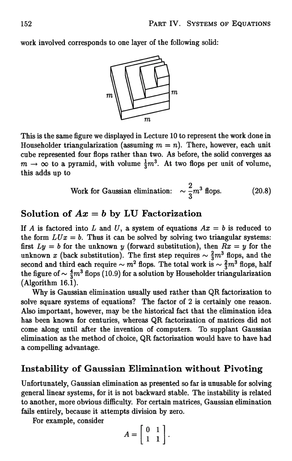
Lecture 20 Gaussian Elimination 147
Lecture 21 Pivoting 155
Lecture 22 Stability of Gaussian Elimination 163
Lecture 23 Cholesky Factorization 172
V Eigenvalues 179
Lecture 24 Eigenvalue Problems 181
Lecture 25 Overview of Eigenvalue Algorithms 190
Lecture 26 Reduction to Hessenberg or Tridiagonal Form 196
Lecture 27 Rayleigh Quotient, Inverse Iteration 202
Lecture 28 QR Algorithm without Shifts 211
Lecture 29 QR Algorithm with Shifts 219
Lecture 30 Other Eigenvalue Algorithms 225
Lecture 31 Computing the SVD 234
VI Iterative Methods 241
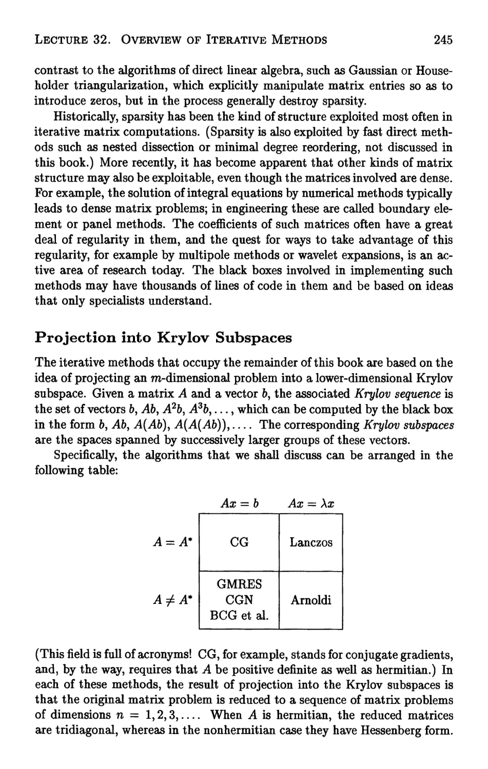
Lecture 32 Overview of Iterative Methods 243
Lecture 33 The Arnoldi Iteration 250
Lecture 34 How Arnoldi Locates Eigenvalues 257
Lecture 35 GMRES 266
Lecture 36 The Lanczos Iteration 276
Lecture 37 From Lanczos to Gauss Quadrature 285
Lecture 38 Conjugate Gradients 293
Lecture 39 Biorthogonalization Methods 303
Lecture 40 Preconditioning 313
Appendix The Definition of Numerical Analysis 321
Notes 329
Bibliography 343
Index 353

Preface
Since the early 1980s, the first author has taught a graduate course in
numerical linear algebra at MIT and Cornell. The alumni of this course, now
numbering in the hundreds, have been graduate students in all fields of
engineering and the physical sciences. This book is an attempt to put this course
on paper.
In the field of numerical linear algebra, there is already an encyclopedic
treatment on the market: Matrix Computations, by Golub and Van Loan,
now in its third edition. This book is in no way an attempt to duplicate
that one. It is small, scaled to the size of one university semester. Its aim
is to present fundamental ideas in as elegant a fashion as possible. We hope
that every reader of this book will have access also to Golub and Van Loan
for the pursuit of further details and additional topics, and for its extensive
references to the research literature. Two other important recent books are
those of Higham and Demmel, described in the Notes at the end (p. 329).
The field of numerical linear algebra is more beautiful, and more
fundamental, than its rather dull name may suggest. More beautiful, because it
is full of powerful ideas that are quite unlike those normally emphasized in
a linear algebra course in a mathematics department. (At the end of the
semester, students invariably comment that there is more to this subject than
they ever imagined.) More fundamental, because, thanks to a trick of
history, "numerical" linear algebra is really applied linear algebra. It is here that
one finds the essential ideas that every mathematical scientist needs to work
effectively with vectors and matrices. In fact, our subject is more than just
ix

X
Preface
vectors and matrices, for virtually everything we do carries over to functions
and operators. Numerical linear algebra is really functional analysis, but with
the emphasis always on practical algorithmic ideas rather than mathematical
technicalities.
The book is divided into forty lectures. We have tried to build each lecture
around one or two central ideas, emphasizing the unity between topics and
never getting lost in details. In many places our treatment is nonstandard.
This is not the place to list all of these points (see the Notes), but we will
mention one unusual aspect of this book. We have departed from the
customary practice by not starting with Gaussian elimination. That algorithm is
atypical of numerical linear algebra, exceptionally difficult to analyze, yet at
the same time tediously familiar to every student entering a course like this.
Instead, we begin with the QR factorization, which is more important, less
complicated, and a fresher idea to most students. The QR factorization is
the thread that connects most of the algorithms of numerical linear algebra,
including methods for least squares, eigenvalue, and singular value problems,
as well as iterative methods for all of these and also for systems of equations.
Since the 1970s, iterative methods have moved to center stage in scientific
computing, and to them we devote the last part of the book.
We hope the reader will come to share our view that if any other
mathematical topic is as fundamental to the mathematical sciences as calculus and
differential equations, it is numerical linear algebra.

Acknowledgments
We could not have written this book without help from many people. We must
begin by thanking the hundreds of graduate students at MIT (Math 335) and
Cornell (CS 621) whose enthusiasm and advice over a period of ten years
guided the choice of topics and the style of presentation. About seventy of
these students at Cornell worked from drafts of the book itself and contributed
numerous suggestions. The number of typos caught by Keith Sollers alone was
astonishing.
Most of Trefethen's own graduate students during the period of writing
read the text from beginning to end—sometimes on short notice and under a
gun. Thanks for numerous constructive suggestions go to Jeff Baggett, Toby
Driscoll, Vicki Howie, Gudbjorn Jonsson, Kim Toh, and Divakar Viswanath.
It is a privilege to have students, then colleagues, like these.
Working with the publications staff at SIAM has been a pleasure; there
can be few organizations that match SIAM's combination of flexibility and
professionalism. We are grateful to the half-dozen SIAM editorial, production,
and design staff whose combined efforts have made this book attractive, and in
particular, to Beth Gallagher, whose contributions begin with first-rate copy
editing but go a long way beyond.
No institution on earth is more supportive of numerical linear algebra—or
produces more books on the subject!—than the Computer Science Department
at Cornell. The other three department faculty members with interests in this
area are Tom Coleman, Charlie Van Loan, and Steve Vavasis, and we would
like to thank them for making Cornell such an attractive center of scientific
xi

xii
Acknowledgments
computing. Vavasis read a draft of the book in its entirety and made many
valuable suggestions, and Van Loan was the one who brought Trefethen to
Cornell in the first place. Among our non-numerical colleagues, we thank
Dexter Kozen for providing the model on which this book was based: The
Design and Analysis of Algorithms, also in the form of forty brief lectures.
Among the department's support staff, we have depended especially on the
professionalism, hard work, and good spirits of Rebekah Personius.
Outside Cornell, though a frequent and welcome visitor, another colleague
who provided extensive suggestions on the text was Anne Greenbaum, one of
the deepest thinkers about numerical linear algebra whom we know.
From September 1995 to December 1996, a number of our colleagues taught
courses from drafts of this book and contributed their own and their
students' suggestions. Among these were Gene Golub (Stanford), Bob Lynch
(Purdue), Suely Oliveira (Texas A & M), Michael Overton (New York
University), Haesun Park and Ahmed Sameh (University of Minnesota), Irwin
Pressmann (Carleton University), Bob Russell and Manfred Trummer (Simon
Eraser University), Peter Schmid (University of Washington), Daniel Szyld
(Temple University), and Hong Zhang and Bill Moss (Clemson University).
The record-breakers in the group were Lynch and Overton, each of whom
provided long lists of detailed suggestions. Though eager to dot the last i,
we found these contributions too sensible to ignore, and there are now
hundreds of places in the book where the exposition is better because of Lynch
or Overton.
Most important of all, when it comes to substantive help in making this a
better book, we owe a debt that cannot be repaid (he refuses to consider it) to
Nick Higham of the University of Manchester, whose creativity and scholarly
attention to detail have inspired numerical analysts from half his age to twice
it. At short notice and with characteristic good will, Higham read a draft of
this book carefully and contributed many pages of technical suggestions, some
of which changed the book significantly.
For decades, numerical linear algebra has been a model of a friendly and
socially cohesive field. Trefethen would like in particular to acknowledge the
three "father figures" whose classroom lectures first attracted him to the
subject: Gene Golub, Cleve Moler, and Jim Wilkinson.
Still, it takes more than numerical linear algebra to make life worth living.
For this, the first author thanks Anne, Emma (5), and Jacob (3) Trefethen,
and the second thanks Heidi Yeh.

Part I
Fundamentals

Lecture 1. Matrix-Vector Multiplication
You already know the formula for matrix-vector multiplication. Nevertheless,
the purpose of this first lecture is to describe a way of interpreting such
products that may be less familiar. If b = Ax, then b is a linear combination of
the columns of A.
Familiar Definitions
Let x be an n-dimensional column vector and let A be an m x n matrix
(m rows, n columns). Then the matrix-vector product b = Ax is the
Tridimensional column vector defined as follows:
n
t>i = Y, aijxj> t = 1,. -., m. (1.1)
Here b{ denotes the ith entry of 6, a^ denotes the i, j entry of A (ith row,
jth column), and x. denotes the jth entry of x. For simplicity, we assume in
all but a few lectures of this book that quantities such as these belong to C,
the field of complex numbers. The space of m-vectors is Cm, and the space of
m x n matrices is Cmxn.
The map x i-> Ax is linear■, which means that, for any xyy G Cn and any
ae C,
A(x + y) = Ax + Ay,
A(ax) = aAx.
3

4
Part I. Fundamentals
Conversely, every linear map from Cn to Cm can be expressed as multiplication
by an m x n matrix.
A Matrix Times a Vector
Let a, denote the jth column of A, an m-vector. Then (1.1) can be rewritten
b = Ax = J2xj"y (1-2)
i=i
This equation can be displayed schematically as follows:
b
=
«1
a2
...
On
= *1
Ol
+ a;2
a2
+ •••+«.
«J
In (1.2), 6 is expressed as a linear combination of the columns a^ Nothing
but a slight change of notation has occurred in going from (1.1) to (1.2). Yet
thinking of Ax in terms of the form (1.2) is essential for a proper understanding
of the algorithms of numerical linear algebra.
We can summarize these different descriptions of matrix-vector products
in the following way. As mathematicians, we are used to viewing the formula
Ax = b as a statement that A acts on x to produce 6. The formula (1.2), by
contrast, suggests the interpretation that x acts on A to produce 6.
Example 1.1. Vandermonde Matrix. Fix a sequence of numbers {xlyx2,
..., xm}. If p and q are polynomials of degree < n and a is a scalar, then
p+q and ap are also polynomials of degree < n. Moreover, the values of these
polynomials at the points x{ satisfy the following linearity properties:
(p + q)(Xi) = pixj + qfa),
Thus the map from vectors of coefficients of polynomials p of degree < n to
vectors (p(xx),p(x2),... >p{xm)) of sampled polynomial values is linear. Any
linear map can be expressed as multiplication by a matrix; this is an example.
In fact, it is expressed by an m x n Vandermonde matrix
<r r2 ... Tn-1 1
U/i U/i U/i I
*^2 *^2 * * * *^2
.7» or»^ ... Of»^* ^ I
^m ^m ^m J
A =

Lecture 1. Matrix-Vector Multiplication
5
If c is the column vector of coefficients of p,
c =
%
<h.
^n-l J
p(x) = c0 + cxx + C2X2 + h cn_xx
n-l
then the product Ac gives the sampled polynomial values. That is, for each i
from 1 to to, we have
(Ac), = cQ + cixi + ^ + ... + c^xr1 = Pfa). (1.3)
In this example, it is clear that the matrix-vector product Ac need not
be thought of as m distinct scalar summations, each giving a different linear
combination of the entries of c, as (LI) might suggest. Instead, A can be
viewed as a matrix of columns, each giving sampled values of a monomial,
A =
1
X
X2
...
x"-1
(1.4)
and the product Ac should be understood as a single vector summation in the
form of (1.2) that at once gives a linear combination of these monomials,
Ac = c0 + cxx + c2x2 H 1- cn_1xn~1 = p(x). D
The remainder of this lecture will review some fundamental concepts in
linear algebra from the point of view of (1.2).
A Matrix Times a Matrix
For the matrix-matrix product B = AC, each column of B is a linear
combination of the columns of A. To derive this fact, we begin with the usual
formula for matrix products. If A is £ x m and C is m x n, then B is £ x n,
with entries defined by
bij = Ylaikckj-
(1.5)
fc=i
Here 6^., aik> and ckj are entries of B, A, and C, respectively. Written in terms
of columns, the product is
61
b2
...
K
=
<*i
a2
...
«m
Cl
C2
...
°n

6
Part I. Fundamentals
and (1.5) becomes
h=Aci = llckjak-
(1.6)
fc=l
Thus bj is a linear combination of the columns ak with coefficients cfcj.
Example 1.2. Outer Product. A simple example of a matrix-matrix
product is the outer product. This is the product of an ra-dimensional column
vector u with an n-dimensional row vector v; the result is an m x n matrix of
rank 1. The outer product can be written
u
[v1 v2 ... vn]
vlu
v2u
...
VnU
=
■ vxux .
:
- t>l«m "
'• Vl 1
:
'• VmJ
The columns are all multiples of the same vector u, and similarly, the rows
are all multiples of the same vector v. D
Example 1.3. As a second illustration, consider B = ARy where R is the
upper-triangular n x n matrix with entries r^ = 1 for i < j and r^ = 0 for
i > j. This product can be written
h
...
K
=
ax
...
«n
The column formula (1.6) now gives
fy = Atj = £afc.
(1.7)
That is, the jth column of B is the sum of the first j columns of A. The
matrix J? is a discrete analogue of an indefinite integral operator. D
Range and Nullspace
The range of a matrix A, written range(A), is the set of vectors that can be
expressed as Ax for some x. The formula (1.2) leads naturally to the following
characterization of range (A).
Theorem 1.1. range(A) is the space spanned by the columns of A.

Lecture l. Matrix-Vector Multiplication
7
Proof. By (1.2), any Ax is a linear combination of the columns of A.
Conversely, any vector y in the space spanned by the columns of A can be written
as a linear combination of the columns, y = £^-1¾¾. Forming a vector x
out of the coefficients Xj, we have y = Ax, and thus y is in the range of A. □
In view of Theorem 1.1, the range of a matrix A is also called the column
space of A.
The nullspace of A G Cmxn, written null(A), is the set of vectors x that
satisfy Ax = 0, where 0 is the 0-vector in Cm. The entries of each vector
x G null (^4) give the coefficients of an expansion of zero as a linear combination
of columns of A: 0 = xxax + x2a2 H 1- xnan.
Rank
The column rank of a matrix is the dimension of its column space. Similarly,
the row rank of a matrix is the dimension of the space spanned by its rows.
Row rank always equals column rank (among other proofs, this is a corollary
of the singular value decomposition, discussed in Lectures 4 and 5), so we refer
to this number simply as the rank of a matrix.
An m x n matrix of full rank is one that has the maximal possible rank (the
lesser of m and n). This means that a matrix of full rank with m > n must
have n linearly independent columns. Such a matrix can also be characterized
by the property that the map it defines is one-to-one.
Theorem 1.2. A matrix A 6 CmXn with m > n has full rank if and only if
it maps no two distinct vectors to the same vector.
Proof (=^) If A is of full rank, its columns are linearly independent, so they
form a basis for range(A). This means that every b G range(A) has a unique
linear expansion in terms of the columns of A, and therefore, by (1.2), every
b G range(A) has a unique x such that b = Ax. (<==) Conversely, if A is
not of full rank, its columns a^ are dependent, and there is a nontrivial linear
combination such that £y=i c^ = 0. The nonzero vector c formed from the
coefficients Cj satisfies Ac = 0. But then A maps distinct vectors to the same
vector since, for any x, Ax = A(x + c). □
Inverse
A nonsingular or invertible matrix is a square matrix of full rank. Note
that the m columns of a nonsingular m x m matrix A form a basis for the
whole space Cm. Therefore, we can uniquely express any vector as a linear
combination of them. In particular, the canonical unit vector with 1 in the
jth entry and zeros elsewhere, written e^ can be expanded:

8
Part I. Fundamentals
e; = £*,i<V (L8)
t=i
Let Z be the matrix with entries z^, and let z± denote the jth column of
Z. Then (1.8) can be written e;- = Azj. This equation has the form (1.6); it
can be written again, most concisely, as
61
...
em
where I is the to x to matrix known as the identity. The matrix Z is the
inverse of A. Any square nonsingular matrix A has a unique inverse, written
-A"1, that satisfies AA~X = A~XA = I.
The following theorem records a number of equivalent conditions that hold
when a square matrix is nonsingular. These conditions appear in linear algebra
texts, and we shall not give a proof here. Concerning (f), see Lecture 5.
Theorem 1.3. For A € CmXm; the following conditions are equivalent:
(a) A has an inverse A"1,
(b) rank (^4) = m,
(c) range(A) = Cm,
(d) null(A) = {0},
(e) 0 is not an eigenvalue of A,
(f) 0 is not a singular value of A,
(g) det(A) ± 0.
Concerning (g), we mention that the determinant, though a convenient notion
theoretically, rarely finds a useful role in numerical algorithms.
A Matrix Inverse Times a Vector
When writing the product x = A~\ it is important not to let the inverse-
matrix notation obscure what is really going on! Rather than thinking of a: as
the result of applying A"1 to 6, we should understand it as the unique vector
that satisfies the equation Ax = b. By (1.2), this means that x is the vector
of coefficients of the unique linear expansion of b in the basis of columns of A.
This point cannot be emphasized too much, so we repeat:
A~xb is the vector of coefficients of the expansion of b
in the basis of columns of A.
Multiplication by A"1 is a change of basis operation:

Lecture 1. Matrix-Vector Multiplication
9
Multiplication by A 1
b: \ f A~xb:
coefficients of \ / coefficients of
[the expansion of b\ I the expansion of b\
in ^,...,0 / \ in {ax,. ..,am}
Multiplication by A
In this description we are being casual with terminology, using "b" in one
instance to denote an m-tuple of numbers, and in another, as a point in an
abstract vector space. The reader should think about these matters until he
or she is comfortable with the distinction.
A Note on m and n
Throughout numerical linear algebra, it is customary to take a rectangular
matrix to have dimensions mxn. We follow this convention in this book.
What if the matrix is square? The usual convention is to give it dimensions
n x n, but in this book we shall generally take the other choice, to x to. Many
of our algorithms require us to look at rectangular submatrices formed by
taking a subset of the columns of a square matrix. If the submatrix is to be
to x n, the original matrix had better be to x to.
Exercises
1.1. Let B be a 4 x 4 matrix to which we apply the following operations:
1. double column 1,
2. halve row 3,
3. add row 3 to row 1,
4. interchange columns 1 and 4,
5. subtract row 2 from each of the other rows,
6. replace column 4 by column 3,
7. delete column 1 (so that the column dimension is reduced by 1).
(a) Write the result as a product of eight matrices.
(b) Write it again as a product ABC (same B) of three matrices.
1.2. Suppose masses tox, to2, to3, m4 are located at positions xv x2, x3, z4 in a
line and connected by springs with spring constants &12, fc23, ku whose natural
lengths of extension are ^12^23^34- Let /1,/2,/3,/4 denote the rightward
forces on the masses, e.g., /x = fci2(z2 — x1 — ^12).

10
Part I. Fundamentals
(a) Write the 4x4 matrix equation relating the column vectors / and x. Let
K denote the matrix in this equation.
(b) What are the dimensions of the entries of K in the physics sense (e.g.,
mass times time, distance divided by mass, etc.)?
(c) What are the dimensions of det(K), again in the physics sense?
(d) Suppose K is given numerical values based on the units meters, kilograms,
and seconds. Now the system is rewritten with a matrix K1 based on
centimeters, grams, and seconds. What is the relationship of K' to K ? What is the
relationship of det(if') to det(tf)?
1.3. Generalizing Example 1.3, we say that a square or rectangular matrix R
with entries r^ is upper-triangular if r^ = 0 for i > j. By considering what
space is spanned by the first n columns of R and using (1.8), show that if R is a
nonsingular to x to upper-triangular matrix, then R"1 is also upper-triangular.
(The analogous result also holds for lower-triangular matrices.)
1.4. Let /1}... ,/8 be a set of functions defined on the interval [1,8] with
the property that for any numbers dx,..., d8, there exists a set of coefficients
cl9...9Cg such that
X>;/y(0 = 4» t = 1,...,8.
i=i
(a) Show by appealing to the theorems of this lecture that dl5..., ds determine
cx,...,c8 uniquely.
(b) Let A be the 8x8 matrix representing the linear mapping from data
dx,..., d8 to coefficients c1?..., c8. What is the iyj entry of A"1 ?

Lecture 2. Orthogonal Vectors and Matrices
Since the 1960s, many of the best algorithms of numerical linear algebra have
been based in one way or another on orthogonality. In this lecture we present
the ingredients: orthogonal vectors and orthogonal (unitary) matrices.
Adjoint
The complex conjugate of a scalar z, written z or z*, is obtained by negating
its imaginary part. For real z, z = z.
The hermitian conjugate or adjoint of an m x n matrix Ay written A*, is
the nxm matrix whose i, j entry is the complex conjugate of the j, i entry of
A. For example,
^11 a21 a31
a12 a22 a32 J
If A = A*, A is hermitian. By definition, a hermitian matrix must be square.
For real A, the adjoint simply interchanges the rows and columns of A. In
this case, the adjoint is also known as the transpose, and is written AT. If a
real matrix is hermitian, that is, A = AT, then it is also said to be symmetric.
Most textbooks of numerical linear algebra assume that the matrices under
discussion are real and thus principally use T instead of *. Since most of the
ideas to be dealt with are not intrinsically restricted to the reals, however, we
have followed the other course. Thus, for example, in this book a row vector
A =
an a12
a21 a22
%1 a32
11

12
Part I. Fundamentals
will usually be denoted by, say, a* rather than aT. The reader who prefers to
imagine that all quantities are real and that * is a synonym for T will rarely
get into trouble.
Inner Product
The inner product of two column vectors x, y € Cm is the product of the
adjoint of x by y:
m
x*y = J2xiVi. (2.1)
t=l
The Euclidean length of a: may be written ||x|| (vector norms such as this are
discussed systematically in the next lecture), and can be defined as the square
root of the inner product of x with itself:
1/2
Eki2) • (2-2)
The cosine of the angle a between x and y can also be expressed in terms of
the inner product:
x*v
Ml h\\
At various points of this book, as here, we mention geometric interpretations
of algebraic formulas. For these geometric interpretations, the reader should
think of the vectors as real rather than complex, although usually the
interpretations can be carried over in one way or another to the complex case
too.
The inner product is bilinear, which means that it is linear in each vector
separately:
(x1 + x2)*y = x\y + x*2y,
{ax)*(Py) = a/3x*y.
We shall also frequently use the easily proved property that for any matrices
or vectors A and B of compatible dimensions,
(AB)* = B*A*. (2.4)
This is analogous to the equally important formula for products of invertible
square matrices,
(AB)~l = B^A-1. (2.5)
The notation A~* is a shorthand for (A*)"1 or (A-1)*; these two are equal, as
can be verified by applying (2.4) with B = A"1.

Lecture 2. Orthogonal Vectors and Matrices
13
Orthogonal Vectors
A pair of vectors x and y are orthogonal if x*y = 0. If x and y are real, this
means they lie at right angles to each other in R,m. Two sets of vectors X
and Y are orthogonal (also stated "X is orthogonal to Yn) if every x G X is
orthogonal to every j/G7.
A set of nonzero vectors S is orthogonal if its elements are pairwise
orthogonal, i.e., if for a, y 6 S, a: ^ y => x*y = 0. A set of vectors is orthonormal if
it is orthogonal and, in addition, every x € S has ||z|| = 1.
Theorem 2.1. The vectors in an orthogonal set S are linearly independent
Proof. If the vectors in S are not independent, then some vk € S can be
expressed as a linear combination of other members vl9..., vn € 5,
n
»* = !>«»*•
Since vk ^ 0, z;]^ = \\vk\\2 > 0. Using the bilinearity of inner products and
the orthogonality of 5, we calculate
n
which contradicts the assumption that the vectors in S are nonzero. □
As a corollary of Theorem 2.1 it follows that if an orthogonal set S C Cm
contains m vectors, then it is a basis for Cm.
Components of a Vector
The most important idea to draw from the concepts of inner products and
orthogonality is this: inner products can be used to decompose arbitrary vectors
into orthogonal components.
For example, suppose that {qX) g2,..., qn} is an orthonormal set, and let v
be an arbitrary vector. The quantity q^v is a scalar. Utilizing these scalars as
coordinates in an expansion, we find that the vector
r = t; - {q{v)qi - {qlv)q2 (g»gn (2.6)
is orthogonal to {qv g2,..., gn}. This can be verified by computing q*r:
q"r = q*v - (qlv)(q*qx) {q*nv){q*qn).
This sum collapses, since q*q- = 0 for i ^ j:
q*r = tfv - (tfvXflta) = 0.

14
Part I. Fundamentals
Thus we see that v can be decomposed into n + 1 orthogonal components:
v = r + £»)fc = r + Y,(qrf!)v.
(2.7)
1=1
1=1
In this decomposition, r is the part of v orthogonal to the set of vectors
{<7i> ¢2)--) 9n}) or) equivalently, to the subspace spanned by this set of vectors,
and (q*v)q{ is the part of v in the direction of q±.
If (¾} is a basis for Cm, then n must be equal to m and r must be the
zero vector, so v is completely decomposed into m orthogonal components in
the directions of the q{:
= X)te*fl)ft = ]C(fttfK
(2.8)
t=i
t=i
In both (2.7) and (2.8) we have written the formula in two different ways,
once with (¾^)¾ and again with (<&g*)v. These expressions are equal, but
they have different interpretations. In the first case, we view v as a sum
of coefficients q*v times vectors q{. In the second, we view v as a sum of
orthogonal projections of v onto the various directions q{. The iih projection
operation is achieved by the very special rank-one matrix q{q*. We shall discuss
this and other projection processes in Lecture 6.
Unitary Matrices
A square matrix Q € cmXm is unitary (in the real case, we also say orthogonal)
if Q* = Q~l, i.e, if Q*Q = I. In terms of the columns of Q, this product can
be written
ql
<&
Qi
0.2
...
?m
=
In other words, q*q- — 8^, and the columns of a unitary matrix Q form an
orthonormal basis of Cm. The symbol 6^ is the Kronecker delta, equal to 1 if
i = j and 0 if i ^ j.
Multiplication by a Unitary Matrix
In the last lecture we discussed the interpretation of matrix-vector products
Ax and A_16. If A is a unitary matrix Q, these products become Qx and
Q*b, and the same interpretations are of course still valid. As before, Qx is
the linear combination of the columns of Q with coefficients x. Conversely,

Lecture 2. Orthogonal Vectors and Matrices
15
Q*b is the vector of coefficients of the expansion of b
in the basis of columns of Q.
Schematically, the situation looks like this:
Multiplication by Q*
Multiplication by Q
These processes of multiplication by a unitary matrix or its adjoint
preserve geometric structure in the Euclidean sense, because inner products are
preserved. That is, for unitary Q,
(Qx)*(Qy)=x*yy (2.9)
as is readily verified by (2.4). The invariance of inner products means that
angles between vectors are preserved, and so are their lengths:
110*11 = Ml- (2-10)
In the real case, multiplication by an orthogonal matrix Q corresponds to a
rigid rotation (if detQ = 1) or reflection (if detQ = -1) of the vector space.
Exercises
2.1. Show that if a matrix A is both triangular and unitary, then it is diagonal.
2.2. The Pythagorean theorem asserts that for a set of n orthogonal vectors
IXXf = Elkll2-
t=l t=l
(a) Prove this in the case n = 2 by an explicit computation of \\xx + z2||2.
(b) Show that this computation also establishes the general case, by induction.
2.3. Let A G Cmxm be hermitian. An eigenvector of A is a nonzero vector
x G Cm such that Ax = Ax for some A G C, the corresponding eigenvalue,
(a) Prove that all eigenvalues of A are real.

16
Part I. Fundamentals
(b) Prove that if a: and y are eigenvectors corresponding to distinct eigenvalues,
then x and y are orthogonal.
2.4. What can be said about the eigenvalues of a unitary matrix?
2.5. Let 5 e Cmxm be skew-hermitian, i.e., 5* = -5.
(a) Show by using Exercise 2.1 that the eigenvalues of 5 are pure imaginary.
(b) Show that I - 5 is nonsingular.
(c) Show that the matrix Q = (/-5)^(/+5), known as the Cayley transform
of 5, is unitary. (This is a matrix analogue of a linear fractional transformation
(1 + 5)/(1 - 5), which maps the left half of the complex s-plane conformally
onto the unit disk.)
2.6. If u and v are to-vectors, the matrix A = I + uv* is known as a rank-one
perturbation of the identity. Show that if A is nonsingular, then its inverse
has the form A'1 = / + auv* for some scalar a, and give an expression for a.
For what u and v is A singular? If it is singular, what is null(A)?
2.7. A Hadamard matrix is a matrix whose entries are all ±1 and whose
transpose is equal to its inverse times a constant factor. It is known that if
A is a Hadamard matrix of dimension m > 2, then to is a multiple of 4. It is
not known, however, whether there is a Hadamard matrix for every such ra,
though examples have been found for all cases m < 424.
Show that the following recursive description provides a Hadamard matrix of
each dimension to = 2fc, k = 0,1,2,...:
[ Hk Hk 1
L Hk -Hk J

Lecture 3. Norms
The essential notions of size and distance in a vector space are captured by
norms. These are the yardsticks with which we measure approximations and
convergence throughout numerical linear algebra.
Vector Norms
A norm is a function || • || : Cm —» IR that assigns a real-valued length to
each vector. In order to conform to a reasonable notion of length, a norm
must satisfy the following three conditions. For all vectors x and y and for all
scalars aeC,
(1) ||z|| > 0, and ||x|| = 0 only if x = 0,
(2) ||* + »||<IW| + ||y||, (3.1)
(3) |M| = |a||N|.
In words, these conditions require that (1) the norm of a nonzero vector is
positive, (2) the norm of a vector sum does not exceed the sum of the norms
of its parts—the triangle inequality, and (3) scaling a vector scales its norm
by the same amount.
In the last lecture, we used || • || to denote the Euclidean length function
(the square root of the sum of the squares of the entries of a vector). However,
the three conditions (3.1) allow for different notions of length, and at times it
is useful to have this flexibility.
17

18
Part I. Fundamentals
The most important class of vector norms, the p-norms, are defined below.
The closed unit ball {x € Cm : ||x|| < 1} corresponding to each norm is
illustrated to the right for the case m = 2.
m
Nli = EI4
2=1
11*11, = (EWJ (!<*<«>).
The 2-norm is the Euclidean length function; its unit ball is spherical. The
1-norm is used by airlines to define the maximal allowable size of a suitcase.
The Sergei plaza in Stockholm, Sweden has the shape of the unit ball in the 4-
norm; the Danish poet Piet Hein popularized this "superellipse" as a pleasing
shape for objects such as conference tables.
Aside from the p-norms, the most useful norms are the weighted p-norms,
where each of the coordinates of a vector space is given its own weight. In
general, given any norm || • ||, a weighted norm can be written as
\\x\\w = \\Wx\\. (3.3)
Here W is the diagonal matrix in which the zth diagonal entry is the weight
w{ ^ 0. For example, a weighted 2-norm || • \\w on Cm is specified as follows:
One can also generalize the idea of weighted norms by allowing W to be an
arbitrary nonsingular matrix, not necessarily diagonal (Exercise 3.1).
The most important norms in this book are the unweighted 2-norm and
its induced matrix norm.
Matrix Norms Induced by Vector Norms
An m x n matrix can be viewed as a vector in an ran-dimensional space:
each of the ran entries of the matrix is an independent coordinate. Any mn-
dimensional norm can therefore be used for measuring the "size" of such a
matrix.
i&4
(3.2)

Lecture 3. Norms
19
However, in dealing with a space of matrices, certain special norms are
more useful than the vector norms (3.2)-(3.3) already discussed. These are
the induced matrix norms, defined in terms of the behavior of a matrix as an
operator between its normed domain and range spaces.
Given vector norms || • ||(n) and || • ||(mj on the domain and the range of
A e Cmxn, respectively, the induced matrix norm ||A||(mn) is the smallest
number C for which the following inequality holds for all x G Cn:
||AB||(mJ < C||*||w. (3.5)
In other words, ||A||(m>nj is the supremum of the ratios ||^||(m)/||^||(n) over
all vectors x e Cn—the maximum factor by which A can "stretch" a vector
x. We say that || • ||(m?n) is the matrix norm induced by || • ||(m) and || • ||(nj.
Because of condition (3) of (3.1), the action of A is determined by its action
on unit vectors. Therefore, the matrix norm can be defined equivalently in
terms of the images of the unit vectors under A:
MIU») = sup nor"1 = sup ll^llw (3-6)
This form of the definition can be convenient for visualizing induced matrix
norms, as in the sketches in (3.2) above.
Examples
Example 3.1. The matrix
A =
1 2
0 2
(3.7)
maps C2 to C2. It also maps R2 to R2, which is more convenient if we want
to draw pictures and also (it can be shown) sufficient for determining matrix
p-norms, since the coefficients of A are real.
Figure 3.1 depicts the action of A on the unit balls of H2 defined by the
1-, 2-, and oo-norms. From this figure, one can see a graphical interpretation
of these three norms of A. Regardless of the norm, A maps e1 = (1,0)* to the
first column of A, namely ex itself, and e2 = (0,1)* to the second column of A,
namely (2,2)*. In the 1-norm, the unit vector x that is amplified most by A is
(0,1)* (or its negative), and the amplification factor is 4. In the oo-norm, the
unit vector x that is amplified most by A is (1,1)* (or its negative), and the
amplification factor is 3. In the 2-norm, the unit vector that is amplified most
by A is the vector indicated by the dashed line in the figure (or its negative),
and the amplification factor is approximately 2.9208. (Note that it must be
at least y/8 « 2.8284, since (0,1)* maps to (2,2)*.) We shall consider how to
calculate such 2-norm results in Lecture 5. □

20
Part I. Fundamentals
1-norm:
2-norm:
oo-norm:
(2,2)*
/
/
¥—fc
PL = 4
IMIa
2.9208
MIL = 3
Figure 3.1. On the left, the unit balls o/H2 with respect to \\ • \\1} \\ • ||2, and
|| • 11^. On the right, their images under the matrix A o/(3.7). Dashed lines
mark the vectors that are amplified most by A in each norm.
Example 3.2. The p-Norm of a Diagonal Matrix. Let D be the
diagonal matrix
D =
*i
Then, as in the second row of Figure 3.1, the image of the 2-norm unit sphere
under D is an m-dimensional ellipse whose semiaxis lengths are given by the
numbers |dj. The unit vectors amplified most by D are those that are mapped
to the longest semiaxis of the ellipse, of length max^ldj}. Therefore, we have
||Z?||2 = niax1<i<m{|dj}. In the next lecture we shall see that every matrix
maps the 2-norm unit sphere to an ellipse—properly called a hyperellipse if
m > 2—though the axes may be oriented arbitrarily.
This result for the 2-norm generalizes to any p: if D is diagonal, then
||Z)||p = max1<i<m|d.|. □
Example 3.3. The 1-Norm of a Matrix. If A is any mxn matrix, then
||^4.|| x is equal to the "maximum column sum" of A. We explain and derive

Lecture 3. Norms
21
this result as follows. Write A in terms of its columns
A =
(3.8)
where each a7 is an m-vector. Consider the diamond-shaped 1-norm unit ball
in Cn, illustrated in (3.2). This is the set {x e Cn : E*=il^| < !}• Any
vector Ax in the image of this set satisfies
IIAclli = HXX-OiL < ENIKIIi < ™?JNIi-
Therefore, the induced matrix 1-norm satisfies \\A\\± < niax1<J-<n||a-||1. By
choosing x = e^ where j maximizes Ha^Hi, we attain this bound, and thus the
matrix norm is
PHi = m^Ja^. (3.9)
D
Example 3.4. The oo-Norm of a Matrix. By much the same argument,
it can be shown that the oo-norm of an m x n matrix is equal to the "maximum
row sum,"
ML = ngx IKIli, (3.10)
where a* denotes the zth row of A. □
Cauchy—Schwarz and Holder Inequalities
Computing matrix p-norms with p ^ 1, oo is more difficult, and to approach
this problem, we note that inner products can be bounded using p-norms. Let
p and q satisfy 1/p + 1/q = 1, with 1 < p, q < oo. Then the Holder inequality
states that, for any vectors x and j/,
l**y| < IMI,||y||c. (3.11)
The Cauchy-Schwarz inequality is the special case p = q = 2:
l»'¥l < H2lly|la- (3.12)
Derivations of these results can be found in linear algebra texts. Both bounds
are tight in the sense that for certain choices of x and y, the inequalities
become equalities.
Example 3.5. The 2-Norm of a Row Vector. Consider a matrix A
containing a single row. This matrix can be written as A — a*, where a
is a column vector. The Cauchy-Schwarz inequality allows us to obtain the
induced matrix 2-norm. For any x, we have ||Ac||2 = \a*x\ < ||a||2|k||2- This
bound is tight: observe that \\Aa\\2 = ||a||22. Therefore, we have
\\A\\2 = sup{||^||2/||s||2} = ||a||2. D

22
Part I. Fundamentals
Example 3.6. The 2-Norm of an Outer Product. More generally,
consider the rank-one outer product A = uv*, where u is an m-vector and v is an
n-vector. For any n-vector z, we can bound ||Ax||2 as follows:
M*||a = IK*II2 = NI2K*I < NI2NI2INI2- (3.13)
Therefore ||A||2 < IM^IM^- Again, this inequality is an equality: consider
the case x = v. □
Bounding ||AJB|| in an Induced Matrix Norm
The induced matrix norm of a matrix product can also be bounded. Let || • ||^,
|| • ||(m), and || • ||(n) be norms on C1, Cm, and Cn, respectively, and let A be
anixm matrix and B an m x n matrix. For any x G Cn we have
||illte||w < ||A||(/>m)||Bx||(TO) < MH^IIBll^lMlw.
Therefore the induced norm of AB must satisfy
P*ll(/,„) < U\\{t,m)\\B\\(m,ny (3.14)
In general, this inequality is not an equality. For example, the inequality
mn|| < Il^l|n holds for any square matrix in any matrix norm induced by a
vector norm, but ||An|| = ||A||n does not hold in general for n > 2.
General Matrix Norms
As noted above, matrix norms do not have to be induced by vector norms. In
general, a matrix norm must merely satisfy the three vector norm conditions
(3.1) applied in the mn-dimensional vector space of matrices:
(1) ||A|| > 0, and ||A|| = 0 only if A = 0,
(2) ||A + 5||<||A|| + ||B||, (3.15)
(3) |M|| = |a|||A||.
The most important matrix norm which is not induced by a vector norm
is the HUbert-Schmidt or Frobenius norm, defined by
Uh = (E £kfj • (3-16)
Observe that this is the same as the 2-norm of the matrix when viewed as
an mn-dimensional vector. The formula for the Frobenius norm can also be

Lecture 3. Norms
23
written in terms of individual rows or columns. For example, if a^ is the jth
column of A, we have
(\ 1/2
ENl22J (3.17)
This identity, as well as the analogous result based on rows instead of columns,
can be expressed compactly by the equation
||A||F = Jti{A*A) = ^tr(iW), (3.18)
where tr(5) denotes the trace of B, the sum of its diagonal entries.
Like an induced matrix norm, the Frobenius norm can be used to bound
products of matrices. Let C = AB with entries cik, and let a* denote the ith.
row of A and fy the jth column of B. Then c^ = a*b^ so by the Cauchy-
Schwarz inequality we have \c^\ < HaJ^ \\bj\\2- Squaring both sides and
summing over all i, j, we obtain
\\ab\\% = ££k/
t=l j=l
n m ty
< EEOk-IUNk)
t=l j=l
71 ty fto ry
= Z)(IKIIO E(lNk) = U\\2f\\b\\%.
t=l j=l
Invariance under Unitary Multiplication
One of the many special properties of the matrix 2-norm is that, like the vector
2-norm, it is invariant under multiplication by unitary matrices. The same
property holds for the Frobenius norm.
Theorem 3.1. For any A G Cmxn and unitary Q G CmXm, we have
\\QA\\2 = ||A||2I \\QA\\F = \\A\\F.
Proof. Since ||Qx||2 = ||z||2 for every x, by (2.10), the invariance in the 2-norm
follows from (3.6). For the Frobenius norm we may use (3.18). □
Theorem 3.1 remains valid if Q is generalized to a rectangular matrix with
orthonormal columns, that is, Q G Cpxm with p > m. Analogous identities
also hold for multiplication by unitary matrices on the right, or more generally,
by rectangular matrices with orthonormal rows.

24
Part I. Fundamentals
Exercises
3.1. Prove that if W is an arbitrary nonsingular matrix, the function || • \\w
defined by (3.3) is a vector norm.
3.2. Let || • || denote any norm on Cm and also the induced matrix norm on
Cmxm. Show that p(A) < \\A\\, where p(A) is the spectral radius of A, i.e.,
the largest absolute value |A| of an eigenvalue A of A,
3.3. Vector and matrix p-norms are related by various inequalities, often
involving the dimensions m or n. For each of the following, verify the
inequality and give an example of a nonzero vector or matrix (for general to, n) for
which equality is achieved. In this problem x is an m-vector and A is an to x n
matrix.
(a) ||*IL ^ Ml*
(b)\\x\\2 < vG»ML,
(*)M~<V*Uh*
(d) ||A||a < V^PIloo-
3.4. Let A be an to x n matrix and let Bbea submatrix of A, that is, a /x x v
matrix (/x < to, v < n) obtained by selecting certain rows and columns of A.
(a) Explain how B can be obtained by multiplying A by certain row and
column "deletion matrices" as in step 7 of Exercise 1.1.
(b) Using this product, show that ||B||p < ||i4||p for any p with 1 < p < oo.
3.5. Example 3.6 shows that if E is an outer product E = uv*, then \\E\\2 —
IMUMta- Is *^e same true ^01 *^e Frobenius norm, i.e., \\E\\F = 11^11^11^(1^ ?
Prove it or give a counterexample.
3.6. Let || • || denote any norm on Cm. The corresponding dual norm \\ • ||; is
defined by the formula ||z||' = sup||y|(==1 \y*x\.
(a) Prove that || • ||' is a norm.
(b) Let x,y G Cm with ||a:|| = \\y\\ = 1 be given. Show that there exists a
rank-one matrix B = yz* such that Bx — y and ||B|| = 1, where ||B|| is the
matrix norm of B induced by the vector norm || -1|. You may use the following
lemma, without proof: given x € Cm, there exists a nonzero z €<Cm such that
1***1 = \\z\\'\\x\\.

Lecture 4. The Singular Value
Decomposition
The singular value decomposition (SVD) is a matrix factorization whose
computation is a step in many algorithms. Equally important is the use of the
SVD for conceptual purposes. Many problems of linear algebra can be better
understood if we first ask the question: what if we take the SVD?
A Geometric Observation
The SVD is motivated by the following geometric fact:
The image of the unit sphere under any m xn matrix is a hyperellipse.
The SVD is applicable to both real and complex matrices. However, in
describing the geometric interpretation, we assume as usual that the matrix is
real.
The term "hyperellipse" may be unfamiliar, but this is just the ra-dimen-
sional generalization of an ellipse. We may define a hyperellipse in Mm as
the surface obtained by stretching the unit sphere in Mm by some factors
^19---i^m (possibly zero) in some orthogonal directions ti1?...,tim G Rm.
For convenience, let us take the «i to be unit vectors, i.e., ||uj|2 = 1. The
vectors {0^} are the principal semiaxes of the hyperellipse, with lengths
cr^... ,am. If A has rank r, exactly r of the lengths ui will turn out to be
nonzero, and in particular, if m > n, at most n of them will be nonzero.
25

26
Part I. Fundamentals
Our opening statement about the image of the unit sphere has the following
meaning. By the unit sphere, we mean the usual Euclidean sphere in n-space,
i.e., the unit sphere in the 2-norm; let us denote it by S. Then AS, the image
of S under the mapping A, is a hyperellipse as just defined.
This geometric fact is not obvious. We shall restate it in the language of
linear algebra and prove it later. For the moment, assume it is true.
Figure 4.1. SVD of a 2 x 2 matrix.
Let S be the unit sphere in Rn, and take any A € Rmxn with m > n. For
simplicity, suppose for the moment that A has full rank n. The image AS is a
hyperellipse in K,m. We now define some properties of A in terms of the shape
of AS. The key ideas are indicated in Figure 4.1.
First, we define the n singular values of A. These are the lengths of the n
principal semiaxes of AS, written ax, cr2,..., crn. It is conventional to assume
that the singular values are numbered in descending order, ox > a2 > • • • >
Next, we define the n left singular vectors of A. These are the unit vectors
{wx,u2,... ,«n} oriented in the directions of the principal semiaxes of AS,
numbered to correspond with the singular values. Thus the vector a^ is the
ith largest principal semiaxis of AS.
Finally, we define the n right singular vectors of A. These are the unit
vectors {v±, v2,..., vn} € S that are the preimages of the principal semiaxes
of AS, numbered so that Av- = a^iy
The terms "left" and "right" in the definitions above are decidedly
awkward. They come from the positions of the factors U and V in (4.2) and
(4.3), below. What is awkward is that in a sketch like Figure 4.1, the left
singular vectors correspond to the space on the right, and the right singular
vectors correspond to the space on the left! One could resolve this problem
by interchanging the two halves of the figure, with the map A pointing from
right to left, but that would go against deeply ingrained habits.

Lecture 4. The Singular Value Decomposition
27
Reduced SVD
We have just mentioned that the equations relating right singular vectors {v^}
and left singular vectors {u^} can be written
Avj = (TjUj, 1 < j < n. (4.1)
This collection of vector equations can be expressed as a matrix equation,
%
«2
...
«»
Vl
v2
...
Vn
or, more compactly, AV = {/E. In this matrix equation, S is an n x n diagonal
matrix with positive real entries (since A was assumed to have full rank n), U
is an m x n matrix with orthonormal columns, and V is an n x n matrix with
orthonormal columns. Thus V is unitary, and we can multiply on the right
by its inverse V* to obtain
A = UtV*. (4.2)
This factorization of A is called a reduced singular value decomposition, or
reduced SVD, of A. Schematically, it looks like this:
Reduced SVD (m > n)
In most applications, the SVD is used in exactly the form just described.
However, this is not the way in which the idea of an SVD is usually formulated
in textbooks. We have introduced the term "reduced" and the hats on U
and S in order to distinguish the factorization (4.2) from the more standard
"full" SVD. This "reduced" vs. "full" terminology and hatted notation will
be maintained throughout the book, and we shall make a similar distinction
between reduced and full QR factorizations. Reminders of these conventions
are printed on the inside front cover.

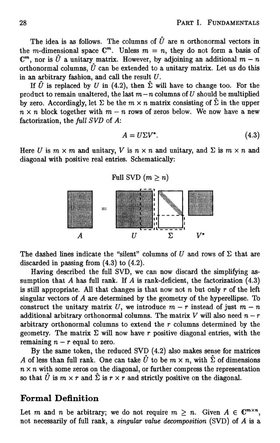
28
Part I. Fundamentals
A.
The idea is as follows. The columns of U are n orthonormal vectors in
the m-dimensional space Cm. Unless ra = n, they do not form a basis of
Cm, nor is U a unitary matrix. However, by adjoining an additional ra — n
orthonormal columns, U can be extended to a unitary matrix. Let us do this
in an arbitrary fashion, and call the result U.
If U is replaced by U in (4.2), then S will have to change too. For the
product to remain unaltered, the last m—n columns of U should be multiplied
by zero. Accordingly, let S be the rax n matrix consisting of S in the upper
n x n block together with m — n rows of zeros below. We now have a new
factorization, the full SVD of A:
A = £/EV*. (4.3)
Here U is ra x ra and unitary, V is n x n and unitary, and S is ra x n and
diagonal with positive real entries. Schematically:
Full SVD (m > n)
A U S V*
The dashed lines indicate the "silent" columns of U and rows of S that are
discarded in passing from (4.3) to (4.2).
Having described the full SVD, we can now discard the simplifying
assumption that A has full rank. If A is rank-deficient, the factorization (4.3)
is still appropriate. All that changes is that now not n but only r of the left
singular vectors of A are determined by the geometry of the hyperellipse. To
construct the unitary matrix C/, we introduce ra - r instead of just m — n
additional arbitrary orthonormal columns. The matrix V will also need n — r
arbitrary orthonormal columns to extend the r columns determined by the
geometry. The matrix S will now have r positive diagonal entries, with the
remaining n — r equal to zero.
By the same token, the reduced SVD (4.2) also makes sense for matrices
A of less than full rank. One can take U to be ra x n, with S of dimensions
nxn with some zeros on the diagonal, or further compress the representation
so that U is ra x r and S is r x r and strictly positive on the diagonal.
Formal Definition
Let ra and n be arbitrary; we do not require ra > n. Given A G Cmxn,
not necessarily of full rank, a singular value decomposition (SVD) of A is a

Lecture 4. The Singular Value Decomposition
29
factorization
where
A = UYV* (4.4)
U e cmxm is unitary,
V e Cnxn is unitary,
E€lRmXn is diagonal.
In addition, it is assumed that the diagonal entries Oy of E are nonnegative and
in nonincreasing order; that is, ax > a2 > • • • > &p > 0, where p = min(ra, n).
Note that the diagonal matrix E has the same shape as A even when A is
not square, but U and V are always square unitary matrices.
It is clear that the image of the unit sphere in Rn under a map A = UYV*
must be a hyperellipse in Mm. The unitary map V* preserves the sphere, the
diagonal matrix E stretches the sphere into a hyperellipse aligned with the
canonical basis, and the final unitary map U rotates or reflects the hyperellipse
without changing its shape. Thus, if we can prove that every matrix has an
SVD, we shall have proved that the image of the unit sphere under any linear
map is a hyperellipse, as claimed at the outset of this lecture.
Existence and Uniqueness
Theorem 4.1. Every matrix A G CmXtt has a singular value decomposition
(4.4). Furthermore, the singular values {(7,-} are uniquely determined, and, if
A is square and the <7y are distinct, the left and right singular vectors {uj} and
{vj} are uniquely determined up to complex signs (i.e., complex scalar factors
of absolute value 1).
Proof. To prove existence of the SVD, we isolate the direction of the largest
action of A, and then proceed by induction on the dimension of A.
Set <tx = ||A||2. By a compactness argument, there must be a vector
vx e Cn with IKI^ = 1 and HuJ^ = crx, where ux = Avv Consider any
extensions of vx to an orthonormal basis {v^} of Cn and of ux to an orthonormal
basis {uj} of Cm, and let £^ and Vx denote the unitary matrices with columns
Uj and v., respectively. Then we have
U*AVX = S =
0 B
(4.5)
where 0 is a column vector of dimension m — 1, w* is a row vector of dimension
n — 1, and B has dimensions (m — 1) x (n — 1). Furthermore,
I [ °1 w*
II 0 B .
' ^i 11
w \\\
> al + w*w = (a\ + w*w)
1/2
W

30
Part I. Fundamentals
implying \\S\\2 > {o\ + w*w)1/2. Since Ut and V1 are unitary, we know that
ll^lb = MII2 = au so ^is implies w = 0.
If n = 1 or m = 1, we are done. Otherwise, the submatrix B describes the
action of A on the subspace orthogonal to vv By the induction hypothesis, B
has an SVD B = U2H2V2. Now it is easily verified that
A = UX
1
0 U,
72 J [ 01 £2 J [ 0
0
v0
v;
is an SVD of A, completing the proof of existence.
For the uniqueness claim, the geometric justification is straightforward: if
the semiaxis lengths of a hyperellipse are distinct, then the semiaxes
themselves are determined by the geometry, up to signs. Algebraically, we can argue
as follows. First we note that ax is uniquely determined by the condition that
it is equal to ||-A||2, as follows from (4.4). Now suppose that in addition to vlt
there is another linearly independent vector w with ||w||2 = 1 and ||^4w||2 = crx.
Define a unit vector v2i orthogonal to vlf as a linear combination of vx and w,
2 lk-(^KII2'
Since ||A||2 = av ||^2||2 < crx; but this must be an equality, for otherwise,
since w = vxc + v2s for some constants c and s with |c|2 + |s|2 = 1, we
would have ||j4w||2 < av This vector v2 is a second right singular vector of
A corresponding to the singular value crx; it will lead to the appearance of
a vector y (equal to the last n — 1 components of V{v2) with \\y\\2 = 1 and
\\By\\2 = av We conclude that, if the singular vector vx is not unique, then
the corresponding singular value ax is not simple. To complete the uniqueness
proof we note that, as indicated above, once alyvv and ux are determined, the
remainder of the SVD is determined by the action of A on the space orthogonal
to vv Since vx is unique up to sign, this orthogonal space is uniquely defined,
and the uniqueness of the remaining singular values and vectors now follows
by induction. □
Exercises
4.1. Determine SVDs of the following matrices (by hand calculation):
(a)
3 0
0 -2
, (b)
2 0
0 3
, (c)
0 2
0 0
0 0
, (d)
1 1
0 0
, (e)
1 1
1 1

Lecture 4. The Singular Value Decomposition
31
4.2. Suppose A is an m x n matrix and B is the n x m matrix obtained by
rotating A ninety degrees clockwise on paper (not exactly a standard
mathematical transformation!). Do A and B have the same singular values? Prove
that the answer is yes or give a counterexample.
4.3. Write a Matlab program (see Lecture 9) which, given a real 2x2
matrix Ay plots the right singular vectors vt and v2 in the unit circle and also
the left singular vectors u± and u2 in the appropriate ellipse, as in Figure 4.1.
Apply your program to the matrix (3.7) and also to the 2x2 matrices of
Exercise 4.1.
4.4. Two matrices AyB e Cmxm are unitarily equivalent if A = QBQ* for
some unitary Q € Cmxm. Is it true or false that A and B are unitarily
equivalent if and only if they have the same singular values?
4.5. Theorem 4.1 asserts that every A € CmXn has an SVD A = UW*.
Show that if A is real, then it has a real SVD (U e RmXm, V G BnXn).

Lecture 5. More on the SVD
We continue our discussion of the singular value decomposition, emphasizing
its connection with low-rank approximation of matrices in the 2-norm and the
Frobenius norm.
A Change of Bases
The SVD makes it possible for us to say that every matrix is diagonal—if only
one uses the proper bases for the domain and range spaces.
Here is how the change of bases works. Any b G Cm can be expanded in
the basis of left singular vectors of A (columns of £/), and any x G Cn can
be expanded in the basis of right singular vectors of A (columns of V). The
coordinate vectors for these expansions are
b' = U% x1 = V*x.
By (4.3), the relation b = Ax can be expressed in terms of bf and xf:
b = Ax «=► U*b = U*Ax = U*UYV*x <=> b' = Ex'.
Whenever b = Axy we have b1 = Ez'. Thus A reduces to the diagonal matrix
S when the range is expressed in the basis of columns of U and the domain is
expressed in the basis of columns of V'.
32

Lecture 5. More on the SVD
33
SVD vs. Eigenvalue Decomposition
The theme of diagonalizing a matrix by expressing it in terms of a new basis
also underlies the study of eigenvalues. A nondefective square matrix A can
be expressed as a diagonal matrix of eigenvalues A, if the range and domain
are represented in a basis of eigenvectors.
If the columns of a matrix X e CmXm contain linearly independent
eigenvectors of A e CmXm, the eigenvalue decomposition of A is
A = XAX~\ (5.1)
where A is an to x m diagonal matrix whose entries are the eigenvalues of A.
This implies that if we define, for 6, x € Cm satisfying b = Ax,
bf = X-% x' = X~lx,
then the newly expanded vectors V and xf satisfy V = Ax'. Eigenvalues are
treated systematically in Lecture 24.
There are fundamental differences between the SVD and the eigenvalue
decomposition. One is that the SVD uses two different bases (the sets of
left and right singular vectors), whereas the eigenvalue decomposition uses
just one (the eigenvectors). Another is that the SVD uses orthonormal bases,
whereas the eigenvalue decomposition uses a basis that generally is not
orthogonal. A third is that not all matrices (even square ones) have an eigenvalue
decomposition, but all matrices (even rectangular ones) have a singular value
decomposition, as we established in Theorem 4.1. In applications, eigenvalues
tend to be relevant to problems involving the behavior of iterated forms of A,
such as matrix powers Ak or exponentials etAy whereas singular vectors tend
to be relevant to problems involving the behavior of A itself, or its inverse.
Matrix Properties via the SVD
The power of the SVD becomes apparent as we begin to catalogue its
connections with other fundamental topics of linear algebra. For the following
theorems, assume that A has dimensions m x n. Let p be the minimum of m
and n, let r < p denote the number of nonzero singular values of A, and let
(xy ?/,..., z) denote the space spanned by the vectors x, y,..., z.
Theorem 5.1. The rank of A isr, the number of nonzero singular values.
Proof. The rank of a diagonal matrix is equal to the number of its nonzero
entries, and in the decomposition A = £/EV*, U and V are of full rank.
Therefore rank (A) = rank(E) = r. □
Theorem 5.2. range(A) = (uly..., uT) and null(A) = (vr+1,..., vn).
Proof This is a consequence of the fact that range(S) = (el5..., eT) C Cm
and null(S) = (er+1,..., en) C Cn. □

34
Part I. Fundamentals
Theorem 5.3. p||2 = ax and \\A\\F = yja\ + a\ + •• • + <r?.
Proof. The first result was already established in the proof of Theorem 4.1:
since A - C/EV* with unitary U and V, ||^4||2 = ||E||2 = max{|aJ|} = av
by Theorem 3.1. For the second, note that by Theorem 3.1 and the remark
following, the Frobenius norm is invariant under unitary multiplication, so
||A||F = ||S||F, and by (3.16), this is given by the stated formula. □
Theorem 5.4. The nonzero singular values of A are the square roots of the
nonzero eigenvalues of A*A or AA*. (These matrices have the same nonzero
eigenvalues.)
Proof. From the calculation
A*A = (C/EV*)*(t/EV*) = VVtrUEV* = F(E*£)V*,
we see that A*A is similar to S*S and hence has the same n eigenvalues (see
Lecture 24). The eigenvalues of the diagonal matrix S*S are or J,<y\,.--,o\<>
with n — p additional zero eigenvalues if n > p. A similar calculation applies
to the m eigenvalues of AA*. D
Theorem 5.5. If A = A*, then the singular values of A are the absolute
values of the eigenvalues of A.
Proof. As is well known (see Exercise 2.3), a hermitian matrix has a complete
set of orthogonal eigenvectors, and all of the eigenvalues are real. An
equivalent statement is that (5.1) holds with X equal to some unitary matrix Q and
A a real diagonal matrix. But then we can write
A = QAQ* = Q|A|sign(A)Q*, (5.2)
where |A| and sign(A) denote the diagonal matrices whose entries are the
numbers |A7-| and sign(A7), respectively. (We could equally well have put the
factor sign(A) on the left of |A| instead of the right.) Since sign(A)Q* is
unitary whenever Q is unitary, (5.2) is an SVD of Ay with the singular values
equal to the diagonal entries of |A|, |Ay|. If desired, these numbers can be put
into nonincreasing order by inserting suitable permutation matrices as factors
in the left-hand unitary matrix of (5.2), Q, and the right-hand unitary matrix,
sign(A)Q*. □
Theorem 5.6. For A e CmXm, |det(A)| = JI<V
t=i

Lecture 5. More on the SVD
35
Proof. The determinant of a product of square matrices is the product of the
determinants of the factors. Furthermore, the determinant of a unitary matrix
is always 1 in absolute value; this follows from the formula U*U = I and the
property det(C/*) = (det(C/))*. Therefore,
m
|det(A)| = |det(t/EV*)| = |det(C/)| |det(S)| |det(V)| = |det(S)| = Uai
□
Low-Rank Approximations
But what is the SVD? Another approach to an explanation is to consider
how a matrix A might be represented as a sum of rank-one matrices.
Theorem 5.7. A is the sum of r rank-one matrices:
A = ±ajUjv*. (5.3)
Proof If we write S as a sum of r matrices SJ} where S^ = diag(0,..., 0, <rjy 0,
..., 0), then (5.3) follows from (4.3). D
There are many ways to express an m x n matrix iasa sum of rank-
one matrices. For example, A could be written as the sum of its m rows, or
its n columns, or its mn entries. For another example, Gaussian elimination
reduces A to the sum of a full rank-one matrix, a rank-one matrix whose first
row and column are zero, a rank-one matrix whose first two rows and columns
are zero, and so on.
Formula (5.3), however, represents a decomposition into rank-one matrices
with a deeper property: the vth partial sum captures as much of the energy
of A as possible. This statement holds with "energy" defined by either the
2-norm or the Frobenius norm. We can make it precise by formulating a
problem of best approximation of a matrix A by matrices of lower rank.
Theorem 5.8. For any v with 0 < v < r, define
V
i=i
ifv = p = min{ra,rc}, define au+x = 0. Then
rank(B)<*/

36
Part I. Fundamentals
Proof. Suppose there is some B with rank(B) < v such that ||A — B||2 <
11^4-^4,,112 = <Vfi- Then there is an (n—z/)-dimensional subspace W C Cn such
that w €W => Bw = 0. Accordingly, for any w € Wy we have Aw = (A—B)w
and
\\Aw\\2 = ||(A - f?M|2 < \\A - B\\2 |H|2 < ^+ilMI2-
Thus W is an (n - z/)-dimensional subspace where ||.Aw|| < <VulM|. But
there is a (u + l)-dimensional subspace where \\Aw\\ > 0"„+ilMI> namely the
space spanned by the first v + 1 right singular vectors of A. Since the sum
of the dimensions of these spaces exceeds n, there must be a nonzero vector
lying in both, and this is a contradiction. □
Theorem 5.8 has a geometric interpretation. What is the best
approximation of a hyperellipsoid by a line segment? Take the line segment to be the
longest axis. What is the best approximation by a two-dimensional ellipsoid?
Take the ellipsoid spanned by the longest and the second-longest axis.
Continuing in this fashion, at each step we improve the approximation by adding
into our approximation the largest axis of the hyperellipsoid not yet included.
After r steps, we have captured all of A. This idea has ramifications in areas
as disparate as image compression (see Exercise 9.3) and functional analysis.
We state the analogous result for the Frobenius norm without proof.
Theorem 5.9. For anyu withO <u<r, the matrix Av of (5 A) also satisfies
\\A-A„\\F = M \\A-B\\F = v^+1 + ..- + al
rank(£)<f
Computation of the SVD
In this and the previous lecture, we have examined the properties of the SVD
but not considered how it can be computed. As it happens, the computation of
the SVD is a fascinating subject. The best methods are variants of algorithms
used for computing eigenvalues, and we shall discuss them in Lecture 31.
Once one can compute it, the SVD can be used as a tool for all kinds of
problems. In fact, most of the theorems of this lecture have computational
consequences. The best method for determining the rank of a matrix is to
count the number of singular values greater than a judiciously chosen
tolerance (Theorem 5.1). The most accurate method for finding an orthonormal
basis of a range or a nullspace is via Theorem 5.2. (For both of these
examples, QR factorization provides alternative algorithms that are faster but not
always as accurate.) Theorem 5.3 represents the standard method for
computing \\A\\2, and Theorems 5.8 and 5.9, the standards for computing low-rank
approximations with respect to || • ||2 and || • ||F. Besides these examples,
the SVD is also an ingredient in robust algorithms for least squares fitting,
intersection of subspaces, regularization, and numerous other problems.

Lecture 5. More on the SVD
37
Exercises
5.1. In Example 3.1 we considered the matrix (3.7) and asserted, among
other things, that its 2-nonn is approximately 2.9208. Using the SVD, work
out (on paper) the exact values of (Tmin(A) and <rmax(A) for this matrix.
5.2. Using the SVD, prove that any matrix in Cmxn is the limit of a sequence
of matrices of full rank. In other words, prove that the set of full-rank matrices
is a dense subset of CmXn. Use the 2-norm for your proof. (The norm doesn't
matter, since all norms on a finite-dimensional space are equivalent.)
5.3. Consider the matrix
A =
-2 11
-10 5
(a) Determine, on paper, a real SVD of A in the form A = IT£VT. The SVD
is not unique, so find the one that has the minimal number of minus signs in
U and V.
(b) List the singular values, left singular vectors, and right singular vectors
of A. Draw a careful, labeled picture of the unit ball in H2 and its image
under A, together with the singular vectors, with the coordinates of their
vertices marked.
(c) What are the 1-, 2-, oo-, and Frobenius norms of A1
(d) Find A'1 not directly, but via the SVD.
(e) Find the eigenvalues A1} A2 of A.
(f) Verify that detA = AXA2 and |det A\ = o^u^.
(g) What is the area of the ellipsoid onto which A maps the unit ball of R,2 ?
5.4. Suppose A € Cmxm has an SVD A = UYV*. Find an eigenvalue
decomposition (5.1) of the 2m x 2ra hermitian matrix
0 A*
A 0

Part II
QR Factorization and Least
Squares

Lecture 6. Projectors
We now enter the second part of the book, whose theme is orthogonality. We
begin with the fundamental tool of projection matrices, or projectors, both
orthogonal and nonorthogonal.
Projectors
A projector is a square matrix P that satisfies
P2 = P (6.1)
(Such a matrix is also said to be idempotent.) This definition includes both
orthogonal projectors, to be discussed in a moment, and nonorthogonal ones. To
avoid confusion one may use the term oblique projector in the nonorthogonal
case.
The term projector might be thought of as arising from the notion that
if one were to shine a light onto the subspace range(P) from just the right
direction, then Pv would be the shadow projected by the vector v. We shall
carry this physical picture forward for a moment.
Observe that if v G range (P), then it lies exactly on its own shadow, and
applying the projector results in v itself. Mathematically, we have v = Px for
some x and
Pv = P2x = Px = v.
From what direction does the light shine when v ^ Pvl In general the answer
depends on v, but for any particular v, it is easily deduced by drawing the
41

42
Part II. QR Factorization and Least Squares
V
Pv — v
range(P) ""--^
Figure 6.1. An oblique projection.
line from v to Pv, Pv-v (Figure 6.1). Applying the projector to this vector
gives a zero result:
P{Pv - v) = P2v - Pv = 0.
This means that Pv — v € null(P). That is, the direction of the light may be
different for different vy but it is always described by a vector in null(P).
Complementary Projectors
If P is a projector, I - P is also a projector, for it is also idempotent:
(I - pf = I - 2P + P2 = I - P.
The matrix I — P is called the complementary projector to P.
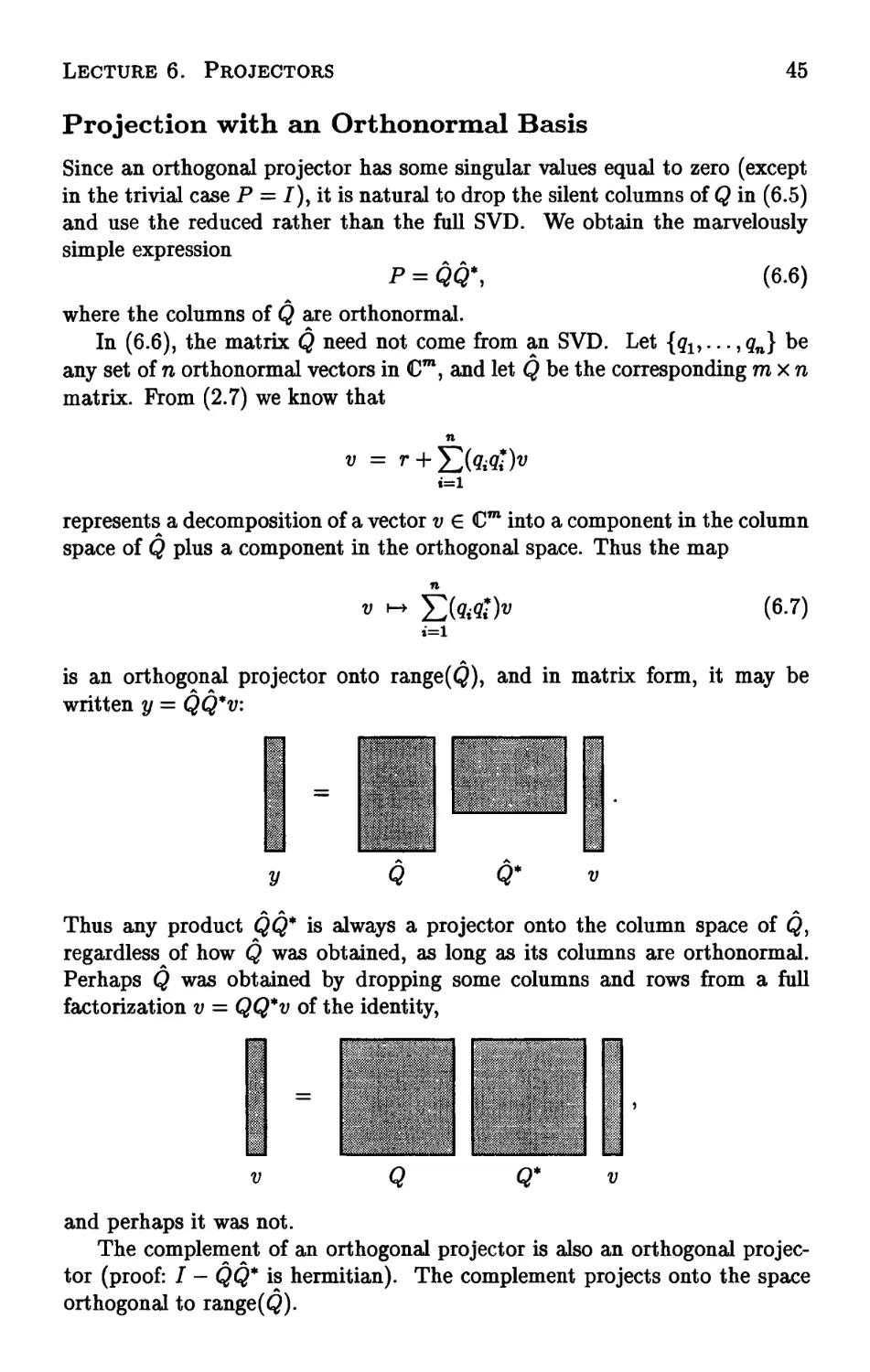
Onto what space does I - P project? Exactly the nullspace of P! We
know that range(J - P) 3 null(P), because if Pv — 0, we have (I - P)v = v.
Conversely, we know that range(/ - P) C null(P), because for any v, we have
(/ — P)v = v — Pv € null(P). Therefore, for any projector P,
range(/ - P) = null(P). (6.2)
By writing P = I - (/ - P) we derive the complementary fact
null(/ - P) = range(P). (6.3)
We can also see that null(J - P) n null(P) = {0}: any vector v in both sets
satisfies v = v - Pv = (I — P)v = 0. Another way of stating this fact is
range(P) n null(P) = {0}. (6.4)
These computations show that a projector separates Cm into two spaces.
Conversely, let Sx and 52 be two subspaces of Cm such that S1 n S2 - {0}

Lecture 6. Projectors
43
^-^ range(P)
V
Pv-v
Pv ^^
Figure 6.2. An orthogonal projection.
and Sx + S2 — €m, where ,¾ + S2 denotes the span of Sx and S2, that is, the
set of vectors sx + s2 with sx G S± and s2 G S2. (Such a pair are said to be
complementary subspaces.) Then there is a projector P such that range(P) =
Sx and null(P) = 52. We say that P is the projector onto Sx along S2.
This projector and its complement can be seen as the unique solution to the
following problem:
Given v, find vectors vx G Sx and v2 G S2 such that vY + v2 = v.
The projection Pv gives vl9 and the complementary projection (I - P)v gives
v2. These vectors are unique because all solutions must be of the form
(Pv + V3) + ((I-P)v-v3) = Vy
where it is clear that v3 must be in both Sx and 52, i.e., v3 = 0.
One context in which projectors and their complements arise is particularly
familiar. Suppose an m x m matrix A has a complete set of eigenvectors
{vy}, as in (5.1), meaning that {v^} is a basis of Cm. We are frequently
concerned with problems associated with expansions of vectors in this basis.
Given x G Cm, for example, what is the component of x in the direction of
a particular eigenvector t/? The answer is Px, where P is a certain rank-one
projector. Rather than give details here, however, we turn now to the special
class of projectors that will be of primary interest to us in this book.
Orthogonal Projectors
An orthogonal projector (Figure 6.2) is one that projects onto a subspace Sx
along a space 52, where Sx and S2 are orthogonal. (Warning: orthogonal
projectors are not orthogonal matrices!)

44
Part II. QR Factorization and Least Squares
There is also an algebraic definition: an orthogonal projector is any
projector that is hermitian, satisfying P* = P as well as (6.1). Of course, we must
establish that this definition is equivalent to the first.
Theorem 6.1. A projector P is orthogonal if and only if P = P*.
Proof If P = P*, then the inner product between a vector Px e Sx and a
vector (I — P)y € S2 is zero:
x*P*(I - P)y = x*{P - P2)y = 0.
Thus the projector is orthogonal, providing the proof in the "if" direction.
For "only if," we can use the SVD. Suppose P projects onto Sx along
S2, where St ± S2 and St has dimension n. Then an SVD of P can be
constructed as follows. Let {qlyq2,. • • ,<7m} be an orthonormal basis for CTO,
where {q^..., qn} is a basis for Sx and {<?n+1,..., qm} is a basis for 52. For
j < ft, we have Pq^ = qjy and for j > n, we have Pq- — 0. Now let Q be the
unitary matrix whose jth column is g-. We then have
PQ =
Qi
...
Qn
0
...
so that
Q*PQ =
= S.
a diagonal matrix with ones in the first n entries and zeros everywhere else.
Thus we have constructed a singular value decomposition of P:
P = QY.Q*.
(6.5)
(Note that this is also an eigenvalue decomposition (5.1).) Prom here we see
that P is hermitian, since P* = (QSQ*)* = QT,*Q* = QZQ* = P. D

Lecture 6. Projectors
45
Projection with an Orthonormal Basis
Since an orthogonal projector has some singular values equal to zero (except
in the trivial case P = J), it is natural to drop the silent columns of Q in (6.5)
and use the reduced rather than the full SVD. We obtain the marvelously
simple expression
P = QQ\ (6.6)
where the columns of Q are orthonormal.
In (6.6), the matrix Q need not come from an SVD. Let {qly..., qn} be
any set of n orthonormal vectors in CTO, and let Q be the corresponding mxn
matrix. Prom (2.7) we know that
n
represents a decomposition of a vector v e CTO into a component in the column
space of Q plus a component in the orthogonal space. Thus the map
v ~ £(fttf )* (6.7)
is an orthogonal projector onto range(Q), and in matrix form, it may be
written y = QQ*v:
Thus any product QQ* is always a projector onto the column space of Q,
regardless of how Q was obtained, as long as its columns are orthonormal.
Perhaps Q was obtained by dropping some columns and rows from a full
factorization v = QQ*v of the identity,
v Q Q* v
and perhaps it was not.
The complement of an orthogonal projector is also an orthogonal
projector (proof: I — QQ* is hermitian). The complement projects onto the space
orthogonal to range(Q).

46
Part II. QR Factorization and Least Squares
An important special case of orthogonal projectors is the rank-one
orthogonal projector that isolates the component in a single direction g, which can
be written
Pq = qq*. (6.8)
These are the pieces from which higher-rank projectors can be made, as in
(6.7). Their complements are the rank m — 1 orthogonal projectors that
eliminate the component in the direction of q:
Pu = I-M*- (6-9)
Equations (6.8) and (6.9) assume that q is a unit vector. For arbitrary nonzero
vectors a, the analogous formulas are
aa*
K = ^ (6.10)
CLCL*
*W--. (6.11)
Projection with an Arbitrary Basis
An orthogonal projector onto a subspace of Cm can also be constructed
beginning with an arbitrary basis, not necessarily orthogonal. Suppose that the
subspace is spanned by the linearly independent vectors {al5..., an}, and let
A be the m xn matrix whose jth column is a;-.
In passing from v to its orthogonal projection y € range(^4), the difference
y — v must be orthogonal to range(A). This is equivalent to the statement
that y must satisfy a^ (y - v) = 0 for every j. Since y G range (^4), we can set
y = Ax and write this condition as a!- (Ax - v) = 0 for each j, or equivalently,
A* (Ax - v) = 0 or A*Ax = A*v. It is easily shown that since A has full rank,
A*A is nonsingular (Exercise 6.3). Therefore
x = (A'A^A'v. (6.12)
Finally, the projection of vy y = Axy is y = A(A*A)~1A*v. Thus the orthogonal
projector onto range (A) can be expressed by the formula
P = A(A*A)~XA\ (6.13)
Note that this is a multidimensional generalization of (6.10). In the orthonor-
mal case A = Qy the term in parentheses collapses to the identity and we
recover (6.6).

Lecture 6. Projectors
47
Exercises
6.1. If P is an orthogonal projector, then I — 2P is unitary. Prove this
algebraically, and give a geometric interpretation.
6.2. Let E be the mxm matrix that extracts the "even part" of an m-vector:
Ex = (x + Fx)/2, where F is the m x m matrix that flips (xl9..., xm)* to
(#m> • • • »xi)*- Is # an orthogonal projector, an oblique projector, or not a
projector at all? What are its entries?
6.3. Given A € CmXtt with ra > n, show that A*A is nonsingular if and only
if A has full rank.
6.4. Consider the matrices
ri o"
0 1
[ 1 0
, B =
"121
0 1
1 oj
Answer the following questions by hand calculation.
(a) What is the orthogonal projector P onto range(^4), and what is the image
under P of the vector (1,2,3)*?
(b) Same questions for 2?.
6.5. Let P 6 Cmxm be a nonzero projector. Show that ||P||2 > 1, with
equality if and only if P is an orthogonal projector.

Lecture 7. QR Factorization
One algorithmic idea in numerical linear algebra is more important than all
the others: QR factorization.
Reduced QR Factorization
For many applications, we find ourselves interested in the column spaces of
a matrix A. Note the plural: these are the successive spaces spanned by the
columns ax, a2,... of A:
(ai) £ (^1,¾) £ (^1,¾^¾) Q ....
Here, as in Lecture 5 and throughout the book, the notation (• • •) indicates the
subspace spanned by whatever vectors are included in the brackets. Thus (ax)
is the one-dimensional space spanned by al3 {cLlya2) is the two-dimensional
space spanned by ax and a2, and so on. The idea of QR factorization is the
construction of a sequence of orthonormal vectors q1,q2>-.. that span these
successive spaces.
To be precise, assume for the moment that A € cmxn (m > n) has full
rank n. We want the sequence ql3 g2,... to have the property
(?i> &>•••> ¢,-) = («i» «2,..., ay>, j = 1,..., n. (7.1)
Prom the observations of Lecture 1, it is not hard to see that this amounts to
48

Lecture 7. QR Factorization
49
the condition
al
a2
...
«n
=
«1
&
...
Qn
rll rl2
r22
'In
, (7.2)
where the diagonal entries rkk are nonzero—for if (7.2) holds, then al5..., ak
can be expressed as linear combinations ofql3...,qki and the invertibility of
the upper-left k x k block of the triangular matrix implies that, conversely,
qly..., qk can be expressed as linear combinations of ax,..., afc. Written out,
these equations take the form
«i = rnQi>
a2 = r12Ql + r22«2)
a3 = r13Ql + r23?2 + ^33¾) ^7,3^
*>n = rinQl + r2nQ2 + '
As a matrix formula, we have
A = QR,
+ rnnqn
(7.4)
where Q is m x n with orthonormal columns and R is n x n and upper-
triangular. Such a factorization is called a reduced QR factorization of A.
Full QR Factorization
A full QR factorization of A € <cmxn (m > n) goes further, appending an
additional m — n orthonormal columns to Q so that it becomes an m x m
unitary matrix Q. This is analogous to the passage from the reduced to the
full SVD described in Lecture 4. In the process, rows of zeros are appended
to R so that it becomes an m x n matrix R, still upper-triangular. The
relationship between the full and reduced QR factorizations is as follows.
Pull QR Factorization (m > n)
VA-v'v ***3>**

50
Part II. QR Factorization and Least Squares
In the full QR factorization, Q is m x m, R is m x n, and the last ra—n columns
of Q are multiplied by zeros in R (enclosed by dashes). In the reduced QR
factorization, the silent columns and rows are removed. Now Q is m x n, R is
n x n, and none of the rows of R are necessarily zero.
Reduced QR Factorization (ra > n)
Notice that in the full QR factorization, the columns qi for j > n are
orthogonal to range(A). Assuming A is of full rank n, they constitute an or-
thonormal basis for range (A)1 (the space orthogonal to range (A)), or equiv-
alently, for null(A*).
Gram—Schmidt Orthogonalization
Equations (7.3) suggest a method for computing reduced QR factorizations.
Given ax, a2,..., we can construct the vectors ql} g2» • • • and entries rtf by a
process of successive orthogonalization. This is an old idea, known as Gram-
Schmidt orthogonalization.
The process works like this. At the jih step, we wish to find a unit vector
g7- G (a1}..., a^) that is orthogonal to g1}..., ¢^. As it happens, we have
already considered the necessary orthogonalization technique in (2.6). From
that equation, we see that
*i = aj - (¢1¾¼ " (¢2¾)¾ (#-l«i)%'-l (7-5)
is a vector of the kind required, except that it is not yet normalized. If we
divide by ||t/y||2, the result is a suitable vector q^
With this in mind, let us rewrite (7.3) in the form
a1
91 = r '
¢2 =
¢3 =
<*2 ~ rl2Ql
'22
fl3 ~ r13?l " r23?2
r33
(7.6)

Lecture 7. QR Factorization
51
From (7.5) it is evident that an appropriate definition for the coefficients r{j
in the numerators of (7.6) is
th = ?;«,• (*'#i). (7.7)
The coefficients r - - in the denominators are chosen for normalization:
K\ = h-i>«fc|2- (™)
t=i
Note that the sign of r- is not determined. Arbitrarily, we may choose r^ > 0,
in which case we shall finish with a factorization A = QR in which R has
positive entries along the diagonal.
The algorithm embodied in (7.6)-(7.8) is the Gram-Schmidt iteration.
Mathematically, it offers a simple route to understanding and proving various
properties of QR factorizations. Numerically, it turns out to be unstable
because of rounding errors on a computer. To emphasize the instability,
numerical analysts refer to this as the classical Gram-Schmidt iteration, as opposed
to the modified Gram-Schmidt iteration, discussed in the next lecture.
Algorithm 7.1. Classical Gram-Schmidt
for j = 1 to n
v- = a-
3 3
for i = 1 to j — 1
*ij = Qiaj
Vj = Vj - rijq{
rjj = IK l|2
% = VilT33
(unstable)
Existence and Uniqueness
All matrices have QR factorizations, and under suitable restrictions, they are
unique. We state first the existence result.
Theorem 7.1. Every A G Cmxn (m > n) has a fall QR factorization, hence
also a reduced QR factorization.
Proof. Suppose first that A has full rank and that we want just a reduced
QR factorization. In this case, a proof of existence is provided by the Gram-
Schmidt algorithm itself. By construction, this process generates orthonormal
columns of Q and entries of R such that (7.4) holds. Failure can occur only
if at some step, Vj is zero and thus cannot be normalized to produce q-.

52
Part II. QR Factorization and Least Squares
However, this would imply a^ £ (g1?..., gy^) = (ax,..., a^), contradicting
the assumption that A has full rank.
Now suppose that A does not have full rank. Then at one or more steps
jf, we shall find that (7.5) gives v- = 0, as just mentioned. At this
moment, we simply pick q^ arbitrarily to be any normalized vector orthogonal to
(?i> • • •) <7j-i)? an(l *hen continue the Gram-Schmidt process.
Finally, the full, rather than reduced, QR factorization of an m x n matrix
with m> n can be constructed by introducing arbitrary orthonormal vectors
in the same fashion. We follow the Gram-Schmidt process through step n,
then continue on an additional m — n steps, introducing vectors q^ at each
step.
The issues discussed in the last two paragraphs came up already in
Lecture 4, in our discussion of the SVD. □
We turn now to uniqueness. Suppose A — QR is a reduced QR
factorization. If the ith column of Q is multiplied by z and the ith row of R is
multiplied by z"1 for some scalar z with \z\ = 1, we obtain another QR
factorization of A. The next theorem asserts that if A has full rank, this is the
only way to obtain distinct reduced QR factorizations.
Theorem 7.2. Each A € cmxn (yn > n) of full rank has a unique reduced
QR factorization A = QR with r^ > 0.
Proof Again, the proof is provided by the Gram-Schmidt iteration. From
(7.4), the orthonormality of the columns of Q, and the upper-triangularity of
J?, it follows that any reduced QR factorization of A must satisfy (7.6)-(7.8).
By the assumption of full rank, the denominators (7.8) of (7.6) are nonzero,
and thus at each successive step j, these formulas determine r- and q- fully,
except in one place: the sign of rJ7, not specified in (7.8). Once this is fixed
by the condition r- > 0, as in Algorithm 7.1, the factorization is completely
determined. □
When Vectors Become Continuous Functions
The QR factorization has an analogue for orthonormal expansions of functions
rather than vectors.
Suppose we replace Cm by L2[— 1,1], a vector space of complex-valued
functions on [—1,1]. We shall not introduce the properties of this space formally;
suffice it to say that the inner product of f and g now takes the form
(/,5) = £j(xjg(x)dx. (7.9)

Lecture 7. QR Factorization
53
Consider, for example, the following "matrix" whose "columns" are the
monomials xj:
(7.10)
Each column is a function in L2[—1,1], and thus, whereas A is discrete as
usual in the horizontal direction, it is continuous in the vertical direction. It
is a continuous analogue of the Vandermonde matrix (1.4) of Example 1.1.
The "continuous QR factorization" of A takes the form
1
X
x2
...
x71'1
A = QR =
Qo(x)
Qi(x)
...
S„-i(z)
rll
'12
r22
rln
where the columns of Q are functions of x, orthonormal with respect to the
inner product (7.9):
Prom the Gram-Schmidt construction we can see that g. is a polynomial
of degree j. These polynomials are scalar multiples of what are known as
the Legendre polynomials, Pj, which are conventionally normalized so that
P^l) = 1. The first few Pj are
P0(*) = l, P1(x) = x, P2{*) = V - i P*(x) = f*3 " \*\ (7.11)
see Figure 7.1. Like the monomials l,x,x2,..., this sequence of
polynomials spans the spaces of polynomials of successively higher degree. However,
P0(x),P1(x),P2(x)>... have the advantage that they are orthogonal, making
them far better suited for certain computations. In fact, computations with
such polynomials form the basis of spectral methods, one of the most powerful
techniques for the numerical solution of partial differential equations.
What is the "projection matrix" QQ* (6.6) associated with Q? It is a
"[—1,1] x [—1,1] matrix," that is, an integral operator
(7.12)
mapping functions in L2[—1,1] to functions in L2[—1,1].

54
Part II. QR Factorization and Least Squares
Figure 7.1. The first four Legendre polynomials (7.11). Apart from scale
factors, these can be interpreted as the columns of Q in a reduced QR factorization
of the "[-1,1] x 4 matrix" [1, x, x2y x3].
Solution of Ax = b by QR Factorization
In closing this lecture we return for a moment to discrete, finite matrices.
Suppose we wish to solve Ax = b for x, where A G <Cmxm is nonsingular. If
A = QR is a QR factorization, then we can write QRx = 6, or
Rx = Q*b. (7.13)
The right-hand side of this equation is easy to compute, if Q is known, and the
system of linear equations implicit in the left-hand side is also easy to solve
because it is triangular. This suggests the following method for computing
the solution to Ax = b:
1. Compute a QR factorization A = QR.
2. Compute y = Q*b.
3. Solve Rx = y for x.
In later lectures we shall present algorithms for each of these steps.
The combination 1-3 is an excellent method for solving linear systems of
equations; in Lecture 16, we shall prove this. However, it is not the standard
method for such problems. Gaussian elimination is the algorithm generally
used in practice, since it requires only half as many numerical operations.

Lecture 7. QR Factorization
55
Exercises
7.1. Consider again the matrices A and B of Exercise 6.4.
(a) Using any method you like, determine (on paper) a reduced QR
factorization A = QR and a full QR factorization A = QR.
(b) Again using any method you like, determine reduced and full QR
factorizations B = QR and B = QR.
7.2. Let A be a matrix with the property that columns 1,3,5,7,... are
orthogonal to columns 2,4,6,8, In a reduced QR factorization A = QR,
what special structure does R possess?
7.3. Let A be an m x m matrix, and let a7 be its jth column. Give an
algebraic proof of Hadamard's inequality:
TO
|detA| <IIIKIl2.
Also give a geometric interpretation of this result, making use of the fact that
the determinant equals the volume of a parallelepiped.
7.4. Let x(1\ y^\ x^2\ and yW be nonzero vectors in M3 with the property
that x^ and y^ are linearly independent and so are x^ and y^2\ Consider
the two planes in R3,
P^ = (x^\i% pW = (x(2\yW).
Suppose we wish to find a nonzero vector v G 1R3 that lies in the intersection
P = pW n P(2\ Devise a method for solving this problem by reducing it to
the computation of QR factorizations of three 3x2 matrices.
7.5. Let A be an m x n matrix (m > n), and let A = QR be a reduced QR
factorization.
(a) Show that A has rank n if and only if all the diagonal entries of R are
nonzero.
(b) Suppose R has k nonzero diagonal entries for some k with 0 < k < n.
What does this imply about the rank of At Exactly fc? At least fc? At most
fc? Give a precise answer, and prove it.

Lecture 8. Gram-Schmidt
Orthogonalization
The Gram-Schmidt iteration is the basis of one of the two principal numerical
algorithms for computing QR factorizations. It is a process of "triangular
orthogonalization," making the columns of a matrix orthonormal via a sequence
of matrix operations that can be interpreted as multiplication on the right by
upper-triangular matrices.
Gram—Schmidt Projections
In the last lecture we presented the Gram-Schmidt iteration in its classical
form. To begin this lecture, we describe the same algorithm again in another
way, using orthogonal projectors.
Let A G Cmxn, m > n, be a matrix of full rank with columns {a,}.
Before, we expressed the Gram-Schmidt iteration by the formulas (7.6)-(7.8).
Consider now the sequence of formulas
_ Pl0l _ P2a2 _ Pnan
In these formulas, each P^ denotes an orthogonal projector. Specifically, Pj
is the m x m matrix of rank m - (j - 1) that projects Cm orthogonally onto
the space orthogonal to (q1}... ,ty_i). (In the case j = 1, this prescription
reduces to the identity: Px = J.) Now, observe that q^ as defined by (8.1) is
56

Lecture 8. Gram-Schmidt Orthogonalization
57
orthogonal to qlt..., qj_lt lies in the space (alt..., a^), and has norm 1. Thus
we see that (8.1) is equivalent to (7.6)-(7.8) and hence to Algorithm 7.1.
The projector P- can be represented explicitly. Let Qj_x denote the m x
(j — 1) matrix containing the first j — 1 columns of Q,
Qi-i =
ft
¢2
%-l
(8.2)
Then P- is given by
P, = I-Q^QU-
(8.3)
By now, the reader may be familiar enough with our notation and with
orthogonality ideas to see at a glance that (8.3) represents the operator applied
to a7- in (7.5).
Modified Gram—Schmidt Algorithm
In practice, the Gram-Schmidt formulas are not applied as we have indicated
in Algorithm 7.1 and in (8.1), for this sequence of calculations turns out to
be numerically unstable. Fortunately, there is a simple modification that
improves matters. We have not discussed numerical stability yet; this will
come in the next lecture and then systematically beginning in Lecture 14.
For the moment, it is enough to know that a stable algorithm is one that is
not too sensitive to the effects of rounding errors on a computer.
For each value of j, Algorithm 7.1 computes a single orthogonal projection
of rank to — (j — 1),
(8.4)
3 3
In contrast, the modified Gram-Schmidt algorithm computes the same result
by a sequence of j — 1 projections of rank m — 1. Recall from (6.9) that PLq
denotes the rank m — 1 orthogonal projector onto the space orthogonal to a
nonzero vector q € Cm. By the definition of P^ it is not difficult to see that
P3 ~ PUj-l " " " P±-q2PUV
(8.5)
again with Px = I. Thus an equivalent statement to (8.4) is
f,- = P^-'-P^Pufy-
(8.6)
The modified Gram-Schmidt algorithm is based on the use of (8.6) instead of
(8.4).

58 Part II. QR Factorization and Least Squares
Mathematically, (8.6) and (8.4) are equivalent. However, the sequences of
arithmetic operations implied by these formulas are different. The modified
algorithm calculates v^ by evaluating the following formulas in order:
vi
V?
V?
vf
= tf
=
=
=
=
°;>
P v{1)
p,^r
p^-rf-
-i)
= tf-fctf,^,
(2) * (2)
= f?"13-¢,--131-^
(8.7)
In finite precision computer arithmetic, we shall see that (8.7) introduces
smaller errors than (8.4).
When the algorithm is implemented, the projector P± can be conveniently
applied to vy for each j > i immediately after q{ is known. This is done in
the description below.
Algorithm 8.1. Modified Gram-Schmidt
for i = 1 to n
Vi = at
i = 1 to n
r« = NI
Qi = vi/ru
for j = t+lton
rH =
Vj =
■ <!>!
Vj - ^¾
In practice, it is common to let vi overwrite a{ and q{ overwrite v{ in order to
save storage.
The reader should compare Algorithms 7.1 and 8.1 until he or she is
confident of their equivalence.
Operation Count
The Gram-Schmidt algorithm is the first algorithm we have presented in this
book, and with any algorithm, it is important to assess its cost. To do so,
throughout the book we follow the classical route and count the number of
floating point operations—"flops"—that the algorithm requires. Each
addition, subtraction, multiplication, division, or square root counts as one flop.

Lecture 8. Gram-Schmidt Orthogonalization
59
We make no distinction between real and complex arithmetic, although in
practice on most computers there is a sizable difference.
In fact, there is much more to the cost of an algorithm than operation
counts. On a single-processor computer, the execution time is affected by
the movement of data between elements of the memory hierarchy and by
competing jobs running on the same processor. On multiprocessor machines
the situation becomes more complex, with communication between processors
sometimes taking on an importance much greater than that of actual
"computation." With some regret, we shall ignore these important considerations,
because this book is deliberately classical in style, focusing on algorithmic
foundations.
For both variants of the Gram-Schmidt iteration, here is the classical
result.
Theorem 8.1. Algorithms 7.1 and 8.1 require ~ 2mn2 flops to compute a
QR factorization of anmxn matrix.
Note that the theorem expresses only the leading term of the flop count.
The symbol " ~ " has its usual asymptotic meaning:
number of flops
Ja.—w— = L
In discussing operation counts for algorithms, it is standard to discard lower-
order terms as we have done here, since they are usually of little significance
unless m and n are small.
Theorem 8.1 can be established as follows. To be definite, consider the
modified Gram-Schmidt algorithm, Algorithm 8.1. When m and n are large,
the work is dominated by the operations in the innermost loop:
V3 = Vi - Wi-
The first line computes an inner product q*Vj, requiring m multiplications and
to—1 additions, and the second computes v,—ry<fc, requiring m multiplications
and m subtractions. The total work involved in a single inner iteration is
consequently ~ 4to flops, or 4 flops per column vector element. All together,
the number of flops required by the algorithm is asymptotic to
£ £ 4to ~ £(t)4m - 2mn2. (8.8)
t=i j=i+i t=i
Counting Operations Geometrically
Operation counts can always be determined algebraically as in (8.8), and this
is the standard procedure in the numerical analysis literature. However, it is

60
Part II. QR Factorization and Least Squares
also enlightening to take a different, geometrical route to the same conclusion.
The argument goes like this. At the first step of the outer loop, Algorithm 8.1
operates on the whole matrix, subtracting a multiple of column 1 from the
other columns. At the second step, it operates on a submatrix, subtracting a
multiple of column 2 from columns 3,..., n. Continuing on in this way, at each
step the column dimension shrinks by 1 until at the final step, only column n
is modified. This process can be represented by the following diagram:
m
(row index)
J n
(outer loop index)
n (column index)
The m x n rectangle at the bottom corresponds to the first pass through the
outer loop, the m x (n — 1) rectangle above it to the second pass, and so on.
To leading order as ra,n —► oo, then, the operation count for Gram-
Schmidt orthogonalization is proportional to the volume of the figure above.
The constant of proportionality is four flops, because as noted above, the two
steps of the inner loop correspond to four operations at each matrix location.
Now as ra,n —► oo, the figure converges to a right triangular prism, with
volume ran2/2. Multiplying by four flops per unit volume gives, again,
Work for Gram-Schmidt orthogonalization: ~ 2mn2 flops. (8.9)
In this book we generally record operation counts in the format (8.9),
without stating them as theorems. We often derive these results via figures
like the one above, although algebraic derivations are also possible. One reason
we do this is that a figure of this kind, besides being a route to an operation
count, also serves as a reminder of the structure of an algorithm. For pictures
of algorithms with different structures, see pp. 75 and 176.

Lecture 8. Gram-Schmidt Orthogonalization
61
Gram—Schmidt as Triangular Orthogonalization
Each outer step of the modified Gram-Schmidt algorithm can be interpreted
as a right-multiplication by a square upper-triangular matrix. For example,
beginning with A, the first iteration multiplies the first column ax by l/rn
and then subtracts rXj times the result from each of the remaining columns
a;. This is equivalent to right-multiplication by a matrix Rx:
V1
V2
...
n
1
rn
1
—ri3
1
—
¢1
(2)
...
«£»
In general, step i of Algorithm 8.1 subtracts r^jr^ times column i of the
current A from columns j > i and replaces column i by l/ri{ times itself. This
corresponds to multiplication by an upper-triangular matrix R{:
R2 —
1 -7*23
Til T22
1
Rz —
^33
At the end of the iteration we have
ARXR2 -Rn = Q.
(8.10)
R
-l
This formulation demonstrates that the Gram-Schmidt algorithm is a method
of triangular orthogonalization. It applies triangular operations on the right
of a matrix to reduce it to a matrix with orthonormal columns. Of course, in
practice, we do not form the matrices R{ and multiply them together explicitly.
The purpose of mentioning them is to give insight into the structure of the
Gram-Schmidt algorithm. In Lecture 20 we shall see that it bears a close
resemblance to the structure of Gaussian elimination.
Exercises
8,1. Let A be an m x n matrix. Determine the exact numbers of floating point
additions, subtractions, multiplications, and divisions involved in computing
the factorization A = QR by Algorithm 8.1.

62 Part II. QR Factorization and Least Squares
8.2. Write a Matlab function [Q,R] = mgs(A) (see next lecture) that
computes a reduced QR factorization A = QR of an m x n matrix A with
m > n using modified Gram-Schmidt orthogonalization. The output
variables are a matrix Q € <cmXTO with orthonormal columns and a triangular
matrix R € CnXn.
8.3. Each upper-triangular matrix iJ. of p. 61 can be interpreted as the
product of a diagonal matrix and a unit upper-triangular matrix (i.e., an
upper-triangular matrix with 1 on the diagonal). Explain exactly what these
factors are, and which line of Algorithm 8.1 corresponds to each.

Lecture 9. MATLAB
To learn numerical linear algebra, one must make a habit of
experimenting on the computer. There is no better way to do this than by using the
problem-solving environment known as Matlab®.* In this lecture we
illustrate Matlab experimentation by three examples. Along the way, we make
some observations about the stability of Gram-Schmidt orthogonalization.
MATLAB
Matlab is a language for mathematical computations whose fundamental
data types are vectors and matrices. It is distinguished from languages like
Fortran and C by operating at a higher mathematical level, including hundreds
of operations such as matrix inversion, the singular value decomposition, and
the fast Fourier transform as built-in commands. It is also a problem-solving
environment, processing top-level comments by an interpreter rather than a
compiler and providing in-line access to 2D and 3D graphics.
Since the 1980s, Matlab has become a widespread tool among numerical
analysts and engineers around the world. For many problems of large-scale
scientific computing, and for virtually all small- and medium-scale
experimentation in numerical linear algebra, it is the language of choice.
* Matlab is a registered trademark of The MathWorks, Inc., 24 Prime Park Way,
Natick, MA 01760, USA, tel. 508-647-7000, fax 508-647-7001, infoOmathworks.com,
http://www.mathworks. com.
63

64
Part II. QR Factorization and Least Squares
In this book, we use Matlab now and then to present certain numerical
experiments, and in some exercises. We do not describe the language
systematically, since the number of experiments we present is limited, and only a
reading knowledge of Matlab is needed to follow them.
Experiment 1: Discrete Legendre Polynomials
In Lecture 7 we considered the Vandermonde "matrix" with "columns"
consisting of the monomials 1, x, x2, and x3 on the interval [—1,1]. Suppose
we now make this a true Vandermonde matrix by discretizing [—1,1] by 257
equally spaced points. The following lines of Matlab construct this matrix
and compute its reduced QR factorization.
x = (-128:128) V128; Set a: to a discretization of [-1,1].
A = [x. "0 x. "1 x. "2 x. "3] ; Construct Vandermonde matrix.
[Q.R] = qr(A,0) ; Find its reduced QR factorization.
Here are a few remarks on these commands. In the first line, the prime
' converts (-128:128) from a row to a column vector. In the second line,
the sequences . ~ indicate entrywise powers. In the third line, qr is a built-in
Matlab function for computing QR factorizations; the argument 0 indicates
that a reduced rather than full factorization is needed. The method used here
is not Gram-Schmidt orthogonalization but Householder triangularization,
discussed in the next lecture, but this is of no consequence for the present
purpose. In all three lines, the semicolons at the end suppress the printed
output that would otherwise be produced (x, A, Q, and R).
The columns of the matrix Q are essentially the first four Legendre
polynomials of Figure 7.1. They differ slightly, by amounts close to plotting accuracy,
because the continuous inner product on [—1,1] that defines the Legendre
polynomials has been replaced by a discrete analogue. They also differ in
normalization, since a Legendre polynomial should satisfy Pk(l) = 1. We can
fix this by dividing each column of Q by its final entry. The following lines of
Matlab do this by a right-multiplication by a 4 x 4 diagonal matrix.
scale = Q(257,:) ; Select last row of Q.
Q = Q*diag(l ./scale) ; Rescale columns by these numbers.
plot (Q) Plot columns of rescaled Q.
The result of our computation is a plot that looks just like Figure 7.1
(not shown). In Fortran or C, this would have taken dozens of lines of code
containing numerous loops and nested loops. In our six lines of Matlab, not
a single loop has appeared explicitly, though at least one loop is implicit in
every line.

Lecture 9. MATLAB
65
Experiment 2: Classical vs. Modified Gram-Schmidt
Our second example has more algorithmic substance. Its purpose is to explore
the difference in numerical stability between the classical and modified Gram-
Schmidt algorithms.
First, we construct a square matrix A with random singular vectors and
widely varying singular values spaced by factors of 2 between 2_1 and 2""80.
[ [U,X] = qr(randn(80));
[V,X] = qr(randn(80));
S=diag(2r(-1:-1:-80));
A = U*S*V;
Set U to a random orthogonal matrix.
Set V to a random orthogonal matrix.
Set S to a diagonal matrix with
exponentially graded entries.
Set A to a matrix with these entries as
singular values.
Now, we use Algorithms 7.1 and 8.1 to compute QR factorizations of A. In
the following code, the programs clgs and mgs are Matlab implementations,
not listed here, of Algorithms 7.1 and 8.1.
[QC,RC] = clgs (A); Compute a factorization QMjjM by
classical Gram-Schmidt.
[QM,RM3 = mgs (A); Compute a factorization Q(m)i?(m) by
modified Gram-Schmidt.
Finally, we plot the diagonal elements rJ7 produced by both computations
(Matlab code not shown). Since rJ7 = HP^H, this gives us a picture of the
size of the projection at each step. The results are shown on a logarithmic
scale in Figure 9.1.
The first thing one notices in the figure is a steady decrease of r^ with
jy closely matching the line 2"K Evidently r^ is not exactly equal to the
jth. singular value of A, but it is a reasonably good approximation. This
phenomenon can be roughly explained as follows. The SVD of A can be
written in the form (5.3) as
A = 2-1^ + 2~2u2V2 + 2"3u3vl + • • • + 2"~80u80z;80,
where {Uj} and {v^} are the left and right singular vectors of A, respectively.
In particular, the jth column of A has the form
a- = 2""1tJilu1 + 2~2vj2u2 + 2-3vj3u3 + • • • + 2~s0v^S0uS0.
Since the singular vectors are random, we can expect that the numbers v^
are all of a similar magnitude, on the order of 80~1/2 «0.1. Now, when we
take the QR factorization, it is evident that the first vector qx is likely to be

66
Part II. QR Factorization and Least Squares
'33
10
10"°
10'
10*1
10^
10
-i r
*t
-¾¾
00¾ Qj O O 0¾ O O
4
oo
^
>w„
»tf
2-> x>
_l L_
y ^machine
^machine
10 20 30 40 50 60 70
80
Figure 9.1. Computed r^ versus j for the QR factorization of a matrix with
exponentially graded singular values. On this computer with about 16 digits of
relative accuracy, the classical Gram-Schmidt algorithm produces the numbers
represented by circles and the modified Gram-Schmidt algorithm produces the
numbers represented by crosses.
approximately equal to uly with rn on the order of 2"1 x 80-1^2. Orthogo-
nalization at the next step will yield a second vector q2 approximately equal
to u2, with r22 on the order of 2~2 x 80"1/2—and so on.
The next thing one notices in Figure 9.1 is that the geometric decrease of
Tjj does not continue all the way to j = 80. This is a consequence of rounding
errors on the computer. With the classical Gram-Schmidt algorithm, the
numbers never become smaller than about 10"8. With the modified Gram-
Schmidt algorithm, they shrink eight orders of magnitude further, down to the
order of 10~16, which is the level of machine epsilon for the computer used in
this calculation. Machine epsilon is defined in Lecture 13.
Clearly, some algorithms are more stable than others. It is well established
that the classical Gram-Schmidt process is one of the unstable ones.
Consequently it is rarely used, except sometimes on parallel computers in situations
where advantages related to communication may outweigh the disadvantage
of instability.
Experiment 3: Numerical Loss of Orthogonality
At the risk of confusing the reader by presenting two instability phenomena
in succession, we close this lecture by exhibiting another, different kind of

Lecture 9. MATLAB
67
instability that affects both the modified and classical Gram-Schmidt
algorithms. In floating point arithmetic, these algorithms may produce vectors
q. that are far from orthogonal. The loss of orthogonality occurs when A is
close to rank-deficient, and, like most instabilities, it can appear even in low
dimensions.
Starting on paper rather than in Matlab, consider the case of a matrix
A =
0.70000 0.70711
0.70001 0.70711
(9.1)
on a computer that rounds all computed results to five digits of relative
accuracy (Lecture 13). The classical and modified algorithms are identical in the
2x2 case. At step j = 1, the first column is normalized, yielding
ru = 0.98996, qx = ajrn =
0.70000/0.98996
0.70001/0.98996
0.70710
0.70711
in five-digit arithmetic. At step j = 2, the component of a2 in the direction
of q1 is computed and subtracted out:
r12 = q{a2 = 0.70710 x 0.70711 + 0.70711 x 0.70711 = 1.0000,
v2 = Q>2 ~ rv&\ =
again with rounding to five digits. This computed v2 is dominated by errors.
The final computed Q is
[ 0.70711'
[ 0.70711
—
' 0.70710 "
0.70711
=
" 0.00001 1
0.00000 J
Q =
0.70710 1.0000
0.70711 0.0000
which is not close to any orthogonal matrix.
On a computer with sixteen-digit precision, we still lose about five digits of
orthogonality if we apply modified Gram-Schmidt to the matrix (9.1). Here
is the Matlab evidence. The "eye" function generates the identity of the
indicated dimension.
A = [.70000 .70711
.70001 .70711];
[Q,R] = qr(A);
norm(Q,*Q-eye(2))
[Q,R] = mgs(A);
norm(Q,*Q-eye(2))
Define A.
Compute factor Q by Householder.
Test orthogonality of Q.
Compute factor Q by modified G-S.
Test orthogonality of Q.
The lines without semicolons produce the following printed output:
ans = 2.3515e-16, ans = 2.3014e-ll.

68
Part II. QR Factorization and Least Squares
Exercises
9.1. (a) Run the six-line Matlab program of Experiment 1 to produce a
plot of approximate Legendre polynomials.
(b) For k = 0,1,2,3, plot the difference on the 257-point grid between these
approximations and the exact polynomials (7.11). How big are the errors, and
how are they distributed?
(c) Compare these results with what you get with grid spacings Ax = 2~v for
other values of v. What power of Ax appears to control the convergence?
9.2. In Experiment 2, the singular values of A match the diagonal elements
of a QR factor R approximately. Consider now a very different example.
Suppose Q = I and A = i?, the rax m matrix (a Toeplitz matrix) with 1 on
the main diagonal, 2 on the first superdiagonal, and 0 everywhere else.
(a) What are the eigenvalues, determinant, and rank of A ?
(b) What is A-1 ?
(c) Give a nontrivial upper bound on crm, the rath singular value of A. You
are welcome to use Matlab for inspiration, but the bound you give should
be justified analytically. (Hint: Use part (b).)
This problem illustrates that you cannot always infer much about the singular
values of a matrix from its eigenvalues or from the diagonal entries of a QR
factor R.
9.3. (a) Write a Matlab program that sets up a 15 x 40 matrix with entries
0 everywhere except for the values 1 in the positions indicated in the picture
below. The upper-leftmost 1 is in position (2,2), and the lower-rightmost 1
is in position (13,39). This picture was produced with the command spy (A).
Op 1 1 1 1 1 1 1 r
-i 1 1 1 i i i i i_
0 5 10 15 20 25 30 35 40
(b) Call svd to compute the singular values of A, and print the results. Plot
these numbers using both plot and semilogy. What is the mathematically
exact rank of A? How does this show up in the computed singular values?
(c) For each i from 1 to rank (A), construct the rank-z matrix B that is the
best approximation to A in the 2-norm. Use the command pcolor(B) with
colormap(gray) to create images of these various approximations.

Lecture 10. Householder Triangularization
The other principal method for computing QR factorizations is Householder
triangularization, which is numerically more stable than Gram-Schmidt or-
thogonalization, though it lacks the latter's applicability as a basis for iterative
methods. The Householder algorithm is a process of "orthogonal
triangularization," making a matrix triangular by a sequence of unitary matrix operations.
Householder and Gram—Schmidt
As we saw in Lecture 8, the Gram-Schmidt iteration applies a succession of
elementary triangular matrices Rk on the right of A, so that the resulting
matrix
AR1R2-Rn = Q
R-1
has orthonormal columns. The product R = R~x • • • R^R^1 is
upper-triangular too, and thus A = QR is a reduced QR factorization of A.
In contrast, the Householder method applies a succession of elementary
unitary matrices Qk on the left of A, so that the resulting matrix
Qn-Q2Q1A = R
> v '
Q*
is upper-triangular. The product Q = Q\Q2 • • • Q* is unitary too, and
therefore A = QR is a full QR factorization of A.
69

70
Part II. QR Factorization and Least Squares
The two methods can thus be summarized as follows:
Gram-Schmidt: triangular orthogonalization,
Householder: orthogonal triangularization.
Triangularizing by Introducing Zeros
At the heart of the Householder method is an idea originally proposed by
Alston Householder in 1958. This is an ingenious way of designing the unitary
matrices Qk so that Qn • • • Q2Q\A is upper-triangular.
The matrix Qk is chosen to introduce zeros below the diagonal in the fcth
column while preserving all the zeros previously introduced. For example, in
the 5x3 case, three operations Qk are applied, as follows. In these matrices,
the symbol x represents an entry that is not necessarily zero, and boldfacing
indicates an entry that has just been changed. Blank entries are zero.
xxx
xxx
xxx
xxx
xxx
A
Qi
X
X
X
X
X
QiA
Q2
XXX
X X
0 X
0 X
0 X
Q2QlA
Q*
—>
xxx"
X X
X
0
0
Q3Q2QiA
(10.1)
First, Qx operates on rows 1,..., 5, introducing zeros in positions (2,1), (3,1),
(4,1), and (5,1). Next, Q2 operates on rows 2,...,5, introducing zeros in
positions (3,2), (4,2), and (5,2) but not destroying the zeros introduced by
Qv Finally, Q3 operates on rows 3,..., 5, introducing zeros in positions (4,3)
and (5,3) without destroying any of the zeros introduced earlier.
In general, Qk operates on rows fc,..., m. At the beginning of step fc, there
is a block of zeros in the first k — 1 columns of these rows. The application
of Qk forms linear combinations of these rows, and the linear combinations of
the zero entries remain zero. After n steps, all the entries below the diagonal
have been eliminated and Qn • • • Q2Q\A = R is upper-triangular.
Householder Reflectors
How can we construct unitary matrices Qk to introduce zeros as indicated
in (10.1)? The standard approach is as follows. Each Qk is chosen to be a
unitary matrix of the form
Qk =
0
F
(10.2)
where I is the (k - 1) x (fc - 1) identity and F is an (m - k + 1) x (m —
k + 1) unitary matrix. Multiplication by F must introduce zeros into the

Lecture 10. Householder Triangularization
71
Fx = \\xl\e,
.'' H
Figure 10.1. A Householder reflection.
fcth column. The Householder algorithm chooses F to be a particular matrix
called a Householder reflector.
Suppose, at the beginning of step fc, the entries fc,..., ra of the fcth column
are given by the vector x e Cm-fe+1. To introduce the correct zeros into the
kih column, the Householder reflector F should effect the following map:
x =
x
X
X
Fx =
IHI
o
0
= x e,
(10.3)
(We shall modify this idea by a ± sign in a moment.) The idea for
accomplishing this is indicated in Figure 10.1. The reflector F will reflect the
space cm~fc+1 across the hyperplane H orthogonal to v = ||^||e1 — x. A hy-
perplane is the higher-dimensional generalization of a two-dimensional plane
in three-space—a three-dimensional subspace of a four-dimensional space, a
four-dimensional subspace of a five-dimensional space, and so on. In general,
a hyperplane can be characterized as the set of points orthogonal to a fixed
nonzero vector. In Figure 10.1, that vector is v = \\x\fa - x, and one can
think of the dashed line as a depiction of H viewed "edge on."
When the reflector is applied, every point on one side of the hyperplane H
is mapped to its mirror image on the other side. In particular, x is mapped
to Hxllcx. The formula for this reflection can be derived as follows. In (6.11)
we have seen that for any y G Cm, the vector
Py = (/-21), = y-jm
\ v*vj \v*v/

72
Part II. QR Factorization and Least Squares
+\\x et-x
Figure 10.2. Two possible reflections. For numerical stability, it is important
to choose the one that moves x the larger distance.
is the orthogonal projection of y onto the space H. To reflect y across H,
we must not stop at this point; we must go exactly twice as far in the same
direction. The reflection Fy should therefore be
Hence the matrix F is
F = I - 2
w
~v*v*
(10.4)
Note that the projector P (rank ra-1) and the reflector F (full rank, unitary)
differ only in the presence of a factor of 2.
The Better of Two Reflectors
In (10.3) and in Figure 10.1 we have simplified matters, for in fact, there
are many Householder reflections that will introduce the zeros needed. The
vector x can be reflected to s||s||ci, where z is any scalar with \z\ = 1. In
the complex case, there is a circle of possible reflections, and even in the real
case, there are two alternatives, represented by reflections across two different
hyperplanes, H+ and H~, as illustrated in Figure 10.2.
Mathematically, either choice of sign is satisfactory. However, this is a
case where the goal of numerical stability—insensitivity to rounding errors—
dictates that one choice should be taken rather than the other. For numerical
stability, it is desirable to reflect x to the vector 211^1^ that is not too close to x
itself. To achieve this, we can choose z = -sign(a;1), where xx denotes the first
component of a:, so that the reflection vector becomes v = —sign(x1)||x||e1 — x,

Lecture 10. Householder Triangularization
73
or, upon clearing the factors —1,
v = sign(a;1)||x||e1 + a:. (10.5)
To make this a complete prescription, we may arbitrarily impose the
convention that sign(xx) = 1 if xt = 0.
It is not hard to see why the choice of sign makes a difference for stability.
Suppose that in Figure 10.2, the angle between H+ and the e1 axis is very
small. Then the vector v = \\x\\e! — x is much smaller than x or \\x\\ev Thus
the calculation of v represents a subtraction of nearby quantities and will tend
to suffer from cancellation errors. If we pick the sign as in (10.5), we avoid
such effects by ensuring that \\v\\ is never smaller than ||x||.
The Algorithm
We now formulate the whole Householder algorithm. To do this, it will be
helpful to utilize a new (MATLAB-style) notation. If A is a matrix, we define
Ai:iij.jt to be the (i;—i+1) x (/-.7+1) submatrix of A with upper-left corner a{j
and lower-right corner ¢^, .f. In the special case where the submatrix reduces
to a subvector of a single row or column, we write A{^, or Ai:i, ., respectively.
The following algorithm computes the factor R of a QR factorization of an
to x n matrix A with m > n, leaving the result in place of A. Along the way,
n reflection vectors vli...ivn are stored for later use.
Algorithm 10.1. Householder QR Factorization
for k = 1 to n
X = ^k.m.k
vk = sign^i)!^!!^!
f* = Vlkll2
A —A
+ x
- 2Vfc(VfcAfc:ro>fcn)
Applying or Forming Q
Upon the completion of Algorithm 10.1, A has been reduced to
upper-triangular form; this is the matrix R in the QR factorization A = QR. The unitary
matrix Q has not, however, been constructed, nor has its n-column submatrix
Q corresponding to a reduced QR factorization. There is a reason for this.
Constructing Q or Q takes additional work, and in many applications, we can
avoid this by working directly with the formula
Q* = Qn — Q2Qi (10.6)
or its conjugate
Q = QiQ2 — Qn- (10.7)

74
Part II. QR Factorization and Least Squares
(No asterisks have been forgotten here; recall that each Qj is hermitian.)
For example, in Lecture 7 we saw that a square system of equations Ax = b
can be solved via QR factorization of A. The only way in which Q was used
in this process was in the computation of the product Q*6. By (10.6), we can
calculate Q*b by a sequence of n operations applied to 6, the same operations
that were applied to A to make it triangular. The algorithm is as follows.
Algorithm 10.2.
for fc = 1 to n
h:m = h:m '
Implicit Calculation of a
-2Vk(vtK.J
Product Q*b
Similarly, the computation of a product Qx can be achieved by the same
process executed in reverse order.
[Algorithm 10.3.
Implicit
for fc = n downto 1
Xk:m = Xk:m
-2¾½¾
Calculation of a
:m/
Product
Qx
The work involved in either of these algorithms is of order 0(mn), not 0(mn2)
as in Algorithm 10.1 (see below).
Sometimes, of course, one may wish to construct the matrix Q explicitly.
This can be achieved in various ways. We can construct QI via Algorithm 10.3
by computing its columns Qel3 Qe2,..., Qem. Alternatively, we can construct
Q*I via Algorithm 10.2 and then conjugate the result. A variant of this idea
is to conjugate each step rather than the final product, that is, to construct
IQ by computing its rows eJQ, e^Q,..., e*mQ as suggested by (10.7). Of these
various ideas, the best is the first one, based on Algorithm 10.3. The reason
is that it begins with operations involving Qn, Qn_v and so on that modify
only a small part of the vector they are applied to; if advantage is taken of
this sparsity property, a speed-up is achieved.
If only Q rather than Q is needed, it is enough to compute the columns
Qev Qe2,..., Qen.
Operation Count
The work involved in Algorithm 10.1 is dominated by the innermost loop,
^fcmj " ^WW- (10.8)
If the vector length is I = m - fc +1, this calculation requires 4Z -1 ~ 4/ scalar
operations: I for the subtraction, I for the scalar multiplication, and 21 — 1 for
the dot product. This is ~ 4 flops for each entry operated on.

Lecture 10. Householder Triangularization
75
We may add up these four flops per entry by geometric reasoning, as in
Lecture 8. Each successive step of the outer loop operates on fewer rows,
because during step fc, rows 1,..., k - 1 are not changed. Furthermore, each
step operates on fewer columns, because columns 1,..., fc — 1 of the rows
operated on are zero and are skipped. Thus the work done by one outer step
can be represented by a single layer of the following solid:
m
(row index)
(outer loop index)
n (column index)
The total number of operations corresponds to four times the volume of the
solid. To determine the volume pictorially we may divide the solid into two
pieces:
+
m — n
The solid on the left has the shape of a ziggurat and converges to a pyramid as
n -> oo, with volume \nz. The solid on the right has the shape of a staircase
and converges to a prism as m, n —> oo, with volume |(m — n)n2. Combined,
the volume is ~ \mn2 — \nz. Multiplying by four flops per unit volume, we
find
Work for Householder orthogonalization:
~ 2ran2 - -n3 flops. (10.9)

76
Part II. QR Factorization and Least Squares
Exercises
10.1. Determine the (a) eigenvalues, (b) determinant, and (c) singular values
of a Householder reflector. For the eigenvalues, give a geometric argument as
well as an algebraic proof.
10.2. (a) Write a Matlab function [W,R] = house (A) that computes an
implicit representation of a full QR factorization A = QR of an m x n matrix
A with m > n using Householder reflections. The output variables are a
lower-triangular matrix W € CmXn whose columns are the vectors vk defining
the successive Householder reflections, and a triangular matrix R € Cn,n.
(b) Write a Matlab function Q = f ormQ(W) that takes the matrix W
produced by house as input and generates a corresponding m x m orthogonal
matrix Q.
10.3. Let Z be the matrix
Z =
12 3
4 5 6
7 8 7
4 2 3
4 2 2
Compute three reduced QR factorizations of Z in Matlab: by the Gram-
Schmidt routine mgs of Exercise 8.2, by the Householder routines house and
f ormQ of Exercise 10.2, and by M ATLAB's built-in command [Q, R] = qr (Z, 0).
Compare these three and comment on any differences you see.
10.4. Consider the 2 x 2 orthogonal matrices
F =
-c s
s c
J =
c s
-s c
(10.10)
where s = sin 9 and c = cos0 for some 0. The first matrix has detF = —1
and is a reflector—the special case of a Householder reflector in dimension 2.
The second has det J = 1 and effects a rotation instead of a reflection. Such
a matrix is called a Givens rotation.
(a) Describe exactly what geometric effects left-multiplications by F and J
have on the plane R,2. (J rotates the plane by the angle 9, for example, but
is the rotation clockwise or counterclockwise?)
(b) Describe an algorithm for QR factorization that is analogous to
Algorithm 10.1 but based on Givens rotations instead of Householder reflections.
(c) Show that your algorithm involves six flops per entry operated on rather
than four, so that the asymptotic operation count is 50% greater than (10.9).

Lecture 11. Least Squares Problems
Least squares data-fitting has been an indispensable tool since its invention by
Gauss and Legendre around 1800, with ramifications extending throughout the
mathematical sciences. In the language of linear algebra, the problem here is
the solution of an overdetermined system of equations Ax = b—rectangular,
with more rows than columns. The least squares idea is to "solve" such a
system by minimizing the 2-norm of the residual b - Ax.
The Problem
Consider a linear system of equations having n unknowns but m > n
equations. Symbolically, we wish to find a vector x G Cn that satisfies Ax = 6,
where A G Cmxn and b G Cm. In general, such a problem has no solution. A
suitable vector x exists only if b lies in range (^4), and since b is an m-vector,
whereas range (^4) is of dimension at most n, this is true only for exceptional
choices of b. We say that a rectangular system of equations with m > n is
overdetermined. The vector known as the residual,
r = b-Ax G Cm, (11.1)
can perhaps be made quite small by a suitable choice of xy but in general it
cannot be made equal to zero.
What can it mean to solve a problem that has no solution? In the case
of an overdetermined system of equations, there is a natural answer to this
question. Since the residual r cannot be made to be zero, let us instead make
77

78
Part II. QR Factorization and Least Squares
it as small as possible. Measuring the smallness of r entails choosing a norm.
If we choose the 2-norm, the problem takes the following form:
Given A G CmXn, m > n, b G Cm,
find x eCn such that \\b - Ax\\2 is minimized.
(11.2)
This is our formulation of the general (linear) least squares problem. The
choice of the 2-norm can be defended by various geometric and statistical
arguments, and, as we shall see, it certainly leads to simple algorithms—
ultimately because the derivative of a quadratic function, which must be set
to zero for minimization, is linear.
The 2-norm corresponds to Euclidean distance, so there is a simple
geometric interpretation of (11.2). We seek a vector x G Cn such that the vector
Ax G Cm is the closest point in range (^4) to 6.
Example: Polynomial Data-Fitting
As an example, let us compare polynomial interpolation, which leads to a
square system of equations, and least squares polynomial data-fitting, where
the system is rectangular.
Example 11.1. Polynomial Interpolation. Suppose we are given m
distinct points xl9... yxm G C and data 2/i» — »2/m, ^ ^ at these points. Then
there exists a unique polynomial interpolant to these data in these points, that
is, a polynomial of degree at most m - 1,
p(x) = ^ + (^ + ---H-c^z
,m-l
(11.3)
with the property that at each x^ p(xi) = y{. The relationship of the data
{xi}> {Vi}to the coefficients {cj can be expressed by the square Vandermonde
system seen already in Example 1.1:
(11.4)
To determine the coefficients {cj for a given set of data, we can solve this
system of equations, which is guaranteed to be nonsingular as long as the
points {xj are distinct (Exercise 37.3).
Figure 11.1 presents an example of this process of polynomial interpolation.
We have eleven data points in the form of a discrete square wave, represented
1 a?!
1 x2
1 x3
1 *m
x\
%2
x3
< •
x?-1'
•• sr1
X3
«»TO—1
xm J
Cq
Cl
C2
- Cm-1 .
=
' Vi 1
V2
%
.ym\

Lecture 11. Least Squares Problems
79
by crosses, and the curve p(x) passes through them, as it must. However,
the fit is not at all pleasing. Near the ends of the interval, p(x) exhibits
large oscillations that are clearly an artifact of the interpolation process, not
a reasonable reflection of the data.
Figure 11.1. Degree 10 polynomial interpolant to eleven data points. The axis
scales are not given, as these have no effect on the picture.
This unsatisfactory behavior is typical of polynomial interpolation. The
fits it produces are often bad, and they tend to get worse rather than better if
more data are utilized. Even if the fit is good, the interpolation process may
be ill-conditioned, i.e., sensitive to perturbations of the data (next lecture). To
avoid these problems, one can utilize a nonuniform set of interpolation points
such as Chebyshev points in the interval [—1,1]. In applications, however, it
will not always be possible to choose the interpolation points at will. D
Example 11.2. Polynomial Least Squares Fitting. Without changing
the data points, we can do better by reducing the degree of the polynomial.
Given xv...>xm and yv..., ym again, consider now a degree n — 1 polynomial
p{x) = c0 + cxx + - - + cn^xn-x (11.5)
for some n < m. Such a polynomial is a least squares fit to the data if it
minimizes the sum of the squares of the deviation from the data,
771
El^)-%|2- (11-6)
t=l

80
Part II. QR Factorization and Least Squares
This sum of squares is equal to the square of the norm of the residual, ||r|||,
for the rectangular Vandermonde system
xx
#3
1 Xm
xr1
x3
„n-l
Co
Cl
:
. Cn-1 .
*■>-»
*■>-»
" Vi 1
Vi
Vz
.ym\
(11.7)
Figure 11.2 illustrates what we get if we fit the same eleven data points from
the last example with a polynomial of degree 7. The new polynomial does not
interpolate the data, but it captures their overall behavior much better than
the polynomial of Example 11.1. Though one cannot see this in the figure, it
is also less sensitive to perturbations. □
Figure 11.2. Degree 7 polynomial least squares fit to the same eleven data
points.
Orthogonal Projection and the Normal Equations
How was Figure 11.2 computed? How are least squares problems solved in
general? The key to deriving algorithms is orthogonal projection.
The idea is illustrated in Figure 11.3. Our goal is to find the closest
point Ax in range (A) to 6, so that the norm of the residual r = b - Ax is
minimized. It is clear geometrically that this will occur provided Ax = Pby
where P G Cmxm is the orthogonal projector (Lecture 6) that maps Cm onto
range (^4). In other words, the residual r — b - Ax must be orthogonal to
range (A). We formulate this condition as the following theorem.
Theorem 11.1. Let A G Cmxn (m > n) and b G Cm be given. A vector
x G Cn minimizes the residual norm \\r\\2 = ||6 — Ax\\2, thereby solving the
least squares problem (11.2), if and only ifr± range(A), that is,
A*r = 0,
(11.8)

Lecture 11. Least Squares Problems
81
-^'range(A)
Figure 11.3. Formulation of the least squares problem (11.2) in terms of
orthogonal projection.
or equivalently,
A*Ax = A*6, (11.9)
or again equivalently,
Pb = Ax, (11.10)
where P eCmxm is the orthogonal projector onto range (A). The nxn system
of equations (11.9), known as the normal equations, is nonsingular if and only
if A has full rank. Consequently the solution x is unique if and only if A has
full rank.
Proof. The equivalence of (11.8) and (11.10) follows from the properties of
orthogonal projectors discussed in Lecture 6, and the equivalence of (11.8)
and (11.9) follows from the definition of r. To show that y = Pbis the unique
point in range(A) that minimizes ||6 — y\\2, suppose z ^ y is another point
in range(A). Since z - y is orthogonal to 6 - j/, the Pythagorean theorem
(Exercise 2.2) gives ||6 - z\\22 = \\b - y\\l + \\y - zf2 > \\b - y\\l as required.
Finally, we note that if A*A is singular, then A*Ax = 0 for some nonzero
xy implying x*A*Ax = 0 (see Exercise 6.3). Thus Ax = 0, which implies
that A is rank-deficient. Conversely, if A is rank-deficient, then Ax = 0 for
some nonzero x, implying A*Ax = 0 also, so A*A is singular. By (11.9), this
characterization of nonsingular matrices A*A implies the statement about the
uniqueness of x. □
Pseudoinverse
We have just seen that if A has full rank, then the solution x to the least
squares problem (11.2) is unique and is given by x = (j4M)-1A*&. The matrix

82
Part II. QR Factorization and Least Squares
{A*A)"1 A* is known as the pseudoinverse of A, denoted by A+:
A+ = (AM)-1^* G Cn'm. (11.11)
This matrix maps vectors b € Cm to vectors x G Cn, which explains why it
has dimensions n x ra—more columns than rows.
We can summarize the full-rank linear least squares problem (11.2) as
follows. The problem is to compute one or both of the vectors
x = A+6, y = Pb, (11.12)
where A+ is the pseudoinverse of A and P is the orthogonal projector onto
range (A). We now describe the three leading algorithms for doing this.
Normal Equations
The classical way to solve least squares problems is to solve the normal
equations (11.9). If A has full rank, this is a square, hermitian positive definite
system of equations of dimension n. The standard method of solving such
a system is by Cholesky factorization, discussed in Lecture 23. This method
constructs a factorization A*A = R*R, where R is upper-triangular, reducing
(11.9) to the equations
R*Rx = A*b. (11.13)
Here is the algorithm.
Algorithm 11.1. Least Squares via Normal Equations
1. Form the matrix A*A and the vector A*b.
2. Compute the Cholesky factorization A*A = R*R.
3. Solve the lower-triangular system R*w — A*b for w.
4. Solve the upper-triangular system Rx = w for x.
The steps that dominate the work for this computation are the first two (for
steps 3 and 4, see Lecture 17). Because of symmetry, the computation of A*A
requires only ran2 flops, half what the cost would be if A and A* were arbitrary
matrices of the same dimensions. Cholesky factorization, which also exploits
symmetry, requires n3/3 flops. All together, solving least squares problems by
the normal equations involves the following total operation count:
Work for Algorithm 11.1: ~ ran2 + -n3 flops. (11.14)

Lecture 11. Least Squares Problems 83
QR Factorization
The "modern classical" method for solving least squares problems, popular
since the 1960s, is based upon reduced QR factorization. By Gram-Schmidt
orthogonalization or, more usually, Householder triangularization, one
constructs a factorization A = QR. The orthogonal projector P can then be
written P = QQ* (6.6), so we have
y = Pb = QQ*b. (11.15)
Since y E range(^4), the system Ax = y has an exact solution. Combining the
QR factorization and (11.15) gives
QRx = QQ% (11.16)
and left-multiplication by Q* results in
Rx = Q*b. (11.17)
(Multiplying by R'1 now gives the formula A+ = RrxQ for the pseudoinverse.)
Equation (11.17) is an upper-triangular system, nonsingular if A has full rank,
and it is readily solved by back substitution (Lecture 17).
Algorithm 11.2. Least Squares via QR Factorization
1. Compute the reduced QR factorization A = QR.
2. Compute the vector Q*b.
3. Solve the upper-triangular system Rx = Q*b for x.
Notice that (11.17) can also be derived from the normal equations. If
A*Ax = A% then R*Q*QRx = R*Q% which implies Rx = Q*b.
The work for Algorithm 11.2 is dominated by the cost of the QR
factorization. If Householder reflections are used for this step, we have from (10.9)
2
Work for Algorithm 11.2: ~ 2mn2 - -n3 flops. (11.18)
SVD
In Lecture 31 we shall describe an algorithm for computing the reduced
singular value decomposition A = UtOV*. This suggests another method for solving
least squares problems. Now P is represented in the form P = UU*, giving
y = Pb = UU% (11.19)
and the analogues of (11.16) and (11.17) are
U±V*x = UU*b
(11.20)

84 Part II. QR Factorization and Least Squares
and
±V*x = U*b. (11.21)
(Multiplying by VS-1 gives A+ = Vt^U*.) The algorithm looks like this.
Algorithm 11.3. Least Squares via SVD
1.
2.
3.
4.
Compute the reduced SVD A =
Compute the vector U*b.
Solve the diagonal system Y>w =
Set x = Vw.
= U±V\
= U*b for w.
Note that whereas QR factorization reduces the least squares problem to a
triangular system of equations, the SVD reduces it to a diagonal system of
equations, which is of course trivially solved. If A has full rank, the diagonal
system is nonsingular.
As before, (11.21) can be derived from the normal equations. If A*Ax =
A% then V±*U*U±V*x = V±*U*b, implying tv*x = U*b.
The operation count for Algorithm 11.3 is dominated by the computation
of the SVD. As we shall see in Lecture 31, for m > n this cost is approximately
the same as for QR factorization, but for m « n the SVD is more expensive.
A typical estimate is
Work for Algorithm 11.3: ~ 2mn2 + lln3 flops, (11.22)
but see Lecture 31 for qualifications of this result.
Comparison of Algorithms
Each of the methods we have described is advantageous in certain situations.
When speed is the only consideration, Algorithm 11.1 may be the best.
However, solving the normal equations is not always stable in the presence of
rounding errors, and thus for many years, numerical analysts have
recommended Algorithm 11.2 instead as the standard method for least squares
problems. This is indeed a natural and elegant algorithm, and we
recommend it for "daily use." If A is close to rank-deficient, however, it turns out
that Algorithm 11.2 itself has less-than-ideal stability properties, and in such
cases there are good reasons to turn to Algorithm 11.3, based on the SVD.
What are these stability considerations that make one algorithm better
than another in some circumstances yet not in others? It is time now to
undertake a systematic discussion of such matters. We shall return to the
study of algorithms for least squares problems in Lectures 18 and 19.

Lecture 11. Least Squares Problems 85
Exercises
11.1. Suppose the mxn matrix A has the form
UJ'
where Ax is a nonsingular matrix of dimension n x n and A2 is an arbitrary
matrix of dimension (m -n) x n. Prove that ||A+||2 < H-Ajf1^.
11.2. (a) How closely, as measured in the L2 norm on the interval [1,2], can
the function f(x) = x~l be fitted by a linear combination of the functions e*,
sin z, and F(x) ? (T(x) is the gamma function, a built-in function in Matlab.)
Write a program that determines the answer to at least two digits of relative
accuracy using a discretization of [1,2] and a discrete least squares problem.
Write down your estimate of the answer and also of the coefficients of the
optimal linear combination, and produce a plot of the optimal approximation.
(b) Now repeat, but with [1,2] replaced by [0,1]. You may find the following
fact helpful: if g(x) = 1/T(z), then g'{0) = 1.
11.3. Take m = 50, n = 12. Using Matlab's linspace, define t to be
the m-vector corresponding to linearly spaced grid points from 0 to 1. Using
Matlab's vander and f liplr, define A to be the mxn matrix associated
with least squares fitting on this grid by a polynomial of degree n — 1. Take b
to be the function cos(4£) evaluated on the grid. Now, calculate and print (to
sixteen-digit precision) the least squares coefficient vector x by six methods:
(a) Formation and solution of the normal equations, using Matlab's \,
(b) QR factorization computed by mgs (modified Gram-Schmidt, Exercise 8.2),
(c) QR factorization computed by house (Householder triangularization,
Exercise 10.2),
(d) QR factorization computed by Matlab's qr (also Householder
triangularization),
(e) x = A\b in Matlab (also based on QR factorization),
(f) SVD, using Matlab's svd.
(g) The calculations above will produce six lists of twelve coefficients. In
each list, shade with red pen the digits that appear to be wrong (affected by
rounding error). Comment on what differences you observe. Do the normal
equations exhibit instability? You do not have to explain your observations.

Part III
Conditioning and Stability

Lecture 12. Conditioning and Condition
Numbers
In this third part of the book we turn to a systematic discussion of two
fundamental issues of numerical analysis that until now we have only skirted.
Conditioning pertains to the perturbation behavior of a mathematical
problem. Stability pertains to the perturbation behavior of an algorithm used to
solve that problem on a computer.
Condition of a Problem
In the abstract, we can view a problem as a function f : X -+ Y from a
normed vector space X of data to a normed vector space Y of solutions. This
function / is usually nonlinear (even in linear algebra), but most of the time
it is at least continuous.
Typically we shall be concerned with the behavior of a problem / at a
particular data point x € X (the behavior may vary greatly from one point to
another). The combination of a problem / with prescribed data x might be
called a problem instance, but it is more usual, though occasionally confusing,
to use the term problem for this notion too.
A well-conditioned problem (instance) is one with the property that all
small perturbations of a: lead to only small changes in f(x). An ill-conditioned
problem is one with the property that some small perturbation of x leads to
a large change in f(x).
89

90
Part III. Conditioning and Stability
The meaning of "small" and "large" in these statements depends on the
application. In particular, sometimes it is most appropriate to measure
perturbations on an absolute scale, and sometimes it is most appropriate to measure
them relative to the norm of the object being perturbed.
Absolute Condition Number
Let 6x denote a small perturbation of x, and write Sf = f(x + 6x) — f(x).
The absolute condition number k = k(x) of the problem / at x is defined as
k = Urn sup M. (12.1)
6->0 \\6x\\<6 \\0X\\
For most problems, the limit of the supremum in this formula can be
interpreted as a supremum over all infinitesimal perturbations 6x, and in the
interest of readability, we shall generally write the formula simply as
k=s,? m- (i22)
with the understanding that 6x and Sf are infinitesimal.
If f is differentiate, we can evaluate the condition number by means of
the derivative of /. Let J(x) be the matrix whose i,j entry is the partial
derivative dfJdXj evaluated at x, known as the Jacobian of / at x. The
definition of the derivative gives us, to first order, Sf « J(x)6x, with equality
in the limit \\Sx\\ —> 0. The absolute condition number becomes
k = \\J(x)\\, (12.3)
where ||t/(z)|| represents the norm of J(x) induced by the norms on X and Y.
Relative Condition Number
When we are concerned with relative changes, we need the notion of relative
condition. The relative condition number k = k(x) is defined by
_ (WL/\M) (124)
h U/(*)ll I IMI)' ( }
or, again assuming Sx and 6f are infinitesimal,
K = snJML/\M). (12.5)
If / is differentiable, we can express this quantity in terms of the Jacobian:
, _ HJ(*)II ,12<n
ll/(*)ll/IM|- ( }
k = lim sup

Lecture 12. Conditioning and Condition Numbers
91
Both absolute and relative condition numbers have their uses, but the
latter are more important in numerical analysis. This is ultimately because the
floating point arithmetic used by computers introduces relative errors rather
than absolute ones; see the next lecture. A problem is well-conditioned if k is
small (e.g., 1, 10, 102), and ill-conditioned if k is large (e.g., 106, 1016).
Examples
Example 12.1. Consider the trivial problem of obtaining the scalar x/2 from
x € C. The Jacobian of the function / : x i-* x/2 is just the derivative
J = f' = 1/2, so by (12.6),
„-„ 1/2
K ||/(*)||/IMI (x/2)/x '
This problem is well-conditioned by any standard. □
Example 12.2. Consider the problem of computing yfx for x > 0. The
Jacobian of / : ih yfx is the derivative J = /' = 1/(2^), so we have
,, l/(2Vi) 1
ll/(*)ll/IMI v£/» 2-
Again, this is a well-conditioned problem. □
Example 12.3. Consider the problem of obtaining the scalar f(x) = x± - x2
from the vector x = (xl9 x2)* € C2. For simplicity, we use the oo-norm on the
data space C2. The Jacobian of / is
J =
df_ a/
dx1 dx2
= [> -M
with || J||oo = 2. The condition number is thus
k =
ll/(*)ll/NI l*i - ^l/max{|*ili k2|}'
This quantity is large if \xx — x2\ « 0, so the problem is ill-conditioned when
xx « x2, matching our intuition of the hazards of "cancellation error." D
Example 12.4. Consider the computation of f(x) = tanx for x near 10100.
In this problem, minuscule relative perturbations in x can result in
arbitrarily large changes in tanz. The result: tan(10100) is effectively uncomputable
on most computers. The same minuscule perturbations result in arbitrary
changes in the derivative of tan a:, so there is little point in trying to calculate
the Jacobian other than to observe that it is not small. For a story whose
punch line depends on precisely this ill-conditioning of tan(10100), see "Lucky
Numbers" in Richard Feynman's Surely You're Joking, Mr. Feynman. U

92
Part III. Conditioning and Stability
Example 12.5. The determination of the roots of a polynomial, given the
coefficients, is a classic example of an ill-conditioned problem. Consider x2 -
2x + 1 = (x — l)2, with a double root at x = 1. A small perturbation
in the coefficients may lead to a larger change in the roots; for example,
x2 - 2x + 0.9999 — {x - 0.99)(z - 1.01). In fact, the roots can change in
proportion to the square root of the change in the coefficients, so in this case
the Jacobian is infinite (the problem is not differentiable), and k ~ oo.
Polynomial rootfinding is typically ill-conditioned even in cases that do not
involve multiple roots. If the ith coefficient a{ of a polynomial p(x) is perturbed
by an infinitesimal quantity 8a{, the perturbation of the jth root Xj is Sxj =
(Sa^xj/p'faj), where p' denotes the derivative of p. The condition number of
Xj with respect to perturbations of the single coefficient a{ is therefore
This number is often very large. Consider the "Wilkinson polynomial"
20
p(x) = J[{x-i) = a0 + axx + • • • + a19x19 + z20. (12.8)
t=i
The most sensitive root of this polynomial is x = 15, and it is most sensitive
to changes in the coefficient a15 « 1.67 x 109. The condition number is
1.67 x 109 • 1514 ci iftl3
k » -t— » 5.1 x 1013.
5! 14!
Figure 12.1 illustrates the ill-conditioning graphically. □
Example 12.6. The problem of computing the eigenvalues of a nonsymmet-
ric matrix is also often ill-conditioned. One can see this by comparing the two
matrices
1 1000
0 1
1 1000
0.001 1
whose eigenvalues are {1,1} and {0,2}, respectively. On the other hand, if a
matrix A is symmetric (more generally, if it is normal), then its eigenvalues
are well-conditioned. It can be shown that if A and A + 6X are corresponding
eigenvalues of A and A + 6A, then |<5A| < ||&A||2, with equality if 6A is a
multiple of the identity (Exercise 26.3). Thus the absolute condition number
of the symmetric eigenvalue problem is k = 1, if perturbations are measured
in the 2-norm, and the relative condition number is k = ||^4||2/|A|. □

Lecture 12. Conditioning and Condition Numbers
93
j*~
Figure 12.1. Wilkinson's classic example of ill-conditioning. The large dots
are the roots of the unperturbed polynomial (12.8). The small dots are the
superimposed roots in the complex plane of100 randomly perturbed polynomials
with coefficients defined by ak = ak(l + 10"10rfc), where rk is a number from
the normal distribution of mean 0 and variance 1.
Condition of Matrix-Vector Multiplication
Now we come to one of the condition numbers of fundamental importance in
numerical linear algebra.
Fix A e €mxn and consider the problem of computing Ax from input
x\ that is, we are going to determine a condition number corresponding to
perturbations of x but not A. Working directly from the definition of «, with
|| • || denoting an arbitrary vector norm and the corresponding induced matrix
norm, we find
K = SUP
8x
(\\A{x + 6x)-Ax\\
I ii*n; £p 11**11 I
\\M
Ml
that is,
«=pii
INI
\\Ax\\
(12.9)
(a special case of (12.6)). This is an exact formula for /c, dependent on both
A and x.
Suppose in the above calculation that A happens to be square and non-
singular. Then we can use the fact that ||a:||/||Ax|| < HA"1!! to loosen (12.9)
to a bound independent of x:
k^wawwa-^w
(12.10)
Or, one might write
K = ^1111^11
(12.11)

94
Part III. Conditioning and Stability
with
For certain choices of z, we have a = 1, and consequently k — HAHHA""1!!.
If II ' II = II ' Il2> *^S W^l occur whenever x is a multiple of a minimal right
singular vector of A.
In fact, A need not have been square. If A € CmXn with m > n has full
rank, equations (12.10)-(12.12) hold with A"1 replaced by the pseudoinverse
A+ defined in (11.11).
What about the inverse problem: given A, compute A_16 from input 6?
Mathematically, this is identical to the problem just considered, except that
A has been replaced by A"1. Thus we have already proved the following
theorem.
Theorem 12.1. Let A 6 Cmxm be nonsingular and consider the equation
Ax = 6. The problem of computing b, given x, has condition number
* = IWljjfj| < IMIHil-i (12.13)
with respect to perturbations of x. The problem of computing x, given b, has
condition number
* = ll^llpj < 114111^11 (12.14)
with respect to perturbations of b. If \\ - \\ = || • ||2, then equality holds in
(12.13) if x is a multiple of a right singular vector of A corresponding to the
minimal singular value am, and equality holds in (12.14) if b is a multiple of
a left singular vector of A corresponding to the maximal singular value ax.
Condition Number of a Matrix
The product ||>1|| ||^4—x|| comes up so often that it has its own name: it is the
condition number of A (relative to the norm || • ||), denoted by k(A):
*(j1) = ||;1|| || A"1!!. (12.15)
Thus, in this case the term "condition number" is attached to a matrix, not
a problem. If k(A) is small, A is said to be well-conditioned; if k{A) is large,
A is ill-conditioned. If A is singular, it is customary to write k(A) = oo.
Note that if || • || = || • ||2, then ||A|| = ax and HA"1!! = l/am. Thus
k{A) = -^- (12.16)
in the 2-norm, and it is this formula that is generally used for computing 2-
norm condition numbers of matrices. The ratio a1/am can be interpreted as

Lecture 12. Conditioning and Condition Numbers 95
the eccentricity of the hyperellipse that is the image of the unit sphere of Cm
under A (Figure 4.1).
For a rectangular matrix A € <CmXn of full rank, m > n, the condition
number is defined in terms of the pseudoinverse: k(A) = ||A|| ||A+||. Since A4"
is motivated by least squares problems, this definition is most useful in the
case || • || = || • ||2, where we have
k(A) = a. (12.17)
Condition of a System of Equations
In Theorem 12.1, we held A fixed and perturbed x or 6. What happens if we
perturb Al Specifically, let us hold b fixed and consider the behavior of the
problem A \-> x = A~xb when A is perturbed by infinitesimal 8A. Then x
must change by infinitesimal 8x, where
(A + 8A)(x + 8x) = 6.
Using the equality Ax — b and dropping the doubly infinitesimal term (8A)(8x),
we obtain (8A)x + A(8x) = 0, that is, 8x = -A~1(8A)x. This equation
implies ||<5z|| < IIA-^llJMIIIIzll, or equivalents,
Equality in this bound will hold whenever 8A is such that
\\a-\6A)x\\ = wa^wwsawwxW,
and it can be shown by the use of dual norms (Exercise 3.6) that for any A and
b and norm || • ||, such perturbations 8A exist. This leads us to the following
result.
Theorem 12.2. Let b be fixed and consider the problem of computing x =
A~xb, where A is square and nonsingular. The condition number of this
problem with respect to perturbations in A is
* = WMWA-'W = «(A). (12.18)
Theorems 12.1 and 12.2 are of fundamental importance in numerical linear
algebra, for they determine how accurately one can solve systems of equations.
If a problem Ax = b contains an ill-conditioned matrix A, one must always
expect to "lose log1Q k(A) digits" in computing the solution, except under
very special circumstances. We shall return to this phenomenon later, and
analogous results for least squares problems will be discussed in Lecture 18.

96
Part III. Conditioning and Stability
Exercises
12.1. Suppose A is a 202 x 202 matrix with ||A||2 = 100 and \\A\\F = 101.
Give the sharpest possible lower bound on the 2-norm condition number k(A).
12.2. In Example 11.1 we remarked that polynomial interpolation in equi-
spaced points is ill-conditioned. To illustrate this phenomenon, let xlf..., xn
and yv..., ym be n and m equispaced points from — 1 to 1, respectively.
(a) Derive a formula for the m x n matrix A that maps an n-vector of data
at {&•} to an m-vector of sampled values {p(y7)}, where p is the degree n — 1
polynomial interpolant of the data (see Example 1.1).
(b) Write a program to calculate A and plot H-AH^ on a semilog scale for
n = 1,2,..., 30, ro = 2n — 1. In the continuous limit m -» oo, the numbers
mil^ are known as the Lebesgue constants for equispaced interpolation, which
are asymptotic to 2n/(e(n — 1) logn) as n —> oo.
(c) For n — 1,2,..., 30 and ra = 2n— 1, what is the oo-norm condition number
k of the problem of interpolating the constant function 1? Use (12.6).
(d) How close is your result for n = 11 to the bound implicit in Figure 11.1?
12.3. The goal of this problem is to explore some properties of random
matrices. Your job is to be a laboratory scientist, performing experiments that lead
to conjectures and more refined experiments. Do not try to prove anything.
Do produce well-designed plots, which are worth a thousand numbers.
Define a random matrix to be an m x m matrix whose entries are
independent samples from the real normal distribution with mean zero and standard
deviation to-1/2. (In Matlab, A = randn(m,m)/sqrt(m).) The factor y/m
is introduced to make the limiting behavior clean as m —> oo.
(a) What do the eigenvalues of a random matrix look like? What happens,
say, if you take 100 random matrices and superimpose all their eigenvalues in a
single plot? If you do this for m = 8,16, 32, 64,..., what pattern is suggested?
How does the spectral radius p(A) (Exercise 3.2) behave as m —> oo ?
(b) What about norms? How does the 2-norm of a random matrix behave as
m —> oo? Of course, we must have p(A) < \\A\\ (Exercise 3.2). Does this
inequality appear to approach an equality as m —> oo ?
(c) What about condition numbers—or more simply, the smallest singular
value crmin? Even for fixed m this question is interesting. What proportions
of random matrices in ]Rmxm seem to have crmin < 2_1, 4"*1, 8_1,...? In other
words, what does the tail of the probability distribution of smallest singular
values look like? How does the scale of all this change with m ?
(d) How do the answers to (a)-(c) change if we consider random triangular
instead of full matrices, i.e., upper-triangular matrices whose entries are samples
from the same distribution as above?

Lecture 13. Floating Point Arithmetic
It did not take long after the invention of computers for consensus to emerge
on the right way to represent real numbers on a digital machine. The secret is
floating point arithmetic, the hardware analogue of scientific notation. Before
we can begin to study the accuracy of the algorithms of numerical linear
algebra, we must examine this topic.
Limitations of Digital Representations
Since digital computers use a finite number of bits to represent a real number,
they can represent only a finite subset of the real numbers (or the complex
numbers, which we discuss at the end of this lecture). This limitation presents
two difficulties. First, the represented numbers cannot be arbitrarily large or
small. Second, there must be gaps between them.
Modern computers represent numbers sufficiently large and small that the
first constraint rarely poses difficulties. For example, the widely used IEEE
double precision arithmetic permits numbers as large as 1.79 x 10308 and as
small as 2.23 x 10~308, a range great enough for most of the problems considered
in this book. In other words, overflow and underflow are usually not a serious
hazard (but watch out if you are asked to evaluate a determinant!).
By contrast, the problem of gaps between represented numbers is a
concern throughout scientific computing. For example, in IEEE double precision
arithmetic, the interval [1,2] is represented by the discrete subset
1, 1 + 2"52, 1 + 2 x2"52, 1 + 3 x2"52, ..., 2. (13.1)
97

98
Part III. Conditioning and Stability
The interval [2,4] is represented by the same numbers multiplied by 2,
2, 2 + 2~51, 2 + 2 x2"51, 2 + 3 x 2~51, ..., 4,
and in general, the interval [2J,2J+1] is represented by (13.1) times V. Thus
in IEEE double precision arithmetic, the gaps between adjacent numbers are
in a relative sense never larger than 2"52 re 2.22 x 10~16. This may seem
negligible, and so it is for most purposes if one uses stable algorithms (see the
next lecture). But it is surprising how many carelessly constructed algorithms
turn out to be unstable!
Floating Point Numbers
IEEE arithmetic is an example of an arithmetic system based on a floating
point representation of the real numbers. This is the universal practice on
general purpose computers nowadays. In a floating point number system, the
position of the decimal (or binary) point is stored separately from the digits,
and the gaps between adjacent represented numbers scale in proportion to the
size of the numbers. This is distinguished from a fixed point representation,
where the gaps are all of the same size.
Specifically, let us consider an idealized floating point number system
defined as follows. The system consists of a discrete subset F of the real numbers
It determined by an integer /3 > 2 known as the base or radix (typically 2)
and an integer t > 1 known as the precision (24 and 53 for IEEE single and
double precision, respectively). The elements of F are the number 0 together
with all numbers of the form
x = ±(m//?4)/?c, (13.2)
where m is an integer in the range 1 < m < /?' and e is an arbitrary integer.
Equivalently, we can restrict the range to /?t_1 < m < /?' - 1 and thereby
make the choice of m unique. The quantity ±(m/j0') is then known as the
fraction or mantissa of x, and e is the exponent.
Our floating point number system is idealized in that it ignores over- and
underflow. As a result, F is a countably infinite set, and it is self-similar:
F = /?F.
Machine Epsilon
The resolution of F is traditionally summarized by a number known as
machine epsilon. Provisionally, let us define this number by
€machine = 2& ' (13.3)
(We shall modify the definition after (13.7).) This number is half the distance
between 1 and the next larger floating point number. In a relative sense, this

Lecture 13. Floating Point Arithmetic
99
is as large as the gaps between floating point numbers get. That is, emachine
has the following property:
For all x G H, there exists xf G F such that \x - x'\ < emachine|z|. (13.4)
For the values of/? and t common on various computers, emachine usually lies
between 10""6 and 10""35. In IEEE single and double precision arithmetic, emachine
is specified to be 2~24 « 5.96 x 10-8 and 2~53 » 1.11 x 10~16, respectively.
Let fl : 1R —► F be a function giving the closest floating point
approximation to a real number, its rounded equivalent in the floating point system.
(For our purposes, ties can be broken arbitrarily, though the treatment of ties
so as to avoid statistical bias is an interesting matter in itself.) The inequality
(13.4) can be stated in terms of fl:
For all x G B, there exists e with |€| < emachine
such that fl(z) = x{l + e).
That is, the difference between a real number and its closest floating point
approximation is always smaller than emachine *n relative terms.
Floating Point Arithmetic
It is not enough to represent real numbers, of course; one must compute with
them. On a computer, all mathematical computations are reduced to certain
elementary arithmetic operations, of which the classical set is +, -, x, and -=-.
Mathematically, these symbols represent operations on R. On a computer,
they have analogues that are operations on F. It is common practice to denote
these floating point operations by ©, ©, (g), and ©.
A computer might be built on the following design principle. Let x and
y be arbitrary floating point numbers, that is, xyy G F. Let * be one of the
operations +, -, x, or -=-, and let ® be its floating point analogue. Then
x © y must be given exactly by
x®y = &(x*y). (13.6)
If this property holds, then from (13.5) and (13.6) we conclude that the
computer has a simple and powerful property.
Fundamental Axiom of Floating Point Arithmetic
For all x,y G F, there exists e with |e| < emachine such that
x®y = (x *?/)(! + e).
(13.7)
In words, every operation of floating point arithmetic is exact up to a relative
error of size at most emachine.

100
Part III. Conditioning and Stability
Machine Epsilon, Again
The rounding error analysis in this book is based on (13.5) and (13.7), not on
the other details of floating point arithmetic described above. This means that
we can be generous in allowing for hardware implementations that may not
perform floating point computations as perfectly as indicated by (13.6). For
such a machine, (13.5) and (13.7) may still be satisfied if emacMne is replaced by
a somewhat larger value. For example, on a computer in which intermediate
quantities are truncated rather than rounded, (13.7) may hold with €,^,¾^
replaced by 2emachine.
The simplest way to allow for such complications is to retain (13.5) and
(13.7) as written, but to modify the definition of emachine. From now on, let
us assume that emachine is defined not by (13.3), but as the smallest number
for which (13.5) and (13.7) hold. For most computers, including all those
implementing IEEE arithmetic, this change in the definition of 6machine makes
no significant change in its value.
Occasionally an unexpectedly large value of emachme may ^e needed to
make (13.7) hold. In late 1994 the Intel Pentium™ microprocessor acquired
notoriety when it was discovered that because of a bug in a table used in
implementing the double precision IEEE standard, its effective precision was
eleven orders of magnitude too coarse, ema^ine «6.1x 10~5. (The bug was
soon corrected.) In fact, there are machines for which (13.7) holds only with
emachine = *• For example, floating point subtraction on Cray computers
produced up to the mid-1990s had this property, because the operation of
subtraction was implemented without a "guard digit." Such computers are
not useless, but they demand a different style of error analysis from the one
in this book.
Fortunately, the benefits of the axiom (13.7), and of the adoption of
uniform standards of computer arithmetic, have become widely accepted by
computer manufacturers in recent years, and the number of machines on the
market that fail to satisfy (13.7) with a small value of emachine is dwindling. Indeed,
IEEE arithmetic itself is rapidly becoming the standard for computers of all
sizes, including, as of 1996, all IBM-compatible personal computers and all
workstations manufactured by SUN, DEC, Hewlett-Packard, and IBM.
Complex Floating Point Arithmetic
Floating point complex numbers are generally represented as pairs of floating
point real numbers, and the elementary operations upon them are computed
by reduction to real and imaginary parts. The result is that the axiom (13.7)
is valid for complex as well as real floating point numbers, except that for (g)
and ©, €machinc must be enlarged from (13.3) by factors on the order of 23/2
and 25/2, respectively. Once emachine is adjusted in this manner, rounding error
analysis for complex numbers can proceed just as for real numbers.

Lecture 13. Floating Point Arithmetic 101
Exercises
13.1. Between an adjacent pair of nonzero IEEE single precision real numbers,
how many IEEE double precision numbers are there?
13.2. The floating point system F defined by (13.2) includes many integers,
but not all of them.
(a) Give an exact formula for the smallest positive integer n that does not
belong to F.
(b) In particular, what are the values of n for IEEE single and double precision
arithmetic?
(c) Figure out a way to verify this result for your own computer. Specifically,
design and run a program that produces evidence that n — 3, n — 2, and n — 1
belong to F but n does not. What about n + 1, n + 2, and n + 3?
13.3. Consider the polynomial p{x) = (x- 2)9 = x9 - 18a:8 + 144a:7 - 672a:6 +
2016a:5 - 4032a:4 + 5376a:3 - 4608a:2 + 2304a: - 512.
(a) Plot p(x) for x = -1.920, -1.919, -1.918,..., 2.080, evaluating p via its
coefficients 1, —18, 144, —
(b) Produce the same plot again, now evaluating p via the expression (a: — 2)9.
13.4. The polynomial p(x) = x5 - 2a:4 - 3a:3 + 3a:2 - 2a: - 1 has three real
zeros. Applying Newton's method to p with initial guess xQ = 0 produces a
series of estimates xlt x2, x3... that converge rapidly to a zero x+ « -0.315.
(a) Compute xv...,x6m floating point arithmetic with emachine ~ 10~16. How
many digits do you estimate are correct in each of these numbers?
(b) Compute a:x,..., x6 again exactly with the aid of a symbolic algebra system
such as Maple or Mathematica. Each Xj is a rational number. How many
digits are there in the numerator and the denominator for each j"?

Lecture 14. Stability
It would be a fine thing if numerical algorithms could provide exact
solutions to numerical problems. Since the problems are continuous while digital
computers are discrete, however, this is generally not possible. The notion
of stability is the standard way of characterizing what is possible—numerical
analysts' idea of what it means to get the "right answer," even if it is not
exact.
Algorithms
In Lecture 12, we defined a mathematical problem as a function / : X —> Y
from a vector space X of data to a vector space Y of solutions.
An algorithm can be viewed as another map / : X —> Y between the .
same two spaces. We make this definition precise as follows. Let a problem
/, a computer whose floating point system satisfies (13.7) (but not necessarily
(13.6)), an algorithm for / (in the loose sense of the term), and an
implementation of this algorithm in the form of a computer program be fixed. Given
data x e Xy let this data be rounded to floating point in a matter satisfying
(13.5) and then supplied as input to the computer program. Now, run the
program. The result is a collection of floating point numbers that belong to
the vector space Y (since the algorithm was designed to solve /). Let this
computed result be called f(x).
The situation couldn't be uglier! As a minimum, f(x) will be affected by
rounding errors. Depending on the circumstances, it may also be affected by all
102

Lecture 14. Stability
103
kinds of other complications such as convergence tolerances or even the other
jobs running on the computer, in cases where the assignment of computations
to processors is not determined until runtime. Thus the "function" f(x) may
even take different values from one run to the next; it may be multivalued. (In
fact, the problem / should really be allowed to be multivalued too; this permits
handling of cases where a nonunique solution is acceptable, e.g., either of the
two square roots of a complex number.) Yet despite all these complications,
we shall find that we can make surprisingly clean statements about /(#), and
hence about the accuracy of the algorithms of numerical linear algebra, based
only on the fundamental axioms (13.5) and (13.7).
The tilde (~) notation is very convenient. Just as / is the computed
analogue of /, other computed quantities in this book will frequently be marked
by tildes. For example, the computed solution to a system of equations Ax = b
may be denoted by x.
Accuracy
Except in trivial cases, / cannot be continuous. Nevertheless, a good
algorithm should approximate the associated problem /. To make this idea
quantitative, we may consider the absolute error of a computation, ||/(z) — /(z)||,
or the relative error',
11/» - /(*)!! ,141>
H/(*)ll ' [ }
In this book we mainly utilize relative quantities, and thus (14.1) will be our
standard error measure.
If / is a good algorithm, one might naturally expect the relative error to
be small, of order emachine- One might say that an algorithm / for a problem
/ is accurate if for each x€l,
ll/» ~ /(*)
ll/(*)ll
= 0(emachine). (14.2)
Loosely speaking, the symbol 0(emachine) in (14.3) means "on the order of
machine epsilon." However, 0(6machine) also has a precise meaning, which we
shall discuss in a moment. That discussion will also clarify how a formula like
(14.2) is to be interpreted if the denominator is zero.
Stability
If the problem / is ill-conditioned, however, the goal of accuracy as defined by
(14.2) is unreasonably ambitious. Rounding of the input data is unavoidable
on a digital computer, and even if all the subsequent computations could
be carried out perfectly, this perturbation alone might lead to a significant
change in the result. Instead of aiming for accuracy in all cases, the most it

104
Part III. Conditioning and Stability
is appropriate to aim for in general is stability. We say that an algorithm /
for a problem / is stable if for each x € X,
ll/W-/W"=0(e_) (14.3)
for some x with
11/(5)11
%-P- = 0(em^e). (14.4)
In words,
A stable algorithm gives nearly the right answer
to nearly the right question.
The motivation for this definition will become clear in the next lecture and in
applications throughout the remainder of this book.
We caution the reader that whereas the definitions of stability given here
are useful in many parts of numerical linear algebra, the condition 0(emachine)
is probably too strict to be appropriate for all numerical problems in other
areas such as differential equations.
Backward Stability
Many algorithms of numerical linear algebra satisfy a condition that is both
stronger and simpler than stability. We say that an algorithm / for a problem
/ is backward stable if for each x € Xy
/(») = /(*) for some x with J!^Lp!l = 0(emachine). (14.5)
This is a tightening of the definition of stability in that the 0(6machine) in
(14.3) has been replaced by zero. In words,
A backward stable algorithm gives exactly the right answer
to nearly the right question.
Examples are given in the next lecture.
The Meaning of 0(€machine)
We now explain the precise meaning of " 0(emachine)" in (14.2)-(14.5).
The notation
V(t) = 0{m) (14.6)
is a standard one in mathematics, with a precise definition. This equation
asserts that there exists some positive constant C such that, for all t sufficiently
close to an understood limit (e.g., t —► 0 or t —► oo),
\ip(t)\ < cat).
(14.7)

Lecture 14. Stability
105
For example, the statement sin2£ = 0(t2) as t —► 0 asserts that there exists a
constant C such that, for all sufficiently small £, | sin2t| < Ct2.
Also standard in mathematics are statements of the form
(p(s, t) = 0(ip(t)) uniformly in s, (14.8)
where (p is a function that depends not only on t but also on another variable
5. The word "uniformly" indicates that there exists a single constant C as in
(14.7) that holds for all choices of s. Thus, for example,
(sin2i)(sin2s) = 0{t2)
holds uniformly as t —> 0, but the uniformity is lost if we replace sin2 5 by 52.
In this book, our use of the "O" symbol follows these standard definitions.
Specifically, we often state results along the lines of
||computed quantity|| = 0(emachine). (14.9)
Here is what (14.9) means. First, "||computed quantity||" represents the norm
of some number or collection of numbers determined by an algorithm / for a
problem /, depending both on the data x € X for / and on emachine- An
example is the relative error (14.1). Second, the implicit limit process is emachine —* 0
(i.e., 6machine is the variable corresponding to t in (14.8)). Third, the "O"
applies uniformly for all data x € X (i.e., x is the variable corresponding to 5).
We shall rarely mention the uniformity with respect to x G X, but it is always
implicit.
In any particular machine arithmetic, the number emachine is & fixed
quantity. In speaking of the limit emachine -* 0, we are considering an idealization
of a computer, or perhaps one should say, of a family of computers. Equation
(14.9) means that if we were to run the algorithm in question on computers
satisfying (13.5) and (13.7) for a sequence of values of emachine decreasing to
zero, then ||computed quantity)) would be guaranteed to decrease in
proportion to emachine or faster. These ideal computers are required to satisfy (13.5)
and (13.7) but nothing else.
Dependence on m and n, not A and b
It cannot hurt to discuss the meaning of 0(emachine) in (14.2)-(14.5) a bit
further. The uniformity of the constant implicit in the "O" can be illustrated
by the following example. Suppose we are considering an algorithm for solving
a nonsingular m x m system of equations Ax = b for x, and we assert that
the computed result x for this algorithm satisfies
l^^- = 0(K(A)6ma4MBe). (14.10)

106
Part III. Conditioning and Stability
This assertion means that the bound
M^l<CK(A)emachine (14.11)
holds for a single constant C, independently of the matrix A or the right-hand
side 6, for all sufficiently small emachine-
If the denominator in a formula like (14.11) is zero, its meaning is defined
by the following convention. When we write (14.11), what we really mean is
||5-x||<CK(^)em^ine|ja;||. (14.12)
There is no difference if ||x|| ^ 0, but if ||z|| = 0, (14.12) makes it clear that
the precise meaning of (14.10) is that \\x — x\\ = 0 for all sufficiently small
^machine *
Though the constant C of (14.11) or (14.12) does not depend on A or 6,
it does depend, in general, on the dimension m. Formally speaking, this is a
consequence of our definition of a problem in Lecture 12. If the dimensions
such as m or n that define a problem / change, then the vector spaces X
and Y must change too, and thus we have a new problem, /'. As a practical
matter, too, the effects of rounding errors on the algorithms of numerical linear
algebra generally grow with m and n. However, this growth is usually slow
enough that it is not serious. The dependence on m or n is typically linear,
quadratic, or cubic in the worst case (the exponent depends on the choice of
norm as well as the choice of algorithm), and the errors for most data are
much smaller than in the worst case, thanks to statistical cancellation.
In principle, a statement like (14.9) might conceal a dimension-dependent
factor such as 2m that would make the bound useless in practice. However,
there is only one place in this book where such a thing happens—in the
discussion of Gaussian elimination with partial pivoting—and we shall give the
reader ample warning at that point to avoid misunderstanding. As a rule,
when the expression 0(6machine) is printed in this book, the chances are that
in an actual calculation on an actual machine, the quantity in question will
be at most 100 or perhaps 1000 times as large as emachine.
Independence of Norm
Our definitions involving 0(emachine) have the convenient property that,
provided X and Y are finite-dimensional, they are norm-independent.
Theorem 14.1. For problems f and algorithms f defined on
finite-dimensional spaces X and Y, the properties of accuracy, stability, and backward stability
all hold or fail to hold independently of the choice of norms in X and Y.
Proof. It is well known (and easily proved) that in a finite-dimensional vector
space, all norms are equivalent in the sense that if || • || and || • ||' are two norms

Lecture 14. Stability
107
on the same space, then there exist positive constants Cx and C2 such that
CilMI ^ IMI' ^ C2IMI f°r all-in that space. It follows that a change of
norm may affect the size of the constant C implicit in a statement involving
0(emachine)> but not t^e existence of such a constant. □
Exercises
14.1. True or False?
(a) sinx = 0(1) as x —► 00.
(b) sinz = 0(1) as x -> 0.
(c) logo: = O(xl/l0°) as x -> 00.
(d) n! = 0((n/e)n) as n -► 00.
(e) A = 0(y2/3) as V —► 00, where ^4 and V are the surface area and volume
of a sphere measured in square miles and cubic microns, respectively.
(f) fl(7r) - 7T = 0(emachine). (We do not mention that the limit is emachine -► 0,
since that is implicit for all expressions 0(6machine) in this book.)
(g) fl(n7r) — n7r = 0(€machine), uniformly for all integers n. (Here nir represents
the exact mathematical quantity, not the result of a floating point calculation.)
14.2. (a) Show that (1 + 0(emachine))(l + 0(emachine)) = 1 + 0(emachine).
The precise meaning of this statement is that if / is a function satisfying
/(^machine) = (1 + 0(^machine))(l + ^machine)) 3S emachine -> 0, then / alSO
satisfies /(emachine) = 1 + 0(emachine) as emachinc -+ 0.
(b) Show that (1 + Ofe^djJ)-1 = 1 + 0(emachine).

Lecture 15- More on Stability
We continue the discussion of stability by considering examples of stable and
unstable algorithms. Then we discuss a fundamental idea linking conditioning
and stability, whose power has been proved in innumerable applications since
the 1950s: backward error analysis.
Stability of Floating Point Arithmetic
The four simplest computational problems are +, -, x, and -=-. There is not
much to say about choice of algorithms! Of course, we shall normally use
the floating point operations 0, ©, (g), and © provided with the computer.
As it happens, the axioms (13.5) and (13.7) imply that these four canonical
examples of algorithms are all backward stable.
Let us show this for subtraction, since this is the elementary operation one
might expect to be at greatest risk of instability. As in Example 12.3, the
data space X is the set of 2-vectors, C2, and the solution space Y is the set of
scalars, C. By Theorem 14.1, we need not specify the norms in these spaces.
For data x = (xlyx2)* € X> the problem of subtraction corresponds to
the function f{xx,x2) = xx - x2, and the algorithm we are considering can be
written
f{x1,x2) = fL(x1)QfL(x2).
This equation means that we first round xx and x2 to floating point values,
then apply the operation ©. Now by (13.5), we have
fl0*i) = Zi(l + ej, fl(z2) = x2(l + e2)
108

Lecture 15. More on Stability
109
for some |ex|, |e2| < emachine. By (13.7), we have
fl(si)0fl(*2) = (fl(o:1)-fl(a:2))(l + 63)
for some |e3| < emachine- Combining these equations gives
fl(a:1)0fl(o:2) = [^(1 + ex) - x2(l + e2)](l + e3)
= ^(1 + ex)(l + e3) - x2{l + e2)(l + e3)
= Xi(l + e4)-x2(l + e5)
for some |e4|, |e5| < 2eroachine + O(eLchme) (see Exercise 14.2). In other words,
the computed result f(x) = fl(^i) 0 ^(¾) is exactly equal to the difference
#1 — 52, where xx and x2 satisfy
1^1 ~ gll = Off } 1^2 ~X2\ n( \
I I ^Vcmachine/J i i '^V^achine/'
and any C > 2 will suffice for the constants implicit in the uO" symbols. For
any choice of norm || • || in the space C2, this implies (14.5).
Further Examples
Example 15.1. Inner Product. Suppose we are given vectors x,y € €m
and wish to compute the inner product a = x*y. The obvious algorithm is to
compute the pairwise products 3¾¾¾ with (g) and add them with ® to obtain
a computed result a. It can be shown that this algorithm is backward stable;
this is done implicitly in Lecture 17. □
Example 15.2. Outer Product. On the other hand, suppose we wish to
compute the rank-one outer product A = xy* for vectors x G Cm, y e Cn.
The obvious algorithm is to compute the mn products xfy^ with (g) and collect
them into a matrix A. This algorithm is stable, but it is not backward stable.
The explanation is that the matrix A will be most unlikely to have rank
exactly 1, and thus it cannot generally be written in the form (x+Sx)(y+6y)*.
As a rule, for problems where the dimension of the solution space Y is greater
than that of the problem space X, backward stability is rare. □
Example 15-3. Suppose we use 0 to compute x + 1, given x G C: f(x) =
fl(z)@ 1. This algorithm is stable but not backward stable. The reason is that
for x « 0, the addition ® will introduce absolute errors of size 0(emachine).
Relative to the size of x, these are unbounded, so they cannot be interpreted
as caused by small relative perturbations in the data. This example indicates
that backward stability is a rather special property, a reasonable goal in some
contexts but not others. Note that if the problem had been to compute x + y
for data x and y, then the algorithm would have been backward stable. □

110
Part III. Conditioning and Stability
Example 15.4. What is it reasonable to expect of a computer program or
calculator that computes sin a: or cosz? Again the answer is stability, not
backward stability. For cos a:, this follows from the fact that cosO ^ 0, as
in the previous example. For both sin a: and cos a:, backward stability is also
ruled out by the fact that the function has derivative equal to zero at certain
points. For example, suppose we evaluate f(x) = sinx on a computer for
x = 7r/2 — <5, 0 < 6 < 1. Suppose we are lucky enough to get as a computed
result the exactly correct answer, rounded to the floating point system: f(x) =
fl(sina;). Since f(x) = cosz « <5, we have f(x) = f(x) for some x with
x - x « {f{x) - f{x))/S = 0(emachine/£). Since 6 can be arbitrarily small, this
backward error is not of magnitude 0(emachine). □
An Unstable Algorithm
These are toy examples. Here is a more substantial one: the use of the
characteristic polynomial to find the eigenvalues of a matrix.
Since z is an eigenvalue of A if and only if p(z) = 0, where p(z) is the
characteristic polynomial det (zl - ^4), the roots of p are the eigenvalues of A
(Lecture 24). This suggests a method for computing the eigenvalues:
1. Find the coefficients of the characteristic polynomial,
2. Find its roots.
This algorithm is not only backward unstable but unstable, and it should
not be used. Even in cases where extracting eigenvalues is a well-conditioned
problem, it may produce answers that have relative errors vastly larger than
^machine *
The instability is revealed in the rootfinding of the second step. As we
saw in Example 12.5, the problem of finding the roots of a polynomial, given
the coefficients, is generally ill-conditioned. It follows that small errors in the
coefficients of the characteristic polynomial will tend to be amplified when
finding roots, even if the rootfinding is done to perfect accuracy.
For example, suppose A = J, the 2x2 identity matrix. The eigenvalues of A
are insensitive to perturbations of the entries, and a stable algorithm should
be able to compute them with errors 0(emachine). However, the algorithm
described above produces errors on the order of v/6machine. To explain this, we
note that the characteristic polynomial is x2 - 2x +1, just as in Example 12.5.
When the coefficients of this polynomial are computed, they can be expected
to have errors on the order of emachine) and these can cause the roots to change
by order v/emachine. For example, if emachine = 10""16, the roots of the computed
characteristic polynomial can be perturbed from the actual eigenvalues by
approximately 10"8, a loss of eight digits of accuracy.
Before you try this computation for yourself, we must be a little more
honest. If you use the algorithm just described to compute the eigenvalues of

Lecture 15. More on Stability
111
the 2x2 identity matrix, you will probably find that there are no errors at
all, because the coefficients and roots of x2 — 2x + 1 are small integers that
will be represented exactly on your computer. However, if the experiment is
done on a slightly perturbed matrix, such as
A =
1 + 10"14 0
0 1
the computed eigenvalues will differ from the actual ones by the expected
order ^machine- Try it!
Accuracy of a Backward Stable Algorithm
Suppose we have a backward stable algorithm / for a problem f : X —> Y.
Will the results it delivers be accurate? The answer depends on the condition
number k = k(x) of /. If k(x) is small, the results will be accurate in the
relative sense, but if it is large, the accuracy will suffer proportionately.
Theorem 15.1. Suppose a backward stable algorithm is applied to solve a
problem f : X —> Y with condition number k on a computer satisfying the
axioms (13.5) and (13.7). Then the relative errors satisfy
^f^ =0{K{X)em^ey (15.1)
Proof. By the definition (14.5) of backward stability, we have f(x) = f(x) for
some x e X satisfying
H*-gH - 0(e )
\\X\\ ^machine,/'
By the definition (12.5) of «(#), this implies
||/(x)|| - (K(ar) + 0(1))nNP (15,2)
where o(l) denotes a quantity that converges to zero as emachine —► 0.
Combining these bounds gives (15.1). □
Backward Error Analysis
The process we have just carried out in proving Theorem 15.1 is known as
backward error analysis. We obtained an accuracy estimate by two steps.
One step was to investigate the condition of the problem. The other was
to investigate the stability of the algorithm. Our conclusion was that if the
algorithm is stable, then the final accuracy reflects that condition number.

112
Part III. Conditioning and Stability
Mathematically, this is straightforward, but it is certainly not the first idea
an unprepared person would think of if called upon to analyze a numerical
algorithm. The first idea would be forward error analysis. Here, the rounding
errors introduced at each step of the calculation are estimated, and somehow,
a total is maintained of how they may compound from step to step.
Experience has shown that for most of the algorithms of numerical linear
algebra, forward error analysis is harder to carry out than backward error
analysis. With the benefit of hindsight, it is not hard to explain why this is
so. Suppose a tried-and-true algorithm is used, say, to solve Ax = b on a
computer. It is an established fact (see Lecture 22) that the results obtained
will be consistently less accurate when A is ill-conditioned. Now, how could
a forward error analysis capture this phenomenon? The condition number
of A is so global a property as to be more or less invisible at the level of the
individual floating point operations involved in solving Ax = b. (We dramatize
this by an example in the next lecture.) Yet one way or another, the forward
analysis will have to detect that condition number if it is to end up with a
correct result.
In short, it is an established fact that the best algorithms for most problems
do no better, in general, than to compute exact solutions for slightly perturbed
data. Backward error analysis is a method of reasoning fitted neatly to this
backward reality.
Exercises
15.1. Each of the following problems describes an algorithm implemented
on a computer satisfying the axioms (13.5) and (13.7). For each one, state
whether the algorithm is backward stable, stable but not backward stable, or
unstable, and prove it or at least give a reasonably convincing argument. Be
sure to follow the definitions as given in the text.
(a) Data: x € C. Solution: 2x, computed as x © x.
(b) Data: x e C. Solution: x2, computed as x (g) x.
(c) Data: x £ C\{0}. Solution: 1, computed as x©x. (A machine satisfying
(13.6) will give exactly the right answer, but our definitions are based on the
weaker condition (13.7).)
(d) Data: x € C. Solution: 0, computed as x Q x. (Again, a real machine
may do better than our definitions based on (13.7).)
(e) Data: none. Solution: e, computed by summing EfcLo 1 A1- fr°m kft t0
right using ® and @, stopping when a summand is reached of magnitude
^ ^machine*
(f) Data: none. Solution: e, computed by the same algorithm as above except
with the series summed from right to left.

Lecture 15. More on Stability
113
(g) Data: none. Solution: 7r, computed by doing an exhaustive search to find
the smallest floating point number x in the interval [3,4] such that s(x) ®
$(#0 < 0. Here s(x) is an algorithm that calculates sin(x) stably in the given
interval, and x1 denotes the next floating point number after x in the floating
point system.
15.2. Consider an algorithm for the problem of computing the (full) SVD
of a matrix. The data for this problem is a matrix A, and the solution is
three matrices U (unitary), S (diagonal), and V (unitary) such that A =
{/EV*. (We are speaking here of explicit matrices U and V, not implicit
representations as products of reflectors.)
(a) Explain what it would mean for this algorithm to be backward stable.
(b) In fact, for a simple reason, this algorithm cannot be backward stable.
Explain.
(c) Fortunately, the standard algorithms for computing the SVD (Lecture 31)
are stable. Explain what stability means for such an algorithm.

Lecture 16. Stability of Householder
Triangularization
In this lecture we see backward error analysis in action. First we observe in
a Matlab experiment the remarkable phenomenon of backward stability of
Householder triangularization. We then consider how the triangularization
step can be combined with other backward stable pieces to obtain a stable
algorithm for solving Ax = 6.
Experiment
Householder factorization is a backward stable algorithm for computing QR
factorizations. We can illustrate this by a Matlab experiment carried out in
IEEE double precision arithmetic, emachine « 1.11 x 10~16.
R = triu(randn(50));
[Q,X] = qr(randn(50));
A = Q*R;
[Q2,R2] = qr(A);
Set R to a 50 x 50 upper-triangular
matrix with normal random entries.
Set Q to a random orthogonal matrix
by orthogonalizing a random matrix.
Set A to the product QR, up to
rounding errors.
Compute QR factorization A « Q2R2
by Householder triangularization.
114

Lecture 16. Stability of Householder Triangularization 115
The purpose of these four lines of Matlab is to construct a matrix with a
known QR factorization, A = QR> which can then be compared with the QR
factorization A = Q2R>2 computed by Householder triangularization. Actually,
because of rounding errors, the QR factors of the computed matrix A are not
exactly Q and i?. However, for the purposes of this experiment they are close
enough. The results about to be presented would not be significantly different
if A were exactly equal to QR (which we could achieve, in effect, by calculating
A = QR in higher precision arithmetic on the computer).
For Q2 and R2, as it happens, are very far from exact:
norm(Q2-Q)
ans = 0.00889
norm(R2-R) /norm(R)
ans = 0.00071
How accurate is Q2?
How accurate is i?2?
These errors are huge! Our calculations have been done with sixteen digits
of accuracy, yet the final results are accurate to only two or three digits. The
individual rounding errors have been amplified by factors on the order of 1013.
(Note that the computed Q2 is close enough to Q to indicate that changes in
the signs of the columns cannot be responsible for any of the errors. If you
try this experiment and get entirely different results, it may be that you need
to multiply the columns of Q and rows of R by appropriate factors ±1.)
We seem to have lost twelve digits of accuracy. But now, an astonishing
thing happens when we multiply these inaccurate matrices Q2 and R^:
norm(A-Q2*R2)/norm(A) How accurate is Q2R2cl
ans = 1.432e-15
The product Q2R2 *s accurate to a full fifteen digits! The errors in Q2 and
i?2 must be "diabolically correlated," as Wilkinson used to say. To one part
in 1012, they cancel out in the product Q2R^^
To highlight how special this accuracy of Q2R^ is, let us construct another
pair of matrices Qz and R3 that are equally accurate approximations to Q and
Ry and multiply them.
Q3 = Q+le-4*randn(50);
R3 = R+le-4*randn(50);
norm(A-Q3+R3)/norm(A)
ans = 0.00088
Set Q3 to a random perturbation of Q
that is closer to Q than Q2 is.
Set i?3 to a random perturbation of R
that is closer to R than R2 is.
How accurate is Q3#3?
This time, the error in the product is huge. Q2 is no better than Q3, and R^ is
no better than i?3, but Q2R2 is twelve orders of magnitude better than Q3RZ.

116
Part III. Conditioning and Stability
In this experiment, we did not take the trouble to make R3 upper-triangular
or Qz orthogonal, but there would have been little difference had we done so.
The errors in Q2 and i22 are forward errors. In general, a large forward
error can be the result of an ill-conditioned problem or an unstable algorithm
(Theorem 15.1). In our experiment, they are due to the former. As a rule,
the sequences of column spaces of a random triangular matrix are exceedingly
ill-conditioned as a function of the entries of the matrix.
The error in Q2^2 *s ^e backward error or residual. The smallness of this
error suggests that Householder triangularization is backward stable.
Theorem
In fact, Householder triangularization is backward stable for all matrices A
and all computers satisfying (13.5) and (13.7). We shall now state a theorem
to this effect. As with most stability results in this book, we shall not give a
proof.
Our result will take the form
QR = A + 6A, (16.1)
where 6A is small. In words, the computed Q times the computed R equals a
small perturbation of the given matrix A. However, a subtlety arises in the way
we shall use these symbols. By R, we mean just what one would expect: the
upper-triangular matrix that is constructed by Householder triangularization
in floating point arithmetic. By Q> however, we mean a certain matrix that is
exactly unitary. Recall that Q is equal to the product Q = QXQ2 • • * Qn (10-7),
where Qk is the Householder reflector defined by the vector vk (10.4)
determined at the fcth step of Algorithm 10.1. In the floating point computation,
we obtain instead a sequence of vectors vk. Let Qk denote the exactly unitary
reflector defined—mathematically, not on the computer—by the floating point
vector vk. Now define
Q = QiQ2 — Q*- (16.2)
This exactly unitary matrix Q will take the role of our "computed Q." This
definition may seem odd at first, but it is the natural one. In applications,
as discussed in Lecture 10, the matrix Q is generally not formed explicitly
anyway, so it would not be useful to define a "computed Q" of the more
obvious kind. It is the vectors vk that are formed explicitly, and these are
what enter into (16.2).
Here is the theorem that explains our Matlab experiment.
Theorem 16.1. Let the QR factorization A = QR of a matrix A € CmXn be
computed by Householder triangularization (Algorithm 10.1) on a computer
satisfying the axioms (13.5) and (13.7), and let the computed factors Q and R

Lecture 16. Stability of Householder Triangularization 117
be defined as indicated above. Then we have
QR = A + 8A, Jjj^jl = 0(emachine) (16.3)
for some 6A e CmXn.
As always in this book, the expression 0(emachine) in (16.3) has the precise
meaning discussed in Lecture 14. The bound holds as emachine —* 0> uniformly
for all matrices A of any fixed dimensions m and n, but not uniformly with
respect to m and n. Because all norms on a finite-dimensional vector space
axe equivalent, we need not specify the norm (Theorem 14.1).
Analyzing an Algorithm to Solve Ax = b
We have seen that Householder triangularization is backward stable but not
always accurate in the forward sense. (The same is true of most of the matrix
factorizations of numerical linear algebra.) Now, QR factorization is generally
not an end in itself, but a means to other ends such as solution of a system of
equations, a least squares problem, or an eigenvalue problem. Is its backward
stability enough to make it a satisfactory piece of a larger algorithm? That is,
is accuracy of the product QR enough for applications, or do we need accuracy
of Q and R individually?
The happy answer is that accuracy of QR is indeed enough for most
purposes. We can show this by surprisingly simple arguments.
The example we shall consider is the use of Householder triangularization
to solve a nonsingular mxm linear system Ax = 6. This idea was discussed at
the end of Lecture 7. Here is a more complete statement of that algorithm.
Algorithm 16.1. Solving Ax = b by QR Factorization
QR = A Factor A into QR by Algorithm 10.1, with Q represented
as the product of reflectors.
y = Q*b Construct Q*b by Algorithm 10.2.
x = R~xy Solve the triangular system Rx — y by back substitution
(Algorithm 17.1).
This algorithm is backward stable, and proving this is straightforward,
given that each of the three steps is itself backward stable. Here, we shall
state backward stability results for the three steps, without proof, and then
give the details of how they can be combined.
The first step of Algorithm 16.1 is QR factorization of A, leading to
computed matrices R and Q. The backward stability of this process has already
been expressed by (16.3).
The second step is computation of Q*b by Algorithm 10.2. (Note that for
the purposes of this argument we do not write Q*b, for at this point of the

118
Part III. Conditioning and Stability
computation, the first step is complete, and the matrix it has produced is not
Q but Q.) When Q*b is computed by Algorithm 10.2, rounding errors will be
made, so the result will not be exactly Q*6. Instead it will be some vector
y. It can be shown that this vector satisfies the following backward stability
estimate*
(0 + SQ)y = b, \\SQ\\ = 0(emacHne). (16.4)
Like (16.3), this equality is exact. In words, the result of applying the
Householder reflectors in floating point arithmetic is exactly equivalent to
multiplying b by a slightly perturbed matrix, (Q + 6Q)~r.
The final step of Algorithm 16.1 is back substitution to compute R~xy.
(Again, it is R and y that are available at this stage; R and y have nothing
to do with it.) In this step new rounding errors will be introduced, but once
more, the computation is backward stable. This time the estimate takes the
form
(R + 6R)x = y, 11¾ = 0(emachine). (16.5)
As always, the equality on the left is exact. It asserts that the floating point
result x is the exact solution of a slight perturbation of the system Rx = y.
In the next lecture we shall derive (16.5) in full detail—more interesting
than it sounds! The result is stated as Theorem 17.1.
Now, taking (16.3)-(16.5) as given, here is the theorem that results. This
is typical of backward stability theorems that can be proved for many of the
algorithms of numerical linear algebra.
Theorem 16.2. Algorithm 16.1 is backward stable, satisfying
(A + AA)x = 6, J!M = 0(6machine) (16.6)
for some AA € <DroXro.
Proof. Composing (16.4) and (16.5), we have
b = (Q + 6Q)(R + 6R)x = [QR+(6Q)R + Q(6R) + (6Q)(6R)]x.
Therefore, by (16.3),
b = [A + 6A + (6Q)R + Q(6R) + (6Q)(6R)]2.
This equation has the form
b = (A + AA)x,
where AA is a sum of four terms. To establish (16.6), we must show that each
of these terms is small relative to A.

Lecture 16. Stability of Householder Triangularization 119
Since QR = A + 6A and Q is unitary, we have
\M<m\\A + 6A\\
\\a\\ ~ l|g " M|| U{1>
as emachine - 0, by (16.3). (It is 1 + 0(emachine) if || • || = || • ||2, but we have
made no assumptions about || • ||.) This gives us
\\(SQ)R\\ < „cOII \\R\\ _ nu v
-W~ - {m W\ " (machine)
by (16.4). Similarly,
Si < „011 Ml M _ nu \
Mil " llv" ||J*|| Mil ^lWhittJ
by (16.5). Finally,
\\A\\ ~ "*011 ||A|| ~ °^e--h-)-
The total perturbation AA thus satisfies
11*41 ||M|| , ||(tt?)Ji|| , \\Q(SR)\\ \\(6Q)(6R)\\
M|| " Mil + Mil + Mil + M|| ~ ^^,
as claimed.
Combining Theorems 12.2, 15.1, and 16.2 gives the following result about
accuracy of solutions of Ax = 6.
Theorem 16.3. The solution x computed by Algorithm 16.1 satisfies
lis — sir
IMI
= 0(/c(A)6machine). (16.7)
Exercises
16.1. (a) Let unitary matrices Qu..., Qk e Cm,m be fixed and consider the
problem of computing, for A € Croxw, the product B = Qk-- QXA. Let
the computation be carried out from right to left by straightforward floating
point operations on a computer satisfying (13.5) and (13.7). Show that this
algorithm is backward stable. (Here A is thought of as data that can be
perturbed; the matrices Q^ are fixed and not to be perturbed.)

120
Part III. Conditioning and Stability
(b) Give an example to show that this result no longer holds if the unitary
matrices Qj are replaced by arbitrary matrices Xj € £mXm#
16.2. The idea of this exercise is to carry out an experiment analogous to the
one described in this lecture, but for the SVD instead of QR factorization.
(a) Write a Matlab program that constructs a 50 x 50 matrix A=U*S*V,
where U and V are random orthogonal matrices and S is a diagonal matrix
whose diagonal entries are random uniformly distributed numbers in [0,1],
sorted into nonincreasing order. Have your program compute [U2,S2,V2] =
svd(A) and the norms of U-U2, V-V2, S-S2, and A-U2*S2*V2\ Do this for
five matrices A and comment on the results. (Hint: Plots of diagCU2 * *U) and
diag(V2'*V) may be informative.)
(b) Fix the signs in your computed SVD so that the difficulties of (a) go away.
Run the program again for five random matrices and comment on the various
norms. Do they have a connection with cond(A)?
(c) Replace the diagonal entries of S by their sixth powers and repeat (b). Do
you see significant diflferences between the results of this exercise and those of
the experiment for QR factorization?

Lecture 17. Stability of Back Substitution
One of the easiest problems of numerical linear algebra is the solution of a
triangular system of equations. The standard algorithm is successive
substitution, called back substitution when the system is upper-triangular. Here we
show in full detail that this algorithm is backward stable, obtaining
quantitative bounds on the effects of rounding errors, with no "0(emachine)".
Triangular Systems
We have seen that a general system of equations Ax = b can be reduced to
an upper-triangular system Rx = y by QR factorization. Lower- and upper-
triangular systems also arise in Gaussian elimination, in Cholesky
factorization, and in numerous other computations of numerical linear algebra. These
systems are easily solved by a process of successive substitution, called
forward substitution if the system is lower-triangular and back substitution if it
is upper-triangular. Although the two cases are mathematically identical, for
definiteness, we treat back substitution in this lecture.
Suppose we wish to solve Rx = 6, that is,
rn ri2 * * * Tlm
r22
771171 J
«1
x2
[Xm .
=
bl\
\
.K\
(17.1)
121

122
Part III. Conditioning and Stability
where b e Cm and R e CmXm, nonsingular and upper-triangular, are given,
and x € Cm is unknown. We can do this by solving for the components
of x one after another, beginning with xm and finishing with xv For later
convenience we write the algorithm as a sequence of formulas rather than a
loop.
Algorithm
Xm-1
Xm-2
Xj
=
=
=
=
17.1. Back Substitution
b /r
vm/ ' mm
\?m-l ~~ XmTm~\,m)l rm-l,m-l
[ym-2 ~~ Xm-lrm-2,m-l ~~ XmTm-
p.- f.', *>,*»]/*n
'm—2,m—2 1
The structure is triangular, with a subtraction and a multiplication at each
position. The operation count is accordingly twice the area of an m x m
triangle:
Work for back substitution: ~ m2 flops. (17.2)
Backward Stability Theorem
In the last lecture, back substitution appeared as one of three steps in the
solution of Ax = b by QR factorization. In (16.3)-(16.5) we asserted that
each of these steps is backward stable, but we did not prove these claims. In
this lecture we shall fill one of these gaps by deriving a bound that implies
(16.5). Our argument is an example of how proofs of backward stability are
organized. This will be the only case in this book in which we give all the
details of such a proof.
Before we can prove that Algorithm 17.1 is backward stable, however, we
must pin down one detail of the algorithm that is not specified by the formulas
as written. Let us decide, arbitrarily, that in the expressions in parentheses
above, the subtractions will be carried out from left to right. (Other orders
are also stable; only the details of the estimates are different.) Now we can
state our theorem.
Theorem 17.1. Let Algorithm 17.1 be applied to a problem (17.1) consisting
of floating point numbers on a computer satisfying (13.7). This algorithm is
backward stable in the sense that the computed solution x G Cm satisfies
(R + SR)x = b
(17.3)

Lecture 17. Stability of Back Substitution
123
for some upper-triangular 8Re Cmxm with
ii*n
Specifically, for each i,j,
\Srv
m = 0(emachine). (17.4)
M
< ^machine + Machine)' (17.5)
In (17.5) and throughout this lecture, we continue to use the convention
of (14.12) that if the denominator is zero, the numerator is implicitly asserted
to be zero also (for all sufficiently small emachine).
To keep the ideas clear and interesting, our proof will be most leisurely.
m = 1
According to (17.3), our task is to express every floating point error as a
perturbation of the input. Let us begin with the simplest case, where R is of
dimension lxl. Back substitution in this case consists of a single step,
(Recall from Lecture 13 that ©, (g), ©, and 0 denote floating point
operations.) The axiom (13.7) for © guarantees that the computed solution is close
to correct:
«1 = ^(1 + 0» 1¾I < Whine-
However, we would like to express the error as if it resulted from a perturbation
in R. To this end, we set e^ = -~ei/(l + ei), whereupon the formula becomes
51 = „ n\jV Wl\ ^ Machine + ^machine)" (17*6)
^lV1 + 6l)
Note that e^ is equal to —e1 plus a term of order ex2. We can freely move
small relative perturbations from numerators to denominators or vice versa,
and the result changes by terms of order Machine (Exercise 14.2(b)).
In (17.6), the equality is exact; the division is mathematical, not floating
point. The formula states that lxl back substitution is backward stable, for
xx is exactly the correct solution to a perturbed problem, namely
(ru + «ru)2! = bv
with Srn = ^rxl\ hence
~\Z T — ^machine ■ ^V^machine/*
Kill

124
Part III. Conditioning and Stability
m = 2
The 2x2 case is slightly less trivial. Suppose we have an upper-triangular
matrix R G C2x2 and a vector b G C2. The computation of x G C2 proceeds
in two steps. The first is the same as in the lxl case:
bo
X2 ~~ ®2 © ^22 ~~
lcll — ^machine
+ 0(6
machine )• (17.7)
»22(1 + 0'
The second step is defined by the formula
*i = (&i 0 (¾ ® r12)) © ru.
To establish backward stability, we must express the errors in these three
floating point operations as perturbations in the entries r^.
The multiplication is easy; we use the axiom (13.7) directly, interpreting
the floating point multiplication as a perturbation in r12:
Si = (&1 0 ^12(1 + O) © rn, N < Whine-
The division and subtraction are more subtle. First, we write the formula
with exact mathematics according to (13.7):
*i = (^-^12(1 +0)(1 + 0 ©'11 (17.8)
(61-^12(1 + 0)(1 + 0,
-(1 + ¾).
(17.9)
11
Here (13.7) guarantees |e3|, |e4| < emachine. Now we shift the e3 and e4 terms
from the numerator to the denominator, as before. This gives
h ~ x2r12(l + e2)
xi =
ru(l + 0(1 + 0'
withal,Kl <
c machine + ^(eLchine), or equivalently,
with |e5| < €machine + ^(emachine)- This formula states that xx would be exactly
correct if r22, r12, and rn were perturbed by factors (1 + e^, (1 + e2), and
(l+2e5), respectively. These perturbations can be summarized by the equation
{R + 6R)x = 6,
where the entries Sr^ of <5i? satisfy
[ l^ul/tail
l^ul/M "
I^mI/I**! .
[ 2|e5|
Nl
10 J
<
cmachine
+ ^(emachine)*
(The "<" here and in similar results below is to be interpreted entrywise.)
This formula guarantees ||<5.R||/||.R|| = 0(emachine) in any matrix norm and
thus that 2x2 back substitution is backward stable.

Lecture 17. Stability of Back Substitution
m = 3
125
The analysis for a 3 x 3 matrix includes all the reasoning necessary for the
general case. The first two steps are the same as before:
£3 = h © r33 =
r33(l + 0'
*2 = (&2 0 (¾ ® r2s)) © »22
&2 - ^23(1 + e2)
where
21¾
11
M
<
'211
I 1 J
»■22(1 + 2¾)
^machine ' ^V^machine/*
(17.11)
(17.12)
The third step involves the computation
*i = K&i Q (¾ ® r12)) 0 {x3 (g) r13)] © ru.
(17.13)
We convert the two (§) operations in (17.13) to mathematical multiplication
by introducing perturbations e4 and e5:
*i = [(&i 0 ^12(1 + «*)) 9 ^13(1 + e5)] © ru.
We convert the 0 operations to mathematical subtractions via perturbations
e6 and e7:
*i = K&i - ^12(1 + ^))(1 + ««) - s3r13(l + ¢,)1(1 + c?) © »11-
Finally, the 0 is eliminated using e8; let us immediately replace this by eg
with |e8| < emachine + O(ciLachine) and put the result in the denominator:
*i
[(h ~ ^12(1 + ¢4))(1 + g») ~ «3*13(1 + eB)](l + e7)
^1(1+4)
Now, the expression above has everything as we need it except the terms
involving e6 and e7, which originated from operations 0. If these are
distributed, they will affect the number bv whereas our aim is to perturb only
the entries r^. The term involving e7 is easily dispatched: we change e7 to 4
and move it to the denominator as usual. The term involving e6 requires a
new trick. We move it to the denominator too, but to keep the equality valid,
we compensate by putting the new factor (1 + 4) m*° *ne ri3 term as well.
Thus
h - x2r12{l + e4) - s3r13(l + eB)(l + 4)
ru(l + 4)(1 + 4)(1 + 4)
Now r13 has two perturbations of size at most emachine» and rn has three.
In this formula, all the errors in the computation have been expressed as
perturbations in the entries of R.

126
Part III. Conditioning and Stability
The result can be summarized as
(R + SR)x = 6,
where the entries 8r^ satisfy
Ift-ul/fcil Iftul/fcal |^13|/|r13|
l<fr22|/|r22| l^asl/lrjal
l^ssl/kaal
General to
1
2
cmachine
+ ^machine)-
The analysis in higher-dimensional cases is similar. For example, in the 5x5
case we obtain the componentwise bound
5 12 3 4
\8R\
\R\
2 3
1 2
2 1
1
''machine
+ ^(€machine)-
(17.14)
The entries of the matrix in this formula are obtained from three components.
The multiplications xkrjk introduce emachine perturbations in the pattern
<g):
1
0
0 1
0
(17.15)
The divisions by rkk introduce perturbations in the pattern
1
©
1
(17.16)
Finally, the subtractions also occur in the pattern (17.15), and, due to the
decision to compute from left to right, each one introduces a perturbation on
the diagonal and at each position to the right. This adds up to the pattern
0
0
3
0 1
1 0
0
(17.17)
Adding (17.15), (17.16), and (17.17) produces the result in (17.14). This
completes the proof of Theorem 17.1.

Lecture 17. Stability of Back Substitution
127
Remarks
The analysis leading to (17.14) is typical of backward error analysis for all
kinds of floating point computations. The only raw ingredient is the floating
point axiom (13.7), ensuring that each operation 0, ©, (g), or © (sometimes
also floating point ^/"") introduces a small relative error. One utilizes this
axiom repeatedly and carefully, interpreting each error in the course of the
calculation as an error in the initial data. Perturbations of order emachine are
composed additively and moved freely between numerators and denominators,
since the difference is of order 6^achine.
More than one error bound can be derived for a given algorithm. In the
present case, we could have perturbed b- as well as rij} avoiding the need for
the trickery represented in (17.17). On the other hand, a final result in which
only R is perturbed is appealingly clean.
Equation (17.5) is a componentwise backward error bound, meaning that
each entry r^ is perturbed by a quantity that is small relative to itself, not
just relative to the norm of R. For example, if r^ = 0, this entry undergoes no
perturbation at all: 6R has the same sparsity pattern as R. Some algorithms
of numerical linear algebra satisfy componentwise backward error estimates,
and some do not; in the latter case we must settle for a weaker normwise
estimate such as (17.4). In the early decades of numerical analysis after the
Second World War, most error estimates were obtained in the normwise form,
whereas in more recent years there has been a shift toward componentwise
analysis, since such results are sharper and algorithms that satisfy
componentwise bounds are less sensitive to scaling of variables. However, we shall not
pursue these matters in this book.
We close with a comment about the relationship between quantitative
bounds like (17.5) or (17.14) and those such as (17.4) that we express in
the 0(emachine) notation (Exercise 17.1). Why do we not dispense with crude
statements like (17.4)? The reason is that quantitative bounds must include
factors such as y/m or m, and these are norm-dependent, unmemorable, and
often pessimistic in practice anyway because of statistical cancellation. We
prefer to avoid such complications by expressing most of our results in terms
°f ^(6machine)—which is, most assuredly, the form in which numerical analysts
remember them.
Exercises
17.1. For any particular choice of norm || • ||, the bound (17.5) implies a more
quantitative normwise bound than (17.4). Derive such bounds for the norms
(a) || • L, (b) || • ||2, (c) || • |L.
17.2. A triangular system (17.1) is solved by back substitution. Exactly what
does Theorem 17.1 imply about the error \\x - a?||?

128
Part III. Conditioning and Stability
17.3. Let L € cmxm be a unit lower-triangular matrix (i.e., with diagonal
entries equal to 1). For convenience, write L in the form
L =
^2,1
—^3,1 —^3,2
L-C,i -*
m,2
cm,3
and define M = L *.
(a) Derive a formula for m^ (which may involve other entries of M). Which
entries of L does m^ depend on?
(b) Suppose the subdiagonal entries of L are independent random numbers
±1 with equal probability. Fix k and define /^ = mkk) fi2 = ™>k+lk, /½ =
mfc+2ik, Write down a system of recurrence relations with random
coefficients for the numbers /^.
(c) Experiments show that random triangular matrices with entries ±1 are
exponentially ill-conditioned in the sense that if Km denotes the 2-nonn condition
number of a matrix of this kind of dimension m, then lim^n.+ooC^m)1^ = ^ for
some constant 1 < C < 1.5. (The limit process can be made precise in various
ways, but we shall not go into the technicalities; think of it as holding "with
probability 1.") Perform numerical experiments involving random matrices
of various dimensions to estimate C to 10% accuracy or better.
(d) Larger scale experiments become feasible if the random matrices of (c)
are replaced by the random sequences /^, /z2, M3,... of (b). Explain (without
proof) why the constant C can also be obtained by considering these sequences,
and carry out numerical experiments to estimate C to 1% accuracy or better.

Lecture 18. Conditioning of Least Squares
Problems
The conditioning of least squares problems is a subtle topic, combining the
conditioning of square systems of equations with the geometry of
orthogonal projection. It is important because it has nontrivial implications for the
stability of least squares algorithms.
Four Conditioning Problems
In this lecture we return to the linear least squares problem (11.2), illustrated
again in Figure 18.1. We assume the matrix defining the problem is of full
rank, and write throughout this lecture || • || = || • ||2:
Given A G CmXn of full rank, m > n, b G Cm,
find x G Cn such that ||6 — Ax\\ is minimized.
The solution x and the corresponding point y = Ax that is closest to b in
range (A) are given by
x = A+b, y = Pb, (18.2)
where A+ € Cnxm is the pseudoinverse (11.11) of A and P = AA+ G Cmxm
is the orthogonal projector onto range(A). We consider the conditioning of
(18.1) with respect to perturbations. Just as the last lecture represented the
most detailed analysis of stability in this book, the present lecture represents
our most detailed analysis of conditioning. We pick the least squares problem
129

130
Part III. Conditioning and Stability
r = b — Ax
^'" y = Ax = Pb
*"' range (A)
Figure 18.1. The least squares problem (repetition of Figure 11.3,).
because the details are interesting and because they have an important
practical consequence, to be discussed in the next lecture: the instability of the
normal equations as a general purpose least squares algorithm.
Conditioning pertains to the sensitivity of solutions to perturbations in
data. For (18.1), we shall investigate two choices of each. The data for the
problem are the m x n matrix A and the ra-vector 6. The solution is either
the coefficient vector x or the corresponding point y = Ax. Thus
Data: Ay 6,
Solution: z,y.
Together, these two pairs of choices define four conditioning questions that we
shall consider, all of which have application in certain contexts.
Theorem
The centerpiece of this lecture is Theorem 18.1, which provides answers to
these questions. The results are expressed in terms of three dimensionless
parameters that appear repeatedly in the analysis of least squares problems.
The first is the condition number of A. For a square matrix, this is k{A) =
||A|| ||A_1||, and in the rectangular case, the definition generalizes to (12.17),
^) = 114111^11 = ^-
(18.3)
The second is the angle 0 marked in Figure 18.1, a measure of the closeness
of the fit:
0 — cos
(18.4)

Lecture 18. Conditioning of Least Squares Problems 131
The third is a measure of how much
value, given ||A|| and ||x||:
IWIII*
V
falls short of its maximum possible
. 1141IMI
llvll ll^ll '
These parameters lie in the ranges
1 < k(A) < oo, 0 < 9 < tt/2, 1 < r} < k(A).
(18.5)
(18.6)
Theorem 18.1. Let b € Cm and A e CmX" of full rank be fixed. The least
squares problem (18.1) has the following 2-norm relative condition numbers
(12.5) describing the sensitivities ofy and x to perturbations in b and A:
y x
1
COS0
COS0
7} COS 6
k(A) +
«(A)2tan0
V
The results in the first row are exact, being attained for certain perturbations
6b, and the results in the second row are upper bounds.
In the special case m = n, (18.1) reduces to a square, nonsingular system
of equations, with 0 = 0. In this case, the numbers in the second column of the
theorem reduce to k(A)/t) and k(A)> which are the results (12.14) and (12.18)
derived earlier, and the number in the lower-left position can be replaced by 0
(Exercise 18.4).
Transformation to a Diagonal Matrix
As a first step in the proof of Theorem 18.1, we note that the least squares
problem becomes easier to analyze if we transform to a convenient choice of
bases. Let A have an SVD of the form A = UTV*^ where S is an mxn diagonal
matrix with positive diagonal entries. Since perturbations are measured in
the 2-norm, their sizes are unaffected by a unitary change of basis, so the
perturbation behavior of A is the same as that of S. Therefore, without loss
of generality, we can deal with S directly. For the remainder of the discussion,
we assume A = S and write
A =
0
(18.7)

132
Part III. Conditioning and Stability
Here Ax is n x n and diagonal; the rest of A is zero.
The orthogonal projection of b onto range (A) is now a triviality. Write
b =
L v2
where 6X contains the first n entries of b. Then the projection y = Pb is
61
y-
0
To find the corresponding x we can write Ax = y as
V
0
x =
"&i
0
which implies
x = A~\. (18.8)
From these formulas it is evident that the orthogonal projector and pseudo-
inverse are the block 2x2 and 1x2 matrices (see Exercise 11.1)
P =
Sensitivity of y to Perturbations in b
We begin with the simplest of our four conditioning results. By (18.2), the
relationship between b and y is just the linear equation y = Pb. The Jacobian
of this mapping is P itself, with ||F|| = 1 by (18.9). By (12.6) and (18.4), the
condition number of y with respect to perturbations in b is accordingly
K = ja_ = j_
b~* \\y\\/\\b\\ cos*"
This establishes the upper-left result of Theorem 18.1. The condition number
is realized (that is, the supremum in (12.5) is attained) for perturbations 8b
with ||P(<56)|| = ||<56||, which occurs when 6b is zero except in the first n entries.
Sensitivity of x to Perturbations in b
The relationship between b and x is also linear, x = A+b, with Jacobian
A+. By (12.6), (18.4), and (18.5), the condition number of z with respect to
perturbations in b is consequently
Kb~x —
p+ll
= p+ll
M \\v\\
= U+\\
1 \\A\\ _ k(A)
\\x\\/\\b\\ " "llvllN " "cos* V 77COS0'
This establishes the upper-right result of Theorem 18.1. Here, the condition
number is realized by perturbations 8b satisfying ||.A+(<5&)|| = ||A+|| ||<56|| =
||£&||/crn, which occurs when 8b is zero except in the nth entry (or perhaps
also in other entries, if A has more than one singular value equal to an).

Lecture 18. Conditioning of Least Squares Problems 133
Tilting the Range of A
The analysis of perturbations in A is a nonlinear problem and more subtle.
We could proceed by calculating Jacobians algebraically, but instead, we shall
take a geometric view. Our starting point is the observation that perturbations
in A affect the least squares problem in two ways: they distort the mapping of
Cn onto range (A), and they alter range (A) itself. Let us consider this latter
effect for a moment.
We can visualize slight changes in range (A) as small "tiltings" of this space.
The question is, what is the maximum angle of tilt 8a that can be imparted
by a small perturbation 8A? The answer can be determined as follows. The
image under A of the unit n-sphere is a hyperellipse that lies flat in range (A).
To change range (A) as efficiently as possible, we grasp a point p = Av on
the hyperellipse (hence \\v\\ — 1) and nudge it in a direction Sp orthogonal
to range (A). A matrix perturbation that achieves this most efficiently is
8A = (8p)v*> which gives (8A)v = Sp with ||<5A|| = || jp|| (Example 3.6). Now
it is clear that to obtain the maximum tilt with a given ||<5p||, we should take
p to be as close to the origin as possible. That is, we want p = <rnun, where
on is the smallest singular value of A and un is the corresponding left singular
vector. With A in the diagonal form (18.7), p is equal to the last column of A,
v* is the n-vector (0,0,..., 0,1), and 6A is a perturbation of the entries of A
below the diagonal in this column. Such a perturbation tilts range(A) by the
angle 6a given by tan(<5a) = ||£p||/0"n. Since \\Sp\\ = ||<5A|| and 6a < tan(<5a),
we have
Sa < m. mK(A), (18,0)
with equality attained for choices 6A of the kind just described, provided they
are infinitesimal (so that 6a = tan(<5a)).
Sensitivity of y to Perturbations in A
Now we are prepared to derive the second row of the table in Theorem 18.1.
We begin with its left-hand entry. Since y is the orthogonal projection of b
onto range(A), it is determined by b and range(A) alone. Therefore, to analyze
the sensitivity of y to perturbations in A, we can simply study the effect on y
of tilting range (A) by some angle 8a.
An elegant geometrical property becomes apparent when we imagine fixing
b and watching y vary as range(A) is tilted (Figure 18.2). No matter how
range (A) is tilted, the vector y € range (A) must always be orthogonal to
y — 6. That is, the line b-y must lie at right angles to the line 0-y. In other
words, as range(A) is adjusted, y moves along the sphere of radius ||6||/2
centered at the point 6/2.
Tilting range (A) in the plane Q-b-y by an angle 6a changes the angle 20 at
the central point 6/2 by 28a. Thus the corresponding perturbation 8y is the

134
Part III. Conditioning and Stability
range (A)
Figure 18.2. Two circles on the sphere along which y moves as range(A)
varies. The large circle, of radius ||6||/2, corresponds to tilting range(A) in
the plane 0—6—2/, and the small circle, of radius (||6||/2)sin0, corresponds to
tilting it in an orthogonal direction. However range (A) is tilted, y remains on
the sphere of radius \\b\\/2 centered at 6/2.
base of an isosceles triangle with central angle 28a and edge length ||6||/2. This
implies ||%|| = \\b\\ sin(<5a). Tilting range(A) in any other direction results in
a similar geometry in a different plane and perturbations smaller by a factor
as small as sin0. Thus for arbitrary perturbations by an angle 6a we have
\\Sy\\ < ||6||sin(<fa) < ||ft||*a. (18.11)
By (18.4) and (18.10), this gives us \\Sy\\ < \\6A\\K(A)\\y\\/\\A\\cos0y that is,
JM /\Ml < M.
||y|| I ||A|| " COS0'
This establishes the lower-left result of Theorem 18.1.
(18.12)
Sensitivity of x to Perturbations in A
We are now ready to analyze the most interesting relationship of Theorem 18.1:
the sensitivity of x to perturbations in A.
A perturbation 6A splits naturally into two parts: one part 8AX in the first
n rows of A, and another part SA2 in the remaining m — n rows:
6 A =
[Ml"
=
' 6At'
0
+
" 0 1
JA2\

Lecture 18. Conditioning of Least Squares Problems 135
First, let us consider the effect of perturbations 6AV Such a perturbation
changes the mapping of A in its range, but not range (^4) itself or y. It perturbs
A1 by 8A1 in the square system (18.8) without changing bv The condition
number for such perturbations is given by (12.18), which here takes the form
M /HMill
Ml I IWI
< k[Ax) = k(A). (18.13)
Next we consider the effect of (infinitesimal) perturbations 6A2. Such a
perturbation tilts range (A) without changing the mapping of A within this
space. The point y and thus the vector 6X are perturbed, but not Av This
corresponds to perturbing bx in (18.8) without changing Av The condition
number for such perturbations is given by (12.14), which takes the form
ll«*ll /ll*MI , «W _ <*)
I
IWI I INI " v(Ai;x)
(18.14)
To finish the argument we need to relate 8b± to 6A2. Now the vector 6X
is y expressed in the coordinates of range(A). Therefore, the only changes
in y that are realized as changes in bx are those that lie parallel to range (A);
orthogonal changes have no effect. In particular, if range(A) is tilted by an
angle 6a in the plane Q-b-y> the resulting perturbation Sy lies not parallel to
range (^4) but at an angle 7r/2 — 0. Consequently, the change in bx satisfies
H66J = sin0||<fy||. By (18.11), we therefore have
HftJ <{\\b\\6a) sm0. (18.15)
Curiously, if range (A) is tilted in a direction orthogonal to the plane 0-fr-t/,
we obtain the same bound, but for a different reason. Now 8y is parallel to
range (A), but it is a factor of sin0 smaller, as discussed above in connection
with Figure 18.2. Thus we have \\6y\\ < (||&||<fa)sin0, and since HftJ < \\8y\\y
we again arrive at (18.15).
All the pieces are now in place. Since H&J = ||6||cos0, we can rewrite
(18.15) as
ftf < (fa)tan*. (18.16)
Relating 6a to ||^2II by (18.10) and combining (18.14) with (18.16), we obtain
\M\ /\\6A2\\ /<A)2tanfl
I
»11 I IWI
Adding this to (18.13) establishes the lower-right result of Theorem 18.1.

136
Part III. Conditioning and Stability
Exercises
18.1. Consider the example
r i l '
1 1.0001
[ 1 1.0001 .
, b =
' 2 1
0.0001
. 4.0001 J
(a) What are the matrices A+ and P for this example? Give exact answers.
(b) Find the exact solutions x and y = Ax to the least squares problem Ax « 6.
(c) What are K(A)y 0, and 77? From here on, numerical answers are acceptable.
(d) What are the four condition numbers of Theorem 18.1?
(e) Give examples of perturbations 8b and 6A that approximately attain these
four condition numbers.
18.2. Social scientists depend on the technique of regression, in which a vector
of observations of some quantity is approximated in the least squares sense
by a linear combination of other vectors. The coefficients of the fit are then
interpreted as representing, say, the effects on annual income of IQ, years of
education, parents' years of education, and parents' income.
One might think that the more variables one included in such /a model, the
more information one would obtain, but this is not always true. Explain this
phenomenon from the point of view of conditioning, making specific reference
to the results of Theorem 18.1.
18.3. Suppose you look across Lake Cayuga at a light from a house on the
other side. If the lake surface is rippled, the reflected light appears as a long
vertical streak. The same effect appears with taillights of the car ahead of you
on a rainy road, or even with reflections of hallway lights on a shiny waxed
floor. It is a real effect, not an optical illusion, and the explanation is a matter
of geometry.
(a) Derive a quantitative theory explaining this phenomenon. Specifically,
suppose you and the house across the lake are each fifty meters above the
surface, and the lake is one kilometer wide. What is the length-to-width ratio
of the streak as it appears in your visual field?
(b) Describe a connection between this problem and one of the geometrical
arguments of this lecture.
18.4. Explain why, as remarked after Theorem 18.1, the condition number
of y with respect to perturbations in A becomes 0 in the case m = n.

Lecture 19. Stability of Least Squares
Algorithms
Least squares problems can be solved by various methods, as described in
Lecture 11, including the normal equations, Householder triangularization, Gram-
Schmidt orthogonalization, and the SVD. Here we compare these methods
and show that the use of the normal equations is in general unstable.
Example
To illustrate the behavior of our algorithms, we shall apply them to a numerical
example with m = 100, n = 15. Here is the Matlab setup:
j m = 100; n = 15;
t = (0:m-l)7(m-l);
A = [] ; for i=l:n,
A = [A t.~(i-l)]; end
b = exp(sin(4*t));
b = b/2006.787453080206;
Set t to a discretization of [0,1].
Construct Vandermonde matrix.
Right-hand side.
Normalization (see text).
The idea behind this example is the least squares fitting of the function
exp(sin(4r)) on the interval [0,1] by a polynomial of degree 14. First we
discretize [0,1], defining a vector t of 100 points equally spaced from 0 to 1.
The matrix A is the 100 x 15 Vandermonde matrix whose columns are the
137

138
Part III. Conditioning and Stability
powers 1, r,..., r14 sampled at the points of i, and the right-hand side b is the
function exp(sin(4r)) sampled at these points.
The reason for the bizarre final line of the code is as follows. For
simplicity, we are going to compare just the coefficients xlb computed by our
various algorithms. Without this final line, the correct value of x1B would be
2006.787453080206... (this figure was obtained with an extended precision
arithmetic package). By dividing by this number, we obtain a problem whose
solution has xlb = 1, making our comparisons easier to follow.
To explain our observations, we shall need the quantities (18.3)-(18.5).
One can determine these to sufficient accuracy by solving the least squares
problem numerically with the aid of Matlab's \ operator:
x = A\b; y = A*x;
kappa = cond(A)
kappa = 2.2718e+10
theta = asin(norm(b-y)/norm(b))
theta = 3.7461e-06
eta = norm(A)*norm(x)/norm(y)
eta = 2.1036e+05
Solve least squares problem.
K(A)
0
V
The result k{A) « 1010 indicates that the monomials 1, £,..., tu form a highly
ill-conditioned basis. The result 0 « 10~6 indicates that exp(sin(4£)) can be
fitted very closely by a polynomial of degree 14. (The fit is so close that we
computed 0 with the formula 0 = sin~1(||6-j/||/||6||) instead of (18.4), to avoid
cancellation error.) As for 77, its value of about 105 is about midway between
the extremes 1 and k(A) permitted by (18.6).
Inserting these numbers into the formulas of Theorem 18.1, we find that
for our example problem, the condition numbers of y and x with respect to
perturbations in b and A are approximately
y x
1.0
2.3 x 1010
1.1 x 105
3.2 x 1010
Householder Triangularization
As mentioned in Lecture 11, the standard algorithm for solving least squares
problems is QR factorization via Householder triangularization (Algorithm
11.2). Here is what we get with a Matlab experiment:
[Q,R] = qr(A.O);
x = R\(Q'*b);
x(15)
ans = 1.00000031528723
Householder triang. of A.
Solve for x.

Lecture 19. Stability of Least Squares Algorithms 139
What can we make of this result? Thanks to our normalization, the correct
answer would be xlb = 1. Thus we have a relative error of about 3 x 10"7. Since
the calculation was done in IEEE double precision arithmetic with emachine ~
10"16, this means that the rounding errors have been amplified by a factor of
order 109. At first sight this looks bad, but a glance at the table above reminds
us that the condition number of z with respect to perturbations in A is of order
1010. Thus the inaccuracy in xlb can be entirely explained by ill-conditioning,
not instability. Algorithm 11.2 appears to be backward stable.
Above, we formed Q explicitly, but as emphasized in Lectures 10 and 16,
this is not necessary. It is enough to store the vectors vk determined at the
fcth step of Algorithm 10.1 (equation (10.5)), which can then be utilized to
compute Q*b by Algorithm 10.2. In Matlab, we can achieve this effect by
computing a QR factorization not just of A but of the rax (n+1) "augmented"
matrix [A &]. In the course of this factorization, the n Householder reflectors
that make A upper-triangular are applied to b also, leaving the vector Q*b in
the first n positions of column n+1. An additional (n + l)st reflector is then
applied to make entries n + 2,..., ra of column n + 1 zero, but this does not
change the first n entries of that column, which are the ones we care about.
Thus:
[Q2.R2] = qr([A b],0);
R2 = R2(l:n,l:n);
Qb = R2(l:n,n+1);
x = R2\Qb;
x(15)
ans = 1.00000031529465
Householder triang. of [A b].
Extract R ...
... and Q*b.
Solve for x.
The answer is almost the same as before. This indicates that the errors
introduced in the QR factorization of A swamp those introduced in the computation
of Q*b.
There is also a third way to solve the least squares problem via Householder
triangularization in Matlab. We can use the built-in operator \, as we did
already in finding k(A), 0, and rj:
x = A\b; Solve for x.
x(15)
ans = 0.99999994311087
This result is distinctly different from the others, and an order of magnitude
more accurate. The reason for this is that Matlab's \ operator makes use
of QR factorization with column pivoting, based on a factorization AP = QR,
where P is a permutation matrix. In this book we shall not discuss column
pivoting.

140
Part III. Conditioning and Stability
From the point of view of normwise stability analysis, these three variants
of QR factorization are equal. All of them, it can be proved, are backward
stable.
Theorem 19.1. Let the full-rank least squares problem (11.2) be solved by
Householder triangularization (Algorithm 11.2J on a computer satisfying (13.5)
and (13.7). This algorithm is backward stable in the sense that the computed
solution x has the property
\\(A + SA)x - »|| = min, JM = 0(cmachine) (19.1)
for some 6A e £mXn. This is true whether Q*b is computed via explicit
formation ofQ or implicitly by Algorithm 10.2. It also holds for Householder
triangularization with arbitrary column pivoting.
Gram—Schmidt Orthogonalization
Another way to solve a least squares problem is by modified Gram-Schmidt
orthogonalization (Algorithm 8.1). For m « n, this takes somewhat more
operations than the Householder approach, but for m > n, the flop counts
for both algorithms are asymptotic to 2mn2.
The following Matlab sequence implements this algorithm in the
obvious fashion. The function mgs is an implementation (not shown) of
Algorithm 8.1—the same as in Experiment 2 of Lecture 9.
[Q,R] = mgs(A);
x = R\(Q'*b);
x(15)
ans = 1.02926594532672
Gram-Schmidt orthog. of A.
Solve for x.
This result is very poor. Rounding errors have been amplified by a factor
on the order of 1014, far greater than the condition number of the problem.
In fact, this algorithm is unstable, and the reason is easily identified. As
mentioned at the end of Lecture 9, Gram-Schmidt orthogonalization produces
matrices Q, in general, whose columns are not accurately orthonormal. Since
the algorithm above depends on that orthonormality, it suffers accordingly.
The instability can be avoided by a reformulation of the algorithm. Since
the Gram-Schmidt iteration delivers an accurate product QR, even if Q does
not have accurately orthogonal columns, one approach is to set up the normal
equations Rx = (Q*Q)_1Q*& for the vector Rx, then get x by back
substitution. As long as the computed Q is at least well-conditioned, this method will
be free of the instabilities described below for the normal equations applied to
arbitrary matrices. However, it involves unnecessary extra work and should
not be used in practice.

Lecture 19. Stability of Least Squares Algorithms 141
A better method of stabilizing the Gram-Schmidt method is to make use
of an augmented system of equations, just as in the second of our two
Householder experiments above:
CQ2,R2] = mgs([A b]);
R2 = R2(l:n,l:n);
Qb = R2(l:n,n+1);
x = R2\Qb;
x(15)
ans = 1.00000005653399
Gram-Schmidt orthog. of [A b].
Extract R ...
... and Q*b.
Solve for x.
Now the result looks as good as with Householder triangularization. It can be
proved that this is always the case.
Theorem 19.2. The solution of the full-rank least squares problem (11.2)
by Gram-Schmidt orthogonalization is also backward stable, satisfying (19.1),
provided that Q*b is formed implicitly as indicated in the code segment above.
Normal Equations
A fundamentally different approach to least squares problems is the solution
of the normal equations (Algorithm 11.1), typically by Cholesky factorization
(Lecture 23). For ra > n, this method is twice as fast as methods depending
on explicit orthogonalization, requiring asymptotically only ran2 flops (11.14).
In the following experiment, the problem is solved in a single line of Matlab
by the \ operator:
x = (A' *A) \ (A' *b); Form and solve normal equations.
x(15)
ans = 0.39339069870283
This result is terrible! It is the worst we have obtained, with not even a
single digit of accuracy. The use of the normal equations is clearly an unstable
method for solving least squares problems. We shall take a moment to explain
this phenomenon, for the explanation is a perfect example of the interplay of
ideas of conditioning and stability. Also, the normal equations are so often
used that an understanding of the risks involved is important.
Suppose we have a backward stable algorithm for the full-rank problem
(11.2) that delivers a solution x satisfying ||(A + <^4)x - b\\ = min for some SA
with ||0A||/||j4|| == 0(emachine). (Allowing perturbations in b as well as A, or
considering stability instead of backward stability, does not change our main
points.) By Theorems 15.1 and 18.1, we have
n =0(lK+-i-)e»H' (192>

142
Part III. Conditioning and Stability
where k — k(A). Now suppose A is ill-conditioned, i.e., « » 1, and 6 is
bounded away from 7r/2. Depending on the values of the various parameters,
two very different situations may arise. If tan0 is of order 1 (that is, the least
squares fit is not especially close) and rj <C k, the right-hand side (19.2) is
^H^machine)- On *^e other hand, if tan0 is close to zero (a very close fit) or
rj is close to «, the bound is 0(«emachine). The condition number of the least
squares problem may lie anywhere in the range k to k2.
Now consider what happens when we solve (11.2) by the normal equations,
(A*A)x = A*b. Cholesky factorization is a stable algorithm for this system of
equations in the sense that it produces a solution x satisfying (A*A + 6H)x =
A*6 for some SH with ||<5tf||/||A*A|| = 0(emachine) (Theorem 23.3). However,
the matrix A*A has condition number /c2, not k. Thus the best we can expect
from the normal equations is
^p11 = 0(«2emachine). (19.3)
The behavior of the normal equations is governed by k2, notk.
The conclusion is now clear. If tan 6 is of order 1 and rj < «, or if k
is of order 1, then (19.2) and (19.3) are of the same order and the normal
equations are stable. If k is large and either tan0 is close to zero or rj is close
to /c, however, then (19.3) is much bigger than (19.2) and the normal equations
are unstable. The normal equations are typically unstable for ill-conditioned
problems involving close fits. In our example problem, with k2 « 1020, it is
hardly surprising that Cholesky factorization yielded no correct digits.
According to our definitions, an algorithm is stable only if it has
satisfactory behavior uniformly across all the problems under consideration. The
following result is thus a natural formalization of the observations just made.
Theorem 19.3. The solution of the full-rank least squares problem (11.2) via
the normal equations (Algorithm 11.lj is unstable. Stability can be achieved,
however, by restriction to a class of problems in which k(A) is uniformly
bounded above or (tan 0)/77 is uniformly bounded below.
SVD
One further algorithm for least squares problems was mentioned in Lecture 11:
the use of the SVD (Algorithm 11.3). Like most computations based on the
SVD, this one is stable:
[U.S.V] = svd(A.O);
x = V*(S\(U'*b));
x(15)
ans = 0.99999998230471
Reduced SVD of A.
Solve for x.

Lecture 19. Stability of Least Squares Algorithms 143
In fact, this is the most accurate of all the results obtained in our experiments,
beating Householder triangularization with column pivoting (Matlab's \) by
a factor of about 3. A theorem in the usual form can be proved.
Theorem 19.4. The solution of the full-rank least squares problem (11.2) by
the SVD (Algorithm 11.3j is backward stable, satisfying the estimate (19.1).
Rank-Deficient Least Squares Problems
In this lecture we have identified four backward stable algorithms for linear
least squares problems: Householder triangularization, Householder
triangularization with column pivoting, modified Gram-Schmidt with implicit
calculation of Q*6, and the SVD. From the point of view of classical normwise
stability analysis of the full-rank problem (11.2), the differences among these
algorithms are minor, so one might as well make use of the simplest and
cheapest, Householder triangularization without pivoting.
However, there are other kinds of least squares problems where column
pivoting and the SVD take on a special importance. These are problems
where A has rank < n, possibly with m < n, so that the system of equations
is underdetermined. Such problems do not have a unique solution unless one
adds an additional condition, typically that x itself should have as small a norm
as possible. A further complication is that the correct solution depends on
the rank of A, and determining ranks numerically in the presence of rounding
errors is never a trivial matter.
Thus rank-deficient least squares problems are not a challenging subclass
of least squares problems, but fundamentally different. Since the definition
of a solution is new, there is no reason that an algorithm that is stable for
full-rank problems must be stable also in the rank-deficient case. In fact, the
only fully stable algorithms for rank-deficient problems are those based on the
SVD. An alternative is Householder triangularization with column pivoting,
which is stable for almost all problems. We shall not give details.
Exercises
19.1. Given A € Cmxn of rank n and b e Cm, consider the block 2x2 system
of equations
r i a-
[ A* 0 .
. x .
=
'61
where I is the m x m identity. Show that this system has a unique solution
(r,x)T, and that the vectors r and x are the residual and the solution of the
least squares problem (18.1).
19.2. Here is a stripped-down version of one of Matlab's built-in m-files.

144
Part III. Conditioning and Stability
[U,S,V] = svd(A);
S = diag(S);
tol = max(size(A))*S(l)*eps;
r = sum(S > tol);
S = diag(ones(r,l)./S(l:r));
X = V(:,l:r)*S*U(:,l:r)';
What does this program compute?

Part IV
Systems of Equations

Lecture 20. Gaussian Elimination
Gaussian elimination is undoubtedly familiar to the reader. It is the simplest
way to solve linear systems of equations by hand, and also the standard method
for solving them on computers. We first describe Gaussian elimination in its
pure form, and then, in the next lecture, add the feature of row pivoting that
is essential to stability.
LU Factorization
Gaussian elimination transforms a full linear system into an upper-triangular
one by applying simple linear transformations on the left. In this respect it is
analogous to Householder triangularization for computing QR factorizations.
The difference is that the transformations applied in Gaussian elimination are
not unitary.
Let A G Cmxm be a square matrix. (The algorithm can also be applied to
rectangular matrices, but as this is rarely done in practice, we shall confine our
attention to the square case.) The idea is to transform A into anmxm upper-
triangular matrix U by introducing zeros below the diagonal, first in column
1, then in column 2, and so on—just as in Householder triangularization.
This is done by subtracting multiples of each row from subsequent rows. This
"elimination" process is equivalent to multiplying A by a sequence of lower-
triangular matrices Lk on the left:
Lm_v-L^A = U. (20.1)
N v '
L-1
147

148
Part IV. Systems of Equations
Setting L = Lx lL2 * • • • £m-i gives A = LU. Thus we obtain an LU
factorization of A,
A = LU, (20.2)
where C/ is upper-triangular and L is lower-triangular. It turns out that L is
unit lower-triangular, which means that all of its diagonal entries are equal
to 1.
For example, suppose we start with a 4 x 4 matrix. The algorithm proceeds
in three steps (compare (10.1)):
X X X X
X X X X
X X X X
X X X X .
A
Li
X X X X
0 X X X
0 X X X
. 0 X X X.
LXA
L2
X X X X
XXX
0 X X
0 X X.
L2LXA
L3
X X X X
XXX
X X
o X
L3L2L1A
(As in Lecture 10, boldfacing indicates entries just operated upon, and blank
entries are zero.) The fcth transformation Lk introduces zeros below the
diagonal in column k by subtracting multiples of row k from rows k + 1,... ,ra.
Since the first k - 1 entries of row k are already zero, this operation does not
destroy any zeros previously introduced.
Gaussian elimination thus augments our taxonomy of algorithms for
factoring a matrix:
Gram-Schmidt: A = QR by triangular orthogonalization,
Householder: A = QR by orthogonal triangularization,
Gaussian elimination: A — LU by triangular triangularization.
Example
In discussing the details, it will help to have a numerical example on the table.
Suppose we start with the 4x4 matrix
A =
2 110
4 3 3 1
8 7 9 5
6 7 9 8
(20.3)
(The entries of A are anything but random; they were chosen to give a simple
LU factorization.) The first step of Gaussian elimination looks like this:
LXA =
1
-2 1
A 1
-3 1
2 110"
4 3 3 1
8 7 9 5
6 7 9 8.
—
2 110
1 1 1
3 5 5
4 6 8

Lecture 20. Gaussian Elimination
149
In words, we have subtracted twice the first row from the second, four times
the first row from the third, and three times the first row from the fourth.
The second step looks like this:
L2LXA =
1
-3 1
-4 1 .
'2110'
1 1 1
3 5 5
4 6 8.
'21101
111
2 2
2 4 J
This time we have subtracted three times the second row from the third and
four times the second row from the fourth. Finally, in the third step we
subtract the third row from the fourth:
L^L2LiA —
1
1
-1 1
2 110"
1 1 1
2 2
2 4.
—
1 1 0
1 1 1
2 2
2
= U.
Now, to exhibit the full factorization A = LU, we need to compute the product
L = L{ 1LJ1I»31. Perhaps surprisingly, this turns out to be a triviality. The
inverse of Lx is just Lx itself, but with each entry below the diagonal negated:
,-1
1 ] T 1
2 1 2 1
4 1 ~ 4 1
3 1 3 1
(20.4)
Similarly, the inverses of L2 and Lz are obtained by negating their subdiago-
nal entries. Finally, the product L^L^L^1 is just the unit lower-triangular
matrix with the nonzero subdiagonal entries of LJ"1, LJ1, and L^1 inserted in
the appropriate places. All together, we have
2 110
4 3 3 1
8 7 9 5
6 7 9 8
A
1
2 1
4 3 1
3 4 11
L
1 1 0
1 1 1
2 2
2
U
(20.5)
General Formulas and Two Strokes of Luck
Here are the general formulas for an m x m matrix. Suppose xk denotes the
Arth column of the matrix at the beginning of step k. Then the transformation

150
Part IV. Systems of Equations
Lk must be chosen so that
** =
xkk
x.
mk
LkXk =
Xlk
bkk
0
To do this we wish to subtract £jk times row k from row j, where £jk is the
multiplier
l» = ? (fc < 3< m). (20.6)
x
kk
The matrix Lk takes the form
h =
~4+i,k 1
-*.
mk
with the nonzero subdiagonal entries situated in column fc. This is analogous
to (10.2) for Householder triangularization.
In the numerical example above, we noted two strokes of luck: that Lk
can be inverted by negating its subdiagonal entries (20.4), and that L can be
formed by collecting the entries £jk in the appropriate places (20.5). We can
explain these bits of good fortune as follows. Let us define
0
/* =
I
0
t
m,k
Then Lk can be written Lk = I — £kek, where ek is, as usual, the column
vector with 1 in position k and 0 elsewhere. The sparsity pattern of £k implies
e\lk = 0, and therefore {I - £ke*k)(I + £ke*k) = /- £ke*k£ke*k = L In other
words, the inverse of Lk is I + £kek, as in (20.4).
For the second stroke of luck we argue as follows. Consider, for example,
the product LkxLklv From the sparsity pattern of £k+1, we have ek£k+l = 0,
and therefore

Lecture 20. Gaussian Elimination
151
Thus Lk 1Lk^1 is just the unit lower-triangular matrix with the entries of both
Lkx and Lk\r inserted in their usual places below the diagonal. When we take
the product of all of these matrices to form L, we have the same convenient
property everywhere below the diagonal:
L — Lx L2 •••Lm_1 —
Though we did not mention it in Lecture 8, the sparsity considerations
that led to (20.7) also appeared in the interpretation (8.10) of the modified
Gram-Schmidt process as a succession of right-multiplications by triangular
matrices Rk.
In practical Gaussian elimination, the matrices Lk are never formed and
multiplied explicitly. The multipliers £jk are computed and stored directly
into L, and the transformations Lk are then applied implicitly.
Algorithm 20.1
\U = A, L = I
for k = 1 to to -
. Gaussian Elimination without Pivoting
1
for j = k + 1 to to
4* =
Uj,k:m
«i*/tt»
= uj*:m '
~ tjkUk,hm
(Three matrices ^4, L, U are not really needed; to minimize memory use
on the computer, both L and U can be written into the same array as A.)
See Exercise 20.4 for an alternative "outer product" formulation of Gaussian
elimination, involving one explicit loop rather than two.
Operation Count
As usual, the asymptotic operation count of this algorithm can be derived
geometrically. The work is dominated by the vector operation in the inner
loop, uik.m = ujik:m—£jkukk:m, which executes one scalar-vector multiplication
and one vector subtraction. If I = m — k + 1 denotes the length of the row
vectors being manipulated, the number of flops is 21: two flops per entry.
For each value of fc, the inner loop is repeated for rows k + 1,..., m. The
4i i
^31 ^32 1
(20.7)
%1 ^m2 * * * ^m,m-l ^

152 Part IV. Systems of Equations
work involved corresponds to one layer of the following solid:
This is the same figure we displayed in Lecture 10 to represent the work done in
Householder triangularization (assuming m = n). There, however, each unit
cube represented four flops rather than two. As before, the solid converges as
m —► oo to a pyramid, with volume \mz. At two flops per unit of volume,
this adds up to
2
Work for Gaussian elimination: ~ -m3 flops. (20.8)
o
Solution of Ax = b by LU Factorization
If A is factored into L and C/, a system of equations Ax = b is reduced to
the form LUx = 6. Thus it can be solved by solving two triangular systems:
first Ly = b for the unknown y (forward substitution), then Rx — y for the
unknown x (back substitution). The first step requires ~ §ra3 flops, and the
second and third each require ~ m2 flops. The total work is ~ §ra3 flops, half
the figure of ~ |ra3 flops (10.9) for a solution by Householder triangularization
(Algorithm 16.1).
Why is Gaussian elimination usually used rather than QR factorization to
solve square systems of equations? The factor of 2 is certainly one reason.
Also important, however, may be the historical fact that the elimination idea
has been known for centuries, whereas QR factorization of matrices did not
come along until after the invention of computers. To supplant Gaussian
elimination as the method of choice, QR factorization would have to have had
a compelling advantage.
Instability of Gaussian Elimination without Pivoting
Unfortunately, Gaussian elimination as presented so far is unusable for solving
general linear systems, for it is not backward stable. The instability is related
to another, more obvious difficulty. For certain matrices, Gaussian elimination
fails entirely, because it attempts division by zero.
For example, consider
A =

Lecture 20. Gaussian Elimination
153
This matrix has full rank and is well-conditioned, with k{A) = (3 + \/5 )/2 «
2.618 in the 2-norm. Nevertheless, Gaussian elimination fails at the first step.
A slight perturbation of the same matrix reveals the more general problem.
Suppose we apply Gaussian elimination to
10-20 1
1 1
A =
(20.9)
Now the process does not fail. Instead, 1020 times the first row is subtracted
from the second row, and the following factors are produced:
L =
1
1020
u =
1Q-20
0 1-10
:20
However, suppose these computations are performed in floating point
arithmetic with emachilie « 10~16. The number 1 - 1020 will not be represented
exactly; it will be rounded to the nearest floating point number. For
simplicity, imagine that this is exactly —1020. Then the floating point matrices
produced by the algorithm will be
L =
1
1020
U =
io-20
0
1
-1020
This degree of rounding might seem tolerable at first. After all, the matrix
U is close to the correct U relative to \\U\\. However, the problem becomes
apparent when we compute the product LU:
IO"20 1
1 0
LU =
This matrix is not at all close to A, for the 1 in the (2,2) position has been
replaced by 0. If we now solve the system LUx = 6, the result will be nothing
like the solution to Ax — b. For example, with b = (1,0)* we get x = (0,1)*,
whereas the correct solution is x « (—1,1)*.
A careful consideration of what has occurred in this example reveals the
following. Gaussian elimination has computed the LU factorization stably:
L and U are close to the exact factors for a matrix close to A (in fact, A
itself). Yet it has not solved Ax — b stably. The explanation is that the LU
factorization, though stable, was not backward stable. As a rule, if one step
of an algorithm is a stable but not backward stable algorithm for solving a
subproblem, the stability of the overall calculation may be in jeopardy.
In fact, for general ra x ra matrices A, the situation is worse than this.
Gaussian elimination without pivoting is neither backward stable nor stable as
a general algorithm for LU factorization. Additionally, the triangular matrices
it generates have condition numbers that may be arbitrarily greater than those
of A itself, leading to additional sources of instability in the forward and back
substitution phases of the solution of Ax = 6.

154
Part IV. Systems of Equations
Exercises
20.1. Let A G Cmxm be nonsingular. Show that A has an LU factorization
if and only if for each k with 1 < k < ra, the upper-left k x k block A1:kl:k
is nonsingular. (Hint: The row operations of Gaussian elimination leave the
determinants det(A1:jbl:fc) unchanged.) Prove that this LU factorization is
unique.
20.2. Suppose A e <Dmxm satisfies the condition of Exercise 20.1 and is
banded with bandwidth 2p + 1, i.e., a{j = 0 for \i - j\ > p. What can you say
about the sparsity patterns of the factors L and U of A ?
20.3. Suppose anmxm matrix A is written in the block form A =
where An isnxn and A22 is (to — n) x (ra — n).
Assume that A satisfies the condition of Exercise 20.1.
(a) Verify the formula
^12
A22 ~~ ^21^11 ^12 J
for "elimination" of the block A21. The matrix A22 - A2lA±iAl2 is known as
the Schur complement of An in A
(b) Suppose A21 is eliminated row by row by means of n steps of Gaussian
elimination. Show that the bottom-right (to — n) x (to — n) block of the result
is again A22 - A21A^A12.
20.4. Like most of the algorithms in this book, Gaussian elimination involves
a triply nested loop. In Algorithm 20.1, there are two explicit for loops,
and the third loop is implicit in the vectors u-k.m and ukk:m. Rewrite this
algorithm with just one explicit for loop indexed by fc. Inside this loop, U
will be updated at each step by a certain rank-one outer product. This "outer
product" form of Gaussian elimination may be a better starting point than
Algorithm 20.1 if one wants to optimize computer performance.
20.5. We have seen that Gaussian elimination yields a factorization A = LU,
where L has ones on the diagonal but U does not. Describe at a high level
the factorization that results if this process is varied in the following ways:
(a) Elimination by columns from left to right, rather than by rows from top
to bottom, so that A is made lower-triangular.
(b) Gaussian elimination applied after a preliminary scaling of the columns of
A by a diagonal matrix D. What form does a system Ax = b take under this
rescaling? Is it the equations or the unknowns that are rescaled by D ?
(c) Gaussian elimination carried further, so that after A (assumed nonsingular)
is brought to upper-triangular form, additional column operations are carried
out so that this upper-triangular matrix is made diagonal.
^11 ^12
*21
122
-A21An I
Hi
i2i
./191 -**-1
12
22

Lecture 21. Pivoting
In the last lecture we saw that Gaussian elimination in its pure form is
unstable. The instability can be controlled by permuting the order of the rows of
the matrix being operated on, an operation called pivoting. Pivoting has been
a standard feature of Gaussian elimination computations since the 1950s.
Pivots
At step k of Gaussian elimination, multiples of row k are subtracted from rows
k + 1,..., m of the working matrix X in order to introduce zeros in entry k
of these rows. In this operation row fc, column fc, and especially the entry xkk
play special roles. We call xkk the pivot. From every entry in the submatrix
-Xfc+i:m,jk:m IS subtracted the product of a number in row k and a number in
column fc, divided by xkk:
x x x x x
xkk X X X
X X X X
X X X X
X X X X
X X X X X
xkk xxx
0 X X X
0 X X X
0 X X X
However, there is no reason why the fcth row and column must be chosen
for the elimination. For example, we could just as easily introduce zeros in
column k by adding multiples of some row i with k < i < m to the other rows
155

156
Part IV. Systems of Equations
fc,..., m. In this case, the entry xik would be the pivot. Here is an illustration
with k = 2 and i = 4:
x
x
x
xik X
X X
X
X
X
X
X
X X
0 X
0 X
0 X
X
X
X
X
X
Similarly, we could introduce zeros in column j rather than column fc. Here
is an illustration with k = 2, i = 4, j = 3:
x x x x x
x x x x
x x x x
X X X X
X X X X X
X 0 X X
X 0 X X
X X{j X X
X 0 X X
All in all, we are free to choose any entry of Xk:mk:m as the pivot, as long
as it is nonzero. The possibility that an entry xkk = 0 might arise implies
that some flexibility of choice of the pivot may sometimes be necessary, even
from a pure mathematical point of view. For numerical stability, however,
it is desirable to pivot even when xkk is nonzero if there is a larger element
available. In practice, it is common to pick as pivot the largest number among
a set of entries being considered as candidates.
The structure of the elimination process quickly becomes confusing if zeros
are introduced in arbitrary patterns through the matrix. To see what is going
on, we want to retain the triangular structure described in the last lecture,
and there is an easy way to do this. We shall not think of the pivot x{-
as left in place, as in the illustrations above. Instead, at step fc, we shall
imagine that the rows and columns of the working matrix are permuted so
as to move x^ into the (fc, k) position. Then, when the elimination is done,
zeros are introduced into entries k +1,..., m of column fc, just as in Gaussian
elimination without pivoting. This interchange of rows and perhaps columns
is what is usually thought of as pivoting.
The idea that rows and columns are interchanged is indispensable
conceptually. Whether it is a good idea to interchange them physically on the
computer is less clear. In some implementations, the data in computer
memory are indeed swapped at each pivot step. In others, an equivalent effect is
achieved by indirect addressing with permuted index vectors. Which approach
is best varies from machine to machine and depends on many factors.
Partial Pivoting
If every entry of Xk:mk.m is considered as a possible pivot at step fc, there are
0((m — k)2) entries to be examined to determine the largest. Summing over

Lecture 21. Pivoting
157
m steps, the total cost of selecting pivots becomes 0(m3) operations, adding
significantly to the cost of Gaussian elimination, not to mention the potential
difficulties of global communication in an unpredictable pattern across all the
entries of a matrix. This expensive strategy is called complete pivoting.
In practice, equally good pivots can be found by considering a much smaller
number of entries. The standard method for doing this is partial pivoting.
Here, only rows are interchanged. The pivot at each step is chosen as the
largest of the m - k +1 subdiagonal entries in column fc, incurring a total cost
of only 0(m — k) operations for selecting the pivot at each step, hence 0(m2)
operations overall. To bring the fcth pivot into the (fc, k) position, no columns
need to be permuted; it is enough to swap row k with the row containing the
pivot.
x x x x x
x x x x
x x x x
xih X X X
X X X X
Pivot selection
Pi
X X X X X
xik XXX
X X X X
X X X X
X X X X
Row interchange
Li
C X X X X
xik X X X
0 X X X
0 X X X
0 X X X
Elimination
As usual in numerical linear algebra, this algorithm can be expressed as
a matrix product. We saw in the last lecture that an elimination step
corresponds to left-multiplication by an elementary lower-triangular matrix Lk.
Partial pivoting complicates matters by applying a permutation matrix Pk
on the left of the working matrix before each elimination. (A permutation
matrix is a matrix with 0 everywhere except for a single 1 in each row and
column. That is, it is a matrix obtained from the identity by permuting rows
or columns.) After m - 1 steps, A becomes an upper-triangular matrix U:
Lm-lPf
TO—1
LJ2LXPXA = U.
(21.1)
Example
To see what is going on, it will be helpful to return to the numerical example
(20.3) of the last lecture,
A =
2 110
4 3 3 1
8 7 9 5
6 7 9 8
(21.2)

158
Part IV. Systems of Equations
With partial pivoting, the first thing we do is interchange the first and third
rows (left-multiplication by Px):
2 1101
4 3 3 1
8 7 9 5
6 7 9 8.
8 7 9 5
4 3 3 1
2 110
6 7 9 8
The first elimination step now looks like this (left-multiplication by Lx):
-\ 1
1
8 7 9 5"
4 3 3 1
2 110
6 7 9 8.
8
1 _3
2 2
3 _5
4 4
I 9
4 4
3
2
_5
4
1Z
4
Now the second and fourth rows are interchanged (multiplication by P2):
1 —3
2 2
3 _5
4 4
I 9
4 4
3
"2
5
"4
II
4
8
II
4
5
4
3
"2
The second elimination step then looks like this (multiplication by Lx):
3 1
7 -1
2
7
8
9 17
4 4
4 4
8 7
II
4
4
7
2
"7
Now the third and fourth rows are interchanged (multiplication by P3):
1
8 7 9
21
4
4
7
2
"7
8 7
II
4
_2
7
4
7
The final elimination step looks like this (multiplication by L3):
-I i
8 7
7
4
9
4
6
7
2
7
17
4
2
7
4
7
8 7
4
_2
7
2
3

Lecture 21. Pivoting 159
pA = LU Factorization and a Third Stroke of Luck
Have we just computed an LU factorization of A1 Not quite, but almost. In
fact, we have computed an LU factorization of PA, where P is a permutation
matrix. It looks like this:
r 1 ] |"2 1 1 0
14 3 3 1
1 8 7 9 5
[ 1 J L 6 7 9 8
PA L U
(21.3)
This formula should be compared with (20.5). The presence of integers there
and fractions here is not a general distinction, but an artifact of our choice of
A. The distinction that matters is that here, all the subdiagonal entries of
L are < 1 in magnitude, a consequence of the property \xkk\ = max^ \xjk\ in
(20.6) introduced by pivoting.
It is not obvious where (21.3) comes from. Our elimination process took
the form
LSPZL2P2L1P1A = U,
which doesn't look lower-triangular at all. But here, a third stroke of good
fortune has come to our aid. These six elementary operations can be reordered
in the form
IjzP3L2P2L1P1 = L3L2L1P3P2P1) (21-4)
where Vk is equal to Lk but with the subdiagonal entries permuted. To be
precise, define
^3 = ^3» L2 = P3L2PZ , Lx = P3P2LrP2 Pz .
Since each of these definitions applies only permutations Pj with j > k to
Lfc, it is easily verified that Lk has the same structure as Lk. Computing the
product of the matrices Lk reveals
LzL2L1PzP2Pi = £3(^3^2^3- )(P3F2^i^2~ P3 )^3^2^1 = LzPzLiP2L2P^
as in (21.4).
In general, for an m x m matrix, the factorization (21.1) provided by
Gaussian elimination with partial pivoting can be written in the form
(LL-i • • • £2^1)(^-1 • • • P*Pi)A = U, (21.5)
where L'k is defined by
L'k = pm-x ■ ■ ■ Pk+iLkPk+i ■ ■ ■ Pm-V (21-6)
-I 1
1 _,* 1 1
8 7
H
4
2
"7
2
0

160
Part IV. Systems of Equations
The product of the matrices Uk is unit lower-triangular and easily invertible
by negating the subdiagonal entries, just as in Gaussian elimination without
pivoting. Writing L = (L^^ • • • L^i)-1 and p - ^m-i * * * ^W we have
PA = LU. (21.7)
In general, any square matrix A, singular or nonsingular, has a
factorization (21.7), where P is a permutation matrix, L is unit lower-triangular with
lower-triangular entries < 1 in magnitude, and U is upper-triangular. Partial
pivoting is such a universal practice that this factorization is usually known
simply as an LU factorization of A.
The famous formula (21.7) has a simple interpretation. Gaussian
elimination with partial pivoting is equivalent to the following procedure:
1. Permute the rows of A according to P
2. Apply Gaussian elimination without pivoting to PA.
Partial pivoting is not carried out this way in practice, of course, since P is
not known ahead of time.
Here is a formal statement of the algorithm.
Algorithm 21.1. Gaussian Elimination with Partial Pivoting
U = A, L = J, P = I
for k — 1 to m — 1
Select i > k to maximize \uik\
uk,k-.m ++ Uifcm (interchange two rows)
4fe,l:*-l ** S,l:fc-1
Pk,: <"► Piy:
for j = k + 1 to m
Ijh = UjklUkk
ujth:m = Ujjkim ~~ ^jkUkyk:m
To leading order, this algorithm requires the same number of floating point
operations (20.8) as Gaussian elimination without pivoting, namely, |ra3. As
with Algorithm 20.1, the use of computer memory can be minimized if desired
by overwriting U and L into the same array used to store A.
In practice, of course, P is not represented explicitly as a matrix. The rows
are swapped at each step, or an equivalent effect is achieved via a permutation
vector, as indicated earlier.

Lecture 21. Pivoting
161
Complete Pivoting
In complete pivoting, the selection of pivots takes a significant amount of
time. In practice this is rarely done, because the improvement in stability is
marginal. However, we shall outline how the algebra changes in this case.
In matrix form, complete pivoting precedes each elimination step with a
permutation Pk of the rows applied on the left and also a permutation Qk of
the columns applied on the right:
An-i^n-i • • • L^L^AQ.Q, ■ ■ ■ Qm_x = U. (21.8)
Once again, this is not quite an LU factorization of A, but it is close. If the
Lk are defined as in (21.6) (the column permutations are not involved), then
(Lfm^ . • • L'MiP^ . • • P2P1)A(Q1Q2 . • • Qm_x) = U. (21.9)
Setting L = {L'm_x ...L'2L[)-\ P = Pm_x---P2PV and Q = QXQ2... Qm_v
we obtain
PAQ = LU. (21.10)
Exercises
21.1. Let A be the 4x4 matrix (20.3) considered in this lecture and the
previous one.
(a) Determine det A from (20.5).
(b) Determine det-A from (21.3).
(c) Describe how Gaussian elimination with partial pivoting can be used to
find the determinant of a general square matrix.
21.2. Suppose A e Cmxm is banded with bandwidth 2p+l, as in Exercise 20.2,
and a factorization PA = LU is computed by Gaussian elimination with
partial pivoting. What can you say about the sparsity patterns of L and U ?
21.3. Consider Gaussian elimination carried out with pivoting by columns
instead of rows, leading to a factorization AQ = LU, where Q is a permutation
matrix.
(a) Show that if A is nonsingular, such a factorization always exists.
(b) Show that if A is singular, such a factorization does not always exist.
21.4. Gaussian elimination can be used to compute the inverse A~x of a
nonsingular matrix A G Cmxm, though it is rarely really necessary to do so.
(a) Describe an algorithm for computing A"1 by solving m systems of
equations, and show that its asymptotic operation count is 8ra3/3 flops.

162
Part IV. Systems of Equations
(b) Describe a variant of your algorithm, taking advantage of sparsity, that
reduces the operation count to 2m3 flops.
(c) Suppose one wishes to solve n systems of equations Ax, = fy, or equiv-
alently, a block system AX = B with B € cmXn. What is the asymptotic
operation count (a function of m and n) for doing this (i) directly from the
LU factorization and (ii) with a preliminary computation of A""1?
21.5. Suppose A e Cmxm is hermitian, or in the real case, symmetric (but
not necessarily positive definite).
(a) Describe a strategy of symmetric pivoting to preserve the hermitian
structure while still leading to a unit lower-triangular matrix with entries \£^\ < 1.
(b) What is the form of the matrix factorization computed by your algorithm?
(c) What is its asymptotic operation count?
21.6. Suppose A € £mxm ig strictly column diagonally dominant, which
means that for each fc,
M >EM' (21-11)
Show that if Gaussian elimination with partial pivoting is applied to A, no
row interchanges take place.
21.7. In Lecture 20 the "two strokes of luck" were explained by the use of the
vectors ek and £k. Give an explanation based on these vectors for the "third
stroke of luck" in the present lecture.

Lecture 22. Stability of Gaussian
Elimination
Gaussian elimination with partial pivoting is explosively unstable for certain
matrices, yet stable in practice. This apparent paradox has a statistical
explanation.
Stability and the Size of L and U
The stability analysis of most algorithms of numerical linear algebra, including
virtually all of those based on unitary operations, is straightforward. The
stability analysis of Gaussian elimination with partial pivoting, however, is
complicated, and has been a point of difficulty in numerical analysis since the
1950s. This is one of the reasons why we saved Gaussian elimination until the
second half of this book.
In (20.9) we gave an example of a 2 x 2 matrix for which Gaussian
elimination without pivoting was unstable. In that example, the factor L had
an entry of size 1020. An attempt to solve a system of equations based on
L introduced rounding errors of relative order emachine, hence absolute order
€machine x iO20. Not surprisingly, this destroyed the accuracy of the result.
It turns out that this example is, in a sense, entirely general. Instability in
Gaussian elimination—with or without pivoting—can arise only if one or both
of the factors L and U is large relative to the size of A. Thus the purpose
of pivoting, from the point of view of stability, is to ensure that L and U are
not too large. As long as all the intermediate quantities that arise during the
163

164
Part IV. Systems of Equations
elimination are of manageable size, the rounding errors they emit are very
small, and the algorithm is backward stable.
The following theorem makes this idea precise. It is stated for Gaussian
elimination without pivoting, but it applies to elimination with pivoting too if
A is taken to represent the original matrix with appropriately permuted rows
and/or columns.
Theorem 22.1. Let the factorization A = LU of a nonsingular matrix A G
CmXm be computed by Gaussian elimination without pivoting (Algorithm 20.1,)
on a computer satisfying the axioms (13.5) and (13.7). If A has an LU
factorization, then for all sufficiently small emachine, the factorization completes
successfully in floating point arithmetic (no zero pivots are encountered), and
the computed matrices L and U satisfy
LU = A + 6A, JjjjjL = 0(emachine) (22.1)
for some 6A e CmXn.
As usual in numerical linear algebra, we make no claims about L — LoiU — U,
only about LU — LU.
At first glance this estimate may look like half a dozen others in this book,
such as (16.3) or (17.3). What makes it different is that the quantity in the
denominator is \\L\\\\U\\f not ||A||. If ||L||||tf|| = 0(||A||), then (22.1) asserts
that Gaussian elimination is backward stable. If ||L|| \\U\\ ^ 0(||A||), however,
we must expect backward instability.
For Gaussian elimination without pivoting, both L and U can be
unboundedly large. That algorithm is unstable by any standard, and we shall not
discuss it further. Instead, from now on, we shall confine our attention to
Gaussian elimination with partial pivoting.
Growth Factors
Consider Gaussian elimination with partial pivoting. Because each pivot
selection involves maximization over a column, this algorithm produces a matrix
L with entries of absolute value < 1 everywhere below the diagonal. This
implies ||L|| = 0(1) in any norm. Therefore, for Gaussian elimination with
partial pivoting, (22.1) reduces to the condition ||<5j4||/||£/|| = 0(emachine). We
conclude that the algorithm is backward stable provided \\U\\ = 0(||j4||).
There is a standard reformulation of this conclusion that is perhaps more
vivid. Gaussian elimination reduces a full matrix A to an upper-triangular
matrix C/. We have just seen that the key question for stability is whether
amplification of the entries takes place during this reduction. In particular,
let the growth factor for A be defined as the ratio
= ma^J
max^. 1^ |

Lecture 22. Stability of Gaussian Elimination
165
If p is of order 1, not much growth has taken place, and the elimination process
is stable. If p is bigger than this, we must expect instability. Specifically, since
||£|| = 0(1), and since (22.2) implies \\U\\ = 0(p\\A\\), the Mowing result is
a corollary of Theorem 22.1.
Theorem 22.2. Let the factorization PA = LU of a matrix A e CmXm be
computed by Gaussian elimination with partial pivoting (Algorithm 21.1) on a
computer satisfying the axioms (13.5) and (13.7). Then the computed matrices
P, L, and U satisfy
LU = PA + 6Ay
\\SA\\
= °(Pemachine)
(22.3)
for some 6A e £mxn; where p is the growth factor for A. If \£^\ < 1 for
each i > j, implying that there are no ties in the selection of pivots in exact
arithmetic, then P = P for all sufficiently small emachine-
Is Gaussian elimination backward stable? According to Theorem 22.2 and
our definition (14.5) of backward stability, the answer is yes if p = 0(1)
uniformly for all matrices of a given dimension ra, and otherwise no.
And now, the complications begin.
Worst-Case Instability
For certain matrices A, despite the beneficial effects of pivoting, p turns out
to be huge. For example, suppose A is the matrix
A =
1
-1 1
-1 -1 1
-1 -1 -1
(22.4)
At the first step, no pivoting takes place, but entries 2,3,..., m in the final
column are doubled from 1 to 2. Another doubling occurs at each subsequent
elimination step. At the end we have
U =
1
2
1 4
1 8
16
(22.5)

166
Part IV. Systems of Equations
The final PA = LU factorization looks like this:
1
-1 1
-1 -1
-1 -1
-1 -1
1
-1
-1
1
-1
1"
1
1
1
1
=
" 1
-1 1
-1 -1
-1 -1
-1 -1
1
-1
-1
1
-1 1
" 1 1
1 2
1 4
1 8
16
For this 5x5 matrix, the growth factor is p = 16. For an m x m matrix of the
same form, it is p = 2m_1. (This is as large as p can get; see Exercise 22.1.)
A growth factor of order 2m corresponds to a loss of on the order of m bits
of precision, which is catastrophic for a practical computation. Since a typical
computer represents floating point numbers with just sixty-four bits, whereas
matrix problems of dimensions in the hundreds or thousands are solved all the
time, a loss of m bits of precision is intolerable for real computations.
This brings us to an awkward point. Here, in the discussion of Gaussian
elimination with pivoting—for the only time in this book—the definitions of
stability presented in Lecture 14 fail us. According to the definitions, all that
matters in determining stability or backward stability is the existence of a
certain bound applicable uniformly to all matrices for each fixed dimension m.
Uniformity with respect to m is not required. Here, for each ra, we have a
uniform bound involving the constant V1"1. Thus, according to our definitions,
Gaussian elimination is backward stable.
Theorem 22.3. According to the definitions of Lecture 14, Gaussian
elimination with partial pivoting is backward stable.
This conclusion is absurd, however, in view of the vastness of 2m_1 for practical
values of to.
For the remainder of this lecture, we ask the reader to put aside our formal
definitions of stability and accept a more informal (and more standard) use
of words. Gaussian elimination for certain matrices is explosively unstable,
as can be confirmed by numerical experiments with Matlab, LINPACK,
LAPACK, or other software packages of impeccable reputation (Exercise 22.2).
Stability in Practice
If Gaussian elimination is unstable, why is it so famous and so popular? This
brings us to a point that is not just an artifact of definitions but a
fundamental fact about the behavior of this algorithm. Despite examples like (22.4),
Gaussian elimination with partial pivoting is utterly stable in practice. Large
factors U like (22.5) never seem to appear in real applications. In fifty years of
computing, no matrix problems that excite an explosive instability are known
to have arisen under natural circumstances.

Lecture 22. Stability of Gaussian Elimination
167
This is a curious situation indeed. How can an algorithm that fails for
certain matrices be entirely trustworthy in practice? The answer seems to be
that although some matrices cause instability, these represent such an
extraordinarily small proportion of the set of all matrices that they "never" arise in
practice simply for statistical reasons.
One can learn more about this phenomenon by considering random
matrices. Of course, the matrices that arise in applications are not random in
any ordinary sense. They have all kinds of special properties, and if one tried
to describe them as random samples from some distribution, it would have
to be a curious distribution indeed. It would certainly be unreasonable to
expect that any particular distribution of random matrices should match the
behavior of the matrices arising in practice in a close quantitative way.
However, the phenomenon to be explained is not a matter of precise
quantities. Matrices with large growth factors are vanishingly rare in applications.
If we can show that they are vanishingly rare among random matrices in some
well-defined class, the mechanisms involved must surely be the same. The
argument does not depend on one measure of "vanishingly" agreeing with the
other to any particular factor such as 2 or 10 or 100.
Figures 22.1 and 22.2 present experiments with random matrices as defined
in Exercise 12.3: each entry is an independent sample from the real normal
distribution of mean 0 and standard deviation m"1/2. In Figure 22.1, a
collection of random matrices of various dimensions have been factored and the
growth factors presented as a scatter plot. Only two of the matrices gave a
growth factor as large as m1/2. In Figure 22.2, the results of factoring one
million matrices each of dimensions m = 8, 16, and 32 are shown. Here,
the growth factors have been collected in bins of width 0.2 and the resulting
data plotted as a probability density distribution. The probability density
of growth factors appears to decrease exponentially with size. Among these
three million matrices, though the maximum growth factor in principle might
have been 2,147,483,648, the maximum actually encountered was 11.99.
Similar results are obtained with random matrices defined by other
probability distributions, such as uniformly distributed entries in [—1,1]
(Exercise 22.3). If you pick a billion matrices at random, you will almost certainly
not find one for which Gaussian elimination is unstable.
Explanation
We shall not attempt to give a full explanation of why the matrices for which
Gaussian elimination is unstable are so rare. This would not be possible, as
the matter is not yet fully understood. But we shall present an outline of an
explanation.
If PA = LC/, then U = L~lPA. It follows that if Gaussian elimination
is unstable when applied to the matrix A, implying that p is large, then L"1
must be large too. Now, as it happens, random triangular matrices tend

168
Part IV. Systems of Equations
growth
factor
10
1/2 s' s*A\±*V .
• ••I
•. • Vtl «••
ia.it.*': • '
1 « : .li.* •
■ • * • *
. . .. i
101
m
10'
10
Figure 22.1. Growth factors for Gaussian elimination with partial pivoting
applied to 496 random matrices (independent, normally distributed entries) of
various dimensions. The typical size of p is of order m1*72, much less than the
maximal possible value 2m_1.
probability
density
10°
io-1
10-8
io"3
1(f
1tf*
1 , | J I , -T" 1 1 1 j
■:::•:
f:!!S
~"i
—J.
11::3::::
i
:::N:::iX:::*W^U:Sti:::"
,i„„S?^iij.!!£,
!ii!iiiiifei!ii!iifi|i!i
.: : : :...
't v: —-r !••••
::::*:::
::::::::
L...
imwwwmwi
umniimiin
k::t:
■ r --.::1-^.
\m\m\md
nmnnssnd
I:2±
•i":::- r. i
9 10
Figure 22.2. Probability density distributions for growth factors of random
matrices of dimensions m = 8, 16, 32, based on sample sizes of one million
for each dimension. The density appears to decrease exponentially with p. The
chatter near the end of each curve is an artifact of the finite sample sizes.

Lecture 22. Stability of Gaussian Elimination
169
to have huge inverses, exponentially large as a function of the dimension m
(Exercise 12.3(d)). In particular, this is true for random triangular matrices
of the form delivered by Gaussian elimination with partial pivoting, with 1 on
the diagonal and entries < 1 in absolute value below.
When Gaussian elimination is applied to random matrices A, however,
the resulting factors L are anything but random. Correlations appear among
the signs of the entries of L that render these matrices extraordinarily well-
conditioned. A typical entry of L""1, far from being exponentially large, is
usually less than 1 in absolute value. Figure 22.3 presents evidence of this
phenomenon based on a single (but typical) matrix of dimension m = 128.
We thus arrive at the question: why do the matrices L delivered by
Gaussian elimination almost never have large inverses?
The answer lies in the consideration of column spaces. Since U is upper-
triangular and PA = LU, the column spaces of PA and L are the same. By
this we mean that the first column of PA spans the same space as the first
column of L, the first two columns of PA span the same space as the first
two columns of L, and so on. If A is random, its column spaces are randomly
oriented, and it follows that the same must be true of the column spaces of
P~lL. However, this condition is incompatible with L-1 being large. It can be
shown that if L~x is large, then the column spaces of L, or of any permutation
P~xLy must be skewed in a fashion that is very far from random.
Figure 22.4 gives evidence of this. The figure shows "where the energy is"
in the successive column spaces of the same two matrices as in Figure 22.3.
The device for doing this is a Q portrait, defined by the Matlab commands
[Q,R] = qr(A), spy( abs(Q) > l/sqrt(m) ). (22.6)
These commands first compute a QR factorization of the matrix A, then plot
a dot at each position of Q corresponding to an entry larger than the standard
deviation, to-1/2. The figure illustrates that for a random A, even after row
interchanges to the form PA, the column spaces are oriented nearly randomly,
whereas for a matrix A that gives a large growth factor, the orientations are
very far from random. It is likely that by quantifying this argument, it can
be proved that growth factors larger than order m1/2 are exponentially rare
among random matrices in the sense that for any a > 1/2 and M > 0,
the probability of the event p > ma is smaller than m~M for all sufficiently
large to. As of this writing, however, such a theorem has not yet been proved.
Let us summarize the stability of Gaussian elimination with partial
pivoting. This algorithm is highly unstable for certain matrices A. For instability
to occur, however, the column spaces of A must be skewed in a very special
fashion, one that is exponentially rare in at least one class of random
matrices. Decades of computational experience suggest that matrices whose column
spaces are skewed in this fashion arise very rarely in applications.

170 Part IV. Systems of Equations
random A random L
max|(L-%| = 2.67 max|(Z_1y = 2.27 x 104
Figure 22.3. Let A be a random 128 x 128 matrix with factorization PA — LU.
On the left, L-1 is shown: the dots represent entries with magnitude > 1. On
the right, a similar picture for L"1, where L is the same as L except that the
signs of its subdiagonal entries have been randomized. Gaussian elimination
tends to produce matrices L that are extraordinarily well-conditioned.
random A random L
Figure 22.4. Q portraits (22.6) of the same two matrices. On the left, the
random matrix A after permutation to the form PA, or equivalently, the factor
L. On the right, the matrix L with randomized signs. The column spaces of
L are skewed in a manner exponentially unlikely to arise in typical classes of
random matrices.

Lecture 22. Stability of Gaussian Elimination
171
Exercises
22.1. Show that for Gaussian elimination with partial pivoting applied to
any matrix A € Cmxm, the growth factor (22.2) satisfies p < 2m~l.
22.2. Experiment with solving 60 x 60 systems of equations Ax = b by
Gaussian elimination with partial pivoting, with A having the form (22.4).
Do you observe that the results are useless because of the growth factor of
order 260? At your first attempt you may not observe this, because the
integer entries of A may prevent any rounding errors from occurring. If so,
find a way to modify your problem slightly so that the growth factor is the
same or nearly so and catastrophic rounding errors really do take place.
22.3. Reproduce the figures of this lecture, approximately if not in full detail,
but based on random matrices with entries uniformly distributed in [—1,1]
rather than normally distributed. Do you see any significant differences?
22.4. (a) Suppose PA = LU (LU factorization with partial pivoting) and
A = QR (QR factorization). Describe a relationship between the last row of
L"1 and the last column of Q.
(b) Show that if A is random in the sense of having independent, normally
distributed entries, then its column spaces are randomly oriented, so that in
particular, the last column of Q is a random unit vector.
(c) Combine the results of (a) and (b) to make a statement about the final
row of L"1 in Gaussian elimination applied to a random matrix A.

Lecture 23. Cholesky Factorization
Hermitian positive definite matrices can be decomposed into triangular factors
twice as quickly as general matrices. The standard algorithm for this, Cholesky
factorization, is a variant of Gaussian elimination that operates on both the
left and the right of the matrix at once, preserving and exploiting symmetry.
Hermitian Positive Definite Matrices
A real matrix A G Rmxm is symmetric if it has the same entries below the
diagonal as above: a^ = a^ for all i, j, hence A = AT. Such a matrix satisfies
xTAy = yTAx for all vectors x,y e Hm.
For a complex matrix A G CmXm, the analogous property is that A is
hermitian. A hermitian matrix has entries below the diagonal that are complex
conjugates of those above the diagonal: a^ = a^, hence A = A*. (These
definitions appeared already in Lecture 2.) Note that this means that the
diagonal entries of a hermitian matrix must be real.
A hermitian matrix A satisfies x*Ay = y*Ax for all x, y G Cm. This means
in particular that for any x G Cm, x*Ax is real. If in addition 3?Ax > 0 for
all x ^ 0, then A is said to be hermitian positive definite (or sometimes just
positive definite). Many matrices that arise in physical systems are hermitian
positive definite because of fundamental physical laws.
If A is an m x m hermitian positive definite matrix and X is an m x n
matrix of full rank with m > n, then the matrix X*AX is also hermitian
positive definite. It is hermitian because (X*AX)* = X*A*X = X*AX, and
172

Lecture 23. Cholesky Factorization
173
it is positive definite because, for any vector x ^ 0, we have Xx ^ 0 and
thus x*(X*AX)x — (Xx)*A(Xx) > 0. By choosing X to be an m x n matrix
with a 1 in each column and zeros elsewhere, we can write any n x n principal
submatrix of A in the form X*AX. Therefore, any principal submatrix of A
must be positive definite. In particular, every diagonal entry of A is a positive
real number.
The eigenvalues of a hermitian positive definite matrix are also positive
real numbers. If Ax = Xx for x ^ 0, we have x*Ax = \x*x > 0 and therefore
A > 0. Conversely, it can be shown that if a hermitian matrix has all positive
eigenvalues, then it is positive definite.
Eigenvectors that correspond to distinct eigenvalues of a hermitian matrix
are orthogonal. (As discussed in the next lecture, hermitian matrices are
normal) Suppose Axx = \xx and Ax2 — A2x2 with Ax ^ A2. Then
2*^1 2 — Xi.Zi.3J o — X2-ZIX1 — A1X2X1 — A1X1X2)
so (Ax — A2)xjx2 = 0. Since Ax ^ A2, we have xjx2 = 0.
Symmetric Gaussian Elimination
We turn now to the problem of decomposing a hermitian positive definite
matrix into triangular factors. To begin, consider what happens if a single
step of Gaussian elimination is applied to a hermitian matrix A with a 1 in
the upper-left position:
A =
wm
w K
w
w~
K — ww*
As described in Lecture 20, zeros have been introduced into the first column
of the matrix by an elementary lower-triangular operation on the left that
subtracts multiples of the first row from subsequent rows.
Gaussian elimination would now continue the reduction to triangular form
by introducing zeros in the second column. However, in order to maintain
symmetry, Cholesky factorization first introduces zeros in the first row to
match the zeros just introduced in the first column. We can do this by a right
upper-triangular operation that subtracts multiples of the first column from
the subsequent ones:
1 ww
0 K-ww*
0 K-ww*
w
0 I
Note that this upper-triangular operation is exactly the adjoint of the lower-
triangular operation that we used to introduce zeros in the first column.
Combining the operations above, we find that the matrix A has been
factored into three terms:
A =
w
w*
K
w
0
K — ww*
w~
(23.1)

174
Part IV. Systems of Equations
The idea of Cholesky factorization is to continue this process, zeroing one
column and one row of A symmetrically until it is reduced to the identity.
Cholesky Factorization
In order for the symmetric triangular reduction to work in general, we need a
factorization that works for any an > 0, not just an = 1. The generalization
of (23.1) is accomplished by adjusting some of the elements of Rx by a factor
of v/a^. Let a = y/a^ and observe:
A =
\ °11 w*
[to K \
[a 0 '
[ w/a I
1 0 1 fa w*/a
OK- ww*/an \ [ 0 I
— R^AiR^.
This is the basic step that is applied repeatedly in Cholesky factorization.
If the upper-left entry of the submatrix K - ww*/an is positive, the same
formula can be used to factor it; we then have A1 = R2A2R2 and thus A =
R\R2A2R2RV The process is continued down to the bottom-right corner,
giving us eventually a factorization
A - R{R2• • • R*m Rm- ■ • R2R\•
R*
R
This equation has the form
A = R*R, r7i > 0,
(23.2)
(23.3)
where R is upper-triangular. A reduction of this kind of a hermitian positive
definite matrix is known as a Cholesky factorization.
The description above left one item dangling. How do we know that the
upper-left entry of the submatrix K — ww*/an is positive? The answer is that
it must be positive because K — ww*/a11 is positive definite, since it is the
(m— 1) x (to— 1) lower-right principal submatrix of the positive definite matrix
Ri *ARi *. By induction, the same argument shows that all the submatrices
Aj that appear in the course of the factorization are positive definite, and thus
the process cannot break down. We can formalize this conclusion as follows.
Theorem 23.1. Every hermitian positive definite matrix A G C71
unique Cholesky factorization (23.3).
has a
Proof Existence is what we just discussed; a factorization exists since the
algorithm cannot break down. In fact, the algorithm also establishes
uniqueness. At each step (23.2), the value a = y/a^ is determined by the form of

Lecture 23. Cholesky Factorization
175
the R*R factorization, and once a is determined, the first row of R{ is
determined too. Since the analogous quantities are determined at each step of the
reduction, the entire factorization is unique. □
The Algorithm
When Cholesky factorization is implemented, only half of the matrix being
operated on needs to be represented explicitly. This simplification allows half
of the arithmetic to be avoided. A formal statement of the algorithm (only
one of many possibilities) is given below. The input matrix A represents the
superdiagonal half of the m x m hermitian positive definite matrix to be
factored. (In practical software, a compressed storage scheme may be used to
avoid wasting half the entries of a square array.) The output matrix R
represents the upper-triangular factor for which A = R*R. Each outer iteration
corresponds to a single elementary factorization: the upper-triangular part
of the submatrix Rklin^:m represents the superdiagonal part of the hermitian
matrix being factored at step fc.
Algorithm
R = A
for k = 1 to
for j -
23.1.
m
Cholesky
= k + 1 to m
Factorization
tim/yRkk
Operation Count
The arithmetic done in Cholesky factorization is dominated by the inner loop.
A single execution of the line
requires one division, m - j + 1 multiplications, and m - j + 1 subtractions,
for a total of ~ 2(ra — j) flops. This calculation is repeated once for each j
from k + 1 to m, and that loop is repeated for each k from 1 to m. The sum
is straightforward to evaluate:
171 171 171 K Tfl -l
E E 2(m-i) ~ 2EEJ ~ E*2 ~ ^3 flops.
fc=lj=]k+l fc=lj=l k=l 6
Thus, Cholesky factorization involves only half as many operations as
Gaussian elimination, which would require ~ |ra3 flops to factor the same matrix.

176
Part IV. Systems of Equations
As usual, the operation count can also be determined graphically. For
each fc, two floating point operations are carried out (one multiplication and
one subtraction) at each position of a triangular layer. The entire algorithm
corresponds to stacking m layers:
As m —► oo, the solid converges to a tetrahedron with volume \mz. Since
each unit cube corresponds to two floating point operations, we obtain again
Work for Cholesky factorization: ~ -m3 flops. (23.4)
Stability
All of the subtleties of the stability analysis of Gaussian elimination vanish
for Cholesky factorization. This algorithm is always stable. Intuitively, the
reason is that the factors R can never grow large. In the 2-norm, for example,
we have ||ii|| = ||iT|| = UAH1/2 (proof: SVD), and in other p-norms with
1 < p < oo, \\R\\ cannot differ from ||A||1/2 by more than a factor of 0n.
Thus, numbers much larger than the entries of A can never arise.
Note that the stability of Cholesky factorization is achieved without the
need for any pivoting. Intuitively, one may observe that this is related to the
fact that most of the weight of a hermitian positive definite matrix is on the
diagonal. For example, it is not hard to show that the largest entry must
appear on the diagonal, and this property carries over to the positive definite
submatrices constructed in the inductive process (23.2).
An analysis of the stability of the Cholesky process leads to the following
backward stability result.
Theorem 23.2. Let A G Cmxm be hermitian positive definite, and let a
Cholesky factorization of A be computed by Algorithm 23.1 on a computer satisfying
(13.5) and (13.7). For all sufficiently small emachine> ^5 process is guaranteed
to run to completion (i.e., no zero or negative corner entries rkk will arise),
generating a computed factor R that satisfies
R*R = A + 6A, f# = 0(emachine) (23.5)
for some 6A € C:

Lecture 23. Cholesky Factorization
177
Like so many algorithms of numerical linear algebra, this one would look
much worse if we tried to carry out a forward error analysis rather than a
backward one. If A is ill-conditioned, R will not generally be close to R;
the best we can say is \\R - i?||/||i?|| = 0(/c(A)emachine). (In other words,
Cholesky factorization is in general an ill-conditioned problem.) It is only
the product R*R that satisfies the much better error bound (23.5). Thus the
errors introduced in R by rounding are large but "diabolically correlated,"
just as we saw in Lecture 16 for QR factorization.
Solution of Ax = b
If A is hermitian positive definite, the standard way to solve a system of
equations Ax — b is by Cholesky factorization. Algorithm 23.1 reduces the
system to R*Rx = 6, and we then solve two triangular systems in succession:
first R*y = b for the unknown y, then Rx = y for the unknown x. Each
triangular solution requires just ~ m2 flops, so the total work is again ~ |m3
flops.
By reasoning analogous to that of Lecture 16, it can be shown that this
process is backward stable.
Theorem 23.3. The solution of hermitian positive definite systems Ax = b
via Cholesky factorization (Algorithm 23A) is backward stable, generating a
computed solution x that satisfies
(A + AA)x = 6, iip^ = 0(emachine) (23.6)
for some AA e Cmxm.
Exercises
23.1. Let A be a nonsingular square matrix and let A = QR and A*A = U*U
be QR and Cholesky factorizations, respectively, with the usual normalizations
Tiv ui3 > ^* *s ** *rue or ^se ^a-t R = U?
23.2. Using the proof of Theorem 16.2 as a guide, derive Theorem 23.3 from
Theorems 23.2 and 17.1.
23.3. Reverse Software Engineering of " \ ". The following Matlab session
records a sequence of tests of the elapsed times for various computations on a
workstation manufactured in 1991. For each part, try to explain: (i) Why was
this experiment carried out? (ii) Why did the result came out as it did? Your

178
Part IV. Systems of Equations
answers should refer to formulas from the text for flop counts. The Matlab
queries help chol and help slash may help in your detective work.
(a) m = 200; Z = randn(m,m);
A = Z'*Z; b = randn(m,l);
tic; x = A\b; toe;
elapsed_time = 1.0368
(b) tic; x = A\b; toe;
elapsed_time = 1.0303
(c) A2 = A; A2(m,l) = A2(m,l)/2;
tic; x = A2\b; toe;
elapsed_time = 2.0361
(d) I = eye(m,m); emin = min(eig(A));
A3 = A - .9*emin*I;
tic; x = A3\b; toe;
elapsed_time = 1.0362
(e) A4 = A - l.l*emin*I;
tic; x = A4\b; toe;
elapsed_time = 2.9624
(f) A5 = triu(A);
tic; x = A5\b; toe;
elapsed_time = 0.1261
(g) A6 = A5; A6(m,l) = A5(l,m);
tic; x = A6\b; toe;
elapsed-time = 2.0012

Part V
Eigenvalues

Lecture 24. Eigenvalue Problems
Eigenvalue problems are particularly interesting in scientific computing,
because the best algorithms for finding eigenvalues are powerful, yet particularly
far from obvious. Here, we review the mathematics of eigenvalues and
eigenvectors. Algorithms are discussed in later lectures.
Eigenvalues and Eigenvectors
Let A € £mXm be a square matrix. A nonzero vector x € Cm is an eigenvector
of A, and A € C is its corresponding eigenvalue, if
Ax = \x. (24.1)
The idea here is that the action of a matrix A on a subspace S of Cm may
sometimes mimic scalar multiplication. When this happens, the special sub-
space S is called an eigenspace, and any nonzero x £ S is an eigenvector.
The set of all the eigenvalues of a matrix A is the spectrum of A, a subset
of C denoted by A(A).
Eigenvalue problems have a very different character from the problems
involving square or rectangular linear systems of equations discussed in the
previous lectures. For a system of equations, the domain of A could be one
space and the range could be a different one. In Example 1.1, for example, A
mapped n-vectors of polynomial coefficients to m-vectors of sampled
polynomial values. To ask about the eigenvalues of such an A would be meaningless.
Eigenvalue problems make sense only when the range and the domain spaces
181

182
Part V. Eigenvalues
are the same. This reflects the fact that in applications, eigenvalues are
generally used where a matrix is to be compounded iteratively, either explicitly
as a power Ak or implicitly in a functional form such as etA.
Broadly speaking, eigenvalues and eigenvectors are useful for two reasons,
one algorithmic, the other physical. Algorithmically, eigenvalue analysis can
simplify solutions of certain problems by reducing a coupled system to a
collection of scalar problems. Physically, eigenvalue analysis can give insight into
the behavior of evolving systems governed by linear equations. The most
familiar examples in this latter class are the study of resonance (e.g., of musical
instruments when struck or plucked or bowed) and of stability (e.g., of fluid
flows subjected to small perturbations). In such cases eigenvalues tend to be
particularly useful for analyzing behavior for large times t See Exercise 24.3.
Eigenvalue Decomposition
An eigenvalue decomposition of a square matrix A, already mentioned in (5.1),
is a factorization
A = XAX-1. (24.2)
(As we discuss below, such a factorization does not always exist.) Here X is
nonsingular and A is diagonal.
This definition can be rewritten
AX = XA, (24.3)
that is,
A
a?!
#2
...
Xm
=
a?!
This makes it clear that if x- is the jth column of X and Ay is the jth diagonal
entry of A, then Axj = XjXj. Thus the jth column of X is an eigenvector of
A and the jth entry of A is the corresponding eigenvalue.
The eigenvalue decomposition expresses a change of basis to "eigenvector
coordinates." If Ax = b and A = XAX-1, we have
(X-x6) = AtX"1*). (24.4)
Thus, to compute Ax, we can expand x in the basis of columns of X, apply
A, and interpret the result as a vector of coefficients of a linear combination
of the columns of X.
x„
Ai

Lecture 24. Eigenvalue Problems
183
Geometric Multiplicity
As stated above, the set of eigenvectors corresponding to a single eigenvalue,
together with the zero vector, forms a subspace of Cm known as an eigenspace.
If A is an eigenvalue of A, let us denote the corresponding eigenspace by Ex. An
eigenspace Ex is an example of an invariant subspace of A; that is, AEX C Ex.
The dimension of Ex can be interpreted as the maximum number of linearly
independent eigenvectors that can be found, all with the same eigenvalue A.
This number is known as the geometric multiplicity of A. The geometric
multiplicity can also be described as the dimension of the nullspace of A - A/,
since that nullspace is again Ex.
Characteristic Polynomial
The characteristic polynomial of A € Cmxm) denoted by pA or simply p, is the
degree m polynomial defined by
pA{z) = det{zl - A). (24.5)
Thanks to the placement of the minus sign, p is monic: the coefficient of its
degree m term is 1.
Theorem 24.1. A is an eigenvalue of A if and only ifpA{\) — 0.
Proof. This follows from the definition of an eigenvalue:
A is an eigenvalue <*=>> there is a nonzero vector x such that Xx — Ax = 0
<=> XI — A is singular
«*=* det(A/-A) = 0. □
Theorem 24.1 has an important consequence. Even if a matrix is real,
some of its eigenvalues may be complex. Physically, this is related to the
phenomenon that real dynamical systems can have motions that oscillate as
well as grow or decay. Algorithmically, it means that even if the input to a
matrix eigenvalue problem is real, the output may have to be complex.
Algebraic Multiplicity
By the fundamental theorem of algebra, we can write pA in the form
pA(z) = (* - XJiz - AJ • • • (* - AJ (24.6)
for some numbers A^ € C. By Theorem 24.1, each A7 is an eigenvalue of
-A, and all eigenvalues of A appear somewhere in this list. In general, an
eigenvalue might appear more than once. We define the algebraic multiplicity

184
Part V. Eigenvalues
of an eigenvalue A of A to be its multiplicity as a root of pA. An eigenvalue is
simple if its algebraic multiplicity is 1.
The characteristic polynomial gives us an easy way to count the number
of eigenvalues of a matrix.
Theorem 24.2. IfAe cmXm; then A has m eigenvalues, counted with
algebraic multiplicity. In particular, if the roots of pA are simple, then A has m
distinct eigenvalues.
Note that in particular, every matrix has at least one eigenvalue.
The algebraic multiplicity of an eigenvalue is always at least as great as
its geometric multiplicity. To prove this, we need to know something about
similarity transformations.
Similarity Transformations
UX e CmXm is nonsingular, then the map A i-» X~XAX is called a similarity
transformation of A. We say that two matrices A and B are similar if there
is a similarity transformation relating one to the other, i.e., if there exists a
nonsingular X e Cmxm such that B = X~lAX. As described above in the
special case of the diagonalization (24.2), any similarity transformation is a
change of basis operation.
Many properties are shared by similar matrices A and X~1AX.
Theorem 24.3. IfX is nonsingular, then A and X~rAX have the same
characteristic polynomial, eigenvalues, and algebraic and geometric multiplicities.
Proof. The proof that the characteristic polynomials match is a
straightforward computation:
Px-iax(*) = det(zl - X~lAX) = detpT1^/ - A)X)
= detiX-1) det{zl - A) det(X) = det{zl - A) = pA{z).
Prom the agreement of the characteristic polynomials, the agreement of the
eigenvalues and algebraic multiplicities follows. Finally, to prove that the
geometric multiplicities agree, we can verify that if Ex is an eigenspace for A,
then X~XEX is an eigenspace for X~XAX, and conversely. □
We can now relate geometric multiplicity to algebraic multiplicity.
Theorem 24.4. The algebraic multiplicity of an eigenvalue X is at least as
great as its geometric multiplicity.

Lecture 24. Eigenvalue Problems
185
Proof. Let n be the geometric multiplicity of A for the matrix A. Form an
m x n matrix V whose n columns constitute an orthonormal basis of the
eigenspace {x : Ax = \x}. Then, extending V to a square unitary matrix Vy
we obtain V*AV in the form
(24.7)
where I is the nxnidentity, C is n x (m-n), and D is (to-n) x (to — n). By
the definition of the determinant, det(^7 — B) = det(zl - XI) det(zl — D) =
(z- X)n det(zI-D). Therefore the algebraic multiplicity of A as an eigenvalue
of B is at least n. Since similarity transformations preserve multiplicities, the
same is true for A. □
Defective Eigenvalues and Matrices
Although a generic matrix has algebraic and geometric multiplicities that are
equal (namely, all 1), this is by no means true of every matrix.
Example 24.1. Consider the matrices
[2
2
I 2
, B =
"2 1 1
2 1
2 J
Both A and B have characteristic polynomial (z — 2)3, so there is a single
eigenvalue A = 2 of algebraic multiplicity 3. In the case of A, we can choose
three independent eigenvectors, for example ely e2, and e3, so the geometric
multiplicity is also 3. For 5, on the other hand, we can find only a single
independent eigenvector (a scalar multiple of ej), so the geometric multiplicity
of the eigenvalue is only 1. □
An eigenvalue whose algebraic multiplicity exceeds its geometric
multiplicity is a defective eigenvalue. A matrix that has one or more defective
eigenvalues is a defective matrix.
Any diagonal matrix is nondefective. For such a matrix, both the algebraic
and the geometric multiplicities of an eigenvalue A are equal to the number of
its occurrences along the diagonal.
Diagonalizability
The class of nondefective matrices is precisely the class of matrices that have
an eigenvalue decomposition (24.2).
Theorem 24.5. An m x m matrix A is nondefective if and only if it has an
eigenvalue decomposition A = XAX~*.
B = V*AV =
XI c
0 D

186
Part V. Eigenvalues
Proof. (<==) Given an eigenvalue decomposition A = XAX"1, we know by
Theorem 24.3 that A is similar to A, with the same eigenvalues and the same
multiplicities. Since A is a diagonal matrix, it is nondefective, and thus the
same holds for A.
(=>) A nondefective matrix must have m linearly independent eigenvectors,
because eigenvectors with different eigenvalues must be linearly independent,
and each eigenvalue can contribute as many linearly independent eigenvectors
as its multiplicity. If these m independent eigenvectors are formed into the
columns of a matrix X, then X is nonsingular and we have A — XkX~x. □
In view of this result, another term for nondefective is diagonalizable.
Does a diagonalizable matrix A in some sense "behave like" its diagonal
equivalent A? The answer depends on what aspect of behavior one measures
and on the condition number of X, the matrix of eigenvectors. If X is highly
ill-conditioned, then a great deal of information may be discarded in passing
from A to A. See "A Note of Caution: Nonnormality" in Lecture 34.
Determinant and Trace
The trace of A e CmXm is the sum of its diagonal elements: tr(A) — Y^JLi ajj-
Both the trace and the determinant are related simply to the eigenvalues.
Theorem 24.6. The determinant det(A) and trace tr(A) are equal to the
product and the sum of the eigenvalues of A, respectively, counted with
algebraic multiplicity:
tn tn
det(A) = IlAi, tr(il) = ]>>,■. (24.8)
j=l j=l
Proof. Prom (24.5) and (24.6), we compute
m
det(A) = (-irdet(-A) = (-1)^(0) = II V
i=i
This establishes the first formula. As for the second, from (24.5), it follows
that the coefficient of the zm~r term of pA is the negative of the sum of the
diagonal elements of A, or —tr(A). On the other hand, from (24.6), this
coefficient is also equal to - £JLi A,-. Thus tr(A) = E^i A,. □
Unitary Diagonalization
It sometimes happens that not only does an m x m matrix A have m linearly
independent eigenvectors, but these can be chosen to be orthogonal. In such

Lecture 24. Eigenvalue Problems
187
a case, A is unitarily diagonalizable, that is, there exists a unitary matrix Q
such that
A = QAQ*. (24.9)
This factorization is both an eigenvalue decomposition and a singular value
decomposition, aside from the matter of the signs (possibly complex) of the
entries of A.
We have already seen a class of matrices that are unitarily diagonaliz-
able: the hermitian matrices. The following result follows from Theorem 24.9,
below.
Theorem 24.7. A hermitian matrix is unitarily diagonalizable, and its
eigenvalues are real.
The hermitian matrices are not the only ones that are unitarily
diagonalizable. Other examples include skew-hermitian matrices, unitary matrices,
circulant matrices, and any of these plus a multiple of the identity. In general,
the class of matrices that are unitarily diagonalizable have an elegant
characterization. By definition, we say that a matrix A is normal if A*A = AA*.
The following result is well known.
Theorem 24.8. A matrix is unitarily diagonalizable if and only if it is nor-
maL
Schur Factorization
One final matrix factorization is actually the one that is most useful in
numerical analysis, because all matrices, including defective ones, can be factored in
this way. A Schur factorization of a matrix A is a factorization
A = QTQ\ (24.10)
where Q is unitary and T is upper-triangular. Note that since A and T are
similar, the eigenvalues of A necessarily appear on the diagonal of T.
Theorem 24.9. Every square matrix A has a Schur factorization.
Proof. We proceed by induction on the dimension m of A. The case m = 1 is
trivial, so suppose m > 2. Let x be any eigenvector of A, with corresponding
eigenvalue A. Take x to be normalized and let it be the first column of a unitary
matrix U. Then, just as in (24.7), it is easily checked that the product U*AU
has the form
" A B
U*AU =
0 C
By the inductive hypothesis, there exists a Schur factorization VTV* of C.
Now write
" 1 0
Q = U
0 V

188 Part V. Eigenvalues
This is a unitary matrix, and we have
This is the Schur factorization we seek. □
Eigenvalue-Revealing Factorizations
In the preceding pages we have described three examples of
eigenvalue-revealing factorizations, factorizations of a matrix that reduce it to a form in which
the eigenvalues are explicitly displayed. We can summarize these as follows.
A diagonalization A = XAX~X exists if and only if A is nondefective.
A unitary diagonalization A — QAQ* exists if and only if A is normal.
A unitary triangularization (Schur factorization) A = QTQ* always exists.
To compute eigenvalues, we shall construct one of these factorizations. In
general, this will be the Schur factorization, since this applies without
restriction to all matrices. Moreover, since unitary transformations are involved,
the algorithms that result tend to be numerically stable. If A is normal, then
the Schur form comes out diagonal, and in particular, if A is hermitian, then
we can take advantage of this symmetry throughout the computation and
reduce A to diagonal form with half as much work or less than is required for
general A.
Exercises
24.1. For each of the following statements, prove that it is true or give
an example to show it is false. Throughout, A £ <Dmxm unless otherwise
indicated, and "ew" stands for eigenvalue. (This comes from the German
"Eigenwert." The corresponding abbreviation for eigenvector is "ev," from
"Eigenvektor.")
(a) If A is an ew of A and fj, G C, then A — fj, is an ew of A — fiL
(b) If A is real and A is an ew of A, then so is —A.
(c) If A is real and A is an ew of A, then so is A.
(d) If A is an ew of A and A is nonsingular, then A-1 is an ew of A-1.
(e) If all the ew's of A are zero, then A = 0.
(f) If A is hermitian and A is an ew of A, then |A| is a singular value of A.
(g) If A is diagonalizable and all its ew's are equal, then A is diagonal.

Lecture 24. Eigenvalue Problems
189
24.2. Here is Gerschgorin's theorem^ which holds for any m x m matrix A,
symmetric or nonsymmetric. Every eigenvalue of A lies in at least one of
the m circular disks in the complex plane with centers a- and radii 1¾^ \a%j\-
Moreover, if n of these disks form a connected domain that is disjoint from
the other m — n disks, then there are precisely n eigenvalues of A within this
domain.
(a) Prove the first part of Gerschgorin's theorem. (Hint: Let A be any
eigenvalue of A, and x a corresponding eigenvector with largest entry 1.)
(b) Prove the second part. (Hint: Deform A to a diagonal matrix and use the
fact that the eigenvalues of a matrix are continuous functions of its entries.)
(c) Give estimates based on Gerschgorin's theorem for the eigenvalues of
/8 1 0\
A= 1 4 e , |e|<l.
\0 6 l)
(d) Find a way to establish the tighter bound |A3 — 1| < e2 on the smallest
eigenvalue of A. (Hint: Consider diagonal similarity transformations.)
24.3. Let A be a 10 x 10 random matrix with entries from the standard normal
distribution, minus twice the identity. Write a program to plot ||e*A||2 against
t for 0 < t < 20 on a log scale, comparing the result to the straight line eta^A\
where a(A) = max^ Re(Aj) is the spectral abscissa of A. Run the program
for ten random matrices A and comment on the results. What property of a
matrix leads to a ||eM||2 curve that remains oscillatory as t —> oo ?
24.4. For an arbitrary A € <DmXm and norm || • ||, prove using Theorem 24.9:
(a) limn_00 ||An|| = 0 <s=^ p(A) < 1, where p is the spectral radius
(Exercise 3.2).
(b) lim^^ ||etA|| = 0 <=> a(A) < 0, where a is the spectral abscissa.

Lecture 25. Overview of Eigenvalue
Algorithms
This and the next five lectures describe some of the classical "direct"
algorithms for computing eigenvalues and eigenvectors, as well as a few modern
variants. Most of these algorithms proceed in two phases: first, a preliminary
reduction from full to structured form; then, an iterative process for the final
convergence. This lecture outlines the two-phase approach and explains why
it is advantageous.
Shortcomings of Obvious Algorithms
Although eigenvalues and eigenvectors have simple definitions and elegant
characterizations, the best ways to compute them are not obvious.
Perhaps the first method one might think of would be to compute the
coefficients of the characteristic polynomial and use a rootfinder to extract its
roots. Unfortunately, as mentioned in Lecture 15, this strategy is a bad one,
because polynomial rootfinding is an ill-conditioned problem in general, even
when the underlying eigenvalue problem is well-conditioned. (In fact,
polynomial rootfinding is by no means a mainstream topic in scientific computing—
precisely because it is so rarely the best way to solve applied problems.)
Another idea would be to take advantage of the fact that the sequence
x Ax A2x A3x
pf'p^'PM'P^I'"'
190

Lecture 25. Overview of Eigenvalue Algorithms 191
converges, under certain assumptions, to an eigenvector corresponding to the
largest eigenvalue of A in absolute value. This method for finding an
eigenvector is called power iteration. Unfortunately, although power iteration is
famous, it is by no means an effective tool for general use. Except for special
matrices, it is very slow.
Instead of ideas like these, the best general purpose eigenvalue algorithms
are based on a different principle: the computation of an eigenvalue-revealing
factorization of A, where the eigenvalues appear as entries of one of the
factors. We saw three eigenvalue-revealing factorizations in the last lecture: di-
agonalization, unitary diagonalization, and unitary triangularization (Schur
factorization). In practice, eigenvalues are usually computed by constructing
one of these factorizations. Conceptually, what must be done to achieve this is
to apply a sequence of transformations to A to introduce zeros in the necessary
places, just as in the algorithms we have considered in the preceding lectures
of this book. Thus we see that finding eigenvalues ends up rather similar in
flavor to solving systems of equations or least squares problems. The
algorithms of numerical linear algebra are mainly built upon one technique used
over and over again: putting zeros into matrices.
A Fundamental Difficulty
Though the flavors are related, however, a new spice appears in the dish when
it comes to computing eigenvalues. What is new is that it would appear that
algebraic considerations must preclude the success of any algorithm of this
kind.
To see the difficulty, note that just as eigenvalue problems can be reduced
to polynomial rootfinding problems, conversely, any polynomial rootfinding
problem can be stated as an eigenvalue problem. Suppose we have the monic
polynomial
p{z) = zm + a^z"1-1 + --- + a1z + a0. (25.1)
By expanding in minors, it is not hard to verify that p(z) is equal to (—l)m
times the determinant of the mxm matrix
1 —z —ax
1 -z —a2
1 '•. :
[ 1 (-z- a,
-i)
(25.2)

192
Part V. Eigenvalues
This means that the roots of p are equal to the eigenvalues of the matrix
T 0 -a0
10 -a1
(We can also get to (25.3) directly, without passing through (25.2), by noting
that if z is a root of p, then it follows from (25.1) that (1, z, z2,..., 2m_1) is
a left eigenvector of A with eigenvalue z.) A is called a companion matrix
corresponding to p.
Now the difficulty is apparent. It is well known that no formula exists for
expressing the roots of an arbitrary polynomial, given its coefficients. This
impossibility result is one of the crowning achievements of a body of
mathematical work carried out by Abel, Galois, and others in the nineteenth century.
Abel proved in 1824 that no analogue of the quadratic formula can exist for
polynomials of degree 5 or more.
Theorem 25.1. For any m > 5, there is a polynomial p(z) of degree m with
rational coefficients that has a real root p(r) = 0 with the property that r
cannot be written using any expression involving rational numbers, addition,
subtraction, multiplication, division, and kth roots.
This theorem implies that even if we could work in exact arithmetic, there
could be no computer program that would produce the exact roots of an
arbitrary polynomial in a finite number of steps. It follows that the same
conclusion applies to the more general problem of computing eigenvalues of
matrices.
This does not mean that we cannot write a good eigenvalue solver. It
does mean, however, that such a solver cannot be based on the same kind of
techniques that we have used so far for solving linear systems. Methods like
Householder reflections and Gaussian elimination would solve linear systems
of equations exactly in a finite number of steps if they could be implemented
in exact arithmetic. By contrast,
Any eigenvalue solver must be iterative.
The goal of an eigenvalue solver is to produce sequences of numbers that
converge rapidly towards eigenvalues. In this respect eigenvalue computations are
more representative of scientific computing than solutions of linear systems of
equations; see the Appendix.
The need to iterate may seem discouraging at first, but the algorithms
available in this field converge extraordinarily quickly. In most cases it is
(25.3)

Lecture 25. Overview of Eigenvalue Algorithms
193
possible to compute sequences of numbers that double or triple the numbers
of digits of accuracy at every step. Thus, although computing eigenvalues is
an "unsolvable" problem in principle, in practice it differs from the solution
of linear systems by only a small constant factor, typically closer to 1 than
10. Theoretically speaking, the dependence of the operation count on emachine
involves terms as weak as log(| log(emachine)|); see Exercise 25.2.
Schur Factorization and Diagonalization
Most of the general purpose eigenvalue algorithms in use today proceed by
computing the Schur factorization. We compute a Schur factorization A =
Q TQ* by transforming A by a sequence of elementary unitary similarity
transformations X i-* Q)XQ^ so that the product
Q*-Q*2Q*1AQ1Q2-Qj (25.4)
Q* 3
converges to an upper-triangular matrix T as j —> oo.
If A is real but not symmetric, then in general it may have complex
eigenvalues in conjugate pairs, in which case its Schur form will be complex. Thus
an algorithm that computes the Schur factorization will have to be capable
of generating complex outputs from real inputs. This can certainly be done;
after all, zerofinders for polynomials with real coefficients have the same
property. Alternatively, it is possible to carry out the entire computation in real
arithmetic if one computes what is known as a real Schur factorization. Here,
T is permitted to have 2x2 blocks along the diagonal, one for each complex
conjugate pair of eigenvalues. This option is important in practice, and is
included in all the software libraries, but we shall not give details here.
On the other hand, suppose A is hermitian. Then Q^ • • • Q2QIAQ1Q2 "Qj
is also hermitian, and thus the limit of the converging sequence is both
triangular and hermitian, hence diagonal. This implies that the same algorithms
that compute a unitary triangularization of a general matrix also compute a
unitary diagonalization of a hermitian matrix. In practice, this is essentially
how the hermitian case is typically handled, although various modifications
are introduced to take special advantage of the hermitian structure at each
step.
Two Phases of Eigenvalue Computations
Whether or not A is hermitian, the sequence (25.4) is usually split into two
phases. In the first phase, a direct method is applied to produce an upper-
Hessenberg matrix if, that is, a matrix with zeros below the first subdiagonal.
In the second phase, an iteration is applied to generate a formally infinite

194
Part V. Eigenvalues
sequence of Hessenberg matrices that converge to a triangular form.
Schematically, the process looks like this:
1" X X X X X
X X X X X
X X X X X
X X X X X
[ X X X X X
Phase 1
—►
" X X X X X "
X X X X X
X X X X
XXX
X X
Phase 2
—►
' X X X X X 1
X X X X
XXX
X X
X J
A^A* H T
The first phase, a direct reduction, requires 0(ra3) flops. The second,
iterative phase never terminates in principle, and if left to run forever would
require an infinite number of flops. However, in practice, convergence to
machine precision is achieved in 0(m) iterations. Each iteration requires 0(ra2)
flops, and thus the total work requirement is 0(ra3) flops. These figures
explain the importance of Phase 1. Without that preliminary step, each iteration
of Phase 2 would involve a full matrix, requiring 0(ra3) work, and this would
bring the total to 0(m*)—or higher, since convergence might also sometimes
require more than 0(m) iterations.
If A is hermitian, the two-phase approach becomes even faster. The
intermediate matrix is now a hermitian Hessenberg matrix, that is, tridiagonal
The final result is a hermitian triangular matrix, that is, diagonal, as
mentioned above. Schematically:
[" X X X X X "
X X X X X
X X X X X
X X X X X
[ X X X X X
Phase 1
—►
XX
XXX
XXX
XXX
X X
Phase 2
—►
"x 1
X
X
X
X J
A = A* T D
In this hermitian case we shall see that if only eigenvalues are required (not
eigenvectors), then each step of Phase 2 can be carried out with only 0(m)
flops, bringing the total work estimate for Phase 2 to 0(m2) flops. Thus, for
hermitian eigenvalue problems, we are in the paradoxical situation that the
"infinite" part of the algorithm is in practice not merely as fast as the "finite"
part, but an order of magnitude faster.
Exercises
25.1. (a) Let A e Cmxm be tridiagonal and hermitian, with all its sub- and
superdiagonal entries nonzero. Prove that the eigenvalues of A are distinct.
(Hint: Show that for any A € C, A - XI has rank at least m - 1.)

Lecture 25. Overview of Eigenvalue Algorithms
195
(b) On the other hand, let A be upper-Hessenberg, with all its subdiagonal
entries nonzero. Give an example that shows that the eigenvalues of A are
not necessarily distinct.
25.2. Let el9e2,e39... be a sequence of nonnegative numbers representing
errors in some iterative process that converge to zero, and suppose there
are a constant C and an exponent a such that for all sufficiently large fc,
e*+i ^ C(eik)a- Various algorithms for "Phase 2" of an eigenvalue calculation
exhibit cubic convergence (a = 3), quadratic convergence (a = 2), or linear
convergence (a — 1 with C < 1), which is also, perhaps confusingly, known as
geometric convergence.
(a) Suppose we want an answer of accuracy 0(6machine). Assuming the amount
of work for each step is 0(1), show that the total work requirement in the case
of linear convergence is 0(log(emachine)). How does the constant C enter into
your work estimate?
(b) Show that in the case of superlinear convergence, i.e., a > 1, the work
requirement becomes 0(log(| log(emachine)|)). (Hint: The problem may be
simplified by defining a new error measure fk = (71^°1-1)¾.) How does the
exponent a enter into your work estimate?
25.3. Suppose we have a 3 x 3 matrix and wish to introduce zeros by left-
and/or right-multiplications by unitary matrices Qj such as Householder
reflectors or Givens rotations. Consider the following three matrix structures:
[x x 0 "
0 x x
[0 0 x
, (b)
x x 0 '
x 0 x
0 x x
, (c)
"x x 0]
0 0 x
0 0 xj
For each one, decide which of the following situations holds, and justify your
claim.
(i) Can be obtained by a sequence of left-multiplications by matrices Q^\
(ii) Not (i), but can be obtained by a sequence of left- and right-multiplications
by matrices Q^
(iii) Cannot be obtained by any sequence of left- and right-multiplications by
matrices Q-.

Lecture 26. Reduction to Hessenberg or
Tridiagonal Form
We now describe the first of the two computational phases outlined in the
previous lecture: reduction of a full matrix to Hessenberg form by a sequence
of unitary similarity transformations. If the original matrix is hermitian, the
result is tridiagonal.
A Bad Idea
To compute the Schur factorization A = Q TQ*y we would like to apply unitary
similarity transformations to A in such a way as to introduce zeros below the
diagonal. A natural first idea might be to attempt direct triangularization by
using Householder reflectors to introduce these zeros, one after another.
The first Householder reflector QJ, multiplied on the left of A, would
introduce zeros below the diagonal in the first column of A. In the process it
will change all of the rows of A. In this and the following diagrams, as usual,
entries that are changed at each step are written in boldface:
[ x x x x x
x x x x x
x x x x x
x x x x x
[ x x x x x
A Q\A
X X X X X
0 X X X X
0 X X X X
0 X X X X
0 X X X X
196

Lecture 26. Reduction to Hessenberg or Tridiagonal Form 197
Unfortunately, to complete the similarity transformation, we must also
multiply by Q1 on the right of A:
[ x x x x x
x x x x
x x x x
x x x x
[ x x x x
Q\A Q*AQ1
This has the effect of replacing each column of the matrix by a linear
combination of all the columns. The result is that the zeros that were previously
introduced are destroyed; we are no better off than when we started.
Of course, with hindsight we know that this idea had to fail, because of the
"fundamental difficulty" described in the previous lecture. No finite process
can reveal the eigenvalues of A exactly.
Curiously, this too-simple strategy, which appears futile as we have
discussed it, does have the effect, typically, of reducing the size of the entries
below the diagonal, even if it does not make them zero. We shall return to
this "bad idea" when we discuss the QR algorithm.
A Good Idea
The right strategy for introducing zeros in Phase 1 is to be less ambitious and
operate on fewer entries of the matrix. We shall only conquer territory we are
sure we can defend.
At the first step, we select a Householder reflector Q\ that leaves the
first row unchanged. When it is multiplied on the left of A, it forms linear
combinations of only rows 2,..., m to introduce zeros into rows 3,..., m of
the first column. Then, when Qx is multiplied on the right of Q\A, it leaves
the first column unchanged. It forms linear combinations of columns 2,..., m
and does not alter the zeros that have been introduced:
x X X X xl
x X X X X
X X X X I
X X X X '
X X X XJ
A Q\A Q*1AQ1
This idea is repeated to introduce zeros into subsequent columns. For example,
the second Householder reflector, Q2, leaves the first and second rows and
X X X X X
X X X X X
X X X X X
X X X X X
X X X X X
X X X X X
X X X X X
X X X X X
X X X X X
x x x x x
x x x x x
X X X X X
0 X X X X
0 X X X X
0 X X X X

198
Part V. Eigenvalues
columns unchanged:
x x x x x
x x x x x
x x x x
x x x x
x x x x
Q\AQX
OS-
X X X X X
X X X X X
X X X X
0 X X X
0 X X X
■Qi
x x X X X
x x x x x
X X X X
XXX
XXX
Q\Q\AQXQ2
After repeating this process m — 2 times, we have a product in Hessenberg
form, as desired:
x x x x x
x x x x x
x x x x
xxx
X X
Q*m-2-QlQ*1AQ1Q2-Qm_2 = H.
Q* Q
The algorithm is formulated below; compare Algorithm 10.1.
Algorithm 26.1. Householder Reduction to Hessenberg
for k — 1 to m — 2
X = Afe+lrm,*
Ujb = sign(a;1)||z||2e1 + a;
^ = tffc/KII2
^k+l.m.kim = Ab+l:TO,fc:m "
^l:m,fc+l:TO ~ ^l:m,lk+l:m -
" 2vk{v*kAk+1:mik:m)
- 2{Al:TnMl.rnVkK
Form
Just as in Algorithm 10.1, here the matrix Q = YHk=iQk IS never formed
explicitly. The reflection vectors vk are saved instead, and can be used to
multiply by Q or reconstruct Q later if necessary. For details, see Lecture 10.
Operation Count
The number of operations required by Algorithm 26.1 can be counted with
the same geometric reasoning we have used before. The rule of thumb is that
unitary operations require four flops for each element operated upon.
The work is dominated by the two updates of submatrices of A. The first
loop applies a Householder reflector on the left of the matrix. The fcth such
reflector operates on the last m — k rows. Since at the time the reflector is
applied, these rows have zeros in the first k — 1 columns, arithmetic has to be

Lecture 26. Reduction to Hessenberg or Tridiagonal Form 199
performed only on the last m — k + 1 entries of each row. The picture is as
follows:
ra— 1
ra — 1
At four flops per element, the
As m —► oo, the volume converges to ~ra3.
amount of work in this loop is ~ §ra3 flops.
The second inner loop applies a Householder reflector on the right of the
matrix. At the fcth step, the reflector operates by forming linear combinations
of the last m — k columns. This loop involves more work than the first one
because there are no zeros that can be ignored. Arithmetic must be performed
on all of the ra entries of each of the columns operated upon, a total of ra(ra-fc)
entries for a single value of fc. The picture looks like this:
m — 1
m— 1
The volume converges as ra -> oo to |ra3, so, at four flops per element, this
second loop requires ~ 2m3 flops.
All together, the total amount of work for unitary reduction of an m x m
matrix to Hessenberg form is:
Work for Hessenberg reduction:
10
m3 flops.
(26.1)
The Hermitian Case: Reduction to Tridiagonal Form
If A is hermitian, the algorithm just described will reduce A to tridiagonal
form (at least, in the absence of rounding errors). This is easy to see: since A
is hermitian, Q*AQ is also hermitian, and any hermitian Hessenberg matrix
is tridiagonal.
Since zeros are now introduced in rows as well as columns, additional
arithmetic can be avoided by ignoring these additional zeros. With this
optimization, applying a Householder reflector on the right is as cheap as applying

200
Part V. Eigenvalues
the reflector on the left, and the total cost of applying the right reflectors is
reduced from 2m3 to |ra3 flops. We have two pyramids to add up instead of
a pyramid and a prism, and the total amount of arithmetic is reduced to §ra3
flops.
This saving, however, is based only on sparsity, not symmetry. In fact, at
every stage of the computation, the matrix being operated upon is hermitian.
This gives another factor of two that can be taken advantage of, bringing the
total work estimate to
Work for tridiagonal reduction: ~ -m3 flops. (26.2)
We shall not give the details of the implementation.
Stability
Like the Householder algorithm for QR factorization, the algorithm just
described is backward stable. Recall from Theorem 16.1 that, for any A € CmXn,
the Householder algorithm for QR factorization computes reflection vectors
equivalent to an implicit, exactly unitary factor Q (16.2), as well as an
explicit upper-triangular factor Ry such that
QR = A + SA, JM = 0(emachine).
The same kind of error estimate can be established for Algorithm 26.1. Let
H be the actual Hessenberg matrix computed in floating point arithmetic,
and let Q, as before, be the exactly unitary matrix (16.2) corresponding to
the reflection vectors vk computed in floating point arithmetic. The following
result can be proved.
Theorem 26.1. Let the Hessenberg reduction A = QHQ* of a matrix A €
CmXm be computed by Algorithm 26.1 on a computer satisfying the axioms
(13.5) and (13.7), and let the computed factors Q and H be defined as indicated
above. Then we have
QHQ* = A + 6A, JM = 0(emachine) (26.3)
for some 6A e CmXm.
Exercises
26.1. Theorem 26.1 and its successors in later lectures show that we can
compute eigenvalues {Xk} of A numerically that are the exact eigenvalues of a

Lecture 26. Reduction to Hessenberg or Tridiagonal Form 201
matrix A+6A with ||M||/||i4|| = 0(emachine). Does this mean they are close to
the exact eigenvalues {Xk} of A? This is a question of eigenvalue perturbation
theory.
One can approach such problems geometrically as follows. Given A € cmxm
with spectrum A(A) C C and e > 0, define the 2-norm e-pseudospectrum
of Ay AC(A), to be the set of numbers z e C satisfying any of the following
conditions:
(i) z is an eigenvalue of A + 6A for some 8A with ||<5A||2 < e;
(ii) There exists a vector u G Cm with ||(A - 2:/)u||2 < e and \\u\\2 = 1;
(iii) am(zI-A)<e;
(iv) \\(zI-A)-%>e-K
The matrix (zl — A)"1 in (iv) is known as the resolvent of A at z\ if z is
an eigenvalue of A, we use the convention \\(zl — A)"1^ = oo. In (iii), am
denotes the smallest singular value.
Prove that conditions (i)-(iv) are equivalent.
26.2. Let A be the 32 x 32 matrix with —1 on the main diagonal, 1 on the
first and second superdiagonals, and 0 elsewhere.
(a) Using an SVD algorithm built into Matlab or another software system,
together with contour plotting software, generate a plot of the boundaries of
the 2-norm e-pseudospectra of A for e = 10"1,10~2,..., 10~8.
(b) Produce a semilogy plot of ||etA||2 against t for 0 < t < 50. What is the
initial growth rate of the curve before the eventual decay sets in? Can you
relate this to your plot of pseudospectra? (Compare Exercise 24.3.)
26.3. One of the best known results of eigenvalue perturbation theory is the
Bauer-Fike theorem. Suppose A € cmxm is diagonalizable with A = VAV"1,
and let 8A € Cmxm be arbitrary. Then every eigenvalue of A + 8A lies in at
least one of the m circular disks in the complex plane of radius k(V)\\8A\\2
centered at the eigenvalues of A, where k is the 2-norm condition number.
(Compare Exercise 24.2.)
(a) Prove the Bauer-Fike theorem by using the equivalence of conditions (i)
and (iv) of Exercise 26.1.
(b) Suppose A is normal. Show that for each eigenvalue A^ of A + 6A, there
is an eigenvalue A7 of A such that
|A,.-A,| < ||&l||a.
(26.4)

Lecture 27, Rayleigh Quotient, Inverse
Iteration
In this lecture we present some classical eigenvalue algorithms. Individually,
these tools are useful in certain circumstances—especially inverse iteration,
which is the standard method for determining an eigenvector when the
corresponding eigenvalue is known. Combined, they are the ingredients of the
celebrated QR algorithm, described in the next two lectures.
Restriction to Real Symmetric Matrices
Throughout numerical linear algebra, most algorithmic ideas are applicable
either to general matrices or, with certain simplifications, to hermitian
matrices. For the topics discussed in this and the next three lectures, this continues
to be at least partly true, but some of the differences between the general and
the hermitian cases are rather sizable. Therefore, in these four lectures, we
simplify matters by considering only matrices that are real and symmetric.
We also assume throughout that || • || = || • ||2.
Thus, for these four lectures: A = AT e Rmxm, x G lRm, x* = xT,
\\x\\ — VxTx. In particular, this means that A has real eigenvalues and a
complete set of orthogonal eigenvectors. We use the following notation:
real eigenvalues: Ax, ..., Am,
orthonormal eigenvectors: q^ ..., qm.
202

Lecture 27. Rayleigh Quotient, Inverse Iteration 203
The eigenvectors are presumed normalized by ||9-|| = 1, and the ordering of
the eigenvalues will be specified as necessary.
Most of the ideas to be described in the next few lectures pertain to Phase 2
of the two phases described in Lecture 25. This means that by the time we
come to applying these ideas, A will be not just real and symmetric, but
tridiagonal. This tridiagonal structure is occasionally of mathematical
importance, for example in choosing shifts for the QR algorithm, and it is always of
algorithmic importance, reducing many steps from 0(ra3) to 0(m) flops, as
discussed at the end of the lecture.
Rayleigh Quotient
The Rayleigh quotient of a vector x € IRm is the scalar
(v x J\.X
x) = —=—.
XTX
Notice that if z is an eigenvector, then r(x) = A is the corresponding
eigenvalue. One way to motivate this formula is to ask: given x, what scalar a
"acts most like an eigenvalue" for x in the sense of minimizing \\Ax — az||2?
This is an m x 1 least squares problem of the form xa « Ax (x is the matrix,
a is the unknown vector, Ax is the right-hand side). By writing the normal
equations (11.9) for this system, we obtain the answer: a = r{x). Thus r(x)
is a natural eigenvalue estimate to consider if x is close to, but not necessarily
equal to, an eigenvector.
To make these ideas quantitative, it is fruitful to view x e HTO as a variable,
so that r is a function Hm —> IR. We are interested in the local behavior of
r(x) when x is near an eigenvector. One way to approach this question is to
calculate the partial derivatives of r(x) with respect to the coordinates x •:
dr{x)
dXj
If we collect these partial derivatives into an m-vector, we find we have
calculated the gradient of r(x), denoted by Vr(x). We have shown:
2
Vr(x) = -if {Ax - r(x)x). (27.2)
Prom this formula we see that at an eigenvector x of A, the gradient of r(x) is
the zero vector. Conversely, if Vr(x) = 0 with x ^ 0, then x is an eigenvector
and r(x) is the corresponding eigenvalue.
Geometrically speaking, the eigenvectors of A are the stationary points of
the function r(x), and the eigenvalues of A are the values of r(x) at these
(27.1)
£:(xTAx) (xTAx)£-(xTx)
{xTxf
XTX
2(Ax)j (xTAx)2Xj _ 2
x*x
x*x

204 Part V. Eigenvalues
Figure 27.1. The Rayleigh quotient r(x) is a continuous function on the unit
sphere \\x\\ = 1 in TRm, and the stationary points ofr(x) are the normalized
eigenvectors of A. In this example with m = 3, there are three orthogonal
stationary points (as well as their antipodes).
stationary points. Actually, since r(x) is independent of the scale of a, these
stationary points lie along lines through the origin in Hm. If we normalize by
restricting attention to the unit sphere ||z|| = 1, they become isolated points
(assuming that the eigenvalues of A are simple), as suggested in Figure 27.1.
Let qj be one of the eigenvectors of A. From the fact that Vr(g7) = 0,
together with the smoothness of the function r(x) (everywhere except at the
origin x = 0), we derive an important consequence:
r(x) - r{qj) = 0{\\x - qj\\2) as x -+ qJm (27.3)
Thus the Rayleigh quotient is a quadratically accurate estimate of an
eigenvalue. Herein lies its power.
A more explicit way to derive (27.3) is to expand a: as a linear
combination of the eigenvectors <h,...,9m of A. If x = £^1¾¾) then r(x) =
Y^xtf^j/Y^iQ'j- Thus r(x) is a weighted mean of the eigenvalues of A,
with the weights equal to the squares of the coordinates of x in the
eigenvector basis. Because of this squaring of the coordinates, it is not hard to see
that if la^/ajl < e for all j ^ J, then r(x) — r(qj) = 0(e2).
Power Iteration
Now we switch tacks. Suppose v^ is a vector with ||^°^|| = 1. The
following process, power iteration, was cited as a not especially good idea at the
beginning of Lecture 25. It may be expected to produce a sequence t/W that
converges to an eigenvector corresponding to the largest eigenvalue of A.

Lecture 27. Rayleigh Quotient, Inverse Iteration 205
Algorithm 27.1. Power Iteration
v(°) = some vector with \\v^\\ =
for k = 1,2,...
w = Av^k~^
y(fc) = w/\\w\\
X(k) = (v(k))TAv{k)
= 1
apply A
normalize
Rayleigh quotient
In this and the algorithms to follow, we give no attention to termination
conditions, describing the loop only by the suggestive expression "for k =
1,2, —" Of course, in practice, termination conditions are very important,
and this is one of the points where top-quality software such as can be found
in LAPACK or Matlab is likely to be superior to a program an individual
might write.
We can analyze power iteration easily. Write v^ as a linear combination
of the orthonormal eigenvectors q{:
v{0) = aiqi + a2q2 + • • • + amqm.
Since v^ is a multiple of Akv^°\ we have for some constants ck
t>« = ckAkv™
= CfcKAfo + a2\k2q2 + - - • + am\kmqj
= ck*i (¾¾ + a2( VA^fe + • • • + am(K/*i)kQm) • (27.4)
From here we obtain the following conclusion.
Theorem 27.1. Suppose \XX\ > |A2| > > |AJ > 0 and gJV°> # 0. Then
the iterates of Algorithm 27.1 satisfy
||««-(±ft)|| = 0
\\W - Aj| = O
2k\
(27.5)
as k —> oo. The ± sign, means that at each step k, one or the other choice of
sign is to be taken, and then the indicated bound holds.
Proof The first equation follows from (27.4), since ax = gJV0) ^ 0 by
assumption. The second follows from this and (27.3). If Ax > 0, then the ±
signs are all + or all —, whereas if Ax < 0, they alternate. □
The ± signs in (27.5) and in similar equations below are not very appealing.
There is an elegant way to avoid these complications, which is to speak of
convergence of subpaces, not vectors—to say that (t/W) converges to (g^), for

206
Part V. Eigenvalues
example. However, we shall not do this, in order to avoid getting into the
details of how convergence of subspaces can be made precise.
On its own, power iteration is of limited use, for several reasons. First, it
can find only the eigenvector corresponding to the largest eigenvalue. Second,
the convergence is linear, reducing the error only by a constant factor « lAa/Ajl
at each iteration. Finally, the quality of this factor depends on having a
largest eigenvalue that is significantly larger than the others. If the largest
two eigenvalues are close in magnitude, the convergence will be very slow.
Fortunately, there is a way to amplify the differences between eigenvalues.
Inverse Iteration
For any (jl G 1R that is not an eigenvalue of A, the eigenvectors of (A - ^/)-1
are the same as the eigenvectors of A, and the corresponding eigenvalues are
{(Xj — m)"1}, where {A^} are the eigenvalues of A. This suggests an idea.
Suppose fji is close to an eigenvalue Xj of A. Then (Xj — /z)"1 may be much
larger than (Ay — /z)-1 for all j ^ J. Thus, if we apply power iteration to
(A — /xl)-1, the process will converge rapidly to g7. This idea is called inverse
iteration.
Algorithm 27.2. Inverse Iteration
y(°) = some vector with ||^0)|| = 1
forfc = 1,2,...
Solve (A - fxl)w = v(k~^ for w
v(fc) = u//||u/||
X(k) = (flWjT^*)
apply (A - ^/)-1
normalize
Rayleigh quotient
What if \i is an eigenvalue of A, so that A — yd is singular? What if it
is nearly an eigenvalue, so that A — fj,I is so ill-conditioned that an accurate
solution of (A — fil)w = v^k~^ cannot be expected? These apparent pitfalls
of inverse iteration cause no trouble at all; see Exercise 27.5.
Like power iteration, inverse iteration exhibits only linear convergence.
Unlike power iteration, however, we can choose the eigenvector that will be
found by supplying an estimate fi of the corresponding eigenvalue.
Furthermore, the rate of linear convergence can be controlled, for it depends on the
quality of /i. If /jl is much closer to one eigenvalue of A than to the others, then
the largest eigenvalue of (A — ^/)-1 will be much larger than the rest. Using
the same reasoning as with power iteration, we obtain the following theorem.
Theorem 27.2. Suppose Xj is the closest eigenvalue to fi and XK is the
second closest, that is, \fi—Xj\ < \li—XK\ < \/j,—Ay| for each j ^ J. Furthermore,

Lecture 27. Rayleigh Quotient, Inverse Iteration 207
suppose qjV^ ^ 0. Then the iterates of Algorithm 27.2 satisfy
||^)-(±gj)|| = 0
fi-XK
|A(fc) -Xj\ = 0
M-Aj
(J,-\K
2k\
as k —> oo, o//iere the ± sign has the same meaning as in Theorem 27.1.
Inverse iteration is one of the most valuable tools of numerical linear
algebra, for it is the standard method of calculating one or more eigenvectors
of a matrix if the eigenvalues are already known. In this case Algorithm 27.2
is applied as written, except that the calculation of the Rayleigh quotient is
dispensed with.
Rayleigh Quotient Iteration
So far in this lecture, we have presented one method for obtaining an eigenvalue
estimate from an eigenvector estimate (the Rayleigh quotient), and another
method for obtaining an eigenvector estimate from an eigenvalue estimate
(inverse iteration). The possibility of combining these ideas is irresistible:
one step of inverse iteration
Rayleigh quotient
(The figure is oversimplified; to get from an approximate Xj to an approximate
qj by a step of inverse iteration, one also needs a preliminary approximation to
g7.) The idea is to use continually improving eigenvalue estimates to increase
the rate of convergence of inverse iteration at every step. This algorithm is
called Rayleigh quotient iteration.
Algorithm 27.3.. Rayleigh Quotient Iteration
VW =
A<°> =
for k
- some vector with ||^°^|| = 1
= (v^)TAv^ = corresponding
• = 1,2,...
Solve (A - \V°-Vl)w = v(k-V
t;(fc) = U//||t*/||
\W = (vWfAvW
Rayleigh quotient
for w apply (A -
normalize
A(fc-
-1)/)-1
Rayleigh quotient

208
Part V. Eigenvalues
The convergence of this algorithm is spectacular: each iteration triples the
number of digits of accuracy.
Theorem 27.3. Rayleigh quotient iteration converges to an
eigenvalue/eigenvector pair for all except a set of measure zero of starting vectors v^. When
it converges, the convergence is ultimately cubic in the sense that if Xj is an
eigenvalue of A and t/W is sufficiently close to the eigenvector qJy then
||t,<fc+1> - (±qj)\\ = 0(||t>« - (±^)||3) (27.6)
and
\\{k+1) - Xj\ = 0(|A<*> - Xj\3) (27.7)
as k —> oo. The ± signs are not necessarily the same on the two sides of
(27.6).
Proof We shall not prove the assertion about convergence for almost all
starting vectors. Here, however, is a proof that if convergence occurs, it is
ultimately cubic. For simplicity, we assume that the eigenvalue Xj is simple.
By (27.3), if ||v(fc) — qj\\ < e for sufficiently small e, then the Rayleigh quotient
yields an eigenvalue estimate A^ with |A^ — Xj\ = 0{c2). By the argument
used to prove Theorem 27.2, if we now take one step of inverse iteration to
obtain a new -y(fc+1) from t/W and X^k\ then
l|f(fc+1) - ¢,11 = 0(|A« - A,| \\v™ - ¢,11) = 0(e3).
Moreover, the constants implicit in the 0 symbols are uniform throughout
sufficiently small neighborhoods of Xj and q3. Thus we have convergence in
the following pattern:
||«« - (±fc)|| |A<*> - A,|
e -► 0(e2)
i /
0(63) -> 0(e6)
i S
0(e9) -► 0(e18)
The estimates (27.6)-(27.7) follow from the uniformity just mentioned. □
Example 27.1. Cubic convergence is so fast that we must give a numerical
example. Consider the symmetric matrix
A =
2 1 1
1 3 1
1 1 4

Lecture 27. Rayleigh Quotient, Inverse Iteration 209
and let v^ = (1,1, l)T/y/S be the initial eigenvector estimate. When Rayleigh
quotient iteration is applied to A, the following values A^ are computed by
the first three iterations:
A<°> = 5, A(1) = 5.2131..., A(2) = 5.214319743184....
The actual value of the eigenvalue corresponding to the eigenvector closest
to v(0) is A = 5.214319743377. After only three iterations, Rayleigh quotient
iteration has produced a result accurate to ten digits. Three more iterations
would increase this figure to about 270 digits, if our machine precision were
high enough. □
Operation Counts
We close this lecture with a note on the amount of work required to execute
each step of the three iterations we have described.
First, suppose A G KmXm is a full matrix. Then each step of power
iteration involves a matrix-vector multiplication, requiring 0(m2) flops. Each
step of inverse iteration involves the solution of a linear system, which might
seem to require 0{mz) flops, but this figure reduces to 0(m2) if the matrix is
processed in advance by LU or QR factorization or another method. In the
case of Rayleigh quotient iteration, the matrix to be inverted changes at each
step, and beating 0(ra3) flops per step is not so straightforward.
These figures improve greatly if A is tridiagonal. Now, all three iterations
require just 0(m) flops per step. For the analogous iterations involving non-
symmetric matrices, incidentally, we must deal with Hessenberg instead of
tridiagonal structure, and this figure increases to 0(ra2).
Exercises
27.1. Let A € <DmXm be given, not necessarily hermitian. Show that a number
z e C is a Rayleigh quotient of A if and only if it is a diagonal entry of Q*AQ
for some unitary matrix Q. Thus Rayleigh quotients are just diagonal entries
of matrices, once you transform orthogonally to the right coordinate system.
27.2. Again let A e Cmxm be arbitrary. The set of all Rayleigh quotients of
A, corresponding to all nonzero vectors x e Cm, is known as the field of values
or numerical range of A, a subset of the complex plane denoted by W^(A).
(a) Show that W(A) contains the convex hull of the eigenvalues of A.
(b) Show that if A is normal, then W(A) is equal to the convex hull of the
eigenvalues of A.
27.3. Show that for a nonhermitian matrix A e cmxmj the Rayleigh
quotient r(x) gives an eigenvalue estimate whose accuracy is generally linear,

210
Part V. Eigenvalues
not quadratic. Explain what convergence rate this suggests for the Rayleigh
quotient iteration applied to nonhermitian matrices.
27.4. Every real symmetric square matrix can be orthogonally diagonalized,
and the developments of this lecture are invariant under orthogonal changes
of coordinates. Thus it would have been sufficient to carry out each derivation
of this lecture under the assumption that A is a diagonal matrix with entries
ordered by decreasing absolute value. Making this assumption, describe the
form taken by (27.4), (27.5), and Algorithm 27.3.
27.5. As mentioned in the text, inverse iteration depends on the solution of
a system of equations that may be exceedingly ill-conditioned, with condition
number on the order of e~ichine- ^e ^now that ** *s impossible in general
to solve ill-conditioned systems accurately. Is this not a fatal flaw in the
algorithm?
Show as follows that the answer is no—that ill-conditioning is not a problem
in inverse iteration. Suppose A is a real symmetric matrix with one eigenvalue
much smaller than the others in absolute value (without loss of generality, we
are taking /jl = 0). Suppose v is a vector with components in the directions
of all the eigenvalues ql3..., qm of Ay and suppose Aw = v is solved backward
stably, yielding a computed vector w. Making use of the calculation on p. 95,
show that although w may be far from w, w/||u)|| will not be far from «//||ti/||.
27.6. What happens to Figure 27.1 if two of the eigenvalues of A are equal?

Lecture 28. QR Algorithm without Shifts
The QR algorithm, dating to the early 1960s, is one of the jewels of numerical
analysis. Here we show that in its simplest form, this algorithm can be viewed
as a stable procedure for computing QR factorizations of the matrix powers
A, A2, A3,....
The QR Algorithm
The most basic version of the QR algorithm seems impossibly simple.
Algorithm 28.1. "Pure"
A<°> = A
for £ = 1,2,...
qWrW = 4(*-D
AW = RWqW
QR Algorithm
QR factorization of itf*-1)
Recombine factors in reverse order
All we do is take a QR factorization, multiply the computed factors Q and R
together in the reverse order iZQ, and repeat. Yet under suitable assumptions,
this simple algorithm converges to a Schur form for the matrix A—upper-
triangular if A is arbitrary, diagonal if A is hermitian. Here, to keep the
discussion simple, we shall continue to assume as in the last lecture that A is
real and symmetric, with real eigenvalues A^ and orthonormal eigenvectors q^
Thus our interest is in the convergence of the matrices A^ to diagonal form.
211

212
Part V. Eigenvalues
For convergence to diagonal form to be useful for finding eigenvalues, of
course, the operations involved must be similarity transformations. This is
easily verified: the QR algorithm first triangularizes A^ by forming i?(fc) =
(Q(fc))rA(*"1J, and the multiplication on the right by Q(fc) then gives A(fc) =
(g(fc))^(^-1)Q(fc). In fact, we have seen this similarity transformation before:
it is the "bad idea" mentioned in Lecture 26. Although this transformation
is a bad idea when trying to reduce A to triangular form in a single step, it
turns out to be quite powerful as the basis of an iteration.
Like the Rayleigh quotient iteration, the QR algorithm for real
symmetric matrices converges cubically. To achieve this performance, however, the
algorithm as presented above must be modified by the introduction of shifts
at each step. The use of shifts is one of three modifications of Algorithm 28.1
that are required to bring it closer to a practical algorithm:
1. Before starting the iteration, A is reduced to tridiagonal form, as
discussed in Lecture 26.
2. Instead of A^k\ a shifted matrix A^ - //*>/ is factored at each step,
where //*) is some eigenvalue estimate.
3. Whenever possible, and in particular whenever an eigenvalue is found,
the problem is "deflated" by breaking A^ into submatrices.
A QR algorithm incorporating these modifications has the following outline.
Algorithm 28.2. "Practical"
(¢(0))^(0)^(0) = A
for k = 1,2,...
Pick a shift /i<*>
A(k) = R(k)Q(k) + M(fc)/
If any
off-diagon
let AjJ+1 --
' Ai 0
. 0 A2.
tnd now a]
QR Algorithm
A<0) is a tridiagonalization of A
e.g., choose pW = j!^
QR factorization of Al*-1* - fi^I
Recombine factors in reverse order
al element AjJ+1 is sufficiently close to zero,
= Aj+1j = 0 to obtain
= aw
pply the QR algorithm to A1 and A2.
This algorithm, the QR algorithm with well-chosen shifts, has been the
standard method for computing all the eigenvalues of a matrix since the early
1960s. Only in the 1990s has a competitor emerged, the divide-and-conquer
algorithm described in Lecture 30.
Tridiagonalization was discussed in Lecture 26, shifts are discussed in the
next lecture, and deflation is not discussed further in this book. For now, let

Lecture 28. QR Algorithm without Shifts
213
us confine our attention to the "pure" QR algorithm and explain how it finds
eigenvalues.
Unnormalized Simultaneous Iteration
Our approach will be to relate the QR algorithm to another method called
simultaneous iteration, whose behavior is more obvious.
The idea of simultaneous iteration is to apply the power iteration to several
vectors at once. (An equivalent term is block power iteration.) Suppose we
start with a set of n linearly independent vectors Vi\..., v£ . It seems
plausible that just as Akv\* converges as k —► oo (under suitable assumptions)
to the eigenvector corresponding to the largest eigenvalue of A in absolute
value, the space <A*40),...,Afct40)> should converge (again under suitable
assumptions) to the space (ql9..., qn) spanned by the eigenvectors gl9..., qn of
A corresponding to the n largest eigenvalues in absolute value.
In matrix notation, we might proceed like this. Define V^ to be the m x n
initial matrix
V{0) =
(0)
,,(°)
(28.1)
and define V^ to be the result after k applications of A:
y{k) _ Aky(0) =
(*0
■■«
(28.2)
Since our interest is in the column space of V^, let us extract a well-behaved
basis for this space by computing a reduced QR factorization of V^:
qWjjJM = y(k\
(28.3)
Here QW and R^ have dimensions m xn and n x n, respectively. It seems
plausible that as k —> oo, under suitable assumptions, the successive columns
of Q^ should converge to the eigenvectors ±qlt ±q2,..., ±gn.
This expectation can be justified by an analysis analogous to that of the
„<*)
,<*>
last lecture. If we expand v) and v) in the eigenvectors of A, we have
„(°>
= *uQi + • • • + amjq,
mjVmy
*>jh) = Ai«ii9i + • • • + ^amigm.
As in the last section, simple convergence results will hold provided that two
conditions are satisfied. The first assumption we make is that the leading n+1
eigenvalues are distinct in absolute value:
N > |A2| > > |AJ > |An+1| > |An+2| > > |AJ.
(28.4)

214
Part V. Eigenvalues
Our second assumption is that the collection of expansion coefficients a^ is
in an appropriate sense nonsingular. Define Q to be the mx n matrix whose
columns are the eigenvectors qv q2,..., qn. (Thus Q> a matrix of eigenvectors,
is entirely different from Q^k\ a factor in a reduced QR factorization.) We
assume the following:
All the leading principal minors of QTV^ are nonsingular. (28.5)
By the leading principal minors of QTV^°\ we mean its upper-left square
submatrices of dimensions 1 x 1, 2 x 2,...,n x n. (The condition (28.5)
happens to be equivalent to the condition that QTV^ has an LU factorization;
see Exercise 20.1.)
Theorem 28.1. Suppose that the iteration (28.1)-(28.3) is carried out and
that assumptions (28.4) and (28.5) are satisfied. Then as k —► oo, the columns
of the matrices Q^ converge linearly to the eigenvectors of A:
Wqf - ±qj\\ = 0(C) (28.6)
for each j with 1 < j < n, where C < 1 is the constant max^^ |Afc+1|/|Afc|.
As in the theorems of the last lecture, the ± sign means that at each step k,
one or the other choice of sign is to be taken, and then the indicated bound
holds.
Proof Extend Q to a full mxm orthogonal matrix Q of eigenvectors of A, and
let A be the corresponding diagonal matrix of eigenvalues; thus A = QAQT.
Just as Q is the leading mxn section of Q, define A (still diagonal) to be the
leading nxn section of A. Then we have
VW = Aky(o) = QAkQTV(0) = qa*Q*V(°) + 0(|An+1|fc)
as k —► oo. If (28.5) holds, then in particular, QTV^ is nonsingular, so we can
multiply the term 0(|An+1|fc) on the right by (QTVr(°))-1QTVr(°) to transform
this equation to
vW = (Qkk + 0(\\n+1\k))QTvW.
Since QTV^ is nonsingular, the column space of this matrix is the same as
the column space of
Qkk + 0(\Xn+1\k).
Prom the form of QKh and the assumption (28.4), it is clear that this column
space converges linearly to that of Q. This convergence can be quantified, for
example, by defining angles between subspaces; we omit the details.
Now in fact, we have assumed that not only is QTV^ nonsingular, but so
are all of its leading principal minors. It follows that the argument above also
applies to leading subsets of the columns of V^ and Q: the first columns, the

Lecture 28. QR Algorithm without Shifts
215
first and second columns, the first and second and third columns, and so on.
In each case we conclude that the space spanned by the indicated columns of
V^ converges linearly to the space spanned by the corresponding columns of
Q. From this convergence of all the successive column spaces, together with
the definition of the QR factorization (28.3), (28.6) follows. □
Simultaneous Iteration
As k -» oo, the vectors Vx ,..., v^ in the algorithm (28.1)-(28.3) all converge
to multiples of the same dominant eigenvector q1 of A. Thus, although the
space they span, (vi\ ...,¾ ), converges to something useful, these vectors
constitute a highly ill-conditioned basis of that space. If we actually carried
out simultaneous iteration in floating point arithmetic as just described, the
desired information would quickly be lost to rounding errors.
The remedy is simple: one must orthonormalize at each step rather than
once and for all. Thus we shall not construct V^ as defined above, but a
different sequence of matrices Z^ with the same column spaces.
Algorithm 28.3.
Pick Q(°) g Rmxn '
for fc = 1,2,...
Z = A&k-V
Q(k)R{k) = z
Simultaneous Iteration
with orthonormal columns.
reduced QR factorization of Z
Prom the form of this algorithm, it is clear that the column spaces of
QW and Z^ are the same, both being equal to the column space of AkQ(°\
Thus, mathematically speaking, this new formulation of simultaneous iteration
converges under the same conditions as the old one.
Theorem 28.2. Algorithm 28.3 generates the same matrices Q^ as the
iteration (28.1)-(28.3) considered in Theorem 28.1 (assuming that the initial
matrices Q(0) are the same), and under the same assumptions (28.4) and (28.5),
it converges as described in that theorem.
Simultaneous Iteration ^=^ QR Algorithm
Now we can explain the QR algorithm. It is equivalent to simultaneous
iteration applied to a full set of n = m initial vectors, namely, the identity,
QW = I. Since the matrices QW are now square, we are dealing with full
QR factorizations and can drop the hats on Q^ and MhK In fact, we shall

216 Part V. Eigenvalues
replace Rw by i?(fc) but Q(fc) by Q(fc) in order to distinguish the Q matrices of
simultaneous iteration from those of the QR algorithm.
Here are the three formulas that define simultaneous iteration with Q^ =
I, followed by a fourth formula that we shall take as a definition of an m x m
matrix A^:
Simultaneous Iteration:
Q(0) = I, (28.7)
Z = Ag(*-1}, (28.8)
Z = QwRik\ (28.9)
A« = {Qw)tAQW. (28.10)
And here are the three formulas that define the pure QR algorithm, followed
by a fourth formula that we shall take as a definition of an m x m matrix Q^:
Unshifted QR Algorithm:
A<°> = A, (28.11)
A(k-1) = Q{k)R(k)^ (2812)
A{k) = rWqW^ (28.13)
Q(*) = qWq(2)...qW. (28.14)
Additionally, for both algorithms, let us define one further mxm matrix I&k\
r(*°) = rWrV<-V...rW. (28.15)
We can now exhibit the equivalence of these two algorithms.
Theorem 28.3. The processes (28.7)-(28.10) and (28.11)-(28.14) generate
identical sequences of matrices wk\ Q^k\ and A^k\ namely, those defined by
the QR factorization of the kth power of A,
Ak = Q{k)R{k\ (28.16)
together with the projection
AW = (QWfAQW. (28.17)
Proof We proceed by induction in fc. The base case k = 0 is trivial. For
both simultaneous iteration and the QR algorithm, equations (28.7)-(28.15)
imply A0 = Q(0) = R{0) = I and j4<°> = A, from which (28.16) and (28.17) are
immediate.

Lecture 28. QR Algorithm without Shifts
217
Consider now the case k > 1 for simultaneous iteration. Formula (28.17)
is valid by virtue of the definition (28.10) (they are identical), so we need only
verify (28.16), which can be done as follows:
Ak = AQ**-1^1* = QWRW&k-V = qWrW.
The first equality follows from the inductive hypothesis on (28.16), the second
from (28.8) and (28.9), and the third from (28.15).
On the other hand, consider the case k > 1 for the QR algorithm. We can
verify (28.16) by the sequence
Ak = AQV°-VrV°-V = Q^A^R^ = qWrM.
The first equality follows from the inductive hypothesis on (28.16), the second
from the inductive hypothesis on (28.17), and the third from (28.12), together
with (28.14) and (28.15). Finally, we can verify (28.17) by the sequence
A(k) = (g(fc))TA(fc-l)g(fc) = (g(*))TAg(fc)
The first equality follows from (28.12) and (28.13), and the second from the
inductive hypothesis on (28.17). □
Convergence of the QR Algorithm
All the pieces are in place. We can now say a great deal about the convergence
of the unshifted QR algorithm.
First, at the level of qualitative understanding: (28.16) and (28.17) are the
key. The first of these explains why the QR algorithm can be expected to find
eigenvectors: it constructs orthonormal bases for successive powers Ak. The
second explains why the algorithm finds eigenvalues. From (28.17) it follows
that the diagonal elements of A^ are Rayleigh quotients of A corresponding
to the columns of Q^ (see Exercise 27.1). As those columns converge to
eigenvectors, the Rayleigh quotients converge (twice as fast, by (27.3)) to the
corresponding eigenvalues. Meanwhile, (28.17) implies that the off-diagonal
elements of A^ correspond to generalized Rayleigh quotients involving
approximations of distinct eigenvectors of A on the left and the right. Since
these approximations must become orthogonal as they converge to distinct
eigenvectors, the off-diagonal elements of A^ must converge to zero.
We cannot emphasize too strongly how fundamental equations (28.16) and
(28.17) are to an understanding of the unshifted QR algorithm. They are
memorable; and from them, everything of importance follows.
As for a more quantitative understanding, we have the following
consequence of Theorem 28.2.

218 Part V. Eigenvalues
Theorem 28.4. Let the pure QR algorithm (Algorithm 28.1) be applied to a
real symmetric matrix A whose eigenvalues satisfy \XX\ > |A2| > •• • > |Am|
and whose corresponding eigenvector matrix Q has all nonsingular leading
principal minors. Then as k —► oo, converges linearly with constant
maxfc | Afc+1|/| Afc| to diag(Al5..., Am), and Q*fc) (with the signs of its columns
adjusted as necessary) converges at the same rate to Q.
Exercises
28.1. What happens if you apply the unshifted QR algorithm to an
orthogonal matrix? Figure out the answer, and then explain how it relates to
Theorem 28.4.
28.2. The preliminary reduction to tridiagonal form would be of little use if
the steps of the QR algorithm did not preserve this structure. Fortunately,
they do.
(a) In the QR factorization A = QR of a tridiagonal matrix A, which entries
of R are in general nonzero? Which entries of Q ? (In practice we do not form
Q explicitly.)
(b) Show that the tridiagonal structure is recovered when the product RQ is
formed.
(c) Explain how Givens rotations or 2 x 2 Householder reflections can be used
in the computation of the QR factorization of a tridiagonal matrix, reducing
the operation count far below what would be required for a full matrix.
28.3. A real symmetric matrix A has an eigenvalue 1 of multiplicity 8, while all
the rest of the eigenvalues are < 0.1 in absolute value. Describe an algorithm
for finding an orthonormal basis of the 8-dimensional eigenspace corresponding
to the dominant eigenvalue.
28.4. Consider one step of Algorithm 28.1 applied to a tridiagonal symmetric
matrix A e Mmxm.
(a) If only eigenvalues are desired, then only A^ is needed at step fc, not
QW. Determine how many flops are required to get from A^k~^ to A^ using
standard methods described in this book.
(b) If all the eigenvectors are desired, then the matrix Q<fc) = Q(1)Q(2) • • • QW
will need to be accumulated too. Determine how many flops are now required
to get from step k — 1 to step fc.

Lecture 29. QR Algorithm with Shifts
What makes the QR iteration fly is the introduction of shifts A —> A — fil at
each step. Here we explain how this idea leads to cubic convergence, thanks
to an implicit connection with the Rayleigh quotient iteration.
Connection with Inverse Iteration
We continue to assume that A € Hmxm is real and symmetric, with real
eigenvalues {A^} and orthonormal eigenvectors (¾}.
As we have seen, the "pure" QR algorithm (Algorithm 28.1) is equivalent
to simultaneous iteration applied to the identity matrix, and in particular,
the first column of the result evolves according to the power iteration applied
to ev There is a dual to this observation. Algorithm 28.1 is also equivalent to
simultaneous inverse iteration applied to a "flipped" identity matrix P, and in
particular, the mth column of the result evolves according to inverse iteration
applied to em.
We can establish this claim as follows. Let <2(fc), as in the last lecture, be
the orthogonal factor at the fcth step of the QR algorithm. In the last lecture,
we showed that the accumulated product (28.14) of these matrices,
qw = ng(i) =
i=i
(*)
¢1
tf}
,(*)
219

220
Part V. Eigenvalues
is the same orthogonal matrix that appears at step k (28.9) of simultaneous
iteration. Another way to put this was to say that Q^ is the orthogonal
factor in a QR factorization (28.16),
Ak = QMgk\
Now consider what happens if we invert this formula. We calculate
A-k = (#(*))-iQ(*)T = Q(*)(fl(*))-r. (29.!)
for the second equality we have used the fact that A'1 is symmetric. Let P
denote the m x m permutation matrix that reverses row or column order:
I" 1 1
H l •
L i J
Since P2 = J, (29.1) can be rewritten as
A~kP = [Qik)P][P{Rw)-TP]. (29.2)
The first factor in this product, Q(fc)P, is orthogonal. The second, P(RW)-TP,
is upper-triangular (start with the lower-triangular matrix (i?^)~T, flip it top-
to-bottom, then flip it again left-to-right). Thus (29.2) can be interpreted as
a QR factorization of A~hP. In other words, we are effectively carrying out
simultaneous iteration on A~l applied to the initial matrix P, which is to
say, simultaneous inverse iteration on A. In particular, the first column of
g(fc)p—the last column of Q^—is the result of applying k steps of inverse
iteration to the vector em.
Connection with Shifted Inverse Iteration
Thus the QR algorithm is both simultaneous iteration and simultaneous
inverse iteration: the symmetry is perfect. But, as we saw in Lecture 27, there
is a huge difference between power iteration and inverse iteration: the latter
can be accelerated arbitrarily through the use of shifts. The better we can
estimate an eigenvalue fi « Aj, the more we shall accomplish by a step of
inverse iteration with the shifted matrix A — /iL Algorithm 28.2 showed how
shifts are introduced into a step of the QR algorithm. Doing this corresponds
exactly to shifts in the corresponding simultaneous iteration and inverse
iteration processes, and their beneficial effect is therefore exactly the same.
Let fj,W denote the eigenvalue estimate chosen at the fcth step of the QR
algorithm. From Algorithm 28.2, the relationship between steps k — 1 and k
of the shifted QR algorithm is
AW-imWi = QWrtk\
AW = R^Q^+^L

Lecture 29. QR Algorithm with Shifts
221
This implies
A« = (Q^fA^Q™, (29.3)
and by induction,
AM = (QWfAQW,
which is unchanged from (28.17). However, (28.16) no longer holds. Instead,
we have the factorization
{A - |i«/)(A - //^/) - • - {A - fi^I) - gWflW, (29.4)
a shifted variation on simultaneous iteration (we omit the proof). In words,
Q{k) = IIjU Q{j) is an orthogonalization of X^^A-^I). The first column
of Q(fc) is the result of applying shifted power iteration to e1 using the shifts
ffi\ and the last column is the result of applying k steps of shifted inverse
iteration to em with the same shifts. If the shifts are good eigenvalue estimates,
this last column of Q^ converges quickly to an eigenvector.
Connection with Rayleigh Quotient Iteration
We have discovered a powerful tool hidden in the shifted QR algorithm: shifted
inverse iteration. To complete the idea, we now need a way of choosing shifts
to achieve fast convergence in the last column of $h\
The Rayleigh quotient is a good place to start. To estimate the eigenvalue
corresponding to the eigenvector approximated by the last column of Qfc, it is
natural to apply the Rayleigh quotient to this last column. This gives us
««? _ (Jih)\TAJh) (0QZ\
V±m ) (/to
If this number is chosen as the shift at every step, the eigenvalue and
eigenvector estimates /*W and q$ are identical to those that are computed by the
Rayleigh quotient iteration starting with em. Therefore, the QR algorithm has
cubic convergence in the sense that q!£) converges cubically to an eigenvector.
Notice that, in the QR algorithm, the Rayleigh quotient r(q$) appears as
the m, m entry of A^—so it comes for free! We mentioned this at the end of
the last lecture, but here is an explicit derivation for emphasis. Starting with
(29.3), we have
4SL = eTmA^em = eTmQ^TAQ^em = q^Ag™. (29.6)
Therefore, (29.5) is the same as simply setting pW — A^m. This is known as
the Rayleigh quotient shift.

222
Part V. Eigenvalues
Wilkinson Shift
Although the Rayleigh quotient shift gives cubic convergence in the generic
case, convergence is not guaranteed for all initial conditions. We can see this
with a simple example. Consider the matrix
A =
0 1
1 0
(29.7)
The unshifted QR algorithm does not converge at all:
A = QWrW =
AM = &»QM =
r o i"
[ 1 0
[ 1 o"
[ 0 1
10]
_ 0 1 J
oil
1 0 J
= A.
The Rayleigh quotient shift fi = Amm, however, has no effect either, since
Amm = 0. Thus it is clear that in the worst case, the QR algorithm with the
Rayleigh quotient shift may fail.
The problem arises because of the symmetry of the eigenvalues. One
eigenvalue is +1, and the other is — 1, so when we attempt to improve the eigenvalue
estimate 0, the tendency to favor each eigenvalue is equal, and the estimate
is not improved. What is needed is an eigenvalue estimate that can break the
symmetry. One such choice is defined as follows. Let B denote the lower-
rightmost 2x2 submatrix of A(fc):
B =
am_i &m_i
"m-l
The Wilkinson shift is defined as that eigenvalue of B that is closer to am,
where in the case of a tie, one of the two eigenvalues of B is chosen arbitrarily.
A numerically stable formula for the Wilkinson shift is
fi = am - sign(«)&_i /(l«l + V^ + ^-i) , (29.8)
where 6 = {am_1 — am)/2. If 6 = 0, sign(<5) can be arbitrarily set equal to 1
or —1.
Like the Rayleigh quotient shift, the Wilkinson shift achieves cubic
convergence in the generic case. Moreover, it can be shown that it achieves at
least quadratic convergence in the worst case. In particular, the QR algorithm
with the Wilkinson shift always converges (in exact arithmetic).
In the example (29.7), the Wilkinson shift is either +1 or —1. Thus the
symmetry is broken, and convergence takes place in one step.

Lecture 29. QR Algorithm with Shifts
223
Stability and Accuracy
This completes our discussion of the mechanics of the QR algorithm, though
many practical details have been omitted, such as conditions for deflation and
"implicit" strategies for shifting. It remains to say a word about stability and
accuracy.
As one might expect from its use of orthogonal matrices, the QR algorithm
is backward stable. As in previous lectures, the simplest way to formulate this
result is to let A denote the diagonalization of A as computed in floating point
arithmetic, and Q the exactly orthogonal matrix associated with the product
of all the numerically computed Householder reflections (or Givens rotations)
utilized along the way. Here is what can be proved.
Theorem 29.1. Let a real, symmetric, tridiagonal matrix A € ]Rmxm be di-
agonalized by the QR algorithm (Algorithm 28.2J on a computer satisfying
(13.5) and (13.7), and let A and Q be defined as indicated above. Then we
have
QAQ* = A + M, Jjj^ = 0(emachine) (29.9)
for some 8Ae Cmxm.
Like most of the algorithms in this book, then, the QR algorithm produces
an exact solution of a slightly perturbed problem. Combining Theorems 26.1
and 29.1, we see that tridiagonal reduction followed by the QR algorithm is a
backward stable algorithm for computing eigenvalues of matrices. To see what
this implies about accuracy of the computed eigenvalues, we may combine this
conclusion with the result (26.4) concerning perturbation of eigenvalues of real
symmetric matrices (a special case of normal matrices). The conclusion is that
the computed eigenvalues A7 satisfy
1¾^ = 0(emachine). (29.10)
This is not a bad result at all for an algorithm that requires just ~ |ra3 flops,
two-thirds the cost of computing the product of a pair ofmxm matrices!
Exercise
29.1. This five-part problem asks you to put together a Matlab program
that finds all the eigenvalues of a real symmetric matrix, using only elementary
building blocks. It is not necessary to achieve optimal constant factors by
exploiting symmetry or zero structure optimally. It is possible to solve the
whole problem by a program about fifty lines long.

224
Part V. Eigenvalues
(a) Write a function T = tridiag(A) that reduces a real symmetric m x m
matrix to tridiagonal form by orthogonal similarity transformations. Your
program should use only elementary Matlab operations—not the built-in
function hess, for example. Your output matrix T should be symmetric and
tridiagonal up to rounding errors. If you like, add a line that forces T at the
end to be exactly symmetric and tridiagonal. For an example, apply your
program to A = hilb(4).
(b) Write a function Tnew = qralg(T) that runs the unshifted QR algorithm
on a real tridiagonal matrix T. For the QR factorization at each step, use
programs [W,R] = house (A) and Q = formQ(W) of Exercise 10.2 if available,
or Matlab's command qr, or, for greater efficiency, a new code based on
Givens rotations or 2 x 2 Householder reflections rather than mxm operations.
Again, you may wish to enforce symmetry and tridiagonality at each step.
Your program should stop and return the current tridiagonal matrix T as
Tnew when the m, m— 1 element satisfies |<m)m_i| < 10*"12 (hardly an industrial
strength convergence criterion!). Again, apply your program to A = hilb(4).
(c) Write a driver program which (i) calls tridiag, (ii) calls qralg to get one
eigenvalue, (iii) calls qralg with a smaller matrix to get another eigenvalue,
and so on until all of the eigenvalues of A are determined. Set things up so that
the values of |"tmjm_i| at every QR iteration are stored in a vector and so that at
the end, your program generates a semilogy plot of these values as a function
of the number of QR factorizations. (Here m will step from length(A) to
length(A)—1 and so on down to 3 and finally 2 as the deflation proceeds,
and the plot will be correspondingly sawtoothed.) Run your program for A =
hilb(4). The output should be a set of eigenvalues and a "sawtooth plot."
(d) Modify qralg so that it uses the Wilkinson shift at each step. Turn in the
new sawtooth plot for the same example.
(e) Rerun your program for the matrix A = diag(15:-l:l) + ones(15,15)
and generate two sawtooth plots corresponding to shift and no shift. Discuss
the rates of convergence observed here and for the earlier matrix. Is the
convergence linear, superlinear, quadratic, cubic... ? Is it meaningful to speak
of a certain "number of QR iterations per eigenvalue?"

Lecture 30. Other Eigenvalue Algorithms
There is more to the computation of eigenvalues than the QR algorithm. In
this lecture we briefly mention three famous alternatives for real symmetric
eigenvalue problems: the Jacobi algorithm, for full matrices, and the bisection
and divide-and-conquer algorithms, for tridiagonal matrices.
Jacobi
One of the oldest ideas for computing eigenvalues of matrices is the Jacobi
algorithm, introduced by Jacobi in 1845. This method has attracted attention
throughout the computer era, especially since the advent of parallel
computing, though it has never quite managed to displace the competition.
The idea is as follows. For matrices of dimension 5 or larger, we know that
eigenvalues can only be obtained by iteration (Lecture 25). However, smaller
matrices than this can be handled in one step. Why not diagonalize a small
submatrix of A, then another, and so on, hoping eventually to converge to a
diagonalization of the full matrix?
The idea has been tried with 4x4 submatrices, but the standard
approach is based on 2 x 2 submatrices. A 2 x 2 real symmetric matrix can be
diagonalized in the form
[a d
[d b _
J =
' #0 0 1
0 #0 J
225

226
Part V. Eigenvalues
where J is orthogonal. Now there are several ways to choose J. One could
take it to be a 2 x 2 Householder reflection of the form
F =
-c s
s c
(30.2)
where s = sin 0 and c = cos0 for some 0. Note that detF = — 1, the hallmark
of a reflection. Alternatively, one can use not a reflection but a rotation,
J =
c s
—s c
(30.3)
with det J = 1. This is the standard approach for the Jacobi algorithm. It
can be shown that the diagonalization (30.1) is accomplished if 0 satisfies
9/7
tan(20) = , (30.4)
o — a
and the matrix J based on this choice is called a Jacobi rotation. (It has the
same form as a Givens rotation (Exercise 10.4); the only difference is that 0
is chosen to make JTAJ diagonal rather than JTA triangular.)
Now let A € ]Rmxm be symmetric. The Jacobi algorithm consists of the
iterative application of transformations (30.1) based on matrices defined by
(30.3) and (30.4). The matrix J is now enlarged to an m x m matrix that is
the identity in all but four entries, where it has the form (30.3). Applying J7
on the left modifies two rows of A, and applying J on the right modifies two
columns. At each step a symmetric pair of zeros is introduced into the matrix,
but previous zeros are destroyed. Just as with the QR algorithm, however,
the usual effect is that the magnitudes of these nonzeros shrink steadily.
Which off-diagonal entries a{j should be zeroed at each step? The
approach naturally fitted to hand computation is to pick the largest off-diagonal
entry at each step. Analysis of convergence then becomes a triviality, for one
can show that the sum of the squares of the off-diagonal entries decreases
by at least the factor 1 — 2/(ra2 - m) at each step (Exercise 30.3). After
0(to2) steps, each requiring 0(m) operations, the sum of squares must drop
by a constant factor, and convergence to accuracy emachine is assured after
0(ra3log(emachine)) operations. In fact, it is known that the convergence is
better than this, ultimately quadratic rather than linear, so the actual
operation count is 0(m3log(|log(emachine)|)) (Exercise 25.2).
On a computer, the off-diagonal entries are generally eliminated in a cyclic
manner that avoids the 0(m2) search for the largest. For example, if the
m(m -1)/2 superdiagonal entries are eliminated in the simplest row-wise
order, beginning with a12, a13,..., then rapid asymptotic convergence is again
guaranteed. After one sweep of 2 x 2 operations involving all of the m(m—1)/2
pairs of off-diagonal entries, the accuracy has generally improved by better
than a constant factor, and again, the convergence is ultimately quadratic.

Lecture 30. Other Eigenvalue Algorithms
227
The Jacobi method is attractive because it deals only with pairs of rows
and columns at a time, making it easily parallelizable (Exercise 30.4). The
matrix is not tridiagonalized in advance; the Jacobi rotations would destroy
that structure. Convergence for matrices of dimension m < 1000 is typically
achieved in fewer than ten sweeps, and the final componentwise accuracy is
generally even better than can be achieved by the QR algorithm.
Unfortunately, even on parallel machines, the Jacobi algorithm is not usually as fast as
tridiagonalization followed by the QR or divide-and-conquer algorithm
(discussed below), though it usually comes within a factor of 10 (Exercise 30.2).
Bisection
Our next eigenvalue algorithm, the method of bisection, is of great practical
importance. After a symmetric matrix has been tridiagonalized, this is the
standard next step if one does not want all of the eigenvalues but just a subset
of them. For example, bisection can find the largest 10% of the eigenvalues,
or the smallest thirty eigenvalues, or all the eigenvalues in the interval [1,2].
Once the desired eigenvalues are found, the corresponding eigenvectors can be
obtained by one step of inverse iteration (Algorithm 27.2).
The starting point is elementary. Since the eigenvalues of a real symmetric
matrix are real, we can find them by searching the real line for roots of the
polynomial p(x) = det(A — xl). This sounds like a bad idea, for did we not
mention in Lectures 15 and 25 that polynomial rootfinding is a highly unstable
procedure for finding eigenvalues? The difference is that those remarks
pertained to the idea of finding roots from the polynomial coefficients. Now, the
idea is to find the roots by evaluating p(x) at various points a:, without ever
looking at its coefficients, and applying the usual bisection process for
nonlinear functions. This could be done, for example, by Gaussian elimination with
pivoting (Exercise 21.1), and the resulting algorithm would be highly stable.
This much sounds useful enough, but not very exciting. What gives the
bisection method its power and its appeal are some additional properties of
eigenvalues and determinants that are not immediately obvious.
Given a symmetric matrix A € ]RmXm, let A(1>,... ,A(m) denote its
principal (i.e., upper-left) square submatrices of dimensions 1,... ,ra. It can be
shown that the eigenvalues of these matrices interlace. Before defining this
property, let us first sharpen it by assuming that A is tridiagonal and
irreducible in the sense that all of its off-diagonal entries are nonzero:
A =
&i a2
&m-l
^m—1
h # o.
(30.5)

228
Part V. Eigenvalues
AW
A(2)
A™
AW
tT
I
I
Figure 30.1. Illustration of the strict eigenvalue interlace property (30.6) for
the principal submatrices {A^} of an irreducible tridiagonal real symmetric
matrix A. The eigenvalues of A^ interlace those of ^fc+1). The bisection
algorithm takes advantage of this property.
(If there are zeros on the off-diagonal, then the eigenvalue problem can be
deflated, as in Algorithm 28.2.) By Exercise 25.1, the eigenvalues of A^ are
distinct; let them be denoted by A(xfc) < X^ < • • • < A^. The crucial
property that makes bisection powerful is that these eigenvalues strictly interlace,
satisfying the inequalities
A(M-l)
< A1
(*)
< $?>
(30.6)
for k = 1,2,..., m — 1 and j = 1,2,..., k — 1. This behavior is sketched in
Figure 30.1.
It is the interlacing property that makes it possible to count the exact
number of eigenvalues of a matrix in a specified interval. For example, consider
the 4x4 tridiagonal matrix
A =
1
0
1
1
2
1
1
-1
From the numbers
det(^) = l, det(A(2>) = -1, det(A^) = -3, det(A<4>) = 4,
we know that A(1) has no negative eigenvalues, A^ has one negative
eigenvalue, A^ has one negative eigenvalue, and A^ has two negative eigenvalues.
In general, for any symmetric tridiagonal A € ]RTOXTO, the number of negative
eigenvalues is equal to the number of sign changes in the sequence
1, det^1*), det(j1(2>),..., det(4(ro)),
(30.7)
which is known as a Sturm sequence. (This prescription works even if zero
determinants are encountered along the way, if we define a "sign change" to

Lecture 30. Other Eigenvalue Algorithms
229
mean a transition from + or 0 to — or from — or 0 to + but not from + or
— to 0.) By shifting A by a multiple of the identity, we can determine the
number of eigenvalues in any interval [a, b): it is the number of eigenvalues in
(—00,6) minus the number in (—00, a).
One more observation completes the description of the bisection algorithm:
for a tridiagonal matrix, the determinants of the matrices {A^} are related by
a three-term recurrence relation. Expanding det(A^) by minors with respect
to its entries bk_l and ak in row k gives, from (30.5),
det(A«) = aifcdet(A(*-1)) - 6JUdet(,4(*-2)). (30.8)
Introducing the shift by xl and writing p^k\x) = det(A^ — xl), we get
pW(x) = (ak - x)^\x) - bl_Jk~2\x). (30.9)
If we define p^~l\x) = 0 and p^(x) = 1, then this recurrence is valid for all
k = 1,2,..., m.
By applying (30.9) for a succession of values of x and counting sign changes
along the way, the bisection algorithm locates eigenvalues in arbitrarily small
intervals. The cost is 0(m) flops for each evaluation of the sequence, hence
0(ralog(€machine)) flops in total to find an eigenvalue to relative accuracy
6machine. If a small number of eigenvalues are needed, this is a distinct
improvement over the 0(m2) operation count for the QR algorithm. On a
multiprocessor computer, multiple eigenvalues can be found independently on
separate processors.
Divide-and-Conquer
The divide-and-conquer algorithm, based on a recursive subdivision of a
symmetric tridiagonal eigenvalue problem into problems of smaller dimension,
represents the most important advance in matrix eigenvalue algorithms since
the 1960s. First introduced by Cuppen in 1981, this method is more than
twice as fast as the QR algorithm if eigenvectors as well as eigenvalues are
required.
We shall give just the essential idea, omitting all details. But the reader
is warned that in this area, the details are particularly important, for the
algorithm is not fully stable unless they are gotten right—a matter that was
not well understood for a decade after Cuppen's original paper.
Let T G HmXm with ra > 2 be symmetric, tridiagonal, and irreducible in
the sense of having only nonzeros on the off-diagonal. (Otherwise, the problem
can be deflated.) Then for any n in the range 1 < n < ra, T can be split into

230 Part V. Eigenvalues
submatrices as follows:
. : ■■:: * • v. ., i
0
10
^
10
(30.10)
Here Tx is the upper-left nxn principal submatrix of T, T2 is the lower-right
(ra — n) x (m — n) principal submatrix, and /? = <n+1 n = £n,n+i / 0- The only
difference between 7\ and 3\ is that the lower-right entry tnn has been replaced
by tnn — /?, and the only difference between T2 and T2 is that the upper-left
entry £n+ij7l+i has been replaced by tn+i>n+i — /?. These modifications of two
entries are introduced to make the rightmost matrix of (30.10) have rank one.
Here is how (30.10) might be expressed in words. A tridiagonal matrix can
be written as the sum of a 2 x 2 block-diagonal matrix with tridiagonal blocks
and a rank-one correction.
The divide-and-conquer algorithm proceeds as follows. Split the matrix
T as in (30.10) with n w m/2. Suppose the eigenvalues of fx and T2 are
known. Since the correction matrix is of rank one, a nonlinear but rapid
calculation can be used to get from the eigenvalues of Tx and T2 to those of T
itself. Now recurse on this idea, finding the eigenvalues of Tj and T2 by further
subdivisions with rank-one corrections, and so on. In this manner an m x m
eigenvalue problem is reduced to a set of 1 x 1 eigenvalue problems together
with a collection of rank-one corrections. (In practice, for maximal efficiency,
it is customary to switch to the QR algorithm when the submatrices are of
sufficiently small dimension rather than to carry the recursion all the way.)
In this process there is one key mathematical point. If the eigenvalues of
T-L and T2 are known, how can those of T be found? To answer this, suppose
that diagonalizations
Ti = Q^Ql, f2 = Q2D2QT2
have been computed. Then from (30.10) it follows that we have
I <52 J V
with zT = (gf ,$), where qf is the last row of Qx and q% is the first row of
Q2. Since this equation is a similarity transformation, we have reduced the
mathematical problem to the problem of finding the eigenvalues of a diagonal
matrix plus a rank-one correction.
(Sfe!
p
p
D1
D*
+ pzr
')[
Ql
Ql
(30.11)

Lecture 30. Other Eigenvalue Algorithms 231
Figure 30.2. Plot of the function /(A) of (30.12) for a problem of dimension 4.
The poles of /(A) are the eigenvalues {d^} of D, and the roots of /(A) (solid
dots) are the eigenvalues of D + wwT'. The rapid determination of these roots
is the basis of each recursive step of the divide-and-conquer algorithm.
To show how this is done, we simplify notation as follows. Suppose we wish
to find the eigenvalues of D + wwT, where D € ]RmXm is a diagonal matrix
with distinct diagonal entries {d-} and w G Hm is a vector. (The choice of a
plus sign corresponds to (3 > 0 above; for (3 < 0 we would consider D — wwT.)
We can assume Wj / 0 for all j, for otherwise, the problem is reducible. Then
the eigenvalues of D + wwT are the roots of the rational function
/(*) = i + Ert (3(U2)
as illustrated in Figure 30.2. This assertion can be justified by noting that if
(D + wwT)q = Ag for some g # 0, then (D — XI)q + w(wTq) = 0, implying
q + (D- XI)-lw(wTq) = 0, that is, wTq + wT{D - \I)~lw{wTq) = 0. This
amounts to the equation f{X)(wTq) = 0, in which wTq must be nonzero, for
otherwise q would be an eigenvector of Z?, hence nonzero in only one position,
implying wTq / 0 after all. We conclude that if q is an eigenvector of D+wwT
with eigenvalue A, then /(A) must be 0, and the converse follows because the
form of /(A) guarantees that it has exactly m zeros. The equation /(A) = 0
is known as the secular equation.
At each recursive step of the divide-and-conquer algorithm, the roots of
(30.12) are found by a rapid iterative process related to Newton's method.
Only 0(1) iterations are required for each root (or 0(log(|log(emachine)|))
iterations if emachine 1S viewed as a variable), making the operation count 0(m)
flops per root for an m x m matrix, or 0(m2) flops all together. If we imagine
a recursion in which a matrix of dimension m is split exactly in half at each
step, the total operation count for finding eigenvalues of a tridiagonal matrix

232
Part V. Eigenvalues
by the divide-and-conquer algorithm becomes
a series which converges to 0(m2) (not 0(m2 log m)) thanks to the squares in
the denominators. Thus the operation count would appear to be of the same
order 0(m2) as for the QR algorithm.
So far, it is not clear why the divide-and-conquer algorithm is
advantageous. Since the reduction of a full matrix to tridiagonal form ("Phase 1"
in the terminology of Lecture 25) requires 4ra3/3 flops (26.2), it would seem
that any improvement in the 0(ra2) operation count for diagonalization of
that tridiagonal matrix ("Phase 2") is hardly important. However, the
economics change if one is computing eigenvectors as well as eigenvalues. Now,
Phase 1 requires 8m3/3 flops but Phase 2 also requires 0(ra3) flops—for the
QR algorithm, « 6m3. The divide-and-conquer algorithm reduces this
figure, ultimately because its nonlinear iterations involve just the scalar function
(30.12), not the orthogonal matrices Qjy whereas the QR algorithm must
manipulate matrices Qj at every iterative step.
An operation count reveals the following. The 0(m3) part of the divide-
and-conquer computation is the multiplication by Qj and Qj in (30.11). The
total operation count, summed over all steps of the recursion, is 4m3/3 flops,
a great improvement over « 6m3 flops. Adding in the 8ra3/3 flops for Phase 1
gives an improvement from w 9m3 to 4m3.
Actually, the divide-and-conquer algorithm usually does even better than
this, for a reason that is not elementary. For most matrices A, many of the
vectors z and matrices Qj that arise in (30.11) turn out to be numerically
sparse in the sense that many of their entries have relative magnitudes less
than machine precision. This sparsity allows a process of numerical deflation,
whereby successive tridiagonal eigenvalue problems are reduced to uncoupled
problems of smaller dimensions. In typical cases this reduces the Phase 2
operation count to an order less than m3 flops, reducing the operation count
for Phases 1 and 2 combined to 8m3/3. For eigenvalues alone, (30.13) becomes
an overestimate and the Phase 2 operation count is reduced to an order lower
than m2 flops. The root of this fascinating phenomenon of deflation, which
we shall not discuss further, is the fact that most of the eigenvectors of most
tridiagonal matrices are "exponentially localized" (Exercise 30.7)—a fact that
has been related by physicists to the phenomenon that glass is transparent.
We have spoken as if there is a single divide-and-conquer algorithm, but in
fact, there are many variants. More complicated rank-one updates are often
used for stability reasons, and rank-two updates are also sometimes used.
Various methods are employed for finding the roots of /(A), and for large
m, the fastest way to carry out the multiplications by Qj is via multipole
expansions rather than the obvious algorithm. A high-quality implementation
of a divide-and-conquer algorithm can be found in the LAPACK library.

Lecture 30. Other Eigenvalue Algorithms
233
Exercises
30.1. Derive the formula (30.4), and give a precise geometric interpretation
of the transformation (30.1) based on this choice of 6.
30.2. How many flops are required for one step (30.1) of the Jacobi algorithm?
How many flops for ra(ra — 1)/2 such steps, i.e., one sweep? How does the
operation count for one sweep compare with the total operation count for
tridiagonalizing a real symmetric matrix and finding its eigenvalues by the
QR algorithm?
30.3. Show that if the largest off-diagonal entry is annihilated at each step of
the Jacobi algorithm, then the sum of the squares of the off-diagonal entries
decreases by at least the factor 1 - 2/(ra2 - ra) at each step.
30.4. Suppose ra is even and your computer has ra/2 processors. Explain
how ra/2 transformations (30.1) can be carried out in parallel if they involve
the disjoint row/column pairs (1,2), (3,4), (5,6),..., (ra - 1, ra).
30.5. Write a program to find the eigenvalues of an ra x ra real symmetric
matrix by the Jacobi algorithm with the standard row-wise ordering, plotting
the sum of the squares of the off-diagonal entries on a log scale as a function of
the number of sweeps. Apply your program to random matrices of dimensions
20, 40, and 80.
30.6. How many eigenvalues does
[110 0]
1110
A~ 0 1 2 1
L 0 0 1 3 J
have in the interval [1,2]? Work out the answer on paper by bisection, making
use of the recurrence (30.9).
30.7. Construct a random real symmetric tridiagonal matrix T of dimension
100 and compute its eigenvalue decomposition, T = QDQT. Plot a few of
the eigenvectors on a log scale (the absolute values of a few columns of Q)
and observe the phenomenon of localization. What proportion of the 10,000
entries of Q are greater than 10""10 in magnitude? What is the answer if
instead of a random matrix, T is the discrete Laplacian with entries 1, -2,1 ?

Lecture 31. Computing the SVD
The computation of the SVD of an arbitrary matrix can be reduced to the
computation of the eigenvalue decomposition of a hermitian square matrix,
but the most obvious way of doing this is not stable. Instead, the standard
methods for computing the SVD are based implicitly on another kind of
reduction to hermitian form. For speed, the matrix is first unitarily bidiagonalized.
SVD of A and Eigenvalues of A*A
As stated in Theorem 5.4, the SVD of the mxn matrix A (m > n), A — t/EV*,
is related to the eigenvalue decomposition of the matrix A*A,
a*a = vs*sy*.
Thus, mathematically speaking, we might calculate the SVD of A as follows:
1. Form A*A\
2. Compute the eigenvalue decomposition A*A = VAV*;
3. Let S be the mxn nonnegative diagonal square root of A;
4. Solve the system f/E = AV for unitary U (e.g., via QR factorization).
This algorithm is frequently used, often by people who have rediscovered the
SVD for themselves. The matrix A*A is known as the covariance matrix of ^4,
and it has familiar interpretations in statistics and other fields. The algorithm
234

Lecture 31. Computing the SVD
235
is unstable, however, because it reduces the SVD problem to an eigenvalue
problem that may be much more sensitive to perturbations.
The difficulty can be explained as follows. We have seen that when a
hermitian matrix A*A is perturbed by SB, the absolute changes in each
eigenvalue are bounded by the 2-norm of the perturbation. By Exercise 26.3(b),
\\k{A*A + SB) - \k{A*A)\ < \\SB\\2. As is implied by equation (31.2) below, a
similar bound holds for the singular values of A itself, \ak(A + SA) — (Tk(A)\ <
||&A||2. Thus a backward stable algorithm for computing singular values would
obtain ak satisfying
ak = ak(A + 6A), ^ = 0(6machine), (31.1)
which would imply
l^-^l=0(6machine||A||).
Now observe what happens if we proceed by computing \k(A*A). If
Xk(A*A) is computed stably, we must expect errors of the order
\K - Afc| = 0(emachinePM||) = 0(6machine||A||2).
Square-rooting to get ak, we find
1¾ - "k\ = 0(1¾ - AJ/V£) = 0(emachinep||2K).
This is worse than the previous result by a factor 0(||-A||/<7fc). This is no
problem for the dominant singular values of A, with ak « ||A||, but it is a big
problem for any singular values with ak <C ||A||. For the smallest singular
value an, we must expect a loss of accuracy of order k(A)—a "squaring of the
condition number," just as in the use of the normal equations for certain least
squares problems (Lecture 19).
A Different Reduction to an Eigenvalue Problem
There is an alternative, stable way to reduce the SVD to an eigenvalue
problem. Assume that A is square, with m = n; this is no essential restriction,
since we shall see that rectangular singular value problems can be reduced to
square ones. Consider the 2m x 2m hermitian matrix
r o a*
mentioned earlier in Exercise 5.4. Since A = UHV* implies AV — £/E and
A*U == FS* = VT, we have the block 2x2 equation
[a o \[u -u
(31.2)
V V
u -u
E 0
0 -E
(31.3)

236
Part V. Eigenvalues
which amounts to an eigenvalue decomposition of H. Thus we see that the
singular values of A are the absolute values of the eigenvalues of H, and the
singular vectors of A can be extracted from the eigenvectors of H.
Thus one could obtain the SVD of a square matrix A by forming the matrix
H and computing its eigenvalue decomposition. In contrast to the use of AA*
or A*A, this approach is stable. The standard algorithms for the SVD are
based on this idea, though in a disguised manner in which no matrices of
dimension as large as m + n are formed explicitly. And the key step to make
the process fast is an initial unitary reduction to bidiagonal form.
Two Phases
We have seen that hermitian eigenvalue problems are usually solved by a two-
phase computation: first reduce the matrix to tridiagonal form, then diago-
nalize the tridiagonal matrix. Since the work of Golub, Kahan, and others in
the 1960s, an analogous two-phase approach has been standard for the SVD.
The matrix is brought into bidiagonal form, and then the bidiagonal matrix
is diagonalized:
[xxxx"
X X X X
xxxx
xxxx
xxxx
[xxxx.
Phase 1
" X
X
X X
X X
X
Phase 2
" X
X
X
X
ABU
Phase 1 involves a finite number of operations, 0(mn2) flops. Phase 2 in
principle requires an infinite number of operations, but the standard algorithms
converge superlinearly, and thus only 0(nlog(|log(emachine)|)) iterations are
needed for convergence to order emachine (Exercise 25.2). In practice, we think
of emachine as a constant and say that convergence is achieved in 0(n) iterations.
Because the matrix operated on is bidiagonal, each of these iterations requires
only 0(n) flops. Phase 2 therefore requires 0(n2) flops all together (assuming
singular values but not vectors are required). Thus, although Phase 1 is
finite and Phase 2 is in principle infinite, in practice the latter is much the less
expensive, just as we found for the symmetric eigenvalue problem.
Golub—Kahan Bidiagonalization
In Phase 1 of the SVD computation, we bring A into bidiagonal form by
applying distinct unitary operations on the left and right. Note how this differs
from the computation of eigenvalues, where the same unitary operations must
be applied on both sides so that each step is a similarity transformation. In

Lecture 31. Computing the SVD
237
that case, it was only possible to introduce zeros below the first subdiagonal.
Here, we are able to completely triangularize and also introduce zeros above
the first superdiagonal.
The simplest method for accomplishing this, Golub-Kahan bidiagonaliza-
tion, proceeds as follows. Householder reflectors are applied alternately on
the left and the right. Each left reflection introduces a column of zeros below
the diagonal. The right reflection that follows introduces a row of zeros to the
right of the first superdiagonal, leaving intact the zeros just introduced in the
column. For example, for a 6 x 4 matrix, the first two pairs of reflections look
like this:
r X X X X "
X X X X
X X X X
X X X X
X X X X
[ X X X X
Ui-
—►
X X X X"
0 X X X
0 X X X
0 X X X
0 X X X
. 0 X X X.
•Vx
—►
"x X 0 01
XXX
XXX
XXX
XXX
x x xj
A U*A U{AV1
xx ]
x X 0
X X
XX *
X X
x xj
U^U{AV1 UZU1AVM
The left-multiplication by U{ modifies rows 1 to m, introducing zeros in
column 1 below the diagonal. The right-multiplication by Vx modifies columns
2 to n, introducing zeros in row 1 without destroying the zeros in column 1.
The process continues with operations on rows 2 to m, then columns 3 to n,
and so on.
At the end of this process, n reflectors have been applied on the left and
n — 2 on the right. The pattern of floating point operations resembles two
Householder QR factorizations interleaved with each other, one operating on
the mxn matrix A, the other on the n x m matrix A*. The total operation
count is therefore twice that of a QR factorization (10.9), i.e.,
Work for Golub-Kahan bidiagonalization: ~ Amn2 - -n3 flops. (31.4)
Faster Methods for Phase 1
For m > n, this operation count is unnecessarily large. A single QR
factorization would introduce zeros everywhere below the diagonal, and for ra > n,
US
x x
XXX
0 X X
0 X X
0 X X
0 X X

238
Part V. Eigenvalues
these are the great majority of the zeros that are needed. Yet the
operation count for the Golub-Kahan method is twice as high. This observation
suggests an alternative method for bidiagonalization with ra > n, first
proposed by Lawson and Hanson and later developed by Chan. The idea, LHC
bidiagonalization, is illustrated as follows:
Lawson-Hanson-Chan bidiagonalization
R-R
Q*A
U*Q*AV
We begin by computing the QR factorization A = QR. Then we compute
the Golub-Kahan bidiagonalization B — U*RV of R. The QR factorization
requires 2mn2 - §n3 flops (10.9), and the Golub-Kahan procedure, which now
only has to operate on the upper n x n submatrix, requires §n3 flops. The
total operation count is
Work for LHC bidiagonalization: ~ 2mn2 + 2n3 flops.
(31.5)
This is cheaper than Golub-Kahan bidiagonalization for ra > §n
(Exercise 31.1). Curiously, the LHC procedure creates zeros and then destroys
them again (in the lower triangle of the upper n x n square of A), but there
is a net gain.
The LHC procedure is advantageous only when m > §n, but the idea
can be generalized so as to realize a saving for any m > n. The trick is to
apply the QR factorization not at the beginning of the computation, but at
a suitable point in the middle. This is advantageous because in the Golub-
Kahan process, a matrix with m> n becomes skinnier as the bidiagonalization
proceeds. If the initial aspect ratio is, say, m/n = 3/2, it will steadily grow to
5/3 and 2 and beyond. After step fc, the aspect ratio of the remaining matrix
is (m — k)/(n - &), and when this figure gets sufficiently large, it makes sense
to perform a QR factorization to reduce the problem to a square matrix.
Three-step bidiagonalization
U?AVl
QTU^AVX U^QTUfAVM

Lecture 31. Computing the SVD
239
flops
n6
Three-step bidiagonalization
5/3
mjn
Figure 31.1. Operation counts for three bidiagonalization algorithms applied to
m x n matrices, from (31.4), (31.5), and (31.6). Three-step bidiagonalization
provides a pleasingly smooth interpolant between the other two methods, though
the improvement is hardly large.
When should the QR factorization be performed? If we aim solely to
minimize the operation count, the answer is simple: when the aspect ratio
reaches (m - k)/(n - k) = 2 (Exercise 31.2). This choice leads to the formula
4 2
Work for three-step bidiagonalization: ~ 4ran2 — -n3 — -(m — nf flops,
(31.6)
a modest improvement over the other two methods for n < m < 2n.
The operation counts for the three methods are plotted as a function of
m/n in Figure 31.1. It must be admitted that the improvement achieved by
the three-step method is small enough that in practice, other matters besides
the count may determine which method is best on a real machine (see p. 59).
Phase 2
In Phase 2 of the computation of the SVD, the SVD of the bidiagonal matrix
B is determined. From the 1960s to the 1990s, the standard algorithm for
this was a variant of the QR algorithm. More recently, divide-and-conquer
algorithms have also become competitive, and in the future, they are likely to
become the standard. We shall not give details.

240
Part V. Eigenvalues
Exercises
31.1. (a) Show that, as claimed in the text and illustrated in Figure 31.1, the
crossover aspect ratio at which LHC bidiagonalization begins to beat Golub-
Kahan bidiagonalization is m/n = 5/3.
(b) By what fraction is three-step bidiagonalization faster than the other two
methods for m/n = 5/3 ?
31.2. Show that in three-step bidiagonalization, the optimal point at which
to perform the QR factorization is when the matrix reaches an aspect ratio
of 2.
31.3. Show that if the entries on both principal diagonals of a bidiagonal
matrix are all nonzero, then the singular values of the matrix are distinct.
(See Exercise 25.1.)
31.4. Let A be the m x m upper-triangular matrix with 0.1 on the main
diagonal and 1 everywhere above the diagonal. Write a program to compute
the smallest singular value of A in two ways: by calling a standard SVD
software, and by forming A*A and computing the square root of its smallest
eigenvalue. Run your program for 1 < m < 30 and plot the results as two
curves on a log scale. Do the results conform to our general discussion of these
algorithms?
31.5. Let A be an m x n matrix whose entries are independent samples from
N(0,1), the normal distribution of mean 0, variance 1 (compare Exercise 12.3).
Let B be a bidiagonal matrix
Xm Vn-l
Xm-1 Vn-2
B=\ ■-. •-.
Xm-{n-2) V\
L Xm-(n-l) J
where each x or y is the positive square root of an independent sample from
the x2 distribution with degree equal to the attached subscript. (The %2
distribution of degree k is equal to the distribution of the sum of squares of k
independent variables from iV(0,1).)
(a) Show that the distributions of the singular values of A and B are the same.
(b) Verify this result by an experiment. Specifically, take m = 100 and n = 50,
construct random matrices A and B as indicated, and plot the singular values
of A against those of B.

Part VI
Iterative Methods

Lecture 32. Overview of Iterative Methods
With this lecture the flavor of the book changes. We move from direct
methods, a classical topic that is rather thoroughly understood, to the relatively
untamed territory of iterative methods. These are the methods that seem
likely to dominate the large-scale computations of the future.
Why Iterate?
The importance of iterative algorithms in linear algebra stems from a simple
fact: noniterative or "direct" algorithms require 0(m3) work. This is too
much! It is too much both in the absolute sense that m3 is huge when m is
large, and in the relative sense that since the input to most matrix problems
involves only 0(m2) numbers, it seems unreasonable that 0(ra3) work must
be expended in solving them.
The following table gives a thumbnail history of matrix computations over
the years:
1950: m = 20 (Wilkinson)
1965: m = 200 (Forsythe and Moler)
1980: m = 2000 (LINPACK)
1995: m = 20000 (LAPACK)
These numbers represent a rough approximation to what dimensions might
have been considered "very large" for a dense, direct matrix computation at
the indicated dates. In the "Forsythe and Moler era" of the mid-1960s (named
here after an influential textbook published in 1967), for example, a matrix of
243

244
Part VI. Iterative Methods
dimension in the hundreds was large, stretching the limits of what could be
calculated on available machines in a reasonable amount of time.
Evidently, in the course of forty-five years, the dimensions of tractable
matrix problems have increased by a factor of 103. This progress is impressive,
but it pales beside the progress achieved by computer hardware in the same
period—a speedup by a factor of 109, from flops to gigaflops. In the fact that
109 is the cube of 103, we see played out in history the 0(m3) bottleneck of
direct matrix algorithms.
To put it another way, if matrix problems could be solved in 0(m2) instead
of 0(ra3) operations, some of the matrices being treated today might be 10 to
100 times larger. This is the aim, achieved for some matrices but not others,
of matrix iterative methods.
Structure, Sparsity, and Black Boxes
Of course, it is not at all obvious that the 0(m3) bottleneck can be beaten,
and indeed, for "random" matrix problems, very likely it cannot. However,
the large matrix problems that arise in practice are far from random, and
there is a simple reason for this. Small matrices, say with dimension 3 or 30,
may arise directly with more or less arbitrary entries in scientific problems—as
representations of the relations between three forces in a structure, perhaps,
or between thirty species in a chemical reaction. Large matrices, by contrast,
usually arise indirectly in the discretization of differential or integral equations.
One might say that if m is very large, it is probably an approximation to oo.
It follows that most large matrices of computational interest are simpler than
their vast numbers of individual entries might suggest. They have some kind
of structure, and as the years have gone by, ways have been found to exploit
this structure in more and more contexts.
The most obvious structure that a large matrix may have is sparsity, i.e.,
preponderance of zero entries. (The opposite of sparse is dense.) For example,
a finite difference discretization of a partial differential equation may lead to
a matrix of dimension to = 105 with only v — 10 nonzero entries per row.
This kind of structure is readily exploited by the iterative methods we shall
discuss, for these algorithms use a matrix in the form of a black box:
BLACK
The iterative algorithm requires nothing more than the ability to determine
Ax for any Z, which in a computer program will be effected by a procedure
whose internal workings need be of no concern to the designer of the iterative
algorithm. (Some iterative algorithms also require the computation of A*x.)
For the example of a sparse matrix A, it is easy to design a procedure to
compute Ax in only 0(vm) rather than 0(m2) operations. This is in marked

Lecture 32. Overview of Iterative Methods
245
contrast to the algorithms of direct linear algebra, such as Gaussian or
Householder triangularization, which explicitly manipulate matrix entries so as to
introduce zeros, but in the process generally destroy sparsity.
Historically, sparsity has been the kind of structure exploited most often in
iterative matrix computations. (Sparsity is also exploited by fast direct
methods such as nested dissection or minimal degree reordering, not discussed in
this book.) More recently, it has become apparent that other kinds of matrix
structure may also be exploitable, even though the matrices involved are dense.
For example, the solution of integral equations by numerical methods typically
leads to dense matrix problems; in engineering these are called boundary
element or panel methods. The coefficients of such matrices often have a great
deal of regularity in them, and the quest for ways to take advantage of this
regularity, for example by multipole methods or wavelet expansions, is an
active area of research today. The black boxes involved in implementing such
methods may have thousands of lines of code in them and be based on ideas
that only specialists understand.
Projection into Krylov Subspaces
The iterative methods that occupy the remainder of this book are based on the
idea of projecting an m-dimensional problem into a lower-dimensional Krylov
subspace. Given a matrix A and a vector 6, the associated Krylov sequence is
the set of vectors 6, Ab, A26, A3b,..., which can be computed by the black box
in the form 6, Ab, A(Ab)> A(A(Ab)), The corresponding Krylov subspaces
are the spaces spanned by successively larger groups of these vectors.
Specifically, the algorithms that we shall discuss can be arranged in the
following table:
Ax = b Ax = Xx
CG
GMRES
CGN
BCG et al.
Lanczos
Arnoldi
(This field is full of acronyms! CG, for example, stands for conjugate gradients,
and, by the way, requires that A be positive definite as well as hermitian.) In
each of these methods, the result of projection into the Krylov subspaces is
that the original matrix problem is reduced to a sequence of matrix problems
of dimensions n = 1,2,3, — When A is hermitian, the reduced matrices
are tridiagonai, whereas in the nonhermitian case they have Hessenberg form.

246
Part VI. Iterative Methods
Thus the Arnoldi iteration, for example, approximates eigenvalues of a large
matrix by computing eigenvalues of certain Hessenberg matrices of successively
larger dimensions.
Number of Steps, Work per Step, and Preconditioning
Gaussian elimination, QR factorization, and most other algorithms of dense
linear algebra fit the following pattern: there are 0(m) steps, each
requiring 0(m2) work, for a total work estimate of 0(ra3). (Of course these figures,
especially the second, may change on a parallel computer.) For iterative
methods, the same figures still apply, but now they represent a typical worst-case
behavior. When these methods succeed, they may do so by reducing one or
both of these factors.
We shall see that the number of steps required for convergence to a
satisfactory precision typically depends on spectral properties of the matrix A,
if the word "spectral" is interpreted broadly. For example, the conjugate
gradient iteration is guaranteed to solve a hermitian positive definite system
Ax = b quickly if the eigenvalues of A are clustered well away from the origin.
Similarly, the Lanczos iteration is guaranteed to compute certain eigenvalues
of a real hermitian matrix quickly if those eigenvalues are well separated from
the rest of the spectrum (and if the initial vector that starts the iteration is
suitably generic). The analysis of the convergence rates of these methods is
a fascinating study that depends on the mathematical field of approximation
theory. Specifically, the convergence of Krylov subspace iterative algorithms is
closely related to problems of approximation of functions f(z) by polynomials
p(z) on subsets of the real axis or the complex plane.
The work per step in a matrix iteration depends mainly on the structure
of the matrix and on what advantage is taken of this structure in the x \-> Ax
black box.
The ideal iterative method in linear algebra reduces the number of steps
from m to 0(1) and the work per step from 0(m2) to 0(ra), reducing the total
work from 0(to3) to 0(m). Such extraordinary speedups do occur in practical
problems, but a more typical improvement is perhaps from 0(ra3) to 0(m2).
In a practical large-scale engineering computation of the mid-1990s, where
iterative algorithms are successful, perhaps a typical result is that they beat
direct algorithms by a factor on the order of 10. As machines get faster and m
gets larger in the future, this factor will increase and iterative algorithms will
become more important, illustrating the fundamental law of computer science:
the faster the computer, the greater the importance of speed of algorithms.
Exact vs. Approximate Solutions
Matrix iterative methods are approximate in the sense that in principle they
do not deliver exact answers, even in the absence of rounding errors, at least

Lecture 32. Overview of Iterative Methods
247
when carried to the number of iterative steps that is of practical interest. This
property tends to make newcomers to these ideas uneasy; they may feel that
iteration is an "engineering solution" of little elegance and doubtful reliability.
This uneasiness tends to diminish as one gets to know these methods better.
After all, even direct methods are inexact when carried out on a computer:
one hopes for answers accurate to machine precision, no better. Since iterative
methods too may be used to achieve the full accuracy of machine precision,
the fact that they are in principle approximate need have little significance.
As for elegance, the ideas that arise here are some of the most beautiful in
numerical linear algebra.
These points are illustrated in Figure 32.1.
direct
Norm of
residual
(log scale)
Ofe
machine
work
0(m3)
Figure 32.1. Schematic illustration of convergence of direct and iterative
methods. Under favorable circumstances, the iterative method converges
geometrically until the residual is on the order o/emachine. The direct method makes
no progress at all until 0(m3) operations are completed, at which point the
residual is again on the order 0/emachine.
Direct Methods That Beat 0(m*)
Finally, we must mention that there exist direct algorithms—finite, in principle
exact—that solve Ax = b and related problems in less than 0(ra3) operations.
The first algorithm of this kind was discovered in 1969 by Volker Strassen,
who reduced Gauss's exponent of 3 to log2(7) « 2.81, and subsequent
improvements have reduced the best known exponent to its current value of
« 2.376 due to Coppersmith and Winograd. The history of these best known
exponents is recorded in Figure 32.2.
So far, these fast algorithms have had negligible impact on practical
computation, for two reasons. One is that in general, little is known about their
stability properties. More fundamental is the fact that although the
exponents in the fast algorithms are striking, the crossover values of m at which

248
Part VI. Iterative Methods
exponent
o.u -
t
2.5-
2.0-
■ : : T: * :
:::1::
t.
; ; ; ; 1 ; ;
—T^
1 1 1 1 1 1
year
1940
1970
2000
Figure 32.2. Best known exponents for direct solution of Ax = b (or equiv-
alently, for computation of A'1, AB, or det A) for m x m matrices, as a
function of time. Until 1968, the best known algorithms were of complexity
0(ra3). The currently best known algorithm solves Ax = b in 0(m2*376) flops,
but the constants are so large that this algorithm is impractical
they begin to beat standard methods are exceedingly high. Strassen's to2,81
algorithm may be made to beat Gaussian elimination for values of m as low as
100, but because 2.81 is so close to 3, the victory never becomes dramatic for
practical values of m. The existing methods with exponents much lower than
this involve such large constant factors that they are slower than Gaussian
elimination for the values of to attainable on current computers.
But what will happen in the future? The truth is that nobody knows. It
is possible that tomorrow somebody will discover a "fast matrix inverse" that
solves Ax = b in ra2logra floating point operations; or you, the reader, may
do so this evening. Such a development would trigger the greatest upheaval
in the history of numerical computation.
Exercises
32.1. An elliptic partial differential equation in three dimensions is discretized
by a boundary element method. The result is a large dense linear system of
equations in which each equation corresponds to a triangular surface element
on a large sphere. To improve the accuracy, one must make the triangles
smaller and thereby increase the number of equations, but the error shrinks
only linearly in proportion to h, the diameter of the largest triangle.
A value of h is chosen, the system is solved by Gaussian elimination, and a
solution accurate to two digits is obtained in one minute of computer time.
It is decided that three digits of accuracy are needed. Assuming storage is

Lecture 32. Overview of Iterative Methods
249
not a constraint, approximately how much time will be required for the new
computation on the same computer?
32.2. Consider the block matrix product
\W X'
[y z _
'A B'
.CD
' E F 1
G H \
where, for simplicity, all the matrices A, 2?,..., Y, Z are assumed to be square
and of the same dimension.
(a) Given A, 5,..., <3, Hy how many (i) matrix additions and (ii) matrix
multiplications does it take to compute W, Xy Y, Z by the obvious algorithm?
(b) Strassen showed that W9 X, Y, Z can also be computed by the formulas
P^iA + DXE + H),
P2 = (C + D)E,
PZ = A(F-H)y
P4 = D(G-E),
W = P1 + PA-Pb + P7,
X = P3 + Pb,
P5 = (A + B)H,
P6 = (C-A)(E + F),
P7 = (B-D)(G + H),
Y = P2 + P^
Z^P1 + PZ-P2 + P^
How many (i) matrix additions or subtractions and (ii) matrix multiplications
are involved now?
(c) Show that by applying Strassen's formulas recursively, one can obtain an
algorithm for multiplying matrices of dimension m = 2k with an operation
count O(ralog2(7)) as m —> oo.
(d) Write a recursive program that implements this idea, and give numerical
evidence that your program works.

Lecture 33. The Arnoldi Iteration
Despite the many names and acronyms that have proliferated in the field of
Krylov subspace matrix iterations, these algorithms are built upon a common
foundation of a few fundamental ideas. One can take various approaches to
describing this foundation. Ours will be to consider the Arnoldi process, a
Gram-Schmidt-style iteration for transforming a matrix to Hessenberg form.
The Arnoldi/Gram-Schmidt Analogy
Suppose, to pass the time while marooned on a desert island, you challenged
yourself to devise an algorithm to reduce a nonhermitian matrix to Hessenberg
form by orthogonal similarity transformations, proceeding column by column
from a prescribed first column qv To your surprise, you would probably
find you could solve this problem in an hour and still have time to gather
coconuts for dinner. The method you would come up with goes by the name
of the Arnoldi iteration. If A is hermitian, the Hessenberg matrix becomes
tridiagonal, an n-term recurrence relation becomes a three-term recurrence
relation, and the name changes to the Lanczos iteration, to be discussed in
Lecture 36.
Here is an analogy. For computing the QR factorization A = QR of a
matrix A, we have discussed two methods in this book: Householder
reflections, which triangularize A by a succession of orthogonal operations, and
Gram-Schmidt orthogonalization, which orthogonalizes A by a succession of
triangular operations. Though Householder reflections lead to a more nearly
250

Lecture 33. The Arnoldi Iteration
251
orthogonal matrix Q in the presence of rounding errors, the Gram-Schmidt
process has the advantage that it can be stopped part-way, leaving one with
a reduced QR factorization of the first n columns of A. The problem of
computing a Hessenberg reduction A = QHQ* of a matrix A is exactly analogous.
There are two standard methods: Householder reflections (applied now on two
sides of A rather than one) and the Arnoldi iteration. Thus Arnoldi is the
analogue of Gram-Schmidt for similarity transformations to Hessenberg form
rather than QR factorization. Like Gram-Schmidt, it has the advantage that
it can be stopped part-way, leaving one with a partial reduction to
Hessenberg form that is exploited in various manners to form iterative algorithms
for eigenvalues or systems of equations.
Thus, this lecture is to Lecture 26 as Lecture 8 is to Lecture 10.
We can summarize the four algorithms just mentioned in a table:
orthogonal structuring
structured orthogonalization
A = QR
A = QHQ*
Householder
Gram-Schmidt
Householder
Arnoldi
For the remainder of this book, m and n < m are positive integers, A is
a real or complex mxm matrix, and || • || = || • ||2. In addition, one further
character will now appear in the drama, an m-vector that we shall denote by b.
The Arnoldi process needs this vector in order to get started. For applications
to eigenvalue problems, we typically assume that b is random. For applications
to systems of equations, as considered in later lectures, it will be the right-hand
side, or more generally, the initial residual (see Exercise 35.5).
Mechanics of the Arnoldi Iteration
A complete reduction of A to Hessenberg form by an orthogonal similarity
transformation might be written A = QHQ*, or AQ — QH. However, in
dealing with iterative methods we take the view that m is huge or infinite, so
that computing the full reduction is out of the question. Instead we consider
the first n columns of AQ = QH. Let Qn be the mxn matrix whose columns
are the first n columns of Q:
Qn =
Qi
?2
(33.1)

252
Part VI. Iterative Methods
Here and in the lectures ahead, it would be consistent with our usage
elsewhere in the book to put hats on the symbols Qn, since these matrices are
rectangular, but to keep the formulas uncluttered we do not do this.
Let Hn be the (n+1) x n upper-left section of Hy which is also a Hessenberg
matrix:
H„ =
hn
"21 ^22
In
6n,n—1
*n+l,n
(33.2)
Then we have
that is,
AQn = Qa+1Hn,
(33.3)
Qi
...
Qn
=
Qi
...
9n+l
ni
fc21
vln
NH-ljn J
The nth column of this equation can be written as follows:
AQn = ^ln?l + "" + KnQn + K+l^Qn+V
(33.4)
In words, qn+l satisfies an (n+ l)-term recurrence relation involving itself and
the previous Krylov vectors.
The Arnoldi iteration is simply the modified Gram-Schmidt iteration that
implements (33.4). The following algorithm should be compared with
Algorithm 8.1.
Algorithm 33.1. Arnoldi Iteration
b = arbitrary, qx = &/||&||
for n = 1,2,3,...
v = Aqn
for j = 1 to n
hjn = QjV
v = v- hjnqj
hn+ln = ||v|| [see Exercise 33.2 concerning hn+ln
tfn+l = VIK+I,n
= 0]

Lecture 33. The Arnoldi Iteration
253
The reader can see at a glance how simple the Arnoldi process is. In a
high-level language such as Matlab, it can be implemented in less than a
dozen lines. The matrix A appears only in the product Aqn, which can be
computed by a black box procedure as described in the last lecture.
QR Factorization of a Krylov Matrix
The power of the Arnoldi process lies in the various interpretations that can
be made of it, and in the algorithms these suggest. For a first interpretation,
consider the recurrence (33.4). It is evident from this formula that the vectors
1¾} form bases of the successive Krylov subspaces generated by A and 6,
defined as follows:
Kn = (6,46,...,^-¾) = <ft,fc,...,0 C <T. (33.5)
Moreover, since the vectors q^ are orthonormal, these are orthonormal bases.
Thus the Arnoldi process can be described as the systematic construction of
orthonormal bases for successive Krylov subspaces.
To express this observation in matrix form, let us define Kn to be the mxn
Krylov matrix
b
Ab
...
A—x6
Then Kn must have a reduced QR factorization
Kn = QnK> (33.7)
where Qn is the same matrix as above. In the Arnoldi process, neither Kn
nor Rn is formed explicitly. Doing so would make for an unstable algorithm,
since these are exceedingly ill-conditioned matrices in general, as the columns
of Kn all tend to approximate the same dominant eigenvector of A. However,
(33.6) and (33.7) give an intuitive explanation of why the Arnoldi process
leads to effective methods for determining certain eigenvalues. Clearly Kn
might be expected to contain good information about the eigenvalues of A
with largest modulus, and the QR factorization might be expected to reveal
this information by peeling off one approximate eigenvector after another,
starting with the dominant one.
The explanation just given may remind the reader of a similar discussion
that appeared earlier in this book. The relationship between (33.6)-(33.7)
and the Arnoldi algorithm is analogous to that between simultaneous iteration
and the QR algorithm for computing eigenvalues of matrices. One is easy to
understand but unstable, the other is subtler but stabler. The difference is

254
Part VI. Iterative Methods
that, whereas the Arnoldi iteration is based upon the QR factorization (33.7)
of the matrix whose columns are 6, A6,..., A71"1^, simultaneous iteration and
the QR algorithm are based upon the QR factorization (28.16) of the matrix
whose columns are Anev..., Anem. We can summarize this parallel in another
table:
straightforward but unstable
subtle but stable
quasi-direct
simultaneous iteration
QR algorithm
iterative
(33.6)-(33.7)
Arnoldi
Projection onto Krylov Subspaces
Another way to view the Arnoldi process is as a computation of projections
onto successive Krylov subspaces. To see this, note that the product Q* QTO+1
is the n x (n + 1) identity, i.e., the n x (n + 1) matrix with 1 on the main
diagonal and 0 elsewhere. Therefore QnQn+i&n is the nxn Hessenberg matrix
obtained by removing the last row of Hn:
Hm =
hn
^21 ^22
*ln
h,
n,n-l
K
(33.8)
Prom (33.3) we accordingly have
Hn = Q*nAQn.
(33.9)
This matrix can be interpreted as the representation in the basis {¢1,...,¾}
of the orthogonal projection of A onto /Cn. Is it clear what this interpretation
means? Here is a precise statement. Consider the linear operator Kn •-* Kn
defined as follows: given v € /Cn, apply A to it, then orthogonally project
Av back into the space /Cn. Since the orthogonal projector of Cm onto JCn
is QnQl> this operator can be written QnQ*nA with respect to the standard
basis of <Dm. With respect to the basis of columns of Qn, it can therefore be
written QlAQn.
The kind of projection just described comes up throughout applied and
numerical mathematics. In another context it is known as the Rayleigh-Ritz
procedure; not coincidentally, in the diagonal elements of Hn one recognizes
the Rayleigh quotients of A with respect to the vectors q^ This projection
process is also one of the ideas underlying finite element methods for solution

Lecture 33. The Arnoldi Iteration 255
of partial differential equations, as well as their younger relatives known as
spectral methods.
Since Hn is a projection of A, one might imagine that its eigenvalues would
be related to those of A in a useful fashion. These n numbers,
{0.} = {eigenvalues of #n}, (33.10)
are called the Arnoldi eigenvalue estimates (at step n) or Ritz values (with
respect to Kn) of A. In the next lecture we shall see that some of these numbers
may be extraordinarily accurate approximations to some of the eigenvalues of
A, even for n <C m.
We summarize the developments of this lecture in a theorem, to be
compared with Theorem 28.3.
Theorem 33.1. The matrices Qn generated by the Arnoldi iteration are
reduced QR factors of the Krylov matrix (33.6):
Kn = QnRn. (33.11)
The Hessenberg matrices Hn are the corresponding projections
Hn = Q*nAQn, (33.12)
and the successive iterates are related by the formula
AQn = Qn+1Hn- (33.13)
Exercises
33.1. Let A e Cmxm and b G Cm be arbitrary. Show that any x € Kn is
equal to p(A)b for some polynomial p of degree < n - 1.
33.2. Suppose Algorithm 33.1 is executed for a particular A and b until at
some step n, an entry /in+1 n = 0 is encountered.
(a) Show how (33.13) can be simplified in this case. What does this imply
about the structure of a full rax ra Hessenberg reduction A = QHQ* of A?
(b) Show that Kn is an invariant subspace of A, i.e., AKn C /Cn.
(c) Show that if the Krylov subspaces of A generated by b are defined by
Kk = (6, Ab,..., Afc_16) as in (33.5), then Kn = /Cn+1 = /Cn+2 = • • • .
(d) Show that each eigenvalue of Hn is an eigenvalue of A.
(e) Show that if A is nonsingular, then the solution x to the system of
equations Ax = b lies in /Cn.

256
Part VI. Iterative Methods
The appearance of an entry /in+i>n = 0 is called a breakdown of the Arnoldi
iteration, but it is a breakdown of a benign sort. For applications in computing
eigenvalues (Lecture 34) or solving systems of equations (Lecture 35), because
of (d) and (e), a breakdown usually means that convergence has occurred and
the iteration can be terminated. Alternatively, a new orthonormal vector gn+1
could be selected at random and the iteration then continued.
33.3. (a) Suppose Algorithm 33.1 is executed for a particular A and b and
runs to completion (n = to), with no breakdown of the kind described in the
last exercise. Show that this implies that the minimal polynomial of A is of
degree to.
(b) Conversely, suppose that the minimal polynomial of A is of degree to.
Show that this does not imply that for a particular choice of 6, Algorithm 33.1
will necessarily run to completion.
(c) Explain why the result of (a) does not contradict Exercise 25.1(b).

Lecture 34. How Arnoldi Locates
Eigenvalues
The Arnoldi iteration is two things: the basis of many of the iterative
algorithms of numerical linear algebra and, more specifically, a technique for
finding eigenvalues of nonhermitian matrices. Here we consider this second,
specific role, and in the process, we describe a connection with polynomial
approximation theory that is of broad importance.
Computing Eigenvalues by the Arnoldi Iteration
The use of the Arnoldi iteration for computing eigenvalues proceeds as follows.
The iteration is carried out as described in the last lecture (Algorithm 33.1).
At each step n, or at occasional steps, the eigenvalues of the Hessenberg matrix
Hn are computed by standard methods such as the QR algorithm. (In
practice this means a call to software such as provided by EISPACK, LAPACK, or
Matlab.) These are the "Arnoldi estimates" or "Ritz values" (33.10). Some
of these numbers are typically observed to converge rapidly, often
geometrically (i.e., linearly; see Exercise 25.2), and when they do, one may assume
with reasonable confidence that the converged values are eigenvalues of A.
Since n < m for a feasible computation, one cannot of course expect to
compute all of the eigenvalues of A by this process. Which eigenvalues, then,
does the Arnoldi iteration find? Typically, it finds extreme eigenvalues, that
is, eigenvalues near the edge of the spectrum of A. Fortunately, these are
precisely the eigenvalues of main interest in most applications.
257

258
Part VI. Iterative Methods
For example, in problems of hydrodynamic stability, the aim is to
determine whether small perturbations to a smooth fluid flow may grow unstably, in
which case the flow is likely to break down into another form that is more
complicated, perhaps turbulent. This determination of stability is conventionally
achieved by linearizing the problem to obtain a Jacobian operator governing
evolution of small perturbations, then calculating the rightmost eigenvalue of
this operator in the complex plane, that is, the eigenvalue with maximal real
part. If this eigenvalue is in the right half-plane, the flow is unstable, whereas
if it is in the left half-plane, it is stable.
Many variations on the Arnoldi method have been devised, such as
acceleration devices for problems in which some parts of the complex plane are
of greater importance than others. Here we confine our attention to the
unadorned Arnoldi method, attempting to give an idea of why it converges, why
it tends to find extreme eigenvalues of A, and how quickly it finds them.
A Note of Caution: Nonnormality
First, however, we call the reader's attention to a cautionary fact. The
physical significance of the eigenvalues of nonhermitian matrices is sometimes not
as great as supposed. If a matrix is far from normal—that is, if its eigenvectors
are far from orthogonal, which implies that its eigenvalues are ill-conditioned—
then the eigenvalues may have little to do with how a physical system governed
by the matrix actually behaves (see Exercises 24.3 and 26.2). In the problem
of fluid flow through a circular pipe, for example, the Jacobian of the
linearized equations has all its eigenvalues in the left half-plane, suggesting that
the flow ought to be stable. In actuality, however, high-speed flows through
pipes are invariably turbulent. The resolution of this paradox is rooted in
the fact that although the linearized problem has all decaying eigenmodes, it
may nevertheless amplify certain nonmodal flow perturbations by many
orders of magnitude. Such phenomena cannot occur with normal matrices or
operators—e.g., symmetric, hermitian, or self-adjoint.
If the answer is highly sensitive to perturbations, you have probably asked
the wrong question. We urge anyone faced with nonhermitian eigenvalue
computations involving highly sensitive eigenvalues to bear this principle in mind.
If you are a numerical analyst, and the problem was given to you by a colleague
in science or engineering, do not accept without scrutiny your colleague's
assurances that it is truly the eigenvalues that matter physically, even though
their condition numbers with respect to perturbations of the matrix entries
are 104. Perhaps situations exist where highly sensitive eigenvalues of nonnor-
mal operators are of genuine physical significance, but they are outnumbered
by situations where eigenvalues are mistakenly investigated when a deeper
analysis is properly called for.

Lecture 34. How Arnoldi Locates Eigenvalues 259
Arnoldi and Polynomial Approximation
Let x be a vector in the Krylov subspace Kn (33.5). Such an x can be written
as a linear combination of powers of A times b:
x = c0b + cxAb + c2A2b + • • • + c^A^b. (34.1)
This expression has a compact description: it is a polynomial in A times b.
That is, if q is the polynomial q(z) = c0 + cxz-\ f- cn_xzn~x^ then we have
x = q{A)b, (34.2)
as pointed out already in Exercise 33.1. Because every vector of the form
(34.1) can be expressed in the form (34.2), Krylov subspace iterations can
always be analyzed in terms of matrix polynomials.
One analysis of the Arnoldi iteration takes the following form. Define
Pn = {monic polynomials of degree n}.
(The word "monic" means that the coefficient of the term of degree n is 1.)
Now consider the following approximation problem.
Arnoldi/Lanczos Approximation Problem. Find pn G Pn such
that
|| pn(A)b || = minimum. (34.3)
As always in this part of the book, || • || = || • ||2. The reason we have used
superscripts on Pn is that in the next lecture, we shall consider the space of
degree-n polynomials normalized by c0 = 1 rather than cn = 1, and for this
space we shall use a subscript.
The Arnoldi iteration has the remarkable property that it solves (34.3)
exactly.
Theorem 34.1. As long as the Arnoldi iteration does not break down (i.e.,
Kn is of full rank n), (34.3) has a unique solution pn, namely, the character-
istic polynomial of Hn.
Proof. First we note that if p G Pn, then the vector p(A)b can be written
p{A)b =-- Anb - Qny for some y G Cn, where Qn is defined by (33.1). In other
words, (34.3) is equivalent to a linear least squares problem: find the point in
Kn closest to Anb, or in matrix terms, find y such that
\\Anb - Qny\\ = minimum.
The solution is characterized by the orthogonality condition pn(A)b J_ /Cn,
illustrated in Figure 34.1, or equivalently, Q*npn(A)b = 0. Now consider the

260
Part VI. Iterative Methods
^*"* Krylov
subspace
x>n
\Pn(A
sV"
^'' QnV
Figure 34.1. The least squares polynomial approximation problem underlying
the Arnoldi iteration.
factorization A = QHQ* mentioned at the beginning of the last lecture. At
step n of the Arnoldi process, we have computed the first n columns of Q and
H\ thus we know that a factorization of this kind exists with
\Qn u
, H =
X2 X3 J
for some ra x (ra—n) matrix U with orthonormal columns that are also
orthogonal to the columns of Qn and some matrices Xx, X2i and X3 of dimensions
n x (ra — n), (ra — n) x n, and (ra — n) x (ra — n), respectively, with all but
the upper-right entry of X2 equal to 0. The orthogonality condition becomes
QnQPn{H)Q*b = 0) which amounts to the condition that the first n entries
of the first column of pn{H) are zero. Because of the structure of H, these
are also the first n entries of the first column of pn(Hn). By the Cayley-
Hamilton theorem, these are zero if pn is the characteristic polynomial of Hn.
Conversely, suppose there were another polynomial pn with pn(A)b JL /Cn.
Taking the difference would give a nonzero polynomial q of degree n — 1 with
q(A) 6 = 0, violating the assumption that Kn is of full rank. □
Theorem 34.1 gives us a new interpretation of the Ritz values generated
by the Arnoldi iteration. They are the roots of the optimal polynomial (34.3).
Invariance Properties
Theorem 34.1 provides an easy way to remember some of the basic properties
of the Arnoldi iteration. For example, since the family Pn of monic
polynomials is invariant with respect to translations z i-> z + a, the Arnoldi iteration is
also translation-invariant. Unlike iterative algorithms for solving Ax = 6, to
be discussed later, such as GMRES, it does not "know where the origin is."

Lecture 34. How Arnoldi Locates Eigenvalues
261
Here is a summary of this and other invariance properties. Each part of
this theorem is a corollary of Theorem 34.1; we do not give proofs.
Theorem 34.2. Let the Arnoldi iteration be applied to a matrix A € CmXm
as described above.
Translation-invariance. If A is changed to A + al for some a G C, and b
is left unchanged, the Ritz values {0^} at each step change to {fy + a}.
Scale-invariance. If A is changed to a A for some a G C, and b is left
unchanged, the Ritz values {0j} change to {<r0j}.
Invariance under unitary similarity transformations. If A is changed to
UA U* for some unitary matrix U, and b is changed to Ub, the Ritz values
{9j} do not change.
In all three cases the Ritz vectors, namely the vectors QnVj corresponding
to the eigenvectors y^ ofHn, do not change under the indicated transformation.
By Theorem 24.9, every matrix A is unitarily similar to an upper-triangular
matrix. Thus the property of invariance under unitary similarity
transformations implies that for understanding convergence properties of the Arnoldi
iteration, it is enough in principle to consider upper-triangular matrices. It
is not, however, enough to consider diagonal matrices. In the nonhermitian
(nonnormal) case, there is more to a matrix than its eigenvalues.
How Arnoldi Locates Eigenvalues
We can now begin to address the problem raised in the title of this lecture.
Theorem 34.1 asserts that at bottom, the "goal" of the Arnoldi iteration is
to solve a polynomial approximation problem, or equivalently, a least squares
problem involving a Krylov subspace. If the Arnoldi iteration tends to find
eigenvalues, it must be as a by-product of achieving this goal.
What does polynomial approximation have to do with the eigenvalues of
A? A little thought shows that there is a connection between these two along
the following lines. If one's aim is to find a polynomial pn with the property
that pn(A) is small, an effective means to that end may be to pick pn to have
zeros close to the eigenvalues of A.
Consider an extreme case. Suppose that A is diagonalizable and has only
n <C m distinct eigenvalues, hence a minimal polynomial of degree n. Then
from Theorem 34.1 it is clear that after n steps, all of these eigenvalues will
be found exactly, at least if the vector b contains components in directions
associated with every eigenvalue. Thus after n steps, the Arnoldi iteration
has computed the minimal polynomial of A exactly.
In practical applications, much the same phenomenon takes place. Now,
however, the agreement of Ritz values with eigenvalues is approximate instead
of exact, and instead of a minimal polynomial, the result is a "pseudo-minimal
polynomial," i.e., a polynomial pn such that ||pn(i4)|| is small.

262 Part VI. Iterative Methods
Arnoldi Lemniscates
This convergence process can be illustrated graphically by plotting lemniscates
in the complex plane. A lemniscate is a curve or collection of curves
{zeC: |p(*)| = C}, (34.4)
where p is a polynomial and C is a real constant. If p is the Arnoldi polynomial
pn for an Arnoldi iteration with matrix A at step n, and C takes the value
_ \\pn(A)b\\
then the curves defined by (34.4) may be called Arnoldi lemniscates. As
the iteration number n increases, components of these lemniscates typically
appear which surround the extreme eigenvalues of A and then shrink rapidly
to a point, namely the eigenvalue itself.
To illustrate these ideas, let A be a square matrix of dimension m = 100
whose entries are independent random numbers from the real normal
distribution of mean 0 and standard deviation ra-1/2 (Exercise 12.3). Since A is
real, its eigenvalues consist of real numbers and complex conjugate pairs. Our
choice of the standard deviation is such that the eigenvalues are approximately
uniformly distributed in the unit disk \z\ < 1. But now we create an outlier
eigenvalue by changing the corner entry an to 1.5. See Figure 34.2.
We apply the Arnoldi iteration to this matrix, beginning with a random
vector qv At step n, the matrix Hn has been constructed and its characteristic
polynomial reflects the iteration's current knowledge about the spectrum of
A. Figure 34.3 plots Arnoldi lemniscates at steps n = 5,6,7,8. At n = 1
(not shown), the lemniscate is an exact circle, little affected by the outlying
eigenvalue. By n = 5, the circle has begun to bulge in the direction of A. At
n = 6, the bulge pinches off and a new component of the lemniscate appears.
This component then proceeds to shrink with each subsequent iteration.
Geometric Convergence
Under certain circumstances, the convergence of some of the Arnoldi
eigenvalue estimates to eigenvalues of A is geometric. These matters are
incompletely understood at present, and we shall not cite theoretical results here.
Instead, we shall just take a look at the convergence in the numerical example
above, and give a partial explanation.
From a figure like Figure 34.3, one cannot assess the rate of convergence
beyond one or two digits of accuracy. Figure 34.4 fills this gap by plotting
|AM — A | as a function of n for the same example as before, where A^ is the
Arnoldi eigenvalue estimate closest to A at step n. The first thing we notice
is that the convergence is clearly geometric. After fifty iterations, we have
(34.5)

Lecture 34. How Arnoldi Locates Eigenvalues 263
Figure 34.2. Eigenvalues of a 100 x 100 matrix A, random except in the 1,1
position. The circle is the unit circle in C. The eigenvalues are approximately
uniformly distributed in the unit disk except for the outlier A « 1.4852.
Figure 34.3. Arnoldi lemniscates (34.4)-(34.5) at steps n = 5,6,7,8 for the
same matrix A. The small dots are the eigenvalues of A, and the large dots
are the eigenvalues of Hn, i.e., the Ritz values. One component of the Arnoldi
lemniscate first "swallows" the outlier eigenvalue, and in subsequent iterations
it then shrinks to a point at a geometric rate.

264
Part VI. Iterative Methods
|A« - A|
Figure 34.4. Convergence of the rightmost Arnoldi eigenvalue estimate.
achieved twelve digits of precision, and this figure would not have been much
different if A had had dimension 1000 instead of 100.
We can be more quantitative. For the first few dozen iterations, at least,
the convergence in Figure 34.3 approximates the rate
'2>n
|A€-» - *l - (D
(34.6)
An explanation of this behavior is as follows. To minimize (34.3), pn must
take a roughly minimal value at each of the eigenvalues of A Consider for
example the candidate polynomial p(z) = z1l~1(z- A), where A is some number
close to A. At each of the eigenvalues of A in the unit disk, \p(z)\ is of order 1
or smaller. At z = A, however, it has magnitude
|P(A)| « (I)" 1A - A|
(this would be an equality if A were exactly equal to 3/2). When n is large,
(3/2)71 is huge. For this number also to be of order 1, |A - A| must be small
enough to balance it, that is, of order (2/3)n, as in (34.6).
Another feature is apparent in Figure 34.4. After the initial few dozen
steps, the convergence begins to accelerate, a phenomenon common in Krylov
subspace iterations. What is happening here is that the iteration is beginning
to resolve some of the other outer eigenvalues of A, near the unit circle. If the
dimension of A had been m = 300, then the cloud of eigenvalues would have
filled the unit disk sufficiently densely that no such acceleration would have
been visible in the fifty iterative steps shown in Figure 34.4.

Lecture 34. How Arnoldi Locates Eigenvalues
265
Exercises
34.1. Given A € Cmxm, b G Cm, and p € Pn, suppose we want to compute
p(A)b. A natural place to start is with Horner's rule, which can be written
p(z) = c0 + z{Cl + z(c2 + ... + z(cm_! + z) - -.)). (34.7)
(a) Write a for loop based on (34.7) (on paper, not on a computer) that
computes p(A) and then applies the result to 6. Determine the number of
flops required by this algorithm, to leading order.
(b) Write another for loop for computing p(A)b, a far better one, in which b
is introduced into the process at the beginning. Again determine the number
of flops required to leading order.
(c) In introductory numerical analysis texts, Horner's rule is recommended
for evaluation of polynomials because it is faster than the obvious method of
computing powers zk, multiplying by coefficients cfc, and adding. Show that
for computing p(A) or p(A)b, by contrast, Horner's rule is not significantly
faster than the obvious method.
34.2. We have seen that the Arnoldi polynomial pn minimizes ||pn(A)6||.
Another polynomial that might give cleaner information about eigenvalues would
be the ideal Arnoldi polynomial, also known as the Chebyshev polynomial of A,
defined as the unique p* G Pn that minimizes ||pn(A)||. (This polynomial is
not used in practice, because there is no fast way to compute it.)
(a) Prove that p* exists.
(b) Prove that provided p*(A) ^ 0, p* is unique. (Hint: Suppose px and p2 are
distinct ideal Arnoldi polynomials for given A and n, set p = (px +p2)/2, and
consider the singular vectors of p(A) corresponding to the maximal singular
value. This is a hard problem.)
34.3. Let A be the N xN bidiagonal matrix with akk+1 = akk = fc-1/2, N =
64. (In the limit N —> oo, A becomes a non-self-adjoint compact operator.)
(a) Produce a plot showing the spectrum A(A) and the boundaries of the e-
pseudospectra A€(A) (Exercises 26.1 and 26.2) for e = lO"1,10~2,10~3,10~4.
(b) Starting from a random initial vector, run the Arnoldi iteration and
compute Ritz values at steps n = 1,2,..., 30. Produce plots to indicate the rates
of convergence to eigenvalues of A, and comment on your results.
(c) The Arnoldi iteration can also be used to approximate pseudospectra of A
by those of Hn or Hn. (In the latter case, the boundary of A€(Hn) is defined
by the condition (rmin(zl - Hn) = e, or equivalently ||(^7 - £Tn)+|| = c"1,
where I is a rectangular version of the identity.) Experiment with this idea
by plotting the e-pseudospectra of Hn for n = 5,10,15,20. How closely do
they match the corresponding pseudospectra of A?

Lecture 35. GMRES
In the last lecture we showed how the Arnoldi process can be used to find
eigenvalues. Here we show that it can also be used to solve systems of
equations Ax = 6. The standard algorithm of this kind is known as GMRES,
which stands for "generalized minimal residuals."
Residual Minimization in /C,
As in the last two lectures, let A G £mXm be a square matrix and b G Cm
a vector, and let Kn denote the Krylov subspace (6, A6,..., An~lb) of (33.5).
Now, however, we assume that A is nonsingular, for our goal is to solve a
system of equations Ax = 6. It will be convenient to have a notation for the
exact solution of this problem: x+ = A_16.
The idea of GMRES is a one-liner. At step n, we shall approximate x+ by
the vector xn G Kn that minimizes the norm of the residual rn = b - Axn.
In other words, we shall determine xn by solving a least squares problem,
illustrated in Figure 35.1.
The obvious way to solve this least squares problem would be as follows.
266

Lecture 35. GMRES
267
..""' AKL
Figure 35.1. The least squares polynomial approximation problem underlying
GMRES: minimize the residual norm \\rn\\. Compare Figure 34.1.
Let Kn be the m xn Krylov matrix (33.6), so that we have
AKn =
Ab
A2b
Anb
(35.1)
The column space of this matrix is AKn. Thus our problem is to find a vector
c € Cn such that
\\AKnc -b\\= minimum, (35.2)
where 11-11 = 11-112)35 always in this part of the book. This could be done by
means of a QR factorization of AKn, in analogy to (33.7). Once c is found,
we would set xn = Knc.
The procedure just described is numerically unstable, however, and it
constructs a factor R that is not needed. Here is what is actually done instead. We
use the Arnoldi iteration (Algorithm 33.1) to construct a sequence of Krylov
matrices Qn whose columns 91}029--- sPan the successive Krylov subspaces
/Cn. Thus we write xn = Qny instead of xn = Knc. Instead of (35.2), our
least squares problem is to find a vector y € Cn such that
||AQTOj/ - b|| = minimum.
(35.3)
Superficially, the problem (35.3) has dimensions mxn. In actuality,
however, because of the special structure of Krylov subspaces, it is essentially
of dimensions (n + 1) x n. We can reveal this as follows. Applying (33.3)
transforms the equation to
WQn+iHnV ~H= minimum.
(35.4)

268
Part VI. Iterative Methods
Now both vectors inside the norm are in the column space of Qn+i. Therefore,
multiplying on the left by Q^+i does not change that norm. Thus a further
equivalent problem is
\\Hny - Ql+M = minimum. (35.5)
Finally, we note that by construction of the Krylov matrices {Qn}, Qn-K& *s
equal to ||&||el9 where e1 = (1,0,0,...)* as usual. Thus we reach at last the
final form of the GMRES least squares problem:
\\Hny - H&HeJ = minimum. (35.6)
At step n of GMRES we solve this problem for y, then set xn = Qny.
Mechanics of GMRES
This completes our derivation of the GMRES algorithm. A high-level
description is as follows.
Algorithm 35.1. GMRES
¢1 = 6/11*11
forn = 1,2,3,...
{ step n of Arnoldi iteration, Algorithm 33.1 )
Find y to minimize \\Hny -
z» = Qnv-
-Il%ill
(= IM)
At each step, GMRES minimizes the norm of the residual rn = b — Axn over
all vectors xn € /Cn. The quantity ||rj| is computed in the course of finding
y; one need not calculate it explicitly from xn.
The inner, "Find ?/" step of Algorithm 35.1 is an (n + 1) x n matrix
least squares problem with Hessenberg structure. It can be solved via QR
factorization in the usual manner described in Lecture 11, at a cost of 0(n2)
flops, thanks to the Hessenberg structure. In addition, it is possible to save
further work by a more specialized approach. Rather than construct QR
factorizations of the successive matrices ^,^,... independently, one can
use an updating process to get the QR factorization of Hn from that of Hn_v
All that is required is a single Givens rotation (Exercise 10.4) and 0(n) work.
See Exercise 35.4.
GMRES and Polynomial Approximation
In the last lecture, we showed that the calculation of eigenvalues by the Arnoldi
iteration is related to the approximation problem (34.3): find pn e Pn to
minimize ||pn(i4)&||, where Pn denotes the set of monic polynomials of degree n.

Lecture 35. GMRES
269
The GMRES iteration also solves an approximation problem, the only
difference being that the space of polynomials is now
Pn = {polynomials p of degree < n with p(0) = 1}. (35.7)
Expressed in terms of polynomial coefficients, our normalization is now c0 = 1
rather than cn = 1. Notationally, we have changed from a superscript to
a subscript as a reminder of the change from normalization at z = oo to
normalization at z = 0.
Here is how GMRES can be reduced to polynomial approximation in Pn.
The iterate xn can be written
*„ = Qn(A)b, (35.8)
where q is a polynomial of degree n — 1; its coefficients are the entries of
the vector c of (35.2). The corresponding residual rn = b — Axn is rn =
(I — Aqn(A))b, where pn is the polynomial defined by pn{z) = 1 — zq(z). In
other words, we have
rn = pn(A)b (35.9)
for some polynomial pn G Pn. The GMRES process chooses the coefficients of
pn to minimize the norm of this residual. Thus we have shown that GMRES
solves the following approximation problem successively for n = 1,2,3 —
GMRES Approximation Problem. Find pn € Pn such that
||pn(A)6|| = minimum. (35.10)
Like the Arnoldi iteration, GMRES satisfies certain invariance properties.
The following theorem is easily proved from (35.10).
Theorem 35.1. Let the GMRES iteration be applied to a matrix A G CmXm
as described above.
Scale-invariance. If A is changed to a A for some a G C, and b is changed
to ab, the residuals {rn} change to {crrn}.
Invariance under unitary similarity transformations. If A is changed to
UA U* for some unitary matrix U, and b is changed to Ub, the residuals {rn}
change to {U*rn}.
GMRES is not invariant under translation, since the normalization p(0) =
1 involves the translation-dependent point 0. On the contrary, its
behavior depends strongly on the position of the origin—loosely speaking, on the
condition number of A.

270
Part VI. Iterative Methods
Convergence of GMRES
How quickly does GMRES converge? How many steps n must be taken before
||rn||/||6|| is reduced to a satisfactory level such as 10""3 or 10~16? As apractical
matter, this often becomes the question of designing a good preconditioner
(Lecture 40). Mathematically, the problem is to investigate what properties
of A determine the size of ||rj|.
We begin with two observations. The first is that GMRES converges mono-
tonically:
Ik+ill < lkJ|. (35.11)
The reason is that \\rn || is as small as possible for the subspace Kn\ by enlarging
Kn to the space /Cn+1, we can only decrease the residual norm, or at worst
leave it unchanged. (Note that Pn C Pn+1, whereas Pn g Pn+1.) The second
is that after at most m steps the process must converge, at least in the absence
of rounding errors:
IkJI = 0- (35.12)
For generic data A and 6, this will happen because Km = Cm, and in special
cases, if b happens to lie in Kn for some n < to, convergence will occur earlier.
Equation (35.12) is useful as a reminder of the mathematics of GMRES, but
it has little practical content, since a GMRES iteration must converge to
satisfactory precision in n < m steps if it is to be useful.
To obtain more useful information about convergence, we must turn to the
polynomial approximation problem (35.10). We know that ||rn|| = ||pn(^)^ll ^
||pn(A)|| H&ll is minimal. Except for problems where the right-hand side b has
special structure related to that of A, the critical factor that determines the
size of this quantity is usually ||pn(^4)||. That is, what determines the
convergence rate of GMRES is generally the inequality
y^&fetA)!. (35.13)
This brings us to the mathematically elegant question: given a matrix A and
a number n, how small can ||pn(A)|| be? This question is the basis of almost
all analyses of convergence of Krylov subspace iterations for solving systems
of equations.
Polynomials Small on the Spectrum
Given A and n, how small can ||pn(i4)|| be? The standard way of obtaining
estimates is to look for polynomials p(z) that are as small as possible on the
spectrum A(A), while still satisfying p(0) = 1. If p is a polynomial and S is
a set in the complex plane, let us define the scalar ||p||5 by
l|p|ls = rop|p(*)|. (35.14)

Lecture 35. GMRES
271
Suppose A is diagonalizable, satisfying A = VAV 1 for some nonsingular
matrix V and diagonal matrix A. Then we have
Mm < 11^1111^)1111^11 = <v)\\P\\MA). (35.15)
Combining this result with (35.13) gives the following basic theorem on
convergence of GMRES.
Theorem 35.2. At step n of the GMRES iteration, the residual rn satisfies
M< MpJMm<4V)MpJPJMA), (35.16)
where A(A) is the set of eigenvalues of A, V is a nonsingular matrix of
eigenvectors (assuming A is diagonalizable), and ||pJ|a(a) *5 defined by (35.14).
This theorem can be summarized in words as follows. If A is not too far
from normal in the sense that k(V) is not too large, and if properly normalized
degree n polynomials can be found whose size on the spectrum A(A) decreases
quickly with ra, then GMRES converges quickly.
Example 35.1. Here is a numerical example. Let A be a 200 x 200 matrix
whose entries are independent samples from the real normal distribution of
mean 2 and standard deviation 0.5/\/200. In Matlab,
m = 200; A = 2*eye(m) + 0.5*randn(m)/sqrt(m) . (35.17)
Figure 35.2 shows the eigenvalues of Ay a set of points roughly uniformly
distributed in the disk of radius 1/2 centered at z = 2 (Exercise 12.3). Figure 35.3
shows the convergence curve for the GMRES iteration applied to the problem
Ax — 6, where b — (1,1,..., 1)*. The convergence in this case is
extraordinarily steady at a rate approximately 4~n. The reason for this is not hard to
spot. Since the spectrum of A approximately fills the disk indicated, ||p(A)||
is approximately minimized by the choice p(z) = (1 — z/2)n. Since I — A/2
is a random matrix scaled so that its spectrum approximately fills the disk of
radius 1/4 about 0, we have ||p(A)|| = \\(I - A/2)n\\ » 4~n. This matrix A
is well-conditioned, with condition number k(A) « 2.03. The deviation from
normality is modest, with k(V) « 141.
Figure 35.3 illustrates the convergence of matrix iterations under favorable
circumstances—when the matrix A is well behaved (which often means a good
preconditioner has been applied). We see that six-digit accuracy is achieved
after ten iterations, at a cost of approximately 10 x 2m2 = 8.0 x 105 flops,
since the work is dominated by the matrix-vector multiplication at each step.
Solving the same system by Gaussian elimination would require §ra3 « 5.3 x
106 flops. This improvement by a factor close to 7 was achieved even though A
has no sparsity to take advantage of and even though the dimension m = 200 is

272
Part VI. Iterative Methods
rt~* **>.
*m~
Figure 35.2. Eigenvalues of the 200 x 200 matrix A of (35.17). The dashed
curve is the circle of radius 1/2 with center z = 2 in C. The eigenvalues are
approximately uniformly distributed within this disk
IU
10° <
10"1
..-.-2
10
10"3
io-1
10"6
4A-8
I 1 1 1 1 1
It
: x
X
: Ni
x
X
X
X
<w
«L
>
X
X
r X 4-»
X^
X
N*
X
X
•L
X
X
X
r X
X
N
A
X
X
1 1 1 1 ^J
J
1
]
*l
"1
3
j
■J
3
1
J
1
i
J
j
10
12
n
Figure 35.3. GMRES convergence curve for the same matrix A. This rapid,
steady convergence is illustrative of Krylov subspace iterations under ideal
circumstances, when A is a well-behaved (or well-preconditioned) matrix.

Lecture 35. GMRES
273
•v.:
* • ••
•••» -
• « • •••
.: * .
r.-
Figure 35.4. Eigenvalues of a 200 x 200 matrix, like that of (35.17) excepi tw'to
a modified diagonal Now, the eigenvalues surround the origin on one side.
llrJI
n
Figure 35.5. GMRES convergence curve for the matrix of Figure 35.4. The
convergence has slowed down greatly. When an iterative method stagnates like
this, it is time to look for a better preconditioned

274
Part VI. Iterative Methods
not high. For the same example with m = 2000, GMRES would beat Gaussian
elimination by a factor more like 70. For a 2000 x 2000 matrix with similar
spectral properties but 90% or 99% sparsity, the factor would improve to on
the order of 700 or 7000, respectively, and the storage required by GMRES
would also diminish dramatically. □
Example 35.2. If the eigenvalues of a matrix "surround the origin," on the
other hand, such rapid convergence cannot be expected. Figures 35.4-35.5
present an example. The matrix is now A1 = A + Z?, where A is the matrix of
(35.17) and D is the diagonal matrix with complex entries
dk = (-2 + 2sin0fc) + icos0k, 0k = -, 0 < k < m - 1.
Tfh —— JL
As is evident in Figure 35.4, the eigenvalues now lie in a semicircular cloud
that bends around the origin. The convergence rate is much worse than before,
making the iterative computation no better than Gaussian elimination for this
problem. The condition numbers are now k(A) « 4.32 and k(V) « 54.0, so the
deterioration in convergence cannot be explained by conditioning alone; it is
the locations of the eigenvalues, not their magnitudes (or those of the singular
values) that are causing the trouble. If the arc extended much further around
the spectrum, the convergence would worsen further. □
Exercises
35.1. Show that if S C C contains infinitely many points, then (35.14)
defines a norm on the vector space of all polynomials with complex coefficients.
Explain what goes wrong if S has only finitely many points.
35.2. (a) Let S C C be a set whose convex hull contains 0 in its interior.
That is, S is contained in no half-plane disjoint from the origin. Show that
there is no p G Px (i.e., no polynomial p of degree 1 with p(0) = 1) such that
Ms < i-
(b) Let A be a matrix, not necessarily normal, whose spectrum A(A) has the
property (a). Show that there is no p G Px such that ||p(A)|| < 1.
(c) Though the convergence in Figure 35.5 is slow, it is clear that HrJI < ||r0||.
Explain why this does not contradict the result of (b). Describe what kind of
polynomial p1 G Px GMRES has probably found to achieve HrJ < ||r0||.
35.3. The recurrence xn+1 = xn + arn = xn + a(b - Axn)> where a is a scalar
constant, is known as a Richardson iteration.
(a) What polynomial p(A) at step n does this correspond to?

Lecture 35. GMRES
275
(b) What choice of a would you recommend for the matrix A of Figure 35.2,
and what would you expect to be the corresponding convergence rate?
(c) Same questions for the matrix of Figure 35.4.
35.4. (a) Describe an 0(n2) algorithm based on QR factorization by Givens
rotations (Exercise 10.4) for solving the least squares problem of Algorithm
35.1.
(b) Show how the operation count can be improved to O(n), as mentioned on
p. 268, if the problem for step n — 1 has already been solved.
35.5. Our statement of the GMRES algorithm (Algorithm 35.1) begins with
the initial guess x0 = 0, r0 = 6. (The same applies to CG and BCG,
Algorithms 38.1 and 39.1.) Show that if one wishes to start with an arbitrary initial
guess z0, this can be accomplished by an easy modification of the right-hand
side 6.
35.6. For larger values of n, the cost of GMRES in operations and storage
may be prohibitive. In such circumstances a method called k-step restarted
GMRES or GMRES(k) is often employed, in which, after k steps, the GMRES
iteration is started anew with the current vector xk as an initial guess.
(a) Compare the asymptotic operation counts and storage requirements of
GMRES and GMRES(fc), for fixed k and increasing n.
(b) Describe an example in which GMRES(fc) can be expected to converge in
nearly as few iterations as GMRES (hence much faster in operation count).
(c) Describe another example in which GMRES(fc) can be expected to fail to
converge, whereas GMRES succeeds.

Lecture 36. The Lanczos Iteration
In the last three lectures we considered Krylov subspace iterations for non-
hermitian matrix problems. We shall return to nonhermitian problems in
Lecture 39, for there is more to this subject than Arnoldi and GMRES. But
first, in this and the following two lectures, we specialize to the hermitian case,
where a major simplification takes place.
Three-Term Recurrence
The Lanczos iteration is the Arnoldi iteration specialized to the case where A
is hermitian. For simplicity of notation, we shall go a step further and assume,
here and in the next two lectures, that A is real and symmetric.
Let us consider what happens to the Arnoldi process in this special case.
Of course, all of the equations of Lectures 33 and 34 still apply, and in each
formula we can replace * by T. The first thing we notice is that it follows from
(33.12) that the Ritz matrix Hn is symmetric. Therefore its eigenvalues, the
Ritz values or Lanczos estimates (33.10), are also real. This seems natural
enough, since the eigenvalues of A are real.
The second thing we notice is more dramatic. Since Hn is both symmetric
and Hessenberg, it is tridiagonal. This means that in the inner loop of the
Arnoldi iteration (Algorithm 33.1), the limits 1 to n can be replaced by n — 1
to n. Thus instead of the (n+ l)-term recurrence (33.4) at step n, the Lanczos
iteration involves just a three-term recurrence. The result is that each step
of the Lanczos iteration is much cheaper than the corresponding step of the
276

Lecture 36. The Lanczos Iteration
277
Arnoldi iteration. In Lecture 38 we shall see that analogously, for solving
Ax = 6, each step of the conjugate gradient iteration is much cheaper than
the corresponding step of GMRES.
The fact that Hn is tridiagonal is so important that it is worth reviewing
how it arises from the symmetry of A. The key equation is (33.12), which we
can write entry-wise for real matrices A, i/n, and Qn as
hij = qfAq^
(36.1)
This implies that h- = 0 for i > j + 1, since Aq^ £ (gx, q2>..., fy+i) and the
Krylov vectors are orthogonal. Taking the transpose gives
h -„tat„
q]A\.
(36.2)
If A = AT, then h^ = 0 for j > i + 1 by the same reasoning as before.
This simple argument leading to a three-term recurrence relation applies to
arbitrary self-adjoint operators, not just to matrices.
The Lanczos Iteration
Since a symmetric tridiagonal matrix contains only two distinct vectors, it is
customary to replace the generic notation a^ by new variables. Let us write
<*« = Kn and Pn = hn+hn = /in>n+1. Then Hn becomes
Tn =
"<*i Pi
Pi <*2
Pi
/¾
a3
• ._
Pn-i
Pn-l
a» J
In this notation Algorithm 33.1 takes the following form.
(36.3)
Algorithm 36.1.
A> =
for
= 0, ?0 = 0, b
n= 1,2,3,...
V = Mn
<*» = ?» »
v = v-pn_i
Pn = lb II
3„+l = V/Pn
Lanczos Iteration
= arbitrary,
[or Aqn
?»-l ~ <*«?»
?i =
~Pn
■■ 6/11*11
-i3«-i for
greater stability]

278
Part VI. Iterative Methods
Each step consists of a matrix-vector multiplication, an inner product, and a
couple of vector operations. If A has enough sparsity or other structure that
matrix-vector products can be computed cheaply, then such an iteration can
be applied without too much difficulty to problems of dimensions in the tens
or hundreds of thousands.
The following theorem summarizes some of the properties of the Lanczos
iteration (when carried out in exact arithmetic, of course, as with all such
theorems in this book). Nothing here is new; these are restatements in the
new notation of the results of Theorems 33.1 and 34.1 for the Arnoldi iteration.
Theorem 36.1. The matrices Qn of vectors qn generated by the Lanczos
iteration are reduced QR factors of the Krylov matrix (33.6),
*. = QnK- (36.4)
The tridiagonal matrices Tn are the corresponding projections
Tn = Q*nAQn, (36.5)
and the successive iterates are related by the formula
AQn = Qn+1fn, (36.6)
which we can write in the form of a three-term recurrence at step n,
Mn = Pn-lQn-l + <*nQn + PnQn+V (36.7)
As long as the Lanczos iteration does not break down (i.e., Kn is of full
rank n), the characteristic polynomial of Tn is the unique polynomial pn €
Pn that solves the Arnoldi/Lanczos approximation problem (34.3), i.e., that
achieves
\\pn{A)b || = minimum. (36.8)
Lanczos and Electric Charge Distributions
In practice, the Lanczos iteration is used to compute eigenvalues of large
symmetric matrices just as the Arnoldi iteration is used for nonsymmetric
matrices (Lecture 34). At each step n, or at occasional steps, the eigenvalues
of the growing tridiagonal matrix Tn are determined by standard methods.
These are the Ritz values or "Lanczos estimates" (33.10) for the given matrix A
and starting vector qv Often some of these numbers are observed to converge
geometrically to certain limits, which can then be expected to be eigenvalues
of A
As with the Arnoldi iteration, it is the outlying eigenvalues of A that are
most often obtained first. This assertion can be made more precise by the
following rule of thumb:

Lecture 36. The Lanczos Iteration
279
If the eigenvalues of A are more evenly spaced than Chebyshev
points, then the Lanczos iteration will tend to find outliers.
Here is what this statement means. Suppose the m eigenvalues {A^} of A
are spread reasonably densely around an interval on the real axis. Since the
Lanczos iteration is scale- and translation-invariant (Theorem 34.2), we can
assume without loss of generality that this interval is [—1,1]. The m Chebyshev
points in [—1,1] are defined by the formula
x4 = cos 0,, 04 = -—^-, l<i<m. (36.9)
The exact definition is not important; what matters is that these points
cluster quadratically near the endpoints, with the spacing between points 0(771-1)
in the interior and 0(m~2) near ±1, The rule of thumb asserts that if the
eigenvalues {Ay} of A are more evenly distributed than this—less clustered at
the endpoints—then the Ritz values computed by a Lanczos iteration will tend
to converge to the outlying eigenvalues first. In particular, an approximately
uniform eigenvalue distribution will produce rapid convergence towards
outliers. Conversely, if the eigenvalues of A are more than quadratically clustered
at the endpoints—a situation not so common in practice—then we can expect
convergence to some of the "inliers."
These observations can be given a physical interpretation. Consider m
point charges free to move about the interval [—1,1]. Assume that the
repulsive force between charges located at x± and xk is proportional to |x - — a**!"1.
(For electric charges in 3D the force would be |x - — xk\~2, but this becomes
\xj — Zfcl"1 in 2D, where we can view each point as the intersection of an
infinite line in 3D with the plane.) Let these charges distribute themselves
in a minimal-energy equilibrium in [—1,1]. Then this minimal-energy
distribution and the Chebyshev distribution are approximately the same, and in
the limit m —► oo, they both converge to a limiting continuous charge density
distribution proportional to (1 - x2)~1/2.
Think of the eigenvalues of A as point charges. If they are distributed
approximately in a minimal-energy configuration in an interval, then the Lanczos
iteration will be useless; there will be little convergence before step n = to.
If the distribution is very different from this, however, then there is likely to
be rapid convergence to some eigenvalues, namely, the eigenvalues in regions
where there is "too little charge" in the sense that if the points were free
to move, more would tend to cluster here. The rule of thumb can now be
restated:
The Lanczos iteration tends to converge to eigenvalues in
regions of "too little charge" for an equilibrium distribution.
The explanation of this observation depends on the connection (36.8) of the
Lanczos iteration with polynomial approximation. Some of the details are
worked out in Exercise 36.2.

280
Part VI. Iterative Methods
p{x)
Figure 36.1. Plot of the Lanczos polynomial at step 9 of the Lanczos iteration
for the matrix (36.10). The roots are the Ritz values or "Lanczos eigenvalue
estimates." The polynomial is small throughout [0,2] U {2.5} U {3.0}. To
achieve this, it must place one root near 2.5 and another very near 3.0.
Example
The convergence of the Lanczos iteration is best illustrated by a numerical
example. Let A be the 203 x 203 matrix
A = diag(0,.01,.02,..., 1.99,2, 2.5, 3.0).
(36.10)
The spectrum of A consists of a dense collection of eigenvalues throughout
[0,2] together with two outliers, 2.5 and 3.0. We carry out a Lanczos iteration
beginning with a random starting vector qv
Figure 36.1 shows the Ritz values and the associated Lanczos polynomial
at step n = 9. Seven of the Ritz values lie in [0,2], and the polynomial is
uniformly small on that interval; the beginnings of a tendency for the Ritz
values to cluster near the endpoints can be detected. The other two Ritz
values lie near the eigenvalues at 2.5 and 3.0. The leading three Ritz values
are
1.93, 2.48, 2.999962.
Evidently we have little accuracy in the lower eigenvalues but five-digit
accuracy in the leading one. A plot like this gives an idea of why outliers tend to
be estimated accurately. The graph of p(x) is so steep for x « 3 that if p(3)
is to be small, there must be a root of p very close to 3. This steepness of the
graph is related to the presence of "too little charge" near this point. If the

Lecture 36. The Lanczos Iteration
281
Ritz
values
• • •
10
15
20
step
number n
Figure 36.2. Ritz values for the first 20 steps of the Lanczos iteration applied to
the same matrix. The convergence to the eigenvalues 2.5 and 3.0 is geometric.
Little useful convergence to individual eigenvalues occurs in the [0,2] part of
the spectrum. Instead, the Ritz values in [0,2] approximate Chebyshev points
in that interval marked by dots on the right-hand boundary.
charges were free to move about [0,3] to minimize energy, more points would
cluster near x = 3, and p(x) would not be so steep there.
At step 20 the leading three Ritz values are
1.9906, 2.499999999987, 3.00000000000000.
Now we have about fifteen digits of accuracy in the leading eigenvalue and
twelve digits in the second. A plot of p(x) would be correspondingly steep
near the points 2.5 and 3.0. Note that convergence to the third eigenvalue is
also beginning to occur, a reflection of the fact that the eigenvalues in [0,2]
are distributed evenly rather than in a Chebyshev distribution.
An "aerial view" of the convergence process appears in Figure 36.2, which
shows the Ritz values for all steps from n = 1 to n = 20. Each vertical slice of
this plot corresponds to the Ritz values at one iteration; the lines connecting
the dots help the eye follow what is going on but have no precise meaning. The
plot shows pronounced convergence to the leading eigenvalue after about n = 5
and to the next one around n = 10. In the interval [0,2] containing the other
eigenvalues, they show a density of Ritz values approximately proportional to
(1 — a:2)"1/2, with very clear bunching at endpoints.

282
Part VI. Iterative Methods
Ritz
values
I 1 2 3 4 5 J
i. I .i i r
40
80
120
step
number n
Figure 36.3. Continuation to 120 steps of the Lanczos iteration. The numbers
indicate multiplicities of the Ritz values. Note the appearance of four "ghost"
copies of the eigenvalue 3.0 and two "ghost" copies of the eigenvalue 2.5.
Rounding Errors and "Ghost" Eigenvalues
Rounding errors have a complex effect on the Lanczos iteration and, indeed,
on all iterations of numerical linear algebra based on three-term recurrence
relations. The source of the difficulty is easily identified. In an iteration based
on an n-term recurrence relation, such as Arnoldi or GMRES, the vectors
<Zi><?2>93>--- are forced to be orthogonal by explicit Gram-Schmidt
operations. Three-term recurrences like Lanczos and conjugate gradients, however,
depend upon orthogonality of the vectors {¢.} to arise "automatically" from
a mathematical identity. In practice, such identities are not accurately
preserved in the presence of rounding errors, and after a number of iterations,
orthogonality is lost.
The loss of orthogonality in practical Lanczos iterations sounds wholly bad,
but the situation is more subtle than that. As it happens, loss of orthogonality
is connected closely with the convergence of Ritz values to eigenvalues of A.
A great deal is known about this subject, though not as much as one might
like; we shall not give details.
Because of complexities like these, no straightforward theorem is known
to the effect that the Lanczos or conjugate gradient iterations is stable in the
sense defined in this book. Nonetheless, these iterations are extraordinarily
useful in practice. Figure 36.3 gives an idea of the way in which instability

Lecture 36. The Lanczos Iteration
283
is often manifested in practice without preventing the iteration from being
useful. The figure is a repetition of Figure 36.2, but for 120 instead of 20
steps of the iteration. Everything looks as expected until around step 30,
when a second copy of the eigenvalue 3.0 appears among the Ritz values. A
third copy appears around step 60, a fourth copy around step 90, and so on.
Meanwhile, additional copies of the eigenvalue 2.5 also appear around step 40
and 80 and (just beginning to be visible) 120. These extra Ritz values are
known as "ghost" eigenvalues, and they have nothing to do with the actual
multiplicities of the corresponding eigenvalues of A.
A rigorous analysis of the phenomenon of ghost eigenvalues is complicated.
Intuitive explanations, however, are not hard to devise. One idea is that in the
presence of rounding errors, one should think of each eigenvalue of A not as a
point but as a small interval of size roughly 0(emachine||^4||); ghost eigenvalues
arise from the need for p(z) to be small not just at the exact eigenvalues but
throughout these small intervals. Another, rather different explanation is that
convergence of a Ritz value to an eigenvalue of A annihilates the corresponding
eigenvector component in the vector being operated upon; but in the presence
of rounding errors, random noise must be expected to excite that component
slightly again. After sufficiently many iterations, this previously annihilated
component will have been amplified enough that another Ritz value is needed
to annihilate it again—and then again, and again.
Both of these explanations capture some of the truth about the behavior of
the Lanczos iteration in floating point arithmetic. The second one has perhaps
more quantitative accuracy.
Exercises
36.1. In Lecture 27 it was pointed out that the eigenvalues of a symmetric
matrix A e MmXm are the stationary values of the Rayleigh quotient r(x) =
(xTAx)/(xTx) for x e Rm. Show that the Ritz values at step n of the Lanczos
iteration are the stationary values of r(x) if x is restricted to /Cn.
36.2. Consider a polynomial p € Pn, i.e., p(z) = Uk=1{z — zk) for some
zkec.
(a) Write log \p(z)\ as a sum of n terms corresponding to the points zk.
(b) Explain why the term involving zk can be interpreted as the potential
corresponding to a negative unit point charge located at zk) if charges repel
in inverse proportion to their separation. Thus log \p(z)\ can be viewed as the
potential at z induced by n point charges.
(c) Replacing each charge -1 by —1/n and taking the limit n —> oo, we get
a continuous charge density distribution /^( £) with integral —1, which we can
expect to be related to the limiting density of zeros of polynomials p € Pn as

284
Part VI. Iterative Methods
n —► oo. Write an integral representing the potential (p(z) corresponding to
^(C), and explain its connection to \p(z)\.
(d) Let S be a closed, bounded subset of C with no isolated points. Suppose we
seek a distribution (j,(z) with support in S that minimizes maxz€5 tp(z). Give
an argument (not rigorous) for why such a fi(z) should satisfy (p(z) = constant
throughout S. Explain why this means that the "charges" are in equilibrium,
experiencing no net forces. In other words, S is like a 2D electrical conductor
on which a quantity — 1 of charge has distributed itself freely. Except for an
additive constant, (p(z) is the Green's function for S.
(e) As a step toward explaining the rule of thumb of p. 279, suppose that A is
a real symmetric matrix with spectrum densely distributed in [a, b) U {c} U [d, e)
for a < b < c < d < e. Thus (6, d) is a region of "too little charge" for the
set S = [a, e]. Explain why rapid convergence of a Ritz value to c can be
expected, and estimate the rate of convergence in terms of the equilibrium
potential (p(z) associated with the set S" = [a, b] U [c,d].
36.3. Let A be the 1000 x 1000 symmetric matrix whose entries are all zero
except for a^ = yfi on the diagonal, a{j = 1 on the sub- and superdiagonals,
and a{j = 1 on the 100th sub- and superdiagonals, i.e., for \i - j\ = 100.
Determine the smallest eigenvalue of A to six digits of accuracy by the Lanczos
iteration.
36.4. As a special case of the Arnoldi lemniscates of Lecture 34, "Lanczos
lemniscates" can be employed to illustrate the convergence of the Lanczos
iteration. Find a way to modify your program of Exercise 36.3 to plot the
Lanczos lemniscates at each step. Your method need not be elegant, efficient,
or numerically robust. Produce plots of Lanczos lemniscates at steps n =
1,2,..., 12 for the example of Figure 36.2 and for an example of your own
choosing.

Lecture 37. From Lanczos to Gauss
Quadrature
If discrete vectors become continuous functions on [—1,1], and the matrix A
is taken to be the operator of pointwise multiplication by x, then the Lanczos
iteration becomes the standard procedure for constructing orthogonal
polynomials via a three-term recurrence relation. Prom here it is a short step to
Gauss quadrature formulas, whose nodes and weights can be computed by
solving a symmetric tridiagona! matrix eigenvalue problem.
Orthogonal Polynomials
In Lecture 7 we considered a continuous analogue of QR factorization. We now
consider a continuous analogue of the Lanczos iteration, restricting attention,
as in the last lecture, to real vectors (now functions) and real symmetric
matrices (now linear operators).
The first thing we do is replace Mm by L2[-l, 1], a vector space of real-
valued functions on [-1,1]. The inner product of two functions «,t/Gl2[-l,l]
is defined by
(uyv)= J u(x)v(x)dx, (37.1)
and the norm of a function u € L2[-l, 1] is \\u\\ = (w,n)1//2.
In Lecture 7 we took A to be a "[—1,1] x n matrix" whose columns were
powers of x. Here, for the Lanczos iteration, A should be square instead of
rectangular. We shall take it to be the "[—1,1] x [—1,1] matrix" corresponding
285

286
Part VI. Iterative Methods
to pointwise multiplication by x. That is, A is the linear operator defined by
the equation
(Au)(x) = xu(x) (37.2)
for each u 6 L2[-l, 1]. This operator is analogous to a diagonal matrix, with
the continuum of values x € [-1,1] along the "diagonal." (One can make
the diagonal matrix idea precise by describing A as an integral operator with
kernel k(x, y) = x8(x — y), where 8 is the Dirac delta function.) In particular,
A is symmetric, and because of the symmetry, the Arnoldi process specializes
to the Lanczos process.
There is one more item to be pinned down. Let us agree that the initial
function b(x) will be a nonzero constant. The corresponding normalized initial
function q^x) will accordingly be q±(x) = l/\/2.
The Lanczos iteration (Algorithm 36.1) now takes the following form.
Algorithm 37.1. Construction of Orthogonal Polynomials
k =
for
= 0, ¢0(^) = 0. ?i(z) =
71 = 1,2,3,...
v(x) = xqn(x)
V{X) = V(X) - /?„_!?„
Pn = Ml
?«+i(z) = v(x)/0n
■l/y/2
-i(z) -
«»?»(*)
Note that the polynomials qly g2, g3,... are of degrees 0,1,2,..., and thus the
polynomial of degree n in this sequence is qn+v
Algorithm 37.1 can be found in many books that have nothing ostensibly
to do with linear algebra. It is precisely the usual three-term recurrence for
constructing the sequence of Legendre polynomials, orthogonal on the interval
[—1,1]. Our statement of the algorithm is unusual, however, in notation and
in normalization. The nth Legendre polynomial is usually written Pn(x), of
degree n, and normalized by Pn(l) = 1. Thus our gn+1(x) is a scalar multiple
of the usual Pn{x). Nevertheless we shall call it a Legendre polynomial.
The Legendre polynomials were considered already in (7.11) and
Figure 7.1, where they were derived by Gram-Schmidt factorization of the "[-1,1]
xn matrix" of monomials mentioned above. That matrix had the form of the
Krylov matrix (33.6) generated by our present initial vector b and operator A,
and that is why the Gram-Schmidt process in Lecture 7 had the same effect
as the Lanczos process here.
We labeled Algorithm 37.1 "Construction of orthogonal polynomials"
rather than "Construction of Legendre polynomials" because it is, in fact, more

Lecture 37. From Lanczos to Gauss Quadrature
287
general. If (37.1) is modified by the inclusion of a nonconstant positive weight
function w(x) in the integrand, then one obtains other families of orthogonal
polynomials such as Chebyshev polynomials and Jacobi polynomials. All of
the developments of this lecture apply to these more general families, but we
shall not give details.
Jacobi Matrices
All the formulas of the foregoing lectures on Arnoldi and Lanczos iterations
remain valid for the polynomial orthogonalization process we have just
described. Of course, they have to be interpreted properly, with 1,2,...,m
replaced by [—1,1] and the usual vector inner product replaced by (37.1). For
example, we now have " [-1,1] x n matrices"
1
X
...
x""1
. Qn =
Qi(x)
&(*)
...
*.(*)
and they are related to one another exactly as in (36.4). (As just mentioned,
Kn is the matrix that was called A in Lecture 7.)
The tridiagonal matrices {Tn} described in the previous lecture are
particularly important. There are still nxn discrete matrices, related to Qn and
A by (36.5) and (36.6). Their entries are given by the analogue of (36.1),
*ij = (ft(s), *%(*)). (37.4)
In the context of orthogonal polynomials, the matrices {Tn} are known as
Jacobi matrices. The three-term recurrence (36.7) takes the form
xqn(x) = &_!&_!(*) + anqn(x) + Pnqn+1(x). (37.5)
The statement of Algorithm 37.1 is perhaps misleading as written. It
would appear that nontrivial computations are involved at each step of this
algorithm: the evaluation of the inner product {qn,v) and norm \\v\\ that
define an and /?n. If (37.1) contained an arbitrary weight function w(x), these
computations would indeed be nontrivial. However, for the particular choice
w(x) = 1 associated with Legendre polynomials, and also for various choices
associated with other classical families of polynomials, the entries {an} and
{/?n} are known analytically. In the notation of (36.3), we have
«. = 0, /?. = \(l - (2n)->)-^ (37.6)
for Legendre polynomials. With the use of these formulas Algorithm 37.1
becomes a trivial mechanical procedure, a three-term recurrence relation and
nothing more.

288
Part VI. Iterative Methods
The Characteristic Polynomial
What becomes of the Arnoldi/Lanczos approximation problem (36.8) in this
context of orthogonal polynomials? The answer comes upon noting that for
our special choices of b and A, we have p(A)b = p{x)/y/2. It follows that
(36.8) can be written in the following way.
Orthogonal Polynomials Approximation Problem. Find pn E Pn
such that
|| pn(x) || = minimum. (37.7)
According to Theorem 36.1, the solution is the characteristic polynomial of
the matrix Tn.
From here it is a short step to a remarkable conclusion. Note that any
p e Pn can be written in the form p(x) = Cqn+1(x) + Qny, where C is a
constant—the inverse of the leading coefficient of ?n+i(z). Note also that
since the functions {qn(x)} are orthogonal, we have ||p|| = (C2 + |M|2)1/2. It
follows that the minimum in (37.7) is achieved by setting y = 0. In other
words, pn(x) is the same as qn+i{x) up to that constant C. We express this
conclusion as a theorem, the final assertion of which is proved in Exercise 37.2.
Theorem 37.1. Let {qn(x)} be the sequence of orthogonal polynomials
generated by Algorithm 37.1, let {Tn} be the associated sequence of tridiagonal
Jacobi matrices, and let pn be the characteristic polynomial ofTn. Then for
u = 0,1,2,...,
Pn(*) = Cnqn+1(x), (37.8)
where Cn is a constant In particular, the zeros ofqn+1(x) are the eigenvalues
of Tn. These n zeros are distinct and lie in the open interval (—1,1).
This theorem is of great computational importance. To determine the
zeros of the Legendre polynomials, all one has to do is compute the eigenvalues
of the associated Jacobi matrices, whose entries are given in closed form by
(37.6). As we have seen in previous lectures, the eigenvalue problem for an
nxn symmetric tridiagonal matrix is well-conditioned and can be solved very
quickly, requiring only 0(n2) flops. By contrast, computing the zeros of the
Legendre polynomials directly, starting from the coefficients of the polynomials
rather than the Jacobi matrices, is inefficient and numerically unstable.
Quadrature Formulas
There is a reason why the zeros of the Legendre polynomials are of
computational interest: they are the nodes of the Gauss-Legendre quadrature formulas.

Lecture 37. From Lanczos to Gauss Quadrature
289
Let us briefly review the idea of numerical quadrature. Suppose f(x) is a
function defined on [—1,1] and we want to compute the integral
1(f) = £j(x)dx. (37.9)
(If an interval of integration other than [—1,1] is of interest, this can be
handled by a linear change of variables.) It is natural to consider approximating
1(f) by a finite sum
W) = !>;/(*;) (37-10)
defined by a set of n nodes or abscissas x^ € [—1,1] and corresponding weights
Wjy chosen independently of /. This is an n-point quadrature formula, a notion
studied by numerical analysts going back to Newton. Various forms of such
formulas, often coupled with adaptive error estimation, interval subdivision,
and order control, are the basis of most numerical integration carried out on
computers today.
Any set of nodes is a candidate for a quadrature formula. The
following result is a consequence of the nonsingularity of Vandermonde matrices
(Exercise 37.3).
Theorem 37.2. Let the nodes {x^} be an arbitrary set of n distinct points
in [—1,1]. Then there is a unique choice of weights {w^} with the property
that the quadrature formula (37.10) has order of accuracy at least n — 1 in the
sense that it is exact if f(x) is any polynomial of degree < n — 1.
If the nodes {x^} are taken equally spaced from — 1 to 1, the quadrature
formula provided by this theorem is known as a Newton-Cotes formula, the
n-point generalization of the familiar trapezoid and Simpson rules. Newton-
Cotes formulas have the order of accuracy guaranteed by this theorem but no
higher. These formulas are simple and useful, especially for lower values of n.
For larger n, their weights Wj have oscillating signs and huge amplitudes, of
order 2n, causing numerical instability.
Gauss Quadrature
The idea of Gauss quadrature is to pick not just the weights {«/-} but also
the nodes {x-} optimally, so as to raise the order of accuracy of (37.10) as
high as possible. As it happens, there is a unique choice of nodes and weights
that achieves this, and the resulting formula has order 2n — 1. This is a
dramatic improvement over order n — 1, a doubling of the number of digits
of accuracy typically attainable for smooth functions and a fixed number of
function evaluations. Moreover, the weights Wj are all positive, making these
formulas stable even for high n.

290
Part VI. Iterative Methods
What is the magic set of nodes xl9...,xn that doubles the order of accuracy
of an n-point quadrature formula? It is nothing more than the set of zeros of
the Legendre polynomial <7n+i(z). The Gauss or Gauss-Legendre quadrature
formula is defined as the quadrature formula (37.10) provided by Theorem 37.2
whose nodes x1}..., xn are the zeros of qn+1(x).
Theorem 37.3. The n-point Gauss-Legendre quadrature formula has order
of accuracy exactly 2n — 1, and no quadrature formula (37.10) has order of
accuracy higher than this.
Proof. Given any set of distinct points {x-}, let f(x) be the polynomial
n?=i(z - xj)2 of degree 2n. Then 1(f) > 0, but In{f) = 0 since f(Xj) — 0 for
each node Xy Thus the quadrature formula is not exact for polynomials of
degree 2n.
On the other hand, suppose f(x) is any polynomial of degree < 2n - 1,
and take {x^} to be the Gauss quadrature nodes, the zeros of {qn+i(x)}. The
function f(x) can be factored in the form
f(x) = g(x)qn+1(x) + r(x),
where g(x) is a polynomial of degree < n — 1 and r(x), the remainder term, is
also a polynomial of degree < n— 1. (In fact, r(x) is the degree n-1 polynomial
interpolant to f in the points {x^}.) Now since qn+i(x) is orthogonal to all
polynomials of lower degree, we have I(gqn+x) = 0. At the same time, since
g(xj)qn+1(xj) = 0 for each node xjy we have In(gqn+x) = 0. Since I and In are
linear operators, these identities imply 1(f) = I(r) and In{f) — In(r)- But
since r(x) is of degree < n — 1, we have I(r) = In(r) by Theorem 37.2, and
combining these results gives 1(f) = /n(/), as claimed. □
Gauss Quadrature via Jacobi Matrices
In six pages we have gone from the Lanczos iteration to Legendre polynomials
and from Legendre polynomials to Gauss quadrature. We have even provided
a fast and stable algorithm for determining the nodes of Gauss quadrature
formulas: just set up the Jacobi matrices {Tn} and compute their eigenvalues.
One final observation will finish the story. Not only the nodes but also the
weights of Gauss quadrature formulas can be obtained from the eigenvalue
problem for Tn. The jth. Gauss weight turns out to be simply Wj = 2(^)5,
that is, twice the square of the first component of the jth eigenvector of
Tn. We state this result without proof. An analogous result holds for Gauss
quadrature formulas defined by inner products (37.1) with general weight
functions w(x).

Lecture 37. From Lanczos to Gauss Quadrature
291
Theorem 37.4. Let Tn be the n x n Jacobi matrix (36.3) defined by
Algorithm 37.1 or (36.5), with entries /?i,...,/?n_i given by (37.6). Let Tn =
VDVT be an orthogonal diagonalization ofTn with V = [v^ • • • \vn] and D =
diag(Al5..., An). Then the nodes and weights of the Gauss-Legendre
quadrature formula are given by
Xj = Xj9 wj = 2(¾.¾. j = l,...,n. (37.11)
Example
As an illustration of the power of Gauss quadrature for integrating smooth
functions, suppose we wish to evaluate the integral
/(o = £
exdx = 2.35040239.
Taking n = 4, we find that the Jacobi matrix for four-point Gauss-Legendre
quadrature is
0 0.577350269
0.577350269 0 0.516397779
0.516397779 0 0.507092553
0.507092553 0
T4 =
The eigenvalues of this matrix give the nodes
Xl = -xA = 0.861136312, x2 = -x3 = 0.339981044,
and the first components of the eigenvectors give the corresponding weights
Wl=w4 = 0.347854845, w2 = w3 = 0.652145155.
Evaluating the sum (37.10) gives
In(ex) = 2.35040209,
which agrees with the exact result to about seven digits. The four-point
Newton-Cotes formula, by contrast, gives In{ex) « 2.3556, accurate to only
about three digits.
Exercises
37.1. The standard recurrence relation for Legendre polynomials is
In — 1 n — 1
Pn(x) = ^-—xP^x) - ?—Pn_2(x) (37.12)
n n

292
Part VI. Iterative Methods
with initial values P0(x) = 1, P^x) = x.
(a) Confirm that (37.12) gives the polynomials P2(x) and P3{x) of (7.11).
(b) Since {Pn(x)} and {qn+1(x)} are normalized differently, (37.12) is not the
same as the recurrence (37.5) with coefficients (37.6). Write down the two
tridiagonal matrices corresponding to these formulas, and derive the
relationship between them.
(c) Use the result of (b) to determine a formula for <7n+i(l), or equivalently,
for ||PJ|.
37.2. Show based on the definition of orthogonality that qn+±{x) has n distinct
zeros, all contained in the open interval (—1,1). (The fact that they are
distinct also follows from Exercise 25.1, but here, use a direct argument.)
37.3. The problem of interpolating n data values {y^} in n distinct data
points {Xj} by a polynomial of degree < n — 1 was expressed in (11.4) as a
square Vandermonde linear system of equations.
(a) Prove that this Vandermonde matrix is nonsingular by arguing that if the
interpolation problem has a solution, it must be unique.
(b) Write down the analogous system of equations implicit in Theorem 37.2.
Using the result of (a), prove this theorem.
37.4. (a) Write a six-line Matlab program that computes the nodes and
weights for the n-point Gauss-Legendre quadrature formula and applies these
numbers to compute the approximate integral of the function /.
(b) Taking f(x) = ex and n = 4, confirm the example in the text. Then plot
\I(ex) — In{ex)\ on a log scale for n = 1,2,..., 40 and comment on the results.
(c) Produce a similar plot for f(x) = c'*', and comment.
37.5. The program of Exercise 37.4 computes the zeros of Legendre
polynomials, also known as Legendre points in [—1,1]. The zeros of Chebyshev
polynomials, Chebyshev points, are given by the explicit formula (36.9).
Perform a sequence of calculations to generate numbers and plots illustrating as
elegantly as you can that in the limit n —> oo, both Legendre and Chebyshev
points approach the limiting density distribution fi(x) = 7r~1(l — x2)"1^2 (in
the notation of Exercise 36.2). Produce further plots and numbers to explore
the question: how close are Legendre points to Chebyshev points for various
values of n?

Lecture 38. Conjugate Gradients
The conjugate gradient iteration is the "original" Krylov subspace iteration,
the most famous of these methods and one of the mainstays of scientific
computing. Discovered by Hestenes and Stiefel in 1952, it solves symmetric
positive definite systems of equations amazingly quickly if the eigenvalues are well
distributed.
Minimizing the 2-Norm of the Residual
As in the last two lectures, let A e KmXm be real and symmetric, and suppose
we wish to solve a nonsingular system of equations Ax = 6, with exact solution
x# = A~xb. Let Kn denote the nth Krylov subspace (33.5) generated by 6,
/Cn = (6,46,...,4-¾). (38.1)
One approach based on this Krylov subspace would be to solve the system
by GMRES. As described in Lecture 35, this would mean that at step n, x+ is
approximated by the vector xn € Kn that minimizes ||rj|2, where rn = 6—Axn.
Actually, the usual GMRES algorithm does more work than is necessary for
minimizing ||rn||2. Since A is symmetric, faster algorithms are available based
on three-term instead of (n + l)-term recurrences at step n. One of these goes
by the names of conjugate residuals or MINRES ("minimal residuals").
These methods, at least when constructed to apply to both definite and
indefinite matrices, involve certain complications. Rather than describe them,
we turn directly to the simpler and more important positive definite case.
293

294
Part VI. Iterative Methods
Minimizing the A-Norm of the Error
Assume that A is not only real and symmetric but also positive definite. As
discussed in Lecture 23, this means that the eigenvalues of A are all
positive, or equivalently, that xTAx > 0 for every nonzero x € Hm. Under this
assumption, the function || • \\A defined by
||x||A = VxTAx (38.2)
is a norm on IRm, as can be verified from the definition (3.1). It is called the
A-norm. (This is the same as the norm \\x\\w of (3.3), if W is a Cholesky
factor of A or any other matrix satisfying WTW = A.)
The vector whose A-norm will concern us is en = x* — xni the error at
step n. The conjugate gradient iteration can be described as follows. It is a
system of recurrence formulas that generates the unique sequence of iterates
{xn e fCn} with the property that at step n, \\en\\A is minimized.
We shall present the formulas for the CG iteration, without motivation at
first, and derive some orthogonality properties (Theorem 38.1). Prom these,
the claim about minimality of ||en||A follows as a corollary (Theorem 38.2),
and the motivation appears belatedly as we interpret CG as a nonlinear
optimization algorithm.
The Conjugate Gradient Iteration
Here is the iteration that Hestenes and Stiefel made famous.
Algorithm 38.1. Conjugate Gradient (CG) Iteration
Zo = °) ro = 6> Po = To
for n= 1,2,3,...
«» = irLlrn-l)/{pZ-lAPn-l)
*n = *n-l + 0»ft»-l
rn = rn-l - <*nApn-!
Pn = (^rJ/(rLi^x)
Pn = rn+PnPn-l
step length
approximate solution
residual
improvement this step
search direction
Before analyzing the mathematical properties of these formulas, let us
examine them operationally. First we note that the CG iteration is
extraordinarily simple—programmable in a few lines of Matlab. Since it deals only with
m-vectors, not with individual entries of vectors or matrices, it is simpler, for
example, than Gaussian elimination with pivoting. The only complication—
which we shall not address—is the choice of a convergence criterion.

Lecture 38. Conjugate Gradients
295
At each step, the CG iteration involves several vector manipulations and
one matrix-vector product, the computation ofApn_1 (which appears twice in
the listing but need be computed only once). If A is dense and unstructured,
this matrix-vector product dominates the operation count, which becomes
~ 2m2 flops for each step. If A is sparse or has other exploitable structure,
Apn_1 may be computable in as few as 0(m) operations, in which case the
operation count may be as low as 0(m) flops per step.
Prom the five lines that define the algorithm, the following properties can
be deduced. Like all the theorems in this book that do not explicitly mention
rounding errors, this one assumes that the computation is performed in exact
arithmetic. If there are rounding errors, these properties fail, and it becomes
a subtle matter to explain the still very impressive performance of CG.
Theorem 38.1. Let the CG iteration (Algorithm 38.1J be applied to a
symmetric positive definite matrix problem Ax = 6. As long as the iteration has
not yet converged (i.e., rn_1 ^ 0), the algorithm proceeds without divisions by
zero, and we have the following identities of subspaces:
Kn = (Xl,x2,...,xn) = (Po, A, ...,?„_,>
= (1-0,^,...,^) = (6,,46,...,^6). (38.3)
Moreover, the residuals are orthogonal,
rlrj = 0 (j< n), (38.4)
and the search directions are "A-conjugate,"
£APi = 0 (j<n). (38.5)
Proof. The proof is by induction on n; we sketch it informally. From the initial
guess x0 = 0 and the formula xn = xn_1 + anpn_i, it follows by induction that
xn belongs to (p0, plf..., p^). From pn = rn + Pnpn^ it follows that this
is the same as (r0, rl9..., rn_i). From rn = rn_x - anApn_^ finally, it follows
that this is the same as (6, Ab,...,^4n_16). This establishes (38.3).
To prove (38.4), we apply the formula rn = rn_1—anApn_l and the identity
{Apn_1)T = Pn_iA to compute
rlr^rl^-a^UAr,.
If j < n — 1, both terms on the right are zero by induction. If j = n — 1, the
difference on the right is zero provided an = (rj,_1rn_1)/(j^_1i4r11_1). Now
this is the same as the line an = (^n-irn-i)/(Pn-i^Pn-i) °f Algorithm 38.1,
except that Pn-i^Pn-i has been replaced by p^_iArn_v Since pn_x and rn_1
differ by /?n_iPn_2> the effect of this replacement is to change the denominator
by /?n_iPn-i^Pn-2> which is zero by the induction hypothesis.

296
Part VI. Iterative Methods
To prove (38.5), we apply the formula pn = rn + /?npn_i to compute
If j < n - 1, both terms on the right are again zero by induction (since (38.4)
has now been established for case n). If j = n — 1, the sum on the right is zero
provided (3n = — {TnApn_1)/(p^_1Apn__1)y which we can write equivalently in
the form /?n = {—OLnr^Apn_1)/(anp'^_1Apn_1). This is the same as the line
Pn = (r;[7^)/(7^^^) of Algorithm 38.1, except that r„rn has been replaced
by rl(-an^pn_i) and r^n-i has been replaced by p£_i(an4Pn-i)- % the
induction hypothesis and lines 3 and 5 of Algorithm 38.1, these replacements
can again readily be shown to have zero effect. □
Optimality of CG
In deriving the orthogonality properties (38.4) and (38.5), we have finished the
real work. It is now a straightforward matter to confirm that CG minimizes
||e||A at each step.
Theorem 38.2. Let the CG iteration be applied to a symmetric positive
definite matrix problem Ax = 6. If the iteration has not already converged (i.e.,
rn-1 zfz 0), then xn is the unique point in Kn that minimizes ||en||A. The
convergence is monotonic,
\K\\a < IK-iL, (38.6)
and en = 0 is achieved for some n <m.
Proof From Theorem 38.1 we know that xn belongs to JCn. To show that
it is the unique point in Kn that minimizes ||e||A, consider an arbitrary point
x — xn — Ax e /Cn, with error e = x+ — x = en + Ax. We calculate
||e|ft = (en + Ax)TA(en + Ax)
= elAen + (Ax)TA(Ax) + 2elA{Ax).
The final term in this equation is 2rJ(Ax), an inner product of rn with a
vector in /Cn, and by Theorem 38.1, any such inner product is zero. This is
the crucial orthogonality property that makes the CG iteration so powerful.
It implies that we have
IMfi = eTnAen + (Ax)TA(Ax).
Only the second of these terms depends on Ax, and since A is positive definite,
that term is > 0, attaining the value 0 if and only if Ax = 0, i.e., xn = x.
Thus ||e||A is minimal if and only if xn = x, as claimed.

Lecture 38. Conjugate Gradients
297
The remaining statements of the theorem now follow readily. The mono-
tonicity property (38.6) is a consequence of the inclusion Kn C /Cn+1, and
since Kn is a subset of Mm of dimension n as long as convergence has not yet
been achieved, convergence must be achieved in at most m steps. □
The guarantee that the CG iteration converges in at most m steps is void
in floating point arithmetic. For arbitrary matrices A on a real computer, no
decisive reduction in ||en||A will necessarily be observed at all when n — m.
In practice, however, CG is used not for arbitrary matrices but for matrices
whose spectra, perhaps thanks to preconditioning, are well-enough behaved
that convergence to a desired accuracy is achieved for n < m (Lecture 32).
The theoretical exact convergence at n = m has no relevance to this use of
the CG iteration in scientific computing.
CG as an Optimization Algorithm
We have just shown that the CG iteration has a certain optimality property:
it minimizes ||en||A at step n over all vectors x E /Cn. In fact, as foreshadowed
already by the use of such terms as "step length" and "search direction," this
iteration can be interpreted as an algorithm of a standard form for minimizing
a nonlinear function of x € Mm. At the heart of the iteration is the formula
Xn = *«-l + anPn-V
This is a familiar equation in optimization, in which a current approximation
xn_1 is updated to a new approximation xn by moving a distance an (the step
length) in the direction pn_1 (the search direction). By a succession of such
steps, the CG iteration attempts to find a minimum of a nonlinear function.
Which function? According to Theorem 38.2, the answer would appear to
be ||e||A, or equivalently, ||e||^. However, although ||e||^ is indeed a function
of a:, it is not one we can evaluate without knowing x+. It would not be very
"standard" to interpret CG as an optimization process applied to a function
that cannot be evaluated!
On the other hand, given A and b and x € B,m, the quantity
tp{z) = \xTAx - xTb (38.7)
can certainly be evaluated. A short computation now reveals
IKIIa = £Aen = (x, - zn)TA(x. - xn)
= xlAxn-2xlAx+ + xlAx*
= x„Axn — 2x„b + x^b = 2 tp(xn) + constant.

298
Part VI. Iterative Methods
Thus (p(x) is the same as ||e||^ except for a factor of 2 and the (unknown)
constant x^b. Like ||e||^, it must achieve its minimum (namely, —xlb/2)
uniquely at x = x+.
The CG iteration can be interpreted as an iterative process for
minimizing the quadratic function tp(x) of x £ Hm. At each step, an iterate
xn = xn_1 + anpn_i is computed that minimizes ip(x) over all x in the one-
dimensional space xn_1 + (pn_i). (It is readily confirmed that the formula
an = (r^_1rn_1)/(p^_1Apn_1) ensures that an is optimal in this sense among
all step lengths a.) What makes the CG iteration remarkable is the choice
of the search direction pn_x, which has the special property that minimizing
ip{x) over xn + (pTO_i) actually minimizes it over all of /Cn.
There is a close analogy between the CG iteration for solving Ax = b
and the Lanczos iteration for finding eigenvalues. The eigenvalues of A, as
discussed in Lecture 27, are the stationary values for x € Mm of the Rayleigh
quotient, r(x) = (xTAx)/(xTx). As pointed out in Exercise 36.1, the eigenvalue
estimates (Ritz values) associated with step n of the Lanczos iteration are the
stationary values of the same function r(x) if x is restricted to the Krylov
subspace /Cn. This is a perfect parallel of what we have shown in the last
two pages, that the solution x* of Ax = b is the minimal point in Mm of the
scalar function (p(x), and the CG iterate xn is the minimal point of the same
function <p(x) if x is restricted to /Cn.
CG and Polynomial Approximation
A theme of the last four lectures has been the connection between Krylov
subspace iterations and polynomials of matrices. The Arnoldi and Lanczos
iterations solve the Arnoldi/Lanczos approximation problem (34.3), and the
GMRES iteration solves the GMRES approximation problem (35.10). For
CG, the appropriate approximation problem involves the A-norm of the error.
CG Approximation Problem. Find pn e Pn such that
lbn(^)e0||A = minimum. (38.8)
Here e0 denotes the initial error, e0 = x+ — x0 = x^ and Pn is again defined
as in (35.7), the set of polynomials p of degree < n with p(0) = 1. From
Theorem 38.2 we may derive the following convergence theorem.
Theorem 38.3. If the CG iteration has not already converged before step n
(i-e., rn_1 7^ 0j, then (38.8) has a unique solution pn G Pn, and the iterate xn
has error en = pn(^4)e0 for this same polynomial pn. Consequently we have
iyu = inf \\mma < inf max | (A), (38 9)
where A(.A) denotes the spectrum of A.

Lecture 38. Conjugate Gradients
299
Proof. Prom Theorem 38.1 it follows that en = p{A)e0 for some p € Pn.
The equality in (38.9) is a consequence of this and Theorem 38.2. As for the
inequality in (38.9), if e0 = Y,f=i QjVj is an expansion of e0 in orthonormal
eigenvectors of A, then we have p(A)e0 = EJ-Li ctjp(\j)Vj and thus
171 771
lleolli = £*fo. \\P(A)e0\\2A = E^iW^i))2-
These identities imply ||p(-A)e0|ft/||e0|ft < maxAeA(A) |p(A)|2, which implies
the inequality in question. □
Rate of Convergence
Theorem 38.3 establishes that the rate of convergence of the CG iteration
is determined by the location of the spectrum of A. A good spectrum is
one on which polynomials pn £ Pn can be very small, with size decreasing
rapidly with n. Roughly speaking, this may happen for either or both of two
reasons: the eigenvalues may be grouped in small clusters, or they may lie well
separated in a relative sense from the origin. The two best-known corollaries
of Theorem 38.3 address these two ideas in their extreme forms.
First, we suppose that the eigenvalues are perfectly clustered but assume
nothing about the locations of these clusters.
Theorem 38.4. If A has only n distinct eigenvalues, then the CG iteration
converges in at most n steps.
Proof. This is a corollary of (38.9), since a polynomial p(x) = n*=i(l—s/Ay) €
Pn exists that is zero at any specified set of n points {A^}. □
At the other extreme, suppose we know nothing about any clustering of
the eigenvalues but only that their distances from the origin vary by at most
a factor k> 1. In other words, suppose we know only the 2-norm condition
number k = Amax/Amin, where Amax and Amin are the extreme eigenvalues of A.
Theorem 38.5. Let the CG iteration be applied to a symmetric positive
definite matrix problem Ax = b, where A has 2-norm condition number k. Then
the A-norms of the errors satisfy
JkL
Ma
<->/\mj<mT]<-<M- <*"■»

300
Part VI. Iterative Methods
Proof. By Theorem 38.3, it is enough to find a polynomial p G Pn whose
maximum value for A € [Amin, Amax] is the middle expression of (38.10). The
polynomial we choose is the scaled and shifted Chebyshev polynomial p(x) =
rn(7 - 2x/(Amax - Amin))/Tn(7), where Tn is the usual Chebyshev polynomial
of degree n and 7 takes the special value 7 = (Amax + Amin)/(Amax - Amin) =
(k + 1)/(k — 1). For x e [AminJ Amax], the argument of Tn in the numerator
of p(x) lies in [—1,1], which means the magnitude of that numerator is < 1.
Therefore, to prove the theorem, it will suffice to show
™=T.m)=i\my<m)
(38.11)
We can do this by making the change of variables x = \{z + z~l), Tn(x) =
\{zn + z~n), standard in the study of Chebyshev polynomials. If (k + 1)/(k —
1) =: ±{z + 2T1), that is, \z2 - (k + 1)/(k - l)z + \ = 0, then we have a
quadratic equation with solution
_ /C+1 + V4K _ (y/K+1)2 _ y/ii+1
K-l ~ (y/K + l)(-v/K - 1) ~ y/R-1'
Thus Tn(7) = i(^n + z_n) for this value of z, which is (38.11), as claimed. □
Theorem 38.5 is the most famous result about convergence of the CG
iteration. Since
y/K-l , 2
r>-' l —
V^+ 1 y/~K,
as k —> oo, it implies that if k is large but not too large, convergence to a
specified tolerance can be expected in 0(^/^) iterations. One must remember
that this is only an upper bound. Convergence may be faster for special right-
hand sides (not so common) or if the spectrum is clustered (more common).
Example
For an example of the convergence of CG, consider a 500 x 500 sparse matrix A
constructed as follows. First we put 1 at each diagonal position and a random
number from the uniform distribution on [—1,1] at each off-diagonal position
(maintaining the symmetry A = AT). Then we replace each off-diagonal entry
with | a^ | > r by zero, where r is a parameter. For r close to zero, the result is
a well-conditioned positive definite matrix whose density of nonzero entries is
approximately r. As r increases, both the condition number and the sparsity
deteriorate.

Lecture 38. Conjugate Gradients
301
10 i 1 1 1 1 r
Figure 38.1. CG convergence curves for the 500 x 500 sparse matrices A
described in the text For r = 0.01, the system is solved about 700 times faster
by CG than by Cholesky factorization. For r = 0.2, the matrix is not positive
definite and there is no convergence.
Figure 38.1 shows convergence curves corresponding to 20 steps of the CG
iteration for matrices of this kind with r = 0.01,0.05,0.1,0.2. (The right-hand
side b was taken to be a random vector.) For r = 0.01, A has 3092 nonzero
entries and condition number k « 1.06. Convergence to machine precision
takes place in 9 steps, about 6 x 104 flops. For r = 0.05, there are 13,062
nonzeros with k « 1.83, and convergence takes 19 steps, about 5 x 105 flops.
For r = 0.1 we have 25,526 nonzeros and k « 10.3, with only 5 digits of
convergence after 20 steps and 106 flops. For r = 0.2, with 50,834 nonzeros,
there is no convergence at all. The lowest eigenvalue is now negative, so A is
no longer positive definite and the use of the CG iteration is inappropriate.
(In fact, the CG iteration often succeeds with indefinite matrices, but in this
case the matrix is not only indefinite but ill-conditioned.)
Note how closely the r == 0.01 curve of Figure 38.1 matches the schematic
ideal depicted in Figure 32.1! For this example, the operation count of 6 x 104
flops beats Cholesky factorization (23.4) by a factor of about 700.
Unfortunately, not every matrix arising in practice has such a well-behaved spectrum,
even after the best efforts to find a good preconditioner.

302
Part VI. Iterative Methods
Exercises
38.1. Based on the condition numbers k reported in the text, determine
the rate of convergence predicted by Theorem 38.5 for the matrices A of
Figure 38.1 with r = 0.01,0.05,0.1. Draw lines on a copy of Figure 38.1
indicating how closely these predictions match the actual convergence rates.
38.2. Suppose A is a real symmetric 805 x 805 matrix with eigenvalues
1.00,1.01,1.02, ..., 8.98,8.99,9.00 and also 10,12,16,24. How many steps
of the conjugate gradient iteration must you take to be sure of reducing the
initial error ||e0|| A by a factor of 106 ?
38.3. The conjugate gradient is applied to a symmetric positive definite
matrix A with the result ||e0|L =: 1, ||e10||A = 2 x 2"10. Based solely on this
data,
(a) What bound can you give on k(A) ?
(b) What bound can you give on ||e20|h?
38.4. Suppose A is a dense symmetric positive definite 1000 x 1000 matrix
with k(A) = 100. Estimate roughly how many flops are required to solve
Ax = b to ten-digit accuracy by (a) Cholesky factorization, (b) Richardson
iteration with the optimal parameter a (Exercise 35.3), and (c) CG.
38.5. We have described CG as an iterative minimization of the function
(p(x) of (38.7). Another way to minimize the same function—far slower, in
general—is by the method of steepest descent.
(a) Derive the formula Vtp(x) = —r for the gradient of <p(x). Thus the steepest
descent iteration corresponds to the choice pn = rn instead of pn = rn+(3npn_x
in Algorithm 38.1.
(b) Determine the formula for the optimal step length an of the steepest
descent iteration.
(c) Write down the full steepest descent iteration. There are three operations
inside the main loop.
38.6. Let A be the 100 x 100 tridiagonal symmetric matrix with 1,2,..., 100
on the diagonal and 1 on the sub- and superdiagonals, and set b = (1,1,..., 1)T.
Write a program that takes 100 steps of the CG and also the steepest descent
iteration to approximately solve Ax = 6. Produce a plot with four curves
on it: the computed residual norms ||rj|2 for CG, the actual residual norms
||6 — ^zJb for CG, the residual norms ||rj|2 for steepest descent, and the
estimate 2(yfk — l)n/(y/K+l)n of Theorem 38.5. Comment on your results.

Lecture 39. Biorthogonalization Methods
Not all Krylov subspace iterations for nonsymmetric systems involve
recurrences of growing length and growing cost. Methods based on three-term
recurrences have also been devised, and they are the most powerful
nonsymmetric iterations available today. The price to be paid, at least for some of the
iterations in this category, is that one must work with two Krylov subspaces
rather than one, generated by multiplications by A* as well as A.
Where We Stand
On p. 245 we presented a table of Krylov subspace matrix iterations:
Ax = b Ax = Xx
CG
GMRES
CGN
BCGetal.
Lanczos
Arnoldi
Our discussions of three of these boxes are now complete, and as for the
fourth, lower-left position, we have already discussed GMRES. In this lecture
we turn to the final two lines of the table. We spend just a moment on CGN,
303

304
Part VI. Iterative Methods
a simple and easily analyzed algorithm, and then move to our main subject,
the biorthogonalization methods represented by the entry "BCG et al."
CGN = CG Applied to the Normal Equations
Let A G Cmxm be nonsingular but not necessarily hermitian, so that Ax = 6,
for any b e Cm, is a nonsingular square system of equations. One of the
simplest methods for solving such a system is to apply the CG iteration to
the normal equations (11.9),
A*Ax = A*b. (39.1)
(The matrix A*A is not formed explicitly, which would require m3 flops.
Instead, each matrix-vector product A*Av is evaluated in two steps as A*(Av).)
Since A is nonsingular, A*A is hermitian positive definite, or symmetric
positive definite if A is real. Thus the theorems of the last lecture apply, and
rapid convergence can be expected if the eigenvalues of A*A are favorably
distributed. This method goes by the name of CGN (also CGNR), which roughly
stands for "CG applied to the normal equations."
Since we have already analyzed the behavior of CG, nothing new is needed
to understand the behavior of CGN. If the initial guess is x0 = 0, as in
Algorithm 38.1, then from Theorem 38.1 we see that the later iterates belong
to a Krylov subspace generated by A*A:
xn e {A%, (A*A)A*by ..., (ATA)"-1^). (39.2)
From Theorem 38.2 we know that the A*A-norm of the error is minimized
over this space at each step, and since ||en||^*A = e*nA*Aen = \\Aen\\l = \\rn\\2,
this is another way of saying that the 2-norm of the residual rn = b — Axn is
minimized:
||rn||2 = minimum. (39.3)
Thus CGN, like GMRES, is a minimal residual method, but since the Krylov
subspaces (33.5) and (39.2) are different, these two methods are by no means
equivalent.
According to Theorem 38.3, the convergence of CGN is controlled by the
eigenvalues of A*A. These numbers are equal to the squares of the singular
values of A. Thus the convergence of CGN is determined by the singular
values of A, and in principle has nothing to do with the eigenvalues of A.
The fact that squares are involved is unfortunate, however. If A has condition
number k, then A*A has condition number «2, and the analogue of (38.10) for
CGN becomes
llroll, - U + lJ • (39-4)
For large «, this is far worse than (38.10); it implies that O(k) iterations are
required for convergence to a fixed accuracy, not 0(^).

Lecture 39. Biorthogonalization Methods
305
This "squaring of the condition number" has given the CGN iteration a
poor reputation, which, on balance, may be deserved. Nevertheless, for some
problems CGN vastly outperforms alternative methods, since their
convergence depends on eigenvalues rather than singular values. All one needs is
a matrix whose singular values are well behaved but whose eigenvalues are
not, such as a well-conditioned matrix whose spectrum surrounds the origin
in the complex plane. An extreme example is provided by the ra x ra circulant
matrix of the form
0 1
0 1
A = \ 0 1 | . (39.5)
0 1
1 0
The singular values of this matrix are all equal to 1, but the eigenvalues are
the rath roots of unity. GMRES requires ra steps for convergence for a general
right-hand side b, while CGN converges in one step. (See Exercise 39.1.)
Another virtue of the CGN iteration is that since it is based on the
normal equations, it applies without modification to least squares problems (cf.
Algorithm 11.1), where A is no longer square. Alternatively, some iterative
methods for least squares problems are based on the block system (19.4) of
Exercise 19.1.
Tridiagonal Biorthogonalization
The Lanczos iteration, as we saw in Lecture 36, is a process of tridiagonal
orthogonalization. If carried a full ra steps (in exact arithmetic), it would
produce a unitary reduction (36.5) of a hermitian matrix to tridiagonal form:
A = QTQ*.
If A is not hermitian, such a reduction is not possible in general: we must
give up either the unitary transformations or the final tridiagonal form. The
Arnoldi iteration, a process of Hessenberg orthogonalization, does the latter.
If carried a full ra steps, it would produce a unitary reduction (33.12) of an
arbitrary square matrix to Hessenberg form: A = QHQ*.
Biorthogonalization methods are based on the opposite choice. If we insist
on a tridiagonal result but give up the use of unitary transformations, we
have a process of tridiagonal biorthogonalization: A = VTV-1, where V is
nonsingular but generally not unitary (Figure 39.1). Taking the adjoint gives
the equivalent equation A* = V^T*^"*)"1. (Recall from p. 12 that V* =
(V*)'1 = (V-1)*.) The term "biorthogonal" refers to the fact that although
the columns of V are not orthogonal to each other, they are orthogonal to the
columns of V~*> as follows trivially from the identity (V~*)*V = V~XV — L
To begin to make this idea into an iterative algorithm, we must see what
is involved for n < ra. Let Vbea nonsingular matrix such that A = VTV1

306
Part VI. Iterative Methods
tridiagonal \ Lanczos
orthogonalization J CG
Hessenberg \ Arnoldi
orthogonalization J GMRES
BCG
tridiagonal \ cqs
biorthogonalization) qmr
Bi-CGSTAB
Figure 39.1. Classification of Krylov subspace iterations. If the matrix is
hermitian (top row), then it can be orthogonalized by a three-term recurrence
relation—a tridiagonal matrix. If it is not hermitian, one must give up either
the tridiagonal structure or the orthogonality.
with T tridiagonal, and define W = V"*. Let t/- and Wj denote the jth
columns of V and W, respectively. These vectors are biorthogonal in the
sense that
wty = 6^ (39.6)
where 6- is the Kronecker delta function (p. 14). For each n with 1 < n < ra,
following (33.1), define the mxn matrices
K =
W =
w,
w„
(39.7)
In matrix form, the biorthogonality condition can be written
w*v = V*W = I
YVn vn vn YVn Jn>
where In is the identity of dimension n.
We can now write down the key formulas that are the basis of
biorthogonalization methods. For the Lanczos iteration, we had (36.5) and (36.6),
AQn = Qn+1Tn, Tn = Q*nAQn.
For the Arnoldi iteration, we had (33.12) and (33.13),
AQn = Qn+1Hn, Hn = Q*nAQn.

Lecture 39. Biorthogonalization Methods
307
These are the corresponding formulas for biorthogonalization methods:
AVn = Vn+1fn, (39.8)
A*Wn = Wn+1Sn, (39.9)
Tn = S*n = W*nAVn. (39.10)
Here Vn and Wn have dimensions to x ra, Tn+1 and Sn+1 are (nonhermitian)
tridiagonal matrices with dimensions (n + l)x», and Tn = 5* is the n x n
matrix obtained by deleting the last row of Tn+1 or the last column of 5*+1.
In analogy to the developments of p. 252, (39.8) can be displayed as
<*i 7i 1
Pi «2 72
Pi <*3 '• »
'•• '•• 7—1
Pn-i <*»
Pn J
which corresponds to the three-term recurrence relation
Avn = 7»-i»«-i + <V»+fl.»»+i- (39.11)
Similarly, (39.9) takes the form
"i Pi _ 1
7i «2 Pi
72 a3 '••
'•• _'•• Pn-1
7„-l "n
7» J
corresponding to
A*wn = P^w^ + anwn + jawn+1. (39.12)
(We have not seen these bars for complex conjugation before, because in the
last three lectures, we assumed that A was real.)
As usual with Krylov subspace iterations, these equations suggest an
algorithm. Begin with vectors vt and w1 that are arbitrary except for satisfying
v\wx = 1, and set /30 = 70 = 0 and v0 = w0 = 0. Now, for each n = 1,2,...,
set an = wlAvn, as follows from (39.6) and (39.11) or (39.12). The
vectors vn+1 and wn+l are then determined by (39.11) and (39.12) up to scalar
Vl
...
Vn
=
«1
...
V»+l
wx
...
W»
=
W1
...
w»+l

308
Part VI. Iterative Methods
factors. These factors may be chosen arbitrarily, subject to the
normalization Wn+ivn+1 = 1, whereupon /?n+1 and 7n+1 are determined by (39.11) and
(39.12).
The vectors generated by the procedure just described lie in the Krylov
subspaces
vn e (vl9 Avlf..., A""1^), wn e K, A*wl9..., (A*)n~X>. (39.13)
For a generic matrix, in exact arithmetic, the procedure will run to completion
after m steps, but for certain special matrices there may also be a breakdown
of the process before this point. If vn = 0 or wn = 0 at some step, an invariant
subspace of A or A* has been found: the tridiagonal matrix T is reducible (cf.
Exercise 33.2). Alternatively, it may also happen that vn / 0 and wn # 0 but
w* vn = 0. The possibility of this more serious kind of breakdown is present
in most biorthogonalization methods. As in other areas of numerical analysis,
the fact that exact breakdown is possible for certain problems implies that
near-breakdown may occur for many other problems, with potentially adverse
consequences in floating point arithmetic. Some methods for coping with these
phenomena are mentioned at the end of this lecture.
BCG = Biconjugate Gradients
One way to use the biorthogonalization process just described is to compute
eigenvalues: as n —► oo, some eigenvalues of Tn may converge rapidly to some
eigenvalues of A. Another application, which we shall now briefly discuss, is
the solution of nonsingular systems of equations Ax = b. The classic algorithm
of this type is known as biconjugate gradients or BCG.
The principle of BCG is as follows. We take vx = 6, so that the first
Krylov subspace in (39.13) becomes fcn = (6, Ab,..., An~lb). Recall that the
principle of GMRES is to pick xn € Kn so that the orthogonality condition
GMRES: rn ± (Ab,A\..., An6) = AKn (39.14)
is satisfied, where rn = b — Axn is the residual corresponding to xn
(Figure 35.1). This choice has the effect of minimizing ||rn||, the 2-norm of the
residual. The principle of the BCG algorithm is to pick xn in the same sub-
space, xn € /Cn, but to enforce the orthogonality condition
BCG: rn ± (wvA*w1,^^{A*)n-1w1). (39.15)
Here wx € Cm is an arbitrary vector satisfying w^ — 1; in applications one
sometimes takes w1 = ^/U^l^. Unlike (39.14), this choice does not minimize
||rn||2, and it is not optimal from the point of view of minimizing the number
of iterations. Its advantage is that it can be implemented with three-term
recurrences rather than the (n + l)-term recurrences of GMRES.

Lecture 39. Biorthogonalization Methods
309
Without giving details of the derivation, we now record the BCG algorithm
in its standard form. What follows should be compared with Algorithm 38.1,
the CG algorithm. The two are the same except that the sequence of search
directions {pn} of CG has become two sequences {pn} and {gn}, and the
sequence of residuals {rn} of CG has become two sequences {rn} and {$n}.
Algorithm 39.1. Biconjugate Gradient (BCG) Iteration
Zo = °> Po = ro = fti ¢0 = 5o = arbitrary
for n — 1,2,3,...
<*« = «-irn-l)/(g*n-l^Pn-l)
rn = ^n-i ~ <*nApn-x
sn = 5n_! - anA*qn_1
Pn = rn+0nPn-l
9» = *»+Aifti-l
As in Theorem 38.1, it is readily shown that s*nr^ — 0 and q^Ap^ = 0 for j < n.
Example
In Figure 38.1 we illustrated the convergence of the CG iteration for a 500 x 500
sparse symmetric positive definite matrix dependent on a parameter r. To
illustrate the convergence of BCG, consider the same matrix with one change:
the signs of all the entries are randomized. This makes the matrix no longer
hermitian, and it changes the dominant entries on the diagonal to 1 and —1
at random, rather than all 1, so that the eigenvalues are clustered around 1
and —1 instead of just 1.
Figure 39.2 shows the convergence of GMRES and BCG for such a matrix
with r = 0.01. Considering first the GMRES curve, we note that the
convergence is half as fast as in Figure 38.1, with essentially no progress at each
odd-numbered step, but steady progress at each even step. This odd-even
effect is a result of the approximate ±1 symmetry of the matrix: a polynomial
p(z) of degree 2fc + 1 with p(0) = 1 can be no smaller at 1 and -1 than a
corresponding polynomial of degree 2fc. Turning now to the BCG curve, we
see that the convergence is comparable in an overall sense, but it is no longer
monotonic, showing spikes of magnitude as great as about 102 at each odd-
numbered step. The accuracy attained at the end has also suffered by more
than a digit. All of these features are typical of BCG computations.

310
Part VI. Iterative Methods
n
Figure 39.2. Comparison of GMRES and BCG for the 500 x 500 matrix labeled
r = 0.01 in Figure 38.1, but with the signs of the entries randomized.
The horizontal axis in Figure 39.2 is the step number n, which is not the
same as the computational cost. At each step, GMRES requires one matrix-
vector multiplication involving A, whereas BCG requires multiplications
involving both A and A*. For problems where matrix-vector multiplications
dominate the work and enough storage is available, GMRES may consequently
be twice as fast as BCG or faster. Here, however, the matrix is sparse enough
that the work associated with handling long recurrences is significant, and in
fact, the BCG calculation of Figure 39.2 was faster than the GMRES
calculation by better than a factor of 2.
QMR and Other Variants
BCG has one great advantage over GMRES: it involves three-term recurrences,
enabling the work per step and the storage requirements to remain under
control even when many steps are needed. On the other hand, it has two
disadvantages. One is that in comparison to the monotonic and often rapid
convergence of GMRES as a function of step number, its convergence is slower
and often erratic, sometimes far more erratic than in Figure 39.2. Irregular
convergence is unattractive, and it may have the consequence of reducing the
ultimately attainable accuracy because of rounding errors (Exercise 39.4). In
the extreme, it becomes the phenomenon of breakdown of the iteration, where
an inner product becomes zero and no further progress is possible, even though

Lecture 39. Biorthogonalization Methods
311
the system of equations may be well-conditioned.
The other problem with BCG is that it requires multiplication by A* as well
as A. Depending on how these products are implemented both mathematically
and in terms of computer architecture, this may be anything from a minor
additional burden to effectively impossible.
In response to these two problems, beginning in the 1980s, more than a
dozen variants of BCG have been proposed. Here are some of the best known
of these; references are given in the Notes.
Look-ahead Lanczos (Parlett, Taylor, and Liu, 1985)
CGS = conjugate gradients squared (Sonneveld, 1989)
QMR = quasi-minimal residuals (Freund and Nachtigal, 1991)
Bi-CGSTAB = stabilized BCG (van der Vorst, 1992)
TFQMR = transpose-free QMR (Freund, 1993)
We shall say a few words about these methods but give no details.
The look-ahead Lanczos algorithm is based on the fact that when a
breakdown is about to take place, it can be avoided by taking two or more steps of
the iteration at once rather than a single step. The original idea of Parlett et
al. has been developed extensively by later authors and is incorporated, for
example, in the version of the QMR algorithm recommended by its authors. The
phenomenon of breakdown can be shown to be equivalent to the phenomenon
of square blocks of identical entries in the table of Pade approximants to a
function, and the look-ahead idea amounts to a method of stepping across
such blocks in one step. In practice, of course, one does not just test for exact
breakdowns; a notion of near-breakdown defined by appropriate tolerances is
involved.
The CGS algorithm is based on the discovery that if two steps of the
BCG are combined into one in a different manner, so that the algorithm
is "squared," then multiplication by A* can be avoided. The result is a
"transpose-free" method that sometimes converges up to twice as quickly as
BCG, though the convergence is also twice as erratic.
The QMR algorithm is based on the observation that although three-term
recurrences cannot be used to minimize ||rn||, they can be used to minimize a
different, data-dependent norm that in practice is usually not so far from ||rn||.
This may have a pronounced effect on the smoothness of convergence,
significantly reducing the impact of rounding errors. The Bi-CGSTAB algorithm is
another method that also significantly smooths the convergence rate of BCG,
and TFQMR is a variant of QMR that combines its smooth convergence with
the avoidance of the need for A*.
Most recently, efforts have been directed at combining these three virtues of
smoothed convergence curves, look-ahead to avoid breakdowns, and transpose-
free operation. So far, all three have not yet been combined fully satisfactorily
in a single algorithm, but this research area is young.

312
Part VI. Iterative Methods
Exercises
39.1. Consider a problem Ax = b for the matrix (39.5) of dimension ra.
(a) Show that the singular values are all 1 and that this implies that CGN
converges in one step.
(b) Show that the eigenvalues are the rath roots of unity and that this implies
that GMRES requires ra steps to converge for general 6.
(c) This matrix A has so much structure that one does not need to consider
eigenvalues or singular values to understand its convergence behavior. In
particular, explain by an elementary argument why GMRES takes ra steps to
converge for the right-hand side b = (1,0,0,..., 0)T.
39.2. As a converse to Exercise 39.1, devise an example of a matrix of
arbitrary dimension ra with almost the opposite property: GMRES converges in
two steps, but CGN requires ra steps.
39.3. (a) If A is hermitian and s0 is chosen appropriately, Algorithm 39.1
reduces to Algorithm 38.1. Confirm this statement and determine the
appropriate 50.
(b) Suppose A is a complex matrix that is symmetric but not hermitian. Show
that with a different choice of s0, Algorithm 39.1 again reduces to an iteration
involving just one three-term recurrence.
39.4. Figure 39.2 illustrated that if the convergence curve for a biorthogo-
nalization method has spikes in it, this may affect the attainable accuracy in
floating point arithmetic. Without trying to be rigorous, explain why this is
so, and comment on the analogy with growth factors in Gaussian elimination
(Lecture 22).
39.5. Which of CG, GMRES, CGN, or BCG would you expect to be most
effective for the following ra x ra problems Ax = 6, and why?
(a) A dense nonhermitian matrix with ra = 104, all but three of whose
eigenvalues are approximately equal to — 1.
(b) The same, but with all but three of the eigenvalues scattered about the
region -10 < Real(A) < 10, -1 < Imag(A) < 1.
(c) A sparse nonhermitian matrix with ra = 106 but only 107 nonzero entries,
with eigenvalues as in (a).
(d) A sparse hermitian matrix with ra = 105 whose eigenvalues are scattered
through the interval [1,100].
(e) The same, except for outlying eigenvalues at 0.01 and 10,000.
(f) The same, but with additional outliers at -1, -10, and —100.
(g) A sparse, normal matrix with ra = 105 whose eigenvalues are complex
numbers scattered about the annulus 1 < |A| < 2.

Lecture 40. Preconditioning
The convergence of a matrix iteration depends on the properties of the matrix—
the eigenvalues, the singular values, or sometimes other information. One of
the developments that made it possible for these methods to take off in the
1970s and 1980s was the discovery that in many cases, the problem of
interest can be transformed so that the properties of the matrix are improved
drastically. This process of "preconditioning" is essential to most successful
applications of iterative methods.
Preconditioners for Ax = b
In the abstract, the idea of preconditioning a system of equations is elementary.
Suppose we wish to solve an to x to nonsingular system
Ax = 6. (40.1)
For any nonsingular ra x to matrix M, the system
M~xAx = M^b (40.2)
has the same solution. If we solve (40.2) iteratively, however, the convergence
will depend on the properties of M~XA instead of those of A. If this pre-
conditioner M is well chosen, (40.2) may be solved much more rapidly than
(40.1).
For this idea to be useful, of course, it must be possible to compute the
operation represented by the product M~M. efficiently. As usual in numerical
313

314
Part VI. Iterative Methods
linear algebra, this will not mean an explicit construction of the inverse M ,
but the solution of systems of equations of the form
My = c. (40.3)
Two extreme cases come quickly to mind. If M = A, then (40.3) is the same
as (40.1), so applying the preconditioner is as hard as solving the original
problem, and nothing has been gained. If M = J, then (40.2) is the same
as (40.1), so applying the preconditioner is a triviality, but it accomplishes
nothing. Between these extremes lie the useful preconditioners, structured
enough so that (40.3) can be solved quickly, but close enough to A in some
sense that an iteration for (40.2) converges more quickly than an iteration for
(40.1).
What does it mean for M to be "close enough to AT' Answering this
question is the matter that has occupied our attention throughout this part of
the book. If the eigenvalues of M~lA are close to 1 and ||M~M. - I\\2 is small,
then any of the iterations we have discussed can be expected to converge
quickly (Exercise 40.1). However, preconditioners that do not satisfy such
a strong condition may also perform well. For example, the eigenvalues of
M~XA could be clustered about a number other than 1, and there might be
some outlier eigenvalues far from the others. For another example, if CGN is
the iteration, it is enough for the singular values of M~XA to be clustered, not
the eigenvalues. Detailed answers to questions of convergence rates depend,
as always, on problems of polynomial approximation in the complex plane; all
that changes for the analysis of preconditioners as opposed to basic iterations
is that now it is the properties of M~lA rather than A that are of interest.
For most problems involving iterations other than CGN, fortunately, a
simple rule of thumb is adequate. A preconditioner M is good if M~XA is not
too far from normal and its eigenvalues are clustered.
Left, Right, and Hermitian Preconditioners
What we have described may be more precisely termed a left preconditioner.
Another idea is to transform Ax = b into AM~lfy = 6, with x = M-1?/, in
which case M is called a right preconditioner. Both left and right
preconditioners are used in practice, and sometimes both are used at once. To keep
the discussion simple, we shall confine our attention to the former.
If A is hermitian positive definite, then it is usual to preserve this property
in preconditioning. Suppose M is also hermitian positive definite, with M =
CC* for some C. Then (40.1) is equivalent to
[C^AC-^C'x = C-Xb. (40.4)
The matrix in brackets is hermitian positive definite, so this equation can
be solved by CG or related iterations. At the same time we observe that

Lecture 40. Preconditioning
315
since C XAC * is similar to C *C 1A = M_1A, it is enough to examine the
eigenvalues of the nonhermitian matrix M~XA to investigate convergence.
Example
Figure 40.1 presents an example of a preconditioned CG iteration for a
symmetric positive definite matrix. The matrix A is adapted from Exercise 36.3:
it is the 1000 x 1000 symmetric matrix whose entries are all zero except for
a^ = 0.5 + yfi on the diagonal, a^ = 1 on the sub- and superdiagonals, and
a^ — 1 on the 100th sub- and superdiagonals, i.e., for \i-j\ = 100. The right-
hand side is b = (1,1,..., l)T. As the figure shows, a straight CG iteration
for this matrix converges slowly, achieving about five-digit residual reduction
after forty iterations. Since the matrix is very sparse, this is an improvement
over a direct method, but one would like to do better.
As it happens, we can do much better with a simple diagonal precondi-
tioner. Take M = diag(A), the diagonal matrix with entries mtf = 0.5 + \fl.
To preserve symmetry, set C = y/~M and consider a new iteration
preconditioned as in (40.4). The figure shows that thirty steps of the iteration now
give convergence to fifteen digits.
10
10
t i i
5 10 15 20 25 30 35 40
n
Figure 40.1. CG and preconditioned CG convergence curves for the 1000 x 1000
sparse matrix A described in the text (the matrix of Exercise 36.3 plus 0.5/j.

316
Part VI. Iterative Methods
Survey of Preconditioners for Ax = b
The preconditioners used in practice are sometimes as simple as this one,
but they are often far more complicated. Rather than consider one or two
examples in detail, we shall take the opposite course and survey at a high
level the wide range of preconditioning ideas that have been found useful over
the years. Details can be found in the references listed in the Notes.
Diagonal scaling or Jacobi. Perhaps the most important preconditioner is
the one just mentioned in the example: M = diag(A), provided that this
matrix is nonsingular. For certain problems, this transformation alone is
enough to make a slow iteration into a fast one. More generally, one may take
M = diag(c) for a suitably chosen vector c £ Cm. It is a hard mathematical
problem to determine a vector c such that k{M~1A) is exactly minimized, but
fortunately, nothing like the exact minimum is needed in practice, and in any
case, as the rule of thumb above shows, there is more to preconditioning than
minimizing the condition number.
Incomplete Cholesky or LU factorization. Another star preconditioner is
the one that made the idea of preconditioning famous in the 1970s. Suppose
A is sparse, having just a few nonzeros per row. The difficulty with methods
such as Gaussian elimination or Cholesky factorization is that these processes
destroy zeros, so that if A = R*R, for example, then the factor R will usually
not be very sparse. However, suppose a matrix R is computed by Cholesky-
like formulas but allowed to have nonzeros only in positions where A has
nonzeros, and we define M = R*R. This incomplete Cholesky preconditioner
may be highly effective for some problems; the acronym ICCG for incomplete
Cholesky conjugate gradients is used. Similar ILU or incomplete LU
preconditioners are useful in nonsymmetric cases. Numerous variants of the idea of
incomplete factorization have been proposed and developed extensively.
These two examples of preconditioners are defined without reference to the
origin of the underlying problem Ax = 6. The best general advice one can
give for designing preconditioners, however, is to examine that problem and
take advantage of its structure. If it were simpler in a certain way, one asks,
could it be solved quickly? If so, that simpler version of the problem may
be an effective preconditioner. Most of our remaining examples are in this
category.
Coarse-grid approximation. A discretization of a partial differential or
integral equation on a fine grid may lead to a huge system of equations. The
analogous discretization on a coarser grid, however, may lead to a small system
that is easy to solve. If a method can be found to transfer solutions on
the coarse grid to the fine grid and back again, e.g. by interpolation, then a
powerful preconditioner may be obtained of the following schematic form:
M = (transfer to fine grid) o Acoarse o (transfer to coarse grid). (40.5)
Typically a preconditioner of this kind does a good job of handling the low-

Lecture 40. Preconditioning
317
frequency components of the original problem, leaving the high frequencies to
be treated by the Krylov subspace iteration. When this technique is iterated,
resulting in a sequence of coarser and coarser grids, we obtain the idea of
multigrid iteration.
Local approximation. A coarse-grid approximation takes into account some
of the larger-scale structure of a problem while ignoring some of the finer
structure. A kind of a converse to this idea is relevant to problems Ax = b where A
represents coupling between elements both near and far from one another. The
elements may be physical objects such as particles, or they may be numerical
objects such as the panels introduced in a boundary element discretization.
In any case, it may be worth considering the operator M analogous to A but
with the longer-range interactions omitted—a short-range approximation to
A. In the simplest cases of this kind, M may consist simply of a few of the
diagonals of A near the main diagonal, making this a generalization of the
idea of a diagonal preconditioner.
Block preconditioners and domain decomposition. Throughout numerical
linear algebra, most algorithms expressed in terms of the scalar entries of a
matrix have analogues involving block matrices. An example is that a diagonal
or Jacobi preconditioner may be generalized to block-diagonal or block- Jacobi
form. This is another kind of local approximation, in that local effects within
certain components are considered while connections to other components are
ignored. In the past decade ideas of this kind have been widely generalized
in the field of domain decomposition, in which solvers for certain subdomains
of a problem are composed in flexible ways to form preconditioners for the
global problem. These methods combine mathematical power with natural
parallelizability.
Low-order discretization. Often a differential or integral equation is dis-
cretized by a higher-order method such as a fourth-order finite difference
formula or a spectral method, bringing a gain in accuracy but making the
discretization stencils bigger and the matrix less sparse. A lower-order
approximation of the same problem, with its sparser matrix, may be an effective
preconditioner. Thus, for example, one commonly encounters finite difference
and finite element preconditioners for spectral discretizations.
Constant-coefficient or symmetric approximation. Special techniques, like
fast Poisson solvers, are available for certain partial differential equations with
constant coefficients. For a problem with variable coefficients, a constant-
coefficient approximation implemented by a fast solver may make a good
preconditioner. Analogously, if a differential equation is not self-adjoint but is
close in some sense to a self-adjoint equation that can be solved more easily,
then the latter may sometimes serve as a preconditioner.
Splitting of a multi-term operator. Many applications involve combinations
of physical effects, such as the diffusion and convection that combine to make
up the Navier-Stokes equations of fluid mechanics. The linear algebra result
may be a matrix problem Ax — b with A = Ar + A2 (or with more than two

318
Part VI. Iterative Methods
terms, of course), often embedded in a nonlinear iteration. If Ax or A2 is easily
invertible, it may serve as a good preconditioner.
Dimensional splitting or ADI. Another kind of splitting takes advantage
of the fact that an operator such as the Laplacian in two or three dimensions
is composed of analogous operators in each of the dimensions separately. This
idea may form the basis of a preconditioner, and in one form goes by the name
of ADI or alternating direction implicit methods.
One step of a classical iterative method. In this book we have not discussed
the "classical iterations" such as Jacobi, Gauss-Seidel, SOR, or SSOR, but
one or more steps of these iterations—particularly Jacobi and SSOR—often
serve excellently as preconditioners. This is also one of the key ideas behind
multigrid methods.
Periodic or convolution approximation. Throughout the mathematical
sciences, boundary conditions are a source of analytical and computational
difficulty. If only there were no boundary conditions, so that the problem were
posed on a periodic domain! This idea can sometimes be the basis of a good
preconditioner. In the simplest linear algebra context, it becomes the idea of
preconditioning a problem involving a Toeplitz matrix A (i.e., a— = a4 •) by
a related circulant matrix M (m^ = fli(t-_j)(modm))> which can be inverted in
0(m log to) operations by a fast Fourier transform. This is a particularly well
studied example in which M~XA may be far from the identity in norm but
have highly clustered eigenvalues.
Unstable direct method. Certain numerical methods, such as Gaussian
elimination without pivoting, deliver inaccurate answers because of instability.
If the unstable method is fast, however, why not use it as a preconditioner?
This is the "fly by wire" approach to numerical computation: solve the problem
carelessly but quickly, and embed that solution in a robust control system. It
is a powerful idea.
Polynomial preconditioners. Finally, we mention a technique that is
different from the others in that it is essentially A~x rather than A itself that is
approximated by the preconditioner. A polynomial preconditioner is a matrix
polynomial M~l = p(A) with the property that p{A)A has better properties
for iteration than A itself. For example, p(A) might be obtained from the first
few terms of the Neumann series A~x = I + (1 — A) + (1 - A)2 -\ , or from
some other expression, often motivated by approximation theory in the
complex plane. Implementation is easy, based on the same "black box" used for
the Krylov subspace iteration itself, and the coefficients of the preconditioner
may sometimes be determined adaptively.
Preconditioners for Eigenvalue Problems
Though the idea has been developed more recently and is not yet as famous,
preconditioners can be effective for eigenvalue problems as well as systems
of equations. Some of the best-known techniques in this area are polynomial

Lecture 40. Preconditioning
319
acceleration, analogous to the polynomial preconditioning just described for
systems of equations, shift-and-invert Arnoldi or the related rational Krylov
iteration, which employ rational functions of A instead of polynomials, and
the Davidson and Jacobi-Davidson methods, based on a kind of diagonal
preconditioner. For example, shift-and-invert and rational Krylov methods
are based on the fact that if r(z) is a rational function and {A^} are the
eigenvalues of A, then the eigenvalues of r(A) are {r(\)}- If r(A) can be
computed with reasonable speed and its eigenvalues are better distributed for
iteration than those of A, this may be a route to fast calculation of eigenvalues.
A Closing Note
In ending this book with the subject of preconditioned, we find ourselves at
the philosophical center of the scientific computing of the future. The
traditional view of computer scientists is that a computational problem is finite:
after a short or long calculation, one obtains the solution exactly. Over the
years, however, this view has come to be appropriate to fewer and fewer
problems. The best methods for large-scale computational problems are usually
approximate ones, methods that obtain a satisfactorily accurate solution in a
short time rather than an exact one in a much longer or infinite time.
Numerical analysis is indeed a branch of analysis, primarily, not algebra—even
when the problems to be solved are from linear algebra. Further speculations
on this phenomenon are presented in the Appendix.
Nothing will be more central to computational science in the next century
than the art of transforming a problem that appears intractable into another
whose solution can be approximated rapidly. For Krylov subspace matrix
iterations, this is preconditioning. For the great range of computational problems,
both continuous and discrete, we can only guess where this idea will take us.
Exercises
40.1. Suppose A = M-Ny where M is nonsingular. Suppose ||JT—Af^JVlk <
1/2, and M is used as a preconditioner as in (40.2).
(a) Show that if GMRES is applied to this preconditioned problem, then the
residual norm is guaranteed to be six orders of magnitude smaller, or better,
after twenty steps.
(b) How many steps of CGN are needed for the same guarantee?
40.2. Show that if a matrix A and a preconditioner M are hermitian positive
definite, then the same CG convergence rate is obtained whether M is used as
a left preconditioner or a right preconditioner. Explain why this result does
not hold for nonhermitian matrices and iterations such as GMRES, CGN, or
BCG.

Appendix. The Definition of Numerical
Analysis
by Lloyd N. Trefethen*
What is numerical analysis? I believe that this is more than a philosophical
question. A certain wrong answer has taken hold among both outsiders to
the field and insiders, distorting the image of a subject at the heart of the
mathematical sciences.
Here is the wrong answer:
Numerical analysis is the study of rounding errors. (Dl)
The reader will agree that it would be hard to devise a more uninviting
description of a field. Rounding errors are inevitable, yes, but they are complicated
and tedious and—not fundamental. If (Dl) is a common perception, it is
hardly surprising that numerical analysis is widely regarded as an unglam-
orous subject. In fact, mathematicians, physicists, and computer scientists
have all tended to hold numerical analysis in low esteem for many years—a
most unusual consensus.
*This essay is reprinted from the November 1992 issue of SI AM News. It was reprinted
previously in the March/April 1993 issue of the Bulletin of the Institute of Mathematics
and Its Applications.
321

322
The Definition of Numerical Analysis
Of course nobody believes or asserts (Dl) quite as baldly as written. But
consider the following opening chapter headings from some standard numerical
analysis texts:
Isaacson & Keller (1966): 1. Norms, arithmetic, and well-posed
computations.
Hamming (1971): 1. Roundoff and function evaluation.
Dahlquist &; Bjorck (1974): 1. Some general principles of numerical
calculation.
2. How to obtain and estimate accuracy
Stoer & Bulirsch (1980): 1. Error analysis.
Conte &; de Boor (1980): 1. Number systems and errors.
Atkinson (1987): 1. Error: its sources, propagation, and
analysis.
Kahaner, Moler &; Nash (1989): 1. Introduction.
2. Computer arithmetic and computational
errors.
"Error" ... "roundoff" ... "computer arithmetic" —these are the words that
keep reappearing. What impression does an inquisitive college student get
upon opening such books? Or consider the definitions of numerical analysis
in some dictionaries:
Webster's New Collegiate Dictionary (1973): "The study of
quantitative approximations to the solutions of mathematical problems
including consideration of the errors and bounds to the errors involved.79
Chambers 20th Century Dictionary (1983): "The study of methods of
approximation and their accuracy, etc."
The American Heritage Dictionary (1992): "The study of approximate
solutions to mathematical problems, taking into account the extent of
possible errors."
"Approximations" ... "accuracy" ... "errors" again. It seems to me that these
definitions would serve most effectively to deter the curious from investigating
further.
The singular value decomposition (SVD) affords another example of the
perception of numerical analysis as the science of rounding errors. Although
the roots of the SVD go back more than 100 years, it is mainly since the 1960s,
through the work of Gene Golub and other numerical analysts, that it has
achieved its present degree of prominence. The SVD is as fundamental an idea
as the eigenvalue decomposition; it is the natural language for discussing all
kinds of questions of norms and extrema involving nonsymmetric matrices or

The Definition of Numerical Analysis
323
operators. Yet today, thirty years later, most mathematical scientists and even
many applied mathematicians do not have a working knowledge of the SVD.
Most of them have heard of it, but the impression seems to be widespread
that the SVD is just a tool for combating rounding errors. A glance at a few
numerical analysis textbooks suggests why. In one case after another, the SVD
is buried deep in the book, typically in an advanced section on rank-deficient
least squares problems, and recommended mainly for its stability properties.
I am convinced that consciously or unconsciously, many people think that
(Dl) is at least half true. In actuality, it is a very small part of the truth.
And although there are historical explanations for the influence of (Dl) in the
past, it is a less appropriate definition today and is destined to become still
less appropriate in the future.
I propose the following alternative definition with which to enter the new
century:
Numerical analysis is the study of algorithms . .
for the problems of continuous mathematics.
Boundaries between fields are always fuzzy; no definition can be perfect. But
it seems to me that (D2) is as sharp a characterization as you could come up
with for most disciplines.
The pivotal word is algorithms. Where was this word in those chapter
headings and dictionary definitions? Hidden between the lines, at best, and
yet surely this is the center of numerical analysis: devising and analyzing
algorithms to solve a certain class of problems.
These are the problems of continuous mathematics. "Continuous'' means
that real or complex variables are involved; its opposite is "discrete." A dozen
qualifications aside, numerical analysts are broadly concerned with continuous
problems, while algorithms for discrete problems are the concern of other
computer scientists.
Let us consider the implications of (D2). First of all it is clear that since
real and complex numbers cannot be represented exactly on computers, (D2)
implies that part of the business of numerical analysis must be to approximate
them. This is where the rounding errors come in. Now for a certain set of
problems, namely the ones that are solved by algorithms that take a finite
number of steps, that is all there is to it. The premier example is Gaussian
elimination for solving a linear system of equations Ax = b. To understand
Gaussian elimination, you have to understand computer science issues such as
operation counts and machine architectures, and you have to understand the
propagation of rounding errors—stability. That's all you have to understand,
and if somebody claims that (D2) is just a more polite restatement of (Dl),
you can't prove him or her wrong with the example of Gaussian elimination.
But most problems of continuous mathematics cannot be solved by finite
algorithms! Unlike Ax = 6, and unlike the discrete problems of computer
science, most of the problems of numerical analysis could not be solved exactly

324
The Definition of Numerical Analysis
even if we could work in exact arithmetic. Numerical analysts know this,
and mention it along with a few words about Abel and Galois when they
teach algorithms for computing matrix eigenvalues. Too often they forget
to mention that the same conclusion extends to virtually any problem with
a nonlinear term or a derivative in it—zerofinding, quadrature, differential
equations, integral equations, optimization, you name it.
Even if rounding errors vanished, numerical analysis would remain.
Approximating mere numbers, the task of floating point arithmetic, is indeed a
rather small topic and maybe even a tedious one. The deeper business of
numerical analysis is approximating unknowns, not knowns. Rapid convergence
of approximations is the aim, and the pride of our field is that, for many
problems, we have invented algorithms that converge exceedingly fast.
These points are sometimes overlooked by enthusiasts of symbolic
computing, especially recent converts, who are apt to think that the existence of
Maple or Mathematica renders Matlab and Fortran obsolete. It is true that
rounding errors can be made to vanish in the sense that in principle, any finite
sequence of algebraic operations can be represented exactly on a computer by
means of appropriate symbolic operations. Unless the problem being solved
is a finite one, however, this only defers the inevitable approximations to the
end of the calculation, by which point the quantities one is working with may
have become extraordinarily cumbersome. Floating point arithmetic is a name
for numerical analysts' habit of doing their pruning at every step along the
way of a calculation rather than in a single act at the end. Whichever way
one proceeds, in floating point or symbolically, the main problem of finding a
rapidly convergent algorithm is the same.
In summary, it is a corollary of (D2) that numerical analysis is concerned
with rounding errors and also with the deeper kinds of errors associated with
convergence of approximations, which go by various names (truncation,
discretization, iteration). Of course one could choose to make (D2) more explicit
by adding words to describe these approximations and errors. But once words
begin to be added it is hard to know where to stop, for (D2) also fails to
mention some other important matters: that these algorithms are implemented on
computers, whose architecture may be an important part of the problem; that
reliability and efficiency are paramount goals; that some numerical analysts
write programs and others prove theorems; and most important, that all of
this work is applied, applied daily and successfully to thousands of
applications on millions of computers around the world. "The problems of continuous
mathematics" are the problems that science and engineering are built upon;
without numerical methods, science and engineering as practiced today would
come quickly to a halt. They are also the problems that preoccupied most
mathematicians from the time of Newton to the twentieth century. As much
as any pure mathematicians, numerical analysts are the heirs to the great
tradition of Euler, Lagrange, Gauss and the rest. If Euler were alive today,
he wouldn't be proving existence theorems.

The Definition of Numerical Analysis
325
* * *
Ten years ago, I would have stopped at this point. But the evolution of
computing in the past decade has given the difference between (Dl) and (D2)
a new topicality.
Let us return to Ax = 6. Much of numerical computation depends on linear
algebra, and this highly developed subject has been the core of numerical
analysis since the beginning. Numerical linear algebra served as the subject
with respect to which the now standard concepts of stability, conditioning, and
backward error analysis were defined and sharpened, and the central figure in
these developments, from the 1950s to his death in 1986, was Jim Wilkinson.
I have mentioned that Ax = b has the unusual feature that it can be solved
in a finite sequence of operations. In fact, Ax — b is more unusual than that,
for the standard algorithm for solving it, Gaussian elimination, turns out to
have extraordinarily complicated stability properties. Von Neumann wrote
180 pages of mathematics on this topic; Turing wrote one of his major papers;
Wilkinson developed a theory that grew into two books and a career. Yet
the fact remains that for certain n x n matrices, Gaussian elimination with
partial pivoting amplifies rounding errors by a factor of order 2n, making it a
useless algorithm in the worst case. It seems that Gaussian elimination works
in practice because the set of matrices with such behavior is vanishingly small,
but to this day, nobody has a convincing explanation of why this should be
so.*
In manifold ways, then, Gaussian elimination is atypical. Few numerical
algorithms have such subtle stability properties, and certainly no other was
scrutinized in such depth by von Neumann, Turing, and Wilkinson. The
effect? Gaussian elimination, which should have been a sideshow, lingered in
the spotlight while our field was young and grew into the canonical algorithm
of numerical analysis. Gaussian elimination set the agenda, Wilkinson set the
tone, and the distressing result has been (Dl).
Of course there is more than this to the history of how (Dl) acquired
currency. In the early years of computers, it was inevitable that arithmetic
issues would receive concerted attention. Fixed point computation required
careful thought and novel hardware; floating point computation arrived as a
second revolution a few years later. Until these matters were well understood
it was natural that arithmetic issues should be a central topic of numerical
analysis, and, besides this, another force was at work. There is a general
principle of computing that seems to have no name: the faster the computer,
the more important the speed of algorithms. In the early years, with the early
computers, the dangers of instability were nearly as great as they are today,
and far less familiar. The gaps between fast and slow algorithms, however,
were narrower.
tThis was written before the results of Lecture 22 were developed.

326
The Definition of Numerical Analysis
A development has occurred in recent years that reflects how far we have
come from that time. Instances have been accumulating in which, even though
a finite algorithm exists for a problem, an infinite algorithm may be better.
The distinction that seems absolute from a logical point of view turns out
to have little importance in practice—and in fact, Abel and Galois
notwithstanding, large-scale matrix eigenvalue problems are about as easy to solve in
practice as linear systems of equations. For Ax = 6, iterative methods are
becoming more and more often the methods of choice as computers grow faster,
matrices grow larger and less sparse (because of the advance from 2D to 3D
simulations), and the 0(N3) operation counts of the usual direct (= finite)
algorithms become ever more painful. The name of the new game is
iteration with preconditioning. Increasingly often it is not optimal to try to solve
a problem exactly in one pass; instead, solve it approximately, then iterate.
Multigrid methods, perhaps the most important development in numerical
computation in the past twenty years, are based on a recursive application of
this idea.
Even direct algorithms have been affected by the new manner of
computing. Thanks to the work of Skeel and others, it has been noticed that
the expense of making a direct method stable—say, of pivoting in Gaussian
elimination—may in certain contexts be cost-ineffective. Instead, skip that
step—solve the problem directly but unstably, then do one or two steps of
iterative refinement. "Exact" Gaussian elimination becomes just another pre-
conditioner!
Other problems besides Ax = b have undergone analogous changes, and
the famous example is linear programming. Linear programming problems
are mathematically finite, and for decades, people solved them by a finite
algorithm: the simplex method. Then Karmarkar announced in 1984 that
iterative, infinite algorithms are sometimes better. The result has been
controversy, intellectual excitement, and a perceptible shift of the entire field of
linear programming away from the rather anomalous position it has
traditionally occupied towards the mainstream of numerical computation.
I believe that the existence of finite algorithms for certain problems,
together with other historical forces, has distracted us for decades from a
balanced view of numerical analysis. Rounding errors and instability are
important, and numerical analysts will always be the experts in these subjects and
at pains to ensure that the unwary are not tripped up by them. But our
central mission is to compute quantities that are typically uncomputable, from
an analytical point of view, and to do it with lightning speed. For guidance to
the future we should study not Gaussian elimination and its beguiling stability
properties, but the diabolically fast conjugate gradient iteration—or Green-
gard and Rokhlin's O(N) multipole algorithm for particle simulations—or the
exponential convergence of spectral methods for solving certain PDEs—or the
convergence in 0(1) iteration achieved by multigrid methods for many kinds
of problems—or even Borwein and Borwein's magical AGM iteration for de-

The Definition of Numerical Analysis 327
termining 1,000,000 digits of ir in the blink of an eye. That is the heart of
numerical analysis.
Notes. Many people, too numerous to name, provided comments on drafts
of this essay. Their suggestions led me to many publications that I would
otherwise not have found.
I do not claim that any of the ideas expressed here are entirely new. In fact,
30 years ago, in his Elements of Numerical Analysis, Peter Henrici defined
numerical analysis as "the theory of constructive methods in mathematical
analysis." Others have expressed similar views; Joseph Traub (Communications
of the ACM, 1972), for example, defined numerical analysis as "the analysis
of continuous algorithms." For that matter, both the Random House and the
Oxford English dictionaries offer better definitions than the three quoted here.
And should the field be called "numerical analysis," "scientific computing,"
or something else entirely? ("mathematical engineering?"). That is another
essay.

Notes
There are a number of textbooks and monographs on numerical linear algebra,
and a particularly notable group have been appearing in the second half of
the 1990s. Rather than give a full survey, we highlight three current books
that every reader who wishes to go further with this subject should be aware
of:
• Golub and Van Loan, Matrix Computations, 3rd ed. [GoVa96],
• Higham, Accuracy and Stability of Numerical Algorithms [Hig96],
• Demmel, Applied Numerical Linear Algebra [Dem97].
The book by Golub and Van Loan, in its earlier editions, has long been the
bible of this field—encyclopedic in its coverage and its references to the
literature. The book by Higham is another encyclopedic treatment, exceedingly
careful about details, with an emphasis on stability but full of algorithmic
information and insights of all kinds. The book by Demmel has almost the
same title as the present volume but is entirely different in style, being more
focused on latest developments and considerations of computer architecture,
less on mathematical foundations.
Other texts on numerical linear algebra include [Cia89], [Dat95], [GMW91],
[Hag88], [Ste73], and [Wat91].
Excellent texts are also available on various more specialized subjects,
including least squares, eigenvalue problems, and iterative methods. These
are listed in the appropriate paragraphs below. For direct sparse matrix
methods, not covered in this book, two standard texts are [GeLi81] and
329

330
Notes
[DER86]. For software, also not covered here, some of the landmark
contributions are LAPACK [And95] and its predecessors EISPACK [Smi76] and
LINPACK [DBMS79], the Basic Linear Algebra Subprograms (BLAS)
developed for simplifying coding of linear algebra operations and maximizing
efficiency on particular machines [DDDH90], the Matlab repository managed
by The Math Works, Inc. (http://www.mathworks.com), and the Netlib
automatic software distribution system (http://www.netlib.org), which has
processed about 13 million requests as of this writing.
Finally, we mention that when it comes to matters of nonnumerical linear
algebra, our own habit is always to turn first to the two remarkable volumes
by Horn and Johnson, [HoJo85] and [HoJo91].
We turn now to notes on the individual Lectures of this text.
Lecture 1. Matrix-Vector Multiplication. It is impossible to
understand the spirit of twentieth-century numerical linear algebra without learning
to think in terms of operations on rows and columns of matrices. Virtually
all the standard algorithms are normally conceived in this way, though
modifications appear when it comes to exploiting sparsity.
In principle, the fastest algorithms for many problems may be recursive
ones that involve manipulations of submatrices and thus require a different
way of thinking. For example, Klyuyev and Kokovkin-Shcherbak showed in
1965 that solving an m x m system of equations solely by row and column
operations requires 0(ra3) operations [KlKo65], but the subsequent work of
Strassen and others (Lecture 32) improved this to 0(m2S1) and below by
recursive fracturing of the matrix into smaller blocks [Str69]. The divide-and-
conquer algorithm for computing eigenvalues (Lecture 30) is another example
where row and column operations are not enough. It is possible that in the
next century, the importance of such algorithms will grow to the point that
new ways of thinking will come to prevail in numerical linear algebra, but we
are not there yet.
Determinants were central to linear algebra in the nineteenth century, but
their importance has diminished. For one perspective on the reasons, see
[Axl95].
In one form or another, the material of this first lecture can be found in
numerous textbooks, such as [Str88]. If there is another text that takes square
matrices by default to have dimensions mxm rather than nxn, however, we
have not found it.
Lecture 2. Orthogonal Vectors and Matrices. The content of this
lecture is standard material in linear algebra, which generalizes in the infinite-
dimensional case to standard material in the theory of Hilbert spaces.
Algorithms based on orthogonal matrices became widespread in the early
1960s with the work of Householder, Francis, Givens, Wilkinson, Golub, and
others, as it came to be recognized that such algorithms combine theoretical
elegance with outstanding properties of numerical stability. The rapid spread

Notes
331
of this point of view can be seen in Wilkinson's 1965 monograph [Wil65] and
in the classic textbooks [Ste73] and [LaHa95] (first published in 1974).
Lecture 3. Norms. Though the use of norms has long been a feature of
functional analysis, it has been slower to become standard in linear algebra,
and even today, these ideas are often not emphasized in nonnumerical linear
algebra texts and courses. The explanation for this is probably that linear
algebra is historically rooted in algebra rather than in analysis, and hence
makes sense in vector spaces more general than IRm and Cm. Most scientific
applications, however, lead to real or complex numbers, for which analysis
is meaningful as well as algebra. In any application with a notion of "size,"
norms are probably useful. One certainly needs them if one wants to talk
about convergence.
The importance of norms in numerical linear algebra was emphasized in
the 1964 book by Householder [Hou64] and in the brief 1967 text on Gaussian
elimination and related matters by Forsythe and Moler [FoMo67].
In infinite dimensions, the use of dual norms as in Exercise 3.6 becomes
the Hahn-Banach theorem [Kat76].
Lectures 4 and 5. The Singular Value Decomposition. The SVD for
matrices was discovered independently by Beltrami (1873) and Jordan (1874)
and again by Sylvester (1889), and related work was done by Autonne (1915),
Tagaki (1925), Williamson (1935), Eckart and Young (1939), and others. The
infinite-dimensional generalization was developed in the context of integral
equations by Schmidt (1907) and Weyl (1912); see [Smi70]. For historical
discussions, see [HoJo91] and [Ste93].
Despite these deep roots, the SVD did not become widely known in
applied mathematics until the late 1960s, when Golub and others showed that it
could be computed effectively and used as the basis for many stable algorithms.
Even after that time, perhaps because of numerical analysts' preoccupation
with numerical stability, the mathematical world was slow to recognize the
fundamental nature of the SVD. Again, the explanation may be the
difference between algebra and analysis, for what makes the SVD so important is
ultimately its analytic properties, as exemplified by Theorem 5.8. The
importance of eigenvalues, by contrast, has been appreciated from the beginning,
for eigenvalues are essentially algebraic in nature.
Closely related to the SVD is the polar decomposition, the representation
of a matrix as a product of a symmetric positive definite matrix and a unitary
matrix.
In the theory of Hilbert spaces, a compact operator is one that can be
approximated by operators of finite rank, that is, one whose singular values
decrease to zero.
Lecture 6. Projectors. Projectors are involved, explicitly or implicitly,
whenever one expands a vector in a basis, and orthogonal projectors are one

332
Notes
and the same as solutions of linear least squares problems. Perhaps it is
unusual to make a discussion of projectors the starting point of a treatment
of these matters, but only mildly so.
For a discussion of some relationships between norms of projectors and
angles between complementary subspaces, see [IpMe95]. A full treatment of
angles between subspaces is generally based on the CS decomposition [GoVa96].
Lecture 7. QR Factorization. The distinction between full and
reduced QR factorizations appears wherever these ideas are applied, which
means throughout numerical linear algebra, but this text is unusual in making
the distinction explicit. More usually the QR factorization is defined in its full
form, and columns of Q and rows of R are then stripped away as needed in
applications. The same applies to the distinction between the full and reduced
SVD.
The recognition of the importance of matrix factorizations for linear
algebra computations is entirely a product of the computer age, beginning in the
1950s.
Concerning spectral methods for the numerical solution of partial
differential equations, see [CHQZ88].
Lecture 8. Gram-Schmidt Orthogonalization. The idea of Gram
(1883) and Schmidt (1907) is old and widely familiar, but its interpretation as
a QR factorization is new to most students. In our view, this interpretation is
an invaluable way to fix the Gram-Schmidt idea precisely in one's mind. The
term QR factorization is due to Francis [Fra61].
The superiority of modified over classical Gram-Schmidt was first
established by Rice (1966) and Bjorck (1967). Details and references are given in
[Bj696] and [Hig96].
Drawing pictures to calculate operation counts is nonstandard in
respectable textbooks, since the same results are easily derived algebraically. But
since we use the pictures in classroom teaching, we decided, why not include
them in the book?
Lecture 9. MATLAB. As of 1996, about 150 textbooks in various fields
of mathematics, science, and engineering have been published based on Mat-
lab, and the number is growing. Virtually all researchers in numerical linear
algebra worldwide use Matlab as their preferred programming language and
environment, and in the Computer Science Department at Cornell, it is the
principal language of all the numerical analysis courses. Information about
Matlab can be obtained from The MathWorks, 24 Prime Park Way, Natick,
MA 01760, USA, tel. 508-647-7000, fax 508-647-7001, info@mathworks.com,
http: //www. mathworks. com.
Lecture 10. Householder Triangularization. Householder triangu-
larization was introduced in a classic four-page paper in 1958 [Hou58].
(Householder reflectors themselves had been previously used as early as 1932, by

Notes
333
Turnbull and Aitken.) For thirty years, researchers in numerical linear
algebra have gathered triennially for a conference on the state of their art, and
these conferences are now known as Householder Symposia.
To make Householder reflections stable, it is not necessary to choose the
sign as we have described. Alternative methods are described in [Par80] and
[Hig96].
The symmetry between triangular orthogonalization and orthogonal trian-
gularization is not novel mathematically, but as far as we are aware, it has
not been stated in this epigrammatic form before.
For a beautiful and surprising connection between the modified Gram-
Schmidt and Householder algorithms, see [BjPa92] or [BJ696].
Lecture 11. Least Squares Problems. Who should get credit for the
idea of least squares fitting? This question led to one of the great priority
disputes in the history of mathematics, between Gauss, who invented the
method in the 1790s, and Legendre, who first published it in 1805 (the same
year in which Gauss invented the fast Fourier transform, which he also didn't
publish). The honor was worth fighting over, as few ideas in mathematics
have as far-reaching implications as least squares, but the fight brought honor
to nobody; see [Sti86].
Troublesome square systems of equations, whose solutions may not seem to
behave as they ought, arise frequently in discretization processes in scientific
computing. The inverses of finite sections of an infinite matrix, for example,
do not always converge as one might like to the sections of the infinite inverse
matrix [B6t95]. Difficulties of this kind can often be avoided by looking at
rectangular finite matrices instead and solving a least squares problem. This
is just what was done in passing from Figure 11.1 to Figure 11.2.
The classic text by Lawson and Hanson gives a beautiful introduction to
how numerical linear algebraists think about least squares problems; a lengthy
appendix in the 1995 edition summarizes developments since the book's
original publication in 1974 [LaHa95]. Other valuable introductions are presented
in [Str88] and [GMW91]. A definitive work on numerical methods for least
squares problems has recently been published by Bjorck [Bj696], and it is here
that one should turn for a full presentation of the state of the art.
Lecture 12. Conditioning and Condition Numbers. The idea of the
condition number of a matrix was introduced in 1948 by Alan Turing [Tur48],
the same Turing who founded theoretical computer science, who predicted the
possibility of chemical waves long before they were discovered in the
laboratory, and who contributed to the "Enigma" code-breaking effort that helped
end the control of the Atlantic by German submarines in World War II.
A classic, more general paper on the subject of conditioning is [Ric66]; see
also [Geu82].
The derivation of condition numbers is a special case of perturbation
theory, and the definitive reference on perturbation theory for matrices and linear

334
Notes
operators is [Kat76].
We have presented a simplified picture in that we only discuss normwise
as opposed to componentwise condition numbers. For the latter increasingly
important topic, see [Hig96] and [Dem97]. An example of a componentwise
idea that we have omitted is that of the Skeel condition number, first proposed
in [Ske79].
In many cases, the condition number of a well-posed problem is inversely
related, at least approximately, to the distance to the nearest ill-posed
problem. This point of view originated in a classic unpublished paper by Kahan
[Kah72] and was developed in detail by Demmel [Dem87].
As mentioned in the text, Example 12.4 comes from Feynman [Fey85],
who regrettably does not mention that the punch line of his story depends on
ill-conditioning.
Concerning the ill-conditioning of roots of polynomials illustrated in
Figure 12.1, two recent papers are [EdMu95] and [ToTr94], where pointers to
earlier literature by Wilkinson and others can be found.
The result that Lebesgue constants for equispaced interpolation in n points
grow asymptotically like 2n/(e(n — 1) logn) was proved by Turetskii in 1940,
but is not widely known. For historical comments, see [TrWe91].
Random matrices are of interest to statisticians and physicists as well as
mathematicians, and the answers to the various parts of Exercise 12.3 can be
found in [Ede88], [Gir90], [Meh91], and [TrVi97].
Lecture 13. Floating Point Arithmetic. Floating point arithmetic
was first implemented as early as 1947, and from that point on, for many
years, the details of the implementations by different manufacturers varied in
ways hard to keep track of. The subject was simplified magnificently by the
introduction and widespread adoption of the IEEE standard in the 1980s. For
careful discussions of the issues involved, see [Gol91] and [Hig96].
Exercise 13.3 comes from Chapter 1 of [Dem97]. A similar plot for a sixth-
order polynomial appears in Chapter 3 of [Code80]. Bob Lynch tells us that
this example is due to Dave Dodson.
The results of Exercise 13.4, for which we thank Toby Driscoll, sometimes
astonish people.
Lectures 14 and 15. Stability. The notion of backward stability is
standard, and that of stability, reasonably so, but to define them formally via a
precise interpretation of 0(emachine) is unusual. Most numerical analysts prefer
to leave these ideas informal, so that they can be adapted to the particular
features of different problems as needed. There are good reasons for this point
of view, and we do not by any means claim that the course we have followed is
the only proper one. Indeed, as mentioned in the text, for arbitrary problems
of scientific computing, conditions involving 0(emachine) are probably too strict
as a basis for definitions of stability.
Much the same formal definitions as ours can be found in [deJ77], a paper

Notes
335
that has had less influence than it deserves.
Backward error analysis is one of the great ideas of numerical analysis,
which made possible all the error estimates of numerical linear algebra that
appear in this book. Credit for the development of this idea may be given
to von Neumann and Goldstine, Turing, Givens, and Wilkinson. In recent
years backward error analysis has been rediscovered by researchers in chaotic
dynamical systems and developed under the name of shadowing [HYG88].
Lecture 16. Stability of Householder Triangularization. The
astonishing difference between the low accuracy of the computed matrix factors
Q and R individually and the high accuracy of their product exemplifies why
backward error analysis is so powerful. In the 1950s and 1960s Wilkinson
showed that similar effects occur in virtually every matrix algorithm. The
first author was lucky enough to hear lectures by Wilkinson on these matters,
which conveyed the wonder of such effects with unforgettable enthusiasm.
Theorems 16.1 and 16.2 are due to Wilkinson [Wil65], and proofs can also
be found in §18.3 of [Hig96]. In the remainder of this book we state a number
of stability theorems without proof. In most cases a proof, or a reference to
another source containing a proof, can be found in [Hig96].
Lecture 17. Stability of Back Substitution. Carrying out a rounding
error analysis in full detail can be deeply satisfying; some students have found
this the most exciting lecture of the book. The results are originally due to
Wilkinson; see [Wil61], [FoMo67], [Hig96].
Our remark at the end of this lecture indicates why we prefer to state
results in terms of 0(emachine) rather than give explicit constants. Many
numerical analysts feel differently, however, including N. J. Higham [Hig96], and
we admit that it is reassuring to know that in most cases, explicit constants
have been worked out and recorded in print.
Exercise 17.3, involving random matrices with entries ±1, is based on
[TrVi97] and subsequent developments from that paper.
Lecture 18. Conditioning of Least Squares Problems. The
literature on this subject is not especially easy to read, partly because of the
complication of rank-deficiency, which we have ignored. Several of the results
in this area were first derived by Wedin [Wed73], and a paper by Stewart
summarizes many of the key issues [Ste77]. The 1990 book by Stewart and
Sun goes further, but is difficult reading [StSu90], and a good place to go
for recent information is [Bj696]. The papers [Geu82] and [Gra96] give exact
condition numbers with respect to the Frobenius norm. For the 2-norm, the
bottom row of Theorem 18.1 represents upper bounds; as far as we are aware,
exact results are not known.
The geometric view of these conditioning questions is not always described
explicitly, but one place where it is emphasized is [vdS75].
The differentiation of pseudoinverses is not useful just for stability analysis;

336
Notes
it also has algorithmic consequences. An influential paper in this area is
[GoPe73].
Exercise 18.1 comes from [GMW91].
Lecture 19. Stability of Least Squares Algorithms. This is standard
material, discussed in many books, including [BJ696], [GoVa96], and [Hig96].
The subject of QR factorization with column pivoting is a large one belonging
to the general area of rank-revealing factorizations; see [BJ696] and [Chlp94].
Lecture 20. Gaussian Elimination. There is nothing unusual here
except our deferral of this topic to the middle of the book. Gauss himself
worked with positive definite systems around 1809; Jacobi extended the
elimination idea to general matrices around 1857. The interpretation as a matrix
factorization was first developed by Dwyer in 1944 [Dwy44].
Lecture 21. Pivoting. The terms "partial" and "complete" are due to
Wilkinson in the 1950s, but pivoting was already being used as early as 1947
by von Neumann and Goldstine.
Numerous variants of the pivoting idea have found application in various
computations of linear algebra. One example is the technique of threshold
pivoting, in which one relaxes the pivot condition so that the pivot element
need not be the largest in its column as long as it is within a prescribed
factor of the largest. Though such a strategy may diminish the stability of the
algorithm, it provides additional freedom that may be used to pick orderings
that minimize fill-in in the treatment of sparse matrices. See [DER86].
Lecture 22. Stability of Gaussian Elimination. In the mid-1940s
it was predicted by Hotelling and von Neumann and others that Gaussian
elimination must be unstable because of exponentially compounding rounding
errors, making the method unsuitable for problems of dimensions greater than
a few dozen. By the early 1950s, computational experience had revealed that
the algorithm was stable after all. Explaining this observation was a major
theoretical challenge, and Wilkinson became famous for his contributions to
the subject, which reduced the question of stability to the question of the size
of the growth factor. Wilkinson's analysis was recorded in a landmark paper
of 1961 [Wil61],
Wilkinson and his contemporaries did not address the problem of why, in
practice, nothing like the worst-case growth factor is ever observed. In The
Algebraic Eigenvalue Problem he comments, "experience suggests that though
such a bound is attainable it is quite irrelevant for practical purposes" [Wil65],
and similar remarks appear in texts from the 1960s to the 1990s. The first
substantial paper on the behavior of growth factors was [TrSc90], which gave
empirical evidence and other arguments that the phenomenon of practical
stability is entirely statistical. The present lecture of this book, making the
connection between large growth factors and exponentially skewed column
spaces, represents the first explanation in print of this statistical phenomenon;

Notes
337
a fuller analysis is forthcoming.
Recently Wright [Wri93] and Foster [Fos94] have constructed examples
of matrices for which Gaussian elimination is unstable which, though they
apparently did not in fact arise in actual computations, plausibly might have
done so.
Lecture 23. Cholesky Factorization. Cholesky factorization can be
described, and programmed, in many different ways, and this lecture offers
just one of the possibilities. As a method that takes advantage of a kind of
structure of the matrix A (positive definiteness), Cholesky factorization is just
the tip of an iceberg. Methods for all kinds of structured matrices have been
devised, including symmetric indefinite, banded, arrowhead, Vandermonde,
Toeplitz, Hankel, and other matrices; see [GoVa96].
As technology advances, the ingenious ideas that make progress possible
tend to vanish into the inner workings of our machines, where only experts may
be aware of their existence. So it often is with numerical algorithms, never of
much interest to the public, yet hidden inside most of the appliances we use.
Exercise 23.2 illustrates this phenomenon in a small way. Traditionally, an
engineer wanting to solve a system of equations would choose the right method
based on the properties of the system, but high-level tools like Matlab's " \ "
prefer to make these decisions by themselves. Still, by careful experimentation
we can still deduce some of the advances in numerical analysis underlying those
decisions.
Lecture 24. Eigenvalue Problems. This is all standard material,
though the emphasis is different from what one would find in a nonnumerical
text. For example, we mention the Schur factorization, which is important in
computations, but not the Jordan canonical form, which usually is not, for
reasons explained in [GoWi76].
Gerschgorin's theorem (Exercise 24.1) has many generalizations, some of
which are reviewed in [BrRy91] and [BrMe94].
The abbreviations "ew" and "ev" (Exercise 24.1) are not standard, but
perhaps they should be. We find them indispensable in the classroom.
Lecture 25. Overview of Eigenvalue Algorithms. Though more
than thirty years old, Wilkinson's The Algebraic Eigenvalue Problem [Wil65]
is still a valuable reference for details on all kinds of questions related to the
computation of eigenvalues. For symmetric matrix problems, the 1980 book
by Parlett is a standard reference and makes excellent reading [Par80]. For
more recent developments, see [Dem97].
Though it is not mentioned in many textbooks, the 0(log(| log(emachine)|))
iteration count of Exercise 25.2 applies to superlinearly converging algorithms
all across scientific computing.
Lecture 26. Reduction to Hessenberg or Tridiagonal Form. The
reduction of a matrix to Hessenberg form can also be carried out by nonuni-

338
Notes
tary operations, and the asymptotic operation count is only half that of (26.1).
In principle, nonunitary reductions are not always stable, but in practice they
work very well. In the EISPACK software library of the 1970s [Smi76],
nonunitary reduction was recommended as the default and unitary reduction was
offered as an alternative. In the more recent LAPACK library [And95], only
unitary reductions are provided for. Why is (nonunitary) Gaussian
elimination the standard method for linear systems while unitary operations are
standard for eigenvalue problems? Though unitary reductions are convenient
for estimating eigenvalue condition numbers and related purposes, there seems
to be no entirely compelling answer. The explanation may be that in view
of the greater complexity of the eigenvalue problem, involving both a direct
phase and an iterative one, numerical analysts have been less willing to take
chances with stability.
For more on pseudospectra, including computed examples, see [Tre91] and
[Tre97].
Lecture 27. Rayleigh Quotient, Inverse Iteration. Inverse iteration
originated with Wielandt in the 1940s; for a history, see [Ips97]. For details
on the phenomenon that an ill-conditioned matrix does not cause instability
(Exercise 27.5), see [PeWi79], [Par80], or [GoVa96].
The convergence of the Rayleigh quotient iteration and its nonsymmetric
generalization was analyzed in a sequence of papers by Ostrowski in the late
1950s [Ost59].
One of the best-known algorithms for computing zeros of polynomials is
that of Jenkins and Traub. As pointed out in the original paper [JeTr70] and
discussed also in the appendix of [ToTr94], the Jenkins-Traub iteration can be
interpreted as a scheme for taking advantage of sparsity in a Rayleigh quotient
iteration applied to a companion matrix, so that the work per step is reduced
from 0(ra3) to 0(m).
Lectures 28 and 29. QR Algorithm. The QR algorithm was invented
independently in 1961 by Francis [Fra61] and Kublanovskaya [Kub61], based
on the earlier LR algorithm of Rutishauser, and came into worldwide use
through the software package EISPACK [Smi76]. Our presentation is adapted
from [Wat82]. Extensive discussions are given in [Par80] and [Wat91].
The computation of eigenvalues of matrices is one of the problems that
has been most extensively studied by numerical analysts, and the amount
of understanding incorporated in state-of-the-art software such as LAPACK
[And95] is very great. Our "practical" Algorithm 28.2 certainly does not
mention all the subtleties that must be addressed for robust computation.
For example, when the QR algorithm is implemented in practice, the shifts
are introduced in a more stable implicit manner by means of "chasing the
bulge." See [Par80], [GoVa96], or [Dem97], where discussions of the properties
of various shifts can also be found.

Notes
339
Lecture 30. Other Eigenvalue Algorithms. Jacobi's major paper on
his eigenvalue algorithm appeared in 1846 [Jac46]; he used the method to find
eigenvalues of a 7 x 7 matrix associated with the seven planets then known
in the solar system. A classic modern reference is [FoHe60], and more recent
developments, including the variant based on 4 x 4 blocks and quarternions,
can be found in [Mac95] and the references therein. Because it avoids the
tridiagonalization step, the Jacobi algorithm when carefully implemented is
more accurate than the QR algorithm in a componentwise sense; see [DeVe92].
Divide-and-conquer algorithms were introduced by Cuppen in 1981 [Cup81]
and made famous by Dongarra and Sorensen [DoSo87]. The literature since
then is extensive. Some of the critical developments concerning stability, as
well as the idea of acceleration via the fast multipole method, were introduced
by Gu and Eisenstat; see [GuEi95] and [Dem97].
Lecture 31. Computing the SVD. The era of numerical
computations of the SVD began in 1965 with the publication of a paper by Golub
and Kahan [GoKa65], which recommended bidiagonalization by Householder
reflections for Phase 1. The idea of applying the QR algorithm for Phase 2
is sometimes credited to the same paper, but in fact, the QR algorithm is
not mentioned there, nor are the papers of Francis [Fra61] referenced. The
key ideas developed very quickly in the late 1960s, however, through work by
Golub, Kahan, Reinsch, and Businger.
Our discussion of alternative methods for Phase 1 is taken from [Bau94],
where details concerning singular vectors as well as values can be found. For
information about Phase II, see [GoVa96] and [Dem97].
Lecture 32. Overview of Iterative Methods. The history of the
emergence of Krylov subspace iterative methods is fascinating. The
foundations were laid in the early 1950s, but the machines of that era were too slow
for these methods to be superior for most problems. Not only were they not
extensively used, naturally enough, but their ultimate advantages concerning
asymptotic complexity were not perceived very clearly. Nowadays, it is
automatic to take note of the asymptotic complexity of algorithms; in the 1950s,
it was not.
On the other hand, certain "classical iterations" such as Gauss-Seidel and
SOR were used extensively in the 1950s for problems arising from
discretizations of partial differential equations. We have given no attention to these
methods here, as they are described in many books but are of diminishing
practical importance today. A classic reference on this subject is [Var62].
For sparse direct matrix algorithms, see [GeLi81] and [DER86].
What is the dimension m of a "large" matrix, as a function of time? In
recent years information on the subject has been collected by Edelman, who
reported in 1994, for example, that he was unaware yet of any solutions of
dense systems with m > 100,000, though matrices with m = 76,800 had been
treated [Ede94].

340
Notes
A number of books have recently been written on iterative methods; we
recommend in particular the monographs by Saad on eigenvalues [Saa92] and
linear systems [Saa96] and the upcoming text on linear systems by Green-
baum [Gre97]. Other books on the subject include [Axe94], with extensive
information on preconditioned, [Kel95], which emphasizes generalizations to
nonlinear problems, and [Bru95], [Fis96], [Hac94], and [Wei96].
Since the 1950s it has been recognized that Krylov subspace methods are
applicable to linear operators, not just matrices. An early reference in this
vein is [Dan71], and a recent advanced one is [Nev93].
The Krylov idea of projection onto low-dimensional subspaces sounds
analogous to one of the central ideas of numerical computation—discretization of
a continuous problem so that it becomes finite-dimensional. One might ask
whether this is more than an analogy, and if so, whether it might be possible to
combine discretization and iteration into one process rather than separately
replacing oo by m (discretization) and m by n (iteration). The answer is
certainly yes, at least in some circumstances. However, many of the
possibilities of this kind have not yet been explored, and at present, most scientific
computations still keep discretization and iteration separate.
Strassen's famous paper appeared in 1969 [Str69], and pointers to the
algorithms with still lower exponents represented in Figure 32.2 can be found in
[Pan84] and [Hig96]. The current best exponent of 2.376 is due to Coppersmith
and Winograd [CoWi90].
What we have called "the fundamental law of computer science" (p. 246)
does not usually go by this name. This principle is discussed in [AHU74]; we
do not know where it was first enunciated.
Lecture 33. The Arnoldi Iteration. Arnoldi's original paper was
written in 1951, but his intentions were rather far from current ones [Arn51].
It took a long while for the various connections between the Arnoldi, Lanczos,
CG, and other methods to be recognized.
Lecture 34. How Arnoldi Locates Eigenvalues. The convergence of
the Lanczos iteration is reasonably well understood; some of the key papers
are by Kaniel [Kan66], Paige [Pai71], and Saad [Saa80]. The convergence of
the more general Arnoldi iteration, however, is not fully understood. For some
of the results that are available, see [Saa92].
Our discussion in terms of lemniscates is nonstandard. The connection
with polynomial approximation, including the notions of ideal Arnoldi and
GMRES polynomials, is developed in [GrTr94]. An algorithm for computing
these polynomials based on semidefinite programming is presented in [ToTr98],
together with examples relating lemniscates to pseudospectra. The idea of
estimating pseudospectra via the Arnoldi iteration comes from [ToTr96].
Concerning the "Note of Caution," see [TTRD93], [Tre91], and [Tre97].
Lecture 35. GMRES. The GMRES algorithm was proposed surpris-

Notes
341
ingly recently, by Saad and Schultz in 1986 [SaSc86], though various related
algorithms had appeared earlier.
Lecture 36. The Lanczos Iteration. The Lanczos iteration dates to
1950 [Lan50]. Though closely related to conjugate gradients, it was conceived
independently. The Lanczos iteration was "rediscovered" in the 1970s, as
tractable matrix problems grew to the size where it became competitive with
other methods [Pai71]. A two-volume treatment was given in 1985 by Cullum
and Willoughby [CuWi85].
The connection of Krylov subspace iterations with potential theory
(electric charges) via polynomial approximation is well established. For a detailed
analysis of what can and cannot be inferred about convergence from potential
theory, see [DTT97].
Lecture 37. Prom Lanczos to Gauss Quadrature. Since 1969 it
has been appreciated that the right way to compute Gauss quadrature nodes
and weights is via tridiagonal matrix eigenvalue problems [GoWe69]. The brief
presentation here describes the connection in full except for one omitted point:
the relation of the weights to the first components of the eigenvectors, which
can be derived from the ChristofFel-Darboux formula. For information on this
and other matters related to orthogonal polynomials, the classic reference is
the book by Szego [Sze75].
On p. 289 it is remarked that nth-order Newton-Cotes formulas have
coefficients of order 2n for large n. As Newton-Cotes formulas can be derived by
interpolation, this is essentially the same factor 2n mentioned in connection
with Lebesgue constants in the notes on Lecture 12, above.
Lecture 38. Conjugate Gradients. The conjugate gradient iteration
originated with Hestenes and Stiefel independently, but communication
between the two men was established early enough (August 1951) for the original
major paper on the subject, one of the great classics of numerical analysis, to
be a joint effort [HeSt52]. Like the Lanczos iteration, CG was "rediscovered"
in the 1970s, and soon became a mainstay of scientific computing. For the
closely intertwined history of the CG and Lanczos iterations, see [GoOL89].
Much of what is known about the behavior of the CG iteration in floating
point arithmetic is due to Greenbaum and her coauthors; see [Gre97].
Lecture 39. Biorthogonalization Methods. The biconjugate gradient
iteration originated with Lanczos in 1952 [Lan52] and was revived (and
christened) by Fletcher in 1976 [Fle76]. The other methods mentioned in the text
are look-ahead Lanczos [PTL85], CGS [Son89], QMR [FrNa91], Bi-CGSTAB
[vdV92], and TFQMR [Fre93]. For a survey as of 1991, see [FGN92], and
for a description of the deep connections of these algorithms with orthogonal
polynomials, continued fractions, Pade approximation, and other topics, see
[Gut92].
For comparisons of the matrix properties that determine convergence of

342
Notes
the various types of nonsymmetric matrix iterations, see [NRT92], where
Exercises 39.1 and 39.2 are also addressed. For specific discussions of the
relationships between BCG and QMR, see [FrNa91] and [CuGr96], where it is
pointed out that spikes in the BCG convergence curve correspond in a precise
way to flat (slow-progress) portions of the QMR convergence curve.
Lecture 40. Preconditioning. The word "preconditioning" originated
with Turing in 1948, and some of the early contributions in the context of
matrix iterations were due to Hestenes, Engeli, Wachspress, Evans, and Axelsson.
The idea became famous in the 1970s with the introduction of incomplete
factorization by Meijerink and van der Vorst [Meva77], and another influential
paper of that decade was [CG076]. For summaries of the current state of the
art we recommend [Axe94] and [Saa96]. Domain decomposition is discussed in
[SBG96], and the use of an unstable direct method as a preconditioner is
considered in [Ske80]. The idea of circulant preconditioners for Toeplitz matrices
originated with Strang [Str86] and has been widely generalized since then.
What about speeding up an iteration by changing the preconditioner adap-
tively at each step, just as the Rayleigh quotient shift speeds up inverse
iteration from linear to cubic convergence? This idea is a promising one, and has
recently been getting some attention; see [Saa96].
Preconditioners for eigenvalue problems have come into their own in the
1990s, though Davidson's original paper dates to 1975 [Dav75]; a good place
to begin with these methods is [Saa92]. Polynomial acceleration devices have
been developed by Chatelin [Cha93], Saad, Scott, Lehoucq and Sorensen
[LeSo96], and others. Shift-and-invert Arnoldi methods have been developed
by Saad and Spence, and rational Krylov iterations by Ruhe; for a recent
survey see [MeRo96]. The Jacobi-Davidson algorithm was introduced by Sleijpen
and van der Vorst [Slvd96].

Bibliography
[AHU74] A. V. Aho, J. E. Hopcroft, and J. D. Ullman, The Design and
Analysis of Computer Algorithms, Addison-Wesley, Reading, MA, 1974.
[And95] E. Anderson et al., LAPACK Users' Guide, 2nd ed., SIAM,
Philadelphia, 1995.
[Arn51] W. E. Arnoldi, The principle of minimized iteration in the solution
of the matrix eigenvalue problem, Quart. Appl. Math. 9 (1951), 17-29.
[Axe94] O. Axelsson, Iterative Solution Methods, Cambridge U. Press,
Cambridge, UK, 1994.
[Axl95] S. Axler, Down with determinants, Amer. Math. Monthly 102 (1995),
139-154.
[Bar94] R. Barrett et al., Templates for the Solution of Linear Systems:
Building Blocks for Iterative Methods, SIAM, Philadelphia, 1994.
[Bau94] D. Bau, Faster SVD for matrices with small m/n, TR94-1414,
Computer Science Dept., Cornell U., 1994.
[Bj696] A. Bjorck, Numerical Methods for Least Squares Problems, SIAM,
Philadelphia, 1996.
[BjPa92] A. Bjorck and C. C. Paige, Loss and recapture of orthogonality in
the modified Gram-Schmidt algorithm, SIAM J. Matrix Anal. Appl. 13 (1992),
176-190.
343

344
Bibliography
[B6t95] A. Bottcher, Infinite matrices and projection methods, in P. Lancaster,
ed., Lectures on Operator Theory and Its Applications, Amer. Math. Soc,
Providence, RI, 1995.
[BrMe94] R. A. Brualdi and S. Mellendorf, Regions in the complex plane
containing the eigenvalues of a matrix, Amer. Math. Monthly 101 (1994), 975-
985.
[BrRy91] R. A. Brualdi and H. J. Ryser, Combinatorial Matrix Theory,
Cambridge U. Press, Cambridge, UK, 1991.
[Bru95] A. M. Bruaset, A Survey of Preconditioned Iterative Methods, Addison-
Wesley Longman, Harlow, Essex, UK, 1992.
[CHQZ88] C. Canuto, M. Y. Hussaini, A. Quarteroni, and T. A. Zang, Spectral
Methods in Fluid Dynamics, Springer-Verlag, New York, 1988.
[Chlp94] S. Chandrasekaran and I. C. F. Ipsen, On rank-revealing
factorisations, SIAM J. Matrix Anal. Appl. 15 (1994), 592-622.
[Cha93] F. Chatelin, Eigenvalues of Matrices, Wiley, New York, 1993.
[Cia89] P. G. Ciarlet, Introduction to Numerical Linear Algebra and
Optimisation, Cambridge U. Press, Cambridge, UK, 1989.
[CG076] P. Concus, G. H. Golub, and D. P. O'Leary, A generalized
conjugate gradient method for the numerical solution of elliptic partial differential
equations, in J. R. Bunch and D. J. Rose, eds., Sparse Matrix Computations,
Academic Press, New York, 1976.
[Code80] S. D. Conte and C. de Boor, Elementary Numerical Analysis: An
Algorithmic Approach, 3rd ed., McGraw-Hill, New York, 1980.
[CoWi90] D. Coppersmith and S. Winograd, Matrix multiplication via
arithmetic progressions, J. Symbolic Comput. 9 (1990), 251-280.
[CuGr96] J. Cullum and A. Greenbaum, Relations between Galerkin and norm-
minimizing iterative methods for solving linear systems, SIAM J. Matrix Anal.
Appl. 17 (1996), 223-247.
[CuWi85] J. K. Cullum and R. A. Willoughby, Lanczos Algorithms for Large
Symmetric Eigenvalue Computations, v. 1 and 2, Birkhauser, Boston, 1985.
[Dan71] J. W. Daniel, The Approximate Minimization of Functionals,
Prentice Hall, Englewood Cliffs, NJ, 1971.
[Dat95] B. N. Datta, Numerical Linear Algebra and Applications, Brooks/
Cole, Pacific Grove, CA, 1995.
[Dav75] E. R. Davidson, The iterative calculation of a few of the lowest
eigenvalues and corresponding eigenvectors of large real symmetric matrices, J.
Comp. Phys. 17 (1975), 87-94.

Bibliography
345
[deJ77] L. S. de Jong, Towards a formal definition of numerical stability, Nu-
mer. Math. 28 (1977), 211-219.
[Dem87] J. W. Demmel, On condition numbers and the distance to the nearest
ill-posed problem, Numer. Math. 51 (1987), 251-289.
[Dem97] J. W. Demmel, Applied Numerical Linear Algebra, SIAM,
Philadelphia, 1997.
[DeVe92] J. Demmel and K. Veselic, Jacobi's method is more accurate than
QR, SIAM J. Matrix Anal. Appl. 13 (1992), 1204-1245.
[DBMS79] J. J. Dongarra, J. R. Bunch, C. B. Moler, and G. W. Stewart,
LINPACK Users' Guide, SIAM, Philadelphia, 1979.
[DDDH90] J. J. Dongarra, J. J. Du Croz, I. S. Duff, and S. J. Hammarling,
Algorithm 679. A set of level 3 basic linear algebra subprograms: Model
implementation and test programs, ACM Trans. Math. Software 16 (1990), 18-28.
[D0S088] J. J. Dongarra and D. C. Sorensen, A fully parallel algorithm for the
symmetric eigenvalue problem, SIAM J. Sci. Stat. Comput. 8 (1987), sl39-
sl54.
[DTT97] T. A. Driscoll, K.-C. Toh, and L. N. Trefethen, Matrix iterations:
The six gaps between potential theory and convergence, submitted to SIAM
Review.
[DER86] I. S. Duff, A. M. Erisman, and J. K. Reid, Direct Methods for Sparse
Matrices, Clarendon Press, Oxford, UK, 1986.
[Dwy44] P. S. Dwyer, A matrix presentation of least squares and correlation
theory with matrix justification of improved methods of solutions, Ann. Math.
Stat. 15 (1944), 82-89.
[Ede88] A. Edelman, Eigenvalues and condition numbers of random matrices,
SIAM J. Matrix Anal. Appl. 9 (1988), 543-560.
[Ede94] A. Edelman, Large numerical linear algebra in 1994; The continuing
influence of parallel computing, Proc. 1994 Scalable High Performance
Computing Conf., IEEE Computer Soc. Press, Los Alamitos, CA, 1994, 781-787.
[EdMu95] A. Edelman and H. Murakami, Polynomial roots from companion
matrix eigenvalues, Math. Comp. 64 (1995), 763-776.
[Fey85] R. P. Feynman, Surely You're Joking, Mr. Feynman! Adventures of a
Curious Character, Norton, New York, 1985.
[Fis96] B. Fischer, Polynomial Based Iteration Methods for Symmetric Linear
Systems, Wiley-Teubner, Chichester, UK, 1996.
[Fle76] R. Fletcher, Conjugate gradient methods for indefinite systems, in G.
A. Watson, ed., Numerical Analysis Dundee 1975, Lee. Notes in Math. v. 506,
Springer-Verlag, Berlin, 1976, 73-89.

346
Bibliography
[FoHe60] G. E Forsythe and P. Henrici, The cyclic Jacobi method for
computing the principal values of a complex matrix, Trans. Amer. Math. Soc. 94
(1960), 1-23.
[FoMo67] G. E. Forsythe and C. B. Moler, Computer Solution of Linear
Algebraic Systems, Prentice Hall, Englewood Cliffs, NJ, 1967.
[Fos94] L. V. Foster, Gaussian elimination with partial pivoting can fail in
practice, SIAM J. Matrix Anal. Appl. 15 (1994), 1354-1362.
[Fra61] J. G. F. Francis, The QR transformation: A unitary analogue to the
LR transformation, parts I and II, Computer J. 4 (1961), 256-72 and 332-45.
[Fre93] R. W. Freund, A transpose-free quasi-minimal residual algorithm for
non-hermitian linear systems, SIAM J. Sci. Stat. Comput. 13 (1992), 425-448.
[FGN92] R. W. Freund, G. H. Golub, and N. M. Nachtigal, Iterative solution
of linear systems, Acta Numerica 1 (1992), 57-100.
[FrNa91] R. W. Freund and N. M. Nachtigal, QMR: A quasi-minimal residual
method for non-Hermitian linear systems, Numer. Math. 60 (1991), 315-339.
[GeLi81] A. George and J. W.-H. Liu, Computer Solution of Large Sparse
Positive Definite Systems, Prentice Hall, Englewood Cliffs, NJ, 1981.
[Geu82] A. J. Geurts, A contribution to the theory of condition, Numer. Math.
39 (1982), 85-96.
[GMW91] P. E. Gill, W. Murray, and M. H. Wright, Numerical Linear Algebra
and Optimization, Addison-Wesley, Redwood City, CA, 1991.
[Gir90] V. L. Girko, Theory of Random Determinants, Kluwer, Dordrecht, the
Netherlands, 1990.
[Gol91] D. Goldberg, What every computer scientist should know about
floating-point arithmetic, ACM Computing Surveys 23 (1991), 5-48.
[GoKa65] G. Golub and W. Kahan, Calculating the singular values and pseudo-
inverse of a matrix, SIAM J. Numer. Anal. 2 (1965), 205-224.
[GoOL89] G. H. Golub and D. P. O'Leary, Some history of the conjugate
gradient and Lanczos methods, SIAM Review 31 (1989), 50-100.
[GoPe73] G. H. Golub and V. Pereyra, The differentiation of pseudoinverses
and nonlinear least squares problems whose variables separate, SIAM J.
Numer. Anal. 10 (1973), 413-432.
[GoVa96] G. H. Golub and C. F. Van Loan, Matrix Computations, 3rd ed.,
Johns Hopkins U. Press, Baltimore, 1996.
[GoWe69] G. H. Golub and J. H. Welsch, Calculation of Gauss quadrature
rules, Math. Comp. 23 (1969), 221-230.

Bibliography 347
[GoWi76] G. H. Golub and J. H. Wilkinson, Ill-conditioned eigensystems and
the computation of the Jordan canonical form, SIAM Review 18 (1976), 578-
619.
[Gra96] S. Gratton, On the condition number of linear least squares problems
in a weighted Frobenius norm, BIT 36 (1996), 523-530.
[Gre97] A. Greenbaum, Iterative Methods for Solving Linear Systems, SIAM,
Philadelphia, 1997.
[GrTr94] A. Greenbaum and L. N. Trefethen, GMRES/CR and Arnoldi/Lanc-
zos as matrix approximation problems, SIAM J. Sci. Comput. 15 (1994), 359-
368.
[GuEi95] M. Gu and S. C. Eisenstat, A divide-and-conquer algorithm for the
symmetric tridiagonal eigenproblem, SIAM J. Matrix Anal. Appl. 16 (1995),
172-191.
[Gut92] M. H. Gutknecht, A completed theory of the unsymmetric Lanczos
process and related algorithms, part I, SIAM J. Matrix Anal. Appl. 13 (1992),
594-639.
[Hac94] W. Hackbusch, Iterative Solution of Large Sparse Linear Systems of
Equations, Springer-Verlag, Berlin, 1994.
[Hag88] W. Hager, Applied Numerical Linear Algebra, Prentice Hall, Engle-
wood Cliffs, NJ, 1988.
[HYG88] S. M. Hammel, J. A. Yorke, and C. Grebogi, Numerical orbits of
chaotic processes represent true orbits, Bull. Amer. Math. Soc. 19 (1988),
465-469.
[HeSt52] M. R. Hestenes and E. Stiefel, Methods of conjugate gradients for
solving linear systems, J. Res. Nat. Bur. Stand. 49 (1952), 409-436.
[Hig96] N. J. Higham, Accuracy and Stability of Numerical Algorithms, SIAM,
Philadelphia, 1996.
[HoJo85] R. A. Horn and C. R. Johnson, Matrix Analysis, Cambridge U.
Press, Cambridge, UK, 1985.
[HoJo9l] R. A. Horn and C. R. Johnson, Topics in Matrix Analysis,
Cambridge U. Press, Cambridge, UK, 1991.
[Hou58] A. S. Householder, Unitary triangularization of a nonsymmetric
matrix, J. Assoc. Comput. Mach. 5 (1958), 339-342.
[Hou64] A. S. Householder, The Theory of Matrices in Numerical Analysis,
Blaisdell, New York, 1964.
[Ips97] I. C. F. Ipsen, A history of inverse iteration, in B. Huppert and
H. Schneider, eds., Helmut Wielandt, Mathematische Werke, Mathematical
Works, v. 2, Walter de Gruyter, Berlin, 1996, 453-463.

348
Bibliography
[IpMe95] I. C. F. Ipsen and C. D. Meyer, The angle between complementary
subspaces, Amer. Math. Monthly 102 (1995), 904-911.
[Jac46] C. G. J. Jacobi, Uber ein leichtes Verfahren die in der Theorie der
Sacularstorungen vorkommenden Gleichungen numerisch aufzulosen, J.
Reine Angew. Math. 30 (1846), 51-94.
[JeTr70] M. A. Jenkins and J. F. Traub, A three-stage variable-shift iteration
for polynomial zeros and its relation to generalized Rayleigh iteration, Numer.
Math. 14 (1970), 252-263.
[Kah72] W. M. Kahan, Conserving confluence curbs ill-condition, unpublished
manuscript, 1972.
[Kan66] S. Kaniel, Estimates for some computational techniques in linear
algebra, Math. Comp. 20 (1966), 369-378.
[Kat76] T. Kato, Perturbation Theory for Linear Operators, 2nd ed., Springer-
Verlag, New York, 1976.
[Kel95] C. T. Kelley, Iterative Methods for Linear and Nonlinear Equations,
SIAM, Philadelphia, 1995.
[KlKo65] V. V. Klyuyev and N. I. Kokovkin-Shcherbak, On the minimization
of the number of arithmetic operations for the solution of linear algebraic
systems of equations, Zh. Vychisl. Mat. i Mat. Fiz. 5 (1965), 21-33; translated
from the Russian by G. J. Tee, Tech. Rep. CS24, Computer Science Dept.,
Stanford University, 1965.
[Koz92] D. C. Kozen, The Design and Analysis of Algorithms, Springer-Verlag,
New York, 1992.
[Kry31] A. N. Krylov, On the numerical solution of equations which in
technical questions are determined by the frequency of small vibrations of material
systems, Izv. Akad. Nauk. S. S. S. R. Otd Mat. Estest. 1 (1931), 491-539.
[Kub61] V. N. Kublanovskaya, On some algorithms for the solution of the
complete eigenvalue problem, USSR Comp. Math. Phys. 3 (1961), 637-657.
[Lan50] C. Lanczos, An iteration method for the solution of the eigenvalue
problem of linear differential and integral operators, J. Res. Nat. Bur. Stand.
45 (1950), 255-282.
[Lan52] C. Lanczos, Solution of systems of linear equations by minimized
iterations, J. Res. Nat. Bur. Stand. 49 (1952), 33-53.
[LaHa95] C. L. Lawson and R. J. Hanson, Solving Least Squares Problems,
SIAM, Philadelphia, 1995 (reprinting with corrections and a new appendix of
a 1974 Prentice Hall text).
[LeSo96] R. B. Lehoucq and D. C. Sorensen, Deflation techniques for an
implicitly restarted Arnoldi iteration, SIAM J. Matrix Anal. Appl. 17 (1996),
789-821.

Bibliography 349
[Mac95] N. Mackey, Hamilton and Jacobi meet again: Quaternions and the
eigenvalue problem, SIAM J. Matrix Anal. Appl. 16 (1995), 421-435.
[MeRo96] K. Meerbergen and D. Roose, Matrix transformations for computing
rightmost eigenvalues of large sparse non-symmetric eigenvalue problems, IMA
J. Numer. Anal. 16 (1996), 297-346.
[Meh91] M. L. Mehta, Random Matrices, 2nd ed., Academic Press, San Diego,
1991.
[Meva77] J. Meijerink and H. van der Vorst, An iterative solution method for
linear systems of which the coefficient matrix is a symmetric M-matrix, Math.
Comp. 31 (1977), 148-162.
[NRT92] N. M. Nachtigal, S. C. Reddy, and L. N. Trefethen, How fast are
nonsymmetric matrix iterations?, SIAM J. Matrix Anal. Appl. 13 (1992),
778-795.
[Nev93] O. Nevanlinna, Convergence of Iterations for Linear Equations, Birk-
hauser, Basel, 1993.
[Ost59] A. M. Ostrowski, On the convergence of the Rayleigh quotient
iteration for the computation of characteristic roots and vectors, IV. Generalized
Rayleigh quotient for nonlinear elementary divisors, Arch. Rational Mech.
Anal. 3 (1959), 341-347.
[Pai71] C. C. Paige, The Computation of Eigenvalues and Eigenvectors of
Very Large Sparse Matrices, PhD diss., U. of London, 1971.
[Pan84] V. Pan, How to Multiply Matrices Faster, Lee. Notes in Comp. Sci.,
v. 179, Springer-Verlag, Berlin, 1984.
[Par80] B. N. Parlett, The Symmetric Eigenvalue Problem, Prentice Hall, En-
glewood Cliffs, NJ, 1980.
[PTL85] B. N. Parlett, D. R. Taylor, and Z. A. Liu, A look-ahead Lanczos
algorithm for unsymmetric matrices, Math. Comp. 44 (1985), 105-124.
[PeWi79] G. Peters and J. H. Wilkinson, Inverse iteration, ill-conditioned
equations and Newton's method, SIAM Review 21 (1979), 339-360.
[Ric66] J. R. Rice, A theory of condition, SIAM J. Numer. Anal. 3 (1966),
287-310.
[Saa80] Y. Saad, On the rates of convergence of the Lanczos and the block
Lanczos methods, SIAM J. Numer. Anal. 17 (1980), 687-706.
[Saa92] Y. Saad, Numerical Methods for Large Eigenvalue Problems,
Manchester U. Press, Manchester, UK, 1992.
[Saa96] Y. Saad, Iterative Methods for Sparse Linear Systems, PWS
Publishing, Boston, 1996.

350 Bibliography
[SaSc86] Y. Saad and M. H. Schultz, GMRES: A generalized minimal
residual algorithm for solving nonsymmetric linear systems, SIAM J. Sci. Stat.
Comput. 7 (1986), 856-869.
[Ske79] R. D. Skeel, Scaling for numerical stability in Gaussian elimination,
J. Assoc. Comput. Mach. 26 (1979), 494-526.
[Ske80] R. D. Skeel, Iterative refinement implies numerical stability for
Gaussian elimination, Math. Comp. 35 (1980), 817-832.
[Slvd96] G. L. G. Sleijpen and H. A. van der Vorst, A Jacobi-Davidson
iteration method for linear eigenvalue problems, SIAM J. Matrix Anal. AppL 17
(1996), 401-425.
[Smi76] B. T. Smith et aL, Matrix Eigensystem Routines—EISPACK Guide,
Springer-Verlag, Berlin, 1976.
[SBG96] B. Smith, P. Bj0rstad, and W. Gropp, Domain Decomposition:
Parallel Multilevel Methods for Elliptic Partial Differential Equations, Cambridge
U. Press, Cambridge, UK, 1996.
[Smi70] F. Smithies, Integral Equations, Cambridge U. Press, Cambridge, UK,
1970.
[Son89] P. Sonneveld, CGS, a fast Lanczos-type solver for nonsymmetric linear
systems, SIAM J. Sci. Stat. Comput. 10 (1989), 36-52.
[Ste73] G. W. Stewart, Introduction to Matrix Computations, Academic Press,
New York, 1973.
[Ste77] G. W. Stewart, On the perturbation of pseudo-inverses, projections,
and linear least squares problems, SIAM Review 19 (1977), 634-662.
[Ste93] G. W. Stewart, On the early history of the singular value
decomposition, SIAM Review 35 (1993), 551-566.
[StSu90] G. W. Stewart and J. Sun, Matrix Perturbation Theory, Academic
Press, Boston, 1990.
[Sti86] S. M. Stigler, The History of Statistics, Harvard U. Press, Cambridge,
MA, 1986.
[Str86] G. Strang, A proposal for Toeplitz matrix calculations, Stud. AppL
Math. 74 (1986), 171-176.
[Str88] G. Strang, Linear Algebra and Its Applications, 3rd ed., Harcourt,
Brace, and Jovanovich, San Diego, 1988.
[Str69] V. Strassen, Gaussian elimination is not optimal, Numer. Math. 13
(1969), 354-356.
[Sze75] G. Szego, Orthogonal Polynomials, 4th ed., Amer. Math. Soc,
Providence, RI, 1975.

Bibliography
351
[ToTr94] K.-C. Toh and L. N. Trefethen, Pseudozeros of polynomials andpseu-
dospectra of companion matrices, Numer. Math. 68 (1994), 403-425.
[ToTr96] K.-C. Toh and L. N. Trefethen, Computation of pseudospectra by the
Arnoldi iteration, SIAM J. Sci. Comput. 17 (1996), 1-15.
[ToTr98] K.-C. Toh and L. N. Trefethen, The Chebyshev polynomials of a
matrix, SIAM J. Matrix Anal. Appl., to appear.
[Tre91] L. N. Trefethen, Pseudospectra of matrices, in D. F. Griffiths and G.
A. Watson, eds., Numerical Analysis 1991, Longman Scientific and Technical,
Harlow, Essex, UK, 1992, 234-266.
[Tre97] L. N. Trefethen, Pseudospectra of linear operators, SIAM Review 39
(1997), to appear.
[TrSc90] L. N. Trefethen and R. S. Schreiber, Average-case stability of
Gaussian elimination, SIAM J. Matrix Anal. Appl. 11 (1990), 335-360.
[TTRD93] L. N. Trefethen, A. E. Trefethen, S. C. Reddy, and T. A. Driscoll,
Hydrodynamic stability without eigenvalues, Science 261 (1993), 578-584.
[TrVi97] L. N. Trefethen and D. Viswanath, The condition number of a
random triangular matrix, submitted to SIAM J. Matrix Anal. Appl.
[TrWe91] L. N. Trefethen and J. A. C. Weideman, Two results on polynomial
interpolation in equally spaced points, J. Approx. Theory 65 (1991), 247-260.
[Tur48] A. M. Turing, Rounding-off errors in matrix processes, Quart. J.
Mech. Appl. Math. 1 (1948), 287-308.
[vdS75] A. van der Sluis, Stability of the solutions of linear least squares
problems, Numer. Math. 23 (1975), 241-254.
[vdV92] H. A. van der Vorst, Bi-CGSTAB: A fast and smoothly convergent
variant of Bi-CG for the solution of nonsymmetric linear systems, SIAM J.
Sci. Stat. Comput. 13 (1992), 631-644.
[Var62] R. S. Varga, Matrix Iterative Analysis, Prentice Hall, Englewood
Cliffs, NJ, 1962.
[Wat82] D. S. Watkins, Understanding the QR algorithm, SIAM Review 24
(1982), 427-440.
[Wat91] D. S. Watkins, Fundamentals of Matrix Computations, Wiley, New
York, 1991.
[Wed73] P.-A. Wedin, Perturbation theory for pseudo-inverses, BIT 13 (1973),
217-232.
[Wei96] R. Weiss, Parameter-Free Iterative Linear Solvers, Akademie Verlag,
Berlin, 1996.
[Wil61] J. H. Wilkinson, Error analysis of direct methods of matrix inversion,
J. Assoc. Comput. Mach. 8 (1961), 281-330.

352
Bibliography
[Wil65] J. H. Wilkinson, The Algebraic Eigenvalue Problem, Clarendon Press,
Oxford, UK, 1965.
[Wri93] S. J. Wright, A collection of problems for which Gaussian elimination
with partial pivoting is unstable, SIAM J. Sci. Comput. 14 (1993), 231-238.

Index
-,59
\ operator in Matlab, 85, 138,
177, 337
Abel, Niels, 192, 324, 326
accuracy, 103, 111
A-conjugate vectors, 295
ADI (alternating direction implicit)
splitting, 318
algorithm, formal definition, 102
angle between vectors or subspaces,
12, 214, 332
A-norm, 294
Arnoldi
approximation problem, 259
iteration, 245, 250-265, 340
eigenvalue estimates, see Ritz
values
lemniscate, 262-263, 340
polynomial, 262
shift-and-invert, 319, 342
augmented matrix, 139, 141
back substitution, 121-128
backward
error, 116
error analysis, 108,111-112,334-
335
stability, 104, 334
banded matrix, 154, 161, 337
base, 98
basis, change of, 8, 15, 32-33, 182
Bauer-Fike theorem, 201
BCG (biconjugate gradients), 245,
303-312, 341
Bi-CGSTAB, 311, 341
biconjugate gradients, see BCG
bidiagonal
matrix, 265
reduction, 236-240
bilinear function, 12
biorthogonalization methods, 303-
312
biorthogonal vectors, 305-306
bisection, 227-229, 233
BLAS (basic linear algebra
subroutines), 330
353

354
Index
block
matrix, 143, 154, 230, 235, 249,
317, 330
power iteration, see
simultaneous iteration
boundary elements, 245, 248, 317
breakdown of Arnoldi iteration, 256
C, 63
cancellation error, 73, 91, 138
Cauchy-Schwarz inequality, 21
Cayley-Hamilton theorem, 260
Cayley transform, 16
Cayuga, Lake, 136
CG, see conjugate gradients
CGN or CGNR, 245, 303-305
CGS (conjugate gradients squared),
311
chaos, 335
characteristic polynomial, 110,183,
184, 190
Chebyshev
points, 79, 279, 292
polynomials, 287, 292, 300
polynomial of a matrix, 265, 340
X2 (chi-squared) distribution, 240
Cholesky factorization, 82,141,172-
178, 301, 337
circulant matrix, 187, 305, 318, 342
column
pivoting, 139-140,143
rank, 7
space, 7
spaces, sequence of, 48, 169, 245
communication, 59, 66
compact operator, 265, 331
companion matrix, 192, 338
complementary subspaces, 43, 332
complete pivoting, 161, 336
complex
arithmetic, 59, 100
conjugate, 11
sign, 29, 72
symmetric matrix, 312
componentwise analysis, 127, 227,
334, 339
computers, speed of, 243-244, 339
conditioning, 89-96, 333
condition number
absolute, 90
computation of, 94
of a matrix, 94, 333
of an eigenvalue, 258
relative, 90
squaring of, 142, 235, 305
conjugate
complex, 11
gradients, 245, 293-302,303, 341
hermitian, 11
residuals iteration, 293
convergence
cubic, 195, 208, 212, 221-222
linear or geometric, 195, 262-264
quadratic, 195, 226
superlinear, 195, 337
Coppersmith and Winograd,
algorithm of, 247, 340
covariance matrix, 234
CS decomposition, 332
Cuppen, J. J. M., 229
data-fitting, see least squares
problem
Davidson method, 319
defective
eigenvalue, 185
matrix, 185
deflation, 212, 223, 232
deletion matrix, 9, 24
Demmel, James W., book by, 329
dense
matrix, 244
subset, 37
determinant, 8, 10, 34, 97, 161, 330
computation of, 161
diagonalizable matrix, see nondefec-
tive matrix
diagonalization, 188

Index
355
diagonally dominant matrix, 162
diagonal matrix, 15, 18, 20, 32
dimensions, physical, 10, 107
direct algorithm, 190, 243, 247
divide-and-conquer algorithm, 212,
229-233, 239
domain decomposition, 317, 342
dual norm, 24, 95, 331
eigenspace, 181, 183
eigenvalue decomposition, 33, 182
eigenvalue-revealing factorization, 188,
191
eigenvalues, 8, 15, 24, 181-189
algebraic multiplicity of, 183-184
computation of, 110,190-233,257-
265
defective, 185
geometric multiplicity of, 183-184
perturbation of, 188, 201, 258,
333
simple, 184
eigenvectors, 15, 43, 181
computation of, 202, 218, 227
localization of, 232, 233
EISPACK, 257, 330, 337, 338
electric charge, 279, 283-284
error
absolute, 103
relative, 99, 103
Euclidean length, 12, 17, 78
ev and ew (abbreviations for
eigenvector and eigenvalue), 188,
337
exponent, 98
exponential of a matrix, 33, 182,
189,201
fast Fourier transform, 63
"fast matrix inverse", 248
fast Poisson solver, 317
Feynman, Richard, 91, 334
field of values, see numerical range
finite differences, 244, 317
finite elements, 254, 317
finite sections, 333
fixed point arithmetic, 98
fl, 99
floating point
arithmetic, 66, 97-101, 334
axioms, 99
numbers, 98
flop (floating point operation), 58
Fortran, 63, 324
Forsythe and Moler, book by, 243,
331
forward error analysis, 108,112,177
4-norm, 18
fraction, 98
Frobenius norm, 22, 34
full rank, matrix of, 7
fundamental law of computer
science, 246, 325, 340
Galois, Evariste, 192, 324, 326
gamma function, 85
Gaussian elimination, x, 35, 54, 61,
106,147-171, 325
stability, 152-154,163-171, 325,
336
Gauss quadrature, 285-292, 341
Gauss-Seidel iteration, 318, 339
generalized minimal residuals, see
GMRES
geometric interpretations, 12, 25, 36,
55, 59,133, 201, 233, 332, 335
Gerschgorin's theorem, 189, 337
ghost eigenvalues, 282-283
Givens rotation, 76, 195, 218, 226,
268, 275
GMRES, 245, 266-275, 293, 303,
340
approximation problem, 269
restarted, 275
Golub, Gene H., 236, 330, 331, 339
Golub and Van Loan, book by, ix,
329

356
Index
Golub-Kahan bidiagonalization, 236-
237
gradient, 203, 302
Gram-Schmidt orthogonalization, 50-
51, 56-62, 70, 148, 250-253,
332
classical vs. modified, 51, 57, 65-
66, 140, 332
graphics, 63
Green's function, 284
growth factor, 163-171, 312, 336
guard digit, 100
Hadamard
inequality, 55
matrix, 16
Hahn-Banach theorem, 331
Hein, Piet, 18
Henrici, Peter, 327
hermitian
conjugate, 11
matrix, 11, 15, 34, 44, 162, 172,
187
positive definite matrix, 172,294
Hessenberg
matrix, 193, 198, 252
orthogonalization, 305-306
reduction, 193,196-201,250-251,
337-338
Hestenes, Magnus, 293, 341
Higham, Nicholas J., xii, 335
book by, ix, 329
Hilbert space, 330, 331
Hilbert-Schmidt norm, see Frobe-
nius norm
Holder inequality, 21
Horn and Johnson, books by, 330
Horner's rule, 265
Householder
Alston, 70, 330, 332
reflector, 70-73
Symposia, 333
triangularization, 64, 69-76,114-
120, 147, 251, 332
tridiagonalization, 196-201, 251
hydrodynamic stability, 258
hyperellipse, 20, 25, 36, 95
hyperplane, 71
ICCG (incomplete Cholesky
factorization), 316
ideal Arnoldi polynomial, see Cheby-
shev polynomial of a matrix
idempotent matrix, 41
identity, 8
IEEE arithmetic, 97, 334
ill-conditioned
matrix, 94
problem, 89, 91
ill-posed problem, 334
ILU (incomplete LU factorization),
316
image processing, 36, 68
incomplete factorization, 316, 342
infinitesimal perturbation, 90, 133,
135
oo-norm, 18, 20, 21
inner product, 12, 52, 109, 285
integral
equation, 245, 331
operator, 6, 53, 286
interlacing eigenvalues, 227-228
interpolation, 10, see also
polynomial interpolation
intersection of subspaces, 36, 55
invariant subspace, 183
inverse, 8
computation of, 161
iteration, 206-207, 210, 219, 338
invertible matrix, see nonsingular
matrix
irreducible matrix, 227
iterative methods, x, 69, 192, 243-
249, 326, 339-340
Jacobi
algorithm, 225-227,233,338-339
Carl Gustav Jacob, 225

Index
357
iteration, 318
matrix, 287-292
polynomial, 287
preconditioner, 316
rotation, 226
Jacobian, 90, 132-133, 258
Jacobi-Davidson methods, 319, 342
Jordan form, 337
Kahan, William M., 236, 334, 339
Karmarkar algorithm, 326
Kronecker delta function, 14
Krylov
matrix, 253
sequence, 245
subspace iteration, 241-327
subspaces, 245, 253
L2[-l,l], 52, 285
Lanczos
iteration, 245, 250,276-284,298,
303, 340
lemniscate, 284
polynomial, 280
LAPACK, 166, 205, 232, 243, 257,
338
least squares problem, 36, 77-85,
129-144, 305, 333
rank-deficient, 143, 335
Lebesgue constants, 96, 334, 341
Legendre
points, 292
polynomial, 53, 54, 64, 68, 285-
292
lemniscate, 262-263
LHC (Lawson-Hanson-Chan) bidi-
agonalization, 237-239
LINPACK, 166, 243
look-ahead Lanczos, 311, 341
low-rank approximation, 35-36,331
computation of, 36
LU factorization, 147, 154, 160
machine epsilon, 66, 98, 100
mantissa, 98
mass-spring system, 9
MathWorks, Inc., The, 63, 330, 332
Matlab, 31, 62, 63-68, 166, 205,
257, 324, 332
matrix
augmented, 139, 141
banded, 154, 161, 337
bidiagonal, 265
block, 143, 154, 230, 235, 249,
317, 330
circulant, 187, 305, 318, 342
companion, 192, 338
complex symmetric, 312
eovariance, 234
defective, 185
deletion, 9, 24
dense, 244
diagonal, 15, 18, 20, 32
diagonalizable, see nondefective
matrix
diagonally dominant, 162
Hadamard, 16
hermitian, 11, 15, 34, 44, 162,
172, 187
hermitian positive definite, 172,
294
Hessenberg, 193, 198, 252
idempotent, 41
identity, 8
ill-conditioned, 94
irreducible, 227
nondefective, 185-186
nonnormal, 186, 258
nonsingular, 7
normal, 92, 173, 187, 201
orthogonal, 14, 218
permutation, 34, 157, 220
positive definite, see hermitian
positive definite matrix
random, 96, 114, 167-171, 189,
233, 240, 244, 262, 271, 334
random orthogonal, 65, 114, 120
random sparse, 300, 309
random triangular, 96, 128, 167

358
Index
skew-hermitian, 16, 187
sparse, 232, 244, 300-301
symmetric, 11, 172
Toeplitz, 68, 318, 337, 342
triangular, 10, 15, 49, 240
tridiagonal, 194, 218
unitarily diagonalizable, see
normal matrix
unitary, 14-16, 119, 163, 187
unit triangular, 62, 148
Vandermonde, 4, 53, 64, 78,137,
289, 292, 337
well-conditioned, 94
matrix-matrix multiplication, 5
matrix-vector multiplication, 3, 93,
330
memory hierarchy, 59
MINRES, 293
multigrid methods, 317, 326
multiplicity of an eigenvalue
algebraic, 183
geometric, 183
multipole methods, 232, 245, 326,
339
nested dissection, 245
Netlib, 330
Newton-Cotes quadrature formula,
289, 341
Newton's method, 101, 231
nondefective matrix, 185-186
nonnormal matrix, 186, 258
nonsingular matrix, 7
normal
distribution, 96, 171, 240
equations, 81, 82, 130, 137, 141,
204
matrix, 92, 173, 187, 201
norms, 17-24, 331
1-, 2-, 4-, oo-, p-, 18
equivalence of, 37, 106, 117
induced, 18
matrix, 18, 22
vector, 17
weighted, 18, 24, 294
normwise analysis, 127, 334
nullspace, 7, 33
computation of, 36
numerical
analysis, definition of, 321-327
range, 209
O ("big O"), 103-106
0(emachine), 104
1-norm, 18, 20
one-to-one function, 7
operation count, 58-60
orthogonal
matrix, 14, 218
polynomials, 285-292, 341
polynomials approximation
problem, 288
projector, 43-47, 56, 81, 83, 129
triangularization, 69-70, 148
vectors, 13
orthogonality, loss of, 66-67, 282-
283, 295
orthonormal
basis, 36
vectors, 13
outer product, 6, 22, 24, 109, see
also rank-one matrix
overdetermined system, 77
overflow, 97
Pade approximation, 311, 341
panel methods, 245
parallel computer, 66, 233
partial differential equations, 53,244,
248, 316-318, 332
partial pivoting, 156, 160, 336
Pentium™ microprocessor, 100
permutation matrix, 34, 157, 220
7r, calculation of, 327
pivot element, 155
pivoting in Gaussian elimination, 155-
162,336
p-norm, 18

Index
359
polar decomposition, 331
polynomial, 4, 101, 181, 283
approximation, 246,258, 268-269,
298-299, 340-341
Chebyshev, 292, 300
interpolation, 78, 96, 292
Legendre, 53, 54,64, 68, 285-292
monic, 183, 259
of a matrix, 259, 265, 318
orthogonal, 285-292
preconditioner, 318
quintic, 192
roots, 92,101,110,190,191,227,
338
positive definite matrix, see hermi-
tian positive definite matrix
potential theory, 279, 283-284, 341
power iteration, 191, 204-206
powers of a matrix, 33, 120, 182,
189
precision, 98
preconditioning, 274, 297, 313-319,
326, 342
principal minors, 154, 214
problem
formal definition, 89, 102
instance, 89
problem-solving environment, 63
projector, 41, 331-332
complementary, 42
oblique, 41
orthogonal, 43-47,56, 81, 83,129
rank-one, 14, 46
pseudoinverse, 81-85, 94, 129, 335
pseudo-minimal polynomial, 261
pseudospectra, 201, 265, 338, 340
computation of, 201, 265, 340
Pythagorean theorem, 15, 81
QMR (quasi-minimal residuals), 310-
311, 341
Q portrait, 169-170
QR algorithm, 211-224, 239, 253-
254, 338
QR factorization, x, 36, 48-55, 48-
55, 83, 253, 332
full, 49
reduced, 49
with column pivoting, 49, 143
quadrature, 285-292
quasi-minimal residuals, see QMR
radix, 98
random matrix, 96, 114, 167-171,
189, 233, 240, 244, 262, 271,
334
orthogonal, 65, 114, 120
sparse, 300, 309
triangular, 96, 128, 167
range, 6, 33
computation of, 36
sensitivity to perturbations, 133-
134
rank, 7, 33, 55
computation of, 36
rank-deficient matrix, 84, 143
rank-one
matrix, 35, see also outer
product
perturbation, 16, 230
projector, 14, 46
rank-revealing factorization, 336
rank-two perturbation, 232
Rayleigh-Ritz procedure, 254
Rayleigh quotient, 203,209,217,254,
283
iteration, 207-209, 221, 338
shift, 221, 342
recursion, 16, 230, 249
reflection, 15, 29, see also
Householder reflector
of light, 136
regression, 136
regularization, 36
residual, 77, 116
resolvent, 201
resonance, 182
Richardson iteration, 274, 302

360
Index
Ritz
matrix, 276
values, 255, 257, 278
rootfinding, see polynomial roots
rotation, 15, 29, 31, see also Givens
rotation
rounding, 99
errors, 321-327
row
rank, 7
vector, 21
Schur
complement, 154
factorization, 187, 193, 337
secular equation, 231
self-adjoint operator, 258
shadowing, 335
shifts in QR algorithm, 212, 219-
224
similarity transformation, 34, 184
similar matrices, 184
simultaneous
inverse iteration, 219
iteration, 213-218, 253-254
singular
value, 8, 26
value decomposition, see SVD
vector, 26
Skeel
condition number, 334
Robert D., 326
skew-hermitian matrix, 16, 187
software, 330
SOR (successive over-relaxation), 318,
339
sparse
direct methods, 339
matrix, 232, 244, 300-301
spectral
abscissa, 189, 258
methods, 53, 255, 317, 326, 332
radius, 24, 189
spectrum, 181, 201
splitting, 317-318
square root, 58, 91, 127
SSOR (symmetric SOR), 318
stability, 57, 66, 72, 84, 89, 102-
113, 326
formal definition, 104
physical, 182, 258
stable algorithm, see stability
stationary point, 203, 283
steepest descent iteration, 302
Stiefel, Eduard, 293, 341
Strassen's algorithm, 247, 249, 330,
340
Sturm sequence, 228
submatrix, 9, 333
subtraction, 91, 108
superellipse, 18
SVD (singular value decomposition),
25-37, 83, 113, 120, 142, 201,
322, 331
computation of, 36,113, 234-240,
339
full, 28
reduced, 27
symbolic computation, 101, 324
symmetric matrix, 11, 172
TFQMR (transpose-free QMR), 311,
341
three-step bidiagonalization, 238-240
three-term recurrence relation, 229,
276, 282, 287, 291
threshold pivoting, 336
tilde (-), 103
Toeplitz matrix, 68, 318, 337, 342
trace, 23
translation-invariance, 261, 269
transpose, 11
transpose-free iterations, 311
Traub, Joseph, 327
triangle inequality, 17
triangular
matrix, 10, 15, 49, 240 see also
random matrix, triangular

Index
orthogonalization, 51, 70, 148
triangularization, 148
system of equations, 54, 82-83,
117, 121-128
tridiagonal
biorthogonalization, 305-306
matrix, 194, 218
orthogonalization, 305-306
reduction, 194, 196-201, 212
Turing, Alan, 325, 333, 335, 342
2-norm, 18, 20, 34
computation of, 36
underdetermined system, 143
underflow, 97
unit
ball, 20
sphere, 25
triangular matrix, 62, 148
unitarily diagonalizable matrix, see
normal matrix
unitary
diagonalization, 187-188
equivalence, 31
matrix, 14-16, 119, 163, 187
triangularization, 188
unstable algorithm, see stability
Vandermonde matrix, 4, 53, 64, 78,
137, 289, 292, 337
Von Neumann, John, 325, 335, 336
wavelets, 245
weighted norm, 18, 24, 294
well-conditioned
matrix, 94
problem, 89, 91
Wilkinson, James H., 115, 325, 330,
335, 336
book by, 331, 337
polynomial, 92
shift, 222, 224
zerofinding, see polynomial roots
ziggurat, 75

"I have used Numerical Linear Algebra in my introductory graduate course and I have found it to
be almost the perfect text to introduce mathematics graduate students to the subject. I like the
choice of topics and the format: a sequence of lectures. Each chapter [or lecture) carefully
builds upon the material presented in previous chapters, providing new concepts in a very clear
manner. Exercises at the end of each chapter reinforce the concepts, and in some cases
introduce new ones. .... The emphasis is on the mathematics behind the algorithms, in the
understanding of why the algorithms work. ... The text is sprinkled with examples and explanations,
which keep the student focused."
—Daniel B. Szyld, Department of Mathematics, Temple University
"A beautifully written textbook offering a distinctive and original treatment. It will be of use to all
who teach or study the subject."
—Nicholas J. Higham, Professor of Applied Mathematics, University of Manchester
".. .this is an ideal book for a graduate course in numerical linear algebra [either in mathematics
or in computer science departments); it presents the topics in such a way that background
material comes along with the course. ...I will use it again next time I teach this course!"
—Suely Oliveira, Texas AS.M University
This is a concise, insightful, and elegant introduction to the field of numerical linear algebra.
Designed for use as a stand-alone textbook in a one-semester, graduate-level course in the
topic, it has already been class-tested by MIT and Cornell graduate students from all fields of
mathematics, engineering, and the physical sciences. The authors' clear, inviting style and
evident love of the field, along with their eloquent presentation of the most fundamental ideas in
numerical linear algebra, have made it popular with teachers and students alike.
Numerical Linear Algebra aims to expand the reader's view of the field and to present the core,
standard material in a novel way. This makes it a perfect companion volume to the encyclopedic
treatment of the topic that already exists in Golub and Van Loan's now-classic Matrix
Computations. All of the most important topics in the field, including iterative methods for systems of
equations and eigenvalue problems and the underlying principles of conditioning and stability,
are covered. Trefethen and Bau offer a fresh perspective on these and other topics, such as an
emphasis on connections with polynomial approximation in the complex plane.
Numerical Linear Algebra is presented in the form of 40 lectures, each of which focuses on one
or two central ideas. Throughout, the authors emphasize the unity between topics, never
allowing the reader to get lost in details and technicalities. The book breaks with tradition by
beginning not with Gaussian elimination, but with the QR factorization — a more important and
fresher idea for students, and the thread that connects most of the algorithms of numerical
linear algebra, including methods for least squares, eigenvalue, and singular value problems, as
well as iterative methods for all of these and for systems of equations.
Lloyd N. Trefethen is a Professor of Computer Science at Cornell University. He has won
teaching awards at both MIT and Cornell. In addition to editorial positions on such journals as SIAM
Journal on Numerical Analysis, Journal of Computational and Applied Mathematics, Numerische
Mathematik, and SIAM Review, he has been an invited lecturer at two dozen international
conferences. While at Cornell, David Bau was a student of Trefethen. He is currently a
Software Developer at Microsoft Corporation, where he works in the Internet Division.
5iajTL
Society for Industrial and Applied Mathematics
3600 University City Science Center
Philadelphia, PA 19104-2688
ISBN 0-89871-361-7
hid mm i ii ill
^80898^1361911
Telephone: 215-382-9800
Fax: 215-386-7999
siam@siam. org
http://www. siam. org
BKOT0050