Numerical
Methods for
Engineers and
Scientists
Second Edition
Revised and Expanded
■1
-v
Joe D. Hoffman

Numerical
Methods for
Engineers and
Scientists

Numerical
Methods for
Engineers and
Scientists
Second Edition
Revised and Expanded
MARCEL
n
Joe D. Hoffman
Department of Mechanical Engineering
Purdue University
West Lafayette, Indiana
Marcel Dekker, Inc. New York • Basel

The first edition of this book was published by McGraw-Hill, Inc. (New York, 1992).
ISBN: 0-8247-0443-6
This book is printed on acid-free paper.
Headquarters
Marcel Dekker, Inc.
270 Madison Avenue, New York, NY 10016
tel: 212-696-9000; fax: 212-685-4540
Eastern Hemisphere Distribution
Marcel Dekker AG
Hutgasse 4, Postfach 812, CH-4001 Basel, Switzerland
tel: 41-61-261-8482; fax: 41-61-261-8896 j
World Wide Web j
http://www.dekker.com j
The publisher offers discounts on this book when ordered in bulk quantities. For more information,
write to Special Sales/Professional Marketing at the headquarters address above.
Copyright © 2001 by Marcel Dekker, Inc. All Rights Reserved. \
Neither this book nor any part may be reproduced or transmitted in any form or by any means,
electronic or mechanical, including photocopying, microfilming, and recording, or by any
information storage and retrieval system, without permission in writing from the publisher.
Current printing (last digit)
10 987654321
PRINTED IN THE UNITED STATES OF AMERICA

To Cynthia Louise Hoffman

Preface
The second edition of this book contains several major improvements over the first edition.
Some of these improvements involve format and presentation philosophy, and some of the
changes involve old material which has been deleted and new material which has been
added.
Each chapter begins with a chapter table of contents. The first figure carries a sketch
of the application used as the example problem in the chapter. Section 1 of each chapter is
an introduction to the chapter, which discusses the example application, the general subject
matter of the chapter, special features, and solution approaches. The objectives of the
chapter are presented, and the organization of the chapter is illustrated pictorially. Each
chapter ends with a summary section, which presents a list of recommendations, dos and
don'ts, and a list of whatyow should be able to do after studying the chapter. This list is
actually an itemization of what the student should have learned from the chapter. It serves
as a list of objectives, a study guide, and a review guide for the chapter.
Chapter 0, Introduction, has been added to give a thorough introduction to the book
and to present several fundamental concepts of relevance to the entire book.
Chapters 1 to 6, which comprise Part I, Basic Tools of Numerical Analysis, have
been expanded to include more approaches for solving problems. Discussions of pitfalls of
selected algorithms have been added where appropriate. Part I is suitable for second-
semester sophomores or first-semester juniors through beginning graduate students.
Chapters 7 and 8, which comprise Part II, Ordinary Differential Equations, have
been rewritten to get to the methods for solving problems more quickly, with less emphasis
on theory. A new section presenting extrapolation methods has been added in Chapter 7.
All of the material has been rewritten to flow more smoothly with less repetition and less
theoretical background. Part II is suitable for juniors through graduate students.
Chapters 9 to 15 of the first edition, which comprised Part III, Partial Differential
Equations, has been shortened considerably to only four chapters in the present edition.
Chapter 9 introduces elliptic partial differential equations. Chapter 10 introduces parabolic
partial differential equations, and Chapter 11 introduces hyperbolic partial differential
equations. These three chapters are a major condensation of the material in Part III of the
first edition. The material has been revised to flow more smoothly with less emphasis on
theoretical background. A new chapter, Chapter 12, The Finite Element Method, has been
added to present an introduction to that important method of solving differential equations.
A new section, Programs, has been added to each chapter. This section presents
several FORTRAN programs for implementing the algorithms developed in each chapter
to solve the example application for that chapter. The application subroutines are written in
v

vi
Preface
a form similar to pseudocode to facilitate the implementation of the algorithms in other
programming languages.
More examples and more problems have been added throughout the book.
The overall objective of the second edition is to improve the presentation format and
material content of the first edition in a manner that not only maintains but enhances the
usefullness and ease of use of the first edition.
Many people have contributed to the writing of this book. All of the people
acknowledged in the Preface to the First Edition are again acknowledged, especially my
loving wife, Cynthia Louise Hoffman. My many graduate students provided much help
and feedback, especially Drs. D. Hofer, R. Harwood, R. Moore, and R. Stwalley. Thanks,
guys. All of the figures were prepared by Mr. Mark Bass. Thanks, Mark. Once again, my
expert word processing specialist, Ms. Janice Napier, devoted herself unsparingly to this
second edition. Thank you, Janice. Finally, I would like to acknowledge my colleague, Mr.
B. J. Clark, Executive Acquisitions Editor at Marcel Dekker, Inc., for his encouragement
and support during the preparation of both editions of this book.
Joe D. Hoffman

Contents
Preface
Chapti
0.1.
0.2.
0.3.
0.4.
0.5.
0.6.
0.7.
0.8.
Part]
1.1.
1.2.
1.3.
1.4.
1.5.
1.6.
1.7.
Chapt
1.1.
1.2.
1.3.
1.4.
1.5.
1.6.
1.7.
1.8.
1.9.
Chapt
2.1.
2.2.
2.3.
zr 0. Introduction
Objectives and Approach
Organization of the Book
Examples
Programs
Problems
Significant Digits, Precision, Accuracy, Errors, and Number Representation
Software Packages and Libraries
The Taylor Series and the Taylor Polynomial
[. Basic Tools of Numerical Analysis
Systems of Linear Algebraic Equations
Eigenproblems
Roots of Nonlinear Equations
Polynomial Approximation and Interpolation
Numerical Differentiation and Difference Formulas
Numerical Integration
Summary
er 1. Systems of Linear Algebraic Equations
Introduction
Properties of Matrices and Determinants
Direct Elimination Methods
LU Factorization
Tridiagonal Systems of Equations
Pitfalls of Elimination Methods
Iterative Methods
Programs
Summary
Exercise Problems
er 2. Eigenproblems
Introduction
Mathematical Characteristics of Eigenproblems
The Power Method
1
1
2
2
3
3
4
6
7
11
11
13
14
14
15
16
16
17
18
21
30
45
49
52
59
67
76
77
81
81
85
89
vii

VIII
Contents
2.4. The Direct Method
2.5. The QR Method
2.6. Eigenvectors
2.7. Other Methods
2.8. Programs
2.9. Summary ,
Exercise Problems
Chapter 3. Nonlinear Equations
3.1. Introduction
3.2. General Features
3.3. Closed Domain
3.4. Open Domain Mejthods
3.5. Polynomials
3.6. Pitfalls of Root FJndini
3.7. Systems of Nonlinear
3.8. Programs
3.9. Summary
Exercise Problem;
i )f Root Finding
(Bracketing) Methods
g Methods and Other Methods of Root Finding
Equations
Chapter 4. Polynomial Approximation and Interpolation
4.1. Introduction
4.2. Properties of Polynomials
4.3. Direct Fit Polynonials
4.4. Lagrange Polynomials
4.5. Divided Difference Tables and Divided Difference Polynomials
4.6. Difference Tables and Difference Polynomials
4.7. Inverse Interpolation
4.8. Multivariate Approximation
4.9. Cubic Splines
4.10. Least Squares Approximation
4.11. Programs
4.12. Summary
Exercise Problems
Chapter 5. Numerical Differentiation and Difference Formulas
5.1. Introduction .'
5.2. Unequally Spaced Data
5.3. Equally Spaced Data
5.4. Taylor Series Approach
5.5. Difference Formulas
5.6. Error Estimation and Extrapolation
5.7. Programs
5.8. Summary
Exercise Problems
Chapter 6. Numerical Integration
6.1. Introduction
6.2. Direct Fit Polynomials
6.3. Newton-Cotes Formulas
101
104
110
111
112
118
119
127
127
130
135
140
155
167
169
173
179
181
187
188
190
197
198
204
208
217
218
221
225
235
242
243
251
251
254
257
264
270
270
273
279
279
285
285
288
290

Contents
ix
6.4. Extrapolation and Romberg Integration 297
6.5. Adaptive Integration 299
6.6. Gaussian Quadrature 302
6.7. Multiple Integrals 306
6.8. Programs 311
6.9. Summary 315
Exercise Problems 316
Part II. Ordinary Differential Equations 323
II. 1. Introduction 323
11.2. General Features of Ordinary Differential Equations 323
11.3. Classification of Ordinary Differential Equations 325
11.4. Classification of Physical Problems 326
11.5. Initial-Value Ordinary Differential Equations 327
11.6. Boundary-Value Ordinary Differential Equations 330
11.7. Summary 332
Chapter 7. One-Dimensional Initial-Value Ordinary Differential Equations 335
7.1. Introduction 336
7.2. General Features of Initial-Value ODEs 340
7.3. The Taylor Series Method 343
7.4. The Finite Difference Method 346
7.5. The First-Order Euler Methods 352
7.6. Consistency, Order, Stability, and Convergence 359
7.7. Single-Point Methods 364
7.8. Extrapolation Methods 378
7.9. Multipoint Methods 381
7.10. Summary of Methods and Results 391
7.11. Nonlinear Implicit Finite Difference Equations 393
7.12. Higher-Order Ordinary Differential Equations 397
7.13. Systems of First-Order Ordinary Differential Equations 398
7.14. Stiff Ordinary Differential Equations 401
7.15. Programs 408
7.16. Summary 414
Exercise Problems 416
Chapter 8. One-Dimensional Boundary-Value Ordinary Differential Equations 435
8.1. Introduction 436
8.2. General Features of Boundary-Value ODEs 439
8.3. The Shooting (Initial-Value) Method 441
8.4. The Equilibrium (Boundary-Value) Method 450
8.5. Derivative (and Other) Boundary Conditions 458
8.6. Higher-Order Equilibrium Methods 466
8.7. The Equilibrium Method for Nonlinear Boundary-Value Problems 471
8.8. The Equilibrium Method on Nonuniform Grids 477
8.9. Eigenproblems 480
8.10. Programs 483
8.11. Summary 488
Exercise Problems 490

X
Part III. Partial Differential Equations 501
III. 1. Introduction 501
111.2. General Features of Partial Differential Equations 502
111.3. Classification of Partial Differential Equations 504
111.4. Classification of Physical Problems 511
111.5. Elliptic Partial Differential Equations 516
111.6. Parabolic Partial Differential Equations 519
111.7. Hyperbolic Partial Differential Equations 520
111.8. The Convection-Diffusion Equation 523
111.9. Initial Values and Boundary Conditions 524
III. 10. Well-Posed Problems 525
III. 11. Summary 526
Chapter 9. Elliptic Partial Differential Equations 527
9.1. Introduction 527
9.2. General Features of Elliptic PDEs ! 531
9.3. The Finite Difference Method 532
9.4. Finite Difference Solution of the Laplace Equation \ 536
9.5. Consistency, Order, and Convergence ' 543
9.6. Iterative Methods of Solution 546
9.7. Derivative Boundary Conditions 550
9.8. Finite Difference Solution of the Poisson Equation 552
9.9. Higher-Order Methods 557
9.10. Nonrectangular Domains 562
9.11. Nonlinear Equations and Three-Dimensional Problems 570
9.12. The Control Volume Method 571
9.13. Programs 575
9.14. Summary 580
Exercise Problems 582
Chapter 10. Parabolic Partial Differential Equations 587
10.1. Introduction 587
10.2. General Features of Parabolic PDEs 591
10.3. The Finite Difference Method 593
10.4. The Forward-Time Centered-Space (FTCS) Method j 599
10.5. Consistency, Order, Stability, and Convergence | 605
10.6. The Richardson and DuFort-Frankel Methods i 611
10.7. Implicit Methods i 613
10.8. Derivative Boundary Conditions ' 623
10.9. Nonlinear Equations and Multidimensional Problems 625
10.10. The Convection-Diffusion Equation 629
10.11. Asymptotic Steady State Solution to Propagation Problems 637
10.12. Programs 639
10.13. Summary 645
Exercise Problems 646
Chapter 11. Hyperbolic Partial Differential Equations 651
11.1. Introduction 651
11.2. General Features of Hyperbolic PDEs 655

Contents
xi
11.3. The Finite Difference Method 657
11.4. The Forward-Time Centered-Space (FTCS) Method and the Lax Method 659
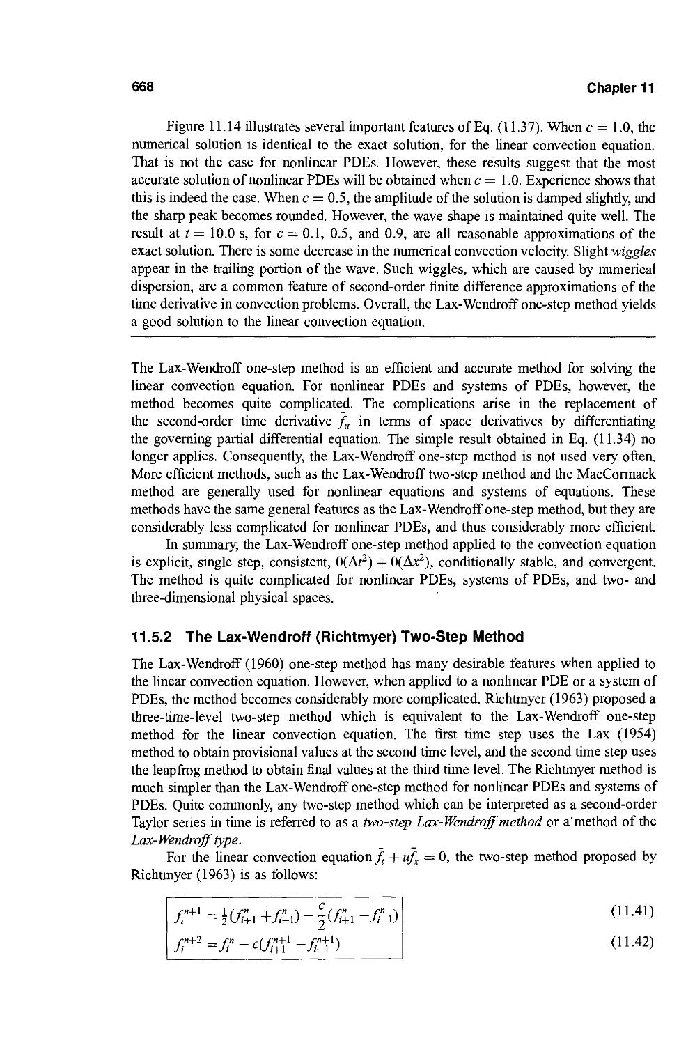
11.5. Lax-Wendroff Type Methods 655
11.6. Upwind Methods 673
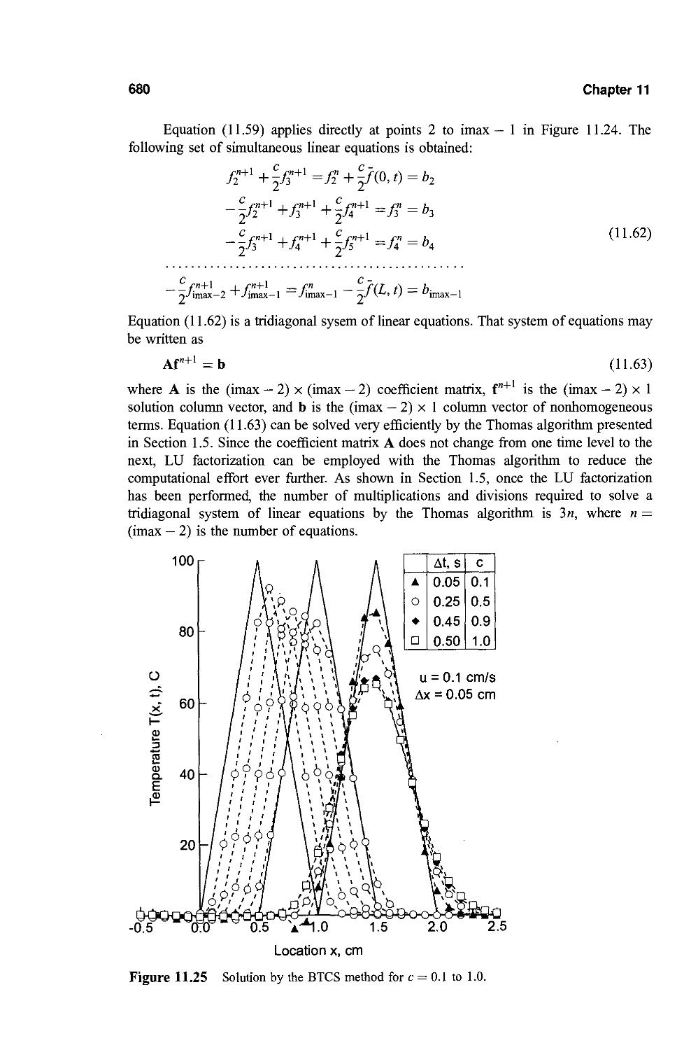
11.7. The Backward-Time Centered-Space (BTCS) Method 677
11.8. Nonlinear Equations and Multidimensional Problems 682
11.9. The Wave Equation 683
11.10. Programs 691
11.11. Summary 701
Exercise Problems 702
Chapter 12. The Finite Element Method 711
12.1. Introduction 711
12.2. The Rayleigh-Ritz, Collocation, and Galerkin Methods 713
12.3. The Finite Element Method for Boundary Value Problems 724
12.4. The Finite Element Method for the Laplace (Poisson) Equation 739
12.5. The Finite Element Method for the Diffusion Equation 752
12.6. Programs 759
12.7. Summary 769
Exercise Problems 770
References 775
Answers to Selected Problems 779
Index
795

0
Introduction
0.1. Objective and Approach
0.2. Organization of the Book
0.3. Examples
0.4. Programs
0.5. Problems
0.6. Significant Digits, Precision, Accuracy, Errors, and Number Representation
0.7. Software Packages and Libraries
0.8. The Taylor Series and the Taylor Polynomial
This Introduction contains a brief description of the objectives, approach, and organization
of the book. The philosophy behind the Examples, Programs, and Problems is discussed.
Several years' experience with the first edition of the book has identified several simple,
but significant, concepts which are relevant throughout the book, but the place to include
them is not clear. These concepts, which are presented in this Introduction, include the
definitions of significant digits, precision, accuracy, and errors, and a discussion of number
representation. A brief description of software packages and libraries is presented. Last,
the Taylor series and the Taylor polynomial, which are indispensable in developing and
understanding many numerical algorithms, are presented and discussed.
0.1 OBJECTIVE AND APPROACH
The objective of this book is to introduce the engineer and scientist to numerical methods
which can be used to solve mathematical problems arising in engineering and science that
cannot be solved by exact methods. With the general accessibility of high-speed digital
computers, it is now possible to obtain rapid and accurate solutions to many complex
problems that face the engineer and scientist.
The approach taken is as follows:
1. Introduce a type of problem.
1

2
Chapter 0
2. Present sufficient background to understand the problem and possible methods
of solution.
3. Develop one or more numerical methods for solving the problem.
4. Illustrate the numerical methods with examples.
In most cases, the numerical methods presented to solve a particular problem proceed from
simple methods to complex methods, which in many cases parallels the chronological
development of the methods. Some poor methods and some bad methods, as well as good
methods, are presented for pedagogical reasons. Why one method does not work is almost
as important as why another method does work.
0.2 ORGANIZATION OF THE BOOK
The material in the book is divided into three main parts:
I. Basic Tools of Numerical Analysis
II. Ordinary Differential Equations
III. Partial Differential Equations
Part I considers many of the basic problems that arise in all branches of engineering
and science. These problems include: solution of systems of linear algebraic equations,
eigenproblems, solution of nonlinear equations, polynomial approximation and
interpolation, numerical differentiation and difference formulas, and numerical integration. These
topics are important both in their own right and as the foundation for Parts II and III.
Part II is devoted to the numerical solution of ordinary differential equations
(ODEs). The general features of ODEs are discussed. The two classes of ODEs (i.e.,
initial-value ODEs and boundary-value ODEs) are introduced, and the two types of
physical problems (i.e., propagation problems and equilibrium problems) are discussed.
Numerous numerical methods for solving ODEs are presented.
Part III is devoted to the numerical solution of partial differential equations (PDEs).
Some general features of PDEs are discussed. The three classes of PDEs (i.e., elliptic
PDEs, parabolic PDEs, and hyperbolic PDEs) are introduced, and the two types of physical
problems (i.e., equilibrium problems and propagation problems) are discussed. Several
model PDEs are presented. Numerous numerical methods for solving the model PDEs are
presented.
The material presented in this book is an introduction to numerical methods. Many
practical problems can be solved by the methods presented here. Many other practical
problems require other or more advanced numerical methods. Mastery of the material
presented in this book will prepare engineers and scientists to solve many of their everyday
problems, give them the insight to recognize when other methods are required, and give
them the background to study other methods in other books and journals.
0.3 EXAMPLES
All of the numerical methods presented in this book are illustrated by applying them to
solve an example problem. Each chapter has one or two example problems, which are
solved by all of the methods presented in the chapter. This approach allows the analyst to
compare various methods for the same problem, so accuracy, efficiency, robustness, and
ease of application of the various methods can be evaluated. (

Introduction
3
Most of the example problems are rather simple and straightforward, thus allowing
the special features of the various methods to be demonstrated clearly. All of the example
problems have exact solutions, so the errors of the various methods can be compared. Each
example problem begins with a reference to the problem to be solved, a description of the
numerical method to be employed, details of the calculations for at least one application of
the algorithm, and a summary of the remaining results. Some comments about the solution
are presented at the end of the calculations in most cases.
0.4 PROGRAMS
Most numerical algorithms are generally expressed in the form of a computer program.
This is especially true for algorithms that require a lot of computational effort and for
algorithms that are applied many times. Several programming languages are available for
preparing computer programs: FORTRAN, Basic, C, PASCAL, etc., and their variations,
to name a few. Pseudocode, which is a set of instructions for implementing an algorithm
expressed in conceptual form, is also quite popular. Pseudocode can be expressed in the
detailed form of any specific programming language.
FORTRAN is one of the oldest programming languages. When carefully prepared,
FORTRAN can approach pseudocode. Consequently, the programs presented in this book
are written in simple FORTRAN. There are several vintages of FORTRAN: FORTRAN I,
FORTRAN II, FORTRAN 66, 77, and 90. The programs presented in this book are
compatible with FORTRAN 77 and 90.
Several programs are presented in each chapter for implementing the more
prominent numerical algorithms presented in the chapter. Each program is applied to
solve the example problem relevant to that chapter. The implementation of the numerical
algorithm is contained within a completely self-contained application subroutine which
can be used in other programs. These application subroutines are written as simply as
possible so that conversion to other programming languages is as straightforward as
possible. These subroutines can be used as they stand or easily modified for other
applications.
Each application subroutine is accompanied by a program main. The variables
employed in the application subroutine are denned by comment statements in program
main. The numerical values of the variables are denned in program /naw,which then calls
the application subroutine to solve the example problem and to print the solution. These
main programs are not intended to be convertible to other programming languages. In
some problems where a function of some type is part of the specification of the problem,
that function is defined in a function subprogram which is called by the application
subroutine.
FORTRAN compilers do not distinguish between uppercase and lowercase letters.
FORTRAN programs are conventionally written in uppercase letters. However, in this
book, all FORTRAN programs are written in lowercase letters.
0.5 PROBLEMS
Two types of problems are presented at the end of each chapter:
1. Exercise problems
2. Applied problems

4
Chapter 0
Exercise problems are straightforward problems designed to give practice in the
application of the numerical algorithms presented in each chapter. Exercise problems
emphasize the mechanics of the methods.
Applied problems involve more applied engineering and scientific applications
which require numerical solutions.
Many of the problems can be solved by hand calculation. A large number of the
problems require a lot of computational effort. Those problems should be solved by
writing a computer program to perform the calculations. Even in those cases, however, it is
recommended that one or two passes through the algorithm be made by hand calculation to
ensure that the analyst fully understands the details of the algorithm. These results also can
be used to validate the computer program.
Answers to selected problems are presented in a section at the end of the book. All of
the problems for which answers are given are denoted by an asterisk appearing with the
corresponding problem number in the problem sections at the end of each chapter. The
Solutions Manual contains the answers to nearly all of the problems.
0.6 SIGNIFICANT DIGITS, PRECISION, ACCURACY, ERRORS, AND
NUMBER REPRESENTATION
Numerical calculations obviously involve the manipulation (i.e., addition, multiplication,
etc.) of numbers. Numbers can be integers (e.g., 4, 17, — 23, etc.), fractions (e.g., 1/2,
— 2/3, etc.), or an inifinite string of digits (e.g., n = 3.1415926535 ...). When dealing
with numerical values and numerical calculations, there are several concepts that must be
considered: ,
1. Significant digits
2. Precision and accuracy
3. Errors
4. Number representation
These concepts are discussed briefly in this section.
Significant Digits
The significant digits, or figures, in a number are the digits of the number which are
known to be correct. Engineering and scientific calculations generally begin with a set of
data having a known number of significant digits. When these numbers are processed
through a numerical algorithm, it is important to be able to estimate how many significant
digits are present in the final computed result.
Precision and Accuracy
Precision refers to how closely a number represents the number it is representing.
Accuracy refers to how closely a number agrees with the true value of the number it is
representing.
Precision is governed by the number of digits being carried in the numerical
calculations. Accuracy is governed by the errors in the numerical approximation. Precision
and accuracy are quantified by the errors in a numerical calculation.

Introduction
5
Errors
The accuracy of a numerical calculation is quantified by the error of the calculation.
Several types of errors can occur in numerical calculations.
1. Errors in the parameters of the problem (assumed nonexistent).
2. Algebraic errors in the calculations (assumed nonexistent).
3. Iteration errors.
4. Approximation errors.
5. Roundoff errors.
Iteration error is the error in an iterative method that approaches the exact solution
of an exact problem asymptotically. Iteration errors must decrease toward zero as the
iterative process progresses. The iteration error itself may be used to determine the
successive approximations to the exact solution. Iteration errors can be reduced to the limit
of the computing device. The errors in the solution of a system of linear algebraic
equations by the successive-over-relaxation (SOR) method presented in Section 1.5 are
examples of this type of error.
Approximation error is the difference between the exact solution of an exact
problem and the exact solution of an approximation of the exact problem. Approximation
error can be reduced only by choosing a more accurate approximation of the exact
problem. The error in the approximation of a function by a polynomial, as described in
Chapter 4, is an example of this type of error. The error in the solution of a differential
equation where the exact derivatives are replaced by algebraic difference approximations,
which have truncation errors, is another example of this type of error.
Roundoff error is the error caused by the finite word length employed in the
calculations. Roundoff error is more significant when small differences between large
numbers are calculated. Most computers have either 32 bit or 64 bit word length,
corresponding to approximately 7 or 13 significant decimal digits, respectively. Some
computers have extended precision capability, which increases the number of bits to 128.
Care must be exercised to ensure that enough significant digits are maintained in numerical
calculations so that roundoff is not significant.
Number Representation
Numbers are represented in number systems. Any number of bases can be employed as
the base of a number system, for example, the base 10 (i.e., decimal) system, the base 8
(i.e., octal) system, the base 2 (i.e., binary) system, etc. The base 10, or decimal, system is
the most common system used for human communication. Digital computers use the base
2, or binary, system. In a digital computer, a binary number consists of a number of binary
bits. The number of binary bits in a binary number determines the precision with which the
binary number represents a decimal number. The most common size binary number is a 32
bit number, which can represent approximately seven digits of a decimal number. Some
digital computers have 64 bit binary numbers, which can represent 13 to 14 decimal digits.
In many engineering and scientific calculations, 32 bit arithmetic is adequate. However, in
many other applications, 64 bit arithmetic is required. In a few special situations, 128 bit
arithmetic may be required. On 32 bit computers, 64 bit arithmetic, or even 128 bit
arithmetic, can be accomplished using software enhancements. Such calculations are
called double precision or quad precision, respectively. Such software enhanced
precision can require as much as 10 times the execution time of a single precision calculation.

6
Chapter 0
Consequently, some care must be exercised when deciding whether or not higher precision
arithmetic is required. All of the examples in this book are evaluated using 64 bit
arithmetic to ensure that roundoff is not significant.
Except for integers and some fractions, all binary representations of decimal
numbers are approximations, owing to the finite word length of binary numbers. Thus,
some loss of precision in the binary representation of a decimal number is unavoidable.
When binary numbers are combined in arithmetic operations such as addition,
multiplication, etc., the true result is typically a longer binary number which cannot be
represented exactly with the number of available bits in the binary number capability of
the digital computer. Thus, the results are rounded off in the last available binary bit. This
rounding off gives rise to roundoff error, which can accumulate as the number of
calculations increases.
0.7 SOFTWARE PACKAGES AND LIBRARIES
Numerous commercial software packages and libraries are available for implementing the
numerical solution of engineering and scientific problems. Two of the more versatile
software packages are Mathcad and Matlab. These software packages, as well as several
other packages and several libraries, are listed below with a brief description of each one
and references to sources for the software packages and libraries.
A. Software Packages
Excel Excel is a spreadsheet developed by Microsoft, Inc., as part of Microsoft Office. It
enables calculations to be performed on rows and columns of numbers. The calculations to
be performed are specified for each column. When any number on the spreadsheet is
changed, all of the calculations are updated. Excel contains several built-in numerical
algorithms. It also includes the Visual Basic programming language and some plotting
capability. Although its basic function is not numerical analysis, Excel can be used
productively for many types of numerical problems. Microsoft, Inc. www.microsoft.com/
office/Excel.
Macsyma Macsyma is the world's first artificial intelligence based math engine
providing easy to use, powerful math software for both symbolic and numerical
computing. Macsyma, Inc., 20 Academy St., Arlington, MA 02476-6412. (781) 646-4550,
webmaster@macsyma.com, www.macsyma.com.
Maple Maple 6 is a technologically advanced computational system with both
algorithms and numeric solvers. Maple 6 includes an extensive set of NAG (Numerical
Algorithms Group) solvers for computational linear algebra. Waterloo Maple, Inc., 57 Erb
Street W, Waterloo, Ontario, Canada N2L 6C2. (800) 267-6583, (519) 747-2373,
info@maplesoft.com, www.maplesoft.com.
Mathematica Mathematica 4 is a comprehensive software package which performs
both symbolic and numeric computations. It includes a flexible and intuitive programming
language and comprehensive plotting capabilities. Wolfram Research, Inc., 100 Trade
Center Drive, Champaign IL 61820-7237. (800) 965-3726, (217) 398-0700, info@
wolfram.com, www.wolfram.com.
Mathcad Mathcad 8 provides a free-form interface which permits the integration of
real math notation, graphs, and text within a single interactive worksheet. It includes
statistical and data analysis functions, powerful solvers, advanced matrix manipulation,

Introduction
7
and the capability to create your own functions. Mathsoft, Inc., 101 Main Street,
Cambridge, MA 02142-1521. (800) 628-4223, (617) 577-1017, info@mathsoft.com,
www.mathcad.com,
Matlab Matlab is an integrated computing environment that combines numeric
computation, advanced graphics and visualization, and a high-level programming
language. It provides core mathematics and advanced graphics tools for data analysis,
visualization, and algorithm and application development, with more than 500
mathematical, statistical, and engineering functions. The Mathworks, Inc., 3 Apple Hill Drive,
Natick, MA 01760-2090. (508) 647-7000, info@mathworks.com, www.mathworks.com.
B. Libraries
GAMS GAMS (Guide to Available Mathematical Software) is a guide to over 9000
software modules contained in some 80 software packages at NIST (National Institute for
Standards and Technology) and NETLIB. gams.nist.gov.
IMSL IMSL (International Mathematics and Statistical Library) is a comprehensive
resource of more than 900 FORTRAN subroutines for use in general mathematics and
statistical data analysis. Also available in C and Java. Visual Numerics, Inc., 1300 W. Sam
Houston Parkway S., Suite 150, Houston TX 77042. (800) 364-8880, (713) 781-9260,
info@houston.vni.com, www.vni.com.
LAPACK LAPACK is a library of FORTRAN 77 subroutines for solving linear
algebra problems and eigenproblems. Individual subroutines can be obtained through
NETLIB. The complete package can be obtained from NAG.
NAG NAG is a mathematical software library that contains over 1000 mathematical
and statistical functions. Available in FORTRAN and C. NAG, Inc., 1400 Opus Place,
Suite 200, Downers Grove, IL 60515-5702. (630) 971-2337, naginfo@nag.com,
www.nag.com.
NETLIB NETLIB is a large collection of numerical libraries, netlib@research.att.
com, netlib@ornl.gov, netlib@nec.no.
C. Numerical Recipes
Numerical Recipes is a book by William H. Press, Brian P. Flannery, Saul A. Teukolsky,
and William T. Vetterling. It contains over 300 subroutines for numerical algorithms.
Versions of the subroutines are available in FORTRAN, C, Pascal, and Basic. The source
codes are available on disk. Cambridge University Press, 40 West 20th Street, New York,
NY 10011. www.cup.org.
0.8 THE TAYLOR SERIES AND THE TAYLOR POLYNOMIAL
A power series in powers of x is a series of the form
00
£>„*" = a0 + a\x + a2^ H (0.1)
«=o
A power series in powers of (x — x0) is given by
Ea„(* -*o)" = a0 + ax(x- x0) + a2(x - x0)2 + • • • (0.2)
«=o

8
Chapter 0
Within its radius of convergence, r, any continuous function, f(x), can be represented
exactly by a power series. Thus,
f(x) = £ an(x - x0)"
«=o
is continuous for (x0 — r) < x < (x0 + r).
A. Taylor Series in One Independent Variable
If the coefficients, a„, in Eq. (0.3) are given by the rule:
ao =fixol ai = 7,/(¾). a2 = 2j/"(*o)> • • •
then Eq. (0.3) becomes the Taylor series of/(x) at x = x0. Thus,
fix) =/(x0) + ^/(x0)(x - x0) + ^/"(x0)(x - x0)2 +
(0.3)
(0.4)
(0.5)
(0.6)
Equation (0.5) can be written in the simpler appearing form
/(*) =/0 +/0'Ax + ^"Ax2 + • • • + Ij^W + ■■■
where/0 =/(x0),/w = df^/dx", and Ax = (x - x0). Equation (0."6) can be written in the
compact form
1
/W=E^/o(")(x-x0)"
n=0nl
(0.7)
When x0 = 0, the Taylor series is known as the Maclaurin series. In that case, Eqs.
(0.5) and (0.7) become
fix) =/(0) +/'(0)x + i/W + ... (0.8)
fix)=t^f{"\0V
(0.9)
It is, of course, impractical to evaluate an infinite Taylor series term by term. The
Taylor series can be written as the finite Taylor series, also known as the Taylor formula or
Taylor polynomial with remainder, as follows:
1 / 2
fix) =f(x0) +f'ix0)(x - x0) + - /"(x0)(x - x0) +
1
+ -,fwixo)ix-x0)n+R'
,n+l
n\
(0.10)
where the term R"+l is the remainder term given by
r"+1 =r-^fn+1\ax-x0rl (o.ii)
(" + 1)!
where t, lies between x0 and x. Equation (0.10) is quite useful in numerical analysis, where
an approximation of f(x) is obtained by truncating the remainder term.

Introduction
9
B. Taylor Series in Two Independent Variables
Power series can also be written for functions of more than one independent variable. For a
function of two independent variables, f(x,y), the Taylor series off(x,y) at (x0,y0) is given
by
2!\9x2
(x - x0) + —
) dy
(x-x0)2+2
0
(y-
0
dxdy
y0)
(x - x0)(y - y0) + —
o °r
(y-y0f) + ---
o /
(0.12)
Equation (0.12) can be written in the general form
f(x,y)=j:-.((x-x0)-+(y-y0)-)f(x,y)\0 (0.13)
„=o"!\ 9x dyj
where the term (• • •)" is expanded by the binomial expansion and the resulting expansion
operates on the function f(x,y) and is evaluated at (x0,y0).
The Taylor formula with remainder for a function of two independent variables is
obtained by evaluating the derivatives in the (n + l)st term at the point (£, rj), where (£, rj)
lies in the region between points (x0,y0) and (x,y).

I
Basic Tools of Numerical Analysis
1.1. Systems of Linear Algebraic Equations
1.2. Eigenproblems
1.3. Roots of Nonlinear Equations
1.4. Polynomial Approximation and Interpolation
1.5. Numerical Differentiation and Difference Formulas
1.6. Numerical Integration
1.7. Summary
Many different types of algebraic processes are required in engineering and science. These
processes include the solution of systems of linear algebraic equations, the solution of
eigenproblems, finding the roots of nonlinear equations, polynomial approximation and
interpolation, numerical differentiation and difference formulas, and numerical integration.
These topics are not only important in their own right, they lay the foundation for the
solution of ordinary and partial differential equations, which are discussed in Parts II and
III, respectively. Figure 1.1 illustrates the types of problems considered in Part I.
The objective of Part I is to introduce and discuss the general features of each of
these algebraic processes, which are the basic tools of numerical analysis.
1.1 SYSTEMS OF LINEAR ALGEBRAIC EQUATIONS
Systems of equations arise in all branches of engineering and science. These equations
may be algebraic, transcendental (i.e., involving trigonometric, logarithmic, exponential,
etc., functions), ordinary differential equations, or partial differential equations. The
equations may be linear or nonlinear. Chapter 1 is devoted to the solution of systems of
linear algebraic equations of the following form:
anx{ + al2x2 + ai3x3 H h alnx„ = bx (I-la)
a21*l + «22*2 + a23x3 + ^ a2nxn = b2 (I- lb)
a«l*l + ««2*2 + ««3*3 + 1- ann*n = K (I. In)
11

12
Parti
where xj {j = 1,2,...,«) denotes the unknown variables, atj (i,j= 1,2,...,«) denotes
the coefficients of the unknown variables, and b,■ {i = 1,2,...,«) denotes the nonhomo-
geneous terms. For the coefficients atJ, the first subscript i corresponds to equation i, and
the second subscript./' corresponds to variable xj. The number of equations can range from
two to hundreds, thousands, and even millions.
Systems of linear algebraic equations arise in many different problems, for example,
(a) network problems (e.g., electrical networks), (b) fitting approximating functions (see
Chapter 4), and (c) systems of finite difference equations that arise in the numerical
solution of differential equations (see Chapters 7 to 12). The list is endless. Figure I.la
illustrates a static spring-mass system, whose static equilibrium configuration is governed
by a system of linear algebraic equations. That system of equations is used throughout
Chapter 1 as an example problem.
■ s , ,, , , . , , S S , , ,
-7-r-T7~rr
rrii
m?
r7-7-r7-7-r-r-r-rTrT7-7-7-7-r-r-r-7m7-T-7-T-r*/
|*-Xl(t) -*| |~x2(t)
(a) Static spring-mass system.
'<^$Br "H -Br ™2 ^
/JSJSJSJJSJJS////J/JS
(b) Dynamic spring-mass system.
(c) Roots of nonlinear equations, (d) Polynomial approximation and interpolation.
I=ir(x)dx
(e) Numerical differentiation.
(f) Numerical integration.
Figure 1.1 Basic tools of numerical analysis, (a) Static spring-mass system, (b) Dynamic spring-
mass system, (c) Roots of nonlinear equations, (d) Polynomial approximation and interpolation,
(e) Numerical differentiation, (f) Numerical integration.

Basic Tools of Numerical Analysis
13
Systems of linear algebraic equations can be expressed very conveniently in terms of
matrix notation. Solution methods can be developed very compactly in terms of matrix
notation. Consequently, the elementary properties of matrices and determinants are
reviewed at the beginning of Chapter 1.
Two fundamentally different approaches can be used to solve systems of linear
algebraic equations:
1. Direct methods
2. Iterative methods
Direct methods are systematic procedures based on algebraic elimination. Several direct
elimination methods, for example, Gauss elimination, are presented in Chapter 1. Iterative
methods obtain the solution asymptotically by an iterative procedure in which a trial
solution is assumed, the trial solution is substituted into the system of equations to
determine the mismatch, or error, and an improved solution is obtained from the mismatch
data. Several iterative methods, for example, successive-over-relaxation (SOR), are
presented in Chapter 1.
The notation, concepts, and procedures presented in Chapter 1 are used throughout
the remainder of the book. A solid understanding of systems of linear algebraic equations
is essential in numerical analysis.
1.2 EIGENPROBLEMS
Eigenproblems arise in the special case where a system of algebraic equations is
homogeneous; that is, the nonhogeneous terms, bi in Eq. (1.1), are all zero, and the
coefficients contain an unspecified parameter, say X, In general, when bx = 0, the only
solution to Eq. (1.1) is the trivial solution, xx = x2 = • • • = xn = 0. However, when the
coefficients a,- ■ contain an unspecified parameter, say X, the value of that parameter can be
chosen so that the system of equations is redundant, and an infinite number of solutions
exist. The unspecified parameter X is an eigenvalue of the system of equations. For
example,
(an — X)x{ + anx2 = 0 (1.2a)
a2\x\ + (a22 ~ tyx2 = 0 (I-2b)
is a linear eigenproblem. The value (or values) of X that make Eqs. (I.2a) and (I.2b)
identical are the eigenvalues of Eqs. (1.2). In that case, the two equations are redundant, so
the only unique solution is xl = x2 = 0. However, an infinite number of solutions can be
obtained by specifying either xx or x2, then calculating the other from either of the two
redundant equations. The set of values of xx andx2 corresponding to a particular value of A
is an eigenvector of Eq. (1.2). Chapter 2 is devoted to the solution of eigenproblems.
Eigenproblems arise in the analysis of many physical systems. They arise in the
analysis of the dynamic behavior of mechanical, electrical, fluid, thermal, and structural
systems. They also arise in the analysis of control systems. Figure I.lb illustrates a
dynamic spring-mass system, whose dynamic equilibrium configuration is governed by a
system of homogeneous linear algebraic equations. That system of equations is used
throughout Chapter 2 as an example problem. When the static equilibrium configuration of
the system is disturbed and then allowed to vibrate freely, the system of masses will
oscillate at special frequencies, which depend on the values of the masses and the spring

14
Parti
constants. These special frequencies are the eigenvalues of the system. The relative values
of xx, x2, etc. corresponding to each eigenvalue X are the eigenvectors of the system.
The objectives of Chapter 2 are to introduce the general features of eigenproblems
and to present several methods for solving eigenproblems. Eigenproblems are special
problems of interest only in themselves. Consequently, an understanding of eigenproblems
is not essential to the other concepts presented in this book.
1.3 ROOTS OF NONLINEAR EQUATIONS
Nonlinear equations arise in many physical problems. Finding their roots, or zeros, is a
common problem. The problem can be stated as follows:
Given the continuous nonlinear function/(x), find the value of x = a such that
/(a) = 0
where a is the root, or zero, of the nonlinear equation. Figure Lie illustrates the problem
graphically. The function/(x) may be an algebraic function, a transcendental function, the
solution of a differential equation, or any nonlinear relationship between an input x and a
response/(x). Chapter 3 is devoted to the solution of nonlinear equations.
Nonlinear equations are solved by iterative methods. A trial solution is assumed, the
trial solution is substituted into the nonlinear equation to determine the error, or mismatch,
and the mismatch is used in some systematic manner to generate an improved estimate of
the solution. Several methods for finding the roots of nonlinear equations are presented in
Chapter 3. The workhorse methods of choice for solving nonlinear equations are Newton's
method and the secant method. A detailed discussion of finding the roots of polynomials is
presented. A brief introduction to the problems of solving systems of nonlinear equations
is also presented.
Nonlinear equations occur throughout engineering and science. Nonlinear equations
also arise in other areas of numerical analysis. For example, the shooting method for
solving boundary-value ordinary differential equations, presented in Section 8.3, requires
the solution of a nonlinear equation. Implicit methods for solving nonlinear differential
equations yield nonlinear difference equations. The solution of such problems is discussed
in Sections 7.11, 8.7, 9.11, 10.9, and 11.8. Consequently, a thorough understanding of
methods for solving nonlinear equations is an essential requirement for the numerical
analyst.
1.4 POLYNOMIAL APPROXIMATION AND INTERPOLATION
In many problems in engineering and science, the data under consideration are known only
at discrete points, not as a continuous function. For example, as illustrated in Figure I.Id,
the continuous function/(x) may be known only at n discrete values of x:
yi=y{xi) (1 = 1,2,...,11) (1.3)
Values of the function at points other than the known discrete points may be needed
(i.e., interpolation). The derivative of the function at some point may be needed (i.e.,
differentiation). The integral of the function over some range may be required (i.e.,
integration). These processes, for discrete data, are performed by fitting an approximating
function to the set of discrete data and performing the desired processes on the
approximating function. Many types of approximating functions can be used.

Basic Tools of Numerical Analysis
15
Because of their simplicity, ease of manipulation, and ease of evaluation,
polynomials are an excellent choice for an approximating function. The general nth-degree
polynomial is specified by
P„(x) = a0 + axx + flji2 + • • • + anx" (1.4)
Polynomials can be fit to a set of discrete data in two ways:
1. Exact fit
2. Approximate fit
An exact fit passes exactly through all the discrete data points. Direct fit polynomials,
divided-difference polynomials, and Lagrange polynomials are presented in Chapter 4 for
fitting nonequally spaced data or equally spaced data. Newton difference polynomials are
presented for fitting equally spaced data. The least squares procedure is presented for
determining approximate polynomial fits.
Figure I.Id illustrates the problem of interpolating within a set of discrete data.
Procedures for interpolating within a set of discrete data are presented in Chapter 4.
Polynomial approximation is essential for interpolation, differentiation, and
integration of sets of discrete data. A good understanding of polynomial approximation is a
necessary requirement for the numerical analyst.
1.5 NUMERICAL DIFFERENTIATION AND DIFFERENCE FORMULAS
The evaluation of derivatives, a process known as differentiation, is required in many
problems in engineering and science. Differentiation of the function/(x) is denoted by
^ (/(*)) =/'(*) (1-5)
The function f(x) may be a known function or a set of discrete data. In general, known
functions can be differentiated exactly. Differentiation of discrete data requires an
approximate numerical procedure. Numerical differentiation formulas can be developed
by fitting approximating functions (e.g., polynomials) to a set of discrete data and
differentiating the approximating function. For polynomial approximating functions, this
yields
| (/(*)) =/(*) = jx (P„(x)) = KM (1.6)
Figure Lie illustrates the problem of numerical differentiation of a set of discrete
data. Numerical differentiation procedures are developed in Chapter 5.
The approximating polynomial may be fit exactly to a set of discrete data by the
methods presented in Chapter 4, or fit approximately by the least squares procedure
described in Chapter 4. Several numerical differentiation formulas based on differentiation
of polynomials are presented in Chapter 5.
Numerical differentiation formulas also can be developed using Taylor series. This
approach is quite useful for developing difference formulas for approximating exact
derivatives in the numerical solution of differential equations. Section 5.5 presents a table
of difference formulas for use in the solution of differential equations.
Numerical differentiation of discrete data is not required very often. However, the
numerical solution of differential equations, which is the subject of Parts II and III, is one

16
Parti
of the most important areas of numerical analysis. The use of difference formulas is
essential in that application.
1.6 NUMERICAL INTEGRATION
The evaluation of integrals, a process known as integration, or quadrature, is required in
many problems in engineering and science. Integration of the function/(x) is denoted by
I = f f(x) dx (1.7)
Ja
The function f{x) may be a known function or a set of discrete data. Some known
functions have an exact integral. Many known functions, however, do not have an exact
integral, and an approximate numerical procedure is required to evaluate Eq. (1.7). When a
known function is to be integrated numerically, it must first be discretized. Integration of
discrete data always requires an approximate numerical procedure. Numerical integration
(quadrature) formulas can be developed by fitting approximating functions (e.g.,
polynomials) to a set of discrete data and integrating the approximating function. For
polynomial approximating functions, this gives
fb rb
I = f(x) dx 2 P„(x) dx (1.8)
Ja Ja
Figure I. If illustrates the problem of numerical integration of a set of discrete data.
Numerical integration procedures are developed in Chapter 6.
The approximating function can be fit exactly to a set of discrete data by direct fit
methods, or fit approximately by the least squares method. For unequally spaced data,
direct fit polynomials can be used. For equally spaced data, the Newton forward-difference
polynomials of different degrees can be integrated to yield the Newton-Cotes quadrature
formulas. The most prominent of these are the trapezoid rule and Simpson's 1 /3 rule.
Romberg integration, which is a higher-order extrapolation of the trapezoid rule, is
introduced. Adaptive integration, in which the range of integration is subdivided
automatically until a specified accuracy is obtained, is presented. Gaussian quadrature, which
achieves higher-order accuracy for integrating known functions by specifying the locations
of the discrete points, is presented. The evaluation of multiple integrals is discussed.
Numerical integration of both known functions and discrete data is a common
problem. The concepts involved in numerical integration lead directly to numerical
methods for solving differential equations.
1.7 SUMMARY
Part I of this book is devoted to the basic tools of numerical analysis. These topics are
important in their own right. In addition, they provide the foundation for the solution of
ordinary and partial differential equations, which are discussed in Parts II and III,
respectively. The material presented in Part I comprises the basic language of numerical
analysis. Familiarity and mastery of this material is essential for the understanding and use
of more advanced numerical methods.

1
Systems of Linear Algebraic Equations
1.1. Introduction
1.2. Properties of Matrices and Determinants
1.3. Direct Elimination Methods
1.4. LU Factorization
1.5. Tridiagonal Systems of Equations
1.6. Pitfalls of Elimination Methods
1.7. Iterative Methods
1.8. Programs
1.9. Summary
Problems
Examples
1.1. Matrix addition
1.2. Matrix multiplication
1.3. Evaluation of a 3 x 3 determinant by the diagonal method
1.4. Evaluation of a 3 x 3 determinant by the cofactor method
1.5. Cramer's rule
1.6. Elimination
1.7. Simple elimination
1.8. Simple elimination for multiple b vectors
1.9. Elimination with pivoting to avoid zero pivot elements
1.10. Elimination with scaled pivoting to reduce round-off errors
1.11. Gauss-Jordan elimination
1.12. Matrix inverse by Gauss-Jordan elimination
1.13. The matrix inverse method
1.14. Evaluation of a 3 x 3 determinant by the elimination method
1.15. The Doolittle LU method
1.16. Matrix inverse by the Doolittle LU method
1.17. The Thomas algorithm
1.18. Effects of round-off errors
1.19. System condition
1.20. Norms and condition numbers
1.21. The Jacobi iteration method
1.22. The Gauss-Seidel iteration method
1.23. The SOR method
17

18
Chapter 1
1.1 INTRODUCTION
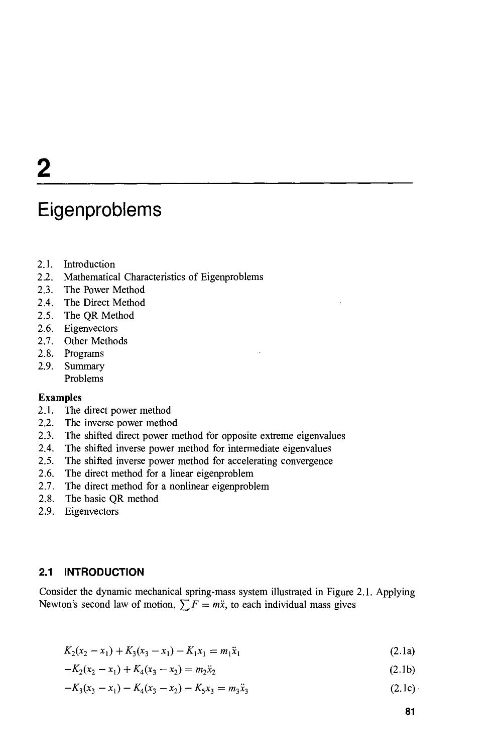
The static mechanical spring-mass system illustrated in Figure 1.1 consists of three masses
mx to /n3, having weights Wx to Wi} interconnected by five linear springs Kx to K5. In the
configuration illustrated on the left, the three masses are supported by forces F: to F3 equal
to weights Wx to W3, respectively, so that the five springs are in a stable static equilibrium
configuration. When the supporting forces Fl to F3 are removed, the masses move
downward and reach a new static equilibrium configuration, denoted by x1; x2, and x3,
where xl,x2, and x3 are measured from the original locations of the corresponding masses.
Free-body diagrams of the three masses are presented at the bottom of Figure 1.1.
Performing a static force balance on the three masses yields the following system of three
linear algebraic equations:
(Kx +K2+ Kt)xx - K2x2 - KiXi = Wx
-K2xx + (K2 + KA)x2 - KAXo, = W2
-K3X! - K4x2 + (K3 +K4+ K5)x3 = W3
(1.1a)
(1.1b)
(1.1c)
When values ofKx to K5 and Wx to W3 are specified, the equilibrium displacements xx to
x3 can be determined by solving Eq. (1.1).
The static mechanical spring-mass system illustrated in Figure 1.1 is used as the
example problem in this chapter to illustrate methods for solving systems of linear
f'S'Sf''''
s s , s s s ? s s /
K3/4| FigKafKaW
K3/4lF2gK4lK3/4
^3(^3-
m^
111
K2(x2-x1)
t
m2
i' i
(Xj-X^ W2 K4(x3-
-x2)
K3(x3
-X1) K4
I I
m3
I I
W3 K5>
(x3-x2)
3
Figure 1.1 Static mechanical spring-mass system.

Systems of Linear Algebraic Equations
19
80x! - 20x2 - 20x3
-20x! + 40x2 - 20x3
-20x! -20x2 + 130x3
= 20
= 20
= 20
algebraic equations. For that purpose, let Kx = 40 N/cm, K2 = K3 = K4 = 20 N/cm, and
K% = 90 N/cm. Let Wx = W2 = Wi = 20 N. For these values, Eq. (1.1) becomes:
(1.2a)
(1.2b)
(1.2c)
The solution to Eq. (1.2) is xx = 0.6 cm, x2 = 1.0 cm, and x3 = 0.4 cm, which can be
verified by direct substitution.
Systems of equations arise in all branches of engineering and science. These
equations may be algebraic, transcendental (i.e., involving trigonometric, logarithmetic,
exponential, etc. functions), ordinary differential equations, or partial differential
equations. The equations may be linear or nonlinear. Chapter 1 is devoted to the solution of
systems of linear algebraic equations of the following form:
anxx + a12x2 + a13x3 H h alirxn = bx (l-3a)
«21*1 + «22*2 + «23*3 + H a2nxn = h (1 -3b)
a„i*i + a«2*2 + a«3*3 + H «««*« = bn (1.3n)
where Xj (j = 1,2,..., «) denotes the unknown variables, a,- • (i,j = 1,2,...,«) denotes
the constant coefficients of the unknown variables, and bt (i = 1,2,...,«) denotes the
nonhomogeneous terms. For the coefficients atj, the first subscript, i, denotes equation i,
and the second subscript^', denotes variable Xj. The number of equations can range from
two to hundreds, thousands, and even millions.
In the most general case, the number of variables is not required to be the same as
the number of equations. However, in most practical problems, they are the same. That is
the case considered in this chapter. Even when the number of variables is the same as the
number of equations, several solution possibilities exist, as illustrated in Figure 1.2 for the
following system of two linear algebraic equations:
auxx + anx2 = bi (1.4a)
a2i*i +a22x2 = b2 (1.4b)
The four solution possibilities are:
1. A unique solution (a consistent set of equations), as illustrated in Figure 1.2a
2. No solution (an inconsistent set of equations), as illustrated in Figure 1.2b
3. An infinite number of solutions (a redundant set of equations), as illustrated in
Figure 1.2c
4. The trivial solution, x}■ = 0 (j = 1,2,...,«), for a homogeneous set of
equations, as illustrated in Figure 1.2d
Chapter 1 is concerned with the first case where a unique solution exists.
Systems of linear algebraic equations arise in many different types of problems, for
example:
1. Network problems (e.g., electrical networks)
2. Fitting approximating functions (see Chapter 4)

20
Chapter 1
/ //
(a) Unique solution. (b) No solution.
/
I (c) Infinite number of solutions.
s>r{<$) Trivial solution.
Figure 1.2 Solution of a system of two linear algebraic equations.
3. Systems of finite difference equations that arise in the numerical solution of
differential equations (see Parts II and III)
The list is endless.
There are two fundamentally different approaches for solving systems of linear
algebraic equations:
1. Direct elimination methods
2. Iterative methods
Direct elimination methods are systematic procedures based on algebraic elimination,
which obtain the solution in a fixed number of operations. Examples of direct elimination
methods are Gauss elimination, Gauss-Jordan elimination, the matrix inverse method, and
Doolittle LU factorization. Iterative methods, on the other hand, obtain the solution
asymptotically by an iterative procedure. A trial solution is assumed, the trial solution is
substituted into the system of equations to determine the mismatch, or error, in the trial
solution, and an improved solution is obtained from the mismatch data. Examples of
iterative methods are Jacobi iteration, Gauss-Seidel iteration, and
successive-over-relaxation (SOR).
Although no absolutely rigid rules apply, direct elimination methods are generally
used when one or more of the following conditions holds: (a) The number of equations is
small (100 or less), (b) most of the coefficients in the equations are nonzero, (c) the system
of equations is not diagonally dominant [see Eq. (1.15)], or (d) the system of equations is
ill conditioned (see Section 1.6.2). Iterative methods are used when the number of
equations is large and most of the coefficients are zero (i.e., a sparse matrix). Iterative
methods generally diverge unless the system of equations is diagonally dominant [see
Eq. (1.15)].
The organization of Chapter 1 is illustrated in Figure 1.3. Following the introductory
material discussed in this section, the properties of matrices and determinants are
reviewed. The presentation then splits into a discussion of direct elimination methods

Systems of Linear Algebraic Equations 21
Systems of Linear
Algebraic Equations
'r
Properties of Matrices
and Determinants
'
<
Direct
Methods
Gauss
Elimination
Matrix
Inverse
LU
Factorization
Gauss-Jordan
Elimination
Iterative
Methods
Jacobi
Iteration
Determinants
Tridiagonal
Systems
>•
Gauss-Seidel
Iteration
i «
Accuracy and
Convergence
Successive
Overrelaxation
Programs
Summary
Figure 1.3 Organization of Chapter 1.
followed by a discussion of iterative methods. Several methods, both direct elimination
and iterative, for solving systems of linear algebraic equations are presented in this chapter.
Procedures for special problems, such as tridiagonal systems of equations, are presented.
All these procedures are illustrated by examples. Although the methods apply to large
systems of equations, they are illustrated by applying them to the small system of only
three equations given by Eq. (1.2). After the presentation of the methods, three computer
programs are presented for implementing the Gauss elimination method, the Thomas
algorithm, and successive-over-relaxation (SOR). The chapter closes with a Summary,
which discusses some philosophy to help you choose the right method for every problem
and lists the things you should be able to do after studying Chapter 1.
1.2 PROPERTIES OF MATRICES AND DETERMINANTS
Systems of linear algebraic equations can be expressed very conveniently in terms of
matrix notation. Solution methods for systems of linear algebraic equations can be

22
Chapter 1
developed very compactly using matrix algebra. Consequently, the elementary properties
of matrices and determinants are presented in this section.
1.2.1. Matrix Definitions
A matrix is a rectangular array of elements (either numbers or symbols), which are
arranged in orderly rows and columns. Each element of the matrix is distinct and separate.
The location of an element in the matrix is important. Elements of a matrix are generally
identified by a double subscripted lowercase letter, for example, a, , where the first
subscript i identifies the row of the matrix and the second subscript j identifies the column
of the matrix. The size of a matrix is specified by the number of rows times the number of
columns. A matrix with « rows and m columns is said to be an « by m, or « x m, matrix.
Matrices are generally represented by either a boldface capital letter, for example, A, the
general element enclosed in brackets, for example, [a,- •], or the full array of elements, as
illustrated in Eq. (1.5):
A = [atj\ =
an an
a2\ a22
nm
*n\ un2
(i = 1,2,...,«; j = 1, 2,..., rri)
(1-5)
Comparing Eqs. (1.3) and (1.5) shows that the coefficients of a system of linear algebraic
equations form the elements of an « x « matrix.
Equation (1.5) illustrates a convention used throughout this book for simplicity of
appearance. When the general element a,- ■ is considered, the subscripts i and j are
separated by a comma. When a specific element is specified, for example, a31, the
subscripts 3 and 1, which denote the element in row 3 and column 1, will not be separated
by a comma, unless i ovj is greater than 9. For example, a37 denotes the element in row 3
and column 7, whereas a1317 denotes the element in row 13 and column 17.
Vectors are a special type of matrix which has only one column or one row. Vectors
are represented by either a boldface lowercase letter, for example, x or y, the general
element enclosed in brackets, for example, [x,] or [yt], or the full column or row of
elements. A column vector is an « x 1 matrix. Thus,
x = [x,] =
*i
x2
(i= 1,2,...,«)
A row vector is a 1 x « matrix. For example,
y = [yj\ = [yi yi ■■■ y«\ (y= 1,2,...,«)
Unit vectors, i, are special vectors which have a magnitude of unity. Thus,
(n + i2i +
+i2ny<2
1
(1.6a)
(1.6b)
(1.7)
where the notation ||i|| denotes the length of vector i. Orthogonal systems of unit vectors,
in which all of the elements of each unit vector except one are zero, are used to define
coordinate systems.

Systems of Linear Algebraic Equations
23
There are several special matrices of interest. A square matrix S is a matrix which
has the same number of rows and columns, that is, m = n. For example,
'11
'12
«21 «22
-*nl
Y«2
•*2«
(1.8)
is a square n x n matrix. Our interest will be devoted entirely to square matrices. The left-
to-right downward-sloping line of elements from au to am is called the major diagonal of
the matrix. A diagonal matrix D is a square matrix with all elements equal to zero except
the elements on the major diagonal. For example,
D =
*11
0
0
0
0
a22
0
0
0
0
a33
0
0
0
0
fl44
(1.9)
is a 4 x 4 diagonal matrix. The identity matrix I is a diagonal matrix with unity diagonal
elements. The identity matrix is the matrix equivalent of the scalar number unity. The
matrix
1 =
10 0 0
0 10 0
0 0 10
0 0 0 1
(1.10)
is the 4 x 4 identity matrix.
A triangular matrix is a square matrix in which all of the elements on one side of the
major diagonal are zero. The remaining elements may be zero or nonzero. An upper
triangular matrix U has all zero elements below the major diagonal. The matrix
U =
14
an al2 an a
0 a22 «23 «24
0 0 a33 a34
0 0 0 a44
(1.11)
is a 4 x 4 upper triangular matrix. A lower triangular matrix L has all zero elements above
the major diagonal. The matrix
L =
an 0 0 0
a2l a22 0 0
«31 «32 «33 °
.«41 «42 «43 «44
(1.12)
is a 4 x 4 lower triangular matrix.

24
Chapter 1
A tridiagonal matrix T is a square matrix in which all of the elements not on the
major diagonal and the two diagonals surrounding the major diagonal are zero. The
elements on these three diagonals may or may not be zero. The matrix
T =
h\
h\
0
0
0
an
a22
«32
0
0
0
«23
«33
fl43
0
0
0
fl34
«44
«54
0
0
0
«45
«55.
(1.13)
is a 5 x 5 tridiagonal matrix.
A banded matrix B has all zero elements except along particular diagonals. For
example,
B =
«11
«21
0
«41
0
«12
«22
«32
0
«52
0
«23
«33
«43
0
«14
0
«34
«44
«54
0
«25
0
«45
«55
(1.14)
is a 5 x 5 banded matrix.
The transpose of an n x m matrix A is the m x n matrix, AT, which has elements
afj = ajj. The transpose of a column vector, is a row vector and vice versa. Symmetric
square matrices have identical corresponding elements on either side of the major
diagonal. That is, atj = a-}j. In that case, A = AT.
A sparse matrix is one in which most of the elements are zero. Most large matrices
arising in the solution of ordinary and partial differential equations are sparse matrices.
A matrix is diagonally dominant if the absolute value of each element on the major
diagonal is equal to, or larger than, the sum of the absolute values of all the other elements
in that row, with the diagonal element being larger than the corresponding sum of the other
elements for at least one row. Thus, diagonal dominance is denned as
£
"v1
(i = i,...,«)
(1.15)
with > true for at least one row.
1.2.2. Matrix Algebra
Matrix algebra consists of matrix addition, matrix subtraction, and matrix multiplication.
Matrix division is not denned. An analogous operation is accomplished using the matrix
inverse.
Matrix addition and subtraction consist of adding or subtracting the corresponding
elements of two matrices of equal size. Let A and B be two matrices of equal size. Then,
A + B = [a,j] + [b,J[ = [atJ + b,j] = [c,j] = C (1.16a)
A - B = [a,j] - [btJ] = [atJ - btJ] = [c,j] = C (1.16b)
Unequal size matrices cannot be added or subtracted. Matrices of the same size are
associative on addition. Thus,
A + (B + C) = (A + B) + C (1.17)

Systems of Linear Algebraic Equations
25
Matrices of the same size are commutative on addition. Thus,
A + B = B + A (1.18)
Example 1.1. Matrix addition.
Add the two 3x3 matrices A and B to obtain the 3 x 3 matrix C, where
A =
1 2 3
2 1 4
1 4 3
From Eq. (1.16a),
cv =
aU + hj
and
B =
3 2 1
-4 1 2
2 3-1
(1.19)
(1.20)
Thus, cn = an + bn = 1 + 3 = 4, c12 = an + bn = 2 + 2 = 4, etc. The result is
A + B =
(1+3) (2 + 2) (3+1)'
(2 - 4) (1 + 1) (4 + 2)
(1+2) (4 + 3) (3-1)
4 4 4
-2 2 6
3 7 2
= C
(1.21)
Matrix multiplication consists of row-element to column-element multiplication and
summation of the resulting products. Multiplication of the two matrices A and B is denned
only when the number of columns of matrix A is the same as the number of rows of matrix
B. Matrices that satisfy this condition are called conformable in the order AB. Thus, if the
size of matrix A is n x m and the size of matrix B is m x r, then
AB = [dijlbij] = [Cjj] = C c, ■ = Y, ai}kbkJ (i = 1,2,...,n, j = I,2,...,r)
k=\
(1.22)
The size of matrix C is n x r. Matrices that are not conformable cannot be multiplied.
It is easy to make errors when performing matrix multiplication by hand. It is helpful
to trace across the rows of A with the left index finger while tracing down the columns of
B with the right index finger, multiplying the corresponding elements, and summing the
products. Matrix algebra is much better suited to computers than to humans.
Multiplication of the matrix A by the scalar a consists of multiplying each element
of A by a. Thus,
ccA = a[atJ] = [<xa,j] = [b^] = B
Example 1.2. Matrix multiplication.
(1.23)
Multiply the 3 x 3 matrix A and the 3 x 2 matrix B to obtain the 3 x 2 matrix C, where
A =
1 2 3
2 1 4
1 4 3
and
B =
2 1
1 2
2 1
(1.24)

26
Chapter 1
From Eq. (1.22),
c;j = E ai,kbkj 0 = 1,2,3, y= 1,2)
Evaluating Eq. (1.25) yields
cn = aubu + al2b2l + a13b3l = (1)(2) + (2)(1) + (3)(2) = 10
c12 = anbn + anb22 + al3bi2 = (1)(1) + (2)(2) + (3)(1) = 8
c32 = aixbl2 + ai2b22 + a33bi2 = (1)(1) + (4)(2) + (3)(1) = 12
Thus,
C = [c,j] =
10 8
13 8
12 12
(1.25)
(1.26a)
(1.26b)
(1.26c)
(1.27)
Multiply the 3 x 2 matrix C by the scalar a = 2 to obtain the 3 x 2 matrix D. From
Eq. (1.23), dn = <xc„ = (2)(10) = 20, dl2 = acl2 = (2)(8) = 16, etc. The result is
D = aC = 2C =
(2)(10) (2)(8)
(2)(13) (2)(8)
(2)(12) (2)(12)
=
"20 16"
26 16
24 24
(1.28)
Matrices that are suitably conformable are associative on multiplication. Thus,
A(BC) = (AB)C (1.29)
Square matrices are conformable in either order. Thus, if A and B are n x n matrices,
AB = C and BA = D (1.30)
where C and D are n x n matrices. However square matrices in general are not
commutative on multiplication. That is, in general,
AB^BA
(1.31)
Matrices A, B, and C are distributive if B and C are the same size and A is conformable to
B and C. Thus,
A(B + C) = AB + AC (1.32)
Consider the two square matrices A and B. Multiplying yields
AB = C (1.33)
It might appear logical that the inverse operation of multiplication, that is, division, would
give
A = C/B (1.34)
Unfortunately, matrix division is not defined. However, for square matrices, an analogous
concept is provided by the matrix inverse.

Systems of Linear Algebraic Equations
27
Consider the two square matrices A and B. If AB = I, then B is the inverse of A,
which is denoted as A-1. Matrix inverses commute on multiplication. Thus,
AA"1 = A"1
I
(1.35)
The operation desired by Eq. (1.34) can be accomplished using the matrix inverse.
Thus, the inverse of the matrix multiplication specified by Eq. (1.33) is accomplished by
matrix multiplication using the inverse matrix. Thus, the matrix equivalent of Eq. (1.34) is
given by
A = B"C
(1.36)
Procedures for evaluating the inverse of a square matrix are presented in Examples 1.12
and 1.16.
Matrix factorization refers to the representation of a matrix as the product of two
other matrices. For example, a known matrix A can be represented as the product of two
unknown matrices B and C. Thus,
A = BC
(1.37)
Factorization is not a unique process. There are, in general, an infinite number of matrices
B and C whose product is A. A particularly useful factorization for square matrices is
A = LU (1.38)
where L and U are lower and upper triangular matrices, respectively. The LU factorization
method for solving systems of linear algebraic equations, which is presented in Section
1.4, is based on such a factorization.
A matrix can be partitioned by grouping the elements of the matrix into submatrices.
These submatrices can then be treated as elements of a smaller matrix. To ensure that the
operations of matrix algebra can be applied to the submatrices of two partitioned matrices,
the partitioning is generally into square submatrices of equal size. Matrix partitioning is
especially convenient when solving systems of algebraic equations that arise in the finite
difference solution of systems of differential equations.
1.2.3. Systems of Linear Algebraic Equations
Systems of linear algebraic equations, such as Eq. (1.3), can be expressed very compactly
in matrix notation. Thus, Eq. (1.3) can be written as the matrix equation
Ax = b
(1.39)
where
a2l
*n\
i21
^nl
"in
a2n
a„
X =
~*1 ~
x2
-x«.
b =
r*ii
b2
-bn_
Equation (1.3) can also be written as
n
Haijxj = bi 0=1,--., n)
7=i
(1.40)
(1.41)

28
Chapter 1
or equivalently as
aijXj = bt
(ij=h
,n)
(1.42)
where the summation convention holds, that is, the repeated index j in Eq. (1.42) is
summed over its range, 1 to n. Equation (1.39) will be used throughout this book to
represent a system of linear algebraic equations.
There are three so-called row operations that are useful when solving systems of
linear algebraic equations. They are:
1. Any row (equation) may be multiplied by a constant (a process known as
scaling).
2. The order of the rows (equations) may be interchanged (a process known as
pivoting).
3. Any row (equation) can be replaced by a weighted linear combination of that
row (equation) with any other row (equation) (a process known as elimination).
In the context of the solution of a system of linear algebraic equations, these three
row operations clearly do not change the solution. The appearance of the system of
equations is obviously changed by any of these row operations, but the solution is
unaffected. When solving systems of linear algebraic equations expressed in matrix
notation, these row operations apply to the rows of the matrices representing the system
of linear algebraic equations.
1.2.4. Determinants
The term determinant of a square matrix A, denoted det(A) or |A|, refers to both the
collection of the elements of the square matrix, enclosed in vertical lines, and the scalar
value represented by that array. Thus,
det(A) = |A| =
a
12
21 a22
xn2
(1.43)
Only square matrices have determinants.
The scalar value of the determinant of a 2 x 2 matrix is the product of the elements
on the major diagonal minus the product of the elements on the minor diagonal.
Thus,
det(A) = |A| =
'ii
'12
21 a22
= ana22 - a2lal2
(1.44)
The scalar value of the determinant of a 3 x 3 matrix is composed of the sum of six triple
products which can be obtained from the augmented determinant:
an
a2l
an
"22
232
a13
a23
a33
a
li
a2l
an
al2
a22
an
(1.45)
The 3x3 determinant is augmented by repeating the first two columns of the determinant
on the right-hand side of the determinant. Three triple products are formed, starting with
the elements of the first row multiplied by the two remaining elements on the right-

Systems of Linear Algebraic Equations
29
downward-sloping diagonals. Three more triple products are formed, starting with the
elements of the third row multiplied by the two remaining elements on the right-upward-
sloping diagonals. The value of the determinant is the sum of the first three triple products
minus the sum of the last three triple products. Thus,
det(A) = |A| = ana22a^ + «12a23«31 + ^13^21^32
— a3ia22a13 — a32a23all — a33a21a12
(1.46)
Example 1.3. Evaluation of a 3 x 3 determinant by the diagonal method.
Let's evaluate the determinant of the coefficient matrix of Eq. (1.2) by the diagonal
method. Thus,
A =
80 -20 -20
-20 40 -20
-20 -20 130
The augmented determinant is
80 -20
-20 40
-20 -20
-20
-20
130
80 -20
-20 40
-20 -20
(1-47)
(1.48)
Applying Eq. (1.46) yields
det(A) = |A| = (80)(40)(130) + (-20)(-20)(-20) + (-20)(-20)(-20)
- (-20)(40)(-20) - (-20)(-20)(80)
- (130)(-20)(-20) = 416,000 - 8,000 - 8,000
- 16,000 - 32,000 - 52,000 = 300,000
(1.49)
The diagonal method of evaluating determinants applies only to 2 x 2 and 3x3
determinants. It is incorrect for 4 x 4 or larger determinants. In general, the expansion of
annx n determinant is the sum of all possible products formed by choosing one and only
one element from each row and each column of the determinant, with a plus or minus sign
determined by the number of permutations of the row and column elements. One formal
procedure for evaluating determinants is called expansion by minors, or the method of
cofactors. In this procedure there are n\ products to be summed, where each product has n
elements. Thus, the expansion of a 10 x 10 determinant requires the summation of 10!
products (10! = 3,628,800), where each product involves 9 multiplications (the product of
10 elements). This is a total of 32,659,000 multiplications and 3,627,999 additions, not
counting the work needed to keep track of the signs. Consequently, the evaluation of
determinants by the method of cofactors is impractical, except for very small determinants.
Although the method of cofactors is not recommended for anything larger than a
4x4 determinant, it is useful to understand the concepts involved. The minor Mtj is the
determinant of the (n - 1) x (n - 1) submatrix of the n x n matrix A obtained by deleting
the i'th row and the jth column. The cofactor Atj associated with the minor MUj is
defined as
auj = (-iy+JMtJ
(1.50)

30
Chapter 1
Using cofactors, the determinant of matrix A is the sum of the products of the elements of
any row or column, multiplied by their corresponding cofactors. Thus, expanding across
any fixed row i yields
det(A) = |A| = E^v = £(-iy+VvM<7
y=i ./=1
Alternatively, expanding down any fixed column j yields
n
n
det(A) = |A| = 2>lV4v = £(-1)^,-,¾
;=i i=i
(1.51)
(1.52)
Each cofactor expansion reduces the order of the determinant by one, so there are n
determinants of order n — 1 to evaluate. By repeated application, the cofactors are
eventually reduced to 3 x 3 determinants which can be evaluated by the diagonal
method. The amount of work can be reduced by choosing the expansion row or column
with as many zeros as possible.
Example 1.4. Evaluation of a 3 x 3 determinant by the cofactor method.
Let's rework Example 1.3 using the cofactor method. Recall Eq. (1.47):
A =
80 -20 -20
-20 40 -20
-20 -20 130
(1.53)
Evaluate |A| by expanding across the first row. Thus,
|A| = (80)
40
-20
-20
130
- (-20)
+ (-20)
-20
-20
40
-20
(1.54)
-20 -20
-20 130
|A| = 80(5200 + 400) - (-20)(-2600 + 400) + (-20)(400 + 800)
= 384000 - 60000 - 24000 = 300000 (1.55)
If the value of the determinant of a matrix is zero, the matrix is said to be singular. A
nonsingular matrix has a determinant that is nonzero. If any row or column of a matrix has
all zero elements, that matrix is singular.
The determinant of a triangular matrix, either upper or lower triangular, is the
product of the elements on the major diagonal. It is possible to transform any nonsingular
matrix into a triangular matrix in such a way that the value of the determinant is either
unchanged or changed in a well-defined way. That procedure is presented in Section 1.3.6.
The value of the determinant can then be evaluated quite easily as the product of the
elements on the major diagonal.
1.3 DIRECT ELIMINATION METHODS
There are a number of methods for the direct solution of systems of linear algebraic
equations. One of the more well-known methods is Cramer's rule, which requires the
evaluation of numerous determinants. Cramer's rule is highly inefficient, and thus not
recommended. More efficient methods, based on the elimination concept, are recom-

Systems of Linear Algebraic Equations
31
mended. Both Cramer's rule and elimination methods are presented in this section. After
presenting Cramer's rule, the elimination concept is applied to develop Gauss elimination,
Gauss-Jordan elimination, matrix inversion, and determinant evaluation. These concepts
are extended to LU factorization and tridiagonal systems of equations in Sections 1.4 and
1.5, respectively.
1.3.1. Cramer's Rule
Although it is not an elimination method, Cramer's rule is a direct method for solving
systems of linear algebraic equations. Consider the system of linear algebraic equations,
Ax = b, which represents n equations. Cramer's rule states that the solution for
Xj (J = 1,..., ri) is given by
det(A')
det(A)
0-=1,...,11)
(1.56)
where A7 is the n x n matrix obtained by replacing column j in matrix A by the column
vector b. For example, consider the system of two linear algebraic equations:
anxx +al2x2 = b{
a2lxl + a22x2 = b2
Applying Cramer's rule yields
and
X; — -
*1
b2
au
a2l
al2
a22
a12
a22
"n
a2l
an
a2l
b,
h
an
«22
(1.57a)
(1.57b)
(1.58)
The determinants in Eqs. (1.58) can be evaluated by the diagonal method described in
Section 1.2.4.
For systems containing more than three equations, the diagonal method presented in
Section 1.2.4 does not work. In such cases, the method of cofactors presented in Section
1.2.4 could be used. The number of multiplications and divisions N required by the
method of cofactors is N = (n - l)(n + 1)!. For a relatively small system of 10 equations
(i.e., n = 10), N = 360,000,000, which is an enormous number of calculations. For
n = 100, N = 10157, which is obviously ridiculous. The preferred method for evaluating
determinants is the elimination method presented in Section 1.3.6. The number of
multiplications and divisions required by the elimination method is approximately
N = n3 +n2 - n. Thus, for n = 10, N = 1090, and for n = 100, N = 1,009,900.
Obviously, the elimination method is preferred.
Example 1.5. Cramer's rule.
Let's illustrate Cramer's rule by solving Eq. (1.2). Thus,
80x! - 20x2 - 20x3 = 20
-20*! + 40x2 - 20x3 = 20
-20*! -20x2 + 130x3 = 20
(1.59a)
(1.59b)
(1.59c)

32
Chapter 1
First, calculate det(A). From Example 1.4,
80 -20 -20
det(A)= -20 40 -20 =300,000
-20 -20 130
Next, calculate det(A'), det(A2), and det(A3). For det(A'),
det(A') =
(1.60)
20 -20 -20
20 40 -20
20 -20 130
= 180,000
(1.61)
In a similar manner, det(A2) = 300,000 and det(A3) = 120,000. Thus,
300,000
_ det(A') _ 180,000
Xl ~ det(A) ~ 300^00 ~
x, =
300,000
= 1.00
x3 =
120,000
300,000
= 0.40
(1.62)
1.3.2. Elimination Methods
Elimination methods solve a system of linear algebraic equations by solving one equation,
say the first equation, for one of the unknowns, say xl5 in terms of the remaining
unknowns, x2 to x„, then substituting the expression for xx into the remaining n — 1
equations to determine n — 1 equations involving x2 to x„. This elimination procedure is
performed n — 1 times until the last step yields an equation involving only x„. This process
is called elimination.
The value of x„ can be calculated from the final equation in the elimination
procedure. Then x„_x can be calculated from modified equation n — 1, which contains
only x„ and x„_x. Then x„_2 can be calculated from modified equation n — 2, which
contains only x„, x„_b and x„_2. This procedure is performed n — 1 times to calculate x„_!
to xx. This process is called back substitution.
1.3.2.1. Row Operations
The elimination process employs the row operations presented in Section 1.2.3, which are
repeated below:
1. Any row (equation) may be multiplied by a constant (scaling).
2. The order of the rows (equations) may be interchanged (pivoting).
3. Any row (equation) can be replaced by a weighted linear combination of that
row (equation) with any other row (equation) (elimination).
These row operations, which change the values of the elements of matrix A and b, do not
change the solution x to the system of equations.
The first row operation is used to scale the equations, if necessary. The second row
operation is used to prevent divisions by zero and to reduce round-off errors. The third row
operation is used to implement the systematic elimination process described above.

Systems of Linear Algebraic Equations
33
1.3.2.2. Elimination
Let's illustrate the elimination method by solving Eq. (1.2). Thus,
80x! - 20x2 - 20x3 = 20 (1.63a)
-20*! + 40x2 - 20x3 = 20 (1.63b)
-20*! - 20x2 + 130x3 = 20 (1.63c)
Solve Eq. (1.63a) forx!. Thus,
xx = [20 - (-20)¾ - (-20)x3]/80 (1.64)
Substituting Eq. (1.64) into Eq. (1.63b) gives
-20{[20 - (-20)¾ - (-20)x3]/80) + 40x2 - 20x3 = 20 (1.65)
which can be simplified to give
35x2-25x3=25 (1.66)
Substituting Eq. (1.64) into Eq. (1.63c) gives
-20{[20 - (-20)¾ - (-20)x3]/80} - 20x2 + 130x3 = 20 (1.67)
which can be simplified to give
-25x2 + 125x3 = 25 (1.68)
Next solve Eq. (1.66) forx2. Thus,
x2 = [25 - (-25)x3]/35 (1.69)
Substituting Eq. (1.69) into Eq. (1.68) yields
-25{[25 - (-25)x3]/35} + 125x3 = 25 (1.70)
which can be simplified to give
2f2x3=^2 (1.71)
Thus, Eq. (1.63) has been reduced to the upper triangular system
80x! - 20x2 - 20x3 = 20 (1.72a)
35x2-25x3=25 (1.72b)
7-fxi=2f (1.72c)
which is equivalent to the original equation, Eq. (1.63). This completes the elimination
process.
1.3.2.3. Back Substitution
The solution to Eq. (1.72) is accomplished easily by back substitution. Starting with Eq.
(1.72c) and working backward yields
x3 = 300/750 = 0.40 (1.73a)
x2 = [25 - (-25)(0.40)]/35 = 1.00 (1.73b)
xx = [20 - (-20)(1.00) - (-20)(0.40)]/80 = 0.60 (1.73c)

34 Chapter 1
Example 1.6. Elimination.
Let's solve Eq. (1.2) by elimination. Recall Eq. (1.2):
80x! - 20x2 - 20x3 = 20 (1.74a)
-20*! + 40x2 - 20x3 = 20 (1.74b)
-20»! - 20x2 + 130x3 = 20 (1.74c)
Elimination involves normalizing the equation above the element to be eliminated by the
element immediately above the element to be eliminated, which is called the pivot element,
multiplying the normalized equation by the element to be eliminated, and subtracting the
result from the equation containing the element to be eliminated. This process
systematically eliminates terms below the major diagonal, column by column, as illustrated
below. The notation i?, — (em)/{ • next to the rth equation indicates that the ith equation is to
be replaced by the ith equation minus em times the j\h equation, where the elimination
multiplier, em, is the quotient of the element to be eliminated and the pivot element.
For example, R2 — (—20/40)/^ beside Eq. (1.75.2) below means replace Eq.
(1.75.2) by Eq. (1.75.2) - (-20/40) x Eq. (1.75.1). The elimination multiplier,
em = (—20/40), is chosen to eliminate the first coefficient in Eq. (1.75.2). All of the
coefficients below the major diagonal in the first column are eliminated by linear
combinations of each equation with the first equation. ,Thus,
80x! - 20x2 - 20x3 = 20
-20*! + 40x2 - 20x3 = 20
(1.75.1)
^2-(-20/80)/^ (1.75.2)
-20*! - 20x2 + 135x3 = 20 J i?3 - (-20/80)/^ (1.75.3)
The result of this first elimination step is presented in Eq. (1.76), which also shows
the elimination operation for the second elimination step. Next the coefficients below the
major diagonal in the second column are eliminated by linear combinations with the
second equation. Thus,
80x! - 20x2 - 20x3 = 20
Ox! + 35x2 — 25x3 = 25
0*! -25x2+ 125x3 =25_
*3"
- (-25/35)/¾
(1.76)
The result of the second elimination step is presented in Eq. (1.77):
(1.77)
80x! - 20x2 - 20x3 = 20
Ox! + 35x2 — 25x3 = 25
0*! + 0x2 + 750/7x3 = 300/7
This process is continued until all the coefficients below the major diagonal are eliminated.
In the present example with three equations, this process is now complete, and Eq. (1.77)
is the final result. This is the process of elimination.
At this point, the last equation contains only one unknown, x3 in the present
example, which can be solved for. Using that result, the next to last equation can be solved

Systems of Linear Algebraic Equations
35
for x2. Using the results for x3 and x2, the first equation can be solved for x{. This is the
back substitution process. Thus,
x3 = 300/750 = 0.40
x2 = [25 - (-25)(0.40)]/35 = 1.00
(1.78a)
(1.78b)
X! = [20 - (-20)(1.00) - (-20)(0.40)/80 = 0.60 (1.78c)
The extension of the elimination procedure to n equations is straightforward.
1.3.2.4. Simple Elimination
The elimination procedure illustrated in Example 1.6 involves manipulation of the
coefficient matrix A and the nonhomogeneous vector b. Components of the x vector are
fixed in their locations in the set of equations. As long as the columns are not interchanged,
column j corresponds to xy. Consequently, the Xj notation does not need to be carried
throughout the operations. Only the numerical elements of A and b need to be considered.
Thus, the elimination procedure can be simplified by augmenting the A matrix with the b
vector and performing the row operations on the elements of the augmented A matrix to
accomplish the elimination process, then performing the back substitution process to
determine the solution vector. This simplified elimination procedure is illustrated in
Example 1.7.
Example 1.7. Simple elimination.
Let's rework Example 1.6 using simple elimination. From Example 1.6, the A matrix
augmented by the b vector is
[A | b] :
80 -20 -20 | 20
-20 40 -20 | 20
-20 -20 130 I 20
(1.79)
Performing the row operations to accomplish the elimination process yields:
80 -20
-20 40
-20 -20
-20 | 20
-20 | 20
130 I 20
(-20/80);?!
(-20/80);?!
(1.80)
80
0
0
80
0
0
-20 -20 | 20
35 -25 | 25
-25 125 I 25
-20
35
0
;?3 - (-25/35)¾
(1.81)
-20
-25
750/7
20
25
300/7
xi = [20 - (-20)(1.00) - (-20)(0.40)]/80
= 0.60
x2 = [25 - (-25)(0.4)]/35 = 1.00
x3 = 300/750 = 0.40
(1.82)
The back substitution step is presented beside the triangularized augmented A matrix.

36
Chapter 1
1.3.2.5. Multiple b Vectors
If more than one b vector is to be considered, the A matrix is simply augmented by all of
the b vectors simultaneously. The elimination process is then applied to the multiply
augmented A matrix. Back substitution is then applied one column at a time to the
modified b vectors. A more versatile procedure based on matrix factorization is presented
in Section 1.4.
Example 1.8. Simple elimination for multiple b vectors.
Consider the system of equations presented in Example 1.7 with two b vectors,
bf = [20 20 20] and b[ = [20 10 20]. The doubly augmented A matrix is
[Alb,
b2] =
80 -20 -20 | 20 | 20
-20 40 -20 | 20 | 10
-20 -20 130 I 20 I 20
(1.83)
Performing the elimination process yields
^80 -20 -20 | 20 20
0 35 -25 | 25 15
0 0 750/7 | 300/7 250/7
(1.84)
Performing the back substitution process one column at a time yields
and
0.60
1.00
0.40
x, =
1/2
2/3
1/3.
(1.85)
1.3.2.6. Pivoting
The element on the major diagonal is called the pivot element. The elimination procedure
described so far fails immediately if the first pivot element an is zero. The procedure also
fails if any subsequent pivot element ait is zero. Even though there may be no zeros on the
major diagonal in the original matrix, the elimination process may create zeros on the
major diagonal. The simple elimination procedure described so far must be modified to
avoid zeros on the major diagonal. This result can be accomplished by rearranging the
equations, by interchanging equations (rows) or variables (columns), before each
elimination step to put the element of largest magnitude on the diagonal. This process is called
pivoting. Interchanging both rows and columns is called full pivoting. Full pivoting is quite
complicated, and thus it is rarely used. Interchanging only rows is called partial pivoting.
Only partial pivoting is considered in this book.
Pivoting eliminates zeros in the pivot element locations during the elimination
process. Pivoting also reduces round-off errors, since the pivot element is a divisor during
the elimination process, and division by large numbers introduces smaller round-off errors
than division by small numbers. When the procedure is repeated, round-off errors can
compound. This problem becomes more severe as the number of equations is increased.

Systems of Linear Algebraic Equations
37
Example 1.9. Elimination with pivoting to avoid zero pivot elements.
Use simple elimination with partial pivoting to solve the following system of linear
algebraic equations, Ax = b:
0
4
-2
1"
1
3
X,
x2
_X3.
=
5"
-3
5
(1.86)
Let's apply the elimination procedure by augmenting A with b. The first pivot element is
zero, so pivoting is required. The largest number (in magnitude) in the first column under
the pivot element occurs in the second row. Thus, interchanging the first and second rows
and evaluating the elimination multipliers yields
4 1 -1
0 2 1
-2 3 -3
R2 - (0/4)«,
^3-(-2/4)^,
(1.87)
(1.88)
Performing the elimination operations yields
'4 1 — 1 | —3
0 2 1 |5
0 7/2 —7/2 17/2
Although the pivot element in the second row is not zero, it is not the largest element in the
second column underneath the pivot element. Thus, pivoting is called for again. Note that
pivoting is based only on the rows below the pivot element. The rows above the pivot
element have already been through the elimination process. Using one of the rows above
the pivot element would destroy the elimination already accomplished. Interchanging the
second and third rows and evaluating the elimination multiplier yields
'4 1 — 1 | —3
0 7/2 -7/2 | 7/2
0 2 115
i?3 - (4/7)¾
(1.89)
Performing the elimination operation yields
x, — —I
1
7/2
0
-l|-3
-7/2 | 7/2
3 I 3
—>• x2 = 2
x3 = 1
(1.90)
The back substitution results are presented beside the triangularized augmented A matrix.
1.3.2.7. Scaling
The elimination process described so far can incur significant round-off errors when the
magnitudes of the pivot elements are smaller than the magnitudes of the other elements in
the equations containing the pivot elements. In such cases, scaling is employed to select
the pivot elements. After pivoting, elimination is applied to the original equations. Scaling
is employed only to select the pivot elements.
Scaled pivoting is implemented as follows. Before elimination is applied to the first
column, all of the elements in the first column are scaled (i.e., normalized) by the largest
elements in the corresponding rows. Pivoting is implemented based on the scaled elements

38
Chapter 1
in the first column, and elimination is applied to obtain zero elements in the first column
below the pivot element. Before elimination is applied to the second column, all of the
elements from 2 to n in column 2 are scaled, pivoting is implemented, and elimination is
applied to obtain zero elements in column 2 below the pivot element. The procedure is
applied to the remaining rows 3 to n — 1. Back substitution is then applied to obtain x.
Example 1.10. Elimination with scaled pivoting to reduce round-off errors.
Let's investigate the advantage of scaling by solving the following linear system:
'3 2
2 -3
1 1
105"
103
3
x =
"104"
98
3
(1.91)
which has the exact solution xx = —1.0, x2 = 1.0, andx3 = 1.0. To accentuate the effects
of round-off, carry only three significant figures in the calculations. For the first column,
pivoting does not appear to be required. Thus, the augmented A matrix and the first set of
row operations are given by
3
2 -
1
which gives
2 105 | 104
-3 103 | 98
1 3 13
R2 - (0.667)^
i?3 - (0.333)i?!
(1.92)
2
-4.33
0.334
105 | 104
33.0 | 28.6
-32.0 1—31.6
i?3-(-0.077l)i?2
(1.93)
Pivoting is not required for the second column. Performing the elimination indicated in
Eq. (1.93) yields the triangularized matrix
3 2 105 | 104
0 -4.33 33.0 | 28.9
0 0 -29.5 I -29.4
(1.94)
Performing back substitution yields x3 = 0.997, x2 = 0.924, andxi = —0.844, which does
not agree very well with the exact solution x3 = 1.0, x2 = 1.0, and Xi = —1.0. Round-off
errors due to the three-digit precision have polluted the solution.
The effects of round-off can be reduced by scaling the equations before pivoting.
Since scaling itself introduces round-off, it should be used only to determine if pivoting is
required. All calculations should be made with the original unsealed equations.
Let's rework the problem using scaling to determine if pivoting is required. The first
step in the elimination procedure eliminates all the elements in the first column under
element an. Before performing that step, let's scale all the elements in column 1 by the
largest element in each row. The result is
a, =
"3/105"
2/103
L V3 J
=
"0.0286"
0.0194
0.3333
(1.95)
where the notation ai denotes the column vector consisting of the scaled elements from
the first column of matrix A. The third element of ai is the largest element in al5 which

Systems of Linear Algebraic Equations
39
indicates that rows 1 and 3 of matrix A should be interchanged. Thus, Eq. (1.91), with the
elimination multipliers indicated, becomes
1 1
2 -3
3 2
3 | 3
103 | 98
105 I 104
■(2/1)«,
■0/1)«,
(1.96)
Performing the elimination and indicating the next elimination multiplier yields
1 1
0 -5
0 -1
3 | 3
97 | 92
96 195
(1.97)
«3-(l/5)«2
Scaling the second and third elements of column 2 gives
a, =
-5/97
-1/96
-0.0516
-0.0104
(1.98)
Consequently, pivoting is not indicated. Performing the elimination indicated in Eq. (1.97)
yields
(1.99)
Solving Eq. (1.99) by back substitution yields xx = 1.00, x2 = 1.00, and x3 = -1.00,
which is the exact solution. Thus, scaling to determine the pivot element has eliminated the
round-off error in this simple example.
1.0
0.0
0.0
1.0 3.0 | 3.0
-5.0 97.0 | 92.0
0.0 76.6 1 76.6
1.3.3. Gauss Elimination
The elimination procedure described in the previous section, including scaled pivoting, is
commonly called Gauss elimination. It is the most important and most useful direct
elimination method for solving systems of linear algebraic equations. The Gauss-Jordan
method, the matrix inverse method, the LU factorization method, and the Thomas
algorithm are all modifications or extensions of the Gauss elimination method. Pivoting
is an essential element of Gauss elimination. In cases where all of the elements of the
coefficient matrix A are the same order of magnitude, scaling is not necessary. However,
pivoting to avoid zero pivot elements is always required. Scaled pivoting to decrease
round-off errors, while very desirable in general, can be omitted at some risk to the
accuracy of the solution. When performing Gauss elimination by hand, decisions about
pivoting can be made on a case by case basis. When writing a general-purpose computer
program to apply Gauss elimination to arbitrary systems of equations, however, scaled
pivoting is an absolute necessity. Example 1.10 illustrates the complete Gauss elimination
algorithm.
When solving large systems of linear algebraic equations on a computer, the
pivoting step is generally implemented by simply keeping track of the order of the rows
as they are interchanged without actually interchanging rows, a time-consuming and
unnecessary operation. This is accomplished by using an order vector o whose elements
denote the order in which the rows of the coefficient matrix A and the right-hand-side

40
Chapter 1
vector b are to be processed. When a row interchange is required, instead of actually
interchanging the two rows of elements, the corresponding elements of the order vector are
interchanged. The rows of the A matrix and the b vector are processed in the order
indicated by the order vector o during both the elimination step and the back substitution
step.
As an example, consider the second part of Example 1.10. The order vector has the
initial value or = [1 2 3]. After scaling, rows 1 and 3 are to be interchanged. Instead of
actually interchanging these rows as done in Example 1.10, the corresponding elements of
the order vector are changed to yield or = [3 2 1]. The first elimination step then uses
the third row to eliminate xx from the second and first rows. Pivoting is not required for the
second elimination step, so the order vector is unchanged, and the second row is used to
eliminate x2 from the first row. Back substitution is then performed in the reverse order of
the order vector, o, that is, in the order 1, 2, 3. This procedure saves computer time for
large systems of equations, but at the expense of a slightly more complicated program.
The number of multiplications and divisions required for Gauss elimination is
approximately N = (n3/3 — n/3) for matrix A and n2 for each b. For w = 10, iV = 430,
and for n = 100, N = 343,300. This is a considerable reduction compared to Cramer's
rule.
The Gauss elimination procedure, in a format suitable for programming on a
computer, is summarized as follows:
1. Define the n x n coefficient matrix A, the n x 1 column vector b, and the n x 1
order vector o.
2. Starting with column 1, scale column k (k = 1,2,...,« — 1) and search for the
element of largest magnitude in column k and pivot (interchange rows) to put
that coefficient into the akk pivot position. This step is actually accomplished by
interchanging the corresponding elements of the n x 1 order vector o.
3. For column k (k = 1,2,..., n — 1), apply the elimination procedure to rows
i (i = k + I, k + 2,..., n) to create zeros in column k below the pivot element,
akk. Do not actually calculate the zeros in column k. In fact, storing the
elimination multipliers, em = (auk/akk), in place of the eliminated elements,
aik, creates the Doolittle LU factorization presented in Section 1.4. Thus,
a =aij-(^)akJ (i,j = k+l,k + 2,...,n) (1.100a)
\ak,k/
£,=£,_&.)£,. (i = k+l,k + 2,...,n) (1.100b)
\ak,J
After step 3 is applied to all k columns, (k = 1,2,..., n - 1), the original A
matrix is upper triangular.
4. Solve for x using back substitution. If more than one b vector is present, solve
for the corresponding x vectors one at a time. Thus,
x„=-^- (1.101a)
"rt,rt
n
Xi= ^ (i = »-1,» -2,...,1) (1.101b)

Systems of Linear Algebraic Equations
41
1,3.4. Gauss-Jordan Elimination
Gauss-Jordan elimination is a variation of Gauss elimination in which the elements above
the major diagonal are eliminated (made zero) as well as the elements below the major
diagonal. The A matrix is transformed to a diagonal matrix. The rows are usually scaled to
yield unity diagonal elements, which transforms the A matrix to the identity matrix, I. The
transformed b vector is then the solution vector x. Gauss-Jordan elimination can be used
for single or multiple b vectors.
The number of multiplications and divisions for Gauss-Jordan elimination is
approximately N = («3/2 — n/2) + n2, which is approximately 50 percent larger than
for Gauss elimination. Consequently, Gauss elimination is preferred.
Example 1.11. Gauss-Jordan elimination.
Let's rework Example 1.7 using simple Gauss-Jordan elimination, that is, elimination
without pivoting. The augmented A matrix is [see Eq. (1.79)]
80 -20 -20 120
-20 40 -20 | 20
-20 -20 130 120
*,/80
(1.102)
Scaling row 1 to give an = 1 gives
1 -1/4 -l/4|l/4'
-20 40 -20| 20
-20 -20 130I 20
R2 - (-20)*,
*3 - (-20)*,
(1.103)
Applying elimination below row 1 yields
R2/35
1 -1/4 -l/4|l/4'
0 35 -25 | 25
0 -25 125 I 25
(1.104)
Scaling row 2 to give a22 = 1 gives
*,-(-1/4)¾
*3 - (-25)¾
Applying elimination both above and below row 2 yields
'1 -1/4 -l/4|l/4'
0 1 -5/7 | 5/7
0 -25 125 I 25
(1.105)
' 1 0 -3/7 | 3/7 n
0 1 -5/7 | 5/7
0 0 750/7 | 300/7 J ^/(750/7)
Scaling row 3 to give a33 = 1 gives
(1.106)
'1 0 -3/7|3/7'
0 1 -5/7 | 5/7
0 0 1 1215
*, - (-3/7)¾
R2 - (-5/7)¾
(1.107)

42
Chapter 1
Applying elimination above row 3 completes the process.
1 0
0 1
0 0
0.60
1.00
0.40
(1.108)
The A matrix has been transformed to the identity matrix I and the b vector has been
transformed to the solution vector, x. Thus, \T = [0.60 1.00 0.40].
The inverse of a square matrix A is the matrix A-1 such that AA_1 = A-1 A = I.
Gauss-Jordan elimination can be used to evaluate the inverse of matrix A by augmenting A
with the identity matrix I and applying the Gauss-Jordan algorithm. The transformed A
matrix is the identity matrix I, and the transformed identity matrix is the matrix inverse,
A-1. Thus, applying Gauss-Jordan elimination yields
[A | I] -* [I | A"1]
(1.109)
The Gauss-Jordan elimination procedure, in a format suitable for programming on a
computer, can be developed to solve Eq. (1.109) by modifying the Gauss elimination
procedure presented in Section I.3.C. Step 1 is changed to augment the n x n A matrix
with the n x n identity matrix, I. Steps 2 and 3 of the procedure are the same. Before
performing Step 3, the pivot element is scaled to unity by dividing all elements in the row
by the pivot element. Step 3 is expanded to perform elimination above the pivot element as
well as below the pivot element. At the conclusion of step 3, the A matrix has been
transformed to the identity matrix, I, and the original identity matrix, I, has been
transformed to the matrix inverse, A-1.
Example 1.12. Matrix inverse by Gauss-Jordan elimination.
Let's evaluate the inverse of matrix A presented in Example 1.7. First, augment matrix A
with the identity matrix, I. Thus,
[A|I] =
80 -20 -20 | 1 0 0
-20 40 -20 | 0 1 0
-20 -20 130 I 0 0 1
(1.110)
Performing Gauss-Jordan elimination transforms Eq. (1.110) to
1 0
0 1
0 0
from which
2/125
1/100
1/250
1/100
1/30
1/150
1/250
1/150
7/750
(1.111)
'2/125 1/100 1/250'
1/100 1/30 1/150
1/250 1/150 7/750
0.016000 0.010000
0.010000 0.033333
0.004000 0.006667
0.004000
0.006667
0.009333
(1.112)
Multiplying A times A ' yields the identity matrix I, thus verifying the computations.

Systems of Linear Algebraic Equations
43
1.3.5. The Matrix Inverse Method
Systems of linear algebraic equations can be solved using the matrix inverse, A-1.
Consider the general system of linear algebraic equations:
Ax = b
Multiplying Eq. (1.113) by A"1 yields
A'Ax = Ix = x = A'b
from which
(1.113)
(1.114)
x = A'b
(1.115)
Thus, when the matrix inverse A-1 of the coefficient matrix A is known, the solution
vector x is simply the product of the matrix inverse A-1 and the right-hand-side vector b.
Not all matrices have inverses. Singular matrices, that is, matrices whose determinant is
zero, do not have inverses. The corresponding system of equations does not have a unique
solution.
Example 1.13. The matrix inverse method.
Let's solve the linear system considered in Example 1.7 using the matrix inverse method.
The matrix inverse A-1 of the coefficient matrix A for that linear system is evaluated in
Example 1.12. Multiplying A-1 by the vector b from Example 1.7 gives
A-'b =
'2/125 1/100 1/250'
1/100 1/30 1/150
1/250 1/150 7/750
20
20
20
Performing the matrix multiplication yields
xx = (2/125)(20) + (1/100)(20) + (1/250)(20) = 0.60
x2 = (1/100)(20) + (1/30)(20) + (1/150)(20) = 1.00
x3 = (1/250)(20) + (1/150)(20) + (7/750)(20) = 0.04
Thus, xT = [0.60 1.00 0.40].
(1.116)
(1.117a)
(1.117b)
(1.117c)
1.3.6. Determinants
The evaluation of determinants by the cofactor method is discussed in Section 1.2.4 and
illustrated in Example 1.4. Approximately N = {n- \)n\ multiplications are required to
evaluate the determinant of an n x n matrix by the cofactor method. For n = 10,
N = 32,659,000. Evaluation of the determinants of large matrices by the cofactor
method is prohibitively expensive, if not impossible. Fortunately, determinants can be
evaluated much more efficiently by a variation of the elimination method.

44
Chapter 1
First, consider the matrix A expressed in upper triangular form:
A =
«11
0
0.
0
al2
a22
0
0
a13 ••
a23 ••
a33 ••
0 ••
U\n
a2n
ain
a„„
(1.118)
Expanding the determinant of A by cofactors down the first column gives an times the
(n — 1) x (n — 1) determinant having a22 as its first element in its first column, with the
remaining elements in its first column all zero. Expanding that determinant by cofactors
down its first column yields a22 times the (n — 2) x (n — 2) determinant having a33 as its
first element in its first column with the remaining elements in its first column all zero.
Continuing in this manner yields the result that the determinant of an upper triangular
matrix (or a lower triangular matrix) is simply the product of the elements on the major
diagonal. Thus,
det(A) = |A| = n aiti
1=1
where the f] notation denotes the product of the ait. Thus,
det(A)= |A| =ana22---ann
(1.119)
(1.120)
This result suggests the use of elimination to triangularize a general square matrix,
then to evaluate its determinant using Eq. (1.119). This procedure works exactly as stated
if no pivoting is used. When pivoting is used, the value of the determinant is changed, but
in a predictable manner, so elimination can also be used with pivoting to evaluate
determinants. The row operations must be modified as follows to use elimination for
the evaluation of determinants.
1. Multiplying a row by a constant multiplies the determinant by that constant.
2. Interchanging any two rows changes the sign of the determinant. Thus, an even
number of row interchanges does not change the sign of the determinant,
whereas an odd number of row interchanges does change the sign of the
determinant.
3. Any row may be added to the multiple of any other row without changing the
value of the determinant.
The modified elimination method based on the above row operations is an efficient way to
evaluate the determinant of a matrix. The number of multiplications required is
approximately N = n3 + n2 —n, which is orders and orders of magnitude less effort than the
N = (n — l)n! multiplications required by the cofactor method.
Example 1.14. Evaluation of a 3 x 3 determinant by the elimination method.
Let's rework Example 1.4 using the elimination method. Recall Eq. (1.53):
A =
80 -20 -20
-20 40 -20
-20 -20 130
(1.121)

Systems of Linear Algebraic Equations 45
From Example 1.7, after Gauss elimination, matrix A becomes
(1.122)
80 -20 -20
0 35 -25
0 0 750/7
There are no row interchanges or multiplications of the matrix by scalars in this example.
Thus,
det(A) = |A| = (80)(35)(750/7) = 300,000 (1.123)
1.4 LU FACTORIZATION
Matrices (like scalars) can be factored into the product of two other matrices in an infinite
number of ways. Thus,
A = BC (1.124)
When B and C are lower triangular and upper triangular matrices, respectively, Eq. (1.124)
becomes
A = LU (1.125)
Specifying the diagonal elements of either L or U makes the factoring unique. The
procedure based on unity elements on the major diagonal of L is called the Doolittle
method. The procedure based on unity elements on the major diagonal of U is called the
Crout method.
Matrix factoring can be used to reduce the work involved in Gauss elimination when
multiple unknown b vectors are to be considered. In the Doolittle LU method, this is
accomplished by denning the elimination multipliers, em, determined in the elimination
step of Gauss elimination as the elements of the L matrix. The U matrix is defined as the
upper triangular matrix determined by the elimination step of Gauss elimination. In this
manner, multiple b vectors can be processed through the elimination step using the L
matrix and through the back substitution step using the elements of the U matrix.
Consider the linear system, Ax = b. Let A be factored into the product LU, as
illustrated in Eq. (1.125). The linear system becomes
LUx = b (1.126)
Multiplying Eq. (1.126) by L-1 gives
L-1LUx = IUx = Ux = IT'b (1.127)
The last two terms in Eq. (1.127) give
Ux = L_1b (1.128)
Define the vector b' as follows:
b' = L-'b (1.129)
Multiplying Eq. (1.129) by L gives
Lb' = LL-1b = lb = b (1.130)

46
Chapter 1
Equating the first and last terms in Eq. (1.130) yields
Lb' = b
(1.131)
Substituting Eq. (1.129) into Eq. (1.128) yields
Ux = b'
(1.132)
Equation (1.131) is used to transform the b vector into the b' vector, and Eq. (1.132)
is used to determine the solution vector x. Since Eq. (1.131) is lower triangular, forward
substitution (analogous to back substitution presented earlier) is used to solve for b'. Since
Eq. (1.132) is upper triangular, back substitution is used to solve for x.
In the Doolittle LUmethod, the U matrix is the upper triangular matrix obtained by
Gauss elimination. The L matrix is the lower triangular matrix containing the elimination
multipliers, em, obtained in the Gauss elimination process as the elements below the
diagonal, with unity elements on the major diagonal. Equation (1.131) applies the steps
performed in the triangularization of A to U to the b vector to transform b to b'. Equation
(1.132) is simply the back substitution step of the Gauss elimination method.
Consequently, once L and U have been determined, any b vector can be considered at any later
time, and the corresponding solution vector x can be obtained simply by solving Eqs.
(1.131) and (1.132), in that order. The number of multiplicative operations required for
each b vector is n2.
Example 1.15. The Doolittle LU method.
Let's solve Example 1.7 using the Doolittle LU method. The first step is to determine the L
and U matrices. The U matrix is simply the upper triangular matrix determined by the
Gauss elimination procedure in Example 1.7. The L matrix is simply the record of the
elimination multipliers, em, used to transform A to U. These multipliers are the numbers in
parentheses in the row operations indicated in Eqs. (1.80) and (1.81) in Example 1.7. Thus,
L and U are given by
L =
1
1/4
1/4
0 0
1 0
-5/7 1
and
U =
80
0
0
-20
35
0
-20
-25
750/7
(1.133)
Consider the first b vector from Example 1.8: bf = [20 20 20]. Equation (1.131) gives
(1.134)
1
1/4
1/4
0 01
1 0
-5/7 1
P'l
b>2
L^J
=
"20"
20
20
Performing forward substitution yields
b\ = 20
#,=20-(-1/4)(20) = 25
b'i = 20 - (-1/4)(20) - (-5/7)(25) = 300/7
(1.135a)
(1.135b)
(1.135c)

Systems of Linear Algebraic Equations
47
The b' vector is simply the transformed b vector determined in Eq. (1.82). Equation
(1.132) gives
80
0
0
-20
35
0
-20"
-25
750/7
X,
x2
_X3.
=
r 2o
25
300/7
Performing back substitution yields xf = [0.60
b[ = [20 10 20] yields
(1.136)
1.00 0.40]. Repeating the process for
1
-1/4
-1/4
80 -
0
0
—
-20
35
0
0
1
5/7
0
0
1_
-20
-25
750/7
b>2
b\
.X3.
20
10
20 _
b\
= 20
b'2= 15
b\ = 250/7
20
15
25C
P.
xx = 1/2
x2 = 2/3
x3 = 1/3
(1.137)
(1.138)
When pivoting is used with LU factorization, it is necessary to keep track of the row
order, for example, by an order vector o. When the rows of A are interchanged during the
elimination process, the corresponding elements of the order vector o are interchanged.
When a new b vector is considered, it is processed in the order corresponding to the
elements of the order vector o.
The major advantage of LU factorization methods is their efficiency when multiple
unknown b vectors must be considered. The number of multiplications and divisions
required by the complete Gauss elimination method \s N = (n3/3 — n/3) + n2. The
forward substitution step required to solve Lb' = b requires N = n2/2 — n/2
multiplicative operations, and the back substitution step required to solve Ux = b' requires
N = n2 /2 + n/2 multiplicative operations. Thus, the total number of multiplicative
operations required by LU factorization, after L and U have been determined, is n2,
which is much less work than required by Gauss elimination, especially for large systems.
The Doolittle LU method, in a format suitable for programming for a computer, is
summarized as follows:
1.
2.
Perform steps 1, 2, and 3 of the Gauss elimination procedure presented in
Section 1.3.3. Store the pivoting information in the order vector o. Store the row
elimination multipliers, em, in the locations of the eliminated elements. The
results of this step are the L and U matrices.
Compute the b' vector in the order of the elements of the order vector o using
forward substitution:
b'
;-i
■Eli A 0' = 2,3,...,«)
k=\
(1.139)
where lik are the elements of the L matrix.
3. Compute the x vector using back substitution:
n
x, = b'j — E ui,kxk/uij (i = n—l,n — 2,.
k=i+\
-.,1)
(1.140)
where uik and uit are elements of the U matrix.

48
Chapter 1
As a final application of LU factorization, it can be used to evaluate the inverse of
matrix A, that is, A-1. The matrix inverse is calculated in a column by column manner
using unit vectors for the right-hand-side vector b. Thus, if bf = [1 0 • • • 0], xx will
be the first column of AJ1. The succeeding columns of A-1 are calculated by letting
bf = [0 1
0], bf = [0 0 1
0], etc., and b^ = [0 0
1]. The
number of multiplicative operations for each column is n2. There are n columns, so the
total number of multiplicative operations is n3. The number of multiplicative operations
required to determine L and U are (n3/3 - n/3). Thus, the total number of multiplicative
operations required is 4n3/3 - n/3, which is smaller than the 3n3/2 - w/2 operations
required by the Gauss-Jordan method.
Example 1.16. Matrix inverse by the Doolittle LU method.
Let's evaluate the inverse of matrix A presented in Example 1.7 by the Doolittle LU
method:
A =
80 -20
-20 40
-20 -20
-20
-20
130
Evaluate the L and U matrices by Doolittle LU factorization. Thus,
L =
1 0
-1/4 1
-1/4 -5/7
and
U =
80
0
0
-20
35
0
-20
-25
750/7
Let bf = [1 0 0]. Then, Lb^ = bx gives
1
-1/4
-1/4
0
1
-5/7
0~
0
1
Ul
b'2
L^J
=
"r
0
0
-b; =
i
1/4
L3/7j
Solve Ux = bj to determine x,. Thus,
80
0
0
-20
35
0
-20 "
-25
750/7
X,
x2
3.
=
1
1/4
3/7
->Xl =
"2/125"
1/100
1/250
(1.141)
(1.142)
(1.143a)
(1.143b)
where xx is the first column of A
[1/100 1/30 1/150], and letting bf = [0
Thus, A-1 is given by
Letting bf = [0 1 0] gives
1] gives xf = [1/250 1/150 7/750].
T
4 =
[Xl
X, =
0.016000
0.01000
0.004000
2/125
1/100
1/250
0.010000
0.033333
0.006667
1/100 1/250"
1/30 1/150
1/150 7/750_
0.004000"
0.006667
0.009333 _
(1.143c)
which is the same result obtained by Gauss-Jordan elimination in Example 1.12.

Systems of Linear Algebraic Equations
49
1.5 TRIDIAGONAL SYSTEMS OF EQUATIONS
When a large system of linear algebraic equations has a special pattern, such as a
tridiagonal pattern, it is usually worthwhile to develop special methods for that unique
pattern. There are a number of direct elimination methods for solving systems of linear
algebraic equations which have special patterns in the coefficient matrix. These methods
are generally very efficient in computer time and storage. Such methods should be
considered when the coefficient matrix fits the required pattern, and when computer
storage and/or execution time are important. One algorithm that deserves special attention
is the algorithm for tridiagonal matrices, often referred to as the Thomas (1949) algorithm.
Large tridiagonal systems arise naturally in a number of problems, especially in the
numerical solution of differential equations by implicit methods. Consequently, the
Thomas algorithm has found a large number of applications.
To derive the Thomas algorithm, let's apply the Gauss elimination procedure to a
tridiagonal matrix T, modifying the procedure to eliminate all unnecessary computations
involving zeros. Consider the matrix equation:
where r
Tx = b
r is a trid
T =
~an
«21
0
0
0
0
iagonal matrix. Thus,
«12
an
«32
0
0
0
0
a23
a33
fl43
0
0
0
0
fl34
«44
0
0
0 •
0
0
«45 •
0 •
0 •
0
0
0
0
' ' an-\,n-2
0
0
0
0
0
a«-l,«-l
an,n-\
0
0
0
0
an-\,n
a„,„
(1.144)
(1.145)
Since all the elements of column 1 below row 2 are already zero, the only element to be
eliminated in row 2 is a21. Thus, replace row 2 by R2 — (a2l/au)Rl. Row 2 becomes
[0 «22-(a2i/an)ai2 a23 0 0 ••• 0 0 0] (1.146)
Similarly, only a32 in column 2 must be eliminated from row 3, only a43 in column 3 must
be eliminated from row 4, etc. The eliminated element itself does not need to be calculated.
In fact, storing the elimination multipliers, em = («21/an), etc., in place of the eliminated
elements allows this procedure to be used as an LU factorization method. Only the
diagonal element in each row is affected by the elimination. Elimination in rows 2 to n is
accomplished as follows:
■-(^.-,,--1 M-u-ito-
u
(1 = 2,...,11)
(1.147)
Thus, the elimination step involves only In multiplicative operations to place T in upper
triangular form.
The elements of the b vector are also affected by the elimination process. The first
element bx is unchanged, The second element b2 becomes
b2 = b2- (a2l/an)bx
(1.148)
Subsequent elements of the b vector are changed in a similar manner. Processing the b
vector requires only one multiplicative operation, since the elimination multiplier,

50
Chapter 1
em = («21/^11)» is already calculated. Thus, the total process of elimination, including the
operation on the b vector, requires only In multiplicative operations.
The n x n tridiagonal matrix T can be stored as an n x 3 matrix A' since there is no
need to store the zeros. The first column of matrix A', elements a'tl, corresponds to the
subdiagonal of matrix T, elements aij_l. The second column of matrix A', elements a'i2,
corresponds to the diagonal elements of matrix T, elements aUi. The third column of
matrix A', elements dui, corresponds to the superdiagonal of matrix T, elements aii+l. The
elements a\ l and a'n 3 do not exist. Thus,
A' =
'2,1
*3,1
'1,2
J2,2
'3,2
'1,3
*2,3
*3,3
*n-l,l
a,
«-1,2 a«-l,3
a'-, —
(1.149)
When the elements of column 1 of matrix A' are eliminated, that is, the elements a\ x,
the elements of column 2 of matrix A' become
'1,2
'1,2
(1.150a)
(1.150b)
ab = <2-«i/a;-i,2)a;-i,3 (i = 2,3,..., n)
The b vector is modified as follows:
bi=bx (1.151a)
*/ = */-«i/fl|-i>2)*/-i (1 = 2,3,...,11) (1.151b)
After a'f 2 (i =2,3,... ,n) and b are evaluated, the back substitution step is as follows:
x„ = bja'nt2 (1.152a)
X,- = (b; - <3*/+i)/<2 (i = » - 1,» - 2,..., 1) (1.152b)
Example 1.17. The Thomas algorithm.
Let's solve the tridiagonal system of equations obtained in Example 8.4, Eq. (8.54). In that
example, the finite difference equation
r,._! - (2 + a2 Ax2)^ + Ti+l = 0
(1.153)
is solved for a = 4.0 and Ax = 0.125, for which (2 + a2 Ax2) = 2.25, for i = 2,..., 8,
with Tx = 0.0 and Tg = 100.0. Writing Eq. (1.153) in the form of the n x 3 matrix A'
(where the temperatures Tt of Example 8.4 correspond to the elements of the x vector)
yields
A' =
1.0
1.0
1.0
1.0
1.0
1.0
-2.25
-2.25
-2.25
-2.25
-2.25
-2.25
-2.25
1.0
1.0
1.0
1.0
1.0
1.0
and
b =
0.0
0.0
0.0
0.0
0.0
0.0
-100.0
(1.154)

Systems of Linear Algebraic Equations
51
(1.157)
The major diagonal terms (the center column of the A' matrix) are transformed
according to Eq. (1.150). Thus, dx2 = -2.25 and a'22 is given by
«2,2 = «2,2 - (02,1/01,2X3 = ~225 ~ [l-0/(-2.25)](1.0) = -1.805556 (1.155)
The remaining elements of column 2 are processed in the same manner. The A' matrix
after elimination is presented in Eq. (1.157), where the elimination multipliers are
presented in parentheses in column 1. The b vector is transformed according to Eq.
(1.151). Thus, bx =0.0, and
b2=b2- {a'2A/a\2)bx = 0.0 - [1.0/(-2.25)](0.0) = 0.0 (1.156)
The remaining elements of b are processed in the same manner. The results are presented
in Eq. (1.157). For this particular b vector, where elements bx to bn_x are all zero, the b
vector does not change. This is certainly not the case in general. The final result is:
— -2.250000 1.01 [ 0.0'
(-0.444444) -1.805556 1.0 0.0
(-0.553846) -1.696154 1.0 0.0
A'= (-0.589569) -1.660431 1.0 and b'= 0.0
(-0.602253) -1.647747 1.0 0.0
(-0.606889) -1.643111 1.0 0.0
(-0.608602) -1.641398 —J [-100.0.
The solution vector is computed using Eq. (1.152). Thus,
x7 = 67/a72 = (-100)/(-1.641398) = 60.923667
x6 = (b6 - a'6,3x7)/a'6 2 = [0 - (1.0)(60.923667)]/(-1.643111)
= 37.078251
Processing the remaining rows yields the solution vector:
1.966751'
4.425190
7.989926
13.552144
22.502398
37.078251
60.923667
Equation (1.158c) is the solution presented in Table 8.9.
(1.158a)
(1.158b)
(1.158c)
Pivoting destroys the tridiagonality of the system of linear algebraic equations, and
thus cannot be used with the Thomas algorithm. Most large tridiagonal systems which
represent real physical problems are diagonally dominant, so pivoting is not necessary.
The number of multiplicative operations required by the elimination step is
N = 2n — 3 and the number of multiplicative operations required by the back substitution
step is N = 3n — 2. Thus, the total number of multiplicative operations is N = 5n — 4 for
the complete Thomas algorithm. If the T matrix is constant and multiple b vectors are to be
considered, only the back substitution step is required once the T matrix has been factored
into L and U matrices. In that case, N = 3« - 2 for subsequent b vectors. The advantages
of the Thomas algorithm are quite apparent when compared with either the Gauss
elimination method, for which N = (n3/3 - n/3) + n2, or the Doolittle LU method, for

52
Chapter 1
which N = n2 - n/2, for each b vector after the first one. The Thomas algorithm, in a
format suitable for programming for a computer, is summarized as follows:
1. Store the n x n tridiagonal matrix T in the n x 3 matrix A'. The right-hand-side
vector b is an n x 1 column vector.
2. Compute the a'i2 terms from Eq. (1.150). Store the elimination multipliers,
em = ^,/^,2, in place of a';i.
3. Compute the 6, terms from Eq. (1.151).
4. Solve for x,- by back substitution using Eq. (1.152).
An extended form of the Thomas algorithm can be applied to block tridiagonal
matrices, in which the elements of T are partitioned into submatrices having similar
patterns. The solution procedure is analogous to that just presented for scalar elements,
except that matrix operations are employed on the submatrix elements.
An algorithm similar to the Thomas algorithm can be developed for other special
types of systems of linear algebraic equations. For example, a pentadiagonal system of
linear algebraic equations is illustrated in Example 8.6.
1.6. PITFALLS OF ELIMINATION METHODS
All nonsingular systems of linear algebraic equations have a solution. In theory, the
solution can always be obtained by Gauss elimination. However, there are two major
pitfalls in the application of Gauss elimination (or its variations): (a) the presence of
roundoff errors, and (b) ill-conditioned systems. Those pitfalls are discussed in this section. The
effects of round-off can be reduced by a procedure known as iterative improvement, which
is presented at the end of this section.
1.6.1. Round-Off Errors
Round-off errors occur when exact infinite precision numbers are approximated by finite
precision numbers. In most computers, single precision representation of numbers
typically contains about 7 significant digits, double precision representation typically
contains about 14 significant digits, and quad precision representation typically contains
about 28 significant digits. The effects of round-off errors are illustrated in the following
example.
Example 1.18. Effects of round-off errors.
Consider the following system of linear algebraic equations:
0.0003X! + 3x2 = 1.0002 (1.159a)
X!+x2 = l (1.159b)
Solve Eq. (1.159) by Gauss elimination. Thus,
0.0003 3 | 1.0002
1 HI
^-^/0.0003 (U6°a)
0.0003 3 | 1.0002
, 1.0002
0 -9999 I 1
0.0003.
(1.160b)

Systems of Linear Algebraic Equations
53
Table 1.1. Solution of Eq. (1.162)
Precision
3
4
5
6
7
8
x2
0.333
0.3332
0.33333
0.333333
0.3333333
0.33333333
X,
3.33
1.333
0.70000
0.670000
0.6670000
0.66670000
The exact solution of Eq. (1.160) is
1.0002 0.0003-1.0002
1 --
-0.9999
x2 =
0.0003
0.0003
0.0003
-9999
-9999 -9999
1.0002-3x2 1.0002-3(1/3) 0.0002 2
0.0003
0.0003
0.0003
(1.161a)
(1.161b)
Let's solve Eq. (1.161) using finite precision arithmetic with two to eight significant
figures. Thus,
1
x2
1.0002
0.0003
-9999
and
1.0002-3x2
0.0003
(1.162)
The results are presented in Table 1.1. The algorithm is clearly performing very poorly.
Let's rework the problem by interchanging rows 1 and 2 in Eq. (1.159). Thus,
xx +x2 — 1
0.0003X! + 3x2 = 1.0002
Solve Eq. (1.163) by Gauss elimination. Thus,
1 1|1
0.0003 3 I 1.0002
R7 - 0.0003iJ,
(1.163a)
(1.163b)
(1.164a)
1 1 |1
0 2.9997 I 0.9999
(1.164b)
x2
0.9999
2.9997
and
Xi — 1 Xt
(1.164c)
Let's solve Eq. (1.164c) using finite precision arithmetic. The results are presented in
Table 1.2. These results clearly demonstrate the benefits of pivoting.

54
Chapter 1
Table 1.2.
(1.164c)
Solution of Eq.
Precision
x2
X,
0.333
0.3333
0.33333
0.667
0.6667
0.66667
Round-off errors can never be completely eliminated. However, they can be minimized by
using high precision arithmetic and pivoting.
1.6.2. System Condition
All well-posed nonsingular numerical problems have an exact solution. In theory, the exact
solution can always be obtained using fractions or infinite precision numbers (i.e., an
infinite number of significant digits). However, all practical calculations are done with
finite precision numbers which necessarily contain round-off errors. The presence of
round-off errors alters the solution of the problem.
A well-conditioned problem is one in which a small change in any of the elements of
the problem causes only a small change in the solution of the problem.
An ill-conditioned problem is one in which a small change in any of the elements of
the problem causes a large change in the solution of the problem. Since ill-conditioned
systems are extremely sensitive to small changes in the elements of the problem, they are
also extremely sensitive to round-off errors.
Example 1.19. System condition.
Let's illustrate the behavior of an ill-conditioned system by the following problem:
xx + 1.0001x2 = 2.0001
Solve Eq. (1.165) by Gauss elimination. Thus,
11 |2
1 1.0001 I 2.0001
R-> — Ri
11 |2
0 0.0001 I 0.0001
(1.165a)
(1.165b)
(1.166a)
(1.166b)
Solving Eq. (1.166b) yields x2 = 1 andx! = 1.
Consider the following slightly modified form of Eq. (1.165) in which a22 is
changed slightly from 1.0001 to 0.9999:
X!+x2=2 (1.167a)
X!+0.9999x2 = 2.0001 (1.167b)
Solving Eq. (1.167) by Gauss elimination gives
11 12
1 0.9999 I 2.0001
R-> — Ri
1 |2
-0.0001 I 0.0001
(1.168a)
(1.168b)

Systems of Linear Algebraic Equations
55
Solving Eq. (1.168b) yields x2 = -1 and xx = 3, which is greatly different from the
solution of Eq. (1.165).
Consider another slightly modified form of Eq. (1.165) in which b2 is changed
slightly from 2.0001 to 2:
X!+x2=2 (1.169a)
x1 + 1.0001x2=2 (1.169b)
Solving Eq. (1.169) by Gauss elimination gives
(1.170a)
11 |2
1 1.0001 I 2
11 \2
0 0.0001 I 0
R2 -i?!
(1.170b)
Solving Eq. (1.170) yields x2 = 0 and xx = 2, which is greatly different from the solution
ofEq. (1.165).
This problem illustrates that very small changes in any of the elements of A or b can
cause extremely large changes in the solution, x. Such a system is ill-conditioned.
With infinite precision arithmetic, ill-conditioning is not a problem. However, with
finite precision arithmetic, round-off errors effectively change the elements of A and b
slightly, and if the system is ill-conditioned, large changes (i.e., errors) can occur in the
solution. Assuming that scaled pivoting has been performed, the only possible remedy to
ill-conditioning is to use higher precision arithmetic.
There are several ways to check a matrix A for ill-conditioning. If the magnitude of
the determinant of the matrix is small, the matrix may be ill-conditioned. However, this is
not a foolproof test. The inverse matrix A-1 can be calculated, and AA-1 can be computed
and compared to I. Similary, (A-1)-1 can be computed and compared to A. A close
comparison in either case suggests that matrix A is well-conditioned. A poor comparison
suggests that the matrix is ill-conditioned. Some of the elements of A and/or b can be
changed slightly, and the solution repeated. If a drastically different solution is obtained,
the matrix is probably ill-conditioned. None of these approaches is foolproof, and none
give a quantitative measure of ill-conditioning. The surest way to detect ill-conditioning is
to evaluate the condition number of the matrix, as discussed in the next subsection.
1.6.3. Norms and the Condition Number
The problems associated with an ill-conditioned system of linear algebraic equations are
illustrated in the previous discussion. In the following discussion, ill-conditioning is
quantified by the condition number of a matrix, which is denned in terms of the norms of
the matrix and its inverse. Norms and the condition number are discussed in this section.

56
Chapter 1
1.6.3.1. Norms
The measure of the magnitude of A, x, or b is called its norm and denoted by ||A||, ||x||,
and ||b||, respectively. Norms have the following properties:
||A||>0 (1.171a)
||A||=0 onlyifA = 0 (1.171b)
||*A|| = |*|||A|| (1.171c)
||A + B||<||A|| + ||B|| (1.171d)
||AB||<||A||||B|| (1.171e)
The norm of a scalar is its absolute value. Thus, \\k\\ = \k\. There are several
definitions of the norm of a vector. Thus,
llxlli = H \xi\ Sum of magnitudes (1.172a)
||x||2 = ||x||e = (Hx$)l/2 Euclidean norm (1.172b)
llxlli = max |x;| Maximum magnitude norm (1.172c)
l <;<«
The Euclidean norm is the length of the vector in n-space.
In a similar manner, there are several definitions of the norm of a matrix. Thus,
n
IIAI^ = max H\a;j\ Maximum column sum (1.173a)
—J— 1=1
n
IIAHoo = max Y\ Wa\ Maximum row sum (1.173b)
i<>-<»y=i
||A||2 = mini,- (eigenvalue) Spectral norm (1.173c)
Inn \'/2
||A||e= [filial) Euclidean norm (1.173d)
V=iy=i /
1.6.3.2. Condition Number
The condition number of a system is a measure of the sensitivity of the system to small
changes in any of its elements. Consider a system of linear algebraic equations:
Ax = b (1.174)
ForEq. (1.174),
l|b||<||A||||x|| (1.175)
Consider a slightly modified form of Eq. (1.174) in which b is altered by <5b, which causes
a change in the solution <5x. Thus,
A(x + <5x) = b + <5b (1.176)
Subtracting Eq. (1.174) from Eq. (1.176) gives
A3x = db (1.177)
Solving Eq. (1.177) for <5x gives
<5x = A-1<5b (1.178)

Systems of Linear Algebraic Equations
57
ForEq. (1.178),
||«5x|| < HA"11|||<5b|| (1.179)
Multiplying the left-hand and right-hand sides of Eqs. (1.175) and (1.179) gives
llbllll^ll^llAllllxllllA-'HII^bll (1.180)
Dividing Eqs. (1.180) by ||b||||x|| yields
^<I|A||||A-'||»=C(A)«
(1.181)
where C(A) is the condition number of matrix A:
C(A)=||A||||A
-ii
(1.182)
Equation (1.182) determines the sensitivity of the solution, ||<5x||/||x||, to changes in
the vector b, ||<5b||/||b||. The sensitivity is determined directly by the value of the condition
number C(A). Small values of C(A), of the order of unity, show a small sensitivity of the
solution to changes in b. Such a problem is well-conditioned. Large values of C(A) show a
large sensitivity of the solution to changes in b. Such a problem is ill-conditioned.
It can be shown by a similar analysis that perturbing the matrix A instead of the
vector b gives
115x11
l|x + <5x||
C(A)
W4
l|A||
(1.183)
The use of the condition number is illustrated in Example 1.20.
Example 1.20. Norms and condition numbers.
Consider the coefficient matrix of Eq. (1.159):
'0.0003 3'
1 1
The Euclidian norm of matrix A is
||A||e = [(0.0003)2 + 32 + 12 + 12]1/2 = 3.3166
The inverse of matrix A is
1 10,000
A-' =
(0.0003)9,999 9,999
1 1
(1.184)
(1.185)
(1.186)
(0.0003)9,999 9,999
The Euclidian norm of A-1 is ||A_1 ||e = 1.1057. Thus, the condition number of matrix A
is
C(A) = HAUIA-1 ||e = 3.3166(1.1057) = 3.6672
(1.187)

58
Chapter 1
This relatively small condition number shows that matrix A is well-conditioned. As shown
in Section 1.6.1, Eq. (1.159) is sensitive to the precision of the arithmetic (i.e., round-off
effects), even though it is well-conditioned. This is a precision problem, not a condition
problem.
Consider the coefficient matrix of Eq. (1.165):
1 1
1 1.0001
(1.188)
The Euclidean norm of matrix A is ||A||e = 2.00005. The inverse of matrix A is
(1.189)
A-> =
10,001 -10,000
-10,000 10,000
The Euclidean norm of A Ms ||A ' ||e = 20,000.5. Thus, the condition number of matrix
A is
C(A) = ||A||e||A_1 ||e = (2.00005)20,000.5 = 40,002.0 (1.190)
This large condition number shows that matrix A is ill-conditioned.
1.6.4. Iterative Improvement
In all direct elimination methods, the effects of round-off propagate as the solution
progresses through the system of equations. The accumulated effect of round-off is
roundoff error in the computed values. Round-off errors in any calculation can be decreased by
using higher precision (i.e., more significant digits) arithmetic. Round-off errors in direct
elimination methods of solving systems of linear algebraic equations are minimized by
using scaled pivoting. Further reduction in round-off errors can be achieved by a procedure
known as iterative improvement.
Consider a system of linear algebraic equations:
Ax = b (1.191)
Solving Eq. (1.191) by a direct elimination method yields x, where x differs from the exact
solution x by the error <5x, where x = x + <5x. Substituting x into Eq. (1.191) gives
Ax=A(x + <5x) = Ax + A<5x = b + <5b (1.192)
From the first and last terms in Eq. (1.192), <5b, is given by
<5b = Ax-b (1.193)
Subtracting Ax = A(x + <5x) = b + A<5x into Eq. (1.193) gives a system of linear
algebraic equations for <5x. Thus,
A <5x = <5b
(1.194)
Equation (1.194) can be solved for <5x, which can be added to x to give an improved
approximation to x. The procedure can be repeated (i.e., iterated) if necessary. A
convergence check on the value of <5x can be used to determine if the procedure should
be repeated. If the procedure is iterated, LU factorization should be used to reduce the

Systems of Linear Algebraic Equations
59
computational effort since matrix A is constant. Equation (1.194) should be solved with
higher precision than the precision used in the solution of Eq. (1.191).
1.7 ITERATIVE METHODS
For many large systems of linear algebraic equations, Ax = b, the coefficient matrix A is
extremely sparse. That is, most of the elements of A are zero. If the matrix is diagonally
dominant [see Eq. (1.15)], it is generally more efficient to solve such systems of linear
algebraic equations by iterative methods than by direct elimination methods. Three
iterative methods are presented in this section: Jacobi iteration, Gauss-Seidel iteration,
and successive-over-relaxation (SOR).
Iterative methods begin by assuming an initial solution vector x(0). The initial
solution vector is used to generate an improved solution vector x^ based on some strategy
for reducing the difference between x(0) and the actual solution vector x. This procedure is
repeated (i.e., iterated) to convergence. The procedure is convergent if each iteration
produces approximations to the solution vector that approach the exact solution vector as
the number of iterations increases.
Iterative methods do not converge for all sets of equations, nor for all possible
arrangements of a particular set of equations. Diagonal dominance is a sufficient condition
for convergence of Jacobi iteration, Gauss-Seidel iteration, and SOR, for any initial
solution vector. Diagonal dominance is defined by Eq. (1.15). Some systems that are not
diagonally dominant can be rearranged (i.e., by row interchanges) to make them diagonally
dominant. Some systems that are not diagonally dominant may converge for certain initial
solution vectors, but convergence is not assured. Iterative methods should not be used for
systems of linear algebraic equations that cannot be made diagonally dominant.
When repeated application of an iterative method produces insignificant changes in
the solution vector, the procedure should be terminated. In other words, the algorithm is
repeated (iterated) until some specified convergence criterion is achieved. Convergence is
achieved when some measure of the relative or absolute change in the solution vector is
less than a specified convergence criterion. The number of iterations required to achieve
convergence depends on:
1. The dominance of the diagonal coefficients. As the diagonal dominance
increases, the number of iterations required to satisfy the convergence criterion
decreases.
2. The method of iteration used.
3. The initial solution vector.
4. The convergence criterion specified.
1.7.1. The Jacobi Iteration Method
Consider the general system of linear algebraic equations, Ax = b, written in index
notation:
£^,=6,- (1 = 1,2,...,») ' (1.195)

60
Chapter 1
In Jacobi iteration, each equation of the system is solved for the component of the solution
vector associated with the diagonal element, that is, x,. Thus,
1 / '-1 " \
X; = 7~\ bi ~ £ a'JxJ ~ £ a'JxJ (1 = 1,2,...,»)
aiJ \ 7=1 /=-4-1 /
(1.196)
An initial solution vector x(0) is chosen. The superscript in parentheses denotes the
iteration number, with zero denoting the initial solution vector. The initial solution vector
x(0) is substituted into Eq. (1.196) to yield the first improved solution vector x(1). Thus,
&
.(0)
- U - 2 «,v*f ~ t <vf I (I' = 1,2,...,«)
ai,i \ /=1 /='+1
(1.197)
This procedure is repeated (i.e., iterated) until some convergence criterion is satisfied. The
Jacobi algorithm for the general iteration step (k) is:
xf+1) = -1- lb, - 2^*f - ± aiA (i = 1,2,..., n)
ai,i \ /=1 7=1+1 /
(1.198)
An equivalent, but more convenient, form of Eq. (1.198) can be obtained by adding
and subtracting x, from the right-hand side of Eq. (1.198) to yield
„(*+!) _ J®
1
,(«
*r+—\bt-Y.«ijxr) o = 1,2, ...,«>
ai,i \ /=1 /
Equation (1.199) is generally written in the form
(1.199)
Jk+\) _ <k) Rj
/=1
(1 = 1,2...
(i = 1,2,.
.,n)
■ ,n)
(1.200a)
(1.200b)
where the term R} ^ is called the residual of equation i. The residuals R) are simply the net
values of the equations evaluated for the approximate solution vector x(t).
The Jacobi method is sometimes called the method of simultaneous iteration because
all values of x, are iterated simultaneously. That is, all values of x- +1) depend only on the
values ofxf\ The order of processing the equations is immaterial.
Example 1.21. The Jacobi iteration method.
To illustrate the Jacobi iteration method, let's solve the following system of linear algebraic
equations:
(1.201)
4
1
0
1
0
-1
4
-1
0
1
0
-1
4
-1
0
1
0
-1
4
-1
0
1
0
-1
4
X,
x2
X,
X4
-*5_
=
100
100
100
100
100

Systems of Linear Algebraic Equations
61
Table 1.3. Solution by the Jacobi Iteration Method
k
0
1
2
3
4
5
16
17
18
x\
0.000000
25.000000
25.000000
25.000000
25.000000
25.000000
25.000000
25.000000
25.000000
x2
0.000000
25.000000
31.250000
34.375000
35.156250
35.546875
35.714284
35.714285
35.714285
xi
0.000000
25.000000
37.500000
40.625000
42.187500
42.578125
42.857140
42.857142
42.857143
*4
0.000000
25.000000
31.250000
34.375000
35.156250
35.546875
35.714284
35.714285
35.714285
*5
0.000000
25.000000
25.000000
25.000000
25.000000
25.000000
25.000000
25.000000
25.000000
Equation (1.201), when expanded, becomes
+ 4x,
-x2 + x4 = 100
-X3+X5 = 100
—x2 + 4x3 — x4 = 100
xi — x3 + 4¾ — x5 = 100
x, -xA + 4xs = 100
(1.202.1)
(1.202.2)
(1.202.3)
(1.202.4)
(1.202.5)
Equation (1.202) can be rearranged to yield expressions for the residuals, Rt. Thus,
Rx = 100 - 4x! + x2 - x4
R2 = 100+xj -4x2+x3
■x5
R*
100+x, -4x, +x4
RA = 100 — Xi + x3 — 4x4 + x5
R5 = 100
■ Xj_ "T X^ ^-^5
(1.203.1)
(1.203.2)
(1.203.3)
(1.203.4)
(1.203.5)
0.0 0.0 0.0]. Substituting these
., 5). Substituting these values into
x\ = X5 = 25.0. The procedure is then repeated
with these values to obtain x^2\ etc.
The first and subsequent iterations are summarized in Table 1.3. Due to the
symmetry of the coefficient matrix A and the symmetry of the b vector, xx = x5 and
X2 = X4. The calculations were carried out on a 13-digit precision computer and iterated
until all I Ax, I changed by less than 0.000001 between iterations, which required 18
iterations.
To initiate the solution, let x
,(0)
(0)7-
[0.0 0.0
values into Eq. (1.203) gives Rf' = 100.0 (i = 1
Eq. (1.200a) gives x^ = xl° = x^
1.7.2. Accuracy and Convergence of Iterative Methods
All nonsingular systems of linear algebraic equations have an exact solution. In principle,
when solved by direct methods, the exact solution can be obtained. However, all real
calculations are performed with finite precision numbers, so round-off errors pollute the

62
Chapter 1
solution. Round-off errors can be minimized by pivoting, but even the most careful
calculations are subject to the round-off characteristics of the computing device (i.e., hand
computation, hand calculator, personal computer, work station, or mainframe computer).
Iterative methods are less susceptable to round-off errors than direct elimination
methods for three reasons: (a) The system of equations is diagonally dominant, (b) the
system of equations is typically sparse, and (c) each iteration through the system of
equations is independent of the round-off errors of the previous iteration.
When solved by iterative methods, the exact solution of a system of linear algebraic
equations is approached asymptotically as the number of iterations increases. When the
number of iterations increases without bound, the numerical solution yields the exact
solution within the round-off limit of the computing device. Such solutions are said to be
correct to machine accuracy. In most practical solutions, machine accuracy is not required.
Thus, the iterative process should be terminated when some type of accuracy criterion (or
criteria) has been satisfied. In iterative methods, the term accuracy refers to the number of
significant figures obtained in the calculations, and the term convergence refers to the point
in the iterative process when the desired accuracy is obtained.
1.7.2.1. Accuracy
The accuracy of any approximate method is measured in terms of the error of the method.
There are two ways to specify error: absolute error and relative error. Absolute error is
defined as
Absolute error = approximate value — exact value (1.204)
and relative error is denned as
„ , . absolute error ,, „„_
Relative error = —^ (1.205)
exact value
Relative error can be stated directly or as a percentage.
Consider an iterative calculation for which the desired absolute error is ±0.001.
If the exact solution is 100.000, then the approximate value is 100.000 ± 0.001, which has
five significant digits. However, if the exact solution is 0.001000, then the approximate
value is 0.001000 ±0.001, which has no significant digits. This example illustrates the
danger of using absolute error as an accuracy criterion. When the magnitude of the exact
solution is known, an absolute accuracy criterion can be specified to yield a specified
number of significant digits in the approximate solution. Otherwise, a relative accuracy
criterion is preferable.
Consider an iterative calculation for which the desired relative error is ±0.00001.
If the exact solution is 100.000, then the absolute error must be 100.000 x
(±0.00001) = ±0.001 to satisfy the relative error criterion. This yields five significant
digits in the approximate value. If the exact solution is 0.001000, then the absolute error
must be 0.001000 x (±0.00001) = ±0.00000001 to satisfy the relative error criterion.
This yields five significant digits in the approximate solution. A relative error criterion
yields the same number of significant figures in the approximate value, regardless of the
magnitude of the exact solution.
1.7.2.2. Convergence
Convergence of an iterative procedure is achieved when the desired accuracy criterion (or
criteria) is satisfied. Convergence criteria can be specified in terms of absolute error or
relative error. Since the exact solution is unknown, the error at any step in the iterative

Systems of Linear Algebraic Equations
63
process is based on the change in the quantity being calculated from one step to the next.
Thus, for the iterative solution of a system of linear algebraic equations, the error,
Ax,- = xf+1) - xfact, is approximated by xf+1) - xf\ The error can also be specified by
the magnitudes of the residuals Rt. When the exact answer (or the exact answer to machine
accuracy) is obtained, the residuals are all zero. At each step in the iterative procedure,
some of the residuals may be near zero while others are still quite large. Therefore, care is
needed to ensure that the desired accuracy of the complete system of equations is achieved.
Let e be the magnitude of the convergence tolerance. Several convergence criteria are
possible. For an absolute error criterion, the following choices are possible:
|(A*,)„
< e
E|Ax,.|
1=1
<e
or
£(A*,-)2
.1=1
1/2
< e
For a relative error criterion, the following choices are possible:
(A*l)n
< e
!=1
Ax,-
< e
or
m
1/2
< e
(1.206)
(1.207)
The concepts of accuracy and convergence discussed in this section apply to all
iterative procedures, not just the iterative solution of a system of linear algebraic equations.
They are relevant to the solution of eigenvalue problems (Chapter 2), to the solution of
nonlinear equations (Chapter 3), etc.
1.7.3. The Gauss-Seidel Iteration Method
In the Jacobi method, all values of x(t+1) are based on x(t). The Gauss-Seidel method is
similar to the Jacobi method, except that the most recently computed values of all x, are
used in all computations. In brief, as better values of x, are obtained, use them immediately.
Like the Jacobi method, the Gauss-Seidel method requires diagonal dominance to ensure
convergence. The Gauss-Seidel algorithm is obtained from the Jacobi algorithm, Eq.
(1.198), by using xjt+1) values in the summation from/ = 1 to i - 1 (assuming the sweeps
through the equations proceed from i = 1 to n). Thus,
7=1+1
1-1
£<
7=1
(i= 1,2,..., n)
(1.208)
Equation (1.208) can be written in terms of the residuals Rt by adding and subtracting x\
from the right-hand side of the equation and rearranging to yield
.«
xf+1)=x^ +
R\
.(*)
(i= 1,2,..., n)
~i,i
D«
i-\
7=1 j=i
., n)
(1.209)
(1.210)
. The Gauss-Seidel method is sometimes called the method of successive iteration
because the most recent values of all x,- are used in all the calculations. Gauss-Seidel
iteration generally converges faster than Jacobi iteration.

64
Chapter 1
Table 1.4. Solution by the Gauss-Seidel Iteration Method
k
0
1
2
3
4
5
13
14
15
*i
0.000000
25.000000
26.074219
24.808502
24.815243
24.926760
25.000002
25.000001
25.000000
*2
0.000000
31.250000
33.740234
34.947586
35.498485
35.662448
35.714287
35.714286
35.714286
xi
0.000000
32.812500
40.173340
42.363453
42.796274
42.863474
42.857142
42.857143
42.857143
H
0.000000
26.953125
34.506226
35.686612
35.791447
35.752489
35.714285
35.714285
35.714286
xs
23.925781
25.191498
25.184757
25.073240
25.022510
25.999999
25.000000
25.000000
Example 1.22. The Gauss-Seidel iteration method.
Let's rework the problem presented in Example 1.21 using Gauss-Seidel iteration. The
residuals are given by Eq. (1.210). Substituting the initial solution vector, x^T =
[0.0 0.0 0.0 0.0 0.0], into Eq. (1.210.1) gives Rf] = 100.0. Substituting that
result into Eq. (1.209.1) gives x^] = 25.0. Substituting xr = [25.0 0.0 0.0 0.0 0.0]
into Eq. (1.210.2) gives
4^ = (100.0 + 25.0)=125.0 (1.211a)
Substituting this result into Eq. (1.209.2) yields
x^ 0.0 + 1^ = 31.25 (1.211b)
1 4
Continuing in this manner yields Rf = 131.250, x[1] = 32.81250, R1^ = 107.81250,
xf = 26.953125, R(p = 95.703125, andx^ = 23.925781.
The first and subsequent iterations are summarized in Table 1.4. The intermediate
iterates are no longer symmetrical as they were in Example 1.21. The calculations were
carried out on a 13-digit precision computer and iterated until all |Ax,| changed by less
than 0.000001 between iterations, which required 15 iterations, which is three less than
required by the Jacobi method in Example 1.21.
1.7.4. The Successive-Over-Relaxation (SOR) Method
Iterative methods are frequently referred to as relaxation methods, since the iterative
procedure can be viewed as relaxing x(0) to the exact value x. Historically, the method of
relaxation, or just the term relaxation, refers to a specific procedure attributed to Southwell
(1940). Southwell's relaxation method embodies two procedures for accelerating the
convergence of the basic iteration scheme. First, the relaxation order is determined by
visually searching for the residual of greatest magnitude, |i?,|max, and then relaxing the
corresponding equation by calculating a new value of x, so that (Ri)maK = 0.0. This
changes the other residuals that depend on x;. As the other residuals are relaxed, the value
of Ri moves away from zero. The procedure is applied repetitively until all the residuals
satisfy the convergence criterion (or criteria).

Systems of Linear Algebraic Equations
65
2 3 4
Relaxation step k
Figure 1.4 Over-relaxation.
Southwell observed that in many cases the changes in x,- from iteration to iteration
were always in the same directions. Consequently, over-correcting (i.e., over-relaxing) the
values of x,- by the right amount accelerates convergence. This procedure is illustrated in
Figure 1.4.
Southwell's method is quite efficient for hand calculation. However, the search for
the largest residual is inefficient for computer application, since it can take almost as much
computer time to search for the largest residual as it does to make a complete pass through
the iteration procedure. On the other hand, the over-relaxation concept is easy to
implement on the computer and is very effective in accelerating the convergence rate of
the Gauss-Seidel method.
The Gauss-Seidel method can be modified to include over-relaxation simply by
multiplying the residual i?J' in Eq. (1.209), by the over-relaxation factor, co. Thus, the
successive-over-relaxation method is given by
(1.212)
(1.213)
(k+l) (k) , K-i
X) ' =X} ' + CO-1—
ai,i
7=1
0 = 1,2,..
.,n)
(/=1,2,..
., n)
When co = 1.0, Eq. (1.212) yields the Gauss-Seidel method. When 1.0 < co < 2.0,
the system of equations is over-relaxed. Over-relaxation is appropriate for systems of linear
algebraic equations. When co < 1.0, the system of equations is under-relaxed. Under-
relaxation is appropriate when the Gauss-Seidel algorithm causes the solution vector to
overshoot and move farther away from the exact solution. This behavior is generally
associated with the iterative solution of systems of nonlinear algebraic equations. The
iterative method diverges if co > 2.0. The relaxation factor does not change the final
solution since it multiplies the residual Rh which is zero when the final solution is reached.
The major difficulty with the over-relaxation method is the determination of the best value
for the over-relaxation factor, co. Unfortunately, there is not a good general method for
determining the optimum over-relaxation factor, coopt.
The optimum value of the over-relaxation factor coopt depends on the size of the
system of equations (i.e., the number of equations) and the nature of the equations (i.e., the

66
Chapter 1
strength of the diagonal dominance, the structure of the coefficient matrix, etc.). As a
general rule, larger values of coopt are associated with larger systems of equations. In
Section 9.6, Eqs. (9.51) and (9.52), a procedure is described for estimating coopt for the
system of equations obtained when solving the Laplace equation in a rectangular domain
with Dirichlet boundary conditions. In general, one must resort to numerical
experimentation to determine coopt. In spite of this inconvenience, it is almost always worthwhile to
search for a near optimum value of co if a system of equations is to be solved many times.
In some problems, the computation time can be reduced by factors as large as 10 to 50. For
serious calculations with a large number of equations, the potential is too great to ignore.
Example 1.23. The SOR method.
To illustrate the SOR method, let's rework the problem presented in Example 1.22 using
co = 1.10. The residuals are given by Eq. (1.213). Substituting the initial solution vector,
^ = [0.0 0.0 0.0 0.0 0.0], into Eq. (1.213.1) gives Rf] = 100.0. Substituting
that value into Eq. (1.212.1) with co = 1.10 gives
x^ = 0.0 + 1.10—— = 27.500000 (1.214a)
Substituting xT = [27.50 0.0 0.0 0.0 0.0] into Eq. (1.213.2) gives
Rf = (100.0 + 27.50) = 127.50 (1.214b)
Substituting this result into Eq. (1.212.2) gives
x(2] = 0.0+1.101 . = 35.062500 (1.214c)
Continuing in this manner yields the results presented in Table 1.5.
The first and subsequent iterations are summarized in Table 1.5. The calculations
were carried out on a 13-digit precision computer and iterated until all |Ax,| changed by
less than 0.000001 between iterations, which required 13 iterations, which is 5 less than
required by the Jacobi method and 2 less than required by the Gauss-Seidel method. The
value of over-relaxation is modest in this example. Its value becomes more significant as
the number of equations increases.
Table 1.5. Solution by the SOR Method
k
0
1
2
3
4
5
11
12
13
*i
0.000000
27.500000
26.100497
24.419371
24.855114
24.987475
24.999996
25.000000
25.000000
x2
0.000000
35.062500
34.194375
35.230346
35.692519
35.726188
35.714285
35.714286
35.714286
*3
0.000000
37.142188
41.480925
42.914285
42.915308
42.875627
42.857145
42.857143
42.857143
H
0.000000
30.151602
35.905571
35.968342
35.790750
35.717992
35.714287
35.714286
35.714286
*5
0.000000
26.149503
25.355629
25.167386
25.010375
24.996719
25.000000
25.000000
25.000000

Systems of Linear Algebraic Equations 67
Table 1.6.
tion of co
co k
1.00 15
1.01 14
1.02 14
1.03 14
1.04 14
1.05 13
Number of Iterations k
co
1.06
1.07
1.08
1.09
1.10
1.11
k
13
13
13
13
13
13
: as a Func-
co k
1.12 13
1.13 13
1.14 13
1.15 14
The optimum value of co can be determined by experimentation. If a problem is to be
worked only once, that procedure is not worthwhile. However, if a problem is to be worked
many times with the same A matrix for many different b vectors, then a search for coopt
may be worthwhile. Table 1.6 presents the results of such a search for the problem
considered in Example 1.23. For this problem, 1.05 < co < 1.14 yields the most efficient
solution. Much more dramatic results are obtained for large systems of equations.
1.8. PROGRAMS
Four FORTRAN subroutines for solving systems of linear algebraic equations are
presented in this section:
1. Simple Gauss elimination
2. Doolittle LU factorization
3. The Thomas algorithm
4. Successive-over-relaxation (SOR)
The basic computational algorithms are presented as completely self-contained
subroutines suitable for use in other programs. Input data and output statements are
contained in a main (or driver) program written specifically to illustrate the use of each
subroutine.
1.8.1. Simple Gauss Elimination
The elimination step of simple Gauss elimination is based on Eq. (1.100). For each column
k(k= 1,2,...,n- 1),
aij = auj ~ (ai,k/aktk)akJ (i,j = k+I, k +2,..., n) (1.215a)
** = */-(«*,*/«*.*)** (i = k+l,k + 2,...,n) (1.215b)
The back substitution step is based on Eq. (1.101):
Xn = b„K,„ (1.216a)
n
bi - _E "ijxj
x,= — (i = n- l,n-2,..., 1) (1.216b)

68
Chapter 1
/
/
/
20
80.
-20.
-20.
.0,
.0,
■ 0,
■ 0,
20.
-20.
40.
-20.
.0,
■ 0,
■ 0,
0, 20.
-20.
-20.
130.
0 /
.0
0
.0
/
/
/
A FORTRAN subroutine, subroutine gauss, for solving these equations, without
pivoting, is presented below. Note that the eliminated elements from matrix A have
been replaced by the elimination multipliers, em, so subroutine gauss actually evaluates
the L and U matrices needed for Doolittle LU factorization, which is presented in Section
1.8.2. Program main defines the data set and prints it, calls subroutine gauss to implement
the solution, and prints the solution.
Program 1.1. Simple Gauss elimination program.
program main
c main program to illustrate linear equation solvers
c ndim array dimension, ndim = 6 in this example
c n number of equations, n
c a coefficient matrix, A(i,j)
c b right-hand side vector, b(i)
c x solution vector, x(i)
dimension a(6,6),b(6),x(6)
data ndim,n /6,3/
data (a(i,1),1=1,3)
data (a(i,2),1=1,3)
data (a(i,3),1=1,3)
data (b(l),1=1,3) /
write (6,1000)
do i=l,n
write (6,1010) i, (a(i,j),j=l,n),b(i)
end do
call gauss (ndim,n,a,b,x)
write (6,1020)
do i=l,n
write (6,1010) i, (a(i, j), j=l, n) ,b(i) ,x(i)
end do
stop
1000 format (' Simple Gauss elimination'/' '/'A and b'/' ')
1010 format (i2,7fl2.6)
1020 format (' '/'A, b, and x after elimination'/' ')
end
subroutine gauss (ndim,n,a,b,x)
c simple gauss elimination
dimension a(ndim,ndim),b(ndim),x(ndim)
c forward elimination
do k=l,n-l
do i=k+l,n
em=a(i,k) /a(k,k)
a(i,k)=em
b(i)=b(i)-em*b(k)
do j-k+l,n
a(i,j)=a(i, j)-em*a (k, j)
end do
end do
end do

Systems of Linear Algebraic Equations
back substitution
x(n)-b(n) /a(n,n)
do 1=11-1,1,-1
x(i)=b(i)
do j=n,i+1,-1
x(i)=x(i)-a(i,j)*x(j)
end do
x(i)=x(i)/a(i,i)
end do
return
end
The data set used to illustrate subroutine gauss is taken from Example 1.7. The
output generated by the simple Gauss elimination program is presented below.
Output 1.1. Solution by simple Gauss elimination.
Simple Gauss elimination
A and b
1 80.000000 -20.000000 -20.000000 20.000000
2 -20.000000 40.000000 -20.000000 20.000000
3 -20.000000 -20.000000 130.000000 20.000000
A, b, and x after elimination
1 80.000000 -20.000000 -20.000000 20.000000 0.600000
2 -0.250000 35.000000 -25.000000 25.000000 1.000000
3 -0.250000 -0.714286 107.142857 42.857143 0.400000
1.8.2. Doolittle LU Factorization
Doolittle LU factorization is based on the LU factorization implicit in Gauss elimination.
Subroutine gauss presented in Section 1.8.1 is modified to evaluate the L and U matrices
simply by removing the line evaluating b(i) from the first group of statements and entirely
deleting the second group of statements, which evaluates the back substitution step. The
modified subroutine is named subroutine lufactor.
A second subroutine, subroutine solve, based on steps 2 and 3 in the description of
the Doolittle LU factorization method in Section 1.4, is required to process the b vector to
the b' vector and to process the b' vector to the x vector. These steps are given by Eqs.
(1.139) and (1.140):
y, = b,
i-i
E h,kb'k
(i = 2, 3,
,»)
xi = b'i- £ Ui,k*klui,i
k=i+\
(i = n — 1, n — 2,
1)
(1.217a)
(1.217b)
FORTRAN subroutines for implementing Doolittle LU factorization are presented
below. Program main defines the data set and prints it, calls subroutine lufactor to evaluate
the L and U matrices, calls subroutine solve to implement the solution for a specified b

70
Chapter 1
vector, and prints the solution. Program main below shows only the statements which are
different from the statements in program main in Section 1.8.1.
Program 1.2. Doolittle LU factorization program.
program main
c main program to illustrate linear equation solvers
c bp b' vector, bp(i)
dimension a(6,6),b(6),bp(6),x(6)
call lufactor (ndim,n,a)
write (6,1020)
do i=l,n
write (6,1010) i, (a(i,j),j=l,n)
end do
call solve (ndim,n,a,b,bp,x)
write (6,1030)
do i=l,n
write (6,1010) i,b(i) ,bp(i) ,x(i)
end do
stop
1000 format (' Doolittle LU factorization'/' '/' A and b'/' ')
1010 format (12, 7£12.6)
1020 format (' '/' L and U stored in A'/' ')
1030 format (' '/' b, bprime, and x vectors'/' ')
end
subroutine lufactor (ndim,n,a)
c Doolittle LU factorization, stores L and U in A
dimension a(ndim,ndim)
do k=l,n-l
do i=k+l,n
em=a (i, k) /a (k, k)
a(i,k) =em
do j=k+l,n
a(i,j)-a(i,j)-em*a(k,j)
end do
end do
end do
return
end
subroutine solve (ndim,n,a,b,bp,x)
c processes b to b' and b' to x
dimension a(ndim,ndim),b(ndim),bp(ndim),x(ndim)
c forward elimination step to calculate b'
bp(l)=b(l)
do i=2,n
bp(i)=b(i)
do j=1,1-1
bp(i)=bp(i)-a(i,j)*bp(j)
end do
end do

Systems of Linear Algebraic Equations
back substitution step to calculate x
x(n)=bp(n)/a(n,n)
do i=n-l,1,-1
x(i)=bp(i)
do j=n,i+1,-1
x(i)=x(i)-a(i,j)*x(j)
end do
x(i)=x(i) /a(i,i)
end do
return
end
The data set used to illustrate subroutines lufactor and solve is taken from Example 1.15.
The output generated by the Doolittle LU factorization program is presented below.
Output 1.2. Solution by Doolittle LU factorization.
Doolittle LU factorization
A and b
1 80.000000 -20.000000 -20.000000
2 -20.000000 40.000000 -20.000000
3 -20.000000 -20.000000 130.000000
L and U matrices stored in A matrix
1 80.000000 -20.000000 -20.000000
2 -0.250000 35.000000 -25.000000
3 -0.250000 -0.714286 107.142857
b, bprime, and x vectors
1 20.000000 20.000000 0.600000
2 20.000000 25.000000 1.000000
3 20.000000 42.857143 0.400000
1.8.3. The Thomas Algorithm
The elimination step of the Thomas algorithm is based on Eqs. (1.150) and (1.151):
ai,2=a'i,2 (1.218a)
<2 = <2 - «iM-i,2K-u 0" = 2, 3,..., n) (1.218b)
bx=bx (1.218c)
*/ = **-«i/fl;-u)*/-i (/ = 2,3,...,11) (1.218d)
The back substitution step is based on Eq. (1.152):
x„ = b„/a'„t2 (1.219a)
x, = (bt - <3X,+1)/flJi2 (i = n - 1, n - 2,..., 1) (1.219b)

72
Chapter 1
A FORTRAN subroutine, subroutine thomas, for solving these equations is
presented below. Note that the eliminated elements from matrix A have been replaced
by the elimination multipliers, em, so subroutine thomas actually evaluates the L and U
matrices needed for Doolittle LU factorization. Program main defines the data set and
prints it, calls subroutine thomas to implement the solution, and prints the solution.
Program 1.3. The Thomas algorithm program.
c
c
c
c
c
c
1000
1010
1020
program main
main program to illustrate 1
ndim array dimension, ndim
n number of equations, n
a coefficient matrix, A(
b right-hand side vector
x solution vector, x(i)
dimension a(9, 3), b(9) ,x(9)
data ndim,n /9,7/
data (a(l,j),j=l,3) / 0.0,
data (a(2,j),j=l,3) / 1.0,
data (a(3,j),j=l,3) / 1.0,
data (a(4,j),j=l,3) / 1.0,
data (a(5,j),j=l,3) / 1.0,
data (a(6,j),j=l,3) / 1.0,
data (a(l,3),3=1,3) / 1.0,
data (b(i) ,i=l,7) / 0.0, 0.0
write (6,1000)
do i=l,n
write (6,1010) i,(a(i,j),
end do
call thomas (ndim,n,a,b,x)
write (6,1020)
do 1=1,n
write (6,1010) i,(a(i,j),
end do
stop
inear equation solvers
= 9 in this example
i,3)
, b(i)
-2.25, 1.0 /
-2.25, 1.0 /
-2.25, 1.0 /
-2.25, 1.0 /
-2.25, 1.0 /
-2.25, 1.0 /
-2.25, 0.0 /
, 0.0, 0.0, 0.0, 0.0, -100.
3=1,3),b(i)
3=1,3),b(i),x(i)
format (' The Thomas algorithm'/' '/' A and b'/' ')
format (i2,6fl2.6)
format (' '/' A, b, and x after elimination'/' ')
end
.0 /
subroutine thomas (ndim,n,a,b,x)
the Thomas algorithm for a tridiagonal system
dimension a(ndim,3),b(ndim),x(ndim)
forward elimination
do i=2,n
em-a(i,l)/a(i-l,2)
a(i, l)-em
a(i,2)=a(i,2)-em*a(i-l,3)
b(i)=b(i)-a(i,l)*b(i-l)
end do

Systems of Linear Algebraic Equations
c back substitution
x(n)=b(n)/a(n,2)
do i=n-l,1,-1
x(i) = (b(i)-a(i,3)*x(i+l))/a(i,2)
end do
return
end
The data set used to illustrate subroutine thomas is taken from Example 1.17. The
output generated by the Thomas algorithm program is presented below.
Output 1.3. Solution by the Thomas algorithm.
The Thomas algorithm
A and b
1
2
3
4
5
6
7
0.
1.
1.
1.
1.
1
1
.000000
.000000
.000000
.000000
.000000
.000000
.000000
-2.
-2.
-2.
-2
-2
-2
-2
.250000
.250000
.250000
.250000
.250000
.250000
.250000
1.
1.
1.
1.
1
1.
0.
.000000
.000000
.000000
.000000
.000000
.000000
.000000
0.
0.
0.
0.
0.
0.
-100.
.000000
.000000
.000000
.000000
.000000
.000000
.000000
A, b, and x after elimination
1
2
3
4
5
6
7
0.
-0.
-0.
-0.
-0.
-0.
-0.
.000000
.444444
.553846
.589569
602253
.606889
.608602
-2.
-1.
-1
-1.
-1.
-1.
-1
.250000
.805556
.696154
.660431
.647747
.643111
.641398
1.
1.
1.
1.
1.
1.
0.
.000000
.000000
.000000
.000000
.000000
.000000
.000000
0.
0.
0.
0.
0.
0.
-100.
.000000
.000000
.000000
000000
000000
.000000
.000000
1.
4.
7.
13.
22.
37.
60.
.966751
.425190
.989926
.552144
.502398
.078251
.923667
1.8.4. Successive-Over-Relaxation (SOR)
Successive-over-relaxation (SOR) is based on Eqs, (1.212) and (1.213):
X(t+D = xf) + w flL_ (/=1,2 «) (1,220a)
ai,i
R(P = b, - E «,v#+1) - t "i/P 0" = 1. 2,..., h) (1.220b)
j=\ j=i
A FORTRAN subroutine, subroutine sor, for solving these equations is presented
below. Program main defines the data set and prints it, calls subroutine sor to implement
the solution, and prints the solution. Input variable iw is a flag for output of intermediate
results. When iw = 0, no intermediate results are output. When iw = 1, intermediate
results are output,

74
Chapter 1
Program 1.4. Successive-over-relaxation (SOR) program.
program main
c main program to illustrate linear equation solvers
c ndim array dimension, ndim = 6 in this example
c n number of equations, n
c a coefficient matrix, A(i,j)
c b right-hand side vector, b(i)
c x solution vector, x(i)
c iter number of iterations allowed
c tol convergence tolerance
c omega over-relaxation factor
c iw flag for intermediate output: 0 no, 1 yes
dimension a(6,6),b(6),x(6)
data ndim,n,iter,tol,omega, iw / 6,5,25,0,000001,1.0,1
data (a(i,l),i=l,5)
data (a(i,2),1=1,5)
data (a(i,3) ,1=1,5)
data (a(i,4) ,1=1,5)
data (a(i,5) ,1=1,5)
data (b(i),1=1,5) /
data (x(i),1=1,5) /
write (6,1000)
do 1=1,n
write (6,1010) i,
end do
write (6,1020)
it=0
write (6,1010) it, (x(i),i=l,n)
call sor (ndim,n,a,b,x,iter, tol, omega, iw, it)
if (iw.eq.O) write (6,1010) it, (x(i),i=l,n)
stop
1000 format (' SOR iteration'/' '/' A and b'/' ')
1010 format (i2,7fl2.6)
1020 format (' '/' i x(l) to x(n)'/' ')
end
subroutine sor (ndim,n,a,b,x, iter, tol, omega, iw, it)
c sor iteration
dimension a(ndim,ndim),b(ndim),x(ndim)
do it=l,iter
dxmax=0.0
do i=l,n
residual=b(i)
do j=l,n
residual=residual-a(i,j) *x(j)
end do
if (abs(residual).gt.dxmax) dxmax=abs(residual)
x(i)=x(i)+omega*residual/a(i,i)
end do
/ 4.0, -1.0, 0.0,
/ -1.0, 4.0, -1.0,
/ 0.0, -1.0, 4.0,
/ 1.0, 0.0, -1.0,
/ 0.0, 1.0, 0.0,
100.0, 100.0, 100,0,
0.0, 0.0, 0,0, 0
(a(i, j) ,3=1,n) ,b(i)
1.0, 0.0 /
0.0, 1.0 /
-1,0, 0.0 /
4.0, -1.0 /
-1.0, 4.0 /
100.0, 100.0 /
.0, 0.0 /

Systems of Linear Algebraic Equations
if (iw.eq.l) write (6,1000) it, (x(i), i-1 ,n)
if (dxmax.lt.tol) return
end do
write (6,1010)
return
1000 format (i2,7fl2.6)
1010 format (' '/' Solution failed to converge'/' ')
end
The data set used to illustrate subroutine sor is taken from Example 1.23. The output
generated by the SOR program is presented below.
Output 1.4. Solution by successive-over^relaxation (SOR).
SOR iteration
A and b
1
2
3
4
5
i
0
1
2
3
4
15
16
4.
-1.
0.
1.
0.
0.
25.
26.
24.
24.
25.
25.
000000
.000000
.000000
000000
.000000
.000000
.000000
.074219
.808502
.815243
.000000
.000000
-1.
4.
-1.
0.
1.
0
31.
33.
34.
35.
35
35.
.000000
.000000
.000000
.000000
.000000
x(l) to
.000000
.250000
.740234
.947586
.498485
.714286
.714286
0.000000
-1.000000
4.000000
-1.000000
0.000000
x(n)
0.000000
32.812500
40.173340
42.363453
42.796274
42.857143
42.857143
1.
0.
-1.
4.
-1.
0.
26.
34.
35.
35.
35.
35.
000000
.000000
.000000
.000000
.000000
.000000
.953125
.506226
.686612
.791447
.714286
.714286
0.
1.
0.
-1.
4.
0.
23.
25.
25.
25.
25.
25.
.000000
.000000
.000000
.000000
.000000
.000000
.925781
.191498
.184757
.073240
.000000
.000000
100.
100.
100.
100.
100.
.000000
.000000
.000000
000000
.000000
1.8.5. Packages for Systems of Linear Algebraic Equations
Numerous libraries and software packages are available for solving systems of linear
algebraic equations. Many work stations and mainframe computers have such libraries
attached to their operating systems. If not, libraries such as IMSL (International
Mathematics and Statistics Library) or LINPACK (Argonne National Laboratory) can be added
to the operating systems.
Most commercial software packages contain solvers for systems of linear algebraic
equations. Some of the more prominent packages are Matlab and Mathcad. The
spreadsheet Excel can also be used to solve systems of equations. More sophisticated
packages, such as Mathematica, Macsyma, and Maple, also contain linear equation
solvers. Finally, the book Numerical Recipes (Press et al., 1989) contains several
subroutines for solving systems of linear algebraic equations.

76
Chapter 1
1.9 SUMMARY
The basic methods for solving systems of linear algebraic equations are presented in this
chapter. Some general guidelines for selecting a method for solving systems of linear
algebraic equations are given below.
• Direct elimination methods are preferred for small systems (n < 50 to 100) and
systems with few zeros (nonsparse systems). Gauss elimination is the method of
choice.
• For tridiagonal systems, the Thomas algorithm is the method of choice.
• LU factorization methods (e.g., the Doolittle method) are the methods of choice
when more than one b vector must be considered.
• For large systems that are not diagonally dominant, the round-off errors can be
large.
• Iterative methods are preferred for large, sparse matrices that are diagonally
dominant. The SOR method is the method of choice. Numerical experimentation
to find the optimum over-relaxation factor coopt is usually worthwhile if the
system of equations is to be solved for many b vectors.
After studying Chapter 1, you should be able to:
1. Describe the general structure of a system of linear algebraic equations.
2. Explain the solution possibilities for a system of linear algebraic equations:
(a) a unique solution, (b) no solution, (c) an infinite number of solutions, and
(d) the trivial solution.
3. Understand the differences between direct elimination methods and iterative
methods.
4. Understand the elementary properties of matrices and determinants.
5. Recognize the structures of square matrices, diagonal matrices, the identity
matrix, upper and lower triangular matrices, tridiagonal matrices, banded
matrices, and singular matrices.
6. Perform elementary matrix algebra.
7. Understand the concept of diagonal dominance.
8. Understand the concept of the inverse of a matrix.
9. Define the determinant of a matrix.
10. Express a system of linear algebraic equations in matrix form.
11. Understand matrix row operations.
12. Explain the general concept behind direct elimination methods.
13. Apply Cramer's rule to solve a system of linear algebraic equations.
14. Solve a system of linear algebraic equations by Gauss elimination.
15. Understand pivoting and scaling in Gauss elimination.
16. Evaluate 2x2 and 3x3 determinants by the diagonal method.
17. Evaluate a determinant by the cofactor method.
18. Evaluate a determinant by Gauss elimination.
19. Solve a system of linear algebraic equations by Gauss-Jordan elimination.
20. Determine the inverse of a matrix by Gauss-Jordan elimination.
21. Solve a system of linear algebraic equations by the matrix inverse method.
22. Explain the concept of matrix factorization.
23. Explain how Doolittle LU factorization is obtained by Gauss elimination.
24. Solve a system of linear algebraic equations by Doolittle LU factorization.
25. Determine the inverse of a matrix by Doolittle LU factorization.

Systems of Linear Algebraic Equations
77
26. Understand the special properties of a tridiagonal matrix.
27. Solve a tridiagonal system of linear algebraic equation by the Thomas
algorithm.
28. Understand the concept of block tridiagonal systems of linear algebraic
equations.
29. Understand the pitfalls of direct elimination methods.
30. Explain the effects of round-off on numerical algorithms.
31. Explain the concept of system condition.
32. Describe the effects of ill-conditioning.
33. Define the norm of a vector or matrix.
34. Define the condition number of a matrix.
35. Explain the significance of the condition number of a matrix.
36. Explain the general concept behind iterative methods.
37. Understand the structure and significance of a sparse matrix.
38. Explain the importance of diagonal dominance for iterative methods.
39. Solve a system of linear algebraic equations by Jacobi iteration.
40. Solve a system of linear algebraic equations by Gauss-Seidel iteration.
41. Solve a system of linear algebraic equations by successive-over relaxation
(SOR).
42. Appreciate the importance of using the optimum overrelaxation factor, coopt.
43. Define the meaning and significance of the residual in an iterative method.
44. Explain accuracy of an approximate method.
45. Understand the difference between absolute error and relative error.
46. Understand convergence of an iterative method and convergence criteria.
47. Choose a method for solving a system of linear algebraic equations based on
its size and structure.
EXERCISE PROBLEMS
Section 1.2. Properties of Matrices and Determinants
The following four matrices are considered in this section:
"1 1 3"
5 3 1
2 3 1
B =
"2 3
3 1
1 3
5"
-2
4
C =
"2 r
3 4
2 5
D =
"i l r
1 3 3
1 3 5
1. Determine the following quantities, if defined: (a) A + B, (b) B + A, (c)
A + D, (d) A + C, (e)B + C.
2. Determine the following quantities, if denned: (a) A - B, (b) B - A, (c)
A - D, (d) B - D, (e) A - C, (f) B - C, (g) C - B, (h) D - C.
3. Determine the following quantities, if denned: (a) AC, (b) BC, (c) C A, (d) CB,
(e) AD, (f) BD, (g) CrA, (h) CrB, (i) CrD, Q) AAr, (k) BBr, (1) DDr.
4. (a) Compute AB and BA and show that AB ^ BA. (b) Compute AD and DA
and show that AD ^ DA. (c) Compute BD and DB and show that BD ^ DB.
5. Show that: (a) (AB)r = BrAr and (b) AB = (Abj Ab2 Ab3), where bl5
b2, and b3 are the columns of B.
6. Work Problem 5 for the general 3x3 matrices A and B.
7. Verify that (a) A + (B + D) = (A + B) + D and (b) A(BD) = (AB)D.

78
Chapter 1
8. Calculate the following determinants by the diagonal method, if denned:
(a)det(A) (b) det(B) (c) det(C) (d) det(D) (e) det(AB)
(f)det(AD) (g)det(BA) (h) det(DA) (i) det(CD) G) det(CrA)
9. Work Problem 8 using the cofactor method.
10. Show that det(A) det(B) = det(AB).
11. Show that det(A) det(D) = det(AD).
12. Show that for the general 2x2 matrices A and B, det(A) det(B) = det(AB).
Section 1.3. Direct Elimination Methods
Consider the following eight systems of linear algebraic equations, Ax = b:
—2x! + 3x2 + x3 = 9
3x! + 4x2 — 5x3 = 0
Xi ZX2 "t X3 == T"
X! + 3x2 + 2x3 — x4 = 9
4x! + 2x2 + 5x3 + x4 = 27
3x! — 3x2 + 2x3 + 4x4 = 19
(A)
(C)
+ 2x2 — 3x3 + 5x4 = 14
2 r
1 2
1 3
~*1
x2
-X3_
=
"-1 "
3
8
(E)
1
5
2
"3
2
0
1
1
3
3
1
1
3
1
"2
3
1
3
1
1_
-1
-2
2
1
3
1
3
(B)
3"
0
2
5
[*,] =
4"
-1
4
-2
5"
2
4
~*i
x2
-X3_
=
0"
-2
-3
(D)
(F)
2
2
-1
2
Cramer's Rule
1
3
2
-2
r*i~
x2
x3
X4
=
7"
10
-14
1
(G)
13.
14.
15.
16.
17.
18.
19.
20.
Solve Eq.
Solve Eq.
Solve Eq.
Solve Eq.
Solve Eq.
Solve Eq.
Solve Eq.
Solve Eq.
(A) by Cramer's rule.
(B) by Cramer's rule.
(C) by Cramer's rule.
(D) by Cramer's rule.
(E) by Cramer's rule.
(F) by Cramer's rule.
(G) by Cramer's rule.
(H) by Cramer's rule.
Gauss Elimination
1 1 r
1 2 1
334
*i
x2
_*3_
=
0"
-4
1
(H)
21.
22.
23.
24.
25.
26.
27.
28.
Solve Eq.
Solve Eq.
Solve Eq.
Solve Eq.
Solve Eq.
Solve Eq.
Solve Eq.
Solve Eq.
(A) by Gauss
(B) by Gauss
(C) by Gauss
(D) by Gauss
(E) by Gauss
(F) by Gauss
(G) by Gauss
(H) by Gauss
elimination
elimination
elimination
elimination
elimination
elimination
elimination
elimination
without
without
without
without
without
without
without
without
pivoting,
pivoting,
pivoting,
pivoting,
pivoting,
pivoting,
pivoting,
pivoting.

Systems of Linear Algebraic Equations
Gauss-Jordan Elimination
29. Solve Eq. (A) by
30. Solve Eq. (B) by
31. Solve Eq. (C) by
32. Solve Eq. (D) by
33. Solve Eq. (E) by
34. Solve Eq. (F) by
35. Solve Eq. (G) by
36. Solve Eq. (H) by
The Matrix Inverse Method
Gauss-Jordan
Gauss-Jordan
Gauss-Jordan
Gauss-Jordan
Gauss-Jordan
Gauss-Jordan
Gauss-Jordan
Gauss-Jordan
elimination,
elimination,
elimination,
elimination,
elimination,
elimination,
elimination,
elimination.
37.
38.
39.
40.
41.
42.
43.
44.
Solve Eq.
Solve Eq.
Solve Eq.
Solve Eq.
Solve Eq.
Solve Eq.
Solve Eq.
Solve Eq.
(A) using
(B) using
(C) using
(D) using
(E) using
(F) using
(G) using
(H) using
the matrix
the matrix
the matrix
the matrix
the matrix
the matrix
the matrix
the matrix
inverse
inverse
inverse
inverse
inverse
inverse
inverse
inverse
method,
method,
method,
method,
method,
method,
method,
method.
Section 1.4. LU Factorization
45. Solve Eq. (A) by the Doolittle LU factorization method.
46. Solve Eq. (B) by the Doolittle LU factorization method.
47. Solve Eq. (C) by the Doolittle LU factorization method.
48. Solve Eq. (D) by the Doolittle LU factorization method.
49. Solve Eq. (E) by the Doolittle LU factorization method.
50. Solve Eq. (F) by the Doolittle LU factorization method.
51. Solve Eq. (G) by the Doolittle LU factorization method.
52. Solve Eq. (H) by the Doolittle LU factorization method.
Section 1.5. Tridiagonal Systems of Equations
Consider the following tridiagonal systems of linear algebraic equations:
^2 1 0 0'
12 10
0 12 1
0 0 12
r*i
x2
x3
X4
=
4"
8
12
11
(I)
3 2 0 0"
2 3 2 0
0 2 3 2
0 0 2 3
Xi
x2
x3
X4
2
1
0
0
4
-1
0
0
1
-2
1
0
-1
4
-1
0
pi"
x2
x3
X4
=
r
2
-7
-1
(K)
0 0
-1 0
4 -1
-1 4
[x,] =
150
200
150
100
(M)
-2
1
0
0
2
1
0
0
1
-2
1
0
-1
2
-1
0
0
1
-2
1
0
-1
2
-1
0
0
1
-2
0'
0
-1
2
x2
x3
X4
Xi
x2
x3

80
Chapter 1
53. Solve Eq. (I) by the Thomas algorithm.
54. Solve Eq. (J) by the Thomas algorithm.
55. Solve Eq. (K) by the Thomas algorithm.
56. Solve Eq. (L) by the Thomas algorithm.
57. Solve Eq. (M) by the Thomas algorithm.
58. Solve Eq. (N) by the Thomas algorithm.
Section 1.7. Iterative Methods
Solve the following problems by iterative methods. Let x(0)r = [0.0 0.0 0.0 0.0]. For
hand calculations, make at least five iterations. For computer solutions, iterate until six
digits after the decimal place converges.
Jacobi Iteration
59. Solve Eq. (I) by Jacobi iteration.
60. Solve Eq. (K) by Jacobi iteration.
61. Solve Eq. (L) by Jacobi iteration.
62. Solve Eq. (M) by Jacobi iteration.
63. Solve Eq. (N) by Jacobi iteration.
Gauss-Seidel Iteration
64. Solve Eq. (I) by Gauss-Seidel iteration.
65. Solve Eq. (K) by Gauss-Seidel iteration.
66. Solve Eq. (L) by Gauss-Seidel iteration.
67. Solve Eq. (M) by Gauss-Seidel iteration.
68. Solve Eq. (N) by Gauss-Seidel iteration.
Successive Over-Relaxation
69. Solve Eq. (I) by the SOR method with a> = 1.27.
70. Solve Eq. (K) by the SOR method with co = 1.27.
71. Solve Eq. (L) by the SOR method with co = 1.27.
72. Solve Eq. (M) by the SOR method with co = 1.05.
73. Solve Eq. (N) by the SOR method with co = 1.25.
74. Solve Eq. (I) by the SOR method for 1.25 < co < 1.35 with Aco = 0.01.
75. Solve Eq. (K) by the SOR method for 1.25 < a> < 1.35 with Aco = 0.01.
76. Solve Eq. (L) by the SOR method for 1.25 < co < 1.35 with Aco = 0.01.
77. Solve Eq. (M) by the SOR method for 1.00 < co = 1.10 with Aco = 0.01.
78. Solve Eq. (N) by the SOR method for 1.25 < co = 1.35 with Aco = 0.01.
Section 1.8. Programs
79. Implement the simple Gauss elimination program presented in Section 1.8.1.
Check out the program using the given data.
80. Solve any of Eqs. (A) to (H) using the Gauss elimination program.
81. Implement the Doolittle LU factorization program presented in Section 1.8.2.
Check out the program using the given data.
82. Solve any of Eqs. (A) to (H) using the Doolittle LU factorization program.
83. Implement the Thomas algorithm program presented in Section 1.8.3. Check
out the program using the given data.
84. Solve any of Eqs. (I) to (N) using the Thomas algorithm program.
85. Implement the SOR program presented in Section 1.8.4. Check out the
program using the given data.
86. Solve any of Eqs. (I) and (K) to (N) using the SOR program.

2
Eigenproblems
2.1. Introduction
2.2. Mathematical Characteristics of Eigenproblems
2.3. The Power Method
2.4. The Direct Method
2.5. The QR Method
2.6. Eigenvectors
2.7. Other Methods
2.8. Programs
2.9. Summary
Problems
Examples
2.1. The direct power method
2.2. The inverse power method
2.3. The shifted direct power method for opposite extreme eigenvalues
2.4. The shifted inverse power method for intermediate eigenvalues
2.5. The shifted inverse power method for accelerating convergence
2.6. The direct method for a linear eigenproblem
2.7. The direct method for a nonlinear eigenproblem
2.8. The basic QR method
2.9. Eigenvectors
2.1 INTRODUCTION
Consider the dynamic mechanical spring-mass system illustrated in Figure 2.1. Applying
Newton's second law of motion, ^, F = m*>to eacn individual mass gives
K2(x2 — xx) + K3(x3 — xx) — Kxxx = m{xx (2.1a)
—K2(x2 — xx) + K4(x3 — x2) = m2x2 (2.1b)
-^3(*3 - xl) - ^4(*3 - xl) - K5*3 = ™3*3 (2-lc)
81

82
Chapter 2
:-M-
rrii
K,/4
—vfiBE^EH 2 = = = —^JJEl^-
m2
K3/4 I J K3/4
K3/4
X3W
rrio
-Wr>
hxiw hx2(t)
;-t(l!r- m.
—^sffi^-p = s s s ^-^aiEr-
m2
—>g8S^-^ 5 5 5 5 ^-^SB&-
7777777777
-777-
rrio
77777777
K* X* ■
K2(x2-x1) •
K3(x3"xl)'
^4^3-¾)'
rrii
■ > i /) > >) > f
rrio
K2(x2-x1)
K3(x3-x1)
■ K4(x3-x2)
m.
777777777
' K5X3
Figure 2.1 Dynamic mechanical spring-mass system.
Rearranging Eq. (2.1) yields:
-(Kl +K2+ JST3)x1 + K2x2 + ^3X3 = mxxx (2.2a)
K2xl - (K2 + K4)x2 + £4X3 = m2x2 (2.2b)
K3xx + K4x2 - (K3 + K4 + K5)xt, = /n3x3 (2.2c)
For steady periodic motion at large time,
x(0 = Xsin(cot) (2.3a)
where x(t)T = [xx(t) x2(t) x3(?)], Xr = [Xx X2 X^\ is the amplitude of the oscillation
of the masses, and a> is the undamped natural frequency of the system. Differentiating Eq.
(2.3a) gives
—- = x = coX cos(cot) and —T = x = -co2X sin(cot)
at at1
Substituting Eq. (2.3b) into Eq. (2.2) gives
-{Kx +K2+ K^ + K2X2 + KyX3 = -1
K2XX - (K2 + K4)X2 + K4X3 = -m2(o2X2
K3XX + K4X2 - (K3 +K4+ K5)X3 = -m3o)%
(2.3ft)
(2.4a)
(2.4b)
(2.4c)

Eigenproblems
83
Rearranging Eq. (2.4) yields the system equation:
(Kx +K2+ K3) - mxco2)Xx - K2X2 - K^ = 0 (2.5a)
-K2XX + (K2 + K4- m2co2)X2 - K4X3 = 0 (2.5b)
-KyXi - KAX2 + (K3 + K4+K5- m3co2)X3 = 0 (2.5c)
Let's nondimensionalize Eq. (2.5) using Kref and mK{. Thus, m = m/mKf and
K = K/KTe{. Substituting these definitions into Eq. (2.5) and dividing by KKf gives:
.,2
Kx+K2+K3- mx
mKf(o-
K.
ref
X,
-K2XX +
'k2+k4-m2(^
\ Aref
- K2X2 — K^X^ — 0
^2-^3=0
—KtXx — KAX2 +
ki + kA+k5- m.
ref
JT, = 0
Define the parameter k as follows:
X =
K,
ref
(2.6a)
(2.6b)
(2.6c)
(2.7)
Substituting Eq. (2.7) into Eq. (2.6) gives the nondimensional system equation:
(Kx +K2+K3- mxl)Xx - K2X2 - K3X3 = O (2.8a)
-K2XX + (K2 +K4- m2X)X2 - K4X3 = 0 (2.8b)
-K3XX - K4X2 + (K3 +K4+K5- m3X)X3 = 0 (2.8c)
Consider a specific system for which Kx = 40 N/cm, K2 — K3 = K4 = 20 N/cm,
and K5 = 90N/cm, and mx = m2 — /n3 = 2 kg. Let Kref = 10N/cm and /nref = 2 kg. For
these values, Eq. (2.8) becomes:
' (2.9a)
(2.9b)
(2.9c)
Equation (2.9) is a system of three homogeneous linear algebraic equations. There
are four unknowns: Xx,X2,Xi, and k (i.e., co). Clearly unique values of the four unknowns
cannot be determined by three equations. In fact, the only solution, other than the trivial
solution X = 0, depends on the special values of k, called eigenvalues. Equation (2.9) is a
classical eigenproblem. The values of k that satisfy Eq. (2.9) are called eigenvalues.
Unique values of XT = [Xx X2 X3) cannot be determined. However, for every value of
k, relative values of XX,X2, and^3 can be determined. The corresponding values of X are
called eigenvectors. The eigenvectors determine the mode of oscillation (i.e., the relative
values ofXl,X2,Xi). Equation (2.9) can be written as
(8 - k)Xx -
-2XX + (4 -
-2XX - 2X2
2X2-
-k)X2
+ (13
2X3 =0
-2X3=0
- X)X3 = 0
(A - kl)X = 0
(2.10)

84
Chapter 2
where
A =
8 -2 -2
-2 4 -2
-2 -2 13
(2.11)
Equation (2.10) is a system of homogeneous linear algebraic equations. Equation (2.10) is
the classical form of an eigenproblem.
Chapter 1 is devoted to the solution of systems of nonhomogeneous linear algebraic
equations:
Ax = b (2.12)
As discussed in Section 1.1, Eq. (2.12) may have a unique solution (the case considered in
Chapter 1), no solution, an infinite number of solutions, or the trivial solution, x = 0, if the
system of equations is homogeneous:
Ax = 0 (2.13)
Chapter 2 is concerned with solutions to Eq. (2.13) other than x = 0, which are possible if
the coefficient matrix A contains an unknown parameter, called an eigenvalue.
Every nonsingular square n x n matrix A has a set of n eigenvalues Xi,(i = 1,..., n)
and n eigenvectors x, (*' = 1,..., n) that satisfy the equation
(A-AI)x = 0 or Ax = 2.x (2.14)
The eigenvalues may be real or complex and distinct or repeated. The elements of the
corresponding eigenvectors x, are not unique. However, their relative magnitudes can be
determined.
Consider an eigenproblem specified by two homogeneous linear algebraic equations:
(an — X)xl + al2x2 = 0 (2.15a)
(a2i*i + («22 _ ^)¾ = 0 (2.15b)
Equation (2.15) represents two straight lines in the xxx2 plane, both passing through the
origin xx = x2 = 0. Rearranging Eq. (2.15) gives
Xl = _(g"~A>x = mx (2.16a)
an
x2 = ^—rXi = m2xx (2.16b)
(a22 - X)
where ml and m2 are the slopes of the two straight lines. Figure 2.2 illustrates Eq. (2.16) in
the xxx2 plane. Both straight lines pass through the origin where = 0, which is the
trivial solution. If the slopes ml and m2 are different, there is no other solution, as
illustrated in Figure 2.2a. However, if mx = m2 = m, as illustrated in Figure 2.2b, then the
two straight lines lie on top of each other, and there are an infinite number of solutions. For
any value of x1; there is a corresponding value of x2. The ratio of x2 to xx is specified by
value of the slope m. The values of X which make ml = m2 = m are called eigenvalues,
and the solution vector x corresponding to X is called an eigenvector. Problems involving
eigenvalues and eigenvectors are called eigenproblems.
Eigenproblems arise in the analysis of many physical systems. They arise in the
analysis of the dynamic behavior of mechanical, electrical, fluid, thermal, and structural

Eigenproblems
85
H\a
1
m1 = m2 = m
(a)m,*m2. (b) m, = m2 = m.
Figure 2.2 Graphical representation of Eq. (2.16).
systems. They also arise in the analysis of control systems. The objectives of this chapter
are to introduce the general features of eigenproblems, to present several methods for
solving simple eigenproblems, and to illustrate those methods by examples.
There are several methods for solving eigenproblems. Equation (2.14) can be solved
directly by setting the determinant of (A — XT) equal to zero and solving the resulting
polynomial, which is called the characteristic equation, for X. An iterative method, called
the power method, is based on the repetitive matrix multiplication of an assumed
eigenvector x by matrix A, which eventually yields both X and x. The power method
and the direct method are illustrated in this chapter. A more general and more powerful
method, called the QR method, is based on more advanced concepts. The QR method is
presented in Section 2.5. Serious students of eigenproblems should use the QR method.
The organization of Chapter 2 is illustrated in Figure 2.3. After a discussion of the
general features of eigenproblems in this section, the mathematical characteristics of
eigenproblems are discussed in Section 2.2. The power method and its variations are
presented in Section 2.3. Section 2.4 presents the direct method. The most powerful
method, the QR method, is developed in Section 2.5. The evaluation of eigenvectors is
discussed in Section 2.6. A brief mention of other methods is then presented. Two
programs for solving eigenproblems follow. The chapter closes with a Summary, which
presents some general philosophy about solving eigenproblems, and lists the things you
should be able to do after studying Chapter 2.
2.2 MATHEMATICAL CHARACTERISTICS OF EIGENPROBLEMS
The general features of eigenproblems are introduced in Section 2.1. The mathematical
characteristics of eigenproblems are presented in this section.
Consider a system of nonhomogeneous linear algebraic equations:
Cx = b
Solving for x by Cramer's rule yields
det(C)
Xj det(C)
0-=1,...,11)
(2.17)
(2.18)
where matrix C is matrix C with columny replaced by the vector b. In general det(C) ^ 0,
and unique values are found for *•.

86
Chapter 2
Eigenproblems
■ >
Mathematical
Characteristics
■
The Power
Method
The Inverse
Power Method
Shifting
Eigenvalues
■
'
The Direct
Method
TheQR
Method
Eigenvectors
»
Other Methods
'
■
Programs
'
■
Summary
Figure 2.3 Organization of Chapter 2.
Consider a system of homogeneous linear algebraic equations:
Cx = 0
Solving for x by Cramer's rule yields
det(C0 0
Xj det(C)
(./=1.
,«)
(2.19)
(2.20)
Therefore, x = 0 unless det(C) = 0. In general, det(C) 7^ 0, and the only solution is the
trivial solution, x = 0. For certain forms of C that involve an unspecified arbitrary scalar X,
the value of X can be chosen to force det(C) = 0, so that a solution other than the trivial
solution, x = 0, is possible. In that case x is not unique, but relative values of Xj can be
found.
Consider the coefficient matrix C to be of the form
C = A - XB
(2.21)

Eigenproblems
87
where X is an unspecified scalar. Then
Cx = (A - XB)x = 0 (2.22)
The values of X are determined so that
det(C) = det(A - AB) = 0 (2.23)
The corresponding values of X are the eigenvalues.
The homogeneous system of equations is generally written in the form
Ax = XBx (2.24)
In many problems B = I, and Eq. (2.24) becomes
Ax = Xx
(2.25)
In problems where B ^ I, define the matrix A = (B A). Then Eq. (2.24) becomes
Ax = Xx
(2.26)
which has the same form as Eq. (2.25). Equation (2.25) can be written in the alternate form
(A - Xl)x = 0
(2.27)
which is the most common form of an eigenproblem statement.
The eigenvalues can be found by expanding det(A — XT) = 0 and finding the roots of
the resulting nth-order polynomial, which is called the characteristic equation. This
procedure is illustrated in the following discussion.
Consider the dynamic spring-mass problem specified by Eq. (2.9):
(A - XT)x =
(8-2) -2 -2
-2 (4 - X) -2
-2 -2 (13 - X)
x = 0
(2.28)
The characteristic equation, |A — AI| = 0, is
(8 - X) [(4 - 2)(13 - X) - 4] - (-2) [(-2)(13 - X) - 4] + (-2)[4 + 2(4 - X)] = 0
(2.29)
X3 - 2522 + 1762- 300 = 0 (2.30)
The eigenvalues are
2=13.870585, 8.620434, 2.508981 (2.31)

88
Chapter 2
which can be demonstrated by direct substitution. From Eq. (2.7), the corresponding
natural frequencies of oscillation, in terms off = 2nai, where a>2 = XKKf/mK{, are
m
ref
/, =2,0,=2,^^,/13.870585)(10)
= 16.656 Hz (2.32a)
/2 = 2na>2 = In /¾ = In /(^0434)(10) = 13>13() Hz ^
V mxei » 2
/3 = 2*0,3 = 2*t^ = 2^-^^1)(10) = ? 0g4 Hz
V wref V 2
where Hz = Hertz = 1.0 cycle/sec.
The eigenvectors corresponding to Xx to X3 are determined as follows. For each
eigenvalue Xt(i = 1,2, 3), find the amplitudes X2 and X3 relative to the amplitude Xl by
letting Xx = 1.0. Any two of the three equations given by Eq. (2.9) can be used to solve for
X2 and X3 with Xx = 1.0. From Eqs. (2.9a) and (2.9c),
(8 - X)XX - 2X2 - 2X3 = 0 (2.33a)
-2Xl -2X2 + (13 - X)X3 = 0 (2.33b)
Solving Eqs. (2.33a) and (2.33b) for X3 and substituting that result in Eq. (2.33a) yields
^3=^^-^ and X2=^-X3 (2.33c)
Substituting kx to A3 into Eq. (2.33c) yields:
For Xx = 13.870586:
X1= [1.000000 0.491779 -3.427072] (2.34a)
For l2 = 8.620434:
X2= [1.000000 -0.526465 0.216247] (2.34b)
For A3 =2.508981:
X3 = [1.000000 2.145797 0.599712] (2.34c)
The modes of oscillation corresponding to these results are illustrated in Figure 2.4.
In summary, eigenproblems arise from homogeneous systems of equations that
contain an unspecified arbitrary parameter in the coefficients. The characteristic equation
is determined by expanding the determinant
det(A -21) = 0 (2.35)
which yields an nth-degree polynomial in X. Solving the characteristic equation yields n
eigenvalues X,, (i = 1,2,..., n). The n eigenvectors x,- (i = 1, 2,..., n), corresponding to
the n eigenvalues Xt(i = 1,2,..., n) are found by substituting the individual eigenvalues
into the homogeneous system of equations, which is then solved for the eigenvectors.
In principle, the solution of eigenproblems is straightforward. In practice, when the
size of the system of equations is very large, expanding the characteristic determinant to
obtain the characteristic equation is difficult. Solving high-degree polynomials for the
eigenvalues presents yet another difficult problem. Consequently, more straightforward

Eigenproblems
77777777-7-77777777777777,
-3.42...
0.49..:
(a) fj = 16.656 Hz.
L
10 -0.52... 0.21.
(b) f2= 13.130 Hz.
1.0 2.14...
(c) f3 =-7.084 Hz.
Figure 2.4 Mode shapes.
0.59..
procedures for solving eigenproblems are desired. An iterative numerical procedure, called
the power method, and its variations are presented in Section 2.3 to illustrate the numerical
solution of eigenproblems. The direct method is presented in Section 2.4. The most
general method, the QR method, is presented in Section 2.5.
2.3 THE POWER METHOD
Consider the linear eigenproblem:
Ax = Xx
(2.36)
The power method is based on repetitive multiplication of a trial eigenvector x(°) by matrix
A with a scaling of the resulting vector y, so that the scaling factor approaches the largest
eigenvalue k and the scaled y vector approaches the corresponding eigenvector x. The
power method and several of its variations are presented in this section.

90
Chapter 2
2.3.1. The Direct Power Method
When the largest (in absolute value) eigenvalue of A is distinct, its value can be found
using an iterative technique called the direct power method. The procedure is as follows:
1. Assume a trial value x(0) for the eigenvector x. Choose one component of x to be
unity. Designate that component as the unity component.
2. Perform the matrix multiplication:
Ax<°> = y(1) (2.37)
3. Scale y(1) so that the unity component remains unity:
yW = A(1)xW (2.38)
4. Repeat steps 2 and 3 with x = x(1). Iterate to convergence. At convergence, the
value X is the largest (in absolute value) eigenvalue of A, and the vector x is the
corresponding eigenvector (scaled to unity on the unity component).
The general algorithm for the power method is as follows:
AXW = ^+1) = A(*+l)X(t+l)
(2.39)
When the iterations indicate that the unity component could be zero, a different unity
component must be chosen. The method is slow to converge when the magnitudes (in
absolute value) of the largest eigenvalues are nearly the same. When the largest
eigenvalues are of equal magnitude, the power method, as described, fails.
Example 2.1. The direct power method.
Find the largest (in absolute value) eigenvalue and the corresponding eigenvector of the
matrix given by Eq. (2.11 ):
A =
8 -2 -2
-2 4 -2
-2 -2 13
(2.40)
Assume x(0)r = [1.0 1.0 1.0]. Scale the third component x3 to unity. Then apply Eq.
(2.39).
Ax<°)
8
-2
-2
-2
4
-2
-2"
-2
13
ri.o"
1.0
1.0
=
"4.00"
0.00
9.00
km = 9.00 x(1) =
0.444444
0.000000
1.000000
(2.41)
Ax<D
-2
-2
-2 -2
4 -2
-2 13
0.444444'
0.000000
1.000000
1.555555
-2.888888
12.111111
X(2) = 12.111111
x(2) =
0.128440'
-0.238532
1.000000
(2.42)

Elgenproblems
91
Table 2.1. The Power Method
k
0
1
2
3
4
5
29
30
I
9.000000
12.111111
13.220183
13.560722
13.694744
13.870583
13.870584
x\
1.000000
0.444444
0.128440
-0.037474
-0.133770
-0.192991
-0.291793
-0.291794
x2
1.000000
0.000000
-0.238532
-0.242887
-0.213602
-0.188895
-0.143499
-0.143499
*3
1.000000
1.000000
1.000000
1.000000
1.000000
1.000000
1.000000
1.000000
The results of the first two iterations presented above and subsequent iterations are
presented in Table 2.1. These results were obtained on a 13-digit precision computer. The
iterations were continued until X changed by less than 0.000001 between iterations. The
final solution for the largest eigenvalue, denoted as Xx, and the corresponding eigenvector
x, is
A, = 13.870584 and
[-0.291794] -0.143499 1.000000] (2.43)
This problem converged very slowly (30 iterations), which is a large number of iterations
for a 3 x 3 matrix. A procedure for accelerating the convergence of a slowly converging
eigenproblem is presented in Example 2.5.
2.3.2. Basis of the Power Method
The basis of the power method is as follows. Assume that A is an n x n nonsingular matrix
having n eigenvalues, XUX2, ■.. ,X„, with n corresponding linearly independent
eigenvectors, \x, x2,..., x„. Assume further that \XX\ > \X2\ > ■■ ■ > \Xn\. Since the
eigenvectors, x, (;' = 1,2,..., n), are linearly independent (i.e., they span the n-dimensional space),
any arbitrary vector x can be expressed as a linear combination of the eigenvectors. Thus,
x = ClXl + Qx2 + • • • + C„x„ = £ C,.x,-
i=\
(2.44)
Multiplying both sides of Eq. (2.44) by A, A2,..., A*, etc., where the superscript denotes
repetitive matrix multiplication, and recalling that Ax, = A,x„ yields
Ax = £C,.Ax,. = £C,A,x, = y(1)
A2x = AyW = £ C;A,Ax,. = £ C^ = y<2)
i=i ;=i
(2.45)
(2.46)
A*x = Ay^ = £ qtf-'Ax, = £ C,A& = y'
v(k)
i=\
i=\
(2.47)

92 Chapter 2
Factoring X\ out of the next to last term in Eq. (2.47) yields
A*x = 4£C,.(£)x,. = y« (2>4g)
Since \XX\ > |A,-| for i = 2,3,...,n, the ratios {XjX^f -> 0 as k -> oo, and Eq. (2.48)
approaches the limit
A*x = X\ ClXl = yW (2.49)
Equation (2.49) approaches zero if \lx\ < 1 and approaches infinity if \XX\ > 1. Thus,
Eq. (2.49) must be scaled between steps.
Scaling can be accomplished by scaling any component of vector y(t) to unity at
each step in the process. Choose the first component of vector y*-k\yf\ to be that
component. Thus, xx = 1.0, and the first component of Eq. (2.49) is
yf = 4Q (2.50)
Applying Eq. (2.49) one more time (i.e., from k to k + 1) yields
^+D = 4+iCi (2>51)
Taking the ratio of Eq. (2.51) to Eq. (2.50) gives
y± _m h
= Xx (2.52)
Thus, if yf = 1, then yf+1) = Xx. If yf+1) is scaled by Xx so that y\k+1) = 1, then
y\ + ' = Xu etc. Consequently, scaling a particular component of vector y each iteration
essentially factors Xx out of vector y, so that Eq. (2.49) converges to a finite value. In the
limit as k —>• oo, the scaling factor approaches Xx, and the scaled vector y approaches the
eigenvector Xj.
Several restrictions apply to the power method.
1. The largest eigenvalue must be distinct.
2. The n eigenvectors must be independent.
3. The initial guess x-0) must contain some component of eigenvector x„ so that
C, * 0.
4. The convergence rate is proportional to the ratio
w
where Xt is the largest (in magnitude) eigenvalue and Xt_x is the second largest (in
magnitude) eigenvalue.
2.3.3. The Inverse Power Method
When the smallest (in absolute value) eigenvalue of matrix A is distinct, its value can be
found using a variation of the power method called the inverse power method. Essentially,
this involves finding the largest (in magnitude) eigenvalue of the inverse matrix A-1,
which is the smallest (in magnitude) eigenvalue of matrix A. Recall the original
eigenproblem:
Ax = Xx (2.53)

Eigenproblems
93
Multiplying Eq. (2.53) by A ' gives
A-1 Ax = Ix = x = AA_1x (2.54)
Rearranging Eq. (2.54) yields an eigenproblem for A-1. Thus,
A-'x = Q)x = 4,
(2.55)
The eigenvalues of matrix A-1, that is, Averse* are me reciprocals of the eigenvalues of
matrix A. The eigenvectors of matrix A-1 are the same as the eigenvectors of matrix A.
The power method can be used to find the largest (in absolute value) eigenvalue of matrix
A-1, Ajnvejse. The reciprocal of that eigenvalue is the smallest (in absolute value) eigenvalue
of matrix A.
In practice the LU method is used to solve the inverse eigenproblem instead of
calculating the inverse matrix A-1. The power method applied to matrix A-1 is given by
A-ixW = y(*+i) (2.56)
Multiplying Eq. (2.56) by A gives
AA-'x^ = Ix<*> = x« = Ay<t+1) (2.57)
which can be written as
Ay(t+1) _ XW
(2.58)
Equation (2.58) is in the standard form Ax = b, where x = y<t+1) and b = x(t). Thus, for a
given x(t), y(t+1) can be found by the Doolittle LU method. The procedure is as follows:
1. Solve for L and U such that LU = A by the Doolittle LU method.
2. Assume x(0). Designate a component of x to be unity.
3. Solve for x' by forward substitution using the equation
Lx' = x(0) (2.59)
4. Solve for y^ by back substitution using the equation
Uy(1) = x' (2.60)
5. Scale y(1) so that the unity component is unity. Thus,
y(1) = 41se*(1) (2.61)
6. Repeat steps 3 to 5 with x(1). Iterate to convergence. At convergence,
k = l/Ajnyejse, and x(t+1) is the corresponding eigenvector.
The inverse power method algorithm is as follows:
(2.62)
(2.63)
(2.64)
Lx ' = !
Uy<t+1)
y(W) =
(*)
= x'
;(*+l)
inverse
x(*+i)

94
Chapter 2
Example 2.2. The inverse power method.
Find the smallest (in absolute value) eigenvalue and the corresponding eigenvector of the
matrix given by Eq. (2.11):
A =
8
-2
-2
-2
4
-2
-2
-2
13
(2.65)
Assume x(0)r = [1.0 1.0 1.0]. Scale the first component of x to unity. The first step is to
solve for L and U by the Doolittle LU method. The results are
1 0(
-1/4 1 (
L-l/4 -5/7 :
Solve for x' by forward substitution using Lx' = x(0).
L =
and
U =
8 -2
0 7/2
0 0
-2
-5/2
75/7
(2.66)
1
-1/4
-1/4
0
1
-5/7
r*n
X2
A.
=
"1.0"
1.0
_1.0_
x; = i.o
4 = 1.0-(-1/4)(1.0) = 5/4
4 = 1.0-(-1/4)(1.0)-(-5/7)(5/4)= 15/7
(2.67)
Solve for yO by back substitution using Uy'
(i)
-2
7/2
0
-2
-5/2
75/7 _
r^i
yf
U°J
=
" 1.0 "
5/4
_15/7_
/p = [1.0 - (-2.0)(0.5) - (-2)(0.2)]/8 = 0.30
yW = [5/4 - (-5/2)(0.2)1/(7/2) = 0.50
,/1) _ ,
^ = (15/7)/(75/7) = 0.20
Scale y(1) so that the unity component is unity.
(2.68)
(2.69)
The results of the first iteration presented above and subsequent iterations are
presented in Table 2.2. These results were obtained on a 13-digit precision computer. The
iterations were continued until X^^^ changed by less than 0.000001 between iterations.
y(D =
0.30
0.50
0.20
i(i)
^inverse
= 0.300000
x<') =
1.000000
1.666667
0.666667
The final solution for the smallest eigenvalue A3 and the corresponding eigenvector
x, is
A3 =
1
Ain
0.398568
= 2.508981 and
x3r = [1.000000 2.145797 0.599712]
(2.70)

Eigenproblems
95
Table 2.2. The Inverse Power Method
k
0
1
2
3
4
12
13
2
^inverse
0.300000
0.353333
0.382264
0.393346
0.398568
0.398568
xi
1.000000
1.000000
1.000000
1.000000
1.000000
1.000000
1.000000
x2
1.000000
1.666667
1.981132
2.094439
2.130396
2.145796
2.145797
*3
1.000000
0.666667
0.603774
0.597565
0.598460
0.599712
0.599712
2.3.4. The Shifted Power Method
The eigenvalues of a matrix A may be shifted by a scalar s by subtracting six = sx from
both sides of the standard eigenproblem, Ax = 2.x. Thus,
Ax-slx-Xx-sx (2.71)
which yields
(A - sl)x = (2- s)x (2.72)
which can be written as
A-shiftedx — ^shifted*
(2.73)
where Ashifted = (A — si) is the shifted matrix and 2shifted = 2 - s is the eigenvalue of the
shifted matrix. Shifting a matrix A by a scalar, s, shifts the eigenvalues by s. Shifting a
matrix by a scalar does not affect the eigenvectors. Shifting the eigenvalues of a matrix can
be used to:
1. Find the opposite extreme eigenvalue, which is either the smallest (in absolute
value) eigenvalue or the largest (in absolute value) eigenvalue of opposite sign
2. Find intermediate eigenvalues
3. Accelerate convergence for slowly converging eigenproblems
2.3.4.1. Shifting Eigenvalues to Find the Opposite Extreme Eigenvalue
Consider a matrix whose eigenvalues are all the same sign, for example 1, 2, 4, and 8. For
this matrix, 8 is the largest (in absolute value) eigenvalue and 1 is the opposite extreme
eigenvalue. Solve for the largest (in absolute value) eigenvalue, ^Largest = 8, by the direct
power method. Shifting the eigenvalues by s = 8 yields the shifted eigenvalues
-7, -6, -4, and 0. Solve for the largest (in absolute value) eigenvalue of the shifted
matrix, Ashifted!Largest = -7, by the power method. Then ASmallest = AshiftedjLargest + 8 =
-7 + 8 = 1. This procedure yields the same eigenvalue as the inverse power method
applied to the original matrix.
Consider a matrix whose eigenvalues are both positive and negative, for example,
-1,2,4, and 8. For this matrix, 8 is the largest (in absolute value) eigenvalue and -1 is the
opposite extreme eigenvalue. Solve for the largest (in absolute value) eigenvalue,

96
Chapter 2
^Largest = 8, by the power method. Shifting the eigenvalues by s = 8 yields the shifted
eigenvalues —9, —6, —4, and 0. Solve for the largest (in absolute value) eigenvalue of the
shifted matrix, AshiftedjLargest = -9, by the power method. Then ALarges,,Negative =
^shifted, Largest + 8 = -9 + 8 = -1.
Both of the cases described above are solved by shifting the matrix by the largest (in
absolute value) eigenvalue and applying the direct power method to the shifted matrix.
Generally speaking, it is not known a priori which result will be obtained. If all the
eigenvalues of a matrix have the same sign, the smallest (in absolute value) eigenvalue will
be obtained. If a matrix has both positive and negative eigenvalues, the largest eigenvalue
of opposite sign will be obtained.
The above procedure is called the shifted direct power method. The procedure is as
follows:
1. Solve for the largest (in absolute value) eigenvalue ALargest.
2. Shift the eigenvalues of matrix A by s = ALargest to obtain the shifted matrix
-^■shifted-
3. Solve for the eigenvalue Ashifted of the shifted matrix Ashifted by the direct power
method.
4. Calculate the opposite extreme eigenvalue of matrix A by k = ^shifted + s.
Example 2.3. The shifted direct power method for opposite extreme eigenvalues.
Find the opposite extreme eigenvalue of matrix A by shifting the eigenvalues by
s = ^Largest = 13.870584. The original and shifted matrices are:
A =
•■shifted
8
-2 -2"
-2 4 -2
-2 -2 13 _
=
"(8- 13.870584)
-2
-2
-2
(4- 13.870584)
-2
(13-
-2
-2
- 13.870584)
(2.74)
-5.870584 -2.000000 -2.000000
-2.000000 -9.870584 -2.000000
-2.000000 -2.000000 -0.870584
(2.75)
Assume x(0)r = [1.0 1.0 1.0]. Scale the second component to unity. Applying the
power method to matrix Ashifted gives
A v1
"^■shifted*
(0)
-5.870584 -2.000000 -2.000000
-2.000000 -9.870584 -2.000000
-2.000000 -2.000000 -0.870584
-9.870584'
-13.870584
-4.870584
= y(1)
1.0
1.0
1.0
(2.76)

Elgenproblems
Table 2.3. Shifting Eigenvalues to Find the Opposite
Extreme Eigenvalue
k
0
1
2
3
4
19
20
''■shifted
-13.870584
-11.996114
-11.639299
-11.486864
-11.361604
-11.361604
xi
1.000000
0.711620
0.573512
0.514510
0.488187
0.466027
0.466027
x2
1.000000
1.000000
1.000000
1.000000
1.000000
1.000000
1.000000
*3
1.000000
0.351145
0.310846
0.293629
0.285948
0.279482
0.279482
Scaling the unity component of y(1) to unity gives
;0)
Ashifted
■13.870584 and
M)
0.711620
1.000000
0.351145
(2.77)
The results of the first iteration presented above and subsequent iterations are presented in
Table 2.3. These results were obtained on a 13-digit precision computer with an absolute
convergence tolerance of 0.000001.
The largest (in magnitude) eigenvalue of Ashifted is -^shifted,Largest = —
11.361604.
Thus, the opposite extreme eigenvalue of matrix A is
A = ^shiftedxargest + 13.870584 = -11.361604 + 13.870586 = 2.508980 (2.78)
Since this eigenvalue, k = 2.508980, has the same sign as the largest (in absolute
value) eigenvalue, X= 13.870584, it is the smallest (in absolute value) eigenvalue of
matrix A, and all the eigenvalues of matrix A are positive.
2.3.4.2. Shifting Eigenvalues to Find Intermediate Eigenvalues
Intermediate eigenvalues 2.lnter lie between the largest eigenvalue and the smallest
eigenvalue. Consider a matrix whose eigenvalues are 1, 2, 4, and 8. Solve for the largest
(in absolute value) eigenvalue, ^Largest = 8, by the power method and the smallest
eigenvalue, Smallest = 1, by the inverse power method. Two intermediate eigenvalues,
Winter = 2 and 4, remain to be determined. If AInter is guessed to be AGuess = 5 and the
eigenvalues are shifted by s = 5, the eigenvalues of the shifted matrix are -4, -3, — 1, and
3. Applying the inverse power method to the shifted matrix gives Xsbifted = -1, from which
A = ^shifted + 5 = -1+5=4. The power method is not an efficient method for finding
intermediate eigenvalues. However, it can be used for that purpose.
The above procedure is called the shifted inverse power method. The procedure as
follows:
1. Guess a value XGuess for the intermediate eigenvalue of the shifted matrix.
2. Shift the eigenvalues by s = XGuess to obtain the shifted matrix Ashifted.
3. Solve for the eigenvalue Ashifted j^, of the inverse shifted matrix A^-fted by the
inverse power method applied to matrix Ashifted.

98
Chapter 2
4. Solve for Ashifted — 1 Mshifted.inverse-
5. Solve for the intermediate eigenvalue AInter = ^shifted + s.
Example 2.4. The shifted inverse power method for intermediate eigenvalues.
Let's attempt to find an intermediate eigenvalue of matrix A by guessing its value, for
example, AGuess = 10.0. The corresponding shifted matrix Ashifted is
'■shifted
— (A — ^GuessI) —
(8-10.0) -2
-2 (4-10.0)
-2 -2
-2.0 -2.0 -2.0"
-2.0 -6.0 -2.0
-2.0 -2.0 3.0_
Solving for L and U by the Doolittle LU method yields:
-2
-2
(13- 10.0)
(2.79)
1.0
1.0
1.0
0.0
1.0
0.0
0.0
0.0
1.0
and
U =
-2.0
0.0
0.0
-2.0
-4.0
0.0
-2.0
0.0
5.0
(2.80)
Assume x(0)r = [1.0 1.0 1.0]. Scale the first component of x to unity. Solve for x' by
forward substitution using Lx' = x(0):
1.0
1.0
1.0
0.0
1.0
0.0
0.0 "
0.0
1.0
r^.i
u_
=
[1.0 "I
1.0
1.0
which yields
x'i = 1.0
x'2= 1.0- 1.0(1.0) = 0.0
4 = 1.0- 1.0(1.0)- 1.0(0.0) = 0.0
ird)
(2.81)
(2.82a)
(2.82b)
(2.82c)
Solve for y(1) by back substitution using UyU) = x'
-2.0 -2.0 -2.0
0.0 -4.0 0.0
0.0 0.0 5.0
m
—
"1.0"
0.0
0.0
(2.83)
which yields
,/1)
$> = 0.0/(5.0) = 0.0
$ = [0.0 - (0.0)(0.0)]/(-4.0) = 0.0
y\
,(i)
= [1.0 - (-2.0)(0.0) - (-2.0)(0.0)]/(-2.0) = -0.50
(2.84a)
(2.84b)
(2.84c)

Eigenproblems
99
Table 2.4. Shifting Eigenvalues to Find Intermediate
Eigenvalues
k
0
1
2
3
4
14
15
^shiftedjnverse
-0.500000
-0.550000
-0.736364
-0.708025
-0.724865
-0.724866
X\
1.000000
1.000000
1.000000
1.000000
1.000000
1.000000
1.000000
x2
1.000000
0.000000
-0.454545
-0.493827
-0.527463
-0.526465
-0.526465
*3
1.000000
0.000000
0.363636
0.172840
0.233653
0.216248
0.216247
Scale yO so that the unity component is unity.
y0) =
-0.50
0.00
0.00
id)
shifted, inverse
= -0.50
,(i) _
1.00'
0.00
0.00
(2.85)
The first iteration and subsequent iterations are summarized in Table 2.4. These results
were obtained on a 13-digit precision computer with an absolute convergence tolerance of
0.000001.
Thus, the largest (in absolute value) eigenvalue of matrix A^-fted is ^shifted, inverse =
—0.724866. Consequently, the corresponding eigenvalue of matrix Ashifted is
1 1
^shifted — '
-1.379566
^shifted, inverse —0.724866
Thus, the intermediate eigenvalue of matrix A is
xi = Shifted + s = -1-379566 + 10.000000 = 8.620434
and the corresponding eigenvector is xT = [1.0 —0.526465 0.216247].
(2.86)
(2.87)
2.3.4.3. Shifting Eigenvalues to Accelerate Convergence
The shifting eigenvalue concept can be used to accelerate the convergence of the power
method for a slowly converging eigenproblem. When an estimate XEst of an eigenvalue of
matrix A is known, for example, from several initial iterations of the direct power method,
the eigenvalues can be shifted by this approximate value so that the shifted matrix has an
eigenvalue near zero. This eigenvalue can then be found by the inverse power method.
The above procedure is called the shifted inverse power method. The procedure is as
follows:
1. Obtain an estimate XBst of the eigenvalue X, for example, by several applications
of the direct power method.
2. Shift the eigenvalues by s = XBst to obtain the shifted matrix, Ashifted.
3. Solve for the eigenvalue ^shifted,inverse of the inverse shifted matrix A;^fted by the
inverse power method applied to matrix Ashifted. Let the first guess for x be the
value of x corresponding to XEst.

100
Chapter 2
4. Solve for Ashifted — 1 Mshifted,inverse-
5. Solve for X = Xshifted + s.
Example 2.5. The shifted inverse power method for accelerating convergence.
The first example of the power method, Example 2.1. converged very slowly since the two
largest eigenvalues of matrix A are close together (i.e., 13.870584 and 8.620434).
Convergence can be accelerated by using the results of an early iteration, say iteration
5, to shift the eigenvalues by the approximate eigenvalue, and then using the inverse power
method on the shifted matrix to accelerate convergence. From Example 2.1, after 5
iterations, X(5) = 13.694744 and \^T = [-0.192991 -0.188895 1.000000]. Thus,
shift matrix A by s = 13.694744:
Ashifted = (A - Si) =
-5.694744 -2.000000 -2.00000
-2.000000 -9.694744 -2.00000
-2.000000 -2.000000 -0.694744
(2.88)
The corresponding L and U matrices are
L =
U =
1.000000
0.351201
0.351201
-5.694744
0.000000
0.000000
0.000000 0.000000
1.000000 0.000000
0.144300 1.000000
-2.000000
-8.992342
0.000000
-2.000000
-1.297598
0.194902
(2.89)
Let x(0)r = x(5)r and continue scaling the third component of x to unity. Applying the
inverse power method to matrix Ashifted yields the results presented in Table 2.5. These
results were obtained on a 13-digit precision computer with an absolute convergence
tolerance of 0.000001. The eigenvalue Ashifted of the shifted matrix Ashifted is
1
1
^shifted —
^shifted.inverse 5.686952
= 0.175841
(2.90)
Table 2.5. Shifting Eigenvalues to Accelerate Convergence
k
0
1
2
3
4
5
6
^shifted, inverse
5.568216
5.691139
5.686807
5.686957
5.686952
5.686952
X\
-0.192991
-0.295286
-0.291674
-0.291799
-0.291794
-0.291794
-0.291794
x2
-0.188895
-0.141881
-0.143554
-0.143496
-0.143498
-0.143498
-0.143498
*3
1.000000
1.000000
1.000000
1.000000
1.000000
1.000000
1.000000

Elgenproblems
101
Thus, the eigenvalue X of the original matrix A is
^ = Shifted+ ^ = 0.175841+ 13.694744= 13.870585 (2.91)
This is the same result obtained in the first example with 30 iterations. The present solution
required only 11 total iterations: 5 for the initial solution and 6 for the final solution.
2.3.5. Summary
In summary, the largest eigenvalue, X = 13.870584, was found by the power method; the
smallest eigenvalue, X ~ 2.508981, was found by both the inverse power method and by
shifting the eigenvalues by the largest eigenvalue; and the third (and intermediate)
eigenvalue, X = 8.620434, was found by shifting eigenvalues. The corresponding
eigenvectors were also found. These results agree with the exact solution of this problem
presented in Section 2.2.
2.4 THE DIRECT METHOD
The power method and its variations presented in Section 2.3 apply to linear eigen-
problems of the form
Ax = Xx (2.92)
Nonlinear eigenproblems of the form
Ax = B(X)x (2.93)
where B(X) is a nonlinear function of X, cannot be solved by the power method. Linear
eigenproblems and nonlinear eigenproblems both can be solved by a direct approach
which involves finding the zeros of the characteristic equation directly.
For a linear eigenproblem, the characteristic equation is obtained from
det(A - XI) = 0 (2.94)
Expanding Eq. (2.94), which can be time consuming for a large system, yields an nth-
degree polynomial in X. The roots of the characteristic polynomial can be determined by
the methods presented in Section 3.5 for finding the roots of polynomials.
For a nonlinear eigenproblem, the characteristic equation is obtained from
det[A - B(X)] = 0 (2.95)
Expanding Eq. (2.95) yields a nonlinear function of X, which can be solved by the methods
presented in Chapter 3.
An alternate approach for solving for the roots of the characteristic equation directly
is to solve Eqs. (2.94) and (2.95) iteratively. This can be accomplished by applying the
secant method, presented in Section 3.4.3, to Eqs. (2.94) and (2.95). Two initial
approximations of X are assumed, X0 and Xx, the corresponding values of the characteristic
determinant are computed, and these results are used to construct a linear relationship
between X and the value of the characteristic determinant. The solution of that linear
relationship is taken as the next approximation to X, and the procedure is repeated

102
Chapter 2
iteratively to convergence. Reasonable initial approximations are required, especially for
nonlinear eigenproblems.
The direct method determines only the eigenvalues. The corresponding eigenvectors
must be determined by substituting the eigenvalues into the system of equations and
solving for the corresponding eigenvectors directly, or by applying the inverse power
method one time as illustrated in Section 2.6.
Example 2.6. The direct method for a linear eigenproblem.
Let's find the largest eigenvalue of the matrix given by Eq. (2.11) by the direct method.
Thus,
A =
8 -2
-2 4
-2 -2
-2'
-2
13
(2.96)
The characteristic determinant corresponding to Eq. (2.96) is
f{k) = det(A - XT) =
(8-A) -2 -2
-2 (4 - X) -2
-2 -2 (13 -X)
= 0
(2.97)
Equation (2.97) can be solved by the secant method presented in Section 3.4.3. Let
A0 = 15.0 and kx = 13.0. Thus,
/(Ao) =/(15.0) =
/(A,) =/(13.0) =
(8 - 15.0)
-2
-2
(8-13.0)
-2
-2
-2
(4-15.0)
-2
-2
(4- 13.0)
-2
-2
-2
(13- 15.0)
-2
-2
(13-13.0)
= -90.0
= 40.0
(2.98a)
(2.98b)
The determinants in Eq. (2.98) were evaluated by Gauss elimination, as described in
Section 1.3.6. Write the linear relationship between k and/(A):
mo-m) = slope jik) -mo
(2.99)
where /(k2) = 0 is the desired solution. Thus,
40.0 - (-90.0)
slope = ,, n v ,, „ ' = -65.0
F 13.0-15.0
Solving Eq. (2.99) for k2 to give/(A2) = 0.0 gives
/-2 — A]
■Wi)
slope
= 13.0
40.0
(-65.0):
13.615385
(2.100)
(2.101)
The results of the first iteration presented above and subsequent iterations are
presented in Table 2.6. The solution is k = 13.870585. The solution is quite sensitive to
the two initial guesses. These results were obtained on a 13-digit precision computer.

Eigenproblems
103
Table 2.6. The Direct Method for a Linear
Eigenproblem
k
0
1
2
3
4
5
6
7
h (deg)
15.000000
13.000000
13.615385
13.952515
13.864536
13.870449
13.870585
13.870585
f(h)
-90.000000
40.000000
14.157487
-4.999194
0.360200
0.008098
-0.000014
0.000000
(slope)t
-65.000000
-41.994083
-56.822743
-60.916914
-59.547441
-59.647887
Example 2.6 presents the solution of a linear eigenproblem by the direct method.
Nonlinear eigenproblems also can be solved by the direct method, as illustrated in
Example 2.7.
Example 2.7. The direct method for a nonlinear eigenproblem.
Consider the nonlinear eigenproblem:
Xj + 0.4x2 = sin(A) Xj
0.2X) + x2 = cos(a) x2
The characteristic determinant corresponding to Eq. (2.102) is
(2.102a)
(2.102b)
f(X) = det[A - B(a)] =
[l-sin(A)] 0.4
0.2 [1 - cos(A)]
= 0
(2.103)
Let's solve Eq. (2.103) by the secant method. Let X0 = 50.0deg and Xx = 55.0deg. Thus,
0.003572
(2.104a)
-0.002882
(2.104b)
RK)
mo
[1 - sin(50)] 0.4
0.2 [1 - cos(50)]
[1 - sin(55)] 0.4
0.2 [1 - cos(55)]
0.233956 0.4
0.2 0.357212
0.180848 0.4
0.2 0.426424
Writing the linear relationship between X and f(X) yields
/(^)-/(^ slope _/(^2)-/U)
X] — An
X~) — X,
where f(X2) = 0.0 is the desired solution, Thus,
(-0.002882) - (-0.003572)
0PC~ 55.0-50.0
Solving Eq. (2.105) for X2 to give/(A2) = 0.0 yields
/a,)
0.001292
A,
h~
slope
»-£S-*-«™
(2.105)
(2.106)
(2.107)

104
Chapter 2
Table 2.7. The Direct Method for a Nonlinear
Eigenproblem
k, deg
f(k)
(Slope),
50.0
55.0
52.767276
53.095189
53.131096
0.003572
-0.002882
0.000496
0.000049
-0.000001
-0.001292
-0.001513
-0.001365
The results of the first iteration presented above and subsequent iterations are
presented in Table 2.7. The solution is X = 53.131096deg. These results were obtained on
a 13-digit precision computer and terminated when the change in f(X) between iterations
was less than 0.000001.
2.5 THE QR METHOD
The power method presented in Section 2.3 finds individual eigenvalues, as does the direct
method presented in Section 2.4. The QR method, on the other hand, finds all of the
eigenvalues of a matrix simultaneously. The development of the QR method is presented
by Strang (1988). The implementation of the QR method, without proof, is presented in
this section.
Triangular matrices have their eigenvalues on the diagonal of the matrix. Consider
the upper triangular matrix U:
U =
'12
«13
"22 "23
0 tt33
"l„
"in
"3»
(2.108)
0 0 0 ••• um
The eigenproblem, (U - XI), is given by
(U - XT) ■
(u
11 -
0
0
X)
"12
("22-
0
X)
"13
"23
("33 -
X) •••
"l«
"2«
"3k
0 0 0 ••• (unn-X)
The characteristic polynomial, |U — AI|, yields
(un - X) (u21 - X) ("33 -X)---(u„„ -X) = 0
The roots of Eq. (2.110) are the eigenvalues of matrix U. Thus,
k = uu 0 = 1.2,...,«)
(2.109)
(2.110)
(2.111)
The QR method use similarity transformations to transform matrix A into triangular
form. A similarity transformation is defined as A' = M_1 AM. Matrices A and A' are said
to be similar. The eigenvalues of similar matrices are identical, but the eigenvectors are
different.

Eigenproblems
105
The Gram-Schmidt process starts with matrix A, whose columns comprise the
column vectors ai, a2, •.., a„, and constructs the matrix Q, whose columns comprise a set
of orthonormal vectors q{, q2, • •., q„. A set of orthonormal vectors is a set of mutually
orthogonal unit vectors. The matrix that connects matrix A to matrix Q is the upper
triangular matrix R whose elements are the vector products
rtj = <li*j (ij =1,2,...,n)
The result is the QR factorization:
(2.112)
QR
(2.113)
The QR process starts with the Gauss-Schmidt process, Eq^ (2.113). That process is
then reversed to give
A=RQ
(2.114)
Matrices A and A' can be shown to be similar as follows. Premultiply Eq. (2.113) by Q '
to obtain
Q1A = Q1QR = IR = R
Postmultiply Eq. (2.115) by Q to obtain
q-'aq = rq = a'
(2.115)
(2.116)
Equation (2.116) shows that matrices A and A' are similar, and thus have the same
eigenvalues.
The steps in the Gram-Schmidt process are as follows. Start with the matrix A
expressed as a set of column vectors:
A =
"11 "12
a2\ a22
a2n
an\ an2
[»i a2
(2.117)
Assuming that the column vectors a, (;' = 1,2,..., n) are linearly independent, they span
the n-dimensional space. Thus, any arbitrary vector can be expressed as a linear
combination of the column vectors a, (*' = 1,2, ...n). An orthonormal set of column
vectors q, (*' = 1,2,...,«) can be created from the column vectors a,- (i = 1,2,..., n) by
the following steps.
Choose qj to have the direction of ai. Then normalize ai to obtain qj:
qi=^T c2-118a)
where ||a, || denotes the magnitude of a^
W*i\\ = tfn+<t2 +--- + 4^12
(2.118b)
To determine q2, first subtract the component of a2 in the direction of q{ to determine
vector a2, which is normal to qt. Thus,
a2 = a2 - (q[a2)q!
(2.119a)

106
Chapter 2
Choose q2 to have the direction of a2. Then normalize a2 to obtain q2:
^2=^ (2.119b)
This process continues until a complete set of n orthonormal unit vectors is obtained.
Let's evaluate one more orthonormal vector q3 to illustrate the process. To determine q3,
first subtract the components of a3 in the directions of f\x and q2. Thus,
a3 = a3 - (qf a3)q, - (q27'a3)q2 (2.120a)
Choose q3 to have the direction of a3. Then normalize a3 to obtain q3:
»3=4« <2l20b)
The general expression for a!; is
■J = a,-- E(q[a/)q* 0 = 2,3,...,«) (2.121)
k=\
and the general expression for q, is
4=^ 0-= 1.2.....») (2.122)
The matrix Q is composed of the column vectors q,- (i = 1,2,...,«). Thus,
Q = [q! 02 ••• q„] (2.123)
The upper triangular matrix R is assembled from the elements computed in the
evaluation of Q. The diagonal elements of R are the magnitudes of the a- vectors:
r,.,. = ||a;|| (1=1,2,...,11) (2.124)
The off-diagonal elements of R are the components of the a, vectors which are subtracted
from the a, vectors in the evaluation of the a- vectors. Thus,
r,
j
q/a, (i= 1,2,...,n,j=i+ 1,..., «) (2.125)
The values of r, ,• and rtj are calculated during the evaluation of the orthonormal unit
vectors q,. Thus, R is simply assembled from already calculated values. Thus,
R =
r\\ r\2 '" r\n
0 r22 ••• r2n
0 0 ■■ r„„
(2.126)
The first step in the QR process is to set A(0) = A and factor A(0) by the Gram-
Schmidt process into Q(0) and R(0). The next step is to reverse the factors Q(0) and R(0) to
obtain
A(D = r(0)q(0) (2.127)
A(1) is similar to A, so the eigenvalues are preserved. A(1) is factored by the Gram-Schmidt
process to obtain Q(1) and R(1), and the factors are reversed to obtain A(2). Thus,
A(2) = r(1)q(D (2.128)

Eigenproblems
107
The process is continued to determine A(3), A(4),..., Aw. When A(w) approaches
triangular form, within some tolerance, the eigenvalues of A are the diagonal elements.
The process is as follows:
A<*> = QWR«
A(t+D = rWqW
(2.129)
(2.130)
Equations (2.129) and (2.130) are the basic QR algorithm. Although it generally
converges, it can be fairly slow. Two modifications are usually employed to increase its
speed:
1. Preprocessing matrix A into a more nearly triangular form
2. Shifting the eigenvalues as the process proceeds
With these modifications, the QR algorithm is generally the preferred method for solving
eigenproblems.
Example 2.8. The basic QR method.
Let's apply the QR method to find all the eigenvalues of matrix A given by Eq. (2.11)
simultaneously. Recall:
8 -2 -2
-2 4 -2
-2 -2 13
a, =
-2
-2
a, =
-2'
4
-2
(2.131)
The column vectors associated with matrix A, A = [ai a2 a3], are
"-2"
a3 = -2 (2.132)
L 13-
First let's solve for q^ Let q{ have the direction of ab and divide by the magnitude
of a^ Thus,
ll«i II = [82 + (-2)2 + (-2)2]1/2 = 8.485281 (2.133)
Solving for q{ = &i/\\al || gives
q[ = [0.942809 - 0.235702 - 0.235702] (2.134)
Next let's solve for q2. First subtract the component of a2 in the direction of qt:
a2 = a2 - (q[a2)q!
' -2"
4
a, =
- [0.942809 -0.235702 -0.235702]
2"
4
2_
(2.135a)
0.942809
-0.235702
_ -0.235702
(2.
135b)

108
Chapter 2
Performing the calculations gives qfa2 = -2.357023 and
-2 -(-2.222222)'
4 -(0.555555)
-2 -(0.555555)
0.222222'
3.444444
-2.555557
(2.136)
The magnitude of a2 is ||a2|| = 4.294700. Thus, q2 = a2/||a2|| gives
q2 = [0.051743 0.802022 -0.595049]
(2.137)
Finally let's solve for q3. First subtract the components of a3 in the directions of q^ and q2:
*3 = a3 - (qfa3)qi - (q2ra3)q2
'-2
- [0.942809 -0.235702 -0.235702]
(2.138)
a, =
-2
13
-[0.051743 0.802022 -0.595049]
-2
-2
13
-2
-2
13
0.051743
0.802022
-0.595049
0.942809
-0.235702
-0.235702
(2.139)
Performing the calculations gives q[a3 = -4.478343, qja3 = -9.443165, and
-2 -(-4.222222) -(-0.488618)
-2 -(1.055554) -(-7.573626)
13 -(1.055554) -(5.619146)
2.710840
4.518072
6.325300
(2.140)
The magnitude of a^ is ||a^|| = 8.232319. Thus, q3 = a^/||a'3|| gives
q3 = [0.329293 0.548821 0.768350]
In summary, matrix Q(0) = [qj q2 q3] is given by
(2.141)
l(0) _
0.942809
-0.235702
-0.235702
0.051743 0.329293'
0.802022 0.548821
-0.595049 0.768350
(2.142)
Matrix R(0) is assembled from the elements computed in the calculation of matrix
Q(0). Thus, ru = || a', || = 8.485281, r22 = ||a2|| = 4.294700, and r33 = ||a3|| =
8.232319. The off-diagonal elements are rn = q[a2 = -2.357023, r13 =
q[a3 = -4.478343, and r23 = qja3 = -9.443165. Thus, matrix R(0) is given by
R<°> =
8.485281 -2.357023 -4.478343
0.000000 4.294700 -9.443165
0.000000 0.000000 8.232819
(2.143)
It can be shown by matrix multiplication that A(0) = Q(0)R(0).

Eigenproblems
109
Table 2.8. The Basic QR Method
k
1
2
3
4
19
20
k
9.611111
10.743882
11.974170
12.929724
13.870584
13.870585
h
9.063588
11.543169
10.508712
9.560916
8.620435
8.620434
h
6.325301
2.712949
2.517118
2.509360
2.508981
2.508981
The next step is to evaluate matrix A(1) = R(0)Q(0). Thus,
A« =
8.485281 -2.357023 -4.478343
0.000000 4.294700 -9.443165
0.000000 0.000000 8.232819
0.942809 0.051743 0.329293
-0.235702 0.802022 0.548821
-0.235702 -0.595049 0.768350
A« =
9.611111 1.213505 -1.940376'
1.213505 9.063588 -4.898631
-1.940376 -4.898631 6.325301
(2.144)
(2.145)
The diagonal elements in matrix A(1) are the first approximation to the eigenvalues of
matrix A. The results of the first iteration presented above and subsequent iterations are
presented in Table 2.8. The final values of matrices Q, R, and A are given below:
*(19) _
R<19) =
A<2°) =
1.000000 -0.000141 0.000000
0.000141 1.000000 0.000000
0.000000 0.000000 1.000000
13.870585 0.003171 0.000000"
0.000000 8.620434 0.000000
0.000000 0.000000 2.508981 _
13.870585 0.001215 0.000000"
0.001215 8.620434 0.000000
0.000000 0.000000 2.508981
(2.146)
(2.147)
(2.148)
The final values agree well with the values obtained by the power method and
summarized at the end of Section 2.3. The QR method does not yield the corresponding
eigenvectors. The eigenvector corresponding to each eigenvalue can be found by the
inverse shifted power method presented in Section 2.6.

110
Chapter 2
2.6 EIGENVECTORS
Some methods for solving eigenproblems, such as the power method, yield both the
eigenvalues and the corresponding eigenvectors. Other methods, such as the direct method
and the QR method, yield only the eigenvalues. In these cases, the corresponding
eigenvectors can be evaluated by shifting the matrix by the eigenvalues and applying
the inverse power method one time.
Example 2.9. Eigenvectors.
Let's apply this technique to evaluate the eigenvector x{ corresponding to the largest
eigenvalue of matrix A, X{ = 13.870584, which was obtained in Example 2.1. From that
example,
(2.149)
8
-2
-2
-2
4
-2
-2
-2
13
A =
Shifting matrix A by X = 13.870584, gives
(A-*I)
^shifted
-5.870584 -2.000000 -2.000000
-2.000000 -9.870584 -2.000000
-2.000000 -2.000000 -0.870584
(2.150)
Applying the Doolittle LU method to Ashifted yields L and U:
1.000000 0.000000 0.000000"
L= 0.340682 1.000000 0.000000
0.340682 0.143498 1.000000
U =
5.870584 -2.000000 -2.000000
0.000000 -9.189221 -1.318637 (2.151)
0.000000 0.000000 0.000001 _
1.0 1.0]. Solve for x' by forward substitution using
Let the initial guess for x(0)r ~ [1.0
Lx' = x.
1.000000
0.340682
0.340682
0.000000
1.000000
0.143498
0.000000 ~
0.000000
1.000000
r*n
A.
UJ
=
"1.0]
1.0
1.0
^ = 1.000000
-* 4=0.659318
4 = 0.564707
Solve for y by back substitution using Uy = x'.
-5.870584
0.000000
0.000000
-2.000000
-9.189221
0.000000
-2.000000"
-1.318637
0.000001
y\
y?.
.y-i.
=
1.000000
0.659318
0.564707
(2.152)
(2.153)
The solution, including scaling the first component to unity, is
y =
-0.132662 x 106'
-0.652404 x 106
0.454642 x 106
_► 0.454642 x 106
-0.291794
-0.143498
1.000000
(2.154)

Eigenproblems
111
Thus, \T = [-0.291794 -0.143498 1.000000], which is identical to the value
obtained by the direct power method in Example 2.1.
2.7 OTHER METHODS
The power method, including its variations, and the direct method are very inefficient when
all the eigenvalues of a large matrix are desired. Several other methods are available in
such cases. Most of these methods are based on a two-step procedure. In the first step, the
original matrix is transformed to a simpler form that has the same eigenvalues as the
original matrix. In the second step, iterative procedures are used to determine these
eigenvalues. The best general purpose method is generally considered to be the QR
method, which is presented in Section 2.5.
Most of the more powerful methods apply to special types of matrices. Many of them
apply to symmetric matrices. Generally speaking, the original matrix is transformed into a
simpler form that has the same eigenvalues. Iterative methods are then employed to
evaluate the eigenvalues. More information on the subject can be found in Fadeev and
Fadeeva (1963), Householder (1964), Wilkinson (1965), Steward (1973), Ralston and
Rabinowitz (1978), and Press, Flannery, Teukolsky, and Vetterling (1989). Numerous
compute programs for solving eigenproblems can be found in the IMSL (International
Mathematical and Statistics Library) library and in the EISPACK program (Argonne
National Laboratory). See Rice (1983) and Smith et al. (1976) for a discussion of these
programs.
The Jacobi method transforms a symmetric matrix into a diagonal matrix. The
off-diagonal elements are eliminated in a systematic manner. However, elimination of
subsequent off-diagonal elements creates nonzero values in previously eliminated
elements. Consequently, the transformation approaches a diagonal matrix iteratively.
The Given method and the Householder method reduce a symmetric matrix to a
tridiagonal matrix in a direct rather than an iterative manner. Consequently, they are
more efficient than the Jacobi method. The resulting tridiagonal matrix can be expanded,
and the corresponding characteristic equation can be solved for the eigenvalues by iterative
techniques.
For more general matrices, the QR method is recommended. Due to its robustness,
the QR method is generally the method of choice. See Wilkinson (1965) and Strang (1988)
for a discussion of the QR method. The Householder method can be applied to
nonsymmetrical matrices to reduce them to Hessenberg matrices, whose eigenvalues can
then be found by the QR method.
Finally, deflation techniques can be employed for symmetric matrices. After the
largest eigenvalue Xx of matrix A is found, for example, by the power method, a new
matrix B is formed whose eigenvalues are the same as the eigenvalues of matrix A, except
that the largest eigenvalue Xl is replaced by zero in matrix B. The power method can then
be applied to matrix B to determine its largest eigenvalue, which is the second largest
eigenvalue k2 of matrix A. In principle, deflation can be applied repetitively to find all the
eigenvalues of matrix A. However, round-off errors generally pollute the results after a few
deflations. The results obtained by deflation can be used to shift matrix A by the
approximate eigenvalues, which are then solved for by the shifted inverse power
method presented in Section 2.3.4 to find more accurate values.

112
Chapter 2
2.8 PROGRAMS
Two FORTRAN subroutines for solving eigenproblems are presented in this section:
1. The power method
2. The inverse power method
The basic computational algorithms are presented as completely self-contained
subroutines suitable for use in other programs. Input data and output statements are
contained in a main (or driver) program written specifically to illustrate the use of each
subroutine.
2.8.1. The Power Method
The direct power method evaluates the largest (in magnitude) eigenvalue of a matrix. The
general algorithm for the power method is given by Eq. (2.39):
AXW = y(*+l) = A(t+DX(*+l) (2_155)
A FORTRAN subroutine, subroutine power, for implementing the direct power
method is presented below. Subroutine power performs the matrix multiplication, Ax = y,
factors out the approximate eigenvalue X to obtain the approximate eigenvector x, checks
for convergence, and returns or continues. After iter iterations, an error message is printed
out and the iteration is terminated. Program main defines the data set and prints it, calls
subroutine power to implement the solution, and prints the solution.
Program 2.1. The direct power method program.
program main
c main program to illustrate eigenproblem solvers
c ndim array dimension, ndim = 6 in this example
c n number of equations, n
c a coefficient matrix, A(i,j)
c x eigenvector, x(i)
c y intermediate vector, y(i)
c norm specifies unity component of eigenvector
c iter number of iterations allowed
c tol convergence tolerance
c shift amount by which eigenvalue is shifted
c iw intermediate results output flag: 0 no, 1 yes
dimension a(6,6),x(6),y(6)
data
data
data
data
data
data
ndim
ndim
(a(i
(a(i
(a(i
(x(i
write (6,
do i =
--1, n
write
end do
,n,norm,
,n,norm,
,1),1=1,
,2),1=1,
,3),1=1,
),1=1,3)
1000)
(6,1010)
iter,
iter.
3)
3)
3)
/
' i,
/
/
/
1
. (a
tol
tol
8.
-2.
-2.
.0,
ifi,
, shift, iw /
, shift,iw/6,
0, -2.0,
0, 4.0,
0, -2.0,
1.0,
-2.
-2,
13,
1.0
j),j=l,n),x
6,
3,
.0
.0
.0
/
(i,
3,
3,
/
/
/
)
3,
50
50,
,1.
1,
. e-
, e-
-6,
■6,
13
0.0,1/
.870584,
■ 2/

Eigenproblems
113
if (shift.gt. 0.0) then
write (6,1005) shift
do i=l,n
a(i,i)=a(i,i)-shift
write (6,1010) i, (a (i,j),j=l,n)
end do
end if
call power (ndim,n,a,x,y,norm,iter, tol, shift, iw,k,ev2)
write (6,1020)
write (6,1010) k,ev2,(x(i),i=l,n)
stop
1000 format (' The power method'/' '/' A and x(0) '/' ')
1005 format (' '/'A shifted by shift = •,£10.6/' ')
1010 format (lx,i3, 6fl2.6)
1020 format (' '/' k lambda and eigenvector components'/' ')
end
subroutine power (ndim,n,a,x,y,norm,iter,tol, shift,iw, k, ev2)
c the direct power method
dimension a(ndim,ndim),x(ndim),y(ndim)
evl=0.0
if (iw.eg.l) write (6,1000)
if (iw.eg.l) write (6,1010) k,evl,(x(i),i=l,n)
do k=l,iter
c calculate yd)
do i=l,n
y(i)=0.0
do j=l,n
y(i)=y(i)+a(i,j)*x(j)
end do
end do
c calculate lambda and x(i)
ev2=y(norm)
if (abs(ev2).le.l.0e-3) then
write (6,1020) ev2
return
else
do i=l,n
x(i)=y(i)/ev2
end do
end if
if (iw.eg.l) write (6,1010) k,ev2, (x(i), i=l,n)
c check for convergence
if (abs(ev2-evl).le.tol) then
if (shift.ne.0.0) then
evl=ev2
ev2=ev2+shift
write (6,1040) evl,ev2
end if
return
else
evl=ev2

114
Chapter 2
end if
end do
write (6,1030)
return
1000 format (' '/' k lambda and eigenvector components' /' ')
1010 format (Ix,13,6fl2.6)
1020 format (' '/' lambda = ',el0.2,' approaching zero, stop')
1030 format (' '/' Iterations did not converge, stop')
1040 format (' '/' lambda shifted =',fl2.6, ' and lambda =' ,f!2.6)
end
The data set used to illustrate the use of subroutine power is taken from Example
2.1. The output generated by the power method program is presented below.
Output 2.1. Solution by the direct power method.
The power method
A and x(0)
1 8.000000
2 -2.000000
3 -2.000000
-2.000000 -2.000000 1.000000
4.000000 -2.000000 1.000000
-2.000000 13.000000 1.000000
lambda and eigenvector components
0
1
2
3
4
5
29
30
0.
9.
12.
13.
13,
13,
13.
13.
.000000
,000000
.111111
.220183
.560722
.694144
.870583
,870584
1.
0.
0.
-0.
-0,
-0.
-0.
-0.
.000000
.444444
.128440
. 03 74 74
.133770
.192991
.291793
.291794
1.
0.
-0.
-0.
-0.
-0,
-0.
-0.
,000000
000000
,238532
,242887
.213602
.188895
.143499
.143499
1.
1.
1.
1.
1.
1,
1,
1.
.000000
.000000
,000000
.000000
.000000
.000000
.000000
.000000
k lambda and eigenvector components
30 13.870584 -0.291794 -0.143499 1.000000
Subroutine power also implements the shifted direct power method. If the input
variable, shift, is nonzero, matrix A is shifted by the value of shift before the direct power
method is implemented. This implements the shifted direct power method. Example 2.3
illustrating the shifted direct power method can be solved by subroutine power simply by
defining norm = 2 and shift =13.870584 in the data statement. The data statement for this
additional case is included in program main as a comment statement.

Eigenproblems
115
2.8.2. The Inverse Power Method
The inverse power method evaluates the largest (in magnitude) eigenvalue of the inverse
matrix, A-1. The general equation for the inverse power method is given by
A_1X = 4^^ (2.156)
This can be accomplished by evaluating A-1 by Gauss-Jordan elimination applied to the
identity matrix I or by using the Doolittle LU factorization approach described in Section
2.3.3. Since a subroutine for Doolittle LU factorization is presented in Section 1.8.2, that
approach is taken here. The general algorithm for the inverse power method based on the
LU factorization approach is given by Eqs. (2.62) to (2.64):
Lx' = xw (2.157a)
Uy(t+1) = x' (2.157b)
y(t+1) = ^!*(M) (2-157C)
A FORTRAN subroutine, subroutine invpower, for implementing the inverse power
method is presented below. Program main defines the data set and prints it, calls
subroutine invpower to implement the inverse power method, and prints the solution.
Subroutine invpower calls subroutine lufactor and subroutine solve from Section 1.8.2 to
evaluate L and U. This is indicated in subroutine invpower by including the subroutine
declaration statements. The subroutines themselves must be included when subroutine
invpower is to be executed. Subroutine invpower then evaluates x', y^+1\A^^e, and
x(i+i) Convergence of X is checked, and the solution continues or returns. After iter
iterations, an error message is printed and the solution is terminated. Program main in this
section contains only the statements which are different from the statements in program
main in Section 2.8.1.
Program 2.2. The inverse power method program.
program main
c main program to illustrate eigenproblem solvers
c xp intermediate solution vector
dimension a( 6, 6) ,x(6) ,xp(6) ,y(6)
data ndim,n,norm,iter,tol,shift, iw / 6,3,1,50,1.e-6, 0.0,1 /
c data ndim,n,norm,iter,tol,shift,iw / 6,3,1,50,1 .e-6,10.0,1 /
c data ndim,n,norm,iter,tol,shift,iw/6, 3, 3, 50,1 .e-6,13.694744,1/
c data ndim,n,norm,iter,tol,shift,iw/6,3, 3,1,1.e-6,13.870584,1/
data (x(i),i=l,3) / 1.0, 1.0, 1.0 /
c data (x(i),1=1,3) / -0.192991, -0.188895, 1.0 /
call invpower (ndim,n,a,x,xp,y,norm,iter, tol, iw, shift,k,ev2)
1000 format (' The inverse power method'/' '/' A and x(0) '/' ')
end
subroutine invpower (ndim,n,a,x,xp,y, norm,iter, tol, iw, shift,k,
1 ev2)
c the inverse power method.
dimension a(ndim,ndim),x(ndim),xp(ndim),y(ndim)

116
Chapter 2
c perform the LU factorization
call lufactor (ndim,n,a)
if (iw.eg.l) then
write (6,1000)
do i=l,n
write (6,1010) i, (a (i,j),j=l,n)
end do
end if
if (iw.eg.l) write (6,1005) (x(i),i=l,n)
c iteration loop
do k=l, i ter
call solve (ndim,n,a,x,xp,y)
ev2=y(norm)
if (abs(ev2).le.l.0e-3) then
write (6,1020) ev2
return
else
do i=l,n
x(i)=y(i)/ev2
end do
end if
if (iw.eg.l) then
write (6,1010) k, (xp(i),i=l,n)
write (6,1015) (y(i),i=l,n)
write (6,1015) (x(i),i=l,n),ev2
end if
c check for convergence
if (abs(ev2-evl).le.tol) then
evl=ev2
ev2=l. 0/ev2
if (iw.eg.l) write (6,1040) evl,ev2
if (shift.ne.0.0) then
evl=ev2
ev2=ev2+shift
if (iw.eg.l) write (6,1050) evl,ev2
end if
return
else
evl=ev2
end if
end do
if (iter.gt.l) write (6,1030)
return
1000 format (' '/' L and U matrices stored in matrix A'/' ')
1005 format (' '/' row 1: k, xprime; row 2: y; row 3: x, ev2'
1 /' '/4x,6fl2.6)
1010 format (lx, i3, 6fl2.6)
1015 format (4x,6fl2.6)
1020 format (' '/' ev2 = ',e!0.2,' is approaching zero, stop')
1030 format (' '/' Iterations did not converge, stop')
1040 format (' '/' lambda inverse =',£12.6,' and lambda ='£12.6)

Eigenproblems
117
1050 format (' '/' lambda shifted =',£12.6,' and lambda =',£12.6)
end
subroutine lufactor (ndim,n,a)
c implements LU factorization and stores L and U in A
end
subroutine solve (ndim,n,a,b,bp,x)
c process b to b' and b' to x
end
The data set used to illustrate subroutine invpower is taken from Example 2.2. The
output generated by the inverse power method program is presented below.
Output 2.2. Solution by the inverse power method.
The inverse power method
A and x(0)
1 8.000000
2 -2.000000
3 -2.000000
-2.000000 -2.000000 1.000000
4.000000 -2.000000 1.000000
-2.000000 13.000000 1.000000
L and U matrices stored in matrix A
1 8.000000
2 -0.250000
3 -0.250000
-2.000000 -2.000000
3.500000 -2.500000
-0.714286 10.114286
row 1: k, xprime; row 2: y; row 3: x, ev2
12
1.000000
1.000000
0.300000
1.000000
1.000000
0.353333
1.000000
1.000000
0.382264
1.000000
1.000000
0.398568
1.000000
1.000000
1.250000
0.500000
1.666667
1.916667
0.700000
1.981132
2.231132
0.800629
2.094439
2.395794
0.855246
2.145796
1.000000
2.142857
0.200000
0.666667
2.285714
0.213333
0.603774
2.447439
0.228428
0.597565
2.560994
0.239026
0.599712
0.
0,
0,
0,
,300000
,353333
.382264
,398568
lambda inverse = 0.398568 and lambda = 2.508983
k lambda and eigenvector components
12 2.508983 1.000000 2.145796
0.599712

118
Chapter 2
Subroutine invpower also implements the shifted inverse power method. If the input
variable, shift, is nonzero, matrix A is shifted by the value of shift before the inverse power
method is implemented. This implements the shifted inverse power method. Example 2.4
illustrating the evaluation of an intermediate eigenvalue by the shifted inverse power
method can be solved by subroutine invpower simply by defining shift = 10.0 in the
data statement. Example 2.5 illustrating shifting eigenvalues to accelerate convergence
by the shifted inverse power method can be solved by subroutine invpower by defining
norm = 3 and shift = 13.694744 in the data statement and defining x(i) = -0.192991,
-0.188895, 1.0. Example 2.9 illustrating the evaluation of the eigenvector corresponding
to a known eigenvalue can be solved by subroutine invpower simply .by defining
shift = 13.870584 and iter = 1 in the data statement. The data statements for these
additional cases are included in program main as comment statements.
2.8.3. Packages for Eigenproblems
Numerous libraries and software packages are available for solving eigenproblems. Many
workstations and mainframe computers have such libraries attached to their operating
systems. If not, libraries such as EISPACK can be added to the operating systems.
Many commercial software packages contain eigenproblem solvers. Some of the
more prominent packages are Matlab and Mathcad. More sophisticated packages, such as
ISML, Mathematica, Macsyma, and Maple, also contain eigenproblem solvers. Finally, the
book Numerical Recipes [Pross et al. (1989)] contains subroutines and advice for solving
eigenproblems.
2.9 SUMMARY
Some general guidelines for solving eigenproblems are summarized below.
• When only the largest and/or smallest eigenvalue of a matrix is required, the
power method can be employed.
• Although it is rather inefficient, the power method can be used to solve for
intermediate eigenvalues.
• The direct method is not a good method for solving linear eigenproblems.
However, it can be used for solving nonlinear eigenproblems.
• For serious eigenproblems, the QR method is recommended.
• Eigenvectors corresponding to a known eigenvalue can be determined by one
application of the shifted inverse power method.
After studying Chapter 2, you should be able to:
1. Explain the physical significance of an eigenproblem.
2. Explain the mathematical characteristics of an eigenproblem.
3. Explain the basis of the power method.
4. Solve for the largest (in absolute value) eigenvalue of a matrix by the power
method.
5. Solve for the smallest (in absolute value) eigenvalue of a matrix by the inverse
power method.
6. Solve for the opposite extreme eigenvalue of a matrix by shifting the
eigenvalues of the matrix by the largest (in absolute value) eigenvalue and applying

Eigenproblems
119
the inverse power method to the shifted matrix. This procedure yields either
the smallest (in absolute value) eigenvalue or the largest (in absolute value)
eigenvalue of opposite sign.
7. Solve for an intermediate eigenvalue of a matrix by shifting the eigenvalues
of the matrix by an estimate of the intermediate eigenvalue and applying the
inverse power method to the shifted matrix.
8. Accelerate the convergence of an eigenproblem by shifting the eigenvalues of
the matrix by an approximate value of the eigenvalue obtained by another
method, such as the direct power method, and applying the inverse power
method to the shifted matrix.
9. Solve for the eigenvalues of a linear or nonlinear eigenproblem by the direct
method.
10. Solve for the eigenvalues of a matrix by the QR method.
11. Solve for the eigenvector corresponding to a known eigenvalue of a matrix by
applying the inverse power method one time.
EXERCISE PROBLEMS
Consider the linear eigenproblem, Ax = Xx, for the matrices given below. Solve the
problems presented below for the specified matrices. Carry at least six figures after the
decimal place. Iterate until the values of X change by less than three digits after the decimal
place. Begin all problems with x(0)r = [1.0 1.0 ■ ■ ■ 1.0] unless otherwise specified.
Show all the results for the first three iterations. Tabulate the results of subsequent
iterations. Several of these problems require a large number of iterations.
D
"2 1"
.3 4.
B =
"3 2-
.3 4.
C =
"2 3"
.1 4.
1 1 2"
2 1 1
1 1 3_
E =
G =
1 1 2"
2 1 3
1 1 1_
F =
2 1 2
1 1 3
1 1 1
1112"
2 111
3 2 12
2 114.
H =
12 12'
2 111
3 2 12
2 114
2.2 Basic Characteristics of Eigenproblems
1. Solve for the eigenvalues of (a) matrix A, (b) matrix B, and (c) matrix C by
expanding the determinant of (A - XT) and solving the characteristic equation
by the quadratic formula. Solve for the corresponding eigenvectors by
substituting the eigenvalues into the equation (A - XT)x = 0 and solving for
x. Let the first component of x be unity.
2. Solve for the eigenvalues of (a) matrix D, (b) matrix E, and (c) matrix F by
expanding the determinant of (A - XI) and solving the characteristic equation
by Newton's method. Solve for the corresponding eigenvectors by substituting
the eigenvalues into the equation (A - Xl)\ = 0 and solving for x. Let the first
component of x be unity.

120
Chapter 2
2.3 The Power Method
The Direct Power Method
3. Solve for the largest (in magnitude) eigenvalue of matrix A and the
corresponding eigenvector x by the power method, (a) Let the first component of x
be the unity component, (b) Let the second component of x be the unity
component, (c) Show that the eigenvectors obtained in parts (a) an (b) are
equivalent.
4. Solve for the largest (in magnitude) eigenvalue of matrix A and the
corresponding eigenvector x by the power method with x(0)r = [1.0 0.0] and
[0.0 1.0]. (a) For each x(0), let the first component of x be the unity
component, (b) For each x<0), let the second component of x be the unity
component.
5. Solve Problem 3 for matrix B.
6. Solve Problem 4 for matrix B.
7. Solve Problem 3 for matrix C.
8. Solve Problem 4 for matrix C.
9. Solve for the largest (in magnitude) eigenvalue of matrix D and the
corresponding eigenvector x by the power method, (a) Let the first component of x
be the unity component, (b) Let the second component of x be the unity
component, (c) Let the third component of x be the unity component, (d) Show
that the eigenvectors obtained in parts (a), (b), and (c) are equivalent.
10. Solve for the largest (in magnitude) eigenvalue of matrix D and the
corresponding eigenvector x by the power method with x(0)r = [1.0 0.0 0.0],
[0.0 1.0 0.0], and [0.0 0.0 1.0]. (a) For each x<°), let the first component
of x be the unity component, (b) For each x(0), let the second component of x
be the unity component, (c) For each x(0), let the third component of x be the
unity component.
11. Solve Problem 9 for matrix E.
12. Solve Problem 10 for matrix E.
13. Solve Problem 9 for matrix F.
14. Solve Problem 10 for matrix F.
15. Solve for the largest (in magnitude) eigenvalue of matrix G and the
corresponding eigenvector x by the power method, (a) Let the first component of x
be the unity component, (b) Let the second component of x be the unity
component, (c) Let the third component of x be the unity component, (d) Let
the fourth component of x be the unity component, (e) Show that the
eigenvectors obtained in parts (a) to (d) are equivalent.
16. Solve for the largest (in magnitude) eigenvalue of matrix G and the
corresponding eigenvector x by the power method with x*°^r =
[1.0 0.0 0.0 0.0], [0.0 1.0 0.0 0.0], [0.0 0.0 1.0 0.0], and
[0.0 0.0 0.0 1.0]. (a) For each x<0), let the first component of x be the
unity component, (b) For each x(0), let the second component of x be the unity
component, (c) For each x<0), let the third component of x be the unity
component, (d) For each x(0), let the fourth component of x be the unity
component.
17. Solve Problem 15 for matrix H.
18. Solve Problem 16 for matrix H.

Eigenproblems
121
The Inverse Power Method
19. Solve for the smallest (in magnitude) eigenvalue of matrix A and the
corresponding eigenvector x by the inverse power method using the matrix
inverse. Use Gauss-Jordan elimination to find the matrix inverse, (a) Let the
first component of x be the unity component, (b) Let the second component of
x be the unity component, (c) Show that the eigenvectors obtained in parts (a)
and (b) are equivalent.
20. Solve for the smallest (in magnitude) eigenvalue of matrix A and the
corresponding eigenvector x by the inverse power method using the matrix
inverse with x(°)r = [1.0 0.0] and [0.0 1.0]. (a) For each x<°\ let the first
component of x be the unity component, (b) For each x(0), let the second
component of x be the unity component.
21. Solve Problem 19 for matrix B.
22. Solve Problem 20 for matrix B.
23. Solve Problem 19 for matrix C.
24. Solve Problem 20 for matrix C.
25. Solve for the smallest (in magnitude) eigenvalue of matrix D and the
corresponding eigenvector x by the inverse power method using the matrix
inverse. Use Gauss-Jordan elimination to find the matrix inverse, (a) Let the
first component of x be the unity component, (b) Let the second component of
x be the unity component, (c) Let the third component of x be the unity
component, (d) Show that the eigenvectors obtained in parts (a), (b), and (c)
are equivalent.
26. Solve for the smallest (in magnitude) eigenvalue of matrix D and the
corresponding eigenvector x by the inverse power method using the matrix
inverse with x(°)r = [1.0 0.0 0.0], [0.0 1.0 0.0], and [0.0 0.0 1.0].
(a) For each x(0), let the first component of x be the unity component, (b) For
each x(0), let the second component of x be the unity component, (c) For each
x(0), let the third component of x be the unity component.
27. Solve Problem 25 for matrix E.
28. Solve Problem 26 for matrix E.
29. Solve Problem 25 for matrix F.
30. Solve Problem 26 for matrix F.
31. Solve for the smallest (in magnitude) eigenvalue of matrix G and the
corresponding eigenvector x by the inverse power method using the matrix
inverse. Use Gauss-Jordan elimination to find the matrix inverse, (a) Let the
first component of x be the unity component, (b) Let the second component of
x be the unity component, (c) Let the third component of x be the unity
component, (d) Let the fourth component of x be the unity component, (e)
Show that the eigenvectors obtained in parts (a) to (d) are equivalent.
32. Solve for the smallest (in magnitude) eigenvalue of matrix G and the
corresponding eigenvector x by the inverse power method using the matrix
inverse with x(°)r = [1.0 0.0 0.0 0.0], [0.0 1.0 0.0 0.0], [0.0 0.0
1.0 0.0], and [0.0 0.0 0.0 1.0]. (a) For each x<°\ let the first component
of x be the unity component, (b) For each x(0), let the second component of x
be the unity component, (c) For each x(0), let the third component of x be the
unity component, (d) For each x(0), let the fourth component of x be the unity
component.

122
Chapter 2
33. Solve Problem 31 for matrix H.
34. Solve Problem 32 for matrix H.
35. Solve Problem 19 using Doolittle LU factorization.
36. Solve Problem 21 using Doolittle LU factorization.
37. Solve Problem 23 using Doolittle LU factorization.
38. Solve Problem 25 using Doolittle LU factorization.
39. Solve Problem 27 using Doolittle LU factorization.
40. Solve Problem 29 using Doolittle LU factorization.
41. Solve Problem 31 using Doolittle LU factorization.
42. Solve Problem 33 using Doolittle LU factorization.
Shifting Eigenvalues to Find the Opposite Extreme Eigenvalue
43. Solve for the smallest eigenvalue of matrix A and the corresponding
eigenvector x by shifting the eigenvalues by s = 5.0 and applying the shifted power
method. Let the first component of x be the unity component.
44. Solve for the smallest eigenvalue of matrix B and the corresponding
eigenvector x by shifting the eigenvalues by s = 6.0 and applying the shifted power
method. Let the first component of x be the unity component.
45. Solve for the smallest eigenvalue of matrix C and the corresponding
eigenvector x by shifting the eigenvalues by s = 5.0 and applying the shifted power
method. Let the first component of x be the unity component.
46. Solve for the smallest eigenvalue of matrix D and the corresponding
eigenvector x by shifting the eigenvalues by s = 4.5 and applying the shifted power
method. Let the first component of x be the unity component.
47. Solve for the smallest eigenvalue of matrix E and the corresponding
eigenvector x by shifting the eigenvalues by s = 4.0 and applying the shifted power
method. Let the first component of x be the unity component.
48. Solve for the smallest eigenvalue of matrix F and the corresponding
eigenvector x by shifting the eigenvalues by s = 4.0 and applying the shifted power
method. Let the first component of x be the unity component.
49. Solve for the smallest eigenvalue of matrix G and the corresponding
eigenvector x by shifting the eigenvalues by s = 6.6 and applying the shifted power
method. Let the first component of x be the unity component.
50. Solve for the smallest eigenvalue of matrix H and the corresponding
eigenvector x by shifting the eigenvalues by s = 6.8 and applying the shifted power
method. Let the first component of x be the unity component.
Shifting Eigenvalues to Find Intermediate Eigenvalues
51. The third eigenvalue of matrix D and the corresponding eigenvector x can be
found in a trial and error manner by assuming a value for X between the
smallest (in absolute value) and largest (in absolute value) eigenvalues, shifting
the matrix by that value, and applying the inverse power method to the shifted
matrix. Solve for the third eigenvalue of matrix D by shifting by s = 0.8 and
applying the shifted inverse power method using Doolittle LU factorization.
Let the first component of x be the unity component.
52. Repeat Problem 51 for matrix E by shifting by s = -0.4.
53. Repeat Problem 51 for matrix F by shifting by s = 0.6.
54. The third and fourth eigenvalues of matrix G and the corresponding eigen-

Eigenproblems
123
vectors x can be found in a trial and error manner by assuming a value for X
between the smallest (in absolute value) and largest (in absolute value)
eigenvalues, shifting the matrix by that value, and applying the shifted inverse
power method to the shifted matrix. This procedure can be quite time
consuming for large matrices. Solve for these two eigenvalues by shifting G
by s = 1.5 and -0.5 and applying the shifted inverse power method using
Doolittle LU factorization. Let the first component of x be the unity
component.
55. Repeat Problem 54 for matrix H by shifting by s = 1.7 and -0.5.
Shifting Eigenvalues to Accelerate Convergence
The convergence rate of an eigenproblem can be accelerated by stopping the iterative
procedure after a few iterations, shifting the approximate result back to determine an
improved approximation of X, shifting the original matrix by this improved approximation
of X, and continuing with the inverse power method.
56. Apply the above procedure to Problem 46. After 10 iterations in Problem 46,
410) = -4.722050 and x(10)r = [1.0 -1.330367 0.047476].
57. Apply the above procedure to Problem 47. After 20 iterations in Problem 47,
Xf® = -4.683851 and x^ = [0.256981 1.0 -0.732794].
58. Apply the above procedure to Problem 48. After 10 iterations in Problem 48,
Xll&> = -4.397633 and x(10)r = [1.0 9.439458 -5.961342].
59. Apply the above procedure to Problem 49. After 20 iterations in Problem 49,
42(5) = -7.388013 and X^T = [1.0 -0.250521 -1.385861 -0.074527].
60. Apply the above procedure to Problem 50. After 20 iterations in Problem 50,
420) = -8.304477 and x(20)r = [1.0 -1.249896 0.587978 -0.270088].
2.4 The Direct Method
61. Solve for the largest eigenvalue of matrix D by the direct method using the
secant method. Let X(0) = 5.0 and X(l) = 4.0.
62. Solve for the largest eigenvalue of matrix E by the direct method using the
secant method. Let X(0) = 5.0 and Xw = 4.0.
63. Solve for the largest eigenvalue of matrix F by the direct method using the
secant method. Let X(0) = 5.0 and Xw = 4.0.
64. Solve for the largest eigenvalue of matrix G by the direct method using the
secant method. Let A(0) = 7.0 and Xm = 6.0.
65. Solve for the largest eigenvalue of matrix H by the direct method using the
secant method. Let X(0) = 7.0 and A(1) = 6.0.
66. Solve for the smallest eigenvalue of matrix D by the direct method using the
secant method. Let X(0) = 0.0 and Xw = -0.5.
67. Solve for the smallest eigenvalue of matrix E by the direct method using the
secant method. Let X{0) = -0.5 and X(l) = -1.0.
68. Solve for the smallest eigenvalue of matrix F by the direct method using the
secant method. Let X(0) = -0.5 and X{1) = -1.0.
69. Solve for the smallest eigenvalue of matrix G by the direct method using the
secant method. Let X(0) = -0.8 and X(l) = -1.0.
70. Solve for the smallest eigenvalue of matrix H by the direct method using the
secant method. Let A(0) = -1.1 and Xw = -1.5.

Chapter 2
The QR Method
71. Solve for the eigenvalues of matrix A by the QR method.
72. Solve for the eigenvalues of matrix B by the QR method.
73. Solve for the eigenvalues of matrix C by the QR method.
74. Solve for the eigenvalues of matrix D by the QR method.
75. Solve for the eigenvalues of matrix E by the QR method.
76. Solve for the eigenvalues of matrix F by the QR method.
77. Solve for the eigenvalues of matrix G by the QR method.
78. Solve for the eigenvalues of matrix H by the QR method.
Eigenvectors
79. Solve for the eigenvectors of matrix A corresponding to the eigenvalues found
in Problem 71 by applying the shifted inverse power method one time. Let the
first component of x be the unity component.
80. Solve for the eigenvectors of matrix B corresponding to the eigenvalues found
in Problem 72 by applying the shifted inverse power method one time. Let the
first component of x be the unity component.
81. Solve for the eigenvectors of matrix C corresponding to the eigenvalues found
in Problem 73 by applying the shifted inverse power method one time. Let the
first component of x be the unity component.
82. Solve for the eigenvectors of matrix D corresponding to the eigenvalues found
in Problem 74 by applying the shifted inverse power method one time. Let the
first component of x be the unity component.
83. Solve for the eigenvectors of matrix E corresponding to the eigenvalues found
in Problem 75 by applying the shifted inverse power method one time. Let the
first component of x be the unity component.
84. Solve for the eigenvectors of matrix F corresponding to the eigenvalues found
in Problem 76 by applying the shifted inverse power method one time. Let the
first component of x be the unity component.
85. Solve for the eigenvectors of matrix G corresponding to the eigenvalues found
in Problem 77 by applying the shifted inverse power method one time. Let the
first component of x be the unity component.
86. Solve for the eigenvectors of matrix H corresponding to the eigenvalues found
in Problem 78 by applying the shifted inverse power method one time. Let the
first component of x be the unity component.
Programs
87. Implement the direct power method program presented in Section 2.8.1. Check
out the program using the given data set.
88. Solve any of Problems 3 to 18 using the direct power method program.
89. Check out the shifted direct power method of finding the opposite extreme
eigenvalue using the data set specified by the comment statements.
90. Solve any of Problems 43 to 50 using the shifted direct power method
program.
91. Implement the inverse power method program presented in Section 2.8.2.
Check out the program using the given data set.

Eigenproblems
125
92. Solve any of Problems 19 to 34 using the inverse power method program.
93. Check out the shifted inverse power method for finding intermediate
eigenvalues using the data set specified by the comment statements.
94. Solve any of Problems 51 to 55 using the shifted inverse power method
program.
95. Check out the shifted inverse power method for accelerating convergence using
the data set specified by the comment statements.
96. Solve any of Problems 56 to 60 using the shifted inverse power method
program.
97. Check out the shifted inverse power method program for evaluating
eigenvectors for a specified eigenvalue using the data set specified by the comment
statements.
98. Solve any of Problems 79 to 86 using the shifted inverse power method
program.

Nonlinear Equations
3.1. Introduction
3.2. General Features of Root Finding
3.3. Closed Domain (Bracketing) Methods
3.4. Open Domain Methods
3.5. Polynomials
3.6. Pitfalls of Root Finding Methods and Other Methods of Root Finding
3.7. Systems of Nonlinear Equations
3.8. Programs
3.9. Summary
Problems
Examples
3.1. Interval halving (bisection)
3.2. False position (regula falsi)
3.3. Fixed-point iteration
3.4. Newton's method
3.5. The secant method
3.6. Muller's method
3.7. Newton's method for simple roots
3.8. Polynomial deflation
3.9. Newton's method for multiple roots
3.10. Newton's method for complex roots
3.11. Bairstow's method for quadratic factors
3.12. Newton's method for two coupled nonlinear equations
3.1 INTRODUCTION
Consider the four-bar linkage illustrated in Figure 3.1. The angle a = QA — % is the input to
this mechanism, and the angle (/> = 82 is the output. A relationship between a and (/> can be
obtained by writing the vector loop equation:
?2+?3+?4-?l=0 (3.1)
127

128
Chapter 3
Figure 3.1 Four-bar linkage.
r *4 #\a = ®4-7C = 'nPut
Let ?j lie along the x axis. Equation (3.1) can be written as two scalar equations,
corresponding to the x and y components of the r vectors. Thus,
r2 cos(02) + r3 cos(03) + rA cos(04) - rx = 0
r2 sin(02) + r3 sin(03) + rA sin(04) = 0
(3.2a)
(3.2b)
Combining Eqs. (3.2a) and (3.2b), letting 62 = <j> and 84 = a + n, and simplifying yields
Freudenstein's (1955) equation:
Rl cos(a) — R2 cos(cj)) + i?3 — cos(a — 4>) = 0
(3.3)
where
*, =-
R2 =
R* =
rt+rt+rl+ri
2r2rA
(3.4)
Consider the particular four-bar linkage specified by rx = 10, r2 = 6, r3 = 8, and
r4 = 4, which is illustrated in Figure 3.1. Thus, Rx = |, R2 = |, i?3 = ^-, and Eq. (3.3)
becomes
| cos(a) -1 cos((/>) + ¥ - cos(a - (/>) = 0
(3.5)
The exact solution of Eq. (3.5) is tabulated in Table 3.1 and illustrated in Figure 3.2. Table
3.1 and Figure 3.2 correspond to the case where links 2, 3, and 4 are in the upper half-
plane. This problem will be used throughout Chapter 3 to illustrate methods of solving for
the roots of nonlinear equations. A mirror image solution is obtained for the case where
links 2, 3, and 4 are in the lower half-plane. Another solution and its mirror image about
the x axis are obtained if link 4 is in the upper half plane, link 2 is in the lower half-plane,
and link 3 crosses the x axis, as illustrated by the small insert in Figure 3.1.

Nonlinear Equations 129
Table 3.1. Exact Solution of the Four-Bar Linkage Problem
a, deg
0.0
10.0
20.0
30.0
40.0
50.0
60.0
4>, deg
0.000000
8.069345
16.113229
24.104946
32.015180
39.810401
47.450827
a, deg
70.0
80.0
90.0
100.0
110.0
120.0
4>, deg
54.887763
62.059980
68.888734
75.270873
81.069445
86.101495
a, deg
130.0
140.0
150.0
160.0
170.0
180.0
4>, deg
90.124080
92.823533
93.822497
92.734963
89.306031
83.620630
Many problems in engineering and science require the solution of a nonlinear
equation. The problem can be stated as follows:
Given the continuous nonlinear function/(x),
find the value x = a such that/(a) = 0.
Figure 3.3 illustrates the problem graphically. The nonlinear equation,/(x) = 0, may be an
algebraic equation (i.e., an equation involving +, -, x, /, and radicals), a transcendental
equation (i.e., an equation involving trigonometric, logarithmic, exponential, etc.,
functions), the solution of a differential equation, or any nonlinear relationship between an
input x and an output/(x).
There are two phases to finding the roots of a nonlinear equation: bounding the root
and refining the root to the desired accuracy. Two general types of root-finding methods
exist: closed domain (bracketing) methods which bracket the root in an ever-shrinking
closed interval, and open domain (nonbracketing) methods. Several classical methods of
both types are presented in this chapter. Polynomial root finding is considered as a special
case. There are numerous pitfalls in finding the roots of nonlinear equations, which are
discussed in some detail.
90 -
nl^-i—i—i—i i i i i i i i i i i i i i i ».
0 90 180
Input a, deg
Figure 3.2 Exact solution of the four-bar linkage problem.
CD
3
Q.
"3
O

130
Chapter 3
f(ai) = 0
f(a2) = 0
Figure 3.3 Solution of a nonlinear equation.
Figure 3.4 illustrates the organization of Chapter 3. After the introductory material
presented in this section, some of the general features of root finding are discussed. The
material then splits into a discussion of closed domain (bracketing) methods and open
domain methods. Several special procedures applicable to polynomials are presented.
After the presentation of the root finding methods, a section discussing some of the pitfalls
of root finding and some other methods of root finding follows. A brief introduction to
finding the roots of systems of nonlinear equations is presented. A section presenting
several programs for solving nonlinear equations follows. The chapter closes with a
Summary, which presents some philosophy to help you choose a specific method for a
particular problem and lists the things you should be able to do after studying Chapter 3.
3.2 GENERAL FEATURES OF ROOT FINDING
Solving for the zeros of an equation, a process known as root finding, is one of the oldest
problems in mathematics. Some general features of root finding are discussed in this
section.
There are two distinct phases in finding the roots of a nonlinear equation: (1)
bounding the solution and (2) refining the solution. These two phases are discussed in
Sections 3.2.1 and 3.2.2, respectively. In general, nonlinear equations can behave in many
different ways in the vicinity of a root. Typical behaviors are discussed in Section 3.2.3.
Some general philosophy of root finding is discussed in Section 3.2.4.
3.2.1. Bounding the Solution
Bounding the solution involves finding a rough estimate of the solution that can be used as
the initial approximation, or the starting point, in a systematic procedure that refines the
solution to a specified tolerance in an efficient manner. If possible, the root should be
bracketed between two points at which the value of the nonlinear function has opposite
signs. Several possible bounding procedures are:
1. Graphing the function
2. Incremental search

Nonlinear Equations
131
Roots of
Nonlinear Equations
General Features of
Root Finding
Closed Domain
(Bracketing) Methods
Polynomials
Pitfalls of
Root Finding
Other Methods
Open Domain
Methods
Systems of
Nonlinear Equations
Prpgrams
Summary
Figure 3.4 Organization of Chapter 3.
3. Past experience with the problem or a similar problem
4. Solution of a simplified approximate model
5. Previous solution in a sequence of solutions
Graphing the function involves plotting the nonlinear function over the range of
interest. Many hand calculators have the capability to graph a function simply by defining
the function and specifying the range of interest. Spreadsheets generally have graphing
capability, as does software like Matlab and Mathcad. Very little effort is required. The
resolution of the plots is generally not precise enough for an accurate result. However, the
results are generally accurate enough to bound the solution. Plots of a nonlinear function
display the general behavior of the nonlinear equation and permit the anticipation of
problems.

132
Chapter 3
6.0-. / \
5.0- / \ »= 40 deg
4.0 - I \
3.0- / \
^/ \
2.0-/ \
1.0- / \
0 m/ i i i i i i i i | \j *■
90 180 270 360
-1.0 - <|>, deg
Figure 3.5 Graph of Eq. (3.5) for a = 40 deg.
As an example of graphing a function to bound a root, consider the four-bar linkage
problem presented in Section 3.1. Consider an input of a = 40 deg. The graph of Eq. (3.5)
with a = 40 deg is presented in Figure 3.5. The graph shows that there are two roots of Eq.
(3.5) when a = 40deg: one root between <j> = 30deg and <j> = 40deg, and one root
between (f> = 350 (or -10) deg and <j> = 360 (or 0)deg.
An incremental search is conducted by starting at one end of the region of interest
and evaluating the nonlinear function at small increments across the region. When the
value of the function changes sign, it is assumed that a root lies in that interval. The two
end points of the interval containing the root can be used as initial guesses for a refining
method. If multiple roots are suspected, check for sign changes in the derivative of the
function between the ends of the interval.
To illustrate an incremental search, let's evaluate Eq. (3.5) with a = 40 deg for <f>
from 0 to 360 deg for A(/> = 10 deg. The results are presented in Table 3.2. The same two
roots identified by graphing the function are located.
Table 3.2. Incremental Search for Eq. (3.5) with a = 40 deg
<f>, deg
0.0
10.0
20.0
30.0
40.0
50.0
60.0
70.0
80.0
90.0
f(4>)
-0.155970
-0.217971
-0.178850
-0.039797
0.194963
0.518297
0.920381
1.388998
1.909909
2.467286
<f>, deg
100.0
110.0
120.0
130.0
140.0
150.0
160.0
170.0
180.0
f(<t>)
3.044194
3.623104
4.186426
4.717043
5.198833
5.617158
5.959306
6.214881
6.376119
<f>, deg
190.0
200.0
210.0
220.0
230.0
240.0
250.0
260.0
270.0
m
6.438119
6.398988
6.259945
6.025185
5.701851
5.299767
4.831150
4.310239
3.752862
<t>, deg
280.0
290.0
300.0
310.0
320.0
330.0
340.0
350.0
360.0
f(4>)
3.175954
2.597044
2.033722
1.503105
1.021315
0.602990
0.260843
0.005267
-0.155970

Nonlinear Equations
133
Whatever procedure is used to bound the solution, the initial approximation must
be sufficiently close to the exact solution to ensure (a) that the systematic refinement
procedure converges, and (b) that the solution converges to the desired root of the
nonlinear equation.
3.2.2. Refining the Solution
Refining the solution involves determining the solution to a specified tolerance by an
efficient systematic procedure. Several methods for refining the solution are:
1. Trial and error
2. Closed domain (bracketing) methods
3. Open domain methods
Trial and error methods simply guess the root, x = a, evaluate/(a), and compare to
zero. If/(a) is close enough to zero, quit. If not, guess another a, and continue until/(a) is
close enough to zero. This approach is totally unacceptable.
Closed domain (bracketing) methods are methods that start with two values of x
which bracket the root, x = a, and systematically reduce the interval while keeping the root
trapped within the interval. Two such methods are presented in Section 3.3:
1. Interval halving (bisection)
2. False position (regula falsi)
Bracketing methods are robust in that they are guaranteed to obtain a solution since the
root is trapped in the closed interval. They can be slow to converge.
Open domain methods do not restrict the root to remain trapped in a closed interval.
Consequently, they are not as robust as bracketing methods and can actually diverge.
However, they use information about the nonlinear function itself to refine the estimates of
the root. Thus, they are considerably more efficient than bracketing methods. Four open
domain methods are presented in Section 3.4:
1. The fixed-point iteration method
2. Newton's method
3. The secant method
4. Muller's method
3.2.3. Behavior of Nonlinear Equations
Nonlinear equations can behave in various ways in the vicinity of a root. Algebraic and
transcendental equations may have distinct (i.e., simple) real roots, repeated (i.e., multiple)
real roots, or complex roots. Polynomials may have real or complex roots. If the
polynomial coefficients are all real, complex roots occur in conjugate pairs. If the
polynomial coefficients are complex, single complex roots can occur.
Figure 3.6 illustrates several distinct types of behavior of nonlinear equations in the
vicinity of a root. Figure 3.6a illustrates the case of a single real root, which is called a
simple root. Figure 3.6b illustrates a case where no real roots exist. Complex roots may

Chapter 3
f(x)
A,
.
a2 = a3
X
(g)
Figure 3.6 Solution behavior, (a) Simple root, (b) No real roots, (c) Two simple roots, (d) Three
simple roots, (e) Two multiple roots, (f) Three multiple roots, (g) One simple and two multiple roots,
(h) General case.
exist in such a case. Situations with two and three simple roots are illustrated in Figure 3.6c
and d, respectively. Situations with two and three multiple roots are illustrated in Figure
3.6e and f, respectively. A situation with one simple root and two multiple roots is
illustrated in Figure 3.6g. Lastly, Figure 3.6h illustrates the general case where any number
of simple or multiple roots can exist.
Many problems in engineering and science involve a simple root, as illustrated in
Figure 3.6a. Almost any root-finding method can find such a root if a reasonable initial
approximation is furnished. In the other situations illustrated in Figure 3.6, extreme care
may be required to find the desired roots.

Nonlinear Equations
135
3.2.4. Some General Philosophy of Root Finding
There are numerous methods for finding the roots of a nonlinear equation. The roots have
specific values, and the method used to find the roots does not affect the values of the
roots. However, the method can determine whether or not the roots can be found and the
amount of work required to find them. Some general philosophy of root finding is
presented below.
1. Bounding methods should bracket a root, if possible.
2. Good initial approximations are extremely important.
3. Closed domain methods are more robust than open domain methods because
they keep the root bracketed in a closed interval.
4. Open domain methods, when they converge, generally converge faster than
closed domain methods.
5. For smoothly varying functions, most algorithms will always converge if the
initial approximation is close enough. The rate of convergence of most
algorithms can be determined in advance.
6. Many, if not most, problems in engineering and science are well behaved and
straightforward. In such cases, a straightforward open domain method, such as
Newton's method presented in Section 3.4.2 or the secant method presented in
Section 3.4.3, can be applied without worrying about special cases and
peculiar behavior. If problems arise during the solution, then the peculiarities
of the nonlinear equation and the choice of solution method can be reevaluated.
7. When a problem is to be solved only once or a few times, the efficiency of the
method is not of major concern. However, when a problem is to be solved
many times, efficiency of the method is of major concern.
8. Polynomials can be solved by any of the methods for solving nonlinear
equations. However, the special techniques applicable to polynomials should
be considered.
9. If a nonlinear equation has complex roots, that must be anticipated when
choosing a method.
10. Analyst's time versus computer time must be considered when selecting a
method.
11. Blanket generalizations about root-finding methods are generally not possible.
Root-finding algorithms should contain the following features:
1. An upper limit on the number of iterations.
2. If the method uses the derivative/'(x), it should be monitored to ensure that it
does not approach zero.
3. A convergence test for the change in the magnitude of the solution, |x,+1 — x,|,
or the magnitude of the nonlinear function, |/(x,+1)|, must be included.
4. When convergence is indicated, the final root estimate should be inserted into
the nonlinear function /(x) to guarantee that /(x) = 0 within the desired
tolerance.
3.3 CLOSED DOMAIN (BRACKETING) METHODS
Two of the simplest methods for finding the roots of a nonlinear equation are:
1. Interval halving (bisection)
2. False position (regula falsi)

136
Chapter 3
In these two methods, two estimates of the root which bracket the root must first be found
by the bounding process. The root, x = a, is bracketed by the two estimates. The objective
is to locate the root to within a specified tolerance by a systematic procedure while keeping
the root bracketed. Methods which keep the root bracketed during the refinement process
are called closed domain, or bracketing, methods.
3.3.1. Interval Halving (Bisection)
One of the simplest methods for finding a root of a nonlinear equation is interval halving
(also known as bisection). In this method, two estimates of the root, x = a to the left of the
root and x = b to the right of the root, which bracket the root, must first be obtained, as
illustrated in Figure 3.7, which illustrates the two possibilities with/'(x) > 0 and/'(x) < 0.
The root, x = a, obviously lies between a and b, that is, in the interval (a, b). The interval
between a and b can be halved by averaging a and b. Thus, c = (a + b)/2. There are now
two intervals: (a, c) and (c, b). The interval containing the root, x = a, depends on the
value of/(c). Iff (a)/(c) < 0, which is the case in Figure 3.7a, the root is in the interval
(a, c). Thus, set b = c and continue. If/(a)/(c) > 0, which is the case in Figure 3.7b, the
root is in the interval (c, b). Thus, set a = c and continue. If f(a)f(c) = 0, c is the root.
Terminate the iteration. The algorithm is as follows:
If /(a)/(c) < 0:
If/(a)/(c) > 0:
a + b
C= 2
a = a and b — c
a = c and b = b
(3.6)
(3.7a)
(3.7b)
Interval halving is an iterative procedure. The solution is not obtained directly by a
single calculation. Each application of Eqs. (3.6) and (3.7) is an iteration. The iterations are
continued until the size of the interval decreases below a prespecified tolerance £1; that is,
\bj — at\ < el, or the value of/(x) decreases below a prespecified tolerance e2, that is,
|/(c,)| < e2, or both.
If a nonlinear equation, such as/(x) = 1 /(x — d) which has a singularity at x = d, is
bracketed between a and b, interval halving will locate the discontinuity, x = d. A check
on |/(x)| as x -> d would indicate that a discontinuity, not a root, is being found.
f(x)
(a)
a
b x
Figure 3.7 Interval halving (bisection).

Nonlinear Equations
137
Example 3.1. Interval halving (bisection).
Let's solve the four-bar linkage problem presented in Section 3.1 for an input of
a = 40 deg by interval halving. In calculations involving trigonometric functions, the
angles must be expressed in radians. However, degrees (i.e., deg) are a more common unit
of angular measure. Consequently, in all of the examples in this chapter, angles are
expressed in degrees in the equations and in the tabular results, but the calculations are
performed in radians. Recall Eq. (3.5) with a = 40.0 deg:
/(0) = f cos(40.0) - §cos(0) + y - cos(40.0 - $) = 0.0 (3.8)
From the bounding procedure presented in Section 3.2, let (j)a = 30.0 deg and
4>b = 40.0deg. From Eq. (3.8),
/(0a) =/(30.0) = f cos(40.0) - |cos(30.0) + ^- cos(40.0 - 30.0)
= -0.03979719
f((j)b) =/(40.0) = f cos(40.0) - §cos(40.0) + ^- cos(40.0 - 40.0)
= 0.19496296
Thus, (f>a = 30.0 deg and 4>b = 40.0 deg bracket the solution. From Eq. (3.6),
<f>c =
4>a + <}>b 30.0 + 40.0
= 35.0 deg
(3.9a)
(3.9b)
(3.10)
2 2
Substituting (j)c = 35.0 deg into Eq. (3.8) yields
/(<k) =/(35.0) = f cos(40.0) - §cos(35.0) + ^- cos(40.0 - 35.0) = 0.06599926
(3.11)
Since /(<j>a)f{^)c) < 0, (j)b = <f>c for the next iteration and 4>a remains the same.
The solution is presented in Table 3.3. The convergence criterion is
l^a — 4>b\ — 0.000001 deg, which requires 24 iterations. Clearly, convergence is rather
slow. The results presented in Table 3.3 were obtained on a 13-digit precision computer.
Table 3.3. Interval Halving (Bisection)
i
1
2
3
4
5
6
7
22
23
24
<t>a, deg
30.0
30.0
30.0
31.250
31.8750
31.8750
31.8750
32.015176
32.015178
32.015179
32.015180
fi4>a)
-0.03979719
-0.03979719
-0.03979719
-0.01556712
-0.00289347
-0.00289347
-0.00289347
-0.00000009
-0.00000004
-0.00000002
-0.00000001
4>b> deg
40.0
35.0
32.50
32.50
32.50
32.18750
32.031250
32.015181
32.015181
32.015181
f(h)
0.19496296
0.06599926
0.01015060
0.01015060
0.01015060
0.00358236
0.00033288
0.00000000
0.00000000
0.00000000
&. deg
35.0
32.50
31.250
31.8750
32.18750
32.031250
31.953125
32.015178
32.015179
32.015180
Mc)
0.06599926
0.01015060
-0.01556712
-0.00289347
0.00358236
0.00033288
-0.00128318
-0.00000004
-0.00000002
-0.00000001

138
Chapter 3
The results in the table are rounded in the sixth digit after the decimal place. The final
solution agrees with the exact solution presented in Table 3.1 to six digits after the decimal
place.
The interval halving (bisection) method has several advantages:
1. The root is bracketed (i.e., trapped) within the bounds of the interval, so the
method is guaranteed to converge.
2. The maximum error in the root is \bn — an\.
3. The number of iterations n, and thus the number of function evaluations,
required to reduce the initial interval, (b0 — a0), to a specified interval,
ipn - an), is given by
(*«-fl«) = ^(*o-flo) (3-12)
since each iteration reduces the interval size by a factor of 2. Thus, n is given by
1 W^ (3.13)
log(2) °\bn-a
The major disadvantage of the interval halving (bisection) method is that the solution
converges slowly. That is, it can take a large number of iterations, and thus function
evaluations, to reach the convergence criterion.
3.3.2. False Position (Regula Falsi)
The interval-halving (bisection) method brackets a root in the interval (a, b) and
approximates the root as the midpoint of the interval. In the false position (regula falsi)
method, the nonlinear function/(x) is assumed to be a linear function g(x) in the interval
(a, b), and the root of the linear function g(x), x = c, is taken as the next approximation of
the root of the nonlinear function f(x), x = a. The process is illustrated graphically in
Figure 3.8. This method is also called the linear interpolation method. The root of the
linear function g(x), that is, x = c, is not the root of the nonlinear function/(x). It is a false
position (in Latin, regula falsi), which gives the method its name. We now have two
intervals, (a, c) and (c, b). As in the interval-halving (bisection) method, the interval
containing the root of the nonlinear function/(x) is retained, as described in Section 3.3.1,
so the root remains bracketed.
The equation of the linear function g(x) is
*&=&-«) (3.14)
c — b
where f(c) = 0, and the slope of the linear function g'(x) is given by
,,, f(P) -f(a) m^
g(x) = — (3.15)
b — a
Solving Eq. (3.14) for the value of c which gives/(c) = 0 yields
, f(b)
C = b'^)
(3.16)

Nonlinear Equations
139
Figure 3.8 False position (regula falsi).
Note that/(a) and a could have been used in Eqs. (3.14) and (3.16) instead off(b) and b.
Equation (3.16) is applied repetitively until either one or both of the following two
convergence criteria are satisfied:
\b — a\ < ex and/or \f{c)\ < e2
(3.17)
Example 3.2. False position (regula falsi).
As an example of the false position (regula falsi) method, let's solve the four-bar linkage
problem presented in Section 3.1. Recall Eq. (3.5) with a = 40.0 deg:
/(0) = f cos(40.0) - |cos(0) + ^- cos(40.0 - ¢) = 0.0
Let (j)a = 30.0 deg and 4>b = 40.0 deg. From Eq. (3.18),
(3.18)
/(0J =/(30.0) = f cos(40.0) - §cos(30.0) + ^- cos(40.0 - 30.0)
= -0.03979719 (3.19a)
/(06) =/(40.0) = f cos(40.0) - §cos(40.0) + ^- cos(40.0 - 40.0)
= 0.19496296 (3.19b)
Thus, (f>a = 30.0 deg and <j>b = 40.0 deg bracket the solution. From Eq. (3.15),
(3.20)
,,.. 0.19496296-(-0.03979719) nn„A„M
g(4>b) = ,„„,„„ = 0.02347602
40.0 - 30.0
Substituting these results into Eq. (3.16) yields
^ = ^_/^ = 40.0-^6^ = 31.695228deg
g(<t>b) 0.02347602 6
(3.21)

140
Chapter 3
Table 3.4. False Position (Regula Falsi)
i
1
2
3
4
5
6
7
8
9
4>a, deg
30.0
31.695228
31.966238
32.007738
32.014050
32.015009
32.015154
32.015176
32.015180
32.015180
Ma)
-0.03979719
-0.00657688
-0.00101233
-0.00015410
-0.00002342
-0.00000356
-0.00000054
-0.00000008
-0.00000001
0.00000000
4>b> deg
40.0
40.0
40.0
40.0
40.0
40.0
40.0
40.0
40.0
mb)
0.19496296
0.19496296
0.19496296
0.19496296
0.19496296
0.19496296
0.19496296
0.19496296
0.19496296
4>c deg
31.695228
31.966238
32.007738
32.014050
32.015009
32.015154
32.015176
32.015180
32.015180
f{4>c)
-0.00657688
-0.00101233
-0.00015410
-0.00002342
-0.00000356
-0.00000054
-0.00000008
-0.00000001
-0.00000000
Substituting <f>c into Eq. (3.18) gives
f(4>c) = f cos(40.0) -1 cos(31.695228) + H _ Cos(40.0 - 31.695228) = -0.00657688
(3.22)
Since f(<t>a)f($c) > 0.0, 4>a is set equal to 4>c and <j>b remains the same. This choice of <j>a
and (j)b keeps the root bracketed.
These results and the results of subsequent iterations are presented in Table 3.4. The
convergence criterion, \<j>b - <j>a\ < 0.000001 deg, is satisfied on the ninth iteration. Notice
that 4>b does not change in this example. The root is approached monotonically from the
left. This type of behavior is common for the false position method.
3.3.3. Summary
Two closed domain (bracketing) methods for finding the roots of a nonlinear equation are
presented in this section: interval halving (bisection) and false position (regula falsi). Both
of these methods are guaranteed to converge because they keep the root bracketed within a
continually shrinking closed interval. The interval-halving method gives an exact upper
bound on the error of the solution, the interval size. It converges rather slowly. The false
position method generally converges more rapidly than the interval halving method, but it
does not give a bound on the error of the solution.
Both methods are quite robust, but converge slowly. The open domain methods
presented in Section 3.4 are generally preferred because they converge much more rapidly.
However, they do not keep the root bracketed, and thus, they may diverge. In such cases,
the more slowly converging bracketing methods may be preferred.
3.4 OPEN DOMAIN METHODS
The interval halving (bisection) method and the false position (regula falsi) method
presented in Section 3.3 converge slowly. More efficient methods for finding the roots of a
nonlinear equation are desirable. Four such methods are presented in this section:
1. Fixed-point iteration
2. Newton's method

Nonlinear Equations
141
3. The secant method
4. Muller's method
These methods are called open domain methods since they are not required to keep the
root bracketed in a closed domain during the refinement process.
Fixed-point iteration is not a reliable method and is not recommended for use. It is
included simply for completeness since it is a well-known method. Muller's method is
similar to the secant method. However, it is slightly more complicated, so the secant
method is generally preferred. Newton's method and the secant method are two of the most
efficient methods for refining the roots of a nonlinear equation.
3.4.1. Fixed-Point Iteration
The procedure known as fixed-point iteration involves solving the problem f(x) = 0 by
rearranging f(x) into the form x = g(x), then finding x = a such that a = g(a), which is
equivalent to /(a) = 0. The value of x such that x = g(x) is called a fixed point of the
relationship x = g(x). Fixed-point iteration essentially solves two functions
simultaneously: x(x) and g(x). The point of intersection of these two functions is the solution
to x = g(x), and thus to/(x) = 0. This process is illustrated in Figure 3.9.
Since g(x) is also a nonlinear function, the solution must be obtained iteratively. An
initial approximation to the solution xx must be determined by a bounding method. This
value is substituted into the function g(x) to determine the next approximation. The
algorithm is as follows:
*(+i = g(xi)
(3.23)
The procedure is repeated (iterated) until a convergence criterion is satisfied. For example,
xi+\ xi\ — el
and/or |/(xi+1)l < «2
(3.24)
Figure 3.9 Fixed-point iteration.

142
Chapter 3
Example 3.3. Fixed-point iteration.
Let's solve the four-bar linkage problem presented in Section 3.1 by fixed-point iteration.
Recall Eq. (3.3):
f(4>) = i?! cos(a) - R2 cos(4>) +Ri~ cos(a - fa = 0 (3.25)
Equation (3.25) can be rearranged into the form (j) = g(fa by separating the term
cos(a — fa and solving for <j>. Thus,
(j) = cc — cos_1[i?! cos(a) — R2 cos((j)) + i?3] = a — cos_1[m((/>)] = g(fa (3.26)
where
u(fa = Rt cos(a) - R2 cos(cj)) + i?3 (3.27)
The derivative of g(fa, that is, g'(fa, is of interest in the analysis of convergence presented
at the end of this section. Recall
d(cos '
Differentiatin
g'(4>) =
which yields
W) = -VT^
g Eq. (3.26) gives
1 du
Vl-w2^
R2sin(fa
du
4Y^u~2
(3.28)
(3.29)
(3.30)
For the four-bar linkage problem presented in Section 3.1, RX=\,R2=\, and
Ri = ±±. Let's find the output (j> for an input a = 40deg. Equations (3.27), (3.26), and
(3.30) become
u{4>t) = § cos(40.0) - f cos(^) + li (3.31)
4>i+l = gM,) = 40.0 - cos-W,-)] (3.32)
^H/"^ (3.33)
Let fa =30.0deg. Substituting (^ =30.0 deg into Eq. (3.25) gives /(^) =
-0.03979719. Equations (3.31) to (3.33) give
w(30.0) = f cos(40.0) - f cos(30.0) + y = 0.945011 (3.34)
fa = 40.0 - cos-1(0.945011) = 20.910798 deg (3.35)
g'(20.910798) = 5- ^10798)- = 2.728369 (3.36)
^/1-(0.945011)2
Substituting fa = 20.910798 deg into Eq. (3.25) givesf(fa) = -0.17027956. The entire
procedure is now repeated with fa = 20.910798 deg.

Nonlinear Equations
143
Table 3.5. Fixed-Point Iteration for the First Form of g(^)
i
1
2
3
4
5
29
30
0,-. deg
30.000000
20.910798
0.780651
-12.388360
-8.065211
-9.747104
-9.747106
-9.747105
m)
-0.03979719
-0.17027956
-0.16442489
0.05797824
-0.03348286
0.00000002
-0.00000001
-0.00000001
"(0,)
0.94501056
0.77473100
0.61030612
0.66828436
0.63480150
0.64616253
0.64616254
g'(0,)
2.548110
0.940796
0.028665
-0.480654
-0.302628
-0.369715
-0.369715
^,-+1. deg
20.910798
0.780651
-12.388360
-8.065211
-10.594736
-9.747106
-9.747106
/(0,+i)
-0.17027956
-0.16442489
0.05797824
-0.03348286
0.01789195
0.00000001
-0.00000001
These results and the results of 29 more iterations are summarized in Table 3.5. The
solution has converged to the undesired root illustrated by the small insert inside the
linkage illustrated in Figure 3.1. This configuration cannot be reached if the linkage is
connected as illustrated in the large diagram. However, this configuration could be reached
by reconnecting the linkage as illustrated in the small insert.
The results presented in Table 3.5 illustrate the major problem of open (nonbracket-
ing) methods. Even though the desired root is bracketed by the two initial guesses, 30 deg
and 40 deg, the method converged to a root outside that interval.
Let's rework the problem by rearranging Eq. (3.25) into another form of 0 = g(0)
by separating the term R2 cos(0) and solving for 0. Thus,
0 = cos"
[i?! cos(a) + i?3 - cos(a - 0)]} = cos '["(0)] = g(0)
(3.37)
where
w(0) = — [R\ cos(a) + R3- cos(a - 0)]
R->
(3.38)
The derivative of g(0) is
sin(a — 0)
g'(0) =
Ri-J\
(3.39)
|, R2 = |, and
For the four-bar linkage problem presented in Section 3.1, R{
i?3 = ^-. Let's find the output <j> for the input a = 40 deg. Equations (3.38), (3.37), and
(3.39) become
u{<j>) = \ [f cos(40.0) + ^- cos(40.0 - ¢)]
0,+1 =g(0,) = COS_1[M(0,)]
g'(0,) =
2 sin(40.0 - 0,)
5 ^1 - Wit
(3.40)
(3.41)
(3.42)

144
Chapter 3
Table 3.6. Fixed-Point Iteration for the Second Form of g(cj))
i
1
2
3
4
5
6
7
8
<t>i, deg
30.000000
31.776742
31.989810
32.012517
32.014901
32.015151
32.015177
32.015180
32.015180
m)
-0.03979719
-0.00491050
-0.00052505
-0.00005515
-0.00000578
-0.00000061
-0.00000006
-0.00000001
"(</>,)
0.85010653
0.84814233
0.84793231
0.84791025
0.84790794
0.84790769
0.84790767
0.84790767
g'(4>)
0.131899
0.107995
0.105148
0.104845
0.104814
0.104810
0.104810
0.104810
4>i+\ deg
31.776742
31.989810
32.012517
32.014901
32.015151
32.015177
32.015180
32.015180
f(4>i+0
-0.00491050
-0.00052505
-0.00005515
-0.00000578
-0.00000061
-0.00000006
-0.00000001
-0.00000000
Let 4>l =30.0deg. Substituting 4>l= 30.0deg into Eq. (3.25) gives f{(j)x) =
-0.03979719. Equations (3.40) to (3.42) give
w(30.0) = 2[|Cos(40.0) + ^- cos(40.0 - 30.0)] = 0.850107 (3.43)
(f>2 = g^j) = g(30.0) = cos-'KSO.O)] = cos_1(0.850107) = 31.776742 deg
^0.0) = 2^0-30^ =0131899
5 ^1-(0.850107)2
(3.44)
(3.45)
Substituting c/>2 = 31.776742 into Eq. (3.25) gives f(4>2) = -0.00491050. The entire
procedure is now repeated with <f>2 = 31.776742 deg.
These results and the results of the subsequent iterations are presented in Table 3.6.
The convergence criterion is \<j>i+x - $t\ < 0.000001 deg, which requires eight iterations.
This is a considerable improvement over the interval halving (bisection) method presented
in Example 3.1, which requires 24 iterations. It is comparable to the false position (regula
falsi) method presented in Example 3.2, which requires nine iterations.
Convergence of the fixed-point iteration method, or any iterative method of the form
x,+1 = g(x,), is analyzed as follows. Consider the iteration formula:
(3.46)
*i+l
; g(xi)
Let x = a denote the solution and let e = (x - a) denote the error. Subtracting a = g(cc)
from Eq. (3.46) gives
e/+i= £(*,.)-£(a) (3-47)
*i+i
a = e.
(3.48)
Expressing g(a) in a Taylor series about x, gives:
g(cc) = g(x,) + g'(0 («-*,)+■■•
where x, < £ < a. Truncating Eq. (3.48) after the first-order term, solving for
[g(x,) -g(a)], and substituting the result into Eq. (3.47) yields
e,+i = g'(Oe,-
(3.49)

Nonlinear Equations
145
Equation (3.49) can be used to determine whether or not a method is convergent, and
if it is convergent, its rate of convergence. For any iterative method to converge,
-i+\
= \g\0\ < 1
(3.50)
Consequently, the fixed-point iteration method is convergent only if |g'(£)l < 1.
Convergence is linear since e,+1 is linearly dependent on e,-. If \g'(0\ > 1, the procedure diverges.
If |g'(£)l < 1 but close to 1.0, convergence is quite slow. For the example presented in
Table 3.5, g(a) = 9.541086, which explains why that form of (/> = g((/>) diverges. For the
example presented in Table 3.6, g'(a) = 0.104810, which means that the error decreases
by a factor of approximately 10 at each iteration. Such rapid convergence does not occur
when IgXa)! is close to 1.0. For example, for IgXa)! = 0.9, approximately 22 times as
many iterations would be required to reach the same convergence criterion.
If the nonlinear equation, f((f>) = 0, is rearranged into the form ¢ = (/) +
f((f>) = g((f>), the fixed-point iteration formula becomes
^+1=^/+/(^) = ^,-) (3-51)
and g,((j)) is given by
g,((/>) = 1 + R2 sin(0) - sin(a - <j>) (3.52)
Substituting the final solution value, (/> = 32.015180deg, into Eq. (3.52) gives
g'((j)) = 2.186449, which is larger than 1.0. The iteration method would not converge to
the desired solution for this rearrangement of /((/>) = 0 into (/> = g((j)). In fact, the solution
converges to <f> = —9.747105 deg, for which g'(</>) = —0.186449. This is also a solution to
the four-bar linkage problem, but not the desired solution.
Methods which sometimes work and sometimes fail are undesirable. Consequently,
the fixed-point iteration method for solving nonlinear equations is not recommended.
Methods for accelerating the convergence of iterative methods based on a
knowledge of the convergence rate can be developed. Aitkens A2 acceleration method applies to
linearly converging methods, such as fixed-point iteration, in which e,+1 = fe,. The
method is based on starting with an initial approximation x, for which
x,- = a + e,- (3.53a)
Two more iterations are made to give
x,+1 =<x + ei+l = a + ket (3.53b)
x,+2 = cc + e,+2 = a + kei+l = a + ^e,- (3.53c)
There are three unknowns in Eqs. (3.53a) to (3.53c): et, a, and k. These three equations can
be solved for these three unknowns. The value of a obtained by the procedure is not the
exact root, since higher-order terms have been neglected. However, it is an improved
approximation of the root. The procedure is then repeated using a as the initial
approximation. It can be shown that the successive approximations to the root, a, converge
quadratically. When applied to the fixed-point iteration method for finding the roots of a
nonlinear equation, this procedure is known as Steffensen 's method. Steffensen's method is
not developed in this book since Newton's method, which is presented in Section 3.4.2, is a
more straightforward procedure for achieving quadratic convergence.

146
Chapter 3
3.4.2. Newton's Method
Newton's method (sometimes called the Newton-Rhapson method) for solving nonlinear
equations is one of the most well-known and powerful procedures in all of numerical
analysis. It always converges if the initial approximation is sufficiently close to the root,
and it converges quadratically. Its only disadvantage is that the derivative fix) of the
nonlinear function/(x) must be evaluated.
Newton's method is illustrated graphically in Figure 3.10. The function/(x) is
nonlinear. Let's locally approximate fix) by the linear function g(x), which is tangent to
fix), and find the solution for g(x) = 0. Newton's method is sometimes called the tangent
method. That solution is then taken as the next approximation to the solution of/(x) = 0.
The procedure is applied iteratively to convergence. Thus,
/'(*,-) = slope off{x) ■■
_/(*i+i) -/(■*,-)
xi+\ ~ xi
(3.54)
Solving Eq. (3.54) forx,+1 with/(x,+1) = 0 yields
xi+\ — xi
(3.55)
Equation (3.55) is applied repetitively until either one or both of the following convergence
criteria are satisfied:
|x,+i - x,-| < fi! and/or |/(x,+1)| < e2
Newton's method also can be obtained from the Taylor series. Thus,
/(*,-+i) =/(*/) +/(*/)(*,-+i -*,-) + •••
(3.56)
(3.57)
Figure 3.10 Newton's method.

Nonlinear Equations
147
Truncating Eq. (3.57) after the first derivative term, setting f(xi+l) = 0, and solving for
x,+1 yields
*l+l •*!
fix,)
/'(*,)
(3.58)
Equation (3.58) is the same as Eq. (3.55).
Example 3.4. Newton's method.
To illustrate Newton's method, let's solve the four-bar linkage problem presented in
Section 3.1. Recall Eq. (3.3):
/(0) = Rx cos(a) — R2 cos(0) + R3 — cos(a — 0) = 0
The derivative of/(0),/(0) is
/'(0) = i?2sin(0)-sin(cc-0)
Thus, Eq. (3.55) becomes
4>t+i = ¢,-
For i?! = f, i?2 = §, i?3 = ^ and a = 40.0 deg, Eqs. (3.59) and (3.60) yield
/(0) = f cos(40.0) - |cos(0) + ^- cos(40.0 - 0)
/'(0) = f sin(0) - sin(40.0 - 0)
(3.59)
(3.60)
(3.61)
(3.62)
(3.63)
For the first iteration let (f>l = 30.0deg. Equations (3.62) and (3.63) give
/(0j) = |cos(40.0) - \cos(30.0) + ^- cos(40.0 - 30.0) = -0.03979719 (3.64)
/'(0j) = |sin(30.0) - sin(40.0 - 30.0) = 1.07635182
Substituting these results into Eq. (3.61) yields
(3.65)
Substituting 02 = 32.118463 deg into Eq. (3.62) gives/(02) = 0.00214376.
These results and the results of subsequent iterations are presented in Table 3.7. The
convergence criterion, |0/+1 - 0,| < 0.000001 deg, is satisfied on the fourth iteration. This
is a considerable improvement over the interval-halving method, the false position method,
and the fixed-point iteration method.
Convergence of Newton's method is determined as follows. Recall Eq. (3.55):
*i+i ~ Ai
x,-
(3.67)

148
Chapter 3
Table 3.7. Newton's
i
1
2
3
4
4>i, deg
30.000000
32.118463
32.015423
32.015180
32.015180
Method
m)
-0.03979719
0.00214376
0.00000503
0.00000000
0.00000000
/'(*,)
1.07635164
1.19205359
1.18646209
1.18644892
0/+1. deg
32.118463
32.015423
32.015180
32.015180
/(0,+1)
0.00214376
0.00000503
0.00000000
0.00000000
Equation (3.67) is of the form
*i+i
= «<*/)
where g(x) is given by
m
g(x) = x ■
/'(*)
(3.68)
(3.69)
As shown by Eq. (3.50), for convergence of any iterative method in the form of Eq. (3.68),
\g'(0\ < 1 (3-70)
where t, lies between x; and a. From Eq. (3.69),
,(x) = j f'(x)f'(x)~f(x)f"(x) =f(x)f'(x)
8 [/'(*)? [f>(x)?
(3.71)
At the root, x = a and/(a) = 0. Thus, g'(a) = 0. Consequently, Eq.(3.70) is satisfied, and
Newton's method is convergent.
The convergence rate of Newton's method is determined as follows. Subtract a from
both sides of Eq. (3.67), and let e = x — a denote the error. Thus,
*i+i
a = e,-
-,+1
= x,-«-4M = e
/'(*,) ' /'(*,)
(3.72)
Expressing /(x) in a Taylor series about x„ truncating after the second-order term, and
evaluating at x = a yields
/(a) =f(x,) +/(x,.)(a - x,.) + !/"(£)(« - x;)2 = 0 x, < £ < cc
Letting e,- = x; - a and solving Eq. (3.73) for/(x,) gives
Substituting Eq. (3.74) into Eq. (3.72) gives
_ fjxfa - \f"{^ _ If'jQ 2
e'+'-e; /'(x,.) 2/'(x,) '
In the limit as i -* oo,x; -* «,/'(*/) ->/(a)./"(0 -►/"(a), ^ Ecl- (3-75) becomes
(3.73)
(3.74)
(3.75)
e,+i = -
2/'(«) '
(3.76)

Nonlinear Equations
149
Equation (3.76) shows that convergence is second-order, or quadratic. The number of
significant figures essentially doubles each iteration.
As the solution is approached,/(x,) -> 0, and Eq. (3.70) is satisfied. For a poor
initial estimate, however, Eq. (3.70) may not be satisfied. In that case, the procedure may
converge to an alternate solution, or the solution may jump around wildly for a while and
then converge to the desired solution or an alternate solution. The procedure will not
diverge disastrously like the fixed-point iteration method when \g'(x)\ > 1. Newton's
method has excellent local convergence properties. However, its global convergence
properties can be very poor, due to the neglect of the higher-order terms in the Taylor
series presented in Eq. (3.57).
Newton's method requires the value of the derivative f'(x) in addition to the value of
the function f(x). When the function f(x) is an algebraic function or a transcendental
function,/'(x) can be determined analytically. However, when the function/(x) is a general
nonlinear relationship between an input x and an output f(x),f'(x) cannot be determined
analytically. In that case, f'(x) can be estimated numerically by evaluating f(x) at xt and
x; + e, and approximating/'(x;) as
/'(x() =/fo+ *)-/&> (3.77)
This procedure doubles the number of function evaluations at each iteration. However, it
eliminates the evaluation of f'(x) at each iteration. If e is small, round-off errors are
introduced, and if e is too large, the convergence rate is decreased. This process is called
the approximate Newton method.
In some cases, the efficiency of Newton's method can be increased by using the same
value of/'(x) f°r several iterations. As long as the sign of/'(x) does not change, the iterates
x, move toward the root, x = a. However, the second-order convergence is lost, so the
overall procedure converges more slowly. However, in problems where evaluation of/"'(x)
is more costly than evaluation of/(x), this procedure may be less work. This is especially
true in the solution of systems of nonlinear equations, which is discussed in Section 3.7.
This procedure is called the lagged Newton s method.
A higher-order version of Newton's method can be obtained by retaining the second
derivative term in the Taylor series presented in Eq. (3.57). This procedure requires the
evaluation of f"(x) and the solution of a quadratic equation for Ax = x,+1 — x,. This
procedure is not used very often.
Newton's method can be used to determine complex roots of real equations or
complex roots of complex equations simply by using complex arithmetic. Newton's
method also can be used to find multiple roots of nonlinear equations. Both of these
applications of Newton's method, complex roots and multiple roots, are discussed in
Section 3.5, which is concerned with polynomials, which can have both complex roots and
multiple roots. Newton's method is also an excellent method for polishing roots obtained
by other methods which yield results polluted by round-off errors, such as roots of deflated
functions (see Section 3.5.2.2).
Newton's method has several disadvantages. Some functions are difficult to
differentiate analytically, and some functions cannot be differentiated analytically at all.
In such cases, the approximate Newton method defined by Eq. (3.77) or the secant method
presented in Section 3.4.3 is recommended. When multiple roots occur, convergence drops
to first order. This problem is discussed in Section 3.5.2 for polynomials. The presence of a

150
Chapter 3
local extremum (i.e., maximum or minimum) in/(x) in the neighborhood of a root may
cause oscillations in the solution. The presence of inflection points in f(x) in the
neighborhood of a root can cause problems. These last two situations are discussed in
Section 3.6.1, which is concerned with pitfalls in root finding.
When Newton's method misbehaves, it may be necessary to bracket the solution
within a closed interval and ensure that successive approximations remain within the
interval. In extremely difficult cases, it may be necessary to make several iterations with
the interval halving method to reduce the size of the interval before continuing with
Newton's method.
3.4.3. The Secant Method
When the derivative function, f'(x), is unavailable or prohibitively costly to evaluate, an
alternative to Newton's method is required. The preferred alternative is the secant method.
The secant method is illustrated graphically in Figure 3.11. The nonlinear function
f{x) is approximated locally by the linear function g(x), which is the secant to/(x), and the
root of g(x) is taken as an improved approximation to the root of the nonlinear function
f(x). A secant to a curve is the straight line which passes through two points on the curve.
The procedure is applied repetitively to convergence. Two initial approximations, x0 and
xl, which are not required to bracket the root, are required to initiate the secant method.
The slope of the secant passing through two points, xj_l and x;, is given by
g'(x,) =
f(X;) -/(X,_,)
X: - X:
(3.78)
The equation of the secant line is given by
xi'+l ~ xi
= g'(*i)
(3.79)
Figure 3.11 The secant method.

Nonlinear Equations
151
where f(xi+l) = 0. Solving Eq. (3.79) forx,+1 yields
(3.80)
xi+l — xi
/(*i)
g'(xd
Equation (3.80) is applied repetitively until either one or both of the following two
convergence criteria are satisfied:
\xi+l-xi\<El and/or |/(x,+1)| < e2 (3.81)
Example 3.5. The secant method.
Let's solve the four-bar linkage problem presented in Section 3.1 by the secant method.
Recall Eq. (3.3):
f((j)) = flj cos(a) - R2 cos(0) + fl3 - cos(a - 0) = 0 (3.82)
Thus, Eq. (3.80) becomes
(3.83)
where ^(0,-) is given by
^,)=^) (3.84)
For R{ = I, R2 = |, fl3 = U and a = 40.0deg, Eq. (3.82) yields
/(0) = | cos(40.0) - §cos(0) + U- - cos(40.0 - 0)
(3.85)
For the first iteration, let 0O = 30.0deg and <l>x — 40.0 deg. Equation (3.85) gives
/(0O) = Icos(40.0) - f cos(30.0) + £ - cos(40.0 - 30.0) = -0.03979719 (3.86a)
/(0!) = |cos(40.0) - §cos(40.0) + y - cos(40.0 - 40.0) = 0.19496296 (3.86b)
Substituting these results into Eq. (3.84) gives
,,,, (0.19496296)-(-0.03979719) „ „„ , „
g'(h) = - 40[0 J30 Q ^ = 0.02347602 (3.87)
Substituting g(<f>x) into Eq. (3.83) yields
0 19496296
^=^-002347602==31^95228^ (3^
Substituting 02 = 31.695228 deg into Eq. (3.85) gives/(02) = -0.00657688.
These results and the results of subsequent iterations are presented in Table 3.8. The
convergence criterion, |0;+1 - 0,. | < 0.000001 deg, is satisfied on the fifth iteration, which
is one iteration more than Newton's method requires.

152 Chapter 3
Table 3.8. The Secant Method
i
0
1
2
3
4
5
4>t, deg
30.000000
40.000000
31.695228
31.966238
32.015542
32.015180
32.015180
f(4>i)
-0.03979719
0.19496296
-0.00657688
-0.00101233
0.00000749
-0.00000001
0.00000000
g'{4>,)
0.02347602
0.02426795
0.02053257
0.02068443
0.02070761
0i+i. deg
31.695228
31.966238
32.015542
32.015180
32.015180
/(0i+,)
-0.00657688
-0.00101233
0.00000749
-0.00000001
0.00000000
The convergence rate of the secant method was analyzed by Jeeves (1958), who showed
that
e,+l =
ri/w(«)i
|2/'(«)J
0.62...
e],,..
Convergence occurs at the rate 1.62..., which is considerably faster than the linear
convergence rate of the fixed-point iteration method but somewhat slower than the
quadratic convergence rate of Newton's method.
The question of which method is more efficient, Newton's method or the secant
method, was also answered by Jeeves. He showed that if the effort required to evaluate
f'{x) is less than 43 percent of the effort required to evaluate/(x), then Newton's method is
more efficient. Otherwise, the secant method is more efficient.
The problems with Newton's method discussed at the end of Section 3.4.2 also apply
to the secant method.
3.4.4. Muller's Method
Muller's method (1956) is based on locally approximating the nonlinear function/(x) by a
quadratic function g(x), and the root of the quadratic function g(x) is taken as an improved
approximation to the root of the nonlinear function f(x). The procedure is applied
repetitively to convergence. Three initial approximations xx, x2, and x3, which are not
required to bracket the root, are required to start the algorithm. The only difference
between Muller's method and the secant method is that g(x) is a quadratic function in
Muller's method and a linear function in the secant method.
Muller's method is illustrated graphically in Figure 3.12. The quadratic function g(x)
is specified as follows:
g(x) = a(x - x,)2 + b(x -Xi) + c (3.90)
The coefficients (i.e., a, b, and c) are determined by requiring g(x) to pass through the
three known points (xhf,), (x,-_i,./j_i), and (£,--2,.//-2)- Thus
g(x,) =ft = a{xt -x,)2 + b(x, -Xi) + c = c (3.91a)
g(x;_ !>=/;_!= a(Xj_! - X,)2 + b(x,_! - x;) + c (3.91b)
g(x;_2) =f,_2 = a(x,_2 - x,.)2 + b(x,_2 - x,.) + c (3.91c)

Nonlinear Equations
f(x)|
153
a,/xi+1 Xj xi_1 X|_2
Figure 3.12 Muller's method.
Equation (3.91a) shows that c =/). Define the following parameters:
(xi-\ ~xi)
and
and
h = (X,_2 - Xj)
«i = (fi-i -ft) and 32 = (/)_2 -/))
Then Eqs. (3.91b) and (3.91c) become
h2a + hlb = 5l
h2a + h2b = d2
Solving Eq. (3.93) by Cramers rule yields
bxh2 — 52hx
hlh2(hl — h2)
and
b =
b2h\ -bxh\
hlh2(hl — h2)
(3.92a)
(3.92b)
(3.93a)
(3.93b)
(3.94)
Now that the coefficients (i.e., a, b, and c) have been evaluated, Eq. (3.90) can be
solved for the value of (xl+l — x;) which gives g(x;+1) = 0. Thus,
g(x,+1) = a(xi+l - xj + b(xi+l - x;) + c = 0
(3.95)
Solving Eq. (3.95) for (x;+1 — xt) by the rationalized quadratic formula, Eq. (3.112), gives
(xi+1 -x,-) = --
2c
b±Jb2- Aac
Solving Eq. (3.96) forx,+1 yields
2c
xi+\ — xi
b±Jb2- Aac
(3.96)
(3.97)
The sign, + or —, of the square root term in the denominator of Eq. (3.97) is chosen to be
the same as the sign of b to keep x,+1 close to x,. Equation (3.97) is applied repetitively
until either one or both of the following two convergence criteria are satisfied:
to+i-x,! <&i and/or l/(xi+1)| < e2 (3.98)

154 Chapter 3
Example 3.6. Muller's method.
Let's illustrate Muller's method by solving the four-bar linkage problem presented in
Section 3.1. Recall Eq. (3.3):
f((j)) = flj cos(a) - R2 cos((/>) + fl3 - cos(a - ¢) = 0 (3.99)
Thus, Eq. (3.97) becomes
4>i+i = <t>i~
b±Jb2- Aac
(3.100)
where c =/((/>,) and a and b are given by Eq. (3.94). For Rx = |, R2 = §, i?3 = y, and
a = 40.0 deg. Eq. (3.99) becomes
f((j)) = f cos(40.0) - §cos(4>) + ^- cos(40.0 - ¢)
(3.101)
For the first iteration, let (j)l = 30.0deg, <f>2 = 30.5deg, and (/>3 = 31.0deg.
Equation (3.101) gives f{(j>x) =fx = -0.03979719,/(c/>2) =f2 = -0.03028443, and/(c/>3) =
/3 = -0.02053252. Thus, c =/3 = -0.02053252. Substituting these values of 4>x, 4>2,fu
and f2 into Eq. (3.92) gives
hx = (</>2 - </>3) = -0.50 and h2 = (cj)1 - ^) =-1.00 (3.102a)
Sl = (f2 -f3) = -0.97519103 and 52 = (fx -/3) = -0.19264670
(3.102b)
Substituting these results into Eq. (3.94) yields
bxh2 — 52hx
hlh2(hl — h2)
b2h\ -bxh\
= -0.00047830092 (3.103)
b = -4-i- ^ = 0.019742971 (3.104)
hlh2(hl — h2)
Substituting these results into Eq. (3.100) yields
«/»,+1=31.0
2.0(-0.02053252)
0.019742971 + ^/(0.019742971)2 - 4.0(0.00047830092)(-0.020532520)
(3.105)
which yields $i+l = 32.015031 deg.
These results and the results of subsequent iterations are presented in Table 3.9. The
convergence criterion, \(f>i+l - <j>t\ < 0.000001 deg, is satisfied on the third iteration.

Nonlinear Equations 155
Table 3.9. Muller's Method
i
1
2
3
4
5
6
0,-2 > deg
30.000000
30.500000
31.000000
30.000000
30.500000
31.000000
32.015180
0,--1. deg
30.500000
31.000000
32.015031
0,-, deg
31.000000
32.015031
32.015180
0,-+1, deg
32.015031
32.015180
32.015180
/(0i+i)
-0.03979717
-0.03028443
-0.02053252
-0.00000309
0.00000000
0.00000000
0.00000000
The convergence rate of Muller's method is 1.84, which is faster than the 1.62 rate of
the secant method and slower than the 2.0 rate of Newton's method. Generally speaking,
the secant method is preferred because of its simplicity, even though its convergence rate,
1.62, is slightly smaller than the convergence rate of Muller's method, 1.84.
3.4.5. Summary
Four open methods for finding the roots of a nonlinear equation are presented in this
section: the fixed-point iteration method, Newton's method, the secant method, and
Muller's; method. The fixed-point iteration method has a linear convergence rate and
converges slowly, or not at all if |g'(a)| > 1.0. Consequently, this method is not
recommended.
Newton's method, the secant method, and Muller's method all have a higher-order
convergence rate (2.0 for Newton's method, 1.62 for the secant method, and 1.84 for
Muller's method). All three methods converge rapidly in the vicinity of a root. When the
derivative f'(x) is difficult to determine or time consuming to evaluate, the secant method
is more efficient. In extremely sensitive problems, all three methods may misbehave and
require some bracketing technique. All three of the methods can find complex roots simply
by using complex arithmetic. The secant method and Newton's method are highly
recommended for finding the roots of nonlinear equations.
3.5 POLYNOMIALS
The methods of solving for the roots of nonlinear equations presented in Sections 3.3 and
3.4 apply to any form of nonlinear equation. One very common form of nonlinear equation
is a polynomial. Polynomials arise as the characteristic equation in eigenproblems, in
curve-fitting tabular data, as the characteristic equation of higher-order ordinary
differential equations, as the characteristic equation in systems of first-order-ordinary
differential equations, etc. In all these cases, the roots of the polynomials must be determined.
Several special features of solving for the roots of polynomials are discussed in this
section.
3.5.1. Introduction
The basic properties of polynomials are presented in Section 4.2. The general form of an
nth-degree polynomial is
Pn(x) = a0 + axx + cijx2 H h anx"
(3.106)

156
Chapter 3
where n denotes the degree of the polynomial and a0 to an are constant coefficients. The
coefficients a0 to an may be real or complex. The evaluation of a polynomial with real
coefficients and its derivatives is straightforward, using nested multiplication and synthetic
division as discussed in Section 4.2. The evaluation of a polynomial with complex
coefficients requires complex arithmetic.
The fundamental theorem of algebra states that an nth-degree polynomial has
exactly n zeros, or roots. The roots may be real or complex. If the coefficients are all
real, complex roots always occur in conjugate pairs. The roots may be single (i.e., simple)
or repeated (i.e., multiple). The single roots of a linear polynomial can be determined
directly. Thus,
Pl(x) = ax + b (3.107)
has the single root, x = a, given by
a =— (3.108)
The two roots of a second-degree polynomial can also be determined directly. Thus,
P2(x) = ax2+bx + c = 0 (3.109)
has two roots, a.x and a2, given by the quadratic formula:
ai,a2 =
-b ± V&2 - Aac
2a
(3.110)
Equation (3.110) yields two distinct real roots when b2 > Aac, two repeated real roots
when b2 = Aac, and a pair of complex conjugate roots when b2 < Aac. When b2 » Aac,
Eq. (3.110) yields two distinct real roots which are the sum and difference of two nearly
identical numbers. In that case, a more accurate result can be obtained by rationalizing
Eq. (3.110). Thus,
-b ± -Jb2 - Aac (-b ^ -Jb2 - Aac\
X = ^ I ; I (3-111)
2a \-bT VZ>2 - Aac)
which yields the rationalized quadratic formula:
(3.112)
Exact formulas also exist for the roots of third-degree and fourth-degree polynomials, but
they are quite complicated and rarely used. Iterative methods are used to find the roots of
higher-degree polynomials.
Descartes' rule of signs, which applies to polynomials having real coefficients, states
that the number of positive roots of Pn(x) is equal to the number of sign changes in the
nonzero coefficients of P„(x), or is smaller by an even integer. The number of negative
roots is found in a similar manner by considering P„(—x). For example, the fourth-degree
polynomial
P4(x) = -4 + 2x + 3jc2-2x3+x4 (3.113)

Nonlinear Equations
157
has three sign changes in the coefficients of P„(x) and one sign change in the coefficients
of P„(-x) = -4 - 2x + 3X2 + 2x3 +X2. Thus, the polynomial must have either three
positive real roots and one negative real root, or one positive real root, one negative real
root, and two complex conjugate roots. The actual roots are — 1, 1, 1 + II, and 1 — II,
where I = V—1.0.
The roots of high-degree polynomials can be quite sensitive to small changes in the
values of the coefficients. In other words, high-degree polynomials can be ill-conditioned.
Consider the factored fifth-degree polynomial:
P5(x) = (x - l)(x - 2)(x - 3)(x - 4)(x - 5) (3.114)
which has five positive real roots, 1, 2, 3, 4, and 5. Expanding Eq. (3.114) yields the
standard polynomial form:
P5(x) = -120 + 274x - 225X2 + 85X3 - 15x4 +X5 (3.115)
Descartes' rule of signs shows that there are either five positive real roots, or three positive
real roots and two complex conjugate roots, or one positive real root and two pairs of
complex conjugate roots. To illustrate the sensitivity of the roots to the values of the
coefficients, let's change the coefficient of x2, which is 225, to 226, which is a change
of only 0.44 percent. The five roots are now 1.0514..., 1.6191..., 5.5075...,
3.4110...+11.0793..., and 3.4110 ... - 11.0793 .... Thus, a change of only 0.44
percent in one coefficient has made a major change in the roots, including the introduction
of two complex conjugate roots. This simple example illustrates the difficulty associated
with finding the roots of high-degree polynomials.
One procedure for finding the roots of high-degree polynomials is to find one root by
any method, then deflate the polynomial one degree by factoring out the known root using
synthetic division, as discussed in Section 4.2. The deflated (n — l)st-degree polynomial is
then solved for the next root. This procedure can be repeated until all the roots are
determined. The last two roots should be determined by applying the quadratic formula to
the P2(x) determined after all the deflations. This procedure reduces the work as the
subsequent deflated polynomials are of lower and lower degree. It also avoids converging
to an already converged root. The major limitation of this approach is that the coefficients
of the deflated polynomials are not exact, so the roots of the deflated polynomials are not
the precise roots of the original polynomial. Each deflation propagates the errors more and
more, so the subsequent roots become less and less accurate. This problem is less serious if
the roots are found in order from the smallest to the largest. In general, the roots of the
deflated polynomials should be used as first approximations for those roots, which are then
refined by solving the original polynomial using the roots of the deflated polynomials as
the initial approximations for the refined roots. This process is known as root polishing.
The bracketing methods presented in Section 3.3, interval halving and false position,
cannot be used to find repeated roots with an even multiplicity, since the nonlinear function
f(x) does not change sign at such roots. The first derivative/'(x) does change sign at such
roots, but using/'(x) to keep the root bracketed increases the amount of work. Repeated
roots with an odd multiplicity can be bracketed by monitoring the sign of/"(x), but even in
this case the open methods presented in Section 3.4 are more efficient.
Three of the methods presented in Section 3.4 can be used to find the roots of
polynomials: Newton's method, the secant method, and Muller's method. Newton's method
for polynomials is presented in Section 3.5.2, where it is applied to find a simple root, a
multiple root, and a pair of complex conjugate roots.

158
Chapter 3
These three methods also can be used for finding the complex roots of polynomials,
provided that complex arithmetic is used and reasonably good complex initial
approximations are specified. Complex arithmetic is straightforward on digital computers. However,
complex arithmetic is tedious when performed by hand calculation. Several methods exist
for extracting complex roots of polynomials that have real coefficients which do not
require complex arithmetic. Among these are Bairstow's method, the QD (quotient-
difference) method [see Henrici (1964)], and Graeffe's method [see Hildebrand (1956)].
The QD method and Graeffe's method can find all the roots of a polynomial, whereas
Bairstow's method extracts quadratic factors which can then be solved by the quadratic
formula. Bairstow's method is presented in Section 3.5.3. These three methods use only
real arithmetic.
When a polynomial has complex coefficients, Newton's method or the secant
method using complex arithmetic and complex initial approximations are the methods
of choice.
3.5.2. Newton's method
Newton's method for solving for the root, x = a, of a nonlinear equation, f(x) = 0, is
presented in Section 3.4. Recall Eq. (3.55):
, -x-/(X;)
Ki+\ — x<
/'to)
(3.116)
Equation (3.116) will be called Newton's basic method in this section to differentiate it
from two variations of Newton's method which are presented in this section for finding
multiple roots. Newton's basic method can be used to find simple roots of polynomials,
multiple roots of polynomials (where the rate of convergence drops to first order), complex
conjugate roots of polynomials with real coefficients, and complex roots of polynomials
with complex coefficients. The first three of these applications are illustrated in this
section.
3.5.2.1. Newton's Method for Simple Roots.
Newton's basic method can be applied directly to find simple roots of polynomials.
Generally speaking, f(x) and f'(x) should be evaluated by the nested multiplication
algorithm presented in Section 4.2 for maximum efficiency. No special problems arise.
Accurate initial approximations are desirable, and in some cases they are necessary to
achieve convergence.
Example 3.7. Newton's method for simple roots.
Let's apply Newton's basic method to find the simple root of the following cubic
polynomial in the neighborhood of x = 1.5:
/(x) = P3(x)=x3-3x2 + 4x-2 = 0 (3.117)
Newton's basic method is given by Eq. (3.116). In this example,/(x,) and/'(x<) wm be
evaluated directly for the sake of clarity. The derivative of f(x),f'(x), is given by the
second-degree polynomial:
f'{x) = p2(x) = 3X2 - 6x + 4 (3.118)

Nonlinear Equations
159
Table 3.10. Newton's Method for Simple Roots
/(¾)
n*i)
A!+l
m+i)
1.50
1.142857
1.005495
1.000000
1.000000
0.6250
0.14577259
0.00549476
0.00000033
0.00000000
1.750
1.06122449
1.00009057
1.00000000
1.142857
1.005495
1.000000
1.000000
0.14577259
0.00549467
0.00000033
0.00000000
Let xl = 1.5. Substituting this value into Eqs. (3.117) and (3.118) gives
/(1.5) = 0.6250 and/'(1.5) = 1.750. Substituting these values into Eq. (3.116) yields
r _r /(xi)-,, °-6250
21 /'(*i) 1-750
1.142857
(3.119)
These results and the results of subsequent iterations are presented in Table 3.10. Four
iterations are required to satisfy the convergence tolerance, |xi+1 — x,| < 0.000001.
Newton's method is an extremely rapid procedure for finding the roots of a
polynomial if a reasonable initial approximation is available.
3.5.2.2. Polynomial Deflation
The remaining roots of Eq. (3.117) can be found in a similar manner by choosing different
initial approximations. An alternate approach for finding the remaining roots is to deflate
the original polynomial by factoring out the linear factor corresponding to the known root
and solving for the roots of the deflated polynomial.
Example 3.8. Polynomial deflation
Let's illustrate polynomial deflation by factoring out the linear factor, (x — 1.0), from Eq.
(3.117). Thus, Eq. (3.117) becomes
P3(x) = (x-1.0)g2(x)
(3.120)
The coefficients of the deflated polynomial Q2 (x) can be determined by applying the
synthetic division algorithm presented in Eq. (4.26). Recall Eq. (3.117):
P3(x) = x3 - 3X2 + 4x - 2
Applying Eq. (4.26) gives
b3 =a3 = 1.0
b2=a2+xbi = -3.0 + (1.0)(1.0) = -2.0
by=ax+ xb2 = 4.0 + (1.0)(-2.0) = 2.0
Thus, Q2{x) is given by
x2-2.0x +2.0 = 0
(3.121)
(3.122.3)
(3.122.2)
(3.122.1)
(3.123)

160
Chapter 3
Equation (3.123) is the desired deflated polynomial. Since Eq. (3.123) is a second-degree
polynomial, its roots can be determined by the quadratic formula. Thus,
-b±Jbi-4ac -(-2.0) ± 7(-2.0)2-4.0(1.0)(2.0)
x = 1 = „im 3.124
2a 2(1.0)
which yields the complex conjugate roots, a12 = 1 ± II.
3.5.2.3. Newton's Method for Multiple Roots
Newton's method, in various forms, can be used to calculate multiple real roots. Ralston
and Rabinowitz (1978) show that a nonlinear function/(x) approaches zero faster than its
derivative fix) approaches zero. Thus, Newton's basic method can be used, but care must
be exercised to discontinue the iterations as fix) approaches zero. However, the rate of
convergence drops to first-order for a multiple root. Two variations of Newton's method
restore the second-order convergence of the basic method:
1. Including the multiplicity m in Eq. (3.116)
2. Solving for the root of the modified function, u{x) =f(x)/f(x)
These two variations are presented in the following discussion.
First consider the variation which includes the multiplicity m in Eq. (3.116):
xi+l =x,-m- '
/'(*/+,)
(3.125)
Equation (3.125) is in the general iteration form, x,+1 = g(x,). Differentiating g(x) and
evaluating the result at x = a yields g'(a) = 0. Substituting this result into Eq. (3.50)
shows that Eq. (3.125) is convergent. Further analysis yields
e,+1=^e2 (3.126)'
where £, is between x, and a, which shows that Eq. (3.125) converges quadratically.
Next consider the variation where Newton's basic method is applied to the function
w(x):
«(x)=|| (3.127)
If f{x) has m repeated roots, f(x) can be expressed as
f{x) = (x - <x)mh(x) (3.128)
where the deflated function &(x) does not have a root at x = a, that is, hi<x) ^ 0.
Substituting Eq. (3.128) into Eq. (3.127) gives
(x - r)mhjx)
mix - a)m_1A(x) + (x - afg'(x)
which yields
<x)= „t7^,,, (3130)
mhix) + (x — a)g'(x)
<*) = — ■v.-i,, x . ,.. -^Z7~: (3.129)

Nonlinear Equations
161
Equation (3.130) shows that u(x) has a single root atx = a. Thus, Newton's basic method,
with second-order convergence, can be applied to w(x) to give
(3.131)
Differentiating Eq. (3.127) gives
Ax)=mm-mm (3.132)
[/'(x)]2
Substituting Eqs. (3.127) and (3.132) into Eq. (3.131) yields an alternate form of Eq.
(3.131):
■ X;
1+1 '' [fwr -/(*/)/"(*,)
(3.133)
The advantage of Eq. (3.133) over Newton's basic method for repeated roots is that
Eq. (3.133) has second-order convergence. There are several disadvantages. There is an
additional calculation for/"(x;). Equation (3.133) requires additional effort to evaluate.
Round-off errors may be introduced due to the difference appearing in the denominator of
Eq. (3.133). This method can also be used for simple roots, but it is less efficient than
Newton's basic method in that case.
In summary, three methods are presented for evaluating repeated roots: Newton's
basic method (which reduces to first-order convergence), Newton's basic method with the
multiplicity m included, and Newton's basic method applied to the modified function,
u(x) =f(x)/f'{x). These three methods can be applied to any nonlinear equation. They are
presented in this section devoted to polynomials simply because the problem of multiple
roots generally occurs more frequently for polynomials than for other nonlinear functions.
The three techniques presented here can also be applied with the secant method, although
the evaluation of f"(x) is more complicated in that case. These three methods are
illustrated in Example 3.9.
Example 3.9. Newton's method for multiple roots.
Three versions of Newton's method for multiple roots are illustrated in this section:
1. Newton's basic method.
2. Newton's basic method including the multiplicity m.
3. Newton's basic method applied to the modified function, u(x) =f{x)/f'(x).
These three methods are specified in Eqs. (3.116), (3.125), and (3.133), respectively, which
are repeated below:
/(*/)
/'(**)
*,+i=x,-^ (3.134)
x^=x'-mfM (3-i35)

162
Chapter 3
where m is the multiplicity of the root, and
Xi+\ — Xi 77~: — Xi T ( J. 1 JO)
M'(x,.) [f>iXi)]2 -f(x,)f>(x,)
where u(x) =/(x)//'(x) has the same roots as f(x). Let's solve for the repeated root,
r = 1, 1, of the following third-degree polynomial:
fix) = P3(x) = (x + l)(x - l)(x - 1) = 0 (3.137)
/(x)=x3-x2-x+l =0 (3.138)
FromEq. (3.138),
f'(x) = 3x2-2x~l (3.139)
/"(x) = 6x-2 (3.140)
Let the initial approximation be xx = 1.50. From Eqs. (3.138) to (3.140),
/(1.50) = 0.6250,/0-50) = 2.750, and/"(1-5) = 7.0. Substituting these values into
Eqs. (3.134) to (3.136) gives
0.6250
x2 = 1.5-^-^-= 2.272727 (3.141)
x2 = 1.5-2.0- °-= 1.045455 (3.142)
2 2.750 v '
x2 = 1.5 (0-6250)(2.750)
(2.750)2 - (0.6250)(7.0)
These results and the results of subsequent iterations required to achieve the convergence
tolerance, |Axi+1| < 0.000001, are summarized in Table 3.11.
Newton's basic method required 20 iterations, while the two other methods required
only four iterations each. The advantage of these two methods over the basic method for
repeated roots is obvious.
3.5.2.4. Newton's Method for Complex Roots
Newton's method, the secant method, and Muller's method can be used to calculate
complex roots simply by using complex arithmetic and choosing complex initial
approximations.
Bracketing methods, such as interval halving and false position, cannot be used to
find complex roots, since the sign of/(x) generally does not change sign at a complex root.
Newton's method is applied in this section to find the complex conjugate roots of a
polynomial with real coefficients.
Example 3.10. Newton's method for complex roots.
The basic Newton method can find complex roots by using complex arithmetic and
choosing a complex initial approximation. Consider the third-degree polynomial:
/(x) = P3(x) = (x - l)(x - 1 - Il)(x - 1 + II) (3.144)
/(x)=x3-3x2 + 4x-2 = 0 (3.145)

Nonlinear Equations 163
Table 3.11. Newton's Method for Multiple Real Roots
Newton's basic method, Eq. (3.134)
i
1
2
3
19
20
xi
1.50
1.272727
1.144082
1.000002
1.000000
1.000001
f(xd
0.6250
0.16904583
0.04451055
0.00000000
0.00000000
0.00000000
xi+\
1.212121
1.144082
1.074383
1.000001
1.000001
/(*,+,)
0.16904583
0.04451055
0.01147723
0.00000000
0.00000000
Newton's multiplicity method, Eq. (3.135), with m — 2
i
1
2
3
4
xi
1.50
1.045455
1.005000
1.000000
1.000000
f(xd
0.6250
0.00422615
0.00000050
0.00000000
0.00000000
xt+\
1.045455
1.00500
1.000000
1.000000
/(*i+i)
0.00422615
0.00000050
0.00000000
0.00000000
Newton's modified method, Eq. (3.136)
i
1
2
3
4
xi
1.50
0.960784
0.999600
1.000000
1.000000
f(xd
0.6250
0.00301543
0.00000032
0.00000000
0.00000000
xt+\
0.960784
0.999600
1.000000
1.000000
/(W
0.00301543
0.00000032
0.00000000
0.00000000
Table 3.12. Newton's Method for Complex Roots
i
1
2
3
4
5
6
7
xi
0.500000 +10.500000
2.000000 + 11.000000
1.400000 + 10.800000
1.006386 + 10.854572
0.987442 + 11.015093
0.999707 +10.999904
1.000000+ 11.000000
1.000000+ 11.000000
/(¾)
1.75000000 -10.25000000
1.00000000 + 17.00000000
0.73600000 +11.95200000
0.53189072 + 10.25241794
-0.03425358 -10.08138309
0.00097047 -10.00097901
-0.00000002 +10.00000034
0.00000000 +10.00000000
fix,)
-1.00000000 +10.50000000
5.00000000 +110.00000000
1.16000000 + 15.12000000
-1.16521249-13.45103149
-2.14100172-13.98388821
-2.00059447 -13.99785801
-1.99999953-14.00000030
The roots of Eq. (3.144) are r = 1, 1 + II, and 1 — II. Let's find the complex root
r = I +11 starting with xx = 0.5 +10.5. The complex arithmetic was performed by a
FORTRAN program for Newton's method. The results are presented in Table 3.12.

164
Chapter 3
3.5.3. Bairstow's Method
A special problem associated with polynomials P„(x) is the possibility of complex roots.
Newton's method, the secant method, and Muller's method all can find complex roots if
complex arithmetic is used and complex initial approximations are specified. Fortunately,
complex arithmetic is available in several programming languages, such as FORTRAN.
However, hand calculation using complex arithmetic is tedious and time consuming. When
polynomials with real coefficients have complex roots, they occur in conjugate pairs,
which corresponds to a quadratic factor of the polynomial P„(x). Bairstow's method
extracts quadratic factors from a polynomial using only real arithmetic. The quadratic
formula can then be used to determine the corresponding pair of real roots or complex
conjugate roots.
Consider the general nth-degree polynomial, P„(x):
Pn(x) = anx" + an_lX"-1 + ■ ■ ■ + aQ (3.146)
Let's factor out a quadratic factor from P„(x). Thus,
P„(x) = (x2 — rx — s)Q„_2(x) + remainder (3.147)
This form of the quadratic factor (i.e., x2 — rx — s) is generally specified. Performing the
division of P„(x) by the quadratic factor yields
P„(x) = (x2 - rx - s)(b„x"~2 + Vi*"-3 + hbix + b2) + remainder (3.148)
where the remainder is given by
Remainder = bl(x-r) + bQ (3.149)
When the remainder is zero, (x2 — rx — s) is an exact factor of P„(x). The roots of the
quadratic factor, real or complex, can be determined by the quadratic formula.
For the remainder to be zero, both bl and bQ must be zero. Both bl and bQ depend on
both r and s. thus,
^=6,(/-,^) and bQ=bQ(r,s) (3.150)
Thus, we have a two-variable root-finding problem. This problem can be solved by
Newton's method for a system of nonlinear equations, which is presented in Section 3.7.
Expressing Eq. (3.150) in the form of two two-variable Taylor series in terms of
Ar = (r* — r) as As = (s* — s), where r* and s* are the values of r and s which yield
bx = b0 = 0, gives
bl(r*,s*) = bl+^Ar + ^As + --- = 0 (3.151a)
ar as
b0(r*,s*) = b0^-Ar + ^-As+ --- = 0 (3.151b)
or ds
where blt b0, and the four partial derivatives are evaluated at point (r, s). Truncating Eq.
(3.151) after the first-order terms and solving for Ar and As gives
dhAr + d^As = -b1 (3.152)
or os
^A,- + ^A, = -»0 (3.153)
dr os

Nonlinear Equations
165
Equations (3.152) and (3.153) can be solved for Ar and As by Cramer's rule or Gauss
elimination. All that remains is to relate bub0, and the four partial derivatives to the
coefficients of the polynomial P„(x), that is, a, (( = 0,1,2,..., n).
Expanding the right-hand side of Eq. (3.148), including the remainder term, and
comparing the two sides term by term, yields
b„ = a„ (3.154.n)
bn_x=an_x+rbn (3.154n-l)
bn_2 = an_2 + rbn_! + sbn (3.154n-2)
bl=al+rb2+sbi (3.154.1)
bQ = aQ + rb1+sb2 (3.154.0)
Equation (3.154) is simply the synthetic division algorithm presented in Section 4.2
applied for a quadratic factor.
The four partial derivatives required in Eqs. (3.152) and (3.153) can be obtained by
differentiating the coefficients bt (i = n,n— I,... ,bl,b0), with respect to r and s,
respectively. Since each coefficient bt contains bi+l and bi+2, we must start with the
partial derivatives of b„ and work our way down to the partial derivatives of bx and bQ.
Bairstow showed that the results are identical to dividing Q„-2(x) by the quadratic factor,
(x2 — rx — s), using the synthetic division algorithm. The details are presented by Gerald
and Wheatley (1999). The results are presented below.
(3.155.n)
(3.155.n-l)
(3.155n-2)
(3.155.2)
(3.155.1)
(3.156a)
(3.156b)
c„
cn-\
cn-2
C2
C\
= K
= K
= bn
= b2
= bx
-l +rcn
-2 + rc„
-1 +scn
+ rc3 + sc4
+ rc2 +
5C3
The required partial derivatives are give
~dr~~
db0
dr '
= c2
= C\
and
and
Thus, Eqs. (3.152) and
dbx
ls- = Ci
db0
3.153) become
c2 Ar + c3 As = —bx
cx Ar + c2As = —b0
(3.157a)
(3.157b)

166
Chapter 3
where Ar = (r* — r) and As = (s* — s). Thus,
ri+l = r,- + Ar,-
si+x = st + As,-
(3.158a)
(3.158b)
Equations (3.157) and (3.158) are applied repetitively until either one or both of the
following convergence criteria are satisfied:
|Ar, | < ej and |As,| < ex
l(*i)/+i - (*i),-l ^ fi2 and \(bQ)i+x - (bo),\ < e2
(3.159a)
(3.159b)
Example 3.11. Bairstow's method for quadratic factors.
Let's illustrate Bairstow's method by solving for a quadratic factor of Eq. (3.145):
fix) = x3 - 3X2 + 4x - 2 = 0
(3.160)
The roots of Eq. (3.160) are r = 1, 1 + II, and 1 - II.
To initiate the calculations, let rl = 1.5 and sx = —2.5. Substituting these values
into Eq. (3.154) gives
b3=a3 = 1.0 (3.161.3)
b2=a2+rb3 = (-3.0) + (1.5)(1) = -1.50 (3.161.2)
bx = ax + rb2+sb3 = 4.0 + (1.5)(-1.5) + (-2.5)(1.0) = -0.750 (3.161.1)
b0=a0 + rbx + sb2 = -2.0 + (1.5)(-0.75) + (-2.5)(-1.5) = 0.6250 (3.161.0)
Substituting these results into Eq. (3.155) gives
c3 =fe3 = 1.0 (3.162.8)
c2 = b2+ rc3 = -(1.5) + (1.5)(1.0) = 0.0 (3.162.2)
cx =^+^2+^3 = (-0.750) + (1.5)(0.0) + (-2.5)(1.0) = -3.250 (3.162.1)
Substituting the values of bx, bQ, c3, c2, and cx into Eq. (3.157) gives
(0.0)Ar + (l.O)As = -(-0.75) = 0.750 (3.163a)
- 3.250Ar + (0.0)As = -0.6250 (3.163b)
Table 3.13. Bairstow's Method for Quadratic Factors
i
1
2
3
4
5
6
r
1.50
1.692308
1.970660
2.005304
1.999988
2.000000
s
-2.50
- 1.750
-1.894041
-2.004132
- 1.999959
-2.000000
Ar
0.192308
0.278352
0.034644
-0.005317
0.000012
0.000000
As
0.750000
-0.144041
-0.110091
0.004173
-0.000041
0.000000

Nonlinear Equations
167
Solving Eq. (3.163) gives
Ar = 0.192308 and As = 0.750 (3.164)
Substituting Ar and As into Eq. (3.158) gives
r2=r1+Ar= 1.50 + 0.192308 = 1.692308 (3.165a)
s2 = sx + As = -2.50 + 0.750 = -1.750 (3.165b)
These results and the results of subsequent iterations are presented in Table 3.13. The
convergence criteria, |Ar,| < 0.000001 and \Ast\ < 0.000001, are satisfied on the sixth
iteration, where r = 2.0 and s = —2.0. Thus, the desired quadratic factor is
x1-rx-s =^-2.0x+ 2.0 = 0 (3.166)
Solving for the roots of Eq. (3.166) by the quadratic formula yields the pair of complex
conjugate roots:
-b±JP-4ac -(-2.0) ± 7(-2.0)2-4.0(1.0)(2.0) ,,,,
X = 2a = -WV =1+11-1-11
(3.167)
3.5.4. Summary
Polynomials are a special case of nonlinear equation. Any of the methods presented in
Sections 3.3 and 3.4 can be used to find the roots of polynomials. Newton's method is
especially well suited for this purpose. It can find simple roots and multiple roots directly.
However, it drops to first-order for multiple roots. Two variations of Newton's method for
multiple roots restore the second-order convergence. Newton's method, like the secant
method and Muller's method, can be used to find complex roots simply by using complex
arithmetic with complex initial approximations. Bairstow's method can find quadratic
factors using real arithmetic, and the quadratic formula can be used to find the two roots of
the quadratic factor. Good initial guesses are desirable and may be necessary to find the
roots of high-degree polynomials.
3.6 PITFALLS OF ROOT FINDING METHODS AND OTHER METHODS OF
ROOT FINDING
The root-finding methods presented in Sections 3.3 to 3.5 generally perform as described.
However, there are several pitfalls, or problems, which can arise in their application. Most
of these pitfalls are discussed in Sections 3.3 to 3.5. They are summarized and discussed in
Section 3.6.1.
The collection of root-finding methods presented in Sections 3.3 to 3.5 includes the
more popular methods and the most well-known methods. Several less well-known root-
finding methods are listed in Section 3.6.2.
3.6.1. Pitfalls of Root Finding Methods
Numerous pitfalls, or problems, associated with root finding are noted in Sections 3.3 to
3.5. These include:

168
Chapter 3
Figure 3.13 Pitfalls of root finding, (a) Closely spaced roots, (b) Inflection point.
1. Lack of a good initial approximation
2. Convergence to the wrong root
3. Closely spaced roots
4. Multiple roots
5. Inflection points
6. Complex roots
7. Ill-conditioning of the nonlinear equation
8. Slow convergence
These problems, and some strategies to avoid the problems, are discussed in this section.
Probably the most serious pitfall associated with root finding is the lack of a good
initial approximation. Lack of a good initial approximation can lead to convergence to the
wrong root, slow convergence, or divergence. The obvious way to avoid this problem is to
obtain a better initial approximation. This can be accomplished by either graphing the
function or a fine incremental search.
Closely spaced roots can be difficult to evaluate. Consider the situation illustrated in
Figure 3.13. It can be difficult to determine where there are no roots, a double root, or two
closely spaced distinct roots. This dilemma can be resolved by an enlargement of a graph
of the function or the use of a smaller increment near the root in an incremental search.
Multiple roots, when known to exist, can be evaluated as described for Newton's
method in Section 3.5.2. The major problem concerning multiple roots is not knowing they
exist. Graphing the function or an incremental search can help identify the possibility of
multiple roots.
Roots at an inflection point can send the root-finding procedure far away from the
root. A better initial approximation can eliminate this problem.
Complex roots do not present a problem if they are expected. Newton's method or
the secant method using complex arithmetic and complex initial approximations can find
complex roots in a straightforward manner. However, if complex roots are not expected,
and the root-finding method is using real arithmetic, complex roots cannot be evaluated.
One solution to this problem is to use Bairstow's method for quadratic factors.
Ill-conditioning of the nonlinear function can cause serious difficulties in root
finding. The problems are similar to those discussed in section 1.6.2 for solving ill-

Nonlinear Equations
169
conditioned systems of linear algebraic equations. In root-finding problems, the best
approach for finding the roots of ill-conditioned nonlinear equations is to use a computing
device with more precision (i.e., a larger number of significant digits).
The problem of slow convergence can be addressed by obtaining a better initial
approximation or by a different root-finding method.
Most root-finding problems in engineering and science are well behaved and can be
solved in a straightforward manner by one or more of the methods presented in this
chapter. Consequently, each problem should be approached with the expectation of
success. However, one must always be open to the possibility of unexpected difficulties
and be ready and willing to pursue other approaches.
3.6.2. Other Methods of Root Finding
Most of the straightforward popular methods for root finding are presented in Sections 3.3
to 3.5. Several additional methods are identified, but not developed in this section.
Brent's (1978) method uses a superlinear method (i.e., inverse quadratic
interpolation) and monitors its behavior to ensure that it is behaving properly. If not, some interval
halving steps are used to ensure at least linear behavior until the root is approached more
closely, at which time the procedure reverts to the superlinear method. Brent's method does
not require evaluation of the derivative. This approach combines the efficiency of open
methods with the robustness of closed methods.
Muller's method (1956), mentioned in Section 3.4.4, is an extension of the secant
method which approximates the nonlinear function/(x) with a quadratic function g(x), and
uses the root of g(x) as the next approximation to the root of/(x). A higher-order version
of Newton's method, mentioned in Section 3.4.2, retains the second-order term in the
Taylor series for/(x). This method is not used very often because the increased complexity,
compared to the secant method and Newton's method, respectively, is not justified by the
slightly increased efficiency.
Several additional methods have been proposed for finding the roots of polynomials.
Graeff's root squaring method (see Hildebrand, 1956), the Lehmer-Schur method (see
Acton, 1970), and the QD (quotient-difference) method (see Henrici, 1964) are three such
methods. Two of the more important additional methods for polynomials are Laguerre's
method (Householder, 1970) and the Jenkins-Traub method. Ralston and Rabinowitz
(1979) present a discussion of these methods. An algorithm for Laguerre's method is
presented by Press et al. (1989). The Jenkins-Traub method is implemented in the IMSL
library.
3.7 SYSTEMS OF NONLINEAR EQUATIONS
Many problems in engineering and science require the solution of a system of nonlinear
equations. Consider a system of two nonlinear equations:
f(x,y) = 0
(3.168a)
(3.168b)

170 Chapter 3
I
y
/-""'
,
^g(x,y) = o
> ^sff(x,y) = o
Q f(x,y)>0 )
g(x,y)<0 /
v / rg(x,y) = 0
X / --^
X/ f(x,y)<0 /
A g(x,y)>o/
/ X
\ / g(x,y)<o \ x
V
f(x,y)>o \
/V^f(x,y) = o
Figure 3.14 Solution of two nonlinear equations.
The problem can be stated as follows:
Given the continuous functions fix, y) and g(x, y), find the
values x = x* andy = y* such thatf(x*,y*) = 0 and g(x*,y*) = 0.
The problem is illustrated graphically in Figure 3.14. The functions f(x,y) and
g(x, y) may be algebraic equations, transcendental equations, the solution of differential
equations, or any nonlinear relationships between the inputs x andy and the outputs f(x,y)
and g(x, y). The/(x, y) = 0 and g(x, y) = 0 contours divide the xy plane into regions where
f{x,y) and g(x,y) are positive or negative. The solutions to Eq. (3.168) are the
intersections of the f(x,y) — g(x,y) = 0 contours, if any. The number of solutions is
not known a priori. Four such intersections are illustrated in Figure 3.14. This problem is
considerably more complicated than the solution of a single nonlinear equation.
Interval halving and fixed-point iteration are not readily extendable to systems of
nonlinear equations. Newton's method, however, can be extended to solve systems of
nonlinear equations. In this section, Newton's method is extended to solve the system of
two nonlinear equations specified by Eq. (3.168).
Assume that an approximate solution to Eq. (3.168) is known: (x,,_y,). Express
f(x,y) and g(x,y) in two-variable Taylor series about (x;,^), and evaluate the Taylor series
at (x*,y*). Thus,
f(x*,y*) =ft +fx\i(x* -x,) +fy\i(y* -y,) +--- = 0 (3.169a)
g(x*,y*) = g, + gMx* -*t) + sy\i(y* -yd+ --- = 0 (3.16%)

Nonlinear Equations
171
Truncating Eq. (3.169) after the first derivative terms and rearranging yields
fx\i A*i +fy\i Aft = ~fi
gx\i ^i + gy\i ^i = ~gi
where Ax,- and Ay,- denote (x* - x,) and (y* - _y,), respectively. Thus,
-*-,'+1 — ^,- ~r lS^[
yi+i =^-+ Ay,-
(3.170a)
(3.170b)
(3.171a)
(3.171b)
Equations (3.170) and (3.171) are applied repetitively until either one or both of the
following convergence criteria are satisfied:
|Ax,|<ex and |Ay;-| < e^ (3.172a)
\f(xi+1,yi+1)<ef and \g(xi+l,yi+l)\ < eg (3.172b)
Example 3.12. Newton's method for two coupled nonlinear equations.
As an example of Newton's method for solving two nonlinear equations, let's solve the
four-bar linkage problem presented in Section 3.1. Recall the two scalar components of the
vector loop equation, Eq. (3.2):
f(62, 03) = r2 cos(02) + r3 cos(03) + r4 cos(04) - rx = 0
g(62, 03) = r2 sin(02) + r3 sin(03) + r4 sin(04) = 0
(3.173a)
(3.173b)
where rl to r4 are specified, 84 is the input angle, and 62 and 8i are the two output angles.
Let 0f and 8$ be the solution to Eq. (3.173), and 82 and 03 be an approximation to
the solution. Writing Taylor series for/(02, 03) and g(82, 83) about (82, 03) and evaluating
at (0f,03*) gives
A03 + ■ • ■ = 0
f(0t 03*) =f\e2,e3 +fe2\e2,e3 A02 +fe3
g(Pl, Of) = g\e2A + ge2\e2,e3 ^i+ge3\e2,e3 A6>3 + • • • = 0
where A82 = (0f - 82) and A03 = (03* - 03). From Eq. (3.173),
fe2 = ~r2 sin(02) and f^ = -r3 sin(03)
ge2 = r2 cos(02) and gflj = r3 cos(03)
Solving Eqs. (3.174) for A82 and A03 yields the following equations:
(3.174a)
(3.174b)
(3.175a)
(3.174b)
(3.176a)
(3.176b)
Equations (3.176a) and (3.176b) can be solved by Cramer's rule or Gauss elimination.
(fe2\e2,e3)A(>2 + (fe3\e2,e3)Adi =
(ge2\e2,e3) A02 + (ge3\e2,e3) A03 =
-/(02,03)
-g(B2, 03)

172
Chapter 3
Table 3.14. Newton's Method for Two Coupled Nonlinear Equations
i
1
2
3
4
02, deg
30.000000
32.520530
32.020311
32.015181
32.015180
03, deg
0.000000
-4.708541
-4.375061
-4.370988
-4.370987
/(02, 03)
0.131975E + 00
-0.319833E-01
-0.328234E-03
-0.405454E-07
g(o2, e3)
0.428850E + 00
-0.223639E-02
-0.111507E-03
-0.112109E-07
A02, deg
2.520530
-0.500219
-0.005130
-0.000001
A03, deg
-4.708541
0.333480
0.004073
0.000000
For the problem presented in Section 3.1, rl = 10, r2 = 6, r3 = 8, and r4 = 4.
Consider the case where 64 = 220.0deg. Let 6^ = 30.0deg and 6^ = 0.0deg. From
Eq. (3.173):
/(30.0, 0.0) = 6.0 cos(30.0) + 8.0 cos(O.O) + 4.0 cos(220.0) - 10.0 = 0.131975
(3.177a)
g(30.0,0.0) = 6.0sin(30.0) + 8.0sin(0.0) + 4.0sin(220.0) = 0.428850 (3.177b)
Equations (3.175a) and (3.175b) give
fe2 =-6.0sin(30.0) = -3.000000 and /flj = -8.0sin(O.O) = 0.0 (3.178a)
gBi = 6.0cos(30.0) = 5.196152 and g„3 = 8.0cos(0.0) = 8.0 (3.178b)
Substituting these results into Eq. (3.176) gives
-3.000000 A02 +0.0 A03 = -0.131975 (3.179a)
5.196152 A02 + 8.0 A03 = -0.428850 (3.179b)
Solving Eq. (3.179) gives
A02 = 0.043992(180/71) = 2.520530 deg (3.180a)
A03 = -0.082180(180/71) = -4.708541 deg (3.180b)
where the factor (180/7t) is needed to convert radians to degrees. Thus,
62 = 32.520530 deg and 03 = -4.708541 deg (3.181)
These results and the results of subsequent iterations are presented in Table 3.14. Four
iterations are required to satisfy the convergence criteria |A02| < 0.000001 and |03| <
0.000001. These results were obtained on a 13-digit precision computer. As illustrated in
Figure 3.1, 62 = ¢. From Table 3.1, $ = 32.015180deg, which is the same as 02.
In the general case,
f(x) = 0
(3.182)
where f(x)r = [/i(x) f2(x) ■■■ f„(\)] and xr = [xx x2 ■■■ x„]. In this case, Eqs.
(3.170) and (3.171) become
AA = f I (3.183)

Nonlinear Equations
173
where A is the n x n matrix of partial derivatives,
(/l)x, (/,).
*2
(/l)x
(Z)x
(./¾ (Z)x2
v/«/x1 \Jn)x2 ' ' ' \Jn)xl
A is the column vector of corrections,
(3.184)
A = [Ax{ Ax2
Ax,
and f is the column vector of function values
fr = [/ /2
/J
(3.185)
(3.186)
The most costly part of solving systems of nonlinear equations is the evaluation of
the matrix of partial derivatives, A. Letting A be constant may yield a much less costly
solution. However, A must be reasonably accurate for this procedure to work. A strategy
based on making several corrections using constant A, then reevaluating A, may yield the
most economical solution.
In situations where the partial derivatives of f(x) cannot be evaluated analytically, the
above procedure cannot be applied. One alternate approach is to estimate the partial
derivatives in Eq. (3.184) numerically. Thus,
df, ffr + Ax,)-/,^)
3x,-
Ax.
(/,./=1, 2,..., #1)
(3.187)
This procedure has two disadvantages. First, the number of calculations is increased.
Second, if Ax, is too small, round-off errors pollute the solution, and if Ax- is too large, the
convergence rate can decrease to first order. Nevertheless, this is one procedure for solving
systems of nonlinear equations where the partial derivatives of f (x) cannot be determined
analytically.
An alternate approach involves constructing a single nonlinear function F(x) by
adding together the sums of the squares of the individual functions fj(x). The nonlinear
function F(x) has a global minimum of zero when all of the individual functions are zero.
Multidimensional minimization techniques can be applied to minimize ^(x), which yields
the solution to the system of nonlinear equations, f(x) = 0. Dennis et al. (1983) discuss
such procedures.
3.8 PROGRAMS
Three FORTRAN subroutines for solving nonlinear equations are presented in this section:
1. Newton's method
2. The secant method
3. Newton's method for two simultaneous equations
The basic computational algorithms are presented as completely self-contained
subroutines suitable for use in other programs. Input data and output statements are
contained in a main (or driver) program written specifically to illustrate the use of each
subroutine.

174
Chapter 3
3.8.1. Newton's Method
The general algorithm for Newton's method is given by Eq. (3.55):
x"=x<-fM> (3-188)
A FORTRAN subroutine, subroutine newton, for implementing Newton's method is
presented in Program 3.1. Subroutine newton requires a function subprogram, function
funct, which evaluates the nonlinear equation of interest. Function funct must be
completely self-contained, including all numerical values and conversion factors. The
value of x is passed to function funct, and the values of/(x) and/'(x) are returned as/ and
fp, respectively. Every nonlinear equation requires its own individual function funct.
Subroutine newton calls function funct to evaluate/(x) and/'(x) for a specified value of x,
applies Eq. (3.188), checks for convergence, and either continues or returns. After iter
iterations, an error message is printed and the solution is terminated. Program 3.1 defines
the data set and prints it, calls subroutine newton to implement the solution, and prints the
solution.
Program 3.1. Newton's method program.
program main
c main program to illustrate nonlinear equation solvers
c xl first guess for the root
c iter number of iterations allowed
c tol convergence tolerance
c iw intermediate results output flag: 0 no, 1 yes
data xl,iter, tol,iw / 30.0, 10, 0.000001, 1 /
write (6,1000)
write (6,1010)
call newton (xl, iter, tol, iw, i)
call funct (xl,fl,fpl)
write (6,1020) i,xl,fl
stop
1000 format (' Newtons method')
1010 format (' '/' i', 6x, 'xi',lOx, 'fi',12x, 'fpi',llx, 'xi+1'/' ')
1020 format (14,£12.4.g,£14.8)
end
subroutine newton (xl, iter, tol, iw, i)
c Newton's method
do i=l,iter
call funct (xl,fl,fpl)
dx=-fl/fpl
x2=xl+dx
if (iw.eq.l) write (6,1000) i,xl,£1,fpl,x2
xl=x2
if (abs(dx).le.tol) return
end do
write (6,1010)
return
1000 format (i4,£12.4.g,2fl4.8, f!2. 6)

Nonlinear Equations
175
1010 format ('
end
'/' Iterations failed to converge')
function funct (x, f,fp)
c evaluates the nonlinear function
data rl,r2,r3,alpha / 1.66666667, 2.5, 1.83333333, 40.0 /
rad=acos(-1.0)/180.0
f=rl*cos(alpha*rad)-r2*cos (x*rad)+r3-cos((alpha-x) *rad)
fp=(r2*sin(x*rad)-sin ((alpha-x) *rad)) *rad
return
end
The data set used to illustrate subroutine newton is taken from Example 3.4. The
output generated by the Newton method program is presented in Output 3.1.
Output 3.1. Solution by Newton's method.
Newtons method
XI
fi
fpi
xi+1
1
2
3
4
4
30.
32.
32.
32.
32.
000000
118463
,015423
,015180
,015180
-0.
0.
0.
0.
0.
03919119
00214316
00000503
00000000
00000000
0.
0.
0.
0.
,01818588
02080526
.02010161
.02010144
32.
32.
32.
32.
118463
015423
,015180
,015180
Subroutine newton can be used to solve most of the nonlinear equations presented
in this chapter. The values in the data statement must be changed accordingly, and
the function subprogram, function funct, must evaluate the desired nonlinear equation.
Complex roots can be evaluated simply by declaring all variables to be complex variables.
As an additional example, function funct presented below evaluates a real coefficient
polynomial up to fourth degree. Ibis function funct is illustrated by solving Example 3.7.
Simple roots can be evaluated directly. Multiple roots can be evaluated in three ways:
directly (which reduces the order to first order), by including the multiplicity m as a
coefficient of/(x) in function funct, or by defining u(x) =f(x)/f'(x) in function funct.
Polynomial function funct.
function funct (x,f,fp)
evaluates a polynomial of up to fourth degree
data a0,al,a2,a3,a4 / -2.0, 4.0, -3.0, 1.0, 0.0 /
f=a0+al*x+a2*x**2+a3*x**3+a4*x**4
fp=al+2.0*a2*x+3.0*a3*x**2+4. 0*a4*x**3
return
end

176
Chapter 3
The data set used to illustrate the polynomial function funct is taken from Example
3.7. The results are presented below.
Solution by Newton's method.
Newtons method
fi
fpi
xi+1
1
2
3
4
4
1,
1.
1.
1.
1.
.500000
.142857
.005495
,000000
,000000
0.
0.
0.
0.
0.
62500000
14577259
00549467
,00000033
00000000
1.
1.
1.
1.
.75000000
,06122449
,00009057
,00000000
1.
1.
1.
1.
.142857
.005495
.000000
,000000
3.8.2. The Secant Method
The general algorithm for the secant method is given by Eq. (3.80):
m
*i'+l
■Xj--
g'(Xi)
(3,189)
A FORTRAN subroutine, subroutine secant, for implementing the secant method is
presented below. Subroutine secant works essentially like subroutine newton discussed in
Section 3.8.1, except two values of x,xl and x2, are supplied instead of only one value.
Program 3.2 defines the data set and prints it, calls subroutine secant to implement the
secant method, and prints the solution. Program 3.2 shows only the statements which are
different from the statements in Program 3.1.
Program 3.2. The secant method program.
program main
c main program to illustrate nonlinear equation solvers
c x2 second guess for the root
data xl,x2, iter, tol,iw / 30.0, 40.0, 10, 0.000001, 1 /
call secant (xl,x2,iter, tol, iw, i)
call funct (xl,fl)
1000 format (' The secant method')
1010 format (' '/' i ', 6x, 'xi',lOx, 'fi ',12x, 'gpi',llx, 'xi+1'/' ')
end
subroutine secant (xl,x2, iter, tol, iw, i)
the secant method
call funct (xl,fl)
if (iw.eg.l) write (6,1000) i,xl,fl
do i=l,iter
call funct (x2,f2)
gp2=(f2-fl)/(x2-xl)
dx=-f2/gp2
x3=x2+dx

Nonlinear Equations
177
if (iw.eq.l) write (6,1000) i,x2,£2,gp2,x3
xl=x3
if (abs(dx).le.tol) return
xl=x2
£1=£2
x2=x3
end do
write (6,1010)
return
1000 format (i4,£12.4.g,2£14.8,fl2.6)
1010 format (' '/' Iterations failed to converge')
end
function funct (x,f)
c evaluates the nonlinear function
end
The data set used to illustrate subroutine secant is taken from Example 3.5. The
output generated by the secant method program is presented in Output 3.2.
Output 3.2. Solution by the secant method.
The secant method
XI
fi
gpi
xi+1
0
1
2
3
4
5
5
30.
40.
31.
31.
32.
32.
32.
.000000
.000000
.695228
.966238
.015542
.015180
.015180
-0.
0.
-0.
-0.
0.
-0.
0.
03979719
19496296
.00657688
00101233
.00000749
.00000001
.00000000
0.02347602 31.695228
0.02426795 31.966238
0.02053257 32.015542
0.02068443 32,015180
0.02070761 32.015180
3.8.3. Newton's Method for Two Coupled Nonlinear Equations
The general algorithm for Newton's method for two simultaneous nonlinear equations is
given by Eqs. (3.170) and (3.171).
fx\itet+fy\t&yi = -ft
gxL-Ax. + gyl, Ay,. = -gl.
y,+1 =yt + Ayt
(3.190a)
(3.190b)
(3.191a)
(3.191b)
The general approach to this problem is the same as the approach presented in Section
3.8.1 for a single nonlinear equation. A FORTRAN subroutine, subroutine simul, for
implementing the procedure is presented below. Program 3.3 defines the data set and prints
it, calls subroutine simul to implement the solution, and prints the solution.

178
Chapter 3
Program 3.3. Newton's method for simultaneous equations program.
program main
c main program to illustrate nonlinear equation solvers
c xl,yl first guess for the root
c iter number of iterations allowed
c tol convergence tolerance
c iw intermediate results output flag: 0 no, 1 yes
data xl,yl,iter, tol,iw / 30.0, 0.0, 10, 0.000001, 1 /
write (6,1000)
write (6,1010)
call simul (xl,yl,iter, tol, iw, i)
cal1 funct (xl,yl,fl,gl,fx,fy, gx, gy)
write (6,1020) i,xl,yl, fl, gl
stop
1000 format (' Newtons method for two coupled nonlinear equations')
1010 format (' '/' i', 6x,'xi',lOx, 'yi',9x, 'fi',lOx, 'gi ', 9x, 'dx',
1 6x, 'dy'/' ')
1020 format (i3,2fl2.6,2el2.4)
end
subroutine simul (xl ,yl, iter, tol, iw, i)
c Newton's method for two coupled nonlinear equations
do i=2,iter
call funct (xl,yl,fl,gl,fx,fy,gx,gy)
del=fx*gy-fy*gx
dx=(fy*gl-fl*gy)/del
dy=(fl*gx-fx*gl)/del
x2=xl+dx
y2=yl+dy
if (iw.eq.l) write (6,1000) i,xl,yl,fl, gl,dx,dy
xl=x2
yl=y2
if ((abs(dx).le.tol).and.(abs(dy).le.tol)) return
end do
write (6,1010)
return
1000 format (i3,2fl2.6,2el2.4, 2f8. 4)
1010 format (' '/' Iteration failed to converge')
end
function funct (x,y,f,g,fx, fy, gx,gy)
c evaluates the two nonlinear functions
data rl,r2,r3,r4,theta4 / 10.0, 6.0, 8.0, 4.0, 220.0 /
rad=acos(-1.0)/180.0
f=r2*cos(x*rad)+r3*cos(y*rad)+r4*cos(theta4*rad)-rl
g=r2*sin(x*rad)+r3*sin(y*rad)+r4*sin(theta4*rad)
fx=(-r2*sin(x*rad)) *rad
fy=(-r3*sin(y*rad)) *rad
gx=(r2*cos(x*rad)) *rad
gy=(r3*cos(y*rad)) *rad
return
end

Nonlinear Equations
179
The data set used to illustrate subroutine simul is taken from Example 3.12. The
output is presented in Output 3.3.
Output 3.3. Solution by Newton's method for simultaneous equations.
Newtons method for two coupled nonlinear equations
yi
fi
g-i
dx
dy
1
2
3
4
4
30.
32.
32.
32.
32.
.000000
520530
.020311
.015181
.015180
0.
-4.
-4.
-4.
-4.
.000000
. 708541
.375061
.370988
.370987
0.
-0.
-0.
-0.
0.
.1320E+00
.3198E-01
.3282E-03
.4055E-07
.0000E+00
0.
-0.
-0.
-0.
0.
.4288E+00
.2236E-02
.1115E-03
.1121E-07
.0000E+00
2.
-0.
-0.
0.
.5205
.5002
.0051
.0000
-4.
0.
0.
0.
.7085
.3335
.0041
.0000
3.8.4. Packages for Nonlinear Equations
Numerous libraries and software packages are available for solving nonlinear equations.
Many workstations and mainframe computers have such libraries attached to their
operating systems.
Many commercial software packages contain nonlinear equation solvers. Some of
the more prominent packages are Matlab and Mathcad. More sophisticated packages, such
as IMSL, Mathematica, Macsyma, and Maple, also contain nonlinear equation solvers.
Finally, the book Numerical Recipes (Press et al., 1989) contains numerous subroutines for
solving nonlinear equations.
3.9 SUMMARY
Several methods for solving nonlinear equations are presented in this chapter. The
nonlinear equation may be an algebraic equation, a transcendental equation, the solution
of a differential equation, or any nonlinear relationship between an input x and a response
fix)-
Interval halving (bisection) and false position (regula falsi) converge very slowly, but
are certain to converge because the root lies in a closed interval. These methods are not
recommended unless the nonlinear equation is so poorly behaved that all other methods
fail.
Fixed-point iteration converges only if the derivative of the nonlinear function is less
than unity in magnitude. Consequently, it is not recommended.
Newton's method and the secant method are both effective methods for solving
nonlinear equations. Both methods generally require reasonable initial approximations.
Newton's method converges faster than the secant method (i.e., second order compared to
1.62 order), but Newton's method requires the evaluation of the derivative of the nonlinear
function. If the effort required to evaluate the derivative is less than 43 percent of the effort
required to evaluate the function itself, Newton's method requires less total effort than the
secant method. Otherwise, the secant method requires less total effort. For functions whose
derivative cannot be evaluated, the secant method is recommended. Both methods can find
complex roots if complex arithmetic is used. The secant method is recommended as the
best general purpose method.
The higher-order variations of Newton's method and the secant method, that is, the
second-order Taylor series method and Muller's method, respectively, while quite effective,
are not used frequently. This is probably because Newton's method and the secant method

180
Chapter 3
are so efficient that the slightly more complicated logic of the higher-order methods is not
justified.
Polynomials can be solved by any of the methods for solving nonlinear equations.
However, the special features of polynomials should be taken into account.
Multiple roots can be evaluated using Newton's basic method or its variations.
Complex roots can be evaluated by Newton's method or the secant method by using
complex arithmetic and complex initial approximations. Complex roots can also be
evaluated by Bairstow's method for quadratic factors.
Solving systems of nonlinear equations is a difficult task. For systems of nonlinear
equations which have analytical partial derivatives, Newton's method can be used.
Otherwise, multidimensional minimization techniques may be preferred. No single
approach has proven to be the most effective. Solving systems of nonlinear equations
remains a difficult problem.
After studying Chapter 3, you should be able to:
1. Discuss the general features of root finding for nonlinear equations
2. Explain the concept of bounding a root
3. Discuss the benefits of graphing a function
4. Explain how to conduct an incremental search
5. Explain the concept of refining a root
6. Explain the difference between closed domain (bracketing methods) and open
domain methods
7. List several closed domain (bracketing) methods
8. List several open domain methods
9. Discuss the types of behavior of nonlinear equations in the neighborhood of a
root
10. Discuss the general philosophy of root finding
11. List two closed domain (bracketing) methods
12. Explain how the internal halving (bisection) method works
13. Apply the interval halving (bisection) method
14. List the advantages and disadvantages of the interval halving (bisection)
method
15. Explain how the false position (regula falsi) method works
16. Apply the false position (regula falsi) method
17. List the advantages and disadvantages of the false position (regula falsi)
method
18. List several open domain methods
19. Explain how the fixed-point iteration method works
20. Apply the fixed-point iteration method
21. List the advantages and disadvantages of the fixed-point iteration method
22. Explain how Newton's method works
23. Apply Newton's method
24. List the advantages and disadvantages of Newton's method
25. Explain and apply the approximate Newton's method
26. Explain and apply the lagged Newton's method
27. Explain how the secant method works
28. Apply the secant method
29. List the advantages and disadvantages of the secant method
30. Explain the lagged secant method

Nonlinear Equations
181
31. Explain how Muller's method works
32. Apply Muller's method
33. List the advantages and disadvantages of Muller's method
34. Discuss the special features of polynomials
35. Apply the quadratic formula and the rationalized quadratic formula
36. Discuss the applicability (or nonapplicability) of closed domain methods and
open domain methods for finding the roots of polynomials
37. Discuss the problems associated with finding multiple roots and complex roots
38. Apply Newton's basic method and its variations to find all the roots of a
polynomial
39. Apply deflation to a polynomial
40. Explain the concepts underlying Bairstow's method for finding quadratic
factors
41. Apply Bairstow's method to find real or complex roots
42. Discuss and give examples of the pitfalls of root finding
43. Suggest ways to get around the pitfalls
44. Explain the concepts underlying Newton's method for a system of nonlinear
equations
45. Apply Newton's method to a system of nonlinear equations
EXERCISE PROBLEMS
In all of the problems in this chapter, carry at least six significant figures in all calculations,
unless otherwise noted. Continue all iterative procedures until four significant figures have
converged, unless otherwise noted. Consider the following four nonlinear equations:
= e* - sin(7cc/3) = 0 (B)
:x3-2x2-2x+l =0 (D)
3.2 Closed Domain Methods
Interval Halving
1. Solve Eq. (A) by interval-halving starting with x = 0.5 and 1.0.
2. Solve Eq. (B) by interval-halving starting with x = — 3.5 and —2.5.
3. Solve Eq. (C) by interval-halving starting with x = 1.0 and 2.0.
4. Solve Eq. (D) by interval-halving starting with x = 0.0 and 1.0.
5. Find the two points of intersection of the two curves y = e* and y = 3x+2
using interval halving. Use (-1.0 and 0.0) and (2.0 and 3.0) as starting values.
6. Find the two points of intersection of the two curves y = e* and y = x4 using
interval halving. Use (-1.0 and 0.0) and (1.0 and 2.0) as starting values.
7. Problems 1 to 6 can be solved using any two initial values of x that bracket the
root. Choose other sets of initial values of x to gain additional experience with
interval halving.
False Position
8. Solve Eq. (A) by false position starting with x = 0.5 and 1.0.
9. Solve Eq. (B) by false position starting with x = —3.5 and —2.5.
10. Solve Eq. (C) by false position starting with x = 1.0 and 2.0.
f(x) = x — cos(x) = 0
f{x) = ex - 2x - 2 = 0
(A)
(C)
/to
/to

182
Chapter 3
11. Solve Eq. (D) by false position starting with x = 0.0 and 1.0.
12. Find the two points of intersection of the two curves y = e* and y = 3x + 2
using false position. Use (-1.0 and 0.0) and (2.0 and 3.0) as starting values.
13. Find the two points of intersection of the two curves y = e* and y = x4 using
false position. Use (—1.0 and 0.0) and (1.0 and 2.0) as starting values.
14. Problems 8 to 13 can be solved using any two initial values of x that bracket
the root. Choose other sets of initial values of x to gain additional experience
with false position.
3.4 Open Domain Methods
Fixed-Point Iteration
15. Solve Eq. (A) by fixed-point iteration with x0 = 0.5.
16. Solve Eq. (A) by fixed-point iteration with x0 = 1.0.
17. Solve Eq. (B) by fixed-point iteration with x0 = —3.5.
18. Solve Eq. (B) by fixed-point iteration with x0 = —2.5.
19. Solve Eq. (C) by fixed-point iteration with x0 = 1.0.
20. Solve Eq. (C) by fixed-point iteration with x0 = 2.0.
21. Solve Eq. (D) by fixed-point iteration with x0 = 0.0.
22. Solve Eq. (D) by fixed-point iteration with x0 = 1.0.
23. Problem 5 considers the function f(x) = e* — (3x + 2) = 0, which can be
rearranged into the following three forms: (a) x = e* — (2x + 2), (b)
x = (f — 2)/3, and (c) x = ln(3x + 2). Solve for the positive root by fixed-
point iteration for all three forms, with x0 = 1.0.
24. Solve Problem 6 by fixed-point iteration with x0 = —1.0 and x0 = 1.0.
25. The function f(x) = (x + 2)(x — 4) =x2 — 2x— 8 = 0 has the two roots
x = —2 and 4. Rearrange /(x) into the form x = g(x) to obtain the root (a)
x = —2 and (b) x = 4, starting with x0 = — 1 and 3, respectively. The function
f(x) can be rearranged in several ways, for example, (a) x = 8/(x — 2), (b)
x = (2x + 8)1/2, and (c) x = (x2 — 8)/2. One form always converges to
x = —2, one form always converges to x = 4, and one form always diverges.
Determine the behavior of the three forms.
26. For what starting values of x might the expression x = 1 /(x + 1) not converge?
27. The function f(x) = e* — 3x2 = 0 has three roots. The function can be
rearranged into the form x = ± [e*/3]1/2. Starting with x0 = 0.0, find the roots
corresponding to (a) the + sign (nearx = 1.0) and (b) the — sign (near —0.5).
(c) The third root is near x = 4.0. Show that the above form will not converge
to this root, even with an initial guess close to the exact root. Develop a form of
x = g(x) that will converge to this root, and solve for the third root.
28. The cubic polynomial/(x) = x3 + 3x2 — 2x — 4 = 0 has a root near x = 1.0.
Find two forms of x = g(x) that will converge to this root. Solve these two
forms for the root, starting with x0 = 1.0.
Newton's Method
29. Solve Eq. (A) by Newton's method. Use x0 = 1.0 as the starting value.
30. Solve Eq. (B) by Newton's method. Use x0 = -3.0 as the starting value.

Nonlinear Equations
183
31. Solve Eq. (C) by Newton's method. Use x0 = 1.0 as the starting value.
32. Solve Eq. (D) by Newton's method. Use x0 = 1.0 as the starting value.
33. Find the positive root of/"(x) = x15 - 1 = 0 by Newton's method, starting with
x0 = l.l.
34. Solve Problem 33 using x = 0.5 as the initial guess. You may want to solve this
problem on a computer, since a large number of iterations may be required.
35. The nth root of the number N can be found by solving the equation
x" — N = 0. (a) For this equation, show that Newton's method gives
_ 1
n
N
(E)
Use the above result to solve the following problems: (a) (161)1/3, (b)
(21.75)1/4, (c) (238.56)1/5. Use x = 6.0, 2.0, and 3.0, respectively, as starting
values.
36. Consider the function f{x) = e* - Ix2 = 0. (a) Find the two positive roots
using Newton's method, (b) Find the negative root using Newton's method.
The Secant Method
37. Solve Eq. (A) by the secant method. Use x = 0.5 and 1.0 as starting values.
38. Solve Eq. (B) by the secant method. Use x0 = —3.0 and —2.5 as starting
values.
39. Solve Eq. (C) by the secant method. Use x0 = 1.0 and 2.0 as starting values.
40. Solve Eq. (D) by the secant method. Use x0 = 0.0 and 1.0 as starting values.
41. Find the positive root of f{x) =x15 — 1 = 0 by the secant method using
x = 1.2 and 1.1 as starting values.
42. Solve Problem 41 by the secant method with x = 0.5 and 0.6 as starting
values. You may want to solve this problem on a computer, since a large
number of iterations may be required.
43. Solve Problems 35(a) to (c) by the secant method. Use the starting values given
there for x0 and let Xj = l.lx0.
44. Solve Problem 36 using the secant method.
3.5. Polynomials
45. Use Newton's method to find the real roots of the following polynomials:
(a) x3 - 5X2 + 7x - 3 = 0 (b) x4 - 9X3 + lAx2 - 36x + 80 = 0
(c) x3-2x2-2x+l =0 (d) 3x3+4x2-8x-2 = 0
46. Use Newton's method to find the complex roots of the following polynomials:
(a) xA - 9x3 + 24X2 - 36x + 80 = 0 (b) x3 + 2X2 + x + 2 = 0
(c) x5-15x4 + 85x3-226x2 + 274x-120 = 0

Chapter 3
Systems of Nonlinear Equations
Solve the following systems of nonlinear equations using Newton's method.
47. (x - 1)2 + (y - if = 3 and x2/4 +//3 = 1. Solve for all roots.
48. y = cosh(x) and x2 +J2 = 2. Solve for both roots.
49. x2 + y* = 2x + y and x^/4 +y* = 1. Solve for all four roots.
50. j2(l-x)=x3 andx2+j2= 1.
51. x3 +yi -3xy = 0 andx^+j2 = 1.
52. (x2 + y2)2 = 2xy and y = x*.
53. (2x)2/3 + J2'3 = (9)1/3 and x2/4 + J2 = 1.
Programs
54. Implement the Newton method program presented in Section 3.8.1. Check out
the program using the given data set.
55. Work any of Problems 29 to 36 using the Newton method program.
56. Implement the secant method program presented in Section 3.8.2. Check out
the program using the given data set.
57. Work any of Problems 37 to 44 using the secant method program.
58. Implement the Newton method program presented in Section 3.8.3 for solving
simultaneous equations. Check out the program using the given data set.
59. Work any of Problems 5, 6, or 47 to 53 using the Newton method program.
60. Write a computer program to solve Freudenstein's equation, Eq. (3.3), by the
secant method. Calculate 4> f°r a = 40 deg to 90 deg in increments
Aa = 10 deg. For a = 40 deg, let 4>0 = 25 deg and (f>1 = 30 deg. For
subsequent values of a, let cj)0 be the solution value for the previous value of a, and
(f>1 = (j>0+ 1.0. Continue the calculations until (f> changes by less than
0.00001 deg. Design the program output as illustrated in Example 3.5.
61. Write a computer program to solve the van der Waal equation of state, Eq. (G)
in Problem 69, by the secant method. Follow the procedure described in
Problem 69 to initiate the calculations. Design the program output as illustrated
in Example 3.5. For P = 10,000kPa, calculate v corresponding to T = 700,
800, 900, 1000, 1100, 1200, 1300, 1400, 1500, and 1600 K. Write the
program so that all the cases can be calculated in one run by stacking input
data decks.
62. Write a computer program to solve the Colebrook equation, Eq. (I) in Problem
70, by the secant method for the friction coefficient/ for specified value of the
roughness ratio e/D and the Reynolds number, Re. Use the approximation
proposed by Genereaux (1939), Eq. (J), and 90 percent of that value as the
initial approximations. Solve Problem 70 using the program.
63. Write a computer program to solve the M — e equation, Eq. (K) in Problem 71,
by Newton's method for specified values of y and e. (a) Solve Problem 71,
using the program, (b) Construct a table of M versus e for 1.0 < e < 10, for
subsonic flow, in increments As = 0.1. For £=1.1, let M0 = 0.8. For
subsequent values of e, let M0 be the previous solution value.
64. Write a computer program to solve the M — e equation, Eq. (K) in Problem 71,
by the secant method for specified values of y and e. (a) Solve Problem 71
using the program, (b) Construct a table of M versus e for 1.0 < e < 10, for

Nonlinear Equations
185
supersonic flow, in increments Ae = 0.1. For £=1.1 let M0 = 1.2 and
Mx = 1.3. For subsequent values of e, let M0 be the previous solution value
andMj = 1.1M0.
65. Write a computer program to solve Eq. (L) in Problem 73 by the secant method
for specified values of y, 5, and Ml. (a) Solve Problem 73 using the program,
(b) Construct
a table of M versus 5 for y = 1.4 and M1 = 1.0, for 0 < 5 < 40deg, in
increments A<5 = 1.0 deg. For S = 1.0 deg, let M0 = 1.06 and Mx = 1.08. For
subsequent values of 5, let M0 be the previous solution value and
Mx = 1.01M0.
APPLIED PROBLEMS
Several applied problems from various disciplines are presented in this section. All of
these problems can be solved by any of the methods presented in this chapter. An infinite
variety of exercises can be constructed by changing the numerical values of the parameters
of the problem, by changing the starting values, or both.
66. Consider the four-bar linkage problem presented in Section 3.1. Solve for any
(or all) of the results presented in Table 3.1.
67. Consider the four-bar linkage problem presented in Section 3.1. Rearrange this
problem to solve for the value of rx such that (j) = 60 deg when a = 75 deg.
Numerous variations of this problem can be obtained by specifying
combinations of (j) and a.
68. Solve the four-bar linkage problem for 64 = 210 deg by solving the two scalar
components of the vector loop equation, Eq. (3.2), by Newton's method. Let
the initial guesses be 82 = 20 deg and 03 = 0 deg. Continue the calculations
until 62 and 03 change by less than 0.00001 deg. Show all calculations for the
first iteration. Summarize the first iteration and subsequent iterations in a table,
as illustrated in Example 3.12.
69. The van der Waal equation of state for a vapor is
(P + ~)(v-b)=RT (F)
where P is the pressure (Pa = N/m2), v is the specific volume (m3/kg), T is
the temperature (K), R is the gas constant (J/kg-K), and a and b are empirical
constants. Consider water vapor, for which R = 461.495 J/kg-K, a =
1703.28Pa-(m3/kg)3, and b = 0.00169099(m3/kg). Equation (F) can be
rearranged into the form
iV - (Pb + RT)v2 + av-ab = 0 (G)
Calculate the specific volume v for P = 10,000 kPa and T - 800 K. Use the
ideal gas law, Pv = RT, to obtain the initial guess (or guesses). Present the
results in the format illustrated in the examples.
70. When an incompressible fluid flows steadily through a round pipe, the pressure
drop due to the effects of wall friction is given by the empirical formula:
AP = -0.5fpV2 (|) (H)

Chapter 3
where AP is the pressure drop, p is the density, V is the velocity, L is the pipe
length, D is the pipe diameter, and/ is the D'Arcy friction coefficient. Several
empirical formulas exist for the friction coefficient f as a function of the
dimensionless Reynolds number, Re = DVp/^i, where 11 is the viscosity. For
flow in the turbulent regime between completely smooth pipe surfaces and
wholly rough pipe surfaces, Colebrook (1939) developed the following
empirical equation for the friction coefficient/:
1 „, /e/D 2.51 \
^ = -2108^- + ^^,] (I)
where e is the pipe surface roughness. Develop a procedure to determine/ for
specified values of e/D and Re. Use the approximation proposed by Genereaux
(1939) to determine the initial approximation(s):
/ = 0.16 Re-0'16 (J)
Solve for/ for a pipe having e/D = 0.001 for Re = 10n, for n = 4, 5, 6, and 7.
Consider quasi-one-dimensional isentropic flow of a perfect gas through a
variable-area channel. The relationship between the Mach number M and the
flow area A, derived by Zucrow and Hoffman [1976, Eq. (4.29)], is given by
-,(7+1)/2(7-1)
_ A _ 1
8~A*~M
y + 1
(K)
where A* is the choking area (i.e., the area where M = 1) and y is the specific
heat ratio of the flowing gas. For each value of e, two values of M exist, one
less than unity (i.e., subsonic flow) and one greater than unity (i.e., supersonic
flow). Calculate both values of M for e = 10.0 and y = 1.4 by Newton's
method. For the subsonic root, let M0 = 0.2. For the supersonic root, let
M0 = 5.0.
Solve Problem 71 by the secant method. For the subsonic root, let M0 = 0.4
and Mj = 0.6. For the supersonic root, let M0 = 3.0 and Mx = 4.0.
Consider isentropic supersonic flow around a sharp expansion corner. The
relationship between the Mach number before the corner (i.e., Mx) and after the
corner (i.e., M2), derived by Zucrow and Hoffman [1976, Eq. (8.11)], is given
by
d = b1/2 tan"1 —?- - tan l' 1
- ((tan-^Mf - l)1'2) - tan-^M2 - l)1'2)) (L)
where b = (y + 1)/(7 — 1) and y is the specific heat ratio of the gas. Develop a
procedure to solve for M2 for specified values of y, S, and Mx. For y = 1.4,
solve for M2 for the following combinations of Mx and 3: (a) 1.0 and 10.0 deg,
(b) 1.0 and 20.0 deg, (c) 1.5 and 10.0 deg, and (d) 1.5 and 20.0 deg. Use
Mf] =2.0 and M^ = 1.5.

4
Polynomial Approximation and
Interpolation
4.1 Introduction
4.2 Properties of Polynomials
4.3 Direct Fit Polynomials
4.4 Lagrange Polynomials
4.5 Divided Difference Tables and Divided Difference Polynomials
4.6 Difference Tables and Difference Polynomials
4.7 Inverse Interpolation
4.8 Multivariate Approximation
4.9 Cubic Splines
4.10 Least Squares Approximation
4.11 Programs
4.12 Summary
Problems
Examples
4.1 Polynomial evaluation
4.2 Direct fit polynomials
4.3 Lagrange polynomials
4.4 Neville's method
4.5 Divided difference table
4.6 Divided difference polynomial
4.7 Difference table
4.8 Newton forward-difference polynomial
4.9 Newton backward-difference polynomial
4.10 Inverse interpolation
4.11 Successive univariate quadratic interpolation
4.12 Direct multivariate linear interpolation
4.13 Cubic splines
4.14 Least squares straight line approximation
4.15 Least squares quadratic polynomial approximation
4.16 Least squares quadratic bivanate polynomial approximation

188
Chapter 4
4.1 INTRODUCTION
Figure 4.1 illustrates a set oftabular data in the form of a set of [x,/(x)] pairs. The function
f(x) is known at a finite set (actually eight) of discrete values of x. The value of the
function can be determined at any of the eight values of x simply by a table lookup.
However, a problem arises when the value of the function is needed at any value of x
between the discrete values in the table. The actual function is not known and cannot be
determined from the tabular values. However, the actual function can be approximated by
some known function, and the value of the approximating function can be determined at
any desired value of x. This process, which is called interpolation, is the subject of Chapter
4. The discrete data in Figure 4.1 are actually values of the function/(x) = 1/x, which is
used as the example problem in this chapter.
In many problems in engineering and science, the data being considered are known
only at a set of discrete points, not as a continuous function. For example, the continuous
function
y=f(*)
(4.1)
may be known only at n discrete values of x:
yi=y(xd 0= i,2,..., n)
X
3.20
3.30
3.35
3.40
3.50
3.60
3.65
3.70
f(x)
0.312500
0.303030
0.298507
0.294118
0.285714
0.277778
0.273973
0.270270
(4.2)
Figure 4.1 Approximation oftabular data.

Polynomial Approximation and Interpolation
189
(a) X
Figure 4.2 Applications of approximating functions, (a) Interpolation, (b) Differentiation, (c)
Integration.
Discrete data, or tabular data, may consist of small sets of smooth data, large sets of
smooth data, small sets of rough data, or large sets of rough data.
In many applications, the values of the discrete data at the specific points are not all
that is needed. Values of the function at points other than the known discrete points may
be needed (i.e., interpolation). The derivative of the function may be required (i.e.,
differentiation). The integral of the function may be of interest (i.e., integration). Thus, the
processes of interpolation, differentiation, and integration of a set of discrete data are of
interest. These processes are illustrated in Figure 4.2. These processes are performed by
fitting an approximating function to the set of discrete data and performing the desired
process on the approximating function.
Many types of approximating functions exist. In fact, any analytical function can be
used as an approximating function. Three of the more common approximating functions
are:
1. Polynomials
2. Trigonometric functions
3. Exponential functions
Approximating functions should have the following properties:
1. The approximating function should be easy to determine.
2. It should be easy to evaluate.
3. It should be easy to differentiate.
4. It should be easy to integrate.
Polynomials satisfy all four of these properties. Consequently, polynomial approximating
functions are used in this book to fit sets of discrete data for interpolation, differentiation,
and integration.
There are two fundamentally different ways to fit a polynomial to a set of discrete
data:
1. Exact fits
2. Approximate fits
An exact fit yields a polynomial that passes exactly through all of the discrete points, as
illustrated in Figure 4.3a. This type of fit is useful for small sets of smooth data. Exact
polynomial fits are discussed in Sections 4.3 to 4.9. An approximate fit yields a polynomial
that passes through the set of data in the best manner possible, without being required to
pass exactly through any of the data points, as illustrated in Figure 4.3b. Several definitions
of best manner possible exist. Approximate fits are useful for large sets of smooth data and

190
Chapter 4
Polynomial
• Discrete points
Polynomial
• Discrete points
(a) x (b) x
Figure 4.3 Polynomial approximation, (a) Exact fit. (b) Approximate fit.
small or large sets of rough data. In this book, the least squares method is used for
approximate fits.
A set of discrete data may be equally spaced or unequally spaced in the independent
variable x. In the general case where the data are unequally spaced, several procedures can
be used to fit approximating polynomials, for example, (a) direct fit polynomials, (b)
Lagrange polynomials, and (c) divided difference polynomials. Methods such as these
require a considerable amount of effort. When the data are equally spaced, procedures
based on differences can be used, for example, (a) the Newton forward-difference
polynomial, (b) the Newton backward-difference polynomial, and (c) several other
difference polynomials. These methods are quite easy to apply. Both types of methods
are considered in this chapter.
Several procedures for polynomial approximation are developed in this chapter.
Application of these procedures for interpolation is illustrated by examples. Numerical
differentiation and numerical integration are discussed in Chapters 5 and 6, respectively.
Figure 4.4 illustrates the organization of Chapter 4. After the brief introduction in
this section, the properties of polynomials which make them useful as approximating
functions are presented. The presentation then splits into methods for fitting unequally
spaced data and methods for fitting equally spaced data. A discussion of inverse
interpolation follows next. Multivariate interpolation is then discussed. That is followed
by an introduction to cubic splines. The final topic is a presentation of least squares
approximation. Several programs for polynomial fitting are then presented. The chapter
closes with a Summary which summarizes the main points of the chapter and presents a
list of what you should be able to do after studying Chapter 4.
4.2 PROPERTIES OF POLYNOMIALS
The general form of an nth-degree polynomial is
P„(x) = a0 + ajX + a2x* H h a„x"
(4.3)
where n denotes the degree of the polynomial and a0 to an are constant coefficients. There
are n + 1 coefficients, so n + 1 discrete data points are required to obtain unique values for
the coefficients.

Polynomial Approximation and Interpolation
191
'
Polynomial Approximation
and Interpolation
Properties of Polynomials
■
Unequally Spaced Data
■>
Direct Fit Polynomials
■'
Lagrange Polynomials
■'
Divided Difference Polynomials
■
Equally Spaced Data
■i
Difference Polynomials
■
Inverse Interpolation
• -
Multivariate Interpolation
1'
Cubic Splines
''
Least Squares Approximation
1 *
Programs
'»
Summary
Figure 4.4 Organization of Chapter 4.
The property of polynomials that makes them suitable as approximating functions is
stated by the Weierstrass approximation theorem:
If f{x) is a continuous function in the closed interval a< x < b
then for every e > 0 there exists a polynomial Pn(x), where the
the value of n depends on the value of e, such that for all x in
the closed interval a < x <b,
\P»(x) -/(x)l < e

192
Chapter 4
Consequently, any continuous function can be approximated to any accuracy by a
polynomial of high enough degree. In practice, low-degree polynomials are employed,
so care must be taken to achieve the desired accuracy.
Polynomials satisfy a uniqueness theorem:
A polynomial of degree n passing exactly
through n + 1 discrete points is unique
The polynomial through a specific set of points may take many different forms, but all
forms are equivalent. Any form can be manipulated into any other form by simple
algebraic rearrangement.
The Taylor series is a polynomial of infinite order. Thus,
/to =/(½) +/(*b)(* - *o) + ^ f"(x0)(x - x0)2 + ■ ■ ■ (4.4)
It is, of course, impossible to evaluate an infinite number of terms. The Taylor polynomial
of degree n is defined by
f(x)=P„(x)+Rn+1(x) (4.5)
where the Taylor polynomial P„(x), and the remainder term i?„+1(x) are given by
Pn(x) =/(*„) +/'(x0)(x - x0) + ■ ■ ■ + i /(M)(x0)(x - x0)" (4.6)
n\
*«+ito = r4w /("+1)(0(x - *o)"+1 *o < S < * (4.7)
(n + 1)!
The Taylor polynomial is a truncated Taylor series, with an explicit remainder, or error,
term. The Taylor polynomial cannot be used as an approximating function for discrete data
because the derivatives required in the coefficients cannot be determined. It does have
great significance, however, for polynomial approximation, because it has an explicit error
term.
When a polynomial of degree n, P„(x), is fit exactly to a set of n + 1 discrete data
points, (x0,/0), (xl,fl),..., (xn,fn), as illustrated in Figure 4.5, the polynomial has no error
at the data points themselves. However, at the locations between the data points, there is an
error which is defined by
Error(x) = Pn(x) -f(x) (4.8)
It can be shown that the error term, Error(x), has the form
(4.9)
Error(x) = —J— (x - x0)(x - x,) ■ ■ ■ (x - x„)f"+1\0
(n + 1)!
where x0 < t, < x„. This form of the error term is used extensively in the error analysis
of procedures based on approximating polynomials. Equation (4.9) shows that the error
in any polynomial approximation of discrete data (e.g., interpolation, differentiation, or
integration) will be the smallest possible when the approximation is centered in the discrete
data because that makes the (x - x,) terms as small as possible, which makes the product
of those terms the smallest possible.

Polynomial Approximation and Interpolation
193
f(x)
Error(x)
Error(x) = Pn(x)-f(x)
Figure 4.5 Error in polynomial approximation.
Differentiation of polynomials is straightforward. For the general term atxf,
— (a.x1) = iatx'
dx '
The derivatives of the nth-degree polynomial Pn(x) are
(4.10)
dP„(x)
dx
= P'nix) = al + 2a2x +■■■ + nanx"^ = Pn_x(x)
(4.11a)
d2P„(x) d
dx2 dx
dPn{x)
dx
= /*'(x) = 2a2 + 6a3x +...+«(«- \)anx" = P„_2(x)
(4.11b)
Pin\x) = n\an
P^+l\x) = 0
(4.1 In)
(4.12)
Integration of polynomials is equally straightforward. For the general term a{£,
a,x' dx = -~rxi+l + constant (4.13)
The integral of the nth-degree polynomial Pn(x) is
I = P„(x)dx = (a0 + axx -\ (- a„x") dx
I = a0x + —x2 + h -^- x"+l + constant = Pn+l(x)
(4.14)
(4.15)

194
Chapter 4
The evaluation of a polynomial, Pn(x), its derivative, P'n(x), or its integral, jP„(x) ax,
for a particular value of x, is straightforward. For example, consider the fourth-degree
polynomial, P4(x), its derivative, -P4(x), and its integral, JP4(x)dx:
P4(x) =a0+ axx + ajx2 + a3x3 + a4x4 (4.16a)
P4(x) = «! + 2a2x + la^x2 + Aa^ = P3(x) (4.16b)
P4(x)c?x = a0x + ^- x2 + y^3 + y*4 + "T*5 + constant = ps(x) (4-16c)
The evaluation of Eq. (4.16a) requires (0+1+2 + 3 +4) = 10 multiplications and
four additions; the evaluation of Eq. (4.16b) requires (2 + 3 + 4) = 9 multiplications and
three additions; and the evaluation of Eq. (4.16c) requires (1+2 + 3 + 4 + 5)= 15
multiplications, four divisions, and five additions. This is a modest amount of work,
even for polynomials of degree as high as 10. However, if a polynomial must be evaluated
many times, or many polynomials must be evaluated, or very high degree polynomials
must be evaluated, a more efficient procedure is desirable. The nested multiplication
algorithm is such a procedure.
The nested multiplication algorithm is based on the following rearrangement of
Eq. (4.16a):
P4(x) = a0 + x{ax + x[a2 + x(a3 + a4x]} (4.17)
which requires four multiplications and four additions. For a polynomial of degree n,
Pn(x), nested multiplication is given by
P„(x) = a0+ x(ax + x{a2 + x[a3 H h x(a„_x + a„x)]})
(4.18)
b„ =an
bj = at + xbi+l
(i = n —
l,n-2,.
.,0)
which requires n multiplications and n additions. Equation (4.18) can be evaluated by
constructing the nested multiplication sequence:
(4.19)
where Pn(x) = b0. Equations (4.16b) and (4.16c) can be evaluated in a similar manner with
minor modifications to account for the proper coefficients. Nested multiplication is
sometimes called Homer's algorithm.
Several other properties of polynomials are quite useful. The division algorithm
states that
Pn(x) = (x-N)Qn_l(x) + R (4.20)
where N is any number, Qn_x(x) is a polynomial of degree n — 1, and R is a constant
remainder. The remainder theorem states that
P„(N)=R (4.21)
The factor theorem states that if P„(N) - 0, then (x - N) is a factor of P„(x), which means
that N is a root, a, or zero, of P„(x). That is, (x-N) — 0, and <x=N.
The derivative of a polynomial P'„(x) can be obtained from Eq. (4.20). Thus,

Polynomial Approximation and Interpolation 195
At x = N,
P'n(N) = Q„-i(N) (4.23)
Consequently, first derivatives of an nth-degree polynomial can be evaluated from the
(n - l)st-degree polynomial Qn_x(x). Higher-order derivatives can be determined by
applying the synthetic division algorithm to £>„-i(x)> etc.
The (n - l)st-degree polynomial Qn_x(x), which can be used to evaluate the
derivative P'n{x) and the remainder R, which yields Pn(N) = R, can be evaluated by the
synthetic division algorithm. Consider P„(x) in the form given by Eq. (4.3):
P„(x) = a0 + axx + a2^ + ■ ■ ■ + anx" (4.24a)
and 2„-i(x) in the form
Qn_x(x) = b1+b2x + bix2 + --- + bn_lX"-2 + V1 (4.24b)
Substituting Eqs. (4.24a) and (4.24b) into Eq. (4.20) and equating coefficients of like
powers of x yields:
b„ = a„ (4.25.n)
bn_x=an_x+xbn (4.25.n-1)
K =a„
bi = at + xbi+1
(i — n —
1, n -2,..
.,0)
bx=ai+xb2 (4.25.1)
b0=a0+xb1=R (4.25.0)
Equation (4.25) can be written as
(4.26)
Equation (4.26) is identical to the nested-multiplication algorithm presented in Eq. (4.19).
Substituting x = N into Eq. (4.24b>-y1elds the value of F„(N).
If a root, a, or zero, of Pn(xf is known, Pn(x) can be deflated by removing the factor
(x — a) to yield the (n — l)st-degree polynomial, 2„-i(x)- From Eq. (4.20), if a is a root of
P„(x), then P„(u) = 0 and R = 0, and Eq. (4.20) yields
Qn-i(x) = 0 (4.27)
The deflated polynomial Q„-\(x) has n — 1 roots, or zeros, which are the remaining roots,
or zeros, of the original polynomial, P„(x).
The properties of polynomials presented in this section make them extremely useful
as approximating functions.
Example 4.1. Polynomial evaluation.
Let's illustrate polynomial evaluation using nested multiplication, polynomial derivative
evaluation using synthetic division, and polynomial deflation using synthetic division.
Consider the fifth-degree polynomial considered in Section 3.5.1, Eq. (3.115):
P5(x) = -120 + 274x - 225x2 + 85X3 - 15x4 + x5 (4.28)

196
Chapter 4
Recall that the roots of Eq. (4.28) are x = 1,2, 3,4, and 5. Evaluate P5(2.5) and P5(2.5),
and determine the deflated polynomial P4(x) obtained by removing the factor (x — 2).
Evaluating -P5(2.5) by nested multiplication using Eq. (4.19) yields
bs = l.O (4.29.5)
bA = -15.0 + 2.5(1.0) = -12.50 (4.29.4)
63 = 85.0 + 2.5(-12.5) = 53.750 (4.29.3)
b2 = -225.0 + 2.5(53.750) = -90.6250 (4.29.2)
bx = 274.0 + 2.5(-90.6250) = 47.43750 (4.29.1)
b0 = -120.0 + 2.5(47.43750) = -1.406250 (4.29.0)
Thus, P5(2.50) = b0 = —1.406250. This result can be verified by direct evaluation of
Eq. (4.28) with x = 2.5.
From Eq. (4.23), P5(2.5) = g4(2.5), where g4(x) is given by
Q4(x) = 47.43750 - 90.6250x + 53.750X2 - 12.50X3 + x4 (4.30)
Evaluating 24(2-5) by nested multiplication using Eq. (4.19), with the b; replaced by c,,
gives
c4 = 1.0 (4.31.4)
c3 =-12.5 + 2.5(1.0) = -10.0 (4.31.3)
c2 = 53.75 + 2.5(-10.0) = 28.750 (4.31.2)
cx = -90.625 + 2.5(28.750) = -18.750 (4.31.1)
c0 = 47.4375 + 2.5(-18.750) = 0.56250 (4.31.0)
Thus, P'5(2.5) = g4(2.5) = c0 = 0.56250. This result can be verified by direct evaluation
ofEq. (4.30) with x = 2.5.
To illustrate polynomial deflation, let's deflate P5(x) by removing the factor (x - 2).
Applying the synthetic division algorithm, Eq. (4.26), with x = 2.0 yields
£)5=1.0 (4.32.5)
b4 = -15.0 + 2.0(1.0) = -13.0 (4.32.4)
63 = 85.0 + 2.0(-13.0) = 59.0 (4.32.3)
b2 = -225.0 + 2.0(59.0) = -107.0 (4.32.2)
bx = 274.0 + 2.0(-107.0) = 60.0 (4.32.1)
b0 = -120.0 + 2.0(60.0) = 0.0 4.32.0)
Thus, the deflated fourth-degree polynomial is
g4(x) = 60.0 - 107.0x + 59-Ox2 - 13.0x3 + x4 (4.33)
This result can be verified directly by expanding the product of the four remaining linear
factors, g4(x) = (x - l)(x - 3)(x - 4)(x - 5).

Polynomial Approximation and Interpolation
197
4.3 DIRECT FIT POLYNOMIALS
First let's consider a completely general procedure for fitting a polynomial to a set of
equally spaced or unequally spaced data. Given n+1 sets of data [x0,f(x0)],
[xx,f(xx)],..., [x„,f(x„)], which will be written as (x0,f0), (xx,fx),..., (xn,fn), determine
the unique nth-degree polynomial P„(x) that passes exactly through the n + 1 points:
P„(x) = a0 + axx + ajx2 H h anx"
(4.34)
For simplicity of notation, let/(x,) =ft. Substituting each data point into Eq. (4.34) yields
n + 1 equations:
f0-a0 + axx0 + a2x\ + h anx"0 (4:35.0)
fi = a0 + axxx + a2x\ H h a„x"x (4.35.1)
fn=a0 + axxn + a2x2n + ---+a„xn„ ' (4.35.n)
There are n + 1 linear equations containing the n + 1 coefficients a0 to an. Equation (4.35)
can be solved for a0 to an by Gauss elimination. The resulting polynomial is the unique
nth-degree polynomial that passes exactly through the n + 1 data points. The direct fit
polynomial procedure works for both equally spaced data and unequally spaced data.
Example 4.2. Direct fit polynomials.
To illustrate interpolation by a direct fit polynomial, consider the simple function
y =f(x) = 1/x, and construct the following set of six significant figure data:
X
3.35
3.40
3.50
3.60
fix)
0.298507
0.294118
0.285714
0.277778
Let's interpolate for y at x = 3.44 using linear, quadratic, and cubic interpolation. The
exact value is
y(3.44) =/(3.44) = -1- = 0.290698... ' (4.36)
Let's illustrate the procedure in detail for a quadratic polynomial:
P2(x) = a + bx + cx2
(4.37)

198
Chapter 4
To center the data around x = 3.44, the first three points are used. Applying P2(x) at each
of these data points gives the following three equations:
0.298507 = a + 6(3.35) + c(3.35)2 (4.38.1)
0.294118 = a + 6(3.40) + c(3.40)2 (4.38.2)
0.285714 = a + 6(3.50) + c(3.50)2 (4.38.3)
Solving Eqs. (4.38) for a, b, and c by Gauss elimination without scaling or pivoting yields
P2(x) = 0.876561 - 0.256080x + 0.0249333X2 (4.39)
Substituting x = 3.44 into Eq. (4.39) gives
p2(3.44) = 0.876561 - 0.256080(3.44) + 0.0249333(3.44)2 = 0.290697 (4.40)
The error is Error (3.44) = P2(3.44) -/(3.44) = 0.290697 - 0.290698 = -0.000001.
For a linear polynomial, use x = 3.40 and 3.50 to center that data around x = 3.44.
The resulting linear polynomial is
Px{x) = 0.579854 - 0.0840400x (4.41)
Substituting x = 3.44 into Eq. (4.41) gives P,(3.44) = 0.290756. For a cubic polynomial,
all four points must be used. The resulting cubic polynomial is
P3(x) = 1.121066 - 0.470839x + 0.0878000X2 - 0.00613333X3 (4.42)
Substituting x = 3.44 into Eq. (4.42) gives P3(3.44) = 0.290698.
The results are summarized below, where the results of linear, quadratic, and cubic
interpolation, and the errors, Error(3.44) = P(3.44) - 0.290698, are tabulated. The
advantages of higher-degree interpolation are obvious.
P(3.44) = 0.290756 linear interpolation Error = 0.000058
= 0.290697 quadratic interpolation = -0.000001
= 0.290698 cubic interpolation = 0.000000
The main advantage of direct fit polynomials is that the explicit form of the
approximating function is obtained, and interpolation at several values of x can be
accomplished simply by evaluating the polynomial at each value of x. The work required
to obtain the polynomial does not have to be redone for each value of x. A second
advantage is that the data can be unequally spaced.
The main disadvantage of direct fit polynomials is that each time the degree of the
polynomial is changed, all of the work required to fit the new polynomial must be redone.
The results obtained from fitting other degree polynomials is of no help in fitting the next
polynomial. One approach for deciding when polynomial interpolation is accurate enough
is to interpolate with successively higher-degree polynomials until the change in the result
is within an acceptable range. This procedure is quite laborious using direct fit
polynomials.
4.4 LAGRANGE POLYNOMIALS
The direct fit polynomial presented in Section 4.3, while quite straightforward in principle,
has several disadvantages. It requires a considerable amount of effort to solve the system

Polynomial Approximation and Interpolation
199
of equations for the coefficients. For a high-degree polynomial (n greater than about 4), the
system of equations can be ill-conditioned, which causes large errors in the values of the
coefficients. A simpler, more direct procedure is desired. One such procedure is the
Lagrange polynomial, which can be fit to unequally spaced data or equally spaced data.
The Lagrange polynomial is presented in Section 4.4.1. A variation of the Lagrange
polynomial, called Neville's algorithm, which has some computational advantages over the
Lagrange polynomial, is presented in Section 4.4.2.
4.4.1. Lagrange Polynomials
Consider two points, [a,f(a)] and [b,f(b)]. The linear Lagrange polynomial Pr(x) which
passes through these two points is given by
^) = ^4f(a) + ^4f(b)
(a-by
(b-aY
Substituting x = a and x
(fl
PM =
(a-by
*W(a
b into Eq. (4.43) yields
™ = ^>+
(b-
(b-
■a)
■a)
(b-ay
■/(b) =/(«)
/(b) =f(b)
(4.43)
(4.44a)
(4.44b)
which demonstrates that Eq. (4.43) passes through the two points. Given three points,
[a,/(a)], [b, f(b)], and [c,f(c)], the quadratic Lagrange polynomial P2(x) which passes
through the three points is given by:
kx)={rb*rc)j(")+i~a)}rclm+{ra}rblm
(a — b)(a — c)
(b - a)(b - cY
(c - a)(c - b)J
(4.45)
Substitution of the values of x substantiates that Eq. (4.45) passes through the three points.
This procedure can be applied to any set of n + 1 points to determine an rath-degree
polynomial. Given n + 1 points, [a,f(a)], [b,f(b)\,..., [k,f(k)]. the rath degree Lagrange
polynomial P„(x) which passes through the n + 1 points is given by:
_ (x- b)(x-c)---(x-k) (x-a)(x- c)■ ■ ■ (x- k)
"W ~ (a - b){a - c) ■ ■ ■ (a - k)HU) + (b - a)(b - c) ■ • • (6 - k)JK '
(x - a)(x -b)--(x -j)
+ ■•• +
(k-a){k-b)---{k-jy
/(*)
(4.46)
The Lagrange polynomial can be used for both unequally spaced data and equally
spaced data. No system of equations must be solved to evaluate the polynomial. However,
a considerable amount of computational effort is involved, especially for higher-degree
polynomials.
The form of the Lagrange polynomial is quite different in appearance from the form
of the direct fit polynomial, Eq. (4.34). However, by the uniqueness theorem, the two
forms both represent the unique polynomial that passes exactly through a set of points.

200
Chapter 4
Example. 4.3. Lagrange polynomials.
Consider the four points given in Example 4.2, which satisfy the simple function
y=f(x)=\/x:
X
3.35
3.40
3.50
3.60
m
0.298507
0.294118
0.285714
0.277778
Let's interpolate for y =/(3.44) using linear, quadratic, and cubic Lagrange interpolating
polynomials. The exact value is y = 1/3.44 = 0.290698
Linear interpolation using the two closest points, x = 3.40 and 3.50, yields
P,(3.44) = )^-^—^77^(0-294118) + )TT^—^^ (0.285714) = 0.290756
(3-44-350)(0 294118)+(3-44-340)(
(3.40 - 3.50){ J + (3.50 - 3.40)'
(4.47)
Quadratic interpolation using the three closest points, x = 3.35, 3.40, and 3.50, gives
_ (3.44-3.40)(3.44-3.50)
^2(3-44) ~ (3.35 - 3.40)(3.35 - 3.50)(°'2985°7)
Cubic interpolation using all four points yields
P,(3 44) - (3-44-3.40)(3.44-3.50)(3.44-3.60)
3(i' } ~ (3.35 - 3.40)(3.35 - 3.50)(3.35 - 3.60)^8^
(3.44 - 3.35)(3.44 - 3.50)(3.44 - 3.60)
(3.40-3.35)(3.40-3.50)(3.40-3.60r '
(3.44-3.35)(3.44-3.40)(3.44-3.60)
(3.50-3.35)(3.50-3.40)(3.50-3.60)1 ' ;
(3.44 - 3.35)(3.44 - 3.40)(3.44 - 3.50)
+ (3.60 - 3.35)(3.60 - 3.40)(3.60 - 3.50) (°-277778) = 0'29°698
(4.49)
The results are summarized below, where the results of linear, quadratic, and cubic
interpolation, and the errors, Error(3.44) =P(3.44) - 0.290698, are tabulated. The
advantages of higher-degree interpolation are obvious.
P(3.44) = 0.290756 linear interpolation Error = 0.000058
= 0.290697 quadratic interpolation = -0.000001
= 0.290698 cubic interpolation = 0.000000
+ ■

Polynomial Approximation and Interpolation
201
These results are identical to the results obtained in Example 4.2 by direct fit polynomials,
as they should be, since the same data points are used in both examples.
The main advantage of the Lagrange polynomial is that the data may be unequally
spaced. There are several disadvantages. All of the work must be redone for each degree
polynomial. All the work must be redone for each value of x. The first disadvantage is
eliminated by Neville's algorithm, which is presented in the next subsection. Both
disadvantages are eliminated by using divided differences, which are presented in Section
4.5.
4.4.2. Neville's Algorithm
Neville s algorithm is equivalent to a Lagrange polynomial. It is based on a series of linear
interpolations. The data do not have to be in monotonic order, or in any structured order.
However, the most accurate results are obtained if the data are arranged in order of
closeness to the point to be interpolated.
Consider the following set of data:
xi
x\
x2
*3
XA
fi
/,
h
/3
/4
Recall the linear Lagrange interpolating polynomial, Eq. (4.43):
(a — b) (b — a)
which can be written in the following form:
(x-a)f(b)-(x-b)f(a)
/w= jp^) (4-51)
In terms of general notation, Eq. (4.51) yields
(4.52)
where the subscript i denotes the base point of the value (e.g., i,i+ 1, etc.) and the
superscript («) denotes the degree of the interpolation (e.g., zeroth, first, second, etc.).
A table of linearly interpolated values is constructed for the original data, which are
denoted asf; '. For the first interpolation of the data,
fP = (X ~ Xi)fi+\ ~ (X ~ Xi+\)fi ,4 ^js
xi+\ ~xi
/°°
(x-
-*)/&
-')_
xi+n
(x-
~x;
xi+n)Ji
-1)

202
Chapter 4
x1
-]fl-ff
*2
T2-T2
x3 h = f3
X4 14 = f4
f(D
f(D_ (x-x1)f20)-(x-x2)fi0)
'1 —
x2_x1
(a)
X1 r^'l - »1 \r
x2
f -f<°>
T2-T2
KD
rri_f - f(0) -/^
*3 13-13
:(1)
?2_
T4-I4
f(D
»3
f(2)
f(2)_ (X-X1)f21)-(X-X3)fj1)
f' =
x3_x1
(b)
I—f -f<°)
1 T1 ~ »1
2Sa_
x2
x3 f3 = f3
X41
T2-f2
-f(0)
I—f -f(°)
1'4 ~ »4
f(D
f(1)
'2
'3
f(2)
F
735"
'1
f(3)_ (X-X1)42)-(X-X4)fj'
1 X4-X1
(2)
(0
Figure 4.6 Neville's method, (a) First set of linear interpolations, (b) Second set of linear
interpolation, (c) Third set of linear interpolations
as illustrated in Figure 4.6a. This creates a column of n — 1 values of f}'. A second
(i)
r(2)
(i)
Jl2) = '
(4.54)
column of n — 2 values of j}L> is obtained by linearly interpolating the column of ft
values. Thus,
{x-x^-{x-xi+1)f}X)
xi+2 ~ xi
which is illustrated in Figure 4.6b. This process is repeated to create a third column off;
values, as illustrated in Figure 4.6c, and so on. The form of the resulting table is illustrated
in Table 4.1.
It can be shown by direct substitution that each specific value in Table 4.1 is identical
to a Lagrange polynomial based on the data points used to calculate the specific value. For
example, /j® is identical to a second-degree Lagrange polynomial based on points 1, 2,
and 3.
The advantage of Neville's algorithm over direct Lagrange polynomial interpolation
is now apparent. The third-degree Lagrange polynomial based on points 1 to 4 is obtained
simply by applying the linear interpolation formula, Eq. (4.52), toff' and^(2) to obtain

Polynomial Approximation and Interpolation
203
Table 4.1.
Algorithm
xi
*i
*•>
*i
X^
/r
c
/f
h
AO)
/4
Table
/0)
//"
/2,U
/3,U
for Neville's
if' 1?'
A.2)
A3)
/2(2) /,
/,. None of the prior work must be redone, as it would have to be redone to evaluate a
third-degree Lagrange polynomial. If the original data are arranged in order of closeness to
the interpolation point, each value in the table, f>"', represents a centered interpolation.
Example 4.4. Neville's algorithm.
Consider the four data points given in Example 4.3. Let's interpolate for/(3.44) using
linear, quadratic, and cubic interpolation using Neville's algorithm. Rearranging the data in
order of closeness to x = 3.44 yields the following set of data:
X
3.40
3.50
3.35
3.60
fix)
0.294118
0.285714
0.298507
0.277778
Applying Eq. (4.52) to the values offp gives
(i) _ (x-x,y2(0)-(x-x2)/',(0) _ (3.44 - 3.40)0.285714 - (3.44 - 3.50)0.294118
1 x2-x, ~ 3.50-3.40
= 0.290756 (4.55a)
Thus, the result of linear interpolation is/(3.44) =/,(,) = 0.290756. To evaluate/,(2),/2(1)
must first be evaluated. Thus,
(i) _ (x-x2y3(0)-(x-x3)/2(()) _ (3.44 - 3.50)0.298507 - (3.44 - 3.35)0.285714
2 x3-x2 ~ 3.35-3.50
= 0.290831 (4.55b)
Evaluating/,^' gives
■(2)
fO) ^-_v-.v(i)
m) = (x ~ XiW'~ (x ~ xi¥\ _ (3-44 - 3.40)0.290831 - (3.44 - 3.35)0.290756
Ix x3-x, ~ 3.35-3.40
= 0.290696 (4.56)

204
Chapter 4
Table 4.2.
xi
x, = 3.40
x2 = 3.50
x3 = 3.35
x4 = 3.60
Neville's Algorithm
f]
0.294118
0.285714
0.298507
0.277778
/0)
0.290756
0.290831
0.291045
J}2)
0.290697
0.290703
JF>
0.290698
Thus, the result of quadratic interpolation is /(3.44) =/, = 0.290696. To evaluate
/,(3),/3(1) and/2(2) must first be evaluated. Then/,(3) can be evaluated. These results, and
the results calculated above, are presented in Table 4.2.
These results are the same as the results obtained by Lagrange polynomials in
Example 4.3.
The advantage of Neville's algorithm over a Lagrange interpolating polynomial, if
the data are arranged in order of closeness to the interpolated point, is that none of the
work performed to obtain a specific degree result must be redone to evaluate the next
higher degree result.
Neville's algorithm has a couple of minor disadvantages. All of the work must be
redone for each new value of x. The amount of work is essentially the same as for a
Lagrange polynomial. The divided difference polynomial presented in Section 4.5
minimizes these disadvantages.
4.5 DIVIDED DIFFERENCE TABLES AND DIVIDED DIFFERENCE
POLYNOMIALS
A divided difference is defined as the ratio of the difference in the function values at two
points divided by the difference in the values of the corresponding independent variable.
Thus, the first divided difference at point i is defined as
f[Xj, x,+I] — -
*v+i
The second divided difference is defined as
/[x,+i, x,+2] —/[*/, xi+1]
/[x,-,x,+I,x,+2]
xi+2 xi
(4.57)
(4.58)
Similar expressions can be obtained for divided differences of any order. Approximating
polynomials for nonequally spaced data can be constructed using divided differences.
4.5.1. Divided Difference Tables
Consider a table of data:
Xi
x0
X,
x2
x3
fi
/o
/,
h
/3

Polynomial Approximation and Interpolation
205
f[x0,xl,x2] = ji — (4.61)
f[x0, X,, . . . , X„] = - — (4.62)
The first divided differences, in terms of standard notation, are
/fro,*,] = ^^ (4-59a)
[X] —x0)
**-*-^5 (4!9b)
etc. Note that
^^ = ^ = ¾¾^^1 (,m
The second divided difference is defined as follows:
_f[xx,x2]-f[x0,xx]
(x2 — x0)
In general,
f[X], X2, ■ ■ ■ , X„] —/fro, Xj,..., X„_j]
(x„ — x0)
By definition,/fr,] =ft.
The notation presented above is a bit clumsy. A more compact notation is defined in
the same manner as the notation used in Neville's method, which is presented in Section
4.4.2. Thus,
f=/IVwl (4-63a)
jf =/[*,. *K-l.*/+2l (4-63b)
In general,
tiH)=flxt,xM,...,xt+A (4.64)
Table 4.3 illustrates the formation of a divided difference table. The first column
contains the values of x, and the second column contains the values of/(x,) =ft, which are
denoted by_^ . The remaining columns contain the values of the divided differences, jf-"\
where the subscript i denotes the base point of the value and the superscript («) denotes the
degree of the divided difference.
The data points do not have to be in any specific order to apply the divided
difference concept. However, just as for the direct fit polynomial, the Lagrange
polynomial, and Neville's method, more accurate results are obtained if the data are arranged in
order of closeness to the interpolated point.
Table 4.3. Table of Divided
differences
AO) M\) A2) M)
x fW
' (1)
*2 /2(0> A //2)
/-0) /-(3)
-3 /f f> A2) A
x f1
XA /4
/-(1)
(0) /3

206
Chapter 4
Example 4.5. Divided difference Table.
Let's construct a six-place divided difference table for the data presented in Section 4.1.
The results are presented in Table 4.4.
Table 4.4. Divided Difference Table
*f
3.20
3.30
3.35
3.40
3.50
3.60
3.65
3.70
/r
0.312500
0.303030
0.298507
0.294118
0.285714
0.277778
0.273973
0.270270
^
-0.094700
-0.090460
-0.087780
-0.084040
-0.079360
-0.076100
-0.074060
f?
0.028267
0.026800
0.024933
0.023400
0.021733
0.020400
j?]
-0.007335
-0.009335
-0.006132
-0.006668
-0.006665
f,m
- 0.000667
0.010677
- 0.001787
0.000010
4.5.2. Divided Difference Polynomials
Let's define a power series for Pn(x) such that the coefficients are identical to the divided
differences, y> '. Thus,
P»(x) =f] + (*- *o)/;(1) + (*- *b)(* - xx)f?] + • • ■
+ (x - x0)(x - X,) • • • (x - xn_x)ft
■(«)
(4.65)
P„(x) is clearly a polynomial of degree n. To demonstrate that Pn{x) passes exactly through
the data points, let's substitute the data points into Eq. (4.65). Thus,
Pn(*o)=f!fi) + (0^ + -jP=fo
p*<xi) =/(0)+(*i - *<>)/;(,)+(*i - *b)«>)/f+• • •
P*(xi) =/o + (*i -xo) j^T^ =/o + (/i -/o) =/l
Pn(*2) =/^ + (¾ - XoV^ + (¾ - *0)(X2 - ^¥i2)
+ (x2-x0)(x2-xI)(0)/;(3) + ---
^(*2)=/o + (*2-*o);(/' _/o)
(Xj — x0)
v (/2 -/1)/(¾ -X,) - (/, -/p)/(x, -X0)
(x2 - x0)
Pn(x2) =/0 + (/2 -/) + (/ -/0) =/2 etc.
+ (X2 — X0)(X2 — Xj ) -
(4.66)
(4.67a)
(4.67b)
(4.68a)
(4.68b)
(4.68c)
Since Pn(x) is a polynomial of degree n and passes exactly through the n + 1 data points, it
is obviously one form of the unique polynomial passing through the data points.

Polynomial Approximation and Interpolation 207
Example 4.6. Divided difference polynomials.
Consider the divided difference table presented in Example 4.5. Let's interpolate for
/(3.44) using the divided difference polynomial, Eq. (4.65), using x0 = 3.35 as the base
point. The exact solution is/(3.44) = 1/3.44 = 0.290698. From Eq. (4.65):
P„(3.44) =/0(0) + (3.44 - x0y0(,) + (3.44 - x0)(3.44 - x,yo(2)
+ (3.44 - x0)(3.44 - x,)(3.44 - x2)/0(3) (4.69)
Substituting the values of x0 to x2 and/0(0) to/P into Eq. (4.69) gives
P„(3.44) = 0.298507 + (3.44 - 3.35)(-0.087780)
+ (3.44 - 3.35)(3.44 - 3.4)(0.024933)
+ (3.44 - 3.35)(3.44 - 3.4)(3.44 - 3.5)(-0.006132) (4.70)
Evaluating Eq. (4.70) term by term gives
P„(3.44) = 0.298507 - 0.007900 + 0.000089 + 0.000001 (4.71)
Summing the terms yields the following results and errors:
P(3.44) = 0.290607 linear interpolation Error(3.44) = -0.000091
= 0.290696 quadratic interpolation = -0.000002
= 0.290697 cubic interpolation = -0.000001
The advantage of higher-degree interpolation is obvious.
The above results are not the most accurate possible since the data points in Table
4.4 are in monotonic order, which make the linear interpolation result actually linear
extrapolation. Rearranging the data in order of closeness to x = 3.44 yields the results
presented in Table 4.5. From Eq. (4.65):
P„(3.44) = 0.294118 + (3.44 - 3.40)(-0.084040)
+ (3.44 - 3.40)(3.44 - 3.50)(0.024940)
+ (3.44 - 3.40)(3.44 - 3.50)(3.44 - 3.35)(-0.006150) (4.72)
Evaluating Eq. (4.72) term by term gives
P„(3.44) = 0.294118 - 0.003362 - 0.000060 + 0.000001 (4.73)
Table 4.5. Rearranged Divided Difference Table
xi
3.40
3.50
3.35
3.60
^
0.294118
0.285714
0.298507
0.277778
^
-0.084040
-0.085287
-0.082916
ff2)
0.024940
0.023710
/P}
-0.006150

208
Chapter 4
Summing the terms yields the following results and errors:
P(3.44) = 0.290756 linear interpolation Error = 0.000058
= 0.290697 quadratic interpolation = -0.000001
= 0.290698 cubic interpolation = 0.000000
The linear interpolation value is much more accurate due to the centering of the data. The
quadratic and cubic interpolation values are the same as before, except for round-off
errors, because the same points are used in those two interpolations. These results are the
same as the results obtained in the previous examples.
4.6 DIFFERENCE TABLES AND DIFFERENCE POLYNOMIALS
Fitting approximating polynomials to tabular data is considerably simpler when the values
of the independent variable are equally spaced. Implementation of polynomial fitting for
equally spaced data is best accomplished in terms of differences. Consequently, the
concept of differences, difference tables, and difference polynomials are introduced in this
section.
4.6.1. Difference Tables
A difference table is an arrangement of a set of data, [x,/(x)], in a table with the x values in
monotonic ascending order, with additional columns composed of the differences of the
numbers in the preceding column. A triangular array is obtained, as illustrated in Table 4.6.
The numbers appearing in a difference table are unique. However, three different
interpretations can be assigned to these numbers, each with its unique notation. The
forward difference relative to point i is (fi+i —ft, the backward difference relative to point
i + 1 is (fj+l —ft, and the centered difference relative to point i + 1/2 is (fi+l —ft. The
forward difference operator A is defined as
A/(x,-) = A/S = (fi+l -ft (4.74)
The backward difference operator V is defined as
V/(x,-+I) = WfM = (fM -ft (4.75)
The centered difference operator 5 is denned as
<5/(*,+I/2) = Vi+i/i = (fi+i -ft (4-76)
A difference table, such as Table 4.6, can be interpreted as a forward-difference
table, a backward-difference table, or a centered-difference table, as illustrated in Figure
Table 4.6. Table of Differences
X
x0
*1
x2
x3
/w
/n
/,
/2
/
(/, -/0)
(/ -/,)
(/ -/)
(/-2/+/0)
(/-2/+/)
(/ - 3/ + 3/ -/)

Polynomial Approximation and Interpolation 209
X
xo
*1
*2
*3
f
fo
f.
h
h
Af
Af„
Af,
Af2
A2f
A^o
^h
A3f
A3f0
X
X_3
X-2
X-l
*0
f
f-3
f-2
f-1
to
Vf
Vf-7
Vf-,
Vfo
V2f
V2f_,
v%
V3f
V3f„
X
*-l
xo
*1
X2
'
f-1
fo
fl
h
8f
«-i/7
8f,rc
8fM
82f
81¾
82f,
83f
83f.n
Figure 4.7 (a) Forward-difference table, (b) Backward-difference table, (c) Centered-difference
table.
4.7. The numbers in the tables are identical. Only the notation is different. The three
different types of interpretation and notation simplify the use of difference tables in the
construction of approximating polynomials, which is discussed in Sections 4.6.2 to 4.6.4.
Example 4.7. Difference table.
Let's construct a six-place difference table for the function/(x) = 1/x for 3.1 < x < 3.9
with Ax = 0.1. The results are presented in Table 4.7, which uses the forward-difference
notation to denote the columns of differences.
Table 4.7. Difference Table
X
3.1
3.2
3.3
3.4
3.5
3.6
3.7
3.8
3.9
/W
0.322581
0.312500
0.303030
0.294118
0.285714
0.277778
0.270270
0.263158
0.256410
A/W
-0.010081
-0.009470
-0.008912
-0.008404
-0.007936
-0.007508
-0.007112
-0.006748
A2/(x)
0.000611
0.000558
0.000508
0.000468
0.000428
0.000396
0.000364
A3/(x)
-0.000053
-0.000050
-0.000040
-0.000040
-0.000032
-0.000032
0.000003
0.000010
0.000000
0.000008
0.000000
0.000007
-0.000010
0.000008
-0.000008

210
Chapter 4
Several observations can be made from Table 4.7. The first and second differences
are quite smooth. The third differences, while monotonic, are not very smooth. The fourth
differences are not monotonic, and the fifth differences are extremely ragged. The
magnitudes of the higher-order differences decrease rapidly. If the differences are not
smooth and decreasing, several possible explanations exist:
1. The original data set has errors.
2. The increment Ax may be too large.
3. There may be a singularity in/(x) or its derivatives in the range of the table.
Difference tables are useful for evaluating the quality of a set of tabular data.
Tabular data have a finite number of digits. The last digit is typically rounded off.
Round-off has an effect on the accuracy of the higher-order differences. To illustrate this
effect, consider a difference table showing only the round-off error in the last significant
digit. The worst possible round-off situation occurs when every other number is rounded
off by one-half in opposing directions, as illustrated in Table 4.8. Table 4.8 shows that the
errors due to round-off in the original data oscillate and double in magnitude for each
higher-order difference. The maximum error in the differences is given by
Maximum round-off error in A"f = ±2
n-\
(4.77)
For the results presented in Table 4.7, A/ oscillates between —10 and +8. From Eq.
(4.77), the maximum round-off error in A5/ is ±25_I = ±16. Consequently, the A5/
values are completely masked by the accumulated round-off error.
Polynomial fitting can be accomplished using the values in a difference table. The
degree of polynomial needed to give a satisfactory fit to a set of tabular data can be
estimated by considering the properties of polynomials. The Hth-degree polynomial P„(x)
is given by
P„(x) = a„x" + (Lower Degree Terms) = a„x" + (LDTs)
In Section 4.2, it is shown that [see Eqs. (4.1 In) and (4.12)]
p(")(x) = n\an = constant
Pi"+»(x) = 0
(4.78)
(4.79)
(4.80)
Table 4.8. Difference Table of Round-off
Errors
X
-
-
—
—
—
-
f
+1/2
-1/2
+ 1/2
-1/2
+1/2
-1/2
A/
A2/
2
-2
2
-2
A3/
-4
4
-4
A4/
8
-8

Polynomial Approximation and Interpolation
211
Let's evaluate the first forward difference of P„(x):
A[P„(x)] = A(a„x") + A(LDTs) (4.81)
A[P„(x)] = a„(x + h)" - a„x" + (LDTs) (4.82)
Expanding (x + h)" in a binomial expansion gives
A[Pn(x)] = [a„x" + a„nx"-]h + ■■■ + a„hn] - a„x" + (LDTs) (4.83)
which yields
A[P„(x)] = a„nhx"-] + (LDTs) = Pn_x (x) (4.84)
Evaluating the second forward difference of P„(x) gives
A2[P„(x)] = A[{annh)x"-X] + A(LDTs) (4.85)
which yields
A2[P„(x)] = ann{n - \)h2x"-2 + (LDTs) (4.86)
In a similar manner it can be shown that
A"P„(x) = ann\h" = constant and A"+IP„(x) = 0 (4.87)
Note the similarity between P(n\x) and A"P„(x). In fact, P(n\x) = A"Pn(x)/hn. Thus,
if/(x) = Pn(x), then A"/(x) = constant. Consequently, if A"/(x) « constant,/(x) can be
approximated by P„(x).
4.6.2. The Newton Forward-Difference Polynomial
Given n + 1 data points, [x,f(x)], one form of the unique rath-degree polynomial that
passes through the n + 1 points is given by
/>„(*) =/o + * A/o + ^ A2fo + SiS-f-2)A%
, 5(5 - 1)(5-2)-••[*-(>!- 1)] AB,,
+ •••+ -, A/0
(4.88)
where s is the interpolating variable
X Xq X Xq
Ax h
and x = x0 + sh (4.89)
Equation (4.88) does not look anything like the direct fit polynomial [see Eq. (4.34)], the
Lagrange polynomial [see Eq. (4.46)], or the divided difference polynomial [see Eq.
(4.65)]. However, if Eq. (4.88) is a polynomial of degree n and passes exactly through the
n + 1 data points, it must be one form of the unique polynomial that passes through this set
of data.
The interpolating variable, s = (x — x0)/h, is linear in x. Consequently, the last term
in Eq. (4.88) is order n, and Eq. (4.88) is an rath-degree polynomial. Let 5 = 0. Then
x = x0,f =f0, and P„(x0) =f0. Let s = 1. Then x = x0 + h = x, J =/,, and P„(x,) =
f0 + A/ =f0 + (/] — f0) =/j. In a similar manner, it can be shown that Pn(x) =/(x) for
the ra + 1 discrete points. Therefore, Pn(x) is the desired unique rath-degree polynomial.
Equation (4.88) is called the Newton forward-difference polynomial.

212
Chapter 4
The Newton forward-difference polynomial can be expressed in a more compact
form by introducing the definition of the binomial coefficient. Thus,
(4.90)
fs\ ^-1)(5-2)-
.(*-[,•-ID
\0~
In terms of binomial coefficients, the Newton forward-difference polynomial is
(4.91)
Pn(x) =/o + (J)a/0 + (^A2/0 + (^A3/0 +
A major advantage of the Newton forward-difference polynomial, in addition to its
simplicity, is that each higher-degree polynomial is obtained from the previous lower-
degree polynomial simply by adding the next term. The work already performed for the
lower-degree polynomial does not have to be repeated. This feature is in sharp contrast
to the direct fit polynomial and the Lagrange polynomial, where all of the work must be
repeated each time the degree of the polynomial is changed. This feature makes it simple
to determine when the desired accuracy has been obtained. When the next term in the
polynomial is less than some prespecified value, the desired accuracy has been obtained.
Example 4.8. Newton forward-difference polynomial.
From the six-place difference table for f(x) = 1/x, Table 4.7, calculate P(3.44) by
the Newton forward-difference polynomial. The exact solution is /(3.44) =
1/3.44 = 0.290698 .... In Table 4.7, h = 0.1. Choose x0 = 3.40. Then,
s = x-xp = 3.44- 3.40 = Q4
h 0.1
Equation (4.88) gives
s{s ~ 1) .2,.,, As , s(s ~ 0(5 - 2) 3,
P(3.44) =/(3.4) + * A/(3.4) + -^-^/(3.4) + ^ ^ '- Aj/(3.4) + • • •
(4.93)
Substituting s = 0.4 and the values of the differences from Table 4.7 into Eq. (4.93) gives
P(3.44) = 0.294118 + (0.4)(-0.008404) + (0.4)(°4~ ^ (0.000468)
+ (0.4)(0.4 1)(0.4- 2) (_0000040) + ... (4.94)
6
Evaluating Eq. (4.94) term by term yields the following results and errors:
P(3.44) = 0.290756 linear interpolation Error(3.44) = 0.000058
= 0.290700 quadratic interpolation = 0.000002
= 0.290698 cubic interpolation = 0.000000
The advantage of higher-degree interpolation is obvious.
In this example, the base point, x0 = 3.4, was selected so that the point of
interpolation, x = 3.44, falls within the range of data used to determine the polynomial,
that is, interpolation occurs. If x0 is chosen so that x does not fall within the range of fit,

Polynomial Approximation and Interpolation
213
extrapolation occurs, and the results are less accurate. For example, let x0 = 3.2, for which
s = 2.4. The following results and errors are obtained:
P(3.44) = 0.289772 linear extrapolation Error = -0.000926
= 0.290709 quadratic extrapolation = 0.000011
= 0.290698 cubic interpolation = 0.000000
The increase in error is significant for linear and quadratic extrapolation. Forx0 = 3.2, the
cubic yields an interpolating polynomial.
The error term for the Newton forward-difference polynomial can be obtained from
the general error term [see Eq. (4.9)]:
Error(x) = —J— (x - x0)(x - x,) • • • (x - xnY(n+X\0 (4.95)
yn + 1)!
From Eq. (4.89),
(x — x0) = (x0 + sh) — x0 = sh (4.96a)
(x — x,) = (x0 + sh) — x, = sh — (x, - x0) = (s — \)h (4.96b)
(x — x„) = (x0 + sh) — x„=sh — (x„ — x0) = (s — n)h (4.96n)
Substituting Eq. (4.96) into Eq. (4.95) gives
Error(x) = —J— s(s - \)(s -2)---(s- n)h"+lf{"+,\0 (4.97)
yn + 1)!
which can be written as
£^0^)=(^^+7^+1^)
(4.98)
From Eq. (4.91), for P„(x), the term after the rath-term is
4,)a"+i/0 ' (4.99)
The error term, Eq. (4.98), can be obtained from Eq. (4.99) by the replacement
An+,/0 -* /!"+y("+,)(£) (4.100)
This procedure can be used to obtain the error term for all polynomials based on a set of
discrete data points.
4.6.3 The Newton Backward-Difference Polynomial
The Newton forward-difference polynomial, Eq. (4.88), can be applied at the top or in the
middle of a set of tabular data, where the downward-sloping forward differences illustrated
in Figure 4.7a exist. However, at the bottom of a set of tabular data, the required forward
differences do not exist, and the Newton forward-difference polynomial cannot be used. In
that case, an approach that uses the upward-sloping backward differences illustrated in
Figure 4.7b is required. Such a polynomial is developed in this section.

214
Chapter 4
Given n + 1 data points, [x,/(x)], one form of the unique rath-degree polynomial that
passes through the n + 1 points is given by
i>.» =/. +,v/o+^±i>vy„+^+1>r2)vVo
+ ...+
2! JU 3!
s(s+l)---[s + (n-l)]„n,
ra! V/o
where s is the interpolating variable
s =
X Xq X Xq
Ax
h
and
x = x0 + sh
(4.101)
(4.102)
The interpolating variable, s = (x — x0)//!, is linear in x. Consequently, the last term
in Eq. (4.101) is order ra, and Eq. (4.101) is an rath-degree polynomial. Let 5 = 0. Then
x = x0,f=f0, and Pn(x0)=f0. Let 5=-1. Then x = x0 - h = x_uf =f_u and
Pn{x_\) =f0 — Vf0 =f0 — (f0 —f-\) =f-\ In a similar manner, it can be shown that
Pn(x) =f(x) for the ra + 1 discrete points. Therefore, Pn(x) is the desired unique rath-
degree polynomial. Equation (4.101) is called the Newton backward-difference
polynomial.
The Newton backward-difference polynomial can be expressed in a more compact
form using a nonstandard definition of the binomial coefficient. Thus,
s(s+l)(s + 2)---(s + [i-l])
(4.103)
In terms of the nonstandard binomial coefficients, the Newton backward-difference
polynomial is
Pn(x) =/o + ( 7 )V/o + ( \ )v2/0 + ( "I )V3/0 +
(4.104)
Example 4.9. Newton backward-difference polynomial.
From the six-place difference table for/(x) = 1/x, Table 4.7, calculate P(3.44) by the
Newton backward-difference polynomial. The exact solution is/(3.44) = 0.290698 .... In
Table 4.7, h = 0.1. Choose x0 = 3.50. Then,
x-x0 3.44-3.50
S~~h~~ 01
Equation (4.101) gives
-0.6
(4.105)
P(3.44)=/(3.5) + 5V/(3.5) + ^±i)v2/(3.5) + ^+y + 2)V3/(3.5) + .
2!
3!
(4.106)

Polynomial Approximation and Interpolation
215
Substituting s = -0.6 and the values of the differences from Table 4.7 into Eq. (4.106)
gives
P(3.44) = 0.285714 + (-0.6)(-0.008404) + (~ 6X~0-6 + ') (0,000508)
+ (-0.6)(-0.6+1)(-0.6 +2) (_0000()5()) + (4 10?)
6
Evaluating Eq. (4.107) term by term yields the following results and errors:
P(3.44) = 0.290756 linear interpolation Error = 0.000058
= 0.290695 quadratic interpolation = -0.000003
= 0.290698 cubic interpolation = 0.000000
The advantages of higher-degree interpolation are obvious.
The error term for the Newton backward-difference polynomial can be obtained
from the general error term, Eq. (4.9), by making the following substitutions:
(x-x0)=sh (4.108a)
(x - xx) = (x0 + sh) -xl=sh + (x0 - xj) = (s + \)h (4.108b)
(x - x„) = (x0 + sh) -xn=sh + (x0 - xn) = (s + ri)h (4.108n
Substituting Eq. (4.108) into Eq. (4.9) yields
Error(x) = / ' tfs + 1)(5 + 2) • • • (s + n - \){s + n)hn+lf{n+l)(0 (4-109)
(«+ 1)!
which can be written as
Enor(x) = ^ ^+^^(0
(4.110)
Equation (4.110) can be obtained from Eq. (4.104) by the following replacement in the
(n + l)st term:
Vn+1/0 -* hn+Yn+X\Q (4.111)
4.6.4. Other Difference Polynomials
The Newton forward-difference polynomial and the Newton-backward-difference
polynomial presented in Sections 4.6.2 and 4.6.3, respectively, are examples of approximating
polynomials based on differences. The Newton forward-difference polynomial uses
forward differences, which follow a downward-sloping path in the forward-difference
table illustrated in Figure 4.7a. The Newton backward-difference polynomial uses
backward differences, which follow an upward-sloping path in the backward-difference table
illustrated in Figure 4.7b. Numerous other difference polynomials based on other paths
through a difference table can be constructed. Two of the more important ones are
presented in this section.
The Newton forward-difference and backward-difference polynomials are essential
for fitting an approximating polynomial at the beginning and end, respectively, of a set of

216
Chapter 4
tabular data. However, other forms of difference polynomials can be developed in the
middle of a set of tabular data by using the centered-difference table presented in Figure
4.7c. The base point for the Stirling centered-difference polynomial is point x0. This
polynomial is based on the values of the centered differences with respect to x0. That is, the
polynomial follows a horizontal path through the difference table which is centered on
point x0. As illustrated in Figure 4.7c, even centered differences with respect to x0 exist,
but odd centered differences do not. Odd centered differences are based on the averages of
the centered differences at the half points x_1/2 and x1/2. The Stirling centered-difference
polynomial is
P*V) = /d + ( ! \\ (#i/2 + 4/ll/2) + \
+
+
1 )2
s+\\\ % , 1
3 )2(^/1/2 + ^/-1/2) + 2
TK)]
[c:x
<52/o
:1)]
<54/o
(4.112)
It can be shown by direct substitution that the Stirling centered-difference polynomials of
even degree are order n and pass exactly through the data points used to construct the
differences appearing in the polynomial. The odd-degree polynomials use data from one
additional point.
The base point for the Bessel centered-difference polynomial is point x1/2- This
polynomial is based on the values of the centered differences with respect to x1/2- That is,
the polynomial follows a horizontal path through the difference table which is centered on
point x1,2. As illustrated in Figure 4.7c, odd centered differences with respect to xl,2 exist,
but even centered differences do not. Even centered differences are based on the averages
of the centered differences at points x0 and xl. The Bessel centered-difference polynomial
is:
^¢0=^(/0+/1) + ^
;kt'
#1/2+(2)^/0+^/1)
1
+ 2
s+\\ (s
s+l\ 1
4 )2[
^/1/2 + (^)^/0 + ^/1) +
(4.113)
It can be shown by direct substitution that the Bessel centered-difference polynomials of
odd degree are order n and pass exactly through the data points used to construct the
centered differences appearing in the polynomial. The even-degree polynomials use data
from one additional point.
Centered-difference polynomials are useful in the middle of a set of tabular data
where the centered differences exist to the full extent of the table. However, from the
uniqueness theorem for polynomials (see Section 4.2), the polynomial of degree n that
passes through a specific set of n + 1 points is unique. Thus, the Newton polynomials and
the centered-difference polynomials are all equivalent when fit to the same data points. The
Newton polynomials are somewhat simpler to evaluate. Consequently, when the exact
number of data points to be fit by a polynomial is prespecified, the Newton polynomials are
recommended.

Polynomial Approximation and Interpolation
217
4.7 INVERSE INTERPOLATION
Interpolation is the process of determining the value of the dependent variable f
corresponding to a particular value of the independent variable x when the function f(x)
is described by a set of tabular data. Inverse interpolation is the process of determining the
value of the independent variable x corresponding to a particular value of the dependent
variable/ In other words, inverse interpolation is evaluation of the inverse function x(f).
Inverse interpolation can be accomplished by:
1. Fitting a polynomial to the inverse function x(f)
2. Solving a direct polynomial/(x) iteratively for x(f)
Fitting a polynomial to the inverse function x(f) appears to be the obvious approach.
However, some problems may occur. The inverse function x(f) may not resemble a
polynomial. The values of/most certainly are not equally spaced. In such cases, a direct fit
polynomial/(x) may be preferred, even though it must be solved iteratively for x(f), for
example, by Newton's method.
Example 4.10. Inverse interpolation.
Consider the following set of tabular data, which corresponds to the function/(x) = 1/x:
X
3.3
3.4
3.5
/to
0.303030
0.294118
0.285714
A/to 2/(x))
IJSSS ««-«
Let's find the value of x for which fix) = 0.30. The exact solution is x=l/
/(x) = 1/0.3 = 3.333333....
Let's evaluate the quadratic Lagrange polynomial, x = x(f), for/ = 0.30. Thus,
(0.30 - 0.294118)(0.30 - 0.285714)
X~ (0.303030 -0.294118)(0.303030- 0.285714)( ' }
(0.30 - 0.303030)(0.30 - 0.285714)
+ (0.294118-0.303030)(0.294118-0.285714)( ' }
(0.30-0.303030)(0.30-0.294118)
(0.285714-0.303030)(0.285714-0.294118)1 ' ; K' '
which yields x = 3.333301. The error is Error = 3.333301 - 3.333333 = - 0.000032.
Alternatively, let's evaluate the quadratic Newton forward-difference polynomial for
/=/to. Thus,
/(x)=/0+5A/0+^^A2/o (4.115)
Substituting the values from the table into Eq. (4.115) yields
0.30 = 0.303030 + 5(-0.008912) + ^ ~ ^ (0.000508) (4.116)

218
Chapter 4
Simplifying Eq. (4.116) gives
0.00050852 - 0.0183325 + 0.006060 = 0 (4.117)
Solving Eq. (4.117) by the quadratic formula yields two solutions, 5 = 0.333654 and
35.752960. The second root is obviously extraneous. Solving for x from the first root
yields
x = x0 +sh = 3.3 + (0.333654)(0.1) = 3.333365 (4.118)
The error is Error = 3.333365 - 3.333333 = 0.000032.
4.8 MULTIVARIATE APPROXIMATION
All of the approximating polynomials discussed so far are single-variable, or univariate,
polynomials, that is, the dependent variable is a function of a single independent variable:
y =f{x). Many problems arise in engineering and science where the dependent variable is
a function of two or more independent variables, for example, z =f(x, y) is a two-variable,
or bivariate, function. Such functions in general are called multivariate functions. When
multivariate functions are given by tabular data, multivariate approximation is required for
interpolation, differentiation, and integration. Two exact fit procedures for multivariate
approximation are presented in this section:
1 Successive univariate polynomial approximation
2. Direct multivariate polynomial approximation
Approximate fit procedures for multivariate polynomial approximation are discussed in
Section 4.10.4.
4.8.1. Successive Univariate Polynomial Approximation
Consider the bivariate function z =f(x,y). A set of tabular data is illustrated in Table 4.9.
Simply stated, successive univariate approximation first fits a set of univariate
approximating functions, for example, polynomials, at each value of one of the
independent variables. For example, at each value of yh fit the univariate polynomials
z,-(x) = z( yh x). Interpolation, differentiation, or integration is then performed on each
of these univariate approximating functions to yield values of the desired operation at the
specified value of the other independent variable. For example, z,(x*) = zt(yi, x*). A
univariate approximating function is then fit to those results as a function of the first
independent variable. For example, fit the univariate polynomial z = z(y) to the values
Table 4.9. Bivariate Tabular
Data
y\
yi
yi
y*
*i
zn
z21
z31
z41
x2
z12
z22
z32
Z42
*3
z13
z23
z33
z43
*4
z14
z24
z34
z44

Polynomial Approximation and Interpolation
219
z.(x*) = z,( yh x*). The final process of interpolation, differentiation, or integration is then
performed on that univariate approximating function. The approximating functions
employed for successive univariate approximation can be of any functional form.
Successive univariate polynomial approximation is generally used.
Example 4.11. Successive univariate quadratic interpolation.
Consider the following values of enthalpy, h(P, 7) Btu/lbm, from a table of properties of
steam, Table 4.10.
Use successive univariate quadratic polynomial interpolation to calculate the
enthalpy £ at P = 1225 psia and 7= 1104 F (the value from the steam tables is
1556.0 Btu/lbm).
First fit the quadratic polynomial
h(Pt, T) = a + bT + cT2 (4.119)
at each pressure level P„ and interpolate for the values of £ at 71 = HOOF. At
P= 1150 psia:
a + 8006 + (800)2c = 1380.4 (4.120a)
a + 10006 + (1000)2c = 1500.2 (4.120b)
a + 12006 + (1200)2c = 1614.5 (4.120c)
Solving for a, 6, and c by Gauss elimination yields
£(1 150, T) = 846.20 + 0.7227571 - 0.0000687572 (4.121)
Evaluating Eq. (4.121) at 7=1100 gives £(1 150, 1100) = 1558.04Btu/lbm. In a
similar manner, at P=1200psia, £(1200, 7) = 825.50 + 0.757257- 0.0000837572,
and £(1200, 1100) = 1557.14Btu/lbm. At P = 1250psia, £(1250, 7) = 823.60 +
0.753507 - 0.0000800072, and £(1250, 1100) = 1555.65 Btu/lbm.
Next fit the quadratic polynomial
h(P, 1100) = a + bP + cP2 (4.122)
at 7 = 1100 F and interpolate for the value of £ at P = 1225 psia.
a+ 11506 + (1150)2c= 1558.04 (4.123a)
a+ 12006+ (1200)2c= 1557.14 (4.123b)
a + 12506 + (1250)2c = 1555.65 (4.123c)
Table 4.10.
Enthalpy of Steam
T,¥
P, psia
800 1000
1200
1150 1380.4 1500.2 1614.5
1200 1377.7 1499.0 1613.6
1250 1375.2 1497.1 1612.6

220
Chapter 4
Solving for a, b, and c by Gauss elimination gives
h(P, 1100)= 1416.59+ 0.258125P-0.00011750P2 (4.124)
Evaluating Eq. (4.124) at P = 1225 yields £(1225, 1100) = 1556.5 Btu/lbm. The error in
this result is Error= 1556.5 - 1556.0 = 0.5 Btu/lbm.
4.8.2. Direct Multivariate Polynomial Approximation
Consider the bivariate function, z =f(x, y), and the set of tabular data presented in Table
4.10. The tabular data can be fit by a multivariate polynomial of the form
z =f(x, y) = a + bx + cy + dxy + ex2 -{-jy2 + gxzy + hxy2 + ix3 +])? -\
(4.125)
The number of data points must equal the number of coefficients in the polynomial. A
linear bivariate polynomial in x and y is obtained by including the first four terms in Eq.
(4.125). The resulting polynomial is exactly equivalent to successive univariate linear
polynomial approximation if the same four data points are used. A quadratic bivariate
polynomial in x and y is obtained by including the first eight terms in Eq. (4.125). The
number of terms in the approximating polynomial increases rapidly as the degree of
approximation increases. This leads to ill-conditioned systems of linear equations for
determining the coefficients. Consequently, multivariate high-degree approximation must
be used with caution.
Example 4.12. Direct multivariate linear interpolation.
Let's solve the interpolation problem presented in Example 4.11 by direct multivariate
linear interpolation. The form of the approximating polynomial is
h = a + bT + cP + dTP (4.126)
Substituting the four data points that bracket P=1225psia and T = HOOF into
Eq. (4.126) gives
1499.0 = a + (1000)6 + (1200)c + (1000)(1200)J (4.127a)
1497.1 = a + (1000)6 + (1250)c +(1000)(1250)J (4.127b)
1613.6 = a + (1200)6 + (1200)c + (1200)(1200)J (4.127c)
1612.6 = a + (1200)6 + (1250)c + (1200)(1250)J (4.127d)
Solving for a, b, c, and d by Gauss elimination yields
h = 1079.60 + 0.465071 -0.1280P + 0.0900 x 10~3TP (4.128)
Substituting T = 1100 and P= 1225 into Eq. (4.128) gives £(1100, 1225) = 1555.5
Btu/lbm. The error in this result is Error= 1555.5 - 1556.0= -0.5Btu/lbm. The
advantage of this approach is that Eq. (4.128) can be evaluated for other values of
(7\ P), if required, without reevaluating the polynomial coefficients.

Polynomial Approximation and Interpolation
221
4.9 CUBIC SPLINES
Several procedures for fitting approximating polynomials to a set of tabular data are
presented in Sections 4.3 to 4.6. Problems can arise when a single high-degree polynomial
is fit to a large number of points. High-degree polynomials would obviously pass through
all the data points themselves, but they can oscillate wildly between data points due to
round-off errors and overshoot. In such cases, lower-degree polynomials can be fit to
subsets of the data points. If the lower-degree polynomials are independent of each other, a
piecewise approximation is obtained. An alternate approach is to fit a lower-degree
polynomial to connect each pair of data points and to require the set of lower-degree
polynomials to be consistent with each other in some sense. This type of polynomial is
called a spline function, or simply a spline.
Splines can be of any degree. Linear splines are simply straight line segments
connecting each pair of data points. Linear splines are independent of each other from
interval to interval. Linear splines yield first-order approximating polynomials. The slopes
(i.e., first derivatives) and curvature (i.e., second derivatives) are discontinuous at every
data point. Quadratic splines yield second-order approximating polynomials. The slopes of
the quadratic splines can be forced to be continuous at each data point, but the curvatures
(i.e., the second derivatives) are still discontinuous.
A cubic spline yields a third-degree polynomial connecting each pair of data points.
The slopes and curvatures of the cubic splines can be forced to be continuous at each data
point. In fact, these requirements are necessary to obtain the additional conditions required
to fit a cubic polynomial to two data points. Higher-degree splines can be defined in a
similar manner. However, cubic splines have proven to be a good compromise between
accuracy and complexity. Consequently, the concept of cubic splines is developed in this
section.
The name spline comes from the thin flexible rod, called a spline, used by draftsmen
to draw smooth curves through a series of discrete points. The spline is placed over the
points and either weighted or pinned at each point. Due to the flexure properties of a
flexible rod (typically of rectangular cross section), the slope and curvature of the rod are
continuous at each point. A smooth curve is then traced along the rod, yielding a spline
curve.
Figure 4.8 illustrates the discrete x space and defines the indexing convection.
There are n + 1 total points, x, (i = 1,2,..., n + 1), n intervals, and n—\ interior grid
points, x, (i = 2, 3,..., n). A cubic spline is to be fit to each interval. Thus,
ft(x) = a, + b-x + CjX2 + djX3 (i = 1,2,..., n)
(4.129)
interval 1 interval i-1 interval i interval n
-¾ <,—• • •—i, <,——
1 2 i-1 i i+1 n n+1
n+1 grid points, x, (i = 1, 2 n+1)
n intervals, x, < x < xl+1 (i = 1, 2, . . ., n)
n cubic splines, f,(x) (i = 1, 2 n)
n-1 interior grid points, x, (i = 2, 3 n)
Figure 4.8 Cubic splines.

222
Chapter 4
defines the cubic spline in interval i, x, < x < xi+l (i = 1,2,...,«). Since each cubic
spline has four coefficients and there are n cubic splines, there are An coefficients to be
determined. Thus, An boundary conditions, or constraints, must be available.
In the direct approach, the following constraints are applied.
1. The function values, f{xt) =ft (i = 2, 3,..., n), must be the same in the two
splines on either side of x, at all of the n — 1 interior points. This constraint
yields 2(n — 1) conditions.
2. The first derivative of the two splines on either side of point x, must be equal at
all of the n — 1 interior points. This constraint yields (n — 1) conditions.
3. The second derivative of the two splines on either side of point x, must be equal
at all of the n — 1 interior points. This constraint yields (n — 1) conditions.
4. The first and last spline must pass through the first (i.e., xx) and last (i.e., xn+1)
points. That is,/,(^) = fx and/n(xn+1) =fn+x. This constraint yields 2
conditions.
5. The curvature [i.e.,/"(x)] must be specified at the first (i.e., xx) and last (i.e.,
xn+1) points. That is,f{'{xx) =f{' wad / (xn+l) = /'+l. This constraint yields 2
conditions.
When all of the conditions given above are assembled, An linear algebraic equations
are obtained for the An spline coefficients at, bt, c,-, and dt (i= 1,2,..., n). This set of
equations can be solved by Gauss elimination. However, simpler approaches exist for
determining cubic splines. Gerald and Wheatley (1999), Chapra and Canale (1998), and
Press et al. (1989) present three such approaches. The approach presented by Chapra and
Canale is followed below.
From the cubic equation, Eq. (4.129), it is obvious that the second derivative within
each interval, f"(x), is a linear function of x. The first-order Lagrange polynomial for the
second derivative f"{x) in interval i, x, < x < x,+1 (i = 1,2,..., n), is given by
x - x,_
^) = =-^^ + ^-^./^
v;+i
xi+i x'
Integrating Eq. (4.130) twice yields expressions fory?(x) andyj(x). Thus,
/(x) =
-V I jL J\fJ\fj I 1 I, J\ I •ArJi/i If
X: X-
l/'+:
■JIU + c
Ki A;+i
S+l •*!
m = ^W/w + ^-^/¼. + Cx + D
xi xi+\
*i+l
(4.130)
(4.131)
(4.132)
Evaluating Eq. (4.132) at x, and x,+1 and combining the results to eliminate the
constants of integration C and D gives
m =
/i'
(x,+1-x)3+^/+' „,(x-x,.)3
6(x,+1 - x,) + 6(x,+1 - x{)
ft fi'(xt+l-xif
xj+l —x,- 6
fi+l fi+lW+l ~xi>
xi+\ ~xi 6
(x,+1 — x)
(X - X,)
(4.133)

Polynomial Approximation and Interpolation
223
Equation (4.133) is the desired cubic spline for increment i expressed in terms of the two
unknown second derivatives/" and/^.
An expression for the second derivatives at the interior grid points,
f"(i = 2,3,..., «), can be obtained by setting fl_x{x,) =/'(x,). An expression for f({x)
can be obtained by differentiating Eq. (4.133). Applying that expression to intervals i — 1
and i and evaluating those results at x = x" gives expressions for/^ (x,) and /'(x,).
Equating those expressions yields
(x,- - xt_x)f_x + 2(x,-+1 - x^)/ + (x,+1 - x,-)/+1 = 6 6 _
xi+\ xi xi xi-\
(4.134)
Applying Eq. (4.134) at the n — 1 interior points gives n — 1 coupled equations for the
n + 1 second derivatives, f"(i = 1,2,... ,n+ I). Two more values off" are required to
close the system of equations.
The two additional conditions are obtained by specifying the values of//' and/^.
Several approaches are available for specifying these two values:
1. Specify//' and/^ if they are known. Letting/" = 0 and/or f£+l = 0 specifies
a natural spline.
2. Specify// and/or/'+1 and use Eq. (4.131) to develop a relationship between/'
and/or/'+1 and/',/" and/", etc. This requires the evaluation of the constant of
integration C, which is not developed in this book.
3. Let/" =/" and/'V, =/".
4. Extrapolate/" and/'^ from interior values of/".
The first approach, letting/" =/'+[ = 0, is the most commonly employed approach.
Example 4.13. Cubic splines.
Let's illustrate the cubic spline by applying it to the data in the following table, which is for
the function/(x) = ex — x3.
i
1
2
3
4
X
-0.50
0.00
0.25
1.00
fix)
0.731531
1.000000
1.268400
1.718282
/"«
0.0
0.0
There are «+1=4 grid points, n = 3 intervals, n = 3 cubic splines to be fit, and
«—1=2 interior grid points at which /" must be evaluated.
The first step is to determine the values of/" at the four grid points, i = 1 to 4. Let's
apply the natural spline boundary condition at i = 1 and i — 4. Thus, /" =/" = 0.0.
Applying Eq. (4.134) at grid points 2 and 3 gives
/ = 2: (x2-xiyi"+2(x3-xiy2" + (x3-x2y3" = 6^^--6^^ (4.135)
i = 3: (x3 -x2y2" + 2(x4 -x2)/" + (x4 -x3)/4" = 6^^-.- 6^^- (4.136)
X4 X3 X3 X2

224
Chapter 4
Substituting values from the table into Eqs. (4.135) and (4.136) gives
(0.5,(0.0, + 2(0.75)^ + (0.25,^ = ,f**«!» - ^¾¾
0.25
0.50
«0.25K + 2(1 W + (0.75)(0.0, = 6(^ - ^)
Evaluating Eqs. (4.137) gives
I.5O/2" + 0.25// = 3.219972
0.25/" + 2.0/" = -2.842544
Solving Eq. (4.138) by Gauss elimination yields
/T = 2.434240 and /" = -1.725552
(4.137a)
(4.137b)
(4.138a)
(4.138b)
(4.139)
The second step is to substitute the numerical values into Eq. (4.133) for the three
intervals, (xux2),(x2,xi), and (x3,x4), to determine the cubic splines for the three
intervals. Thus, for interval 1, that is, (x!,x2), Eq. (4.133) becomes
/iW:
fit rll
' (x2—x) + — -(x — xx)
6(x2-xj)
6(x2-xj)
+
/1 fM-xJ
X9 X]
(x2 - x) +
fl fl (x2 — xl)
X2 — X\
(X-Xj)
(4.140)
Similar equations are obtained for intervals 2 and 3. Substituting values into these three
equations gives
m = (o.o) + ^¾ - (-0.5)]3 + (°4^- - 0.0V0.0 - x)
+
6(0.5)
1.0 2.434240(0.5)'
05 6
0.5
[x-(-0.5)]
(4.141a)
2.434240 , -1.725552 ,
/2W = 7,nZ*,(°-25 ~ *) + ^77^1^ (* ~ 0-0)
+
+
6(0.25) K"~~ "' ' 6(0.25)
1.0 2.434240(0.25)'
(0.25 - x)
0.25 6
1.268400 -1.725552(0.25)
/3W =
0.25
1.725552
(1.0-x)3+ (0.0) +
+
6(0.75)
1.718282 (0.0)(0.75)-
(x-0.0) (4.141b)
1.268400 -1.725552(0.75)
0.75
0.75
(x - 0.25)
(1.0 -x)
(4.141c)

Polynomial Approximation and Interpolation 225
Evaluating Eq. (4.141) yields
fx{x) = 0.811413(x+0.5)3 - 1.463062x+ 1.797147(x+ 0.5)3 (4.142a)
/2(x) = 1.622827(0.25 -x)3 - 1.150368x3 +3.898573(0.25 -x) +5.145498x
(4.142b)
/3(x) = -0.383456(1.0 -x)3 + 1.906894(1.0 -x) + 2.291043(x - 0.25) (4.142c)
Equation (4.142) can be verified by substituting the values in the table into the equations.
4.10 LEAST SQUARES APPROXIMATION
Section 4.1 discusses the need for approximating functions for sets of discrete data (e.g.,
for interpolation, differentiation, and integration), the desirable properties of
approximating functions, and the benefits of using polynomials for approximating functions. For small
sets of smooth data, exact fits such as presented in Sections 4.3 to 4.9 are desirable.
However, for large sets of data and sets of rough data, approximate fits are desirable.
Approximate polynomial fits are the subject of this section.
4.10.1 Introduction
An approximate fit yields a polynomial that passes through the set of points in the best
possible manner without being required to pass exactly through any of the points. Several
definitions of best possible manner exist. Consider the set of discrete points,
[x,-, Y(xt)] = (x,-, Y{), and the approximate polynomial y(x) chosen to represent the set of
discrete points, as illustrated in Figure 4.9. The discrete points do not fall on the
approximating polynomial. The deviations (i.e., distances) of the points from the
approximating function must be minimized in some manner. Some ambiguity is possible
in the definition of the deviation. For example, if the values of the independent variable x,
y(x)'
Yi(Xi)
Y|
.
• /
e
/ •
•
i ^
► *^ •
^-y(x)
Figure 4.9 Approximate fit.

226
Chapter 4
are considered exact, then all the deviation is assigned to the dependent variable Yt, and the
deviation e, is the vertical distance between Yt and yt =f(xt). Thus,
ei = Yi-yi
(4.143)
It is certainly possible that the values of Yt are quite accurate, but the corresponding values
of x,- are in error. In that case, the deviation would be measured by the horizontal distance
illustrated in Figure 4.9. If x, and Yt both have uncertainties in their values, then the
perpendicular distance between a point and the approximating function would be the
deviation. The usual approach in approximate fitting of tabular data is to assume that the
deviation is the vertical distance between a point and the approximating function, as
specified by Eq. (4.143).
Several best fit criteria are illustrated in Figure 4.10 for a straight line approximation.
Figure 4.10a illustrates the situation where the sum of the deviations at two points is
minimized. Any straight line that passes through the midpoint of the line segment
connecting the two points yields the sum of the deviations equal to zero. Minimizing
the sum of the absolute values of the deviations would yield the unique line that passes
exactly through the two points. That procedure also has deficiencies, however, as
illustrated in Figure 4.10b, where two points having the same value of the independent
variable have different values of the dependent variable. The best straight line obviously
passes midway between these two points, but any line passing between these two points
yields the same value for the sum of the absolute values of the deviations. The minimax
criterion is illustrated in Figure 4.10c, where the maximum deviation is minimized. This
procedure gives poor results when one point is far removed from the other points. Figure
.
y(x)
Y(x)
a)
,
/
/
/
t
e
J^^~
_^-^/
'i
-e
/
/
/
r Ee-.
—►■
y(x)
Y(x)
(b)
£fo|
y(x)
Y(x)
(c)
y(x)
Y(x)
(d)
E(e^
Figure 4.10 Best fit criteria, (a) Minimize J2ef 05) Minimize £)|e,|. (c) Minimax. (d) Least
squares.

Polynomial Approximation and Interpolation
227
4.10d illustrates the least squares criteria, in which the sum of the squares of the deviations
is minimized. The least squares procedure yields a good compromise criterion for the best
fit approximation.
The least squares method is defined as follows. Given N data points,
[x,, Y(xt)] = (x,, y,), choose the functional form of the approximating function to be fit,
y — y(x), and minimize the sum of the squares of the deviations, e,- = (Yt — yt).
4.10.2 The Straight Line Approximation
The simplest polynomial is a linear polynomial, the straight line. Least squares straight line
approximations are an extremely useful and common approximate fit. The least squares
straight line fit is determined as follows. Given N data points, (x,, Yt), fit the best straight
line through the set of data. The approximating function is
y = a + bx
(4.144)
At each value of x„ Eq. (4.144) gives
yt = a + bxt (i= 1,..., N) (4.145)
The deviation e, at each value of x, is
ei = Yi-yi (i= 1,...,N) (4.146)
The sum of the squares of the deviations defines the function S(a, b):
S{a, b)=Z (ef = Jt(Y,-a- bxf (4.147)
i=i i=i
The function S(a, b) is a minimum when dS/da = dS/db = 0. Thus,
-=E2(Y,-a-bx,)(-l) = 0 (4.148a)
da i=i
«- = E 2(Yt - a - bxM-xd = 0 (4.148b)
ob /=i
Dividing Eqs. (4.148) by 2 and rearranging yields
aN + bZxt='£Yi
i=i i=i
N N N
aJ^Xi + bJ^xf = T,xiYi
1=1 i=i i=i
(4.149a)
(4.149b)
Equations (4.14y; are called the normal equations of the least squares fit. They can be
solved for a and b by Gauss elimination.
Example 4.14. Least squares straight line approximation.
Consider the constant pressure specific heat for air at low temperatures presented in
Table 4.11, where Tis the temperature (K) and Cp is the specific heat (J/gm-K). The exact
values, approximate values from the least squares straight line approximation, and the

228 Chapter 4
Table 4.11. Specific Heat of Air at Low
Temperatures
T,K
300
400
500
600
700
800
900
1000
c
^p, exact
1.0045
1.0134
1.0296
1.0507
1.0743
1.0984
1.1212
1.1410
c
0.9948
1.0153
1.0358
1.0564
1.0769
1.0974
1.1180
1.1385
Error, %
-0.97
0.19
0.61
0.54
0.24
-0.09
-0.29
-0.22
percent error are also presented in the table. Determine a least squares straight line
approximation for the set of data:
Cp = a + bT (4.150)
For this problem, Eq. (4.149) becomes
o g
ia + bZTi = ECpJ (4.151)
i=i /=i
«E 7,. +A £7? = £7^,, (4.152)
/=i /=1 i=i
Evaluating the summations and substituting into Eqs. (4.151) and (4.152) gives
8a+ 52006 = 8.5331 (4.153a)
5200a + 3,800,0006 = 5632.74 (4.153b)
Solving for a and b by Gauss elimination without scaling or pivoting yields
(4.154)
Cp = 0.933194 + 0.205298 x 10^7
Substituting the initial values of T into Eq. (4.154) gives the results presented in Table
4.11, which presents the exact data, the least squares straight line approximation, and the
percent error. Figure 4.11 presents the exact data and the least squares straight line
approximation. The straight line is not a very good approximation of the data.
4.10.3. Higher-Degree Polynomial Approximation
The least squares procedure developed in Section 4.10.2 can be applied to higher-degree
polynomials. Given the N data points, (x,, Yt), fit the best rath-degree polynomial through
the set of data. Consider the rath-degree polynomial:
• = a0 + axx + a2^ H h anx"
(4.155)

Polynomial Approximation and Interpolation
229
1.15
i
E
a.
O
(0
(D
-C
o
it
'o
(D
O.
1.10
1.05
1.00
0 500
Temperature T K
Figure 4.11 Least squares straight line approximation
1000
The sum of the squares of the deviations is given by
N N
S(a0, au ..., an) = £ (e,) = £ (Yt - a0 - axxt anx?)
i=i
/=i
(4.156)
The function S(a0, als..., a„) is a minimum when
dS N
— = E 2(1-,- - a„ - a,x, «„x?)(-l) = 0
3«o i=i
(4.157a)
dS N
— = E 2(1-,- - a„ - a,x, «„x?)(-x?) = 0
3«„ ,=1
Dividing Eqs. (4.157) by 2 and rearranging yields the normal equations:
(4.157b)
(4.158a)
(4.158b)
Equation (4.158) can be solved for a0 to an by Gauss elimination.
A problem arises for high-degree polynomials. The coefficients in Eq. (4.158), N to
E*?"* can vary over a range of several orders of magnitude, which gives rise to ill-
conditioned systems. Normalizing each equation helps the situation. Double precision
«o^ + «iE
i=i
i=i
x, H \-a,
N
EA+1 + -
i=i
N
EA
/=i
■ + an
N
= EYt
1=1
E*?n =
i=i
N
E
/=i
A?i

230
Chapter 4
calculations are frequently required. Values of n up to 5 or 6 generally yield good results,
values of n between 6 and 10 may or may not yield good results, and values of n greater
than approximately 10 generally yield poor results.
Example 4.15. Least squares quadratic polynomial approximation.
Consider the constant pressure specific heat of air at high temperatures presented in
Table 4.12, where Tis the temperature (K) and Cp is the specific heat (J/gm-K). The exact
values, approximate values from a least squares quadratic polynomial approximation, and
the percent error are also presented in the table. Determine a least squares quadratic
polynomial approximation for this set of data:
Cp=a + bT+ cT2
For this problem, Eq. (4.158) becomes
a£ 7? + 6£ 7? + c£ 7? = £ T?CpJ
Evaluating the summations and substituting into Eq. (4.160) gives
5a + 10 x 1036 + 22.5 x 106c = 6.1762
10 x 103a + 22.5 x 1066 + 55 x 109c = 12.5413 x 103
22.5 x 106a + 55 x 1096 + 142.125 x 1012c = 288.5186 x 106
Solving for a, b, and c by Gauss elimination yields
Cp = 0.965460 + 0.211197 x lO^T - 0.0339143 x 10~6T2
(4.159)
(4.160a)
(4.160b)
(4.160c)
(4.161a)
(4.161b)
(4.161c)
(4.162)
Substituting the initial values of T into Eq. (4.162) gives the results presented in
Table 4.12. Figure 4.12 presents the exact data and the least squares quadratic polynomial
approximation. The quadratic polynomial is a reasonable approximation of the discrete
data.
Table 4.12. Specific Heat of Air at High
Temperatures
T,K
1000
1500
2000
2500
3000
c
^p,exact
1.1410
1.2095
1.2520
1.2782
1.2955
c
1.1427
1.2059
1.2522
1.2815
1.2938
Error, %
0.15
-0.29
0.02
0.26
-0.13

Polynomial Approximation and Interpolation
231
1.3
I
a.
O
| 1.2
o
'o
<D
O.
CO
1.1'
1000 2000
Temperature T, K
Figure 4.12 Least squares quadratic approximation.
3000
4.10.4. Multivariate Polynomial Approximation
Many problems arise in engineering and science where the dependent variable is a function
of two or more independent variables, for example, z=f(x,y) is a two-variable, or
bivariate, function. Two exact fit procedures for multivariate approximation are presented
in Section 4.8. Least squares multivariate approximation is considered in this section.
Given the N data points, (*;,}>,•, Zt), fit the best linear bivariate polynomial through
the set of data. Consider the linear polynomial:
z = a + bx + cy
The sum of the squares of the deviations is given by
S(a, b,c) = j: (e,.)2 = £ (Z,- - a - bx, - cyf
The function S(a, b,c) is a minimum when
ya = E 2(Z, - a - bxt - cy,)(-1) = 0
= E 2(Z,- - a - bxj - cy,)(-x,) = 0
dS
~db
- = E 2(Z,- - a - bxt - cyX-yd = 0
(4.163)
(4.164)
(4.165a)
(4.165b)
(4.165c)

232
Chapter 4
Dividing Eqs. (4.165) by 2 and rearranging yields the normal equations:
a E*< + 6 E*? + cY.xd>i = T,xizi
a X>, + *l¥i + c T,yf = T,ytz,
(4.166a)
(4.166b)
(4.166c)
Equation (4.166) can be solved for a, b, and c by Gauss elimination.
A linear fit to a set of bivariate data may be inadequate. Consider the quadratic
bivariate polynomial:
z = a + bx + cy + dx1 + ey2 +ficy
(4.167)
The sum of the squares of the deviations is given by
S(a, b,c,d, e,f) = £ (¾ ~ « ~ bxt - cyt - dxf - ey} -fxyf (4.168)
The function S(a, b,... ,f) is a minimum when
ya = E 2(Z, - a - bxt - cy, - dxf - eyj -^,-)(-1) = 0 (4.169a)
~ = E 2(Z, - a - bx, - cyt -dxj-eyj -fry,.)(-¾^) = 0 (4.169f)
V
Dividing Eqs. (4.169) by 2 and rearranging yields the normal equations:
atf + 6 2>, + c 2>, + <* X>? + e X>? +/EW = E Z, (4.170a)
a Y.xt + bY.A +cEw + <*E4 + eZxri +fZ*bi = X>/Z/ (4- 170b)
aEyi + bEm + cEyf + dE4yi + eEyl+fExiy} = EyiZi (4-i70<o
aExf + bE^ + cExfyi + dE4 + eExfyf+fi:xbi = Efa (4. nod)
aEyf + bE^ + cE^ + dExfyf + eEyt+fE^y] = Ey}Zi (4.noe)
« E*^; + 6 E*fri + CE ^ + ^ E*b; + e E^ +/ T,xjy} = T,xiyizi
(4.170f)
Equation (4.170) can be solved for a to /by Gauss elimination.
Example 4.16. Least squares quadratic bivariate polynomial approximation.
Let's rework Example 4.12 to calculate the enthalpy of steam at P = 1225 psia and
T = 1100 F, based on the data in Table 4.10, using a least squares quadratic bivariate

Polynomial Approximation and Interpolation
233
polynomial. Let the variables x, y and Z in Eq. (4.170) correspond to P, T, and h,
respectively. Evaluating the summations and substituting into Eq. (4.170) gives
9E0
10.800 E3
9.000 E3
12.975 E6
9.240 E6
10.800 E6
10.800 E3
12.975 E6
10.800 E6
15.606 E9
11.088 E9
12.975 E9
"13.4703 E3"
16.1638 E6
13.6118 E6
19.4185 E9
14.1122 E9
_ 16.3337 E9.
9.000 E3
10.800 E6
9.240 E6
12.975 E9
9.720 E9
11.088 E9
12.975 E6
15.606 E9
12.975 E9
18.792 E12
13.321 E12
15.606 E12
9.240 E6
11.088 E9
9.720 E9
13.321 E12
10.450 E12
11.664 E12
10.800 E6 "
12.975 E9
11.088 E9
15.606 E12
11.664 E12
13.321 E12
(4.171)
Due to the large magnitudes of the coefficients, they are expressed in exponential format
(i.e., x.xxx E« = x.xxxx 10"). Each row in Eq. (4.171) should be normalized by the
exponential term in the first coefficient of each row. Solving the normalized Eq. (4.171) by
Gauss elimination yields
h{T, P) = 914.033 - 0.0205000P + 0.64550071 - 0.000040000P2
- 0.000077500712 + 0.000082500/T
(4.172)
Evaluating Eq. (4.172) yields /z(1100.0, 1225.0) = 1556.3 Btu/lbm. The error is Error =
1556.3 — 1556.0 = 0.3 Btu/lbm. which is smaller than the error incurred in Example 4.12
obtained by direct multivariate linear interpolation.
Equation (4.170) can be written as the matrix equation
Ac = b
(4.173)
where A is the 6 x 6 coefficient matrix, c is the 6 x 1 column vector of polynomial
coefficients (i.e., a to/), and b is the 6 x 1 column vector of nonhomogeneous terms. The
solution to Eq. (4.173) is
= A'b
(4.174)
where A-1 is the inverse of A. In general, solving Eq. (4.173) for c by Gauss elimination is
more efficient than calculating A-1. However, for equally spaced data (i.e. Ax = constant
and Ay = constant) in a large table, a considerable simplification can be achieved. This is
accomplished by locally transforming the independent variables so that x = y = 0 at the
center point of each subset of data. In this case, A is constant for the entire table, so A-1
can be determined once for the entire table, and Eq. (4.174) can be used to calculate the
coefficients a to / at any point in the table very efficiently. Only the nonhomogeneous
vector b changes from point to point and must be recalculated.

234
Chapter 4
4.10.5. Nonlinear Functions
One advantage of using polynomials for least squares approximation is that the normal
equations are linear, so it is straightforward to solve for the coefficients of the polynomials.
In some engineering and science problems, however, the underlying physics suggests
forms of approximating functions other than polynomials. Examples of several such
functions are presented in this section.
Many physical processes are governed by a nonlinear equation of the form
y = axb (4.175)
Taking the natural logarithm of Eq. (4.175) gives
ln(y) = ln(a) + b ln(x) (4.176)
Let / = ln(y), a' = ln(a), and x1 = ln(x). Equation (4.176) becomes
y/ = a' + bx' (4.177)
which is a linear polynomial. Equation (4.177) can be used as a least squares
approximation by applying the results developed in Section 4.10.2.
Another functional form that occurs frequently in physical processes is
y = aebx (4.178)
Taking the natural logarithm of Eq. (4.178) gives
\n(y) = ln(a) + bx (4.179)
which can be written as the linear polynomial
yf = a/ + bx (4.180)
Equations (4.175) and (4.178) are examples of nonlinear functions that can be
manipulated into a linear form. Some nonlinear functions cannot be so manipulated. For
example, consider the nonlinear function
1 + bx
For a given set of data, (xt, Yt){i — 1,2,..., N), the sum of the squares of the deviations is
*<a'6) = Hr'-TTW (4-182)
The function S(a, b) is a minimum when
Sl = ^(y,-T^r)(-~)=0 (4.183a)
da \ ' 1 + bx,J \ 1 + bxu
£ = £2(r,-,_!L_)[_±L_ =0 (4.183b)
dS
db~^~y i + bx,j \(i + hxty
Equation (4.183) comprises a pair of nonlinear equations for determining the coefficients a
and b. They can be solved by methods for solving systems of nonlinear equations, for
example, by Newton's method, as discussed in Section 3.7.

Polynomial Approximation and Interpolation
235
4.11 PROGRAMS
Five FORTRAN subroutines for fitting approximating polynomials are presented in this
section:
1. Direct fit polynomials
2. Lagrange polynomials
3. Divided difference polynomials
4. Newton forward-difference polynomials
5. Least squares polynomials
All of the subroutines are written for a quadratic polynomial, except the linear least
squares polynomial. Higher-degree polynomials can be constructed by following the
patterns of the quadratic polynomials. The variable ndeg, which specifies the degree of the
polynomials, is thus not needed in the present programs. It is included, however, to
facilitate the addition of other-dgree polynomials to the subroutines, in which case the
degree of the polynomial to be evaluated must be specified.
The basic computational algorithms are presented as completely self-contained
subroutines suitable for use in other programs. FORTRAN subroutines direct, lagrange,
divdiff and newtonfd are presented in Sections 4.11.1 to 4.11.4 for implementing these
procedures. A common program main defines the data sets and prints them, calls one of
the subroutines to implement the solution, and prints the solution. The complete program
main is presented with subroutine direct. For the other three subroutines, only the changed
statements are included. Program main for subroutine lesq is completely self-contained.
4.11.1. Direct Fit Polynomials
The direct fit polynomial is specified by Eq. (4.34):
Pn(x) = a0 + axx + a2^ + h anx" (4.184)
A FORTRAN subroutine, subroutine direct, for implementing a quadratic direct fit
polynomial is presented below. Program main (Program 4.1) defines the data set and
prints it, calls subroutine direct to implement the solution, and prints the solution.
Subroutine gauss is taken from Section 1.8.1.
Program 4.1. Direct fit polynomial program.
program main
c main program to illustrate polynomial fitting subroutines
c ndim array dimension, ndim = 6 in this example
c ndeg degree of the polynomial, ndeg = 2 in this example
c n number of data points and polynomial coefficients
c xp value of x at which the polynomial is evaluated
c x values of the independent variable, x(i)
c f values of the dependent variable, f(i)
c fxp interpolated value, f(xp)
c c coefficients of the direct fit polynomial, c(i)
dimension x(6),f(6),a(6,6),b(6),c(6)
data ndim,ndeg,n,xp / 6, 2, 3, 3.44 /
data (x(i),i=l,3) / 3.35, 3.40, 3.50 /
data (f(i),i=l,3) / 0.298507, 0.294118, 0.285714 /

236
Chapter 4
write (6,1000)
do i=l,n
write (6,1010) i,x(i),f(i)
end do
call direct (ndim,ndeg,n,x,f,xp,fxp,a,b, c)
write (6,1020) xp.fxp
stop
1000 format (' Quadratic direct fit polynomial'/' '/' x and f'/' ')
1010 format (i4,2fl2.6)
1020 format (' '/' £(',£6.3,') = ',f!2.6)
end
subroutine direct (ndim,ndeg,n,x, f,xp,fxp,a,b,c)
c quadratic direct fit polynomial
dimension x(ndim),f(ndim), a(ndim,ndim),b(ndim),c(ndim)
do i=l,n
a(i,1)=1.0
a(i,2)=x(i)
a(i,3)=x(i)**2
b(i)=f(i)
end do
call gauss (ndim,n,a,b,c)
write (6,1000) (c(i),i=l,n)
fxp=c(l)+c(2) *xp+c(3) *xp**2
return
1000 format (' '/' f(x) = ',el3. 7, ' + ',el3.7, ' x + ',el3. 7, ' x**2')
end
subroutine gauss (ndim,n,a,b,x)
c implements simple Gauss elimination
end
The data set used to illustrate subroutine direct is taken from Example 4.2. The
output generated by the direct fit polynomial program is presented below.
Output 4.1. Solution by a quadratic direct fit polynomial.
Quadratic direct fit polynomial
x and f
1 3.350000 0.298507
2 3.400000 0.294118
3 3.500000 0.285714
f(x) = 0.8765607E+00 + -.2560800E+00 x + 0.2493333E-01 x**2
f( 3.440) = 0.290697

Polynomial Approximation and Interpolation
237
4.11.2. Lagrange Polynomials
The equation for the general Lagrange polynomial is given by Eq. (4.46). The quadratic
Lagrange polynomial is given by Eq. (4.45):
™ = rX~MrX~>>+ £~avrC> + t~tc~^c) (4-185)
(a — b)(a — c) (o — a)(b — c) (c - a)(c — b)
A FORTRAN subroutine, subroutine lagrange, for implementing the quadratic Lagrange
polynomial is presented below. Program main (Program 4.2) defines the data set and prints
it, calls subroutine lagrange to implement the solution, and prints the solution. It shows
only the statements which are different from the statements in Program 4.1.
Program 4.2. Quadratic Lagrange polynomial program.
program main
c main program to illustrate polynomial fitting subroutines
dimension x(6),f(6)
call lagrange (ndim,n,x,f,xp,fxp)
1000 format (' Quadratic Lagrange polynomial'/' '/' x and f/' ')
end
subroutine lagrange (ndim,n,x,f,xp,fxp)
c quadratic Lagrange polynomial
dimension x(ndim),f(ndim)
£pl=(xp-x(2))*(xp-x(3))/(x(l)-x(2))/(x(l)-x(3))*f(l)
fp2=(xp-x(l))*(xp-x(3))/(x(2)-x(l))/(x(2)-x(3))*f(2)
fp3=(xp-x(l))*(xp-x(2))/(x(3)-x(l))/(x(3)-x(2))*f(3)
fxp=fpl+fp2+fp3
return
end
The data set used to illustrate subroutine lagrange is taken from Example 4.3. The
output generated by the Lagrange polynomial program is presented in Output 4.2.
Output 4.2. Solution by a quadratic Lagrange polynomial.
Quadratic Lagrange polynomial
x and f
1 3.350000 0.298507
2 3.400000 0.294118
3 3.500000 0.285714
f( 3.440) = 0.290697

238 Chapter 4
4.11.3. Divided Difference Polynomial
The general formula for the divided difference polynomial is given by Eq. (4.65):
P&) =f} + (*- *o)/;(1) + (* - x0)(x - x^
+ ••• + (*- x0)(x - x,) ■ ■ ■ (x - xn_x)f}n) (4.186)
A FORTRAN subroutine, subroutine divdiff, for implementing a quadratic divided
difference polynomial is presented below. Program main (Program 4.3) defines the data
set and prints it, calls subroutine divdiff to implement the solution, and prints the solution.
It shows only the statements which are different from the statements in Program 4.1.
Program 4.3. Quadratic divided difference polynomial program.
program main
c main program to illustrate polynomial fitting subroutines
dimension x(6),f(6)
call divdiff (ndim,n,x,f,xp, fxp)
1000 format (' Quadratic divided diff. poly.'/' '/' x and £'/' ')
end
subroutine divdiff (ndim,n,x,f,xp,fxp)
c quadratic divided difference polynomial
dimension x(ndim),f(ndim)
fll = (f(2)-f(l))/(x(2)-x(D)
f21=(f(3)-f(2))/(x(3)-x(2))
fl2=(f21-fll)/(x(3)-x(l))
fxp=f(l)+(xp-x(l)) *fll+(xp-x(l)) *(xp-x(2)) *fl2
return
end
The data set used to illustrate subroutine divdiff is taken from Example 4.6. The
output generated by the divided difference polynomial program is presented in Output 4.3.
Output 4.3. Solution by a quadratic divided difference polynomial.
Quadratic divided diff. polynomial
x and f
1 3.350000 0.298507
2 3.400000 0.294118
3 3.500000 0.285714
£( 3.440) = 0.290697

Polynomial Approximation and Interpolation 239
4.11.4. Newton Forward-Difference Polynomial
The general formula for the Newton forward-difference polynomial is given by Eq. (4.88):
P„(x)=/o + ,A/0 + ^AV0 + fc^AV0
+ - + ^-^-2>7^-1)]A"/o (4.187)
n\
A FORTRAN subroutine, subroutine newtonfd, for implementing a quadratic Newton
forward difference polynomial is presented below. Program main (Program 4.4) defines
the data set and prints it, calls subroutine newtonfd to implement the solution, and prints
the solution. It shows only the statements which are different from the statements in
Program 4.1.
Program 4.4. Quadratic Newton forward-difference polynomial program.
program main
c main program to illustrate polynomial fitting subroutines
dimension x(6),f(6)
data (x(i),i=l,3) / 3.40, 3.50, 3.60 /
data (f(i),i=l,3) / 0.294118, 0.285714, 0.27778 /
call newtonfd (ndim,n,x,f,xp,fxp)
1000 format (' Quadratic Newton FD polynomial'/' '/' x and f'/' ')
end
subroutine newtonfd (ndim,n,x,f,xp,fxp)
c quadratic Newton forward-difference polynomial
dimension x(ndim),f(ndim)
dll=f(2)-f(l)
dl2=f(3)-f(2)
d21=dl2-dll
s=(xp-x(l))/(x(2)-x(l))
fxp=f (1)+s*dll+s*(s-1.0)/2.0*d21
return
end
The data set used to illustrate subroutine newtonfd is taken from Example 4.8. The
output generated by the Newton forward-difference polynomial program is presented in
Output 4.4.
Output 4.4. Solution by quadratic Newton forward-difference polynomial.
Quadratic Newton FD polynomial
x and f
1 3.400000 0.294118
2 3.500000 0.285714
3 3.600000 0.277780
f( 3.440) = 0.290700

240
Chapter 4
4.11.5. Least Squares Polynomial
The normal equations for a general least squares polynomial are given by Eq. (4.158). The
normal equations for a linear least squares polynomial are given by Eq. (4.149):
aN + bJ2x( = T,Yi (4.188a)
i=i i=i
N N N
aX>, + 6£x? = X>,y, (4.188b)
i=i i=i i=i
A FORTRAN subroutine, subroutine lesq, for implementing a linear least squares
polynomial is presented below. Program main (Program 4.5) defines the data set and
prints it, calls subroutine lesq to implement the solution, and prints the solution.
Program 4.5. Linear least squares polynomial program.
program main
c main program to illustrate subroutine lesq
c ndim array dimension, ndim = 10 in this example
c ndeg degree of the polynomial
c n number of data points and polynomial coefficients
c x values of the independent variable, x(i)
c f values of the dependent variable, f(i)
c c coefficients of the least squares polynomials, c(i)
dimension x(10), f(10) ,a(10,10) ,b(10), c(10)
data ndim,ndeg,n / 10, 1,8/
data (x(i), i=l,8) / 300.0, 400.0, 500.0, 600.0, 700.0,
1 800.0, 900.0, 1000.0 /
data (f(i), i=l,8) / 1.0045, 1.0134, 1.0296, 1.0507, 1.0743,
1 1.0984, 1.1212, 1.1410 /
write (6,1000)
call lesq (ndim,ndeg,n,x,f,a,b,c)
write (6,1010)
do i=l,n
fi=c(l)+c(2)*x(i)
error=100.0*(f(i)-fi)
write (6,1020) i,x(i),f(i),fi,error
end do
stop
1000 format (' Linear least squares polynomial')
1010 format (' '/' i',5x,'x',9x, 'f,9x, 'fi',7x, 'error'/ ' ')
1020 format (i4,fl0.3,2fl0.4,f9.2)
end
subroutine lesq (ndim,ndeg,n,x,f,a,b,c)
c linear least squares polynomial
dimension x(ndim),f(ndim), a(ndim,ndim),b(ndim),c(ndim)
sumx=0.0
sumxx=0.0
sumf=0. 0
sumxf=0.0

Polynomial Approximation and Interpolation 241
do i=l,n
sumx=sumx+x (i)
sumxx=sumxx+x(i) **2
sumf=sumf+f(i)
sumxf=sumxf+x(i) *f(i)
end do
a(l,l)=float(n)
a(1,2) =sumx
a(2, l)=sumx
a (2,2)=sumxx
b(l)=sumf
b(2)=sumxf
call gauss (ndim,ndeg+l,a,b,c)
write (6,1000) (c(i),i=l,ndeg+l)
return
1000 format (' '/' f(x) = ',el3.7,' + ',el3.7,' x')
end
subroutine gauss (ndim,n,a,b,x)
c implements simple gauss elimination
end
The data set used to illustrate subroutine lesq is taken from Example 4.14. The
output generated by the linear least squares polynomial program is presented in Output 4.5.
Output 4.5. Solution by a linear least squares polynomial.
Linear least squares polynomial
f(x) = 0.9331940E+00 + 0.2052976E-03 x
i
1
2
3
4
5
6
7
8
X
300.
400.
500.
600.
700.
800.
900.
1000.
000
000
,000
000
,000
,000
000
,000
f
1.0045
1.0134
1.0296
1.0507
1.0743
1.0984
1.1212
1.1410
fi
0.9948
1.0153
1.0358
1.0564
1.0769
1.0974
1.1180
1.1385
error
0.97
-0.19
-0.62
-0.57
-0.26
0.10
0.32
0.25
4.11.6. Packages for Polynomial Approximation
Numerous libraries and software packages are available for polynomial approximation and
interpolation. Many workstations and mainframe computers have such libraries attached to
their operating systems.
Many commercial software packages contain routines for fitting approximating
polynomials and interpolation. Some of the more prominent packages are Matlab and
Mathcad. More sophisticated packages, such as IMSL, Mathematica, Macsyma, and

242
Chapter 4
Maple, also contain routines for fitting approximating polynomials and interpolation.
Finally, the book Numerical Recipes, Pross et al. (1989) contains numerous subroutines for
for fitting approximating polynomials and interpolation.
4.12 SUMMARY
Procedures for developing approximating polynomials for discrete data are presented in
this chapter. For small sets of smooth data, exact fits are desirable. The direct fit
polynomial, the Lagrange polynomial, and the divided difference polynomial work well
for nonequally spaced data. For equally spaced data, polynomials based on differences are
recommended. The Newton forward-difference and backward-difference polynomials are
simple to fit and evaluate. These two polynomials are used extensively in Chapters 5 and 6
to develop procedures for numerical differentiation and numerical integration, respectively.
Procedures are discussed for inverse interpolation and multivariate approximation.
Procedures for developing least squares approximations for discrete data also are
presented in this chapter. Least squares approximations are useful for large sets of data and
sets of rough data. Least squares polynomial approximation is straightforward, for both
one independent variable and more than one independent variable. The least squares
normal equations corresponding to polynomial approximating functions are linear, which
leads to very efficient solution procedures. For nonlinear approximating functions, the least
squares normal equations are nonlinear, which leads to complicated solution procedures.
Least squares polynomial approximation is a straightforward, simple, and accurate
procedure for obtaining approximating functions for large sets of data or sets of rough
data.
After studying Chapter 4, you should be able to:
1. Discuss the general features of functional approximation
2. List the uses of functional approximation
3. List several types of approximating functions
4. List the required properties of an approximating function
5. Explain why polynomials are good approximating functions
6. List the types of discrete data which influence the type of fit required
7. Describe the difference between exact fits and approximate fits
8. Explain the significance of the Weirstrass approximation theorem
9. Explain the significance of the uniqueness theorem for polynomials
10. List the Taylor series and the Taylor polynomial
11. Discuss the error term of a polynomial
12. Evaluate, differentiate, and integrate a polynomial
13. Explain and apply the nested multiplication algorithm
14. State and apply the division algorithm, the remainder theorems, and the factor
theorem
15. Explain and apply the synthetic division algorithm
16. Explain and implement polynomial deflation
17. Discuss the advantages and disadvantages of direct fit polynomials
18. Fit a direct fit polynomial of any degree to a set of tabular data
19. Explain the concept underlying Lagrange polynomials
20. Discuss the advantages and disadvantages of Lagrange polynomials
21. Fit a Lagrange polynomial of any degree to a set of tabular data

Polynomial Approximation and Interpolation
243
22. Discuss the advantages and disadvantages of Neville's algorithm
23. Apply Neville's algorithm
24. Define a divided difference and construct a divided difference table
25. Discuss the advantages and disadvantages of divided difference polynomials
26. Construct a divided difference polynomial
27. Define a difference and construct a difference table
28. Discuss the effects of round-off on a difference table
29. Discuss the advantages and disadvantages of difference polynomials.
30. Apply the Newton forward-difference polynomial
31. Apply the Newton backward-difference polynomial
32. Discuss the advantages of centered difference polynomials
33. Discuss and apply inverse interpolation
34. Describe approaches for multivariate approximation
35. Apply successive univariate polynomial approximation
36. Apply direct multivariate polynomial approximation
37. Describe the concepts underlying cubic splines
38. List the advantages and disadvantages of cubic splines
39. Apply cubic splines to a set of tabular data
40. Discuss the concepts underlying least squares approximation
41. List the advantages and disadvantages of least squares approximation
42. Derive the normal equations for a least squares polynomial of any degree
43. Apply least squares polynomials to fit a set of tabular data
44. Derive and solve the normal equations for a least squares approximation of a
nonlinear function
45. Apply the computer programs presented in Section 4.11 to fit polynomials and
to interpolate
46. Develop computer programs for applications not implemented in Section 4.11.
EXERCISE PROBLEMS
4.2 Properties of Polynomials
1. For the polynomial P3(x) = x3 - 9^2 + 26x - 24, calculate (a) P3(1.5) by
nested multiplication, (b) /^(1.5) by constructing Q2(x) and evaluating
02(1-5) by nested multiplication, and (c) the deflated polynomial Q2(x)
obtained by removing the factor (x — 2).
2. Work Problem 1 for x = 2.5 and remove the factor (x — 3).
3. Work Problem 1 for x = 3.5 and remove the factor (x — 4).
4. For the polynomial P4(x) = x4 - 10x3 + 35¾2 - 50x + 24, calculate (a)
P4(1.5) by nested multiplication, (b) P4(1.5) by constructing g3(x) and
evaluating Q3(l.5) by nested multiplication, and (c) the deflated polynomial
Qi(x) obtained by removing the factor (x — 1).
5. Work Problem 4 for x = 2.5 and remove the factor (x — 2).
6. Work Problem 4 for x = 3.5 and remove the factor (x — 3).
7. Work Problem 4 for x = 4.5 and remove the factor (x — 4).
8. For the polynomial P5(x) = x5 - 20x4 + 155x3 - 580*2 + 1044x - 720,
calculate (a) /"5(1.5) by nested multiplication, (b) P'5(l.5) by constructing QA(x)

244
Chapter 4
and evaluating g4(1.5) by nested multiplication, and (c) the deflated
polynomial Q4(x) obtained by removing the factor (x — 2).
9. Work Problem 8 for x = 2.5 and remove the factor (x — 3).
10. Work Problem 8 for x = 3.5 and remove the factor (x — 4).
11. Work Problem 8 for x = 4.5 and remove the factor (x — 5).
12. Work Problem 8 for x = 5.5 and remove the factor (x — 6).
4.3 Direct Fit Polynomials
Table 1 is for the function f(x) = 2/x + x2. This table is considered in several of the
problems which follow.
Table 1. Tabular Data.
X
0.4
0.6
0.8
1.0
1.2
M
5.1600
3.6933
3.1400
3.0000
3.1067
X
1.4
1.6
1.8
2.0
m
3.3886
3.8100
4.3511
5.0000
X
2.2
2.4
2.6
2.8
m
5.7491
6.5933
7.5292
8.5543
13. The order n of an approximating polynomial specifies the rate at which the
error of the polynomial approximation approaches zero as the increment in the
tabular data approaches zero, that is, Error = C Ax". Estimate the order of a
linear direct fit polynomial by calculating/(2.0) for the data in Table 1 using
x=1.6 and 2.4 (i.e., Ax = 0.8), and x=1.8 and 2.2 (i.e., Ax = 0.4),
calculating the errors, and calculating the ratio of the errors.
14. Consider the tabular set of generic data shown in Table 2: Determine the direct
fit quadratic polynomials for the tabular set of generic data for (a)
Ax_ = Ax+ = Ax and (b) Ax_ ^ Ax+.
Table 2. Generic Data
x,_i = -Ax_ fi^
x,• = 0 f,
xi+\ = +Ax+ fi+\
15. The formal order of a direct fit polynomial Pn(x) can be determined by
expressing all function values in the polynomial (i.e.,_/J_1,^+1, etc.) in terms of
a Taylor series at the base point and comparing that result to the Taylor series
for/(x) at the base point. For the direct fit polynomials developed in Problem
14, show that the order is 0(Ax3) for part (a) and O(Axi) + 0(Ax^_) for part (b).
16. Consider the data in the range 0.4 < x < 1.2 in Table 1. Using direct fit
polynomials, calculate (a) P2(0.9) using the first three points, (b) P2(0-9) using
the last three points, (c) ^(0.9) using the first four points, (d) -P3(0.9) using the
last four points, and (e) P4(0.9) using all five data points.
17. Work Problem 16 for the range 1.2 < x < 2.0 for x = 1.5.

Polynomial Approximation and Interpolation
245
18. Work Problem 16 for the range 2.0 < x < 2.8 for x = 2.5.
19. The constant pressure specific heat C and enthalpy h of low pressure air are
tabulated in Table 3. Using direct fit polynomials with the base point as close to
the specified value of Tas possible, calculate (a) Cp(l 120) using two points, (b)
(^,(1120) using three points, (c) Cp(1480) using two points, and (d) Cp(l4S0)
using three points.
Table 3. Properties of Air
T, K C„, kJ/kg-K h, kJ/kg
T, K C kJ/kg-K h, kJ/kg
1000
1100
1200
1300
1.1410
1.1573
1.1722
1.1858
1047.248
1162.174
1278.663
1396.578
1400
1500
1600
1.1982
1.2095
1.2197
1515.792
1636.188
1757.657
20. Work Problem 19 for h{T) instead of CAT).
4.4 Lagrange Polynomials
21. Work
22. Work
23. Work
24. Work
25. Work
26. Work
27. Work
28. Work
29. Work
30. Work
Problem
Problem
Problem
Problem
Problem
Problem
Problem
Problem
Problem
Problem
16 using
17 using
18 using
19 using
20 using
16 using
17 using
18 using
19 using
20 using
Lagrange
Lagrange
Lagrange
Lagrange
Lagrange
Neville's
Neville's
Neville's
Neville's
Neville's
polynomials.
polynomials.
polynomials.
polynomials.
polynomials.
algorithm.
algorithm.
algorithm.
algorithm.
algorithm.
4.5 Divided Difference Tables and Divided Difference Polynomials
Divided Difference Tables
31.
32.
33.
34.
Construct a six-place divided difference table for the function
f(x) = x2-9x2 + 26x - 24 in the range 1.1 < x < 1.9 for x = 1.10, 1.15,
1.20, 1.30. 1.35, 1.45, 1.6. 1.75, and 1.90.
Construct a divided difference table for the data in Table 1.
Construct a divided difference table for Cp(T) for the data presented in
Table 3.
Construct a divided difference table for h(T) for the data presented in Table 3.
Divided Difference Polynomials
35.
36.
From the divided difference table constructed in Problem 31, interpolate for
/(1.44) using: (a) two points, (b) three points, and (c) four points. In each case
use the closest points to x — 1.44.
Using the divided difference table constructed in Problem 32, evaluate/(0.9)
using: (a) two points, (b) three points, and (c) four points. In each case use the
closest points to x — 0.9.

246
Chapter 4
37. From the divided difference table constructed in Problem 33, calculate
Cp(l 120) using: (a) two points, (b) three points, and (c) four points. In each
case use the closest points to T = 1120K.
38. From the divided difference table constructed in Problem 34, calculate h{\ 120)
using: (a) two points, (b) three points, and(c) four points. In each case use the
closest points to T = 1120K.
4.6 Difference Tables and Difference Polynomials
Difference Tables
39. Construct a six-place difference table for the function f(x) =
x3 - 9X2 + 26x - 24 in the range 1.1 <x< 1.9 for Ax = 0.1. Discuss the
results. Analyze the effects of round off.
40. Construct a difference table for the data in Table 1. Discuss the results.
Analyze the effects of round off. Comment on the degree of polynomial
required to approximate these data at the beginning, middle, and end of the
table.
41. Construct a difference table for Cp(T) for the data presented in Table 3.
Discuss the results. Analyze the effects of round-off. What degree of
polynomial is required to approximate this set of data?
42. Work Problem 41 for h(T).
The Newton Forward-Difference Polynomial
43. Work Problem 16 using Newton forward-difference polynomials.
44. Work Problem 17 using Newton forward-difference polynomials.
45. Work Problem 18 using Newton forward-difference polynomials.
46. Work Problem 19 using Newton forward-difference polynomials.
47. Work Problem 20 using Newton forward-difference polynomials.
The Newton Backward-Difference Polynomial
48. Work Problem 16 using Newton backward-difference polynomials.
49. Work Problem 17 using Newton backward-difference polynomials.
50. Work Problem 18 using Newton backward-difference polynomials.
51. Work Problem 19 using Newton backward-difference polynomials.
52. Work Problem 20 using Newton backward-difference polynomials.
53. For the data in Table 3 in the temperature range 1200 < T < 1400, construct a
quadratic direct fit polynomial, a quadratic Newton forward-difference
polynomial, and a quadratic Newton backward-difference polynomial for Cp(T).
Rewrite both Newton polynomials in the form Cp(T) = a + bT + CT2, and
show that the three polynomials are identical.
54. Work Problem 53 including a quadratic Lagrange polynomial.
Other Difference Polynomials
55. Work Problem 16 using the Stirling centered-difference polynomial.
56. Work Problem 17 using the Stirling centered-difference polynomial.
57. Work Problem 18 using the Stirling centered-difference polynomial.
58. Work Problem 19 using the Stirling centered-difference polynomial.
59. Work Problem 20 using the Stirling centered-difference polynomial.

Polynomial Approximation and Interpolation
247
60. Work Problem 16 using the Bessel centered-difference polynomial.
61. Work Problem 17 using the Bessel centered-difference polynomial.
62. Work Problem 18 using the Bessel centered-difference polynomial.
63. Work Problem 19 using the Bessel centered-difference polynomial.
64. Work Problem 20 using the Bessel centered-difference polynomial.
4.8 Multivariate Interpolation
65. The specific volume « (m3/kg) of steam, corresponding to the van der Waal
equation of state (see Problem 3.69), as a function of pressure P (kN/m2) and
temperature TQL) in the neighborhood of P = 10,000 kN/m2 and T = 800 K,
is tabulated in Table 4.
Table 4. Specific Volume of Steam
P, kN/m2
9,000
10,000
11,000
700
0.031980
0.028345
0.025360
T,K
800
0.037948
0.033827
0.030452
900
0.043675
0.039053
0.035270
Use successive quadratic univariate interpolation to calculate «(9500,750). The exact value
from the steam tables is « = 0.032965 m3/kg.
66. Work Problem 65 for «(9500,850). The exact value is 0.038534m3/kg.
67. Work Problem 65 for «(10500,750). The exact value is 0.029466 m3/kg.
68. Work Problem 65 for «(10500,850). The exact value is 0.034590 m3/kg.
69. Solve Problem 65 by direct linear bivariate interpolation for «(9500.750):
v = a + bT + cP + dPT
70. Work Problem 69 for «(9500,850).
71. Work Problem 69 for «(10500,750).
72. Work Problem 69 for «(10500,850).
73. Solve Problem 65 by direct quadratic bivariate interpolation for «(9500,750):
« = a + bT + cP + dPT + eT2 +fP2
74. Work Problem 73 for «(9500,850).
75. Work Problem 73 for «(10500,750).
76. Work Problem 73 for «(10500,850).
4.10 Least Squares Approximation
77. Consider the data for the specific heat Cp of air, presented in Table 3 for the
range 1,000 < T < 1,400. Find the best straight line approximation to this set
of data. Compute the deviations at each data point.
78. Work Problem 77 using every other data point. Compare the results with the
results of Problem 77.
79. Work Problem 77 for a quadratic polynomial. Compare the results with the
results of Problem 77.

248
Chapter 4
80. Consider the data for the specific volume of steam, v = v(P, T), given in Table
4. Develop a least squares linear bivariate polynomial for the set of data in the
form
v = a + bT + cP + dPT
Compute the derivation at each data point. Calculate t>(9500,750) and compare
with the result from Problem 69.
81. Work Problem 80 for the least squares quadratic bivariate polynomial and
compute the deviations.
v = a + bT + cP + dPT + eT2 +fP2
Compare the result with the result from Problem 73.
82. Fit the Cp(T) data in Table 3 to a fourth-degree polynomial and compute the
deviations.
Cp(T) = a + bT + cT2 + dT3 + eT4
4.11 Programs
83. Implement the quadratic direct fit polynomial program presented in Section
4.11.1. Check out the program with the given data.
84. Solve any of Problems 16 to 20 with the program.
85. Modify the quadratic direct fit polynomial program to consider a linear direct
fit polynomial. Solve any of Problems 16 to 20 with the modified program.
86. Modify the quadratic direct fit polynomial program to consider a cubic direct
fit polynomial. Solve any of Problems 16 to 20 with the modified program.
87. Implement the quadratic Lagrange polynomial program presented in Section
4.11.2. Check out the program with the given data.
88. Solve any of Problems 16 to 20 with the program.
89. Modify the quadratic Lagrange polynomial program to consider a linear
Lagrange polynomial. Solve any of Problems 16 to 20 with the modified
program.
90. Modify the quadratic Lagrange polynomial program to consider a cubic
Lagrange polynomial. Solve any of Problems 16 to 20 with the modified
program.
91. Implement the quadratic divided difference polynomial program presented in
Section 4.11.3. Check out the program with the given data.
92. Solve any of Problems 16 to 20 with the program.
93. Modify the quadratic divided difference polynomial program to consider a
linear divided difference polynomial. Solve any of Problems 16 to 20 with the
modified program.
94. Modify the quadratic divided difference polynomial program to consider a
cubic divided difference polynomial. Solve any of Problems 16 to 20 with the
modified program.
95. Implement the quadratic Newton forward-difference polynomial program
presented in Section 4.11.4. Check out the program with the given data.
96. Solve any of Problems 16 to 20 with the program.
97. Modify the quadratic Newton forward-difference polynomial program to
consider a linear Newton forward-difference polynomial. Solve any of
Problems 16 to 20 with the modified program.

Polynomial Approximation and Interpolation
249
98. Modify the quadratic Newton forward-difference polynomial program to
consider a cubic Newton forward-difference polynomial. Solve any of
Problems 16 to 20 with the modified program A.
99. Implement the linear least squares polynomial program presented in Section
4.11.5. Check out the program with the given data.
100. Solve Problem 77 or 78 with the program.
101. Extend the linear least squares polynomial program to consider a quadratic
least squares polynomial. Solve Problem 77 using the program.
102. Extend the linear least squares polynomial program to consider a fourth-
degree least squares polynomial. Solve Problem 82 using the program.
103. Modify the linear least squares polynomial program to consider a linear
bivariate least squares polynomial. Solve Problem 80 with the program.
104. Modify the linear least squares polynomial program to consider a quadratic
bivariate least squares polynomial. Solve Problem 81 with the program.
APPLIED PROBLEMS
105. When an incompressible fluid flows steadily through a round pipe, the
pressure drop AP due to friction is given by
AP = -0.5fPV2(L/D)
where p is the fluid density, V is the velocity, L/D is the pipe length-to-
diameter ratio, and/is the D'Arcy friction coefficient. For laminar flow, the
friction coefficient f can be related to the Reynolds number, Re, by a
relationship of the form
/ = aRe*
Use the measured data in Table 5 to determine a and b by a least squares fit.
Table 5. Friction Coefficient
Re
f
500
0.0320
1000
0.0160
1500
0.0107
2000
0.0080
106. Reaction rates for chemical reactions are usually expressed in the form
For a particular reaction, measured values of the forward and backward
reaction rates Kj- and Kb, respectively, are given by
Table 6. Reaction Rates
t;k
1000
2000
3000
4000
5000
Kf
7.5 E+ 15
3.8 E+ 15
2.5 E+ 15
1.9 E+ 15
1.5 E+ 15
Kh
4.6 E + 07
5.9 E + 04
2.5 E + 08
1.4 E+ 10
1.5 E+ 11

250
Chapter 4
(a) Determine B and a for the backward reaction rate Kb for which E/R = 0.
(b) Determine B, a and E/R for the forward reaction rate Kj-.
107. The data in Table 1 can be fit by the expression
X
Develop a least squares procedure to determine a and b. Solve for a and b and
compute the deviations.

Numerical Differentiation and
Difference Formulas
5.1. Introduction
5.2. Unequally Spaced Data
5.3. Equally Spaced Data
5.4. Taylor Series Approach
5.5. Difference Formulas
5.6. Error Estimation and Extrapolation
5.7. Programs
5.8. Summary
Problems
Examples
5.1. Direct fit, Lagrange, and divided difference polynomials
5.2. Newton forward-difference polynomial, one-sided
5.3. Newton forward-difference polynomial, centered
5.4. Newton polynomial difference formulas
5.5. Taylor series difference formulas
5.6. Third-order nonsymmetrical difference formula forfx
5.7. Error estimation and extrapolation
5.1 INTRODUCTION
Figure 5.1 presents a set of tabular data in the form of a set of [x,/(x)] pairs. The function
f(x) is known only at discrete values of x. Interpolation within a set of discrete data is
discussed in Chapter 4. Differentiation within a set of discrete data is presented in this
chapter. The discrete data presented in Figure 5.1 are values of the function/(x) = 1/x,
which are used as the example problem in this chapter.
The evaluation of a derivative is required in many problems in engineering and
science:
|(/M) =/(*)=/,(*)
(5.1)
251

252
Chapter 5
f(x)
X
3.20
3.30
3.35
3.40
3.50
3.60
3.65
3.70
f(x)
0.312500
0.303030
0.298507
0.294118
0.285714
0.277778
0.273973
0.270270
Figure 5.1 Differentiation of tabular data.
where the alternate notations/'(x) and/(x) are used for the derivatives. The function/(x),
which is to be differentiated, may be a know function or a set of discrete data. In general,
known functions can be differentiated exactly. Differentiation of discrete data, however,
requires an approximate numerical procedure. The evaluation of derivatives by
approximate numerical procedures is the subject of this chapter.
Numerical differentiation formulas can be developed by fitting approximating
functions (e.g., polynomials) to a set of discrete data and differentiating the approximating
function. Thus,
dx
(/(x))-&(P"(x))
(5.2)
This process is illustrated in Figure 5.2. As illustrated in Figure 5.2, even though the
approximating polynomial P„(x) passes through the discrete data points exactly, the
derivative of the polynomial F„(x) may not be a very accurate approximation of the
derivative of the exact function/(x) even at the known data points themselves. In general,
numerical differentiation is an inherently inaccurate process.
To perform numerical differentiation, an approximating polynomial is fit to the
discrete data, or a subset of the discrete data, and the approximating polynomial is

Numerical Differentiation and Difference Formulas
253
f(x)
Pn(x)
/*— Pn(x)
Figure 5.2 Numerical differentiation.
differentiated. The polynomial may be fit exactly to a set of discrete data by the methods
presented in Sections 4.3 to 4.9, or approximately by a least squares fit as described in
Section 4.10. In both cases, the degree of the approximating polynomial chosen to
represent the discrete data is the only parameter under our control.
Several numerical differentiation procedures are presented in this chapter.
Differentiation of direct fit polynomials, Lagrange polynomials, and divided difference
polynomials can be applied to both unequally spaced data and equally spaced data.
Differentiation formulas based on both Newton forward-difference polynomials and
Newton backward-difference polynomials can be applied to equally spaced data.
Numerical differentiation formulas can also be developed using Taylor series. This approach is
quite useful for developing difference formulas for approximating exact derivatives in the
numerical solution of differential equations.
The simple function
fix) = -
X
(5.3)
which has the exact derivatives
^w=/,(x)=~?
(5.4a)
(5.4b)
is considered in this chapter to illustrate numerical differentiation procedures. In particular,
at x = 3.5:
1
(3-5)z
2
(3jy
■ = -0.081633...
/'(3-5) =
/"(3.5) = 7rTT = 0.046647 ...
(5.5a)
(5.5b)

254 Chapter 5
Numerical Differentiation
Difference Formulas
I
Unequally Spaced Data
■
'
Equally Spaced Data
'
•
Taylor Series Approach
1
'
Difference Formulas
'
<
Error Estimation
Extrapolation
*
'
Programs
■
•
Summary
Figure 5.3 Organization of Chapter 5.
The organization of Chapter 5 is illustrated in Figure 5.3. Following the introductory
discussion in this section, differentiation using direct fit polynomials, Lagrange
polynomials, and divided difference polynomials as the approximating function is discussed.
The development of differentiation formulas based on Newton difference polynomials is
presented in Section 5.3. Section 5.4 develops difference formulas directly from the Taylor
series. A table of difference formulas is presented in Section 5.5. A discussion of error
estimation and extrapolation is presented in Section 5.6. Several programs for
differentiating tabular data numerically are presented in Section 5.7. The chapter closes with a
Summary which includes a list of what you should be able to do after studying Chapter 5.
5.2 UNEQUALLY SPACED DATA
Three straightforward numerical differentiation procedures that can be used for both
unequally spaced data and equally spaced data are presented in this section:

Numerical Differentiation and Difference Formulas
255
1. Direct fit polynomials
2. Lagrange polynomials
3. Divided difference polynomials
5.2.1 Direct Fit Polynomials
A direct fit polynomial procedure is based on fitting the data directly by a polynomial and
differentiating the polynomial. Recall the direct fit polynomial, Eq. (4.34):
P„(x) = a0+a{x + a2xz + ha/ (5.6)
where P„(x) is determined by one of the following methods:
1. Given N = n + 1 points, [x,-,/(x,)], determine the exact rath-degree polynomial
that passes through the data points, as discussed in Section 4.3.
2. Given N > n + 1 points, [x,-,/(x,)], determine the least squares rath-degree
polynomial that best fits the data points, as discussed in Section 4.10.3.
After the approximating polynomial has been fit, the derivatives are determined by
differentiating the approximating polynomial. Thus,
fix) 9iFn(x) = ax+ 2a2x + la^x2 + ■■■ (5.7a)
f"{x) 2 P'^x) = 2a2 + 6a3x + • • • (5.7b)
Equations (5.7a) and (5.7b) are illustrated in Example 5.1.
5.2.2. Lagrange Polynomials
The second procedure that can be used for both unequally spaced data and equally spaced
data is based on differentiating a Lagrange polynomial. For example, consider the second-
degree Lagrange polynomial, Eq. (4.45):
(x - b)(x - c) (x - a)(x - c) (x - a)(x - b)
(a — b)(a — c) (b — a)(b — c) (c — a)(c — b)
Differentiating Eq. (5.8) yields:
(a — b)(a — c) (b — a)(b — c) (c — a)(c — b)
(5.9a)
Differentiating Eq. (5.9a) yields:
f"(x) - P"(x) - 2f(a) + lf{h) + 2f(c) (5 9b)
fix)-F2ix)-(a-b)(a-c) + (b-a)(b-c) + (c-a)(c-b) ^
Equations (5.9a) and (5.9b) are illustrated in Example 5.1.
5.2.3. Divided Difference Polynomials
The third procedure that can be used for both unequally spaced data and equally spaced
data is based on differentiating a divided difference polynomial, Eq. (4.65):
P»<x) =/^ + (^ - x0)/;(1) + (x - x0)(x - x,)/P + (x - x0)(x - x,)(x - x2)ff) + ■■■
(5.10)

256 Chapter 5
Differentiating Eq. (5.10) gives
f(x) - Pn<x) =jjX) + [2x - (x0 + x:)]J<2)
+ [3X2 - 2(x0 +x: +x2)x+ {xqXx + x0x2 +xlx2)]fi H (5.11a)
Differentiating Eq. (5.11a) gives
f"{x) * Pfa) = 2ff2) + [fix - 2(x0 + xx + x2)]ff3) + ■■■ (5.1 lb)
Equations (5.10a) and (5.10b) are illustrated in Example 5.1.
Example 5.1. Direct fit, Lagrange, and divided difference polynomials.
Let's solve the example problem presented in Section 5.1 by the three procedures presented
above. Consider the following three data points:
X
3.4
3.5
3.6
m
0.294118
0.285714
0.277778
First, fit the quadratic polynomial, P2{x) = a0 + axx + ^x2, to the three data points:
0.294118 = a0 + ^(3.4) + a2(3.4)2 (5.12a)
0.285714 = a0 + ax(3.5) + a2(3.5)2 (5.12b)
0.277778 = a0 + ax (3.6) + a2(3.6)2 (5.12c)
Solving for a0,a1, and a2 by Gauss elimination gives a0 = 0.858314, ax = —0.245500,
and a2 = 0.023400. Substituting these values into Eqs. (5.7a) and (5.7b) and evaluating at
x = 3.5 yields the solution for the direct fit polynomial:
/*2(3.5) = -0.245500 + (0.04680)(3.5) = -0.081700 (5.12d)
P£(x) = 0.046800 (5.12e)
Substituting the tabular values into Eqs. (5.9a) and (5.9b) and evaluating at x = 3.5
yields the solution for the Lagrange polynomial:
f,(3 5)- 2(3-5>-(3-5 + 3-6> (0 294118)+ 2(3-5)~(3-4 + 3-6> (0 285714)
^5^ ~ (3.4 - 3.5)(3.4 - 3.6) ^y411J» + (3.5 - 3.4)(3.5 - 3.6) ^M/1^
+ nVKlltz ^ (0-277778) = -0.081700 (5.13a)
(3.6 — 3.4)(3.6 — 3.5)
2(0.294118) 2(0.285714) 2(0.277778)
(3.4 - 3.5)(3.4 - 3.6) (3.5 - 3.4)(3.5 - 3.6) (3.6 - 3.4)(3.6 - 3.5)
= 0.046800 (5.13b)
A divided difference table must be constructed for the tabular data to use the divided
difference polynomial. Thus,

Numerical Differentiation and Difference Formulas
257
xi
3.4
3.5
3.6
/r
0.294118
0.285714
0.277778
^
-0.084040
-0.079360
jf
0.023400
Substituting these values into Eqs. (5.11a) and (5.11b) yields the solution for the divided
difference polynomial:
i*2(3.5) = -0.084040 + [2(3.5) - (3.4 + 3.5)](0.023400) = -0.081700 (5.14a)
P£(3.5) = 2(0.023400) = 0.046800 (5.14b)
The results obtained by the three procedures are identical since the same three points
are used in all three procedures. The error in /'(3.5) is Error =/'(3.5) — /^(3.5) =
-0.081700 - (-0.081633) = -0.000067, and the error in/"(3.5) is Error =/"(3.5)-
P'i(3.5) = 0.046800 - (0.046647) = 0.000153.
5.3 EQUALLY SPACED DATA
When the tabular data to be differentiated are known at equally spaced points, the Newton
forward-difference and backward-difference polynomials, presented in Section 4.6, can be
fit to the discrete data with much less effort than a direct fit polynomial, a Lagrange
polynomial, or a divided difference polynomial. This can significantly decrease the amount
of effort required to evaluate derivatives. Thus,
/'(*)^ £(/>„(*)) = /"„(*)
(5.15)
where P„(x) is either the Newton forward-difference or backward-difference polynomial.
5.3.1. Newton Forward-Difference Polynomial
Recall the Newton forward-difference polynomial, Eq. (4.88):
Pn(x)=f0+sAf0+S^A2f0+siS-l)}S-2)Aif0 + ... + Enor (5.16)
Error = (^ ^+7^(0 x0 < £ < x„ (5.17)
where the interpolating parameter s is given by
s = —r1 -* x = x0+sh (5.18)
Equation (5.15) requires that the approximating polynomial be an explicit function
of x, whereas Eq. (5.16) is implicit in x. Either Eq. (5.16) must be made explicit in x by
introducing Eq. (5.18) into Eq. (5.16), or the differentiation operations in Eq. (5.15) must
be transformed into explicit operations in terms of s, so that Eq. (5.16) can be used directly.

258
Chapter 5
The first approach leads to a complicated procedure, so the second approach is taken. From
Eq. (5.18), x = x(s). Thus,
FromEq. (5.18),
ds _ 1
dx h
Thus, Eq. (5.19) gives
(5.19)
(5.20)
/'(x) Si ^) = -(P^))
(5.21)
Substituting Eq. (5.16) into Eq. (5.21) and differentiating gives
P'n{x) =-{Af0 + A[(* - 1) + s]A2f0 +^[(s- \)(s -2)+ s(s - 2)
+ s(s-\)]A3f0 + ---)
Simplifying Eq. (5.22) yields
1
TO = ^A/0+ 2
2.-lA2 3^+2A,/o.
(5.23)
The second derivative is obtained as follows:
A*). |(/v(,)) = m = |to)§ = \L{m)
Substituting Eq. (5.23) into Eq. (5.24), differentiating, and simplifying yields
(5.24)
™=\d\{K(s))=¥(A2fo+{s~l) a3/o+"" °
(5.25)
Higher-order derivatives can be obtained in a similar manner. Recall that A"f
becomes less and less accurate as n increases. Consequently, higher-order derivatives
become increasingly less accurate.
At x = x0, s = 0.0, and Eqs. (5.23) and (5.25) becomes
^*o) = ^(a/o-Aa2/0 + Aa3/0-
P^o) = ^(A2/o-A3/o + --0
-^4/o + -
-)
(5.26)
(5.27)
Equations (5.26) and (5.27) are one-sided forward-difference formulas.

Numerical Differentiation and Difference Formulas 259
The error associated with numerical differentiation can be determined by
differentiating the error term, Eq. (5.17). Thus,
1
d m ^ d
— (Error) = —
ax as
s
n +
)h"+Y"+1\0
h
From the definition of the binomial coefficient, Eq. (4.90):
s
n+ 1
s(s - \)(s - 2) • • • (s - n)
(n + 1)!
Substituting Eq. (5.29) into Eq. (5.28) and differentiating yields
(5.28)
(5.29)
— (Error) = h"f(n+1\0
dx
At x = x0, s = 0.0, and Eq. (5.30) gives
^[Error(x0)] = ^1/,-/(-+1^) ± 0
ax (n + 1)
(s - 1)(5 - 2) • • • (s - n) + ■ ■ ■ + s(s - 1) • • • (s - n + 1)'
(n + 1)!
(5.30)
(5.31)
Even though there is no error in P„(x0), there is error in P'n(x0).
The order of an approximation is the rate at which the error of the approximation
approaches zero as the interval h approaches zero. Equation (5.31) shows that the
onesided first derivative approximation P'„(xq) is order n, which is written 0(h"), when the
polynomial Pn(x) includes the «th forward difference. For example, P[(x) is 0(h), F2(x) is
0(h2), etc. Each additional differentiation introduces another h into the denominator of the
error term, so the order of the result drops by one for each additional differentiation. Thus,
Fn(x0) is 0(h"), P'^(x0) is O^""1), etc.
A more direct way to determine the order of a derivative approximation is to recall
that the error term of all difference polynomials is given by the first neglected term in the
polynomial, with A("+1)/ replaced by /!"+1/("+1)(<J). Each differentiation introduces an
additional h into the denominator of the error term. For example, from Eqs. (5.26) and
(5.27), if terms through A2/0 are accounted for, the error for P'2(x) is 0(^)/h = 0(h2) and
the error for P'^(x) is 0(h2)/h2 = 0(h). To achieve 0(h2) for K(x0), P3(x) must be used.
Example 5.2. Newton forward-difference polynomial, one-sided.
Let's solve the example problem presented in Section 5.1 using a Newton forward-
difference polynomial with base point x0 = 3.5, so x0 = 3.5 in Eqs. (5.26) and (5.27).
Selecting data points from Figure 5.1 and constructing the difference table gives
x
3.5
3.6
3.7
3.8
/W
0.285714
0.277778
0.270270
0.263158
A/W
-0.007936
-0.007508
-0.007112
A2/W
0.000428
0.000396
A3/(x)
- 0.000032

260
Chapter 5
Substituting values into Eq. (5.26) gives
(5.32)
P'(3.5) = —
"v ; 0.1
(-0.007936) -^(0.000428) + ^(-0.000032) +
The order of the approximation of P'„(x) is the same as the order of the highest-order
difference included in the evaluation. The first term in Eq. (5.32) is Af0, so evaluating that
term gives an 0(h) result. The second term in Eq. (5.32) is A2f0, so evaluating that term
yields an 0(h2) result, etc. Evaluating Eq. (5.32) term by term yields
P^(3.5) = -0.07936_ first order Error = 0.00227_
= -0.08150_ second order = 0.00013_
= -0.08161_ third order = 0.00002_
The first-order result is quite inaccurate. The second- and third-order results are quite
good. In all cases, only five significant digits after the decimal place are obtained.
Equation (5.27) gives
03.5) = —L-[0.000428 - (-0.000032) + • • •] (5.33)
The order of the approximation of P%(x) is one less than the order of the highest-order
difference included in the evaluation. The first term in Eq. (5.33) is A2/0, so evaluating that
term gives an 0(h) result. The second term in Eq. (5.33) is A3/^, so evaluating that term
yields an 0(h2) result, etc. Evaluating Eq. (5.33) term by term yields
03.5) = 0.0428__ first order Error = -0.0038__
= 0.0460__ second order = -0.0006__
The first-order result is very poor. The second-order result, although much more accurate,
has only four significant digits after the decimal place.
The results presented in this section illustrate the inherent inaccuracy associated with
numerical differentiation. Equations (5.26) and (5.27) are both one-sided formulas. More
accurate results can be obtained with centered differentiation formulas.
Centred-difference formulas can be obtained by evaluating the Newton forward-
difference polynomial at points within the range of fit. For example, at x = xl, s = 1.0, and
Eqs. (5.23) and (5.25) give
i"„(*i) = \ (a/0 + \ A2/o - \ A3/o +
0*i) = ^(a2/o + -^A4/0 + .
(5.34)
(5.35)
From Eq. (5.34), Pifo) is 0(h) and P'2(xi) is 0(h2), which is the same as the one-sided
approximation, Eq. (5.26). However, P'{(xi) is 0(h2) since the A3/^ term is missing,
whereas the one-sided approximation, Eq. (5.27), is 0(h). The increased order of the
approximation of P{(x\) is due to centering the polynomial fit at point xx.

Numerical Differentiation and Difference Formulas
261
Example 5.3. Newton forward-difference polynomial, centered.
To illustrate a centered-difference formula, let's rework Example 5.2 using x0 = 3.4 as the
base point, so that xl = 3.5 is in the middle of the range of fit. Selecting data points from
Figure 5.1 and constructing the difference table gives:
X
3.4
3.5
3.6
3.7
fix)
0.294118
0.285714
0.277778
0.270270
4ftt
-0.008404
-0.007936
-0.007508
A2/W
0.000468
0.000428
A3/W
-0.000040
Substituting values into Eq. (5.34) gives
^(3.5) = ^
-0.008404 + -(0.000468) --(-0.000040) +
2 6
Evaluating Eq. (5.36) term by term yields
/"„(3.5) = -0.08404_ first order
=-0.08170_ second order
= -0.08163_ third order
(5.36)
Error = -0.00241.
= -0.00007.
= 0.00000_
Equation (5.35) gives
i"„'(3.5) =
(0.1)-
(0.000468 + ---)
which yields
03.5) = 0.0468.
(5.37)
second order Error = 0.0002.
The error of the first-order result for f'(3.5) is approximately the same magnitude as
the error of the first-order result obtained in Example 5.2. The current result is a backward-
difference approximation, whereas the result in Example 5.2 is a forward-difference
approximation. The second-order centred-difference approximation of /"(3.5) is
more accurate than the second-order forward-difference approximation of /"(3.5) in
Example 5.2.
5.3.2. Newton Backward-Difference Polynomial
Recall the Newton backward-difference polynomial, Eq. (4.101):
i>,w=/»+»v/o+*±i)vy„+s-&if±2V3/o + .
(5.38)

262
Chapter 5
The first derivative f'(x) is obtained from Pn(x) as illustrated in Eq. (5.21):
^^-^ = ^^
Substituting Eq. (5.38) into Eq. (5.39), differentiating, and simplifying gives
(5.39)
n(*)4(v/o + ^V2/0 +
* + *±l^ + .
(5.40)
The second derivative F^(x) is given by
™ = ^(V2/o + (s+l)V3/0 + ---)
(5.41)
Higher-order derivatives can be obtained in a similar manner. Recall that Wf becomes less
and less accurate as n increases. Consequently higher-order derivatives become
increasingly less accurate.
At x = x0, s = 0.0, and Eqs. (5.40) and (5.41) become
K(*o) = \ (v/0 + \ V2/0 + \ V3/0 + • • •)
n'(^o)=^(V2/o + V3/0 + ..-)
(5.42)
(5.43)
Equations (5.42) and (5.43) are one-sided backward-difference formulas.
Centered-difference formulas are obtained by evaluating the Newton backward-
difference polynomial at points within the range of fit. For example, at x = x_x, s = — 1.0,
and Eqs. (5.40) and (5.41) give
/*(*_,) = \ (v/0 - \ V2/0 - \ V3/0 + ■
nX*-i) = ^(v2/o--^v4/0 + .
(5.44)
(5.45)
The order of the derivative approximations are obtained by dividing the order of the
first neglected term in each formula by the appropriate power of h, as discussed in Section
5.3.1 for derivative approximations based on Newton forward-difference polynomials.
5.3.3. Difference formulas
The formulas for derivatives developed in the previous subsections are expressed in terms
of differences. Those formulas can be expressed directly in terms of function values if the
order of the approximation is specified and the expressions for the differences in terms of
function values are substituted into the formulas. The resulting formulas are called
difference formulas. Several difference formulas are developed in this subsection to
illustrate the procedure.

Numerical Differentiation and Difference Formulas
263
Consider the one-sided forward-difference formula for the first derivative, Eq.
(5.26):
F„(x0) = I (Vo - \ A2/o + \ AVo - • • •) (5-46)
Recall that the error term associated with truncating the Newton forward-difference
polynomial is obtained from the leading truncated term by replacing A"f0 by f("\^)h".
Truncating Eq. (5.46) after Af0 gives
K(^) = l^fo+0(h2)] (5.47)
where 0(h2) denotes the error term, and indicates the dependence of the error on the step
size, h. Substituting Af0 = {fx -f0) into Eq. (5.47) yields
Px{x0)=f-^ + m (5.48)
Equation (5.48) is a one-sided first-order forward-difference formula for/'(xo)' Truncating
Eq. (5.46) after the A2f0 term gives
P2(x0) = - (A/o - - A% + 0(^)} (5.49)
Substituting Af0 and A2f0 into Eq. (5.49) and simplifying yields
^(½) = ~3/° +2h ' ~h + 0(^) (5-5°)
Higher-order difference formulas can be obtained in a similar manner.
Consider the one-sided forward-difference formula for the second derivative,
Eq, (5,27). The following difference formulas can be obtained in the same manner that
Eqs, (5,48) and (5.50) are developed,
P'lixo) =f°~2£+f2 +0^) (5-51)
n'(*o) = 2/°~5/l^4/2~/3 + °(*2) (5-52)
Centered-difference formulas for P'„(xx) and ^'(xi) can be derived from Eqs, (5.34)
and (5.35). Thus,
^(^)=^2^ + 0(¾2) (5.53)
*?(*l) =/0 ~ 2(2 +fl + ^) (5-54)
Difference formulas of any order can be developed in a similar manner for
derivatives of any order, based on one-sided, centred, or nonsymmetrical differences, A
selection of difference formulas is presented in Table 5,1,

264
Chapter 5
Example 5.4. Newton polynomial difference formulas.
Let's illustrate the use of difference formulas obtained from Newton polynomials by
solving the example problem presented in Section 5.1, Calculate the second-order
centered-difference approximation of/'(35) and/"(3.5) using Eqs. (5.53) and (5,54).
Thus,
vm _/(3-6) - 2/(3.5)+/(3.4) _ 0.277778 - 2(0.285714) + 0.294118
^2 (3 -5) — ^ — s
(0.1)2 (0.1)2
= 0.0468__ (5.56)
These results are identical to the second-order results obtained in Example 5.3.
5.4 TAYLOR SERIES APPROACH
Difference formulas can also be developed using Taylor series. This approach is especially
useful for deriving finite difference approximations of exact derivatives (both total
derivatives and partial derivatives) that appear in differential equations.
Difference formulas for functions of a single variable, for example, /(x), can be
developed from the Taylor series for a function of a single variable, Eq. (0,6):
/to =/o +/o' Ax + i/0" Ax2 + • • • + -U("} Ax" + • • • (5.57)
2 n\
where/, =/(x0),/)' =/'(xo)> etc. The continuous spatial domain D(x) must be dis-cretized
into an equally space grid of discrete points, as illustrated in Figure 5,4, For the discretized
x space,
/to) =ft (5.58)
where the subscript i denotes a particular spatial location. The Taylor series for/(x) at grid
points surrounding point i can be combined to obtain difference formulas fbr/'(*i)'/"(*i)>
etc.
Difference formulas for functions of time, f(t), can be developed from the Taylor
series for/(7):
/(0 =/0 +/0' At +1/0" Af + • • • + ^f^ At" + • • • (5.59)
2 n\
D(x)
i-2 i-1 i i+1 i+2 x
Figure 5.4 Continuous spatial domain D(x) and discretized x space.

Numerical Differentiation and Difference Formulas
265
n+1
D(t)
n-1
Figure 5.5 Continuous temporal domain D{t) and discretized t space.
where f0 =f if), ft, =f'(t°), etc. The continuous temporal domain D(t) must be
discretized into a grid of discrete points, as illustrated in Figure 5.5. For the discretized t space,
/(<") =/"
(5.60)
where the superscript n denotes a particular temporal location. The Taylor series for/(?) at
grid points surrounding grid point n can be combined to obtain difference formulas for
/'(/"),/"(/"), etc.
Difference formulas for functions of several variables, for example, fix, t), can be
developed from the Taylor series for a function of several variables, Eq. (0.12):
/(*> 0 =/o + (fx\o Ax +/t|0 A0 + i(/„|0 Ax2 + 2/Jo Ax At +f„\0 At2)
1 /a 9 a d\\
+ -+^(^ + ^)^ + -
(5.61)
where ^ =/(x0, ^o).AIo =^(xo> ?o)» etc- The expression (• • •)" is expanded by the
binomial expansion, the increments in Ax and At are raised to the indicated powers, and
terms such as (3/3x)", etc., are interpreted as 9"/3x", etc. The continuous xt domain,
D(x, t), must be discretized into an orthogonal equally spaced grid of discrete points, as
illustrated in Figure 5.6, For the discrete grid,
/(½ n =/r
(5.62)
D(x,t)
n+1
n
•n-1
V-2 M i i+1 i+2
Figure 5.6 Continuous xt domain D(x, i) and discretized xt space.

266
Chapter 5
where the subscript i denotes a particular spatial location and the superscript n denotes a
particular time level. The Taylor series for/(x, t) at grid points surrounding point (i, ri) can
be combined to obtain difference formulas forfx,ft,fn, etc.
For partial derivatives of/(x, t) with respect to x, t = t0 = constant, At = 0, and Eq.
(5.61) becomes
fix, t0) =/0 +fx\0 Ax + ~fj0 Ax2 + ■ ■■ + -U)x|0 Ax" + • • • (5.63)
Equation (5.63) is identical in form to Eq. (5,57), where^ corresponds to^|0, etc. The
partial derivative fx\0 of the function/(x, t) can be obtained from Eq. (5.63) in exactly the
same manner as the total derivative, f0\ of the function/(x) is obtained from Eq. (5.57).
Since Eqs. (5.57) and (5.63) are identical in form, the difference formulas for^' and^|0
are identical if the same discrete grid points are used to develop the difference formulas.
Consequently, difference formulas for partial derivatives of a function of several variables
can be derived from the Taylor series for a function of a single variable. To emphasize this
concept, the following common notation for derivatives will be used in the development of
difference formulas for total derivatives and partial derivatives:
^ (/(*))=/* (5.64)
l(f(x,t))=fx (5.65)
In a similar manner, partial derivatives of f(x, t) with respect to t with x = x0 = constant
can be obtained from the expression
/(*b. 0 =/o +/lo ^ + i/Jo A/2 + • • -+^/(,,)/10 Af + ... (5,66)
Partial derivatives of/(x, t) with respect to t are identical in form to total derivatives off(t)
with respect to t.
This approach does not work for mixed partial derivatives, such as fxt. Difference
formulas for mixed partial derivatives must be determined directly from the Taylor series
for several variables, Eq. (5.61).
The Taylor series for the function/(x), Eq. (5.57), can be written as
Rx) =/0 +/x|0 Ax + l-fxx\0 Ax2 + ■ ■ ■ + I/(l0r|0 Ax" + • • • (5.67)
The Taylor formula with remainder is given by Eq. (0.10):
fix) =/o +/lo Ax + i/J0 Ax2 + • • • + i/(B)r|0 Ax" + R"+l (5.68)
where the remainder term R"+1 is given by
*n+1=jfhrM*® ^+1 (5-69)
where x0 < <J < x0 + Ax.
The infinite Taylor series, Eq. (5.67), and the Taylor formula with remainder, Eq.
(5.68), are equivalent. The error incurred by truncating the infinite Taylor series after the
«th derivative is exactly the remainder term of the rath-order Taylor formula. Truncating the
Taylor series is equivalent to dropping the remainder term of the Taylor formula. Finite
difference approximations of exact derivatives can be obtained by solving for the exact
derivative from either the infinite Taylor series or the Taylor formula, and then either

Numerical Differentiation and Difference Formulas
267
truncating the Taylor series or dropping the remainder term of the Taylor formula. These
two procedures are identical. The terms which are truncated from the infinite Taylor series,
which are identical to the remainder term of the Taylor formula, are called the truncation
error of the finite difference approximation of the exact derivative. In most cases, our main
concern is the order of the truncation error, which is the rate at which the truncation error
approaches zero as Ax -> 0. The order of the truncation error, which is the order of the
remainder term, is denoted by the notation 0(Ax").
Consider the equally spaced discrete finite difference grid illustrated in Figure 5.4.
Choose point i as the base point, and write the Taylor series for/+1 and/^:
fi+1 =ft +/,1, Ax + I/J, Ax2 +\fm\t Ax3 +£/OT|, Ax4 + • • • (5.70)
fi-x =fi -fx\t^x + \fxx\t A*2 -\fm\t Ax3 + ^/^1,- Ax4 - ••• (5.71)
Subtracting Eq. (5.71) for/_! from Eq. (5.70) for/+1 gives
/+1 -/_! = 2/|, Ax + ±/J, Ax3 + • • • (5.72)
Letting the/^ term be the remainder term and solving for/|, yields
where xt_x < £ <x,+1. Equation (5.73) is an exact expression for/I,. If the remainder
term is truncated, which is equivalent to truncating the infinite Taylor series, Eqs. (5.70)
and (5.71), Eq. (5.73) yields an 0(4^) finite difference approximation of/|,. Thus,
r I _Ji+\ Ji-\
JxU ~ 2 Ax
(5.74)
The truncated result is identical to the result obtained from the Newton forward-difference
polynomial, Eq. (5.53).
Adding Eq. (5.70) for/+1 and Eq. (5.71) for/., gives
/+1 +/_! = 2/ +/J, Ax2 + ^/«J, Ax4 + • • • (5.75)
Letting the fxxxx term be the remainder term and solving for /J, yields
/-1.=-^ 2/ +/_! _ J_ ~
(5.76)
where xi_l < <J < x,+1. Truncating the remainder term yields a finite difference
approximation for/j 1,. Thus,
r I _fi+\ ~ Vx +fi-l
JxxU - ^2
(5.77)
The truncated result is identical to the result obtained from the Newton forward-difference
polynomial, Eq. (5.54).

268
Chapter 5
Equations (5.74) and (5.77) are centered-difference formulas. They are inherently
more accurate than one-sided difference formulas.
Example 5.5. Taylor series difference formulas.
Let's illustrate the use of difference formulas obtained from Taylor series by evaluating
/'(3.5) and/"(3.5) for the data presented in Figure 5.1 using Eqs. (5.74) and (5.77),
respectively. To obtain the most accurate results possible, use the closest data points to
x = 3.5, that is, x = 3.4 and 3.6. Thus, from Eq. (5.74),
From Eq. (5.77),
_/(3.6) -2.0/(3.5) +/(3.4) _ 0.279778 - 2.0(0.285714) + 0.294118
* ^ • '~ 2.0(0.1) ~ 2.0(0.1)
= 0.0468__ (5.79)
These are the same results that are obtained with the difference formulas developed from
the Newton forward-difference polynomials illustrated in Example 5.4, Eqs. (5.55) and
(5.56).
Equations (5.74) and (5.77) are difference formulas for spatial derivatives.
Difference formulas for time derivatives can be developed in a similar manner. The time
dimension can be discretized into a discrete temporal grid, as illustrated in Figure 5.5,
where the superscript n denotes a specific value of time. Thus,/(fn) =/". Choose point n
as the base point, and write the Taylor series for/"+1 and/"-1:
r+l=r+ftlnAt + Lftt\nAt2 + ... (5.80)
fn~l=f"-ft\nAt + \ftt\nAt2---- (5.81)
Letting the f„|" term be the remainder term and solving Eq. (5.80) for/|" yields
fn+1 rn 1
(5.82)
where f < x < f+l. Equation (5.82) is a first-order forward-difference formula for/|".
Subtracting Eq. (5.81) for/"-1 from Eq. (5.80) for/"+1 gives
/n+1 _/B_1 = 2ff ^ + i/JB A/3 + . . . (583)
Letting the/„|" term be the remainder term and solving for/|" yields
fn+l _ fn-l 1
/|«=^f— -fm(r)Af
(5.84)

Numerical Differentiation and Difference Formulas
269
where t"~l < f < f+l. Equation (5.84) is a second-order centred-difference formula for
ft\n. Centred-difference formulas are inherently more accurate than one-sided difference
formulas, such as Eq. (5.82).
Difference formulas of any order, based on one-sided forward differences, one-sided
backward differences, centered differences, nonsymmetrical differences, etc., can be
obtained by different combinations of the Taylor series for f(x) or f(t) at various grid
points. Higher-order difference formulas require more grid points, as do formulas for
higher-order derivatives.
Example 5.6. Third-order nonsymmetrical difference formula for fx.
Let's develop a third-order, nonsymmetrical, backward-biased, difference formula for fx.
The Taylor series for/(x) is:
fix) =ft +/,1,- Ax + \fxx\i Ax2 + ±/J,- Ax3 + £/«J, Ax4 + ■ • • (5.85)
Three questions must be answered before the difference formula can be developed: (a)
What is to be the order of the remainder term, (b) how many grid points are required, and
(c) which grid points are to be used? The coefficient of/ is Ax. If the remainder term in
the difference formula is to be 0(Ax3), then the remainder term in the Taylor series must be
0(Ax4), since the formulas must be divided by Ax when solving for/. Consequently, three
grid points, in addition to the base point i, are required, so that fxx and /^. can be
eliminated from the Taylor series expansions, thus giving a third-order difference formula
for/. For a backward-biased difference formula, choose grid points i+ 1,/- 1, and /-2.
The fourth-order Taylor series for/+1,/_!, and/_2 are:
/+1 =/ +/1,- Ax + I/J,. Ax2 + \fm\t Ax3 + £/«„(£,) Ax4 + • ■ ■ (5.86)
/-i =/-/1/ Ax + 1/,1, Ax2- ±/J,Ax3 + £/„„(£_,) Ax4 -■•■ (5.87)
/-2 =/ - 2/1,- Ax + if„\. Ax2 - §/„!,. Ax3 + iS/OT(£_2) Ax4 - ■ • • (5.88)
Forming the combination (/+1 — /_,) gives
(/+1 -/-i) = 2/x|,- Ax + fZJ,. Ax3 + 0(Ax5) (5.89)
Forming the combination (4/+1 — /_2) gives
(4/+1 -/_2) = 3/ + 6/|,. Ax + f/^1,- Ax3 - i/ro(0 Ax4 + 0(Ax5) (5.90)
where x,_2 < £ < x,+1. Multiplying Eq. (5.89) by 6 and subtracting Eq. (5.90) gives
6(/+i -/_i) - (4/+1 -/_2) = -3/ + 6/|,. Ax + i2/ro(0 Ax4 (5.91)
Solving Eq. (5.91) for/|(. yields
f^=fi-2~6f,-i6i3fi+2f,+i-\f^^
(5.92)

270
Chapter 5
Truncating Eq. (5.92) yields a third-order, nonsymmetrical, backward-biased, difference
formula for fx\,-.
In summary, the procedure for developing difference formulas by the Taylor series
approach is as follows.
1. Specify the order n of the derivative f,^ for which the difference formula is to
be developed.
2. Choose the order m of the reminder term in the difference formula Axm.
3. Determine the order of the remainder term in the Taylor series, Ax"1"1"".
4. Specify the type of difference formula desired: centered, forward, backward, or
nonsymmetrical.
5. Determine the number of grid points required, which is at most (m + n — 1).
6. Write the Taylor series of order (m + n) at the (m + n — 1) grid points.
7. Combine the Taylor series to eliminate the undesired derivatives, and solve for
the desired derivative and the leading truncation error term.
For temporal derivatives, replace x by t in steps 1 to 7.
5.5 DIFFERENCE FORMULAS
Table 5.1 presents several difference formulas for both time derivatives and space
derivatives. These difference formulas are used extensively in Chapters 7 and 8 in the
numerical solution of ordinary differential equations, and in Chapters 9 to 11 in the
numerical solution of partial differential equations.
5.6 ERROR ESTIMATION AND EXTRAPOLATION
When the functional form of the error of a numerical algorithm is known, the error can be
estimated by evaluating the algorithm for two different increment sizes. The error estimate
can be used both for error control and extrapolation.
Consider a numerical algorithm which approximates an exact calculation with an
error that depends on an increment, h. Thus,
/exact =f(h) + Ah" + Bhn+m + Chn+2m + ■■■ (5.113)
where n is the order of the leading error term and m is the increment in the order of the
following error terms. Applying the algorithm at two increment sizes, hx — h and
h2 = h/R, gives
/exact =f(h) + Ah"+0(h"+m)
/exact =fWR) + A(h/R)" + 0(h"+m)
Subtracting Eq. (5.114b) from Eq. (5.114a) gives
0 =/(/0 -f(h/R)+Ah"+A(h/R)n + Q{hn+m) (5.115)
(5.114a)
(5.114b)

Numerical Differentiation and Difference Formulas
Table 5.1. Difference Formulas
f+1 _ f 1
f.\"=—xr--2f"{x)At (5-93)
^^^-+^^ (5-94)
/■«4-1 _ fn i
/i"+1/--^7^-^)^2 (5-95)
/"«+1 _ fn-\ 1
^"=Sir-/»WA(2 (5%)
f*li=fj±A^r-l2f™{i)Ax (5-97)
/,1^=^^ + ^(0^ (5.98)
/I,-=^2^-^(0^ (5.99)
/I,- = "^ +2£ ~fM ~ j/»«) ^ (5-10°)
/I,- =^2~24/^'+3^+^(0 Ax2 (5.101)
/,1,- - ~11^ + 18^61~^+2+2^3 - ;/«,(« A*3 (5.102)
/j,=-^t^-iy.,+n>;+i/ot(0 ^ (5,03)
/,1,- J-2-^+Jf.+V,+ i _ _^({) ^3 (5 1Q4)
fxli = -^-¥, + 6f,+i-fl+2 + l_fxxxx(0 ^ (5 105)
/I,- =^2 ~ ^1^1 "/W +^(0 ^4 (5.106)
/»l/ =^~2/^2+^+2 -/»«) ^ (5-107)
/»i/ =^~2 ~fr'+^ +/»«) ^ (5-108)
/,1.- =^+' ~^2+fi~l - ^/««(0 ^2 (5.109)
/J, = ^ " 5/+'^+2 ~fi+3+£fm® A*2 (5.110)
/,i,- = ~f-3+4^75^'+ 2fl+n/m(o ^ (5.111)

272
Chapter 5
Solving Eq. (5.115) for the leading error terms in Eqs. (5.114a) and (5.114b) yields
(5.116a)
Error(/0 = Ah" = -JL-(f(h/R) -f(h))
Enor(h/R) = A{h/R)n = -±-(f(h/R) -f{h))
(5.116b)
Equation (5.116) can be used to estimate the leading error terms in Eq. (5.114).
The error estimates can be added to the approximate results to yield an improved
approximation. This process is called extrapolation. Adding Eq. (5.116b) to Eq. (5.114b)
gives
Extrapolated value =f(h/R) + —^— (f(h/R) -f{h)) + 0(h"+m)
Rn — 1
(5.117)
The error of the extrapolated value is 0(h"+m). Two 0(h"+m) extrapolated results can be
extrapolated to give an 0(h"+2m) result, where the exponent, n, in Eq. (5.117) is replaced
with the exponent, n + m. Higher-order extrapolations can be obtained by successive
applications of Eq. (5.117).
Example 5.7. Error estimation and extrapolation.
Example 5.5 evaluates/'(3.5) using Eq. (5.73) with Ax = 0.1. A more accurate result
could be obtained by evaluating Eq. (5.73) with Ax = 0.05, which requires data at
x = 3.45 and 3.55. As seen in Figure 5.1, those points are not available. However, data
are available at x = 3.3 and 3.7, for which Ax = 0.2. Applying Eq. (5.73) with Ax = 0.2
gives
™=fj^p - 027027;-°,303030 - — <5"8>
The exact error in this result is Error = -0.081900 - (-0.081633) = -0.000267, which
is approximately four times larger than the exact error obtained in Example 5.5 where
/'(3.5) = -0.081700, for which the exact error is Error = -0.081700 - (-0.081633) =
-0.000067.
Now that two estimates of/'(3.5) are available, the error estimate for the result with
the smaller Ax can be calculated from Eq. (5.116b). Thus,
Error(Ax/2) = ^[-0.081700 - (-0.081900)] = 0.000067 (5.119)
Applying the extrapolation formula, Eq. (5.117), gives
Extrapolated value = -0.081700 + 0.000067 = -0.081633 (5.120)
which is the exact value to six digits after the decimal place. The value of error estimation
and extrapolation are obvious in this example.

Numerical Differentiation and Difference Formulas
273
5.7 PROGRAMS
Two procedures for numerical differentiation of tabular data are presented in this section:
1. Derivatives of unequally spaced data
2. Derivatives of equally space data
All of the subroutines are written for a quadratic polynomial. Higher-degree polynomials
can be constructed by following the patterns of the quadratic polynomials. The variable
ndeg, which specifies the degree of the polynomials, is thus not needed in the present
programs. It is included, however, to facilitate the addition of other-degree polynomials to
the subroutines, in which case the degree of the polynomial to be evaluated must be
specified.
The basic computational algorithms are presented as completely self-contained
subroutines suitable for use in other programs. Input data and output statements are
contained in a main (or driver) program written specifically to illustrate the use of each
subroutine.
5.7.1. Derivatives of Unequally Spaced Data
Three procedures are presented for differentiating unequally spaced data:
1. Differentiation of a direct fit polynomial
2. Differentiation of a Lagrange polynomial
3. Differentiation of a divided difference polynomial
FORTRAN subroutines direct, lagrange, and divdiff are presented in this subsection for
implementing these procedures. A common program main defines the data sets and prints
them, calls one of the subroutines to implement the solution, and prints the solution. The
only change in program main for the three subroutines is the call statement to the
particular subroutine and the output format statement identifying the particular subroutine.
5.7.1.1 Direct Fit Polynomial
The first- and second-order derivatives of a direct fit polynomial are given by Eq. (5.7):
/"„(*) = a^+ 2a2x + la^x2 -] + na„x"~x (5.121a)
P'fa) = 2a2 + 6a3x +---+n(n- \)a„x"~2 (5.121b)
A FORTRAN subroutine, subroutine direct, for implementing Eq. (5.121) for a quadratic
direct fit polynomial is presented in Program 5.1.
Program 5.1. Differentiation of a direct fit polynomial program.
program main
c main program to illustrate numerical diff. subroutines
c ndim array dimension, n = 3 in this example
c ndeg degree of polynomial, ndeg = 2 in this example
c n number of data points
c xp value of x at which to evaluate the derivatives
c x independent variable, x(i)

274
Chapter 5
c f dependent variable, f(i)
c fx numerical approximation of first derivative
c fxx numerical approximation of second derivative
dimension x(3), £(3) ,a(3, 3) ,b(3) ,c(3)
data ndim,ndeg,n,xp / 3, 2, 3, 3.5 /
data (x(i),i=l,3) / 3.4, 3.5, 3.6 /
data (f(i),i=l,3) / 0.294118, 0.285714, 0.277778 /
write (6,1000)
do i=l,n
write (6,1010) i,x(i),f(i)
end do
call direct (ndim,ndeg,n,x,f,xp,fx,fxx,a,b, c)
write (6,1020) fx,fxx
stop
1000 format (' Direct fit polynomial'/' '/' i', 6x, 'x', llx, 'f'/' ')
1010 format (i3,5fl2.6)
1020 format (' '/' fx =',£12.6, ' and fxx =',£12.6)
end
subroutine direct (ndim,ndeg, n, x, f, xp, fx, fxx, a,b, c)
c direct fit polynomial differentiation
dimension x(ndim),f(ndim), a(ndim,ndim),b(ndim),c(ndim)
do i=l,n
a(i,1)=1.0
a(i,2)=x(i)
a(i,3)=x(i) **2
b(i)=f(i)
end do
call gauss (ndim,n,a,b,c)
£x=c(2)+2.0*c(3)*xp
fxx=2.0*c(3)
return
end
subroutine gauss (ndim,n,a,b,x)
c implements simple gauss elimination
end
The data set used to illustrate subroutine direct is taken from Example 5.1. The
output generated by the program is presented in Output 5.1.
Output 5.1. Solution by differentiation of a direct fit polynomial.
Direct fit polynomial
i x f
1 3.400000 0.294118
2 3.500000 0.285714
3 3.600000 0.277778
fx = -0.081700 and fxx = 0.046800

Numerical Differentiation and Difference Formulas
275
5.7.1.2 Lagrange Polynomial
The first- and second-order derivatives of a quadratic Lagrange polynomial are given by
Eq. (5.9):
fM ~ pM _ 2x-(fe + c) 2x-(a + c) 2x-(a + fe)
/ (x) = P2(x) - {a _ b)(a _ c)f{a) + {b_ a){b _ c)J{b) + (c _ ^ _ fe)y(c)
(5.122a)
^,^,,,.^^ + ™» + w* (M22k)
(a - &)(# - c) (ft - a)(o - c) (c - a){c - b)
A FORTRAN subroutine, subroutine lagrange, for implementing Eq. (5.122) is presented
in Program 5.2.
Program 5.2. Differentiation of a Lagrange polynomial program.
program main
c main program to illustrate numerical diff. subroutines
dimension x(3), f(3)
call lagrange (ndim, ndeg,n, x,f, xp, fx, fxx, a, b, c)
1000 format (' Lagrange polynomial'/' '/' i', 6x, •x',llx, '£'/' ')
end
subroutine lagrange (ndim,ndeg,n, x, f, xp, fx, fxx)
c Lagrange polynomial differentiation
dimension x(ndim), f(ndim)
a=x(l)
b=x(2)
c=x(3)
fx=(2.0*xp-(b+c))*f(l)/(a-b)/(a-c)+(2.0*xp-(a+c)) *f(2)/(b-a)
1 /(b-c)+(2.0*xp-(a+b)) *f(3)/(c-a)/(c-b)
fxx=2.0*f(l)/(a-b)/(a-c)+2.0*f(2)/(b-a)/(b-c)+2.0*f(3)/(c-a)
1 /(c-b)
return
end
The data set used to illustrate subroutine Lagrange is taken from Example 5.1. The
output generated by the program is presented in Output 5.2.
Output 5.2. Solution by differentiation of a Lagrange polynomial.
Lagrange polynomial
i x f
1 3.400000 0.294118
2 3.500000 0.285714
3 3.600000 0.277778
fx = -0.081700 and fxx = 0.046800

276 Chapter 5
5.7.1.3. Divided Difference Polynomial
The first- and second-order derivatives of a divided difference polynomial are given by
Eq.(5.11):
/'(x) - P'n{x) =fjx) + [2x - (x0 + Xl)]f?]
+ [3k2 - 2(x0 + *i + x2)x + (xqX] + x0x2 + X!X2)]y;(3) H
(5.123a)
f"{x) - P:(x) = 2jf2) + [6x - 2(x0 + X; + x2)]ffi) + ■■■ (5.123b)
A FORTRAN subroutine, subroutine divdiff, for implementing Eq. (5.123) for P2(x) is
presented in Program 5.3.
Program 5.3. Differentiation of a divided difference polynomial program.
program main
c main program to illustrate numerical diff. subroutines
dimension x(3),f(3)
call divdiff (ndim,ndeg,n,x,f,xp,fx,fxx,a,b,c)
1000 format (' Divided diff. poly.'/' '/' i ', 6x, 'x',llx, 'f/ ' ')
end
subroutine divdiff (ndim,ndeg,n,x,f,xp, fx, fxx)
c divided difference polynomial differentiation
dimension x(ndim),f(ndim)
fll=(f(2)-f(l))/(x(2)-x(l))
£21=(£(3)-£(2))/(x(3)-x(2))
fl2=(f21-fll)/(x(3)-x(l>)
fx=fll+(2.0*xp-x(l)-x(2)) *fl2
fxx=2.0*fl2
return
end
The data set used to illustrate subroutine divdiff is taken from Example 5.1. The
output generated by the program is presented in Output 5.3.
Output 5.3. Solution by differentiation of a divided difference polynomial.
Divided diff. polynomial
i x f
1 3.400000 0.294118
2 3.500000 0.285714
3 3.600000 0.277778
fx = -0.081700 and fxx = 0.046800

Numerical Differentiation and Difference Formulas
277
5.7.2 Derivatives of Equally Spaced Data
The first and second derivatives of a Newton forward-difference polynomial are given by
Eqs. (5.26) and (5.27), respectively:
K(x0) = I (a/0 - ^A2/0 +~A3/0 + ■ ■ ■) (5.124a)
P;'(x0) = ^(A2/o-A3/o + ---) (5.124b)
The extrapolation formulas are given by Eqs. (5.116b) and (5.117).
Error(/!/2) = \[f\h/2) -f'(h)] (5.125a)
Extrapolated value =f'(h/2) + Enor(h/2) (5.125b)
A FORTRAN subroutine, subroutine deriv, for evaluating Eqs (5.124) and (5.125) for
P2(x) is presented in Program 5.4. It defines the data set and prints it, calls subroutine deriv
to implement the solution, and prints the solution.
Program 5.4. Differentiation of a quadratic Newton forward-difference polynomial
program.
program main
main program to illustrate numerical diff. subroutines
array dimension, n = 5 in this example
degree of polynomial, ndeg = 2 in this example
number of derivative evaluations for extrapolation
number of data points
independent variable, x(i)
dependent variable, f(i)
numerical approximation of derivative, fx(i,j)
dimension x(5),f(5),dx(2), fx(2,2),fxx(2,2)
data ndim,ndeg,num,n / 5, 2,2,5/
data (x(i),i=l,5) / 3.3, 3.4, 3.5, 3.6, 3.1 /
data (f(i),i=l,5) / 0.303030, 0.294118, 0.285714, 0.277778,
1 0.270270 /
write (6,1000)
do i=l,n
write (6,1005) i,x(i), f(i)
end do
call deriv (ndim, ndeg,num,n,x,f,dx,fx,fxx)
write (6,1010)
write (6,1020) dx(l),fx(l, 1),fx(l, 2)
write (6,1030) dx(2), fx(2,1)
write (6,1050)
write (6,1040) dx(l),fxx(l,1),fxx(l,2)
write (6,1030) dx(2), fxx(2,1)
stop
c
c
c
c
c
c
c
c
mam
ndim
ndeg
num
n
X
f
fx

278
Chapter 5
2000 format (' Equally spaced data'/'
1005 format (i4,2fl2.6)
1010 format (' '/lOx, 'dx' ,8x, '0(h**2)■
1020 format (' fx ',3fl2.6)
1030 format (4x,3fl2.6)
1040 format (' fxx' ,3fl2.6)
1050 format (' ')
end
6x,
llx, 'f'/' ')
,5x, '0(h**4> '/' ')
subroutine deriv (ndim, ndeg, num, n,x, f, dx, fx, fxx)
c numerical differentiation and extrapolation for P2(x)
dimension x(ndim), f (ndim) ,dx(num), fx (num, num), fxx (num, num)
dx(l)=x(3)-x(l)
dx(2)=x(2)-x(l)
fx(l,1)=0. 5*(f (5)-f (1)) /dx(l)
fx(2,1)=0.5*(f(4)-f(2))/dx(2)
fx(l,2) = (4.0*fx(2,l)-fx(l,l)) /3.0
fxx(1,1) = (f (5)-2. 0*f (3)+ f (1)) /dx(l) **2
fxx(2,l) = (f (4)-2. 0*f (3)+f (2))/dx (2) **2
fxx(1,2) = (4.0*fxx(2,1) -fxx(1,1))/3.0
return
end
The data set used to illustrate subroutine deriv is taken from Examples 5.2 and 5.7.
The output generated by the program is presented in Output 5.4.
Output 5.4. Solution by differentiation of a Newton forward-difference polynomial.
Equally spaced data
1
2
3
4
5
3.300000
3.400000
3.500000
3.600000
3.700000
0.303030
0.294118
0.285714
0.277778
0.270270
fx
dx
0.200000
0.100000
0(h**2)
-0.081900
-0.081700
0(h**4)
-0.081633
fxx
0.200000
0.100000
0.046800
0.046800
0.04 6800
5.7.3. Packages for Numerical Differentiation
Numerous libraries and software packages are available for numerical differentiation.
Many workstations and mainframe computers have such libraries attached to their
operating systems.

Numerical Differentiation and Difference Formulas 279
Many commercial software packages contain numerical differentiation algorithms.
Some of the more prominent packages are Matlab and Mathcad. More sophisticated
packages, such as IMSL, MATHEMATICA, MACSYMA, and MAPLE, also contain
routines for numerical differentiation. Finally, the book Numerical Recipes (Press et al.,
1989) contains a routine for numerical differentiation.
5.8 SUMMARY
Procedures for numerical differentiation of discrete data and procedures for developing
difference formulas are presented in this chapter. The numerical differentiation formulas
are based on approximating polynomials. The direct fit polynomial, the Lagrange
polynomial, and the divided difference polynomial work well for both unequally spaced
data and equally spaced data. The Newton polynomials yield simple differentiation
formulas for equally spaced data. Least squares fit polynomials can be used for large
sets of data or sets of rough data.
Difference formulas, which approximate derivatives in terms of function values
in the neighborhood of a particular point, are derived by both the Newton polynomial
approach and the Taylor series approach. Difference formulas are used extensively in the
numerical solution of differential equations.
After studying Chapter 5, you should be able to:
1. Describe the general features of numerical differentiation
2. Explain the procedure for numerical differentiation using direct fit polynomials
3. Apply direct fit polynomials to evaluate a derivative in a set of tabular data
4. Apply Lagrange polynomials to evaluate a derivative in a set of tabular data
5. Apply divided difference polynomials to evaluate a derivative in a set of tabular
data
6. Describe the procedure for numerical differentiation using Newton forward-
difference polynomials
7. Describe the procedure for numerical differentiation using Newton backward-
difference polynomials
8. Describe the procedure for developing difference formulas from Newton
difference polynomials
9. Develop a difference formula of any order for any derivative from Newton
polynomials
10. Describe the procedure for developing difference formulas from Taylor series
11. Develop a difference formula of any order for any derivative by the Taylor
series approach
12. Be able to use the difference formulas presented in Table 5.1
13. Explain the concepts of error estimation and extrapolation
14. Apply error estimation
15. Apply extrapolation
EXERCISE PROBLEMS
Table 1 gives values of/(x) = exp(x). This table is used in several of the problems in this
chapter.

280
Chapter 5
Table 1. Values off(x)
X
0.94
0.95
0.96
0.97
0.98
/to
2.55998142
2.58570966
2.61169647
2.63794446
2.66445624
X
0.99
1.00
1.01
1.02
/to
2.69123447
2.71828183
2.74560102
2.77319476
X
1.03
1.04
1.05
1.06
/to
2.80106584
2.82921701
2.85765112
2.88637099
5.2 Unequally Spaced Data
Direct Fit Polynomials
1. For the data in Table 1, evaluate/'(1.0) and/"( 1.0) using direct fit polynomials
with the following data points: (a) 1.00 and 1.01, (b) 1.00, 1.01, and 1.02, and
(c) 1.00, 1.01, 1.02, and 1.03. Compute and compare the errors.
2. For the data in Table 1, evaluate/'(1.0) and/"( 1.0) using direct fit polynomials
with the following data points: (a) 0.99 and 1.00, (b) 0.98, 0.99, and 1.00, and
(c) 0.97, 0.98, 0.99, and 1.00. Compute and compare the errors.
3. For the data in Table 1, evaluate/'(1 0) and/"(l .0) using direct fit polynomials
with the following data points: (a) 0.99 and 1.01, and (b) 0.99, 1.00, and 1.01.
Compute and compare the errors.
4. Compare the errors in Problems 1 to 3 and discuss.
5. For the data in Table 1, evaluate/'(l .0) and/"(l 0) using direct fit polynomials
with the following data points: (a) 0.98 and 1.02, (b) 0.98, 1.00, and 1.02, (c)
0.96 and 1.04, and (d) 0.96, 1.00, and 1.04. Compute the errors and compare
the ratios of the errors for parts (a) and (c) and parts (b) and (d). Compare the
results with the results of Problem 3.
Difference formulas can be derived from direct fit polynomials by fitting a polynomial to a
set of symbolic data and differentiating the resulting polynomial. The truncation errors of
such difference formulas can be obtained by substituting Taylor series into the difference
formulas to recover the derivative being approximated accompanied by all of the neglected
terms in the approximation. Use the symbolic Table 2, where Ax is considered constant, to
work the following problems. Note that the algebra is simplified considerably by letting the
base point value of x be zero and the other values of x be multiples of the constant
increment size Ax.
Table 2. Symbolic Values off(x)
X
xi-2
*i-l
xi
fix)
/-2
/-1
/
X
xi+\
xi+2
/to
/+1
/+2
6. Derive difference formulas for f'(x) by direct polynomial fit using the
following data points: (a) i and i + 1, (b) i — 1 and i, (c) i — 1 and i+l, (d)
i - 1, i, and i + 1, (e) i, i + 1, and i + 2, and (f) i - 2, i - 1, i, i + 1, and i + 2.

Numerical Differentiation and Difference Formulas 281
For each result, determine the leading truncation error term. Compare with the
results presented in Table 5.1.
7. Derive difference formulas for/"(x) by direct polynomial fit using the following
data points: (a)/- 1,/, and/+ 1, (b)/, / + 1, and/ + 2, (c) i- 2, /- 1,/,/+1,
and / + 2, and (d) /, /+1,/ + 2, and / + 3. For each result, determine
the leading truncation error term. Compare with the results presented in
Table 5.1.
Lagrange Polynomials
8. Work Problem 1 using Lagrange polynomials.
9. Work Problem 2 using Lagrange polynomials.
10. Work Problem 3 using Lagrange polynomials.
11. Work Problem 5 using Lagrange polynomials.
12. Derive differentiation formulas for the third-degree Lagrange polynomial.
Divided Difference Polynomials
13. Work Problem 1 using divided difference polynomials.
14. Work Problem 2 using divided difference polynomials.
15. Work Problem 3 using divided difference polynomials.
16. Work Problem 5 using divided difference polynomials.
5.3 Equally Spaced Data
The data presented in Table 1 are used in the following problems. Construct a difference
table for that set of data through third differences for use in these problems.
17. For the data in Table 1, evaluate f'(\.0) and/"(1.0) using Newton forward-
difference polynomials of orders 1, 2, and 3 with the following points: (a) 1.00
to 1.03, and (b) 1.00 to 1.06. Compare the errors and ratios of the errors for the
two increment sizes.
18. For the data in Table 1, evaluate f'(\.0) and/"(1.0) using Newton backward-
difference polynomials of orders 1, 2, and 3 with the following points: (a) 0.97
to 1.00, and (b) 0.94 to 1.00. Compare the errors and the ratios of the errors for
the two increment sizes.
19. For the data in Table 1, evaluate/'(10) and/"(1.0) using Newton forward-
difference polynomials of orders 1 and 2 with the following points: (a) 0.99 to
1.01, and (b) 0.98 to 1.02. Compare the errors and the ratios of the errors for
these two increment sizes. Compare with the results of Problems 17 and 18 and
discuss.
20. Derive Eq. (5.23).
21. Derive Eq. (5.25).
22. Derive Eq. (5.40).
23. Derive Eq. (5.41).
Difference formulas can be derived from Newton polynomials by fitting a polynomial to a
set of symbolic data and differentiating the resulting polynomial. The truncation error can
be determined from the error term of the Newton polynomial. The symbolic data in Table 2
are used in the following problems. Construct a difference table for that set of data.

282
Chapter 5
24. Derive difference formulas for/'(x) using Newton forward-difference
polynomials using the following data points: (a) / and i + 1, (b) i - 1 and /, (c) i — 1
and /+1, (d) i—l,i, and /+1, (e) /,/+1, and / + 2, and (f)
/-2,/- 1,/,/+ 1, and / + 2. For each result, determine the leading
truncation error term. Compare with the results presented in Table 5.1.
25. Derive difference formulas for/"(x) using Newton forward-difference
polynomials using the following data points: (a) /-1, /, and i + 1, (b) /, /+1, and
i + 2, (c) /-2,/- 1, /, / + 1, and / + 2, and (d) /, /+ 1,/ + 2, and / + 3. For
each result, determine the leading truncation error term. Compare with the
results presented in Table 5.1
5.4 Taylor Series Approach
26. Derive Eqs. (5.93) to (5.96).
27. Derive Eqs. (5.97) to (5.106).
28. Derive Eqs. (5.107) to (5.112).
5.5 Difference Formulas
29. Verify Eq. (5.96) by substituting Taylor series for the function values to recover
the first derivative and the leading truncation error term.
30. Verify Eq. (5.99) by substituting Taylor series for the function values to recover
the first derivative and the leading truncation error term.
31. Verify Eq. (5.109) by substituting Taylor series for the function values to
recover the second derivative and the leading truncation error term.
32. Verify Eq. (5.92) by substituting Taylor series for the function values to recover
the first derivative and the leading truncation error term.
5.6 Error Estimation and Extrapolation
33. For the data in Table 1, evaluate/(1.0) using Eq. (5.99) for Ax = 0.04, 0.02,
and 0.01. (a) Estimate the error for the Ax = 0.02 result, (b) Estimate the error
for the Ax = 0.01 result, (c) Extrapolate the results to 0(Ax4).
34. For the data in Table 1, evaluate/"(1.0) using Eq. (5.109) for Ax = 0.04, 0.02,
and 0.01. (a) Estimate the error for the Ax = 0.02 result, (b) Estimate the error
for the Ax = 0.01 result, (c) Extrapolate the results to 0(Ax4).
5.7 Programs
35. Implement the program presented in Section 5.7.1 for the differentiation of a
quadratic direct fit polynomial. Check out the program using the given data.
36. Solve Problems lb and 2b using the program.
37. Modify the program to consider a linear direct fit polynomial. Solve Problems
la and 2a using the program.
38. Extend the program to consider a cubic direct fit polynomial. Solve Problems
lc and 2c using the program.
39. Implement the program presented in Section 5.7.2 for the differentiation of a
quadratic Lagrange polynomial. Check out the program using the given data.
40. Solve Problems lb and 2b using the program.

Numerical Differentiation and Difference Formulas
283
41. Modify the program to consider a linear Lagrange polynomial. Solve Problems
la and 2a using the program.
42. Extend the program to consider a cubic Lagrange polynomial. Solve Problems
lc and 2c using the program.
43. Implement the program presented in Section 5.7.3 for the differentiation of a
quadratic divided difference polynomial. Check out the program using the
given data.
44. Solve Problems lb and 2b using the program.
45. Modify the program to consider a linear divided difference polynomial. Solve
Problems la and 2a using the program.
46. Extend the program to consider a cubic divided difference polynomial. Solve
Problems lc and 2c using the program.
47. Implement the program presented in Section 5.7.4 for the differentiation of a
quadratic Newton forward-difference polynomial. Check out the program
using the given data.
48. Solve Problems lb and 2b using the program.
49. Modify the program to consider a linear Newton forward-difference
polynomial. Solve Problems la and 2a using the program.
50. Extend the program to consider a cubic Newton forward-difference
polynomial. Solve Problems lc and 2c using the program.
APPLIED PROBLEMS
51. When a fluid flows over a surface, the shear stress x (N/m2) at the surface is
given by the expression
du
dy
(1)
surface
where \i is the viscosity (N-s/m2), u is the velocity parallel to the surface (m/s),
and y is the distance normal to the surface (cm). Measurements of the velocity
of an air stream flowing above a surface are made with an LDV (laser-Doppler-
velocimeter). The values given in Table 3 were obtained.
Table 3
y
0.0
1.0
Velocity Measurements
u
0.00
55.56
y
2.0
3.0
u
88.89
100.00
At the local temperature, \i = 0.00024N-s/m2. Calculate (a) the difference
table for u(y), (b) du/dy at the surface based on first-, second-, and third-order
polynomials, (c) the corresponding values of the shear stress at the surface, and
(d) the shear force acting on a flat plate 10 cm long and 5 cm wide.

284
Chapter 5
52. When a fluid flows over a surface, the heat transfer rate q (J/s) to the surface is
given by the expression
dT
q = -kA
dy
(2)
surface
where k is the thermal conductivity (J/s-m-K), T is the temperature (K), and y
is the distance normal to the surface (cm). Measurements of the temperature of
an air stream flowing above a surface are made with a thermocouple. The
values given in Table 4 were obtained.
Table 4. Temperature Measurements
y T y T
0.0 1000.00 2.0 355.56
1.0 533.33 3.0 300.00
At the average temperature, k = 0.030 J/s-m-K. Calculate (a) the difference
table for T{ y\ (b) dT/dy at the surface based on first-, second-, and third-order
polynomials, (c) the corresponding values of the heat flux q/A at the surface,
and (d) the heat transfer to a flat plate 10 cm long and 5 cm wide.

Numerical Integration
6.1.
6.2.
6.3.
6.4.
6.5.
6.6.
6.7.
6.8.
6.9.
Introduction
Direct Fit Polynomials
Newton-Cotes Formulas
Extrapolation and Romberg Integration
Adaptive Integration
Gaussian Quadrature
Multiple Integrals
Programs
Summary
Problems
Examples
6.1.
6.2.
6.3.
6.4.
6.5.
6.6.
6.7.
6.1
Direct fit polynomial
The trapezoid rule
Simpson's 1/3 rule
Romberg integration
Adaptive integration using the trapezoid rule
Gaussian quadrature
Double integral
INTRODUCTION
A set of tabular data is illustrated in Figure 6.1 in the form of a set of [x,/(x)] pairs. The
function/(x) is known at a finite set of discrete values of x. Interpolation within a set of
discrete data is presented in Chapter 4. Differentiation within a set of tabular data is
presented in Chapter 5. Integration of a set of tabular data is presented in this chapter. The
discrete data in Figure 6.1 are actually values of the function/(x) = 1/x, which is used as
the example problem in this chapter.
The evaluation of integrals, a process known as integration or quadrature, is
required in many problems in engineering and science.
Ja
x)dx (6.1)
285

286
f(x)
X
3.1
3.2
3.3
3.4
3.5
3.6
3.7
3.8
3.9
f(x)
0.32258065
0.31250000
0.30303030
0.29411765
6.28571429
0.27777778
0.27027027
0.26315789
0.25641026
Figure 6.1 Integral of tabular data.
The function/(x), which is to be integrated, may be a known function or a set of discrete
data. Some known functions have an exact integral, in which case Eq. (6.1) can be
evaluated exactly in closed form. Many known functions, however, do not have an exact
integral, and an approximate numerical procedure is required to evaluate Eq. (6.1). In
many cases, the function/(x) is known only at a set of discrete points, in which case an
approximate numerical procedure is again required to evaluate Eq. (6.1). The evaluation of
integrals by approximate numerical procedures is the subject of this chapter.
Numerical integration (quadrature) formulas can be developed by fitting
approximating functions (e.g., polynomials) to discrete data and integrating the approximating
function:
1 =
f(x) dx *
a .
Pn(x)dx
a
This process is illustrated in Figure 6.2.
(a) (b)
Figure 6.2 Numerical integration, (a) Exact integral, (b) Approximate integral.

Numerical Integration
287
Several types of problems arise. The function to be integrated may be known only at
a finite set of discrete points. In that case, an approximating polynomial is fit to the discrete
points, or several subsets of the discrete points, and the resulting polynomial, or
polynomials, is integrated. The polynomial may be fit exactly to a set of points by the
methods presented in Sections 4.3 to 4.6, or by a least squares fit as described in Section
4.10. In either case, the degree of the approximating polynomial chosen to represent the
discrete data is the only parameter under our control.
When a known function is to be integrated, several parameters are under our control.
The total number of discrete points can be chosen arbitrarily. The degree of the
approximating polynomial chosen to represent the discrete data can be chosen. The
locations of the points at which the known function is discretized can also be chosen to
enhance the accuracy of the procedure.
Procedures are presented in this chapter for all of the situations discussed above.
Direct fit polynomials are applied to prespecified unequally spaced data. Integration
formulas based on Newton forward-difference polynomials, which are called Newton-
Cotes formulas, are developed for equally spaced data. An important method, Romberg
integration, based on extrapolation of solutions for successively halved increments, is
presented. Adaptive integration, a procedure for minimizing the number of function
evaluations required to integrate a known function, is discussed. Gaussian quadrature,
which specifies the locations of the points at which known functions are discretized, is
discussed. The numerical evaluation of multiple integrals is discussed briefly.
The simple function
(6.3)
is considered in this chapter to illustrate numerical integration methods. In particular,
3.9
- dx = ln(x)
3.1 x
3.9
3.9
= ln( -L.) = 0.22957444... (6.4)
3.1 \3.1.
The procedures presented in this chapter for evaluating integrals lead directly into
integration techniques for ordinary differential equations, which is discussed in Chapters 7
and 8.
The organization of Chapter 6 is illustrated in Figure 6.3. After the background
material presented in this section, integration using direct fit polynomials as the
approximating function is discussed. This section is followed by a development of
Newton-Cotes formulas for equally spaced data, among which the trapezoid rule and
Simpson's 1/3 rule are the most useful. Romberg integration, an extremely accurate and
efficient algorithm which is based on extrapolation of the trapezoid rule, is presented next.
Adaptive integration is then discussed. The following section presents Gaussian
quadrature, an extremely accurate procedure for evaluating the integral of known functions in
which the points at which the integral is evaluated is chosen in a manner which doubles the
order of the integration formula. A brief introduction to multiple integrals follows. A
summary closes the chapter and presents a list of what you should be able to do after
studying Chapter 6.

288
Chapter 6
Numerical Integration
'
>
Direct Fit Polynomials
''
Newton-Cotes Formulas
i
'
Extrapolation
Romberg Integration
'
'
Adaptive Integration
'
'
Gaussian Quadrature
'
■
Multiple Integrals
■
>
Programs
'
r
Summary
Figure 6.3 Organization of Chapter 6.
6.2 DIRECT FIT POLYNOMIALS
A straightforward numerical integration procedure that can be used for both unequally
spaced data and equally spaced data is based on fitting the data by a direct fit polynomial
and integrating that polynomial. Thus,
f(x) £* Pn(x) = a0 + alx + a2xz + ---
(6.5)
where P„{x) is determined by one of the following methods:
1. Given N = n + 1 sets of discrete data, [x,-,/(x,)], determine the exact Hth-degree
polynomial that passes through the data points, as discussed in Section 4.3.
2. Given N > n + 1 sets of discrete data, [x,,/(x,)], determine the least squares
rath-degree polynomial that best fits the data points, as discussed in Section 4.10.

Numerical Integration
289
3. Given a known function f(x) evaluate f(x) at N discrete points and fit a
polynomial by an exact fit or a least squares fit.
After the approximating polynomial has been fit, the integral becomes
b rb
fix) dx =* Pn(x) dx (6.6)
i Ja
Substituting Eq. (6.5) into Eq. (6.6) and integrating yields
( x2 x3 \b
I = I a0x + ax — + a2 — + • • • 1 (6.7)
Introducing the limits of integration and evaluating Eq. (6.7) gives the value of the integral.
Example 6.1. Direct fit polynomial
Let's solve the example problem presented in Section 6.1 by a direct fit polynomial. Recall:
- dx ■
3.1 x
3.9
Pn(x) dx (6.8)
3.1
Consider the following three data points from Figure 6.1:
fix)
3.1 0.32258065
3.5 0.28571429
3.9 0.25641026
Fit the quadratic polynomial, P2i*) = a0 + axx + ajx2, to the three data points by the
direct fit method:
0.32258065 =a0 + 0,(3.1) + a2(3-l)2 (6.9a)
0.28571429 = a0 + ^(3.5) + a2(3.5)2 (6.9b)
0.25641026 = a0 + ^(3.9) + a2(3.9)2 (6.9c)
Solving for a0, a{, and a2 by Gauss elimination gives
P2(x) = 0.86470519 - 0.24813896x + 0.02363228X2 (6.10)
Substituting Eq. (6.10) into Eq. (6.8) and integrating gives
I = [(0.86470519)^ + 1(-0.24813896)¾2 +1(0.02363228)¾¾ (6.11)
Evaluating Eq. (6.11) yields
I = 0.2295797'4
(6.12)
The error is Error = 0.22957974 - 0.22957444 = 0.00000530.

290
Chapter 6
6.3 NEWTON-COTES FORMULAS
The direct fit polynomial procedure presented in Section 6.2 requires a significant amount
of effort in the evaluation of the polynomial coefficients. When the function to be
integrated is known at equally spaced points, the Newton forward-difference polynomial
presented in Section 4.6.2 can be fit to the discrete data with much less effort, thus
significantly decreasing the amount of effort required. The resulting formulas are called
Newton-Cotes formulas. Thus,
(6.13)
1 =
J
*b [b
f(x) dx =
P„(x) dx
a Ja
where Pn(x) is the Newton forward-difference polynomial, Eq. (4.88):
/>„(*) =/o + sAf0 + S-^A% + ^-^-2)A3/o
^^,(,-1)(,-2)...^-(,-1)]^^^
(6.14)
n\
where the interpolating parameter s is given by
X — Xn ,
s = — > x = x0 + sn
ft
and the Error term is
Error = (*+ V+1/<"+1>(£) x0 < x < x„
Equation (6.13) requires that the approximating polynomial be an explicit function
of x, whereas Eq. (6.14) is implicit in x. Either Eq. (6.14) must be made explicit in x by
introducing Eq. (6.16) into Eq. (6.14), or the second integral in Eq. (6.13) must be
transformed into an explicit function of s, so that Eq. (6.14) can be used directly. The first
approach leads to a complicated result, so the second approach is taken. Thus,
(6.15)
(6.16)
f(x) dx =
where, from Eq. (6.15)
dx = hds
P„(x) dx = h
■s(b)
s(a)
P„(s)ds
(6.17)
(6.18)
The limits of integration, x — a and x = b, are expressed in terms of the interpolating
parameter s by choosing x = a as the base point of the polynomial, so that x = a
corresponds to s = 0 and x = b corresponds to s = s. Introducing these results into Eq.
(6.17) yields
(6.19)
Each choice of the degree n of the interpolating polynomial yields a different
Newton-Cotes formula. Table 6.1 lists the more common formulas. Higher-order formulas
have been developed [see Abramowitz and Stegun (1964)], but those presented in Table
6.1 are sufficient for most problems in engineering and science. The rectangle rule has
I = h
Pn(x0+sh) ds
0

Numerical Integration
291
Table 6.1
Formulas
Newton-Cotes
Formula
0 Rectangle rule
1 Trapezoid rule
2 Simpson's 1/3 rule
3 Simpson's 3/8 rule
poor accuracy, so it is not considered further. The other three rules are developed in this
section.
Some terminology must be defined before proceeding with the development of the
Newton-Cotes formulas. Figure 6.4 illustrates the region of integration. The distance
between the lower and upper limits of integration is called the range of integration. The
distance between any two data points is called an increment. A linear polynomial requires
one increment and two data points to obtain a fit. A quadratic polynomial requires two
increments and three data points to obtain a fit. And so on for higher-degree polynomials.
The group of increments required to fit a polynomial is called an interval. A linear
polynomial requires an interval consisting of only one increment. A quadratic polynomial
requires an interval containing two increments. And so on. The total range of integration
can consist of one or more intervals. Each interval consists of one or more increments,
depending on the degree of the approximating polynomial.
6.3.1 The Trapezoid Rule
The trapezoid rule for a single interval is obtained by fitting a first-degree polynomial to
two discrete points, as illustrated in Figure 6.5. The upper limit of integration xx
corresponds to s = 1. Thus, Eq. (6.19) gives
l
M = h
(/o + s A/o) ds = hlsf0 + — A/o
(6.20)
where h = Ax. Evaluating Eq. (6.20) and introducing Af0 = (f -f0) yields
A/ = A(/o-+iA/0) = A[/o + §(/i -/o)] (6.21)
where A/ denotes the integral for a single interval. Simplifying yields the trapezoid rule for
a single interval:
A/ = U(/o+/i)
(6.22)
range of integration
interval 1 interval 2
interval n
increment
Figure 6.4 Range, intervals, and increments.

292
Chapter 6
0 1 n-1 n
Figure 6.5 The trapezoid rule.
The composite trapezoid rule is obtained by applying Eq. (6.22) over all the intervals
of interest. Thus,
(6.23)
where hi = (x,+1 — x,). Equation (6.23) does not require equally spaced data. When the
data are equally spaced, Eq. (6.23) simplifies to
1 = \h(f0 + 2/1+2/2 + -.. + 2/.! +/„)
(6.24)
where Ax,- = Ax = ¾ = constant.
The error of the trapezoid rule for a single interval is obtained by integrating the
error term given by Eq. (6.16). Thus,
Error = ¾
{1 SK^-h2f"iO ds = -±h3f'(Q = 0(¾3)
Thus, the local error is 0(¾3). The total error for equally spaced data is given by
£ Error = £ - ±h?f''(Q = n[- ±h3f"(Z)]
i=0
i=0
where x0 < £, < x„. The number of steps n = (x„— x0)/h. Therefore,
Total Error = -£(*„ -x0)h2f"(O = 0(¾2)
(6.25)
(6.26)
(6.27)
Thus, the global (i.e., total) error is 0(¾2).
Example 6.2. The trapezoid rule
Let's solve the example problem presented in Section 6.1 by the trapezoid rule. Recall that
f(x) = 1/x. Solving the problem for the range of integration consisting of only one interval
of ¾ = 0.8 gives
I(h = 0.8)
0.8
(0.32258065 + 0.25641026) = 0.23159636
(6.28)

Numerical Integration
293
Let's break the total range of integration into two intervals of h = 0.4 and apply the
composite rule. Thus,
I(h = 0.4) = ^[0.32258065 + 2(0.28571429) + 0.25641026] = 0.23008389
(6.29)
For four intervals of h — 0.2, the composite rule yields
I(h = 0.2) = 9—[0.32258065 + 2(0.30303030 + 0.28571429
+ 0.27027027) + 0.25641026]
= 0.22970206 (6.30)
Finally, for eight intervals of h = 0.1,
I(h = 0.1) = —^ [0.32258065 + 2(0.31250000 + • • • + 0.26315789)
+ 0.25641026]
= 0.22960636 (6.31)
Recall that the exact answer is I = 0.22957'444.
The results are tabulated in Table 6.2, which also presents the errors and the ratios of
the errors between successive interval sizes. The global error of the trapezoid rule is 0(h2).
Thus, for successive interval halvings,
E(h) _ 0(h2)
E(h/2) ~ 0(h/2)2
Ratio = i^hk = -Z~i = 22 = 4 (6.32)
The results presented in Table 6.2 illustrate the second-order behavior of the trapezoid rule.
6.3.2 Simpsons 1/3 Rule
Simpson's 1/3 rule is obtained by fitting a second-degree polynomial to three equally
spaced discrete points, as illustrated in Figure 6.6. The upper limit of integration x2
corresponds to s = 2. Thus, Eq. (6.19) gives
AI = h
f
Jo
/0+5A/0 + -^-^A2/o
ds (6.33)
Table 6.2 Results for the Trapezoid Rule
h
0.8
0.4
0.2
0.1
I
0.23159636
0.23008389
0.22970206
0.22960636
Error
-0.00202192
-0.00050945
-0.00012762
-0.00003192
Ratio
3.97
3.99
4.00

294
Chapter 6
0 1 2
Figure 6.6 Simpson's 1/3 rule.
Performing the integration, evaluating the result, and introducing the expressions for A/0
and A2f0, yields Simpson's 1/3 rule for a single interval of two increments:
M = U(f0 + 4f1+f2)
(6.34)
The composite Simpson's 1/3 rule for equally spaced points is obtained by applying Eq.
(6.34) over the entire range of integration. Note that the total number of increments must
be even. Thus,
I = \Kf» + ¥i + 2/2 + 4/3 + • • • + ¥„-1 +f„)
(6.35)
The error of Simpson's 1/3 rule for a single interval of two increments is obtained by
evaluating the error term given by Eq. (6.16). Thus,
Error = h
\2s{s-\){s-2)l3fm
hyxo ds = 0
(6.36)
This surprising result does not mean that the error is zero. It simply means that the cubic
term is identically zero, and the error is obtained from the next term in the Newton
forward-difference polynomial. Thus,
Error = h
r^-^-2XJ-3),yV(OA=_^yV(
(6.37)
Thus, the local error is 0(h5). By an analysis similar to that performed for the trapezoid
rule, it can be shown that the global error is 0(h4).
Example 6.3. Simpson's 1/3 Rule
Let's solve the example problem presented in Section 6.1 using Simpson's 1/3 rule. Recall
that f(x) = 1/x. Solving the problem for two increments of h = 0.4, the minimum
permissible number of increments for Simpson's 1/3 rule, and one interval yields
I(h = 0.4) = ^[0.32258065 + 4(0.28571429) + 0.25641026] = 0.22957974
(6.38)

Numerical Integration
Table 6.3 Results for Simpson's 1/3 Rule
295
h
0.4
0.2
0.1
I
0.22957974
0.22967478
0.22957446
Error
-0.00000530
-0.00000034
-0.00000002
Ratio
15.59
15.45
Breaking the total range of integration into four increments of h = 0.2 and two intervals
and applying the composite rule yields:
I(h = 0.2) = ^[0.32258065 + 4(0.30303030) + 2(0.28571429)
+ 4(0.27027027) + 0.25641026]
= 0.22957478
Finally, for eight increments of h = 0.1 and four intervals,
I(h = 0.1) = —[0.32258065 + 4(0.31250000) + 2(0.30303030)
(6.39)
+ 4(0.29411765) + 2(0.28571429) + 4(0.27777778)
+ 2(0.27027027) + 4(0.26315789) + 0.25641026]
= 0.22957446
(6.40)
Recall that the exact answer is I = 0.22957444.
The results are tabulated in Table 6.3, which also presents the errors and the ratios of
the errors between successive increment sizes. The global error of Simpson's 1/3 rule is
0(¾4). Thus, for successive increment halvings,
0(/04 ,
Ratio
E(h/2) 0(h/2)4
16
(6.41)
The results presented in Table 6.3 illustrate the fourth-order behavior of Simpson's 1/3
rule.
6.3.3 Simpsons 3/8 Rule
Simpson's 3/8 rule is obtained by fitting a third-degree polynomial to four equally spaced
discrete points, as illustrated in Figure 6.7. The upper limit of integration x3 corresponds to
5 = 3. Thus, Eq. (6.19) gives
M = h
3r
0L
/0+^0+^^^/0+^-^-2^¾
ds
(6.42)
Performing the integration, evaluating the result, and introducing expressions for Af0, A2f0,
and A3/, yields Simpson's 3/8 rule for a single interval of three increments:
A/= |A(/0 + 3/i+ 3/2+/3)
(6.43)

296
Chapter 6
0 12 3
Figure 6.7 Simpson's 3/8 rule.
The composite Simpson's 3/8 rule for equally spaced points is obtained by applying Eq.
(6.43) over the entire range of integration. Note that the total number of increments must
be a multiple of three. Thus,
I = iKfo + 3/i + 3/2 + 2/3 + 3/4 + -.. + 3/,^ +/„)
(6.44)
The error of Simpson's 3/8 rule for a single interval of three increments is obtained
by evaluating the error term given by Eq. (6.16). Thus,
Error = h
* s(s - \)(s - 2)(s - 3)
, 24
h4f(0 ds
80
h5fiv(0
(6.45)
Thus, the local error is 0(h5) and the global error is 0(h4).
Simpson's 1/3 rule and Simpson's 3/8 rule have the same order, 0(h4), as shown by
Eqs. (6.37) and (6.45). The coefficient in the local error of Simpson's 1/3 rule is —1/90,
whereas the corresponding coefficient for Simpson's 3/8 rule is —3/80. Consequently,
Simpson's 1/3 rule should be more accurate than Simpson's 3/8 rule. In view of this result,
what use, if any, is Simpson's 3/8 rule? Simpson's 3/8 rule is useful when the total number
of increments is odd. Three increments can be evaluated by the 3/8 rule, and the remaining
even number of increments can be evaluated by the 1/3 rule.
6.3.4 Higher-Order Newton-Cotes Formulas
Numerical integration formulas based on equally spaced increments are called Newton-
Cotes formulas. The trapezoid rule and Simpson's 1/3 and 3/8 rules are the first three
Newton-Cotes formulas. The first 10 Newton-Cotes formulas are presented in Abramowitz
and Stegun (1964). Newton-Cotes formulas can be expressed in the general form:
(6.46)
where n denotes both the number of increments and the degree of the polynomial, /? and a,
are coefficients, and Error denotes the local error term. Table 6.4 presents n, /?, a,, and
Error for the first seven Newton-Cotes formulas.
1 =
J
r*
f(x) dx =
a
--nPh(a0f0 + a1f1 + -
■ •) + Error

Numerical Integration 297
Table 6.4 Newton-Cotes Formulas
n
1
2
3
4
5
6
7
P
1/2
1/6
1/8
1/90
1/288
1/840
1/17280
«0
1
1
1
7
19
41
751
a.
1
4
3
32
75
216
3577
a2
1
3
12
50
27
1323
a3
1
32
50
272
2989
a4
7
75
27
2989
a5
19
216
1323
«6
41
3577
a7
751
Local Error
-l/12/(2)/i3
-1/90/(4)¾5
-3/80/(4)¾5
-8/945/(6)¾7
-275/12096/(6)¾7
-9/1400/(8)¾9
-8183/518400/(8)¾9
6.4 EXTRAPOLATION AND ROMBERG INTEGRATION
When the functional form of the error of a numerical algorithm is known, the error can be
estimated by evaluating the algorithm for two different increment sizes, as discussed in
Section 5.6. The error estimate can be used both for error control and extrapolation. Recall
the error estimation formula, Eq. (5.116b), written for the process of numerical integration,
that is, with f(h) = 1(h). Thus,
Enor(h/R) = ^_ [I(h/R) _ 1{h)] (6.47)
where R is the ratio of the increment sizes and n is the global order of the algorithm. The
extrapolation formula is given by Eq. (5.117):
Extrapolated value =f(h/R) + Error(h/R) (6.48)
When extrapolation is applied to numerical integration by the trapezoid rule, the
result is called Romberg integration. Recall the composite trapezoid rule, Eq. (6.24):
I = £ ^ = \Kfo + 2/i + 2/2 + • • • + 2fn_, +f„) (6.49)
!=0
It can be shown that the error of the composite trapezoid rule has the functional form
Error = CJi2 + C2h4 + C^6 + ■■■ (6.50)
Thus, the basic algorithm is 0(h2), son = 2. The following error terms increase in order in
increments of 2.
Let's apply the trapezoid rule for a succession of smaller and smaller increment sizes,
where each successive increment size is one-half of the preceding increment size. Thus,
R = h/(h/2) = 2. Applying the error estimation formula, Eq. (6.47), gives
Error(/*/2) = ^y [/(A/2) - 1(h)] (6.51)
For the trapezoid rule itself, n = 2, and Eq. (6.51) becomes
Error(A/2) = f [I(h/2) - 1(h)] (6.52)
Equation (6.52) can be used for error estimation and error control.
Applying the extrapolation formula, Eq. (6.48), for R = 2 gives
Extrapolated value =f(h/2) + Error(A/2) + 0(A4) + • • • (6.53)

298
Chapter 6
Equation (6.53) shows that the result obtained by extrapolating the 0(h2) trapezoid rule is
0(h4).
If two extrapolated 0(h4) values are available, which requires three 0(h2) trapezoid
rule results, those two values can be extrapolated to obtain an 0(h6) value by applying Eq.
(6.47) with n = 4 to estimate the 0(h4) error, and adding that error to the more accurate
0(h4) value. Successively higher-order extrapolations can be performed until round-off
error masks any further improvement. Each successive higher-order extrapolation begins
with an additional application of the 0(h2) trapezoid rule, which is then combined with the
previously extrapolated values to obtain the next higher-order extrapolated result.
Example 6.4. Romberg integration
Let's apply extrapolation to the results obtained in Example 6.2, in which the trapezoid rule
is used to solve the example problem presented in Section 6.1. Recall that the exact answer
is I = 0.22957444. Substituting I(h = 0.8) and I(h = 0.4) from Table 6.2 into Eq. (6.52)
gives
Error(/!/2) = ±(0.23008389 - 0.23159636) = -0.00050416 (6.54)
Substituting this result into Eq. (6.53) gives
Extrapolated value = 0.23008389 + (-0.00050416) = 0.22957973 (6.55)
Repeating the procedure for the h = 0.4 and h = 0.2 results gives Error = —0.00012728
and Extrapolated value = 0.22957478. Both of the extrapolated values are 0(h4).
Substituting the two 0(h4) extrapolated values into Eq. (6.51), with n = 4, gives
Error(/!/2)
1
(0.22957478 - 0.22957973) = -0.00000033
24- 1
Substituting this result into Eq. (6.53) gives
Extrapolated value = 0.22957478 + (-0.00000033) = 0.22957445
(6.56)
(6.57)
These results, and the results of one more application of the trapezoid rule and its
associated extrapolations, are presented in Table 6.5.
The 0(h4) results are identical to the results for the 0(h4) Simpson's 1/3 rule
presented in Table 6.3. The second 0(h6) result agrees with the exact value to eight
significant digits.
Table 6.5 Romberg
h 1,0(/i2)
0.8 0.23159636
0.4 0.23008389
0.2 0.22970206
0.1 0.22960636
Integration
Error
-0.00050416
-0.00012728
-0.00003190
0(/.4)
0.22957973
0.22957478
0.22957446
Error
-0.00000033
-0.00000002
0(/i6)
0.22957445
0.22957444

Numerical Integration
299
The results presented in Table 6.5 illustrate the error estimation and extrapolation
concepts. Error control is accomplished by comparing the estimated error to a specified
error limit and terminating the process when the comparison is satisfied. For example, if an
error limit of 10.000001001 is specified, that limit is obtained for the first 0(hA) error
estimate presented in Table 6.5. One would continue and add the error estimate of
-0.00000033 to the 0(h4) value to obtain the first 0(h6) value, 0.22957445, but the process
would then be terminated and no further trapezoid rule values or extrapolations would be
calculated. For the present case, the actual error for the more accurate 0(h4) value is
Error = 0.22957478 - 0.22957444 = 0.00000034, which is very close to the error
estimate (except the signs are reversed as discussed below). The actual error in the
corresponding 0(h6) extrapolation is Error = 0.22957445 - 0.22957444 = 0.00000001.
The Error calculated by the extrapolation formula is based on the formula
/exact =f(h) + Error(/i)
which yields
Error(/i) =/exact -f(h)
The Error in the numerical results throughout this book is defined as
Error(/0 =f(h) -/exact
These two Error terms have the same magnitude, but opposite signs. Care must be
exercised when both types of Error terms are discussed at the same time.
6.5 ADAPTIVE INTEGRATION
Any desired accuracy (within round-off limits) can be obtained by the numerical
integration formulas presented in Section 6.3 by taking smaller and smaller increments.
This approach is generally undesirable, since evaluation of the integrand function/(x) is
the most time-consuming portion of the calculation.
When the function to be integrated is known so that it can be evaluated at any
location, the step size h can be chosen arbitrarily, so the increment can be reduced as far as
desired. However, it is not obvious how to choose h to achieve a desired accuracy. Error
estimation, as described in Section 6.4, can be used to choose h to satisfy a prespecified
error criterion. Successive extrapolation, that is, Romberg integration, can be used to
increase the accuracy further. This procedure requires the step size h to be a constant over
the entire region of integration. However, the behavior of the integrand function/(x) may
not require a uniform step size to achieve the desired overall accuracy. In regions where the
integrand function is varying slowly, only a few points should be required to achieve the
desired accuracy. In regions where the integrand function is varying rapidly, a large
number of points may be required to achieve the desired accuracy.
Consider the integrand function illustrated in Figure 6.8. In Region d-e, f(x) is
essentially constant, and the increment h may be very large. However, in region a-d,/(x)
varies rapidly, and the increment h must be very small. In fact, region a-d should be
broken into three regions, as illustrated. Visual inspection of the integrand function can
identify regions where h can be large or small. However, constructing a plot of the
integrand function is time consuming and undesirable. A more straightforward automatic
numerical procedure is required to break the overall region of integration into subregions
in which the values of h may differ greatly.

300
Chapter 6
f(x)
Figure 6.8 Integrand function.
Adaptive integration is a generic name denoting a strategy to achieve the desired
accuracy with the minimum number of integrand function evaluations. A basic integration
formula must be chosen, for example, the trapezoid rule or Simpson's 1 /3 rule. The overall
range of integration is broken into several subranges, and each subrange is evaluated to the
desired accuracy by subdividing each individual subrange as required until the desired
accuracy is obtained. Extrapolation may or may not be used in each subrange.
Example 6.5. Adaptive integration using the trapezoid rule
Let's illustrate adaptive integration by evaluating the following integral using the trapezoid
rule:
- dx
o.i x
(6.58)
The exact solution is
I = ln(x)|°j = ln(0.9/0.1) = 2.197225 ...
(6.59)
First, let's evaluate Eq. (6.58) with a uniform increment h over the total range of
integration, starting with h = (0.9 — 0.1) = 0.8, and successively having h until the error
estimate given by Eq. (6.52) is less than 0.001 in absolute value. Recall Eq. (6.52):
Error(/!/2) = i[/(A/2) - 1(h)]
(6.60)
The results are presented in Table 6.6. To satisfy the error criterion, |Error| < 0.001, 129
integrand function evaluations with h = 0.00625 are required. Extrapolating the final
result yields
I = 2.197546 + (-0.000321) = 2.197225
(6.61)
which agrees with the exact value to six digits after the decimal place.
Next, let's break the total range of integration into two subranges, 0.1 < x < 0.5 and
0.5 < x < 0.9, and apply the trapezoid rule in each subrange. The error criterion for the
two subranges is 0.001/2 = 0.0005. The results for the two subranges are presented in
Table 6.7. To satisfy the error criterion requires 65 and 17 function evaluations,

Numerical Integration
301
Table 6.6
Rule
Integration Using the Trapezoid
n
2
3
5
9
17
33
65
129
h
0.80000
0.40000
0.20000
0.10000
0.05000
0.02500
0.01250
0.00625
I
4.444444
3.022222
2.463492
2.273413
2.217330
2.202337
2.198509
2.197546
Error
-0.474074
-0.186243
-0.063360
-0.018694
-0.004998
-0.001276
-0.000321
respectively, in the two subranges, for a total of 82 function evaluations. This is 47 less
than before, which is a reduction of 36 percent. Extrapolating the two final results yields
A = 1.609750 + (-0.000312) = 1.609438
I2 = 0.587931 + (-0.000144) = 0.587787
which yields
/ = ^+/., =2.197225
which agrees with the exact answer to six digits after the decimal place.
(6.62)
(6.63)
(6.64)
Example 6.5 is a simple example of adaptive integration. The extrapolation step
increases the accuracy significantly. This suggests that using Romberg integration as the
basic integration method within each subrange may yield a significant decrease in the
number of function evaluations. Further increases in efficiency may be obtainable by
subdividing the total range of integration into more than two subranges. More sophisti-
Table 6.7 Adaptive Integration Using the Trapezoid
Rule
Subrange
0.1 <x<0.5
0.5 <x<0.9
n
2
3
5
9
17
33
65
2
3
5
9
17
h
0.40000
0.20000
0.10000
0.05000
0.02500
0.01250
0.00625 '
0.40000
0.20000
0.10000
0.05000
0.02500
I
2.400000
1.866667
1.683333
1.628968
1.614406
1.610686
1.609750
0.622222
0.596825
0.590079
0.588362
0.587931
Error
-0.177778
-0.061111
-0.018122
-0.004854
-0.001240
-0.000312
-0.008466
-0.002249
-0.000572
-0.000144

302
Chapter 6
cated strategies can be employed to increase the efficiency of adaptive integration even
further. The strategy employed in Example 6.5 is the simplest possible strategy.
6.6 GAUSSIAN QUADRATURE
The numerical integration methods presented in Section 6.3 are all based on equally
spaced data. Consequently, if n points are considered, an (n + l)st-degree polynomial can
be fit to the n points and integrated. The resulting formulas have the form:
/(x)<fc=£c,./(*,)
(6.65)
where xt are the locations at which the integrand function f(x) is known and C,- are
weighting factors. When the locations x; are prespecified, this approach yields the best
possible result. However, when a known function is to be integrated, an additional degree
of freedom exists: the locations x, at which the integrand function f(x) is evaluated.
Thus, if n points are used, In parameters are available: x,,(i = 1, 2,..., n) and
CL(i= 1,2,..., ri). With In parameters it is possible to fit a polynomial of degree
2« — 1. Consequently, it should be possible to obtain numerical integration methods of
much greater accuracy by choosing the values of x, appropriately. Gaussian quadrature is
one such method.
Gaussian quadrature formulas are obtained by choosing the values of x, and C, in Eq.
(6.65) so that the integral of a polynomial of degree In - 1 is exact. To simplify the
development of the formulas, consider the integral of the function F{t) between the limits
of t = -1 and t = +1:
F{t)dt=Y.CF{t,)
i=i
(6.66)
First, consider two points (i.e., n = 2), as illustrated in Figure 6.9. Choose tu t2, Cu and
C2 so that I is exact for the following four polynomials: F(t) = 1, t, t2, and t3. Thus,
I[F(t) = 1] =
(1) dt = f|_j = 2 = d(l) + C2(l) = Cx + C2
■•I
I[F(t) = t]=\ tdt = \i1\\l=Q = Cxtx + C2t2
f1
I[F(t) = ?]= t1dt = if3|^ = 2 = Cxt\ + C2t22
J-i
■•I
I[F(t) = f3] = t2 dt = if4|^ = 0 = Citl + C2t*2
(6.67a)
(6.67b)
(6.67c)
(6.67d)
Solving Eqs. (6.67) yields

Numerical Integration
-It, 0 t2 1 t
Figure 6.9 Gaussian quadrature.
Thus, Eq. (6.66) yields
1 =
/w*=n-vjj+Fivj
,a
(6.69)
The actual problem of interest is
1 =
fix) dx
(6.70)
The problem presented in Eq. (6.70) can be transformed from x space to t space by the
transformation
x = mt + c
where x = a ->■ t = —I, x = b -*■ t = I, and dx = m dt. Thus,
a = m(— l) + c and b = m(l) + c
which gives
b-a
and
b + a
Thus, Eq. (6.71) becomes
fb — d\ b + a
and Eq. (6.70) becomes
f1
-
Jc
fix) dx :
fWA dt =
f(mt + c)m dt
Define the function F(t):
F(t)=f[x(t)]=f(mt + c)
(6.71)
(6.72)
(6.73)
(6.74)
(6.75)
(6.76)

304
Chapter 6
Table 6.8 Gaussian Quadrature Parameters
Order
2
3
4
-1/V3
1/V3
-VoU
0
VoU
-0.8611363116
-0.3399810436
0.3399810436
0.8611363116
1
1
5/9
8/9
5/9
0.3478548451
0.6521451549
0.6521451549
0.3478548451
3
5
7
Substituting Eqs. (6.73) and (6.76) into Eq. (6.75) yields
'-*?]
pi
F{t) dt
-l
(6.77)
Higher-order formulas can be developed in a similar manner. Thus,
(6.78)
Table 6.8 presents tt and C, for n = 2, 3, and 4. Higher-order results are presented by
Abramowitz and Stegun (1964).
Example 6.6. Gaussian quadrature
To illustrate Gaussian quadrature, let's solve the example problem presented in Section 6.1,
where/(x) = 1/x, a = 3.1, and b = 3.9. Consider the two-point formula applied to the
total range of integration as a single interval. From Eq. (6.73),
b~a n a j 6 + aoc
m = —-— = 0.4 and c = —-— = 3.5
(6.79)
Equations (6.74) and (6.76) become
x = 0.4f + 3.5 and F(t) = -
1
0.4f + 3.5
Substituting these results into Eq. (6.78) with n = 2 gives
(6.80)
/ = 0.4
F(t) dt = 0.4
d)F|i) + C.>F(-L
(6.81)

Numerical Integration
305
Evaluating F{t) gives
F
F
A-) = 1
73/ 0.4(-1/73) + 3.5
1 \ 1
0.30589834
= 0.26802896
vV3/ 0.4(1/^3) + 3.5
Substituting Eq. (6.82) into Eq. (6.81) yields
I = 0.4[(1)(0.30589834) + (1)(0.26802896)] = 0.22957092
(6.82a)
(6.82b)
(6.83)
Recall that the exact value is I = 0.22957444. The error is Error =
0.22957092 - 0.22957444 = -0.00000352. This result is comparable to Simpson's 1/3
rule applied over the entire range of integration in a single step, that is, h = 0.4.
Next, let's apply the two-point formula over two intervals, each one-half of the total
range of integration. Thus,
/ =
3.9
dx =
3.1 x
3.5
3.1
dx +
3.9
3.5 x
dx = L + L
(6.84)
For Ix, a = 3.1, b = 3.5, (b - a)/2 = 0.2, and (b + a)/2 = 3.3. Thus,
1
x = 0.2f + 3.3
Fit)-.
Ix = 0.2
Ix = 0.2
F(t) dt = 0.2
1
0.2/ + 3.3
-+-
i
0.12136071
_0.2(-l/V3) + 3.3 0.2(l/V3) + 3.3.
For I2, a = 3.5, b = 3.9, (b - a)/2 = 0.2, and (b + a)/2 = 3.7. Thus,
(6.85)
(6.86)
(6.87)
x = 0.2?+ 3.7 F{t) =
1
0.2/ + 3.7
I2 = 0.2
I2 = 0.2
F(t) dt = 0.2
1
(1,Fl-7l)+(1K^
- + -
1
.0.2(-1/^3) + 3.7 0.2(1/73) + 3.7.
Summing the results yields the value of the total integral:
/ = /,+/2 = 0.12136071 + 0.10821350 = 0.22957421
= 0.10821350
(6.88)
(6.89)
(6.90)
(6.91)
The error is Error = 0.22957421 - 0.22957444 = -0.00000023. This result is
comparable to Simpson's 1/3 rule with h — 0.2.

306
Chapter 6
Next let's apply the three-point formula over the total range of integration as a single
interval. Thus,
a = 3.1
6 = 3.9
= 0.4
and
b + a
= 3.
1
x=0.4f+3.5 f(t)-.
Jy' 0.4f + 3.5
I = 0.4[|F(- V06) + |F(0) + |F(V06)]
"5 1 8 1
/ = 0.4
5
+ 7:-
1
_90.4(-VO6) + 3.5 90.4(0) + 3.5 90.4(70¾ + 3.5.
= 0.22957443
(6.92)
(6.93)
(6.94)
The error is Error = 0.22957443 - 0.22957444 = -0.00000001. This result is
comparable to Simpson's 1/3 rule with h = 0.1.
As a final example, let's evaluate the integral using the sixth-order formula based on
the fifth-degree Newton forward-difference polynomial. That formula is (see Table 6.4)
5h
I = j^iWo + 75/1 + 50/2 + 50/3 + 75/4 + 19/s) + Oih7)
For five equally spaced increments, h = (3.9 — 3.1)/5 = 0.16. Thus,
/ = :^-1^19(1/3.10) + 75(1/3.26) + 50(1/3.42) + 50(1/3.58)
Zoo
+ 75(1/3.74)+19(1/3.90)]
= 0.22957445
(6.95)
(6.96)
The error is Error = 0.22957445 - 0.22957444 = 0.00000001. This result is comparable
to Gaussian quadrature with three points.
6.7 MULTIPLE INTEGRALS
The numerical integration formulas developed in the preceding sections for evalulating
single integrals can be used to evaluate multiple integrals. Consider the double integral:
fix, y) dx dy
Equation (6.97) can be written in the form:
/ =
fix,y)dx) dy
F(y)dy
where
F(y) =
fix, y) dx y = Constant
(6.97)
(6.98)
(6.99)
The double integral is evaluated in two steps:

Numerical Integration
307
a b x
Figure 6.10 Double integration.
1. Evaluate F(y) at selected values of y by any numerical integration formula.
2. Evaluate I = $F(y) dy by any numerical integration formula.
If the limits of integration are variable, as illustrated in Figure 6.10, that must be accounted
for.
Example 6.7. Double integral
To illustrate double integration with variable limits of integration, let's calculate the mass
of water in a cylindrical container which is rotating at a constant angular velocity a>, as
illustrated in Figure 6.11a. A meridional plane view through the axis of rotation is
presented in Figure 6.11b. From a basic fluid mechanics analysis, it can be shown that the
shape of the free surface is given by
z{r) =A+Br2
(6.100)
From measured data, z(0) = zx and z(R) = z2. Substituting these values into Eq. (6.100)
gives
z{f) = zx +
(z2 - zxy
R2
(6.101)
(a) Physical arrangement. (b) Meridional plane view.
Figure 6.11 Spinning cylindrical container.

308
Chapter 6
In a specific experiment, R = 10.0 cm, zx = 10.0 cm, and z2 = 20.0 cm. In this case,
Eq. (6.101) gives
z{r) = 10.0 + O.lr2
(6.102)
Let's calculate the mass of water in the container at this condition. The density of
water is p = 1.0 g/cm3. Due to axial symmetry in the geometry of the container and the
height distribution, the mass in the container can be expressed in cylindrical coordinates as
m =
dm =
pz(r)(2nr dr) = 2np
■Rr
Zl +
(z2 - zxy
R2
which has the exact integral
m = np
2 , (z2~zl)R2
z,Rz +
(6.103)
(6.104)
Substituting the specified values of p, R, zx, and z2 into Eq. (6.104) yields m =
15007ig = 4712.388980 g.
To illustrate the process of numerical double integration, let's solve this problem in
Cartesian coordinates. Figure 6.12(a) illustrates a discretized Cartesian grid on the bottom
of the container. In Cartesian coordinates, dA — dx dy, and the differential mass in a
differential column of height z{f) is given by
dm = pz(r)dA (6.105)
Substituting Eq. (6.101) into Eq. (6.105), where r2 = x2 + y2, and integrating gives
Substituting the specific values of p, R, zl, and z2 into Eq. (6.106) gives
m = 1.0
[10 + 0.1(^+/)]^^
(6.106)
(6.107)
"0 R x
(a) Discretized grid.
Figure 6.12 Cartesian coordinates.
(Ax)final
'0 x(y) R X
(b) Relationship of x and y.

Numerical Integration
309
Table 6.9 Geometrical Parameters
j
1
2
3
4
5
6
,7
8
9
10
11
j>, cm
0.0
1.0
2.0
3.0
4.0
5.0
6.0
7.0
8.0
9.0
10.0
x(y), cm
10.000000
9.949874
9.797959
9.539392
9.165151
8.660254
8.000000
7.141428
6.000000
4.358899
0.000000
imax(y)
11
10
10
10
10
9
9
8
7
5
1
x(imax(y))
10.0
9.0
9.0
9.0
9.0
8.0
8.0
7.0
6.0
4.0
0.0
(Affinal
0.000000
0.949874
0.797959
0.539392
0.165151
0.660254
0.000000
0.141428
0.000000
0.358899
0.000000
Table 6.10 Integrand of Eq.
(6.111) aty= 5.0cm
;'
1
2
3
4
5
F(x)
12.500
12.600
12.900
13.400
14.100
;'
6
7
8
9
10
F(x)
15.000
16.100
17.400
18.900
20.000
Due to symmetry about the x and y axes, Eq. (6.107) can be expressed as
m = 4(1.0)
m
[lo + o.itf+fyidx
dy = A
F(y)dy
where F(y) is defined as
F(y) =
[10.0 + 0.1(^+/)]^
and y and x(y) are illustrated in Figure 6.12(b). Thus,
Table 6.11 Values of F(y)
(6.108)
(6.109)
(6.110)
J y,cm
F(y)
y, cm
F(y)
1
2
3
4
5
6
0.0
1.0
2.0
3.0
4.0
5.0
133.500000
133.492600
133.410710
133.068144
132.128255
130.041941
7
8
9
10
11
6.0
7.0
8.0
9.0
10.0
126.000000
118.664426
105.700000
81.724144
0.000000

310 Chapter 6
Table 6.12. Results for nx=U, 21, 41,81 and 161
nx
11
21
41
81
161
m, g
4643.920883
4687.527276
4703.442452
4709.188100
4711.248087
Error, g
-68.468097
-24.861705
-8.946528
-3.200880
-1.140893
Error ratio
2.75
2.78
2.80
2.81
Let's discretize they axis into 10 equally spaced increments with Ay = 1.0cm. For
each value ofy = (j — 1) Ay (/ = 1,2,..., 11) let's calculate x(y) from Eq. (6.110). At
each value of y, let's discretize the x axis into (imax(y) — 1) equally spaced increments
with Ax = 1.0 cm, with a final increment (Ax)final between x = (imax(y — 1)- 1) Ax and
x(y). The resulting geometrical parameters are presented in Table 6.9.
The values of F(y), defined in Eq. (6.109), are evaluated by the trapezoid rule. As an
example, consider j = 6 for which y — 5.0 cm. Equation (6.109) becomes
F(5.0) =
$.000000
[10.0 + 0.1(x2 + 25.0)] dx =
0.0
i.oooooo
F{x)dx (6.111)
0.0
Table 6.10 presents the integrand F(x) of Eq. (6.111).
Integrating Eq. (6.111) by the trapezoid rule gives
F(5.0) = ^[12.500 + 2(12.600 + 12.900 + 13.400 + 14.000 + 15.000
+ 16.100 + 17.400) + 18.900] + °"66^254(18.900 + 20.000)
= 130.041941 (6.112)
Repeating this procedure for every value of y in Table 6.9 yields the results
presented in Table 6.11.
Integrating Eq. (6.108) by the trapezoid rule, using the values of F(y) presented in
Table 6.11, yields
m = 4.0^[133.500 + 2(133.492600 + 133.410710 + 133.068144 + 132.128255
+ 130.041941 + 126.000000 + 118.664426 + 105.700000 + 81.724144)
+ 0.000000]
= 4643.920883 g (6.113)
The error is Error = 4643.920883 - 4712.388980 = -68.468047g. Repeating the
calculations for nx = 2l, 41, 81, and 161 yields the results presented in Table 6.12. These
results show the procedure is behaving better than first order, but not quite second order.
Example 6.7 illustrates the complexity of multiple integration by numerical methods,
especially with variable limits of integration. The procedure is not difficult, just
complicated. The procedure can be extended to three or more independent variables in
a straightforward manner, with a corresponding increase in complexity.
Example 6.7 uses the trapezoid rule. Simpson's 1/3 rule could be used instead of the
trapezoid rule. When the integrand is a known function, adaptive integration techniques
can be employed, as can Gaussian quadrature.

Numerical Integration
311
6.8 PROGRAMS
Three FORTRAN subroutines for numerical integration are presented in this section:
1. The trapezoid rule
2. Simpson's 1/3 rule
3. Romberg integration
The basic computational algorithms are presented as completely self-contained
subroutines suitable for use in other programs. Input data and output statements are
contained in a main (or driver) program written specifically to illustrate the use of each
subroutine.
6.8.1. The Trapezoid Rule
The general algorithm for the trapezoid rule is give by Eq. (6.24):
I = I h(f0 + 2/, + 2/2 + ■ • • + 2/B_, +/„) (6.114)
A FORTRAN subroutine, subroutine trap, for implementing the trapezoid rule is
presented in Program 6.1. Program main defines the data set and prints it, calls subroutine
trap to implement the solution, and prints the solution (Output 6.1).
Program 6.1 The trapezoid rule program.
program main
c main program to illustrate numerical integration subroutines
c ndim array dimension, ndim = 9 in this example
c n number of data points
c x independent variable array, x(i)
c f dependent variable array, f(i)
c sum value of the integral
dimension x(9),f(9)
data ndim,n /9,9/
data (x(i),i=l,9)/3.1, 3.2, 3.3, 3.4, 3.5, 3.6, 3.7, 3.8, 3.9/
data (f(i),i=l,9) / 0.32258065, 0.31250000, 0.30303030,
1 0.29411765, 0.28571429, 0.27777778, 0.27027027, 0.26315789,
2 0.25641026 /
write (6,1000)
do i=l,n
write (6,1010) i,x(i),f(i)
end do
call trap (ndim,n,x,f,sum)
write (6,1020) sum
stop
1000 format (' Trapezoid rule'/' '/' i ', 7x, 'x',13x, 'f'/' ')
1010 format (i4,2fl4.8)
1020 format (' '/' I =',f!4.8)
end
subroutine trap (ndim,n,x,f, sum)
c trapezoid rule integration
dimension x(ndim),f(ndim)
sum=f(l)+f(n)

312
do i=2,n-l
sum=sum+2.0*f(i)
end do
sum=sum*(x(n)-x(l))/float(n-1)/2.0
return
end
The data set used to illustrate subroutine trap is taken from Example 6.2. The output
generated by the trapezoid rule program is presented in Output 6.1.
Output 6.1 Solution by the trapezoid rule
Trapezoid rule
i
1
2
3
4
5
6
7
8
9
I =
3.
3.
3.
3.
3.
3.
3.
3.
3,
0.
X
.10000000
,20000000
.30000000
.40000000
.50000000
.60000000
.70000000
.80000000
.90000000
.22960636
0.
0.
0.
0.
0.
0.
0.
0.
0.
f
.32258065
.31250000
.30303030
.29411765
.28571429
.27777778
.27027027
.26315789
.25641026
6.8.2. Simpson's 1/3 Rule
The general algorithm for Simpson's 1/3 rule is given by Eq. (6.35):
I = \Kh + 4/i + 2/2 + 4/3 + • • • + 4/B_, +/„) (6.115)
A FORTRAN subroutine, subroutine simpson, for implementing Simpson's 1/3 rule
is presented in Program 6.2. Subroutine simpson works essentially like subroutine trap
discussed in Section 6.8.1, except Simpson's 1/3 rule is used instead of the trapezoid rule.
Program main defines the data set and prints it, calls subroutine simpson to implement
Simpson's 1/3 rule, and prints the solution. Only the statements in program main which
are different from program main in Section 6.8.1 are presented.
Program 6.2 Simpson's 1/3 rule program
program main
c main program to illustrate numerical integration subroutines
call simpson (ndim,n,x,f,sum)
1000 format (' Simpsons 1/3 rule'/' '/' i', 7x, 'x', 13x,'f'/' ')
end
subroutine simpson (ndim,n,x,f, sum)

Numerical integration
c Simpson's 1/3 rule integration
dimension x(ndim),f(ndim)
sum2=0.0
sum4=0.0
do i=3,n-l,2
sum2=sum2+f(i)
end do
do i=2,n-l,2
sum4=sum4+f(i)
end do
sum=(£ (1)+2.0*sum2+4.0*sum4+f(n)) * (x(2) -x(l) )/3.0
return
end
The data set used to illustrate subroutines Simpson is taken from Example 6.3. The
output generated by Simpson's 1/3 rule program is presented in Output 6.2.
Output 6.2 Solution by Simpson's 1/3 rule
Simpsons 1/3 rule
i x £
1
2
3
4
5
6
7
8
9
I =
3.
3,
3.
3.
3.
3.
3.
3.
3
0.
,10000000
.20000000
.30000000
.40000000
.50000000
.60000000
.70000000
.80000000
.90000000
.22957446
0.
0.
0.
0.
0.
0.
0.
0.
0
.32258065
.31250000
.30303030
.29411765
.28571429
.27777778
.27027027
.26315789
.25641026
6.8.3. Romberg Integration
Romberg integration is based on extrapolation of the trapezoid rule, Eq. (6.114). The
general extrapolation formula for Romberg integration is given by Eq. (6.51):
Error(V2) = ^^ [/(A/2) - 1(h)] (6.116)
A FORTRAN subroutine, subroutine romberg, for implementing the procedure is
presented in Program 6.3. Program main defines the data set and prints it, calls subroutine
romberg to implement the solution, and prints the solution (Output 6.3). Only the
statements in program main which are different from program main in Section 6.8.1 are
presented.

314
Chapter 6
Program 6.3 Romberg integration program
program mam
c main program to illustrate numerical integration subroutines
c s array of integrals and extrapolations, s(i,j)
dimension x(9), f(9),s(9,9)
data ndim,n,num /9,9,4/
call romberg (ndim,n,num,x,f,s)
write (6,1020)
do i=l,num
write (6,1010) i, (s(i,j),j=l,num+l-i)
end do
stop
1000 format (' Romberg integration'/' '/' i' ,lx, ' x' ,13x, ' f / ' ')
1010 format (i3,4fl4.8)
1020 format (' '/' i', 6x, 's(i,1)', 8x, 's(i,2) ',8x, 's(i,3)',8x,
1 's(i,4) '/' ')
end
subroutine romberg (ndim,n,num,x, f, s)
c Romberg integration
dimension x(ndim),f(ndim),s(ndim,ndim)
c trapezoid rule integration
k=n
dx=(x(n)-x(l))
s(l,l) = (f(l)+f(n))*<3x/2.0
do j=2,num
dx=dx/2.0
sum-0.0
k=k/2
do i=k+l,n~l,k
sum-sum+f(i)
end do
s(j,l)=(f(1)+2.0*sum+f(n))*dx/2.0
end do
c Romberg extrapolation
do j=2,num
ex=float(2*(j-l>)
den=2.0**ex-1.0
k=num+l-j
do i=l,k
s(i, j)=s(i+l, 3-1) + (s(i+l,j-l)-s(i,j-l)) /den
end do
end do
return
end
The data set used to illustrate subroutine romberg is taken from Example 6.5. The
output is presented in Output 6.3.

Numerical Integration
315
Output 6.3 Solution by Romberg integration
Romberg integration
1
2
3
4
5
6
7
8
9
3.
3,
3.
3.
3,
3
3.
3.
3.
,10000000
.20000000
.30000000
,40000000
.50000000
.60000000
.70000000
.80000000
.90000000
0.
0.
0.
0.
0.
0.
0.
0.
0.
.32258065
.31250000
.30303030
.29411765
.28571429
.27777778
.27027027
.26315789
.25641026
s(i,l)
0.23159636
0.23008390
0.22970206
0.22960636
s(i,2)
0.22957974
0.22957478
0.22957446
s(i,3)
0.22957445
0.22957444
s(i,4)
0.22957444
6.8.4. Packages for Numerical Integration
Numerous libraries and software packages are available for numerical integration. Many
workstations and mainframe computers have such libraries attached to their operating
systems.
Many commercial software packages contain numerical integration algorithms.
Some of the more prominent are Matlab and Mathcad. More sophisticated packages,
such as IMSL, MATHEMATICA, MACSYMA, and MAPLE, also contain numerical
integration algorithms. Finally, the book Numerical Recipes [Press et al. (1989)] contains
numerous routines for numerical integration.
6.9 SUMMARY
Procedures for the numerical integration of both discrete data and known functions are
presented in this chapter. These procedures are based on fitting approximating polynomials
to the data and integrating the approximating polynomials. The direct fit polynomial
method works well for both equally spaced data and nonequally spaced data. Least squares
fit polynomials can be used for large sets of data or sets of rough data. The Newton-Cotes
formulas, which are based on Newton foward-difference polynomials, give simple
integration formulas for equally spaced data.
Methods of error estimation and error control are presented. Extrapolation, or the
deferred approach to the limit, is discussed. Romberg integration, which is extrapolation of
the trapezoid rule, is developed. Adaptive integration procedures are suggested to reduce
the effort required to integrate widely varying functions. Gaussian quadrature, which

316
Chapter 6
increases the accuracy of integrating known functions where the sampling locations can be
chosen arbitrarily, is presented. An example of multiple integration is presented to
illustrate the extension of the one-dimensional integration formulas to multiple
dimensions.
Of all the methods considered, it is likely that Romberg integration is the most
efficient. Simpson's rules are elegant and intellectually interesting, but the first
extrapolation of Romberg integration gives comparable results. Subsequent extrapolations of
Romberg integration increase the order at a fantastic rate. Simpson's 1/3 rule could be
developed into an extrapolation procedure, but that yields no advantage over Romberg
integration.
After studying Chapter 6, you should be able to:
1. Describe the general features of numerical integration
2. Explain the procedure for numerical integration using direct fit polynomials
3. Apply direct fit polynomials to integrate a set of tabular data
4. Describe the procedure for numerical integration using Newton forward-
difference polynomials
5. Derive the trapezoid rule
6. Apply the trapezoid rule
7. Derive Simpson's 1/3 rule
8. Apply Simpson's 1/3 rule
9. Derive Simpson's 3/8 rule
10. Apply Simpson's 3/8 rule
11. Describe the relative advantage and disadvantages of Simpson's 1/3 rule and
Simpson's 3/8 rule
12. Derive Newton-Cotes formulas of any order
13. Apply Newton-Cotes formulas of any order
14. Explain the concepts of error estimation, error control, and extrapolation
15. Describe Romberg integration
16. Apply Romberg integration
17. Describe the concept of adaptive integration
18. Develop and apply a simple adaptive integration algorithm
19. Explain the concepts underlying Gaussian quadrature
20. Derive the two-point Gaussian quadrature formula
21. Describe how to develop Gaussian quadrature formula for more than two points
22. Apply Gaussian quadrature
23. Describe the process for numerically evaluating multiple integrals
24. Develop a procedure for evaluating double integrals
25. Apply the double integral numerical integration procedure
EXERCISE PROBLEMS
6.1
The following integrals are used throughout this chapter to illustrate numerical integration
methods. All of these integrals have exact solutions, which should be used for error
analysis in the numerical problems.

Numerical Integration
317
(A)
(C)
(E)
(G)
(3X2 + 2) dx
(5x4 + 4X3 + 2x + 3) dx
o
■it/4
(e2* + cos x) dx
1.0
e* c6c
(B)
(D)
(F)
(H)
2.0
(x3+3x2 + 2x + \)dx
1.0
(5 + sinx) dx
o
•2.5
lnx dx
1.5
1.2
0.1
tanx dx
0.2
In the numerical integration problems, the term range of integration denotes the
entire integration range, the word interval denotes subdivisions of the total range of
integration, and the word increment denotes a single increment Ax.
6.2 Direct Fit Polynomials
1. Evaluate integrals (A), (B), and (C) by direct fit polynomials of order 2 and
order 3 over the total range of integration. Repeat the calculations, breaking the
total range of integration into two equal intervals. Compute the errors and the
ratios of the errors for the two intervals.
2. Evaluate integrals (D), (E), and (F) by direct fit polynomials of order 2 and order
3 over the total range of integration. Repeat the calculations, breaking the total
range of integration into two equal intervals. Compute the errors and the ratios
of the errors for the two intervals.
3. Evaluate integrals (G) and (H) by direct fit polynomials of order 2 and order 3
over the total range of integration. Repeat the calculations, breaking the total
range of integration into two equal intervals. Compute the errors and the ratios
of the errors for the two intervals.
6.3 Newton-Cotes Formulas
The Trapezoid Rule
4. Evaluate integrals (A), (B), and (C) by the trapezoid rule for «=1,2, 4, and 8
intervals. Compute the errors and the ratios of the errors.
5*. Evaluate integrals (D), (E), and (F) by the trapezoid rule for «=1,2, 4, and 8
intervals. Compute the errors and the ratios of the errors.
6. Evaluate integrals (G) and (H) by the trapezoid rule for n = 1, 2, 4, and 8
intervals. Compute the errors and the ratios of the errors.
7*. Consider the function f(x) tabulated in Table 1. Evaluate the integral
J04/(x) dx using the trapezoid rule with « = 1, 2, 4, and 8 intervals. The
exact value is 5.86420916. Compute the errors and the ratios of the errors.
Table 1 Tabular Data
X
0.4
0.6
0.8
1.0
1.2
/to
5.1600
3.6933
3.1400
3.0000
3.1067
X
1.4
1.6
1.8
2.0
/to
3.3886
3.8100
4.3511
5.0000
X
2.2
2.4
2.6
2.8
/to
5.7491
6.5933
7.5292
8.5543

318
Chapter 6
8. Consider the function f(x) tabulated in Table 1. Evaluate the integral
J12/(x) dx using the trapezoid rule with « = 1, 2, 4, and 8 intervals. The
exact value is 8.43592905. Compute the errors and the ratios of the errors.
Table 2
X
0.4
0.6
0.8
1.0
1.2
; Tabular Data
/to
6.0900
7.1400
7.4850
7.5000
7.3100
X
1.4
1.6
1.8
2.0
/to
6.9686
6.5025
5.9267
5.2500
X
2.2
2.4
2.6
2.8
/to
4.4782
3.6150
2.6631
1.6243
9. Consider the function f(x) tabulated in Table 2. Evaluate the integral
Jo 4 /(x) dx using the trapezoid rule with «=1,2,4, and 8 intervals. The
exact value is 10.92130980. Compute the errors and the ratios of the errors.
10. Consider the function f(x) tabulated in Table 2. Evaluate the integral
Ji 2 /(x) dx using the trapezoid rule with n = 1,2, 4, and 8 intervals.
Simpson's 1/3 Rule
11. Evaluate integrals (A), (B), and (C) using Simpson's 1/3 rule for « = 1,2, and
4 intervals. Compute the errors and the ratio of the errors.
12*. Evaluate integrals (D), (E), and (F) using Simpson's 1/3 rule for «=1,2, and
4 intervals. Compute the errors and the ratio of the errors.
13. Evaluate integrals (G) and (H) using Simpson's 1/3 rule for « = 1, 2, and 4
intervals. Compute the errors and the ratio of the errors.
14. Consider the function f(x) tabulated in Table 1. Evaluate the integral
J04/(x) dx using Simpson's 1/3 rule with « = 1, 2, and 4 intervals.
15. Consider the function /(x) tabulated in Table 1. Evaluate the integral
ll'lf{x) dx using Simpson's 1/3 rule with «=1,2, and 4 intervals.
16. Consider the function f(x) tabulated in Table 2. Evaluate the integral
\l'lf{x) dx using Simpson's 1/3 rule with «=1,2, and 4 intervals.
17*. Consider the function f(x) tabulated in Table 2. Evaluate the integral
Ji 2/(x) dx using Simpson's 1/3 rule with «=1,2, and 4 intervals.
Simpson's 3/8 Rule
18. Evaluate integrals (A), (B), and (C) using Simpson's 3/8 rule for « = 1, 2, and
4 intervals. Compute the errors and the ratio of the errors.
19*. Evaluate integrals (D), (E), and (F) using Simpson's 3/8 rule for «=1,2, and
4 intervals'. Compute the errors and the ratio of the errors.
20. Evaluate integrals (G) and (H) using Simpson's 3/8 rule for «=1,2, and 4
intervals. Compute the errors and the ratio of the errors.
21. Consider the function f(x) tabulated in Table 1. Evaluate the integral
Jo46/(x) dx using Simpson's 3/8 rule with « = 1 and 2 intervals.
22. Consider the function f(x) tabulated in Table 1. Evaluate the integral
ll'lfix) dx using Simpson's 3/8 rule with « = 1 and 2 intervals.
23. Consider the function f{x) tabulated in Table 2. Evaluate the integral
lit fix) dx using Simpson's 3/8 rule with « = 1 and 2 intervals.

Numerical Integration
319
24. Consider the function f(x) tabulated in Table 2. Evaluate the integral
fj 2f(x) dx using Simpson's 3/8 rule with n = 1 and 2 intervals.
25. Evaluate integrals (A), (B), and (C) using Simpson's rules with n = 5 and 7
increments.
26. Evaluate integrals (D), (E), and (F) using Simpson's rules with n = 5 and 7
increments.
27. Evaluate integrals (G) and (H) using Simpson's rules with n = 5 and 7
increments.
Higher-Order Newton-Cotes Formulas
28. Derive the Newton-Cotes formulas for polynomials of degree n = 4, 5, 6,
and 7.
29. Evaluate integrals (D), (E), and (F) by the Newton-Cotes fourth-order formula
with one and two intervals. Compute the errors and the ratios of the errors.
30. Evaluate integrals (D), (E), and (F) by the Newton-Cotes fifth-order formula
with one and two intervals. Compute the errors and the ratios of the errors.
31. Evaluate integrals (D), (E), and (F) by the Newton-Cotes sixth-order formula
with one and two intervals. Compute the errors and the ratios of the errors.
32. Evaluate integrals (D), (E), and (F) by the Newton-Cotes seventh-order
formula with one and two intervals. Compute the errors and the ratios of the
errors.
6.4 Extrapolation and Romberg Integration
33. Evaluate the following integrals using Romberg integration with four intervals.
Let the first interval be the total range of integration.
(a) Jq tanxdx (b) j0 e~x dx (c) J0 e~^ dx (d) £'5(x5—x1)dx
34. Evaluate integrals (A), (B), and (C) using Romberg integration with four
intervals. Let the first interval be the total range of integration.
35*. Evaluate integrals (D), (E), and (F) using Romberg integration with four
intervals. Let the first interval be the total range of integration.
36. Evaluate integrals (G) and (H) using Romberg integration with four intervals.
Let the first interval be the total range of integration.
37. Consider the function f(x) tabulated in Table 1. Evaluate the integral
J0.4/W dx using Romberg integration with n = 1, 2, 4, and 8 intervals.
38. Consider the function f(x) tabulated in Table 2. Evaluate the integral
Jo4/(x) dx using Romberg integration with n = 1, 2, 4, and 8 intervals.
39. Which row of a Romberg table yields Jfl f(x) dx exactly if/(x) is a polynomial
of degree k, where (a) k = 3, (b) k = 5, and (c) k = 7? Verify your conclusion for
J0 xk dx. Start with one interval.
6.5 Adaptive Integration
40. Evaluate I = J_240 e~x dx using Romberg integration, (a) Let the first interval
be the total range of integration, (b) Divide the total range of integration into
two equal intervals and use Romberg integration in each interval. Let the first
subinterval in each interval be the total range of integration for that interval,
(c) Divide the total range of integration into the two intervals, —2.0 <

320
Chapter 6
x < -0.4 and -0.4 < x < 0.4, and repeat part (b). (d) Compare the errors
incurred for the three cases.
41. Evaluate / = Jx ln(x) dx using Romberg integration, (a) Start with the total
interval. Let the first subinterval be the total interval, (b) Divide the total range
of integration into two equal intervals and use Romberg integration in each
interval. Let the first subinterval in each interval be the total interval.
6.6 Gaussian Quadrature
42. Evaluate integrals (A), (B), and (C) by two-point Gaussian quadrature for
«=1,2, and 4 intervals. Compute the errors and the ratios of the errors.
43*. Evaluate integrals (D), (E), and (F) by two-point Gaussian quadrature for
n = 1, 2, and 4 intervals. Compute the errors and the ratios of the errors.
44. Evaluate integrals (G) and (H) by two-point Gaussian quadrature for n = 1,2,
and 4 intervals. Compute the errors and the ratios of the errors.
45. Evaluate integrals (A), (B), and (C) by three-point Gaussian quadrature for
n = 1,2, and 4 intervals. Compute the errors and the ratios of the errors.
46*. Evaluate integrals (D), (E), and (F) by three-point Gaussian quadrature for
n = 1, 2, and 4 intervals. Compute the errors and the ratios of the errors.
47. Evaluate integrals (G) and (H) by three-point Gaussian quadrature for n = 1,2,
and 4 intervals. Compute the errors and the ratios of the errors.
48. Evaluate integrals (A), (B), and (C) by four-point Gaussian quadrature for
n = 1,2, and 4 intervals. Compute the errors and the ratios of the errors.
49*. Evaluate integrals (D), (E), and (F) by four-point Gaussian quadrature for
n = 1, 2, and 4 intervals. Compute the errors and the ratios of the errors.
50. Evaluate integrals (G) and (H) by four-point Gaussian quadrature for n = 1,2,
and 4 intervals. Compute the errors and the ratios of the errors.
51. Evaluate the following integrals using A>point Gaussian quadrature for k = 2,
3, and 4, with n = 1, 2, and 4 intervals. Compare the results with the exact
solutions.
(a) Jj' xe-*2 dx (b)l £ coshx dx (c)lj^sinhx dx (d) J_x e~xsinxc6c
52. (a) What is the smallest k for which A>point Gaussian quadrature is exact for a
polynomial of degree 7? (b) Verify the answer to part (a) by evaluating
fix1 dx.
6.7 Multiple Integrals
53. Evaluate the multiple integral J" Jo (4X3 — 2x2y + Ixy2) dx dy. (a) analytically,
(b) using the trapezoid rule, and (c) using Simpson's 1/3 rule.
54. Evaluate the multiple integral Jj, fQ sh^x2 + y2) dx dy. (a) analytically, (b)
using the trapezoid rule, and (c) using Simpson's 1/3 rule.
55. Evaluate the multiple integral J0 £ (x2 + \/y) dy dx: (a) analytically, (b) using
the trapezoid rule for both integrals, (c) using three-point Gaussian quadrature
for both integrals; (d) using the trapezoid rule for the y integral and three-point
Gaussian quadrature for the x integral, and (e) using three-point Gaussian
quadrature for the y integral and the trapezoid rule for the x integral.
56. Evaluate the multiple integral J_x J0 xy dy dx by the procedures described in
the previous problem.

Numerical Integration
321
6.8 Programs
57. Implement the trapezoid rule program presented in Section 6.8.1. Check out
the program using the given data set.
58. Solve any of Problems 4 to 10 using the program.
59. Implement the Simpson's 1/3 rule program presented in Section 6.8.2. Check
out the program using the given data set.
60. Solve any of Problems 11 to 17 using the program.
61. Implement the Simpson's 3/8 rule program presented in Section 6.8.3. Check
out the program using the given data set.
62. Solve any of Problems 18 to 24 using the program.
APPLIED PROBLEMS
63. Evaluate the integral JJi?exp[(x+j2)1^2] dy dx, where R is the area enclosed
by the circle x1 +y*- = \. Use Cartesian coordinates.
64. Find the volume of a circular pyramid with height and base radius equal to 1.
Use Cartesian coordinates.

II
Ordinary Differential Equations
II. 1. Introduction
11.2. General Features of Ordinary Differential Equations
11.3. Classification of Ordinary Differential Equations
11.4. Classification of Physical Problems
11.5. Initial-Value Ordinary Differential Equations
11.6. Boundary-Value Ordinary Differential Equations
II. 7. Summary
11.1 INTRODUCTION
Differential equations arise in all fields of engineering and science. Most real physical
processes are governed by differential equations. In general, most real physical processes
involve more than one independent variable, and the corresponding differential equations
are partial differential equations (PDEs). In many cases, however, simplifying
assumptions are made which reduce the PDEs to ordinary differential equations (ODEs). Part II is
devoted to the solution of ordinary differential equations.
Some general features of ordinary differential equations are discussed in Part II. The
two classes of ODEs (i.e., initial-value ODEs and boundary-value ODEs) are introduced.
The two types of physical problems (i.e., propagation problems and equilibrium problems)
are discussed.
The objectives of Part II are (a) to present the general features of ordinary differential
equations; (b) to discuss the relationship between the type of physical problem being
solved, the class of the corresponding governing ODE, and the type of numerical method
required; and (c) to present examples to illustrate these concepts.
11.2 GENERAL FEATURES OF ORDINARY DIFFERENTIAL EQUATIONS
An ordinary differential equation (ODE) is an equation stating a relationship between a
function of a single independent variable and the total derivatives of this function with
respect to the independent variable. The variable y is used as a generic dependent variable
throughout Part II. The dependent variable depends on the physical problem being
modeled. In most problems in engineering and science, the independent variable is
either time t or space x. Ordinary differential equations are the subject of Part II. If
more than one independent variable exists, then partial derivatives occur, and partial
323

324
Part II
differential equations (PDEs) are obtained. Partial differential equations are the subject of
Part III of this book.
The order of an ODE is the order of the highest-order derivative in the differential
equation. The general first-order ODE is
%=f<t>y) («•!)
where f(t,y) is called the derivative function. For simplicity of notation, differentiation
usually will be denoted by the superscript "prime" notation:
/=! «u)
Thus, Eq. (II. 1) can be written as
y'=f(t,y) (II.3)
The general rath-order ODE for y(t) has the form
ajn) + a^J"^ + ■ ■ ■ + a^' + V + a^y = F{t) (II.4)
where the superscripts (ra), (n — 1), etc. denote rath-order differentiation, etc.
The solution of an ordinary differential equation is that particular function, y(t) or
y{x), that identically satisfies the ODE in the domain of interest, D(t) or D(x), respectively,
and satisfies the auxiliary conditions specified on the boundaries of the domain of interest.
In a few special cases, the solution of an ODE can be expressed in closed form. In the
majority of problems in engineering and science, the solution must be obtained by
numerical methods. Such problems are the subject of Part II.
A linear ODE is one in which all of the derivatives appear in linear form and none of
the coefficients depends on the dependent variable. The coefficients may be functions of
the independent variable, in which case the ODE is a variable-coefficient linear ODE. For
example,
y' + ay = F(t) (II.5)
is a linear, constant-coefficient, first-order ODE, whereas
y' + aty = F(t) (0.6)
is a linear, variable-coefficient, first-order ODE. If the coefficients depend on the
dependent variable, or the derivatives appear in a nonlinear form, then the ODE is
nonlinear. For example,
yy1 + ay = 0 (II.7)
(y')2 + ay=0 (II.8)
are nonlinear first-order ODEs.
A homogeneous differential equation is one in which each term involves the
dependent variable or one of its derivatives. A nonhomogeneous differential equation
contains additional terms, known as nonhomogeneous terms, source terms, or forcing
functions, which do not involve the dependent variable. For example,
/ + ocy = 0 (II.9)

Ordinary Differential Equations
325
is a linear, first-order, homogeneous ODE, and
y' + ay = F(t) (11.10)
is a linear, first-order, nonhomogeneous ODE, where F(t) is the known nonhomogeneous
term.
Many practical problems involve several dependent variables, each of which is a
function of the same single independent variable and one or more of the dependent
variables, and each of which is governed by an ordinary differential equation. Such
coupled sets of ordinary differential equations are called systems of ordinary differential
equations. Thus, the two coupled ODEs
y'=f(t,y,z) (II. Ha)
*=g(t,y,z) (II. lib)
comprise a system of two coupled first-order ordinary differential equations.
The general solution of a differential equation contains one or more constants of
integration. Thus, a family of solutions is obtained. The number of constants of integration
is equal to the order of the differential equation. The particular member of the family of
solutions which is of interest is determined by auxiliary conditions. Obviously, the number
of auxiliary conditions must equal the number of constants of integration, which is the
same as the order of the differential equation.
As illustrated in the preceding discussion, a wide variety of ordinary differential
equations exists. Each problem has its own special governing equation or equations and its
own peculiarities which must be considered individually. However, useful insights into the
general features of ODEs can be obtained by studying two special cases. The first special
case is the general nonlinear first-order ODE:
y=f(t,y)
(11.12)
where/(7, y) is a nonlinear function of the dependent variable y. The second special case is
the general nonlinear second-order ODE:
y"+P(x,y)y' + Q(x,y)y = F(x)
(11.13)
These two special cases are studied in the following sections.
11.3 CLASSIFICATION OF ORDINARY DIFFERENTIAL EQUATIONS
Physical problems are governed by many different ordinary differential equations. There
are two different types, or classes, of ordinary differential equations, depending on the type
of auxiliary conditions specified. If all the auxiliary conditions are specified at the same
value of the independent variable and the solution is to be marched forward from that
initial point, the differential equation is an initial-value ODE. If the auxiliary conditions
are specified at two different values of the independent variable, the end points or
boundaries of the domain of interest, the differential equation is a boundary-value ODE.
Figure II. 1 illustrates the solution of an initial-value ODE. The initial value of the
dependent variable is specified at one value of the independent variable, and the solution
domain D{i) is open. Initial-value ODEs are solved by marching numerical methods.

326
Part II
Figure II.l Initial-value ODE.
X-| X2 x
Figure II.2 Boundary-value ODE.
Figure II.2 illustrates the solution of a boundary-value ODE. The boundary values of
the dependent variable are specified at two values of the independent variable, and the
solution domain D(x) is closed. Boundary-value ODEs can be solved by both marching
numerical methods and equilibrium numerical methods.
11.4 CLASSIFICATION OF PHYSICAL PROBLEMS
Physical problems fall into one of the following three general classifications:
1. Propagation problems
2. Equilibrium problems
3. Eigenproblems
Each of these three types of physical problems has its own special features, its own
particular type of ordinary differential equation, its own type of auxiliary conditions, and
its own numerical solution methods. A clear understanding of these concepts is essential if
meaningful numerical solutions are to be obtained.
Propagation problems are initial-value problems in open domains in which the
known information (initial values) are marched forward in time or space from the initial
state. The known information, that is, the initial values, are specified at one value of the
independent variable. Propagation problems are governed by initial-value ordinary
differential equations. The order of the governing ordinary differential equation may be
one or greater. The number of initial values must be equal to. the order of the differential
equation.

Ordinary Differential Equations
327
Open domain D(t) [or D(x)]
0 t [or x]
Figure II.3 Solution domain for propagation problems.
Closed domain D(x)
x^| o
Figure II.4 Solution domain for equilibrium problems.
Propagation problems may be unsteady time (i.e., t) marching problems or steady
space (i.e., x) marching problems. The marching direction in a steady space marching
problem is sometimes called the time-like direction, and the corresponding coordinate is
called the time-like coordinate. Figure II.3 illustrates the open solution domains D(t) and
D(x) associated with time marching and space marching propagation problems,
respectively.
Equilibrium problems are boundary-value problems in closed domains in which the
known information (boundary values) are specified at two different values of the
independent variable, the end points (boundaries) of the solution domain. Equilibrium
problems are governed by boundary-value ordinary differential equations. The order of the
governing differential equation must be at least 2, and may be greater. The number of
boundary values must be equal to the order of the differential equation. Equilibrium
problems are steady state problems in closed domains. Figure II.4 illustrates the closed
solution domain D(x) associated with equilibrium problems.
Eigenproblems are a special type of problem in which the solution exists only for
special values (i.e., eigenvalues) of a parameter of the problem. The eigenvalues are to be
determined in addition to the corresponding configuration of the system.
11.5 INITIAL-VALUE ORDINARY DIFFERENTIAL EQUATIONS
A classical example of an initial-value ODE is the general nonlinear first-order ODE:
y=f(?.y) y(t0)=y0
(11.14)
Equation (11.14) applies to many problems in engineering and science. In the following
discussion, the general features of Eq. (11.14) are illustrated for the problem of transient
heat transfer by radiation from a lumped mass to its surroundings and the transient motion
of a mass-damper-spring system.
Consider the lumped mass m illustrated in Figure II.5. Heat transfer from the lumped
mass m to its surroundings by radiation is governed by the Stefan-Boltzmann law of
radiation:
qr = Asa(T4 - T4.) (11.15)
where qr is the heat transfer rate (J/s), A is the surface area of the lumped mass (m2), e is
the Stefan-Boltzmann constant (5.67 x 10~8 J/m2-K4-s), a is the emissivity of the body
(dimensionless), which is the ratio of the actual radiation to the radiation from a black
body, T is the internal temperature of the lumped mass (K), and Ta is the ambient

328
Part II
temperature (K) (i.e., the temperature of the surroundings). The energy E stored in the
lumped mass is given by
E = mCT (11.16)
where m is the mass of the lumped mass (kg) and C is the specific heat of the material
(J/kg-K). An energy balance states that the rate at which the energy stored in the lumped
mass changes is equal to the rate at which heat is transferred to the surroundings. Thus,
d(mCT) . , , ,
The minus sign in Eq. (11.17) is required so that the rate of change of stored energy is
negative when T is greater than Ta. For constant m and C, Eq. (11.17) can be written as
^=r = -a(T*-TZ) (11.18)
where
Asa
a = — 11.19)
mC
Consider the case where the temperature of the surroundings is constant and the
initial temperature of the lumped mass is 7(0.0) = T0. The initial-value problem is stated
as follows:
T' = -oc(T4 - 7?) =f(t, T) T(0) = T0
(11.20)
Equation (11.20) is in the general form of Eq. (11.14). Equation (11.20) is a nonlinear first-
order initial-value ODE. The solution of Eq. (11.20) is the function T(t), which describes
the temperature history of the lumped mass corresponding to the initial condition,
T(0) = T0. Equation (11.20) is an example of a nonlinear first-order initial-value ODE.
An example of a higher-order initial-value ODE is given by the nonlinear second-
order ODE governing the vertical flight of a rocket. The physical system is illustrated in
Figure II.6. Applying Newton's second law of motion, £F = ma, yields
I,F=T-Mg-D = Ma = MV' = My" (11.21)
where T is the thrust developed by the rocket motor (N), M is the instantaneous mass of
the rocket (kg), g is the acceleration of gravity (m/s2), which depends on the altitude y (m),
D is the aerodynamic drag (N), a is the acceleration of the rocket (m/s2), V is the velocity
of the rocket (m/s), and y is the altitude of the rocket (m). The initial velocity,
F(0.0) = V0, is zero, and the initial elevation, y(0.0) = y0, is zero. Thus, the initial
conditions for Eq. (11.21) are
F(0.0) =/(0.0) = 0.0 and y(0.0) = 0.0 (11.22)
T(0)=T0 T(t) = ?
~7 Ta . qr = Aeer(T4-T^)
Figure II.5 Heat transfer by radiation from a lumped mass.

Ordinary Differential Equations 329
ZF = T-Mg-D = Ma = MV = My'
y(0.0) = 0.0 and V(0.0) = 0.0
y(t) = ? and V(t) = ?
Figure II.6 Vertical flight of a rocket.
In general, the thrust T is a variable, which depends on time and altitude. The
instantaneous mass M is given by
f
Jo
M{t) = M0 - m(t) dt (11.23)
Jo
where M0 is the initial mass of the rocket (kg), and m(t) is the instantaneous mass flow rate
being expelled by the rocket (kg/s). The instantaneous aerodynamic drag D is given by
D{p, V,y) = CD(p, V,y)\p(y)AV2 (11.24)
where CD is an empirical drag coefficient (dimensionless), which depends on the rocket
geometry, the rocket velocity V and the properties of the atmosphere at altitude y(m); p is
the density of the atmosphere (kg/m3), which depends on the altitude y (m); and A is the
cross-sectional frontal area of the rocket (m2).
Combining Eqs. (11.21) to (11.24) yields the following second-order nonlinear initial-
value ODE:
„ F(t,y) CD(p,V,y)y(y)AV2
y =^,—c • / w -g(y) —ft.,w— (IL25)
M0 — J0 m(t) dt Mq — J0 m(t) dt
Consider a simpler model where T, m, and g are constant, and the aerodynamic drag
D is neglected. In that case, Eq. (11.25) becomes
y" = ,, F . - g y(0.0) = 0.0 and /(0.0) = F(0.0) = 0.0
Mq — mt
(11.26)
The solution to Eq. (11.25) or (11.26) is the function y(t), which describes the vertical
motion of the rocket as a function of time t. Equations (11.25) and (11.26) are examples of
second-order initial-value ODEs.
In summary, two classical examples of initial-value ODEs are represented by Eqs.
(11.20) and (11.26). Many more complicated examples of initial-value ODEs arise in the
fields of engineering and science. Higher-order ODEs and systems of ODEs occur

330
Part II
frequently. Numerical procedures for solving initial-value ODEs are presented in
Chapter 7.
11.6 BOUNDARY-VALUE ORDINARY DIFFERENTIAL EQUATIONS
A classical example of a boundary-value ODE is the general second-order ODE:
(11.27)
y" + P(x, y)y' + Q(x, y)y = F(x) y(Xl) = yx and y(x2) = y2
Equation (11.27) applies to many problems in engineering and science. In the following
discussion, the general features of Eq. (11.27) are illustrated for the problem of steady one-
dimensional heat diffusion (i.e., conduction) in a rod.
Consider the constant cross-sectional-area rod illustrated in Figure II.7. Heat
diffusion transfers energy along the rod and energy is transferred from the rod to the
surroundings by convection. An energy balance on the differential control volume yields
q(x) = q(x + dx) + qc(x) (11.28)
which can be written as
q{x) = q(x) + — [q(x)] dx + qc(x) (11.29)
which yields
^-[q(x)]dx + qc(x) = 0 (11.30)
ax
Heat diffusion is governed by Fourier's law of conduction, which states that
q(x)=-kA — (11.31)
where q(x) is the energy transfer rate (J/s), k is the thermal conductivity of the solid
(J/s-m-K), A is the cross-sectional area of the rod (m2), and dT/dx is the temperature
gradient (K/m). Heat transfer by convection is governed by Newton's law of cooling:
qc(x) = hA(T - Ta) (11.32)
where h is an empirical heat transfer coefficient (J/s-m2-K), A is the surface area of the rod
(A = P dx, m2), P is the perimeter of the rod (m), and Ta is the ambient temperature (K)
(i.e., the temperature of the surroundings). Substituting Eqs. (11.31) and (11.32) into Eq.
(11.30) gives
— (~kA ^)dx + h{P dx){T -Ta) = 0 (11.33)
dx\ dx)
For constant k, A, and P, Eq. (11.33) yields
d2T hP
^ = -^-7-., = 0 (,,.,4,
which can be written as
~' (11.35)
T" -azT= -azTn
where a2 = hP/kA.

Ordinary Differential Equations
331
<l
T(x) = ?
q(x)
A
q(x+dx)
/4 x x+dx
Figure II.7 Steady heat conduction in a rod,
|t2
Equation (11.35) is in the general form of Eq. (11.27). Equation (11.35) is a linear
second-order boundary-value ODE. The solution of Eq. (11.35) is the function T(x), which
describes the temperature distribution in the rod corresponding to the boundary conditions
T(Xl) = Tx
and
T(x2)
(11.36)
Equation (11.35) is an example of a second-order linear boundary-value problem.
An example of a higher-order boundary-value ODE is given by the fourth-order
ODE governing the deflection of a laterally loaded symmetrical beam. The physical system
is illustrated in Figure II.8. Bending takes place in the plane of symmetry, which causes
deflections in the beam. The neutral axis of the beam is the axis along which the fibers do
not undergo strain during bending. When no load is applied (i.e., neglecting the weight of
the beam itself), the neutral axis is coincident with the x axis. When a distributed load q(x)
is applied, the beam deflects, and the neutral axis is displaced, as illustrated by the dashed
line in Figure II.8. The shape of the neutral axis is called the deflection curve.
As shown in many strength of materials books (e.g., Timoshenko, 1955), the
differential equation of the deflection curve is
d2y
EI{x)-£=-M{x)
(11.37)
where E is the modulus of elasticity of the beam material, I(x) is the moment of inertia of
the beam cross section, which can vary along the length of the beam, and M(x) is the
bending moment due to transverse forces acting on the beam, which can vary along the
qM
A
7\
I. L 1
EI(x)^=q(x)
dx4
y(0) = 0, y"(0) = 0; y(L) = 0, and y"(L) = 0
Figure II.8 Deflection of a beam.

332
Part II
length of the beam. The moment M(x) is related to the shearing force V(x) acting on each
cross section of the beam as follows:
dM(x)
dx
V(x)
The shearing force V(x) is related to the distributed load q{x) as follows:
dV(x)
dx
= -q(x)
(11.38)
(11.39)
Combining Eqs. (11.37) to (11.39) yields the differential equation for the beam deflection
curve:
EI(x)^ = q(x)
(11.40)
Equation (11.40) requires four boundary conditions. For a horizontal beam of
length L,
y(0.0) = y(L) = 0.0
For a beam fixed (i.e., clamped) at both ends,
/(0.0)=/(1) = 0.0
For a beam pinned (i.e., hinged) at both ends,
/'(0.0) =/'(£) = 0.0
For a beam cantilevered (i.e., free) at either end,
/"(0.0) = 0.0 or /"(Z) = 0.0
(11.41)
(11.42)
(11.43)
(11.44)
Any two combinations of these four boundary conditions can be specified at each end.
Equation 11.40 is a linear example of the general nonlinear fourth-order boundary-
value ODE:
/"=/(*,*/,/,/")
(11.45)
which requires four boundary conditions at the boundaries of the closed physical domain.
11.7 SUMMARY
The general features of ordinary differential equations are discussed in this section.
Ordinary differential equations are classified as initial-value differential equations or
boundary-value differential equations according to whether the auxiliary conditions are
specified at a single initial time (or location) or at two locations, respectively. Examples of
several ordinary differential equations that arise in engineering and science are presented
in this section.
The classical example of a first-order nonlinear initial-value ODE is
y=f(f,y) y(t0) = y0
(11.46)

Ordinary Differential Equations
333
Chapter 7 presents several numerical methods for solving Eq. (11.46) and illustrates those
methods with numerical examples.
The classical example of a second-order nonlinear boundary-value ODE is
y"+P(x,y)y +Q(x,y)y = F(x) y(Xl) = yi and y(x2)=y2
(11-47)
Chapter 8 presents several numerical methods for solving Eq. (11.47) and illustrates those
methods with numerical examples.

7
One-Dimensional Initial-Value Ordinary
Differential Equations
7.1. Introduction
7.2. General Features of Initial-Value ODEs
7.3. The Taylor Series Method
7.4. The Finite Difference Method
7.5. The First-Order Euler Methods
7.6. Consistency, Order, Stability, and Convergence
7.7. Single-Point Methods
7.8. Extrapolation Methods
7.9. Multipoint Methods
7.10. Summary of Methods and Results
7.11. Nonlinear Implicit Finite Difference Equations
7.12. Higher-Order Ordinary Differential Equations
7.13. Systems of First-Order Ordinary Differential Equations
7.14. Stiff Ordinary Differential Equations
7.15. Programs
7.16. Summary
Problems
Examples
7.1. The Taylor series method
7.2. The explicit Euler method
7.3. The implicit Euler method
7.4. Consistency and order analysis of the explicit Euler FDE
7.5. Linearization of a nonlinear ODE
7.6. Stability analysis of the Euler methods
7.7. The modified midpoint method
7.8. The modified Euler method
7.9. Consistency and order analysis of the fourth-order Runge-Kutta method
7.10. Stability analysis of the fourth-order Runge-Kutta method
7.11. The fourth-order Runge-Kutta method
7.12. The extrapolated modified midpoint method
7.13. Stability analysis of the fourth-order Adams-Bashforth FDE

336
Chapter 7
7.14. The fourth-order Adams-Bashforth-Moulton method
7.15. Time linearization
7.16. Newton's method
7.17. Reduction of a second-order ODE to two first-order ODEs
7.18. Two coupled first-order ODEs
7.19. The stiff ODE by the explicit Euler method
7.20. The stiff ODE by the implicit Euler method
7.1 INTRODUCTION
Most people have some physical understanding of heat transfer due to its presence in many
aspects of our daily life. Consequently, the nonlinear first-order ODE governing unsteady
radiation heat transfer from a lumped mass, illustrated at the top of Figure 7.1 and
discussed in Section II.5, is considered in this chapter to illustrate finite difference methods
for solving first-order initial-value ODEs. That equation, Eq. (11.20), is
r = -a(r* - r4) =f(t, t) r(o.o) = r0 = 2500.0 Ta = 250.0
(7.1)
where a is defined in Section II.5.
The exact solution to Eq. (7.1) can be obtained by separating variables, expressing
l/(r4 — T4) by a partial fraction expansion, integrating, and applying the initial condition.
The result is
1
tan"Uhtani£>+^L(r-rj(r0 + ra).
\T0-Ta)(T+Tj
= 2aT«t
(7.2)
For T0 = 2500.0 K, Ta = 250.0 K, and a = 4.0 x 10"12 (K3-s)"\ Eq. (7.2) becomes
, ( T \ _! /2500\ 1,
to (250)-tan (Wj+2ln
= 2(4.0 x 10~12)2503f
(2500 - 250)(7 + 250)'
(T - 250)(2500 + 250)
(7.3)
The exact solution at selected values of time, obtained by solving Eq. (7.3) by the secant
method, is tabulated in Table 7.1 and illustrated in Figure 7.2.
The vertical flight of a rocket, illustrated at the bottom of Figure 7.1, is considered in
this chapter to illustrate finite difference methods for solving higher-order initial-value
ODEs. This problem is discussed in Section II.5 and solved in Sections 7.12 and 7.13.
The general features of initial-value ordinary differential equations (ODEs) are
discussed in Section II. 5. In that section it is shown that initial-value ODEs govern
propagation problems, which are initial-value problems in open domains. Consequently,
initial-value ODEs are solved numerically by marching methods. This chapter is devoted
to presenting the basic properties of finite difference methods for solving initial-value (i.e.,
propagation) problems and to developing several specific finite difference methods.
The objective of a finite difference method for solving an ordinary differential
equation (ODE) is to transform a calculus problem into an algebra problem by:
1. Discretizing the continuous physical domain into a discrete finite difference
grid

One-Dimensional Initial-Value Ordinary Differential Equations
337
mCT~
"Z - qr = Asa(T4-T*)
^T=_a(T4-Ta4), T(0) = T0, T(t) = ?
SF = T-Mg-D = Ma = MV = My'
y(0.0) = 0.0 and V(0.0) = 0.0
y(t) = ? and V(t) = ?
Figure 7.1 Heat transfer by radiation and rocket trajectory.
2. Approximating the exact derivatives in the ODE by algebraic finite difference
approximations (FDAs)
3. Substituting the FDAs into the ODE to obtain an algebraic finite difference
equation (FDE)
4. Solving the resulting algebraic FDE
Table 7.1 Exact Solution of the Radiation
Problem
t, s T(t), K
0.0 2500.00000000
1.0 2360.82998845
2.0 2248.24731405
3.0 2154.47079576
4.0 2074.61189788
5.0 2005.41636581
t,s
6.0
7.0
8.0
9.0
10.0
7X0, K
1944.61841314
1890.58286508
1842.09450785
1798.22786679
1758.26337470

338
Chapter 7
2500
2300
IS 2100
1900
1700.
5
Time t, s
Figure 7.2 Exact solution of the radiation problem.
10
Numerous initial-value ordinary differential equations arise in engineering and
science. Single ODEs governing a single dependent variable arise frequently, as do
coupled systems of ODEs governing several dependent variables. Initial-value ODEs
may be linear or nonlinear, first- or higher-order, and homogeneous or nonhomogeneous.
In this chapter, the majority of attention is devoted to the general nonlinear first-order
ordinary differential equation (ODE):
/ = -^=/0.)0 y{k)=ya
(7.4)
where y' denotes the first derivative and/(7,)/) is the nonlinear derivative function. The
solution to Eq. (7.4) is the function y(t). This function must satisfy an initial condition at
t = t0, y(t0) = y0. In most physical problems, the initial time is t = 0.0 andy(t0) = y(0.0).
The solution domain is open, that is, the independent variable t has an unspecified (i.e.,
open) final value. Several finite difference methods for solving Eq. (7.4) are developed in
this chapter. Procedures for solving higher-order ODEs and systems of ODEs, based on the
methods for solving Eq. (7.4), are discussed.
The objective of Chapter 7 is to develop/mfe difference methods for solving initial-
value ODEs such as Eq. (7.4). Three major types of methods are considered:
1. Single-point methods
2. Extrapolation methods
3. Multipoint methods
Single-point methods advance the solution from one grid point to the next grid point
using only the data at the single grid point. Several examples of single-point methods are
presented. The most significant of these is the fourth-order Runge-Kutta method, which is
presented in Section 7.7. Extrapolation methods evaluate the solution at a grid point for

One-Dimensional Initial-Value Ordinary Differential Equations
339
several values of grid size and extrapolate those results to obtain a more accurate solution.
The extrapolated modified midpoint method is presented in Section 7.8 as an example of
extrapolation methods. Multipoint methods advance the solution from one grid point to the
next grid point using the data at several known points. The fourth-order Adams-Bashforth-
Moulton method is presented in Section 7.9 as an example of multipoint methods. These
three types of methods can be applied to solve linear and nonlinear single first-order
ODEs. The Gear method for solving stiff ODEs is presented in Section 7.14.
Initial-Value
Ordinary Differential Equations
'
'
General Features
'
'
Taylor Series Method
■
'
Finite Difference
Methods
'
>
Euler Methods
Consistency, Order,
Stability, and Convergence
Single-Point
Methods
Extrapolation
Methods
jE
Nonlinear FDEs
T
l
Multipoint
Methods
J
Higher-Order ODEs
Systems of ODEs
J
Stiff ODEs
Programs
Summary
Figure 7.3 Organization of Chapter 7.

340
Chapter 7
The organization of Chapter 7 is illustrated in Figure 7.3. The general features of
initial-value ordinary differential equations (ODEs) are discussed first. The Taylor series
method is then presented. This is followed by an introduction to finite difference methods.
Two first-order methods are then developed: the explicit Euler method and the implicit
Euler method. Definitions and discussion of the concepts of consistency, order, stability,
and convergence are presented. The material then splits into a presentation of the three
fundamentally different types of methods for solving initial-value ODEs: single-point
methods, extrapolation methods, and multipoint methods. Then follows a discussion of
nonlinear finite difference equations, higher-order ODEs, and systems of ODEs. A brief
introduction to stiff ODEs follows. Programs are then presented for the fourth-order
Runge-Kutta method, the extrapolated modified-midpoint method, and the fourth-order
Adams-Bashforth-Moulton method. The chapter closes with a summary, which
summarizes the contents of the chapter, discusses the advantages and disadvantages of
the various methods, and lists the things you should be able to do after studying Chapter 7.
7.2 GENERAL FEATURES OF INITIAL-VALUE ODEs
Several general features of initial-value ordinary differential equations (ODEs) are
presented in this section. The properties of the linear first-order ODE are discussed in
some detail. The properties of nonlinear first-order ODEs, systems of first-order ODEs,
and higher-order ODEs are discussed briefly.
7.2.1 The General Linear First-Order ODE
The general nonlinear first-order ODE is given by Eq. (7.4). The general linear first-order
ODE is given by
y> + ay = F{t) y(t0) = y0
(7.5)
where a is a real constant, which can be positive or negative.
The exact solution of Eq. (7.5) is the sum of the complementary solution yc(t) and
the particular solution yp(t):
y(t)=yc(t) + yp(t) (7.6)
The complementary solution yc{i) is the solution of the homogeneous ODE:
y'c + «yc = o (7.7)
The complementary solution, which depends only on the homogeneous ODE, describes
the inherent properties of the ODE and the response of the ODE in the absence of external
stimuli. The particular solution yp(t) is the function which satisfies the nonhomogeneous
term F{t):
y'p + ayp = F{t) (7.8)
The particular solution describes the response of the ODE to external stimuli specified by
the nonhomogeneous term F{t).
The complementary solution yc{t) is given by
yc{t)=Ae-«' (7.9)

One-Dimensional Initial-Value Ordinary Differential Equations
341
which can be shown to satisfy Eq. (7.7) by direct substitution. The coefficient A can be
determined by the initial condition, y{ta) = y0, after the complete solution y{t) to the ODE
has been obtained. The particular solution yp(t) is given by
yp(t) = B0F(t) + BxF'{t) + B2F"{t) +■■■ (7.10)
where the terms F'{t), F"(t), etc. are the derivatives of the nonhomogeneous term. These
terms, BjF^(t), continue until F^{i) repeats its functional form or becomes zero. The
coefficients B0, Bx, etc. can be determined by substituting Eq. (7.10) into Eq. (7.8),
grouping similar functional forms, and requiring that the coefficient of each functional
form be zero so that Eq. (7.8) is satisfied for all values of the independent variable t.
The total solution of Eq. (7.5) is obtained by substituting Eqs. (7.9) and (7.10) into
Eq. (7.6). Thus,
y(t)=Ae-",+yJt)
(7.11)
The constant of integration A can be determined by requiring Eq. (7.11) to satisfy the
initial condition, y(t0) = y0.
The homogeneous ODE, y' + ay = 0, has two completely different types of
solutions, depending on whether a is positive or negative. Consider the pair of ODEs:
y' + ay = 0 (7.12)
y'-ay=0 (7.13)
where a is a positive real constant. The solutions to Eqs. (7.12) and (7.13) are
y{t)=Ae-'u (7.14)
y(i)=Ae*< (7.15)
Equations (7.14) and (7.15) each specify a family of solutions, as illustrated in Figure 7.4.
A particular member of either family is chosen by specifying the initial condition,
y(0) = y0, as illustrated by the dashed curves in Figure 7.4.
For the ODE y' + ay = 0, the solution, y(t) = Ae~xt, decays exponentially with time.
This is a stable ODE. For the ODE y' - ay = 0, the solution, y{t) = Ae*', grows
exponentially with time without bound. This is an unstable ODE. Any numerical
method for solving these ODEs must behave in a similar manner.
7.2.2 The General Nonlinear First-Order ODE
The general nonlinear first-order ODE is given by
y'=f(t,y) y(h) = yQ
(7.16)
where the derivative function/(7, y) is a nonlinear function ofy. The general features of the
solution of a nonlinear first-order ODE in a small neighborhood of a point are similar to
the general features of the solution of the linear first-order ODE at that point.

342
Chapter 7
y(t)l
(a)
y(t)| /
y(t) = y0ea7//
// /
// '
// '
// /
/// /
/ / i /
/// /
/ / / X
.. .fc.
(b)
Figure 7.4 Exact solutions of the linear first-order homogeneous ODEs. (a) y' + ay = 0. (b)
/ - ay = 0.
The nonlinear ODE can be linearized by expressing the derivative function f(t,y) in
a Taylor series at an initial point (t0,y0) and dropping all terms higher than first order.
Thus,
f(t,y) =/o +ft\0(t - h) +fy\0(y-y0) + ••■
f(t,y) = (fo -ft\ok -fMo) +fty+fy\oy +
which can be written as
f{t, y) = —ay + Fit) + higher-order terms
where a and Fit) are defined as follows:
a = -fy\o
Ht) = (fo ~ft\ok -fy\ayo) +ft\ot
(7.17a)
(7.17b)
(7.18)
(7.19)
(7.20)
Truncating the higher-order terms and substituting Eqs. (7.18) to (7.20) into the nonlinear
ODE, Eq. (7.16), gives
y' + ay = Fit) yit0) = y0
(7.21)
Most of the general features of the numerical solution of a nonlinear ODE can be
determined by analyzing the linearized form of the nonlinear ODE. Consequently, Eq.
(7.21) will be used extensively as a model ODE to investigate the general behavior of
numerical methods for solving initial-value ODEs, both linear and nonlinear.
7.2.3 Higher-Order ODEs
Higher-order ODEs generally can be replaced by a system of first-order ODEs. Each
higher-order ODE in a system of higher-order ODEs can be replaced by a system of first-

One-Dimensional Initial-Value Ordinary Differential Equations
343
order ODEs, thus yielding coupled systems of first-order ODEs. Consequently, Chapter 7
is devoted mainly to solving first-order ODEs. A discussion of the solution of higher-order
ODEs is presented in Section 7.12.
7.2.4 Systems of First-Order ODEs
Systems of coupled first-order ODEs can be solved by solving all the coupled first-order
differential equations simultaneously using methods developed for solving single first-
order ODEs. Consequently, Chapter 7 is devoted mainly to solving single first-order
ODEs. A discussion of the solution of systems of coupled first-order ODEs is presented in
Section 7.13.
7.2.5 Summary
Four types of initial-value ODEs have been considered:
1. The linear first-order ODE
2. The nonlinear first-order ODE
3. Higher-order ODEs
4. Systems of first-order ODEs
The general features of all four types of ODEs are similar. Consequently, Chapter 7 is
devoted mainly to the numerical solution of nonlinear first-order ODEs.
The foregoing discussion considers initial-value (propagation) problems in time
(i.e., t), which are unsteady time marching initial-value problems. Steady space marching
(i.e., x) initial-value problems are also propagation problems. Both types of problems are
initial-value (propagation) problems. Occasionally the space coordinate in a steady space
marching problem is referred to as a timelike coordinate. Throughout Chapter 7, time
marching initial-value problems are used to illustrate the general features, behavior, and
solution of initial-value ODEs. All the results presented in Chapter 7 can be applied
directly to steady space marching initial-value problems simply by changing t to x in all of
the discussions, equations, and results.
7.3 THE TAYLOR SERIES METHOD
In theory, the infinite Taylor series can be used to evaluate a function, given its derivative
function and its value at some point. Consider the nonlinear first-order ODE:
y'=f(t,y) y(t0)=y0
(7.22)
The Taylor series for y(t) at t = t0 is
y(t) = y(t0) + y'(t0)(t -10) + \y"(h)(t - O2 + ly'"(to)(t -10?
+ ---+-^0^-^ + - (7-23)
Equation (7.23) can be written in the simpler appearing form:
At) = y0 +/lo ^ + \y\ A/2 + i/"|0 A? + ■ ■ ■ (7.24)
where y'(t0) = /|0, etc., At — {t — t0), and, for convenience, At" denotes (At)", not A(f).

344
Chapter 7
Equation (7.24) can be employed to evaluate y(t) if y0 and the values of the
derivatives at t0 can be determined. The value of y0 is the initial condition specified in Eq.
(7.22). The first derivative y'\0 can be determined by evaluating the derivative function
f(t, y) at t0: y'\0 =/(^0,^0)- The higher-order derivatives in Eq. (7.24) can be determined
by successively differentiating the lower-order derivatives, starting with y'. Thus,
Recall that dy/dt = y<'. Substituting Eq. (7.25c) into Eq. (7.25a) yields
y"=y',+yW (7-25d)
In a similar manner,
y = <// .^_iW+^) + iW + <rt| (7.26a)
y" = »', + W + y',y', + 6#V+)4,002 (7.26b)
Higher-order derivatives become progressively more complicated. It is not practical to
evaluate a large number of the higher-order derivatives. Consequently, the Taylor series
must be truncated. The remainder term in a finite Taylor series is:
Remainder = , ' ,,,^+1^) Af+l (7.27)
(« + 1)!
where t0 < x < t. Truncating the remainder term yields a finite truncated Taylor series.
Error estimation is difficult, since x is unknown.
Example 7.1. The Taylor series method
Let's solve the radiation problem presented in Section 7.1 by the Taylor series method.
Recall Eq. (7.1):
V =f(f, T) = -01(74 - TAa) 7(0.0) = 2500.0 Ta = 250.0 (7.28)
where a = 4.0 x 10-'2 (K3-s)_I. The Taylor series for T(t) is given by
r(0 = t0 + ry + \ ry1 +1 r'y' + ± i<\tA + ■ ■
(7.29)
where At = t-t0 = t. From Eq. (7.28), T0 = 2500.0, and
T'\0 = -a(r4 - rX = -(4.0 x 10-,2)(2500.04 - 250.04) = -156.234375
(7.30)

One-Dimensional Initial-Value Ordinary Differential Equations
345
Solving for the higher-order derivatives yields:
T" = (T1)' = —+ —r = 0.0 - 4ar3r (7.3la)
*■ ' dt dT
T£ = -4(4.0 x 10-,2)2500.03(-156.234375) = 39.058594 (7.31b)
T" = 4^(77 - T*TaA) . (7.31c)
T'" = (T")' = — + — r = 0.0 + 4^(776 - 3T2Tt)T' (7.32a)
dt dT
T$' = 4(4.0 x 10~'2)2
x (7 x 2500.06 - 3 x 2500.02 x 250.04)(-156.234375)
= -17.087402 (7.32b)
T'" = -4a\7Tw - 107¾ + 37¾) (7.32c)
r(4) = (r/«y = ^_ + ^_ T, = 00 _ 4a3(70r9 _ 60r5^ + 67Ta8)r' (7.33a)
dt dT
T(4) = -4(4.0 x 10_,2)3(70 x 2500.09 - 60 x 2500.05 x 250.04 + 6
x 2500.0 x 250.08)(-156.234375) = 10.679169 (7.33b)
Substituting the above values into Eq. (7.29) yields
T(t) = 2500.0 - 156.284375? + 19.529297/2 - 2.847900?3 + 0.444965?4 (7.34)
The exact solution and the solution obtained from Eq. (7.34) are tabulated in Table 7.2,
where T(tfl\ T(if2\ etc. denote the Taylor series through the first, second, etc. derivative
terms. These results are also illustrated in Figure 7.5.
From Figure 7.5, it is obvious that the accuracy of the solution improves as the
number of terms in the Taylor series increases. However, even with four terms, the solution
is not very accurate for t > 2.0 s. The Taylor series method is not an efficient method for
solving initial-value ODEs.
Even though the Taylor series method is not an efficient method for solving initial-
value ODEs, it is the basis of many excellent numerical methods. As illustrated in Figure
7.5, the solution by the Taylor series method is quite accurate for small values oft. Therein
lies the basis for more accurate methods of solving ODEs. Simply put, use the Taylor
series method for a small step in the neighborhood of the initial point. Then reevaluate the
coefficients (i.e., the derivatives) at the new point. Successive reevaluation of the
Table 7.2 Solution by the Taylor Series Method
t, s
0.0
1.0
2.0
3.0
4.0
5.0
^exactw> K-
2500.00
2360.83
2248.25
2154.47
2074.61
2005.42
r(0(1), k
2500.00
2343.77
2187.53
2031.30
1875.06
1718.83
T(tf\ K
2500.00
2363.29
2265.65
2207.06
2187.53
2207.06
T(tf\ K
2500.00
2360.45
2242.87
2130.17
2005.27
1851.07
T{tf\ K
2500.00
2360.89
2249.98
2166.21
2119.18
2129.18

346
Chapter 7
i
2500
2400
2300
© 2200
| 2100
a.
| 2000
1900
1800
1700
Figure 7..
\
1
Exact solution
---- First order
- Second order
Ots Fourth order
\ ^-.-.
\ >\"
\
\
\
\
>i i i ^
)12 3 4 5^
Time t, s
5 Solution by the Taylor series method.
coefficients as the solution progresses yields a much more accurate solution. This concept
is the underlying basis of most numerical methods for solving initial-value ODEs.
7.4 THE FINITE DIFFERENCE METHOD
The objective of a finite difference method for solving an ordinary differential equation
(ODE) is to transform a calculus problem into an algebra problem by:
1. Discretizing the continuous physical domain into a discrete finite difference grid
2. Approximating the exact derivatives in the initial-value ODE by algebraic finite
difference approximations (FDAs)
3. Substituting the FDAs into the ODE to obtain an algebraic finite difference
equation (FDE)
4. Solving the resulting algebraic FDE
Discretizing the continuous physical domain, approximating the exact derivatives by finite
difference approximations, and developing finite difference equations are discussed in this
section. Brief discussions of errors and smoothness close the section.
7.4.1 Finite Difference Grids
The solution domain D(t) [or D(x)] and a discrete finite difference grid are illustrated in
Figure 7.6. The solution domain is discretized by a one-dimensional set of discrete grid
points, which yields the finite difference grid. The finite difference solution of the ODE is
obtained at these grid points. For the present, let these grid points be equally spaced having
uniform spacing At (or Ax). The resulting finite difference grid is illustrated in Figure 7.6.

One-Dimensional Initial-Value Ordinary Differential Equations
347
D(t) [or D(x)]
• • > i' } • • • • *
0 12 n-2 n-1 n n+1 t(orx)
Figure 7.6 Solution domain, D(t) [or D(x)], and discrete finite difference grid.
Nonuniform grids in which At (or Ax) is variable are considered later in the chapter. The
subscript n is used to denote the physical grid points, that is, tn (or x„). Thus, grid point n
corresponds to location tn (or x„) in the solution domain D(t) [or D(x)]. The total number
of grid points is denoted by nmax. For the remainder of this chapter, time t will be chosen
as the independent variable. Similar results hold for steady space marching problems in
which space x is the independent variable. All the results in terms of time t can be applied
directly to space x simply by changing t to x everywhere.
The dependent variable at grid point n is denoted by the same subscript notation that
is used to denote the grid points themselves. Thus, the function y{t) at grid point n is
denoted by
y(tn)=yn (7.35)
In a similar manner, derivates are denoted by
t(0 = /('„) = A (7.36)
7.4.2 Finite Difference Approximations
Now that the finite difference grid has been specified, finite difference approximations
(FDAs) of the exact derivatives in the ODE must be developed. This is accomplished using
the Taylor series approach developed in Section 5.4, where approximations of various
types (i.e., forward, backward, and centered) of various orders (i.e., first order, second
order, etc.) are developed for various derivatives (i.e., first derivative, second derivative,
etc.). Those results are presented in Table 5.1.
In the development of finite difference approximations of differential equations, a
distinction must be made between the exact solution of the differential equation and the
solution of the finite difference equation which is an approximation of the exact differential
equation. For the remainder of this chapter, the exact solution of the ODE is denoted by an
overbar on the symbol for the dependent variable [i.e., y(t)], and the approximate solution
is denoted by the symbol for the dependent variable without an overbar [i.e., y(t)]. Thus,
y(t) = exact solution
y(t) = approximate solution
This very precise distinction between the exact solution of a differential equation and the
approximate solution of a differential equation is required for studies of consistency, order,
stability, and convergence, which are defined and discussed in Section 7.6.

348
Chapter 7
Exact derivatives, such as y', can be approximated at a grid point in terms of the
values of y at that grid point and adjacent grid points in several ways. Consider the
derivative y'. Writing the Taylor series for yn+x using grid point n as the base point gives
j>„+, = j>„ + y'l„ Af + ij>"|„ A?2 + |y"'|„ A?3 + • - ■ . (7.37)
where the convention (At)m -» Af is employed for compactness. Equation (7.37) can be
expressed as the Taylor polynomial with remainder:
y„+l =y„+ y'\„ At + \y"\n At2 + ■ ■ ■ + ~fm\ Af + Rm+l (7.38a)
where the remainder term Rm+X is given by
Rm+X = , ' ,^m+%) A^+I (7.38b)
(m + 1)!
where t < x < t + At. The remainder term is simply the next term in the Taylor series
evaluated at t = x. If the infinite Taylor series is truncated after the mth derivative term to
obtain an approximation of yn+x, the remainder term Rm+X is the error associated with the
truncated Taylor series. In most cases, our main concern is the order of the error, which is
the rate at which the error goes to zero as At -» 0.
Solving Eq. (7.37) for y'\„ yields
y '" = AT" ~ 2/1« At ~ \r\n ^---- (7.39)
If Eq. (7.39) is terminated after the first term on the right-hand side, it becomes
y\n =y-^^-\y"{x)At (7.40)
A finite difference approximation of y'\n, which will be denoted by y'\„, can be
obtained from Eq. (7.40) by truncating the remainder term. Thus,
y'\n=yj!±j~ o(ao
(7.41)
where the 0(At) term is shown to remind us of the order of the remainder term which was
truncated, which is the order of the approximation ofJ>'|„. The remainder term which has
been truncated to obtain Eq. (7.41) is called the truncation error of the finite difference
approximation of >■'!„. Equation (7.41) is a first-order forward-difference approximation of
y' at grid point n.
A first-order backward-difference approximation of y' at grid point n + 1 can be
obtained by writing the Taylor series for y„ using grid point n + 1 as the base point and
solving for>>'|„+I. Thus,
yn = yn+i + y'n+x (-A0 + \y'U\ (-^)2 + ■ ■ ■ (7.42)
y'l+r=yjl±J~+l2y"(r)At (7.43)
Truncating the remainder term yields
(7.44)
/1,+1=¾^1 0(A0

One-Dimensional Initial-Value Ordinary Differential Equations
349
A second-order centered-difference approximation of y' at grid point n + \ can be
obtained by writing the Taylor series for yn+l and y„ using grid point n + \ as the base
point, subtracting the two Taylor series, and solving for;p'|„+i/2- Thus,
yn+x = y„+l/2 + #+1/2(Af/2) + lfy';+m(At/2)2 + \y':+vl{At/2? + ■■■ (7.45a)
% = yn+U2 +y'n+m(-^/2) + \y';+xl2{-At/2f + i^;I/2(-Ar/2)3 + ■ ■ ■
(7.45b)
Subtracting Eq. (7.45b) from Eq. (7.45a) and solving for;p'|„+I/2 yields
A+i/2 = y-n±}K~ - &?"(*) ^ (7-46)
Truncating the remainder term yields
A+i/2 = ^±t-^ oca/2)
(7.47)
Note that Eqs. (7.41), (7.44), and (7.47) are identical algebraic expressions. They all yield
the same numerical value. The differences in the three finite difference approximations are
in the values of the truncation errors, given by Eqs. (7.40), (7.43), and (7.46), respectively.
Equations (7.39) to (7.47) can be applied to steady space marching problems simply
by changing t to x in all the equations.
Occasionally a finite difference approximation of an exact derivative is presented
without its development. In such cases, the truncation error and order can be determined
by a consistency analysis using Taylor series. For example, consider the following finite
difference approximation (FDA):
FDA = y"+\~y" (7.48)
At
The Taylor series for the approximate solution y{t) with base point n is
V«+\ =yn+ y\ & + \y\ A/2 + ■ ■ ■ (7.49)
Substituting the Taylor series for yn+x into the FDA, Eq. (7.48), gives
FDA = y,+AAr + iA^ + --y. = A + bx At + (? 50)
As At -» 0, FDA -» y'\n, which shows that FDA is an approximation of the exact
derivative y at grid point n. The order of FDA is 0(Ar). The exact form of the truncation
error relative to grid point n is determined. Choosing other base points for the Taylor series
yields the truncation errors relative to those base points.
A finite difference approximation (FDA) of an exact derivative is consistent with the
exact derivative if the FDA approaches the exact derivative as At -» 0, as illustrated in Eq.
(7.50). Consistency is an important property of the finite difference approximation of
derivatives.
7.4.3 Finite Difference Equations
Finite difference solutions of differential equations are obtained by discretizing the
continuous solution domain and replacing the exact derivatives in the differential equation
by finite difference approximations, such as Eqs. (7.41), (7.44), or (7.47), to obtain a finite

350
Chapter 7
difference approximation of the differential equation. Such approximations are called finite
difference equations (FDEs).
Consider the general nonlinear initial-value ODE:
y'=fit,y) m=h (7.51)
Choose a finite difference approximation (FDA), y', fory'. For example, from Eq. (7.41) or
(7.44):
/ _ yn+\ -yn , _ yn+\ -y„ n ,7s
V»- At or yn+x- A( (7.52)
f(t,y), and solve for y„+l:
(7.53a)
(7.53b)
Solving Eq. (7.53a) for yn+l yields
yn+\ =y„ + &f(tn, y„) =y„ + Atfn (7.54a)
Solving Eq. (7.53b) for y„+l yields
yn+\ =yn + A?/(?„+,, )v,) = y„ + Atfn+l (7.54b)
Equation (7.54a) is an explicit finite difference equation, since/„ does not depend on
yn+i, and Eq. (7.54a) can be solved explicitly foryn+1. Equation (7.54b) is an implicit finite
difference equation, since/„+, depends on yn+x. If the ODE is linear, then/„+, is linear in
y„+l, and Eq. (7.54b) can be solved directly for y„+l. If the ODE is nonlinear, then/„+1 is
nonlinear in y„+l, and additional effort is required to solve Eq. (7.54b) for yn+l.
7.4.4 Smoothness
Smoothness refers to the continuity of a function and its derivatives. The finite difference
method of solving a differential equation employs Taylor series to develop finite difference
approximations (FDAs) of the exact derivatives in the differential equation. If a problem
has discontinuous derivatives of some order at some point in the solution domain, then
FDAs based on the Taylor series may misbehave at that point.
For example, consider the vertical flight of a rocket illustrated in Figure 7.1 and
Example 7.18. When the rocket engine is turned off, the thrust drops to zero instantly. This
causes a discontinuity in the acceleration of the rocket, which causes a discontinuity in the
second derivative of the altitude y(t). The solution is not smooth in the neighborhood of the
discontinuity in the second derivative of y{t).
At a discontinuity, single-point methods such as presented in Section 7.7, or
extrapolation methods such as presented in Section 7.8, should be employed, since the
step size in the neighborhood of a discontinuity can be chosen so that the discontinuity
occurs at a grid point. Multipoint methods such as presented in Section 7.9 should not be
employed in the neighborhood of a discontinuity in the function or its derivatives.
Problems which do not have any discontinuities in the function or its derivatives are
called smoothly varying problems. Problems which have discontinuities in the function or
its derivatives are called nonsmoothly varying problems.
Substitute the FDA for y' into the exact ODE, y' =
yn = —^— =f(t„,yn) =f„
7«+l — T^ —JVln+\'yn+\)—Jn+\

One-Dimensional Initial-Value Ordinary Differential Equations
351
7.4.5 Errors
Five types of errors can occur in the numerical solution of differential equations:
1. Errors in the initial data (assumed nonexistent)
2. Algebraic errors (assumed nonexistent)
3. Truncation errors
4. Roundoff errors
5. Inherited error
These errors, their interactions, and their effects on the numerical solution are discussed
in this section. This discussion is equally relevant to the numerical solution of ODEs,
which is the subject of Part II, and the numerical solution of PDEs, which is the subject
of Part III.
A differential equation has an infinite number of solutions, depending on the initial
conditions. Thus, a family of solutions exists, as illustrated in Figure 7.7 for the linear first-
order homogeneous ODEs given by Eqs. (7.12) and (7.13). Figure 7.7a illustrates a family
of converging solutions for a stable ODE, and Figure 7.7b illustrates a family of diverging
solutions for an unstable ODE. An error in the initial condition or an algebraic error simply
moves the solution to a different member of the solution family. Such errors are assumed to
be nonexistent.
Any error in the numerical solution essentially moves the numerical solution to a
different member of the solution family. Consider the converging family of solutions
illustrated in Figure 7.7a. Since the members of the solution family converge as t increases,
errors in the numerical solution of any type tend to diminish as t increases. By contrast, for
the diverging family of solutions illustrated in Figure 7.7b, errors in the numerical solution
of any type tend to grow as t increases.
Truncation error is the error incurred in a single step caused by truncating the Taylor
series approximations for the exact derivatives. Truncation error depends on the step
size—0(Af). Truncation error decreases as the step size At decreases. Truncation errors
propagate from step to step and accumulate as the number of steps increases.
Figure 7.7 Numerical solutions of the first-order linear homogeneous ODEs.

352
Chapter 7
Round-off error is the error caused by the finite word length employed in the
calculations. Round-off error is more significant when small differences between large
numbers are calculated. Consequently, round-off error increases as the step size At
decreases, both because the changes in the solution are smaller and more steps are
required. Most computers have either 32 bit or 64 bit word length, corresponding to
approximately 7 or 13 significant decimal digits, respectively. Some computers have
extended precision capability, which increases the number of bits to 128. Care must be
exercised to ensure that enough significant digits are maintained in numerical calculations
so that round-off is not significant. Round-off errors propagate from step to step and tend
to accumulate as the number of calculations (i.e., steps) increases.
Inherited error is the sum of all accumulated errors from all previous steps. The
presence of inherited error means that the initial condition for the next step is incorrect.
Essentially, each step places the numerical solution on a different member of the solution
family. Assuming that algebraic errors are nonexistent and that round-off errors are
negligible, inherited error is the sum of all previous truncation errors. On the first step, the
total error at the first solution point is the local truncation error. The initial point for the
second step is on a different member of the solution family. Another truncation error is
made on the second step. This truncation error is relative to the exact solution passing
through the first solution point. The total error at the second solution point is due both to
the truncation error at the first solution point, which is now called inherited error, and the
local truncation error of the second step. This dual error source, inherited error and local
truncation error, affects the solution at each step. For a converging solution family,
inherited error remains bounded as the solution progresses. For a diverging solution family,
inherited error tends to grow as the solution progresses. One practical consequence of
these effects is that smaller step sizes may be required when solving unstable ODEs which
govern diverging solution families than when solving stable ODEs which govern
converging solution families.
7.5 THE FIRST-ORDER EULER METHODS
The explicit Euler method and the implicit Euler method are two first-order finite
difference methods for solving initial-value ODEs. Although these methods are too
inaccurate to be of much practical value, they are useful to illustrate many concepts
relevant to the finite difference solution of initial-value ODEs.
7.5.1 The Explicit Euler Method
Consider the general nonlinear first-order ODE:
y'=f(t,y) Kk)=h
(7.55)
Choose point n as the base point and develop a finite difference approximation of Eq.
(7.55) at that point. The finite difference grid is illustrated in Figure 7.8, where the cross
(i.e., x) denotes the base point for the finite difference approximation of Eq. (7.55). The
first-order forward-difference finite difference approximation of y' is given by Eq. (7.40):
^1 = ^-^¾)^ (7.56)

One-Dimensional Initial-Value Ordinary Differential Equations
353
n n+1 t
Figure 7.8 Finite difference grid for the explicit Euler method.
Substituting Eq. (7.56) into Eq. (7.55) and evaluating f(t, y) at point n yields
^^ - \y"(r„) At =f(tn,yn) =/„ (7.57)
Solving Eq. (7.57) for yn+l gives
y„+l =y„ + Atf„ + \y"(r„) At2 =y„+ Atf„ + 0(A/2) (7.58)
Truncating the remainder term, which is 0(Af2), and solving for yn+l yields the explicit
Euler finite difference equation (FDE):
yn+\=yn + &tfn O(A^)
(7.59)
where the 0(Af2) term is included as a reminder of the order of the local truncation error.
Several features of Eq. (7.59) are summarized below.
1. The FDE is explicit, since /„ does not depend on yn+l.
2. The FDE requires only one known point. Hence, it is a single point method.
3. The FDE requires only one derivative function evaluation [ie.,f(t,y)] per step.
4. The error in calculating y„+l for a single step, the local truncation error, is
0(At2).
5. The global (i.e., total) error accumulated after N steps is 0(At). This result is
derived in the following paragraph.
Equation (7.59) is applied repetitively to march from the initial point t0 to the final
point, tN, as illustrated in Figure 7.9. The solution at point N is
N-l N-l
yN = y0 + E (y„+i - yn) = y<> + E Ay«+i
n=0 n=0
The total truncation error is given by
Error = ^' M*») ^ = ^Vto At2
n=0
(7.60)
(7.61)
| Error-yN-y(tN)
t.
*i
tK
t
Figure 7.9 Repetitive application of the explicit Euler method.

354
Chapter 7
where t0 <r <tN. The number of steps N is related to the step size At as follows
N = -
At
Substituting Eq. (7.62) into Eq. (7.61) yields
Error = UtN- ta)y"{x) At = 0(Af)
(7.62)
(7.63)
Consequently, the global (i.e., total) error of the explicit Euler FDE is 0(Af), which is the
same as the order of the finite difference approximation of the exact derivative y', which is
0(Af), as shown in Eq. (7.56).
The result developed in the preceding paragraph applies to all finite difference
approximations of first-order ordinary differential equations. The order of the global error
is always equal to the order of the finite difference approximation of the exact derivative y'.
The algorithm based on the repetitive application of the explicit Euler FDE to solve
initial-value ODEs is called the explicit Euler method.
Example 7.2. The explicit Euler method
Let's solve the radiation problem presented in Section 7.1 using Eq. (7.59). The derivative
function is f(t, T) = —a(T4 — T*). The explicit Euler FDE is given by Eq. (7.59). Thus,
r„+I=r„-Ara(7^-^)
Let At = 2.0 s. For the first time step,
/0 = -(4.0 x 10-,2)(2500.04 - 250.04) = -156.234375
7, = 2500.0 + 2.0(-156.234375) = 2187.531250
(7.64)
(7.65a)
(7.65b)
These results and the results of subsequent time steps for t from 4.0 s to 10.0s are
summarized in Table 7.3. The results for At = 1.0 s are also presented in Table 7.3.
Table 7.3 Solution by the Explicit Euler Method
t„
fn+\
0.0
2.0
4.0
6.0
8.0
10.0
0.0
1.0
2.0
3.0
9.0
10.0
T
?n+\
2500.000000
2187.531250
2004.370270
1875.279058
1776.374478
1696.747960
2500.000000
2343.765625
2223.078626
2125.397688
1768.780668
1729.644115
/„
-156.234375
-91.580490
-64.545606
-49.452290
-39.813255
-156.234375
-120.686999
-97.680938
-81.608926
-39.136553
Tn+\
2248.247314
2074.611898
1944.618413
1842.094508
1758.263375
2360.829988
2248.247314
2154.470796
1798.227867
1758.263375
Error
-60.716064
-70.241628
-69.339355
-65.720030
-61.515406
-17.064363
-25.168688
-29.073108
-29.447199
-28.619260

One-Dimensional Initial-Value Ordinary Differential Equations
355
Several important features of the explicit Euler method are illustrated in Table 7.3.
First, the solutions for both step sizes are following the general trend of the exact solution
correctly. The solution for the smaller step size is more accurate than the solution for the
larger step size. In fact, the order of the method can be estimated by comparing the errors
att= 10.0 s. FromEq. (7.63),
E(At = 2.0) = 1 (tN - /b)7"'(T)(2.0) (7.66a)
E(At = 1.0) = UtN - t0)T" (t)(l.O) (7.66b)
Assuming that the values of T"(x) in Eqs. (7.66a) and (7.66b) are approximately equal, the
ratio of the theoretical errors is
E(At = 2.0) 2.0 „ft ,„.„-
Ratl0 = ^Ti = T^ = 2° (767)
From Table 7.3, at t = 10.0 s, the ratio of the numerical errors is
E{At = 2.0) -61.515406 „ ,r tn eo.
Ratl0 = ^Ti = =28119260 = 2-15 (768)
Equation (7.68) shows that the method is first order. The value of 2.15 is not exactly equal
to the theoretical value of 2.0 due to the finite step size. The theoretical value of 2.0 is
achieved only in the limit as At -» 0. Order is discussed in more detail in Section 7.6.
Another feature illustrated in Table 7.3 is that the errors are relatively large. This is
due to the large first-order, 0(A?), truncation error. The errors are all negative, indicating
that the numerical solution leads the exact solution. This occurs because the derivative
function/(f, T) decreases as t increases, as illustrated in Table 7.3. The derivative function
in the FDE is evaluated at point n, the beginning of the interval of integration, where it has
its largest value for the interval. Consequently, the numerical solution leads the exact
solution.
The final feature of the explicit Euler method which is illustrated in Table 7.3 is that
the numerical solution approaches the exact solution as the step size decreases. This
property of a finite difference method is called convergence. Convergence is necessary for
a finite difference method to be of any use in solving a differential equation. Convergence
is discussed in more detail in Section 7.6.
When the base point for the finite difference approximation of an ODE is point n, the
unknown value yn+x appears in the finite difference approximation of y', but not in the
derivative function f(t,y). Such FDEs are called explicit FDEs. The explicit Euler method
is the simplest example of an explicit FDE.
When the base point for the finite difference approximation of an ODE is point
n + 1, the unknown value yn+x appears in the finite difference approximation of y' and also
in the derivative function f{t,y). Such FDEs are called implicit FDEs. An example of an
implicit FDE is presented in the next section.
7.5.2 The Implicit Euler Method
Consider the general nonlinear first-order ODE:
y=f(.t>y) Kto)=y0
(7.69)

356
Chapter 7
n n+1 *
Figure 7.10 Finite difference grid for the implicit Euler method.
Choose point n + 1 as the base point and develop a finite difference approximation of Eq.
(7.69) at that point. The finite difference grid is illustrated in Figure 7.10. The first-order
backward-difference finite difference approximation of y' is given by Eq. (7.43):
y'l+r=yjl±IK^ + \y"(r„+r)At (7.70)
Substituting Eq. (7.70) into Eq. (7.69) and evaluating f(t, y) at point n + 1 yields
y»+i-y»+ir(Tn+l) At =f(t„+l,yn+l) =/„+, (7.71)
Solving Eq. (7.71) for y„+x gives
h+i =yn+ Atfn+l - \'y"{tn+x) At2=y„ + Atf„+l + 0(A/2) (7.72)
Truncating the 0(At2) remainder term yields the implicit Euler FDE:
yn+\ = yn + Atf„+X 0(A/2)
(7.73)
Several features of Eq. (7.73) are summarized below.
1. The FDE is implicit, since fn+x depends on yn+l. Iff(t, y) is linear in y, ihznfn+x
is linear in yn+x, and Eq. (7.73) is a linear FDE which can be solved directly for
yn+\- If f(t,y) is nonlinear in y, then Eq. (7.73) is a nonlinear FDE, and
additional effort is required to solve for yn+i.
2. The FDE is a single-point FDE.
3. The FDE requires only one derivative function evaluation per step if/(7, y) is
linear in y. Iff(t, y) is nonlinear in y, Eq. (7.73) is nonlinear in yn+x, and several
evaluations of the derivative function may be required to solve the nonlinear
FDE.
4. The single-step truncation error is 0(At2), and the global error is 0(At).
The algorithm based on the repetitive application of the implicit Euler FDE to solve
initial-value ODEs is called the implicit Euler method.
Example 7.3. The implicit Euler method
Let's solve the radiation problem presented in Section 7.1 using Eq. (7.73). The derivative
function is f(t, T) = -tx(T4 - T*). The implicit Euler FDE is given by Eq. (7.73). Thus,
Tn+x = Tn-AHT'n+x~Tt) {1.1 A)
Equation (7.74) is a nonlinear FDE. Procedures for solving nonlinear implicit FDEs are
presented in Section 7.11. Let At = 2.0 s. For the first time step,
Tx = 2500.0 - 2.0(4.0 x lO-'2)^,4 - 250.04) (7.75)
Equation (7.75) is a fourth-order polynomial. It is solved by Newton's method in Example
7.16. The result is Tx = 2373.145960. This result and the results of subsequent time steps

One-Dimensional Initial-Value Ordinary Differential Equations
357
for t from 4.0 s to 10.0 s are presented in Table 7.4. The results for At = 1.0 s are also
presented in Table 7.4.
The results presented in Table 7.4 behave generally the same as the results presented
in Table 7.3 and discussed in Example 7.2. An error analysis at t = 10.0 s gives
Ratio =
E(At = 2.0) _ 48.455617
E(At= 1.0) ""25.468684
= 1.90
(7.76)
which shows that the method is first order. The errors are all positive, indicating that the
numerical solution lags the exact solution. This result is in direct contrast to the error
behavior of the explicit Euler method, where a leading error was observed. In the present
case, the derivative function in the FDE is evaluated at point n + 1, the end of the interval
of integration, where it has its smallest value. Consequently, the numerical solution lags
the exact solution.
7.5.3 Comparison of the Explicit and Implicit Euler Methods
The explicit Euler method and the implicit Euler method are both first-order [i.e., 0(At)]
methods. As illustrated in Examples 7.2 and 7.3, the errors in these two methods are
comparable (although of opposite sign) for the same step size. For nonlinear ODEs, the
explicit Euler method is straightforward, but the implicit Euler method yields a nonlinear
FDE, which is more difficult to solve. So what is the advantage, if any, of the implicit Euler
method?
The implicit Euler method is unconditionally stable, whereas the explicit Euler
method is conditionally stable. This difference can be illustrated by solving the linear first-
order homogeneous ODE
y'+y = 0 j>(0) = l (7.77)
for which f(t,y) = —y, by both methods. The exact solution of Eq. (7.77) is
m = e-' (7.78)
Table 7.4. Solution by the Implicit Euler Method
K
(n+\
0.0
2.0
4.0
6.0
8.0
10.0
0.0
1.0
2.0
9.0
10.0
T
T„+\
2500.000000
2282.785819
2120.934807
1994.394933
1891.929506
1806.718992
2500.000000
2373.145960
2267.431887
1824.209295
1783.732059
T„+\
2248.247314
2074.611898
1944.618413
1842.094508
1758.263375
2360.829988
2248.247314
1798.227867
1758.263375
Error
34.538505
46.322909
49.776520
49.834998
48.455617
12.315972
19.184573
25.981428
25.468684

358
Chapter 7
Solving Eq. (7.77) by the explicit Euler method yields the following FDE:
yn+\ =yn + Atfn = y„ + At(-y„) (7.79)
yn+\ =(1- At)y„
(7.80)
Solutions of Eq. (7.80) for several values of At are presented in Figure 7.11. The numerical
solutions behave in a physically correct manner (i.e., decrease monotonically) for At < 1.0
as t -» oo, and approach the exact asymptotic solution, y(oo) = 0. For At = 1.0, the
numerical solution reaches the exact asymptotic solution, j>(oo) = 0, in one step.
For 1.0 < At < 2.0, the numerical solution overshoots and oscillates about the exact
asymptotic solution, y(oc) = 0, in a damped manner and approaches the exact asymptotic
solution as t -» oo. For At = 2.0, the numerical solution oscillates about the exact
asymptotic solution in a stable manner but never approaches the exact asymptotic solution.
Thus, solutions are stable for At < 2.0.
For At > 2.0, the numerical solution oscillates about the exact asymptotic solution in
an unstable manner that grows exponentially without bound. This is numerical instability.
Consequently, the explicit Euler method is conditionally stable for this ODE, that is, it is
stable only for At < 2.0.
The oscillatory behavior for 1.0 < At < 2.0 is called overshoot and must be
avoided. Overshoot is not instability. However, it does not model physical reality, thus it
is unacceptable. The step size At generally must be 50 percent or less of the stable step size
to avoid overshoot.
Solving Eq. (7.77) by the implicit Euler method gives the following FDE:
yn+\ =y„ + Atfn+l =yn + At{-yn+x)
Since Eq. (7.81) is linear in yn+x, it can be solved directly for yn+x to yield
yn+\ =
yn
1 +At
(7.81)
(7.82)
~ 1
T3
C
(0
,¾ 0
to
c
o
"O
c
LL
-1
-2
At =1.0
At = 1.5
At = 2.0
At = 2.5
Figure 7.11 Behavior of the explicit Euler method.
At = 3.0

One-Dimensional Initial-Value Ordinary Differential Equations
359
Time t
Figure 7.12 Behavior of the implicit Euler method.
Solutions of Eq. (7.82) for several values of A? are presented in Figure 7.12. The numerical
solutions behave in a physically correct manner (i.e., decrease monotonically) for all
values of At. This is unconditional stability, which is the main advantage of implicit
methods. The error increases as At increases, but this is an accuracy problem, not a
stability problem.
Stability is discussed in more detail in Section 7.6.
7.5.4 Summary
The two first-order Euler methods presented in this section are rather simple single-point
methods (i.e., the solution at point n + 1 is based only on values at point ri). More accurate
(i.e., higher-order) methods can be developed by sampling the derivative function, f(t, y),
at several locations between point n and point n + 1. One such method, the Runge-Kutta
method, is developed in Section 7.7. More accurate results also can be obtained by
extrapolating the results obtained by low-order single-point methods. One such method,
the extrapolated modified midpoint method, is developed in Section 7.8. More accurate
(i.e., higher-order) methods also can be developed by using more known points. Such
methods are called multipoint methods. One such method, the Adams-Bashforth-Moulton
method is developed in Section 7.9.
Before proceeding to the more accurate methods, however, several theoretical
concepts need to be discussed in more detail. These concepts are consistency, order,
stability, and convergence.
7.6 CONSISTENCY, ORDER, STABILITY, AND CONVERGENCE
There are several important concepts which must be considered when developing finite
difference approximations of initial-value differential equations. They are (a) consistency,
(b) order, (c) stability, and (d) convergence. These concepts are defined and discussed in
this section.
A FDE is consistent with an ODE if the difference between them (i.e., the truncation
error) vanishes as At -» 0. In other words, the FDE approaches the ODE.
The order of a FDE is the rate at which the global error decreases as the grid size
approaches zero.

360
Chapter 7
A FDE is stable if it produces a bounded solution for a stable ODE and is unstable if
it produces an unbounded solution for a stable ODE.
A finite difference method is convergent if the numerical solution of the FDE (i.e.,
the numerical values) approaches the exact solution of the ODE as At -» 0.
7.6.1 Consistency and Order
All finite difference equations (FDEs) must be analyzed for consistency with the
differential equation which they approximate. Consistency analysis involves changing
the FDE back into a differential equation and determining if that differential equation
approaches the exact differential equation of interest as At -» 0. This is accomplished by
expressing all terms in the FDE by a Taylor series having the same base point as the FDE.
This Taylor series is an infinite series. Thus, an infinite-order differential equation is
obtained. This infinite-order differential equation is called the modified differential
equation (MDE). The MDE is the actual differential equation which is solved by the FDE.
Letting At -» 0 in the modified differential equation (MDE) yields a finite-order
differential equation. If this finite order differential equation is identical to the exact
differential equation whose solution is desired, then the FDE is a consistent approximation
of that exact differential equation.
The order of a FDE is the order of the lowest-order terms in the modified differential
equation (MDE).
Example 7.4. Consistency and order analysis of the explicit Euler FDE
As an example, consider the linear first-order ODE:
y' + ay = F(t) (7.83)
The explicit Euler FDE is:
yn+\=yn + W„ (7.84)
Substituting Eq. (7.83) into Eq. (7.84) gives
yn+\ =yn~ °#» + hFn (7.85)
where h = At. Let grid point n be the base point, and write the Taylor series for yn+x, the
approximate solution. Thus,
yn+x =yn+ hy'\n + \h2y"\n + \h3y"'\n + ■■■ (7.86)
Substituting Eq. (7.86) into Eq. (7.85) gives
yn + hy'\n + \h2y\ + \tfy'"\n + • • • = V* - «hy„ + hFn (7.87)
Cancelling zero-order terms (i.e., the y„ terms), dividing through by h, and rearranging
terms yields the modified differential equation (MDE):
y'\n + ayn=Fn-\hy"\n-\h2y'"\n
(7.88)
Equation (7.88) is the actual differential equation which is solved by the explicit Euler
method.

One-Dimensional Initial-Value Ordinary Differential Equations 361
Let h = At -» 0 in Eq. (7.88) to obtain the ODE with which Eq. (7.85) is consistent.
Thus, Eq. (7.88) becomes
y\ + *y„=Fn-\(0)/'|„ -1(0)V"l„ - • • • (7.89)
y'\n + «yn=Fn
(7.90)
Equation (7.90) is identical to the linear first-order ODE, y' + ay = F(t). Consequently,
Eq. (7.85) is consistent with that equation.
The order of the FDE is the order of the lowest-order term in Eq. (7.88). From Eq.
(7.88),
y'\n+ayn=Fn + 0(h) + --- (7.91)
Thus, Eq. (7.85) is an 0(At) approximation of the exact ODE, y' + ay = F(t).
7.6.2 Stability
The phenomenon of numerical instability was illustrated in Section 7.5 for the explicit
Euler method. All finite difference equations must be analyzed for stability. A FDE is
stable if it produces a bounded solution for a stable ODE and is unstable if it produces an
unbounded solution for a stable ODE. When the ODE is unstable, the numerical solution
must also be unstable. Stability is not relevant in that case.
Consider the exact ODE, y' =f(t,y), and a finite difference approximation to it,
y' =f(t,y). The exact solution of the FDE can be expressed as
y„+i = Gy„
(7.92)
where G, which in general is a complex number, is called the amplification factor of the
FDE.
The global solution of the FDE at T = N At is
yN = GNy0 (7.93)
For yN to remain bounded as N -» oo,
I<?I<1
(7.94)
Stability analysis thus reduces to:
1. Determining the amplification factor G of the FDE
2. Determining the conditions to ensure that |G| < 1
Stability analyses can be performed only for linear differential equations. Nonlinear
differential equations must be linearized locally, and the FDE that approximates the
linearized differential equation is analyzed for stability. Experience has shown that
applying the resulting stability criteria to the FDE which approximates the nonlinear
differential equation yields stable numerical solutions. Recall the linearization of a
nonlinear ODE, Eq. (7.21), presented in Section 7.2:
y' + ay = F{t) where a = -f\ 0
(7.95)

362
Chapter 7
Example 7.5. Linearization of a nonlinear ODE
Consider the nonlinear first-order ODE governing the example radiation problem:
7" =f(t, t) = -a{fA - Ta4) r(O.O) = t0 (7.96)
Express f(t, t) in a Taylor series with base point t0:
fit, f) =f0 +ft\0(t ~ to) +/t\o(T - r0) + • ■ • (7.97)
ft = 0 and fT = -4afi (7.98)
fit, f) =/0 + (0)(/ - f0) + (-4ar03)(r - f0) + • • ■ '(7.99)
fit, f) = -(4ar03)r + (/0 + 4ar03r0) + • • • (7. l oo)
Substituting Eq. (7.100) into Eq. (7.96) and truncating the higher-order terms yields the
linearized ODE:
f =f(t, t) = -(4ar03)r + (/0 + 4ar3r0) (7.101)
Comparing this ODE with the model linear ODE, y' + ay = 0 (where a. is used instead of
a to avoid confusion with a in Eq. (7.96)), gives
a = -fT\0 = 4ar03 = 4(4.0 x 10"-,2)2500.03 = 0.2500 (7.102)
Note that a changes as T0 changes. Thus, the stable step size changes as the solution
progresses.
For a linear differential equation, the total solution is the sum of the complementary
solution yc{t), which is the solution of the homogeneous differential equation, and the
particular solution y (t) which satisfies the nonhomogeneous term F(t). The particular
solution yp(t) can grow or decay, depending on F{t). Stability is not relevant to the
numerical approximation of the particular solution. The complementary solution yc(t) can
grow or decay depending on the sign of a. Stability is relevant only when a > 0.
Thus, the model differential equation for stability analysis is the linear first-order
homogeneous differential equation:
y' + ay = 0
(7.103)
Stability analysis is accomplished as follows:
1. Construct the FDE for the model ODE, y> + ay = 0.
2. Determine the amplification factor, G, of the FDE.
3. Determine the conditions to ensure that |G| < 1.
In general, At must be 50 percent or less of the stable At to avoid overshoot and 10
percent or less of the stable At to obtain an accurate solution.
Stability analyses can be performed only for linear differential equations. Nonlinear
differential equations must be linearized locally, and a stability analysis performed on the
finite difference approximation of the linearized differential equation. Experience has
shown that applying the stability criteria applicable to a linearized ODE to the
corresponding nonlinear ODE yields stable numerical solutions.
Experience has also shown that, for most ODEs of practical interest, the step size
required to obtain the desired accuracy is considerably smaller than the step size required

One-Dimensional Initial-Value Ordinary Differential Equations
363
for stability. Consequently, instability is generally not a problem for ordinary differential
equations, except for stiff ODEs, which are discussed in Section 7.14. Instability is a
serious problem in the solution of partial differential equations.
Example 7.6. Stability analysis of the Euler methods
Consider the explicit Euler method:
y„+l=y„ + Atf„ (7.104)
Applying the explicit Euler method to the model ODE, y + ay = 0, for which
f(t,y) — —ay, gives
yn+x =yn + At(~ayn) = (1 - a Ai)yn = Gyn (7.105)
(7.106)
G =(1-a At)
For stability, \G\ < 1. Thus,
-l<(l-aAf)<l (7.107)
The right-hand inequality is always satisfied for a At > 0. The left-hand inequality is
satisfied only if
a At < 2
(7.108)
which requires that At < 2/a. Consequently, the explicit Euler method is conditionally
stable.
Consider the implicit Euler method:
yn+x=yn + &fn+x (7.109)
Applying the implicit Euler method to the model ODE, y' + ay = 0, gives
yn+i =y„ + W-«yn+i) (7.H0)
y"+^TTa^Aty" = Gy" (7-m)
G= l
1 +a At
(7.112)
For stability, |G| < 1, which is true for all values of a At. Consequently, the implicit Euler
method is unconditionally stable.
7.6.3 Convergence
Convergence of a finite difference method is ensured by demonstrating that the finite
difference equation is consistent and stable. For example, for the explicit Euler method,
Example 7.4 demonstrates consistency and Example 7.6 demonstrates conditional stability.
Consequently, the explicit Euler method is convergent.

364
Chapter 7
7.6.4 Summary
In summary, the concepts of consistency, order, stability, and convergence must always be
considered when solving a differential equation by finite difference methods. Consistency
and order can be determined from the modified differential equation (MDE), as illustrated
in Example 7.4. Stability can be determined by a stability analysis, as presented in
Example 7.6. Convergence can be ensured by demonstrating consistency and stability.
In general, it is not necessary to actually develop the modified differential equation
to ensure consistency and to determine order for a finite difference approximation of a
first-order ODE. Simply by approximating the first derivative and the nonhomogeneous
term at the same base point, the finite difference equation will always be consistent. The
global order of the finite difference equation is always the same as the order of the finite
difference approximation of the exact first derivative. Even so, it is important to understand
the concept of consistency and to know that it is satisfied.
7.7 SINGLE-POINT METHODS
The explicit Euler method and the implicit Euler method are both single-point methods.
Single-point methods are methods that use data at a single point, point n, to advance the
solution to point n + 1. Single-point methods are sometimes called single-step methods or
single-value methods. Both Euler methods are first-order single-point methods. Higher-
order single-point methods can be obtained by using higher-order approximations of y'.
Four second-order single-point methods are presented in the first subsection: (a) the
midpoint method, (b) the modified midpoint method, (c) the trapezoid method, and (d) the
modified trapezoid method (which is generally called the modified Euler method). The
first, third, and fourth of these second-order methods are not very popular, since it is quite
straightforward to develop fourth-order single-point methods. The second-order modified
midpoint method, however, is very important, since it is the basis of the higher-order
extrapolation method presented in Section 7.8.
Runge-Kutta methods are introduced in the second subsection. The fourth-order
Runge-Kutta method is an extremely popular method for solving initial-value ODEs.
Methods of error estimation and error control for single-point methods are also presented.
7.7.1 Second-Order Single-Point Methods
Consider the general nonlinear first-order ODE:
y=f(t,y) Kt0)=y0
(7.113)
Choose point n + \jz as the base point. The finite difference grid is illustrated in Figure
7.13. Express yn+l and_y„ in Taylor series with base point n + 1/2:
JWi =^+1/2 +j'l„+i/2(y)+^"l„+i/2(y) +^"lB+i/2(y) +■■■ (7-H4)
Vn =5Wi/2 +yVi/2(-yJ + 5^+1/2(-yj +s*"Vi/2(-y) + ■ ■ ■
(7.115)

One-Dimensional Initial-Value Ordinary Differential Equations
365
• * • -*►
n n+1 t
Figure 7.13 Finite difference grid for the midpoint method.
Subtracting Eq. (7.115) from Eq. (7.114) and solving for5>'|n+i/2 &ves
. y„+\ - y„
y
■~y\x)^
i«+i/2 - At
where t„ < x < tn+l. Substituting Eq. (7.116) into Eq. (7.113) gives
y^±1~L + 0(A/2) =f(tn+l/2,yn+l/2) =/„+1/2
Solving for y„+1 gives
yn+\ =yn + ^f„+1/2 + o(Ati)
Truncating the remainder term yields the implicit midpoint FDE:
yn+i=yn + ^fn+i,2 0(A'3)
(7.116)
(7.117)
(7.118)
(7.119)
where the 0(At2) term is a reminder of the local order of the FDE. The implicit midpoint
FDE itself is of very little use since f„+i/2 depends onyn+l/2, which is unknown.
However, if y„+1/2 is first predicted by the first-order explicit Euler FDE, Eq. (7.59),
andf„+l/2 is then evaluated using that value of yn+\/2, the modified midpoint FDEs are
obtained:
p _ At
Jk+1/2 — y» + y/n
yn+i =yn + btfn+yi
(7.120)
(7.121)
where the superscript P in Eq. (7.120) denotes that y^+\i2 is a predictor value, the
superscript P in Eq. (7.121) denotes that fnp+l,2 is evaluated using y%+l,2, and the
superscript C in Eq. (7.121) denotes that y%+l is the corrected second-order result.
Consistency analysis and stability analysis of two-step predictor-corrector methods
are performed by applying each step of the predictor-corrector method to the model ODE,
y' + ccy = 0, for which f(t,y) = — ay, and combining the resulting FDEs to obtain a
single-step FDE. The single-step FDE is analyzed for consistency, order, and stability.
From Eq. (7.58) for At/2,
Pn+i/i =y„ + y {-<&„) + 0(A/2) = (l~ ^-~\yn + 0(A/2) (7.122)
Substituting Eq. (7.122) into Eq. (7.118) gives
5>n+\ =yn-
yn+\ =
l
-a At
\(l-^
* (a At)1'
- a At + v „ '
2
\
J5>„ + 0(A^)
yn + OiAfi)
+ 0(Af3)
(7.123)
(7.124)

366
Chapter 7
Truncating the 0(At2) remainder term yields the single-step FDE corresponding to the
modified midpoint FDE:
(7.125)
Substituting the Taylor series for yn+l into Eq. (7.125) and letting At -» 0 gives
y'n = — ay„, which shows that Eq. (7.125) is consistent with the exact ODE, y' + ay = 0.
Equation (7.124) shows that the local truncation error is 0(Af3).
The amplification factor G for the modified midpoint FDE is determined by applying
the FDE to solve the model ODE, y' + ay = 0, for which f(t, y) — —ay. The single-step
FDE corresponding to Eqs. (7.120) and (7.121) is given by Eq. (7.125). From Eq. (7.125),
the amplification factor, G ~y„+i/y„ is
(a At)2
G=l-aAt + ^—~ (7.126)
Substituting values of (a At) into Eq. (7.126) yields the following results:
a At
0.0
0.5
1.0
G
1.000
0.625
0.500
a At
1.5
2.0
2.1
G
0.625
1.000
1.105
These results show that |G| < 1 if a At < 2.
The general features of the modified midpoint FDEs are presented below.
1. The FDEs are an explicit predictor-corrector set of FDEs which requires two
derivative function evaluations per step.
2. The FDEs are consistent, 0(Af3) locally and 0(A/2) globally.
3. The FDEs are conditionally stable (i.e., a At < 2).
4. The FDEs are consistent and conditionally stable, and thus, convergent.
The algorithm based on the repetitive application of the modified midpoint FDEs is
called the modified midpoint method.
Example 7.7. The modified midpoint method
To illustrate the modified midpoint method, let's solve the radiation problem presented in
Section 7.1 using Eqs. (7.120) and (7.121). The derivative function is f(t,T) =
-a(r4 - 7?). Equations (7.120) and (7.121) yield
/„ =/('„, T„) = -atf - 250.04) (7.127)
3t+i/2 = r„+y/B (7.128)
^+1/2 =/(4*1/2. ^+1/2) = -^+1/2)4 ~ 250.04] (7.129)
r„c+1=r„ + A^+1/2 (7.130)

One-Dimensional Initial-Value Ordinary Differential Equations
367
Let At = 2.0 s. For the first time step, the predictor FDE gives
/0 = -(4.0 x 10-12)(2500.04 - 250.04) = -156.234375
7f/2 = 2500.0 + (2.0/2)(-156.234375) = 2343.765625
The corrector FDE yields
ff/2 = -(4.0 x 10~12)(2343.7656254 - 250.04) = -120.686999
7f = 2500.0 + 2.0(-120.686999) = 2258.626001
(7.131)
(7.132)
(7.133)
(7.134)
These results, the results for subsequent time steps for t = 4.0 s to 10.0 s, and the solution
for At = 1.0 s are presented in Table 7.5.
The errors presented in Table 7.5 for the second-order modified midpoint method for
At = 1.0 s are approximately 15 times smaller than the errors presented in Table 7.3 for the
first-order explicit Euler method. This illustrates the advantage of the second-order
method. To achieve a factor of 15 decrease in the error for a first-order method requires
a reduction of 15 in the step size, which increases the number of derivative function
evaluations by a factor of 15. The same reduction in error was achieved with the second-
order method at the expense of twice as many derivative function evaluations. An error
analysis at t = 10.0s gives
E(At = 2.0) 8.855320 „_
Ratl° = I(Ar=Wr L908094 = 464
(7.135)
Table 7.5 Solution by the Modified Midpoint Method
tn
(n+\
0.0
2.0
4.0
6.0
8.0
10.0
0.0
1.0
2.0
9.0
10.0
T
Tn+\
2500.000000
2343.765625
2258.626001
2154.544849
2086.267223
2010.505442
1955.587815
1897.101633
1851.996968
1804.955935
1767.118695
2500.000000
2421.882812
2362.398496
2300.112824
2250.455756
1800.242702
1779.243988
1760.171468
/„
/1+1/2
-156.234375
-120.686999
-104.081152
-86.179389
-75.761780
-65.339704
-58.486182
-51.795424
-47.041033
-42.439137
-156.234375
-137.601504
-124.571344
-111.942740
-102.583087
-41.997427
-40.071233
^1+1
2248.247314
2074.611898
1944.618413
1842.094508
1758.263375
2360.829988
2248.247314
1798.227867
1758.263375
Error
10.378687
11.655325
10.969402
9.902460
8.855320
1.568508
2.208442
2.014835
1.908094

368
Chapter 7
which demonstrates that the method is second order, since the theoretical error ratio for an
(KAf2) method is 4.0.
An alternate approach for solving the implicit midpoint FDE, Eq. (7.119), is
obtained as follows. Recall Eq. (7.118):
h+i =)>n+ Atf„+l/2 = 0( Af3) (7.136)
Write Taylor series for/„+1 and/„ with base point n + 1/2:
/„+i =/„+i/2 +/'l„+i/2 (y) + 0( At2) (7.137)
/„ =/,+1/2 +/'lB+i/2(-y) +0(A/2) (7.138)
Adding Eqs. (7.137) and (7.138) and solving for/„+1/2 gives
/+i/2 = -2 (/ +/+i) + 0( At2) (7.139)
Substituting Eq. (7.139) into Eq. (7.136) yields
jWi =y* + Y [/»+/-+1 + °(A?2)] + °(A^) (7-14°)
Truncating the third-order remainder terms yields the implicit trapezoid FDE:
At ,
yn+l = y„ + y (/ +/+i) 0(Af3)
(7.141)
Equation (7.141) can be solved directly for y„+l for linear ODEs. For nonlinear ODEs, Eq.
(7.141) must be solved iteratively for>>„+1.
However, if y„+l is first predicted by the first-order explicit Euler FDE, Eq. (7.59),
an(i/+i is then evaluated using that value of>>„+1, then the modified trapezoid FDEs are
obtained:
fn+l =y„ + Atfn
y%+\ =y» + Y (/»+/«+i)
(7.142)
(7.143)
The superscript P in Eq. (7.142) denotes that j£+1 is a predictor value, the superscript P in
Eq. (7.143) denotes thaty^_j is evaluated using j£+1 and the superscript C in Eq. (7.143)
denotes that y^+l is the corrected second-order result.
Equations (7.142) and (7.143) are usually called the modified Euler FDEs. In some
instances, they have been called the Heun FDEs. We shall call them the modified Euler
FDEs.
The corrector step of the modified Euler FDEs can be iterated, if desired, which may
increase the absolute accuracy, but the method is still d{Af-). Iteration is generally not as
worthwhile as using a smaller step size.
Performing a consistency analysis of Eqs. (7.142) and Eq. (7.143) shows that they
are consistent with the general nonlinear first-order ODE and that the global error is

One-Dimensional Initial-Value Ordinary Differential Equations
369
0(A/2). The amplification factor G for the modified Euler FDEs is determined by applying
the algorithm to solve the model ODE y' + ay = 0, for which f{t,y) = -ay. Thus,
fn+1 =yn + Atfn = yn + At(-ayn) = (1 - a At)yn (7.144)
yn+i = yn + y (/ +/+i) = y« + jK-«y») - «0 - « ^)yn] (7.145)
G=>k=i_aA, + ^ (7.146)
y« 2
This expression for G is identical to the amplification factor of the modified midpoint
FDEs, Eq. (7.126), for which |G| < 1 for a At < 2. Consequently, the same result applies
to the modified Euler FDEs.
The general features of the modified Euler FDEs are presented below.
1. The FDEs are an explicit predictor-corrector set of FDEs which requires two
derivative function evaluations per step.
2. The FDEs are consistent, 0(Af3) locally, and 0(At2) globally.
3. The FDEs are conditionally stable (i.e., a At < 2).
4. The FDEs are consistent and conditionally stable, and thus, convergent.
The algorithm based on the repetitive application of the modified Euler FDEs is
called the modified Euler method.
Example 7.8. The modified Euler method
To illustrate the modified Euler method, let's solve the radiation problem presented in
Section 7.1 using Eqs. (7.142) and (7.143). The derivative function is f(t,T)~
~a(T4 - r4). Equations (7.142) and (7.143) yield
L =f(t„, Tn) = -a(r„4 - 250.04) (7.147)
T^+l=Tn + Atfn (7.148)
/f+i =/(4,+1 • O = -«[(3t+i)4 - 250-04] (7.149)
T^+l=T„+~{f„+f„p+l) (7.150)
Let At = 2.0 s. For the first time step, the predictor FDE gives
/0 = -(4.0 x 10~12)(2500.04 - 250.04) = -156.234375 (7.151)
7f = 2500.0 + 2.0(-156.234375) = 2187.531250 (7.152)
The corrector FDE yields
ff = -(4.0 x 10-12)(2187.5312504 - 250.04) = -91.580490 (7.153)
If = 2500.0 + 1 (2.0)(-156.234375 - 91.580490) = 2252.185135 (7.154)
These results, the results for subsequent time steps for t = 4.0 s to 10.0 s, and the solution
for At = 1.0 s are presented in Table 7.6.
The errors presented in Table 7.6 for the second-order modified Euler method for
At = 1.0 s are approximately 32 times smaller than the errors presented in Table 7.3 for the
first-order explicit Euler method. This illustrates the advantage of the second-order
method. To achieve a factor of 32 decrease in the error for a first-order method requires

370
Chapter 7
Table 7.6 Solution by the Modified Euler Method
tn
0.0
2.0
4.0
6.0
8.0
10.0
0.0
1.0
2.0
9.0
10.0
T
Tp
1n+\
Tc
1n+\
2500.000000
2187.531250
2252.185135
2046.387492
2079.154554
1929.687219
1948.972960
1833.575660
1846.077767
1753.193135
1761.860889
2500.000000
2343.765625
2361.539313
2237.149114
2249.255256
1799.174556
1757.276752
1759.161712
/„
Jn+\
-156.234375
-91.580490
-102.898821
-70.131759
-74.733668
-55.447926
-57.698650
-45.196543
-46.442316
-37.774562
-156.234375
-120.686999
-124.390198
-100.177915
-102.364338
-41.897804
-38.127884
^n+i
2248.247314
2074.611898
1944.618413
1842.094508
1758.263375
2360.829988
2248.247314
1798.227867
1758.263375
Error
3.937821
4.542656
4.354547
3.983259
3.597515
0.709324
1.007942
0.946689
0.898337
a reduction of 32 in the step size, which increases the number of derivative function
evaluations by a factor of 32. The same reduction in error was achieved with the second-
order method at the expense of twice as many derivative function evaluations. An error
analysis at t = 10.0s gives
E(At = 2.0) 3.597515
Ratio =
E(At=l.0) 0.898337
4.00
(7.155)
which demonstrates that the method is second order, since the theoretical error ratio for an
0(At2) method is 4.0.
The modified midpoint method and the modified Euler method are two of the
simplest single-point methods. A more accurate class of single-point methods, called
Runge-Kutta methods, is developed in the following subsection.
7.7.2 Runge-Kutta Methods
Runge-Kutta methods are a family of single-point methods which evaluate Ay =
(yn+l — yn) as the weighted sum of several Ay,- (i = 1,2,...), where each Ay, is evaluated
as At multiplied by the derivative function f(t, y), evaluated at some point in the range
tn < t < t„+1, and the C, (i= 1, 2,...) are the weighting factors. Thus,
y„+i = y„ + Ay„ = y„ + (y„+1 - y„)
(7.156)

One-Dimensional Initial-Value Ordinary Differential Equations
where Ay is given by
Ay = Cx Ay; + C2 Ay2 + C3 Ay3 + ■
371
(7.157)
The second-order Runge-Kutta method is obtained by assuming that
Ay = (y„+l — y„) is a weighted sum of two Ay's:
yn+\ = yn + Cx Ay; + C2 Ay2
(7.158)
where Ay[ is given by the explicit Euler FDE:
Ayx=Atf(tn,yn) = Atfn (7.159)
and Ay2 is based on f(t,y) evaluated somewhere in the interval tn < t < tn+l:
Ay2 = Atf[t„ + (a At), y„ + {ft AVl)] (7.160)
where a and j5 are to be determined. Let At = h. Substituting Ay[ and Ay2 into Eq. (7.158)
gives
Vn+\ =y» + CiWn) + C2hf[t„ + (ah),y„ + (jS Ayx)]
Expressing f(t,y) in a Taylor series at grid point n gives
f(t,y)=f„+ft\„h+fy\„Ay + ---
(7.161)
(7.162)
Evaluating f(t, y) at t = t„ + (ah) (i.e., At = ah) and y = y„ + (P Ay„) (i.e., Ay = fthf„)
gives
/ft, + (ah),y„ + (ft Ay„)) =f„ + (ah)ft\n + (fihfH)fy\H + 0(h2)
Substituting this result into Eq. (7.161) and collecting terms yields
yn+i =y„ + (Q + c2)hf„ + h2(ac2f,\„ + pc2fnfy\n) + o(/>3)
(7.163)
(7.164)
The four free parameters, C1; C2, a, and j5, can be determined by requiring Eq.
(7.164) to match the Taylor series for y(f) through second-order terms. That series is
~yn+\ = ~yn+y'\nh + \y"\nh2 + ■
y'l =f(t„,yn)=fn
y\ = (y'Y\n =/'!„ =
dt
= ft\n +MJ\n + '
Substituting Eqs. (7.166) and (7.167) into Eq. (7.165), where y'|„ =/„, gives
Vn+i =yn + ¥„ +\h2(ft\n +f„fy\„) + 0(h3)
Equating Eqs. (7.164) and (7.168) term by term gives
(7.165)
(7.166)
(7.167)
(7.168)
C, + C2 = 1
aCx =\
pc2=\
(7.169)

372
Chapter 7
There are an infinite number of possibilities. Letting Cl = \ gives C2 = A a = 1, and
j5 = 1, which yields the modified Euler FDEs. Thus,
Ayl=hf(tn,y„) = hf„ (7.170)
Ay2 = ¥(t„+l,y„+l) = hfn+x (7.171)
h
yn+i=yn+12Ayl+2:Ay2=yn+-(fn+fn+1) ^-172)
Letting C\ = 0 gives C2 = \,<x=\, and j5 = ± which yields the modified midpoint FDEs.
Thus,
Ayx=hf{tn,yn) = hfn (7.173)
Ay2 = hf(tH + ^yn+~\= ¥„+i/2 (7.174)
yn+i =yn+ (0) Aft + (1) Ay2 = y„ + A/^1/2 (7.175)
Other methods result for other choices for Cx and C2.
In the general literature, Runge-Kutta formulas frequently denote the Ay/s by k's
(i = 1,2,...). Thus, the second-order Runge-Kutta FDEs which are identical to the
modified Euler FDEs, Eqs. (7.170) to (7.172), are given by
yn+\ =yn + \(.h+k2) (7.176)
kl=hf(t„,yn) = hf„ (7.178)
k2 = hf(t„ + At, yn+k1) = hf„+l (7.178)
7.7.3 The Fourth-Order Runge-Kutta Method
Runge-Kutta methods of higher order have been devised. One of the most popular is the
following fourth-order method:
yn+\ =yn+\ (Ay\ +2Ay2 + 2 Ay2 + AyA)
(7.179)
Ay, = hf{tn,yn) Ay2 = hf(tn + ^+-^) (7.180a)
Ay3 =hf(tn+^,yn+ ^) Ay, = hf(tn +h,yn + Ay,) (7.180b)
To perform a consistency and order analysis and a stability analysis of the fourth-
order Runge-Kutta method, Eqs. (7.179) and (7.180) must be applied to the model ODE,

One-Dimensional Initial-Value Ordinary Differential Equations
373
y + ocy = 0, for which f(t,y) = -ay, and the results must be combined into a single-step
FDE. Thus,
Ayi = hf(tn,yn) = h(-ayn) = -(ah)y„ (7.181)
(7.182a)
Ay2 = hf(tn +^,yn+^j= h(~a{yn +1 [-{ah)yn}})
Ay2 = -(a%„ 1
(ah)
Ay3 = ¥[tH+Y>y»+ ~y) = h(-Ayn + 2
, («*) («hf
2 4
Ay3 = -(a%„
Ay4 = A/(f„ + Af,y„ + Ay3)
= /!(-aU„ +
(7.182b)
"-»„(1-^)]}) (7.183a)
(7.183b)
-(«%»[ 1--+-4-
Ay4 = -(a%„
1 - (ah) +
(ah)2 (ahf
(7.184a)
(7.184b)
Substituting Eqs. (7.181), (7.182b), (7.183b), and (7.184b) into Eq. (7.179) yields the
single-step FDE corresponding to Eqs. (7.179) and (7.180):
yn+\ =yn~ (a%„ + \(ah)2yn -\(ah)iy„ + ^(ah)4y„
(7.185)
Example 7.9. Consistency and order analysis of the Runge-Kutta method
A consistency and order analysis of Eq. (7.185) is performed by substituting the Taylor
series fory„+1 with base point n into Eq. (7.185). Thus
■„ +y'\nh+y>\„h2+y"\„h3+£/v>i„a4+tWV + • • •
y,
= yn- (a%„ + \ (ahfyn - ± (ah)'y„ + £ (ah)4y„ (7.186)
For the model ODE, y' + ay = 0, /|„ = -ayn, y"\n = a2yn, y'"\n = -a3y„, fv\ = aAyn,
andy(v)|„ = —a5y„. Substituting these results into the left-hand side of Eq. (7.186) gives
yn + y'\nh + \(ah)2y„ -1 (ahfy„ + ±(ah)4y„ + -±(ah)5y„ + ■■■
= yn~ (*h)yn + i (ah)2yn - \ (ahfyn + £ (ahfyn (7.187)
Canceling like terms yields
y'\nh+Jr0y{v)(ah)5 + ■■■ = -(ah)yn (7.188)
Dividing through by h yields the modified differential equation (MDE):
^ + % = -noy(vW + --- (7.189)
Letting h -» 0 in Eq. (7.189) gives y'„ + ay„ = 0, which is consistent with the model
equation, y' + ay = 0. From Eq. (7.189), Eq. (7.185) is 0(h4).

374
Chapter 7
Example 7.9 demonstrates that the fourth-order Runge-Kutta method is consistent
and 0(h4). A stability analysis is presented in Example 7.10.
Example 7.10. Stability analysis of the Runge-Kutta method
The single-step FDE corresponding to Eq. (7.179) is given by Eq. (7.185). Solving that
equation for the amplification factor, G = y„+l \y„, yields
G = 1 - (ah) +1 (ah)2 -1 {ah? + £ (ah)
(7.190)
Recall that a is positive, so that (ah) is positive. Substituting values of (ah) into Eq. (7.190)
gives the following results:
(ah)
0.0
0.5
1.0
1.596...
2.0
G
1.000000
0.606771
0.375000
0.270395
0.333333
(ah)
2.5
2.6
2.7
2.785 ...
2.8
G
0.648438
0.754733
0.878838
1.000000
1.022400
These results show that \G\ < 1 if (ah) < 2.785 .
In summary, the fourth-order Runge-Kutta FDEs have the following characteristics:
1. The FDEs are explicit and require four derivative function evaluations per step.
2. The FDEs are consistent, 0(At5) locally and 0(Af4) globally.
3. The FDEs are conditionally stable (i.e., a At < 2.785...).
4. The FDEs are consistent and conditionally stable, and thus, convergent.
Algorithms based on the repetitive application of Runge-Kutta FDEs are called
Runge-Kutta methods.
Example 7.11. The fourth-order Runge-Kutta method
To illustrate the fourth-order Runge-Kutta method, let's solve the radiation problem
presented in Section 7.1 using Eqs. (7.179) and (7.180). The derivative function is
fit, T) = -a(TA - TAa). Equations (7.179) and (7.180) yield
Tn+i = T„ + \(ATX +2AT2 + 2 AT, + AT,)
AT, = Atf(tn, Tn) = Atf„
» . &t „ AT
AT2 = Atf[t„+-,T„+^
(7.191)
(7.192)
AT3 = Atf[t„ + ^,TH+^) AT4 = Atf(t„ + At,TH + AT3) (7.193)

One-Dimensional Initial-Value Ordinary Differential Equations
375
Let At = 2.0 s. For the first time step,
ATi = (2.0)(-4.0 x 10_12)(2500.04 - 250.04) = -312.46875000
AT2 = (2.0)(-4.0 x 10-12)
2500.0-312-462875000) -250.04
241.37399871
-250.04
= -241.37399871
Ar3 = (2.0)(-4.0 x 10-12) ( 2500.0
= -256.35592518
Ar4 = (2.0)(-4.0 x 10~12)[(2500.0 - 256.35592518)4 - 250.04]
= -202.69306346
T, = 2500.0 + i [-312.46875000 + 2(-241.37399871)
+ 2(-256.35592518) - 202.69306346]
= 2248.22972313
(7.194)
(7.195)
(7.196)
(7.197)
(7.198)
These results, the results for subsequent time steps for t = 4.0 s to 10.0 s, and the solution
for At = 1.0 s are presented in Table 7.7.
Table 7.7 Solution by the Fourth-Order Runge-Kutta Method
tn
{n+\
0.0
2.0
4.0
6.0
8.0
10.0
0.0
1.0
2.0
9.0
10.0
T
n
Tn+\
2500.000000000
2248.229723129
2074.596234925
1944.605593419
1842.083948884
1758.254519132
2500.000000000
2360.829563365
2248.246807810
1798.227583359
1758.263114333
AT/,
A7/3
-312.468750000
-256.355925175
-204.335495214
-175.210831240
-148.160603003
-130.689901700
-114.366138259
-102.884298188
-92.083178136
-84.038652301
-156.234375000
-139.731281344
-124.240707542
-112.896277161
-41.809631378
-39.984283934
AT2
ATA
-241.373998706
-202.693063461
-169.656671860
-147.710427814
-128.100880073
-114.201682488
-101.492235905
-92.010660768
-83.213391686
-76.389312398
-137.601503560
-124.122675002
-111.669705704
-102.123860057
-39.898370905
-38.211873099
Error
-0.017590925
-0.015662958
-0.012819719
-0.010558967
-0.008855569
-0.000425090
-0.000506244
-0.000283433
-0.000260369

376
Chapter 7
The error at t = 10.0 s for At = 1.0 s is approximately 110,000 times smaller than
the error presented in Table 7.3 for the explicit Euler method and 3,500 times smaller than
the error presented in Table 7.6 for the modified Euler method. Results such as these
clearly demonstrate the advantage of higher-order methods. An error analysis at t = 10.0 s
gives
„ . £(Af = 2.0) -0.008855569 , „
Ratl° = £(A,= 1.0) = -0.000260369 = 34"01
which shows that the method is fourth order, since the theoretical error ratio for 0(Af4)
method is 16.0. The value Ratio = 34.01 instead of 16.0 is obtained since the higher-order
terms in the truncation error are still significant.
7.7.4 Error Estimation and Error Control for Single-Point Methods
Consider a FDE of 0(Af"). For a single step:
Kt„+l)=y(t„+l,At)+AAtm+l
(7.199)
where y(t„+l) denotes the exact solution at tn+l, y(t„+l,At) denotes the approximate
solution at t„+l with increment At, and A Atm+l is the local truncation error. How can the
magnitude of the local truncation errors Af"+l be estimated? Repeat the calculation using
step size At/2. Thus,
^+1)=^+1^)+2
"f
m+\'
(7.200)
This process is illustrated in Figure 7.14. Subtract Eq. (7.200) from Eq. (7.199) and solve
for A Atm+l, which is the local trucation error.
Error = A Atm+l =
At
yn+x\tn+x, — \ -yn+x{tn+x, At)
2m- 1
(7.201)
If |Error| < (lower error limit), increase (double) the step size. If |Error| > (upper
error limit), decrease (halve) the step size. Care must be taken in the specification of
the values of (lower error limit) and (upper error limit). This method of error estimation
requires 200 percent more work. Consequently, it should be used only occasionally.

One-Dimensional Initial-Value Ordinary Differential Equations
377
yn
l
«
>y(tn+i)
^iy(tn+1,At/2)
► y(tn+1,At)
p.
t„
n+1/2
'n+1
Figure 7.14 Step size halving for error estimation.
7.7.5 Runge-Kutta Methods with Error Estimation
Runge-Kutta methods with more function evaluations have been devised in which the
additional results are used for error estimation. The Runge-Kutta-Fehlberg method
[Fehlberg (1966)] uses six derivative function evaluations:
v — v -L. fJ6. k 4- 6656 k A- 28561 k —S-lr -4--2-^
yn+\ — y« T ^135 /C] "I" 12g25 /C3 "I" 56430 /C4 5Q K5 -t- 55 K6)
v — v 4- ( 25 h 4- 1408 lr 4- 2197 lr — l lr \
yn+\ -^« + ^216«! +2565^ +4101^4 ~5 «5 J
0(¾5)
0(¾6)
(7.202)
(7.203)
*i=tof(t„y,)
(7.204a)
(7.204b)
(7.204c)
(7.204d)
513--3-4104^ (7.204e)
K = Atf(tn + \h,yn -±kl+2k2- 3SMt3 + ifg*4 -ii^) (7.204f)
The error is estimated as follows. Equations (7.202) and (7.203) can be expressed as
follows:
*2 = ^/('B+iA.yB+J*i)
ki = At f(tH+\h, yn+± kx+l2k2)
l- — \t f(t j. 12 1, v j. 1932 u _7200 u . 7296i. \
K4 — IMJ [ln -f- 13 n, yn -|- 2197 /q 2197 /C2 -\- 2197/^3^
*5 = Af/(f„ + h,yn+^6k1- M2 + *f *3 - SfakJ
yn+i=yn+i + o(h6)
yn+x = Pn+i + 0(¾5) + 0(h6) = yn+l + Error + 0(¾6)
(7.205)
(7.206)
Substituting yn+l and yn+l, Eqs. (7.202) and (7.203), into Eqs. (7.205) and (7.206) and
subtracting yields
Error = -Lt, - m^ _ im.^ + ±ks + i^fi + 0(¾6)
(7.207)
The error estimate, Error, is used for step size control. Use yn+l, which is 0(¾6) locally, as
the final value of y„+l.
The general features of the Runge-Kutta-Fehlberg method are presented below.
1. The FDEs are explicit and require six derivative function evaluations per step.
2. The FDEs are consistent, 0(At6) locally and 0(At5) globally.

378
Chapter 7
3. The FDEs are conditionally stable.
4. The FDEs are consistent and conditionally stable, and thus, convergent.
5. An estimate of the local error is obtained for step size control.
7,7.6 Summary
Several single-point methods have been presented. Single-point methods work well for
both smoothly varying problems and nonsmoothly varying problems. The first-order Euler
methods are useful for illustrating the basic features of finite difference methods for
solving initial-value ODEs, but they are too inaccurate to be of any practical value. The
second-order single-point methods are useful for illustrating techniques for achieving
higher-order accuracy, but they also are too inaccurate to be of much practical value.
Runge-Kutta methods can be developed for any order desired. The fourth-order Runge-
Kutta method presented in this section is the method of choice when a single-point method
is desired.
7.8 EXTRAPOLATION METHODS
The concept of extrapolation is applied in Section 5.6 to increase the accuracy of second-
order finite difference approximations of derivatives, and in Section 6.4 to increase the
accuracy of the second-order trapezoid rule for integrals (i.e., Romberg integration).
Extrapolation can be applied to any approximation of an exact process/(0 if the functional
form of the truncation error dependence on the increment in the numerical process/(/, h)
is known. Thus,
/(¾) =/(?,, h) + 0(A") + W+r) + ■■■ (7.208)
where/(7,) denotes the exact value of/(0 at t = t(, f(tt, h) denotes the approximate value
of/(0 at t = tj computed with increment h, n is the order of the leading truncation error
term, and r is the increase in order of successive truncation error terms. In most numerical
processes, r = 1, and the order of the error increases by one for successive error terms. In
the two processes mentioned above, r = 2, and the order of the error increases by 2 for
each successive error term. Thus, successive extrapolations increase the order of the result
by 2 for each extrapolation. This effect accounts for the high accuracy obtainable by the
two processes mentioned above. A similar procedure can be developed for solving initial-
value ODEs. Extrapolation is applied to the modified midpoint method in this section to
obtain the extrapolated modified midpoint method.
7.8.1 The Extrapolated Modified Midpoint Method
Gragg (1965) has shown that the functional form of the truncation error for the modified
midpoint method is
jfo+l) = ti'n+l • A0 + °(A^) + °(A'4) + °(A'6) + • ' • (7-209)
Thus, r = 2. Consequently, extrapolation yields a rapidly decreasing error. The objective
of the procedure is to march the solution from grid point n to grid point n + 1 with time
step At. The step from n to n + 1 is taken for several substeps using the modified midpoint
method. The substeps are taken for h = At/M, for M = 2, 4, 8, 16, etc. The results for

One-Dimensional Initial-Value Ordinary Differential Equations
379
M = 8 . . • ■ • . . ■ .
(VI = 4 • • • • •
M=2 • • •
■ » »
n n+1 t
Figure 7.15 Grids for the extrapolated modified midpoint method.
y(t„+l, At/M) for the various substeps are then extrapolated to give a highly accurate result
for yn+l. This process is illustrated in Figure 7.15.
The version of the modified midpoint method to be used with extrapolation is
presented below:
z0=y„ (7.210a)
Zl=z0 + hf(tn, z0) (7.210b)
z, = z,_2 + 2hf[tn + (i - \)h,Zi_{\ (i = 2,..., M) (7.210c)
yn+x = \ [zM-i +zM + hf(t„ + At, zM)] (7.211)
A table of values for y(tn+x, At/M) is constructed for the selected number of values of M,
and these results are successively extrapolated to higher and higher orders using the
general extrapolation formula, Eq. (5.117).
nr xm^t MAV-LAV 2"MAV-LAV r „,„x
IV = MAV + = (7.212)
2" - 1 2" - 1 v
where IV denotes the extrapolated (i.e., improved) value, MAV denotes the more accurate
(i.e., smaller h result) value of the two results being extrapolated, and LAV denotes the less
accurate (i.e., larger h result) value of the two values being extrapolated.
The algorithm based on the repetitive application of the extrapolated modified
midpoint FDEs is called the extrapolated modified midpoint method.
Example 7.12. The extrapolated modified midpoint method
Let's solve the radiation problem presented in Section 7.1 by the extrapolated modified
midpoint method. Recall Eq. (7.1):
r = -a(T4 - 250.04) =f(t, T) 7(0.0) = 2500.0 (7.213)
Apply the modified midpoint method with At = 2.0 s to solve this problem. For each time
step, let M = 2, 4, 8, and 16. Thus, four values of Tn+l will be calculated at each time step
At. These four values will be successively extrapolated from the 0(A/2) results obtained for

380 Chapter 7
the modified midpoint method itself to 0(Af4), 0(Af6), and 0(Ats). For the first time step for
M = 2, h = At/2 = 1.0 s. The following results are obtained
z0 = T0 = 2500.0 (7.214a)
zl=z0 + hf0 (7.214b)
z; =2500.0+ 1.0(-4.0 x 10~12)(2500.04 -250.04) = 2343.765625 (7.214c)
z2=z0 + 2hfl (7.214d)
z2 = 2500.0 + 2(1.0)(-4.0 x 10~12)(2343.7656254 - 250.04)
= 2258.626001 (7.214e)
T2 = 2-(zl+z2+hf2) (7.215)
T2 = I [2343.765625 + 2258.626001
+ 1.0(-4.0 x 10~12)(2258.6260014 -250.04)]
= 2249.15523693 (7.216)
Repeating these steps for M — 4, 8, and 16 yields the second-order results for T2 presented
in the second column of Table 7.8.
Extrapolating the four 0(h2) results yields the three 0(h4) results presented in column
3. Extrapolating the three 0(h4) results yields the two 0(h6) results presented in column 4.
Extrapolating the two 0(h6) results yields the final 0(hs) result presented in column 5. The
0(hs) value of T2 = 2248.24731430K is accepted as the final result for T2.
Repeating the procedure at t — 4.0, 6.0, 8.0, and 10.0 s yields the results presented in
Table 7.9.
Let's compare these results with the results obtained by the fourth-order Runge-Kutta
method in Example 7.11. The extrapolated modified midpoint method required 31
derivative function evaluations per overall time step, for a total of 151 derivative function
evaluations with At = 2.0s to march from t = 0s to t= 10.0s. The final error at
? = 10.0s is 0.0000001 OK. The fourth-order Runge-Kutta method with Af = 2.0s
required four derivative function evaluations per overall time step, for a total of 20
derivative function evaluations to march from t = 0 s to t = 10.0 s. The final error at
t = 10.0 s for the Runge-Kutta solution is —0.00885557 K. To reduce this error to the size
of the error of the extrapolated modified midpoint method would require a step size
reduction of approximately (0.00885557/0.00000010)1/4 = 17, which would require a
total of 5 x 17 = 85 time steps. Since each time step requires four derivative function
evaluations, a total of 340 derivative function evaluations would be required by the Runge-
Table 7.8 First Step Solution for the Extrapolated Modified Midpoint Method
M
2
4
8
16
T2, 0(/.2)
2249.15523693
2248.48522585
2248.30754055
2248.26241865
4 MAV - LAV
3
2248.26188883
2248.24831212
2248.24737802
16 MAV-LAV
15
2248.24740700
2248.24731574
64 MAV - LAV
63
2248.24731430

One-Dimensional Initia
Table 7.9 Solution by
K
ln+\
0.0
2.0
4.0
8.0
10.0
T(At/2)
T(At/4)
T(At/S)
T(At/l6)
Tn+\
2500.00000000
2249.15523693
2248.48522585
2248.30754055
2248.26241865
2248.24731430
2075.00025328
2074.71131895
2074.63690642
2074.61815984
2074.61189807
1842.09450797
1758.33199904
1758.28065012
1758.26770120
1758.26445688
1758.26337480
l-Value Ordinary Differential Equations
the Extrapolated Modified Midpoint Method
0(AtA)
0( A?4)
0( A?4)
Tn+\
2248.26188883
2248.24831212
2248.24737802
2248.24731405
2074.61500750
2074.61210224
2074.61191099
2074.61189788
1758.26353381
1758.26338489
1758.26337543
1758.26337470
0(At6)
0(At6)
Error
2248.24740700
2248.24731574
0.00000024
2074.61190855
2074.61189824
0.00000019
1842.09450785
1758.26337496
1758.26337480
0.00000010
0( A?8)
2248.24731430
2074.61189807
0.00000012
1758.26337480
381
Kutta method to achieve the accuracy achieved by the extrapolated modified midpoint
method with 151 derivative functions evaluations. This comparison is not intended to show
that the extrapolated modified midpoint method is more efficient than the fourth-order
Runge-Kutta method. Comparable accuracy and efficiency can be obtained with the two
methods.
7.8.2 The Bulirsch-Stoer Method
Stoer and Bulirsch (1980) proposed a variation of the extrapolated modified midpoint
method presented above in which the substeps are taken for h = At/M, for M = 2, 4, 6, 8,
12, 16,..., and the extrapolation is performed using rational functions instead of the
extrapolation formula used above. These modifications somewhat increase the efficiency
of the extrapolated modified midpoint method presented above.
7.8.3 Summary
The extrapolated modified midpoint method is an excellent method for achieving high-
order results with a rather simple second-order algorithm. This methods works well for
both smoothly varying problems and nonsmoothly varying problems.
7.9 MULTIPOINT METHODS
The methods considered so far in this chapter are all single-point methods; that is, only one
known point, point n, is required to advance the solution to point n+l. Higher-order

382
Chapter 7
">
t.
« • •
n-3
q = 4
Pk(»)
A
n-2
q = 3
n-1
q = 2
•)
(
>
n
q = 1
I
"\
n+1
t
Figure 7.16 Finite difference grid for general explicit multipoint methods.
explicit and implicit methods can be derived by using more points to advance the solution
(i.e., points n, n — 1, n — 2, etc.). Such methods are called multipoint methods. Multipoint
methods are sometimes called multistep methods or multivalue methods.
There are several ways to derive multipoint methods, all of which are equivalent. We
shall derive them by fitting Newton backward-difference polynomials to the selected points
and integrating from some back point, n+ 1 — q, to point n + 1. Consider the general
nonlinear first-order ODE:
y = -£=f<f,y) y{t0)=y0
(7.217)
which can be written in the form
dy =f(t,y) dt =f[t,y(t)] dt = F(t) dt
(7.218)
/ =
J
y»+i
j„+i-
dy =
<7
''«+1
ln+l-
[Pk(t)]„
<7
dt
Consider the uniform finite difference grid illustrated in Figure 7.16. General explicit
FDEs are obtained as follows:
(7.219)
where the subscript q identifies the back point, the subscript k denotes the degree of the
Newton backward-difference polynomial, and the subscript n denotes that the base point
for the Newton backward-difference polynomial is point n. A two-parameter family of
explicit multipoint FDEs results corresponding to selected combinations of q and k.
Consider the uniform finite difference grid illustrated in Figure 7.17. General
implicit FDEs are obtained as follows:
/ =
dy =
yn+\-q J
"+1 [Pk(t)]„+i dt
'n+l-q
(7.220)
I
•N
I
•
« • •
n-3
q = 4
A
n-2
q = 3
n-1
q = 2
I
n
q = 1
n+1
t
Figure 7.17 Finite difference grid for general implicit multipoint methods.

One-Dimensional Initial-Value Ordinary Differential Equations
383
A two-parameter family of implicit multipoint FDEs results corresponding to selected
combinations of q and k, where the subscript n + 1 denotes that the base point for the
Newton backward-difference polynomial is point n + 1.
Predictor-corrector methods, such as the modified Euler method presented in Section
7.7, can be constructed using an explicit multipoint method for the predictor and an
implicit multipoint method for the corrector.
When the lower limit of integration is point n (i.e., q = 1), the resulting FDEs are
called Adams FDEs. Explicit Adams FDEs are called Adams-Bashforth FDEs (Bashforth
and Adams, 1883), and implicit Adams FDEs are called Adams-Moulton FDEs. When
used in a predictor-corrector combination, the set of equations is called an Adams-
Bashforth-Moulton FDE set. The fourth-order Adams-Bashforth-Moulton FDEs are
developed in the following subsection.
7.9.1 The Fourth-Order Adams-Bashforth-Moulton Method
The fourth-order Adams-Bashforth FDE is developed by letting q = 1 and k = 3 in the
general explicit multipoint formula, Eq. (7.219). Consider the uniform finite difference
grid illustrated in Figure 7.18. Thus,
(7.221)
Recall the third-degree Newton backward-difference polynomial with base point n, Eq.
(4.101):
I =
dy =
[P3(t)]n dt
(s+l)s 2- , (s + 2)(s+ 1>
'3J
p3(s) =/„+s v/„ + ^-^ v% + i—^—'- vy„
+ (s + 3)(s + 2)(s+l)sh4-{%) (?222)
The polynomial P3(s) is expressed in terms of the variable s, not the variable t. Two
approaches can be taken to evaluate this integral: (a) substitute the expression for s in
terms oft into the polynomial and integrate with respect to t, or (b) express the integral in
terms of the variable s and integrate with respect to s. We shall take the second approach.
Recall the definition of the variable s, Eq. (4.102):
s = -^-^ -> t = tn+sh-+ dt = hds (7.223)
h
The limits of integration in Eq. (7.221), in terms of s, are
tn -> s = 0 and tn+l -> s = 1 (7.224)
P3({) I
( Y \
• » » m « _».
n-3 n-2 n-1 n n+1 '
Figure 7.18 Finite difference grid for the fourth-order Adams-Bashforth method.

384
Chapter 7
Thus, Eq. (7.221) becomes
yn+\ -yn = h
P3(s) ds + h
Error(s) ds
(7.225)
Substituting Eq. (7.222) into Eq. (7.225), where the second integral in Eq. (7.225) is the
error term, gives.
yn+\ -yn = h
+ h
' V - - *2
^fn+sWn+ 2
^^^ + ^
ls4 + 6s2 + l \s2 + 6s
n 24
hAP\x) ds
(7.226)
Integrating Eq. (7.226) and evaluating the result at the limits of integration yields
h+i =y„ + h(f„ + \ V/„ + h V2/„ +1 V3/„) + |i h5'f%) (7.227)
The backward differences in Eq. (7.227) can be expressed in terms of function values from
the following backward-difference table:
ln-3
tn-2
tn-\
n
ln+l
f
fn-3
fn-2
fn-\
/.
fn+\
w
(fn-2 —fn-l)
(fn-\ ~fn-2)
a -/,-,)
(/,+ 1 ~fn)
v27
(/-1-2/,-2+/,-3)
(/,-2/,-,+/,-2)
(/,+1-2/,+/,-,)
v37
(/,-3/,_,+3/,_2
(/,+1 - 3/, + 3/,_,
-/,-3)
-/,-2)
Substituting the expressions for the appropriate backward differences into Eq. (7.227)
gives
yn+x =y„ + h[fn + i (7, -/„_,) + £(/„- 2/B-i +/„_2)
+1(7„ - 37„_! + 3/„_2 -/„_3)] + f#/^5)(T) (7.228)
Collecting terms and truncating the remainder term yields the fourth-order Adams-
Bashforth FDE:
yn+y = y„ + ^(55/„ - 59/B_, + 37/„_2 - 9/„_3)
(7.229)
The general features of the fourth-order Adams-Bashforth FDE are summarized
below.
1. The FDE is explicit and requires one derivative function evaluation per step.
2. The FDE is consistent, 0(Af5) locally and 0(Af4) globally.
3. The FDE is conditionally stable (a At ^ 0.3).
4. The FDE is consistent and conditionally stable, and thus, convergent.

One-Dimensional Initial-Value Ordinary Differential Equations
385
P3(0
n-3 n-2 n-1 n n+1 *
Figure 7.19 Finite difference grid for the fourth-order Adams-Moulton method.
The fourth-order Adams-Moulton FDE is developed by letting q = 1 and k = 3 in
the general implicit multipoint equation, Eq. (7.220). Consider the uniform finite
difference grid illustrated in Figure 7.19. Thus,
/ =
y„+i
dy =
h„ j
•'n+l
[P2(t)]n+i dt
tn
(7.230)
Recall the third-degree Newton backward-difference polynomial with base point n+l,
Eq. (4.101), with n -+n+l:
B(\ ? -l. 17? , (^+1)^2? , (s + 2)(s+l)s^i7
Pi(s) =fn+l + S Wn+l + ~ V /B+1 + V /B+i
| (, + 3)(. + 2)(.+ l>/2y4)(T)
(7.231)
As done for the Adams-Bashforth FDE, the integral will be expressed in terms of s. The
limits of integration in Eq. (7.230), in terms of s, are
L-+s = -l
and
'n+l
-*s = 0
(7.232)
Thus,
yn+\ -yn = h
P^s) ds + h
Error(s) ds
(7.233)
Substituting P^s) into Eq. (7.233), integrating, substituting for the appropriate backward
differences, collecting terms, and simplifying, gives
h+i = 'yn + ^(%+i +1% - 5/„_, +/„_2) - ^h5f\x)
Truncating the remainder term yields the fourth-order Adams-Moulton FDE:
yn+i = yn + 24(9/,+1 + 19/« - 5/«-i +fn-i)
(7.234)
(7.235)
The general features of the fourth-order Adams-Moulton FDE are summarized
below.
1. The FDE is implicit and requires one derivative function evaluation per step.
2. The FDE is consistent, 0(At5) locally and 0(At4) globally.
3. The FDE is conditionally stable (a At £ 3.0).
4. The FDE is consistent and conditionally stable, and thus, convergent.

386
Chapter 7
The Adams-Moulton FDE is implicit. It can be used as a corrector FDE with the
Adams-Bashforth FDE as a predictor FDE. Thus, from Eqs. (7.229) and (7.235):
fn+i = yn + ^(5% - 5%-i + 37/„_2 - %_3)
ycn+i =yn + ^ (%+i +1% - 5/B_, +/„_2)
(7.236a)
(7.236b)
(7.239)
Stability analysis of multipoint methods is a little more complicated than stability
analysis of single-point methods. To illustrate the procedure, let's perform a stability
analysis of the fourth-order Adams-Bashforth FDE, Eq. (7.229):
yn+x = yn + ya <55/» - 59/»-i + 3%-2 ~ 9/-s) (7-237)
Example 7.13. Stability analysis of the fourth-order Adams-Bashforth FDE
The amplification factor G is determined by applying the FDE to solve the model ODE,
y + ay = 0, for which f(t,y) = —ocy. Thus, Eq. (7.237) yields
Vn+i = yn + 24 [55(-0%) - 59(-0^,,.,) + 37(-ay„_2) - 9(-ayn_3)] (7.238)
For a multipoint method applied to a linear ODE with constant At, the amplification factor
G is the same for all time steps. Thus,
G = yn+\ _ yn =yn-i =y»-i
yn yn-\ y„~z y„-3
Solving Eq. (7.239) for y„_u y„_2, and y„_3 gives
yn yn yn /<n ^\ a(\\
yn-\ = q yn-i = ¢2 yn-z = ^i (7-24°)
Substituting these values into Eq. (7.238) gives
JVi=y„-^p(55y„ -59^+37^- 9^) (7.241)
Solving for G = yn+x/yn gives
Multiplying Eq. (7.242) by G3 and rearranging yields
°A+(^r - l)Gi - ^°2+^r G -1?=° (7243)
For each value of (ah), there are four values of G, G,,(i = 1,..., 4). For stability, all four
values of G, must satisfy |G,| < 1. Solving Eq. (7.243) for the four roots by Newton's
method gives the following results:
(ah)
0.00
0.10
0.20
0.30
0.31
G,
1.000
0.905
0.819
0.742
0.735
G2
0.000
- 0.523
- 0.773
- 1.000
- 1.022
G3 and G4
0.000 ± 10.000
0.195 ±10.203
0.248 ± 10.239
0.285 ± 10.265
0.289 ± 10.268
\G3\ and |G4|
0.000
0.281
0.344
0.389
0.394

One-Dimensional Initial-Value Ordinary Differential Equations 387
These results show that \G\ < 1 for (a At) < 0.3.
The general features of the Adams-Bashforth-Moulton predictor-corrector FDEs are
summarized below.
1. The FDEs are explicit and require two derivative function evaluations per step.
2. The FDEs are consistent, 0(At5) locally and 0(Af4) globally.
3. The FDEs are conditionally stable (a At ;S 3.0).
4. The FDEs are consistent and conditionally stable, and thus, convergent.
5. Four equally spaced starting points are needed. Use the fourth-order Runge-
Kutta method.
The algorithm based on the repetitive application of the Adams-Bashforth-Moulton
FDEs is called the Adams-Bashforth-Moulton method.
Example 7.14. The Fourth-Order Adams-Bashforth-Moulton method
To illustrate the Adams-Bashforth-Moulton method, let's solve the radiation problem
presented in Section 7.1, for which the derivative function is f(t, T) = —a{T — T*).
Recall Eq. (7.236):
fn = /(<„, TH) = -«(7? - 250.04) (7.244a)
2?+i = Tn+ ^(55/„ - 59/B_, + 37/„_2 - 9/B_3) (7.244b)
fn+x =f(tn+i , O = -a[(rf+1)4 - 250.04] (7.245a)
r„c+1 = T„ + ~(9fnp+l + 19/B- 5/B_, +/B_2) (7.245b)
Let At = 1.0 s. In general, starting values would be obtained by the fourth-order Runge-
Kutta method. However, since the exact solution is known, let's use the exact solution at
t = 1.0, 2.0, and 3.0 s for starting values. These values are given in Table 7.10, along with
the corresponding values of^. For t4 = 4.0 s,
jf = 2154.47079576 + ^[55(-86.16753966) - 59(-102.18094603)
+ 37(-124.24079704) - 9(-158.23437500)]
= 2075.24833822 (7.246)
fl = -(4.0 x 10-12)(2075.248338224 - 2504)
= -74.17350708 (7.247)
r4c = 2154.47079576 + ^[9(-74.17350708) + 19(-86.16753966)
- 5(-102.18094603) + (-124.24079704)]
= 2074.55075892 (7.248)
These results and the results of the remaining time steps from t — 5.0 s to t = 10.0 s are
presented in Table 7.10.
Let's compare these results with the results obtained in Table 7.7 by the fourth-order
Runge-Kutta method. For Af=1.0s, Table 7.7 gives an error at ? = 10.0s of
—0.00026037, which is approximately 284 times smaller than the corresponding error

388
Chapter 7
Table 7.10 Solution by the Fourth-Order Adams-Bashforth-Moulton
Method
K
ln+\
0.0
1.0
2.0
3.0
4.0
5.0
6.0
9.0
10.0
T
-4 n
TP
1n+l
1n+\
2500.00000000
2360.82998845
2248.24731405
2154.47079576
2075.24833822
2074.55075892
2005.68816488
2005.33468855
1944.70704983
1944.53124406
1798.14913834
1758.21558333
1758.18932752
fn
fp
-156.23437500
-124.24079704
-102.18094603
-86.16753966
-74.17350708
-74.07380486
-64.71557210
-64.66995205
-57.19500703
-57.17432197
-41.80233360
-38.20946276
^n+i
exact
solution
2074.61189788
2005.41636581
1944.61841314
1798.22786679
1758.26337470
Error
-0.06113896
-0.08167726
-0.08716907
-0.07872845
-0.07404718
in Table 7.10. However, the Runge-Kutta method requires four derivative function
evaluations per step compared to two for the Adams-Bashforth-Moulton method. The
Runge-Kutta results for At — 2.0 s presented in Table 7.7 required the same number of
derivative function evaluations as the results in Table 7.10 for At = 1.0 s. The error at
t = 10.0 s for At = 2.0 s in Table 7.7 is -0.008855569. The corresponding error in Table
7.10 is -0.07404718, which is approximately 8.4 times larger. The fourth-order Runge-
Kutta method is more efficient in this problem.
7.9.2 General Adams Methods
Adams methods of any order can be derived by choosing different degree Newton
backward-difference polynomials to fit the solution at the data points. The finite difference
grid for the general explicit Adams-Bashforth FDEs is illustrated in Figure 7.20. The
general formula for the explicit Adams-Bashforth FDEs is:
(7.249)
-1
(
•
•
\
dy = h
pi
0
n-3
q = 4
n-2
q = 3
n-1
q = 2
Y
n
q = 1
I
A
^
n+1
t
Figure 7.20 Finite difference grid for general Adams-Bashforth methods.

One-Dimensional Initial-Value Ordinary Differential Equations
389
Table 7.11 Coefficients for the General Explicit Adams-Bashforth FDEs
k
0
1
2
3
4
5
P
1
1/2
1/12
1/24
1/720
1/1440
a0
1
3
23
55
1901
4277
a-i
-1
-16
-59
-2774
-7923
<*-2
5
37
2616
9982
<*-3
-9
-1274
-7298
a_4
251
2877
<*-5
-475
«
1
2
3
4
5
6
C
2.0
1.0
0.5
0.3
0.2
where k denotes the order of the Newton backward-difference polynomial fit at base point
n. Integrating Eq. (7.249), evaluating the result for the limits of integration, introducing the
expressions for the appropriate backward differences at point n, and simplifying the result
yields the general explicit Adams-Bashforth FDE:
yB+i=yB + W«o/B + a-i/B-i+a-2/B-2 + "-) 0(A"), a At < C
(7.250)
where the coefficients j5 and a, (i = 0, — 1, —2,...), the global order n and the stability
limit, a At < C, are presented in Table 7.11.
The finite difference grid for the general implicit Adams-Moulton FDEs is illustrated
in Figure 7.21. The general formula for the implicit Adams-Moulton FDEs is:
pWi
■>y«
dy =
(°
--h
J —
[Pk(s)]n+l ds
l
(7.251)
where k denotes the order of the Newton backward-difference polynomial fit at base point
n+l. Integrating Eq. (7.251), evaluating the results for the limits of integration,
introducing the expressions for the appropriate backward differences at point n + 1, and
simplifying the result yields the general implicit Adams-Moulton FDE:
yn+l =y„ + phfa f„+l +a0f„ + <x_x fn_x + ■■■) 0(hn), ccAt<C
(7.252)
where the coefficients j5 and a,- (i = 1, 0, -1,...), the global order n, and the stability
limit, a At < C, are presented in Table 7.12.
I
"*
(.
• • •
n-3
q = 4
A
n-2
q = 3
n-1
q = 2
n
q = 1
■"*
n+1
t
Figure 7.21 Finite difference grid for general Adams-Moulton methods.

390
Chapter 7
Table 7.12 Coefficients for the General Implicit Adams-Moulton FDEs
k [} a, a0 a_] a_2 <*-3 a_4
0
1
2
3
4
1
1/2
1/12
1/24
1/720
1
1
5
9
251
1
8
19
646
-1
-5
-264
1
106
1
2
3
4
5
00
00
6.0
3.0
1.9
-19
1/1440 475 1427 -798 482 -173 27
7.9.3 Error Estimation, Error Control, and Extrapolation
An efficient method of error estimation and error control can be developed for predictor-
corrector methods. Consider the fourth-order Adams-Bashforth-Moulton FDEs given by
Eq. (7.236). These equations can be expressed as
j>B+,=rf+i+lA/VV) (7-253)
^+1=^+1-^^^(^) (7-254)
where t„_3 < xp < t„ and t„_2 <tc < tn+l. Assuming that y^\xp) = y(y\xc) = yiv\x),
which is a reasonable approximation, Eqs. (7.253) and (7.254) can be combined to give
>£h-^i=^^(tX^ + D (7-255)
from which
A'5 yi%) = 19^510^1 ~/n+l) (?-256)
Thus, the corrector error in Eq. (7.254) is given by
Corrector Error = - ^ At5 /%) = - ^-^ °^+1 " ^+l) (7'257)
If |Corrector Error| is less than a prescribed lower error limit, increase (double) the step
size. If |Corrector Error| is greater than a prescribed upper error limit, decrease (halve) the
step size. This method of error estimation requires no additional derivative function
evaluations. When the step size is doubled, every other previous solution point is used to
determine the four known points. When the step size is halved, the solution at the two
additional points at n + \ and n + \ can be obtained by fourth-order interpolation, or the
solution can be restarted by the fourth-order Runge-Kutta method at grid point n.
Once an estimate of the error has been obtained, it can be used to extrapolate the
solution. For the predictor, the truncation error is given by
Predictor Error = 1^5 ^¢) = ^2^^ -/H+l) (7.258)
Unfortunately, y^+1 is not known until the corrector FDE is evaluated. An estimate of the
predictor error can be obtained by lagging the term (j£+1 -j£+1). Thus, assume that

One-Dimensional Initial-Value Ordinary Differential Equations
391
(y«+i ~ j£+i) — (yn ~y^i)- The mop up correction (i.e., extrapolation) for the fourth-order
Adams-Bashforth predictor FDE is
4>tf =
251
19 + 251
tfn-fn)
The mopped up (i.e., extrapolated) predictor solution is
/£=&x + *&
M
(7.259)
(7.260)
On the first time step at t0, Eq. (7.260) cannot be applied, since the values on the right-hand
side are lagged one step.
The value of ypn^[ is used to evaluate f£ff for use in the fourth-order Adams-
Moulton corrector FDE, Eq. (7.236b). Thus,
fn+l — fn+l —J\tn+\>yn+\)
ycn+i = yn + ~(9f„p^ + i% - 5/„_, +/„_2)
(7.261)
(7.262)
The mop up correction (i.e., extrapolation) for the fourth-order Adams-Moulton corrector
FDE is then
W = ~
19
19 + 251
(yJr+i -f„+i)
(7.263)
Note that j£+1, not yf'^l is used in Eq. (7.263). The mopped up (i.e., extrapolated)
corrector solution is
ycnfl=ycn+l + Aycn
+i
(7.264)
7.9.4 Summary
Multipoint methods work well for smoothly varying problems. For nonsmoothly varying
problems, single-point methods and extrapolation methods are preferred. The fourth-order
Adams-Bashforth-Moulton method is an excellent example of a multipoint method.
Multipoint methods other than Adams-Bashforth-Moulton methods can be derived by
integrating from back points other than point n. The fourth-order Adams-Bashforth-
Moulton method is one of the best, if not the best, example of this type of method. It has
excellent stability limits, excellent accuracy, and a simple and inexpensive error estimation
procedure. It is recommended as the method of choice when a multipoint method is
desired.
7.10 SUMMARY OF METHODS AND RESULTS
Several finite difference methods for solving first-order initial-value ordinary differential
equations are presented in Sections 7.5 to 7.9. Seven of the more prominent methods are
summarized in Table 7.13.
The radiation problem presented in Section 7.1 was solved by these seven methods.
The errors for a step size of At = 1.0 s are presented in Figure 7.22. The first-order explicit

392 Chapter 7
Table 7.13 Summary of Selected Finite Difference Methods
The Explicit Euler Method
yn+\=yn + &fn (7.265)
The Implicit Euler Method
yn+t=yn + &tfn+l (7.266)
The Modified Midpoint Method
.Vn+1/2 =yn + -yfn> Zi+1/2 =/Un+l/2>>>H-l/2)>
^+,=^+^+,/2 (7.267)
The Modified Euler Method
fn+l =yn + &fn, ff+l =f{tn+x,fn+x),
yc„+l=y„+{-&(/„+ff+l) (7.268)
The Fourth-Order Runge-Kutta Method
yn+t=y„+16 (Ay, + 2 Ay2 + 2 Ay3 + AyA) (7.269)
Ayi=Atf(tn,yn), Ay2 = Atf(t„+^-,y„+^j (7.270)
Ay3 = Atf(tn+~,y„+^y
Ay, = Atf(t„ + At,yn + Ay3) (7.271)
The Extrapolated Modified Midpoint Method
*a=y*, 2, = ^0 + A/ft,, z0) (7.272)
z, =z,_2 + 2hf[tn+(i- 1)/., z,_,] {i = 2,...,M) (7.273)
y„+l = \ fc„_, + 2W + A/fc + At, zM)] {1.21'4)
MAV-LAV 2"MAV-LAV
IV = MAV + = : (7.275)
2" - 1 2" - 1
The Adams-Bashforth-Moulton Method
fn+l =yn+Y4{55f" ~59/"-' + 37/"-2 - 9/"-3)'
Afn?x=%(ycn-fn) (7.276)
ycn+i =yn+Y4{9f™ +19/" -5/-' +/-2)'
A^+T = -^^+,-^+,) (7.277)
Euler method, the second-order modified Euler method, and the second-order modified
midpoint method are clearly inferior to the fourth-order methods. The fourth-order Runge-
Kutta method is an excellent method for both smoothly varying and nonsmoothly varying
problems. However, it lacks an efficient error control procedure.
The fourth-order Adams-Bashforth-Moulton method and the fourth-order
extrapolated modified midpoint method yield comparable results. Both of these methods have
excellent error control procedures. The higher-order (sixth- and eighth-order) extrapolated
modified midpoint methods yield extremely accurate results for this smoothly varying
problem.

One-Dimensional Initial-Value Ordinary Differential Equations
393
10"
10°
10"
-* io-2
I-
I
t_
2
1(T
10"4
10"1
10"1
First-order explicit Euler method
Second-order modified Euler method
Second-order modified midpoint method, M - 2
Fourth-order Adams-Bashford-Moulton method
—& & A- A
\ Fourth-order extrapolated modified midpoint method, M = 4
Fourth-order Runge-Kutta method
- Sixth-order extrapolated modified midpoint method, M = 8
Eighth-order extrapolated modified midpoint method, M = 16
Figure 7.22 Errors in the solution of the radiation problem.
7.11 NONLINEAR IMPLICIT FINITE DIFFERENCE EQUATIONS
Several finite difference methods have been developed in this chapter for solving the
general nonlinear first-order initial-value ordinary differential equation:
y'=f(t,y) Kk) = h
(7.278)
The derivative function f(t, y) may be linear or nonlinear in y. When/(?,>>) is linear in y,
the corresponding FDE is linear in yn+l, for both explicit FDEs and implicit FDEs. When
f(t,y) is nonlinear iny, explicit FDEs are still linear myn+x. However, implicit FDEs are
nonlinear myn+x, and special procedures are required to solve iovyn+l. Two procedures for
solving nonlinear implicit FDEs are:

394
Chapter 7
1. Time linearization
2. Newton's method
These two procedures are presented in this section.
7.11.1 Time Linearization
One approach for solving a nonlinear implicit FDE is time linearization, in which the
nonlinear derivative function is expressed in a Taylor series about the known point n and
truncated after the first derivative term. To illustrate this procedure, consider the implicit
Euler method [see Eq. (7.73)]:
y„+i = y„ + Atf„+1
Express f(t, y) in a two-variable Taylor series. Thus,
fn+l =fn +ft\n At +fy\nb>n+\ ~ )V> + ' ' '
Truncating Eq. (7.280) and substituting into Eq. (7.279) yields
yn+\ =y„ + M/„ +ft\n At +fyl(yn+i -jOI
Equation (7.281) is linear inyn+l. Solving for yn+l yields
yn+\
y„ + Atf„ + At2ft\n-Aty„fy\n
1 - Af/J„
(7.279)
(7.280)
(7.281)
(7.282)
Example 7.15. Time linearization
In Example 7.3, the radiation problem presented in Section 7.1 is solved by the implicit
Euler method. The FDE is
Tn+\ —^n+ Atfn+\
Table 7.14 Solution by Time Linearization
(7.283)
tn
tn+\
0.0
2.0
4.0
6.0
8.0
10.0
0.0
1.0
2.0
9.0
10.0
T
^1+1
2500.000000
2291.687500
2132.409031
2006.190233
1903.232170
1817.261400
2500.000000
2375.012500
2270.220672
1827.215365
1786.606661
fn
-156.234375
-110.311316
-82.691332
-64.780411
-52.468392
-156.234375
-127.253656
-106.235194
-44.572473
Mn
-0.250000
-0.192569
-0.155143
-0.129192
-0.110305
-0.250000
-0.214347
-0.187208
-0.097609
T„+\
2248.247314
2074.611898
1944.618413
1842.094508
1758.263375
2360.829988
2248.247314
1798.227867
1758.263375
Error
43.440186
57.797133
61.571820
61.137662
58.998026
14.182512
21.973358
28.987498
28.343286

One-Dimensional Initial-Value Ordinary Differential Equations
395
The derivative function f(t, T) is given by
fit, T) = -a(r4 - TAa) (7.284)
Thus,
f = 0 and fT = -4oiT3 (7.285)
Substituting Eq. (7.285) into Eq. (7.282) yields
Tn + Atfn-AtTnfT\n
r"+1= T=*M, (7'286)
Let At = 2.0 s. For the first time step,
f0 = -(4.0 x 10~12)(2500.04 - 250.04) = -156.234375 (7.287)
fT\0 = -4(4.0 x 10-12)2500.03 = -0.250000 (7.288)
2500.0 + 2.0(-156.234375) - 2.0(2500.0)(-0.250000)
1 - 2.0(-0.250000)
= 2291.687500 (7.289)
T: =
These results and the results of subsequent time steps for t from 4.0 s to 10.0 s are
presented in Table 7.14, which also presents the results for At — 1.0 s.
7.11.2 Newton's Method
Newton's method for solving nonlinear equations is presented in Section 3.4. A nonlinear
implicit FDE can be expressed in the form
yn+l = G(yn+l) (7.290)
Equation (7.290) can be rearranged into the form
F(y„+l) = y„+l-G(yn+l) = 0 (7.291)
Expanding F(yn+X) in a Taylor series about the value yn+1 and evaluating at y*+l yields
F(yt+i) = F(yn+x) + F'(y„+l)(y*„+l -y„+i) + --- = 0 (7.292)
where y*+1 is the solution of Eq. (7.290). Truncating Eq. (7.292) after the first-order term
and solving for yn+l yields
(*+i)_ (t) F(y%)
yn+\ — yn+\ (k) s
(7.293)
Equation (7.293) must be solved iteratively. Newton's method works well for nonlinear
implicit FDEs. A good initial guess may be required.
Example 7.16. Newton's method
Let's illustrate Newton's method by solving the radiation problem presented in Section 7.1
and solved in Example 7.3 by the implicit Euler method. Thus,
Tn+X =Tn + Atfn+l = Tn-a Af(7*+1 - T4) (7.294)

396
Chapter 7
Rearranging Eq! (7.294) into the form of Eq. (7.291) yields
F(Tn+l) = Tn+l -Tn+At a(r„4+1 - 7?) = 0
The derivative of F(Tn+l) is
F\T„+l)=\+4AtaTin+l
Equation (7.293) yields
rUk+l) _ T(k) _ F(Tn+\)
"+1 ~ "+1 F'(7£\)
Let At = 2.0 s. For the first time step, -_
F{TX) = TX- 2500.0 + (2.0)(4.0 x 10-12)(Zf - 250.04)
F'{TX) = 1+4(2.0)(4.0 x 10-12)rf
Let 7f0) = 2500.0 K. Then
F(jf]) = 2500.0 - 2500.0 + (2.0)(4.0 x 10~12)(2500.04 - 250.04)
= 312.468250
F'ilf*) = 1+4(2.0)(4.0 x 10~12)2500.03 = 1.500000
Substituting these values into Eq. (7.297) gives
*"-soo-o-^5-2»..«w«.
Repeating the procedure three more times yields the converged result 7f4) = 2282.785819.
These results are presented in Table 7.15, along with the final results for the subsequent
time steps from t = 4.0 s to 10.0 s.
The results presented in Tables 7.14 and 7.15 differ due to the additional truncation
error associated with time linearization. However, the differences are quite small. Time
linearization is quite popular for solving nonlinear implicit FDEs which approximate
(7.295)
(7.296)
(7.297)
(7.298)
(7.299)
(7.300)
(7.301)
(7.302)
Table 7.15 Solution by Newton's Method
'»+i
FL
Error
0.0
2.0
4.0
6.0
8.0
10.0
0
1
2
3
4
2500.000000
2500.000000
2291.687500
2282.800203
2282.785819
2282.785819
2120.934807
1994.394933
1891.929506
1806.718992
312.468750
12.310131
0.019859
0.000000
1.500000
1.385138
1.380674
1.380667
2248.247314
2074.611898
1944.618413
1842.094508
1758.263375
34.538505
46.322909
49.776520
49.834998
48.455617

One-Dimensional Initial-Value Ordinary Differential Equations
397
nonlinear PDEs. When the exact solution to an implicit nonlinear FDE is desired, Newton's
method is recommended.
7.12 HIGHER-ORDER ORDINARY DIFFERENTIAL EQUATIONS
Sections 7.5 to 7.11 are devoted to the solution of first-order ordinary differential equations
by finite difference methods. Many applications in engineering and science are governed
by higher-order ODEs. In general, a higher-order ODE can be replaced by a system of
first-order ODEs. When a system of higher-order ODEs is involved, each individual
higher-order ODE can be replaced by a system of first-order ODEs, and the coupled
system of higher-order ODEs can be replaced by coupled systems of first-order ODEs. The
systems of first-order ODEs can be solved as described in Section 7.13.
Consider the second-order initial-value ODE developed in Section II.5 for the
vertical flight of a rocket, Eq. (11.25), and the simpler model given by Eq. (11.26):
S-^M-^-yZZmf- (7.303,
M0 — J0 m(t) at M0 — J0 m{t) at
y" = —^-r- - g /0.0) = 0.0 and /(0.0) = f (0.0) = 0.0 (7.304)
M0 — mt
Equations (7.303) and (7.304) both can be reduced to a system of two coupled initial-value
ODEs by the procedure described below.
Consider the general rath-order ODE:
^)=/(^,/,/,...,/-1))
y(t0)=y0 and y®(t0)=y® (i= 1,2,...,«-1)
(7.305)
(7.306)
Equation (7.305) can be replaced by an equivalent system of n coupled first-order ODEs
by defining n auxiliary variable. Thus,
yl=y (7.307.1)
y2=y'=y[ (7.307.2)
y2=y"=y'2 (7.307.3)
yn=y(»-»=y'n_l (7.307.n)
Differentiating Eq. (7.307.n) gives
/=/") (7.308)
Rearranging Eqs. (7.307.2) to (7.307.n) and substituting these results and Eq, (7.308) into
Eq. (7.305) yields the following system of n coupled first-order ODEs:
y\=y2 yi(0) = y0 (7.309.1)
/=½ y2(0)=;/o (7.309.2)
y'n-i=yn y„-i(0) = yt~2) (7.309.n-i)
y'„ = F(t, y„y2,...,yn) y„(0) = y^l) (7.309.n)

398
Chapter 7
where Eq. (7.309.n) is the original rath-order ODE, Eq. (7.305), expressed in terms of the
auxiliary variables yt (i = 1,2,..., n).
The result is a system of n coupled first-order ODEs, which can be solved by the
procedure discussed in Section 7.13. This reduction can nearly always be done. Thus, the
general features of a higher-order ODE are similar to the general features of a first-order
ODE.
Example 7.17. Reduction of a second-order ODE to two coupled first-order ODEs
To illustrate the reduction of a higher-order ODE to a system of coupled first-order ODEs,
let's reduce Eq. (7.304) to a system of two coupled first-order ODEs. Recall Eq. (7.304):
T
y" = _ . - g y(0.0) = 0.0 and /(0.0) = F(0.0) = 0.0 (7.310)
Let y' = V. Then Eq. (7.310) reduces to the following pair of coupled first-order ODEs:
y'=V /0.0) = 0.0 (7.311)
V'=A. T . -g F(0.0) = 0.0 (7.312)
M0 — mt
Equations (7.311) and (7.312) comprise a system of two coupled first-order ODEs for/?)
and V{t). The solution to Eqs. (7.311) and (7.312) by the fourth-order Runge-Kutta
method is presented in Example 7.18 in Section 7.13.
7.13 SYSTEMS OF FIRST-ORDER ORDINARY DIFFERENTIAL EQUATIONS
Sections 7.5 to 7.11 are devoted to the solution of a single first-order ordinary differential
equation by finite difference methods. In many applications in engineering and science,
systems of coupled first-order ODEs governing several dependent variables arise. The
methods for solving a single first-order ODE can be used to solve systems of coupled first-
order ODEs.
Consider the general system of n coupled first-order ODEs:
(7.313)
(7.314)
Each ODE in the system of ODEs can be solved by any of the methods developed for
solving single ODEs. Care must be taken to ensure the proper coupling of the solutions.
When predictor-corrector or multistep methods are used, each step must be applied to all
the equations before proceeding to the next step. The step size must be the same for all the
equations.
y'i = ~fi(uh
/(0) = Yt
/-••
(»• =
ry„)
1,2,.
('•=
.,«)
1
2,..
.,n)

One-Dimensional Initial-Value Ordinary Differential Equations 399
Example 7.18. Solution of two coupled first-order ODEs
Consider the system of two coupled linear first-order initial-value ODEs developed in
Example 7.17 in Section 7.12 for the vertical motion of a rocket, Eqs. (7.311) and (7.312):
y'=V y(0.0) = 0.0 (7.315)
V' = —^- -g ^(0.0) = 0.0 (7.316)
Mq — mt
where M0 is the initial mass, m is the mass expulsion rate, and g is the acceleration of
gravity. These parameters are discussed in detail in Section II.6. The exact solution of Eq.
(7.316) is
T ( mt^
V(t) = -^ln[l--~)-gt (7.317)
m \ M0 '
Substituting Eq. (7.317) into Eq. (7.315) and integrating yields the exact solution of Eq.
(7.315):
Mn l \ , mt\, , mt\ it , -,
X0 = ^r(z)(i--rr)ln(1-7^)+--k^ (7-318)
^(-Vi--Wi--V-
m \mj\ MJ \ MJ m
As an example, let T = 10,000N, M0 = 100.0 kg, m = 5.0kg/s, andg = 9.8 m/s2.
Equations (7.315) and (7.316) become
y' =f(t,y, V)=V y(0.0) = 0.0 (7.319)
10,000.0
100.0-5.0?
V = g(t, y, V) = .l0'000.0^ - 9.8 F(0.0) = 0.0 (7.320)
Equations (7.317) and (7.318) become
V(t) = -1,000 ln(l - 0.050 - 9.8? (7.321)
y(t) = 10,000(1 - 0.05?) ln(l - 0.05?) + 2000? - 4.9/2 (7.322)
Let's solve this problem by the fourth-order Runge-Kutta method, Eqs. (7.179) and
(7.180), for F(10.0) and y(\0.0) with At = 1.0s. Let Ayt (i = 1,2,3,4) denote the
increments in y(t) and AVt (i = 1, 2, 3,4) denote the increments in V(t). Thus,
JVh = yn + i (Ayi +2Ay2+2 Ay3 + Ay4) (7.323)
Vn+1 = V„+l(AV1+2AV2 + 2AVi + AV4) (7.324)

400
Chapter 7
where Ay,- (i = 1, 2, 3, 4) and AVt (i = 1,2, 3, 4) are given by Eq. (7.180):
Ay, = Atf(t„,y„, Vn) AF, = At g(tn,yn, Vn)
Ay2 = Atf
( At
+
Ay,
v„ + -
AF,
,„ .( At Ay, Tr AV,\
(7.325a)
(7.325b)
. . J , At Ay2 Tr AV2
Ayi=Atf\t„+ — ,y„+^,Vn+-^
./ &t Ay2 AV7\
(7.325c)
(7.325d)
Ay4 = Atf(t„ + At,y„ + Ay3, Vn + AF3)
AV4 = Atg{tn + At,y„ + Ay3, Vn + AF3)
Due to the coupling, Ay, and AF, both must be computed before Ay2 and AV2 can be
computed, Ay2 and AV2 both must be computed before Ay3 and AF3 can be computed, etc.
The derivative functions, f(t, y, V) and g(t,y, V), are given by Eqs. (7.319) and
(7.320), respectively. Thus, Eq. (7.325) reduces to
a /t,n at, a ( 10,000.0
Ayl=At(Vn) AV:=At
100.0 - 5.0t,
AF,
2
AF2
IT
AF, = At
Ay2 = At\V„ +
Ay, = At(vn +
Ay4 = At(V„ + AF3) AF, = At
-9.8
10,000.0
AF3 = At
100.0 ~5.0(t„+At/2)
10,000.0
_100.0-5.0(f„+Af/2)
10,000.0
-9.8
-9.8
Let At = 1.0. For the first time step,
Ay, = 1.0(0.0) = 0.000000
10,000.0
AF, = 1.0
100.0 - 5.0(0.0)
-9.8
100.0-5.0(f„ + A0
= 90.200000
-9.8
Ay2 = 1.01 0.0+ 902W000U 45.100000
AF2 = 1.0
2 ,
10,000.0
100.0-5.0(0.0+1.0/2)
-9.
= 95.463158
Ay3 = 1.01 0.0 + 9546.3158 )= 47.731579
AF, = 1.0
2
10,000.0
-9.8
100.0-5.0(0.0+1.0/2)
Ay4 = 1.0(0.0 + 95.463158) = 95.463158
10,000.0
= 95.463158
AV* = 1.0
100.0-5.0(0.0+1.0)
-9.8
= 101.311111
(7.326a)
(7.326b)
(7.326c)
(7.326d)
(7.327a)
(7.327b)
(7.327c)
(7.327d)
(7.327e)
(7.327f)
(7.327g)
(7.327h)

One-Dimensional Initial-Value Ordinary Differential Equations
401
Substituting these results into Eqs. (7.323) and (7.324) gives
yx =I[0.0 +2(45.100000+ 47.731579)+ 95.463158] = 46.854386 m (7.328)
Vx =1 [90.200000 + 2(95.463158 + 95.463158)+ 101.311111]
= 95.560624 m/s (7.329)
These results and the results for the subsequent time steps for t = 2.0 to 10.0 s are
presented in Table 7.16.
The results presented in Example 7.18 are deceptively simple since Eq. (7.316) is a
simplified version of the actual problem specified by Eq. (7.303). Recall Eq. (7.303) for y",
from which V' = y" is given by
V
F{t,y)
M0 — Jq m(t) dt
-g(y)-
CD{P,V,y){P(y)AV2
M0-f0m(t)dt
(7.330)
The evaluation of AV{ is done at (tn,yn,Vn). The evaluation of AV2 is done at
(tn + At/2,yn + Ayi/2, V„ + AJ^/2). This requires that F, M, p, and CD be evaluated
at tn + At/2, yn + Ay:/2, and Vn +AVx/2. This is a considerably more complicated
calculation. However, the basic features of the Runge-Kutta method are unchanged.
7.14 STIFF ORDINARY DIFFERENTIAL EQUATIONS
A special problem arising in the numerical solution of ODEs is stiffness. This problem
occurs in single linear and nonlinear ODEs, higher-order linear and nonlinear ODEs, and
systems of linear and nonlinear ODEs. There are several definitions of stiffness:
1. An ODE is stiff if the step size required for stability is much smaller than the
step size required for accuracy.
Table 7.16 Solution of Two Coupled First-Order ODEs
tn
tn+\
0.00
1.00
2.00
3.00
9.00
10.00
yn
vn
yn+\
vn+i
0.00000000
0.00000000
45.95470085
92.78659469
187.41229123
191.12104493
430.25599278
295.63788278
4450.68315419
1107.47425871
5647.05250670
1288.29474933
Ay,
AF,
0.00000000
90.20000000
92.78659469
95.46315789
191.12104493
101.31111111
295.63788278
107.84705882
1107.47425871
172.01818182
4y2
AV2
45.10000000
92.76410256
140.51817364
98.30810811
241.77660049
104.48571429
349.56141219
111.41212121
1193.48334962
180.67619048
4y3
AF3
46.38205128
92.76410256
141.94064875
98.30810811
243.36390207
104.48571429
351.34394338
111.41212121
1197.81235395
180.67619048
Ay4
AF4
92.76410256
95.46315789
191.09470280
101.31111111
295.60675922
107.84705882
407.05000399
115.20000000
1288.15044919
190.20000000

402
Chapter 7
2. An ODE is stiff if it contains some components of the solution that decay
rapidly compared to other components of the solution.
3. A system of ODEs is stiff if at least one eigenvalue of the system is negative and
large compared to the other eigenvalues of the system.
4. From a practical point of view, an ODE is stiff if the step size based on cost (i.e.,
computational time) is too large to obtain an accurate (i.e., stable) solution.
An example of a single stiff ODE is presented in the next subsection, and an
example of a system of stiff ODEs is presented in the following subsection. The Gear
(1971) method for solving stiff ODEs is presented in the final subsection.
7.14.1 A Single First-Order ODE
Although stiffness is usually associated with a system of ODEs, it can also occur in a
single ODE that has more than one time scale of interest; one time scale associated with
the complementary solution and one time scale associated with the particular solution.
Gear (1971) considered the following ODE:
y' =f(t, y) = -a(y - F(t)) + F'(t), y(t0) = y0
(7.331)
which has the exact solution
y(t) = (y0-F(0))e-«!+F(t)\ (7.332)
When a is a large positive constant and F{t) is a smooth slowly varying function, Eq.
(7.332) exhibits two widely different time scales: a rapidly changing term associated with
exp(—at) and a slowly varying term associated with F(t).
As an example, let a = 1000, F(t) = t + 2, andy(0) = 1. Equation (7.331) becomes
y'=f(t,y) = -W00(y -(/ + 2))+1, y(0)=l (7.333)
and Eq. (7.332) becomes
(7.334)
y(t) = -e-imw + t + 2
The exact solution at small values oft, which is dominated by the exp(-1000t) term, is
presented in Figure 7.23. The exact solution for large values oft, which is dominated by
the (t + 2) term, is presented in Figure 7.24. Note how rapidly the exponential term
decays.
The error is controlled by At, but stability is controlled by a At For stability of many
explicit methods, a At < 2, which, for a = 1000, gives At < 2/a = 2/1000 = 0.002. To
avoid overshoot, At < 0.002/2 = 0.001. For reasonable accuracy, At < 0.002/10 =
0.0002. To reach t = 5, N = 5/0.0002 = 25,000 time steps are required.

One-Dimensional Initial-Value Ordinary Differential Equations 403
y(t)=-e-1UUUt+t + 2
1 1 1 1 1 h—
0.005 0.010
Timet
Figure 7.23 Exact solution of the stiff ODE at small time.
Figure 7.24 Exact solution of the stiff ODE at large time.
Example 7.19. Solution of the stiff ODE by the explicit Euler method
Let's solve Eq. (7.333) by the explicit Euler method, Eq. (7.59):
yn+x=yn + tefn (7.335)
Substituting the derivative function, f(t, y), denned in Eq. (7.333), into Eq. (7.335) gives
yn+l =yn+ At(- 1000(y„ - (tn +2))+1) (7.336)
Consider four different step sizes: At = 0.0005, 0.001, 0.002, and 0.0025. The results are
tabulated in Table 7.17 and illustrated in Figure 7.25.

404
Chapter 7
The stability limit is At < 2/ot. = 0.002. For At = 0.0005, the solution is a
reasonable approximation of the exact solution, although the errors are rather large. For
At = 0.001, the solution reaches the asymptotic large time solution, y(t) = t + 2, in one
step. For At = 0.002, the solution is stable but oscillates about the large time solution,
y(t) = t + 2. For At = 0.0025, the solution is clearly unstable.
From this example, it is obvious that the stable step size is controlled by the rapid
transient associated with the exponential term. At large times, that transient has completely
died out and the solution is dominated totally by the asymptotic large time solution,
y(t) = t + 2. If an accurate small time solution is required, then the small step size required
for stability may be larger than the small step size required for accuracy. In that case,
explicit methods can be used. However, if the early transient solution is of no interest, and
an accurate large time solution is required, explicit methods are unsuitable because of the
small stable step size.
Example 7.19 clearly illustrates the effect of stiffness of the ODE on the numerical
solution by the explicit Euler method. In Example 7.20, the implicit Euler method is used
to reduce the problems associated with stiffness.
Example 7.20. Solution of the stiff ODE by the implicit Euler method
Let's solve Eq. (7.333) by the implicit Euler method, Eq. (7.73):
yn+l=yn + Atfn+l (7.337)
Substituting the derivative function, f(t, y), defined in Eq. (7.333), into Eq. (7.337) yields
yn+l =yn+ At(- 1000(y„+1 - (*„+, +2))+1) (7.338)
Table 7.17 Solution of the Stiff ODE by the Explicit Euler Method
t„
0.0000
0.0005
0.0010
0.0015
0.0020
0.0100
'»
0.000
0.002
0.004
0.006
0.008
0.010
At = 0.0005
yn
1.000000
1.500500
1.751000
1.876500
1.939500
2.009999
At = 0.002
yn
1.000000
3.002000
1.004000
3.006000
1.008000
3.010000
yn
1.393969
1.633121
1.778370
1.866665
2.009955
yn
1.866665
1.985684
2.003521
2.007665
2.009955
tn
0.000
0.001
0.002
0.003
0.004
0.010
tn
0.0000
0.0025
0.0050
0.0075
0.0100
At = 0.001
yn
1.000000
2.001000
2.002000
2.003000
2.004000
2.010000
At = 0.0025
yn
1.000000
3.502500
-0.245000
5.382500
-3.052500
yn
1.633121
1.866665
1.953213
1.985684
2.009955
%
1.920415
1.998262
2.006947
2.009955

One-Dimensional Initial-Value Ordinary Differential Equations 405
>. ^
■a
to «*
S 2
in
c
•S 1
o
c
o At = 0.0005
• At = 0.0010
D At = 0.0020
■ At = 0.0025
— Exact
A
/1
' >
' 1
a/
1 mf
■ \0.001
Time t ~
Figure 7.25 Solution of the stiff ODE by the explicit Euler method.
Equation (7.338) is implicit in yn+l. However, since f{t,y) is linear in y, Eq. (7.338) is
linear in yn+l, and it can be rearranged to give:
yn+\ =
l
1 + 1000 At
(y„+1000(f„+1+2)A/ + A0
(7.339)
Consider four different step sizes: 0.01, 0.05, 0.10, and 0.5. The results for the three small
time steps are tabulated in Table 7.18, and the results for At = 0.5 are illustrated in Figure
7.26.
The implicit Euler method is unconditionally stable. Consequently, there is no limit
on the stable step size. As illustrated in Table 7.18 and Figure 7.26, the solutions are all
stable. However, as the step size is increased, the accuracy of the early time transient due to
the exponential term suffers. In fact, the entire early time transient is completely lost for
large values of At. However, even in those cases, the large time solution is predicted quite
accurately. If the early time transient is of interest, then a small step size is required for
Table 7.18.
Solution of the Stiff ODE by the Implicit Euler Method
At = 0.01 At = 0.05
t.
yn yn tn y„
yn
0.00
0.01
0.02
0.03
0.04
0.05
0.06
0.07
0.08
0.09
0.10
1.000000
1.919091
2.011736
2.029249
2.039932
2.049994
2.059999
2.070000
2.080000
2.090000
2.100000
2.009955
2.020000
2.030000
2.040000
2.050000
2.060000
2.070000
2.080000
2.090000
2.100000
0.00
0.05
0.10
0.0
0.1
1.000000
2.030392
2.099616
At = 0.1
yn
1.000000
2.090099
2.050000
2.100000
yn
2.100000

406
Chapter 7
l
7
S 6
>.
1 5
CD
£ 4
>>
i
,
1 3" ^"
o 2 *-v Exact
u. / • Implicit Euler
nl 1 1 1 1
■>—*■
0 12 3 4 5
Time t
Figure 7.26 Solution of the stiff ODE by the implicit Euler method.
accuracy. If only the large time solution is of interest, then implicit methods can be
employed to reduce the computational effort.
7.14.2 Systems of First-Order ODEs
Consider the general system of first-order ODEs discussed in Section 7.13, Eq. (7.313):
y'i=m,h,y2,...,yn) (/=1,2,...,«) (7.340)
For a system of coupled linear ODEs, Eq. (7.340) can be expressed as
y' = Ay + F (7.341)
where yT = \yxy2 ■ ■ -.PJ> A is an « x « matrix, and FT = [FXF2 ■ ■ .F„]. Stability and
stiffness are related to the eigenvalues, a, (i = 1,..., n), of the matrix A. For stability,
Kl < 1 0 = 1,...,«). A system of ODEs is stiff if at least one eigenvalue has a large
negative real part which causes the corresponding component of the solution to vary
rapidly compared to the typical scale of variation displayed by the rest of the solution. The
stiffness ratio is defined as:
Stiffness ratio =
Max|Re(q,)|
Min|Re(a,)|
(7.342)
A system of coupled linear ODEs can be uncoupled to yield a system of uncoupled
linear ODEs. Consider the system of two coupled linear ODEs:
u' — F(t, m, v)
v' = G(t, u, v)
These two ODEs can be uncoupled to yield
y'=f(t,y)
z'=g(t,z)
(7.343)
(7.344)
(7.345)
(7.346)

One-Dimensional Initial-Value Ordinary Differential Equations
407
where y and z are functions of u and v. Consider the uncoupled system of ODEs:
y> = -y, y(0) = 1 (7.347)
z' = -lOOOz, z(0) = 1 (7.348)
which corresponds to some coupled system of ODEs in terms of the variables u and v.
Equations (7.347) and (7.348) can be analyzed separately for stability. Consider an explicit
finite difference method for which the stability limit is a At < C, where C is a constant of
order unity. For Eqs. (7.347) and (7.348), a, = 1 and a2 = 1000, respectively. Thus, for
C=l,
Atl<- = C and At2 < -£— = 0.001C (7.349)
If a coupled system of equations such as Eqs. (7.343) and (7.344), which are equivalent to
an uncoupled system of ODEs such as Eqs. (7.347) and (7.348), is solved by an explicit
method, the common time step must be the smaller of the two values corresponding to Eqs.
(7.347) and (7.348), that is, At = At2 < 0.001 C. The exact solutions of Eqs. (7.347) and
(7.348) are:
y(t) = e-' (7.350)
z(t) = e-mot (7.351)
The function z(t) decays to a negligible value after a few time steps, during which time the
function y(t) has changed only slightly. Small time steps must still be taken in the solution
for y(t) because of the stability limit associated with z(i).
When a system of ODEs can be uncoupled, as in the previous paragraph, each ODE
can be solved by a method appropriate to its own peculiarities. However, when the system
of ODEs cannot be uncoupled, the problem of stiffness of the system becomes critical. In
such cases, implicit finite difference methods are useful. However, when the derivative
function is nonlinear, nonlinear implicit FDEs result. The system of nonlinear implicit
FDEs can be solved by Newton's method, Section 3.7.
7.14.3 Higher-Order Implicit Methods
The problems of stiffness illustrated in the previous sections occur for both single ODEs
and systems of ODEs. When even the most rapid transient component of the solution is of
interest, small time steps are required for accuracy as well as stability, and explicit finite
difference methods can be used to generate the solution. However, when the effects of the
rapid transients have decayed to insignificant levels, small time steps must still be
Table 7.19 Coefficients for the Gear FDEs
k
1
2
3
4
5
6
7
1
1/3
1/11
1/25
1/137
1/147
J»
1
2
6
12
60
60
a0
1
4
18
48
300
360
a_i
-1
-9
-36
-300
-450
a_2
2
16
200
400
a_3
-3
-75
-225
a_4
12
72
a_5
-10

408
Chapter 7
employed due to the stability limit, not accuracy requirements. In that case, implicit finite
difference methods can be used to take larger time steps.
The implicit Euler FDE, Eq. (7.73), is unconditionally stable. However, it is only
first-order accurate. The implicit trapezoid FDE, Eq. (7.141), is also unconditionally
stable, but it is only second-order accurate. Higher-order methods are desirable.
Any of the Adams-Moulton FDEs can be used to devise a higher-order implicit
method. However, the stability limits of these FDEs are quite restrictive when applied to
stiff ODEs.
Gear (1971) has devised a series of implicit FDEs that has much larger stability
limits. The Gear formulas are presented below:
yn+i = y(P¥n+i + Ow, + a-i.v-1 + «-2yn-2 + •••))
(7.352)
where k denotes the global order of the FDE and the coefficients y, ft, and
a,- (i = 0,1, 2,...) are presented in Table 7.19.
The Gear FDEs have been incorporated into a FORTRAN package named LSODE,
which was developed at the Lawrence Livermore National Laboratory. This package has
an elaborate error control procedure based on using various-order Gear FDEs in
conjunction with step size halving and doubling.
7.14.4 Summary
Stiff ODEs are especially challenging problems. Explicit methods are generally unsuitable
for solving stiff ODEs. Implicit methods, especially the family of Gear methods, are
recommended for solving stiff ODEs.
7.15 PROGRAMS
Three FORTRAN subroutines for integrating initial-value ordinary differential equations
are presented in this section:
1. The fourth-order Runge-Kutta method
2. The extrapolated modified midpoint method
3. The fourth-order Adams-Bashforth-Moulton method
The basic computational algorithms are presented as completely self-contained
subroutines suitable for use in other programs. Input data and output statements are
contained in a main (or driver) program written specifically to illustrate the use of each
subroutine.
7.15.1 The Fourth-Order Runge-Kutta Method
The general algorithm for the fourth-order Runge-Kutta method is given by Eqs. (7.179)
and (7.180):
yn+\ =yn+z (4Vi + 2 Ay2 + 2 Ay, + AyA) (7.353)
Ay, = hf(tn,y„) Ay2 = hf[tn +^, yn + ^-) (7.354a)
Ay, =hf(tH+±,yn+ -½) AyA = hf(t„ + h,y„ + Ay,) (7.354b)

One-Dimensional Initial-Value Ordinary Differential Equations
409
c
c
c
c
c
c
r
r
r
z
mam
ndim
nmax
t
y
VP
IW
t(l)
yd)
dt
A FORTRAN subroutine, subroutine rk, for implementing the fourth-order Runge-
Kutta method, Eqs. (7.353) and (7.354), is presented in Program 7.1. Program main
defines the data set and prints it, calls subroutine rk to implement the solution, and prints
the solution. A FORTRAN function, function f, specifies the derivative function,
y'=f(uy).
Program 7.1 The fourth-order Runge-Kutta method program.
program main
main program to illustrate ODE solvers
array dimension, ndim = 101 in this example
number of integration steps
independent variable array, t(n)
dependent variable array, y(n)
derivative function array, yp(n)
intermediate output flag: 0 no, 1 yes
initial value of t, tO
initial value of y, yO
time step
dimension t (101) ,y(101) ,yp(101)
data ndim,nmax,n,iw,dt / 101, 11, 1, 1, 1.0 /
data til) / 0.0 /
data y(l) / 2500.0 /
write (6,1000)
if (iw.eg.O) write (6,1010)
if (iw.eg.l) write (6,1020)
write (6,1030) n,t(l),y(l)
do n=l,nmax-l
call rk (ndim,n,dt, t,y, iw)
write (6,1030) n+1, t (n+1) ,y(n+l)
end do
stop
1000 format (' Fourth-order Runge-Kutta'/' '/' n',4x, 'tn ',9x, 'yn',
1010 format (' ')
1020 format (18x, 'dyl',llx, 'dy2',llx, 'dy3 ',llx, 'dy4'/' ')
1030 format (i3, f8.3,2fl5.8)
end
subroutine rk (ndim,n,dt, t,y, iw)
z implements the fourth-order Runge-Kutta method
dimension t(ndim),y(ndim)
dyl=dt*f(t(n),y(n))
dy2=dt*f(t(n)+dt/2.0,y(n)+dyl/2.0)
dy3=dt*f(t(n)+dt/2.0,y(n)+dy2/2.0)
dy4=dt*f(t(n)+dt,y(n)+dy3)
y(n+l)=y(n) + (dyl+2.0*(dy2+dy3)+dy4)/6. 0
t(n+l)=t(n)+dt
if (iw.eg.l) write (6,1000) dyl,dy2,dy3,dy4
return
1000 format (llx, f15.8,3f14.8)
end

410 Chapter 7
function f(t,y)
c derivative function
alpha=4.0e-12
f=-alpha*(y**4-250.0**4)
return
end
The data set used to illustrate subroutine rk is taken from Example 7.11. The output
generated by the fourth-order Runge-Kutta program is presented in Output 7.1.
Output 7.1 Solution by the fourth-order Runge-Kutta method
Fourth-order Runge-Kutta
n tn yn
dyl dy2 dy3 dy4
1 0.000 2500.00000000
-156.23437500 -137.60150356 -139.73128134 -124.12267500
2 1.000 2360.82956337
-124.24070754 -111.66970570 -112.89627716 -102.12386006
3 2.000 2248.24680781
9 8.000 1842.09419793
-46.04261410 -43.78299210 -43.89190534 -41.80727846
10 9.000 1798.22758336
-41.80963138 -39.89837091 -39.98428393 -38.21187310
11 10.000 1758.26311433
7.15.2 The Extrapolated Modified Midpoint Method
The general algorithm for the extrapolated modified midpoint method is given by Eqs.
(7.210) to (7.212):
z0=yn (7.355a)
Zl=z0 + hf(tn,z0) (7.355b)
z,. = z,._2+2fc/(f„ + (/-l)M,._i) (/ = 2,..., M) (7.355c)
yn+x = 3 fotf-i +^ + ¥('» + M zM)] (7.356)
MAV - LAV 2"MAV - LAV
IV = MAV + ^ : = z ; (7.357)
2" - 1 2" - 1
A FORTRAN subroutine, subroutine midpt, for implementing the extrapolated
modified midpoint method is presented in Program 7.2. Subroutine midpt works essentially
like subroutine rk discussed in Section 7.15.1, except the extrapolated modified midpoint
method is used instead of the fourth-order Runge-Kutta method. Program main defines the
data set and prints it, calls subroutine midpt to implement the extrapolated modified
midpoint method, and prints the solution. Only the statements in program main which are
different from the statements in program main in Section 7.15.1 are presented.

One-Dimensional Initial-Value Ordinary Differential Equations 411
Program 7.2 The extrapolated modified midpoint method program
program main
c main program to illustrate ODE solvers
data ndim,nmax,n,iw,dt / 101, 6, 1, 1, 2.0 /
call midpt (ndim,n,dt, t,y, iw)
1000 format (' Extrapolated mod. midpoint method'/' '/' n',4x,'tn',
15x,'yn, 0(h**2)',6x, '0(h**4)',7x, '0(h**6)',7x, '0(h**8) '/' ')
1030 format (i3,f8.3,fl5.8,fl4.8)
end
subroutine midpt (ndim,n,dt, t,y,iw)
c implements the extrapolated modified midpoint method
c kmax number of segmentations, M, within each interval
dimension t(ndim),y(ndim),w(4,4), z(33),g(33)
kmax=4
jmax=2
dtk=dt
c calculate w(l, k)=y(n+l) for k=kmax segments
z(l)=y(n)
g(l)=f(t(n),y(n))
do k=l,kmax
dtk=dtk/2.0
jmax=2*jmax-l
z(2)=z(l)+dtk*g(l)
g(2)=f(t(n)+dtk,z(2))
do j=3,jmax
tj=t(n)+float(j-l) *dtk
z(j)=z(j-2)+2.0*dtk*g(j-l)
g(j)=f(tj,z(j))
end do
w(l,k) =0.5* (z(jmax-l) +z (jmax) +dtk*g(jmax))
end do
c extrapolation
do k=2,kmax
c=2.0**(2.0*float(k-l))
do j=l,kmax+l-k
w(k,j) = (c*w(k-l,j+l)-w(k-l,j))/(c-l)
end do
end do
if (iw.eg.l) then
do k=l,kmax
write (6,1000) (w(j,k),j=l,kmax+l-k)
end do
end if
t(n+l)=t(n)+dt
y(n+l)=w(kmax,1)
return
1000 format (llx, fl5.8,3fl4.8)
end

412
function f(t,y)
c derivative function
end
The data set used to illustrate subroutine midpt is taken from Example 7.12. The
output generated by the extrapolated modified midpoint method program is presented in
Output 7.2.
Output 7.2 Solution by the extrapolated modified midpoint method
Extrapolated mod. midpoint method
n tn yn, 0(h**2) 0(h**4) 0(h**6) 0(h**8)
1 0.000 2500.00000000
2249.15523693 2248.26188883 2248.24740700 2248.24731430
2248.48522585 2248.24831212 2248.24731574
2248.30754055 2248.24737802
2248.26241865
2 2.000 2248.24731430
2075.00025328 2074.61500750 2074.61190855 2074.61189807
2074.71131895 2074.61210224 2074.61189824
2074.63690642 2074.61191099
2074.61815984
3 4.000 2074.61189807
5 8.000 1842.09450797
1758.33199904 1758.26353381 1758.26337496 1758.26337480
1758.28065012 1758.26338489 1758.26337480
1758.26770120 1758.26337543
1758.26445688
6 10.000 1758.26337480
7.15.3 The Fourth-Order Adams-Bashforth-Moulton Method
The general algorithm for the fourth-order Adams-Bashforth-Moulton method is given by
Eq. (7.236):
fn+l = yn + ^(55f„ - 5%_, + 37/„_2 - %_3) (7.358a)
yCn+x =yn+^(9fnP+i + 1% - 5/,,., +/„_2) (7.358b)
A FORTRAN subroutine, subroutine abm, for implementing the procedure is presented in
Program 7.3. Subroutine abm works essentially like subroutine rk discussed in Section
7.15.1, except the fourth-order Adams-Bashforth-Moulton method is used instead of the
fourth-order Runge-Kutta method. Program main defines the data set and prints it, calls
subroutine abm to implement the solution, and prints the solution. Only the statements in
program main which are different from the statements in program main in Section 7.15.1
are presented.

One-Dimensional Initial-Value Ordinary Differential Equations 413
Program 7.3 The fourth-order Adams-Bashforth-Moulton method program
program main
c main program to illustrate ODE solvers
data ndim,nmax,n,iw, dt / 101, 11, 1, 1, 1.0 /
data (t(n),n=l,4) / 0.0, 1.0, 2.0, 3.0 /
data (y(n),n=l,4) / 2500.0, 2360.82998845, 2248.24731405,
1 2154.47079576 /
data (yp(n),n=l,4) / -156.23437500, -124.24079704,
1 -102.18094603, -86.16753966 /
do n=l,4
write (6,1030) n, t (n),y(n),yp(n)
end do
do n=4,nmax-l
call abm (ndim,n,dt, t,y,yp, iw)
write (6,1030) n+1, t(n+l) ,y(n+l) ,yp(n+l)
end do
1000 format (' Adams-B-M method'/' •/'n',5x, 'tn',9x, 'yn',13x, 'fn')
1020 format (16x, 'yPred', lOx, 'fPred'/' ')
end
subroutine abm (ndim,n,dt, t,y,yp,iw)
c the fourth-order Adams-Bashforth-Moulton method
dimension t(ndim),y(ndim),yp(ndim)
ypred=y(n)+dt*(55. 0*yp(n)-59.0*yp(n-l)+37,0*yp(n-2)
1 -9.0*yp(n-3))/24.0
fpred=f(t(n)+dt, ypred)
y(n+l)=y(n)+dt*(9. *fpred+19. *yp(n)-5. *yp(n-l)+yp(n-2))/24.0
t(n+l)=t(n)+dt
yp(n+l)=f(t(n+l),y(n+l))
if (iw.eg.l) write (6,1000) ypred,fpred
return
1000 format (llx,2fl5.8)
end
function f(t,y)
c derivative function
end
The data set used to illustrate subroutine abm is taken from Example 7.14. The
output generated by the fourth-order Adams-Bashforth-Moulton program is presented in
Output 7.3.
Output 7.3 Solution by the fourth-order Adams-Bashforth-Moulton method
Adams-B-M method
n tn yn fn
yPred fPred
1 0.000 2500.00000000 -156.23437500
2 1.000 2360.82998845 -124.24079704
3 2.000 2248.24731405 -102.18094603

414
Chapter 7
3 2.000 2248.24731405 -102.18094603
4 3.000 2154.47079576 -86.16753966
2075.24833822 -74.17350708
5 4.000 2074.55075892 -74.07380486
2005.68816487 -64.71557210
6 5.000 2005.33468855 -64.66995205
10 9.000 1798.14913834 -41.80233360
1758.21558333 -38.20946276
11 10.000 1758.18932752 -38.20717951
7.15.4 Packages for Integrating Initial-Value ODEs
Numerous libraries and software packages are available for integrating initial-value
ordinary differential equations. Many work stations and main frame computers have
such libraries attached to their operating systems.
Many commercial software packages contain algorithms for integrating initial-value
ODEs. Some of the more prominent packages are Matlab and Mathcad. More
sophisticated packages, such as IMSL, MATHEMATICA, MACSYMA, and MAPLE, also
contain algorithms for integrating initial-value ODEs. Finally, the book Numerical Recipes
[Press et al. (1989)] contains numerous subroutines for integrating initial-value ordinary
differential equations.
7.16 SUMMARY
Methods for solving one-dimensional initial-value ordinary differential equations are
presented in this chapter. Procedures for discretizing the continuous solution domain,
representing exact derivatives by finite difference approximations, and developing finite
difference equations are discussed. The concepts of consistency, order, stability, and
convergence are defined and discussed. A procedure for investigating consistency and
determining order by developing and analyzing a modified differential equation is
presented. A procedure for determining stability criteria by analyzing the amplification
factor G, the single-step exact solution of a finite difference equation, is presented.
Three types of methods for solving initial-value ODEs are presented:
1. Single-point methods
2. Extrapolation methods
3. Multipoint methods
These methods can be used to solve single first-order ODEs, higher-order ODEs, and
systems of first-order ODEs.
Finite difference equations of any order can be developed for all three types of
methods. Generally speaking, fourth-order methods are the best compromise between
accuracy and simplicity for the single-point and multipoint methods. The extrapolated
modified midpoint method can be extended easily to higher order.
The fourth-order Runge-Kutta method is an excellent general purpose single-point
method, which works well for both smoothly-varying and nonsmoothly-varying problems.
However, error estimation and error control can be expensive, so it may not be the most
efficient method.

One-Dimensional Initial-Value Ordinary Differential Equations
415
The extrapolated modified midpoint method is an excellent method for both
smoothly varying problems and nonsmoothly varying problems. It can give extremely
accurate results. Error estimation and error control are straightforward and efficient.
However, for nonsmoothly varying problems, the Runge-Kutta method may be more
straightforward.
Multipoint methods, such as the fourth-order Adams-Bashforth-Moulton method,
work well for smoothly varying problems. Error estimation and error control are
straightforward and efficient. However, for nonsmoothly varying problems, the Runge-
Kutta method generally behaves better. Even for smoothly varying problems, the
extrapolated modified midpoint method is generally more efficient than a multipoint method.
Stiff initial-value ODEs present an especially difficult problem. The Gear family of
FDEs is recommended for stiff ODEs. For nonlinear stiff ODEs, the resulting nonlinear
FDEs must be solved iteratively, usually by Newton's method. Although expensive, this
procedure gives good results.
Any of the methods presented in this chapter for solving initial-value ODEs can be
used to solve any initial-value ODE. The choice of a method for a particular problem
depends on both the characteristics of the problem itself and the personal preference of the
analyst.
After studying Chapter 7, you should be able to:
1. Describe the general features of initial-value ordinary differential equations
2. Discuss the general features of the linear first-order ODE, including the
complimentary solution and the particular solution
3. Discuss the general features of a nonlinear first-order ODE
4. Linearize a nonlinear first-order ODE
5. Explain the difference between a stable ODE and an unstable ODE
6. Explain the concept of a family of solutions of an ODE and how a particular
member is chosen
7. Describe how higher-order ODEs and systems of first-order ODEs can be
solved using the procedures for solving a single first-order ODE
8. Explain the relationship between the solution of time-marching propagation
problems and space marching propagation problems
9. Explain and implement the Taylor series method
10. Explain the objective of a finite difference method for solving an ODE
11. Describe the steps in the finite difference solution of an ODE
12. Discretize a continuous solution domain into a discrete finite difference grid
13. Develop a finite difference approximation of an exact derivative by the Taylor
series approach
14. Explain how to develop an explicit FDE and an implicit FDE
15. Describe the effect of truncation error on the solution of an ODE
16. Derive and use the first-order explicit Euler method
17. Derive and use the first-order implicit Euler method
18. Explain the relative advantages and disadvantages of the explicit and implicit
Euler methods
19. Define and discuss the concept of consistency
20. Define and discuss the concept of order
21. Define and discuss the concept of stability
22. Define and discuss the concept of convergence

416
Chapter 7
23. Derive the modified differential equation (MDE) corresponding to a FDE
24. Analyze the MDE to determine consistency and order of a FDE
25. Develop the amplification factor, G, for a FDE
26. Analyze the amplification factor, G, to determine the stability criterion for a
FDE
27. Determine whether or not a finite difference method is convergent
28. Explain the concept of a single-point method
29. Derive and use the midpoint and modified midpoint methods
30. Derive and use the trapezoid and modified Euler methods
31. Explain the concepts underlying Runge-Kutta methods
32. Apply the fourth-order Runge-Kutta method
33. Derive and apply error estimation and error control methods for single-point
methods
34. Explain the concept underlying extrapolation methods
35. Derive and apply the extrapolated modified midpoint method
36. Explain the concepts underlying multipoint methods
37. Derive an explicit multipoint method
38. Derive an implicit multipoint method
39. Derive and apply the fourth-order Adams-Bashforth-Moulton method
40. Derive and apply error estimation, error control, and extrapolation methods for
multipoint methods
41. Discuss the relative advantages and disadvantages of single-point methods,
extrapolation methods, and multipoint methods
42. Apply time linearization to solve a nonlinear implicit FDE
43. Apply Newton's method to solve a nonlinear implicit FDE
44. Reduce a higher-order ODE to a system of first-order ODEs
45. Solve a system of first-order ODEs
46. Explain the concept of a stiff ODE
47. Discuss the problems arising in the solution of stiff ODEs
48. Describe and apply the Gear method for solving stiff ODEs
49. Choose and implement a finite difference method for solving initial-value
ODEs
EXERCISE PROBLEMS
7.1 Introduction
1. Derive the exact solution of the radiation problem presented in Eq. (7.3).
2. Use the secant method to solve Eq. (7.3) for the times presented in Table 7.1.
7.2 General Features of Initial-Value ODEs
3. Derive the exact solution of Eq. (7.5).
4. Derive the exact solution of the following ODE:
y' = ay + b + ct + dt2 y(t0) = y0

One-Dimensional Initial-Value Ordinary Differential Equations 417
5. Derive the exact solution of Eq. (7.12). Let y(0,0) = 1.0. Plot the solution
from t = 0.0 to 5.0 for a = 1.0 and 10.0.
6. Derive the exact solution of Eq. (7.13). Let y(0, 0) = 1.0. Plot the'solution
from t = 0.0 to 5.0 for a = 1.0 and 10.0.
7. Express the following ODE in the linearized form of Eq. (7.21) and identify a.
j>'=j?suu+10 j>(0) = i>0
8. Express the following ODE in the linearized form of Eq. (7.21) and identify a.
7.3 The Taylor Series Method
9. Solve the example radiation problem presented in Section 7.1 by the Taylor
series method including (a) the fifth derivative term and (b) the sixth derivative
term. Compare the results with the results presented in Table 7.2.
10. Solve the following ODE by the Taylor series method including the fourth
derivative term for t = 0.0 to 10.0 at intervals of At = 1.0. Compare the results
with the exact solution.
y' = t+y #0) = 1
11. Solve the following ODE by the Taylor series method including the fourth
derivative term for t = 0.0 to 10.0 at intervals of At = 1.0. Compare the results
with the exact solution.
y' = t-y #0)=1
7.4 The Finite Difference Method
Finite Difference Approximations
12. Using the Taylor series approach, derive the following finite difference
approximations (FDAs) of y' = dy/dt, including the leading truncation error
term: (a) /|„+0(Af), (b) y'\n+l+0(At), (c) y'\n+0(At2\ and (d)
/1.+1/2 +OCA/2).
13. Using Taylor series, determine what derivative is represented by the following
finite difference approximation (FDA) and the leading truncation error term.
FDA = 2yn+i + 3.V„ - 6y„_i +yn_2
6 At
The problems in Sections 7.5 and 7.7 to 7.9 are concerned with solving initial-value
ODEs by finite difference methods. Those problems are concerned with the ODEs
presented below, along with their exact solutions. Carry at least six digits after the decimal

418
Chapter 7
place in all calculations. For all problems, compare the errors for the two step sizes and
calculate the ratio of the errors at t = 1.0.
^ = 2-2/ + 4/2-4^-4/4. K0) = 3>0 = 1,
M^yv+lt-f+lf-t4-^ (A)
= l-y, y(0)=y0=0, y(t) = (y0 - l)e> + 1 (B)
= t+y, y(0)=y0 = l, y(t) = (y0 + l)e/-t-l (C)
= e-'+y, j>(0)=j>0 = 0, j)(/) = (y0 + iy-^- (D)
= ?y, y(0)=y0 = \, y(t)=y0e<3/3 (E)
= 2sin/+j>, y(0) = y0 = 1, y(t) = e'(y0 + 1)- sin/ - cos/ (F)
= 2cos/ + j>, ^(0)=^0 = ^ KO = ^(Po- 1) +sin/-cos/ (G)
= 1 + O.Sy2, j>(0) =y0 = 0.5, j)(/) = ^L=tan[V05/ + tan"1 (VO5y0)] (H)
0.5
2
= /^, K0) = j>0 = l, K0 = ^ + 2^) (i)
= /^, j)(0)=j)0 = l, K0 = -f2 2,.- (J)
^2 - 2/^o
1 KO)=j>o = l. ^-^(y0 + l)-j)-l=/ (K)
^+3^
An infinite variety of additional problems can be obtained from Eqs. (A) to (K) by
(a) changing the coefficients in the ODEs, (b) changing the initial conditions, (c) changing
the integration step size, (d) changing the range of integration, and (e) combinations of the
above changes.
7.5 The First-Order Euler Methods
The Explicit Euler Method
14. Solve ODE (A) by the explicit Euler method from / = 0.0 to 1.0 with A/ = 0.2
and 0.1.
15.* Solve ODE (B) by the explicit Euler method from / = 0.0 to 1.0 with
A/= 0.2 and 0.1.
16. Solve ODE (C) by the explicit Euler method from / = 0.0 to 1.0 with A/ = 0.2
and 0.1.
17. Solve ODE (D) by the explicit Euler method from / = 0.0 to 1.0 with A/ = 0.2
and 0.1.
18. Solve ODE (E) by the explicit Euler method from / = 0.0 to 1.0 with A/ = 0.2
and 0.1.
19. Solve ODE (F) by the explicit Euler method from / = 0.0 to 1.0 with A/ = 0.2
and 0.1.
20. Solve ODE (G) by the explicit Euler method from / = 0.0 to 1.0 with A/ = 0.2
and 0.1.
21.* Solve ODE (H) by the explicit Euler method from / = 0.0 to 1.0 with
A/= 0.2 and 0.1.

One-Dimensional Initial-Value Ordinary Differential Equations 419
22. Solve ODE (I) by the explicit Euler method from t = 0.0 to 1.0 with At = 0.2
and 0.1.
23. Solve ODE (J) by the explicit Euler method from t = 0.0 to 1.0 with At = 0.2
and 0.1.
24. Solve ODE (K) by the explicit Euler method from t = 0.0 to 1.0 with At = 0.2
and 0.1.
The Implicit Euler Method
25. Solve ODE (A) by the implicit Euler method from t = 0.0 to 1.0 with At = 0.2
and 0.1.
26.* Solve ODE (B) by the implicit Euler method from t = 0.0 to 1.0 with
At = 0.2 and 0.1.
27. Solve ODE (C) by the implicit Euler method from t = 0.0 to 1.0 with At = 0.2
and 0.1.
28. Solve ODE (D) by the implicit Euler method from t = 0.0 to 1.0 with At = 0.2
and 0.1.
29. Solve ODE (E) by the implicit Euler method from t = 0.0 to 1.0 with At = 0.2
and 0.1.
30. Solve ODE (F) by the implicit Euler method from t = 0.0 to 1.0 with At = 0.2
and 0.1.
31. Solve ODE (G) the implicit Euler method from t = 0.0 to 1.0 with At = 0.2
and 0.1.
7.6 Consistency, Order, Stability, and Convergence
Consistency and Order
32. Develop the explicit Euler approximation of the linear first-order ODE,
y + xy = F(t). Derive the corresponding modified differential equation
(MDE), including the leading truncation error term. Investigate consistency
and order.
33. Solve Problem 32 for the implicit Euler method.
34. Solve Problem 32 for the implicit midpoint method.
35. Solve Problem 32 for the modified midpoint method.
36. Solve Problem 32 for the implicit trapezoid method.
37. Solve Problem 32 for the modified Euler method.
38. Solve Problem 32 for the fourth-order Runge-Kutta method.
The order of a finite difference equation is the order of the leading truncation error
term. Order can be estimated numerically by solving an ODE that has an exact solution for
two different steps sizes and comparing the ratio of the errors. For step size halving, the
ratio of the errors, as At —> 0, is given by
Error(ft)
ErrorO/2)
= 2"
where n is the order of the FDE. For ODEs that do not have an exact solution, order can be
estimated by solving the ODE numerically for three step sizes, each one being one-half the
previous one, letting the most accurate solution (the solution for the smallest step size) be
an approximation of the exact solution, and applying the procedure described above.

420
Chapter 7
39.* Apply the above procedure to Eq. (H) solved by the explicit Euler method.
40.* Apply the above procedure to Eq. (H) solved by the modified Euler method.
41. Apply the above procedure to Eq. (H) solved by the fourth-order Runge-Kutta
. method.
42. Apply the above procedure to Eq. (H) solved by the Adams-Bashforth-
Moulton method.
43. Apply the above procedure to Eq. (J) solved by the explicit Euler method.
44. Apply the above procedure to Eq. (J) solved by the modified Euler method.
45. Apply the above procedure to Eq. (J) solved by the fourth-order Runge-Kutta
method.
46. Apply the above procedure to Eq. (J) solved by the Adams-Bashforth-Moulton
method.
Stability
47. Perform a stability analysis of the explicit Euler FDE, Eq. (7.59).
48. Perform a stability analysis of the implicit Euler FDE, Eq. (7.73).
49. Perform a stability analysis of the implicit midpoint FDE, Eq. (7.119).
50. Perform a stability analysis for the modified midpoint FDEs, Eqs. (7.120) and
(7.121). The predictor and corrector FDEs must be combined into a single-step
FDE.
51. Perform a stability analysis of the implicit trapezoid FDE, Eq. (7.141).
52. Perform a stability analysis of the modified Euler FDEs, Eq. (7.142) and
(7.143). The predictor and corrector FDEs must be combined into a single-step
FDE.
53. Perform a stability analysis of the fourth-order Runge-Kutta FDEs, Eq. (7.179)
and (7.180). The four-step FDEs must be combined into a single-step FDE.
54. Perform a stability analysis of the fourth-order Adams-Bashforth FDE, Eq.
(7.229).
55. Perform a stability analysis of the «th-order Adams-Bashforth FDEs, Eq.
(7.250), for (a) n = 1, (b) n = 2, and (c) n = 3 (see Table 7.11).
56. Perform a stability analysis of the fourth-order Adams-Moulton FDE, Eq.
(7.235).
57. Perform a stability analysis of the «th-order Adams-Moulton FDEs, Eq.
(7.252), for (a) n = 1, (b) n = 2, and (c) n = 3 (see Table 7.12).
7.7 Single-Point Methods
Second-Order Single-Point Methods
58. Solve ODE (A) by the modified midpoint method.
59.* Solve ODE (B) by the modified midpoint method.
60. Solve ODE (C) by the modified midpoint method.
61. Solve ODE (D) by the modified midpoint method.
62. Solve ODE (E) by the modified midpoint method.
63. Solve ODE (F) by the modified midpoint method.
64. Solve ODE (G) by the modified midpoint method.
65.* Solve ODE (H) by the modified midpoint method.
66. Solve ODE (I) by the modified midpoint method.
67. Solve ODE (J) by the modified midpoint method.

One-Dimensional Initial-Value Ordinary Differential Equations
421
68. Solve ODE (K) by the modified midpoint method.
69. Solve ODE (A) by the modified Euler method.
70.* Solve ODE (B) by the modified Euler method.
71. Solve ODE (C) by the modified Euler method.
72. Solve ODE (D) by the modified Euler method.
73. Solve ODE (E) by the modified Euler method.
74. Solve ODE (F) by the modified Euler method.
75. Solve ODE (G) by the modified Euler method.
76.* Solve ODE (H) by the modified Euler method.
77. Solve ODE (I) by the modified Euler method.
78. Solve ODE (J) by the modified Euler method.
79. Solve ODE (K) by the modified Euler method.
Runge-Kutta Methods
80. Derive the general second-order Runge-Kutta method, Eqs. (7.158) and
(7.169).
81. Derive the general third-order Runge-Kutta method:
yn+\ =yn + cxkx + c2k2 + c3£3
Show that one such method is given by
(£i+3£2 + £3) ,
yn+i =yn + ——f—- h = Atf(tn,yn)
. J At *A , A / 2 At 2k2\
k2 = Atfitn + — ,yn + ^\ ki = Atf\tn + — ,yn+ -J.\
Fourth-Order Runge-Kutta Method
82. Derive the general fourth-order Runge-Kutta method. Show that Eqs. (7.179)
and (7.180) comprise one such method.
83. Solve ODE (A) by the fourth-order Runge-Kutta method.
84.* Solve ODE (B) by the fourth-order Runge-Kutta method.
85. Solve ODE (C) by the fourth-order Runge-Kutta method.
86. Solve ODE (D) by the fourth-order Runge-Kutta method.
87. Solve ODE (E) by the fourth-order Runge-Kutta method.
88. Solve ODE (F) by the fourth-order Runge-Kutta method.
89. Solve ODE (G) by the fourth-order Runge-Kutta method.
90.* Solve ODE (H) by the fourth-order Runge-Kutta method.
91. Solve ODE (I) by the fourth-order Runge-Kutta method.
92. Solve ODE (J) by the fourth-order Runge-Kutta method.
93. Solve ODE (K) by the fourth-order Runge-Kutta method.
Runge-Kutta Methods with Error Estimation
94.* Solve ODE (J) by the Runge-Kutta-Fehlberg method, Eqs. (7.202) to
(7.204). Compare the results with the results of Problem 92. Evaluate the
error at each step.
95. Solve ODE (K) by the Runge-Kutta-Fehlberg method, Eqs. (7.202) to
(7.204). Compare the results with the results of Problem 93. Evaluate the
error at each step.

Chapter 7
96. The Runge-Kutta-Merson method is as follows:
yn+\ =yn + z(ki+ 4k* + *s)> Error = so(2ki ~ 9h + M4 - ks)>
ki=Atf(t„,y„)
k2=Atf{tn+\At,yn+\kx),
h=Atf(tn+\At,yn+\kx+\k2)
K = Atf(tn + \At,yn+\kx + |*3),
ks = Atf(t„ + At,y„ + \kx - 2*3 + 2k4)
97. Solve ODE (J) by the Runge-Kutta-Merson method. Compare the results with
the results of Problems 92 and 94.
98. Solve ODE (K) by the Runge-Kutta-Merson method. Compare the results
with the results of Problems 93 and 95.
Extrapolation Methods
99. Solve Eq. (A) by the extrapolated modified midpoint method for At — 0.2
andM = 2, 4, 8, and 16.
100.* Solve Eq. (B) by the extrapolated modified midpoint method for At — 0.2
andM = 2, 4, 8, and 16.
101. Solve Eq. (C) by the extrapolated modified midpoint method for At = 0.2 and
M = 2, 4, 8, and 16.
102. Solve Eq. (D) by the extrapolated modified midpoint method for At = 0.2
andM = 2, 4, 8, and 16.
103. Solve Eq. (E) by the extrapolated modified midpoint method for At = 0.2 and
M = 2, 4, 8, and 16.
104. Solve Eq. (F) by the extrapolated modified midpoint method for At = 0.2 and
M = 2,4, 8, and 16.
105. Solve Eq. (G) by the extrapolated modified midpoint method for At = 0.2
andM = 2, 4, 8, and 16.
106.* Solve Eq. (H) by the extrapolated modified midpoint method for At = 0.2
andM = 2, 4, 8, and 16.
107. Solve Eq. (I) by the extrapolated modified midpoint method for At = 0.2 and
M = 2, 4, 8, and 16.
108. Solve Eq. (J) by the extrapolated modified midpoint method for At = 0.2 and
M = 2, 4, 8, and 16.
109. Solve Eq. (K) by the extrapolated modified midpoint method for At = 0.2
andM = 2, 4, 8, and 16.
Multipoint Methods
110. Derive the fourth-order Adams-Bashforth FDE, Eq. (7.229), with the leading
truncation error term.
111. Derive the Mth-order Adams-Bashforth FDEs, Eq. (7.250), for (a) n = 1, (b)
n = 2, and (c) n = 3.
112. Derive the fourth-order Adams-Moulton FDE, Eq. (7.235), with the leading
truncation error term.

One-Dimensional Initial-Value Ordinary Differential Equations
423
113. Derive the «th-order Adams-Moulton FDEs, Eq. (7.252), for (a) n = 1, (b)
n = 2, and (c) n = 3.
114. Develop the error estimation formulas for the fourth-order Adams-Bashforth-
Moulton method, Eqs. (7.257) and (7.258).
In Problems 115 to 136, use the exact solution for starting values. Compare the
results in Problems 126 to 136 with the results for the corresponding ODEs in Problems
115 to 125.
115. Solve ODE (A) by the fourth-order Adams-Bashforth-Moulton method.
116.* Solve ODE (B) by the fourth-order Adams-Bashforth-Moulton method.
117. Solve ODE (C) by the fourth-order Adams-Bashforth-Moulton method.
118. Solve ODE (D) by the fourth-order Adams-Bashforth-Moulton method.
119. Solve ODE (E) by the fourth-order Adams-Bashforth-Moulton method.
120. Solve ODE (F) by the fourth-order Adams-Bashforth-Moulton method.
121. Solve ODE (G) by the fourth-order Adams-Bashforth-Moulton method.
122.* Solve ODE (H) by the fourth-order Adams-Bashforth-Moulton method.
123. Solve ODE (I) by the fourth-order Adams-Bashforth-Moulton method.
124. Solve ODE (J) by the fourth-order Adams-Bashforth-Moulton method.
125. Solve ODE (K) by the fourth-order Adams-Bashforth-Moulton method.
126. Solve ODE (A) by the fourth-order Adams-Bashforth-Moulton method with
mop up.
127. Solve ODE (B) by the fourth-order Adams-Bashforth-Moulton method with
mop up.
128. Solve ODE (C) by the fourth-order Adams-Bashforth-Moulton method with
mop up.
129. Solve ODE (D) by the fourth-order Adams-Bashforth-Moulton method with
mop up.
130. Solve ODE (E) by the fourth-order Adams-Bashforth-Moulton method with
mop up.
131. Solve ODE (F) by the fourth-order Adams-Bashforth-Moulton method with
mop up.
132. Solve ODE (G) by the fourth-order Adams-Bashforth-Moulton method with
mop up.
133.* Solve ODE (H) by the fourth-order Adams-Bashforth-Moulton method with
mop up.
134. Solve ODE (I) by the fourth-order Adams-Bashforth-Moulton method with
mop up.
135. Solve ODE (J) by the fourth-order Adams-Bashforth-Moulton method with
mop up.
136. Solve ODE (K) by the fourth-order Adams-Bashforth-Moulton method with
mop up.
In Problems 137 to 147, use the fourth-order Runge-Kutta method to obtain starting
values. Compare the results with the results for the corresponding ODEs in Problems 115
to 125.
137. Solve ODE (A) by the fourth-order Adams-Bashforth-Moulton method.
138. Solve ODE (B) by the fourth-order Adams-Bashforth-Moulton method.
139. Solve ODE (C) by the fourth-order Adams-Bashforth-Moulton method.
140. Solve ODE (D) by the fourth-order Adams-Bashforth-Moulton method.

424
Chapter 7
141. Solve ODE (E) by the fourth-order Adams-Bashforth-Moulton method.
142. Solve ODE (F) by the fourth-order Adams-Bashforth-Moulton method.
143. Solve ODE (G) by the fourth-order Adams-Bashforth-Moulton method.
144. Solve ODE (H) by the fourth-order Adams-Bashforth-Moulton method.
145. Solve ODE (I) by the fourth-order Adams-Bashforth-Moulton method.
146. Solve ODE (J) by the fourth-order Adams-Bashforth-Moulton method.
147. Solve ODE (K) by the fourth-order Adams-Bashforth-Moulton method.
148. Solve ODE (H) by the fourth-order Adams-Bashforth-Moulton method with
mop up using the fourth-order Runge-Kutta method to obtain starting values.
Compare the results with the results of Problems 122, 133, and 144.
149. Solve ODE (I) by the fourth-order Adams-Bashforth-Moulton method with
mop up using the fourth-order Runge-Kutta method to obtain starting values.
Compare the results with the results of Problems 123, 134, and 145.
150. Solve ODE (J) by the fourth-order Adams-Bashforth-Moulton method with
mop up using the fourth-order Runge-Kutta method to obtain starting values.
Compare the results with the results of Problems 124, 135, and 146.
151. Solve ODE (K) by the fourth-order Adams-Bashforth-Moulton method with
mop up using the fourth-order Runge-Kutta method to obtain starting values.
Compare the results with the results of Problems 125, 136, and 147.
7.11 Nonlinear Implicit Finite Difference Equations
Time Linearization
152. Solve ODE (A) by the implicit Euler method using time linearization.
153.* Solve ODE (B) by the implicit Euler method using time linearization.
154. Solve ODE (C) by the implicit Euler method using time linearization.
155. Solve ODE (D) by the implicit Euler method using time linearization.
156. Solve ODE (E) by the implicit Euler method using time linearization.
157. Solve ODE (F) by the implicit Euler method using time linearization.
158. Solve ODE (G) by the implicit Euler method using time linearization.
159. Solve ODE (H) by the implicit Euler method using time linearization.
160. Solve ODE (I) by the implicit Euler method using time linearization.
161. Solve ODE (J) by the implicit Euler method using time linearization.
162. Solve ODE (K) by the implicit Euler method using time linearization.
Newton's Method
163. Solve ODE (A) by the implicit Euler method using Newton's method.
164. Solve ODE (B) by the implicit Euler method using Newton's method.
165. Solve ODE (C) by the implicit Euler method using Newton's method.
166. Solve ODE (D) by the implicit Euler method using Newton's method.
167. Solve ODE (E) by the implicit Euler method using Newton's method.
168. Solve ODE (F) by the implicit Euler method using Newton's method.
169. Solve ODE (G) by the implicit Euler method using Newton's method.
170. Solve ODE (H) by the implicit Euler method using Newton's method.
171. Solve ODE (I) by the implicit Euler method using Newton's method.
172. Solve ODE (J) by the implicit Euler method using Newton's method.
173. Solve ODE (K) by the implicit Euler method using Newton's method.

One-Dimensional Initial-Value Ordinary Differential Equations 425
7.12 Higher-Order Ordinary Differential Equations
174. Reduce the following ODE to a pair of first-order ODES:
ay" + by'+cy = d y(0) = y0 and /(0) = y'0
175. Reduce the following ODE to a pair of first-order ODES:
ay" + b\y'\y' + cy = F(t) y(0) = y0 and /(0) = /
176. Reduce the following ODE to a set of first-order ODES:
ay"' + bf + cy'+dy = e y(0) = y0, /(0) = y'0 and/(0) = /
177. Reduce the following pair of ODEs to a set of four first-order ODES:
ay" + by' + cz' + dy + ez = F(t) /0) = y0 and /(0) = y'0
Az" + By' + Cz'+Dy + Ez = G(t) z(0) = z0 and z'(0) = z'0
178. The ODE governing the displacement x(t) of a mass-damper-spring system is
mx" + Cx' + Kx = F(t) x(0) = x0 and x'(0) = x'0
Reduce this second-order ODE to a pair of coupled first-order ODEs.
179. The ODE governing the charge q(t) in a series L (inductance), R (resistance),
and C (capacitance) circuit is
W +^'+^ = ^ <7(°) = *o and q'(0) = q'0
Reduce this second-order ODE to two coupled first-order ODEs.
180. The angular displacement 6(t) of a frictionless pendulum is governed by the
ODE
6" +1 sin 6 = 0 9(0) = 60 and 0'(O) = 9'0
Reduce this second-order ODE to a pair of first-order ODEs.
181. The governing equation for the displacement y(t) of a projectile shot
vertically upward is
my" + C\V\V=-mg /0) = 0, /(0) = V(0) = V0
where V = dy/dt is the projectile velocity, C is a drag parameter, and g is the
acceleration of gravity. Reduce this second-order ODE to a pair of first-order
ODEs.
182. The governing ODEs for the position, x(t) and/?), of a projectile shot at an
angle a with respect to the horizontal are
mx" + C\ V\ V cos 6 = 0, x(0) = 0, x"(0) = m(0) = V0 cos a
my" + C\ V\ V sin 6 = -mg /0) = 0, /(0) = v(0) = V0 sin a
where V = (u2 + v2)l/2, 0 = tan_1(u/M), u = dx/dt, v = dy/dt, C is a drag
perameter, and g is the acceleration of gravity. Reduce this pair of coupled
second-order ODEs to a set of four first-order ODEs.

426
Chapter 7
183. The governing equation for the laminar boundary layer over a flat plate is
<Pf d2f
d$+fd^ = ° /(0) = l' /,(0) = °' and/'('?) "" l as n "" °°
Reduce this ODE to a set of three first-order ODEs.
184. The governing equation for a laminar mixing layer is
% +/|+ (|)2= °° /(0) = 0'/,(0) = °' and/'(,?) "> °
as rj —> oo
Reduce this ODE to a set of three first-order ODEs.
7.13 Systems of First-Order Ordinary Differential Equations
185. Solve the following pair of initial-value ODEs by the explicit Euler method
from t = 0.0 to 1.0 with At = 0.2 and 0.1.
y' = 2y + z+l,y(0) = 1 and z' = y +z + 1, z(0) = 1 (L)
186. Solve ODE (L) by the modified Euler method.
187. Solve ODE (L) by the fourth-order Runge-Kutta method.
188. Solve the following pair of initial-value ODEs by the explicit Euler method
from t = 0.0 to 1.0 with At = 0.2 and 0.1.
y' = 2y + z + t, y(0) = 1 and z' = y + z + t, z(0) = 1 (M)
189. Solve ODE (M) by the modified Euler method.
190. Solve ODE (M) by the fourth-order Runge-Kutta method.
191. Solve the following pair of intial-value ODEs by the explicit Euler method
from t = 0.2 to 1.0 with At = 2.0 and 0.1.
y' = 2y+z + e',y(0)= 1 and z' =y+z+ l,z(0)= 1 (N)
192. Solve ODE (N) by the modified Euler method.
193. Solve ODE (N) by the fourth-order Runge-Kutta method.
194. Solve the following pair of initial-value ODEs by the explicit Euler method
from t = 0.0 to 1.0 with At = 0.2 and 0.1.
y' = 2^ + 5 + ^ + \ +1, y(0) = 0 and z' =y + z + t,z(0) = 1 (0)
195. Solve ODE (0) by the modified Euler method.
196. Solve ODE (0) by the fourth-order Runge-Kutta method.
197. Solve the following pair of initial-value ODEs by the explicit Euler method
from t = 0.0 to 1.0 with Af = 0.2 and 0.1.
y' = z, y(0) = 1 and z' = -Ay - 5z + \+1 + e', z(0) = 1 (P)
198. Solve ODE (P) by the modified Euler method.
199. Solve ODE (P) by the fourth-order Runge-Kutta method.
200. Solve the following pair of initial-value ODEs by the explicit Euler method
from t = 0.0 to 1.0 with At = 0.2 and 0.1.
y1 = z, y(0) = 1 and z' = -6.25y - Az + 1+1 + 2e', z(0) = 1 (Q)

One-Dimensional Initial-Value Ordinary Differential Equations 427
201. Solve ODE (Q) by the modified Euler method.
202. Solve ODE (Q) by the fourth-order Runge-Kutta method.
203. Solve the following pair of initial-value ODEs by the explicit Euler method
from t = 0.0 to 1.0 with At = 0.2 and 0.1.
y = O.lz2 + 1, j(0) = 1 and z' = 0.\f + O.lz2, z(0) = 1 (R)
204. Solve ODE (R) by the modified Euler method.
205. Solve ODE (R) by the fourth-order Runge-Kutta method.
7.14 Stiff Ordinary Differential Equations
The following problems involving stiff ODEs require small step sizes and large numbers of
steps. Consequently, programs should be written to solve these problems.
206. Consider the model stiff ODE:
j>' = -1000[y-(7 + 2)]+l j(0)=l (S)
Solve ODE (S) by the explicit Euler method from t = 0.0 to 0.01 with
At = 0.0005, 0.001, 0.002, and 0.0025. Compare the solution with the exact
solution.
207. Solve Eq. (S) by the implicit Euler method from t = 0.0 to 0.1 with
At = 0.01, 0.05, and 0.1.
208. Solve Eq. (S) by the implicit trapezoid method from t = 0.0 to 0.1 with
At = 0.01, 0.05, and 0.1.
209. Solve Eq. (S) by the modified Euler method from t = 0.0 to 0.01 with
At = 0.0005, 0.001, 0.002, and 0.0025.
210. Solve Eq. (S) by the second-order Gear method from t = 0.0 to 0.1 with
At = 0.01 and 0.02. Use the exact solution for starting values.
211. Solve Eq. (S) by the fourth-order Gear method from t = 0.0 to 0.1 with
At = 0.01 and 0.02. Use the exact solution for starting values.
212. Solve Eq. (S) by the fourth-order Gear method from t = 0.0 to 0.1 with
At = 0.01 using the first-, second-, and third-order Gear methods to obtain
starting values.
213. Solve the second-order ODE
sy" + y' + y = 1 K0) = 0 and y'(0) = 1 (T)
by the explicit Euler method from t = 0.0 to 1.6 for b = 0.01 with At = 0.01,
0.02, and 0.025.
214. Solve Eq. (T) by the implicit Euler method from t = 0.0 to 1.0 with At = 0.1
0.2, and 0.25.
215. Solve Eq. (T) by the implicit trapezoid method from t = 0.0 to 1.0 with
At = 0.1, 0.2 and 0.25.
216. Solve Eq. (T) by the modified Euler method from t = 0.0 to 1.0 with
At = 0.01, 0.02, and 0.025.
217. Solve Eq. (T) by the first-order Gear method from t = 0.0 to 1.0 with
At = 0.1 and 0.2.
218. Solve Eq. (T) by the second-order Gear method from t = 0.0 to 1.0 with
At = 0.1. Use the first-order Gear method for starting values.

428
Chapter 7
219. Solve Eq. (T) by the fourth-order Gear method from t = 0.0 to 1.0 with
At = 0.1 using the first-, second-, and third-order Gear methods to obtain
starting values.
220. Consider the pair of ODEs
y = ~y, K0) = 1 and z' = -1 OOy, z(0) = 1 (U)
Assume that these two equations must be solved simultaneously with the
same At as part of a larger problem. Solve these equations by the explicit
Euler method from t = 0.0 to 1.0. Let At = 0.1, 0.2, and 0.25.
221. Solve Eq. (U) by the implicit Euler method from t = 0.0 to 1.0 with At = 0.1,
0.2, and 0.25.
222. Solve Eq. (U) by the implicit trapezoid method from t = 0.0 to 1.0. with
At = 0.1 and 0.2, and 0.25.
223. Solve Eq. (U) by the modified Euler method from t = 0.0 to 1.0 with
At = 0.1, 0.2, and 0.25.
224. Solve Eq. (U) by the first-order Gear method from t = 0.0 to 1.0 with
At = 0.1 and 0.2.
225. Solve Eq. (U) by the second-order Gear method from t = 0.0 to 1.0 with
At = 0.1 and 0.2. Use the first-order Gear method for starting values.
226. Solve Eq. (U) from t = 0.0 to 1.0 by the fourth-order Gear method with
At = 0.1. Use the first-, second-, and third-order Gear methods to obtain
starting values.
227. Consider the coupled pair of ODEs:
y = 998j + 1998z, j>(0) = 1 and z' = -999y - 1999z, z(0) = 1 (V)
Solve these two equations by the explicit Euler method from t = 0.0 to 0.1
with At = 0.001, 0.002, and 0.0025.
228. Solve Eq. (V) by the implicit Euler method from t = 0.0 to 0.1 with
At = 0.01, 0.02, and 0.025.
229. Solve Eq. (V) by the implicit trapezoid method from t = 0.0 to 0.1 with
At = 0.01, 0.02, and 0.025.
230. Solve Eq. (V) by the modified Euler method from t = 0.0 to 0.1 with
At = 0.001, 0.002, and 0.0025.
231. Solve Eq. (V) by the first-order Gear method from t = 0.0 to 0.1 At = 0.01
and 0.02.
232. Solve Eq. (V) by the second-order Gear method from t = 0.0 to 0.1 with
At = 0.01 and 0.02. Use the first-order Gear method for starting values.
233. Solve Eq. (V) by the fourth-order Gear method from t = 0.0 to 0.1 with
At = 0.01 using the first-, second-, and third-order Gear methods to obtain
starting values.
234. Solve the following coupled pair of ODEs by the explicit Euler method from
t = 0.0 to 100.0:
y = -y + 0.999z, j>(0) = 1 and z' = 0.00lz, z(0) = 1 (W)
Let At = 1.0,2.0, and 2.5.
235. Solve Eq. (W) by the implicit Euler method from t = 0.0 to 100.0 with
At = 10.0, 20.0, and 25.0.
236. Solve Eq. (W) by the implicit trapezoid method from t = 0.0 to 100.0 with
At = 10.0, 20.0, and 25.0.

One-Dimensional Initial-Value Ordinary Differential Equations
429
237. Solve Eq. (W) by the modified Euler method from t = 0.0 to 100.0 with
At = 1.0, 2.0, and 2.5.
238. Solve Eq. (W) by the first-order Gear method from t = 0.0 to 100.0 with
At = 10.0 and 20.0.
239. Solve Eq. (W) by the second-order Gear method from t = 0.0 to 100.0 with
At = 10.0 and 20.0. Use the first-order Gear method for starting values.
240. Solve Eq. (W) from t = 0.0 to 100.0 by the fourth-order Gear method with
At = 10.0. Use the first-, second-, and third-order Gear methods to obtain
starting values.
241. Solve the following coupled pair of ODEs by the explicit Euler method from
t = 0.0 to 100.0:
y' = -y + 0.999z, y(0) = 2 and z' = -O.OOlz, z(0) = 1 (X)
Let At = 1.0, 2.0, and 2.5.
242. Solve Eq. (X) by the implicit Euler method from t = 0.0 to 100.0 with
At = 10.0, 20.0, and 25.0.
243. Solve Eq. (X) by the implicit trapezoid method from t = 0.0 to 100.0 with
At = 10.0, 20.0, and 25.0.
244. Solve Eq. (X) by the modified Euler method from t = 0.0 to 100.0 with
At= 1.0, 2.0, and 2.5.
245. Solve Eq. (X) by the first-order Gear method from t = 0.0 to 100.0 with
At = 10.0 and 20.0.
246. Solve Eq. (X) by the second-order Gear method from t = 0.0 to 100.0 with
At = 10.0 and 20.0. Use the exact solution for starting values.
247. Solve Eq. (X) from t = 0.0 to 100.0 by the fourth-order Gear method with
At = 10.0. Use the first-, second-, and third-order Gear methods to obtain
starting values.
7.15 Programs
248. Implement the fourth-order Runge-Kutta method program presented in
Section 7.15.1. Check out the program using the given data set.
249. Solve any of Problems 83 to 93 with the fourth-order Runge-Kutta method
program.
250. Modify the fourth-order Runge-Kutta method program to implement the
Runge-Kutta-Fehlberg method. Check out the modified program using the
given data set.
251. Solve any of Problems 83 to 93 with the Runge-Kutta-Fehlberg method
program.
252. Modify the fourth-order Runge-Kutta method program to implement the
Runge-Kutta-Merson method. Check out the modified program using the
given data set.
253. Solve any of Problems 83 to 93 with the Runge-Kutta-Merson method
program.
254. Implement the extrapolated modified midpoint method program presented in
Section 7.15.2. Check out the program using the given data set.
255. Solve any of Problems 99 to 109 with the extrapolated modified midpoint
method program.

430
Chapter 7
256. Implement the fourth-order Adams-Bashforth-Moulton method program
presented in Section 7.15.3. Check out the program using the given data set.
257. Solve any of Problems 115 to 125 with the fourth-order Adams-Bashforth-
Moulton method program.
APPLIED PROBLEMS
Several applied problems from various disciplines are presented in this section. These
problems can be solved by any of the methods presented in this chapter. An infinite variety
of exercises can be constructed by changing the numerical values of the parameters, the
step size At, and so forth. Most of these problems require a large amount of computation to
obtain accurate answers. Consequently, it is recommended that they be solve by computer
programs.
258. Population growth of any species is frequently modeled by an ODE of the
form
dN
— = aN- bN2 7V(0) = N{
dt
o
where N is the population, aN represents the birthrate, and bN2 represents the
death rate due to all causes, such as disease, competition for food supplies,
and so on. If JV0 = 100,000, a = 0.1, and b = 0.0000008, calculate N(t) for
t = 0.0 to 20.0 years.
259. A lumped mass m initially at the temperature T0 is cooled by convection to
its surroundings at the temperature Ta. From Newton's law of cooling,
<7conv. = hA{T — Ta), where h is the convective cooling coefficient and A is
the surface area of the mass. The energy E stored in the mass is E = mCT,
where C is the specific heat. From an energy balance, the rate of change of E
must equal the rate of cooling due to convection <7conv . Thus,
dT hA
Consider a sphere of radius r = 1.0 cm made of an alloy for which p =
3,000.0kg/m3 and C = 1,000.0 J/(kg-K). If h = 500.0 J/(s-m2-K), T(0) =
500.0 C, and Ta = 50.0 C, calculate T(t) for t = 0.0 to 10.0 s.
260. Consider the radiation problem presented in Part II.5, Eq. (11.20):
ii—^-^ m = T»
Consider a sphere of radius r = 1.0 cm made of an alloy for which p =
8,000 kg/m3 and C = 500.0 J/(kg-K). If b = 0.5, T(0) = 2,500.0 K, and
Ta = 100.0 K, calculate T(t) for t = 0.0 to 10.0 s. The Stefan-Boltzmann
constant a = 5.67 x 10"8 J/(s-m2-K4).
261. Combine Problems 259 and 260 to consider simultaneous cooling by
radiation and convection. Let the convective cooling coefficient h =
600.0 J/(s-m2-K). Calculate T{t) for t = 0.0 to 10.0 s and compare the results
with the results of the previous problems.

One-Dimensional Initial-Value Ordinary Differential Equations
431
262. When an ideal gas flows in a variable-area passage in the presence of friction
and heat transfer, the Mach number M is governed by the following ODE [see
Eq. (9.112) in Zucrow and Hoffman, Vol. 1 (1976)]:
dM M[\ + (y - \)M2/2]
dx \-M2
1 dA 1 ,.4/ 1,, lir2,l dT
■ATX+2yMi + 2(X+yM)YTX
where x is the distance along the passage (cm), y is the ratio of specific heats
(dimensionless), A is the cross-sectional flow area (cm2), / is the friction
coefficient (dimensionless), D is the diameter of the passage (cm), and T is
the stagnation temperature (K). For a conical flow passage with a circular
cross section, A = nD2/4, where D(x) = D, + ax, where D, is the inlet
diameter. Thus,
dA d /n -a n d rn x2 n ,^ -, n^
^ = ^)=47^^=2^ + ^ = ^20
The stagnation temperature T is given by
where Q(x) is the heat transfer along the flow passage (J/cm) and C is the
specific heat (kJ/kg-K). Thus,
dT__\_ dQ
dx C dx
For a linear heat transfer rate, Q = Qt + fix, and
dT 1 </ „ ^ p
Tx=Cdx^ + pX) = C
The friction coefficient/ is an empirical function of the Reynolds number and
passage surface roughness. It is generally assumed to be constant for a
specific set of flow conditions. Consider a problem where / = /? = 0.0,
a = 0.25 cm/cm, y = 1.4, and D, = 1.0 cm. Calculate M{x) for x = 0.0 to
5.0 cm for (a) Mt = 0.7 and (b) M, = 1.5.
263. For Problem 262, let a = $ = 0.0, / = 0.005, y = 1.4, and D; = 1.0 cm,
where a = 0.0 specifies a constant-area tube. Calculate M{x) for x = 0.0 to
5.0 cm for (a) Mt = 0.7 and (b) Mt = 1.5.
264. For Problem 262, let a =/ = 0.0, 7^ = 1,000.0 K, /? = 50.0 J/cm, C =
1.0kJ/(kg-K), and D = 1.0 cm. Calculate M(x) for x = 0.0 to 5.0 cm for
(a) Mt = 0.5 and (b) M,- = 2.0.
265. Solve Problem 264 for (3 = -50.0 J/cm.
266. Consider combined area change and friction in the fluid mechanics problem
described in Problem 262. Solve Problem 262 with the addition of/ = 0.005.
267. Consider combined friction and heat transfer in the fluid mechanics problem
described in Problem 262. Solve Problem 264 with the addition of/ = 0.005.
268. The governing equation for a projectile shot vertically upward is
m^=-mg-C\V\V X0) = 0 and/(0) =K0
where m is the mass of the projectile (kg), y(t) is the height (m), g is the

432
Chapter 7
acceleration of gravity (9.80665 m/s2), C is an aerodynamic drag parameter,
and V = dy/dt is the velocity. For m= 10.0 kg, C = 0.1 N-s2/m2, and
V0 = 500.0 m/s, calculate (a) the maximum height attained by the projectile,
(b) the time required to reach the maximum height, and (c) the time required
to return to the original elevation.
269. A machine of mass m (kg) rests on a support that exerts both a damping force
and a spring force on the machine. The support is subjected to the
displacement y(i) = Y0 sincot. From Newton's second law of motion,
\dt dt)
^% = -c\~-'^\-^iy-Y)
where iy—Y) is the relative displacement between the machine and the
support, C is the damping coefficient, and K is the spring constant. Determine
the motion of the machine during the first cycle of oscillation of the support
for m = 1,000.0kg, C = 5,000.0N-s/m, K = 50,000.0N/m, Y0 = 1.0cm,
(o = 100.0 rad/s, and/0) =/(0) = 0.0.
270. The current i(t) in a series L-R-C circuit is governed by the ODE
Ljt+Ri+cq= nt) /(0) ='°and ?(0) = q°
where i is the current (amps), q is the charge (coulombs), dq/dt = i, L is the
inductance (henrys), C is the capacitance (farads), and V is the applied
voltage (volts). Let/, = lOO.OmH, R = 10.0ohms, C = 1 mf, V = 10.0 volts,
i0 = 0.0, and q0 = 0.0. Calculate i(t) and q(t) for t = 0.0 to 0.05 s. What is the
maximum current, and at what time does it occur?
271. Solve Problem 270 for V = 10.0 sin cot, where co is the frequency (1/s) of the
applied voltage, which is given by a> = 2nf, where/ = 60.0 cycles/s.
272. The angular displacement 6(t) (radians) of a frictionless pendulum is
governed by the equation
^- + j sin 6 = 0 6(0) = 60 and 0'(O) = 6'0
where g is the acceleration of gravity (9.80665 m/s2) and L is the length of
the pendulum (m). For small 6, the governing equation simplifies to
dt2 L
Solve for 8(t) for one period of oscillation for 0(0.0) = 0.1 and 0.5 radians,
#'(0.0) = 0.0, and L = 0.1, 1.0, and 10.0 m, using the simplified equation.
273. Solve Problem 272 using the exact governing equation. Compare the results
with the results of Problem 272.
274. The population of two species competing for the same food supply can be
modeled by the pair of ODEs:
dNl = N^ - BXNX - C,AT2) AT,(0) = Nuo
dt
dN2
dt
dN2 = N2(A2 - B2N2 - C2N{) N2(0) = N2,0

One-Dimensional Initial-Value Ordinary Differential Equations 433
where AN is the birthrate, BN2 models the death rate due to disease, and
CN^ models the death rate due to competition for the food supply. If
AT,(0.0) = #2(0.0) = 100, 000,/I i = 0.1, 5, = 0.0000008, C, = 0.0000010,
A2 = 0.1, B2 = 0.0000008, and C2 = 0.0000001, calculate N^t) and N2(t)
fort = 0.0 to 10.0 years.
275. Consider a projectile of mass m (kg) shot upward at the angle a (radians) with
respect to the horizontal at the initial velocity V0 (m/s). The two ODEs that
govern the displacement, x(t) and y(t) (m), of the projectile from the launch
location are
m-£=-C\V\V cos 6 x(0) = 0 and x'(0) = w(0) = V0 cos a
dtz
m -y = -C\ V\ V sin 6 - mg y(0) = 0 and /(0) = u(0) = V0 sin a
at1
where the vector velocity V = iw + ]v, u = dx/dt and v = dy/dt, C is a drag
parameter, 6 = tan~l(v/u), and g is the acceleration of gravity
(9.80665 m/s2). For m= 10.0 kg, C = 0.1 N-s2/m2, V0 = 500.0 m/s,
a = 1.0 radian, and a level terrain, calculate (a) the maximum height attained
by the projectile, (b) the corresponding time, (c) the maximum range of the
projectile, (d) the corresponding time, and (e) the velocity V at impact.
276. The inherent features of finite rate chemical reactions can be modeled by the
prototype rate equation
where C is the instantaneous nonequilibrium mass fraction of the species
under consideration, Ce is its equilibrium mass fraction corresponding to the
local conditions, and t has the character of a chemical relaxation time.
Assume that Ce varies quadratically with time. That is, Ce = Ce0 + at2. Let
C(0.0) = 0.0, Cet0 = 0.1, a = 0.5, and 1 = 0.0001. Solve for C(t) from
t = 0.0 to 0.01.

8
One-Dimensional Boundary-Value
Ordinary Differential Equations
8.1. Introduction
8.2. General Features of Boundary-Value ODEs
8.3. The Shooting (Initial-Value) Method
8.4. The Equilibrium (Boundary-Value) Method
8.5. Derivative (and Other) Boundary Conditions
8.6. Higher-Order Equilibrium Methods
8.7. The Equilibrium Method for Nonlinear Boundary-Value Problems
8.8. The Equilibrium Method on Nonuniform Grids
8.9. Eigenproblems
8.10. Programs
8.11. Summary
Problems
Examples
8.1. The second-order shooting method by iteration
8.2. The second-order shooting method by superposition
8.3. The second-order shooting method by extrapolation
8.4. The second-order equilibrium method
8.5. The second-order equilibrium method by extrapolation
8.6. A fourth-order ODE by the second-order equilibrium method
8.7. A derivative BC by the shooting method
8.8. A derivative BC by the equilibrium method
8.9. The compact three-point fourth-order equilibrium method
8.10. A nonlinear implicit FDE using iteration
8.11. A nonlinear implicit FDE using Newton's method
8.12. The equilibrium method on a nonuniform grid
8.13. Approximation of eigenvalues by the equilibrium method

436
Chapter 8
8.1 INTRODUCTION
The steady one-dimensional heat transfer problem illustrated in Figure 8.1 consists of heat
diffusion (i.e., heat conduction) along a constant-area rod with heat convection to the
surroundings. The ends of the rod are maintained at the constant temperatures Tx and T2.
An energy balance on a differential element of the rod, presented in Section II. 6, yields the
following second-order boundary-value ordinary differential equation (ODE):
rylt
*2T =
-a2 Ta T(xx) = 7-(0.0) = T{ T(x2) = T(L) = T2
(8.1)
where T is the temperature of the rod (C), a2 = hP/kA (cm-2) (where h, P, k, and A are
defined in Section II.6), and Ta is the ambient (i.e., surroundings) temperature (C).
The general solution of Eq. (8.1) is
T(x) = Ae™ + Be'™ + Ta (8.2)
which can be demonstrated by direct substitution. Substituting the boundary conditions
into Eq. (8.2) yields
A.=
(T2 - Ta) - (7\ - T2)e
,-a.L
and
B =
{Tx - T2)e«L - (T2 - Ta)
gxL _ e-xL
(8.3)
"1
qcw
h2
■M
d-I_a2T = -a2Ta, ^) = ^ andT(x2) = T2
dx
q(x)
a ::::""":::: a*
I L 1
El(x)
dx4
!9(x)
y(0) = 0, y"(0) = 0, y(L) = 0, and y"(L) = 0
Figure 8.1 Steady one-dimensional heat transfer and deflection of a beam.

Boundary-Value Ordinary Differential Equations
437
Consider a rod 1.0 cm long (i.e., L = 1.0 cm) with T(0.0) = 0.0 C and T(1.0) =
100.0C. Let
yields
v2 _
16.0 cm-2 and Ta= 0.0 C. For these conditions, Eq. (8.2)
T(x)= 1.832179(e4x-<r4x)
„-^x\
(8.4)
The exact solution at selected values of x is tabulated in Table 8.1 and illustrated in
Figure 8.2.
The deflection of a laterally loaded symmetrical beam, illustrated at the bottom of
Figure 8.1, is considered in this chapter to illustrate finite difference methods for solving
fourth-order boundary value ODEs. This problem is discussed in Section II.6 and solved in
Section 8.4.3.
The general features of boundary-value ordinary differential equations {ODEs) are
discussed in Section II. 6. In that section it is shown that boundary-value ODEs govern
equilibrium problems, which are boundary-value problems in closed domains. This
chapter is devoted to presenting the basic properties of boundary-value problems and to
developing several methods for solving boundary-value ODEs.
Numerous boundary-value ordinary differential equations arise in engineering and
science. Single ODEs governing a single dependent variable are quite common. Coupled
systems of ODEs governing several dependent variables are also quite common.
Boundary-value ODEs may be linear or nonlinear, second- or higher-order, and
homogeneous or nonhomogeneous. In this chapter, the majority of attention is devoted to the
Table 8.1 Exact Solution of the Heat Transfer
Problem
x, cm
T(x), C
T(x), C
0.000
0.125
0.250
0.375
0.500
0.000000
1.909479
4.306357
7.802440
13.290111
0.625
0.750
0.875
1.000
22.170109
36.709070
60.618093
100.000000
£
I-
1
,
100
80
60
40
20
,
/
/
-J 1 1 ! 1 1 1 1 1
a.
e
"0 0.2 0.4 0.6 0.8 1.0
Location x, cm
Figure 8.2 Exact solution of the heat transfer problem.

438
Chapter 8
general second-order nonlinear boundary-value ODE and the general second-order linear
boundary-value ODE:
f+P(x,y))/ + Q(x,y)y = F(x) y(xx) = yx and^fe) =½ (8-5)
Z+Py' + Qy = F(x) y(xx) = yx andy\x2) = y2 (8.6)
The solution to these ODEs is the function y(x). This function must satisfy two boundary
conditions at the two boundaries of the solution domain. The solution domain D{x)
is closed, that is, xx < x < x2. Several numerical methods for solving second-order
boundary-value ODEs are presented in this chapter. Procedures for solving higher-order
ODEs and systems of ODEs are discussed.
First, consider a class of methods called finite difference methods. There are two
fundamentally different types of finite difference methods for solving boundary-value
ODEs:
1. The shooting (initial-value) method
2. The equilibrium (boundary-value) method
Several variations of both of these methods are presented in this chapter.
The shooting method transforms the boundary-value ODE into a system of first-
order ODEs, which can be solved by any of the initial-value (propagation) methods
developed in Chapter 7. The boundary conditions on one side of the closed domain can be
used as initial conditions. Unfortunately, however, the boundary conditions on the other
side of the closed domain cannot be used as initial conditions. The additional initial
conditions needed are assumed, the initial-value problem is solved, and the solution at the
other boundary is compared to the known boundary conditions on that boundary. An
iterative approach, called shooting, is employed to vary the assumed initial conditions on
one boundary until the boundary conditions on the other boundary are satisfied.
The equilibrium method constructs a finite difference approximation of the exact
ODE at every point on a discrete finite difference grid, including the boundaries. A system
of coupled finite difference equations results, which must be solved simultaneously, thus
relaxing the entire solution, including the boundary conditions, simultaneously.
A second class of methods for solving boundary-value ODEs is based on
approximating the solution by a linear combination of trial functions, for example, polynomials,
and determining the coefficients in the trial functions so as to satisfy the boundary-value
ODE in some optimum manner. The most common examples of this type of method are
1. The Rayleigh-Ritz method
2. The collocation method
3. The Galerkin method
4. The finite element method
These four methods are discussed in Chapter 12.
The organization of Chapter 8 is illustrated in Figure 8.3. A discussion of the general
features of boundary-value ordinary differential equations (ODEs) begins the chapter. The
material then splits into a presentation of the two fundamentally different approaches for
solving boundary-value ODEs: the shooting method and the equilibrium method.
Procedures are then presented for implementing derivative (and other) boundary
conditions. Then follows a discussion of higher-order equilibrium methods, nonlinear problems,
and nonuniform grids. A brief introduction to eigenproblems arising from boundary-value

Boundary-Value Ordinary Differential Equations
439
Boundary-Value
Ordinary Differential Equations
General Features of
Boundary-Value ODEs
Shooting Method
Equilibrium Method
Derivative Boundary Conditions
Other Boundary Conditions
£
Higher-Order Methods
Nonlinear Problems
Nonuniform Grids
Eigenproblems
Programs
Summary
Figure 8.3 Organization of Chapter 8.
ODEs follows. The chapter closes with a Summary, which discusses the advantages and
disadvantages of the shooting method and the equilibrium method, and lists the things you
should be able to do after studying Chapter 8.
8.2 GENERAL FEATURES OF BOUNDARY-VALUE ODEs
Several general features of boundary-value ordinary differential equations (ODEs) are
presented in this section. The general second-order linear ODE is discussed in some detail.
Nonlinear second-order ODEs, systems of ODEs, and higher-order ODEs are discussed
briefly.
8.2.1 The Linear Second-Order Boundary-Value ODE
The general linear second-order boundary-value ODE is given by Eq. (8.6):
y"+Py' + Qy = F(x) y{xx) = yx and y(x2) = y2
(8.7)
where P and Q are constants.

440
Chapter 8
As discussed in Section 7.2 for initial-value ODEs, the exact solution of an ordinary
differential equation is the sum of the complementary solution yc(x) of the homogeneous
ODE and the particular solution yp(x) of the nonhomogeneous ODE. The complementary
solution yc{x) has the form
yc(x)=Aeix (8.8)
Substituting Eq. (8.8) into Eq. (8.7) with F(x) = 0 yields the characteristic equation:
X2+P1 + Q = 0 (8.9)
Equation (8.9) has two solutions, kx and X2. They can both be real, or they can be a
complex conjugate pair. Thus, the complementary solution is given by
yc(x) = Ae^x + Be^x (8.10)
As discussed in Section 7.2, the particular solution has the form
yp(x) = B0 F(x) + Bx F'{x) + B2 F"(x) + ■■■ (8.11)
where the terms F'(x), F"(x), etc., are the derivatives of the function F(x). Thus, the total
solution is
y(x)=Ae^x+Be^x+yp(x)
(8.12)
The constants of integration A and B are determined by requiring Eq. (8.12) to satisfy the
two boundary conditions.
8.2.2 The Nonlinear Second-Order Boundary-Value ODE
The general nonlinear second-order boundary-value ODE is given by Eq. (8.5):
/ + P(x,y))/ + Q(x, y)y = F(x) ^) = yx andy(x2) = y2
(8.13)
where the coefficients P(x, y) and Q(x, y) may be linear or nonlinear functions of y. When
solved by the shooting method, which is based on methods for solving initial-value ODEs,
the nonlinear terms pose no special problems. However, when solved by the equilibrium
method, in which the exact ODE is replaced by an algebraic finite difference equation
which is applied at every point in a discrete finite difference grid, a system of nonlinear
finite difference equations results. Solving such systems of nonlinear finite difference
equations can be quite difficult.
8.2.3 Higher-Order Boundary-Value ODEs
Higher-order boundary-value ODEs can be solved by the shooting method by replacing
each higher-order ODE by a system of first-order ODEs, which can then be solved by the
shooting method. Some higher-order ODEs can be reduced to systems of second-order
ODEs, which can be solved by the equilibrium method. Direct solution of higher-order
ODEs by the equilibrium method can be quite difficult.

Boundary-Value Ordinary Differential Equations
441
8.2.4 Systems of Second-Order Boundary-Value ODEs
Systems of coupled second-order boundary-value ODEs can be solved by the shooting
method by replacing each second-order ODE by two first-order ODEs and solving the
coupled systems of first-order ODEs. Alternatively, each second-order ODE can be solved
by the equilibrium method, and the coupling between the individual second-order ODEs
can be accomplished by relaxation. By either approach, solving coupled systems of
second-order ODEs can be quite difficult.
8.2.5 Boundary Conditions
Boundary conditions (BCs) are required at the boundaries of the closed solution domain.
Three types of boundary conditions are possible:
1. The function y(x) may be specified (Dirichlet boundary condition)
2. The derivative /(x) may be specified (Neumann boundary condition)
3. A combination of y(x) and /(x) may be specified (mixed boundary condition)
The terminology Dirichlet, Neumann, and mixed, when applied to boundary conditions, is
borrowed from partial differential equation (PDE) terminology. The procedures for
implementing these three types of boundary conditions are the same for ODEs and
PDEs. Consequently, the same terminology is used to identify these three types of
boundary conditions for both ODEs and PDEs.
8.2.6 Summary
Four types of boundary-value ordinary differential equations (ODEs) have been
considered:
1. The general linear second-order boundary-value ODE
2. The general nonlinear second-order boundary-value ODE
3. Higher-order boundary-value ODEs
4. Systems of second-order boundary-value ODEs
Solution methods for ODE types 2, 3, and 4 are based on the solution methods for
ODE type 1. Consequently, Chapter 8 is devoted mainly to the development of solution
methods for the general linear second-order boundary-value ODE, Eq. (8.7), subject to
boundary conditions at the boundaries of the closed solution domain. Keep in mind that
equilibrium problems are steady state problems in closed solution domains. Equilibrium
problems are not unsteady time dependent problems.
8.3 THE SHOOTING (INITIAL-VALUE) METHOD
The shooting method transforms a boundary-value ODE into a system of first-order
ODEs, which can be solved by any of the initial-value methods presented in Chapter 7.
The boundary conditions on one side of the closed solution domain D(x) can be used as
initial conditions for the system of initial-value ODEs. Unfortunately, however, the
boundary conditions on the other side of the closed solution domain cannot be used as
initial conditions on the first side of the closed solution domain. The additional initial
conditions needed must be assumed. The initial-value problem can then be solved, and the
solution at the other boundary can be compared to the known boundary conditions on that

442
Chapter 8
side of the closed solution domain. An iterative approach, called shooting is employed to
vary the assumed initial conditions until the specified boundary conditions are satisfied. In
this section, the shooting method is applied to the general nonlinear second-order
boundary-value ODE with known function (i.e., Dirichlet) boundary conditions, Eq.
(8.13). A brief discussion of the solution of higher-order boundary-value ODEs by the
shooting method is presented. Derivative (i.e., Neumann) boundary conditions are
discussed in Section 8.5.
As discussed in Section 7.4.2, when solving differential equations by an approximate
method, a distinction must be made between the exact solution of the differential equation
and the approximate solution of the differential equation. Analogously to the approach
taken in Section 7.4, the exact solution of a boundary-value ODE is denoted by an overbar
on the symbol for the dependent variable [i.e., y(x)], and the approximate solution is
denoted by the symbol for the dependent variable without an overbar [i.e., y(x)]. Thus,
y{x) = exact solution
y(x) = approximate solution
This very precise distinction between the exact solution of a differential equation and the
approximate solution of a differential equation is required for studies of consistency, order,
stability, and convergence.
When solving boundary-value ODEs by the shooting method, consistency, order,
stability, and convergence of the initial-value ODE solution method must be considered.
These requirements are discussed thoroughly in Section 7.6 for marching methods for
solving initial-value problems. Identical results are obtained when solving boundary-value
problems by marching methods. Consequently, no further attention is given to these
concepts in this section.
8.3.1 The Second-Order Boundary-Value ODE
Consider the general nonlinear second-order boundary-value ODE with Dirichlet
boundary conditions, written in the following form:
f = f(x,y,y') Kx\) = h andy\x2) =y2 (8.14)
The exact solution of Eq. (8.14) is illustrated in Figure 8.4. The boundary conditions
y(xx) = yx and y(x2) = y2 are both specified. The first derivative y'(xx)=y'\x is not
specified as a boundary condition, but it does have a unique value which is obtained as part
of the solution.
Let's rewrite the second-order ODE, Eq. (8.14), as two first-order ODEs. Define the
auxiliary variable z(x) = /(x). Equation (8.14) can be expressed in terms of y and z as
follows:
y'=z y(xx)=yx (8-15)
z'=y"=f(x,y,z) z(x,)=/(x,)=/|,=? (8.16)
An initial-value problem is created by assuming a value for z(xx) = y'\x. Choose an initial
estimate for /|b denoted by /ij1^, and integrate the two coupled first-order ODEs, Eqs.
(8.15) and (8.16), by any initial-value ODE integration method (e.g., the Runge-Kutta
method). The solution is illustrated in Figure 8.5 by the curve labeled/\\ . The solution at

Boundary-Value Ordinary Differential Equations
443
Figure 8.4 Solution of the general second-order boundary-value problem.
x2 is y(x2) = y2, which is not equal to the specified boundary condition y(x2) =y2-
Assume a second value for z(xx) = y\\\ and repeat the process to obtain the solution
labeled /|f . The solution at x2 is y(x2) = y2\ which again is not equal to the specified
boundary condition y(x2) = y2. This procedure is continued until the value for z(xx) = /|(
is determined for which y(x2) = y2 within a specified tolerance.
For a nonlinear ODE, this is a zero finding problem for the function
y{x2)=f(z(xl))=y2
(8.17)
which can be solved by the secant method (see Section 3.6). Thus,
yi-Ti
y\ -y\ '
/1^-/1^ y\f-y\tx)
= slope
(8.18)
where the superscript («) denotes the iteration number. Solving Eq. (8.18) for/|" gives
(n+l)
(8.19)
The entire initial-value problem is reworked with z(xx) = /|f+1) until y{x2) approaches y2
within a specified tolerance.
1
y
V
,
v'l(2)
Li—-
JVX
y'l(i1)
► y(22)
•y2
»y(21)
x2 X
Figure 8.5 Iterative solution for the boundary condition.

444
Chapter 8
Example 8.1 The second-order shooting method using iteration
As an example of the shooting method using iteration, let's solve the heat transfer
problem presented in Section 8.1. The boundary-value ODE is [see Eq. (8.1)]:
T" -<x2T=-<x2Ta r(0.0) = 0.0 C and 7Y1.0)= 100.0 C (8.20)
Rewrite the second-order ODE, Eq. (8.20), as two first-order ODEs:
T'=U T(0) = 0.0 (8.21)
£/' = a2(r - Ta) £/(0.0) = T'(O.O) (8.22)
Equations (8.21) and (8.22) can be solved by the implicit trapezoid method, Eq. (7.141):
Ti+l = Ti+^(Ui + Ui+l) (8.23a)
Ui+l = ^+^ tfWi - Ta) + a2(Ti+l - TJ] (8.23b)
For nonlinear ODEs, the implicit trapezoid method yields nonlinear implicit finite
difference equations, which can be solved by the modified Euler (i.e., the modified
trapezoid) method, Eqs. (7.141) and (7.142), or by Newton's method for systems of
nonlinear equations, Section 3.7. However, for linear ODEs, such as Eqs. (8.21) and
(8.22), the finite difference equations are linear and can be solved directly. Rearranging
Eq. (8.23) yields
Ax Ax . „ .
Ti+l- — Ui+l = Tt + — Ut (8.24a)
- ^ Tm + Ui+X = ^ (r, - 2Ta) + U, (8.24b)
Equation (8.24) can be solved directly for Ti+l and Ui+l.
Let a2 = 16.0 cm-2, Ta = 0.0 C, and Ax = 0.25 cm. To begin the solution, let
£/(0.0)(1) = r(0.0)(1) = 7.5 C/cm, and £/(0.0)(2) = r'(0.0)(2) = 12.5 C/cm. The
solutions for these two values of £/(0.0) are presented in Table 8.2 and Figure 8.6. From
Table_ 8.2, T(1.0)(1) = 75.925926 C, which does not equal the specified boundary
condition r(1.0) = 100.0C, and T(1.0)(2) = 126.543210C, which also does not equal 100.0C.
Applying the secant method yields:
siope=r(io);;;-r(io)"=i26-5432i°-i5m59ie=^.m^ ^
£/(0.0)(2) - £/(0.0)(1) 12.5-7.5
£/(0.0)(3) = £/(0.0)(2) ^00-0-^0-°)^ 9.878049 (8.26)
Slope
The solution for £/(0.0)(3) = 9.878049 C/cm is presented in Table 8.3 and illustrated in
Figure 8.6. For this linear problem, T(1.0)(3) = 100.0C, which is the desired value. The
three solutions for 7"(0.0)(1', r(0.0)(2), and T'(0.0)(3) are presented in Figure 8.6. The final
solution is presented in Table 8.4, along with the exact solution T(x) and the error,
Error(x) = [T(x) - f(x)].
Repeating the solution for Ax = 0.125 cm yields the results presented in Table 8.5.
The accuracy of a numerical algorithm is generally assessed by the magnitude of the
errors it produces. Individual errors, such as presented in Tables 8.4 and 8.5, present a

Boundary-Value Ordinary Differential Equations
445
Table 8.2 Solution for £/(0.0)(1) = 7.5 C/cm and £/(0.0)(2) = 12.5 C/cm
X
0.00
0.25
0.50
0.75
1.00
r(*)(1)
0.000000
2.500000
8.333333
25.277778
75.925926
U(xf>
7.500000
12.500000
34.166667
101.388889
303.796296
T(x)V
0.000000
4.166667
13.888889
42.129630
126.543210
U(xf>
12.500000
20.833333
56.944444
168.981481
506.327160
O
"x"
1-
1
CO
<D
a.
F
,<w
1-
140
120
100
80
60
40
20
0<
• T (0.0) = 9.878049 C/cm
OT' (0.0) = 7.5 C/cm
of (0.0) = 12.5 C/cm
0.2 0.4 0.6 0.8
Location x, cm
Figure 8.6 Solution by the shooting method.
1.0
Table 8.3 Solution for £/(0.0)(3) = 9.878049 C/cm
X
0.00
0.25
0.50
0.75
1.00
T(xf>
0.000000
3.292683
10.975610
33.292683
100.000000
C/(*)<3)
9.878049
16.463415
45.000000
133.536585
400.121951
Table 8.4 Solution by Shooting Method for
Ax = 0.25 cm
x, cm
0.00
0.25
0.50
0.75
1.00
T(x), C
0.000000
3.292683
10.975610
33.292683
100.000000
f(x), C
0.000000
4.306357
13.290111
36.709070
100.000000
Error(A:), C
-1.013674
-2.314502
-3.416388

446
Chapter 8
Table 8.5 Solution by the Shooting Method for
Ax = 0.125 cm
x, cm
0.000
0.125
0.250
0.375
0.500
0.625
0.750
0.875
1.000
T(x), C
0.000000
1.792096
4.062084
7.415295
12.745918
21.475452
35.931773
59.969900
100.000000
T(x), C
0.000000
1.909479
4.306357
7.802440
13.290111
22.170109
36.709070
60.618093
100.000000
Error(x), C
-0.117383
-0.244273
-0.387145
-0.544194
-0.694658
-0.777298
-0.648193
detailed picture of the error distribution over the entire solution domain. A measure of the
overall, or global, accuracy of an algorithm is given by the Euclidean norm of the errors,
which is the square root of the sum of the squares of the individual errors. The individual
errors and the Euclidean norms of the errors are presented for all of the results obtained in
Chapter 8.
The Euclidean norm of the errors in Table 8.4 is 4.249254 C. The Euclidean norm of
the errors in Table 8.5 at the three common grid points (i.e., x = 0.25, 0.50, and 0.75 cm)
is 0.979800 C. The ratio of the norms is 4.34. The ratios of the individual errors at the three
common points in the two grids are 4.14, 4.25, and 4.39, respectively. Both of these results
demonstrate that the method is second order (for step size halving the ratio of errors is 4.0
for a second-order method in the limit as Ax ->• 0).
The errors in Table 8.5 are rather large, indicating that a smaller step size or a higher-
order method is needed. The errors from Tables 8.4 and 8.5 are plotted in Figure 8.7,
which also presents the errors from the extrapolation of the second-order shooting method
results, which is presented in Example 8.3, as well as the errors for the solution by the
Second-order
trapezoid method
Fourth-order
Runge-Kutta
method
0.25 0.50 0.75 1.00
Location x, cm
Figure 8.7 Errors in the solution by the shooting method.

Boundary-Value Ordinary Differential Equations
447
fourth-order Runge-Kutta method (not presented here). For the Runge-Kutta method, the
Euclidean norms of the errors at the three common grid points for the two step sizes are
0.159057Cand0.015528C, respectively. The ratio of the norms is 10.24. The ratios of the
individual errors at the three common points in the two grids are 8.68, 10.05, and 10.46.
Both of these results suggest that the method is fourth order (for step size halving the ratio
of the errors is 16.0 for a fourth-order method in the limit as Ax ->• 0).
8.3.2 Superposition
For a linear ODE, the principle of superposition applies. First, compute two solutions for
z(xx) =/1,^ and z(xx) =/li , denoted by y(x)m and .y(x)(2), respectively. Then form a
linear combination of these two solutions:
y{x) = Cxy{xf)+C2y{xf)
(8.27)
Apply Eq. (8.27) at x = xx and x = x2. Thus,
Atx = xi: yx = Cxyx + C^ (8.28)
At x = x2: y2 = Cxy2l) + cj? (8.29)
Solving Eqs. (8.28) and (8.29) for Cx and C2 yields
(8.30)
c,
yi-
,,(1)
y\
(2)
-y\
(2)
-yi
and
Q
,,(1'
y\
~~ ,,(1)
yi -
-yi
,,(¾
-yi
Substituting Cx and C2 into Eq. (8.27) yields the solution. No iteration is required for
linear ODEs.
Example 8.2. The second-order shooting method using superposition
The heat transfer problem considered in Example 8.1 is governed by a linear
boundary-value ODE. Consequently, the solution can be obtained by generating two
solutions for two assumed values of £/(0.0) = 7"(0.0) and superimposing those two
solutions. The results of the first two solutions by the implicit trapezoid method with
Ax = 0.25 cm are presented in Table 8.2 and repeated in Table 8.6. From Table 8.6,
jW = 75.925926 and T2(2) = 126.543210. The specified value of f2 is 100.0 C.
Substituting these values into Eq. (8.30) gives
= 100.000000-126.543210
1 75.925926-126.543210 V ;
„ 75.925926-100.000000 n „_,, /n „„,
C2= 75.925926-126.543210 = °475611 >32)
Substituting these results into Eq. (8.27) yields
(8.33)
T(x) = 0.524389r(xrJ +0.47561 lT(x)
(1) -l-H A7^£1 1 t<v>(2)

448 Chapter 8
Table 8.6 Solution by Superposition for
Ax = 0.25 cm
x, cm
0.00
0.25
0.50
0.75
1.00
T{xf\ C
0.000000
2.500000
8.333333
25.277778
75.925926
T(xf\ C
0.000000
4.166667
13.888889
42.129630
126.543210
T{x), C
0.000000
3.292683
10.975610
33.292683
100.000000
Solving Eq. (8.33) for y{x) gives the values presented in the final column of Table 8.6,
which are identical to the values presented in Table 8.4.
8.3.3 Extrapolation
The concept of extrapolation is presented in Section 5.6. As shown there, the error of any
numerical algorithm that approximates an exact calculation by an approximate calculation
having an error that depends on an increment h can be estimated if the functional
dependence of the error on the increment h is known. The estimated error can be added to
the approximate solution to obtain an improved solution. This process is known as
extrapolation, or the deferred approach to the limit. The extrapolation formula is given by
Eq. (5.117):
Improved value = more accurate value
+ ——- (more accurate value — less accurate value)
(8.34)
where improved value is the extrapolated result, less accurate value and more accurate
value are the results of applying the numerical algorithm for two increments h and h/R,
respectively, where R is the ratio of the two step sizes (usually 2.0) and n is the order of the
leading truncation error term of the numerical algorithm.
Example 8.3. The second-order shooting method using extrapolation
Let's apply extrapolation to the heat transfer problem presented in Section 8.1. The
boundary-value ODE is [see Eq. (8.1)]:
T"-a2T = -a2Ta T(0.0) = 0.0 C and T(1.0) = 100.0 C (8.35)
Let a2 = 16.0 cm"2 and Ta = 0.0 C.
This problem is solved in Example 8.1 by the second-order implicit trapezoid
method for Ax = 0.25 and 0.125 cm. The results are presented in Tables 8.4 and 8.5,
respectively. The results at the three common grid points in the two grids are summarized
in Table 8.7. For these results, R = 0.25/0.125 = 2.0, and Eq. (8.34) gives
IV = MAV + -^—x (MAV - LAV) = 4MAV ~ LAV (8.36)

Boundary-Value Ordinary Differential Equations
449
Table 8.7 Solution by Extrapolation of the Second-Order Shooting Method Results
x, cm
0.00
0.25
0.50
0.75
1.00
J(LAV), C
0.000000
3.292683
10.975610
33.292683
100.000000
J(MAV), C
0.000000
4.062084
12.745918
35.931773
100.000000
T(TV),C
0.000000
4.318551
13.336020
36.811469
100.000000
m, C
0.000000
4.306357
13.290111
36.709070
100.000000
Error(jt), C
0.012195
0.045909
0.102399
where IV denotes improved value, MAV denotes more accurate value corresponding to
h = 0.125 cm, and LAV denotes less accurate value corresponding to h = 0.25 cm. Table
8.7 presents the results obtained from Eq. (8.36). The Euclidean norm of these errors is
0.112924 C, which is 8.68 times smaller than the Euclidean norm of the errors in Table
8.5. These results and the corresponding errors are presented in Figure 8.6.
8.3.4 Higher-Order Boundary-Value ODEs
Consider the third-order boundary-value problem:
T =f(x,y,y,y") X*i) = 3>i> y\x\) =3^1. andJfo) = h
(8.37)
Rewriting Eq. (8.37) as three first-order ODEs gives:
j/=z
1 = w=f
W =z" =}/" =f(x,y,z,w)
Kxi)=yi
z(xl)=y'(xl)=y'\l
w(xx)=y"{xx)=y"\x
= ?
(8.38)
(8.39)
(8.40)
An initial-value problem is created by assuming a value for w(xx) = y"(xx) = y"\x. Assume
values for/'lj and proceed as discussed for the second-order boundary-value problem.
For fourth- and higher-order boundary-value problems, proceed in a similar manner.
Start the initial-value problem from the boundary having the most specified boundary
conditions. In many cases, more than one boundary condition may have to be iterated. In
such cases, use Newton's method for systems of nonlinear equations (see Section 3.7) to
conduct the iteration.
The solution of linear higher-order boundary-value problems can be determined by
superposition. For an /rth-order boundary-value problem, n solutions are combined
linearly:
y(x) = C, y(x)w + C2 yix)^ + ■ ■ ■ + Cn y(x)
,(¾
\(")
(8.41)
The weighting factors C, (i = 1,2,..., n) are determined by substituting the n boundary
conditions into Eq. (8.41), as illustrated in Eqs. (8.28) to (8.30) for the second-order
boundary-value problem.

450
Chapter 8
8.4 THE EQUILIBRIUM (BOUNDARY-VALUE) METHOD
The solution of boundary-value problems by the equilibrium (boundary-value) method is
accomplished by the following steps:
1. Discretizing the continuous solution domain into a discrete finite difference grid
2. Approximating the exact derivatives in the boundary-value ODE by algebraic
finite difference approximations (FDAs)
3. Substituting the FDAs into the ODE to obtain an algebraic finite difference
equation (FDE)
4. Solving the resulting system of algebraic FDEs
When the finite difference equation is applied at every point in the discrete finite difference
grid, a system of coupled finite difference equations results, which must be solved
simultaneously, thus relaxing the entire solution, including the boundary points,
simultaneously. In this section, the equilibrium method is applied to the linear, variable
coefficient, second-order boundary-value ODE with known function (i.e., Dirichlet)
boundary conditions. Derivative (i.e., Neumann) boundary conditions are considered in
Section 8.5, and nonlinear boundary-value problems are considered in Section 8.7.
When solving boundary-value problems by the equilibrium method, consistency,
order, and convergence of the solution method must be considered. Stability is not an
issue, since a relaxation procedure, not a marching procedure is employed. Consistency
and order are determined by a Taylor series consistency analysis, which is discussed in
Section 7.6 for marching methods. The same procedure is applicable to relaxation
methods. Convergence is guaranteed for consistent finite difference approximations of a
boundary-value ODE, as long as the system of FDEs can be solved. In principle, this can
always be accomplished by direct solution methods, such as Gauss elimination.
8.4.1 The Second-Order Boundary-Value ODE
Consider the linear, variable coefficient, second-order boundary-value problem with
Dirichlet boundary conditions:
y" + P(x) y' + Q(x) y = F(x) y(xx) = yx and y(x2) = y2
(8.42)
The discrete finite difference grid for solving Eq. (8.42) by the equilibrium method is
illustrated in Figure 8.8. Recall the second-order centered-difference approximations of y'\i
and j/'l, at grid point i developed in Section 5.4 [Eqs. (5.73) and (5.76), respectively]:
^1,=^^^+0(^) (8.43)
f\i = h+X ~A^2 + J)'"' + 0(^) (8-44)
Substituting Eqs. (8.43) and (8.44) into Eq. (8.42) and evaluating the coefficients P{x) and
Q(x) at grid point i yields
'^'"f^'-'+OCA*2)
+ Pt
2 Ax
+ 0(Ax2)
+ Qi'yi=Fi (8.45)

Boundary-Value Ordinary Differential Equations
451
/
/
/1
/
D(x)
i-1 i i+1
~\
imax
/
Figure 8.8 Solution domain D{x) and finite difference grid.
All of the approximations in Eq. (8.45) are 0(Ax2). Multiplying Eq. (8.45) through by Ax2,
gathering terms, and truncating the remainder terms yields:
(l - y^y,-, + (-2 + Ax2 Qfo, + (l + ~P)jyi+X = Ax2 Ft
(8.46)
Applying Eq. (8.46) at each point in a discrete finite difference grid yields a tridiagonal
system of FDEs, which can be solved by the Thomas algorithm (see Section 1.5).
Example 8.4. The second-order equilibrium method
Let's solve the heat transfer problem presented in Section 8.1 by the second-order
equilibrium method. The boundary-value ODE is Eq. (8.1):
T" -a2T = -a2T„
T(O.O) = 0.0 C and T(1.0) = 100.0 C
(8.47)
Replacing T" by the second-order centered-difference approximation, Eq. (8.44), and
evaluating all the terms at grid point i gives
T,+l ^+Ti~l + O(A^) - a^ = -a2Ta
(8.48)
Multiplying through by Ax2, gathering terms, and truncating the remainder term yields the
FDE:
7;-_i - (2 + a2 Ax2)^. + Ti+l = -a2 Ax2 Ta (8.49)
Let a2 = 16.0 cm"2, Ta = 0.0 C, and Ax = 0.25 cm. Then Eq. (8.49) becomes
(8.50)
- 3.or, + TM = 0
i-+i
Applying Eq. (8.50) at the three interior grid points, x = 0.25, 0.50, and 0.75 cm, gives
x = 0.25
x = 0.50
x = 0.75
71! -3.0r2 + r3 =0.0 7^=7^=0.0
r2-3.or3 + r4 = o.o
r3-3.or4 + r5 = o.o ^ = 7^ = 100.0
(8.51a)
(8.51b)
(8.51c)
Transferring Tx and T5 to the right-hand sides of Eqs. (8.51a) and (8.51c), respectively,
yields the following tridiagonal system of FDEs:
-3.0 1.0 0.0'
1.0 -3.0 1.0
0.0 1.0 -3.0
~T2~\
T,
T4
=
0.0]
0.0
-100.0
(8.52)

452
Chapter 8
Table 8.8 Solution by the Equilibrium Method for
Ax = 0.25 cm
x, cm
0.00
0.25
0.50
0.75
1.00
T(x), C
0.000000
4.761905
14.285714
38.095238
100.000000
f(x), C
0.000000
4.306357
13.290111
36.709070
100.000000
Error(x), C
0.455548
0.995603
1.386168
Solving Eq. (8.52) by the Thomas algorithm yields the results presented in Table 8.8. The
exact solution and the errors are presented for comparison.
Let's repeat the solution for Ax = 0.125 cm. In this case Eq. (8.49) becomes
'/-I
- 2.257;- + Ti+X = 0
Applying Eq. (8.53) at the seven interior grid points gives
x = 0.125
x = 0.250
x = 0.375
x = 0.500
x = 0.625
x = 0.750
x = 0.875
Tx - 2.25T2 + T3 = 0.0 Tx = fx = 0.0
T2 -2.25r3 +r4 = o.o
r3 -2.25r4 + r5 = o.o
r4-2.25r5 + r6 = o.o
T5 -2.25T6 + T7 = 0.0
r6-2.25r7 + r8 = o.o
r7-2.25r8 + r9 = o.o
Tg = Tg= 100.0
(8.53)
(8.54a)
(8.54b)
(8.54c)
(8.54d)
(8.54e)
(8.54f)
(8.54g)
Transferring Tx and Tg to the right-hand sides of Eqs. (8.54a) and (8.54g), respectively,
yields a tridiagonal system of equations. That tridiagonal system of equations is solved
by the Thomas algorithm in Example 1.17 in Section 1.5. The results are presented in
Table 8.9.
Table 8.9 Solution by the Equilibrium Method for
Ax = 0.125 cm
T(x), C
f(x), C
Error(x), C
0.000
0.125
0.250
0.375
0.500
0.625
0.750
0.875
1.000
0.000000
1.966751
4.425190
7.989926
13.552144
22.502398
37.078251
60.923667
100.000000
0.000000
1.909479
4.306357
7.802440
13.290111
22.170109
36.709070
60.618093
100.000000
0.057272
0.118833
0.187486
0.262033
0.332288
0.369181
0.305575

Boundary-Value Ordinary Differential Equations
453
1(T
<-> -1
ri 10
x
IK
I
X
E
2 -10-21-
LU
Ax = 0.25
Second-order
equilibrium method
Extrapolation of
the second-order
method
- Fourth-order
equilibrium method
10"
0 0.25 0.50 0.75 1.00
Location x, cm
Figure 8.9 Errors in the solution by the equilibrium method.
The Euclidean norm of the errors in Table 8.8 is 1.766412 C. The Euclidean norm of the
errors in Table 8.9 at the three common grid points is 0.468057 C. The ratio of the norms is
3.77. The ratios of the individual errors at the three common points in the two grids are
3.83, 3.80, and 3.75. Both of these results demonstrate that the method is second order.
The errors in Tables 8.8 and 8.9 are about 40 percent of the magnitude of the errors
in Tables 8.4 and 8.5, respectively, which present the solution by the second-order shooting
method. The errors in both cases can be decreased by using a smaller step size or a higher-
order method. The errors are illustrated in Figure 8.9, which also presents the errors for the
compact three-point fourth-order equilibrium method presented in Example 8.9 in Section
8.6, as well as the errors from extrapolation of the second-order method, which is
presented in Example 8.5. For the fourth-order method, the Euclidean norms of the
errors at the three common grid points in the two grids are 0.092448 C and 0.005919 C,
respectively. The ratio of the norms is 15.62, which demonstrates the fourth-order behavior
of the method.
8.4.2 Extrapolation
Extrapolation was applied in Example 8.3 to the results obtained by the second-order
shooting method. The second-order results obtained in Example 8.4 by the equilibrium
method can be extrapolated by the same procedure presented in Section 8.3, Eqs. (8.34)
and (8.36).

454
Chapter 8
Example 8.5 The second-order equilibrium method by extrapolation
Let's apply extrapolation to the results obtained in Example 8.4. Those results are
presented in Tables 8.8 and 8.9. The results at the three common grid points in the two
grids are summarized in Table 8.10. For these results, R = 0.25/0.125 = 2.0. The results
obtained by applying Eq. (8.36) to the results presented in Table 8.10 are also presented in
Table 8.10 and Figure 8.9. The Euclidean norm of these errors is 0.035514C, which is
13.18 times smaller than the Euclidean norm of the errors presented in Table 8.9.
Table 8.10 Solution by Extrapolation of the Second-Order Equilibrium Method Results
x, cm
0.00
0.25
0.50
0.75
1.00
T(LAV), c
0.000000
4.761905
14.285714
38.095238
100.000000
r(MAV), C
0.000000
4.425190
13.552144
37.078251
100.000000
r(iv), c
0.000000
4.312952
13.307621
36.739255
100.000000
t(x), C
0.000000
4.306357
13.290111
36.709070
100.000000
Error(jt), C
0.006595
0.017510
0.030185
8.4.3 Higher-Order Boundary-Value ODEs
Consider the general nonlinear fourth-order boundary-value problem presented in Section
II.6, Eq. (11.45):
/"=/(*,*/,/,/")
(8.55)
Since Eq. (8.55) is fourth-order, four boundary conditions are required. At least one
boundary condition must be specified on each boundary of the closed solution domain.
The two remaining boundary conditions can be specified on the same boundary, or one on
each boundary. These boundary conditions can depend on y, /, /', or /".
A finite difference approximation (FDA) must be developed for every derivative in
Eq. (8.55). All the FDAs should be the same order. Second-order centered-difference
FDAs can be developed for all four derivatives in Eq. (8.55). The first and second
derivatives involve three grid points, points i — 1 to i + 1. The third and fourth derivatives
involve five grid points, points i — 2 to i + 2. Consequently, the resulting finite difference
equation (FDE) involves five grid points, points i - 2 to i + 2. Applying this FDE at each
point in a finite difference grid yields a pentadiagonal system of FDEs, which can be
solved by an algorithm similar to the Thomas algorithm for a tridiagonal system of FDEs.
Example 8.6. A fourth-order ODE by the second-order equilibrium method
Let's solve the deflection problem presented in Section II.6 for a laterally loaded
symmetrical beam, Eq. (11.40), expressed in the form of Eq. (8.55):
' EI(x)
(8.56)

Boundary-Value Ordinary Differential Equations
455
where E is the modulus of elasticity of the beam material, I(x) is the moment of inertia of
the beam cross section, and q(x) is the distributed load on the beam. Let's consider a
rectangular cross-section beam, for which I = wh3/\2, where w is the width of the beam
and h is the height of the beam, and a uniform distributed load q(x) = q = constant.
The ends of the beam are at the same elevation, which can be chosen as y = 0.0.
Thus, y(0.0) = y(L) = 0.0, where L is the length of the beam. One additional boundary
condition is required at each end of the beam. If the beam is fixed, then/ is specified. If
the beam is pinned (i.e., clamped), then f = 0.0. If the beam is free (i.e., cantilevered),
then /" = 0.0. Let's assume that both ends of the beam are pinned. Thus,
/(0.0)=/(1) = 0.0.
Thus, the problem to be solved, including the boundary conditions, is given by
/" = J- /0.0) = /(0.0) = y(L) = y"(L) = 0.0 (8.57)
EI
The exact solution of Eq. (8.57) is
^) = -^--i^l + *^ (8.58)
yK) 24EI 12EI 24EI
As an example, let q = -2000.0N/m, L = 5.0m, w = 5.0cm, h = 10.0cm, and
E = 90 x 109 N/m2. Then Eqs. (8.57) and (8.58) become
/" = -0.0024 /0.0) = /(0.0) = /5.0) = /(5.0) = 0 (8.59)
y(x) = 0.000100x4 - 0.001000X3 + 0.012500x (8.60)
Let's solve this problem using a second-order centered-difference approximation for
/". Write Taylor series for /±1 and yi±2 with base point i:
yi±l =/ ±y% Ax + 1/1,- Ax2 ±±/"|,- Ax3 +±f"\i Ax4
± ^1,. Ax5 + ^% Ax6 ± • • • (8.61)
yi±2 = y, ± 2/,- Ax + f/|,- Ax2 ± |/'|,- Ax3 + %?'% Ax4
± %.$% Ax5 + ^% Ax6 ± • ■ • (8.62)
Adding yi+l and/_i gives
(P/+i +9,-0 = 2y, + \f\t Ax2 + £jT 1,. Ax4 + ^\ Ax6 + • • • (8.63)
Adding yi+2 and /_2 gives
(y,+2 +y,-2) = 2y, + f A Ax2 + g/"|,- Ax4 + ^\ Ax6 + • • • (8.64)
Subtracting 4(yi+x +/_0 from (yi+2 +/_2) gives
(yi+2 +7/-2) - 4fc+, + *,_,) = 6y, +?"% Ax4 + ij)(vi)|,- Ax6 + • • ■ (8.65)
Solving Eq. (8.64) for/"|, yields
r."" i
y i/ = -
j),.-2-4j),._1+6/-4/+1+/+2 _ ^vi)(0 ^ (g 66)
Ax4
where x,_2 < £ < i + 2. Truncating the remainder term yields a second-order centered-
difference approximation for/"|,:
„""1 7/-2 ~ 4y,-i + 6y, - 4yi+l +yi+2
y I/- ^4 (8-67)

456
Chapter 8
Substituting Eq. (8.67) into Eq. (8.59) yields
y,..2 - 4y,-_1 + 6y, - 4yi+l +yi+2 = -0.0024 Ax4
(8.68)
Let Ax = 1.0 m. Applying Eq. (8.68) at the four interior points illustrated in Figure
8.10 gives
x = 1.0
x = 2.0
x = 3.0
x = 4.0
yA ~ 4Vi + 6y2 - 4^3 + y4 = -0.0024
y\ - 4½ + 6y3 - 4y4 +y5 = -0.0024
y2 - 4y3 + 6y4 - 4y5 +y6 = -0.0024
y3 - 4^4 + 6y5 - 4^6 +^, = -0.0024
(8.69a)
(8.69b)
(8.69c)
(8.69d)
Note that ^i in Eq. (8.69a) and^6 in Eq. (8.69b) are zero. Grid points A and B are outside
the physical domain. Thus, yA and yB are unknown. These values are determined by
applying the boundary conditions y"(0.0) = y"(L) = 0.0. Applying Eq. (8.44) at grid
points 1 and 6 gives
/1,=^-^ + ^ = 0.0
y\6=-
Ax2
Ax2
= 0.0
Solving Eq. (8.70) for yA and yB, with yx—y6 = 0.0, gives
yA = -y2 and yB = -y5
(8.70a)
(8.70b)
(8.71)
Substituting these values into Eq. (8.69a) and (8.69d), respectively, and rearranging those
two equations yields the following system equation:
5^2-4y3+ y4 =-0.0024
-4y2 + 6y3 - 4y4 + y5 = -0.0024
y2 - 4y3 + 6y4 - 4y5 = -0.0024
yi - 4¼ + 5^5 = -0.0024
Expressing Eq. (8.72) in matrix form yields
5
-4
1
0
-4
6
-4
1
1
-4
6
-4
0"
1
-4
5
[>2~
^3
^4
V^
" -0.0024
-0.0024
-0.0024
-0.0024
(8.72a)
(8.72b)
(8.72c)
(8.72d)
(8.73)
Although it is not readily apparent, Eq. (8.73) is a pentadiagonal matrix, which can be
solved very efficiently by a modified Gauss elimination algorithm similar to the Thomas
algorithm for tridiagonal matrices presented in Section 1.5. Solving Eq. (8.73) yields the
0.0 1.0 2.0 3.0 4.0 5.0
Figure 8.10 Finite difference grid for the beam.

Boundary-Value Ordinary Differential Equations
Table 8.11 Solution by the Equilibrium Method
with Ax = 1.0 m
x, m
0.00
1.00
2.00
3.00
4.00
5.00
y{x), m
0.000000
0.012000
0.019200
0.019200
0.012000
0.000000
y(x), m
0.000000
0.011600
0.018600
0.018600
0.011600
0.000000
Error(x), m
'
0.000400
0.000600
. 0.000600
0.000400
results presented in Table 8.11. The exact solution and the errors are presented for
comparison.
Let's repeat the solution for Ax = 0.5 m. In this case, Eq. (8.73) becomes
0.000150'
0.000150
0.000150
0.000150
0.000150
0.000150
0.000150
0.000150
0.000150
5
4
1
0
0
0
0
0
0
-4
6
-4
1
0
0
0
0
0
1
-4
6
-4
1
0
0
0
0
0
1
-4
6
-4
1
0
0
0
0
0
1
-4
6
-4
1
0
0
0
0
0
1
-4
6
-4
1
0
0
0
0
0
1
-4
6
-4
1
0
0
0
0
0
1
-4
6
-4
0"
0
0
0
0
0
1
-4
5
' yi ~
•V3
y*
ys
ye
yi
y%
yg
.yw _
=
(8.74)
The pentadiagonal structure of Eq. (8.74) is readily apparent. Solving Eq. (8.74) yields the
results presented in Table 8.12.
The Euclidean norm of the errors in Table 8.11 is 0.123456 m. The Euclidean norm
of the errors in Table 8.12 at the four common grid points is 0.012345 m. The ratio of the
norms is 3.99. The ratios of the individual errors at the four common grid points in the two
Table 8.12 Solution by the Equilibrium Method
with Ax = 0.5 m
x, m
0.0
0.5
1.0
1.5
2.0
2.5
3.0
3.5
4.0
4.5
5.0
y{x), m
0.000000
0.006188
0.011700
0.016013
0.018750
0.019688
0.018750
0.016013
0.011700
0.006188
0.000000
y(x), m
0.000000
0.006131
0.011600
0.015881
0.018600
0.019531
0.018600
0.015881
0.011600
0.006131
0.000000
Error(x), m
0.000056
0.000100
0.000131
0.000150
0.000156
0.000150
0.000131
0.000100
0.000056

458
Chapter 8
grids are 3.96, 3.97, 3.98, and 3.99. Both of these results demonstrate that the method is
second order.
8.5 DERIVATIVE (AND OTHER) BOUNDARY CONDITIONS
The boundary-value problems considered so far in this chapter have all had Dirichlet (i.e.,
known function value) boundary conditions. Many problems in engineering and science
have derivative (i.e., Neumann) boundary conditions. A procedure for implementing
derivative boundary conditions for one-dimensional boundary-value problems is
developed in this section. This procedure is directly applicable to derivative boundary
conditions for elliptic and parabolic partial differential equations, which are discussed in
Sections 9.6 and 10.7, respectively. Implementation of derivative boundary conditions by
both the shooting method and the equilibrium method are discussed in this section.
The heat transfer problem presented in Section 8.1 is modified to create a derivative
boundary condition by insulating the right end of the rod, so T'{L) = 0.0, as illustrated in
Figure 8.11. The boundary-value problem is specified as follows:
T" -tx2T= -tx2Ta T(O.O) = Tx and T'{L) = 0.0
(8.75)
The general solution of Eq. (8.75) is [see Eq. (8.2)]
T(x) = Aem + Be~m + Ta (8.76)
Substituting the boundary conditions into Eq. (8.76) yields
A=(TX- Ta){\ + e2^)"1 and B = (Tx - Ta)e2aL(\ + e2aL)~l (8.77)
Let a2 = 16.0 cm"2, L= 1.0cm, T(0.0) = 100.0C, 7"(1.0) = 0.0C/cm, and Ta = 0.0C.
Substituting these values into Eq. (8.77) and the results into Eq. (8.76) gives the exact
solution:
T(x) = 0.0335350 \(e4x + 99.96646499e"4;c) (8.78)
The solution at intervals of Ax = 0.125 cm is tabulated in Table 8.13 and illustrated in
Figure 8.12.
qc(x) = hP(T-Ta)dx
/
q(x+dx) ^T'(L) = 0
JT
x,=0 q(x) = -kA^ x2 = L
Figure 8.11 Heat transfer in a rod with an insulated end.

Boundary-Value Ordinary Differential Equations
459
Table 8.13 Exact Solution for a Rod with an
Insulated End
x, cm
0.000
0.125
0.250
0.375
0.500
f(x), C
100.000000
60.688016
36.866765
22.455827
13.776782
x, cm
0.625
0.750
0.875
1.000
f{x), C
8.614287
5.650606
4.129253
3.661899
0.2 0.4 0.6 0.8 1.0
Location x, cm
Figure 8.12 Exact solution for a rod with an insulated end.
8.5.1 The Shooting Method
The shooting method for derivative boundary conditions is analogous to the shooting
method for Dirichlet boundary conditions, except that we shoot for the value of the
derivative instead of the value of the function at the boundary. As an example, consider the
linear second-order boundary-value problem:
y+Pj/ + Qy = F(x) y{xx) = yx and j/(x2) = j/\2
Rewrite Eq. (8.79) as a system of two first-order ODEs:
y = z yQci)=yi
z'= F(x) - Pz - Qy z(xx)=j/(xx)=y/\x=7
The derivative boundary condition yl(x2) = /|2 yields
(8.79)
(8.80a)
(8.80b)
(8.81)
Consequently, the shooting method described in Section 8.3 applies directly, with the
single change that as we vary z(xx) =/1,, we are shooting for z(x2) = /|2 rather than for
y{x2)=y2-

460
Chapter 8
Example 8.7 A derivative BC by the shooting method
As an example of the shooting method with a derivative BC, let's solve Eq. (8.75).
The implicit trapezoid method for this problem is presented in Example 8.1, Eqs. (8.23)
and (8.24). Let a2 = 16.0 cm"2, Ta = 0.0 C, and Ax = 0.25 cm. Let T(0.0) = 100.0 C and
£/(0.0) = 7"(0.0) be the initial conditions at x = 0.0 cm, and shoot for the boundary
condition at x = 1.0cm, 7"(1.0) = £/(1.0) = O.OC/cm. Let £/(0.0)(1) = -405.0C/cm
and £/(0.0)(2) = 395.0 C/cm. The solution for these two values of £/(0.0) are presented
in Table 8.14 and Figure 8.13. For £/(0.0)(1) = -405.0 C/cm, r'(1.0)(1) =
-207.469136C/cm, and for £/(0.0)(2) = -395.0C/cm, r'(1.0)(2) = 197.592593C/cm.
The final solution (obtained by superposition), the exact solution, and the errors are
presented in Table 8.15. The final solution is also plotted in Figure 8.13.
Table 8.14 Solution for U(0.0)w = -405.0 C/cm and £/(0.0)^ = -395.0 C/cm
(2) _
x, cm
0.00
0.25
0.50
0.75
1.00
T(xf\ C
100.000000
31.666667
5.555556
-13.148148
-49.382716
U(xf\ C/cm
-405.000000
-141.666667
-67.222222
- 82.407407
-207.469136
T(xf\ C
100.000000
35.000000
16.666667
20.555556
51.851852
U(xf\ C/cm
-395.000000
-125.000000
-21.666667
52.777778
197.592593
Repeating the solution with Ax = 0.125 cm yields the results presented in Table
8.16.
• T' (0.0) = -399.878086 C/cm
o T' (0.0) = -395.0 C/cm
OT' (0.0) = -405.0 C/cm
Location x, cm
Figure 8.13 Solution by the shooting method.

Boundary-Value Ordinary Differential Equations
Table 8.15 Solution with a Derivative BC by the
Shooting Method for Ax = 0.25 cm
x, cm
0.00
0.25
0.50
0.75
1.00
T(x), C
100.000000
33.373971
11.246571
4.114599
2.468760
Table 8.16 Solution with
x, cm
0.000
0.125
0.250
0.375
0.500
0.625
0.750
0.875
1.000
T(xf\ C
100.000000
60.000000
36.000000
21.600000
12.960000
7.776000
4.665600
2.799360
1.679616
t(x), C
100.000000
36.866765
13.776782
5.650606
3.661899
a Derivative
T(xf\ C
100.000000
60.266667
36.604444
22.703407
14.856612
10.971581
10.012304
11.722974
16.559771
Error(x), C
-3.492794
-2.530211
-1.536007
-1.193140
BC by the Shooting
T(x), C
100.000000
60.030083
36.068189
21.724478
13.173962
8.136502
5.268775
3.806056
3.358285
Method for Ax
t{x), C
100.000000
60.688016
36.866765
22.455827
13.776782
8.614287
5.650606
4.129253
3.661899
= 0.125 cm
Error(x),.C
-0.657932
-0.798576
-0.731349
-0.602820
-0.477786
-0.381831
-0.323197
-0.303615
The Euclidean norm of the errors in Table 8.15 for Ax = 0.25 cm is 4.731224. The
Euclidean norm of the errors in Table 8.16 at the four common grid points is 1.113145 C.
The ratio of the norms is 4.25. These results demonstrate that the method is second order.
These Euclidean norms are comparable to the Euclidean norms for the errors in Tables 8.4
and 8.5, 4.249254 C and 0.979800 C, respectively, which were obtained for the heat
transfer problem with Dirichlet boundary conditions.
8.5.2 The Equilibrium Method
When the equilibrium method is used to solve a boundary-value problem with a derivative
boundary condition, a finite difference procedure must be developed to solve for the value
of the function at the boundary where the derivative boundary condition is imposed.
Consider the linear, variable coefficient, second-order boundary-value problem:
f + P(x) y! + Q(x) y = F(x) y(xx) = j>, and y\x2)
■■yii
(8.82)
A finite difference equation must be developed to evaluate y{x2).
Consider the finite difference grid in the neighborhood of point x2, which is
illustrated in Figure 8.14. The second-order centered-difference approximation of Eq.
(8.82) at boundary point x2 is given by Eq. (8.46) evaluated at i = I:
X - y^z-i + (-2 + Ax2 Qjfrj +(l+ Ypi)yi+i =^ Pi
(8.83)

462
Chapter 8
1-1
1
x = x~
1+1
Figure 8.14 Finite difference grid at the right boundary.
where point I + 1 is outside of the solution domain. The value of yI+l is unknown. It can
be approximated by expressing the derivative boundary condition at point I in finite
difference form as follows. From Eq. (8.43),
y\i =
■V/+1 -.V/-1
+ 0(Ax2)
2Ax
Solving Eq. (8.84) for yI+l gives
h+x = h-x + 2 Axj/|7 + Ax 0(Ax2)
Truncating the remainder term yields an expression for>>/+i:
yI+i =yi-x +2 Axy'\r
Substituting Eq. (8.86) into Eq. (8.83) and simplifying yields the desired FDE:
2_y7_i + (-2 + Ax2(¾)¾ = Ax2 F7 - Ax(2 + Ax P^y'^
(8.84)
(8.85)
(8.86)
(8.87)
When Eq. (8.87) is used in conjunction with the centered-difference approximation
at the interior points, Eq. (8.46), a tridiagonal system of equations results, which can be
solved by the Thomas algorithm.
Example 8.8. A derivative BC by the equilibrium method
Let's solve the heat transfer problem in a rod with an insulated end, Eq. (8.75), using
the equilibrium method. Recall Eq. (8.75):
T" - a2T = -a2Ta T(0.0) = 100.0 and T'{\ .0) = 0.0 (8.88)
The interior point FDE is presented in Section 8.4, Eq. (8.46):
r,_i - (2 + a2 Ax2)^- + Ti+X = -a2 Ax2 Ta (8.89)
Applying Eq. (8.87) at theright end of the rod with P = F = 0 and Q = -a2 gives
27}_i-(2 + oe2 Ax2)^ =-2 Ax 7"|7 (8.90)
Let a2 = 16.0 cm-2, Ta = 0.0 C, 7"(1.0) = 0.0, and Ax = 0.25 cm. Equations (8.89) and
(8.90) become
7)-1-3.0^ + 7)+, =0 (/=1,2,...,/-1)
27}_i - 3.07} = 0 (/ = /)
(8.91a)
(8.91b)

Boundary-Value Ordinary Differential Equations
463
Applying Eqs. (8.91a) and (8.91b) at the four grid points yields the following tridiagonal
system of equations, which can be solved by the Thomas algorithm:
x = 0.25: Tx - 3.0r2 + T3 = 0.0 ^ = ^ = 100.0 (8.92a)
x = 0.50: T2 - 3.0r3 + T4 = 0.0 (8.92b)
x = 0.75: T3 - 3.0r4 + T5 = 0.0 (8.92c)
x = 1.00: 2.0r4 - 3.0r5 = 0.0 fx\ i.o = 0.0 (8.92d)
The results are presented in Table 8.17. Repeating the solution with Ax = 0.125 cm yields
the results presented in Table 8.18. The errors are presented in Figure 8.15, which also
present the errors for extrapolation of these second-order results.
The Euclidean norm of the errors in Table 8.17 is 2.045460 C. The Euclidean norm
of the errors in Table 8.18 at the four common grid points is 0.536997 C. The ratio of the
errors is 3.81. These results demonstrate that the method is second order. These Euclidean
norms are comparable to the Euclidean norms for the errors in Tables 8.7 and 8.8,
1.766412 C and 0.468057 G, respectively, which were obtained for the solution of the heat
transfer problem with Dirichlet boundary conditions by the equilibrium method.
Table 8.17 Solution with a Derivative BC by the
Equilibrium Method for Ax = 0.25 cm
x, cm
0.00
0.25
0.50
0.75
1.00
T(x), C
100.000000
38.297872
14.893617
6.382979
4.255319
T(x\ C
100.000000
36.866765
13.776782
5.650606
3.661899
Error(x), C
0.000000
1.431107
1.116835
0.732373
0.593420
Table 8.18 Solution with a Derivative BC by the
Equilibrium Method for Ax = 0.125 cm
x, cm
0.000
0.125
0.250
0.375
0.500
0.625
0.750
0.875
1.000
T(x), C
100.000000
60.998665
37.246996
22.807076
14.068925
8.848006
5.839088
4.289942
3.813282
T(x), C
100.000000
60.688016
36.866765
22.455827
13.776782
8.614287 .
5.650606
4.129253
3.661899
Error(x), C
0.310649
0.380231
0.351249
0.292144
0.233719
0.188482
0.160690
0.151383

464
Chapter 8
10u
o
IK 10"1
I
"X
E
2 102fcr
10"'
Extrapolation
0.25 0.50 0.75 1.00
Location x, cm
Figure 8.15 Errors in the solution by the equilibrium method.
8.5.3 Mixed Boundary Conditions
A mixed boundary condition at the right-hand boundary x2 has the form
Ay{x2) + Bf{x2) = C
(8.93)
Mixed boundary conditions are implemented in the same manner as derivative boundary
conditions, with minor modifications.
A mixed boundary condition is implemented in the shooting method simply by
varying the assumed initial condition until the mixed boundary condition, Eq. (8.93), is
satisfied at the other boundary.
A mixed boundary condition is implemented in the equilibrium method in the same
manner as a derivative boundary condition is implemented. A finite difference
approximation for yI+i is obtained by approximating yl(x2) by the second-order centered-difference
approximation, Eq. (8.43). Thus, Eq. (8.93) becomes
.V/+1 -yi-i
2Ax
Ayi+B-"+\ /"l+0(Ax1) = C
(8.94)
Solving Eq. (8.94) for>>/+i and truncating the remainder term yields
2 Ax
yi+i =yi-i+ —£- (c ~ Ayi)
(8.95)
Solving Eq. (8.95) in conjunction with the second-order centered-difference
approximation of the boundary-value ODE at the interior points, Eq. (8.46), yields a tridiagonal
system of FDEs, which can be solved by the Thomas algorithm.

Boundary-Value Ordinary Differential Equations
465
8.5.4 Boundary Condition at Infinity
Occasionally one boundary condition is given at infinity, as illustrated in Figure 8.16. For
example, for bodies moving through the atmosphere, infinity simply means very far away.
In such a case, the boundary conditions might be
y(0) = y0 and y(oo) = y0
(8.96)
Derivative boundary conditions can also be specified at infinity. Two procedures for
implementing boundary conditions at infinity are:
1. Replace oo with a large value of x, say x = X.
2. An asymptotic solution at large values of x.
8.5.4.1 Finite Domain
In this approach, the boundary condition at x = oo is simply replaced by the same
boundary condition applied at a finite location, x = X. Thus,
X°°) = J^oo -+ yVO = h
large X
(8.97)
This procedure is illustrated in Figure 8.17. The boundary-value problem is then solved in
the usual manner.
The major problem with this approach is determining what value of X, if any, yields
a reasonable solution to the original problem. In most cases, our interest is in the near
y
B
A<
,
(y(0) = A
y(oo) = B
►■
0 x
Figure 8.16 Boundary condition at infinity.
Near region
y(») = B
0 X., X2 X3 x
Figure 8.17 Finite domain approximation.

466
Chapter 8
region far away from infinity. In that case, successively larger values of X, denoted by Xh
X2, etc., can be chosen, and the boundary-value problem is solved for each value of X. The
solution in the near region can be monitored as X increases, until successive solutions in
the region of interest change by less than some prescribed tolerance.
8.5.4.2 Asymptotic Solution
A second approach for implementing boundary conditions at infinity is based on an
asymptotic solution for large values of x. In many problems, the behavior of the solution
near x = oo is much simpler than the behavior in the near region. The governing
differential equation can be simplified, perhaps by linearization, and the simplified
differential equation can be solved exactly, including the boundary condition at infinity,
to yield the solution
AsymptoticM =F(x) X < x < oo (8.98)
The boundary condition for the solution of the original differential equation is determined
by choosing a finite location, x = X, and substituting that value of x into Eq. (8.98) to
obtain
JWmptoticW =^) = ^ (8.99)
The boundary condition .y(oo) = y^ is replaced by the boundary condition y(X) = Y, as
illustrated in Figure 8.18. As discussed in the previous subsection, the value of X can be
varied to determine its effect on the solution in the near region.
8.6 HIGHER-ORDER EQUILIBRIUM METHODS
Consider the general linear second-order boundary-value ODE:
(8.100)
y+P? + Qy = F{x) y{xx) = ~yx andy(x2) = y2
When solving ODEs such as Eq. (8.100) by the shooting method, it is quite easy to
develop higher-order methods (e.g., the fourth-order Runge-Kutta method). However, it is
more difficult to develop equilibrium methods higher than second order. Two procedures
for obtaining fourth-order equilibrium methods are presented in this section:
1.
2.
The five-point method
The compact three-point method
Near region
y(oo) = B
OX x
Figure 8.18 Asymptotic solution approximation.

Boundary-Value Ordinary Differential Equations
467
8.6.1 The Five-Point Fourth-Order Equilibrium Method
Consider the five-point finite difference grid illustrated in Figure 8.19. Fourth-order
approximations for y1 and y" require five grid points: /-2 to i + 2. The sixth-order
Taylor series for y(x) at these points with base point / are given by
h+i = h +71/(2 Ax) + ij/'|;(2 Ax)2 +1/1,-(2 Ax)3 + ^/1,-(2 Ax)4
+ ^1,(2 Ax)5 +^1,.(2 Ax)6 + • • • (8.101a)
yi+x = h +y\, ax+± n ax2+\r\i ax3+y^\t ax4
+ ^v|; Ax5 +^0y% Ax6 + ••• (8.101b)
j>,._, = y, -y% Ax + \y'% Ax2 - i/'|, Ax3 + ±J\ Ax4
-^/1,. Ax5 +^1,^ + --- (8.101c)
^/-2 = y, -^1,-(2 Ax) + i/|/(2 Ax)2 - ±/"1/2 Ax)3 + ±y%(2 Ax)4
- ^/1,-(2 Ax)5 + ^f\{2 Ax)6 + • • • (8.lOld)
A finite difference approximation (FDA) for /|(- can be obtained by forming the
combination —yi+2 + 8/+i — 8/_( +/_2- Thus,
-,, = -yi+i + 8j><+1 - 8/_t +j>,-_2 ^8_ 4
y1, 12 Ax +120^ig
(8.102)
A FDA for /'|(. can be obtained by forming the combination —yi+2 +
16j),+i — 30j>, + 16y,_i — j>,_2. The result is
-,,, _ -yi+2 + 16/+1 - 30½ + 16j),_! - j),_2 _% ^ 4
yi,'~ 12 Ax2 +720y ^
(8.103)
These FDAs can be substituted into the boundary-value ODE to give an 0(Ax4) finite
difference equation (FDE).
Problems arise at the points adjacent to the boundaries, where the centered fourth-
order FDA cannot be applied. Nonsymmetrical fourth-order FDAs can be used at these
points, or second-order FDEs can be used with some loss of accuracy. A pentadiagonal
matrix results. A method similar to the Thomas algorithm for tridiagonal matrices can be
used to give an efficient solution of the pentadiagonal system of FDEs.
8.6.2 The Compact Three-Point Fourth-Order Equilibrium Method
Implicit three-point fourth-order FDAs can be devised. When the overall algorithm is
implicit, as it is when solving boundary-value problems by the equilibrium method,
implicitness is already present in the FDEs.
i-2 i-1 i i+1 i+2
Figure 8.19 Five-point finite difference grid.

468
Chapter 8
First, let's develop the compact three-point fourth-order finite difference
approximation for % Subtract the Taylor series for j^_j, Eq. (8.101c), from the Taylor series for j>,+i,
Eq. (8.101b):
/+i -Pi-i = 2 Axy\, +i Ax3y"% + (XAx5) (8.104)
Dividing Eq. (8.104) by 2 Ax gives
yi+\~£~X =n +1 ^ 'f'\i + °(^4) (8.105)
Write Taylor series for j/\i+l and y'\i_l with base point i. Thus,
/1,-+1 = y\, +y"\i Ax + \y"\ Ax2 + \f\t Ax3 + £ A- Ax4 + • ■ ■ (8.106)
/l,-i = y% -A *x + \r\t Ax2 - \9y\t Ax3 +±y% Ax4---- (8.107)
Adding Eqs. (8.106) and (8.107) yields
y\l+l - 2y% +yV, = Ax2/'!,- + 0(Ax4) (8.108)
Dividing Eq. (8.108) by 6, adding and subtracting f\h and rearranging gives
/1^(/1,-+1-2/1,+/1,.,) =y\ + \ Ax2j)"'|,. + 0(Ax4) (8.109)
The right-hand sides of Eqs. (8.105) and (8.109) are identical. Equating the left-hand sides
of those two equations gives
y% + L6 (/1,-+1 -2A-+JV,) =^+^"'+0(Ax4) (8.110)
Define the first-order and second-order centered differences 5yt and S2y'\l, respectively, as
follows:
<5/=/+1-/-1 (8.111)
<52/l,=/l,+i-2A+A-i (8.112)
Substituting Eqs. (8.111) and (8.112) into Eq. (8.110) gives
2Ax
Solving Eq. (8.113) for f\t yields
/1,= ^-5— + 0( Ax4) (8.114)
' 2Ax(l+<52/6)
Truncating the remainder term yields an implicit three-point fourth-order centered-
difference approximation for j/|,:
/I, + ^2/I,=^t: + 0(Ax4) (8.113)
/1,= *'
2 Ax(l+(52/6)
(8.115)
Now let's develop the compact three-point fourth-order finite difference
approximation for y/. Adding the Taylor series for yl+l, Eq. (8.101b), and j);_b Eq. (8.101c), gives
/+i -2j>,+j>,_, = Ax2j>"|,+ii Ax4/v|,. + 0(Ax6) (8.116)

Boundary-Value Ordinary Differential Equations 469
Dividing Eq. (8.116) by Ax2 gives
~~l ~Ax>+yi~l ='/]i + " **^ + °(Ax4) (8>11?)
Write Taylor series for j/'|j+1 and j>"|,_i with base point i. Thus,
A+i = 'f\i +y'"\i Ax +\y% Ax2 +1/1,. Ax3 + ij)vi|; Ax4 + • • • (8.118)
/l,-i = A -/'b Ax + ij)lv|,- Ax2 - i/|,. Ax3 +^1,. Ax4 - • ■ ■ (8.119)
Adding Eqs. (8.118) and (8.119) yields
/1,-+1 - 2/|y + /|;_, = Ax2 /I,- + 0(Ax4) (8.120)
Dividing Eq. (8.120) by 12, adding and subtracting /1,-, and rearranging gives
/i,-+^(A-+i -2/1,+/vo =/1,+1½ ^ /i,+o(Ax4) (8.120
The right-hand sides of Eqs. (8.117) and (8.121) are identical. Equating the left-hand sides
of those equations gives
1
/I,- + Ti (/1/+1 - 2/1,- +/V0 = ^ (Pi+i ~ 2yf +/_,) + 0(Ax4)
Define the second-order centered-differences 52yt and <52_y"|; as follows:
<52/=/+l -2j;+j>,_i
<52/l,-=/1,+,-2/|,.+/Vi
Substituting Eqs. (8.123) and (8.124) into Eq. (8.122) gives
/l,+lk«52/l,- = § + 0(Ax4)
Solving Eq. (8.125) for y"\{ yields
,5¾
r\i =
Ax2(l+(52/12)
+ 0(Ax4)
(8.122)
(8.123)
(8.124)
(8.125)
(8.126)
Truncating the remainder term yields an implicit three-point fourth-order centered-
difference approximation for y"\{.
yh =
s2y<
Ax2(l+(5712)
Consider the second-order boundary-value ODE:
y+P(x,y}y> + Q(pc,y)y = F(x)
(8.127)
(8.128)
Substituting Eqs. (8.115) and (8.127) into Eq. (8.128) yields the implicit fourth-order finite
difference equation:
#y>
+ Pf,
By,
Ax2(l+(5712) '2 Ax(l +(576)
+ Qiyi = Fi
(8.129)
If P and/or Q depend on y, the system of FDEs is nonlinear. If not, the system is linear.

470
Chapter 8
Example 8.9. The compact three-point fourth-order equilibrium method
As an example of the compact three-point fourth-order method, let's solve the heat
transfer problem presented in Section 8.1. Thus,
T"-a2T=-orTa T(0.0) = 0.0 C and T( 1.0) = 100.0 C (8.130)
Substituting Eq. (8.127) into Eq. (8.130) gives
d2 T,
-oc'T^-orTa (8.131)
Ax2(l+(52/12)
Simplifying Eq. (8.131) yields
<527) - or Ax^l +<52/12)7) = _a2 Ax^l +^/12)7), (8.132)
Expanding the second-order centered-difference operator S2 gives
(Ti+l - 27) + 7)_,) - a2 Ax2 7) - ^-__(r;+1 - 27) + 7).,) = -a2 Ax2 Ta
(8.133)
where 52Ta = 0 since Ta is constant. Defining /? = a2 Ax2/12 and gathering terms yields
(1 - P)Tt-x -(2+ 10$ 7) + (1- P)Ti+x = -1207;
(8.134)
Let a2 = 16.0 cm 2, Ta = 0.0C, and Ax = 0.25 cm, which gives
P = 16(0.25)2/12 = 0.083333. Equation (8.134) becomes
0.9166677).1 - 2.8333337) + 0.916667r;+i = 0
(8.135)
Applying Eq. (8.15) at the three interior grid points, transferring the boundary conditions
to the right-hand sides of the equations, and solving the tridiagonal system of FDEs by the
Thomas algorithm yields the results presented in Table 8.19. Repeating the solution with
Ax = 0.125 cm yields the results presented in Table 8.20.
The Euclidean norm of the errors in Table 8.19 is 0.092448 C, which is 19.11 times
smaller than the Euclidean norm of 1.766412 C for the errors in Table 8.8. The Euclidean
norm of the errors in Table 8.20 at the common grid points of the two grids is 0.005918 C,
Table 8.19 Solution by the Compact Fourth-Order
Equilibrium Method for Ax = 0.25 cm
x, cm
0.00
0.25
0.50
0.75
1.00
T(x), C
0.000000
4.283048
13.238512
36.635989
100.000000
f(x), C
0.000000
4.306357
13.290111
36.709070
100.000000
Error(x), C
-0.023309
-0.051599
-0.073081

Boundary-Value Ordinary Differential Equations
Table 8.20 Solution by the Compact Fourth-Order
Equilibrium Method for Ax = 0.125 cm
x, cm
0.000
0.125
0.250
0.375
0.500
0.625
0.750
0.875
1.000
T(x), C
0.000000
1.908760
4.304863
7.800080
13.286807
22.165910
36.704394
60.614212
100.000000
f(x), C
0.000000
1.909479
4.306357
7.802440
13.290111
22.170109
36.709070
60.618093
100.000000
Error(x), C
-0.000719
-0.001494
-0.002360
-0.003305
-0.004200
-0.004677
-0.003880
which is 79.09 times smaller than the Euclidean norm of 0.468057 C for the errors in Table
8.9. The ratio of the norms is 15.62, which demonstrates that the method is fourth order.
8.7 THE EQUILIBRIUM METHOD FOR NONLINEAR BOUNDARY-VALUE
PROBLEMS
Consider the general nonlinear second-order boundary-value ODE:
y" + P{x, y)y' + Q(x, y)y = F{x) y(xx) = yx andy(x2) = y2
(8.136)
The solution of Eq. (8.136) by the shooting method, as discussed in Section 8.3, is
straightforward. The shooting method is based on finite difference methods for solving
initial-value problems. Explicit methods, such as the Runge-Kutta method, solve nonlinear
initial-values ODEs directly. Consequently, such methods can be applied directly to
nonlinear boundary-value ODEs as described in Section 8.3 for linear boundary-value
ODEs.
The solution of Eq. (8.136) by the equilibrium method is more complicated, since
the corresponding finite difference equation (FDE) is nonlinear, which yields a system of
nonlinear FDEs. Two methods for solving nonlinear boundary-value ODEs by the
equilibrium method are presented in this section:
1. Iteration
2. Newton's method
8.7.1 Iteration
The iteration method for solving nonlinear boundary-value ODEs is similar to the fixed-
point iteration method presented in Section 3.4 for solving single nonlinear equations. In
that method, the problem/(x) = 0 is rearranged into the form x = g(x), and an initial value

472
Chapter 8
3.
4.
5.
6.
of x is assumed and substituted into g(x) to give the next approximation for x. The
procedure is repeated to convergence.
The solution of a nonlinear boundary-value ODE by iteration proceeds in the
following steps.
1. Develop a finite difference approximation of the ODE. Linearize the ODE by
lagging all the nonlinear coefficients. Preserve the general character of the ODE
by lagging the lowest-order terms in a group of terms. For example,
y'W2 -* (y"f+V)(V/2)W (8.137)
Choose finite difference approximations for the derivatives and construct the
linearized FDE.
2. Assume an initial approximation for the solution: y(xf°\ A good initial
approximation can reduce the number of iterations. A bad initial approximation
may not converge. Choose the initial approximation similar in form to the
expected form of the solution. For example, for the Dirichlet boundary
conditions y{xx) = yx and y(x2) = y2, the initial approximation y(x)^ could
be a step function at xx, a step function at x2, a linear variation from xx to x2, or a
quadratic variation from xx to x2, as illustrated in Figure 8.20. The step functions
are obviously less desirable than the linear or quadratic variations. The linear
variation is quite acceptable in many cases. If additional insight into the problem
suggests a quadratic variation, it should be used.
Calculate the lagged coefficients, P{x,y) = P[x,y(x){0)] = P(x){0\ etc.
Solve the system of linear FDEs to obtain y{x)^x\
Calculate the lagged coefficients based on the new solution, y(xfl\ P(x)m,
Repeat steps 4 and 5 to convergence.
etc.
Initial step function
Quadratic function
Linear function
Final step
function
a b x
Figure 8.20 Initial approximations for iteration.

3oundary-Value Ordinary Differential Equations
473
Example 8.10. A nonlinear implicit FDE using iteration
Consider the following nonlinear boundary-value ODE:
f + 2yj/ = 4 + 4x3 XI -0) = 2-0 and#2.0) = 4.5
The exact solution to Eq. (8.138) is
■j 1
y(x) = x2+-
(8.138)
(8.139)
Let's solve Eq. (8.138) by iteration using the second-order equilibrium method.
Let's approximate y1 and y" by second-order centered-difference approximations,
Eqs. (8.43) and (8.44), and lag the nonlinear coefficient of j/. This gives
(*^B^fV>H
y, ,\(*+1) %
(8.140)
Multiplying Eq. (8.140) by Ax2 and gathering terms yields the nonlinear FDE:
(1 - Axyf^yf^ - 2yf+» +(1+ Axyf^yf^ = 4 At^l + x3) (8.141)
Let Ax = 0.25. Applying Eq. (8.141) at the three interior points of the uniform grid gives
x = 1.25: (1 - V25yf)yf+X) - 2yf+l) + (1+ 0.25^)yf+1)
x= 1.50:
x= 1.75:
(1
0.25yf)y?+l) - 2yf+l)
= 4(0.25)2(1 + (1.25)3) (8.142a)
+ (1+0.25^)^+1)
= 4(0.25)2(1 + (1.50)3) (8.142b)
(1 - 0.25.yf )yf+1) - 2y?+" +(1+ 0.25y?)yf+l)
= 4(0.25)2(1+(1.75)3) (8.142c)
Transferring >>(1.0) = 2.0 and y(2.0) = 4.5 to the right-hand sides of Eqs. (8.142a) and
(8.142c), respectively, yields a tridiagonal system of FDEs, which can be solved by the
Thomas algorithm.
For the initial approximation of y{x), y(xf\ assume a linear variation between the
boundary values. Thus,
Xx)(0) =-0.5 + 2.5x (8.143)
The values of.y(x)(0) are presented in the first line of Table 8.21, which corresponds to
k = 0. Substituting these values into Eq. (8.142) yields the following system of linear
algebraic FDEs, which can be solved by the Thomas algorithm:
(8.144)
The solution y(x)m to Eq. (8.144) is presented in the second line of Table 8.21. Equation
(8.142) is then reevaluated with y(xfl\ and a new tridiagonal system of linear FDEs is
assembled and solved by the Thomas algorithm. This solution y(xf2^ is presented in the
2.00000
0.18750
0.00000
1.65625
-2.00000
0.03125
0.00000
1.81250
-2.00000
y?
^
^4.
=
0.050781
1.093750
-7.269531

474
Chapter 8
Table 8.21
(*) yOc)
0 y(x)W
1 y(x)(i)
2 y(x)V
lV y(x)^
m
Error
Solution of the Nonlinear Implicit FDE by Iteration
1.00
2.0
2.0
2.0
2.0
2.0
1.25
2.625000
2.477350
2.395004
2.354750
2.362500
-0.007750
X
1.50
3.250000
3.022177
2.943774
2.911306
2.916667
-0.005361
1.75
3.875000
3.681987
3.643216
3.631998
3.633929
-0.001931
2.00
4.5
4.5
4.5
4.5
4.5
third line of Table 8.21. This procedure is repeated a total of 11 times until the solution
satifies the convergence criterion \yf+V) -yf'\ < 0.000001.
8.7.2 Newton's Method
Newton's method for solving nonlinear boundary-value problems by the equilibrium
method consists of choosing an approximate solution to the problem 7(x) and assuming
that the exact solution y(x) is the sum of the approximate solution Y(x) and a small
perturbation ?y(x). Thus,
y(x) = Y(x) + r1(x)
(8.145)
Equation (8.145) is substituted into the nonlinear ODE, and terms involving products of
r\{x) and its derivatives are assumed to be negligible compared to linear terms in rj(x) and
its derivatives. This process yields a linear ODE for ?y(x), which can be solved by the
equilibrium method. The solution is not exact, since higher-order terms in r\{x) and its
derivatives were neglected. The procedure is repeated with the approximate solution until
r\{x) changes by less than some prescribed tolerance at each point in the finite difference
grid.
The procedure is implemented as follows. Assume 7(x)( '. Solve the corresponding
linear problem for ?y(x)(0). Substitute these results in Eq. (8.145) to obtain y(xfl\
y(x)m = 7(x)(0) + n{xf] = 7(x)(1) (8.146)
The next trial value for 7(x) is 7(x)(1) = y(xfl\ Solve for the corresponding ?y(x)(1).
Substituting these results into Eq. (8.145) gives y(xf2\ This procedure is applied
repetitively until rj(x) changes by less than some prescribed tolerance at each point in
the finite difference grid. The general iteration algorithm is
7(x)
(*+i)
#+i)
y(xfK+l> = Y(xfK>+ri(xy
,(*).
#)
(8.147)
Newton's method converges quadratically. Convergence is faster if a good initial
approximation is available. The procedure can diverge for a poor (i.e., unrealistic) initial
approximation. Newton's method, with its quadratic convergence, is especially useful if the

Boundary-Value Ordinary Differential Equations 475
same boundary-value problem must be worked many times with different boundary
conditions, grid sizes, etc.
Example 8.11. A nonlinear implicit FDE using Newton's method
Let's solve the problem presented in Example 8.10 by Newton's method.
y" + 2yy' =4+4x3 j>(l-0) = 2.0andj>(2.0) = 4.5 (8.148)
Let 7(x) be an approximate solution. Then
y(x) = 7(x) + r\{x) (8.149)
y'=Y' + r1' (8.150)
y" = Y" + ri" (8.151)
Substituting Eqs. (8.149) to (8.151) into Eq. (8.148) gives
(Y" + r\") + 2(7 + n){Y' + if) = 4 + 4x3 (8.152)
Expanding the nonlinear term yields
(Y" + r\") + 2(77' + Yri' + t]Y' + t/t/') = 4 + 4x3 (8.153)
Neglecting the nonlinear term r\r\' in Eq. (8.153) yields the linear ODE:
7/" + 27t/' + 27'77 = G(x)
(8.154)
where G(x) is given by
G(x) = 4 + 4x3 - 7" - 277' (8.155)
The boundary conditions on y{x) must be transformed to boundary conditions on
rj(x). At x = 1.0,
1/(1.0) = #1-0) - 7(1.0) = 0.0 - 0.0 = 0.0 (8.156)
since the approximate solution 7(x) must also satisfy the boundary condition. In a similar
manner, rj(2.0) = 0.0. Equation (8.154), with the boundary conditions
?y(1.0) = 7/(2.0) = 0.0, can be solved by the equilibrium method to yield r\(x), which
yields y(x) = 7(x) + rj(x). The procedure is applied repetitively to convergence.
Let's approximate rf and r\" by second-order centered-difference approximations.
Equation (8.154) becomes
1i+l ~ 2??,- +??,-_! r\i+x - r\i_x ,
Ax~2 +2Yi 2 Ax +2Y^i-°i (8-157)
Values of Y'\t and 7"|, are also approximated by second-order centered-difference
approximations:
^--=¾^ md n=y,+1~^+y<-1 (8.158)
Multiplying Eq. (8.157) by Ax2 and gathering terms yields the linear FDE:
(1 - Ax 7,)77,., +(-2 + 2 Ax2 71,)7/,. + (1 + Ax 7,)t/,+1 = Ax2 G, (8.159)

476
Chapter 8
Table 8.22 Values of x, Y(xf\ Y'(xf\ Y"(xf\
and G{x)
X
1.00
1.25
1.50
1.75
2.00
Y(xf>
2.000
2.625
3.250
3.875
4.500
Y'(xp
2.50
2.50
2.50
Y„(xf)
0.0
0.0
0.0
G(x)
-1.3125
1.2500
6.0625
Let Ax = 0.25. For the initial approximation y{x)^ assume a linear variation
between the boundary values, as given by Eq. (8.153). These values of Xx)(0) = Y{xf<5)
are presented in column 2 of Table 8.22. The values of Y'(x){0\ Y"(x){0\ and G(x) are also
presented in Table 8.22.
Applying Eq. (8.159) at the three interior points of the uniform grid gives
x=1.25: 0.34375¾ - 1.68750^2 + 1.65625¾ = -0.082031 (8.160a)
x=1.50: 0.18750¾-1.68750¾+ 1.81540¾ = 0.078125 (8.160b)
x=1.75: 0.03125¾-1.68750¾+ 1.96875¾ =0.378906 (8.160c)
Substituting r\x = rj5 = 0 into Eq. (8.160) and writing the result in matrix form gives
-1.68750 1.65625 0.00000
0.18750 -1.68750 1.81250
0.00000 0.03125 -1.68750
12
.14.
-0.082031
0.078125
0.378906
(8.161)
The results are presented in Table 8.23. The first line presents the values of x, and the
second line presents the values of X*)(0) = 7(x)(0). Solving Eq. (8.161) by the Thomas
algorithm yields the values of ?y(x)(0) shown in line 3 of Table 8.23. Adding lines 2 and 3 of
Table 8.23 gives y(x)m = 7(x)(0) + /y(x)(0) presented in line 4, which will be used as
Table 8.23 Solution of the Nonlinear Implicit FDE by Newton's Method
k
0
1
2
3
4
yOOw = Y{xfk)
ni4k)
y(xf> = Y(xp
„(*)<">
y(XfS> = Y(x)(i)
/?(*)<'>
y(X)(2) = Y(x)(2)
ni42)
y(Xf) = Y(xf>
nixf]
yixP
K*>
Error(jt)
1.00
2.0
0.0
2.0
0.0
2.0
0.0
2.0
0.0
2.0
2.0
1.25
2.625000
-0.269211
2.355789
-0.001037
2.354752
-0.000002
2.354750
0.000000
2.354750
2.362500
-0.007750
X
1.50
3.250000
-0.323819
2.926181
-0.014870
2.911311
-0.000005
2.911306
0.000000
2.911306
2.916667
-0.005361
1.75
3.875000
-0.230533
3.644466
-0.012439
3.632027
-0.000029
3.631998
0.000000
3.631998
3.633929
-0.001931
2.00
4.5
0.0
4.5
0.0
4.5
0.0
4.5
0.0
4.5
4.5

Boundary-Value Ordinary Differential Equations
477
7(x)(1) for the next iteration. Repeating the solution with Y(x)m yields lines 5 and 6 in
Table 8.23. Four iterations are required to reach convergence to \y) +1) -y) ^ < 0.000001.
The final solution y(xf4\ the exact solution y(x), and the Error(x) — y{xf^ -y\x) are
presented at the bottom of the table. Eleven iterations are required by the iteration method
presented in Example 8.10.
8.8 THE EQUILIBRIUM METHOD ON NONUNIFORM GRIDS
All of the results presented in Sections 8.3 to 8.7 are based on a uniform grid. In problems
where the solution is nonlinear, a nonuniform distribution of grid points generally yields a
more accurate solution if the grid points are clustered closer together in regions of large
gradients and spread out in regions of small gradients. Methods for implementing the
solution by the finite difference approach on nonuniform grids are presented in this
section. The use of nonuniform grids in the finite element method is discussed in Example
12.5 in Section 12.3.
Some general considerations apply to the use of nonuniform grids. Foremost of these
considerations is that the nonuniform grid point distribution should reflect the nonuniform
nature of the solution. For example, if the exact solution has a particular functional form,
the nonuniform grid point distribution should attempt to match that functional form.
Secondarily, the nonuniform grid point distribution should be relatively smooth. Abrupt
changes in the grid point distribution can yield undesirable abrupt changes in the solution.
Once a nonuniform grid point distribution has been determined, there are two
approaches for developing a finite difference solution on the nonuniform grid:
1. Direct solution on the nonuniform grid using nonequally spaced finite difference
approximations (FDAs)
2. Solution on a transformed uniform grid using equally spaced FDAs
In the first approach, nonequally spaced finite difference approximations for all of the
derivatives in the differential equation are developed directly on the nonuniform grid. In
the second approach, the differential equation is transformed from the nonuniformly
discretized physical space D(x) to a uniformly discretized transformed space D(0> and
equally spaced finite difference approximations are employed in the uniformly discretized
transformed space. The first approach is illustrated in Example 8.12. The second approach
is not developed in this book.
Let's develop centered-difference approximations for the first and second derivatives
f'(x) and/"(x), respectively, on the nonuniform finite difference grid illustrated in Figure
8.21. Consider/"(x) first. Write Taylor series foryj+1 andyj_(:
fi+i =fi +/,1,- Ax+ + i/j,- &+ + i/j,- A4 + • • • (8.162)
/_, =/ -/J,- Ax_ + i/j; Ax2. - i£J,. Ax3. + • • • (8.163)
where Ax+ = (xi+1 - x,) and Ax. = (x, - xt_x). Multiply Eq. (8.162) by Ax. and multiply
Eq. (8.163) by Ax+ and add the results to obtain
Ax_/+1 + Ax+/_, = (Ax. + Ax+yt + (OKI,- + i(Ax_ Ax2, + Ax+ Axiyj,-
+ g(Ax_ Ax3. - Ax+ Axlf^lj H
(8.164)

478
Chapter 8
Ax
Ax.1
i-1 i i+1 x
Figure 8.21 Nonuniform finite difference grid.
Dividing Eq. (8.164) by Ax_ and letting /? = Ax+/Ax_ gives
f,+l + #j_, = (1 + m + \(Ax2, + Ax+ Ax_yj,. +1 (A4 - Ax+ Ax2,)4,1,. + • • •
(8.165)
Rearranging Eq. (8.165) gives
i/J,- Ax_ Ax+(/? + 1) =fi+l -(1+/^ + #j_, -1 Ax+ Ax2.^2 - 1)/^1,. + •
Solving Eq. (8.166) for 41; yields
Jxxii
Ax+Ax_(l+£) 3 "*+VP ,i/jQa;l'
A*+(0 -1)4,1,+
(8.166)
(8.167)
Truncating the remainder term yields the desired result, which is first-order accurate:
Jxxli
2[/i+l~(\+m+Pfi-i]
Ax+ Ax_(l + /?)
(8.168)
A finite difference approximation for the first derivative, fx\h can be developed in a
similar manner. The result is
AxM+P) 6'
Truncating the remainder term yields the desired result:
fx\,
fi+l
-(1 -/¾-/^.,
Ax+(l+£)
(8.169)
(8.170)
Note that Eq. (8.170) is second-order accurate even on a nonuniform grid.
Example 8.12. The equilibrium method on a nonuniform grid
Let's solve the heat transfer problem presented in Section 8.1 using the first-order
nonuniform grid finite difference approximation given by Eq. (8.168). The boundary-value
problem is
T" - a2T = -a2Ta T(0.0) = 0.0 and T(1.0) = 100.0
Substituting Eq. (8.168) for T" yields
2^-(1+1)7-, + 17^]
Ax2. P(\ + P)
a Tj = — a Ta
(8.171)
(8.172)

Boundary-Value Ordinary Differential Equations
479
Let a2 = 16.0 cm-2 and Ta = 0.0 C. Rearranging Eq. (8.172) yields
Wi-i ~ [(1 + P) + 8 Ax2. P(\ + fi]T, + Ti+l = 0 (8.173)
From the results obtained in Sections 8.3 and 8.4, we see that the solution to the heat
transfer problem changes slowly at the left end of the rod and rapidly at the right end of the
rod. Thus, the grid points should be sparsely spaced near the left end of the rod and closely
spaced near the right end of the rod. As a simple nonuniform grid example, let's choose a
second-order function to relate the nonuniformly-spaced grid points, denoted by x, to the
uniformly-spaced grid points, denoted by x. Thus,
x = a-\-b'x^-cx1 (8.174)
Three sets of (x, x) values are required to determine the coefficients a, b, and c. Two sets of
values are obviously specified by the boundary points: x = 0.0 where x = 0.0 and x = 1.0
where x = 1.0. The third set is chosen to effect the desired grid point distribution. For
example, let x = 0.875 where x = 0.75. Substituting these three defining sets of (x, x)
values into Eq. (8.174) and solving the resulting system of equations for a, b, and c gives
-0.458333 + 0.5x - 0.041667X2
(8.175)
Substituting x = 0.25 and x = 0.5 into Eq. (8.175) yields the complete nonuniform grid
point distribution presented in Table 8.24. Figure 8.22 illustrates the nonuniform grid point
distribution.
Table 8.25 presents the values of x, Ax_, Ax+, fi, and the coefficient of Tt in
Eq. (8.173) at grid points 2 to 4 specified in Table 8.24. Applying Eq. (8.173) at the three
interior grid points gives:
x = 0.375000
x = 0.666667
x = 0.875000
0.7777787^ - 3.333333r2 + T3 = 0 (8.176a)
0.714286r2 - 2.547619r3 + T4 = 0 (8.176b)
0.600000r3 - 1.9333337^ + T5 = 0 (8.176c)
Table 8.24 Nonuniform
Grid Geometry
X
0.00
0.25
0.50
0.75
1.00
x, cm
0.000000
0.375000
0.666667
0.875000
1.000000
0.375 0.6666670.8751.0
0.00 0.25 0.50 0.75 1.00 x
Figure 8.22 Nonuniform grid point distribution.

480
Chapter 8
Table 8.25 Metric Data for the Nonuniform Grid
i
1
2
3
4
5
x, cm
0.0
0.375000
0.666667
0.875000
1.0
Az_, cm
0.375000
0.291667
0.208333
Ax+, cm
0.291667
0.208333
0.125000
P
0.777778
0.714286
0.600000
(■■■)Ti
-3.333333
-2.547619
-1.933333
Table 8.26 Solution by the Equilibrium Method on a
Nonuniform Grid
£
x, cm
T(x), C
T(x), C
Error(jt), C
0.0
0.375000
0.666667
0.875000
1.0
0.000000
7.670455
25.568182
59.659091
100.000000
0.000000
7.802440
26.241253
60.618093
100.000000
-0.131986
-0.673072
-0.959002
Transferring Tx =0.0 and T5 = 100.0 to the right-hand sides of Eqs. (8.176a) and
(8.176c), respectively, yields the following tridiagonal system of FDEs:
-3.333333 1.000000 0.000000
0.714286 -2.547610 1.000000
0.000000 0.600000 -1.933333
r 7-7.1
T,
L^J
=
0.0"
0.0
-100.0
(8.177)
Solving Eq. (8.177) by the Thomas algorithm yields the results presented in Table 8.26.
The Euclidean norm of the errors in Table 8.26 is 1.179038 C, which is about 33 percent
smaller than the Euclidean norm of 1.766412 C for the errors obtained for the uniform grid
solution presented in Table 8.7.
8.9 EIGENPROBLEMS
Eigenproblems arise in equilibrium problems in which the solution exists only for special
values (i.e., eigenvalues) of a parameter of the problem. Eigenproblems occur when
homogeneous boundary-value ODEs also have homogeneous boundary conditions. The
eigenvalues are to be determined in addition to the corresponding equilibrium
configuration of the system. Shooting methods are not well suited for solving eigenproblems.
Consequently, eigenproblems are generally solved by the equilibrium method.
8.9.1 Exact Eigenvalues
Consider the linear homogeneous boundary-value problem:
y + iSy^o xo)=XO = o
(8.178)

Boundary-Value Ordinary Differential Equations
481
The exact solution to this problem is
y\x) = A sin(fcc) + B cos(fcc) (8.179)
where A: is an unknown parameter to be determined. Substituting the boundary values into
Eq. (8.179) gives
XO) = A sm(kO) + B cos(£0) = 0^5 = 0 (8.180)
Xl)=^sin(A:l) = 0 (8.181)
Either ^ = 0 (undesired) or sin(k) = 0, for which
k = -kn%
1,2,...
(8.182)
The values of k are the eigenvalues of the problem. There are an infinite number of
eigenvalues. The solution of the differential equation is
y(x) — A sin(«7ix)
(8.183)
The value of A is not uniquely determined. One of the major items of interest in
eigenproblems are the eigenvalues of the system. For each eigenvalue of the system,
there is an eigenfunction y(x) given by Eq. (8.183).
8.9.2 Approximate Eigenvalues
Eigenvalues of homogeneous boundary-value problems can also be obtained by numerical
methods. In this approach, the boundary-value ODE is approximated by a system of finite
difference equations, and the values of the unknown parameter (i.e., the eigenvalues)
which satisfy the system of FDEs are determined. These values are approximations of the
exact eigenvalues of the boundary-value problem.
Example 8.13. Approximation of eigenvalues by the equilibrium method
Let's solve Eq. (8.178) for its eigenvalues by the finite difference method. Choose an
equally spaced grid with four interior points, as illustrated in Figure 8.23. Approximate y"
with the second-order centered-difference approximation, Eq. (8.44). The corresponding
finite difference equation is:
^1 ~S + J)'"' + 0(Ax2) + k2yi = 0
(8.184)
Multiplying by Ax2, truncating the remainder term, and rearranging gives the FDE:
(8.185)
yt_x - (2 - Ax2 k2)yt +y,
i+i
0
Apply the FDE, with Ax = 0.2, at the four interior points:
x = 0.2
x = 0.4
x = 0.6
x = 0.8
^-(2-0.04^2+^3=0 ^,=0
^2-(2-0.04^3+^4 = 0
^3-(2-0.04^4+^ = 0
y4 -(2- 0.04^+ y6 = 0 y6 = 0
(8.186a)
(8.186b)
(8.186c)
(8.186d)

482
Chapter 8
41
/
/JO 0.2 0.4 0.6 0.8
Figure 8.23 Finite difference grid for the eigenproblem.
1 <
Writing Eq. (8.186) in matrix form gives
"(2-0.04A:2) -1 0 0
-1 (2-0.04A:2) -1 0
0 -1 (2-0.04A:2) -1
0 0-1 (2-0.04/t2)_
which can be expressed as
(A - AI)y = 0
[V,] = 0 (8.187)
(8.188)
where X = 0.04A2 and A is defined as
2
1
0
0
-1
2
-1
0
0
-1
2
-1
0
0
-1
2
(8.189)
This is a classical eigenproblem. The characteristic equation is given by
det(A-Al) = 0 (8.190)
Define Z = (2 — 0.04A2). The characteristic equation is determined by expanding the
determinant |A — 2I\ = 0, which gives
Z4-3Z2 + 1=0 (8.191)
which is quadratic in Z2. Solving Eq. (8.191) by the quadratic formula yields
Z = (2 - 0.04/t2) = ±1.618 ... ± 0.618 ... (8.192)
The values of Z, k, £(exact), and percent error are presented in Table 8.27.
The first eigenvalue is reasonably accurate. The higher-order eigenvalues become
less and less accurate. To improve the accuracy of the eigenvalues and to obtain higher-
order eigenvalues, more grid points are required. This is not without disadvantages,
however. Expanding the determinant becomes more difficult, and finding the zeros of high-
order polynomials is more difficult. Numerical methods for finding the eigenvalues, which
are introduced in Chapter 2, may be used to determine the eigenvalues for large systems of
FDEs.
Table 8.27 Solution of the Eigenproblem
&(exact)
Error, %
1.618
0.618
0.618
1.618
±3.090
±5.878
±8.090
±9.511
±71 =
±271 =
±371 =
±4tc =
= ±3.142
= ±6.283
= ±9.425
= ±12.566
Tl-66
T6.45
T14.16
T24.31

Boundary-Value Ordinary Differential Equations
483
8.10 PROGRAMS
Two FORTRAN subroutines for integrating boundary-value ordinary differential equations
are presented in this section:
1. The fourth-order Runge-Kutta shooting method
2. The second-order equilibrium method
The basic computational algorithms are presented as completely self-contained
subroutines suitable for use in other programs. Input data and output statements are
contained in a main (or driver) program written specifically to illustrate the use of each
subroutine.
8.10.1 The Fourth-Order Runge-Kutta Shooting Method
The general nonlinear second-order boundary-value ODE is given by Eq. (8.14):
y"=f(x,y,y') 5^,)=^ and X*2)= 5½ (8.193)
Equation (8.193) can be written as a pair of coupled nonlinear first-order initial-value
ODEs:
yf=z y{^)=h (8-194)
z'=f(x,y,z) z(xx)=y'{xx)=y'\x=l (8.195)
The general algorithm for the fourth-order Runge-Kutta method is given by Eqs. (7.179)
and (7.180). These equations are implemented in subroutine rk in Section 7.15.1 for a
single first-order initial-value ODE. That subroutine has been expanded in this section to
solve the system of two coupled first-order ODEs, Eqs. (8.194) and (8.195), which arise
from Eq. (8.193). The secant method for satisfying the right-hand side boundary condition
is given by Eqs. (8.18) and (8.19):
- _ («) («) _ (n-i)
.-^,. yi ,, = -^-,—Vl. „ = slope (8.196)
,,(m+1) ,,(m) ,.(m) j\(n-\) ^ V '^"/
y\\ -y\\' yii -yii
where the superscript («) denotes the iteration number. Solving Eq. (8.196) fory|(j"+1)
gives
,,(-+1) »,(»0+^zi! (8197)
slope
A FORTRAN subroutine, subroutine shoot, for implementing the fourth-order
Runge-Kutta shooting method is presented in Program 8.1. Program main defines the
data set and prints it, calls subroutine shoot to implement the solution, and prints the
solution. Equations (8.194) and (8.195) are solved by the Runge-Kutta method in
subroutine rkl. A FORTRAN function, function f, specifies the derivative function
specified by Eq. (8.193).
Program 8.1. The fourth-order Runge-Kutta shooting method program
program main
c main program to illustrate boundary-value ODE solvers
c ndim array dimension, ndim = 9 in this example

Chapter 8
imax number of grid points
x independent variable array, x(i)
y dependent variable array, y(i)
z derivative dy/dx array, z(i)
yl,zl left-hand side boundary condition values
y2,z2 right-hand side boundary condition values
by,bz right-hand-side boundary condition flags: 0.0 or 1.0
za,zb first and second guesses for z(l)
dx grid increment
iter maximum number of iterations
tol convergence tolerance
iw intermediate results output flag: 0 none, 1 some, 2 all
dimension x(9),y(9),z(9)
data ndim,imax,iter, tol,iw /9, 5, 3, 1.0e-06, 1 /
data (x(i),i=l,5), dx / 0.0, 0.25, 0.50, 0.75, 1.00, 0.25 /
data y(l),za,zb / 0.0, 7.5, 12.5 /
data by,bz,yl,zl,y2, z2 /1.0, 0.0, 0.0, 0.0, 100.0, 0.0 /
write (6,1000)
call shoot (ndim,imax,x,y, z,by,bz,yl, zl,y2,z2,za,zb,dx,iter,
1 tol,iw)
if (iw.ne.l) write (6,1010) (i,x(i) ,y(i), z (i), i=l, imax)
stop
1000 format (' Shooting method'/' '/' i', 7x, 'x',12x, 'y', 12x, 'z'
1 /' ')
1010 format (i3,3fl3.6)
1020 format (' ')
end
subroutine shoot (ndim,imax,x,y,z,by,bz,yl, zl,y2,z2, za, zb, dx,
1 iter, tol, iw)
c the shooting method
dimension x(ndim),y(ndim),z(ndim)
rhs=by*y2+bz*z2
z(l)=za
do it=l,iter
call rk2 (ndim,imax,x,y,z,dx,iw)
if (iw.gt.l) write (6,1000)
if (iw.gt.O) write (6,1010) (i,x(i) ,y(i), z (i), i=l, imax)
if (iw.gt.O) write (6,1000)
if (it.eg.l) then
rhsl=by*y(imax) +bz*z (imax)
z(l)=zb
else
rhs2=by*y(imax) +bz*z (imax)
if (abs(rhs2-rhs).le.tol) return
zb=z(l)
slope=(rhs2-rhsl)/(zb-za)
za=zb
rhsl=rhs2
z(l)=z(l)+(rhs-rhs2)/slope
end if
end do
484
c
c
c
c
c
c
c
c
c
c
c
c

Boundary-Value Ordinary Differential Equations 485
if (iter.gt.3) write (6,1020) iter
return
1000 format (' ')
1010 format (i3,3fl3.6)
1020 format (' '/' The solution failed to converge, iter = ',i3)
end
subroutine rk2 (ndim, imax,x, y, z,dx, iw)
c implements the fourth-order Runge-Kutta method for two odes
dimension x(ndim),y(ndim), z(ndim)
do i-2, imax
dyl-dx*z(i-l)
dzl=dx*f(x(i-l),y(i-l),z(i-l>)
dy2=dx*(z(i-l)+dzl/2.0)
dz2-dx*f(x(i-l)+dx/2.0,y(i-l)+dyl/2. 0, z(i-l) +dzl/2.0)
dy3=dx*(z(i-l)+dz2/2.0)
dz3=dx*f (x(i-l) +dx/2.0,y(i-l) +dy2/2.0,z(i-l) +dz2/2. 0)
dy4=dx*(z(i-l)+dz3)
dz4=dx*f(x(i-l)+dx,y(i-l)+dy3,z(i-l)+dz3)
y(i)=y(i-l) + (dyl+2.0* (dy2+dy3)+dy4) /6.0
z(i)=z(i-l) + (dzl +2.0* (dz2+dz3) +dz4 )/6.0
if (iw.eq.2) write (6,1000) i, dyl, dy2, dy3 ,dy4,y(i)
if (iw.eq.2) write (6,1000) i,dzl,dz2,dz3,dz4, z(i)
end do
return
1000 format (i3,5fl3.6)
end
function f(x,y,z)
c derivative function
c p coefficient of yp in the ode
c q coefficient of y in the ode
c fx nonhomogeneous term
data p,q,fx / 0.0, -16.0, 0.0 /
f=fx-p*z-q*y
return
end
The data set used to illustrate subroutine shoot is taken from Example 8.1 with the
fourth-order Runge-Kutta method replacing the second-order implicit trapezoid method.
The output generated by the fourth-order Runge-Kutta program is presented in Output 8.1.
Output 8.1. Solution by the fourth-order Runge-Kutta shooting method
Shooting method
i
1
2
3
4
5
0.
0,
0.
0.
1.
X
.000000
.250000
.500000
.750000
.000000
0.
2.
6.
18.
50.
y
.000000
.187500
.744792
.574761
.422002
7.
11.
28.
74.
201.
z
.500000
.562500
.033854
.694553
.836322

486
1
2
3
4
5
1
2
3
4
5
0.
0.
0.
0.
1.
0.
0.
0.
0.
1.
.000000
.250000
.500000
.750000
.000000
.000000
.250000
.500000 .
.750000
.000000
0.
3.
11.
30.
■ 84.
0.
4.
13.
36.
100.
.000000
.645833
.241319
.957935
.036669
.000000
.338384
.376684
.838604
.000000
12.
19.
46.
124.
336.
14.
22.
55.
148.
400.
.500000
.270833
.723090
.490922
.393870
.874459
.931458
.598456
.138810
.294148
Example 8.7 is concerned with a derivative (i.e., Neumann) boundary condition.
That problem can be solved by subroutine shoot by changing the following variable
values: y(l) = 100.0, by = 0.0, bz= 1.0,y2 = 0.0, za=-405.0, mdzb = -395.0.
8.10.2 The Second-Order Equilibrium Method
The general second-order nonlinear boundary-value ODE is given by Eq. (8.136):
y" = P(x, y)y' + Q(x, y)y = F(x) y{xx) = yx and y(x2) =y2 (8.198)
The second-order centered-difference FDE which approximates Eq. (8.198) is given by
Eq. (8.46):
{^-Yp)yi-l+(-2 + AxlQi)yi + (l+TP)yi+l = AxlFi (8'199)
Equation (8.199) is applied at every interior point in a finite difference grid. The resulting
system of FDEs is solved by the Thomas algorithm. An initial approximation y{xf<5) must
be specified. If the ODE is linear, the solution is obtained in one pass. If the ODE is
nonlinear, the solution is obtained iteratively.
A FORTRAN subroutine, subroutine equil, for implementing the second-order
equilibrium method is presented in Program 8.2. Program main defines the data set and
prints it, calls subroutine equil to set up and solve the system of FDEs, and prints the
solution. A first guess for the solution y(i) must be supplied in a data statement. Subroutine
thomas, Section 1.8.3, is used to solve the system equation.
Program 8.2. The second-order equilibrium method program
program main
c main program to illustrate boundary-value ODE solvers
c insert comment statements from subroutine shoot main program
dimension x(9),y(9), a(9,3),b(9),w(9)
data ndim,imax,iter, tol,iw / 9, 5, 1, 1.0e-06, 1 /
data (x(i), i=l,5),dx / 0.0, 0.25, 0.50, 0.75, 1.00, 0.25 /
data (yd), i=l,5) / 0.00, 25.0, 50.0, 75.0, 100.0 /
data by,bz,yl,zl,y2,z2 / 1.0, 0.0, 0.0, 0.0, 100.0, 0.0 /
write (6,1000)
if (iw.gt.O) write (6,1010) (i,x(i) ,y(i), i=l, imax)
call equil (ndim, imax,x,y,by,yl, zl,y2, z2,a,b, w,dx, iter, tol, iw)
if (iw.gt.O) write (6,1020)
if (iw.ne.l) write (6,1010) (i,x(i),y(i),i=l,imax)
stop

Boundary-Value Ordinary Differential Equations
487
1000 format (' Equilibrium method'/' '/' i', 7x, 'x',12x, 'y'/' ')
1010 format (i3,2f!3.6)
1020 format (' ')
end
subroutine equil (ndim, imax,x,y,by,yl, zl,y2, z2,a,b,w,dx, iter,
1 tol.iw)
c the equilibrium method for a nonlinear second-order ode
c fx nonhomogeneous term
c p coefficient of yp in the ode
c q coefficient of y in the ode
dimension x(ndim),y(ndim), a(ndim,3),b(ndim), w(ndim)
data fx,p,q / 0.0, 0.0, -16.0 /
a(l,2)=1.0
a(l,3)=0.0
b(l)=y(l)
if (by.eq.l) then
a(imax,1)=0.0
adrnax, 2)=1.0
b(imax)=y2
else
a(imax,1)=2.0
a (imax, 2)=-2.0+q*dx**2
b(imax)=fx*dx**2-2.0*z2*dx**2
end if
do it=l,iter
do i=2,imax-1
a(i,1)=1.0-0.5*p*dx
a(i,2)=-2.0+q*dx**2
a(i,3)=1.0+0.5*p*dx
b(i)=fx*dx**2
end do
call thomas (ndim,imax,a,b,w)
dymax=0.0
do 1=1, imax
dy=abs(y(i)-w(i))
if (dy.gt.dymax) dymax=dy
y(i)=w(i)
end do
if (iw.gt.O) write (6,1000)
if (iw.gt.O) write (6,1010) (1 ,x(i),y(i) ,1=1, imax)
if (dymax.le.tol) return
end do
if (iter.gt.l) write (6,1020) iter
return
1000 format (' ')
1010 format (13,2f13.6)
1020 format (' '/' The solution failed to converge, it = ',13)
end
subroutine thomas (ndim,n,a,b,x)
c the Thomas algorithm for a tridiagonal system
end

488
Chapter 8
The data set used to illustrate subroutine equil is taken from Example 8.4. The output
generated by the second-order equilibrium method program is presented in Output 8.2.
Output 8.2. Solution by the second-order equilibrium method
Equilibrium method
i x y
0.
0.
0.
0.
1.
0.
0.
0.
0.
1.
.000000
.250000
.500000
.750000
.000000
.000000
,250000
.500000
. 750000
000000
0.
25.
50.
75.
100.
0.
4.
14.
38.
100.
.000000
.000000
.000000
.000000
.000000
.000000
.761905
.285714
.095238
.000000
Example 8.8 is concerned with a derivative (i.e., Neumann) boundary condition. That
problem can be solved by subroutine equil by changing the following variables in the data
statements: (y(i), i = 1,5)/100.0, 75.0, 50.0, 25.0, 0.0/, by = 0.0, bz=1.0, and yl = 100.0.
8.10.3 Packages for Integrating Boundary-Value ODEs
Numerous libraries and software packages are available for integrating boundary-value
ordinary differential equations. Many work stations and main frame computers have such
libraries attached to their operating systems.
Many commercial software packages contain algorithms for integrating boundary-
value ODEs. Some of the more prominent packages are Matlab and Mathcad. More
sophisticated packages, such as IMSL, MATHEMATICA, MACSYMA, and MAPLE, also
contain algorithms for integrating boundary-value ODEs. Finally, the book Numerical
Recipes (Press et al, 1989) contains numerous routines for integrating boundary-value
ordinary differential equations.
8.11 SUMMARY
Two finite difference approaches for solving boundary-value ordinary differential
equations are presented in this chapter: (1) the shooting method and (2) the equilibrium
method. The advantages and disadvantages of these methods are summarized in this
section.
The shooting method is based on marching methods for solving initial-value ODEs.
The advantages of the shooting method are:
1. Any initial-value ODE solution method can be used.
2. Nonlinear ODEs are solved directly.
3. It is easy to achieve fourth- or higher-order accuracy.
4. There is no system of FDEs to solve.

Boundary-Value Ordinary Differential Equations
489
The disadvantages of the shooting method are:
1. One or more boundary conditions must be satisfied iteratively (by shooting).
2. Shooting for more than one boundary condition is time consuming.
3. Nonlinear problems require an iterative procedure (e.g., the secant method) to
satisfy the boundary conditions.
The equilibrium method is based on relaxing a system of FDEs simultaneously,
including the boundary conditions. The major advantage of the equilibrium method is that
the boundary conditions are applied directly and automatically satisfied. The disadvantages
of the equilibrium method are:
1. It is difficult to achieve higher than second-order accuracy.
2. A system of FDEs must be solved.
3. Nonlinear ODEs yield a system of nonlinear FDEs, which must be solved by
iterative methods.
No rigid guidelines exist for choosing between the shooting method and the
equilibrium method. Experience is the best guide. Shooting methods work well for
nonsmoothly varying problems and oscillatory problems where their error control and
variable grid size capacity are of great value. Shooting methods frequently require more
computational effort, but they are generally more certain of producing a solution.
Equilibrium methods work well for smoothly varying problems and for problems with
complicated or delicate boundary conditions.
After studying Chapter 8, you should be able to:
1. Describe the general feature of boundary-value ordinary differential equations
(ODEs)
2. Discuss the general features of the linear second-order ODE, including the
complementary solution and the particular solution
3. Discuss the general features of the nonlinear second-order ODE
4. Describe how higher-order ODEs and systems of second-order ODEs can be
solved using the procedures for solving a single second-order ODE
5. Discuss the number of boundary conditions required to solve a boundary-value
ODE
6. Discuss the types of boundary conditions: Dirichlet, Neumann, and mixed
7. Explain the concept underlying the shooting (initial-value) method
8. Reformulate a boundary-value ODE as a system of initial-value ODEs
9. Apply any initial-value ODE finite difference method to solve a boundary-
value ODE by the shooting method
10. Solve a nonlinear boundary-value ODE by the shooting method with iteration
11. Solve a linear boundary-value ODE by the shooting method with superposition
12. Explain the concept of extrapolation as it applies to boundary-value ODEs
13. Apply extrapolation to increase the accuracy of the solution of boundary-value
problems by the shooting method
14. Explain the concepts underlying the equilibrium (boundary-value) method
15. Solve a linear second-order boundary-value ODE by the second-order
equilibrium method
16. Apply extrapolation to increase the accuracy of the solution of boundary-value
problems by the equilibrium method

490
Chapter 8
17. Solve a boundary-value problem with derivative boundary conditions by the
shooting method
18. Solve a boundary-value problem with derivative boundary conditions by the
equilibrium method
19. Discuss mixed boundary conditions and boundary conditions at infinity
20. Derive the five-point fourth-order equilibrium method and discuss its
limitations
21. Derive the compact three-point fourth-order finite difference approximations
(FDAs)for>/and>/'
22. Apply the compact three-point fourth-order FDAs to solve a second-order
boundary-value ODE
23. Explain the difficulties encountered when solving a nonlinear boundary-value
problem by the equilibrium method
24. Explain and apply the iteration method for solving nonlinear boundary-value
problems
25. Explain and apply Newton's method for solving nonlinear boundary-value
problems
26. Derive finite difference approximations for y/ and y" on a nonuniform grid
27. Solve a second-order boundary-value ODE on a nonuniform grid
28. Discuss the occurrence of eigenproblems in boundary-value ODEs
29. Solve simple eigenproblems arising in the solution of boundary-value ODEs
30. List the advantages and disadvantages of the shooting method for solving
boundary-value ODEs
31. List the advantages and disadvantages of the equilibrium method for solving
boundary-value ODEs
32. Choose and implement a finite difference method for solving boundary-value
ODEs
EXERCISE PROBLEMS
8.1 Introduction
1. Derive the exact solution of the heat transfer problem presented in Section 8.1,
Eq. (8.4). Calculate the solution presented in Table 8.1.
8.2 General Features of Boundary-Value ODEs
2. Derive the exact solution of the linear second-order boundary-value ODE,
Eq. (8.7), where y{xx) = yx, y(x2) — y2, and F(x) = a exp(foc) + c + dx.
3. Evaluate the exact solution of Problem 8.2 for P = 5.0, Q = 4.0, F = 1.0,
X0.0) = 0.0, and XI 0) = 1.0. Tabulate the solution for x = 0.0 to 1.0 at
intervals of Ax = 0.125. Plot the solution.
The following problems involve the numerical solution of boundary-value ODEs.
These problems can be worked by hand calculation or computer programs. Carry at least
six digits after the decimal place in all calculations. An infinite variety of additional
problems can be obtained from these problems by (a) changing the coefficients in the
ODEs, (b) changing the boundary conditions, (c) changing the step size, (d) changing the
range of integration, and (e) combinations of the above changes.

Boundary-Value Ordinary Differential Equations
491
For all problems solved by a shooting method, let/(0.0) = 0.0 and 1.0 for the first
two guesses, unless otherwise noted. For all problems solved by an equilibrium method, let
the first approximation for y(x) be a linear variation consistent with the boundary
conditions. For all nonlinear ODEs, repeat the overall solution until |Ay,-max| < 0.00|.
8.3 The Shooting (Initial-Value) Method
4. * Solve the following ODE by the shooting method using the first-order explicit
Euler method with (a) Ax =0.25, (b) Ax =0.125, and (c) Ax =0.0625.
Compare the errors and calculate the ratio of the errors at x = 0.5.
/' + 5/ + 4j>=l y(0) = 0mdy(\)= 1 (A)
5. *Solve Problem 4 by the second-order modified Euler method.
6. * Solve Problem 4 by the fourth-order Runge-Kutta method.
7. Solve the following ODE by the shooting method using the first-order explicit
Euler method with (a) Ax = 0.25, (b) Ax = 0.125, and (c) Ax = 0.0625.
Compare the errors and calculate the ratio of the errors at x = 0.5.
/'+ 4/+ 6.25J) = 1 j>(0) = 0andj>(0= 1 (B)
8. Solve Problem 7 by the second-order modified Euler method.
9. Solve Problem 7 by the fourth-order Runge-Kutta method.
10. Solve the following ODE by the shooting method using the first-order explicit
Euler method with (a) Ax = 0.25, (b) Ax = 0.125, and (c) Ax = 0.0625.
Compare the errors and calculate the ratio of the errors at x = 0.5.
? + 5y! + Ay = <? y(0) = 0 andy(\) = 1 (C)
11. Solve Problem 10 by the second-order modified Euler method.
12. Solve Problem 10 by the fourth-order Runge-Kutta method.
13. Solve the following ODE by the shooting method using the first-order explicit
Euler method with (a) Ax = 0.25, (b) Ax = 0.125, and (c) Ax = 0.0625.
Compare the errors and calculate the ratio of the errors at x = 0.5.
7 + 4/ + 6.253) = ^ j>(0) = 0andj>(l)= 1 (D)
14. Solve Problem 13 by the second-order modified Euler method.
15. Solve Problem 13 by the fourth-order Runge-Kutta method.
16. Solve the following ODE by the shooting method using the first-order explicit
Euler method with (a) Ax = 0.25, (b) Ax = 0.125, and (c) Ax = 0.0625.
Compare the errors and calculate the ratio of the errors at x = 0.5.
7+5/ + 43) = 2^ + 1+x X0) = 0 and3)(1) = 1 (E)
17. Solve Problem 16 by the second-order modified Euler method.
18. Solve Problem 16 by the fourth-order Runge-Kutta method.
19. Solve the following ODE by the shooting method using the first-order explicit
Euler method with (a) Ax = 0.25, (b) Ax = 0.125, and (c) Ax = 0.0625.
Compare the errors and calculate the ratio of the errors at x = 0.5.
/ + 4/ + 6.253) = 2^ + 1+x 3)(0) = 0 andXO = 1 (F)
20. Solve Problem 19 by the second-order modified Euler method.
21. Solve Problem 19 by the fourth-order Runge-Kutta method.

492
Chapter 8
22. Solve the following ODE by the shooting method using the first-order explicit
Euler method with (a) Ax = 0.25, (b) Ax = 0.125, and (c) Ax = 0.0625.
Compare the errors and calculate the ratio of the errors at x = 0.5.
y" + (1+ x)y' + (1 + x)y = 1 y(0) = 0 andy(\) = 1 (G)
23. Solve Problem 22 by the second-order modified Euler method.
24. Solve Problem 22 by the fourth-order Runge-Kutta method.
25. Solve the following ODE by the shooting method using the first-order explicit
Euler method with (a) Ax = 0.25, (b) Ax = 0.125, and (c) Ax = 0.0625.
Compare the errors and calculate the ratio of the errors at x = 0.5.
/ + (1+^ + (1+^ = ^ j>(0) = 0andXl)=l (H)
26. Solve Problem 25 by the second-order modified Euler method.
27. Solve Problem 25 by the fourth-order Runge-Kutta method.
28. Solve the following ODE by the shooting method using the first-order explicit
Euler method with (a) Ax = 0.25, (b) Ax = 0.125, and (c) Ax = 0.0625.
Compare the errors and calculate the ratio of the errors at x = 0.5.
y" + (1+ x)y' + (1+ x)y = 2e*/2 + 1 + x y(0) = 0 andy(\) = 1
a)
29. Solve Problem 28 by the second-order modified Euler method.
30. Solve Problem 28 by the fourth-order Runge-Kutta method.
31. Solve the following third-order boundary-value ODE by the shooting method
using the first-order explicit Euler method with (a) Ax = 0.25 and (b)
Ax = 0.125. Compare the solutions.
y>» - rf + 14? - 8y = 1 y(0) = 0, j)'(0) = 1, and y{\) = 1 (J)
32. Solve Problem 31 by the second-order modified Euler method.
33. Solve Problem 31 by the fourth-order Runge-Kutta method.
34. Solve the following third-order boundary-value ODE by the shooting method
using the first-order explicit Euler method with (a) Ax = 0.25 and (b)
Ax = 0.125. Compare the solutions.
y'" - ly" + 14j>' - 8j> = 2e^/2 + 1 + x
y(0) = 0, >/(0) = 1, and y(\) = 1 (K)
35. Solve Problem 34 by the second-order modified Euler method.
36. Solve Problem 34 by the fourth-order Runge-Kutta method.
37. * Solve the following ODE by the shooting method using the first-order explicit
Euler method with (a) Ax = 0.25, (b) Ax = 0.125, and (c) Ax = 0.0625.
Compare the solutions at x = 0.5.
y" + {\+y)y' + {\+y)y= l j>(0) = 0andj)(i) = l (L)
38. Solve Problem 37 by the second-order modified Euler method.
39. Solve Problem 37 by the fourth-order Runge-Kutta method.
40. Solve the following ODE by the shooting method using the first-order explicit
Euler method with (a) Ax = 0.25, (b) Ax = 0.125, and (c) Ax = 0.0625.

Boundary-Value Ordinary Differential Equations 493
Compare the solutions at x = 0.5.
/ + (1 + x+j>)y' + (l + x+y)y = 2e*/2+l + x
X0) = 0andKl)= 1 (M)
41. Solve Problem 40 by the second-order modified Euler method.
42. Solve Problem 40 by the fourth-order Runge-Kutta method.
8.4 The Equilibrium (Boundary-Value) Method
43. *Solve Problem 4 by the second-order equilibrium method.
44. Solve Problem 7 by the second-order equilibrium method.
45. Solve Problem 10 by the second-order equilibrium method.
46. Solve Problem 13 by the second-order equilibrium method.
47. Solve Problem 16 by the second-order equilibrium method.
48. Solve Problem 19 by the second-order equilibrium method.
49. Solve Problem 22 by the second-order equilibrium method.
50. Solve Problem 25 by the second-order equilibrium method.
51. Solve Problem 28 by the second-order equilibrium method.
52. Solve Problem 31 by letting z = y', thus reducing the third-order ODE to a
second-order ODE forz(x). Solve this system of two coupled ODEs by solving
the second-order ODE for z(x) by the second-order equilibrium method and the
first-order ODE for y(x) by the second-order modified Euler method. Solve the
problem for (a) Ax = 0.25 and (b) Ax = 0.125. Compare the solutions at
x = 0.5.
53. Solve Problem 34 by the procedure described in Problem 52. Compare the
solutions at x = 0.5.
8.5 Derivative (and Other) Boundary Conditions
Shooting Method
54. *Solve the following ODE by the shooting method using the second-order
modified Euler method with Ax = 0.125.
y" + 5y' + Ay = 1 y(0) = 1 and y'{\) = 0 (N)
55. Solve the following ODE by the shooting method using the second-order
modified Euler method with Ax = 0.125.
y" + 4y' + 6.25j> = 1 y(0) = 1 and y'{\ ) = 0 (0)
56. Solve the following ODE by the shooting method using the second-order
modified Euler method with Ax = 0.125.
yP + 5? + 4y = t? j)(0)= 1 and j/(l) = 0 (P)
57. Solve the following ODE by the shooting method using the second-order
modified Euler method with Ax = 0.125.
y" + Ay' + 6.25J) = t? y(0) = 1 and y'(\) = 0 (Q)

494
Chapter 8
58. Solve the following ODE by the shooting method using the second-order
modified Euler method with Ax = 0.125.
y" + (1+ x)y' + (1 + x)y = 1 y(0) = 1 and y\\) = 0 (R)
59. Solve the following ODE by the shooting method using the second-order
modified Euler method with Ax = 0.125.
/ + (1+ x)y' +(1+ x)y = 2e*/2 + 1 + x y(0) = 1 and y\\) = 0
(S)
The Equilibrium Method
60. * Solve Problem 54 by the second-order equilibrium method.
61. Solve Problem 55 by the second-order equilibrium method.
62. Solve Problem 56 by the second-order equilibrium method.
63. Solve Problem 57 by the second-order equilibrium method.
64. Solve Problem 58 by the second-order equilibrium method.
65. Solve Problem 59 by the second-order equilibrium method.
Mixed Boundary Conditions
66. *Solve the following ODE by the shooting method using the first-order explicit
Euler method with (a) Ax = 0.125 and (b) Ax = 0.0625.
y" + 5y' + 4y=l y(0) = 0 andXI) - 0.5/(1) = 0.5 (T)
67. Solve Problem 66 by the second-order modified Euler method.
68. Solve Problem 66 by the fourth-order Runge-Kutta method.
69. Solve the following ODE by the shooting method using the first-order explicit
Euler method with (a) Ax = 0.125 and (b) Ax = 0.0625.
y" + Ay + 6.25j> = <? y(0) = 0 and j>(0 - 0.5/(1) = 0.5 (U)
70. Solve Problem 69 by the second-order modified Euler method.
71. Solve Problem 69 by the fourth-order Runge-Kutta method.
72. Solve Problem 66 by the second-order equilibrium method. Implement the
mixed boundary condition by applying the PDE at the boundary.
73. Solve Problem 69 by the second-order equilibrium method. Implement the
mixed boundary condition by applying the PDE at the boundary.
Boundary Conditions at Infinity
74. * Solve the following ODE by the shooting method using the first-order explicit
Euler method with (a) Ax = 0.25 and (b) Ax = 0.125.
y'-y = 0 y(0)= 1 andj>(°o) = 0 (V)
Let /(0.0) = 0.0 and —1.0 for the first two passes. Implement the boundary
condition at infinity by applying that BC at x = 2.0, 5.0, 10.0, etc., until the
solution at x = 1.0 changes by less than 0.001.
75. Work Problem 74 by the second-order modified Euler method.
76. Work Problem 74 by the fourth-order Runge-Kutta method.

Boundary-Value Ordinary Differential Equations
495
77. Solve the following ODE by the shooting method using the first-order explicit
Euler method with (a) Ax = 0.25 and (b) Ax = 0.125.
y/'+j/-2y=l K0)= 1 andj>(°o) = 0 (W)
78. Work Problem 77 by the second-order modified Euler method.
79. Work Problem 77 by the fourth-order Runge-Kutta method.
80. Solve Problem 74 by the second-order equilibrium method.
81. Solve Problem 77 by the second-order equilibrium method.
8.6 Higher-Order Equilibrium Methods
The Five-Point Fourth-Order Equilibrium Method
82. Solve ODE (A) using the five-point fourth-order equilibrium method for
Ax = 0.125. Use the three-point second-order equilibrium method at points
adjacent to the boundaries.
83. Solve ODE (B) by the procedure described in Problem 82.
84. Solve ODE (C) by the procedure described in Problem 82.
85. Solve ODE (D) by the procedure described in Problem 82.
The Compact Three-Point Fourth-Order Equilibrium Method
86. *Compact three-point fourth-order finite difference approximations are
presented in Section 8.6.2 for y"(x) and y(x). When used in a second-order
boundary-value ODE, an implicit fourth-order FDE, Eq. (8.129), is obtained.
This equation is straightforward in concept but difficult to implement
numerically. When the first, derivative, y(x) does not appear in the ODE, however, a
simple FDE can be developed, such as Eq. (8.134) in Example 8.9. Apply this
procedure to solve the following ODE with (a) Ax = 0.25 and (b) Ax = 0.125.
y"+y=l K0) = 0andKO= 1
87. Solve the following ODE by the procedure described in Problem 86:
y"+y = 1+x + e* y(0) = 0 andj>(0 = 1
88. Solve the following ODE by the procedure described in Problem 86:
f-y=\ K0) = 0andXl) = l
89. Solve the following ODE by the procedure described in Problem 86:
y" -y=\+x + eK y(0) = 0 and y(\) = \
8.7 The Equilibrium Method for Nonlinear Boundary-Value Problems
Iteration
90. *Solve the following ODE by the second-order equilibrium method with
Ax = 0.25 and 0.125 by iteration. Compare the solutions at x = 0.5.
f + (i +yW + (i + y)y = i X0) = o and xo = 1 (x)

496
Chapter 8
91. Solve the following ODE by the second-order equilibrium method with
Ax = 0.25 and 0.125 by iteration. Compare the solutions at x = 0.5.
y" + (1 +x+y)y> + (1 + x+y)y = le1'2 + l+x
j)(0) = 0andKl) = 1 (Y)
Newton's Method
92. Solve the following ODE by the second-order equilibrium method with
Ax = 0.25 and 0.125 by Newton's method. Compare the solutions at x = 0.5.
/ + 0+^ + 0+^=1 H0) = 0andXD=l. (Z)
93. Solve the following ODE by the second-order equilibrium method with
Ax — 0.25 and 0.125 by Newton's method. Compare the solutions at x = 0.5.
/ + (1 +x+y)y' + (\ +x+y)y = 2ex/2 + \ +x
j)(0) = 0andKl) = l (AA)
8.8 The Equilibrium Method on Nonuniform Grids
94. Solve the following ODE by the second-order equilibrium method on the
nonuniform grid specified in Table 8.25.
f + Sj/ + Ay = 1 j>(0) = 0 and j)(l) = 1 (BB)
Compare the results with the results obtained in Problem 5.
95. Solve Problem by the second-order equilibrium method on the transformed
grid specified in Table 8.25. Compare the results with the results obtained in
Problem 5.
96. Solve Problem 94 by the second-order modified Euler method. Compare the
results with the results obtained in Problem 5.
97. Solve the following ODE by the second-order equilibrium method on the
nonuniform grid specified in Table 8.25.
f + Ay' + 6.25y = 1 y(0) = 0 andXI) = 1 (CC)
Compare the results with the results obtained in Problem 8.
98. Solve Problem 97 by the second-order equilibrium method on the
transformed grid specified in Table 8.25. Compare the results with the results
obtained in Problem 8.
99. Solve Problem 97 by the second-order modified Euler method. Compare the
results with the results obtained in Problem 8.
100. Solve the following ODE by the second-order equilibrium method on the
nonuniform grid specified in Table 8.25.
y" + 5? + Ay = e* y(0) = 0 and y{\) = 1 (DD)
Compare the results with the results obtained in Problem 11.
101. Solve Problem 100 by the second-order equilibrium method on the
transformed grid specified in Table 8.25. Compare the results with the results
obtained in Problem 11.
102. Solve Problem 100 by the second-order modified Euler method. Compare the
results with the results obtained in Problem 11.

Boundary-Value Ordinary Differential Equations
497
103. Solve the following ODE by the second-order equilibrium method on the
nonuniform grid specified in Table 8.25.
/ + 47 + 6.25^ = ^ j>(0) = 0andj>(0= 1 (EE)
Compare the results with the results obtained in Problem 14.
104. Solve Problem 103 by the second-order equilibrium method. Compare the
results with the results obtained in Problem 14.
105. Solve Problem 103 by the second-order modified Euler method. Compare the
results with the results obtained in Problem 14.
8.9 Eigenproblems
106. Consider the eigenproblem described by Eq. (8.178). The exact solution of
this eigenproblem is k = ±nn (n = 1, 2,.. .)• The finite difference equation
corresponding to the eigenproblem is given by Eq. (8.185). The numerical
solution of this eigenproblem for Ax = j is presented in Table 8.27.
Determine the solution to this eigenproblem for (a) Ax = | and (b) Ajc = |.
Compare the three sets of results in normalized form, that is, k/n.
107. Consider the eigenproblem
y-i?y = o xo)=xn = o
This problem has no solution except the trivial solution y(x) = 0. (a)
Demonstrate this result analytically, (b) Illustrate this result numerically by
setting up a system of second-order finite difference equations with Ax = 0.2,
and show that there are no real values of k.
108. Consider the eigenproblem
/+5/ + ^ = 0 j>(0)=XO = o
Estimate the first three eigenvalues by setting up a system of second-order
finite difference equations with Ax = 0.25.
109. Work Problem 108 for the eigenproblem
f+(l+x)y/+k2y = 0 j>(0)=XO = 0
110. Work Problem 108 for the eigenproblem
y+)/+t*(l+x)y = 0 X0)=KD = 0
8.10 Programs
111. Implement the fourth-order Runge-Kutta shooting method program presented
in Section 8.10.1. Check out the program using the given data set.
112. Solve any of Problems 6, 9, 12,..., 42 with the fourth-order Runge-Kutta
method program.
113. Implement the second-order equilibrium method program presented in
Section 8.10.2. Check out the program using the given data set.
114. Solve any of Problems 43 to 51 with the second-order equilibrium method
program.

498
Chapter 8
APPLIED PROBLEMS
Several applied problems from various disciplines are presented in this section. All these
problems can be solved by any of the methods presented in this chapter. An infinite variety
of exercises can be constructed by changing the numerical values of the parameters, the
grid size Ax, and so on.
115. The temperature distribution in the wall of a pipe through which a hot liquid
is flowing is given by the ODE
»2 T"1 1 J71
-^ + -— = 0 T(\) = 100 C and 7Y2) = 0 C
arz r dr
Determine the temperature distribution in the wall.
116. The pipe described in Problem 115 is cooled by convection on the outer
surface. Thus, the heat conduction gcond at the outer wall is equal to the heat
convection gtonv to the surroundings:
9cond = -^-fr = ^conv = hA(T ~ Ta)
where the thermal conductivity k = 100.0 J/(s-m-K), the convective cooling
coefficient h = 500.0 J/(s-m2-K), and Ta = 0.0 C is the temperature of the
surroundings. Determine the temperature distribution in the wall.
117. The temperature distribution in a cylindrical rod made of a radioactive isotope
is governed by the ordinary differential equation
21 ....
7"(0) = 0 and T(R) = 0
d2T }_dT_A
dr2 r dr
1 +
©
Solve this problem for T(r), where R = 1.0 and A = -100.0.
118. The velocity distribution in the laminar boundary layer formed when an
incompressible fluid flows over a flat plate is related to the solution of the
ordinary differential equation
drf1 dr\
t4 +/-t4 = ° /(°) = °. /(0) = o. md fin) -* 1 as n -» oo
where/ is a dimensionless stream function, the velocity u is proportional to
f'(rj), and r\ is proportional to distance normal to the plate. Solve this problem
for/ft).
119. The deflection of a simply supported and uniformly loaded beam is governed
by the ordinary differential equation (for small deflections)
£/S='f ^4 X0) = 0andXI) = 0
where q is the uniform load per unit length, L is the length of the beam, I is
the moment of inertia of the beam cross section, and E is the modulus of

Boundary-Value Ordinary Differential Equations
499
elasticity. For a rectangular beam, I = wfi/ll, where w is the width and h is
the height. Consider a beam (E = 200 GN/m2) 5.0 m long, 5.0 cm wide, and
10.0 cm high, which is subjected to the uniform load q = —1,500.0 N/m on
the 5.0 cm face. Solve for the deflection y(x).
120. When the load on the beam described in Problem 120 is applied on the
10.0 cm face, the deflection will be large. In that case, the governing
differential equation is
Eljcfy/dx2) _ qlx qx2
[1 + {dy/dxff12 ~ 2~ + T
For the properties specified in Problem 120, determine y{x).

Ill
Partial Differential Equations
III. 1. Introduction
111.2. General Features of Partial Differential Equations
111.3. Classification of Partial Differential Equations
111.4. Classification of Physical Problems
III. 5. Elliptic Partial Differential Equations
111.6. Parabolic Partial Differential Equations
111.7. Hyperbolic Partial Differential Equations
III. 8. The Convection-Diffusion Equation
III.9. Initial Values and Boundary Conditions
III. 10. Well-Posed Problems
III. 11. Summary
111.1 INTRODUCTION
Partial differential equations (PDEs) arise in all fields of engineering and science. Most
real physical processes are governed by partial differential equations. In many cases,
simplifying approximations are made to reduce the governing PDEs to ordinary
differential equations (ODEs) or even to algebraic equations. However, because of the ever
increasing requirement for more accurate modeling of physical processes, engineers and
scientists are more and more required to solve the actual PDEs that govern the physical
problem being investigated. Part III is devoted to the solution of partial differential
equations by finite difference methods.
For simplicity of notation, the phrase partial differential equation frequently will be
replaced by the acronym PDE in Part III. This replacement generally makes the text flow
more smoothly and more succinctly, without losing the meaning of the material.
Some general features of partial differential equations are discussed in this section.
The three classes of PDEs (i.e., elliptic, parabolic, and hyperbolic PDEs) are introduced.
The two types of physical problems (i.e., equilibrium and propagation problems) are
discussed.
501

502
Part III
The objectives of Part III are:
1. To present the general features of partial differential equations
2. To discuss the relationship between the type of physical problem being solved,
the classification of the corresponding governing partial differential equation,
and the type of numerical method required
3. To present examples to illustrate these concepts.
111.2 GENERAL FEATURES OF PARTIAL DIFFERENTIAL EQUATIONS
A partial differential equation (PDE) is an equation stating a relationship between a
function of two or more independent variables and the partial derivatives of this function
with respect to these independent variables. The dependent variable/ is used as a generic
dependent variable throughout Part III. In most problems in engineering and science, the
independent variables are either space (x, y, z) or space and time (x, y, z, t). The dependent
variable depends on the physical problem being modeled. Examples of three simple partial
differential equations having two independent variables are presented below:
d1/ tff
1-4
dt2 c dx
a-cZl&2 (In-3)
Equation (III. 1) is the two-dimensional Laplace equation, Eq. (III.2) is the
one-dimensional diffusion equation, and Eq. (III.3) is the one-dimensional wave equation. For
simplicity of notation, Eqs. (III. 1) to (III.3) usually will be written as
/«+4 = o (III.4)
/r = «/» (HI.5)
/,, = 0% (HI.6)
where the subscripts denote partial differentiation.
The solution of a partial differential equation is that particular function, f(x, y) or
f(x, t), which satisfies the PDE in the domain of interest, D{x,y) or D(x, i), respectively,
and satisfies the initial and/or boundary conditions specified on the boundaries of the
domain of interest. In a very few special cases, the solution of a PDE can be expressed in
closed form. In the majority of problems in engineering and science, the solution must be
obtained by numerical methods. Such problems are the subject of Part III.
Equations (III.4) to '(III.6) are examples of partial differential equations in two
independent variables, x and y, or x and t. Equation (III.4), which is the two-dimensional
Laplace equation, in three independent variables is
V2/=/„+4+/zz = 0 (III.7)

Partial Differential Equations
503
where V2 is the Laplacian operator, which in Cartesian coordinates is
v*=4+4+4 (IH.8)
dx2 dy2 dz2
Equation (III.5), which is the one-dimensional diffusion equation, in four independent
variables is
f, = «(fa+fyy+fa) = «V2f (III-9)
The parameter a is the diffusion coefficient. Equation (111.6), which is the one-dimensional
wave equation, in four independent variables is
ft = <?(& +fyy +/J = C2 V2/ (III. 10)
The parameter c is the wave propagation speed. Problems in two, three, and four
independent variables occur throughout engineering and science.
Equations (III.4) to (III. 10) are all second-order partial differential equations. The
order of a PDE is determined by the highest-order derivative appearing in the equation. A
large number of physical problems are governed by second-order PDEs. Some physical
problems are governed by a first-order PDE of the form
aft + bfx = 0 (III. 11)
where a and b are constants. Other physical problems are governed by fourth-order PDEs
such as
Jxxxx ~T~Jxxyy ~T~Jyyyy " (Wl. IZ)
Equations (III.4) to (III. 12) are all linear partial differential equations. A linear PDE
is one in which all of the partial derivatives appear in linear form and none of the
coefficients depends on the dependent variable. The coefficients may be functions of the
independent variables, in which case the PDE is a linear, variable coefficient, PDE. For
example,
aft + bxfx = 0 (III. 13)
where a and b are constants, is a variable coefficient linear PDE, whereas Eqs. (III.4) to
(III. 12) are all linear PDEs. If the coefficients depend on the dependent variable, or the
derivatives appear in a nonlinear form, then the PDE is nonlinear. For example,
#, + ¾ = 0 (III. 14)
af^+bfy = Q (III. 15)
are nonlinear PDEs.
Equations (III.4) to (III. 15) are all homogeneous partial differential equations. An
example of a nonhomogeneous PDE is given by
V2/ =/„ +fyy +f2 = F(x, y, z) (III. 16)
Equation (III. 16) is the nonhomogeneous Laplace equation, which is known as the Poisson
equation. The nonhomogeneous term, F{x,y,z), is a forcing function, a source term, or a
dissipation function, depending on the application. The appearance of a nonhomogeneous
term in a partial differential equation does not change the general features of the PDE, nor
does it usually change or complicate the numerical method of solution.

504
Part III
Equations (III.4) to (III. 16) are all examples of a single partial differential equation
governing one dependent variable. Many physical problems are governed by a system of
PDEs involving several dependent variables. For example, the two PDEs
af+bgx = 0 (III. 17a)
Agt+Bfx = 0 (III. 17b)
comprise a system of two coupled partial differential equations in two independent
variables (x and i) for determining the two dependent variables,/(x, t) and g(x, t). Systems
containing several PDEs occur frequently, and systems containing higher-order PDEs
occur occasionally. Systems of PDEs are generally more difficult to solve numerically than
a single PDE.
As illustrated in the preceding discussion, a wide variety of partial differential
equations exists. Each problem has its own special governing equation or equations and its
own peculiarities which must be considered individually. However, useful insights into the
general features of PDEs can be obtained by studying three special cases. The first special
case is the general quasilinear (i.e., linear in the highest-order derivative) second-order
nonhomogeneous PDE in two independent variables, which is
Af„ + Bf„+Qyy+Dfx+Efy+Ff = G
(III. 18)
where the coefficients A to C may depend on x, y,fx, and fy, the coefficients D to F may
depend on x, y, and f, and the nonhomogeneous term G may depend on x and y. The
second special case is the general quasilinear first-order nonhomogeneous PDE in two
independent variables, which is
aft + bfx = c
(III. 19)
where a, b, and c may depend on x, t, and/. The third special case is the system of two
general quasilinear first-order nonhomogeneous PDEs in two independent variables, which
can be written as
aft + ¥x + cgt +dgx = e
Aft+Bfx + Cgt+Dgx=E
(111.20a)
(III.20b)
where the coefficients a to d and A to D and the nonhomogeneous terms e and E may
depend on x, t,f, and g. The general features of these three special cases are similar to the
general features of all the PDEs discussed in this book. Consequently, these three special
cases are studied thoroughly in the following sections.
111.3 CLASSIFICATION OF PARTIAL DIFFERENTIAL EQUATIONS
Physical problems are governed by many different partial differential equations. A few
problems are governed by a single first-order PDE. Numerous problems are governed by a
system of first-order PDEs. Some problems are governed by a single second-order PDE,
and numerous problems are governed by a system of second-order PDEs. A few problems

Partial Differential Equations
505
are governed by fourth-order PDEs. The classification of PDEs is most easily explained for
a single second-order PDE. Consequently, in the following discussion, the general
quasilinear (i.e., linear in the highest-order derivative) second-order nonhomogeneous
PDE in two independent variables [i.e., Eq. (III. 18)] is classified first. The classification of
the general first-order nonhomogeneous PDE in two independent variables [i.e., Eq.
(III. 19)] is studied next. Finally, the classification of the system of two quasilinear first-
order nonhomogeneous PDEs [i.e., Eq. (111.20)] is studied. The classification of higher-
order PDEs, larger systems of PDEs, and PDEs having more than two independent
variables is considerably more complicated.
The general quasilinear second-order nonhomogeneous partial differential equation
in two independent variables is [see Eq. (111.18)]
44+¾ + Cf^ + Dfs+Efy+Ff = G (111.21)
The classification of Eq. (III.21) depends on the sign of the discriminant, B2 — 44 C, as
follows:
B2 - 4AC Classification
Negative Elliptic
Zero Parabolic
Positive Hyperbolic
The terminology elliptic, parabolic, and hyperbolic chosen to classify PDEs reflects
the analogy between the form of the discriminant, B2 - 4AC, for PDEs and the form of the
discriminant, B2 — 4AC, which classifies conic sections. Conic sections are described by
the general second-order algebraic equation
Ay2 + Bxy + Cy2 + Dx + Ey + F = 0 (111.22)
The type of curve represented by Eq. (HI. 22) depends on the sign of the discriminant,
B2-4AC, as follows:
B2 -4AC Type of curve
Negative Ellipse
Zero Parabola
Positive Hyperbola
The analogy to the classification of PDEs is obvious. There is no other significance to the
terminology.
What is the significance of the above classification? What impact, if any, does the
classification of a PDE have on the allowable and/or required initial and boundary
conditions? Does the classification of a PDE have any effect on the choice of numerical
method employed to solve the equation? These questions are discussed in this section, and
the results are applied to physical problems in the next section.
The classification of a PDE is intimately related to the characteristics of the PDE.
Characteristics are (n — l)-dimensional hypersurfaces in ^-dimensional hyperspace that

506
Part III
have some very special features. The prefix hyper is used to denote spaces of more than
three dimensions, that is, xyzt spaces, and curves and surfaces within those spaces. In two-
dimensional space, which is the case considered here, characteristics are paths (curved, in
general) in the solution domain along which information propagates. In other words,
information propagates throughout the solution domain along the characteristics paths.
Discontinuities in the derivatives of the dependent variable (if they exist) also propagate
along the characteristics paths. If a PDE possesses real characteristics, then information
propagates along these characteristics. If no real characteristics exist, then there are no
preferred paths of information propagation. Consequently, the presence or absence of
characteristics has a significant impact on the solution of a PDE (by both analytical and
numerical methods).
A simple physical example can be used to illustrate the physical significance of
characteristic paths. Convection is the process in which a physical property is propagated
(i.e., convected) through space by the motion of the medium occupying the space. Fluid
flow is a common example of convection. The convection of a property/ of a fluid particle
in one dimension is governed by the convection equation
ft + «fx = 0 (111.23)
where u is the convection velocity. A moving fluid particle carries (convects) its mass,
momentum, and energy with it as it moves through space. The location x(t) of the fluid
particle is related to its velocity u{t) by the relationship
dx
jru (111.24)
The path of the fluid particle, called its pathline, is given by
x = x0 + i/(0 dt (111.25)
The pathline is illustrated in Figure III.la.
Along the pathline, the convection equation [i.e., Eq. (111.23)] can be written as
f< + uf*=f<+Jtf*=ft = ° (IIL26)
which can be integrated to yield f — constant. Consequently, the fluid property f is
convected along the pathline, which is the characteristic path associated with the
convection equation. Equation (111.24), which is generally called the characteristic
equation, is the differential equation of the characteristic path. The physical significance
of the pathline (i.e., the characteristic path) as the path of propagation of the fluid property
f(x)
x
(a) Pathline. (b) Triangular property distribution.
Figure III.l Pathline as the characteristic for the convection equation.

Partial Differential Equations
507
f is quite apparent for fluid convection. Equation (111.26), which is generally called the
compatibility equation, is the differential equation which applies along the characteristic
path.
To illustrate further the property of a characteristic path as the path of propagation in
a convection problem, consider the triangular property distribution illustrated in Figure
III. lb. As the fluid particles move to the right at the constant convection velocity u, each
particle carries with it its value of the property/. Consequently, the triangular property
distribution simply moves (i.e., convects) to the right at the constant convection velocity u,
unchanged in magnitude and shape. The apex of the triangle, which is a point of
discontinuous slope in the property distribution, convects as a discontinuity in slope at
the convection velocity u. This simple convection example illustrates the significance of
characteristic paths.
Let's return to the classification of Eq. (111.21). Several procedures exist for
determining the characteristics, and hence the classification, of PDEs. Because
discontinuities in the derivatives of the solution, if they exist, must propagate along the
characteristics, one approach is to answer the following question; Are there any paths in
the solution domain D(x, y) passing through a general point P along which the second
derivatives off(x, y), that is,/^,/^, and/^, are multivalued or discontinuous? Such paths,
if they exist, are the paths of information propagation, that is, the characteristics.
One relationship for determining the three second derivatives of f(x, y) is given by
the partial differential equation itself, Eq. (111.21). Two more relationships are obtained by
applying the chain rule to determine the total derivatives of/ and/-, which are themselves
functions of x and y. Thus,
d{fx) =fxx dx +/^ dy
d{fy) =fyx dx +fyy dy
Equations (III.21) and (111.27) can be written in matrix form as follows:
■F + G'
(III.27a)
(III.27b)
(111.28)
Equation (111.28) can be solved by Cramer's rule to yield unique finite values of/^.,/^, and
f unless the determinant of the coefficient matrix vanishes. In that case, the second
derivatives of/(x,>>) are either infinite, which is physically meaningless, or they are
indeterminate, and thus multivalued or discontinuous.
Setting the determinant of the coefficient matrix of Eq. (111.28) equal to zero yields
ABC
dx dy 0
0 dx dy
Jxx
f„
Jyy _
=
--Dfx-Efy-
■ d(fx)
I d(fy)
A{dyf - B(dx)(dy) + C{dxf = 0
(111.29)
Equation (111.29) is the characteristic equation corresponding to Eq. (III.21). Equation
(111.29) can be solved by the quadratic formula to yield
dy _B± VB1
dx
■4AC
2A
(111.30)
Equation (111.30) is the differential equation for two families of curves in the xy plane,
corresponding to the ± signs. Along these two families of curves, the second derivatives of

508
Part III
fix, y) may be multivalued or discontinuous. These two families of curves, if they exist, are
the characteristic paths of the original PDE, Eq. (III.21).
The two families of characteristic curves may be complex, real and repeated, or real
and distinct, according to whether the discriminant, B2 — 44 C, is negative, zero, or
positive, respectively. Accordingly, Eq. (111.21) is classified as follows:
B2 — 4A C Characteristic curves Classification
Negative
Zero
Positive
Complex
Real and repeated
Real and distinct
Elliptic
Parabolic
Hyperbolic
Consequently, elliptic PDEs have no real characteristic paths, parabolic PDEs have one
real repeated characteristic path, and hyperbolic PDEs have two real distinct characteristic
paths.
The presence of characteristic paths in the solution domain leads to the concepts of
domain of dependence and range of influence. Consider a point P in the solution domain,
D(x, y). The domain of dependence of point P is defined as the region of the solution
domain upon which the solution at point P,f(xp,yp), depends. In other words, f(xp, yp)
depends on everything that has happened in the domain of dependence. The range of
influence of point P is defined as the region of the solution domain in which the solution
f(x,y) is influenced by the solution at point P. In other words, f(xp,yp) influences the
solution at all points in the range of influence.
Recall that parabolic and hyperbolic PDEs have real characteristic paths.
Consequently, they have specific domains of dependence and ranges of influence. Elliptic PDEs,
on the other hand, do not have real characteristic paths. Consequently, they have no
specific domains of dependence or ranges of influence. In effect, the entire solution
domain of an elliptic PDE is both the domain of dependence and the range of influence of
every point in the solution domain. Figure III.2 illustrates the concepts of domain of
dependence and range of influence for elliptic, parabolic, and hyperbolic PDEs.
Unlike the second-order PDE just discussed, a single first-order PDE is always
hyperbolic. Consider the classification of the single general quasilinear first-order non-
homogeneous PDE, Eq. (III. 19):
af,+bf=c
(III.31)
B,
1—I—I—I—b
(a)
(b)
Figure III.2 Domain of dependence (horizontal hatching) and range of influence
(vertical hatching) of PDEs: (a) eliptic PDE; (b) parabolic PDE; (c) hyperbolic PDE.

Partial Differential Equations
509
The characteristic paths, if they exist, are determined by answering the following question:
Are there any paths in the solution domain D(x, t) passing through a general point P along
which the first derivatives of/(x, t) may be discontinuous? Such paths, if they exist, are the
characteristics of Eq. (III. 31).
One relationship for determining ft and fx is given by Eq. (III. 31). Another
relationship is given by the total derivative of f(t, x):
df=ftdt+fxdx
Equations (111.31) and (111.32) can be written in matrix form as
a b
dt dx
ft
J*.
C
df
(111.32)
(111.33)
As before, the partial derivatives/, and/ are uniquely determined unless the determinant
of the coefficient matrix of Eq. (111.33) is zero. Setting that determinant equal to zero gives
the characteristic equation, which is
a dx — b dt = 0
Solving Eq. (III. 34) for dx/dt gives
(III. 34)
dx _b
dt a
(111.35)
Equation (111.35) is the differential equation for a family of paths in the solution domain
along which ft and fx may be discontinuous, or multivalued. Since a and b are real
functions, the characteristic paths always exist. Consequently, a single quasilinear first-
order PDE is always hyperbolic. The convection equation, Eq. (111.23), is an example of
such a PDE.
As a third example, consider the classification of the system of two general coupled
quasilinear first-order nonhomogeneous partial differential equations, Eq. (111.20):
aft + bf + cgt + dgx = e
Aft+Bfx + Cgt+Dgx=E
(III.36a)
(III.36b)
The characteristic paths, if they exist, are determined by answering the following question:
Are there any paths in the solution domain D(x, t) passing through a general point P along
which the first derivatives of/(x, t) and g(x, t) are not uniquely determined? Such paths, if
they exist, are the characteristics of Eq. (111.36).
Two relationships for determining the four first derivatives of/(x, t) and g(x, t) are
given by Eq. (111.36). Two more relationships are given by the total derivatives of/ and g:
df=fdt+fxdx
dg = gtdt + gx dx
(III.37a)
(III.37b)

510
Part III
abed
A B C D
dt dx 0 0
0 0 dt dx
ft
fr
gt
.&..
e
E
df
dg
Equations (111.36) and (111.37), which comprise a system of four equations for determining
fvfxi gt> and gx, can be written in matrix form as follows:
(IH.38)
As before, the partial derivatives are uniquely determined unless the determinant of the
coefficient matrix of Eq. (III. 3 8) is zero. Setting that determinant equal to zero yields the
characteristic equation, which is
(aC - Ac)(dxf - (aD -Ad + bC- Bc)(dx)(dt) + (bD - Bd)(dtf = 0 (111.39)
Equation (111.39), which is a quadratic equation in dx/dt, may be written as
A(dxf - B(dx)(dt) + C(dtf = 0 (111.40)
where A = (aC - Ac), B = (aD-Ad + bC- Be), and C = {bD - Bd). Equation (111.40)
can be solved by the quadratic formula to yield
dx _B±VB2-4AC
dt~ 2A
(111.41)
Equation (111.41) is the differential equation for two families of curves in the xt
plane, corresponding to the ± signs. Along these two families of curves, the first
derivatives of f(x,t) and g(x,t) may be multivalued. These two families of curves, if
they exist, are the characteristic paths of the original system of PDEs, Eq. (III. 36). The
slopes of the two families of characteristic paths may be complex, real and repeated, or real
and distinct, according to whether the discriminant, B — 4AC, is negative, zero, or
positive, respectively. Accordingly, Eq. (III. 36) is classified as follows:
B2 - 4A C
Classification
Negative
Zero
Positive
Elliptic
Parabolic
Hyperbolic
In summary, the physical interpretation of the classification of a partial differential
equation can be explained in terms of its characteristics. If real characteristics exist,
preferred paths of information propagation exist. The speed of propagation of information
through the solution domain depends on the slopes of the characteristics. Specific domains
of dependence and ranges of influence exist for every point in the solution domain.
Physical problems governed by PDEs that have real characteristics are propagation
problems. Thus, parabolic and hyperbolic PDEs govern propagation problems.
If the slopes of the characteristics are complex, then no real characteristics exist.
There are no preferred paths of information propagation. The domain of dependence and
range of influence of every point is the entire solution domain. The solution at every point
depends on the solution at all the other points, and the solution at each point influences the

Partial Differential Equations
511
solution at all the other points. Since there are no curves along which the derivatives may
be discontinuous, the solution throughout the entire solution domain must be continuous.
Physical problems governed by PDEs that have complex characteristics are equilibrium
problems. Thus, elliptic PDEs govern equilibrium problems. These concepts are related to
the classification of physical problems in the next section.
The significance of the classification of a PDE as it relates to the numerical
approximation of the PDE is as follows. For an elliptic PDE which contains only
second-order spatial derivatives, there are no preferred physical information propagation
paths. Consequently, all points are dependent on all other points and all points influence all
other points. This physical behavior should be accounted for in the numerical
approximation of the PDE.
For a parabolic PDE which contains only second-order spatial derivatives, the
preferred physical information propagation paths are lines (or surfaces) of constant time
(or constant timelike variable). In other words, at each time (or timelike variable) level, all
points are dependent on all other points and all points influence all other points. This
physical behavior should be accounted for in the numerical approximation of the PDE.
For a hyperbolic PDE which contains only first-order spatial derivatives, distinct
physical information propagation paths exist. Physical information propagates along these
distinct physical propagation paths. This physical behavior should be accounted for in the
numerical approximation of the PDE.
Elliptic and parabolic PDEs exist which contain first-order spatial derivatives in
addition to second-order spatial derivatives. In such cases, the physical behavior associated
with the second-order spatial derivatives is the same as before, but the physical behavior
associated with the first-order spatial derivatives acts similarly to the behavior of the first-
order spatial derivatives in a hyperbolic PDE. This physical behavior should be accounted
for in the numerical approximation of such PDEs.
III.4 CLASSIFICATION OF PHYSICAL PROBLEMS
Physical problems fall into one of the following three general classifications:
1. Equilibrium problems
2. Propagation problems
3. Eigenproblems
Each of these three types of physical problems has its own special features, its own
particular type of governing partial differential equation, and its own special numerical
solution method. A clear understanding of these concepts is essential if meaningful
numerical solutions are to be obtained.
111.4.1 Equilibrium Problems
Equilibrium problems are steady-state problems in closed domains D(x, y) in which the
solution/(x, y) is governed by an elliptic PDE subject to boundary conditions specified at
each point on the boundary B of the domain. Equilibrium problems are jury problems in
which the entire solution is passed on by a jury requiring satisfaction of all internal
requirements (i.e., the PDE) and all the boundary conditions simultaneously.
As illustrated in the previous section, elliptic PDEs have no real characteristics.
Thus, the solution at every point in the solution domain is influenced by the solution at all
the other points, and the solution at each point influences the solution at all the other

512
Part III
Domain D (x, y)
Boundary B
f(B) given
'Domain of dependence
and
Range of influence
Figure III.3. Solution domain for an equilibrium problem.
points. Figure III. 3 illustrates the closed solution domain D{x, y) and its boundary B.
Consequently, equilibrium problems are solved numerically by relaxation methods.
A classical example of an equilibrium problem governed by an elliptic PDE is steady
heat diffusion (i.e., conduction) in a solid (see Section III.5). The governing PDE is the
Laplace equation
V2r = 0 (111.42)
where T is the temperature of the solid. In two dimensions, Eq. (111.42) is
T„ + T„ = 0 (111.43)
Along the boundary B, the temperature T(x,y) is subject to the boundary condition
aT + bT„=c (111.44)
at each point on the boundary, where Tn denotes the derivative normal to the boundary.
Equilibrium problems arise in all fields of engineering and science. Equilibrium
problems in partial differential equations are analogous to boundary-value problems in
ordinary differential equations, which are considered in Chapter 8.
Hl.4.2 Propagation Problems
Propagation problems are initial-value problems in open domains (open with respect to
one of the independent variables) in which the solution f(x, t) in the domain of interest
D(x, t) is marched forward from the initial state, guided and modified by boundary
conditions. Propagation problems are governed by parabolic or hyperbolic PDEs.
Propagation problems in PDEs are analogous to initial-value problems in ODEs, which are
considered in Chapter 7.
The majority of propagation problems are unsteady problems. The diffusion
equation, Eq. (III. 5), is an example of an unsteady propagation problem in which the
initial property distribution at time t0,f(x, t0) = F(x), is marched forward in time:
ft = «/» (HI.45a)
A few propagation problems are steady-state problems. An example of a steady-state
propagation problem is
fy = Pfa on-45b)

Partial Differential Equations
513
in which the initial property distribution at locationy0,f(x, y0) — F(x), is marched forward
in space in the y direction. The general features of these two PDEs, Eqs. (III.45a) and
(III.45b), are identical, with the space coordinate y in Eq. (III.45b) taking on the character
of the time coordinate t in the diffusion equation. Consequently, the marching direction
in a steady-state space propagation problem is called the timelike direction, and the
corresponding coordinate is called the timelike coordinate. The space direction in which
diffusion occurs [i.e., the x direction in Eqs. (III.45a) and (III.45b)] is called the spacelike
direction, and the corresponding coordinate is called the spacelike coordinate. In the
present discussion, unsteady and steady propagation problems are considered
simultaneously by considering the time coordinate t in the diffusion equation, Eq. (III.45a), to be a
timelike coordinate, so that Eq. (III.45a) models both unsteady and steady propagation
problems.
The solution of a propagation problem is subject to initial conditions specified at a
particular value of the timelike coordinate and boundary conditions specified at each point
on the spacelike boundary. The domain of interest D(x, i) is open in the direction of the
timelike coordinate. Figure III. 4 illustrates the open solution domain D(x, i) and its
boundary B which is composed of the initial time boundary and the two physical
boundaries. Propagation problems are initial-value problems, which are solved by
marching methods.
A classical example of a propagation problem governed by a parabolic PDE is
unsteady heat diffusion in a solid (see Section III.6). The governing PDE is the diffusion
equation:
Tt = aV2T (111.46)
where T is the temperature and a is the thermal diffusivity of the solid. In one space
dimension, Eq. (in.46) is
T, = *T„ (111.47)
Since Eq. (111.47) is first order in time, values of T must be specified along the initial time
boundary. Since Eq. (111.47) is second order in space, values of T must be specified along
both space boundaries.
Parabolic PDEs have real repeated characteristics. As shown in Section III. 6 for the
diffusion equation, parabolic PDEs have specific domains of dependence and ranges of
influence and infinite information propagation speed. Thus, the solution at each point in
t
f(0,tN
0
Open boundary
March
^f(L,t)
►■
0 'f(x.O) L *
Figure III.4. Solution domain for a propagation problem.

514
Part III
the solution domain depends on a specific domain of dependence and influences the
solution in a specific range of influence.
In two variables (e.g., space x and time t), parabolic PDEs have two real repeated
families of characteristics. As illustrated in Figure III.5, both families of characteristics
have zero slope in the xt plane, which corresponds to an infinite information propagation
speed. Consequently, parabolic PDEs behave like hyperbolic PDEs in the limit where the
information propagation speed is infinite. Thus, the solution at point P depends on the
entire solution domain upstream of and including the horizontal line through point P itself.
The solution at point P influences the entire solution domain downstream of and including
the horizontal line through point P itself. However, the solution at point P does not depend
on the solution downstream of the horizontal line through point P, nor does the solution at
point P influence the solution upstream of the horizontal line through point P. Numerical
methods for solving propagation problems governed by parabolic PDEs must take the
infinite information propagation speed into account.
A classical example of a propagation problem governed by a hyperbolic PDE is
acoustic wave propagation (see Section 111.7). The governing PDE is the wave equation
P'„ = a2 V2/"
(III. 48)
where P' is the acoustic pressure (i.e., the pressure disturbance) and a is the speed of
propagation of small disturbances (i.e., the speed of sound). In one space dimension,
Eq. (111.48) is
P' = ctP1
(111.49)
Since Eq. (111.49) is second order in time, initial values of both P' andP't must be specified
along the initial time boundary. Since Eq. (111.49) is second order in space, values of P'
must be specified along both space boundaries.
Hyperbolic PDEs have real distinct characteristics. As shown in Section III.7 for the
wave equation, hyperbolic PDEs have finite domains of dependence and ranges of
influence and finite information propagation speed. Thus, the solution at each point in
the solution domain depends only on the solution in a finite domain of dependence and
influences the solution only in a finite range of influence.
In two variables (e.g., space x and time t), hyperbolic PDEs have two real and
distinct families of characteristics. As illustrated in Figure III.6, both families of
March
Open
boundary
Figure III.5. Solution domain for a parabolic propagation problem.

Partial Differential Equations
515
characteristics have finite slope in the x1 plane, which corresponds to a finite information
speed. For acoustic fields, these two real families of characteristics are the right-running
(i.e., in the positive x direction) and left-running (i.e., in the negative x direction) acoustic
waves. These characteristics are illustrated in Figure III.6 at a particular point P. The
characteristics have finite information propagation speed, thus giving rise to a finite
domain of dependence and a finite range of influence for each point in the solution
domain. The solution at point P depends only on the solution within the domain of
dependence defined by the characteristics from the upstream portion of the solution
domain. The solution at point P influences only the solution within the range of influence
denned by the downstream propagating characteristics. The portion of the solution domain
outside of the domain of dependence and the range of influence of point P neither
influences the solution at point P nor depends on the solution at point P. Numerical
methods for solving propagation problems governed by hyperbolic PDEs must take the
finite information propagation speed into account.
From the above discussion, it is seen that propagation problems are governed by
either a parabolic or a hyperbolic PDE. These two types of PDEs exhibit many similarities
(e.g., an open boundary, initial data, boundary data, domains of dependence, and ranges of
influence). Both types of problems are solved numerically by marching methods. However,
there are significant differences in propagation problems governed by parabolic PDEs and
hyperbolic PDEs, due to the infinite information propagation speed associated with
parabolic PDEs and the finite information propagation speed associated with hyperbolic
PDEs. These differences must be accounted for when applying marching methods to these
two types of partial differential equations.
Propagation problems arise in all fields of engineering and science. Propagation
problems governed by hyperbolic PDEs are somewhat analogous to initial-value problems
in ODEs, while propagation problems governed by parabolic PDEs share some of the
features of both initial-value and boundary-value problems in ODEs. Table III. 1
summarizes the general features of PDEs as presented in this section.
111.4.3 Eigenproblems
Eigenproblems are special problems in which the solution exists only for special values
(i.e., eigenvalues) of a parameter of the problem. The eigenvalues are to be determined in
Figure III.6. Solution domain for a hyperbolic propagation problem.

516
Part
Table III.1 General Features of Partial Differential Equations
Mathematical
classification
ofthePDE
Characteristics
Information
propagation
speed
Domain of
dependence
Range of
influence
Type of
numerical
method
Equilibrium
Elliptic
Complex
Undefined
Entire
solution
domain
Entire
solution
domain
Relaxation
Type of physical problem
Propagation
Parabolic
Real and repeated
Infinite
Present and
entire past
solution domain
Present and
entire future
solution domain
Marching
Hyperbolic
Real and distinct
Finite
Past solution
domain between
characteristics
Future solution
domain between
characteristics
Marching
addition to the corresponding configuration of the system. Eigenproblems for PDEs are
analogous to eigenproblems for ODEs, which are considered in Section 8.9.
Eigenproblems for PDEs are not considered in this book.
III.5 ELLIPTIC PARTIAL DIFFERENTIAL EQUATIONS
A classical example of an elliptic PDE is the Laplace equation:
V2/ = 0
(111.50)
The Laplace equation applies to problems in ideal fluid flow, mass diffusion, heat
diffusion, electrostatics, etc. In the following discussion, the general features of the
Laplace equation are illustrated for the problem of steady two-dimensional heat diffusion
in a solid.
Consider the differential cube of solid material illustrated in Figure III.7. Heat flow
in a solid is governed by Fourier's law of conduction, which states that
q = -M^- (in.5i)
an
where q is the energy transfer per unit time (J/s), T is the temperature (K), A is the area
across which the energy flows (m2), dT/dn is the temperature gradient normal to the area A
(K/m), and k is the thermal conductivity of the solid (J/m-s-K), which is a physical
property of the solid material. The net rate of flow of energy into the solid in the x direction
is
?NeU = ?(*) ~ fa + dx) = ?(*)
l(x)+^-dx
dx
dq(x)
dx
(111.52)

Partial Differential Equations
517
q(x)
y
A
/
■
dy
/
q(x+dx)
/- '■
V
dx
Figure III.7. Physical model of heat diffusion.
Introducing Eq. (111.51) into Eq. (III.52) yields
^=-l(-wD*=l(*l)rfK (iil53)
where dV = A dx is the volume of the differential cube of solid material. Similarly,
aNe
For steady heat flow, there is no net change in the amount of energy stored in the solid, so
the sum of the net rate of flow of energy in the three directions is zero. Thus,
d_
dx
(. dr\ a / an a / an n
{kTx)+By{k^)+Jz{k^)^0
(111.56)
Equation (111.56) governs the steady diffusion of heat in a solid. When the thermal
conductivity k is constant (i.e., neither a function of temperature or location), Eq. (111.56)
simplifies to
±xx > ±yy ' Azz r * — w
which is the Laplace equation.
For steady two-dimensional heat diffusion, Eq. (III. 5 7) becomes
T +T = 0
(111.57)
(111.58)
In terms of the general second-order PDE defined by Eq. (111.21), A = 1, B = 0, and
C = 1. The discriminant, B2 — 4AC, is
B2 - AAC = 02 - 4(1)(1) = -4 < 0
Consequently, Eq. (111.58) is an elliptic PDE.
(111.59)

518
Part III
The characteristics associated with Eq. (111.58) are determined by performing a
characteristic analysis. In this case, Eq. (111,28) becomes
(111.60)
The characteristic equation corresponding to Eq. (III. 5 8) is determined by setting the
determinant of the coefficient matrix of Eq. (111.60) equal to zero and solving the resulting
equation for the slopes of the characteristic paths. Thus,
10 1"
dx dy 0
0 dx dy
~T
XX
T
*y
T
_ yy.
=
" 0 "
d{Tx)
ld(Ty)\
(l)(dy)2 + (\)(dx)2 = 0
dx
(111.61)
(111.62)
Equation (111.62) shows that there are no real characteristics associated with the steady
two-dimensional heat conduction equation. Physically, this implies that there are no
preferred paths of information propagation, and that the domain of dependence and
range of influence of every point is the entire solution domain. The temperature at every
point depends on the temperature at all the other points, including the boundaries of the
solution domain, and the temperature at each point influences the temperature at all the
other points. The temperature distribution is continuous throughout the solution domain
because there are no paths along which the derivative of temperature may be
discontinuous. The domain of dependence and the range of influence of point P are illustrated
schematically in Figure III.3.
Another classical example of an elliptic PDE is the Poisson equation, which is the
nonhomogeneous Laplace equation. Consider the problem of steady heat conduction in a
solid with internal energy generation E (J/s) given by
E = Q(x,y,z)dV
(111.63)
where Q is the energy generation rate per unit volume (J/m3-s). For steady heat flow, the
sum of the energy transferred to the solid by conduction and the internal energy generation
must equal zero. Thus, Eq. (111.56) becomes
a
dx
/ an a / an a / an - n
(111.64)
When the thermal conductivity k is constant (i.e., neither a function of temperature nor
location), Eq. (111.64) becomes
+ T + T = V T = ■
' yy ' zz
Q
(111.65)
Equation (111.65) is the Poisson equation. The presence of the nonhomogeneous (i.e.,
source) term Q/k does not affect the classification of the nonhomogeneous Laplace
equation. All the general features of the Laplace equation discussed above apply to the
Poisson equation.

Partial Differential Equations
519
In summary, steady heat conduction is an equilibrium problem and must be solved
by relaxation methods. The PDE governing steady heat conduction is a classical example
of an elliptic PDE.
III.6 PARABOLIC PARTIAL DIFFERENTIAL EQUATIONS
A classical example of a parabolic PDE is the diffusion equation:
f, = aV2f (111.66)
The diffusion equation applies to problems in mass diffusion, momentum diffusion, heat
diffusion, etc. The general features of the diffusion equation are illustrated for the problem
of unsteady one-dimensional heat diffusion in a solid.
Consider the heat diffusion analysis presented in Section III.5. The net flow of heat
in the x, y, and z directions is given by Eqs. (111.53) to (111.55), respectively. For steady-
state heat flow, there is no net change in the amount of energy stored in the solid, so the
sum of the net heat flow components is zero. In an unsteady situation, however, there can
be a net change with time in the amount of energy stored in the solid. The energy E (J)
stored in the solid mass dm (kg) is given by
J stored
dm CT = (p dV)CT = (pCT) dV (111.67)
where p is the density of the solid material (kg/m3), dV is the differential volume (m3), T
is the temperature (K), and C is the specific heat (J/kg-K), which is a physical property of
the solid material. The sum of the net heat flow components must equal the time rate of
change of the stored energy. Thus,
d(pCT)
dt
=!(*SK(*£K(*S
Equation (111.68) governs the unsteady diffusion of heat in a solid. When the thermal
conductivity k, density p, and specific heat C are all constant (i.e., neither functions of
temperature or position), Eq. (111.68) simplifies to
Tt = *(T„ + Tw + Ta) = aV2T
(111.69)
where a = k/pC is the thermal diffusivity (m2/s). Equation (111.69) is the diffusion
equation.
For unsteady one-dimensional heat diffusion, Eq. (111,69) becomes
T, = aTa (111.70)
In terms of the general second-order PDE defined by Eq. (111.21), A = a, B = 0, and
C = 0. The discriminant, B2 - AAC, is
B2 - AAC = 02 - 4(a)(0) = 0 (111.71)
Consequently, Eq. (111.70) is a parabolic PDE.

520
Part III
The characteristics associated with Eq. (111.70) are determined by performing a
characteristic analysis. In this case, Eq. (111.28) becomes
(111.72)
The characteristic equation corresponding to Eq. (111.70) is determined by setting the
determinant of the coefficient matrix of Eq. (111.72) equal to zero and solving for the slopes
of the characteristic paths. In the present case, this yields
a 0 0"
dx dt 0
0 dx dt
* XX
T*
Jtt.
=
T,
d(Tx)
d(Tt)
dt2 = 0
dt=±0
t = constant
(IH.73)
(111.74)
(111.75)
Equation (111.74) shows that there are two real repeated roots associated with the
characteristic equation, and Eq. (III.75) shows that the characteristics are lines of constant
time. The speed of propagation of information along these characteristic paths is
dx dx
c = —- = —- = ±oo
dt ±0
(111.76)
Consequently, information propagates at an infinite speed along lines of constant time.
This situation is illustrated schematically in Figure III.5. The information at point P
propagates at an infinite speed in both directions. Consequently, the temperature at point P
depends on the temperature at all other points in physical space at all times preceding and
including the current time, and the temperature at point P influences the temperature at all
other points in physical space at all times after and including the current time. In other
words, the domain of dependence of point/5 is the finite region ahead of and including the
current time line. The range of influence of point P is the semi-infinite region after and
including the current time line. In this regard, the diffusion equation behaves somewhat
like an elliptic PDE at each time level.
In summary, unsteady heat diffusion is a propagation problem which must be solved
by marching methods. The PDE governing unsteady heat diffusion is a classical example
of a parabolic PDE.
111.7 HYPERBOLIC PARTIAL DIFFERENTIAL EQUATIONS
A classical example of a hyperbolic PDE is the wave equation:
fu = c2 V2/
(111.77)
The wave equation applies to problems in vibrations, electrostatics, gas dynamics,
acoustics, etc. The general features of the wave equation are illustrated in this section
for the problem of unsteady one-dimensional acoustic wave propagation.
Fluid flow is governed by the law of conservation of mass (the continuity equation),
Newton's second law of motion (the momentum equation), and the first law of
thermodynamics (the energy equation). As shown in any text on fluid dynamics [e.g., Fox and

Partial Differential Equations
521
McDonald (1985) or Zucrow and Hoffman (1976)], those basic physical laws yield the
following system of quasi-linear first-order PDEs:
Pt + V-(pV) = 0 (111.78)
pV( + p(VV)V + VP = 0 (111.79)
Pt + V-VP - a2(Pt + V-Vp) = 0 (111.80)
where p is the fluid density (kg/m3), V is the fluid velocity vector (m/s), P is the static
pressure (N/m2), and a is the speed of propagation of small disturbances (m/s) (i.e., the
speed of sound). Equations (111.78) to (III.80) are restricted to the flow of a pure substance
with no body forces or transport phenomena (i.e., no mass, momentum, or energy
diffusion). For unsteady one-dimensional flow, Eqs. (111.78) to (III.80) yield:
pt + pux+upx = 0 (III- 81)
put + puux + PX = 0 (111.82)
Pt + uPx - a2(pt + upx) = 0 (111.83)
Equations (111.81) to (111.83) are more general examples of the simple
one-dimensional convection equation
ft+ufx = 0 (m.84)
where the property f is being convected by the velocity u through the solution domain
D(x, t). Equation (111,84) in three independent variables is
Dt
ft + "/* + vfy + wfz =f, + V-V/ = -£ = 0 (111.85)
where u, v, and w are the velocity components in the x, y, and z directions, respectively, and
the vector operator DjDt is called the substantial derivative:
D d d d d d
— = - + M— + v— + w— = - + V-V 011.86)
Dt dt dx dy dz dt v
Equations 011.81) and (111.83) are frequently combined to eliminate the derivatives
of density. Thus,
P, + uPx + pa\ = 0 (III. 87)
Equations (111.81) to 011.83), or Eqs. 011.82) and 011.87), are classical examples of a
system of nonlinear first-order PDEs.
Acoustics is the science devoted to the study of the motion of small amplitude
disturbances in a fluid medium. Consider the classical case of infinitesimally small
perturbations in velocity, presure, and density in a stagnant fluid. In that case,
u = u0+u'=u' p = p0+p' p = p0+p' a = a0+a' (III. 88)
where u0,P0, p0, and a0 are the undisturbed properties of the fluid, and w', F, p', and a' are
infinitesimal perturbations. For a stagnant fluid, w0 = 0. Substituting Eq. 011.88) into Eqs.
011.82) and 011.87) and neglecting all products of perturbation quantities yields the
following system of linear PDEs:
pou't+Fx = 0 011.89)
Ft + Poa20u'x = 0 (111.90)

522
Part III
Equations (111.89) and (111,90) can be combined to solve explicitly for either the pressure
perturbation P' or the velocity perturbation w'. Differentiating Eq. (111.89) with respect to x
and Eq. (111.90) with respect to t and combining the results to eliminate u'xt yields the wave
equation for the pressure perturbation, P':
P'u = a\P\
2d'
(111.91)
Differentiating Eq. (111.89) with respect to t and Eq. (111.90) with respect to x and
combining the results to eliminate P'xt yields the wave equation for the velocity
perturbation u':
u'tt = ao*4
(III. 92)
Equations (111.91) and (111.92) show that the properties of a linearized acoustic field
are governed by the wave equation. In terms of the general second-order PDE defined by
Eq. (111.21), A = 1, B = 0, and C = -al. The discriminant, B2 - 4AC, is
B2 - AAC = 0 - 4(l)(-fl§) = Aal > 0
(111.93)
1 0
dt dx
0 dt
-a\
0
dx
P'
P'
rxt
P'
_ XX _
—
0
d{P'x)
ld(P't)
Consequently, Eqs. (111.91) and (111.92) are hyperbolic PDEs.
Since Eqs. (111.91) and (111.92) both involve the same differential operators [i.e.,
( )« — ao( )xxi> mev nave me same characteristics. Consequently, it is necessary to study
only one of them, so Eq. (111.91) is chosen. The characteristics associated with Eq. (111.91)
are determined by performing a characteristics analysis. In this case, Eq. (111.28) becomes
(111.94)
The characteristic equation corresponding to Eq. (111.91) is determined by setting the
determinant of the coefficient matrix of Eq. (111.94) to zero and solving for the slopes of
the characteristic paths. This yields
(dx)2 - a\(dt)2 = 0 (111.95)
Equation (111.95) is a quadratic equation for dx/dt. Solving for dx/dt gives
~=±a0 (111.96)
x = x0 ± a0t (111.97)
Equation (111.96) shows that there are two real distinct roots associated with the
characteristic equation, and Eq. (111.97) shows that the characteristic paths are straight
lines having the slopes ± 1 /a0 in the xt plane. The speed of propagation of information
along these characteristic paths is
dx
c = Tt
Consequently, information propagates at the acoustic speed a0 along the characteristic
paths. This situation is illustrated schematically in Figure III.5. Information at point P
propagates at a finite rate in physical space. Consequently, the perturbation pressure at
■= ±«o
(IH.98)

Partial Differential Equations
523
point P depends only upon the solution within the finite domain of dependence illustrated
in Figure III.6. Likewise, the perturbation pressure at point P influences the solution only
within the finite range of influence illustrated in Figure III.6. The finite speed of
propagation of information and the finite domain of dependence and range of influence
must be accounted for when solving hyperbolic PDEs.
Equations (111.89) and (111.90) are examples of a system of two coupled first-order
convection equations of the general form:
ft+agx = 0 (III.99a)
gt+afx = 0 (III. 99b)
Differentiating Eq. (III.99a) with respect to t, differentiating Eq. (III.99b) with respect to x
and multiplying by a, and subtracting yields the wave equation:
fn = ff„ (IIL100)
Consequently, the second-order wave equation can be interpreted as a system of two
coupled first-order convection equations.
In summary, unsteady wave motion is a propagation problem which must be solved
by marching methods. The wave equation governing unsteady wave motion is a classical
example of a hyperbolic PDE.
111.8 THE CONVECTION-DIFFUSION EQUATION
The Laplace equation and the Poisson equation govern steady diffusion processes. The
diffusion equation governs unsteady diffusion processes. The convection equation and the
wave equation govern unsteady convection processes. When convection and diffusion are
both present in a physical process, the process is governed by the convection-diffusion
equation. The unsteady convection-diffusion equation is given by
^+V-V/ = aV2/
(III. 101)
and the steady convection-diffusion equation is given by
(III. 102)
V-V/ = a vy
Equations (III. 101) and (III. 102) are both second-order PDEs. Consider the unsteady
one-dimensional convection-diffusion equation:
/ + «/» = «/„ (HI. 103)
The discriminant of Eq. (III. 103) is B2 - 4AC = 0. Consequently, Eq. (III. 103) is a
parabolic PDE. Performing a characteristic analysis of Eq. (III. 103) yields the
characteristic paths dt — ±0, which shows that physical information propagates at an infinite rate.
However, as shown in Section III.3, the term ufx models physical convection, which
is a hyperbolic process with the distinct characteristic path
dx
— = m (III. 104)
dt

524
Part III
This characteristic path is not found in a classical characteristic analysis of the unsteady
convection-diffusion equation.
Consider the steady two-dimensional convection-diffusion equation:
«/» + «£ = «(/„+/»,) (ni. 105)
The discriminant of Eq. (III. 105) is B2 - 4AC = -4. Consequently, Eq. (III. 105) is an
elliptic PDE, with no real characteristic paths. However, the terms ufx and vf model
physical convection, which has distinct information propagation paths. These information
propagation paths are not found in a classical characteristic analysis of the steady
convection-diffusion equation.
The significance of the above discussion is as follows. When numerically
approximating PDEs which contain both first-order and second-order spatial derivatives, the
different physical behavior associated with the different spatial derivatives should be taken
into account.
111.9 INITIAL VALUES AND BOUNDARY CONDITIONS
A differential equation governs a family of solutions. A particular member of the family of
solutions is specified by the auxiliary conditions imposed on the differential equation.
For steady-state equilibrium problems, the auxiliary conditions consist of boundary
conditions on the entire boundary of the closed solution domain. Three types of boundary
conditions can be imposed:
1. Dirichlet boundary condition: The value of the function is specified.
f is specified on the boundary. (III. 106)
2. Neumann boundary condition: The value of the derivative normal to the
boundary is specified.
— is specified on the boundary. (III. 107)
dn
3. Mixed boundary condition: A combination of the function and its normal
derivative is specified on the boundary.
af + b— is specified on the boundary. (III. 108)
dn
One of the above types of boundary conditions must be specified at each point on the
boundary of the closed solution domain. Different types of boundary conditions can be
specified on different portions of the boundary.
For unsteady or steady propagation problems, the auxiliary conditions consist of an
initial condition (or conditions) along the time (or timelike) boundary and boundary
conditions on the physical boundaries of the solution domain. No auxiliary conditions can
be applied on the open boundary in the time (or timelike) direction. For a PDE containing
a first-order time (or timelike) derivative, one initial condition is required along the time
(or timelike) boundary:
f(x, y, z, 0) = F(x, y, z) on the time boundary (III. 109)

Partial Differential Equations
525
For a PDE containing a second-order time (or timelike) derivative, two initial conditions
are required along the time (or timelike) boundary:
f(x, y, z, 0) = F(x, y, z) on the time boundary (III. 110a)
ft{x, y, z, 0) = G(x, y, z) on the time boundary (III. 110b)
The required boundary conditions on the physical boundaries of the solution domain can
be of the Dirichlet type, Eq. (III. 106), the Neumann type, Eq. (III. 107), or the mixed type,
Eq. (III. 108). Different types of boundary conditions can be specified on different portions
of the boundary.
Proper specifications of the type and number of auxiliary conditions is a necessary
condition to obtain a well-posed problem, as discussed in Section III. 10.
111.10 WELL-POSED PROBLEMS
The general features of partial differential equations are discussed in the preceding
sections. Elliptic PDEs govern equilibrium problems in closed domains. No real
characteristics exist. Parabolic PDEs govern propagation problems in open domains. Real
repeated characteristics exist. Hyperbolic PDEs govern propagation problems in open
domains. Real distinct characteristics exist. In all three cases, auxiliary conditions (i.e.,
initial values and boundary conditions) are required to specify a particular solution of a
PDE. The interrelationship between the type of PDE, the auxiliary data, and whether or not
a solution exists and is unique gives rise to the concept of a well-posed problem.
Hadamard (1923) states that a physical problem is well posed if its solution exists, is
unique, and depends continuously on the boundary and/or initial data.
For an elliptic PDE, the solution domain D(x,y) must be closed, and continuous
boundary conditions must be specified along the entire physical boundary B. The boundary
conditions may be of three types: (a) Dirichlet boundary conditions, (b) Neumann
boundary conditions, or (c) mixed boundary conditions.
For a parabolic PDE, the solution domain D(x, t) must be open in the time (or
timelike) direction, initial data must be specified along the time (or timelike) boundary, and
continuous boundary conditions must be specified along the physical boundaries of the
solution domain. The boundary conditions can be of the Dirichlet type, the Neumann type,
or the mixed type.
For a hyperbolic PDE, the solution domain D(x, t) must be open in the time (or
timelike) direction, initial data must be specified along the time (or timelike) boundary, and
continuous boundary conditions must be specified along the physical boundaries of the
solution domain. The boundary conditions can be of the Dirichlet type, the Neumann type,
or the mixed type. For a hyperbolic PDE, the initial data cannot be specified along only
one characteristic curve (or surface). A pure initial-value problem (the Cauchy problem)
can be defined for a hyperbolic PDE by specifying initial data along several characteristic
curves (or surfaces). An initial-boundary-value problem is defined by specifying initial
data along a noncharacteristic curve and boundary conditions along the physical
boundaries of the solution domain.
Care must be exercised to ensure that a problem is well posed. Only well-posed
problems are considered in this book.

526
Part III
111.11 SUMMARY
The general features of partial differential equations have been presented, and the concept
of characteristics has been introduced. Characteristics are the physical paths along which
information propagates. Partial differential equations are classified as elliptic, parabolic, or
hyperbolic, according to whether there.are no real characteristics, real repeated
characteristics, or real distinct characteristics, respectively. Examples of several partial differential
equations that arise in engineering and science have been presented.
The Laplace equation is a classical example of an elliptic PDE, which must be
solved by relaxation methods:
V2/ = 0 (III. Ill)
Chapter 9 is devoted to the solution of the Laplace equation. The diffusion equation is a
classical example of a parabolic PDE, which must be solved by marching methods:
ft = aV2f (III. 112)
Chapter 10 is devoted to the solution of the diffusion equation. The convection equation is
a classical example of a hyperbolic PDE, which must be solved by marching methods:
ft + V-Vf = 0 (III. 113)
Chapter 11 is devoted to the solution of the convection equation. When convection and
diffusion are both present, the process is governed by the convection-diffusion equation:
/i+V-V/ = aV2/ an. 114)
The convection-diffusion equation is a more complicated example of a parabolic PDE,
which must be solved by marching methods. Section 10.9 is devoted to the solution of the
convection-diffusion equation. Some physical problems are governed by a system of
convection equations. In some cases, they can be recast as the wave equation:
fu = c2 V2/ (III.120)
The wave equation is a more complicated example of a hyperbolic PDE, which must be
solved by marching methods. Section 11.8 is devoted to the solution of the wave equation.

Elliptic Partial Differential Equations
9.1. Introduction
9.2. General Features of Elliptic PDEs
9.3. The Finite Difference Method
9.4. Finite Difference Solution of the Laplace Equation
9.5. Consistency, Order, and Convergence
9.6. Iterative Methods of Solution
9.7. Derivative Boundary Conditions
9.8. Finite Difference Solution of the Poisson Equation
9.9. Higher-Order Methods
9.10. Nonrectangular Domains
9.11. Nonlinear Equations and Three-Dimensional Problems
9.12. The Control Volume Method
9.13. Programs
9.14. Summary
Problems
Examples
9.1. Solution of the heat diffusion problem by the five-point method
9.2. Consistency and order analysis of the five-point method
9.3. Solution of the heat diffusion problem by the Gauss-Seidel method
9.4. Solution of the heat diffusion problem by the SOR method
9.5. Solution of the heat diffusion problem with a derivative boundary condition
9.6. Solution of the heat diffusion problem with internal energy generation by the five-
point method
9.7. Solution of the heat diffusion problem by the compact fourth-order method
9.8. Solution of the heat diffusion problem by extrapolation
9.9. Solution of the heat diffusion problem with internal energy generation for a
nonrectangular domain
9.10. Solution of the heat diffusion problem by the control volume method
9.1 INTRODUCTION
The two thermal systems illustrated in Figure 9.1 are considered in this chapter to illustrate
methods for solving elliptic partial differential equations (PDEs). The top figure illustrates
a thin plate of width w = 10 cm, height ft = 15 cm, and thickness t — 1 cm. The faces of
527

528
Chapter 9
the plate are insulated so that no heat flows in the direction of the thickness t. The top edge
of the plate is maintained at temperature T = 100 sin(roc/w) C, and the other three edges
are maintained at T = 0 C. Heat flows into the plate through the top edge and out of the
plate through the other three edges. There is no internal energy generation within the plate.
The interna] temperature distribution within the plate T(x, y) is required, and the total heat
transfer rate through the top of the plate q required. The temperature distribution within the
plate is governed by the two-dimensional Laplace equation:
+ Tyy = 0
(9.1)
which is subject to the boundary conditions specified on the four edges of the plate.
The exact solution to this linear PDE is obtained by assuming a product solution of
the form T(x, y) = X{x)Y{y), substituting this functional form into the PDE and separating
T specified on
boundaries
Txx+Tyy = °. T(x-y) = ?
u
jf
/
/
/
/
/
/
/y
A / 1 /
/\ ' 1 /
/ 7
t /
T specified on
boundaries
w-
Txx+Tyy+f = 0'T(X'y) = ?
Figure 9.1 Steady heat diffusion problems.

Elliptic Partial Differential Equations
529
variables, integrating the resulting two ordinary differential equations for X(x) and Y(y),
and applying the boundary conditions at x = 0, x = w, y = 0, and y = h. The result is
T(x,y) = 100
sinh(ny/w) sin(roc/w)
smh(nh/w)
(9.2)
The exact solution at selected locations is tabulated in Table 9.1 for the left half of the
plate. The solution is symmetrical about the vertical centerline. Selected isotherms (i.e.,
lines of constant temperature) are illustrated in Figure 9.2.
The total heat transfer rate through the top of the plate q is determined by integrating
the local heat transfer rate across the top of the plate. From Fourier's law of conduction
kdA k{tdx) JAdT ,, ar
dq= — = --dA—=-k(tdx) —
H dT dy dT/dy dy dy
(9.3)
where k — 0.4 J/s-cm-C is the thermal conductivity of the plate. Differentiating Eq. (9.2)
gives
dT = sin(7ix/w) (n
dy sinh(nh/w)
©"O
(9.4)
Substituting Eq. (9.4) into Eq. (9.3), setting y = h, and integrating from x = 0 to x = 10
yields
q = -
200/cr
tanh(7iA/w)
(9.5)
For the values of w, h, t, and k specified above, q = 80.012913 J/s.
The bottom figure in Figure 9.1 illustrates a long rectangular electrical conductor
which has internal energy generation due to electrical resistance heating. The temperature
Table 9.1 Exact Solution of the Heat Diffusion Problem.
y, cm
15.000000
13.750000
12.500000
11.250000
10.000000
8.750000
7.500000
6.250000
5.000000
3.750000
2.500000
1.250000
0.000000
x - 0.00 cm
0.000000
0.000000
0.000000
0.000000
0.000000
0.000000
0.000000
0.000000
0.000000
0.000000
0.000000
0.000000
0.000000
x = 1.25 cm
38.268343
25.837518
17.442631
11.772363
7.940992
5.350040
3.594789
2.401061
1.582389
1.010893
0.597304
0.277016
0.000000
Temperature T{x,y),
x = 2.50 cm
70.710678
47.741508
32.229780
21.752490
14.673040
9.885585
6.642304
4.436582
2.923873
1.867887
1.103674
0.511860
0.000000
C
x = 3.75 cm
92.387953
62.377286
42.110236
28.420998
19.171250
12.916139
8.678589
5.796673
3.820225
2.440512
1.442020
0.668777
0.000000
x = 5.00 cm
100.000000
67.516688
45.579791
30.762667
20.750812
13.980329
9.393637
6.274274
4.134981
2.641592
1.560831
0.723879
0.000000

530
Chapter 9
100
c
o
"3
o
o
0 5 10
Location x, cm
Figure 9.2 Exact solution of the heat diffusion problem.
distribution within the conductor T(x, y) is required. The temperature distribution within
the conductor is governed by the two-dimensional Poisson equation:
Q
T + T = — —
(9.6)
where k is the thermal conductivity of the conductor and Q is the volumetric heating rate
(J/cm3-s). This problem is considered in Section 9.8 to illustrate finite difference methods
for solving the Poisson equation.
Numerous elliptic partial differential equations arise in engineering and science. Two
of the more common ones are the Laplace equation and the Poisson equation, presented
below for the generic dependent variable f(x,y):
/» +fyy = 0
fx*+fyy=F(.x>y)
(9.7)
(9.8)
where F(x,y) is a known nonhomogeneous term. The Laplace equation applies to
problems in mass diffusion, heat diffusion (i.e., conduction), neutron diffusion,
electrostatics, inviscid incompressible fluid flow, etc. In fact, the Laplace equation governs the
potential of many physical quantities where the rate of flow of a particular property is
proportional to the gradient of a potential. The Poisson equation is simply the
nonhomogeneous Laplace equation. The presence of the nonhomogeneous term F(x, y) can greatly

Elliptic Partial Differential Equations
531
complicate the exact solution of the Poisson equation. However, the presence of this term
does not complicate the numerical solution of the Poisson equation. The nonhomogeneous
term is simply evaluated at each physical location and added to the finite difference
approximation of the Laplace equation. Consequently, the present chapter is devoted
mainly to the numerical solution of the Laplace equation. All the results apply directly to
the numerical solution of the Poisson equation.
The solution of Eqs. (9.7) and (9.8) is the function f(x,y). This function must satisfy
a set of boundary conditions on the boundaries of the closed solution domain. These
boundary conditions may be of the Dirichlet type (i.e., specified values of/), the Neumann
type (i.e., specified values of the derivative of/), or the mixed type (i.e., a specified
combination of/ and its derivative). The basic properties of finite difference methods for
solving equilibrium problems governed by elliptic PDEs are presented in this chapter.
Figure 9.3 presents the organization of Chapter 9. After the introductory discussion
presented in this section, the general features of elliptic partial differential equations are
reviewed. This is followed by a discussion of the finite difference method, which leads into
the finite difference solution of the Laplace equation. The concepts of consistency, order,
and convergence are introduced and discussed. Iterative methods of solution of the system
of finite difference equations are presented. A procedure for implementing derivative
boundary conditions is presented next. A brief introduction to finite difference methods for
solving the Poisson equation follows. A discussion of several special topics then follows:
higher-order methods, nonrectangular domains, nonlinear problems, and
three-dimensional problems. All of the above discussions are based on the finite difference approach.
A brief introduction to the control volume method is then presented. A presentation of a
computer program for solving the Laplace equation and the Poisson equation follows. A
summary wraps up the chapter. The numerical methods presented in this chapter are
applied to solve the thermal systems presented in this section.
9.2 GENERAL FEATURES OF ELLIPTIC PDEs
The general features of elliptic partial differential equations (PDEs) are discussed in
Section III.5. In that section it is shown that elliptic PDEs govern steady-state equilibrium
problems, which are boundary-value problems in closed domains. Consequently, elliptic
PDEs are solved numerically by relaxation methods. As shown in Section III.5, problems
governed by elliptic PDEs have no real characteristic paths. Physically, this means that
there are no preferred paths of information propagation and that the domain of dependence
and the range of influence of every point is the entire solution domain. The solution at
every point depends on the solution at all other points, including the boundaries of the
solution domain, and the solution at every point influences the solution at all other points.
The solution is continuous throughout the solution domain since there are no paths along
which the derivatives of the solution may be discontinuous. These general features of
elliptic PDEs are illustrated in Figure 9.4.
Every exact partial derivative in a PDE should be approximated in a manner
consistent with the physical requirements of the problem. For an elliptic PDE, the solution
at every point in the solution domain depends on the solution at all the other points, in
particular, the immediate neighboring points. Thus, the exact partial derivatives in elliptic
PDEs are approximated by centered-difference approximations, as discussed in Section
9.3.2.

532 Chapter 9
Eiiiptic PDEs
- 1
General Features of
Eiiiptic PDEs
i
The Finite Difference Method
Solution of the Lapiace Equation
by the Five-Point Method
r
Consistency, Order
and Convergence
I
iterative Methods
Derivative BCs
I
Solution of the Poisson Equation
f
-* 1 ►
1
'
Higher-Order
Methods
'
>
—*■
'
—+—
>
Nonrectangular
Domains
'
'
'
—*-i
<
Nonlinear
Equations
'
•
>
| The Control Voiume Method
■
'
Programs
■
'
Summary
>
Three-dimensional
Problems
'
'
Figure 9.3 Organization of Chapter 9.
9.3 THE FINITE DIFFERENCE METHOD
The finite difference method is a numerical procedure which solves a partial differential
equation (PDE) by discretizing the continuous physical domain into a discrete finite
difference grid, approximating the individual exact partial derivatives in the PDE by
algebraic finite difference approximations (FDAs), substituting the FDAs into the PDE to
obtain an algebraic finite difference equation (FDE), and solving the resulting algebraic
finite difference equations (FDEs) for the dependent variable. For simplicity of notation,
the phrase "finite difference equation" frequently will be replaced by the acronym "FDE"

Elliptic Partial Differential Equations
533
/- Boundary
conditions
Ciosed
boundary
Figure 9.4 General features of elliptic PDEs.
in Part III of this book. Some general characteristics of finite difference grids and finite
difference approximations for equilibrium problems governed by elliptic PDEs are
discussed in this section.
9.3.1 Finite Difference Grids
The closed solution domain D(x, y) in xy space for a two-dimensional equilibrium problem
is illustrated in Figure 9.5. The solution domain must be covered by a two-dimensional
grid of lines, called the finite difference grid. The intersections of these grid lines are the
grid points at which the finite difference solution to the partial differential equation is to be
obtained. For the present, let these grid lines be equally spaced lines perpendicular to the x
and y axes having uniform spacings Ax and Ay, respectively, but with Ax and Ay not
necessarily equal. The resulting finite difference grid is illustrated in Figure 9.5. The
subscript i is used to denote the physical grid lines corresponding to constant values of x
[i.e., x; = (i — 1) Ax], and the subscript j is used to denote the physical grid lines
corresponding to constant values of y [i.e., ys — (j — 1) Ay]. Thus, grid point (ij)
corresponds to location (x,-,^) in the solution domain D(x,y). The total number of x
grid lines is denoted by imax, and the total number of y grid lines is denoted by jmax.
Three-dimensional physical spaces can be covered in a similar manner by a three-
dimensional grid of planes perpendicular to the coordinate axes, where the subscripts i,j,
Solution domain D(x,y)
fr>
y
jmax
j+1
j
j-1
2
1
1 2 i-1 i i+1 imax x
Figure 9.5 Solution domain D(x, y) and discrete difference grid.

534
Chapter 9
and k denote the physical grid planes perpendicular to the x, y, and z axes, respectively.
Thus, grid point (/,/, k) corresponds to location (xt,yj, zk) in the solution domain D(x,y, z).
The dependent variable at a grid point is denoted by the same subscript notation that
is used to denote the grid points themselves. Thus, the function/(x, y) at grid point (7,/) is
denoted by
f (fit, yd =ftj (9.9)
In a similar manner, derivatives are denoted by
JK ' JJ =±- =f\.. and ' = — = f 1-- (9 101
3x 3x ,, Jxl,J dx2 dx2 ,-, Jxxi,J (W)
Analogous notation applies in three-dimensional spaces.
9.3.2 Finite Difference Approximations
Now that the finite difference grid has been specified, finite difference approximations
(FDAs) of the individual exact partial derivatives appearing in the partial differential
equation must be developed. This is accomplished by writing Taylor series for the
dependent variable at several neighboring grid points using grid point (i,f) as the base
point, and combining these Taylor series to solve for the desired partial derivatives. This is
done in Chapter 5 for functions of one independent variable, where approximations of
various types (i.e., forward, backward, and centered) having various orders of accuracy
(i.e., first order, second order, etc.) are developed for various derivatives (i.e., first
derivative, second derivative, etc.). Those results are presented in Table 5.1.
The forms of the finite difference approximations of the individual exact partial
derivatives in a PDE should be governed by the physics being represented by the PDE. For
elliptic PDEs containing only second derivatives, a characteristic analysis shows that there
are no preferred physical informative propagation paths. Thus, the solution at all points
depends on the solution at all other points, and the solution at all points influences the
solution at all the other points. Consequently, centered-space finite difference
approximations should be used for the second-order spatial derivatives in the Laplace equation and
the Poisson equation.
In the development of finite difference approximations, a distinction must be made
between the exact solution of a partial differential equation and the approximate solution
of the partial differential equation. For the remainder of this chapter, exact solutions will be
denoted by an overbar over the symbol for the dependent variable [i.e., f(x,y)], and
approximate solutions will be denoted by the symbol for the dependent variable without an
overbar [i.e.,/(x,>>)]- Thus,
f(x, y) = exact solution
f(x, y) = approximate solution
Individualexact partial derivatives may be approximated at grid point (/,/) in terms
of the values off at grid point (/,/) itself and adjacent grid points in a number of ways. For

Elliptic Partial Differential Equations
535
example, consider the partial derivative fxx. Writing the Taylor series for f!+XJ andyj_i^
using grid point (i,j) as the base point gives
fi+lJ =Jij +fx\,j Ax + \L\tj Ax2 + g«|,v Ax3 + U^hj Ax4 + • • • (9.11)
Ji-U =f:j -/,1,-,, Ax + \fJij Ax2 - gj,v Ax3 + i/OT|,v Ax4 + • • • (9.12)
where the convention (Ax)" ->■ Ax" is employed for compactness. Equations (9.11) and
(9.12) can be expressed as Taylor formulas with remainders:
fi+xj =fij +/,1/,, Ax + \fjtj Ax2 +1/^1,.,. Ax3 + £/„„1,,, Ax4 + Rn+x{Z+) (9.13)
Ji-ij =fij -fx\ij Ax + \fjij Ax2 - i/OT|;V Ax3 + Jj/^Jy Ax4 + Rn+l(U (9.13)
where the remainder term Rn+l is given by
iU, = —~ C^Ax"+1 (9.15)
Sj+1
(n + 1)! 3x"+1
where x, <£,+ < xi+x and x,_i < £_ < x,. If the infinite Taylor series are truncated after
the «th derivative to obtain approximations offj+lj- andf^ij, then the remainder term Rn+l
is the error associated with the truncated Taylor series. In most cases, our main concern
will be the order of the error, which is the rate at which the error goes to zero as Ax ->• 0.
The remainder term depends on Ax"+1. Consequently, as Ax ->• 0, the error goes to zero as
Ax"+1. Thus, the order of the truncated Taylor series approximations of fi±lj is n + 1,
which is denoted by the symbol 0(Ax"+1).
Adding Eqs. (9.13) and Eq. (9.14) and solving for/J^ yields
L\ij =fi+XJ 2^2+fi~lJ-hf^(0 Ax2 (9.16)
where x,_i < S, <xi+l. Truncating the remainder term yields a second-order centered-
space approximation off^j, which is denoted by /^/.
f | _ J1+1J ViJ +/i-l j
JxxliJ" Ax2
(9.17)
The remainder term in Eq. (9.16) which was truncated to obtain Eq. (9.17) is called
the truncation error of the finite difference approximation of/Jj ■. Equation (9.17) is a
second-order centered-space approximation of f^ at grid point (i,j).
Performing the analogous procedure in the y direction yields the following result:
fyy\u Jj+l~^+J]j~~ iWl) A/ (9.18)
where >",_i < *1 <>v+i- Truncating the remainder term yields a second-order centered-
space approximation offyy\ij, which is denoted by^|;y. Thus,
(9.19)

536
Chapter 9
9.3.3 Finite Difference Equations
Finite difference equations are obtained by replacing the individual exact partial
derivatives in a partial differential equation by finite difference approximations, such as Eqs.
(9.17) and (9.19), to obtain a finite difference approximation of the partial differential
equation, which is called a. finite difference equation (FDE). A finite difference
approximation of the two-dimensional Laplace equation is developed in Section 9.4, and a finite
difference approximation of the two-dimensional Poisson equation is developed in Section
9.8.
9.4 FINITE DIFFERENCE SOLUTION OF THE LAPLACE EQUATION
Consider the two-dimensional Laplace equation:
L+fyy = 0 (9.20)
Replacing/„. and^ by the second-order centered-difference approximations at grid point
(ij), Eqs. (9.17), and (9.19), respectively, yields
f.
+i,'
2fu +fi-ij . fu+i ~ 2fu +/,-
Ax2
Ay1
0
(9.21)
Equation (9.21) is a second-order centered-space approximation of Eq. (9.20). Equation
(9.21) can be written as
fl+lJ + /?%+1 +f,.u + ffij-x ~ 2(1 + 0% = 0
where /? is the grid aspect ratio:
Ay
(9.22)
(9.23)
Solving Eq. (9.22) for/ ■ yields
Jij
/+1,
+ /%+,+/-„
2(1+)82)
+ /fy/-i
(9.24)
The implicit nature of the finite difference equation is apparent in Eq. (9.24). The
solution at every grid point depends on the solutions at the four neighboring grid points,
which are not known until the entire solution is known. This implicit behavior of the finite
difference equation is typical of the finite difference approximation of elliptic partial
differential equations which govern equilibrium physical problems.
In the special case where Ax = Ay, the grid aspect ratio /? is unity, and Eqs. (9.22)
and (9.24) become
fi+lJ +fiJ+l +/Mi/ +/,_! - % - 0
fij ~ 4(/+1, +/,+1 +/-i,- +/,-1)
(9.25)
(9.26)

Elliptic Partial Differential Equations
537
Figure 9.6 Finite difference stencil for the five-point method.
Although there is no formal mathematical advantage when /? is unity, values of /? greater
than unity tend to produce less accurate solutions than values of /? in the neighborhood of
unity. Equation (9.26) has a very simple physical interpretation. It shows that, for a grid
aspect ratio of unity, the solution at every point is the arithmetic average of the solutions at
the four neighboring points. This result applies only to the Laplace equation (i.e., no
nonhomogeneous term).
The finite difference solution of a partial differential equation is obtained by solving
a finite difference equation, such as Eq. (9.22) or Eq. (9.25), at every point in the
discretized solution domain.
A finite difference equation can be illustrated pictorially by & finite difference stencil,
which is a picture of the finite difference grid used to develop the finite difference
equation. The grid points employed in the finite difference approximations of the exact
partial derivatives are denoted by open circles with the weighting factor associated with
each grid point inside the circle. The finite difference stencil for Eq. (9.25) is illustrated in
Figure 9.6. Equations (9.22) and (9.25) are called the five-point approximation of the
Laplace equation.
The rate at which the truncation errors of the finite difference solution approach zero
as Ax and Ay go to zero is called the order of the finite difference equation. The total error
at any point in the solution domain is directly related to the local truncation errors
throughout the entire solution domain. Consequently, the total error at a given point
depends on Ax and Ay in exactly the same manner as the local truncation errors depend on
Ax and Ay. Thus, the order of a finite difference solution of a partial differential equation is
the order of the truncation errors of the finite difference approximations of the individual
exact partial derivatives in the partial differential equation. For example, for Eqs. (9.22)
and (9.25), the truncation error is 0(Ax2) + O(Aj^). Consequently, the total error at a point
decreases quadratically as Ax and Ay —> 0. The finite difference solution is second-order
accurate in space.
Let's illustrate the five-point approximation of the Laplace equation by solving the
heat diffusion problem presented in Section 9.1. The rectangular physical domain is 10 cm
wide and 15 cm high. Discretizing the domain into a 5 x 7 finite difference grid yields the
grid illustrated in Figure 9.7. For this grid, the grid aspect ratio /? is unity, so Eq. (9.25)
is the relevant FDE. The temperature across the top edge of the plate is
T(x, h) = 100sin(7ix/w)C, and the temperatures on the other three edges of the plate
are T = 0 C. The temperatures at the four corners of the plate are not required by the five-
point FDE.

538
Chapter 9
y
15.0
12.5
§ io.o
:>;
| 7.5
o
o
1
T26
T25
T24
T23
T22
T36
T35
T34
T33
T32
T46
T45
T44
T43
T42
►•
5.0
2.5
0 2.5 5.0 7.5 10.0 x
Location x, cm
Figure 9.7 Finite difference grid for Ax = Ay = 2.5 cm.
Applying Eq. (9.25) at every point in the finite difference grid yields the following
system of FDEs:
0.0 + 0.0
0.0 + T22
0.0 + r23
0.0 + T24
0.0+T25-4T26
T22 + 0.0
^23 + ^32
tu + r33
^25 + ^34
T26 + Tis ~
Tn + 0.0 -
^33 + r«
^34 + ^43
?35 + ?44
r36 + r4s - 4r46
— 4722 + ^23 + ^32
- 4r23 + tu + r33
- 4r24 + t25 + r34
- 4r25 + t26 + r35
+ 70.710678 + T36
- 4¾ + t33 + r42
- 4733 + r34 + r43
- 4r34 + r35 + r^
- 4r35 + r36 + r45
4r36 +100.0+ r46
- 47-42 + r43 + 0.00
- 47-43 + r44 + 0.0
- 47-44 + r45 + 0.0
- 47-45 + T46 + 0.0
+ 70.710678 + 0.0
= 0
= 0
= 0
= 0
= 0
= 0
= 0
= 0
= 0
= 0
= 0
= 0
= 0
= 0
= 0
(9.27)
where the subscripts i, j have been written as ij for simplicity, and the boundary point
values of temperature are transferred to the right-hand sides of the equations before solving

Elliptic Partial Differential Equations
539
them. Equation (9.27) consists of 15 FDEs. Equation (9.27) can be written in matrix form
as follows:
4
1
0
0
0
1
1
-4
1
0
0
0
1
0
1
-4
1
0
0
0
1
0
0
1
-4
1
0
0
0
1
0
0
0
1
-4
0
0
0
0
1
1
0
0
0
0
-4
1
0
0
0
1
1
0
0
0
1
-4
1
0
0
0
1
1
0
0
0
1
-4
1
0
0
0
1
1
0
0
0
1
-4
1
0
0
0
1
1
0
0
0
1
-4
0
0
0
0
1
1
0
0
0
0
-4
1
0
0
0
1
0
0
0
1
-4
1
0
0
1
0
0
0
1
-4
1
0
1
0
0
0
1
-4
1
1
0
0
0
1
-4
X
~T22-
T2i
Tia
T2s
T2e
Ti2
r33
^34
^35
^36
T42
T*
T44
Tas
-TA6-
=
0
0
0
0
-70.710678
0
0
0
0
-100
0
0
0
0
_-70.710678
ich is in the general form
AT
r = b
(9.28)
(9.29)
where A is a (15 x 15) coefficient matrix, and T and b are (15 x 1) column vectors. All
the terms not shown in the lower-left and upper-right portions of matrix A are zero.
Equation (9.28) is a banded matrix.
Some discussion of terminology is called for at this point. The individual equation
that approximates an exact PDE at a grid point, for example, Eqs. (9.22) and (9.25), is

540
Chapter 9
called a finite difference equation (FDE). When solving elliptic PDEs, all of the FDEs are
coupled, and a system of FDEs must be solved, for example, Eq. (9.28). This system of
FDEs is called the system equation. The system equation can be solved by the methods
presented in Chapter 1.
The system equation obtained in this section, Eq. (9.28), can be solved by either a
direct method (e.g., Gauss elimination) or an iterative method (e.g., successive-over-
relaxation). The results presented in the remainder of this section were obtained by Gauss
elimination. Iterative methods for solving the system equation are presented in Section 9.6.
Example 9.1. Solution of the heat diffusion problem by the five-point method
Let's solve the heat diffusion problem on the 5 x 7 grid illustrated in Figure 9.7 by solving
the system equation, Eq. (9.28), by Gauss elimination. The solution is tabulated in Table
9.2, which also presents the solution for a 9 x 13 grid at the common points of the two
grids. Due to symmetry, the solution along the x = 7.5 cm line is identical to the solution
along the x = 2.5 cm line. Consequently, the solution along the x = 7.5 cm line is not
presented. Errors in the solution, Error(x, y) = [T(x, y) — f(x, y)], are presented directly
below the solution values. The errors presented in Table 9.2 for the 5 x 7 grid, while not
enormous, are rather large.
Let's rework the problem with Ax = Ay = 1.25 cm. In this case, imax = 9 and
jmax = 13, and there are (imax — 2) x (jmax — 2) = 7 x 11 = 77 unknown temperatures.
The solution for the 9 x 13 grid is obtained as before. The amount of computational effort
is increased considerably because of the larger number of equations to be solved. The
solution at the common locations with the 5 x 7 grid is also tabulated in Table 9.2. The
solution on the 9 x 13 grid is also presented in Figure 9.8, where the numerical solution is
indicated by the dashed lines. The numerical solution is obviously a good approximation
of the exact solution.
Table 9.2 Solution of the Heat Diffusion Problem by the Five-Point Method
y, cm
15.0
12.5
10.0
7.5
5.0
2.5
0.0
Ax = Ay = 2.5 cm,
x = 2.5 cm
70.710678
33.459590
1.229810
15.808676
1.135636
7.418270
0.775966
3.373387
0.449514
1.304588
0.200914
0.000000
Error(x, y) =
5x7 grid
x = 5.0 cm
100.000000
47.319006
1.739215
22.356844
1.606032
10.491019
1.097382
4.770690
0.635709
1.844967
0.284136
0.000000
T(x,y), C
= Mx,y)-
-T(x,y)],C
Ax = Ay= 1.25
x = 2.5 cm
70.710678
32.549586
0.319806
14.964426
0.291386
6.838895
0.196591
3.036510
0.112637
1.153627
0.049953
0.000000
i cm, 9x13 grid
x = 5.0 cm
0.000000
46.032067
0.452276
21.162895
0.412083
9.671658
0.278021
4.294274
0.159293
1.631475
0.070644
0.000000

Elliptic Partial Differential Equations
541
100
c
o
"5
o
o
0 5 10
Location x, cm
Figure 9.8 Numerical solution of the heat diffusion problem on a 9 x 13 grid.
Comparing the results in Table 9.2 for the two grids shows that the errors for the
9x13 grid are approximately one-fourth the size of the errors for the 5 x 7 grid. The
second-order accuracy of the finite difference equation is quite apparent.
The total heat transfer rate q across the top of the plate is given by
dq=\ -
Jo Jo
k{t dx)
dT(x, h)
dy
(9.30)
)o Jo
The temperature derivative dT(x, h)/dy can be evaluated at each axial grid location by any
of the one-sided difference formulas presented in Chapter 5. Let's apply the second-order
one-sided-difference formula given by Eq. (5.101). Thus,
T I-
■'(0n>ax-2 ^■■'iomax-1 ~i -'■'i
ijmax
yiijmax
2 Ay
(9.31)
Evaluating Eq. (9.31) along the vertical centerline of the plate, x — 5.0cm, using the data
presented in Table 9.2 for the 5 x 7 grid gives
T(5.0,10.0) - 47X5.0, 12.5) + 3r(5.0, 15.0)
Ty(5.0, 15.0) =
Tv(5.0, 15.0) =
2 Ay
22.356844 - 4(47.319006) + 3(100.0)
2(2.5)
(9.32)
= -26.616164 C/cm
(9.33)

542
Chapter 9
Table 9.3 Temperature Derivatives along the Top Edge of the Plate
T(x, 15.0), C/cm
Ax = Ay = 2.5 cm, 5x7 grid
Ax = Ay = 1.25 cm, 9x13 grid
x, cm
0.0
2.5
5.0
7.5
10.0
Ty, C/cm
0.000000
-18.820470
-26.616164
-18.820470
0.000000
x, cm
0.00
1.25
2.50
3.75
5.00
Ty, C/cm
0.000000
-11.423466
-21.107812
-27.578685
-29.850954
x, cm
6.25
7.50
8.75
10.00
Ty, C/cm
-27.578685
-21.107812
-11.423465
0.000000
Table 9.3 presents this result and the results at the remaining grid points along the top edge
of the plate for the solutions presented in Table 9.2 for both grid sizes.
Equation (9.30) can be integrated by Simpson's 1/3 rule, Eq. (6.35). Applying Eq.
(6.35) to integrate Eq. (9.30) for the 5 x 7 grid results gives
q= -(0.4)(1.0)^p[0.000000 + 4(-18.820470) +2(-26.616164)
+ 4(-18.820470) + 0.000000] = 67.932030 J/s
(9.34)
From Section 9.1, the exact solution is q = 80.012913 J/s. Thus, the error is
-12.080884 J/s. Repeating the calculation for the 9 x 13 grid results gives
q = 76.025061 J/s, for which the error is -3.987852 J/s. The ratio of the errors is
Ratio
E{Ax = Ay = 2.5) -12.080884
= 3.03
(9.35)
E(Ax = Ay = 1.25) -3.987852
which shows that the procedure is approximately second order.
The numerical solution obtained on the 9 x 13 grid is sufficiently accurate for most
practical applications. If a more accurate solution is required, it can be obtained by
decreasing the grid size even more and repeating the solution. In principle, this process can
be repeated indefinitely. However, in practice, the amount of computational effort increases
rapidly as the sizes of the grid spacings decrease (or conversely, as the number of grid
points increases).
The results presented in this section were obtained by Gauss elimination. As
mentioned in Section 1.3, the number of multiplicative operations, TV, required for
Gauss elimination to solve a system of linear algebraic equations is given by
1„3
7V = jm
(9.36)
where n is the number of equations to be solved. Thus, the amount of computational effort
increases approximately as the cube of the number of grid points. For a two-dimensional
problem, the number of grid points increases as the square of the reciprocal of the grid size
(assuming that the grid aspect ratio /S remains constant as the grid size is reduced).
Consequently, the amount of computational effort increases approximately as the sixth
power of the reciprocal of the grid size. For the two grid sizes chosen in this section (i.e.,
Ax = Ay = 2.5 cm and Ax = Ay = 1.25 cm), the number of operations N = 1,345 and

Elliptic Partial Differential Equations 543
158,081, respectively. Clearly the amount of computational effort increases at an alarming
rate.
Equation (9.36) is applicable to Gauss elimination for a full coefficient matrix. The
coefficient matrices arising in the numerical solution of partial differential equations are
banded matrices, as illustrated in Eq. (9.28). When such systems are solved by Gauss
elimination, all of the zero coefficients outside of the outer bands remain zero and do not
need to be computed. A significant amount of computational effort can be saved by
modifying the Gauss elimination algorithm to omit the calculation of those terms.
However, the bands of zeros between the central tridiagonal band of coefficients and the
outer bands fill up with nonzero coefficients, which must be computed. Consequently, even
when the banded nature of the coefficient matrix is accounted for, Gauss elimination still
requires a large amount of computational effort for large systems of equations. In that case,
iterative methods, which are discussed in Section 9.6, should be employed.
Another problem that arises in the direct solution of systems of linear algebraic
equations is the large amount of computer memory required to store the coefficient matrix.
From Eq. (9.28), it is apparent that many of the elements in the (15 x 15) coefficient
matrix are zero. In fact only 59 of the 225 elements are nonzero, that is, 26 percent. For the
(77 x 77) coefficient matrix associated with the 9x13 grid, only 169 of the 5,929
elements are nonzero, that is, 2.9 percent. The percent of nonzero elements decreases
dramatically as the size of the coefficient matrix increases, since the total number of
elements is n2, whereas the number of nonzero elements is somewhat less than 5«. To
illustrate this point more dramatically, if Ax = Ay — 0.1 cm, then imax=101 and
jmax = 151, and there are n — 99 x 149 = 14,751 interior grid points. The coefficient
matrix for the corresponding system of finite difference equations would contain
14,751 x 14,751 = 217,592,001 elements. This exceeds the memory of all but the most
advanced computers, and clearly cannot be considered. However, each finite difference
equation contains at most five nonzero elements. Thus, the minimum amount of computer
memory in which the coefficient matrix can be stored is 5«, not n2. However, if Gauss
elimination is used to solve the system of FDEs, then computer memory must be reserved
for all of the nonzero elements of the coefficient matrix within and including the outer
bands.
Iterative methods, on the other hand, use only the nonzero elements of the coefficient
matrix. As shown in Eq. (9.22), these nonzero elements are 1, /?\ 1, /S2, and -2(1 + /?2),
corresponding to grid points (/ + 1,/), (i,J + 1), (i - 1 ,/), (i,j - 1), and (*',/), respectively.
These five coefficients are the same for all of the finite difference equations. Thus, there is
no need to store even these 5« coefficients if iterative methods are used. Only the
n = imax x jmax values of TUj, the solution array itself, must be stored. Consequently,
iterative methods, which are discussed in Section 9.6, should be employed when the
number of grid points is large.
9.5 CONSISTENCY, ORDER, AND CONVERGENCE
There are three important properties of finite difference equations, for equilibrium
problems governed by elliptic PDEs, that must be considered before choosing a specific
numerical approach. They are
1. Consistency

544 Chapter 9
2. Order
3. Convergence
These concepts are defined and discussed in this section.
9.5.1 Consistency
First consider the concept of consistency.
A finite difference equation is consistent with a partial differential equation if
the difference between the FDE and the PDE (i.e., the truncation error)
vanishes as the sizes of the grid spacings go to zero independently.
When the truncation errors of the finite difference approximations of the individual
exact partial derivatives are known, proof of consistency is straightforward. When the
truncation errors of the finite difference approximations of the individual exact partial
derivatives are not known, the complete finite difference equation must be analyzed for
consistency. That is accomplished by expressing each term in the finite difference equation
[i.e., f(x, y), not/(x,>>)] in a Taylor series with base point (i,j). The resulting equation,
which is called the modified differential equation (MDE), can then be simplified to yield
the exact form of the truncation error of the complete finite difference equation.
Consistency can be investigated by letting the grid spacings go to zero.
Warming and Hyett (1974) developed a convenient technique for analyzing the
consistency of finite difference equations which approximate propagation type PDEs. The
technique can be applied to FDEs that approximate elliptic PDEs. The technique involves
determining the actual partial differential equation that is solved by a finite difference
equation. This actual partial differential equation is called the modified differential
equation (MDE). Following Warming and Hyett, the MDE is determined by expressing
each term in a finite difference equation in a Taylor series at some base point. Effectively,
this changes the FDE back into a PDE.
Terms appearing in the MDE which do not appear in the original partial differential
equation are truncation error terms. Analysis of the truncation error terms leads directly to
the determination of consistency and order.
Example 9.2. Consistency and order analysis of the five-point method
As an example, consider the five-point approximation of the Laplace equation,
L +fyy = 0, for Ax = Ay, Eq. (9.25):
fl+lJ +fiJ+l +Uj +^_, - ¥,j = 0 (9.37)
Equation (9.37) can be rearranged as follows:
(//+1./ +fi-ij) + (fu+i +fij-i) - Vij = 0 (9.38)
The Taylor series, with base point (i,j), for all values off(x,y) appearing in Eq. (9.38) are:
fi±xj =fij ±fx\ij Ax + \fJtj Ax2 ± \fxJtJ Ax3 + y^j Ax4 ± • • • (9.39)
f,J±l =fij ±f>\ij *y + \fyy\ij V ± \fyyy\ij ^ + ^fyyyylij A/ ± • • • (9.40)

Elliptic Partial Differential Equations 545
Dropping the notation |,^ for clarity and substituting Eqs. (9.39) and (9.40) into Eq. (9.38)
gives
(2/+/„ Ax2 +ym Ax4+ ■■■) + (2/+4 A/ +^/^ A/ + • • •) - 4/ = 0
(9.41)
Cancelling zero-order terms, dividing through by Ax = Ay, and rearranging terms yields
the MDE:
Jxx 'Jyy \2Jxxxx ^** ' ' ' 12-ow j
(9.42)
As Ax ->• 0 and Ay ->• 0, Eq. (9.42) approaches f„ +fyy = 0, which is the Laplace
equation. Consequently, Eq. (9.37) is a consistent approximation of the Laplace equation.
9.5.2 Order
Next consider the concept of order.
The order of a finite difference approximation of a partial dfferential equation
is the rate at which the error of the finite difference solution approaches zero
as the sizes of the grid spacings approach zero.
The order of a finite difference equation is the order of the truncation error terms in the
finite difference approximations of the individual exact partial derivatives in the PDE.
When the truncation errors of the finite difference approximations of the individual
exact partial derivatives are known, as in Eqs. (9.16) and (9.18), the order of the FDE is
obvious. When the truncation errors of the finite difference approximations of the
individual exact partial derivatives are not known, the order can be determined from the
modified differential equation. For example, the order of the five-point finite difference
approximation of the Laplace equation, Eq. (9.37), can be obtained from the
corresponding MDE, Eq. (9.42). From Eq. (9.42), Eq. (9.37) is an OtAx2) + 0(Ay2) approximation of
the Laplace equation.
9.5.3 Convergence
Consider the concept of convergence.
A finite difference method is convergent if the solution of the finite difference
equation approaches the exact solution of the partial differential equation as
the sizes of the grid spacings go to zero.
Let fj denote the exact solution of the partial differential equation, ftJ denote the
exact solution of the finite difference equation, and EtJ denote the difference between
them. The statement of convergence is
fij -fij = EtJ ^0 as Ax -+ 0 and Ay -+ 0 (9.43)
The proof of convergence of a finite difference solution is in the domain of the
mathematician. We shall not attempt to prove convergence directly. Numerous discussions
of convergence appear in the literature, for example, Forsythe and Wasow (1960). We shall

546
Chapter 9
assume that if a finite difference approximation of an elliptic PDE is a consistent
approximation of the PDE, then the finite difference method is convergent.
9.6 ITERATIVE METHODS OF SOLUTION
Direct solutions of the system equation approximating the Laplace equation for the two-
dimensional heat diffusion problem, Eq. (9.28), are presented in Section 9.4. As discussed
at the end of that section, direct solutions require excessive computational effort and
computer memory as the number of grid points increases. In such cases, iterative methods
should be employed.
Several iterative methods are discussed in Section 1.7, namely:
1. Jacobi iteration
2. Gauss-Seidel iteration
3. Successive-over-relaxation (SOR)
As discussed in Section 1.7, iterative methods require diagonal dominance to guarantee
convergence. Diagonal dominance requires that
|fl«l> E \atj\ (i=l ») (9.44)
with the inequality satisfied for at least one equation. The system equation arising from the
five-point second-order centered-space approximation of the Laplace equation is always
diagonally dominant, as illustrated by the finite difference stencil presented in Figure 9.6
and the coefficient matrix presented in Eq. (9.28). Consequently, iterative methods can be
employed to solve the system equation approximating the Laplace equation.
The Jacobi method converges slowly, so it will not be used here. The Gauss-Seidel
method, which is the limiting case of the SOR method when the over-relaxation factor
co = 1.0, will be used to demonstrate the general features of iterative methods. However,
successive-over-relaxation (SOR) is the recommended method and should be used in general.
9.6.1 The Gauss-Seidel Method
The Gauss-Seidel method, applied to the finite difference approximation of the Laplace
equation, is obtained by adding the term, ±fjj, to Eq. (9.24) and rearranging as follows:
f.k+l = fk. + M*+l
Jij Jij ~ ^Ji,,
'J
■k _i_ R2fk j_ fk+l , a2.fk+\
k+l _&u + ff/fci +£% + ftfcl - 2(1 + ?)$
J 2(1+)82)
(9.45)
(9.46)
where the superscript k (k = 0,1,2,...) denotes the iteration number. The term A/j*+1 is
called the residual in the relaxation method. Equation (9.46) is based on the sweep
directions illustrated in Figure 9.9. The order of the sweeps is irrelevant, but once chosen,
it should be maintained.
An initial approximation (k = 0) must be made for ^-. to start the process. Several
choices are available. For example,
1. Letyj^ = 0.0 at all of the interior points.
2. Approximate _/j ■ by some weighted average of the boundary values.
3. Construct a solution on a coarser grid, then interpolate for starting values on a
finer grid. This procedure can be repeated on finer and finer grids.

Elliptic Partial Differential Equations
547
/
y
jmax
j+1
J
j-1
1
o level k
<
<
<
(
3 1
> f
i ' t
1 , <
l
» 1
1 1
•level k+1
3 f
> <
1 1
1 <
3
3
1
1
outer
sweep
►•
1
i-1
i i+1 imax x
inner sweep
Figure 9.9 Sweep directions for the Gauss-Seidel method.
Iterative methods do not yield the exact solution of the system equation directly.
They approach the exact solution asymptotically as the number of iterations increases.
When the number of iterations increases without bound, the iterative solution yields the
exact solution of the system equation, within the round-off limit of the computer. However,
in most practical problems, such extreme precision is not warranted. Consequently, the
iterative process is usually terminated when some form of convergence criterion has been
achieved. Various convergence criteria are possible. For example:
|A/£+1|<e (for all*,/)
ElAfi
*+ii
\Vfrl/Jij\<e (for all i,/)
•j
£(4/^)2
>j
1/2
< E
DA^+1/4)2
ij
1/2
< S
(9.47)
(9.48)
(9.49)
where e is the convergence tolerance. The three criteria on the left are absolute criteria and
are useful when the magnitude of the solution is known so that a meaningful value of e can
be specified. The three criteria on the right are relative criteria and are useful when the
magnitude of the solution is not known, in which case a meaningful absolute convergence
tolerance cannot be specified. Caution in the use of relative criteria is necessary if any of
thefjj are close to zero in magnitude.
Example 9.3. Solution of the heat diffusion problem by the Gauss-Seidel method
Let's solve the two-dimensional heat diffusion problem presented in Section 9.1 by the
Gauss-Seidel method using the 5x7 finite difference grid illustrated in Figure 9.7.
Let T(j = 0.0 be the initial guess. The solution at selected iteration steps is presented in

548
Chapter 9
Table 9.4 Temperatures aty = 10 cm for the 5 x 7 Grid as a Function of Iteration Number k for
the Gauss-Seidel Method
Iteration
number k
0
1
2
3
4
5
10
20
30
40
00
Exact
Error
x = 2.5 cm
0.000000
4.419417
8.925485
11.920843
13.566276
14.484384
15.696510
15.807760
15.808669
15.808676
15.808676
14.673040
1.135636
Temperature T(x, 10.0), C
x = 5.0 cm
0.000000
8.459709
14.899272
18.169362
19.921549
20.906785
22.232231
22.355825
22.356836
22.356844
22.356844
20.750812
1.606032
x = 7.5 cm
8.373058
11.834527
13.551171
14.481619
15.012409
15.739435
15.808109
15.808672
15.808676
15.808676
14.673040
1.135636
|Ar,v|max
2.94E + 01
1.05E + 01
3.74E + 00
1.75E + 00
9.85E-01
7.74E - 02
6.29E - 04
5.16E - 06
4.24E - 08
Table 9.4 for the three grid points along the horizontal grid line y = 10 cm, along with the
maximum value of |A7^-| = |A7^|max in the entire grid. The solution has converged to
five significant figures on the 20th iteration. The maximum residual continues to decrease
as the iterative process continues, as illustrated in Figure 9.10, but no changes occur in the
solution in the first five significant digits. The converged (to 13 significant digits) solution
is presented in the third line from the bottom of Table 9.4. These are the same values
obtained by the Gauss-Seidel method in Example 9.1. The exact solution is presented in
the second line from the bottom of the table. The difference between the converged
solution of the system equation and the exact solution of the partial differential equation,
which is the truncation error of the finite difference solution, is presented in the last line of
Table 9.4.
The maximum residual, | A7^j|max, is presented in Figure 9.10 as a function of the iteration
number k. The curve labeled "Gauss-Seidel" corresponds to the results presented in Table
9.4. The curves labeled "SOR" are discussed in the next subsection. The maximum
residual decreases exponentially with increasing k.
9.6.2 The Successive-Over-Relaxation (SOR) Method
The convergence rate of the relaxation method can be greatly increased by using over-
relaxation. The Gauss-Seidel method, Eq. (9.45), becomes over-relaxation simply by over-
relaxing the residual, A/J+1, by the over-relaxation factor co. Thus,
f-
■k+\ _ rk
f,+
co A/?/1
(9.50)
where the residual, A/J*+1, is given by Eq. (9.46), as before. When Eq. (9.50) is applied
repetitively, it is called the successive-over-relaxation (SOR) method. When co = 1.0, the

Elliptic Partial Differential Equations
549
ghted average)
\/- SOR (0.1
-10.0
Figure 9.10 Maximum residual as a function of the iteration number, k.
SOR method reduces to the Gauss-Seidel method. The maximum rate of convergence is
achieved for some optimum value of co, denoted by coopt, which lies between 1.0 and 2.0.
In some special cases, the optimum over-relaxation factor coopt can be predicted
theoretically. For a rectangular region with Dirichlet boundary conditions (i.e., specified
values of the dependent variable), coopt, can be estimated from [Frankel (1950)]:
= 2(!^LH) (9.;i)
CO,
opt
where
£
cos(n/I) + B2 cos(n/J)
V+J2
(9.52)
where I = (imax - 1) is the number of spatial increments in the x direction,
J = (jmax - 1) is the number of spatial increments in the y direction, and B = Ax /Ay
is the grid aspect ratio. Values of a>opt for the 10 cm by 15 cm physical space considered in
the heat diffusion problem are presented in Table 9.5 for several grid sizes.
Example 9.4. Solution of the heat diffusion problem by the SOR method
Table 9.6 presents the solution of the heat diffusion problem presented in Section 9.1 for
the 5 x 7 grid using the SOR method with coQpt = 1.23647138. The convergence history is
illustrated in Figure 9.10. The curve labeled "SOR (0.0)" uses TtJ = 0.0 as the initial
approximation. The curve labeled "SOR (weighted average)" uses the linearly weighted
Table 9.5 Values of a>nnl for Several Grid Sizes
Grid size
imax x jmax
"opt
Grid size
imax x jmax
"opt
3x4
5x7
9x 13
1.01613323
1.23647138
1.50676003
17x25
33 x49
65 x97
1.71517254
1.84615581
1.91993173

550
Chapter 9
Table 9.6
Temperatures at y =
the SOR Method with a>opt
Iteration
number k
0
1
2
3
4
5
10
15
20
00
Exact
Error
x = 2.5 cm
0.000000
6.756677
12.696767
15.197910
15.549183
15.714157
15.808558
15.808676
15.808676
15.808676
14.673040
1.135636
10cm for the 5 x 7 Grid as a
Temperature T(x, 10
x = 5.0 cm
0.000000
13.732603
20.924918
21.700940
22.137471
22.288290
22.356761
22.356844
22.356844
22.356844
20.750812
1.606032
.0), C
Function of Iteration Number k for
x = 7.5 cm
0.000000
14.601036
14.977353
15.539634
15.720817
15.784980
15.808648
15.808676
15.808676
15.808676
14.673040
1.135636
lAT^U
3.05E + 01
6.93E + 00
2.02E + 00
3.53E-01
1.33E-01
2.78E - 04
3.17E-07
3.09E - 10
average of the four corresponding boundary values as the initial approximation. As
illustrated in Figure 9.10, the initial approximation has little effect on the convergence rate.
Comparing Tables 9.4 and 9.6 shows that the solution converges much more rapidly using
the SOR method. In fact, the solution has converged to five significant digits by the 1 Oth
iteration for the SOR method, as compared to 20 iterations for the Gauss-Seidel method.
Figure 9.10 presents the maximum residual, \ATjj\max, as a function of iteration number k
for the SOR method with coopt for comparison with the results of the Gauss-Seidel method.
9.7 DERIVATIVE BOUNDARY CONDITIONS
All the finite difference solutions to the Laplace equation presented thus far have been for
Dirichlet boundary conditions; that is, the values off(x, y) are specified on the boundaries.
In this section, a procedure for implementing a derivative, or Neumann, boundary
condition is presented. We will solve the steady two-dimensional heat diffusion problem
presented in Section 9.1 by recognizing that the vertical midplane of the rectangular plate
considered in that problem is a plane of symmetry. Thus, no heat crosses the midplane, and
the temperature gradient at that location is zero. This is true only when the boundary
conditions on the edges of the plate are symmetrical, which is the case in this particular
problem.
The formal statement of the problem is as follows. A rectangular plate of height
h= \5 cm, width w = 5 cm, and thickness t — 1 cm is insulated on both faces so that no
heat flows in the direction of the thickness t. The temperature on the top edge of the plate is
held at 100 sin(7ix/w) C, and the temperatures on the left and bottom edges of the plate are
held at OC. The right edge of the plate is insulated, so dT/dx = 0 along that edge. This
boundary condition is
Tx(5.0,y) = 0
(9.53)

Elliptic Partial Differential Equations
551
100
E
o
:£
c
g
13
o
o
0 5
Location x, cm
Figure 9.11 Exact solution of the heat diffusion problem with a derivative boundary condition.
The temperature distribution f(x,y) in the plate is required. The exact solution to this
problem is the same as the exact solution to the problem presented in Section 9.1, which is
given by Eq. (9.2). The plate, the boundary conditions, and the exact solution are presented
in Figure 9.11, for selected isotherms.
In this section, we will solve this problem numerically using the finite difference
method developed in Section 9.4, modified to account for the derivative boundary
condition along the right edge of the plate, Eq. (9.53).
Let's apply the interior point finite difference equation, Eq. (9.22), at grid point (I,j)
on the right edge of the plate, as illustrated in Figure 9.12.
//+1./ + ^//./+1 +//-1./ + Hj-\ - 2(1 + PYij = o
//,/+1
Ij-
(9.54)
Grid point (I + 1 J) is outside of the solution domain, so/}+1 • is not defined. However, a
value for/}+i ■ can be determined from the derivative boundary condition on the right edge
of the plate.
The finite difference approximations employed in Eq. (9.54) for the spatial
derivatives fxx and fw are second order. It's desirable to match this truncation error by
using a second-order centered-difference approximation for the derivative boundary
condition, fx\tj = known. Apply Eq. (5.99) at grid point (I,j):
fxllj -
fl+lj —fl-
2Ax
i J
O(A^)
(9.55)

552
Chapter 9
IJ+l.K
1-3,3
I-2,j
I-1J
hi
I+l,j
IJ-1 -¾
Figure 9.12 Finite difference grid at the boundary.
Solving Eq. (9.55) for/}+1 • and truncating the remainder term gives
fi+ij =//-1,/ + 2fx\ij Ax
Substituting Eq. (9.56) into Eq. (9.54) yields
ffij+i + 2//-1,- + ffij-x ~ 2(1 + P2)fij = -2/1/,,- Ax
(9.56)
(9.57)
In the present problem, fx\jj = 0. However, in general, fx\jj ^ 0.
Example 9.5. Solution of the heat diffusion problem with a derivative boundary
condition
As an example, let's work the two-dimensional heat diffusion problem with a derivative
boundary condition on a 5 x 13 grid using Eq. (9.57) along the right edge of the plate. The
results are presented in Figure 9.13, where the numerical solution is indicated by the
dashed lines. The numerical solution is obviously a good approximation of the exact
solution. These results are identical to the results illustrated in Figure 9.8 and tabulated in
Table 9.2 for the 9 x 13 grid for the full plate solution. This would not be the case, in
general. The solution and the error, Error(5.0,.y) = |T(5.0,.y) - t{5$,y)], along the right
edge of the plate are presented in Table 9.7 for every other grid point.
The numerical results presented in this section were obtained by Gauss elimination for a
5x13 grid. The objective of the numerical studies presented in this section was to
demonstrate procedures for implementing derivative boundary conditions. Accuracy and
computational efficiency were not of primary interest. More accurate solutions can be
obtained using finer grids. When a large number of grid points are considered, iterative
methods should be employed.
9.8 FINITE DIFFERENCE SOLUTION OF THE POISSON EQUATION
The numerical solution of the Laplace equation is considered in Sections 9.4 to 9.7. In this
section, the numerical solution of the Poisson equation is discussed. The Poisson equation
is simply the nonhomogeneous Laplace equation. It applies to problems in mass diffusion,
heat diffusion (i.e., conduction), incompressible fluid flow, etc., in which a
nonhomogeneous term is present.

Elliptic Partial Differential Equations
553
100
E
o
c
g
o
o
0 5
Location x, cm
Figure 9.13 Solution of the heat diffusion problem with a derivative boundary condition.
Table 9.7 Solution Along the Right Edge of the Plate
Location
(5.0,^), cm
(5.0,15.0)
(5.0,12.5)
(5.0,10.0)
(5.0,7.5)
(5.0,5.0)
(5.0,2.5)
(5.0,0.0)
T(5.0,y), C
100.000000
46.032068
21.162895
9.671658
4.294274
1.631476
0.000000
Temperature
t(5.0,y), C
100.000000
45.579791
20.750812
9.393637
4.134981
1.560831
0.000000
Emx(5.0,y), C
0.452277
0.412083
0.278021
0.159293
0.070595
The thermal system illustrated in Section 9.1, consisting of a rectangular electrical
conductor with internal heat generation due to electrical resistance heating, is governed by
the following Poisson equation:
T + T =
Q
(9.58)
which is subject to boundary conditions specified on the four sides of the conductor. The
conductor is made of a copper alloy (k = 0.4 J/cm-s-C). The conductor has a width
w= 1.0 cm and a height h — 1.5 cm. Negligible heat flows along the length of the

554
Chapter 9
conductor. Energy is generated within the conductor by electrical resistance heating at the
rate Q = 400 J/cm3-s. The four sides of the conductor are held at 0 C. The conductor
cross-section_ and boundary conditions are illustrated in Figure 9.14. The temperature
distribution T(x, y) in the conductor cross section is required. The exact solution to this
problem is
T(x,y)
{Q/k^/A-x2) 4*2(0/*)
E
«=0
(-l)"cos[(2» + l)ra:/w]cosh[(2» + \)ny/w\
{In + 1)3 cosh[(2» + \)nh/2w\
(9.59)
where x and y are measured from the center of the conductor. The exact solution for
w = 1.0 cm and h = 1.5 cm is presented in Figure 9.14 for selected isotherms.
In this section the two-dimensional heat diffusion problem with internal energy
generation is solved using the finite difference equations developed in Section 9.4 for
solving the Laplace equation. Those equations must be modified to include the non-
homogeneous (i.e., source) term.
Replacing 7^ and Tw by the second-order centered-difference approximations at
grid point (i,j) Eqs. (9.17) and (9.19), respectively, evaluating Q at grid point (i,j),
multiplying by Ax2, and introducing the grid aspect ratio fi defined by Eq. (9.23) yields:
(9.60)
E
o
c
o
1
o
0.0 0.5
Location x, cm
Figure 9.14 Exact solution of the heat diffusion problem with internal energy generation.

Elliptic Partial Differential Equations
555
Solving Eq. (9.60) for Tu gives
Tt+U + fTU+i+Tt-U + PTU-
x+Ax\QiJlk)
UJ 2(1 + fi)
(9.61)
In the special case where Ax = Ay, the grid aspect ratio /? is unity, and Eqs. (9.60) and
(9.61) become
Ti+lJ + TiJ+l + 7}_u + Tu.x - 4TU + Ax2 fej = 0
T _ Ti+U + Tu+i + Ti-U + TU-i + ^(Qij/k)
(9.62)
(9.63)
Equations (9.60) to (9.63) are analogous to Eqs. (9.22) to (9.26) presented in Section
9.4 for solving the Laplace equation numerically. All the general features of the numerical
solution of the Laplace equation presented in Sections 9.4 to 9.7 apply directly to the
numerical solution of the Poisson equation.
Example 9.6. Solution of the heat diffusion problem with internal energy generation
by the five-point method.
As an example, let's solve the two-dimensional heat diffusion problem with internal energy
generation described at the beginning of this section on a 5x7 grid, for
Ax = Ay = 0.25 cm, for which /1 = 1.0. Equation (9.62) is the relevant FDE. For this
grid, there are 3 x 5 = 15 interior points and 15 corresponding finite difference equations.
This system of linear algebraic equations is solved by Gauss elimination. The results are
presented in Table 9.8 for the upper left quadrant of the solution domain. Due to symmetry
Table 9.8 Solution of the Heat Diffusion Problem with Internal Energy Generation
T(x,y), C
t(x,y), C
Enor(x,y) = [T(x,y) - f(x,y)], C
y, cm
Ax = Ay = 0.25 cm, 5x7 grid
0.25 cm
x = 0.50 cm
Ax = Ay = 0.125 cm, 9x13 grid
x = 0.25 cm
x = 0.50 cm
1.25
1.00
0.75
48.462813
50.442904
-1.980101
68.943299
71.018567
-2.075268
74.604197
76.606298
-2.002101
62.407953
64.619671
-2.211718
90.206185
92.938713
-2.732528
98.030191
100.771385
-2.741194
49.910484
50.442904
-0.532420
70.482926
71.018567
-0.535641
76.095208
76.606298
-0.511090
64.045535
64.619671
-0.574136
92.228966
92.938713
-0.709747
100.064542
100.771383
-0.706843

556
Chapter 9
£
o
c
o
TO
O
O
0.5 1.0
Location x, cm
Figure 9.15 Solution of the heat diffusion problem with internal energy generation.
about the horizontal and vertical centerlines, the solutions in the other three quadrants are
mirror images of the results presented in Table 9.8. The errors are rather large. Comparing
these results with the results presented in Table 9.2 for the solution of a heat diffusion
problem without internal energy generation shows that the errors in Table 9.8 are
considerably larger in some regions. The larger errors are due to the presence of the
source term.
Let's rework the problem on a 9 x 13 grid. The amount of computational effort is
increased considerably because of the larger number of equations to be solved. The
solution at the common locations with the 5 x 7 grid is presented in Table 9.8 and
illustrated in Figure 9.15, where the numerical solution is indicated by the dashed lines.
Comparing the results presented in Table 9.8 for the two grid sizes shows that the errors for
the 9 x 13 grid are approximately one-fourth the size of the errors for the 5 x 7 grid,
which demonstrates that the method is second order. For the 9 x 13 grid, the numerical
solution is a good approximation of the exact solution. No special problems arise due to
the presence of the source term.

Elliptic Partial Differential Equations
557
9.9 HIGHER-ORDER METHODS
The five-point method developed in Section 9.4 and employed in Sections 9.4 to 9.8 is a
second-order method. The objective of this section is to present some fourth-order
methods. Three such methods are considered in this section:
1. The explicit fourth-order centered-difference FDA
2. The implicit compact fourth-order centered-difference FDA
3. Extrapolation of the five-point FDE developed in Section 9.4
Each of these methods has limitations. The explicit fourth-order FDA use five grid
points along both the x andy axes to obtain fourth-order approximations off^ and/^. The
result for f^ is given by Eq. (5.112) in Chapter 5. When applied at points adjacent to a
boundary, these FDAs require a point outside of the boundary, and thus cannot be used. An
unsymmetrical fourth-order FDA or the second-order five-point method must be used at
these points, thus reducing the accuracy somewhat. Consequently, this approach is not
developed in this book.
The implicit compact fourth-order approach is based on the implicit compact three-
point FDAs developed in Chapter 8, Eqs. (8.115) and (8.127). This approach works well
for Dirichlet boundary conditions. However, it is difficult to obtain fourth-order accuracy
at the boundaries for Neumann (i.e., derivative) boundary conditions.
Extrapolation of the five-point FDE, Eqs. (9.22) and (9.25) developed in Section 9.4,
is straightforward. However, successively reducing the grid size to obtain several solutions
for extrapolation becomes computationally expensive, since each halving of the grid
spacing increases the number of grid points by four for a two-dimensional problem and by
eight for a three-dimensional problem.
9.9.1 Compact Fourth-Order Method
The compact fourth-order method is based on the compact three-point fourth-order
approximations developed in Section 8.6.2. Consider the Laplace equations,
fxx +fyy = 0- Recall Eq. (8.127) for y^, written for f^, and the corresponding expression
tofyy-
fJ"-wn-*m (964)
where 52x and b2y are second-order centered differences in x and y, respectively. Substituting
Eqs. (9.64) and (9.65) into the Laplace equation gives
__8xfu %ftj _n (966)
Ax2(l + 81/12) Aj^(l +^/12)

558
Chapter 9
Multiplying Eq. (9.66) by (1 + ^/12)(1 + ^/12) gives
>mn+m:
Equation (9.67) can be rearranged as follows:
~62x S2 /A*»+AjA S2X S2
Ax2 Ay2 \ 12 / ^2 A^
/,/= o
/,/ = °
(9.67)
(9.68)
Applying the first two operators, (Sx/Ax2) and (Sy/Ay2), and the final operator,
(Sy/Ay2), gives
fi+lJ~Vj+fi-lJ fi,j+l ~ ViJ +/,/-
Ax2 Ay2
A^+AjA 52x (fu+i-2fu+fi.
m
U-l
12 ) Ax2\ Af
Applying the remaining operator, (52X/Ax2), gives
//+1J ~ ViJ +/-1,/ fij+l ~ 2/,/ +Aj-1
)■'
(9.69)
Ax2
Ay2
(Ax1 + AjA (fi+Xj+x ~ 2fu+l +ft-u+l
\ MAy2 )\ Ax2
,/+1,/ ~ ViJ +fi-lj , fi+\J-l ~ ViJ-l +/-1,/-
Ax2
Ax2
0
(9.70)
Equation (9.70) can be simplified by multiplying by MAx2 Ay2/(Ax2 + Ay2), gathering
terms, and introducing the grid aspect ratio, /? = Ax/A>", to yield
2(5 - j?)
fi+XJ+X +fi+XJ-X +./1-1,./+1 + /-1,/-1 "I D2 , , (//+1,/+/-1,/)
2(5)82 - 1)
^ + 1
^ + 1
(fu+x+fij-i) -20/,, = 0
(9.71)
For unity grid aspect ratio (i.e., /? = 1.0), Eq. (9.71) becomes
ft+xj+i +fi+ij-i +fi-ij+i +/-1,/-1 + 4(/+i,/ +/,/+1 +/-1,/ +/,/-0
-20/, = 0
(9.72)
Equations (9.71) and (9.72) are the compact fourth-order finite difference approximations
of the Laplace equation. The finite difference stencil for Eq. (9.72) is illustrated Figure
9.16.

Elliptic Partial Differential Equations 559
Figure 9.16 Finite difference stencil for the compact fourth-order method.
Example 9.7. Solution of the heat diffusion problem by the compact fourth-order
method
Let's work the heat diffusion problem presented in Section 9.1 by the compact fourth-order
method for the 5 x 7 grid illustrated in Figure 9.7, for which /? = 1.0. Apply Eq. (9.72) at
every point in the finite difference grid. For each unknown grid point, (i, j), apply Eq.
(9.72) in grid point order (i-l,j- 1), (i - 1, j), (i~\,j+ 1), (i, j - 1), etc. This yields
the following system of FDEs:
o.o + 4(0.0) + o.o + o.o - 2or22 + 4r23 + o.o + 4r32 + r33 = o
o.o + 4(0.0) + o.o + 4r22 - 2or23 + 4T24 + r32 + 4r33 + r34 = o
o.o + 4(0.0) + o.o + 4r23 - 2or24 + 4T25 + r33 + 4r34 + r35 = o
o.o + 4(0.0) + o.o + 4r24 - 2or25 + 4r26 + r34 + 4r35 + r36 = o
0.0 + 4(0.0) + 0.0 + 4T25 - 20T26 + 4(70.710678) + T35 + 4T36 + 100.0 = 0
o.o + 4r22 + T2i + 4(0.0) - 2or32 + 4r33 + o.o + 4r42 + r43 = o
t22 + 4r23 + r24 + 4r32 - 2or33 + 4r34 + r42 + 4r43 + r44 = o
^23 + 4r24 + t25 + 4r33 - 2or34 + 4r35 + r43 + 47^ + t45 = o
T24 + 4¾ + T26 + 4TU - 20r35 + 4r36 + T44 + 4T45 + T46 = 0
T25 + 4T26 + 70.710678 + 47^ - 20r36 + 4(100.0) + T45 + 47^ + 4(70.710678) = 0
o.o + 4r32 + r33 + 4(0.0) - 2or42 + 4r43 + o.o + 4(0.0) + o.o = o
r32 + 4r33 + tu + 4T42 - 2or43 + 4r44 + o.o + 4(0.0) + o.o = o
^33 + 4r34 + r3s + 4r43 - 2or44 + 4r45 + o.o + 4(0.0) + o.o = o
Tu + 4^5 + r36 + 4r44 - 2or45 + 4r46 + o.o + 4(0.0) + o.o = o
T35 + 4736 + 100.0 + 47-45 - 207-46 + 70.710678 + 0.0 + 4(0.0) + 0.0 = 0
(9.73)

560
Chapter 9
where the subscripts i, j have been written as ij for simplicity. The boundary point values
of temperature are transferred to the right-hand sides of the equations before solving them.
Equation (9.73) consists of 15 FDEs. Writing Eq. (9.73) in matrix form yields
20
4
0
0
0
4
1
4
-20
4
0
0
1
4
1
0
4
-20
4
0
0
1
4
1
0
0
4
-20
4
0
0
1
4
1
0
0
0
4
-20
0
0
0
1
4
4
1
0
0
0
-20
4
0
0
0
4
1
1
4
1
0
0
4
-20
4
0
0
1
4
1
1
4
1
0
0
4
-20
4
0
0
1
4
1
1
4
1
0
0
4
-20
4
0
0
1
4
1
1
4
0
0
0
4
-20
0
0
0
1
4
4
1
0
0
0
-20
4
0
0
0
1
4
1
0
0
4
-20
4
0
0
1
4
1
0
0
4
-20
4
0
1
4
1
0
0
4
-20
4
1
4
0
0
0
1
-20
'22
'23
'24
'25
'26
i 32
'33
'34
'35
'36
'42
'43
'45
'46.
0
0
0
0
382.842712
0
0
0
0
753.553390
0
0
0
0
170.710678
(9.74)
All the terms not shown in the lower-left and upper-right portions of matrix A are zero.
Equation (9.74) is the system equation corresponding to Eq. (9.28) for the five-point
method. Solving Eq. (9.74) by Gauss elimination yields the results tabulated in Table 9.9
which also presents the results for a 9 x 13 grid. The results are an excellent
approximation of the exact solution. Comparing these results with the results of the second-order
five-point method presented in Table 9.2 shows that the errors of the compact fourth-order
method are approximately two orders of magnitude smaller than the errors of the second-

Elliptic Partial Differential Equations
561
Table 9.9 Solution of the Heat Diffusion Problem by the Compact Fourth-Order Method
y, cm
12.5
10.0
7.5
5.0
2.5
Ax = Ay = 2.5 cm,
x = 2.5 cm
32.230760
0.000980
14.673929
0.000889
6.642901
0.000597
2.924214
0.000341
1.103825
0.000151
Error(jt, y) -
5x7 grid
x = 5.0cm
45.581178
-0.001387
20.752069
-0.001257
9.394481
0.000844
4.135463
0.000482
1.561044
0.000213
T(x,y\ C
= [T(x,y)-
-T(x,y)],C
Ax = Ay= 1.25 cm,
x = 2.5 cm
32.229792
0.000012
14.673049
0.000009
6.642308
0.000004
2.923875
0.000002
1.103674
0.000000
9 x 13 grid
x = 5.0 cm
45.579809
-0.000018
20.750825
-0.000013
9.393644
0.000007
4.134984
0.000003
1.560831
0.000000
order five-point method. The solution obtained by the compact fourth-order method is
sufficiently accurate for most engineering applications.
9.9.2 Extrapolation
The concept of extrapolation can be used to extrapolate the results of the second-order
five-point method to fourth-order by calculating the solutions for a 5 x 7 grid and a 9 x 13
grid and applying the extrapolation formula at the common grid points. The extrapolation
formula is:
IV = MAV +
1
2"-l
(MAV - LAV)
(9.75)
where IV is the improved (i.e., extrapolated) value, MAV is the more accurate value (i.e.,
the 9 x 13 grid results), LAV is the less accurate value (i.e., the 5 x 7 grid results), and n is
the order of the method. For the second-order five-point method, n = 2, and Eq. (9.75)
becomes
IV = MAV +
1
22-l
(MAV - LAV) =
4 MAV - LAV
(9.76)
Example 9.8. Solution of the heat diffusion problem by extrapolation
The solution of the heat diffusion problem presented in Section 9.1 by the second-order
five-point method is presented in Section 9.4 for a 5 x 7 grid and a 9 x 7 grid in Table 9.2.
Those results for x = 2.5 cm and x = 5.0 cm, at y = 12.5, 10.0, 7.5, 5.0, and 2.5 cm, and
the extrapolated values obtained using Eq. (9.76) are presented in Table 9.10. The results
obtained by extrapolation are not as accurate as the results obtained by the compact fourth-

562
Chapter 9
Table 9.10 Solution of the Heat Diffusion Problem by Extrapolation
y, cm
12.5
10.0
7.5
5.0
2.5
5 x
x = 2.5 cm
33.459590
1.229810
15.808676
1.135636
7.418270
0.775966
3.373387
0.449514
1.304588
0.200914
Error(x
T{x,y), C
,y) = [T(x,y)-
Second-order five-point method
7 grid
x = 5.0 cm
47.319006
1.739215
22.356844
1.606032
10.491010
1.097382
4.770690
0.635709
1.844967
0.284136
" T(x,y)], C
9 x 13 grid
x = 2.5 cm
32.549586
0.319806
14.964426
0.291386
6.838895
0.196591
3.036510
0.112637
1.153627
0.049953
x = 5.0 cm
46.032067
0.452276
21.162895
0.412083
9.671658
0.278021
4.294274
0.159293
1.631425
0.070644
Extrapi
x = 2.5 cm
32.246251
0.016471
14.683009
0.009969
6.645770
0.003466
2.924218
0.000345
1.103307
-0.000367
slation
x = 5.0 cm
45.603087
0.023296
20.764912
0.014100
9.398538
0.004901
4.135469
0.000488
1.560311
-0.000520
order method on a 5 x 7 grid presented in Table 9.9. However, the results are in excellent
agreement with the exact solution.
Extrapolation can be applied to successively higher-order results to obtain even
higher-order results. For example, the heat diffusion problem can be solved a third time by
the five-point method on a 17 x 33 grid. The results obtained on the 9x13 and 17 x 33
grids can be extrapolated to fourth order as done in Example 9.8 for the results obtained on
the 5 x 7 and 9x13 grids. Both sets of extrapolated results are fourth order, that is, n = 4.
Equation (9.75) can be applied with n = 4 to these two sets of fourth-order results to
obtain sixth-order results. The extrapolation formula is given by
1 16MAV-LAV
IV = MAV + — 7(MAV - LAV) = —
24-l
15
(9.77)
However, sixth-order results are obtained only at the common points in the three grids, that
is, at the points corresponding to the 5 x 7 grid.
9.10 NONRECTANGULAR DOMAINS
The methods presented so far have all been concerned with rectangular physical spaces
and rectangular finite difference grids. Several significant simplifications result in this case:
1. Grid points of the finite difference grid fall on the boundary of the physical
space, so boundary conditions can be specified.
2. The computational grid is uniform and orthogonal, so accurate finite difference
approximations of exact partial derivatives can be derived.
3. The grid spacing adjacent to the boundaries is uniform and orthogonal.

Elliptic Partial Differential Equations
563
• i (>
11—, (i
11 (i
11 . 11
11 ii
11—ii—ii—ii—11 >
11--=5- 1 1
II -^
II V—
11 4
i I'n i ii • »
Figure 9.17 Rectangular and nonrectangular physical spaces, (a) Rectangular physical space,
(b) Quarter-round physical space.
Figure 9.17a illustrates this situation. When the physical space is not rectangular, however,
problems arise. Consider the quarter-round physical space illustrated in Figure 9.17b,
which is discretized by a rectangular finite difference grid. Except for rare points, grid
points do not fall on the curved boundary of the physical space, thus making it impossible
to specify boundary conditions. The finite difference grid is not uniform at interior points
adjacent to the curved boundary. Obviously, some new finite difference approach is
required.
There are several approaches available for modeling nonrectangular physical spaces:
1. Approximate physical boundary
2. Other coordinate systems
3. Nonuniform finite difference approximations
4. Transformed spaces
Approximate physical boundaries can be developed by specifying a very dense finite
difference grid (i.e., a large number of grid points) and letting the grid points closest to the
physical boundary represent the physical boundary. This approach is not recommended.
When the physical space has cylindrical or spherical symmetry, the governing partial
differential equations can be expressed in cylindrical or spherical coordinates,
respectively, and a uniform orthogonal cylindrical or spherical finite difference grid can be used.
Alternately, a rectangular grid can be imposed on the nonrectangular physical space, as
illustrated in Figure 9.17b, the boundary conditions can be imposed at the points where the
grid lines intersect the physical boundary, and nonuniform finite difference approximations
of the individual exact partial derivatives in the partial differential equation (PDE) can be
applied at the interior points adjacent to the physical boundary. This approach is developed
in this section. The final approach listed above, transformed spaces, is in general the
preferred approach. That approach is described, but not developed, in Section 9.10.2.
9.10.1 Nonuniform Finite Difference Approximations
Figure 9.18 presents the local finite difference grid for a nonuniform finite difference grid.
Let's develop nonuniform finite difference approximations of f^ andf^. for this nonuni-

564
Chapter 9
(i-1.j)
Ax_
y
(
Ay+
Ax+
(I+1J) x
Ay_
•(iJ-D
Figure 9.18 Finite difference grid for a nonuniform grid.
form grid. Let the grid increments be denoted by Ax± and Ay±. First consider the finite
difference approximation of/^.|,-y. Writing Taylor series for^+i ■ and^_( j gives
ft+U =fu +fx\,j Ax+ + \fju A4 + lfm\tJ Ax3+ + • • • (9.78)
fi-ij =f,j -l\ij Ax_ + i/„|,>; Ax2. - i/^|,. j Ax3_ + • - • (9.79)
Multiplying Eq. (9.78) by Ax_ and Eq. (9.79) by Ax+ and adding the results gives
&c-fi+ij + A*+JLi,y = (A*+ + te-Vij + j(Ax_ + Ax^ + Ax+ AxL)f„\,j
+ i(Ax_ Ax3+ - Ax+ AxLlLly + •' • (9-80)
Solving Eq. (9.80) for f^j gives
2 Ax+ - 2(Ax_ + Ax+)
Jxx\i,j
(Ax_ Ax^_ + Ax+ Ax2,)
2Ax_
(Ax_ Ax2. + Ax, Ax2_Yi+lJ 3
fi~l J (Ax_ Ax2. + Ax+ Ax?./J
■fi+U - t(Ax+ - Ax_)£„(£)
(9.81)
where x,_j < £ < x,+1. Truncating the remainder term yields the first-order centered-space
approximation of/jj,-,-, denoted by ./J,./
,. 2Ax+ 2(Ax_ + Ax+)
/»I/J /A.. A..2 , A.. A.J\/i-lj /Av A^±Av Av2^W'
7 (Ax_ Ax+ + Ax+ Ax2.)
2Ax_
(Ax_ Ax^ + Ax+ Ax2.)'
(Ax_ Ax\_ + Ax+ Ax?.)
fi+hj
(9.82)
Repeating these steps forfyy\tj yields
Jyy'u
2Av+
(A^A^ + Ay+A^?.)^-1
^(Ay_Ayl + Ay+Ayiy,J-
2(Ay_ + Ay+)
(Ay_Ay2+ + Ay+Ayi_)J,'J
l
(9.83)
Equations (9.82) and (9.83) are formally first-order approximations. However, as shown in
Eq. (9.81), the leading truncation error term contains the difference of Ax+ and Ax_, which

Elliptic Partial Differential Equations
565
is significantly smaller than Ax+ or Ax_ themselves. Consequently, while not formally
second order, Eqs. (9.82) and (9.83) generally yields results which approach second order.
Example 9.9. Solution of the heat diffusion problem with internal energy generation
for a nonrectangular domain
As an example of a problem with a nonrectangular boundary, let's consider a circular
electrical conductor with internal energy generation due to electrical resistance heating. As
discussed in Section 9.8, this problem is governed by the Poisson equation:
Q
k
7» + ^ + T = ° (9-84)
For a circular conductor, Eq. (9.84), expressed in cylindrical coordinates, is
- |"(rTr)+f = 0 (9.85)
r or k
Let's assume that the internal energy generation is specified by the relationship
0 = ^(1.0-0.9^) (9.86)
where A = 400 J/cm^-s and the radius of the conductor is i? = 1.0 cm. The thermal
conductivity of the conductor is k — 0.4 J/cm-s-C. The exact solution of Eq. (9.85) is
given by
, A
T(r)=-
^-^.0.9^-^
4 9
For the specified values of Q and k, Eq. (9.87) gives
T{r) = 250(1 - r2) - 100(1 - r3)
(9.87)
(9.88)
Equation (9.84), expressed in Cartesian coordinates, is
7» + ^ + f = 0 (9.89)
Superimposing a rectangular finite difference grid on the quarter-round physical space
leads to the problems discussed relative to Figure 9.17b. This problem obviously should be
solved using Eq. (9.85). However, let's solve Eq. (9.89) to illustrate the application of a
nonuniform finite difference approximation on a nonrectangular grid (i.e., a circular
boundary in a rectangular space). Substituting Eqs. (9.82) and (9.83) into Eq. (9.89) yields
the desired FDE:
A+jTt+lJ ~ 2AljT,j + A-jT^j + B+j TiJ+l - IB^T^ + BTjT,^ +^ = 0
(9.90)
where the coefficients, Afjt etc., are defined as the corresponding coefficients in Eqs.
(9.82) and (9.83).

566
Chapter 9
Let Ax = Ay = 0.25 cm. The resulting solution domain and finite difference grid are
illustrated in Figure 9.19. The values of Ax and Ay between the grid points adjacent to the
circular boundary are noted on the figure. For the present problem, Q/k is given by
§ ™(i.o-5a = iooo
£ 0.4 \ R )
,_-)
(9.91)
Due to symmetry about the x and y axes, Eq. (9.90) can be applied there by setting
Ti-\,j = Ti+Xj along the^ axis and Tuj_x = Tij+X along the x axis. Applying Eq. (9.90) at
the 15 unknown points in Figure 9.19 yields the following system of FDEs:
32.0000¾ + 32.0000¾ - 64.0000¾ = -1000.0000
32.0000¾ + 16.0000¾ + 16.0000¾ - 64.0000¾ = -775.0000
16.0000¾ - 64.0000¾ =
16.0000¾ -64.0000¾ =
325.0000
775.0000
16.0000¾ -
16.0000¾ -
16.0000¾
32.0000¾ + 16.0000¾ + 16.0000¾ - 64.0000¾ = -550.0000
32.0000¾ + 16.0000(0)
16.0000¾ + 32.0000¾
16.0000¾ + 16.0000¾
16.0000¾ + 16.0000¾
-19.5709(0) + 16.0000¾
+ 16.0000¾ - 64.0000¾ = -681.8019
16.0000¾ - 64.0000¾ = -496.8847
17.0850¾ - 68.6559¾ = -288.4875
16.0000¾ + 32.0000¾ + 16.000071.
16.0000¾
16.0000¾
30.1107(0)4
'41
h 16.0000¾
h 16.0000¾
47.0940(0) -f
16.0000(0)
'21
16.000071-
22
64.0000¾ = -550.0000
16.0000¾ - 64.0000¾ = -496.8847
f 16.0000¾ + 16.0000¾ - 64.0000¾ = -363.6039
19.4440¾+ 21.8564¾-118.5051¾ = -188.7510
f 32.0000¾ + 16.0000¾ - 64.0000¾ = -325.0000
19.5709(0) + 16.0000¾ + 17.0850¾ + 16.0000¾ - 68.6559¾ = -288.4875
47.0940(0)+ 30.1107(0)+ 21.3564¾+ 19.4440¾-118.5051¾ =-188.7510
(9.92)
Equation (9.92) is the system equation for this problem. Solving Eq. (9.92) by the SOR
method with an absolute convergence tolerance of 0.000001 yields the results presented in
Table 9.11.
Repeating the solution with Ax = Ay = 0.125 cm yields the results presented in
Table 9.12, which presents the solution only at the common grid points of the two grids.
Comparing Table 9.11 with Table 9.9 and Table 9.12 with Table 9.10 shows that the errors
for the nonrectangular domain are comparable to the errors for the rectangular domain.
Comparing the errors in Tables 9.11 and 9.12 shows that the method is behaving
second order.
9.10.2 Transformed Grids
The governing differential equations of engineering and science are generally derived and
expressed in a Cartesian (i.e., rectangular) coordinate system. All the examples considered
in Chapters 9 to 11 are expressed in Cartesian coordinates.
Finite difference methods for solving differential equations require that the
continuous physical space be discretized into a uniform orthogonal computational space. The

Elliptic Partial Differential Equations
567
it
0.2182
T14
T13
T12
T11
T 0.1160
>24
T23
T22
T21
T^Nl
0.1614\
0.1614
T33
C
T32
T31
T4\
.1160\
T42 V
0.2182 "\
T41 _
• +
5 1.00
4 0.75
3 0.50
2 0.25
j = 1 0.00
0.00 0.25 0.50 0.75 1.00 x
i = 1 2 3 4 5
Figure 9.19 Finite difference grid for the quarter-round space.
Table 9.11 Solution of the Heat Diffusion Problem for a Nonrectan-
gular Domain on a 5 x 5 Grid
y, cm
0.75
0.50
0.25
0.00
x = 0.0 cm
52.3761
51.5625
0.8136
101.8453
100.0000
1.8453
139.0117
135.9375
3.0742
154.6367
150.0000
4.6367
T(x,
T(x
Error(jt, y) = [T
x = 0.25 cm
43.6732
43.1606
0.5126
90.8093
89.3443
1.4650
125.5637
123.1694
2.3943
139.0117
135.9375
3.0742
y),
y),
C
C
x,y)-T(x,y)],C
x- 0.50 cm
20.0274
20.1128
-0.0854
61.0997
60.3553
0.7444
90.8093
89.3443
1.4650
101.8453
100.0000
1.8453
x = 0.75 cm
20.0274
20.1128
0.0854
43.6732
43.1606
0.5126
52.3761
51.5625
0.8136

568
Chapter 9
Table 9.12 Solution of the Heat Diffusion Problem for a Nonrectan-
gular Domain on a 9 x 9 Grid
T(x.y),C
Errors, y) = [T(x, y) - f(x, y)), C
y, cm
0.75
0.50
0.25
0.00
x = 0.0 cm
51.7754
0.2129
100.4552
0.4552
136.6561
0.7186
151.0689
1.0689
x = 0.25 cm
43.3193
0.1587
89.7267
0.3824
123.7572
0.5878
136.6561
0.7186
x = 0.50 cm
20.1659
0.0531
60.5859
0.2306
89.7267
0.3824
100.4552
0.4552
x = 0.75 c
20.1659
0.0531
43.3193
0.1587
51.7754
0.2129
application of boundary conditions requires that the boundaries of the physical space fall
on coordinate lines of the coordinate system. Accurate resolution of the solution requires
that grid points be clustered in regions of large gradients. Economy requires that grid
points be spread out in regions of small gradients. These requirements are generally
incompatible with a Cartesian coordinate system.
As an example, consider the physical space illustrated in Figure 9.20, which is
bounded by the four boundaries x = XU x=X2, y — 0, and y = Y(x), in which the
function f(x, y) is governed by a partial differential equation. Assume that the x gradient
(i.e., fx) is much larger near x — 0 than at any other location. Superimposing a uniform
orthogonal Cartesian grid on the physical space, as illustrated in Figure 9.20, leads to the
following problems:
1. The upper boundary of the physical space [i.e., the y — Y(x) boundary] does not
fall on a coordinate line (i.e., a line of constant y), so the application of
boundary conditions is difficult.
2. The grid spacings adjacent to the upper boundary are not uniform, so centered-
space finite difference approximations (FDAs) are not second-order.
3. In view of the large values of fx near x = 0, the uniform grid spacing in the x
direction (i.e., Ax) is either too large near x = 0 if Ax is chosen based on the
smaller values of fx near x =Xl and X2, or too small away from x = 0 if Ax is
chosen based on the larger values of fx near x = 0.
Figure 9.20 Physical space and a Cartesian grid.

Elliptic Partial Differential Equations
569
The first two problems listed above can be eliminated by using the body-fitted clustered
grid illustrated in Figure 9.21a. However, the grid spacings Ax and Ay are both nonuniform
everywhere, and the grid is not orthogonal. This problem can be eliminated by
transforming the nonuniform nonorthogonal physical space illustrated in Figure 9.21a
into the uniform orthogonal computational space illustrated in Figure 9.21b.
The transformation relating the physical space xy and the computational space £?y is
specified by the direct transformation:
£ = £(x,y) and r\ = r\(x,y)
(9.93)
The transformation from computational space £?y to physical space xy is specified by the
inverse transformation:
x = x(£,ri) and y=y{^,r\)
(9.94)
The determination of the coordinate transformation is called grid generation.
Once the coordinate transformation has been determined, the differential equations
must be transformed from physical space xy to computational space ^r\. For example,
consider the first-order PDE:
ox dy
(9.95)
Equation (9.95) is transformed from physical space xy to computational space £rj by
applying the chain rule for partial derivatives. Thus,
V=¥% V<*n = £¥ ¥
dy d£ dy dr\ dy ^^ + n> drj
(9.96)
(9.97)
where the derivatives £x, ^, r\x, and r\ are the metrics of the direct transformation.
Substituting Eqs. (9.96) and (9.97) into Eq. (9.95) yields the transformed PDE. Thus,
« + K,)| + (^ + H)| = c
(9.98)
(a) Physical space.
Figure 9.21 Body-fitted coordinate system.
'max
(b) Computational space.

570
Chapter 9
Equation (9.98) is solved in the uniform orthogonal computational space, fy, using
second-order centered-difference finite difference approximations (FDAs).
The advantages of transforming the differential equations to a body-fitted uniform
orthogonal computational space are:
1. The boundaries of the physical space fall on coordinate lines of the
computational space, so boundary conditions can be implemented accurately and easily.
2. The finite difference approximations of the exact partial derivatives are obtained
on a uniform orthogonal grid.
3. Grid points can be clustered in regions of large gradients and spread out in
regions of small gradients.
The most significant disadvantage is that the transformed PDEs are more complicated, so
the resulting finite difference equations (FDEs) are also more complicated.
The book by Thompson et al. (1985) presents a thorough discussion of the
transformed space concept.
9.11 NONLINEAR EQUATIONS AND THREE-DIMENSIONAL PROBLEMS
The partial differential equations considered so far in this chapter are linear (i.e., the
Laplace equation and the Poisson equation). Consequently, the corresponding finite
difference equations are linear. All the examples considered so far are for two-dimensional
problems. Some of the problems that arise for nonlinear partial differential equations and
for three-dimensional problems are discussed briefly in this section.
9.11.1 Nonlinear Equations
When a nonlinear elliptic partial differential equation is solved by finite difference
methods, a system of nonlinear finite difference equations results. Several approaches
can be used to solve the system of nonlinear equations.
Two procedures are presented in Section 8.7 for solving the systems of nonlinear
finite difference equations that arise when one-dimensional boundary-value problems are
solved by the equilibrium method:
1. The iteration method
2. Newton's method
In the iteration method, the finite difference equations are linearized, and the system
of linearized finite difference equations is solved by an iterative technique, such as SOR.
This approach can be extended to solve nonlinear elliptic partial differential equations in
two or three space dimensions. This approach involves a two-step procedure. Step 1
involves the evaluation of the nonlinear coefficients in the system of finite difference
equations, based on the current estimate of the solution. These coefficients are updated
periodically, typically by under-relaxation. Step 2 involves the solution of the system of
linearized FDEs by an iterative technique. Steps 1 and 2 are repeated until the system of
nonlinear FDEs converges to the desired tolerance. It is not necessary to solve the
linearized equations to a small tolerance during the early stages of the overall two-step
procedure. As the two-step procedure approaches convergence, the tolerance of the linear
equation solver should be decreased towards the desired final tolerance.

Elliptic Partial Differential Equations
571
In Newton's method, the solution f(x,y) is assumed to be the solution of a trial
function F(x,y) and a small perturbation r\{x,y). Thus,"
f(x,y)=F(x,y) + ri(x,y) (9.99)
This expression is substituted into the nonlinear PDE, and nonlinear terms involving r\ and
its derivatives are neglected. A linear elliptic PDE for r\{x,y) is obtained, which has
t](x,y) = 0.0 on the boundaries. This linear elliptic PDE can be solved by the method
presented in Section 9.4 or 9.6 for r\(x,y). Adding this solution for r\{x,y) to F(x,y) yields
an improved approximation for f(x,y). This procedure is repeated to convergence.
The multigrid method discussed by Brandt (1977) can be applied directly to solve
nonlinear elliptic partial differential equations. Unfortunately, this method is beyond the
scope of this text. Any serious effort to solve nonlinear elliptic PDEs should consider the
multigrid method very seriously. It works equally well for linear and nonlinear PDEs and
for one-, two-, or three-space dimensions. The book by Hackbusch (1980) presents a
comprehensive discussion of the multigrid method.
9.11.2 Three-Dimensional Problems
Three-dimensional problems can be solved by the same methods that are used to solve
two-dimensional problems by including the finite difference approximations of the exact
partial derivatives in the third direction. The major complication is that the size of the
system of FDEs increases dramatically. The efficient solution of nonlinear
three-dimensional elliptic PDEs is beyond the scope of this book. The multigrid method can be applied
to three-dimensional problems. It is probably the most efficient procedure for solving
three-dimensional elliptic PDEs, both linear and nonlinear.
9.12 THE CONTROL VOLUME METHOD
All the methods presented so far in Chapter 9 are based on the finite difference approach.
The control volume approach is introduced in this section. The control volume approach is
especially useful for problems where interfaces exist between regions having different
physical properties. The control volume approach is based on flux balances on a finite
control volume instead of the governing partial differential equations.
To illustrate the control volume approach, let's apply it to solve the heat diffusion
problem presented in Section 9.1. The continuous physical domain D(x,y) is first
discretized into a discrete finite difference grid, as illustrated in Figure 9.5. Four cells
surround grid point (i, j). A finite size control volume is drawn around each grid point, as
illustrated in Figure 9.22 by the dashed lines. For simplicity, the grid points are denoted by
the single subscripts 0 to 8. Two heat fluxes q cross the boundaries of the control volume in
each cell, and a total of eight heat fluxes cross the boundary of the control volume. At
steady state, the net heat flux into the control volume is zero. Thus,
4i5 + qis + q2s + kib ~ fte ~ ?37 ~ ^47 ~ ^48 = 0 (9.100)
The heat flux q is specified by Fourier's law of conduction:
q = -kA^- (9.101)
On

572
Chapter 9
J+1 -*
. 3
J ~*
i 1 —I
J ?1
k6
Cell 2
«136—•"
q36—•>
Cell 3
^26
f
1
^47
0
4"
L2
^25
f
t
148
L5
CelM
1—*qi5
1
—^^18
Cell 4
8T
i-1 i
Figure 9.22 Control volume discretization.
i+1
where dT/dn denotes the temperature gradient in the direction normal to a face of the
control volume, k is the thermal conductivity of the substance, A is the area across which
heat flows, and the negative sign arises because heat flows in the direction opposite to the
sign of the temperature gradient. Note that the thermal conductivity k can vary from cell to
cell in this approach. Expressions must be derived for the eight heat fluxes in terms of the
temperatures at the nine grid points.
The eight heat fluxes depend on the temperature gradients at the midpoints of the
eight segments of the control volume boundary illustrated in Figure 9.22. Thus, the
temperature gradients at these eight points must be approximated. That is accomplished by
developing an interpolating polynomial for each cell and differentiating the interpolating
polynomials to determine dT/dn at the midpoints of the eight segments.
Consider cell 1 in Figure 9.22. Assume an interpolating polynomial of the following
form:
T(x, y) = a + bx + cy + dxy
(9.102)
Let the origin of the local coordinate system be at grid point 0. Thus, point 1 is at (Ax, 0),
point 2 is at (0, Ax), and point 5 is at (Ax, Ay). Substituting the four values of T at points 0,
1, 2, and 5 into Eq. (9.102) gives
T0 = a
Tx = a + b Ax
T2 — a + c Ay
T5 =a + 6Ax + cAy + ^AxA.y
(9.103a)
(9.103b)
(9.103c)
(9.103d)

Elliptic Partial Differential Equations 573
Solving Eq. (9.103) by Gauss elimination gives
Heat flux ql5 is evaluated by differentiating Eq. (9.104) with respect to x and
evaluating the result at (Ax/2, Ay/4). Thus,
dT(x,y) /T, - T0\ , (T0 + T5-TX- T2
iw) = (IlzIo) + (I
dx \ Ax ) \
dx \ Ax ) \ Ax Ay
dT(Ax/2, Ay/4) (Tx - T0
dy \ Ax
) + V Ax Ay )4
3(7-,-
(9.105)
- T0) + T5-T2
4Ax
(9.106)
Substituting Eq. (9.106) into Eq. (9.101), where A = Ay/2, gives
<7i5 = -(^)t3(ri - ro) + T5- T2] (9.107)
In a similar manner,
ar(x,.y)
3^
(^)+(¾^
dT(Ax/4, Ay/2) (T2 - T0\ , [T0 + T5 - Tx - T2\ Ax _ 3(T2 - T0) + T5 - T,
\ Ay / V ^A^ /4
9y \ Ay ) \ Ax Ay )4 4 Ay
(9.109)
\% Ay)
¢25 = -(^13(7-2-^) + ^-^] (9.110)
Equations (9.107) and (9.110) specify the two heat fluxes in cell 1. Applying the same
procedure to cells 2, 3, and 4 yields the other six heat fluxes at the surface of the control
volume. Thus,
<?26 = - (|^) [3(72 - W + T6- T{\ (9.111)
<?36 = -(^)[3(7-0 -7-3) + 7-2- 7-6] (9.112)
<?37 = - (~) [3(7-0 - 7-3) + r4- T7] (9.113)
<747 = -(g^jjPCT-o - 7-4) + 7-3 - r7] (9.114)
(£ Ax\
g^J[3(7-0-r4) + r,-r8] (9.115)
<7i8 = - (^) [3(7-, - r0) + Ts - T4] (9.116)

574
Chapter 9
Figure 9.23 Computational stencil for the control volume method.
Substituting Eqs. (9.107), (9.110), and (9.111) to (9.116) into Eq. (9.100), collecting
terms, and simplifying yields the control volume approximation of the heat diffusion
equation:
(9.117)
where /? = Ax/Ay is the grid aspect ratio. For unity grid aspect ratio (i.e., /? = 1), Eq.
(9.117) becomes
2(3-
- /?2)(r,+ r3) + 2(3/?2 -
x (T5 + T6 + T7 + Ts) -
-1)(7-2 + 7-4) + (/^ + 1)
- 12(£2 + 1)7-,, = 0
2(7-1 + T2 + 7-3 + 7-4) + (7-j + T6 + r7 + 7-g) - 127¾ = 0
(9.118)
The computational stencil corresponding to Eq. (9.118) is illustrated in Figure 9.23.
Example 9.10. Solution of the heat diffusion problem by the control volume method
Table 9.13 Solution of the Heat Diffusion Problem by the Control Volume
Method
v, cm
12.5
10.0
7.5
5.0
2.5
Ax = Ay = 2.5
x = 2.5 cm
31.561725
-0.668055
14.073316
-0.599724
6.243305
-0.398999
2.698021
-0.225852
1.004366
-0.099308
T(x,
Enor(x,y) = [T(
cm, 5x7 grid
x = 5.0 cm
44.635020
-0.944771
19.902674
-0.848138
8.829366
-0.564271
3.815578
-0.319403
1.420389
-0.140442
y),c
x,y)-T(x,y)],C
Ax = Ay = 1.25
x = 2.5 cm
3.062060
-0.167720
14.518283
-0.154757
6.535827
-0.106477
2.861504
-0.062369
1.075579
-0.028095
cm, 9 x 13 grid
x = 5.0 cm
45.343460
-0.236331
20.533330
-0.217482
9.244523
-0.149114
4.047952
-0.087029
1.521725
-0.039106

Elliptic Partial Differential Equations
575
Let's solve the heat diffusion problem presented in Section 9.1 by the control volume
method for the 5 x 7 grid illustrated in Figure 9.7, for which /9 = 1.0. Applying Eq.
(9.118) at every point in the finite difference grid yields a system of equations similar to
Eq. (9.27) and a system equation similar to Eq. (9.28). The solution and the errors, which
were obtained by applying the SOR method to solve the system equation, are tabulated in
Table 9.13. The results for a 9 x 13 grid are also presented. Comparing these results with
the results obtained by the five-point method, which are presented in Table 9.2 in Example
9.1, shows that the errors are a little larger for the control volume method. Comparing the
errors for the 5 x 7 and 9x13 grids in Table 9.13 shows that the method is second order.
9.13 PROGRAMS
Three FORTRAN subroutines for solving the Laplace equation and the Poisson equation
are presented in this section;
1. The five-point method for the Laplace equation with Dirichlet BCs
2. The five-point method for the Laplace equation with Neumann BCs
3. The five-point method for the Poisson equation with Dirichlet BCs
The basic computational algorithms are presented as completely self-contained
subroutines suitable for use in other programs. Input data and output statements are
contained in a main (or driver) program written specifically to illustrate the use of each
subroutine.
9.13.1 The Five-Point Method for the Laplace Equation with Dirichlet BCs
The Laplace equation is given by Eq. (9.7):
fXX+fyy = 0 (9.119)
When Dirichlet (i.e., specified/) boundary conditions are imposed, those values must be
specified at the boundary points. That type of boundary condition is considered in this
section. The second-order centered-space approximation of Eq. (9.119) is given by Eq.
(9.22):
fi+U + P%+x +fi-ij + P%-i ~ 2(1 + hftj = 0 (9.120)
where /? is the grid aspect ratio, /? = Ax/Ay.
A FORTRAN subroutine, subroutine pdel, for solving the system equation arising
from the application of Eq. (9.120) at every point in a rectangular finite difference grid is
presented in Program 9.1. The system equation is solved by successive-over-relaxation. A
value for the over-relaxation factor co must be specified. Program main defines the data set
and prints it, calls subroutine pdel to implement the solution, and prints the solution.
Program 9.1. The five-point method Laplace equation solver with Dirichlet BCs
program
program main
c main program to illustrate Laplace (Poisson) equation solvers
c nxdim x-direction array dimension, nxdim = 9 in this program

576
Chapter 9
c nydim y-direction array dimension, nydim = 13 in this program
c imax number of grid points in the x direction
c jmax number of grid points in the y direction
c iw intermediate results output flag: 0 none, 1 all
c ix output increment.- 1 every point, n every nth point
c x x direction array, x(i,j)
c y y direction array, y(i,j)
c f solution array, f(i,j)
c fx right-hand side derivative boundary condition
c fxy nonhomogeneous term in the Poisson equation
c dx,dy x-direction and y-direction grid increments
c iter maximum number of iterations
c tol convergence tolerance
c omega sor overrelaxation factor
dimension x(9,13),y(9,13), f(9,13)
data nxdim,nydim,imax,jmax,iw,ix /9, 13, 5, 7,0,1/
data (f(i,l) ,i=l,5)/0.0, 70. 71067812,100.0, 70. 71067812,0.0/
data (f(i,7),i=l,5) / 0.0, 0.0, 0.0, 0.0, 0.0 /
data (f(l,j),3=2,6) / 0.0, 0.0, 0.0, 0.0, 0.0 /
data (f(5,3),3=2,6) / 0.0, 0.0, 0.0, 0.0, 0.0 /
data fx,fxy /0.0, 0.0 /
data dx,dy,iter, tol,omega/2.5, 2.5, 25, 1.0e-06, 1.23647138/
c initialize interior points to 0.0 and print initial values
do i=2,imax-1
do 3=2, jmax-1
f(i,3)=0.0
end do
end do
write (6,1000)
if (iw.eg.l) then
do j'=l, jmax, ix
write (6,1010) (f(i,j),i=l,imax,ix)
end do
end if
c solve the pde and print the solution
call pdel (nxdim, nydim, imax, jmax, x, y, f, fx,fxy, dx, dy, iter, tol,
1 omega,iw,ix)
do j=l,jmax,ix
write (6,1010) (f(i,j),i=l,imax,ix)
end do
stop
1000 format (' Laplace equation with Dirichlet BCs'/' ')
1010 format (5fl2.6)
end
subroutine pdel (nxdim, nydim, imax, jmax, x, y, f, fx, fxy, dx, dy,
1 iter, tol,omega, iw, ix)
c Laplace equation solver with Dirichlet BCs
dimension x(nxdim, nydim),y (nxdim, nydim), f (nxdim, nydim)
beta2=(dx/dy)**2
d=2.0*(1.0+beta2)
do it=l,iter

Elliptic Partial Differential Equations
577
dfmax-0.0
do j-2,jmax-l
do i=2,imax-1
df=(f(i+l,j)+beta2*f(i,j+l)+f(i-l,j)+beta2*f(i,j-l)
1 -d*£(i,j))/d
i£ (abs(df).gt.dfmax) dfmax=d£
f(i,j)-f(i,j)+omega*df
end do
end do
if (iw.eq.l) then
do j=l,jmax,ix
write (6,1000) (f(i,j),i=l,imax,ix)
end do
end if
if (dfmax.le. tol) then
write (6,1010) it
return
end if
end do
write (6,1000) iter
return
1000 format (5fl2.6)
1010 format (' The solution has converged, it = ',i3/' ')
1020 format (' The solution failed to converge, iter = ',i3/' ')
end
The data set used to illustrate subroutine pdel is taken from Example 9.1. The output
generated by the program is presented in Output 9.1.
Output 9.1. Solution of the Laplace equation with Dirichlet BCs by the five-point
method
Laplace equation with Dirichlet BCs
The solution converged, it = 14
0.000000
0.000000
0.000000
0.000000
0.000000
0.000000
0.000000
70. 710678
33.459590
15.808676
7.418270
3.373387
1.304588
0.000000
100.000000
47.319006
22.356844
10.491019
4.770690
1.844967
0.000000
70.710678
33.459590
15.808676
7.418271
3.373387
1.304589
0.000000
0.000000
0.000000
0.000000
0.000000
0.000000
0.000000
0.000000
9.13.2 The Five-Point Method for the Laplace Equation with Neumann BCs
When Neumann boundary conditions are imposed, a finite difference equation based on
that boundary condition must be solved at the boundary points. Equation (9.57) presents

578
Chapter 9
the relevant FDE for a derivative boundary condition on the right-hand side of a
rectangular domain:
f?fIJ+x + 2/,.,,,. + /%_, - 2(1 + fMj = -2/^jAx (9.121)
Subroutine pdel presented in Section 9.13.1 can be modified to include the derivative BC
on the right-hand side simply by solving Eq. (9.121) for/(imax,/) (j = 2,jmax — 1).
Similar procedures can be implemented on the other three sides of a rectangular domain.
A FORTRAN subroutine, subroutine pde2, for implementing the system equation
arising from the application of Eq. (9.120) at every interior point in a rectangular finite
difference grid and Eq. (9.121) at every right-hand side boundary point is presented in
Program 9.2. Only the statements which are different from the statements in program main
and program pdel in Section 9.13.1 are presented. Program main defines the data set and
prints it, calls subroutine pde2 to implement the solution, and prints the solution.
Program 9.2. The five-point method Laplace equation solver with Neumann BCs
program
program main
c main program to illustrate Laplace (Poisson) equation solver
data nxdim,nydim,imax,jmax, iw, ix / 9, 13, 3, 7,0,1/
data (f(i,l),i=l,3) / 0.0, 70.71067812, 100.0 /
data <f(i,13),i=l,5) / 0.0, 0.0, 0.0, 0.0, 0.0 /
data (1(1,3),3=2,12) /0.,0.,0.,0.,0.,0.,0.,0.,0.,0.,0. /
data (£(5,3),3=2,12) / 0.,0.,0.,0.,0.,0.,0.,0.,0.,0.,0. /
data dx,dy, iter,tol,omega /2.5, 2.5, 25, 1.0e-06, 1.23647138/
call pde2 (nxdim,nydim, imax, jmax, x,y, f, fx, fxy,dx,dy, iter, tol,
1 omega, iw, ix)
1000 format (' Laplace equation with Neumann BCs'/' ')
end
subroutine pde2 (nxdim, nydim, imax, jmax, x, y, f, fx, fxy, dx, dy,
1 iter, tol, omega,iw, ix)
c Laplace equation solver with Neumann BCs
do i=2,imax
if(i. It.imax) then
df=(f(i+l,j)+beta2*f(i,j+l)+f(i-l,j)+beta2
1 *f(i,j-l)-d*f(i,j))/d
else
df=(beta2*f (i, j+1)+2. 0*f(i-l, j)+beta2*f (i, j-1)
1 -d*f(i,j)+2.0*fx*dx)/d
end if
end do
The data set used to illustrate subroutine pde2 is taken from Example 9.5. The output
generated by the program is presented in Output 9.2.

Elliptic Partial Differential Equations 579
Output 9.2. Solution of the Laplace equation with Neumann BCs by the five-point
method
Laplace equation with Neumann BCs
The solution has converged, it = 14
0.
0.
0.
0.
0.
0.
0.
000000
000000
.000000
000000
.000000
.000000
.000000
70,
33.
15.
7.
3.
1.
0.
.710678
.459590
.808676
.418270
.373387
.304589
.000000
100.
47.
22.
10.
4.
1.
0.
.000000
319006
.356844
491019
.770690
.844967
.000000
9.13.3 The Five-Point Method for the Poisson Equation with Dirichlet BCs
The Poisson equation is given by Eq. (9.8):
fXX+fyy=F^y) (9.122)
where F(x, y) is the nonhomogeneous term. The second-order centered-space
approximation of Eq. (9.122) is given by Eq. (9.120) with the term Ax2FUj included:
fi+lJ + P%+1 +./?_,,,- + p%-i - 2(1 + /?% = Ax2 FUj (9.123)
where /? is the grid aspect ratio, p = Ax/Ay. Subroutine pdel presented in Section 9.13.1
for solving the Laplace equation includes the nonhomogeneous term F(x,y).
Consequently, that subroutine also solves the Poisson equation. The only difference is that the
variable specifying the value of the nonhomogeneous term ficy must be specified.
A FORTRAN subroutine, subroutine pde3, for implementing the system equation
arising from the application of Eq. (9.123) at every point in a rectangular finite difference
grid is presented in Program 9.3. Only the statements which are different from the
statements in program main and program pdel in Section 9.13.1 are presented. Program
main defines the data set and prints it, calls subroutinepde3 to implement the solution, and
prints the solution.
Program 9.3. The five-point method Poisson equation solver with Dirichlet BCs
program
program main
c main program to illustrate Laplace (Poisson) equation solvers
data fx,fxy /0.0, -1000.0 /
data dx.dy,iter, tol, omega /0.25,0.25,25,1.Oe-06,1.23647138/
cal1 pde3 (nxdim,nydim,imax,jmax,x,y, f,fx, fxy, dx, dy, iter, tol,
1 omega, iw, ix)
1000 format (' Poisson equation with Dirichlet BCs'/' ')
end
subroutine pde3 (nxdim, nydim, imax, jmax, x,y, f, fx, fxy, dx, dy,
1 iter, tol,omega,iw,ix)

580
Chapter 9
c Poisson equation solver with Dirichlet BCs
df=(f(i+l,j)+beta2*f(i,j+l)+f(i-l,j)+beta2*f(i,j-l)
1 -d*£(i,j)-£xy*dx**2)/d
end
The data set used to illustrate subroutine pde3 is taken from Example 9.6. The output
generated by the program is presented in Output 9.3.
Output 9.3. Solution of the Poisson equation with Dirichlet BCs by the five-point
method
Poisson equation with Dirichlet BCs
The solution has converged, it
17
0.
0.
0.
0.
0.
0.
0.
.000000
.000000
.000000
.000000
.000000
000000
.000000
0.
48.
68.
74.
68.
48.
0.
.000000
.462813
.943299
.604197
.943299
.462813
.000000
0.
62.
90.
98.
90.
62.
0.
.000000
.407953
.206185
.030191
.206186
.407953
.000000
0.
48.
68.
74.
68.
48.
0.
.000000
.462813
.943299
.604197
.943299
.4 62813
.000000
0.
0.
0.
0.
0.
0.
0.
000000
000000
.000000
000000
.000000
000000
000000
The Poisson equation solver can be extended to account for Neumann (i.e.,
derivative) BCs in the manner described in Section 9.13.2 for the Laplace equation solver.
9.13.4 Packages for Integrating the Laplace and Poisson Equations
Numerous libraries and software packages are available for integrating the Laplace and
Poisson equations. Many work stations and main frame computers have such libraries
attached to their operating systems.
Many commercial software packages contain algorithms for integrating the Laplace
and Poisson equations. Due to the wide variety of elliptic PDEs governing physical
problems, many elliptic PDE solvers (i.e., programs) have been developed. For this reason,
no specific programs are recommended in this section.
9.14 SUMMARY
The numerical solution of elliptic partial differential equations by finite difference methods
is discussed in this chapter. Elliptic PDEs govern equilibrium problems, which have no
preferred paths of information propagation. The domain of dependence and range of
influence of every point is the entire closed solution domain. Such problems are solved
numerically by relaxation methods. The two-dimensional Laplace equation is considered
as the model elliptic PDE in this chapter.
Finite difference methods, as typified by the five-point method, yield a system of
finite difference equations, called the system equation, which must be solved by relaxation
methods. The successive-over-relaxation (SOR) method is generally the method of choice.
The multigrid method (Brandt, 1977) shows the best potential for rapid convergence.
Nonlinear partial differential equations yield nonlinear finite difference equations.
Systems of nonlinear FDEs can be extremely difficult to solve. The multigrid method can

Elliptic Partial Differential Equations
581
be applied directly to nonlinear PDEs. Three-dimensional PDEs are approximated simply
by including the finite difference approximations of the spatial derivatives in the third
direction. The relaxation techniques used to solve two-dimensional problems generally can
be used to solve three-dimensional problems, at the expense of a considerable increase in
computational effort.
After studying Chapter 9, you should be able to:
1. Discuss the general features of elliptic PDEs
2. Recognize the Laplace equation and the Poisson equation
3. Explain the general features of the Laplace equation and the Poisson equation
4. Describe the three types of boundary conditions applicable to PDEs
5. Discretize a continuous physical space into a discrete finite difference grid
6. Develop finite difference approximations (FDAs) of the individual exact partial
derivatives appearing in PDEs
7. Develop a finite difference approximation of an elliptic PDE
8. Determine the order of a FDA of an elliptic PDE
9. Apply the five-point method to solve the Laplace equation and the Poisson
equation
10. Develop the system equation for the finite difference approximation of an
elliptic PDE
11. Express the system equation in matrix form
12. Discuss the advantages and disadvantages of both direct methods and iterative
methods for solving the system equation
13. Solve the system equation by Gauss elimination
14. Solve the system equation by successive-over-relaxation (SOR)
15. Explain the importance of the optimum overrelaxation factor coopt
16. Apply the modified differential equation concept to develop the MDE
corresponding to the finite difference approximation of an elliptic PDE
17. Determine the consistency of a FDE from the MDE
18. Determine the order of a FDE from the MDE
19. Determine if a finite difference method is convergent
20. Apply derivative boundary conditions for an elliptic PDE
21. Apply the compact fourth-order method to solve an elliptic PDE
22. Apply the extrapolation method to solve an elliptic PDE
23. Develop unequally spaced FDAs of partial derivatives
24. Solve an elliptic PDE on a nonrectangular domain
25. Explain the complications that arise in the finite difference solution of
nonlinear PDEs
26. Suggest some approaches for solving nonlinear elliptic PDEs
27. Explain the complications that arise in the finite difference solution of three-
dimensional problems
28. Suggest some approaches for solving three-dimensional problems
29. Explain the control volume concept
30. Apply the control volume concept to solve an elliptic PDE
31. Choose a method for solving a linear elliptic PDE and implement the method
to obtain a numerical solution

582
Chapter 9
EXERCISE PROBLEMS
Section 9.1 Introduction
1. Consider the two-dimensional Laplace equation, f^ +/^, = 0. Classify this
PDE. Determine the characteristic curves. Discuss the significance of these
results as regards domain of dependence, range of influence, signal propagation
speed, auxiliary conditions, and numerical solution procedures.
2. Develop the exact solution of the heat diffusion problem presented in Section
9.1, Eq. (9.2).
3. By hand, calculate the exact solution for r(5.0, 12.5).
Section 9.3 The Finite Difference Method
4. Develop the second-order centered-space approximations for fxx and ^,, Eqs.
(9.16) and (9.18), respectively, including the leading truncation error terms.
5. Develop a second-order centered-space approximation of the mixed partial
derivative^ for the finite difference grid illustrated in Figure 9.5.
Section 9.4 Finite Difference Solution of the Laplace Equation
6. Develop the five-point finite difference approximation of the Laplace equation
for (a) Ax = Ay, and (b) Sx/hy = p^\.
7. *Solve the heat diffusion problem presented in Section 9.1 by hand using the
five-point method with Ax = Ay = 5.0 cm using Gauss elimination. Compare
the results with the exact solution in Table 9.1.
8. Solve the heat diffusion problem presented in Section 9.1 by hand using the
five^point method with Ax = Ay = 2.5 cm using Gauss elimination. Compare
the results with the exact solution in Table 9.1. Compare the errors and the
ratio of the errors with the results of Problem 7.
9. *Modify the heat diffusion problem presented in Section 9.1 by letting
r = 0.0C on the top boundary and T = 100.0C on the right boundary.
Solve this problem by hand using the five-point method with Ax = Ay =
5.0 cm using Gauss elimination.
10 Modify the heat diffusion problem presented in Section 9.1 by letting
T = 0.0C on the top boundary and T = 100.0 C on the right boundary.
Solve this problem by hand using the five-point method with Ax = Ay =
2.5 cm using Gauss elimination.
11. ""Consider steady heat diffusion in the unit square, 0.0<x<1.0 and
0.0<^<1.0. Let T(0,y) = T(x,0) = 100.0 and T{\,y) = T(x, 1) = 0.0.
Solve this problem by hand using the five-point method with Ax = Ay =
0.25 using Gauss elimination.
Section 9.5 Consistency, Order, and Convergence
12. Derive the modified differential equation (MDE) for the five-point
approximation of the Laplace equation with Ax = Ay, Eq. (9.25). Discuss consistency
and order of this FDE.

Elliptic Partial Differential Equations
583
13. Consider the following finite difference approximations of the Laplace
equation:
(a) fi+\,j+\ +/+1,/ +-//+1,/-1 +/,/+1 +/,/-1 +./1-1,/+1 +/-1,/
+//-,,,--,-8/5,,- = 0 (A)
(b) fi+ij+i + 2//+1 j +.//+1,/-1 + 2//,/+1 + 2//,/-1 +/-1,/+1
+ 2/.,,+/.,,,.,-12/,, = 0 (B)
(c) -/+2/ + 16/+1,,- -/,,-+2 + 16/,,+, + 16/,,-1 -/,/-2
+ 16/_i,, -/-2, - 60/,, = 0 (C)
(d) /+1,,+1 + 4/+i,,- +/+1,,-1 + 4/,y+i + 4/,-i +/_i,,+i
+ 4/.,,,+/.,,,.,-20/,, = 0 (D)
Derive the MDE for each of these FDEs. Discuss consistency and order.
Section 9.6 Iterative Methods of Solution
The Gauss-Seidel Method
14. Solve the heat diffusion problem presented in Section 9.1 by hand using the
five-point method with Ax = Ay = 5.0 cm using Gauss-Seidel iteration. Iterate
until |Armax|<£= 1.0.
The Successive-Over-Reiaxation (SOR) Method
15. Use the program presented in Section 9.13.1 to solve the Laplace equation in a
rectangle with Dirichlet boundary conditions. Solve the heat diffusion problem
presented in Section 9.1 with Ax = Ay — 5.0 cm and compare the results with
Table 9.1 and Problem 7.
16. Use the program presented in Section 9.13.A to solve the Laplace equation in a
rectangle with Dirichlet boundary conditions. Solve the heat diffusion problem
presented in Section 9.1 with Ax = Ay = 2.5 cm and compare the results with
Tables 9.1 and 9.2 and Problem 8.
17. Solve Problem 16 with co — coQpt from Eq. (9.51). Compare the rates of
convergence of Problems 16 and 17.
18. Solve Problem 11 with Ax = Ay = 0.1 using the program presented in Section
9.13.1 with (a) co = 1.0 and (b) co = coQpt from Eq. (9.51), both for
s = 0.000001. Compare the rates of convergence.
19. Use the computer program presented in Section 9.13.1 to determine coopt
numerically for the unit square, 0.0 < x < 1.0 and 0.0 < y < 1.0, Problem 18.
Let A = Ax = A.y and £ = 0.000001. For A = 0.25, 0.125, and 0.0625,
calculate coopt and compare with the values obtained from Eq. (9.51).
Section 9.7 Derivative Boundary Conditions
20. Work Example 9.5 by hand with Ax = Ay = 2.5 cm using Gauss elimination.
21. Consider steady heat diffusion in the unit square, 0.0<x<1.0 and
0.0 <y < 1.0. Let T(0.0,y) = T(x, 0.0) = 100.0 and Tx(l.0,y) =

584
Chapter 9
Ty(x, 1.0) = 0.0. Solve this problem using the five-point method with
Ax = Ay = 0.25 by hand using Gauss elimination.
22. Consider steady heat diffusion in the unit square, 0.0<x<1.0 and
0.0 <y < 1.0. Let T(x, 0.0) = 0.0, T(x, 1.0) = 100.0, and T(1.0, 0.0) = 0.0.
The left side of the square is cooled by convection to the surroundings. For
steady conditions, the rate of convection qcom must equal the rate of
conduction qzoni at the boundary. Thus,
tfconv = hA(T ~ Ta) = tfcond = ~^~ (E)
(a) Develop a finite difference approximation of the convection boundary
condition, Eq. (E). Let h = 100.0 J/(s-m2-K), k = 5.0 J/(s-m-K), and
Ta = 10.0 C. Solve this problem by hand for Ax = Ay = 0.25 cm using
Gauss elimination.
23. Implement the program presented in Section 9.13.2 to consider a derivative BC
along the right side of a rectangle. Solve Example 9.5 using the program.
Compare the results with the results presented in Table 9.7.
Section 9.8 Finite Difference Solution of the Poisson Equation
24. Develop the five-point finite difference approximation of the Poisson equation
for (a) Ax = Ay, and (b) Ax/Ay = 0^1.
25. Derive the modified differential equation (MDE) for the five-point
approximation of the Poisson equation with Ax = Ay. Discuss consistency and order of
the FDE.
26. * Solve the heat diffusion problem presented in Section 9.8 by hand using the
five-point method with Ax = Ay = 0.5 cm using Gauss elimination.
27. Solve the heat diffusion problem presented in Section 9.8 by hand using the
five-point method with Ax = Ay = 0.25 cm using Gauss elimination.
28. Implement the program presented in Section 9.13.3 to solve the Poisson
equation in a rectangle with Dirichlet boundary conditions using SOR. Solve
the heat diffusion problem presented in Section 9.8 with co = 1.0 and
8 = 0.000001.
29. Solve Problem 28 with co = coopt from Eq. (9.51).
Section 9.9 Higher-Order Methods
Compact Fourth-Order Method
30. Solve the heat diffusion problem presented in Section 9.1 using Eq. (D) from
Problem 13 with Ax = Ay = 5.0 cm. Compare the results with the exact
solution in with Table 9.1 and the results obtained in Problem 7.
31. Solve the heat diffusion problem presented in Section 9.1 using Eq. (D) from
Problem 13 with Ax = Ay = 2.5 cm. Compare the results with the exact
solution in Table 9.1 and the results obtained in Problem 8.
Extrapolation
32. Extrapolate the results obtained in Problems 15 and 16. Compare the results
with the results of Problem 31.

Elliptic Partial Differential Equations
585
Section 9.10 Nonrectangular Domains
33. Solve Example 9.9 for Ax = Ay = 5.0cm by hand using Gauss elimination.
34. Write a program to solve the Poisson equation on a nonrectangular domain by
successive-over-relaxation (SOR). Solve Example 9.9 using the program.
Compare the results with the results presented in Example 9.9.
Section 9.11 Nonlinear Equations and Three-Dimensional Problems
35. Derive the seven-point finite difference approximation of the three-dimensional
Laplace equation with Ax = Ay = Az.
36. Consider steady heat diffusion in the unit cube, 0.0 < x < 1.0, 0.0 < y < 1.0,
and 0.0 < z < 1.0. Let T = 100.0 on the surface z = 1.0 and T = 0.0 on the
other five surfaces. Solve this problem by hand by the seven-point method with
Ax = Ay = Az = 0.5.
37. Solve Problem 36 with Ax = Ay = Az — 1/3 using Gauss elimination.
38. Solve Problem 36 with Ax = Ay = Az = 1/4 using Gauss-Seidel iteration
with e = 0.1. Let if}. =0.0.
Section 9.12 The Control Volume Method
39. Solve the heat diffusion problem presented in Section 9.1 by the control
volume method using Eq. (9.118) with Ax = Ay — 5.0 cm. Compare the
results with the exact solution presented in Table 9.1 and the results obtained
in Problem 7.
40. Solve the heat diffusion problem presented in Section 9.1 by the control
volume method using Eq. (9.118) with Ax = Ay = 2.5 cm. Compare the
results with the exact solution presented in Table 9.1 and the results obtained
in Problem 8.
Section 9.13 Programs
41. Implement the five-point method for the Laplace equation with Dirichlet BCs
program presented in Section 9.13.1. Check out the program using the given
data set.
42. Solve any of Problems 15 to 20 with the program.
43. Implement the five-point method for the Laplace equation with Neumann BCs
program presented in Section 9.13.2. Check out the program using the given
data set.
44. Solve any of Problems 20 to 23 with the program.
45. Implement the five-point method for the Poisson equation with Dirichlet BCs
program presented in Section 9.13.3. Check out the program using the given
data set.
46. Solve any of Problems 26 to 29 with the program.

10
Parabolic Partial Differential
Equations
10.1. Introduction
10.2. General Features of Parabolic PDEs
10.3. The Finite Difference Method
10.4. The Forward-Time Centered-Space (FTCS) Method
10.5. Consistency, Order, Stability, and Convergence
10.6. The Richardson and DuFort-Frankel Methods
10.7. Implicit Methods
10.8. Derivative Boundary Conditions
10.9. Nonlinear Equations and Multidimensional Problems
10.10. The Convection-Diffusion Equation
10.11. Asymptotic Steady State Solution of Propagation Problems
10.12. Programs
10.13. Summary
Problems
Examples
10.1. The FTCS method applied to the diffusion equation
10.2. Consistency and order analysis of the FTCS method
10.3. Stability analysis of the FTCS method
10.4. The BTCS method applied to the diffusion equation
10.5. The Crank-Nicolson method applied to the diffusion equation
10.6. Derivative boundary condition for the diffusion equation
10.7. The FTCS method applied to the convection-diffusion equation
10.8. The BTCS method applied to the convection-diffusion equation
10.9. Asymptotic steady state solution of the convection-diffusion equation
10.1 INTRODUCTION
Figure 10.1 illustrates two heat diffusion problems. The plate illustrated at the top of the
figure has a thickness L = 1.0 cm and thermal diffiisivity a — 0.01 cm2/s. The internal
temperature distribution is governed by the unsteady one-dimensional heat diffusion
equation:
Tt = aT^ (10.1)
587

588
Chapter 10
Tt = aT^, T(x,0) = F(x), T(x,t) = ?
Tt+uTx = aT^, T(x,0) = F(x), T(x,t) = ?
Figure 10.1 Unsteady heat diffusion problems.
The plate is heated to an initial temperature distribution, T(x, 0), at which time the heat
source is turned off. The initial temperature distribution in the plate is specified by
T(x, 0.0) = 200.0x 0.0 < x < 0.5 (10.2a)
T(x, 0.0) = 200.0(1.0 -x) 0.5<x<1.0 (10.2b)
where T is measured in degrees Celcius (C). This initial temperature distribution is
illustrated by the top curve in Figure 10.2. The temperatures on the two faces of the plate
are held at 0.0 C for all time. Thus,
r(0.o, t) = r(i.o, t) = o.o (io.2c)
The temperature distribution within the plate, T{x, t), is required.
The exact solution to this problem is obtained by assuming a product solution of the
form T(x, t) = X(x)f(t), substituting this functional form into the PDE and separating
variables, integrating the two resulting ordinary differential equations for X(x) and T(t),
applying the boundary conditions at x = 0 and x = L, and superimposing an infinite

Parabolic Partial Differential Equations
589
a = 0.01 cm2/s
0.0 0.1 0.2 0.3 0.4 0.5 0.6 0.7 0.8 0.9 1.0
Location x, cm
Figure 10.2 Exact solution of the heat diffusion problem.
number of harmonic functions (i.e., sines and cosines) in a Fourier series to satisfy the
initial conditions T(x, 0). The result is
T(x, 0 = ^ £ ( ir 7sm[(2m + \)nx]e^2m+^2at
n1 mtb(2m + l)2
(10.3)
The exact solution at selected values of time is tabulated in Table 10.1 and illustrated in
Figure 10.2. The solution is symmetrical about the midplane of the plate. The solution
smoothly approaches the asymptotic steady state solution, T(x, oo) = 0.0.
The second problem illustrated in Figure 10.1 is a combined convection-diffusion
problem, which is governed by the convection-diffusion equation. This problem is similar
to the first problem, with the added feature that the plate is porous and a cooling fluid flows
through the plate. The exact solution and the numerical solution of this problem are
presented in Section 10.10.
A wide variety of parabolic partial differential equations are encountered in
engineering and science. Two of the more common ones are the diffusion equation and
the convection-diffusion equation, presented below for the generic dependent variable
ft=<*fxx
f, + ufx = af^
(10.4)
(10.5)

590
Chapter 10
Table 10.1 Exact Solution of the Heat Diffusion Problem
Temperature T(x, t), C
t,s
0.0
0.5
1.0
2.0
3.0
4.0
5.0
10.0
20.0
50.0
00
x = 0.0
0.0
0.0
0.0
0.0
0.0
0.0
0.0
0.0
0.0
0.0
0.0
x = 0.1
20.0000
19.9997
19.9610
19.3513
18.1235
16.6695
15.2059
9.3346
3.4794
0.1801
0.0000
x = 0.2
40.0000
39.9847
39.6551
37.6601
34.8377
31.8585
28.9857
17.7561
6.6183
0.3427
0.0000
x = 0.3
60.0000
59.6604
57.9898
53.3353
48.5749
44.1072
40.0015
24.4405
9.1093
0.4716
0.0000
x = 0A
80.0000
76.6674
72.0144
64.1763
57.7018
52.0966
47.1255
28.7327
10.7086
0.5544
0.0000
x = 0.5
100.0000
84.0423
77.4324
68.0846
60.9128
54.8763
49.5912
30.2118
11.2597
0.5830
0.0000
where a is the diffusivity and u is the convection velocity. The diffusion equation applies to
problems in mass diffusion, heat diffusion (i.e., conduction), neutron diffusion, etc. The
convection-diffusion equation applies to problems in which convection occurs in
combination with diffusion, for example, fluid mechanics and heat transfer. The present chapter
is devoted mainly to the numerical solution of the diffusion equation. All of the results also
apply to the numerical solution of the convection-diffusion equation, which is considered
briefly in Section 10.10.
The solution of Eqs. (10.4) and (10.5) is the function f(x, t). This function must
satisfy an initial condition at t = 0,f(x, 0) = F(x). The time coordinate has an unspecified
(i.e., open) final value. Since Eqs. (10.4) and (10.5) are second order in the spatial
coordinate x, two boundary conditions are required. These may be of the Dfrichlet type
(i.e., specified values off), the Neumann type (i.e., specified values off) , or the mixed
type (i.e., specified combinations off and f). The basic properties of finite difference
methods for solving propagation problems governed by parabolic PDEs are presented in
this chapter.
The organization of Chapter 10 is presented in Figure 10.3. Following the
Introduction, the general features of parabolic partial differential equations are discussed. This
discussion is followed by a discussion of the finite difference method. The solution of the
diffusion equation by the forward-time centered-space (FTCS) method is then presented.
This presentation is followed by a discussion of the concepts of consistency, order, stability,
and convergence. Two additional explicit methods, the Richardson (leapfrog) method and
the DuFort-Frankel method are then presented to illustrate an unstable method and an
inconsistent method. Two implicit methods are then presented: the backward-time
centered-space (BTCS) method and the Crank-Nicholson method. A procedure for
implementing derivative boundary conditions is presented next. A discussion of nonlinear
equations and multidimensional problems follows. A brief introduction to the solution of
the convection-diffusion equation is then presented. This is followed by a discussion of the
asymptotic steady-state solution of propagation problems as a procedure for solving mixed
elliptic-parabolic and mixed elliptic-hyperbolic problems. A brief presentation of a
program for solving the diffusion equation follows. A summary wraps up the chapter.

Parabolic Partial Differential Equations 591
Parabolic PDEs
■'
General Features of
Parabolic PDEs
"
I The Finite Difference Method
The FTCS Method
I
<
Consistency, Order,
Stability, and Convergence
'
r i
Implicit
Methods
'
>
'
Derivative
BCs
'
_r
i
The
Convection-Diffusion
Equation
''
'
'
"
Nonlinear PDEs
Multidimensional
Problems
J
■'
Asymptotic
Steady State
Solutions
"
Programs
Summary
Figure 10.3 Organization of Chapter 10.
10.2 GENERAL FEATURES OF PARABOLIC PDEs
Several concepts must be considered before a propagation type PDE can be solved by a
finite difference method. In this section, some fundamental considerations are discussed,
the general features of diffusion are presented, and the concept of characteristics is
introduced.
10.2.1 Fundamental Considerations
Propagation problems are initial-boundary-value problems in open domains (open with
respect to time or a timelike variable) in which the solution in the domain of interest is
marched forward from the initial state, guided and modified by the boundary conditions.
Propagation problems are governed by parabolic or hyperbolic partial differential equa-

592
Chapter 10
tions. The general features of parabolic and hyperbolic PDEs are discussed in Part III.
Those features which are relevant to the finite difference solution of both parabolic and
hyperbolic PDEs are presented in this section. Those features which are relevant only to
the finite difference solution of hyperbolic PDEs are presented in Section 11.2.
The general features of parabolic partial differential equations (PDEs) are discussed
in Section III.6. In that section it is shown that parabolic PDEs govern propagation
problems, which are initial-boundary-value problems in open domains. Consequently,
parabolic PDEs are solved numerically by marching methods. From the characteristic
analysis presented in Section III.6, it is known that problems governed by parabolic PDEs
have an infinite physical information propagation speed. As a result, the solution at a given
point P at time level n depends on the solution at all other points in the solution domain at
all times preceding and including time level n, and the solution at a given point P at time
level n influences the solution at all other points in the solution domain at all times
including and after time level n. Consequently, the physical information propagation speed
c = dx/dt is infinite. These general features of parabolic PDEs are illustrated in Figure 10.4.
10.2.2 General Features of Diffusion
Consider pure diffusion, which is governed by the diffusion equation:
ft = <xfxx
(10.6)
where a is the diffusion coefficient. Consider an initial property distribution,
f(x, 0) = 4>{x), given the general term of an exponential Fourier series:
<P(x)=Amenc-x (10.7)
where I = V—T, km = 2nm/2L is the wave number, and L is the width of the physical
space. Assume that the exact solution of Eq. (10.6) is given by
f(x,t) = e-<'(P(x) (10.8)
Substituting Eq. (10.7) into Eq. (10.8) yields
f(x,t) = e-^'Ame"
Jk„x
(10.9)
Boundary
condition
bouffij t March
' Range of influenceyy/y.
-Boundary
condition
Figure 10.4 General features of parabolic PDEs.

Parabolic Partial Differential Equations
593
Differentiating Eq. (10.9) with respect to t and x gives
ft = -u&e^Aj** = -a^"*^) (10.10)
/„ = e-<'Am{Ikmf^ = -kie-^'^x) (10.11)
Substituting Eqs. (10.10) and (10.11) into Eq. (10.6) demonstrates that Eq. (10.8) is the
exact solution of the diffusion equation:
f(x, t) = e-<'cf>{x)
(10.12)
Equation (10.12) shows that the initial property distribution (f>{x) simply decays with time
at the exponential rate exp(-afc^). Thus, the rate of decay depends on the square of the
wave number km. The initial property distribution does not propagate in space.
For an arbitrary initial property distribution represented by a Fourier series, Eq.
(10.12) shows that each Fourier component simply decays exponentially with time, but
that each component decays at a rate which depends on the square of its individual wave
number km. Thus, the total property distribution changes shape. Consequently, pure
diffusion causes the initial property distribution to decay and change shape, but the
property distribution does not propagate in space.
10.2.3 Characteristic Concepts
The concept of characteristics of partial differential equations is introduced in Section
III.3. In two-dimensional space, which is the case considered here (i.e., space x and time i),
characteristics are paths (curved, in general) in the solution domain D(x, t) along which
physical information propagates. If a partial differential equation possesses real
characteristics, then physical information propagates along the characteristic paths. The presence of
characteristics has a significant effect on the solution of a partial differential equation (by
both analytical and numerical methods).
Consider the unsteady one-dimensional diffusion equation ft = af^. It is shown in
Section III.6 that the characteristic paths for the unsteady one-dimensional diffusion equation
are the lines of constant time. Thus, physical information propagates at an infinite rate
throughout the entire physical solution domain. Every point influences all the other points,
and every point depends on the solution at all the other points, including the boundary points.
This behavior should be considered when solving parabolic PDEs by numerical methods.
10.3 THE FINITE DIFFERENCE METHOD
The objective of a finite difference method for solving a partial differential equation (PDE)
is to transform a calculus problem into an algebra problem by
1. Discretizing the continuous physical domain into a discrete difference grid
2. Approximating the individual exact partial derivatives in the partial differential
equation (PDE) by algebraic finite difference approximations (FDAs)
3. Substituting the FDAs into the PDE to obtain an algebraic finite difference
equation (FDE)
4. Solving the resulting algebraic FDEs
There are several choices to be made when developing a finite difference solution to
a partial differential equation. Foremost among these are the choice of the discrete finite

594
Chapter 10
C = ±00 P C = ±oo
n+1
Figure 10.5 Physical domain of dependence of parabolic PDEs.
difference grid used to discretize the continuous physical domain and the choice of the
finite difference approximations used to represent the individual exact partial derivatives in
the partial differential equation. Some fundamental considerations relevant to the finite
difference approach are discussed in the next subsection. The general features of finite
difference grids and finite difference approximations, which apply to both parabolic and
hyperbolic PDEs, are discussed in the following subsections.
10.3.1 Fundamental Considerations
The objective of the numerical solution of a PDE is to march the solution at time level n
forward in time to time level n+l, as illustrated in Figure 10.5, where the physical
domain of dependence of a parabolic PDE is illustrated. In view of the infinite physical
information propagation speed c = dx/dt associated with parabolic PDEs, the solution at
point P at time level n + 1 depends on the solution at all of the other points at time level
n+l.
Finite difference methods in which the solution at point P at time level n + 1
depends only on the solution at neighboring points at time level n have a finite numerical
information propagation speed cn = Ax/At, Such finite difference methods are called
explicit methods because the solution at each point is specified explicitly in terms of the
known solution at neighboring points at time level n. This situation is illustrated in Figure
10.6, which resembles the physical domain of dependence of a hyperbolic PDE. The
numerical information propagation speed cn = Ax/At is finite.
Finite difference methods in which the solution at point P at time level n + 1
depends on the solution at neighboring points at time level n + 1 as well as the solution at
time level n have an infinite numerical information propagation speed c„ = Ax/At. Such
methods couple the finite difference equations at time level n + 1 and result in a system of
finite difference equations which must be solved at each time level. Such finite difference
methods are called implicit methods because the solution at each point is specified
implicitly in terms of the unknown solution at neighboring points at time level n+l.
This situation is illustrated in Figure 10.7, which resembles the physical domain of
dependence of a parabolic PDE. The numerical information propagation speed,
c„ = Ax/At, is infinite.

Parabolic Partial Differential Equations
595
Numerical domain
of dependence
n+1
Figure 10.6 Numerical domain of dependence of explicit methods.
The similarities of and the differences between explicit and implicit numerical
marching methods are illustrated in Figures 10.6 and 10.7. The major similarity is that
both methods march the solution forward from one time level to the next time level. The
major difference is that the numerical information propagation speed for explicit marching
methods is finite, whereas the numerical information propagation speed for implicit
marching methods is infinite.
Explicit methods are computationally faster than implicit methods because there is
no system of finite difference equations to solve. Thus, explicit methods might appear to
be superior to implicit methods. However, the finite numerical information propagation
speed of explicit methods does not correctly model the infinite physical information
propagation speed of parabolic PDEs, whereas the infinite numerical information
propagation speed of implicit methods correctly models the infinite physical information
propagation speed of parabolic PDEs. Thus, implicit methods appear to be well suited
for solving parabolic PDEs, and explicit methods appear to be unsuitable for solving
parabolic PDEs. In actuality, only an infinitesimal amount of physical information
propagates at the infinite physical information propagation speed. The bulk of the physical
information travels at a finite physical information propagation speed. Experience has
shown that explicit methods as well as implicit methods can be employed to solve
parabolic PDEs.
Ax Ax
Cn = "XT = ±0° Cn = tt = ±0°
"At p " At
9Z Numerical domain of dependence Oy
i n+ i
>n
►-
Figure 10.7 Numerical domain of dependence of implicit methods.

596
Chapter 10
1
March
Solution domain D(x
■t)
t
nmax
n+1
n
1
12 i-1 i i+1 imax x
Figure 10.8 Solution domain, D(x, t), and finite difference grid.
10.3.2 Finite Difference Grids
The solution domain D(x, t) in xt space for an unsteady one-dimensional propagation
problem is illustrated in Figure 10.8. The solution domain must be covered by a two-
dimensional grid of lines, called the finite difference grid. The intersections of these grid
lines are the grid points at which the finite difference solution of the partial differential
equation is to be obtained. For the present, let the spatial grid lines be equally spaced lines
perpendicular to the x axis having uniform spacing Ax. The temporal grid line spacing At
may or may not be equally spaced. The resulting finite difference grid is also illustrated in
Figure 10.8. The subscript i is used to denote the physical grid lines [i.e., x,- = (i — 1) Ax],
and the superscript n is used to denote the time grid lines (i.e., f = n At if At is constant).
Thus, grid point (i, ri) corresponds to location (x,, f) in the solution domain D(x, t). The
total number of x grid lines is denoted by imax, and the total number of time steps is
denoted by nmax.
Two-dimensional physical spaces can be covered in a similar manner by a three-
dimensional grid of planes perpendicular to the coordinate axes, where the subscripts i and
j denote the physical grid planes perpendicular to the x and y axes, respectively, and the
superscript n denotes time planes. Thus, grid point (i,j, n) corresponds to location
(Xj,yj,f) in the solution domain D(x,y,t). Similarly, in three-dimensioinal physical
space, grid point (i,j,k,n) corresponds to location {xt,yj,zk,f) in the solution domain
D(x, y, z, i).
The dependent variable at a grid point is denoted by the same subscript-superscript
notation that is used to denote the grid points themselves. Thus, the function/(x, t) at grid
point (i, n) is denoted by
f(*,,n=jr o°-13)
In a similar manner, derivatives are denoted by
a/(x,., n = df
dt dt
=f,\1
and
dx2 dx2
= f\"
(10.14)
Similar results apply in two- and three-dimensional spaces.

Parabolic Partial Differential Equations
597
10.3.3 Finite Difference Approximations
Now that the finite difference grid has been specified, finite difference approximations of
the individual exact partial derivatives in the partial differential equation must be obtained.
This is accomplished by writing Taylor series for the dependent variable at one or more
grid points using a particular grid point as the base point and combining these Taylor series
to solve for the desired partial derivatives. This is done in Chapter 5 for functions of one
independent variable, where approximations of various types (i.e., forward, backward, and
centered) of various orders (i.e., first order, second order, etc.) are developed for various
derivatives (i.e., first derivative, second derivative, etc.). Those results are presented in
Table 5.1.
In the development of finite difference approximations, a distinction must be made
between the exact solution of a partial differential equation and the solution of the finite
difference equation which is an approximate solution of the partial differential equation.
For the remainder of this chapter, the exact solution of a PDE is denoted by an overbar over
the symbol for the dependent variable, that is, f(x, t), and the approximate solution is
denoted by the symbol for the dependent variable without an ovarbar, that is,/(x, i). Thus,
f(x, t) = exact solution
fix, i) = approximate solution
Exact partial derivatives, such as/, and/^, which appear in the parabolic diffusion
equation can be approximated at a grid point in terms of the values of/ at that grid point
and adjacent grid points in several ways. The exact time derivative/ can be approximated
at time level n by a first-order forward-time approximation or a second-order centered-time
approximation. It can also be approximated at time level n + 1 by a first-order backward-
time approximation or at time level n + 1 /2 by a second-order centered-time
approximation. The spatial derivative/„ must be approximated at the same time level at which the
time derivative/ is evaluated.
The second-order spatial derivative /^. is a model of physical diffusion. From
characteristic concepts, it is known that the physical information propagation speed
associated with second-order spatial derivatives is infinite, and that the solution at a
point at a specified time level depends on and influences all of the other points in the
solution domain at that time level. Consequently, second-order spatial derivatives, such as
fa, should be approximated by centered-space approximations at spatial location i. The
centered-space approximations can be second-order, fourth-order, etc. Simplicity of the
resulting finite difference equation usually dictates the use of second-order centered-space
approximations for second-order spatial derivatives.
10.3.3.1 Time Derivatives
Consider the partial derivative/. Writing the Taylor series for/"+1 using grid point (i, n)
as the base point gives
f"+X=f,n+ft\1^ + \ftt\ni ^ + -.- (10.15)

598
Chapter 10
where the convention {At)m ->• Af is employed for compactness. Solving Eq. (10.15) for
ft\1 yields
«+1 fn
Ml
fn+Y __ r\
n Ji Ji
At
■£/*(*) Af
(10.16)
where t < % < t + At. Truncating the remainder term yields the first-order forward-time
approximation of^|", denoted byft\":
m
rn+l __ f}
n Ji Ji
At
(10.17)
The remainder term which has been truncated in Eq. (10.17) is called the truncation error
of the finite difference approximation of^|f. A first-order backward-time approximation
and a second-order centered time approximation can be developed in a similar manner by
choosing base points n + 1 and n+ 1/2, respectively.
10.3.3.2 Space Derivatives
Consider the partial derivatives^, and^. Writing Taylor series for^j andf"i_l using grid
point (i, n) as the base point gives
f"+x =IT +/*I7 Ax + tfj} Ax2 + l£J7 Ax3 + i/TO|? Ax4 + • • •
JT-i =f" -l\" Ax + \Ul Ax2 -\fm\1 Ax3 + yaJ1 Ax4 + • • •
Subtracting Eq. (10.19) from Eq. (10.18) and solving for/J? gives
/,17
fn fn
n _Ji+\ Ji-l If /« a „2
2 Ax ^
-)/^) Ax2
(10.18)
(10.19)
(10.20)
where xi_l <£,< xi+l. Truncating the remainder term yields the second-order centered-
space approximation offx\", denoted by fx\":
(10.21)
Adding Eqs. (10.18) and (10.19) and solving for/„|" gives
Jxxn
7in_fiu yr+fa-^/^(^)ax2
Ax2
(10.22)
where xt_x < £ < xi+x. Truncating the remainder term yields the second-order centered-
space approximation of^J", denoted by/„]":
f |« _fi+l *fi +/-1
Jxx\i
Ax2
(10.23)
Second-order centered-difference finite difference approximations (FDAs) of fx and
fxx at time level n + 1 are obtained simply by replacing n by n + 1 in Eqs. (10.21) and
(10.23).

Parabolic Partial Differential Equations
599
10.3.4 Finite Difference Equations
Finite difference equations are obtained by substituting the finite difference
approximations of the individual exact partial derivatives into the PDE. Two types of FDEs can be
developed, depending on the base point chosen for the FDAs. If grid point (i, n) is chosen
as the base point of the FDAs, thenyj"+1 appears only in the finite difference
approximation ofyj. In that case, the FDE can be solved directly foryj"+1. Such FDEs are called
explicit FDEs. However, if grid point (i,« -+- l) is chosen as the base point of the FDAs,
thenyj"+1 appears in the finite difference approximations of bothyj and /„, andyj^1 and
f"-x aPPear i11 me finite difference approximation of/„. In that case,_/J"+1 cannot be solved
for directly, sincef"+l depends onfffi1 andfffl, which are also unknown. Such FDEs are
called implicit FDEs.
Explicit FDEs are obviously easier to evaluate numerically than implicit FDEs.
However, there are advantages and disadvantages of both explicit and implicit FDEs.
Examples of both types of FDEs for solving the unsteady one-dimensional diffusion
equation are developed in this chapter.
10.4 THE FORWARD-TIME CENTERED-SPACE (FTCS) METHOD
In this section the unsteady one-dimensional parabolic diffusion equation f = ofxx is
solved numerically by the forward-time centered-space (FTCS) method. In the FTCS
method, the base point for the finite difference approximation (FDA) of the partial
differential equation (PDE) is grid point (i, ri). The finite difference equation (FDE)
approximates the partial derivative^ by the first-order forward-time approximation, Eq.
(10.17), and the partial derivative/^. by the second-order centered-space approximation,
Eq. (10.23). The finite difference stencil is illustrated in Figure 10.9, where the grid points
used to approximate ft are denoted by the symbol x and the grid points used to
approximate f^ are denoted by the symbol • . Thus,
rn+\ fn fn _ ypi , fn
}i a h =aJi+x !\+h-x (10.24)
A? Ax2 v
Solving foryj"+1 yields the desired FDE:
fr=fr+d<jr+l~-2f+fr_l)
(10.25)
where d = a At/Ax2 is called the diffusion number. Equation (10.25) is the FTCS
approximation of the unsteady one-dimensional diffusion equation.
The general features of the FTCS approximation of the diffusion equation can be
illustrated by applying it to solve the heat diffusion problem described in Section 10.1.
Several solutions are presented in Example 10.1.
(l,n+1)
X
(H.n) (i,n) (i+i,n)
Figure 10.9 The FTCS method stencil.

600
Chapter 10
Example 10.1. The FTCS method applied to the diffusion equation
Let's solve the heat diffusion problem presented in Section 10.1 by the FTCS method with
Ax = 0.1 cm. Let At = 0.1 s, so d = a At/Ac2 = (0.01)(0.1)/(0.1)2 = 0.1. The
numerical solution T(x, t) and errors, Error = [T(x, t) — f(x, t)], at selected times are presented
in Table 10.2 and illustrated in Figure 10.10. Due to the symmetry of the solution, results
are tabulated only for* = 0.0 to 0.5 cm. It is apparent that the numerical solution is a good
approximation of the exact solution. The error at the midpoint (i.e., x = 0.5 cm) is the
largest error at each time level. This is a direct result of the discontinuity in the slope of the
initial temperature distribution at that point. However, the magnitude of this error
decreases rapidly as the solution progresses, and the initial discontinuity in the slope is
smoothed out. The errors at the remaining locations grow initially due to the accumulation
of truncation errors, and reach a maximum value. As the solution progresses, however, the
numerical solution approaches the exact asymptotic solution, T(x, oo) = 0.0, so the errors
decrease and approach zero. The numerical results presented in Table 10.2 present a very
favorable impression of the FTCS approximation of the diffusion equation.
The results obtained with d = 0.1 are quite good. However, a considerable
amount of computational effort is required. The following question naturally arises: Can
acceptable results be obtained with larger values of At, thus requiring less computational
effort? To answer this question, let's rework the problem with At = 0.5 s (i.e., d = 0.5),
which requires only one-fifth of the computational effort to reach a given time level. The
results at selected times are illustrated in Figure 10.11. Although the solution is still
Figure 10.10 Solution by the FTCS method with d = 0.l.

era
c
Temperature T(x, t), C
o
o
00
o
CO
o
o
o
■ o ♦ o • > ►
o 01 *■ w jo ^ p
O O O O O O Ol
in
3
o
o
01
I—*
o'
3
X
o
3
ex
II
o
Ol
£
II
o
en
CO
K,
II
o
o
d
o
o
o
3
M
CO
©
©
©
©
©
©
-t-
©
©
©
©
©
to
"©
©
"©
— ©
© ©
© ©
© ©
© vo © yi © CT\ © oo © vo
"m 4* "t- i>J "t- Ij © to © i>J
s]IOM^\OOOOOMWyiW
I
©
"©
©
vo ©
Lrt ©
-J ©
UimWu-jho^vo^IOUvIO
— to
© 7-J © vo ©
to vo io k) to
O C\ a Ul L/l
4* — 4* © --J
VO © U> © 0\
U> U> U> U> 4*
to © yi © -~j © vo ©
'^- to © '^- bo © av ©
to 4?» 4* 4* Ln Ln Ov
© 4* O p O 4^ O 00 o u> © oo ©
K) v] w t>j Ji yi A b w ^j K) io b
t/i©©Lnvo«to*-oo*-to©©
to 4* t-rt Lrt Ov si 00
© VO © sj © JO © 00 © 4* © to ©
t>J © 4* On t-rt On Lrt to C\ bo ^-J 00 ©
U>ON00©tOtOV0V000ONV0^-©
K)UtMsloOUtWUlMUiO\MO
O\WLAO^DUl000\^O^DWO
u> Lft Lrt On On
p p p p p Ul p » p 00 « „
u> l/i Ln '^- l/i 4* On <-n bo vo to on ©
UiOi«OsIUiO\OOWm4>vIO
©«CT\»-JCT\tOOO«©4* — 4*©
O00OMOH0WmO0\
©
©
— ©
o
©
II
o
II
o
II
o
o
4*
©
w
St
o
o
£■
o
a;
ft
o

602
Chapter 10
100
90
80
O 70
5 60
1 50
"co
a 4o
E
(2
h 30
20
10
01
(-
-
▲
•
♦
-
-
- /
/ i
t,s
1.0
2.0
3.0
i
n
1
2
3
17
\
♦
1
m a = 0.01 cm2/s
: i /l\ | ■ Ax = 0.1 cm
/ i//\\! : At = 1.0 s
/ / / '. \ I d = 1-0
|Xl^_jJ\ \
•' » , ; '■ ' / •■\\\
/ \ • ! 1 \ ' i \\
■ * ' 5 * ^ X^
1 : ' •■' \^
*' \
1! \
i iii i i i 'a
0.0 0.1 0.2 0.3 0.4 Q.5 0.6 0.7 0.8 0.9 1.0
Locatlqp x, cm
Figure 10.12 Solution by the FTCS method with d = l.Q.
reasonable, it is apparent that the solution is no longer smooth. A slight oscillation about
the exact solution is apparent. Every numerically computed point is on the opposite side of
the exact solution than its two neighbors.
Let's rework the problem again with At = 1.0 s (i.e., d = 1.0). The results after each
of the first three time steps are illustrated in Figure 10.12. This solution is obviously
physically incorrect. Severe oscillations have developed in the solution. These oscillations
grow larger and larger as time increases. Values of T(x, t) greater than the initial value of
100.0 and less than the boundary values of 0.0 are predicted. Both of these results are
physically impossible. These results are numerically unstable.
The results presented in Figure 10.11, while qualitatively correct, appear on the
verge of behaving like the results presented in Figure 10.12. The value d = 0.5 appears to
be the boundary between physically meaningful results for d less than 0.5 and physically
meaningless results for d greater than 0.5. To check out this supposition, let's rework the
problem for two more values of d: d = 04 and d = 0.6. These results are illustrated in
Figure 10.13 at t = 6.0 s. The numerical solution with d = 0.4 is obviously modeling
physical reality, while the solution with d = 0.6 is not. These results support the

Parabolic Partial Differential Equations
603
Figure 10.13 Solution by the FTCS method at t = 6.0 s.
supposition that the value d = 0.5 is the boundary between physically correct solutions
and physically incorrect solutions.
The apparent stability restriction, d < 0.5, imposes a serious limitation on the usefulness
of the FTCS method for solving the diffusion equation. One procedure for deciding
whether or not a solution is accurate enough is to cut Ax in half and repeat the solution up
to the same specified time level to see if the solution changes significantly. For the FTCS
method, cutting Ax in half while holding d constant requires a factor of four decreases in
At. Thus, four times as many time steps are required to reach the previously specified time
level, and twice as much work is required for each time step since twice as many physical
grid points are involved. Thus, the total computational effort increases by a factor of 8!
To further illustrate the FTCS approximation of the diffusion equation, consider a
parametric study in which the temperature at x = 0.4 cm and t = 5.0 s, r(0.4, 5.0), is
calculated using values of Ax = 0.1, 0.05, 0.025 and 0.0125 cm for values of d = 0.1 and
0.5. The value of At for each solution is determined by the specified values of Ax and d.
The exact solution is 7X0.4, 5.0) = 47.1255 C. The results are presented in Table 10.3.
The truncation error of the FTCS method is 0(At) + ©(Ax2). For a constant value of d,
At — d Ax2/a. Thus, as Ax is successively halved, At is quartered. Consequently, both the
0(At) error term and the 0(Ax2) error term, and thus the total error, should decrease by a
factor of approximately 4 as Ax is halved for a constant value of d. This result is clearly
evident from the results presented in Table 10.3.

604 Chapter 10
Table 10.3 Parametric Study of 7(0.4, 5.0) by the FTCS Method
Ax, cm
0.1
0.05
0.025
0.0125
Error
t,s
0.1
0.025
0.00625
0.0015625
(0.4
7(0.4, 5
, 5.0) = [7(0.4.
d = 0A
47.6070
0.4815
47.2449
0.1194
47.1553
0.0298
47.1329
0.0074
•0),C
, 5.0) - 7(0.4, 5.0)]
t, s
0.5
0.125
0.03125
0.0078125
,c
rf = 0.5
45.8984
-1.2271
47.4117
0.2862
47.1970
0.0715
47.1434
0.0178
The forward-time centered-space (FTCS) method has a finite numerical information
propagation speed c„ = Ax/At. Numerically, information propagates one physical grid
increment in all directions during each time step. The diffusion equation has an infinite
physical information propagation speed. Consequently, the FTCS method does not
correctly model the physical information propagation speed of the diffusion equation.
However, the bulk of the information propagates at a finite speed, and the FTCS method
yields a reasonable approximation of the exact solution of the diffusion equation. For
example, consider the results presented in this section. The solution at t = 5.0 s is
presented in Table 10.4 for d = 0.1 and 0.5. The grid spacing, Ax = 0.1 cm, is the
same for both solutions. The time step is determined from At = d Ax2/a. Thus, the
numerical information propagation speed c„ = Ax/At is given by
Ax Ax a 0.01 0.1 , „„„^
C» = A7 = JAx> = JAx = J(0lj = TCm/S (1026)
Thus, c„ = 1.0cm/s for d = 0.1 and c„ = 0.2 cm/s for J = 0.5. Consequently, the
numerical information propagation speed varies by a factor of five for the results presented
in Table 10.4. Those results show very little influence of this large change in the numerical
information propagation speed, thus supporting the observation that the bulk of the
physical information travels at a finite speed.
The explicit FTCS method can be applied to nonlinear PDEs simply by evaluating
the nonlinear coefficients at base point (i, n). Systems of PDEs can be solved simply by
Table 10.4 Solution by the FTCS Method at t = 5.0 s
d
0.1
0.5
x = 0.0
0.0
0.0
T(x,
Error = [T(x, 5
x = 0.1
15.3371
0.1312
15.6250
0.4191
x = 0.2
29.2500
0.2643
28.3203
-0.6654
5.0), C
.0) - t(x, 5.0)],
x = 0.3
40.3905
0.3890
41.0156
1.0141
C
x = 0.4
47.6070
0.4815
45.8984
-1.2271
x = 0.5
50.1072
0.5160
50.7812
1.1900

Parabolic Partial Differential Equations
605
solving the corresponding system of FDEs. Multdimensional problems can be solved
simply by adding on the finite difference approximations of the y and z partial derivatives.
Consequently, the FTCS method can be used to solve nonlinear PDEs, systems of PDEs,
and multidimensional problems by a straightforward extension of the procedure presented
in this section. The solution of nonlinear equations and multidimensional problems is
discussed further in Section 10.9.
In summary, the forward-time centered-space (FTCS) approximation of the diffusion
equation is explicit, single step, consistent, 0(At) + 0(Ax2), conditionally stable, and
convergent. It is somewhat inefficient because the time step varies as the square of the
spatial grid size.
10.5 CONSISTENCY, ORDER, STABILITY, AND CONVERGENCE
There are four important properties of finite difference methods, for propagation problems
governed by parabolic and hyperbolic PDEs, that must be considered before choosing a
specific approach. They are:
1. Consistency
2. Order
3. Stability
4. Convergence
These concepts are defined and discussed in this section.
A finite difference equation is consistent with a partial differential equation if the
difference between the FDE and the PDE (i.e., the truncation error) vanishes as the sizes of
the grid spacings go to zero independently.
The order of a FDE is the rate at which the global error decreases as the grid sizes
approach zero.
A finite difference equation is stable if it produces a bounded solution for a stable
partial differential equation and is unstable if it produces an unbounded solution for a
stable PDE.
A finite difference method is convergent if the solution of the finite difference
equation (i.e., the numerical values) approaches the exact solution of the partial differential
equation as the sizes of the grid spacings go to zero.
10.5.1 Consistency and Order
All finite difference equations must be analysed for consistency with the differential
equation which they approximate. When the truncation errors of the finite difference
approximations of the individual exact partial derivatives are known, proof of consistency
is straightforward. When the truncation errors of the individual finite difference
approximations are not known, the complete finite difference equation must be analyzed for
consistency. That is accomplished by expressing each term in the finite difference equation
[i.e., f(x, t), not f(x, t)] by a Taylor series with a particular base point. The resulting
equation, which is called the modified differential equation (MDE), can be simplified to
yield the exact form of the truncation error of the complete finite difference equation.
Consistency can be investigated by letting the grid spacings go to zero. The order of the
FDE is given by the lowest order terms in the MDE.

606
Chapter 10
Wanning and Hyett (1974) developed a convenient technique for analyzing the
consistency of finite difference equations. The technique involves determining the actual
partial differential equation that is solved by a finite difference equation. This actual partial
differential equation is called the modified differential equation (MDE). Following
Warming and Hyett, the MDE is determined by expressing each term in a finite difference
equation in a Taylor series at some base point. Effectively, this changes the FDE back into
a PDE.
Terms expressing in the MDE which do not appear in the original partial differential
equation are truncation error terms. Analysis of the truncation error terms leads directly to
the determination of consistency and order. A study of these terms can also yield insight
into the stability of the finite difference equation. However, that approach to stability
analysis is not presented in this book.
Example 10.2. Consistency and order analysis of the FTCS method.
As an example, consider the FTCS approximation of the diffusion equation/ = txf^ given
by Eq. (10.25):
frl=f?+d{f?+l-2f?+fl{) (10.27)
where d = a At /Ax2 is the diffusion number. Let grid point (/, n) be the base point, and
write Taylor series for all of the terms in Eq. (10.27). Thus,
ITX =1? +f,\l ^ + \fu\1 ^ +\fm\ni ^ +■■■ (10-28)
f?±l =f? ±/,|? Ax + i/J? A^il/^lf Ax3 +£/„J? Ax4
-■- f20 Jxxxxxii **X ' 720 Jxxxxxxu ^ ±--- (,11). 2.J)
Dropping the notation |" for clarity and substituting Eqs. (10.28) and (10.29) into Eq.
(10.27) gives
f+fAt + \fttA?+\ftttAt' + ---
=f + ^(2/ +/„ Ax2 + £ fm Ax4 + 3¾ fmxx Ax6 + • • • - 2/) (10.30)
Cancelling zero-order terms (i.e.,/), dividing through by At, and rearranging terms yields
the MDE:
ft = af~-\f*l*-\fmtf--"
(10.31)
As At -»■ 0 and Ax ->• 0, Eq. (10.31) approaches/ = xf^, which is the diffusion equation.
Consequently, Eq. (10.27) is a consistent approximation of the diffusion equation.
Equation (10.31) shows that the FDE is 0(At) + 0(Ax2).
10.5.2 Stability
First, the general behavior of the exact solution of the PDE must be considered. If the
partial differential equation itself is unstable, then the numerical solution also must be
unstable. The concept of stability does not apply in that case. However, if the PDE itself is

Parabolic Partial Differential Equations
607
stable, then the numerical solution must be bounded. The concept of stability applies in
that case.
Several methods have been devised to analyze the stability of a finite difference
approximation of a PDE. Three methods for analysing the stability of FDEs are
1. The discrete perturbation method
2. The von Neumann method
3. The matrix method
The von Neumann method will be used to analyze stability for all of the finite difference
equations developed in this book.
Stability analyses can be peformed only for linear PDEs. Consequently, nonlinear
PDEs must be linearized locally, and the FDE which approximates the linearized PDE is
analyzed for stability. Experience has shown that the stability criteria obtained for the FDE
approximating the linearized PDE also apply to the FDE approximating the nonlinear
PDE. Instances of suspected nonlinear instabilities have been reported in the literature, but
it is not clear whether those phenomena are due to actual instabilities, inconsistent finite
difference equations, excessively large grid spacings, inadequate treatment of boundary
conditions, or simply incorrect computations. Consequently, in this book, the stability
analysis of the finite difference equation which approximates a linearized PDE will be
considered sufficient to determine the stability criteria for the FDE, even for nonlinear
partial differential equations.
The von Neumann method of stability analysis will be used exclusively in this book.
In the von Neumann method, the exact solution of the finite difference equation is obtained
for the general Fourier component of a complex Fourier series representation of the initial
property distribution. If the solution for the general Fourier component is bounded (either
conditionally or unconditionally), then the finite difference equation is stable. If the
solution for the general Fourier component is unbounded, then the finite difference
equation is unstable.
Consider the FTCS approximation of the unsteady diffusion equation, Eq. (10.25):
f?+l =f? + d(f?+l - Iff +/£,) (10.32)
The exact solution of Eq. (10.32) for a single step can be expressed as
ir = or?
(10.33)
where G, which is called the amplification factor, is in general a complex constant. The
solution of the FDE at time T = N At is then
ff = GNf? (10.34)
where/? =f(xh T) and./;0 =f(xh 0). For./* to remain bounded,
|G|<1
(10.35)
Stability analysis thus reduces to the determination of the single step exact solution of the
finite difference equation, that is, the amplification factor G, and an investigation of the
conditions necessary to ensure that \G\ < 1.

608
Chapter 10
From Eq. (10.32), it is seen thatf^1 depends not only on/J", but also on/?, and
ft"+l. Consequently,/£, and^, must be related to/J", so that Eq. (10.32) can be solved
explicitly for G. That is accomplished by expressing/(x, f) = F(x) in a complex Fourier
series. Each component of the Fourier series is propagated forward in time independently
of all of the other Fourier components. The complete solution at any subsequent time is
simply the sum of the individual Fourier components at that time.
The complex Fourier series for/(x, t") = F(x) is given by
00 00
f(x,f)=F(pc) = £ AmJw= £ Fm (10.36)
m=—oo m=—oo
where the wave number km is defined as
km = 2mn/2L
Let/J" =f(Xj, f) consist of the general term Fm. Thus,
f?=Fm= Ajk"*> = Ajk^ "> = Aj^ "> (10.37)
Then/S, =/(x,.±1) Misgiven by
/£, = Aj^*^ = AJk^i±x^ = Aj^ ^e±J^ "> =/J"e±7^ ^ (10.38)
Equation (10.38) relates/2i to/J". A similar analysis of/(x;, f+l) gives
/2+1 =^+le±/fcAx) (1Q J9)
Substituting these results into a FDE expresses the FDE in terms of f" and f"+l only,
which enables the exact solution, Eq. (10.33), to be determined.
Equations (10.38) and (10.39) apply to the mth component of the complex Fourier
series, Eq. (10.36). To ensure stability for a general property distribution, all components
of Eq. (10.36) must be considered, and all values of Ax must be considered. This is
accomplished by letting m vary from —oo to +oo and letting Ax vary from 0 to L. Thus,
the product km Ax varies from —oo to +oo.
The complex exponentials in Eqs. (10.38) and (10.39), that is, exp[±/(&m Ax)],
represent sine and cosine functions, which have a period of 2n. Consequently, the values of
these exponentials repeat themselves with a period of 2n. Thus, it is only necessary to
investigate the behavior of the amplification factor G over the range 0 < {km Ax) < 2%. In
view of this behavior, the term (km Ax) will be denoted simply as 6, and Eqs. (10.38) and
(10.39) can be written as
&!=/?<*"> and /2+1 =/J"+'e^
(10.40)
Equation (10.40) can be expressed in terms of sin 6 and cos0 using the relationships
e"> + e-ie , . n e">-
e
,-/0
cos0 = and sin0 = (10.41)
2 21
The steps for performing a von Neumann stability analysis of a finite difference
equation (FDE) are summarized below.
1. Substitute the complex Fourier components for/2i and/2+1 into the FDE.
2. Express exp(±/0) in terms of sin 6 and cos0 and determine the amplification
factor, G.
3. Analyze G (i.e., \G\ < 1) to determine the stability criteria for the FDE.

Parabolic Partial Differential Equations
Example 10.3. Stability analysis of the FTCS method
609
As an example of the von Neumann method of stability analysis, let's perform a stability
analysis of the FTCS approximation of the diffusion equation, Eq. (10.25):
f^ =f? + d(f»+l - 2f» +fJLx) (10.42)
The required Fourier components are given by Eq. (10.40). Substituting Eq. (10.40) into
Eq. (10.42) gives
tf+l =f» + d(f»Je - 2ff +f?e~ie) (10.43a)
which can be written as
-/0
j?+l=/ni+d(e?e + e-ie-2)]=f?
\+2d
{^fl_i)
(10.43b)
Introducing the relationship between the cosine and exponential functions, Eq. (10.41),
yields
Thus, the amplification factor G is defined as
G= l+2J(cos0-l)
(10.45)
The amplification factor G is the single step exact solution of the finite difference
equation for the general Fourier component, which must be less than unity in magnitude to
ensure a bounded solution. For a specific wave number km and grid spacing Ax, Eq. (10.45)
can be analysed to determine the range of values of the diffusion number d for which
\G\ < 1. In the infinite Fourier series representation of the property distribution, km ranges
from — oo to +oo. The grid spacing Ax can range from zero to any finite value up to L,
where L is the length of the physical space. Consequently, the product (km Ax) = 6 ranges
continuously from — oo to +oo. To ensure that the FDE is stable for an arbitrary property
distribution and arbitrary Ax, Eq. (10.45) must be analysed to determine the range of
values of d for which \G\ < 1 as 6 ranges continuously from —oo to +oo.
Solving Eq. (10.45) for \G\ < 1 yields
-1 < 1 +2d(cosd-\)< 1 (10.46)
Note that d = a At/Ax1 is always positive. The upper limit is always satisfied for d > 0
because (cos0 — 1) varies between —2 and 0 as 0 ranges from —oo to +oo. From the
lower limit,
d<- 2 (10.47)
1 - cos 9 v '
The minimum value of d corresponds to the maximum value of (1 — cos0). As 6 ranges
from -oo to +oo, (1 - cos 6) varies between 0 and 2. Consequently, the minimum value
of d is i Thus, \G\ < 1 for all values of 6 = km Ax if
ds\
(10.48)

610
Chapter 10
Consequently, the FTCS approximation of the diffusion equation is conditionally stable.
This result explains the behavior of the FTCS method for d = 0.6 and d = 1.0 illustrated
in Example 10.1.
The behavior of the amplification factor G also can be determined by graphical methods.
Equation (10.45) can be written in the form
G = (\ -2d)+2dcos6 (10.49)
In the complex plane, Eq. (10.49) represents an oscillation on the real axis, centered at
(1 -2d +10), with an amplitude of 2d, as illustrated in Figure 10.14. The stability
boundary, \G\ = 1, is a circle of radius unity in the complex plane. For G to remain on or
inside the unit circle, — 1 < \G\ < 1, as 6 varies from —oo to +oo, 2d < 1. The graphical
approach is very useful when G is a complex function.
10.5.3 Convergence
The proof of convergence of a finite difference method is in the domain of the
mathematician. We shall not attempt to prove convergence directly. However, the
convergence of a finite difference method is related to the consistency and stability of
the finite difference equation. The Lax equivalence theorem [Lax (1954) states:
Given a properly posed linear initial-value problem and a finite difference
approximation to it that is consistent, stability is the necessary and sufficient condition for
convergence.
Thus, the question of convergence of a finite difference method is answered by a study of
the consistency and stability of the finite difference equation. If the finite difference
equation is consistent and stable, then the finite difference method is convergent.
The Lax equivalence theorem applies to well-posed, linear, initial-value problems.
Many problems in engineering and science are not linear, and nearly all problems involve
boundary conditions in addition to the initial conditions. There is no equivalence theorem
for such problems. Nonlinear PDEs must be linearized locally, and the FDE that
approximates the linearized PDE is analysed for stability. Experience has shown that the
stability criteria obtained for the FDE which approximates the linearized PDE also apply to
Stability boundaries-
Figure 10.14 Locus of the amplification factor G for the FTCS method.

Parabolic Partial Differential Equations
611
the FDE which approximates the nonlinear PDE, and that FDEs that are consistent and
whose linearized equivalent is stable generally converge, even for nonlinear initial-
boundary-value problems.
10.5.3 Summary
The concepts of consistency, stability, and convergence must be considered when choosing
a finite difference approximation of a partial differential equation. Consistency is
demonstrated by developing the modified differential equation (MDE) and letting the
grid increments go to zero. The MDE also yields the order of the FDE. Stability is
ascertained by developing the amplification factor, G, and determining the conditions
required to ensure that \G\ < 1.
Convergence is assured by the Lax equivalence theorem if the finite difference
equation is consistent and stable.
10.6 THE RICHARDSON AND DUFORT-FRANKEL METHODS
The forward-time centered-space (FTCS) approximation of the diffusion equation/, = txf^
presented in Section 10.4 has several desirable features. It is an explicit, two-level, single-
step method. The finite difference approximation of the spatial derivative is second order.
However, the finite difference approximation of the time derivative is only first order. An
obvious improvement would be to use a second-order finite difference approximation of
the time derivative. The Richardson (leapfrog) and DuFort-Frankel methods are two such
methods.
10.6.1 The Richardson (Leapfrog) Method
Richardson (1910) proposed approximating the diffusion equation/ = af^ by replacing
the partial derivative/ by the three-level second-order centered-difference approximation
based on time levels n — 1, n, and n + 1, and replacing the partial derivative/^ by the
second-order centered-difference approximation, Eq. (10.23). The corresponding finite
difference stencil is presented in Figure 10.15. The Taylor series for/"+1 and/"-1 with
base point (i, n) are given by
IrX =f" +f,\1 Af + i/X At1 +I/„|» AP +±fm\» A?4 + •• • (10.50)
Irx =J? -m &+\ftt\ni ^-iftu\i a;3+ym\i M4 + ■ ■ ■ (10.51)
(i.n+1)
\y
(i-1,n)
(i.n) (i+1,n)
(i.n-1)
Figure 10.15 The Richardson (leapfrog) method stencil.

612
Chapter 10
Adding Eqs. (10.50) and (10.51) gives
fi+X +frl = V? +ftt\1 At2 + ±Jm\l At4 + ■ ■ ■ (10.52)
Solving Eq. (10.52) forft\? gives
7»+l ~rn— 1
ft\" Jl-^i Tif^) ^ (10-53)
where f~x < % < f+x. Truncating the remainder term yields the second-order centered-
time approximation:
(10.54)
Substituting Eqs. (10.54) and (10.23) into the diffusion equation gives
fn+\ _ rn-\ fn __ jfn , rn
h , /'• = aJi+l f';+/''-' (10.55)
2 At Ax2 v '
Solving Eq. (10.55) for^+1 yields
(10.56)
jr+l=jr-l+2d(f^-2j?+jr-o
where d = a At/Ax1 is the diffusion number.
The Richardson method appears to be a significant improvement over the FTCS
method because of the increased accuracy of the finite difference approximation of ft.
However, Eq. (10.56) is unconditionally unstable. Performing a von Neumann stability
analysis of Eq. (10.56) (where J? = G/J"-1) yields
G = -L + 4J(cos0-l) (10.57)
G
which yields
G2+bG- 1=0 (10.58)
where b = -4d(cos6 — 1) = 8dsin2(0/2). Solving Eq. (10.58) by the quadratic formula
yields
G = -^VFT4 (10;9)
When b = 0, |G\ — 1. For all other values of b, \G\ > 1. Consequently, the Richardson
(leapfrog) method is unconditionally unstable when applied to the diffusion equation.
Since the Richardson method is unconditionally unstable when applied to the
diffusion equation, it cannot be used to solve that equation, or any other parabolic PDE.
This conclusion applies only to parabolic differential equations. The combination of a
three-level centered-time approximation of^ combined with a centered-space
approximation of a spatial derivative may be stable when applied to hyperbolic partial differential
equations. For example, when applied to the hyperbolic convection equation, where it is
known simply as the leapfrog method, a conditionally stable finite difference method is
obtained. However, when applied to the convection-diffusion equation, an unconditionally
unstable finite difference equation is again obtained. Such occurrences of diametrically

Paraboiic Partial Differential Equations
613
opposing results require the numerical analyst to be constantly alert when applying finite
difference approximations to solve partial differential equations.
10.6.2 The DuFort-Frankel Method
DuFort and Frankel (1953) proposed a modification to the Richardson method for the
diffusion equation ft = oc/^. which removes the unconditional instability. In fact, the
resulting FDE is unconditionally stable. The central grid point value f" in the second-
order centered-difference approximation off^" is replaced by the average ofyj at time
levels n + 1 and n - 1, that is, ./J" = (f?+l +JJ>-l)/2. Thus, Eq. (10.55) becomes
j± -■/-■ = g*+i V< +/'• > +-//-1 (10.60)
2 At Ax2 K
At this point, it is not obvious how the truncation error is affected by this replacement. The
value f"+l appears on both sides of Eq. (10.60). However, it appears linearly, so Eq.
(10.60) can be solved explicitly for/J"+1. Thus,
(l +2d)/rl = (i -2d)/rx +2dv"x +/£,)
(10.61)
where d = a At/ Ax? is the diffusion number.
The modified differential equation (MDE) corresponding to Eq. (10.61) is
,/., r A? , . At4 ,
ft = «/« -i fitter af„-£g - &«/,„-££+ ■ ■ ■
+ T2«fxxxx^+JSo<xfxxxxxx&Xi + ■■■ (10.62)
As At -> 0 and Ax -> 0, the terms involving the ratio (At/Ax) do not go to zero. In fact,
they become indeterminate. Consequently, Eq. (10.62) is not a consistent approximation of
the diffusion equation. A von Neumann stability analysis does show that | G\ < 1 for all
values of d. Thus, Eq. (10.61) is unconditionally stable. However, due to the inconsistency
illustrated in Eq. (10.62), the DuFort-Frankel method is not an acceptable method for
solving the parabolic diffusion equation, or any other parabolic PDE. Consequently, it will
not be considered further.
10.7 IMPLICIT METHODS
The forward-time centered-space (FTCS) method is an example of an explicit finite
difference method. In explicit methods, the finite difference approximations of the
individual exact partial derivatives in the partial differential equation are evaluated at
the known time level n. Consequently, the solution at a point at the solution time level
n + 1 can be expressed explicitly in terms of the known solution at time level n. Explicit
finite difference methods have many desirable features. However, they share one
undesirable feature: they are only conditionally stable, or as in the case of the DuFort-Frankel
method, they are not consistent with the partial differential equation. Consequently, the
allowable time step is generally quite small, and the amount of computational effort
required to obtain the solution of some problems is quite large. A procedure for avoiding
the time step limitation is obviously desirable. Implicit finite difference methods provide
such a procedure.

614
Chapter 10
In implicit methods, the finite difference approximations of the individual exact
partial derivatives in the partial differential equation are evaluated at the solution time level
n + 1. Fortuitously, implicit difference methods are unconditionally stable. There is no
limit on the allowable time step required to achieve a numerically stable solution. There is,
of course, some practical limit on the time step required to maintain the truncation errors
within reasonable limits, but this is not a stability consideration; it is an accuracy
consideration. Implicit methods do have some disadvantages, however. The foremost
disadvantage is that the solution at a point in the solution time level n + 1 depends on the
solution at neighboring points in the solution time level, which are also unknown.
Consequently, the solution is implied in terms of unknown function values, and a
system of finite difference equations must be solved to obtain the solution at each time
level. Additional complexities arise when the partial differential equations are nonlinear. In
that case, a system of nonlinear finite difference equations results, which must be solved by
some manner of linearization and/or iteration.
In spite of their disadvantages, the advantage of unconditional stability makes
implicit finite difference methods attractive. Consequently, two implicit finite difference
methods are presented in this section: the backward-time centered-space (BTCS) method
and the Crank-Nicolson (1947) method. ,
10.7.1 The Backward-Time Centered-Space (BTCS) Method
In this subsection the unsteady one-dimensional diffusion equation,^ = af^, is solved by
the backward-time centered-space (BTCS) method. This method is also called the fully
implicit method. The finite difference equation which approximates the partial differential
equation is obtained by replacing the exact partial derivative ft by the first-order backward-
time approximation, which is developed below, and the exact partial derivative^, by the
second-order centered-space approximation, Eq. (10.23), evaluated at time level n + 1.
The finite difference stencil is illustrated in Figure 10.16. The Taylor series for^" with base
point (/, n + 1) is given by
J? =yr+1 +ft\rl(-^)+L2ftt\i+l(-^)2 + ■■■ oo.63)
Solving Eq. (10.63) fovft\^+l gives
/,17+1 =' A/' + ¥*V A' (10.64)
Truncating the remainder term yields the first-order backward-time approximation:
rn+\ _ rn
y-iH+1 Ji Ji
(I; —
At
(10.65)
(i-1,n+1) (i,n+1) (i+1,n+1)
• * •
(i.n)
Figure 10.16 The BTCS method stencil.

Parabolic Partial Differential Equations
615
Substituting Eqs. (10.65) and (10.23) into the diffusion equation,/, = afxx, yields
rn+\ fn fn+\ 7f"+l _i_ /"«+1
Ji ~Ji _ Ji+l ~ ZJi +Ji-l
At Ax2
Rearranging Eq. (10.66) yields the implicit BTCS FDE:
(10.66)
-Ci +0+2)/
71+1
■4f$l=JP
(10.67)
where d = a At/Ax2 is the diffusion number.
Equation (10.67) cannot be solved explicitly for/"+1 because the two unknown
neighboring values/""^1 and/++1 also appear in the equation. The value of/"+1 is implied
in Eq. (10.67), however. Finite difference equations in which the unknown solution value
/"+1 is implied in terms of its unknown neighbors rather than being explicitly given in
terms of known initial values are called implicit FDEs.
The modified differential equation (MDE) corresponding to Eq. (10.67) is
7» = og/ic + i/« Ar - i/"w A/2 ■
12 °/cx
*^X + .jgp 0/^
Ax4-
(10.68)
As At ->■ 0 and Ax ->■ 0, all of the truncation error terms go to zero, and Eq. (10.68)
approaches/ = ctf^. Consequently, Eq. (10.67) is consistent with the diffusion equation.
The truncation error is 0(Af) + 0(Ax2). From a von Neumann stability analysis, the
amplification factor G is
G=i + 2.(i-cose) (1069)
The term (1 — cos 6) is greater than or equal to zero for all values of 6 = (km Ax).
Consequently, the denominator of Eq. (10.69) is always > 1. Thus, \G\ < 1 for all positive
values of d, and Eq. (10.67) is unconditionally stable. The BTCS approximation of the
diffusion equation is consistent and unconditionally stable. Consequently, by the Lax
Equivalence Theorem, the BTCS method is convergent.
Consider now the solution of the unsteady one-dimensional diffusion equation by
the BTCS method. The finite difference grid for advancing the solution from time level n
/- Boundary condition f(0,t)
Boundary condition f(L,t) —"""
12 3 i-1 i i+1 imax
0 L x
Figure 10.17 Finite difference grid for implicit methods.

616
Chapter 10
to time level n + 1 is illustrated in Figure 10.17. For Dirichlet boundary conditions (i.e.,
the value of the function is specified at the boundaries), the finite difference equation must
be applied only at the interior points, points 2 to imax - 1. At grid point 1 ,f"+l =/(0, t),
and at grid point imax, ./^1 =f(L, t). The following set of simultaneous linear equations
is obtained:
(l+2dy2n+i - d/3n+i =/2"+dm t) = h
-df2n+i + (i + 2dy3"+l - df4"+l =j? = b3
-dfn+i +{l+ 2dYtX - <¥5n+i =f4n = b4 (10.70)
-«!-2 +(1+ W££!-i =/lLx-i + df(L, t) = b^_x
Equation (10.70) comprises a tridiagonal system of linear algebraic equations. That
system of equations may be written as
Af"+1 = b (10.71)
where A is the (imax — 2 x imax — 2) coefficient matrix, f"+1 is the (imax — 2x1)
solution column vector, and b is the (imax — 2x1) column vector of nonhomogeneous
terms. Equation (10.71) can be solved very efficiently by the Thomas algorithm presented
in Section 1.5. Since the coefficient matrix A does not change from one time level to the
next, LU factorization can be employed with the Thomas algorithm to reduce the
computational effort even further.
The FTCS method and the BTCS method are both first order in time and second order
in space. So what advantage, if any, does the BTCS method have over the FTCS method?
The BTCS method is unconditionally stable. The time step can be much larger than the time
step for the FTCS method. Consequently, the solution at a given time level can be reached
with much less computational effort by taking time steps much larger than those allowed for
the FTCS method. In fact, the time step is limited only by accuracy requirements.
Example 10.4. The BTCS method applied to the diffusion equation.
Let's solve the heat diffusion problem described in Section 10.1 by the BTCS method with
Ax = 0.1 cm. For the first case, let At = 0.5 s, so d = a At/Ax2 = 0.5. The results at
selected time levels are presented in Figure 10.18. It is obvious that the numerical solution
is a good approximation of the exact solution. The general features of the numerical
solution presented in Figure 10.18 are qualitatively similar to the numerical solution
obtained by the FTCS method for At = 0.5 s and d = 0.5, which is presented in Figure
10.11. Although the results obtained by the BTCS method are smoother, there is no major
difference. Consequently, there is no significant advantage of the BTCS method over the
FTCS method for d = 0.5.
The numerical solutions at t = 10.0 s, obtained with At = 1.0, 2.5, 5.0, and 10.0 s,
for which d = 1.0, 2.5, 5.0, and 10.0, respectively, are presented in Figure 10.19. These
results clearly demonstrate the unconditional stability of the BTCS method. However, the
numerical solution lags the exact solution seriously for the larger values of d. The
advantage of the BTCS method over explicit methods is now apparent. If the decreased
accuracy associated with the larger time steps is acceptable, then the solution can be

Parabolic Partial Differential Equations 617
Location x, cm
Figure 10.18 Solution by the BTCS method with d = 0.5.
Location x, cm
Figure 10.19 Solution by the BTCS method at t = 10.0 s.

618
Chapter 10
obtained with less computational effort with the BTCS method than with the FTCS
method. However, the results presented in Figure 10.19 suggest that large values of the
diffusion number, d, lead to serious decreases in the accuracy of the solution.
The final results presented for the BTCS method are a parametric study in which the value
of T(0A, 5.0) is calculated using values of Ax = 0.1, 0.05, 0.025, and 0.0125 cm, for
values ofd = 0.5, 1.0, 2.0, and 5.0. The value of At for each solution is determined by the
specified values of Ax and d. The exact solution is r(0.5, 5.0) = 47.1255 C. The results
are presented in Table 10.5. The truncation error of the BTCS method is 0(Af) + 0(Ax2).
For a constant value of d, At = d Ax2/a. Thus, as Ax is successively halved, At is
quartered. Consequently, both the 0(At) error term and the 0(Ax2) error term, and thus the
total error, should decrease by a factor of approximately 4 as Ax is halved for a constant
value of d. This result is clearly evident from the results presented in Table 10.5.
The backward-time centered-space (BTCS) method has an infinite numerical
information propagation speed. Numerically, information propagates throughout the
entire physical space during each time step. The diffusion equation has an infinite physical
information propagation speed. Consequently, the BTCS method correctly models this
feature of the diffusion equation.
When a PDE is nonlinear, the corresponding FDE is nonlinear. Consequently, a
system of nonlinear FDEs must be solved. For one-dimensional problems, this situation is
the same as described in Section 8.7 for ordinary differential equations, and the solution
procedures described there also apply here. When systems of nonlinear PDEs are
considered, a corresponding system of nonlinear FDEs is obtained at each solution point,
and the combined equations at all of the solution points yield block tridiagonal systems of
FDEs. For multidimensional physical spaces, banded matrices result. Such problems are
frequently solved by alternating-direction-implicit (ADI) methods or
approximate-factorization-implicit (AFI) methods, as described by Peaceman and Rachford (1955) and
Douglas (1962). The solution of nonlinear equations and multidimensional problems are
discussed in Section 10.9. The solution of a coupled system of several nonlinear
multidimensional PDEs by an implicit finite difference method is indeed a formidable task.
Table 10.5 Parametric Study of r(0.4,5.0) by the BTCS
Method
7(0.4, 5.0), C
Error (0.4, 5.0) = [7(0.4, 5.0) - 7(0.4, 5.0)], C
Ax, cm
0.1
0.05
0.025
0.0125
^ = 0.5
48.3810
1.2555
47.4361
0.3106
47.2029
0.0774
47.1448
0.0193
d= 1.0
49.0088
1.8830
47.5948
0.4693
47.2426
0.1171
47.1548
0.0293
^ = 2.5
50.7417
3.6162
48.0665
0.9410
47.3614
0.2359
47.1845
0.0590
^ = 5.0
53.1162
5.9907
48.8320
1.7065
47.5587
0.4332
47.2340
0.1085

Parabolic Partial Differential Equations
619
In summary, the backward-time centered-space approximation of the diffusion
equation is implicit, single step, consistent, 0(At) + 0(Ax2), unconditionally stable, and
convergent. Consequently, the time step is chosen based on accuracy requirements, not
stability requirements. The BTCS method can be used to solve nonlinear PDEs, systems of
PDEs, and multidimensional problems. However, in those cases, the solution procedure
becomes quite complicated.
10.7.2 The Crank-Nicolson Method
The backward-time centered-space (BTCS) approximation of the diffusion equation
ft = afxx, presented in the previous subsection, has a major advantage over explicit
methods: It is unconditionally stable. It is an implicit single step method. The finite
difference approximation of the spatial derivative is second order. However, the finite
difference approximation of the time derivative is only first order. Using a second-
order finite difference approximation of the time derivative would be an obvious
improvement.
Crank and Nicolson (1947) proposed approximating the partial derivative^ at grid
point (i, n+ 1/2) by the second-order centered-time approximation obtained by
combining Taylor series for^"+1 and/J". Thus,
rn+l _ fi+l/2 , ?,n+l/2 (*"
fr=fr^+ft\r
y) +i£ir1/2(y) +Uir1/2(y) +- 00-72)
3
^=ri/2-/(rI/2(y)+^rI/2(y) -arI/2(y) +••• 00.73)
Subtracting these two equations and solving forf,\" ' gives
/,tI/2 =f-^r- ~ ^'(T) A(1 (10-74)
where f <x < f+l. Truncating the remainder term in Eq. (10.74) yields the second-order
centered-time approximation of^:
£«+1 rn
f,\1+V1 = A(Ji (10.75)
The partial derivative f^ at grid point (i, n + A) is approximated by
/J7+1/2 = £(/J7+1+/„l7) (10.76)
The order of the FDE obtained using Eqs. (10.75) and (10.76) is expected to be
0(Af2) + 0(Ax2), but that must be proven from the MDE. The partial derivative f^ at time
levels n and n + 1 are approximated by the second-order centered-difference
approximation, Eq. (10.23), applied at time levels n and n + 1, respectively. The finite difference
stencil is illustrated in Figure 10.20. The resulting finite difference approximation of the
one-dimensional diffusion equation is
Ji ~Ji . 1 ///+1 4// +/,-1 .//+1 ~ 4// +/;-
r"—Uw ^ J"+JM 2yJ'-' <'»•">

620
Chapter 10
(i-1,n+1) (i,n+1) (i+1,n+1)
-- (i.n+1/2)
(i-1,n) (i,n) (i+1,n)
Figure 10.20 The Crank-Nicolson method stencil.
Rearranging Eq. (10.77) yields the Crank-Nicolson finite difference equation:
-^+2(1+^-^+11
= dfC_x+2{\-dY,n+df!\
:+i
(10.78)
where d = a. At/Ax2 is the diffusion number.
The modified differential equation (MDE) obtained by writing Taylor series for
f(x, t) about point (i, « -)- 4) is
ft = «f» -yttt&?+---+\^tt At2
i 12 "vxxxx^*-*- ' 360 Jxxxxxx1-**- '
(10.79)
As At -+■ 0 and Ax -> 0, all of the truncation error terms go to zero, and Eq. (10.79)
approaches/ = ctf^. Consequently, Eq. (10.78) is consistent with the diffusion equation.
The leading truncation error terms are 0(At2) and 0(Ax2). From a von Neumann stability
analysis, the amplification factor G is
1 -d{\-cosQ)
G =
(10.80)
l-M(l-cos0)
The term (1 - cos0) > 0 for all values of 6 = (km Ax). Consequently \G\ < 1 for all
positive values of d, and Eq. (10.78) is unconditionally stable. The Crank-Nicolson
approximation of the diffusion equation is consistent and unconditionally stable.
Consequently, by the Lax equivalence theorem, the Crank-Nicolson approximation of the
diffusion equation is convergent.
Now consider the solution of the unsteady one-dimensional diffusion equation by
the Crank-Nicolson method. The finite difference grid for advancing the solution from
time level n to time level n + 1 is illustrated in Figure 10.17. For Dirichlet boundary
conditions (i.e., the value of the function is specified at the boundaries), the finite
difference equation must be applied only at the interior points, points 2 to imax — 1. At
grid point l,f"+l =/(0, t), and at grid point imax,
J££ =f(L> 0- The following set of
simultaneous linear equations is obtained:
2(1 + dV2n+l ~ df3n+l = dft + 2(1 - dy2n + dft + df(0, t) = b2
-df2n+l + 2(1 + dy3n+i - dft1 = df2n + 2(1 - dy3" + df? = b,
-df?+l + 2(1 + dyA"+l - df5n+i = dfi + 2(1 - d)fS + df5n = bA
-C£!_2 + 2(l +<i-i =dJ^-2 + W-dVL*-i + #L* + df(L,t) = C-i
(10.81)

Parabolic Partial Differential Equations
621
Equation (10.81) comprises a tridiagonal system of linear algebraic equations, which is
very similar to the system of equations developed in Section 10.7.1. for the backward-time
centered-space (BTCS) method. Consequently, the present system of equations can be
solved by the Thomas algorithm, as discussed in that section.
Like the backward-time centered space (BTCS) method, the Crank-Nicolson method
is unconditionally stable. Consequently, the solution at a given time level can be reached
with much less computational effort by taking large time steps. The time step is limited
only by accuracy requirements.
Example 10.5. The Crank-Nicolson method applied to the diffusion equation
Let's solve the heat diffusion problem described in Section 10.1 by the Crank-Nicolson
method with Ax = 0.1cm. Let At = 0.5 s, so d = 0.5. The numerical solution is
presented in Figure 10.21. As expected, the results are more accurate than the
corresponding results presented in Figure 10.18 for the BTCS method.
The numerical solution at t = 10.0 s, obtained with At = 1.0, 2.5, 5.0, and 10.0 s,
for which d = 1.0, 2.5, 5.0, and 10.0, respectively, is presented in Figure 10.22. These
results clearly demonstrate the unconditional stability of the Crank-Nicolson method.
However, an overshoot and oscillation exists in the numerical solution for all values of d
considered in Figure 10.22. These oscillations are not due to an instability. They are an
inherent feature of the Crank-Nicolson method when the diffusion number becomes large.
The source of these oscillations can be determined by examining the eigenvalues of the
Figure 10.21 Solution by the Crank-Nicolson method with d = 0.5.

622
Chapter 10
Location x, cm
Figure 10.22 Solution by the Crank-Nicolson method at t = 10.0 s.
coefficient matrix for the complete system of linear equations, Eq. (10.81). The results
presented in Figure 10.22 suggest that values of the diffusion number d much greater than
1.0 lead to a serious loss of accuracy in the transient solution.
The final results presented for the Crank-Nicolson method are a parametric study in which
the value of T(0.4,5.0) is calculated using values of Ax =0.1, 0.05, 0.025, and
0.0125 cm, for values of d — 0.5, 1.0, 2.0, and 5.0. The value of At for each solution is
determined by the specified values of Ax and d. The exact solution is
r(0.4, 5, 0) = 46.1255 C. Results are presented in Table 10.6. The truncation error of
the Crank-Nicolson method is 0(Af2) + 0(Ax2). For a given value of d, At = d Ax2/a.
Thus, as Ax is successively halved, At is quartered. Consequently, the 0(Af2) term should
decrease by a factor of approximately 16 and the 0(Ax2) term should decrease by a factor
of approximately 4 as Ax is halved for a constant value ofd. The results presented in Table
10.6 show that the total error decreases by a factor of approximately 4, indicating that the
0(Ax2) term is the dominant error term.
The Crank-Nicolson method has an infinite numerical information propagation
speed. Numerically, information propagates throughout the entire physical space during
each time step. The diffusion equation has an infinite physical information propagation
speed. Consequently, the Crank-Nicolson method correctly models this feature of the
diffusion equation.

Parabolic Partial Differential Equations 623
Table 10.6 Parametric Study of 7(0.4,5.0) by the Crank-
Nicolson Method
r(0.4, 5.0), C
Error (0.4, 5.0) = [7(0.4, 5.0) - 7(0.4, 5.0)], C
Ax, cm
0.1
0.05
0.025
0.0125
^ = 0.5
47.7269
0.6014
47.2762
0.1507
47.1632
0.0377
47.1349
0.0094
d=\.0
47.7048
0.5793
47.2744
0.1489
47.1631
0.0376
47.1349
0.0094
^ = 2.5
46.1511
-0.9744
47.2831
0.1576
47.1623
0.0368
47.1349
0.0094
^ = 5.0
47.9236
0.7981
47.0156
-0.1099
47.1584
0.0329
47.1347
0.0092
The implicit Crank-Nicolson method can be used to solve nonlinear PDEs, systems
of PDEs, and multidimensional PDEs. The techniques and problems are the same as those
discussed in the previous section for the BTCS method and in Section 10.9.
In summary, the Crank-Nicolson approximation of the diffusion equation is implicit,
single step, consistent, 0(Af2) + 0(Ax2), unconditionally stable, and convergent.
Consequently, the time step size is chosen based on accuracy requirements, not stability
requirements.
10.8 DERIVATIVE BOUNDARY CONDITIONS
All of the finite difference solutions of the unsteady one-dimensional diffusion equation
presented thus far in this chapter have been for Dirichlet boundary conditions, that is, the
values of the function are specified on the boundaries. In this section, a procedure for
implementing derivative, or Neumann, boundary conditions is presented.
The general features of a derivative boundary condition can be illustrated by
considering a modification of the heat diffusion problem presented in Section 10.1, in
which the thickness of the plate is L = 0.5 cm and the boundary condition on the right side
of the plate is
fx(0.5, 0 = 0.0 (10.82)
The initial condition, t(x, 0.0), and the boundary condition of the left side, r(0.0, t), are
the same as in the original problem. This problem is identical to the original problem due
to the symmetry of the initial condition and the boundary conditions. The exact solution is
given by Eq. (10.3), tabulated in Table 10.1, and illustrated in Figure 10.23. The solution
smoothly approaches the asymptotic steady state solution, f(x, oo) = 0.0.
In this section, we will solve this problem numerically using the forward-time
centered-space (FTCS) method at the interior points. The implementation of a derivative
boundary condition does not depend on whether the problem is an equilibrium problem or
a propagation problem, nor does the number of space dimensions alter the procedure.
Consequently, the procedure presented in Section 8.5 for implementing a derivative
boundary condition for one-dimensional equilibrium problems can be applied directly to

624
Chapter 10
0.0 0.1 0.2 0.3 0.4 0.5
Location x, cm
Figure 10.23 Exact solution with a derivative BC.
one-dimensional propagation problems. The finite difference grid for implementing a
right-hand side derivative boundary condition is illustrated in Figure 10.24.
Let's apply the FTCS finite difference equation (FDE) at grid point I on the right-
hand boundary, as illustrated in Figure 10.24. The FDE is Eq. (10.25):
fri=fr+d{f?^-2f?+f?+i)
(10.83)
Grid point / -)-1 is outside of the solution domain, sof"+x is not defined. However, a value
for f"+l can be determined from the boundary condition on the right-hand boundary
fx\" = known.
The finite difference approximation employed in Eq. (10.83) for the space derivative
fn is second order. It's desirable to match this truncation error by using a second-order
(1-1, n+1) (I.n+1) (1+1, n+1)
• (
• 1
*
/
/
/
/
/
/
Y
•
•
(1-1 ,n) (I,n) (1+1,n)
Figure 10.24 Finite difference stencil for right-hand side derivative BC.

Parabolic Partial Differential Equations
625
finite difference approximation for the derivative boundary condition fx\" = known.
Applying Eq. (10.21) at grid point I gives
f\1 =^"+2^f' + 0(^2) (10-84)
Truncating the remainder term and solving Eq. (10.84) for/^ gives
Ai=yT-i+2/xl7Ax (10.85)
Substituting Eq. (10.85) into Eq. (10.83) yields
//+1 =ff + d[f% - Iff + {f,U + mi Ax)] (10.86)
Rearranging Eq. (10.86) gives the FDE applicable at the right-hand side boundary:
fn+l =fj" +2d(fI% -f" +^ Ax)
(10.87)
Equation (10.87) must be examined for consistency and stability. Consider the
present example where fx\" = 0. The modified differential equation (MDE) corresponding
to Eq. (10.87) is
ft = <*fxx -k ft A/ -Ifca&x + Yifmb? + ■■■ (10.88)
As Ax -^- 0 and At ->■ 0, all of the truncation error terms go to zero, and Eq. (10.88)
approaches/ = af^. Consequently, Eq. (10.87) is consistent with the diffusion equation.
A matrix method stability analysis yields the stability criterion d < \.
Example 10.6. Derivative boundary condition for the diffusion equation.
Let's work the example problem with Ax = 0.1 cm and At = 0.1 s, so d = 0.1, using Eq.
(10.25) at the interior points and Eq. (10.87) at the right-hand boundary. The results are
presented in Figure 10.25. The numerical solution is a good approximation of the exact
solution. These results are identical to the results presented in Figure 10.10 for this
problem which has a symmetrical initial condition and symmetrical boundary conditions.
10.9 NONLINEAR EQUATIONS AND MULTDIMENSIONAL PROBLEMS
All of the finite difference equations and examples presented so far in this chapter are for
the linear unsteady one-dimensional diffusion equation. Some of the problems which arise
for nonlinear partial differential equations and multidimensional problems are discussed
briefly in this section.
10.9.1 Nonlinear Equations
Consider the nonlinear unsteady one-dimensional convection-diffusion equation:
f, + <f)fx = «tf)fxx
(10.89)

626
Chapter 10
100
90
80
o 70
^ 60
l-
Temperature
o o o
20
10
-
-
-
~
A
A
•
O
♦
o
■
t,s
0.5
1.0
2.0
3.0
4.0
5.0
10.0
n
5
10
20
30
40
50
100
/ n
&/ »^^ °01 cm2/s
Jp s* Ax = 0.1 cm
- Jm At = 0.1s
// d = 0.1
V \ \ i i I
0.0 0.1 0.2 0.3 0.4 0.5
Location x, cm
Figure 10.25 Solution with a derivative BC.
where the convection velocity u and the diffusion coefficient a. depend on f. The FTCS
approximation of Eq. (10.89) is
ft
■n+l
At
fn fn
Ji_ + unJ±+\
2 Ax
fn fn
/1-1 _ r/>JJ±L.
— (X;
VP+flL
/-1
Ax2
(10.90)
The nonlinear coefficients are simply evaluated at the base point (/, ri) where f", and hence
u" and a", are known. The FDE can be solved directly for^"+1. The nonlinear coefficients
cause no numerical complexities. This type of result is typical of all explicit finite
difference approximations.
The BTCS approximations of Eq. (10.89) is
/r -jp
At
+ u':
fn+l fn+l /vi+1 9/""+! _i_ fn+l
.n+l//+1 Ji-l _ -Ji+l/i+1 LJi +//-1
2AJC
= a.
Ax1
(10.91)
The nonlinear coefficients present a serious numerical problem. The nonlinear coefficients
u"+l and a"+1 depend on^"+1, which is unknown. Equation (10.91), when applied at every
point in the finite difference grid, yields a system of coupled nonlinear finite difference
equations. The system of coupled nonlinear FDEs can be solved by simply lagging the
nonlinear coefficients (i.e., letting «"+1 = u" and a"+1 = a"), by iteration, by Newton's
method, or by time linearization. Iteration and Newton's method are discussed in Section
8.7 for nonlinear one-dimensional boundary-value problems. Time linearization is

Parabolic Partial Differential Equations
627
presented in Section 7.11 for nonlinear one-dimensional initial-value problems. The Taylor
series for^"+1 with base point (/', ri) is
f?+l=f?+f,\" At + OiAt2) (10.92)
The derivative^|" is obtained from the PDE, which is evaluated at grid point (i, ri) using
the same spatial finite difference approximations used to derive the implicit FDE. Values of
u"+l and a."+l can be evaluated for the value f"+l obtained from Eq. (10.92). Time
linearization requires a considerable amount of additional work. It also introduces
additional truncation errors that depend on At, which reduces the accuracy and generally
restricts the time step, thus reducing the advantage of unconditional stability associated
with implicit finite difference equations.
10.9.2 Multidimensional Problems
All of the finite difference equations and examples presented so far in this chapter are for
the linear unsteady one-dimensional diffusion equation. Some of the problems which arise
for multidimensional problems are discussed in this section.
Consider the linear unsteady two-dimensional diffusion equation:
ft = <fxx +fyy)
(10.93)
The FTCS approximation of Eq. (10.93) is
f+\ rn /fn _ ^fn . fn fn 9/n 1 fn \
At \ Ax2 Ay2 )
Equation (10.94) can be solved directly for f"j~x. No additional numerical complexities
arise because of the second spatial derivative. For the three-dimensional diffusion
equation, the additional derivative^, is present in the PDE. Its finite different
approximations is simply added to Eq. (10.94) without further complications. This type of result is
typical of all explicit finite difference approximations.
The BTCS approximation of Eq. (10.93) is
fn+\ _ rn /Y"+l _ ?/""+' J_ /""+' /-1+1 _ 0/"«+l i /""+1\
JJJ •/v = aP'+iJ *>ij ~t~Ji-lJ .JiJ+l LJij -TJij-\\ (1095)
At \ Ax1 Ay1 J
Applying Eq. (10.95) at every point in a two-dimensional finite difference grid yields a
banded pentadiagonal matrix, which requires a large amount of computational effort.
Successive-over-relaxation (SOR) methods can be applied for two-dimensional problems,
but even that approach becomes almost prohibitive for three-dimensional problems.
Alternating-direction-implicit (ADI) methods [Peaceman and Rachford (1955) and
Douglas (1962)] and approximate-factorization-implicit (AFI) methods can be used to
reduce the banded matrices to two (or three for three-dimensional problems) systems of
tridiagonal matrices, which can be solved successively by the Thomas algorithm (see
Section 1.5).
10.9.2.1 Alternating-Direction-Iimplicit (ADI) Method
The alternating-direction-implicit (ADI) approach consists of solving the PDE in two
steps. In the first time step, the spatial derivatives in one direction, say y, are evaluated at

628
Chapter 10
the known time level n and the other spatial derivatives, say x, are evaluated at the
unknown time level n + 1. On the next time step, the process is reversed. Consider the
two-dimensional diffusion equation, Eq. (10.93). For the first step, the semidiscrete (i.e.,
time equation, discretization only) finite difference approximation yields
^ ~/iJ = «,+ 1 + «fyy\lj (10.96)
For the second step,
£»+2 _ £«+1
J A;'v = «;'+«fy,\*f (io-97)
If the spatial derivatives in Eqs. (10.96) and (10.97) are replaced by second-order centered-
difference approximations, Eqs. (10.96) and (10.97) both yield a tridiagonal system of
FDEs, which can be solved by the Thomas algorithm (see Section 1.5). Ferziger (1981)
shows that the alternating-direction-implicit method is consistent, 0(Af2) + ^(Ax2) +
0(4)^), and unconditionally stable.
Alternating-direction-implicit (ADI) procedures can also be applied to
three-dimensional problems, in which case a third permutation of Eqs. (10.96) and (10.97) involving
the z-direction derivatives is required. A direct extension of the procedure presented above
does not work. A modification that does work in three dimensions is presented by Douglas
(1962) and Douglas and Gunn (1964).
The ADI method must be treated carefully at the n + 1 time step at the boundaries.
No problem arises for constant BCs. However, for time dependent BCs, Eq. (10.96), which
is 0(Af), yields less accurate solutions than Eq. (10.97), which is 0(Af2). When accurate
BCs are specified, the errors in the solution at the boundaries at time steps n + 1 and n + 2
are different orders, which introduces additional errors into the solution. Ferziger (1981)
discusses techniques for minimizing this problem.
10.9.2.2 Approximate-Factorization-Implicit (AFI) Method
The approximate-factorization-implicit (AFI) approach can be illustrated for the BTCS
approximation of the two-dimensional diffusion equation, Eq. (10.93), by expressing it in
the semidiscrete operator form
IT*'-ft J? , $ i,„+i
a, =^+5^ 00-98)
Collecting term yields the two-dimensional operator
92 92
f"?X =f,"i (10-99)
Equation (10.99) can be approximated by the product of two one-dimensional operators:
l-aA^fl-aA^W1^" (10.100)
dx2J V fy2

Parabolic Partial Differential Equations
629
Equation (10.100) can be solved in two steps:
!-aA^H=^ (10-101)
!-aA^y/'=/t- (io-102)
If the spatial derivatives in Eqs. (10.101) and (10.102) are replaced by three-point second-
order centered-difference approximations, Eqs. (10.101) and (10.102), both yield a tridia-
gonal sytstem of FDEs, which can be solved by the Thomas algorithm (see Section 1.5).
Multiplying the two operators in Eq. (10.100) yields the single operator
,,92 P\ 2 ,292 92-
fu+i =fu (10.103)
The 0(At2) term in Eq. (10.103) is not present in the original finite difference equation, Eq.
(10.99). Thus, the factorization has introduced a local 0(Af2) error term into the solution.
For this reason this approach is called an approximate factorization.The local error of the
BTCS approximation is 0(At2), so the approximate factorizaton preserves the order of the
BTCS approximation.
Approximate factorization can be applied to three-dimensional problems, in which
case a third one-dimensional operator is added to Eq. (10.100) with a corresponding third
step in Eqs. (10.101) and (10.102).
10.10 THE CONVECTION-DIFFUSION EQUATION
The solution of the parabolic unsteady diffusion equation has been discussed in Sections
10.2 to 10.9. The solution of the parabolic convection-diffusion equation is discussed in
this section.
10.10.1 Introduction
Consider the unsteady one-dimensional parabolic convection-diffusion equation for the
generic dependent variable/(x, t):
ft + ufx = afn
(10.104)
where u is the convection velocity and a is the diffusion coefficient. Since the classification
of a PDE is determined by the coefficients of its highest-order derivatives, the presence of
the first-order convection term ufx in the convection-diffusion equation does not affect its
classification. The diffusion equation and the convection-diffusion equation are both
parabolic PDEs. However, the presence of the first-order convection term has a major
influence on the numerical solution procedure.
Most of the concepts, techniques, and conclusions presented in Sections 10.2 to 10.9
for solving the diffusion equation are directly applicable, sometimes with very minor
modifications, for solving the convection-diffusion equation. The finite difference grids
and finite difference approximations presented in Section 10.3 also apply to the
convection-diffusion equation. The concepts of consistency, order, stability, and convergence
presented in Section 10.5 also apply to the convection-diffusion equation. The present

630
Chapter 10
section is devoted to the numerical solution of the convection-diffusion equation, Eq.
(10.104).
The solution to EqL (10.104) is the function/(x, t). This function must satisfy an
initial condition at t = 0,f(x, 0) = F(x). The time coordinate has an unspecified (i.e, open)
final value. Equation (10.104) is second order in the space coordinate x. Consequently, two
boundary conditions (BCs) are required. These BCs may be of the Dirichlet type (i.e.,
specified values off), the Neumann type (i.e., specified values offx), or the mixed type
(i.e., specified combinations off and fx). The space coordinate x must be a closed physical
domain.
The convection-diffusion equation applies to problems in mass transport, momentum
transport, energy transport, etc. Most people have some physical feeling for heat transfer
due to its presence in our everyday life. Consequently, the convection-diffusion equation
governing heat transfer in a porous plate is considered in this chapter to demonstrate
numerical methods for solving the convection-diffusion equation. That equation is
presented in Section III.8, Eq. (III.101), which is repeated below:
Tt + V-VT = aV2T (10.105)
where T is the temperature, V is the vector convection velocity, and a is the thermal
diffusivity. For unsteady one-dimensional heat transfer, Eq. (10.105) becomes
Tt + uTx = aTxx (10.106)
The following problem is considered in this chapter to illustrate the behavior of finite
difference methods for solving the convection-diffusion equation. A porous plate of
thickness L = 1.0 cm is cooled by a fluid flowing through the porous material, as
illustrated in Figure 10.26. The thermal conductivity of the porous material is small
compared to the thermal conductivity of the fluid, so that heat conduction through the
porous material itself is negligible compared to heat transfer through the fluid by
convection and diffusion (i.e., conduction). The temperatures on the two faces of the
plate are
7(0.0, t) = 0.0 C and T(L, t) = 100.0 C (10.107)
The initial fluid velocity is zero, so the initial temperature distribution is the pure diffusion
distribution:
T(x,0.0)= 100.0x/I 0.0<x<£ (10.108)
Figure 10.26 Heat convection-diffusion in a porous plate.

Parabolic Partial Differential Equations
631
100
90
O
L_
3
03
(D
Q.
E
|2
▲
A
•
O
♦
o
t, s
0.0
0.5
2.5
5.0
10.0
oo
0.0 0.1 0.2 0.3 0.4 0.5 0.6 0.7 0.8 0.9 1.0
Location x, cm
Figure 10.27 Exact solution of the heat convection-diffusion problem for P — 10.
This initial temperature distribution is illustrated by the top curve in Figure 10.27. The
diffusion coefficient of the fluid is a = 0.01 cm2/s. At time t — 0, the fluid in the plate is
instantaneously given a constant velocity « = 0.1 cm/s to the right. The temperature
distribution T(x, t) in the fluid is required.
The exact solution to this problem is obtained by replacing the original problem with
two auxiliary problems. Both problems satisfy Eq. (10.106). For the first problem,
T(x, 0.0) = 0.0, T(0.0, t) = 0.0, and T(L, t) = 100.0. For the second problem, T(x, 0.0)
is given by Eq. (10.108), T(0.0, t) = 0.0, and T(L, t) = 0.0. Since Eq. (10.106) is linear,
the solution to the original problem is the sum of the solutions to the two auxiliary
problems. The exact solution to each of the two auxiliary problems is obtained by
assuming a product solution of the form T(x, t) = X(x)T(t), separating variables,
integrating the resulting two ordinary differential equations, applying the boundary conditions at
x = 0 and x = L, and superimposing an infinite number of harmonic functions (i.e., sines
and cosines) in a Fourier series to satisfy the initial condition. The final result is
T(x, t) = 100
exp(Px/I) - 1
+
exp(P) - 1
An exp(Px/2I) sinh(P/2)
exp(P) - 1
£ Am + 2% exp(Px/2I) £ B„
m~\ m=l
(10.109)

632
Chapter 10
where P is the Peclet number
the coefficients Am and Bm are given by
Am = (-l)mmp-1 sm(mnx/L)e
-Kt
B„
. /mnx\ ]
Sm(—> ™
and
K = (f) +(mn)2
u2 m2n2a a.fim
Am=4^+~ir=zi2'
(10.110)
(10.111)
(10.112)
(10.113)
(10.114)
The exact transient solution at selected values of time t for £=1.0 cm,
u = 0.1 cm/5, and a = 0.01 cm2/s, for which the Peclet number P = uL/a = 10, is
tabulated in Table 10.7 and illustrated in Figure 10.27. As expected, heat flows out of
the faces of the plate to the surroundings by diffusion, and heat is convected out of the
plate by convection. The temperature distribution smoothly approaches the asymptotic
steady-state solution
T(x,oo)= 100
exp(Px/I) - 1
exp(P) - 1
(10.115)
From Table 10.7, it can be seen that the transient solution has reached the asymptotic
steady state by t = 50.0 s.
Table 10.7 Exact Solution of the Heat Convection-Diffusion Problem for P = 10
t,s
0.0
0.5
1.0
1.5
2.0
2.5
5.0
10.0
50.00
(X)
x = 0.0
0.00
0.00
0.00
0.00
0.00
0.00
0.00
0.00
0.00
0.00
x=0.2
20.00
15.14
11.36
8.67
6.72
5.29
1.80
0.30
0.03
0.03
x=0.4
40.00
35.00
30.05
25.39
21.25
17.71
7.13
1.38
0.24
0.24
Temperature T(x, t), C
x = 0.6
60.00
55.00
50.00
45.02
40.14
35.46
17.74
4.81
1.83
1.83
x = 0.7
70.00
65.00
60.02
55.07
50.18
45.41
25.64
9.09
4.97
4.97
x = 0.8
80.00
75.02
70.18
65.50
60.91
56.43
36.78
18.39
13.53
13.53
x = 0.9
90.00
85.43
81.57
77.99
74.55
71.20
56.13
40.96
36.79
36.79
x= 1.0
100.00
100.00
100.00
100.00
100.00
100.00
100.00
100.00
100.00
100.00

Parabolic Partial Differential Equations
633
(i.n+1)
a * a
(i-1 ,n) (i,n) (i+1 ,n)
Figure 10.28 The FTCS stencil method.
10.10.2 The Forward-Time Centered-Space Method
In this section the convection-diffusion equation ft + ufx = af^ is solved numerically by
the forward-time centered-space (FTCS) method. The base point for the finite difference
approximations (FDAs) of the individual exact partial derivatives is grid point (i, n). The
partial derivative^ is approximated by the first-order forward-difference FDA, Eq. (10.17),
the partial derivative^, is approximated by the second-order centered-difference FDA, Eq.
(10.21), and the partial derivative /„ is approximated by the second-order centered-
difference FDA, Eq. (10.23). The corresponding finite difference stencil is illustrated in
Figure 10.28. The resulting finite difference equation (FDE) is
/rl =/? -\ur+i -fiU)+d{f?+l - 2/t +^,)
(10.116)
where c = u At/Ax is the convection number and d = a At/'Ax2 is the diffusion number.
The modified differential equation (MDE) corresponding to Eq. (10.116) is
ft + ufx = afxx-{fttAt-lftttAt2 iuf^Ax2
+ ±afmxAxA + --- (10.117)
As At ->■ 0 and Ax ->■ 0, Eq. (10.117) approaches ft + ufx = <*/„. Consequently, Eq.
(10.116) is a consistent approximation of the convection-diffusion equation, Eq. (10.104).
The FDE is 0(At) + 0(Ax2). The amplification factor G corresponding to Eq. (10.116) is
G = (l -2d) + 2d cosd-Ic sind (10.118)
For —oo < e < oo, Eq. (10.118) represents an ellipse in the complex plane, as illustrated
in Figure 10.29. The center of the ellipse is at (1 — 2d +10) and the axes are 2d and c. For
stability, \G\ < 1, which requires that the ellipse lie on or within the unit circle \G\ = 1.
From Figure 10.29, two stability criteria are obvious. The real and imaginary axes of the
ellipse must both be less than or equal to unity. From curves a and b,
c < 1 and 2d < 1 (10.119)
In addition, at point (1 +10) the curvature of the ellipse must be greater than the curvature
of the unit circle, or the ellipse will not remain within the unit circle even though c < 1 and
d < 1/2, as illustrated by curve c. This condition is satisfied if
c2 <2d (10.120)
which, with 2d < 1, includes the condition c < 1. Thus, the stability criteria for the FTCS
approximation of the convection-diffusion equation are
^52^51 (10.121)

634
Figure 10.29 Locus of the amplification factor G for the FTCS method.
Consequently, the method is conditionally stable. Curve d in Figure 10.29 illustrates a
stable condition. The FTCS approximation of the convection-diffusion equation is
consistent and conditionally stable. Consequently, by the Lax equivalence theorem, it is
a convergent approximation of that equation.
Example 10.7. The FTCS method applied to the convection-diffusion equation
Let's solve the heat convection-diffusion problem using Eq. (10.116) with Ax = 0.1 cm.
The exact solution at selected times is presented in Table 10.7. The numerical solution for
Af = 0.5s, for which c = u At/Ax = (0.1)(0.5)/(0.1) = 0.5 and d = a At/Ax2 =
(0.01)(0.5)/(0.1)2 = 0.5 is presented in Figure 10.30, it is apparent that the numerical
solution is a reasonable approximation of the exact solution. Compare these results with
the solution of the diffusion equation presented in Example 10.1 and illustrated in Figure
10.11. It is apparent that the solution of the convection-diffusion equation has larger errors
than the solution of the diffusion equation. These larger errors are a direct consequence of
the presence of the convection term ufx. As the solution progresses in time, the numerical
solution smoothly approaches the steady-state solution.
At t = 50 s, the exact asymptotic steady state solution has been reached. The
numerical solution at t = 50.0 s is a reasonable approximation of the steady state
solution.
In summary, the FTCS approximation of the convection-diffusion equation is
explicit, single step, consistent, 0(At) + 0(Ax2), conditionally stable, and convergent.
The FTCS approximation of the convection-diffusion equation yields reasonably accurate
transient solutions.

Parabolic Partial Differential Equations
635
100
90
O
H
<D
3
*-»
03
(D
a
£
80 -
70
60
40
A
A
•
O
♦
t,s
0.5
2.5
5.0
10.0
50.0
n
1
5
10
20
100
a = 0.01 cm2/s
u = 0.10 cm/s
Ax = 0.1 cm
At = 0.5 s
c = 0.50
d = 0.50
P=10
0.0 0.1 0.2 0.3 0.4 0.5 0.6 0.7 0.8 0.9 1.0
Location x, cm
Figure 10.30 Solution by the FTCS method for P = 10.
10.10.3 The Backward-Time Centered-Space Method
The BTCS method is applied to the convection-diffusion equation f, + ufx = af^ in this
section. The base point for the finite difference approximation of the individual exact
partial derivatives is grid point (i,n+ 1). The partial derivative^ is approximated by the
first-order backward-difference FDA, Eq. (10.65), the partial derivative^ is approximated
by the second-order centered-difference FDA, Eq. (10.21), and the partial derivative/„ is
approximated by the second-order centered-difference FDA, Eq. (10.23), both evaluated at
time level n + 1. The corresponding finite difference stencil is illustrated in Figure 10.31.
The resulting finite difference equation (FDE) is
fi
■n+\
fn fn+i fn+i
'' I ui+l ~/'~1
At 2 Ax
= a.
..//+1
-2/r+l+f;.
pi+i
Ax2
(10.122)
(i-1,n+1) (i,n+1) (i+1,n+1)
&
(i.n)
-a
Figure 10.31 The BTCS method stencil.

636
Chapter 10
Rearranging Eq. (10.122) yields
(10.123)
- g + d)f»_\x +(1+ 2d)f?+l + g - ^+1 =tf
where c = u At/Ax is the convection number and d = uAt/Ax2 is the diffusion number.
Equation (10.123) cannot be solved explicitly for f"+x because the two unknown
neighboring values _/J"|' andyj^1 also appear in the equation. Consequently, an implicit
system of finite difference equations results.
The modified differential equation (MDE) corresponding to Eq. (10.123) is
f, + ufx = «fa+\fu &-\fm& + \ufm Ax2 + • • • +^0/^ Ax2 + • • •
(10.124)
As At ->■ 0 and Ax ->■ 0, Eq. (10.124) approaches ft + ufx = af^. Consequently, Eq.
(10.123) is a consistent approximation of the convection-diffusion equation, Eq. (10.104).
From a von Neumann stability analysis, the amplification factor G is
G= l+2d(l -cos6)+Icsing (10.125)
The term (1 — cos 6) is > 0 for all values of 6 = (km Ax). Consequently, the denominator
of Eq. (10.125) is always > 1, \G\ < 1 for all values of c and d, and Eq. (10.123) is
unconditionally stable. The BTCS approximation of the convection-diffusion equation is
consistent and unconditionally stable. Consequently, by the Lax Equivalence Theorem it is
a convergent approximation of that equation.
Consider now the solution of the convection-diffusion equation by the BTCS
method. As discussed in Section 10.7 for the diffusion equation, a tridiagonal system of
equations results when Eq. (10.123) is applied at every grid point. That system of
equations can be solved by the Thomas algorithm (see Section 1.5). For the linear
convection-diffusion equation, LU factorization can be used.
Example 10.8. The BTCS method applied to the convection-diffusion equation
Let's solve the heat convection-diffusion problem using Eq. (10.123) with Ax = 0.1 cm
and Af = 0.5s. The transient solution for At = 0.5 s, for which c = d = 0.5 s, is
presented in Figure 10.32. These results are a reasonable approximation of the exact
transient solution. At t = 50.0 s, the exact asymptotic steady state solution has been
reached. The numerical solution at t = 50.0 s is a reasonable approximation of the steady
state solution.
The implicit BTCS method becomes considerably more complicated when applied
to nonlinear PDEs, systems of PDEs, and multidimensional problems. A brief discussion
of these problems is presented in Section 10.9.
In summary, the BTCS approximation of the convection-diffusion equation is implicit,
single step, consistent, 0(At) + 0(Ax2), unconditionally stable, and convergent. The implicit
nature of the method yields a set of finite difference equations which must be solved
simultaneously. For one-dimensional problems, that can be accomplished by the Thomas
algorithm. The BTCS approximation of the convection-diffusion equation yields reasonably
accurate transient solutions for modest values of the convection and diffusion numbers.

Parabolic Partial Differential Equations 637
Figure 10.32 Solution by the BTCS method for P = 10.
10.11 ASYMPTOTIC STEADY STATE SOLUTION TO PROPAGATION
PROBLEMS
Marching methods are employed for solving unsteady propagation problems, which are
governed by parabolic and hyperbolic partial differential equations. The emphasis in those
problems is on the transient solution itself
Marching methods also can be used to solve steady equilibrium problems and steady
mixed (i.e., elliptic-parabolic or elliptic-hyperbolic) problems as the asymptotic solution in
time of an appropriate unsteady propagation problem. Steady equilibrium problems are
governed by elliptic PDEs. Steady mixed problems are governed by PDEs that change
classification from elliptic to parabolic or elliptic to hyperbolic in some portion of the
solution domain, or by systems of PDEs which are a mixed set of elliptic and parabolic or
elliptic and hyperbolic PDEs. Mixed problems present serious numerical difficulties due to
the different types of solution domains (closed domains for equilibrium problems and open
domains for propagation problems) and different types of auxiliary conditions (boundary
conditions for equilibrium problems and boundary conditions and initial conditions for
propagation problems). Consequently, it may be easier to obtain the solution of a steady
mixed problem by reposing the problem as an unsteady parabolic or hyperbolic problem
and using marching methods to obtain the asymptotic steady state solution. That approach
to solving steady state problems is discussed in this section.
The appropriate unsteady propagation problem must be governed by a parabolic or
hyperbolic PDE having the same spatial derivatives as the steady equilibrium problem or

638
Chapter 10
the steady mixed problem and the same boundary conditions. As an example, consider the
steady convection-diffusion equation:
Hfx = <*/»
(10.126)
The solution to Eq. (10.126) is the function/(x), which must satisfy two boundary
conditions. The boundary conditions may be of the Dirichlet type (i.e., specified values of
f), the Neumann type (i.e., specified values of/.), or the mixed type (i.e., specified
combinations of/ and/.).
An appropriate unsteady propagation problem for solving Eq. (10.126) as the
asymptotic solution in time is the unsteady convection-diffusion equation:
f, + ¥x = «L (10.127)
The solution to Eq. (10.127) is the function/(x, t), which must satisfy an initial condition,
f(x, 0) = F(x), and two boundary conditions. If the boundary conditions for/(x, t) are the
same as the boundary conditions for/(x), then
fix) = Lim f(x, t) =f(x, oo)
t-+oo
(10.128)
As long as the asymptotic solution converges, the particular choice for the initial condition,
f(x, 0) = F(x), should not affect the steady state solution. However, the steady state
solution may be reached in fewer time steps if the initial condition is a reasonable
approximation of the general features of the steady state solution.
The steady state solution of the transient heat convection-diffusion problem
presented in Section 10.10 is considered in this section to illustrate the solution of
steady equilibrium problems as the asymptotic solution of unsteady propagation problems.
The exact solution to that problem is
T(x) = 100 (10.129)
where P = {uL/a) is the Peclet number. The solution for P = 10 is tabulated in Table 10.7
as the last row of data in the table corresponding to t = oo.
As shown in Figures 10.30 and 10.32, the solution of the steady state convection-
diffusion equation can be obtained as the asymptotic solution in time of the unsteady
convection-diffusion equation. The solution by the FTCS method required 100 time steps.
The solution by the BTCS method also required 100 time steps. However, the BTCS
method is unconditionally stable, so much larger time steps can be taken if the accuracy of
the transient solution is not of interest. The results of this approach are illustrated in
Example 10.9.
Example 10.9. Asymptotic steady state solution of the convection-diffusion
equation
Let's solve the unsteady heat convection-diffusion problem for the asymptotic steady state
solution with Ax = 0.1 cm by the BTCS method. Figure 10.33 presents seven solutions of
the heat convection-diffusion equation, each one for a single time step with a different

Parabolic Partial Differential Equations
639
Location x, cm
Figure 10.33 Single-step solutions by the BTCS method for P = 10.
value of At. As At is increased from 2.0 s to 1000.0 s, the single-step solution approaches
the steady state solution more and more closely. In fact, the solution for At = 1000.0 s is
essentially identical to the steady state solution and was obtained in a single step.
In summary, steady equilibrium problems, mixed elliptic/parabolic problems, and
mixed elliptic/hyperbolic problems can be solved as the asymptotic steady state solution
of an appropriate unsteady propagation problem. For linear problems, the asymptotic
steady state solution can be obtained in one or two steps by the BTCS method, which is the
recommended method for such problems. For nonlinear problems, the BTCS method
becomes quite time consuming, since several time steps must be taken to reach the
asymptotic steady-state solution. The asymptotic steady state approach is a powerful
procedure for solving difficult equilibrium problems and mixed equilibrium/propagation
problems.
10.12 PROGRAMS
Three FORTRAN subroutines for solving the diffusion equation are presented in this
section:
1. The forward-time centered-space (FTCS) method
2. The backward-time centered-space (BTCS) method
3. The Crank-Nicolson (CN) method

640
Chapter 10
The basic computational algorithms are presented as completely self-contained
subroutines suitable for use in other programs. Input data and output statements are
contained in a main (or driver) program written specifically to illustrate the use of each
subroutine.
10.12.1 The Forward-Time Centered-Space
(FTCS) Method
The diffusion equation is given by Eq. (10.4):
f, = *f» (10.130)
When Dirichlet (i.e., specified/) boundary conditions are imposed, those values must be
specified at the boundary points. That type of boundary condition is considered in this
section. The first-order forward-time second-order centered-space (FTCS) approximation
of Eq. (10.130) is given by Eq. (10.25):
/"+1 =f? - dUT+x + 2-0/" +/"_!) (10.131)
A FORTRAN subroutine, subroutine ftcs, for solving Eq. (131) is presented in
Program 10.1. Program main defines the data set and prints it, calls subroutine ftcs to
implement the solution, and prints the solution.
Program 10.1. The FTCS method for the diffusion equation program
program main
c main program to illustrate diffusion equation solvers
c nxdim x-direction array dimension, nxdim = 11 in this progran,
c ntdim t-direction array dimension, ntdim = 101 in this progra
c imax number of grid points in the x direction
c nmax number of time steps
c iw intermediate results output flag: 0 none, 1 all
c ix output increment: 1 every grid point, n every nth point
c it output increment: 1 every time step, n every nth step
c f solution array, f(i,n)
c dx x-direction grid increment
c dt time step
c alpha diffusion coefficient
dimension f(11,101)
data nxdim,ntdim,imax,nmax,iw,ix, it/11,101,11,101, 0, 1, 10/
data (f(i,l),i=l,11) / 0.0, 20.0, 40.0, 60.0, 80.0, 100.0,
1 80.0, 60.0, 40.0, 20.0, 0.0 /
data dx,dt,alpha,n,t / 0.1, 0.1, 0.01, 1, 0.0 /
write (6,1000)
call ftcs (nxdim,ntdim,imax,nmax, f,dx, dt,alpha, n, t, iw, ix)
if (iw.eq.l) stop
do n=l,nmax,it

Parabolic Partial Differential Equations 641
t=float(n-l) *dt
write (6,1010) n, t, (f(i,n), i=l,imax,ix)
end do
stop
1000 format (' Diffusion equation solver (FTCS method)'/' '/
1 ' n',2x, 'time',3x, -f(i,n)'/' ')
1010 format (i3,f5.1,llf6.2)
end
subroutine ftcs (nxdim,ntdim, imax,nmax, f, dx,dt, alpha, n, t, iw, ix)
c the FTCS method for the diffusion equation
dimension f(nxdim,ntdim)
d=alpha*dt/dx**2
do n=l,nmax-l
t=t+dt
do i=2, imax-1
f(i,n+l)=f(i,n)+d*(f(i+l,n)-2.0*f(i,n)+f(i-l,n))
end do
if (iw.eq.l) write (6,1000) n+1, t, (f(i,n+l),i=l,imax, ix)
end do
return
1000 format (i3, fl.3,1116.2)
end
The data set used to illustrate subroutine ftcs is taken from Example 10.1. The output
generated by the program is presented in Output 10.1.
A Neumann (i.e., derivative) boundary condition on the right-hand side of the
solution domain can be implemented by solving Eq. (10.87) at grid point imax. Example
10.6 can be solved to illustrate the application of this boundary condition.
Output 10.1. Solution of the diffusion equation by the FTCS method
Diffusion equation solver (FTCS method)
n time f(i,n)
0.00 20.00 40.00 60.00 80.00100.00 80.00 60.00 40.00 20.00 0.00
0.00 19.96 39.68 58.22 72.81 78.67 72.81 58.22 39.68 19.96 0.00
0.00 19.39 37.81 53.73 64.87 68.91 64.87 53.73 37.81 19.39 0.00
0.00 18.21 35.06 48.99 58.30 61.58 58.30 48.99 35.06 18.21 0.00
0.00 16.79 32.12 44.51 52.63 55.45 52.63 44.51 32.12 16.79 0.00
0.00 15.34 29.25 40.39 47.61 50.11 47.61 40.39 29.25 15.34 0.00
0.00 13.95 26.57 36.63 43.11 45.35 43.11 36.63 26.57 13.95 0.00
0.00 12.67 24.11 33.20 39.06 41.07 39.06 33.20 24.11 12.67 0.00
0.00 11.49 21.86 30.10 35.39 37.21 35.39 30.10 21.86 11.49 0.00
0.00 10.42 19.82 27.28 32.07 33.72 32.07 27.28 19.82 10.42 0.00
0.00 9.44 17.96 24.72 29.07 30.56 29.07 24.72 17.96 9.44 0.00
1
11
21
31
41
51
61
71
81
91
.01
0.
1.
2.
3.
4.
5.
6.
7.
8.
9.
10.
.0
,0
,0
.0
.0
,0
.0
.0
.0
.0
.0

642
Chapter 10
10.12.2 The Backward-Time Centered-Space
(BTCS) Method
The first-order backward-time second-order centered-space (BTCS) approximation of
Eq. (10.130) is given by Eq. (10.67):
-C-"!1 + 0 + 2dW+l ~ dfm =f" (10.132)
A FORTRAN subroutine, subroutine btcs, for solving the system equation arising
from the application of Eq. (10.132) at every interior point in a finite difference grid is
presented in Program 10.2. Subroutine thomas presented in Section 1.8,3 is used to solve
the tridiagonal system equation. Only the statements which are different from the
statements in program main and program ftcs in Section 10.12.1 are presented. Program
main defines the data set and prints it, calls subroutine btcs to implement the solution, and
prints the solution.
Program 10.2. The BTCS method for the diffusion equation program
program main
7 main program to illustrate diffusion equation solvers
dimension f(11,101),a(11,3),b(ll) ,w(ll)
call btcs(nxdim,ntdim,imax,nmax,f,dx,dt, alpha, n, t, iw,ix,a,b,w
1000 format (' Diffusion equation solver (BTCS method) '/' '/
1 ' n',2x, 'time',3x, 'f(i,n)'/' ')
end
subroutine btcs (nxdim,ntdim,imax,nmax,f,dx,dt,alpha,n, t,iw,
1 ix,a,b,w)
z implements the BTCS method for the diffusion equation
dimension f(nxdim,ntdim),a(nxdim,3),b(nxdim),w(nxdim)
d=alpha*dt/dx**2
a (1,2 )=1.0
a(l,3)=0.0
b(l)=0.0
a(imax,1)-
a(imax, 2) =
b(imax)=0.
--0.0
--1.0
,0
do n=l,nmax-l
t=t+dt
do i=2,
a (i,
a(i,
a(i,
b(i,
end do
imax-1
l)=-d
,2)=1.0+2
3;=-d
)=f(i,n)
0*d

Parabolic Partial Differential Equations
643
call thomas (nxdim, imax, a,b,w)
do i=2,imax-1
f(i,n+l)=w(i)
end do
if (iw.eq.l) write (6,1000) n+1, t, (f(i,n+l),i=l,imax,ix)
end do
return
1000 format (i3, f5.1,llf6.2)
end
The data set used to illustrate subroutine btcs is taken from Example 10.4. The output
generated by the program is presented in Output 10.2.
Output 10.2. Solution of the diffusion equation by the
BTCS method
Diffusion equation solver (BTCS method)
n time f(i,n>
1
3
5
7
9
11
13
15
n
IS
21
0.
1.
2.
3.
4.
5.
6.
7.
8.
9.
10.
.0
.0
0
0
.0
0
.0
,0
.0
.0
.0
0.
0.
0.
0.
0.
0.
0.
0.
0.
0.
0.
.00
.00
00
00
00
.00
.00
.00
.00
.00
.00
20.
19.
19.
18.
16.
15.
14.
12.
11.
10.
9.
.00
79
10
03
75
.42
.11
.87
73
.67
.70
40.
39.
37.
34.
32.
29.
26.
24.
22.
20.
18.
.00
.25
.40
91
.19
.50
.93
.53
.33
.31
.46
60.
57.
53.
49.
44.
40.
37.
33.
30.
27.
25.
.00
.66
.62
20
91
.90
.22
.84
77
.97
.42
80.
73.
65.
59.
53.
48.
43.
39.
36.
32.
29.
.00100.
■ 06
58
06
39
.38
.90
.86
.21
,90
.90
80.
70.
62.
56.
50.
46.
41.
38.
34.
31.
.00
.76
.28
65
.39
.99
.22
.94
.09
■ 60
.44
80.
73.
65.
59.
53.
48.
43.
39.
36.
32.
29.
00
.06
58
06
39
38
.90
■ 86
,21
.90
.90
60.
57.
53.
49.
44.
40.
37.
33
30.
27.
25.
■ 00
.66
.62
.20
.91
.90
.22
.84
.77
.97
.42
40.
39.
37.
34.
32.
29.
26.
24.
22,
20,
18.
.00
.25
40
.91
19
.50
.93
.53
.33
.31
.46
20.
19.
19.
18.
16.
15.
14.
12.
11.
10.
9.
.00
.79
10
03
75
42
.11
.87
73
.67
.70
0.
0.
0.
0.
0.
0.
0.
0.
0.
0.
0.
.00
.00
00
00
.00
.00
.00
.00
.00
.00
.00
10.12.3 The Crank-Nicolson (CN) Method
The Crank-Nicolson approximation of Eq. (10.130) is given by Eq. (10.78):
-C-t1 + 2(1 + d]f»+1 - df?+f = dflx + 2(1 - dy? + df?+l (10.133)
A FORTRAN subroutine, subroutine en, for implementing the system equation
arising from the application of Eq. (10.133) at every interior point in a finite difference grid
is presented in Program 10.3. Only the statements which are different from the statements
in program main and program btcs in Section 10.12.2 are presented. Program main defines
the data set and prints it, calls subroutine en to implement the solution, and prints the
solution.

644
Chapter 10
Program 10.3. The CN method for the diffusion equation program
program main
c main program to illustrate diffusion equation solvers
call en (nxdim,ntdim, imax,nmax, f,dx,dt,alpha,n, t, iw, ix, a,b,w)
1000 format (' Diffusion equation solver (CN method)'/' '/
1 ' n',2x, 'time',3x, 'f(i,n)'/' ')
end
subroutine en (nxdim, ntdim, imax,nmax, f,dx,dt, alpha, n, t, iw, ix,
1 a,b,w)
c the CN method for the diffusion equation
a(i,2)=2.0*(1.0+d)
b(i)=d*f(i-l,n)+2.0*(1.0-d)*f(i,n)+d*f(i+l,n)
end
subroutine thomas (ndim,n,a,b,x)
c the thomas algorithm for a tridiagonal system
end
The data set used to illustrate subroutine en is taken from Example 10.5. The output
generated by the program is presented in Output 10.3.
Output 10.3. Solution of the diffusion equation by the CN method
Diffusion equation solver (CN method)
n time f(i,n)
1
3
5
7
9
11
13
15
17
19
21
0.
1.
2.
3.
4,
5.
6.
7.
8.
9,
10.
,0
.0
.0
.0
,0
.0
.0
.0
.0
.0
.0
0.
0.
0.
0.
0.
0.
0.
0.
0.
0.
0.
.00
,00
.00
00
.00
00
.00
.00
.00
.00
.00
20.
19.
19.
18.
16.
15.
13.
12.
11.
10.
9.
.00
.92
.34
.19
.80
.36
.98
.70
.53
.46
.49
40.
39.
37.
35.
32.
29.
26.
24.
21.
19.
18.
.00
59
.76
.06
.15
.30
.64
.18
.94
.90
.04
60.
58.
53.
49.
44.
40.
36.
33.
30.
27.
24.
.00
.20
75
.04
.59
48
.73
31
.21
.39
■ 84
80.
72.
64.
58.
52.
47.
43.
39.
35.
32.
29.
.00100.
.93
.97
41
.74
.73
.23
.18
.52
.21
.20
78.
69.
61.
55.
50.
45.
41.
37.
33.
30.
.00
,79
.06
72
.59
.24
.48
.21
.35
.86
.70
80.
72.
64.
58.
52.
47.
43.
39.
35.
32.
29.
.00
93
.97
.41
.74
73
.23
.18
.52
.21
.20
60.
58.
53.
49.
44.
40.
36.
33.
30.
27.
24.
.00
,20
.75
.04
.59
.48
.73
.31
.21
.39
.84
40.
39.
37.
35.
32.
29.
26.
24.
21.
19.
18.
.00
.59
.76
.06
.15
.30
64
.18
.94
.90
.04
20.
19.
19.
18.
16.
15.
13.
12.
11.
10
9.
.00
.92
.34
19
.80
.36
.98
.70
.53
.46
.49
0.
0.
0.
0.
0.
0.
0.
0.
0.
0
0.
.00
.00
.00
.00
.00
.00
.00
.00
.00
.00
.00
10.12.4 Packages For Solving The Diffusion
Equation
Numerous libraries and software packages are available for solving the diffusion equation.
Many work stations and main frame computers have such libraries attached to their
operating systems.

Parabolic Partial Differential Equations
645
Many commercial software packages contain algorithms for integrating diffusion
type (i.e., parabolic) PDEs. Due to the wide variety of parabolic PDEs governing physical
problems, many parabolic PDE solvers (i.e., programs) have been developed. For this
reason, no specific programs are recommended in this section.
10.13 SUMMARY
The numerical solution of parabolic partial differential equations by finite difference
methods is discussed in this chapter. Parabolic PDEs govern propagation problems which
have an infinite physical information propagation speed. They are solved numerically by
marching methods. The unsteady one-dimensional diffusion equation/j = afa is
considered as the model parabolic PDE in this chapter.
Explicit finite difference methods, as typified by the FTCS method, are conditionally
stable and require a relatively small step size in the marching direction to satisfy the
stability criteria. Implicit methods, as typified by the BTCS method, are unconditionally
stable. The marching step size is restricted by accuracy requirements, not stability
requirements. For accurate solutions of transient problems, the marching step size for
implicit methods cannot be very much larger than the stable step size for explicit methods.
Consequently, explicit methods are generally preferred for obtaining accurate transient
solutions. Asymptotic steady state solutions can be obtained very efficiently by the BTCS
method with a large marching step size.
Nonlinear partial differential equations can be solved directly by explicit methods.
When solved by implicit methods, systems of nonlinear FDEs must be solved.
Multidimensional problems can be solved directly by explicit methods. When solved by implicit
methods, large banded systems of FDEs results. Alternating-direction-implicit (ADI)
methods and approximate-factorization-implicit (AFI) methods can be used to solve
multidimensional problems.
After studying Chapter 10, you should be able to:
1. Describe the physics of propagation problems governed by parabolic
PDEs
2. Describe the general features of the unsteady diffusion equation
3. Understand the general features of pure diffusion
4. Discretize continuous physical space
5. Develop finite difference approximations of exact partial derivatives of any
order
6. Develop a finite difference approximation of an exact partial differential
equation
7. Understand the differences between an explicit FDE and an implicit FDE
8. Understand the theoretical concepts of consistency, order, stability, and
convergence, and how to demonstrate each
9. Derive the modified differential equation (MDE) actually solved by a FDE
10. Perform a von Neumann stability analysis
11. Implement the forward-time centered-space method
12. Implement the backward-time centered-space method
13. Implement the Crank-Nicolson method

646
Chapter 10
14. Describe the complications associated with nonlinear PDEs
15. Explain the difference between Dirichlet and Neumann boundary conditions
and how to implement both.
16. Describe the general features of the unsteady convection-diffusion equation
17. Understand how to solve steady state problems as the asymptotic solution in
time of an appropriate unsteady propagation problem
18. Choose a finite difference method for solving a parabolic PDE
EXERCISE PROBLEMS
Section 10.2 General Features of Parabolic PDEs
1. Consider the unsteady one-dimensional diffusion equation ft = vfa. Classify
this PDE. Determine the characteristic curves. Discuss the significance of these
results as regards domain of dependence, range of influence, signal propagation
speed, auxiliary conditions, and numerical solution procedures.
2. Develop the exact solution of the heat diffusion problem presented in Section
lO.l, Eq. (10.3).
3. By hand, calculate the exact solution for T(0.5, 10.0).
Section 10.4 The Forward-Time Centered-Space
(FTCS) Method
4. Derive the FTCS approximation of the unsteady one-dimensional diffusion
equation, Eq. (10.25), including the leading truncation error terms in At
and Ax.
5.* By hand calculation, determine the solution of the example heat diffusion
problem by the FTCS method at t = 0.5 s for Ax = 0.1 cm and At = 0.1 s.
6. By hand calculation, derive the results presented in Figures 10.12 and 10.13.
7. Implement the program presented in Section 10.12.1 to reproduce Table 10.2.
Compare the results with the exact solution presented in Table 10.1.
8. Solve Problem 7 with Ax = 0.1 cm and At = 0.5 s. Compare the results with the
exact solution presented in Table 10.1.
9. Solve Problem 8 with Ax = 0.05 cm and At = 0.125 s. Compare the errors and
the ratios of the errors for the two solutions at t = 5.0 s.
Section 10.5 Consistency, Order, Stability,
and Convergence
Consistency and Order
10. Derive the MDE corresponding to the FTCS approximation of the diffusion
equation, Eq. (10.25). Analyze consistency and order.
11. Derive the MDE corresponding to the Richardson approximation of the
diffusion equation, Eq. (10.56). Analyze consistency and order.

Parabolic Partial Differential Equations
647
12. Derive the MDE corresponding to the DuFort-Frankel approximation of the
diffusion equation, Eq. (10.61). Analyze consistency and order.
13. Derive the MDE corresponding to the BTCS approximation of the diffusion
equation, Eq. (10.67). Analyze consistency and order.
14. Derive the MDE corresponding to the Crank-Nicolson approximation of the
diffusion equation, Eq. (10.78). Analyze consistency and order.
Stability
15. Perform a von Neumann stability analysis of Eq. (10.25).
16. Perform a von Neumann stability analysis of Eq. (10.56).
17. Perform a von Neumann stability analysis of Eq. (10.61).
18. Perform a von Neumann stability analysis of Eq. (10.67).
19. Perform a von Neumann stability analysis of Eq. (10.78).
Section 10.6 The Richardson and Du-Fort-Frankel methods
20. Derive the Richardson approximation of the unsteady one-dimensional
diffusion equation, Eq. (10.56), including the leading truncation error terms in At
and Ax.
21. Derive the DuFort-Frankel approximation of the unsteady one-dimensional
diffusion equation, Eq. (10.61), including the leading truncation error terms in
At and Ax.
Section 10.7 Implicit Methods
The Backward-Time Centered-Space (BTCS) Method
22. Derive the BTCS approximation of the unsteady one-dimensional diffusion
equation, Eq. (10.67), including the leading truncation error terms in At and
Ax.
23.* By hand calculation, determine the solution of the example heat diffusion
problem by the BTCS method at t = 0.5 s for Ax = 0.1 cm and At = 0.5 s.
24. Implement the program presented in Section 10.12.2 to reproduce the results
presented in Figure 10.18. Compare the results with the exact solution
presented in Table 10.1.
25. Implement the program presented in Section 10.12.2 and repeat the
calculations requested in the previous problem for Ax = 0.05 cm and At = 0.125 s.
Compare the errors and ratios of the errors for the two solutions at t = 10.0 s.
25. Implement the program presented in Section 10,12.2 to reproduce the results
presented in Figure 10.19.
The Crank-Nicolson Method
27. Derive the Crank-Nicolson approximation of the unsteady one-dimensional
diffusion equation, Eq. (10.78), including the leading truncation error terms in
At and Ax.
28.* By hand calculation, determine the solution of the example heat diffusion
problem by the Crank-Nicolson method at t = 0.5 s for Ax = 0.1 cm and
At = 0.5 s.
29. Implement the program presented in Section 10.12.3 to reproduce the results

648
Chapter 10
presented in Figure 10.21. Compare the results with the exact solution
presented in Table 10.1.
30. Implement the program developed in Section 10.12.3 and repeat the
calculations requested in the previous problem for Ax = 0.05 cm and At = 0.25 s.
Compare the errors and the ratios of the errors for the two solutions at t = 10.0 s.
31. Use the program presented in Section 10.12.3 to reproduce the results
presented in Figure 10.22.
Section 10.8 Derivative Boundary Conditions
32. Derive Eq. (10.87) for a right-hand side derivative boundary condition.
33.* By hand calculation using Eq. (10.87) at the boundary point, determine the
solution of the example heat diffusion problem presented in Section 10.8 at
t = 2.5 s for Ax = 0.1 cm and At = 0.5 s.
34. Modify the program presented in Section 10.12.1 to incorporate a derivative
boundary condition on the right-hand boundary. Check out the program by
reproducing Figure 10.25.
Section 10.9 Nonlinear Equations and Multidimensional Problems
Nonlinear Equations
35. Consider the following nonlinear parabolic PDE for the generic dependent
variable f(x,y), which serves as a model equation in fluid mechanics:
ffx = tfyy (A)
where f(x, 0) =fu f(x, Y) =f2, and /(0,y) = F(y). (a) Derive the FTCS
approximation of Eq. (A), (b) Perform a von Neumann stability analysis of
the linearized FDE. (c) Derive the MDE corresponding to the linearized FDE.
Investigate consistency and order, (d) Discuss a strategy for solving this
problem numerically.
36. Solve the previous problem for the BTCS method. Discuss a strategy for
solving this problem numerically (a) using linearization, and (b) using
Newton's method.
37. Equation (A) can be written as
(f2/2)x = *f„ (B)
(a) Derive the FTCS approximation for this form of the PDE. (b) Derive the
BTCS approximation for this form of the PDE.
Multidimensional Problems
38. Consider the unsteady two-dimensional diffusion equation:
ft = «(/„ +f„) (Q
(a) Derive the FTCS approximation of Eq. (C), including the leading truncation
error terms in At, Ax, and Ay. (b) Derive the corresponding MDE. Analyze
consistency and order, (c) Perform a von Neumann stability analysis of the
FDE.
39. Solve Problem 38 using the BTCS method.

Parabolic Partial Differential Equations
649
40. Derive the FTCS approximation of the unsteady two-dimensional convection-
diffusion equation:
ft + ufx + vfy = *(/„+/„) (D)
41. Derive the MDE for the FDE derived in Problem 40.
42. Derive the amplification factor G for the FDE derived in Problem 40.
43. Derive the BTCS approximation of the unsteady two-dimensional convection-
diffusion equation, Eq. (D).
44. Derive the MDE for the FDE derived in Problem 43.
45. Derive the amplification factor G for the FDE derived in Problem 43.
Section 10.10 The Convection-Diffusion Equation
Introduction
46. Consider the unsteady one-dimensional convection-diffusion equation:
ft+t<rx = °L (E)
Classify Eq. (E). Determine the characteristic curves. Discuss the significance
of these results as regards domain of dependence, range of influence, signal
propagation speed, auxiliary conditions, and numerical solution procedures.
47. Develop the exact solution for the heat transfer problem presented in Section
10.10, Eqs. (10.109) and (10.115).
48. By hand calculation, evaluate the exact solution of the heat transfer problem
for P = 10 for r(0.8, 5.0) and T(0.8, oo).
The Forward-Time Centered-Space Method
49. Derive the FTCS approximation of the unsteady one-dimensional convection-
diffusion equation, Eq. (10.116), including the leading truncation error terms
in At and Ax.
50. Derive the modified differential equation (MDE) corresponding to Eq.
(10.116). Analyze consistency and order.
51. Perform a von Neumann stability analysis of Eq. (10.116).
52. By hand calculation, determine the solution of the example heat transfer
problem for P = 10.0 at t = 1.0 s by the FTCS method for Ax = 0.1 cm and
At = 0.5 s. Compare the results with the exact solution in Table 10.7.
53. Modify the program presented in Section 10.12.1 to implement the numerical
solution of the example convection-diffusion problem by the FTCS method.
Use the program to reproduce the results presented in Figure 10.30.
54. Use the program to solve the example convection-diffusion problem with
Ax = 0.05 cm and At = 0.125 s.
The Backward-Time Centered-Space Method
55. Derive the BTCS approximation of the unsteady one-dimensional convection-
diffusion equation, Eq. (10.123), including the leading truncation error terms
in At and Ax.
56. Derive the modified differential equation (MDE) corresponding to Eq.
(10.123). Analyze consistency and order.
57. Perform a von Neumann stability analysis of Eq. (10.123).

650
Chapter 10
58. By hand calculation, determine the solution of the example heat transfer
problem for P = 10.0 at t = 1.0 s with Ax = 0.1 cm and At = 1.0 s.
59. By hand calculation, estimate the asymptotic steady state solution of the
example heat transfer problem for P = 10.0 with Ax = 0.1 cm by letting
At = 1000.0 s.
60. Modify the program presented in Section 10.12.2 to implement the numerical
solution of the example convection-diffusion problem by the BTCS method.
Use the program to reproduce the results presented in Figure 10.32.
61. Use the program to solve the convection-diffusion problem for Ax = 0.05 cm
and At = 0.25 s. Compare the errors and the ratios of the errors for the two
solutions t = 5.0 s.
Section 10.11 Asymptotic Steady State Solution of Propagation Problems
62. Consider steady heat transfer in a rod with an insulated end, as discussed in
Section 8.6. The steady boundary-value problem is specified by
f„ - a2(f -Ta) = 0 f (0) = Tx and fx(L) = 0 (F)
where a2 = hP/kA, which is defined in Section 8.6. The exact solution for
7\ = 100.0, a = 2.0, and L = l.O is given by Eq. (8.70) and illustrated in
Figure 8.10. This steady state problem can be solved as the asymptotic solution
in time of the following unsteady problem:
Pf, = f„- *2{T - Ta) f (0) = Tx and TX(L) = 0 (G)
with the initial temperature distribution T(x, 0) = F(x), where fi = pC/k, p is
the density of the rod (kg/m3), C is the specific heat (J/kg-K), and k is the
thermal conductivity (J/s-m-K). Equation (G) can be derived by combining the
analyses presented in Sections II. 5 and II. 6. (a) Derive Eq. (G). (b) Develop the
FTCS approximation of Eq. (G). (c) Let r(0.0) = 100.0, Tx(\.0) = 0.0,
Ta = 0.0, L = 1.0, a. = 2.0, /? = 10.0, and the initial temperature distribution
t(x, 0.0) = 100.0(1.0 — x). Solve for the steady state solution by solving Eq.
(G) by the FTCS method with Ax = 0.1 cm and At = 0.1 s. Compare the
results with the exact solution presented in Table 8.9.
63. Solve Problem 61 using the BTCS method. Try large values of At to reach the
steady state as rapidly as possible.
Section 10.12 Programs
64. Implement the forward-time centered-space (FTCS) program for the diffusion
equation presented in Section 10.12.1. Check out the program using the given
data set.
65. Solve any of Problems 5 to 9 with the program.
66. Implement the backward-time centered-space (BTCS) program for the
diffusion equation presented in Section 10.12.2. Check out the program using the
given data set.
67. Solve any of Problem 23 to 26 with the program.
68. Implement the Crank-Nicolson program for the diffusion equation presented in
Section 10.12.3. Check out the program using the given data set.
69. Solve any of Problems 28 to 31 with the program.

11
Hyperbolic Partial Differential
Equations
11.1. Introduction
11.2. General Features of Hyperbolic PDEs
11.3. The Finite Difference Method
11.4. The Forward-Time Centered-Space Method and the Lax Method
11.5. Lax-Wendroff Type Methods
11.6. Upwind Methods
11.7. The Backward-Time Centered-Space Method
11.8. Nonlinear Equations and Multidimensional Problems
11.9. The Wave Equation
11.10. Programs
11.11. Summary
Problems
Examples
11.1. The FTCS method applied to the convection equation
11.2. The Lax method applied to the convection equation
11.3. The Lax-Wendroff one-step method applied to the convection equation
11.4. The Lax-Wendroff (Richtmyer) two-step method applied to the
convection equation
11.5. The MacCormack method applied to the convection equation
11.6. The first-order upwind method applied to the convection equation
11.7. The second-order upwind method applied to the convection equation
11.8. The BTCS method applied to the convection equation
11.9. The Lax-Wendroff one-step method applied to the wave equation
11.1 INTRODUCTION
The constant-area tube illustrated in Figure 11. l is filled with a stationary incompressible
fluid having a very low thermal conductivity, so that heat diffusion is neglible. The fluid is
heated to an initial temperature distribution, T(x, 0), at which time the heat source is turned
off and the fluid is instantaneously given the velocity u = O.l cm/s to the right. The
651

652 Chapter 11
Incompressible Liquid
TV
ft+ufx = 0, f(x,0) = F(x), f(x,t) = ?
Compressible Gas
^V J V fsr
f^a2^, f(x,0) = F(x), ft(x,0) = G(x), f(x,t) = ?
Figure 11.1 Unsteady wave propagation problems.
temperature distribution within the tube is required. The temperature distribution is
governed by the unsteady one-dimensional convection equation:
Tt+uTx = 0 (11.1)
In the range 0.0 < x < 1.0, the initial temperature of the fluid is given by
T(x, 0.0) = 200.0* 0.0 < x < 0.5 (11.2a)
T(x, 0.0) = 200.0(1.0 -x) 0.5<x<1.0 (11.2b)
where T(x, t) is measured in degrees Celsius (C). The initial temperature is zero
everywhere outside of this range. This initial temperature distribution is illustrated by the curve
labelled t = 0.0 in Figure 11.2.
For the present problem, the temperature distribution specified by Eq. (11.2) simply
moves to the right at the speed « = 0.1 cm/s. The exact solutions for several values of time
are presented in Figure 11.2. Note that the discontinuity in slope at the peak of the
temperature distribution is preserved during convection.
The lower sketch in Figure 11.1 illustrates a long duct filled with a stagnant
compressible gas. The gas is initially at rest. A small triangularly shaped acoustic pressure
perturbation is created in the duct. As shown in Section III.7, the acoustic motion within
the duct is governed by a set of coupled first-order PDEs, Eqs. (111.89) and (111.90), where
the subscript zero and the superscript prime have been dropped for clarity:
put+Px = 0 (11.3)
Pt + pa2ux = 0 (11.4)

Hyperbolic Partial Differential Equations
653
▲
A
•
O
♦
o
■
t,s
0.0
1.0
2.0
3.0
4.0
5.0
10.0
u = 0.1 cm/s
-0.5 0.0 0.5 1.0 1.5 2.0
Location x, cm
Figure 11.2 Exact solution of the heat convection problem.
As shown in Section III.7, Eqs. (11.3) and (11.4) can be combined to yield the wave
equation:
Ptt = a2P„ (11-5)
The acoustic pressure distribution within the duct P(x, t) is required. The specific problem,
its exact solution, and its numerical solution are presented in Section 11.9.
Quite a few hyperbolic partial differential equations are encountered in engineering
and science. Two of the more common ones are the convection equation and the wave
equation, presented below for the generic dependent variable/(x, t):
Jtt = C J XX
0
(11.6)
(11.7)
where u is the convection velocity and c is the wave propagation speed. The convection
equation applies to problems in fluid mechanics, heat transfer, etc. The wave equation
applies to problems of vibrating systems, such as acoustic fields and strings.
The convection equation models a wave travelling in one direction, the direction of the
velocity u. Thus, the convection equation models the essential features of the more complex
wave motion governed by the wave equation, in which waves travel in both directions at the
velocities +c and —c. The general features of the numerical solution of the convection
equation also apply to the numerical solution of the wave equation. Consequently, this
chapter is devoted mainly to the numerical solution of the convection equation to gain

654
Chapter 11
insight into the numerical solution of more complicated hyperbolic PDEs such as the wave
equation. Section 11.9 presents an introduction to the numerical solution of the wave
equation.
The solution to Eqs. (11.6) and (11.7) is the function f(x,t). For Eqs. (11.6) and
(11.7), this function must satisfy an initial condition at time t = 0, f(x, 0) = F(x).
Equation (11.7) must also satisfy a second initial condition ft(x, 0) = G(x). Since Eq.
(11.6) is first order in space x, only one boundary condition can be applied. Since Eq.
(11.7) is second order in space, it requires two boundary conditions. In both cases, these
boundary conditions may be of the Dirichlet type (i.e., specified values off), the Neumann
type (i.e., specified values of/.), or the mixed type (i.e., specified combinations off and
fx). The basic properties of finite difference methods for solving propagation problems
governed by hyperbolic PDEs are presented in this chapter.
Figure 11.3 presents the organization of Chapter 11. After this introductory section,
the general features of hyperbolic PDEs are reviewed. This discussion is followed by an
Hyperbolic PDEs
General Features of
Hyperbolic PDEs
The Finite Difference Method
The FTCS and
Lax Methods
Lax-Wendroff
Type Methods
Upwind
Methods
The BTCS
Method
Nonlinear PDEs and
Multidimensional Problems
The Wave
Equation
Programs
Summary
Figure 11.3 Organization of Chapter 11.

Hyperbolic Partial Differential Equations
655
introduction to the finite difference method as it applies to hyperbolic PDEs. At this point,
the presentation splits into a discussion of four major types of finite difference methods for
solving hyperbolic PDEs: (1) the FTCS and Lax methods, (2) Lax-Wendroff type methods,
(3) upwind methods, and (4) the BTCS method. Following these four sections, a brief
discussion of nonlinear PDEs and multidimensional problems is presented. An
introduction to the numerical solution of the wave equation follows. Several programs for solving
the simple convection equation are then presented. The chapter ends with a summary.
11.2 GENERAL FEATURES OF HYPERBOLIC PDES
Several concepts must be considered before a propagation type PDE can be solved by a
finite difference method. Most of these concepts are discussed in Section 10.2, which is
concerned mainly with finite difference methods for solving parabolic PDEs. That section
should be reviewed and considered relevant to finite difference methods for solving
hyperbolic PDEs. In this section, the concepts which are different for hyperbolic PDEs are
presented, the general features of convection are illustrated, and the concept of
characteristics is discussed.
11.2.1 Fundamental Considerations
Propagation problems are initial-boundary-value problems in open domains (open with
respect to time or a timelike variable) in which the solution in the domain of interest is
marched forward from the initial state, guided and modified by the boundary conditions.
Propagation problems are governed by parabolic or hyperbolic partial differential
equations. The general features of parabolic and hyperbolic PDEs are discussed in Part III.
Those features which are relevant to the finite difference solution of parabolic PDEs are
summarized in Section 10.2. Those features which are relevant to the finite difference
solution of hyperbolic PDEs are summarized in this section.
The general features of hyperbolic partial differential equations (PDEs) are
discussed in Section III.7. In that section it is shown that hyperbolic PDEs govern
propagation problems, which are initial-boundary-value problems in open domains.
Consequently, hyperbolic PDEs are solved numerically by marching methods. From the
characteristic analysis presented in Section III.7, it is known that problems governed by
hyperbolic PDEs have a finite physical information propagation speed. As a result, the
solution at a given point P at time level n depends on the solution only within a finite
domain of dependence in the solution domain at times preceding time level n, and the
solution at a given point P at time level n influences the solution only within a finite range
of influence in the solution domain at times after time level n. Consequently, the physical
information propagation speed, c = dx/dt, is finite. These general features of hyperbolic
PDEs are illustrated in Figure 11.4.
11.2.2 General Features of Convection
Consider pure convection, which is governed by the convection equation:
ft + ufx = 0 (11.8)
where u is the convection velocity. The exact solution of Eq. (11.8) is given by
f(x,t)=F(x-ut) (11.9)

656
Chapter 11
Boundary
condition-
0 = -¾ = finite
dt
Initial condition
Figure 11.4 General features of hyperbolic PDEs.
Boundary
condition
which can be demonstrated by direct substitution. Equation (11.9) defines a right-traveling
wave which propagates (i.e., convects) the initial property distribution to the right at the
convection velocity u. The first-order (in time) convection equation requires one initial
condition:
fix, 0) = <j>{x)
Substituting Eq. (11.10) into Eq. (11.9) gives
F(x) = cf>(x)
(11.10)
(11.11)
Equation (11.11) shows that the functional form of F(x — ut) is identical to the functional
form of </>(x). That is, F(x — ut) = </>(x — ut). Thus, Eq. (11.9) becomes
f(x, t) = cj)(x - ut)
(11.12)
Equation (11.12) is the exact solution of the convection equation. It shows that the initial
property distribution f(x, 0) = </>(x) simply propagates (i.e., convects) to the right at the
constant convection velocity u unchanged in magnitude and shape.
11.2.3 Characteristic Concepts
The concept of characteristics of partial differential equations is introduced in Section
III.3. In two-dimensional space, which is the case considered here (i.e., physical space x
and time t), characteristics are paths (curved, in general) in the solution domain D(x, t)
along which physical information propagates. If a partial differential equation possesses
real characteristics, then physical information propagates along the characteristic paths.
The presence of characteristics has a significant impact on the solution of a partial
differential equation (by both analytical and numerical methods).
Consider the unsteady one-dimensional convection equation^ + ufx = 0. It is shown
in Section III.3 that the pathline is the characteristic path for the convection equation:
dx
It
= u
(11.13)

Hyperbolic Partial Differential Equations
657
Consider the one-dimensional wave equation^, = a2/^. It is shown in Section III.7 that
the wavelines are the characteristic paths for the wave equation:
dx
-~ = ±a
dt
(11.14)
Thus, information propagates along the characteristic paths. These preferred information
propagation paths should be considered when solving hyperbolic PDEs by numerical
methods.
11.3 THE FINITE DIFFERENCE METHOD
The objective of a finite difference method for solving a partial differential equation (PDE)
is to transform a calculus problem into an algebra problem by:
1. Discretizing the continuous physical domain into a discrete finite difference grid
2. Approximating the individual exact partial derivatives in the partial differential
equation (PDE) by algebraic finite difference approximations (FDAs)
3. Substituting the FDAs into the PDE to obtain an algebraic finite difference
equation (FDE)
4. Solving the resulting algebraic FDEs
These steps are discussed in detail in Section 10.3. That section should be reviewed and
considered equally relevant to the finite difference solution of hyperbolic PDEs.
The objective of the numerical solution of a hyperbolic PDE is to march the solution
at time level n forward in time to time level n + 1, as illustrated in Figure 11.5, where the
physical domain of dependence of a hyperbolic PDE is illustrated. In view of the finite
physical information propagation speed c = dx/dt associated with hyperbolic PDEs, the
solution at point P at time level n + 1 should not depend on the solution at any of the other
points at time level n + 1. This requires a finite numerical information propagation speed,
cn = Ax/At.
A discussion of explicit and implicit finite difference methods is presented in Section
10.2. From that discussion, it is obvious that the numerical domain of dependence of
explicit finite difference methods matches the physical domain of dependence of
hyperbolic PDEs. Consequently, hyperbolic PDEs should be solved by explicit finite difference
n+1
Figure 11.5 Physical domain of dependence of hyperbolic PDEs.

658
Chapter 11
methods. The only exception is when solving steady state problems as the asymptotic
solution in time of an appropriate unsteady propagation problem. In that case, as discussed
in Section 10.11, implicit methods may have some advantages over explicit methods.
The solution domain D(x, t) is discretized for the finite difference solution of a
hyperbolic PDE in the same manner as done for a parabolic PDE, as illustrated in Figure
10.8.
Finite difference approximations of the individual exact partial derivatives in a PDE
must be developed. As in Chapters 9 and 10, the exact solution of the PDE will be denoted
by an overbar over the symbol for the dependent variable, that is, f(x, t), and the
approximate solution of the PDE will be denoted by the symbol for the dependent
variable without an overbar, that is/(x, t). Thus,
f(x, t) = exact solution
f(x, t) = approximate solution
The exact time derivative^ can be approximated by forward-time, backward-time, or
centered-time finite difference approximations, as described in Section 10.2.
The first-order space derivative fx is a model of physical convection. From
characteristic concepts, it is known that the physical information propagation speed
associated with first-order spatial derivatives is finite, and that information propagates
along distinct characteristic paths. For the convection equation, the characteristic paths are
the pathlines, given by dx/dt = u, and the physical information propagation speed is the
convection velocity u. The solution at a point depends only on the information in the
domain of dependence specified by the upstream characteristic paths, and the solution at a
point influences the solution only in the range of influence specified by the downstream
propagation paths.
These characteristic concepts suggest that first-order spatial derivatives, such as fx,
should be approximated by one-sided approximations in the direction from which the
physical information is being propagated. Such approximations are called upwind
approximations. A first-order backward-space approximation of the first-order_ spatial
derivative/j. can be obtained by writing the backward-space Taylor series for fj_l and
solving for fx\t. Thus,
Li =fi +/xl,-(-Ax) + \ /JiC-Ax2) +1 /^1,-C-Ax3) + • ■ ■ (11.15)
Solving Eq. (11.15) for^.|,- gives
/xli.=^^ + ^(0 Ax (11.16)
where x,_j < £ < xt. Truncating the remainder term yields the first-order backward-space
(i.e., upwind) approximation offx\h denoted by fx\t:
(11.17)
Two upwind approximations of the convection equation are presented in Section 11.6.
First-order spatial derivatives can also be approximated with centered-space
approximations with acceptable results. A second-order centered-space approximation of the first-

Hyperbolic Partial Differential Equations
659
order spatial derivative/ can be obtained by combining the forward-space Taylor series for
fj+l, presented below, with the backward-space Taylor series for/_1; Eq. (11.15). Thus,
/+1 =ft +/x|,. Ax +1 /J,- ^2 +1 fm\i & + ■ ■ ■ (11.18)
Subtracting Eq. (11.15) from Eq. (11.18) and solving for/|,- gives
/^-=½¾^^/«*(9 Ax2 (U-19)
where xt_x < t, < xi+1. Truncating the remainder term yields the second-order centered-
space approximation of/.|,-, denoted by/|,-:
n =fi+i-fi-i (11.20)
JxU 2 Ax V '
Several centered-space approximations of the convection equation are presented in
Sections 11.4, 11.5, and 11.7.
A characteristic analysis of the wave equation shows that information propagates
along two distinct characteristic paths, dx/dt — ±a, in both the positive and negative
directions, with the propagation speed a. Since both directions of physical information
propagation are implicit in the PDEs, upwind spatial derivative approximations cannot be
employed directly. However, centered spatial derivative approximations can be employed,
since both forward and backward information are used in the finite difference
approximations. This approach is applied to the wave equation in Section 11.9.
11.4 THE FORWARD-TIME CENTERED-SPACE (FTCS) METHOD AND THE
LAX METHOD
The most straightforward finite difference method for solving hyperbolic partial
differential equations might appear to be the forward-time centered-space (FTCS) method. The
FTCS method is applied to the diffusion equation in Section 10.4. It is shown there that the
FTCS approximation of the diffusion equation is conditionally stable (i.e.,
d = a. Af/Ax2 < |). However, when applied to the convection equation/ + ufx = 0, the
FTCS method is unconditionally unstable. A modification of the FTCS method suggested
by Lax (1954) removes the unconditional instability of the FTCS method, but introduces
an inconsistency into the FDE, which results in excessive numerical damping (i.e.,
numerical diffusion). These two methods are presented in this section. An introduction
to numerical diffusion and numerical dispersion is presented at the end of the section.
11.4.1 The Forward-Time Centered-Space (FTCS) Method
Introducing the first-order forward-difference approximation for/, Eq. (10.17), and the
second-order centered-difference approximation for/, Eq. (11.20), into the convection
equation/ + ufx = 0 yields
£«+1 _ fn fn _ fn
Ji A Ji +u Ji+\ /'-1 = 0 (11.21)
At 2 Ax v '
Solving Eq. (11.21) for/"+1 yields the FTCS approximation of the convection equation:
/vi+l rn { fn rn \
Ji —Ji — -W+l ~Ji-\)
(11.22)

660
Chapter 11
(i.n+1)
a-
v
/s
H
(i-1,n) (i,n) (i+1,n)
Figure 11.6 The FTCS method stencil.
where c = u At/Ax is the convection number. The corresponding finite difference stencil is
illustrated in Figure 11.6, where the circle denotes the base point for the FDAs, the crosses,
x, denote the points used to approximate^, and the open squares denote the points used to
approximate fx.
The modified differential equation (MDE) corresponding to Eq. (11.22) is
fi + Hfx = -lftt^-lfm^'
fi UJxxx^X 12n UJxxxx^
(11.23)
As At -> 0 and Ax ->- 0, Eq. (11.23) approaches ft + ufx = 0, which is the convection
equation. Consequently, Eq. (11.22) is a consistent approximation of that equation. The
truncation error is 0(At) + 0(Ax2). From a von Neumann stability analysis, the
amplification factor G corresponding to Eq. (11.22) is
G= 1 -7csin0
The magnitude of G is
\G\ =(l+c2sin20)1/2
(11.24)
(11.25)
which is greater than unity for c > 0. Consequently, Eq. (11.22) is unconditionally
unstable. From a graphical point of view, Eq. (11.24) represents a vertical line segment
in the complex plane, as illustrated in Figure 11.7. Its center is at (1 + /0), and the entire
line segment is outside of the unit circle for all values of c > 0. Consequently, Eq. (11.22)
is unconditionally unstable.
Unit circle ^y
-it
Im'
I
IH
\
-I
|G| \
■
1 Re
Figure 11.7 Locus of the amplification factor G for the FTCS method.

Hyperbolic Partial Differential Equations
A
At, S
0.5
c
0.5
u = 0.1 cm/s
Ax = 0.1 cm
j$$&! 1JD~T5"2~6~~2~5
',: • f Lpcaticjn x, cm
V t r , i
Figure 11.8 Solution by the FTCS method with c = 0.5.
Example 11.1. The FTCS method applied to the convection equation
To illustrate the unstable behavior of the FTCS method applied to the convection equation,
the solution to the convection problem presented in Section 11.1 is presented in Figure
11.8 for Ax = 0.1 cm with At = 0.5 s, for which c = u At/Ax = (0.1)(0.5)/0.1 = 0.5.
The solution is presented at times from 1.0 to 5.0 s and at 10.0 s. The amplitude of the
solution increases in an unstable manner as the wave propagates to the right. Solutions for
larger values of c are not shown because they are totally unrealistic. All of the other
examples in this chapter are solved with Ax = 0.05 cm and At = 0.25 s. For the FTCS
method, that combination, for which c = 0.5 as in the present example, goes unstable more
rapidly, so the results could not be illustrated in the figure.
In summary, the FTCS approximation of the convection equation is unconditionally
unstable. Consequently, it is unsuitable for solving the convection equation, or any other
hyperbolic PDE.
11.4.2 The Lax Method
Lax (1954) proposed a modification to the FTCS method that yields a conditionally stable
method. In that modification, the value f" in the finite difference approximation off(\" used
in Eq. (ll.2l) is approximated by^J" = (/¾ +/^)/2. The resulting finite difference
equation is
fi" -2(/Ji+j(*-i)-;(/f+rii*i)
c
2{
(ll.26)

662
Chapter 11
O.n+1)
\/
/ ^
s—©—s
(i-1,n) (i,n) (i+1,n)
Figure 11.9 The Lax method stencil.
Equation (11.26) is the Lax approximation of the convection equation. The corresponding
finite difference stencil is illustrated in Figure 11.9. The modified differential equation
(MDE) corresponding to Eq. (11.26) is
Ax2
f< + ¥x = ~\f„ b-yM ^ ---+^-^--^ Ax2 - ••• (11.27)
As At ->■ 0 and Ax -^- 0, the third term on the right-hand side of Eq. (11.27) becomes
indeterminate. Consequently, Eq. (11.26) is not a consistent approximation of the
convection equation. From a von Neumann stability analysis, the amplification factor G
corresponding to Eq. (11.26) is
G = cos0-/csin0 (11.28)
The magnitude of G is
|G| = (cos2 6 + c2 sin2 0)1/2 = [1 - sin2 0(1 - c2)]172 (11.29)
Since sin2 6 > 0 for all values of 6 = (km Ax), \G\ < 1 if
(11.30)
c =
u At
<
Ax
1
Thus, the Lax approximation of the convection equation is conditionally stable. Equation
(11.30) is the celebrated Courant-Friedrichs-Lewy (1928) stability criterion, commonly
called the CFL stability criterion. In essence, Eq. (11.30) states that the numerical speed of
information propagation u„ = Ax/At must be greater than or equal to the physical speed of
information propagation u = dx/dt. From a graphical point of view, Eq. (11.28) is an
ellipse in the complex plane, as illustrated in Figure 11.10. The center of the ellipse is at
(0 +10), and the axes are 1 and c. For stability, \G\ < 1, which requires that the ellipse
remain on or within the unit circle. From Figure 11.10, it is obvious that the ellipse remains
on or within the unit circle for c < 1.
The Lax approximation of the convection equation may behave in a numerically
consistent manner if c is held constant as Ax or At is changed. It is conditionally stable.
Consequently, by the Lax equivalence theorem, it may behave as a convergent
approximation of the convection equation.
Example 11.2. The Lax method applied to the convection equation
Let's solve the convection problem presented in Section 11.1 using Eq. (11.26) for
Ax = 0.05 cm, for At = 0.05, 0.25, 0.45, and 0.50 s. For u = 0.1 cm/s and Ax = 0.05 cm,
c~u At J Ax = (0. \)At /(0.05) = 2 At. Thus, the value of c is twice the value of At for this

Hyperbolic Partial Differential Equations
Unit circle^.
-iT
Kill
Im'
I(
-I
Ky*^
/v
\\ c
X
J1
»
Re
Figure 11.10 Locus of the amplification factor G for the Lax method.
▲
o
♦
D
At, S
0.05
0.25
0.45
0.50
c
0.1
0.5
0.9
1.0
u = 0.1 cm/s
Ax = 0.05 cm
-0.5 0.0 0.5 1.0 1.5
Location x, cm
Figure 11.11 Solution by the Lax method.
2.5

664
Chapter 11
choice of physical properties. The results are presented in Figure 11.11 at times from 1.0 to
5.0 s fore = 0,5, and at 10.0 s for c= 0.1, 0.5, 0.9, and 1.0. The solution is presented at
every other grid point.
Several important features are illustrated in Figure 11.11. When c— 1.0, the
numerical solution is identical to the exact solution, for the linear convection equation.
This is not true for nonlinear PDEs. When c = 0.5, the amplitude of the solution is
severely damped as the wave propagates, and the peak of the wave is rounded. The general
shape of the solution is maintained, but the leading and trailing edges of the wave are quite
smeared out. The result at t — 10.0 s for c = 0.1 is completely smeared out. The numerical
solution does not even resemble the general shape of the exact solution. These effects are
the result of the numerical damping that is present in the Lax method. In effect, the initial-
data distribution is being both convected and diffused, and the effect of diffusion increases
as the time step is decreased. The solution for c = 0.9 is much closer to the exact solution,
except at the peak, which is severely damped. The presence of large amounts of numerical
damping at small values of the convection number, c, is a serious problem with the Lax
method.
In summary, the Lax approximation of the convection equation is explicit, single step,
inconsistent, 0(At) + 0(Ax2) + 0(Ax2/Af), and conditionally stable. Excessive numerical
damping is present, which makes the Lax method a poor choice for solving hyperbolic
PDEs.
Example 11.2 shows that the accuracy of the solution increases as the convection
number is increased. In fact, the exact solution is obtained for c = 1.0, for the linear
convection equation. For nonlinear PDEs, the exact solution is not obtained for c = 1.0.
However, these results suggest that the most accurate solution might correspond to
c = 1.0. This is indeed the case. The convection number c can be written as
0 = ^ = ^ = - (11.31)
Ax Ax/At u„
where u„ is the numerical information propagation speed. Using values of c close to 1.0
causes the numerical information propagation speed to be close to the physical information
propagation speed, which accounts for the increase in accuracy when c is close to 1.0. This
result is true for all explicit finite difference methods.
11.4.3 Numerical Diffusion and Dispersion
The severe numerical damping present the Lax method is a result of the leading spatial
truncation error term in the MDE, Eq. (11.27). This term contains the second-order spatial
derivative fa, which acts in the same manner as real physical diffusion. Hence, this effect is
called numerical diffusion, or numerical damping. As shown in Section 10.2 for physical
diffusion, the effect of the second spatial derivative is to diffuse, or spread out, the initial
property distribution as time progresses. The same result is obtained when the second
spatial derivative is present in a truncation error term. For the Lax method, the numerical
diffusion coefficient (Ax2/2 At) becomes very large as At decreases. This effect is
responsible for the severe damping present in the Lax method. In a more general sense,
all even spatial derivatives in the truncation error contribute to numerical diffusion.
Although the concept is not developed in this book, it can be shown that all odd
spatial derivatives in the truncation error contribute to numerical dispersion, which is a

Hyperbolic Partial Differential Equations
665
type of higher-order convection which tends to distort the shape of the property
distribution in space and causes wiggles in the solution. Numerical diffusion and/or
numerical dispersion are present in all numerical solutions of all PDEs.
11.5 LAX-WENDROFF TYPE METHODS
Lax and Wendroff (1960) proposed an 0(Af2) + 0(¾2) method based on an 0(Af2) forward-
time Taylor series for/"+1. The first and second time derivatives in the Taylor series are
expressed in terms of first and second spatial derivatives, respectively, by using the PDE to
obtain ft = —ufx and by differentiating the PDE to obtain ftt = u1/^. This gives a semi-
discrete expression for f"+l in terms of fx and /,. The spatial derivatives are then
approximated by second-order centered-difference approximations. When first published,
this approach was called the Lax-Wendroff method. Several other methods have been
developed subsequently, which can be interpreted as Lax-Wendroff type methods. The
original Lax-Wendroff method, which is now called the Lax-Wendroff one-step method, a
two-step Lax-Wendroff type method developed by Richtmyer (1963), and a predictor-
corrector Lax-Wendroff type method developed by MacCormack (1969) are presented in
this section.
11.5.1 The Lax-Wendroff One-Step Method
The Lax-Wendroff (1960) one-step method is a very popular 0(At2) + (Ax2) explicit finite
difference method. For the unsteady one-dimensional convection equation, / + ufx = 0,
the function to be determined isf(x, i). Expanding fix, i) in a Taylor series in time gives
Jn+i =fn ^n At + ljttln tf + ^
(11.32)
The first-order time derivative ft is determined directly from the partial differential
equation:
f, = -¥x (11-33)
The second-order time derivative/, is determined by differentiating the partial differential
equation with respect to time. Thus,
f« = (ft), = (-«/,), = -«(/), = -«(-«/*), = "%* (11 -34)
Note that this procedure does not work for a nonlinear PDE where u = u{f). Substituting
Eqs. (11.33) and (11.34) into Eq. (11.32) yields
f?+l =f? - «/»l? ^ + \u2~fjl A?2 + 0(Af3) (11.35)
Truncating the remainder term, and approximating the two spatial derivatives/. |" and/JJ1
by second-order centered-difference approximations, Eqs. (11.20) and (10.23),
respectively, gives
f*+l =ff - "fe^fiV + 2^(^1 ~2£2 +y;~'W (11.36)

666
Chapter 11
(i,n+1)
&
-s
(i-1,n) (i,n) (i+1,n)
Figure 11.12 The Lax-Wendroff one-step method stencil.
Introducing the convection number, c = u At/Ax, yields
c2
/r =ir -^i -JT-O+w(/?+i - vr +f"-i)
(11.37)
Equation (11.37) is the Lax-Wendroff one-step approximation of the linear convection
equation. The corresponding finite difference stencil is presented in Figure 11.12.
The modified differential equation (MDE) corresponding to Eq. (11.37) is
f, + »fx = ~\fn A/ ~\fm ^-hfutt A'3
\ufxxM
2 •/«*-" (yJm^ 24-
+ Wf^At + T4u2fxx,M^+--- (11-38)
As At ->■ 0 and Ax ->■ 0, Eq. (11.38) approaches^ + ufx. Consequently, Eq. (11.37) is a
consistent approximation of the convection equation. Equation (11.38) suggests that the
FDE is 0(Af) + 0(Ax2). However, substituting f„ = u2/^ into Eq. (11.38) shows that the
two 0(At) terms cancel exactly, and the FDE is 0(At2) + 0(Ax2). From a von Neumann
stability analysis, the amplification factor G is given by
G = [(l - c2) + c2 cos0]-/csin0 (11.39)
Equation (11.39) represents an ellipse in the complex plane, as illustrated in Figure 11.13.
The center of the ellipse is at (1 — c2 +10), and the axes are c and c2. For stability,
Im
Unit circle—\ ^~^~
/\|1| /
-iT I
-i
,
|G|
/\0
— C2-yL
(
1
Re
Figure 11.13 Locus of the amplification factor G for the Lax-Wendroff one-step method.

Hyperbolic Partial Differential Equations
667
\G\ < 1, which requires that the ellipse lie on or within the unit circle. From Figure 11.13,
three conditions are obvious. The axes c and c2 must both be less than or equal to unity,
that is, c < 1. In addition, at point (1 +10), the curvature of the ellipse must be greater
than the curvature of the unit circle. With some further analysis, it can be shown that this
condition is satisfied if c < 1. All three necessary conditions are satisfied by the single
sufficient condition
(11.40)
Consequently, the FDE is conditionally stable. The Lax-Wendroff one-step approximation
of the convection equation is consistent and conditionally stable. Consequently, by the Lax
equivalence theorem, it is a convergent finite difference approximation of the convection
equation.
c =
u At
=
Ax
<
1
Example 11.3.
equation.
The Lax-Wendroff one-step method applied to the convection
Let's solve the convection problem presented in Section 11.1 using Eq. (11.37) for
Ax = 0.05 cm. The results are presented in Figure 11.14 at times from 1.0 to 5.0s for
c = 0.5, and at 10.0 s for c = 0.1, 0.5, 0.9, and 1.0.
▲
o
♦
a
At.s
0.05
0.25
0.45
0.50
c
0.1
0.5
0.9
1.0
u = 0.1 cm/s
Ax = 0.05 cm
Location x, cm
Figure 11.14 Solution by the Lax-Wendroff one-step method.

668
Chapter 11
Figure 11.14 illustrates several important features of Eq. (11.37). When c = 1.0, the
numerical solution is identical to the exact solution, for the linear convection equation.
That is not the case for nonlinear PDEs. However, these results suggest that the most
accurate solution of nonlinear PDEs will be obtained when c = 1.0. Experience shows that
this is indeed the case. When c = 0.5, the amplitude of the solution is damped slightly, and
the sharp peak becomes rounded. However, the wave shape is maintained quite well. The
result at t = 10.0 s, for c = 0.1, 0.5, and 0.9, are all reasonable approximations of the
exact solution. There is some decrease in the numerical convection velocity. Slight wiggles
appear in the trailing portion of the wave. Such wiggles, which are caused by numerical
dispersion, are a common feature of second-order finite difference approximations of the
time derivative in convection problems. Overall, the Lax-Wendroff one-step method yields
a good solution to the linear convection equation.
The Lax-Wendroff one-step method is an efficient and accurate method for solving the
linear convection equation. For nonlinear PDEs and systems of PDEs, however, the
method becomes quite complicated. The complications arise in the replacement of
the second-order time derivative ftt in terms of space derivatives by differentiating
the governing partial differential equation. The simple result obtained in Eq. (11.34) no
longer applies. Consequently, the Lax-Wendroff one-step method is not used very often.
More efficient methods, such as the Lax-Wendroff two-step method and the MacCormack
method are generally used for nonlinear equations and systems of equations. These
methods have the same general features as the Lax-Wendroff one-step method, but they are
considerably less complicated for nonlinear PDEs, and thus considerably more efficient.
In summary, the Lax-Wendroff one-step method applied to the convection equation
is explicit, single step, consistent, 0(Af2) + 0(Ax2), conditionally stable, and convergent.
The method is quite complicated for nonlinear PDEs, systems of PDEs, and two- and
three-dimensional physical spaces.
11.5.2 The Lax-Wendroff (Richtmyer) Two-Step Method
The Lax-Wendroff (1960) one-step method has many desirable features when applied to
the linear convection equation. However, when applied to a nonlinear PDE or a system of
PDEs, the method becomes considerably more complicated. Richtmyer (1963) proposed a
three-time-level two-step method which is equivalent to the Lax-Wendroff one-step
method for the linear convection equation. The first time step uses the Lax (1954)
method to obtain provisional values at the second time level, and the second time step uses
the leapfrog method to obtain final values at the third time level. The Richtmyer method is
much simpler than the Lax-Wendroff one-step method for nonlinear PDEs and systems of
PDEs. Quite commonly, any two-step method which can be interpreted as a second-order
Taylor series in time is referred to as a two-step Lax-Wendroff method or a method of the
Lax-Wendroff type.
For the linear convection equation ft + ufx = 0, the two-step method proposed by
Richtmyer (1963) is as follows:
yr+1=4(/r+i+y;"-i) -\u^-fU)
fr2=fin-c(f&x-f?-\x)
(11.41)
(11.42)

Hyperbolic Partial Differential Equations
669
(i.n+2)
&
(i.n+1)
—¥—
■e-
S—
(i-1,n+1)
■a
e
-*-
—0
(i+1,n+1)
(i-1,n) (i,n) (i+1,n) (i,n)
Figure 11.15 The Lax-Wendroff (Richtmyer) two-step method stencil.
where Eq. (11.41) is the Lax method, Eq. (11.26), applied from time level n to time n + 1,
and Eq. (11.42) is the leapfrog method, which is described in Section 10.6, applied from
time level n + 1 to time level n + 2. The first step (i.e., the Lax method) is a provisional
step. The results of this step are used only to implement the second step. The result of the
second step is the desired solution. The finite difference stencil is illustrated in Figure
11.15.
Equations (11.41) and (11.42) do not look anything like the Lax-Wendroff one-step
method, Eq. (11.37). However, substituting Eq. (11.41) applied at grid points (i — 1) and
(i + 1) into Eq. (11.42) gives Eq. (11.37), for a time step of 2 At and a space increment of
2 Ax. Consequently, the two methods are equivalent for the linear convection equation.
Thus, for specific values of At and Ax, the global error of the Lax-Wendroff two-step
method is four times larger than the global error of the Lax-Wendroff one-step method.
Alternatively, to obtain the same global error, At and Ax for the Lax-Wendroff two-step
method must be one-half the values of At and Ax of the Lax-Wendroff one-step method.
Thus, four times as much work is required to reach the same time level. For nonlinear
PDEs or systems of PDEs, the two methods, while similar in behavior, are not identical.
Equations (11.41) and (11.42) comprise a Lax-Wendroff type two-step method for
the linear convection equation. This Lax-Wendroff two-step method is an explicit, three-
time-level, two-step, (At2) + 0(Ax2), finite difference method. The third time level is not a
problem because the value off"+1 can be stored in place off", so only two levels of
computer storage are required.
Since the Lax-Wendroff two-step method proposed by Richtmyer is equivalent to the
Lax-Wendroff one-step method for the linear convection equation, it follows that the
consistency and stability analyses are identical. Thus, as demonstrated for the Lax-
Wendroff one-step method, the method is consistent with the convection equation,
0(Af2) -)- 0(Ax2), conditionally stable (c = u At/Ax < 1), and convergent.
Example 11.4. The Lax-Wendroff (Richtmyer) two-step method applied to the
convection equation
Let's solve the convection problem presented in Section 11.1 using Eqs. (11.41) and
(11.42) for Ax = 0.05 cm The results are presented in Figure 11.16 at times from 1.0 to
5.0s for c = 0.5, and at 10.0s for c = 0.1, 0.5, 0.9, and 1.0. The general features of the

670
Chapter 11
▲
o
♦
□
At.s
0.05
0.25
0.45
0.50
c
0.1
0.5
0.9
1.0
u = 0.1 cm/s
Ax = 0.05 cm
2.0 2.5
Location x, cm
Figure 11.16 Solution by the Lax-Wendroff (Richtmyer) two-step method.
numerical solution are similar to those presented in Figure 11.14 for the Lax-Wendroff
one-step method. The errors are somewhat larger, however, because the Lax-Wendroff
two-step method is equivalent to the Lax-Wendroff one-step method with a time step of
2 At and a spatial grid size of 2 Ax. In fact, applying the Lax-Wendroff two-step method
with Ax = 0.025 cm, with a corresponding halving of At, yields the same results as
presented in Figure 11.14.
In summary, the Lax-Wendroff two-step method is explicit, three-time-level, two-step,
consistent, 0(At2) + 0(Ax2), conditionally stable, and convergent. The method is
equivalent to the Lax-Wendroff one-step method for the linear convection equation. However, for
nonlinear PDEs, systems of PDEs, and two- and three-dimensional physical spaces, the
Lax-Wendroff two-step method is much easier to apply than the Lax-Wendroff one-step
method. The explicit Lax-Wendroff two-step method can be used in a straightforward
manner to solve nonlinear PDEs, systems of PDEs, and multidimensional problems, as
discussed in Section 11.9.
11.5.3 The MacCormack Method
MacCormack (1969) proposed a predictor-corrector method of the Lax-Wendroff type.
The MacCormack method uses the same grid spacings as the Lax-Wendroff (I960) one-
step method, thus eliminating the requirement of more grid points associated with the Lax-

Hyperbolic Partial Differential Equations
671
Wendroff (Richtmyer) two-step method. The MacCormack method can be used to solve
linear partial differential equations, nonlinear PDEs, and systems of PDEs with equal ease,
whereas the Lax-Wendroff one-step method becomes quite complicated for nonlinear
PDEs and systems of PDEs. Consequently, the MacCormack method is a widely used
method.
The basis of the Lax-Wendroff one-step method is the second-order Taylor series
given in Eq. (11.32), where/; is determined directly from the PDE and/j( is determined by
differentiating the PDE with respect to time. MacCormack (1969) proposed an alternate
approach for evaluating ftt\" which employs a first-order forward-time Taylor series for
ft\"+l with base point (i, n). Thus,
ft\rl=ft\i+ f<M A/+ 0(^) (11.43)
Solving Eq. (11.43) for/ff|? yields
7,n+\ _ fin
/,,17= ' A/'+°(Af) <1L44)
Substituting Eq. (11.44) into Eq. (11.32) gives
f?+i =f? +Hf,\i +f,\"+l)(^ + 0(Af3) (11 -45)
Introducing the PDE,/j = —ufx, into Eq. (11.45) gives
Jn+X ^fn_l(ufxln+ufxln+l)At + 0(Ati) (1 L46)
Replacing fx\" an&fx\"+x by second-order centered-difference approximations and
truncating the remainder terms yields an 0(Af3) + 0(Ax2) FDE, which has 0(Af2) global
order. This replacement yields an implicit FDE, which is difficult to solve for nonlinear
PDEs.
MacCormack proposed a predictor-corrector procedure which calculates provisional
(i.e., predicted) values oif"+x using first-order forward-difference approximations oift\"
and/J? to give
f?+l=/?-c(f?+l-fn
(11.47)
where c = u At/Ax is the convection number. In the second (i.e., corrector) step, Eq.
(11.46) is solved by evaluating fx\" using the first-order forward-space approximation used
in Eq. (11.47) and evaluating ^.|"+1_using the first-order backward-space approximation
based on the provisional values off"+i. Equation (11.46) becomes
f?+i =fi" ~ \ W+i -fD + ci/F1 -&] (11 -48)
Rearranging Eq. (11.48) and introducing Eq. (11.47) yields a computationally more
efficient form of the corrector equation:
i?+l =\if? +irl -<v?+l -is1)]
(11.49)
Equations (11.47) and (11.49) comprise the MacCormack approximation of the linear
convection equation. The finite difference stencils are presented in Figure 11.17.

Chapter 11
H
a
(i.nj (i+1,n) (i,n) (i+1,n)
Figure 11.17 The MacCormack method stencil.
Equation (11.47) employs a forward-difference approximation of fx\" and Eq.
(11.49) employs a backward-difference approximation offx\"+l. This differencing can
be reversed. Either way, there is a slight bias in the solution due to the one-sided
differences. If desired, this bias can be reduced by alternating the direction of the predictor
and corrector spatial differences from one time level to the next.
The properties of the MacCormack method are not readily apparent from Eqs.
(11.47) and (11.49). The time averaging of the space derivatives in the corrector, Eq.
(11.48), suggest that the method may be 0(Af2). Since both space derivatives are one-sided
first-order differences, it would appear that the overall method is 0(Ax). However, a very
fortuitous cancellation of the 0(Ax) truncation error terms occurs, and the MacCormack
method is 0(Ax2).
Equations (11.47) and (11.49) do not look anything like the Lax-Wendroff one-step
method, Eq. (11.37). However, substituting Eq. (11.47), applied at grid points (i,n) and
(i — 1,«), into Eq. (11.49) gives Eq. (11.37) identically. Consequently, the two methods
are identical for the linear convection equation. For nonlinear PDEs or systems of PDEs,
the two methods, while similar in behavior, are not identical.
Since the MacCormack method is identical to the Lax-Wendroff one-step method,
for the linear convection equation, it follows that the consistency and stability analyses are
identical. Thus, the method is consistent with the convection equation, 0(At2) + 0(Ax2),
conditionally stable (i.e., c = u Af/Ax < 1), and convergent.
Example 11.5. The MacCormack method applied to the convection equation
The MacCormack approximation of the linear convection equation is identical to the Lax-
Wendroff one-step approximation of the linear convection equation. Consequently, the
results presented in Example 11.3 also apply to the MacCormack method. The
MacCormack method is an excellent method for solving convection problems.
When the partial differential equation being solved is nonlinear (i.e., the coefficient oifx
depends on/), the coefficient is simply evaluated at grid point (i, n) for the predictor and at
grid point (i, n + 1) for the corrector. When solving systems of PDEs, Eqs. (11.47) and
(11.49) are simply applied to every PDE in the system. The MacCormack method extends
directly to two- and three-dimensional physical spaces simply by adding on the appropriate
one-side finite difference approximations of the y and z space derivatives. The stability
boundaries are more restrictive in those cases. The MacCormack method also can be used
672
O.n+1)
—¥—
(i-1,n+1) (i,n+1)
0
■a
0

Hyperbolic Partial Differential Equations
673
to solve the parabolic convection-diffusion equation discussed in Section 10.10. In view of
these features of the MacCormack method, it is a very popular method for solving PDEs.
In summary, the MacCormack approximation of the convection equation is explicit,
two step (i.e., predictor-corrector), 0(Af2) + 0(Ax2), conditionally stable, and convergent.
The method is identical to the Lax-Wendroff one-step method for the linear convection
equation. However, for nonlinear equations, systems of equations, and two- and three-
dimensional physical spaces, the MacCormack method is much more efficient than the
Lax-Wendroff one-step method.
11.6 UPWIND METHODS
From a method of characteristics analysis of the convection equation, it is known that
information propagates along the characteristic paths specified by dx/dt = u [see Eq.
(11.13)]. Thus, information propagates from either the left or the right side of the solution
point, depending on whether u > 0 or u < 0, respectively. This type of information
propagation is referred to as upwind propagation, since the information comes from the
direction from which the convection velocity comes, that is, the upwind direction. Finite
difference methods that account for the direction of information propagation are called
upwind methods. Two such methods are presented in this section.
11.6.1 The First-Order Upwind Method
The simplest procedure for developing an upwind finite difference equation is to replace
the time derivative/J |" by the first-order forward-difference approximation at grid point
(i,«), Eq. (10.17), and to replace the space derivative fx\" by the first-order one-sided
approximation in the upwind direction, Eq. (II. 17), for u > 0. The corresponding finite
difference stencil is presented in Figure 11.18. Substituting Eqs. (10.17) and (11.17) into
the convection equation gives
r«+l rn rn rn
, Jt +uJi /'-' =0 (11.50)
At Ax
Solving Eq. (11.50) for ^+1 yields
f,n+X=f,n-c(J?-f?-x)
(11.51)
where c = uAt/Ax is the convection number.
The modified differential equation (MDE) corresponding to Eq. (11.51) is
ft + ufx = -\fttAt-\ftttAe--..+\ufxxAx-\ufxxxAx2 + --. (11.52)
O.n+1)
Q
(i-1,n) (i,n)
Figure 11.18 The first-order upwind method stencil.

674
Chapter 11
Unit circle
c
u At
Ax
<
1
Figure 11.19 Locus of the amplification factor G for the first-order upwind method.
As At ->■ 0 and Ax ->■ 0, Eq. (11.52) approaches/; + ufx = 0. Consequently, Eq. (11.50) is
consistent with the convection equation. The truncation error is 0(At) + 0(Ax). From a von
Neumann stability analysis, the amplification factor G is given by
G = (l -c) + ccos0-/csfn0 (11.53)
Equation (11.53) is the equation of a circle in the complex plane, as illustrated in Figure
11.19. The center of the circle is at (1 — c +10), and its radius is c. For stability, \G\ < 1,
which requires the circle to be on or within the unit circle. This is guaranteed if
(11.54)
Equation (11.54) is the CFL stability criterion. Consequently, the first-order upwind
approximation of the convection equation is conditionally stable. It is also consistent.
Consequently, by the Lax Equivalence Theorem, it is a convergent approximation of the
convection equation.
Example 11.6. The first-order upwind method applied to the convection equation
As an example of the first-order upwind method, let's solve the convection problem
presented in Section 11.1 using Eq. (11.51) for Ax = 0.05 cm. The results are presented
in Figure 11.20 at times from 1.0 to 5.0 s for c = 0.5, and at 10.0 s for c = 0.1, 0.5, 0.9,
and 1.0.
Several important features of Eq. (11.51) are illustrated in Figure 11.20. When
c = 1.0, the numerical solution is identical to the exact solution, for the linear convection
equation. This is not true for nonlinear PDEs. When c — 0.5, the amplitude of the solution
is damped as the wave moves to the right, and the sharp peak becomes rounded. The
results at t = 10.0 s for c = 0.1, 0.5, 0.9, and 1.0 show that the amount of numerical
damping (i.e., diffusion) depends on the convection number, c. The large errors associated
with the numerical damping make the first-order upwind method a poor choice for solving
the convection equation, or any hyperbolic PDE.

Hyperbolic Partial Differential Equations
675
▲
o
♦
D
At, s
0.05
0.25
0.45
0.50
c
0.1
0.5
0.9
1.0
u = 0.1 cm/s
Ax = 0.05 cm
-0.5 0.0 0.5 1.0 1.5 2.0 2.5
Location x, cm
Figure 11.20 Solution by the first-order upwind method.
The first-order upwind method applied to the convection equation is explicit, single step,
consistent, 0(Af) + 0(Ax), conditionally stable, and convergent. However, it introduces
significant amounts of numerical damping into the solution. Consequently, it is not a very
accurate method for solving hyperbolic PDEs. Second-order upwind methods can be
developed to give more accurate solutions of hyperbolic PDEs.
11.6.2 The Second-Order Upwind Method
An 0(At) + 0(Ax2) finite difference approximation of the unsteady convection equation
can be derived by replacing/j by the first-order forward-difference approximation at grid
point (i,n), Eq. (10.17), and replacing^, by the second-order one-sided upwind-space
approximation based on grid points i,i— 1, and i — 2, Eq. (5.96). Unfortunately, the
resulting FDE is unconditionally unstable. It cannot be used to solve the unsteady
convection equation, or any other hyperbolic PDE.
An 0(Af2) + 0(Ax2) finite difference approximation of the unsteady convection
equation is given, without derivation, by the following FDE:
ftn+x =J? - c(f? -JT-d -C\^(f? - 2/£, +f!L2)
(11.55)

676
Chapter 11
(i.n+1)
s a—m
(i-2,n) (i-1,n) (i,n)
Figure 11.21 The second-order upwind method stencil.
where c = u At/Ax is the convection number. The corresponding finite difference stencil
is illustrated in Figure 11.21. The modified differential equation (MDE) corresponding to
Eq. (11.55) is
ft + ufx^\fttAt-yMAt1 + \u2Atfxx + (luAx1-\u2 AxAt)fxxx + -.- (11.56)
As At ->■ 0 and Ax ->■ 0, Eq. (11.56) approaches/; + ufx = 0. Consequendy, Eq. (11.55) is
consistent with the convection equation. Equation (11.56) appears to be 0(Af) + 0(Ax2).
However, when/;, = u2/^ is substituted into Eq. (11.56), the two 0(At) terms cancel, and
Eq. (11.56) is seen to be 0(Af2) + 0(Ax2), as desired.
From a von Neumann stability analysis, the amplification factor, G, is given by
G= (l -3^ + y + (2c-c2)cos0+ (c2-^)cos20j
-l((2c-c2)sme+(c2~^\sm2d\ (11.57)
Equation (11.57) is too complicated to solve analytically for the conditions required to
ensure that \G[ < 1. Equation (11.57) can be solved numerically by parametrically varying
6 from 0 to 27i in small increments (say 5deg), then at each value of 6 varying c
parametrically from 0 to some upper value, such as 2.2, in small increments (say 0.1), and
calculating \G\ at each combination of 6 and c. Searching these results for the range of
values of c which yields \G\ < 1 for all values of 6 yields the stability range for Eq.
(11.55). Performing these calculations shows that \G\ < 1 for c < 2. Thus, Eq. (11.55) is
conditionally stable. It is also consistent with the convection equation. Consequently, by
the Lax equivalence theorem, it is a convergent approximation of the convection equation.
Example 11.7. The second-order upwind method applied to the convection equation
As an example of the second-order upwind method, let's solve the convection problem
presented in Section 11.1 using Eq. (11.55) for Ax = 0.05 cm. The results are presented in
Figure 11.22 at times from 1.0 to 5.0 s for c = 0.5, and at 10.0 s for c = 0.1, 0.5, 0.9,
and 1.0.
Several important features are illustrated in Figure 11.22. When c= 1.0, the
numerical solution is identical to the exact solution, for the linear convection equation.
This is not true for nonlinear PDEs. When c — 0.5, the amplitude of the solution is
damped only slighdy as the wave propagates (i.e., convects) to the right. The results at
t — 10.0 s for c = 0.1, 0.5, 0.9, and 1.0 show that the amount of numerical damping is

Hyperbolic Partial Differential Equations
677
▲
o
♦
D
At, S
0.05
0.25
0.45
0.50
c
0.1
0.5
0.9
1.0
u = 0.1 cm/s
Ax = 0.05 cm
-0.5 0.0 0.5 1.0
Location x, cm
Figure 11.22 Solution by the second-order upwind method.
much less than for the first-order upwind method. The second-order upwind method is a
good choice for solving the convection equation, or any hyperbolic PDE.
The second-order upwind method applied to the convection equation is explicit, single
step, consistent, 0(At2) + 0(Ax2), conditionally stable (c < 2), and convergent. It is a good
method for solving hyperbolic PDEs. Explicit upwind methods can be used in a
straightforward manner to solve nonlinear PDEs, systems of PDEs, and multidimensional
problems, as discussed in Section 11.8. Although upwind methods do not match the
physical information propagation paths exactly, they do account for the direction of
physical information propagation. Thus, they match the physics of hyperbolic PDEs more
accurately than centered-space methods.
11.7 THE BACKWARD-TIME CENTERED-SPACE (BTCS) METHOD
The Lax method, the Lax-Wendroff type methods, and the upwind methods, are all
examples of explicit finite difference methods. In explicit methods, the finite difference
approximations to the individual exact partial derivatives in the partial differential equation
are evaluated at grid point i at the known time level n. Consequently, the solution at grid
point i at the next time level n + 1 can be expressed explicitly in terms of the known
solution at grid points at time level n. Explicit finite difference methods have many
desirable features. Foremost among these for hyperbolic PDEs is that explicit methods
have a finite numerical information propagation speed, which gives rise to finite numerical

678
Chapter 11
domains of dependence and ranges of influence. Hyperbolic PDEs have a finite physical
information propagation speed, which gives rise to finite physical domains of dependence
and ranges of influence. Consequently, explicit finite difference methods closely match the
physical propagation properties of hyperbolic PDEs.
However, explicit methods share one undesirable feature: they are only conditionally
stable. Consequently, the allowable time step is usually quite small, and the amount of
computational effort required to obtain the solution of some problems is immense. A
procedure for avoiding the time step limitation would obviously be desirable. Implicit
finite difference methods furnish such a procedure. Implicit finite difference methods are
unconditionally stable. There is no limit on the allowable time step required to achieve a
stable solution. There is, of course, some practical limit on the time step required to
maintain the truncation errors within reasonable limits, but this is not a stability
consideration; it is an accuracy consideration.
Implicit methods do have some disadvantages, however. The foremost disadvantage
is that the solution at a point at the solution time level n + 1 depends on the solution at
neighboring points at the solution time level n + 1, which are also unknown.
Consequently, the solution is implied in terms of other unknown solutions at time level n + 1,
systems of FDEs must be solved to obtain the solution at each time level, and the
numerical information propagation speed is infinite. Additional complexities arise when
the partial differential equations are nonlinear. This gives rise to systems of nonlinear finite
difference equations, which must be solved by some manner of linearization and/or
iteration. However, the major disadvantage is the infinite numerical information
propagation speed, which gives rise to infinite domains of dependence and ranges of influence.
This obviously violates the finite domains of dependence and ranges of influence
associated with hyperbolic PDEs. In spite of these disadvantages, the advantage of
unconditional stability makes implicit finite difference methods attractive for obtaining
steady state solutions as the asymptotic solution in time of an appropriate unsteady
propagation problem. This concept is discussed in Section 10.11. Consequently, the
backward-time centered-space (BTCS) method is presented in this section.
In this section, we will solve the unsteady one-dimensional convection equation by
the backward-time centered-space (BTCS) method. This method is also called the fully
implicit method. The finite difference equation (FDE) which approximates the partial
differential equation is obtained by replacing the exact partial derivative ft by the first-order
backward-difference approximation, Eq. (10.65), and the exact partial derivative^, by the
second-order centered-space approximation, Eq. (11.20), evaluated at time level n + 1.
The finite difference stencil is presented in Figure 11.23. The resulting finite difference
approximation of the convection equation is
J± ^- + J/-i+i ^tJ- = 0 (11.58)
At 2 Ax
(i-1,n+1) (i,n+1) (i+1,n+1)
S ¥ 0
X
(i,n)
Figure 11.23 The BTCS method stencil.

Hyperbolic Partial Differential Equations
679
Rearranging Eq. (11.58) yields
C fn+l _l_ f"+l _l_ - fn+l — f
yi'-i 'Ji 2 +1 '
(11.59)
where c = u At/Ax is the convection number.
Equation (11.59) cannot be solved explicitly for f"+l because the two unknown
neighboring values/^1 andyj^1 also appear in the equation. The value off"+l is implied
in Eq. (11.59), however. Finite difference equations in which the unknown value of/J"+1 is
implied in terms of its unknown neighbors, rather than being given explicitly in terms of
known initial values, are called implicit finite difference equations.
The modified differential equation (MDE) corresponding to Eq. (11.59) is
ft + ufx = \fu kt-lfutAt1 1 ufm Ax2 - 1½ ufxxxxx Ax4 (11.60)
As At —»■ 0 and x —> 0, the truncation error terms go to zero, and Eq. (11.60) approaches
ft + ufx = 0. Consequently, Eq. (11.59) is consistent with the convection equation. From
Eq. (11.60), the FDE is 0(At) + 0(Ax2). From a von Neumann stability analysis, the
amplification factor, G, is given by
G = - ^-r-z (11.61)
Since |1 +/csin0| > 1 for all values of 9 and all values of c, the BTCS method is
unconditionally stable when applied to the convection equation. The BTCS method
applied to the convection equation is consistent and unconditionally stable. Consequently,
by the Lax Equivalence Theorem, it is a convergent finite difference approximation of the
convection equation.
Consider now the solution of the unsteady one-dimensional convection equation by
the BTCS method. The finite difference grid for advancing the solution from time level n
to time level n + 1 by an implicit finite difference method is illustrated in Figure 11.24.
There is an obvious problem with the boundary conditions for a pure initial-value problem,
such as the convection problem presented in Section 11.1. Boundary conditions can be
simulated in an initial-value problem by placing the open boundaries at a large distance
from the region of interest and applying the initial conditions at those locations as
boundary conditions.
t
S~ Boundary condition f(0,t)
Boundary condition f(L,t) -"
12 3 i-1 i i+1 imax-1
0 L
Figure 11.24 Finite difference grid for implicit methods.

680
Chapter 11
Equation (11.59) applies directly at points 2 to imax — 1 in Figure 11.24. The
following set of simultaneous linear equations is obtained:
/2"+1 +^jt1=j?+lm t) = h
(11.62)
-~f2n+l+frl^-fn+l
+y?
fn+i , fn+i
:/3 +/4
r
=An = bA
--f.n+l
2Jh
cn+\
C-,
imax-2 '/imax-1 /imax-1 jJK^t*) "imax-1
Equation (11.62) is a tridiagonal sysem of linear equations. That system of equations may
be written as
Af"+1=b (11.63)
where A is the (imax — 2) x (imax — 2) coefficient matrix, f"+1 is the (imax — 2) x 1
solution column vector, and b is the (imax — 2) x 1 column vector of nonhomogeneous
terms. Equation (11.63) can be solved very efficiently by the Thomas algorithm presented
in Section 1.5. Since the coefficient matrix A does not change from one time level to the
next, LU factorization can be employed with the Thomas algorithm to reduce the
computational effort ever further. As shown in Section 1.5, once the LU factorization
has been performed, the number of multiplications and divisions required to solve a
tridiagonal system of linear equations by the Thomas algorithm is 3«, where n =
(imax — 2) is the number of equations.
100
-0.5
▲
0
♦
□
At, S
0.05
0.25
0.45
0.50
c
0.1
0.5
0.9
1.0
u = 0.1 cm/s
Ax = 0.05 cm
OYff
0.5 a"*1.0 1.5
Location x. cm
2.0
2.5
Figure 11.25 Solution by the BTCS method for c = 0.1 to 1.0.

Hyperbolic Partial Differential Equations 681
Example 11.8. The BTCS method applied to the convection equation
Let's solve the convection problem presented in Section 11.1 by the BTCS method for
Ax = 0.05 cm. For this initial-value problem, numerical boundaries are located 100 grid
points to the left and right of the initial triangular wave, that is, at x = —5.0 cm and
x = 6.0 cm, respectively. The results are presented in Figure 11.25 at times from 1.0 to
5.0 s fore = 0.5, and at 10.0 s for c = 0.1, 0.5, 0.9, and 1.0, and in Figure 11.26 at 10.0 s
forc= 1.0, 2.5, 5.0, and 10.0.
Several important features of the BTCS method applied to the convection equation
are illustrated in Figures 11.25 and 11.26. for c = 0.5, the solution is severely damped as
the wave propagates, and the peak of the wave is rounded. These effects are due to implicit
numerical diffusion and dispersion. At t = 10.0 s, the best solutions are obtained for the
smallest values of c. For the large values of c (i.e., c > 5.0), the solutions barely resemble
the exact solution. These results demonstrate that the method is indeed stable for c > 1, but
that the quality of the solution is very poor. The peaks in the solutions at t = 10.0 s for the
different values of c are lagging further and further behind the peak in the exact solution,
which demonstrates that the numerical information propagation speed is less than the
physical information propagation speed. This effect is due to implicit numerical
dispersion. Overall, the BTCS method applied to the convection equation yields rather poor
transient results.
Location x, cm
Figure 11.26 Solution by the BTCS method for c = 1.0 to 10.0.

682
Chapter 11
The BTCS method is 0(At). An 0(Af2) implicit FDE can be developed using the Crank-
Nicolson approach presented in Section 10.7.2 for the diffusion equation. The procedure is
straightforward. The major use of implicit methods for solving hyperbolic PDEs is to
obtain the asymptotic steady state solution of mixed elliptic/hyperbolic problems. As
pointed out in Section 10.11, the BTCS method is preferred over the Crank-Nicolson
method for obtaining asymptotic steady state solutions. Consequently the Crank-Nicolson
method is not developed for the convection equation.
The implicit BTCS method becomes considerably more complicated when applied
to nonlinear PDEs, systems of PDEs, and multidimensional problems. A discussion of
these problems is presented in Section 11.8.
In summary, the BTCS approximation of the convection equation is implicit, single
step, consistent, 0(At) + 0(Ax2), unconditionally stable, and convergent. The implicit
nature of the method yields a system of finite difference equations which must be solved
simultaneously. For one-dimensional problems, that can be accomplished by the Thomas
algorithm. The infinite numerical information propagation speed does not correctly model
the finite physical information propagation speed of hyperbolic PDEs. The BTCS
approximation of the convection equation yields poor results, except for very small
values of the convection number, for which explicit methods are generally more efficient.
11.8 NONLINEAR EQUATIONS AND MULTIDIMENSIONAL PROBLEMS
Some of the problems associated with nonlinear equations and multdimensional problems
are summarized in this section.
11.8.1 Nonlinear Equations
The finite difference equations and examples presented in this chapter are for the linear
one-dimensional convection equation. In each section in this chapter, a brief paragraph is
presented discussing the suitability of the method for solving nonlinear equations. The
additional complexities associated with solving nonlinear equations are discussed in
considerable detail in Section 10.9.1 for parabolic PDEs. The problems and solutions
discussed there apply directly to finite difference methods for solving nonlinear hyperbolic
PDEs.
Generally speaking, explicit methods can be extended direcdy to solve nonlinear
hyperbolic PDEs. Implicit methods, on the other hand, yield nonlinear FDEs when applied
to nonlinear PDEs. Methods for solving systems of nonlinear FDEs are discussed in
Section 10.9.
11.8.2 Multidimensional Problems
The finite difference equations and examples presented in this chapter are for the linear
one-dimensional convection equation. In each section a brief paragraph is presented
discussing the suitability of the method for solving multidimensional problems. The
additional complexities associated with solving multidimensional problems are also
discussed in considerable detail in Section 10.9.2 for parabolic PDEs. The problems
and solutions discussed there apply directly to finite difference methods for solving
hyperbolic PDEs.
Generally speaking, explicit methods can be extended directly to solve
multidimensional hyperbolic PDEs. When applied to multidimensional problems, implicit

Hyperbolic Partial Differential Equations
683
methods result in large banded systems of FDEs. Methods for solving these problems,
such as alternating-direction-implicit (ADI) methods and approximate-factorization-
implicit (AFI) methods, are discussed in Section 10.9.2.
11.9 THE WAVE EQUATION
The solution of the hyperbolic convection equation is discussed in Sections 11.4 to 11.8.
The solution of the hyperbolic wave equation is discussed in this section.
11.9.1 Introduction
Consider the one-dimensional wave equation for the generic dependent variable/(x, t):
Jtt — C Jxx
(11.64)
where c is the wave propagation speed. As shown in Section III.7, Eq. (11.64) is equivalent
to the following set of two coupled first-order convection equations:
(11.65)
(11.66)
Equations (11.65) and (11.66) suggest that the wave equations can be solved by the same
methods that are employed to solve the convection equation.
Sections 11.4 to 11.8 are devoted to the numerical solution of the convection
equation, Eq. (11.6). Most of the concepts, techniques, and conclusions presented in
Sections 11.4 to 11.8 for solving the convection equation are directly applicable,
sometimes with very minor modifications, for solving the wave equation. The present section is
devoted to the numerical solution of the wave equation, Eq. (11.64), expressed as a set of
two coupled convection equations, Eqs. (11.65) and (11.66).
The finite difference grids and the finite difference approximations presented in
Sections 10.3 and 11.3 are used to solve the wave equation. The concepts of consistency,
order, stability, and convergence presented in Section 10.5 are directly applicable to the
wave equation.
The exact solution of Eqs. (11.65) and (11.66) consists of the two functions/(x, t)
and g(x, t). These functions must satisfy initial conditions at t = 0:
f(x,0)=F(x) and g(x,0) = G(x) (11.67)
and boundary conditions at x_ = 0 or x = L. The boundary conditions may be of the
Dirichlet type (i.e., specified/ and g), the Neumann type (i.e., specified derivatives of
/ and g), or the mixed type (i.e., specified combinations of/ and g and derivatives of/
and g).
As shown in Section 11.2, the exact solution of a single convection equation, for
example, Eq. (11.6), is given by Eq. (11.12):
f(x,t) = (j)(x-ut) (11.68)

684
Chapter 11
which can be demonstrated by direct substitution. Equation (11.68) defines a right-
traveling wave which propagates (i.e., convects) the initial property distribution,
f(x, 0) = (f)(x), to the right at the velocity u, unchanged in magnitude and shape.
The exact solution of the wave equation, Eq. (11.64), is given by
fix, t) = F{x - ct) + Gix + ct) (11.69)
which can be demonstrated by direct substitution. Equation (11.69) represents the
superposition of a positive-traveling wave, F(x - ct), and a negative-traveling wave, G(x + ct),
which propagate information to the right and left, respectively, at the wave propagation
speed c, unchanged in magnitude and shape. The second-order (in time) wave equation
requires two initial conditions:
/(x,0) = <Kx) and f,ix,0) = dix) (11.70)
Substituting Eq. (11.70) into Eq. (11.69) gives
<f>ix) = fix, 0) = Fix) + Gix) (11.71)
dix) =ftix, 0) = -cF\x) + cG\x) (11.72)
where the prime denotes ordinary differentiation with respect to the arguments of F and G,
respectively. Integrating Eq. (11.72) yields
-Fix) + Gix) = -
c
mx (11.73)
where x0 is a reference location and ^ is a dummy variable. Subtracting Eq. (11.73) from
Eq. (11.71) gives
<Kx)--f mdq (11.74)
C J*o /
Adding Eqs. (11.71) and (11.73) gives
ea)dA (11.75)
Gix) = X-Uix)+-c
*0
Equations (11.74) and (11.75) show that the functional forms of F(x — ct) and G(x + ct)
are identical to the functional forms specified in Eqs. (11.74) and (11.75) with x replaced
by (x — ct) and ix-\-ct), respectively. Substituting these values into Eqs. (11.74) and
(11.75), respectively, and substituting those results into Eq. (11.69) yields
(11.76)
Equation (11.76) is the exact solution of the wave equation. It is generally called the
D'Alembert solution.
The wave equation applies to problems of vibrating systems, such as vibrating
strings and acoustic fields. Most people have some physical feeling for acoustics due to its
presence in our everyday life. Consequently, the wave equation governing acoustic fields is

Hyperbolic Partial Differential Equations
685
•A J \_ j\r
Figure 11.27 Acoustic wave propagation in an infinite duct.
considered in this section to demonstrate numerical methods for solving the wave
equation. That equation is presented in Section III.7, Eq. (111.91), and repeated below.
P„ = a2Pxx (11.77)
where P is the acoustic pressure perturbation (N/m2 = Pascals = Pa) and a is the speed of
sound (m/s). The superscript prime on P and the subscript 0 on a have been dropped for
clarity. Equation (11.77) requires two initial conditions P(x, 0) and Pt(x, 0). As shown in
Section III.7, Eq. (11.77) is obtained by combining Eqs. (111.89) and (111.90), which are
repeated below:
put + Px = 0 (11.78)
Pt + pa2ux = 0 (11.79)
where p is the density (kg/m3) and u is the acoustic velocity perturbation (m/s). Equations
(11.78) and (11.79) can be expressed in the form of Eqs. (11.65) and (11.66) in terms of P
and the secondary variable Q = (Pa)u, where Pa is a constant. Thus, Qt + aPx = 0 and
Pt + aQx = 0.
The following problem is considered in this section to illustrate the behavior of finite
difference methods for solving the wave equation. A long duct, illustrated in Figure 11.27,
is filled with a stagnant compressible gas for which the density p = 1.0 kg/m3 and the
acoustic wave velocity a = 1000.0 m/s. The fluid is initially at rest, u(x, 0) = 0.0, and has
an initial acoustic pressure distribution given by
P(x, 0) = 200.0(x - 1) 1.0<x<1.5 (11.80)
P(x, 0) = 200.0(2 -x) 1.5<x<2.0 (11.81)
where P is measured in Pa (i.e., N/m2) and x is measured in meters. This initial pressure
distribution is illustrated in Figure 11.28. For an infinitely long duct, there are no boundary
conditions (except, of course, at infinity, which is not of interest in the present problem).
The pressure distribution P(x, t) is required.
For the acoustic problem discussed above, combining Eq. (11.79) and the initial
condition u(x, 0) = 0.0 shows that Pt(x, 0) = 0, so that d(x) = 0. Combining Eqs. (11.69)
and (11.76) shows that
f(x, t) = F(x - at) + G(x + at) = \ [</>(* - at) + (j)(x + at)] (11.82)
Equation (11.82) must hold for all combinations of x and t. Thus,
F(x -at) =^ (j>(x - at) and G(x + at) = \(j>(x +at) (11.83)
Equation (11.83) shows that at t = 0, F(x) = 0(x)/2 and G(x) = (j>(x)/2. Thus, the exact
solution of the acoustics problem consists of the superposition of two identical traveling
waves, each having one-half the amplitude of the initial wave. One wave propagates to the
right and one wave propagates to the left, both with the wave propagation speed a.
Essentially, the initial distribution, which is the superposition of the two identical waves,
simply decomposes into the two individual waves. The exact solution for P(x, t) for several

686
Chapter 11
100 r a = 1000m/s
▲
A
•
O
♦
o
□
t, ms
0.0
0.1
0.2
0.3
0.4
0.5
1.0
-0.5 0.0 0.5 1.0 1.5 2.0 2.5 3.0 3.5
Location x, m Pres
Figure 11.28 Exact solution of the wave propagation problem.
values of time t, in ms (millisec), is presented in Figure 11.28. Note that the discontinuities
in the slope of the initial pressure distribution at x = 1.0, 1.5, and 2.0 m are preserved
during the wave propagation process.
11.9.2 Characteristic Concepts
The concept of characteristics of partial differential equations is introduced in Section
III.3. In two independent variables, which is the case considered here (i.e., physical space x
and time f), characteristics are paths (curved, in general) in the solution domain D(x, t)
along which physical information propagates. If a partial differential equation possesses
real characteristics, then information propagates along the characteristic paths. The
presence of characteristic paths has a significant impact on the solution of a partial
differential equation (by both analytical and numerical methods).
Let's apply the concepts presented in Sections III.3 and III.7 to determine the
characteristics of the system of two coupled convection equations, Eqs. (11.65) and
(11.66), where c has been replaced by a to model acoustic wave propagation:
jj+«& = <> (11-84)
gt + afx = 0 (11.85)
Applying the chain rule to the continuous functions f(x, t) and g(x, t) yields
df =ftdt +fx dx and dg -gtdt-\- gx dx (11.86)

Hyperbolic Partial Differential Equations
687
Writing Eqs. (11.84) to (11.86) in matrix form yields
1 0
0 a
dt dx
0 0
0 a "
1 0
0 0
dt dx
r>n
/x
&
_&j
" 0 "
0
df
_dg _
(11.87)
The characteristics of Eqs. (11.84) and (11.85) are determined by setting the determinant
of the coefficient matrix of Eq. (11.87) equal to zero. This gives the characteristic equation:
(l)[-(dx)2] + dt(a2dt) = 0
Solving Eq. (11.88) for dx/dt gives
(11.88)
(11.89)
Equation (11.89) shows that there are two real distinct roots associated with the
characteristic equation. The physical speed of information propagation c along the
characteristic curves is
dx
c = — = ±a
dt
(11.90)
Consequently, information propagates in both the positive and negative x directions at the
wave speed a.
11.9.3 The Lax-Wendroff One-Step Method
The one-step method developed by Lax and Wendroff (1960) is a very popular
0(Af2) + (Ax2) explicit finite difference method for solving hyperbolic PDEs. For the
pair of first-order PDEs that correspond to the linear wave equation, ft + agx = 0 and
gt + afx = 0, the functions to be determined are/(x, i) and g(x, i). Expanding fix, i) in a
Taylor series in time gives
f"+X =f" +f,\" A/ + Sfu\1 A*2 + 0(Af3)
(11.91)
The derivative ft is determined directly from the PDE:
f, = -agx (11.92)
The derivative ftt is determined by differentiating Eq. (11.92) with respect to time. Thus,
ftt = ift)t = (-agx)t = ~a(g,)x = -a(-afx)x = a2fxx (11.93)
Substituting Eqs. (11.92) and (11.93) into Eq. (11.91) yields
/rl =f? - agx\1 At + \a2~fJ! At2 + 0(Af3) (11.94)
Approximating the two space derivativesgx\" and/w|" by second-order centered-difference
approximations, Eqs. (11.20) and (10.23), respectively, gives
a At
a2 At2
frl =j? - 2-A^1 - *?-!> + JAx2~(j;n+l ~ 2fr +/r-l)
(11.95)

688
Chapter 11
Introducing the convection number c = a At/Ax yields
JT+l=JT ~2^+i
■gf-i) + j(^i-^"+^i)
(11.96)
Performing the same steps for the function g(x, t) yields
c2
gf+i = g" -» C/5Ti -fi-x) + t<s?+i - 2gf+glx)
(11.97)
Equations (11.96) and (11.97) are the Lax-Wendroff one-step approximation of the
coupled convection equations that correspond to the linear wave equation.
The MDE corresponding to Eq. (11.96) is
f,+a& = -if„ At - ym &-ym Af3 - • • •
-iag^Ax2 _ ... + lfl2/„ A/ + ^a2fm A/ Ax2 + • • • (11.98)
Substituting Eq. (11.93) into Eq. (11.98) gives
ft + agx = i(a3 At2 - a Ax2)gxxx + \{a" A? - a2 At Ax2]fxxxx + • • • (11.99)
As At ->■ 0 and Ax -^- 0, the remainder terms in Eq. (11.98) go to zero, and Eq. (11.98)
approaches^ + agx. Consequently, Eq. (11.96) is consistent with^ + agx = 0. From Eq.
(11.99), the FDE is 0(Af2) + 0(Ax2). Similar results and conclusions apply to Eqs. (11.97).
Performing a von Neumann stability analysis of Eqs. (11.96) and (11.97) gives
f?+l = 17 - \i£JB -t£e-'9)+C-V?J9 - If? +f?e-IB)
gl+x=gl--2Uie
c2
f?e-w)+-(£i
■2g?+g?e-ie)
(11.100)
(11.101)
Introducing the relationships between the exponential functions and the sine and cosine
functions gives
f?+i =f"~ g?Ic sin 6 + c2f,n(cos 0-1)
gf+1 = gl -f"lc sin 0 + c2g»(cos 0-1)
Equations (11.102) and (11.103) can be written in the matrix form
'fP+v
f?
gl
(11.102)
(11.103)
(11.104)
where G is the amplification matrix:
G =
1 -l-c^cose- 1) -7csin0
-7csin0 l+c^cose- 1)
(11.105)
For Eqs. (11.96) and (11.97) to be stable, the eigenvalues, A, of the amplification matrix,
G, must be < 1. Solving for the eigenvalues gives
[1 + c2(cos 0 - 1) - A] -Ic sin 0
-Ic sin0 [l+c^CcosO-1)-A]
= 0
(11.106)

Hyperbolic Partial Differential Equations
689
Solving Eq. (11.106) gives
[l+c^cose- l)-;i]2 + c2sin20 = O (11.107)
Solving Eq. (11.107) for X gives
A± = (l-c2) + c2cos0±7csin0 (11.108)
Equation (11.108) represents an ellipse in the complex plane with center at (1 — c2 +10)
and axes c and c2. For stability, |A±| < 1. This is guaranteed if the convection number
c = a At/Ax < 1. The Lax-Wendroff one-step approximation of the wave equation is
consistent and conditionally stable. Consequently, by the Lax equivalence theorem, it is a
consistent approximation of that equation.
Example 11.9. The Lax-Wendroff one-step method applied to the wave equation
Now let's solve the acoustics problem presented at the beginning of this section by the
Lax-Wendroff one-step method Eqs. (11.96) and (11.97), with Ax = 0.05 m. Let/ = P
and g = Q — (Pa)u. Let g(x, 0) = (Pa)u(x, 0) = 0.0. The results are presented in Figure
11.29 at times from 0.1 to 0.5 ms for c = 0.5, corresponding to At = 0.025 ms, and at
t = 1.0 ms for c = 0.1, 0.5, 0.9, and 1.0, corresponding to At = 0.005, 0.025, 0.045, and
0.05 ms, respectively.
Location x, m
Figure 11
.29
Solution of the wave propagation problem by the Lax-Wendroff one-step method.

690
Chapter 11
When c = 1.0, the numerical solution is identical to the exact solution, for the linear
wave equation. This is not true for nonlinear PDEs. For the other three values of c, the
solutions are all quite good. As c decreases, the numerical solution lags the exact solution
slightly due to numerical dispersion. The peak of the wave is slightly rounded. Overall, the
Lax-Wendroff one-step method gives excellent results for hyperbolic PDEs.
As demonstrated in Example 11.9, the Law-Wendroff one-step method is an efficient and
accurate method for solving the linear wave equation. For nonlinear PDEs and systems of
PDEs, however, the method becomes quite complicated. The complications arise in the
replacement of the second-order time derivatives^ and gtt in terms of spatial derivatives
by differentiating the governing partial differential equations. The simple result obtained in
Eq. (11.93) no longer applies. Consequently, the Lax-Wendroff one-step method is not
used very often. More efficient methods, such as the Lax-Wendroff two-step method
presented in Section 11.5.2 and the MacCormack method presented in Section 11.5.3 are
generally used for nonlinear equations and systems of equations. These methods have the
same general features as the Lax-Wendroff one-step method, but they are considerably less
complex for nonlinear PDEs, and thus considerably more efficient.
In summary, the Lax-Wendroff one-step method applied to the coupled convection
equations and the wave equation is explicit, single step, consistent, 0(Af2) + 0(Ax2),
conditionally stable, and convergent. The method is quite complicated for nonlinear PDEs,
systems of PDEs, and two- and three-dimensional problems.
11.9.4 Flux-Vector-Splitting Methods
As shown in Section 11.9.2, the coupled system of two linear convection equations, Eqs.
(11.84) and (11.85), that corresponds to the linear wave equation, (Eq. (11.64), has
preferred physical information propagation paths: dx/dt — +a and dx/dt = —a.
Information comes from and propagates to both the positive and negative directions at every point.
When the spatial derivatives are approximated by centered-difference approximations, the
preferred paths of information propagation are ignored. Upwind methods account for the
preferred paths of information propagation. However, the upwind direction is not readily
apparent in Eqs. (11.84) and (11.85). The flux-vector-splitting method identifies these
preferred propagation paths in a system of hyperbolic PDES.
Consider the system of two coupled linear convection equations, Eqs. (11.84) and
(11.85):
ft + agx = °
it + afx = 0
(11.109)
(11.110)
Assume f(t, x) and g(t, x) are continuous functions. Thus,
df=ftdt+fxdx (11.111)
dg=gtdt + gxdx (11.112)
which can be written as

Hyperbolic Partial Differential Equations
691
Along the positive-traveling wave, dx/dt = +a, Eqs. (11.113) and (11.114) give
ft = ~f, + afx and f = & + «& (H-H5)
and along the negative-traveling wave, dx/dt = -a, Eqs. (11.113) and (11.114) give
d{t=ft-afx and § = fr"«& (11.116)
Adding Eqs. (11.115a) and (11.115b) yields
(ft + afx) + (gt+agx) = 0 (11.117)
which applies along dx/dt = +a, and adding Eqs. (11.116a) and (11.116b) yields
(ft-afy-(gt-agx) = 0 (11.118)
which applies along dx/dt = —a.
The spatial flux derivatives (i.e., fx and gx) in Eqs. (11.117) and (11.118) are
associated with positive-traveling waves and negative-traveling waves, respectively.
Consequently, they should be differenced in the appropriate upwind directions. Let's
attach superscripts + and — to the spatial flux derivatives in Eqs. (11.117) and (11.118),
respectively, to remind us that they are associated with positive-traveling and negative-
traveling waves, respectively. Thus,
(Jt + afx+) + (gt + ag+) = 0 (11.119)
(f,-^)-(g,-ag-) = 0 (11.120)
Solving Eqs. (11.119) and (11.120) explicitly for^ and g, yields the final form of the flwc-
vector-split PDEs:
8t+\ (&+ - &)+\ (fx++&)
(11.121)
(11.122)
Equations (11.121) and (11.122) are in a form suitable for developing upwind finite
difference approximations. First-order FDEs can be developed using finite difference
approximations such as Eq. (11.51), and second-order FDEs can be developed using finite
difference approximations such as Eq. (11.55).
11.10 PROGRAMS
Five FORTRAN subroutines for solving the convection equation are presented in this
section:
1. The Lax method
2. The Lax-Wendroff one-step method
3. The MacCormack method
4. The upwind method
5. The backward-time centered-space (BTCS) method

692
Chapter 11
The basic computational algorithms are presented as completely self-contained
subroutines suitable for use in other programs. Input data and output statements are
contained in a main (or driver) program written specifically to illustrate the use of each
subroutine.
11.10.1 The Lax Method
The convection equation is given by Eq. (I l .6):
ft + ufx = 0 (11.123)
The Lax approximation of the convection is given by Eq. (I l .26):
f"+X =Wt+x +JP-i)-,U?+l -JT-i) (M.124)
A FORTRAN subroutine, subroutine lax, for implementing Eq. (II. 124) is
presented in Program 11.1. Program main defines the data set and prints it, calls
subroutine lax to implement the solution, and prints the solution.
Program 11.1. The Lax method for the convection equation program
program main
c main program to illustrate convection equation solvers
c nxdim x-direction array dimension, nxdim = 61 in this program
c ntdim t-direction array dimension, ntdim = 41 in this program
c imax number of grid points in the x direction
c nmax number of time steps
c iw intermediate results output flag: 0 none, 1 all
c ix grid point output interval: 1 all, n every nth point
c it time level output interval: 1 all, n every nth level
c f solution array, f(i,n)
c dx x-direction grid increment
c dt time step
c u convection velocity
dimension f(61,41)
data nxdim,ntdim,imax,nmax,iw,ix,it /61, 41, 61, 41, 0, 2, 4/
data (f(i,l),i=l,20) / 0.,0.,0.,0.,0.,0.,0.,0.,0.,0.,0.,0.,
1 0.,0.,0.,0.,0.,0.,0.,0. /
data (f(i,l),i=21,41) / 0.,10.,20.,30., 40., 50., 60., 10., 80.,
1 90.,100.,90.,80.,70.,60.,50.,40.,30.,20.,10.,0. /
data (f(i,l),i=42, 61) / 0.,0.,0.,0.,0.,0.,0.,0.,0.,0.,0.,0.,
1 0.,0.,0.,0.,0.,0.,0.,0. /
data dx,dt,u / 0.05, 0.25, 0.1 /
c=u*dt/dx
write (6,1000) c

Hyperbolic Partial Differential Equations
693
call lax (nxdim, ntdim, imax,nmax, f, dx, dt, u, c, iw, ix, it)
if (iw.eq.l) stop
do n=l,nmax,it
t=float(n-l) *dt
write (6,1010) n-1, t, (f(i,n),i=l,imax, ix)
end do
stop
1000 format (' Convection equation solver (Lax method), c=',f4.2
1 /' '/' n',2x, 'time',3x,'f(i,n)'/' ')
1010 format (i3,f5.1,llf6.2/14x,10f6.2/14x,10f6.2/14x, 10f6.2/
1 14x,10f6.2/14x,10f6.2)
end
subroutine lax (nxdim,ntdim, imax,nmax, f, dx,dt,u, c, iw, ix, it)
c implements the Lax method for the convection equation
dimension f(nxdim,ntdim)
do n-1,nmax-1
t=float(n-l) *dt
f(l,n+l)=f(l,l)
do i=2, imax-1
f(i,n+l)=0.5* (f(i+l,n)+f(i-l,n))-0.5*c*(f(i+l,n)-f(i-l,n))
end do
f (imax, n+l)=f (imax, 1)
if (iw.eq.l) write (6,1000) n+1, t, (f(i,n+l), i=l, imax,ix)
end do
return
1000 format (i3,f5.1,llf6.2/14x,10f6.2/14x,10f6.2/14x, 10f6.2/
1 14x,10f6.2/14x,10f6.2)
end
The data set used to illustrate subroutine lax is taken from Example 11.2. The output
generated by the program is presented in Output 11.1.
Output 11.1. Solution of the convection equation by the Lax method
Convection equation solver (Lax method), c = 0.50
n time f(i,n)
0 0.0 0.00 0.00 0.00 0.00 0.00 0.00 0.00 0.00 0.00 0.00 0.00
20.00 40.00 60.00 80.00100.00 80.00 60.00 40.00 20.00 0.00
0.00 0.00 0.00 0.00 0.00 0.00 0.00 0.00 0.00 0.00
4 1.0 0.00 0.00 0.00 0.00 0.00 0.00 0.00 0.00 0.00 0.08 1.09
6.33 20.00 40.00 59.84 77.81 87.34 80.00 60.00 40.08 21.09
6.33 0.00 0.00 0.00 0.00 0.00 0.00 0.00 0.00 0.00

694
Chapter 11
8 2.0 0.00 0.00 0.00 0.00 0.00 0.00 0.00 0.00 0.01 0.09 0.64
2.91 9.34 21.99 39.82 58.72 74.17 81.31 76.00 60.09 40.64
22.91 9.34 2.00 0.00 0.00 0.00 0.00 0.00 0.00 0.00
20 5.0 0.00 0.00 0.00 0.00 0.00 0.00 0.00 0.00 0.00 0.02 0.10
0.38 1.20 3.23 7.47 14.97 26.12 39.98 54.09 65.05 69.75
66.62 56.45 42.13 27.39 15.17 6.88 2.37 0.55 0.06 0.00
40 10.0 0.00 0.00 0.00 0.00 0.00 0.00 0.00 0.00 0.00 0.00 0.00
0.02 0.05 0.14 0.37 0.89 1.96 3.95 7.35 12.58 19.86
28.90 38.81 48.10 55.01 58.03 56.38 50.34 41.10 29.32 0.00
11.10.2 The Lax-Wendroff One-Step Method
The Lax-Wendroff one-step approximation of the convection equation is given by Eq.
(11.37):
f-+x =f?-\{&i -jin-o+^ur+i-2jr+jr-o (11-125)
A FORTRAN subroutine, subroutine Iwl, for implementing Eq. (11.125) is
presented in Program 11.2. Only the statements which are different from the statements
in program main and program lax in Section 11.10.1 are presented. Program main defines
the data set and prints it, calls subroutine Iwl to implement the solution, and prints the
solution.
Program 11.2. The Lax-Wendroff method for the convection
equation program
program main
c main program to illustrate convection equation solvers
call Iwl (nxdim,ntdim,imax,nmax,f,dx,dt,u, c, iw, ix, it)
1000 format (' Convection equation solver (Lax-Wendroff method), '
1 ' c= ',f4.2/' '/' n',2x, 'time',3x, 'f(i,n)'/' ')
end
subroutine Iwl (nxdim, ntdim, imax, nmax, f, dx, dt, u, c, iw, ix, i t)
c the Lax-Wendroff method for the convection equation
f(i,n+l)=f(i,n)-0.5*c*(f(i+l,n)~f(i~l,n))+0.5*c**2
1 *(f(i+l,n)~2.0*f(i,n)+f(i-l,n))
end

Hyperbolic Partial Differential Equations
695
The data set used to illustrate subroutine Iwl is taken from Example 11.3. The output
generated by the program is presented in Output 11.2.
Output 11.2. Solution of the convection equation by the Lax-Wendroff method
Convection equation solver (Lax-Wendroff method), c = 0.50
n time f(i,n)
0 0.0 0.00 0.00 0.00 0.00 0.00 0.00 0.00 0.00 0.00 0.00 0.00
20.00 40.00 60.00 80.00100.00 80.00 60.00 40.00 20.00 0.00
0.00 0.00 0.00 0.00 0.00 0.00 0.00 0.00 0.00 0.00
4 1.0 0.00 0.00 0.00 0.00 0.00 0.00 0.00 0.00 0.00 -0.05 -0.75
1.98 20.00 40.00 60.11 81.50 96.04 80.00 60.00 39.95 19.25
1.98 0.00 0.00 0.00 0.00 0.00 0.00 0.00 0.00 0.00
8 2.0 0.00 0.00 0.00 0.00 0.00 0.00 0.00 0.00 -0.01 -0.09 0.47
-1.87 2.66 20.08 40.18 59.05 83.74 94.67 79.85 59.91 40.47
18.13 2.66 0.07 0.00 0.00 0.00 0.00 0.00 0.00 0.00
20 5.0 0.00 0.00 0.00 0.00 0.00 0.00 0.00 0.00 0.00 -0.01 0.06
-0.20 0.49 -0.27 -3.02 3.68 20.80 39.04 60.54 86.08 92.45
78.99 60.45 39.73 16.95 3.80 0.41 0.02 0.00 0.00 0.00
40 10.0 0.00 0.00 0.00 0.00 0.00 0.00 0.00 0.00 0.00 0.00 0.00
0.00 -0.01 -0.01 0.10 -0.33 0.35 0.93 -2.32 -3.62 5.56
20.23 38.28 64.68 86.92 89.88 78.47 60.68 37.64 16.48 0.00
11.10.3 The MacCormack Method
The MacCormack approximation of the convection equation is given by Eqs. (11.47) and
(11.49):
f?+i=f!'-c(f?+l-fn (11.126)
JT+1 = \ U? +JT* - <UFl -JR1)] (11.127)
A FORTRAN subroutine, subroutine mac, for implementing Eqs. (11.126) and (11.127) is
presented in Program 11.3. Only the statements which are different from the statements in
program main and program lax in Section 11.10.1 are presented. Program main defines the
data set and prints it, calls subroutine mac to implement the solution, and prints the
solution.

696
Chapter 11
Program 11.3. The MacCormack method for the convection
equation program
program main
c main program to illustrate convection equation solvers
dimension f(61, 41), g(61, 41)
call mac (nxdim,ntdim,imax,nmax,f,g, dx,dt,u, c, iw, ix, it)
1000 format (' Convection equation solver (MacCormack method), '
1 ' c= ',f4.2/' •/• n',2x, 'time',3x, 'f (i,n) '/' ')
end
subroutine mac (nxdim,ntdim, imax,nmax, f,g,dx,dt,u,c, iw, ix, it)
c the MacCormack method for the convection equation
dimension f(nxdim,ntdim),g (nxdim,ntdim)
do i=l,imax-1
g(i,n+l)=f(i,n)-c*(f(i+l,n)-f(i,n))
end do
do i=2,imax-1
f(i,n+l)=0.5*(f(i,n)+g(i,n+l)-c*(g(i,n+l)-g(i-l,n+l)))
end do
end
The data set used to illustrate subroutine mac is taken from Example 10.5. The output
generated by the program is presented in Output 11.3.
Output 11.3. Solution of the convection equation by the
MacCormack method
Convection equation solver (MacCormack method), c = 0.50
n time f(i,n)
0 0.0 0.00 0.00 0.00 0.00 0.00 0.00 0.00 0.00 0.00 0.00 0.00
20.00 40.00 60.00 80.00100.00 80.00 60.00 40.00 20.00 0.00
0.00 0.00 0.00 0.00 0.00 0.00 0.00 0.00 0.00 0.00
4 1.0 0.00 0.00 0.00 0.00 0.00 0.00 0.00 0.00 0.00 -0.05 -0.75
1.98 20.00 40.00 60.11 81.50 96.04 80.00 60.00 39.95 19.25
1.98 0.00 0.00 0.00 0.00 0.00 0.00 0.00 0.00 0.00
8 2.0 0.00 0.00 0.00 0.00 0.00 0.00 0.00 0.00 -0.01 -0.09 0.47
-1.87 2.66 20.08 40.18 59.05 83.74 94.67 79.85 59.91 40.47
18.13 2.66 0.07 0.00 0.00 0.00 0.00 0.00 0.00 0.00

Hyperbolic Partial Differential Equations
697
20 5.0 0.00 0.00 0.00 0.00 0.00 0.00 0.00 0.00 0.00 -0.01 0.06
-0.20 0.49 -0.27 -3.02 3.68 20.80 39.04 60.54 86.08 92.45
78.99 60.45 39.73 16.95 3.80 0.41 0.02 0.00 0.00 0.00
40 10.0
0.00 0.00 0.00
0.00 -0.01
20.23 38.28
0.00
-0.01
64.68
0.00
0.10
86.92
0.00
-0.33
89.88
0.00
0.35
78.47
0.00 0.00
0.93 -2.32
60.68 37.64
0.00
-3.62
16.48
0.00
5.56
0.00
11.10.4 The Upwind Method
The first-order upwind approximation of the convection equation is given by
Eq. (11.51):
yr+1 =yr - </r-yr-i) a 1.128)
The second-order upwind approximation of the convection equation is given by Eq.
(11.55):
f?+l =f? ~ cU? -fa) -C-^r^(f? - 2fa +fa) (11.129)
A FORTRAN subroutine, subroutine up, for implementing Eqs. (11.128) and
(11.129) is presented in Program 11.4. When iu = 1, the first-order upwind method is
implemented. When iu = 2, the second-order upwind method is implemented. Only the
statements which are different from the statements in program main and program lax in
Section 11.10.1 are presented. Program main defines the data set and prints it, calls
subroutine up to implement the solution, and prints the solution.
Program 11.4. The upwind method for the convection
equation program
program main
c main program to illustrate convection equation solvers
c iu upwind method selector: 1 first-order, 2 second-order
data dx,dt,u,iu / 0.05, 0.25, 0.1, 2 /
write (6,1000) iu,c
call up (nxdim, ntdim, imax, nmax, f,g, dx, dt, u, c, iw, ix, it, iu)

698
Chapter 11
1000 format (' Convection equation solver (Upwind method), iu = ',
1 il,' and c = ',f4.2/' '/' n',3x,'time',3x,'f(i,n)'/' ')
end
subroutine up (nxdim, ntdim, imax,nmax, f,g, dx, dt, u, c, iw, ix, it, iu,)
: the upwind method for the convection equation
do i-2, imax~l
f(i,n+l)=f(i,n)-c*(f(i,n)~f(i~l,n))
if (iu.eq.2) f(i,n+l)=f(i,n+l)-0.5*c*(c~l.0) *(f(i,n)
1 -2.0*f(i-l,n)+f(i-2,n))
end do
end
The data set used to illustrate subroutine up is taken from Example 11.7. The output
generated by the program is presented in Output 11.4.
Output 11.4. Solution of the convection equation by the second-order upwind
method
Convection equation solver (Upwind method), iu = 2 and c = 0.50
n time f(i,n)
0 0.0 0.00 0.00 0.00 0.00 0.00 0.00 0.00 0.00 0.00 0.00 0.00
20.00 40.00 60.00 80.00100.00 80.00 60.00 40.00 20.00 0.00
0.00 0.00 0.00 0.00 0.00 0.00 0.00 0.00 0.00 0.00
4 1.0 0.00 0.00 0.00 0.00 0.00 0.00 0.00 0.00 0.00 0.00 0.00
5.49 20.65 40.02 60.00 80.00 89.01 78.69 59.95 40.00 20.00
5.49 0.65 0.02 0.00 0.00 0.00 0.00 0.00 0.00 0.00
8 2.0 0.00 0.00 0.00 0.00 0.00 0.00 0.00 0.00 0.00 0.00 0.00
1.21 7.88 21.87 40.27 60.02 77.58 84.25 76.26 59.47 39.96
21.21 7.88 1.87 0.27 0.02 0.00 0.00 0.00 0.00 0.00
20 5.0 0.00 0.00 0.00 0.00 0.00 0.00 0.00 0.00 0.00 0.00 0.00
0.01 0.17 1.19 4.71 12.55 25.23 41.44 58.10 70.67 74.92
69.52 56.62 40.23 24.51 12.51 5.24 1.77 0.48 0.10 0.00
40 10.0 0.00 0.00 0.00 0.00 0.00 0.00 0.00 0.00 0.00 0.00 0.00
0.00 0.00 0.00 0.02 0.10 0.45 1.54 4.18 9.31 17.60
28.85 41.70 53.74 62.15 64.79 61.04 51.99 40.00 27.72 0.00
Example 11.6, which illustrates the first-order upwind method, can be solved by setting
iu = 1 in program main.

Hyperbolic Partial Differential Equations 699
11.10.5 The BTCS Method
The BTCS approximation of the convection equation is given by Eq. (11.59):
- y$ +/?+i + j//[v =j? (i i.i30)
A FORTRAN subroutine, subroutine btcs, for solving the system equation arising
from the application of Eq. (11.130) at every interior grid point is presented in Program
11.5. Only the statements which are different from the statements in program main and
program lax in Section 11.10.1 are presented. To close the implicit solution grid, 100 grid
points are added to the left and right sides of the triangular initial-value data. Program
main defines the data set and prints it, calls subroutine btcs to implement the solution, and
prints the solution. Subroutine thomas from Section 1.8.4 is used to solve the tridiagonal
system equation.
Program 11.5. The BTCS method for the convection
equation program
program main
c main program to illustrate convection equation solvers
dimension f(221,41), a(221,3),b(221),w(221)
data nxdim,ntdim,imax,nmax,iw,ix, it/221,41, 221, 41, 0, 2, 4/
data (£(i,l),i=101,121) /0.,10.,20.,30.,40.,50.,60.,70.,80.,
1 90. ,100.,90.,80.,70.,60.,50. ,40. ,30.,20.,10.,0. /
data dx/dt.u, / 0.05, 0.25, 0.1 /
do 1=1,100
£(i,1)=0.0
end do
do i=122,221
£(1,1)=0.0
end do
call btcs (nxdim, ntdim, imax,nmax, £,dx,dt, u,c,n, t, iw, ix, it,a,b,w)
1000 format (' Convection equation solver (BTCS method), '
1 ' c= ',£4.2/' '/• n',2x, 'time',3x,'£(i,n)'/' ')
end
subroutine btcs (nxdim, ntdim, imax,nmax, £,dx,dt,u, c,n, t, iw, ix,
1 it,a,b,w)
c the BTCS method for the diffusion equation
dimension f(nxdim, ntdim), a(nxdim, 3),b(nxdim), w(nxdim)
d=alpha*dt/dx**2
a(l,2)=1.0
a(l,3)=0.0
b(l)=0.0

700
Chapter 11
a (imax, 1)=0. 0
a (imax, 2)=1. 0
b(imax)=0. 0
do n=l,nmax~l
t=t+dt
do i=2,imax-l
a(i,l)=-0.5*c
a(i,2)=1.0
a(i, 3)=0. 5*c
b(i)=f(i,n)
end do
call thomas (nxdim, imax, a, b, w)
do i=2,imax-1
f(i,n+l)=w(i)
end do
if (iw.eq.l) write (6,1000) n+1, t, (f(i,n+1),i=81,141,ix)
end do
return
The data set used to illustrate subroutine btcs is taken from Example 11.8. The output
generated by the program is presented in Output 11.5.
Output 11.5. Solution of the convection equation by the
BTCS method
Convection equation solver (BTCS method), c = 0.50
n time c(i,n)
0 0.0 0.00 0.00 0.00 0.00 0.00 0.00 0.00 0.00 0.00 0.00 0.00
20.00 40.00 60.00 80.00100.00 80.00 60.00 40.00 20.00 0.00
0.00 0.00 0.00 0.00 0.00 0.00 0.00 0.00 0.00 0.00
4 1.0 0.00 0.00 0.00 0.00 0.00 0.00 0.00 -0.02 -0.13 -0.68 -1.23
3.94 20.59 40.32 61.37 82.47 92.13 78.88 59.75 39.31 18.76
3.94 0.55 0.06 0.01 0.00 0.00 0.00 0.00 0.00 0.00
8 2.0 0.00 0.00 0.00 0.00 0.00 -0.01 -0.04 -0.18 -0.56 -0.76 0.61
-1.11 6.00 22.36 41.73 58.83 82.35 88.53 76.96 58.81 40.53
18.80 5.64 1.24 0.22 0.03 0.00 0.00 0.00 0.00 0.00
20 5.0 0.00 -0.01 -0.03 -0.09 -0.21 -0.39 -0.44 -0.11 0.32 0.35 0.83
0.84 0.51 -1.10 0.79 8.48 22.85 40.36 61.82 78.27 82.14
73.57 58.30 38.79 20.74 8.93 3.18 0.96 0.25 0.06 0.01
40 10.0 -0.28 -0.27 -0.11 0.18 0.45 0.59 0.60 0.40 -0.03 -0.29 -0.30
-0.28 -0.25 -0.01 0.00 0.06 0.01 -0.36 0.07 4.05 12.55
25.87 43.26 60.72 72.35 74.84 68.20 54.65 38.24 23.32 12.45

Hyperbolic Partial Differential Equations
701
11.10.6 Packages For Solving The Convection
Equation
Numerous libraries and software packages are available for solving the convection
equation. Many work stations and mainframe computers have such libraries attached to
their operating systems.
Many commercial software packages contain algorithms for integrating convection
type (i.e., hyperbolic) PDEs. Due to the wide variety of hyperbolic PDEs governing
physical problems, many hyperbolic PDE solvers (i.e., programs) have been developed.
For this reason, no specific programs are recommended in this section.
11.11 SUMMARY
The numerical solution of hyperbolic partial differential equations by finite difference
methods is discussed in this chapter. Hyperbolic PDEs govern propagation problems,
which have a finite physical information propagation speed. They are solved numerically
by marching methods. The unsteady one-dimensional convection equation^ + ufx = 0 is
considered as the model hyperbolic PDE in this chapter.
Explicit finite difference methods, as typified by the Lax-Wendroff type methods and
the upwind methods, are conditionally stable and require a relatively small step size in the
marching direction to satisfy the stability criteria. Implicit methods, as typified by the
BTCS method, are unconditionally stable. The marching step size is restricted by accuracy
requirements, not stability requirements. For accurate solutions of transient problems,
explicit methods are recommended, When steady state solutions are to be obtained as the
asymptotic solution in time of an appropriate unsteady propagation problem, the BTCS
method with a large step size is recommended.
In all the examples solved by explicit FDEs in this chapter, the most accurate
solutions are obtained for the largest value of the convection number, c—u At/Ax. In fact,
for linear PDEs, the exact solution is obtained for c = 1. Although this is not the case for
nonlinear PDEs, these results suggest that all explicit finite difference methods applied to
hyperbolic PDEs should march forward in time with the largest possible time step allowed
by stability considerations.
Nonlinear partial differential equations can be solved direcdy by explicit methods,
When solved by implicit methods, systems of nonlinear FDEs must be solved,
Multidimensional problems can be solved directly by explicit methods, When solved by implicit
methods, large banded systems of FDEs result, As discussed in Section 10.9.2, alternating
direction implicit (ADI) methods and approximate factorization implicit (AFI) methods
can be used to solve multidimensional problems.
After studying Chapter 11, you should be able to:
1. Describe the physics of propagation problems governed by hyperbolic PDEs
2. Describe the general features of the unsteady convection equation
3. Understand the general features of pure convection
4. Discretize continuous physical space
5. Understand the differences between an explicit FDE and an implicit FDE
6. Understand the theoretical concepts of consistency, order, stability, and
convergence

702 Chapter 11
7. Derive the modified differential equation (MDE) actually solved by a FDE
y8. Perform a von Neumann stability analysis
9. Implement the Lax method
10. Describe the concepts underlying Lax-Wendroff type methods
11. Implement the Lax-Wendroff one-step method
12. Implement the Law-Wendroff (Ritchtmyer) two-step method
13. Implement the MacCormack method
14. Describe the concepts underlying upwind methods
15. Implement the first-order upwind method
16. Implement the second-order upwind method
17. Implement the backward-time centered-space (BTCS) method
18. Describe the complications associated with nonlinear PDEs
19. Describe the complications associated with multidimensional problems
20. Describe the differences between explicit and implicit FDEs
21. Describe the general features of the wave equation
22. Describe the similarities and differences between the convection equation and
the wave equation
23. Solve linear wave propagation problems by the Law-Wendroff one-step
method
24. Describe the concepts underlying flux-vector splitting
25. Choose a finite difference method for solving a hyperbolic PDE
EXERCISE PROBLEMS
Section 11.2 General Features of Hyperbolic PDEs
1. Consider the unsteady one-dimensional convection equation ft + ufx = 0.
Classify this PDE. Determine the characteristic curves. Discuss the significance of
these results as regards domain of dependence, range of influence, physical
information propagation speed, auxiliary conditions, and numerical solution
procedures.
2. Discuss the general feaures of hyperbolic PDEs.
3. Discuss the major similarities of parabolic and hyberboic PDEs.
4. Discuss the major differences between parabolic and hyperbolic PDEs.
5. Develop the exact solution of the convection equation, Eq. (11.12).
6. Discuss the significance of Eq. (11.12) as regards the general behavior of
convection problems.
Section 11.4 The Forward-Time Centered-Space (FTCS) Method and The
Lax Method
The Forward-Time Centered Space Method
7. Derive the forward-time centered-space (FTCS) approximation of the unsteady
one-dimensional convection equation, (Eq. (11.22), including the leading
truncation error terms in At and Ax.

Hyperbolic Partial Differential Equations
703
8. Perform a von Neumann stability analysis of Eq. (11.22).
9.* By hand calculation, solve the convection problem presented in Section 11.1 by
the FTCS method with Ax = 0.1 cm and At = 1.0 s for t = 2.0 s.
The Lax method
10. Derive the Lax approximation of the unsteady one-dimensional convection
equation, Eq. (11.26), including the leading truncation error terms in At and
Ax.
11. Derive the modified differential equation (MDE) corresponding to Eq. (11.26).
Analyze consistency and order.
12. Perform a von Neumann stability analysis of Eq. (11.26).
13.* By hand calculation, solve the convection problem presented in Section 11.1
by the Lax method with Ax = 0,1 cm and At = 0.5 s for t = 1,0 s, Compare
the results with the exact solution,
14. Implement the program presented in Section 11.10.1 to solve the example
convection problem by the Lax method. Use the program to solve the example
convection problem with Ax = 0.1 cm and At = 0,5 s for t = 10.0 s. Compare
the results with the exact solution and the results of Problem 13,
15. Use the program to reproduce the results presented in Figure 11.11, where
Ax = 0.05 cm. Compare the errors with the errors in Problem 14 at selected
locations and times.
Section 11.5 Lax-Wendroff-Type Methods
The Lax-Wendroff One-Step Method
16. Derive the Lax-Wendroff one-step approximation of the unsteady
one-dimensional convection equation, Eq. (11.37), including the leading truncation error
terms in At and Ax.
17. Derive the MDE corresponding to Eq. (11.37). Analyze consistency and order.
18. Perform a von Neumann stability analysis of Eq. (11.37).
19. By hand calculation, solve the convection problem presented in Section 11.1
by the Lax-Wendroff one-step metehod with Ax = 0.1 cm and At = 0.5 s for
t = 1.0 s. Compare the results with the exact solution.
20. Implement the program presented in Section 11.10.2 to solve the example
convection problem by the Lax-Wendroff one-step method. Use the program to
solve the example convection problem with Ax = 0.1 cm and At = 0.5 s for
t — 10.0 s. Compare the results with the exact solution and the results of
Problem 19.
21. Use the program to reproduce the results presented in Figure 11.14, where
Ax = 0.05 cm. Compare the errors with the errors in Problem 20 at selected
locations and times.
The Lax-Wendroff (Richtmyer) Two-Step Method
22. Discuss the Lax-Wendroff (Richtmyer) two-step approximation of the unsteady
one-dimensional convection equation, Eqs. (11.41) and (11.42). Show that, for

704
Chapter 11
the linear convection equation, the two-step method is equivalent to the Lax-
Wendroff one-step method for 2 At and 2 Ax.
23. By hand calculation, solve the convection problem presented in Section 11.1
by the Lax-Wendroff two-step method with Ax = 0.1 cm and At = 0.5 s for
t— 1,0 s. Compare the results with the exact solution.
24. Modify the program presented in Section 11.10.2 to solve the example
convection problem by the Lax-Wendroff (Richtmyer) two-step method. Use
the program to solve the example convection problem with Ax = 0.1 cm and
At = 0.5 s for t = 10.0 s. Compare the results with the exact solution and the
results of Problem 23.
25. Use the program to reproduce the results presented in Figure 11.16, where
Ax = 0.05 cm. Compare the errors with the errors in Problem 24 at selected
locations and times.
The MacCormack Method
26. Develop the MacCormack approximation of the unsteady one-dimensional
convection equation, Eqs. (11.47) and (11.49), including the leading truncation
error terms. Show that, for the linear convection equation, the two-step method
is identical to the Lax-Wendroff one-step method.
27.* By hand calculation, solve the convection problem presented in Section 11.1
by the MacCormack method with Ax = 0.1 cm and At = 0.5 s for t = 1.0 s.
Compare the results with the exact solution and the results of Problem 19.
28. Implement the program presented in Section 11.10.3 to solve the example
convection problem by the MacCormack method. Use the program to solve the
example convection problem with Ax = 0.1 cm and At = 0.5 s for t = 10.0 s.
Compare the results with the exact solution and the results of Problem 27.
29. Use the program to reproduce the results presented in Figure 11.14, where
Ax = 0.05 cm. Compare the errors with the errors of Problems 21 and 28.
Section 11.6 Upwind Methods
The First-Order Upwind Method
30. Derive the first-order upwind approximation of the unsteady one-dimensional
convection equation for u > 0, Eq. (I l.5l), including the leading truncation
error terms in At and Ax.
31. Derive the MDE corresponding to Eq. (11.51). Analyze consistency and order.
32. Perform a von Neumann stability analysis of Eq. (I l .51).
33.* By hand calculation, solve the convection problem presented in Section l l.l
by the first-order upwind method with Ax = 0.1 cm and At — 0.5 s for
t = 1.0 s. Compare the results with the exact solution.
34. Implement the program presented in Section 11.10.4 to solve the example
convection problem by the first-order upwind method. Use the program to
solve the example convection problem with Ax = 0.1 cm and At — 0.5 s for
t— 10.0 s. Compare the results with the exact solution and the results of
Problem 33.

Hyperbolic Partial Differential Equations
705
35. Use the program to reproduce the results presented in Figure 11.20, where
Ax = 0.05 cm. Compare the errors with the errors in Problem 34 at selected
locations and times.
The Second-Order Upwind Method
36. A second-order upwind approximation of the unsteady one-dimensional
convection equation can be developed by using the second-order backward
difference approximation iorfx specified by Eq. (5.101). (a) Derive the FDE,
including the leading truncation error terms in At and Ax. (b) Perform a von
Neumann stability analysis of this FDE.
37. Derive the MDE corresponding to Eq. (11.55). Analyze consistency and order.
38. Perform a von Neumann stability analysis of Eq. (11.55). This is best
accomplished numerically.
39. By hand calculation, solve the convection problem presented in Section 11.1
by the second-order upwind method with Ax = 0.1 cm and At = 0.5 s for
t = 1.0 s. Compare the results with the exact solution.
40. Implement the program presented in Section 11.10.4 to solve the example
convection problem by the second-order upwind method. Use the program to
solve the example convection problem with Ax = 0.1 cm and At = 0.5 s for
t = 10.0 s. Compare the results with the exact solution and the results of
Problem 39.
41. Use the program to reproduce the results presented in Figure 11.22, where
Ax = 0.05 cm. Compare the errors with the errors of Problem 40 at selected
locations and times.
Section 11.7 The Backward-Time Centered-Space Method
42. Derive the BTCS approximation of the unsteady one-dimensional convection
equation, Eq. (11.59), including the leading truncation error terms in At and
Ax.
43. Derive the MDE corresponding to Eq. (I l .59). Analyze consistency and order.
44. Peform a von Neumann stability analysis of Eq. (11.59).
45.* By hand calculation, determine the solution of the example convection
problem by the BTCS method for t = l .0 s for Ax = 0.25 cm and
At = l.O s. Apply the initial conditions as boundary conditions at x = —0.5
and l .5 cm. Compare the results with the exact solution.
46. Implement the program presented in Section H.10.5 to solve the example
convection problem by the BTCS method. Use the program to solve the
example convection problem with Ax = 0.1 cm and At — 0.5 s for t = 10.0 s.
Apply the initial conditions as boundary conditions 100 grid points to the left
and right of the initial triangular wave. Compare the results with the exact
solution.
47. Use the program to reproduce the results presented in Figure 11.25, where
Ax = 0.05 cm. Apply the initial conditions as boundary conditions 100 grid

706
Chapter 11
points to the left and right of the initial triangular wave. Compare the errors
with the errors in Problem 46 at selected locations and times.
48. Use the program to reproduce the results presented in Figure 11.26. Discuss
these results.
Section 11.8 Nonlinear Equations and Multidimensional Problems
Nonlinear Equations
49. Consider the following hyperbolic PDE for the generic dependent variable
f(x, t), which serves as a model equation in fluid dynamics:
ft +ffx = 0 (A)
where f(x, 0) = F(x). (a) Develop the Lax approximation of Eq. (A), (b)
Discuss a strategy for solving this problem numerically.
50. Solve Problem 49 by the MacCormack method.
51. Solve Problem 49 by the BTCS method. Discuss a strategy for solving this
problem numerically by (a) linearization, (b) iteration, and (c) Newton's
method.
52. Equation (A) can be written as
ft + (f2/2\ = 0 (B)
which is the conservation form of the nonlinear PDE. (a) Develop the Lax
approximation of Eq. (B). (b) Discuss a strategy for solving this problem
numerically.
53. Solve Problem 52 by the MacCormack method. Develop the MacCormack
approximation of Eq. (B). Discuss a strategy for solving this problem
numerically.
54. Solve Problem 52 by the BTCS method. Develop the BTCS approximation of
Eq. (B). Discuss a strategy for solving this problem numerically by (a)
linearization, (b) iteration, and (c) Newton's method.
55. Equation (B) can be written in the form
Q,+Ex = 0 (C)
where Q =f and E = (f2/2). Solving Eq. (C) by the BTCS method yields a
nonlinear FDE:
^-^+2^^-^) = ° <°>
Equation (D) can be time linearized as follows:
£»+> = E" + §■ |"(0"+1 - fi") = E" + A*{&+x -Qn) (E)

Hyperbolic Partial Differential Equations
707
where A" = (dE/dQ)n. Combining Eqs. (D) and (E) and letting AQ =
(Q"+l - Q") yields the delta form of the FDE, which is linear in AQ:
AQi +2^(^+lAa+1 -^-1^-1) = -2^(^1-^-1) (F)
Apply this procedure to develop a strategy for solving Eq. (B).
56. Write a program to solve Problem 55 numerically for F(x) = 200.0x for
0.0 < x < 0.5 and F(x) = 200.0(1.0 - x) for 0.5 < x < 1.0. March from
t = 0.0 to t = 10.0 s with Ax = 0.1 cm and At = 1.0 s.
Multidimensional Problems
57. Consider the unsteady two-dimensional convection equation:
ft+ufx + vfy = 0 (G)
(a) Derive the Lax-Wendroff one-step approximation of Eq. (G), including the
leading truncation error terms in At, Ax, and Ay. (b) Derive the corresponding
MDE. Analyse consistency and order, (c) Perform a von Neumann stability
analysis of the FDE.
58. Solve Problem 57 by the BTCS method, (a) Derive the backward-time
centered-space (BTCS) approximation of Eq. (G), including the leading
truncation error terms in At, Ax, and Ay. (b) Derive the corresponding
MDE. Analyze consistency and order, (c) Peforma a von Neumann stability
analysis of the FDE.
Section 11.9 The Wave Equation
Introduction
59. Consider the set of two coupled unsteady one-dimensional convection
equations:
ft+agx = 0 and gt+afx = 0 (H)
Classify this set of PDEs. Determine the characteristic curves. Discuss the
significance of these results as regards domain of dependence, range of
influence, physical information propagation speed, and numerical solution
procedures.
60. Develop the exact solution for the acoustics problem presented in Section
11.9.1 and discuss its significance.
Characteristic Concepts
61. Develop the method gf characteristics analysis of the two coupled unsteady
one-dimensional convection equations presented in Section 11.9.2. Discuss the
effects of nonlinearities on the results.
The Lax-Wendroff One-Step Method
62. Derive the Lax-Wendroff one-step approximation of the coupled convection
equations, Eq. (H), including the leading truncation error terms in At and Ax.
63. Derive the MDE corresponding to the finite difference approximation of Eq.
(H). Analyze consistency and order.

708
Chapter 11
64. Perform a von Neumann stability analysis of the finite difference
approximation of Eq. (H).
65. By hand calculation, determine the solution of the example acoustics problem
at t = 0.1 ms by the Lax-Wendroff one-step method with Ax = 0.1 m and
At = 0.05 ms. Compare the results with the exact solution.
66. Modify the program presented in Section 11.10.2 to solve the example
acoustics problem by the Lax-Wendroff one-step method with Ax = 0.1 m
and At = 0.05 ms for t = 1.0 ms. Compare the results with the results of
Problem 65.
67. Use the program to reproduce the results in Figure 11.29 where Ax = 0.05 m.
Compare the errors with the errors in Problem 66.
Flux-Vector-Splitting Methods
68. Develop the flux-vector-splitting approximation of Eq. (C), Q, +EX = 0.
69. Substitute the first-order upwind finite difference approximation, Eq. (11.51),
into Eqs. (11.121) and (11.122) to derive the first-order flux-vector-split FDEs.
Derive the corresponding MDEs. Investigate consistency and order. Perform a
von Neumann stability analysis of the FDEs.
70. By hand calculation, determine the solution of the example acoustics problem
by the first-order flux-vector-splitting method with Ax = 0.1 m and
At = 0.05 ms for t = 0.1 ms. Compare the results with the exact solution.
71. Modify the program presented in Section 11.10.2 to solve the example
acoustics problem by the first-order flux-vector-spiitting method with
Ax = 0.1 m and At = 0.05 ms for t = 1.0 ms. Compare the results with the
results of Problem 70.
72. Use the program to solve the example acoustics problem with Ax = 0.05 m
and At = 0.01, 0.025, 0.045, and 0.05 ms for t = 1.0 ms. Compare the errors
with the errors in Problem 71.
73. Substitute the second-order finite difference approximation, Eq. (11.55), into
Eqs. (11.121) and (11.122) to derive the second-order flux-vector-split FDEs.
Derive the corresponding MDEs. Investigate consistency and order. Perform a
von Neumann stability analysis of the FDEs.
74. By hand calculation, determine the solution of the example acoustics problem
by the second-order flux-vector-splitting method with Ax = 0.1m and
At = 0.05 ms for t = 0.1 ms. Compare the results with the exact solution
and the results of Problem 65.
75. Modify the program presented in Section 11.10.2 to solve the example
acoustics problem by the second-order flux-vector-splitting method with
Ax = 0.1 m and At = 0.05 ms for t = 1.0 ms. Compare the results with the
results of Problem 74.
76. Use the program to solve the example acoustics problem with Ax = 0.05 m
and At = 0.025 ms for t = 1.0 ms. Compare the errors with the errors in
Problem 75.
Section 11.10 Programs
77. Implement the Lax method program presented in Section 11.10.1. Check out
the program using the given data set.

Hyperbolic Partial Differential Equations
709
78. Solve any of Problems 13 to 15 with the program.
79. Implement the Lax-Wendroff method program presented in Section 11.10.2.
Check out the program using the given data set.
80. Solve any of Problems 19 to 21 with the program.
81. Implement the MacCormack method program presented in Section 11.10.3.
Check out the program using the given data set.
82. Solve any of Problems 27 to 29 with the program.
83. Implement the upwind method program presented in Section 11.10.4. Check
out the program using the given data set.
84. Solve any of the Problems 33 to 35 and 38 to 40 with the program.
85. Implement the BTCS method program presented in Section 11.10.5. Check out
the program using the given data set.
86. Solve any of Problems 44 to 46 with the program.

12
The Finite Element Method
12.1. Introduction
12.2. The Rayleigh-Ritz, Collocation, and Galerkin Methods
12.3. The Finite Element Method for Boundary-Value Problems
12.4. The Finite Element Method for the Laplace (Poisson) Equation
12.5. The Finite Element Method for the Diffusion Equation
12.6. Programs
12.7. Summary
Problems
Examples
12.1. The Rayleigh-Ritz method
12.2. The collocation method
12.3. The FEM on a one-dimensional uniform grid
12.4. The FEM on a one-dimensional nonuniform grid
12.5. The FEM with a derivative boundary condition
12.6. The FEM for the Laplace equation
12.7. The FEM for the Poisson equation
12.8. The FEM for the diffusion equation
12.1. INTRODUCTION
All the methods for solving differential equations presented in Chapters 7 to 11 are based
on the finite difference approach. In that approach, all of the derivatives in a differential
equation are replaced by algebraic finite difference approximations, which changes the
differential equation into an algebraic equation that can be solved by simple arithmetic.
Another approach for solving differential equations is based on approximating the exact
solution by an approximate solution, which is a linear combination of specific trial
functions, which are typically polynominals. The trial functions are linearly independent
functions that satisfy the boundary conditions. The unknown coefficients in the trial
functions are then determined in some manner.
To illustrate this approach, consider the one-dimensional boundary-value problem:
/' + Qy = F wim appropriate boundary conditions
(12.1)
711

712
Chapter 12
where Q = Q(x) and F = F(x). Let's approximate the exact solution y{x) by an
approximate solution y(x), which is a linear combination of specific trial functions
yi(x)(i= 1,2,..., /):
y(x) % y(x) = £C,-j;,-(x)
/=i
(12.2)
This approach can be applied to the global solution domain D(x). The Rayleigh-Ritz
method, the collocation method, and the Galerkin weighted residual method for
determining the coefficients, C,, (i = 1, 2,..., I) for the global solution domain are presented in
Section 12.2. The heat transfer problem illustrated in Figure 12.1a is solved by these
methods in Section 12.2.
1
.QcM
q(x)-
b
T"-ot2T -ot2Ta> T(x) = ?
(a) One-dimensional boundary-value problem.
f specified on
boundaries
fxx+fyy = F(x,y), f(x,y) = ?
(b) The Laplace (Poisson) equation.
f(O.t) -^'
f(U)
ft = af^, f(x,0) = F(x), f(x,t) = ?
(c) The diffusion equation.
Figure 12.1. Finite element problems.

The Finite Element Method
713
Another approach is based on applying Eq. (12.2) to a subdomain of the global
solution domain Dt(x), which is called an element of the global solution domain. The
solutions for the individual elements are assembled to obtain the global solution. This
approach is called the finite element method. The finite element method for solving Eq.
(12.1) is presented in Section 12.3. The heat transfer problem illustrated in Figure 12.1a is
solved by the finite element method in Section 12.3.
The finite element method also can be applied to solve partial differential equations.
Consider the two-dimensional Poisson equation:
fxx +fyy ~ F(x> y) with appropriate boundary conditions
(12.3)
The finite element method for solving Eq. (12.3) is presented in Section 12.4. Figure 12. lb
illustrates the heat transfer problem presented in Chapter 9 to illustrate finite difference
methods for solving elliptic partial differential equations. That problem is solved by the
finite element method in Section 12.4.
Consider the one-dimensional diffusion equation:
ft = afxx with appropriate initial and boundary conditions
(12.4)
Figure 12.1c illustrates the heat transfer problem presented in Chapter 10 to illustrate finite
difference methods for solving parabolic partial differential equations. That problem is
solved in Section 12.5 to illustrate the application of the finite element method for solving
unsteady time marching partial differential equations.
The treatment of the finite element method presented in this chapter is rather
superficial. A detailed treatment of the method requires a complete book devoted entirely
to the finite element method. The books by Rao (1982), Reddy (1993), Strang and Fix
(1973), and Zienkiewicz and Taylor (1989 and 1991) are good examples of such books.
The objective of this chapter is simply to introduce this important approach for solving
differential equations.
The organization of Chapter 12 is illustrated in Figure 12.2. After the general
introduction presented in this section, the Rayleigh-Ritz, collocation, and Galerkin
methods are presented for one-dimensional boundary-value problems. That presentation
is followed by a discussion of the finite element method applied to one-dimensional
boundary-value problems. Brief introductions to the application of the finite element
method to the Laplace (Poisson) equation and the diffusion equation follow. The chapter
closes with a Summary, which discusses the advantages and disadvantages of the finite
element method, and lists the things you should be able to do after studying Chapter 12.
12.2. THE RAYLEIGH-RITZ, COLLOCATION, AND GALERKIN METHODS
Consider the one-dimensional boundary-value problem specified by Eq. (12.1):
y" + Qy = F with appropriate boundary conditions
(12.5)
where Q = Q(x) and F — F(x). The Rayleigh-Ritz, collocation, and Galerkin methods for
solving Eq. (12.5) are presented in this section.

714
Chapter 12
'
The Finite Element Method
"
General Features of
The Finite Element Method
■i'
, w .
Rayleigh-Ritz
Method
*
Collocation
Method
' '
'
'
Galerkin
Method
r ' '
'
The Finite Element Method for
One-dimensional Boundary-Value Problems
'
'
The Finite Element Method for
The Poisson Equation
'
'
The Finite Element Method for
The Diffusion Equation
'
'
Summary
Figure 12.2. Organization of Chapter 12.
12.2.1. The Rayleigh-Ritz Method
The Rayleigh-Ritz method is based on the branch of mathematics known as the calculus of
variations. The objective of the calculus of variations is to extremize (i.e., minimize or
maximize) a special type of function, called a functional, which depends on other
unknown functions. The simplest problem of the calculus of variations in one independent
variable (i.e., x) is concerned with the extremization of the following integral:
I\y(x)] = G(x, y, y/)dx
(12.6)
where G(x, y, f), which is called the fundamental function, is a function of the
independent variable x, the unknown function y(x), and its first derivative yf(x). The end
points a and b are fixed. The square bracket notation, I\y(x)], is used to emphasize that /is
not a function of x; it is a function of the function y(x). In fact, I\y(x)] does not depend on x
at all since x is not present in the result when the definite integral is evaluated for a specific
function y(x). The objective of the calculus of variations is to determine the particular
function y{x) which extremizes (i.e., minimizes or maximizes) the functional Z[y(x)].

The Finite Element Method
715
Functionals are extremized (i.e., minimized or maximized) in a manner analogous to
extremizing ordinary functions, which is accomplished by setting the first derivative of the
ordinary function equal to zero. The derivative of a functional is called a variation and is
denoted by the symbol S to distinguish it from the derivative of an ordinary function,
which is denoted by the symbol d. The first variation of Eq. (12.6) (for fixed end points a
and b) is given by
"<&&><&>
I dGd{8y)\dx
d/ dx
(12.7)
where by1 = S(dy/dx) = d(8y)/dx from continuity requirements. Integrating the last term
in Eq. (12.7) by parts yields
b
fdGdjby)
}ady dx
dx
[b d (dG\ . , dG .
='\adx{wrdx+wSy
(12.8)
where the last term in Eq. (12.8) is zero since by = 0 at the boundaries for fixed end points.
Substituting Eq. (12.8) into Eq. (12.7) and setting bl = 0 gives
SI
-r
Ja
dG _ d_ /dG
dy dx \d/
Sydx = 0
(12.9)
Equation (12.9) must be satisfied for arbitrary distributions of by, which requires that
dy dx \dy
(12.10)
Equation (12.10) is known as the Euler equation of the calculus of variations.
How does the calculus of variations relate to the solution of a boundary-value
ordinary differential equation? To answer this question, consider the following simple
linear boundary-value problem with Dirichlet boundary conditions:
? + Qy = F K*\) = 5>\ and y(x2) = y2
(12.11)
where Q = Q(x) and F = F(x). The problem is to determine a functional I\y(x)] whose
extremum (i.e., minimum or maximum) is precisely Eq. (12.11). If such a functional can
be found, extremizing that functional yields the solution to Eq. (12.11).
The particular functional whose extremization yields Eq. (12.11) is given by
Wx)]
= Uiy'f - Qf
Ja
+ 2Fy]dx
where the fundamental function G(x, y, y1) is defined as
G(x, y, ?) = &?- Q?+2Fy
(12.12)
(12.13)
Applying the Euler equation, Eq. (12.10), to the fundamental function given by Eq. (12.13)
gives
a
IP
W)2 -Q? + 2Fy] = ~ jA[(y')2 - Q? + 2Fy\}
(12.14)

716
Chapter 12
Performing the differentiations gives
~2Qy + 2F = lm = 2§ (12.15)
which yields the result
?' + & = F (12.16)
which is identically Eq. (12.11). Thus, the function y(x) which extremizes the functional
■f[y(X)] given by Eq. (12.12) also satisfies the boundary-value ODE, Eq. (12.11).
The Rayleigh-Ritz method is based on approximating the exact solution y(x) of the
variational problem by an approximate solution y(x), which depends on a number of
unspecified parameters a, b,.... That is, y(x) ^y{x)-y{x, a, b,...). Thus, Eq. (12.12)
becomes
/IPC*)] * i\y(x)] = I\y(x, a,b,...)] (12.17)
Taking the first variation of Eq. (12.17) with respect to the parameters a, b, etc., yields
r\T or
SI\y(x, a, b,...)] = —Sa + —Sb+--- (12.18)
aa do
which is satisfied only if
dl dl
srar-=0 (12-19)
Equation (12.19) yields exactly the number of equations required to solve for the
parameters a, b, . .., which determines the function y{x) that extremizes the functional
I\y(x)]. The function y(x) is also the solution of the differential equation, Eq. (12.11).
In summary, the steps in the Rayleigh-Ritz method are as follows:
1. Determine the functional I\y(x)] that yields the boundary-value ODE when the
Euler equation s applied.
2. Assume that the functional form of the approximate solution y(x) is given by
y(x)Ky(x) = J2Cyi(x) (12.20)
Choose the functional forms of the trial functions yt(x), and ensure that they are
linearly independent and satisfy the boundary conditions.
3. Substitute the approximate solution, Eq. (12.20), into the functional I\y(x)] to
obtain 7[C,-].
4. Form the partial derivatives of /[C,] with respect to C„ and set them equal to
zero:
^ = 0 (1-=1,2,...,/) (12.21)
5. Solve Eq. (12.21) for the coefficients C, (i = 1, 2,..., I).
Let's illustrate the Rayleigh-Ritz method by applying it to solve the boundary-value
problem specified by Eq. (12.11):
y" + 05 = f K*i) =y>\ andK^) =½
(12.22)

The Finite Element Method
717
As a specific example, let the boundary conditions be .y(O.O) = 0.0 and y( 1.0) = Y. Thus,
Eq. (12.22) becomes
j" + 0} = F ^(0.0) = 0.0 andKl-0) = K (12.23)
Step 1. The functional I\y(x)] corresponding to Eq. (12.23) is given by Eq. (12.12):
I\Kx)] = f Wf -Q?+ 2Fy] dx (12.24)
Jo
where the fundamental function G(x,y,y'~i) is defined as
G(x, y, y') = (yf -Qy2 + 2Fy (12.25)
As shown by Eqs. (12.14) to (12.16), the function y(x) which extremizes the functional
7[y(x)] given by Eq. (12.24) also satisfies the boundary-value ordinary differential
equation, Eq. (12.23).
Step 2. Assume that the functional form of the approximate solution y(x) is given by
y(x) = Cxyx(x) + C2y2(x) + C3 y3(x) = Cxx + C2x(x -1) + C^{x - 1) (12.26)
The three trial functions in Eq. (12.26) are linearly independent. Applying the boundary
conditions yields Cx = Y. Thus, the approximate solution is given by
y(x) = Yx+ C2x(x -1) + C^{x -1)= y(x, C2, C3) (12.27)
Step 3. Substituting the approximate solution, Eq. (12.27), into Eq. (12.24) gives
IW)\ = f Wf -Qy2 + 2Fy]dx = I[C2, C3] (12.28)
Jo
Step 4. Form the partial derivatives of Eq. (12.28) with respect to C2 and C3:
^=i^f^-ii^^+i^m]dx=° °2-29a)
di
Evaluating Eq. (12.29) yields
■=ii[^^-i^^+t^]ds=o (i2-2%)
=1^^-1^^1^^=° °2-3oa)
J 2/ ^- dx - \^Qy~ dx + }q2F^ dx = 0 (12.30b)
dC2
3C3
Step 5. Solve Eq. (12.30) for C2 and C3. Equation (12.30) requires the functions y(x),
dy/dC2, 9y/3C3,/(x), d)//dC2, and ty/dC3. Recall Eq. (12.27):
y(x) =Yx + C2x(x -1) + C^ix - 1) (12.31)
Differentiating Eq. (12.31) with respect to x, C2, and C3 gives
y'(x) = Y + C2(2x -1) + C^Qx2 - 2x) (12.32)
^ = {x2-x) and 1^ = (^-¾2) (12.33)

718 Chapter 12
Differentiating Eq. (12.32) with respect to C2 and C3 gives
;j£- = (2x-l) and -^ = (3x2-2x) (12.34)
Substituting Eqs. (12.31) to (12.34) into Eq. (12.30) and dividing through by 2 gives
[Y + C2(2x -1) + C3QX2 - 2x)](2x -\)dx
h
- Q[Yx + C^x2 -x) + C^x3 - x2)]^? -x)dx+\ Fix2 -x)dx = 0 (12.35a)
Jo Jo
fl
[Y + C2(2x -1) + C^Qx2 - 2x)](3x2 - 2x) dx
D
- [ Q[Yx + C^x2 -x) + C3(x3 - x2)]^3 - x2) dx + [ F(x3 ~x2)dx = 0 (12.35b)
Jo Jo
The functions Q = Q(x) and F = F(x) must be substituted into Eq. (12.35) before
integration.
At this point, all that remains is a considerable amount of simple algebra, integration,
evaluation of the integrals at the limits of integration, and simplification of the results.
Integrate Eq. (12.35) for Q = constant and F = constant and evaluate the results. The final
result is:
Solving Eq. (12.36) for C2 and C3 and substituting the results into Eq. (12.27) yields the
approximate solution y(x).
Example 12.1. The Rayleigh-Ritz method.
Let's apply the Rayleigh-Ritz method to solve the heat transfer problem presented in
Section 8.1. The boundary-value ODE is [see Eq. (8.1)]
T" - a2T = -<x2Ta T(0.0) = 0.0 and T(1.0) = 100.0 (12.37)
Let Q = -a2 = -16.0 cm-2, Ta = 0.0 (which gives F = 0.0), and Y = 100.0. For these
values, Eq. (12.36) becomes
C2(I + !?)+C,(-l + -^=<«°»> (,2381,)
2\6 60^1 3Vl5 105^ 20 V '
Solving Eq. (12.38) gives C2 = 57.294430 and C3 = 193.103448. Substituting these
results into Eq. (12.27) gives the approximate solution T(x):
T(x) = lOOx + 57.294430(^ - x) + 193.103448(x3 - x2) (12.39)

The Finite Element Method 719
Table 12.1 Solution by the Rayleigh-Ritz Method
x, cm
0.00
0.25
0.50
0.75
1.00
T(x), C
0.000000
5.205570
11.538462
37.102122
100.000000
t(x), C
0.000000
4.306357
13.290111
36.709070
100.000000
Error(x), C
0.899214
-1.751650
0.393052
Simplifying Eq. (12.39) yields the final solution:
(12.40)
T(x) = 42.705570* - 135.809109X2 + 193.103448*3
Table 12.1 presents values from Eq. (12.40) at five equally spaced points (i.e.,
Ax = 0.25 cm). The solution is most accurate near the boundaries and least accurate in the
middle of the physical space. The Euclidean norm of the errors in Table 12.1 is
2.007822 C, which is comparable to the Euclidean norm of 1.766412 C for the errors
obtained by the second-order equilibrium method presented in Table 8.8.
12.2.2. The Collocation Method
The collocation method is a member of a family of methods known as residual methods. In
residual methods, an approximate form of the solution y(x) is assumed, and the residual
R(x) is denned by substituting the approximate solution into the exact differential equation.
The approximate solution is generally chosen as the sum of a number of linearly
independent trial functions, as done in the Rayleigh-Ritz method. The coefficients are
then chosen to minimize the residual in some sense. In the collocation method, the residual
itself is set equal to zero at selected locations. The number of locations is the same as the
number of unknown coefficients in the approximate solution y(x).
In summary, the steps in the collocation method are as follows:
1. Determine the differential equation which is to be solved, for example, Eq.
(12.5).
2. Assume that the functional form of the approximate solution y(x) is given by
y(x)Ky(x) = Y,Ciyi{x) (12.41)
i=i
Choose the functional form of the trial functions yt(x) and ensure that they are
linearly independent and satisfy the boundary conditions.
3. Substitute the approximate solution y(x) into the differential equation and define
the residual R(x):
R(x) =/ + Qy-F = R(x, C,, C2,..., Q). (12.42)
4. Set R(x, Cu C2,..., Cr) = 0atl values of x.
5. Solve the system of residual equations for the coefficients C, (i = 1, 2,..., I).

720
Chapter 12
Let's illustrate the collocation method by applying it to solve the boundary-value
problem specified by Eq. (12.11). Consider the specific example given by Eq. (12.23):
f + Qy = F y(0.0) = 0.0andy(l.0) = Y
(12.43)
Step 1. The differential equation to be solved is given by Eq. (12.43).
Step 2. Assume that the functional form of the approximate solution y(x) is given by Eq.
(12.27):
y(x) = Yx+ C2x(x -\) + Cy£{x-\) (12.44)
Step 3. Define the residual R(x):
R(x)=f + Qy-F (12.45)
From Eq. (12.44):
/'(*) = 2C2 + C3(6x - 2) (12.46)
Substituting Eqs. (12.44) and (12.46) into Eq. (12.45) gives
R(x) = 2C2 + C3(6x -2) + Q[Yx + C2(^ -x) + C3(x3 - x2)] - F (12.47)
Step 4. Since there are two unknown coefficients in Eq. (12.47), the residual can be set
equal to zero at two arbitrary locations. Choose x = 1/3 and 2/3. Thus,
*(l/3) = 2C2 + C3(f-2)+fi[f + C2(i-i) + ^(l-i)
tf(2/3) = 2C2 + C3(y-2)+0
■^+c2^-?) + c3l
3 2\9 3/ 3V27 9
F = 0
(12.48a)
)]
-F = 0
(12.48b)
Step 5. Solve Eq. (12.48) for C2 and C3. The final result is:
(2-?M
!>-f-
2-^)C2 + |2
-*Q\
2QY
2TyC3 = -i-+F
(12.49a)
(12.49b)
Solving Eq. (12.49) for C2 and C3 and substituting the results into Eq. (12.44) yields the
approximate solution y(x).
Example 12.2. The collocation method.
To illustrate the collocation method, let's solve the heat transfer problem presented in
Section 8.1 [see Eq. (8.1)]:
T" -ol2T= -a2Ta T(O.O) = 0.0 and T{\ .0) = 100.00
(12.50)

The Finite Element Method
721
Table 12.2 Solution by the Collocation Method
x, cm
0.00
0.25
0.50
0.75
1.00
m C
0.000000
5.848837
14.000000
40.151163
100.000000
t(x), C
0.000000
4.306357
13.290111
36.709070
100.000000
Error(x), C
1.542480
0.709888
3.442092
Let Q - -a2 = -16.0 cm-2, Ta = 0.0 C (which gives F = 0.0), and Y = 100.0. Equation
(12.49) becomes
32
2 + -
9
32
32
2+-^- C,+ —G =
1600
27
,-, . „ 64\ 3200
(12.51a)
(12.51b)
Solving Eq. (12.51) gives C2 = 60.279070 and C3 = 167.441861. Substituting these
results into Eq. (12.44) gives the approximate solution T(x):
T(x) = 100^ + 60.279070(^-^) + 167.441861(x3 -x2)
Simplifying Eq. (12.52) yields the final solution:
T(x) = 39.720930*- 107.162791X2 + 167.441861*3
(12.52)
(12.53)
Table 12.2 presents values from Eq. (12.53) at five equally spaced points (i.e.,
Ax = 0.25 cm). The Euclidean norm of the errors is 3.838122 C, which is 91 percent larger
than the Euclidean norm of the errors for the Rayleigh-Ritz method presented in Example
12.1.
12.2.3. The Galerkin Weighted Residual Method
The Galerkin weighted residual method, like the collocation method, is a residual method.
Unlike the collocation method, however, the Galerkin weighting residual method is based
on the integral of the residual over the domain of interest. In fact, the residual R(x) is
weighted over the domain of interest by multiplying R(x) by weighting functions
Wj(x)(J= l, 2,...), integrating the weighted residuals over the range of integration,
and setting the integrals of the weighted residuals equal to zero to give equations for the
evaluation of the coefficients C, of the trial functions y,(x)-
In principle, any functions can be used as the weighting functions W,(x). For
example, letting Wj{x) be the Dirac delta function yields the collocation method presented
in Section 12.2.2. Galerkin showed that basing the weighting functions Wj{x) on the trial
functions yt(x) of the approximate solution y(x) yields exceptionally good results. That
choice is presented in the following analysis.
In summary, the steps in the Galerkin weighted residual method are as follows:
l. Determine the differential equation which is to be solved, for example Eq.
(12.5).

722
Chapter 12
2. Assume that the functional form of the approximate solution y(x) is given by
m*y{x) = i:ciyi{x) (12.54)
1=1
Choose the functional form of the trial functions yt(x), and ensure that they are
linearly independent and satisfy the boundary conditions.
3. Introduce the approximate solution y(x) into the differential equation and define
the residual R(x):
R(x)=y" + Qy~F (12.55)
4. Choose the weighting functions Wj(x) (J = 1, 2,...).
5. Set the integrals of the weighted residuals Wj{x)R{x) equal to zero:
(-¾
Wj(x)R(x) dx = 0 (/=1.2,...) (12.56)
Jx,
6. Integrate Eq. (12.56) and solve the system of weighted residual integrals for the
coefficients C,, (i = 1, 2,..., I).
To illustrate the Galerkin weighted residual method, let's apply it to solve the
boundary-value problem specified by Eq. (12.11). Consider the specific example given by
Eq. (12.23):
f + Qy-F K0-0) = 0.0andXl-0)=y (12.57)
Step 1. The differential equation to be solved is given by Eq. (12.57).
Step 2. Assume the functional form of the approximate solution y{x) given by Eq. (12.27):
y(x) = Yx+ C2x(x -1) + C^ix - 1) (12.58)
Step 3. Define the residual R(x):
R(x)=/ + Qy-F (12.59)
From Eq. (12.58):
y" = 2C2 + C3(6x - 2) (12.60)
Substituting Eqs. (12.58) and (12.60) into Eq. (12.59) gives
R(x) = 2C2 + C3(6x -2) + Q[Yx + C^x2 -x)+ C3(x3 - x2)] - F (12.61)
which is the same as the residual given by Eq. (12.47) for the collocation method.
Step 4. Choose two weighting functions W2(x) and W3(x). Let W2(x)=y2(x) and
Wi(x)=yi(x) from Eq. (12.26). Thus,
W2(x) = x2-x and W3(x) = x3 - x2 (12.62)

The Finite Element Method
723
Step 5. Set the integrals of the weighted residuals equal to zero. Thus,
f (x2 - x){2C2 + C3(6x -2) + Q[Yx + C^x2 - x) + C^x3 - x2)] - F) dx = 0
Jo
(12.63a)
f (x3 - 7?){2C2 + C3(6x -2) + Q[Yx + C^x2 - x) + C3(x3 -x2)] - F} dx = 0
Jo
(12.63b)
The functions Q = Q(x) and F = F(x) must be substituted into Eq. (12.63) before
integrating.
Step 6. Integrate Eq. (12.63), for Q = constant andF = constant, evaluate the results, and
collect terms. The final result is
C2(I_ 2^(1-2)=-2^ (12.64a)
2V3 30/ 3\6 60/ 12 6 v
c3fi_e\+ (A_A) = _ei+£ (12.64b)
3\6 60/ 3\15 105/ 20 12 V '
Equation (12.64) is identical to the result obtained by the Rayleigh-Ritz method, Eq.
(12.36). This correspondence always occurs when the weighting functions
Wj(x) (J = 1, 2,...), are chosen as the trial functions, y,(x).
12.2.4. Summary
The Rayleigh-Ritz method, the collocation method, and the Galerkin weighted residual
method are based on approximating the global solution to a boundary-value problem by a
linear combination of specific trial functions. The Rayleigh-Ritz method is based on the
calculus of variations. It requires a functional whose extremum (i.e., minimum or
maximum) is also a solution to the boundary-value ODE. The collocation method is a
residual method in which an approximate solution is assumed, the residual of the
differential equation is defined, and the residual is set equal to zero at selected points.
The collocation method is generally not as accurate as the Rayleigh-Ritz method and the
Galerkin weighted residual method, so it is seldom used. Its main utility lies in the
introduction of the concept of a residual, which leads to the Galerkin weighted residual
method in which the integral of a weighted residual over the domain of interest is set equal
to zero. The most common choices for the weighting functions are the trial functions of the
approximate solution y{x). In that case, the Rayleigh-Ritz method and the Galerkin method
yield identical results.
There are problems in which the Rayleigh-Ritz approach is preferred, and there are
problems in which the Galerkin weighted residual approach is preferred. If the variational
functional is known, then it is logical to apply the Rayleigh-Ritz approach directly to the
functional rather than to develop the corresponding differential equation and then apply the
Galerkin weighted residual approach. This situation arises often in solid mechanics
problems where Hamilton's principle (a variational approach on an energy principle)
can be employed. If the governing differential equation is known, then it is logical to apply
the Galerkin weighted residual approach rather than look for the functional corresponding
to the differential equation. This situation arises often in fluid mechanics and heat transfer
problems.

724
Chapter 12
12.3. THE FINITE ELEMENT METHOD FOR BOUNDARY-VALUE
PROBLEMS
The Rayleigh-Ritz method presented in Section 12.2.1 and the Galerkin weighted residual
method presented in Section 12.2.3 are based on approximating the exact solution of a
boundary-value ordinary differential equation y(x) by an approximate solution y(x), which
is a combination of linearly independent trial functions yt(x) (i = 1, 2,...) that apply over
the global solution domain D(x). The trial functions are typically polynominals. To
increase the accuracy of either of these two methods, the degree of the polynominal trial
functions must be increased. This leads to rapidly increasing complexity. As discussed in
Chapter 4, increased accuracy of polynominal approximations can be obtained more easily
by applying low degree polynominals to subdomains of the global domain. That is the
fundamental idea of the finite element method. The finite element method (FEM)
discretizes the global solution domain D(x) into a number of subdomains
Dj(x) (i = 1, 2,...), called elements, and applies either the Rayleigh-Ritz method or the
Galerkin weighted residual method to the discretized global solution domain.
The finite element method is developed in this section by applying it to solve the
following simple linear boundary-value problem with appropriate boundary conditions
(BCs):
y" + Qy = F with appropriate boundary conditions
(12.65)
where Q = Q(x) and F = F(x).
The concept underlying the extension of the basic Rayleigh-Ritz approach or the
Galerkin weighted residual approach to the finite element approach is illustrated in Figure
12.3. Figure 12.3a illustrates the global solution domain D(x). The functional 7[C;] from
the Rayleigh-Ritz approach, or the weighted residual integral 7(C;) from the Galerkin
weighted residual approach, applies over the entire global solution domain D(x). Let the
symbol /denote either/[Q] or/(C;). Figure 12.3b illustrates the discretized global solution
domain D(x) which is discretized into /nodes and I — 1 elements. Note that the symbol /is
being used for the functional I[Ct], the weighted residual integral /(C;), and the number of
nodes. The subscript i denotes the grid points, or nodes, and the superscript (i) denotes the
elements. Element (i) starts at node i and ends at node i + 1. The element lengths (i.e., grid
increments) are Ax; =x1+l —xt. Figure 12.3c illustrates the discretization of the global
integral / into the sum of the discretized integrals I®(i = 1, 2,..., I — 1). Each
discretized integral /® in Figure 12.3c is evaluated exactly as the global integral I in
Figure 12.3a. This process yields a set of equations relating the nodal values within each
element, which are called the nodal equations.
The global integral I = XV(;) could be differentiated directly with respect to C; in
one step by differentiating all of the individual element integrals (i.e., dl^/dC,) and
summing the results. This approach would immediately yield I equations for the I nodal
values C,. However, the algebra is simplified considerably by differentiating a single
generic discretized integral /® with respect to every C, present in /(!), to obtain a generic
set of equations involving those values of C}. These equations are called the element
equations. This generic set of element equations is then applied to all of the discretized
elements to obtain a complete set of/equations for the nodal values Ct. This complete set
of element equations is called the system equation. The system equation is adjusted to

The Finite Element Method
I = I[CJorI(q)
x2
(a) Global Integral, I.
D(x)
D^xjD^x) DM(x)D,<x) Dj.,(x)
Elements (1) (2) ' (/-1) (/) (1-1)
Nodes 1 2 3 /-1 / /+1 1-1 J *
(b) Discretized global solution domain, D(x).
i
t(D t(2)
i a •
I = ZIW
t(M)
i
• <
» *■
12 3 J-1 J x
(c) Discretized integral, I.
Figure 12.3. Finite element discretization.
account for the boundary conditions, and the adjusted system equation is solved for the
nodal values Ct, (i = 1, 2,..., I).
In summary, the steps in the finite element approach are as follows:
1. Formulate the problem. If the Rayleigh-Ritz approach is to be used, find the
functional I to be extremized. If the Galerkin weighted residual approach is to be
used, determine the differential equation to be solved.
2. Discretize the global solution domain D(x) into subdomains (i.e., elements)
Dt(x) (i = 1, 2,..., I). Specify the type of element to be used (i.e., linear,
quadratic, etc.).
3. Assume the functional form of the approximate solution y^'\x) within each
element, and choose the interpolating functions for the elements.
4. For the Rayleigh-Ritz approach, substitute the approximate solution y(x) into the
functional I to determine I[Ct]. For the Galerkin weighed residual approach,
substitute the approximate solution y(x) into the differential equation to
determine the residual R(x), weight the residual with the weighting functions
Wj(x), and form the weighted residual integral 7(C,).
5. Determine the element equations. For the Rayleigh-Ritz approach, evaluate the
partial derivatives of the functional I[Ct] with respect to the nodal values Ch and
equate them to zero. For the Galerkin weighted residual approach, evaluate the
partial derivatives of the weighted residual integral I{C,) with respect to the
nodal values C-, and equate them to zero.

726
Chapter 12
6. Assemble the element equations to determine the system equation.
7. Adjust the system equation to account for the boundary conditions.
8. Solve the adjusted system equation for the nodal values Ct.
Discretization of the global solution domain and specification of the interpolating
polynominals are accomplished in the same manner for both the Rayleigh-Ritz approach
and the Galerkin weighted residual approach. Consequently, those steps are considered in
the next section before proceeding to the Rayleigh-Ritz approach and the Galerkin
weighted residual approach developments in Sections 12.3.2 and 12.3.3, respectively.
12.3.1. Domain Discretization and the Interpolating Polynominals
Let's discretize the global solution domain D(x) into I nodes and I — l elements, as
illustrated in Figure 12.4, where the subscript i denotes the grid points, or nodes, and the
superscript (i) denotes the elements. Element (i) starts at node i and ends at node i -)- l. The
element lengths (i.e., grid increments) are Ax, = xi+1 — xt.
Let the global exact solution y(x) be approximated by the global approximate
solution y(x), which is the sum of a series of local interpolating polynominals
y('\x) (i = l, 2,..., I — l) that are valid within each element.
y(x) = y{x\x) +/2\x) + ■■■ + ;,%) + • ■ ■ +/'-%) = £ />(x)
The local interpolating polynominals yr'(x) are denned as follows:
JHx)=yiNlHx)+yl+lN®l(x)
(12.66)
(12.67)
where j, and yj+l are the values of y(x) at nodes i and i + 1, respectively, and N>''(x) and
Nj^x) are linear interpolating polynominals within element (i). The subscript i denotes
the grid point where N®(x) = 1.0, and the superscript (i) denotes the element within which
N-'\x) applies. The interpolating polynominals are generally called shape functions in the
finite element literature. The shape functions are denned to be unity at their respective
nodes, zero at the other nodes, and zero everywhere outside of their element. Thus,
y^\x,) = yt, that is, the to-be-determined coefficients yt represent the solution at the nodes.
Figure 12.5 illustrates the linear shape functions for element (i). From Figure 12.4,
Np(x) = - x~x>+x = -^-fi±i (12.68)
N^ = 7^ = X-AT (12-69>
Substituting Eqs. (12.68) and (12.69) into Eq. (12.67) gives
y»W =,,(-^)+3^) (12.70)
Elements <(1)>(2)> ^j®, tf^l
Nodes 12 3 /-1/ /+1 J-1 I
Figure 12.4. Discretized global solution domain.

The Finite Element Method
727
1-0~rvrf? Nis
I Ax,- /+1
Figure 12.5. Linear shape functions for element (/).
Equation (12.70) is actually a linear Lagrange polynominal applied to element (f). Since
there are / — 1 elements, there are 2(/- 1) shape functions in the global solution domain
D(x). The 2(/ - 1) shape functions in Eqs. (12.68) and (12.69) form a linearly independent
set.
The interpolating polynominal presented in Eq. (12.70) is a linear polynominal. The
corresponding element is called a linear element. Higher-order interpolating polynomials
can be developed by placing additional nodes within each element. Thus, quadratic, cubic,
etc., elements can be denned. All of the results presented in this chapter are based on linear
elements.
12.3.2. The Rayleigh-Ritz Approach
As discussed in Section 12.2.1, the Rayleigh-Ritz approach is based on extremizing (i.e.,
minimizing or maximizing) the following functional [see Eq. (12.6)]:
I\y(x)]= [ G(x,y,y')dx
Ja
(12.71)
where the functional Z[y(x)] yields the boundary-value ODE, Eq. (12.65), when the Euler
equation, Eq. (12.10), is applied.
In terms of the global approximate solution y(x) and the discretized global solution
domain illustrated in Figure 12.4, Eq. (12.71) can be written as follows:
IW))
f*2 f*
Gdx +
JX, JX;
f*2 f*3
Gdx+ Gdx+ ■ ■ • +
Jx2
Gdx +
JX:_, JX,
Gdx+ h Gdx
(12.72)
i\y(x)] = i{l)\y(x)] + f2)W)] + ■■■+ i{i-l)\y(x)] + /(0[y«] + • ■ ■ + i{,'X)W)]
(12.73)
where G(x, y, /) within each element (i) depends on the interpolating polynominal within
that element y®(x). Consider element (i). Substituting Eq. (12.67) for y®(x) into the
integral in Eq. (12.73) corresponding to element (i) gives
I®Wx)] = TV, y, y')dx = /%%)] = /%,, yi+l]
JX:
(12.74)

728
Chapter 12
Thus, Eq. (12.73) can be expressed in terms of the nodal values yt (i = 1, 2,..., I), as
follows:
IW)} = /(1)bi, y2) + /(2)[y2, j>3] + ■ • ■ + ^'"'^-i, ^
+ ^/,^+11 + --- + ^^/-1.¾]
(12.75)
Extremizing (i.e., minimizing or maximizing) Eq. (12.75) is accomplished by setting
the first variation SI of l\y(x)] equal to zero. This gives
SlWx)] = —Syi + — <5y2 + ■ ■ ■ +
dyj dy,
0
(12.76)
Since the individual variations 5yt (i = 1, 2,..., I) are arbitrary, Eq. (12.76) is satisfied
only if
#Vl ^2 ^' ^/
(12.77)
Equation (12.77) yields I equations for the determination of the I nodal values
3/,(1=1,2,...,/).
Consider the general nodal equation corresponding to dl/dyt. From Eq. (12.75), yi
appears only in /(!-1)[>Vi, y,\ and I^ty, yi+\\- Thus,
81 di{'-l) 31® n „„„m
3y,- 3v,- 9y,-
which yields
a/ 3 p r
/-"(x),
<& +
_3_ |*h
9J; L
x, j/<V)
^[y(0W
<&
dx = 0
(12.79)
The result of evaluating Eq. (12.79) is the nodal equation corresponding to node i. A
similar nodal equation is obtained at all the other nodes. For Dirichlet boundary
conditions, yx = yx and yj = yh so Syl = <5y7 = 0, and nodal equations are not needed
at the boundaries. For Neumann boundary conditions, /j = j^ and y'j = ]/t, and y\ and yt
are not specified. Thus, 5yl and Sy, are arbitrary. In that case, the Euler equation must be
supplemented by equations arising from the variations of the boundary points, which
yields nodal equations at the boundary points. That process is not developed in this
analysis. The results presented in the remainder of this section are based on Dirichlet
boundary conditions. Neumann boundary conditions are considered in Section 12.3.3,
which is based on the Galerkin weighted residual approach. Gathering all the nodal
equations into a matrix equation yields the system equation, which can be solved for the
nodal values, yt(i = 2, 3,..., I — 1).
Let's develop the finite element method using the Rayleigh-Ritz approach to solve
Eq. (12.65). As shown in Section 12.2.1, the functional whose externum (i.e., minimum or
maximum) is equivalent to Eq. (12.65) is [see Eq. (12.12)]
I\y(x)] =
[ V)2 - Qf
Ja
+ 2Fy] dx
(12.80)

The Finite Element Method
729
where the fundamental function G(x, y, y1) is defined as
G(x, y, y') = (yf - Qf + 2Fy (12.81)
Let's evaluate the second integral in Eq. (12.79), dl^/dy;, to illustrate the procedure.
The corresponding result for the first integral in Eq. (12.79), dl^~^/dyh will be presented
later. Substituting Eq. (12.81), withjp(x) approximated by y(x), into the second integral in
Eq. (12.79) and differentiating with respect to yt gives
^- = - G(x,y,y/)dx = —\ [(yf - Qy2 + 2Fy] dx (12.82)
^- = 2 yf-A-2 gy^-dx + 2 F^-dx (12.83)
Equation (12.83) requires the functions y(l)(x), 9[y(;)(x)]/#y,-, /(x) = ^[^(x)]/^, and
d\y(x)]/dyt. Recall Eq. (12.70) forj/!)(x):
^M-'-^^Cir) <1284>
Differentiating Eq. (12.84) with respect to yi yields
3[y«(x)]_ x-x;+1
^i AX;
Differentiating Eq. (12
y(x) = ^)]
ax
Differentiating Eq. (12
WW 1
.84) with respect
Ax,- Ax,-
.86) with respect
to x gives
yi+\ -yi
Ax,-
to yi gives
d_y,- Ax,-
Substituting Eqs. (12.84) to (12.87) into Eq. (12.83) yields
a/®
(12.85)
(12.86)
(12.87)
€h?)(-i)-€<-*-^
-i"QU-
Ar Ar j I 1 \ / -A' -A' -
Ax,- ) -"+iV Ax,-
X x^_
Ax,-
dx (12.88)
where the order of the second and third terms in Eq. (12.83) has been interchanged.
Simplifying the integrals in Eq. (12.88) gives
9Vf Jx,- Ax/ L
Ax,-
r,+i 2v
- 2 -^(x2 - 2xi+lx + xf+l)dx
+ 2 | ^±i(x2 -x,x - x!+1x + XjXi+l)dx (12.89)

730
Chapter 12
Now let's evaluate the integrals in Eq. (12.89). Let the values of Q and F in Eq.
(12.89) be average values, so they can be taken out of the integrals. Thus,
(12.90)
(12.91)
d(i) (Qt + a+i)
^ 2
p)_ (F,-+F,-+1)
ating Eq. (12.89) yields
3/» 2(yl+l-yi)
fy Ax2
*'+1 2F« /x2 \
, ~ A*; (2 "H
Ax? \l W+t+iX)
Ax2 V3
x2 x2
*,■ 2 *.-+i 2
xi+
Xj
xi+l
+ xz-xl+1x 1
(12.92)
Evaluating Eq. (12.92) gives
a/(0 2(y,+1 -j,,)
dyt Ax2
2¾ A?-
(X;+1 -X;)-
2F« /x2
Ax,- V 2
.3
x2
.V/ /^7+1 3 J ^1 2 2 \
— I —Z X!+i + X;+i — + Xi+IH — X7+iX,- I
Ax2
20^ /*L, x,.x? -3
2Q-' /x,.+1 X;X?+1 x,+1 , x^ x£ 5fi+i_ 7 Vl9 93-)
+ A^J;+1V"1~ 2 2 +Xf+lX'' 3 + 2+ 2 ^+1^(12.93)
The four terms in parentheses involving x,- and xi+1 on the right-hand side of Eq. (12.93)
reduce as follows:
Term 1: Ax,
Term 2: -Ax2/2
Term 3: Ax3/3
Term 4: -Ax3/6
Substituting Eq. (12.94) into Eq. (12.93) and dividing through by 2 yields
3/(i) ^ fa-! +y,) F(,) Ax,- QMy, Ax, g%/+1 Ax,
3>>,- Ax,- 2 3 6
(12.94)
(12.95)
The first integral in Eq. (12.79), 3/(i ^/dy,, is evaluated by repeating the steps
presented above. The result is
3V/
Ax,-_

The Finite Element Method
731
Substituting Eqs. (12.95) and (12.96) into Eq. (12.79), collecting terms, and
multiplying through by — 1 yields the nodal equation for node i for a nonuniform grid:
tt-i
1
Ax,-
■ +
£>(''-') Ax,_
-yt
1 1 Qf-V&Xf.i QP&xi
+
Ax,-. Ax
.(')
(F('-1)Ax,-_1+F(')Ax,)
(12.97)
Equation (12.97) is valid for a nonuniform grid. Letting Ax,_, = Ax,• = Ax and
multiplying through by Ax yields the nodal equation for node i for a uniform grid:
3>,-_i 1+ 2 -¾¾
Ax2
1 -
(0O-D +0(0) Ax2'
+ J/+1 1 +
g« Ax2
^0-1) + fW
(12.98)
Example 12.3. The FEM on a one-dimensional uniform grid.
Let's apply the results obtained in this section to solve the heat transfer problem presented
in Section 8.1. The boundary-value ODE is [see Eq. (8.1)]
T" -a2T =
-a2r„
T(O.O) = 0.0 and T(1.0) = 100.00
(12.99)
Let Q- -a2 = -16.0 cm"2, Ta = 0.0 C (which gives F = 0.0), and Ax =0.25 cm,
corresponding to the physical domain discretization illustrated in Figure 12.6. For these
values, Eq. (12.98) becomes
171--,-1^ + 1^,=0
Applying Eq. (12.100) at nodes 2 to 4 in Figure 12.5 gives
Node 2 :17-,-17-2 + 57-3=0
Node3:|r2-|r3+fr4 = 0
Node4:|r3-fr4+|r5 = 0
Setting T\ = 0.0 and T5 = 100.0 yields the following system of linear algebraic equations'.
(12.100)
(12.101a)
(12.101b)
(12.101c)
-2.666667
0.833333
0.000000
0.833333 0.000000
-2.666667 0.833333
0.833333 -2.666667
7-2
7*3
T4
0.000000
0.000000
-83.333333
(12.102)
1
•—
0.0
(1)
(2)
0.25
3
—•—
0.50
(3)
(4)
0.75
1.0
Figure 12.6. Uniform physical domain discretization.

732
Chapter 12
Table 12.3
Grid
Solution by the FEM on a Uniform
x, cm
0.00
0.25
0.50
0.75
1.00
■T(x), C
0.000000
3.792476
12.135922
35.042476
100.000000
f(x), C
0.000000
4.306357
13.290111
36.709070
100.000000
Errorfx), C
-0.513881
-1.154189
-1.666594
Solving Eq. (12.102) using the Thomas algorithm yields the results presented in Table
12.3. The Euclidean norm of the errors in Table 12.3 is 2.091354C, which is 18 percent
larger than the Euclidean norm of 1.766412 C for the errors for the second-order
equilibrium finite difference method presented in Table 8.8.
Let's illustrate the variable Ax capability of the finite element method by reworking
Example 12.3 on a nonuniform grid.
Example 12.4. The FEM on a one-dimensional nonuniform grid.
Let's solve the heat transfer problem in Example 12.3, Eq. (12.99), by applying Eq. (12.97)
on the nonuniform grid generated in Example 8.12 in Section 8.8 and illustrated in Figures
8.22 and 12.7. Let Q = -a2 = -16.0 cm"2 and Ta = 0.0 C (which gives F = 0.0). The
geometric data from Table 8.25 are tabulated in Table 12.4. Those results and the
coefficients of Ti_l, Tt, and Tl+l in Eq. (12.97) are presented in Table 12.4.
Applying Eq. (12.97) at nodes 2 to 4 gives:
Node 2
Node 3
Node 4
1.6666677^ - 9.6507947½ + 2.6507947^ = 0 (12.103a)
2.6507947^ - 10.8952387^ + 4.244445F4 = 0 (12.103b)
4.2444457½ - 14.5777787^ + 7.6666677½ = 0 (12.103c)
Setting T{ = 0.0 and T5 — 100.0 yields the following tridiagonal system of FDEs:
-9.650794 2.650794 0.000000
2.650794 -10.895238 4.244445
0.000000 4.244445 -14.577778
T2
T4
0.000
0.000
-766.667
(12.104)
1
•-
(1)
2
(2)
3
(3) 4(4)
0.0
Figure 12.7.
Table 12.4 Geometric Data and Coefficients for the Nonuniform Grid
0.375 0.666667 0.875 1.0
Nonuniform physical domain discretization.
Node
Ax_, cm
Ax+, cm (• ■ -)^/-
(-..)7-,
("■Fh
1
2
3
4
5
0.000
0.375
0.666667
0.875
1.000
0.375000
0.291667
0.208333
0.291667
0.208333
0.125000
1.666667
2.650794
4.244445
-9.650794
-10.895238
-14.577778
2.650794
4.244445
7.666667

The Finite Element Method
733
Table 12.5 Solution by the FEM on a Nonuniform Grid
Node
x, cm
T(x\ C
T(x), C
Error(;t), C
1
2
3
4
5
0.0
0.375
0.666667
0.875
1.0
0.000000
6.864874
24.993076
59.868411
100.000000
0.000000
7.802440
26.241253
60.618093
100.000000
-0.937566
-1.248179
-0.749682
Solving Eq. (12.104) using the Thomas algorithm yields the results presented in Table
12.5.
Comparing these results with the results presented in Table 12.3 for a uniform grid
shows that the errors are a little larger at the left end of the rod and a little smaller at the
right end of the rod. The Euclidean norm of the errors in Table 12.5 is 1.731760 C, which
is smaller than the Euclidean norm of 2.091354 C for the uniform grid results in Table
12.3, and which is comparable to the Euclidean norm of 1.766412 C for the errors
presented in Table 12.7 for the second-order equilibrium finite difference method.
12.3.3. The Galerkin Weighted Residual Approach
The Rayleigh-Ritz approach is applied in Section 12.3.2 to develop the finite element
method. As discussed in Section 12.2.4, the Galerkin weighted residual approach is
generally more straightforward than the Rayleigh-Ritz approach, since there is no need to
look for the functional corresponding to the boundary-value ODE. The finite element
method based on the Galerkin weighted residual approach is illustrated in this section by
applying it to solve the following simple linear boundary-value problem:
/' + & = F with appropriate boundary conditions
(12.105)
where Q = Q(x) and F = F(x).
As discussed in Section 12.2.3, the Galerkin weighted residual method is based on
the residual obtained when the exact solution y(x) of the boundary-value ODE, Eq.
(12.105), is approximated by an approximate solution y(x). The resulting residual R(x) is
then
R(x)=f + Qy-F
(12.106)
The residual R(x) is multiplied by a set of weighting factors Wj{x) (j = 1, 2,...) and
integrated over the global solution domain D(x) to obtain the weighted residual integral:
I(y(x)) = Wj(x)R(x) dx = 0
Ja
Substituting Eq. (12.106) into Eq. (12.107) gives
/(K*))
\Wj
Ja
:(x)(y" + Qy-F)dx = 0
(12.107)
(12.108)

734
Chapter 12
Integrating the first term in Eq. (12.108) by parts gives
fb eb b »4
Wjy"dx= - yW'j dx+y'Wj = - y'W'j dx +y'bWj(b) -)/alVj(a) (12.109)
Ja Ja a *a
The last two terms in Eq. (12.109) involve the derivative at the boundary points. For
Dirichlet boundary conditions, these terms are not needed. For Neumann boundary
conditions, these two terms introduce the derivative boundary conditions at the boundaries
of the global solution domain. Substituting Eq. (12.109) into Eq. (12.108) yields
/(K*)) = f i-y'W'j + QyWj - FWj)dx + )/bWj(b) -y'aWj{a) = 0 (12.110)
Ja
In terms of the global approximate solution y(x) and the discretized global solution
domain illustrated in Figure 12.4, Eq. (12.110) can be written as follows:
/(K*)) = /(1)(K*)) + /(2)W*)) + ■ ■ ■ + /(/-1)(K*)) + /(0(K*)) + • ■ •
+ I(I-l)(y(x)) + y'b Wr{b) - y'a W,(a)
= 0 (12.111)
where I^(y(x)) is given by
l(,)iy{x)) = j (-y -1^ + QyWj - FWjj dx (12.112)
where y^(x) is the interpolating polynominal and Wj(x) denotes the weighting factors
applicable to element (i). The interpolating polynominal y^'\x) is given by Eq. (12.67):
/>(x) = ytN?\x) +yi+xN<?lx{x) (12.113)
where the shape functions Ay (x) and Ay+i(x) are given by Eqs. (12.68) and (12.69):
AT«(x) = -^tti (12.114)
N^(x)=^ (12.115)
In the Galerkin weighted residual approach, the weighting factors Wfix) are chosen
to be the shape functions TVfV) and N^x). Recall that NJ°(x) and N^(x) are defined to
be zero everywhere outside of element (i). Letting Wj = Ay in Eq. (12.112) gives
MX)) = f+1 (-y ^¾^ + QyN? - FnA dx = 0 (12.116)
Equation (12.116) is equal to zero since N{'\x) is zero in all the integrals except /w(y(x))
andNJ%) = NJ\b) = 0.0. Letting W,(x) = N^(x) in Eq. (12.112) gives
I(yix)) = ^'Ly'd^^ + QyN^-FN^)dx = 0 (12.117)
Equations (12.116) and (12.117) are the element equations for element (j).
An alternate approach is based on the function Nj(x) illustrated in Figure 12.8. Thus,
Nfc) = JVf-1)(x) +A#°(x) (12.118)

The Finite Element Method
735
/-1 / /+1
Figure 12.8. Shape function for node ;'.
Equation (12.118) simply expresses the fact that N((x) — A/f (x) in element (i — 1) and
Nt(x) = NJ°(x) in element (i). Letting PFJ(x) = N{(x) in Eq. (12.110) gives
I(j(x)) =
r
dx
dx
+
dx
dx = 0
(12.119)
Equation (12.119) is the nodal equation for node i.
Note that Eq. (12.116), which is the first element equation for element (i), is identical
to the second integral in Eq. (12.119). When the element equations are developed for
element (i — 1), it is found that the second element equation for element (i — 1), which
corresponds to Eq. (12.117) for element (i), is identical to the first integral in Eq. (12.119).
Thus, Eq. (12.119) can be obtained by combining the proper element equations from
elements (i — 1) and (i). This process is called assemblying the element equations. Thus,
the element equation approach and the nodal equation approach yield identical results.
Which of two approaches is preferable? For one-dimensional domains, there is no
appreciable difference in the amount of effort involved in the two approaches. However,
for two- and three-dimensional domains, the element approach is considerably simpler.
Thus, the element approach is used in the remainder of this section to illustrate that
approach.
Let's illustrate the Galerkin weighted residual approach by applying it to solve Eq.
(12.105). Steps 1 and 2, discretizing the solution domain and choosing the interpolating
polynominals, are discussed in Section 12.3.1 and illustrated in Figures 12.4 and 12.5. For
element (i), the shape functions and the linear interpolating polynominal are given by Eqs.
(12.68) to (12.70). Thus,
N?(x) -
x — x,
i+i
Ax,-
..av.A_.. I *-*>+i
and
r\x)=yi
Ax,
/(<) /v> -
W = ^T
+y,
<+i
Ax,-
(12.120)
(12.121)

736
Chapter 12
Note that Eq. (12.121) is simply a linear Lagrange interpolating polynominal for element
(i). The element equations for element (i) are given by Eqs. (12.116) and (12.117). Thus,
>xi+\
-y
I(y(x)) = r
(xi+l
i(y(x)) =
JXj
FromEq. (12.120),
d[Np(x)] _ 1
dx Ax,-
4a£W] = J_
dx Ax,
■'^)(x)] + e^')-^'
dx
-S^ + QyN^-mU
/(0 . faK<)
dx = 0
dx = 0
(12.122)
(12.123)
(12.124)
(12.125)
Substituting Eqs. (12.124) and (12.125) into Eqs. (12.122) and (12.123), respectively,
gives
— /<& + A^gytft- Nl')Fdx = 0
-— /<& + JV^gytfc- N\lxFdx = 0
I J Xj J Xj J Xj
(12.126a)
(12.126b)
Equation (12.126) requires the functions y(x), /(x), NJ'\x), and N-^ (x), which are
given by Eqs. (12.121), (12.86), and (12.120). Substituting all of these expressions into
Eq. (12.126), evaluating Q(x) and F(x) as average values for each element as done in Eqs.
(12.90) and (12.191), integrating, and evaluating the results at the limits of integration
yields the two element equations:
1 O^AxA ( 1 O^AxA F«Ax, n
'\Ax, 3
1 g® Ax/
M77 +
Ax, 6
■yi+i
i+1VAx,. ' 6 / 2
1_ _ OP Axt\ F® Ax,-
Ax,- 3
= 0
(12.127a)
(12.127b)
Equation (12.127) is valid for nonuniform Ax. Letting Ax, = Ax = constant and
multiplying through by Ax yields
yd i -
gWAx2
+y,+i 1 +
Qfi Ax2\ F(,) Ax2
= 0
y,[ 1 +
QfS> Ax2
-yt+i
0^ Ax2^ F(,) Ax2
6 / "+iV 3
Equation (12.128) is valid for uniform Ax.
= 0
(12.128a)
(12.128b)

The Finite Element Method
737
Let's assemble the element equations for a uniform grid, Eq. (12.128). Applying Eq.
(12.128) for element (i— 1) gives:
-J,-i 1 -^ + 7 1 + ^ » = 0 (12.129a)
3 y V 6 / 2
Applying Eq. (12.128) for element (i) gives:
/, ^Ax2^ / ^Ax2^ F^Ax2 n ,,.,,,,^
-7 1-^-+7+1 1+^- ^- = ° (12.130a)
^,,+^.^,.2^.^.0 (.2.,30,,
Adding Eqs. (12.129b) and (12.130a) yields the nodal equation for node i. Thus,
,, , g(''-1}Ax^ ( &-» + Q^)Ax>\ , f, , ^Ax2
7-11 1 + 2 ) ~ 27|1 g J +7,+11^1 + g—
Ax2
6
(12.131)
Equation (12.131) is identical to Eq. (12.98), which was obtained by the Rayleigh-
Ritz nodal approach. Applying the assembly step to Eq. (12.127), which is valid for
Ax,_i 7^ Ax,-, yields Eq. (12.97). These results demonstrate that the nodal approach and the
element approach yield identical results, and that the Rayleigh-Ritz approach and the
Galerkin weighted residual approach yield the same results when the weighting factors
Wj(x) are the shape functions of the interpolating polynomials.
At the left and right boundaries of the global solution domain, elements (1) and (I),
respectively, Eq. (12.110) shows that y'aWl(a) andybW,{b), respectively, must be added to
the element equations corresponding to W\ = N\\l\x) and Wt = n\'~1\x). Note that
Wx(a) = 1.0 and W^b) = 1.0. Subtracting /, =/(a) from Eq. (12.128a) and adding
/ =/(£) to Eq. (12.128b) yields
/, 0(1)Ax2\ / Q(1)Ax2\ F^Ax2
-7i (1-^- +72 1+^- )=-^- + Ax/ (12.132)
/, ^Ax^ / ^Ax2\ FOAx2 A ,
yi-\l+^Y~)~yi{ 3~)=~l—^1 (12-133)
For Dirichlet boundary conditions, y(x{)=yx and 7(x/)=7/> and Eqs. (12.132) and
(12.133) are not needed. However, for Neumann boundary conditions, /(xj) =/, and
/(x/)=/, Eqs. (12.132) and (12.133) are included as the first and last equations,
respectively, in the system equation.

738
Chapter 12
Example 12.5. The FEM with a derivative boundary condition.
Let's apply the Galerkin finite element method to solve the heat transfer problem presented
in Section 8.5. The boundary-value ODE is [see Eq. (8.75)]
T" - a2T = -a2Ta T(0.0) = 100.0 and 7"(1.0) = 0.0 (12.134)
Let g=-a2 =-16.0 cm-2, ra=0.0C (which gives F = 0.0), and Ax = 0.25 cm,
corresponding to the physical domain discretization illustrated in Figure 12.6. For interior
nodes 2 to 4, the nodal equations are the same as Eq. (12.101) in Example 12.3:
Node 2
Node 3
Node 4
17,-17-2 + 17-3 = 0
|r2-|r3 + |r4 = o
|r3-|r4 + fr5 = o
(12.135a)
(12.135b)
(12.135c)
In Eq. (12.135a), T{ = 100.0. The boundary condition at x = 1.0cm is 7^ = 0.0.
Applying Eq. (12.133) at node 5 yields
Node 5 :
5 T 4 T1
6M ~2IS -
(0.0)(0.25)2
- (0.25)(0.0) = 0
(12.135d)
Equation (12.135) yields the following system of linear algebraic equations:
-2.666667 0.833333
0.833333 -2.666667
0.000000 0.833333
0.000000 0.000000
-83.333333"
0.000000
0.000000
0.000000
0.000000
0.833333
-2.666667
0.833333
0.000000
0.000000
0.833333
-1.333333
(12.136)
Solving Eq. (12.136) using the Thomas algorithm yields the results presented in Table
12.6. The Euclidean norm of the errors in Table 12.6 is 2.359047 C, which is 15 percent
larger than the Euclidean norm of 2.045460 C for the errors for the second-order
equilibrium finite difference method results presented in Table 8.17.
Table 12.6 Solution by the FEM with a Derivative
Boundary Condition
x, cm
0.00
0.25
0.50
0.75
1.00
T{x), C
100.000000
35.157568
12.504237
4.856011
3.035006
f(x), C
100.000000
36.866765
13.776782
5.650606
3.661899
Error(x), C
-1.709197
-1.272545
-0.794595
-0.626893

The Finite Element Method
739
12.3.4. Summary
The finite element method is an extremely important and popular method for solving
boundary-value problems. It is one of the most popular methods for solving boundary-
value problems in two and three dimensions, which are elliptic PDEs. The application of
the finite element method to elliptic PDEs is discussed in Section 12.4.
The finite element method breaks the global solution domain into a number of
subdomains, called elements, and applies either the Rayleigh-Ritz approach or the
Galerkin weighted residual approach to the individual elements. The global solution is
obtained by assemblying the results for all of the elements. As discussed in Section 12.2.4,
the choice between the Rayleigh-Ritz approach and the Galerkin weighted residual
approach generally depends on whether the variational principle is known or the governing
differential equation is known.
Two approaches can be taken to the finite element method: the nodal approach and
the element approach. The ultimate objective of both approaches is to develop a system of
nodal equations, called the system equation, for the global solution. The nodal approach
yields a set of nodal equations directly, which gives the system equation directly. The
element approach yields a set of element equations, which must be assembled to obtain the
nodal equations and the system equation. For one-dimensional problems, the two
approaches are comparable in effort since each node belongs only to the two elements
lying on either side of the node. However, in two- and three-dimensional problems, each
node can belong to many elements, thus, the element approach is generally simpler and
preferred.
One of the major advantages of the finite element method is that the element sizes do
not have to be uniform. Thus, many small elements can be placed in regions of large
gradients, and fewer large elements can be placed in regions of small gradients. This
feature is extremely useful in two- and three-dimensional problems. The finite element
method is a very popular method for solving boundary-value problems.
12.4. THE FINITE ELEMENT METHOD FOR THE LAPLACE (POISSON)
EQUATION
The finite element method is applied to one-dimensional boundary-value problems in
Section 12.3. In this section, the finite element method is applied to the two-dimensional
Laplace (Poisson) equation:
fxx +fyy = ^Xx> y) with appropriate boundary conditions
(12.137)
The steps in the finite element approach presented in Section 12.3 also apply to
multidimensional problems. The Galerkin weighted residual approach presented in Section
12.3.3 is applied to develop the element equations for a rectangular element. The element
equations are assembled to develop the system equation for a rectangular physical space.
12.4.1. Domain Discretization and the Interpolating Polynomials
Consider the rectangular global solution domain D(x, y) illustrated in Figure 12.9a. The
global solution domain D(x, y) can be discretized in a number of ways. Figure 12.9b
illustrates discretization into rectangular elements, and Figure 12.9c illustrates
discretization into right triangles.

740
Chapter 12
Triangular elements and quadrilateral elements are the two most common forms of
two-dimensional elements. Figure 12.10a illustrates a general triangular element, and
Figure 12.10b illustrates a set of right triangular elements. Figure 12.11a illustrates a
general quadrilateral element, and Figure 12.11b illustrates a rectangular quadrilateral
element.
(a) Global domain. (b) Rectangular elements, (c) Triangular elements.
Figure 12.9. Rectangular solution domain D(x, y).
(a) General triangular elements.
3 4 4 3 4
(b) Right triangular elements.
Figure 12.10. Triangular elements.
(a) General quadrilateral element.
Figure 12.11. Quadrilateral elements.
(b) Rectangular element.

The Finite Element Method
741
In this section, we'll discretize the rectangular global solution domain D(x, y)
illustrated in Figure 12.9a into rectangular elements, as illustrated in Figure 12.12. The
global solution domain D(x, y) is covered by a two-dimensional grid of lines. There are I
lines perpendicular to the x axis, which are denoted by the subscript i. There are J lines
perpendicular to the y axis, which are denoted by the subscript j. There are
(I — 1) x (J — 1) elements, which are denoted by the superscript (/,_/). Element (i,f)
starts at node i, j and ends at node i+ 1,/+ 1. The grid increments are Ax, = xi+l - xt
and Ayj = yj+i - yj.
Let the global exact solution f(x, y) be approximated by the global approximate
solution f{x, y), which is the sum of a series of local interpolating polynominals
f('J\x, y)(i= 1, 2,..., I - 1,/ = 1, 2,..., J - 1) that are valid within each element.
Thus,
fix, y) = E E /M(*, y) (12-138)
Let's define the local interpolating polynominal f^J\x, y) as a linear bivariate
polynomial. Element (i,j) is illustrated in Figure 12.13. Let's use a local coordinate system, where
node i,j is at (0.0), node i+ 1, j is at (Ax, 0), etc. Denote the grid points as 1,2,3, and 4.
The linear interpolating polynominal,/^*, y), corresponding to element (i,j) is given by
f(iJ\x, y) =fyNy{x, y) +f2N2(x, y) +f3N3(x, y) +fN4(x, y) (12.139)
where f,f2, etc., are the values of/(x, y) at nodes 1, 2, etc., respectively, and Nx{x, y),
N2(x, y), etc., are linear interpolating polynominals within element (i,j). The interpolating
polynominals, N{(x, y), N2(x, y), etc., are called shape functions in the finite element
literature. The subscripts of the shape functions denote the node at which the
corresponding shape function is equal to unity. The shape function is defined to be zero at the other
y
J 1 1 1 1 1
J-1
j
2
1 2 M ; /+1 I x
Figure 12.12. Discretized global solution domain D(x, y).

742
Chapter 12
(0,0)
Figure 12.13.
(Ax,0)
Rectangular element (*', j).
three nodes and zero everywhere outside of the element. Since the element approach is
being used, only one element is involved. Thus, the superscript (i, j) identifying the
element will be omitted for clarity. Figure 12.14 illustrates the shape functions 7/,(x, y),
N2(x, y), etc.
Next, let's develop the expressions for the shape functions 7/, (x, y), N2(x, y), etc.
First, consider Ny(x, y):
7/,(x, y) = a0 + axx + a^y + a3xy
(12.140)
where x and y are normalized values of x and y, respectively, that is, x = x/Ax and
y =y/Ay. Introducing the values of 7/,(x, y) at the four nodes into Eq. (12.140) gives
7/,(0,0)= 1.0 = a0 + ax (0) + a2(0) + a3 (0)(0) = a0 (12.141a)
7/,(1, 0) = 0.0 = a0 + a,(l) + a2(0) + a3( 1)(0) = a0 + a{ (12.141b)
7/,(0, 1) = 0.0 = a0 + a,(0) + a2(\) + a3 (0)(1) = a0 + a2 (12.141c)
7/,(1, l) = 0.0 = a0 + a,(l) + tf2(l) + a3(l)(l) = a0 + ai +a2 + a3 (12.141d)
(a)N,(x,y).
1" 2
(c)N3(x,y). (d)N4(x,y).
Figure 12.14. Rectangular element shape functions.

The Finite Element Method
743
Let ar = [a0 a^ a2 a^\. Solving Eq. (12.141) by Gauss elimination yields
ar = [1.0 -1.0 -1.0 0.0]. Thus, N{(x, y) is given by
Nl(x,y)=l.0-x-y + xy (12.142a)
In a similar manner, it is found that
N2(x, y) = x - xy (12.142b)
N3(x, y)=xy (12.142c)
N4(x,y)=y-xy (12.142d)
Equation (12.142) comprises the shape functions for a rectangular element. Substituting
Eq. (12.142) into Eq. (12.139) yields
f(x, y) =/1(1.0 - x - y + xy) +f2(x - xy) +Mxy) +f4(y - xy)
(12.143)
Equation (12.143) is the interpolating polynominal for a rectangular element.
12.4.2. The Galerkin Weighted Residual Approach
The Galerkin weighted residual approach is applied in this section to develop a finite
element approximation of the Laplace (Poisson) equation, Eq. (12.137):
fa +f = F(x, y) with appropriate boundary conditions
(12.144)
Let's approximate the exact solution/(x, y) by the approximate solution/(x, y) given by
Eq. (12.138). Substituting f(x, y) into Eq. (12.144) gives the residual R(x, y):
R(x,y)=fxx+fyy-F (12.145)
The residual R(x, y) is multiplied by a set of weighting functions Wk(x, y) (k = 1, 2,...)
and integrated over the global solution domain D(x, y) to obtain the weighted residual
integral I(f(x, y)), which is equated to zero. Consider the general weighting function
W(x, y). Then
/(/(*. J0) = jj Wif^+f^-I^dxdy (12.146)
The first two terms in Eq. (12.146) can be integrated by parts. Thus,
Wfxx = W{fx\ = (WfX ~ WJX (12.147a)
Wyy = W(fy)y = (Wy)y ~ Wyfy (12.147b)
Substituting Eq. (12.147) into Eq. (12.146) gives
/(/(*. y» = \\ ((Wei + (Wy)y - WJX - Wyfy - WF)dxdy (12.148)
The first two terms in Eq. (12.148) can be transformed by Stokes' theorem to give
f f (Wfx)xdxdy = I Wfxnxds (12.149a)
J JD JB
J (Wfy)ydxdy = I Wfynyds (12.149b)

744
Chapter 12
where the line integrals in Eq. (12.149) are evaluated around the outer boundary B of the
global solution domain D(x, y) and nx and ny are the components of the unit normal vector
to the outer boundary n. Note that the flux of/(x, y) crossing the outer boundary B of the
global solution domain D(x, y) is given by
qn = n.Vf = nxfx + nyfy (12.150)
Substituting Eqs. (12.149) and (12.150) into Eq. (12.148) yields
/(/(*. JO) = - [ [ {WJX + Wyfy + WF)dxdy + I Wqnds (12.151)
J JD JB
The line integral in Eq. (12.151) specifies the flux q„ normal to the outer boundary B
of the global solution domain D(x, y). For all interior elements which do not coincide with
a portion of the outer boundary, these fluxes cancel out when all the interior elements are
assembled. For any element which has a side coincident with a portion of the outer
boundary, the line integral expresses the boundary condition on that side. For Dirichlet
boundary conditions, fix, y) is specified on the boundary, and the line integral is not
needed. For Neumann boundary conditions, the line integral is used to apply the derivative
boundary conditions.
In terms of the global approximate solution f{x, y) and the discretized global
solution domain illustrated in Figure 12.12, Eq. (12.151) can be written as follows:
I(f(x, y)) = /(U)(/(x, j0) + ---+ I{iJ\f(x, y)) + ---+ f-XJ-x\f{x, y))
+ 1 Wqnds = 0
where I^^\f{x, y)) is given by
I{ij\f)(x, >0) = " J J (W*f* + Wyfy + WF)dxdy (12.153)
where/(x, y) is the approximate solution given by Eq. (12.143) and W(x, y) is an as yet
unspecified weighting function.
The evaluation of the weighed residual integral, Eq. (12.153), requires the function
f(x, y) and its partial derivatives with respect to x and j;. From Eqs. (12.143),
f(x,y)=m-x-y + xy)+f2$-jy)+f&+f*<y->y) (12.154)
Differentiating Eq. (12.154) with respect to x and y gives

The Finite Element Method
745
Substituting Eq. (12.155) into Eq. (12.153) yields
/(/(*> *)) = J J ^[/1(-1+® +^(1 -y) +/(?) +M-y)]dxdy
1
WFdxdy = 0 (12.156)
^t-[/i(-1 +*) +/2(-¾ +/3© +/4(1 -*)]<**<*>>
D
where the superscript (i, j) has been dropped from I for simplicity.
In the Galerkin weighed residual approach, the weighting factors
Wk(x, y) {k = 1, 2,...) are chosen to be the shape functions N{(x, y), N2(x, y), etc.
specified by Eq. (12.142). Let's evaluate Eq. (12.156) for W(x, y) = Nx(x, y). From Eq.
(12.142a),
Wi(x, y) = Ni(x, y) = l-x-y-xy (12.157)
Differentiating Eq. (12.157) with respect to x and y gives
^={-h+L) and ^={-h+i) (12-158)
Substituting Eqs. (12.157) and (12.158) into Eq. (12.156) yields
/(/(*,y)) = -^2 J J (-1 +^/(-1 +^)+/2(1 -~y)+m+M-y)]dxdy
1
VJJV
(-1 +3c)[/i(-l +^)+/2(-^)+/3(^)+/4(1 -*)]<&<$;
(l-x-j + xy)F<&</y==0 (12.159)
Recall that x = x/Ax, and y=y/Ay. Thus, <& = Axdx and £?y = Aj£(y. Thus, Eq.
(12.159) can be written as
= f'[f<
J0U0
I(f(x,y))=\ {(■■■) Ax dx
Aydy (12.160)
where the integrand of the inner integral, denoted as (...), is obtained from Eq. (12.159).
Evaluating the inner integral in Eq. (12.160) gives
fi 1
(• ..) = -Axj — [£(1-2$+^)+6(-1+2}-?)
+M-y+f)+f4(y-y2)]dx
f1 1
- Axjo —2 [/,(1 - 25 + x2) +f2(x - x2)
+/3(-5 + 52) +/(-1 + 25 - x2)] dx
- Ax\ (1 -x-y + xy)Fdx (12.161)
Jo

746
Chapter 12
Let F denote the average value of F(x, y) in the element. Integrating Eq. (12.161) gives
Ax
(---) = -^^(^^+^)+/2(-1+2^-^)+/3(-3)+^)+/4^-72)]^
Ax2
Ax
/,i^4M?-?M-?4
+/4 [-X + X2-
X3
x2 x2y" '
— AxF(x — — — xy + —
(12.162)
Evaluating Eq. (12.162) yields
Ax
(---) = -^1/1(1-2^+^)+/2(-1+23)-^)+/3(-^+^)+/4^-72)]
Ax /1 1 1 1
_a7V3/i+6/2~6/3~3/4
AxF
(l-j)
Substituting Eq. (12.163) into Eq. (12.160) gives
/(/(*, y)) = ~ ^f { f/i (1 ~ 2j + y2) +/2(-1 + 2jJ - y2)
+M-y+f)+f4(y-f)]dy
AxAvf'/l , 1 , 1 , 1,,,-
f'F
-AxAj -(1 ~y)dy
(12.163)
(12.164)
Integrating Eq. (12.164) gives
Ax A7
I(f(x,y)) = --
Ax2
?
/1^-^+^+/2-^ + ^-^+/3
2 3
♦*(?-r
AxAy/1
' A72 V3
/1 + 7/2 - l/ - 7/4 J 3*
Ax AyF (_ y1
~~2 \y ~ 2"
= 0
(12.165)
Evaluating Eq. (12.165) and collecting terms yields
I (Ay Ax\ 1/2 Ay Ax\ I (Ay Ax\ 1 / Ay 2Ax\
~3 VA^ + A^/1+6^^^ + 6^ + ^/3 + 6V~Ax + ^W
AxAjF
= 0
(12.166a)

The Finite Element Method
747
Repeating the steps in Eqs. (12.156) to (12.166) for W2 - N2, W3 =N3, and WA =N4
yields the following results:
1/2 Ay
61^7
Ax
■\r I {Ay Ax\r 1/ Ay 2Ax\.
AxAyF
1 /Ay Ax
+ 6{te + AyU*
1 /Ay Ax
6\Ax Ay
,4(-^+
1 /2 Ay Ax"
4
2Ax
Ax ' Ay
AxAyF
- = 0
1 {Ay Ax^
2 ~ 3 V^ +Ay/3
= 0
Ay 2 Ax
6V Ax Ay
1 {Ay
,+>(^y2+i^-^,3
3 V Ax
+
6 V Ax Ay/
AxAyF
6 \ Ax Ay
&~
= 0
(12.166b)
(12.166c)
(12.166d)
Equations (12.166a) to (12.166d) are the element equations for element (i, j) for Ax ^ Ay.
The next step is to assemble the element equations, Eqs. (12.166a) to (12.166d), to
obtain the nodal equation for node i,j. This process is considerably more complicated for
two- and three-dimensional problems than for one-dimensional problems because each
node belongs to several elements. Consider the portion of the discretized global solution
domain which surrounds node i,j, which is illustrated in Figure 12.15. Note that
Ax_ = (xt - xt_x) ^ Ax+ = (x1+1 - x,), and Ay_ = (yt -yt-{) ^ Ay+ = (yi+1 -yt).
These differences in the grid increments must be accounted for while assemblying the
equations for four different elements using the element equations derived for a single
element. Also note that the average value of F(x, y), denoted by F, can be different in the
four elements surrounding node i,j. Local node 0 is surrounded by local elements (1), (2),
(3), and (4). The assembled nodal equation for node 0 is obtained by combining all of the
element equations for elements (1), (2), (3), and (4), respectively, which correspond to the
shape functions associated with node 0.
Figure 12.16 illustrates the process. Figure 12.16a illustrates the basic element used
to derive Eqs. (12.166a) to (12.166d). Figures 12.16b to 12.16e illustrate elements (1) to
(4), respectively, from Figure 12.15. Consider element (1) illustrated in Figure 12.16b.
y+1
•—Ax_—•
Hj)
U
(/-1,/-1)
■ ,,-..,- — i
•—Ax+—*
('J)
(//-1)
t
f
Ay_
l
< ■ i
(4)
0
(1)
, 1
(3)
(2)
/-1 ; i+*\ 4
Figure 12.15. Portion of global grid surrounding node /, y.

748
Chapter 12
1 1
(ij)
i 1
i
• ••—
(1)
1
i -,-...,.-,-...,,, i
(2)
, (
i 1
(3)
—— ' - ■■■<
(4)
i i
1 27 44 80 13 0
(a) 07). (b)(1). (c)(2). (d)(3). (e)(4).
Figure 12.16. Element correspondence.
Node 0 in element (1) corresponds to node 3 in the basic element. Thus, the element
equation corresponding to node 3, Eq. (12.166c), is part of the nodal equation for node 0.
Renumbering the function values in Eq. (12.166c) to correspond to the nodes in Figure
12.16b yields:
Element (1) Equation (12.166c) with Ax = Ax_ and Ay = Ay_.
1(^
6\Ax_
+
+ -
1
Ax_
aJ_
2 Ay
+
1
6 V Ax_
6
Ax.
4^
Ax
_ 2Ax_
Ax_ Ay_F^
3 \Ax_
= 0
+
Ax_
4^
(12.167a)
Repeating the process for elements (2) to (4) show that Eq. (12.166d) corresponds to
element (2), Eq. (12.166a) corresponds to element (3), and Eq. (12.166b) corresponds to
element (4). Renumbering the function values in those equations to agree with the node
numbers in Figure 12.16 yields the remaining three element equations corresponding to
node 0.
Element (2) Equation (12.166d) with Ax = Ax+ and Ay = Ay_.
Ay_ 2 Ax+
Ax+ Ay_
1 /Ay_ AxH
3 \Ax+ Ay_
+ 1(^+^
4 6\Ax+ Ay.
Ax, Ay_Fi2)
+ -
1 {2Ay_ Ax,
6 V Ax,
= 0
Element (3) Equation (12.166a) with Ax = Ax+ and Ay = Ay4
1_/2AZ±_ Ax+\ 1/¾ AxA
6\Ax+ Ay+/1+6VAx+ Ay+/5
UAy+ AxH
3VAx+ + A^
+ -
+ -
1
Ay+ 2 Ax
Ax+ Ay+
2Ax+\
Ay,
Ax+ Ay+F®
= 0
6 V Ax^ ' Av^ fL 4
Element (4) Equation (12.166b) with Ax = Ax_ and Ay = Ay,
1 /2 Ay+ Ax_
6\ Ax_ Ay,
1 (Ay+ Ax_
3 \Ax_ Ay,
1 ( Ay+ 2Ax_
0 + 6 V Ax_ + Ay,
\(Ay+ Ax\ Ax^Ay+F^
+ 6\AxZ + AT+r 4 "
(12.167b)
(12.167c)
(12.167d)

The Finite Element Method
749
Summing Eqs. (12.167a) to (12.167d) yields the nodal equation for node 0:
/o
" l/Ay_ Ax\ UAy_ AxA 1/Aj4
3\Ax_ Ay_) 3\Ax+ Ay J 2,\Ax^
+/i
+/2
+/3
+/4
"l/2Ay_ AxA 1 (2Ay+ AxA"
6 \ Ax+ Ay_/ 6 \ Ax+ Ay+) _
- AyJ
ri/ Aj,+ ( 2AxA ^/ AJ+ ! 2Ax \1
6\ Ax+ Ay+ J 6\ Ax_ Ay+ J
~\(2Ay_ Ax\ \(2Ay+ Ax_\~
6 \ Ax_ Ay_) 6 \ Ax_ Ay+) _
"1 / Ay_ 2Ax\ 1/ Aj_ 2 AxA"
6\ Ax_ Ay_ ) 6\ Ax+ Ay_ J
1 /Ay+ AxA 1 (Ay+ Ax\
+h 6 \Ax^ + A^J +h 6 VAx! + Aj, J
+/7
1 My_ Ax \ 1 /Aj_ Ax A
6 \Ax- Aj; J /8 6 \Ax+ Ay J
l(Ay+
3\,Ax_
Ax _V
- i (Ax_ Ay_Fm + Ax+ Ay_F(2) + Ax+ Aj;+F(3) + Ax_ Aj;+F(4))
= 0 (12.168)
Let Ax_ = Ax, = Ax and Ay_ = Ay+ = Ay, multiply through by 3, and collect terms.
-4^+**
\Ax Ay
+ l^-|>
Ay
2 Ay
Ax
Ax
Ay,
2 Ay Ax\
Ax AyP
/2Ax AjA \(Ay Ax\ r r „ „N
Ax Aj<F(1) + F(2) + F(3) + F<4>)
= 0
For Ax = Ay = AI and F = constant, Eq. (12.169) yields
-8/o + (/, +/2 +/3 +/4 +/5 +/6 +/7 +/8) - AL2F = 0
(12.169)
(12.170)
Example 12.6. The FEM for the Laplace equation.
Let's apply the results obtained in this section to solve the heat transfer problem presented
in Section 9.1. The elliptic partial differential equation is [see Eq. (9.1)]
T + T = 0
(12.171)
with T(x, 15.0) = 100.0sin(7ix/10.0) and T(x, 0.0) = T(0.0, y) = T(10.0, y) = 0.0. The
exact solution to this problem is presented in Section 9.1. Let Ax = Ay = 2.5 cm. The
discretized solution domain is illustrated in Figure 12.17.

750
Chapter 12
y
15.0
12.5
| 10.0
.1 7.5
8
o
-* 5.0
,
T26
T25
T24
T23
T22
T36
T35
T34
T33
T32
T46
T45
T44
T43
T42
2.5
0 2.5 5.0 7.5 10.0 x
Location x, cm
Figure 12.17. Discretized solution domain D(x, y).
In terms of the 1, j notation, Eq. (12.170) becomes
+ T^j + 7).,,,.,) = 0
(12.172)
Solving Eq. (12.172) for TUj, adding the term, ±7^, to the result, and applying the over-
relaxation factor, co, yields
jk+\ _ Tk _,_ ^\Tk+l
AT^=-
Tfj + coATfj
Ti+\J+\ + Ti+\.j + Ti+\J-\ + TiJ+1 + TiJ-\
+ ^-1^+1 + Ti-lj + Ti-\J-\ ~ %TiJ
(12.173a)
(12.173b)
where the most recent values of the terms in the numerator of Eq. (12.173b) are used.
Let if) =0.0 at all the interior nodes and let co = 1.23647138, which is the
optimum value of co for the five point finite difference method. Solving Eq. (12.173) yields
the results presented in Table 12.7.
The solution for both a 5 x 7 grid and a 9 x 13 grid are presented in Table 12.7.
Comparing these results with the results obtained by the five point finite difference method
in Section 9.4, which are presented in Table 9.2, shows that the finite element method has
slightly larger errors. The Euclidean norms of the errors in Table 9.2 for the two grid sizes
are 3.3075 C and 0.8503 C, respectively. The ratio of the norms is 3.89, which shows that
the five-point method is second order. The Euclidean norm of the errors in Table 12.7 for
the two grid sizes is 3.5889 C and 0.8679 C, respectively, which are slightly larger than the
norms obtained by the five-point method. The ratio of the norms is 4.14, which shows that
the finite element method is second order.

The Finite Element Method 751
Table 12.7 Solution of the Laplace Equation by the FEM
T(x, y), C
Error (x, y) = [T(x, y) - f(x, y)\ C
Ax = Ay = 2.5 cm, 5x7 grid Ax = Ay = 1.25 cm, 9x13 grid
y, cm
12.5
10.0
7.5
5.0
2.5
x — 2.5 cm
30.8511
-1.3787
13.4487
-1.2243
5.8360
-0.8063
2.4715
-0.4524
0.9060
-0.1977
rf=5:0cm
43.6301
-1.9497
19.0194
-1.7314
8.2534
-1.1402
3.4952
-0.6398
1.2813
-0.2795
x = 2.5 cm
31.9007
-0.3291
14.3761
-0.2969
6.4438
-0.1985
2.8110
-0.1129
1.0539
-0.0498
x = 5.0 cm
45.1144
-0.4654
20.3308
-0.4200
9.1129
-0.2807
3.9754
-0.1596
1.4904
-0.0704
Example 12.6 illustrates the application of the finite element method to the Laplace
equation. Let's demonstrate the application of the finite element method to the Poisson
equation by solving the heat diffusion problem presented in Example 9.6.
Example 12.7. The FEM for the Poisson equation.
Let's apply the FEM to solve the heat diffusion problem presented in Section 9.8. The
elliptic partial differential equation is [see Eq. (9.58)]
r„ + rw = -f (12.174)
with T(x, y) = 0.0 C on all the boundaries and Q/k = 1000.0 C/cm2. The width of the
solution domain is 1.0 cm and the height of the solution domain is 1.5 cm. The exact
solution to this problem is presented in Section 9.8. Let Ax = Ay = 0.25 cm. The
discretized solution domain is presented in Figure 12.17.
Equations (12.173a) and (12.173b) also apply to this problem, with the addition of
the source term, Ax2F(x, y) = -Ax2Q/k = 1000.0 Ax2. Thus,
Tf+'^ + coAT?/1 (12.175a)
Ti+\j+\ + Ti+\j + Ti+ij-i + Tij+\ + Tij-\
A7*+i = + Wi + Ti-v + Wi - *tjj + ^f>j
v 8
(12.175b)
where the most recent values of the terms in the numerator of Eq. (12.175b) are used.
Let JJj = 0.0 at all the interior nodes and a> = 1.23647138, which is the optimum
value of co for the five-point finite difference method. Solving Eq. (12.175) gives the
results presented in Table 12.8.
Table 12.8 presents the solution for both a 5 x 7 grid and a 9 x 13 grid. Comparing
these results with the results presented in Table 9.8 for the five-point method shows that

752
Chapter 12
Table 12.8
y, cm
Ax
x =
Solution of the Poisson Equation by
= Ay
= 0.25
T(x, y), C
T(x, y), C
Error (x, y) = [T(x, y) —
= 0.25 cm, 5 x 7 grid Ax
cm x = 0.50 cm x-
T(x,
= Ay
= 0.25
theFEM
y)],c
= 0.125 cm
cm x =
9x grid
0.50 cm
1.25
1.00
0.75
52,9678
50.4429
2.5249
73.2409
71.0186
2.2223
78.7179
76.6063
2.1116
66.9910
64.6197
2.3713
96.0105
92.9387
3.0718
103.7400
10.7714
2.9686
51.0150
50.4429
0.5721
71.5643
71.0186
0.5457
77.1238
76.6063
0.5175
65.2054
64.6197
0.5857
93.6686
92.9387
0.7299
101.4930
100.7714
0.7216
the finite element method has about 10 percent larger errors than the five-point method.
The Euclidean norms of the errors in Table 9.8 are 5.6663 C and 1.4712 C, respectively.
The ratio of the norms is 3.85, which shows that the five-point method is second order. The
Euclidean norms of the errors in Table 12.8 are 6.2964C and 1.5131 C, respectively. The
ratio of the norms is 4.16, which shows that the finite element method is second order.
12.5. THE FINITE ELEMENT METHOD FOR THE DIFFUSION EQUATION
Section 12.4 presents the application of the finite element method to the two-dimensional
Laplace (Poisson) equation. In this section, the finite element method is applied to the one-
dimensional diffusion equation:
ft — afxx + Of — F wim appropriate auxiliary conditions
(12.176)
where Q — Q(x) and F = F(x). The steps in the finite element approach presented in
Section 12.3 also apply to initial-boundary-value problems, with modifications to account
for the time derivative. The Galerkin weighted residual method is applied in this section to
develop the element equations for the one-dimensional diffusion equation.
12.5.1. Domain Discretization and the Interpolating Polynomials
Consider the global solution domain D(x, f) illustrated in Figure 12.18. The physical space
is discretized into I nodes and I — 1 elements. The subscript i denotes the nodes and the
superscript (i) denotes the elements. Element (i) starts at node i and ends at node i + 1. The
element lengths (i.e., grid increments) are Ax, = xi+1 — xt. The time axis is discretized into
time steps At" = f+1 - f. The time steps At" can be variable, that is, At"'1 7= At", or
constant, that is, At"'1 = At" = At = constant.

The Finite Element Method
753
t
n+1
n
1
n
(M)
w
i -
i 1
1 M /' /+1 J x
Figure 12.18. Finite element discretization.
Let the global exact solution f(x, y) be approximated by the global approximate
solution f(x, t), which is the sum of a series of local interpolating polynominals
f®(x, f) {i~ \,2,..., I — \) that are valid within each element. Thus,
/-i
f(x, t) =fm(x, t) + -. -f\x, t) + -. -f«-\x, t) = £/%, t)
(12.177)
(=i
The local interpolating polynominals, f®(x, i), are defined by Eqs. (12.67) to (12.70),
where the nodal values, f (i = 1, 2,..., /), are functions of time. Thus,
f\x, f) ^f(t)Nl%)+fl+1(t)N^(x)
NP(x) =
X — X
i+1
Ki+\
Ki+\ xi
Ax,-
*&(*) =
xi+i —x; Ax,-
Substituting Eqs. (12.179) and (12.180) into Eq. (12.178) yields
/»fco-/4-"-^)+/«<o(^)
(12.178)
(12.179)
(12.180)
(12.181)
Equation (12.181) is a linear Lagrange polynominal applied to element (i). Since there are
I — 1 elements, there are 2(/- 1) shape functions in the global physical space. The
2(/-1) shape functions specified by Eqs. (12.179) and (12.180) form a linearly
independent set.
12.5.2. The Galerkin Weighted Residual Approach
The Galerkin weighted residual approach is applied in this section to develop a finite
element approximation of the one-dimensional diffusion equation, Eq. (12.176):
ft — afxx + Qf ~ F wim appropriate auxiliary conditions
(12.182)

754
Chapter 12
where Q = Q(x) and F = F(x). Substituting the approximate solution f(x, t) into Eq.
(12.182) yields the residual R(x, t):
R{x,t)=ft-«f„-Qf + F
(12.183)
The residual R(x, t) is multiplied by a set of weighting functions Wk(x) (k = 1, 2,...) and
integrated over the global physical domain D(x) to obtain the weighted residual integral,
which is equated to zero. Consider the general weighting function W(x). Then,
-J"
Jc
I(f(x, 0) =\W{ft- af„ -Qf + F)dx = 0
(12.184)
where I(f(x, t)) denotes the weighted residual integral.
The second term on the right-hand size of Eq. (12.184) can be integrated by parts.
Thus,
- f W<tfadx = f aWJxdx - (Wafx)ba
•fa Ja
(12.185)
The last term in Eq. (12.185) cancels out at all the interior nodes when the element
equations are assembled. It is applicable only at nodes 1 and I when derivative boundary
conditions are applied. Consequently, that term will be dropped from further consideration
except when a derivative boundary condition is present. Substituting Eq. (12.185), without
the last term, into Eq. (12.184) gives
/(/(*. 0)
Wftdx +
a.WJxdx-
WQfdx +
WFdx = 0
(12.186)
In terms of the global approximate solution, f(x, t), and the discretized global
physical domain illustrated in Figure 12.18, Eq. (12.186) can be written as follows:
i(f(x, 0) = i{1\f(x, 0) + --- + i®(f(x, 0) + ---+ i{I~l){f{x, 0) = 0
(12.187)
where I®(f(x, i)) is given by
I®(f(x, 0) = +' WfPdx + [ MaWxf®dx - ['+' WQf® dx+i
Jx. JX; JX: JX;
WFdx = 0
(12.188)
where f®(x, t) is given by Eq. (12.181) and W(x) is an as yet unspecified weighting
function. Since the shape functions A/j- (x) and N^(x) are defined to be zero everywhere
outside of element (i), each individual weighted residual integral I^'\f(x, t)) must be zero
to satisfy Eq. (12.187).
The evaluation of Eq. (12.188) requires the function f®(x, t) and its partial
derivatives with respect to t and x. From Eqs. (12.178) to (12.80),
/»(x, o =fm\*)+ft+x<mlx{x)
NP(x) = -
Ax,
(')
and N^(x)
Ax,-
(12.189)
(12.190)

The Finite Element Method
755
Differentiating Eq. (12.189) with respect to t and x gives
f? =M ~
*i+i
Ax,-
+f
x — x,
SP-ti Ax)+fi+\Ax.J- Ax,-
+1» Ax,
1 \ _fi+i -ft
(12.191)
(12.192)
where/; = d[f^t)]ldt and/,+1 = d[fi+l(t)/dt]. Substituting Eqs. (12.189) to (12.192) into
Eq. (12.188) yields
/(0(/(*, 0) = f'+' W(fM° +fi+^)dx+£^Wxf^^dx
f
.r«
A1)
I
WQ -fW +fi+iN}+i)dx + WFdx = ° (12-193)
Let's denote /w(/(x, y)) symbolically as
I{i\f(x, y))=A + B + C + D
(12.194)
where A, B, etc., denote the four integrals in Eq. (12.193).
In the Galerkin weighted residual approach, the weighting factors Wk (k = 1, 2,...)
are chosen to be the shape functions TV,- (x) and N^(x) specified by Eq. (12.190). Let
W(x) = JVf (x). Then,
Mm --x ~Xi^ ■ "' l
W{x) = N?\x) ■
*i+i
and W=--
Ax,- "x Ax,
Substitute W(x) and Wx into Eq. (12.193) and evaluate integrals A, B, C, and D.
(X — X;
(12.195)
fA-X-^)+fJX *
(12.196)
i fx,+i •
-4=^2 [^-2^.-+1^ + ^+1)-^+1(^-^-+1^-^ + ^+1¾)]^ (12.197)
f(X J2. J2. \ f I xi+lx xi& \
Ji I y - xi+\* + */+i* I -/7+11 y 2 2~ + x'+lX'x)
Introducing the limits of integration and simplifying Eq. (12.198) gives
AX;
A=-^(2ft+fi+l)
Substituting Eq. (12.195) into integral B and evaluating gives
B =
^-PlH^dx^-^^x
Ax,/ Ax,- Axf
<f+i -ft)
Ax,-
Substituting Eq. (12.195) into integral C gives
C = -
*7+l
AX;
Q
/(-^)+/^
x — x,
AX;
dx
(12.198)
(12.199)
(12.200)
(12.201)

756
Chapter 12
Let Q denote the average value of Q(x) over element (i). Then,
q r,+i
C = - ^5 Mi*2 ~ 2xi+ix + -^+1)-^+1(-^- *,+i* - xpc + xi+lx,)\ dx
(12.202)
Integrating Eq. (12.202) and evaluating the result yields
QAX:
C=-^(2fi+fi+l) (12.203)
Finally, substituting Eq. (12.195) into integral D, integrating, and evaluating the result
yields
-n-
x-^y*=M-™
•;+i
dx = —— (12.204)
where F denotes the average value of F(x) over element (1). Substituting the results for A,
B, C, and D into Eq. (12.194) yields the first element equation for element (1). Thus,
/«(/(*, y)) = %Wt +fi+l) - ^¾^ -epw +/«) + ^ = o
(12.205)
Next, let FF(x) = N^fx). Then,
^(*)=JVj+i(*)=^T-^ and Wx = -T~ (12.206)
Substituting Eq. (12.206) into Eq. (12.193) and evaluating integrals A, B, C, and D yields
the second element equation for element (1). Thus,
^f^y)) = ^(fl + ^) + ^^-^U + ^) + ^ = o
(12.207)
Equations (12.205) and (12.207) are the element equations for element (i).
Next let's assemble the element equations to obtain the nodal equation for node i.
Figure 12.19a illustrates the portion of the discretized global physical domain surrounding
node i. Note that hxt_x = x; - x,_, ^ Ax, = xl+l - xt. Consider element (1 - 1) in Figure
12.19a. Node i in element (i — 1) corresponds to node (i+ 1) in the general element
illustrated in Figure 12.19b. Thus, the element equation corresponding to node i in element
(1 - 1) is Eq. (12.207) with i replaced by i - 1. Thus
^«_1 + 2^)+^^)_e^a_l+M+^p=0<12.208)

The Finite Element Method
757
Elements
(/-1)
(')
Nodes /-1 / /+1 x
(a) Portion of global grid surrounding node i.
(/)
(M)
(0
/' /+1 /-1 /
(b) General element. (c) Element /-1.
Figure 12.19. Element correspondence.
/+1
(d) Elememt i.
Consider element (i) in Figure 12.19c. Node f in element (f) corresponds to node i in the
general element illustrated in Figure 12.19a. Thus, the element equation corresponding to
node i in element (i) is Eq. (12.205). Thus,
^ (2ft +fa)~
y-a+x-fd e(°Ax4
Ax,
(2fi+fi+l) +
Ax, F«
= 0 (12.209)
Multiplying Eq. (12.208) by 6/Ax_ and Eq. (12.209) by 6/Ax+ and adding yields the
nodal equation for node i:
L,+ti +fa + ^4^ - ^¼^ - e"-1^-.+^
Axl Ax^_
- QP&fi +fi+x) + W^ + f«) = o
(12.210)
Next, let's develop a finite difference approximation for/. Several possibilities exist.
For example,
/" =
At J At J At
rn+\ rn fn+\ fn
■n _J J j-n+l J J
f"+l =■
f
■n+1/2
(12.211)
The first expression is a first-order forward-time approximation, the second expression is a
first-order backward-time approximation, and the third expression is a second-order
centered-time approximation. When using any of these finite difference approximations,
the function values in Eq. (12.210) must be evaluated at the corresponding time level.
Let's develop the forward-time approximation. Substituting the first expression in
Eq. (12.211) into Eq. (12.210), evaluating all the function values in Eq. (12.210) at time
level n, and multiplying through by At yields
fn+l + 4fn+l +fn+l = ^ + 4fn +fn+^
6* At (J?-fa) | 6aAt(fa-fa
Ax2_ Ax^_
+ At&'-'Xfa + 2fa + At&Xlf? +fa)
-3At(F(-i-^+F^) = 0
(12.212)

758
Chapter 12
Let Ax_ = Ax+ = Ax, Q = constant, F = constant, and d = a. At/Ax2. Equation (12.212)
becomes
fn+l + 4fn+l +fn+l = {f^ + Afn + fn+{) + 6^-, _ 2f» +fn+{)
+ to<XfiLl+4fr+fr+l)-6AtF
(12.213)
Equation (12.212) is the nodal equation for a nonuniform grid, and Eq. (12.213) is the
nodal equation for a uniform grid with Q = constant and F = constant.
Example 12.8. The FEM for the diffusion equation.
Let's apply the results obtained in this section to obtain the solution of the steady heat
transfer problem presented in Section 8.1 as the asymptotic steady-state solution of the
one-dimensional diffusion equation at large time. The boundary-value ODE is [see Eq.
(8.1)]:
T" -u2T=-a.2Ta 7(0.0) = 0.0 7(1.0)=100.0 (12.214)
where a2 = 16.0 cm-2 and Ta = 0.0 C. The exact solution to this steady-state problem is
presented in Section 8.1. Applying Eq. (12.176) to this heat transfer problem gives
Tt = aTxx + QT-F (12.215)
Note that a2 in Eq. (12.214) is not the same a as the a in Eq. (12.215). For the present
problem, let a = 0.01 cm2/s, |Q=-0.16s_1, Ta = 0.0 (for which F = 0.0), and
Ax = 0.25 cm. The discretized physical space is illustrated in Figure 12.20. Let the initial
temperature distribution be T(x, 0.0) = lOO.Ox. Let At = 1.0 s, and march 50 time steps to
approach the asymptotic steady-state solution.
For these data, 6d = 6a At/Ax2 = 6(0.01)(1.0)/(0.25)2 = 0.96 and (1 +AtQ) =
(1 + 1.0(-0.16)) = 0.84. Equation (12.213) gives
f„+X + 4f]n+l +f„+X = QM{fn_x + 4fn +fn+i) + 0.96(/-, - 2//1 +J™.,)
Applying Eq. (12.216) at nodes 2 to 4 gives
Node 2
Node 3
Node 4
77+1 + 47^+1 + 77+1 = h
(12.216)
(12.217a)
(12.217b)
(12.217c)
(12.218)
Setting 7,(0.0) = 0.0, 72(0.0) = 25.0, 73 = (0.0) = 50.0, r4(0.0) = 75.0, and
75(0.0) = 100.0 and applying the Thomas algorithm to solve Eq. (12.217) yields the
solution presented in line 2 of Table 12.9. The results for subsequent time steps are also
72+1 + 477+1 + 7^+1 = b3
Tn+\ + 4Tn+l + Tn+\ = ^
where
b, = 0.84(/1-, + 4/T +./£,) + 0.96(/-, - 2f» +/-.,)
1
•—
0.0
(1)
2
—•—
0.25
(2)
3
—•—
0.50
(3)
4
—•—
075
(4)
1.0
Figure 12.20. Discretized physical space.

The Finite Element Method 759
Table 12.9 Solution of the Diffusion Equation by the FEM
t, s
0.0
1.0
2.0
3.0
4.0
5.0
10.0
20.0
30.0
40.0
50.0
Steady-state
Exact
0.00
0.0
0.0
0.0
0.0
0.0
0.0
0.0
0.0
0.0
0.0
0.0
0.0
0.0
0.25
25.000000
20.714286
18.466122
14.646134
12.119948
9.907778
5.132565
3.855092
3.795402
3.792612
3.792482
4.761905
4.306357
x, cm
0.50
50.000000
43.142857
33.621224
28.524884
23.955433
20.941394
14.030479
12.224475
12.140060
12.136116
12.135931
14.285714
13.290111
0.75
75.000000
58.714286
52.146122
46.770934
43.684876
41.271152
36.383250
35.105092
35.045402
35.042612
35.042482
38.095238
36.709070
1.00
100.0
100.0
100.0
100.0
100.0
100.0
100.0
100.0
100.0
100.0
100.0
100.0
100.0
presented in Table 12.9. The next to the last line presents the solution obtained by the
second-order equilibrium method in Example 8.4, and the last line presents the exact
solution.
The Euclidean norm of the errors in the steady-state solution obtained in Example
8.4 is 1.766412 C. The Euclidean norm of the errors in Table 12.9 at t = 50.0 s is
2.091343 C, which is 18 percent larger.
12.6. PROGRAMS
Three FORTRAN programs for implementing the finite element method are presented in
this section:
1. Boundary-value ordinary differential equations
2. The two-dimensional Laplace (Poisson) equation
3. The one-dimensional diffusion equation
The basic computational algorithms are presented as completely self-contained
subroutines suitable for use in other programs. Input data and output statements are
contained in a main (or driver) program written specifically to illustrate the use of each
subroutine.
12.6.1. Boundary-Value Ordinary Differential Equations
The boundary-value ordinary differential equation considered in Section 12.3 is given by
Eq. (12.65):
f'' + 0' — F with appropriate boundary conditions (12.218)

760
Chapter 12
The finite element method applied to Eq. (12.218) yields Eq. (12.97) for a nonuniform
grid. For a uniform grid, the corresponding result is given by Eq. (12.98). These equations
are applied at every interior point in a finite difference grid. The resulting system of FDEs,
which is called the system equation, is solved by the Thomas algorithm. An initial
approximation j>(x)(0) must be specified. If the ODE is linear, the solution is obtained in
one pass. If the ODE is nonlinear, the solution is obtained iteratively
A FORTRAN subroutine, subroutine fern 1, for implementing Eqs. (12.97) and Eq.
(12.98) is presented below in Program 12.1. Program main defines the data set and prints
it, calls subroutine fern 1 to set up and solve the system of FDEs, and prints the solution. A
first guess for the solution y{iy', must be supplied in a data statement. Subroutine thomas,
Section 1.8.3, is used to solve the system equation.
Program 12.1. The boundary-value ordinary differential equation FEM program.
program main
c main program to illustrate the FEM for ODEs
c nd array dimension, nd = 9 in this program
c imax number of grid points in the x direction
c x x direction grid points, x(i)
c dxm dx- grid increment
c dxp dx+ grid increment
c y solution array, y(i)
c q coefficient of y in the ODE
c fx nonhomogeneous term
c be right side boundary condition, 1.0 y, 2.0 y'
c yp2 right side derivative boundary condition, y'
c iter maximum number of iterations
c tol convergence tolerance
c iw intermediate results output flag: 0 none, 1 all
c ix output increment: 1 all points, n every nth point
dimension x(9),dxm(9),dxp(9) ,y(9), a(9, 3) ,b(9), z(9)
data nd,imax,iter, tol, ix,iw /9, 5, 1, 1.0e-06, 1, 1/
data (x(i),1=1,5) /0.0, 0.25, 0.50, 0.75, 1.00/
c2 data (x(i),i=l,5) /0.0, 0.375, 0.66666667, 0.875, 1.0/
data (y(i),i=l,5) /0.00, 25.0, 50.0, 75.0, 100.0/
c2 data (y(i),i=l,5) /0.0, 37.5, 66.666667, 87.5, 100.0/
c3 data (y(i),i=l,5) /100.0, 75.0, 50.0, 25.0, 0.0/
data bc,yp2 /1.0, 0.0/
c3 data bc,yp2 /2.0, 0.0/
data fx,q /0.0, -16.0/
write (6,1000)
if (iw.eq.l) write (6,1010) (i,x(i),y(i),i=l,imax,ix)
do i=2,imax-1
dxm(i)=x(i) -x(i-l)
dxp (i)=x(i+l)-x(i)
end do
call feml (nd,imax,x,dxm,dxp,y,q,fx,be,yp2,a,b,z,iter,
1 tol, ix, iw)
if (iw.eq.O) write (6,1010) (i,x(i) ,y(i), i=l, imax, ix)
stop

The Finite Element Method
761
1000 format (' Finite element method for ODEs'/' '/' i',7x,
1 'x',12x, •£•/• ')
1010 format (i3,2fl3.6)
end
subroutine feml (nd,imax,x, dxm,dxp,y,g,fx,bc,yp2,a,b,z,
1 iter,tol,ix,iw)
c implements the FEU for a second-order ODE
dimension x(nd) ,dxm(nd) ,dxp(nd) ,y(nd) ,a(nd, 3) ,b(nd),
1 z(nd)
a(l,2)=1.0
a(l,3)=0.0
b(l)=y(l)
if (be.eg.1.0) then
a(imax,1)=0.0
a(imax,2)=1.0
b (imax) =y(imax)
else
a. (imax, 1)=1,0+g*dxp(imax-1) **2/6.0
a (imax, 2) =- (1. 0-g*dxp(imax-l) **2/3 . 0)
b(imax)=0.5*fx*dxp(imax-l) **2-dxp(imax-l) *yp2
end if
do it=l,iter
do i=2,imax'l
a(i,l)=1.0/dxm(i)+g*dxm(i)/6.0
a(i, 2)=-(1.0/dxm(i)+l.0/dxp(i)-g*dxm(i)/3.0
1 -g*dxp(i)/3.0)
a(i,3)=1. 0/dxp(i) +g*dxp(i)/6.0
b(i)=0.5*(fx*dxm(i)+fx*dxp (i))
end do
call thomas (nd,imax,a,b, z)
dymax=0.0
do i=l,imax
dy=abs(y(i)-z(i))
if (dy.gt.dymax) dymax=dy
y(i)=z(i)
end do
if (iw.eg.l) write (6,1000)
if (iw.eg.l) write (6,1010)(i,x(i),y(i),i=l,imax,ix)
if (dymax.le.tol) return
end do
if (iter.gt.l) write (6,1020) iter
return
1000 format (' ')
1010 format (i3,2fl3.6)
1020 format (' '/' Solution failed to converge, it = ' ,i3)
end
subroutine thomas (ndim,n,a,b,x)
c the Thomas algorithm for a tridiagonal system
end

762
Chapter 12
The data set used to illustrate subroutine feml for a uniform grid is taken from
Example 12.3. The uniform grid is denned in the data statements. The output generated by
the program is presented in Output 12.1.
Output 12.1. Solution of a boundary-value ODE with a uniform grid by the FEM.
Finite element method for ODEs
i
1
2
3
4
5
1
2
3
4
5
0.
0.
0.
0.
1.
0.
0.
0.
0.
1.
X
.000000
,250000
.500000
. 750000
.000000
.000000
.250000
.500000
.750000
.000000
0.
25.
50.
75.
100.
0.
3.
12.
35.
100.
y
.000000
.000000
.000000
.000000
.000000
.000000
.792476
.135922
.042476
.000000
The solution for a nonuniform grid also can be obtained by subroute feml. All that is
required is to define the nonuniform grid in a data statement. The data set used to illustrate
this option is taken from Example 12.4. The required data statements are included in
program main as comment statements c2. The output generated by the program for a
nonuniform grid is illustrated in Output 12.2.
Output 12.2. Solution of a boundary-value ODE with a nonuniform grid by the
FEM.
Finite element method for ODEs
i
1
2
3
4
5
1
2
3
4
5
0.
0.
0.
0.
1.
0.
0.
0.
0.
1.
X
.000000
375000
.666667
.875000
.000000
.000000
.375000
.666667
.875000
.000000
0.
37.
66.
87.
100.
0.
6.
24.
59.
100.
y
.000000
.500000
.666667
.500000
.000000
.000000
.864874
.993076
.868411
.000000
Lastly, the solution of a boundary-value ODE with a derivative boundary condition
also can be obtained by subroutine feml. The data set used to illustrate subroutine feml for

The Finite Element Method
763
a uniform grid with a derivative boundary condition is taken from Example 12.5. The
required data statements are included in program main as comment statements c3. The
output generated by the program is presented in Output 12.3.
Output 12.3. Solution of a boundary-value ODE with a derivative boundary
condition.
Finite element method for ODEs
1
2
3
4
5
1
2
3
4
5
0.
0.
0.
0.
1.
0.
0.
0.
0.
1,
000000
,250000
500000
750000
,000000
,000000
,250000
.500000
.750000
.000000
100.
75.
50.
25.
0.
100.
35.
12.
4.
3,
000000
,000000
,000000
,000000
,000000
.000000
.157578
,504249
.856019
.035012
12.6.2. The Laplace (Poisson) Equation
The Laplace (Poisson) equation is given by Eq. (12.137):
fa +fyy = F(x, y) with appropriate boundary conditions (12.221)
The finite element algorithm for solving Eq. (12.221) for a rectangular global domain with
rectangular elements for uniform Ax and Ay is presented in Eq. (12.168). The
corresponding algorithm for Ax = constant and Ay = constant, but Ax ^ Ay, is presented in Eq,
(12.169). For Ax = Ay — constant, the corresponding algorithm is given by Eq. (12.170).
A FORTRAN subroutine, subroutine fern 2, for implementing Eq. (12.170) is presented in
Program 12.2. Program main defines the data set and prints it, calls subroutine fem2 to
implement the solution, and prints the solution.
Program 12.2. The Laplace (Poisson) equation FEM program
program main
c main program to illustrate the FEM for PDEs
c nxd x-direction array dimension, nxd = 9
c nyd y-direction array dimension, nyd = 13
c imax number of grid points in the x direction
c jmax number of grid points in the y direction
c iw intermediate results output flag: 0 none, 1 all
c ix output increment: 1 all points, n every nth point
c x x direction array, x(i,j)
c y y direction array, y(i,j)
c f solution array, f(i,j)
c fx right-hand side derivative boundary condition

764
Chapter 12
/0.0, 0.0,
/0.0, 0.0,
/0.0, 0.0,
/0.0, 0.0,
0/
0.0,
0.0,
0.0,
0.0,
0.0,
0.0,
0.0,
0.0,
0.0/
0.0/
0.0/
0.0/
c fxy nonhomogeneous term in the Poisson equation
c dx,dy x-direction and y-direction grid increments
c iter maximum number of iterations
c tol convergence tolerance
c omega sor overrelaxation factor
dimension x(9,13) ,y(9,13), f(9,13)
data nxd,nyd,imax,jmax,iw,ix /9, 13, 5, 1,0,1/
data (f(i,l),i=l,5) /0.0, 100.0, 70.71067812,
1 70.71067812, 0.0/
c2 data (f(i,l),i=l,5)
data (f(i,7),i=l,5)
data (f(1,3),3=2,6)
data (f(5,3),3-2,6)
data fx,fxy /0.0, 0.
c2 data fx, fxy /0.0, 1000.0/
data dx,dy,iter, tol,omega /2.5, 2.5, 25, 1.0e-06,
1 1.23647138/
c2 data dx,dy,iter,tol,omega /0.25, 0.25, 25, 1.0e-06,
c2 1 1.23647138/
do i=2,imax-l
do j=2,jmax-1
f(i,3)=0.0
end do
end do
write (6,1000)
if (iw.eq.l) then
do 3=1,jmax,ix
write (6,1010) (f(i,j),i=l,imax,ix)
end do
end if
call fem2 (nxd,nyd,imax,jmax,x,y,f,fx,fxy,dx,dy,iter,
1 tol, omega,iw, ix)
if (iw.eq.O) then
do 3=l,jmax,ix
write (6,1010) (f(i,j),i=l,imax,ix)
end do
end if
stop
1000 format (' FEM Laplace (Poisson) equation solver'/' ')
1010 format {5112.6)
end
subroutine fem2 (nxd,nyd,imax,jmax,x,y,f,fx, fxy,dx,dy,
1 iter, tol,omega,iw,ix)
c Laplace (Poisson) equation solver with Dirichlet BCs
dimension x(nxd,nyd),y(nxd,nyd),f(nxd,nyd)
do it=l,iter
dfmax=0.0
do j=2,jmax-1
do i=2,imax-1
d£=(f(i+l,j+l)+f(i+l,j)+£(i+l,j-l)+f(i,j+D
1 +f(i,3-l)+f(i-l,3+l)+f(i-l,3)+f(i-l,3-l)
2 -8.0*f(i,3)+3.0*dx**2*fxy)/8.0
if (abs(df).gt.dfmax) dfmax=abs(df)

The Finite Element Method
if (abs(df).gt.dfmax) dfmax=abs(df)
f(i,j)=f(i,j)+omega*df
end do
end do
if (iw.eq.l) then
do j=l, j'max, ix
write (6,1000) (f(i,j),i=l,imax,ix)
end do
end if
if (dfmax.le.tol) then
write (6,1010) it,dfmax
return
end if
end do
write (6,1020) iter
return
000 format (5fl2.6)
010 format (' Solution converged, it = ',i3,
1 ', dfmax =',e!2.6/' ')
020 format (' Solution failed to converge, iter =',i3/' ')
end
The data set used to illustrate subroutine fem2 for the Laplace equation is taken from
Example 12.6. The output generated by the program is presented in Output 12.4.
Output 12.4. Solution of the Laplace equation by the FEM.
FEM Laplace (Poisson) equation solver
The solution converged, it = 14, dfmax =0.361700E-06
0.000000
0.000000
0.000000
0.000000
0.000000
0.000000
0.000000
70.710678
30.851112
13.448751
5.836032
2.471489
0.905997
0.000000
100.000000
43.630061
19.019405
8.253395
3.495213
1.281273
0.000000
70.710678
30.851112
13.448751
5.836032
2.471489
0.905997
0.000000
0.000000
0.000000
0.000000
0.000000
0.000000
0.000000
0.000000
The solution of the Poisson equation also can be obtained with subroutine fem2. The
only additional data required are the boundary values and the value of the nonhomoge-
neous term F(x, y). The data set used to illustrate this option is taken from Example 12.7.
The present subroutine fern is limited to a constant value of F(x, y). The necessary data
statements are included in program main as comment statements c2. The output generated
by the Poisson equation program is presented in Output 12.5.
Output 12.5. Solution of the Poisson equation by the FEM.
FEM Laplace (Poisson) equation solver
The solution converged, it = 16, dfmax =0.300418E-06
0.000000 0.000000 0.000000 0.000000
0.000000 52.967802 66.990992 52.967802
0.000000
0.000000

766
Chapter 12
0.000000
0.000000
0.000000
0.000000
0.000000
73.240903
78. 717862
73.240903
52.967802
0.000000
96.010522
103.740048
96.010522
66.990991
0.000000
73.240903
78.717862
73.240903
52.967802
0.000000
0.000000
0.000000
0.000000
0.000000
0.000000
12.6.3. The Diffusion Equation
The diffusion equation is given by Eq. (12.176):
ft = afxx + Qf ~ F(x) with appropriate auxiliary conditions
(12.222)
The finite element algorithm for solving Eq. (12.222) for a nonuniform grid is given by Eq.
(12.211). The corresponding algorithm for a uniform grid is given by Eq. (12.212).
A FORTRAN subroutine, subroutine femi, for implementing Eq. (12.211) is
presented in Program 12.3. Program main defines the data set and prints it, calls
subroutine fem3 to implement the solution, and prints the solution.
Program 12.3. The diffusion equation FEM program.
program main
main program to illustrate the FEM for PDEs
nxd x-direction array dimension, nxd = 9
ntd t-direction array dimension, ntd = 101
imax number of grid points in the x direction
nmax number of time steps
iw intermediate results output flag: 0 none, 1 all
ix,it output increment: 1 all points, n every nth point
c
c
c
c
c
c
c
c
c
c
c
c
c
c
c
c2
c2
C2
C2
f solution array, f(i,n)
q coefficient of f in differential equation
fx nonhomogeneous term
x x axis grid points, x(i)
dxm dx- grid increment
dxp dx+ grid increment
dt time step
alpha diffusion coefficient
dimension f(9,101),x(9),dxm(9),dxp(9),a(9,3),b(9),z(9)
data nxd, ntd,imax, nmax,iw, ix, it /9,101,5,50,0,1,1/
data nxd,ntd,imax,nmax,iw,ix,it /9,101,5,101,0,1,2/
data (x(i) ,i=l,5) /0.0, 0.25, 0.50, 0.75, 1.0/
375, 0.66666667, 0.875, 1
data (x(i),i=l, 5) /0.0, 0
data (f(1,1),1=1,5) /0.0, 25.0, 50.0, 75.0
data (f(i,1),1=1,5) /0.0, 37.5, 66.666667,
data dt, alpha, n,t,q,fx /1.0, 0.01, 1, 0.0,
data dt,alpha,n,t,q,fx /0.5, 0.01, 1, 0.0,
do 1=2,imax-1
dxm(i)=x(i)-x(i-l)
dxp(i)=x(i+l)-x(i)
end do
write (6,1000)
write (6,1010) n,t, (f(1,1),i=l,imax, ix)
0/
100.0/
87.5,100.0/
16, 0.
-0.
-0.16,
,0/
.0/

The Finite Element Method
767
call fem3 (nxd,ntd, imax, nmax, f,q,fx, dxm,dxp,dt,alpha,n,
1 t, iw, ix,a,b, z)
if (iw.eg.l) stop
do n=it+l,nmax,it
t=float(ix*(n-1)) *dt
write (6,1010) n,t,(f(i,n),i=l,imax,ix)
end do
stop
1000 format (' FEM diffusion equation solver'/' '/
1 ' n',lx, 'time',18x, 'f(i,n)'/' ')
1010 format (i3,f5.1, 9f8.3)
end
subroutine fem3 (nxd,ntd,imax,nmax,f,g,fx,dxm,dxp,dt,
1 alpha,n, t, iw, ix,a,b, z)
c implements the FEM for the diffusion eguation
dimension f(nxd,ntd),dxm(nxd),dxp(nxd), a(nxd,3),
1 b(nxd), z(nxd)
if (iw.eg.l) write (6,1000) n,t, (f(i,1),i=l,imax, ix)
a(l,2)=1.0
a(l,3)=0.0
b(l)=f(l,l)
a(imax,1)=0.0
a(imax,2)=1.0
b(imax)=f(imax,1)
do n=l,nmax-l
t=t+dt
do i=2,imax-1
a(i,l)=dxm(i)
a(i,2)=2.0*(dxm(i)+dxp(i))
a(i,3)=dxp(i)
b(i)=dxm(i) *f(i-l,n)+2.0*(dxm(i)+dxp(i)) *f(i,n)
1 +dxp(i)*f(i+l,n)
2 +6.0*alpha*dt*((f(i+l,n)-f(i,n))/dxp(i)
3 -(f(i,n)-f(i-l,n))/dxm(i))
4 +g*dt*dxp(i) *(2.0*f(i,n)+f(i+l,n))
5 +g*dt*dxm(i)*(f(i-l,n)+2.0*f(i,n))
6 -3.0*dt*(dxm(i)*fx+dxp(i)*fx)
end do
call thomas (nxd, imax, a, b, z)
do i=l,imax
f(i,n+l)=z(i)
end do
if (iw.eg.l)write(6,1000)n,t,(f(i,n+l),i=l,imax,ix)
end do
return
1000 format (i3,f5.l,9f8.3)
end
subroutine thomas (ndim,n,a,b,x)
c the Thomas algorithm for a tridiagonal system
end

768
Chapter 12
The data set used to illustrate subroutine fem3 for a uniform grid is taken from
Example 12.8. The output generated by the diffusion equation program is presented in
Output 12.6.
Output 12.6. Solution of the diffusion equation by the FEM for a uniform grid.
FEM diffusion equation solver
n
0
1
2
3
4
5
50
time
0.0
1.0
2.0
3.0
4.0
5.0
50.0
0.
0.
0.
0.
0.
0.
0.
000
000
000
000
.000
,000
000
25.
20.
18.
14.
12.
9.
3.
.000
.714
.466
.646
.120
.908
.792
f(i.n)
50.000
43.143
33.621
28.525
23.955
20.941
12.136
75.
58.
52.
46.
43.
41.
35.
.000
714
.146
771
685
.271
.042
100.
100.
100.
100.
100.
100.
100.
000
000
000
.000
.000
000
000
Subroutine fern 3 also can implement the solution for a nonuniform physical grid. All
that is required is to define the nonuniform physical grid in a data statement. The data set
used to illustrate subroutine fern for a nonuniform grid is taken from Example 12.9. The
necessary data statements are included in program main as comment statements c2. The
output generated by the diffusion equation program is presented in Output 12.7.
Output 12.7. Solution of the diffusion equation by the FEM for a nonuniform grid.
FEM diffusion equation solver
n
1
2
3
4
5
6
101
time
0.0
0.5
1.0
1.5
2.0
2.5
50.0
0.
0.
0.
0.
0.
0.
0.
.000
000
.000
.000
000
.000
.000
37.
34.
31.
29.
26.
24.
6.
500
422
.916
.365
.889
.567
.865
f(i,n)
66.667
61.692
55.796
50.990
47.062
43.815
24.993
87.
78.
75.
72.
70.
68.
59.
.500
.888
.263
549
.424
.729
.868
100.
100.
100.
100.
100.
100.
100.
.000
000
.000
.000
.000
.000
.000
12.6.4. Packages for the Finite Element Method
Numerous libraries and software packages are available for implementing the finite
element method for a wide variety of differential equations, both ODEs and PDEs.
Many work stations and mainframe computers have such libraries attached to their
operating systems.

The Finite Element Method 769
Several large commercial programs are available for solid mechanics problems,
acoustic problems, fluid mechanics problems, heat transfer problems, and combustion
problems. These programs generally have one-, two-, and in some cases three-dimensional
capabilities. Many of the programs consider both steady and unsteady problems. They
contain rather sophisticated discretization procedures and graphical output capabilities.
Generally speaking, the use of these programs requires an experienced user.
12.7. SUMMARY
The Rayleigh-Ritz method, the collocation method, and the Galerkin weighted residual
method for solving boundary-value ordinary differential equations are introduced in this
chapter. The finite element method, based on the Galerkin weighted residual approach, is
developed for a boundary-value ODE, the Laplace (Poisson) equation, and the diffusion
equation. The examples presented in this chapter are rather simple, in that they all involve
a linear differential equation and linear elements. Extension of the finite element method to
more complicated differential equations and higher-order elements is conceptually
straightforward, although it can be quite tedious. The objective of this chapter is to
introduce the finite element method for solving differential equations so that the reader is
prepared to study more advanced treatments of the subject.
After studying Chapter 12, you should be able to:
1. Describe the basic concepts underlying the calculus of variations
2. Describe the general features of the Rayleigh-Ritz method
3. Apply the Rayleigh-Ritz method to solve simple linear one-dimensional
boundary-value problems
4. Describe the general features of residual methods
5. Describe the general features of the collocation method
6. Apply the collocation method to solve simple linear one-dimensional
boundary-value problems
7. Describe the general features of the Galerkin weighted residual method
8. Apply the Galerkin weighted residual method to solve simple linear one-
dimensional boundary-value problems
9. Describe the general features of the finite element method for solving
differential equations
10. Disceretize a one-dimensional space into nodes and elements
11. Develop and apply the shape functions for a linear one-dimensional element
12. Apply the Galerkin weighted residual approach to develop a finite element
solution of simple linear one-dimensional boundary-value differential equations
13. Discretize a two-dimensional rectangular space into nodes and elements
14. Develop and apply the shape functions for a linear two-dimensional
rectangular element
15. Apply the Galerkin weighted residual approach to develop a finite element
solution of the Laplace equation and the Poisson equation
16. Describe how the time derivative is approximated in a finite element solution
of a partial differential equation
17. Apply the Galerkin weighted residual approach to develop a finite element
solution of the one-dimensional diffusion equation

770
Chapter 12
EXERCISE PROBLEMS
12.2. The Rayleigh-Ritz, Collocation, and Galerkin Methods
The Rayleigh-Ritz Method
1. Derive the Rayleigh-Ritz algorithm, Eq. (12.36), for the boundary-value ODE,
Eq. (12.5).
2. Solve Example 12.1 with 7(0.0) = 0.0C, 7(1.0) = 200.0 C, and
Ta = 100.0 C. Evaluate the solution at increments of Ax = 0.25 cm. Compare
the results with the results obtained in Example 12.1.
3. Solve Example 12.1 with 7(0.0) = 0.0 C, 7(1.0) = 200.0 C, and Ta = 0.0 C.
4. Apply the Rayleigh-Ritz approach to solve the following boundary-value
ODE:
y" + Py+Qy = F y(0.0) = 0.0 andy{\.0) = Y (A)
where P, Q, and F are constants. Let P = 5.0, 2 = 4.0, F— 1.0, and
y(l.0) = 1.0. Evaluate the resulting algorithm for these values. Calculate the
solution at increments of Ax = 0.25. Compare the results with the exact
solution.
5. Solve Problem 4 with P = 4.0, Q = 6.25, and F = 1.0.
6. Solve Problem 4 with P = 5.0, Q ~ 4.0, and F(x) = -1.0.
7. Solve Problem 4 with P = 4.0, Q = 6.25, and F(x) = -1.0.
The Collocation Method
8. Derive the collocation algorithm, Eq. (12.49), for the boundary-value ODE,
Eq. (12.5).
9. Solve Example 12.2 with 7(0.0) = 0.0 C, 7(1.0) = 200.0 C, and
Ta = 100.0 C. Compare the results with the results obtained in Example 12.2.
10. Solve Example 12.2 with 7(0.0) = 0.0 C, 7(1.0) = 200.0 C, and Ta = 0.0 C.
11. Apply the collocation approach to solve boundary-value ODE (A). Let
P = 5.0, Q = 4.0, F = 1.0, andj(l.O) = 1.0. Evaluate the resulting algorithm
for these values. Calculate the solution at increments of Ax = 0.25. Compare
the results with the exact solution.
12. Solve Problem 11 with P = 4.0, Q = 6.25, and F = 1.0.
13. Solve Problem 11 with P = 5.0, Q = 4.0, and F(x) = -1.0.
14. Solve Problem 11 with P = 4.0, Q = 6.25, and F(x) = -1.0.
The Galerkin Weighted Residual Method
15. Derive the Galerkin weighted residual algorithm, Eq. (12.64), for the
boundary-value ODE, Eq. (12.5).
16. Solve Example 12.1 with 7(0.0) = 0.0 C, 7(1.0) = 200.0 C, and
Ta = 100.0 C. Compare the results with the results obtained in Example 12.1.
17. Solve Example 12.1 with 7(0.0) = 0.0 C, 7(1.0) = 200.0 C, and Ta = 0.0 C.
18. Apply the Galerkin weighted residual approach to solve boundary-value ODE
(A). Let P = 5.0, Q = 4.0, F = 1.0, y(0.0) = 0.0, andj(l.O) = 1.0. Evaluate
the resulting algorithm for these values. Calculate the solution at increments of
Ax = 0.25. Compare the results with the exact solution.

The Finite Element Method
771
19. Solve Problem 18 with P = 4.0, Q = 6.25, and F = 1.0.
20. Solve Problem 18 with P = 5.0, Q = 4.0, and F(x) = -1.0.
21. Solve Problem 18 with P = 4.0, Q = 6.25, and F(x) = -1.0.
12.3. The Finite Element Method for Boundary-Value Problems
22. Derive the finite element algorithm Eqs. (12.97) and (12.98), for the boundary-
value ODE, Eq. (12.65).
23. Solve Example 12.3 with r(0.0) = 0.0 C, 7^ 1.0) = 200.0 C, and
Ta = 100.0 C, using Eq. (12.98). Compare the results with the results obtained
in Example 12.3.
24. Solve Example 12.3 with T(0.0) = 0.0 C, T(1.0) = 200.0 C, and Ta = 0.0 C
using Eq. (12.98).
25. Solve Example 12.4 with r(0.0) = 0.0C, T(1.0) = 200.0 C, and
Ta = 100.0 C, using Eq. (12.97) for a nonuniform grid. Compare the results
with the results obtained in Example 12.4.
26. Solve Example 12.4 with T(0.0) = 0.0 C, T(1.0) = 200.0 C, and Ta = 0.0 C
using Eq. (12.97) for a nonuniform grid.
27. Apply the finite element approach to solve boundary-value ODE (A), where P,
Q, and F are constants. Apply the Galerkin weighted residual approach. Let
P = 5.0, Q = 4.0, F = 1.0, and y(l.0) = 1.0. Apply the resulting algorithm
for these values. Evaluate the solution for Ax = 0.25. Compare the results with
the exact solution.
28. Solve Problem 27 with P = 4.0, Q = 6.25, and F = 1.0.
29. Solve Problem 27 with P = 5.0, Q = 4.0, and F(x) = -1.0.
30. Solve Problem 27 with P = 4.0, Q = 6.25, and F(x) = -1.0.
31. Apply the finite element method to solve boundary-value ODE (A), where P,
Q, and F are constants. Let P = 5.0, Q = 4.0, F = 1.0, and j(1.0) = 1.0.
Apply the resulting algorithm for these values. Evaluate the solution for
Ax = 0.25. Compare the results with the exact solution.
32. Solve Problem 31 with P = 4.0, Q = 6.25, and F = 1.0.
33. Solve Problem 31 with P = 5.0, Q = 4.0, and F(x) = -1.0.
34. Solve Problem 31 with P = 4.0, Q = 6.25, and F(x) = -1.0.
12.4. The Finite Element Method for the Laplace (Poisson) Equation
35. Derive the finite element algorithm, Eqs. (12.168), (12.169), and (12.170), for
solving Laplace (Poisson) equation.
36. Implement the program presented in Section 12.6.2 and solve the problem
presented in Example 12.6.
37. Solve Example 12.6 with Ax = Ay — 5.0 cm.
38. Solve Example 12.6 with Ax = Ay = 1.25 cm. Let variable ix = 2 to print
every other point.
39. Solve Example 12.6 with T(x, 15.0) = 200.0 sin(7ix/10.0).
40. Modify the problem presented in Example 12.6 by letting T = 0.0 C on the top
boundary and 7" = 10.0sin(7iy/15.0)C on the right boundary. Solve this
problem by the FEM program for Ax = Ay = 2.5 cm.
41. Consider steady heat diffusion in the unit square, 0.0<x<1.0 and
0.0 < y < 1.0. Let r(0.0, y) = T(x, 0.0) = 100.0 C and T(1.0, y) =

772
Chapter 12
T(x, 1.0) = 0.0 C. Solve this problem using the FEM program with
Ax = Ay = 0.25.
42. Solve Problem 41 with T(0.0, y) = T(x, 0.0) = 0.0 C and T(1.0, y) =
T(x, 1.0)= 100.0 C.
43. Implement the program presented in Section 12.6.2 and solve the problem
presented in Example 12.7.
44. Work Example 12.7 with Ax = Ay - 5.0 cm.
45. Solve Example 12.7 with Ax = Ay = 1.25 cm. Let variable ix = 2 to print
every other point.
46. Solve Example 12.7 with Q/k = -2000.0 C/cm2.
12.5. The Finite Element Method for the Diffusion Equation
47. Derive the finite element algorithm, Eqs. (12.212) and (12.213), for the one-
dimensional diffusion equation.
48. Implement the program presented in Section 12.6.3 and solve the problem
presented in Example 12.8.
49. Solve Example 12.8 using the nonuniform grid presented in Example 12.4.
50. Work Example 12.8 with Ax = Ay = 0.125 cm.
51. Develop the finite element algorithm for the one-dimensional diffusion
equation, Eqs. (12.212) and (12.213), using the backward-time approximation
for f. Modify the program presented in Section 12.6.3 to implement the
algorithm. Solve Example 12.8 using the modified finite element program.
Compare the results with the results obtained in Examples 12.3 and 12.8.
52. Develop the finite element algorithm for the one-dimensional diffusion
equation, Eqs. (12.212) and (12.213), by using the centered-time
approximation for/. Modify the program presented in Section 12.6.3 to implement the
algorithm. Solve Example 12.8 using the modified finite element program.
Compare the results with the results obtained in Example 12.3 and 12.8.
12.6. Programs
53. Implement the boundary-value ordinary differential equation FEM program
presented in Section 12.6.1. Check out the program using the given data.
54. Solve any of Problems 23 to 26 or 28 to 30 using the boundary-value ODE
FEM program.
55. Implement the Laplace (Poisson) equation FEM program presented in Section
12.6.2. Check out the program using the given data.
56. Solve any of Problems 37 to 39 or 41 to 44 with the Laplace (Poisson) equation
FEM program.
57. Modify the Laplace (Poisson) equation FEM program to account for variable
Ax and Ay in the manner in which variable Ax is accounted for in the
boundary-value ordinary differential equation FEM program presented in
Section 12.6.1. The algorithm is given by Eq. (12.169). Solve Example 12.6
using the quadratic transformation presented in Example 8.12 to pack constant
x lines on the left and right sides of the physical domain and constant;; lines at
the top of the physical domain.
58. Implement the diffusion equation FEM program presented in Section 12.6.3.
Check out the program using the given data.

The Finite Element Method
773
59. Solve any of Problems 48 to 52 using the diffusion equation FEM program.
APPLIED PROBLEMS
60. The deflection of a simply supported and uniformly loaded beam is governed
by the ordinary differential equation (for small defections)
EI% = -^ + ^ y(0) = 0 and j<I) = 0 (B)
where q is the uniform load per unit length, L is the length of the beam, /is the
moment of inertia of the beam cross section, and E is the modulus of elasticity.
For a rectangular beam, I = wh3/12, where w is the width and h is the height.
Consider a beam (E = 200GN/m2) 5.0m long, 5.0cm wide, and 10.0cm
high, which is subjected to the uniform load q = —lt 500N/m on the 5.0cm
face. Evaluate F for each element by integrating F(x) for each element by the
trapezoid rule. Solve for the deflection y(x). Compare the results with the
results obtained in Example 8.6 and Problem 8.119.

References
Abramowitz, M., and Stegun, I. A. (1964), Handbook of Mathematical Functions, Applied
Mathematics Series No. 55, National Bureau of Standards, Washington, D.C.
Acton, F. S. (1970), Numerical Methods That Work, Harper and Row, New York.
Bashforth, F. and Adams, J. C. (1883), An Attempt to Test the Theories of Capillary Action.. .with an
Explanation of the Method of Integration Employed, Cambridge University Press, Cambridge.
Brandt, A. (1977), Multi-Level Adaptive Solutions to Boundary-Value Problems, Mathematics of
Computation, vol. 31, no. 138, pp. 333-390.
Brent, R. P. (1973), Algorithms for Minimization without Derivatives, Chaps. 3 and 4, Prentice Hall,
Englewood Cliffs, NJ.
Chapra, S. C, and Canale, R. P. (1998), Numerical Methods for Engineers, 3rd ed., McGraw-Hill,
New York.
Colebrook, C. F. (1939), Turbulent Flow in Pipes with Particular Reference to the Transition between
Smooth and Rough Pipes, Journal of the Institute of Civil Engineers, London.
Courant, R., Friedricks, K. 0., andLewy, H. (1928), Uber die Partiellen Differenzengleichungen der
Mathematischen Physik, vol. 100, pp. 32-74.
Crank, J., and Nicolson, P. (1947), A Practical Method for Numerical Evaluation of Solutions of
Partial Differential Equations of the Heat-Conduction Type, Proceedings of the Cambridge
Philosophical Society, vol. 43, no. 50, pp. 50-67.
Dennis, J. E., and Schnabel, R. B. (1983), Numerical Methods of Unconstrained Optimization and
Nonlinear Equations, Prentice Hall, Englewood Cliffs, NJ.
Douglas, J. (1962), Alternating Direction Methods for Three Space Variables, Numerische Mathe-
matik, vol. 4, pp. 41-63.
Douglas, J., and Gunn, J. E. (1964), A General Formulation of Alternating Direction Implicit
Methods, Part I: Parabolic and Hyperbolic Problems, Numerische Mathematik, vol. 6, pp. 428-
453.
DuFort, E. C, and Frankel, S. P. (1953), Stability Conditions in the Numerical Treatment of
Parabolic Differential Equations, Mathematical Tables and Other Aids to Computation, vol. 7, pp.
135-152.
Fadeev, D. K., and Fadeeva, V N. (1963), Computational Methods of Linear Algebra, Freeman, San
Francisco, CA.
Fehlberg, E. (1966), New High-Order Runge-Kutta Formulas with an Arbitrary Small Truncation
Error, Zeitschrift fur Angewandte Mathematik und Mechanik, vol. 46, pp. 1-16.
Ferziger, J. H. (1981), Numerical Methods for Engineering Application, John Wiley & Sons, New
York.
Fox, R. W, and McDonald, A. T. (1999), Introduction to Fluid Mechanics, 6th ed., John Wiley &
Sons, New York
Forsythe, G. E., and Wasow, W. (1960), Finite Difference Methods for Partial Differential Equations,
John Wiley & Sons, New York
775

776
References
Frankel, S. P. (1950), Convergence Rates of Iterative Treatments of Partial Differential Equations,
Mathematical Tables and Other Aids to Computation, vol. 4, pp. 65-75.
Freudenstein, F. (1955), Approximate Synthesis of Four-Bar Linkages, Transactions of the American
Society of Mechanical Engineers, vol. 77, pp. 853-861.
Gear, C. W. (1971), Numerical Initial Value Problems in Ordinary Differential Equations, Prentice-
Hall, Englewood Cliffs, NJ.
Genereaux, R. P. (1939), Fluid Flow Design Methods, Industrial Engineering Chemistry, vol. 29, no.
4, pp. 385-388.
Gerald, C. F, and Wheatley, P. O. (1999), Applied Numerical Analysis, 6th ed., Addison-Wesley,
Reading, MA.
Gragg, W. (1965), On Extrapolation Algorithms for Ordinary Initial Value Problems, Journal Soc.
Ind. Appl. Math., Numer. Anal. Ser. B2, pp. 384-403.
Hackbusch, W. (1980), Multi-Grid Methods and Applications, Springer-Verlag, Berlin, Heidelberg.
Hadamard, J. (1923), Lectures on Cauchy's Problem in Linear Partial Differential Equations, Yale
University Press, New Haven, CT.
Henrici, P. K. (1964), Elements of Numerical Analysis, John Wiley & Sons, New York.
Hildebrand, F. B. (1956), Introduction to Numerical Analysis, McGraw-Hill, New York.
Householder, A. S. (1964), The Theory of Matrices in Numerical Analysis, Blaisdell, New York.
Householder, A. S. (1970), The Numerical Treatment of a Single Nonlinear Equation, McGraw-Hill,
New York.
Jeeves, T. A. (1958) Secant Modification of Newton's Method, Communications of the Association of
Computing Machinery, vol. 1, no. 8, pp. 9-10.
Lax, P. D. (1954), Weak Solutions of Nonlinear Hyperbolic Equations and their Numerical
Computation, Comm. Pure and Appl. Math., vol. 2, pp. 159-193.
Lax, P. D., and Wendroff, B. (1960), Systems of Conservation Laws, Comm. Pure and Appl. Math.,
vol. 13, pp. 217-237.
MacCormack, R. W (1969), The Effect of Viscosity in Hypervelocity Impact Cratering, American
Institute of Aeronautics and Astronautics, Paper 69-354.
Muller, D. E. (1956), A Method of Solving Algebraic Equations Using an Automatic Computer,
Mathematical Tables and Other Aids to Computation (MTAC), vol. 10, pp. 208-215.
Peaceman, D. W, and Rachford, H. H. (1955), The Numerical Solution of Parabolic and Elliptic
Differential Equations, Journal Soc. Ind. Appl. Math., vol. 3, pp. 28-41.
Press, W H., Flannery, B. P., Teukolsky, S. A., and Vetterling, W T. (1989), Numerical Recipes—The
Art of Scientific Computing, Cambridge University Press, Cambridge, England.
Ralston, A., and Rabinowitz, P. (1978), A First-Course in Numerical Analysis, 2nd ed., McGraw-
Hill, New York.
Rao, S. S. (1982), The Finite Element Method in Engineering, Pergamon Press, New York
Reddy, J. N. (1993), An Introduction to the Finite Element Method, 2nd ed., McGraw-Hill, New
York.
Rice, J. R. (1983), Numerical Methods, Software and Analysis, McGraw-Hill, New York
Richardson, L. F. (1970), The Appropriate Arithmetical Solution by Finite Differences of Physical
Problems with an Application to the Stresses in a Masonary Dam, Phil. Trans. Roy. Soc, London
Series A, vol. 210, pp. 307-357.
Richtmyer, R. D. (1963), A Survey of Difference Methods for Nonsteady Fluid Dynamics, NCAR
Technical Note 63-2, National Center for Atmospheric Research, Boulder, CO.
Smith, B. T, Boyle, J. M., Dongerra, J. J., Garbow, B. S., Ikebe, Y, Klema, V C, and Moler, C. B.
(1976), Matrix Eigensystem Routines—EISPACK Guide, Lecture Notes in Computer Science, vol.
6, Springer-Verlag, Heidelberg.
Southwell, R. V (1940), Relaxation Methods in Engineering Science, Oxford University Press,
London.
Stewart, G. W (1973), Introduction to Matrix Computation, Academic Press, New York.
Stoer, J., and Bulirsch, R. (1980), Introduction to Numerical Analysis, Chapter 7, Springer-Verlag,
New York.

References
777
Strang, G. (1988), Linear Algebra and Its Applications, 3rd ed., pp. 172-176, 376-378, Harcourt
Brace Jovanovich, San Diego, CA.
Strong, G. and Fix, G. J. (1973), An Analysis of the Finite Element Method, Prentice Hall, Englewood
Cliffs, NJ.
Thomas, L. H. (1949), Elliptic Problems in Linear Difference Equations Over a Network, Watson
Scientific Computing Laboratory Report, Columbia University Press, New York.
Thompson, J. E, Warsi, Z. U. A., and Mastin, C. W (1985), Numerical Grid Generation,
Foundations and Applications, North-Holland, New York.
Timoschenko, S. (1955), Strength of Materials, D. Van Nostrand Company, New York.
Warming, R. E, and Hyett, B. J. (1974), The Modified Equation Approach to the Stability and
Accuracy Analysis of Finite-Difference Methods, Journal of Computational Physics, vol. 14, pp.
159-179.
Wilkinson, J. H. (1965), The Algebraic Eigenvalue Problem, Clarendon Press, Oxford, England.
Zienkiewicz, O. C. and Taylor, R. L. (1991), The Finite Element Method, vols. 1 and 2, McGraw-Hill,
New York.
Zucrow, M. J., and Hoffman, J. D (1976), Gas Dynamics, vols. I and II, John Wiley & Sons, New
York.

Answers to Selected Problems
All of the problems for which answers are given in this section are denoted in the
individual chapters by an asterisk appearing before the corresponding problem numbers.
Chapter 1. Systems of Linear Algebraic Equations
3. (a)
(g)
"11 20"
21 22
15 19_
"21 17
31 28
(b)
11"
12_
"23
5
19
(h)
39
-3
33 _
"15 1
19 2
(e)
5 12"
2 17_
5 13 19
9 17 19
6 14 16_
(i)
" 7 1
10 2
(f)
7 21"
8 38_
10 26 36
2 0-4
8 22 30
0)
11 11
11 35
8 20
20
14
(k)
38
-1
31
-1
14
-2
31"
-2
26
(1)
3 7 9
7 19 25
9 25 35
9.
13.
15.
21.
23.
29.
31.
(a) 24
(a) 24
(b)
(b)
18
rT _
J ^
xr = [l
(d)
(d)
x' =[-1 2 1]
= [1 2 3 4]
= [-1 2 1]
x7=[l 2 3 4]
= [-1 2 1]
4]
37. A"1 =
2 3
'0.272727
0.363636
0.454545
(e) 432
(e) 432
(0 96
(0 96
(g) 432
(g) 432
0.227273
0.136364
0.045455
0.863636'
0.318182
0.772727
x =
(h) 96
(h) 96
-1
2
1
39. A"1 =
164
14
-127
-49
-107
-9
83
32
84
7
-65
-25
-13"
-1
10
4
x =
"1"
2
3
4
779

780
Answers to Selected Problems
45. LU =
b' =
47. LU =
b' =
x =
-2.000000 3.000000
-1.500000 8.500000
-0.500000 -0.058824
9.000000
0.000000
-4.000000
1.00 3.00
4.00 -10.00
3.00 1.20
-1.00 -0.50
9.000000
-9.000000
2.800000
1.000000
2 3 4]
-1
2
1
2.00
-3.00
-0.40
6.25
"1"
2
3
4
1.000000
-3.500000
1.294118
-1.00
5.00
1.00
0.25
x =
53. xr = [1
59. k = 10, xr = [0.805664 1.611328
k = 75, xr = [1.000000 2.000000
64. k = 10, xr = [1.017937 1.976521
k = 33, xr = [1.000001 1.999999
69. k = 10, xr = [0.999989 1.999969
k = 14, xT = [1.000000 2.000000
2.685547
3.000000
3.018995
3.000001
2.999997
3.000000
3.759766]
4.000000]
3.990502]
3.999999]
4.000004]
4.000000]
Chapter 2. Elgenproblems
9. k = 5, X = 4:506849, xr = [1.000000 0.936778 1.285106]
15. it = 7, A = 6.634483, xr = [1.000000 0.902441 1.437482 1.647300]
25. The inverse power method fails when xx is the unity component, let x2 be the unity
component. k=\2,X = -0.285157, xr = [-0.578414 1.000000 - 0.128329]
31. The inverse power method fails when xx or x2 is the unity component. Let x3 be
the unity component. £=15, A =-0.407585, xr = [0.874085 - 1.799727
-1.000000 -0.215193]
46. A =
-3.5
2.0
1.0
1.0
-3.5
1.0
2.0
1.0
-1.5
k = 30, X = -0.284702, xr = [1.000000 -1.726150 0.220675]
51. D =
0.2 1.0 2.0
2.0 0.2 1.0
1.0 1.0 2.2
LU =
0.200000 1.000000 2.000000
10.000000 -9.800000 -19.000000
5.000000 0.408163 -0.044898
k = 5, X = 0.778124, xr = [1.000000 6.792161 -3.507019]

Answers to Selected Problems
781
54. Ds =
LU =
"-0.5 1.0
2.0 -0.5
3.0 2.0
2.0 1.0
"-0.500000
-4.000000
-6.000000
.-4.000000
1.0 2.0"
1.0 1.0
-0.5 2.0
1.0 2.5.
1.000000
3.500000
2.285714 -
1.428571
>
1.000000
5.000000
-5.928571
0.361446
2.000000
9.000000
-6.571429
0.018072
k=5, X = 1.508563, xr = [1.000000 5.046599 5.671066
1.5 1.0 1.0 2.0'
D =
-5.104551]
LU =
2.0 1.5
3.0 2.0
2.0 1.0
"1.500000
1.333333
2.000000
.1.333333
1.0 1.0
1.5 2.0
1.0 4.5.
'
1.000000
0.166667
0.000000
-2.0000
00
1.000000
-0.333333
-0.500000
2.000000
2.000000"
-1.666667
-2.000000
2.500000.
k = 14, X = -0.407454, xr = [1.000000 -2.058322 1.143127
56. X = 410) + 4.5 = -4.722050 + 4.5 = -0.222050
1.222050 1.000000 2.000000"
2.000000 1.222050 1.000000
1.000000 1.000000 3.222050
1.222050 1.000000 2.000000
1.636594 -0.414544 -2.273188
0.818297 -0.438320 0.589073
-0.246129]
D =
LU =
k = 5, XSii = -15.836736, Xs = -0.063093, X = Xs - 0.222050
X = -0.285143, xr = [1.000000 -1.728895 0.221876]
61. k = 7, X = 4.507019, det(D) = -0.000001
66. k = l,X= -0.285142, det(D) = 0.000000
" 1.000000 0.000000 0.000000
74. Q(10) = 0.000000 1.000000 0.000456
_ 0.000000 0.000456 -1.000000
"4.507018 0.749863 0.197048 ~
0.000000 0.777730 1.182967
0.000000 0.000000 0.285287
"4.507019 0.749951 -0.196706
0.000000 0.778268 -1.182613
0.000000 0.000130 -0.285287
R(io) =
l (10)
k = 9,k\= 4.507019, X2 = 0.778268, A3 = -0.285287

782
Answers to Selected Problems
82. A, = 4.507019, xf = [1.000000 0.936734 1.285143]
Chapter 3. Roots of Nonlinear Equations
1. i = 13, x = 0.739075,/(x) - 0.00001745
6. i = 15,x = -0.815582,/(^) = -0.00007538
i=l6,x= 1.42961 l,/(x) = 0.00000465
8. i = 4,x = 0.739083,/(x) = -0.00000288
13. i = S,x = -0.815544,/(x) = 0.00002565
i=l6,x= 1.429600,/(x) = 0.00008531
15. x = cos(x) = g(x), g/(x) = — sin(x)
i = 22,x = 0.739050, g'(x) = -0.673586
24. x = exp(x)025 = g(x),g'(x) = 0.25/exp(x)0'75
i =\2,x= 1.429605, g'(x) = 0.085563
29. i = 4,x = 0.739085,/(x) = 0.00000000
33. i = 4,x= 1.000000,/(x) = 0.00000000
37. i = 4,x = 0.739085,/(x) = 0.00000000
41. i = l,x= 1.000000,/(x) = 0.00000011
45. (a) x0 = 1.5, i =\2,x= 1.000088,/(x) = -0.00000002
x0 = 2.5, i = 6,x = 3.000000,/(jc) = 0.00000002
x0 = -3.0, i = 17, x = 0.999923,/(x) = -0.00000001
46. (a) x0 = 1.0 +/1.0, i = 11
x0= 1.0-/1.0,/= 11
x0 = 2.0 + /0.0, i = 6
x0 = 5.0 + /1.0,( = 9
47. (x0, y0) = (1.0, 1.0), i = 6, (x, y) = (1.906287, 0.523977)
(x0, y0) = (0.0, 1.0), i = 5, (x, y) = (-0.691051, 1.625373)
Chapter 4. Polynomial Approximation and Interpolation
1. (a) P3(1.5) = -1.8750, (b) ^(1.5) = 5.7500, (c) Q2(x) =x2 - 7x+ 12
13. (a) /(2.0, 0.8) = 5.201650, Error = 0.201650, Ratio = 4.02
/(2.0, 0.4) = 5.050100, Error = 0.050100
16. (a) P2(x)= 10.8336- 18.7510*+ 11.4175^,/^(0.9) = 3.205875
(b) P2(x) = 6.16700 - 6.25075* + 3.08375X2, P2(0.9) = 3.039163
(c) P3(x)= 12.8340-29.5865x +30.1713X2- 10.4187x3,P3(0.9) = 3.049594
(d) P3(x) = 9.49900 - 16.5244x+ 13.4963X2 - 3.47083x3,P3(0.9) = 3.028750
(e) P4(x)= 14.5015 - 40.2863x + 54.8364X2 - 34.7365x3 + 8.68490*4,
P4(0.9) = 3.036566

Answers to Selected Problems
783
21. (a) 3.205875 (b) 3.039163 (c) 3.049594 (d) 3.028750 (e) 3.036566
26. (a) 3.205875 (b) 3.039163 (c) 3.049594 (d) 3.028750 (e) 3.036566
43. (a) 3.205875 (b) 3.039163 (c) 3.049594 (d) 3.028750 (e) 3.036566
48. (a) 3.205875 (b) 3.039163 (c) 3.049594 (d) 3.028750 (e) 3.036566
65. v(9000, T) = -0.0165440 + 0.0777550 x 10-3 r - 0.0120500 x 10~6r2,
K9000, 750) = 0.034994
v(10000, T) = -0.0171970 + 0.0740200 x 10-3 r - 0.0128000 x 10~6T2,
v(10000, 750) = 0.031118
v(11000, T) = -0.0172360 + 0.0697700 x 10~3r - 0.0127000 x 10~6r2,
v(11000, 750) = 0.027948
v(P, 750) = 0.101644-0.0105819 x 10~3P + 0.353000 x lO^P2,
v(9500, 750) = 0.032968
69. v(P, T) = -7.69900 x 10~3 + 0.103420 x 10-3 r - 0.233000 x 10~6P - 4.86000
x io~9pr
v(9500, 750) = 0.033025
77. Cp(T) = 0.999420 + 0.142900 x 10~3r
82. ^,(7^ = 0.853364 + 0.454921 x 10~3T - 0.228902 x 10^2 + 0.0729798
x 10~9r3- 0.0113636 x 10_
105. f = 15.9146/Re0-999125
Chapter 5. Numerical Differentiation and Difference Formulas
1. (a) f(x) = -0.01363717 + 2.73191900*
fix) = 2.73191900,/(1.0) = 2.73191900, Error = 0.01363717
f"(x) = 0,/(1.0) cannot be calculated
(b) f{x) = 1.37284033 - 0.027308500* + 1.37275000X2
fix) = -0.02730850 + 2.745500x,/(1.0) = 2.71819150, Error = -0.00009033
fix) = 2.74550000,/(1.0) = 2.74550000, Error = 0.02721817
(c) fx) = 0.08937973 + 1.39568450* - 0.03620000X2 + 0.46500000*3
fix) = 1.39568450 - 0.07240000*+ 1.39500000*2
/(1.0) = 2.71828450, Error = 0.00000267
fix) = -0.0724000 + 2.79000000*,
/(1.0) = 2.71760000, Error = -0.00068183
8- (a) /'(*) = ^001^(271828183) + ^ ooi°0)(2-74560102)
/(1.0) = 2.73191900, Error = 0.01363717
/(*) cannot be calculated

784
Answers to Selected Problems
(b) /(*) = (2^»»»?3}(2-71828183) + (2* 2°2) (2.74560102)
v v 0.0002 v ' -0.0001 v '
+ ^^(2.77319476)
0.0002 v '
/(1.0) = 2.71819150, Error =-0.00009033
/'(1.0) = 2.74550000, Error = 0.02711817
(c) /(1.0) = 2.71828450, Error = 0.00000267
/'(1.0) = 2.71760000, Error = -0.00068183
13. x, ^ /> rf» f> ~
1.00 2.71828183
2.73191900
1.01 2.74560102 1.37275000
2.75937400 0.46500000
1.02 2.77319476 1.38670000
2.78710800
1.03 2.80106584
f'(x) = 2.73191900 + [2x- (^+^)1(1.37275000)
+ [ix2 - 2(x0 + xx + x2)x + (xqXi + x0x2 + ^^2)1(0.46500000)
(a) /(1.0) = 2.731919000, Error = 0.01363717
f"(x) cannot be calculated
(b) /(1.0) = 2.71829150, Error = -0.00009033
/'(1.0) = 2.74550000, Error = 0.02721817
(c) /(1.0) = 2.71828450, Error = 0.00000267
/'(1.0) = 2.71760000, Error = -0.00068183
17. x f(x) Af(x) A2f(x) A3/(x)
1.00 2.71828183
0.02731919
1.01 2.74560102 0.00027455
0.02759374 0.00000279
1.02 2.77319476 0.00027734
0.02787108
1.03 2.80106584

Answers to Selected Problems
785
(a)/(1.0) =
0.01
0.02731919 - ^(0.00027455) + -(0.00000279)
/(1.0) = 2.73191900,2.71819150,2.71828450
Error = 0.01363717, -0.00009033, -0.00000267
1
/(1.0):
(0.01)-
Error = 0.02721817, -0.00068183
1
[0.00027455 - 0.00000279] = 2.74550000,2.71760000
(b)/(1-0) =
0.02
0.05491293--(0.00110932) + -(0.00002241)
/(1.0) = 2.74564650, 2.71791350,2.71828700
Error = 0.02736467, -0.00036833,0.00000517
1
/(1.0)=-
r [0.00110932- 0.00002241]
(0.02)z
= 2.77330000,2.71727500
Error = 0.05501817, -0.00100683
33. /(1.0) = 2.71900675,2.71846300,2.71832750
1
(a) Error =
-(2.71846300 - 2.71900675) = -0.00018125
22-l
(b) Error = -^-(2.71832750 - 2.71846300) = -0.00004517
Extrapolated value = 2.71846300 - 0.00018125 = 2.71828175
Extrapolated value = 2.71832750 - 0.00004517 = 2.71828233
51. (b) 1/(0.0) = -^
55.5600 --(-22.2300) + ^(0.0100)
55.5600, 66.6750, 66.6783
Chapter 6. Numerical Integration
5. (D) n
1. n
1
2
4
8
71
71/2
7C/4
71/8
Error
Exact 17.70796327
Ratio
15.70796327 -2.00000000 4.66
17.27875959 -0.42920368 4.13
17.60408217 -0.10388110 4.03
17.68219487 -0.02576840
Error
Ratio
1
2
4
8
1.6
0.8
0.4
0.2
8.12800000
6.54936000
6.05468000
5.91394000
2.26379084
0.68515084
0.19047084
0.04973084
3.30
3.60
3.83
Exact 5.86420916

786
Answers to Selected Problems
12. (D)
19. (D)
n
1
2
4
n
1
2
4
A
71/2
71/4
7C/8
Exact
A
71/3
71/6
71/12
Exact
/
17.80235837
17.71252302
17.70823244
17.70796327
I
17.74848755
17.70997311
17.70808265
17.70796327
Error
0.09439510
0.00455975
0.00026917
Error
0.04052428
0.00200984
0.00011938
Ratio
20.70
16.94
Ratio
20.16
16.84
35. (D) n
0(h2)
0(h4)
0(h6)
1
2
4
8
7C
7C/2
7C/4
7C/8
15.70796327
17.27875959
17.60408217
17.68219487
17.80235837
17.71252302
17.70823244
17.70653400
17.70794640
0(A8)
17.70796882
Exact 17.70796327
43.
46.
49.
(D)
(D)
(D)
n
1
2
4
n
1
2
4
«
1
2
4
A
7C
71/2
71/4
Exact
A
7C
7C/2
7C/4
Exact
A
7C
71/2
7C/4
/
17.64378284
17.70490849
17.70778360
17.70796327
I
17.70935218
17.70797951
17.70796351
17.70796327
/
17.70794750
17.70796322
17.70796327
Error
-0.06418043
-0.00305478
-0.00017967
Error
0.00138891
0.00001624
0.00000024
Error
-0.00001577
-0.00000005
-0.00000000
Ratio
21.01
17.00
Ratio
85.52
67.67
Ratio
315.4
Exact 17.70796327

Answers to Selected Problems
Chapter 7. One-Dimensional Initial-Value Problems
15. At = 0.2, j;(1.0) = 0.672320,5(0.2) = 0.040199, Ratio = 2.09
At = 0.1,^(1.0) = 0.651322, £(0.1) = 0.019201
21. At = 0.2,y(l.0) = 2.102601, £(0.2) = -0.345453, Ratio = 1.69
At = 0.1, XI-0) = 2.243841,5(0.1) = -0.204213
26. At = 0.2, XI-0) = 0.598122,5(0.2) = -0.033998, Ratio = 1.92
Af = 0.1,Xl-0) = 0.614457,5(0.1) = -0.017664
39. At = 0.2, XI-0) = 2.102601,5(0.2) = -0.232621, Ratio = 2.54
Af = 0.1,X10) = 2.243841,5(0.1) = -0.091381
Af = 0.05,Xl-0) = 2.335222
40. At = 0.20,Xl-0) = 2.426707,5(0.2) = -0.019843, Ratio = 4.59
At = 0.10.X1-0) = 2.442230,5(0.1) = -0.004320
At = 0.05, XI 0) = 2.446550
59. At = 0.2, XI 0) = 0.629260,5(0.2) = -0.002860, Ratio = 4.32
At = 0.1.X1-0) = 0.631459,5(0.1) = -0.000662
65. At = 0.2,XI-0) = 2.401971,5(0.2) = -0.046084, Ratio = 3.39
At = 0.1, XL0) = 2.434473,5(0.1) = -0.013581
70. At = 0.2, XI-0) = 0.629260,5(0.2) = -0.002860, Ratio = 4.32
At = O.l.XLO) = 0.631459,5(0.1) = -0.000662
76. At = 0.2.X1-0) = 2.426707,5(0.2) = -0.021348, Ratio = 3.66
At = 0.1,X10) = 2.442230,5(0.1) = -0.005825
84. At = 0.2, XI 0) = 0.63211476,5(0.2) = -0.00000580, Ratio = 17.6
At = O.l.Xl-0) = 0.63212023,5(0.1) = -0.00000033
90. At = 0.2,X10) = 2.44802522,5(0.2) = -0.00002910, Ratio = 35.9
At = O.l.XLO) = 2.44805351,5(0.1) = -0.00000081
94. At = 0.2,XI 0) = 2.00007303,5(0.2) = -0.00007303, Ratio = 26.0
At = 0.1,XI 0) =2.00000281,5(0.1) = -0.00000281
10°- M (-0 2^1 0(hh 4 MAV - LAV 16MAV-LAV 64 MAV - LAV
3 15 63
2 0.18100000 0.18126833 0.18126925 0.18126925
4 0.18120125 0.18126919 0.18126925
8 0.18125220 0.18126924
16 0.18126498

788
Answers to Selected Problems
106.
K
0.0
0.2
0.4
0.6
0.8
1.0
M
2
4
8
16
K
0.0
0.2
0.4
0.6
0.8
1.0
yn
0.00000000
0.18126925
0.32967995
0.45118836
0.55067104
0.63212056
X0.2), 0(¾2)
0.73860604
0.73854044
0.73852374
0.73851955
yn
0.00000000
0.73851815
1.01535175
1.35522343
1.80248634
2.44805432
%
0.00000000
0.18126925
0.32967995
0.45118836
0.55067104
0.63212056
Error
0.00000000
0.00000000
0.00000000
0.00000000
0.00000000
4 MAV - LAV 16 MAV - LAV
3 15
0.73851857
0.73851818
0.73851815
%
0.00000000
0.73851815
1.01535175
1.35522343
1.80248634
2.44805432
0.73851815
0.73851815
Error
0.00000000
0.00000000
0.00000000
0.00000000
0.00000000
64 MAV - LAV
63
0.73851815
116. At--
At--
122. At--
At--
127. At--
At:
133. At:
At:
135. At-.
At:
159. At:
At:
164. At--
At:
170. At--
At:
185. At:
At:
0.2,J<1.0):
0.1,^(10) =
0.2,j;(1.0):
0.1,^(1.0):
0.2,j;(1.0):
0.1,^(1.0):
:0.2,;K1.0):
:0.1,^(1.0):
:0.2^(10):
:0.1,^(1.0):
:0.2,Xl-0):
:0.1,3<l-0):
= 0.2,3;(1.0):
:0.1,^(1.0):
:0.2,^(1-0):
= 0.1,3^(1.0):
:0.2,3;(1.0):
: 0.1,^(1-0) :
0.63213778,5(0.2)
0.63212173,5(0.1)
2.44802270,5(0.2)
2.44821893,5(0.1)
0.63211820,5(0.2)
0.63212047,5(0.1)
2.44835945,5(0.2)
2.44809007,5(0.1)
:0.598122,5(0.2) =
:0.614457,5(0.1) =
:3.039281,5(0.2) =
:2.725422,5(0.1) =
:0.598122,5(0.2) =
:0.614457,5(0.1) =
:3.837679,5(0.2) =
:2.793804,5(0.1) =
: 12.391680, z(l. 0) =
: 15.654961, z(1.0) =
= 0.00001722, Ratio = 14.7
= 0.00000117
= -0.00003162, Ratio is meaningless
= 0.00016461
= -0.00000236, Ratio = 26.2
= -0.00000009
= 0.00030513, Ratio = 8.54
= 0.00003575
-0.033998, Ratio = 1.92
-0.017664
0.591227, Ratio = 2.13
0.277367
-0.033998, Ratio = 1.92
-0.017664
1.389625, Ratio = 4.02
0.345749
= 8.655360
: 10.685748

Answers to Selected Problems
789
187. At = 0.2,X10) = 21.25212768,z(1.0) = 14.15934151
At = 0.1.X1-0) = 21.27386712, 1.0) = 14.17277742
210. At = 0.1,XI-0) = 2.100000, £(0.01) = 0.000000
At = 0.2.X0-1) = 2.099918, £(0.05) = -0.000082
220. At = 0.010, X0.990) = 0.369730, z(0.99) = -62.027036
XL000) = 0.366032, z(l.00) = -62.396766
At = 0.020, X0.980) = 0.371602, z(0.98) = -61.839829
XI 000) = 0.364170,z(l.000000) = -62.583032
At = 0.025, X0.975) = 0.372546, z(0.975) = -61.745391
XL000) = 0.363232, z(l.000) = -62.676756
227. At = 0.0010, X0.0990) = 3.622791, z(0.0990) = -1.811396
X0.1000) = 3.619169, z(0.1000) = -1.809584
At = 0.0020, X0.0980) = 6.626240, z(0.0980) = -4.813120
XO. 1000) = 0.618987, z(0.1000) = 1.190506
At = 0.0025, X0.0025) = 8.490000, z(0.0025) = -6.495000
X0.0050) = -2.769975, z(0.0050) = 4.759988
234. At = 1.0, X99.0) = 0.905698, z(99.0) = 0.905698
X100.0) = 0.904792, z(100.0) = 0.904792
At = 2.0, X98.0) = -0.093440, z(98.0) = 0.906560
X100.0) = 1.904747, z(100.0) = 0.904747
At = 2.5, X2-5) = -0.502500, z(2.5) = 0.997500
X5.0) = 3.245006, z(5.0) = 0.995006
Chapter 8. One-Dimensional Boundary-Value Problems
4.
X
y(x)
Ax = 0.25
y(x) Error
Ax = 0.125
y(x) Error
Ax = 0.0625
y(x) Error
0.00
0.25
0.50
0.75
1.00
0.000000
1.045057
1.233303
1.149746
1.000000
0.000000
2.027778
1.583333
1.250000
1.000000
0.982721
0.350031
0.100254
0.000000
1.327386
1.392072
1.203698
1.000000
0.282329
0.158769
0.053952
0.000000
1.162644
1.304867
1.175560
1.000000
0.117587
0.071564
0.028515
Ax = 0.25
Ax = 0.125
Ax = 0.0625
y(x)
y(x)
Error
y(x)
Error
y(x)
Error
0.00 0.000000 0.000000 0.000000
0.25 1.045057 0.819554 -0.225503 1.002372
0.50 1.233303 1.077398 -0.155905 1.206372
0.75 1.149746 1.087621 -0.062125 1.139889
1.00 1.000000 1.000000 1.000000
0.000000
-0.042685 1.036161 -0.008896
-0.026931 1.227779 -0.005523
-0.009857 1.147752 -0.001994
1.000000

790
Answers to Selected Problems
Ax = 0.25
Ax = 0.125
Ax = 0.0625
y(x)
y(x)
Error
y(x)
Error
y(x)
Error
0.00 0.000000 0.000000 0.000000 0.000000
0.25 1.045057 1.031965 -0.013092 1.044519 -0.000539 1.045030 -0.000027
0.50 1.233303 1.225251 -0.008052 1.232974 -0.000329 1.233286 -0.000017
0.75 1.149746 1.146878 -0.002868 1.149630 -0.000116 1.149740 -0.000006
1.00 1.000000 1.000000 1.000000 1.000000
37.
X
Ax = 0.25
y(x)
Ax = 0.125
y(x)
Ax = 0.0625
y(x)
0.00
0.25
0.50
0.75
1.00
0.000000
0.318463
0.619809
0.858085
0.999622
0.000000
0.371144
0.683537
0.896714
0.999981
0.000000
0.394892
0.708655
0.909746
0.999956
43.
X
y(x)
Ax = 0.25
y(x) Error
Ax = 0.125
y(x) Error
Ax = 0.0625
y(x) Error
54. x
0.00
0.25
0.50
0.75
1.00
X
0.000
0.125
0.250
0.375
0.500
0.625
0.750
0.875
1.000
0.000000 0.000000
1.045057 1.176150 0.131093
1.233303 1.305085 0.071782
1.149764 1.172518 0.022772
1.000000 1.000000
Kx)
1.000000
0.653429
0.449272
0.330781
0.263622
0.227045
0.208528
0.200534
0.198542
y(x)
1.000000
0.653457
0.444518
0.320687
0.249256
0.209876
0.189911
0.181536
0.179923
0.000000
1.072659
1.249448
1.155177
1.000000
Error
0.000027
-0.004753
-0.010093
-0.014366
-0.017169
-0.018617
-0.018998
-0.018619
0.027601
0.016146
0.005431
0.000000
1.051705
1.237241
1.151086
1.000000
0.006648
0.003939
0.001340

Answers to Selected Problems
60.
66.
74.
86.
X
0.000
0.125
0.250
0.375
0.500
0.625
0.750
0.875
1.000
X
0.00
0.25
0.50
0.75
1.00
X
0.00
0.25
0.50
0.75
1.00
y(x)
1.000000
0.653429
0.449272
0.330781
0.263622
0.227045
0.208528
0.200534
0.198542
Ax =
y(x)
0.000000
0.645062
0.546296
0.472222
0.416667
y(2.0) =
y(x)
1.000000
0.646682
0.442720
0.326706
0.262284
0.227955
0.211022
0.204009
0.202525
= 0.25
/(*)
2.580247
-0.395062
-0.296296
-0.222222
-0.166667
= 0.0
Ax = 0.25 Ax = 0.125 Ax
Ax)
1.000000
0.741458
0.545417
0.395717
0.280105
y(x)
Error
-0.006748
-0.006551
-0.004074
-0.001338
0.000910
0.002494
0.003475
0.003983
Ax = 0.125
y(x) y(x)
0.000000 2.506447
0.446421 0.367691
0.497341 -0.106313
0.463610 -0.178353
0.419605 -0.160791
y(5.0) = 0.0
= 0.25 Ax = 0.125
y(x) y(x)
1.000000 1.000000 1.000000
0.756494 0.749982 0.765603
0.567634 0.562463 0.586138
0.419969 0.421819 0.448727
0.303028 0.316329 0.343513
jKIO.O) = o.o
Ax = 0.25
y(x)
1.000000
0.750000
0.562500
0.421875
0.316406
Ax = 0.125
y(x)
1.000000
0.765625
0.586182
0.448795
0.343609
X
0.00
0.25
0.50
0.75
1.00
m
0.00000000
0.18994383
0.43025304
0.70598635
1.00000000
Ax =
y(x)
0.00000000
0.18994276
0.43025117
0.70598554
1.00000000
= 0.250
Error
Ax = 0.125
y(x)
0.00000000
-0.00000108 0.18994377
-0.00000127 0.43025296
-0.00000081 0.70598630
1.00000000
Error
-0.00000007
-0.00000008
-0.00000005

0000000
0000000
0000000
0000000
0000000
£££££££8
£££££££8
0000000
0000000
0000000
0000000
0000000
00
OS
001
OSl
001
OS
00
"9Z
OOOOOOOOl
0000000
0000000
0000000
0000000
OOOOOOOOl
OOOOOOOS
6ZMLS'SZ
msszn
0000000
OOOOOOOOl
\L9iZY\L
OOOOOOOS
6ZWZ.S"8Z
0000000
OOOOOOOOl
98ZWZ/S8
IL5SZVIL
ooooooos
0000000
OOOOOOOOl
OOOOOOOOl
OOOOOOOOl
OOOOOOOOl
OOOOOOOOl
000
9Z0
090
9L'0
001
001
9L0
090
9Z0
00
11
OOOOOOOOl
OOOOOOOOl
OOOOOOOOl
OOOOOO'OOl
0000000
££££££££
££££££'££
0000000
0000000
0000000
0000000
0000000
00
OS
001
OSl
001
OS
00
'6
0000000
0000000
0000000
OOOOOO'OOl
0000000
/,999999
/,99999-93
OOOOOOOOl
0000000
0000000
0000000
OOOOOOOOl
00
OS
001
OSl
001
OS
00
suouenbg \e\\u9i9u\Q jeiued oildmg -6 Jajdeqo
000000'l
^966160
Z0L6ZL0
0M9W0
0000000
000000'I
S89£Z6'0
ZP19ZL0
sozoz^o
0000000
001
SZ.0
oso
sro
000
(*K
(Xy
9ZV0 = *V SZ'0 = *V
06
siuaiqojd pajoaias 0) sjgmsuv
Z6Z

Answers to Selected Problems 793
Chapter 10. Parabolic Partial Differential Equations
5. x, cm
t,s 0.0 0.1 0.2 0.3 0.4 0.5
0.0
0.1
0.2
0.3
0.4
0.0000
0.0000
0.0000
0.0000
0.0000
20.0000
20.0000
20.0000
20.0000
20.0000
40.0000
40.0000
40.0000
40.0000
39.9960
60.0000
60.0000
60.0000
59.9600
59.8640
80.0000
80.0000
79.6000
78.9600
78.1800
100.0000
96.0000
92.8000
90.1600
87.9200
23.
28.
33.
0.5
t,s
0.0
0.5
t,s
0.0
0.5
t, s
0.0000
0.0
0.0000
0.0000
0.0
0.0000
0.0000
0.0
19.9996
0.1
20.0000
19.9448
0.1
20.0000
19.9881
0.1
39.9832
x,
0.2
40.0000
39.7790
x,
0.2
40.0000
39.9286
x,
0.2
59.7088
cm
0.3
60.0000
59.1713
cm
0.3
60.0000
59.5837
cm
0.3
77.3224
0.4
80.0000
76.9061
0.4
80.0000
77.5736
0.4
85.9720
0.5
100.0000
88.4530
0.5
100.0000
85.8579
0.5
0.0
0.5
1.0
1.5
2.0
2.5
0.0000
0.0000
0.0000
0.0000
0.0000
0.0000
20.0000
20.0000
20.0000
20.0000
20.0000
18.7500
40.0000
40.0000
40.0000
40.0000
37.5000
37.5000
60.0000
60.0000
60.0000
55.0000
55.0000
50.0000
80.0000
80.0000
70.0000
70.0000
62.5000
62.5000
100.0000
80.0000
80.0000
70.0000
70.0000
62.5000
Chapter 11.
9.
t, s 0.0
Hyperbolic Partial Differential Equations
x, cm
0.1 0.2 0.3 0.4 0.5 0.6 0.7 0.8
0.9
1.0 1.1 1.2
0.0 0.00 20.00 40.00 60.00 80.00 100.00 80.00 60.00 40.00 20.00 0.00 0.00 0.00
1.0 -10.00 0.00 20.00 40.00 60.00 100.00 100.00 80.00 60.00 40.00 10.00 0.00 0.00
2.0 -10.00 -15.00 0.00 20.00 30.00 80.00 110.00 100.00 80.00 65.00 30.00 5.00 0.00

Answers to Selected Problems
x, cm
t, s 0.0 0.1 0.2 0.3 0.4 0.5 0.6 0.7 0.8 0.9 1.0 1.1 1.2
0.0 0.00 20.00 40.00 60.00 80.00 100.00 80.00 60.00 40.00 20.00 0.00 0.00 0.00
0.5 5.00 10.00 30.00 50.00 70.00 80.00 90.00 70.00 50.00 30.00 15.00 0.00 0.00
1.0 2.50 11.25 20.00 40.00 57.50 75.00 77.50 80.00 60.00 41.25 22.50 11.25 0.00
x, cm
t, s 0.0 0.1 0.2 0.3 0.4 0.5 0.6 0.7 0.8 0.9 1.0 1.1 1.2
0.0 0.00 20.00 40.00 60.00 80.00 100.00 80.00 60.00 40.00 20.00 0.00 0.00 0.00
0.5 -2.50 10.00 30.00 50.00 70.00 95.00 90.00 70.00 50.00 30.00 7.50 0.00 0.00
1.0 -3.12 2.81 20.00 40.00 59.38 86.25 94.38 80.00 60.00 40.31 16.88 2.81 0.00
x, cm
t, s 0.0 0.1 0.2 0.3 0.4 0.5 0.6 0.7 0.8 0.9 1.0 1.1 1.2
0.0 0.00 20.00 40.00 60.00 80.00 100.00 80.00 60.00 40.00 20.00 0.00 0.00 0.00
0.5 0.00 10.00 30.00 50.00 70100 90.00 90.00 70.00 50.00 30.00 10.00 0.00 0.00
1.0 0.00 5.00 20.00 40.00 60.00 80.00 90.00 80.00 60.00 40.00 20.00 5.00 0.00
x, cm
t, s -0.5 -0.25 0.0 0.25 0.50 0.75 1.00 1.25 1.50
0.0 0.00 0.00 0.00 50.00 100.00 50.00 0.00 0.00 0.00
1.0 0.00 1.16 -5.82 30.27 92.85 66.03 12.70 2.54 0.00

Index
Abramowitz, M., 290, 296, 303
Absolute error, 62
Accelerating convergence of eigenproblems,
99-101
Accuracy, 4, 62
criterion, 62
machine, 62
Acoustic wave propagation, 514, 521-523,
684-686
exact solution, 685-686
Acoustics, 521
example problem, 652-654
Acronyms, definitions of:
BC, boundary condition, 441
BTCS, backward-time centered-space, 614
FDA, finite difference approximation, 347
FDE, finite difference equation, 350
FEM, finite element method, 724
FTCS, forward-time centered-space, 599,
659
MDE, modified differential equation, 544,
605
ODE, ordinary differential equation, 323
PDE, partial differential equation, 501
Acton, F.S., 169
Adams, J.C., 383
Adams methods for ODEs, 383
Adams-Bashforth fourth-order FDE, 383-384
stability analysis, 386-387
Adams-Bashforth methods for ODEs, 383
coefficients, table of, 389
stability, 389
Adams-Bashforth-Moulton fourth-order
method, 383-388
example, 387
program for, 412-413
Adams-Moulton fourth-order FDE, 385
Adams-Moulton methods for ODEs, 383
coefficients, table of, 390
stability, 390
Adaptive integration, 299-302
ADI method (see Alternating-direction implicit
method)
Adjusted system equation (FEM), 725
AFI method (see Approximate-factorization
implicit method)
Aitken's acceleration method, 145
Algebraic equations (see Systems of linear
algebraic equations)
definition of, 129
Alternating-direction implicit (ADI) method:
hyperbolic PDEs, 683
parabolic PDEs, 627-628
Amplification factor G for ODEs:
definition of, 361
for FDEs: 361, 363, 366, 369, 374,
386-387
Amplification factor G for PDEs:
convection equation FDEs, 660, 662, 666,
674, 676, 679
convection-diffusion equation FDEs,
633-636
definition of, 607
diffusion equation FDEs, 609, 612, 615,
620
wave equation FDEs, 688-689
Application subroutine, 3
Applied problems, definition of, 4
Approach of the book, 1
Approximate fits, 189-190, 225
Approximate-factorization implicit (AFI)
method:
hyperbolic PDEs, 683
parabolic PDEs, 623-629
Approximate Newton's method, 149
Approximate physical boundaries, 563
795

796
Index
Approximate solution notation:
ODEs, 347, 442
PDEs, 534, 597, 658
Approximating functions (see Polynomial
approximation)
Approximating polynomials (see Polynomial
approximation)
Approximation error, 5
Assembling finite element equations:
boundary-value problem, 736
diffusion equation, 756-758
Laplace (Poisson) equation, 748-750
Associative property of matrices, 24
Asymptotic steady-state solution of PDEs,
637-639
Auxiliary conditions:
ODEs, 324, 325
PDEs, 524-525
Back substitution, 33, 35
Backward difference:
definition of, 208
operator, 208
table, 209
Backward-time centered-space method (see
BTCS method)
Bairstow's method, 164-167
Banded matrix, 24
for the five-point method, 539
Bashforth, E, 383
Basic, 3
Basic Tools of Numerical Analysis, Part 1,11-16
BC, acronym, 441
BCs (see Boundary conditions)
Beam (laterally loaded), 331, 436-437
Beam applied problems, 498-499
Bessel centered-difference polynomial, 216
Best manner possible fit, 189-190, 225
Binomial coefficient, 212
nonstandard, 214
Bisection method (see Interval halving
method)
Block tridiagonal matrix, 52
Block tridiagonal systems, 52
Boundary conditions:
for ODEs, 441
for PDEs, 524-525
Dirichlet, 441, 524
mixed, 441, 524
Neumann, 441, 524
Boundary-value ODEs (see ODEs,
Boundary-value)
Bounding a root, 129, 130-133
Bracketing methods, 129, 133, 135-140
Brandt, A., 571, 580
Brent, R.P., 169
Brent's method, 169
BTCS, acronym, 614
BTCS method:
convection equation, 677-682
convection-diffusion equation, 635-637
diffusion equation, 614-619
Bulirsch, R., 381
C,3
Calculus of variations, 714
Canale, R.P., 222
Cauchy problem, 525
Centered difference:
definition of, 208
operator, 208
table, 209
Centered-difference formulas for
differentiation, 260-261, 267-268,
271
CFL stability criterion (see
Courant-Friedrichs-Lewy stability
criterion)
Chapra, S.C., 222
Characteristic concepts:
for hyperbolic PDEs, 656-657
for parabolic PDEs, 593
for upwind approximations, 658
Characteristic curves (see Characteristic paths)
Characteristic equation (see Characteristic
paths)
Characteristic equation in eigenproblems, 85,
87, 88
Characteristic paths:
definition of, 505-506, 526
for the convection equation, 506, 507, 509
for the convection-diffusion equation,
523-524
for the diffusion equation, 520
for first-order PDEs, 506, 509
for hyperbolic PDEs, 514-515
for the Laplace equation, 518
for parabolic PDEs, 513-514
for PDEs, 505-515
for second-order PDEs, 507-508
for a system of first-order PDEs, 509-510
for the wave equation, 522
Chemical reaction applied problem, 432-433
Circular pyramid volume applied problem, 321

Index
797
Classification of:
ODEs, 325-326
PDEs, 504-511
physical problems, 326-327, 511-516
Closed domain, 327, 511
Closed domain methods (see Nonlinear
equations, Roots of)
Colebrook, C.F., 186
Colebrook equation applied problem, 186
Collocation method, 438, 719-721
for boundary-value problem, 720
numerical example, 720-721
steps in, 719-720
Column vector, 22
Commutative property of matrices, 25
Compact fourth-order approximations:
first derivative, 468
second derivative, 468-469
Compact fourth-order method:
boundary-value ODEs, 467-471
PDEs, 557-561
Compatibility equation, 507
Complementary solution of ODEs, 340-341,
440
Complex characteristics, 511
Complex roots of polynomials, 158, 162-163
Computational stencils (see Finite difference
stencils)
Conditional stability, 358
Conformable property of matrices, 25
Conic sections, 505
Conservation of mass {see Continuity
equation)
Consistency for ODE methods:
boundary-value ODEs, 442, 452
initial-value ODEs, 359-361, 365-366,
368-369, 373, 378, 384, 385
Consistency for PDE methods:
elliptic PDEs, 544-545
hyperbolic PDEs, 660, 662, 666, 674, 676,
679, 688
parabolic PDEs, 605-606, 613, 615, 620,
633
Continuity equation, 520
Control volume discretization, 571-574
Control volume method, 571-575
Convection, 506
definition of, 506
general features of, 506, 655-656
Convection equation, 506, 521, 526, 652-653,
655-656
characteristic equation for, 506
compatibility equation for, 506
exact solution of, 652-653, 656
programs for, 691-701
Convection equation, Numerical examples,
661, 662-664, 667-668, 669-670,
672, 674-675, 676-677, 680-682
Convection equation, Numerical methods:
BTCS method, 677-682
FTCS method, 659-661
Lax method, 661-664
Lax-Wendroff one-step method, 665-668
Lax-Wendroff two-step method, 668-670
MacCormack method, 670-673
upwind methods, 673-677
Convection of heat, 330
Convection-diffusion equation, 523-524, 526,
629-637
asymptotic steady-state solution,
638-639
BTCS method, 635-637
exact solution of, 630-632
FTCS method, 633-635
introduction to, 629-632
Convection-diffusion equation, Numerical
examples, 634-635, 636-637,
638-639
Convection-diffusion equation, Numerical
methods:
asymptotic steady-state solution,
637-639
BTCS method, 635-637
FTCS method, 633-635
Convection number, definition of, 633, 660
Convergence:
boundary-value ODE methods, 450
elliptic PDE methods, 545
hyperbolic PDE methods, 662
initial-value ODE methods, 360, 363, 364
parabolic PDE methods, 610-611
Convergence criteria, 547
Convergence rate:
fixed-point iteration, 144-145
Newton's method for roots, 147-149
secant method, 152
Converging solutions of ODEs, 351
Courant, R., 662
Courant-Friedrichs-Lewy stability criterion,
662
Cramer's rule, 31-32
in characteristic analysis, 507
in eigenproblems, 85-86
Crank, J., 619

798
Index
Crank-Nicolson method, 619-623
diffusion equation, 619-623
system equation for, 620
Crout LU factorization method, 45
Cubic splines, 221-225
Curve fitting (see Polynomial approximation)
Cylindrical coordinates, 563
d'Alembert solution of the wave equation,
683-684
Deflated polynomial, 195
Deflation of matrices, 111
Deflation of polynomials, 159-160, 195-196
Deflation technique for eigenvalues, 111
Dennis, J.E., 173
Derivative BCs:
boundary-value ODEs, 458-464
elliptic PDEs, 550-552
finite element method, 735, 745, 754
parabolic PDEs, 623-625
Derivative function for ODEs, 324, 338
Descartes' rule of signs, 156
Determinants, 28-30
cofactor of, 29
definition of, 28
evaluation by cofactors, 29
evaluation by diagonal method, 28-30
evaluation by elimination, 43-45
minor of, 29
nonsingular, 30
singular, 30
Deviations (least squares), 225
Diagonal dominance, definition of, 24
Diagonal matrix, 23
Differences, 208-211
backward, 208
centered, 208
forward, 208
Difference formulas:
introduction to, 15
from polynomial differentiation, 262-264
table of, 271
from Taylor series, 270-271
Difference tables, 208-211
backward, 209
centered, 209
definition of, 208-209
example of, 209
forward, 209
polynomial fitting, 210-211
round-off errors, 210
Difference polynomials, 208, 211-216
Bessel centered-difference, 216
Newton backward-difference, 213-215
Newton forward-difference, 211-213
Stirling centered-difference, 216
Differential equations, Ordinary (see ODEs)
Differential equations, Partial (see PDEs)
Differentiation of discrete data, 251
Differentiation, Numerical (see Numerical
differentiation)
Differentiation of polynomials, 193, 194-195
Diffusion equation, 502, 512-513, 519-520,
526, 587-589
classification of, 519-520
domain of dependence, 520, 594
derivative BCs, 623-626
exact solution of, 588-589, 592-593
example problem, 587-589
finite element solution of, 712-713
general features of, 592-593
implicit methods, 613-623
introduction to, 592-593
multidimensional problems, 627-629
nonlinear equations, 625-626
range of influence, 520, 592
signal propagation speed, 520, 593
Diffusion equation, Numerical examples, 600-
605, 616-618, 621-623, 625-626,
758-759
Diffusion equation, Numerical methods:
BTCS method, 614-619
Crank-Nicolson method, 619-623
derivative BCs, 623-625
DuFort-Frankel method, 613
finite element method, 752-759
FTCS method, 599-605
Richardson method, 611-613
Diffusion of heat, 330
Diffusion number, definition of, 599, 633
Diffusion, numerical (see Implicit numerical
diffusion)
Diffusion, physical, 592
Dirac delta function, 721
Direct elimination methods (see System of
linear algebraic equations)
Direct fit polynomials: 197-198
differentiation of, 255-257
error of, 198
fitting, 197-198
integration of, 288-289
interpolation with, 197-198
programs for, 235-236
Direct method for eigenvalues, 101-104

Index
799
Direct methods for systems of linear algebraic
equations {see Systems of linear
algebraic equations)
Direct power method for eigenvalues, 90-91
Direct fit multivariate polynomials, 220
Dirichlet BCs:
ODEs, 441
PDEs, 524
Discrete perturbation stability analysis, 607
Discriminant:
of conic sections, 505
of the convection-diffusion equation, 523
of the diffusion equation, 519
of the Laplace equation, 517
of PDEs, 505
of two coupled convection equations, 510
of the wave equation, 522
Dispersion, numerical {see Implicit numerical
dispersion)
Dissipation function, 503
Distributive property of matrices, 26
Diverging solution of ODEs, 351
Divided difference, 204
definition of, 204
operator, 204
table, 204-206
Divided difference polynomials, 206-208
differentiation of, 255-257
error of, 207-208
fitting, 206
interpolation with, 207-208
program for, 238
Division algorithm for polynomials, 194
Domains:
closed for ODEs, 327
closed for PDEs, 511
open for ODEs, 327
open for PDEs, 512
Domain of dependence of differential
equations:
convection equation, 506
definition of, 508
diffusion equation, 520
elliptic PDEs, 508, 512, 518, 531
hyperbolic PDEs, 508, 528, 655, 657
Laplace equation, 518
parabolic PDEs, 508, 520, 592, 593
wave equation, 523
Domain of dependence, numerical:
of explicit methods, 595, 657
of implicit methods, 595
Domain discretization for the finite element
method:
one-dimensional, 726, 753
two-dimensional, 740-742
Doolittle LU factorization method, 45-48
in eigenproblems, 93-95
for matrix inverse, 48
Double precision, 5
Douglas, J., 618, 627, 628
Drag coefficient, 329
DuFort, E.C., 613
DuFort-Frankel method, 613
Eigenproblems, Chapter 2, 81-125:
basic characteristics of, 81-85
basis of power method, 91-92
for boundary-value ODEs, 327, 480-482
approximate eigenvalues, 481-482
exact eigenvalues, 480-481
characteristic equation for, 87, 88
classical form, 87
Cramer's rule, 85-86
definition of, 83-84
deflation techniques, 111
direct method, 101-104
linear eigenproblems, 102-103
nonlinear eigenproblems, 103-104
direct power method, 90-91
Doolittle LU method for inverse power
method, 93
example of, 81-84
illustration of, 84-85
introduction to, 81-85
inverse power method, 92-95
largest eigenvalue, 90-92
mathematical characteristics of, 85-89
nonlinear eigenproblems, 101-104
other methods, 111
packages, 118
programs for, 112-118
PDEs, 514-515
power method, 89-104
programs for, 112-118
direct power method, 112-114
inverse power method, 115-118
QR method, 104-109
shifting eigenvalues, 95-101
to accelerate convergence, 99-101
for intermediate eigenvalues, 97-99
for opposite extreme eigenvalues, 95-97
smallest eigenvalue, 95-96
summary, 101
unity component, 90, 92

800
Index
Eigenproblems, Boundary-value ODEs, 480-482
approximate eigenvalues, 481-482
exact eigenvalues, 480-481
example, 481^82
Eigenproblems, Numerical examples, 90-91,
94-104, 107-109, 110-111
Eigenproblems in PDEs, 515-516
Eigenvalues {see Eigenproblems)
characteristic equation for, 87, 88
definition of, 13, 83, 84, 87
example of, 81-84, 84-85
Eigenvalues of ODEs, 327, 480-482
approximate, 481-482
exact, 480^81
Eigenvectors:
definition of, 13, 83, 84, 88
determination of 88, 110-111
unity component of, 90, 92, 110
EISPACK, 111, 118
Electric circuit applied problems, 431-432
Elements, FEM, 724
one-dimensional, 724-725
rectangular, 740-741
trapezoidal, 740-741
triangular, 740-741
Elementary row operations, 32
Element equations, FEM, 724, 735, 748, 756
boundary-value ODEs, 737
diffusion equation, 756
Laplace (Poisson) equation, 748
Elimination, 32-39
Elimination methods {see Systems of linear
algebraic equations)
Elliptic PDEs {see Laplace (Poisson) equation)
Elliptic PDEs, Chapter 9, 527-585:
consistency, 544-545
convergence, 545-546
definition of, 505
the finite difference method for, 532-536
Laplace equation, 516
multidimensional problems, 571
nonlinear equations, 570-571
packages, 580
Poisson equation, 518
programs for, 575-580
summary, 580-581
Energy equation, 520
Equally spaced data:
differentiation of, 257-264
fitting polynomials to, 208-216
integration of, 290-299
interpolation of, 208-216
Equations:
algebraic {see Systems of linear algebraic
equations)
Colebrook, 186
convection, 526, 652-653, 655-656
convection-diffusion, 523-524, 526,
629-637
diffusion, 512-514, 519-520, 524,
587-591, 599-626
Fourier's law of conduction, 330, 516, 529,
571 -
Laplace, 502, 516-518, 526, 528, 530,
536-552
least squares normal, 227 229, 232
linear {see Systems of linear algebraic
equations)
Newton's law of cooling, 330
Poisson, 503, 518, 530, 552-557
Stefan-Boltzmann law of radiation, 328
van der Waal, 185
wave, 653, 683-691
Equilibrium method for boundary-value
ODEs, 438, 450^58
advantages of, 489
derivative BCs, 461-464
disadvantages of, 489
extrapolation, 453-454
higher-order ODEs, 466-471
nonlinear problems
iteration, 471^74
Newton's method, 474-477
second-order ODE, 450^53
Equilibrium problems:
ODEs, 326-327, 437
PDEs, 511-512, 516-519
Equivalence theorem for ODEs, 363
Equivalence theorem for PDEs, 610
Error control for ODEs {see Error estimation
for ODE methods)
Error estimation for numerical
approximations:
for difference formulas, 272
of numerical algorithms, 270, 272
Error estimation for ODE methods:
fourth-order Adams-Bashforth-Moulton
method, 390-391
multipoint methods, 390-391
Runge-Kutta-Fehlberg method, 377-378
single-point methods, 376
Error propagation, 351-352
Error term:
polynomial, 192

Index
801
Taylor polynomial, 8, 192
Errors, 5, 62
absolute, 62
approximation, 5
iteration, 5
relative, 62
round-off, 5
Errors in the solution of ODEs, 351-352
absolute error, 62
algebraic errors, 351
global, 292, 294, 296
inherited error, 352
initial data errors, 351
local, 292, 294, 296, 297
relative error, 62
round-off error, 352
truncation error, 351
Euclidean norm:
of errors in ODE solutions, 446-447
of a matrix, 56
of a vector, 56
Euler equation in calculus of variations, 714
Euler's explicit method (see Explicit Euler
method)
Euler's implicit method (see Implicit Euler
method)
Euler's modified method (see Modified Euler
method)
Exact fits, 189-190
Exact solution notation, 347, 442, 534, 597,
658
Exact solutions:
boundary-value ODEs, 436^37
convection equation, 652-653, 656
convection-diffusion equation, 630-632
diffusion equation, 587-589
initial-value ODEs, 336, 398
Laplace equation, 528-530
linear first-order ODE, 340-341
linear second-order ODE, 440
Poisson equation, 553-554
Excel, 6, 75
Exercise problems, definition of, 4
Evaluation of polynomials, 194-198
Explicit Euler method, 352-355
comparison with implicit Euler method,
357-359
consistency, 360-361
convergence, 363
order, 353, 361
as predictor, 368-370
stability of, 363
for stiff ODEs, 403^04
Explicit method, definition of, 350, 355
Explicit methods:
hyperbolic PDEs, 657
initial-value ODEs, 350
parabolic PDEs, 594
Extrapolated modified midpoint method,
378-381
Bulirsch-Stoer method, 381
comparison with Runge-Kutta method,
380-381
concept, 378
program for, 410-412
Extrapolation:
of boundary-value ODE solutions,
448^49
of difference formulas, 272
of integration formulas, 297-299
of initial-value ODE solutions, 378-381
of Laplace equation solutions, 561-562
of numerical algorithms, 270, 272
Extremization, 714
Factor theorem for polynomials, 194
Fadeev, D.K., 111
Fadeeva, VN., 111
False position method, 135, 138-140
FDA, acronym, 347
FDE, acronym, 350
Fehlberg, E., 377
Fehlberg method (see Runge-Kutta-Fehlberg
method)
FEM, acronym, 724
Ferziger, J.H., 628
Finite difference approximations for:
boundary-value ODEs, 450-451
elliptic PDEs, 534-536
hyperbolic PDEs, 658-659
initial-value ODEs, 347-349
parabolic PDEs, 597-598
Finite difference grids for:
boundary-value ODEs, 450-451
elliptic PDEs, 533-534
hyperbolic PDEs, 658
initial-value ODEs, 346-347
parabolic PDEs, 596
Finite difference equations:
elliptic PDEs, 536
explicit, 350
hyperbolic PDEs, 658-659
implicit, 350
introduction to ODEs, 349-350

802
Index
parabolic PDEs, 599
Finite difference method for ODEs:
approximate solution, 348
exact solution, 347
finite difference approximations, 347-349
finite difference equations, 349-350
finite difference grids, 346-347
Finite difference method for PDEs:
elliptic PDEs, 532-536
hyperbolic PDEs, 657-659
parabolic PDEs, 593-599
Finite difference stencil, definition of, 537
Finite difference stencils:
convection equation
BTCS FDE, 678
FTCS FDE, 660
Lax FDE, 662
Lax-Wendroff one-step FDE, 666
Lax-Wendroff two-step FDEs, 669
MacCormack FDEs, 672
upwind (first order) FDE, 673
upwind (second-order) FDE, 676
convection-diffusion equation
BTCS FDE, 635
FTCS FDE, 633
diffusion equation
BTCS FDE, 614
Crank-Nicolson FDE, 620
derivative BC, 624
FTCS FDE, 599
Richardson FDE, 611
Laplace (Poisson) equation
compact fourth-order FDE, 559
control volume method, 574
derivative BC, 552
five-point FDE, 537
nonuniform grid, 564
Finite element method, Chapter 12, 711-773:
for boundary-value problems, 438,
724-740
for the diffusion equation, 752-759
Galerkin method, 721-723
introduction to, 711-713
for the Laplace (Poisson) equation,
740-752
packages, 769
programs for, 759-769
Rayleigh-Ritz method, 714-719
summary, 769-770
Finite element method, boundary-value ODEs,
438, 724-740
assembly, 736, 738
boundary conditions, 738-739
domain discretization, 726
element equations, 728, 735, 737
functional, 727
Galerkin weighted residual approach,
734-739
interpolating polynomials, 726-727, 735
nodal equation, 728, 731, 736, 738
numerical examples, 731-732, 732-733,
739
Rayleigh-Ritz approach, 727-734
shape functions, 726-727, 735
steps in, 725-726
system equation, 728
weighted residual integral, 734
weighting factors, 734, 735
Finite element method, diffusion equation,
752-759
assembly, 756-757
domain discretization, 753
element equations, 756
Galerkin weighted residual approach,
754-758
interpolating polynomials, 753-754
nodal equations, 758
numerical example, 758-759
shape functions, 753-754
weighted residual integral, 754
weighting factors, 755
Finite element method, Laplace (Poisson)
equation, 740-752
assembly, 748-750
domain discretization, 740^742
element equation, 748
Galerkin weighted residual approach,
744-750
interpolating polynomials, 742
nodal equation, 750
numerical examples, 750-752
shape functions, 742-744
weighted residual integral, 744
weighting factors, 746
First law of thermodynamics, 520
Five-point approximation of the Laplace
equation, 536-543
Fix, G.J., 713
Fixed point, 141
Fixed-point iteration, 140, 141-145
convergence rate of, 144-145
Flannery, B.P. (see Press, W.H.)
Flow problems, 430^31
Flux-vector-splitting method, 690-691

Index
803
Forsythe, G.E., 545
FORTRAN, 3
Forcing function, 324, 503
Forward-difference:
definition of, 208
operator, 208
table, 209
Forward substitution, 46
Forward-time centered-space method {see
FTCS method)
Four-bar linkage, 127-129
Four-bar linkage applied problems, 185
Fourier components, 608
Fourier series, 608
Fourier's law of conduction, 330, 516, 529,
571
Fourth-order methods for ODEs:
Adams-Bashforth method, 383-387
Adams-Bashforth-Moulton method,
383-388
Adams-Moulton method, 385-388
extrapolated modified midpoint method,
378-381
Gear method, 407
Runge-Kutta method, 373-376
Fox, R.W., 519
Frankel, S.R, 549, 613
Frequency of oscillation, natural, 82, 88
Freudenstein, F, 128
Freudenstein's equation, 128
Friction coefficient applied problems,
185-186,249,430^31
Friedrichs, K.O., 662
FTCS, acronym, 599, 659
FTCS method:
hyperbolic PDEs, 659-661
amplification factor, 660
convection number, 660
finite difference equation, 659
modified differential equation, 660
numerical solution, 661
stability analysis, 660
parabolic PDEs, 599-605
amplification factor, 609
diffusion number, 599
finite difference equation, 599
modified differential equation, 606
multidimensional problems, 605
nonlinear PDEs, 604
numerical information propagation
speed, 604
parametric studies, 600-605
stability analysis, 609-610
Fully implicit method, 614, 678
Function subprogram, 3
Functional, 714, 725
Fundamental function, 714
Rayleigh-Ritz method, 714
Fundamental theorem of algebra, 156
Galerkin method, 438
Galerkin weighted residual method:
boundary-value ODE, 721-723
steps in, 721-722
weighted residual integral, 722
weighted residuals, 721
weighting functions, 721
Galerkin weighted residual approach:
FEM for boundary-value ODEs,
734-739
assembly, 736
domain discretization, 726
element equations, 735
examples, 731-733
interpolating polynomial, 735
nodal equation, 736, 738
shape functions, 735
weighted residual integral, 734
weighting factors, 734, 735
FEM for diffusion equation, 752-759
assembly, 756-758
domain discretization, 753
element equations, 756
examples, 758-759
interpolating polynomials, 753-754
nodal equation, 758
shape functions, 753
weighted residual integral, 754
weighting factors, 755
FEM for Laplace (Poisson) equation,
740-752
assembly, 748-756
domain discretization, 740-742
element equations, 748
examples, 750-752
interpolating polynomials, 740-744
nodal equation, 750
shape functions, 742-744
weighted residual integral, 744
weighting factors, 746
Gauss elimination (see Systems of linear
algebraic equations)
Gauss-Jordan elimination (see Systems of
linear algebraic equations)

804
Index
Gauss-Seidel iteration (see Systems of linear
algebraic equations)
Gauss-Seidel method for the Laplace equation,
546-548
Gaussian quadrature (see Numerical
integration, Gaussian quadrature)
GAMS, 7
Gear, C.W., 402, 407
Gear method for stiff ODEs, 407^08
Generalized coordinate transformations,
566-570
Genereaux, R.P., 186
Genereaux equation, 186
Gerald, C.F., 165, 222
General features of:
boundary-value ODEs, 330-332, 439^41
elliptic PDEs, 531-532
hyperbolic PDEs, 655-657
initial-value ODEs, 327-330, 340-343
ODEs, 323-325
parabolic PDEs, 591-593
PDEs, 502-504, 516
General linear first-order initial-value ODE,
340-341
General linear second-order boundary-value
ODE, 438, 439^40
General nonlinear first-order initial-value
ODE, 341-342
General nonlinear second-order
boundary-value ODE, 438, 440
General quasilinear first-order
nonhomogeneous PDE, 504, 508
General quasilinear second-order
nonhomogeneous PDE, 504
General second-order algebraic equation, 505
General system of quasilinear first-order
nonhomogeneous PDEs, 504
Given method for eigenvalues, 111
Graeff's root squaring method, 169
Gragg, W, 378
Gram-Schmidt process, 105
Graphing the solution, 130-132
Grid aspect ratio, 536, 549
Grid lines, 596
Grid points, 596
Gunn, J.E., 628
Hackbush, W, 571
Hadamard, J., 525
Hamilton's principle, 723
Heat conduction (see Heat diffusion)
Heat convection, 330
Heat diffusion:
Fourier's law of conduction, 330, 516, 529,
571
governing equation, 512, 516-517
with internal energy generation, 552-556
Laplace (Poisson) equation for, 552-556
steady one-dimensional, 330, 436-437
steady two-dimensional, 516-517,
527-530
unsteady one-dimensional 519-520,
587-589
Heat diffusion problem, one-dimensional,
444-449, 451^54
boundary-value ODE, 436^37
compact three-point fourth-order method,
470-471
derivative BCs, 458^61, 462^64
equilibrium method, 451-454
example problem, 436-437
shooting method, 444-449
Heat diffusion problem, two-dimensional,
536-543
compact fourth-order method, 557-561
control volume method, 571-575
derivative BCs, 550-552
example problem, 527-530
five-point method, 547-548, 549-550
Heat radiation (see Stefan-Boltzmann
equation)
Heat transfer coefficient, 330
Heat transfer problem (see Heat diffusion
problem)
Heat transfer applied problems, 429^30, 498
Heat transfer rate, 541
Henrici, P.K., 158, 169
Hessenberg matrix, 111
Heun method, 368
High-degree polynomial approximation:
cubic splines, 221-223
direct fit, 197
divided difference, 204-205
Lagrange, 199
least squares, 228-231
Newton-backward-difference, 213-214
Newton-forward-difference, 211-212
Higher-order boundary-value ODEs, 440
solution by the equilibrium method,
454-458
solution by the shooting method, 449
solution by superposition, 449
Higher-order PDEs, 503
Higher-order equilibrium methods:

Index
805
boundary-value ODEs, 466-471
compact three-point fourth-order
method, 467-471
five-point fourth-order method, 467
Higher-order methods for the Laplace
(Poisson) equation:
compact fourth-order method, 557-561
extrapolation, 561-562
fourth-order centered-difference method,
557
Higher-order Newton-Cotes formulas,
296-297
Higher-order ODEs:
boundary-value, 449, 454-458
initial-value, 396-397
Hildebrand, F.B., 158, 169
Hoffman, J.D., 186, 430, 521
Homogeneous:
ordinary differential equations, 324
partial differential equations, 504
systems of linear algebraic equations, 19
Horner's algorithm, 194
Householder, A.S, 111, 169
Householder method for eigenvalues, 111
Hyett, B.J., 544
Hyperbolic PDEs, Chapter 11, 651-709:
convection equation (see Convection
equation)
definition of, 505
finite difference method for, 657-659
general features of, 514-515, 655-657
introduction to, 651-655
multidimensional problems, 682-683
nonlinear equation, 682
packages, 701
programs for, 691-701
summary, 701-702
wave equation (see Wave equation)
Hyperspace, 505
Hypersurface, 505
Identity matrix, 23
Ill-conditioned polynomial, 157
Ill-conditioned problem, 54
Ill-conditioned system of equations, 52-55
Implicit Euler method, 355-357
comparison with explicit Euler method,
357-359
Newton's method for, 356
order, 356
stability of, 363
for stiff ODEs, 403^06
Implicit FDE, definition of, 350, 355
Implicit methods for PDEs:
hyperbolic PDEs, 657
parabolic PDEs, 594, 611-623
Implicit numerical diffusion, 664-665
Implicit numerical dispersion, 664-665
IMSL, 7, 75, 111, 169, 179, 241, 413, 488
Inconsistent set of equations, 19
Increment, in numerical integration, 291
Incremental search, 130, 132
Index notation:
dependent variable, 596
grid point, 596
independent variable, 596
Information propagation speed:
for hyperbolic PDEs, 655
numerical, 595, 657
for parabolic PDEs, 594
physical, 655, 656
Inherited error, 351
Initial values:
for ordinary differential equations, 325
for partial differential equations, 524-525
Initial-value problems (see ODEs,
Initial-value)
Instability, numerical:
explicit Euler method, 358-359
of finite difference approximations of
ODEs, 361-363
of finite difference approximations of
propagation type PDEs, 606-610
Integration, numerical (see Numerical
integration)
Integration of polynomials, 193
Intermediate eigenvalues, 95
Interpolating functions for the FEM, 725
Interpolating polynomials for the FEM,
726-727, 735, 740-744, 753-754
one-dimensional, 753-754
two-dimensional, 742
Interpolation (see Polynomial approximation)
Interpolation, Chapter 4, 187-250:
Bessel centered-difference polynomial, 216
cubic splines, 221-225
direct fit polynomial, 197-198
divided difference polynomial, 206-208
inverse, 217-218
Lagrange polynomial, 198-204
least square, 225-234
multivariate polynomials, 218-220
Newton backward-difference polynomial,
213-215

806
Index
Newton forward-difference polynomial,
211-213
Stirling centered-difference polynomial,
216
successive univariate polynomials,
218-220
summary, 242-243
Interval, in numerical integration, 291
Interval halving method, 135-138
Introduction, Chapter 0, 1-9
Introduction to:
basic tools of numerical analysis, 11-16
the book, 1-10
boundary-value ODEs, 436-439
eigenproblems, 81-85
elliptic PDEs, 527-531
the finite element method, 711-713
hyperbolic PDEs, 651-655
initial-value ODEs, 336-340
interpolation, 188-190
nonlinear equations, roots of, 127-130
numerical differentiation, 251-254
numerical integration, 285-288
ODEs, 323-333
parabolic PDEs, 587-591
polynomial approximation, 188-190
PDEs, 501-502
systems of linear algebraic equations,
18-21
Inverse interpolation, 217-218
Inverse of a matrix, 26-27
evaluation by Doolittle LU factorization, 48
evaluation by Gauss-Jordan elimination, 42
Inverse power method for eigenvalues, 92-95
Iteration:
BTCS approximation of the diffusion
equation, 626
nonlinear boundary-value problems,
471^74
for systems of linear algebraic equations,
59-67
Iteration error, 5
Iterative improvement, 58-59
Iterative methods, 20
Iterative methods for eigenvalues (see
Eigenproblems)
Iterative methods for the Laplace equation, 543
Iterative methods for systems of linear
algebraic equations, 59-67
accuracy, 62
convergence, 62-63
Gauss-Seidel iteration, 63-64
Jacobi iteration, 59-61
over-relaxation factor, 65-65
successive-over-relaxation (SOR), 64-67
Jacobi iteration, 59-61
Jacobi method for eigenvalues, 111
Jeeves, T.A., 152
Jenkins-Traub method, 169
Jury problem, 511
Lagged Newton's method, 149
Languages (see Programming languages)
Lagrange polynomials, 198-204
differentiation of, 255
fitting, 199
interpolation with, 200-201
Neville's algorithm, 201-204
program for, 237
Laguerre's method, 169
LAPACK, 7
Laplace equation, 502, 512, 516, 526, 528,
530, Chapter 9
boundary conditions, 531
coefficient matrix size, 543
compact fourth-order method, 557-561
consistency, 544-545
control volume method, 571-575
convergence, 545-546
convergence criteria, 547
derivative BCs, 550-553
direct methods, 537-541
exact problem, 528-530
example problem, 528-530
extrapolation, 561-562
finite difference approximations, 534-535
finite difference grids, 533-534
finite element method (FEM), 712-713,
740-752
five-point method, 536-537
Gauss-Seidel method, 546-548
grid aspect ratio, 536
higher-order methods, 557-562
initial guess, effect of, 549-550
introduction to, 527-531
iterative methods, 546-550
nonhomogeneous (see Poisson equation)
nonrectangular domain, 562-570
order, 537
over-relaxation factor, 548-549
over-relaxation factor, optimum, 549
operation count, 542-543
packages, 580

Index
807
programs for, 575-580
residual, 546, 548
SOR method, 548-550
solution domain, 532-534
successive-over-relaxation (SOR) method,
548-550
summary, 580-581
system equation, 540
three-dimensional problems, 571
Laplace equation, Numerical examples,
540-542, 547-548, 549-550,
552-553, 559-561, 561-562,
565-568, 574-575
Laplace equation, Numerical methods:
compact fourth-order method, 557-561
control volume method, 571-575
finite element method, 740-752
five-point method, 536-537
Gauss-Seidel method, 546-548
iterative methods, 546-550
SOR method, 548-550
successive-over-relaxation method,
548-550
Laplacian operator, 503
Lax, P.D., 610, 661, 665, 668, 687
Lax equivalence theorem, 610, 615, 620, 634,
636, 662
Lax method, 659-664
amplification factor, 660
finite difference equation, 659
modified differential equation, 662
numerical solution using, 663
stability analysis, 662
Lax-Wendroff one-step method, 665-668
convection equation, 665-668
amplification factor G, 666
finite difference equation, 666
finite difference stencil, 666
modified differential equation, 666
numerical example, 667-668
stability analysis, 666-667
wave equation, 687-690
amplification matrix G, 688
finite difference equations, 688
modified differential equation, 688
numerical example, 689-690
stability analysis, 688-689
Lax-Wendroff (Richtmyer) two-step method,
668-670
finite difference equations, 668
finite difference stencil, 669
numerical example, 669-670
Lax-Wendroff type methods, 665-673
Lax-Wendroff one-step method, 665-668
Lax-Wendroff (Richtmyer) two-step
method, 668-670
MacCormack method, 670-673
Leapfrog method, 611-613
Least squares approximation, 225-234
deviations, 225
examples, 227-228, 230-231, 232-233
higher-degree polynomials, 228-231
introduction to, 225-227
multivariate polynomials, 231-233
nonlinear functions, 234
normal equations, 227
program for, 240-241
straight line, 227-228
Lehmer-Schur method, 169
Lewy, H., 662
Libraries, software, 6-7
GAMS, 7
IMSL, 7
LAPACK, 7
NAG, 7
NETLIB, 7
Linear differential equations:
first-order initial-value ODE, 340-341
ordinary differential equations, 324
partial differential equations, 503
second-order boundary-value ODE,
439^40
Linear element in FEM, 727
Linear equations (see Systems of linear
algebraic equations)
Linear systems (see Systems of linear
algebraic equations)
Linearization:
of nonlinear ODEs, 342, 361-362
of nonlinear PDEs, 626-627
LINPACK, 75
Lower triangular matrix, 23
LU factorization, 27, 45^8
Crout method, 45
Doolittle method, 46-48
MacCormack, R.W, 665, 670
MacCormack method, 670-673
finite difference equations, 671
finite difference stencil, 672
numerical example, 672
Machine accuracy, 62
Maclaurin series, 8
Machine vibration applied problem, 431

808
Index
Macsyma, 6, 75, 179, 241, 488
Major diagonal of a matrix, 23
Maple, 6, 75, 179, 242, 413, 488
Mastin, C.W, 570
Mathcad, 6, 131, 179, 241, 413, 488
Mathematica, 6, 75, 179, 241, 413, 488
Matlab, 7, 131, 179, 241, 413, 488
Matrices, 21-28
addition, 24
associative property of, 24
augmented matrix, 35-36
banded matrix, 24
block tridiagonal matrix, 52
commutative property of, 25
conformable matrices, 25
definition of, 22-24
deflation, 111
determinant of, 28-30
determinants (see Determinants)
diagonal matrix, 23
diagonally dominant, 24
distributive property of, 26
division, 24
elementary algebra, 24-27
elementary properties of, 21-27
factorization, 27
identity matrix, 23
ill conditioned matrix, 54-55
inverse matrix, 26-27
by Doolittle LU method, 48
by Gauss-Jordan elimination, 42
lower triangular matrix, 23
LU factorization, 27, 45^8
major diagonal, 23
multiplication, 24
notation, 22
nonsingular, 30
numerical examples, 25-26
partitioned, 27
QR factorization, 104-107
row operations, 28
singular, 30
size, 22
sparse matrix, 24
square matrix, 23
subtraction, 24
symmetric matrix, 24
systems of linear algebraic equations,
27-28
transpose matrix, 24
triangular matrix, 23
tridiagonal matrix, 24, 49-52
unity matrix, 23
upper triangular matrix, 23
Matrix deflation, 111
Matrix method of stability analysis, 607
Matrix notation, 22
Matrix partitioning, 27
McDonald, A.T., 521
MDE, acronym, 544, 605
MDEs:
convection equation, 660, 662, 666, 673,
676, 679
convection-diffusion equation, 633, 636
definition of, 360, 544
diffusion equation, 606, 613, 615, 620,
625
Laplace equation, 544-545
for ODEs, 360-361
for PDEs, 544
wave equation, 688
Merson method (see Runge-Kutta-Merson
method)
Midpoint method, 364-365
Minimax criterion, 226
Mixed boundary conditions:
boundary-value ODEs, 441, 464
equilibrium method, 464
shooting method, 464
PDEs, 523
Mixed elliptic/hyperbolic problems, 637-639
Mixed elliptic/parabolic problems, 637-639
Mode of oscillation, 83, 88
Model equations:
ODE stability analysis, 362
PDEs, 524-525
stiff ODE, 402^03
Modified differential equation (see MDE)
Modified Euler method, 368-370
consistency, 368
example, 369-370
order, 369
stability, 369
Modified midpoint method, 365-368
consistency, 365-366
example, 366-368
order, 366
stability, 366
Momentum equation (see Newton's second law
of motion)
Mop up, 391
Muller, D.E., 152, 169
Muller's method, 141, 152-155
convergence rate of, 155

Index
809
Multidimensional problems:
elliptic PDEs, 571
hyperbolic PDEs, 682-683
parabolic PDEs, 627-629
Multidimensional approximation {see
Multivariate approximation)
Multidimensional interpolation {see
Multivariate interpolation)
Multigrid method, 571, 580
Multiple b vectors, 36
Multiple integrals, 306-310
Multiple root, 133-134
Multipoint methods for ODEs, 381-391
Adams FDEs, 383
Adams-Bashforth FDEs, 383
Adams-Bashforth-Moulton FDEs, 383
Adams-Moulton FDEs, 383
concept, 381-383
explicit Adams-Bashforth FDEs, 388-389
explicit multipoint methods, 382
fourth-order Adams-Bashforth method,
383-384
fourth-order Adams-Bashforth-Moulton
method, 386, 387-388
fourth-order Adams-Moulton method, 385
general Adams methods, 388-390
implicit Adams-Moulton FDEs, 389-390
implicit multipoint methods, 382-383
Multistep methods for ODEs, 382
Multivalue methods for ODEs, 382
Multivariate interpolation, 218-220
direct multivariate polynomial, 220
least squares polynomials, 231-233
successive univariate polynomials,
218-220
Multivariate polynomials, 218-220
direct multivariate polynomials, 220
least squares polynomials, 231-233
successive univariate polynomials,
218-220
NAG, 7
Nested multiplication algorithm, 194, 195-196
NETLIB, 7
Neumann boundary conditions:
for boundary-value ODEs, 441
for PDEs, 524
Neville's algorithm, 201-204
Newton backward-difference polynomial,
213-215
differentiation of, 261-262
error of, 215
example, 214-215
fitting, 213-214
interpolation with, 214-215
Newton-Cotes formulas, 290-297
Newton forward-difference polynomial,
211-213
differentiation of, 257-261
error of, 213
example, 212-213
fitting, 211-212
integration of, 290-291
interpolation with, 212-213
program for, 239
Newton's law of cooling, 330
Newton's method for nonlinear
boundary-value problems, 474-477
Newton's method for nonlinear implicit FDEs,
394-396
Newton's method for roots of nonlinear
equations {see Nonlinear equations,
Roots of, Newton's method)
Newton's method for systems of nonlinear
equations, 170-173, 444
Newton-Raphson method {see Nonlinear
equations, Roots of, Newton's
method)
Newton's second law of motion:
dynamic spring-mass system, 81
in eigenproblems, 81
flight of a rocket, 329
fluid mechanics, 520
Newton-Cotes formulas:
coefficients, table of, 297
definition of, 290
derivation of, 290-297
Nicolson, P., 619
Nodal equations, FEM:
boundary-value ODE, 736, 738
diffusion equation, 758
Laplace (Poisson) equation, 750
Nonbracketing methods, 129, 133, 140-155
Nonconformable matrices, 25
Nonhomogeneous:
ordinary differential equations, 325
partial differential equations, 504
system of linear algebraic equations, 19
Nonlinear boundary-value problems, 471-477
Nonlinear differential equations:
ordinary differential equation, 324
partial differential equation, 503
elliptic, 570-571
hyperbolic, 682

810
Index
parabolic, 625-627
Nonlinear equations, Roots of, Chapter 3,
127-186:
Aitken's acceleration method, 145
Bairstow's method, 164-167
behavior of nonlinear equations, 132-135
bisection method (see interval halving)
bounding roots, 130-133
Brent's method, 169
closed domain methods, 135-140
comparison of Newton's method and the
secant method, 104
example problem, 127-129
false position, 138-140
fixed-point iteration, 141-145
convergence rate, 144-145
error analysis, 144-145
four-bar linkage example, 127-129
general features of, 130-135
general philosophy of root finding, 135
graphing the function, 131-132
Graeff's method, 169
incremental search, 132
interval halving, 135-138
introduction to, 127-130
Jenkins-Traub method, 169
Laguerre's method, 169
Lehmer-Schur method, 169
Muller's method, 141, 152-155
Newton's method, 140, 146-150
approximate method, 149
complex roots, 162-163
convergence rate, 148-149
error analysis, 148-149
lagged method, 149
for polynomials, 158-163
open domain methods, 140-155
pitfalls of root finding, 167-169
polishing roots, 149, 157
polynomials, 155-167
packages, 179
programs for, 173-179
quotient-difference (QD) method, 169
regula falsi (see false position method)
refining roots, 133
secant method, 150-152
convergence rate, 152
Steffensen's method, 145
summary, 179-181
systems of nonlinear equations, 169-173
Nonlinear equations, Numerical examples,
137-138, 139-140, 142-144,
147-148, 151-152, 154-155,
158-159, 159-160, 161-162,
162-163, 166-167, 171-172
Nonlinear equations, Systems of, 169-173
Nonlinear first-order initial-value ODE, 338,
341-343
linearization of, 342
Nonlinear implicit finite difference equations:
boundary-value ODEs, 393-396
Newton's method, 394-396
time linearization, 393-394
elliptic PDEs, 570-571
iteration method, 570
Newton's method, 571
hyperbolic PDEs, 682
parabolic PDEs, 625-627
iteration, 626
Newton's method, 626
Nonlinear second-order boundary-value
ODEs, 438, 440
Nonlinear functions, least squares fit, 234
Nonrectangular domains, 562-570
approximate physical boundaries, 563
cylindrical coordinates, 563
nonuniform FDAs, 563-568
spherical coordinates, 563
transformed spaces, 563, 566, 568-570
Nonsmoothly varying problems, 350
Nonsymmetrical difference formulas, 269-270
Nonuniform FDAs, 563-568
Nonuniform grids:
boundary value ODEs, 477^80
finite element method, 731, 758
nonequally spaced FDAs, 477-478
solution on a nonuniform grid, 477-480
transformed uniform grid, 477
Normal equations (least squares):
higher-degree polynomials, 228-230
multivariate polynomials, 232
straight line, 227
Norms, 55-58
definition of, 56
matrix, 56
scalar, 56
vector, 56
Notation (see Index notation)
Number representation, 5
Numbers, 5
Numerical differentiation, Chapter 5, 251-284:
centered differences, 260-261, 262, 263,
268
difference formulas, 262-264, 270-271

Index
811
direct fit polynomials, 255-256
divided difference polynomials, 255-256
equally spaced data, 257-264, 276-278
error estimation, 270, 272
example, 253
extrapolation, 270, 272
introduction to, 251-254
Lagrange polynomials, 255-256
Newton backward-difference polynomial,
261-262
Newton forward-difference polynomial,
257-261
one-sided differences, 258, 262, 263, 268
order of approximation, 259, 267
packages, 278-279
programs for, 273-278
space derivatives, 264-268
summary, 279
Taylor series approach, 264-270
time derivatives, 268-269
truncation error, 267
unequally spaced data, 254-257, 273-276
Numerical differentiation, Numerical
examples, 256-257, 259-260, 261,
264, 268, 269-270, 272
Numerical differentiation, Numerical methods:
difference formulas, 262-264, 271
direct fit polynomial, 255-256
divided difference polynomial, 255-257
known functions, 252
Lagrange polynomial, 255-256
Newton backward-difference polynomial,
261-262
Newton forward-difference polynomial,
257-261
Taylor series approach, 264-270
Numerical diffusion, 664-665
Numerical dispersion, 664-665
Numerical information propagation speed,
455, 456
Numerical integration, Chapter 6, 285-321:
adaptive integration, 299-302
composite formulas, 292, 294, 296
direct fit polynomials, 288-289
equally spaced data, 288-289, 290-297
error control, 297-298
error estimation, 297-298
error, global (total), 292, 294, 296
error, local, 292, 294, 296
example, 287
extrapolation, 297-299
Gaussian quadrature, 302-306
table of parameters, 304
higher-order Newton-Cotes formulas,
296-297
increment, 291
interval, 291
introduction to, 16, 285-288
know functions, 286
multiple integrals, 306-310
Newton-Cotes formulas, 290-297
nonequally spaced data, 288-289
packages, 315
programs for, 310-315
quadrature, 285
range of integration, 291
rectangle rule, 290-291
Romberg integration, 297-299
Simpson's 1/3 rule, 293-295
Simpson's 3/8 rule, 295-296
summary, 315-316
tabular data, 286
trapezoid rule, 291-293
Numerical integration, Numerical examples,
289, 292-293, 294-295, 298-299,
300-301, 304-306, 306-310
Numerical integration, Numerical methods:
adaptive, 299-302
direct fit polynomial, 288-289
extrapolation, 297-299
Gaussian quadrature, 302-306
multiple integrals, 306-310
Newton-Cotes formulas, 290-297
Newton forward-difference polynomials,
290-297
Romberg integration, 297-299
Simpson's 1/3 rule, 293-295
Simpson's 3/8 rule, 295-296
trapezoid rule, 291-293
Objective of the book, 1
ODE:
acronym ODE, 323
boundary-value, 435-499
definition of, 323
initial-value, 335-433
stable, 341
unstable, 341
ODEs, Boundary-Value, Chapter 8, 435^99:
boundary conditions, 441
boundary conditions at infinity, 441,
465^66
definition of, 323, 330-332
derivative BCs:

812
Index
equilibrium method, 461-464
example problem, 458-459
shooting method, 459-461
Dirichlet boundary conditions, 441
eigenproblems, 480-482
equilibrium method, 438, 450-458
exact solution of, 440, 455
example problem, 436-437, 455
general features of, 439-441
higher-order ODEs, 440
introduction to, 436-439
linear second-order ODE, 439
linearization of, 472
mixed boundary conditions, 441
Neumann boundary conditions, 441
nonlinear second-order ODE, 438, 440,
471^77
nonuniform grids, 477-480
packages, 488
programs for, 483-488
shooting method, 438, 441^49
summary, 441, 488^90
systems of ODEs, 441
ODEs, Boundary-value, Equilibrium method:
boundary condition at infinity, 463-466
asymptotic solution, 466
finite domain, 465-466
boundary conditions, 441
compact three-point fourth-order method,
467^71
consistency, 450
convergence, 450
derivative boundary conditions,
461^64
eigenproblems, 480-482
approximate eigenvalues, 481-482
exact eigenvalues, 480-481
example, 481^82
extrapolation, 453-454
finite difference approximations, 450
finite difference grids, 450-451
five-point fourth-order method, 466-467
higher-order methods, 466-471
mixed boundary condition, 464
nonlinear boundary-value problems,
471^77
iteration, 471^74
Newton's method, 474-477
order, 450
second-order boundary-value problem,
450-451
summary, 488-490
ODEs, Boundary-value, Equilibrium method,
Numerical examples, 451-458,
462^64, 470-471, 473^80
ODEs, Boundary-value, Equilibrium method,
Numerical methods:
compact fourth-order method, 467-471
extrapolation, 453-454
five-point fourth-order method, 469
second-order method, 450-453
ODEs, Boundary-value, Shooting method:
advantages of, 488
boundary condition at infinity, 465-466
asymptotic solution, 466
finite domain, 465-466
boundary conditions, 441
concept, 441-442
consistency, 442
convergence, 442
derivative boundary conditions, 458-461,
464-466
disadvantages of, 489
extrapolation, 448-449
fourth-order Runge-Kutta method, 446-447
higher-order ODEs, 449
higher-order methods, 466
by iteration, 444-447
mixed boundary condition, 464
nonlinear boundary-value problem, 471
order, 442
second-order boundary-value ODE,
442^49
second-order shooting method, 444-448
stability, 442
summary, 488^90
superposition of solutions, 447-448
ODEs, Boundary-value, Shooting method,
Numerical examples, 444-447,
447^48, 448^49, 460^61
ODEs, Boundary-value, Shooting method,
Numerical methods:
extrapolation, 448-449
implicit trapezoid method, 444-447
modified Euler method, 444
Runge-Kutta method, 446-447
ODEs, Initial-value, Chapter 7, 335^33:
consistency, 349, 359-361, 364
convergence, 360, 363, 364
definition of, 323, 327-330
derivative function, 338
equivalence theorem for convergence, 363
error control, 390-391
error estimation, 390-391

Index
813
errors, 351-352
exact solution of, 340, 341
example problems, 327-330, 336-338,
398
extrapolation, 390-391
extrapolation methods, 378-381
families of solutions, 341-342
finite difference approximations, 347-349
finite difference equations, 349-350
finite difference girds, 346-347
finite difference method, 346-352
general features of, 340-343
general nonlinear first-order ODE, 338
higher-order ODEs, 342-343, 396-397
single-point methods, 364-378
introduction to, 327-330, 336-340
linear first-order ODE, 340-341
multipoint methods, 381-391
multistep methods, 382
multivalue methods, 382
nonlinear first-order ODE, 341-342
nonlinear implicit FDEs, 383-396
time linearization, 393-394
Newton's method, 394-396
order, 359-361, 364
packages, 413
programs for, 408-413
smoothness, 350
stability, 360, 361-363, 364
single-point methods, 364-378
single-step methods, 364
single-value methods, 364
stiff ODEs, 400-408
summary, 343, 414-416
summary of methods, 391-393
summary of results, 391-393
systems of, 343, 397-400
ODEs, Initial-value, Numerical examples,
344-346, 354-355, 356-357,
366-368, 369-370, 374-376,
379-381, 387-388, 393-394, 395,
398^00, 403, 404-^105
ODEs, Initial-value, Numerical methods:
Adams methods, 383
Adams-Bashforth method, 383-385,
388-389
Adams-Bashforth-Moulton method,
387-388
Adams-Moulton method, 385-386,
389-390
Bulirsch-Stoer method, 381
explicit Euler method, 352-355
comparison to implicit Euler method,
357-359
extrapolated modified midpoint method,
378-381
extrapolation methods, 378-381
Gear's methods, 407^08
Heun method, 368
implicit Euler method, 355-357
comparison to explicit Euler method,
357-359
implicit midpoint method, 365
implicit trapezoid method, 368
modified Euler method 368-370
modified midpoint method, 365-368
modified trapezoid method, 368
multipoint methods, 381-391
predictor-corrector methods, 249-251,
383-388
Runge-Kutta methods, 370-376
single-point methods, 364-378
summary, 414-416
systems of ODEs, 397-400
Taylor series method, 343-346
ODEs, Part II, 323-333:
auxiliary conditions, 324, 325
boundary-value ODEs, 325, 330-332
classification of ODEs, 325-326
boundary-value, 325
initial-value, 326
closed domain, 326
constant coefficient, 324
derivative function, 324
eigenproblems, 327
equilibrium problems, 327
examples:
heat conduction, 330-331
heat radiation, 328-329
laterally loaded beam, 331-332
rocket flight, 329-330
families of solutions, 325
forcing function, 324
general features of, 323-325
general first-order ODE, 325, 333
general second-order ODE, 325, 333
homogeneity, 324-325
initial-value ODEs, 325, 327-330
introduction to, 323, 330-332
linear, 324
nonlinear, 324
open domain, 325
order of, 324
physical problem classification, 326-327

814
Index
eigenproblems, 327
equilibrium, 326-327
propagation, 326-327
propagation problems, 327
source term, 324
summary, 332-333
systems of ODEs, 325
time-like coordinate, 327
time-like direction, 327
variable coefficient, 324
One-dimensional boundary-value problems
(see ODEs, Boundary-value)
One-dimensional initial-value problems (see
ODEs, Initial-value)
One-sided difference formulas, 268
Open domain:
for ODEs, 326
forPDEs, 512, 513
Open domain methods (see Nonlinear
equations, Roots of)
Opposite extreme eigenvalue, 95-97
Optimum over-relaxation factor, 65-67
effect of grid aspect ratio on, 549
for five-point method, 549-550
Order:
of difference formulas, 267
of FDAs of boundary-value ODEs, 442,
450
of FDAs of elliptic PDEs, 535, 545
of FDAs of initial-value ODEs, 359-361,
of FDAs of parabolic PDEs, 605-606
of ODEs, 324
of PDEs, 503
Ordinary differential equations (see ODEs)
Organization of the book, 2
Over-relaxation (see
Successive-over-relaxation)
Over-relaxation factor, 65-67
for the five-point method, 548-550
optimum value of, 65-67, 549
Overshoot, 358
Packages:
boundary-value ODEs, 488
eigenproblems, 118
elliptic PDEs, 580
finite element method, 769
hyperbolic PDEs, 701
initial-value ODEs, 413
nonlinear equation, roots of, 179
numerical differentiation, 278-279
numerical integration, 315
parabolic PDEs, 645
polynomial approximation, 241-242
systems of linear algebraic equations, 118
Parabolic PDEs, Chapter 10, 587-650:
asymptotic steady-state solutions, 637-639
backward-time centered-space (BTCS)
method, 614-619
consistency, 605-606
convection-diffusion equation, 522,
629-637
convergence, 610-111
Crank-Nicolson method, 619-623
definition of, 505
diffusion equation, 519
the finite difference method for, 593-599
forward-time centered-space (FTCS)
method, 599-605
general features of, 512-515, 591-593
introduction to, 587-591
order, 605-606
packages, 645
programs for, 639-645
stability, 605-610
summary, 645-646
Parabolic PDEs, Convection-diffusion
equation (see Convection-diffusion
equation)
Parabolic PDEs, Diffusion equation (see
Diffusion equation)
Part I, Basic Tools of Numerical Analysis,
11-16
Part II, Ordinary Differential Equations,
323-333
Part III, Partial Differential Equations,
501-526
Partial differential equations (see PDEs)
Partial pivoting, 36
Particular solution of ODEs, 340-341, 440
PASCAL, 3
Path of propagation (see Propagation path)
Pathline, 506, 656
for the convection equation, 506
for the convection-diffusion equation, 522
PDE, acronym, 501
PDEs, Examples of:
convection equation (see Chapter 11)
convection-diffusion equation (see
Chapter 10)
diffusion equation (see Chapter 10)
Laplace (Poisson) equation (see Chapter 9)
wave equation (see Chapter 11)
PDEs, Part III, 501-526:

815
auxiliary conditions, 524-525
boundary conditions, 524
Cauchy problem, 525
characteristic curves (paths), 505-506, 509,
510, 513, 514, 520, 522, 526
characteristic equation, 506, 507, 520, 522
classification of PDEs, 504-511
classification of physical problems,
511-516
closed domain, 511
compatibility equation, 507
complex characteristics, 510
conic sections, 505
convection equation (see Convection
equation)
convection-diffusion equation (see
Convection-diffusion equation)
definition of PDE, 502
diffusion equation (see Diffusion equation)
Dirichlet BC, 524
discontinuous derivatives, 506-507
discriminant of PDEs, 505, 510, 517, 519,
522, 523
domain of dependence, 508
elliptic PDEs, 508, 512, 518, 531
hyperbolic PDEs, 508, 523, 655, 657
parabolic PDEs, 508, 520, 592, 593
eigenproblems, 515-516
elliptic PDEs, 505, 516-519
equilibrium problems, 511
examples
acoustic wave propagation, 514-515,
520-523
convection, 506, 521
steady heat diffusion, 512, 516-517
unsteady heat diffusion, 513, 519
general features of, 502-504
general features, table of, 516
general quasilinear first-order PDE, 504,
508-509
general quasilinear second-order PDE, 504,
507-508
general system of quasilinear first-order
PDEs, 504, 509-510
homogeneity, 503
hyperbolic PDEs, 505, 511, 520-523
information propagation path, 510, 518,
520, 523
information propagation speed, 510, 520,
523
initial values, 524-525
initial-value problem, 512
introduction to, 501-502
jury problem, 511
Laplace equation (see Laplace (Poisson)
equation)
linear PDE, 503
mixed BC, 524
Neumann BC, 524
nonhomogeneous term, 50
nonlinear PDE, 503
open domain, 512
order of a PDE, 503
parabolic PDEs, 505, 511, 519-520
path of propagation, 506, 510-511
pathline, 506
physical problem classification, 511-516
Poisson equation (see Laplace (Poisson)
equation)
propagation problems, 511, 512-515
range of influence, 508
elliptic PDEs, 509, 510-511
hyperbolic PDEs, 510, 523
parabolic PDEs, 510, 520
space-like coordinate, 513
substantial derivative, 521
summary, 526
systems of PDEs, 504
time-like coordinate, 513
types of PDEs, 504-511
variable coefficient, 503
wave equation (see Wave equation)
well posed problems, 525
Peaceman, D.W, 618, 627
Peclet number, 632
Pendulum applied problems, 432
Physical information propagation speed, 454,
455
Physical problems governed by ODEs:
classification of, 326-327
eigenproblems, 326-327
equilibrium problems, 326-327
propagation problems, 326-327
Physical problems governed by PDEs,
511-515
classification of, 511-515
eigenproblems, 514-515
equilibrium problems, 512
propagation problems, 512-514
Piecewise approximation for interpolation, 221
Pitfalls of elimination methods, 52-59
Pitfalls of root finding methods, 150, 167-169
Pivoting, 36-37
Poisson equation, 503, 518, 530, 552-556

816
Index
five-point method for, 554-555
numerical example, 555-556
Polishing roots, 149, 157
Polynomial approximation, Chapter 4,
187-250:
approximate fits, 189
approximating functions, 188-190
Bessel polynomial, 216
cubic splines, 221-225
difference polynomials, 211-216
difference tables, 208-210
differentiation, 251-284
direct fit polynomials, 197-198
direct fit multivariate polynomials,
218-220
divided difference polynomials, 204,
206-208
divided difference tables, 204-206
exact fits, 189
general features of, 188-190
integration, 285-321
interpolation, 187-250
introduction to, 14, 188-199
inverse interpolation, 217-218
Lagrange polynomials, 198-204
least squares polynomials (see Least
squares approximation), 225-234
multivariate polynomials, 218-220
Neville's algorithm, 201-204
Newton backward-difference polynomials,
211-213
Newton forward-difference polynomials,
213-215
properties of polynomials (see
Polynomials, Properties of)
programs for, 235-241
Stirling polynomial, 216
successive univariate polynomials,
218-220
summary, 242-243
Polynomial approximation, Numerical
examples, 197-198, 200-201,
203-204, 207-208, 212-213,
214-215, 217-218, 219-220, 220,
223-225, 227-228, 230-231,
232-233
Polynomial deflation, 195-196
Polynomial interpolation (see Polynomial
approximation)
Polynomials, Properties of, 190-196
deflation, 195-196
differentiation of, 193, 194-195
division algorithm, 194
error term, 192
evaluation of, 194-196
factor theorem, 194
general form of, 190
Horner's algorithm, 194
integration of, 193
nested multiplication, 194, 195-196
remainder theorem, 194
synthetic division, 195-196
Taylor polynomial, 192
remainder term, 192
Polynomial roots of, 155-167
Bairstow's method, 164-167
Descartes' rule of signs, 156-157
ill-conditioned polynomials, 157
introduction to, 155-158
Newton's method for complex roots,
162-163
Newton's method for multiple roots,
160-162
basic method, 160
modified function method, 160
multiplicity method, 160
Newton's method for simple roots,
158-163
polynomial deflation, 159-160
quadratic formula, 156
rationalized quadratic formula, 156
root polishing, 157
summary, 167
Population growth applied problems, 429, 432
Power method (see Eigenproblems, power
method)
basis of, 91-92
direct power method, 90-91
inverse power method, 92-95
shifted power method, 95-101
Power series, 7-8
Precision, 4
double, 5
single, 5
quad, 5
Predictor-corrector methods for ODEs:
Adams-Bashforth-Moulton method,
383-388
modified Euler method, 368-370
Press, W.H, 7, 75, 111, 169, 179, 222, 242,
279,315,413,488
Program, main, 3
Programs, general philosophy of, 3
Programming languages, 3

Index
817
Programs:
boundary-value ODEs, 483^88
fourth-order Runge-Kutta shooting
method, 483^86
second-order equilibrium method,
486-488
convection equation, 691-701
BTCS method, 699-701
Lax method, 692-694
Lax-Wendroff one-step method,
694-695
MacCormack method, 695-697
upwind method, 697-699
eigenvalues, 112-118
direct power method, 112-114
inverse power method, 115-118
finite element method, 759-769
boundary-value ODEs, 760-763
diffusion equation, 766-769
Laplace (Poisson) equation, 763-766
initial-value ODEs, 408^13
extrapolated modified midpoint method,
410-412
fourth-order Adams-Bashforth-Moulton
method, 412^13
fourth-order Runge-Kutta method,
408^10
Laplace (Poisson) equation, 575-580
five-point method, Dirichlet BCs,
575-577
five-point method Neumann BCs,
577-579
Poisson equation, 579-580
nonlinear equations, roots of, 173-179
Newton's method, 173, 174-176
secant method, 173, 176-177
systems of equations, 173, 177-179
numerical differentiation, 273-278
direct fit polynomial, 273-274
divided difference polynomial, 276
Lagrange polynomial, 275
Newton forward-difference polynomial,
277-278
numerical integration, 310-315
Romberg integration, 313-315
Simpson's 1/3 rule, 312-313
trapezoid rule, 310-312
parabolic PDEs, 639-645
BTCS method, 642-643
Crank-Nicolson method, 643-645
FTCS method, 640-642
polynomial approximation, 235-241
direct fit polynomial, 235-236
divided difference polynomial, 238
Lagrange polynomial, 237
least squares polynomial, 240-241
Newton forward-difference polynomial,
239
systems of linear algebraic equations,
67-75
Doolittle LU factorization, 69-71
simple Gauss elimination, 67-69
successive-over-relaxation (SOR),
73-75
Thomas algorithm, 71-73
Projectile applied problems, 431, 432
Propagation path, 510-511
for the convection-diffusion equation, 523
for the convection equation, 506
for the Laplace equation, 518
Propagation problems:
ODEs, 326
PDEs, 510, 512-514
Propagation problems for hyperbolic PDEs
(see Convection equation)
Propagation problems for hyperbolic PDEs
(see Wave equation)
Propagation problems for parabolic PDEs (see
Diffusion equation)
Propagation problems for parabolic PDEs (see
Convection-diffusion equation)
Propagation problems for PDEs, General
concepts:
asymptotic steady state solutions, 637-639
consistency, 605-606
convection, general features of, 655-657
convergence, 605, 610-611
diffusion, general features of, 592-593
domain of dependence, 592, 655-656, 657
exact solutions for
convection, 652-653, 656
diffusion, 587-589
explicit methods, 594-595, 599, 657
finite difference approximations, 597-598,
658-659
space derivatives, 598
time derivatives, 597-598
finite difference equations, 599
finite difference grids, 596, 658
fundamental considerations, 591-596,
657-658
implicit methods, 594-595, 599, 657
implicit numerical diffusion, 664-665
implicit numerical dispersion, 664-665

818
Index
information propagation speed, numerical,
594, 595
information propagation speed, physical,
592, 595, 655
introduction to, 587-591, 651-655
Lax equivalence theorem, 610
modified differential equation (see MDEs)
order, 605-606
range of influence, 592, 655-656
stability, 606-610
summary, 645-646, 701-702
Propagation problems for PDEs, Stability
analysis, 606-610:
amplification factor, 607
definition of, 605
discrete perturbation method, 607
examples, 609-610, 612, 615, 620, 633,
636, 660, 662, 666-667, 674,
679, 688-689
Fourier components, 608
Fourier series, 608
matrix method, 607
methods of, 607
nonlinear instability, 607
von Neumann method, 607-610
wave number, 608
Pseudocode, 3
QD method (see Quotient-Difference method)
QR factorization, 105
QR method for eigenproblems, 104-109
Quad precision, 5
Quadrilateral elements, FEM, 740-741
Quadratic convergence, 149
Quadratic formula, 156
rationalized, 153, 156
Quadrature (see Numerical integration):
definition of, 285-286
introduction to, 16
Quasilinear PDE, definition of, 504
Quotient-Difference method, 169
Rabinowitz, P., Ill, 169
Rachford, H.H., 618, 627
Radiation heat transfer problem, 336-338
Ralston, A., Ill, 169
Range of influence:
convection equation, 506, 656
definition of, 508
diffusion equation, 520
Laplace equation, 518
wave equation, 523
Range of integration, 291
Rao, S.S., 713
Rationalized quadratic formula, 153, 156
Rayleigh-Ritz approach to FEM, 727-734
element equation, 728
functional, 727
nodal equation, 728, 731
numerical example, 731-732, 732-734
Rayleigh-Ritz method, 438, 714-719
basis of, 716
for boundary-value problems, 717-718
numerical example, 718-719
steps in, 716
Reaction (chemical) rate applied problem,
249-250
Real characteristics, 511
Refining a root, 129, 133
Rectangular elements, FEM, 740-741
Reddy, J.N., 713
Redundant set of equations, 19
Regula falsi method (see False position
method)
Relative error, 62
Relaxation (Southwell) method, 64
Relaxation factor (see Over-relaxation factor)
Remainder term of Taylor polynomial, 348
Remainder theorem for polynomials, 194
Residual in linear system iterative methods,
60, 63, 65
Residual methods for ODEs, 719, 721
Rice, J.R., 111
Richardson, L.F., 611
Richardson method:
diffusion equation, 611-612
parabolic PDEs, 611
Richtmyer, R.D., 665, 668
Richtmyer method (see Lax-Wendroff two-step
method)
Rocket, vertical flight of, 328-329, 336-337,
396, 398^00
Romberg integration, 297-299
Roots of nonlinear equations (see Nonlinear
equations, Roots of)
Roots, types of, 133
Root finding (see Nonlinear equations, Roots
of)
Roots of polynomials (see Polynomials, Roots
of)
Round-off effect on difference tables, 210
Round-off error, 5, 52-54, 351-352
Rounding, effects of, 210
Row operations for linear systems, 28, 32

Index
819
elimination, 28
pivoting, 28
scaling, 28
Row vector, 22
Runge-Kutta methods, 370-378
basic concept, 370-371
error control, 376-378
error estimation, 376-378
fourth-order method, 372-376
program for, 408-410
Runge-Kutta-Fehlberg method, 377-378
Runge-Kutta-Merson method, 421
second-order method, 371-372
third-order method, 420
Runge-Kutta-Fehlberg method, 377-378
Runge-Kutta-Merson method, 421
Scaling, 37
Scaled pivoting, 37-39
Schnabel, R.B., 173
Secant to a curve, 150
Secant method {see Nonlinear equations,
Roots of)
Shape functions for FEM, 735, 742-744, 753
one-dimensional, 726-727, 735
two-dimensional, 742-744
Sharp corner expansion applied problem, 73
Shifted matrix, 95
Shifted power method, 95-101
to accelerate convergence, 99-101
for intermediate eigenvalues, 97-99
for opposite extreme eigenvalue, 95-97
Shifting eigenvalues, 95
Shooting method for boundary-value ODEs
{see ODEs, Boundary-value,
Shooting method)
Significant digits, 4
Similarity transformations, 104
Simple elimination, 35
Simple root, 133-134
Simpson's 1/3 rule, 293-295
Simpson's 3/8 rule, 295-296
Simultaneous linear algebraic equations {see
Systems of linear algebraic
equations)
Single-point methods, 364-378
error estimation for, 376-377
fourth-order Runge-Kutta method, 372-376
implicit midpoint method, 364-365
implicit trapezoid method, 368
modified Euler method, 368-370
modified midpoint method, 365-368
modified trapezoid method, 368
Runge-Kutta methods, 370-376
second-order methods, 364-370
second-order Runge-Kutta method,
371-372
Single-step methods for ODEs, 364
Single-value methods for ODEs, 364
Singular determinant, 30
Singular matrix, 30
Size of a matrix, 22
Smith, B.T. et al., 111
Smoothly varying problems, 350
Smoothness, 350
nonsmoothly varying problems, 350
smoothly varying problems, 350
Software packages, 6-7
Excel, 6
Macsyma, 6
Maple, 6
Mathematica, 6
Mathcad, 6
Matlab, 7
Solutions Manual, 4
SOR {see Systems of linear algebraic
equations, SOR)
Source terms, 324, 503
Southwell, R.V., 64
Southwell's relaxation method, 64-65
Space marching initial-value problem, 327,
343
Spacelike coordinate, 512-513
Sparse matrix, 24
Speed of propagation, 510
for the convection equation, 506
for the diffusion equation, 520
for the wave equation, 522
Specific heat of air, 228, 230
Spherical coordinates, 563
Spline, 221
Spring-mass system:
dynamic, 87-88
static, 18-19
Square matrix, 23
Stability analysis of ODEs, 360-364
amplification factor G, 361
conditional stability, 359
definition of, 360
explicit Euler method, 363
fourth-order Adams-Bashforth method,
386-387
fourth-order Runge-Kutta method, 374
implicit Euler method, 363

820
Index
linear ODEs, 362
model equation, 362
modified Euler method, 366
nonlinear ODEs, 361-362
procedure, 362
stable FDE, 361
summary, 364
unconditional stability, 359
unstable FDE, 361
Stability analysis of PDEs, discrete
perturbation method, 607
Stability analysis of PDEs, matrix method, 607
Stability analysis of PDEs, von Neumann
method, 607-610
amplification factor G, 607
convection equation
BTCS method, 679
FTCS method, 660
Lax method, 662
Lax-Wendroff one-step method,
666-667
upwind (first-order) method, 674
upwind (second-order) method, 676
convection-diffusion equation
BTCS method, 636
FTCS method, 633-634
diffusion equation
BTCS method, 615
Crank-Nicolson method, 620
DuFort-Frankel method, 613
FTCS method, 609-610
Richardson method, 612
Fourier components, 608
nonlinear instabilities, 607
procedure, 608
wave equation
Lax-Wendroff one-step method,
688-689
Stable ODE, definition of, 341, 351
Stefan-Boltzmann constant, 327, 430
Stefan-Boltzmann law of radiation, 327
Steffensen's method, 145
Stegun, I.A., 290, 296, 303
Stencils (see Finite difference stencils)
Step size control, 376-378, 390-391
Stewart, G.W., 111
Stiff initial-value ODEs, 400-408
definition of stiffness, 400-401
explicit Euler method, 403-404
Gear method, 407-408
higher-order implicit methods, 407-408
implicit Euler method, 403, 405^06
model ODE, 402^03
single first-order ODE, 401^06
stiffness ratio, 406
systems of first-order ODEs, 406-407
Stirling centered-difference polynomial, 216
Stoer, J., 381
Straight line approximation, least squares,
227-228
Strang, G., 104, 111, 713
Substantial derivative, 521
Successive-over-relaxation (see System of
linear algebraic equations, SOR)
Successive univariate polynomials, 218-220
Successive univariate interpolation, 218-220
Summation convention, 28
Superposition of linear boundary-value ODE
solutions, 447-448
Symmetric matrix, 24
Synthetic division algorithm for polynomials,
195-196
System condition, 54-55
System equation:
for BTCS method, 546, 616, 680
for Crank-Nicolson method, 620-621
for eigenproblems, 83
for finite element methods, 724, 728
Systems of:
first-order initial-value ODEs, 343
linear algebraic equations (see Systems of
linear algebraic equations)
ordinary differential equations (ODEs), 325
partial differential equations (PDEs), 504
second-order boundary-value ODEs, 441
Systems of linear algebraic equations,
Chapter 1, 17-80:
accuracy, 61-62
back substitution, 32-33
block tridiagonal system, 52
consistent system, 19
convergence, 62-63
definition of, 19
diagonal dominance, 59
direct elimination methods, 20, 30-52
elimination, 32-35
elimination methods, 32-39
errors, 62
example, 18-19
Gauss elimination, 39-40
Gauss-Jordan elimination, 41-42
for matrix inverse, 42
Gauss-Seidel iteration, 63-64
homogeneous system, 19

Index
821
in eigenproblems, 84-86
ill-conditioned systems, 52-59
inconsistent system, 19
introduction to, 11, 18-21
iterative methods, 20, 59-67
Jacobi method, 59-61
matrix notation for, 27
methods of solution, 20
direct elimination, 20
iterative, 20
multiple b vectors, 36
pivoting, 36-37
programs for, 67-75
redundant system, 19
relaxation (Southwell), 64
residual, 60, 63, 65
row operation, 28
scaled pivoting, 37-39
scaling, 37-39
simple elimination, 35
solution possibilities, 19
SOR {see successive-over-relaxation)
successive-over-relaxation, 64-67
summary, 76-77
trivial solution, 19
unique solution, 19
Systems of linear algebraic equations,
Numerical examples, 31-32, 34-35,
35, 36, 37, 38-39, 41-42, 42, 43,
44-45, 46-47, 48, 50-51, 52-54,
54-55, 57-58, 60-61, 64, 66
Systems of linear algebraic equation,
Numerical methods:
Cramer's rule, 31-32
Crout LU factorization, 45
direct elimination methods, 20, 30-45
Doolittle LU factorization, 45^8
elimination methods, 32-39
Gauss-elimination, 39-40
Gauss-Jordan elimination, 41-42
for finding matrix inverse, 42
for solving linear systems, 41-42
Gauss-Seidel method, 63-64
iterative methods, 20, 59-67
Jacobi method, 59-61
LU factorization, 45-48
matrix inverse method, 43
matrix inversion, 42
multiple b vectors, 36
operation counts, 40, 41, 43, 47, 51,
542-543
relaxation (Southwell), 64-65
simple elimination, 35
successive-over-relaxation (SOR), 64-67,
548-550
optimum over-relaxation factor, 67, 549
over-relaxation factor, 65-67, 548-549
Thomas algorithm, 49-52
tridiagonal systems, 49-52
block tridiagonal systems, 52
definition of, 49
LU factorization, 51
Thomas algorithm, 49-51
Systems of nonlinear equations, 169-173
multidimensional minimization, 173
Newton's method, 170-173
Tangent method, 146
Taylor, R.L., 713
Taylor formula, 8, 535
Taylor polynomial, 7, 8, 34, 182
remainder term, 348
truncation error, 348
Taylor series, 7, 192
in consistency analysis, 349
difference formulas from, 264-270
one independent variable, 8
remainder term, 8
two-independent variables, 9
Taylor series method for ODEs, 353-346
Temperature gradient applied problem, 284
Teukolsky, S.A. {see Press, WH.)
Thermal difrusivity, 519
Thomas, L.H., 49
Thomas algorithm, 49-52
Thompson, J.F., 570
Three-dimensional problems for elliptic PDEs,
571
Time linearization:
boundary-value ODEs, 393-394
nonlinear parabolic PDEs, 626-627
Time marching initial-value ODEs, 327, 343
Timelike coordinate, 327, 343, 513
Timelike direction, 327, 512
Timoshenko, S., 331
Transcendental equations, 129
Transformation metrics, 569
Transformed spaces, 563, 566, 568-570
Transpose matrix, 24
Trapezoid method for ODEs, 364, 368
Trapezoid rule {see Numerical integration)
Trial functions:
collocation method, 719
finite element method, 724

822
Index
Galerkin weighted residual method, 721
Rayleigh-Ritz method, 716
Triangular elements, FEM, 740-741
Triangular matrix, 23
lower triangular, 23
upper triangular, 23
Tridiagonal matrices, 24, 49-52
block tridiagonal, 52
Tridiagonal system of equations, 49-51
block tridiagonal, 52
definition of, 49
LU factorization, 51
numerical example, 50-51
Thomas algorithm, 49-52
Trivial solution, 19
Truncation error:
definition of, 351
of difference formulas, 267
of PDE approximations, 535
of ODE approximations, 351
of Taylor polynomial, 348
Unconditional stability, 359
BTCS method, 616, 679
Crank-Nicolson method, 620
implicit Euler method, 357-359
Undamped natural frequency, 82
Under-relaxation, 65
Unequally spaced data:
differentiation of, 254-257
fitting polynomials to, 197-208
integration of, 288-289, 292
interpolation of, 197-208
Unique solution of a linear system, 19-20
Uniqueness theorem for polynomials, 192
Unit vector, 22
Unstable ODE, definition of, 341, 351
Upper triangular matrix, 23
Upwind methods, 673-677
first-order upwind method, 673-675
amplification factor G, 674
finite difference equation, 673
finite difference stencil, 673
modified differential equation, 673
numerical example, 674-675
stability analysis, 674
second-order upwind method, 675-677
amplification factor G, 676
finite difference equation, 675
finite difference stencil, 676
modified differential equation, 676
numerical example, 676-677
stability analysis, 676
Variable-area channel applied problems, 186,
430-431
Variable-area passage applied problems, 186,
430-431
Variation, calculus of variations, 715
van der Waal equation applied problem, 185
Variable grid spacing (see Nonuniform grids)
Vectors:
column vector, 22
definition of, 22
orthogonal vectors, 22
row vector, 22
unit vector, 22
Velocity distribution applied problem, 498
Velocity gradient applied problem, 283
Vetterling, W.T., (see Press, W.H.)
Vibrating masses, 81-83
Vibration of a machine applied problem, 431
von Neumann method (see Stability analysis,
von Neumann method)
Warming, R.F., 544
Warsi, Z.U.A., 570
Wasow, W, 545
Wave equation, 502, 520-523, 526, 683-691
auxiliary conditions, 683
characteristics concepts, 686-687
classification of, 522
coupled convection equations, 523, 685
d'Alembert solution of, 684
derivation of, 520-522
example problem, 684-686
general features of, 683-686
introduction to, 502, 520-523, 653,
683-686
numerical example, 689-690
Wave equation, Numerical methods:
flux-vector-splitting methods, 690-691
Lax-Wendroff one-step method, 687-690
amplification matrix G, 688
finite difference equations, 688
modified differential equation (MDE),
688
numerical example, 689-690
stability analysis, 688-689
Wave number, 608
Wave propagation speed, 653
Wavelines, 657
Weierstrass approximation theorem, 191
Weighting factors for FEM, 734, 746, 755

Index
823
Weighted residuals, 721
Weighted residual integral, 725, 734, 744,
boundary-value ODE, 722, 734
diffusion equation, 754
Laplace (Poisson) equation, 754
Weighting factors (functions), 721
boundary-value problems, 722, 735
diffusion equation, 755
Laplace equation, 746
Well-conditioned problem, 54
Well-posed problems, 525
Wendroff, B., 665, 668, 687
Wheatley, P.O., 165, 222
Wilkinson, J.H., 111
Zienkiewicz, O.C., 713
Zeros (see Nonlinear equations, Roots of)
Zucrow, M.J., 186, 430, 521