/


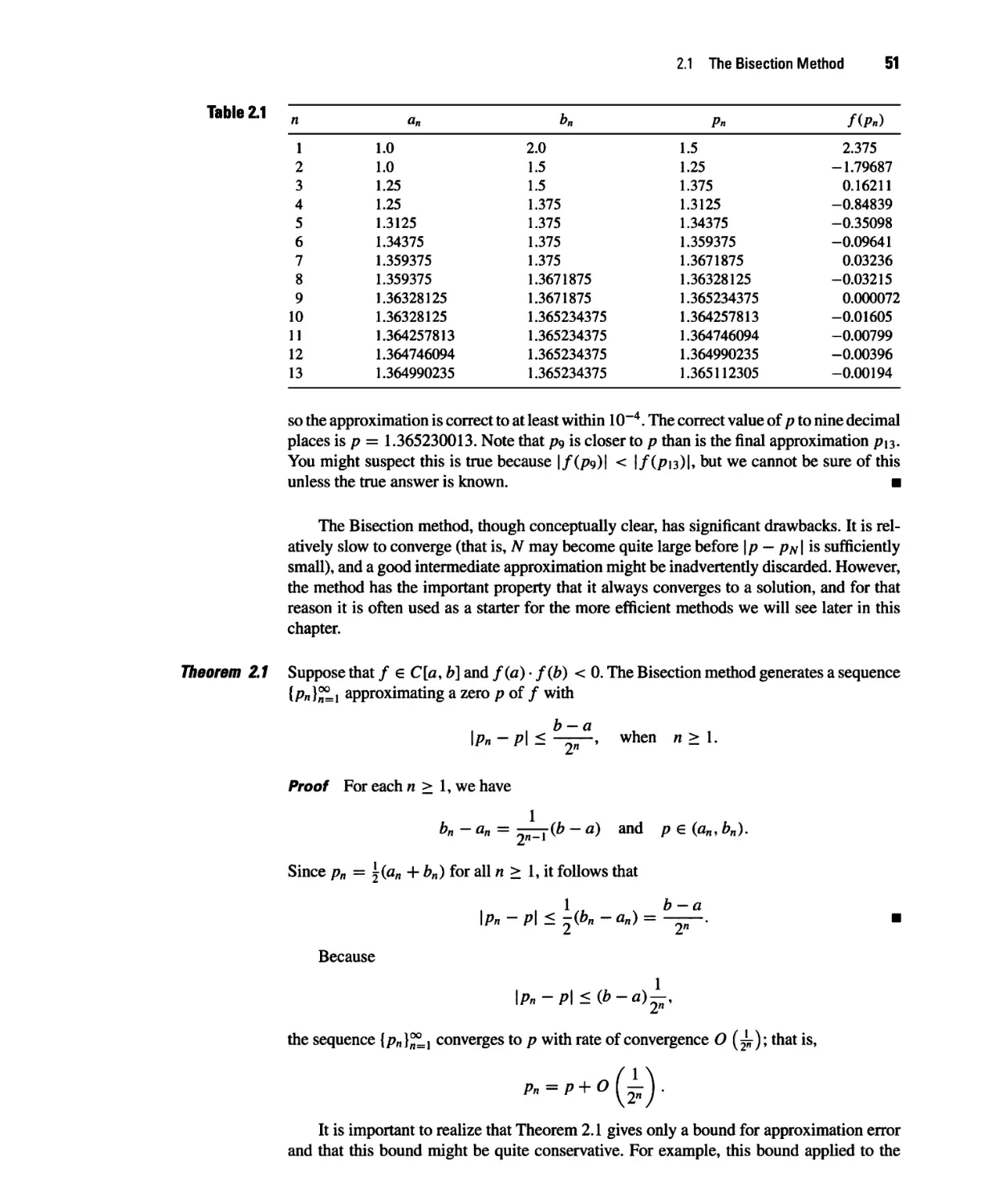


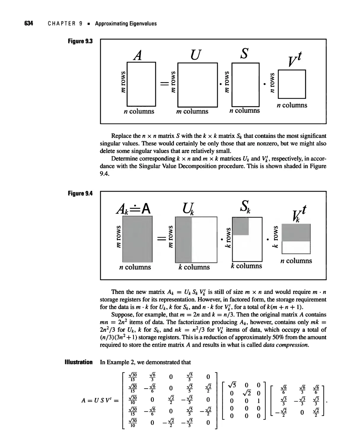
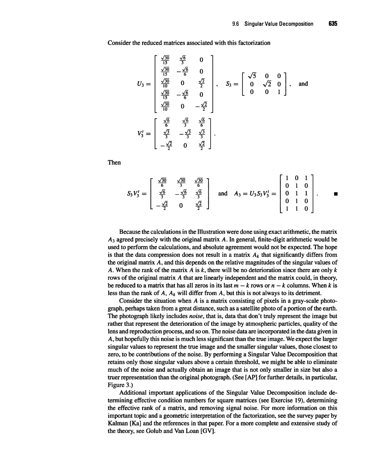


Текст
This is an electronic version of the print textbook. Due to electronic rights restrictions, some third party content may be suppressed. Editorial
review has deemed that any suppressed content does not materially affect the overall learning experience. The publisher reserves the right to
remove content from this title at any time if subsequent rights restrictions require it. For valuable information on pricing, previous
editions, changes to current editions, and alternate formats, please visit www.cengage.com/highered to search by
ISBN#, author, title, or keyword for materials in your areas of interest.
Important Notice: Media content referenced within the product description or the product text may not be available in the eBook version.
Numerical Analysis
Numerical Analysis
TENTH EDITION
Richard L. Burden
Youngstown University
J. Douglas Faires
Youngstown University
Annette M. Burden
Youngstown University
,*VC ENGAGE
*% Learning*
Australia • Brazil • Mexico • Singapore • United Kingdom • United States
VCENGAGE
* Learning*
Numerical Analysis,
Tenth Edition
Richard L Burden, J. Douglas Faires,
Annette M. Burden
Product Director: Terence Boyle
Senior Product Team Manager: RichardStratton
Associate Content Developer: Spencer Arritt
Product Assistant: Kathryn Schrumpf
Market Development Manager: Julie Schuster
Content Project Manageny/V/Qu/rm
Senior Art Director: Linda May
Manufacturing Planner: Doug Bertke
IP Analyst: Christina Ciaramella
IP Project Manager.John Sarantakis
Production Service: Cenveo Publisher Services
Compositor: Cenveo Publisher Services
Cover Image: © agsandrew/Shutterstockxom
© 2016,2011,2005 Cengage Learning
WCN: 02-300
ALL RIGHTS RESERVED. No part of this work covered by the copyright herein
may be reproduced, transmitted, stored, or used in any form or by any means
graphic, electronic, or mechanical, including but not limited to photocopying,
recording, scanning, digitizing, taping, web distribution, information networks,
or information storage and retrieval systems, except as permitted under Section
107 or 108 of the 1976 United States Copyright Act, without the prior written
permission of the publisher.
For product information and technology assistance, contact us at
Cengage Learning Customer & Sales Support,
1-800-354-9706
For permission to use material from this text or product,
submit all requests online at
www.cengage.com/permissions.
Further permissions questions can be emailed to
permissionrequest@cengage.com.
Library of Congress Control Number: 2014949816
ISBN: 978-1-305-25366-7
Cengage Learning
20 Channel Center Street
Boston, MA 02210
USA
Cengage Learning is a leading provider of customized learning solutions with
office locations around the globe, including Singapore, the United Kingdom,
Australia, Mexico, Brazil, and Japan. Locate your local office at
www.cengage.com/global.
Cengage Learning products are represented in Canada by Nelson Education, Ltd.
To learn more about Cengage Learning Solutions, visit www.cengage.com.
Purchase any of our products at your local college store or at our preferred
online store www.cengagebrain.com.
Printed in the United States of America
Print Number: 01 Print Year: 2014
This edition is dedicated to the memory of
J. Douglas Faires
Doug was a friend, colleague, and coauthor for over 40 years.
He will be sadly missed.
Contents
Preface xi
1 Mathematical Preliminaries and Error Analysis 1
1.1 Review of Calculus 2
1.2 Round-off Errors and Computer Arithmetic 14
1.3 Algorithms and Convergence 29
1.4 Numerical Software 38
2 Solutions of Equations in One Variable 47
2.1 The Bisection Method 48
2.2 Fixed-Point Iteration 55
2.3 Newton's Method and Its Extensions 66
2.4 Error Analysis for Iterative Methods 78
2.5 Accelerating Convergence 86
2.6 Zeros of Polynomials and Miiller's Method 91
2.7 Numerical Software and Chapter Review 101
3 Interpolation and Polynomial Approximation 103
3.1 Interpolation and the Lagrange Polynomial 104
3.2 Data Approximation and Neville's Method 115
3.3 Divided Differences 122
3.4 Hermite Interpolation 134
3.5 Cubic Spline Interpolation 142
3.6 Parametric Curves 162
3.7 Numerical Software and Chapter Review 168
4 Numerical Differentiation and Integration 171
4.1 Numerical Differentiation 172
4.2 Richardson's Extrapolation 183
4.3 Elements of Numerical Integration 191
vii
4.4 Composite Numerical Integration 202
4.5 Romberg Integration 211
4.6 Adaptive Quadrature Methods 219
4.7 Gaussian Quadrature 228
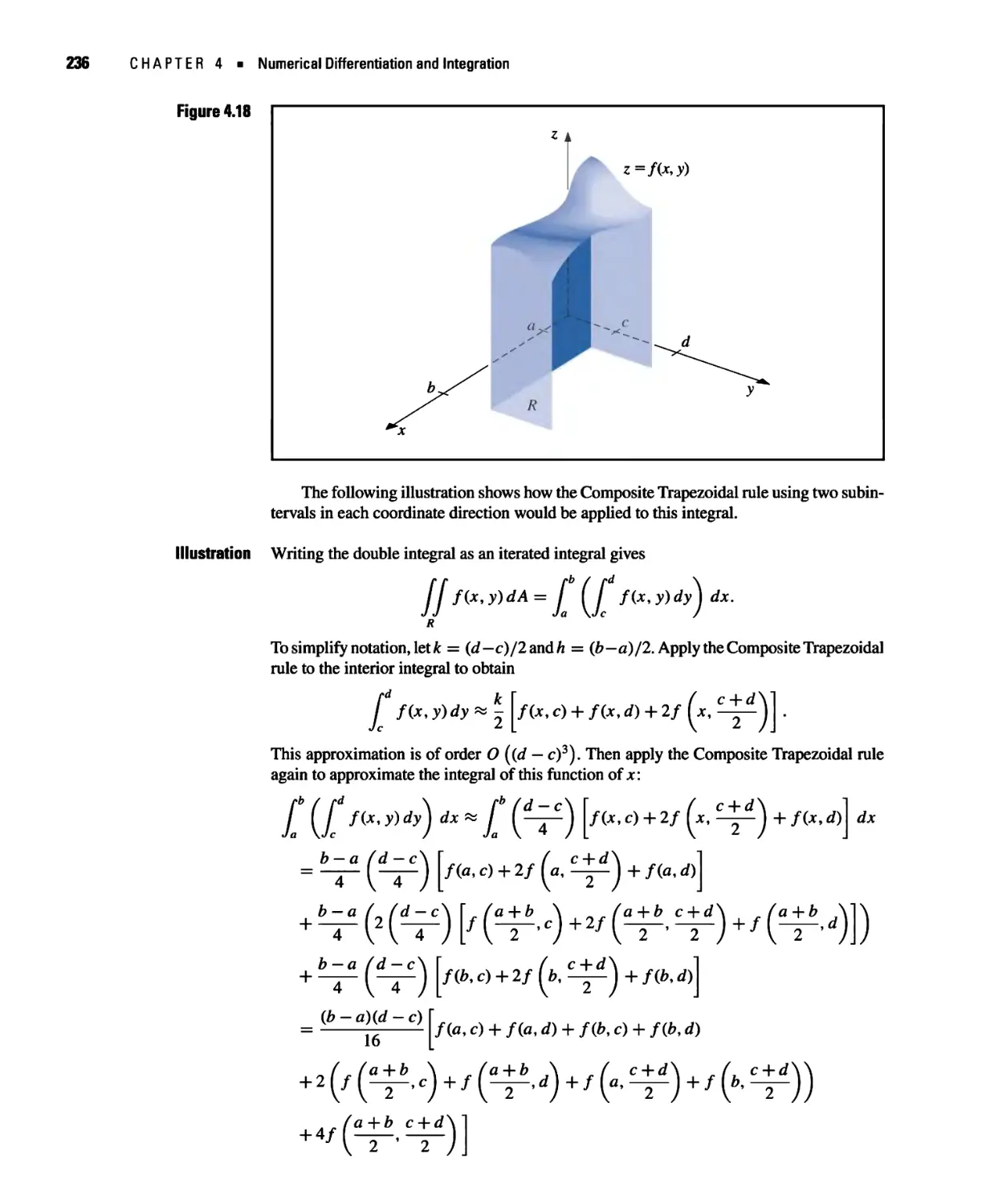
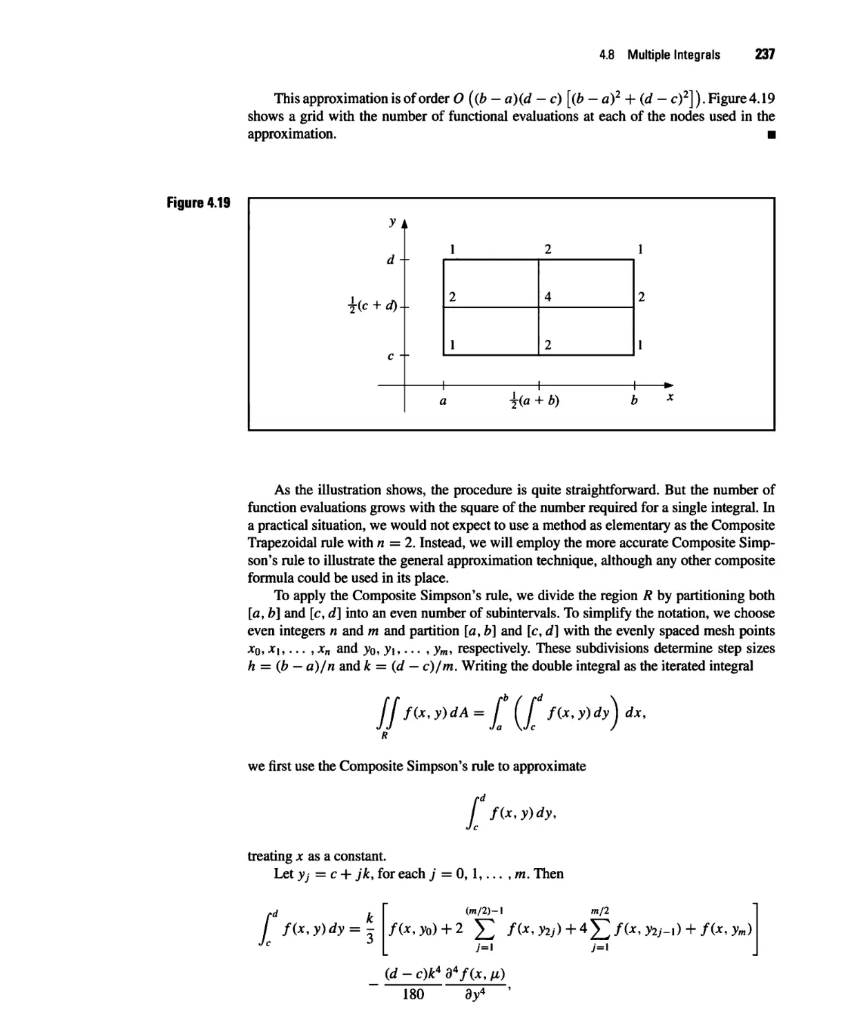
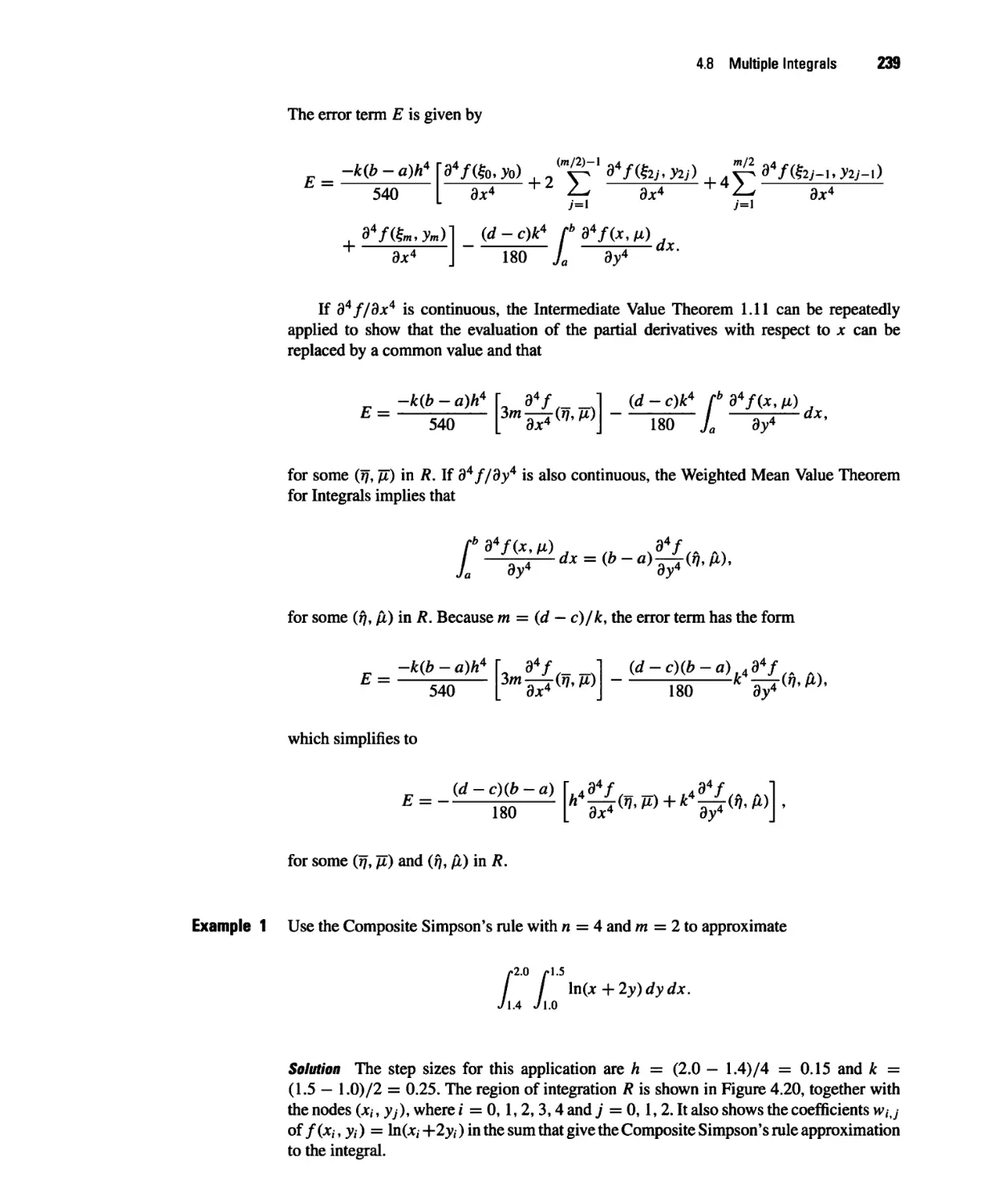
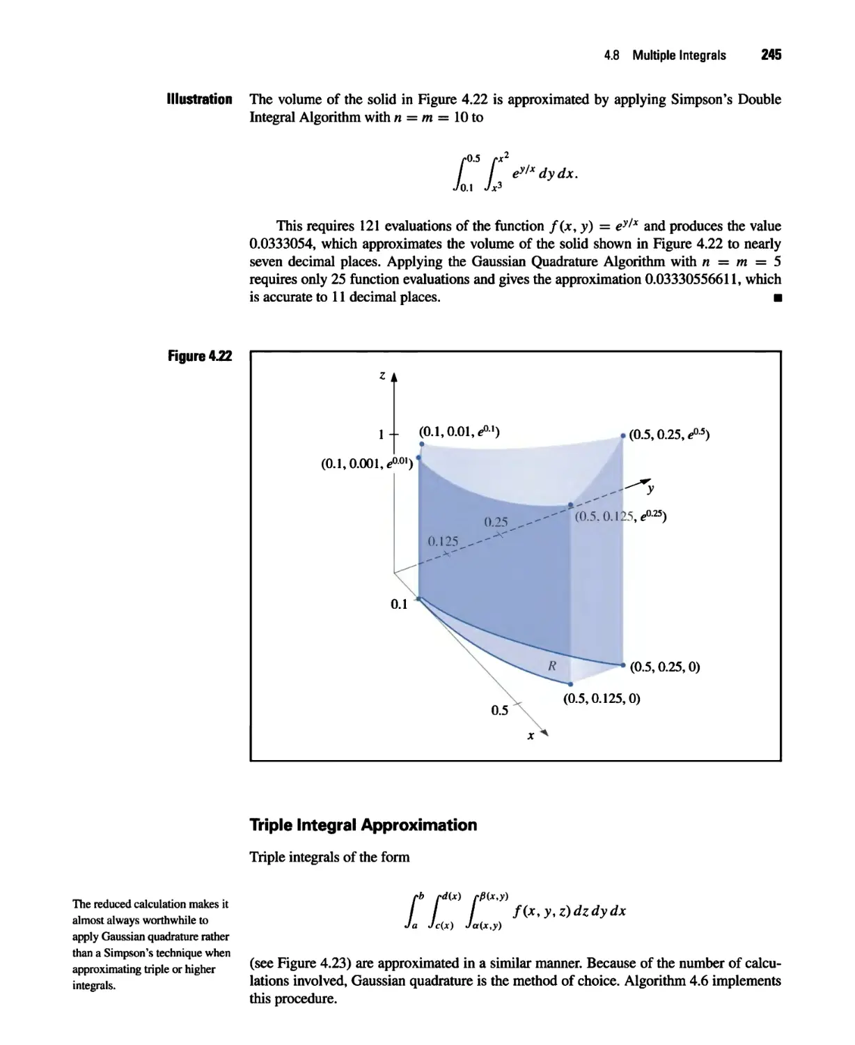
4.8 Multiple Integrals 235
4.9 Improper Integrals 250
4.10 Numerical Software and Chapter Review 256
5 Initial-Value Problems for Ordinary Differential
Equations 259
5.1 The Elementary Theory of Initial-Value Problems 260
5.2 Euler's Method 266
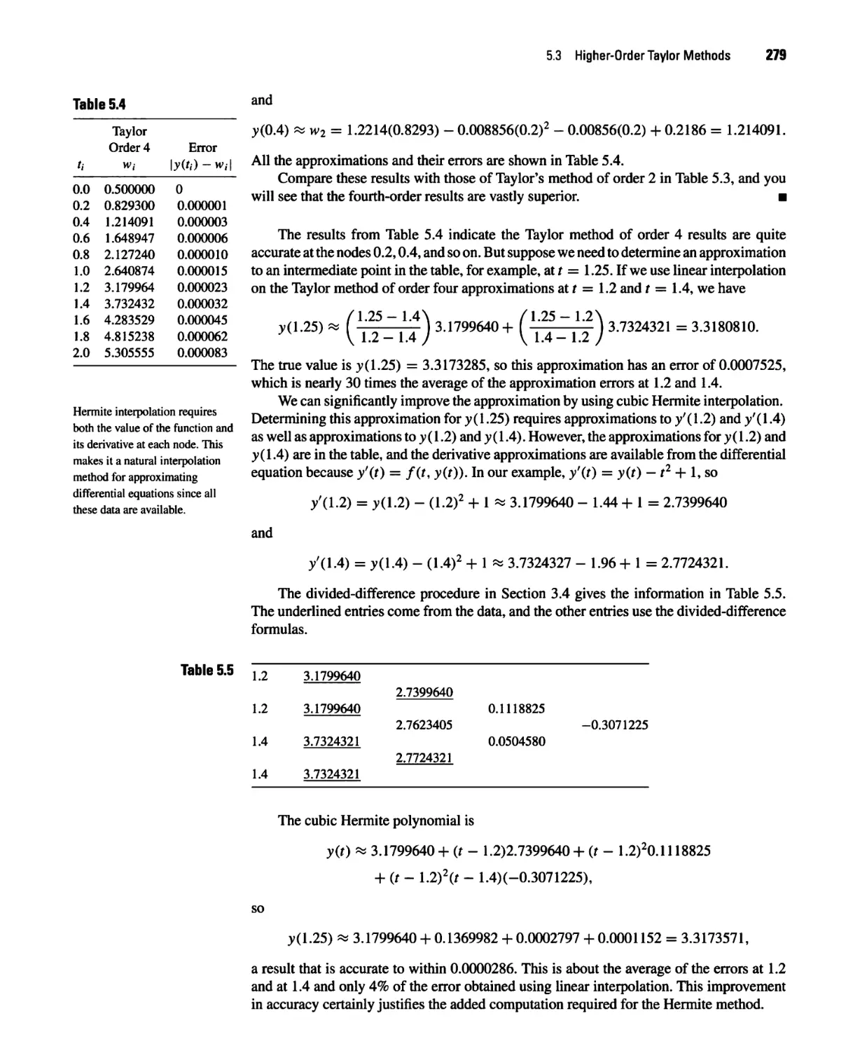
5.3 Higher-Order Taylor Methods 275
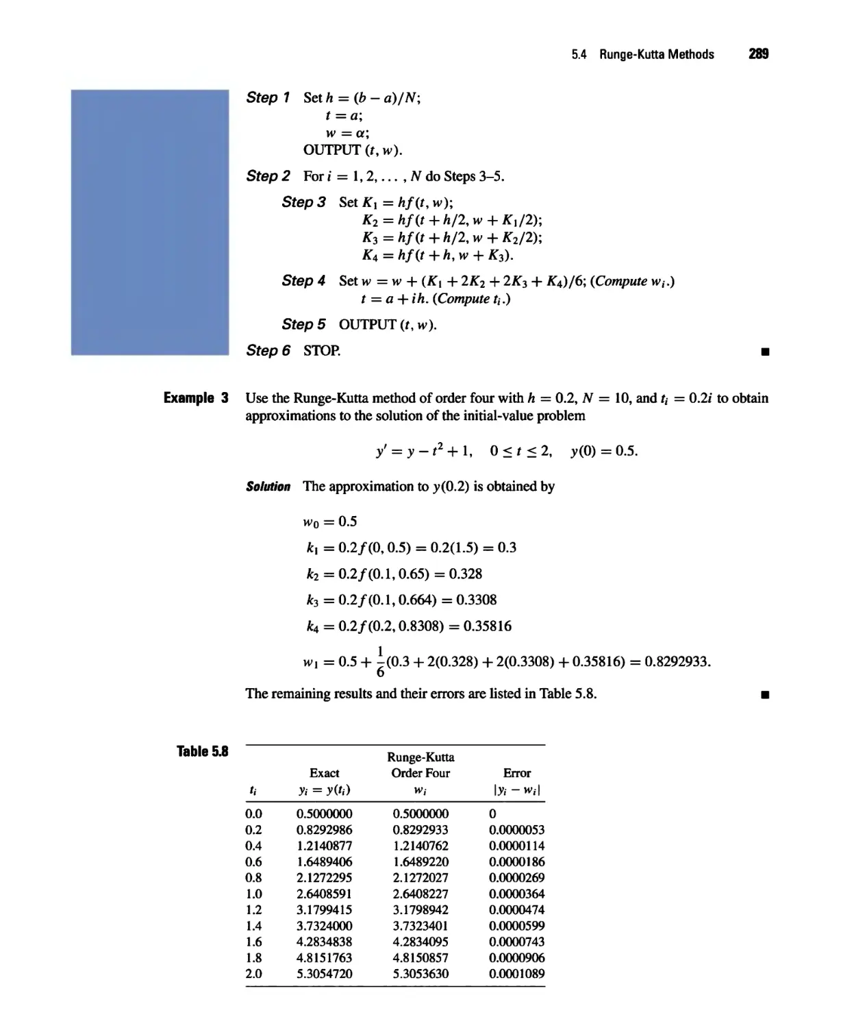
5.4 Runge-Kutta Methods 282
5.5 Error Control and the Runge-Kutta-Fehlberg Method 294
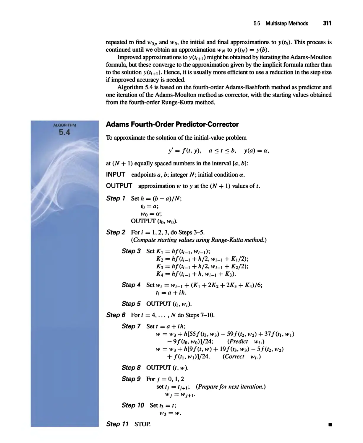
5.6 Multistep Methods 302
5.7 Variable Step-Size Multistep Methods 316
5.8 Extrapolation Methods 323
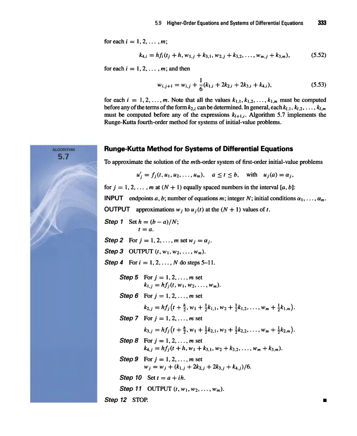
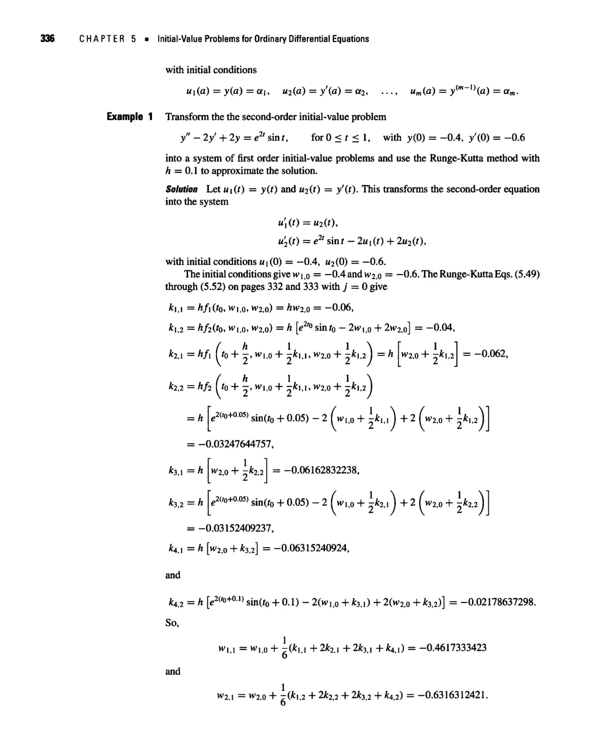
5.9 Higher-Order Equations and Systems of Differential Equations 331
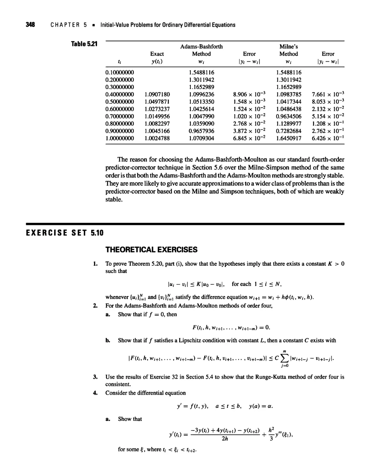
5.10 Stability 340
5.11 Stiff Differential Equations 349
5.12 Numerical Software 357
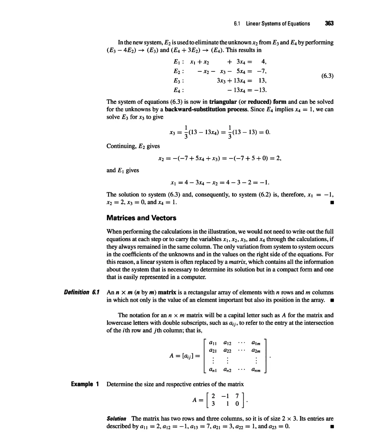
6 Direct Methods for Solving Linear Systems 361
6.1 Linear Systems of Equations 362
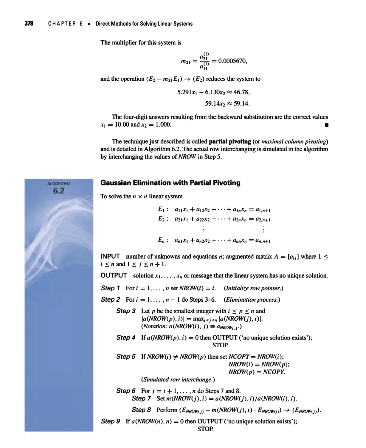
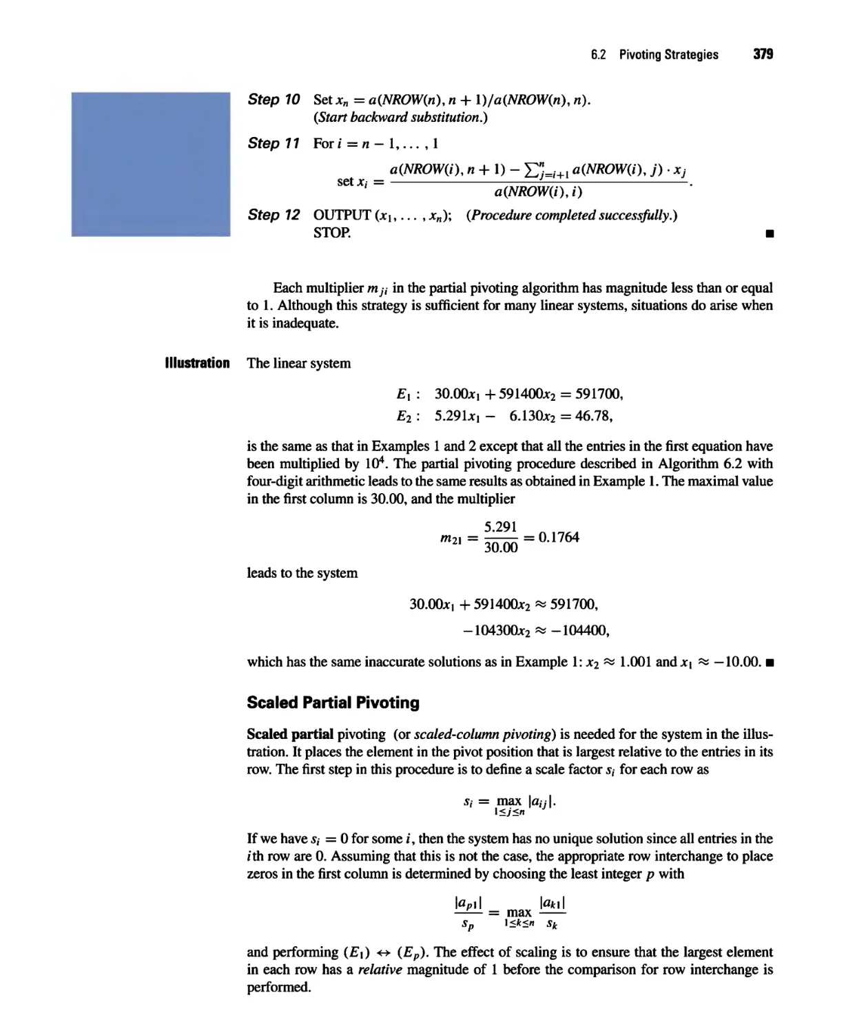
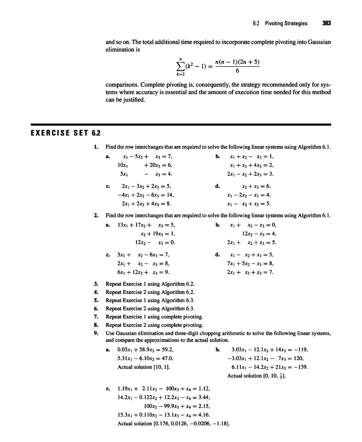
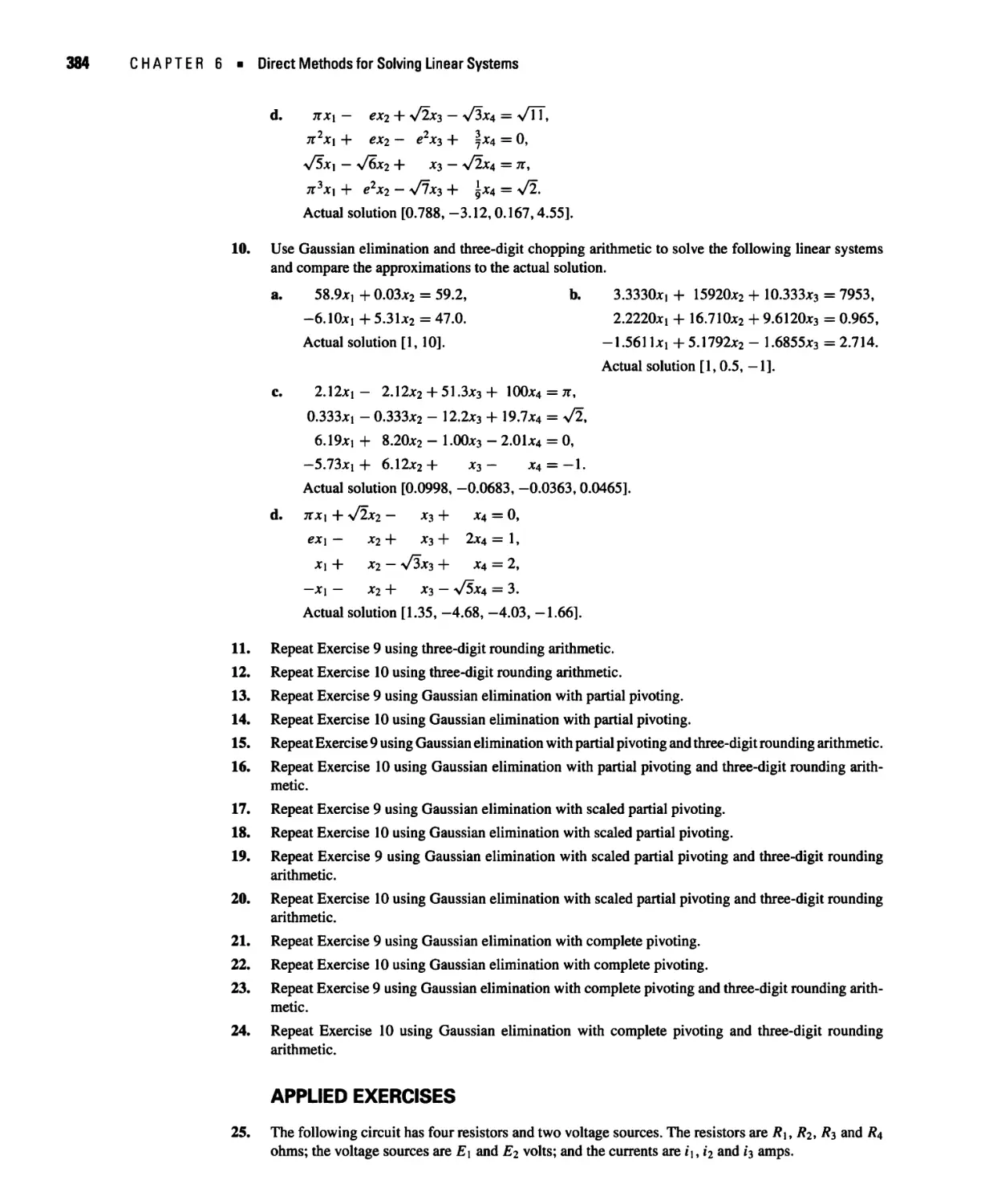
6.2 Pivoting Strategies 376
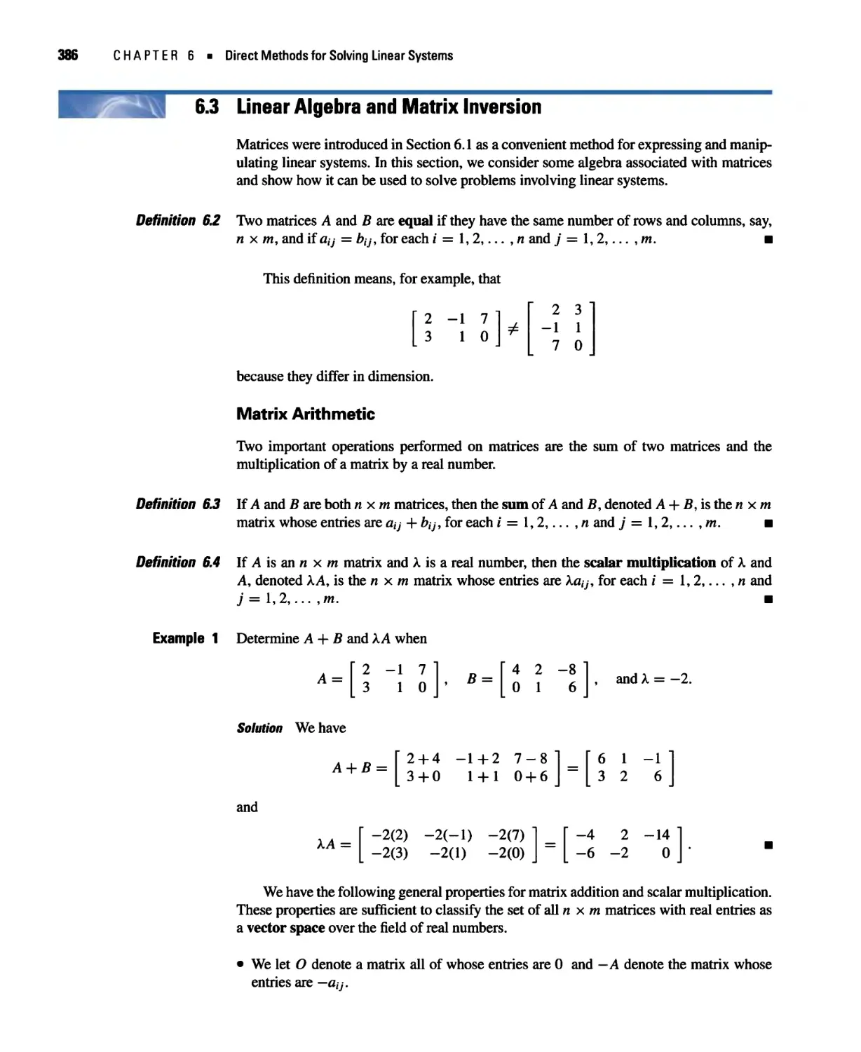
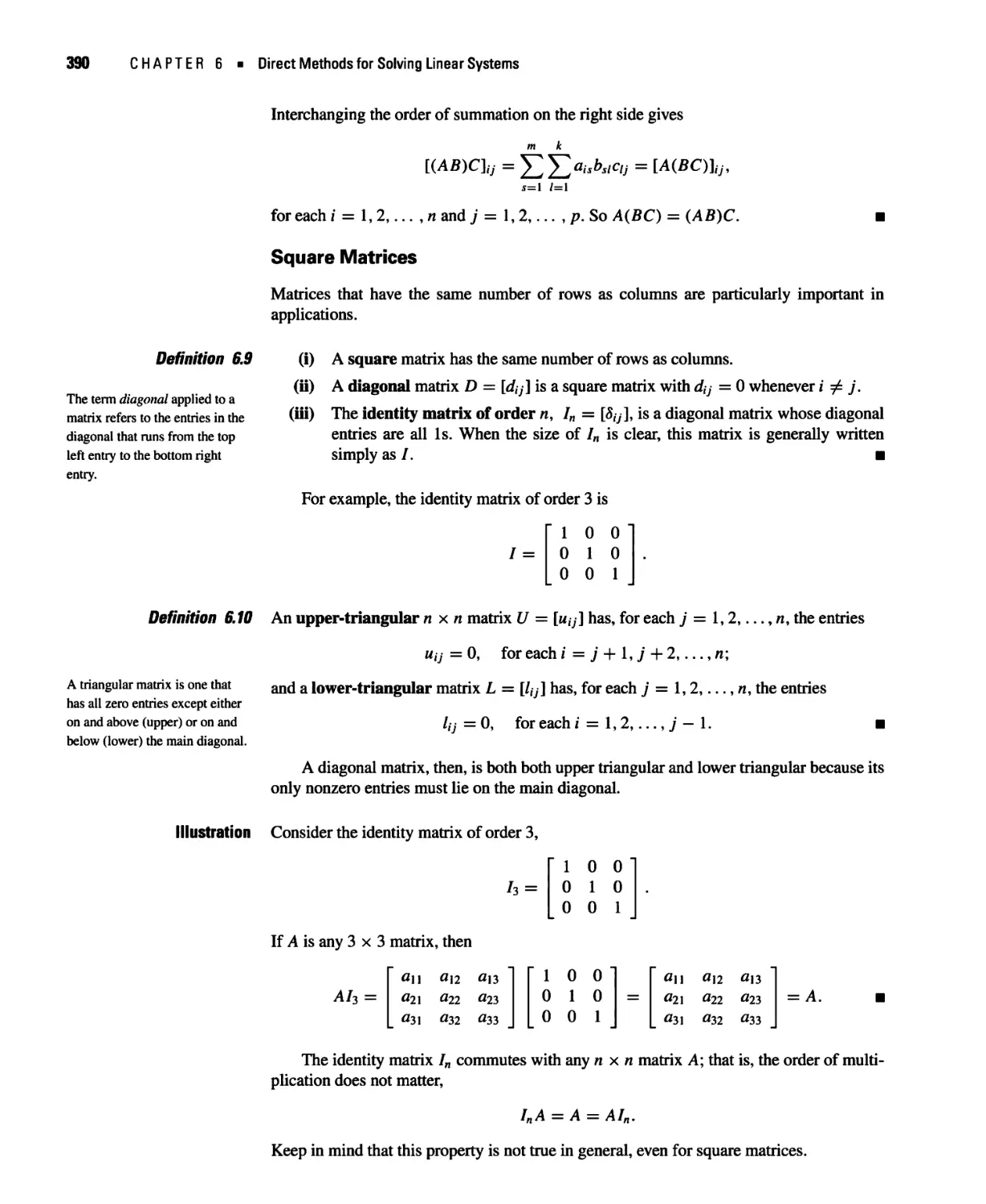
6.3 Linear Algebra and Matrix Inversion 386
6.4 The Determinant of a Matrix 400
6.5 Matrix Factorization 406
6.6 Special Types of Matrices 416
6.7 Numerical Software 433
7 Iterative Techniques in Matrix Algebra 437
7.1 Norms of Vectors and Matrices 438
7.2 Eigenvalues and Eigenvectors 450
7.3 The Jacobi and Gauss-Siedel Iterative Techniques 456
7.4 Relaxation Techniques for Solving Linear Systems 469
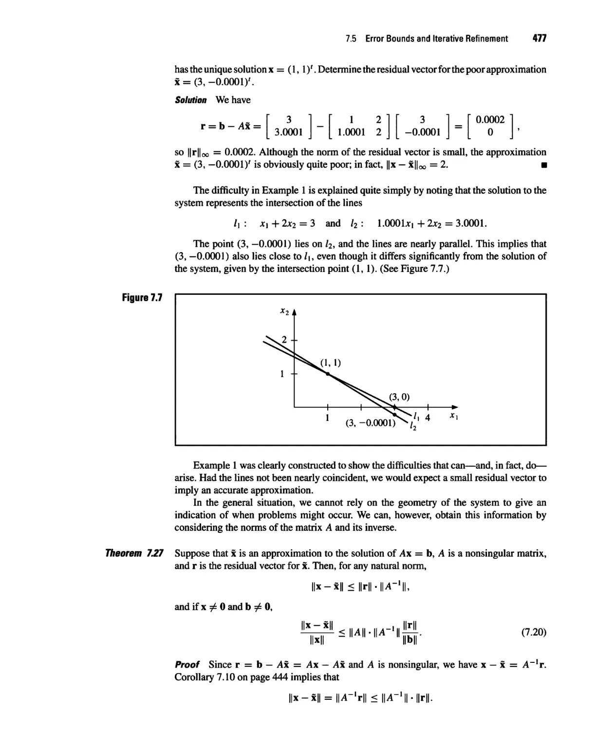
7.5 Error Bounds and Iterative Refinement 476
7.6 The Conjugate Gradient Method 487
7.7 Numerical Software 503
Contents ix
8 Approximation Theory 505
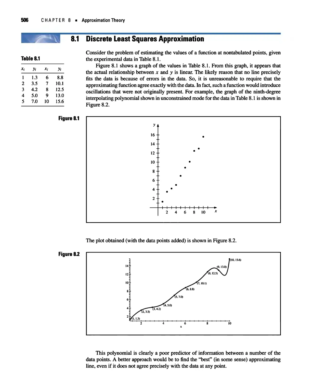
8.1 Discrete Least Squares Approximation 506
8.2 Orthogonal Polynomials and Least Squares Approximation 517
8.3 Chebyshev Polynomials and Economization of Power Series 526
8.4 Rational Function Approximation 535
8.5 Trigonometric Polynomial Approximation 545
8.6 Fast Fourier Transforms 555
8.7 Numerical Software 567
9 Approximating Eigenvalues 569
9.1 Linear Algebra and Eigenvalues 570
9.2 Orthogonal Matrices and Similarity Transformations 578
9.3 The Power Method 585
9.4 Householder's Method 602
9.5 The QR Algorithm 610
9.6 Singular Value Decomposition 624
9.7 Numerical Software 638
10 Numerical Solutions of Nonlinear Systems of
Equations 641
10.1 Fixed Points for Functions of Several Variables 642
10.2 Newton's Method 651
10.3 Quasi-Newton Methods 659
10.4 Steepest Descent Techniques 666
10.5 Homotopy and Continuation Methods 674
10.6 Numerical Software 682
11 Boundary-Value Problems for Ordinary Differential
Equations 685
11.1 The Linear Shooting Method 686
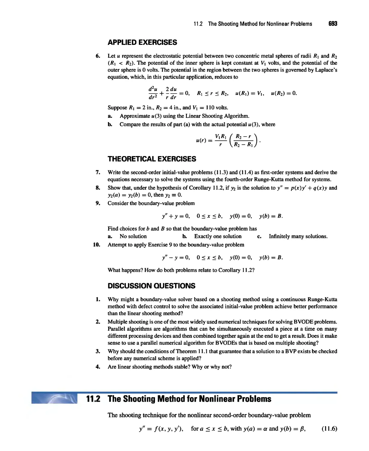
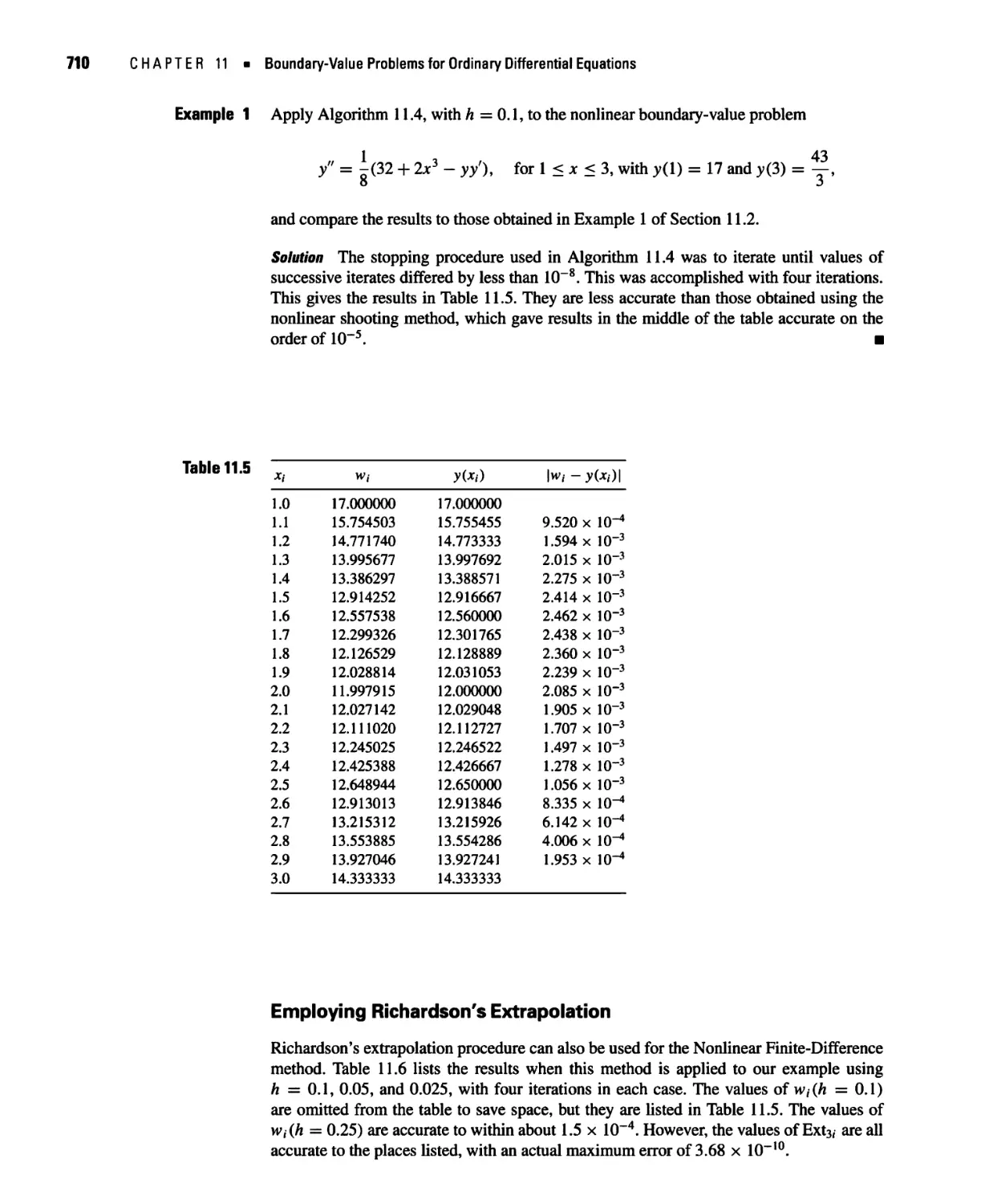
11.2 The Shooting Method for Nonlinear Problems 693
11.3 Finite-Difference Methods for Linear Problems 700
11.4 Finite-Difference Methods for Nonlinear Problems 706
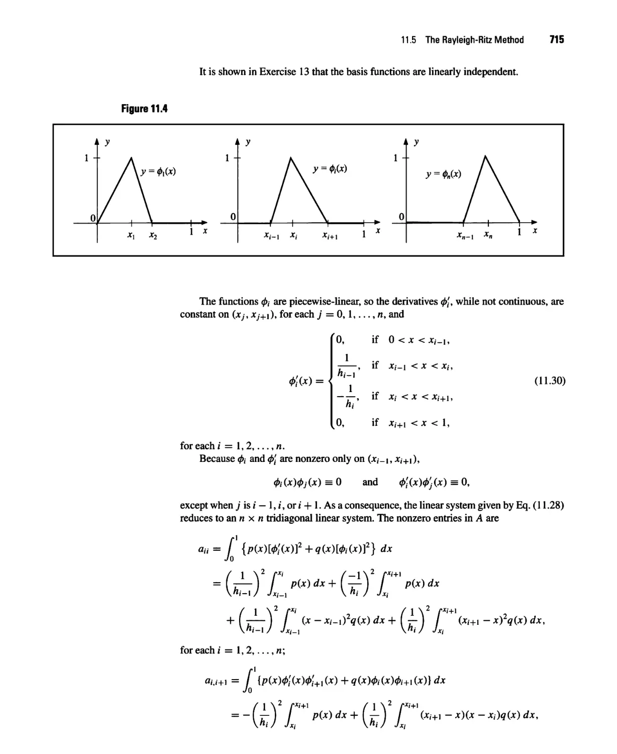
11.5 The Rayleigh-Ritz Method 712
11.6 Numerical Software 728
x Contents
12 Numerical Solutions to Partial Differential
Equations 731
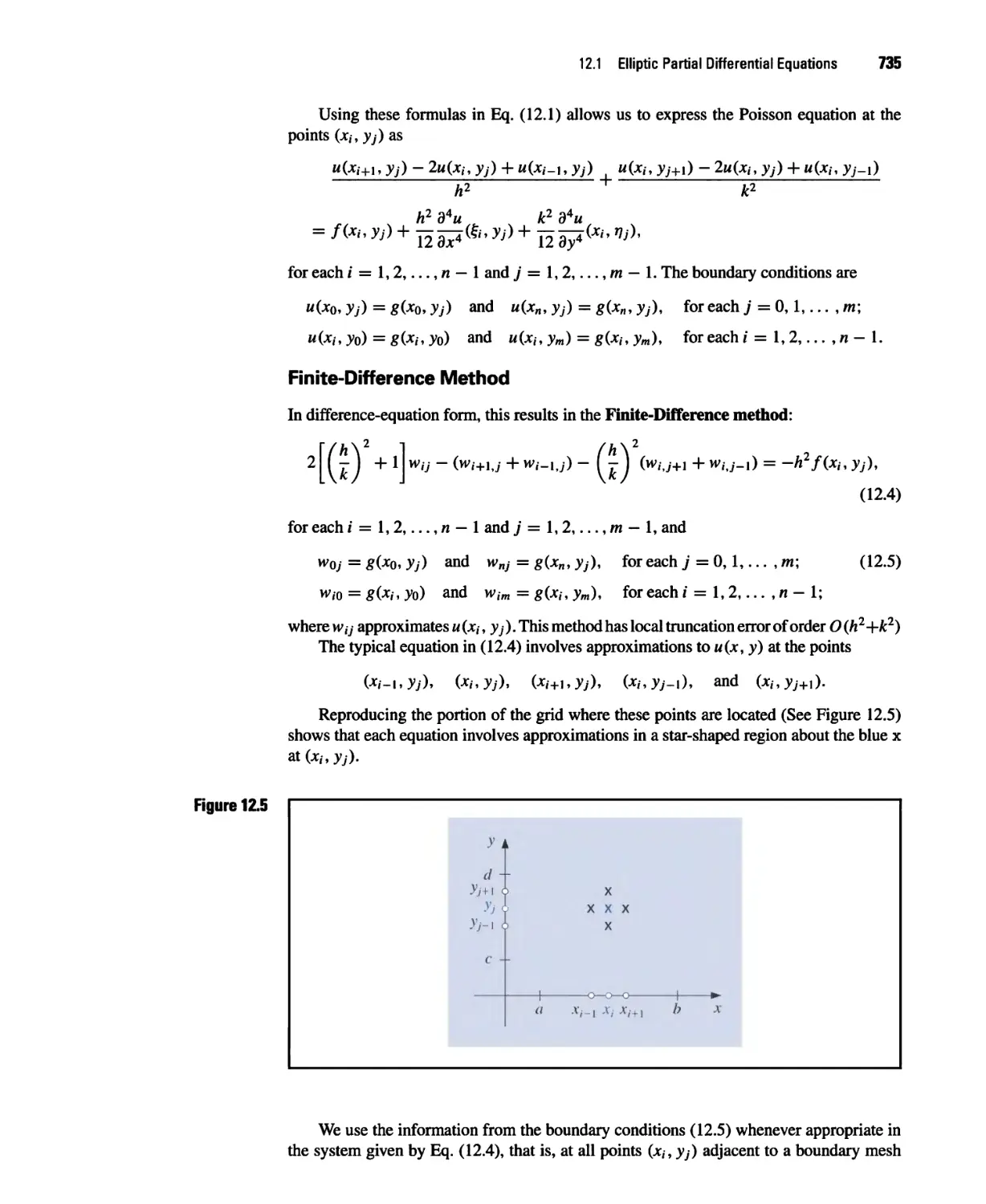
12.1 Elliptic Partial Differential Equations 734
12.2 Parabolic Partial Differential Equations 743
12.3 Hyperbolic Partial Differential Equations 757
12.4 An Introduction to the Finite-Element Method 765
12.5 Numerical Software 779
Bibliography 781
Answers to Selected Exercises 787
Index 889
Preface
About the Text
This text was written for a sequence of courses on the theory and application of numerical
approximation techniques. It is designed primarily for junior-level mathematics, science,
and engineering majors who have completed at least the first year of the standard college
calculus sequence. Familiarity with the fundamentals of matrix algebra and differential
equations is useful, but there is sufficient introductory material on these topics so that
courses in these subjects are not needed as prerequisites.
Previous editions of Numerical Analysis have been used in a wide variety of situations.
In some cases, the mathematical analysis underlying the development of approximation
techniques was given more emphasis than the methods; in others, the emphasis was reversed.
The book has been used as a core reference for beginning graduate-level courses in
engineering, mathematics, computer science programs, and in first-year courses in introductory
analysis offered at international universities. We have adapted the book to fit these diverse
users without compromising our original purpose:
To introduce modern approximation techniques; to explain how, why, and when they
can be expected to work; and to provide a foundation for further study of numerical
analysis and scientific computing.
The book contains sufficient material for at least a full year of study, but we expect
many people will use the text only for a single-term course. In such a single-term course,
students learn to identify the types of problems that require numerical techniques for their
solution and see examples of the error propagation that can occur when numerical methods
are applied. They accurately approximate the solution of problems that cannot be solved
exactly and learn typical techniques for estimating error bounds for their approximations.
The remainder of the text then serves as a reference for methods that are not considered in the
course. Either the full-year or the single-course treatment is consistent with the philosophy
of the text.
Virtually every concept in the text is illustrated by example, and this edition contains
more than 2500 class-tested exercises ranging from elementary applications of methods
and algorithms to generalizations and extensions of the theory. In addition, the exercise
sets include numerous applied problems from diverse areas of engineering as well as from
the physical, computer, biological, economic, and social sciences. The applications, chosen
clearly and concisely, demonstrate how numerical techniques can and often must be applied
in real-life situations.
A number of software packages, known as Computer Algebra Systems (CAS), have
been developed to produce symbolic mathematical computations. Maple©, Mathematica©,
and MATLAB© are predominant among these in the academic environment. Student
versions of these software packages are available at reasonable prices for most common
xi
computer systems. In addition, Sage, a free open source system, is now available.
Information about this system can be found at the site
http://www.sagemath.org
Although there are differences among the packages, both in performance and in price,
all can perform standard algebra and calculus operations.
The results in most of our examples and exercises have been generated using problems
for which exact values can be determined because this better permits the performance of
the approximation method to be monitored. In addition, for many numerical techniques,
the error analysis requires bounding a higher ordinary or partial derivative of a function,
which can be a tedious task and one that is not particularly instructive once the techniques
of calculus have been mastered. So having a symbolic computation package available
can be very useful in the study of approximation techniques because exact solutions can
often be obtained easily using symbolic computation. Derivatives can be quickly obtained
symbolically, and a little insight often permits a symbolic computation to aid in the bounding
process as well.
Algorithms and Programs
In our first edition, we introduced a feature that at the time was innovative and somewhat
controversial. Instead of presenting our approximation techniques in a specific programming
language (FORTRAN was dominant at the time), we gave algorithms in a pseudocode that
would lead to a well-structured program in a variety of languages. Beginning with the
second edition, we listed programs in specific languages in the Instructor's Manual for the
book, and the number of these languages increased in subsequent editions. We now have the
programs coded and available online in most common programming languages and CAS
worksheets. All of these are on the companion website for the book (see "Supplements").
For each algorithm, there is a program written in Fortran, Pascal, C, and Java. In
addition, we have coded the programs using Maple, Mathematica, and MATLAB. This
should ensure that a set of programs is available for most common computing systems.
Every program is illustrated with a sample problem that is closely correlated to the text.
This permits the program to be run initially in the language of your choice to see the form
of the input and output. The programs can then be modified for other problems by making
minor changes. The form of the input and output are, as nearly as possible, the same in each
of the programming systems. This permits an instructor using the programs to discuss them
generically without regard to the particular programming system an individual student uses.
The programs are designed to run on a minimally configured computer and given
in ASCII format to permit flexibility of use. This permits them to be altered using any
editor or word processor that creates standard ASCII files. (These are also commonly called
"text-only" files.) Extensive README files are included with the program files so that
the peculiarities of the various programming systems can be individually addressed. The
README files are presented both in ASCII format and as PDF files. As new software is
developed, the programs will be updated and placed on the website for the book.
For most of the programming systems, the appropriate software is needed, such as
a compiler for Pascal, Fortran, and C, or one of the computer algebra systems (Maple,
Mathematica, and MATLAB). The Java implementations are an exception. You need the
system to run the programs, but Java can be freely downloaded from various sites. The best
way to obtain Java is to use a search engine to search on the name, choose a download site,
and follow the instructions for that site.
Preface xiii
New for This Edition
The first edition of this book was published more than 35 years ago, in the decade after major
advances in numerical techniques were made to reflect the new widespread availability of
computer equipment. In our revisions of the book, we have added new techniques in an
attempt to keep our treatment current. To continue this trend, we have made a number of
significant changes for this edition:
• Some of the examples in the book have been rewritten to better emphasize the problem
being solved before the solution is given. Additional steps have been added to some of
the examples to explicitly show the computations required for the first steps of iteration
processes. This gives readers a way to test and debug programs they have written for
problems similar to the examples.
• Chapter exercises have been split into computational, applied, and theoretical to give
the instructor more flexibility in assigning homework. In almost all of the computational
situations, the exercises have been paired in an odd-even manner. Since the odd problems
are answered in the back of the text, if even problems were assigned as homework,
students could work the odd problems and check their answers prior to doing the even
problem.
• Many new applied exercises have been added to the text.
• Discussion questions have been added after each chapter section primarily for instructor
use in online courses.
• The last section of each chapter has been renamed and split into four subsections:
Numerical Software, Discussion Questions, Key Concepts, and Chapter Review. Many of
these discussion questions point the student to modem areas of research in software
development.
• Parts of the text were reorganized to facilitate online instruction.
• Additional PowerPoints have been added to supplement the reading material.
• The bibliographic material has been updated to reflect new editions of books that we
reference. New sources have been added that were not previously available.
As always with our revisions, every sentence was examined to determine if it was phrased
in a manner that best relates what we are trying to describe.
Supplements
The authors have created a companion website containing the supplementary materials
listed below. The website located at
https://sites.google.com/site/numericalanalysis 1 burden/
is for students and instructors. Some material on the website is for instructor use only.
Instructors can access protected materials by contacting the authors for the password.
Some of the supplements can also be obtained at
https://www.cengagebrain.com
by searching the ISBN.
1. Student Program Examples that contain Maple, Matlab, and Excel code for student
use in solving text problems. This is organized to parallel the text chapter by chapter.
Commands in these systems are illustrated. The commands are presented in very
short program segments to show how exercises may be solved without extensive
programming.
2. Student Lectures that contain additional insight to the chapter content. These
lectures were written primarily for the online learner but can be useful to students
taking the course in a traditional setting.
3. Student Study Guide that contains worked-out solutions to many of the problems.
The first two chapters of this guide are available on the website for the book in
PDF format so that prospective users can tell if they find it sufficiently useful.
The entire guide can be obtained only from the publisher by calling Cengage
Learning Customer & Sales Support at 1-800-354-9706 or by ordering online at
http://www.cengagebrain.com/.
4. Algorithm Programs that are complete programs written in Maple, Matlab,
Mathematical C, Pascal, Fortran, and Java for all the algorithms in the text. These
programs are intended for students who are more experienced with programming
languages.
5. Instructor PowerPoints in PDF format for instructor use in both traditional and
online courses. Contact authors for password.
6. Instructor's Manual that provides answers and solutions to all the exercises in
the book. Computation results in the Instructor's Manual were regenerated for
this edition using the programs on the website to ensure compatibility among the
various programming systems. Contact authors for password.
7. Instructor Sample Tests for instructor use. Contact authors for password.
8. Errata.
Possible Course Suggestions
Numerical Analysis is designed to allow instructors flexibility in the choice of topics as well
as in the level of theoretical rigor and in the emphasis on applications. In line with these
aims, we provide detailed references for the results that are not demonstrated in the text
and for the applications that are used to indicate the practical importance of the methods.
The text references cited are those most likely to be available in college libraries and have
been updated to reflect recent editions. We also include quotations from original research
papers when we feel this material is accessible to our intended audience. All referenced
material has been indexed to the appropriate locations in the text, and Library of Congress
call information for reference material has been included to permit easy location if searching
for library material.
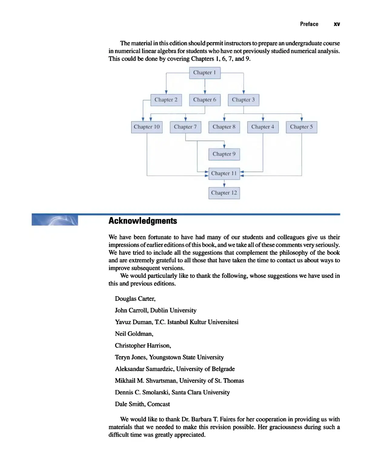
The following flowchart indicates chapter prerequisites. Most of the possible sequences
that can be generated from this chart have been taught by the authors at Youngstown State
University.
Preface xv
The material in this edition should permit instructors to prepare an undergraduate course
in numerical linear algebra for students who have not previously studied numerical analysis.
This could be done by covering Chapters 1, 6,7, and 9.
1
' ^
\
l
Chapter 2
c
u.
>,- i
V_^i icij'iv^i i
1
Chapter 6
i
Chaptei 10
Chapter 7
■ Chapter 3
i i
▼ T
Chapter 8
Chapter 4
T
Chapter 9
Chapter 11 t
\
f
Chapter 5
T
1
Chapter 12
Acknowledgments
We have been fortunate to have had many of our students and colleagues give us their
impressions of earlier editions of this book, and we take all of these comments very seriously.
We have tried to include all the suggestions that complement the philosophy of the book
and are extremely grateful to all those that have taken the time to contact us about ways to
improve subsequent versions.
We would particularly like to thank the following, whose suggestions we have used in
this and previous editions.
Douglas Carter,
John Carroll, Dublin University
Yavuz Duman, T.C Istanbul Kultur Universitesi
Neil Goldman,
Christopher Harrison,
Teryn Jones, Youngstown State University
Aleksandar Samardzic, University of Belgrade
Mikhail M. Shvartsman, University of St. Thomas
Dennis C. Smolarski, Santa Clara University
Dale Smith, Comcast
We would like to thank Dr. Barbara T. Faires for her cooperation in providing us with
materials that we needed to make this revision possible. Her graciousness during such a
difficult time was greatly appreciated.
As has been our practice in past editions of the book, we have used student help at
Youngstown State University in preparing the tenth edition. Our able assistant for this
edition was Teryn Jones who worked on the Java applets. We would like to thank Edward
R. Burden, an Electrical Engineering doctoral student at Ohio State University, who has
been checking all the application problems and new material in the text. We also would
like to express gratitude to our colleagues on the faculty and administration of Youngstown
State University for providing us the opportunity and facilities to complete this project.
We would like to thank some people who have made significant contributions to
the history of numerical methods. Herman H. Goldstine has written an excellent book
titled A History of Numerical Analysis from the 16th Through the 19th Century [Golds].
Another source of excellent historical mathematical knowledge is the MacTUtor History of
Mathematics archive at the University of St. Andrews in Scotland. It has been created by
John J. O'Connor and Edmund F. Robertson and has the Internet address
http://www-gap.dcs.st-and.ac.uk/~history/
An incredible amount of work has gone into creating the material on this site, and we have
found the information to be unfailingly accurate. Finally, thanks to all the contributors to
Wikipedia who have added their expertise to that site so that others can benefit from their
knowledge.
In closing, thanks again to those who have spent the time and effort to contact us
over the years. It has been wonderful to hear from so many students and faculty who used
our book for their first exposure to the study of numerical methods. We hope this edition
continues this exchange and adds to the enjoyment of students studying numerical analysis.
If you have any suggestions for improving future editions of the book, we would, as always,
be grateful for your comments. We can be contacted most easily by e-mail at the addresses
listed below.
Richard L Burden
rlburden @ ysu.edu
Annette M. Burden
amburden @ ysu.edu
Mathematical Preliminaries
and Error Analysis
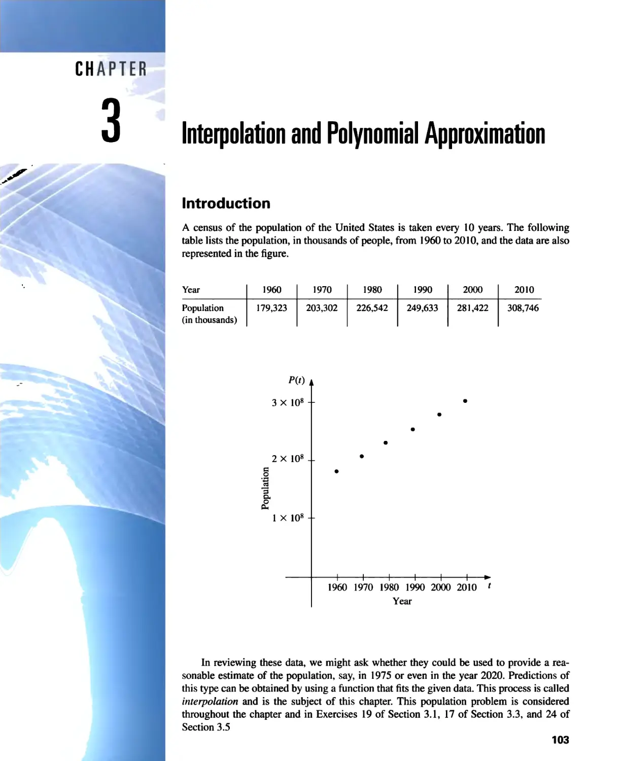
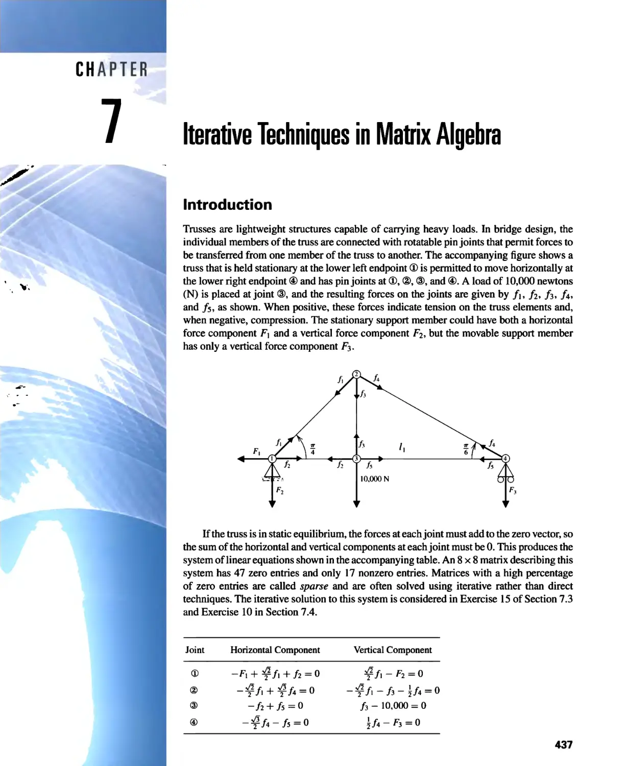
Introduction
In beginning chemistry courses, we see the ideal gas law,
PV =NRT,
which relates the pressure P, volume V, temperature T, and number of moles N of an
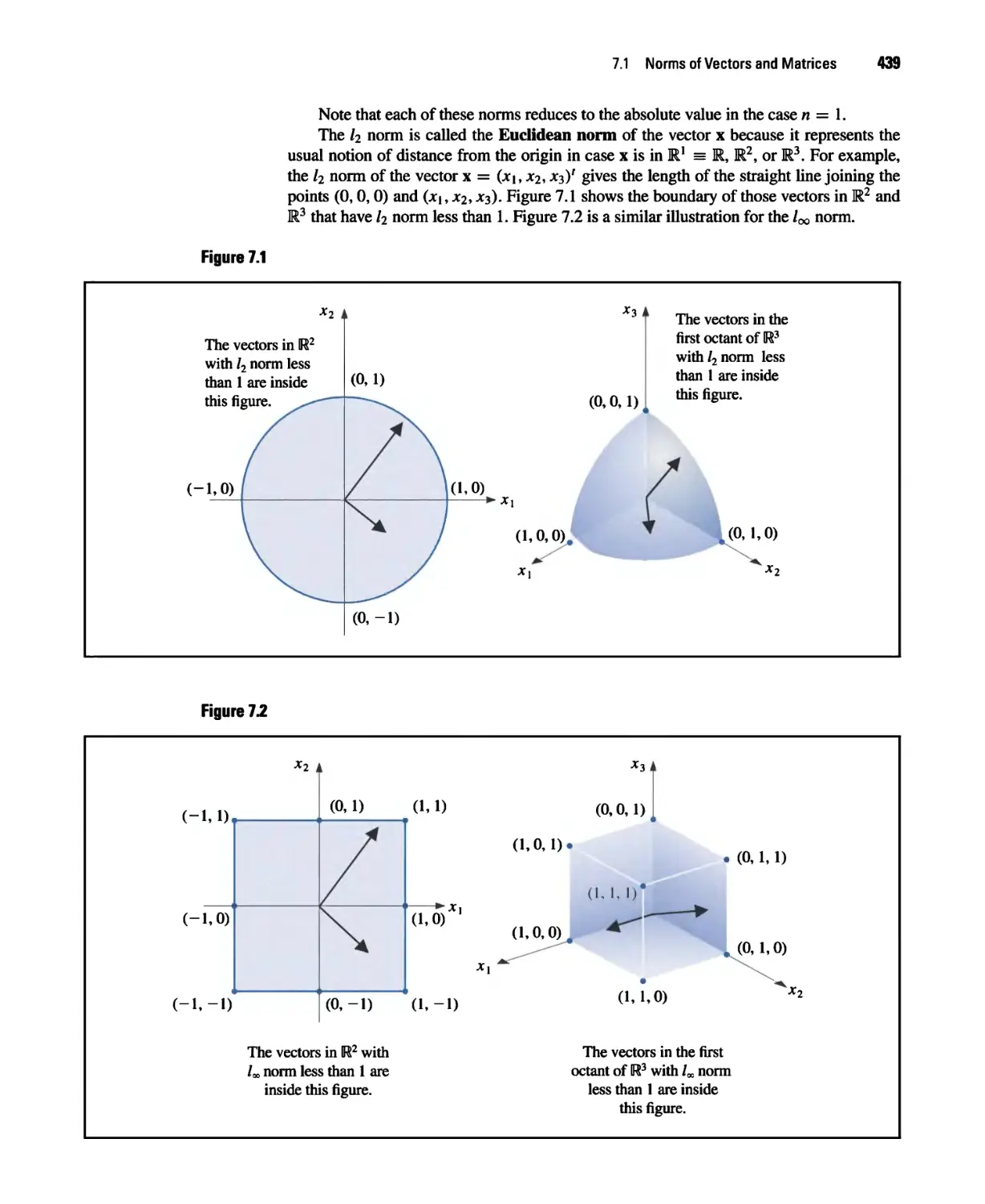
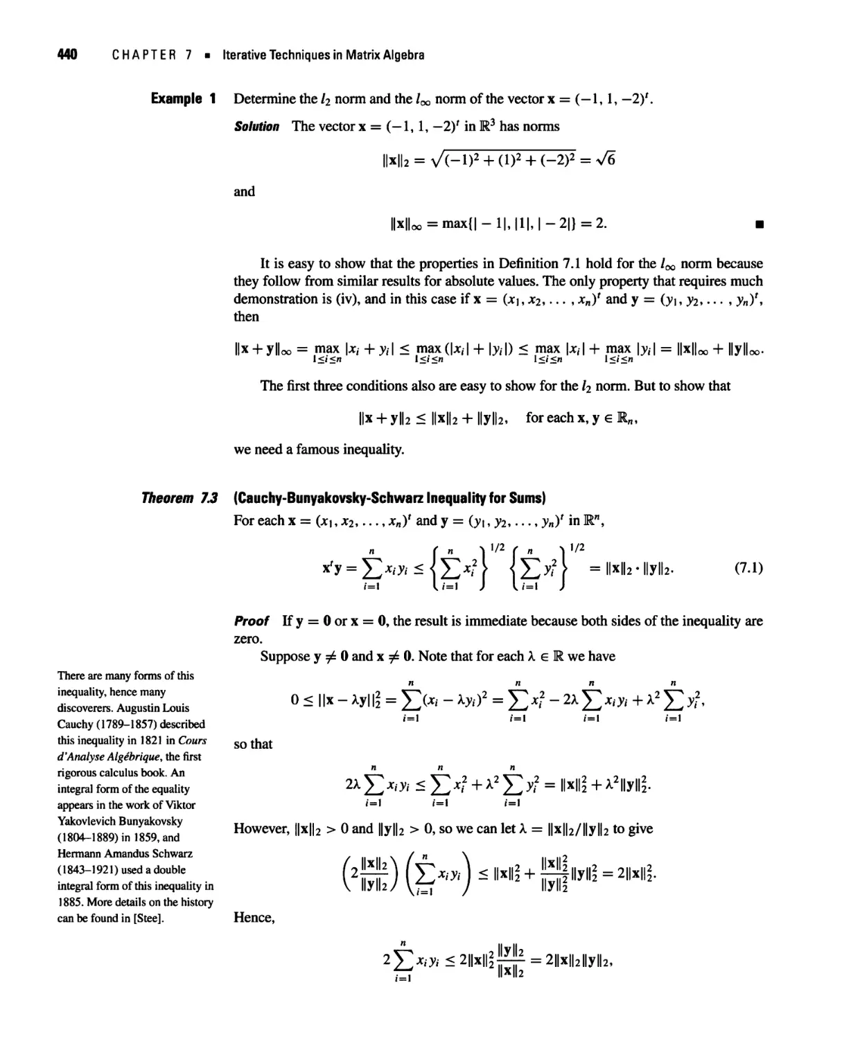
"ideal" gas. In this equation, R is a constant that depends on the measurement system.
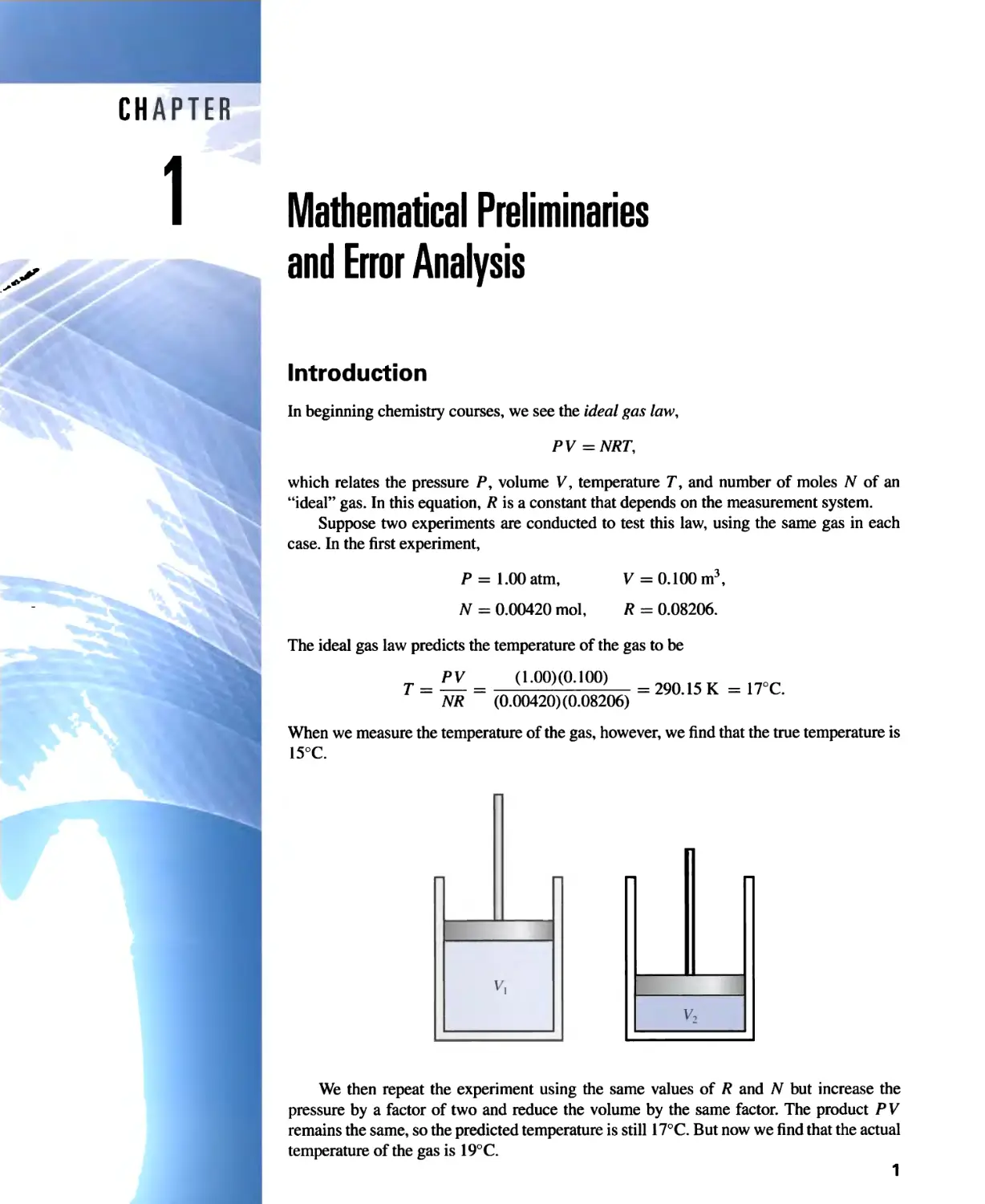
Suppose two experiments are conducted to test this law, using the same gas in each
case. In the first experiment,
/» = 1.00atm, V = 0.100 m3,
N = 0.00420 mol, R = 0.08206.
The ideal gas law predicts the temperature of the gas to be
PV (1.00) (0.100)
T =
NR (0.00420) (0.08206)
= 290.15 K =17°C.
When we measure the temperature of the gas, however, we find that the true temperature is
15°C.
V-,
We then repeat the experiment using the same values of R and N but increase the
pressure by a factor of two and reduce the volume by the same factor. The product PV
remains the same, so the predicted temperature is still 17°C. But now we find that the actual
temperature of the gas is 19°C.
1
2 CHAPTER 1 ■ Mathematical Preliminaries and Error Analysis
Clearly, the ideal gas law is suspect, but before concluding that the law is invalid in
this situation, we should examine the data to see whether the error could be attributed to
the experimental results. If so, we might be able to determine how much more accurate our
experimental results would need to be to ensure that an error of this magnitude does not
occur.
Analysis of the error involved in calculations is an important topic in numerical analysis
and is introduced in Section 1.2. This particular application is considered in Exercise 26 of
that section.
This chapter contains a short review of those topics from single-variable calculus
that will be needed in later chapters. A solid knowledge of calculus is essential for an
understanding of the analysis of numerical techniques, and more thorough review might
be needed for those who have been away from this subject for a while. In addition there is
an introduction to convergence, error analysis, the machine representation of numbers, and
some techniques for categorizing and minimizing computational error.
1.1 Review of Calculus
Limits and Continuity
The concepts of limit and continuity of a function are fundamental to the study of calculus
and form the basis for the analysis of numerical techniques.
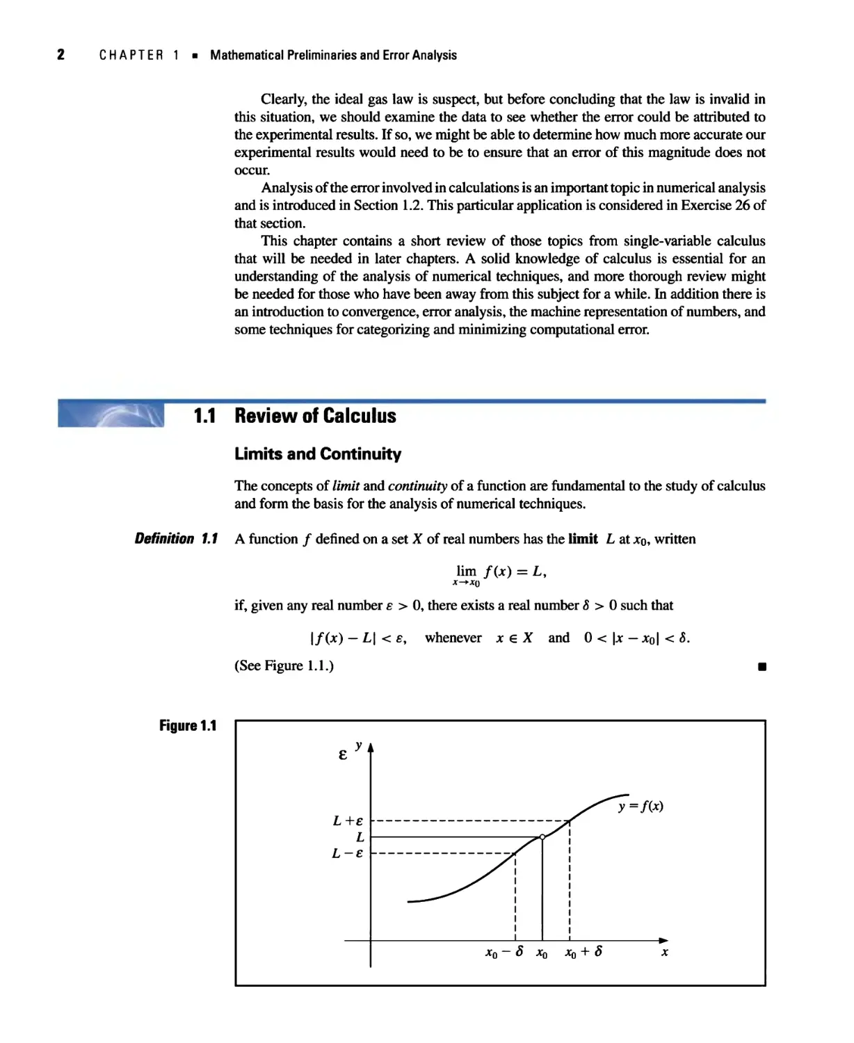
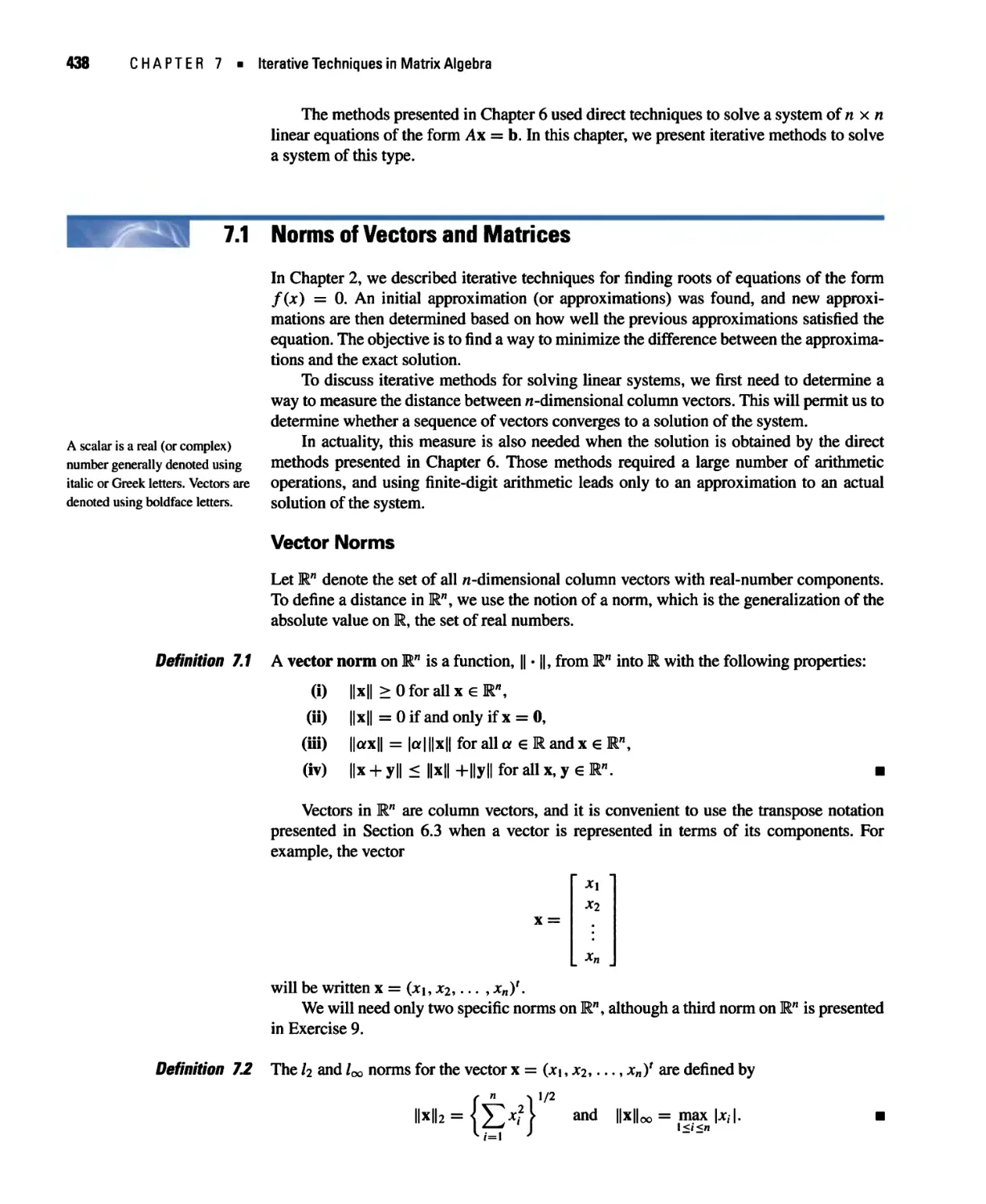
Definition 1.1 A function / defined on a set X of real numbers has the limit L at jco, written
lim f{x) = L,
if, given any real number e > 0, there exists a real number S > 0 such that
|/(jc) — L\ < e, whenever x e X and 0 < \x — jco| < &.
(See Figure 1.1.) ■
e"
L+£
L
L-e
i
x0 — S x
^^7=m
0 Xo + S x
1.1 Review of Calculus 3
Definition 1.2
The basic concepts of calculus
and its applications were
developed in the late 17th and
early 18th centuries, but the
mathematically precise concepts
of limits and continuity were not
described until the time of
Augustin Louis Cauchy
(1789-1857), Heinrich Eduard
Heine (1821-1881), and Karl
Weierstrass (1815 -1897) in the
latter portion of the 19th century.
Let / be a function defined on a set X of real numbers and jco e X. Then / is continuous
at xo if
lim f(x) = f(x0).
The function / is continuous on the set X if it is continuous at each number in X. m
The set of all functions that are continuous on the set X is denoted C(X). When X is
an interval of the real line, the parentheses in this notation are omitted. For example, the
set of all functions continuous on the closed interval [a, b] is denoted C[a,b\. The symbol
E denotes the set of all real numbers, which also has the interval notation (—oo, oo). So
the set of all functions that are continuous at every real number is denoted by C(R) or by
C(—oo, oo).
The limit of a sequence of real or complex numbers is defined in a similar manner.
Definition 1.3 Let {x^}^ be an infinite sequence of real numbers. This sequence has the limit x
(converges to x) if, for any s > 0, there exists a positive integer N(s) such that \xn — x \ < e
whenever n > N(e). The notation
lim xn = jc, or x„ —► x as n —► oo,
n-*oo
means that the sequence [xn }£ij converges to x. m
Theorem 1.4 If / is a function defined on a set X of real numbers and x0 e X, then the following
statements are equivalent:
a. / is continuous at xo;
b. If {JtnJ^j is any sequence in X converging to jcq, then lim,,-^ f(xn) = /(jcq).
The functions we will consider when discussing numerical methods will be assumed to
be continuous because this is a minimal requirement for predictable behavior. Functions that
are not continuous can skip over points of interest, which can cause difficulties in attempts
to approximate a solution to a problem.
Differentiability
More sophisticated assumptions about a function generally lead to better approximation
results. For example, a function with a smooth graph will normally behave more predictably
than one with numerous jagged features. The smoothness condition relies on the concept
of the derivative.
Definition 1.5 Let / be a function defined in an open interval containing jco. The function / is
differentiate at xo if
/ (*o) = lim
►*o
X — Xq
exists. The number f'(xo) is called the derivative of / at jco. A function that has a derivative
at each number in a set X is differentiable on X. m
The derivative of / at jco is the slope of the tangent line to the graph of / at (jco, /C*o))5
as shown in Figure 1.2.
4 CHAPTER 1 ■ Mathematical Preliminaries and Error Analysis
Figure 1.2
y t
/(*o) -
The tangent line has slope/'(;c0)
1 Ife
1 ^
Xq x
Theorem 1.6 If the function / is differentiable at jco, then / is continuous at jcq.
The theorem attributed to Michel
Rolle (1652-1719) appeared in
1691 in a little-known treatise
titled Methode pour resoundre les
egalites. Rolle originally
criticized the calculus that was
developed by Isaac Newton and
Gottfried Leibniz but later
became one of its proponents.
Theorem 17
The next theorems are of fundamental importance in deriving methods for error
estimation. The proofs of these theorems and the other unreferenced results in this section can
be found in any standard calculus text.
The set of all functions that have n continuous derivatives on X is denoted Cn (X), and
the set of functions that have derivatives of all orders on X is denoted C°°(X). Polynomial,
rational, trigonometric, exponential, and logarithmic functions are in C°°(X), where X
consists of all numbers for which the functions are defined. When X is an interval of the
real line, we will again omit the parentheses in this notation.
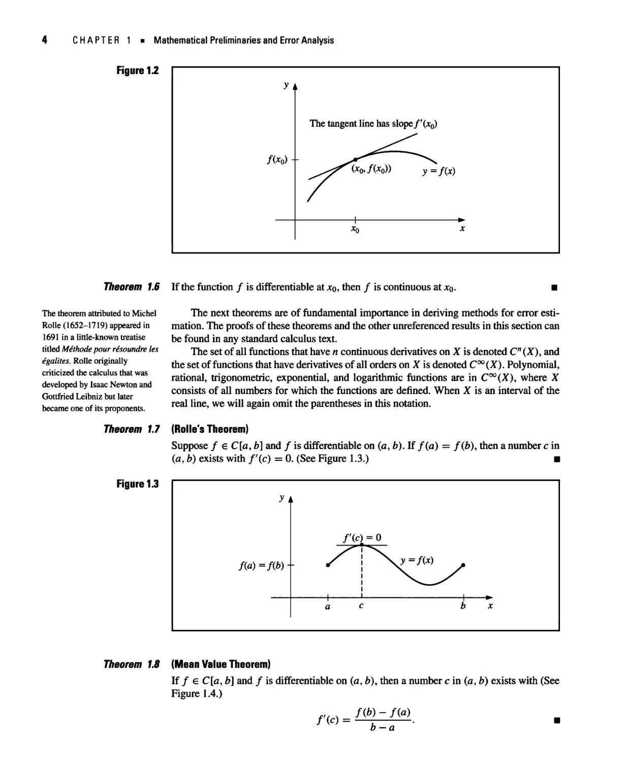
(Rolle's Theorem)
Suppose / g C[a, b] and / is differentiable on (a, b). If f(a) = /(&), then a number c in
(a, b) exists with f'{c) = 0. (See Figure 1.3.) ■
Figure 1.3
y i
f{a)=f{b)-
f'(cl=0
a c b x
Theorem 1.8 (Mean Value Theorem)
If / € C[a, b] and / is differentiable on (a, b), then a number c in (a, b) exists with (See
Figure 1.4.)
fib) - f{a)
f'(c) =
b-a
1.1 Review of Calculus
Figure 1.4
y a
Slope/'(c)
fib) -f(a)
Parallel lines
y=f(x)
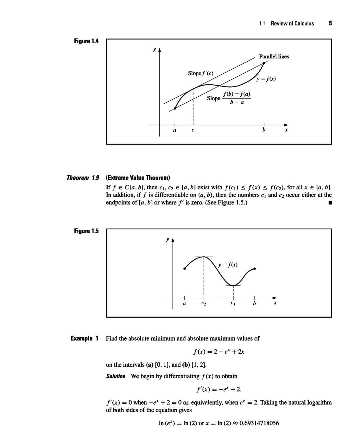
Theorem 1.9 (Extreme Value Theorem)
If / e C[a, b]9 then c\,C2 e [a, b] exist with f(c\) < f(x) < /(C2), for all x e [ay b].
In addition, if / is differentiable on (0, b)9 then the numbers c\ and C2 occur either at the
endpoints of [a, b] or where /' is zero. (See Figure 1.5.) ■
Figure 1.5
y t
i
/
—1—
a
^~r\
—1—
\y=m
1
1
—1—
b
►
X
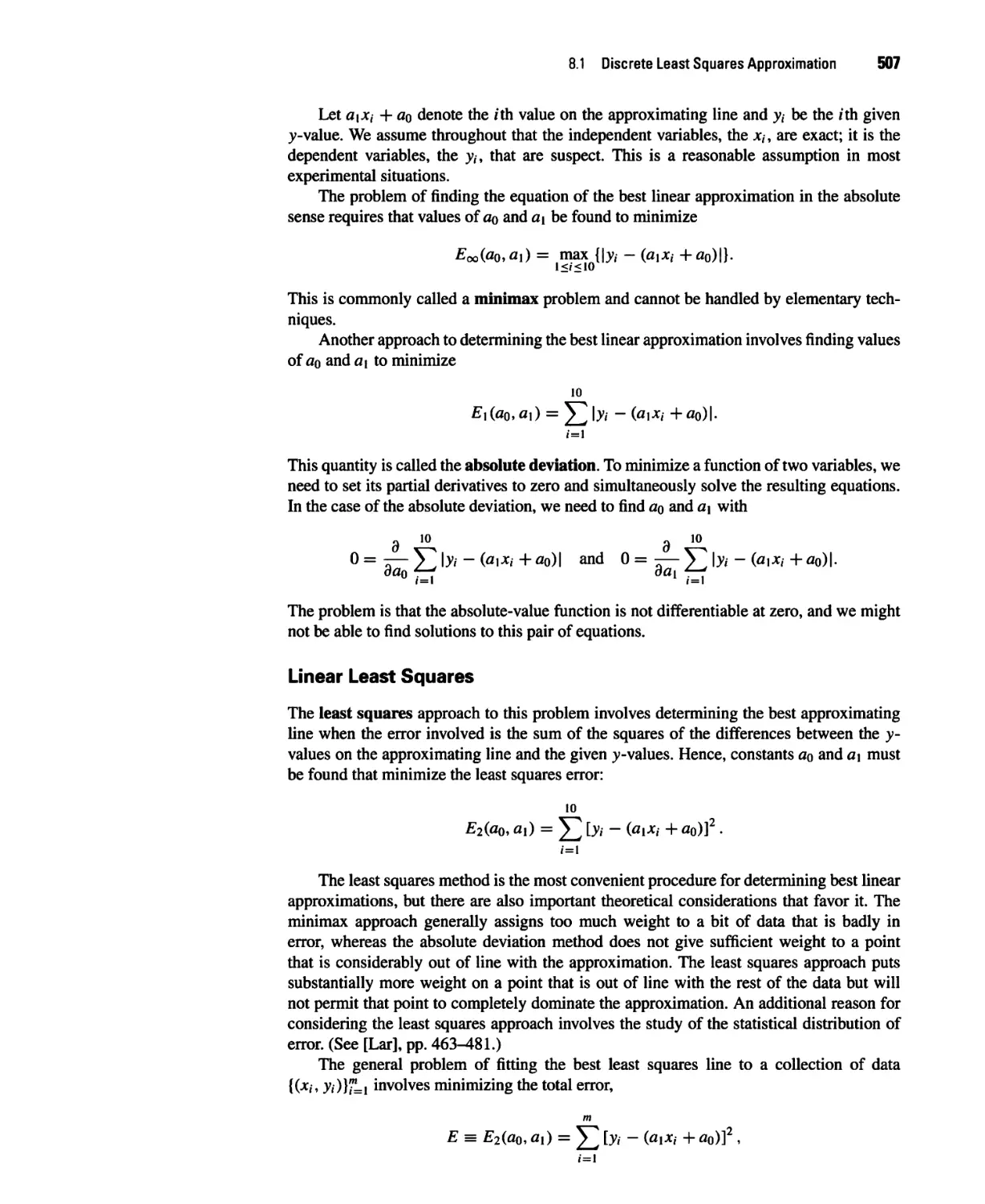
Example 1 Find the absolute minimum and absolute maximum values of
f{x) = 2 - e* + 2*
on the intervals (a) [0,1], and (b) [1,2].
Solution We begin by differentiating f(x) to obtain
f'(x) = -ex+2.
fix) = 0 when — e* + 2 = 0 or, equivalently, when e* = 2. Taking the natural logarithm
of both sides of the equation gives
In (e*) = In (2) or x = In (2) % 0.69314718056
6 CHAPTER 1 ■ Mathematical Preliminaries and Error Analysis
(a) When the interval is [0,1], the absolute extrema must occur at /(0), /(In (2)), or
/(l). Evaluating, we have
/(0) = 2-e° + 2(0) = l
/(In (2)) = 2 - e]n (2) + 2 In (2) = 2 In (2) ^ 1.38629436112
/(l) = 2 - e + 2(1) = 4 - e % 1.28171817154.
Thus, the absolute minimum of f(x) on [0,1] is /(0) = 1 and the absolute
maximum is /(In (2)) = 2In (2).
(b) When the interval is [1,2], we know that f'(x) ^ 0 so the absolute extrema occur
at /(l) and /(2). Thus, /(2) = 2 - e2 + 2(2) = 6 - e2 * -1.3890560983. The
absolute minimum on [1, 2] is 6 — e2 and the absolute maximum is 1.
We note that
max |/(jc)| = |6 - e2\ ^ 1.3890560983. ■
0<jc<2
The following theorem is not generally presented in a basic calculus course but is
derived by applying Rolle's Theorem successively to /, /',..., and, finally, to fin~]).
This result is considered in Exercise 26.
Theorem 1.10 (Generalized Rolle's Theorem)
Suppose / g C[a, b] is n times differentiable on (a, b). If f(x) = 0 at the n + 1 distinct
numbers a < xq < x\ < ... < xn < b, then a number c in (jto, xn) and hence in (a, b)
exists with /(n) (c) = 0. ■
We will also make frequent use of the Intermediate Value Theorem. Although its
statement seems reasonable, its proof is beyond the scope of the usual calculus course. It
can, however, be found in most analysis texts (see, for example, [Fu], p. 67).
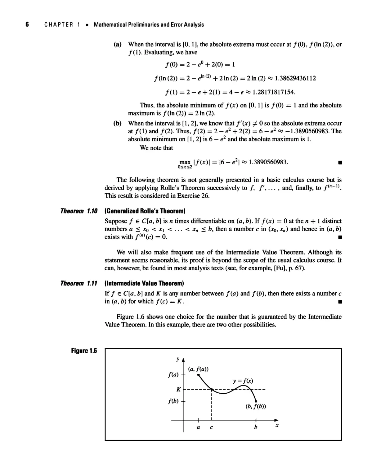
Theorem 1.11 (Intermediate Value Theorem)
If / G C[a, b] and K is any number between f(a) and f(b), then there exists a number c
in (a, b) for which f(c) = K. m
Figure 1.6 shows one choice for the number that is guaranteed by the Intermediate
Value Theorem. In this example, there are two other possibilities.
Figure 1.6
y t
/(«) -
K
fib) -
V
ia,fia))
\ y =fix)
\ ibJib))
1 ' 1 fe.
a c b x
1.1 Review of Calculus 7
Example 2 Show that jc5 - 2jc3 + 3x2 - 1 = 0 has a solution in the interval [0,1].
Solution Consider the function defined by /(jc) = jc5 — 2jc3 + 3jc2 — 1. The function / is
continuous on [0,1]. In addition,
/(0) = -1 < 0 and 0 < 1 = /(l).
Hence, the Intermediate Value Theorem implies that a number c exists, with 0 < c < 1, for
which c5 - 2c3 + 3c2 - 1 = 0. ■
As seen in Example 2, the Intermediate Value Theorem is used to determine when
solutions to certain problems exist. It does not, however, give an efficient means for finding
these solutions. This topic is considered in Chapter 2.
Integration
The other basic concept of calculus that will be used extensively is the Riemann integral.
Definition 1.12
George Fredrich Berhard
Riemann (1826-1866) made
many of the important
discoveries classifying the
functions that have integrals. He
also did fundamental work in
geometry and complex function
theory and is regarded as one of
the profound mathematicians of
the 19th century.
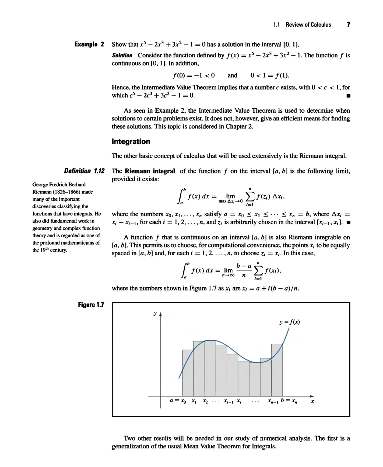
The Riemann integral of the function / on the interval [a, b] is the following limit,
provided it exists:
pb n
/ f(x) dx = lim V* f(zi) Ax,-,
Ja t |=1
where the numbers jc0, jci ,..., jc„ satisfy a = xo < x\ < • • • < xn = b, where Ajc, =
xi — Jt,_i, for each i = 19 29..., n, and zi is arbitrarily chosen in the interval [jc,_i , jc,]. ■
A function / that is continuous on an interval [a, b] is also Riemann integrable on
[a, b]. This permits us to choose, for computational convenience, the points jc, to be equally
spaced in [a, b] and, for each i = 1,2,..., n, to choose z, = jc,. In this case,
Ja
b b — an
f(x) dx = lim —— ^2 /(*■").
n->oo ft
1=1
where the numbers shown in Figure 1.7 as jc,- are x,- =a + i(b — a)/n.
Figure 1.7
y i
i
y
=/(*)
a = xQ x} *2 ... x,_, Xj ... x„_, b = x„ x
Two other results will be needed in our study of numerical analysis. The first is a
generalization of the usual Mean Value Theorem for Integrals.
8 CHAPTER 1 ■ Mathematical Preliminaries and Error Analysis
Theorem 1.13 (Weighted Mean Value Theorem for Integrals)
Suppose / G C[a, b], the Riemann integral of g exists on [a, b], and g(x) does not change
sign on [a, b\. Then there exists a number c in {a, b) with
pb pb
I f(x)g(x) dx = /(c) / g(x) dx. u
Ja Ja
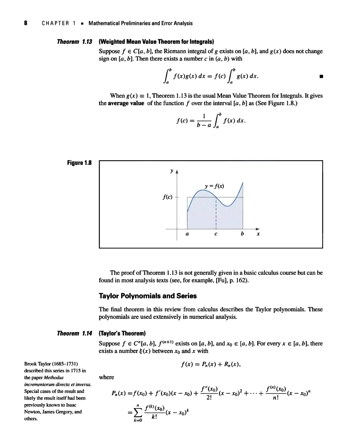
When g(x) = 1, Theorem 1.13 is the usual Mean Value Theorem for Integrals. It gives
the average value of the function / over the interval [a, b] as (See Figure 1.8.)
f(c)
1 fb
~ b-aja
f(x) dx.
Figure 1.8
y i
m -
i
y=f(x) I
a c b x
The proof of Theorem 1.13 is not generally given in a basic calculus course but can be
found in most analysis texts (see, for example, [Fu], p. 162).
Taylor Polynomials and Series
The final theorem in this review from calculus describes the Taylor polynomials. These
polynomials are used extensively in numerical analysis.
Theorem 1.14 (Taylor's Theorem)
Suppose / g Cn[a, b], /(n+1) exists on [a, b], and jc0 e [a, b\. For every jc g [a, b]9 there
exists a number £(x) between x0 and jc with
Brook Taylor (1685-1731)
described this series in 1715 in
the paper Methodus
incrementorum directa et inverse.
Special cases of the result and
likely the result itself had been
previously known to Isaac
Newton, James Gregory, and
others.
f(x) = Pn(x) + Rn(x),
where
Pn(x) =/(*o) + f(x0)(x - X0) +
/"(*o)
2!
(jc - xq)2 + ■ ■ • +
fw(xo)
n\
(x - x0y
1.1 Review of Calculus 9
Colin Maclaurin (1698-1746) is
best known as the defender of the
calculus ofNewton when it came
under bitter attack by Irish
philosopher Bishop George
Berkeley.
Maclaurin did not discover the
series that bears his name; it was
known to century mathematicians
before he was born. However, he
did devise a method for solving a
system of linear equations that is
known as Cramer's rule, which
Cramer did not publish until
1750.
and
(n + 1)!
Here Pn(x) is called the nth Taylor polynomial for / about jco, and R„(x) is called
the remainder term (or truncation error) associated with Pn(x). Since the number £(jc)
in the truncation error Rn(x) depends on the value of jc at which the polynomial Pn(x) is
being evaluated, it is a function of the variable jc. However, we should not expect to be
able to explicitly determine the function £(jc). Taylor's Theorem simply ensures that such a
function exists and that its value lies between x and jco. In fact, one of the common problems
in numerical methods is to try to determine a realistic bound for the value of /(w+1)(£(*))
when x is in some specified interval
The infinite series obtained by taking the limit of Pn (jc) as n -► oo is called the Taylor
series for / about jco- In the case jco = 0, the Taylor polynomial is often called a Maclaurin
polynomial, and the Taylor series is often called a Maclaurin series.
The term truncation error in the Taylor polynomial refers to the error involved in
using a truncated, or finite, summation to approximate the sum of an infinite series.
Example 3 Let /(jc) = cos x and jco = 0. Determine
(a) the second Taylor polynomial for / about jc0; and
(b) the third Taylor polynomial for / about jco.
Solution Since / e C°°(R), Taylor's Theorem can be applied for any n > 0. Also,
/'(jc) = — sinjc, /"(jc) = — cosjc, /'"(jc) = sinjc, and /(4)(jc) = cosjc,
so
/(0) = 1, /'(0) = 0, /"(0) = -1, and /"'(0) = 0.
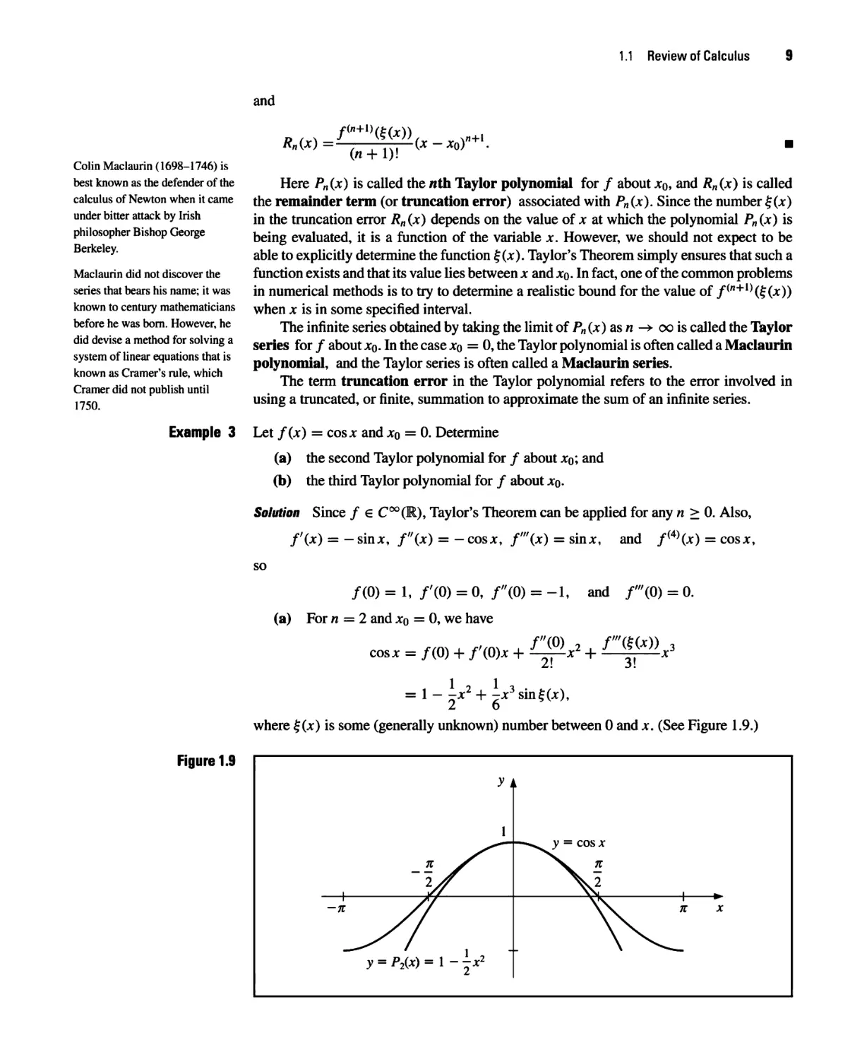
(a) For n = 2 and jc0 = 0, we have
cos* = /(0) + / (0)x H ^—jr H x*
2!
1 i 1 i
= 1 - -* + -x sin£(x),
2 6
3!
where %(x) is some (generally unknown) number between 0 and jc. (See Figure 1.9.)
Figure 1.9
y = P2(X)=l--X*
Mathematical Preliminaries and Error Analysis
When jc = 0.01, this becomes
cosO.01 = 1 - i(0.01)2 + ^(O.Ol)3sin£(0.01) = 0.99995 + ^— sin£(0.01).
2 6 6
The approximation to cos 0.01 given by the Taylor polynomial is therefore 0.99995. The
truncation error, or remainder term, associated with this approximation is
10"6 - ,
—- sin£(0.01) = 0.16 x 10"6sin£(0.01),
6
where the bar over the 6 in 0.16 is used to indicate that this digit repeats indefinitely.
Although we have no way of determining sin £(0.01), we know that all values of the sine
lie in the interval [—1, 1], so the error occurring if we use the approximation 0.99995 for
the value of cos 0.01 is bounded by
| cos(0.01)-0.999951 =0.16 x 10~6|sin£(0.01)| <0.16x 10~6.
Hence, the approximation 0.99995 matches at least the first five digits of cos 0.01, and
0.9999483 < 0.99995 - 1.6 x 10"6 < cos 0.01
< 0.99995 + 1.6 x 10~6 < 0.9999517.
The error bound is much larger than the actual error. This is due in part to the poor
bound we used for | sin £(jc)|. It is shown in Exercise 27 that for all values of jc, we have
| shuc| < |jc|. Since 0 < £ < 0.01, we could have used the fact that | sin£(jc)| < 0.01 in
the error formula, producing the bound 0.16 x 10~8.
(b) Since /'"(0) = 0, the third Taylor polynomial with remainder term about
jco = 0 is
cosjc = 1 — -jc + —jc cos£(jc),
2 24
where 0 < f (jc) < 0.01. The approximating polynomial remains the same, and the
approximation is still 0.99995, but we now have much better accuracy assurance. Since
| cos f (jc)| < 1 for all jc, we have
—*4cosf(x)
< -5-(0-01)4(l)^4.2x 10"10.
- 24
So,
| cos 0.01 - 0.99995| < 4.2 x 10"10,
and
0.99994999958 = 0.99995 - 4.2 x 10"10
< cos 0.01 < 0.99995 + 4.2 x 10"10 = 0.99995000042. ■
Example 3 illustrates the two objectives of numerical analysis:
(i) Find an approximation to the solution of a given problem.
(ii) Determine a bound for the accuracy of the approximation.
The Taylor polynomials in both parts provide the same answer to (i), but the third Taylor
polynomial gave a much better answer to (ii) than the second Taylor polynomial.
We can also use the Taylor polynomials to give us approximations to integrals.
1.1 Review of Calculus 11
Illustration We can use the third Taylor polynomial and its remainder term found in Example 3 to
approximate J0' cos x dx. We have
/ cos* dx = I I 1 — -x2 J dx + — I *4cosf (*) dx
r l ]01 l /-0-1
= be — -x3\ +— / x4cos%(x)dx
L 6 J 0 24 J0
24 J0
1 1 f01
= 0.1 - t(0.1)3 + — / x4cos£U) dx.
Therefore,
7
cosjc dx % 0.1 - ^r(O.l)3 = 0.09983.
6
A bound for the error in this approximation is determined from the integral of the Taylor
remainder term and the fact that | cos f (jc) | < 1 for all jc :
1 I f0A ~ I 1 f0A
—-\ / jc4cos|(jc) dx\ < —r / x4\cos£(x)\dx
24\J0 I ~ 24 y0
~24 J0
a,*4rfjc=(?_l)! = 83xl0-8
120
The true value of this integral is
/
Jo
0.1 lO.l
cosjc dx = sinjc
= sin 0.1 ^ 0.099833416647,
Jo
so the actual error for this approximation is 8.3314 x 10 8, which is within the error
bound. ■
EXERCISE SET 1.1
1. Show that the following equations have at least one solution in the given intervals.
a. xcosx - 2x2 + 3jc - 1 = 0, [0.2,0.31 and fl.2,1.3]
b. (jc - 2)2 - In jc = 0, [1,2] and [e, 4]
c. 2jc cos(2jc) - (jc - 2)2 = 0, [2, 3] and [3,4]
d. jc-(lnjc)x = 0, [4,5]
2. Show that the following equations have at least one solution in the given intervals.
a. yfx — cosjc = 0, [0,1]
b. ex - x2 + 3jc - 2 = 0, [0, H
c. -3 tan(2jc) + jc = 0, [0,1]
d. lnjc-jc2+|jc-l=0, [i, l]
3. Find intervals containing solutions to the following equations.
a. jc - 2~x = 0
b. 2jc cos(2jc) - (jc + I)2 = 0
c. 3jc - e* = 0
d. jc+ 1 -2sin(7rjc) = 0
Mathematical Preliminaries and Error Analysis
Find intervals containing solutions to the following equations.
a. x - 3~x = 0
b. 4jc2 - e" = 0
c. jc3 - 2jc2 - Ax + 2 = 0
d. x3 + 4.001*2 + 4.002* + 1.101 =0
Find maxa<j<j, \f(x)\ for the following functions and intervals.
a. f(x) = (2-e* + 2x)/3, [0,1]
b. fix) = {Ax - 3)/(x2 - 2x), [0.5,1]
c. f(x) = 2x cos(2jc) - (jc - 2)2, [2,4]
d. f{x) = ]+e-cosix-1), [1,2]
Find maxa<x<b 1/001 for the following functions and intervals.
a. fix) = 2jc/(jc2 + 1), [0, 2]
b. /(jc) = jcV(4-jc), [0,4]
c. fix) = jc3- Ax + 2, [1,2]
d. /(jc) = jcV(3-jc2), [0,11
Show that f'{x) is 0 at least once in the given intervals.
a. fix) =l-ex + {e-\) sin((;r/2)jc), [0, 1]
b. f{x) = {x — 1) tan jc + jc sin jtjc, [0,1]
c. f{x) = x sin itx — {x — 2) In jc, [1, 2]
d. fix) = (jc - 2) sin jc ln(jc + 2), [-1,3]
Suppose / € C[a, b] and /'(jc) exists on (a, b). Show that if /'(jc) ^ 0 for all jc in (a, 6), then there
can exist at most one number pin [a, b] with f{p) = 0.
Let fix) = jc3.
a. Find the second Taylor polynomial P2OO about jco = 0.
b. Find /?2(0.5) and the actual error in using PziQ.5) to approximate /(0.5).
c Repeat part (a) using jco = 1.
d. Repeat part (b) using the polynomial from part (c).
Find the third Taylor polynomial P3OO for the function /(jc) = y/x + 1 about jc0 = 0. Approximate
V05, V0?75, VT25, and Vh5 using P$(x) and find the actual errors.
Find the second Taylor polynomial Pj{x) for the function f(x) = e* cos jc about xq = 0.
a. Use P2(0.5) to approximate /(0.5). Find an upper bound for error |/(0.5) — P2(0.5)| using the
error formula and compare it to the actual error.
b. Find a bound for the error |/(jc) — P2OOI in using P2OO to approximate /(jc) on the interval
[0, 11.
c. Approximate J0 f{x) dx using J0 Pi{x) dx.
d. Find an upper bound for the error in (c) using J0 | /?2(*) dx \ and compare the bound to the actual
error.
Repeat Exercise 11 using xo = jt/6.
Find the third Taylor polynomial P$(x) for the function f(x) = (x — 1) Inx about xq = 1.
a. Use ^3(0.5) to approximate /(0.5). Find an upper bound for error |/(0.5) — P3(0.5)| using the
error formula and compare it to the actual error.
b. Find a bound for the error |/(jc) — Pi(x)\ in using P3&) to approximate f(x) on the interval
[0.5, 1.5].
c. Approximate f0'5 f(x)dx using J05 P^(x) dx.
d. Find an upper bound for the error in (c) using J05 \R?>(x) dx\ and compare the bound to the
actual error.
Let /(jc) = 2jc cos(2x) - (jc - 2)2 and jc0 = 0.
a. Find the third Taylor polynomial P$(x) and use it to approximate /(0.4).
1.1 Review of Calculus 13
b. Use the error formula in Taylor's Theorem to find an upper bound for the error |/(0.4) — P3(0.4)|.
Compute the actual error.
c. Find the fourth Taylor polynomial P*(x) and use it to approximate /(0.4).
d. Use the error formula in Taylor's Theorem to find an upper bound for the error | /(0.4) — ^4(0.4) |.
Compute the actual error.
15. Find the fourth Taylor polynomial P4C*) for the function /(jc) = xe* about jco = 0.
a. Find an upper bound for |/(jc) — Pa{x)\9 for 0 < x < 0.4.
b. Approximate J0' f{x) dx using J0' P*{x) dx.
c. Find an upper bound for the error in (b) using JQ' P*{x) dx.
d. Approximate /'(0.2) using ^4(0.2) and find the error.
16. Use the error term of a Taylor polynomial to estimate the error involved in using sin jc ^ x to
approximate sin 1°.
17. Use a Taylor polynomial about 7r/4 to approximate cos 42° to an accuracy of 10~6.
18. Let /(jc) = (1 — jc)"1 and jco = 0. Find the nth Taylor polynomial P„(jc) for /(jc) about xq. Find a
value of n necessary for Pn{x) to approximate /(jc) to within 10"6 on [0,0.5].
19. Let /(jc) = ex and jco = 0. Find the nth Taylor polynomial P„(jc) for /(jc) about jco. Find a value of
n necessary for Pn(x) to approximate fix) to within 10~6 on [0,0.5].
20. Find the nth Maclaurin polynomial Pn(x) for /(jc) = arctan jc.
21. The polynomial P2U) = 1 —jjc2 is to be used to approximate/(jc) = cosjcin[— 5, ^]. Findabound
for the maximum error.
22. Use the Intermediate Value Theorem 1.11 and Rolle's Theorem 1.7 to show that the graph of /(jc) =
jc3 + 2jc + k crosses the x-axis exactly once, regardless of the value of the constant k.
23. A Maclaurin polynomial for ex is used to give the approximation 2.5 to e. The error bound in this
approximation is established to be E = £. Find a bound for the error in E.
24. The error function defined by
2 fx
\fit Jo
erf(jc) = —= I e~t2 dt
gives the probability that any one of a series of trials will lie within x units of the mean, assuming that
the trials have a normal distribution with mean 0 and standard deviation >/2/2. This integral cannot
be evaluated in terms of elementary functions, so an approximating technique must be used.
2
a. Integrate the Maclaurin series for e x to show that
b. The error function can also be expressed in the form
2 , A 2kx7k+l
erfW=VT gl-3S...(2*+1)
*=0
Verify that the two series agree for k = 1, 2,3, and 4. [Hint: Use the Maclaurin series for e~x .]
c. Use the series in part (a) to approximate erf(l) to within 10~7.
d. Use the same number of terms as in part (c) to approximate erf(l) with the series in part (b).
e. Explain why difficulties occur using the series in part (b) to approximate erf(jc).
THEORETICAL EXERCISES
25. The nth Taylor polynomial for a function / at jcq is sometimes referred to as the polynomial of degree
at most n that "best" approximates / near jco.
a. Explain why this description is accurate.
■ Mathematical Preliminaries and Error Analysis
b. Find the quadratic polynomial that best approximates a function / near jco = 1 if the tangent
line at jco = 1 has equation y = Ax — 1 and if /"(l) = 6.
26. Prove the Generalized Rolle's Theorem, Theorem 1.10, by verifying the following.
a. Use Rolle's Theorem to show that /'(z,-) = 0 for n — 1 numbers in [a, b] with a < z\ < z2 <
• • • < zn-\ < b.
b. Use Rolle's Theorem to show that /"(w/) = 0 for n — 2 numbers in [a, b] with z\ <w\ < z2 <
w2 • • • w„_2 < Zn-\ < b.
c. Continue the arguments in parts (a) and (b) to show that for each 7 = l,2,...,n — 1, there are
n — j distinct numbers in [a, b]9 where /(y) is 0.
d. Show that part (c) implies the conclusion of the theorem.
27. Example 3 stated that for all x we have | sin jc | < |jc|. Use the following to verify this statement.
a. Show that for all x > 0, f(x) = x — sin x is nondecreasing, which implies that sin x < x with
equality only when x = 0.
b. Use the fact that the sine function is odd to reach the conclusion.
28. A function / : [a, b] -> R is said to satisfy a Lipschitz condition with Lipschitz constant L on [a, b]
if, for every x,y e [a, b], we have \f(x) - f{y)\ < L\x - y\.
a. Show that if / satisfies a Lipschitz condition with Lipschitz constant L on an interval [a, b]y
then/ 6 C[a,b].
b. Show that if / has a derivative that is bounded on [a,b] by L, then / satisfies a Lipschitz
condition with Lipschitz constant L on [a, b].
c. Give an example of a function that is continuous on a closed interval but does not satisfy a
Lipschitz condition on the interval.
29. Suppose / e C[a, b] and jci and x2 are in [a, b].
a. Show that a number f exists between x\ and x2 with
/(£) = j = 2^(jri) 2^ 2)*
b. Suppose ci and c2 are positive constants. Show that a number £ exists between x\ and *2 with
-ffv = ci/(*i)+ ca/(s2)
ci + c2
c. Give an example to show that the result in part (b) does not necessarily hold when c\ and c2 have
opposite signs with c\ ^ — c2.
30. Let / € C[a, b]9 and let p be in the open interval (a, b).
a. Suppose /(/?) ^ 0. Show that a S > 0 exists with /(*) ^ 0, for all x in[p — 8, p + S]9 with
[p — 5, p + 5] a subset of [a, b].
b. Suppose /(/?) = 0 and k > 0 is given. Show that a 5 > 0 exists with \f(x)\ < k, for all jc in
[p — 5, p + 5], with [p — 5, /? + 5] a subset of [a, fc].
DISCUSSION QUESTION
1. In your own words, describe the Lipschitz condition. Give several examples of functions that satisfy
this condition or give several examples of functions that do not satisfy this condition.
1.2 Round-off Errors and Computer Arithmetic
The arithmetic performed by a calculator or computer is different from the arithmetic in
algebra and calculus courses. You would likely expect that we always have as true statements
things such as 2+2 = 4,4 • 8 = 32, and (s/3)2 = 3. However, with computer arithmetic, we
1.2 Round-off Errors and Computer Arithmetic 15
Error due to rounding should be
expected whenever computations
are performed using numbers that
are not powers of 2. Keeping this
error under control is extremely
important when the number of
calculations is large.
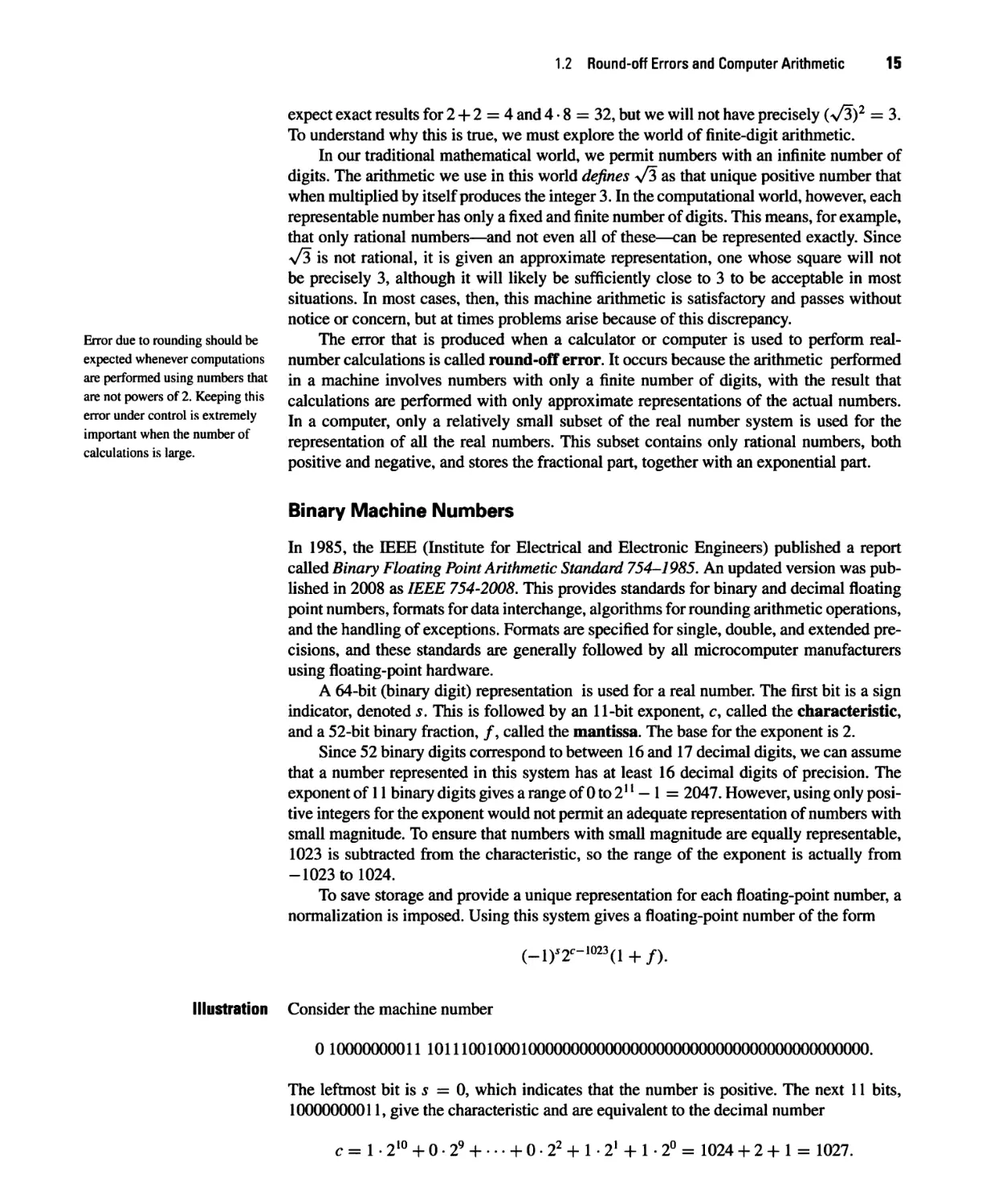
expect exact results for 2 + 2 = 4 and 4 • 8 = 32, but we will not have precisely (v^3)2 = 3.
To understand why this is true, we must explore the world of finite-digit arithmetic.
In our traditional mathematical world, we permit numbers with an infinite number of
digits. The arithmetic we use in this world defines >/3 as that unique positive number that
when multiplied by itself produces the integer 3. In the computational world, however, each
representable number has only a fixed and finite number of digits. This means, for example,
that only rational numbers—and not even all of these—can be represented exactly. Since
a/3 is not rational, it is given an approximate representation, one whose square will not
be precisely 3, although it will likely be sufficiently close to 3 to be acceptable in most
situations. In most cases, then, this machine arithmetic is satisfactory and passes without
notice or concern, but at times problems arise because of this discrepancy.
The error that is produced when a calculator or computer is used to perform real-
number calculations is called round-off error. It occurs because the arithmetic performed
in a machine involves numbers with only a finite number of digits, with the result that
calculations are performed with only approximate representations of the actual numbers.
In a computer, only a relatively small subset of the real number system is used for the
representation of all the real numbers. This subset contains only rational numbers, both
positive and negative, and stores the fractional part, together with an exponential part.
Binary Machine Numbers
In 1985, the IEEE (Institute for Electrical and Electronic Engineers) published a report
called Binary Floating Point Arithmetic Standard 754-1985. An updated version was
published in 2008 as IEEE 754-2008. This provides standards for binary and decimal floating
point numbers, formats for data interchange, algorithms for rounding arithmetic operations,
and the handling of exceptions. Formats are specified for single, double, and extended
precisions, and these standards are generally followed by all microcomputer manufacturers
using floating-point hardware.
A 64-bit (binary digit) representation is used for a real number. The first bit is a sign
indicator, denoted s. This is followed by an 11-bit exponent, c, called the characteristic,
and a 52-bit binary fraction, /, called the mantissa. The base for the exponent is 2.
Since 52 binary digits correspond to between 16 and 17 decimal digits, we can assume
that a number represented in this system has at least 16 decimal digits of precision. The
exponent of 11 binary digits gives a range of 0 to 211 — 1 = 2047. However, using only
positive integers for the exponent would not permit an adequate representation of numbers with
small magnitude. To ensure that numbers with small magnitude are equally representable,
1023 is subtracted from the characteristic, so the range of the exponent is actually from
-1023 to 1024.
To save storage and provide a unique representation for each floating-point number, a
normalization is imposed. Using this system gives a floating-point number of the form
vsoc-1023
(-1)52C~1UZJ(1 + /).
Illustration Consider the machine number
0 10000000011 1011100100010000000000000000000000000000000000000000.
The leftmost bit is s = 0, which indicates that the number is positive. The next 11 bits,
10000000011, give the characteristic and are equivalent to the decimal number
c = 1 • 210 + 0 • 29 + ... + 0 • 22 + 1 • 21 + 1 ■ 2° = 1024 + 2 + 1 = 1027.
Mathematical Preliminaries and Error Analysis
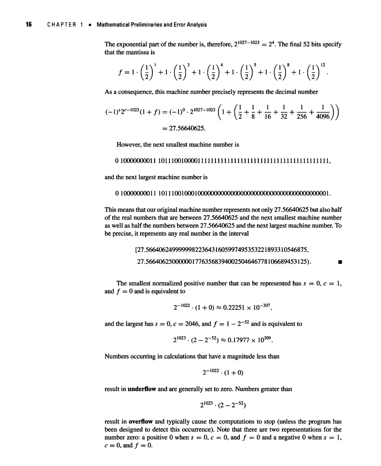
The exponential part of the number is, therefore, 21027 1023 = 24. The final 52 bits specify
that the mantissa is
'-G)'-G)'-(i)'"G)'-©"'"(!)"
As a consequence, this machine number precisely represents the decimal number
(-iyr-im(i + /) = (-i)° ■ 21027-1023 (i + (I + I + ± + ± + -L + J—))
v ' v J) v ; V \2 8 16 32 256 4096/)
= 27.56640625.
However, the next smallest machine number is
010000000011 1011100100001111111111111111111111111111111111111111,
and the next largest machine number is
0 10000000011 101110010001000000000000000000000000000000^
This means that our original machine number represents not only 27.56640625 but also half
of the real numbers that are between 27.56640625 and the next smallest machine number
as well as half the numbers between 27.56640625 and the next largest machine number. To
be precise, it represents any real number in the interval
[27.5664062499999982236431605997495353221893310546875,
27.5664062500000017763568394002504646778106689453125). ■
The smallest normalized positive number that can be represented has s = 0, c = 1,
and / = 0 and is equivalent to
2"1022 • (1 + 0) * 0.22251 x 10"307,
and the largest has s = 0, c = 2046, and / = 1 — 2"52 and is equivalent to
21023 . (2 _ 2-52) % QJ7977 x 1Q309
Numbers occurring in calculations that have a magnitude less than
2-1022. (1+Q)
result in underflow and are generally set to zero. Numbers greater than
21023 . (2 _ 2-52j
result in overflow and typically cause the computations to stop (unless the program has
been designed to detect this occurrence). Note that there are two representations for the
number zero: a positive 0 when s = 0, c = 0, and / = 0 and a negative 0 when s = l9
c = 0, and / = 0.
1.2 Round-off Errors and Computer Arithmetic 17
The error that results from
replacing a number with its
floating-point form is called
round-off error regardless of
whether the rounding or the
chopping method is used.
Decimal Machine Numbers
The use of binary digits tends to conceal the computational difficulties that occur when a
finite collection of machine numbers is used to represent all the real numbers. To examine
these problems, we will use more familiar decimal numbers instead of binary representation.
Specifically, we assume that machine numbers are represented in the normalized decimal
floating-point form
±0.^2 . •. dk x 10", 1 < dx < 9, and 0 < d{ < 9,
for each i = 2,... , k. Numbers of this form are called fc-digit decimal machine numbers.
Any positive real number within the numerical range of the machine can be normalized
to the form
y = 0.dxd2 •.. dkdk+xdk+2 ... x 10".
The floating-point form of y, denoted //()>), is obtained by terminating the mantissa of
y at k decimal digits. There are two common ways of performing this termination. One
method, called chopping, is to simply chop off the digits dk+\dk+i This produces the
floating-point form
fl(y) = 0.d\d2...dk x 10\
The other method, called rounding, adds 5 x 10""(*+1) to y and then chops the result to
obtain a number of the form
fl(y) = 0.<5,52.. Skx 10*.
For rounding, when <4+i > 5, we add 1 to dk to obtain fl(y)\ that is, we round up. When
<4+i < 5, we simply chop off all but the first k digits; that is, round down. If we round
down, then 6/ = dx, for each i = 1, 2,... , k. However, if we round up, the digits (and even
the exponent) might change.
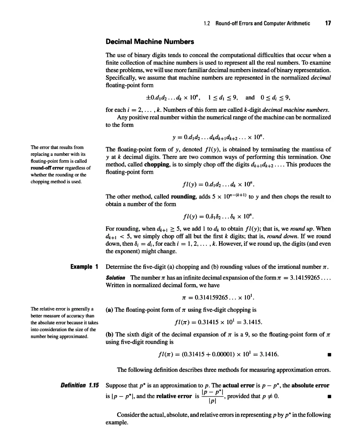
Example 1 Determine the five-digit (a) chopping and (b) rounding values of the irrational number it.
Solution The number n has an infinite decimal expansion of the form n = 3.14159265 ...
Written in normalized decimal form, we have
The relative error is generally a
better measure of accuracy than
the absolute error because it takes
into consideration the size of the
number being approximated.
n =0.314159265... x 101.
(a) The floating-point form of n using five-digit chopping is
fHjt) = 0.31415 x 10l = 3.1415.
(b) The sixth digit of the decimal expansion of n is a 9, so the floating-point form of it
using five-digit rounding is
fl(n) = (0.31415 + 0.00001) x 101 = 3.1416. ■
The following definition describes three methods for measuring approximation errors.
Definition 1.15 Suppose that /?* is an approximation to p. The actual error is p — /?*, the absolute error
\p — P*\
is \p — p*|, and the relative error is —■ , provided that p^0. ■
\P\
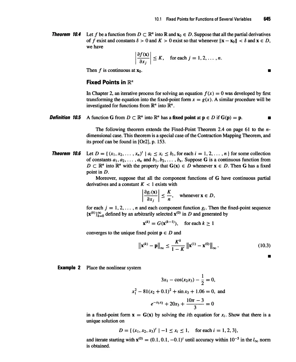
Consider the actual, absolute, and relative errors in representing p by /?* in the following
example.
18 CHAPTER 1 ■ Mathematical Preliminaries and Error Analysis
Example 2 Determine the actual, absolute, and relative errors when approximating p by p* when
(a) p = 0.3000 x 101 and p* = 0.3100 x 101;
(b) p = 0.3000 x 10"3 and p* = 0.3100 x 10"3;
(c) p = 0.3000 x 10⁴ and p* = 0.3100 x 10⁴.
We often cannot find an accurate
value for the true error in an
approximation. Instead, we find a
bound for the error, which gives
us a "worst-case" error.
Solution
(a) For p = 0.3000 x 101 and /?* = 0.3100 x lO^the actual error is -0.1, the
absolute error is 0.1, and the relative error is 0.3333 x 10"1.
(b) For/? = 0.3000x 10"3 and/?* = 0.3100x 10"3, the actual error is-0.1 x 10"4,
the absolute error is 0.1 x 10~4, and the relative error is 0.3333 x 10"1.
(c) For p = 0.3000 x 10⁴ and p* = 0.3100 x 10⁴, the actual error is -0.1 x 10³,
the absolute error is 0.1 x 10³, and the relative error is again 0.3333 x 10"1.
This example shows that the same relative error, 0.3333 x 10"1, occurs for widely varying
absolute errors. As a measure of accuracy, the absolute error can be misleading and the
relative error more meaningful because the relative error takes into consideration the size
of the value. ■
An error bound is a nonnegative number larger than the absolute error. It is sometimes
obtained by the methods of calculus for finding the maximum absolute value of a function.
We hope to find the smallest possible upper bound for the error to obtain an estimate of the
actual error that is as accurate as possible.
The following definition uses relative error to give a measure of significant digits of
accuracy for an approximation.
Definition 1.16 The number p* is said to approximate p to t significant digits (or figures) if t is the largest
The term significant digits is
often used to loosely describe the
number of decimal digits that
appear to be accurate. The
definition is more precise, and
provides a continuous concept.
nonnegative integer for which
\P\
<5x 10-'.
Table 1.1 illustrates the continuous nature of significant digits by listing, for the various
values of /?, the least upper bound of \p — p* |, denoted max \p — p* |, when p* agrees with
p to four significant digits.
Table 1.1
p
max \p — p*\
0.1
0.00005
0.5
0.00025
100
0.05
1000
0.5
5000
2.5
9990
4.995
10000
5.
Returning to the machine representation of numbers, we see that the floating-point
representation fl{y) for the number y has the relative error
y - /'GO
If/: decimal digits and chopping are used for the machine representation of
y = 0.d\d2... dfcdk+i... x 10",
1.2 Round-off Errors and Computer Arithmetic 19
then
y - //(y)
0.d\d2...dkdk+i ... x 10"- O.d^... dk x 10"
0.d\d2
ojk+ldk+2...xi(yt-lc
0.did2... x 10"
x 10"
O.dk+idk+2
0.dtd2
x 10
-k
Since d\ ^ 0, the minimal value of the denominator is 0.1. The numerator is bounded above
by 1. As a consequence,
y - fiiy)
< -Lxio-* = io-*+1.
" 0.1
In a similar manner, a bound for the relative error when using fc-digit rounding arithmetic
is 0.5 x 10"*+1. (See Exercise 28.)
Note that the bounds for the relative error using fc-digit arithmetic are independent of the
number being represented. This result is due to the manner in which the machine numbers
are distributed along the real line. Because of the exponential form of the characteristic,
the same number of decimal machine numbers is used to represent each of the intervals
[0.1, 1], [1, 10], and [10, 100]. In fact, within the limits of the machine, the number of
decimal machine numbers in [10", 10/l+1] is constant for all integers n.
Finite-Digit Arithmetic
In addition to inaccurate representation of numbers, the arithmetic performed in a computer
is not exact. The arithmetic involves manipulating binary digits by various shifting, or
logical, operations. Since the actual mechanics of these operations are not pertinent to this
presentation, we shall devise our own approximation to computer arithmetic. Although our
arithmetic will not give the exact picture, it suffices to explain the problems that occur. (For
an explanation of the manipulations actually involved, the reader is urged to consult more
technically oriented computer science texts, such as [Ma], Computer System Architecture.)
Assume that the floating-point representations fl(x) and fl(y) are given for the real
numbers x and y and that the symbols ©, ©, ®, and © represent machine addition,
subtraction, multiplication, and division operations, respectively. We will assume a finite-digit
arithmetic given by
x © y = //(//(jc) + //(y)), jc <8> y = //(//(jc) x //(y)),
xey = //(//(jc) - //(y)), x ©y = //(//(jc) -=- //(y)).
This arithmetic corresponds to performing exact arithmetic on the floating-point
representations of x and y and then converting the exact result to its finite-digit floating-point
representation.
Example 3 Suppose that jc = | and y = j. Use five-digit chopping for calculating jc + y, x — y, jc x y,
and jc -=- y.
Solution Note that
1
jc = - = 0.714285 and y = - = 0.3
7 3
implies that the five-digit chopping values of jc and y are
//(jc) = 0.71428 x 10° and //(y) = 0.33333 x 10°.
ER 1 ■ Mathematical Preliminaries and Error Analysis
Table 1.2
Thus,
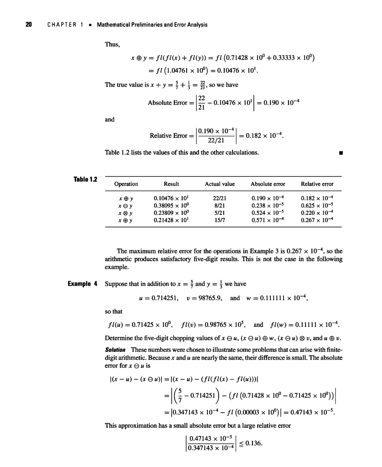
x 0 y = //(//(jc) + fl(y)) = fl (0.71428 x 10° + 0.33333 x 10°)
= // (1.04761 x 10°) = 0.10476 x 101.
The true value is x + y = | + j = |y, so we have
Absolute Error =
??- 0.10476 x 101
21
= 0.190 x 10
,-4
and
Relative Error =
0.190 x 10
-4
22/21
= 0.182 x 10"
Table 1.2 lists the values of this and the other calculations.
Operation
Result
Actual value
Absolute error
Relative error
X® V
xQ v
*<8> v
X @ V
0.10476 x 10'
0.38095 x 10°
0.23809 x 10°
0.21428 x 10'
22/21
8/21
5/21
15/7
0.190 x 10⁻⁴
0.238 x 10"5
0.524 x 10"5
0.571 x 10⁻⁴
0.182 x 10⁻⁴
0.625 x 10"5
0.220 x lO-4
0.267 x lO"4
The maximum relative error for the operations in Example 3 is 0.267 x 10~4, so the
arithmetic produces satisfactory five-digit results. This is not the case in the following
example.
Example 4 Suppose that in addition to jc = | and y = j we have
u = 0.714251, v = 98765.9, and w = 0.111111 x 10"4,
so that
fl(u) = 0.71425 x 10°, fl(v) = 0.98765 x 10⁵, and fl(w) = 0.11111 x 10"4.
Determine the five-digit chopping values of jc © w, (x Q u) © w, (jc © u) ® v, and u © v.
Solution These numbers were chosen to illustrate some problems that can arise with finite-
digit arithmetic. Because jc and u are nearly the same, their difference is small. The absolute
error for x © u is
1{X _ u) _ (x e w)( = |(JC _ u) _ (//(//(*> - //(„)»!
= ( - - 0.714251) - (// (0.71428 x 10° - 0.71425 x 10°))
= |0.347143 x 10"4 - // (0.00003 x 10°) | = 0.47143 x 10~5.
This approximation has a small absolute error but a large relative error
0.47143 x 10"5
0.347143 x 10"4
< 0.136.
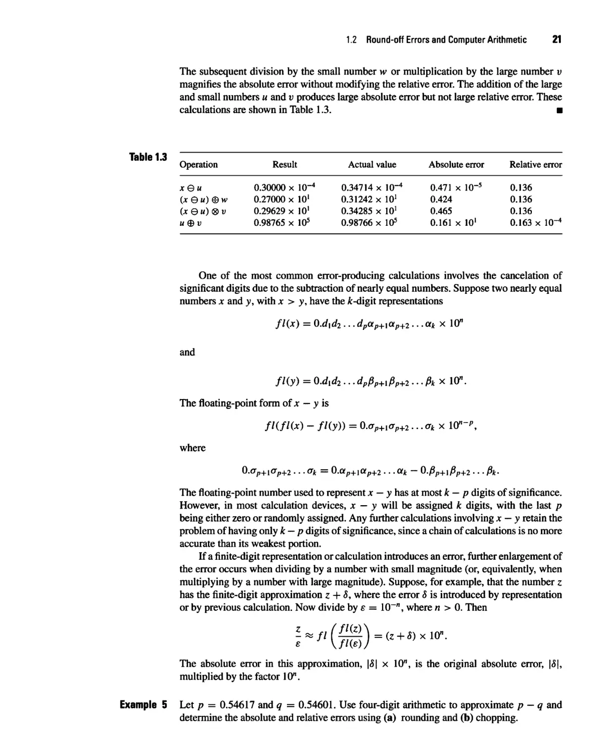
1.2 Round-off Errors and Computer Arithmetic 21
The subsequent division by the small number w or multiplication by the large number v
magnifies the absolute error without modifying the relative error. The addition of the large
and small numbers u and v produces large absolute error but not large relative error. These
calculations are shown in Table 1.3. ■
Operation
xQu
(x G u) © w
(xQu)®v
u © v
Result
0.30000 x 10"4
0.27000 x 10'
0.29629 x 10'
0.98765 x 10⁵
Actual value
0.34714 x 10"4
0.31242 x 101
0.34285 x 101
0.98766 x 10⁵
Absolute error
0.471 x 10"5
0.424
0.465
0.161 x 10'
Relative error
0.136
0.136
0.136
0.163 x 10"4
One of the most common error-producing calculations involves the cancelation of
significant digits due to the subtraction of nearly equal numbers. Suppose two nearly equal
numbers x and y, with x > y, have the A:-digit representations
fl(x) = 0.d\d2 ... dpoip+\oip+2 ...oik x lO^1
and
fl(y) = 0.d{d2...dppp+lpp+2... fa x 10\
The floating-point form of x — y is
fl(fKx) - fl(y)) = 0.crp+{crp+2 ^^kx lO""',
where
0.crp+i<rp+2 .-.cric= Q.ctp+\Ctp+2 ... <*k — ®-PP+\Pp+2 • ■ • A-
The floating-point number used to represent jc — y has at most k — p digits of significance.
However, in most calculation devices, x — y will be assigned k digits, with the last p
being either zero or randomly assigned. Any further calculations involving jc — y retain the
problem of having only k — p digits of significance, since a chain of calculations is no more
accurate than its weakest portion.
If a finite-digit representation or calculation introduces an error, further enlargement of
the error occurs when dividing by a number with small magnitude (or, equivalently, when
multiplying by a number with large magnitude). Suppose, for example, that the number z
has the finite-digit approximation z + 5, where the error 8 is introduced by representation
or by previous calculation. Now divide by s = 10~n, where n > 0. Then
The absolute error in this approximation, |5| x 10n, is the original absolute error, |j|,
multiplied by the factor 10".
Example 5 Let p = 0.54617 and q = 0.54601. Use four-digit arithmetic to approximate p — q and
determine the absolute and relative errors using (a) rounding and (b) chopping.
22 CHAPTER 1 ■ Mathematical Preliminaries and Error Analysis
Solution The exact value of r = p — q is r = 0.00016.
(a) Suppose the subtraction is performed using four-digit rounding arithmetic.
Rounding p and q to four digits gives p* = 0.5462 and q* = 0.5460, respectively, and
r* = p* — q* = 0.0002 is the four-digit approximation to r. Since
r -r
10.00016 - 0.0002|
= 0.25,
\r\ |0.00016|
the result has only one significant digit, whereas p* and q* were accurate to four
and five significant digits, respectively.
(b) If chopping is used to obtain the four digits, the four-digit approximations to p, q,
and r are p* = 0.5461, q* = 0.5460, and r* = p* - q* = 0.0001. This gives
|0.00016-0.0001|
\r -r
= 0.375,
\r\ |0.00016|
which also results in only one significant digit of accuracy.
The loss of accuracy due to round-off error can often be avoided by a reformulation of
the calculations, as illustrated in the next example.
Illustration The quadratic formula states that the roots of ax2 + bx + c = 0, when a ^ 0, are
The roots x\ and X2 of a general
quadratic equation are related to
the coefficients by the fact that
b ^ c
X[+X2 = — and x\X2 = -.
a a
This is a special case of Vieta's
Formulas for the coefficients of
polynomials.
-b + y/b2 - 4ac , -b - <Jb2 - 4ac
jcj = and X2 = —
2a
2a
(1.1)
Consider this formula applied to the equation x2 + 62.10* + 1=0, whose roots are
approximately
jci = -0.01610723 and x2 = -62.08390.
We will again use four-digit rounding arithmetic in the calculations to determine the root. In
this equation, b2 is much larger than 4ac, so the numerator in the calculation for jci involves
the subtraction of nearly equal numbers. Because
y/b2 - 4ac = \/(62.10)2 - (4.000) (1.000) (1.000)
= V3856.-4.000 = V3852T = 62.06,
we have
//(*i) =
-62.10 + 62.06
-0.04000
= -0.02000,
2.000 2.000
a poor approximation to *i = —0.01611, with the large relative error
1-0.01611 + 0.020001
-0.016111
2.4 x 10
-l
On the other hand, the calculation for *2 involves the addition of the nearly equal
numbers — b and — >/b2 — 4ac. This presents no problem since
„, x -62.10-62.06 -124.2
fl(x2) = ^rrz = = -62.10
has the small relative error
2.000
|-62.08 + 62.10|
2.000
- 62.08|
3.2 x 10
,-4
1.2 Round-off Errors and Computer Arithmetic 23
To obtain a more accurate four-digit rounding approximation for jci , we change the
form of the quadratic formula by rationalizing the numerator:
-b + y/b2 - 4ac ( -b- Jb2-4ac\ b2 - (b2 - 4ac)
xi = —
— 4ac\
— 4acJ
2a y-fc- y/b2-4ac) 2a(-b - y/b2-4ac)'
which simplifies to an alternate quadratic formula:
-2c
xi = ,. A . (12)
b + <Jb2 - Aac
Using Eq. (1.2) gives
-2.000 -2.000
fuXx) = = = -0.01610,
J V " 62.10 + 62.06 124.2
which has the small relative error 6.2 x 10"4.
The rationalization technique can also be applied to give the following alternative
quadratic formula for X2'.
_ ~2c
b — y/b2 — 4ac
This is the form to use if b is a negative number. In the illustration, however, the mistaken use
of this formula for X2 would result in not only the subtraction of nearly equal numbers, but
also the division by the small result of this subtraction. The inaccuracy that this combination
produces,
*„ v ~2c -2.000 -2.000 __
fl(x2) = . = = = -50.00,
b-Vb2- Aac 62.10-62.06 0.04000
has the large relative error 1.9 x 10"1. ■
• The lesson: Think before you compute!
Nested Arithmetic
Accuracy loss due to round-off error can also be reduced by rearranging calculations, as
shown in the next example.
Example 6 Evaluate /(jc) = jc3 — 6.1jc2 + 3.2jc + 1.5 at jc = 4.71 using three-digit arithmetic.
Solution Table 1.4 gives the intermediate results in the calculations.
Table 1.4
jc2 jc3 6.1jc2 3.2jc
Exact 4.71 22.1841 104.487111 135.32301 15.072
Three-digit (chopping) 4.71 22.1 104. 134. 15.0
Three-digit (rounding) 4.71 22.2 105. 135. 15.1
To illustrate the calculations, let us look at those involved with finding jc3 using three-
digit rounding arithmetic. First we find
x2 = 4.712 = 22.1841 which rounds to 22.2.
24 CHAPTER 1 ■ Mathematical Preliminaries and Error Analysis
Then we use this value of x2 to find
x3 = x2 • x = 22.2 • 4.71 = 104.562 which rounds to 105.
Also,
and
6.1jc2 = 6.1(22.2) = 135.42 which rounds to 135,
3.2* = 3.2(4.71) = 15.072 which rounds to 15.1.
The exact result of the evaluation is
Exact: /(4.71) = 104.487111 - 135.32301 + 15.072 + 1.5 = -14.263899.
Using finite-digit arithmetic, the way in which we add the results can effect the final result.
Suppose that we add left to right. Then for chopping arithmetic we have
Three-digit (chopping): /(4.71) = ((104. - 134.) + 15.0) + 1.5 = -13.5,
and for rounding arithmetic we have
Three-digit (rounding): /(4.71) = ((105. - 135.) + 15.1) + 1.5 = -13.4.
(You should carefully verify these results to be sure that your notion of finite-digit arithmetic
is correct.) Note that the three-digit chopping values simply retain the leading three digits,
with no rounding involved, and differ significantly from the three-digit rounding values.
The relative errors for the three-digit methods are
Chopping:
-14.263899+13.5
-14.263899
0.05, and Rounding:
-14.263899+13.4
-14.263899
0.06.
Remember that chopping (or
rounding) is performed after each
calculation.
Illustration As an alternative approach, the polynomial /(jc) in Example 6 can be written in a nested
manner as
f(x) = jc3 - 6.1jc2 + 3.2* + 1.5 = ((jc - 6.1)jc + 3.2)jc + 1.5.
Using three-digit chopping arithmetic now produces
/(4.71) =((4.71 - 6.1)4.71 + 3.2)4.71 + 1.5 = ((-1.39)(4.71) + 3.2)4.71 + 1.5
=(-6.54 + 3.2)4.71 + 1.5 = (-3.34)4.71 + 1.5 = -15.7+1.5 = -14.2.
In a similar manner, we now obtain a three-digit rounding answer of —14.3. The new relative
errors are
Three-digit (chopping):
Three-digit (rounding):
14.263899+14.2
-14.263899
-14.263899 + 14.3
14.263899
* 0.0045;
* 0.0025.
Nesting has reduced the relative error for the chopping approximation to less than 10%
of that obtained initially. For the rounding approximation, the improvement has been even
more dramatic; the error in this case has been reduced by more than 95%. ■
1.2 Round-off Errors and Computer Arithmetic 25
EXERCISE SET 1.2
Polynomials should always be expressed in nested form before performing an
evaluation because this form minimizes the number of arithmetic calculations. The decreased
error in the illustration is due to the reduction in computations from four multiplications
and three additions to two multiplications and three additions. One way to reduce round-off
error is to reduce the number of computations.
1. Compute the absolute error and relative error in approximations of p by /?*.
a. p = 7T, p* = 22/7 b. p = n,p* = 3.1416
c. /? = *,/>* = 2.718 d. p = Vl, p* = 1.414
2. Compute the absolute error and relative error in approximations of p by p*.
a. p = e}0, p* = 22000 b. p = 10*, p* = 1400
c. p = 8!, p* = 39900 d. p = 91 p* = y/Ttor(9/e)9
3. Suppose p* must approximate p with relative error at most 10~3. Find the largest interval in which
p* must lie for each value of p.
a. 150 b. 900
c. 1500 d. 90
4. Find the largest interval in which p* must lie to approximate p with relative error at most 10"4 for
each value of p.
a. n b. e
c. V2 d. y/l
5. Perform the following computations (i) exactly, (ii) using three-digit chopping arithmetic, and (iii)
using three-digit rounding arithmetic, (iv) Compute the relative errors in parts (ii) and (iii).
4 1 .41
" 5 + 3 b" 5'3
c- G~rr) + I) d- G + rr)-^
6. Use three-digit rounding arithmetic to perform the following calculations. Compute the absolute error
and relative error with the exact value determined to at least five digits.
a. 133 + 0.921 b. 133-0.499
c. (121 - 0.327) - 119 d. (121 - 119) - 0.327
7. Use three-digit rounding arithmetic to perform the following calculations. Compute the absolute error
and relative error with the exact value determined to at least five digits.
13 _ 6 3
a _!i L b. -10jt+6<?- —
a' 2e-5A 62
>/T3 + yn
• (§)•(?)
d.
VT3-VT1
8. Repeat Exercise 7 using four-digit rounding arithmetic.
9. Repeat Exercise 7 using three-digit chopping arithmetic.
10. Repeat Exercise 7 using four-digit chopping arithmetic.
11. The first three nonzero terms of the Maclaurin series for the arctangent function are x — (l/3);t3 +
(1/5)*5. Compute the absolute error and relative error in the following approximations of n using
the polynomial in place of the arctangent:
arctan
b. 16 arctan ( - 1 — 4 arctan f —- J
■ Mathematical Preliminaries and Error Analysis
12. The number e can be defined by e = X^loO/w!), where n! = n(n — 1) • • -2-1 forw ^ OandO! = 1.
Compute the absolute error and relative error in the following approximations of e:
5 t 10
a.
13. Let
n=0 «=0
x cos x — sin x
f(x) = : .
x — sin x
a. Find lim*_>o / (*) •
b. Use four-digit rounding arithmetic to evaluate /(0.1),
c. Replace each trigonometric function with its third Maclaurin polynomial and repeat part (b).
d. The actual value is /(0.1) = —1.99899998. Find the relative error for the values obtained in
parts (b) and (c).
14. Let
/(*) =
e* — e x
a. Find lim*_>o(£* — e~x)/x-
b. Use three-digit rounding arithmetic to evaluate /(0.1).
c. Replace each exponential function with its third Maclaurin polynomial and repeat part (b).
d. The actual value is /(0.1) = 2.003335000. Find the relative error for the values obtained in
parts (b) and (c).
15. Use four-digit rounding arithmetic and the formulas (1.1), (1.2), and (1.3) to find the most accurate
approximations to the roots of the following quadratic equations. Compute the absolute errors and
relative errors.
1 7 123 1 „
a. -x2 x + - = 0
3 4 6
b. -x2+—x--=0
3 4 6
c. 1 .002jc2 - 11.01 x + 0.01265 = 0
d. 1.002a:2 + 1 1.01a: + 0.01265 = 0
16. Use four-digit rounding arithmetic and the formulas (1.1), (1.2), and (1.3) to find the most accurate
approximations to the roots of the following quadratic equations. Compute the absolute errors and
relative errors.
a. x2-y/lx + y/2 = 0
b. ttjc2 + 13jc + 1 =0
c. x2 + x — e = 0
d. x2 - V35a: -2 = 0
17. Repeat Exercise 15 using four-digit chopping arithmetic.
18. Repeat Exercise 16 using four-digit chopping arithmetic.
19. Use the 64-bit-long real format to find the decimal equivalent of the following floating-point machine
numbers.
a. 0 10000001010 10010011000000000000000000000000000000^
b. 1 10000001010 1001001100000000000000 W
c. 0 01111111111 0101001 lOOOOOOOOOOOOOOOOOOOOOCW
d. 0 01111111111 01010011000000000000000000000000000m
20. Find the next largest and smallest machine numbers in decimal form for the numbers given in
Exercise 19.
1.2 Round-off Errors and Computer Arithmetic 27
21. Suppose two points (jco, yo) and (jci , yO are on a straight line with y\ ^ yo. Two formulas are available
to find the Jt-intercept of the line:
*oyi -x\yo (x\-x0)yo
x = and jc = jco .
y\ - yo y\ - yo
a. Show that both formulas are algebraically correct.
b. Use the data (*o, yo) = (1.31,3.24) and (jci, yO = (1.93,4.76) and three-digit rounding
arithmetic to compute the jc-intercept both ways. Which method is better, and why?
22. The Taylor polynomial ofdegreen for/(jc) = ex is SLoC*1/* 0- Use the Taylor polynomial of degree
nine and three-digit chopping arithmetic to find an approximation to e~5 by each of the following
methods.
-5. x^(-5)'* ^(-l)'S'
sl. e *
if ~~ ^ it
i=0 * i=0
h .--'- '
e5 V9 * "
c. An approximate value of e~5 correct to three digits is 6.74 x 10~3. Which formula, (a) or (b),
gives the most accuracy, and why?
23. The two-by-two linear system
ax + by = e,
cx + dy = /,
where a, b, c, d, ey f are given, can be solved for x and y as follows:
c
set m = -, provided a ^ 0;
a
dx
/i
y
X
= d-
= /-
_ (£j
mfe;
-me;
-fry)
Solve the following linear systems using four-digit rounding arithmetic.
a. 1.130* - 6.990y = 14.20 b. 8.110jc + 12.20y = -0.1370
1.013* - 6.099y = 14.22 -18.11* + 112.2y = -0.1376
24. Repeat Exercise 23 using four-digit chopping arithmetic.
25. a. Show that the polynomial nesting technique described in Example 6 can also be applied to the
evaluation of
f(x) = l.Ole4* - 4.62e3* - 3.11^ + 12.2^ - 1.99.
b. Use three-digit rounding arithmetic, the assumption that e1,53 = 4.62, and the fact that enx =
(ex)n to evaluate /(1.53) as given in part (a).
c. Redo the calculation in part (b) by first nesting the calculations.
d. Compare the approximations in parts (b) and (c) to the true three-digit result /(1.53) = —7.61.
Mathematical Preliminaries and Error Analysis
APPLIED EXERCISES
The opening example to this chapter described a physical experiment involving the temperature of a
gas under pressure. In this application, we were given P = LOO atm, V = 0.100 m3, N = 0.00420 mol,
and R = 0.08206. Solving for T in the ideal gas law gives
PV (1.00)(0.100)
T = = —- - — = 290.15 K = 17°C.
NR (0.00420)(0.08206)
In the laboratory, it was found that T was 15°C under these conditions, and when the pressure was
doubled and the volume halved, T was 19°C. Assume that the data are rounded values accurate to the
places given, and show that both laboratory figures are within the bounds of accuracy for the ideal
gas law.
THEORETICAL EXERCISES
The binomial coefficient
(m\ m!
k) = k\{m-k)\
describes the number of ways of choosing a subset of k objects from a set of m elements.
a. Suppose decimal machine numbers are of the form
±0.did2d3d4 x 10", with 1 < di < 9, 0 < 4 < 9,
if i =2, 3,4 and \n\ < 15.
What is the largest value of m for which the binomial coefficient (™) can be computed for all k
by the definition without causing overflow?
b. Show that (™) can also be computed by
(m\ rm\(m — 1\ fm — k + \\
k) = \l) \k-l)"\ 1 /
c. What is the largest value of m for which the binomial coefficient (™) can be computed by the
formula in part (b) without causing overflow?
d. Use the equation in (b) and four-digit chopping arithmetic to compute the number of possible
five-card hands in a 52-card deck. Compute the actual and relative errors.
Suppose that fl{y) is a fc-digit rounding approximation to y. Show that
y - my)
<0.5x 10"*+1.
[Hint: If dk+] < 5, then fl(y) = 0.d}d2... dk x 10". If dk+] > 5, then fl(y) = 0.d]d2 ...dkxlOn +
10""*.]
Let / € C[a, b] be a function whose derivative exists on (a, b). Suppose / is to be evaluated at jco in
{a, b)y but instead of computing the actual value /(x0), the approximate value, /(jco), is the actual
value of / at jco + 6; that is, /(*o) = /C*o + O-
a. Use the Mean Value Theorem 1.8 to estimate the absolute error | /(xo) — /(*o) I and the relative
error \f(x0) - /(x0)|/|/(x0)|, assuming f(x0) ^ 0.
b. If 6 = 5 x 10~6 and xq = 1, find bounds for the absolute and relative errors for
i. f(x) = ex
ii. f(x) = sinjc
c. Repeat part (b) with e = (5 x lO"6)^ and xq = 10.
1.3 Algorithms and Convergence 29
DISCUSSION QUESTIONS
1. Discuss the difference between the arithmetic performed by a computer and traditional arithmetic.
Why is it so important to recognize the difference?
2. Provide several real-life examples of catastrophic errors that have occurred from the use of finite
digital arithmetic and explain what went wrong.
3. Discuss the various different ways to round numbers.
4. Discuss the difference between a number written in standard notation and one that is written in
normalized decimal floating-point form. Provide several examples.
1.3 Algorithms and Convergence
The use of an algorithm is as old
as formal mathematics, but the
name derives from the Arabic
mathematician Muhammad
ibn-Msa al-Khwararizmi (c.
780-850). The Latin translation
of his works begins with the
words "Dixit Algorismi,"
meaning "al-Khwararizmi says."
Throughout the text, we will be examining approximation procedures, called algorithms,
involving sequences of calculations. An algorithm is a procedure that describes, in an
unambiguous manner, a finite sequence of steps to be performed in a specified order. The
object of the algorithm is to implement a procedure to solve a problem or approximate a
solution to the problem.
We use a pseudocode to describe the algorithms. This pseudocode specifies the form
of the input to be supplied and the form of the desired output. Not all numerical procedures
give satisfactory output for arbitrarily chosen input. As a consequence, a stopping technique
independent of the numerical technique is incorporated into each algorithm to avoid infinite
loops.
Two punctuation symbols are used in the algorithms:
• A period (.) indicates the termination of a step.
• A semicolon (;) separates tasks within a step.
Indentation is used to indicate that groups of statements are to be treated as a single entity.
Looping techniques in the algorithms are either counter-controlled, such as
For i = 1, 2,... , n
Set Xi =a + i -h
or condition-controlled, such as
Whilei < NdoSteps 3-6.
To allow for conditional execution, we use the standard
If...then
or
If... then
else
constructions.
The steps in the algorithms follow the rules of structured program construction. They
have been arranged so that there should be minimal difficulty translating pseudocode into
any programming language suitable for scientific applications.
30 CHAPTER 1 ■ Mathematical Preliminaries and Error Analysis
The algorithms are liberally laced with comments. These are written in italics and
contained within parentheses to distinguish them from the algorithmic statements.
NOTE: When the termination of certain nested steps is difficult to determine, we will
use a comment such as (End Step 14) to the right of or below the terminating statement.
See, for example, the comment on step 5 in Example 1.
N
Illustration The following algorithm computes x\ + X2 H h x^ = YJ jc,-, given N and the numbers
1=1
X\9 X29 . . . , Xtf.
INPUT N9xux2 xn.
OUTPUT SUM=Y,t\xi-
Step 1 Set SUM = 0. (Initialize accumulator.)
Step 2 For i = 1,2,... , AT do
set SUM = SUM + jc, . (Add the next term.)
Step 3 OUTPUT (SUM);
STOP. ■
Example 1 The Nth Taylor polynomial for /(jc) = In jc expanded about jco = 1 is
(-1)'
N * «v+i
PN(x) = Ty-^— (Jt-1)',
tr '
and the value of In 1.5 to eight decimal places is 0.40546511. Construct an algorithm to
determine the minimal value of N required for
|lnl.5-Pw(1.5)| < 10-5
without using the Taylor polynomial remainder term.
Solution From calculus, we know that if Y^\ an is an alternating series with limit A
whose terms decrease in magnitude, then A and the iVth partial sum An = Yln=i a» differ
by less than the magnitude of the (N + l)st term; that is,
\A-AN\ < \aN+i\.
The following algorithm uses this bound.
INPUT value jc, tolerance TOL, maximum number of iterations M.
OUTPUT degree JV of the polynomial or a message of failure.
Stepl SetN = l;
v = x - 1;
SUM = 0;
POWER = y;
TERM = y;
SIGN = — 1. ( Used to implement alternation of signs.)
Step 2 While N < M do Steps 3-5.
Step 3 Set SIGN = -SIGN; (Alternate the signs.)
SUM = SUM + SIGN ■ TERM; (Accumulate the terms.)
1.3 Algorithms and Convergence 31
POWER = POWER • y;
TERM = POWER/(N + 1). (Calculate the next term.)
Step 4 If | TERM | < TOL then (Test for accuracy.)
OUTPUT (N);
STOP. (The procedure was successful.)
Step 5 Set N = N + 1. (Prepare for the next iteration. (End Step 2))
Step 6 OUTPUT ('Method Failed'); (The procedure was unsuccessful)
STOP
The input for our problem is x = 1.5, TOL = 10"5, and perhaps M = 15. This choice
of M provides an upper bound for the number of calculations we are willing to perform,
recognizing that the algorithm is likely to fail if this bound is exceeded. Whether the output
is a value for N or the failure message depends on the precision of the computational
device. ■
The word stable has the same
root as the words stand and
standard. In mathematics, the
term stable applied to a problem
indicates that a small change in
initial data or conditions does not
result in a dramatic change in the
solution to the problem.
Characterizing Algorithms
We will be considering a variety of approximation problems throughout the text, and in each
case we need to determine approximation methods that produce dependably accurate results
for a wide class of problems. Because of the differing ways in which the approximation
methods are derived, we need a variety of conditions to categorize their accuracy. Not all
of these conditions will be appropriate for any particular problem.
One criterion we will impose on an algorithm whenever possible is that small changes
in the initial data produce correspondingly small changes in the final results. An algorithm
that satisfies this property is called stable; otherwise, it is unstable. Some algorithms are
stable only for certain choices of initial data and are called conditionally stable. We will
characterize the stability properties of algorithms whenever possible.
To further consider the subject of round-off error growth and its connection to algorithm
stability, suppose an error with magnitude E0 > 0 is introduced at some stage in the
calculations and that the magnitude of the error after n subsequent operations is denoted by
En. The two cases that arise most often in practice are defined as follows.
Definition 1.17 Suppose that E0 > 0 denotes an error introduced at some stage in the calculations and En
represents the magnitude of the error after n subsequent operations.
• If En ^ CnEo, where C is a constant independent of w, then the growth of error is
said to be linear.
• If En ^ Cn Eq9 for some C > 1, then the growth of error is called exponential. ■
Linear growth of error is usually unavoidable, and when C and Eo are small, the results
are generally acceptable. Exponential growth of error should be avoided because the term Cn
becomes large for even relatively small values of n. This leads to unacceptable inaccuracies,
regardless of the size of E0- As a consequence, an algorithm that exhibits linear growth of
error is stable, whereas an algorithm exhibiting exponential error growth is unstable. (See
Figure 1.10.)
32 CHAPTER 1 ■ Mathematical Preliminaries and Error Analysis
Figure 1.10
En A
Ent
Unstable exponential error growth
• En = CnE^
Stable linear error growth
En = Cn£0
H 1 1 1 1 h
12 3 4 5 6 7 8
Illustration For any constants c\ and c2,
?"=c,G)
x +c23",
is a solution to the recursive equation
10
Pn = YPn~] ~ ^"~2' f0rW = 2' 3'
This can be seen by noting that
TPn~l -Pn~2 = T [C1 G) + C2r~\ ~ [C] G)
/iy-2rio i
= C,UJ It"3"
+ c23]
w-2
+ C23»-' .3-1
(1.4)
- +c23n = /7n.
Suppose that we are given po = 1 and /?i = |. Using these values and Eq. (1.4) we can
determine unique values for the constants as c\ = 1 and c2 = 0. So, pn = (|) for all n.
If five-digit rounding arithmetic is used to compute the terms of the sequence given by
this equation, then po = 1.0000 and p\ = 0.33333, which requires modifying the constants
to c\ = 1.0000 and c2 = —0.12500 x 10"5. The sequence {pn}^=Q generated is then given
by
©"-■
12500 x 10~3(3)",
pn = 1.0000
which has round-off error,
pn-pn= 0.12500 x 10~5(3n)
5/l\n
1.3 Algorithms and Convergence 33
This procedure is unstable because the error grows exponentially with n, which is reflected
in the extreme inaccuracies after the first few terms, as shown in Table 1.5.
Table 1.5
n
0
1
2
3
4
5
6
7
8
Computed p„
0.10000 x 101
0.33333 x 10°
0.11110 x 10°
0.37000 x 10"1
0.12230 x 10"1
0.37660 x 10"2
0.32300 x 10"3
-0.26893 x 10"2
-0.92872 x 10"2
Correct p„
0.10000 x 10'
0.33333 x 10°
0.11111 x 10°
0.37037 x 10"'
0.12346 x 10"1
0.41152 x 10~2
0.13717 x 10"2
0.45725 x 10"3
0.15242 x 10"3
Relative error
9 x 10"5
1 x 10"3
9 x 10"3
8 x 10"2
8 x 10"1
7x 10°
6x 101
Now consider this recursive equation:
pn = 2pn-i - pn-2, for n = 2, 3,
It has the solution pn = c\ + c2n for any constants c\ and c2 because
2p„_! - p„_2 = 2(ci + c2(n - 1)) - (ci + c2(n - 2))
= c{(2 - 1) +c2(2n -2-n + 2) = cx+c2n = pn.
If we are given po = 1 and p\ = j, then constants in this equation are uniquely
determined to be c\ = 1 and c2 = — |. This implies that pn = \ — \n.
If five-digit rounding arithmetic is used to compute the terms of the sequence given
by this equation, then po = 1.0000 and p\ = 0.33333. As a consequence, the five-digit
rounding constants are C\ = 1.0000 and c2 = —0.66667. Thus,
pn = 1.0000 -0.66667w,
which has round-off error
Pn- Pn= f 0.66667 - - j n.
This procedure is stable because the error grows linearly with n, which is reflected in the
approximations shown in Table 1.6. ■
Table 1.6
n
0
1
2
3
4
5
6
7
8
Computed p„
0.10000 x 101
0.33333 x 10°
-0.33330 x 10°
-0.10000 x 101
-0.16667 x 101
-0.23334 x 101
-0.30000 x 101
-0.36667 x 10l
-0.43334 x 101
Correct p„
0.10000 x 101
0.33333 x 10°
-0.33333 x 10°
-0.10000 x 10'
-0.16667 x 101
-0.23333 x 101
-0.30000 x 101
-0.36667 x 10l
-0.43333 x 101
Relative error
9 x 10"5
0
0
4 x 10~5
0
0
2 x 10"5
34 CHAPTER 1 ■ Mathematical Preliminaries and Error Analysis
The effects of round-off error can be reduced by using high-order-digit arithmetic such
as the double- or multiple-precision option available on most computers. Disadvantages in
using double-precision arithmetic are that it takes more computation time and the growth
of round-off error is not entirely eliminated.
One approach to estimating round-off error is to use interval arithmetic (that is, to
retain the largest and smallest possible values at each step) so that, in the end, we obtain an
interval that contains the true value. Unfortunately, a very small interval may be needed for
reasonable implementation.
Rates of Convergence
Since iterative techniques involving sequences are often used, this section concludes with a
brief discussion of some terminology used to describe the rate at which convergence occurs.
In general, we would like the technique to converge as rapidly as possible. The following
definition is used to compare the convergence rates of sequences.
Definition 1.18 Suppose [fin }^LX is a sequence known to converge to zero and {an }^j converges to a number
a. If a positive constant K exists with
\an -a| < K\pn\, for large w,
then we say that {an}2Li converges to a with rate, or order, of convergence 0(pn). (This
expression is read "big oh of f$n".) It is indicated by writing an = a + 0(f5n). m
Although Definition 1.18 permits [otn}^=l to be compared with an arbitrary sequence
[Pn}n*L\i in nearly every situation we use
Pn = —,
for some number p > 0. We are generally interested in the largest value of p with an =
a + 0(l/nP).
Example 2 Suppose that, for n > 1,
otn =
w + 1
and an =
n + 3
n<
nJ
Both linirt-xx) an = 0 and lim^oo &n = 0, but the sequence {&„} converges to this limit
much faster than the sequence {an}. Using five-digit rounding arithmetic, we have the values
shown in Table 1.7. Determine rates of convergence for these two sequences.
Table 1.7
There are numerous other ways
of describing the growth of
sequences and functions, some of
which require bounds both above
and below the sequence or
function under consideration.
Any good book that analyzes
algorithms, for example, [CLRS],
will include this information.
n
A
1
2.00000
4.00000
2
0.75000
0.62500
3
0.44444
0.22222
4
0.31250
0.10938
5
0.24000
0.064000
6
0.19444
0.041667
7
0.16327
0.029155
Solution Define the sequences pn = 1/n and fi„ = 1/n2. Then
n + 1
\0tn " 0| =
n
2 —
< —^ = 2 - - = 2)SW
JT
n
1.3 Algorithms and Convergence 35
and
n + 3 n + 3n , 1 ~
!&„ -0| = —^— < — =4--=4fin.
n3 n3
n<
Hence, the rate of convergence of {an} to zero is similar to the convergence of {1 /n} to zero,
whereas {&n} converges to zero at a rate similar to the more rapidly convergent sequence
{1/w2}. We express this by writing
an=0+o(-] and an=0+o(— j. ■
We also use the O (big oh) notation to describe the rate at which functions converge.
Definition 1.19 Suppose that lim^o G(h) = 0 and linv,_>0 F(h) = L. If a positive constant K exists with
\F(h) - L\ < K\G(h)l for sufficiently small h9
then we write F(h) = L + 0(G(h)). m
The functions we use for comparison generally have the form G(h) = hp, where
p > 0. We are interested in the largest value of p for which F(h) = L + 0(hp).
Example 3 Use the third Taylor polynomial about h = 0 to show that cos h + -h2 = 1 + 0(h4).
Solution In Example 3(b) of Section 1.1, we found that this polynomial is
cosh = 1 — -h1 + —h4 cos 1(A),
2 24
for some number |(/r) between zero and h. This implies that
1 n 1 a
cosh + -h2 = 1 + — /rcosf (/»).
2 24
Hence,
(cos/i + -/i2J -
— cosf(fc)
A4 * ^
so as /i -^ 0, cos /i + lh2 converges to its limit, 1, about as fast as h4 converges to 0. That
is,
cosh + ^h2 = l + 0(h4).
EXERCISE SET 1.3
1. Use three-digit chopping arithmetic to compute the following sums. For each part, which method is
more accurate, and why?
a. E2,(l/'2)firstby} + i + -.- + ^andthenbyT^ + Jr + ...+ |.
b. E!!i0/'*3)firstbyi + i + ^ + ...+ 14andthenby!^ + ^ + ...+ i.
2. The number e is defined by e = J^^U/*!)* where n\ = n(n — 1) • • • 2 • 1 for n ^ 0 and 0! = 1.
Use four-digit chopping arithmetic to compute the following approximations to e and determine the
absolute and relative errors.
■ Mathematical Preliminaries and Error Analysis
5 1 5 1
a. e ^ 5^ — b. e^Y^ —
10 , 10
(10-7)!
c. ^^y^ — d-^^y^ —
/i=0 j=0
3. The Maclaurin series for the arctangent function converges for — 1 < x < 1 and is given by
arctanx = lim Pn(x) = lim ^(-l)1
v2i-l
+1 J*
2i ~ i
a. Use the fact that tan n/4 = 1 to determine the number of n terms of the series that need to be
summed to ensure that |4P„(1) — n\ < 10~3.
b. The C++ programming language requires the value of n to be within 10"10. How many terms
of the series would we need to sum to obtain this degree of accuracy?
4. Exercise 3 details a rather inefficient means of obtaining an approximation to n. The method can
be improved substantially by observing that n/4 = arctan ^ + arctan j and evaluating the series
for the arctangent at \ and at \. Determine the number of terms that must be summed to ensure an
approximation to n to within 10~3.
5. Another formula for computing n can be deduced from the identity 7r/4 = 4 arctan \ — arctan 535.
Determine the number of terms that must be summed to ensure an approximation to n to within 10~3.
6. Find the rates of convergence of the following sequences as n -► 00.
a. lim sin - = 0 b. lim sin — = 0
n-*oo n n-*oo nl
c. HmfriniV-O d' K»0n(» +D-lnOOl-O
7. Find the rates of convergence of the following functions as ft -* 0.
„. sin A « 1 — cosft
a. lim = 1 b. lim = 0
h^0 ft h-*0 ft
,. sin ft — ft cos ft ^ 1 — eh
c. km - =0 d. lim =-1
*->o ft h-+o ft
THEORETICAL EXERCISES
8. Suppose that 0 < q < p and that an = a + O (n~p).
a. Show that an = a + O (n~*).
b. Make a table listing 1/n, 1/n2, 1/n3, and 1/n4 for n = 5, 10,100, and 1000 and discuss the
varying rates of convergence of these sequences as n becomes large.
9. Suppose that 0 < q < p and that F(ft) = L + O (hp).
a. Show that F(h) = L + O (ft*).
b. Make a table listing ft, ft2, ft3, and ft4 for ft = 0.5, 0.1,0.01, and 0.001 and discuss the varying
rates of convergence of these powers of ft as ft approaches zero.
10. Suppose that as x approaches zero,
Fi(x) = Ii + 0(x°) and F2(x) = L2 + 0(xfi).
Let c\ and c2 be nonzero constants and define
F(x) = ciFi(jc) + c2F2(x) and G(x) = F,(c,;t) + F2(c2x).
Show that if y = minimum {a, p}> then, as x approaches zero,
a. F(x) = c{L{ + c2L2 + 0(xy)
b. G(x) = Ll+L2 + 0(Xy).
1.3 Algorithms and Convergence 37
The sequence {F„} described by Fo = 1, F\ = 1, and F„+2 = Fn + F„+\, if n > 0, is called
a Fibonacci sequence. Its terms occur naturally in many botanical species, particularly those with
petals or scales arranged in the form of a logarithmic spiral. Consider the sequence {*„}, where
xn = Fn+\fFn. Assuming that lim,,.^x„ = x exists, show that x = (1 + V5)/2. This number is
called the golden ratio.
Show that the Fibonacci sequence also satisfies the equation
Describe the output of the following algorithm. How does this algorithm compare to the illustration
on page 32?
INPUT n, X\, X2i • • • i xn.
OUTPUT SUM.
Step 1 Set SUM = ^i.
Step 2 For / = 2,3,... , n do Step 3.
Step 3 SUM = SUM + jc,.
Step 4 OUTPUT SUM;
STOP.
Compare the following three algorithms. When is the algorithm of part la correct.?
a. INPUT n, X\, X2i • • • i xn.
OUTPUT PRODUCT.
Step 1 Set PRODUCT = 0.
Step 2 For i = 1,2,.... n do
Set PRODUCT = PRODUCT * xh
Step 3 OUTPUT PRODUCT;
STOP.
b. INPUT
OUTPUT PRODUCT.
Step 1 Set PRODUCT =1.
Step 2 For i = 1,2,... , n do
Set PRODUCT = PRODUCT * jc,.
Step 3 OUTPUT PRODUCT;
STOP.
c. INPUT
OUTPUT PRODUCT.
Step 1 Set PRODUCT =1.
Step2 For i = 1,2,... ,ndo
if jc, = 0 then set PRODUCT = 0;
OUTPUT PRODUCT;
STOP
else set PRODUCT = PRODUCT * jc,.
Step 3 OUTPUT PRODUCT;
STOP.
a. How many multiplications and additions are required to determine a sum of the form
b. Modify the sum in part (a) to an equivalent form that reduces the number of computations.
■ Mathematical Preliminaries and Error Analysis
DISCUSSION QUESTIONS
1. Write an algorithm to sum the finite series J21=i xi m reverse order.
2. Construct an algorithm that has as input an integer n > 1, numbers jto, Jti,... , x„, and a number x
and that produces as output the product (x — x0)(x — x\) • • • (jc — xn).
3. Let P(x) = anx" + a„-\xn~l H h a\x + ao be a polynomial and let jc0 be given. Construct an
algorithm to evaluate P(xo) using nested multiplication.
4. Equations (1.2) and (1.3) in Section 1.2 give alternative formulas for the roots jci and X2 of ax2 +
bx + c = 0. Construct an algorithm with input a9 b, c and output jci, *2 that computes the roots jci
and JC2 (which may be equal or be complex conjugates) using the best formula for each root.
5. Assume that
1-2jc 2*-4a;3 4a:3 - 8a:7 1+2*
• « O . A * * A O '
1-x+jt2 ' 1-jc2 + a:4 ' 1-a:4 + a:8 1+jc+jc2'
for a: < l, and let x = 0.25. Write and execute an algorithm that determines the number of terms
needed on the left side of the equation so that the left side differs from the right side by less than 10~6.
6. What do the algorithms in part (a) and part (b) compute?
a.
INPUT
ao,ai,xo,x\.
OUTPUT S.
Step 1
Step 2
Step 3
Step 4
INPUT
For i = 0,1 do set s,- = a,-.
For i = 0,1 do
for j = 0,1 do
/. . (* — ■*/)
for i ^ j set si = — * si.
(x, - xj)
Set 5 = so + •si-
output S;
STOP.
ao,a\,a2,xo,xi,X2.
OUTPUT S.
Step 1
Step 2
Step 3
Step 4
For i=0,... , 2 do set 5,- = a,-.
Fori =0,1,2 do
for j = 0,1 do
(JC — JC;)
if i ^ j then set s,- = — * st
iXi - Xj)
Set S = so + st + ■s2-
OUTPUTS;
STOP,
c. Generalize the algorithms to have input n, a^ ..., a„, jc0, ..., xn. What is the output value of S?
1.4 Numerical Software
Computer software packages for approximating the numerical solutions to problems are
available in many forms. On our website for the book
https://sites.google.com/site/numericalanalysislburden/
we have provided programs written in C, FORTRAN, Maple, Mathematica, MATLAB,
and Pascal as well as JAVA applets. These can be used to solve the problems given in the
examples and exercises and will give satisfactory results for most problems that you may
need to solve. However, they are what we call special-purpose programs. We use this term
to distinguish these programs from those available in the standard mathematical subroutine
libraries. The programs in these packages will be called general purpose.
1.4 Numerical Software 39
The programs in general-purpose software packages differ in their intent from the
algorithms and programs provided with this book. General-purpose software packages
consider ways to reduce errors due to machine rounding, underflow, and overflow. They
also describe the range of input that will lead to results of a certain specified accuracy.
These are machine-dependent characteristics, so general-purpose software packages use
parameters that describe the floating-point characteristics of the machine being used for
computations.
Illustration To illustrate some differences between programs included in a general-purpose package
and a program that we would provide for use in this book, let us consider an algorithm that
computes the Euclidean norm of an w-dimensional vector x = (jci, X2,... , xn)'. This norm
is often required within larger programs and is defined by
l|x||2 =
n 1 1/2
L' = J
The norm gives a measure for the distance from the vector x to the vector 0. For example,
the vector x = (2, 1, 3, -2, -1)' has
||x||2 = [22 + l2 + 32 + (-2)2 + (-1)2]1/2 = VT9,
so its distance from 0 = (0, 0,0, 0,0)' is J\9 ^ 4.36.
An algorithm of the type we would present for this problem is given here. It includes
no machine-dependent parameters and provides no accuracy assurances, but it will give
accurate results "most of the time."
INPUT n9xux2f... 9x„.
OUTPUT NORM.
Step 1 Set SUM = 0.
Step 2 For/ = 1,2,... , n set SUM = SUM + xf.
Step 3 Set NORM = St/A/1'2.
Step 4 OUTPUT (NORM);
STOP. ■
A program based on our algorithm is easy to write and understand. However, the
program could fail to give sufficient accuracy for a number of reasons. For example, the
magnitude of some of the numbers might be too large or too small to be accurately represented in
the floating-point system of the computer. Also, this order for performing the calculations
might not produce the most accurate results, or the standard software square-root routine
might not be the best available for the problem. Matters of this type are considered by
algorithm designers when writing programs for general-purpose software. These programs are
often used as subprograms for solving larger problems, so they must incorporate controls
that we will not need.
General-Purpose Algorithms
Let us now consider an algorithm for a general-purpose software program for computing
the Euclidean norm. First, it is possible that although a component jc, of the vector is within
the range of the machine, the square of the component is not. This can occur when some |jc/ |
is so small that xf causes underflow or when some \xt | is so large that xf causes overflow.
Mathematical Preliminaries and Error Analysis
It is also possible for all these terms to be within the range of the machine, but overflow
occurs from the addition of a square of one of the terms to the previously computed sum.
Accuracy criteria depend on the machine on which the calculations are being performed,
so machine-dependent parameters are incorporated into the algorithm. Suppose we are
working on a hypothetical computer with base 10, having t > 4 digits of precision, a
minimum exponent emin, and a maximum exponent emax. Then the set of floating-point
numbers in this machine consists of 0 and the numbers of the form
x = f.Uf, where / = ±(f{l0'1 + /21(T2 + • • • + /,1(T'),
where 1 < /i < 9 and 0 < ft < 9, for each i = 2,... , f, and where emin < e < emax.
These constraints imply that the smallest positive number represented in the machine is
a = 10*"1"1"1, so any computed number x with |jc| < a causes underflow and results in
jc being set to 0. The largest positive number is k = (1 — 10~')10*max\ and any computed
number x with |jc | > A causes overflow. When underflow occurs, the program will continue,
often without a significant loss of accuracy. If overflow occurs, the program will fail.
The algorithm assumes that the floating-point characteristics of the machine are
described using parameters Af, s, 5, y, and Y. The maximum number of entries that can be
summed with at least t/2 digits of accuracy is given by N. This implies the algorithm will
proceed to find the norm of a vector x = (*i , jc2, ... , xnY only if n < N. To resolve the
underflow-overflow problem, the nonzero floating-point numbers are partitioned into three
groups:
• small-magnitude numbers x9 those satisfying 0 < |jc| < y;
• medium-magnitude numbers jc, where y < \x\ < Y;
• large-magnitude numbers jc, where Y < \x\.
The parameters y and Y are chosen so that there will be no underflow-overflow
problem in squaring and summing the medium-magnitude numbers. Squaring small-magnitude
numbers can cause underflow, so a scale factor S much greater than 1 is used with the result
that (Sjc)2 avoids the underflow even when jc2 does not. Summing and squaring numbers
having a large magnitude can cause overflow. So in this case, a positive scale factor s much
smaller than 1 is used to ensure that C?jc)2 does not cause overflow when calculated or
incorporated into a sum, even though jc2 would.
To avoid unnecessary scaling, y and Y are chosen so that the range of medium-
magnitude numbers is as large as possible. The algorithm that follows is a modification
of one described in [Brow, W], p. 471. It incorporates a procedure for adding scaled
components of the vector that are small in magnitude until a component with medium magnitude
is encountered. It then unscales the previous sum and continues by squaring and summing
small and medium numbers until a component with a large magnitude is encountered. Once
a component with large magnitude appears, the algorithm scales the previous sum and
proceeds to scale, square, and sum the remaining numbers.
The algorithm assumes that, in transition from small to medium numbers, unsealed
small numbers are negligible when compared to medium numbers. Similarly, in transition
from medium to large numbers, unsealed medium numbers are negligible when compared to
large numbers. Thus, the choices of the scaling parameters must be made so that numbers are
equated to 0 only when they are truly negligible. Typical relationships between the machine
characteristics as described by f, a, A, emin, and emax and the algorithm parameters Af, s,
5, y, and Y are given after the algorithm.
The algorithm uses three flags to indicate the various stages in the summation process.
These flags are given initial values in Step 3 of the algorithm. FLAG 1 is 1 until a medium or
1.4 Numerical Software 41
large component is encountered; then it is changed to 0. FLAG 2 is 0 while small numbers
are being summed, changes to 1 when a medium number is first encountered, and changes
back to 0 when a large number is found. FLAG 3 is initially 0 and changes to 1 when a
large number is first encountered. Step 3 also introduces the flag DONE, which is 0 until
the calculations are complete, and then changes to 1.
INPUT N, s, S, v, Y, k, n, x\, X2,... , x„.
OUTPUT NORM or an appropriate error message.
Step 1 If n < 0 then OUTPUT ('The integer n must be positive.');
STOP.
Step 2 Un>N then OUTPUT ('The integer n is too large.');
STOP.
Step 3 Set SUM = 0;
FLAGl = 1; (The small numbers are being summed.)
FLAG2 = 0;
FLAG3 = 0;
DONE = 0;
i = l.
Step 4 While (/ < n and FLAG1 = 1) do Step 5.
Step 5 U\xi\<y then set SUM = SUM +(S*,)2;
i=/ + l
else set FLAGl = 0. (A non-small number encountered.)
Step 6 lfi>n then set NORM = (SUM) {'2/S;
DONE = 1
else set SUM = (SUM/S)/S; (Scale for larger numbers.)
FLAGl = 1.
Step 7 While (/ < n and FLAGl = 1) do Step 8. (Sum the medium-sized numbers.)
Step 8 If \Xi:\ < Y then set SUM = SUM + xf;
i = i + 1
else set FLAGl = 0. (A large number has been encountered.)
Step 9 If DONE =0 then
if i > n then set NORM = (SUM)i/2',
DONE = 1
else set SUM = ((SUM)s)s; (Scale the large numbers.)
FLAG3 = 1.
Step 10 While (i < n and FLAG3 = 1) do Step 11.
Step 11 Set SUM = SUM +(sxi)2; (Sum the large numbers.)
i' = i + 1.
Step 12 UDONE = 0 then
if SUM1'2 < ks then set NORM = (SUM)l'2/s;
DONE = 1
else set SUM = k. (The norm is too large.)
Step 13 If DONE = 1 then OUTPUT ('Norm is', NORM)
else OUTPUT ('Norm >\NORM, 'overflow occurred').
Step 14 STOP.
42 CHAPTER 1 ■ Mathematical Preliminaries and Error Analysis
The first portable computer was
the Osborne I, produced in 1981,
although it was much larger and
heavier than we would currently
think of as portable.
The system FORTRAN
(FORmula TRANslator) was the
original general-purpose
scientific programming language.
It is still in wide use in situations
that require intensive scientific
computations.
The EISPACK project was the
first large-scale numerical
software package to be made
available in the public domain
and led the way for many
packages to follow.
Software engineering was
established as a laboratory
discipline during the 1970s and
1980s. EISPACK was developed
at Argonne Labs and UNPACK
there shortly thereafter. By the
early 1980s, Argonne was
internationally recognized as a
world leader in symbolic and
numerical computation.
The relationships between the machine characteristics f, or, A, emin, and emax and the
algorithm parameters N, s9 S, y, and Y were chosen in [Brow, W], p. 471, as
AT = 10**, where e^ = l(t — 2)/2J, the greatest integer less than or equal to
it - 2)/2;
s = 10*5, where es = I—(emax + eN)/2\\
S = 10*5, where es = f(l — emin)/2], the smallest integer greater than or equal
to (1 — emin)/2;
y = 10^, where ey = \(emin +1 - 2)/2"|;
Y = 10*r, where eY = l(emax — eN)/2\.
The reliability built into this algorithm has greatly increased the complexity compared to
the algorithm given earlier in the section. In the majority of cases, the special-purpose and
general-purpose algorithms give identical results. The advantage of the general-purpose
algorithm is that it provides security for its results.
Many forms of general-purpose numerical software are available commercially and in
the public domain. Most of the early software was written for mainframe computers, and
a good reference for this is Sources and Development of Mathematical Software, edited by
Wayne Cowell [Co].
Now that personal computers are sufficiently powerful, standard numerical software
is available for them. Most of this numerical software is written in FORTRAN, although
some packages are written in C, C++, and FORTRAN90.
ALGOL procedures were presented for matrix computations in 1971 in [WR]. A
package of FORTRAN subroutines based mainly on the ALGOL procedures was then developed
into the EISPACK routines. These routines are documented in the manuals published by
Springer-Verlag as part of their Lecture Notes in Computer Science series [Sm,B] and [Gar].
The FORTRAN subroutines are used to compute eigenvalues and eigenvectors for a variety
of different types of matrices.
LINPACK is a package of FORTRAN subroutines for analyzing and solving systems
of linear equations and solving linear least squares problems. The documentation for this
package is contained in [DBMS]. A step-by-step introduction to LINPACK, EISPACK, and
BLAS (Basic Linear Algebra Subprograms) is given in [CV].
The LAPACK package, first available in 1992, is a library of FORTRAN subroutines
that supersedes LINPACK and EISPACK by integrating these two sets of algorithms into
a unified and updated package. The software has been restructured to achieve greater
efficiency on vector processors and other high-performance or shared-memory multiprocessors.
LAPACK is expanded in depth and breadth in version 3.0, which is available in FORTRAN,
FORTRAN90, C, C++, and JAVA. C and JAVA are available only as language interfaces
or translations of the FORTRAN libraries of LAPACK. The package BLAS is not a part of
LAPACK, but the code for BLAS is distributed with LAPACK.
Other packages for solving specific types of problems are available in the public
domain. As an alternative to netlib, you can use Xnetlib to search the database and retrieve
software. More information can be found in the article Software Distribution Using Netlib
by Dongarra, Roman, and Wade [DRW].
These software packages are highly efficient, accurate, and reliable. They are
thoroughly tested, and documentation is readily available. Although the packages are portable,
it is a good idea to investigate the machine dependence and read the documentation
thoroughly. The programs test for almost all special contingencies that might result in error and
failures. At the end of each chapter we will discuss some of the appropriate general-purpose
packages.
1.4 Numerical Software 43
In 1970, IMSL became the first
large-scale scientific library for
mainframes. Since that time, the
libraries have been made
available for computer systems
ranging from supercomputers to
personal computers.
The Numerical Algorithms
Group (NAG) was instituted in
the UK in 1971 and developed
the first mathematical software
library. It now has over 10,000
users worldwide and contains
over 1000 mathematical and
statistical functions ranging from
statistical, symbolic,
visualisation, and numerical
simulation software to compilers
and application development
tools.
MATLAB was originally written
to provide easy access to matrix
software developed in the
UNPACK and EISPACK
projects. The first version was
written in the late 1970s for use
in courses in matrix theory, linear
algebra, and numerical analysis.
There are currently more than
500,000 users of MATLAB in
more than 100 countries.
The NAG routines are compatible
with Maple beginning with
version 9.0.
Commercially available packages also represent the state of the art in numerical
methods. Their contents are often based on the public-domain packages but include methods in
libraries for almost every type of problem.
IMSL (International Mathematical and Statistical Libraries) consists of the libraries
MATH, STAT, and SFUN for numerical mathematics, statistics, and special functions,
respectively. These libraries contain more than 900 subroutines originally available in
FORTRAN 77 and now available in C, FORTRAN90, and JAVA. These subroutines solve the
most common numerical analysis problems. The libraries are available commercially from
Visual Numerics.
The packages are delivered in compiled form with extensive documentation. There is an
example program for each routine as well as background reference information. IMSL
contains methods for linear systems, eigensystem analysis, interpolation and approximation,
integration and differentiation, differential equations, transforms, nonlinear equations,
optimization, and basic matrix/vector operations. The library also contains extensive statistical
routines.
The Numerical Algorithms Group (NAG) has been in existence in the United Kingdom
since 1970. NAG offers more than 1000 subroutines in a FORTRAN 77 library, about 400
subroutines in a C library, more than 200 subroutines in a FORTRAN 90 library, and an
MPI FORTRAN numerical library for parallel machines and clusters of workstations or
personal computers. A useful introduction to the NAG routines is [Ph]. The NAG library
contains routines to perform most standard numerical analysis tasks in a manner similar to
those in the IMSL. It also includes some statistical routines and a set of graphic routines.
The IMSL and NAG packages are designed for the mathematician, scientist, or engineer
who wishes to call high-quality C, Java, or FORTRAN subroutines from within a program.
The documentation available with the commercial packages illustrates the typical driver
program required to use the library routines. The next three software packages are
standalone environments. When activated, the user enters commands to cause the package to solve
a problem. However, each package allows programming within the command language.
MATLAB is a matrix laboratory that was originally a Fortran program published by
Cleve Moler [Mo] in the 1980s. The laboratory is based mainly on the EISPACK and
LINPACK subroutines, although functions such as nonlinear systems, numerical integration,
cubic splines, curve fitting, optimization, ordinary differential equations, and graphical tools
have been incorporated. MATLAB is currently written in C and assembler, and the PC
version of this package requires a numeric coprocessor. The basic structure is to perform
matrix operations, such as finding the eigenvalues of a matrix entered from the command
line or from an external file via function calls. This is a powerful self-contained system that
is especially useful for instruction in an applied linear algebra course.
The second package is GAUSS, a mathematical and statistical system produced by Lee
E. Ediefson and Samuel D. Jones in 1985. It is coded mainly in assembler and based
primarily on EISPACK and LINPACK. As in the case of MATLAB, integration/differentiation,
nonlinear systems, fast Fourier transforms, and graphics are available. GAUSS is oriented
less toward instruction in linear algebra and more toward statistical analysis of data. This
package also uses a numeric coprocessor if one is available.
The third package is Maple, a computer algebra system developed in 1980 by the
Symbolic Computational Group at the University of Waterloo. The design for the original
Maple system is presented in the paper by B.W. Char, K.O. Geddes, W.M. Gentlemen, and
G.H. Gonnet [CGGG].
Maple, which is written in C, has the ability to manipulate information in a symbolic
manner. This symbolic manipulation allows the user to obtain exact answers instead of
numerical values. Maple can give exact answers to mathematical problems such as integrals,
differential equations, and linear systems. It contains a programming structure and permits
Mathematical Preliminaries and Error Analysis
text, as well as commands, to be saved in its worksheet files. These worksheets can then be
loaded into Maple and the commands executed.
The equally popular Mathematica, released in 1988, is similar to Maple.
Numerous packages are available that can be classified as supercalculator packages for
the PC. These should not be confused, however, with the general-purpose software listed
here. If you have an interest in one of these packages, you should read Supercalculators on
the PC by B. Simon and R. M. Wilson [SW].
Additional information about software and software libraries can be found in the books
by Cody and Waite [CW] and by Kockler [Ko], and in the 1995 article by Dongarra and
Walker [DW]. More information about floating-point computation can be found in the book
by Chaitini-Chatelin and Frayse [CF] and the article by Goldberg [Go].
Books that address the application of numerical techniques on parallel computers
include those by Schendell [Sche], Phillips and Freeman [PF], and Golub and Ortega [GO].
DISCUSSION QUESTION
1. Discuss the differences between some of the software packages available for
numerical computation.
KEY CONCEPTS
Limits
Rolle's Theorem
Intermediate Value Theorem
Weighted Mean Value Theorem
Finite digit arithmetic
Convergence
CHAPTER REVIEW
Let's review Chapter 1 in terms of skills that you will need in subsequent chapters.
In Section 1.1 you should be able to use Rolle's Theorem, the Intermediate Value
Theorem, and the Extreme Value Theorem where appropriate to:
i. Determine whether an equation has at least one solution on a given interval.
ii. Find an interval that contains a solution to a given equation.
iii. Show that /'(*) = 0 on a given interval.
iv. Maximize a function on a given interval.
You should also be able to use Taylor's Theorem to find the nth degree Taylor polynomial
Pn{x) for a given function, / about Jto* In addition, you should be able to use the Extreme
Value Theorem to maximize the remainder (error) term for that expansion. Students should
note that when computing an upper bound for the remainder term Rn (x) we usually minimize
the error bound. This is accomplished by finding the maximum of the absolute value of a
particular derivative over the appropriate interval.
In Section 1.2 you should be able to convert numbers into k- digit decimal machine
form. You should also be able to competently use rounding or chopping arithmetic as
required. You should be able to compute the real error, absolute error, and relative error in
approximations of p by /?* and be able to find the largest interval in which /?* must lie to
approximate p with a relative error that is within a specified tolerance. Students should be
Continuity
Extreme Value Theorem
Integration
Taylor's Theorem
round-off errors
Stability
Differentiability
Generalized Rolle's Theorem
Riemann Integral
Finite digit representation
algorithms
Numerical software
1.4 Numerical Software 45
aware that when performing finite digit arithmetic, each individual computation must be
rounded or chopped prior to performing any other steps.
In Section 1.3 whenever possible, you should be able to determine the numbers of terms
of a series that need to be summed to ensure that the absolute error lies within a specified
tolerance. When dealing with series that alternate in sign, the error produced by truncating
the series at any term is less than the magnitude of the next term. Whenever possible, you
should be able to determine the rate of convergence of a sequence. You should be able to
follow the steps of an algorithm and describe the output.
Section 1.4 highlights some of the differences between general-purpose software
packages and the algorithms provided in this text. The main "take away" from this section is to
be exposed to the fact that the general-purpose software packages consider ways to reduce
errors due to machine rounding, underflow, and overflow. They also describe the range of
input that will lead to results of a certain specified accuracy.
Solutions of Equations in One Variable
Introduction
The growth of a population can often be modeled over short periods of time by assuming that
the population grows continuously with time at a rate proportional to the number present
at that time. Suppose N(t) denotes the number in the population at time t and X denote the
constant birthrate of the population. Then the population satisfies the differential equation
dN(t)
dt
= XN(t),
whose solution is N(t) = NoeM, where No denotes the initial population.
A/(A)4
1000 +
435
N(\) = 1000eA + -^—(e* - 1)
Birthrate
This exponential model is valid only when the population is isolated, with no
immigration. If immigration is permitted at a constant rate v, then the differential equation
becomes
dN(t)
dt
= XN(t) + v,
whose solution is
N(f) = N0ek' + -V' - 1).
A
47
48 CHAPTER 2 ■ Solutions of Equations in One Variable
Suppose that a certain population contains N(0) = 1,000,000 individuals initially,
that 435,000 individuals immigrate into the community in the first year, and that Af(l) =
1,564,000 individuals are present at the end of one year. To determine the birthrate of this
population, we need to find X in the equation
1,564,000=1,000,000^ +
x , 435,000 k
*■ -■- 0A - 1).
It is not possible to solve explicitly for X in this equation, but numerical methods discussed in
this chapter can be used to approximate solutions of equations of this type to an arbitrarily
high accuracy. The solution to this particular problem is considered in Exercise 22 of
Section 2.3.
2.1 The Bisection Method
In this chapter we consider one of the most basic problems of numerical approximation,
the root-finding problem. This process involves finding a root, or solution, of an equation
of the form f(x) = 0, for a given function /. A root of this equation is also called a zero
of the function /.
The problem of finding an approximation to the root of an equation can be traced back
at least to 1700 B.C.E. A cuneiform table in the Yale Babylonian Collection dating from that
period gives a sexigesimal (base-60) number equivalent to 1.414222 as an approximation to
\/2, a result that is accurate to within 10~5. This approximation can be found by applying
a technique described in Exercise 19 of Section 2.2.
In computer science, the process
of dividing a set continually in
half to search for the solution to a
problem, as the Bisection method
does, is known as a binary search
procedure.
Bisection Technique
The first technique, based on the Intermediate Value Theorem, is called the Bisection, or
Binary-search, method.
Suppose / is a continuous function defined on the interval [a, b]9 with f(a) and f(b)
of opposite sign. The Intermediate Value Theorem implies that a number p exists in (a, b)
with /(p) = 0. Although the procedure will work when there is more than one root in the
interval (a, b)9 we assume for simplicity that the root in this interval is unique. The method
calls for a repeated halving (or bisecting) of subintervals of [a> b] and, at each step, locating
the half containing p.
To begin, set a\ = a and b\ =b and let p\ be the midpoint of [a, b\\ that is,
Pi = a\ +
b\ —a\ a\ +b\
If /(pi) = 0, then p = pi, and we are done.
If /(pi) 7^ 0, then /(pi) has the same sign as either f(a\) or f{b\).
o If /(pi) and f(a\) have the same sign, p e (pi, b\). Set 02 = pi and b2 = b\.
o If /(pi) and f(a\) have opposite signs, p e (a\, pi). Set a>i = a\ and fc2 = Pi-
Then reapply the process to the interval [ai, bi\. This produces the method described in
Algorithm 2.1. (See Figure 2.1.)
2.1 The Bisection Method 49
Figure 2.1
y t
fib) -
/(Pi) "
/(P2) -
1
I
0i
•
a2
7 =/(*)/
P3 X
1 1 * 1
Pi/PP\
P\
p2 b2
a3 p3 b3
i i i
i
b = bx
1>x
l
W 1
X
ALGORITHM
.1
Bisection
To find a solution to f(x) =0 given the continuous function / on the interval [a, b], where
fia) and fib) have opposite signs:
INPUT endpoints a, b; tolerance TOL; maximum number of iterations No.
OUTPUT approximate solution p or message of failure.
Step 1 Set/ = 1;
FA = f(a).
Step 2 While / < W0 do Steps 3-6.
Step 3 Set p = a + (b - a)/2; iCompute p,.)
FP = fip).
Step 4 UFP = 0orib- a)/2 < TOL then
OUTPUT (p); iProcedure completed successfully.)
STOP.
Step 5 Set i = i + 1.
Step 6 KFAFP>0 then set a = p; (Compute a,, bt.)
FA=FP
else set b = p. (FA is unchanged.)
Step 7 OUTPUT ('Method failed after N0 iterations, N0 =', AT0);
(The procedure was unsuccessful.)
STOP. ■
Other stopping procedures can be applied in Step 4 of Algorithm 2.1 or in any of
the iterative techniques in this chapter. For example, we can select a tolerance e > 0 and
generate pi,... , Pn until one of the following conditions is met:
50 CHAPTER 2 ■ Solutions of Equations in One Variable
\Pn
\Pn
— Pn-\\
- Pn-\\
\Pn\
\Hpn)\
<€,
^ £
<• *»
< €.
(2.1)
< €, pN± 0, or (2.2)
(2.3)
Unfortunately, difficulties can arise using any of these stopping criteria. For example,
there are sequences {pn}^L^ with the property that the differences pn — pn-\ converge to
zero while the sequence itself diverges. (See Exercise 19.) It is also possible for f(pn) to be
close to zero while pn differs significantly from p. (See Exercise 20.) Without additional
knowledge about / or /?, Inequality (2.2) is the best stopping criterion to apply because it
comes closest to testing relative error.
When using a computer to generate approximations, it is good practice to set an upper
bound on the number of iterations. This eliminates the possibility of entering an infinite
loop, a situation that can arise when the sequence diverges (and also when the program is
incorrectly coded). This was done in Step 2 of Algorithm 2.1 where the bound A^ was set
and the procedure terminated if i > No.
Note that to start the Bisection Algorithm, an interval [a, b] must be found with f(a) •
f{b) < 0. At each step the length of the interval known to contain a zero of / is reduced
by a factor of 2; hence, it is advantageous to choose the initial interval [a, b] as small as
possible. For example, if f(x) = 2x3 — x2 + x — 1, we have both
/(-4)./(4)<0 and /(0) •/(I) < 0,
so the Bisection Algorithm could be used on [—4,4] or on [0,1]. Starting the Bisection
Algorithm on [0, 1] instead of [—4,4] will reduce by 3 the number of iterations required to
achieve a specified accuracy.
The following example illustrates the Bisection Algorithm. The iteration in this example
is terminated when a bound for the relative error is less than 0.0001. This is ensured by
having
\P~Pn\ _ f„-4
min{|aj, \bn\)
< 10"
Example 1 Show that f(x) = x3 + Ax2 — 10 = 0 has a root in [1,2] and use the Bisection method to
determine an approximation to the root that is accurate to at least within 10"4.
Solution Because /(l) = —5 and /(2) = 14, the Intermediate Value Theorem 1.11
ensures that this continuous function has a root in [1,2].
For the first iteration of the Bisection method, we use the fact that at the midpoint
of [1,2] we have /(1.5) = 2.375 > 0. This indicates that we should select the interval
[1, 1.5] for our second iteration. Then we find that /(1.25) = —1.796875, so our new
interval becomes [1.25,1.5], whose midpoint is 1.375. Continuing in this manner gives the
values in the Table 2.1.
After 13 iterations, pu = 1.365112305 approximates the root p with an error
\p - Pn\ < I*i4 " <*i4l = 11.365234375 - 1.365112305| = 0.000122070.
Since |ai4| < |p|, we have
IP^Pd < l^^ul ^ 9Q x lQ-s
\P\ \au\
2.1 The Bisection Method 51
Table 2.1
n
1
2
3
4
5
6
7
8
9
10
11
12
13
a„
1.0
1.0
1.25
1.25
1.3125
1.34375
1.359375
1.359375
1.36328125
1.36328125
1.364257813
1.364746094
1.364990235
b„
2.0
1.5
1.5
1.375
1.375
1.375
1.375
1.3671875
1.3671875
1.365234375
1.365234375
1.365234375
1.365234375
Pn
1.5
1.25
1.375
1.3125
1.34375
1.359375
1.3671875
1.36328125
1.365234375
1.364257813
1.364746094
1.364990235
1.365112305
f(Pn)
2.375
-1.79687
0.16211
-0.84839
-0.35098
-0.09641
0.03236
-0.03215
0.000072
-0.01605
-0.00799
-0.00396
-0.00194
so the approximation is correct to at least within 10~4. The correct value of p to nine decimal
places is p = 1.365230013. Note that pg is closer to p than is the final approximation pi3.
You might suspect this is true because \f(pg)\ < |/(pi3)|, but we cannot be sure of this
unless the true answer is known. ■
The Bisection method, though conceptually clear, has significant drawbacks. It is
relatively slow to converge (that is, N may become quite large before \p — p#l is sufficiently
small), and a good intermediate approximation might be inadvertently discarded. However,
the method has the important property that it always converges to a solution, and for that
reason it is often used as a starter for the more efficient methods we will see later in this
chapter.
Theorem 2.1 Suppose that / e C[a, b] and f(a) -fib) < 0. The Bisection method generates a sequence
{pn}%L\ approximating a zero p of f with
\Pn - p\ < -^—, when n ^ 1-
Proof For each n > 1, we have
*>*-<** = 2F^^b ~a>) and P G (*»' bn^'
Since pn = \{an + bn) for all n > 1, it follows that
\Pn -P\< -(K - an) = -^j-. ■
Because
|Pn-p| <(b-a)—9
the sequence {pn}n*L\ converges to p with rate of convergence O (^-); that is,
p"=p+°(?)-
It is important to realize that Theorem 2.1 gives only a bound for approximation error
and that this bound might be quite conservative. For example, this bound applied to the
52 CHAPTER2 ■ Solutions of Equations in One Variable
problem in Example 1 ensures only that
|p-/>9l<^^2xlO-J,
^-3
but the actual error is much smaller:
|/7 - p9\ = 11.365230013 - 1.365234375| ^ 4.4 x 10"6.
Example 2 Determine the number of iterations necessary to solve f(x) = x3 + 4x2 — 10 = 0 with
accuracy 10~3 using a\ = 1 and b\ = 2.
Solution We we will use logarithms to find an integer AT that satisfies
>-iv
-AT
*-3
\Pn ~P\< 2-"(fc - a) = 2~" < 10
Logarithms to any base would suffice, but we will use base-10 logarithms because the
tolerance is given as a power of 10. Since 2~N < 10"3 implies that log10 2~~N < logI0 10~3 =
—3, we have
-Ariog102<-3 and N >
9.96.
log102
Hence, 10 iterations are required for an approximation accurate to within 10"3.
Table 2.1 shows that the value of pg = 1.365234375 is accurate to within 10"4. Again,
it is important to keep in mind that the error analysis gives only a bound for the number of
iterations. In many cases, this bound is much larger than the actual number required. ■
The bound for the number of iterations for the Bisection method assumes that the
calculations are performed using infinite-digit arithmetic. When implementing the method on
a computer, we need to consider the effects of round-off error. For example, the computation
of the midpoint of the interval [an, bn] should be found from the equation
Pn=^n-\ r— instead of pn = —-—.
The Latin word signum means
"token" or "sign." So the signum
function quite naturally returns
the sign of a number (unless the
number is 0).
The first equation adds a small correction, (b„ - an)/2, to the known value a„. When bn - an
is near the maximum precision of the machine, this correction might be in error, but the
error would not significantly affect the computed value of pn. However, it is possible for
(an +bn)/2 to return a midpoint that is not even in the interval [an ,bn].
As a final remark, to determine which subinterval of [an, bn] contains a root of /, it is
better to make use of the signum function, which is defined as
— 1, if jc < 0,
sgn(x)= <0, if jc = 0,
1, ifjc>0.
The test
sgn (f(an)) sgn (/(/>„)) < 0 instead of f(an)f(pn) < 0
gives the same result but avoids the possibility of overflow or underflow in the multiplication
of/(an) and/(/>„).
2.1 The Bisection Method 53
EXERCISE SET 2.1
1. Use the Bisection method to find p3 for /(jc) = </x — cos jc = 0 on [0, 1].
2. Let f(x) = 3(jc + 1)(jc — j)(jc — 1) = 0. Use the Bisection method on the following intervals to find
a. [-2,1.5] b. [-1.25,2.5]
3. Use the Bisection method to find solutions accurate to within 10"2 for jc3 — lx2 + I Ax — 6 = 0 on
each interval.
a. [0,1] b. [1,3.2] c. [3.2,4]
4. Use the Bisection method to find solutions accurate to within 10~2 for x4 — 2x3 — Ax2 + Ax + A = 0
on each interval.
a. [-2,-1] b. [0,2] c. [2,3] d. [-1,0]
5. Use the Bisection method to find solutions accurate to within 10~5 for the following problems.
a. x - 2~x = 0 for 0 < x < 1
b. e*-jc2 + 3jc-2 = 0 for0<jc<l
c. 2x cos(2jc) - (x + l)2 = 0 for -3 < x < -2 and -1 < x < 0
d. jccosjc-2jc2 + 3jc- 1 =0 for 0.2 < x < 0.3 and 1.2<jc<1.3
6. Use the Bisection method to find solutions, accurate to within 10~5 for the following problems.
a. 3jc - e* = 0 for 1 < x < 2
b. 2x + 3 cos x - ex = 0 for 0 < x < 1
c. x2 -Ax + 4-lnx = 0 for 1 < x < 2 and 2 < x < A
d. x + 1 - 2sin;r;t = 0 for 0 < x < 0.5 and 0.5 < x < 1
7. a. Sketch the graphs of y = x and y = 2 sin x.
b. Use the Bisection method to find an approximation to within 10~5 to the first positive value of
jc with* = 2 sin jr.
8. a. Sketch the graphs of y = jc and y = tan jc.
b. Use the Bisection method to find an approximation to within 10~5 to the first positive value of
jc withjc = tanjc.
9. a. Sketch the graphs of y = e* — 2 and y = cos(e* — 2).
b. Use the Bisection method to find an approximation to within 10~5 to a value in [0.5, 1.5] with
ex - 2 = cos(e* - 2).
10. a. Sketch the graphs of y = jc2 — 1 and y = el~x .
b. Use the Bisection method to find an approximation to within 10~3 to a value in [—2,0] with
11. Let /(jc) = (jc + 2)(jc + 1)jc(jc — 1)3(jc — 2). To which zero of / does the Bisection method converge
when applied on the following intervals?
a. [-3,2.5] b. [-2.5,3] c. [-1.75,1.5] d. [-1.5,1.75]
12. Let /(jc) = (jc + 2)(jc + 1 )2jc(jc — 1 )3(jc — 2). To which zero of / does the Bisection method converge
when applied on the following intervals?
a. [-1.5,2.5] b. [-0.5,2.4] c. [-0.5,3] d. [-3,-0.5]
13. Find an approximation to -^25 correct to within 10~4 using the Bisection Algorithm. [Hint: Consider
/(jc) = jc3 - 25.]
14. Find an approximation to \/3 correct to within 10~4 using the Bisection Algorithm. [Hint: Consider
/(jc) = jc2 - 3.]
APPLIED EXERCISES
15. A trough of length L has a cross section in the shape of a semicircle with radius r. (See the
accompanying figure.) When filled with water to within a distance h of the top, the volume V of water
is
V = L [0.57rr2 - r2arcsin(/i/r) - h(r2 - ft2)1'2] .
■ Solutions of Equations in One Variable
^ ^^
Suppose L = 10 ft, r = 1 ft, and V = 12.4 ft3. Find the depth of water in the trough to within
0.01 ft.
16. A particle starts at rest on a smooth inclined plane whose angle 6 is changing at a constant rate
— = co < 0.
dt
At the end of t seconds, the position of the object is given by
g I em - e~m
x(t) = -;z—J I = sina>t
0
)
Suppose the particle has moved 1.7 ft in 1 second. Find, to within 10 5, the rate co at which 6 changes.
Assume that g = 32.17 ft/s2.
THEORETICAL EXERCISES
17. Use Theorem 2.1 to find a bound for the number of iterations needed to achieve an approximation
with accuracy 10"4 to the solution of x3 — x — 1=0 lying in the interval [1,2]. Find an approximation
to the root with this degree of accuracy.
18. Use Theorem 2.1 to find a bound for the number of iterations needed to achieve an approximation
with accuracy 10"3 to the solution of x3 +x — 4 = 0 lying in the interval [1,4]. Find an approximation
to the root with this degree of accuracy.
19. Let [pn] be the sequence defined by pn = YH=\ £• Show that [pn] diverges even though
limn_oo(/7n - p„_i) = 0.
20. Let f(x) = (jc - l)10, p = 1, and pn = 1 + l/n. Show that \f(pn)\ < 10"3 whenever n > 1 but
that \p- pn\< 10~3 requires that n > 1000.
21. The function defined by f{x) = sin nx has zeros at every integer. Show that when — 1 < a < 0 and
2 < b < 3, the Bisection method converges to
a. 0, if a+b<2 b. 2, if a+b>2 c. 1, if a + b = 2
DISCUSSION QUESTIONS
1. Derive a function / for which the Bisection method converges to a value that is not a zero of /.
2. Derive a function / for which the Bisection method converges to a zero of / but / is not continuous
at that point.
3. Is the Bisection method sensitive to the starting value? Why or why not?
2.2 Fixed-Point Iteration 55
2.2 Fixed-Point Iteration
A fixed point for a function is a number at which the value of the function does not change
when the function is applied.
Definition 22 The number p is a fixed point for a given function g if g(p) = p. m
In this section, we consider the problem of finding solutions to fixed-point problems
and the connection between the fixed-point problems and the root-finding problems we
wish to solve. Root-finding problems and fixed-point problems are equivalent classes in the
following sense:
• Given a root-finding problem f(p) = 0, we can define functions g with a fixed point at
p in a number of ways, for example, as
g(x) = x - f{x) or as g(x) =x + 3f(x).
• Conversely, if the function g has a fixed point at p, then the function defined by
/(*) = x - g(x)
has a zero at p.
Although the problems we wish to solve are in the root-finding form, the fixed-point
form is easier to analyze, and certain fixed-point choices lead to very powerful root-finding
techniques.
We first need to become comfortable with this new type of problem and to decide
when a function has a fixed point and how the fixed points can be approximated to within
a specified accuracy.
Example 1 Determine any fixed points of the function g(x) = x2 — 2.
Solution A fixed point p for g has the property that
p = g(p) = p2 - 2, which implies that 0 = p2 - p - 2 = (p + l)(p - 2).
A fixed point for g occurs precisely when the graph of y = g{x) intersects the graph of
y = jc, so g has two fixed points, one at p = — 1 and the other at p = 2. These are shown
in Figure 2.2. ■
Fixed-point results occur in many
areas of mathematics and are a
major tool of economists for
proving results concerning
equilibria. Although the idea
behind the technique is old, the
terminology was first used by the
Dutch mathematician
L. E. J. Brouwer (1882-1962) in
the early 1900s.
CHAPTER 2 ■ Solutions of Equations in One Variable
Figure 2.2
The following theorem gives sufficient conditions for the existence and uniqueness of
a fixed point.
Theorem 2.3 (i) If g e C[a9 b] and g(x) e [a, b] for all x e [a, b]9 then g has at least one fixed
point in [ayb],
(ii) If, in addition, g'(x) exists on (a, b) and a positive constant k < 1 exists with
\g'(x)\ <k, for all jc e (a,fc),
then there is exactly one fixed point in [a, b]. (See Figure 2.3.)
Figure 2.3
Proof
(i) If g(a) = a or g(b) = b, then g has a fixed point at an endpoint. If not, then
g(a) > a and g(b) < b. The function h(x) = g(x) — x is continuous on [ay b],
with
h(a) = g(a) - a > 0 and h{b) = g{b) - fc < 0.
2.2 Fixed-Point Iteration 57
The Intermediate Value Theorem implies that there exists p € (a, b) for which
h(p) = 0. This number p is a fixed point for g because
0 = h(p) = g(p) - p implies that g(p) = p.
(ii) Suppose, in addition, that \g'(x)\ <k<l and that p and q are both fixed points
in [a, b\. If p ^ q, then the Mean Value Theorem implies that a number £ exists
between p and q and hence in [a, b] with
g(p) - g(q) ,/t,
p-q
Thus,
\P ~ q\ = \8(P) ~ g(l)\ = \g'm\p -q\<k\p-q\<\p-ql
which is a contradiction. This contradiction must come from the only supposition,
p ^q. Hence, p = q, and the fixed point in [a, b] is unique. ■
Example 2 Show that g(x) = (x2 — l)/3 has a unique fixed point on die interval [—1,1].
Solution The maximum and minimum values of g(x) for jc in [— 1,1] must occur either
when jc is an endpoint of the interval or when the derivative is 0. Since g'(x) = 2*/3, the
function g is continuous, and g'(x) exists on [—1,1]. The maximum and minimum values
of g(x) occur at x = -1, x = 0, or* = 1. Butg(-l) = 0, g(l) = 0, andg(0) = -1/3,
so an absolute maximum for g(x) on [— 1,1] occurs at x = — 1 and x = 1 and an absolute
minimum at x = 0.
Moreover,
\g'(x)\ =
2x
2
<-, for all x e (-1,1).
3
So g satisfies all the hypotheses of Theorem 2.3 and has a unique fixed point in [—1,1]. ■
For the function in Example 2, the unique fixed point p in the interval [—1,1] can be
determined algebraically. If
P = 8(P)=^—, then p2-3p-l=0,
which, by the quadratic formula, implies, as shown on the left graph in Figure 2.4, that
= i(3 - Vl3).
P 2
Note that g also has a unique fixed point p = ^(3+\/l3)forthe interval [3,4]. However,
g(4) = 5 and g'(4) = | > 1, so g does not satisfy the hypotheses of Theorem 2.3 on [3,4].
This demonstrates that the hypotheses of Theorem 2.3 are sufficient to guarantee a unique
fixed point but are not necessary. (See the graph on the right in Figure 2.4.)
58 CHAPTER 2 ■ Solutions of Equations in One Variable
Figure 2.4
(i(3_Vf3),i(3-Vl3))
-1 +
4 *
g(3 + Vl3).£(3 + Vi3))
Example 3 Show that Theorem 2.3 does not ensure a unique fixed point of g(x) = 3 * on the interval
[0,1], even though a unique fixed point on this interval does exist.
Solution g'(x) = —3~* In 3 < 0 on [0,1], the function g is strictly decreasing on [0, 1].
So
S(U = i < g(*) < 1 = g(0), for 0<*<1.
Thus, for jc g [0,1], we have g(x) e [0,1]. The first part of Theorem 2.3 ensures that there
is at least one fixed point in [0,1].
However,
g'(0) = -ln3 = -1.098612289,
so \g'(x)\ ^ 1 on (0,1), and Theorem 2.3 cannot be used to determine uniqueness. But g
is always decreasing, and it is clear from Figure 2.5 that the fixed point must be unique. ■
Figure 2.5
y k
l <
\v = 3_x
y = x
^M
i ■■ |
1 x
2.2 Fixed-Point Iteration 59
Fixed-Point Iteration
Figure 2.6
We cannot explicitly determine the fixed point in Example 3 because we have no way to
solve for p in the equation p = g(p) = 3_/\ We can, however, determine approximations
to this fixed point to any specified degree of accuracy. We will now consider how this can
be done.
To approximate the fixed point of a function g, we choose an initial approximation p0
and generate the sequence [pn }£i0 by letting p„ = g(pn-\), for each n > 1. If the sequence
converges to p and g is continuous, then
p = lim pn = lim g(pn-\) = g ( lim /?„_,) = g(p),
n—►£» n-*-oo \n—>-oo /
and a solution to x = g(x) is obtained. This technique is called fixed-point, or functional
iteration. The procedure is illustrated in Figure 2.6 and detailed in Algorithm 2.2.
y i
Pi = g(p\)
ft = g(P2)
P\ = 8(Po)
y = x
P3 = g(Pi)
Pi = g(P\)
P\ = 8(Po)
(P*PJL^y = gix)
(a)
ALGORITHM
Fixed-Point Iteration
To find a solution to p = g(p) given an initial approximation po:
INPUT initial approximation po; tolerance TOL\ maximum number of iterations TVo.
OUTPUT approximate solution p or message of failure.
Step 7 Seti = l.
Step 2 While / < AT0 do Steps 3-6.
Step 3 Set p = g(po). (Compute pt.)
Step 4 If \p - pol < TOL then
OUTPUT (p); (The procedure was successful.)
STOP.
Step5 Set/= / + l.
Step 6 Set p0 = p. (Update p0.)
E R 2 ■ Solutions of Equations in One Variable
Step 7 OUTPUT (The method failed after N0 iterations, N0 =\ N0);
(The procedure was unsuccessful.)
STOP.
The following illustrates some features of functional iteration.
Illustration The equation x3+4x2 —10 = 0 has a unique root in [ 1,2]. There are many ways to change
the equation to the fixed-point form x = g(x) using simple algebraic manipulation. For
example, to obtain the function g described in part (c), we can manipulate the equation
jc3 + 4jc2 — 10 = 0 as follows:
4jt2 = 10-;t3, so jc2 = j(10-jc3), and jc = ±^(10-jc3)1/2.
To obtain a positive solution, gz(x) is chosen. It is not important for you to derive the
functions shown here, but you should verify that the fixed point of each is actually a solution
to the original equation, jc3 + 4x2 — 10 = 0.
1/2
(a) x = g1(x)=x-x*-4x2 + 10
(c) x = g3(x) = i(10 - *3),/2
(b) * = g2(*)
(d) x = g4(x) =
(e) x=g5(x)=x
x3+4*2-10
3x2 + Sx
With po = 1.5, Table 2.2 lists the results of the fixed-point iteration for all five choices
ofg.
Table 22
n
0
1
2
3
4
5
6
7
8
9
10
15
20
25
30
(a)
1.5
-0.875
6.732
-469.7
1.03 x 10⁸
(b)
1.5
0.8165
2.9969
(-8.65)1/2
(O
1.5
1.286953768
1.402540804
1.345458374
1.375170253
1.360094193
1.367846968
1.363887004
1.365916734
1.364878217
1.365410062
1.365223680
1.365230236
1.365230006
1.365230013
(d)
1.5
1.348399725
1.367376372
1.364957015
1.365264748
1.365225594
1.365230576
1.365229942
1.365230022
1.365230012
1.365230014
1.365230013
(c)
1.5
1.373333333
1.365262015
1.365230014
1.365230013
The actual root is 1.365230013, as was noted in Example 1 of Section 2.1. Comparing
the results to the Bisection Algorithm given in that example, it can be seen that excellent
results have been obtained for choices (d) and (e) (the Bisection method requires 27 iterations
for this accuracy). It is interesting to note that choice (a) was divergent and that choice (b)
became undefined because it involved the square root of a negative number. ■
2.2 Fixed-Point Iteration 61
Although the various functions we have given are fixed-point problems for the same
root-finding problem, they differ vastly as techniques for approximating the solution to the
root-finding problem. Their purpose is to illustrate what needs to be answered:
• Question: How can we find a fixed-point problem that produces a sequence that reliably
and rapidly converges to a solution to a given root-finding problem?
The following theorem and its corollary give us some clues concerning the paths we
should pursue and, perhaps more important, some we should reject.
Theorem 24 (Fixed-Point Theorem)
Let g e C[a, b] be such that g(x) e [a, b], for all x in [a, b]. Suppose, in addition, that g'
exists on (a, b) and that a constant 0 < k < 1 exists with
\g\x)\ <k, for all jc e (a,b).
Then, for any number po in [a,b], the sequence defined by
Pn = g(Pn-\), n>\,
converges to the unique fixed point p in [a, b].
Proof Theorem 2.3 implies that a unique point p exists in [a, b] with g(p) = p. Since g
maps [a, b] into itself, the sequence {pn}^Lo is defined for all n > 0, and pn e [a, b] for all
w. Using the fact that \g'(x)\ < k and the Mean Value Theorem 1.8, we have, for each n,
\Pn - P\ = \g(Pn-l) - g(p)\ = l^(^)IIP«-l - P\ < *|Pn-l - Pi
where £„ e (a, b). Applying this inequality inductively gives
\Pn -p\< k\pn-\ - p\ < k2\pn-2 -p\<--<kn\po- p\. (2.4)
Since 0 < k < 1, we have lim„_>oo kn = 0 and
lim \pn - p\ < lim kn\p0 - p\ = 0.
Hence, {pw}£i0 converges to p. ■
Corollary 2.5 If g satisfies the hypotheses of Theorem 2.4, then bounds for the error involved in using pn
to approximate p are given by
\Pn - p\ < kn max{/70 - a, fc - Po) (2.5)
and
kn
\Pn-p\<z rlPi-pol. forall n > 1. (2.6)
1 — k
Proof Because p e[a, b]9 the first bound follows from Inequality (2.4):
\pn - P\ < kn\p0 - p\ < knmax{/?0 -a%b- p0}-
For n > 1, the procedure used in the proof of Theorem 2.4 implies that
\Pn+\ ~Pn\ = \g(Pn) - g(Pn-\)\ < k\pn - pn-\ \ <•' < kn\pX - p0\.
62 CHAPTER 2 ■ Solutions of Equations in One Variable
Thus, form > n > 1,
\Pm - Pn\ = \Pm - Pm-\ + Pm-\ H Pn+\ ~ Pn\
5 \Pm — Pm-\\ + \Pm-l ~ Pm-l\ H V \pn+l ~ Pn\
< tf-'lPi - Pol + km~2\Pl - pol + • • • + *"|pi - Pol
= *"|pi - Pol (1 +k + k2 + • • • +*m-"-') .
By Theorem 2.3, lim^oo pm = p, so
m—n—1 oo
|p - pn\ = lim |pm - p„\ < lim fcn|p, - pol V kl < fc"|p, - p0| Y>''.
i=0 i=0
But X]/M) *' *s a geometric series with ratio k and 0 < k < 1. This sequence converges to
1/(1 — fc), which gives the second bound:
kn
\p-Pn\ < z r\P\ -Pol- ■
1 —A:
Both inequalities in the corollary relate the rate at which {pn }£L0 converges to the bound
k on the first derivative. The rate of convergence depends on the factor kn. The smaller the
value of k, the faster the convergence. However, the convergence may be very slow if k is
close to 1.
Illustration Let us reconsider the various fixed-point schemes described in the preceding illustration in
light of the Fixed-Point Theorem 2.4 and its Corollary 2.5.
(a) For g\ (x) = x — x3 — Ax2 + 10, we have g\ (1) = 6 and g\ (2) = —12, so g\ does
not map [1,2] into itself. Moreover, g\ (x) = 1 — 3jc2 — 8jc, so \g[ (x)\ > 1 for all
x in [1,2]. Although Theorem 2.4 does not guarantee that the method must fail
for this choice of g, there is no reason to expect convergence.
(b) Withg2U) = [(10/jc)-4jc]1/2,wecanseethatg2doesnotmap[l,2]into[l,2],
and the sequence {pn}%Lo is not defined when po = 1.5. Moreover, there is no
interval containing p ^ 1.365 such that Ig^OOl < 1 because I^C/7)! ^ 3.4.
There is no reason to expect that this method will converge.
(c) For the function g3(x) = j(10 — *3)l/2, we have
g'3(x) = ~x2(lO-x3rl/2<0 on [1,2],
so g3 is strictly decreasing on [1,2]. However, |#3(2)| & 2.12, so the condition
Ig^OOl < k < 1 fails on [1, 2]. A closer examination of the sequence {pn}%Lo
starting with po = 1.5 shows that it suffices to consider the interval [1,1.5]
instead of [1,2]. On this interval, it is still true that g'3(x) < 0 and #3 is strictly
decreasing, but, additionally,
1 < 1.28 * g3(1.5) < g3W < g3(D = 1.5,
for all x e [1,1.5]. This shows that g3 maps the interval [1,1.5] into itself. It
is also true that |g3(jc)| < |g3(1.5)| ^ 0.66 on this interval, so Theorem 2.4
confirms the convergence of which we were already aware.
2.2 Fixed-Point Iteration 63
EXERCISE SET 2.2
(d) For g4(x) = (10/(4 + x))l/2, we have
-5
i*;<*)i =
^(4 + *)3/2
^(5)3/2
<0.15, for all jc g [1,2].
The bound on the magnitude of g'4(x) is much smaller than the bound (found in
(c)) on the magnitude of g'3(x), which explains the more rapid convergence using
#4.
(e) The sequence defined by
x3+4x2- 10
*5(*) = *- 3*3 + 8*
converges much more rapidly than our other choices. In the next sections, we will
see where this choice came from and why it is so effective. ■
From what we have seen, the
• Question: How can we find a fixed-point problem that produces a sequence that reliably
and rapidly converges to a solution to a given root-finding problem?
might have the
• Answer: Manipulate the root-finding problem into a fixed point problem that satisfies the
conditions of Fixed-Point Theorem 2.4 and has a derivative that is as small as possible
near the fixed point.
In the next sections, we will examine this in more detail.
1. Use algebraic manipulation to show that each of the following functions has a fixed point at p precisely
when f(p) = 0, where f(x) = x4 + 2x2-x-3.
/ , ~ 4\ 1/2
a. *,(*) = (3+ *-2*2)1/4 b. g2(x)=^X + 52~X j
c *W={-T£2) g4(X)= 4*3+4,-1
2. a. Perform four iterations, if possible, on each of the functions g defined in Exercise 1. Let po = 1
and pn+x = g(/?„), for n = 0, 1,2, 3.
b. Which function do you think gives the best approximation to the solution?
3. Let f(x) = x3 — 2x + 1. To solve f(x) = 0, the following four fixed-pint problems are proposed.
Derive each fixed point method and compute p\9 p2, /?3, p*. Which methods seem to be appropriate?
a. x = -U3 + 1), po = ^ b- x = ~ ~ ^l' Po = 2
c. jc=W2 , po = - d. * = -^1 -2x, Po= -
4. Let f(x) = jc4 + 3jc2 — 2. To solve f(x) = 0, the following four fixed-pint problems are
proposed. Derive each fixed point method and compute p\9 p2, /?3, and p^. Which methods seem to be
appropriate?
Solutions of Equations in One Variable
a. x = d —-—, po = 1 b. x = \/2 - 3x2, p0 = 1
2-*4 3/2^3P"
c- * = ~37~' ^0==1 <*. x = \j—x—• ^0=1
The following four methods are proposed to compute 211/3. Rank them in order, based on their
apparent speed of convergence, assuming p0 = 1 •
20p„_1+21/pn2_, P„3-i-21
a. P„ = — O. Pn = Pn-I
* = Pn~X ~ e,-21
21 " "" 3^_
/>*_,-21p„_,
d- »-(£)
1/2
The following four methods are proposed to compute 71/5. Rank them in order, based on their apparent
speed of convergence, assuming po = 1-
\ Pn-\ /
a. pn = pw_, 1 + £*-L b. pw = p„_, -
PU - 7
/>*2-i
n „ „ Pn-1 - 7 , „ n P,-l - 7
5/£-i 12
Use a fixed-point iteration method to determine a solution accurate to within 10~2 for jc4 — 3jc2 -3 = 0
on [1, 2], Use po= 1.
Use a fixed-point iteration method to determine a solution accurate to within 10~2 for jc3 — jc — 1 = 0
on [1, 2]. Use po = 1.
Use Theorem 2.3 to show that g(x) = n + 0.5 sin(jc/2) has a unique fixed point on [0, 27r]. Use
fixed-point iteration to find an approximation to the fixed point that is accurate to within 10"2, Use
Corollary 2.5 to estimate the number of iterations required to achieve 10"2 accuracy and compare this
theoretical estimate to the number actually needed.
Use Theorem 2.3 to show that g(jc) = 2~x has a unique fixed point on [i, 1]. Use fixed-point iteration
to find an approximation to the fixed point accurate to within 10"4. Use Corollary 2.5 to estimate the
number of iterations required to achieve 10"4 accuracy and compare this theoretical estimate to the
number actually needed.
Use a fixed-point iteration method to find an approximation to V3 that is accurate to within 10"4.
Compare your result and the number of iterations required with the answer obtained in Exercise 14
of Section 2.1.
Use a fixed-point iteration method to find an approximation to ^25 that is accurate to within 10~4.
Compare your result and the number of iterations required with the answer obtained in Exercise 13
of Section 2.1.
For each of the following equations, determine an interval [a, b] on which fixed-point iteration will
converge. Estimate the number of iterations necessary to obtain approximations accurate to within
10~5 and perform the calculations.
2-ex+x2 r_ 5
a. X = D. X = —r + 2
3 x2
c. jc = (*73)1/2 d. jc=5"*
e. jc = 6~x f. jc = 0.5(sin;c + cos jc)
For each of the following equations, use the given interval or determine an interval [a, b] on which
fixed-point iteration will converge. Estimate the number of iterations necessary to obtain
approximations accurate to within 10"5 and perform the calculations.
a. 2 + sinjc-jc = 0 use [2, 3] b. jc3 - 2jc - 5 = 0 use [2,3]
c. 3jc2 — ex = 0 d. x — cosjc = 0
Find all the zeros of /(jc) = jc2 +10 cos jc by using the fixed-point iteration method for an appropriate
iteration function g. Find the zeros accurate to within 10"4.
Use a fixed-point iteration method to determine a solution accurate to within 10"4 for jc = tan jc, for
jc in [4,5].
Use a fixed-point iteration method to determine a solution accurate to within 10"2 for jc = 2 sin (;tjc) +
jc = 0, for jc on [1, 2]. Use po = 1-
2.2 Fixed-Point Iteration 65
APPLIED EXERCISES
An object falling vertically through the air is subjected to viscous resistance as well as to the force
of gravity. Assume that an object with mass m is dropped from a height so and that the height of the
object after t seconds is
where g = 32.17 ft/s2 and k represents the coefficient of air resistance in Ib-s/ft. Suppose sq = 300 ft,
m = 0.25 lb, and k = 0.1 lb-s/ft. Find, to within 0.01 second, the time it takes this quarter-pounder to
hit the ground.
THEORETICAL EXERCISES
Let g € Cx[ay b] and p be in (a, b) with g(p) = p and \g'(p)\ > 1. Show that there exists a S > 0
such that if 0 < \po — p\ < 8, then \po — p\ < \p\ — p\. Thus, no matter how close the initial
approximation po is to /?, the next iterate p\ is farther away, so the fixed-point iteration does not
converge if po ^ p.
Let A be a given positive constant and g(x) = 2x — Ax2.
a. Show that if fixed-point iteration converges to a nonzero limit, then the limit is p = 1/A, so the
inverse of a number can be found using only multiplications and subtractions.
b. Find an interval about 1/A for which fixed-point iteration converges, provided po is in that
interval.
Find a function g defined on [0,1] that satisfies none of the hypotheses of Theorem 2.3 but still has
a unique fixed point on [0, 1].
a. Show that Theorem 2.3 is true if the inequality |g'(jc)| < k is replaced by g'(x) < ky for all
x e (a,b). [Hint: Only uniqueness is in question.]
b. Show that Theorem 2.4 may not hold if inequality |g'(Jt)| < k is replaced by g'(x) < k. [Hint:
Show that g{x) = 1 - *2, for x in [0, 1], provides a counter example.]
a. Use Theorem 2.4 to show that the sequence defined by
xn = -xn_i + , forn > 1,
2 xn-\
converges to \/2 whenever jc0 > \/2.
b. Use the fact that 0 < (xo — y/2)2 whenever xo ^ y/2 to show that if 0 < xq < >/2,thenjti > y/2.
c. Use the results of parts (a) and (b) to show that the sequence in (a) converges to \fl whenever
jc0 > 0.
a. Show that if A is any positive number, then the sequence defined by
1 A
xn = -*«-i + , for n > 1,
2 2*„_i
converges to *J~A whenever xq > 0.
b. What happens if xq < 0?
Replace the assumption in Theorem 2.4 that "a positive number k < 1 exists with |g'(*)| < /:" with
ug satisfies a Lipschitz condition on the interval [a, b] with Lipschitz constant L < 1." (See Exercise
28, Section 1.1.) Show that the conclusions of this theorem are still valid.
Suppose that g is continuously differentiable on some interval (c, d) that contains the fixed point p
ofg. Show that if \g'(p)\ < 1, then there exists a5 > 0 such that if \po — p\ < 5, then the fixed-point
iteration converges.
66 CHAPTER 2 ■ Solutions of Equations in One Variable
DISCUSSION QUESTION
1. Provide an overview of how chaos theory and fixed-point iteration are related. As a starting point,
look at the following:
http://pages.cs.wisc.edu/-~goadl/cs412/examples/chaosNR.pdf and
http://www.cut-the-knot.org/blue/chaos.shtml. Summarize your readings.
2.3 Newton's Method and Its Extensions
Isaac Newton (1641-1727) was
one of the most brilliant scientists
of all time. The late 17th century
was a vibrant period for science
and mathematics, and Newton's
work touched nearly every aspect
of mathematics. His method for
solving was introduced to find a
root of the equation
y3 - 2y - 5 = 0. Although he
demonstrated the method only for
polynomials, it is clear that he
realized its broader applications.
Joseph Raphson (1648-1715)
gave a description of the method
attributed to Isaac Newton in
1690, acknowledging Newton as
the source of the discovery.
Neither Newton nor Raphson
explicitly used the derivative in
their description since both
considered only polynomials.
Other mathematicians,
particularly James Gregory
(1636-1675), were aware of the
underlying process at or before
this time.
Newton's (or the Newton-Raphsori) method is one of the most powerful and well-known
numerical methods for solving a root-finding problem. There are many ways of introducing
Newton's method.
Newton's Method
If we want only an algorithm, we can consider the technique graphically, as is often done in
calculus. Another possibility is to derive Newton's method as a technique to obtain faster
convergence than offered by other types of functional iteration, as is done in Section 2.4. A
third means of introducing Newton's method, which is discussed next, is based on Taylor
polynomials. We will see there that this particular derivation produces not only the method
but also a bound for the error of the approximation.
Suppose that / e C2[a, b]. Let po e [a, b] be an approximation to p such that
f'(p0) ^ 0 and | p — po I is "small." Consider the first Taylor polynomial for f(x) expanded
about po and evaluated at x = p:
f(p) = /(Po) + (p - Po)/'(po) + (P "2P0) /"(£(p)),
where %(p) lies between p and pq. Since /(/?) = 0, this equation gives
0 = /(po) + (P - Po)/'(Po) + iP ~2P0) f"(g(j>)).
Newton's method is derived by assuming that since \p—po | is small, the term involving
(P ~ Po)2 is much smaller, so
0 * /(po) + (P - Po)/'(Po).
Solving for p gives
Po-
/(Po)
/'(Po)
= P1.
This sets the stage for Newton's method, which starts with an initial approximation po
and generates the sequence {pn]^L0, by
pn = pn-\ -
f(Pn-l)
f'iPn-lV
forn > 1.
(2.7)
Figure 2.7 illustrates how the approximations are obtained using successive tangents.
(Also see Exercise 31.) Starting with the initial approximation po, the approximation p\ is
the x-intercept of the tangent line to the graph of / at (po, /(po)). The approximation p2
is the x-intercept of the tangent line to the graph of / at (p\, f(p\)) and so on. Algorithm
2.3 implements this procedure.
2.3 Newton's Method and Its Extensions 67
Figure 2.7
\ y t
Slope/'(/?,)y• y =f(x)
p» pJV \^^ slope/'(Po)
1 X^-^P. x
ALGORITHM
2.3
Newton's Method
To find a solution to f(x) = 0 given an initial approximation po:
INPUT initial approximation po; tolerance TOL; maximum number of iterations No-
OUTPUT approximate solution p or message of failure.
Stepl Seti = l.
Step 2 While i < N0 do Steps 3-6.
Step 3 Set p = po - f(Po)/f(Po)- (Compute p,.)
Step 4 If |p - pol < TOL then
OUTPUT (p); (The procedure was successful.)
STOP.
Step5 Seti=i + 1.
Step 6 Set po = p. (Update po.)
Step 7 OUTPUT ('The method failed after N0 iterations, N0 =', N0);
(The procedure was unsuccessful.)
STOP.
The stopping-technique inequalities given with the Bisection method are applicable to
Newton's method. That is, select a tolerance e > 0 and construct p\,... pu until
\pN - pN-i\ <£,
\pN - Pn-\\
\Pn\
<e, pN^ 0,
(2.8)
(2.9)
or
I/(Pa/) I < e.
(2.10)
68 CHAPTER2 ■ Solutions of Equations in One Variable
A form of Inequality (2.8) is used in Step 4 of Algorithm 2.3. Note that none of the
inequalities (2.8), (2.9), or (2.10) give precise information about the actual error \pn — pi
(See Exercises 19 and 20 in Section 2.1.)
Newton's method is a functional iteration technique with pn = g(pn-\), for which
g(Pn-\) = Pn-\ -
f(Pn-l)
f'iPn-\Y
for n > 1.
(2.11)
Example 1
In fact, this is the functional iteration technique that was used to give the rapid convergence
we saw in column (e) of Table 2.2 in Section 2.2.
It is clear from Equation (2.7) that Newton's method cannot be continued if /' (/?„_ i) =
0 for some n. In fact, we will see that the method is most effective when /' is bounded
away from zero near p.
Consider the function f(x) = cos x — x = 0. Approximate a root of / using (a) a fixed-point
method, and (b) Newton's method.
Solution (a) A solution to this root-finding problem is also a solution to the fixed-point
problem x = cosjc, and the graph in Figure 2.8 implies that a single fixed point p lies in
[0,7T/2].
Figure 2.8
Note that the variable in the
trigonometric function is in
radian measure, not degrees. This
will always be the case unless
specified otherwise.
Table 2.3
n
0
1
2
3
4
5
6
7
Pn
0.7853981635
0.7071067810
0.7602445972
0.7246674808
0.7487198858
0.7325608446
0.7434642113
0.7361282565
Table 2.3 shows the results of fixed-point iteration with po = n/4. The best we could
conclude from these results is that p «* 0.74.
(b) To apply Newton's method to this problem, we need f'(x) = — sin x — 1. Starting
again with po = ^/4, we have
P\ = Po -
Po
/'(Po)
It COS(7T/4) — TtjA
4 — sin(;r/4) — 1
_ n V2/2 - it/4
~ 4 - V2/2 - 1
= 0.7395361337
_ _ cos(pi) - pi
P2~Pl -sin(p,)-l
= 0.7390851781
2.3 Newton's Method and Its Extensions 69
Table 2.4
Newton's Method
0
1
2
3
4
0.7853981635
0.7395361337
0.7390851781
0.7390851332
0.7390851332
We continue generating the sequence by
Pn = Pn-l -
/(ft-i)
= Pn-\ -
COS pn-] " pn-]
f(Pn-\) rn * -sin/7n_! - 1
This gives the approximations in Table 2.4. An excellent approximation is obtained with
n = 3. Because of the agreement of p$ and p^ we could reasonably expect this result to
be accurate to the places listed. ■
Theorem 2.6
Convergence Using Newton's Method
Example 1 shows that Newton's method can provide extremely accurate approximations
with very few iterations. For that example, only one iteration of Newton's method was
needed to give better accuracy than seven iterations of the fixed-point method. It is now
time to examine Newton's method more carefully to discover why it is so effective.
The Taylor series derivation of Newton's method at the beginning of the section points
out the importance of an accurate initial approximation. The crucial assumption is that the
term involving (p — po)2 is, by comparison with \p — po\, so small that it can be deleted.
This will clearly be false unless po is a good approximation to p. If po is not sufficiently
close to the actual root, there is little reason to suspect that Newton's method will converge
to the root. However, in some instances, even poor initial approximations will produce
convergence. (Exercises 15 and 16 illustrate some of these possibilities.)
The following convergence theorem for Newton's method illustrates the theoretical
importance of the choice of po-
Let / e C2[a, b\. If p e (a,b) such that /(p) = 0 and /'(p) ^ 0, then there exists a
8 > 0 such that Newton's method generates a sequence {pn}l*L[ converging to p for any
initial approximation po € [p — 8, p + 8].
Proof The proof is based on analyzing Newton's method as the functional iteration scheme
Pn = g(Pn-\), for n > 1, with
Let k be in (0,1). We first find an interval [p — 8, p + 8] that g maps into itself and for
which |g'(*)| < k, for all x € (p - 8, p + 8).
Since /' is continuous and /'(p) # 0, part (a) of Exercise 30 in Section 1.1 implies
that there exists a 8\ > 0, such that /'(*) ^ 0 for x € [p — 8\, p + 8\] C [a, b]. Thus, g is
defined and continuous on [p — 8\, p + 8\ ]. Also,
g'W = 1 -
fix) fix) - f{x)f"{x) f(x)f"(x)
[f'(x)V
[/'(*)]
|2 '
for x € [p — 8\, p + <$i], and, since / € C2[a, b], we have g € Cl[p — <$i, p + 8\].
By assumption, /(p) = 0, so
Since g' is continuous and 0 < k < 1, part (b) of Exercise 30 in Section 1.1 implies that
there exists a 5, with 0 < 8 < 8\9 for which
\g'(x)\ <fc, for all x e [p-8,p + 8].
70 CHAPTER 2 ■ Solutions of Equations in One Variable
It remains to show that g maps [p — 8, p + 8] into [p — 5, p + 8]. If x e[p — 8, p + 5],
the Mean Value Theorem implies that for some number £ between x and p9 \g(x) — g(p) \ =
|g'(S)||*-/7|.S0,
\g(x) -P\ = \g(x) - g(p)\ = \g'(S)\\* - Pi < k\x - p| < |x - p\.
Since x e [p — 8, p + 5], it follows that |jc — p\ < 8 and that \g(x) — p\ < 8. Hence, g
maps [p — 5, p + 8] into [p — 5, p + 5].
All the hypotheses of the Fixed-Point Theorem 2.4 are now satisfied, so the sequence
{/*,}"„ defined by
Pn = g(Pn-\) = P/i-1 -
converges to p for any p$ e[p — 8, p + 8].
f(Pn-l)
fiPn-lY
torn > 1,
Theorem 2.6 states that, under reasonable assumptions, Newton's method converges,
provided that a sufficiently accurate initial approximation is chosen. It also implies that
the constant k that bounds the derivative of g and, consequently, indicates the speed of
convergence of the method decreases to 0 as the procedure continues. This result is important
for the theory of Newton's method, but it is seldom applied in practice because it does not
tell us how to determine 8.
In a practical application, an initial approximation is selected, and successive
approximations are generated by Newton's method. Either these will generally converge quickly
to the root or it will be clear that convergence is unlikely.
The word secant is derived from
the Latin word secan, which
means "to cut." The Secant
method uses a secant line, a line
joining two points that cut the
curve, to approximate a root.
The Secant Method
Newton's method is an extremely powerful technique, but it has a major weakness: the need
to know the value of the derivative of / at each approximation. Frequently, f'(x) is far
more difficult and needs more arithmetic operations to calculate than f(x).
To circumvent the problem of the derivative evaluation in Newton's method, we
introduce a slight variation. By definition,
/Wi) =
If pn-2 is close to Pn-\, then
lim
fW-fiPn-l)
X ~ Pn-\
f'(Pn-l)
/(Ai-2) - /(Pn-l) /(P*-l) " f(Pn-l)
Pn-2 - Pn-]
Pn-\ - Pn-2
Using this approximation for f'(pn-\) in Newton's formula gives
Pn = Pn-\ -
f(Pn-\)(Pn-\ - Pn-l)
f(Pn-\)- f(Pn-2)
(2.12)
This technique is called the Secant method and is presented in Algorithm 2.4. (See
Figure 2.9.) Starting with the two initial approximations po and p\, the approximation p<i is
the x-intercept of the line joining (po, f(po)) and (p\, f(p\)). The approximation /?3 is the
jc-intercept of the line joining (/?], f(p\)) and (p2, f(pi)) and so on. Note that only one
function evaluation is needed per step for the Secant method after p2 has been determined.
In contrast, each step of Newton's method requires an evaluation of both the function and
its derivative.
2.3 Newton's Method and Its Extensions 71
Figure 2.9
ft///
Po Pi)\/P/
/\/)fP* Pi ~x 1
ALGORITHM
.4
Secant Method
To find a solution to f(x) = 0 given initial approximations po and p\:
INPUT initial approximations po, p\; tolerance TOL; maximum number of iterations No-
OUTPUT approximate solution p or message of failure.
Step 1 Set i = 2;
tfo = /(po);
?«= /(pi).
Step 2 While i < iV0 do Steps 3-6.
Step 3 Set p = p\ - q\(pi - po)/(qi - go)- (Compute p,.)
Step 4 If \p - p\ | < TOL then
OUTPUT (p); (The procedure was successful.)
STOP.
Step5 Set/= i + l.
Step 6 Set Po = Pi; (Update p0t qo,pi, q\.)
qo = q\\
P\ =P'y
q\ = /(P).
Step 7 OUTPUT ('The method failed after N0 iterations, N0 =', N0);
(The procedure was unsuccessful.)
STOP. ■
The next example involves a problem considered in Example 1, where we used Newton's
method with po = tt/4.
Example 2 Use the Secant method to find a solution to jc = cos* and compare the approximations
with those given in Example 1, which applied Newton's method.
Solution In Example 1, we compared fixed-point iteration and Newton's method starting
with the initial approximation po = jt/4. For the Secant method, we need two initial
72 CHAPTER 2 ■ Solutions of Equations in One Variable
Table 2.5
n
0
1
2
3
4
5
Secant
P*
0.5
0.7853981635
0.7363841388
0.7390581392
0.7390851493
0.7390851332
n
0
1
2
3
4
Newton
Pn
0.7853981635
0.7395361337
0.7390851781
0.7390851332
0.7390851332
The term Regula Falsi, literally
"false rule" or "false position,"
refers to a technique that uses
results that are known to be false,
but in some specific manner, to
obtain convergence to a true
result. False position problems
can be found on the Rhind
papyrus, which dates from about
1650 B.C.E.
approximations. Suppose we use p0 = 0.5 and p\ = n/4:
(P\ - PoKcospi -p\)
P2 = P\ -
(COS px - p\) - (COS p2 - pi)
(tt/4 - 0.5)(cos(tt/4) - jt/4)
(cos(tt/4) - tt/4) - (cos 0.5 - 0.5)
= 0.7363841388.
Succeeding approximations are generated by the formula
(/>„_! - pn-2)(COS pn-i - pn-i)
Pn = Pn-\ -
(COS p„_i - pn-\) - (COS pn-2 - pn-2) '
for n > 2.
These give the results in Table 2.5. We note that although the formula for p2 seems to
indicate a repeated computation, once f(po) and f(p\) are computed, they are not computed
again. ■
Comparing the results in Table 2.5 from the Secant method and Newton's method, we
see that the Secant method approximation ps is accurate to the 10th decimal place, whereas
Newton's method obtained this accuracy by p$. For this example, the convergence of the
Secant method is much faster than functional iteration but slightly slower than Newton's
method. This is generally the case. (See Exercise 14 of Section 2.4.)
Newton's method or the Secant method is often used to refine an answer obtained by
another technique, such as the Bisection method, since these methods require good first
approximations but generally give rapid convergence.
The Method of False Position
Each successive pair of approximations in the Bisection method brackets a root p of the
equation; that is, for each positive integer w, a root lies between an and bn. This implies
that, for each n, the Bisection method iterations satisfy
\Pn~ P\ < ^Wn-Kl
which provides an easily calculated error bound for the approximations.
Root bracketing is not guaranteed for either Newton's method or the Secant method.
In Example 1, Newton's method was applied to /(jc) = cos x — jc, and an approximate root
was found to be 0.7390851332. Table 2.5 shows that this root is not bracketed by either po
and pi or pi and p2. The Secant method approximations for this problem are also given in
Table 2.5. In this case, the initial approximations po and p\ bracket the root, but the pair of
approximations p3 and p* fail to do so.
The method of False Position (also called Regula Falsi) generates approximations
in the same manner as the Secant method, but it includes a test to ensure that the root is
always bracketed between successive iterations. Although it is not a method we generally
recommend, it illustrates how bracketing can be incorporated.
First, choose initial approximations po and p\ with f(po) • f(p\) < 0. The
approximation p2 is chosen in the same manner as in the Secant method as the jc-intercept of the
line joining (/?0, f(po)) and (pi, f(p\)). To decide which secant line to use to compute
p3, consider f(p2) • f(p}) or, more correctly, sgn f(p2) • sgn f(p\).
• If sgn f(p2) • sgn f(pi) < 0, then p\ and p2 bracket a root. Choose p$ as the jc-intercept
of the line joining {pu f(p\)) and (p2, f(pi)).
2.3 Newton's Method and Its Extensions 73
• If not, choose p3 as the jc-intercept of the line joining (/?o, fipo)) and (/?2, f{pi)) and
then interchange the indices on po and p\.
In a similar manner, once p$ is found, the sign of f(p$) • /(P2) determines whether we
use P2 and p$ or 773 and p\ to compute P4. In the latter case a relabeling of P2 and /?i is
performed. The relabeling ensures that the root is bracketed between successive iterations.
The process is described in Algorithm 2.5, and Figure 2.10 shows how the iterations can
differ from those of the Secant method. In this illustration, the first three approximations
are the same, but the fourth approximations differ.
Figure 2.10
ALGORITHM False Position
.5
To find a solution to /(*) = 0 given the continuous function / on the interval [po, p\\
where f(po) and f(p\) have opposite signs:
INPUT initial approximations po, p\; tolerance TOL; maximum number of iterations No.
OUTPUT approximate solution p or message of failure.
Step 1 Set i = 2;
1o = f(Po)\
Q\ = f(Pi)-
Step 2 While i < N0 do Steps 3-7.
Step 3 Set p = pi - qi(p\ - po)/(qi - qo). (Compute p,.)
Step 4 If |p - pi | < TOL then
OUTPUT (p); (The procedure was successful.)
STOP.
Step5 Seti = i + 1;
q = /(P).
Step 6 If q • q\ < 0 then set po = p\\
qo = qi-
74 CHAPTER 2 ■ Solutions of Equations in One Variable
Step 7 Set p{ = p\
Step 8 OUTPUT ('Method failed after N0 iterations, N0 =\ N0);
(The procedure was unsuccessful.)
STOP. ■
Example 3 Use the method of False Position to find a solution to x = cos x and compare the
approximations with those given in Example 1, which applied fixed-point iteration and Newton's
method, and to those found in Example 2, which applied the Secant method.
Solution To make a reasonable comparison we will use the same initial approximations as
in the Secant method; that is, po = 0.5 and p\ = n/4. Table 2.6 shows the results of the
method of False Position applied to fix) = cos x — x together with those we obtained using
the Secant and Newton's methods. Notice that the False Position and Secant approximations
agree through p$ and that the method of False Position requires an additional iteration to
obtain the same accuracy as the Secant method. ■
n
0
1
2
3
4
5
6
False Position
Pn
0.5
0.7853981635
0.7363841388
0.7390581392
0.7390848638
0.7390851305
0.7390851332
Secant
Pn
0.5
0.7853981635
0.7363841388
0.7390581392
0.7390851493
0.7390851332
Newton
Pn
0.7853981635
0.7395361337
0.7390851781
0.7390851332
0.7390851332
The added insurance of the method of False Position commonly requires more
calculation than the Secant method, just as the simplification that the Secant method provides over
Newton's method usually comes at the expense of additional iterations. Further examples
of the positive and negative features of these methods can be seen by working Exercises 13
and 14.
EXERCISE SET 2.3
1. Let /(jc) = x2 - 6 and po = 1- Use Newton's method to find p2-
2. Let /(jc) = —*3 — cos* and po = — 1. Use Newton's method to find p2- Could po = 0 be used?
3. Let f(x) = x2 - 6. With p0 = 3 and p} = 2, find p3.
a. Use the Secant method.
b. Use the method of False Position.
c. Which of part (a) or (b) is closer to \/6?
4. Let fix) = — jc3 — cosjc. With po = — 1 and p\ = 0, find ^3.
a. Use the Secant method. b. Use the method of False Position.
5. Use Newton's method to find solutions accurate to within 10"4 for the following problems.
a. jc3 - 2x2 - 5 = 0, [1,4] b. jc3 + 3jc2 - 1 = 0, [-3, -2]
c. x - cos jc = 0, [0,7T/2] d. x - 0.8 - 0.2 sin jc = 0, [0, tt/2]
6. Use Newton's method to find solutions accurate to within 10~5 for the following problems.
a. **+2-*+2cosjc-6 = 0 for 1 < jc < 2
b. ln(jc - 1) + cos(x - 1) = 0 for 1.3 < jc < 2
2.3 Newton's Method and Its Extensions 75
c. 2x cos2jc - (jc - 2)2 = 0 for 2 < x < 3 and 3 < x < 4
d. (jc - 2)2 - hue = 0 for 1 < x < 2 and e < x < 4
e. ex - 3x2 = 0 for 0 < x < 1 and 3 < jc < 5
f. sin jc -<r*=0 for0<jc<13<jc<4and6<jc<7
Repeat Exercise 5 using the Secant method*
Repeat Exercise 6 using the Secant method.
Repeat Exercise 5 using the method of False Position.
Repeat Exercise 6 using the method of False Position.
Use all three methods in this section to find solutions to within 10~5 for the following problems.
a. 3jc - e* = 0 for 1 < x < 2
b. 2x + 3 cos x - ex = 0 for 1 < x < 2
Use all three methods in this section to find solutions to within 10~7 for the following problems.
a. x2 - 4x + 4 - In x = 0 for 1 < x < 2 and for 2 < x < 4
b. x + 1 - 2sin7rx = 0 forO < x < 1/2 and for 1/2 < jc < 1
The fourth-degree polynomial
/(jc) = 230jc4 + 18jc3 + 9jc2 - 221 jc - 9
has two real zeros, one in [-1,0] and the other in [0, 1]. Attempt to approximate these zeros to within
10"6 using the
a. method of False Position
b. Secant method
c. Newton's method
Use the endpoints of each interval as the initial approximations in parts (a) and (b) and the midpoints
as the initial approximation in part (c).
The function f(x) = tan7rjc — 6 has a zero at (l/7r)arctan6 «* 0.447431543. Let p0 = 0 and
p} = 0.48 and use 10 iterations of each of the following methods to approximate this root. Which
method is most successful, and why?
a. Bisection method
b. Method of False Position
c Secant method
The equation 4jc2 — ex — e~x = 0 has two positive solutions jci and JC2. Use Newton's method to
approximate the solution to within 10"5 with the following values of po-
a. p0 = —10 b. po = — 5 c. p0 = —3
d. po = -1 e. po = 0 f. po = 1
g. Po = 3 h. po = 5 i. po = 10
The equation jc2 —10 cos jc = Ohas two solutions, ±1.3793646. Use Newton's method to approximate
the solutions to within 10~5 with the following values of po.
a. p0 = —100 b. po = -50 c. po =-25
d. po = 25 e. po = 50 f. p0 = 100
The function described by /(jc) = ln(jc2 + 1) - e°Ax cos nx has an infinite number of zeros.
a. Determine, within 10~6, the only negative zero.
b. Determine, within 10"6, the four smallest positive zeros.
c. Determine a reasonable initial approximation to find the nth smallest positive zero of /. [Hint:
Sketch an approximate graph of /.]
d. Use part (c) to determine, within 10~6, the 25th smallest positive zero of /.
Use Newton's method to solve the equation
„ 1 1 2 1 ., *
0 = - + tjc — jc sinjc — - cos 2*, with po = —.
2 4 2 2
Iterate using Newton's method until an accuracy of 10~5 is obtained. Explain why the result seems
unusual for Newton's method. Also, solve the equation with po = 5jt and po = 107r.
76 CHAPTER 2 ■ Solutions of Equations in One Variable
APPLIED EXERCISES
19. Use Newton's method to approximate, to within 1CT4, the value of x that produces the point on the
graph of y = x2 that is closest to (1,0). [Hint: Minimize [d(x)]2, where d(x) represents the distance
from(jc,JC2)to(l,0).]
20. Use Newton's method to approximate, to within 10"4, the value of x that produces the point on the
graph of y = 1/jc that is closest to (2, 1).
21. The sum of two numbers is 20. If each number is added to its square root, the product of the two sums
is 155.55. Determine the two numbers to within 10~4.
22. Find an approximation for X, accurate to within 10"4, for the population equation
435 000
1,564,000 = 1,000,000**" + : {ek - 1),
A
discussed in the introduction to this chapter. Use this value to predict the population at the end of the
second year, assuming that the immigration rate during this year remains at 435,000 individuals per
year.
23. Problems involving the amount of money required to pay off a mortgage over a fixed period of time
involve the formula
A =^[1-(1+i)-"L
i
known as an ordinary annuity equation. In this equation, A is the amount of the mortgage, P is the
amount of each payment, and i is the interest rate per period for the n payment periods. Suppose that
a 30-year home mortgage in the amount of $135,000 is needed and that the borrower can afford house
payments of at most $1000 per month. What is the maximal interest rate the borrower can afford to
pay?
24. The accumulated value of a savings account based on regular periodic payments can be determined
from the annuity due equation,
A= *[(l+i)"-l].
In this equation, A is the amount in the account, P is the amount regularly deposited, and i is the
rate of interest per period for the n deposit periods. An engineer would like to have a savings account
valued at $750,000 upon retirement in 20 years and can afford to put $1500 per month toward this
goal. What is the minimal interest rate at which this amount can be invested, assuming that the interest
is compounded monthly?
25. The logistic population growth model is described by an equation of the form
Pit) = PL
1 - ce~kt'
where Pi, c, and k > 0 are constants and P(t) is the population at time t. Pi represents the limiting
value of the population since lim,.^ P(t) = PL. Use the census data for the years 1950, 1960, and
1970 listed in the table on page 103 to determine the constants Pi, c, and k for a logistic growth
model. Use the logistic model to predict the population of the United States in 1980 and in 2010,
assuming t = 0 at 1950. Compare the 1980 prediction to the actual value.
26. The Gompertz population growth model is described by
/>(,) = PL<TC<~",
where PL, c, and k > 0 are constants and P(t) is the population at time t. Repeat Exercise 25 using
the Gompertz growth model in place of the logistic model.
27. Player A will shut out (win by a score of 21-0) player B in a game of racquetball with probability
2 U-p + p'l •
2.3 Newton's Method and Its Extensions 77
where p denotes the probability A will win any specific rally (independent of the server). (See [Keller,
J], p. 267.) Determine, to within 10"3, the minimal value of p that will ensure that A will shut out B
in at least half the matches they play.
A drug administered to a patient produces a concentration in the bloodstream given by c(t) = Ate~t/3
milligrams per milliliter, t hours after A units have been injected. The maximum safe concentration
is 1 mg/mL.
What amount should be injected to reach this maximum safe concentration, and when does this
maximum occur?
An additional amount of this drug is to be administered to the patient after the concentration falls
to 0.25 mg/mL. Determine, to the nearest minute, when this second injection should be given.
Assume that the concentration from consecutive injections is additive and that 75% of the amount
originally injected is administered in the second injection. When is it time for the third injection?
In the design of all-terrain vehicles, it is necessary to consider the failure of the vehicle when attempting
to negotiate two types of obstacles. One type of failure is called hang-up failure and occurs when the
vehicle attempts to cross an obstacle that causes the bottom of the vehicle to touch the ground. The
other type of failure is called nose-in failure and occurs when the vehicle descends into a ditch and
its nose touches the ground.
The accompanying figure, adapted from [Bek], shows the components associated with the nose-
in failure of a vehicle. In that reference, it is shown that the maximum angle a that can be negotiated
by a vehicle when ft is the maximum angle at which hang-up failure does not occur satisfies the
equation
a.
b.
c.
Asincrcosa + fisin2a — Ccosa — Esina = 0,
where
A=/sin0i, B=lcospu C= (h +0.5Z))sinft - O.5Z)tan0i,
and E = (h + 0.5D) cos p} - 0.5D.
a. It is stated that when / = 89 in., h = 49 in., D = 55 in., and >3i = 11.5°, angle a is approximately
33°. Verify this result.
b. Find a for the situation when /, h, and fi\ are the same as in part (a) but D = 30 in.
-p'l
THEORETICAL EXERCISES
The iteration equation for the Secant method can be written in the simpler form
Pn =
/(pw-i)pw-2 - /(p„-2)P/i-i
/(Pw-l) " f(Pn-l)
Explain why, in general, this iteration equation is likely to be less accurate than the one given in
Algorithm 2.4.
The following describes Newton's method graphically: Suppose that /'(jc) exists on [a, b] and that
f'(x) ^ 0 on [a,b]. Further, suppose there exists one p e [a9b] such that f(p) = 0 and let
CHAPTER 2 ■ Solutions of Equations in One Variable
Po e [a, b] be arbitrary. Let p\ be the point at which the tangent line to / at (po, f(Po)) crosses the
x-axis. For each n > 1, let pn be the jc-intercept of the line tangent to / at (pn-\, /(p„_i)). Derive
the formula describing this method.
32. Derive the error formula for Newton's method
M 2
\P ~ P*+| < -.-,, ..\P - Pn\
assuming the hypothesis of Theorem 2.6 hold, that \f'(pn)\ ^ 0, and M = max |/"(*)|. [Hint: Use
the Taylor polynomial as in the derivation of Newton's Method in the beginning of this section.]
DISCUSSION QUESTIONS
1. Does Newton's method converge for any given starting approximation *o? If so, what is the rate of
convergence, and what is the order of convergence? Does the method still converge when f(x) has
multiple zeros at p?
2. If the initial estimate is not close enough to the root, the Newton method may not converge or may
converge to the wrong root. Find one or two examples where this might occur and provide a rationale
as to why it does.
3. The function f(x) = 0.5jc3-6jc2 + 21.5jc-22 has a zero at x =4. Using a starting point of
p(0) = 5 and p^ = 5, p\ = 4.5 for the Secant method, compare the results of the Secant and
Newton methods.
4. The function f(x) = jc(1/3) has a root at x = 0. Using a starting point of x = 1 and po = 5,
Pi = 0.5 for the Secant method, compare the results of the Secant and Newton methods.
2.4 Error Analysis for Iterative Methods
In this section, we investigate the order of convergence of functional iteration schemes and,
as a means of obtaining rapid convergence, rediscover Newton's method. We also consider
ways of accelerating the convergence of Newton's method in special circumstances. First,
however, we need a new procedure for measuring how rapidly a sequence converges.
Order of Convergence
Definition 2.7 Suppose {p*}£L0 *s a sequence that converges to /?, with pn ^ p for all n. If positive
constants X and a exist with
limi^±l^l=x,
n^°° \Pn - P\*
then {pn}^Lo converges to p of order a, with asymptotic error constant A. ■
An iterative technique of the form pn = g(pn-\) is said to be of order a if the sequence
{Pn]%Lo converges to the solution p = g(p) of order a.
In general, a sequence with a high order of convergence converges more rapidly than a
sequence with a lower order. The asymptotic constant affects the speed of convergence but
not to the extent of the order. Two cases of order are given special attention:
(i) If a = 1 (and k < 1), the sequence is linearly convergent.
(ii) If or = 2, the sequence is quadratically convergent.
The next illustration compares a linearly convergent sequence to one that is
quadratically convergent. It shows why we try to find methods that produce higher-order convergent
sequences.
2.4 Error Analysis for Iterative Methods 79
Illustration Suppose that {pn}%Lo *s linearly convergent to 0 with
Ifli+il
lim
= 0.5
n^oo \pn\
and that {pn}^ is quadratically convergent to 0 with the same asymptotic error constant,
,. \Pn+\\ AC
hm _ .„ = 0.5.
^-►oo
\Pn\:
For simplicity, we assume that for each n, we have
-—— «0.5 and ,„ „ %
\Pn\ \Pn\2
For the linearly convergent scheme, this means that
\Pn -0| = |/>„| %0.5|p„_i| * (0.5)2|pn_2|
whereas the quadratically convergent procedure has
0.5.
Cv . . . Cv
(0.5)n|/70|,
\Pn -0| = |p„| *0.5|/>n_,|2 « (0.5)[0.5|p„_2|2]2 = (0.5)3|p„_2|4
\7i=. 18
(0.5)3[(0.5)|p„_3|2]4 = (0.5)7|p„_3|
KZ • • • J<5
(0.5)2"-'|p0|2fl.
Table 2.7 illustrates the relative speed of convergence of the sequences to 0 if |pol =
IPol = 1.
Table 2.7
n
1
2
3
4
5
6
7
Linear Convergence
sequence {p„}^Lq
(0.5)"
5.0000 x 10"'
2.5000 x 10"1
1.2500 x 10"'
6.2500 x 10"2
3.1250 x 10"2
1.5625 x 10"2
7.8125 x 10"3
Quadratic Convergence
Sequence {p„}%Q
(0.5)2""1
5.0000 x 10"'
1.2500 x 10"1
7.8125 x 10⁻³
3.0518 x 10"5
4.6566 x lO"10
1.0842 x 10"19
5.8775 x 10"39
The quadratically convergent sequence is within 10 38 of 0 by the seventh term. At
least 126 terms are needed to ensure this accuracy for the linearly convergent sequence. ■
Quadratically convergent sequences are expected to converge much quicker than those
that converge only linearly, but the next result implies that an arbitrary fixed-point technique
that generates a convergent sequences does so only linearly.
Theorem 2.8 Let g e C[a, b] be such that g(x) e [a, b], for all x e [a, b\. Suppose, in addition, that g'
is continuous on {a, b) and that a positive constant k < 1 exists with
\g'(x)\ <£, for all x e (a,b).
If g'(p) ^ 0, then for any number po # P in [a, b], the sequence
Pn = g(Pn-i), forw > 1,
converges only linearly to the unique fixed point p in [a, b].
80 CHAPTER2 ■ Solutions of Equations in One Variable
Proof We know from the Fixed-Point Theorem 2.4 in Section 2.2 that the sequence
converges to p. Since g' exists on (a, b), we can apply the Mean Value Theorem to g to show
that for any n,
p„+l - p = g(pn) - g(p) = g'(%n)(Pn ~ P),
where £„ is between pn and p. Since {p„ }£L0 converges to p, we also have {£„ }^0 converging
to p. Since g' is continuous on (a, b), we have
lim g'(£„) = g'(p).
/1-KX)
Thus,
lim ^^ = Urn g'(£„) = ^(p) and lim 'f+1 " *' = |g'(p)|.
Hence, if g'(p) ^ 0, fixed-point iteration exhibits linear convergence with asymptotic error
constant | g'(p) |. ■
Theorem 2.8 implies that higher-order convergence for fixed-point methods of the form
g(p) = p can occur only when g'(p) = 0. The next result describes additional conditions
that ensure the quadratic convergence we seek.
Theorem 2.9 Let p be a solution of the equation x = g(x). Suppose that gf(p) = 0 and g" is continuous
with |g"(Jt)| < M on an open interval / containing p. Then there exists a 8 > 0 such that,
for po g [p — 5, p + 5], the sequence defined by pn = g(p„_i), when n > 1, converges at
least quadratically to p. Moreover, for sufficiently large values of «,
IP/i+i -Pi < y|p*-p|2.
Proof Choose & in (0,1) and 8 > 0 such that on the interval [p — 8, p + 5], contained
in /, we have |g'(jt)| < k and g" continuous. Since \g\x)\ < k < 1, the argument
used in the proof of Theorem 2.6 in Section 2.3 shows that the terms of the sequence
[Pn]%Lo are contained in [p — 5, p + 8]. Expanding g(x) in a linear Taylor polynomial for
x e[p-8,p + 8] gives
g(x) = g(p) + ^(pX* - p) + ^P~(x - p)2,
where £ lies between x and p. The hypotheses g(p) = p and g'(p) = 0 imply that
g(*) = p + —^— (x-py.
In particular, when # = p„,
p„+l = g{pn) = p+ (pn ~ P) ,
with £„ between p„ and p. Thus,
P/i-hi - P = —j-(^ ~ />) •
Since \g'(x)\ < k < 1 on [p — 5, p + 5] and g maps [p — 8, p + 8] into itself, it follows
from the Fixed-Point Theorem that [pn }^0 converges to p. But £w is between p and pw for
each w, so {£W}£10 also converges to p, and
ipw+1 - P\ \g"(P)\
lim ~, rr = —«—•
"^°° \Pn ~ P\2 2
2.4 Error Analysis for Iterative Methods 81
This result implies that the sequence {p«}£i0 ls quadratically convergent if g"(p) ^ 0 and
of higher-order convergence if g"(p) = 0.
Because g" is continuous and strictly bounded by M on the interval [p — <5, p + &],
this also implies that, for sufficiently large values of a,
M r
\Pn+\ -P\< —\Pn - PV. ■
Theorems 2.8 and 2.9 tell us that our search for quadratically convergent fixed-point
methods should point in the direction of functions whose derivatives are zero at the fixed
point. That is,
• For a fixed point method to converge quadratically, we need to have both g(p) = p, and
g\p) = 0.
The easiest way to construct a fixed-point problem associated with a root-finding
problem f(x) = 0 is to add or subtract a multiple of f(x) from x. Consider the sequence
Pn =g(Pn-\), torn > 1,
for gin the form
g(x) =x-<f>(x)f(x),
where <f> is a differentiable function that will be chosen later.
For the iterative procedure derived from g to be quadratically convergent, we need to
have g'(p) = 0 when f(p) = 0. Because
g'(x) = l-<f>'(x)f(x)-f'(x)<l>(x)
and f(p) = 0, we have
g'(P) = l - <f>\p)f(P) - f'{p)4>ip) = 1 - <t>'(p) • o - f(p)Hp) = 1 - f'U>)4>(ph
and g'(p) = 0 if and only if <f>(p) = 1//'(/>).
If we let </>(*) = 1//'C*), then we will ensure that <f>(p) = l/f'(p) and produce the
quadratically convergent procedure
, v f(Pn-\)
Pn = g(Pn-\) = Pn-\ " 777 T-
This, of course, is simply Newton's method. Hence,
• If f(p) = 0 and f'{p) ^ 0, then for starting values sufficiently close to p, Newton's
method will converge at least quadratically.
Multiple Roots
In the preceding discussion, the restriction was made that f'(p) ^ 0, where p is the solution
to f(x) = 0. In particular, Newton's method and the Secant method will generally give
problems if f'(p) = 0 when f(p) = 0. To examine these difficulties in more detail, we
make the following definition.
Definition 2.10 A solution p of f(x) = 0 is a zero of multiplicity m of / if for x ^ p, we can write
f{x) = (x - p)mq(x), where lim,^p q(x) #0. ■
82 CHAPTER 2 ■ Solutions of Equations in One Variable
For polynomials, p is a zero of In essence> q ^ represents that portion of f(x) that does not contribute to the zero of
mu up icily m o / 1 - ^^ f0yowjng resuft gives a means to easily identify simple zeros of a function, those
f(x) = (x- p)mq(x), where , . , • f .
( )=6 0 that have multiplicity one.
Theorem Z11 The function / € C![a, ft] has a simple zero at p in (a, ft) if and only if f(p) = 0 but
f'ip) # o.
Proof If / has a simple zero at p, then f(p) = 0 and /(*) = (x — p)q(x), where
linwp q(x) ^ 0. Since / € C1 [a, fc],
/'(p) = lim /'(*) = limteOO + (* - p)<?'(*)] = lim q(x) # 0.
Conversely, if /(p) = 0 but /'(p) ^ 0, expand / in a zeroth Taylor polynomial about p.
Then
f(x) = f(p) + /'<$(*))<* - p) = (x - p)/'(£(;c)),
where t=(x) is between jc and p. Since / e C1 [a, fc],
lim /'(£(*)) = /' f lim *(*)) = /'(p) # 0.
Letting q = f o % gives /(jc) = (jc - p)#(jc), where lim^^C*) ^ 0. Thus, / has a
simple zero at p. ■
The following generalization of Theorem 2.11 is considered in Exercise 12.
Theorem 2.12 The function f eCm[a,b] has a zero of multiplicity m at p in (a, fc) if and only if
0 = /(p) = /,(p) = /,,(p) = --- = /(m-1)(p), but /(m)(p)^0. ■
The result in Theorem 2.12 implies that an interval about p exists where Newton's
method converges quadratically to p for any initial approximation po = P> provided that p
is a simple zero. The following example shows that quadratic convergence might not occur
if the zero is not simple.
Example 1 Let /(jc) = ex - jc - 1. (a) Show that / has a zero of multiplicity 2 at jc = 0. (b) Show
that Newton's method with po = 1 converges to this zero but not quadratically.
Solution (a) We have
/(*)=e*-x-l, /'(*)=e*-l, and f"(x)=e\
so
f(0) = e° -0-1 = 0, /'(0) = e° - 1 = 0, and /"(0)=e° = l.
Theorem 2.12 implies that / has a zero of multiplicity 2 at jc = 0.
(b) The first two terms generated by Newton's method applied to / with po = 1 are
Pi = Po - t^T = l - e~^7 * a58198
f'(po) e - 1
and
/(Pi) 0.20760
P2 = P|-7^"0-58198-a78957^0-31906-
2.4 Error Analysis for Iterative Methods 83
Figure 2.11
Table 2.8
n
0
1
2
3
4
5
6
7
8
9
10
11
12
13
14
15
16
Pn
1.0
0.58198
0.31906
0.16800
0.08635
0.04380
0.02206
0.01107
0.005545
2.7750 x 10"3
1.3881 x 10"3
6.9411 x 10"4
3.4703 x 10"4
1.7416 x 10"4
8.8041 x 10"5
4.2610 x 10"5
1.9142 x 10"6
The first eight terms of the sequence generated by Newton's method are shown in Table
2.8. The sequence is clearly converging to 0 but not quadratically. The graph of / is shown
in Figure 2.11. ■
1 T
e-2+ 0.«-2)
(~Ue~l) e-\\ /
\v S'fW = ex ~ x - 1
1 ^*^*
-1
1
1 x
One method of handling the problem of multiple roots of a function / is to define
fi(x) =
/'(*)'
If p is a zero of / of multiplicity m with f(x) = (x — p)mq(x), then
(x - p)mq(x)
ji(x) =
m{x - p)m-lq(x) + (x- p)mq'(x)
= (x-p)-
q(x)
mq(x) + (x- p)q'(x)
also has a zero at p. However, q{p) ^ 0, so
i(p)
= 1*0.
mq(p) + (p- p)q'(p) m
and p is a simple zero of fi(x). Newton's method can then be applied to p,(x) to give
2(X)=X-^=X /(*)//'(*)
* li'ix) {[fix)]2 - [f(x)][f» (*)]}/[/'(x)]2'
which simplifies to
8W = X-T7r<
f(x)f'(x)
[f'(x)]2 - fix)f'(x)
(2.13)
If g has the required continuity conditions, functional iteration applied to g will be
quadratically convergent regardless of the multiplicity of the zero of /. Theoretically, the
only drawback to this method is the additional calculation of f"ix) and the more laborious
procedure of calculating the iterates. In practice, however, multiple roots can cause serious
round-off problems because the denominator of Eq. (2.13) consists of the difference of two
numbers both of which are close to 0.
Example 2 In Example 1, it was shown that fix) = ex — x — 1 has a zero of multiplicity 2 at jc = 0 and
that Newton's method with po = 1 converges to this zero but not quadratically. Show that the
modification of Newton's method as given in Eq. (2.13) improves the rate of convergence.
84 CHAPTER 2 ■ Solutions of Equations in One Variable
Table 2.9
Pn
1
2
3
4
5
-2.3421061 x 10"1
-8.4582788 x 10"3
-1.1889524 x 10"5
-6.8638230 x 10"6
-2.8085217 x 10"7
Illustration
Solution Modified Newton's method gives
/(po)/'(Po)
Px = Po -
f'ipo)2 - /(Po)/"(Po)
= 1-
(g_2)(g-l)
(e - l)2 -(e - 2)e
-2.3421061 x 10
-i
This is considerably closer to 0 than the first term using Newton's method, which was
0.58918. Table 2.9 lists the first five approximations to the double zero at x = 0. The results
were obtained using a system with 10 digits of precision. The relative lack of improvement
in the last two entries is due to the fact that using this system, both the numerator and die
denominator approach 0. Consequently, mere is a loss of significant digits of accuracy as
the approximations approach 0.
The following illustrates that the modified Newton's method converges quadratically
even when in the case of a simple zero.
In Section 2.2, we found that a zero of f(x) = x3 + 4x2 - 10 = 0 is p = 1.36523001.
Here we will compare convergence for a simple zero using both Newton's method and the
modified Newton method listed in Eq. (2.13). Let
P^+^-io
(i) pn = p„_l -
3p2_,+8p„_i
from Newton's method,
and, from the modified Newton's method given by Eq. (2.13),
(pLi+4p^_1-10)(3p2_1+8p„_1)
(0) pn = pn-\ -
With po = 1.5, we have
Newton's method
(3flf_, + 8p„-i)2 - (pn_x +4p<„_l - 10)(6/7„_, + 8)
px = 1.37333333, p2 = 1.36526201, and p3 = 1.36523001.
Modified Newton's method
px = 1.35689898, p2 = 1.36519585, and p3 = 1.36523001.
Bom mediods are rapidly convergent to the actual zero, which is given by both methods as
P3. Note, however, that in the case of a simple zero, the original Newton's method requires
substantially less computation. ■
EXERCISE SET 2.4
2.
1. Use Newton's method to find solutions accurate to within 10 to the following problems.
a. x2 - 2xe~x + e_2x = 0, for0<jc<l
b. cos(jc + V2)+Jc(jc/2 + VI)=0, for-2<x<-l
c. jc3 - 3jc2(2-*) + 3^(4"') - 8-* = 0, for 0 < x < 1
d. «& + 3(ln 2)2e2* - (In %)eAx - (In 2)3 = 0, for -1 < x < 0
Use Newton's method to find solutions accurate to within 10-5 to the following problems.
a. 1 — 4jccosjc+ 2x2 + cos2x = 0, for0<x<l
b. x2 + 6x5 + 9jc4 - 2x3 - 6x2 + 1 = 0, for -3 < x < -2
c sin 3x + 3c-2x sin jc — 3e~x sin 2x — e~ix =0, for 3 < jc < 4
d. e* - 21 x6 + 21 x V - 9x2e2x =0, for 3 < jc < 5
2.4 Error Analysis for Iterative Methods 85
Repeat Exercise 1 using the modified Newton's method described in Eq. (2.13). Is there an
improvement in speed or accuracy over Exercise 1?
Repeat Exercise 2 using the modified Newton's method described in Eq. (2.13). Is there an
improvement in speed or accuracy over Exercise 2?
Use Newton's method and the modified Newton's method described in Eq. (2.13) to find a solution
accurate to within 10~5 to the problem
e** + 1.441*2* - 2.079e4x - 0.3330 = 0, for - 1 < x < 0.
This is the same problem as 1(d) with the coefficients replaced by their four-digit approximations.
Compare the solutions to the results in 1(d) and 2(d).
THEORETICAL EXERCISES
Show that the following sequences converge linearly to p = 0. How large must n be before \pn — p \ <
5 x 10~2?
a. pn = -, n > 1 b. pn = -r, n > 1
n nz
a. Show that for any positive integer k, the sequence defined by p„ = \/nk converges linearly to
p = 0.
b. For each pair of integers k and m, determine a number N for which 1 fNk < 10~m.
a. Show that the sequence pn = 10~2" converges quadratically to 0.
b. Show that the sequence pn = 10 n does not converge to 0 quadratically, regardless of the size
of the exponent it > 1.
a. Construct a sequence that converges to 0 of order 3.
b. Suppose a > 1. Construct a sequence that converges to 0 of order a.
Suppose p is a zero of multiplicity m of /, where f^m) is continuous on an open interval containing
p. Show that the following fixed-point method has g'(p) = 0:
f \ mf(x)
Show that the Bisection Algorithm 2.1 gives a sequence with an error bound that converges linearly
toO.
Suppose that / has m continuous derivatives. Modify the proof of Theorem 2.11 to show that / has
a zero of multiplicity m at p if and only if
0 = f(p) = f\p) = ■ ■ • = f{m-l\p\ but /(m)(p) ^ 0.
The iterative method to solve f(x) = 0, given by the fixed-point method g(x) = jc, where
Pn = g(pn-\) = P/i-1 -
f{Pn-\) f'\Pn-\) \f(Pn-l)12
/'(ft-l) 2/'(/>„-l)
ff{Pn-x)\
for n = 1,2,3,.,
has g'(p) = g"(p) = 0. This will generally yield cubic (a = 3) convergence. Expand the analysis of
Example 1 to compare quadratic and cubic convergence.
It can be shown (see, for example, [DaB], pp. 228-229) that if [pn}%Lo are convergent Secant
method approximations to /?, the solution to f(x) = 0, then a constant C exists with \pn+i — p\ ^
C \pn - p\ \pn-] — p\ for sufficiently large values of n. Assume {/?„} converges to p of order a and
show that a = (1 + \/5)/2. (Note: This implies that the order of convergence of the Secant method
is approximately 1.62.)
DISCUSSION QUESTIONS
The speed at which the sequence generated by an iterative method converges is called the method's rate
of convergence. There are many types of convergence rates: linear, superlinear, sublinear, logarithmic,
86 CHAPTER 2 ■ Solutions of Equations in One Variable
quadratic, cubic, and so on. The drawback of these convergence rates is that they do not catch
some sequences that still converge reasonably fast but whose "speed" is variable. Select one of the
convergence rates and describe how that rate can be accelerated.
2. Discuss when Newton's method gives linear or quadratic convergence for the function f(x) =
x2(x - 1).
3. Read the document found at http://www.uark.edu/misc/arnold/publicJitml/4363/OrderConv.pdf and
explain in your own words what the asymptotic error constant implies.
4. What is the difference between the rate of convergence and the order of convergence? Have they any
relationship to each other? Could two sequences have the same rates of convergence but different
orders of convergence, or vice versa?
2.5 Accelerating Convergence
Theorem 2.8 indicates that it is rare to have the luxury of quadratic convergence. We
now consider a technique called Aitken's A2 method, which can be used to accelerate the
convergence of a sequence that is linearly convergent, regardless of its origin or application.
Alexander Aitken (1895-1967)
used this technique in 1926 to
accelerate the rate of convergence
of a series in a paper on algebraic
equations [Ai]. This process is
similar to one used much earlier
by Japanese mathematician
Takakazu Seki Kowa
(1642-1708).
Aitken's A2 Method
Suppose {pn }£L0 is a linearly convergent sequence with limit p. To motivate the construction
of a sequence [pn}^Lo *at converges more rapidly to p than does {pn}%Lo, let us assume
that the signs of pn — p, pn+\ — p, and pn+2 — p agree and that n is sufficiently large that
Pn+l " P ^ Pn+2 " P
Then
so,
and
Pn" P Pn+\ - P
(pn+\ - pf * (pn+2 - P)(Pn " P),
|>2+1 - IPn^P + P2 * Pn+2Pn - (ft + Pn+i)P + P'
Solving for p gives
(pn+2 + pn-2pn+l)p*pn+2pn-pl+l.
Pn+2Pn - Pn+\
Pn+2 — 2>Pn+\ + Pn
Adding and subtracting the terms p2 and 2pnpn+\ in the numerator and grouping terms
appropriately gives
^ PnPn+2 - lpnPn+\ + p\ ~ p\+\ + ^PnPn+l - Pn
P "*N->
Pn+2 - 2/?„+| + Pn
_ PnJPn+2 - 2Pn+\ + Pn) — (Pn+\ ~ ^PnPn+l + P2n)
Pn+2 — 2Pn+\ + Pn
(Pn+\ - Pn)2
= Pn-
Pn+2 - 2Pn+\ + Pn
2.5 Accelerating Convergence 87
Aitken's A2 method is based on the assumption that the sequence {pn}%Lo, defined by
Pn= Pn Z , (2.14)
Pn+2 - 2/?„+i + pn
converges more rapidly to p than does the original sequence {p/i}£l0.
Example 1 The sequence {p„}£lj, where pn = cos(l/w), converges linearly to p = 1. Determine the
Table Z.10 grst gve terms 0f the sequence given by Aitken's A2 method.
_ _ Solution In order to determine a term pn of the Aitken's A2 method sequence, we need to
1 0.54030 0.96178 have the terms pn, p„+i, and p„+2 of the original sequence. So, to determine ps, we need
2 0.87758 0.98213 the first seven terms of {pn}. These are given in Table 2.10. It certainly appears that {pn}n*L\
3 0.94496 0.98979 converges more rapidly to p = 1 than does {pnY?-\. ■
4 0.96891 0.99342 W~I
5 0.98007 0.99541
6 0.98614 The A notation associated with this technique has its origin in the following definition.
7 0.98981
Definition 213 For a given sequence {pnY^=^ the forward difference Apn (read "delta /?„") is defined by
&Pn = Pn+\ - Pn, f Or W > 0.
Higher powers of the operator A are defined recursively by
Akpn = A(Ak-lpn), for k > 2. ■
The definition implies that
A Pn = AQ?„+i - /?„) = Apn+\ - A/?w = (/>w+2 - Pn+\) - (Pn+\ — Pn)*
So, A2p„ = pn+2 — 2pn+\ + Pn, and the formula for p„ given in Eq. (2.14) can be written
as
Pn = Pn-(4r^> for*>0. (2.15)
To this point in our discussion of Aitken's A2 method, we have stated that the sequence
[pn}n*Lo converges to p more rapidly than does the original sequence [pn)™^ but we have
not said what is meant by the term "more rapid" convergence. Theorem 2.14 explains and
justifies this terminology. The proof of this theorem is considered in Exercise 16.
Theorem 2.14 Suppose that {pn}n*Lo *s a sequence that converges linearly to the limit p and that
,. Pn+\ — P 1
hm < 1.
n^oo pn- p
Then the Aitken's A2 sequence [pn}n*Lo converges to p faster than {pn}n*Lo *n the sense that
lim^P=0.
rt^OO p„- p
88 CHAPTER2 ■ Solutions of Equations in One Variable
Steffensen's Method
By applying a modification of Aitken's A2 method to a linearly convergent sequence
obtained from fixed-point iteration, we can accelerate the convergence to quadratic. This
procedure is known as Steffensen's method and differs slightly from applying Aitken's
A2 method directly to the linearly convergent fixed-point iteration sequence. Aitken's A2
method constructs the terms in order:
PO, P\ = g(Po), Pi = g(P\), Po = {A2}(p0),
P3 = g(Pi), P\ = {A2K/>i),-..,
where {A2} indicates that Eq. (2.15) is used. Steffensen's method constructs the same
first four terms, /?o, pu Pi> and po. However, at this step, we assume that po is a better
approximation to p than is P2 and apply fixed-point iteration to po instead of P2. Using this
notation, the sequence generated is
pS", pi0, = *(pS0)). ftm-*(pf). pS" -CA'Kft"). Pi"-*/-?')
Every third term of the Steffensen sequence is generated by Eq. (2.15); the others use
fixed-point iteration on the previous term. The process is described in Algorithm 2.6.
algorithm Steffensen's Method
.6
To find a solution to p = g(p) given an initial approximation po:
INPUT initial approximation po\ tolerance TOL; maximum number of iterations No.
OUTPUT approximate solution p or message of failure.
Step 7 Seti = l.
Step 2 While i < N0 do Steps 3-6.
Step 3 Set p{ = g(po)\ (Compute p\'~l).)
Pi = g(P\)\ (Compute p{2 ~!).)
P = Po-(P\- Po)2/(Pi - 2p\ + Po)- (Compute p$\)
Step 4 If \p-po\ <rOLthen
OUTPUT (p); (Procedure completed successfully.)
STOP.
StepS Set/ = i + l.
Step 6 Set po = p. (Update p0.)
Step 7 OUTPUT ('Method failed after N0 iterations, N0 =', Wo);
(Procedure completed unsuccessfully.)
STOP.
Note that A2pn might be 0, which would introduce a 0 in the denominator of the next
iterate. If this occurs, we terminate the sequence and select p(£~X) as the best approximation.
Johan Frederik Steffensen
(1873-1961) wrote an influential
book titled Interpolation in 1927.
2.5 Accelerating Convergence 89
Illustration To solve x3 + Ax2 -10 = 0 using Steffensen's method, let x3 + Ax2 = 10, divide by jc + 4,
and solve for x. This procedure produces the fixed-point method
8(x)
\x+4j
1/2
We considered this fixed-point method in Table 2.2 column (d) of Section 2.2.
Applying Steffensen's procedure with p0 = 1.5 gives the values in Table 2.11. The
iterate Pq2) = 1.365230013 is accurate to die ninth decimal place. In this example, Steffensen's
method gave about die same accuracy as Newton's method applied to this polynomial. These
results can be seen in the illustration at the end of Section 2.4. ■
Table 2.11
Po
P\
(*)
Which yields the following table
0
1
2
1.5
1.365265224
1.365230013
1.348399725
1.365225534
Pi
0
1
2
n(0)
Po
Po = Po -
n(2) - n(l)
Po — Po
(p{0) - P{o0))2
pf-2/><0) + p00)
\P\ - Po )
Pi ~2P2 + PO
P?=8(p?>
pP-sIpS')
pf = g(p{0))
P?>-8(P?)
1.367376372
1.365230583
From the illustration, it appears that Steffensen's method gives quadratic convergence
without evaluating a derivative, and Theorem 2.14 states that this is die case. The proof of
this theorem can be found in [He2], pp. 90-92, or [IK], pp. 103-107.
Theorem 2.15
Suppose that x = g(x) has die solution p with g'(p) ^ 1. If mere exists a 8 > 0 such
that g e C3[p — 8, p + 5], then Steffensen's method gives quadratic convergence for any
Po € [p - 8, p + 8]. ■
EXERCISE SET 2.5
l.
2.
3.
4.
The following sequences are linearly convergent. Generate the first five terms of the sequence [p„)
using Aitken's A2 method.
a. po = 0.5, p„ = (2 - e*-i + p2_,)/3, n > 1
b. po = 0.75, p„ = (<?'-'/3)l/2, n > 1
c. p0 = 0.5, p„=3-p'-i, n>\
d. po = 0.5, p„ = cosp„_,, n > 1
Consider the function /(jc) = e6* + 3(ln2)2e2x - (ln8)e4x - (ln2)3. Use Newton's method with
po = 0 to approximate a zero of /. Generate terms until | pn+\ — p„ \ < 0.0002. Construct the sequence
{p„}. Is the convergence improved?
Let g(x) = cos(ac — 1) and p0Q) = 2. Use Steffensen's method to find pQl\
Let g(x) = I + (sinx)2 and po0) = 1. Use Steffensen's method to find p0{) and p02\
Solutions of Equations in One Variable
Steffensen's method is applied to a function g(x) using p^ = 1 and pf* = 3 to obtain /?q1} = 0.75.
Whatisp{0)?
Steffensen's method is applied to a function g(x) using p^ = 1 and pj0) = V2 to obtain p^ =
2.7802. What is /?f?
Use Steffensen's method to find, to an accuracy of 10~4, the root of jc3 — x - 1 =0 that lies in [1,2]
and compare this to the results of Exercise 8 of Section 2.2.
Use Steffensen's method to find, to an accuracy of 10-4, the root of x — 2~x = 0 that lies in [0, 1]
and compare this to the results of Exercise 10 of Section 2.2.
Use Steffensen's method with po = 2 to compute an approximation to V3 accurate to within 10~4.
Compare this result with the results obtained in Exercise 11 of Section 2.2 and Exercise 14 of
Section 2.1.
Use Steffensen's method with p0 = 3 to compute an approximation to \^25 accurate to within
10"4. Compare this result with the results obtained in Exercise 12 of Section 2.2 and Exercise 13 of
Section 2.1.
Use Steffensen's method to approximate the solutions of the following equations to within 10"5.
a. x = (2 — e* + jc2)/3, where g is the function in Exercise 13(a) of Section 2.2.
b. x = 0.5(sin x + cos jc), where g is the function in Exercise 13(f) of Section 2.2.
c. x = (ex/3)]t2, where g is the function in Exercise 13(c) of Section 2.2.
d. x = 5~*, where g is the function in Exercise 13(d) of Section 2.2.
Use Steffensen's method to approximate the solutions of the following equations to within 10"5.
a. 2 + sin* — jc = 0, where g is the function in Exercise 14(a) of Section 2.2.
b. jc3 - 2x — 5 = 0, where g is the function in Exercise 14(b) of Section 2.2.
c. 3jc2 — ex = 0, where g is the function in Exercise 14(c) of Section 2.2.
d. x — cos jc = 0, where g is the function in Exercise 14(d) of Section 2.2.
THEORETICAL EXERCISES
The following sequences converge to 0. Use Aitken's A2 method to generate [pn] until \pn\ < 5x 10~2:
a. pn = -, n > 1 b. pn = -j, n > 1
n n2
A sequence [p„] is said to be superlinearly convergent to p if
limlf7"+l~Pl=0.
n^°° \Pn - P\
a. Show that if pn -► p of order a for a > 1, then {/?„} is superlinearly convergent to p.
b. Show that pn = ^ is superlinearly convergent to 0 but does not converge to 0 of order a for any
a > 1.
Suppose that [pn] is superlinearly convergent to p. Show that
lim lfr+1-ftl =L
»->0° \Pn ~ P\
Prove Theorem 2.14. [Hint: Let Sn = (p„+] - p)/(pn — p) — A. and show that lim,,-^ Sn = 0. Then
express (p„+i - p)/(pn - p) in terms of Snj S„+i, and k.]
Let Pn(x) be the nth Taylor polynomial for f(x) = ex expanded about jco = 0.
a. For fixed jc, show that pn = Pn (jc) satisfies the hypotheses of Theorem 2.14.
b. Let jc = 1 and use Aitken's A2 method to generate the sequence po,... , p%.
c. Does Aitken's method accelerate convergence in this situation?
2.6 Zeros of Polynomials and Mtiller's Method 91
DISCUSSION QUESTIONS
1. Read the short paper titled "A Comparison of Iterative Methods for the Solution of Non-Linear
Systems," by Noreen Jamil found at http://ijes.info/3/2/42543201 .pdf. Look at some of the references.
Summarize your readings.
2. Bisection is sometimes paired with the Newton and Secant methods until a small enough interval
about the root has been identified to make a good initial guess. Another approach is to use Brent's
method. Describe this method. Does it accelerate convergence, and, if so, why?
2.6 Zeros of Polynomials and Miiller's Method
A polynomial of degree n has the form
P(x) = anxn + an-\xn~] H h axx + a0j
where the a,'s, called the coefficients of P, are constants and an ^ 0. The zero function,
P(x) = 0 for all values of x9 is considered a polynomial but is assigned no degree.
Algebraic Polynomials
Theorem 2.16 (Fundamental Theorem of Algebra)
If P(x) is a polynomial of degree n > 1 with real or complex coefficients, then P(x) = 0
has at least one (possibly complex) root. ■
Although the Fundamental Theorem of Algebra is basic to any study of elementary
functions, the usual proof requires techniques from the study of complex function theory.
The reader is referred to [SaS], p. 155, for the culmination of a systematic development of
the topics needed to prove this theorem.
Example 1 Determine all the zeros of the polynomial P(x) = x3 — 5x2 + Ylx — 13.
Solution It is easily verified that P(l) = 1 — 5 + 17 — 13 = 0, so x = 1 is a zero of P and
(x — 1) is a factor of the polynomial. Dividing P(x) by x — 1 gives
P(jc) = (jc-1)(jc2-4jc + 13).
Carl Friedrich Gauss 0
(1777-1855), one of the greatest ^° determine the zeros of x1 — 4x + 13, we use the quadratic formula in its standard form,
mathematicians of all time, which gives the complex zeros
proved the Fundamental Theorem
of Algebra in his doctoral -(-4) ± \/(-4)2 -4(1)(13) _ 4 ± V~36 _
dissertation and published it in 2(1) ~~ 2
1799. He published different
proofs of this result throughout Hence, the third-degree polynomial P(x) has three zeros, X\ = 1, X2 = 2 — 3/, and
his lifetime, in 1815,1816, and as ^2 = 2 + 3i. ■
late as 1848. The result had been
stated, without proof, by Albert
Girard (1595-1632), and partial ^n *he preceding example, we found that the third-degree polynomial had three distinct
proofs had been given by Jean zeros. An important consequence of the Fundamental Theorem of Algebra is the following
d'Alembert (1717-1783), Euler, corollary. It states that this is always the case provided that when the zeros are not distinct,
and Lagrange. we count the number of zeros according to their multiplicities.
92 CHAPTER2 ■ Solutions of Equations in One Variable
Corollary 2.17 If P(x) is a polynomial of degree n > 1 with real or complex coefficients, then there exist
unique constants x\, x2, ..., **, possibly complex, and unique positive integers m\, m2,
..., m*, such that Ym=\ mi = n anc*
P(x) = an(x - jci)mi(x - x2)m2 •••(*- xk)mk. m
By Corollary 2.17, the collection of zeros of a polynomial is unique and, if each zero
jc/ is counted as many times as its multiplicity m,, a polynomial of degree n has exactly n
zeros.
The following corollary of the Fundamental Theorem of Algebra is used often in this
section and in later chapters.
Corollary 2.18 Let P(x) and Q(x) be polynomials of degree at most n.1fx\9X29... , **, with k > w, are
distinct numbers with P(jc,) = Q(xt) for i = 1,2,... , fc, then P(x) = Q(jc) for all values
of jc. ■
This result implies that to show that two polynomials of degree less than or equal to n
are the same, we need only show that they agree at n + 1 values. This will be frequently
used, particularly in Chapters 3 and 8.
William Horner (1786-1837) was
a child prodigy who became
headmaster of a school in Bristol
at age 18. Horner's method for
solving algebraic equations was
published in 1819 in the
Philosophical Transactions of the
Royal Society.
Theorem 2.19
Paolo Ruffini (1765-1822) had
described a similar method that
won him the gold medal from the
Italian Mathematical Society for
Science. Neither Ruffini nor
Horner was the first to discover
this method; it was known in
China at least 500 years earlier.
Horner's Method
To use Newton's method to locate approximate zeros of a polynomial P(jc), we need to
evaluate P(x) and P'(x) at specified values. Since both P(x) and P'(x) are polynomials,
computational efficiency requires that the evaluation of these functions be done in the nested
manner discussed in Section 1.2. Horner's method incorporates this nesting technique and,
as a consequence, requires only n multiplications and n additions to evaluate an arbitrary
nth-degree polynomial.
(Horner's Method)
Let
P(x) = anxn + an-\xn~x H h a\x + a0.
Define bn = an and
bk = ak + fcfc+i^o* for k = n — 1, n — 2,... ,1,0.
Then bo = P(xo). Moreover, if
Q(x) = bnxn-{ + bn-x xn~2 + ... + b2X + bu
then
P(x) = (x-x0)Q(x) + b0.
Proof By the definition of Q(x)9
(x - x0)Q(x) + b0 = (x- x0)(bnxn-] + • • • + b2x + bx) + b0
= (bnxn + bn-xxn-1 + • • • + b2x2 + bxx)
- (bnx0xn~l H h b2x0x + b\x0) + b0
= bnxn + (bn-\ - bnx0)xn~] H h (b\ - b2x0)x + (b0 - b\x0).
By the hypothesis, bn = an and bk — fc*+i*0 = a*, so
(x -x0)Q(x) + b0 = P(x) and b0 = P(x0). ■
2.6 Zeros of Polynomials and Muller's Method 93
Example 2 Use Horner's method to evaluate P(x) = 2x4 - 3x2 + 3x - 4 at x0 = -2.
Solution When we use hand calculation in Homer's method, we first construct a table,
which suggests the synthetic division name that is often applied to the technique. For this
problem, the table appears as follows:
*o = -2
The word "synthetic" has its
roots in various languages. In
standard English, it generally
provides the sense of something
that is "false" or "substituted."
But in mathematics, it takes the
form of something that is
"grouped together." Synthetic
geometry treats shapes as whole
rather than as individual objects,
which is the style in analytic
geometry. In synthetic division of
polynomials, the various powers
of the variables are not explicitly
given but kept grouped together.
Coefficient
of*4
a4 = 2
Coefficient
of*3
a3=0
b4x0 = -4
Coefficient
of*2
02 = —3
Z>3*o = 8
Coefficient
of*
a\ = 3
b2x0 = -10
Constant
term
oq = -4
b\Xo = 14
bA = 2
b3 = -4
b2 = 5
*,=-7
b0 = 10
So,
P(x) = (x + 2)(2jc3 - 4x2 + 5x - 7) + 10.
An additional advantage of using the Horner (or synthetic-division) procedure is that,
since
where
P(x) = (x - x0)Q(x) + b0,
Q(x) = b„xn-1 + bn-ixn-2 + • • • + b2x + bx,
differentiating with respect to * gives
P'(x) = Q(x) + (x-x0)Q'(x) and P'(x0) = Q(x0).
(2.16)
When the Newton-Raphson method is being used to find an approximate zero of a
polynomial, P(x) and P'(x) can be evaluated in the same manner.
Example 3 Find an approximation to a zero of
/,(x)=2*4-3jc2 + 3;c-4,
using Newton's method with *o = —2 and syntiietic division to evaluate P(xn) and P'(xn)
for each iterate *„.
Solution With *o = —2 as an initial approximation, we obtained P(—2) in Example 1 by
*o = -2
0-3 3-4
-4 8 -10 14
-7
10
= P(-2).
2-4 5
Using Theorem 2.19 and Eq. (2.16),
Q(x)=2x3-4x2 + 5x-l and P'(-2) = G(-2),
so P'(—2) can be found by evaluating Q(—2) in a similar manner:
*o = -2
2 -4
-4
~2 ^8~
5 -7
16 -42
21
-49 = G(-2) = P'(-2)
CHAPTER 2 ■ Solutions of Equations in One Variable
and
ALGORITHM
.7
x _, p<*>> -x ^o)_ 10 ^
Repeating the procedure to find xi gives
-1.796
2
2
0
-3.592
-3.592
-3.592
-3
6.451
3.451
12.902
3
-6.197
-3.197
-29.368
-4
5.742
1.742
= P(x{)
2 -7.184 16.353 -32.565 = Q(Xl) = />'(*,).
So, P(-1.796) = 1.742, />'(-1.796) = 0(-1.796) = -32.565, and
1 742
In a similar manner, x$ = — 1.73897, and an actual zero to five decimal places is — 1.73896.
Note that the polynomial Q(x) depends on the approximation being used and changes
from iterate to iterate. ■
Algorithm 2.7 computes P(xo) and P'(xo) using Horner's method.
Horner's Method
To evaluate the polynomial
P(x) = anxn + a„-\xn~l H h axx + a0 = (x - x0)Q(x) + bo
and its derivative at Jto:
INPUT degree n\ coefficients ao, a\,... , an\ jc0.
OUTPUT y = P(jc0); z = P'to).
Step 1 Set y = an\ {Compute bn for P.)
z = an. (Compute bn-\ for Q.)
Step 2 For j = n - 1, n - 2,... , 1
set y = xoy + aj; (Compute bj for P.)
z = xqz + y. (Compute bj-\ for Q.)
Step 3 Set y = x$y + ao. (Compute bo for P.)
Step 4 OUTPUT (y,z);
STOP. ■
If the Nth iterate, *#, in Newton's method is an approximate zero for P, then
P(x) = (x- xN)Q(x) + b0 = (x- xN)Q(x) + P(xN) ^ (x - xN)Q(x).
So, x — xn is an approximate factor of P(x). Letting Jci = xn be the approximate zero of
P and Q\ (x) = Q(x) be the approximate factor gives
P(x)**{x-*i)Qi(x).
We can find a second approximate zero of P by applying Newton's method to Q\ (x).
2.6 Zeros of Polynomials and Muller's Method 95
If P (x) is an nth-degree polynomial with n real zeros, this procedure applied repeatedly
will eventually result in (n — 2) approximate zeros of P and an approximate quadratic
factor Qn-i(x). At this stage, Qn-i(x) = 0 can be solved by the quadratic formula to
find the last two approximate zeros of P. Although this method can be used to find all the
approximate zeros, it depends on repeated use of approximations and can lead to inaccurate
results.
The procedure just described is called deflation. The accuracy difficulty with deflation
is due to the fact that, when we obtain the approximate zeros of P(x), Newton's method is
used on the reduced polynomial Qk(x), that is, the polynomial having the property that
P(x) *(x-x})(x -x2)---(x-xk)Qk(x).
An approximate zero jc*+i of Qk will generally not approximate a root of P(x) = 0 as
well as it does a root of the reduced equation Qk(x) = 0, and inaccuracy increases as
k increases. One way to eliminate this difficulty is to use the reduced equations to find
approximations *2, £3,... , jc* to the zeros of P and then improve these approximations by
applying Newton's method to the original polynomial P{x).
Complex Zeros: Muller's Method
One problem with applying the Secant, False Position, or Newton's method to polynomials
is the possibility of the polynomial having complex roots even when all the coefficients are
real numbers. If the initial approximation is a real number, all subsequent approximations
will also be real numbers. One way to overcome this difficulty is to begin with a complex
initial approximation and do all the computations using complex arithmetic. An alternative
approach has its basis in the following theorem.
Theorem 2.20
If z = a + bi is a complex zero of multiplicity m of the polynomial P{x) with real
coefficients, then z = a — bi is also a zero of multiplicity m of the polynomial P(jc), and
(jc2 - lax + a2 + b2)m is a factor of P(x). m
Muller's method is similar to the
Secant method. But whereas the
Secant method uses a line
through two points on the curve
to approximate the root, Muller's
method uses a parabola through
three points on the curve for the
approximation.
A synthetic division involving quadratic polynomials can be devised to approximately
factor the polynomial so that one term will be a quadratic polynomial whose complex roots
are approximations to the roots of the original polynomial. This technique was described
in some detail in our second edition [BFR]. Instead of proceeding along these lines, we
will now consider a method first presented by D. E. MiiUer [Mu]. This technique can be
used for any root-finding problem, but it is particularly useful for approximating the roots
of polynomials.
The Secant method begins with two initial approximations po and p\ and determines
the next approximation p2 as the intersection of the x-axis with the line through (po, f(po))
and (/?i, f(p\)). (See Figure 2.12(a).) Muller's method uses three initial approximations,
Po, p\9 and P2, and determines the next approximation p?> by considering the intersection
of the jc-axis with the parabola through (/?0, f(po)), (p\, f(p\)), and (/?2, f(pi)). (See
Figure 2.12(b).)
96 CHAPTER 2 ■ Solutions of Equations in One Variable
Figure 2.12
The derivation of Muller's method begins by considering the quadratic polynomial
P(x) = a(x - pi)1 + b(x -p2) + c
that passes through (po, /(po)), (pi, /(pi)), and (p2, f(pi)). The constants a, b, and c
can be determined from the conditions
and
to be
f(p0) = a(p0 - p2f + b(p0 - pi) + c,
f(P\) = a(p\ - pi)1 + b(p\ - pi) + c,
f(P2)=a>01 + bO + c = c
c = f(pi),
and
b =
a =
(A> ~ P2)2[/(Pl) ~ f(P2)} - (Pi - P2)2[/(P0) - /(/*)]
(PO - P2)(Pl - P2)(P0 - Pi)
(Pi ~ P2)[/(Po) ~ /(P2)] ~ (PO ~ P2)[/(Pl) ~ /(P2>]
(PO - P2)(Pl - P2)(P0 - Pi)
(2.17)
(2.18)
(2.19)
(2.20)
(2.21)
(2.22)
To determine p$, a zero of P, we apply the quadratic formula to P(x) = 0. However,
because of round-off error problems caused by the subtraction of nearly equal numbers, we
apply the formula in the manner prescribed in Eqs. (1.2) and (1.3) of Section 1.2:
p3 — p2 =
-2c
b±y/b2-4ac
This formula gives two possibilities for p?,, depending on the sign preceding the radical term.
In Muller's method, the sign is chosen to agree with the sign of b. Chosen in this manner,
the denominator will be the largest in magnitude and will result in p-$ being selected as the
2.6 Zeros of Polynomials and Mtiller's Method 97
closest zero of P to p2. Thus,
2c
P3 = Pi —
b + &gn(b)^b2 — Aac
where a, b, and c are given in Eqs. (2.20) through (2.22).
Once p3 is determined, the procedure is reinitialized using p\, p2> and p$ in place of po,
px, and p2 to determine the next approximation, p*. The method continues until a satisfactory
conclusion is obtained. At each step, the method involves the radical y/b2 — Aac, so the
method gives approximate complex roots when b2 — Aac < 0. Algorithm 2.8 implements
this procedure.
Miiller's Method
To find a solution to f(x) = 0 given three approximations, po, p\, and P2:
INPUT po, p\, pi\ tolerance TOL; maximum number of iterations Nq.
OUTPUT approximate solution p or message of failure.
Step 1 Set hi = p\ - p0;
h2 = P2- Pi;
Sx=(f(pi)-f(po))/hi',
h = (f(P2) - f(Pi))/h2;
d = (82-8i)/(h2 + hiy,
i = 3.
Step 2 While i < NQ do Steps 3-7.
Step 3 b = S2 + h2d;
D = (b2 — Af(p2)d)1/2. (Note: May require complex arithmetic.)
Step 4 If \b - D\ < \b + D\ then set E = b + D
else set E = b — D.
Step 5 Seth = -2f(p2)/E;
p = p2 + h.
Step 6 lf\h\ < TOL then
OUTPUT (p); (The procedure was successful.)
STOP.
Step 7 Set po = P\; (Prepare for next iteration.)
Pi = P2',
P2 = p;
hi= Pi- po;
h2 = P2- Pu
8i = (f(pi)-f(po))/hi;
82 = (f(P2)-f(Pi))/h2;
d = (82-8i)/(h2 + hi);
i = i + l.
Step 8 OUTPUT ('Method failed after N0 iterations, N0 = , No);
(The procedure was unsuccessful.)
STOP.
CHAPTER 2 ■ Solutions of Equations in One Variable
Illustration Consider the polynomial f(x) = x4 — 3x3 + x2 + x + 1 , part of whose graph is shown in
Figure 2.13.
Figure 2.13
Three sets of three initial points will be used with Algorithm 2.8 and TOL = 10^ to
approximate the zeros of /. The first set will use po = 0.5, p\ = —0.5, and p2 = 0. The
parabola passing through these points has complex roots because it does not intersect the
jc-axis. Table 2.12 gives approximations to the corresponding complex zeros of /.
Table 2.12
i
3
4
5
6
7
8
9
po = 0.5, pi =
Pi
-0.100000 + 0.8888191
-0.492146 + 0.447031/
-0.352226 + 0.484132/
-0.340229 + 0.443036/
-0.339095 + 0.446656/
-0.339093 + 0.446630/
-0.339093 + 0.446630/
-0.5, p2 = 0
f(Pi)
-0.01120000 + 3.014875548/
-0.1691201-0.7367331502/
-0.1786004 + 0.0181872213/
0.01197670 - 0.0105562185/
-0.0010550 + 0.000387261/
0.000000 + 0.000000/
0.000000 + 0.000000/
Table 2.13 gives the approximations to the two real zeros of /. The smallest of these
usespo = 0.5, pi = 1.0, and/?2 = 1.5, and the largest root is approximated when p0 = 1-5,
Pi = 2.0, and p2 = 2.5.
Table 2.13
po = 0.5, p\ = 1.0,
' Pi
P2 = 1.5
fiPi)
po = 1.5, p\ = 2.0,
' Pi
p2 = 2.5
fiPi)
3
4
5
6
1.40637
1.38878
1.38939
1.38939
-0.04851
0.00174
0.00000
0.00000
3
4
5
6
7
2.24733
2.28652
2.28878
2.28880
2.28879
-0.24507
-0.01446
-0.00012
0.00000
0.00000
The values in the tables are accurate approximations to the places listed. ■
2.6 Zeros of Polynomials and Muller's Method 99
EXERCISE SET 2.6
The illustration shows that Miiller's method can approximate the roots of polynomials
with a variety of starting values. In fact, Muller's method generally converges to the root of
a polynomial for any initial approximation choice, although problems can be constructed
for which convergence will not occur. For example, suppose that for some i we have
f(pi) = f(pi+\) = f(Pi+i) # 0. The quadratic equation then reduces to a nonzero
constant function and never intersects the jc-axis. This is not usually the case, however,
and general-purpose software packages using Muller's method request only one initial
approximation per root and will even supply this approximation as an option.
1. Find the approximations to within 10"4 to all the real zeros of the following polynomials using
Newton's method.
a. f{x) = jc3 - 2x2 - 5
b. fix) = jc3 + 3jc2 - 1
c. fix) = jc3 — jc — 1
d. /(jt) = Jt4 + 2jt2-jc-3
e. f{x) = jc3 + 4.001 x2 + 4.002jc + 1.101
f. fix) = jc5 - x4 + 2jc3 - 3jc2 + x - 4
2. Find approximations to within 10~5 to all the zeros of each of the following polynomials by first
finding the real zeros using Newton's method and then reducing to polynomials of lower degree to
determine any complex zeros.
a. fix) = jc4 + 5jc3 - 9jc2 - 85* - 136
b. fix) = x4 - 2x3 - 12jc2 + 16jc - 40
c. fix) = x4 + jc3 + 3x2 + 2x + 2
d. fix) =x5 + ]\x4- 2\x3 - 10jc2 - 21jc - 5
e. fix) = 16jc4 + 88jc3 + 159a:2 + 76* - 240
f. fix) = x4 - 4jc2 - 3x + 5
g. fix) = x4 - 2jc3 - 4x2 +4x +4
h. /(jc)=jc3~7jc2+14jc~6
3. Repeat Exercise 1 using Muller's method.
4. Repeat Exercise 2 using Muller's method.
5. Use Newton's method to find, within 10~3, the zeros and critical points of the following functions.
Use this information to sketch the graph of /.
a. fix) = x3- 9x2 + 12 b. fix) = x4 - 2jc3 - 5x2 + 12* - 5
6. fix) = IOjc3 - 8.3jc2 + 2.295jc - 0.21141 = 0 has a root at x = 0.29. Use Newton's method with
an initial approximation jc0 = 0.28 to attempt to find this root. Explain what happens.
7. Use each of the following methods to find a solution in [0.1,1 ] accurate to within 10"4 for
600*4 - 550jc3 + 200jc2 - 20jc - 1 = 0.
a. Bisection method c. Secant method e. Muller's method
b. Newton's method d. method of False Position
APPLIED EXERCISES
8. Two ladders crisscross an alley of width W. Each ladder reaches from the base of one wall to some
point on the opposite wall. The ladders cross at a height H above the pavement. Find W given that
the lengths of the ladders are jci = 20 ft and x2 = 30 ft and that H = 8 ft.
Solutions of Equations in One Variable
-< W »
A can in the shape of a right circular cylinder is to be constructed to contain 1000 cm3. The circular
top and bottom of the can must have a radius of 0.25 cm more than the radius of the can so that the
excess can be used to form a seal with the side. The sheet of material being formed into the side of
the can must also be 0.25 cm longer than the circumference of the can so that a seal can be formed.
Find, to within 10"4, the minimal amount of material needed to construct the can.
I
h
r
In 1224, Leonardo of Pisa, better known as Fibonacci, answered a mathematical challenge of John of
Palermo in the presence of Emperor Frederick II: find a root of the equation jc3 + 2x2 + 10jc = 20.
He first showed that the equation had no rational roots and no Euclidean irrational root—that is, no
root in any of the forms a ± y/b, y/a ± \/fe, ya ± y/b9 or y y/a ± %/F, where a and b are rational
numbers. He then approximated the only real root, probably using an algebraic technique of Omar
Khayyam involving the intersection of a circle and a parabola. His answer was given in the base-60
number system as
How accurate was his approximation?
DISCUSSION QUESTIONS
Discuss the possibility of combining the method of False Position with Miiller's method to obtain a
method for which convergence is accelerated. Compare this approach to Brent's method.
Discuss the difference, if one exists, between Miiller's method and Inverse Quadratic Interpolation.
2.7 Numerical Software and Chapter Review 101
2.7 Numerical Software and Chapter Review
Given a specified function / and a tolerance, an efficient program should produce an
approximation to one or more solutions of f(x) = 0, each having an absolute or relative
error within the tolerance, and the results should be generated in a reasonable amount of time.
If the program cannot accomplish this task, it should at least give meaningful explanations
of why success was not obtained and an indication of how to remedy the cause of failure.
IMSL has subroutines that implement Miiller's method with deflation. Also included
in this package is a routine due to R. P. Brent that uses a combination of linear interpolation,
an inverse quadratic interpolation similar to Miiller's method, and the Bisection method.
Laguerre's method is also used to find zeros of a real polynomial. Another routine for finding
the zeros of real polynomials uses a method of Jenkins-Traub, which is also used to find
zeros of a complex polynomial.
The NAG library has a subroutine that uses a combination of the Bisection method,
linear interpolation, and extrapolation to approximate a real zero of a function on a given
interval. NAG also supplies subroutines to approximate all zeros of a real polynomial or
complex polynomial, respectively. Both subroutines use a modified Laguerre method.
The netlib library contains a subroutine that uses a combination of the Bisection and
Secant method developed by T. J. Dekker to approximate a real zero of function in the
interval. It requires specifying an interval that contains a root and returns an interval with a width
that is within a specified tolerance. Another subroutine uses a combination of the Bisection
method, interpolation, and extrapolation to find a real zero of the function on the interval.
Notice that in spite of the diversity of methods, the professionally written packages
are based primarily on the methods and principles discussed in this chapter. You should be
able to use these packages by reading the manuals accompanying the packages to better
understand the parameters and the specifications of the results that are obtained.
There are three books that we consider to be classics on the solution of nonlinear
equations, those by Traub [Tr], by Ostrowski [Os], and by Householder [Ho]. In addition,
the book by Brent [Bre] served as the basis for many of the currently used root-finding
methods.
DISCUSSION QUESTIONS
1. Discuss the differences between some of the software packages available for the
numerical computation of a solution to f(x) = 0.
2. Compare and contrast the rates of convergence in at least two of the methods
discussed in this chapter.
3. Compare and contrast Cauchy's method and Miiller's method.
KEY CONCEPTS
Bisection Method
Secant Method
Steffensen's Method
Measure of Error
CHAPTER REVIEW
Let's review Chapter 2 in terms of skills that were developed in this chapter.
In this chapter, we have considered the problem of solving the equation / (jc) = 0, where
/ is a given continuous function. All the methods began with initial approximations and
Fixed-Point Iteration Newton's Method
Method of False Position Aitken's A2 Method
Miiller's Method Horner's Method
Convergence Rates
Solutions of Equations in One Variable
generated a sequence that converged to a root of the equation, if the method is successful. If
[a, b] was an interval on which f(a) and f(b) are of opposite sign, then the Bisection method
and the method of False Position converged. However, we found that the convergence of
these methods might be slow. We learned that faster convergence was generally obtained
using the Secant method or Newton's method. However, two good initial approximations
were required for the Secant method, and one good initial approximation was required for
Newton's method. We found that the root-bracketing techniques such as the Bisection or
the False Position method could be used as starter methods for the Secant or Newton's
method.
We saw that Muller's method gave rapid convergence without a particularly good
initial approximation. Although it was not quite as efficient as Newton's method, its order
of convergence near a root was approximately a = 1.84 compared to the quadratic, a = 2,
order of Newton's method. However, it was better than the Secant method, whose order
is approximately a = 1.62, and it had the added advantage of being able to approximate
complex roots.
Deflation was generally used with Newton's or Muller's method once an approximate
root of a polynomial had been determined. We discovered that after an approximation to the
root of the deflated equation had been determined, we were able to use either Muller's method
or Newton's method on the original polynomial with this root as the initial approximation.
This procedure ensured that the root being approximated was a solution to the true equation,
not to the deflated equation. We recommended Muller's method for finding all the zeros
of polynomials, real or complex. We noted that Muller's method could also be used for an
arbitrary continuous function.
Other high-order methods are available for determining the roots of polynomials. If
this topic is of particular interest, we recommend that consideration be given to Laguerre's
method, which gives cubic convergence and also approximates complex roots (see [Ho],
pp. 176-179 for a complete discussion), the Jenkins-Traub method (see [JT]), and Brent's
method (see [Bre]).
Another method of interest, Cauchy's method, is similar to Miiller's method but avoids
the failure problem of Muller's method when /(*,) = /(jc,+i) = /(;c,+2)> for some i. For
an interesting discussion of this method, as well as more detail on Muller's method, we
recommend [YG], Sections 4.10,4.11, and 5.4.
TER
3
Interpolation and Polynomial Approximation
Introduction
A census of the population of the United States is taken every 10 years. The following
table lists the population, in thousands of people, from 1960 to 2010, and the data are also
represented in the figure.
Year
Population
(in thousands)
1960
179,323
1970
203,302
1980
226,542
1990
249,633
2000
281,422
2010
308,746
3 X 10⁸ +
2 X 10⁸ 1
§
1 X 10⁸ +
H h
-\ I h
1960 1970 1980 1990 2000 2010 '
Year
In reviewing these data, we might ask whether they could be used to provide a
reasonable estimate of the population, say, in 1975 or even in the year 2020. Predictions of
this type can be obtained by using a function that fits the given data. This process is called
interpolation and is the subject of this chapter. This population problem is considered
throughout the chapter and in Exercises 19 of Section 3.1, 17 of Section 3.3, and 24 of
Section 3.5
103
104 CHAPTER 3 ■ Interpolation and Polynomial Approximation
3.1 Interpolation and the Lagrange Polynomial
One of the most useful and well-known classes of functions mapping the set of real numbers
into itself is the algebraic polynomials, the set of functions of the form
Pn(x) = anxn + an-\xn~x H h axx + ao,
where n is a nonnegative integer and ao,... ,an are real constants. One reason for their
importance is that they uniformly approximate continuous functions. By this we mean that
given any function, defined and continuous on a closed and bounded interval, there exists
a polynomial that is as "close" to the given function as desired. This result is expressed
precisely in the Weierstrass Approximation Theorem. (See Figure 3.1.)
Figure 3.1
t y=f(x) + e
^y = P(x)
^'"/,y=f(x)
/'~^~^7^/y=m-€
a b x \
Theorem 3.1
Karl Weierstrass (1815-1897) is
often referred to as the father of
modern analysis because of his
insistence on rigor in the
demonstration of mathematical
results. He was instrumental in
developing tests for convergence
of series and determining ways to
rigorously define irrational
numbers. He was the first to
demonstrate that a function could
be everywhere continuous but
nowhere differentiable, a result
that shocked some of his
contemporaries.
(Weierstrass Approximation Theorem)
Suppose / is defined and continuous on [a, b]. For each e > 0, there exists a polynomial
P(jc), with the property that
\f(x) - P(x)\ < e, for all x in [a, b]. m
The proof of this theorem can be found in most elementary texts on real analysis (see,
for example, [Bart], pp. 165-172).
Another important reason for considering the class of polynomials in the approximation
of functions is that the derivative and indefinite integral of a polynomial are easy to determine
and are also polynomials. For these reasons, polynomials are often used for approximating
continuous functions.
The Taylor polynomials were introduced in Section 1.1, where they were described
as one of the fundamental building blocks of numerical analysis. Given this prominence,
you might expect that polynomial approximation would make heavy use of these functions.
However, this is not the case. The Taylor polynomials agree as closely as possible with a
given function at a specific point, but they concentrate their accuracy near that point. A good
approximating polynomial needs to provide a relative accuracy over an entire interval, and
Taylor polynomials do not generally do this. For example, suppose we calculate the first
3.1 Interpolation and the Lagrange Polynomial 105
Very little of Weierstrass's work
was published during his lifetime,
but his lectures, particularly on
the theory of functions, had
significant influence on an entire
generation of students.
six Taylor polynomials about xo = 0 for f(x) = ex. Since the derivatives of f(x) are all
ex, which evaluated at jco = 0 gives 1, the Taylor polynomials are
P0(X) = 1, Pi(X) = l+X, P2(X) = 1+X+—, P3(X) = 1+X + — + —,
2 2 o
Y *~ Y "V "V Y "V Y
/>4W=l+x+y + - + -, and />,(,)=,+*+_ + _ + _ + _.
The graphs of the polynomials are shown in Figure 3.2. (Notice that even for the
higher-degree polynomials, the error becomes progressively worse as we move away from
zero.)
Figure 32
y 4
20+
y = P5(x)
\y = P4(x)
y = P£x)
. y = P2ix)
Although better approximations are obtained for f(x) = ex if higher-degree Taylor
polynomials are used, this is not true for all functions. Consider, as an extreme example,
using Taylor polynomials of various degrees for f{x) = 1/jc expanded about jco = 1 to
approximate /(3) = 1/3. Since
/(JC)=jc-1, /'(*) =-jT2, /"(*) = (-l)22-jr3,
and, in general,
the Taylor polynomials are
K*)
/W(jc) = (-I)**!*
-*-i
Pn(x) = j^ ^-(X - If = f>l)*(* - 1)*.
To approximate /(3) = 1/3 by Pn(3) for increasing values of n, we obtain the values in
Table 3.1—rather a dramatic failure! When we approximate /(3) = 1 /3 by P„ (3) for larger
values of n, the approximations become increasingly inaccurate.
Table 3.1
n
PnO)
0
1
1
-1
2
3
3
-5
4
11
5
-21
6
43
7
-85
106 CHAPTER 3 ■ Interpolation and Polynomial Approximation
For the Taylor polynomials, all the information used in the approximation is
concentrated at the single number *o, so these polynomials will generally give inaccurate
approximations as we move away from jco. This limits Taylor polynomial approximation
to the situation in which approximations are needed only at numbers close to jco. For
ordinary computational purposes, it is more efficient to use methods that include information
at various points. We consider this in the remainder of the chapter. The primary use of
Taylor polynomials in numerical analysis is not for approximation purposes but rather for
the derivation of numerical techniques and error estimation.
Lagrange Interpolating Polynomials
The problem of determining a polynomial of degree one that passes through the distinct
points (jco, yo) and (x\, y\) is the same as approximating a function / for which /(jco) = yo
and f(x\) = y\ by means of a first-degree polynomial interpolating, or agreeing with, the
values of / at the given points. Using this polynomial for approximation within the interval
given by the endpoints is called polynomial interpolation.
Define the functions
X — X\ X — Xq
Lq(x) = and L\(x) =
Xo — X] X\ — Xo
The linear Lagrange interpolating polynomial through (jco, yo) and (x\, y\) is
P(x) = L0(x)f(xQ) + Ll(x)f(xl) = ^^-f(xQ) + ^^-/Oti).
Xo — X\ X\ — Xq
Note that
Lo(xo) = 1, L0(x\) = 0, Li(x0) = 0, and L\(x\) = 1,
which implies that
P(x0) = 1 • f(x0) + 0 • /(*,) = /(x0) = y0
and
/^i) = 0 • /(*0) + 1 • /(jci) = /(*i) = yi •
So, P is the unique polynomial of degree at most one that passes through (xo, yo) and
(x\,yi).
Example 1 Determine the linear Lagrange interpolating polynomial that passes through the points (2,4)
and (5,1).
Solution In this case, we have
x — 5 1 jc — 2 1
L0(x) = j—^ = --(x - 5) and L,(x) = —- = -(x - 2),
so
1 1 4 20 1 2
P(x) = --(x -5)-4+-{x-2)-l = --x+ — + -x-- = -x + 6.
The graph of y = P(x) is shown in Figure 3.3. ■
3.1 Interpolation and the Lagrange Polynomial 107
Figure 3.3
y 4
4
3
2
1
y = P(x) = -x + 6
(5,1)
H 1 1 1 h
12 3 4 5
To generalize the concept of linear interpolation, consider the construction of a
polynomial of degree at most n that passes through then + I points
(See Figure 3.4.)
(*0, f(Xo)), (*1, /(X|)), • • • , (Xn, /(*„))•
Figure 3.4
In this case, we first construct, for each k = 0,1,... , n, a function £„,*(*) with the
property that £„,*(*,) = 0 when i ^ k and Lb>*(jc*) = 1. To satisfy £„,*(.*,•) = 0 for each
/ ^ k requires that the numerator of L„tt(x) contain the term
(x - xQ)(x - xt) • • • (x - xk-i)(x - xM)- • • (x - xn).
To satisfy L„,*(x*) = 1, the denominator of £„,*(•*) must be this same term but evaluated
at x = xk. Thus,
J-n,kix) =
(x-x0)---(x-**_])(* -xk+l) • • • (x -xn)
(xk - xq) • • • (** - xk-i)(xk - xk+i) •••(xk- xn)
A sketch of the graph of a typical Ln<k (when n is even) is shown in Figure 3.5.
108 CHAPTER 3 ■ Interpolation and Polynomial Approximation
Figure 3.5
Theorem 32
The interpolation formula named
for Joseph Louis Lagrange
(1736-1813) was likely known
by Isaac Newton around 1675,
but it appears to first have been
published in 1779 by Edward
Waring (1736-1798). Lagrange
wrote extensively on the subject
of interpolation, and his work had
significant influence on later
mathematicians. He published
this result in 1795.
The symbol fj is used to write
products compactly and parallels
the symbol J^, which is used for
writing sums. For example,
rfc'=ofl« ~ai *a2 *°3-
Example 2
The interpolating polynomial is easily described once the form of Ln^ is known. This
polynomial, called the nth Lagrange interpolating polynomial, is defined in the following
theorem.
If jto, *i,... , xn are n + 1 distinct numbers and / is a function whose values are given at
these numbers, then a unique polynomial P(x) of degree at most n exists with
f{Xk) = P{xk)y for each k = 0, 1,... , n.
This polynomial is given by
n
P(x) = f(x0)L„i0(x) + • • • + f(xn)Ln,n(x) = J2 f(*k)Uk(x), (3.1)
*=0
where, for each k = 0,1,... , n,
(X - XQ)(X - Xi) • • • (X - Xk-i)(x - Xk+i) '--(X-Xn)
Ln,k(x) =
(Xk — Xo)(Xk — X\) • ' • (Xk — Xk-l)(Xk — Xjt+l) • • • (Xk — Xn)
(X-Xj)
(Xk - Xt) '
(3.2)
n(x-Xj)
(y,-
i=0
i¥*
We will write !.„,*(*) simply as Lk(x) when there is no confusion as to its degree.
(a) Use the numbers (called nodes)
xq = 2, jci = 2.75, and X2 = 4 to find the second Lagrange interpolating polynomial
for f(x) = l/x.
(b) Use this polynomial to approximate /(3) = 1/3.
Solution (a) We first determine the coefficient polynomials LoC*), Li(x), and L2C*). In
nested form, they are
L,U) = (2.75-2X2.75-4) = "is* "2)(* "4)'
and
w-k&m-h-**-™
3.1 Interpolation and the Lagrange Polynomial 109
Also, f(x0) = /(2) = 1/2, /(*,) = /(2.75) =4/11, and f(x2) = /(4) = 1/4, so
2
P(x) = Y,f(*k)Lk(x)
*=0
= I(jc - 2.75)(* - 4) - ^(x - 2){x - 4) + ^(* - 2)(x - 2.75)
1
35 49
22 88 +44"
(b) An approximation to /(3) = 1/3 (see Figure 3.6) is
™ „„x 9 105 49 29 ,^™«
/(3) « P(3) = — - —- + — = — « 0.32955.
J 22 88 44 88
RecaU that in the opening section of this chapter (see Table 3.1), we found that no Taylor
polynomial expanded about jto = 1 could be used to reasonably approximate f(x) = l/x
at x = 3. ■
Figure 3.6
The next step is to calculate a remainder term or bound for the error involved in
approximating a function by an interpolating polynomial.
Theorem 13
Suppose Jto, jci, ... , xn are distinct numbers in the interval [a, b]andf e Cn+][a, ft].Then,
for each x in [a, b]9 a number £(jc) (generally unknown) between minjjco, x\,... , *„}, and
the max{jto, x\,... , Jt„}and hence in (a, b), exists with
There are other ways that the
error term for the Lagrange
polynomial can be expressed, but
this is the most useful form and
the one that most closely agrees
with the standard Taylor
polynomial error form.
/(n+1) (£(*))
f{x) = P(x) + — (X - X0)(X - X\) • • • (X - Xn),
(rt + 1)!
where P{x) is the interpolating polynomial given in Eq. (3.1).
(3.3)
Proof Note first that if x = xk, for any k = 0,1,... , n, then f(xk) = P(xk), and
choosing £(**) arbitrarily in (0, b) yields Eq. (3.3).
Interpolation and Polynomial Approximation
If x ^ jc*, for all k = 0, 1,... , n, define the function g for t in [a, b] by
it - x0)(t - xi) ■ ■ ■ it - x„)
git) = f(t) - Pit) - [fix) - Pix)]
=nt) - ph) - uix) - Pix)] n £—x,)
ix - x0)ix - Xi) • •• ix - xn)
it-Xj)
ix - xi)'
i=0
Since / € C+1 [a, b], and P € C°°[a, b], it follows that g € C+1 [a, b]. For t = xk, we
have
(**-*«)
8ixk) = fixk) - Pixk) - [fix) - Pix)] H ^ ^ = 0 - [fix) - Pix)] -0 = 0.
Moreover,
i=0
ix-Xi)
8ix) = fix)-Pix)-[fix)-Pix)]l[)-—^- = fix)-Pix)-[fix)-Pix)] = 0
i=0
ix - xi)
Thus, g € Cn+l[a, b], and g is zero at the n + 2 distinct numbers x,xo,x\,... , xn. By
Generalized Rolle's Theorem 1.10, there exists a number § in (a, b) forwhichg("+,)(§) = 0.
So,
0 = g(n+l)i$) = /(n+,)(£) - P("+,)(£) - [/(*) - Pix)]
dt"+l
TT it ~ Xj)
(3.4)
'=t
However, Pix) is a polynomial of degree at mostn, so the (n+l)st derivative, Pin+l)ix),
is identically zero. Also, n"=ot(f — *«)/(* — *•)] is a polynomial of degree (« + 1), so
11 (y - rA
j=0
ix - X()
Ln?-o(*-*/)j
♦»+1
fw+ + (lower-degree terms in t),
and
</"+' jwjt-x,) = (» + !)!
Equation (3.4) now becomes
0 = /(n+,)(S) - 0 - [f(x) - F(jc)] (l> + 1)! .,
ll=o U - */)
and, upon solving for /(*),we have
^ = p^ + ^T§fl^-"'>-
1=0
The error formula in Theorem 3.3 is an important theoretical result because Lagrange
polynomials are used extensively for deriving numerical differentiation and integration
methods. Error bounds for these techniques are obtained from the Lagrange error formula.
Note that the error form for the Lagrange polynomial is quite similar to that for the Taylor
polynomial. The «th Taylor polynomial about jto concentrates all the known information at
jcq and has an error term of the form
(» + l)!
(JC - JC0>
n+\
3.1 Interpolation and the Lagrange Polynomial 111
The Lagrange polynomial of degree n uses information at the distinct numbers x0, x\,
... , xn, and, in place of (x — xo)n, its error formula uses a product of the n + 1 terms
(x -x0), (x -*i),... ,(* -xn):
— (X - X0)(X -*!)•••(*- *„).
(n + 1)!
Example 3 In Example 2, we found the second Lagrange polynomial for f(x) = l/x on [2,4] using
the nodes xo = 2,x\ = 2.75, and X2 = 4. Determine the error form for this polynomial and
the maximum error when the polynomial is used to approximate f(x) for x e [2,4].
Solution Because f(x) = jc"1, we have
/'(*) = -x"2, /"(jc) = 2jc"3, and /'"(*) = -6x"4.
As a consequence, the second Lagrange polynomial has the error form
f',f(£(x))
3> (jc-jco)(^-^)(^-^2) = -(^(jc))"4(jc-2)(jc-2.75)(jc-4), for§(jt)in(2,4)
The maximum value of (£(jc))~4 on the interval is 2~4 = 1/16. We now need to determine
the maximum value on this interval of the absolute value of the polynomial
* 35 0 49
g(x) = (jc - 2)(jc - 2.75)(jc - 4) = x3 - —x1 + — x - 22.
4 2
Because
/ , 35 0 49 \ .35 49 1
d^ Ix3 - -x2 + yx-22) =3x Yx + Y = 2°x"7)(2jc"7)'
the critical points occur at
7 /7\ 25 7 /7\ 9
^ = 3,with^-j=—, and * = 2-v/i<hs{2) = -l6-
Hence, the maximum error is
9
|(JC - JC0)(-« - *l)(* - -^2)1 < TT
16
256
0.03515625.
The next example illustrates how the error formula can be used to prepare a table of
data that will ensure a specified interpolation error within a specified bound.
Example 4 Suppose a table is to be prepared for die function /(jc) = e*, for jc in [0,1]. Assume die
number of decimal places to be given per entry is d > 8 and that the difference between
adjacent jc-values, die step size, is h. What step size h will ensure mat linear interpolation
gives an absolute error of at most 10~6 for all x in [0,1]?
Solution Let xo,x\,... be the numbers at which / is evaluated and jc be in [0,1] and
suppose j satisfies Xj <x < Xj+\. Eq. (3.3) implies mat me error in linear interpolation is
|/(jc) - P(jc)| =
{X - Xj)(x - Xj+i)
2!
The step size is h, so jc7 = jh, Xj+\ = (j + l)h, and
\(x - xj)\\(x - xj+i)\.
l/(2)(t)l
I/G0 " P(x)\ < U 2;S;'|(jc - jh)(x - (j + l)A)|.
112 CHAPTER 3 ■ Interpolation and Polynomial Approximation
Hence,
|/(jc)-P(;c)|<maXg€o[0J]g max \(x-jh)(x-(j + W)\
2 Xj<X<Xj+l
< 6- max \{x - jh)(x - (j + l)h)\.
2 Xj<X<Xj + \
Consider the function g(x) = (x — jh)(x — (j + l)h), for jh < x < (j + l)h. Because
g'(x) = (x- (j + l)h) + (x - jh) = 2 (x - jA - |V
the only critical point for g is at jc = j/* + A/2, with g(jh + h/2) = (A/2)2 = h2/4.
Since gO'A) = 0 and g((j + \)h) = 0, the maximum value of \gf{x)\ in [jh, (j + l)h]
must occur at the critical point, which implies that (See Exercise 21)
€ € h €n
\f(x)-P(x)\< max \g(x)\ < - . - = —.
2*j<x<xj+\ 2 4 8
Consequently, to ensure that the the error in linear interpolation is bounded by 10~6, it is
sufficient for h to be chosen so that
eh2
— < 1(T6. This implies that h < 1.72 x 10"3.
Because n = (1 — 0)/h must be an integer, a reasonable choice for the step size is
h =0.001. ■
EXERCISE SET 3.1
1. For the given functions /(jc), let jco = 0, jcj = 0.6, and X2 = 0.9. Construct interpolation polynomials
of degree at most one and at most two to approximate /(0.45) and find the absolute error.
a. /(jc) = cos* c. f(x) = ln(jc + 1)
b. /(*) = VTT3c d. /(jc) = tanjc
2. For the given functions/(jc), let jc0 = 1,jcj = 1.25,andjC2 = 1.6. Construct interpolation polynomials
of degree at most one and at most two to approximate /(1.4) and find the absolute error.
a. f(x) = sinnr* c. f(x) = log10(3* - 1)
b. f(x) = y7^T d. /(jc)=^-jc
3. Use Theorem 3.3 to find an error bound for the approximations in Exercise 1.
4. Use Theorem 3.3 to find an error bound for the approximations in Exercise 2.
5. Use appropriate Lagrange interpolating polynomials of degrees one, two, and three to approximate
each of the following:
a. /(8.4) if/(8.1) = 16.94410, /(8.3) = 17.56492, /(8.6) = 18.50515, /(8.7) = 18.82091
b. / (-|) if /(-0.75) = -0.07181250, /(-0.5) = -0.02475000, /(-0.25) = 0.33493750,
/(0) = 1.10100000
c. /(0.25) if /(0.1) = 0.62049958, /(0.2) = -0.28398668, /(0.3) = 0.00660095, /(0.4) =
0.24842440
d. /(0.9) if/(0.6) = -0.17694460, /(0.7) = 0.01375227, /(0.8) = 0.22363362, /(1.0) =
0.65809197
6. Use appropriate Lagrange interpolating polynomials of degrees one, two, and three to approximate
each of the following:
a. /(0.43) if /(0) = 1, /(0.25) = 1.64872, /(0.5) = 2.71828, /(0.75) = 4.48169
b. /(0) if /(-0.5) = 1.93750, /(-0.25) = 1.33203, /(0.25) = 0.800781, /(0.5) = 0.687500
3.1 Interpolation and the Lagrange Polynomial 113
c. /(0.18) if /(O.l) = -0.29004986, /(0.2) = -0.56079734, /(0.3) = -0.81401972,
/(0.4) =-1.0526302
d. /(0.25) if /(-l) = 0.86199480, /(-0.5) = 0.95802009, /(O) = 1.0986123, /(0.5) =
1.2943767
7. The data for Exercise 5 were generated using the following functions. Use the error formula to find a
bound for the error and compare the bound to the actual error for the cases n = 1 and n = 2.
a. f(x) = jclnjc
b. f(x) = jc3 + 4.001 x2 + 4.002* + 1.101
c. f(x) = jc cos jc — 2x2 + 3jc - 1
d. /(jc) = sin(e* - 2)
8. The data for Exercise 6 were generated using the following functions. Use the error formula to find a
bound for the error and compare the bound to the actual error for the cases n = 1 and n = 2.
a. /(jc) = e2*
b. /(jc)=jc4-jc3+jc2-jc + 1
c. /(jc) = jc2cosjc - 3jc
d. /(x) = ln(e*+2)
9. Let P3(x) be the interpolating polynomial for the data (0,0), (0.5, y), (1, 3), and (2,2). The coefficient
of jc3 in P$(x) is 6. Find y.
10. Let /(jc) = \Jx — x2 and Pi(x) be the interpolation polynomial on jc0 = 0, jcj and JC2 = 1. Find the
largest value of jci in (0, 1) for which /(0.5) - P2(0.5) = -0.25.
11. Use the following values and four-digit rounding arithmetic to construct a third Lagrange
polynomial approximation to /(1.09). The function being approximated is /(jc) = log10(tanjc). Use this
knowledge to find a bound for the error in the approximation.
/(1.00) = 0.1924 /(1.05) = 0.2414 /(1.10) = 0.2933 /(1.15) = 0.3492
12. Use the Lagrange interpolating polynomial of degree three or less and four-digit chopping arithmetic
to approximate cos 0.750 using the following values. Find an error bound for the approximation.
cos 0.698 = 0.7661 cos 0.733 = 0.7432 cos 0.768 = 0.7193 cos 0.803 = 0.6946
The actual value of cos 0.750 is 0.7317 (to four decimal places). Explain the discrepancy between the
actual error and the error bound.
13. Construct the Lagrange interpolating polynomials for the following functions and find a bound for
the absolute error on the interval [jc0, jc„].
a. /(jc) = e2* cos 3jc, jco = 0, x\ = 0.3, JC2 = 0.6, n = 2
b. /(jc) = sin(ln jc), jco = 2.0, jci = 2.4, JC2 = 2.6, n = 2
c. /(jc) = lnjc, xq = 1, x\ = 1.1, JC2 = 1.3, JC3 = 1.4, n = 3
d. /(jc) = cos jc + sinjc, jc0 = 0, jci = 0.25, JC2 = 0.5, x-$ = 1.0, n = 3
14. Construct the Lagrange interpolating polynomials for the following functions, and find a bound for
the absolute error on the interval [jco, jc„].
a. /(jc) = e"2* sin 3jc, jco = 0, jci = ^, JC2 = j, n = 2
b. /(jc) = log,0 jc, jco = 3.0, jci = 3.2, X2 = 3.5, n = 2
c. /(jc) = e* + e~x, jc0 = -0.3, jci = 0, jc2 = 0.3, n = 2
d. /(jc) = cos(21n(3jc)), jc0 = 0,jci = 0.3, jc2 = 0.5, *3 = 1.0,n = 3
15. Let /(jc) = e", for 0 < jc < 2.
a. Approximate /(0.25) using linear interpolation with jc0 = 0 and *i = 0.5.
b. Approximate /(0.75) using linear interpolation with jco = 0.5 and jci = 1.
c. Approximate /(0.25) and /(0.75) using the second interpolating polynomial with jco = 0,
jci = l,and JC2 = 2.
d. Which approximations are better, and why?
■ Interpolation and Polynomial Approximation
16.
17.
18.
19.
20.
Let fix) = e~x cos xy for 0 < x < 1.
a. Approximate /(0.25) using linear interpolation with xq = 0 and jci = 0.5.
Approximate /(0.75) using linear interpolation with xq = 0.5 and x\ = 1.
Approximate /(0.25) and /(0.75) using the second interpolating polynomial with jco = 0,
x\ = 0.5, and x-i = 1.0.
Which approximations are better, and why?
Suppose you need to construct eight-decimal-place tables for the common, or base-10, logarithm
function from x = 1 to x = 10 in such a way that linear interpolation is accurate to within 10~6.
Determine a bound for the step size for this table. What choice of step size would you make to ensure
that x = 10 is included in the table?
In Exercise 24 of Section 1.1, a Maclaurin series was integrated to approximate erf( 1), where erf(*)
is the normal distribution error function defined by
b.
c.
d.
erf(jc) =-^= [ e-'2dt.
y/n Jo
a. Use the Maclaurin series to construct a table for erf(jc) that is accurate to within 10"4 for erf(jc,),
where jc, = 0.2i\ for i = 0, 1,... , 5.
b. Use both linear interpolation and quadratic interpolation to obtain an approximation to erf( j).
Which approach seems most feasible?
APPLIED EXERCISES
a. The introduction to this chapter included a table listing the population of the United States from
1960 to 2010. Use Lagrange interpolation to approximate the population in the years 1950,1975,
2014, and 2020.
b. The population in 1950 was approximately 150,697,360, and in 2014 the population was
estimated to be 317,298,000. How accurate do you think your 1975 and 2020 figures are?
It is suspected that the high amounts of tannin in mature oak leaves inhibit the growth of the winter
moth {Operophtera bromata L., Geometridae) larvae that extensively damage these trees in certain
years. The following table lists the average weight of two samples of larvae at times in the first 28
days after birth. The first sample was reared on young oak leaves, whereas the second sample was
reared on mature leaves from the same tree.
a. Use Lagrange interpolation to approximate the average weight curve for each sample.
b. Find an approximate maximum average weight for each sample by determining the maximum
of the interpolating polynomial.
Day
Sample 1 average weight (mg)
Sample 2 average weight (mg)
0
6.67
6.67
6
17.33
16.11
10
42.67
18.89
13
37.33
15.00
17
30.10
10.56
20
29.31
9.44
28
28.74
8.89
THEORETICAL EXERCISES
21. Show that max \g(x)\ = h2/4, where g(x) = (jc - jh)(x - (j + l)h).
Xj<X<Xj+i
22. Prove Taylor's Theorem 1.14 by following the procedure in the proof of Theorem 3.3. [Hint: Let
git) = fit) - Pit) - [fix) - Pix)]. ) ^—,
where P is the nth Taylor polynomial, and use the Generalized Rolle's Theorem 1.10.]
23. The Bernstein polynomial of degree n for / € C[0, 1] is given by
«.<*>=t (;)/(„-) *'<>-*>■-*•
3.2 Data Approximation and Neville's Method 115
where (nk) denotes n\/k\(n — k)\. These polynomials can be used in a constructive proof of the
Weierstrass Approximation Theorem 3.1 (see [Bart]) because lim Bn(x) = /(*), for each jc € [0,1].
a. Find B${x) for the functions
i. f(x) = x
b. Show that for each k <n,
u.
fix) = 1
\k-l) \n) U)'
Use part (b) and the fact, from (ii) in part (a), that
1 = ^ (* V(1 " *>""*• foreach ">
to show that, for fix) = jc2,
^-O^r1)
xz + -jc.
n
d. Use part (c) to estimate the value of n necessary for |B„(jc) — jc2| < 10""6 to hold for all x in
[0,11.
DISCUSSION QUESTIONS
1. Suppose that we use the Lagrange polynomial to fit two given data sets that match exactly
except for a small perturbation in one of the data points due to measurement error. Although
the perturbation is small, the change in the Lagrange polynomial is large. Explain why this
discrepancy occurs.
2. If we decide to increase the degree of the interpolating polynomial by adding nodes, is there
an easy way to use a previous interpolating polynomial to obtain a higher-degree interpolating
polynomial, or do we need to start over?
3.2 Data Approximation and Neville's Method
Illustration
Table 3.2
X
1.0
1.3
1.6
1.9
2.2
fix)
0.7651977
0.6200860
0.4554022
0.2818186
0.1103623
In the previous section, we found an explicit representation for Lagrange polynomials and
their error when approximating a function on an interval. A frequent use of these polynomials
involves the interpolation of tabulated data. In this case, an explicit representation of the
polynomial might not be needed, only the values of the polynomial at specified points. In
this situation, the function underlying the data might not be known, so the explicit form of
the error cannot be used. We will now illustrate a practical application of interpolation in
such a situation.
Table 3.2 lists values of a function / at various points. The approximations to /(1.5)
obtained by various Lagrange polynomials that use these data will be compared to try and
determine the accuracy of the approximation.
The most appropriate linear polynomial uses jto = 1.3 and jci = 1.6 because 1.5 is between
1.3 and 1.6. The value of the interpolating polynomial at 1.5 is
rri^-(L5~L6)m<n ■ (L5~L3)fn^
P,(L5)-(1.3-L6)/(1-3)+(L6-1.3)/(L6)
= (|'!~ I'^(0.6200860) + ^4—1^(0.4554022) = 0.5102968.
(1.3 — 1.6) (1.6 — 1.3)
116 CHAPTER 3 ■ Interpolation and Polynomial Approximation
Two polynomials of degree two can reasonably be used, one with xo = 1.3, x\ = 1.6, and
JC2 = 1.9, which gives
™ - :":SI:3:I>™>> ♦ £:S£:5«"»«» >
and one with xo = 1.0, x\ = 1.3, and *2 = 1.6, which gives ^2(1-5) = 0.5124715.
In the third-degree case, there are also two reasonable choices for the polynomial, one
with Jt0 = 1.3, jci = 1.6, x2 = 1.9, and jc3 = 2.2, which gives P3(1.5) = 0.5118302. The
second third-degree approximation is obtained with jco = 1.0, x\ = 1.3, x<i = 1.6, and
jc3 = 1.9, which gives P3(1.5) = 0.5118127.
The fourth-degree Lagrange polynomial uses all the entries in the table. With xo = 1.0,
jci = 1.3, JC2 = 1.6, jc3 = 1.9, and JC4 = 2.2, the approximation is P4Q.5) = 0.5118200.
Because P3(1.5), P3(1.5), and P4O.5) all agree to within 2 x 10"5 units, we expect
this degree of accuracy for these approximations. We also expect A(1-5) to be the most
accurate approximation since it uses more of the given data.
The function we are approximating is actually the Bessel function of the first kind of
order zero, whose value at 1.5 is known to be 0.5118277. Therefore, the true accuracies of
the approximations are as follows:
|P!(1.5)-/(1.5)|^1.53xl0-3,
|P2(L5) - /(1.5)| « 5.42 x 10"4,
|P2(1.5)-/(1.5)|^6.44xl0-4,
|P3(1.5)-/(1.5)|^2.5xl0-6,
|P3(1.5)-/(1.5)|^1.50x 10"5,
|P4(l-5)-/(1.5)|^7.7x 10"6.
Although P3(l .5) is the most accurate approximation, if we had no knowledge of the actual
value of /(1.5), we would accept AC 1.5) as the best approximation since it includes the
most data about the function. The Lagrange error term derived in Theorem 3.3 cannot be
applied here because we have no knowledge of the fourth derivative of /. Unfortunately,
this is generally the case. ■
Neville's Method
A practical difficulty with Lagrange interpolation is that the error term is difficult to apply,
so the degree of the polynomial needed for the desired accuracy is generally not known
until computations have been performed. A common practice is to compute the results
given from various polynomials until appropriate agreement is obtained, as was done in
the previous illustration. However, the work done in calculating the approximation by the
second polynomial does not lessen the work needed to calculate the third approximation,
nor is the fourth approximation easier to obtain once the third approximation is known
and so on. We will now derive these approximating polynomials in a manner that uses the
previous calculations to greater advantage.
Definition 3.4 Let / be a function defined at jco, jci , *2,... , xn and suppose that m\, #12, ..., w* are k
distinct integers, with 0 < mx < n for each 1. The Lagrange polynomial that agrees with
f(x) at the k points xm], *m2,... , xmk is denoted Pm],m2 mfc(x). m
3.2 Data Approximation and Neville's Method 117
Example 1 Suppose that x0 = 1, x\ = 2, X2 = 3, *3 = 4, x* = 6, and /(*) = e*. Determine the
interpolating polynomial denoted Pi,2,400 and use this polynomial to approximate /(5).
Solution This is the Lagrange polynomial that agrees with f(x) at x\ = 2, JC2 = 3, and
JC4 = 6. Hence,
(jc-3)(jc-6) 2 , (s-2)(x-6) 3 , (x-2)(x-3) 6
i A4v / (2 _ 3)(2 _ 6) t (3 _ 2)(3 _ 6) (6 _ 2)(6 _ 3)
So,
/(5) * p(5) =(5-3)(5-6) (5-2)(5-6)3 (5-2)(5-3)
M; w (2-3)(2-6) (3-2)(3-6) (6-2)(6-3)
= - L2 + e3 + -e6 * 218.105. ■
2 2
The next result describes a method for recursively generating Lagrange polynomial
approximations.
Theorem 3.5 Let / be defined at jco, x\,... , jc* and let jc, and jc/ be two distinct numbers in this set. Then
p( v _ (* — *;)Po,i,...,y-ilj+il...,fcOO — (* — Xj)Pqj i-ij+i k(x)
(*i - Xj)
is the kth Lagrange polynomial that interpolates / at the k + 1 points xq, x\,... , jc*.
Proof For ease of notation, let Q = Po,i,...,i-u+i,...,* and Q = Po,i,...,,/-i,y+i,...,*. Since
Q(x) and <200 are polynomials of degree k — 1 or less, POO is of degree at most k.
First, note that Q(xi) = /(*/) implies that
PM. (»>-»,)&(»»-te-^gte). p^iifM=/U().
wC| X i \Xf XI /
Similarly, since Q(xj) = f(xj), we have P(xj) = f(xj).
In addition, if 0 < r < k and r is neither i nor 7, then Q(xr) = QUr) = /(*,•). So,
But, by definition, Po, 1 it OO is the unique polynomial of degree at most k that agrees with
/atJt0,jti,... ,**. Thus, P = P0,i *. ■
Theorem 3.5 implies that the interpolating polynomials can be generated recursively.
For example, we have
P0,1 = [(* "*0)Pl + (JC -*l)PoL Pl,2 = 1(X -X0P2 + (JC -*2)P,],
X\ — Xq X2 — X\
Po,l,2 = [(X - X0)P\,2 + (X - X2)P0j],
x2 — *0
and so on. They are generated in the manner shown in Table 3.3, where each row is completed
before the succeeding rows are begun.
118 CHAPTER 3 ■ Interpolation and Polynomial Approximation
Table 3.3
*0
X\
X2
*3
X4
Po
Pi
Pi
Pi
Pa
POA
Pu
P2,i
P*A
Pq.\.2
Pl,2,$
Pl,\4
Po, 1,2,3
^1,2,3,4
A), 1,2,3,4
Eric Harold Neville (188^-1961)
gave this modification of the
Lagrange formula in a paper
published in 1932. [N]
The procedure that uses the result of Theorem 3.5 to recursively generate interpolating
polynomial approximations is called Neville's method. The P notation used in Table 3.3
is cumbersome because of the number of subscripts used to represent the entries. Note,
however, that as an array is being constructed, only two subscripts are needed. Proceeding
down the table corresponds to using consecutive points jc, with larger /, and proceeding to
the right corresponds to increasing the degree of the interpolating polynomial. Since the
points appear consecutively in each entry, we need to describe only a starting point and the
number of additional points used in constructing the approximation.
To avoid the multiple subscripts, we let Qij (jc), for 0 < j < i, denote the interpolating
polynomial of degree j on the (j + 1) numbers jc/_y, jc,_;+i,... , jc,_i , jc, ; that is,
Qui — Pi-iJ-i+\ /-u-
Using this notation provides the Q notation array in Table 3.4.
Table 3.4
*0
X\
*2
X3
X4
Po = Go,o
Pi = Quo
Pi = Ql,0
P3 = 03,0
Pa = G4,o
Po,i = Qui
Pui = Qia
^2,3 = 03,1
^3,4 = QAA
^0,1,2 = Q2,2
Pl,2,3 = G3,2
^2,3,4 = G4,2
^0,1,2,3 = (?3,3
P\ ,2,3,4 = G4,3
Po, 1,2,3,4 = G4,4
Table 3.5
X
1.0
1.3
1.6
1.9
2.2
/(•*)
0.7651977
0.6200860
0.4554022
0.2818186
0.1103623
Example 2 Values of various interpolating polynomials at jc = 1.5 were obtained in the illustration at
the beginning of this section using the data shown in Table 3.5. Apply Neville's method to
the data by constructing a recursive table of the form shown in Table 3.4.
Solution Let jc0 = 1.0, x\ = 1.3, JC2 = 1.6, JC3 = 1.9, and JC4 = 2.2, then Qo,o = /(10),
Ci.o = /(1-3), Qifi = /(1.6), £3,0 = /(1.9), and Q4t0 = /(2.2). These are the five
polynomials of degree zero (constants) that approximate /(1.5) and are the same as data
given in Table 3.5.
Calculating the first-degree approximation G 1,1 (1.5) gives
Gu(1.5) =
(*-*o)6i,o-(*-*i)6o,o
X\ — Xq
(1.5-1.0)j2i,o-(1.5-1.3)6o.o
1.3-1.0
0.5(0.6200860) - 0.2(0.7651977)
03
= 0.5233449.
Similarly,
fi2.i(1.5) =
(1.5 - 1.3) (0.4554022) - (1.5 - 1.6) (0.6200860)
1.6-1.3
63,i(15) = 0.5132634, and 04,i(1.5) = 0.5104270.
= 0.5102968,
3.2 Data Approximation and Neville's Method 119
The best linear approximation is expected to be 02, i because 1.5 is between jci = 1.3
and X2 = 1.6.
In a similar manner, approximations using higher-degree polynomials are given by
(1.5 - 1.0)(0.5102968) - (1.5 - 1.6)(0.5233449) n-„A-.-
^2,2(1.5) = T"7 T^ = U.M24/I3,
1.0 — l.U
23,2(1-5) = 0.5112857, and 24,2(1-5) = 0.5137361.
The higher-degree approximations are generated in a similar manner and are shown in
Table 3.6. ■
Table 3.6
1.0
1.3
1.6
1.9
2.2
0.7651977
0.6200860
0.4554022
0.2818186
0.1103623
0.5233449
0.5102968
0.5132634
0.5104270
0.5124715
0.5112857
0.5137361
0.5118127
0.5118302
0.5118200
Table 3.7
i
0
1
2
Xj
2.0
2.2
2.3
In*,-
0.6931
0.7885
0.8329
If the latest approximation, Q^, was not sufficiently accurate, another node, xs, could
be selected and another row added to the table:
*s Qs,o Qs,i Qs,2 Qs,3 Qsa Qs,s-
Then Q44, <2s,4> and (25,5 could be compared to determine further accuracy.
The function in Example 2 is the Bessel function of the first kind of order zero, whose
value at 2.5 is —0.0483838, and the next row of approximations to /(1.5) is
2.5 -0.0483838 0.4807699 0.5301984 0.5119070 0.5118430 0.5118277.
The final new entry, 0.5118277, is correct to all seven decimal places.
Example 3 Table 3.7 lists the values of f(x) = In jc accurate to the places given. Use Neville's method
and four-digit rounding arithmetic to approximate /(2.1) = In 2.1 by completing the
Neville table.
Solution Because jc — xo = 0.1, jc — x\ = —0.1, and x — X2 = —0.2 and we are given
G0.0 = 0.6931, Qi,o = 0.7885, and Q2,o = 0.8329, we have
1 0.1482
Ci.i = Q2 K0.D0.7885 - (-0.1)0.6931] = -^- = 0.7410
and
1 0.07441
Qi 1 = — [(-0.1)0.8329 - (-0.2)0.7885] = = 0.7441.
' 0.1 0.1
The final approximation we can obtain from this data is
1 0.2276
02,i = Q-3 [(0.1)0.7441 - (-0.2)0.7410] = -^- = 0.7420.
These values are shown in Table 3.8. ■
Table 3.8
x-Xi Qi0 Qn Qi2
0.7420
0
1
2
2.0
2.2
2.3
0.1
-0.1
-0.2
0.6931
0.7885
0.8329
0.7410
0.7441
120 CHAPTER 3 ■ Interpolation and Polynomial Approximation
In the preceding example, we have /(2.1) = In 2.1 = 0.7419 to four decimal places,
so the absolute error is
-4
|/(2.1) - P2(2.1)\ = |0.7419-0.7420| = 10
However,/'(x) = l/x,f"(x) = —l/x2,andf'"(x) = 2/xi, so the Lagrange error formula
(3.3) in Theorem 3.3 gives the error bound
1/(2.1)-P2(2.1)| =
/"'(t(2.1))
3!
(x - x0)(x - xi)(x - x2)
3 (£(2.1))
1 (0.1)(-0.1)(-0.2)
0.002 - c
* w=8-3 x ,0
Notice that the actual error, 10~4, exceeds the error bound, 8.3 x 10~5. This apparent
contradiction is a consequence of finite-digit computations. We used four-digit rounding
arithmetic, and the Lagrange error formula (3.3) assumes infinite-digit arithmetic. This
caused our actual errors to exceed the theoretical error estimate.
• Remember: You cannot expect more accuracy than the arithmetic provides.
Algorithm 3.1 constructs the entries in Neville's method by rows.
algorithm Neville's Iterated Interpolation
3.1
To evaluate the interpolating polynomial P on the n + 1 distinct numbers Jto,... , xn at the
number x for the function /:
INPUT numbers jc, jco, *i,... , xn; values f(xo), /(*i), •.. , f(xn) as the first column
Go,o, (?i,o> -. , Qn,oof Q.
OUTPUT the table Q with P(x) = (?„,„.
Step 1 For i = 1,2,... , n
forj = 1,2,... ,/
(x - Xi-j)Qij-{ - (x - */)Qi-ij-i
set Qtj =
Step 2 OUTPUT (Q);
STOP.
X( X[— i*
EXERCISE SET 3.2
1. Use Neville's method to obtain the approximations for Lagrange interpolating polynomials of degrees
one, two, and three to approximate each of the following:
a. /(8.4) if /(8.1) = 16.94410, /(8.3) = 17.56492, /(8.6) = 18.50515, /(8.7) = 18.82091
b. / (-|) if /(-0.75) = -0.07181250, /(-0.5) = -0.02475000, /(-0.25) = 0.33493750,
/(0) = 1.10100000
c. /(0.25) if /(0.1) = 0.62049958, /(0.2) = -0.28398668, /(0.3) = 0.00660095, /(0.4) =
0.24842440
d. /(0.9) if /(0.6) = -0.17694460, /(0.7) = 0.01375227, /(0.8) = 0.22363362, /(1.0) =
0.65809197
3.2 Data Approximation and Neville's Method 121
2. Use Neville's method to obtain the approximations for Lagrange interpolating polynomials of degrees
one, two, and three to approximate each of the following:
a. /(0.43) if /(0) = 1, /(0.25) = 1.64872, /(0.5) = 2.71828, /(0.75) = 4.48169
b. /(0) if /(-0.5) = 1.93750, /(-0.25) = 1.33203, /(0.25) = 0.800781, /(0.5) = 0.687500
c. /(0.18) if /(0.1) = -0.29004986, /(0.2) = -0.56079734, /(0.3) = -0.81401972,
/(0.4) =-1.0526302
d. /(0.25) if /(-l) = 0.86199480, /(-0.5) = 0.95802009, /(0) = 1.0986123, /(0.5) =
1.2943767
3. Use Neville's method to approximate y/3 with the following functions and values.
a. f(x) = y and the values jco = —2, x\ = — 1, x2 = 0, jc3 = 1, and *4 = 2.
b. f(x) = */x and the values jco = 0, x\ = 1, X2 = 2, x$ = 4, and x* = 5.
c. Compare the accuracy of the approximation in parts (a) and (b).
4. Let P3(x) be the interpolating polynomial for the data (0,0), (0.5, y), (1, 3), and (2, 2). Find y if the
coefficient of jc3 in P3OO is 6.
5. Neville's method is used to approximate /(0.4), giving the following table.
jco = 0 P0 = 1
xx = 0.25 Pi = 2 P01 = 2.6
x2=0.5 P2 Pi,2 Po,u
jc3 = 0.75 P3 = 8 P2,3 = 2.4 P,,2,3 = 2.96 P0,1,2,3 = 3.016
Determine P2 = /(0.5).
6. Neville's method is used to approximate /(0.5), giving the following table.
jc0 = 0 P0 = 0
Xl = 0.4 Pi = 2.8 P0,i = 3.5
*2 = 0.7 P2 Pi,2 Po,i,2 = y
Determine P2 = /(0.7).
7. Suppose Xj = j, for j = 0, 1, 2, 3, and it is known that
PoaW = 2x + 1, P0,2(jc) = x + 1, and Pi,2,3(2.5) = 3.
Find P0,i,2,3(2.5).
8. Suppose Xj = 7, for j = 0, 1, 2, 3, and it is known that
PaiOO = x + 1, Pli2(x) = 3x - 1, and Pi,2,3(L5) = 4.
FindPo,i,2,3(1.5).
9. Neville's Algorithm is used to approximate /(0) using /(—2), /(—1), /(l), and /(2). Suppose
/(—1) was understated by 2 and /(l) was overstated by 3. Determine the error in the original
calculation of the value of the interpolating polynomial to approximate /(0).
10. Neville's Algorithm is used to approximate /(0) using /(-2), /(—1), /(l), and /(2). Suppose
/(—1) was overstated by 2 and /(l) was understated by 3. Determine the error in the original
calculation of the value of the interpolating polynomial to approximate /(0).
THEORETICAL EXERCISES
11. Construct a sequence of interpolating values yn to /(l + </T0), where /(jc) = (1 + jc2)"1 for
-5 < x < 5, as follows: For each n = 1,2,... , 10, let ft = 10/n and yn = P„(l + vT0), where
Pn(x) is the interpolating polynomial for f(x) at the nodes Xq*\ x\n\ ... , x^ and x^ = — 5 + jh9
for each j = 0,1,2,... , n. Does the sequence {yn} appear to converge to /(l + VTO)?
122 CHAPTER 3 ■ Interpolation and Polynomial Approximation
12.
Inverse Interpolation Suppose / e C1 [a, &], f'(x) ^ 0 on [a, b] and / has one zero p in [a, b].
Let jco, *.. , xn be n + 1 distinct numbers in [a, b] with /(**) = y*. for each fc = 0,1,... , n. To
approximate p, construct the interpolating polynomial of degree n on the nodes yo, ... ,yn for f~l.
Since y* = /(**) and 0 = /(/?), it follows that f~l(yk) = ** and /? = /-1(0)- Using iterated
interpolation to approximate /^(O) is called iterated inverse interpolation.
Use iterated inverse interpolation to find an approximation to the solution of x — e"x = 0, using the
data
X
e~x
0.3
0.740818
0.4
0.670320
0.5
0.606531
0.6
0.548812
13. Construct an algorithm that can be used for inverse interpolation.
DISCUSSION QUESTIONS
1. Reliability: What is it, and how is it measured? Read the paper found at http://www.slideshare.net/
analisedecurvas/reliability-what-is-it-and-how-is-it-measured. Summarize your findings and describe
how Neville's method is applied to measure the error.
2. Can Neville's method be used to obtain the interpolation polynomial at a general point as opposed
to a specific point?
3.3 Divided Differences
Iterated interpolation was used in the previous section to generate successively higher-degree
polynomial approximations at a specific point. Divided-difference methods introduced in
this section are used to successively generate the polynomials themselves.
Divided Differences
As in so many areas, Isaac
Newton is prominent in the study
of difference equations. He
developed interpolation formulas
as early as 1675, using his A
notation in tables of differences.
He took a very general approach
to the difference formulas, so
explicit examples that he
produced, including Lagrange's
formulas, are often known by
other names.
Suppose that Pn(x) is the wth interpolating polynomial that agrees with the function / at
the distinct numbers Jto, jci xn. Although this polynomial is unique, there are alternate
algebraic representations that are useful in certain situations. The divided differences of /
with respect to Jto, x\,... , xn are used to express Pn(x) in the form
Pn(x) = ao + a\(x-xo) + a2(x-xo)(x -x\) H han(x -x0) • • • (x - x„_i), (3.5)
for appropriate constants ao, at,... , an. To determine the first of these constants, ao, note
that if Pn(x) is written in the form of Eq. (3.5), then evaluating Pn(x) at jc0 leaves only the
constant term a0; that is,
Oo = Pn(X0) = f(x0).
Similarly, when P(x) is evaluated at Jti, the only nonzero terms in the evaluation of
Pn(x\) are the constant and linear terms,
f(x0)+a{(xi -xo) = Pn(x{) = /(xi);
so,
a\ =
/(*i)-/(*o)
(3.6)
We now introduce the divided-difference notation, which is related to Aitken's A2
notation used in Section 2.5. The zeroth divided difference of the function / with respect
3.3 Divided Differences 123
to Xi, denoted /[jc, ], is simply the value of / at jc/ :
f[xt] = fto). (3.7)
The remaining divided differences are defined recursively; the first divided difference
of / with respect to */ and Xi+\ is denoted /[*/, jc/+i] and defined as
f[xi, Xi+{] = . (3.8)
The second divided difference, f[xt, jc,+i , JC1+2L is defined as
/ L*/» xi+l»*f+2J — •
Similarly, after the (k — l)st divided differences,
/[*/» *i+l» *i+2» • • • »■*/+*-ll an(^ /[*i + l> •*/ +2> • • • »■*/+*-!» *j+*L
have been determined, the fcth divided difference relative to jc,- , jc/+i , jc,-+2» • • • >Jcf-.|-jt is
^r , /L*i+1» *i+2» • • • »*i+*] ~~ /[*m *i + l» • • • »*i+*-ll /~ nv
/[*,-,*,+!,... ,xf+ik_i, *,-+*] = . (3.9)
xi+k ~~ xi
The process ends with the single nth divided difference,
/[*i,*2,. ..,**] — /[*o»*i» • ••»*n-i]
f[XQjX\, . . . , *„] —
Xn — Xq
Because of Eq. (3.6), we can write a] = /[*<>, jci], just as ao can be expressed as a0 =
/(jc0) = /[jc0]. Hence, the interpolating polynomial in Eq. (3.5) is
Pn(x) = f[x0] + f[x0f x\](x - x0) + a2(x - x0)(x - x\)
+ • • • + an(x - x0)(x - xx) • • • (x - x„«i).
As might be expected from the evaluation of ao and a\, the required constants are
ak = f[xQ9x\fx2,... ,**],
for each k = 0, 1,... , n. So, Pn(x) can be rewritten in a form called Newton's Divided-
Difference:
n
Pnix) = /[*0] + J^ /[*0, *1 Xk](x -X0)'--(X- Xk-{). (3.10)
The value of /[*<>, jci,... , jc*] is independent of the order of the numbers jc0, X],... , jc*,
as is shown in Exercise 23.
The generation of the divided differences is outlined in Table 3.9. Two fourth and one
fifth difference can also be determined from these data.
124 CHAPTER 3 ■ Interpolation and Polynomial Approximation
Table 3.9
First Second Third
/(jc) divided differences divided differences divided differences
*o flxo]
„ , /[*il - /[*ol
/[*o,*il =
X\ — JCo
x\ f[x{] f[xo,xuxi]=
X2 —XO
rr t f[X2\-f[x\] _ . f[X\, *2, *3l - /[*0, *1, X2]
f[X\,X2] = /[*0, X\,X2, X3] =
X2 —X\
Xi flx2] f[x\, *2, *3l =
X3~X\
„ , /[*3]-/[*2l „ ,
/[*2, ^3] = f[X\, X2, X3, X4] =
JC3 -JC2
rf , ,r i /[*3.^4l-/[*2.^3l
*3 /tol /L*2, *3, *4l =
XA-X2
/[*3, ^4] = f[X2, *3, X4, *5] =
*4 — X3 X5 — X2
„ , rr i /[*4,*5]-/[*3,*4l
*4 /[*4l /[*3* *4, ^5] = -
/to,
/to,
^3,
*4,
*3-
.*4l"
^4"
^5]-
-*o
-f[xu
-x\
-flX2,
X2<
X3,
X3]
X4]
X5 f[X5]
,r , f[X5]-f[X4]
f[X4,X5] =
*5~*4
*5~*3
algorithm Newton's Divided-Difference Formula
3.
To obtain the divided-difference coefficients of the interpolatory polynomial P on the (n+1)
distinct numbers xo, *i,... , xn for the function /:
INPUT numbers *0, *i»•. • ■*«; values /(*o), /(*i), ... , /(*„) as F0,0, Fi,0,... , Fw,0.
OUTPUT the numbers Fo,o, Fij,... , Fw,„ where
n i-l
Pn(*) = F0,o + ^ FM JJ(x - xj). (Fu is f[x0, x},... , xt].)
Step 1 Fori = 1,2,... ,n
For 7 = 1,2,... , 1
Set r[j = . \**i%j = JlXi—j* • • • 5 ^iJO
Step 2 OUTPUT (F0,o, F,,,, F„,„);
STOP. ■
The form of the output in Algorithm 3.2 can be modified to produce all the divided
differences, as shown in Example 1.
Example 1 Complete the divided difference table for the data used in Example 1 of Section 3.2, and
Table 3.10 reproduced in Table 3.10 and construct the interpolating polynomial that uses all these data.
f(x) Solution The first divided difference involving xq and x\ is
1.0 0.7651977 /[*,] - /[*0] 0.6200860 - 0.7651977 n,Qr7ft„
1.3 0.6200860 /[*0, *il = —^— = 13-10 = -°-4837057'
1.6 0.4554022 ' °
1.9 0.2818186 The remaining first divided differences are found in a similar manner and are shown in the
2.2 0.1103623 fourth column in Table 3.11.
3.3 Divided Differences 125
Table 3.11
i
0
1
2
3
4
x,
1.0
1.3
1.6
1.9
2.2
/[X/l
0.7651977
0.6200860
0.4554022
0.2818186
0.1103623
/[*,_,,*,]
-0.4837057
-0.5489460
-0.5786120
-0.5715210
f[Xj-2,Xj-),Xi]
-0.1087339
-0.0494433
0.0118183
/[*,_3)... ,Xj]
0.0658784
0.0680685
/ l-^i—4i • • • * Xil
0.0018251
The second divided difference involving Jto, x\, and *2 is
-r , /[*i,*2]-/[x0txi] -0.5489460 - (-0.4837057)
*2 — *o 1.6—1.0
The remaining second divided differences are shown in the fifth column of Table 3.11.
The third divided difference involving Jto, x\9 *2, and x$ and the fourth divided difference
involving all the data points are, respectively,
, f[xi, jc2, x3] - f[x0, xx, x2] -0.0494433 - (-0.1087339)
/ L*0> X\» X2, Xi\ = = — —
JC3 — JCo 1.9—1.0
= 0.0658784,
and
/[*!, jc2, jc3, jc4] - /[Jc0, jci, jc2, jc3] 0.0680685 - 0.0658784
j[*0i*l»*2»*3»*4j = = ^ 77i
X4 —jco 2.2— 1.0
= 0.0018251.
All the entries are given in Table 3.11.
The coefficients of the Newton forward-divided-difference form of the interpolating
polynomial are along the diagonal in the table. This polynomial is
P4(x) = 0.7651977 - 0.4837057(jc - 1.0) - 0.1087339(jc - 1.0)(jc - 1.3)
+ 0.0658784(jc - 1.0)(jc - 1.3)(jc - 1.6)
+ 0.0018251(jc - 1.0)(jc - 1.3)(jc - 1.6)(jc - 1.9).
Notice that the value ^4(1.5) = 0.5118200 agrees with the result in Table 3.6 for Example
2 of Section 3.2, as it must because the polynomials are the same. ■
The Mean Value Theorem 1.8 applied to Eq. (3.8) when i = 0,
/[*o?*il =
X\ — Xq
implies that when /' exists, f[xo, x\] = /'(£) for some number £ between jc0 and x\. The
following theorem generalizes this result.
Theorem 3.6 Suppose that f e Cn[a,b] and jcq, jci ,... , xn are distinct numbers in [a, ft]. Then a number
£ exists in (0, b) with
ft i - f(n)&
J L*o> x\,... , xn\ — —.
Interpolation and Polynomial Approximation
Proof Let
Six) = f(x) - Pn(x).
Since /(*,■) = Pn{xi) for each i = 0, 1,... , n, the function g has n + 1 distinct zeros
in [a,b]. Generalized Rollers Theorem 1.10 implies that a number £ in (a, fc) exists with
£<">(£) = 0, SO
0 = /wG)-P™($).
Since Pn(x) is a polynomial of degree n whose leading coefficient is /[>o, xj ,... , jc„],
Pi[,i)(jc) = ii!/[jco,jci,... ,**],
for all values of x. As a consequence,
/(w)(§)
j[Xq, X\, . . . , *„] —
n!
Newton's divided-difference formula can be expressed in a simplified form when the
nodes are arranged consecutively with equal spacing. In this case, we introduce the notation
h = jc/+i — jc,, for each i = 0, 1,... , n — 1 and let jc = xo + sh. Then the difference x — jc,
is x — xt = (s — i)h. So, Eq. (3.10) becomes
Pn(x) = Pn(x0 + sh) = f[x0] + shf[x0,x\] + s(s - l)h2f[x0,X],x2]
H \-s(s - l)-(s -n + \)hn f[xo, xu ... ,xn]
n
= f[xo] + ^s(s-l)--(s-k+ l)hkf[x0, xu ... , **].
Using binomial coefficient notation,
's\ s(s - 1) • • • (s - k + 1)
0-
we can express P„(x) compactly as
Pn(x) = Pn(x0 + sh) = f[x0] + J2 \l)k\hkf[x0,jc/ **]. (3.11)
Forward Differences
The Newton forward-difference formula is constructed by making use of the forward-
difference notation A introduced in Aitken's A2 method. With this notation,
f[x0,Xl] = f(Xl) ~ /(*0) = !(/(*,) - /Oto)) = ^A/Uo)
x\ — xq h h
f[xo, x\, X2] = —
in
and, in general,
1
A/CxO-A/Uo)
= ^/C*).
f[Xo, X\, . . . , Xk] = TJ7T& /(*<))•
Since f[x0] = /(jcq), Eq. (3.11) has the following form.
3.3 Divided Differences 127
Newton Forward-Difference Formula
50
Pn(x) = f(x0) + 2J , JA /(*o) (3.12)
Backward Differences
If the interpolating nodes are reordered from last to first as xn, jc„_i, ... , Jto, we can write
the interpolatory formula as
Pn(x) = f[xn] + f[xn, Xn-\](x - Xn) + f[xn,Xn-\, Xn-l\{x - Xn){x - Xn-\)
+ • • • + /[**, • • • , *o](* - xn)(x - xn-\) • • • (x - *i).
If, in addition, the nodes are equally spaced with x = xn + sh and x = jc,? + (s+n — i)h,
then
Pnto = Pn(xn + Sh)
= f[xn] + shf[xn,xn-\] + s(s + l)h2f[xn, *„_i, xn-2] + • • •
+ s(s + 1) • • • (s + n - \)hnf[xn *oL
This is used to derive a commonly applied formula known as the Newton backward-
difference formula. To discuss this formula, we need the following definition.
Definition 3J Given the sequence {pw}£!0, define the backward-difference Vpn (read nabla pn) by
Vpn =Pn - Pn-\, forrt > 1.
Higher powers are defined recursively by
Vkpn = VfV*"1 pn), for k>2. m
Definition 3.7 implies that
f[xn,Xn-\] = -V/(^w), f[Xn,Xn-\,Xn-2] = jZjV2/(*»)»
and, in general,
Consequently,
f[*n> Xn-\, . . . , Xn-k\ = TJTT^ f(xn).
Pn(x) = /[*„] + sVf(xn) + - VUf(xn) + • • • + ; V f(xn).
2 n\
If we extend the binomial coefficient notation to include all real values of s by letting
{>
-s(-s - 1). ■. (s - k + 1) = (_l)kHs + 1) • • • (s + k - 1)
then
This gives the following result.
128
CHAPTER 3 ■ Interpolation and Polynomial Approximation
Newton Backward-Difference Formula
Pn(x) =
f[Xn] + ^2(-l)k(^Wf(xn)
(3.13)
Illustration The divided-difference Table 3.12 corresponds to the data in Example 1.
Table 3.12
First divided Second divided Third divided Fourth divided
differences differences differences differences
1.0 0.7651977
1.3 0.6200860
1.6 0.4554022
1.9 0.2818186
2.2 0.1103623
-0.4837057
-0.1087339
-0.0494433
0.0118183
0.0658784
0.0680685
0.0018251
Only one interpolating polynomial of degree at most four uses these five data points, but we
will organize the data points to obtain the best interpolation approximations of degrees one,
two, and three. This will give us a sense of accuracy of the fourth-degree approximation for
the given value of x.
If an approximation to /(1.1) is required, the reasonable choice for the nodes would
be jco = 1.0, jci = 1.3, X2 = 1.6, x^ = 1.9, and X4 = 2.2, since this choice makes the
earliest possible use of the data points closest to x = 1.1 and also makes use of the fourth
divided difference. This implies that h = 0.3 and s = j, so the Newton forward-divided-
difference formula is used with the divided differences that have a solid underline ( ) in
Table 3.12:
P4(l.l) = ^4(1.0+^(0.3))
= 0.7651977 + i(0.3)(-0.4837057) + r (-|) (0.3)2(-0.1087339)
+ l(~l) (~l) (a3>3<°-0658784>
I ("I) ("I) ("I) «>-3)4(0.0018251)
+
= 0.7196460.
To approximate a value when x is close to the end of the tabulated values, say, jc = 2.0, we
would again like to make the earliest use of the data points closest to x. This requires using
the Newton backward-divided-difference formula with s = — | and the divided differences
in Table 3.12 that have a wavy underline ( ). Notice that the fourth divided difference
3.3 Divided Differences 129
is used in both formulas:
P4(2.0) = />4(2.2-|(0.3))
= 0.1103623 - |(0.3)(-0.5715210) - | ( i J
" I ft) (i) ^(WW"^ " § (|) (5) g) (0.3A0.00J8251)
(0.3)2(0.0118183)
= 0.2238754.
James Stirling (1692-1770)
published this and numerous
other formulas in Methodus
Differentialis'm 1720.
Techniques for accelerating the
convergence of various series are
included in this work.
Centered Differences
The Newton forward- and backward-difference formulas are not appropriate for
approximating f(x) when x lies near the center of the table because neither will permit the
highest-order difference to have xo close to jc. A number of divided-difference formulas
are available for this case, each of which has situations when it can be used to maximum
advantage. These methods are known as centered-difference formulas. We will consider
only one centered-difference formula, Stirling's method.
For the centered-difference formulas, we choose x$ near the point being approximated
and label the nodes directly below jco as jci , x2,... and those directly above as jc_i , jc_2,
With this convention, Stirling's formula is given by
sh
Pn(x) = P2m+lC0 = f[Xo\ + y(/[*-l,*ol + f[XO>X\])+S2h2f[X-i9Xo,Xi] (3.14)
s(s2 - l)h3
+ f[X-2>X-i9Xo,Xi] + f[X-i9Xo,Xi9X2])
+ ...+ j V _ l)(s2 _ 4) . . . (s2 _ (||f _ l)2)h2mf[x_m9 Xm]
t -z (jix-m-\9... , xm\ -r JiX-.m9... 9xm+\\)9
if n = 2m + 1 is odd. If n = 2m is even, we use the same formula but delete the last line.
The entries used for this formula are underlined in Table 3.13.
Table 3.13
x
X-2
X-\
Xi)
X]
X2
fix)
/[*-2]
f[x-i]
flxp]
f[xi]
f[x2]
First divided
differences
/[*_2.*-l]
flx-uxd
f[xo,xi]
f[xi,x2]
Second divided
differences
f[X-29X-\9Xo\
f[X-\9XQ9X\\
f[X0,XUX2]
Third divided
differences
f[X-2,X-\9XQ,X\]
f[X-i9Xo9X\9X2]
Fourth divided
differences
f\X-2i X-\9 Xq, X\, X2]
Example 2 Consider the table of data given in the previous examples. Use Stirling's formula to
approximate /(1.5) with jco = 1.6.
Solution To apply Stirling's formula, we use the underlined entries in the difference
Table 3.14.
130 CHAPTER 3 ■ Interpolation and Polynomial Approximation
Table 3.14
X
1.0
1.3
1.6
1.9
2.2
fix)
0.7651977
0.6200860
0.4554022
0.2818186
0.1103623
First divided
differences
-0.4837057
-0.5489460
-0.5786120
-0.5715210
Second divided
differences
-0.1087339
-0.0494433
0.0118183
Third divided
differences
0.0658784
0.0680685
Fourth divided
differences
0.0018251
The formula, with h = 0.3, xq = 1.6, and s = — j, becomes
= 0.4554022 + (-i ) ( ^ J ((-0.5489460) + (-0.5786120))
+ (-i J (0.3)2(-0.0494433)
+ \ \ ~\ ) ( ( ~\ ) ~ * ) (°-3)3(a0658784 + 0.0680685)
i'l) (("0 -1)(°-3)4(()0018251)=a
+ -r
= 0.5118200.
Most texts on numerical analysis written before the widespread use of computers have
extensive treatments of divided-difference methods. If a more comprehensive treatment of
this subject is needed, the book by Hildebrand [Hild] is a particularly good reference.
EXERCISE SET 3.3
l.
2.
3.
Use Eq. (3.10) or Algorithm 3.2 to construct interpolating polynomials of degree one, two, and three
for the following data. Approximate the specified value using each of the polynomials.
a. /(8.4) if/(8.1) = 16.94410, /(8.3) = 17.56492, /(8.6) = 18.50515, /(8.7) = 18.82091
b. /(0.9) if/(0.6) = -0.17694460, /(0.7) = 0.01375227, /(0.8) = 0.22363362, /(1.0) =
0.65809197
Use Eq. (3.10) or Algorithm 3.2 to construct interpolating polynomials of degree one, two, and three
for the following data. Approximate the specified value using each of the polynomials.
a. /(0.43) if /(0) = 1, /(0.25) = 1.64872, /(0.5) = 2.71828, /(0.75) = 4.48169
b. /(0) if /(-0.5) = 1.93750, /(-0.25) = 1.33203, /(0.25) = 0.800781, /(0.5) = 0.687500
Use the Newton forward-difference formula to construct interpolating polynomials of degree one,
two, and three for the following data. Approximate the specified value using each of the polynomials.
a. / (-|) if /(-0.75) = -0.07181250, /(-0.5) = -0.02475000, /(-0.25) = 0.33493750,
/(0) = 1.10100000
b. /(0.25) if /(0.1) = -0.62049958, /(0.2) = -0.28398668, /(0.3) = 0.00660095, /(0.4) =
0.24842440
3.3 Divided Differences 131
4. Use the Newton forward-difference formula to construct interpolating polynomials of degree one,
two, and three for the following data. Approximate the specified value using each of the polynomials.
a. /(0.43) if /(0) = 1, /(0.25) = 1.64872, /(0.5) = 2.71828, /(0.75) = 4.48169
b. /(0.18) if /(0.1) = -0.29004986, /(0.2) = -0.56079734, /(0.3) = -0.81401972,
/(0.4) =-1.0526302
5. Use the Newton backward-difference formula to construct interpolating polynomials of degree one,
two, and three for the following data. Approximate the specified value using each of the polynomials.
a. /(-1/3) if /(-0.75) = -0.07181250, /(-0.5) = -0.02475000, /(-0.25) = 0.33493750,
/(0) = 1.10100000
b. /(0.25) if /(0.1) = -0.62049958, /(0.2) = -0.28398668, /(0.3) = 0.00660095, /(0.4) =
0.24842440
6. Use the Newton backward-difference formula to construct interpolating polynomials of degree one,
two, and three for the following data. Approximate the specified value using each of the polynomials.
a. /(0.43) if /(0) = 1, /(0.25) = 1.64872, /(0.5) = 2.71828, /(0.75) = 4.48169
b. /(0.25) if /(-l) = 0.86199480, /(-0.5) = 0.95802009, /(0) = 1.0986123, /(0.5) =
1.2943767
7. a. Use Algorithm 3.2 to construct the interpolating polynomial of degree three for the unequally
spaced points given in the following table:
X
-0.1
0.0
0.2
0.3
fix)
5.30000
2.00000
3.19000
1.00000
b. Add /(0.35) = 0.97260 to the table and construct the interpolating polynomial of degree four.
8. a. Use Algorithm 3.2 to construct the interpolating polynomial of degree four for the unequally
spaced points given in the following table:
X
0.0
0.1
0.3
0.6
1.0
fix)
-6.00000
-5.89483
-5.65014
-5.17788
-4.28172
b. Add /(l. 1) = —3.99583 to the table and construct the interpolating polynomial of degree five.
9. a. Approximate /(0.05) using the following data and the Newton forward-difference formula:
X
fix)
0.0
1.00000
0.2
1.22140
0.4
1.49182
0.6
1.82212
0.8
2.22554
b. Use the Newton backward-difference formula to approximate /(0.65).
c. Use Stirling's formula to approximate /(0.43).
10. a. Approximate /(—0.05) using the following data and the Newton forward-difference formula:
X
fix)
-1.2
0.18232
-0.9
-0.105083
-0.6
-0.51036
-0.3
-1.20397
0.0
-3.12145
b. Use the Newton backward-difference formula to approximate /(—0.2).
c. Use Stirling's formula to approximate /(-0.43).
Interpolation and Polynomial Approximation
The following data are given for a polynomial P(x) of unknown degree.
X
P(x)
0
2
1
-1
2
4
Determine the coefficient of x2 in P(x) if all third-order forward differences are 1.
The following data are given for a polynomial P(x) of unknown degree.
X
P(x)
0
4
1
9
2
15
3
18
Determine the coefficient of jc3 in P(x) if all fourth-order forward differences are 1.
The Newton forward-difference formula is used to approximate /(0.3) given the following data.
X
f(x)
0.0
15.0
0.2
21.0
0.4
30.0
0.6
51.0
Suppose it is discovered that /(0.4) was understated by 10 and /(0.6) was overstated by 5. By what
amount should the approximation to /(0.3) be changed?
For a function /, the Newton divided-difference formula gives the interpolating polynomial
/>3(jc) = 1 + 4jc -I- 4jc(jc - 0.25) + — x(x - 0.25)(jc - 0.5),
on the nodes xQ = 0,xx = 0.25, x2 = 0.5 and x3 = 0.75. Find /(0.75).
A fourth-degree polynomial P(x) satisfies A4/>(0) = 24, A3P(0) = 6, and A2P(0) = 0, where
AP(x) = P(x + 1) - P(x). Compute A2P(10).
For a function /, the forward-divided differences are given by
jt0 = 0.0 /[jc0]
f[xo, xx]
*,=0.4 f[Xi] f[x0,xux2] = f
/[*,,x2]=10
x2 = 0-7 f[x2] = 6
Determine the missing entries in the table.
APPLIED EXERCISES
a. The introduction to this chapter included a table listing the population of the United States from
1960 to 2010. Use appropriate divided differences to approximate the population in the years
1950, 1975,2014, and 2020.
b. The population in 1950 was approximately 150,697,360, and in 2014 the population was
estimated to be 317,298,000. How accurate do you think your 1975 and 2020 figures are?
The fastest time ever recorded in the Kentucky Derby was by a horse named Secretariat in 1973. He
covered the 1 i mile track in 1:591 (1 minute and 59.4 seconds). Times at the quarter-mile, half-mile,
and mile poles were 0:25^, 0 : 49^, and 1:36|.
a. Use interpolation to predict the time at the three-quarter mile pole and compare this to the actual
time of 1:13.
b. Use the derivative of the interpolating polynomial to estimate the speed of Secretariat at the end
of the race.
3.3 Divided Differences 133
THEORETICAL EXERCISES
19. Show that the polynomial interpolating the following data has degree three.
X
fix)
-2
1
-1
4
0
11
1
16
2
13
3
-4
20. a. Show that the cubic polynomials
P(x) = 3 - 2(x + 1) + 0(jc + l)(x) + (jc + l)(x)(x - 1)
and
Q(X) = -1 + 4(x + 2) - 3(* + 2)(jc + !) + (* + 2)(jc + !)(*)
both interpolate the data
X
fix)
-2
-1
-1
3
0
1
1
-1
2
3
b. Why does part (a) not violate the uniqueness property of interpolating polynomials?
21. Given
Pn(x) = f[x0] + f[x0, x\](x - x0) + a2(x - x0)(x - x})
+ a3(x - x0)(x - x{)(x - x2) + • • ■
+ an(x - xQ)(x - x{) • • • (x - x„_i),
use Pn(x2) to show that a2 = f[xo, x\> x2].
22. Show that
f[xQ,x\9... ,xn,x] =
for some £(x). [Hint: From Eq. (3.3),
(n + 1)! '
(w + 1)!
Considering the interpolation polynomial of degree n + 1 on jc0, x\y... , jc„, jc, we have
/(*) = P/1+1W = ^U) + /[*o, *i, • • • . xn, x](x -xq)--(x- x„).
23. Letio, ii9... ,/« be a rearrangement of the integers 0,1,... ,/t. Show that/[*/0, *,♦,,...,*/,,] = f[xo,
x\, ..., xn]. [Hint: Consider the leading coefficient of the wth Lagrange polynomial on the data
[XQi X\,... , xn) = \Xiq, X/|,... , X(n j.j
DISCUSSION QUESTIONS
1. Compare and contrast the various divided-difference methods you read about in this chapter.
2. Is it easier to add a new data pair using divided-difference methods or the Lagrange polynomial
in order to obtain a higher-degree polynomial?
3. The Lagrange polynomial was used to derive the error formula for polynomial interpolation.
Could any of the divided-difference formulas be used to derive that error? why or Why not?
134 CHAPTER 3 ■ Interpolation and Polynomial Approximation
3.4 Hermite Interpolation
The Latin word osculum, literally
a "small mouth" or "kiss," when
applied to a curve, indicates that
it just touches and has the same
shape. Hermite interpolation has
this osculating property. It
matches a given curve, and its
derivative forces the interpolating
curve to "kiss" the given curve.
Definition 18
Charles Hermite (1822-1901)
made significant mathematical
discoveries throughout his life in
areas such as complex analysis
and number theory, particularly
involving the theory of equations.
He is perhaps best known for
proving in 1873 that e is
transcendental; that is, it is not the
solution to any algebraic equation
having integer coefficients. This
led in 1882 to Lindemann's proof
that TV is also transcendental,
which demonstrated that it is
impossible to use the standard
geometry tools of Euclid to
construct a square that has the
same area as a unit circle.
Theorem 19
In 1878, Hermite gave a
description of a general
osculatory polynomial in a letter
to Carl W. Borchardt, to whom he
regularly sent his new results. His
demonstration is an interesting
application of the use of complex
integration techniques to solve a
real-valued problem.
Osculating polynomials generalize both the Taylor polynomials and the Lagrange
polynomials. Suppose that we are given n + 1 distinct numbers jco, Jti,... , xn in [a, b] and
nonnegative integers mo, m\,... , m„, and m = max{mo, m\,... , m„}. The osculating
polynomial approximating a function / e Cm[a, b] at jtf, for each i = 0,... , n, is the
polynomial of least degree that has the same values as the function / and all its derivatives
of order less than or equal to mf- at each */. The degree of this osculating polynomial is at
most
M = \J hi/ + n
i=0
because the number of conditions to be satisfied is Ym=o mt + (n + 0» and a polynomial
of degree M has M + 1 coefficients that can be used to satisfy these conditions.
Let jco, Jti, , xn be n + 1 distinct numbers in [a, b]9 and for i = 0,1,... , w, let m, be a
nonnegative integer. Suppose that / e Cm[ay b], where m = maxo<i<„ m;.
The osculating polynomial approximating / is the polynomial P(x) of least degree
such that
dkP(Xi) dkf(x()
dxk
dxk
for each i = 0,1,... , n and k = 0,1,
m;
Note that when n = 0, the osculating polynomial approximating / is the moth Taylor
polynomial for / at jco- When m/ = 0 for each i, the osculating polynomial is the nth
Lagrange polynomial interpolating / on *o, Jti,... , xn.
Hermite Polynomials
The case when m, = 1, for each i = 0, lf... , n9 gives the Hermite polynomials. For
a given function /, these polynomials agree with / at jco, x\,... , jc„. In addition, since
their first derivatives agree with those of /, they have the same "shape" as the function
at (jc/, f(xi)) in the sense that the tangent lines to the polynomial and the function agree.
We will restrict our study of osculating polynomials to this situation and consider first a
theorem that describes precisely the form of the Hermite polynomials.
If / g Cl [a, b] and *o,... , x„ e [a, b] are distinct, the unique polynomial of least degree
agreeing with / and /' at jco, ... , xn is the Hermite polynomial of degree at most In + 1
given by
n n
H2n+\(X) = J2f(Xj)HnJ(x) + Y^f'(*j)Hnj(xh
j=0 j=0
where, for L„j (x) denoting the jth Lagrange coefficient polynomial of degree n, we have
Hnj(x) = [l-2(x-Xj)L'nJ(xj)]Llj(x) and HnJ(x) = (x - Xj)L2nJ(x).
Moreover, if / € C2""1"2^, b], then
f(x) = H2n+i(x) +
{X - X0)2 ... (X - Xnf_fi2n+2)im)t
(2n + 2)\
for some (generally unknown) £(x) in the interval (a, b)
3.4 Hermite Interpolation 135
Proof First, recall that
Lnj(Xi) =
f0, if/ #7,
[1, if/ = j.
Hence, when i ^ j,
Hnj(xi)=0 and HnJ(xi) = 0,
whereas, for each i,
HnA*i) = [1 - 2te - Xi)L'nJ(Xi)] 1 = 1 and &„,,(*,) = (x( - *,) • l2 = 0.
As a consequence,
n n
H2n+i(xi) = Y, /<*;) • ° + /to) •J + £ /'W • ° = /to)'
so Hzn+i agrees with / at*o, x\,... , x„.
To show the agreement of H^-h wim /' at me nodes, first note that L„j (x) is a factor
of H'n j(x), so H^ j(xi) = 0wheni ^ j. In addition, when/ = j, we have !,„,,• (*,■) = l,so
//„',,.(*,) = -2L;j(x/) • !.*,<*) + [1 - 2(Xi - xdL'^xdMLn^xdL'^ixd
= -2L'nJ(xi)+2L'nJ(xi)=0.
Hence, Hfnjfa) = 0 for all i and j.
Finally,
H'^iXi) = L*y(x,) + to - JC;)2Lw,yfc)L;j(jcl)
= LnJ(xi)[LnJ(Xi) + 2(xi - Xj)L'nj(xi)],
so H^jixi) = 0 if i ^ j and H^ixi) = 1. Combining these facts, we have
n n
^+i to) = X] /to)' ° + J2 fM • ° + /'to) • 1 = /'to).
y=o y=o
Mi
Therefore, H2n+i agrees with / and H^+] with /' at xo, X],... , *,,.
The uniqueness of this polynomial and the derivation of the error formula are
considered in Exercise 11. ■
Example 1 Use the Hermite polynomial that agrees with the data listed in Table 3.15 to find an
approximation of/(1.5).
Table3'15 * xk Hxk) f'(xk)
0 1.3 0.6200860 -0.5220232
1 1.6 0.4554022 -0.5698959
2 1.9 0.2818186 -0.5811571
Interpolation and Polynomial Approximation
Solution We first compute the Lagrange polynomials and their derivatives. This gives
T , , (*-Jt,)(*-jt2) 50 , 175 152 T, , x 100 175
L2,o(*) = 7 77 r = -5-* - "H-* + -5-' L2,o(*) = -5-* - "H-;
0to-*i)(;to-*2) 9 9 9 9 9
r , x ix-xdix-xi) -100 2 320 247 F, , x -200 , 320
(xi - x0)(xi - x2) 9 9 9' 99
and
(*-*o)(*-*i) 50 2 145 104 100 145
^2,2 = 7 77 7 = -pr* r-Jf + -j7-, ^2,2^) = TT* n~-
(x2 - x0)(x2 - xi) 9 9 9 '99
The polynomials H2j(x) and H2j(x) are then
/50 - 175 152\2
H2,0(x) = [1 - 2(* - 1.3)(-5)] l-x2 -—x + — \
1/ft /50 2 175 152\2
= (10* - 12) (jX2 -—x + —),
„ , x , /-100 2 320 247\2
H2,dx) = 1 • (^—*2 + -9-* " -9-J •
/50 , 145 104\2
H2,2(x) = 10(2 - x) l-x2 - — x + — J ,
a / x , , ^ f50 2 175 152\2
Hioix) = (x- 1.3) f —x2 - —* + —J ,
a , x , , ^ /"-100 2 32° 247\2
#2,1 (jc) = (jc - 1.6) ( ——x2 + —x - — 1
9 9/ '
and
/50 - 145 104\2
H2,2(x) = (x- 1.9) f-jc2 - —x + — j .
Finally,
H5(x) = 0.6200860#2,o(*) + 0.4554022ff2,i (*) + 0.28181 S6H2t2(x)
- 0.5220232#2,o(x) - 0.5698959#2,i(*) - 0.5811571#2,2(*)
and
H5(l.5) =0.6200860 ( |-J +0.4554022 (51 J +0.2818186 (^- J
- 0.5220232 ( — J - 0.5698959 (— ) - 0.5811571 ( — ) = 0.5118277,
\405/ \405/ \405/
a result that is accurate to the places listed. ■
Although Theorem 3.9 provides a complete description of the Hermite polynomials, it
is clear from Example 1 that the need to determine and evaluate the Lagrange polynomials
and their derivatives makes the procedure tedious even for small values of n.
3.4 Hermite Interpolation 137
Hermite Polynomials Using Divided Differences
There is an alternative method for generating Hermite approximations that has as its basis
the Newton interpolatory divided-difference formula (3.10) at xo, x\,... , xn\ that is,
n
Pn(x) = f[x0] + ^T f[x0, XU . . . , Xk](x -X0)---(X- Xk-{).
k=\
The alternative method uses the connection between the nth divided difference and the nth
derivative of /, as outlined in Theorem 3.6 in Section 3.3.
Suppose that the distinct numbers jco, x\,... , xn are given together with the values of
/ and /' at these numbers. Define a new sequence zo, Zi,... , Z2n+i by
Zn = Z2/+1 = *i ♦ for each i = 0, 1,... ,«,
and construct the divided difference table in the form of Table 3.9 that uses zo, Z\9 ...,
Z2n+l-
Since zn = Z2/+1 = *; for each 1, we cannot define /[Z2i,Z2i+il by the divided-
difference formula. However, if we assume, based on Theorem 3.6, that the reasonable
substitution in this situation is /[Z2/, Z2/+1] = f'izn) = /'(*,), we can use the entries
f'(xohf'(xi),...,f'(xn)
in place of the undefined first divided differences
/[Zo, Zl], /[Z2, Z3L • • • 1 f[Z2n, Z2n+lL
The remaining divided differences are produced as usual, and the appropriate divided
differences are employed in Newton's interpolatory divided-difference formula. Table 3.16 shows
the entries that are used for the first three divided-difference columns when determining the
Hermite polynomial H$(x) for jco, *i, and *2. The remaining entries are generated in the
same manner as in Table 3.9. The Hermite polynomial is then given by
2n+l
#2/i+l (*) = /[Z0] + ]T) ^Z°' ' ' ' * Z*K* " Z°X* - Zl) • • ' (* - Z*-l)-
k=\
A proof of this fact can be found in [Pow], p. 56.
Table 3.16 First divided
Second divided
f(z) differences differences
zo = xo f[zo] = f(x0)
/[zo,zil = /'(*o)
zi = *o /[zil = /(*o) /[zo. zi, Z2I =
/[zo,zil = /'(*>)
/[Z2l-/[Zll
/[Zl,Z2l =
Z2-Z1
Z2=*l /[Z2J = /(^l) /[Zl,Z2,Z3l =
/[z2,Z3] = /'(*l)
Z3 = X\ /[Z3] = f(X\) /[Z2. Z3, Z4l =
„ . /[Z4] " /[Z3]
/[Z3, Z4\ =
Z4-Z3
Z4 = X2 /[Z4] = /fo) /[Z3, Z4, Z5l =
/[z4,Z5] = /'(*2)
Z5 = *2 /[Z5] = f(Xl)
zi-
f[Z2y Z$\ -
Z3"
/[Z3i Z4] "
Z4-
/[Z4, Z5] "
-zo
-/[Zl,Z2l
"Zl
- /[Z2, Z3]
-Z2
" /[Z3, Z4]
Z5 -Z3
138 CHAPTER 3 ■ Interpolation and Polynomial Approximation
Example 2 Use the data given in Example 1 and the divided difference method to determine the Hermite
polynomial approximation at x = 1.5.
Solution The underlined entries in the first three columns of Table 3.17 are the data given
in Example 1. The remaining entries in this table are generated by the standard divided-
difference formula (3.9).
For example, for the second entry in the third column we use the second 1.3 entry in
the second column and the first 1.6 entry in that column to obtain
0.4554022 - 0.6200860
1.6-1.3
= -0.5489460.
For the first entry in the fourth column, we use the first 1.3 entry in the third column and
the first 1.6 entry in that column to obtain
-0.5489460 - (-0.5220232)
= -0.0897427.
1.6-1.3
The value of the Hermite polynomial at 1.5 is
#5(15) = /[1.3] + /'(1.3)(1.5 - 1.3) + /[1.3,1.3,1.6](1.5 - 1.3)2
-I- /[1.3,1.3,1.6,1.6](1.5 - 1.3)2(1.5 - 1.6)
+ /[1.3,1.3,1.6,1.6,1.9](1.5 - 1.3)2(1.5 - 1.6)2
-I- /[1.3,1.3,1.6,1.6,1.9,1.9](1.5 - 1.3)2(1.5 - 1.6)2(1.5 - 1.9)
= 0.6200860 + (-0.5220232) (0.2) + (-0.0897427)(0.2)2
+ 0.0663657(0.2)2(-0.1) + 0.0026663(0.2)2(-0.1)2
-I- (-0.0027738)(0.2)2(-0.1)2(-0.4)
= 0.5118277.
1.3
1.3
1.6
1.6
1.9
L?_
0.6200860
0.6200860
0.4554022
0.4554022
0.2818186
0.2818186
-0.5220232
-0.5489460
-0.5698959
-0.5786120
-0.5811571
-0.0897427
-0.0698330
-0.0290537
-0.0084837
0.0663657
0.0679655
0.0685667
0.0026663
0.0010020
-0.0027738
The technique used in Algorithm 3.3 can be extended for use in determining other
osculating polynomials. A concise discussion of the procedures can be found in [Pow],
pp. 53-57.
3.4 Hermite Interpolation 139
ALGORITHM
3.3
Hermite Interpolation
To obtain the coefficients of the Hermite interpolating polynomial H (*) on the (n + 1)
distinct numbers xq, ... , xn for the function /:
INPUT numbersx0,xu... ,xn\ values /(x0), • • , /(*«) and fix0),..., fix»).
OUTPUT the numbers g0,o» Gi.i, • • • , Q2n+\,2n+\ where
Hix) = Qo,0 + Quix - x0) + Q2,2ix - x0)2 + Q3,3ix -*o)2(* -*i)
+ Qaa(.x-xo)Hx-x1)2 + ---
+ Q2n+l,2n+\iX - X0)2ix - Xi)2 • • • (x - Xn_i)2(* - X„).
Step 1 For / = 0,1,... , n do Steps 2 and 3.
Step2 Setz2/=*»;
Z2i+\ =Xi',
Qufi = /(*<);
G21+1.0 = f(xi);
Qn+u = f'(xi).
Step3 Ifi^Othenset
Q2i,0 — 621-I.O
G2/.1 =
Step 4 For i = 2,3,... , In + 1
for j = 2,3,... ,i set Qij =
Z2i — Z2i-l
Qij-i — Qi-ij-i
Zi Zi-j
Step5 OUTPUTiQ0,0, Qu,..., C2n+i.2«+i);
STOP.
EXERCISE SET 3.4
1. Use Theorem 3.9 or Algorithm 3.3 to construct an approximating polynomial for the following data.
a.
c.
8.3
8.6
fix)
17.56492
18.50515
fix)
fix)
3.116256
3.151762
-0.5
-0.25
0
-0.0247500
0.3349375
1.1010000
/'(*)
d.
0.7510000
2.1890000
4.0020000
X
0.8
1.0
X
0.1
0.2
0.3
0.4
fix)
0.22363362
0.65809197
fix)
2.1691753
2.0466965
fix)
-0.62049958
-0.28398668
0.00660095
0.24842440
fix)
3.58502082
3.14033271
2.66668043
2.16529366
2. Use Theorem 3.9 or Algorithm 3.3 to construct an approximating polynomial for the following data.
a.
c.
X
0
0.5
X
0.1
0.2
0.3
fix)
1.00000
2.71828
fix)
-0.29004
-0.56079
-0.81401
fix)
2.0C
5.43
996
734
972
1000
(656
fix)
-2.8019975
-2.6159201
-2.9734038
-0.25
0.25
fix)
d.
-1
-0.5
0
0.5
1.33203
0.800781
fix)
fix)
0.86199480
0.95802009
1.0986123
1.2943767
0.437500
-0.625000
fix)
0.15536240
0.23269654
0.33333333
0.45186776
Interpolation and Polynomial Approximation
The data in Exercise 1 were generated using the following functions. Use the polynomials constructed
in Exercise 1 for the given value of x to approximate f(x) and calculate the absolute error.
a. f(x) = x lnx; approximate /(8.4).
b. f(x) = sin(e* — 2); approximate /(0.9).
c. f(x) = x3 + 4.001a:2 + 4.002jc + 1.101; approximate /(-1/3).
d. f(x) = x cosx — 2x2 + 3x — 1; approximate /(0.25).
The data in Exercise 2 were generated using the following functions. Use the polynomials constructed
in Exercise 2 for the given value of x to approximate f(x) and calculate the absolute error.
a. f(x) = e2*; approximate /(0.43).
f(x) = x4 — x3 + x2 — x + 1; approximate /(0).
f(x) = x2co$x — 3jc; approximate /(0.18).
f(x) = ln(^ + 2); approximate /(0.25).
Use the following values and five-digit rounding arithmetic to construct the Hermite interpolating
polynomial to approximate sin 0.34.
b.
c.
d.
a.
sinjc
Dxsinx = cos*
0.30
0.32
0.35
0.29552
0.31457
0.34290
0.95534
0.94924
0.93937
b. Determine an error bound for the approximation in part (a) and compare it to the actual error.
c. Add sin 0.33 = 0.32404 and cos 0.33 = 0.94604 to the data and redo the calculations.
Let f(x) = 3*** - e2*.
a. Approximate /(1.03) by the Hermite interpolating polynomial of degree at most three using
*0 = 1 and *i = 1.05. Compare the actual error to the error bound.
b. Repeat (a) with the Hermite interpolating polynomial of degree at most five using *o = 1,
xi = 1.05, and x2 = 1.07.
The following table lists data for the function described by f(x) = e0Ax . Approximate /(1.25) by
using #5(1.25) and #3(1.25), where H$ uses the nodes x$ = l9x\ =2, and x2 = 3 and H$ uses the
nodes Jfo = 1 and Jci = 1.5. Find error bounds for these approximations.
xo
X\
Xl
X2
X
= x0 = 1
= 1.5
= 2
= 3
f(x) = e01*2
1.105170918
1.252322716
1.491824698
2.459603111
/'(*) = O.lxe01*2
0.2210341836
0.3756968148
0.5967298792
1.475761867
APPLIED EXERCISES
A baseball pitcher throws a fastball from the pitcher's mound to the catcher. Although the distance
from the mound to home plate is 60 feet 6 inches, the ball typically travels about 55 feet 5 inches.
Suppose the initial velocity of the ball is 95 miles per hour and that the terminal velocity at home
plate is 92 miles per hour. Construct a Hermite interpolating polynomial for the data
Time t (in seconds)
Distance d (in feet)
Speed (miles per hour)
0
0
95
0.4
55.5
92
3.4 Hermite Interpolation 141
a. Use the derivative of the Hermite polynomial to estimate the speed of the baseball in miles per
hour at t = 0.2 seconds.
b. Does the maximum velocity of the ball occur at t = 0, or does the derivative of the Hermite
polynomial have a maximum exceeding 95 miles per hour? If so, does this seem reasonable?
[Hint: Convert miles per hour to feet per second to solve the problem and then convert back to
miles per hour to give the answers.]
A car traveling along a straight road is clocked at a number of points. The data from the observations
are given in the following table, where the time is in seconds, the distance is in feet, and the speed is
in feet per second.
Time
Distance
Speed
0
0
75
3
225
77
5
383
80
8
623
74
13
993
72
a. Use a Hermite polynomial to predict the position of the car and its speed when t = 10 seconds.
b. Use the derivative of the Hermite polynomial to determine whether the car ever exceeds a
55-mile-per-hour speed limit on the road. If so, what is the first time the car exceeds this speed?
c. What is the predicted maximum speed for the car?
THEORETICAL EXERCISES
Let zo = xo> Z\ = *o, Z2 = *i> and Z3 = x\. Form the following divided-difference table.
zo = *o /Uo] = /(*o)
/[zo, z\\ = f'(x0)
Z[ = X0 f[Z{] = /(*o) f[Z0, Zu Z2]
f[ZuZl\ /[Z0,Zl,Z2,Z3]
Z2=X\ /[Z2l = /(*l) f[ZuZ2,Zl\
/[z2,Z3] = /'Ul)
Z3 =X[ /[Z3] = /(*l)
Show that the cubic Hermite polynomial H$(x) can also be written as f[zo\ + f[zo> z\](x — jco) +
/[Zo, ZU Z2\(X - *o)2 + /[ZO, Zl, Z2, Z3K* ~ X0)2(x - *i).
a. Show that H2n+\ (x) is the unique polynomial of least degree agreeing with / and /' at xo,... , xn.
[Hint: Assume that P(x) is another such polynomial and consider D = #2**1 — P and D' at
XQ, X\, . . . , Xn.\
b. Derive the error term in Theorem 3.9. [Hint: Use the same method as in the Lagrange error
derivation, Theorem 3.3, defining
8(0 = /O - #2n+l(0 - ?~*l2mm'{!~XH\2lf(x) - #2n+l(*)l
(x — x0r •••(* — xny
and using the fact that g'{t) has (2n + 2) distinct zeros in [a, b].]
DISCUSSION QUESTIONS
1. One of the problems with polynomial interpolation is that although it fits the points, the shape of
the curve doesn't always match very well. One approach is to use interpolating polynomials and
match the derivatives as well as the points. Describe in your own words how this is accomplished.
2. In this section, two methods for finding the Hermite polynomial were presented. Explain the
usefulness for each of the two methods.
3. Investigate the derivation of the divided difference method to compute the Hermite interpolating
polynomial. [Hint: Look at the Powell reference].
142 CHAPTER 3 ■ Interpolation and Polynomial Approximation
3.5 Cubic Spline Interpolation'
The previous sections concerned the approximation of arbitrary functions on closed intervals
using a single polynomial. However, high-degree polynomials can oscillate erratically; that
is, a minor fluctuation over a small portion of the interval can induce large fluctuations over
the entire range. We will see a good example of this in Figure 3.14 at the end of this section.
An alternative approach is to divide the approximation interval into a collection of
subintervals and construct a (generally) different approximating polynomial on each subin-
terval. This is called piecewise-polynomial approximation.
Piecewise-Polynomial Approximation
The simplest piecewise-polynomial approximation is piecewise-linear interpolation, which
consists of joining a set of data points
{(*o, /Uo)), Ui, f(xx)),... , (*„, /(*„))}
by a series of straight lines, as shown in Figure 3.7.
Figure 3.7
y i
i
/
1
1
*0
r
l
1
*1
^**r
1
1
x2
1
1
• XJ
y=f(x)
1 |
1 1
xJ+\ xj+2
1
1
1
1
Xn
X
A disadvantage of linear function approximation is that there is likely no
differentiability at the endpoints of the subintervals, which, in a geometrical context, means that
the interpolating function is not "smooth " Often it is clear from physical conditions that
smoothness is required, so the approximating function must be continuously differentiable.
An alternative procedure is to use apiecewise polynomial of Hermite type. For example,
if the values of / and of /' are known at each of the points xq < x\ < • • • < jc„, a cubic
Hermite polynomial can be used on each of the subintervals [jco, x\ ], [x\ , xi\,... , [Jt„_i, *„]
to obtain a function that has a continuous derivative on the interval [jco, *«].
Determining the appropriate Hermite cubic polynomial on a given interval is simply a
matter of computing H$ (x) for that interval. The Lagrange interpolating polynomials needed
'The proofs of the theorems in this section rely on results in Chapter 6.
3.5 Cubic Spline Interpolation 143
to determine H3 are of first degree, so this can be accomplished without great difficulty.
However, to use Hermite piecewise polynomials for general interpolation, we need to know
the derivative of the function being approximated, and this is frequently unavailable.
The remainder of this section considers approximation using piecewise polynomials
that require no specific derivative information, except perhaps at the endpoints of the interval
on which the function is being approximated.
The simplest type of differentiable piecewise-polynomial function on an entire interval
[*o, xn] is the function obtained by fitting one quadratic polynomial between each successive
pair of nodes. This is done by constructing a quadratic on [jco, jci ] agreeing with the function
at jco and jci , another quadratic on [jci , X2] agreeing with the function at jci and X2, and so
on. A general quadratic polynomial has three arbitrary constants—the constant term, the
coefficient of jc, and the coefficient of x2—and only two conditions are required to fit the
data at the endpoints of each subinterval. So, flexibility exists that permits the quadratics to
be chosen so that the interpolant has a continuous derivative on [jco, xn]. The difficulty arises
because we generally need to specify conditions about the derivative of the interpolant at
the endpoints xo and xn. There is not a sufficient number of constants to ensure that the
conditions will be satisfied. (See Exercise 34.)
Cubic Splines
The most common piecewise-polynomial approximation uses cubic polynomials between
each successive pair of nodes and is called cubic spline interpolation. A general cubic
polynomial involves four constants, so there is sufficient flexibility in the cubic spline
procedure to ensure that the interpolant not only is continuously differentiable on the interval
but also has a continuous second derivative. The construction of the cubic spline does not,
however, assume that the derivatives of the interpolant agree with those of the function it is
approximating, even at the nodes. (See Figure 3.8.)
S(x) 1
L
5,
So/
1 1
1 1
x0 x}
1
1
X>2 •
Sj
Sftj+O =f(xj+\)= Sj+\(xj+i)
Sj(xj+l) = Sj+l(Xj+l)
£/(*/+1) = Sj+\(xj+\)
1 1 1
1 1 1
Xj JCy+j Xj+2
1 1 i- fe.
Xn-2 Xn-\ Xn X
Definition 3.10 Given a function / defined on [a, b] and a set of nodes a = Jto < x\ < • • • < xn = b, a
cubic spline interpolant S for / is a function that satisfies the following conditions:
Isaac Jacob Schoenberg
(1903-1990) developed his work
on splines during World War II
while on leave from the
University of Pennsylvania to
work at the Army's Ballistic
Research Laboratory in
Aberdeen, Maryland. His original
work involved numerical
procedures for solving
differential equations. The much
broader application of splines to
the areas of data fitting and
computer-aided geometric design
became evident with the
widespread availability of
computers in the 1960s.
The root of the word "spline" is
the same as that of "splint." It was
originally a small strip of wood
that could be used to join two
boards. Later, the word was used
to refer to a long, flexible strip,
generally of metal, that could be
used to draw continuous, smooth
curves by forcing the strip to pass
through specified points and
tracing along the curve.
Figure 3.8
144 CHAPTER 3 ■ Interpolation and Polynomial Approximation
(a) S(x) is a cubic polynomial, denoted Sj(x), on the subinterval [xj9 jt/+i ] for each
A natural spline has no conditions j = 0, 1, ... , n — 1;
imposed for the direction at its « , x /.• x i ~ • v ,-, x ^ i . ^ * *
endpoints, so the curve takes the (b) SjW = /<*'> alld ^<*/H> = /<**H> for each .7 = 0, 1, ... , n - 1;
shape of a straight line after it (c) 5y+1 (jcj+j ) = S/ (*/+i ) for each j = 0,1,... , n - 2; {Implied by (b).)
passes through the interpolation ... . ,
points nearest its endpoints. TTie <d> S;+i(*,+1 ) = $/*,+.) breach ./= 0, 1, ...,«-2;
name derives from the fact that (e) 5j+] (jc,+]) = Sj(.Xj+j) for each j = 0, 1, ... , n - 2;
this is the natural shape a flexible
strip assumes if forced to pass <*> °ne of the lowing sets of boundary conditions is satisfied:
constraints. (See Figure 3.9.)
(ii) S'(jt0) =/'(Jt0) and S'(jc„) = /'(*„) (clamped boundary).
Although cubic splines are defined with other boundary conditions, the conditions
■ ' given in part (f) are sufficient for our purposes. When the free boundary conditions occur,
ii% the spline is called a natural spline, and its graph approximates the shape that a long,
j^™ " . flexible rod would assume if forced to go through the data points {(jco, /C*o))> (*1> /(*i))>
"... 9(xn,f(xn))}.
Figure 3.9 In general, clamped boundary conditions lead to more accurate approximations because
they include more information about the function. However, for this type of boundary
condition to hold, it is necessary to have either the values of the derivative at the endpoints
or an accurate approximation to those values.
Example 1 Construct a natural cubic spline that passes through the points (1,2), (2, 3), and (3,5).
Solution This spline consists of two cubics. The first for the interval [1,2], denoted
So(x) = a0 + b0(x - 1) + c0(x - l)2 + d0(x - l)3,
and the other for [2, 3], denoted
5,(jc) = a, + bx(x - 2) + c,(jc - 2)2 + d}(x - 2)3.
There are eight constants to be determined, and this requires eight conditions. Four
conditions come from the fact that the splines must agree with the data at the nodes. Hence,
2 = /(l) = oq9 3 = /(2) = a0 + b0 + c0 + d0, 3 = /(2) = au and
5 = f{?>)=a\+b\+cx+d\.
Two more come from the fact that S'0(2) = S[(2) and S£(2) = S"(2). These are
^(2) = S\ (2) : b0 + 2c0 + 3dQ = bx and Sj'(2) = 5j'(2): 2c0 + 6d0 = 2c,.
The final two come from the natural boundary conditions:
5o(l) = 0 : 2c0 = 0 and 5" (3) = 0 : 2cY + 6dY = 0.
Solving this system of equations gives the spline
5( f 2 + f(*-l)+i(jt-l)3, forjce[l,2
{ 3 + |0c-2) + !(*-2)2-I(*-2)3,
2]
for* e [2,3].
3.5 Cubic Spline Interpolation 145
Construction of a Cubic Spline
Clamping a spline indicates that
the ends of the flexible strip are
fixed so that it is forced to take a
specific direction at each of its
endpoints. This is important, for
example, when two spline
functions should match at their
endpoints. This is done
mathematically by specifying the
values of the derivative of the
curve at the endpoints of the
spline.
As the preceding example demonstrates, a spline defined on an interval that is divided
into n subintervals will require determining An constants. To construct the cubic spline
interpolant for a given function /, the conditions in the definition are applied to the cubic
polynomials
Sj(x) =Gj+ bj(x - Xj) + Cj(x - Xj)2 + dj(x - *;)3,
for each j = 0,1,... , n — 1. Since Sj(xj) = aj = f(Xj), condition (c) can be applied to
obtain
aj+i = S/+iC*/+i) = S/C*/+i) = aj +bj(Xj+\ -Xj) + Cj(xj+\ -Xj) +dj(Xj+\ -Xj) ,
for each j = 0,1,... , n — 2.
The terms */+i — xj are used repeatedly in this development, so it is convenient to
introduce the simpler notation
hj = Xj+) — Xj,
for each j = 0,1,... , n — 1. If we also define an = /(*„), then the equation
aJ+] = aj + bjhj + cjh) + djh) (3.15)
holds for each j = 0, 1,... , n — 1.
In a similar manner, define bn = S\xn) and observe that
Sfa) = bj + 2cj(x - xj) + 3dj(x - xj)2
implies Sj(xj) = bj, for each j = 0,1,... , n — 1. Applying condition in part (d) gives
bj+x = bj + Icjhj + 3djh2j, (3.16)
for each j = 0,1,... , n — 1.
Another relationship between the coefficients of Sj is obtained by defining cn =
S"(xn)/2 and applying condition in part (e). Then, for each j = 0,1,... , n - 1,
c/+i = cj + 3djhj.
(3-17)
Solving for dj inEq. (3.17) and substituting this value into Eqs. (3.15) and (3.16) gives,
for each j = 0,1,... , n — 1, the new equations
h2i
aj+l = aj + bjhj + y (2cy + cy+1)
(3.18)
and
bj+\ =bj+hj(cj+cj+i).
(3.19)
The final relationship involving the coefficients is obtained by solving the appropriate
equation in the form of Eq. (3.18), first for bj,
bj = J^(aJ+i ~ ai) ~ -f(2cJ + c7+i)«
(3.20)
146 CHAPTER 3 ■ Interpolation and Polynomial Approximation
and then, with a reduction of the index, for bj-\. This gives
1 L m
bj-[ = t—iflj " flj-i) " -^-(2cy--i +cj).
hj-] 3
Substituting these values into the equation derived from Eq. (3.19), with the index reduced
by one, gives the linear system of equations
3 3
hj-iCj-x + 2(hj-} + hj)cj + hjCj+\ = — (aj+] - aj) - (aj - a,_i), (3.21)
hj hj-x
for each j = 1, 2,... , n — 1. This system involves only the {c/}"=0 as unknowns. The
values of {hj}^z}Q and {o/}y=0 are given, respectively, by the spacing of the nodes {xj}nj=0
and the values of / at the nodes. So, once the values of {cj}nj=0 are determined, it is a
simple matter to find the remainder of the constants {fc/}"~o fr°m ^ (3.20) and {rf/J^Io
from Eq. (3.17). Then we can construct the cubic polynomials {Sy(jt)}"~0.
The major question that arises in connection with this construction is whether the
values of {c/}y=0 can be found using the system of equations given in Eq. (3.21) and, if
so, whether these values are unique. The following theorems indicate that this is the case
when either of the boundary conditions given in part (f) of the definition are imposed.
The proofs of these theorems require material from linear algebra, which is discussed in
Chapter 6.
Natural Splines
Theorem 3.11 If / is defined at a = jco < x\ < • • • < xn = b, then / has a unique natural spline
interpolant 5 on the nodes jco, xi, ..., jc„; that is, a spline interpolant that satisfies the
natural boundary conditions S"(a) = 0 and S"(b) = 0.
Proof The boundary conditions in this case imply that cn = S"(xn)/2 = 0 and that
0 = S"(xo) = 2c0 + 6d0(x0 - *0),
so Co = 0. The two equations Co = 0 and cn = 0 together with the equations in (3.21)
produce a linear system described by the vector equation Ax = b, where A is the (n + 1) x
(n + 1) matrix
l"l 0 0-. 0 1
I " * ■ • *
\hQ 2(h0 + hi) h[ '■.. :
0. h{. 2{hx +h2) h2.. ""•-... :
A = : '*■•. '■••. '"•••. "■•-.. ''•••• :
: ••• ••• •■■• •■•. ' 6
: '•••• "•••• '••■• •-.
• '"••... hn-2 2(h„-2 + h„-\) ' hn-i\
0 •••••••0 0 1
3.5 Cubic Spline Interpolation 147
and b and x are the vectors
b =
0
jTfte-fli)-^1 -*o)
j^ifln - <*„_,) - zh(an-x - 0.-2)
0
and x =
C[
The matrix A is strictly diagonally dominant; that is, in each row, the magnitude of
the diagonal entry exceeds the sum of the magnitudes of all the other entries in the row. A
linear system with a matrix of this form will be shown by Theorem 6.21 in Section 6.6 to
have a unique solution for c0, c\,... , cn. ■
The solution to the cubic spline problem with the boundary conditions 5"(jco) =
S"(x„) = 0 can be obtained by applying Algorithm 3.4.
ALGORITHM
3.
Natural Cubic Spline
To construct the cubic spline interpolant 5 for the function /, defined at the numbers
jco < x\ < • • • < x„, satisfying S"(jto) = S"(x„) = 0:
INPUT n;x0,xu... ,xn;ao = f(x0),ax = f(xx),... ,an = f(xn).
OUTPUT ay, bj, Cj, dj for j = 0,1,... , n — 1.
(Note: S(x) = Sj(x) = aj +bj(x — Xj) + Cj(x — xj)2 + dj(x — Xj)3forxj < x < xj+l.)
Step 1 For / = 0,1,... , n — 1 set A, = jc,-+i — *,-.
Step2 For/ = 1,2,... ,n- 1 set
3 3
hi hi-\
Step 3 Set /o = 1; (Steps 3, 4, and 5 and part of Step 6 solve a tridiagonal linear
system using a method described in Algorithm 6.7.)
Mo = 0;
Zo = 0.
Step4 Fori = 1,2,... ,n-1
set/,- = 2(x,+i -xi-i) - hi-iiii-r,
ixt = hi/lr,
H = («/ -ht-\zi-\)/li.
Step 5 Set/„ = 1;
zn=0;
C„=0.
Step 6 For j = n — 1, n — 2,... ,0
set cj = Zj - lXjCj+\;
bj = (aJ+] - aj)/hj - hj(cJ+] + 2cy)/3;
dj = (Cj+i - cj)/(3hj).
Step 7 OUTPUT (a}, bj, c}, dj for j = 0,1,... , n - 1);
STOP. ■
148 CHAPTER 3 ■ Interpolation and Polynomial Approximation
Example 2 At the beginning of Chapter 3, we gave some Taylor polynomials to approximate the
exponential f(x) = e*. Use the data points (0,1), (1, e), (2, e2), and (3, e3) to form a
natural spline S(x) that approximates f(x) = e*.
Solution We have n = 3, ho = h\ = A2 = 1, ao = 1, a\ = e, a2 = e2, and 03 = e3. So,
the matrix A and the vectors b and x given in Theorem 3.11 have the forms
A =
1000"
14 10
0 14 1
0 0 0 1
, b =
0
3(e2 - 2e + 1)
3(e3 - 2e2 + e)
0
and x =
Co
C\
C3
The vector-matrix equation Ax = b is equivalent to the system of equations
c0 = 0,
co + 4ci +c2 = 3(e2 -2e + 1),
ci + 4c2 + c3 = 3(e3 - 2e2 + e),
c3=0.
This system has the solution Co = c3 = 0, and to five decimal places,
c, = i(-e3 + 6e2 - 9e + 4) * 0.75685, and c2 = ^(4e3 - 9e2 + 6e - 1) % 5.83007.
Solving for the remaining constants gives
and
h = — (fli - flo) - ^(ci + 2c0)
/io 3
= (e - 1) - «^(-e3 + 6e2 - 9e + 4) » 1.46600,
1 h
b\ = — (a2 - fli) - -=-(<* + 2ci)
«i 3
= (e2 - e) - ^-(2e3 + 3e2 - Yle + 7) % 2.22285,
1 /i2
*2 = T-(03 - «2) - ^r-(C3 + 2c2)
/*2 3
= (e3 - e2) - ---(8<?3 - 18e2 + 12<? - 2) a* 8.80977,
db = tJ-(c, - c0) = -^-(-e3 + 6e2 - 9e + 4) % 0.25228,
3«o 15
dt = ^-(c2 - ci) = i(e3 - 3e2 + 3e - 1) * 1.69107,
3«i 3
rf2 = ti-(c3 - ci) = — (-4e3 + 9e2 - 6e + 1) % -1.94336.
3«2 15
3.5 Cubic Spline Interpolation 149
The natural cubic spine is described piecewise by
S(x) = {
[ 1 + 1.46600* + 0.25228*3, for x e [0,1],
2.71828+ 2.22285(jc-1)+0.75685(jc-1)2 + 1.69107(jc-1)3, for* e [1,2],
[7.38906 + 8.80977(jc-2) + 5.83007(*-2)2 - 1.94336(*-2)3, for* e [2, 3].
The spline and its agreement with /(*) = ex are shown in Figure 3.10.
Figure 3.10
Once we have determined a spline approximation for a function, we can use it to
approximate other properties of the function. The next illustration involves the integral of
the spline we found in the previous example.
Illustration To approximate the integral of /(*) = ex on [0, 3], which has the value
r3
Jo
ex dx = e5 - 1 ^ 20.08553692 - 1 = 19.08553692,
we can piecewise integrate the spline that approximates / on this interval. This gives
r3 /O
/ S(x) = /
Jo Jo
1 + 1.46600* + 0.25228*3 dx
t>
+ / 2.71828 + 2.22285(jc - 1) + 0.75685(jc - lr + 1.69107(jc - l)3 dx
+ J 7.38906 + 8.80977(jc - 2) + 5.83007(jc - 2)2 - 1.94336(jc - 2)3 dx.
150 CHAPTER 3 ■ Interpolation and Polynomial Approximation
Integrating and collecting values from like powers gives
x2 x4
/ S(X) =
JO
x + 1.46600— + 0.25228 —
2 4
+
+
2 t,,_i\3 /-*._i\4-i2
(x-lv (x—lr (x-1)
2.71828(^-1) + 2.22285v n ' + 0.75685v „ J + 1.69107v '
3 4
(x—T\2 (x-2\3 fjc-214"13
7.38906(^-2) + 8.80977v „ ' + 5.83007v „ J - 1.94336^—--
= (1 + 2.71828 + 7.38906) + ]- (1.46600 + 2.22285 + 8.80977)
+ i (0.75685 + 5.83007) + \ (0.25228 + 1.69107 - 1.94336)
3 4
= 19.55229.
Because the nodes are equally spaced in this example, the integral approximation is
simply
f2 111
/ S(x)dx = (ao + a]+a2)+-(bo + b]+b2) + -(co + ci+c2) + -(do + d]+d2).
Jo 2 3 4
(3.22)
Clamped Splines
Example 3 In Example 1, we found a natural spline S that passes through the points (1,2), (2,3),
and (3,5). Construct a clamped spline s through these points that has s'(l) = 2 and
s'(3) = 1.
Solution Let
so(x) =ao + b0(x - 1) + c0(x - l)2 + d0(x - l)3
be the cubic on [1,2] and the cubic on [2, 3] be
st(x) = ax + bt(x - 2) + cx{x - 2)2 + di(x - 2)3.
Then most of the conditions to determine the eight constants are the same as those in
Example 1. That is,
2 = /(l)=ao, 3 = /(2) = a0 + fco + c0 + do, 3 = /(2) = a,, and
5 = /(3)=a, + 6,+c, +rf,.
s'0(2) = s\ (2): bo + 2c0 + 3d0 = bl and s'0\2) = s'{(2) : 2c0 + 6d0 = 2ci
3.5 Cubic Spline Interpolation 151
However, the boundary conditions are now
s0(l) = 2 : b0 = 2 and s[(3) = 1 : bx + 2c, + 3d, = 1.
Solving this system of equations gives the spline as
- 1) - |(jc - l)2 + |(jc - l)3, for* € [1,2]
^ w-r2(x-2)2-|l
_r 2+2U-
~l 3 + |(jc-
2) + 2(x - 2)2 - f (x - 2)3, forx e [2,3]
In the case of general clamped boundary conditions, we have a result that is similar to
the theorem for natural boundary conditions described in Theorem 3.11.
Theorem 3.12 If / is defined at a = x0 < *i < • • • < xn = b and differentiable at a and b, then / has a
unique clamped spline interpolant S on the nodes xq, xi ,... , xn; that is, a spline interpolant
that satisfies the clamped boundary conditions S'(a) = f'(a) and S'(b) = f'(b).
Proof Since f'(a) = 5'(a) = S'(x0) = fc0, Eq. (3.20) with j = 0 implies
/'(a) = J-Ca.-aoJ-^co+c,).
Consequently,
3
2h0c0 + h0Ci = — (a\ - a0) - 3/ (a).
Similarly,
f'(b) = bn= bn-\ + /i„-i(c„_i + c„),
so Eq. (3.20) with j = n — \ implies that
f(b) = a" " fl"~1 - ^-(2c„_, + c„) + ^_,(c„_, + c„)
«n - a„-\ hn-\
+ -=—(c»-i + 2c„),
and
/i„_i 3
3
/i„_,c„_, + 2/t„_,cn = 3/ (&) - -—(a„ - a„-i).
nn-\
Equations (3.21) together with the equations
and
3
2hoc0 + h0ci = —(a\ - a0) - 3/'(a)
ho
3
hn-tCn-i + 2hn-\cn = 3/ (b) - -—(a„ - a„_0
fln-l
CHAPTER 3 ■ Interpolation and Polynomial Approximation
determine the linear system Ax = b, where
[2*o h0 0-.:::
h0 2(h0+hi) hi
0.. hi.. 2(hi + h2) h2
A =
0
0
0
b =
£(a, - oo) - 3/'(a)
^(a2 - fli) - ^(ax - flo)
^(an - a„-i) - ^(fl«-i - an-2)
IfW-^ifin-an-i)
7tn_2 2(h„-2 + h„-i) '' h„-i
'■■0 hn-x 2hn-x
and x =
co
This matrix A is also strictly diagonally dominant, so it satisfies the conditions of
Theorem 6.21 in Section 6.6. Therefore, the linear system has a unique solution for cq, ci ,... , cn.
ALGORITHM
3.5
The solution to the cubic spline problem with the boundary conditions S'(*o) = /'(*o)
and S'(xn) = f'(x„) can be obtained by applying Algorithm 3.5.
Clamped Cubic Spline
To construct the cubic spline interpolant 5 for the function / defined at the numbers
xq < xi < • • • < x„, satisfying S'(x0) = f'(x0) and S'(x„) = f(xn):
INPUT n\ xq,x\,... ,x„; oq = f(x0), a\ = f(xi),... ,a„ = /(*„); FPO = f'(x0y,
FPN=f'(xn).
OUTPUT ah bh c}, d-} for j = 0, 1,... , n - 1.
(Note: S(x) = S/(x) = a} -I- bj(x — Xj) + Cj(x — Xj)2 + dj(x — Xj)3forXj <x< Xj+\.)
Step 1 Fori =0,1,... ,n — \ seth( = jc,+i — *,.
Step 2 Set a0 = 3(ai - ao)/h0 - 3FPO;
an = 3FPN- 3(a„ - a„_,)//t„_i.
Step 3 For i = l,2,... , n — 1
3 3
seta,- = —(a,+i -at) - -—(a, - a,_i).
hi A/_,
Step 4 Set Iq = 2/io; (Steps 4, 5, and 6 and part of Step 7 solve a tridiagonal linear
system using a method described in Algorithm 6.7.)
Po = 0.5;
zq = (xq/Io.
Step5 Fori = 1,2,... ,n- 1
set/,- = 2(xi+i - xi-i) - hi-ip,i-i;
Pi = hf/lr,
Zi =(a/ -hi-XZi-\)/li.
3.5 Cubic Spline Interpolation 153
Step 6 Set /„ = fc„_,(2 - /*„_,);
zn = (an -hn-iz„-i)/l„;
C« = Zn-
Step 7 For7 =n- l,n-2,... ,0
SetCy =Z; -/AyCy+i;
Z>y = (aj+i -aj)/hj-hj(cj+i +2cj)/3;
dj = (cj+i - Cj)/(3hj).
Step 8 OUTPUT (a,, bh cj, dj for j = 0,1,... , n - 1);
STOP.
Example 4 Example 2 used a natural spline and the data points (0,1), (1, c), (2, c2), and (3, c3) to form
a new approximating function S(x). Determine the clamped spline s(x) that uses these data
and the additional information that, since f'(x) = ex, f'(0) = 1 and /'(3) = c3.
Solution As in Example 2, we have n = 3, ho = h\ = h2 = 1, ao = 0. <*i = e,a2 = e2,
and 03 = e3. This, together with the information that /'(0) = 1 and /'(3) = c3, gives the
the matrix A and the vectors b and x with the forms
A =
'2 10 0"
14 10
0 14 1
0 0 12
, b =
3(c-2)
3(e2 - 2e + 1)
3(c3 - 2c2 + c)
3e2
and x =
co
C\
Cl
C3
The vector-matrix equation Ax = b is equivalent to the system of equations
2c0+c, = 3(c-2),
c0 + 4ci + c2 = 3(c2 -2e + 1),
c\ + 4c2 + c3 = 3(e3 - 2e2 + c),
c2 + 2c3 = 3c2.
Solving this system simultaneously for Co, c\, c2 and C3 gives, to five decimal places,
co = ^(2e3 - 12c2 + 42c - 59) = 0.44468,
c, = -j^(-4c3 + 24c2 - 39c + 28) = 1.26548,
c2 = -j!-(14c3 - 39c2 + 24c - 8) = 3.35087,
c3 = tt(-7*3 + 42c2 - 12c + 4) = 9.40815.
Solving for the remaining constants in the same manner as Example 2 gives
b0 = 1.00000, bx = 2.71016, b2 = 7.32652,
and
do = 0.27360, dx = 0.69513, d2 = 2.01909.
154 CHAPTER 3 ■ Interpolation and Polynomial Approximation
This gives the clamped cubic spine
{1 + x + 0.44468*2 + 0.27360jc3 , if 0 < jc < 1,
2.71828+ 2.71016(x-1) + 1.26548(jc-1)2+0.69513(x-1)3, if 1 < jc < 2,
7.38906 + 7.32652(jc-2) + 3.35087(jc-2)2 + 2.01909(jc-2)3, if 2 < jc < 3.
The graph of the clamped spline and /(jc) = ex are so similar that no difference can be
seen. ■
We can also approximate the integral of / on [0, 3] by integrating the clamped spline.
The exact value of the integral is
i
3
ex dx = e3 - 1 ** 20.08554 - 1 = 19.08554.
o
Because the data are equally spaced, piecewise integrating the clamped spline results in the
same formula as in (3.22); that is,
/ s(x) dx = (oo + a{ + a2) + -(bo + b{ + b2)
Jo 2
+ ~(co + ci + c2) + -(d0+d{ +d2).
3 4
Hence, the integral approximation is
i.
3 i
s(x) dx = (1+ 2.71828 + 7.38906) + -(1 + 2.71016 + 7.32652)
+ 1(0.44468 + 1.26548 + 3.35087) + 1(0.27360 + 0.69513 + 2.01909)
3 4
= 19.05965.
The absolute error in the integral approximation using the clamped and natural splines are
Natural: 119.08554 - 19.55229| = 0.46675
and
Clamped: 119.08554 - 19.05965| = 0.02589.
For integration purposes, the clamped spline is vastly superior. This should be no surprise
since the boundary conditions for the clamped spline are exact, whereas for the natural
spline we are essentially assuming that, since //;(jc) = ex,
0 = S"(jc) * /"(0) = e[ = 1 and 0 = S"(3) * /"(3) = e3 % 20.
The next illustration uses a spline to approximate a curve that has no given functional
representation.
Illustration Figure 3.11 shows a ruddy duck in flight. To approximate the top profile of the duck, we
have chosen points along the curve through which we want the approximating curve to pass.
Table 3.18 lists the coordinates of 21 data points relative to the superimposed coordinate
system shown in Figure 3.12. Notice that more points are used when the curve is changing
rapidly than when it is changing more slowly.
3.5 Cubic Spline Interpolation 155
Figure 3.11
Table 3.18
X
fix)
0.9
1.3
1.3
1.5
1.9
1.85
2.1
2.1
2.6
2.6
3.0
2.7
3.9
2.4
4.4
2.15
4.7
2.05
5.0
2.1
6.0
2.25
7.0
2.3
8.0
2.25
9.2
1.95
10.5
1.4
11.3
0.9
11.6
0.7
12.0
0.6
12.6
0.5
13.0
0.4
13.3
0.25
Figure 3.12
fix) <
4
3
2
1
i
*
■
-H
m
>
1
2 3 <
^••<
t <
\
► <
>—i
[ 5 H ? f
<>
/
i
/
y
/
>-«
•
? 9-1
•
><
> j
<
>•
0 11 12 13
^.
JC
Using Algorithm 3.4 to generate the natural cubic spline for these data produces the
coefificients shown in Table 3.19. This spline curve is nearly identical to the profile, as shown
in Figure 3.13.
CD
■
CO
S 5
P 03
Q .54- ;-
oo o
►* O* «
j[ £ ft
C 00 tyj*
Q
*«*
^
—
.
-1^-
•+-* ■
Cs-
- "-J
- 00-
vO
o
tNj
U>"
X 1
N- *S> U> -I** W
/
yl
/
I
%
\
/
/
'
\
/
f
\
/
'
a
>
CD
O^00n]O\U^WN)n-O^00^5\^^WK)>-O
3
CD
Q5
WWK)N)N-h-O)O0e^pNU^^WWN)jg^H-p
wbbsbbswUiobbob^^vob^J-voujvo
03
3
OOOppO-^jOjOWlOjOMMMlOMNNN
ivj !^ L^ bs ^ ^ ^ ^ k> Lo k> ^ b ^ *4^ ^ on *^ bo Ln u>
U\
U\ Lh
Ln
Ln in
Ln
3
O
5'
I I I I I I I I
poop
o o o o o o
o
N)
OS
o
o
-^
o
-^
00
o
U\
o
o
o
to
o
Lh
VO
H- ^*
SS
O
-^
N>
o
LH
■^
o
X
3
03
I I I I I I I I
oooooooooo
o — o o
I I I
O n- O *-
o o
LHOOnOh- — O — QO^-*N>OO^pOJ-^t>iO
^O^^UiOU-50J0\n100WO5>1nOO
o o o
•— o
I
o
oo — ^-oooo
I
I
o
g^bbowbbbbbipUwbMii^to^k)
^
3.5 Cubic Spline Interpolation 157
Figure 3.14
4
3
2
1
i
4
'
I
V
r
^
12 3^
■>»*
<-^
V
^-/
r- )
lj
i
T 4
!■ 5 |6 7 8 9 ip'l)_12 \|
1
/
t
►
X
To use a clamped spline to approximate this curve, we would need derivative
approximations for the endpoints. Even if these approximations were available, we could expect
little improvement because of the close agreement of the natural cubic spline to the curve
of the top profile. ■
Constructing a cubic spline to approximate the lower profile of the ruddy duck would
be more difficult since the curve for this portion cannot be expressed as a function of jc, and
at certain points the curve does not appear to be smooth. These problems can be resolved
by using separate splines to represent various portions of the curve, but a more effective
approach to approximating curves of this type is considered in the next section.
The clamped boundary conditions are generally preferred when approximating
functions by cubic splines, so the derivative of the function must be known or approximated
at the endpoints of the interval. When the nodes are equally spaced near both endpoints,
approximations can be obtained by any of the appropriate formulas given in Sections 4.1
and 4.2. When the nodes are unequally spaced, the problem is considerably more difficult.
To conclude this section, we list an error-bound formula for the cubic spline with
clamped boundary conditions. The proof of this result can be found in [Schul], pp. 57-58.
Theorem 3.13
Let / g C4[fl, b] with maxa<x<j, |/(4)(*)l = M. If 5 is the unique clamped cubic spline
interpolant to / with respect to the nodes a = xq < x\ < • • • < xn = b, then, for all x in
l/(*)-S0OI<
5M
3S4 0<j<n-\
max (Xj+i -Xjf
A fourth-order error-bound result also holds in the case of natural boundary conditions,
but it is more difficult to express. (See [BD], pp. 827-835.)
The natural boundary conditions will generally give less accurate results than the
clamped conditions near the ends of the interval [jc0, xn] unless the function / happens to
nearly satisfy /"(jco) = /"(*«) = 0. An alternative to the natural boundary condition that
does not require knowledge of the derivative of / is the not-a-knot condition (see [Deb2],
pp. 55-56). This condition requires that Sm(x) be continuous at jci and at xn-\.
158 CHAPTER 3 ■ Interpolation and Polynomial Approximation
EXERCISE SET 3.5
1.
2.
3.
5.
6.
7.
8.
9.
10.
Determine the natural cubic spline S that interpolates the data /(0) = 0, /(l) = 1, and /(2) = 2.
Determine the clamped cubic spline s that interpolates the data /(0) = 0, /(I) = 1 and /(2) = 2
and satisfies s'(Q) = s'(2) = 1.
Construct the natural cubic spline for the following data.
a.
c.
X
8.3
8.6
X
/(*)
17.56492
18.50515
fix)
-0.5
-0.25
0
d.
-0.0247500
0.3349375
1.1010000
X
0.8
1.0
X
0.1
0.2
0.3
0.4
fix)
0.22363362
0.65809197
fix)
-0.62049958
-0.28398668
0.00660095
0.24842440
4. Construct the natural cubic spline for the following data.
a.
c.
0.1
0.2
0.3
X
0
0.5
X
fix)
1.00000
2.71828
fix)
-0,25
0.25
fix)
d.
-0.29004996
-0.56079734
-0.81401972
-1
-0.5
0
0.5
1.33203
0.800781
0.86199480
0.95802009
1.0986123
1.2943767
The data in Exercise 3 were generated using the following functions. Use the cubic splines constructed
in Exercise 3 for the given value of* to approximate fix) and fix) and calculate the actual error.
a. fix) = x In*; approximate /(8.4) and /'(8.4).
b. fix) = sin(e* - 2); approximate /(0.9) and /'(0.9).
c. f(x) = x3 + 4.001*2 + 4.002* + 1.101; approximate /(-1) and /'(-1).
d. f(x) = x cosx - 2x2 + 3x - 1; approximate /(0.25) and /'(0.25).
The data in Exercise 4 were generated using the following functions. Use the cubic splines constructed
in Exercise 4 for the given value of* to approximate /(*) and /'(*) and calculate the actual error.
a. fix) = e2*; approximate /(0.43) and /'(0.43).
b. fix) = x4 - x3 + x2 - x + 1; approximate /(0) and /'(0).
c. /(*) = *2cos* — 3jc; approximate/(0.18) and/'(0.18).
d. /(*) = ln(e* + 2); approximate /(0.25) and /'(0.25).
Construct the clamped cubic spline using the data of Exercise 3 and the fact that
a. /'(8.3) = 1.116256 and /'(8.6) = 1.151762.
b. /'(0.8) = 2.1691753 and /'(1.0) = 2.0466965.
c. /'(-0.5) = 0.7510000 and /'(0) = 4.0020000.
d. /'(0.1) = 3.58502082 and /'(0.4) = 2.16529366.
Construct the clamped cubic spline using the data of Exercise 3 and the fact that
a. /'(0) = 2 and /'(0.5) = 5.43656.
b. /'(-0.25) = 0.437500 and /'(0.25) = -0.625000.
c. /'(0.1) = -2.8004996 and /'(0) = -2.9734038.
d. /'(-I) = 0.15536240 and /'(0.5) = 0.45186276.
Repeat Exercise 5 using the clamped cubic splines constructed in Exercise 7.
Repeat Exercise 6 using the clamped cubic splines constructed in Exercise 8.
3.5 Cubic Spline Interpolation 159
A natural cubic spline S on [0, 2] is defined by
So(jc) = 1 + 2jc-jc3, if 0<jc < 1,
-{:
' S,(jc) = 2 + b(x - 1) + c(x - l)2 + d(x - l)3, if 1 < x < 2.
Find &, c, and d.
A natural cubic spline S is defined by
SW =
__ f S0(x) = 1 + B(jc - 1) - D(jc - l)3, if 1 < x < 2,
~ \sx(x) = 1 + 6U - 2) - f (jc - 2)2 + d(x - 2)3, if 2 < x < 3.
If S interpolates the data (1, 1), (2, 1), and (3,0), find 5, £>, &, and d.
A clamped cubic spline s for a function / is defined on [1,3] by
= f s0(x) = 3(
= . -_ = 3(;c - 1) + 2(jc - l)2 - (jc - l)3, if 1 < x < 2,
+ Z>(jc-2) + c(jc-2)2 + rf(jc-2)\ if 2 < jc < 3.
Given /'(l) = /'(3), find a, b, c, and rf.
A clamped cubic spline s for a function / is defined by
, , js0(x) = l + Bx + 2x2- 2x\
*(x) = \ *>
\sx (x) = 1 + b(x - 1) - 4(x - l)2 +'
if 0<jc < 1,
s{x) = < ^ ""
7(*-l)3, if 1 <jc<2.
Find /'(O) and /'(2).
Given the partition jco = 0, jci = 0.05, and *2 = 0.1 of [0,0.11, find the piecewise linear interpolating
function F for /(jc) = e2*. Approximate J0* e2* dx with /0* F(jc) dx and compare the results to
the actual value.
Given the partition jc0 = 0, jci = 0.3, and jc2 = 0.5 of [0,0.5], find the piecewise linear interpolating
function F for /(jc) = sin 3jc. Approximate J0 sin 3jc dx with /0' F(jc) dx and compare the results
to the actual value.
Construct a natural cubic spline to approximate /(jc) = cos^jc by using the values given by /(jc) at
jc = 0,0.25,0.5,0.75, and 1.0. Integrate the spline over [0,1] and compare the result to /0 costtjc^jc =
0. Use the derivatives of the spline to approximate /'(0.5) and /"(0.5). Compare these approximations
to the actual values.
Construct a natural cubic spline to approximate/(jc) = e"* by using the values given by /(jc)atjc = 0,
0.25, 0.75, and 1.0. Integrate the spline over [0,1] and compare the result to J0 e~x dx = 1 — 1/e.
Use the derivatives of the spline to approximate /'(0.5) and /"(0.5). Compare the approximations
to the actual values.
Repeat Exercise 17, constructing instead the clamped cubic spline with /'(0) = /'(l) = 0.
Repeat Exercise 18, constructing instead the clamped cubic spline with /'(0) = — 1, /'(l) = —e~x.
Given the partition jc0 = 0, xx = 0.05, jc2 =0.1 of [0,0.1] and /(jc) = s2*:
a. Find the cubic spline s with clamped boundary conditions that interpolates /.
b. Find an approximation for J0' e2* dx by evaluating J0' s(x) dx.
c. Use Theorem 3.13 to estimate max0<^<o.i 1/00 — s(x)\ and
\ /(jc)djc-/ s(x)dx
\Jq Jo
d. Determine the cubic spline S with natural boundary conditions and compare 5(0.02), s(0.02),
andea04= 1.04081077.
Given the partition jc0 = 0, x\ = 0.3, jc2 = 0.5 of [0,0.5] and /(jc) = sin 3jc:
a. Find the cubic spline s with clamped boundary conditions that interpolates /.
b. Find an approximation for/0' sin 3jc dx with J0' s(x)dx and compare the results to the actual
value.
Interpolation and Polynomial Approximation
APPLIED EXERCISES
A car traveling along a straight road is clocked at a number of points. The data from the observations
are given in the following table, where the time is in seconds, the distance is in feet, and the speed is
in feet per second.
Time
Distance
Speed
0
0
75
3
225
77
5
383
80
8
623
74
13
993
72
a. Use a clamped cubic spline to predict the position of the car and its speed when t = 10 seconds.
b. Use the derivative of the spline to determine whether the car ever exceeds a 55-mile-per-hour
speed limit on the road; if so, what is the first time the car exceeds this speed?
c. What is the predicted maximum speed for the car?
a. The introduction to this chapter included a table listing the population of the United States from
1960 to 2010. Use natural cubic spline interpolation to approximate the population in the years
1950, 1975,2014, and 2020.
b. The population in 1950 was approximately 150,697,360, and in 2014 the population was
estimated to be 317,298,000. How accurate do you think your 1975 and 2020 figures are?
It is suspected that the high amounts of tannin in mature oak leaves inhibit the growth of the winter
moth (Opewphtera bromata L., Geometridae) larvae that extensively damage these trees in certain
years. The following table lists the average weight of two samples of larvae at times in the first 28
days after birth. The first sample was reared on young oak leaves, whereas the second sample was
reared on mature leaves from the same tree.
a. Use a natural cubic spline to approximate the average weight curve for each sample.
b. Find an approximate maximum average weight for each sample by determining the maximum
of the spline.
Day
Sample 1 average weight (mg)
Sample 2 average weight (mg)
0
6.67
6.67
6
17.33
16.11
10
42.67
18.89
13
37.33
15.00
17
30.10
10.56
20
29.31
9.44
28
28.74
8.89
The 2014 Kentucky Derby was won by a horse named California Chrome (5:2 odds favorite) in a time
of 2:03.66 (2 minutes and 3.66 seconds) for the 1 |-mile race. Times at the quarter-mile, half-mile,
and mile poles were 0:23.04,0:47.37, and 1:37.45.
a. Use these values together with the starting time to construct a natural cubic spline for California
Chrome's race.
b. Use the spline to predict the time at the three-quarter-mile pole and compare this to the actual
time of 1:11.80.
c. Use the spline to predict California Chrome's starting speed and speed at the finish line.
The upper portion of this noble beast is to be approximated using clamped cubic spline interpolants.
The curve is drawn on a grid from which the table is constructed. Use Algorithm 3.5 to construct the
three clamped cubic splines.
3.5 Cubic Spline Interpolation 161
28. Repeat Exercise 27, constructing three natural splines using Algorithm 3.4.
fix),
8
7
6
5
4
3
2
1
i
/
r
<
t
/
51o
je
k
c
:ur
Slope
ve.
1
0
*>
2
3
\.
15
Slope 3
l
20
1 V |
Curve 2'
Slope
25
-4
t
y
[
^
v
\
^urve:
^ Slope
V
NC1
> Slope
^-
30 x
Curve 1
Curve 2
Curve 3
i
0
1
2
3
4
5
6
7
8
Xi
1
2
5
6
7
8
10
13
17
/(JC/)
3.0
3.7
3.9
4.2
5.7
6.6
7.1
6.7
4.5
/'(*/)
1.0
-0.67
i
0
1
2
3
4
5
6
*i
17
20
23
24
25
27
27.7
/(*/)
4.5
7.0
6.1
5.6
5.8
5.2
4.1
f\Xi)
3.0
-4.0
i
0
1
2
3
x;
27.7
28
29
30
fix,)
4.1
4.3
4.1
3.0
fix,)
0.33
-1.5
THEORETICAL EXERCISES
29.
30.
31.
32.
33.
34.
Suppose that f(x) is a polynomial of degree three. Show that /(jc) is its own clamped cubic spline
but that it cannot be its own natural cubic spline.
Suppose the data {*,-, /(Xj))}"=1 lie on a straight line. What can be said about the natural and clamped
cubic splines for the function /? [Hint: Take a cue from the results of Exercises 1 and 2.J
Extend Algorithms 3.4 and 3.5 to include as output the first and second derivatives of the spline at the
nodes.
Extend Algorithms 3.4 and 3.5 to include as output the integral of the spline over the interval [xo, xn].
Let / € C2[a, b] and let the nodes a = xo < x\ < • • • < xn = b be given. Derive an error estimate
similar to that in Theorem 3.13 for the piecewise linear interpolating function F. Use this estimate to
derive error bounds for Exercise 15.
Let / be defined on [a, b] and let the nodes a = xo < x\ < X2 = b be given. A quadratic spline
interpolating function S consists of the quadratic polynomial
So(x) =Oq + bo(x - xo) + co(x - xo)2 on [x0, *i]
and the quadratic polynomial
Si(x) =a\ + bi(x - x\) + c\(x -x\)2 on[xi,x2].
162 CHAPTER 3 ■ Interpolation and Polynomial Approximation
such that
i. S(x0) = /(jco), 5U0 = /(*,), and S(x2) = f(x2),
ii. Se C][x(hx2l
Show that conditions (i) and (ii) lead to five equations in the six unknowns a0, b^, c0, ci\, b\9 and ci.
The problem is to decide what additional condition to impose to make the solution unique. Does the
condition S e C2[xQ, x2] lead to a meaningful solution?
35. Determine a quadratic spline s that interpolates the data /(0) = 0, /(I) = 1, and /(2) = 2 and
satisfies s'(0) = 2.
DISCUSSION QUESTIONS
1. Piecewise linear interpolation and cubic spline interpolation were discussed in this section. Quadratic
spline interpolation was introduced in an exercise. Higher-degree splines can be computed. Compare
the use of quadratic spline interpolation versus cubic spline interpolation.
2. Investigate the so-called not-a-knot interpolation, which is an alternative to natural and clamped cubic
spline interpolation.
3.6 Parametric Curves
None of the techniques developed in this chapter can be used to generate curves of the form
shown in Figure 3.15, because this curve cannot be expressed as a function of one coordinate
variable in terms of the other. In this section, we will see how to represent general curves
by using a parameter to express both the jc- and the y-coordinate variables. Any good book
on computer graphics will show how this technique can be extended to represent general
curves and surfaces in space. (See, for example, [FVFH].)
Figure 3.15
A straightforward parametric technique for determining a polynomial or piecewise
polynomial to connect the points (jcq, yo)» (*i * y\)* • • • * (*«* yn) in the order given is to use
3.6 Parametric Curves 163
a parameter t on an interval [f0, f«], with fo < t\ <•••<*„, and construct approximation
functions with
Xi = jc(f,-) and y, = y(f,), for each i = 0, 1,... , n.
The following example demonstrates the technique in the case where both
approximating functions are Lagrange interpolating polynomials.
Example 1 Construct a pair of Lagrange polynomials to approximate the curve shown in Figure 3.15,
using the data points shown on the curve.
Solution There is flexibility in choosing the parameter, and we will choose the points fa }f=0
equally spaced in [0,1], which gives the data in Table 3.20.
Table 3.20
i
U
Xi
y,
0
0
-1
0
1
0.25
0
1
2
0.5
1
0.5
3
0.75
0
0
4
1
1
-1
This produces the interpolating polynomials
*(0 = (((64f- 2«)f + 60)/-£)f-l and y(t) = (((-ft + 48) t -x-f) t + 11) t.
Plotting this parametric system produces the graph shown in blue in Figure 3.16.
Although it passes through the required points and has the same basic shape, it is quite a
crude approximation to the original curve. A more accurate approximation would require
additional nodes, with the accompanying increase in computation. ■
Figure 3.16
Parametric Hermite and spline curves can be generated in a similar manner, but these
also require extensive computational effort.
164 CHAPTER 3 -
Interpolation and Polynomial Approximation
A successful computer design
system needs to be based on a
formal mathematical theory so
that the results are predictable,
but this theory should be
performed in the background so
that the artist can base the design
on aesthetics.
Applications in computer graphics require the rapid generation of smooth curves that
can be easily and quickly modified. For both aesthetic and computational reasons, changing
one portion of these curves should have little or no effect on other portions of the curves.
This eliminates the use of interpolating polynomials and splines since changing one portion
of these curves affects the whole curve.
The choice of curve for use in computer graphics is generally a form of the piece-
wise cubic Hermite polynomial. Each portion of a cubic Hermite polynomial is completely
determined by specifying its endpoints and the derivatives at these endpoints. As a
consequence, one portion of the curve can be changed while leaving most of the curve the same.
Only the adjacent portions need to be modified to ensure smoothness at the endpoints. The
computations can be performed quickly, and the curve can be modified a section at a time.
The problem with Hermite interpolation is the need to specify the derivatives at the
endpoints of each section of the curve. Suppose the curve has n + l data points (Jt(fo), y(to)),
... ,(*(*„), y(tn)) and we wish to parameterize the cubic to allow complex features. Then
we must specify x'fa) and /(*,-)» for each i = 0, 1,... , n. This is not as difficult as it would
first appear since each portion is generated independently. We must ensure only that the
derivatives at the endpoints of each portion match those in the adjacent portion. Essentially,
then, we can simplify the process to one of determining a pair of cubic Hermite polynomials
in the parameter f, where to = 0 and t\ = 1, given the endpoint data (jc(0), y(0)) and
(jc(1), .y(l)) and the derivatives dy/dx (at t = 0) and dy/dx (at t = 1).
Notice, however, that we are specifying only six conditions, and the cubic polynomials
in x(t) and y(t) each have four parameters, for a total of eight. This provides flexibility in
choosing the pair of cubic Hermite polynomials to satisfy the conditions because the natural
form for determining x(t) and y(t) requires that we specify jc'(0), jc'(1), y'(0), and y'(l).
The explicit Hermite curve in x and y requires specifying only the quotients
dxK ' *'(0)
dx jc'(1)
By multiplying jc'(0) and /(0) by a common scaling factor, the tangent line to the curve
at (jc(0), y (0)) remains the same, but the shape of the curve varies. The larger the scaling
factor, the closer the curve comes to approximating the tangent line near (jc(0), .y(O)). A
similar situation exists at the other endpoint (jc(1), .y(l)).
To further simplify the process in interactive computer graphics, the derivative at an
endpoint is specified by using a second point, called a guidepoint, on the desired tangent
line. The farther the guidepoint is from the node, the more closely the curve approximates
the tangent line near the node.
In Figure 3.17, the nodes occur at (jco, yo) and (jci , yi), the guidepoint for (jco, yo) is
(jc0 + a0, yo + A)), and the guidepoint for (jci , y\) is (x{ — ot\, y\ — fi\). The cubic Hermite
polynomial x(t) on [0, l] satisfies
jt(0)=jto, jc(1) = jci, jc/(0)=ao» and jc/(l) = ai.
The unique cubic polynomial satisfying these conditions is
x(t) = [2(jc0 -xx) + (a0 + a,)]f3 + [3(*, - x0) - (c*i + 2a0)]t2 + a0t + x0. (3.23)
In a similar manner, the unique cubic polynomial satisfying
y(0) = y0, y(l) = yi. Z(0) = ft, and /(l) = fix
is
y(t) = [2(y0 - yi) + <A> + £,)]r3 + [3(y, - y0) - 08, + 2A>)]/2 + fa + y0. (3.24)
3.6 Parametric Curves 165
Figure 3.17
y 4
(*o+ ao^o + A))
(x,-alty, -A)
(Jfo^o)
(•"fi.^i)
?*
(0,1)
(0,0)
Example 2
^_puidcpointsv
><M)
\ •
\ •
S •
•' Nodes \
(1.1)
Figure 3.18
Pierre Etienne B6zier
(1910-1999) was head of design
and production for Renault
motorcars for most of his
professional life. He began his
research into computer-aided
design and manufacturing in
1960, developing interactive tools
for curve and surface design, and
initiated computer-generated
milling for automobile modeling.
The Bezier curves that bear his
name have the advantage of being
based on a rigorous mathematical
theory that does not need to be
explicitly recognized by the
practitioner who simply wants to
make an aesthetically pleasing
curve or surface. These are the
curves that are the basis of the
powerful Adobe Postscript
system and produce the freehand
curves that are generated in most
sufficiently powerful computer
graphics packages.
Determine the graph of the parametric curve generated by Eqs. (3.23) and (3.24) when the
endpoints are (jco, yo) = (0,0) and (jcj, yi) = (1,0) and respective guide points, as shown
in Figure 3.18, are (1, 1) and (0,1).
Solution The endpoint information implies that x0 = 0, jci = 1, yo = 0, and y] = 0, and
the guidepoints at (1,1) and (0,1) imply that c*o = 1, t*i = 1, fio = 1, and ft] = -1. Note
that the slopes of the guide lines at (0,0) and (1,0) are, respectively,
— =- = 1 and — = —- =-1.
c*o 1 ai 1
Equations (3.23) and (3.24) imply that for t e [0,1], we have
x(t) =[2(0 - 1) + (1 + l)]f3 + [3(0 - 0) - (1 + 2 • l)]f2 + 1 • / + 0 = t
and
y{t) =[2(0 - 0) + (1 + (-1))]*3 + [3(0 - 0) - (-1 + 2 • l)]f2 + 1 • t + 0 = -f2 +1.
This graph is shown as (a) in Figure 3.19, together with some other possibilities of
curves produced by Eqs. (3.23) and (3.24) when the nodes are (0,0) and (1,0) and the
slopes at these nodes are 1 and —1, respectively. ■
The standard procedure for determining curves in an interactive graphics mode is to first
use a mouse or touchpad to set the nodes and guidepoints to generate a first approximation
to the curve. These can be set manually, but most graphics systems permit you to use your
input device to draw the curve on the screen freehand and will select appropriate nodes and
guidepoints for your freehand curve.
The nodes and guidepoints can then be manipulated into a position that produces an
aesthetically pleasing curve. Since the computation is minimal, the curve can be determined
so quickly that the resulting change is seen immediately. Moreover, all the data needed to
compute the curves are embedded in the coordinates of the nodes and guidepoints, so no
analytical knowledge is required of the user.
166 CHAPTER 3 ■ Interpolation and Polynomial Approximation
Figure 3.19
-vf -vf
1 (1,1)
A \ /
/' ^ (0.75,0.25)
y i
2-
l -
-l -
i i ^"
1 2 *
(a)
i y i
(2,2)
>• 2-
/
/
/
/
/
/
/ — - —.
>' ^ "\
/ / > \
/ i N^ ! '-
\ /
v
/ ■--.. _--■•-"
W > x
\
N
N
\
\
\
\
\
\
\
\
^ -1 -
(2,-1)
(c)
1 1 ^
1 2 x \
(b)
(0.5,0.5)
•
•
•
•
~ —— 1 i *
>\ 2
\
N
\
\
\
\
\
\
\
\
\
\
(2,^-1)
(d)
Popular graphics programs use this type of system for their freehand graphic
representations in a slightly modified form. The Hermite cubics are described as Bezier polynomials,
which incorporate a scaling factor of three when computing the derivatives at the endpoints.
This modifies the parametric equations to
x{t) = [2(jc0 -*i) + 3(c*o + a\)]t3 + [3(*i -x0) - 3(c*i + 2a0)]t2 + 3aQt + x0 (3-25)
and
y(t) = [2(y0 - yi) + 3(A> + /J,)]f3 + [3(y, - y0) - 3(fit + 2fo)]t2 + 3fo + yo, (3.26)
for 0 < t < 1, but this change is transparent to the user of the system.
3.6 Parametric Curves 167
ALGORITHM
3.6
Algorithm 3.6 constructs a set of Bezier curves based on the parametric equations in
Eqs. (3.25) and (3.26).
Bezier Curve
To construct the cubic Bezier curves Co,.. - , C„_i in parametric form, where C, is
represented by
(xi(0. MO) = («S° + aft + a^t2 + aft\ *<° + bft + bft2 + bft\
for 0 < t < 1, as determined by the left endpoint (*,-, y,), left guidepoint (xf, yf), right
endpoint (jc,+i , y,+i), and right guidepoint (xf+l, yf+l) for each i = 0,1,... , n — 1:
INPUT n\ (x0, y0),... , (x„, y„); (x£, y£),... , (*+_, , ?+_,); (*j~, yf),... , (x~, y~).
OUTPUT coefficients {aj'\ oj0, of, a?, ti&\ *i'\ b%\ b$\ for 0 < i < n - 1}.
Step 1 For each i = 0,1,...,«- 1 do Steps 2 and 3.
Step 2 Setaj'}=jcj;
^° = *;
£»i° = 3(yf-y,);
0^=3(^+^,-2^);
*<'> = 3(^+^,-2^);
a3 = */+i — a:/ + 3xi — 3*l+1;
^° = yI+i - y,- + 3y^ - 3y^x;
Step 3 OUTPUT (nj0, nj'\ <4'\ nj°f *«>, *j'\ fc<°, fc<°).
Step 4 STOP. ■
Three-dimensional curves are generated in a similar manner by additionally specifying
third components zq and z\ forthe nodes and zo+yoandzi—j/] for the guidepoints. The more
difficult problem involving the representation of three-dimensional curves concerns the loss
of the third dimension when the curve is projected onto a two-dimensional computer screen.
Various projection techniques are used, but this topic lies within the realm of computer
graphics. For an introduction to this topic and ways that the technique can be modified for
surface representations, see one of the many books on computer graphics methods, such as
[FVFH].
EXERCISE SET 3.6
1. Let (*o, yo) = (0,0) and (jci, y\) = (5,2) be the endpoints of a curve. Use the given guidepoints to
construct parametric cubic Hermite approximations (x(t), y(t)) to the curve and graph the
approximations.
a, (1,1) and (6,1) c. (1, 1) and (6, 3)
b. (0.5,0.5) and (5.5,1.5) d. (2, 2) and (7,0)
Interpolation and Polynomial Approximation
Repeat Exercise 1 using cubic Bezier polynomials.
Construct and graph the cubic B6zier polynomials given the following points and guidepoints.
a. Point (1, 1) with guidepoint (1.5,1.25) to point (6, 2) with guidepoint (7,3)
b. Point (1,1) with guidepoint (1.25, 1.5) to point (6,2) with guidepoint (5,3)
c. Point (0,0) with guidepoint (0.5,0.5) to point (4,6) with entering guidepoint (3.5,7) and exiting
guidepoint (4.5,5) to point (6,1) with guidepoint (7, 2)
d. Point (0,0) with guidepoint (0.5,0.5) to point (2, 1) with entering guidepoint (3,1) and exiting
guidepoint (3, 1) to point (4,0) with entering guidepoint (5, 1) and exiting guidepoint (3, —1)
to point (6,-1) with guidepoint (6.5, —0.25)
Use the data in the following table and Algorithm 3.6 to approximate the shape of the letter N.
i
0
1
2
3
4
*;
3
2
6
5
6.5
y>
6
2
6
2
3
oti
3.3
2.8
5.8
5.5
fit
6.5
3.0
5.0
2.2
«;
2.5
5.0
4.5
6.4
A.
2.5
5.8
2.5
2.8
THEORETICAL EXERCISES
Suppose a cubic B6zier polynomial is placed through (w0, i>o) and (u^ v$) with guidepoints (u\,v\)
and (i/2> V2), respectively.
a. Derive the parametric equations for u(t) and v(t) assuming that
w(0) = w0, «(1) = K3, k'(0)=«i-m0. m'(1) = m3-«2
and
v(0) = V0, V(l) = U3, l/(0) = V\ - l>0, l/(l) = l>3 - t>2-
b. Let f(i/3) = it,-, for i = 0, 1,2,3, and g(i/3) = vh for 1 = 0, 1, 2, 3. Show that the Bernstein
polynomial of degree three in t for / is u(t) and the Bernstein polynomial of degree three in t
for g is v(t). (See Exercise 23 of Section 3.1.)
DISCUSSION QUESTIONS
1. Investigate the usefulness of the methods in this section to graphics packages.
Numerical Software and Chapter Review
Interpolation routines included in the IMSL Library are based on the book A Practical Guide
to Splines by Carl de Boor [Deb] and use interpolation by cubic splines. There are cubic
splines to minimize oscillations and to preserve concavity. Methods for two-dimensional
interpolation by bicubic splines are also included.
The NAG library contains subroutines for polynomial and Hermite interpolation, for
cubic spline interpolation, and for piecewise cubic Hermite interpolation. NAG also contains
subroutines for interpolating functions of two variables.
The netlib library contains the subroutines to compute the cubic spline with various
endpoint conditions. One package produces the Newton's divided-difference coefficients for
a discrete set of data points, and there are various routines for evaluating Hermite piecewise
polynomials.
3.7 Numerical Software and Chapter Review 169
DISCUSSION QUESTIONS
1. Interpolating polynomials are adversely affected by bad data. That is, an error
in one data point will affect the entire interpolating polynomial. Splines make it
possible to confine the ill effects of an erroneous data point. Discuss how this is
accomplished.
2. Cubic splines have the following properties: (a) they interpolate the given data;
(b) they have continuity of the zeroth, first, and second derivatives at interior
points; and (c) they satisfy certain boundary conditions. Discuss the options for
the boundary conditions.
KEY CONCEPTS
Interpolation
Weierstrass Approximation Theorem
Divided Differences
Forward Difference
Stirling's Formula
Backward-Difference Operator
Osculating Polynomial
Piecewise Polynomial Approximation
Clamped Boundary Condition
Natural Cubic Spline
Parametric Curve
Error Formulas
CHAPTER REVIEW
In this chapter, we considered approximating a function using polynomials and piecewise
polynomials. We found that the function could be specified by a given defining equation
or by providing points in the plane through which the graph of the function passes. A set
of nodes jco, x\,... , x„ was given in each case, and more information, such as the value
of various derivatives, may also have been required. We needed to find an approximating
function that satisfied the conditions specified by these data.
The interpolating polynomial P(x) was the polynomial of least degree that satisfied,
for a function /,
P(xi) = /(*,), for each i = 0, 1,... , n.
We found that although this interpolating polynomial was unique, it could take many
different forms. The Lagrange form was most often used for interpolating tables when n was small
and for deriving formulas for approximating derivatives and integrals. Neville's method was
used for evaluating several interpolating polynomials at the same value of jc. We saw that
Newton's forms of the polynomial were more appropriate for computation and were also
used extensively for deriving formulas for solving differential equations. However,
polynomial interpolation had the inherent weaknesses of oscillation, particularly if the number of
nodes was large. In this case, there were other methods that could be better applied.
The Hermite polynomials interpolated a function and its derivative at the nodes. They
could be very accurate but required more information about the function being
approximated. When there were a large number of nodes, the Hermite polynomials also exhibited
oscillation weaknesses.
Lagrange Polynomial
Neville's Method
Newton's Divided-Difference Formula
Backward Difference
Forward-Difference Operator
Hermite Interpolation
Cubic Spline Interpolation
Natural Boundary Condition
Cubic Spline
Clamped Cubic Spline
Bezier Curve
Interpolation and Polynomial Approximation
The most commonly used form of interpolation was piecewise-polynomial
interpolation. If function and derivative values were available, piecewise cubic Hermite interpolation
was recommended. In fact, this was the preferred method for interpolating values of a
function that was the solution to a differential equation. We noted that when only the function
values were available, natural cubic spline interpolation could be used. This spline forced
the second derivative of the spline to be zero at the endpoints. Other cubic splines required
additional data. For example, the clamped cubic spline needed values of the derivative of
the function at the endpoints of the interval.
As we stated in Section 3.3, our treatment of divided-difference methods was brief
since the results in this section will not be used extensively in subsequent material. Most
older texts on numerical analysis have extensive treatments of divided-difference methods.
If a more comprehensive treatment is needed, the book by Hildebrand [Hild] is a particularly
good reference.
As a final note, there are other methods of interpolation that are commonly used.
Trigonometric interpolation, in particular, the Fast Fourier Transform discussed in Chapter
8, is used with large amounts of data when the function is assumed to have a periodic nature.
Interpolation by rational functions is also used.
If the data are suspected to be inaccurate, smoothing techniques can be applied, and
some form of least squares fit of data is recommended. Polynomials, trigonometric functions,
rational functions, and splines can be used in least squares fitting of data. We consider these
topics in Chapter 8.
General references to the methods in this chapter are the books by Powell [Powl and
by Davis [Da]. The seminal paper on splines is due to Schoenberg [Scho]. Important books
on splines are by Schultz [Schul], De Boor [Deb2], Dierckx [Di], and Schumaker [Schum].
Numerical Differentiation and Integration
Introduction
A sheet of corrugated roofing is constructed by pressing a flat sheet of aluminum into one
whose cross section has the form of a sine wave.
L /
A corrugated sheet 4 ft long is needed, the height of each wave is 1 in. from the center
line, and each wave has a period of approximately 2n in. The problem of finding the length
of the initial flat sheet is one of determining the length of the curve given by f(x) = sinjc
from x = 0 in. to x = 48 in. From calculus, we know that this length is
L = j yjl + (f'(x))2 dx= I Vl + (cosjc)2rfjc,
so the problem reduces to evaluating this integral. Although the sine function is one of
the most common mathematical functions, the calculation of its length involves an elliptic
integral of the second kind, which cannot be evaluated explicitly. Methods are developed in
this chapter to approximate the solution to problems of this type. This particular problem
is considered in Exercise 21 of Section 4.4, Exercise 15 of Section 4.5, and Exercise 10 of
Section 4.7.
We mentioned in the introduction to Chapter 3 that one reason for using algebraic
polynomials to approximate an arbitrary set of data is that, given any continuous
function defined on a closed interval, there exists a polynomial that is arbitrarily close to the
function at every point in the interval. Also, the derivatives and integrals of
polynomials are easily obtained and evaluated. It should not be surprising, then, that many
procedures for approximating derivatives and integrals use the polynomials that approximate the
function.
171
172 CHAPTER 4 ■ Numerical Differentiation and Integration
4.1 Numerical Differentiation
The derivative of the function / at xq is
/'(jco) = Hm
f(x0 + h)-f(x0)
This formula gives an obvious way to generate an approximation to /'(Jto); simply compute
f(x0 + h) - f(x0)
for small values of A. Although this may be obvious, it is not very successful due to our old
nemesis round-off error. But it is certainly a place to start.
To approximate /'(*o), suppose first that xq e (a, b), where / e C2[a, b]9 and that
jti = jc0+h for some h ^ 0 that is sufficiently small to ensure that x\ e [a, b]. We construct
the first Lagrange polynomial Po, i (*) for / determined by xq and jci , with its error term:
m = po.,(x)+(*-*"><*-*'y«(*»
f(xo)(x-xo-h) , /(jt0 + A)(j:-xo) (* - xoHx - Jto - h) „
" =A + h + 2 f (HX)1
for some ^(jc) between xq and jci. Differentiating gives
/'(*) =
f(xQ + h)-f(xQ)
+ DX
(x-Xo)(x-x°-h)f(m)
f(x0 + h)- f(x0) 2(x -x0)-h
-h + / (f (x))
+ ix-XoKx-Xo-h)DAf>xm)).
Deleting the terms involving £(*) gives
fix) *
f(x0 + h)- f(xQ)
Difference equations were used
and popularized by Isaac Newton
in the last quarter of the
seventeenth century, but many of
these techniques had previously
been developed by Thomas
Harriot (1561-1621) and Henry
Briggs (1561-1630). Harriot
made significant advances in
navigation techniques, and Briggs
was the person most responsible
for the acceptance of logarithms
as an aid to computation.
One difficulty with this formula is that we have no information about Dxf"{%(x))> so the
truncation error cannot be estimated. When jc is Jto, however, the coefficient of Dxf"(t;(x))
is 0, and the formula simplifies to
fM = nxo+h)h-f(Xo)-^
(4.1)
For small values of h, the difference quotient [/(*o + h) — f(.x0)]/h can be used to
approximate /'(*o) with an error bounded by M\h\/2, where M is a bound on \f"(x)\ for
jc between x0 and xq + h. This formula is known as the forward-difference formula if
h > 0 (see Figure 4.1) and the backward-difference formula ifh < 0.
4.1 Numerical Differentiation
173
Figure 4.1
?4
Slope /'(*„)
+
+
Slope
f(xo + h)-f(x0)
Xq Xq ~r ft
Example 1 Use the forward-difference formula to approximate the derivative of fix) = In x at xo = 1.8
using h = 0.1, h = 0.05, and h = 0.01 and determine bounds for the approximation errors.
Solution The forward-difference formula
/(1.8 + /i)-/(1.8)
with h = 0.1 gives
In 1.9 - In 1.8 0.64185389 - 0.58778667
= 0.5406722.
0.1 0.1
Because /"(jc) = —l/x2 and 1.8 < £ < 1.9, a bound for this approximation error is
\hfm \h\ o.i
2£2 2(1. %y
= 0.0154321.
The approximation and error bounds when h = 0.05 and h = 0.01 are found in a similar
manner, and the results are shown in Table 4.1.
Table 4.1
h
0.1
0.05
0.01
/(1.8 + A)
0.64185389
0.61518564
0.59332685
/(1.8 + *)-/(1.8)
h
0.5406722
0.5479795
0.5540180
1*1
2(1.8)2
0.0154321
0.0077160
0.0015432
Since /'(jc) = 1/jc, the exact value of /'(1.8) is 0.555, and in this case the error bounds
are quite close to the true approximation error. ■
To obtain general derivative approximation formulas, suppose that {jco, x\,... , xn) are
(n + 1) distinct numbers in some interval / and that / e Cn+l(I). From Theorem 3.3 on
page 109,
/(*) = j^ f(xk)Lk{x) + (^-^•••U-^)/(/l+l)(t(jc)))
*=o
(n + 1)!
Numerical Differentiation and Integration
for some £(jc) in /, where I*(jt) denotes the kth Lagrange coefficient polynomial for / at
jco, jci ,... , xn. Differentiating this expression gives
, (X-X0)'--(X-Xn)
(X-X0)'--(X-X„)
(n + l)»
(n + 1!)
Dx[f{n+lHttx))].
We again have a problem estimating the truncation error unless x is one of the numbers
Xj. In this case, the term multiplying Dx[f(n+l)(!-(x))] is 0, and the formula becomes
/'(*;) = E fMLfa) + /(r^n?}) n(^ - Xk)> (4-2)
k=0
which is called an (#i + 1)-point formula to approximate /'(*/).
In general, using more evaluation points in Eq. (4.2) produces greater accuracy,
although the number of functional evaluations and growth of round-off error discourages this
somewhat. The most common formulas are those involving three and five evaluation points.
We first derive some useful three-point formulas and consider aspects of their errors.
Because
2x — X] — X2
r < x (x-X\Kx-*2) u Jf, .
Lo(jc) = — 7, we have L0(x) =
Similarly,
£',(*) =
(x0 - x{)(xo - x2)
2x — Xq — X2
Hence, from Eq. (4.2),
f'(Xj) = /(jco)
(*i -*o)C*i -x2)
2Xj — X\ — X2
and L'2(x) =
+ f(x2)
(xQ- xx)(xo-x2) J
2Xj — Xq — X\
(x2 - x0)(x2 - xt)
+ /(*l)
(x0 -xi)(x0 -x2)'
2x — Xq— Xi
(x2 -x0)(x2 -x{)'
2xj — x0 — x2
l(xl -x0)(xi -x2)\
1 2
+ t/(3)(£;)II(*;-**),
(4.3)
t=0
for each j = 0, 1,2, where the notation £y indicates that this point depends on Xj.
Three-Point Formulas
The formulas from Eq. (4.3) become especially useful if the nodes are equally spaced, that
is, when
xi=xo+h and x2 = xo + 2h, for some h^O.
We will assume equally spaced nodes throughout the remainder of this section.
Using Eq. (4.3) with Xj = xq, x\ =xq+ h, and x2 = xq + 2h gives
Z'Uo) =
1
-|/(jito) + 2/(jci)-i/te)
+ y/(3)(*o).
Doing the same for Xj = x\ gives
/'(*,) =i
-\f(xo)+\f(x2)
- £/(3)(£.)
4.1 Numerical Differentiation 175
and, for Xj = x2,
f'(x2) = T
j/W-2/(xi) + |/(xa)
+ y/(3)(fc).
Since x\ =xo + h and *2 = *o + 2A, these formulas can also be expressed as
f'(x0) = i
h
f(x0 + h) = ]-
h
f(x0 + 2h) = i
h
-\fW + 2/fo + h)- l-f(x0 + 2h)
+ y/(3)(So),
-^f(x0)+-f(x0 + 2h)
-£/<»<*,), and
2/(*o) - 2/(jc0 + A) + -/(x0 + 2*)
+ y/(3)(k).
As a matter of convenience, the variable substitution xo for jc0 + h is used in the middle
equation to change this formula to an approximation for /'(Jto)- A similar change, jc0 for
jc0 + 2A, is used in the last equation. This gives three formulas for approximating f'(xo):
/'(*>> = i[-3/(*o) + 4/(x0 + h) - f(x0 + 2/i)] + ^/(3)(£0),
2h 3
f'(x0) = 2^-[-/(*o - A) + /(*o + A)] - ^-/(3)(£,), and
/'(*>) = ^[f(xo - 2h) - 4/(*0 - h) + 3/fo)] + y/(3)(&).
Finally, note that the last of these equations can be obtained from the first by simply replacing
h with —A, so there are actually only two formulas:
Three-Point Endpoint Formula
• /'<*>) = 2^[-3/(*o) + 4/to + *) - /<*> + 2/01 + y/(3)(£o),
where f0 lies between jcq and jc0 + 2h.
(4.4)
Three-Point Midpoint Formula
2« 6
where £1 lies between xq — h and xo + h.
(4.5)
Although the errors in both Eqs. (4.4) and (4.5) are 0(h2), the error in Eq. (4.5) is
approximately half the error in Eq. (4.4). This is because Eq. (4.5) uses data on both sides
of xo and Eq. (4.4) uses data on only one side. Note also that / needs to be evaluated at
only two points in Eq. (4.5), whereas in Eq. (4.4) three evaluations are needed. Figure 4.2
gives an illustration of the approximation produced from Eq. (4.5). The approximation in
Eq. (4.4) is useful near the ends of an interval because information about / outside the
interval may not be available.
T E R 4 ■ Numerical Differentiation and Integration
Figure 4.2
y i
Slope f'(x0)
Slope ■^V(x0 + h)-f(x0-h)1
Xq — h Xq Xq + h
Five-Point Formulas
The methods presented in Eqs. (4.4) and (4.5) are called three-point formulas (even though
the third point f(xo) does not appear in Eq. (4.5)). Similarly, there are five-point formulas
that involve evaluating the function at two additional points. The error term for these
formulas is 0(h4). One common five-point formula is used to determine approximations for
the derivative at the midpoint.
Five-Point Midpoint Formula
Yin 5\)
(4.6)
where £ lies between jco — 2h and x$ + 2h.
The derivation of this formulas is considered in Section 4.2. The other five-point formula
is used for approximations at the endpoints.
Five-Point Endpoint Formula
# /'(*o) = ^[-25/(*o) + 48/(x0 + h) - 36f(x0 + 2h)
h4
+ 16/(jc0 + 3/i) - 3/(jc0 + 4*)] + y /(5)(f )f
(4.7)
where f lies between jcq and jcq + 4A.
Left-endpoint approximations are found using this formula with h > 0 and right-endpoint
approximations with h < 0. The five-point endpoint formula is particularly useful for the
clamped cubic spline interpolation of Section 3.5.
Example 2 Values for f{x) = xex are given in Table 4.2. Use all the applicable three-point and five-
point formulas to approximate /'(2.0).
4.1 Numerical Differentiation 177
Table 4.2
X
1.8
1.9
2.0
2.1
2.2
/(*)
10.889365
12.703199
14.778112
17.148957
19.855030
Solution The data in the table permit us to find four different three-point approximations.
We can use the endpoint formula (4.4) with h = 0.1 or with h = —0.1, and we can use the
midpoint formula (4.5) with h = 0.1 or with h = 0.2.
Using the endpoint formula (4.4) with h = 0.1 gives
-?-[-3/(2.0) +4/(2.1) - /(2.2] = 5[-3(14.778112) +4(17.148957) - 19.855030)]
= 22.032310
and with h = -0.1 gives 22.054525.
Using the midpoint formula (4.5) with h = 0.1 gives
-!-[/(2.1) - /(1.9] = 5(17.148957 - 12.7703199) = 22.228790
and with h = 0.2 gives 22.414163.
The only five-point formula for which the table gives sufficient data is the midpoint
formula (4.6) with Ai =0.1. This gives
-i-[/(1.8) - 8/(1.9) + 8/(2.1) - /(2.2)] = -i-[10.889365 - 8(12.703199)
+ 8(17.148957) - 19.855030]
= 22.166999.
If we had no other information, we would accept the five-point midpoint approximation
using h = 0.1 as the most accurate and expect the true value to be between that approximation
and the three-point midpoint approximation, that is, in the interval [22.166, 22.229].
The true value in this case is /'(2.0) = (2 + l)e2 = 22.167168, so the approximation
errors are actually as follows:
Three-point endpoint with h = 0.1: 1.35 x 10" l\
Three-point endpoint with h = —0.1: 1.13 x 10"1;
Three-point midpoint with h = 0.1: —6.16 x 10~2;
Three-point midpoint with h = 0.2: -2.47 x 10"1;
Five-point midpoint with A = 0.1: 1.69 x 10~4. ■
Methods can also be derived to find approximations to higher derivatives of a function
using only tabulated values of the function at various points. The derivation is algebraically
tedious, however, so only a representative procedure will be presented.
Expand a function / in a third Taylor polynomial about a point x0 and evaluate at Jto+h
andjco — h. Then
/<*o + h) = /(jco) + f(x0)h + i/"(*0)/*2 + lf"\x0)h3 + ^/(4)(£,)/i4
and
f(xo -h) = f(x0) - f'(x0)h + i/"(x0)h2 - l-f'"(x0)h3 + LfW^_l)h\
where xq — h < £_i < jcq < f i < jcq + h.
178 CHAPTER 4 ■ Numerical Differentiation and Integration
If we add these equations, the terms involving f'(xo) and — /"'(Jto) cancel, so
/(*o + h) + /(jco - h) = 2/to) + f"(x0)h2 + ^[/(4)(£,) + f(4\^)]h4.
Solving this equation for /"(Jto) gives
f"(xo) = ^[/(*o - h) - 2f(x0) + f(x0 + h)] - ^[/(4)(£,) + /<4)(*-i)]. (4.8)
Suppose /(4) is continuous on [jco — h, xq + h]. Since j[/(4)(£i) + /(4)(£-i)] is between
/(4)(£i) and /(4)(£-0> the Intermediate Value Theorem implies that a number f exists
between £i and £_i and hence in (jco — h, x$ + h) with
/<4)«) = i[/(4)«i)+/(4)«-i)]-
This permits us to rewrite Eq. (4.8) in its final form.
Second Derivative Midpoint Formula
• /"(*o) = ^[/(*o - h) - 2/(jc0) + f(x0 + «)] - ^/(4)(S),
for some f, where xq — h < £ < xq + h.
(4.9)
Table 4.3
fix)
If /(4) is continuous on [jco — «, xq+«], it is also bounded, and the approximation is 0(h2).
Example 3 In Example 2, we used the data shown in Table 4.3 to approximate the first derivative of
/(*) = xe* at x = 2.0. Use the second derivative formula (4.9) to approximate /"(2.0).
Solution The data permit us to determine two approximations for /"(2.0). Using (4.9) with
h = 0.1 gives
1.8 10.889365
1.9 12.703199
2.0 14.778112
2.1 17.148957
2.2 19.855030
1
0.01
[/(1.9) - 2/(2.0) + /(2.1)] = 100[12.703199 - 2(14.778112) + 17.148957]
= 29.593200,
and using (4.9) with h = 0.2 gives
1
0.04
[/(1.8) - 2/(2.0) + /(2.2)] = 25[10.889365 - 2(14.778112) + 19.855030]
= 29.704275.
Because /"(*) = {x + 2)e\ the exact value is /"(2.0) = 29.556224. Hence, the actual
errors are —3.70 x 10⁻² and —1.48 x 10⁻¹, respectively. ■
Round-Off Error Instability
It is particularly important to pay attention to round-off error when approximating
derivatives. To illustrate the situation, let us examine the three-point midpoint formula Eq. (4.5),
/'(Jco) = —[/(*> + A) - f(xo - A)] - ^/(3)(£,),
2ft 6
4.1 Numerical Differentiation 179
more closely. Suppose that in evaluating f(xo + h) and f(x0 — h), we encounter round-off
errors e(xo + h) and e(xo — h). Then our computations actually use the values /(jc0 + h)
and /(jc0 — h), which are related to the true values /(jc0 + h) and f(xo — h) by
f(x0 + h) = f(x0 + h) + e(x0 + h) and f(x0 - h) = f(x0 -h) + e(x0 - h).
The total error in the approximation,
f(.x0 + h)-f(.x0-h)
f'M -
2h
e(x0 + h)- e(x0 - h) h2 (3)
Yh ~6f (fl)'
is due both to round-off error, the first part, and to truncation error. If we assume that the
round-off errors e(xo ± h) are bounded by some number e > 0 and that the third derivative
of / is bounded by a number M > 0, then
/'(*o) -
f(x0 + h)-f(x0-h)
2h
To reduce the truncation error, h2M/6, we need to reduce h. But as h is reduced, the
roundoff error e/h grows. In practice, then, it is seldom advantageous to let h be too small,
because in that case the round-off error will dominate the calculations.
Illustration Consider using the values in Table 4.4 to approximate /' (0.900), where f(x) = sin jc. The
true value is cos 0.900 = 0.62161. The formula
Table 4.4
/'(0.900)
/(0.900 + h) - /(0.900 - h)
ill '
with different values of h, gives the approximations in Table 4.5.
Table 4.5
X
0.800
0.850
0.880
0.890
0.895
0.898
0.899
sin*
0.71736
0.75128
0.77074
0.77707
0.78021
0.78208
0.78270
X
0.901
0.902
0.905
0.910
0.920
0.950
1.000
sin*
0.78395
0.78457
0.78643
0.78950
0.79560
0.81342
0.84147
Approximation
to /'(0.900)
Error
0.001
0.002
0.005
0.010
0.020
0.050
0.100
0.62500
0.62250
0.62200
0.62150
0.62150
0.62140
0.62055
0.00339
0.00089
0.00039
-0.00011
-0.00011
-0.00021
-0.00106
The optimal choice for h appears to lie between 0.005 and 0.05. We can use calculus
to verify (see Exercise 29) that a minimum for
e h2
e(h) = - + -M,
h 6
occurs at h = $3e/M, where
M= max \f'"(x)\= max | cosx\ = cos0.8 » 0.69671.
xe[0.800,l.00] xe[0.800,l.00]
Because values of / are given to five decimal places, we will assume that the round-off
error is bounded by e = 5 x 10⁻⁶. Therefore, the optimal choice of h is approximately
3/3(0~
= V-o-
000005)
.69671
which is consistent with the results in Table 4.6.
0.028,
180 CHAPTER 4 >
Numerical Differentiation and Integration
In practice, we cannot compute an optimal h to use in approximating the derivative
since we have no knowledge of the third derivative of the function. But we must remain
aware that reducing the step size will not always improve the approximation. ■
Keep in mind that difference
method approximations might
be unstable.
We have considered only the round-off error problems that are presented by the three-
point formula Eq. (4.5), but similar difficulties occur with all the differentiation formulas.
The reason can be traced to the need to divide by a power of h. As we found in Section 1.2
(see, in particular, Example 3), division by small numbers tends to exaggerate round-off
error, and this operation should be avoided if possible. In the case of numerical
differentiation, we cannot avoid the problem entirely, although the higher-order methods reduce the
difficulty.
As approximation methods, numerical differentiation is unstable since the small values
of h needed to reduce truncation error also cause the round-off error to grow. This is the first
class of unstable methods we have encountered, and these techniques would be avoided if it
were possible. However, in addition to being used for computational purposes, the formulas
are needed for approximating the solutions of ordinary and partial-differential equations.
EXERCISE SET 4.1
i.
4.
Use the forward-difference formulas and backward-difference formulas to determine each missing
entry in the following tables.
0.5
0.6
0.7
fix)
0.4794
0.5646
0.6442
fix)
0.0
0.2
0.4
fix)
0.00000
0.74140
1.3718
fix)
2. Use the forward-difference formulas and backward-difference formulas to determine each missing
entry in the following tables.
a.
X
-0.3
-0.1
-0.1
fix)
1.9507
2.0421
2.0601
fix)
b.
X
1.0
1.2
1.4
fix)
1.0000
1.2625
1.6595
fix)
The data in Exercise 1 were taken from the following functions. Compute the actual errors in Exercise
1, and find error bounds using the error formulas.
a. fix) = sin* b. fix) = e* - 2x2 + 3* - 1
The data in Exercise 2 were taken from the following functions. Compute the actual errors in Exercise 2
and find error bounds using the error formulas.
a. /(*) = 2cos2jc-;t b. fix) = jc2ln* + 1
Use the most accurate three-point formula to determine each missing entry in the following tables.
X
1.1
1.2
1.3
1.4
fix)
9.025013
11.02318
13.46374
16.44465
fix)
X
8.1
8.3
8.5
8.7
fix)
16.94410
17.56492
18.19056
18.82091
/'(*)
c.
X
2.9
3.0
3.1
3.2
fix)
-4.827866
-4.240058
-3.496909
-2.596792
fix)
X
2.0
2.1
2.2
2.3
fix)
3.6887983
3.6905701
3.6688192
3.6245909
fix)
4.1 Numerical Differentiation 181
Use the most accurate three-point formula to determine each missing entry in the following tables.
a.
X
-0.3
-0.2
-0.1
0
fix)
-0.27652
-0.25074
-0.16134
0
fix)
X
1A
7.6
7.8
8.0
fix)
-68.3193
-71.6982
-75.1576
-78.6974
fix)
c.
X
1.1
1.2
1.3
1.4
fix)
1.52918
1.64024
1.70470
1.71277
fix)
d.
X
-2.7
-2.5
-2.3
-2.1
fix)
0.054797
0.11342
0.65536
0.98472
fix)
The data in Exercise 5 were taken from the following functions. Compute the actual errors in Exercise
5 and find error bounds using the error formulas.
a. f(x) = e2x b. /(*)=* In jc
c. f(x) = x cos x — x2 sin x
d. /(*)=2(ln;t)2 + 3sin;t
The data in Exercise 6 were taken from the following functions. Compute the actual errors in Exercise
6 and find error bounds using the error formulas.
a. f(x) = e2* - cos 2x b. f(x) = ln(x + 2) - (x + l)2
c. f(x) = x sin* + x2 cos* d. fix) = (cos3*)2 — e2*
Use the formulas given in this section to determine, as accurately as possible, approximations for each
missing entry in the following tables.
a.
X
2.1
2.2
2.3
2.4
2.5
2.6
fix)
-1.709847
-1.373823
-1.119214
-0.9160143
-0.7470223
-0.6015966
fix)
X
-3.0
-2.8
-2.6
-2.4
-2.2
-2.0
fix)
9.367879
8.233241
7.180350
6.209329
5.320305
4.513417
/'(*)
Use the formulas given in this section to determine, as accurately as possible, approximations for each
missing entry in the following tables.
a.
X
1.05
1.10
1.15
1.20
1.25
1.30
fix)
-1.709847
-1.373823
-1.119214
-0.9160143
-0.7470223
-0.6015966
fix)
X
-3.0
-2.8
-2.6
-2.4
-2.2
-2.0
fix)
16.08554
12.64465
9.863738
7.623176
5.825013
4.389056
fix)
The data in Exercise 9 were taken from the following functions. Compute the actual errors in Exercise 9
and find error bounds using the error formulas and Maple.
a. f(x) = tan x b. fix) = ex/3 + x2
The data in Exercise 10 were taken from the following functions. Compute the actual errors in
Exercise 10 and find error bounds using the error formulas and Maple.
a. fix) = tan2* b. fix) = e~x - 1 + x
Use the following data and the knowledge that the first five derivatives of / are bounded on [1,5] by
2, 3, 6, 12, and 23, respectively, to approximate /'(3) as accurately as possible. Find a bound for the
error.
X
fix)
1
2.4142
2
2.6734
3
2.8974
4
3.0976
5
3.2804
Repeat Exercise 13, assuming instead that the third derivative of / is bounded on [1, 5] by 4.
Numerical Differentiation and Integration
Repeat Exercise 1 using four-digit rounding arithmetic and compare the errors to those in Exercise 3.
Repeat Exercise 5 using four-digit chopping arithmetic and compare the errors to those in Exercise 7.
Repeat Exercise 9 using four-digit rounding arithmetic and compare the errors to those in Exercise 11.
Consider the following table of data:
X
fix)
0.2
0.9798652
0.4
0.9177710
0.6
0.808038
0.8
0.6386093
1.0
0.3843735
a. Use all the appropriate formulas given in this section to approximate /'(0.4) and /"(0.4).
b. Use all the appropriate formulas given in this section to approximate /'(0.6) and /"(0.6).
Let f(x) = COS7TJC. Use Eq. (4.9) and the values of f(x) at x = 0.25, 0.5, and 0.75 to approximate
/"(0.5). Compare this result to the exact value and to the approximation found in Exercise 15 of
Section 3.5. Explain why this method is particularly accurate for this problem and find a bound for
the error.
Let f{x) = 3xex — cos x. Use the following data and Eq. (4.9) to approximate /"(l .3) with h = 0.1
and with A = 0.01.
X
fix)
1.20
11.59006
1.29
13.78176
1.30
14.04276
1.31
14.30741
1.40
16.86187
Compare your results to /"(1.3).
Consider the following table of data:
X
fix)
0.2
0.9798652
0.4
0.9177710
0.6
0.8080348
0.8
0.6386093
1.0
0.3843735
a. Use Eq. (4.7) to approximate /'(0.2).
b. Use Eq. (4.7) to approximate /' (1.0).
c. Use Eq. (4.6) to approximate /'(0.6).
APPLIED EXERCISES
In a circuit with impressed voltage £{t) and inductance L, Kirchhoff's first law gives the relationship
di
S(t) = L— + Ri,
at
where R is the resistance in the circuit and i is the current. Suppose we measure the current for several
values of t and obtain
t
i
1.00
3.10
1.01
3.12
1.02
3.14
1.03
3.18
1.0
3.24
where t is measured in seconds, i is in amperes, the inductance L is a constant 0.98 henries, and the
resistance is 0.142 ohms. Approximate the voltage £(t) when t = 1.00, 1.01, 1.02, 1.03, and 1.04.
In Exercise 9 of Section 3.4, data were given describing a car traveling on a straight road. That problem
asked to predict the position and speed of the car when t = 10 seconds. Use the following times and
positions to predict the speed at each time listed.
Time
Distance
0
0
3
225
5
383
8
623
10
742
13
993
4.2 Richardson's Extrapolation 183
THEORETICAL EXERCISES
Derive an 0(h4) five-point formula to approximate f'(xo) that uses f(xo — ft), /(*o), /C*o +
ft)> /(*o + 2ft), and /(jcq + 3ft). [Hint: Consider the expression Af(xo — ft) + Bf(xo + ft) +
Cf(xo + 2ft) + Df(xo + 3ft). Expand in fourth Taylor polynomials and choose A, B, C, and D
appropriately.]
Use the formula derived in Exercise 24 and the data of Exercise 21 to approximate /' (0.4) and /' (0.8).
a. Analyze the round-off errors, as in Example 4, for the formula
ft 2
b. Find an optimal ft > 0 for the function given in Example 2.
All calculus students know that the derivative of a function / at x can be defined as
,,, , r /(* + *)-/(*)
/ (*) = hm .
*-*o ft
Choose your favorite function /, nonzero number x, and computer or calculator. Generate
approximations /„'(*) to f(x) by
_ fix + 10-) - fix)
for n = 1,2,... ,20, and describe what happens.
Derive a method for approximating f'ixo) whose error term is of order ft2 by expanding the function
/ in a fourth Taylor polynomial about jco and evaluating at xo ± ft and xq ± 2ft.
Consider the function
e ft2
eih) = - + —M,
ft 6
where M is a bound for the third derivative of a function. Show that eih) has a minimum at $3e/M.
DISCUSSION QUESTIONS
In this section, you were exposed to a variety of formulas to approximate derivatives. Compare and
contrast these formulas and their measure of error. How do you know which formula to use?
Derive a method for approximating fixo) whose error term is of order ft2 by expanding the function
of / in a fourth Taylor polynomial about xq and evaluating at jcq + 2ft.
Richardson's Extrapolation
Richardson's extrapolation is used to generate high-accuracy results while using low-
order formulas. Although the name attached to the method refers to a paper written by
L. F. Richardson and J. A. Gaunt [RG] in 1927, the idea behind the technique is much
older. An interesting article regarding the history and application of extrapolation can be
found in [Joy].
Extrapolation can be applied whenever it is known that an approximation technique
has an error term with a predictable form, one that depends on a parameter, usually the step
size ft. Suppose that for each number ft ^ 0, we have a formula AT] (ft) that approximates
an unknown constant M and that the truncation error involved with the approximation has
the form
M - N}ih) = Kxh + K2h2 + K3h3 + • • ■ ,
for some collection of (unknown) constants K\9 K2, K$,
184 CHAPTER 4 ■ Numerical Differentiation and Integration
Lewis Fry Richardson
(1881-1953) was the first person
to systematically apply
mathematics to weather
prediction while working in
England for the Meteorological
Office. As a conscientious
objector during World War I, he
wrote extensively about the
economic futility of warfare,
using systems of differential
equations to model rational
interactions between countries.
The extrapolation technique that
bears his name was the
rediscovery of a technique with
roots that are at least as old as
Christiaan Hugyens (1629-1695)
and possibly Archimedes
(287-212 B.C.E.).
The truncation error is 0(h), so unless there was a large variation in magnitude among
the constants K\, K2, A3,...,
M - N{(Q.l) « 0.1KU M - N{(QM) « 0.01KU
and, in general, M — N\(h) w K\h.
The object of extrapolation is to find an easy way to combine these rather
inaccurate 0(h) approximations in an appropriate way to produce formulas with a higher-order
truncation error.
Suppose, for example, we can combine the N\ (h) formulas to produce an 0(h2)
approximation formula, N2Q1), for M with
M - N2(h) = K2h2 + K3h3 + • • • ,
for some, again unknown, collection of constants K2, £3, Then we would have
M - tf2(0.1) % 0.0l£2, M - #2(0.01) « 0.000l£2,
and so on. If the constants K\ and K2 are roughly of the same magnitude, then the N2(h)
approximations would be much better than the corresponding N\ (h) approximations. The
extrapolation continues by combining the #2 (ft) approximations in a manner that produces
formulas with 0(h3) truncation error and so on.
To see specifically how we can generate the extrapolation formulas, consider the 0(h)
formula for approximating M
M = N{(h) + Kxh + K2h2 + K3h3 +
(4.10)
The formula is assumed to hold for all positive A, so we replace the parameter h by half its
value. Then we have a second 0(h) approximation formula
M=w,g)+4+4+4+
(4.11)
Subtracting Eq. (4.10) from twice Eq. (4.11) eliminates the term involving K\ and gives
M-NA-
H»^)-H+*(t-a2)+*'(t-a3)
+
(4.12)
Define
N2(h) = Ni (J) + U Q) - NM)
Then Eq. (4.12) is an 0(h2) approximation formula for M:
M = N2(h) _ **h2 _ 3J^Lhi _
(4.13)
Example 1 In Example 1 of Section 4.1, we used the forward-difference method with h = 0.1 and
h = 0.05 to find approximations to /'(1.8) for f(x) = ln(jc). Assume that this formula
has truncation error 0(h). Use extrapolation on these values to see if this results in a better
approximation.
Solution In Example 1 of Section 4.1, we found that
with /2 = 0.1: /'(1.8) * 0.5406722, and with h = 0.05: /'(1.8) % 0.5479795.
4.2 Richardson's Extrapolation 185
This implies that
W,(0.1)= 0.5406722 and ^(0.05) = 0.5479795.
Extrapolating these results gives the new approximation
Af2(0.1) = N{(Q.Q5) + (^(0.05) - A^ (0.1)) = 0.5479795 + (0.5479795 - 0.5406722)
= 0.555287.
The h = 0.1 and h = 0.05 results were found to be accurate to within 1.5 x 10~2 and
7.7x 10~3, respectively. Because/'(1.8) = 1/1.8 = 0.5, the extrapolated value is accurate
to within 2.7 x 10"4. ■
Extrapolation can be applied whenever the truncation error for a formula has the form
ro-1
j=i
for a collection of constants Kj and when ct\ < a-i < a3 < • • • < otm. Many formulas used
for extrapolation have truncation errors that contain only even powers of A, that is, have the
form
M = NxQi) + Kxh2 + K2h4 + K3h6 + • • •
(4.14)
The extrapolation is much more effective than when all powers of h are present because the
averaging process produces results with errors 0(h2), 0(h4), 0(h6),..., with essentially
no increase in computation, over the results with errors, 0(h), 0(h2), 0(h3),
Assume that approximation has the form of Eq. (4.14 ). Replacing h with h/2 gives
the 0(h2) approximation formula
M = NX f^\ + Kx
Subtracting Eq. (4.14) from 4 times this equation eliminates the h2 term,
h2 v h4 v h6
4 16 64
3M =
4*. (*)_*»)]+*,(£-*)+*(£-*•)
Dividing this equation by 3 produces an 0(h4) formula
*.i
4AT,
8-H+t(?-K(£-*)+
Defining
produces the approximation formula with truncation error 0(hA):
h4 5h6
M = N2(h)-K2--K3-— + --.
4 16
Now replace h in Eq. (4.15) with h/2 to produce a second 0(h4) formula
5/i6
(4.15)
fh\ hA
1024
186 CHAPTER 4 ■ Numerical Differentiation and Integration
Subtracting Eq. (4.15) from 16 times this equation eliminates the h4 term and gives
15M =
16N2
6)-
N2(h)
v 15/i6
+ ^^4" +
Dividing this equation by 15 produces the new 0(h6) formula
-B
16N2
0-
N2(h)
+ *364 +
We now have the 0(h6) approximation formula
»M = ±
16N2 Q) - N2(h)] = N2 (?\ + i \n2 C£\ - N2(h)
Continuing this procedure gives, for each j = 2,3,..., the 0(h2j) approximation
.,(A/2)-i^_i(*)
Nj(h) = Nj-t Q) + ^
4i-i _ i
Table 4.6 shows the order in which the approximations are generated when
M = Ni(h) + Kxh1 + K2h4 + K3h6 + ■■■ . (4.16)
It is conservatively assumed that the true result is accurate at least to within the agreement
of the bottom two results in the diagonal, in this case, to within {N^ifi) — iV*4(/i)|.
Table 4.6
0(h2)
1: Ni(h)
2: iVi(|)
4: JV,<|)
7: #,(£)
0(h4)
3: N2(h)
5: JV2(f)
8: Afc(j)
0(/i6)
6: Ni(h)
9: tf3(f)
0(/i8)
10: N4(h)
Example 2 Taylor's theorem can be used to show that the centered-difference formula in Eq. (4.5) to
approximate /'(jc0) can be expressed with an error formula:
/'(*o) = ^-[/(*o + h) - /(jco - h)] - jf"(x0) - ^q/(5)Uo)
Find approximations of order 0{h2), 0(h4), and 0(h6) for /'(2.0) when f(x) = *e* and
ft = 0.2.
Solution The constants K] = -/'"(jc0)/6, tf2 = -/(5)(*o)/120,..., are not likely to be
known, but this is not important. We need to know only that these constants exist in order
to apply extrapolation.
We have the 0(h2) approximation
/'(*<,) = N{(h) - y/"'(*o) - ]^/(5)(*o)
(4.17)
where
Nt(h) = 2J-[/(*o + h) - f(x0 - h)].
4.2 Richardson's Extrapolation 187
This gives us the first 0(h2) approximations
AT, (0.2) = — [/(2.2) - /(1.8)] = 2.5(19.855030 - 10.889365) = 22.414160
and
AT, (0.1) = -!-[/(2.1) - /(1.9)] = 5(17.148957 - 12.703199) = 22.228786.
Combining these to produce the first 0(h4) approximation gives
#2(0.2) = #i(0.1) + i(#i(0.1) - #i(0.2)) = 22.228786 + i(22.228786 - 22.414160)
= 22.166995.
To determine an 0(h6) formula, we need another 0(h4) result, which requires us to find
the third 0(h2) approximation
AT, (0.05) = tW(2.05) - /(1.95)] = 10(15.924197 - 13.705941) = 22.182564.
We can now find the 0(h4) approximation
#2(0.1) = AT, (0.05) + i (AT, (0.05) - AT, (0.1))
= 22.182564 + ^(22.182564 - 22.228786)
= 22.167157
and finally the 0(h6) approximation
AT3(0.2) = #2(0.1) + -^(#2(0.1) - #,(0.2))
= 22.167157 + -!-(22.167157 - 22.166995)
= 22.167168.
We would expect the final approximation to be accurate to at least the value 22.167 because
#2(0.2) and #3(0.2) give this same value. In fact, #3(0.2) is accurate to all the listed
digits. ■
Each column beyond the first in the extrapolation table is obtained by a simple
averaging process, so the technique can produce high-order approximations with minimal
computational cost. However, as k increases, the round-off error in #, (h/2k) will generally
increase because the instability of numerical differentiation is related to the step size h/2k.
Also, the higher-order formulas depend increasingly on the entry to their immediate left in
the table, which is the reason we recommend comparing the final diagonal entries to ensure
accuracy.
In Section 4.1, we discussed both three- and five-point methods for approximating
/'(*o) given various functional values of /. The three-point methods were derived by
differentiating a Lagrange interpolating polynomial for /. The five-point methods can be
obtained in a similar manner, but the derivation is tedious. Extrapolation can be used to
more easily derive these formulas, as illustrated below.
188 CHAPTER 4 ■ Numerical Differentiation and Integration
Illustration Suppose we expand the function / in a fourth Taylor polynomial about x0. Then
fix) =f(x0) + f'(xo)(x - jco) + i/"0c0)0c - *o)2 + ^f'"(x0)(x - x0)3
+ ^/(4)(*o)(* - x0)4 + y^/(5)(£K* " *o)5,
for some number £ between x and xo. Evaluating / at xo + h and xo — h gives
f(x0 + h) =/(*„) + f'(x0)h + l-f"{x0)h2 + l-f'"(x0)h3
+ ^f(A)(x0)h4 + ,Lf5\^)h5 (4.18)
and
f(x0 - h) =f(x0) - f(x0)h + l-f"(x0)h2 - l-f'"(x0)h3
+ ^f(4\x0)h4 - -Lf5\^2)h5, (4.19)
where jco — h < £2 < *o < £1 < *o + to-
Subtracting Eq. (4.19) from Eq. (4.18) gives a new approximation for /'(*)):
f(x0 + h)- f(x0 -h) = 2hf'(x0) + jf'"(x0) + ]^[/(5)(£i) + /(5)(&)1. (4.20)
which implies that
/'(*o) = ^[/(*o + h) - f(x0 - h)] - ^/"'(*o) - ^[/(5)(fi) + fl5)(h)l
If /(5) is continuous on [jcq — h, #o + h]9 the Intermediate Value Theorem 1.11 implies that
a number f in (jc0 — h, xo + h) exists with
/(5)(f) = i[/(5)(^.) + /(5)(l2)].
As a consequence,we have the 0(h2) approximation
/'(*o) = ^[/(*o + h) - f(x0 - h)] - ^/'"Uo) - ^o/(5)(f )• (4.21)
Although the approximation in Eq. (4.21) is the same as that given in the three-point
formula in Eq. (4.5), the unknown evaluation point occurs now in /(5) rather than in /'".
Extrapolation takes advantage of this by first replacing h in Eq. (4.21) with 2h to give the
new formula
f'(x0) = -£[/(*> + 2/i) - f(x0 - 2/i)] - ^/'"(*o) - ^/(5)(£)> (4-22)
where f is between xo — 2h and xo + 2h.
Multiplying Eq. (4.21) by 4 and subtracting Eq. (4.22) produces
3/'(*o) = \lfito + h) - f(x0 - h)] - i-[/(*0 + 2/0 - f(x0 - 2h)]
4.2 Richardson's Extrapolation 189
EXERCISE SET 4.2
Even if /(5) is continuous on [*0 — 2A, *o + 2h], the Intermediate Value Theorem 1.11
cannot be applied as we did to derive Eq. (4.21) because here we have the difference of
terms involving /(5). However, an alternative method can be used to show that /(5)(f) and
/(5)(|) can still be replaced by a common value /(5)(£)- Assuming this and dividing by 3
produces the five-point midpoint formula Eq. (4.6) that we saw in Section 4.1:
1 h4
f'ixo) = j2^[/(*o - 2A) - 8/(*o - h) + 8/(*o + h) - f(x0 + 2h)] + ^jf^ti)- ■
Other formulas for first and higher derivatives can be derived in a similar manner. See,
for example, Exercise 8.
The technique of extrapolation is used throughout the text. The most prominent
applications occur in approximating integrals in Section 4.5 and for determining approximate
solutions to differential equations in Section 5.8.
1. Apply the extrapolation process described in Example 1 to determine AT3(/z), an approximation to
/'(*o), for the following functions and step sizes.
a. f{x) = In*, *0 = 1.0, h = 0.4 c. /(*) = 2X sin*, *0 = 1.05, h = 0.4
b. /(*) = x + exy *0 = 0.0, h = 0.4 d. f(x) = x3 cos*, x0 = 2.3, h = 0.4
2. Add another line to the extrapolation table in Exercise 1 to obtain the approximation A^(A).
3. Repeat Exercise 1 using four-digit rounding arithmetic.
4. Repeat Exercise 2 using four-digit rounding arithmetic.
5. The following data give approximations to the integral
M = I sin* dx.
Jo
N{(h) = 1.570796, N{ (| j = 1.896119, Nx (jj = 1.974232, N{ (^ j = 1,993570.
Assuming M = N\(h) + K\h2 + K2hA + K3h6 + KAh% + 0(ft10), construct an extrapolation table
to determine iV4(h).
6. The following data can be used to approximate the integral
M = / cos* dx.
Jo
N}(h) = 2.356194, Nt (-) = -0.4879837,
Ni (-) = -0.8815732, Nx (- J = -0.9709157.
Assume a formula exists of the type given in Exercise 5 and determine N4(h).
THEORETICAL EXERCISES
7. Show that the five-point formula in Eq. (4.6) applied to f(x) = xex at xq = 2.0 gives #2(0-2) in
Table 4.6 when h = 0.1 and N2(0A) when h = 0.05.
8. The forward-difference formula can be expressed as
f'ixo) = Uf(x0 + h) - /(*„)! - £/"(*o) - ^/'"(*o) + 0(h3).
ft z o
Use extrapolation to derive an 0(ft3) formula for /'(*o).
Numerical Differentiation and Integration
Suppose that N(h) is an approximation to M for every ft > 0 and that
M = N (ft) + Kxh + K2h2 + K3h3 + ■ • • ,
for some constants Jfi, £2, £3, Use the values N(h)9 N (|), and N (|) to produce an 0(ft3)
approximation to M.
Suppose that N(ft) is an approximation to M for every ft > 0 and that
M = AT(ft) + Kxh2 + AT2ft4 + K3ft6 + ■ ■ ■ ,
for some constants K\, K2, AT3, Use the values AT (ft), N (|), and N (|) to produce an 0(ft6)
approximation to M.
In calculus, we learn that e = lim/^oO + ft)1'*.
a. Determine approximations to e corresponding to ft = 0.04,0.02, and 0.01.
b. Use extrapolation on the approximations, assuming that constants K\9 K2y .. ., exist with e =
(l+h)l/h + Kxh + K2h2+K3h3-\ , to produce an 0(ft3) approximation to ey where ft = 0.04.
c. Do you think that the assumption in part (b) is correct?
a. Show that
ft-o \2 -
h\l/h
h)
lim ( -—t I = e.
b. Compute approximations to e using the formula N(h) = (|z£) , for ft = 0.04,0.02, and 0.01.
c. Assume that e = Af (ft) + K\h + K2h2 + K3h3 H . Use extrapolation, with at least 16 digits of
precision, to compute an 0(ft3) approximation to e with ft = 0.04. Do you think the assumption
is correct?
d. Show that N(-h) = AT (ft).
e. Use part (d) to show that K\ = £3 = K$ = • • • = 0 in the formula
e = AT (ft) + Kxh + K2h2 + K3h3K4h4 + K5h5 + • ■ •
so that the formula reduces to
e = AT (ft) + K2h2 + K4h4 + K6h6 + .. ■ .
f. Use the results of part (e) and extrapolation to compute an 0(h6) approximation to e with
ft = 0.04.
Suppose the following extrapolation table has been constructed to approximate the number M with
M = Nx(h) + K{h2 + K2h4 + K3h6:
Nx(h)
Nx Q) N2(h)
Nx (j\ N2 (j\ N3(h)
a. Show that the linear interpolating polynomial Po,\(h) through (ft2, Nx(h)) and (ft2/4, Nx (ft/2))
satisfies P0,i(0) = Af2(ft). Similarly, show that Pi,2(0) = AT2(ft/2).
b. Show that the linear interpolating polynomial P^2(h) through (ft4, N2{h)) and (ft4/16, N2(h/2))
satisfies P0,2(0) = Af3(ft).
Suppose that Nx (ft) is a formula that produces 0(h) approximations to a number M and that
M = A^ft) + A:,ft + A:2ft2 + .-. ,
for a collection of positive constants Kx, K2, Then A^i(ft), Afi(ft/2), ATi(ft/4),... are all lower
bounds for M. What can be said about the extrapolated approximations Af2(ft), N3(h)9...?
4.3 Elements of Numerical Integration 191
The semiperimeters of regular polygons with k sides that inscribe and circumscribe the unit circle
were used by Archimedes before 200 B.C.E. to approximate 7r, the circumference of a semicircle.
Geometry can be used to show that the sequence of inscribed and circumscribed semiperimeters {/?*}
and {P*}, respectively, satisfy
pk = ksin (—J and Pk = fctan (-J ,
with pk < 7t < Pky whenever k > 4.
a. Show that p4 = 2\/2 and P4 = 4.
b. Show that for k > 4, the sequences satisfy the recurrence relations
Pik = —=- and p2* = y/Pkp2k-
Pk + "k
c. Approximate 7r to within 10""4 by computing pk and P* until Pk — Pk < 10~4-
d. Use Taylor Series to show that
and
n3 /1\2 n5 /1\4
n=Pk+3l{k) -sTUJ + ""
e. Use extrapolation with h = \/kto better approximate n.
DISCUSSION QUESTIONS
How can Richardson's Extrapolation be applied to integration? How does this application affect the
measure of error?
If Richardson's Extrapolation is applied to an unstable procedure such as numerical differentiation,
will the instability show in the extrapolation table as h gets small?
Elements of Numerical Integration
The need often arises for evaluating the definite integral of a function that has no explicit
antiderivative or whose antiderivative is not easy to obtain. The basic method involved in
approximating Ja f(x) dx is called numerical quadrature. It uses a sum ]C?=o **'/(*')
to approximate Ja f(x) dx.
The methods of quadrature in this section are based on the interpolation polynomials
given in Chapter 3. The basic idea is to select a set of distinct nodes {jto,... , xn} from the
interval [a,b]. Then integrate the Lagrange interpolating polynomial
n
Pn(x) = y52f(xi)Li(x)
i=0
and its truncation error term over [a, b] to obtain
rb rb * pb » /(w+1)(£(jc))
/ f(x)dx= f Y^f(xi)Li{x)dx+ f f[(x-Xi)fn ^^ dx
J a J a i_q J a |=q ifl-rl).
= y\*/cx,) + —i— / fhx-xt)f<^lH^))dx9
±Z (n + 1)1 Ja fj
,=o v ■ ' "u i=o
192 CHAPTER 4 ■ Numerical Differentiation and Integration
When we use the term trapezoid,
we mean a four-sided figure that
has at least two of its sides
parallel. The European term for
this figure is trapezium. To further
confuse the issue, the European
word trapezoidal refers to a
four-sided figure with no sides
equal, and the American word for
this type of figure is trapezium.
where £(*) is in [a, b] for each jc and
at = / U
Ja
(jc) dx, for each i = 0,1,
n.
The quadrature formula is, therefore,
rb
fWdx^^jTaifiXi),
with error given by
1 f* "
(n + l)\ Ja JJ
Before discussing the general situation of quadrature formulas, let us consider formulas
produced by using first and second Lagrange polynomials with equally spaced nodes. This
gives the Trapezoidal rule and Simpson's rule, which are commonly introduced in calculus
courses.
The Trapezoidal Rule
To derive the Trapezoidal rule for approximating Ja f(x) dx, let xq = a, x\ =b,h =b—a
and use the linear Lagrange polynomial:
D/ . (x-xi) (x-x0)
pi(x) = - r/(*o) + t r/(*i)-
Then
(*o — *i)
fX1 \ (x — X\)
(*1 - Xo)
(X - Xq)
xi) (jci — a:0)
/(*l)
J a Jxq \.(x0 —
+ x / ' /"(£(*))(* - x0)(x - xi) dx
dx
(4.23)
The product (jc — xo)(x — x\ ) does not change sign on [jco, x\ ], so the Weighted Mean Value
Theorem for Integrals 1.13 can be applied to the error term to give, for some f in (jcq, jci),
fXl /"(*(*))(* - x0)(x - jci) dx = /"(£) f\x - jc0)(jc - jci) dx
Jxq Jxq
h3
(X\ + Xq) 2
1*1
X -\-X$X]X
Jx0
Consequently, Eq. (4.23) implies that
Ja
fix) dx =
(x-x{)2
2(oc0-xi)
(*1 - Xq)
/(JCO) +
(X - Xq)2
2(X\ — Xq)
f(Xi)
x\
*0
h3
- —/"(I)
h3
2 lf(x0) + f(Xi)]--/"($).
4.3 Elements of Numerical Integration 193
Figure 4.3
Figure 4.4
Using the notation h = x\ —x0 gives the following rule:
Trapezoidal Rule:
/
Ja
fix) dx = ^[/(jc0) + /(*,)] - ^/"(£)-
This is called the Trapezoidal rule because when / is a function with positive values,
la /(■*) dx is approximated by the area in a trapezoid, as shown in Figure 4.3.
y i
L
a=x0
y=m
y = /»,(*)
jc, = b x
The error term for the Trapezoidal rule involves /", so the rule gives the exact result
when applied to any function whose second derivative is identically zero, that is, any
polynomial of degree one or less.
Simpson's Rule
Simpson's rule results from integrating over [a, b] the second Lagrange polynomial with
equally spaced nodes xq = a, X2 = by and x\ = a + h, where h = (b — a)/2. (See
Figure 4.4.)
y i
i
a = x0
1
1
X,
y=m
y = P2to
x2 = b x
Therefore,
/ f(x)dx
Ja
= r2 Ux-
Jxo LC*o -
-xO(x-x2) (x-x0)(x-x2) _. .
f(xo) + z 77 r/(*i)
ix0 lv-u X\)(Xq — X2)
(x-x0)(x-xi)
(xi - *o)(*i - x2)'
(x2 - X0)(X2 - X{)
f(x2)
dx
r
*2 (x - x0)(x - xO(x - x2) H3)
fv>(ttx))dx.
194 CHAPTER 4 ■ Numerical Differentiation and Integration
Deriving Simpson's rule in this manner, however, provides only an 0(h4) error term
involving /(3). By approaching the problem in another way, a higher-order term involving
/(4) can be derived.
To illustrate this alternative method, suppose that / is expanded in the third Taylor
polynomial about x\ . Then, for each x in [jto, jc2], a number £(*) in (jco, x2) exists with
fix) = /(jci) + f'ixMx - jci) + ^p^-i* - xi)2 + £^(x - jc,)3
24 (X~X{>
and
/.
X1 f(x) dx =
*0
£( \t \ x f (Xl) , x2 i / (X\) , x3
fix\)ix - x\) + —-—ix -x\Y + —7—(* " xi>
L O
+ ~2A~
2+^r fwM*wx -jc,)4 dx- (4-24)
Because (jc — jci)4 is never negative on [jc0, xi], the Weighted Mean Value Theorem for
Integrals 1.13 implies that
24 / /(£(*))(* - *i) dx = ix- x{f dx = (* - Af,r ,
for some number £1 in (jcq, X2).
However, h = X2 — x\ = x\ — xq, so
ixi - X])2 - (*0 - x\)2 = C*2 - *i)4 - (jco - *i)4 = 0,
whereas
0*2 - jci)3 - (jco - jci)3 = 2h3 and (jc2 - Jti)5 - (jco - Jti)5 = 2h5.
Consequently, Eq. (4.24) can be rewritten as
J* f(x)dx = 2hf(xl)+jf"(xl) + ^-^-h\
If we now replace f"(x\) by the approximation given in Eq. (4.9) of Section 4.1, we
have
/(x)rfjc = 2*/(x,) + y j^E/to) - 2/(jc,) + /(**)] - i2/(4)fe)| + ;L"^^5
= j[/M +4/(jc,) + f(x2)} - ^
i/(4)(?2) - ^/(4)(d
It can be shown by alternative methods (see Exercise 26) that the values £1 and £2 in this
Thomas Simpson (1710-1761) expression can be replaced by a common value £ in (jc0, JC2). This gives Simpson's rule,
was a self-taught mathematician
who supported himself during his Simpson's Rule:
early years as a weaver. His
primary interest was probability fx2 h h* u\
theory, although in 1750he J /(*) dx = J t/fo) +4/(*l) + Z(*2>] ~ ^f '(£)•
published a two-volume calculus °
book titled The Doctrine and The error term in Simpson's rule involves the fourth derivative of /, so it gives exact
Application of Fluxions. results when applied to any polynomial of degree three or less.
4.3 Elements of Numerical Integration 195
Example 1 Compare the Trapezoidal rule and Simpson's rule approximations to J0 f(x) dx when f(x)
is
(a) x2 (b) x4 (c) (x + 1)-1
(d) Vl+Jt2 (e) sin* (f) ex
Solution On [0, 2], the Trapezoidal and Simpson's rules have the forms
Trapezoidal: / /(jc) dx * /(0) + /(2) and
Jo
Simpson's: / /(jc) dx * -[/(0) +4/(1) + /(2)].
When /(jc) = jc2, they give
Trapezoidal: / /(jc) djc ^ 02 + 22 = 4 and
Jo
Simpson's: / /(jc) dx * i[(02) + 4 • l2 + 22] = ?
Jo 3 3
The approximation from Simpson's rule is exact because its truncation error involves /(4),
which is identically 0 when /(jc) = jc2.
The results to three places for the functions are summarized in Table 4.7. Notice that
in each instance, Simpson's rule is significantly superior.
Table 4.7
fix)
Exact value
Trapezoidal
Simpson's
(a)
X2
2.667
4.000
2.667
(b)
X4
6.400
16.000
6.667
(c)
(x + I)"1
1.099
1.333
1.111
(d)
Vl+Jt*
2.958
3.326
2.964
(e)
sin*
1.416
0.909
1.425
(D
e"
6.389
8.389
6.421
Measuring Precision
The standard derivation of quadrature error formulas is based on determining the class of
polynomials for which these formulas produce exact results. The next definition is used to
facilitate the discussion of this derivation.
Definition 4.1 The degree of accuracy, or precision, of a quadrature formula is the largest positive integer
n such that the formula is exact for jc*, for each k = 0,1,... , n.
Definition 4.1 implies that the Trapezoidal and Simpson's rules have degrees of preci-
The improved accuracy of sion Qne and ^^ respectively.
impson s ru e over e Integration and summation are linear operations; that is,
Trapezoidal rule is intuitively
explained by the fact that
Simpson's rule includes a
midpoint evaluation that provides
better balance to the and
approximation.
pb pb pb
/ (af(x) + Pg(x))dx=a f(x)dx+0 g(x)dx
J a J a Ja
i=0 i=0 1=0
for each pair of integrable functions / and g and each pair of real constants a and p. This
implies (see Exercise 25) that
196 CHAPTER 4 ■ Numerical Differentiation and Integration
^ j , j . . • the degree of precision of a quadrature formula is n if and only if the error is zero for all
The open and closed terminology
formethodsimplies thattheopen polynomials of degree k = 0,1,... , n, but is not zero for some polynomial of degree
methods use as nodes only points W -h 1 -
in the open interval, (a, b) to
approximate /* f(x) dx. The The Trapezoidal and Simpson's rules are examples of a class of methods known as Newton-
closed methods include the points Cotes formulas. There are two types of Newton-Cotes formulas: open and closed.
a and b of the closed interval
[a, b] as nodes. Closed Newton-Cotes Formulas
The (n+l)-point closed Newton-Cotesformulauses nodes*, = x0+ih,fori = 0, 1,... , n,
where xq = a, xn = b and h = (b — a)/n. (See Figure 4.5.) It is called closed because the
endpoints of the closed interval [a, b] are included as nodes.
Figure 4.5
y'
\
a = x0
i
1
X,
y=f(x)
i
*2
y^Pnix)
I
1 1
Xn-l Xn = b
X
The formula assumes the form
rb
where
/ ftodx^^OifiXi),
Ja i=0
at= I Li(x)dx=l II **'**■
Theorem 4.2
Roger Cotes (1682-1716) rose
from a modest background to
become, in 1704, the first
Plumian Professor at Cambridge
University. He made advances in
numerous mathematical areas,
including numerical methods for
interpolation and integration.
Newton is reputed to have said of
Cotes, "If he had lived we might
have known something."
The following theorem details the error analysis associated with the closed Newton-
Cotes formulas. For a proof of this theorem, see [IK], p. 313.
Suppose that ]££=ofli/(*i) denotes the (n + l)-point closed Newton-Cotes formula with
xq = a, xn = b, and h = (b — a)/n. There exists £ e (a, b) for which
/ f(x) dx = TaifiXi) + ' , / f2(f-l)-. ■(*-») A,
Ja f^ (w + 2)! Jo
if n is even and / e Cn+2[a, b]9 and
i=0
if n is odd and / e C+1 [a, Z>].
rb » hn+2f(n+l)(£) fn
/ /(*)rfx = ^/(xi) + , \ n, / r(/-i).-.(/-n)Af
./<, frf (w + l)! Jo
4.3 Elements of Numerical Integration 197
Note that when n is an even integer, the degree of precision is n + 1, although the
interpolation polynomial is of degree at most n. When n is odd, the degree of precision is
only n.
Some of the common closed Newton-Cotes formulas with their error terms are listed.
Note that in each case the unknown value £ lies in (a, ft).
n = 1: Trapezoidal rule
/.
" fix) dx = £[/(*o) + /(*,)] - £r/" (f), where x0 < £ < jc, . (4.25)
I.
n sb 2: Simpson's rule
f*2 "(jc) dx = j[f(*o) + 4/0ci) + fixi)l - ^/(4)(S), where jc0 < £ < x2.
(4.26)
n = 3: Simpson's Three-Eighths rule
/*3 2h 3h5 a
fix) dx = —U(x0) + 3/(xi) + 3/fe) + /(^)1 - -gQ-/(4)G). (4-27)
where xo < £ < *3-
if = 4:
f*4 2/i 8A7
" } dX = 45[?/(jCo) + 32/(jC,) + 12/(aC2) + 32/(X3) + lf(X4)] ~ 945 /<<S>(f )f
where *o < I < *4. (4.28)
j£
Open Newton-Cotes Formulas
The open Newton-Cotes formulas do not include the endpoints of [a, b] as nodes. They
use the nodes jc, = *o + /ft, for each i = 0,1,... , n, where ft = (ft — a)/(n + 2) and
jc0 = a + ft. This implies that jc„ = b — ft, so we label the endpoints by setting x-\ = a
and jc„+i = ft, as shown in Figure 4.6. Open formulas contain all the nodes used for the
approximation within the open interval (a, ft). The formulas become
/ f{x) dx= I f{x) dx * ^a.fixt),
Ja Jx-\ |=0
fb
where a, = / L,(jc)rfjc.
Ja
198 CHAPTER 4 ■ Numerical Differentiation and Integration
Figure 4.6
The following theorem is analogous to Theorem 4.2; its proof is contained in [IK],
p. 314.
Theorem 4.3 Suppose that YH=oaif(xi) denotes the (n + l)-point open Newton-Cotes formula with
jc_i = a, jc„+i = b, and h = (b — a)/(n + 2). There exists £ e (a, b) for which
/ f(x) dx = X>/(*/) + / ,w / f2(' - D ■■■('- «) du
if w is even and / e Cn+2[a, b]9 and
rb JL_ hn+2 f{n+l)(£) fn+l
/ f(x)dx = Y^<*if(Xi) +
(n +1)!
t(t-l)
(t - n) dt,
if h is odd and / e C+1 [a, b]. ■
Notice, as in the case of the closed methods, we have the degree of precision
comparatively higher for the even methods than for the odd methods.
Some of the common open Newton-Cotes formulas with their error terms are as
follows:
n = 0: Midpoint rule
/"
1 f{x) dx = 2hf(xo) + y/"(£), where x_, < £ < jc, . (4.29)
» = 1:
r
X2 3h 3h3
f(x) dx = — [/(jc0) + f(xx)] + -j-f'\S), where jc_, < H < *2- (4.30)
4.3 Elements of Numerical Integration 199
n = 2:
/:
*3 Ah \4h5
f(x) dx = — [2/(x0) - /(*i) + 2f(x2)} + -^/(4)(S), (4.31)
,_, 3 45
where jc_i < £ < x$.
n = 3:
L
m 5/1 95
f(x) dx = — [llf(x0) + /(*,) + f(x2) + ll/fe)] + —h5f<4)($), (4.32)
where *_i < £ < X4.
Example 2 Compare the results of the closed and open Newton-Cotes formulas listed as Eq. (4.25)
through (4.28) and Eq. (4.29) through (4.32) to approximate
Table 4.8
J.
■JT/4
sin* dx = 1 - n/2/2 ** 0.29289322.
0
Solution For the closed formulas, we have
Or/4)
n=l
n = 2
n = 3
« = 4
[sin 0 + sin jl * 0.27768018
^-^- [sin 0 + 4 sin %- + sin -1 % 0.29293264
3 L 8 4J
3(tt/12)
8
2(tt/16)
45
and for the open formulas, we have
[sin 0 + 3 sin ^- + 3 sin %■ + sin -1 % 0.29291070
L 12 6 4J
7sin0 -I- 32 sin 1-12 sin —I- 32 sin I- 7 sin —
16 8 16 4
0.29289318
n = 0 : 2(jt/8) [sin |1 % 0.30055887
[sin ^- + sin ^1 « 0.29798754
L 12 6J
3(tt/12) r . it
n = 1:
2
: 0.29285866
4(7r/16) L . it .it n . 3n
n = 2 : — 2 sin sin —1-2 sin —
3 16 8 16
, 5(>r/20)
n = 3 :
,, . ^ . n" .3^- ,, . it
llsin- + sin- + s,n- + lls,nJ
0.29286923
24
Table 4.8 summarizes these results and shows the approximation errors. ■
n 0 12 3 4
Closed formulas 0.27768018 0.29293264 0.29291070 0.29289318
Error 0.01521303 0.00003942 0.00001748 0.00000004
Open formulas 0.30055887 0.29798754 0.29285866 0.29286923
Error 0.00766565 0.00509432 0.00003456 0.00002399
200 CHAPTER 4 ■ Numerical Differentiation and Integration
EXERCISE SET 4.3
1.
2.
3.
4.
5.
6.
7.
8.
9.
10.
11.
12.
13.
14.
15.
16.
17.
Approximate the following integrals using the Trapezoidal rule.
0.5 2
dx b.
a.
c.
J0.5
f}5 7
I x Inx dx
i:
i:
2x
dx
r, X2-4
rx/4
x sin x dx
J
Jo
f
Jo
f
Jo
f
Jo
auezoidai
f°
J-Q.1
J e
a.
t
h.
x-4
dx
0.35 2
dx
x2e~x
x2-4
dx
e sin 2x dx
Approximate the following integrals using the Trapezoidal rule.
/»0,25 r0
a. / (cosx)2dx b. / xln(x + l)dx
J-0.25 J-Q.5
c. / ((sin*)2 — 2xsin* +1) dx d. / dx
*ln*
Find a bound for the error in Exercise 1 using the error formula and compare this to the actual error.
Find a bound for the error in Exercise 2 using the error formula and compare this to the actual error.
Repeat Exercise 1 using Simpson's rule.
Repeat Exercise 2 using Simpson's rule.
Repeat Exercise 3 using Simpson's rule and the results of Exercise 5.
Repeat Exercise 4 using Simpson's rule and the results of Exercise 6.
Repeat Exercise 1 using the Midpoint rule.
Repeat Exercise 2 using the Midpoint rule.
Repeat Exercise 3 using the Midpoint rule and the results of Exercise 9.
Repeat Exercise 4 using the Midpoint rule and the results of Exercise 10,
The Trapezoidal rule applied to /0 f(x) dx gives the value 4, and Simpson's rule gives the value 2.
What is/(l)?
The Trapezoidal rule applied to /0 f(x) dx gives the value 5, and the Midpoint rule gives the value
4. What value does Simpson's rule give?
Approximate the following integrals using formulas (4.25) through (4.32). Are the accuracies of the
approximations consistent with the error formulas?
i. / vT
./o
'• /'
J\.\
+ x dx
ex dx
^ /
Jo
(sin*) dx
.1/3
dx
Approximate the following integrals using formulas (4.25) through (4.32). Are the accuracies of
the approximations consistent with the error formulas? Which of parts (c) and (d) give the better
approximation?
-f
(In*)3
dx
«io
3jc
r1 a
c. I — dx
J\ x
Given the function / at the following values,
b.
d.
5xe3*2 dx
!'■
J0.5
,5.5 j ,10 !
/ xdX+ xdX
J\ x J5.5 x
X
fix)
1.8
3.12014
2.0
4.42569
2.2
6.04241
2.4
8.03014
2.6
10.46675
approximate J{ 8 /(*) dx using all the appropriate quadrature formulas of this section.
4.3 Elements of Numerical Integration 201
Suppose that the data of Exercise 17 have round-off errors given by the following table.
X
Error in f(x)
1.8
2x 10"6
2.0
-2 x 10~6
2.2
-0.9 x 10"6
2.4
-0.9 x 10"6
2.6
2 x 10"6
Calculate the errors due to round-off in Exercise 17.
THEORETICAL EXERCISES
Find the degree of precision of the quadrature formula
/>-,(-#)+/(f)
Let ft = (b — a)/3, x$ = a,x\ = a + ft, and xi = b. Find the degree of precision of the quadrature
formula
/
f{x)dx = 9-hf{xx)+\hf{x2).
4 4
The quadrature formula f_} f(x) dx = co/(—1) + ci/(0) + ^/(l) is exact for all polynomials of
degree less than or equal to two. Determine co, c\9 and c2.
The quadrature formula /0 f(x) dx = co/(0) + ci/(l) + C2/(2) is exact for all polynomials of
degree less than or equal to two. Determine c0, c\9 and c2.
Find the constants c0, C|, and jt| so that the quadrature formula
/
1
f(x)dx = cof(0) + c{f(x{)
its
has the highest possible degree of precision.
Find the constants x$,x\, and c\ so that the quadrature formula
f(x)dx = -f(x0) + c]f(xl)
j
Jo
V
has the highest possible degree of precision.
Prove the statement following Definition 4.1; that is, show that a quadrature formula has degree of
precision n if and only if the error E(P(x)) = 0 for all polynomials P(x) of degree k = 0, 1,... , n,
but E(P(x)) ^ 0 for some polynomial P(x) of degree n + 1.
Derive Simpson's rule with error term by using
/ 2 f(x) dx = aof(x0) +alf(xl) +a2f{x2) +*/(4)(?).
Find a0, fli, and <22 from the fact that Simpson's rule is exact for /(jc) = xn when n = 1, 2, and 3.
Then find i by applying the integration formula with f(x) = jc4.
Derive the open rule with n = 1 with error term by using Theorem 4.3.
Derive Simpson's Three-Eighths rule (the closed rule with n = 3) with error term by using
Theorem 4.2.
DISCUSSION QUESTIONS
The basic method for approximating a definite integral of a function that has no explicit antiderivative
or whose antiderivative is not easy to obtain is called a numerical quadrature. You were exposed to a
variety of quadrature methods in Section 4.3, discuss them.
202 CHAPTER 4 ■ Numerical Differentiation and Integration
2. Discuss using open formulas to integrate a function from 0 to 1 that has a singularity at 0. For example,
nx)=4=-
V*
3. Select one of the functions in Example 1 of Section 4.3 and create a spreadsheet that will approximate
the integral from 0 to 2 using the Trapezoidal rule. Compare your approximation to the result obtained
in Table 4.7.
4. Select one of the functions in Example 1 of Section 4,3 and create a spreadsheet that will approximate
the integral from 0 to 2 using Simpson's rule. Compare your approximation to the result obtained in
Table 4.7.
4.4 Composite Numerical Integration
The Newton-Cotes formulas are generally unsuitable for use over large integration
intervals. High-degree formulas would be required, and the values of the coefficients in these
formulas are difficult to obtain. Also, the Newton-Cotes formulas are based on interpola-
tory polynomials that use equally spaced nodes, a procedure that is inaccurate over large
Piecewise approximation is often intervals because of the oscillatory nature of high-degree polynomials,
effective. Recall that this was In this section, we discuss a piecewise approach to numerical integration that uses the
used for spline interpolation. low-order Newton-Cotes formulas. These are the techniques most often applied.
Example 1 Use Simpson's rule to approximate J0 ex dx and compare this to the results obtained by
adding the Simpson's rule approximations for J0 e* dx and J2 ex dx and adding those for
J0 ex dx, J{ ex dx, J2 ex dx, and J3 ex dx.
Solution Simpson's rule on [0,4] uses h = 2 and gives
r
ex dx * \{eQ + 4e2 + e4) = 56.76958.
o 3
The exact answer in this case is e4 — e° = 53.59815, and the error —3.17143 is far larger
than we would normally accept.
Applying Simpson's rule on each of the intervals [0,2] and [2,4] uses h = 1 and gives
/ ex dx = f ex dx + f
Jo Jo Ji
ex dx + I ex dx
*l-(e° + 4e + e2)+l-(e2 + 4e3+e4)
= l(eo + 4e + 2e2+4e3 + e4)
= 53.86385.
The error has been reduced to —0.26570.
4.4 Composite Numerical Integration 203
For the integrals on [0,1],[1,2],[3,4], and [3,4], we use Simpson's rule four times
with h = \ giving
rex dx = / ex dx + / ex dx + / ex dx + ex dx
J0 J] Jl J3
* \ (e0+4e^2+e) + i (e + 4e3<2 + e2)
+ l-(e2+ Ae5'2 + e3) + i (*3 + 4e7'2 + S)
= i (e° + 4e1'2 + 2e + 4e3'2 + 2e2 + 4e5'2 + 2e3 + Ae1'2 + e4)
6
= 53.61622.
The error for this approximation has been reduced to —0.01807. ■
To generalize this procedure for an arbitrary integral Ja f(x) dx, choose an even
integer n. Subdivide the interval [a, b] into n subintervals and apply Simpson's rule on each
consecutive pair of subintervals. (See Figure 4.7.)
Figure 4.7
With h = (b — a)/n and Xj = a + jh, for each j = 0,1,... , n, we have
/ f(x)dx = Y, f^dx
J a - , Jx2j-2
n/2
= E { j[/(*2y-2) + 4/te7-i) + f(x2j)] - ^/(4)(^)} .
for some £y with JC2,_2 < Hj < *2y> provided that / e C4[a, &]. Using the fact that for
each j = 1, 2,... , (n/2) - 1 we have /(*27) appearing in the term corresponding to the
interval [*2y-2, X2j] and also in the term corresponding to the interval [jt27, *2y+2L we can
reduce this sum to
i.
f(x) dx = -
(n/2)-l n/2
/to)+ 2 J] /(*2,) + 4£/0c2,_,)+ /(*„)
a5 n/2
204 CHAPTER 4 ■ Numerical Differentiation and Integration
The error associated with this approximation is
hs »/2
90
where X27-2 < £/ < *2j, for each .7 = 1,2,..., n/2.
If / € C4 [a, b], the Extreme Value Theorem 1.9 implies that /(4) assumes its maximum
and minimum in [a, b]. Since
min /(4)(*) </(4)($,) < max /<4)(jc),
we have
£ min /<4>(*) < £/(4)(Sy) * £ max /<4>(;c)
2 x€[a,b] ^—' 2 *€[fl,fc]
and
2-/2
min1 /(4)(*)<-V/(4%)< max/<4>(;c).
7 = 1
By the Intermediate Value Theorem 1.11, there is a /x € (0, fc) such that
Thus,
%=»
£(/) = -^E/(4)^) = -^/(4)<^
or, since h = (b — a)/n,
90 ^ "'' 180
£(/) = -0_£>AV(4)GK).
These observations produce the following result.
Theorem 4.4 Let / e C4[fl, 6], n be even, h = (b — a)/n9 and xy = 0 + yA, for each j = 0,1,... , n.
There exists a/i e (a,b) for which the Composite Simpson's rule for n subintervals can
be written with its error term as
/
Ja
b h
f{x) dx = -
(«/2)-l n/2
f(a) + 2 Y, f(x2j)+4Y,f(x2j-i) + f(b)
j=\ j=\
180 J VW
Notice that the error term for the Composite Simpson's rule is 0(h4), whereas it was
0(h5) for the standard Simpson's rule. However, these rates are not comparable because
for the standard Simpson's rule, we have h fixed at h = (b — a)/29 but for the Composite
Simpson's rule, we have h = (b—a)/n9forn an even integer. This permits us to considerably
reduce the value of h.
Algorithm 4.1 uses the Composite Simpson's rule on n subintervals. This is the most
frequently used general-purpose quadrature algorithm.
4.4 Composite Numerical Integration 205
ALGORITHM
.1
Composite Simpson's Rule
To approximate the integral / = fa f(x) dx:
INPUT endpoints a, b; even positive integer n.
OUTPUT approximation XI to /.
Step 1 Set h = (b - a)/n.
Step 2 Set XIO = f(a) + f(b);
XII = 0; (Summation 0//(*2«-i)-)
XI2 = 0. (Summation of f(x2i).)
Step 3 For i = 1,..., n — 1 do Steps 4 and 5.
Step 4 Set X = a + ih.
Step 5 If i is even then set XI2 = XI2 + f(X)
else set X/l =XIl+f(X).
Step 6 Set XI = h(XI0 + 2-XI2 + 4- XIl)/3.
Step 7 OUTPUT (XI);
STOP.
Figure 4.8
The subdivision approach can be applied to any of the Newton-Cotes formulas. The
extensions of the Trapezoidal (see Figure 4.8) and Midpoint rules are given without proof.
The Trapezoidal rule requires only one interval for each application, so the integer n can
be either odd or even.
y i
i
^
a=x0 xt Xj
V
-1 Xj Xn-
y=f(x)
., b = xn x
Theorem 4.5 Let / e C2[a, b]9 h = (b — a)/n, and Xj =a + jh, for each j = 0,1,... , n. There exists
a /x e (a,b) for which the Composite Trapezoidal rule for n subintervals can be written
with its error term as
/
Ja
f(x)dx = -
n-\
/(*> +2 £/<*,) + /<&)
b-a
,2f>
12
h*f"(n).
For the Composite Midpoint rule, n must again be even. (See Figure 4.9.)
CHAPTER 4 ■ Numerical Differentiation and Integration
Figure 4.9
Theorem 4.6 Let f e C2[a9 b]9 n be even, h = (b - a)/(n + 2), and xj = a + (j + Y)h for each
j = — 1,0,... , n + 1. There exists a /x e (a,b) for which the Composite Midpoint rule
for n + 2 subintervals can be written with its error term as
/
Ja
n'2 b -
f{x) dx = 2h^ ftej) + —^-h2f\n).
7=0
Example 2 Determine values of h that will ensure an approximation error of less than 0.00002 when
approximating f* sin jc dx and employing
(a) Composite Trapezoidal rule and (b) Composite Simpson's rule.
Solution (a) The error form for the Composite Trapezoidal rule for f(x) = sin x on [0, tt]
is
Tt
h2
12
/V)
7th7
12
(—sin/x)
7T/Z2
12
|sin/x|.
To ensure sufficient accuracy with this technique, we need to have
nh2, . , nh2
sin/x < < 0.00002.
12 12
Since h = n/n9 we need
r3
7T
\2n2
< 0.00002, which implies that
B>(l2(5Ji
00002)/
V'2
359.44,
and the Composite Trapezoidal rule requires n > 360.
(b) The error form for the Composite Simpson's rule for fix) = sin x on [0, tt] is
TT
h4
180
/(4V)
JT
h*
180
sin/a
7i7t4
T801
sin/Lt|.
To ensure sufficient accuracy with this technique, we need to have
nhA Tth4
—— |sin/Lt| < —- < 0.00002.
180 ^ 180
4.4 Composite Numerical Integration 207
Using again the fact that n = n/h gives
5 / 5 \ 1/4
-^—r < 0.00002, which implies that n > ( ,n ^^^ ) ^ 17.07.
180n4 F V18°(000002)/
So, the Composite Simpson's rule requires only n > 18.
The Composite Simpson's rule with n = 18 gives
f
Jo
71
smx ax «* —
54
2 > sin -— 1 + 4 > sin
JT[ \9J jrt \ 18 J
= 2.0000104.
This is accurate to within about 10 5 because the true value is — cos(7r) — (— cos(0))
= 2. ■
Numerical integration is expected
to be stable, whereas numerical
differentiation is unstable.
The Composite Simpson's rule is the clear choice if you wish to minimize computation.
For comparison purposes, consider the Composite Trapezoidal rule using h = tt/18 for
the integral in Example 2. This approximation uses the same function evaluations as the
Composite Simpson's rule, but the approximation in this case,
l
sin* ax % —-
o 36
17 / • \
5-(3
-j-sinO-j-shur
71
36
= 1.9949205,
17 / • \
5-S
is accurate only to about 5 x 10
i-3
Round-Off Error Stability
In Example 2, we saw that ensuring an accuracy of 2 x 10~5 for approximating JJJ1" sin x dx
required 360 subdivisions of [0, it] for the Composite Trapezoidal rule and only 18 for the
Composite Simpson's rule. In addition to the fact that fewer computations are needed for the
Simpson's technique, you might suspect that this method would also involve less round-off
error. However, an important property shared by all the composite integration techniques is
a stability with respect to round-off error. That is, the round-off error does not depend on
the number of calculations performed.
To demonstrate this rather amazing fact, suppose we apply the Composite Simpson's
rule with n subintervals to a function /on [a, b] and determine the maximum bound for
the round-off error. Assume that /(*/) is approximated by /(*,) and that
f(*i) = f(Xi) + ei> for each i = 0,1,... ,«,
where e{ denotes the round-off error associated with using /(*,) to approximate /(*/).
Then the accumulated error, e(h), in the Composite Simpson's rule is
e(h) =
(n/2)-\ n/2
e0 + 2 ])T e2j+4^2e2j-i+en
;=i
;=i
h
< —
~ 3
(n/2)-\ n/2
kol+2 J] \e2j\+4^2\e2j-i\ + \en\
j=\ 7=1
208 CHAPTER 4 ■ Numerical Differentiation and Integration
EXERCISE SET 4.4
If the round-off errors are uniformly bounded by s, then
e(h) < - [e + 2 Q - l) s + 4 Q) s + e] = -3ne = nhe.
But nh = b — a, so
a bound independent of h (and n). This means that, even though we may need to divide
an interval into more parts to ensure accuracy, the increased computation that is required
does not increase the round-off error. This result implies that the procedure is stable as h
approaches zero. Recall that this was not true of the numerical differentiation procedures
considered at the beginning of this chapter.
1. Use the Composite Trapezoidal rule with the indicated values of n to approximate the following
integrals.
a. / xlnxdx, n = 4 b. / x3ex dx, n = 4
f2 2 fn
c. / -r -dx, n = 6 d. / x2cosxdx, n = 6
JQ xz + 4 Jo
f2 f3 x
e. / e2* sin3x dx, n = 8 f. / —z dx, n = 8
Jo J\ x2+4
g. / —== dx, n = S h. / tanxdx, n = S
J3 y/x2 - 4 Jo
2. Use the Composite Trapezoidal rule with the indicated values of n to approximate the following
integrals.
a. / cos2 jc dx, n = 4 b. / x \n{x + 1) dx, n = 6
^-0.5 ^-0.5
p\J5 f>e+2 j
c. / (sin2 x — 2x sinx + 1) dx, « = 8 d. / —— dx, n = 8
7.75 Je *ln*
3. Use the Composite Simpson's rule to approximate the integrals in Exercise 1.
4. Use the Composite Simpson's rule to approximate the integrals in Exercise 2.
5. Use the Composite Midpoint rule with n + 2 subintervals to approximate the integrals in Exercise 1.
6. Use the Composite Midpoint rule with n + 2 subintervals to approximate the integrals in Exercise 2.
7. Approximate /0 x2 ln(*2 + 1) dx using h = 0,25. Use
a. Composite Trapezoidal rule.
b. Composite Simpson's rule.
c. Composite Midpoint rule.
8. Approximate /0 x2e~x dx using h = 0.25. Use
a. Composite Trapezoidal rule.
b. Composite Simpson's rule.
c. Composite Midpoint rule.
9. Suppose that /(0) = 1, /(0.5) = 2.5, /(l) = 2, and /(0.25) = /(0.75) = a. Find a if the
Composite Trapezoidal rule with n = 4 gives the value 1.75 for JQ f(x) dx.
10. The Midpoint rule for approximating J_{ f(x) dx gives the value 12, the Composite Midpoint rule
with n = 2 gives 5, and the Composite Simpson's rule gives 6. Use the fact that /(— 1) = /(l) and
/(-0.5) = /(0.5) - 1 to determine /(-l), /(-0.5), /(0), /(0.5), and /(l).
4.4 Composite Numerical Integration 209
Determine the values of n and h required to approximate
e2* sin 3* dx
I
Jo
to within 10~4. Use
a. Composite Trapezoidal rule.
b. Composite Simpson's rule.
c. Composite Midpoint rule.
Repeat Exercise 11 for the integral JJJ1" x2 cos x dx.
Determine the values of n and h required to approximate
dx
j
Jo
x+4
to within 10~5 and compute the approximation. Use
a. Composite Trapezoidal rule.
b. Composite Simpson's rule.
c. Composite Midpoint rule.
Repeat Exercise 13 for the integral J{ x In* dx.
Let / be defined by
/<*) = <
c3 + l,
0<jc <0.1,
1.001 + 0.03(jc - 0.1) + 0.3(jc - 0.1)2 + 2(x - 0.1)3, 0.1 < x < 0.2,
[ 1.009 + 0.15(jc - 0.2) + 0.9(x - 0.2)2 + 2(x - 0.2)3, 0.2 < x < 0.3.
a. Investigate the continuity of the derivatives of /.
b. Use the Composite Trapezoidal rule with n = 6 to approximate f0' f(x) dx and estimate the
error using the error bound.
c. Use the Composite Simpson's rule with n = 6 to approximate /0' f(x) dx. Are the results
more accurate than in part (b)?
In multivariate calculus and in statistics courses, it is shown that
J — c
1
a-Jlit
e-«mwdx = u
for any positive a. The function
/(*) =
crVlx
-(l/2)U/<x)2
is the normal density function with mean fi = 0 and standard deviation a. The probability that a
randomly chosen value described by this distribution lies in [a, b] is given by fa f(x)dx. Approximate
to within 10"5 the probability that a randomly chosen value described by this distribution will lie in
a. [-a, a] b. [-2or, 2or] c. [-3a, 3a]
APPLIED EXERCISES
Determine to within 10"6 the length of the graph of the ellipse with equation Ax2 + 9y2 = 36.
A car laps a race track in 84 seconds. The speed of the car at each 6-second interval is determined
using a radar gun and is given from the beginning of the lap, in feet per second, by the entries in the
following table.
Time
Speed
0
124
6
134
12
148
18
156
24
147
30
133
36
121
42
109
48
99
54
85
60
78
66
89
72
104
78
116
84
123
How long is the track?
Numerical Differentiation and Integration
A particle of mass m moving through a fluid is subjected to a viscous resistance /?, which is a function
of the velocity v. The relationship between the resistance /?, velocity v, and time t is given by the
equation
rv(t)
Jv(t0)
m
du.
R(u)
Suppose that R(v) = —v<s/v for a particular fluid, where R is in newtons and v is in meters per
second. If m = 10 kg and v(0) = 10 m/s, approximate the time required for the particle to slow to
v = 5 m/s.
To simulate the thermal characteristics of disk brakes (see the following figure), D. A. Secrist and
R. W. Hornbeck [SH] needed to approximate numerically the "area averaged lining temperature," T9
of the brake pad from the equation
f°T(r)repdr
T =
/
r0pdr
where re represents the radius at which the pad-disk contact begins, ro represents the outside radius
of the pad-disk contact, 9P represents the angle subtended by the sector brake pads, and T(r) is the
temperature at each point of the pad, obtained numerically from analyzing the heat equation (see
Section 12.2). Suppose that r€ = 0.308 ft, r0 = 0.478 ft, and 9P = 0.7051 radians and that the
temperatures given in the following table have been calculated at the various points on the disk.
Approximate T.
r(ft)
0.308
0.325
0.342
0.359
T(r) (°F)
640
794
885
943
r(ft)
0.376
0.393
0.410
0.427
T(r) (°F)
1034
1064
1114
1152
-*'—-^/
Brafce'>v
pad /
r(ft)
0.444
0.461
0.478
T(r) (°F)
1204
1222
1239
Brake disk
Find an approximation to within 10"4 of the value of the integral considered in the application opening
this chapter:
Jo
1 + (COSJC)2rfjC.
The equation
Jq v2tt
4.5 Romberg Integration 211
can be solved for x by using Newton's method with
/(jc)= / -^e-t2/2dt-0A5
Jo yjln
and
V2jt
To evaluate / at the approximation p*, we need a quadrature formula to approximate
rPk i -
JO V27T
a. Find a solution to f(x) = 0 accurate to within 10"5 using Newton's method with p0 = 0-5 and
the Composite Simpson's rule.
b. Repeat (a) using the Composite Trapezoidal rule in place of the Composite Simpson's rule.
THEORETICAL EXERCISES
Show that the error £(/) for the Composite Simpson's rule can be approximated by
A4
180
U"\b) - f'"{a)l
[Hint: Y?jlx f{4)(Sj)(2h) is a Riemann Sum for fi /(4)(jc) dx.]
a. Derive an estimate for E(f) in the Composite Trapezoidal rule using the method in Exercise 23.
b. Repeat part (a) for the Composite Midpoint rule.
Use the error estimates of Exercises 23 and 24 to estimate the errors in Exercise 12.
Use the error estimates of Exercises 23 and 24 to estimate the errors in Exercise 14.
DISCUSSION QUESTIONS
Derive a composite method based on Simpson's three-eighths rule.
Simpson's three-eighths rule is another method for numerical integration. How does this method differ
from Simpson's method? Is it worth it? Why or why not?
Romberg Integration
In this section, we will illustrate how Richardson's extrapolation applied to results from the
Composite Trapezoidal rule can be used to obtain high accuracy approximations with litde
computational cost.
In Section 4.4, we found that the Composite Trapezoidal rule has a truncation error of
order OQi2). Specifically, we showed that for h = (b — a)/n and Xj = a + jh, we have
Ja
fix) dx=h-
n-\
f(a) + 2j2f(xj) + f(b)
j=i
(b-a)f"(fi)K2
12
for some number fi in (a, b).
212 CHAPTER 4 ■ Numerical Differentiation and Integration
By an alternative method, it can be shown (see [RR]> pp.136-140) that if / e C°° [a, b]9
the Composite Trapezoidal rule can also be written with an error term in the form
fb h
J f{x)dx = -
n-l
f(a) + 2^2f(xj) + f(b)
7 = 1
+ Kxh2 + K2h4 + K3h6 +
(4.33)
where each K( is a constant that depends only on f(2i~l)(a) and f(2i~X){b).
Recall from Section 4.2 that Richardson's extrapolation can be performed on any
approximation procedure whose truncation error is of the form
w-l
Y^KjhaJ + 0{ham)y
j=\
for a collection of constants Kj and when ot\ < a2 < <*3 < • • • < am. In that section, we
gave demonstrations to illustrate how effective this technique is when the approximation
procedure has a truncation error with only even powers of A, that is, when the truncation
error has the form
m-\
^Kjh2j + 0(h2m).
;=i
Werner Romberg (1909-2003)
devised this procedure for
improving the accuracy of the
Trapezoidal rule by eliminating
the successive terms in the
asymptotic expansion in 1955.
Because the Composite Trapezoidal rule has this form, it is an obvious candidate for
extrapolation. This results in a technique known as Romberg integration.
To approximate the integral Ja f(x)dx,vte use the results of the Composite
Trapezoidal rule with n = 1, 2,4, 8, 16,..., and denote the resulting approximations,
respectively, by J?ifi, J?2,i» /?3,i, and so on. We then apply extrapolation in the manner given in
Section 4.2; that is, we obtain 0(h4) approximations /?2,2> #3,2> #4,2, and so on, by
**,2 = fiu + 3 (flu - Kft-u), for k = 2, 3,...
and then 0(h6) approximations #3,3, #4,3, #5,3, can be obtained by
rt*,3 = rt*,2 + j^(rt*,2 - fifc-1,2). for k = 3,4,...
In general, after the appropriate Rkj-\ approximations have been obtained, we determine
the 0(h2j) approximations from
RktJ = Rkj-i + _ (RkJ-i - **-ij-i), fork = 7,7 + 1
Example 1 Use the Composite Trapezoidal rule to find approximations to J0* sinjc dx with n = 1, 2,
4, 8, and 16. Then perform Romberg integration on the results.
4.5 Romberg Integration 213
The Composite Trapezoidal rule for the various values of n gives the following
approximations to the true value 2:
/?! ! = —[sinO + sin;r] = 0,
R2,\ = j [sinO + 2sin y + sin7rl = 1.57079633,
R3l = ^ sin0 + 2(sinj + siny+ sin-^j +sinjr = 1.89611890,
n
*" = 16
sin
0 + 2 I sin — + sin — -\ 1- sin — + sin — I + sin n\
=1.97423160, and
R5X ~ 32
sin
« ~ ( . n . * . 7;r . 157r\
0 + 2 I sin — + sin — -\ 1- sin — + sin —— I + sin jt
\ 16 8 8 16 /
= 1.99357034.
The 0(h4) approximations are
*2,2 = *2,i + i(/?2,i - *i.i) = 2.09439511,
*3,2 = *3,i + j(/?3,i - «2,i) = 2.00455976,
#4,2 = &u + t(&u - &u) = 2.00026917, and
Rsa = Rsj + jC/fs.i - /?4,i) = 2.00001659.
The 0{h6) approximations are
/?3.3 = *3,2 + 77(^3,2 - /?2,2) = 1.99857073,
/?4,3 = /?4,2 + -jt(*4,2 - /?3,2) = 1.99998313, and
*5,3 = /?5,2 + ^5.2 - Ra,i) = 1.99999975.
The two 0{hP) approximations are
&u = &u + tt(*4,3 - *3,3) = 2.00000555 and R5A = R5,3 + —(fl5,3 - K4.3)
= 2.00000001,
and the final 0(h10) approximation is
*5,5 = ^5.4 + 2^5 (^5,4 - Raa) = 1-99999999.
These results are shown in Table 4.9.
Table 4.9
o
1.57079633 2.09439511
1.89611890 2.00455976 1.99857073
1.97423160 2.00026917 1.99998313 2.00000555
1.99357034 2.00001659 1.99999975 2.00000001 1.99999999
214 CHAPTER 4 ■ Numerical Differentiation and Integration
Notice that when generating the approximations for the Composite Trapezoidal rule
approximations in Example 1, each consecutive approximation included all the function's
evaluations from the previous approximation. That is, Ru used evaluations at 0 and n, and
/?2, i used these evaluations and added an evaluation at the intermediate point n/2. Then Rx i
used the evaluations of /?2,i and added two additional intermediate ones at jt/4 and 3n/4.
This pattern continues with /?4fi using the same evaluations as R^\ but adding evaluations
at the four intermediate points jt/8, 3jt/8, 5jt/8, 7jt/8, and so on.
This evaluation procedure for the Composite Trapezoidal rule approximations holds
for an integral on any interval [a9b]. In general, the Composite Trapezoidal rule denoted
/?*+i, i uses the same evaluations as /?*, i but adds evaluations at the 2k~2 intermediate points.
Efficient calculation of these approximations can therefore be done in a recursive manner.
To obtain the Composite Trapezoidal rule approximations for Ja f(x)dx, let hk =
(b - a)/mk = (b- a)/2k~l. Then
* 1,1 = y [/(fl) + fib)] = *^[/(fl) + /(*)],
and
*2.i = y [/(<0 + fib) + If {a + h2)l
By reexpressing this result for /fe, i, we can incorporate the previously determined
approximation R\ i
#2,1 =
(*-*)
f(a) + f(b) + If (a + ^y^)| = ^[*i,i + *i/(« + h2)].
In a similar manner, we can write
*3,i = ^ {^2,1 + h2[f(a + h3) + fia + 3h3)]h
and, in general (see Figure 4.10), we have
Ru = 2
ik-2
J^-U + **-i ]£ / (a + Hi - l)hk)
i=i
(4.34)
Figure 4.10
for each k = 2,3,... , n. (See Exercises 18 and 19.)
4.5 Romberg Integration 215
Extrapolation then is used to produce 0{hj) approximations by
Rkj = Rkj-\ + Aj_x _ 1 (Rkj-i - /?*-i,,/-i)» f°r^ = 7. J + 1' • • • *
as shown in Table 4.10.
Table 4.10 k 0{hl) 0{hf) 0 (/j6} 0 (/lf) 0{hf)
1
2
3
4
*u
/?2,l
*3,1
^4,1
/?2,2
#3,2
#4,2
#3,3
#4,3
^4,4
# Rn,\ Rn,2 Rn,3 RnA "'" Rn,n
The effective method to construct the Romberg table makes use of the highest order of
approximation at each step. That is, it calculates the entries row by row, in the order R\\,
^2,i» ^?2,2> #3,i> ^3,2> ^3,3> and so on. This also permits an entire new row in the table to
be calculated by doing only one additional application of the Composite Trapezoidal rule.
It then uses a simple averaging on the previously calculated values to obtain the remaining
entries in the row. Remember
• Calculate the Romberg table one complete row at a time.
Example 2 Add an additional extrapolation row to Table 4.9 to approximate J£ sinxdx.
Solution To obtain the additional row, we need the Trapezoidal approximation
24
*.-!
. {2k-Y)7t
sin
16 fcf 32
= 1.99839336.
The values in Table 4.9 give
#6.2 = #6,1 + ~(#6.i - #5,1) = 1.99839336+ -(1.99839336 - 1.99357035)
= 2.00000103,
#6,3 = #6,2 + 7T<#6,2 - #5,2) = 2.00000103 + -^(2.00000103 - 2.00001659)
= 2.00000000,
#6,4 = #6,3 + rr(^6,3 — #5,3) = 2.00000000, #6,5 = #6,4 + Z3r(#6,4 ~ #5,4)
= 2.00000000,
and #6,6 = #6,5 + i^3 (#6,5 - #5.5) = 2.00000000. The new extrapolation table is shown
in Table 4.11. ■
CHAPTER 4 ■ Numerical Differentiation and Integration
Table 4.11
o
1.57079633
1.89611890
1.97423160
1.99357034
1.99839336
2.09439511
2.00455976
2.00026917
2.00001659
2.00000103
1.99857073
1.99998313
1.99999975
2.00000000
2.00000555
2.00000001
2.00000000
1.99999999
2.00000000
2.00000000
ALGORITHM
Notice that all the extrapolated values except for the first (in the first row of the second
column) are more accurate than the best Composite Trapezoidal approximation (in the
last row of the first column). Although there are 21 entries in Table 4.11, only the six in
the left column require function evaluations since these are the only entries generated by
the Composite Trapezoidal rule; the other entries are obtained by an averaging process.
In fact, because of the recurrence relationship of the terms in the left column, the only
function evaluations needed are those to compute the final Composite Trapezoidal rule
approximation. In general, Rk,i requires 1 + 2k~l function evaluations, so in this case
1+ 25 = 33 are needed.
Algorithm 4.2 uses the recursive procedure to find the initial Composite Trapezoidal
rule approximations and computes the results in the table row by row.
Romberg Integration
To approximate the integral / = / f(x) dx, select an integer n > 0.
Ja
IN PUT endpoints a, b\ integer n.
OUTPUT an array R. {Compute R by rows; only the last two rows are saved in storage.)
Step 1 Seth = b-a;
*U = |(/(a)+ /<*)).
Step 2 OUTPUT (/?,,!).
Step 3 For i = 2,... , n do Steps 4-8.
Step 4 Set R2,i = -
>/-2
Ru+ fc£/(<i + (Jfc-0.5)A)
*=i
(Approximation from Trapezoidal method.)
Step 5 For j = 2,... , i
set R2J = R2j-\ H J7-\ 1^~' (Extrapolation.)
Step 6 OUTPUT (/?2,y for j = 1,2,... ,1).
Step 7 Scth = h/2.
Step 8 For j = 1, 2,... , i set R{j = R2j. (Update row 1 ofR.)
Step 9 STOP.
Algorithm 4.2 requires a preset integer n to determine the number of rows to be
generated. We could also set an error tolerance for the approximation and generate n9 within
4.5 Romberg Integration 217
The adjective cautious used in
the description of a numerical
method indicates that a check is
incorporated to determine if the
continuity hypotheses are likely
to be true.
some upper bound until consecutive diagonal entries /?„_!,„_! and Rnn agree to within
the tolerance. To guard against the possibility that two consecutive row elements agree
with each other but not with the value of the integral being approximated, it is common
to generate approximations until not only \Rn-^n-\ — Rn,n\ is within the tolerance but
l^7i-2,n-2 — ^n-i,n-i I is as well. Although not a universal safeguard, this will ensure that
two differently generated sets of approximations agree within the specified tolerance before
Rnn is accepted as sufficiently accurate.
Rombeig integration applied to a function / on the interval [a, b] relies on the
assumption that the Composite Trapezoidal rule has an error term that can be expressed in the
form of Eq. (4.33); that is, we must have / e C2k+2[a, b] for the ifcth row to be generated.
General-purpose algorithms using Romberg integration include a check at each stage to
ensure that this assumption is fulfilled. These methods are known as cautious Romberg
algorithms and are described in [Joh]. This reference also describes methods for using the
Romberg technique as an adaptive procedure, similar to the adaptive Simpson's rule, which
will be discussed in Section 4.6.
EXERCISE SET 4.5
1. Use Romberg integration to compute R$j for the following integrals.
I x2 In x dx b.
a.
/'
Jo
c.
e.
/•0.35
Jo
x2e x dx
7T/4
dx
o *2-4
■jr/4
sin 2x dx
f e3x sir
o
i;
dx
d.
f.
h.
/ x2 sin x dx
Jo
fL6 2x
I (cosjc)2dx
Jo
dx
h VP^4
Use Romberg integration to compute R^s for the following integrals
/l /-0.75
(cos x)2 dx b. / x \n{x + 1) dx
c. / ((sinx)2— Ixsinx+ l) dx d. / —r—dx
c. / ((sinjc)2 — 2#sin;c + l) dx
f
J-o,
Je xln
3. Calculate #4,4 for the integrals in Exercise 1.
4. Calculate R44 for the integrals in Exercise 2.
5. Use Romberg integration to approximate the integrals in Exercise 1 to within 10~6. Compute the
Romberg table until either \Rn-\,n-\ — RH,n\ < 10"6 or n = 10. Compare your results to the exact
values of the integrals.
6. Use Romberg integration to approximate the integrals in Exercise 2 to within 10~6. Compute the
Romberg table until either |/?„_!,„_! — Rn,n\ < 10"6 or n = 10. Compare your results to the exact
values of the integrals.
7. Use the following data to approximate /, f(x) dx as accurately as possible.
X
fix)
1
2.4142
2
2.6734
3
2.8974
4
3.0976
5
3.2804
Numerical Differentiation and Integration
Use the following data to approximate /0 f(x) dx as accurately as possible.
X
fix)
0
0
0.75
0.866025
1.5
1.22474
2.25
1.5
3
1.7321
3.75
1.9365
4.5
2.1213
5.25
2.2913
6
2.4495
Romberg integration is used to approximate
/'
fix) dx.
If /(2) = 0.51342, /(3) = 0.36788, tf3i = 0.43687, and R& = 0.43662, find /(2.5).
Romberg integration is used to approximate
/'
Jo
l+x^
dx.
If Rn = 0.250 and /?22 = 0.2315, what is tf2i?
Romberg integration for approximating jQ f(x) dx gives R\\ = 8, #22 = 16/3, and R33 = 208/45.
Find /?3i.
Romberg integration for approximating f0 f(x) dx gives R\\ = 4 and R22 = 5. Find /(1/2).
Use Romberg integration to compute the following approximations to
r48
/ \/l + (cosJt)2 dx.
Jo
[Note: The results in this exercise are most interesting if you are using a device with between seven-
and nine-digit arithmetic]
a. Determine R^u ^2,1* ^3,i> #4,1 and #5,1, and use these approximations to predict the value of
the integral.
Determine /?2,2> #3,3, #4,4* and R$j and modify your prediction.
Determine Rstu /?6,2, ^6,3, ^6,4, /?6,5, and J?6,6 and modify your prediction.
Determine fl7j, /?s,8> *9,9> and /?io,io and make a final prediction.
Explain why this integral causes difficulty with Romberg integration and how it can be
reformulated to more easily determine an accurate approximation.
In Exercise 24 of Section 1.1, a Maclaurin series was integrated to approximate erf(l), where erf(x)
is the normal distribution error function defined by
b.
c
d.
e.
erf(jc) = 4= / «~'2 dt-
\fn Jo
Approximate erf(l) to within 10
-7
APPLIED EXERCISES
Find an approximation to within 10"4 of the value of the integral considered in the application opening
this chapter:
/•48
/ ^
Jo
+ (cos*)2 dx.
In Section 4.4 Exercise 19, the Composite Simpson's method was used to approximate the time
required for a particle to slow to 5 meters per second. The particle has mass m = 10 kg and is moving
through a fluid. The particle is subjected to a viscous resistance R = —v*Jv where v is the velocity
in meters per second of the particle.
The relationship between R, u, and time t is given by
rvif)
Jv(0)
m
R(u)
-du
4.6 Adaptive Quadrature Methods 219
Assuming v(0) = 10 meters per second, use Romberg integration with n = 4 to obtain the
approximation.
THEORETICAL EXERCISES
Show that the approximation obtained from /?*,2 is the same as that given by the Composite Simpson's
rule described in Theorem 4.4 with /t = A*.
Show that, for any k7
2*"'— 1 2*~2 9*~2—1
5J / (« + jA*-i) = £ / (« + (i - 0 A*-i) + £ /(« + i**-i).
Use the result of Exercise 18 to verify Eq. (4.34); that is, show that for all k,
1
**•' = 2
/?*_!,, + hk-x £ / (a + (i - l- J /i*_, J
DISCUSSION QUESTIONS
One modification to Romberg integration is to construct /?*(/i) by doubling the step size h9 and the
other is to construct Rk(h) by halving the step size h. Discuss the usefulness of both modifications if
a limited number of data values (tk, Ik) is given as input.
Re-create Table 4.9 by creating a spreadsheet that will approximate the integral. Compare your
approximation to the result obtained in Table 4.9. Describe the similarities and differences in the
tables.
The average value of a function is defined by f dx using the function T(x) = O.OOlf4 —
(b-a)
0.280*2 + 25, where t is the number of hours from noon (—12 < t < 12). Can Richardon's
extrapolation be used to find the average value? If so, what modifications, if any, need to be made?
If one chooses to use the Composite Simpson's rule rather than the Trapezoidal rule as the first column
in a Romberg table, will the columns to the right be different than those in the original Romberg table?
Adaptive Quadrature Methods
The composite formulas are very effective in most situations, but they suffer occasionally
because they require the use of equally spaced nodes. This is inappropriate when integrating
a function on an interval that contains both regions with large functional variation and regions
with small functional variation.
The unique solution to the differential equation /' + 6/ + 25 = 0 that additionally
satisfies y(0) =0 and /(0) = 4 is y(x) = e~3x sin 4*. Functions of this type are common
in mechanical engineering because they describe certain features of spring and shock
absorber systems and in electrical engineering because they are common solutions to
elementary circuit problems. The graph of y(x) for x in the interval [0,4] is shown in
Figure 4.11.
220
CHAPTER 4 ■ Numerical Differentiation and Integration
Figure 4.11
Suppose that we need the integral of y(x) on [0,4]. The graph indicates that the
integral on [3,4] must be very close to 0 and on [2, 3] would also not be expected to be
large. However, on [0, 2], there is significant variation of the function, and it is not at all
clear what the integral is on this interval. This is an example of a situation where composite
integration would be inappropriate. A very low order method could be used on [2,4], but a
higher-order method would be necessary on [0,2]. ■
The question we will consider in this section is this:
• How can we determine what technique should be applied on various portions of the
interval of integration, and how accurate can we expect the final approximation to be?
We will see that under quite reasonable conditions, we can answer this question and also
determine approximations that satisfy given accuracy requirements.
If the approximation error for an integral on a given interval is to be evenly distributed,
a smaller step size is needed for the large-variation regions than for those with less variation.
An efficient technique for this type of problem should predict the amount of functional
variation and adapt the step size as necessary. These methods are called Adaptive quadrature
methods. Adaptive methods are particularly popular for inclusion in professional software
packages because, in addition to being efficient, they generally provide approximations that
are within a given specified tolerance.
In this section, we consider an Adaptive quadrature method and see how it can be used
to reduce approximation error and also to predict an error estimate for the approximation
that does not rely on knowledge of higher derivatives of the function. The method we discuss
is based on the Composite Simpson's rule, but the technique is easily modified to use other
composite procedures.
Suppose that we want to approximate fa f(x) dx to within a specified tolerance s > 0.
The first step is to apply Simpson's rule with step size h = (b — a)/2. This produces (see
Figure 4.12)
/
Ja
fix) dx = S(a,b)-^f *>($),
for some £ in (a,b),
(4.35)
4.6 Adaptive Quadrature Methods 221
where we denote the Simpson's rule approximation on [a, b] by
S(a, b) = -[/(a) + 4/(ii + h) + fib)].
Figure 4.12
The next step is to determine an accuracy approximation that does not require /(4)(£)-
To do this, we apply the Composite Simpson's rule with n = 4 and step size (b—a)/4 = h/2,
giving
h
j f(x)dx = -\f(a)+4f
(a + ^\+2f(a + h)+4f
for some f in (a, b). To simplify notation, let
(»?)
+/(«
(a. ^) = \ [/«,) + 4/ (a + |) + /* + *>
and
(4.36)
Then Eq. (4.36) can be rewritten (see Figure 4.13) as
jf™*-*(*sTi)*«(4i-»K(£)'"*- (437)
222 CHAPTER 4 ■ Numerical Differentiation and Integration
Figure 4.13
The error estimation is derived by assuming that £ ^ f or, more precisely, that /(4) (£) ^
/(4) (|), and the success of the technique depends on the accuracy of this assumption. If it
is accurate, then equating the integrals in Eqs. (4.35) and (4.37) gives
so
90J KSJ 15
;*-»-«(*4i)-*(4i-»)]
Using this estimate in Eq. (4.37) produces the error estimation
\ff^-s(^)-s(^,b)\
iQ/^iH-4^)-^,»)|
This implies that S(a, (a + b)/2) + 5((a + b)/2, b) approximates £ f(x) dx about 15
times better than it agrees with the computed value S(a, b). Thus, if
/ a + b\ /a+b \\
S(a,b)-S la, -I-J - S f -I-,b) < 15e, (4.38)
4.6 Adaptive Quadrature Methods 223
we expect to have
and
<s,
(4.39)
is assumed to be a sufficiently accurate approximation to Ja /(jc) dx.
Example 1 Check the accuracy of the error estimate given in Inequalities (4.38) and (4.39) when applied
to the integral
/•JT/2
I
sinx dx = 1
by comparing
sK^)-»(^)-»(7-?)i"ir-"*t-*(^)-a(i-i)
Solution We have
7T\ 7T/4
5 (0, ?-) = — [sin 0 + 4sin % + sin £1 = ^(2^2 + 1) = 1.002279878
V 2/ 3 L 4 2J 12
and
^ /~ n\ „ fn x\ ^r/8
it n \ 7r/8
= ~3~
= 1.000134585
. ^ , . 7Z . 7T 37T . 7T
sinO + 4 sin — + 2 sm — + 4 sin — + sin —
So,
I5 (°' f) " 5 (°' I") " 5 (z§ f) I = I1-002279878 " 1-000134585| = 0.002145293.
The estimate for the error obtained when using S(a, (a +b)) + S((a +b),b) to approximate
L /(*) dx is consequently
_L|S(0,|)-S(o,|)-S(—)|= 0.000,43020,
which closely approximates the actual error
rn/2
I
Jo
sinxdx- 1.000134585
= 0.000134585,
even though D* sin x = sin x varies significantly in the interval (0, jt/2).
224 CHAPTER 4 ■ Numerical Differentiation and Integration
It is a good idea to include a
margin of safety when it is
impossible to verify accuracy
assumptions.
When the approximations in Inequality (4.38) differ by more than 15s, we can apply the
Simpson's rule technique individually to the subintervals [a, (a + b)/2] and [(a + b)/29 b].
Then we use the error estimation procedure to determine if the approximation to the integral
on each subinterval is within a tolerance of e/2. If so, we sum the approximations to produce
an approximation to Ja f(x) dx within the tolerance e.
If the approximation on one of the subintervals fails to be within the tolerance e/2, then
that subinterval is itself subdivided, and the procedure is reapplied to the two subintervals to
determine if the approximation on each subinterval is accurate to within e/4. This halving
procedure is continued until each portion is within the required tolerance.
Problems can be constructed for which this tolerance will never be met, but the
technique is usually successful because each subdivision typically increases the accuracy of the
approximation by a factor of 16 while requiring an increased accuracy factor of only 2.
Algorithm 4.3 details this Adaptive quadrature procedure for Simpson's rule, although
the implementation differs slightly from the preceding discussion. For example, in Step 1,
the tolerance has been set at 10s rather than the 15s figure in Inequality (4.38). This bound
is chosen conservatively to compensate for error in the assumption /(4)(£) ^ /(4)(f)- In
problems where /(4) is known to be widely varying, this bound should be decreased even
further.
The procedure listed in the algorithm first approximates the integral on the leftmost
subinterval in a subdivision. This requires the efficient storing and recalling of previously
computed functional evaluations for the nodes in the right-half subintervals. Steps 3, 4,
and 5 contain a stacking procedure with an indicator to keep track of the data that will be
required for calculating the approximation on the subinterval immediately adjacent and to
the right of the subinterval on which the approximation is being generated. The method is
easier to implement using a recursive programming language.
ALGORITHM
4.3
Adaptive Quadrature
fb
To approximate the integral / = / f(x)dx to within a given tolerance:
Ja
INPUT endpoints a, b; tolerance TOL', limit N to number of levels.
OUTPUT approximation APP or message that N is exceeded.
Step 1 Set APP = 0;
i = l;
TOLi = 10 TOL;
a, = a;
hi=(b-a)/2;
FAi = /(a);
FQ = f(a+hi);
FBt = /(*);
Si = hi(FAj + 4FC, + FB;)/3; (Approximation from Simpson's
method for entire interval)
Lj = 1.
Step 2 While i > 0 do Steps 3-5.
4.6 Adaptive Quadrature Methods 225
Step 3 Set FD = f(at + /t,/2);
FE=f(fl,+3hi/2);
51 = hiiFAi + 4FD + FQ)/6; (Approximationsfrom Simpson's
method for halves of subintervals.)
52 = hiiFQ + 4FE + FB,)/6;
v\ = a«; (Save data at this level.)
v2 =FAr,
v3 = FCr,
v4=FBr,
v5=hi\
v6 = TOLr,
v7 = Sr,
Step 4 Set i = i - 1. (Delete the level.)
Step 5 If |51 + 52 — u7| < v6
then set APP = APP +(S1 + 52)
else
if(v»>N)
then
OUTPUT ('LEVEL EXCEEDED'); (Procedure fails.)
STOP,
else (Add one level.)
set i = i + 1; (Data for right-half subinterval.)
at = vi+ v5;
FAi = u3;
FQ = FE;
FBt = v4;
hi = v5/2;
TOLi = v6/2;
Si = 52;
Li = u8 + 1;
set / = i + 1; (Data for left-half subinterval.)
at = wj;
FAi = v2;
FQ = FD;
FBf = v3;
hi = hi-i;
TOLi = TOLi.x;
S; = 51;
Li = L,-_i.
Sfep ff OUTPUT (APP)', (APP approximates I to within TOL)
STOP. i
Illustration The graph of the function f(x) = (100/jc2) sin(10/jt) for jc in [1,3] is shown in Figure
4.13. Using the Adaptive Quadrature Algorithm 4.3 with tolerance 10~4 to approximate
/i f(x)dx produces—1.426014, a result that is accurate to within 1.1 x 10⁻⁵. The
approximation required that Simpson's rule with n = 4 be performed on the 23 subintervals whose
endpoints are shown on the horizontal axis in Figure 4.14. The total number of functional
evaluations required for this approximation is 93.
226
CHAPTER 4 ■ Numerical Differentiation and Integration
Figure 4.14
r, i 100 . /10\
y=/W=^r- sin I—J
The largest value of h for which the standard Composite Simpson's rule gives 10"4
accuracy is h = 1/88. This application requires 177 function evaluations, nearly twice as
many as Adaptive quadrature. ■
EXERCISE SET 4.6
1. Compute the Simpson's rule approximations S(ay b), S(a, (a + &)/2), and S((a + b)/2, b) for the
following integrals and verify the estimate given in the approximation formula.
#2ln;t dx
x2-4
dx
b. / .
Jo
d. / x sin x dx
Jo
x2e x dx
2. Compute the Simpson's rule approximations S(a, b)7 S(a, (a + &)/2), and S((a + b)/2, b) for the
following integrals and verify the estimate given in the approximation formula.
4.6 Adaptive Quadrature Methods 227
/■JT/4 r
i. / e3x sin 2x dx b. /
c. / , . dx d. /
h V^=4 Jo
Use Adaptive quadrature to find approximations to within 10 3 for the integrals in Exercise 1. Do not
use a computer program to generate these results.
Use Adaptive quadrature to find approximations to within 10~3 for the integrals in Exercise 2. Do not
use a computer program to generate these results.
Use Adaptive quadrature to approximate the following integrals to within 10"5.
/ e2* sin 3jc dx b. / e3x sin 2x dx
. / (2x cos(2jc) - (x - 2)2) dx d. / (4* cos(2jc) - (jc - 2)2) dx
Jo Jo
Use Adaptive quadrature to approximate the following integrals to within 10 5.
a. / (smx + cosx)dx b. / (x + sin4x)dx
/ (sin x + cos jc) dx b. /
/I /-7T/2
jcsin4*rfjt d. / (6
i Jo
cos 4jc + 4 sin 6x)ex dx
Use the Composite Simpson's rule with n = 4,6, 8,... , until successive approximations to the
following integrals agree to within lO""6. Determine the number of nodes required. Use the Adaptive
Quadrature Algorithm to approximate the integral to within lO^6, and count the number of nodes.
Did Adaptive quadrature produce any improvement?
pit pit
a. jx cos x2 dx b. / x sin x2 dx
Jo Jo
Use the Composite Simpson's rule with n = 4,6, 8,... , until successive approximations to the
following integrals agree to within 10"6. Determine the number of nodes required. Use the Adaptive
Quadrature Algorithm to approximate the integral to within 10~6, and count the number of nodes.
Did Adaptive quadrature produce any improvement?
pit pTt
a. / x2cosxdx b. / jr2sinjcrfjc
jo Jo
Sketch the graphs of sin(l/jc) and cos(l/*) on [0.1, 2]. Use Adaptive quadrature to approximate the
following integrals to within 10~3.
f2 1 f2 1
a. / sin - dx b. / cos — dx
Jo.\ x Jo.x *
APPLIED EXERCISES
The study of light diffraction at a rectangular aperture involves the Fresnel integrals
c(t) = I cos — w dw and s{t) = I sin— w'dw.
Jo 2 Jo 2
Construct a table of values for c(t) and s(t) that is accurate to within 10"4 for values of t =
0.1,0.2,... ,1.0.
The differential equation
mu"(t) + ku{t) = F0 cos art
describes a spring-mass system with mass m, spring constant ky and no applied damping. The term
Fq cos cot describes a periodic external force applied to the system. The solution to the equation when
the system is initially at rest (w'(0) = w(0) = 0) is
^o
u(t) = *-^—r- (cos cot — cos coot), where coo = \ — ^ co.
m(a)Q -co2) V m
Numerical Differentiation and Integration
Sketch the graph of u when m = 1, k = 9, Fo = 1, to = 2, and t e [0, 2jt]. Approximate f0* u(t) dt
to within 10"4.
If the term cu'(t) is added to the left side of the motion equation in Exercise 7, the resulting differential
equation describes a spring-mass system that is damped with damping constant c ^ 0. The solution
to this equation when the system is initially at rest is
U(t) = C\ery% + C<2enX + -^—2 r— — (cwSltiCDt + TYl (wl - 0?) COSfcrf) ,
C2(D2 + m2((OQ — (D2)2 V \ u / /
where
—c + \Jc2 — 4o)rim2 m —c — \/c2 — Awhn2
r, = 1— ^— and r2 = ?— *!_.
2m 2m
a. Let m = 1, k = 9, Fo = 1, c = 10, and co = 2. Find the values of c\ and C2 so that
k(0) = w'(0) = 0.
b. Sketch the graph of u(t) for t € [0, 2tt] and approximate J0 u(t) dt to within 10"4.
THEORETICAL EXERCISES
Let T(a, b) and T{a% ^) + T(^, b) be the single and double applications of the Trapezoidal rule
to J /(jc) dx. Derive the relationship between
and
ru.»>-r(*4±)-r(i±±.»)|
^-T^-T^.
DISCUSSION QUESTIONS
Could Romberg integration replace Simpson's rule in Adaptive quadrature? If so, how would n be
determined?
The efficiency of Adaptive quadrature is substantially decreased if the function has integrable
singularities at the interval ends. This situation may require thousands of iterations to decrease the integration
error to a level that is acceptable. Discuss how this can be avoided.
Gaussian Quadrature
The Newton-Cotes formulas in Section 4.3 were derived by integrating interpolating
polynomials. The error term in the interpolating polynomial of degree n involves the (n + l)st
derivative of the function being approximated, so a Newton-Cotes formula is exact when
approximating the integral of any polynomial of degree less than or equal to n.
All the Newton-Cotes formulas use values of the function at equally spaced points.
This restriction is convenient when the formulas are combined to form the composite rules
we considered in Section 4.4, but it can significantly decrease the accuracy of the
approximation. Consider, for example, the Trapezoidal rule applied to determine the integrals of
the functions whose graphs are shown in Figure 4.15.
Figure 4.15
4.7 Gaussian Quadrature 229
y i
y
=/« ^—^
y i
a = jcj x2 = b x
i
<
^»
y k
>
a = xx x2 = b x
y=f(x)
o = jcj jc2 = b x
Figure 4.16
The Trapezoidal rule approximates the integral of the function by integrating the linear
function that joins the endpoints of the graph of the function. But this is not likely the best
line for approximating the integral. Lines such as those shown in Figure 4.16 would likely
give much better approximations in most cases.
Gauss demonstrated his method
of efficient numerical integration
in a paper that was presented to
the Gottingen Society in 1814.
He let the nodes as well as the
coefficients of the function
evaluations be parameters in the
summation formula and found
the optimal placement of the
nodes. Goldstine [Goldsl, pp.
224-232, has an interesting
description of his development.
In Gaussian quadrature, the points for evaluation are chosen in an optimal rather than
an equally spaced way. The nodes x\, *2,... ,xn in the interval [a9 b] and coefficients
c\, C2,... , cn are chosen to minimize the expected error obtained in the approximation
/
Ja
f(x)dx^J2af(xi).
1=1
To measure this accuracy, we assume that the best choice of these values produces the exact
result for the largest class of polynomials, that is, the choice that gives the greatest degree
of precision.
The coefficients c\f C2,... , cn in the approximation formula are arbitrary, and the
nodes jci , x2,... ,xn are restricted only by the fact that they must lie in [a9 b]9 the interval
of integration. This gives us 2n parameters to choose. If the coefficients of a polynomial
are considered parameters, the class of polynomials of degree at most 2n — 1 also contains
2n parameters. This, then, is the largest class of polynomials for which it is reasonable to
expect a formula to be exact. With the proper choice of the values and constants, exactness
on this set can be obtained.
Numerical Differentiation and Integration
To illustrate the procedure for choosing the appropriate parameters, we will show how
to select the coefficients and nodes when n = 2 and the interval of integration is [— 1,1]. We
will then discuss the more general situation for an arbitrary choice of nodes and coefficients
and show how the technique is modified when integrating over an arbitrary interval.
Suppose we want to determine c\, c2, *i * and x<i so that the integration formula
/ f(x)dx*c{f(xO + c2f(x2)
gives the exact result whenever /(jc) is a polynomial of degree 2(2) — 1 = 3 or less, that
is, when
f(x) = ao + a\x + a2x2 + a$x3,
for some collection of constants, ao, 01* 02* and a$. Because
/ (ao + a\x + a2x2 + 03.x3) dx = ao I 1 dx + a\ I x dx +a2 / x2 dx + a?> / jc3 dx,
this is equivalent to showing that the formula gives exact results when /(jc) is 1, jc, jc2,
and jc3. Hence, we need c\9 c2j jci, and JC2, so that
c\ • 1 + c2 • 1 = / 1 dx = 2, c\ • jci + c2 • JC2 = / jc dx = 0,
c\ • x2 + c2 • jcf = / x2 dx = -, and c\ • jc3 + c2 • jc^ = / jc3 dx = 0.
A little algebra shows that this system of equations has the unique solution
C, = 1, C2= 1, X] =
which gives the approximation formula
/
V3
3 '
--?)
and
«(
x2 =
'#)
" 3 '
fix)dx**f\-Z-\+f\^-\. (4.40)
This formula has degree of precision three; that is, it produces the exact result for every
polynomial of degree three or less.
Legendre Polynomials
The technique we have described could be used to determine the nodes and coefficients for
formulas that give exact results for higher-degree polynomials, but an alternative method
obtains them more easily. In Sections 8.2 and 8.3, we will consider various collections of
orthogonal polynomials, functions that have the property that a particular definite integral
of the product of any two of them is 0. The set that is relevant to our problem is the Legendre
polynomials, a collection {Po(x)y P\ (jc), ... , Pw(jc), ... ,} with the following properties:
(1) For each n, Pn (jc) is a monic polynomial of degree n.
L
(2) / P(x)Pn (jc) dx = 0 whenever P(x) is a polynomial of degree less than n.
4.7 Gaussian Quadrature 231
Recall that monk polynomials
have leading coefficient 1.
Adrien-Marie Legendre
(1752-1833) introduced this set
of polynomials in 1785. He had
numerous priority disputes with
Gauss, primarily due to Gauss's
failure to publish many of his
original results until long after he
had discovered them.
The first few Legendre polynomials are
P0(x) = 1, PX (X) = X, P2(X) =*2-y
Ps(x) = x3--x, and P4(x) = x4 - -x2 + —.
The roots of these polynomials are distinct, lie in the interval (—1, 1), have a symmetry
with respect to the origin, and, most important, are the correct choice for determining the
parameters that give us the nodes and coefficients for our quadrature method.
The nodes x\, x2,... , xn needed to produce an integral approximation formula that
gives exact results for any polynomial of degree less than 2n are the roots of the nth-degree
Legendre polynomial. This is established by the following result.
Theorem 4.7 Suppose that x\ , *2,... , xn are the roots of the nth Legendre polynomial Pn (x) and that
for each i = 1,2,... , n, the numbers cf are defined by
'-/.nf^*-
;=i
If P(x) is any polynomial of degree less than 2n, then
*i
/ P(x)dx = fZclP{xi)
J-l 1=1
Proof Let us first consider the situation for a polynomial P(x) of degree less than n.
Rewrite P(x) in terms of (n — l)st Lagrange coefficient polynomials with nodes at the
roots of the nth Legendre polynomial Pn (jc). The error term for this representation involves
the nth derivative of P(x). Since P{x) is of degree less than n, the nth derivative of P(x)
is 0, and this representation of is exact. So,
x — x;
P(x) = £ P(jc,)L,(jc) = ^n^2p(jc')
1=1 7 = 1 Xi Xj
J¥i
1=1
and
/ P(x)dx= !
X — X,
«=) y-i X' XJ
dx
-E
1 = 1
dx
P(xi) = Y,ciP(xi).
1=1
Hence, the result is true for polynomials of degree less than n.
Now consider a polynomial P(x) of degree at least n but less than In. Divide P(x) by
the nth Legendre polynomial P„(x). This gives two polynomials Q(x) and R(x), each of
degree less than n, with
P(x) = Q(x)Pn(x) + R(x).
232 CHAPTER 4 ■ Numerical Differentiation and Integration
Note that jc, is a root of Pn(x) for each i = 1,2,... , n, so we have
P(Xi) = Q(Xi)Pn(Xi) + R(Xi) = /?(*,).
We now invoke the unique power of the Legendre polynomials. First, the degree of the
polynomial Q(x) is less than h, so (by Legendre property (2)),
L
Q(x)Pn(x)dx=0.
Then, since R(x) is a polynomial of degree less than n, the opening argument implies that
/i "
R{x) dx = S^CiR(Xi).
Putting these facts together verifies that the formula is exact for the polynomial P(x):
P{x) dx = / [Q(x)P„(x) + R(x)] dx= R(x) dx = Y]c//?(jc,) = Vc,P(jc/)
.1 J-X J-X j=l M
The constants c, needed for the quadrature rule can be generated from the equation
in Theorem 4.7, but both these constants and the roots of the Legendre polynomials are
extensively tabulated. Table 4.12 lists these values for n = 2,3,4, and 5.
Table 4.12
n
2
3
4
5
Roots r„j
0.5773502692
-0.5773502692
0.7745966692
0.0000000000
-0.7745966692
0.8611363116
0.3399810436
-0.3399810436
-0.8611363116
0.9061798459
0.5384693101
0.0000000000
-0.5384693101
-0.9061798459
Coefficients cnj
1.0000000000
1.0000000000
0.5555555556
0.8888888889
0.5555555556
0.3478548451
0.6521451549
0.6521451549
0.3478548451
0.2369268850
0.4786286705
0.5688888889
0.4786286705
0.2369268850
/:
Example 1 Approximate / ex cosxdx using Gaussian quadrature with n = 3.
Solution The entries in Table 4.12 give us
/
excosxdx «0.5c0774596692cos0.774596692
+ 0.8 cos 0 + 0.5e-°-774596692 cos(-0.774596692)
= 1.9333904.
Integration by parts can be used to show that the true value of the integral is 1.9334214, so
the absolute error is less than 3.2 x 10~5. ■
4.7 Gaussian Quadrature 233
Figure 4.17
Gaussian Quadrature on Arbitrary Intervals
An integral Ja f(x) dx over an arbitrary [a, b] can be transformed into an integral over
[—1,1] by using the change of variables (see Figure 4.17):
2x-a-b 1
t = —- <=* x = -[(fc - a)t + a + b].
b — a 2
This permits Gaussian quadrature to be applied to any interval [a, b] because
Example 2 Consider the integral
/•--
x2 sin(2jc) dx = 317.3442466.
(a) Compare the results for the closed Newton-Cotes formula with n = 1, the open
Newton-Cotes formula with n = 1, and Gaussian quadrature when n = 2.
(b) Compare the results for the closed Newton-Cotes formula with n = 2, the open
Newton-Cotes formula with n = 2, and Gaussian quadrature when n = 3.
Solution (a) Each of the formulas in this part requires two evaluations of the function
f(x) = jc6 — x2 sin(2jc). The Newton-Cotes approximations are
Closed n = 1: - [/(l) + /(3)] = 731.6054420;
3(2/3)
Open n = 1: -lJ_i [/(5/3) + /(7/3)] = 188.7856682.
Gaussian quadrature applied to this problem requires that the integral first be transformed
into a problem whose interval of integration is [—1, 1]. Using Eq. (4.41) gives
J x6-x2 sin(2jc) dx= J (t + 2)6 - (t + 2)2 sin(2(f + 2)) dt.
Gaussian quadrature with n = 2 then gives
.6 Jl
j
x° - xz sin(2x) dx % /(-0.5773502692 + 2) + /(0.5773502692 + 2)
= 306.8199344.
234 CHAPTER 4 ■ Numerical Differentiation and Integration
(b) Each of the formulas in this part requires three function evaluations. The Newton-Cotes
approximations are
Closedn = 2: i [/(l) + 4/(2) + /(3)] = 333.2380940;
Open w = 2: ^-^ [2/(1.5) - /(2) + 2/(2.5)] = 303.5912023.
Gaussian quadrature with n = 3, once the transformation has been done, gives
r3
/
x° - xL sin(2*) dx % 0.5/(-0.7745966692 + 2)
i
+ 0.8/(2) + 0.5/(-0.7745966692 + 2) = 317.2641516.
The Gaussian quadrature results are clearly superior in each instance.
EXERCISE SET 4.7
1. Approximate the following integrals using Gaussian quadrature with n = 2 and compare your results
to the exact values of the integrals.
i. / x2\nxdx b. / .
Ji Jo
,0.35 2 ,*/4
z- y. —*dx d-1
x2e x dx
x2 sin x dx
2. Approximate the following integrals using Gaussian quadrature with n = 2 and compare your results
to the exact values of the integrals.
7T/4 fU6 2r
dx
i. / e3x sin 2x dx b. /
c. / . ^ dx d. /
y3 v^3^ Jo
2
(cosjc) rfjc
3. Repeat Exercise 1 with n = 3.
4. Repeat Exercise 2 with n = 3.
5. Repeat Exercise 1 with n = 4.
6. Repeat Exercise 2 with n = 4.
7. Repeat Exercise 1 with n = 5.
8. Repeat Exercise 2 with n = 5.
APPLIED EXERCISES
9. Approximate the length of the graph of the ellipse 4jc2 + 9y2 = 36 in the first quadrant using
Gaussian Quadrature with n=5. Determine the error in the approximation given that the actual length
is 3.7437137.
10. Use Composite Gaussian Quadrature to approximate the integral
r48
\/l + (COSJC)2 dx,
J
JO
considered in the application opening this chapter. For the approximation, divide the interval [0,48]
into 16 subintervals and sum the approximations obtained by using Gaussian Quadrature with n = 5
for each of the subintervals. How does the approximation compare to the actual value of the integral?
4.8 Multiple Integrals 235
THEORETICAL EXERCISES
Determine constants a, b, c, and d that will produce a quadrature formula
L
f(x) dx = af(-l) + bf(\) + cf'(-l) + df'(l)
that has degree of precision three.
Determine constants a, b, c, and d that will produce a quadrature formula
J f(x)dx=af(-]) + bf(0) + cf(l) + df'(-l) + ef'O)
that has degree of precision four.
Verify the entries for the values of n = 2 and 3 in Table 4.12 on page 232 by finding the roots of the
respective Legendre polynomials and use the equations preceding this table to find the coefficients
associated with the values.
Show that the formula Q(P) = YH=\ ci^(xi) cannot have degree of precision greater than 2n — 1,
regardless of the choice of c\,... , cn and jci ,,.. ,xn. [Hint: Construct a polynomial that has a double
root at each of the jc,- 's.]
DISCUSSION QUESTIONS
Describe the differences and similarities between Gaussian quadrature and the adaptive Gaussian
quadrature method known as Gauss-Kronrod quadrature.
Describe the differences and similarities between Hermite-Gauss quadrature and Gaussian
quadrature.
Multiple Integrals
The techniques discussed in the previous sections can be modified for use in the
approximation of multiple integrals. Consider the double integral
///(..
y)dA9
where R = {(x, y) \ a < x < b, c < y < d}, for some constants a, b, c, and d, is a
rectangular region in the plane. (See Figure 4.18.)
CHAPTER 4 ■ Numerical Differentiation and Integration
Figure 4.18
The following illustration shows how the Composite Trapezoidal rule using two subin-
tervals in each coordinate direction would be applied to this integral.
Illustration Writing the double integral as an iterated integral gives
JJf(x9y)dA = J^ (J f(x,y)dy\dx.
R
To simplify notation, let/: = (d—c)/2andh = (b—a) /2. Apply the Composite Trapezoidal
rule to the interior integral to obtain
rd i
f(x,y)dy
f(x,c) + f(x,d) + 2f
(-■■n
This approximation is of order O {{d — c)3). Then apply the Composite Trapezoidal rule
again to approximate the integral of this function of x:
I (/ f<-x'y)dy)dxS* J (~r) \f(x'c)+2f (*■ ^r^)+f(x-d)]dx
(b - a){d - c)
16
f{a, c) + f(a, d) + f{b, c) + f(b, d)
+2(,(^.)+/(^+/(^)+,(^))
fa+b c + d\l
\ 2 ' 2 )\
+ 4/
4.8 Multiple Integrals 237
This approximation is of order O ((b — a)(d — c) [(b — a)2 + (d — c)2]). Figure 4.19
shows a grid with the number of functional evaluations at each of the nodes used in the
approximation. ■
Figure 4.19
y l
d-
\{c + d)-
c -
1
2
2
1
1
a
4
2
1
2
1
1 1 ►
\(a + b) b x
As the illustration shows, the procedure is quite straightforward. But the number of
function evaluations grows with the square of the number required for a single integral. In
a practical situation, we would not expect to use a method as elementary as the Composite
Trapezoidal rule with n = 2. Instead, we will employ the more accurate Composite
Simpson's rule to illustrate the general approximation technique, although any other composite
formula could be used in its place.
To apply the Composite Simpson's rule, we divide the region R by partitioning both
[a, b] and [c, d] into an even number of subintervals. To simplify the notation, we choose
even integers n and m and partition [a, b] and [c, d] with the evenly spaced mesh points
jto, jti,... , xn and yo, yi, • - • Jm» respectively. These subdivisions determine step sizes
h = (b — a)/n and k = (d — c)/m. Writing the double integral as the iterated integral
JJf(x,y)dA = J (J f(x9y)dy>\dx9
we first use the Composite Simpson's rule to approximate
rd
r.
f(x,y)dy,
treating x as a constant.
Let yj = c + jk, for each j = 0, 1,
, m. Then
f.
f(x,y)dy = -
(m/2)-l m/2
f(x,yo) + 2 J^ f(x>yij) + 4Y,f(x>y2j-i) + f(x,ym)
(d-c)k*d4f(x,fi)
180 8y4
Numerical Differentiation and Integration
for some [i in (c, d). Thus,
/b pd
J f(x,y)dydx
-SL£
(m/2)-1 b
f(x,y0)dx+2
f(x,y2j)dx
y=i Ja
'"I- po pb I
+ 41L f(x,yy-i)dx+ f(x,ym)dx\
• 1 J a J a J
(</-c)fc4 fbdAf{x,ix) J
m/2 „b
180
/
Ja
dy4
The Composite Simpson's rule is now employed on the integrals in this equation. Let
jCf = a + ih, for each i = 0,1,... , n. Then, for each j = 0,1,... , m, we have
/b l
f(x,yj)dx = -
(n/2)-l n/2
(b-a)h4d4f
180 3x4
(£y. ?y).
for some £,• in (a, fc). The resulting approximation has the form
(n/2)-l
/•* /^ /jjt r r
n/2
+ 4 ]£ /(*2i-l, yo) + /(*n, ?o)
i=l
(m/2)-l
+ 2
(m/2)-l (n/2)-l
X /ta.?sy) + 2 X X) /to.yy)
y=l y-1 «=1
(m/2)-l n/2 (m/2)-l
+ 4 S ]£/(*2/-i.;yiy) + H /<*»«>*7>
y-i «=i y=i
+ 4
m/2
m/2 (n/2)-!
y=i y=i i=i
m/2 n/2 m/2
y-i «=i y=i
+
(n/2)-l n/2
/(*0,;ym)+2 X /(•c2i,>'m)+4X/('C2i-l,>'m)
+/U
n,ym)\ >•
4.8 Multiple Integrals 239
The error term E is given by
E =
-k(b - a)h4
540
d4f^m,ym)
d4f(^yo) , ^A'V/fcy.yy) , A^d4mj-uy2j-i)
+
dx*
a*4 +2 f-f a*4
(d-c)k4 fbdAf{x,(i)
+4£
dx4
180
/
Ja
dyA
dx.
If d4f/dx4 is continuous, the Intermediate Value Theorem 1.11 can be repeatedly
applied to show that the evaluation of the partial derivatives with respect to x can be
replaced by a common value and that
E =
-k{b - a)h4
540
a4/
(d-c)k4 fbd*f(x,ti)
180
/
3/
dx,
for some (j/, /a) in R. If d4f/dy4 is also continuous, the Weighted Mean Value Theorem
for Integrals implies that
/
Ja
b d4f(x, fx)
34/,
dy— dx = (b-a)-^(r,,ii),
for some (fj, fi) in R. Because m = (d — c)/k, the error term has the form
E =
-k(b - a)h4
540
a4/ '
3m -^ O7, fi)
(d-c)(b-a) 4 a4/
180
3y4
which simplifies to
E =
(d-c)(b-a)
180
,d4f ,d4f
3jc4
for some (rj, fi) and 0), ft) in R.
Example 1 Use the Composite Simpson's rule with n = 4 and m = 2 to approximate
/•2.0 i-1.5
/ / ln(x +2y)dydx.
JlA Jl.O
Solution The step sizes for this application are h = (2.0 — 1.4)/4 = 0.15 and k =
(1.5 — 1.0)/2 = 0.25. The region of integration R is shown in Figure 4.20, together with
thenodes(jc,, yy), where/ =0,1,2,3,4 and y =0,1,2. It also shows the coefficients w,,y
of /(*,-, y,) = ln(jrI-+2y/) in the sum that give the Composite Simpson's rule approximation
to the integral.
240 CHAPTER 4 ■ Numerical Differentiation and Integration
Figure 4.20
y k
1.50 -
1.25 -
1.00-
1
4
4
1
1
1.40
2
16
4
1
1.55
4
8
2
—1
1.70
1
16
4
1
1.85
4
1
—1
2.00
—►
X
The approximation is
r2.0 H.5
4 2
T /" , / „ *., _, (0.15X0.25)^ ^
Vi.4 7..0 9 ^^
= 0.4295524387.
We have
?Vr , -6
ajc4^'^-(jc+2),)4
and
9\f
dy
-96
4^^-(jc+2),)4'
and the maximum values of the absolute values of these partial derivatives occur on R when
x = 1.4 and y = 1.0. So, the error is bounded by
\E\<
(0.5)(0.6)
180
(0.15)4 max
+ (0.25)4 max
96
< 4.72 x 10~6.
(*7y)inK (jc + 2y)4 ' v ' (x"y)^R (x +2y)4\
The actual value of the integral to 10 decimal places is
/•2.0 M.5
/ / ln(jc + 2y) dy dx = 0.4295545265,
J 1.4 Jl.0
so the approximation is accurate to within 2.1 x 10~6.
The same techniques can be applied for the approximation of triple integrals as well
as higher integrals for functions of more than three variables. The number of functional
evaluations required for the approximation is the product of the number of functional
evaluations required when the method is applied to each variable.
Gaussian Quadrature for Double Integral Approximation
To reduce the number of functional evaluations, more efficient methods, such as Gaussian
quadrature, Romberg integration, or Adaptive quadrature, can be incorporated in place of the
Newton-Cotes formulas. The following example illustrates the use of Gaussian quadrature
for the integral considered in Example 1.
Example 2 Use Gaussian quadrature with n = 3 in both dimensions to approximate the integral
rr
JlA J 1.0
ln(x +2y)dydx.
4.8 Multiple Integrals 241
Solution Before employing Gaussian quadrature to approximate this integral, we need to
transform the region of integration
R = {(x,y) | 1.4 <jc <2.0, 1.0 <y < 1.5} into
R = { (M, V) | -1 < U < 1, -1 < V < 1 }.
The linear transformations that accomplish this are
" = 20-14(2""L4"I0) md V= tglto^-10-1^
or, equivalently, x = 0.3m + 1.7 and y = 0.25 v + 1.25. Employing this change of variables
gives an integral on which Gaussian quadrature can be applied:
/2.0 i«1.5 r\ r\
I ln(jc + 2)0 dy dx = 0.075 / / ln(0.3w + 0.5v + 4.2) dv du.
.4 J 1.0 J-\ J-\
The Gaussian quadrature formula for n = 3 in both u and v requires that we use the nodes
U[ = v{ = r3,2 = 0, u0 = vo = r3li = -0.7745966692,
and
u2 = v2 = r3,3 = 0.7745966692.
The associated weights are c$2 = 0.8 and c^i = £3,3 = 0.5. (These are given in Table 4.12
on page 232.) The resulting approximation is
/>2.0 i-1.5
J\A J].0
r2.0 rl.5 3 3
ln(jc + 2)>) dy rfjc % 0.075 ^ ^ c3,£c3iy ln(0.3r3j + 0.5r3J + 4.2)
1=1 ;=i
= 0.4295545313.
Although this result requires only nine functional evaluations compared to 15 for the
Composite Simpson's rule considered in Example 1, it is accurate to within 4.8 x 10"9, compared
to 2.1 x 10"6 accuracy in Example 1. ■
IMonrectangular Regions
The use of approximation methods for double integrals is not limited to integrals with
rectangular regions of integration. The techniques previously discussed can be modified to
approximate double integrals of the form
/7
Ja Jc{
b rd(x)
f(x,y)dydx (4.42)
cM
or
rd rb(y)
J I
f(x,y)dxdy. (4.43)
00
In fact, integrals on regions not of this type can also be approximated by performing
appropriate partitions of the region. (See Exercise 10.)
To describe the technique involved with approximating an integral in the form
j>b rd(x)
/ / f(x9y)dydx,
Ja Jc(x)
242 CHAPTER 4 ■ Numerical Differentiation and Integration
we will use the basic Simpson's rule to integrate with respect to both variables. The step
size for the variable x is h = (b — a)/2, but the step size for y varies with x (see Figure
4.21) and is written
*(*) =
d(x) — c(x)
Figure 421
y''
dia) -
d(b) -
c(a)-
k(a +
i
>{
h)
r^y = d(x)
^
y
= c(x)
}k(b)
II 1 "
a a + h b x
(a)
z k
z=fix,y)
A(v)
——.. R y = d(x)
x y = c(x)
(b)
y
This gives
rb rd(x)
I I f{x,y)dydx*z /
Ja Jc(x) Ja
k{x)
[f(x, c(x)) + A fix, c(x) + k(x)) + f(x, dix))]dx
j{ ^f-Uia, da)) + Afia, da) + *(«)) + /(a, dia))]
Akia + h)
+ V „ \fia + h, da + h)) + Afia + h, da + h)
+ kia + h)) + fia + h, dia + h))]
+ ^-Uib, cib)) + A fib, db) + kib)) + fib, dib))]
}•
Algorithm 4.4 applies the Composite Simpson's rule to an integral in the form (4.42).
Integrals in the form (4.43) can, of course, be handled similarly.
4.8 Multiple Integrals 243
ALGORITHM
.4
Simpson's Double Integral
To approximate the integral
=//
Ja Jc(
b rd(x)
f(x,y)dydx:
c(x)
INPUT endpoints a, b: even positive integers m, n.
OUTPUT approximation J to I.
Step 1 Set h = (b - a)/n;
J\ = 0; (End terms.)
J2 = 0; (Even terms.)
73=0. (Odd terms.)
Step 2 For i = 0,1,... , n do Steps 3-8.
Step 3 Set x = a + ih; (Composite Simpson's method for x.)
HX = (d(x) - c(x))/m\
K\ = f(x, c(x)) + f(x, d(x)); (End terms.)
Kt = 0; (Even terms.)
K$ = 0. (Odd terms.)
Step 4 For j = 1,2,... , m — 1 do Step 5 and 6.
StepS Set y = c(x) +jHX\
Q = f(x,y).
Step 6 If j is even then set K2 = Ki + Q
else set AT3 = *T3 + Q.
Step 7 Set L = (Ki + 2K2 + 4K3)HX/3.
(rd(xi) \
L % / f(Xi,y)dy by the Composite Simpson's method. I
Step 5 If i = 0 or i = n then set J\ = J\ + L
else if i is even then set J2 = h + L
else set J3 = fa + L. (End Step 2)
Step 9 Set J = h(Jx + 2J2 + 4/3)/3.
Step 10 OUTPUT (J);
STOP.
Applying Gaussian quadrature to the double integral
pb pd(x)
/ / f(x,y)dydx
Ja Jc(x)
first requires transforming, for each x in [a, b], the variable y in the interval [c(x), d(x)]
into the variable t in the interval [—1,1]. This linear transformation gives
,, , ,/ (d(x)-c(x))t+d(x) + c(x)\ d(x)-c(x).
f(x, y) = f I *, ^ ) and rf;y = 2
244 CHAPTER 4 ■ Numerical Differentiation and Integration
The reduced calculation makes it
generally worthwhile to apply
Gaussian quadrature rather than a
Simpson's technique when
approximating double integrals.
Then, for each jc in [a, b]9 we apply Gaussian quadrature to the resulting integral
fdM *i > a fl * ( (d(x) - c(x))t + d(x) + c(x)\ _
/ f(**y)dy= fix, \dt
to produce
\ I f(x,y)dydx
Ja Jch
fc(x)
Ja
d{x)-c{x)
(d(x) - c(x))rnJ + djx) + c(x) \
dx,
where, as before, the roots rnj and coefficients cnj come from Table 4.12 on page 232.
Now the interval [a, b] is transformed to [—1,1], and Gaussian quadrature is applied to
approximate the integral on the right side of this equation. The details are given in
Algorithm 4.5.
ALGORITHM
4.5
Gaussian Double Integral
To approximate the integral
/ / f(x,y)dydx:
Ja Jc(x)
INPUT endpoints a, b\ positive integers m, n.
(The roots r,-,y and coefficients c,-,y need to be available for i
and for 1 < j < i.)
OUTPUT approximation J to /.
Step 7 Set/i, = (b-a)/2;
h2 = (b + a)/2;
/ = 0.
Step 2 For / = 1,2,... , m do Steps 3-5.
Step 3 Set/X = 0;
x =hirmj +/12;
d\ = d(x);
c\ = c(x);
*, = (<*,-c,)/2;
*2 = (4+Ci)/2.
Step 4 For j = 1,2,... , n do
sety = klrnJ+k2\
Q = f(x,y);
JX = JX + cnJQ.
Step 5 Set J = J + cmJkiJX. (End Step 2)
Step 6 SetJ = htJ.
Step 7 OUTPUT (7);
STOP.
= max{m, n)
4.8 Multiple Integrals 245
Illustration The volume of the solid in Figure 4.22 is approximated by applying Simpson's Double
Integral Algorithm with n = m = 10 to
/>0.5 [X2
I I eylxdydx.
JOA Jx*
This requires 121 evaluations of the function /(*, y) = ey/x and produces the value
0.0333054, which approximates the volume of the solid shown in Figure 4.22 to nearly
seven decimal places. Applying the Gaussian Quadrature Algorithm with n = m = 5
requires only 25 function evaluations and gives the approximation 0.03330556611, which
is accurate to 11 decimal places. ■
Figure 4JZ2
z i
1 J- (0.1,0.01, <?01)
(0.5,0.25, e05)
(0.1,0.001, *001)
0.125
0.25
^^ (0.5.0.125, e0-25)
Triple Integral Approximation
Triple integrals of the form
The reduced calculation makes it
almost always worthwhile to
apply Gaussian quadrature rather
than a Simpson's technique when
approximating triple or higher
integrals.
* fd(x) rfi(xty)
J a Jc(x) Ja{x,y)
f(x9y,z)dzdydx
(see Figure 4.23) are approximated in a similar manner. Because of the number of
calculations involved, Gaussian quadrature is the method of choice. Algorithm 4.6 implements
this procedure.
246
CHAPTER 4 ■ Numerical Differentiation and Integration
Figure 4.23
z = l%x9y)
ALGORITHM
.6
Gaussian Triple Integral
To approximate the integral
/ / / f(x,y,z)dzdydx :
Ja Jc(x) Ja(x,y)
INPUT endpoints a, b; positive integers m, n, p.
(The roots rij and coefficients Cjj need to be available for i
and for 1 < j < i.)
OUTPUT approximation J to /.
Step 1 Set hx=(b- a)/2;
h2 = (b + a)/2;
J = 0.
Step 2 For i = 1,2,... , m do Steps 3-8.
Step 3 SetJX = 0;
x =h\rmj + h2;
d\ = d(x);
cx = c(x);
k{ = (d,-c,)/2;
fc2 = (d)+Cl)/2.
Step 4 For j = 1,2,... , n do Steps 5-7.
Step 5 Setyy=0;
y = kirnJ + k2\
Pi = P(x, y);
of! = a(x, y);
/i=(A-a.)/2;
h = (P\ +«i)/2.
= max{«, m, p)
4.8 Multiple Integrals 247
Step 6 For k = 1,2,.... p do
sets = /,>>,*+/2;
Q = f(x,y,z)\
JY = JY+cPtkQ.
Step 7 Set JX = JX + cjhJY. (End Step 4)
Step 8 Set J = J + cmyikxJX. (End Step 2)
Step 9 SetJ = h1J.
Step 10 OUTPUT (/);
STOP.
The following example requires the evaluation of four triple integrals.
Illustration The center of a mass of a solid region D with density function a occurs at
t . (Myz Mxz MXy\
where
M*=K
xa(x,y,z)dV, Mxz
-IIL
ya(x,y,z)dV
and
Mx
*xy= /// Ztr(x,y,z)dV
are the moments about the coordinate planes and the mass of D is
M = fff <r(x,y,z)dV.
The solid shown in Figure 4.24 is bounded by the upper nappe of the cone z2
and the plane z = 2. Suppose that this solid has density function given by
cr(x,y,z) = y/x2 + y2.
x2 + y2
Figure 424
248 CHAPTER 4 ■ Numerical Differentiation and Integration
Applying the Gaussian Triple Integral Algorithm 4.6 with n = m = p = 5 requires
125 function evaluations per integral and gives the following approximations:
/ / t y/x2 + y2dzdydx
2 J- V4-*2 JJx1+y1
2 r*/4-x2 p2
p2 py/A-x1 p2
= 4 / / / y/x2 + y2dz dy dx « 8.37504476,
J0 J0 Jjx^+J*
!y/x^
r2 pJA-x2 r2
I I xy/x2 + y2dzdydx % -5.55111512 x 10"17,
2 J--/4-x1 Jjx2+y2
/ / yy/x2 + y2dzdydx % -8.01513675 x 10"'7 and
2 J-Ja-x* Jjx2+v2
/2 pi/4-x2 p2
/ / z\/x2 + y2dzdydx % 13.40038156.
2 J-y/4^ Jy/x^
This implies that the approximate location of the center of mass is
(x, y,z) = (0,0,1.60003701).
These integrals are quite easy to evaluate directly. If you do this, you will find that the exact
center of mass occurs at (0,0,1.6). ■
EXERCISE SET 4.8
Use Algorithm 4.4 with n = m = 4 to approximate the following double integrals and compare the
results to the exact answers.
p2.5 p\A p0.5 p0.5
/ / xy2dydx b. / / ey~x dy dx
Jl,\ J\2 Jo Jo
/»2.2 p2x /»1.5 px
/ / (x2 + y3)dydx d. / / (x2 + Jy)dydx
J 2 Jx J\ JO
2. Find the smallest values for n = m so that Algorithm 4.4 can be used to approximate the integrals in
Exercise 1 to within 10~6 of the actual value.
3. Use Algorithm 4.5 with n = m = 2 to approximate the integrals in Exercise 1 and compare the results
to those obtained in Exercise 1.
4. Find the smallest values of n = m so that Algorithm 4.5 can be used to approximate the integrals in
Exercise 1 to within 10~6. Do not continue beyond n = m = 5. Compare the number of functional
evaluations required to the number required in Exercise 2.
5. Use Algorithm 4.4 with (i) n = 4, m = 8, (ii) n = 8, m = 4, and (iii) n = m = 6 to approximate the
following double integrals and compare the results to the exact answers.
a.
pit IA pcosx pe px
/ / (2;ysinjc+cos2x)rf;ydjc b. / / Inxydydx
Jo Jsinx •'l -Jl
4.8 Multiple Integrals 249
rl p2x fl f2x
c (x2 + y3)dydx d. / / (y2 + x3)dydx
JO Jx JO Jx
pn px pn px
e. I I cos x dy dx f. / / cos y dy dx
Jo Jo Jo Jo
pTtfA psinx i p3x/2 plx
g. / / . dy dx h. / / (y sin x + x cos y) dy dx
Jo Jo v 1 — y2 J-7t Jo
Find the smallest values for n = m so that Algorithm 4.4 can be used to approximate the integrals in
Exercise 5 to within 10~6 of the actual value.
Use Algorithm 4.5 with (i) n = m = 3, (ii) n = 3, m = 4, (iii) n = 4, m = 3, and (iv) n = m = 4 to
approximate the integrals in Exercise 5.
Use Algorithm 4.5 with n = m = 5 to approximate the integrals in Exercise 5. Compare the number
of functional evaluations required to the number required in Exercise 6.
Use Algorithm 4.4 with n = m = 14 and Algorithm 4.5 with n = m = 4 to approximate
//■
e-(*+y) dA
for the region R in the plane bounded by the curves y = x2 and y = y/x.
Use Algorithm 4.4 to approximate
// y/xy + y2dA%
R
where R is the region in the plane bounded by the lines x + y = 6, 3y — x = 2, and 3# — y = 2.
First partition R into two regions R\ and R2 on which Algorithm 4.4 can be applied. Use n = m = 6
on both R) and R2.
Use Algorithm 4.6 with n=m = p = 2to approximate the following triple integrals and compare
the results to the exact answers.
p\ pi p0.5 p\ p\ py
a. / / / ex+y+zdzdydx b. / / / yhdzdydx
Jo J\ Jo Jo Jx Jo
pi px px+y p\ px px+y
c. Ill ydzdydx d. Ill zdzdydx
Jo Jx2 Jx-y Jo Jx2 Jx-y
pn px pxy | .1-1 pXy
e. / / / - sin-dzdydx f. / / / ex+y dzdydx
JO Jo JO y y Jo Jo J-xy
Repeat Exercise 11 using n = m = p = 3.
Repeat Exercise 11 using n = m = p = 4.
Repeat Exercise 11 using n = m = p = 5.
Use Algorithm 4.6 with n = m = p = 5to approximate
///
sfxyzdV,
whereSis the regionin the first octant bounded by the cylinderx2+y2 = 4, the sphere x2+y2+z2 = 4,
and the plane x + y + z = 8. How many functional evaluations are required for the approximation?
Use Algorithm 4.6 with n = m = p = 4to approximate
///
xysin(yz) dV,
s
where S is the solid bounded by the coordinate planes and the planes x = n, y = 7r/2 and z = 7r/3.
Compare this approximation to the exact result.
Numerical Differentiation and Integration
APPLIED EXERCISES
A plane lamina is a thin sheet of continuously distributed mass. If a is a function describing the
density of a lamina having the shape of a region R in the *y-plane, then the center of the mass of the
lamina (x, y) is
ffxcr(x, y) dA ff ya(x9 y) dA
X~ Jf°(x,y)dA' y~ JJa(x,y)dA-
R R
Use Algorithm 4.4 with n = m = 14 to find the center of mass of the lamina described by R =
{ (jc, y) | 0 < x < 1,0 < y < VI —x2} with the density function a(x, y) = £~(*2+y2). Compare the
approximation to the exact result.
Repeat Exercise 17 using Algorithm 4.5 with n = m = 5.
The area of the surface described by z = f(x, y) for (jc, y) in R is given by
UAx,y)]2 + [fy(x,y)]2 + ldA.
R
Use Algorithm 4.4 with n = m = 8 to find an approximation to the area of the surface on the
hemisphere x2 + y2 + z2 = 9, z > 0 that lies above the region in the plane described by R = [ (jc, y) \
0<x < l,0<y < 1).
Repeat Exercise 19 using Algorithm 4.5 with n = m = 4.
DISCUSSION QUESTIONS
Monte Carlo methods are easy to apply to multidimensional integration methods. These methods can
yield better accuracy than the methods discussed in this section. One such method is the Metropolis-
Hastings algorithm. Compare and contrast this method with Simpson's Double Integral method.
Monte Carlo methods are easy to apply to multidimensional integration methods. These methods can
yield better accuracy than the methods discussed in this section. One such method is the Metropolis-
Hastings algorithm. Compare and contrast this method with the Gaussian Triple Integral method.
Monte Carlo methods are easy to apply to multidimensional integration methods. These methods
can yield better accuracy than the methods discussed in this section. One such method is the Gibb's
Sampling algorithm. Compare and contrast this method with Simpson's Double Integral method.
Monte Carlo methods are easy to apply to multidimensional integration methods. These methods
can yield better accuracy than the methods discussed in this section. One such method is the Gibb's
Sampling algorithm. Compare and contrast this method with the Gaussian Triple Integral method.
Improper Integrals
Improper integrals result when the notion of integration is extended either to an interval
of integration on which the function is unbounded or to an interval with one or more
infinite endpoints. In either circumstance, the normal rules of integral approximation must
be modified.
Left Endpoint Singularity
We will first consider the situation when the integrand is unbounded at the left endpoint
of the interval of integration, as shown in Figure 4.25. In this case, we say that / has
a singularity at the endpoint a. We will then show how other improper integrals can be
reduced to problems of this form.
H
4.9 Improper Integrals 251
Figure 4.25
y k
a b x
It is shown in calculus that the improper integral with a singularity at the left endpoint,
rb dx
J
Ja
,a (x-a)P'
converges if and only if 0 < p < 1, and in this case, we define
/
Ja
b 1 mm (x-a){-P\x-b (h-n\*-p
dx = lim
a (X — d)P A/-*a+ 1 — p
(b-a)x
x=M
1-P
fl 1 f] 1
Example 1 Show that the improper integral / —= dx converges but that / —r dx diverges.
Jo Vx Jo x
Solution For the first integral, we have
/ —=dx= lim / x~~{,2dx = lim 2x
J0 y/X m^O+Jm M->0+
1/21^=1 =2_0 = 2
but the second integral
/ — dx = lim / jc 2rfjc = lim — x 11* ..
y0 X2 M^0+JM il#->0+ ,Jf=Af
is unbounded.
If / is a function that can be written in the form
/(*) =
(x-a)P*
where 0 < p < 1 and g is continuous on [a, b]9 then the improper integral
rb
J
Ja
f(x) dx
also exists. We will approximate this integral using the Composite Simpson's rule, provided
that g e C5[a, b]. In that case, we can construct the fourth Taylor polynomial, P^ix), for g
about a,
g"(a)
g"\a)
gw(a)
P4(x) = g{fi) + g'(a)(x -a) + ^-(jc - a)2 + ^r^(x - af + 2-^-(jc - a)\
2!
3!
4!
252 CHAPTER 4 ■ Numerical Differentiation and Integration
and write
\ f(x) dx = — -— dx + / — dx. (4.44)
Ja Ja (x-a)P Ja (x-a)P
Because P(x) is a polynomial, we can exactly determine the value of
)k+l-p
(4.45)
This is generally the dominant portion of the approximation, especially when the Taylor
polynomial /^(jc) agrees closely with g(x) throughout the interval [a, b].
To approximate the integral of /, we must add to this value the approximation of
/
Ja
b g(x) - P4(x)
dx.
To determine this, we first define
{g{x)-P4(x) tf b
0, if x = a.
This gives us a continuous function on [a9b]. In fact, 0 < p < 1 and P^\a) agrees with
g(/:)(fl) for each fc = 0,1,2,3,4, so we have G e C*[a,b]. This implies that the Composite
Simpson's rule can be applied to approximate the integral of G on [a, b]. Adding this
approximation to the value in Eq. (4.45) gives an approximation to the improper integral of
/ on [a, b], within the accuracy of the Composite Simpson's rule approximation.
Example 2 Use the Composite Simpson's rule with h = 0.25 to approximate the value of the improper
integral
/o \f*
f ^=dx.
Jo
Solution The fourth Taylor polynomial for ex about x = 0 is
X2 X3 X4
f{ e*
so the dominant portion of the approximation to / —= dx is
Jo y/x
fl *ȣ> dx = f (x~m + ,1/2 + 1 3/2 + 1 5/2 + 1 7,2\ dx
Jo V* Jo V 2 6 24 J
= lim L^ + ^ + ijc^ + l^+^H1
m-o+ L 3 5 21 108 J M
4.9 Improper Integrals 253
Table 4.13
G(x)
0.00 0
0.25 0.0000170
0.50 0.0004013
0.75 0.0026026
1.00 0.0099485
Figure 4.26
For the second portion of the approximation to / —= dx, we need to approximate
Jo V*
!
G(x) dx, where
L
G(x) = {
1
—= (ex - P4(x)), if 0 < jc < 1,
0, if x = 0.
Table 4.13 lists the values needed for the Composite Simpson's rule for this approximation.
Using these data and the Composite Simpson's rule gives
/ G(x)dx
Jo
0.25
[0 + 4(0.0000170) + 2(0.0004013) + 4(0.0026026) + 0.0099485]
= 0.0017691.
Hence,
I
' ** A
0 \lx
2.9235450 + 0.0017691 = 2.9253141.
This result is accurate to within the accuracy of the Composite Simpson's rule approximation
for the function G. Because |G(4)(*)I < 1 on [0,1], the error is bounded by
1-0
180
Right-Endpoint Singularity
(0.25)4 = 0.0000217.
To approximate the improper integral with a singularity at the right endpoint, we could
develop a similar technique but expand in terms of the right endpoint b instead of the left
endpoint a. Alternatively, we can make the substitution
z = —jc,
dz = — dx
to change the improper integral into one of the form
/ fix) dx = f Q f(-z) dz,
J a J-b
which has its singularity at the left endpoint. Then we can apply the left-endpoint singularity
technique we have already developed. (See Figure 4.26.)
(4.46)
254 CHAPTER 4 ■ Numerical Differentiation and Integration
An improper integral with a singularity at c, where a < c < b, is treated as the sum of
improper integrals with endpoint singularities since
pb pc pb
I f(x)dx = f(x)dx + f(x)dx.
J a Ja Jc
Infinite Singularity
The other type of improper integral involves infinite limits of integration. The basic integral
of this type has the form
/ — dx,
Ja XP
for p > 1. This is converted to an integral with left-endpoint singularity at 0 by making the
integration substitution
t = jc"1 , dt = — jc~2 dx, so dx = — x2 dt = — t~2 dt.
Then
roc , ,0 fP ri/a j
Ja *P J\/a t2 J0 t2~P
In a similar manner, the variable change t = x x converts the improper integral
f™ f(x)dx into one that has a left-endpoint singularity at zero:
jf° f(x) dx = J ° r2f (J\ dt. (4.47)
It can now be approximated using a quadrature formula of the type described earlier.
Example 3 Approximate the value of the improper integral
f°° 1
/ = / *~3/2sin- dx.
J\ x
Solution We first make the variable change t = jc"l, which converts the infinite singularity
into one with a left-endpoint singularity. Then
dt = —jc dx, so dx = —jc dt = —~dt,
t2
and
rx=oo 1 w=0 / 1 \ -3/2
jc"3/2 sin - dx = / 1-1 sinr f—2dt} = / f~X,2^tdt'
The fourth Taylor polynomial, P*(t\ for sin/ about 0 is
1 i
so
G(0 = <
sinf-r + rf3
6-, if 0 < r < 1
H/2
0, ifr = 0
4.9 Improper Integrals 255
is in C4[0,1], and we have
-I^-H+j:*1^*
fl sin t -1 + i?3
= 0.61904761+ / ,., 6 dt.
Jo *,/2
The result from the Composite Simpson's rule with n = 16 for the remaining integral is
0.0014890097. This gives a final approximation of
/ = 0.0014890097 + 0.61904761 = 0.62053661,
which is accurate to within 4.0 x 10~8. ■
EXERCISE SET 4.9
Use the Composite Simpson's rule and the given values of n to approximate the following improper
integrals.
Jfl fl e2*
f jc"1/4sinjc dx, n=4 b. / ~j=dx, n = 6
o Jo vjc2
f2 Inx t n fx cos 2x ,
c- I o^Wdx> n = 8 d* I ~^dx' n = 6
Use the Composite Simpson's rule and the given values of n to approximate the following improper
integrals.
fl e~x f
i. / —j^^= dx, n = 6 b. /
Jo v 1 - x Jo
2 xex
VoT^W
dx, n = 8
Use the transformation t = jc"1 and then the Composite Simpson's rule and the given values of n to
approximate the following improper integrals.
a,
J\
f°° i f°° i
/ -^—- dx, n = 4 b. / j dx, n = 4
c. / —r— ajc, n = 6 d. / jc sin jc ajc, n = 6
The improper integral /0°° f(x) dx cannot be converted into an integral with finite limits using
the substitution t = \/x because the limit at zero becomes infinite. The problem is resolved by first
writing /0°° f(x) dx = /0 /(jc) dx + J,00 f(x) dx. Apply this technique to approximate the following
improper integrals to within 10"6.
I l+x*dX k I (\+xV
APPLIED EXERCISES
Suppose a body of mass m is traveling vertically upward starting at the surface of the earth. If all
resistance except gravity is neglected, the escape velocity i; is given by
f°° x
v2 = 2gR / z~2 dz, where z = —,
J\ R
R = 3960 miles is the radius of the earth, and g = 0.00609 mi/s2 is the force of gravity at the earth's
surface. Approximate the escape velocity v.
256 CHAPTER 4 ■ Numerical Differentiation and Integration
THEORETICAL EXERCISES
6. The Laguerre polynomials {Lo(jc), L\(x)...} form an orthogonal set on [0, oo) and satisfy
f£° e~xLi(x)Lj(x) dx = 0, for i ^ j. (See Section 8.2.) The polynomial Ln(x) has n distinct
zeros xi, JC2,... , x„ in [0, oo). Let
dx.
Xi - Xj
Show that the quadrature formula
/
Jo
f(x)e-xdx = Y,cnJf(Xi)
i=\
has degree of precision 2w — 1. [Hint: Follow the steps in the proof of Theorem 4.7.]
The Laguerre polynomials Lq(x) = 1, L\(x) = 1 — jc, L2GO = jc2 — 4jc + 2, and L$(x) =
—x3 + 9x2 — 18jc + 6 are derived in Exercise 11 of Section 8.2. As shown in Exercise 6, these
polynomials are useful in approximating integrals of the form
/
Jo
00
—jc .
e~xf(x) dx = 0.
0
a. Derive the quadrature formula using n = 2 and the zeros of L2(x).
b. Derive the quadrature formula using n = 3 and the zeros of L$(x).
8. Use the quadrature formulas derived in Exercise 7 to approximate the integral
/
00
«Jxe~~x dx.
0
9. Use the quadrature formulas derived in Exercise 7 to approximate the integral
1
I
J—c
dx.
DISCUSSION QUESTIONS
1. Describe how singularities are handled when approximating improper integrals.
2. The efficiency of Adaptive quadrature is substantially decreased if the function has integrable
singularities at the interval ends. This situation may require thousands of iterations to decrease the integration
error to a level that is acceptable. Discuss how the AutoGKSingular subroutine solves this problem.
4.10 Numerical Software and Chapter Review
Most software for integrating a function of a single real variable is based on either the
adaptive approach or extremely accurate Gaussian formulas. Cautious Romberg integration
is an adaptive technique that includes a check to make sure that the integrand is smoothly
behaved over subintervals of the integral of integration. This method has been successfully
used in software libraries. Multiple integrals are generally approximated by extending good
adaptive methods to higher dimensions. Gaussian-type quadrature is also recommended to
decrease the number of function evaluations.
4.10 Numerical Software and Chapter Review 257
The main routines in both the IMSL and the NAG Libraries are based on QUADPACK:
A Subroutine Package for Automatic Integration by R. Piessens, E. de Doncker-Kapenga,
C. W. Uberhuber, and D. K. Kahaner and published by Springer-Verlag in 1983 [PDUK].
The IMSL Library contains an adaptive integration scheme based on the 21-point
Gaussian-Kronrod rule using the 10-point Gaussian rule for error estimation. The Gaussian
rule uses the 10 points x\,... , x\o and weights w i,... , w io to give the quadrature formula
S/=i wt /(*/)t0 approximate Ja f(x) dx. The additional points x\\,... , JC21, and the new
weights v\,... , V2\, are then used in the Kronrod formula ^i=l v/ /(*/)• The results of the
two formulas are compared to eliminate error. The advantage in using x\,... , jcjo in each
formula is that / needs to be evaluated only at 21 points. If independent 10- and 21-point
Gaussian rules were used, 31 function evaluations would be needed. This procedure permits
endpoint singularities in the integrand.
Other IMSL subroutines allow for endpoint singularities, user-specified singularities,
and infinite intervals of integration. In addition, there are routines for applying Gauss-
Kronrod rules to integrate a function of two variables and a routine to use Gaussian
quadrature to integrate a function of n variables over n intervals of the form [af, bx?].
The NAG Library includes a routine to compute the integral of / over the interval
[a, b] using an adaptive method based on Gaussian quadrature using Gauss 10-point and
Kronrod 21-point rules. It also has a routine to approximate an integral using a family of
Gaussian-type formulas based on 1,3,5,7,15,31,63,127, and 255 nodes. These interlacing
high-precision rules are due to Patterson [Pat] and are used in an adaptive manner. NAG
includes many other subroutines for approximating integrals.
Although numerical differentiation is unstable, derivative approximation formulas are
needed for solving differential equations. The NAG Library includes a subroutine for the
numerical differentiation of a function of one real variable with differentiation to the 14th
derivative being possible. IMSL has a function that uses an adaptive change in step size for
finite differences to approximate the first, second, or third derivative of / at x to within a
given tolerance. IMSL also includes a subroutine to compute the derivatives of a function
defined on a set of points using quadratic interpolation. Both packages allow the
differentiation and integration of interpolatory cubic splines constructed by the subroutines mentioned
in Section 3.5.
DISCUSSION QUESTIONS
1. Give an overview of the AutoGKSmooth subroutine found in the ALGLIB
numerical software package.
2. Give an overview of the AutoGKSmoothW subroutine found in the ALGLIB
numerical software package.
3. Discuss how multiple integrals are handled in MAPLE. Are there any situations
that might create a problem when using MAPLE?
4. Discuss how multiple integrals are handled in MATLAB. Are there any situations
that might create a problem when using MALAB?
5. Discuss how multiple integrals are handled in Mathematica. Are there any
situations that might create a problem when using Mathematica?
Numerical Differentiation and Integration
KEY CONCEPTS
Numerical Differentiation
Round-Off Error
Numerical Integration
Trapezoidal Rule
Degree of Precision
Newton-Cotes Closed Formulas
Composite Trapezoidal Rule
Romberg Integration
Gaussian Quadrature
Multiple Integral Methods
Singularity
CHAPTER REVIEW
In this chapter, we considered approximating integrals of functions of one, two, or three
variables and approximating the derivatives of a function of a single real variable.
The Midpoint rule, Trapezoidal rule, and Simpson's rule were studied to introduce
the techniques and error analysis of quadrature methods. We found that the Composite
Simpson's rule was easy to use and produced accurate approximations unless the function
oscillated in a subinterval of the interval of integration. We found that Adaptive quadrature
could be used if the function was suspected of oscillatory behavior. We also saw that
using Gaussian quadrature gave us the ability to minimize the number of nodes while
maintaining accuracy. Romberg integration was introduced to take advantage of the easily
applied Composite Trapezoidal rule and extrapolation.
For further reading on numerical integration, we recommend the books by Engels [E]
and by Davis and Rabinowitz [DR]. For more information on Gaussian quadrature, see
Stroud and Secrest [StS]. Books on multiple integrals include those by Stroud [Stro] and
by Sloan and Joe [SJ].
Difference Formulas
Richardson's Extrapolation
Numerical Quadrature
Simpson's Rule
Newton-Cotes Open Formulas
Measure of Precision
Composite Simpson's Rule
Adaptive Quadrature Methods
Legendre Polynomials
Improper Integrals
Initial-Value Problems
for Ordinary Differential Equations
Introduction
The motion of a swinging pendulum under certain simplifying assumptions is described by
the second-order differential equation
-jy + f sin (9 = 0,
dt2 L
where L is the length of the pendulum, g % 32.17 ft/s2 is the gravitational constant of the
earth, and 0 is the angle the pendulum makes with the vertical. If, in addition, we specify
the position of the pendulum when the motion begins, 9 (to) = #o> and its velocity at that
point, 6'(to) = 0q, we have what is called an initial-value problem.
For small values of 0, the approximation 6 % sin 6 can be used to simplify this problem
to the linear initial-value problem
—=- + f 9 = 0,
dt2 L
o(to) = e0, e'ifa) = 0q.
This problem can be solved by a standard differential-equation technique. For larger values
of 6, the assumption that 0 = sin 6 is not reasonable, so approximation methods must be
used. A problem of this type is considered in Exercise 7 of Section 5.9.
Any textbook on ordinary differential equations details a number of methods for
explicitly finding solutions to first-order initial-value problems. In practice, however, few of
the problems originating from the study of physical phenomena can be solved exactly.
259
Initial-Value Problems for Ordinary Differential Equations
The first part of this chapter is concerned with approximating the solution y(t) to a
problem of the form
dy
-f- = /(f,y), fora<t<b,
at
subject to an initial condition y (a) = a. Later in the chapter, we deal with the extension of
these methods to a system of first-order differential equations in the form
dy\
—r- = fv(t,yuy2,... ,)>„),
dy2
-j- = hit^yuyi y„),
at
-7- = fn(t,y{,y2,... ,y„),
at
for a < t < b9 subject to the initial conditions
y\(a)=ctu y2(a)=a2, ..., yn(a)=an.
We also examine the relationship of a system of this type to the general nth-order initial-
value problem of the form
yw = f(t,y9?,yr9...9y«-l\
for a < t < b, subject to the initial conditions
y(a) =c*i, y'(a)=a2, ..., yn~](a)=an.
The Elementary Theory of Initial-Value Problems
Differential equations are used to model problems in science and engineering that involve
the change of some variable with respect to another. Most of these problems require the
solution of an initial-value problem, that is, the solution to a differential equation that
satisfies a given initial condition.
In common real-life situations, the differential equation that models the problem is too
complicated to solve exactly, and one of two approaches is taken to approximate the solution.
The first approach is to modify the problem by simplifying the differential equation to one
that can be solved exactly and then use the solution of the simplified equation to approximate
the solution to the original problem. The other approach, which we will examine in this
chapter, uses methods for approximating the solution of the original problem. This is the
approach that is most commonly taken because the approximation methods give more
accurate results and realistic error information.
The methods that we consider in this chapter do not produce a continuous
approximation to the solution of the initial-value problem. Rather, approximations are found at
certain specified and often equally spaced points. Some method of interpolation, commonly
Hermite, is used if intermediate values are needed.
We need some definitions and results from the theory of ordinary differential equations
before considering methods for approximating the solutions to initial-value problems.
5.1 The Elementary Theory of Initial-Value Problems 261
Definition 5.1 A function f{t,y) is said to satisfy a Lipschitz condition in the variable y on a set D c M2
if a constant L > 0 exists with
l/C.yi)-/('.».)! <£|yi -yil.
whenever (f, yi) and (f, ^2) are in D. The constant L is called a Lipschitz constant
for/. ■
Example 1 Show that /(r, y) = t\y\ satisfies a Lipschitz condition on the interval D = {(r, y) | 1 <
f < 2 and - 3 < y < 4}.
Solution For each pair of points (f, yi) and (f, y2) in D, we have
l/a, yi) - /a. »)l = \t\y\ I - 'M = I'l llw I - \n\\ < 2|yi - 3*1-
Thus, / satisfies a Lipschitz condition on D in the variable y with Lipschitz constant 2.
The smallest value possible for the Lipschitz constant for this problem is L = 2 because,
for example,
|/(2,1)-/(2,0)| = |2-0| = 2|1-0|. ■
Definition 5.2 A set D c R2 is said to be convex if whenever (t\9y\) and fo, ^2) belong to £>, then
((1 — k)t\ + kt2i (1 — X)y\ + kyi) also belongs to D for every X in [0, 1]. ■
In geometric terms, Definition 5.2 states that a set is convex provided that whenever
two points belong to the set, the entire straight-line segment between the points also belongs
to the set. (See Figure 5.1 and Exercise 7.) The sets we consider in this chapter are generally
of the form D = {(r, y) \ a < t < b and — 00 < y < 00} for some constants a and b. It
is easy to verify (see Exercise 9) that these sets are convex.
Figure 5.1
Convex
Not convex
Rudolf Lipschitz (1832-1903)
worked in many branches of
mathematics, including number
theory, Fourier series, differential
equations, analytical mechanics,
and potential theory. He is best
known for this generalization of
the work of Augustin-Louis
Cauchy (1789-1857) and
Guiseppe Peano (1856-1932).
Theorem 5.3 Suppose /(r, y) is defined on a convex set D c M2. If a constant L > 0 exists with
<L, forall(f,y) e D, (5.1)
then / satisfies a Lipschitz condition on D in the variable y with Lipschitz constant L. ■
3/
dy
The proof of Theorem 5.3 is discussed in Exercise 8; it is similar to the proof of the
corresponding result for functions of one variable discussed in Exercise 28 of Section 1.1.
As the next theorem will show, it is often of significant interest to determine whether
the function involved in an initial-value problem satisfies a Lipschitz condition in its second
262 CHAPTER 5 ■ Initial-Value Problems for Ordinary Differential Equations
variable, and condition (5.1) is generally easier to apply than the definition. We should
note, however, that Theorem 5.3 gives only sufficient conditions for a Lipschitz condition
to hold. The function in Example 1, for instance, satisfies a Lipschitz condition, but the
partial derivative with respect to y does not exist when y = 0.
The following theorem is a version of the fundamental existence and uniqueness
theorem for first-order ordinary differential equations. Although the theorem can be proved with
the hypothesis reduced somewhat, this form of the theorem is sufficient for our purposes.
(The proof of the theorem, in approximately this form, can be found in [BiR], pp. 142-155.)
Theorem 5.4 Suppose that D = {(t, y) \ a < t < b and — oo < y < oo} and that fit, y) is continuous
on D. If / satisfies a Lipschitz condition on D in the variable y, then the initial-value
problem
y\t) = fit, y), a<t<b, y(a) = a,
has a unique solution y it) for a < t < b. ■
Example 2 Use Theorem 5.4 to show that there is a unique solution to the initial-value problem
/ = 1 +1 sin(ry), 0 < / < 2, y(0) = 0.
Solution Holding t constant and applying the Mean Value Theorem to the function
/(f,>0 = l+fsin(oO,
we find that when y{ < y2, a number £ in (yi, y2) exists with
f(t,y2)- fit,y\) d 2
= 7-/C, H) = r cos(£/).
yi - y\ dy
Thus,
l/a, yi) - fit, y0\ = \y2 - yi||r2cos($/)l < 4|y2 - y\ I
and / satisfies a Lipschitz condition in the variable y with Lipschitz constant L = 4.
Additionally, fit, y) is continuous when 0 < t < 2 and -co < y < 00, so Theorem 5.4
implies that a unique solution exists to this initial-value problem.
If you have completed a course in differential equations, you might try to find the exact
solution to this problem. ■
Well-Posed Problems
Now that we have, to some extent, taken care of the question of when initial-value
problems have unique solutions, we can move to the second important consideration when
approximating the solution to an initial-value problem. Initial-value problems obtained by
observing physical phenomena generally only approximate the true situation, so we need
to know whether small changes in the statement of the problem introduce correspondingly
small changes in the solution. This is also important because of the introduction of round-off
error when numerical methods are used. That is,
• Question: How do we determine whether a particular problem has the property that small
changes, or perturbations, in the statement of the problem introduce correspondingly
small changes in the solution?
As usual, we first need to give a workable definition to express this concept.
5.1 The Elementary Theory of Initial-Value Problems 263
Definition 5.5 The initial-value problem
-T = /('> 30. <*<*<*>> yia) = a, (5.2)
at
is said to be a well-posed problem if:
• A unique solution, y{t), to the problem exists, and
• There exist constants £o > 0 and k > 0 such that for any s9 in (0, so), whenever S(t)
is continuous with |5(OI < £ for all t in [a, b]9 and when |$o| < £* the initial-value
problem
dz
-T = fit,z) + 8(t)9 a<t <b9 z(a) = a + 80, (5.3)
at
has a unique solution z(t) that satisfies
|z(r) - y(f)l < ^ for all t in [a, ft]. ■
The problem specified by Eq. (5.3) is called a perturbed problem associated with
the original problem in Eq. (5.2). It assumes the possibility of an error being introduced in
the statement of the differential equation as well as an error S0 being present in the initial
condition.
Numerical methods may involve solving a perturbed problem because any round-off
error introduced in the representation perturbs the original problem. Unless the original
problem is well posed, there is little reason to expect that the numerical solution to a
perturbed problem will accurately approximate the solution to the original problem.
The following theorem specifies conditions that ensure that an initial-value problem is
well posed. The proof of this theorem can be found in [BiR], pp. 142-147.
Theorem 5.6 Suppose D = {(f, y) \ a < t < b and — oo < y < oo}. If/is continuous and satisfies a
Lipschitz condition in the variable y on the set D, then the initial-value problem
dy
— = fit, y), a<t<b, y(a) = a
at
is well posed. ■
Example 3 Show that the initial-value problem
dy _.. ,2
-^ = y - t' + 1, 0 < t < 2, y(0) = 0.5, (5.4)
at
is well posed on D = {(r, y) \ 0 < t < 2 and — oo < y < oo}.
Solution Because
\diy-t2 + l)
dy
= |1| = 1,
Theorem 5.3 implies that fit, y) = y — t2 +1 satisfies a Lipschitz condition in y on D with
Lipschitz constant 1. Since / is continuous on Z), Theorem 5.6 implies that the problem is
well posed.
As an illustration, consider the solution to the perturbed problem
^ = z - t2 + 1 +5, 0 < t < 2, z(0) = 0.5 + <$o, (5.5)
at
264 CHAPTER 5 ■ Initial-Value Problems for Ordinary Differential Equations
where 8 and $o are constants. The solutions to Eqs. (5.4) and (5.5) are
y(t) = (t+I)2-0.5ef and z(t) = (t + l)2 + (8 + 80 - 0.5)*' - <5,
respectively.
Suppose that s is a positive number. If \8\ < s and |$o| < £, then
\y(t) - Z(t)\ = |(5 + 80)ef - 5| < \8 + 80\e2 + \8\ < (2e2 + l)e
for all /. This implies that problem (5.4) is well posed with k(s) = 2e2 + 1 for all
s >0. ■
EXERCISE SET 5.1
1. Use Theorem 5.4 to show that each of the following initial-value problems has a unique solution and
find the solution.
a. y' = ycost, 0 < t < 1, y(0) = 1.
b. y = -y + t2e\ 1 < / < 2, y(l) = 0.
2 „ ^
c- / = —y + rV, 1 < t < 2, y(l) = y/2e.
d- y, = r^74'°5/51' y(0) = i.
2. Show that each of the following initial-value problems has a unique solution and find the solution.
Can Theorem 5.4 be applied in each case?
a. y' = e'-y, 0 < t < 1, y(0) = 1.
b. y' = /-2(sin2r - 2ty), 1 < t < 2, y(\) = 2.
c. y' = -y + 0>1/2, 2 < t < 3, y(2) = 2.
d. /=^tA 2<r<4, rfy(2)=4.
ty + t
3. For each choice of /(/, y) given in parts (a)-(d):
i. Does / satisfy a Lipschitz condition on D = {(f, y) | 0 < f < 1, — oo < y < oo}?
ii. Can Theorem 5.6 be used to show that the initial-value problem
y' = f(t,y), 0<f<l, y(0) = l,
is well posed?
, 4/
a. fit, y) = t2y +lb. f(t, y) = ty c f(t, y) = 1 - y d. /(/, y) =-ty +-
y
4. For each choice of /(/, y) given in parts (a)-(d):
i. Does / satisfy a Lipschitz condition on D = {(t, y) \ 0 < t < 1, —oo < y < oo J?
ii. Can Theorem 5.6 be used to show that the initial-value problem
y' = f(t,y), 0<r<l, y(0) = l,
is well posed?
a. f(t, y) = e'-y c /(/, y) = cos(yt)
1 +y y2
b. /(r,y)=__Z d. f(t,y)= y
l+t •"'■" \+t
5.1 The Elementary Theory of Initial-Value Problems 265
For the following initial-value problems, show that the given equation implicitly defines a solution.
Approximate y(2) using Newton's method.
a- / = -,/2!L 1<* <2,y(l) = l; y3t + yt = 2
(3y2+ l)t
V COS t H- *2,t€^
b. y = -4 T-—^,l<t<2, y(l)=0; ysin/ + /V + 2y = l
sin t + t2ey + 2
Suppose the perturbation 8 (r) is proportional to t, that is, &(t) = St for some constant 8. Show directly
that the following initial-value problems are well posed.
a. / = 1 -y,0<t <2,y(0) = 0 b. y'= t+ y,0 < t <2,y(0) =-\
2 2
c. y' =-y + t2e',l <t <2,y(l)=0 d. / = —y + /V, 1 < t < 2, y(l) = y/2e
THEORETICAL EXERCISES
Show that any point on the line joining (t\9 y\) to (*2, yi) corresponds to ((l—k)t\+kt2, (l—k)y\+ky2)
for some choice of k.
Prove Theorem 5.3 by applying the Mean Value Theorem 1.8 to f(t, y), holding t fixed.
Show that, for any constants a and b, the set D = {(f, y) \ a < t < b, -00 < y < 00} is convex.
Picard's method for solving the initial-value problem
/ = /('* y), a<t<b, y(a) = a,
is described as follows: Let yo(t) = a for each t in [a, b]. Define a sequence {y*(0} of functions
by
ydt)
= a+ f(x, yk-i(r)) dx, * = 1,2,
Ja
a. Integrate y' = f(t, y(t)) and use the initial condition to derive Picard's method.
b. Generate yo(t), y\ (t), y2(0, and y$(t) for the initial-value problem
y' = -y + t + \, 0<t < 1, y(0) = l.
c. Compare the result in part (b) to the Maclaurin series of the actual solution y(t) = t + e~x.
DISCUSSION QUESTIONS
Numerical methods are always concerned with solving perturbed problems since round-off error
introduced in the representation perturbs the original problem. How can you decide if your approximation
to a perturbed problem accurately approximates the solution to the original problem?
The following initial-value problem
{
y = fix, y)
y(0) = 0
where / is the function
s\n(\/y) y^O
<•'>-{ o'
f{**J>- 1 ft y = Q
is continuous but not Lipschitz in a neighborhood of (0,0). Why is the solution unique?
266 CHAPTER 5 ■ Initial-Value Problems for Ordinary Differential Equations
5.2 Euler's Method
The use of elementary difference
methods to approximate the
solution to differential equations
was one of the numerous
mathematical topics that was first
presented to the mathematical
public by the most prolific of
mathematicians, Leonhard Euler
(1707-1783).
Euler's method is the most elementary approximation technique for solving initial-value
problems. Although it is seldom used in practice, the simplicity of its derivation can be
used to illustrate the techniques involved in the construction of some of the more advanced
techniques, without the cumbersome algebra that accompanies these constructions.
The object of Euler's method is to obtain approximations to the well-posed initial-value
problem
dy
37 = /(>> y)9 a <t <b, y(a) = a.
at
(5.6)
A continuous approximation to the solution y (t) will not be obtained; instead,
approximations to y will be generated at various values, called mesh points, in the interval [a, b].
Once the approximate solution is obtained at the points, the approximate solution at other
points in the interval can be found by interpolation.
We first make the stipulation that the mesh points are equally distributed throughout
the interval [a, b]. This condition is ensured by choosing a positive integer N, setting
h = (b — a)/N, and selecting the mesh points
U =a + ih, for each i = 0,1,2,... , N.
The common distance between the points h = ti+\ — tt is called the step size.
We will use Taylor's Theorem to derive Euler's method. Suppose that y(t), the
unique solution to (5.6), has two continuous derivatives on [a, ft], so that for each
i =0, 1,2 N-l,
yfo+i) = y(ti) + ft+i - f,)/ft) + ('/+12~'/) /'(&),
for some number £, in (/,-, f/+i). Because h = f,+i — f,-, we have
h2
y(ti+i) = yto + hy'to) + y/'(&),
and, because y(t) satisfies the differential equation (5.6),
h2
y(tw) = y(ti) + hfifu yifi)) + y/(*.-).
Euler's method constructs u>, ^ yfa), for each i = 1,2,.
remainder term. Thus, Euler's method is
(5.7)
N, by deleting the
H>0 = a,
wl+1 = wi + hf(th w/), for each i = 0,1,
,Af- 1.
(5.8)
Illustration In Example 1, we will use an algorithm for Euler's method to approximate the solution to
/ = y -12 + 1, 0 < t < 2, y(0) = 0.5,
at t = 2. Here we will simply illustrate the steps in the technique when we have h = 0.5.
For this problem, /(f, y) = y — t2 + 1; so,
wo = y(0) = 0.5;
wi = w0 + 0.5 (w0 - (0.0)2 + 1) = 0.5 + 0.5(1.5) = 1.25;
w2 = wi + 0.5 (w, - (0.5)2 + 1) = 1.25 + 0.5(2.0) = 2.25;
w3=w2 + 0.5 (w2 - (1.0)2 + 1) = 2.25 + 0.5(2.25) = 3.375;
5.2 Euler's Method 267
and
y(2) % w4 = w3 + 0.5 (w3 - (1.5)2 + l) = 3.375 + 0.5(2.125) = 4.4375. ■
Equation (5.8) is called the difference equation associated with Euler's method. As
we will see later in this chapter, the theory and solution of difference equations parallel,
in many ways, the theory and solution of differential equations. Algorithm 5.1 implements
Euler's method.
algorithm Euler's Method
5.1
To approximate the solution of the initial-value problem
y' = fit* y)> "<t<b, y(a) = or,
at (N + 1) equally spaced numbers in the interval [a, b]:
INPUT endpoints a, b\ integer N\ initial condition a.
OUTPUT approximation w to y at the (AT + 1) values of f.
Step 1 Set h = (b - a)/N;
t =a\
w = a;
OUTPUT (r, w).
Step 2 For i = 1,2,... , N do Steps 3,4.
Step 3 Set w = w + hf{ty w); (Compute w,.)
t = a + ih. (Compute r,.)
Step 4 OUTPUT (f,w).
Step 5 STOP. ■
To interpret Euler's method geometrically, note that when w, is a close approximation
to y(U), the assumption that the problem is well posed implies that
f(ti,wi)*y'(ti) = f(thy(ti)).
The graph of the function highlighting yfc) is shown in Figure 5.2. One step in Euler's
method appears in Figure 5.3, and a series of steps appears in Figure 5.4.
y i
y(tN) = y(b) -
X'z) -
yd) -
Ah) = «"
i
- y'=My),
y(a) = a >
l l 1
t0 = a t} t2 ...
1 ►
tN=b ~f
TER 5 ■ Initial-Value Problems for Ordinary Differential Equations
.3
?4
a-F
/=/(', y),
y(a) = a
Slope y'(a) = f(a, a)
tn = a t.
t« = b
lN
Figure 5.4
y k
y(b)l
y'=f(t,y),
y(a) = a
Example 1 Euler's method was used in the first illustration with h = O.S to approximate the solution
to the initial-value problem
y = y -12 + 1, 0 < t < 2, y(0) = 0.5.
Use Algorithm 5.1 with N = 10 to determine approximations and compare these with the
exact values given by y(t) = (t + l)2 — 0.5e'.
Solution With N = 10, we have h = 0.2, P, = 0.2t, w0 = 0.5, and
wi+l = wi + h(wt -t? + l) = wi + 0.2[Wi - 0.04/2 + 1] = 1.2w,- - 0.008/2 + 0.2,
fort = 0,1,... ,9. So,
W! = 1.2(0.5) - 0.008(0)2 + 0.2 = 0.8, w2 = 1.2(0.8) - 0.008(1)2 + 0.2 = 1.152,
and so on. Table 5.1 shows the comparison between the approximate values at r, and the
actual values. ■
Table 5.1
u
0.0
0.2
0.4
0.6
0.8
1.0
1.2
1.4
1.6
1.8
2.0
Wi
0.5000000
0.8000000
1.1520000
1.5504000
1.9884800
2.4581760
2.9498112
3.4517734
3.9501281
4.4281538
4.8657845
yi = yUd
0.5000000
0.8292986
1.2140877
1.6489406
2.1272295
2.6408591
3.1799415
3.7324000
4.2834838
4.8151763
5.3054720
\yi -w/l
0.0000000
0.0292986
0.0620877
0.0985406
0.1387495
0.1826831
0.2301303
0.2806266
0.3333557
0.3870225
0.4396874
Note that the error grows slightly as the value of t increases. This controlled error
growth is a consequence of the stability of Euler's method, which implies that the error is
expected to grow in no worse than a linear manner.
Error Bounds for Euler's Method
Although Euler's method is not accurate enough to warrant its use in practice, it is sufficiently
elementary to analyze the error that is produced from its application. The error analysis for
5.2 Euler's Method 269
the more accurate methods that we consider in subsequent sections follows the same pattern
but is more complicated.
To derive an error bound for Euler's method, we need two computational lemmas.
Lemma 5.7 For all x > — 1 and any positive m, we have 0 < (1 + x)m < emx.
Proof Applying Taylor's Theorem with /(jc) = ex, xo = 0, and n = 1 gives
ex = 1+jc + -jcV,
where £ is between x and zero. Thus,
0<1+*<1+jc + -jcV = e*,
and, because 1 + x > 0, we have
0<(l+x)m <(ex)m =emx. ■
Lemma 5.8 Ifs and / are positive real numbers, {fl£}f=0 is a sequence satisfying ao > —t/s, and
fli+i < (1 + s)ai +1, for each i = 0, 1,2,... , k - 1, (5.9)
then
Proof For a fixed integer i, Inequality (5.9) implies that
ai+i <(l+s)aj+t
< (1 + s)[(l + 5)0,., +1] +1 = (1 + s)2a,_, + [1 + (1+ s)]t
< (1 + 5) V2 + [1 + 0 + J) + 0 + *)2] /
< (1 + s)i+lao + [1 + (1 + 5) + (1 + s)2 + • • • + (1 + 5)'] t.
But
J
1 + (1 + s) + (1+ s)2 + • • • + (1+ s)( = 5^(1 + s)j
is a geometric series with ratio (1 + s) that sums to
l-(l+s) s
Thus,
OH-i < (1 + *),+10o + (1 + S)'+l " 1 r = (1 + *)'+1 L + -) --,
s \ s J s
and using Lemma 5.7 with x = 1 + s gives
270 CHAPTER 5 ■ Initial-Value Problems for Ordinary Differential Equations
Theorem 5.9 Suppose / is continuous and satisfies a Lipschitz condition with constant L on
D = {it, y) | a < t < b and — oo < y < oo}
and that a constant M exists with
\y"(t)\<M, for all te [a, b],
where y(t) denotes the unique solution to the initial-value problem
/ = fit, y), a<t<b, y(a) = a.
Let wo, h?i ,... , wn be the approximations generated by Euler's method for some positive
integer N. Then, for each i = 0,1,2,... , N,
|ya-)-w,l<^[eL(''-fl)-i]. (5.10)
Proof When / = 0, the result is clearly true since y(fo) = wo = a.
From Eq. (5.7), we have
h2
y(ti+i) = y to) + hfin, y(tt)) + - /(&),
for i = 0, 1,..., N — 1, and from the equations in (5.8),
w/+i =Wi+hf(ti,wi).
Using the notation v, = y to) and yl+i = yto+i), we subtract these two equations to obtain
h2 „
yi+1 - wi+1 = yt - w, + h[f(ti, yi) - /to, w,)] + y/Cfc)
Hence,
A2
ly«+i - %i I < ly< - w,-| + fc|/to, y,) - /to, w,)| + — |/(&)|.
Now / satisfies a Lipschitz condition in the second variable with constant L, and
|y"(OI < M, so
h2M
|y,+i - wl+i| < (1 -ML)|y,- - w,| + —.
Referring to Lemma 5.8 and letting s = hL, t = h2M/2, and aj = |y, — Wj |, for each
7 = 0,1,... , N, we see that
Because |yo — vt>ol = 0 and (/ + \)h = f,-+i — to = f,+i — a, this implies that
|y/+i-w,+,|<^(e<*+'-)L-l),
for each / = 0, 1,... , N — 1.
5.2 Euler's Method 271
The weakness of Theorem 5.9 lies in the requirement that a bound be known for the
second derivative of the solution. Although this condition often prohibits us from obtaining
a realistic error bound, it should be noted that if both df/dt and df/dy exist, the chain rule
for partial differentiation implies that
fit) = %{t) = ^(r, y(t)) = ^(r, y(t)) + §^(r, y(t)) ■ /(/, y(t)).
at at at ay
So, it is at times possible to obtain an error bound for y"(t) without explicitly knowing y(t).
Example 2 The solution to the initial-value problem
yf = y-t2 + l, 0<f <2, 3>(0) = 0.5,
was approximated in Example 1 using Euler's method with h = 0.2. Use the inequality in
Theorem 5.9 to find a bound for the approximation errors and compare these to the actual
errors.
Solution Because /(f, y) = y — t2 + 1, we have 3/(f, y)/dy = 1 for all y, so L = 1. For
this problem, the exact solution is y{t) = (t + l)2 — 0.5er, so y"(t) = 2 — 0.5er and
1/(01 < 0.5e2 - 2, for all t e [0,2].
Using the inequality in the error bound for Euler's method with h = 0.2, L = 1, and
M = 0.5e2 — 2 gives
|y/-u;/|<0.1(0.5^-2)(^-l).
Hence,
\y(0.2) - w,| <0.1(0.5e2 - 2)(e0'2 - 1) = 0.03752,
\y(0A) - w2\ <0.1(0.5*2 - 2)(e0A - 1) = 0.08334,
and so on. Table 5.2 lists the actual error found in Example 1, together with this error bound.
Note that even though the true bound for the second derivative of the solution was used,
the error bound is considerably larger than the actual error, especially for increasing values
oft. ■
Table 5.2
ti
Actual Error
Error Bound
0.2
0.02930
0.03752
0.4
0.06209
0.08334
0.6
0.09854
0.13931
0.8
0.13875
0.20767
1.0
0.18268
0.29117
1.2
0.23013
0.39315
1.4
0.28063
0.51771
1.6
0.33336
0.66985
1.8
0.38702
0.85568
2.0
0.43969
1.08264
The principal importance of the error-bound formula given in Theorem 5.9 is that the
bound depends linearly on the step size h. Consequently, diminishing the step size should
give correspondingly greater accuracy to the approximations.
Neglected in the result of Theorem 5.9 is the effect that round-off error plays in the
choice of step size. As h becomes smaller, more calculations are necessary, and more
round-off error is expected. In actuality then, the difference-equation form
wo = a,
wt+\ = w, + hf(tj, w,), for each i = 0, 1,... , AT - 1,
272 CHAPTER 5 ■ Initial-Value Problems for Ordinary Differential Equations
is not used to calculate the approximation to the solution y,- at a mesh point f/. We use
instead an equation of the form
u0 = a + So,
Ui+{ =i*i +hf(ti,Ui) + &i+u for each/ = 0, 1,... , N - 1, (5.11)
where <5, denotes the round-off error associated with ut. Using methods similar to those in
the proof of Theorem 5.9, we can produce an error bound for the finite-digit approximations
to yi given by Euler's method.
Theorem 5.10 Let y(t) denote the unique solution to the initial-value problem
/ = /(', y), a<t<b, y(a) = a, (5.12)
and wo, u\,... , un be the approximations obtained using Eq. (5.11). If |5,-| < 8 for each
i = 0, 1,... , N and the hypotheses of Theorem 5.9 hold for Eq. (5.12), then
\y(tt) - ml < i (^ + 0 [««*-> -1] + |<$okL("-a\ (5.13)
for each i = 0, 1,... , Af. ■
The error bound (5.13) is no longer linear in h. In fact, since
(hM 8\
hm —- + - = oo,
h^o\ 2 h)
the error would be expected to become large for sufficiently small values of h. Calculus can
be used to determine a lower bound for the step size h. Letting E(h) = (hM/2) + (S/h)
implies that E'{h) = (Af/2) - (8/h2):
If h < y/28/M, then E'(h) < 0 and E(h) is decreasing.
If h > \/28/M, then E'(h) > 0 and E(h) is increasing.
The minimal value of E(h) occurs when
[28
k = ;-. (5.14,
Decreasing h beyond this value tends to increase the total error in the approximation.
Normally, however, the value of 8 is sufficiently small that this lower bound for h does not
affect the operation of Euler's method.
EXERCISE SET 5.2
1. Use Euler's method to approximate the solutions for each of the following initial-value problems.
a. y' = te3' - 2y, 0 < / < 1, y(0) = 0, with h = 0.5
b. y' = 1 + (/ - y)2, 2 < t < 3, y(2) = 1, with h = 0.5
c. y' = 1 + y/t, 1 < t < 2, y(l) = 2, with h = 0.25
d. y' = cos2f + sin3f, 0 < f < 1, y(0) = 1, with h = 0.25
5.2 Euler's Method 273
Use Euler's method to approximate the solutions for each of the following initial-value problems.
a. y' = e'-\ 0<t<l, y(0) = 1, withft = 0.5
b. y' = -^-, 1 < t < 2, y(l) = 2, with ft = 0.5
c. y' = -y + tyV2, 2<t<3, y(2) = 2, withft = 0.25
d. y' = f"2(sin2t - 2ty), 1 < t < 2, y(l) = 2, with /i = 0.25
The actual solutions to the initial-value problems in Exercise 1 are given here. Compare the actual
error at each step to the error bound.
Ill 1
a. y(t) = -te3' - —e3' + —e'2' b. v(f) = / +
5 25 25 " \-t
c. y{t) = t\sxt + 2t d. v(f) = -sin2f--cos3r+-
J 2 3 3
The actual solutions to the initial-value problems in Exercise 2 are given here. Compare the actual
error at each step to the error bound if Theorem 5.9 can be applied.
a. y(t) = \n(e' +e-\) b. y(t) = \A2 + 2/ + 6 - 1
,^/~ n: ,n\i , ,^ 4 +cos 2 — cos 2*
c y{t)=(t-2 + y/2ee-'l2) d. y(f) = —2
Use Euler's method to approximate die solutions for each of the following initial-value problems.
a. y' = y/t-(y/t)2, l</<2, y(l)= 1, with ft =0.1
b. y' = 1 + y/t + (y/t)2, 1 < t < 3, y(l) = 0, with ft = 0.2
c. y' = -(y + \)(y + 3), 0 < / < 2, y(0) = -2, with ft =0.2
d. y' = -5y + 5t2 + 2t, 0 < t < 1, y(0) = i, with ft = 0.1
Use Euler's method to approximate the solutions for each of the following initial-value problems.
2-2fy
a. /=-2—p 0<f<l, y(0) = 1, with ft =0.1
v2
b. y' = -^—, 1 < f < 2, y(l) = -(ln2)"1, with ft = 0.1
c. y' = /"• (y2 + y), 1 < t < 3, y(l) = -2, with ft = 0.2
d. y' = -ty + Aty~\ 0 < t < 1, y(0) = 1, with ft = 0.1
The actual solutions to die initial-value problems in Exercise 5 are given here. Compute die actual
error in die approximations of Exercise 5.
a. y(t) = , * b. y(f) = ftan(lnO
1+lnf
c. y(,) = -3 + -—-^ d. y(t)=t2+-e-5t
The actual solutions to the initial-value problems in Exercise 6 are given here. Compute the actual
error in the approximations of Exercise 6.
2f+l , -1
a- ^(0 = i-T b. y(t) =
/2+l J ln(/ + l)
It
1 -It
Given the initial-value problem
c. y(,) = 2r d. y(r) = V4-3^2
1 — 2r
/ = ->>+fV, i<*<2, y(D = o,
with exact solution y(t) = f2(e' — e):
a. Use Euler's method with h = 0.1 to approximate the solution and compare it with the actual
values of y.
b. Use the answers generated in part (a) and linear interpolation to approximate the following values
of y and compare them to the actual values.
Initial-Value Problems for Ordinary Differential Equations
/^-f-y2, 1<'<2, y(D = -l,
i. y(1.04) ii. y(1.55) Hi. y(1.97)
c. Compute the value of h necessary for \y{U) — n>/1 < 0.1, using Eq. (5.10).
Given the initial-value problem
t2 t
with exact solution y(t) = —1//:
a. Use Euler's method with h = 0.05 to approximate the solution and compare it with the actual
values of y.
b. Use the answers generated in part (a) and linear interpolation to approximate the following values
of y and compare them to the actual values.
i. y(1.052) ii. y(1.555) iii. y(1.978)
c. Compute the value of h necessary for \y(U) — w,-| < 0.05 using Eq. (5.10).
Given the initial-value problem
y' = -y + t + ], 0<t <5, y(0) = l,
with exact solution y(t) = e~* + t:
a. Approximate y(5) using Euler's method with h = 0.2, h =0.1, and h = 0.05.
b. Determine the optimal value of h to use in computing y(5), assuming that S = 10"6 and that
Eq. (5.14) is valid.
Consider the initial-value problem
/ = -10y, 0<f<2, y(0) = l,
which has solution y(t) = e~10'. What happens when Euler's method is applied to this problem with
h = 0.1? Does this behavior violate Theorem 5.9?
Use the results of Exercise 5 and linear interpolation to approximate the following values of y(t).
Compare the approximations obtained to the actual values obtained using the functions given in
Exercise 7.
a. y(1.25) and y(1.93) b. y(2A) and y(2.75)
c y(1.4) and y(1.93) d. y(0.54) and y(0.94)
Use the results of Exercise 6 and linear interpolation to approximate the following values of y(t).
Compare the approximations obtained to the actual values obtained using the functions given in
Exercise 8.
a. y(0.25) and y(0.93) b. y(\.25) and y(1.93)
c. y(2.10) and y(2.75) d. y(0.54) and y(0.94)
t r^,x hM S
Let £(*) = — + -.
a. For the initial-value problem
y' = -y + h 0<f<l, y(0)=0,
compute the value of A to minimize E(h). Assume 8 = 5 x 10~(M+1) if you will be using n-digit
arithmetic in part (c).
b. For the optimal h computed in part (a), use Eq. (5.13) to compute the minimal error obtainable.
c. Compare the actual error obtained using h = 0.1 and h = 0.01 to the minimal error in part (b).
Can you explain the results?
APPLIED EXERCISES
In a circuit with impressed voltage 6 having resistance R, inductance L, and capacitance C in parallel,
the current i satisfies the differential equation
~di~ ~diT + ~R~di + I '
5.3 Higher-Order Taylor Methods 275
Suppose C = 0.3 farads, R = 1.4 ohms, and L = 1.7 henries and the voltage is given by
£{t) = e-006m sin(2f - n).
If i (0) = 0, find the current i for the values t = 0. \j, where j = 0, 1,..., 100.
In a book titled Looking at History Through Mathematics, Rashevsky [Ra], pp. 103-110, considers a
model for a problem involving the production of nonconformists in society. Suppose that a society has
a population of x{t) individuals at time f, in years, and that all nonconformists who mate with other
nonconformists have offspring who are also nonconformists, while a fixed proportion r of all other
offspring are also nonconformist. If the birth rates and death rates for all individuals are assumed to
be the constants b and d, respectively, and if conformists and nonconformists mate at random, the
problem can be expressed by the differential equations
^l = (b-d)x(t) and ?^ = (b-d)xn(t) + rb(x(t)-xn(t)),
at at
where xn(t) denotes the number of nonconformists in the population at time t.
a. Suppose the variable p(t) = xn(t)/x(t) is introduced to represent the proportion of
nonconformists in the society at time t. Show that these equations can be combined and simplified to
the single differential equation
^=r«l-„(,)>.
at
b. Assuming p(0) = 0.01, b = 0.02, d = 0.015, and r = 0.1, approximate the solution p(t) from
t = 0 to t = 50 when the step size is h = 1 year.
c. Solve the differential equation for p{t) exactly and compare your result in part (b) when t = 50
with the exact value at that time.
DISCUSSION QUESTIONS
Provide an overview of Euler's method using the website http://www.mathscoop.com/calculus/
differential-equations/euler-method.php as your starting point. Pay close attention to the measure of
error. Why is this method not practical?
Describe how Euler's method could be implemented in a spreadsheet such as Excel.
Use Euler's method to approximate a solution to the initial value problem dy/dt = e* cos t for t
between 0 and 5. Start with a step size of 0.25, then try a step size of 0.1 or even 0.05 or smaller.
Use a spreadsheet or a computer algebra system for the computations. Does the solution do what you
expect? What is happening, and why?
Higher-Order Taylor Methods
Since the object of a numerical techniques is to determine accurate approximations with
minimal effort, we need a means for comparing the efficiency of various approximation
methods. The first device we consider is called the local truncation error of the method.
The local truncation error at a specified step measures the amount by which the exact
solution to the differential equation fails to satisfy the difference equation being used for
the approximation at that step. This might seem like an unlikely way to compare the error
of various methods. We really want to know how well the approximations generated by
the methods satisfy the differential equation, not the other way around. However, we don't
know the exact solution, so we cannot generally determine this, and the local truncation
error will serve quite well to determine not only the local error of a method but also the
actual approximation error.
276 CHAPTER 5 ■ Initial-Value Problems for Ordinary Differential Equations
Consider the initial value problem
/ = /(', y), a<t <b, y(a) = a.
Definition 5.11 The difference method
w/+i = Wi + h<f>{ti, Wi), for each i = 0,1,... , N — 1,
has local truncation error
ri+\(h) = = 0(f/,y/).
h h
for each i = 0,1,... , N — 1, where y,- and yi+\ denote the solution of the differential
equation at tt and f/+i, respectively, ■
For example, Euler's method has local truncation error at the ith step
t/+i(/i) =
tt+i - yi
h
- ~ f(U* yt)y for each i = 0, 1,... , AT — 1.
This error is a local error because it measures the accuracy of the method at a specific
step, assuming that the method was exact at the previous step. As such, it depends on the
differential equation, the step size, and the particular step in the approximation.
By considering Eq. (5.7) in the previous section, we see that Euler's method has
rl+i (h) = -/'(&), for some & in fo, 4+1).
When y"(t) is known to be bounded by a constant Af on [a, b]9 this implies
The methods in this section use
Taylor polynomials and the
knowledge of the derivative at a
node to approximate the value of
the function at a new node.
|t,+i(A)| < -M,
so the local truncation error in Euler's method is 0(h).
One way to select difference-equation methods for solving ordinary differential
equations is in such a manner that their local truncation errors are 0(hp) for as large a value
of p as possible while keeping the number and complexity of calculations of the methods
within a reasonable bound.
Since Euler's method was derived by using Taylor's Theorem with n = 1 to approximate
the solution of the differential equation, our first attempt to find methods for improving the
convergence properties of difference methods is to extend this technique of derivation to
larger values of n.
Suppose the solution y(t) to the initial-value problem
y' = /('. y)> "<t<b, y(a) = a,
has (n +1) continuous derivatives. If we expand the solution, y(f), in terms of its nth Taylor
polynomial about u and evaluate at f,+i, we obtain
h2 hn hn+x
yft+i) = y(ti) + hy'to) + -/'(*) + • • • + —ywfc) + ——yfr+'Jfc), (5.15)
2 n\ (n + l)\
for some £,- in (f,-, f,+i).
Successive differentiation of the solution, y(f), gives
y\t) = /(/, y(0), /'(f) = /U y(t))9 and, generally, yw(t) = f{k~l)(t9 y(t))
5.3 Higher-Order Taylor Methods 277
Substituting these results into Eq. (5.15) gives
h2
y(ti+i) = y(ti) + hf(ti,y(ti)) + —f{th y{ti)) + • • • (5.16)
+ ^fin-n(th yfo)) + -^|_/(")(^, y(&)).
n\ (rt+1)!
The difference-equation method corresponding to Eq, (5.16) is obtained by deleting
the remainder term involving £,-.
Taylor method of order n
w0 = a,
w,+i = w( + hT{n)(ti, wt), for each i = 0, 1,... , N - 1, (5.17)
where
T{n)(th wi) = /(/,, wt) + lf'(th wd + • • • + *^/fr-»fof Wi).
Euler's method is Taylor's method of order one.
Example 1 Apply Taylor's method of orders (a) two and (b) four with N = 10 to the initial-value
problem
y' = y-t2+l, 0 < t < 2, y(0) = 0.5.
Solution (a) For the method of order two, we need the first derivative of f(t, y(t)) =
y(t) — t2 + 1 with respect to the variable t. Because y' = y — t2 + 1, we have
/'('. y(0) = x0> - '2 +1) = / - 2r = y - *2 +1 - 21,
so
r(2)(4,w,) = /(*,-,w,) + If'itt,Wi) = Wi-tf + l + j{Wi -tf + l-2t()
= (i + ^\(wi-t}+l)-hth
Because N = 10, we have h = 0.2, and f, = 0.2/ for each i = 1,2,... ,10. Thus, the
second-order method becomes
w0 = 0.5,
wl+l = w( + h \( 1 + j J (wi -tf + l)- htA
= W( + 0.2 | ( 1 4- ^y) (wi ~ao4/2 + !) -004/j
= \.22w( - 0.0088/2 - 0.008* + 0.22.
The first two steps give the approximations
y(0.2) % w, = 1.22(0.5) - 0.0088(0)2 - 0.008(0) + 0.22 = 0.83
278 CHAPTER 5 ■ Initial-Value Problems for Ordinary Differential Equations
Table 5.3
and
ti
0.0
0.2
0.4
0.6
0.8
1.0
1.2
1.4
1.6
1.8
2.0
Taylor
Order 2
wt
0.500000
0.830000
1.215800
1.652076
2.132333
2.648646
3.191348
3.748645
4.306146
4.846299
5.347684
Error
\y(u)-wi\
0
0.000701
0.001712
0.003135
0.005103
0.007787
0.011407
0.016245
0.022663
0.031122
0.042212
y(0.4) % w2 = 1.22(0.83) - 0.0088(0.2)2 - 0.008(0.2) + 0.22 = 1.2158.
All the approximations and their errors are shown in Table 5.3.
(b) For Taylor's method of order 4, we need the first three derivatives of f(t, y(t)) with
respect to t. Again using y' = y — t2 + 1, we have
fit, y(0) = y - t2 + 1 - It,
fit, y(t)) = ^-(y-t2+l-2t) = y'-2t-2
at
= y - t2 + 1 - It - 2 = y - t2 - It - 1,
and
so
f"'(t,y(t)) = -(y -12 -2t - I) = y' -2t -2 = y -12 -2t - U
at
r(4)(f,-, Wi) = f(th w() + ^f\ti, wt) + ^f"(th wd + ^f'iti, w{)
h h2
= Wi-tf + l + -(Wi -tf + l-2ti) + —(w, -if- 2ti - 1)
L O
+ 24(W'~^~2','~1)
/ h h2 h3\, - / h h2\/t x
= (1 + 2 + T+24J(W'-^)-(1+3+l2J(,If')
t h h2 h2
+ 1 + 2"T-24-
Hence, Taylor's method of order four is
u»o = 0.5,
h h2 h3
+ , + 2"T-24
fori =0,1,... ,N-l.
Because N = 10 and h = 0.2, the method becomes
W/+1 = Wi
T/ 0.2 0.04 0.008 \ nnA.
/ 0.2 0.04\ _.x , 0.2 0.04 0
008
24
= 1.2214u>, - 0.008856/2 - 0.00856/ + 0.2186,
for each i = 0,1,... , 9. The first two steps give the approximations
y(0.2) % w, = 1.2214(0.5) - 0.008856(0)2 - 0.00856(0) + 0.2186 = 0.8293
5.3 Higher-Order Taylor Methods 279
Table 5.4
ti
0.0
0.2
0.4
0.6
0.8
1.0
1.2
1.4
1.6
1.8
2.0
Taylor
Order 4
wt
0.500000
0.829300
1.214091
1.648947
2.127240
2.640874
3.179964
3.732432
4.283529
4.815238
5.305555
Error
\y(t<)-wi\
0
0.000001
0.000003
0.000006
0.000010
0.000015
0.000023
0.000032
0.000045
0.000062
0.000083
Hermite interpolation requires
both the value of the function and
its derivative at each node. This
makes it a natural interpolation
method for approximating
differential equations since all
these data are available.
and
y(0A) *w2 = 1.2214(0.8293) - 0.008856(0.2)2 - 0.00856(0.2) + 0.2186 = 1.214091.
All the approximations and their errors are shown in Table 5.4.
Compare these results with those of Taylor's method of order 2 in Table 5.3, and you
will see that the fourth-order results are vastly superior. ■
The results from Table 5.4 indicate the Taylor method of order 4 results are quite
accurate at the nodes 0.2,0.4, and so on. But suppose we need to determine an approximation
to an intermediate point in the table, for example, at t = 1.25. If we use linear interpolation
on the Taylor method of order four approximations at t = 1.2 and t = 1.4, we have
y(1.25)
/1.25-1.4X
\^ 1.2-1.4 J
3.1799640 +
/1.25-1.2\
V 1.4- 1.2 J
3.7324321 =3.3180810.
The true value is y(1.25) = 3.3173285, so this approximation has an error of 0.0007525,
which is nearly 30 times the average of the approximation errors at 1.2 and 1.4.
We can significantly improve the approximation by using cubic Hermite interpolation.
Determining this approximation for y{\.25) requires approximations to y'(1.2) and y'(l.4)
as well as approximations to y(1.2) and y(1.4). However, the approximations for y(1.2) and
y (1.4) are in the table, and the derivative approximations are available from the differential
equation because y'(f) = /(f, y(f)). In our example, y'(f) = y(f) — f2 + 1, so
and
/(1.2) = y(1.2) - (1.2)2 + 1 * 3.1799640 - 1.44 + 1 = 2.7399640
/(1.4) = y(1.4) - (1.4)2 + 1 * 3.7324327 - 1.96 + 1 = 2.7724321.
The divided-difference procedure in Section 3.4 gives the information in Table 5.5.
The underlined entries come from the data, and the other entries use the divided-difference
formulas.
Table 5.5
1.2
1.2
1.4
1.4
3.1799640
3.1799640
3.7324321
3.7324321
2.7399640
2.7623405
2.7724321
0.1118825
0.0504580
-0.3071225
The cubic Hermite polynomial is
y(f) * 3.1799640 + (f - 1.2)2.7399640 + (f - 1.2)20.1118825
+ (f - 1.2)2(f - 1.4)(-0.3071225),
y(1.25) * 3.1799640 + 0.1369982 + 0.0002797 + 0.0001152 = 3.3173571,
a result that is accurate to within 0.0000286. This is about the average of the errors at 1.2
and at 1.4 and only 4% of the error obtained using linear interpolation. This improvement
in accuracy certainly justifies the added computation required for the Hermite method.
so
280 CHAPTER 5 ■ Initial-Value Problems for Ordinary Differential Equations
Theorem 5.12 If Taylor's method of order n is used to approximate the solution to
y\t) = /(f, y(*)), a<t<b, y(a) = a,
with step size h and if y e Cw+1 [a, b]> then the local truncation error is 0(hn).
Proof Note that Eq. (5.16) on page 277 can be rewritten
h2 hn hn+]
yi+i - yi - hf(th yd - -f'(th yi) -fin-})(th yi) = __/<»<&, y(&))f
2 n\ (n + l)l
for some £,- in (r,, f,-+i). So the local truncation error is
WA) = ^^ - rWfo. )>,) = _^_/«(ft. v(&)),
n (n + 1)!
for each / = 0,1,... , N - 1. Since y e Cn+1[a, b], we have y(n+1)(f) = /(n)(f, y(0) is
bounded on [a, b] and r; (/i) = 0(hn), for each / = 1,2,... , N. m
EXERCISE SET 5.3
1. Use Taylor's method of order two to approximate the solutions for each of the following initial-value
problems.
a. y' = te3t-2y, 0</<l, y(0) = 0, withft = 0.5
b. y' = 1 + (/ - y)2, 2 < t < 3, y(2) = 1, with ft = 0.5
c. y' = ]+y/t, l<f<2, y(l) = 2, with ft = 0.25
d. y' = cos2f + sin3f, 0 < r < 1, y(0) = 1, withft =0.25
2. Use Taylor's method of order two to approximate the solutions for each of the following initial-value
problems.
a. y' = e'-\ 0<t<l, y(0) = 1, with ft =0.5
b. y'= l±i, 1 < t < 2, y(l) = 2, with ft = 0.5
c. y' = -y + fy1/2, 2 < t < 3, y(2) = 2, with ft = 0.25
d. y' = f-2(sin It - 2ty), 1 < / < 2, y(l) = 2, with ft = 0.25
3. Repeat Exercise 1 using Taylor's method of order four.
4. Repeat Exercise 2 using Taylor's method of order four.
5. Use Taylor's method of order two to approximate the solution for each of the following initial-value
problems.
a. y' = y/t-(y/t)2, l<t<\.2, y(l) = 1, withft = 0.1
b. y' = sint + e~', 0 < r < 1, y(0) = 0, with ft = 0.5
c. y' = (y2 + y)/t, 1 < t < 3, y(l) = -2, with ft = 0.5
d. y' = -ty + Aty~\ 0 < t < 1, y(0) = 1, with ft = 0.25
6. Use Taylor's method of order two to approximate the solution for each of the following initial-value
problems.
,_2-2ty
t2 + l
y'= 2 , ; , 0 < f < 1, y(0) = l, withft =0.1
v2
y'=-p—, l<f<2, y(l) = -(ln2)-1, withft =0.1
5.3 Higher-Order Taylor Methods 281
c. y = (y2 + y)/f, 1 < t < 3, y(l) = -2, with A = 0.2
d. yf = -ty + 4f/y, 0 < t < 1, y(0) = 1, with A = 0.1
7. Repeat Exercise 5 using Taylor's method of order four.
8. Repeat Exercise 6 using Taylor's method of order four.
9. Given the initial-value problem
y'=*y + *V, 1 <t <2, y(l)=0,
with exact solution y(t) = t2{el — e):
a. Use Taylor's method of order two with h = 0.1 to approximate the solution and compare it with
the actual values of y.
b. Use the answers generated in part (a) and linear interpolation to approximate y at the following
values and compare them to the actual values of y.
i. y(1.04) ii. y(1.55) Hi. y(1.97)
c. Use Taylor's method of order four with h = 0.1 to approximate the solution and compare it with
the actual values of y.
d. Use the answers generated in part (c) and piecewise cubic Hermite interpolation to approximate
y at the following values and compare them to the actual values of y.
i. y(1.04) ii. y(1.55) iii. y(1.97)
10. Given the initial-value problem
t* t
with exact solution y(t) = — 1/f:
a. Use Taylor's method of order two with h = 0.05 to approximate the solution and compare it
with the actual values of y.
b. Use the answers generated in part (a) and linear interpolation to approximate the following values
of y and compare them to the actual values.
i. y (1.052) ii. y(1.555) iii. y(1.978)
c. Use Taylor's method of order four with h = 0.05 to approximate the solution and compare it
with the actual values of y.
d. Use the answers generated in part (c) and piecewise cubic Hermite interpolation to approximate
the following values of y and compare them to the actual values.
i. y( 1.052) ii. y( 1.555) iii. y( 1.978)
11. Use the Taylor method of order two with h = 0.1 to approximate the solution to
yf = 1 +1 sin(fy), 0 < t < 2, y(0) = 0.
APPLIED EXERCISES
12. A projectile of mass m = 0.11 kg shot vertically upward with initial velocity v(0) = 8 m/s is slowed
due to the force of gravity, Fg = — mg, and due to air resistance, Fr = — kv\v\> where g — 9.8 m/s2
and k = 0.002 kg/m. The differential equation for the velocity v is given by
mv = — mg — kv\v\.
a. Find the velocity after 0.1,0.2,... , 1.0 s.
b. To the nearest tenth of a second, determine when the projectile reaches its maximum height and
begins falling.
13. A large tank holds 1000 gallons of water containing 50 pounds of dissolved salt. Suppose a solution
of salt water with a concentration of 0.02 pounds of salt per gallon of water flows into the tank at a
rate of 5 gallons per minute. The solution in the tank is well stirred and flows out a hole in the bottom
of the tank at the constant rate of 3 gallons per minute.
282 CHAPTER 5 ■ Initial-Value Problems for Ordinary Differential Equations
Let x(t) be the amount in pounds of salt in the tank at time f, where jc(0) = 50 pounds. The
differential equation giving the rate of change x'(t) of salt measured in pounds per minute in the
tank is
x'(t) = 0A-
3*(Q
1000 + 2*'
a. Find when the tank will hold 1010 gallons of salt water.
b. Using Taylor's method of order 4 with h = 0.5, find the concentration of salt when the tank
holds 1010 gallons of water.
DISCUSSION QUESTIONS
1. Discuss the similarities and differences between Euler's method and Taylor's method. Is one method
better than the other?
2. Use Taylor's method or order four to approximate a solution to the given initial value problem
dy/dt = e* sin(f) for t between 0 and 5. Start with a step size of 0.25, then try a step size of 0.1 and
0.025. Use a spreadsheet or a computer algebra system for the computations. Does the solution do
what you expect? What is happening, and why?
5.4 Runge-Kutta Methods
In the later 1800s, Carl Runge
(1856-1927) used methods
similar to those in this section to
derive numerous formulas for
approximating the solution to
initial-value problems.
Theorem 513
In 1901, Martin Wilhelm Kutta
(1867-1944) generalized the
methods that Runge developed in
1895 to incorporate systems of
first-order differential equations.
These techniques differ slightly
from those we currently call
Runge-Kutta methods.
The Taylor methods outlined in the previous section have the desirable property of high-
order local truncation error but the disadvantage of requiring the computation and evaluation
of the derivatives of f(t9 y). This is a complicated and time-consuming procedure for most
problems, so the Taylor methods are seldom used in practice.
Runge-Kutta methods have the high-order local truncation error of the Taylor methods
but eliminate the need to compute and evaluate the derivatives of f(t, y). Before presenting
the ideas behind their derivation, we need to consider Taylor's Theorem in two variables.
The proof of this result can be found in any standard book on advanced calculus (see, for
example, [Fu], p. 331).
Suppose that f(t, y) and all its partial derivatives of order less than or equal to n + 1 are
continuous on D = { (t, y) \ a < t < b, c < y < d} and let (to, yo) e D. For every
(t, y) e D9 there exists £ between t and to and fi between y and yo with
f(t,y) = Pn(t,y) + Rn(tjy)9
where
Pn(t,y) = f(t0,yo) +
(t-t0)2d2f
3/ 9/
(t - fo)T7te>, yo) + (y - yo)ir(to, yo)
dt ay
d2f
2 at2 (r°'yo) + (r" to^y " ^aTa"^0, yo)
(y - yo)2 Pf
2 dy2
(to, yo)
^E(")<<-<o>"-^-^3^<'o-*>>
5.4 Runge-Kutta Methods 283
and
The function />„(*, y) is called the nth Taylor polynomial in two variables for the
function / about (fo, yo), and Rn(t, y) is the remainder term associated with Pn(t, y).
Example 1 Determine P2(t, y), the second Taylor polynomial about (2,3) for the function
(,_2)2 (y-3)2i
fit, y) = exp
cos(2r + y - 7).
Solution To determine /^(f, y), we need the values of / and its first and second partial
derivatives at (2,3). We have the following:
fit, y) = exp
it - 2)
21
exp
iy - 3)
21
cos(2(r - 2) + (y - 3))
/(2,3) = e<-°2/4-°2/4) cos(4 + 3 - 7) = 1,
<r — 2)2"| f (y-3)2
3/
—(f, y) = exp
at
exp
IE-
2)cos(2(f-2) + (y-3))
1
+ _(sin(2(f-2) + (y-3))
3/
df
—it, y) = exp
<*y
it - 2)
21
exp
iy - 3)2
IK-
3)cos(2(r-2)
+ (y - 3)) + sin(2(f - 2) 4- (y - 3))
3/
^-(2,3) = 0,
dy
3V
3f2
(f, y) = exp
it - 2)
21
exp
iy - 3):
■][(-I+^)
x cos(2(f - 2) + (y - 3)) + lit - 2) sin(2(r - 2) + (y - 3))
32/ 9
-^it, y) = exp
it ~ 2)
21
exp
iy - 3):
;][(-?^)
x cos(2(f - 2) + (y - 3)) + (y - 3) sin(2a - 2) + (y - 3))
32/ 3
284 CHAPTER 5 ■ Initial-Value Problems for Ordinary Differential Equations
and
92/
dtdy
d2f
{t, y) = exp
C-2)21
exp
(y - 3):
IK-
2 +
(*-2)(y-3)
x cos(2(f - 2) + (y - 3)) + (^y^ + (y - 3)) sin(2(f - 2) + (y - 3))1
dtdy
So,
(2,3) = -2.
ft(f. y) = /(2.3) +
9/ 9/
(r - 2)-£<2,3)+ (y-3)^(2.3)
9/ 9y
2 dt2
(2,3)
92/ (y - 3) 92/
+ (f-2)(y-3)974(2'3) + ^9?-(2'3)
= 1 - \(f - 2)2 - 2(t - 2)(y - 3) - f-(y - 3)2.
4 4
An illustration of the accuracy of /^(f. y) near (2,3) is seen in Figure 5.5.
Figure 5.5
fiuy)
P2(t,y) = l-jit - If - 2(t - 2)(y - 3) - J(y - 3)2
#, y) = exp {-(t - 2)2/4 - (y - 3)2/4} cos (2? + y - 7) y
Runge-Kutta Methods of Order Two
The first step in deriving a Runge-Kutta method is to determine values for fli, «i, and fii
with the property that a\ f(t + ai, y + fa) approximates
T{2\t,y) = f(t,y) + -f(t,y),
5.4 Runge-Kutta Methods 285
with error no greater than 0(h2), which is the same as the order of the local truncation error
for the Taylor method of order two. Since
f'(*>y) = irS1* y"> = %(*> y) + t-(*> y) • /« and y<o = /<*, y>,
ar 9r 9y
we have
T(2)(r, y) = f(t, y) + ^(f. y) + ^(l. y) • /(r, y). (5.18)
Expanding /(f + aj, y + fi\) in its Taylor polynomial of degree one about (f, y) gives
9/
fli/(f + ofi, y + /5i) = ai/(f, y) + fliai—(r, y)
of
+ a,/3,^-(f,y)+a1-/f,a+a1,y + i81), (5.19)
dy
where
/J.Ha^ + ^^^^+a^ (5.20)
for some £ between r and t + ot\ and ^ between y and y + j8i.
Matching the coefficients of / and its derivatives in Eqs. (5.18) and (5.19) gives the
three equations
f{t, y): a{ = 1; — (t, y): aw = -; and — (t, y): a\fa = -/(f, y).
The parameters a\, ot\, and fi\ are therefore
/i h
a\ = 1, on = -, and fit = -f(t, y),
so
Ti2\t, y) = f(t + ^,y + h-fit, y)) - *, (t + \, y + £/<*, y)) ,
and from Eq. (5.20),
,2 q2
*i(i + ±.y + \flu y)) = ^«. m) + ^/0. 3»££<*. /0
h1 ,a2/
+ -g-(/(^y))23yr«.M).
If all the second-order partial derivatives of / are bounded, then
*i(»+|.y+|/(».y))
is 0(h2). As a consequence:
• The order of error for this new method is the same as that of the Taylor method of order
two.
The difference-equation method resulting from replacing T(2) (f, y) in Taylor's method
of order two by f(t + (ft/2), y + (h/2)f(t, y)) is a specific Runge-Kutta method known
as the Midpoint method.
286 CHAPTER 5 ■ Initial-Value Problems for Ordinary Differential Equations
Midpoint Method
wo = a,
Wi+i =wi +hf ff/ + -,w,+ -/(f/,w/)J , for i =0, 1,... ,N - 1.
Only three parameters are present in a\f(t + ofi, y + fi\), and all are needed in the
match of T(2). So a more complicated form is required to satisfy the conditions for any of
the higher-order Taylor methods.
The most appropriate four-parameter form for approximating
r(3)(f, y) = fit, y) + jf'(t, y) + h-f\t, y)
is
a\ fit, y) + a2f(t + a2, y + 82f(t, y))9 (5.21)
and even with this, there is insufficient flexibility to match the term
6
3/ l2
fit, y),
i°y j
resulting from the expansion of (h2/6)f"(t, y). Consequently, the best that can be obtained
from using (5.21) are methods with 0(h2) local truncation error.
The fact that (5.21) has four parameters, however, gives a flexibility in their choice,
so a number of 0(h2) methods can be derived. One of the most important is the Modified
Euler method, which corresponds to choosing a\ = 02 = \ an£* «2 = fa = h. It has the
following difference-equation form.
Modified Euler Method
Wo =0t,
w;+i = Wi + -jVfiti, Wi) + f(ti+i, wi + hf(ti, w,-))]t for / = 0,1,... , N - 1.
Example 2 Use the Midpoint method and the Modified Euler method witii N = 10, h = 0.2, t-, = 0.2i,
and wo = 0.5 to approximate the solution to our usual example,
y = y - t2 + 1, 0 < t < 2, y(0) = 0.5.
Solution The difference equations produced from the various formulas are
Midpoint method: w/+) = 1.22w, - 0.0088/2 - 0.008/ + 0.218
and
Modified Euler method: w,+, = 1.22w, - 0.0088/2 - 0.008/ + 0.216,
for each / = 0, 1,... , 9. The first two steps of these methods give
Midpoint method: w 1 = 1.22(0.5) - 0.0088(0)2 - 0.008(0) + 0.218 = 0.828
5.4 Runge-Kutta Methods 287
and
Modified Euler method: wi = 1.22(0.5) - 0.0088(0)2 - 0.008(0) + 0.216 = 0.826
and
Midpoint method: w2 = 1.22(0.828) - 0.0088(0.2)2 - 0.008(0.2) + 0.218
= 1.21136
and
Modified Euler method: w2 = 1.22(0.826) - 0.0088(0.2)2 - 0.008(0.2) + 0.216
= 1.20692.
Table 5.6 lists all the results of the calculations. For this problem, the Midpoint method
is superior to the Modified Euler method. ■
t>
0.0
0.2
0.4
0.6
0.8
1.0
1.2
1.4
1.6
1.8
2.0
yifd
0.5000000
0.8292986
1.2140877
1.6489406
2.1272295
2.6408591
3.1799415
3.7324000
4.2834838
4.8151763
5.3054720
Midpoint
Method
0.5000000
0.8280000
1.2113600
1.6446592
2.1212842
2.6331668
3.1704634
3.7211654
4.2706218
4.8009586
5.2903695
Error
0
0.0012986
0.0027277
0.0042814
0.0059453
0.0076923
0.0094781
0.0112346
0.0128620
0.0142177
0.0151025
Modified Euler
Method
0.5000000
0.8260000
1.2069200
1.6372424
2.1102357
2.6176876
3.1495789
3.6936862
4.2350972
4.7556185
5.2330546
Error
0
0.0032986
0.0071677
0.0116982
0.0169938
0.0231715
0.0303627
0.0387138
0.0483866
0.0595577
0.0724173
Higher-Order Runge-Kutta Methods
The term r(3)(f, y) can be approximated with error 0(h3) by an expression of the form
f(t+auy + «i/(r + a2, y + 82f(t, y)))9
involving four parameters, and the algebra involved in the determination of a\, S\, <*2, and
$2 is quite involved The most common 0(h3) method is Heun's method, given by
w/+i = Wi + J (/(*,-, Wi) + 3 (/ {u + f, wt + ff {u + |, Wi + \f{th w,))))),
for 1 = 0, 1,... , AT — 1.
Illustration Applying Heun's method with N = 10, h = 0.2, u = 0.2/, and wq = 0.5 to approximate
the solution to our usual example,
/ = y-'2 + l. 0<t <2, y(0) = 0.5,
Karl Heun (1859-1929) was a
professor of the Technical
University of Karlsruhe. He
introduced this technique in a
paper published in 1900. [Heu]
288 CHAPTER 5 ■ Initial-Value Problems for Ordinary Differential Equations
Table 5.7
gives the values in Table 5.7. Note the decreased error throughout the range over the Midpoint
and Modified Euler approximations. ■
ti
0.0
0.2
0.4
0.6
0.8
1.0
1.2
1.4
1.6
1.8
2.0
y(u)
0.5000000
0.8292986
1.2140877
1.6489406
2.1272295
2.6408591
3.1799415
3.7324000
4.2834838
4.8151763
5.3054720
Heun's
Method
0.5000000
0.8292444
1.2139750
1.6487659
2.1269905
2.6405555
3.1795763
3.7319803
4.2830230
4.8146966
5.3050072
Error
0
0.0000542
0.0001127
0.0001747
0.0002390
0.0003035
0.0003653
0.0004197
0.0004608
0.0004797
0.0004648
Runge-Kutta methods of order three are not generally used. The most common Runge-
Kutta method in use is of order four in difference-equation form, given by the following.
Runge-Kutta Order Four
ALGORITHM
5.
w0 =<x,
ki =hf(ti,Wi),
ki = hf U + -, wi + -*, J ,
*3 = hf It, + -, wi + -k2 J ,
k4 = hf(ti+i,Wi+ks),
wi+\ = wi + -(fc, + 2*2 + 2*3 + *4),
o
for each i = 0,1,... , N — 1. This method has local truncation error 0(h4), provided that
the solution y (t) has five continuous derivatives. We introduce the notation k\, £2*^3»&4 into
the method to eliminate the need for successive nesting in the second variable of /(r, y).
Exercise 32 shows how complicated this nesting becomes.
Algorithm 5.2 implements the Runge-Kutta method of order four.
Runge-Kutta Method (Order Four)
To approximate the solution of the initial-value problem
/ = /('> >0> a<t <b, y(a) = a,
at (N + 1) equally spaced numbers in the interval [a9b]:
INPUT endpoints a, b\ integer N; initial condition a.
OUTPUT approximation w to 3; at the (N + 1) values of t.
5.4 Runge-Kutta Methods 289
Step 1 Set h = (b - a)/N;
t = a;
w = w,
OUTPUT (t, w).
Step 2 For i = 1,2,... , N do Steps 3-5.
Step 3 Set Kx = hf(t, vt>);
K2 = hfit + hf%w + Kxl2)\
K3=hf(t + h/2,w + K2/2);
K4 = hf(t+h,w + K3).
Step 4 Set w = w + (K{ + 2K2 + 2K3 + K4)/6; (Compute w(.)
t = a + ih. (Compute U.)
Step 5 OUTPUT (t, w).
Step 6 STOP. ■
Example 3 Use the Runge-Kutta method of order four with h = 0.2, N = 10, and tt = 0.2i to obtain
approximations to the solution of the initial-value problem
y = y -11 + 1, 0 < t < 2, y(0) = 0.5.
Solution The approximation to y(0.2) is obtained by
wo = 0.5
ki = 0.2/(0,0.5) = 0.2(1.5) = 0.3
k2 = 0.2/(0.1,0.65) = 0.328
k3 = 0.2/(0.1,0.664) = 0.3308
k4 = 0.2/(0.2,0.8308) = 0.35816
wi = 0.5 + i(0.3 + 2(0.328) + 2(0.3308) + 0.35816) = 0.8292933.
6
The remaining results and their errors are listed in Table 5.8. ■
ti
0.0
0.2
0.4
0.6
0.8
1.0
1.2
1.4
1.6
1.8
2.0
Exact
yt = yd)
0.5000000
0.8292986
1.2140877
1.6489406
2.1272295
2.6408591
3.1799415
3.7324000
4.2834838
4.8151763
5.3054720
Runge-Kutta
Order Four
Wi
0.5000000
0.8292933
1.2140762
1.6489220
2.1272027
2.6408227
3.1798942
3.7323401
4.2834095
4.8150857
5.3053630
Error
\yi-w(\
0
0.0000053
0.0000114
0.0000186
0.0000269
0.0000364
0.0000474
0.0000599
0.0000743
0.0000906
0.0001089
290 CHAPTER 5 ■ Initial-Value Problems for Ordinary Differential Equations
Computational Comparisons
The main computational effort in applying the Runge-Kutta methods is the evaluation
of /. In the second-order methods, the local truncation error is 0(h2)9 and the cost is
two function evaluations per step. The Runge-Kutta method of order four requires four
evaluations per step, and the local truncation error is 0(h4). Butcher (see [But] for a
summary) has established the relationship between the number of evaluations per step
and the order of the local truncation error shown in Table 5.9. This table indicates why
the methods of order less than five with smaller step size are used in preference to the
higher-order methods using a larger step size.
laDie 3.9 Evaluations per step
5 < n < 1
8 <n <9
10 <n
Best possible local 2 3 4 , 2 0(ftn_3)
truncation error
One measure of comparing the lower-order Runge-Kutta methods is described as
follows:
• The Runge-Kutta method of order four requires four evaluations per step, whereas Euler's
method requires only one evaluation. Hence, if the Runge-Kutta method of order four is
to be superior, it should give more accurate answers than Euler's method with one-fourth
the step size. Similarly, if the Runge-Kutta method of order four is to be superior to the
second-order Runge-Kutta methods, which require two evaluations per step, it should
give more accuracy with step size h than a second-order method with step size h/2.
The following illustrates the superiority of the Runge-Kutta fourth-order method by
this measure for the initial-value problem that we have been considering.
Illustration For the problem
/ = y-f2 + l, 0<f <2, y(0) = 0.5,
Euler's method with h = 0.025, the Midpoint method with h = 0.05, and the Runge-
Kutta fourth-order method with h = 0.1 are compared at the common mesh points of
these methods 0.1, 0.2, 0.3, 0.4, and 0.5. Each of these techniques requires 20 function
evaluations to determine the values listed in Table 5.10 to approximate y(0.5). In this
example, the fourth-order method is clearly superior. ■
Table 5.10
u
0.0
0.1
0.2
0.3
0.4
0.5
Exact
0.5000000
0.6574145
0.8292986
1.0150706
1.2140877
1.4256394
Euler
h = 0.025
0.5000000
0.6554982
0.8253385
1.0089334
1.2056345
1.4147264
Modified
Euler
h = 0.05
0.5000000
0.6573085
0.8290778
1.0147254
1.2136079
1.4250141
Runge-Kutta
Order Four
h = 0.1
0.5000000
0.6574144
0.8292983
1.0150701
1.2140869
1.4256384
5.4 Runge-Kutta Methods 291
EXERCISE SET 5.4
1. Use the Modified Euler method to approximate the solutions to each of the following initial-value
problems and compare the results to the actual values.
a. y' = te3t - 2y, 0 < f < 1, y(0) = 0, with A = 0.5; actual solution y(t) = \te3t - ±e3t +
b. y' = 1 + (t - y)2, 2 < t < 3, y(2) = 1, with A = 0.5; actual solution y(t) = t + y^.
c. y' = 1 + y/t, 1 < t < 2, y(1) = 2, with A = 0.25; actual solution y(t) =tlnt + 2t.
d. y' = cos2f + sin3r, 0 < t < 1, y(0) = 1, with A = 0.25; actual solution y(r) =
isin2f — |cos3f + |.
2. Use the Modified Euler method to approximate the solutions to each of the following initial-value
problems and compare the results to the actual values.
a. y' = e'~y9 0 < t < 1, y(0) = 1, with A = 0.5; actual solution y(t) = ln(e' + e - 1).
b. yf = , 1 < t < 2, y(l) = 2, withA = 0.5; actual solution y(t) = Vf2 + 2f+ 6-1.
c. y' = -y + fy1/2, 2 < t < 3, y(2) = 2, with A = 0.25; actual solution y(t) =
(^ - 2 + Jlee-*!2)2.
d. y' = f"2(sin2f - 2/y), 1 < t < 2, y(l) = 2, with A = 0.25; actual solution y(t) =
4 + cos 2 — cos 2t
2T2 '
3. Use the Modified Euler method to approximate the solutions to each of the following initial-value
problems and compare the results to the actual values.
a. y' = y/t - (y/f)2, 1 < t < 2, y(l) = 1, with A = 0.1; actual solution y(t) = //(l+lnr).
b. y' = l+y/t+(y/t)2, 1 < t < 3, y(l) = 0, withA = 0.2; actual solution y(t) = f tan(lnf).
c. y' = -(y + l)(y + 3), 0 < t < 2, y(0) = -2, with A = 0.2; actual solution y(t) =
-3 + 2(l+*-2T1.
d. y' = -5y+5f2+2r, 0 < f < 1, y(0) = ±, withA = 0.1; actual solution y{t) = r2 + ^"5f.
4. Use the Modified Euler method to approximate the solutions to each of the following initial-value
problems and compare the results to the actual values.
a. y' = ——p 0 < t < 1, y(0) = 1, with A = 0.1; actual solution y(t) = -^—-.
y2 i -1
b. y' = -f-—, 1 < t < 2, y(l) = i~, with A = 0.1; actual solution y(t) =
1 + r' " ~ ' 'v ln2' * ' ' ' ln(r + D"
(y2 + y) 2r
c. y' = — —, 1 < t < 3, y(l) = -2, with A = 0.2; actual solution y(t) =
d. y' = -ty + At/y, 0 < f < 1, y(0) = 1, with A = 0.1; actual solution y(f) = \/A - 3e~':
5. Repeat Exercise 1 us
6. Repeat Exercise 2 us
7. Repeat Exercise 3 us
8. Repeat Exercise 4 us
9. Repeat Exercise 1 us
10. Repeat Exercise 2 us
11. Repeat Exercise 3 us
12. Repeat Exercise 4 us
13. Repeat Exercise 1 us
14. Repeat Exercise 2 us
15. Repeat Exercise 3 us
16. Repeat Exercise 4 usi
ng the Midpoint method.
ng the Midpoint method.
ng the Midpoint method.
ng the Midpoint method.
ng Heun's method.
ng Heun's method.
ng Heun's method.
ng Heun's method.
ng the Runge-Kutta method of order four.
ng the Runge-Kutta method of order four.
ng the Runge-Kutta method of order four.
ng the Runge-Kutta method of order four.
Initial-Value Problems for Ordinary Differential Equations
Use the results of Exercise 3 and linear interpolation to approximate values of y(t) and compare the
results to the actual values.
a. y(l.25) and y(L93) b. y(2A) and y(2J5)
c. y(l.3) and ;y(1.93) d. y(0.54) and ;y(0.94)
Use the results of Exercise 4 and linear interpolation to approximate values of y (t) and compare the
results to the actual values.
a. y(0.54) and y(0.94) b. y(l.25) and y(\.93)
c. y(l .3) and y(2.93) d. y(0.54) and y(0.94)
Repeat Exercise 17 using the results of Exercise 7.
Repeat Exercise 18 using the results of Exercise 8.
Repeat Exercise 17 using the results of Exercise 11.
Repeat Exercise 18 using the results of Exercise 12.
Repeat Exercise 17 using the results of Exercise 15.
Repeat Exercise 18 using the results of Exercise 16.
Use the results of Exercise 15 and Cubic Hermite interpolation to approximate values of y(t) and
compare the approximations to the actual values.
a. y(l.25) and y(1.93) b. y(2A) and y(2J5)
c. y(l.3) and y(1.93) d. y(0.54) and y(0.94)
Use the results of Exercise 16 and Cubic Hermite interpolation to approximate values of y(t) and
compare the approximations to the actual values.
a. y(0.54) and y(0.94) b. y(l.25) and y(1.93)
c. y(1.3) and y(2.93) d. y(0.54) and y(0.94)
APPLIED EXERCISES
The irreversible chemical reaction in which two molecules of solid potassium dichromate (K2Cr207),
two molecules of water (H2O), and three atoms of solid sulfur (S) combine to yield three molecules of
the gas sulfur dioxide (SO2), four molecules of solid potassium hydroxide (KOH), and two molecules
of solid chromic oxide (Q^C^) can be represented symbolically by the stoichiometric equation:
2K2Cr207 + 2H20 + 3S —► 4KOH + 2Cr203 + 3S02.
If n\ molecules of K2Cr207, n>i molecules of H2O, and /13 molecules of S are originally available, the
following differential equation describes the amount x(t) of KOH after time t:
£=<M)2M)Vt)'.
where k is the velocity constant of the reaction. If k = 6.22 x 10~19, wi=W2 = 2xl03, and
«3 = 3x 10³, use the Runge-Kutta method of order four to determine how many units of potassium
hydroxide will have been formed after 0.2 s.
Water flows from an inverted conical tank with circular orifice at the rate
at A(x)
where r is the radius of the orifice, x is the height of the liquid level from the vertex of the cone,
and A{x) is the area of the cross section of the tank x units above the orifice. Suppose r = 0.1 ft,
g = 32.1 ft/s2, and the tank has an initial water level of 8 ft and initial volume of 512(jt/3) ft3. Use
the Runge-Kutta method of order four to find the following:
a. The water level after 10 min with h = 20 s
b. When the tank will be empty, to within 1 min
5.4 Runge-Kutta Methods 293
THEORETICAL EXERCISES
Show that the Midpoint method and the Modified Euler method give the same approximations to the
initial-value problem
y' = -y + t + i9 0<t < l, y(0) = l,
for any choice of h. Why is this true?
Show that the difference method
Wo =Of,
w,+i = wi + ai/fa, Wi) + a2f(ti + a2, wi + <$2/(//, w,)),
for each i = 0, 1,... , N — 1, cannot have local truncation error 0(h3) for any choice of constants
0ii02>ff2, and^.
Show that Heun's method can be expressed in difference form, similar to that of the Runge-Kutta
method of order four, as
wo = a,
k\ =hf(ti9Wi)9
h = hf\ti + -tWi + -ki),
w/+, = wt + ~{k\ + 3*3),
for each i = 0,1,... , N — 1.
The Runge-Kutta method of order four can be written in the form
W0 = Qf,
h h
w/+i = wi + -/(*/, w^ + -f(U + a{h, Wi + &\hf(ti, w/))
o j
+ j f(tt + «2h, w, + &2hf(ti + y2h, Wi + y3hf(ti,Wi)))
+ jrf(ti +a3h, wi + fcA/fo + y4h, wt + y5hf(ti + y6h, Wi + yjhfdh *,)))).
Find the values of the constants
<*i, a2, as, &t, &2, *3» Yi- Kj. Y4, Ks. ye. and yi.
DISCUSSION QUESTIONS
Describe the Midpoint method and the Modified Euler method. What is the relationship between these
methods?
In many of the methods discussed thus far, as h is decreased the calculation takes longer but is more
accurate. However, decreasing h too much could cause significant errors. Why does this occur?
Discuss how a spreadsheet can be used to implement the Runge-Kutta method.
Discuss the differences between the Runge-Kutta method and Euler's method.
294 CHAPTER 5 ■ Initial-Value Problems for Ordinary Differential Equations
5.5 Error Control and the Runge-Kutta-Fehlberg Method
In Section 4.6, we saw that the appropriate use of varying step sizes for integral
approximations produced efficient methods. In itself, this might not be sufficient to favor these methods
due to the increased complication of applying them. However, they have another feature
that makes them worthwhile. They incorporate in the step-size procedure an estimate of
the truncation error that does not require the approximation of the higher derivatives of the
function. These methods are called adaptive because they adapt the number and position
of the nodes used in the approximation to ensure that the truncation error is kept within a
specified bound.
There is a close connection between the problem of approximating the value of a
definite integral and that of approximating the solution to an initial-value problem. It is
not surprising, then, that there are adaptive methods for approximating the solutions to
initial-value problems and that these methods not only are efficient but also incorporate the
control of error.
Any one-step method for approximating the solution, y(f), of the initial-value problem
y' = f(t9 y)9 for a < t < b9 with y (a) = a9
can be expressed in the form
w/+i = Wi+hi4>(ti,Wi,hi\ for/ = 0,1 N - 1,
for some function 0.
An ideal difference-equation method
w,+i =Wi+hi4>(ti9wi9hi)9 i = 0,1,... ,N - 1,
for approximating the solution, y (f), to the initial-value problem
/ = /(*,y). a<t <b9 y{a) = a9
would have the property that, given a tolerance £ > 0, a minimal number of mesh points
could be used to ensure that the global error, |y(fj) — w>/1, did not exceed e for any i =
0, 1,... , N. Having a minimal number of mesh points and also controlling the global
error of a difference method is, not surprisingly, inconsistent with the points being equally
spaced in the interval. In this section, we examine techniques used to control the error of a
difference-equation method in an efficient manner by the appropriate choice of mesh points.
Although we cannot generally determine the global error of a method, we will see
in Section 5.10 that there is a close connection between the local truncation error and the
global error. By using methods of differing order, we can predict the local truncation error
and, using this prediction, choose a step size that will keep it and the global error in check.
To illustrate the technique, suppose that we have two approximation techniques. The
first is obtained from an nth-order Taylor method of the form
yfo+i) = yfc) + A0fct yft), h) + 0{hn+x)
and produces approximations with local truncation error r,+i (h) = 0(hn). It is given by
wq = a
w/+i = Wi + h<p(ti9 w>/, A), for i > 0.
In general, the method is generated by applying a Runge-Kutta modification to the Taylor
method, but the specific derivation is unimportant.
You might like to review the
Adaptive Quadrature material in
Section 4.6 before considering
this material.
5.5 Error Control and the Runge-Kutta-Fehlberg Method 295
The second method is similar but one order higher; it comes from an (n + l)st-order
Taylor method of the form
yfc+1) = y(fi) + hWtt, y(ti), h) + 0{hn+1)
and produces approximations with local truncation error ?/+i (h) = 0(hn+l). It is given by
vvi+1 = M>i + h4>{ti% w,, h), for i > 0.
We first make the assumption that w,- ^ yih) ^ vvf and choose a fixed step size h to
generate the approximations w,+i and vt>,+i to y(/,-+i). Then
ri+i(A) = - 0(f,-, yfo). h)
h
y(ti+i)-Wi
= 7 0('i» W/, A)
_ yfo+i) - [w,- + h<t>(tj, wh h)]
h
= -(y(f/+i)-w/+i).
In a similar manner, we have
r,+i(A) = -(yfa+i) - w/+i).
As a consequence, we have
t/+i(A) = -riyiti+i) - w/+i)
= r[(yft"+i) ~ */+i) + (*/+i ~ w,-+i)]
= rf+i(/i) + -(w,+i - wl+!).
But rl+J(/i) is 0(hn) and f/+i(/i) is 0{hn^), so the significant portion of r/+i(A) must
come from
1
/i
This gives us an easily computed approximation for the local truncation error of the O (hn)
method:
Letrt = i|u>/+i -wi+i|.
The object, however, is not simply to estimate the local truncation error but to adjust the
step size to keep it within a specified bound. To do this, we now assume that since rf+i (h)
is 0(hn), a number K, independent of h, exists with
296 CHAPTER 5 ■ Initial-Value Problems for Ordinary Differential Equations
Then the local truncation error produced by applying the nth-order method with a new step
size qh can be estimated using the original approximations u>/+i and vv,+i:
h
To bound Ti+[ (qh) by e, we choose q so that
that is, so that
— |wi+1 -wi+i| ^ |t/+1(^/i)| <e,
*- \\wi+l-wi+l\) \RJ
(5.22)
Erwin Fehlberg developed this
and other error control techniques
while working for the NASA
facility in Huntsville, Alabama,
during the 1960s. In 1969, he
received NASA's Exceptional
Scientific Achievement Medal for
his work.
Runge-Kutta-Fehlberg Method
One popular technique that uses Inequality (5.22) for error control is the Runge-Kutta-
Fehlberg method. (See [Fe].) This technique uses a Runge-Kutta method with local
truncation error of order five,
16 ,
6656 28561 _ 9 2
12825*3 + 5643TJ4 50*5 + 55*6'
to estimate the local error in a Runge-Kutta method of order four given by
25, 1408, 2197, 1,
Ww = W> + 2l6*' + 2565*3 + 4104*4 " 5*5'
where the coefficient equations are
k\ =hf(thWi),
k2=hf
k2 = hf
kA = hf
k5=hf
h = hf
h
U + -, w-t +
4
3h 3, 9,\
ti +
Ylh
IT
w( +
1932
2197
kx-
7200
2197
k2 +
7296 \
2197 7'
439, ol 3680,
t{ + h, wt + -—kx - 8A2 + -rrr*3 -
2197
845
216
513
4104
h 8, „, 3544, 1859,
« + 2>W'-r7k*+2k2-2565k3 + 4mk4
)■
-5*)
An advantage to this method is that only six evaluations of / are required per step. Arbitrary
Runge-Kutta methods of orders four and five used together (see Table 5.9 on page 290)
require at least four evaluations of / for the fourth-order method and an additional six for
the fifth-order method, for a total of at least 10 function evaluations. So the Runge-Kutta-
Fehlberg method has at least a 40% decrease in the number of function evaluations over the
use of a pair of arbitrary fourth- and fifth-order methods.
In the error-control theory, an initial value of h at the i th step is used to find the first
values of wi+\ and vvf+i, which leads to the determination of q for that step, and then the
calculations are repeated. This procedure requires twice the number of function evaluations
per step as without the error control. In practice, the value of q to be used is chosen somewhat
5.5 Error Control and the Runge-Kutta-Fehlberg Method 297
ALGORITHM
5.3
differently in order to make the increased function-evaluation cost worthwhile. The value
of q determined at the ith step is used for two purposes:
• When R > e, we reject the initial choice of h at the ith step and repeat the calculations
using qh9 and
• When R < e, we accept the computed value at the ith step using the step size h but
change the step size to qh for the (i + l)st step.
Because of the penalty in terms of function evaluations that must be paid if the steps are
repeated, q tends to be chosen conservatively. In fact, for the Runge-Kutta-Fehlberg method
with n = 4, a common choice is
q=[ — r =0.84 1- = 0.841-) .
In Algorithm 5.3 for the Runge-Kutta-Fehlberg method, Step 9 is added to eliminate
large modifications in step size. This is done to avoid spending too much time with small step
sizes in regions with irregularities in the derivatives of y and to avoid large step sizes, which
can result in skipping sensitive regions between the steps. The step-size increase procedure
could be omitted completely from the algorithm and the step-size decrease procedure used
only when needed to bring the error under control.
Runge-Kutta-Fehlberg Method
To approximate the solution of the initial-value problem
y' = /('■ }0. a<* <b, y(a) = a,
with local truncation error within a given tolerance:
INPUT endpoints a, b\ initial condition a; tolerance TOL; maximum step size hmax\
minimum step size hmin.
OUTPUT t,w,h, where w approximates y (f) and the step size h was used or a message
that the minimum step size was exceeded.
Step 1 Set t = a;
w = a;
h = hmax;
FLAG=U
OUTPUT (f, w).
Step 2 While (FLAG = 1) do Steps 3-11.
Step 3 Set *j = hf (r, w);
K* = hf(t + lh,w + ^Kx + ±K2);
K4 = hf (t + yjA, W + 2197^1 "" 2197 ^2 + 2197^);
K5 = hf(t+h9w + %KX - 8tf2 + ff K3 - 1£ ff4);
#6 = hf [t + jh, W — 27*1 + 2*2 — 2565 ^3 + 4104^4 — 40 ^5) •
298 CHAPTER 5 ■ Initial-Value Problems for Ordinary Differential Equations
Step 4 Set rt = ^l^tfi - ^K3 - ^#4 + ^#5 + ^K6\.
(Note: R = i|w/+, - w,+,| * \ri+l(h)\.)
Step 5 If fl < TOL then do Steps 6 and 7.
Step 6 Set f = t + A; (Approximation accepted.)
W - W + 216*» + 2565*3 + 4104*4 ~ 5A5.
Step 7 OUTPUT (f,w, A). (EndStep 5)
Step 8 Set 5 = 0.84(701//?) ^4.
Step 9 If 8 < 0.1 then set h = O.lh
else ifS>4 then set /i = 4/t
else set h = Sh. (Calculate new h.)
Step 10 If A > Amajc then set A = hmax.
Step 11 Ift>b then set FLAG = 0
else if t + /t > b then set /t = b — t
else if h < hmin then
set FLAG = 0;
OUTPUT ('minimum h exceeded*).
(Procedure completed unsuccessfully.)
(End Step 3)
Step 12 (The procedure is complete.)
STOP. ■
Example 1 Use the Runge-Kutta-Fehlberg method with a tolerance TOL — 10"5, a maximum step size
hmax = 0.25, and a minimum step size hmin = 0.01 to approximate the solution to the
initial-value problem
y' = y-t2+l, 0<t<2, y(0) = 0.5,
and compare the results with the exact solution y(t) = (t + l)2 — 0.5e'.
Solution We will work through the first step of the calculations and men apply Algorithm
5.3 to determine the remaining results. The initial condition gives to = 0 and vt>o = 0.5. To
determine w\ using h = 0.25, the maximum allowable step size, we compute
kx = hf(t0, w0) = 0.25 (0.5 - 02 + l) = 0.375,
k2 = hflto + ^h, wo + 7*1 ) = °-25/ ( T°-25> °-5 + j0.375 J = 0.3974609,
/ 3 3 9 \
*3 = ¥[ to + g>». wo + —k} + —k2\
= 0.25/ (0.09375,0.5 -I- ^0.375 -I-1-0.3974609 J = 0.4095383,
V 32 32 /
,J 12, 1932, 7200, 7296, \
h = hf^to + -K wo + — kt - —k2 + — k3j
( 1932 7200 7296 \
= 0.25/ I 0.2307692,0.5 -I- r-r=0.375 - ——0.3974609 + ——0.4095383 J
J \ 2197 2197 2197 /
= 0.4584971,
5.5 Error Control and the Runge-Kutta-Fehlberg Method 299
/ 439 3680 845 \
k5=hflto + h, wo + —*i - 8*2 + Tj3-*3 - 4T04*4 J
/ 439 3680 845 \
= 0.25/ [0.25,0.5 + zttO.375 - 8(0.3974609) + ——0.4095383 - ——0.4584971]
= 0.4658452,
and
,,/ 1, 8 , „, 3544, 1859, 11, \
*6 = hf[t0 + -A, w0 - -kx + 2k2 - — k3 + —*4 - -k5 j
(8 3544 1859
0.125,0.5 - —0.375 + 2(0.3974609) - ——0.4095383 + ——0.4584971
- ^0.4658452 ]
40 )
= 0.4204789.
The two approximations to ;y(0.25) are then found to be
16 , 6656 , 28561, 9, 2 ,
^=W0 + ^, + 12^fc3 + 56430/:4-50fc5 + 55^
16 6656 28561 9
= 0.5 + —0.375 + -rrr^O.4095383 + ^tt^O.4584971 - —0.4658452
135 12825 56430 50
+ ^0.4204789
0.9204870,
25, 1408, 2197, 1,
W,=W0+2l6/:i + 2565fc3 + 4lb4/:4-5/:5
25 1408 2197 1
= 0.5 + —0.375 + -—0.4095383 + 0.4584971 - -0.4658452
216 2565 4104 5
= 0.9204886.
This also implies that
111, 128 , 2197 , 1 , 2,1
R = k\ k3 k4 H k5 H k6\
0.25 1360 4275 3 75240 50 5 55 6|
I 1 128 2197
= 4—0.375 - ——0.4095383 - =7^0.4584971
1360 4275 75240
+ ^-0.4658452 + ^0.4204789
= 0.00000621388,
and
/£\i/4 / 0.00001 \1/4
q = 0.84 ( -) = 0.84 nnnnnn^t^00 I = 0.9461033291.
H \R) \ 0.00000621388/
300 CHAPTER 5 ■ Initial-Value Problems for Ordinary Differential Equations
Since R < 10~5, we can accept the approximation 0.9204886 for ;y(0.25), but we should
adjust the step size for the next iteration to h = 0.9461033291(0.25) ^ 0.2365258.
However, only the leading 5 digits of this result would be expected to be accurate because R
has only about 5 digits of accuracy. Because we are effectively subtracting the nearly equal
numbers Wj and Wj when we compute R, there is a good likelihood of round-off error. This
is an additional reason for being conservative when computing q.
The results from the algorithm are shown in Table 5.11. Increased accuracy has been
used to ensure that the calculations are accurate to all listed places. The last two columns
in Table 5.11 show the results of the fifth-order method. For small values of f, the error is
less than the error in the fourth-order method, but the error exceeds that of the fourth-order
method when t increases. ■
Table 5.11
ti
0
0.2500000
0.4865522
0.7293332
0.9793332
1.2293332
1.4793332
1.7293332
1.9793332
2.0000000
yi = y(t()
0.5
0.9204873
1.3964884
1.9537446
2.5864198
3.2604520
3.9520844
4.6308127
5.2574687
5.3054720
RKF-4
Wi
0.5
0.9204886
1.3964910
1.9537488
2.5864260
3.2604605
3.9520955
4.6308268
5.2574861
5.3054896
hi
0.2500000
0.2365522
0.2427810
0.2500000
0.2500000
0.2500000
0.2500000
0.2500000
0.0206668
Ri
6.2 x lO"6
4.5 x 10"6
4.3 x 10"6
3.8 x 10"6
2.4 x 10"6
7 x 10"7
1.5 x 10"6
4.3 x 10"6
\yi -Wj\
0.5
1.3 x 10"6
2.6 x 10"6
4.2 x 10"6
6.2 x 10"6
8.5 x 10"6
1.11 x 10"5
1.41 x 10"5
1.73 x 10"5
1.77 x 10"5
RKF-5
Wj
0.9204870
1.3964900
1.9537477
2.5864251
3.2604599
3.9520954
4.6308272
5.2574871
5.3054896
\yi -Wi\
2.424 x 10"7
1.510 x 10"6
3.136 x 10"6
5.242 x 10"6
7.895 x 10"6
1.096 x 10"5
1.446 x 10"5
1.839 x 10"5
1.768 x 10"5
EXERCISE SET 5.5
1. Use the Runge-Kutta-Fehlberg method with tolerance TOL = 10"4, hmax = 0.25, and hmin = 0.05
to approximate the solutions to the following initial-value problems. Compare the results to the actual
values.
a. y' = te3t - 2y, 0 < / < 1, y(0) = 0; actual solution y(t) = \te3t - ±e3t + ^e'2*.
b. / = 1 + (t - y)2, 2 < t < 3, y(2) = 1; actual solution y(t) = t + 1/(1 - t).
c. y' = 1 + y/t, 1 < t < 2, y(\) = 2; actual solution y(t) = t ln t + It.
d. y' = cos It + sin 3f, 0 < t < 1, y(0) = 1; actual solution y(t) = \ sin It - \ cos 3f + |.
2. Use the Runge-Kutta Fehlberg Algorithm with tolerance TOL = 10~4 to approximate the solution to
the following initial-value problems.
a. y' = (y/t)2 + y/t, 1 < t < 1.2, y(l) = 1, with hmax - 0.05 and hmin = 0.02.
b. y' = sinr + e"', 0 < t < 1, y(0) = 0, with hmax = 0.25 and hmin = 0.02.
c. / = (y2 + y)/t, 1 < t < 3, y(l) = -2, with hmax = 0.5 and hmin = 0.02.
d. y' = t2, 0 < t < 2, y(0) = 0, with hmax = 0.5 and hmin = 0.02.
3. Use the Runge-Kutta-Fehlberg method with tolerance TOL — 10~6, hmax = 0.5, and hmin = 0.05
to approximate the solutions to the following initial-value problems. Compare the results to the actual
values.
a. y' = y/t - (y/t)2, 1 < t < 4, y(l) = 1; actual solution y(t) = f/(l + hit).
b. y' = 1 + y/t + (y/t)2, 1 < t < 3, y(\) = 0; actual solution y(t) = t tan(ln t).
c. y' = -(y + l)(y + 3), 0 < t < 3, y(0) = -2; actual solution y(f) = -3 + 2(1 + *-*)-'.
d. / = (f + 2r3)y3 - ty, 0 < r < 2, y(O) = \; actual solution y(r) = (3 + It2 + 6ef2)'l/2.
5.5 Error Control and the Runge-Kutta-Fehlberg Method 301
Use the Runge-Kutta-Fehlberg method with tolerance TOL = 10"6, hmax = 0.5, and hmin = 0.05
to approximate the solutions to the following initial-value problems. Compare the results to the actual
values.
a. y = ^^, 0 < t < 3, y(0) = 1; actual solution y(t) = (2/ + l)/(r2 + 1).
b. y' = -£, 1 < t < 4, y(l) = -(ln2)"1; actual solution y(t) = ~*
c. / = -ty + 4t/y, 0 < f < 1, y(0) = 1; actual solution y(t) = \fA-3e~t2.
d. / = -y + ryI/2, 2 < t < 4, y(2) = 2; actual solution y(f) = (t - 2 + \/2e £"//2)2.
APPLIED EXERCISES
In the theory of the spread of contagious disease (see [Bal] or [Ba2]), a relatively elementary
differential equation can be used to predict the number of infective individuals in the population at any
time, provided appropriate simplification assumptions are made. In particular, let us assume that all
individuals in a fixed population have an equally likely chance of being infected and, once infected,
to remain in that state. Suppose x(t) denotes the number of susceptible individuals at time t and y(t)
denotes the number of infectives. It is reasonable to assume that the rate at which the number of
infectives changes is proportional to the product of x{t) and y(t) because the rate depends on both
the number of infectives and the number of susceptibles present at that time. If the population is large
enough to assume that x{t) and y(t) are continuous variables, the problem can be expressed as
y\t) = kx(t)y(t),
where k is a constant and x(t) + y(t) = m, the total population. This equation can be rewritten
involving only y(t) as
y'(t)=k(m-y(t))y(t).
a. Assuming that m = 100,000, y(0) = 1000, that k = 2 x 10"6, and that time is measured in
days, find an approximation to the number of infective individuals at the end of 30 days.
b. The differential equation in part (a) is called a Bernoulli equation and it can be transformed into
a linear differential equation in u(t) = (y(t))~l. Use this technique to find the exact solution to
the equation, under the same assumptions as in part (a), and compare the true value of y(t) to
the approximation given there. What is lim,.^ y(f)? Does this agree with your intuition?
In the previous exercise, all infected individuals remained in the population to spread the disease.
A more realistic proposal is to introduce a third variable z(t) to represent the number of individuals
who are removed from the affected population at a given time t by isolation, recovery and consequent
immunity, or death. This quite naturally complicates the problem, but it can be shown (see [Ba2]) that
an approximate solution can be given in the form
x(t) = ^(O)*-*1^*0 and y(t) =m- x(t) - z(t),
where k\ is the infective rate, *2 is the removal rate, and zit) is determined from the differential
equation
z\t) = k2 (m - z(t) - x(0)e'ikl/k2)z{t)).
The authors are not aware of any technique for solving this problem directly, so a numerical procedure
must be applied. Find an approximation to z(30), y(30), and x(30), assuming that m = 100,000,
x(0) = 99,000, k} = 2 x 10~6, and k2 = 10~4.
THEORETICAL EXERCISES
The Runge-Kutta-Verner method (see [VeJ) is based on the formulas
13 2375 5 12 3
W'+1=Vt'' + l60*1 + 5984*3+l6*4+85*5+44*6 aDd
3, 875 , 23, 264 , 125 , 43 ,
Initial-Value Problems for Ordinary Differential Equations
where
and
kt =hfl.ti,Wj),
k2 = hfU + -,Wi + -kA,
k3 = hf{ti+-,Wi + -k> + -k2y
,J 2h 5, 8, 5, \
k4 = hfU + —,wi + -ki - -k2 + -k3\,
/ 5h 165, 55, 425, 85, \
*5 = V(ft + T,m ~ jfkx + -k2 - —h + -*4j ,
( 12 4015 11 88 \
k6 = hflu + h, Wi + y*! - 8*2 + -gj^ - 5g*4 + 2«*5 ) ,
,,/ h 8263, 124, 643, 81, 2484 , \
*7 = V(* + I?' "' " 15000*' + -T5"*2 " 680*3 " 250*4 + i06^5*5J '
, J , 3501, 300, 297275, 319, 24068, 3850 \
*8 = hf^ + h, Wi + _*, - — k2 + -^t* - —k4 + —k5 + ^3*7j .
The sixth-order method Wi+\ is used to estimate the error in the fifth-order method w,-+i. Construct an
algorithm similar to the Runge-Kutta-Fehlberg Algorithm and repeat Exercise 3 using this new method.
DISCUSSION QUESTIONS
The Runge-Kutta-Fehlberg method is an adaptive method. What does that mean?
What is the RK56 method, and how does it differ from the RKF45 method?
What is the Runge-Kutta-Marson method, and how does it differ from the Runge-Kutta-Fehlberg
method?
What is the Butcher tableau, and what does it have to do with Runge-Kutta methods?
The Runge-Kutta-Fehlberg method has two methods: one of order four and the other of order five.
Discuss the extended Butcher tableau for each.
When the error has been controlled, one has an approximation from a method of order 4 and one from
a method of order 5. The procedure accepts the approximation from the method of order 4. Why not
accept the approximation from the method of order 5 instead?
A Runge-Kutta method is uniquely identified by its Butcher tableau. Describe the Butcher tableau for
the Runge-Kutta-Verner method described in Exercise 7.
Multistep Methods
The methods discussed to this point in the chapter are called one-step methods because
the approximation for the mesh point rl+J involves information from only one of the
previous mesh points, tt. Although these methods might use function-evaluation information
at points between f, and f,+i, they do not retain that information for direct use in future
approximations. All the information used by these methods is obtained within the subinterval
over which the solution is being approximated.
The approximate solution is available at each of the mesh points to,t\,... , t\ before
the approximation at f,+j is obtained, and because the error |wy — y{fj)\ tends to increase
with y, so it seems reasonable to develop methods that use these more accurate previous
data when approximating the solution at f,+i.
5.6 Multistep Methods 303
Methods using the approximation at more than one previous mesh point to determine
the approximation at the next point are called multistep methods. The precise definition of
these methods follows, together with the definition of the two types of multistep methods.
Definition 5.14 An m-step multistep method for solving the initial-value problem
y = /('■ )>)> a<t<b9 y(a) = a9
(5.23)
The Adams-Bashforth techniques
are due to John Couch Adams
(1819-1892), who did significant
work in mathematics and
astronomy. He developed these
numerical techniques to
approximate the solution of a
fluid-flow problem posed by
Bashforth.
Forest Ray Moulton (1872-1952)
was in charge of ballistics at the
Aberdeen Proving Grounds in
Maryland during World War I.
He was a prolific author, writing
numerous books in mathematics
and astronomy, and developed
improved multistep methods for
solving ballistic equations.
has a difference equation for finding the approximation u>l+i at the mesh point rl+i
represented by the following equation, where m is an integer greater than 1:
wi+i = am-X w( + am-2w/_i + — + aoWi+1-m (5.24)
+ h[bmf(ti+i9Wi+i) + bm-if(ti9Wi)
+ ••• + *o/(fi+i-m.Wi+i_w)]f
for/ = m —l,m,... , N— 1,where/i = (b—a)/N9ihcaQ9a\9... ,flm_i andbo9b\9... 9bm
are constants, and the starting values
w0 = a, wi=<*i, w2 = Qf2,
wm-\ = am-\
are specified.
When bm = 0, the method is called explicit, or open, because Eq. (5.24) then gives
w/+i explicitly in terms of previously determined values. When bm ^ 0, the method is called
implicit or closed, because h>/+i occurs on both sides of Eq. (5.24), so wi+\ is specified
only implicitly.
For example, the equations
wo = a9 w\=a\9 W2=a2* vv3=ar3,
h
h>/+i = wi + — [55/fo, Wi) - 59/fo_i, Wi_i) + 37/(fi-2. Wi-i) - 9/(rf-3, ^_3)],
(5.25)
for each/ = 3,4,... , N—\9 define an explicit four-step method known as the fourth-order
Adams-Bashforth technique. The equations
Wo =a9 W] =<*i, H>2 =«2,
wi+t = Wi + — [9/(r/+1, w/+l) + 19f(th w^ - 5f(fi-u w/-i) + /tt-2, w/.2)l,
(5.26)
for each i = 2, 3,... , N — 1, define an implicit three-step method known as the fourth-
order Adams-Moulton technique.
The starting values in either Eq. (5.25) or Eq. (5.26) must be specified, generally by
assuming wo = ct and generating the remaining values by either a Runge-Kutta or the
Taylor method. We will see that the implicit methods are generally more accurate then the
explicit methods, but to apply an implicit method such as (5.25) directly, we must solve the
implicit equation for wi+\. This is not always possible, and even when it can be done, the
solution for w,+i may not be unique.
Example 1 In Example 3 of Section 5.4 (see Table 5.8 on page 289), we used the Runge-Kutta method
of order four with h = 0.2 to approximate the solutions to the initial value problem
y' = y-t2 + l9 0 < t < 2, y(0) = 0.5.
304 CHAPTER 5 ■ Initial-Value Problems for Ordinary Differential Equations
The first four approximations were found to be y(0) = wo = 0.5, y(0.2) & w\ =
0.8292933, y(0.4) « w2 = 1.2140762, and y(0.6) ^ h>3 = 1.6489220. Use these as
starting values for the fourth-order Adams-Bashforth method to compute new
approximations for y(0.8) and y(1.0) and compare these new approximations to those produced by
the Runge-Kutta method of order four.
Solution For the fourth-order Adams-Bashforth method, we have
y(0.8) * w4 = w3 + ^(55/(0.6, w3) - 59/(0.4, w2) + 37/(0.2, w,) - 9/(0, w0))
= 1.6489220+ 5^(55/(0.6,1.6489220) - 59/(0.4,1.2140762)
+ 37/(0.2,0.8292933) - 9/(0,0.5))
= 1.6489220 + 0.0083333(55(2.2889220) - 59(2.0540762)
+ 37(1.7892933)-9(1.5))
= 2.1272892
and
0.2
y(l.0) kW5=W4+ — (55/(0.8, w4) - 59/(0.6, w3) + 37/(0.4, w2) - 9/(0.2, w,))
= 2.1272892 + ^(55/(0.8, 2.1272892) - 59/(0.6, 1.6489220)
+ 37/(0.4,1.2140762) - 9/(0.2,0.8292933))
= 2.1272892 + 0.0083333(55(2.4872892) - 59(2.2889220)
+ 37(2.0540762) - 9(1.7892933))
= 2.6410533.
The error for these approximations at / = 0.8 and t = 1.0 are, respectively,
12.1272295 - 2.1272892| = 5.97 x 10"5 and |2.6410533 - 2.64085911 = 1.94 x 10"4.
The corresponding Runge-Kutta approximations had errors
12.1272027 - 2.1272892| = 2.69 x 10⁻⁵ and |2.6408227 - 2.64085911 = 3.64 x 10⁻⁵.
Adams was particularly
interested in using his ability for
accurate numerical calculations
to investigate the orbits of the
planets. He predicted the
existence of Neptune by
analyzing the irregularities in the
planet Uranus and developed
various numerical integration
techniques to assist in the
approximation of the solution of
differential equations.
To begin the derivation of a multistep method, note that the solution to the initial-value
problem
y' = fit,y), a<t <b, y(a) = a,
if integrated over the interval [f,-, f,+i], has the property that
3>ft+i)
-y(ti)= / y'(t)dt= / f(t9y(t))dt.
Consequently,
yft+0 =
r'i+i
= y(ti) + \
f(t,y(t))dt.
(5.27)
5.6 Multistep Methods 305
However, we cannot integrate f(t, y(t)) without knowing y(f), the solution to the
problem, so we instead integrate an interpolating polynomial P(t) to f(t, y(t))y one that is
determined by some of the previously obtained data points (fy, vvo), (fi, wO,... , (ff, w,).
When we assume, in addition, that y(u) ^ wt, Eq. (5.27) becomes
yfc+i) ^ wf- + / '+I P(t) dt. (5.28)
Jti
Although any form of the interpolating polynomial can be used for the derivation, it is most
convenient to use the Newton backward-difference formula because this form more easily
incorporates the most recently calculated data.
To derive an Adams-Bashforth explicit m-step technique, we form the backward-
difference polynomial Pm-\ (t) through
(fi. f(ti9 y(tt))), (ti-u f{ti-uy(!i-<i)))9... , (ff-+i_m, /te+i-m, y(ti+\-m))).
Since Pm_i(f) is an interpolatory polynomial of degree m — 1, some number £f in (f,+i_m, ij)
exists with
/('. y(t)) = ft.-i(0 + J lft'* (' - u)(t - n.i) • • • (r - *,+,-,).
m!
Introducing the variable substitution t = % + sh, with dt = h ds, into Pw-i(0 and the
error term implies that
r'i+i ^Zi
/
m!
+ —r / 5(5 + l)...(5 + m-l)/0")(6fy(6))rf5.
ml J0
The integrals (— 1)* J0 ( ^) ds for various values of k are easily evaluated and are listed in
Table 5.12. For example, when k = 3,
6 W 8
+ 2s) ds
i r 4 il
1 \s* '
As a consequence,
f'+} f(t,y(t))dt = h
Jti
= 6 J+S+S
f(ti, y(ti)) + iv/ft, yto)) + ^V2f(ti, yUi)) +
hm+l fl
+ —- / S(s + l)--(s+m- l)/(m)(&, ?(&)) <fc. (5.29)
" Jo
m!
306 CHAPTER 5 ■ Initial-Value Problems for Ordinary Differential Equations
Because s(s + 1) • • • (s + ra — 1) does not change sign on [0,1], the Weighted Mean
Value Theorem for Integrals can be used to deduce that for some number fij, where f,-+i _m <
fii <//+i, the error term in Eq. (5.29) becomes
i,m+1 p\
/ of c _i_ 1 \... f e _i_ ™ _ i \ f(™)
Jo
ml
s(s + 1) • • • (s + m - l)/w(fc, y(6)) ds
ml
Hence, the error in Eq. (5.29) simplifies to
i:
s(s + 1) • • • (s + m — 1) ds.
f(ti, yfo)) + iv/ft, yfo)) + ^V2/fo, yto)) +
But y(f,+i) - y(f,) = J"/'+1 /(f, y(f)) rff, so Eq. (5.27) can be written as
y(ti+i) = y(t{) + h
+ hm+lf™(»h yiniM-l)"1 f (~£\ ds. (5.31)
Example 2 Use Eq. (5.31) with m = 3 to derive the three-step Adams-Bashforth technique.
Solution We have
y(ti+l) * y(tt)+h \f(th y(ti)) + iv/fo, yfo)) + ^V2/fo. yfo))
= yfe) + *{/fo, yfo)) + i[/(f/, y(ti)) - f(ti-u yfo-i
))]
+ ^[/fo, yft)) - 2/ft_,, y(f,_,)) + /fo_2f yft_2))]}
= y(U) + ^[23/fo, yfo)) - 16/fo_„ yfo-i)) + 5/(f,_2, yfo_2))].
The three-step Adams-Bashforth method is, consequently,
Wo=a, wi=ai, u>2 = a2,
wi+i = w, + —[23/fo, Wi) - 16/(f/_i, w,_,)] + 5/to_2, w/_2)],
for/ = 2, 3,... , Af — 1. ■
Multistep methods can also be derived using Taylor series. An example of the
procedure involved is considered in Exercise 17. A derivation using a Lagrange interpolating
polynomial is discussed in Exercise 16.
The local truncation error for multistep methods is defined analogously to that of
one-step methods. As in the case of one-step methods, the local truncation error provides a
measure of how the solution to the differential equation fails to solve the difference equation.
Definition 5.15 If y(t) is the solution to the initial-value problem
/ = f{t, y), a<t<b, y(a) = a,
5.6 Multistep Methods 307
and
w>/+i = am-iWi + am-2Wi-i + -• + 0Ow/+i_m
+ h\bmf{ti+uM>i+\) + bm-\ f(thWi) + • • • + fco/fo+1-m, ">/+!-/*)]
is the (/ + l)st step in a multistep method, the local truncation error at this step is
,.* y(*i+i) - 0m-i3>fo) a0y(ti+i-m)
r/+i(ft) = (5.32)
h
- [bmf(ti+u ytt+l)) + " " ' + *b/fo+l-m. yft"+l-m))].
for each i = m — 1, m,... , N — 1. ■
Example 3 Determine the local truncation error for the three-step Adams-Bashforth method derived in
Example 2.
Solution Considering the form of the error given in Eq. (5.30), the appropriate entry in
Table 5.12 gives
*4/(3W y(M)K-l)3 J f 3 J ds = — f(3)(m, y(m)).
Using the fact that /(3)(Mm yifa)) = y(4)(Mi) and the difference equation derived in
Example 2, we have
r,+1(A) = y(r,>l)/|"y(r/) - ^[23/fo, yfo)) - 16/fo.,, yfo.,)) + 5/fo-2, yft-2»]
1.
ft
3/t3
= -g-y^(Mi)' for some M« € (ti-2, U+l).
Adams-Bashforth Explicit Methods
Some of the explicit multistep methods, together with their required starting values and
local truncation errors, are as follows. The derivation of these techniques is similar to the
procedure in Examples 2 and 3.
Adams-Bashforth Two-Step Explicit Method
w0 = a, wl=al,
h
wi+x = Wi + -[3/(4, wi) - /(*,-_,, w,-_,)], (5.33)
where i = 1,2,... ,N — I. The local truncation error is ri+i(h) = ^ym(Hi)h2, for some
Hi €(r,_i,fI+i).
Adams-Bashforth Three-Step Explicit Method
wo = a, wi=ati, W2 = (X2,
h
W+i = wi + ^[23f(t{, w^ - 16/(f,_,, h>,_.) + 5/fo_2, w,-_2)], (5.34)
where i = 2,3,... , N — 1. The local truncation error is r,+i (h) = | v(4)(/a,)/i3, for some
lli 6 fo_2,ff+i).
Initial-Value Problems for Ordinary Differential Equations
Adams-Bashforth Four-Step Explicit Method
w0=a, w, =ai, w2=a2, W3=cci,
wi+l = Wi + — [55f(ti, w^ -59/(/,_,, w,_i) + 37/fo_2, w,-2) -9/fe_3, w,_3)],
(5.35)
where/ = 3,4,... , N— 1. The local truncation error is x,+\(h) = ^y(5)(/i,)A4, for some
fli € (f/_3,f,+l).
Adams-Bashforth Five-Step Explicit Method
H>0=a, Wi=ai, W2=OC2, W3=QC3, W4=«4,
w/+i = Wi + —[1901/fo, wi) - 2774/fe_,, w,_,)
+ 2616/fo_2, w,-2) - 1274/fe_3, w,_3) + 251/(f,_4, w,_4)], (5.36)
where 1 = 4,5,... , Af — 1. The local truncation error is r,+i (/t) = ^y(6) (^i)h5, for some
/A; € (f,-_4, f/+l).
Adams-Moulton Implicit Methods
Implicit methods are derived by using (f,+i, fif,+\, y (t,+\))) as an additional interpolation
node in the approximation of the integral
rh+\
/ f(t,y(t))dt.
Jt{
Some of the more common implicit methods are as follows.
Adams-Moulton Two-Step Implicit Method
H>o=CK, Wi=CKi,
wi+i = Wi + —[5f(ti+i, wi+i) + 8/fo, wd - /(*,_,, W/_i)], (5.37)
where 1 = 1,2,... , N — 1. The local truncation error is Zi+i(h) = — 2^y(4)(M«)^3» for
somejti, € (ti-i,ti+i).
Adams-Moulton Three-Step Implicit Method
w0=a, wi=aj, >V2=a2,
h
Wi+x = wi + —[9/fo+i, wi+i) + 19/fc, Wi) - 5f(ti-uWi-i) + f(ti-2, Wi-2)l
(5.38)
where / = 2, 3,... , N — 1. The local truncation error is r,+i (h) = — ^y(5)(M;)/i4, for
somejti, € (ti-2,ti+i).
5.6 Multistep Methods 309
Adams-Moulton Four-Step Implicit Method
h
Wi+\ = Wi + —[251/fo+i. wi+0 + 646/fo, wf) - 264/ft_,, w,_i)
+ 106/fo-2, w,_2) - 19/fo.3, w,_3)], (539)
where i = 3,4,... , N — 1. The local truncation error is ri+\(h) = —^yl6)(fii)h59 for
someji, G (f|-3,f,-+i).
It is interesting to compare an m-step Adams-Bashforth explicit method with an (m—1)-
step Adams-Moulton implicit method. Both involve m evaluations of / per step, and both
have the terms ;y(m+1)(/x,)/im in their local truncation errors. In general, the coefficients of
the terms involving / in the local truncation error are smaller for the implicit methods than
for the explicit methods. This leads to greater stability and smaller round-off errors for the
implicit methods.
Example 4 Consider the initial-value problem
y' = y-t2 + u 0<t<2, y(0) = 0.5.
Use the exact values given from y(t) = (t + l)2 — 0.5^' as starting values and h = 0.2 to
compare the approximations from (a) by the explicit Adams-Bashforth four-step method
and (b) the implicit Adams-Moulton three-step method.
Solution (a) The Adams-Bashforth method has the difference equation
Wi+i = wi + —[55/fe, wt) - 59/fe-i, w,_i) + 37/fe_2, w,-_2) - 9/fo_3, w,-_3)],
for / = 3,4,... , 9. When simplified using fit, y) = y — t2 + 1, h = 0.2, and tx = 0.2/,
it becomes
wi+i = ^[35w, - 11.8w,_, + 7.4w,_2 - 1.8w,_3 - 0.192/2 - 0.192/ + 4.736].
(b) The Adams-Moulton method has the difference equation
h
wt+i = Wi + — [9f(ti+i, wi+{) + 19f(ti, Wi) - 5/(f,_i, Wi-i) + f(ti-2, w,.2)l
for i = 2, 3,... 19. This reduces to
1 ■>
w/+i = — [1.8w/+i + 27.8h>, - wi-x + 0.2wi-2 - 0.192/2 - 0.192/ + 4.736].
To use this method explicitly, we meed to solve the equation explicitly solve for u>/+i.
This gives
wi+i = —[27.8w, - w/_i + Q.2wi-2 - 0.192/2 - 0.192/ +4.736],
for i = 2, 3,... , 9.
The results in Table 5.13 were obtained using the exact values from y(t) = (t + l)2 —
0.5e' for a, orj, «2, and ar3 in the explicit Adams-Bashforth case and for or, a\, and c*2
in the implicit Adams-Moulton case. Note that the implicit Adams-Moulton method gives
consistently better results. ■
310 CHAPTER 5 ■ Initial-Value Problems for Ordinary Differential Equations
5.13
U
0.0
0.2
0.4
0.6
0.8
1.0
1.2
1.4
1.6
1.8
2.0
Exact
0.5000000
0.8292986
1.2140877
1.6489406
2.1272295
2.6408591
3.1799415
3.7324000
4.2834838
4.8151763
5.3054720
Adams-
Bashforth
Wi
2.1273124
2.6410810
3.1803480
3.7330601
4.2844931
4.8166575
5.3075838
Error
0.0000828
0.0002219
0.0004065
0.0006601
0.0010093
0.0014812
0.0021119
Adams-
Moulton
Wi
1.6489341
2.1272136
2.6408298
3.1798937
3.7323270
4.2833767
4.8150236
5.3052587
Error
0.0000065
0.0000160
0.0000293
0.0000478
0.0000731
0.0001071
0.0001527
0.0002132
Predictor-Corrector Methods
In Example 4, the implicit Adams-Moulton method gave better results than the explicit
Adams-Bashforth method of the same order. Although this is generally the case, the implicit
methods have the inherent weakness of first having to convert the method algebraically to
an explicit representation for u>/+i. This procedure is not always possible, as can be seen
by considering the elementary initial-value problem
y = e>,
0<t <0.25, y(0) = l.
Because f(t, y) = ey9 the three-step Adams-Moulton method has
w,+, = Wi + %r[9eWi+] + 19*"' - 5*1*'-1 + ew'-2]
as its difference equation, and this equation cannot be algebraically solved for w,+i.
We could use Newton's method or the secant method to approximate h>/+i, but this
complicates the procedure considerably. In practice, implicit multistep methods are not
used as described above. Rather, they are used to improve approximations obtained by
explicit methods. The combination of an explicit method to predict and an implicit method
to improve the prediction is called a predictor-corrector method.
Consider the following fourth-order method for solving an initial-value problem. The
first step is to calculate the starting values wo, wi, W2, and W3 for the four-step explicit
Adams-Bashforth method. To do this, we use a fourth-order one-step method, the Runge-
Kutta method of order four. The next step is to calculate an approximation, w*pj to y (U)
using the explicit Adams-Bashforth method as predictor:
*4p = "3 + 24[55/(f3, W3) " 59/<f2, w2) + 37/fof wi) - 9/(f0, w0)].
This approximation is improved by inserting w^p in the right side of the three-step implicit
Adams-Moulton method and using that method as a corrector. This gives
W4 = W3 + ^>/foh W4p) + 19/fe, W3) - 5/(f2, W2) + /(*!, Wi)].
The only new function evaluation required in this procedure is /(^, W4P) in the corrector
equation; all the other values of / have been calculated for earlier approximations.
The value W4 is then used as the approximation to y fo), and the technique of using the
Adams-Bashforth method as a predictor and the Adams-Moulton method as a corrector is
5.6 Multistep Methods 311
ALGORITHM
5.4
repeated to find wsp and w5, the initial and final approximations to y(ts). This process is
continued until we obtain an approximation wn to y(tN) = y(b).
Improved approximations to y(ti+l) might be obtained by iterating the Adams-Moulton
formula, but these converge to the approximation given by the implicit formula rather than
to the solution y(ti+l). Hence, it is usually more efficient to use a reduction in the step size
if improved accuracy is needed.
Algoritiim 5.4 is based on the fourth-order Adams-Bashforth method as predictor and
one iteration of the Adams-Moulton method as corrector, with the starting values obtained
from the fourth-order Runge-Kutta method.
Adams Fourth-Order Predictor-Corrector
To approximate me solution of the initial-value problem
y' = fit,y), a<t <b, y(a) = a,
at (N + 1) equally spaced numbers in the interval [a, b]:
INPUT endpoints a, b; integer N; initial condition a.
OUTPUT approximation w to y at the (N + 1) values of t.
Step 1 Set h = (b - a)IN;
tQ=a\
wo = or;
OUTPUT (t0, w0).
Step 2 For i = 1,2,3, do Steps 3-5.
(Compute starting values using Runge-Kutta method.)
Step 3 Set A", = fc/(f,_,, w/_,);
K2 = hf(U-X + h/2, w/_i + Kx/2);
K3 = hfiu-x + h/2, w,_, + K2/2)>,
K4 = hf(t-,-X + h, Wi-X + K3).
Step 4 Set w,- = w,-_, + (Kx + 2K2 + 2K3 + K4)/&,
t( =a + ih.
Steps OUTPUT fa, w/).
Step 6 For i = 4,... , AT do Steps 7-10.
Step 7 Sett=a + ih;
w=w3+ h[55f(t3, w3) - 59f(t2, w2) + 37/fo, wt)
-9f(to,w0)]/24; (Predict w{.)
w = w3 + h[9f(t, w) + 19 f(t3, w3) - 5f(t2, w2)
+ /('i,Wi)]/24. (Correct w{.)
Step 8 OUTPUT (t, w).
Step 9 Fory =0,1,2
set tj = tj+x; (Prepare for next iteration.)
Wj=Wj+x.
Step 10 Set t3 = t;
w3 = w.
Step 11 STOP.
312 CHAPTER 5 ■ Initial-Value Problems for Ordinary Differential Equations
Example 5 Apply the Adams fourth-order predictor-corrector method with h = 0.2 and starting values
from the Runge-Kutta fourth-order method to the initial-value problem
y' = y-t2 + l9 0 < t < 2, y(0) = 0.5.
Solution This is a continuation and modification of the problem considered in Example 1
at the beginning of the section. In that example, we found that the starting approximations
from Runge-Kutta are
y(0) = w0 = 0.5, y(0.2) * w, = 0.8292933, y(0A) *w2 = 1.2140762, and
y(0.6)*H>3 = 1.6489220,
and the fourth-order Adams-Bashforth method gave
y<0.8) * w4p = w3 + ^ (55/(0.6, w3) - 59/(0.4, w2) + 37 f (0.2, w,) - 9/(0, w0))
= 1.6489220+^(55/(0.6, 1.6489220) - 59/(0.4, 1.2140762)
+ 37/(0.2,0.8292933) - 9/(0,0.5))
= 1.6489220 + 0.0083333(55(2.2889220) - 59(2.0540762)
+ 37(1.7892933)-9(1.5))
= 2.1272892.
We will now use w4p as the predictor of the approximation to y(0.8) and determine the
corrected value W4, from the implicit Adams-Moulton method. This gives
y(0.8) % w4 = w3 + 24 (9/(0.8, w4p) + 19/(0.6, w3) - 5/(0.4, w2) + /(0.2, w,))
= 1.6489220+ ^(9/(0.8,2.1272892) + 19/(0.6,1.6489220)
- 5/(0.4,1.2140762) + /(0.2,0.8292933))
= 1.6489220 + 0.0083333(9(2.4872892) + 19(2.2889220) - 5(2.0540762)
+ (1.7892933))
= 2.1272056.
Now we use this approximation to determine the predictor, wsp, for y(1.0) as
y(1.0) * w5p = w4 + ^(55/(0.8, w4) - 59/(0.6, w3) + 37/(0.4, w2) - 9/(0.2, w,))
0.2
= 2.1272056 + —(55/(0.8,2.1272056) - 59/(0.6, 1.6489220)
+ 37/(0.4,1.2140762) - 9/(0.2,0.8292933))
= 2.1272056 + 0.0083333(55(2.4872056) - 59(2.2889220)
+ 37(2.0540762) - 9(1.7892933))
= 2.6409314
5.6 Multistep Methods 313
and correct this with
0.2
y(L0) kw5 = W4 + ^- (9/(1.0, w5p) + 19/(0.8, w4) - 5/(0.6, w3) + /(0.4, w2))
24
0.2
= 2.1272056 + —(9/(1.0,2.6409314) + 19/(0.8,2.1272892)
- 5/(0.6, 1.6489220) + /(0.4,1.2140762))
= 2.1272056 + 0.0083333(9(2.6409314) + 19(2.4872056) - 5(2.2889220)
+ (2.0540762))
= 2.6408286.
In Example 1, we found that using the explicit Adams-Bashforth method alone produced
results that were inferior to those of Runge-Kutta. However, these approximations to y(0.S)
and y( 1.0) are accurate, respectively, to within
12.1272295 - 2.1272056| = 2.39 x 10"5 and |2.6408286 - 2.64085911 = 3.05 x 10⁻⁵,
compared to those of Runge-Kutta, which were accurate, respectively, to within
12.1272027 - 2.1272892| = 2.69 x 10⁻⁵ and |2.6408227 - 2.64085911 = 3.64 x 10"5.
The remaining predictor-corrector approximations were generated using Algorithm 5.4 and
are shown in Table 5.14. ■
Table 5.14
U
0.0
0.2
0.4
0.6
0.8
1.0
1.2
1.4
1.6
1.8
2.0
yi = y(*i)
0.5000000
0.8292986
1.2140877
1.6489406
2.1272295
2.6408591
3.1799415
3.7324000
4.2834838
4.8151763
5.3054720
Wi
0.5000000
0.8292933
1.2140762
1.6489220
2.1272056
2.6408286
3.1799026
3.7323505
4.2834208
4.8150964
5.3053707
Error
\yi-Wi\
0
0.0000053
0.0000114
0.0000186
0.0000239
0.0000305
0.0000389
0.0000495
0.0000630
0.0000799
0.0001013
Edward Arthur Milne
(1896-1950) worked in ballistic
research during World War T and
then for the Solar Physics
Observatory at Cambridge. In
1929, he was appointed to the
W. W. Rouse Ball Chair at
Wadham College in Oxford.
Simpson's name is associated
with this technique because it is
based on Simpson's rule for
integration.
Other multistep methods can be derived using integration of interpolating polynomials
over intervals of the form [tj, f,+i], for j < i — 1, to obtain an approximation to y(f,-+j).
When an interpolating polynomial is integrated over [f,_3, f/+j], the result is the explicit
Milne's method:
Ah
Wf+i = Wi-3 + y [2/fe, Wi) - f{ti-u Wf-i) + 2/(f,_2, Wf-2)],
which has local truncation error |f/i4)>(5)(£i)> f°r some & € (*/-3» f«+0-
Milne's method is occasionally used as a predictor for the implicit Simpson's method,
h
wi+] = w/_i + -[/(f/+i, W/+0 +4f(tj, wi) + f(U-u w;-i)],
which has local truncation error—(h4/90)y{5)(^), for some & e (f/_j, fl+i), and is obtained
by integrating an interpolating polynomial over [r,-_i, ti+\].
314 CHAPTER 5 ■ Initial-Value Problems for Ordinary Differential Equations
EXERCISE SET 5.6
The local truncation error involved with a predictor-corrector method of the Milne-
Simpson type is generally smaller than that of the Adams-Bashforth-Moulton method. But
the technique has limited use because of round-off error problems, which do not occur with
the Adams procedure. Elaboration on this difficulty is given in Section 5.10.
1. Use all the Adams-Bashforth methods to approximate the solutions to the following initial-value
problems. In each case, use exact starting values and compare the results to the actual values.
a. y' = te3i - 2y, 0 < t < 1, y(0) = 0, with h = 0.2; actual solution y(t) = \te3t - ±e3t +
b. y' = 1 + (t - y)2, 2 < t < 3, y(2) = 1, with h = 0.2; actual solution y(t) = t+^.
c. y' = 1 + y/t, 1 < t < 2, y(l) = 2, with h = 0.2; actual solution y(t) = t In/ + 2f.
d. y' = cos 2/ + sin3f, 0 < t < 1, y(0) = 1, with h = 0.2; actual solution y(f) =
±sin2/ - j cos 3f + |.
2. Use all the Adams-Bashforth methods to approximate the solutions to the following initial-value
problems. In each case use exact starting values and compare the results to the actual values.
a. y' = 1 + y/t + (y/02, 1 < t < 1.5, y(l) = 0, with h =0.1; actual solution y(t) =
t tan(lnO-
b. y' = sinf+e"', 0 < t < 0.5, y(0) = 0, with/i = 0.1; actual solution y(t) = 2-cosr-^-'.
c. / = ^p, 1 < t < 1.5, y(\) = 1, with h = 0.1; actual solution y(t) = 2/ - 1.
d. / = f2, 0 < r < 0.5, y(O) = 0, with h = 0.1; actual solution y(t) = |*3.
3. Use each of the Adams-Bashforth methods to approximate the solutions to the following initial-value
problems. In each case, use starting values obtained from the Runge-Kutta method of order four.
Compare the results to the actual values.
-> t
a. y' = y/t - (y/f) . 1 5 t < 2, y(l) = 1, with h = 0.1; actual solution y(t) = -—■—.
1 +lnf
b. y' = l+y/t+(y/t)2, 1 < t < 3, y(l) = 0, with/i = 0.2; actual solution y(t) = rtan(lnr).
c. y' = -(y + l)(y + 3), 0 < t < 2, y(0) = -2, with A = 0.1; actual solution y(t) =
-3 + 2/(1+^).
d. y' = -5y + 5r2 + 2r, 0 < t < 1, y(0) = 1/3, with A = 0.1; actual solution y(t) =
t2+\e~*.
4. Use each of the Adams-Bashforth methods to approximate the solutions to the following initial-value
problems. In each case, use starting values obtained from the Runge-Kutta method of order four.
Compare the results to the actual values.
2 - 2ty 2t + 1
a. y' = ——p 0 < t < 1, y(0) = 1, with h = 0.1 actual solution y(t) = -5—r-
v2 , -1
b. y' = -f-—, 1 < t < 2, y(l) = j~, with A = 0.1 actual solution y(t) =
\+t' ~ " f ^w ,n2' ' ^w ln(r + l)'
2r
c. y' = (y2 + y)ft, 1 < f < 3, y(l) = -2, with h = 0.2 actual solution y{t) =
1 -2f
d. y' = -fy + 4r/y, 0 < t < 1, y(0) = 1, with h = 0.1 actual solution y(f) = \A-3e-'2.
5. Use all the Adams-Moulton methods to approximate the solutions to the Exercises 1(a), 1(c), and
1(d). In each case, use exact starting values and explicitly solve for wi+\. Compare the results to the
actual values.
6. Use all the Adams-Moulton methods to approximate the solutions to the Exercises 2(b), 2(c), and
2(d). In each case, use exact starting values and explicitly solve for w,+!. Compare the results to the
actual values.
7. Use Algorithm 5.4 to approximate the solutions to the initial-value problems in Exercise 1.
5.6 Multistep Methods 315
Use Algorithm 5.4 to approximate the solutions to the initial-value problems in Exercise 2.
Use Algorithm 5.4 to approximate the solutions to the initial-value problems in Exercise 3.
Use Algorithm 5.4 to approximate the solutions to the initial-value problems in Exercise 4.
Use the Milne-Simpson predictor-corrector method to approximate the solutions to the initial-value
problems in Exercise 3.
Use the Milne-Simpson predictor-corrector method to approximate the solutions to the initial-value
problems in Exercise 4.
The initial-value problem
y' = ey, 0<f<0.20, y(0) = l,
has solution
y(t) = 1 -ln(l -et).
Applying the three-step Adams-Moulton method to this problem is equivalent to finding the fixed
point wl+i of
£(w) = Wi + — (9ew + 19£?"' - 5ew'-1 + eWi~2).
24
a. With h — 0.01, obtain n>/+i by functional iteration for i = 2,..., 19 using exact starting values
wo, w%9 and n>2. At each step, use n>; to initially approximate w,-+i.
b. Will Newton's method speed the convergence over functional iteration?
APPLIED EXERCISES
The Gompertz differential equation
Ar/(0 = «ln-^TAT(0
N(t)
serves as a model for the growth of tumors where N(t) is the number of cells in a tumor at time t. The
maximum number of cells that can be supported is K, and a is constant related to the proliferative
ability of the cells.
In a particular type of cancer, a = 0.0439, k = 12000, and t is measured in months. At the
time (r = 0) the tumor is detected, AT(0) = 4000. Using the Adams predictor-corrector method with
h = 0.5, find the number of months it takes for N(t) = 11000 cells, which is the lethal number of
cells for this cancer.
THEORETICAL EXERCISES
Change Algorithm 5.4 so that the corrector can be iterated for a given number p iterations. Repeat
Exercise 9 with p = 2, 3, and 4 iterations. Which choice of p gives the best answer for each initial-
value problem?
a. Derive the Adams-Bashforth two-step method by using the Lagrange form of the interpolating
polynomial.
b. Derive the Adams-Bashforth four-step method by using Newton's backward-difference form of
the interpolating polynomial.
Derive the Adams-Bashforth three-step method by the following method. Set
yfo+i) = yfo) + ahf{th y(t,)) + bhf{t,-l9 y(f,_i)) + chf(tt-2, y(r,_2)).
Expand y(f,-+i)f /(fi-2, y(f/-2))i and /(f/-i, yfo-i)) in Taylor series about (*,, y{U)) and equate the
coefficients of A, h2, and h3 to obtain a, b9 and c.
Derive the Adams-Moulton two-step method and its local truncation error by using an appropriate
form of an interpolating polynomial.
■ Initial-Value Problems for Ordinary Differential Equations
19. Derive Simpson's method by applying Simpson's rule to the integral
r'i+i
yfo+i) - yfo-i) = fl fit, y(t)) dt.
20. Derive Milne's method by applying the open Newton-Cotes formula (4.29) to the integral
yto+i) - yfc-3) = /'+1 /('. y(t)) dt.
21. Verify the entries in Table 5.12 on page 305.
DISCUSSION QUESTIONS
1. The Adams-Bashforth/Adams Moulton predictor-corrector method requires 4 starting values, one of
which is supplied by the initial condition. Usually, the other starting values are obtained from the
Runge-Kutta method order 4. Would the method be improved by using higher-order starting values?
2. Consider the possibility of changing the order of an explicit Adams-Bashforth method based on the
backward-difference representation of the method. Can this be done efficiently?
3. Consider a predictor-corrector method based on using a one-step method to supply the predictor for
the implicit multistep corrector method. Is this a feasible combination?
4. In a predictor-corrector method, there is usually only one correction using an implicit method. Discuss
correcting more than one time using the preceding correction as a new prediction.
5.7 Variable Step-Size Multistep Methods
The Runge-Kutta-Fehlberg method is used for error control because at each step it provides,
at little additional cost, two approximations that can be compared and related to the local
truncation error. Predictor-corrector techniques always generate two approximations at each
step, so they are natural candidates for error-control adaptation.
To demonstrate the error-control procedure, we construct a variable step-size predictor-
corrector method using the four-step explicit Adams-Bashforth method as predictor and the
three-step implicit Adams-Moulton method as corrector.
The Adams-Bashforth four-step method comes from the relation
yfo+1) = yto) + ^[55/fo, yfo)) - 59/ft-., yfo-0)
251
+ 37/fc-2, yfc-2» - 9/a_3, yfo-s))] + —y<»(A,)A5f
for some /ft,- e (f/_3, f/+i). The assumption that the approximations h>o, w\9... , w,- are all
exact implies that the Adams-Bashforth local truncation error is
**+'>-">■'+' = U^W.)*4- (5-40)
A similar analysis of the Adams-Moulton three-step method, which comes from
yfo+i) = y(h) + 2j[9f(ti+i, yfo+i)) + 19/(1-.-, y(ti)) - 5/fc_,, yfo_,))
+ /ft-2. yft-2»] - ^^(Ai)*5.
57 Variable Step-Size Multistep Methods 317
for some #,- e (f,_2, f/+i), leads to the local truncation error
y('w);w'+1=-£/»(*»*. (5.4D
To proceed further, we must make the assumption that for small values of A, we have
yw(Af)*yw(A.').
The effectiveness of the error-control technique depends directly on this assumption.
If we subtract Eq. (5.41) from Eq. (5.40), we have
W,+l ~hWpJ+l = ^U5lym(fii) + I9y<»(fi,)]« jVv(5)to),
so
y{5)(fii) « 3^j(wI+) - wpJ+l). (5.42)
Using this result to eliminate the term involving y(5)(£i)^4 from Eq. (5.41) gives the
approximation to the Adams-Moulton local truncation error
. .... \y(tj+i)-Wi+i\ ^ 19/t4 8 I9\wi+i-wp,i+i\
Suppose we now reconsider (Eq. 5.41) with a new step size qh generating new
approximations u^z+i and wi+\. The object is to choose q so that the local truncation error given
in Eq. (5.41) is bounded by a prescribed tolerance e. If we assume that the value y^(fi) in
Eq. (5.41) associated with qh is also approximated using Eq. (5.42), then
\y(ti+qh)-Wi+i\ 19^ (5 ^ 1VA4 r
qh 720 iy W,~ 720
\9q4 \wl+i -wpJ+i\
8
3h5
^K+i -wPil+1|
< s.
270 h
and we need to choose q so that
\y(tj + qh) - wi+i\ ^ I9q4 \wi+i - wPti+i\
qh ~ 270 h
That is, choose q so that
,<(*» h.i )"\2( *f V'4.
V 19 |w/+i -wpj+\\J \\wi+\ -wpj+\\J
A number of approximation assumptions have been made in this development, so in
practice q is chosen conservatively, often as
,-uf * )
1/4
A change in step size for a multistep method is more costly in terms of function
evaluations than for a one-step method because new equally spaced starting values must be
computed. As a consequence, it is common practice to ignore the step-size change whenever
the local truncation error is between s/10 and e, that is, when
i. < h+lW| = !*»+■>—*+■< „ »!»«+■—»+■! < ,.
10 ' + " h 270A
Initial-Value Problems for Ordinary Differential Equations
In addition, q is given an upper bound to ensure that a single unusually accurate
approximation does not result in too large a step size. Algorithm 5.5 incorporates this safeguard
with an upper bound of 4.
Remember that the multistep methods require equal step sizes for the starting values.
So any change in step size necessitates recalculating new starting values at that point. In
Steps 3, 16, and 19 of Algorithm 5.5, this is done by calling a Runge-Kutta subalgorithm
(Algorithm 5.2), which has been set up in Step 7.
Adams Variable Step-Size Predictor-Corrector
To approximate the solution of the initial-value problem
/ = /(', y), a<t<b, y(a) = a
with local truncation error within a given tolerance:
INPUT endpoints a, b\ initial condition a; tolerance TOL; maximum step size hmax\
minimum step size hmin.
OUTPUT i, t(, Wi■, ft, where at the ith step w, approximates y (U) and the step size ft was
used, or a message that the minimum step size was exceeded.
Step 1 Set up a subalgorithm for the Runge-Kutta fourth-order method to be called
RK4(h, vq, jco, Vi,x\,v2,x2jv$, x$) that accepts as input a step size ft and
starting values vo % y(xo) and returns {(Xj, Vj) \ j = 1, 2, 3} defined by the
following:
fory = 1,2,3
set K\ =hf(xj-],Vj-\);
K2 = hfixj-i + ft/2, vj-} + Kt/2)
K3 = hf(Xj-X + ft/2, vj-x + K2/2)
K4 = hf(xj-l+hyVj-l+K3)
vj = vHX + (Kx + 2K2 + 2K3 + K4)/6;
Xj =x0 + jh.
Step 2 Set t0 = a;
wo =ot\
ft = hmax;
FLAG = 1; (FLAG will be used to exit the loop in Step 4.)
LAST = 0; (LASTwill indicate when the last value is calculated.)
OUTPUT (f0, wo).
Step 3 Call RKA(h, w0, *o, w\, t\, w2j t2j w3, f3);
Set NFLAG = 1; (Indicates computation from RK4.)
i=4;
t = f3 + ft.
Step 4 While (FLAG = 1) do Steps 5-20.
Step 5 Set WP = w,_, + —[55/fo_,, w,-_i) - 59/(r,_2, w,_2)
+ 37/fo_3, w,_3) - 9/a,-_4, w,_4)]; (Prefer w,-.)
WC = w,-_, + ^19 fit, WP) + 19/fe_,, w,-_,)
- 5/(r,_2, w,-2) + /fo-3, wf_3)]; (Correct w,-.)
<x = 19|WC - WP\/(210h).
5.7 Variable Step-Size Multistep Methods 319
Step 6 If a < TOL then do Steps 7-16 (Result accepted.)
else do Steps 17-19. (Result rejected.)
Step 7 Set wi = WC; (Result accepted.)
tj = t.
Step 8 If NFLAG = 1 then for j-i- 3, i - 2, i - 1, i
OUTPUT 0\*/,w/, A);
(Previous results also accepted.)
else OUTPUT (i, tt, wt, h).
(Previous results already accepted.)
Step 9 If LAST = 1 then set FLAG = 0 (Next step is 20.)
else do Steps 10-16.
Step 10 Set/= / + l;
NFLAG = 0.
Step 11 If a < 0.1 TOL or f/_i +h> b then do Steps 12-16.
(Increase h if it is more accurate than required or decrease
h to include basa mesh point.)
Step 12 Set $ = (TOL/(2a))x'A.
Step 13 If q > 4 then set h = Ah
else set h = qh.
Step 14 If h > hmax then set h = hmax.
Step 15 If tj-\ +4h>b then
set/i = (&-*,-_ 0/4;
LAST= 1.
Step 76 Call RKA(h, w,_i, r,_i, w,, f,-, wI+i, ti+l, wi+2, U+2)',
Set NFLAG = 1;
i =i+3. (7r«e branch completed. End Step 6..)
Next step is 20
Step 17 Set q = (TOL/(2a))1/4. (False branch from Step 6: Result
rejected.)
Step 18 If q < 0.1 then set h = 0. lh
else set h = 4/1.
Step 19 lfh< hmin then set FLAG = 0;
OUTPUT ('/imin exceeded')
else
if NFLAG = 1 then set i = i- 3;
(Previous results also rejected.)
Call RKA(h, w,_i, r,-_i, w;, /;, w/+1,
ft+l.Wi+2,f/+2);
set 1=1+ 3;
NFLAG = \.(EndStep 6.)
Step 20 Set t = f,_i + h.(End Step 4.)
Step 21 STOP. ■
320 CHAPTER 5 ■ Initial-Value Problems for Ordinary Differential Equations
Example 1 Use the Adams variable step-size predictor-corrector method with maximum step size
hmax = 0.2, minimum step size hmin = 0.01, and tolerance TOL = 10"5 to approximate
the solution of the initial-value problem
/ = y - t2 + 1, 0 < t < 2, y(Q) = 0.5.
Solution We begin with h = hmax = 0.2 and obtain wo, w\9 w2, and w$ using Runge-
Kutta, then find wp4 and wc4 by applying the predictor-corrector method. These calculations
were done in Example 5 of Section 5.6, where it was determined that the Runge-Kutta
approximations are
y(0) = w0 = 0.5, y(0.2) * wi = 0.8292933, y(0A) *w2 = 1.2140762, and
y(0.6) % w3 = 1.6489220.
The predictor and corrector gave
y(0) = w0 = 0.5, y(0.2) % wi = 0.8292933, y(0A) ^w2 = 1.2140762, and
y(0.6) % w3 = 1.6489220
and
y(0.8) * w4p = w3 + ^ (55/(0.6, w3) - 59/(0.4, w2) + 37/(0.2, w,) - 9/(0, w0))
= 2.1272892
and
y(0.8) % W4c = w3 + ^ (9/(0.8, w4/>) + 19/(0.6, w3) - 5/(0.42, w2) + /(0.2, w,))
= 2.1272056.
We now need to determine if these approximations are sufficiently accurate or if there needs
to be a change in the step size. First, we find
° = 2^|W4c " W4pl = 27^2)|2'1272056 " 2'1272892' = 2'941 x 10"5'
Because this exceeds the tolerance of 10"5, a new step size is needed, and the new step size
is
/io-5\1/4 / 10-5 \I/4
«A=(ir) - (2(2.94! x 10-')) (02) =0.642(0.2)^0.128.
As a consequence, we need to begin the procedure again computing the Runge-Kutta values
with this step size and then use the predictor-corrector method with this same step size to
compute the new values of w4p and w4c. We then need to run the accuracy check on these
approximations to see that we have been successful. Table 5.15 shows that this second run
is successful and lists the all results obtained using Algorithm 5.5. ■
5.7 Variable Step-Size Multistep Methods 321
5.15 ,
0
0.12841297
0.25682594
0.38523891
0.51365188
0.64206485
0.77047782
0.89889079
1.02730376
1.15571673
1.28412970
1.38980552
1.49548134
1.60115716
1.70683298
1.81250880
1.91818462
1.93863847
1.95909231
1.97954616
2.00000000
y(td
0.5
0.70480460
0.93320140
1.18390410
1.45545014
1.74617653
2.05419248
2.37734803
2.71319871
3.05896505
3.41148675
3.70413577
3.99668536
4.28663498
4.57120536
4.84730747
5.11150794
5.16095461
5.20978430
5.25796697
5.30547195
W(
0.5
0.70480402
0.93320019
1.18390218
1.45544767
1.74617341
2.05418856
2.37734317
2.71319271
3.05895769
3.41147778
3.70412572
3.99667414
4.28662249
4.57119105
4.84729107
5.11148918
5.16093546
5.20976475
5.25794701
5.30545159
hi
0.12841297
0.12841297
0.12841297
0.12841297
0.12841297
0.12841297
0.12841297
0.12841297
0.12841297
0.12841297
0.10567582
0.10567582
0.10567582
0.10567582
0.10567582
0.10567582
0.02045384
0.02045384
0.02045384
0.02045384
Oi
4.431680 x
4.431680 x
4.431680 x
4.431680 x
5.057497 x
5.730989 x
6.522850 x
7.416639 x
8.433180 x
9.588365 x
7.085927 x
7.085927 x
7.085927 x
7.085927 x
7.844396 x
8.747367 x
1.376200 x
1.376200 x
1.376200 x
1.376200 x
IO"6
IO"6
IO"6
IO"6
IO"6
IO"6
10"6
IO"6
IO"6
IO"6
IO"6
10~6
IO"6
IO"6
IO"6
IO"6
io-8
lO"8
IO"8
IO"8
\y(td-wi\
0.0000005788
0.0000012158
0.0000019190
0.0000024670
0.0000031210
0.0000039170
0.0000048660
0.0000060010
0.0000073570
0.0000089720
0.0000100440
0.0000112120
0.0000124870
0.0000143120
0.0000163960
0.0000187650
0.0000191530
0.0000195490
0.0000199540
0.0000203670
EXERCISE SET 5.7
1. Use the Adams Variable Step-Size Predictor-Corrector Algorithm with tolerance TOL = IO'4,
hmax = 0.25, and hmin = 0.025 to approximate the solutions to the given initial-value problems.
Compare the results to the actual values.
a. / = te* -2y, 0 < t < 1, y(Q) = 0; actual solution y(t) = \te* - ±e3t + ^e'^\
b. y' = l + (t -y)2, 2<r<3, y(2) = l; actual solution y(t) = t + 1/(1 - 0*
c. y = 1 + y/t, 1 < t < 2, y(1) = 2; actual solution y(t) = tlnt + 2t.
d. yf = cos It + sin 3f, 0 < t < 1, y(0) = 1; actual solution y(t) = \ sin It - \ cos 3f + \.
2. Use the Adams Variable Step-Size Predictor-Corrector Algorithm with TOL = IO"4 to approximate
the solutions to the following initial-value problems:
a. yf = (y/t)2 + y/t, l<t < 1.2, >>(!) = 1, with hmax = 0.05 and hmin = 0.01.
b. y = sin/ + e"', 0 < t < 1, y(0) = 0, with hmax = 0.2 and hmin = 0.01.
c. y = (\/t)(y2 + y), 1 < t < 3, y(l) = -2, with hmax = 0.4 and hmin = 0.01.
d. yf = f2, 0 < f < 2, y(0) = 0, with hmax = 0.5 and hmin = 0.02.
3. Use the Adams Variable Step-Size Predictor-Corrector Algorithm with tolerance TOL = 10~6,
hmax = 0.5, and hmin = 0.02 to approximate the solutions to the given initial-value problems.
Compare the results to the actual values.
a. yf = y/t - (y/t)2, 1 < t < 4, y(l) = 1; actual solution y(t) = t/(\ + lnr).
b. yf = 1 + y/t + (y/t)2, 1 < t < 3, y(l) = 0; actual solution y(t) = t tan(ln r).
c. yf = -(y + l)(y + 3), 0 < t < 3, y(0) = -2; actual solution y(t) = -3 + 2(1 + e"2')"1.
d. / = (t + 2t3)y3 -ty, 0 < t < 2, y(0) = ±; actual solution y(r) = (3 + It2 + 6e'Vl/2.
4* Use the Adams Variable Step-Size Predictor-Corrector Algorithm with tolerance TOL = 10~5,
hmax = 0.2, and hmin = 0.02 to approximate the solutions to the given initial-value problems.
Compare the results to the actual values.
Initial-Value Problems for Ordinary Differential Equations
2 — 2ty
a. y' = ——p 0 < t < 3, y(0) = 1; actual solution y(t) = {It + l)/(f2 + 1).
y2 i -l
b. y = -^—, 1 < t < 4, y(l) = -(ln2)~'; actual solution >(r) =
1+T ~ - '" ln(f + l)
At /
c. yf = -ty H , 0 < t < 1, y(0) = 1; actual solution y(t) = V4 - 3e"/2.
d. / = -y + ry1/2, 2 < r < 4, y(2) = 2; actual solution y(t) = {t -2 + s/2e e'*12)2.
APPLIED EXERCISES
An electrical circuit consists of a capacitor of constant capacitance C = 1.1 farads in series with a
resistor of constant resistance /?o = 2.1 ohms. A voltage £(t) = 110 sin t is applied at time t = 0.
When the resistor heats up, the resistance becomes a function of the current /,
R(t) = R0 + ki, where k = 0.9,
and the differential equation for i(t) becomes
/ 2k\di
1 ._ 1 dS
RqC1 " tf0C dt '
Find i (2), assuming that i(0) = 0.
The temperature inside an SUV is T(Q) = 100°F, while the temperature outside the SUV is a constant
M(t) = A/o = 80°. The owner of the SUV gets in and sets the air conditioning to T\ = 66°. Based
on Newton's Law of Cooling, the temperature T(t) at time t satisfies the differential equation
T\t) = K{[M(t) - T(t)] + K2[TX - r(f)],
where the constants K\ and K2 are based on the properties of the SUV and the air conditioning.
Suppose K\ = ij^r and K2 = \^. Find how long it takes for the temperature inside the SUV
to cool to 70°F. Use TOL =0.1, hmin = 0.01, and hmax = 0.2 in the Adams variable step-size
predictor-corrector Method.
Let P(t) be the number of individuals in a population at time f, measured in years. If the average
birth rate b is constant and the average death rate d is proportional to the size of the population (due
to overcrowding), then the growth rate of the population is given by the logistic equation
dt
= bP(t)-k[P(t)Y,
where d = kP(t). Suppose P(0) = 50,976, b = 2.9 x 10"2, and* = 1.4 x 10"7. Find the population
after 5 years.
THEORETICAL EXERCISES
Construct an Adams Variable Step-Size Predictor-Corrector Algorithm based on the Adams-Bashf orth
five-step method and the Adams-Moulton four-step method. Repeat Exercise 3 using this new method.
DISCUSSION QUESTIONS
Discuss varying the order in addition to varying the step size in a predictor-corrector method based
on the backward-difference representation.
Discuss the possibility of a variable step-size predictor-corrector method that permits only halving or
doubling the step size. Is this easier to implement than Algorithm 5.5?
Discuss the error involved in a Milne-Simpson predictor-corrector method with Runge-Kutta starting
values compared to the error involved in the Adam's variable step-size predictor-corrector method
using Runge-Kutta starting values.
5.8 Extrapolation Methods 323
Extrapolation Methods
Extrapolation was used in Section 4.5 for the approximation of definite integrals, where we
found that by correctly averaging relatively inaccurate trapezoidal approximations,
exceedingly accurate new approximations were produced. In this section, we will apply
extrapolation to increase the accuracy of approximations to the solution of initial-value problems.
As we have previously seen, the original approximations must have an error expansion of
a specific form for the procedure to be successful.
To apply extrapolation to solve initial-value problems, we use a technique based on the
Midpoint method:
w/+1 = wf-_i + 2hf(fh w,), for i > 1. (5.43)
This technique requires two starting values since both wo and w \ are needed before the first
midpoint approximation, u>2, can be determined. One starting value is the initial condition
for wo = y(a) = or. To determine the second starting value, w\9 we apply Euler's method.
Subsequent approximations are obtained from Eq. (5.43). After a series of approximations
of this type are generated ending at a value t9 an endpoint correction is performed that
involves the final two midpoint approximations. This produces an approximation w(t, h)
to y(t) that has the form
oc
y(t) = w(t,h) + Y,&kh2k, (5.44)
*=i
where the 5* are constants related to the derivatives of the solution y (t). The important point
is that the <5* do not depend on the step size h. The details of this procedure can be found in
the paper by Gragg [Gr].
To illustrate the extrapolation technique for solving
y\t) = /(f, y), a<t<b, y(a) = a,
assume that we have a fixed step size h. We wish to approximate y(t\) = y(a + h).
For the first extrapolation step, we let h0 = h/2 and use Euler's method with wo = a
to approximate y(a + ho) = y(a + h/2) as
u>i =wo + h0f(a,wo).
We then apply the Midpoint method with f/_i = a and tj = a + ho = a + h/2 to produce
a first approximation to y(a + h) = y(a + 2ho),
w2 = wo + 2h0f(a + ho, w}).
The endpoint correction is applied to obtain the final approximation to y (a + h) for the step
size Ao- This results in the 0(hfy approximation to y(t\)
y\A = A^i + wi + h0f(a + 2h09 w2)].
We save the approximation yu and discard the intermediate results W{ and w2>
To obtain the next approximation, y2, l, to y {t\), we let h\ = h/A and use Euler's method
with w0 = a to obtain an approximation to y(a + h\) = y(a + h/4)9 which we will call
wx:
w\ =w0 + h{f(aJwo).
Initial-Value Problems for Ordinary Differential Equations
Next, we approximate y(a + 2h\) = y(a + h/2) with m>2, y(a + 3h\) = y(a + 3h/4)
with W3, and W4 to y(a + 4h\) = y(t\) using the Midpoint method:
u>2 = wo + 2h\f(a + h\,w\),
u>3 = wi +2h\f(a + 2h\,w2),
and
h>4 = w2 + 2h\f(a + 3h\, u>3).
The endpoint correction is now applied to W3 and W4 to produce the improved 0(h2)
approximation to y(t\)y
)>2,i = -[W4 + W3+ hxf (a+4huw4)].
Because of the form of the error given in Eq. (5.44), the two approximations to y {a+h)
have the property that
y(a + h) = yiA+8{ Qj +S2[l)
*h2 *h*
H— = yi.i +Si^- + S2T7 +
4 10
and
6)"«6)'
2 (h\A h2 h4
We can eliminate the 0(h2) portion of this truncation error by averaging the two formulas
appropriately. Specifically, if we subtract the first formula from four times the second and
divide the result by three, we have
1 h4
y(a + h) = y2,i + -(^2,1 - 3>i.i) - 52tt + • • • •
So, the approximation to y(t\) given by
)>2,2 = ya.i + 3(3^.1 -yu)
has error of order 0(h4).
We next let h2 = h/6 and apply Euler's method once followed by the Midpoint method
five times. Then we use the endpoint correction to determine the h2 approximation, 3/3,1,
to y(a + h) = y(t\). This approximation can be averaged with >?2,i to produce a second
0(h4) approximation that we denote 3^2- Then 3^,2 and 3^,2 are averaged to eliminate the
0(h4) error terms and produce an approximation with error of order 0(h6). Higher-order
formulas are generated by continuing the process.
The only significant difference between the extrapolation performed here and that used
for Romberg integration in Section 4.5 results from the way the subdivisions are chosen. In
Romberg integration, there is a convenient formula for representing the Composite
Trapezoidal rule approximations that uses consecutive divisions of the step size by the integers
1,2,4, 8, 16,32,64,... This procedure permits the averaging process to proceed in an
easily followed manner.
We do not have a means for easily producing refined approximations for initial-value
problems, so the divisions for the extrapolation technique are chosen to minimize the
number of required function evaluations. The averaging procedure arising from this choice of
5.8 Extrapolation Methods 325
Table 5.16
subdivision, shown in Table 5.16, is not as elementary, but, other than that, the process is
the same as that used for Romberg integration.
yi,i =w(f,fto)
y2X =w{t,h\)
m = w(f»h2)
yia = y2.i +
)>3,2 = WJ +
*1
hl-h]
(yz\ -yu)
hi
hi
h\-h\
>(yx\ -3^2,1) yxi = 3^3,2 + 72—u(».2 -3^2,2)
, Al0 — tl2
Algorithm 5.6 uses nodes of the
form 2n and T • 3. Other choices
can be used.
Algorithm 5.6 uses the extrapolation technique with the sequence of integers.
q0 = 2, qx = 4, q2 = 6, q3 = 8, q4 = 12, #> = 16, q6 = 24, and q7 = 32.
A basic step size h is selected, and the method progresses by using hi = hjqi, for each
1 = 0,... , 7, to approximate y (t + h). The error is controlled by requiring that the
approximations yu, 3>2,2,... be computed until \yu — yi-\j-\ | is less than a given tolerance. If
the tolerance is not achieved by i = 8, then h is reduced, and the process is reapplied.
Minimum and maximum values of A, hmin, and hmax, respectively, are specified to
ensure control of the method. If yi%i is found to be acceptable, then w\ is set to yi%i and
computations begin again to determine w2, which will approximate y(t2) = y(a + 2h). The
process is repeated until the approximation w^ to y(b) is determined.
ALGORITHM
5.6
Extrapolation
To approximate the solution of the initial-value problem
/ = /('> y)> "<t<b, y(a) = a,
with local truncation error within a given tolerance:
INPUT endpoints 0, b\ initial condition a; tolerance TOL; maximum step size hmax\
minimum step size hmin.
OUTPUT T9 W, h9 where W approximates y(t) and step size h was used, or a message
that minimum step size was exceeded.
Step 1 Initialize the array NK = (2,4,6,8,12,16,24,32).
Step 2 Set TO = 0;
WO=a;
h = hmax\
FLAG = 1. {FLAG is used to exit the loop in Step 4.)
Step3 For/= 1,2, ...,7
fory = 1,...,/
set Qu = (NKi+l/NKj)\ (Note: Qu = Aj/*?+1.)
Step 4 While (FLAG = 1) do Steps 5-20.
StepS Set A: = 1;
NFLAG = 0. (When desired accuracy is achieved, NFLAG is
set to 1.)
Initial-Value Problems for Ordinary Differential Equations
Step 6 While (it < 8 and NFLAG = 0) do Steps 7-14.
Step 7 SetHK = h/NKk;
T = TO\
W2 = WO;
W3 = W2 + HK ■ f(T, W2); (Euler's first step.)
T = TO + HK.
Step 8 For j = 1,..., NKk - 1
setWl =W2;
W2 = W3;
W3 = Wl+ 2HK • f{T, W2); (Midpoint method.)
T = TO + (j + l)- HK.
Step 9 Set yk = [W3 + W2 + HK- f(T, W3)]/2.
(Endpoint correction to compute yic,\-)
Step 10 If k > 2 then do Steps 11-13.
(Note: yk-t = yk-]ti, yk-2 = yk-2,2, • • •, ?i = ^-i,Jt-i since only
the previous row of the table is saved.)
Step 11 Sety=ik;
v = yi. (Saveyk-i,k-i.)
Step 12 While 0" > 2) do
■«a-.-*+03*~W-'.:
Qk-u-i - 1
(Extrapolation to compute yj-\ = ^,Jt-y+2-)
[NOte: »->= hU-nl )
Step 13 If \yi - v\ < TOL then set NFLAG = 1.
(y\ is accepted as the new w.)
Step 14 Set k = k + 1. (End Step 6)
Step 15 Set k = k - 1. (Part of Step 4)
Step 16 If NFLAG = 0 then do Steps 17 and 18 (Result rejected.)
else do Steps 19 and 20. (Result accepted.)
Step 17 Set h = h/2. (New value for w rejected, decrease h.)
Step 18 \fh< hmin then
OUTPUT ('hmin exceeded');
Set FLAG = 0. (End Step 16)
(True branch completed, next step is back to
Step 4.)
Step 19 Set WO = y\\ (New value for w accepted.)
TO = TO + h\
OUTPUT (TO, WO, h).
5.8 Extrapolation Methods 327
Step 20 lfTO>b then set FLAG = 0
{Procedure completed successfully.)
else if TO + h > b then seth = b-TO
(Terminate att = b.)
else if (k < 3 and h < 0.5(hmax) then set h = 2h.
(Increase step size if possible.) (End of Step 4 and 16)
Step 21 STOP. ■
Example 1 Use the extrapolation method with maximum step size hmax = 0.2, minimum step size
hmin = 0.01, and tolerance TOL = 10"9 to approximate the solution of the initial-value
problem
y' = y-t2 + \, 0<t<2, y(0)=0.5.
Solution For the first step of the extrapolation method, we let wq = 0.5, t0 = 0, and
h = 0.2. Then we compute
h0 = h/2 = 0.1,
wx = wq + hof(t0, wq) = 0.5 + 0.1(1.5) = 0.65,
and
w2 = w0 + 2h0f(t0 + h0, wi) = 0.5 + 0.2(1.64) = 0.828,
and the first approximation to >>(0.2) is
yn = ^(w2 + wi+ hof(t0 + 2h0, w2)) = -(0.828 + 0.65 + 0.1/(0.2,0.828))
= 0.8284.
For the second approximation to y(0.2), we compute
ht=h/4 = 0.05,
wi=w0 + hxf(to, wo) = 0.5 + 0.05(1.5) = 0.575,
w2 = wq + 2hif(t0 + huwi) = 0.5 + 0.1(1.5725) = 0.65725,
w3 = wx + 2hxf(to + 2hu w2) = 0.575 + 0.1(1.64725) = 0.739725,
and
w4 = w2+ 2/i,/(/o + 3A|, w3) = 0.65725 + 0.1(1.717225) = 0.8289725.
Then the endpoint correction approximation is
^21 = 2<M;4 + H'3 + fcl/(f0 + 4'Ii,H>4))
= i (0.8289725 + 0.739725 + 0.05/(0.2,0.8289725)) = 0.8290730625.
This gives the first extrapolation approximation
y* = »«+ ((i/2)(»-a/4)0(y21 ~yn)=°-8292974167-
328 CHAPTER 5 ■ Initial-Value Problems for Ordinary Differential Equations
The third approximation is found by computing
h2 = h/6 = 0.03,
wi = wo 4- h2f(t0, wq) = 0.55,
w2 = w0 + 2h2f(t0 + h2, wO = 0.6032592593,
w>3 = w\ + 2h2f(t0 + 2h2t w2) = 0.6565876543,
^4 = ^2 + 2h2f(t0 + 3/*2, w3) = 0.7130317696,
^5 = ^3+ 2h2f(t0 + Ah2, w4) = 0.7696045871,
w6 = w4 + 2h2f(to + 5h2t ws) = 0.8291535569,
and then the endpoint correction approximation
J3i = r(n>6 + w5+ h2f(t0 + 6h2, w6) = 0.8291982979.
We can now find two extrapolated approximations,
(1/6)2
y32
= y3J + (
(1/4)2 -(1/6)2
and
3*33 = V32 +
(
d/6)2
(1/2)2 _ (1/6)2
(y3i - y2i) = 0.8292984862
CV32 - m) = 0.8292986199.
Because
|v33 -V22| = 1.2x10
,-6
does not satisfy the tolerance, we need to compute at least one more row of the
extrapolation table. We use /13 = h/S = 0.025 and calculate w\ by Euler's method, w2, • • • , wg,
by the moidpoint method and apply the endpoint correction. This will give us the new
approximation y4i, which permits us to compute the new extrapolation row
y41 = 0.8292421745 y42 = 0.8292985873 y43 = 0.8292986210 V44 = 0.8292986211.
Comparing \y& — V33I = 1.2 x 10⁻⁹, we find that the accuracy tolerance has not been
reached. To obtain the entries in the next row, we use h4 = h/\2 = 0.06. First,
calculate w\ by Euler's method, then w2 through w\2 by the Midpoint method. Finally, use the
endpoint correction to obtain ysi. The remaining entries in the fifth row are obtained using
extrapolation and are shown in Table 5.17. Because y55 = 0.8292986213 is within 10-9 of
>>44, it is accepted as the approximation to y(0.2). The procedure begins anew to
approximate v(0.4). The complete set of approximations accurate to the places listed is given in
Table 5.18. ■
Table 5.17
yM = 0.8284000000
yu =0.8290730625
y3,i =0.8291982979
y4,i =0.8292421745
y5A =0.8292735291
j2,2 = 0.8292974167
^2 = 0.8292984862
y4,2 = 0.8292985873
^2 = 0.8292986128
y3,3 = 0.8292986199
y4,3 = 0.8292986210
y5,3 = 0.8292986213
y4,4 = 0.8292986211
y5A = 0.8292986213
y5,5 = 0.8292986213
5.8 Extrapolation Methods 329
ti
0.200
0.400
0.600
0.700
0.800
0.900
0.925
0.950
1.000
1.100
1.200
1.300
1.400
1.450
1.475
1.525
1.575
1.675
1.775
1.825
1.875
1.925
1.975
2.000
yt = yifd
0.8292986210
1.2140876512
1.6489405998
1.8831236462
2.1272295358
2.3801984444
2.4446908698
2.5096451704
2.6408590858
2.9079169880
3.1799415386
3.4553516662
3.7324000166
3.8709427424
3.9401071136
4.0780532154
4.2152541820
4.4862274254
4.7504844318
4.8792274904
5.0052154398
5.1280506670
5.2473151731
5.3054719506
Wi
0.8292986213
1.2140876510
1.6489406000
1.8831236460
2.1272295360
2.3801984450
2.4446908710
2.5096451700
2.6408590860
2.9079169880
3.1799415380
3.4553516610
3.7324000100
3.8709427340
3.9401071050
4.0780532060
4.2152541820
4.4862274160
4.7504844210
4.8792274790
5.0052154290
5.1280506570
5.2473151660
5.3054719440
hi
0.200
0.200
0.200
0.100
0.100
0.100
0.025
0.025
0.050
0.100
0.100
0.100
0.100
0.050
0.025
0.050
0.050
0.100
0.100
0.050
0.050
0.050
0.050
0.025
k
5
4
4
5
4
7
8
3
3
7
6
8
5
7
3
4
3
4
4
3
3
4
8
3
The proof that the method presented in Algorithm 5.6 converges involves results from
summability theory; it can be found in the original paper of Gragg [Gr]. A number of other
extrapolation procedures are available, some of which use the variable step-size techniques.
For additional procedures based on the extrapolation process, see the Bulirsch and Stoer
papers [BS1], [BS2], and [BS3] or the text by Stetter [Stet]. The methods used by Bulirsch and
Stoer involve interpolation with rational functions instead of the polynomial interpolation
used in the Gragg procedure.
EXERCISE SET 5.8
1. Use the Extrapolation Algorithm with tolerance TOL = 10"4, hmax = 0.25, and hmin = 0.05 to
approximate the solutions to the following initial-value problems. Compare the results to the actual
values.
a. y' = te3t - 2y, 0 < t < 1, y(Q) = 0; actual solution y(t) = \te3t - ±e3t + ^e'2*\
b. / = 1 + (t - y)2, 2 < t < 3, y(2) = 1; actual solution y(t) = t + 1/(1 - t).
c. y' = 1 + y/t, 1 < t < 2, y(l) = 2; actual solution y(t) = tlnt + 2t.
d. y' = cos2r + sin3r, 0 < t < 1, y(0) = 1; actual solution y(t) = ± sin2f - |cos3r + |.
2. Use the Extrapolation Algorithm with TOL = 10"4 to approximate the solutions to the following
initial-value problems:
a. yf = (y/t)2 + y/t, 1 < t < 1.2, y(l) = 1, with hmax = 0.05 and hmin = 0.02.
b. yf = sin t + £?-', 0 < t < 1, y(0) = 0, with hmax = 0.25 and hmin = 0.02.
c. yf = (y2 + y)/t9 1 < t < 3, y(Q) = -2, with hmax = 0.5 and hmin = 0.02.
d. y = r2, 0 < / < 2, y(0) = 0, with hmax = 0.5 and hmin = 0.02.
Initial-Value Problems for Ordinary Differential Equations
Use the Extrapolation Algorithm with tolerance TOL = 10~6, hmax = 0.5, and hmin = 0.05 to
approximate the solutions to the following initial-value problems. Compare the results to the actual
values.
a. y' = y/t - (y/t)2, 1 < t < 4, y(l) = 1; actual solution y(t) = r/(l + In/).
b. y' = 1 + y/t + (y/t)2, 1 < t < 3, y(l) = 0; actual solution y (f) = t tan(lnf).
c. y' = -(y + l)(y + 3), 0 < r < 3, y(0) = -2; actual solution y(f) = -3 + 2(1 + e~2T1.
d. y' = (f + 2f3)y3 - fy, 0 < t < 2, y(0) = ±; actual solution y(f) = (3 + It2 + 6e'V1/2.
Use the Extrapolation Algorithm with tolerance TOL = 10~6, hmax = 0.5, and hmin = 0.05 to
approximate the solutions to the following initial-value problems. Compare the results to the actual
values.
2-2ry (2r + l)
a. y' = ——p 0 < t < 3, y(0) = 1; actual solution y = ———.
v2 i -1
b. y' = -f-—, 1 < t < 4, y(l) = -(ln2)~1; actual solution y(0 =
1+r' " - 7 "w ln(r + l)
4/ /
c. / = -ry H , 0 < t < 1, y(0) = 1; actual solution y(t) = y4 - 3^~/2.
d. / = -y + tyl/2, 2 < t < 4, y(2) = 2; actual solution y(f) = (/ - 2 + V2 e e~t/2)2.
APPLIED EXERCISES
Suppose a wolf is chasing a rabbit. The path of the wolf toward the rabbit is called a curve of pursuit.
Assume the wolf runs at the constant speed a and the rabbit at the constant speed £. Let the wolf
begin at time t = 0 at the origin and the rabbit at the point (0, 1). Assume the rabbit runs up the line
x = 1. Let (jc(0, y(t)) denote the position of the wolf at time t.
The differential equation describing the curve of pursuit is
£ = ![(!-,)-«*-(!-,)»*]
Suppose the wolf runs at the speed 35 miles per hour and the rabbit runs at the speed 25 miles per
hour. Find the location (jt(f)i y(t)) where the wolf catches the rabbit using the Extrapolation method
with TOL = 10"10, hmin = 10"12, and hmax =0.1.
The Gompertz population model was described in Exercise 26 of Section 2.3. The population is given
by
P(t) = PLe~ce~kt
where Pi, c, and k > 0 are constants and P(t) is the population at time t. P(t) satisfies the differential
equation
P'(t) = k[lnPL-\nP(t)]P(t).
a. Using / = 0 as 1960 and the data given in the table on page 103, approximate Pi, c, and k.
b. Apply the Extrapolation method with TOL = 1 to the differential equation to approximate
P(1990), P(2000), and P(2010).
c. Compare the approximations to the values of the Gompertz function and to the actual population.
DISCUSSION QUESTIONS
Compare the accuracy of the Extrapolation method in Algorithm 5.6 to a fourth-order Runge-Kutta
method for a given number of function evaluations.
Discuss the similarities and differences between the method in Algorithm 5.6 and the Bulirsch-Stoer
method.
5.9 Higher-Order Equations and Systems of Differential Equations 331
5.9 Higher-Order Equations and Systems of Differential Equations
This section contains an introduction to the numerical solution of higher-order initial-
value problems. The techniques discussed are limited to those that transform a higher-
order equation into a system of first-order differential equations. Before discussing the
transformation procedure, some remarks are needed concerning systems that involve first-
order differential equations.
An mth-order system of first-order initial-value problems has the form
dU[ * <* \
at
du2
-j- = flit, uuu2 um)9 (5.45)
at
dUm * <* \
—7— = Jm\U U\9 W2, . .., Wm),
dt
for a < t < b9 with the initial conditions
u\(a) = au u2(a) = a2 um(a) = am. (5.46)
The object is to find m functions u \ (t), u2(t)9..., um (f) that satisfy each of the differential
equations together with all the initial conditions.
To discuss existence and uniqueness of solutions to systems of equations, we need to
extend the definition of the Lipschitz condition to functions of several variables.
Definition 5.16 The function f(t, y{,... , ym), defined on the set
D = {(f, iii,... , um) \a <t <b and — 00 < uk < 00, for each 1 = 1,2,... , m},
is said to satisfy a Lipschitz condition on D in the variables u\, u2j... , um if a constant
L > 0 exists with
m
l/(M*l Um)- f(t,Z\ Zm)\ <L^2\Uj - Zj\, (5.47)
j=l
for all (r, mi,... , um) and(r, zu ••• ,z*,)in£>. ■
By using the Mean Value Theorem, it can be shown that if / and its first partial
derivatives are continuous on D and if
3/(r,wi,... ,wm)
dui
<L,
for each i = 1,2,... , m and all (f, u \,... ,um)in D, then / satisfies a Lipschitz condition
on D with Lipschitz constant L (see [BiR], p. 141). A basic existence and uniqueness
theorem follows. Its proof can be found in [BiR], pp. 152-154.
Theorem 5.17 Suppose that
D = [ (/, iii, u2,... , um) \a <t <b and — oo < ux < oo, for each i = 1,2,... , m },
and let fi(f9u\9... , wm), for each i = 1,2,... , m, be continuous and satisfy a Lipschitz
condition on Z). The system of first-order differential equations (5.45), subject to the initial
conditions (5.46), has a unique solution u\ (f),... , um(t)9 for a < t < b. ■
332 CHAPTER 5 ■ Initial-Value Problems for Ordinary Differential Equations
Methods to solve systems of first-order differential equations are generalizations of the
methods for a single first-order equation presented earlier in this chapter. For example, the
classical Runge-Kutta method of order four given by
h = hf(tijwi)J
k2 = hf(ti + -Jwi + -k\
k3 = hf(ti + -,Wi + -k2\
W/+i = wt + -(k{ + 2&2 + 2&3 + £4), for each i = 0,1,..., AT — 1,
6
used to solve the first-order initial-value problem
y = f(t,y), a<t <b, y(a) = a,
is generalized as follows.
Let an integer N > 0 be chosen and set h = (b — a)/N. Partition the interval [a, b]
into N subintervals with the mesh points
tj = a + jh, for each j = 0,1,..., N.
Use the notation wiJ9 for each j = 0,1,..., N and i = 1,2,... 9 m, to denote an
approximation to w, (tj). That is, wy approximates the fth solution u\ (t) of (5.45) at the 7th
mesh point tj. For the initial conditions, set (see Figure 5.6)
wi,0 = c*i, w2,o = <*2, • • •, hvo = a„
(5.48)
Figure 5.6
y t
W12-
Wl3"
1
•
"\ f, „ W,(/)
«,(a) = ar 1V'
1 1 1 1 k
1 1 1 1 ^
a = t0 tx t2 h l
y 4
w22
W21-1-
y t
u2(t)
*"m2
W*|4-
\
w2(a) = Oz
\ h
a — h tx t2 h t
"*(«) = <Xm
"*(')
1 1 1 1—»*
a = h tt t2 t3 t
Suppose that the values w\j, W2j,... , wmj have been computed. We obtain w\j+\,
W2j+\, • • • , wm„/+i by first calculating
(5.49)
(5.50)
*u = hM*j> w\,j> w2j, . • •, wmj), for each / = 1,2,..., m,
. , ( h 1, 1, 1. \
*2.i = «/i I 0 + «' WU + 2*'.'' w2</ + 2*1'2'' *' • Wm>J + 7 1,m J '
for each i = 1, 2,... , m;
*3,i = hfi f r,- + -, wij + -k2,\, w2j + -*2.2, • • •, wmj + Am ), (5.51)
5.9 Higher-Order Equations and Systems of Differential Equations 333
for each/ = 1,2,... ,m;
*4,i = hfiifj + ft, W\j + k3y\,W2J + ^3,2, • • • , ™mj + fc3,m), (5.52)
for each i = 1,2,... , m; and then
w/J+j = Wij + -(ku + 2k2j + 2k3J + /c4ll), (5.53)
for each i = 1,2,..., m. Note that all the values k\%\, k\^ .. •, k\>m must be computed
before any of the terms of the formal can be determined. In general, each ki j, fc/t2, •.., k^m
must be computed before any of the expressions fc/+i,/. Algorithm 5.7 implements the
Runge-Kutta fourth-order method for systems of initial-value problems.
algorithm Runge-Kutta Method for Systems of Differential Equations
5.7
To approximate the solution of the mth-order system of first-order initial-value problems
u'j = ■/)('• "i»«2. • • •. um), a <t <b, with Uj(a) = a,-,
for j = 1,2,... , m at (N + 1) equally spaced numbers in the interval [a, b\:
INPUT endpoints a, b\ number of equations m; integer N; initial conditions ct\>...,am.
OUTPUT approximations Wj to Uj (t) at the (N + 1) values of t.
Step 1 Seth = (b- a)/N;
t =a.
Step 2 For j; = 1,2,..., m set Wj = a/.
Step 3 OUTPUT (t, w\, w2,..., wm).
Step 4 For i = 1,2,..., N do steps 5-11.
Step 5 For y = 1,2,..., m set
k]j = hfj(t, wu w2,..., wm).
Step 6 For 7 = 1,2,..., m set
*2„/ = hfj (t + f, M>1 + jfcij , Vt>2 + 5*1,2. • • •, Wm + J*l.m)-
Step 7 For7 = 1,2,...,m set
*3,y = A/y (f + f, Wi + ^2,1, VV2 + ^2,2, . . . , Wm + ^2,m)-
Step 8 For 7 = 1,2,..., m set
*4,./ = hfj(t +h,W[+ k^U W2 + h,2 Wm + k^m)-
Step 9 For j = 1,2,..., m set
WJ = w/ + (*W + 2*2.7 + 2fc3,y + *4,y)/6.
Step 10 Set f = a + ih.
Step 11 OUTPUT (r, wi, w2,..., wm).
Step 12 STOP. ■
T E R 5 ■ Initial-Value Problems for Ordinary Differential Equations
Illustration KirchhofFs Law states that the sum of all instantaneous voltage changes around a closed
circuit is zero. This law implies that the current / (f) in a closed circuit containing a resistance
of R ohms, a capacitance of C farads, an inductance of L henries, and a voltage source of
£(0 volts satisfies the equation
LI'(t) + RI(t) + ^- I I(t) dt = E(t)
hi
Figure 5.7
The currents h it) and h(t) in the left and right loops, respectively, of the circuit shown in
Figure 5.7 are the solutions to the system of equations
27,(0 + 6[/,(/) - I2(t)] + 2I[it) = 12,
^ jhit) dt + 4/2(f) + 6[/2(r) - hit)] = 0.
If the switch in the circuit is closed at time t = 0, we have the initial conditions 1\ (0) = 0
and 72(0) = 0. Solve for I [it) in the first equation, differentiate the second equation, and
substitute for I [it) to get
/,' = /i it, h, h) = -47, + 372 + 6, 7, (0) = 0,
1'2 = f2it, 7,, h) = 0.67,' - 0.272 = -2.47i + 1.672 + 3.6, 72(0) = 0.
The exact solution to this system is
hit) = -3.375e"2' + 1.875e"a4' + 1.5,
72(r) = -2.25e_2/ +2.25<r0-4'.
We will apply the Runge-Kutta method of order four to this system with h = 0.1. Since
wi,o = h (0) = 0 and w2,o = 72(0) = 0,
*i.i = A/i(<6, W|,o, w2.o) = 0.1 /,(0,0,0) = 0.1 (-4(0) + 3(0) + 6) = 0.6,
*i,2 = Wo, wifo, w2.o) = 0.1 /2(0,0, 0) = 0.1 (-2.4(0) + 1.6(0) + 3.6) = 0.36,
*2,1 = hfy (t0 + -k, W,,o + -*|,|, W2,0 + ^A = ai /l(005' °'3' °-
18)
= 0.1 (-4(0.3) + 3(0.18) + 6) = 0.534,
*2,2 = hf2 (t0 + -h, wi,0 + 2*u. w2,o + 2*1,2) = 0.1 /2(0.05,0.3,0.18)
= 0.1 (-2.4(0.3) + 1.6(0.18) + 3.6) = 0.3168.
5.9 Higher-Order Equations and Systems of Differential Equations 335
Generating the remaining entries in a similar manner produces
*3,i = (0.1)/i(0.05,0.267,0.1584) = 0.54072,
*3.2 = (0.1)/2(0.G5,0.267,0.1584) = 0.321264,
*4J = (0.1)/, (0.1,0.54072,0.321264) =0.4800912,
*4,2 = (0.1)/2(0.1,0.54072,0.321264) = 0.28162944.
As a consequence,
7,(0.1) as WU = HH.0+ -(*i,i +2*2.1 +2*3.1 +*4.l)
o
= 0 + i (0.6 + 2(0.534) + 2(0.54072) + 0.4800912) = 0.5382552
6
and
/2(0.1) « w2,i = w2,o + t(*i,2 + 2*2.2 + 2*3,2 + *4,2> = 0.3196263.
o
The remaining entries in Table 5.19 are generated in a similar manner.
5.19
';
0.0
0.1
0.2
0.3
0.4
0.5
Wl.j
0
0.5382550
0.9684983
1.310717
1.581263
1.793505
W%j
0
0.3196263
0.5687817
0.7607328
0.9063208
1.014402
\h(tj)-wij\
0
0.8285 x 10"5
0.1514 x 10~4
0.1907 x 10"4
0.2098 x 10"4
0.2193 x 10"4
\h(tj)-W2j\
0
0.5803 x 10"5
0.9596 x 10~5
0.1216 x 10"4
0.1311 x 10"4
0.1240 x 10"4
Higher-Order Differential Equations
Many important physical problems—for example, electrical circuits and vibrating systems—
involve initial-value problems whose equations have orders higher than one. New techniques
are not required for solving these problems. By relabeling the variables, we can reduce
a higher-order differential equation into a system of first-order differential equations and
then apply one of the methods we have already discussed.
A general mth-order initial-value problem
y<»>(0 = /(/, y, / /"-»), a < t < b,
with initial conditions y(a) = a\9 y'(a) = a2,..., y(m_1)(<z) = am, can be converted into
a system of equations in the form (5.45) and (5.46).
Let U[(t) = y(r), u2(t) = /(f),..., and um(i) = y{m~X)(t). This produces the first-
order system
dux dy du2 dy' dum-\ dy{m~2)
and
dt ~ dt ~"2' dt ~ dt ~"3' '" ' dt " dt ~"m'
du dv(m~V
~-^ = ^--— = yim) = f(t,y,y' /-«>) = /(/,«,. u2 um),
at at
336 CHAPTER 5 ■ Initial-Value Problems for Ordinary Differential Equations
with initial conditions
ui(a) = y(a)=cti, u2(a) = y'(a) =a2, .... um{a) = y{m~x\a) =am.
Example 1 Transform the the second-order initial-value problem
y" - 2/ + 2y = e2t sin f, for 0 < t < 1, with y(0) = -0.4, y'(0) = -0.6
into a system of first order initial-value problems and use the Runge-Kutta method with
h = 0.1 to approximate the solution.
Solution Let u\(t) = y(t) and u2(t) = y'(t). This transforms the second-order equation
into the system
u\(t) = u2(t),
u'2(t) = e2* sint - 2ul(t) + 2u2(t),
with initial conditions «i(0) = —0.4, u2(0) = —0.6.
The initial conditions give w io = — 0.4andw2,o = —0.6. The Runge-Kutta Eqs. (5.49)
through (5.52) on pages 332 and 333 with j = 0 give
fci.i = hfi(to, vvi.o, H>2,o) = hw2fi = -0.06,
*i,2 = hf2(to, wifi, vt>2,o) = h [e2f° sinr0 - 2wi>0 + 2w2,o] = -0.04,
,* ( h i, i, \ , r i,
k2,i = «/i I t0 + -, m>i,o + -*i,i, w2,o + r*u 1 = « h>2,o + r*i,
k2,2 = hf2 f t0 + -, W|,o + -*i,i, W2,o + 2^1.2 )
= h L2('o+o°5) sin(ro + o.05) - 2 f wlt0 + l-k{,{\ + 2 (h>2,0 + i*i.2)l
= -0.03247644757,
= -0.062,
k3A = h
*3,2 = h
W2,0 + rfc2,2
= -0.06162832238,
,2(ro+O.05)
sin(r0 + 0.05) - 2 (w,,0 + -*2,i J + 2 (w2fi + -k2,2)
= -0.03152409237,
*4,i = h [w2,o + *3.2] = -0.06315240924,
and
Jt4,2 = h [e2^+0A) sin(r0 + 0.1) - 2(wlfi + *3,i) + 2(h>2,o + k3,2)] = -0.02178637298.
So,
wi.i = w1>0 + — (*i.i + 2Jfc2,i + 2kXi + fcu) = -0.4617333423
6
and
W2,i = w2>o + 7(^1,2 + 2fc2,2 + 2*3)2 + k4,2) = -0.6316312421.
6
5.9 Higher-Order Equations and Systems of Differential Equations 337
The value m>i,, approximates «i(0.1) = y(0.1) = 0.2e2(0,)(sin0.1 - 2cos0.1), and
h>2,i approximates «2(0.1) = y'(O.l) = 0.2e2(OI)(4sin0.1 - 3cos0.1).
The set of values w\j and w2j, for j = 0,1,..., 10, are presented in Table 5.20 and
are compared to the actual values of u\(t) = 0.2e2'(sinf — 2 cos/) and k2(0 = u\(t) =
0.2e2'(4shu-3cosf). ■
Table 5.20
0
0.0
0.1
0.2
0.3
0.4
0.5
0.6
0.7
0.8
0.9
1.0
y(tj) = ui(tj)
-0.40000000
-0.46173297
-0.52555905
-0.58860005
-0.64661028
-0.69356395
-0.72114849
-0.71814890
-0.66970677
-0.55643814
-0.35339436
*hj
-0.40000000
-0.46173334
-0.52555988
-0.58860144
-0.64661231
-0.69356666
-0.72115190
-0.71815295
-0.66971133
-0.55644290
-0.35339886
y'itj) = u2(tj)
-0.6000000
-0.6316304
-0.6401478
-0.6136630
-0.5365821
-0.3887395
-0.1443834
0.2289917
0.7719815
1.534764
2.578741
W2.y
-0.60000000
-0.63163124
-0.64014895
-0.61366381
-0.53658203
-0.38873810
-0.14438087
0.22899702
0.77199180
1.5347815
2.5787663
\y(tj)-whj\
0
3.7 x 10~7
8.3 x 10"7
1.39 x 10"6
2.03 x 10"6
2.71 x lO"6
3.41 x 10"6
4.05 x 10"6
4.56 x 10"6
4.76 x 10"6
4.50 x 10"6
\y'(tj)-w2J\
0
7.75 x 10"7
1.01 x 10"6
8.34 x 10"7
1.79 x 10"7
5.96 x 10"7
7.75 x 10"7
2.03 x 10"6
5.30 x 10"6
9.54 x 10"6
1.34 x 10"5
The other one-step methods can be extended to systems in a similar way. When error
control methods like the Runge-Kutta-Fehlberg method are extended, each component of the
numerical solution (w\j, w2j, ..., wmj) must be examined for accuracy. If any of the
components fail to be sufficiently accurate, the entire numerical solution (w\j, w2j, • ■., wmj)
must be recomputed.
The multistep methods and predictor-corrector techniques can also be extended to
systems. Again, if error control is used, each component must be accurate. The extension
of the extrapolation technique to systems can also be done, but the notation becomes quite
involved. If this topic is of interest, see [HNW1].
Convergence theorems and error estimates for systems are similar to those considered
in Section 5.10 for the single equations, except that the bounds are given in terms of vector
norms, a topic considered in Chapter 7. (A good reference for these theorems is [Gel],
pp. 45-72.)
EXERCISE SET 5.9
1. Use the Runge-Kutta method for systems to approximate the solutions of the following systems of
first-order differential equations and compare the results to the actual solutions.
a. u\ = 3wi + 2w2 - (2t2 + l)e2,t m,(0) = 1;
u'2 = 4ui +u2 + (t2 + 2t- 4)e2tf u2(0) =1; 0 < t < 1; h = 0.2;
actual solutions m(t) = \e5t - \e~* + e^ and u2(t) = \e5t + \e'f + fa2*.
b. u\ = -4mi -2m2 + cosj + 4sin/, u}(0) = 0;
u'2 = 3wi +M2-3sinf, w2(0) =-1; 0 < t < 2; A =0.1;
actual solutions u\(t) = 2e~r - 2e~2t + sin t and u2(t) = -3e~* + 2e~2t.
c. u\=U2, U](0) = l;
u'2 = -u{ -2ex + 1, w2(0) = 0;
k£ = -iii-e' + l, w3(0) = l; 0 < t < 2; h = 0.5;
actual solutions u\(t) = cosf + sin/ — e* + 1, u2{t) = —sin/ + cos/ — e', and
W3(/) = — sin/ + cos/.
Initial-Value Problems for Ordinary Differential Equations
d. u\ = U2 — U3 + t, u\(0) = 1;
u'2 = 3f2, ii2(0) = 1;
u'3 = U2 + e-', w3(0) = -l; 0<f<l; fc = 0.1;
actual solutions u{(t) = -0.05*5 + 0.25f4 + t + 2 - *r', w2(r) = t3 + 1, and w3(f) =
0.25*4+ *-*-'.
Use the Runge-Kutta method for systems to approximate the solutions of the following systems of
first-order differential equations and compare the results to the actual solutions.
a. u\ = u\— U2 + 2, wi(0) = -l;
u'2 = -u{ + w2 + 4f, m2(0) = 0; 0<f<l; A =0.1;
actual solutions ux(t) = --e2t + t2 + 2t - - and w2(f) = -e2* + t2 .
2 2 2 2
1 2 1,2
b. u\ = -M! - jw2 - -f2 + -, wi(0) = -3;
u'2 = u2 + 3t - 4, w2(0) =5; 0 < f < 2; /z = 0.2;
actual solutions wi(f) = -3ef +12 and w2(f) = 4e* - 3f + 1.
c. u\ = wi + 2k2 - 2«3 + *-', wi(0) = 3;
u'2 = «2 + "3 - 2e~/, w2(0) = -1;
^ = m! + 2k2+ £?-', w3(0) = 1; 0<r < 1; A = 0.1;
3 _ 3 21 2
actual solutions u\ (t) = — 3e~' — 3 sin / + 6 cos t, M2(f) = -e~' + — sin f — — cos / — -e2*,
12 9 2
andM3(f) = — e~~x + —cos/ + - sinf — -e2*.
d. w'j = 3ki + 2w2 - w3 - 1 -3f -2sinf, wi(0) = 5;
u2 = u{ -2u2 + 3u3 + 6-t + 2sinf+ cos/, w2(0) = -9;
u'3 = 2wi + 4w3 + 8 - It, w3(0) = -5; 0 < t < 2; A = 0.2;
actual solutions ux(t) = 2e3t + le'2* + f, u2(t) = -8£T2' + e4' - 2e3t + sinf, and
u3(t) = 2e4' - 4e3' - e"2' - 2.
Use the Runge-Kutta for Systems Algorithm to approximate the solutions of the following higher-
order differentia] equations, and compare the results to the actual solutions.
a. y" - 2yf + y = te* - r, 0 < t < 1, y(0) = y'(0) = 0, with h = 0.1; actual solution
y(t) = xzt3e' -te< +2e< -t-2.
b. r2y" - 2ty' + 2y = f3ln/, 1 < r < 2, y(l) = 1, y'(l) = 0, with h = 0.1; actual
solution y(t) = |f + j'3lnf - ff3.
c. y'" + 2y" -y' -2y = e\ 0 < f < 3, y(0) = 1, y'(0) = 2, y"(0) = 0, with h = 0.2;
actual solution y(t) = ^e* + \e~* - \e~2t + \tex.
d. r3y'"-f2y" + 3fy'-4y = 5f3lnr + 9f3, 1 < t < 2, y(l) = 0, y'(l) = 1, y"(l) = 3,
with h = 0.1; actual solution y(f) = -t2 +1 cos(lnf) + / sin(lnr) + r3ln/.
Use the Runge-Kutta for Systems Algorithm to approximate the solutions of the following higher-
order differential equations and compare the results to the actual solutions.
a. y" - 3y' + 2y = 6e~', 0 < t < 1, y(0) = y'(0) = 2, with h = 0.1; actual solution
y(f)=2*2'-e'+£T'.
b. t2y"+ty' -4y = -3f, 1 < t < 3, y(l) = 4, y'(l) = 3, with h = 0.2; actual solution
y(f) = 2r2 + f + *-2.
c. y'" + y" - 4y; - 4y = 0, 0 < t < 2, y(0) = 3, /(0) = -1, y"(0) = 9, with h = 0.2;
actual solution y(t) = e~l +e2t + e~~2t.
d. f3y'" + t2y" - 2fy' + 2y = 8r3 - 2, 1 < t < 2, y(l) = 2, y'(l) = 8, y"(l) = 6, with
h = 0.1; actual solution y(t) = 2t - f1 + r2 + r3 - 1.
APPLIED EXERCISES
The study of mathematical models for predicting the population dynamics of competing species has
its origin in independent works published in the early part of the 20th century by A. J. Lotka and
V. Volterra (see, for example, [Lol], [Lo2], and [Vo].).
5.9 Higher-Order Equations and Systems of Differential Equations 339
Consider the problem of predicting the population of two species, one of which is a predator,
whose population at time t is x2(t)9 feeding on the other, which is the prey, whose population is x\ (t).
We will assume that the prey always has an adequate food supply and that its birthrate at any time
is proportional to the number of prey alive at that time; that is, birthrate (prey) is k\x\(t). The death
rate of the prey depends on both the number of prey and predators alive at that time. For simplicity,
we assume death rate (prey) = fc2*i (0*2(0- The birthrate of the predator, on the other hand, depends
on its food supply, *i(0 as well as on the number of predators available for reproduction purposes.
For this reason, we assume that the birthrate (predator) is £3*1 (0*2(0- The death rate of the predator
will be taken as simply proportional to the number of predators alive at the time; that is, death rate
(predator) = k4x2(t).
Since x[(t) and x'2(t) represent the change in the prey and predator populations, respectively,
with respect to time, the problem is expressed by the system of nonlinear differential equations
x[(t) = kixi(t) - k2x}(t)x2(t) and x'2(t) = Mi(0*2(0 - k4x2(t).
Solve this system for 0 < t < 4, assuming that the initial population of the prey is 1000 and of the
predators is 500 and that the constants are k\ = 3,k2 = 0.002, £3 = 0.0006, and k4 = 0.5. Sketch a
graph of the solutions to this problem, plotting both populations with time, and describe the physical
phenomena represented. Is there a stable solution to this population model? If so, for what values x\
and x2 is the solution stable?
In Exercise 5, we considered the problem of predicting the population in a predator-prey model.
Another problem of this type is concerned with two species competing for the same food supply. If
the numbers of species alive at time t are denoted by x\ (0 and x2(t), it is often assumed that, although
the birthrate of each of the species is simply proportional to the number of species alive at that time,
the death rate of each species depends on the population of both species. We will assume that the
population of a particular pair of species is described by the equations
dXl{f) = X](0[4 - 0.0003*1 (0 - 0.0004*2(01 and
dt
dx2(t)
dt
= *2(0[2 - 0.0002*i(0 - 0.0001*2(01.
If it is known that the initial population of each species is 10,000, find the solution to this system for
0 < t < 4. Is there a stable solution to this population model? If so, for what values of x\ and x2 is
the solution stable?
Suppose the swinging pendulum described in the lead example of this chapter is 2 ft long and that
g = 32.17 ft/s2. With h = 0.1 s, compare the angle 6 obtained for the following two initial-value
problems at t = 0, 1, and 2 s.
d29 2 n
a. —r + f sine = 0, 0(0) = -, 0'(O) = 0,
at* L o
d29 2 it
b. -y + f 0 = 0, 0(0) = -, 6'(0) = 0,
at* L o
THEORETICAL EXERCISES
Change the Adams Fourth-Order Predictor-Corrector Algorithm to obtain approximate solutions to
systems of first-order equations.
Repeat Exercise 1 using the algorithm developed in Exercise 5.
Repeat Exercise 2 using the algorithm developed in Exercise 5.
DISCUSSION QUESTIONS
The system below describes the chemical reaction of Robertson. This is considered to be a "stiff"
system of ODEs. Can Algorithm 5.7 be applied to this system on 0 < * < 40 with good results? Why
340 CHAPTER 5 ■ Initial-Value Problems for Ordinary Differential Equations
or why not?
y\ = -OMyt + ltfy2y3
y'2 = -0.04y, - 10S» - 3 * lO'yj
y'3=3*\Q1yl
2. What are Rosenbrock methods, and why are they used?
5.10 Stability
Definition 5.18
A number of methods have been presented in this chapter for approximating the solution
to an initial-value problem. Although numerous other techniques are available, we have
chosen the methods described here because they generally satisfied three criteria:
• Their development is clear enough so that you can understand how and why they work.
• One or more of the methods will give satisfactory results for most of the problems that
are encountered by students in science and engineering.
• Most of the more advanced and complex techniques are based on one or a combination
of the procedures described here.
One-Step Methods
In this section, we discuss why these methods are expected to give satisfactory results when
some similar methods do not. Before we begin this discussion, we need to present two
definitions concerned with the convergence of one-step difference-equation methods to the
solution of the differential equation as the step size decreases.
A one-step difference-equation method with local truncation error t/(/i) at the /th step is
said to be consistent with the differential equation it approximates if
lim max |r,(/i)| =0. ■
h-+Q\<i<N
A one-step method is consistent
if the difference equation for the
method approaches the
differential equation as the step
size goes to zero.
Note that this definition is a local definition since, for each of the values r,(/i), we
are assuming that the approximation w,_i and the exact solution y(f/-i) are the same. A
more realistic means of analyzing the effects of making h small is to determine the global
effect of the method. This is the maximum error of the method over the entire range of the
approximation, assuming only that the method gives the exact result at the initial value.
Definition 5.19
A method is convergent if the
solution to the difference
equation approaches the solution
to the differential equation as the
step size goes to zero.
A one-step difference-equation method is said to be convergent with respect to the
differential equation it approximates if
lim max \wt — y(f,-)| = 0,
h-+0\<i<N
where y(r,) denotes the exact value of the solution of the differential equation and wt is the
approximation obtained from the difference method at the ith step. ■
5.10 Stability 341
Example 1 Show that Euler's method is convergent.
Solution Examining Inequality (5.10) on page 270, in the error-bound formula for Euler's
method, we see that under the hypotheses of Theorem 5.9,
A method is stable when the
results depend continuously on
the initial data.
max- \Wi-y(ti)\ < —-\e
L{b-a)
II-
However, MyLya> and b are all constants, and
Mh
lim max |u>, — y(f/)| < lim —— \e
h-+o\<i<N h-+o 2L
L{b-a)
1|=0.
So Euler's method is convergent with respect to a differential equation satisfying the
conditions of this definition. The rate of convergence is O (A). ■
A consistent one-step method has the property that the difference equation for the
method approaches the differential equation when the step size goes to zero. So the local
truncation error of a consistent method approaches zero as the step size approaches zero.
The other error-bound type of problem that exists when using difference methods to
approximate solutions to differential equations is a consequence of not using exact results.
In practice, neither the initial conditions nor the arithmetic that is subsequently performed
is represented exactly because of the round-off error associated with finite-digit arithmetic.
In Section 5.2, we saw that this consideration can lead to difficulties even for the convergent
Euler's method.
To analyze this situation, at least partially, we will try to determine which methods
are stable in the sense that small changes or perturbations in the initial conditions produce
correspondingly small changes in the subsequent approximations.
The concept of stability of a one-step difference equation is somewhat analogous to the
condition of a differential equation being well posed, so it is not surprising that the Lipschitz
condition appears here, as it did in the corresponding theorem for differential equations,
Theorem 5.6 in Section 5.1.
Part (i) of the following theorem concerns the stability of a one-step method. The
proof of this result is not difficult and is considered in Exercise 1. Part (ii) of Theorem 5.20
concerns sufficient conditions for a consistent method to be convergent. Part (iii) justifies the
remark made in Section 5.5 about controlling the global error of a method by controlling
its local truncation error and implies that when the local truncation error has the rate of
convergence 0{hn), the global error will have the same rate of convergence. The proofs of
parts (ii) and (iii) are more difficult than that of part (i) and can be found within the material
presented in [Gel], pp. 57-58.
Theorem 5.20 Suppose the initial-value problem
? = fit* y), a<t<b, y(a) = a,
is approximated by a one-step difference method in the form
wo = or,
Wi+{ = wi + h(j>{ti, wi9 h).
Suppose also that a number ho > 0 exists and that <f>(t, u>, h) is continuous and satisfies a
Lipschitz condition in the variable w with Lipschitz constant L on the set
D = {(r, u>, h) I a < t < b and - oo < w < oo, 0 < h < h0 }.
342 CHAPTER 5 ■ Initial-Value Problems for Ordinary Differential Equations
Then
(i) The method is stable;
(ii) The difference method is convergent if and only if it is consistent, which is
equivalent to
0C y* 0) = /(f, y), for all a < t < b\
(iii) If a function r exists and, for each / = 1, 2,... , JV, the local truncation error
Ti(h) satisfies |r,-(A)l < r(h) whenever 0 < h <h0, then
\y(ti)-wi\<T-f-e^-a\ m
Example 2 The Modified Euler method is given by w0 = a,
h
w,+i = wt + - [fin, Wi) + f(ti+l,Wi+hf(ti, wt))], for/ = 0,1,... , N - 1.
Verify that this method is stable by showing that it satisfies the hypothesis of Theorem 5.20.
Solution For this method,
4>{t, w, h) = -f(t, w) + -f(t + h,w+ hfit, w)).
If / satisfies a Lipschitz condition on {it, w) \ a < t < b and — oo < w < oo} in
the variable w with constant L, then, since
<(>it, w, h) - <(>it, W, h) = -fit, w) + -fit +h,w+ hfit, w))
-^fit,W)--fit+h,W + hfit,W)),
the Lipschitz condition on / leads to
\<f>it, w, h) - <f>it, W, h)\ < -L\w - W\ + -L \w + hfit, w) - W - hfit, w)\
< L\w - W\+ l-L \hfit, w) - hfit, w)\
1 o
< L\w - W\ + -hLz\w - W\
= (l + \hl>)
w — w\
Therefore, <f> satisfies a Lipschitz condition in w on the set
{(r, w, h) | a < t < b, —oo < w < oo, and 0 < h < ho},
for any ho > 0 with constant
L' = L + ^hQL2.
Finally, if / is continuous on {(f, w) \ a < t < b, —oo < w < oo}, then <f> is
continuous on
{(r, w, h) | a < t < b, —oo < w < oo, and 0 < h < ho},
5.10 Stability 343
so Theorem 5.20 implies that the Modified Euler method is stable. Letting h = 0, we have
4>(t, w, 0) = -/(*, w) + -f(t + 0, w + 0 • f(t9 w)) = fit, w),
so the consistency condition expressed in Theorem 5.20, part (ii), holds. Thus, the method
is convergent. Moreover, we have seen that for this method, the local truncation error is
0(h2)9 so the convergence of the Modified Euler method is also Oiti1). ■
Multistep Methods
For multistep methods, the problems involved with consistency, convergence, and stability
are compounded because of the number of approximations involved at each step. In the one-
step methods, the approximation w,+i depends directly only on the previous approximation
wh whereas the multistep methods use at least two of the previous approximations, and the
usual methods that are employed involve more.
The general multistep method for approximating the solution to the initial-value
problem
/ = fit, y), a<t <b, yia) = a, (5.54)
has the form
Wo =<*, Wi =<*i, ... , Wm_i =<*m_i,
w/+i = am-\Wi + am-2Wi-\ + ■ • • + a0wi+i-m + hFiU, h, wi+u W/,... , w/+i_w),
(5.55)
for each i = m — 1, w,... , N — 1, where ao,a\,... , am+\ are constants and, as usual,
h = ib — a)/N and f,- =a + ih.
The local truncation error for a multistep method expressed in this form is
iu\ y(r'+i) " flm-iyfo) a0yiti+]-m)
h
- F{th h, yfo+i), y(ti),... , y(f,-+i_«)),
for each i = m — 1, m,... , N — 1. As in the one-step methods, the local truncation
error measures how the solution y to the differential equation fails to satisfy the difference
equation.
For the four-step Adams-Bashforth method, we have seen that
251
t/+i ih) = 72o3>(5)(M/)A4. for some /i, e (f/_3, *,+1),
whereas the three-step Adams-Moulton method has
19
Ti+iih) = "720>'(5)('i<)/l4' for SOme M/ G (/|"2, r'+l)'
provided, of course, that y e C5[a,b].
344 CHAPTER 5 ■ Initial-Value Problems for Ordinary Differential Equations
Throughout the analysis, two assumptions will be made concerning the function F:
• If / = 0 (that is, if the differential equation is homogeneous), then F = 0 also.
• F satisfies a Lipschitz condition with respect to {Wj} in the sense that a constant L exists,
and, for every pair of sequences {vj}^=0 and {0/}yLo anc^ for / = m — 1, m,..., N — 1,
we have
m
IFfa.A.Uf+i,... 9Vi+i-m)-F(ti9h9Vi+i 5/+l-m)l < Lj^k+l-y — f>/H_i_y |.
y=o
The explicit Adams-Bashforth and implicit Adams-Moulton methods satisfy both of
these conditions, provided / satisfies a Lipschitz condition. (See Exercise 2.)
The concept of convergence for multistep methods is the same as that for one-step
methods.
• A multistep method is convergent if the solution to the difference equation approaches
the solution to the differential equation as the step size approaches zero. This means that
lim^0maxo<,<^ I wf- - y(/,-)| = 0.
For consistency, however, a slightly different situation occurs. Again, we want a multi-
step method to be consistent provided that the difference equation approaches the differential
equation as the step size approaches zero; that is, the local truncation error approaches zero
at each step as the step size approaches zero. The additional condition occurs because of
the number of starting values required for multistep methods. Since usually only the first
starting value, wo = a, is exact, we need to require that the errors in all the starting values
{a,} approach zero as the step size approaches zero. So,
lim |?/(/z)l = 0, for all / = jw, m + 1,... , N, and (5.56)
lim la,-?(*/)!= 0, forall/' = l,2,... ,m-l, (5.57)
must be true for a multistep method in the form (5.55) to be consistent. Note that Eq. (5.57)
implies that a multistep method will not be consistent unless the one-step method generating
the starting values is also consistent.
The following theorem for multistep methods is similar to Theorem 5.20, part (iii),
and gives a relationship between the local truncation error and global error of a multistep
method. It provides the theoretical justification for attempting to control global error by
controlling local truncation error. The proof of a slightly more general form of this theorem
can be found in [IK], pp. 387-388.
Theorem 521 Suppose the initial-value problem
y' = f(*,y), a<t <by y(a) = a,
is approximated by an explicit Adams predictor-corrector method with an m-step Adams-
Bashforth predictor equation
w/+i = wi + h[bm-if(ti9Wi) + • • • + fco/te+i-m, w/+i_m)],
with local truncation error r,+i (ft), and an (m — l)-step implicit Adams-Moulton corrector
equation
Wi+i =Wi+h [£m_i/(f/+i, Vf/+i) + bm-2f(ti, W/) + • • ■ + b0f(ti+2-m> Wf-+2-m)] .
5.10 Stability 345
with local truncation error ff+i Qi). In addition, suppose that /(f, y) and fy(f, y) are
continuous on D = {(f, y) | a < t < b and — oo < y < oo} and that fy is bounded. Then the
local truncation error ai+\ (h) of the predictor-corrector method is
3/
Oi+\(h) = f/+i(/i) + r/+i(/i)fcm_i--(r/+i,^+i),
dy
where 0,+i is a number between zero and Arl+j (A).
Moreover, there exist constants k\ and fo such that
|w/-yfo)| <
wherecr(/i) = maxm<y<w |<r/(/i)l
max Iw/ — y(ti)\ + k\o(h)
0<j<m-\ ' '
ek2(*i-<*)
Before discussing connections between consistency, convergence, and stability for
multistep methods, we need to consider in more detail the difference equation for a multistep
method. In doing so, we will discover the reason for choosing the Adams methods as our
standard multistep methods.
Associated with the difference equation (5.55) given at the beginning of this discussion,
W0 = Of, Wi = G?i, . . . , Wm_! = Ofm_i,
w/+i =am-\Wi +am-2Wi-X + --- + a0Wi+\-m + hF(ti,h9wi+\9wi9... ,w,-+i_m),
is a polynomial, called the characteristic polynomial of the method, given by
P(X) = km- am-{km-{ - am-2\m-2 a\k - a0. (5.58)
The stability of a multistep method with respect to round-off error is dictated the by
magnitudes of the zeros of the characteristic polynomial. To see this, consider applying the
standard multistep method (5.55) to the trivial initial-value problem
/ = 0, y(a) = a, where a ± 0. (5.59)
This problem has exact solution y(t) = a. By examining Eqs. (5.27) and (5.28) in Section
5.6 (see page 304), we can see that any multistep method will, in theory, produce the exact
solution wn = a for all n. The only deviation from the exact solution is due to the round-off
error of the method.
The right side of the differential equation in (5.59) has /(f, y) = 0, so by assumption
(1), we have F(t{?, /z, wi+\, wf+2,... , w/+i_m) = 0 in the difference equation (5.55). As a
consequence, the standard form of the difference equation becomes
w;+i = am-{Wi + am-2Wi-X + • ■ • + a0wi+i-m. (5.60)
Suppose X is one of the zeros of the characteristic polynomial associated with Eq. (5.55).
Then wn = Xn for each n is a solution to Eq. (5.59) since
lH-1
- am-xX1 - am-2X-x a0XM-m = X^~m[Xm - a^X™-1 a0] = 0.
In fact, if k\9 X2,... , Xm are distinct zeros of the characteristic polynomial for Eq. (5.55),
it can be shown that every solution to Eq. (5.60) can be expressed in the form
i = l
for some unique collection of constants c\, c2,... , cm.
346 CHAPTER 5 ■ Initial-Value Problems for Ordinary Differential Equations
Since the exact solution to Eq. (5.59) is y(t) = a, the choice wn = a, for all w, is a
solution to Eq. (5.60). Using this fact in Eq. (5.60) gives
0 = a - aam-\ - aam-2 aa0 = a[\ - am-\ - am-2 0oL
This implies that X = 1 is one of the zeros of the characteristic polynomial (5.58). We will
assume that in the representation (5.61), this solution is described by X\ = 1 and c\ = or,
so all solutions to Eq. (5.59) are expressed as
m
Wii=« + X]c^. (5.62)
If all the calculations were exact, all the constants C2, C3,... , cm would be zero. In practice,
the constants C2, C3,... , cm are not zero due to round-off error. In fact, the round-off error
grows exponentially unless |A.,-1 < 1 for each of the roots X2, A.3,... , Xm. The smaller the
magnitude of these roots, the more stable the method with respect to the growth of round-off
error.
In deriving Eq. (5.62), we made the simplifying assumption that the zeros of the
characteristic polynomial are distinct. The situation is similar when multiple zeros occur.
For example, if A* = A.*+i = • • • = Xk+P for some k and p, it simply requires replacing the
sum
ckXnk + ck+\knM H hck+pXnk+p
in (5.62) with
chXnk + cMnXnk~] + ck+2n(n - l)knk~2 + • • ■ + ck+p[n(n - 1) • • • (#1 - p + l)]Xnk~p.
(5.63)
(See [He2], pp. 119-145.) Although the form of the solution is modified, the round-off
error if \Xk\ > 1 still grows exponentially.
Although we have considered only the special case of approximating initial-value
problems of the form (5.59), the stability characteristics for this equation determine the
stability for the situation when f(t,y) is not identically zero. This is because the solution to
the homogeneous equation (5.59) is embedded in the solution to any equation. The following
definitions are motivated by this discussion.
Definition 5.22 Let Xi, A.2,... , Xm denote the (not necessarily distinct) roots of the characteristic equation
P(X) = Xm - am-{Xm-1 axX - a0 = 0
associated with the multistep difference method
vi>o=a, w}=au ..., wm_1=am-i
W/+! = am_iwi + am-2Wi-\ + • • • + floWf+i-m + hF{th h, wi+u wf- u>,+i_m).
If 1^, I < 1, for each / = 1,2,... , m, and all roots with absolute value 1 are simple roots,
then the difference method is said to satisfy the root condition. ■
Definition 5.23 (i) Methods that satisfy the root condition and have X = 1 as the only root of the
characteristic equation with magnitude one are called strongly stable.
(ii) Methods that satisfy the root condition and have more than one distinct root with
magnitude one are called weakly stable.
(iii) Methods that do not satisfy the root condition are called unstable. ■
5.10 Stability 347
Consistency and convergence of a multistep method are closely related to the round-off
stability of the method. The next theorem details these connections. For the proof of this
result and the theory on which it is based, see [IK], pp. 410-417.
Theorem 5.24 A multistep method of the form
w0=a, n>i=ai, ..., wm_i=am_i,
vt^+i = am-iWi + am-2Wi-\ +••• + a0Wi+i-m + hF(tiy h, w,-+i, wi9... , w,+i_m)
is stable if and only if it satisfies the root condition. Moreover, if the difference method
is consistent with the differential equation, then the method is stable if and only if it is
convergent. ■
Example 3 The fourth-order Adams-Bashforth method can be expressed as
w/+i =wi +hF(ti,h,Wi+{,Wi,... ,vv/_3),
where
h
F{th hy w/+i,,... , w,_3) = — [55/(f/, w/) - 59/fa_i, w,_i)
+ 37/(4-2. h>,-2) - 9/(4-3, Wf-3)].
Show that this method is strongly stable.
Solution In this case, we have m = 4, ao = 0, a\ = 0, a2 = 0, and a^ = 1, so the
characteristic equation for this Adams-Bashforth method is
0 = P(X) = X4 - X3 = X3(X - 1).
This polynomial has roots X\ = 1, X2 = 0, X$ = 0, and X4 = 0. Hence, it satisfies the root
condition and is strongly stable.
The Adams-Moulton method has a similar characteristic polynomial, P(X) = X3 — A.2,
with zeros X\ = 1, X2 = 0, and A.3 = 0, and is also strongly stable. ■
Example 4 Show that the fourth-order Milne method, the explicit multistep method given by
4/1
U>/+i = W/-3 + y [2/(4, Wi) - /(4-1, W/-i) + 2/(4-2, W/-2)] ,
satisfies the root condition, but it is only weakly stable.
Solution The characteristic equation for this method, 0 = P(X) = X4 — 1, has four roots
with magnitude one: X\ = 1, X2 = — 1, A.3 = i, and A.4 = —1. Because all the roots have
magnitude 1, the method satisfies the root condition. However, there are multiple roots with
magnitude 1, so the method is only weakly stable. ■
Example 5 Apply the strongly stable fourth-order Adams-Bashforth method and the weakly stable
Milne method with h = 0.1 to the initial-value problem
y = -6y + 6, 0<f <1, y(0) = 2,
which has the exact solution y(t) = 1 + e~6t.
Solution The results in Table 5.21 show the effects of a weakly stable method versus a
strongly stable method for this problem. ■
348 CHAPTER 5 ■ Initial-Value Problems for Ordinary Differential Equations
ti
O.IOOOOOOO
0.20000000
0.30000000
0.40000000
0.50000000
0.60000000
0.70000000
0.80000000
0.90000000
1.00000000
Exact
y(td
1.0907180
1.0497871
1.0273237
1.0149956
1.0082297
1.0045166
1.0024788
Adams-Bashforth
Method
Wi
1.5488116
1.3011942
1.1652989
1.0996236
1.0513350
1.0425614
1.0047990
1.0359090
0.9657936
1.0709304
Error
\yi-Wi]
8.906 x 10"3
1.548 x 10"3
1.524 x 10~2
1.020 x 10~2
2.768 x 10"2
3.872 x 10~2
6.845 x 10"2
Milne's
Method
Wi
1.5488116
1.3011942
1.1652989
1.0983785
1.0417344
1.0486438
0.9634506
1.1289977
0.7282684
1.6450917
Error
\yt-Wi\
7.661 x 10"3
8.053 x 10"3
2.132 x 10"2
5.154 x 10"2
1.208 x 10-'
2.762 x 10"'
6.426 x 10"'
The reason for choosing the Adams-Bashforth-Moulton as our standard fourth-order
predictor-corrector technique in Section 5.6 over the Milne-Simpson method of the same
order is that both the Adams-Bashforth and the Adams-Moulton methods are strongly stable.
They are more likely to give accurate approximations to a wider class of problems than is the
predictor-corrector based on the Milne and Simpson techniques, both of which are weakly
stable.
EXERCISE SET 5.10
THEORETICAL EXERCISES
1. To prove Theorem 5.20, part (i), show that the hypotheses imply that there exists a constant K > 0
such that
\U( — V[\ < K\uq — vol, for each 1 < i < N,
whenever {m,}^ and {vj}^ satisfy the difference equation wt+\ = w, + h<f>(ti9 wi9 A).
2. For the Adams-Bashforth and Adams-Moulton methods of order four,
a. Show that if / = 0, then
F(th h, w/+i,... , w/+i_m) = 0.
b. Show that if / satisfies a Lipschitz condition with constant L, then a constant C exists with
m
\F(ti,hfWi+u..- ,w/+i_m)- F(ti,h9Vi+\9... , u,>i-m)| < C^lvv,^-; -u/+i_,-|.
3. Use the results of Exercise 32 in Section 5.4 to show that the Runge-Kutta method of order four is
consistent.
4. Consider the differential equation
/ = fit, y), a<t <b, y(a) = a.
a. Show that
yft).-^> + y-***> + £,.«,),
2ft 3
for some £, where f/ < & < f,+2.
5.11 Stiff Differential Equations 349
b. Part (a) suggests the difference method
wl+2 = 4wl+i - 3wt - 2hf(tiy wi), for i = 0, 1,... , AT - 2.
Use this method to solve
/=l-y, 0<f<l, y(0)=0,
with h =0.1. Use the starting values wo = 0 and w\ = y(t\) — 1 — e~0A.
c. Repeat part (b) with h = 0.01 and wx = 1 - £T001.
d. Analyze this method for consistency, stability, and convergence.
5. Given the multistep method
3 1
w,-+i = --w,- + 3w,_i - -w/_2 + 3A/(f/,w/), for i = 2,... ,N - 1,
with starting values h>o, wi, W2:
a. Find the local truncation error.
b. Comment on consistency, stability, and convergence.
6. Obtain an approximate solution to the differential equation
y' = -y, 0 < t < 10, y(0) = 1
using Milne's method with h = 0.1 and then h = 0.01, with starting values w0 = 1 and w\ = e~h in
both cases. How does decreasing h from A = 0.1 to h = 0.01 affect the number of correct digits in
the approximate solutions at t = 1 and / = 10?
7. Investigate stability for the difference method
W+i = -4w/ + 5wf-, + 2fc[/(f/, w:) + 2hf(ti-u w*-i)],
for i = 1, 2,... , N — 1, with starting values w>o, w\.
8. Consider the problem yf = 0,0 < t < 10, y(0) = 0, which has the solution y = 0. If the difference
method of Exercise 4 is applied to the problem, then
w/+i = 4w,- — 3w,_i, for i = 1,2,... , N — 1,
wo = 0, and w\ =ct\.
Suppose w\ = ai = £, where e is a small rounding error. Compute w/ exactly for i = 2,3,... , 6 to
find how the error s is propagated.
DISCUSSION QUESTIONS
1. Discuss the difference between local truncation error, local error, global truncation error, and global
error.
2. Describe the stability regions for Euler's method, Runge's 2nd order method, and Kutta-Simpson's
rule of 4th order.
3. For almost all well-conditioned initial value problems, a strongly unstable method will (in floating
point arithmetic) typically produce solutions that quickly become useless. Discuss why this happens.
11 Stiff Differential Equations
All the methods for approximating the solution to initial-value problems have error terms that
involve a higher derivative of the solution of the equation. If the derivative can be reasonably
bounded, then the method will have a predictable error bound that can be used to estimate the
350 CHAPTER 5 ■ Initial-Value Problems for Ordinary Differential Equations
Stiff systems derive their name
from the motion of spring and
mass systems that have large
spring constants.
accuracy of the approximation. Even if the derivative grows as the steps increase, the error
can be kept in relative control, provided that the solution also grows in magnitude. Problems
frequently arise, however, when the magnitude of the derivative increases but the solution
does not. In this situation, the error can grow so large that it dominates the calculations.
Initial-value problems for which this is likely to occur are called stiff equations and are
quite common, particularly in the study of vibrations, chemical reactions, and electrical
circuits.
Stiff differential equations are characterized as those whose exact solution has a term
of the form e~c\ where c is a large positive constant. This is usually only a part of the
solution, called the transient solution. The more important portion of the solution is called
the steady-state solution. The transient portion of a stiff equation will rapidly decay to zero
as t increases, but since the nth derivative of this term has magnitude cne~c\ the derivative
does not decay as quickly. In fact, since the derivative in the error term is evaluated not at t
but at a number between zero and t, the derivative terms can increase as t increases—and
very rapidly indeed. Fortunately, stiff equations generally can be predicted from the physical
problem from which the equations are derived, and, with care, the error can be kept under
control. The manner in which this is done is considered in this section.
Illustration The system of initial-value problems
1 4
u\ = 9u\ + 24u2 + 5 cos t — - sinf, u\(0) = -
1 2
u'2 = -24u\ -5\u2 -9cosr + -sinr, m2(0) = -
has the unique solution
u\(t) = 2e~3t -e~39t + -cost, u2(t) = -e~3t + 2e~39t - -cos*.
3 3
The transient term e~39t in the solution causes this system to be stiff. Applying
Algorithm 5.7, the Runge-Kutta fourth-order method for systems, gives results listed in Table
5.22. When h = 0.05, stability results, and the approximations are accurate. Increasing the
step size to h = 0.1, however, leads to the disastrous results shown in the table. ■
Table 5.22
t
0.1
0.2
0.3
0.4
0.5
0.6
0.7
0.8
0.9
1.0
«i(0
1.793061
1.423901
1.131575
0.9094086
0.7387877
0.6057094
0.4998603
0.4136714
0.3416143
0.2796748
wi(0
h = 0.05
1.712219
1.414070
1.130523
0.9092763
9.7387506
0.6056833
0.4998361
0.4136490
0.3415939
0.2796568
Wi(t)
h = 0A
-2.645169
-18.45158
-87.47221
-934.0722
-1760.016
-7848.550
-34989.63
-155979.4
-695332.0
-3099671.
"2(0
-1.032001
-0.8746809
-0.7249984
-0.6082141
-0.5156575
-0.4404108
-0.3774038
-0.3229535
-0.2744088
-0.2298877
w2(t)
h = 0.05
-0.8703152
-0.8550148
-0.7228910
-0.6079475
-0.5155810
-0.4403558
-0.3773540
-0.3229078
-0.2743673
-0.2298511
w2(t)
A = 0.1
7.844527
38.87631
176.4828
789.3540
3520.00
15697.84
69979.87
311959.5
1390664.
6199352.
Although stiffness is usually associated with systems of differential equations, the
approximation characteristics of a particular numerical method applied to a stiff system can
5.11 Stiff Differential Equations 351
be predicted by examining the error produced when the method is applied to a simple test
equation,
y' = ky, y(0) = a, where k < 0. (5.64)
The solution to this equation is y(t) = aekt> which contains the transient solution ekt. The
steady-state solution is zero, so the approximation characteristics of a method are easy to
determine. (A more complete discussion of the round-off error associated with stiff systems
requires examining the test equation when A, is a complex number with negative real part;
see [Gel], p. 222.)
First, consider Euler's method applied to the test equation. Letting h = (b — a)/N and
tj = jh, for j = 0,1,2,..., N, Eq. (5.8) on page 266 implies that
wo = a, and wy+i = Wj + h(k\Vj) = (1 + hk)wj,
so
Wy-+, = (1 + hk)J+lw0 = (1 + W+1a, for j = 0,1,..., N - 1. (5.65)
Since the exact solution is y(t) = aeXt, the absolute error is
\y(tj) - Wj\ = \e*hk - {l+hk)J\ |<x| = \{ehkV - (l+h\)j\ \al
and the accuracy is determined by how well the term 1 +hk approximates ehk. When X < 0,
the exact solution (ehk)j decays to zero as j increases, but by Eq. (5.65), the approximation
will have this property only if |1 + hk\ < 1 , which implies that —2<hk< 0. This
effectively restricts the step size h for Euler's method to satisfy h < 2/|A.|.
Suppose now that a round-off error So is introduced in the initial condition for Euler's
method,
wo = a + So.
At the 7 th step, the round-off error is
Sj = (l+hk)jSQ.
Since X < 0, the condition for the control of the growth of round-off error is the same as
the condition for controlling the absolute error, 11 + hk\ < 1, which implies that h <2/\k\.
So,
• Euler's method is expected to be stable for
/ = ky, y(0) = a, where k < 0,
only if the step size h is less than 2/\k\.
The situation is similar for other one-step methods. In general, a function Q exists with
the property that the difference method, when applied to the test equation, gives
w/+i = Q(hk)Wi. (5.66)
The accuracy of the method depends on how well QQik) approximates ehk, and the error
will grow without bound if \Q(hk)\ > 1. An nth-order Taylor method, for example, will
have stability with regard to both the growth of round-off error and absolute error, provided
that h is chosen to satisfy
1 + hk + -h2k2 + • • • + —hnkn
2 n\
< 1.
CHAPTER 5 ■ Initial-Value Problems for Ordinary Differential Equations
Exercise 10 examines the specific case when the method is the classical fourth-order Runge-
Kutta method,which is essentially a Taylor method of order four.
When a multistep method of the form (5.54) is applied to the test equation, the result is
h>;+i = am-iWj + ha0Wj+i-m + hk(bmWj+\ + bm-\Wj H + b0Wj+i-m),
for j = m — 1,... , N — 1, or
(1 - hkbm)wj+i - (am-i + hkbm^)Wj (a0 + hkb0)Wj+i-m = 0.
Associated with this homogeneous difference equation is a characteristic polynomial
Q(z, hk) = (1 - hkbm)zm - fa*-! + hkbm^)zm-} (ao + hkb0).
This polynomial is similar to the characteristic polynomial (5.58), but it also incorporates
the test equation. The theory here parallels the stability discussion in Section 5.10.
Suppose wo,... , wm_i are given and, for fixed hk, let fi\,... , fim be the zeros of the
polynomial Q(z, hk). If fi\,... , fim are distinct, then c\,... , cm exist with
m
wj = Y, Ck(fik)J, for j = 0,... , N. (5.67)
If Q(z, hk) has multiple zeros, Wj is similarly defined. (See Eq. [5.63] in Section 5.10.)
If Wj is to accurately approximate y(tj) = ejhk = (ehx)j, then all zeros /}* must satisfy
l/J* I < 1; otherwise, certain choices of of will result in c* ^ 0, and the term c*(/}*); will not
decay to zero.
Illustration The test differential equation
y = -30y, o<*<i.5, y(0)=l-
has exact solution y = \e~30t. Using h = 0.1 for the Euler Algorithm 5.1, the Runge-Kutta
Fourth-Order Algorithm 5.2, and the Adams Predictor-Corrector Algorithm 5.4 gives the
results at t = 1.5 in Table 5.23. ■
Table 5.23 Exact soiution 9.54173 x 10~21
Euler's method -1.09225 x 10⁴
Runge-Kutta method 3.95730 x 101
Predictor-corrector method 8.03840 x 10⁵
The inaccuracies in the illustration are due to the fact that \Q(hk)\ > 1 for Euler's
method and the Runge-Kutta method and that Q(z, hk) has zeros with modulus exceeding
one for the predictor-corrector method. To apply these methods to this problem, the step
size must be reduced. The following definition is used to describe the amount of step-size
reduction that is required.
Definition 5.25 The region R of absolute stability for a one-step method is R = {hk e C \ \Q(hk)\ < 1},
and for a multistep method, it is R = { hk e C \ |j8* | < 1, for all zeros fik of Q(z, hk)}. ■
Equations (5.66) and (5.67) imply that a method can be applied effectively to a stiff
equation only if hk is in the region of absolute stability of the method, which for a given
problem places a restriction on the size of A. Even though the exponential term in the exact
5.11 Stiff Differential Equations 353
This method is implicit because it
involves wj+\ on both sides of
the equation.
solution decays quickly to zero, kh must remain within the region of absolute stability
throughout the interval of t values for the approximation to decay to zero and the growth of
error to be under control. This means that, although h could normally be increased because
of truncation error considerations, the absolute stability criterion forces h to remain small.
Variable step-size methods are especially vulnerable to this problem because an examination
of the local truncation error might indicate that the step size could increase. This could
inadvertently result in kh being outside the region of absolute stability.
The region of absolute stability of a method is generally the critical factor in producing
accurate approximations for stiff systems, so numerical methods are sought with as large
a region of absolute stability as possible. A numerical method is said to be A-stable if its
region R of absolute stability contains the entire left half-plane.
The Implicit Trapezoidal method, given by
Wo =Of,
(5.68)
W/+, = Wj + - [f(tj+u Wy+l) + f(tj, Wj)] , 0<j<N-l9
is an A-stable method (see Exercise 14) and is the only A-stable multistep method. Although
the Trapezoidal method does not give accurate approximations for large step sizes, its error
will not grow exponentially.
The techniques commonly used for stiff systems are implicit multistep methods.
Generally, W{+\ is obtained by solving a nonlinear equation or nonlinear system iteratively,
often by Newton's method. Consider, for example, the Implicit Trapezoidal method
h
W;+, = Wj + -[/(*/+!, Wy+O + f(tj, Wj)].
Having computed tj$ f/+i, and wy, we need to determine w7+i, the solution to
F(w) = w - wj - -[/(f/+i, w) + f(tj, Wj)] = 0.
(5.69)
To approximate this solution, select Wj+]9 usually as wy, and generate w^ by applying
Newton's method to Eq. (5.69),
= w
p(w£i»)
l-|/,(ry+l,<+-/>)
until \wfli — w^r/,| is sufficiently small. This is the procedure that is used in Algorithm
5.8. Normally, only three or four iterations per step are required because of the quadratic
convergence of Newton's method.
The Secant method can be used as an alternative to Newton's method in Eq. (5.69),
but then two distinct initial approximations to Wj+\ are required. To employ the Secant
method, the usual practice is to let wfl} = Wj and obtain w^, from some explicit multistep
method. When a system of stiff equations is involved, a generalization is required for either
the Newton or the Secant method. These topics are considered in Chapter 10.
CHAPTER 5 ■ Initial-Value Problems for Ordinary Differential Equations
ALGORITHM
5.8
Trapezoidal with Newton Iteration
To approximate the solution of the initial-value problem
y' = fit, y), for a < t < b, with y(a) = a
at {N + 1) equally spaced numbers in the interval [a, b]:
INPUT endpoints a, b\ integer N\ initial condition a; tolerance TOL; maximum number
of iterations M at any one step.
OUTPUT approximation w to y at the (N + 1) values of t or a message of failure.
Step 1 Set h = (b - a)/N\
t = a;
w = a;
OUTPUT (f, w).
Step 2 For / = 1,2,..., N do Steps 3-7.
h
Step 3 Set it, = w + |/(f, w);
FLAG = 0.
Sfep 4 While FLAG = 0 do Steps 5-6.
wo - t/O + *, w0) - *i
Sfep 5 Set w = w0 —,
l"/y(' + A.w0)
2'
Sfep 6 If |w - wo | < TOL then set FLAG = 1
else set j = j + 1;
w0 = w;
if j > M then
OUTPUT ('The maximum number of
iterations exceeded');
STOP.
Sfep 7 Set f = a + ih;
OUTPUT (/, w). End of Step 2
Step 8 STOP.
Illustration The stiff initial-value problem
y' = 5e5'(y-/)2 + l, 0 < / < 1, y(0) = -1
has solution y(t) = t — e~5t. To show the effects of stiffness, the Implicit Trapezoidal
method and the Runge-Kutta fourth-order method are applied both with N = A, giving
h = 0.25, and with N = 5, giving h = 0.20.
The Trapezoidal method performs well in both cases using M = 10 and TOL = 10~6,
as does Runge-Kutta with h = 0.2. However, h = 0.25 is outside the region of absolute
stability of the Runge-Kutta method, which is evident from the results in Table 5.24. ■
5.11 Stiff Differential Equations
355
5.24
//
0.0
0.2
0.4
0.6
0.8
1.0
h
0.0
0.25
0.5
0.75
1.0
Runge-Kutta Method
h
Wi
-1.0000000
-0.1488521
0.2684884
0.5519927
0.7822857
0.9934905
h-.
Wi
-1.0000000
0.4014315
3.4374753
1.44639 x 10²³
Overflow
= 0.2
\yto)-wi\
0
1.9027 x 10~2
3.8237 x 10"3
1.7798 x 10"3
6.0131 x 10"4
2.2845 x 10"4
= 0.25
lyfo)-w*l
0
4.37936 x 10"1
3.01956 x 10°
1.44639 x 10²³
Trapezoidal Method
h =
W(
-1.0000000
-0.1414969
0.2748614
0.5539828
0.7830720
0.9937726
h =
Wi
-1.0000000
0.0054557
0.4267572
0.7291528
0.9940199
= 0.2
\y(ti)-Wi\
0
2.6383 x 10"2
1.0197 x 10"2
3.7700 x 10"3
1.3876 x 10"3
5.1050 x 10~4
:0.25
\y(ti)-Wi\
0
4.1961 x 10"2
8.8422 x 10"3
2.6706 x 10"3
7.5790 x 10"4
We have presented here only brief introduction to what the reader frequently
encountering stiff differential equations should know. For further details, consult [Ge2], [Lam], or
[SGe].
EXERCISE SET 5.11
1. Solve the following stiff initial-value problems using Euler's method and compare the results with
the actual solution.
a. / = -9y, 0 < t < 1, y(0) = e, with h = 0,1; actual solution y(t) = el~9t.
b. y' = -20(y - t2) + 2r, 0 < t < 1, y(0) = j, with h =0.1; actual solution y(t) =
t2+\e-™.
c. yf = -20y + 20 sin t + cosf, 0 < t < 2, y(0) = 1, with h = 0.25; actual solution
y{t) = sinf+ £T20'.
d. y' = 50/y - 50y, 0 < t < 1, y(0) = Vl, with h = 0.1; actual solution y(t) =
(1+£r1000l/2
2. Solve the following stiff initial-value problems using Euler's method and compare the results with
the actual solution.
a. y' = -5y + 6ef, 0 < t < 1, y(0) = 2, with h = 0.1; actual solution y(t) = e'5t + e*.
b. / = -lOy+lOf+1, 0 < t < 1, y(0) = e, withA = 0.1; actual solution y(t) = e~IOr+1+f.
c. y' = -15(y - t'3) - 3/r4, 1 < t < 3, y(l) = 0, with h = 0.25; actual solution
y(t) = -e-l5t + r\
d. yf = -20y + 20 cos t - sinf, 0 < t < 2, y(0) = 0, with /i = 0.25; actual solution
y(t) = -e~20t +cos/.
3. Repeat Exercise 1 using the Runge-Kutta fourth-order method,
4. Repeat Exercise 2 using the Runge-Kutta fourth-order method.
5. Repeat Exercise 1 using the Adams fourth-order predictor-corrector method.
6. Repeat Exercise 2 using the Adams fourth-order predictor-corrector method.
7. Repeat Exercise 1 using the Trapezoidal Algorithm with TOL = 10"5.
■ Initial-Value Problems for Ordinary Differential Equations
8. Repeat Exercise 2 using the Trapezoidal Algorithm with TOL = 10 5.
9. Solve the following stiff initial-value problem using the Runge-Kutta fourth-order method with (a)
h = 0.1 and (b) h =0.025.
2 2 1
u\ = 32«j +66«2 + Tr + T' °<* < 0-5' *i(0) = ^
u'2 = -66mi - 133w2 - t* - -, 0 < t < 0.5, w2(0) = -.
Compare the results to the actual solution,
udt) = lt+te->-l-e-l00< and u2(t) = -\t - l-e~' + \e~™.
THEORETICAL EXERCISES
10. Show that the fourth-order Runge-Kutta method,
k\ =hf(ti,Wi),
k2 = hf(ti+h/2,wi+k]/2),
k3 = hf(ti+h/2,Wj+k2/2),
k4 = hf(t( +hywi +h)y
Wi+i = Wi + -(*i + 2k2 + 2k3 + k4),
o
when applied to the differential equation y' = ky, can be written in the form
tM = (l + hk + ]-(hk)2 + ]-(hk)3 + ^(hk)4) w,.
11. The Backward Euler one-step method is defined by
w/+i = Wi + hf(ti+]9 W/+,), for i = 0,... , N - 1.
Show that Q{hk) = 1/(1 - hA.) for the Backward Euler method.
12. Apply the Backward Euler method to the differential equations given in Exercise 1. Use Newton's
method to solve for w/+i.
13. Apply the Backward Euler method to the differential equations given in Exercise 2. Use Newton's
method to solve for w>/+i.
14. a. Show that the Implicit Trapezoidal method is A-stable.
b. Show that the Backward Euler method described in Exercise 12 is A-stable.
DISCUSSION QUESTIONS
1. Discuss consistency, stability, and convergence for the Implicit Trapezoidal method
w/+i =w/ + -(/(f/+i,wH_!) + /(*/,w/)), for* =0,1,... ,JV- 1,
with wo = a applied to the differential equation
/ = /(*, y), a<t<b, y{a) = a.
Wi
5.12 Numerical Software 357
2. The system below describes the chemical reaction of Robertson. This is considered to be a "stiff"
system of ODEs. Can Algorithm 5.8 be applied to this system on 0 < x < 40? Why or why not?
y[ = -0.04y, + 104y2>>3
y'2 = -0.04^ - I04y2y3 - 3 x 10⁷yf
^ = 3xl07y22
5.12 Numerical Software
The IMSL Library includes two subroutines for approximating the solutions of initial-value
problems. Each of the methods solves a system of m first-order equations in m variables.
The equations are of the form
—- = fi(t,ux,u2,.>. ,wm), fori = 1,2,... ,m,
at
where w,('o) is given for each i. A variable step-size subroutine is based on the Runge-
Kutta-Verner fifth- and sixth-order methods described in Exercise 7 of Section 5.5. A
subroutine of Adams type is also available to be used for stiff equations based on a method
of C. William Gear. This method uses implicit multistep methods of order up to 12 and
backward differentiation formulas of order up to 5.
Runge-Kutta-type procedures contained in the NAG Library are based on the Merson
form of the Runge-Kutta method. A variable-order and variable step-size Adams method is
also in the library, as is a variable-order, variable step-size backward-difference method for
stiff systems. Other routines incorporate the same methods but iterate until a component of
the solution attains a given value or until a function of the solution is zero.
The netlib Library includes several subroutines for approximating the solutions of
initial-value problems in the package ODE. One subroutine is based on the Runge-Kutta-
Verner fifth- and sixth-order methods, another on the Runge-Kutta-Fehlberg fourth- and
fifth-order methods as described on page 296 of Section 5.5. A subroutine for stiff ordinary
differential equation initial-value problems, is based on a variable coefficient backward-
differentiation formula.
DISCUSSION QUESTIONS
1. Select two methods that were discussed in this chapter and compare and contrast
their usefulness and stability.
2. Select one of the algorithms presented in the chapter and discuss how an Excel
spreadsheet could be used to implement the algorithm.
3. Select one of the algorithms presented in the chapter and discuss how MAPLE
could be used to implement the algorithm.
4. Select one of the algorithms presented in the chapter and discuss how MATLAB
could be used to implement the algorithm.
5. Select one of the algorithms presented in the chapter and discuss how Mathematica
could be used to implement the algorithm.
Initial-Value Problems for Ordinary Differential Equations
KEY CONCEPTS
Initial Value Problem
Well-Posed Problem
Euler's Method
Higher-Order Taylor Method
Runge-Kutta-Fehlberg (RKF) Method
Multistep Methods
Local Truncation Error
Variable Step-Size Multistep Methods
Higher-Order Equations
RK Method for Systems
Characteristic Polynomial
Region of Stability
Lipschitz Condition
Perturbed Problem
Error Bounds for Euler's Method
Runge-Kutta Methods
Error Control in RKF Method
Adams-Bashforth
Adams-Moulton
Predictor-Corrector Methods
Extrapolation Methods
Systems of Differential Equations
Stability
Stiff Differential Equation
A-Stable
CHAPTER REVIEW
In this chapter, we have considered methods to approximate the solutions to initial-value
problems for ordinary differential equations. We began with a discussion of the most
elementary numerical technique, Euler's method. This procedure is not sufficiently accurate to be
of use in applications, but it illustrates the general behavior of the more powerful techniques
without the accompanying algebraic difficulties. The Taylor methods were then considered
as generalizations of Euler's method. They were found to be accurate but cumbersome
because of the need to determine extensive partial derivatives of the defining function of
the differential equation. The Runge-Kutta formulas simplified the Taylor methods without
increasing the order of the error. To this point, we had considered only one-step methods,
techniques that use only data at the most recently computed point.
Multistep methods are discussed in Section 5.6, where explicit methods of Adams-
Bashforth type and implicit methods of Adams-Moulton type were considered. These
culminate in predictor-corrector methods, which use an explicit method, such as an Adams-
Bashforth, to predict the solution and then apply a corresponding implicit method, such as
an Adams-Moulton, to correct the approximation.
Section 5.9 illustrated how these techniques can be used to solve higher-order initial-
value problems and systems of initial-value problems.
The more accurate adaptive methods are based on the relatively uncomplicated one-
step and multistep techniques. In particular, we saw in Section 5.5 that the Runge-Kutta-
Fehlberg method is a one-step procedure that seeks to select mesh spacing to keep the local
error of the approximation under control. The variable step-size predictor-corrector method
presented in Section 5.7 is based on the four-step Adams-Bashforth method and three-step
Adams-Moulton method. It also changes the step size to keep the local error within a given
tolerance. The Extrapolation method discussed in Section 5.8 is based on a modification
of the Midpoint method and incorporates extrapolation to maintain a desired accuracy of
approximation.
The final topic in the chapter concerned the difficulty that is inherent in the
approximation of the solution to a stiff equation, a differential equation whose exact solution contains
a portion of the form e~kt9 where X is a positive constant. Special caution must be taken
with problems of this type, or the results can be overwhelmed by round-off error.
Methods of the Runge-Kutta-Fehlberg type are generally sufficient for nonstiff
problems when moderate accuracy is required. The extrapolation procedures are
recommended for nonstiff problems where high accuracy is required. Extensions of the
5.12 Numerical Software 359
Implicit Trapezoidal method to variable-order and variable step-size implicit Adams-type
methods are used for stiff initial-value problems.
Many books specialize in the numerical solution of initial-value problems. Two classics
are by Henrici [Hel] and Gear [Gel]. Other books that survey the field are by Botha and
Pinder [BP], Ortega and Poole [OP], Golub and Ortega [GO], Shampine [Sh], and Dormand
[Do].
Two books by Hairer, Norsett, and Warner provide comprehensive discussions on
nonstiff [HNWl ] and stiff [HNW2] problems. The book by Burrage [Bur] describes parallel
and sequential methods.
Direct Methods for Solving Linear Systems
Introduction
Kirchhoff's laws of electrical circuits state that both the net flow of current through each
junction and the net voltage drop around each closed loop of a circuit are zero. Suppose that
a potential of V volts is applied between the points A and G in the circuit and that 11, i2y
13,14, and £5 represent current flow as shown in the diagram. Using G as a reference point,
Kirchhoff's laws imply that the currents satisfy the following system of linear equations:
5ii + 5/2 = V,
h - «4 - is = 0,
2/4 - 3/5 = 0,
i\ - h - h = 0,
5/2 — 7/3 — 2/4 = 0.
V volts
The solution of systems of this type will be considered in this chapter. This application
is discussed in Exercise 23 of Section 6.6.
Linear systems of equations are associated with many problems in engineering and
science as well as with applications of mathematics to the social sciences and the quantitative
study of business and economic problems.
In this chapter, we consider direct methods for solving a linear system of n equations
in n variables. Such a system has the form
E\ : au*i +a\2x2 + VaXnxn =bi9
E2 : fl21*l + 022*2 H h ainXn = b2,
(6.1)
En : On\X\ + an2x2 H h annxn = bn.
In this system, we are given the constants a,,, for each i, j = 1,2,... , n, and bx, for each
i = l,2,...,n, and we need to determine the unknowns jci, ... , jc„.
361
362 CHAPTER6 ■ Direct Methods for Solving Linear Systems
Direct techniques are methods that theoretically give the exact solution to the system in
a finite number of steps. In practice, of course, the solution obtained will be contaminated by
the round-off error that is involved with the arithmetic being used. Analyzing the effect of
this round-off error and determining ways to keep it under control will be a major component
of this chapter.
A course in linear algebra is not assumed to be prerequisite for this chapter, so we
will include a number of the basic notions of the subject. These results will also be used
in Chapter 7, where we consider methods of approximating the solution to linear systems
using iterative methods.
6.1 Linear Systems of Equations
We use three operations to simplify the linear system given in Eq. (6.1):
1. Equation Et can be multiplied by any nonzero constant X with the resulting equation
used in place of £f. This operation is denoted (XEt) -» (£,).
2. Equation Ej can be multiplied by any constant X and added to equation £, with the
resulting equation used in place of ££. This operation is denoted (£,- + XEj) ->
3. Equations £f and Ej can be transposed in order. This operation is denoted (£,) <+
(Ej).
By a sequence of these operations, a linear system will be systematically transformed into to
a new linear system that is more easily solved and has the same solutions (See Exercise 13).
The sequence of operations is illustrated in the following.
Illustration The four equations
E\ : x\ + X2 + 3x4 = 4,
£2: 2x\ + x2- x3+ x4 = 1,
(o.z)
£3 : 3*i — JC2 — X3 + 2*4 = —3,
£4 : —jci + 2x2 + 3*3 — JC4 = 4,
will be solved for x\, x2, *3, and JC4. We first use equation E\ to eliminate the unknown x\
from equations £2, £3, and £4 by performing (£2 — 2E\) -» (£2), (£3 — 3,£i) -> (£3),
and (£4 + £1) -► (£4). For example, in the second equation,
(£2-2£1)->(£2)
produces
(2jci + jc2 — Jc3 + jc4) - 2(jci +x2 + 3jc4) = 1 - 2(4),
which simplifies to the result shown as £2 in
£1 : x\ + X2 + 3x4 = 4,
£2 1 — X2 — ^3 — 5.K4 = —7,
£3 : — 4*2 — JC3 — 7*4 = —15,
£4 : 3*2 + 3*3 + 2*4 = 8.
For simplicity, the new equations are again labeled £1, E2, £3, and E4.
6.1 Linear Systems of Equations 363
In the new system, £2 is used to eliminate the unknown X2 from £3 and £4 by performing
(£3 - 4E2) -> (£3) and (£4 + 3£2) -> (£4). This results in
E\ : x\ + X2 + 3*4 = 4,
£2 •' — *2 — *3 — 5*4 = —7,
£3 : 3*3 + 13*4 = 13,
£4 : — 13*4 = —13.
(6.3)
The system of equations (6.3) is now in triangular (or reduced) form and can be solved
for the unknowns by a backward-substitution process. Since £4 implies X4 = 1, we can
solve £3 for JC3 to give
jc3 = i(13-13jc4) = i(13-13) = 0.
Continuing, £2 gives
and E[ gives
x2 = -(-7 + 5x4 +x3) = -(-7 + 5 + 0) = 2,
x\ = 4 — 3*4 — jc2 = 4 — 3 — 2 = — 1.
The solution to system (6.3) and, consequently, to system (6.2) is, therefore, jci = — 1,
JC2 = 2, JC3 = 0, and X4 = 1. ■
Matrices and Vectors
When performing the calculations in the illustration, we would not need to write out the full
equations at each step or to carry the variables jci, #2, *3, and X4 through the calculations, if
they always remained in the same column. The only variation from system to system occurs
in the coefficients of the unknowns and in the values on the right side of the equations. For
this reason, a linear system is often replaced by a matrix, which contains all the information
about the system that is necessary to determine its solution but in a compact form and one
that is easily represented in a computer.
Definition 6.1 An n x m (n by m) matrix is a rectangular array of elements with n rows and m columns
in which not only is the value of an element important but also its position in the array. ■
The notation for an n x m matrix will be a capital letter such as A for the matrix and
lowercase letters with double subscripts, such as a^, to refer to the entry at the intersection
of the 1 th row and 7 th column; that is,
A = [au] =
Example 1 Determine the size and respective entries of the matrix
A =
Solution The matrix has two rows and three columns, so it is of size 2x3. Its entries are
described by an = 2, a\2 = — 1,013 = 7, #21 = 3, #22 = 1»an^ #23 = 0. ■
«11 Ol2
«2I A22
O/il On2
• •
s of the matrix
2 -1
3 1
7 "
0
• «lm
• G2m
• O-nm
*
364 CHAPTER6 ■ Direct Methods for Solving Linear Systems
The 1 x n matrix
A = [an 012 ••• a\n\
is called an w-dimensional row vector, and an/ixl matrix
A =
an
«21
0/ii
is called an n-dimensional column vector. Usually, the unnecessary subscripts are omitted
for vectors, and a boldface lowercase letter is used for notation. Thus,
*i
X =
Xn
denotes a column vector and
y = b>i yi
yn]
a row vector. In addition, row vectors often have commas inserted between the entries to
make the separation clearer. So, you might see y written as y = [y\, y2, - - - , y«]-
An n x (n + 1) matrix can be used to represent the linear system
011*1 + 012*2 H +a\nxn =b\,
021*1 + 022*2 + ■ ■ ■ + a2nxn = b2,
by first constructing
0/il*l + 0/i2*2 H 1" 0««*/i = ^«5
A = [0/7] =
011 012
021 022
0w 1 0«2
01/i
02*
and b =
bx
b2
bn
Augmented refers to the fact that
the right-hand side of the system
has been included in the matrix.
[A,b] =
011 012
021 022
0/i 1 0/i2
01/i
02/i
0/m
*2
ft.
where the vertical dotted line is used to separate the coefficients of the unknowns from the
values on the right-hand side of the equations. The array [A, b] is called an augmented
matrix.
Repeating the operations involved in the illustration on page 362 with the matrix
notation results in first considering the augmented matrix:
1
2
3
1
1
1
-1
2
0
-1
-1
3
3
1
2
-1
4
1
-3
4
6.1 Linear Systems of Equations 365
Performing the operations as described in that example produces the augmented matrices
A technique similar to Gaussian
elimination first appeared during
the Han dynasty in China in the
text Nine Chapters on the
Mathematical Arty which was
written about 200 b.c.e. Joseph
Louis Lagrange (1736-1813)
described a technique similar to
this procedure in 1778 for the
case when the value of each
equation is 0. Gauss gave a more
genera] description in Theoria
Motus corporum coelestium
sectionibus solem ambientium,
which described the least squares
technique he used in 1801 to
determine the orbit of the minor
planet Ceres.
110 3
0 -1 -1 -5
0 -4 -1 -7
0 3 3 2
4
-7
-15
8
and
110 3
0 -1 -1 -5
0 0 3 13
0 0 0 -13
4
-7
13
-13
The final matrix can now be transformed into its corresponding linear system, and
solutions for x\, *2, *3, and jc4, can be obtained. The procedure is called Gaussian elimination
with backward substitution.
The general Gaussian elimination procedure applied to the linear system
(6.4)
em
E2:
a\\xi +a\2X2 + --
Cl2\X\ +022*2 + "
• + a\„x„ = b\,
■ + QlnXn = b2,
En : an\x\ + a„2X2 H 1- annx„ = bn,
is handled in a similar manner. First, form the augmented matrix A,
A = [AM =
an
021
0*1
012 '
022
0*2 '
■• 01«
■• 02w
1 ' 0/tw
01,«+1
02,«+l
0/t,w+l
(6.5)
where A denotes the matrix formed by the coefficients. The entries in the (n + l)st column
are the values of b; that is, 0,>+i = bt for each i = 1,2,..., n.
Provided a\\ ^ 0, we perform the operations corresponding to
(Ej - (aj\/au)E\) -» (Ej) for each j = 2,3,... , n
to eliminate the coefficient of x\ in each of these rows. Although the entries in rows
2, 3,... , n are expected to change, for ease of notation we again denote the entry in the
/th row and the yth column by a,7. With this in mind, we follow a sequential procedure for
i = 2, 3,... , n — 1 and perform the operation
(Ej — (aji/aa)Ei) —► (Ej) for each j = i + 1, i + 2,..., ny
provided an ^ 0. This eliminates (changes the coefficient to zero) xx in each row below the
i th for all values of i = 1,2,... , n — 1. The resulting matrix has the form
A =
011
0.
012
«22
01«
02n
0
0 an
01,n+l
02,w+l
0«,«+l
where, except in the first row, the values of a\j are not expected to agree with those in the
original matrix A. The matrix A represents a linear system with the same solution set as the
original system.
The new linear system is triangular,
011*1 +012*2 +
022*2 +
+ 01«*« = 01,«+1>
+ 02«*« = 02,«+l i
0/in*/i — 0n,n+l >
Direct Methods for Solving Linear Systems
so backward substitution can be performed. Solving the nth equation for xn gives
an
Solving the (n — l)st equation for xn-\ and using the known value for xn yields
xn-\ =
fl/t-l,w+l ~~ fl/i-l,w*/i
0/i-l,n-l
Continuing this process, we obtain
v-^rt
Xi =
0<>+i — <z/,/+i*/+i ai,n-\xn-\ — 0/,n*n fli,«+i " 2-7=1+1 aUxJ
a,
a;
for each i = w — 1, n — 2,..., 2,1.
Gaussian elimination procedure is described more precisely although more intricately
by forming a sequence of augmented matrices A(1), A(2),..., A(n), where A(1) is the matrix
A given in Eq. (6.5) and A(k\ for each fc = 2, 3,... , w, has entries a^\ where
a>- = <
0,
when i = l,2,... , k — 1 and 7 = 1,2,... ,» + 1,
when i =k,k+\ n and j = 1,2,...,k — 1,
a,
(*-0
U
a
(k-l)
i,k-l Jk-l)
(k-l)
'■k-l,k-l
a
ak-i,j- wnen i = k,k + I,... , n and j = k, k + 1,... , n + 1.
Thus,
r „(»)
A(k) =
a
,0)
(i)
a12 a13
P. 022® og>
a(1) aW
(2)
2,*-l
a
0
0
"2*
(*-l) (*-l)
«
«
a
(i)
In
"2/i
Ak-\)
ak-\,n
a
kn
a
(k)
a{2)
ak-\,n+l
a
(k)
*,w+l
a{k)
an,n+\
(6.6)
represents the equivalent linear system for which the variable jc*_i has just been eliminated
from equations £"*, Zs*+i,... , En.
The procedure will fail if one of the elements a\\\ a^y afy$,... , fl^J^_1, a^ is zero
because either the step
(
Ei fk\(Ek)
Ei
(i)
,(«-D
cannot be performed (this occurs if one of a\x}, ..., crnZ\*n-\ is zero) or the backward
substitution cannot be accomplished (in the case a$ = 0). The system may still have a
solution, but the technique for finding the solution must be altered. An illustration is given
in the following example.
6.1 Linear Systems of Equations 367
Example 2 Represent the linear system
£i
E2
Ei
£4
The pivot element for a specific
column is the entry that is used to
place zeros in the other entries in
that column.
X\ — *2 ~h 2*3 — -*4 = —8,
2jci - 2jc2 + 3jc3 - 3jc4 = -20,
X{+ X2+ X3 = -2,
X[ — *2 + 4*3 + 3*4 = 4,
as an augmented matrix and use Gaussian elimination to find its solution.
Solution The augmented matrix is
A = A(,) =
1
2
1
1
-1
-2
1
-1
2
3
1
4
-1
-3
0
3
-8
-20
-2
4
Performing the operations
(£2-2£,)^(£2), (E3-E1)
(£3), and (£4 - Ex) -+ (£4),
gives
1
0
0
0
-1
0
2
0
2
-1
-1
2
-1
-1
1
4
-8
' -4
6
12
A(2) =
The diagonal entry a^, called the pivot element, is 0, so the procedure cannot continue
in its present form. But operations (£,) «> (£,) are permitted, so a search is made of
the elements af^ and a^ for the first nonzero element. Since a^ ¥=- 0> the operation
(£2) «* (£3) is performed to obtain a new matrix,
1
0
0
0
-1
2
0
0
2
-1
-1
2
-1
1
-1
4
-8
6
-4
12
A(2)' =
Since jc2 is already eliminated from £3 and £4, A(3) will be A(2), and the computations
continue with the operation (£4 + 2£3> -*■ (£4), giving
A(4) =
Finally, the matrix is converted back into a linear system that has a solution equivalent to
the solution of the original system, and backward substitution is applied:
x -4-2
[-4 -(-0*4] .
*3 = ; = 2,
1
0
0
0
-1
2
0
0
2
-1
-1
0
-1
1
-1
2
-8
6
-4
4
x2 =
-1
[6-[(-l)*3+*4]]
= 3,
*i =
[-8-[(-l)x2 + 2x3 + (-l)*4]]
1
= -7.
Direct Methods for Solving Linear Systems
Example 2 illustrates what is done if af^ = 0 for some k = 1,2,... , n — 1. The kth
column of A(*_1) from the kth row to the nth row is searched for the first nonzero entry. If
a$ ^ 0 for some py with k + 1 < p < ny then the operation (£*) <-> (Ep) is performed
to obtain A(*~!)\ The procedure can then be continued to form A{k) and so on. If a$ = 0
for each p, it can be shown (see Theorem 6.17 on page 402) that the linear system does not
have a unique solution and the procedure stops. Finally, if a$ = 0, the linear system does
not have a unique solution, and again the procedure stops.
Algorithm 6.1 summarizes Gaussian elimination with backward substitution. The
algorithm incorporates pivoting when one of the pivots a$ is 0 by interchanging the kth row
with the pth row, where p is the smallest integer greater than k for which a^l ^ 0.
Gaussian Elimination with Backward Substitution
To solve the n x n linear system
Ex : aux\ + anx2 H + aXnxn = ahn+i
El : 021*1 + ^22*2 H h VlnXn = 02,*+i
En : an\X\ + an2X2 H h annxn = an>n+\
INPUT number of unknowns and equations n\ augmented matrix A = [cy], where 1 <
i < n and 1 < j < n + 1.
OUTPUT solution jci, JC2, , *« or message that the linear system has no unique
solution.
Step 1 For / = 1,... , n — 1 do Steps 2-4. (Elimination process.)
Step 2 Let p be the smallest integer with i < p <n and api ^ 0.
If no integer p can be found
then OUTPUT ('no unique solution exists');
STOP.
Step 3 If p ^ i then perform (Ep) «* (£,).
Step 4 For y = i + 1,... , n do Steps 5 and 6.
Step 5 Set myl- = ay/an.
Step 6 Perform (Ej — myEO -► (Ej);
Step 7 If ann = 0 then OUTPUT ('no unique solution exists');
STOP.
Step 8 Set xn = «„,„+1 jann. (Starr backward substitution.)
Step 9 For i = n - 1,... , 1 set *,- = U,w+i - £J=/+i <ty*y I A" •
Step 70 OUTPUT (jci ,... , xn); (Procedure completed successfully.)
STOP. ■
6.1 Linear Systems of Equations 369
Illustration The purpose of this illustration is to show what can happen if Algorithm 6.1 fails. The
computations will be done simultaneously on two linear systems:
X\ + X2+ X3= 4,
2x\ -+- 2*2 "I- <*3 = 6,
*1 + X2 + 2X3 = 6,
and
X\ + *2 + *3 = 4,
2x\ + 2^2 + *3 = 4,
*1 + *2 + 2^3 = 6.
These systems produce the augmented matrices
A =
1
2
1
1
2
1
1
1
2
4
6
6
and
A =
1 1 1
2 2 1
1 1 2
4
4
6
Since an = 1, we perform (#2 — 2#i) —► (Ej) and (£3 — £1) ->> (£3) to produce
A =
1 1 1
0 0-1
0 0 1
4
-2
2
and
A =
1 1 1
0 0-1
0 0 1
4
-4
2
At this point, a22 = 032 = 0. The algorithm requires that the procedure be halted, and no
solution to either system is obtained. Writing the equations for each system gives
*! + *2 + *3 = 4,
-*3 = -2,
X3= 2,
*1 + *2 + *3 = 4,
and —JC3 = —4,
x3= 2.
The first linear system has an infinite number of solutions, which can be described by
X3 = 2, X2 = 2 — xi, and x\ arbitrary.
The second system leads to the contradiction X3 = 2 and JC3 = 4, so no solution exists.
In each case, however, there is no unique solution, as we conclude from Algorithm 6.1. ■
Although Algorithm 6.1 can be viewed as the construction of the augmented matrices
A(1),... , A(n), the computations can be performed in a computer using only one «x(n+l)
array for storage. At each step, we simply replace the previous value of a,y by the new one.
In addition, we can store the multipliers nij, in the locations of a/,- because a,, has the value
0 for each 1 = 1,2,... , n — 1 and j = i + l,i +2,... , n. Thus, A can be overwritten
by the multipliers in the entries that are below the main diagonal (that is, the entries of the
form aji, with j > i) and by the newly computed entries of A(n) on and above the main
diagonal (the entries of the form a,-7, with j < /)• These values can be used to solve other
linear systems involving the original matrix A, as we will see in Section 6.5.
Operation Counts
Both the amount of time required to complete the calculations and the subsequent round-off
error depend on the number of floating-point arithmetic operations needed to solve a routine
problem. In general, the amount of time required to perform a multiplication or division on a
computer is approximately the same and is considerably greater than that required to perform
an addition or subtraction. The actual differences in execution time, however, depend on the
particular computing system. To demonstrate the counting operations for a given method,
we will count the operations required to solve a typical linear system of n equations in
n unknowns using Algorithm 6.1. We will keep the count of the additions/subtractions
separate from the count of the multiplications/divisions because of the time differential.
Direct Methods for Solving Linear Systems
No arithmetic operations are performed until Steps 5 and 6 in the algorithm. Step
5 requires that {n — i) divisions be performed. The replacement of the equation Ej by
(Ej — ntjiEi) in Step 6 requires that m7/ be multiplied by each term in £",, resulting in a
total of (n — i)(n — i +1) multiplications. After this is completed, each term of the resulting
equation is subtracted from the corresponding term in Ej. This requires (n — i)(n — i + 1)
subtractions. For each / = 1, 2,... , n — 1, the operations required in Steps 5 and 6 are as
follows.
Multiplications/divisions:
(n - i) + (n - i)(n - i + 1) = (n - i)(n - i + 2).
Additions/subtractions:
(n-i)(ii-i + l).
The total number of operations required by Steps 5 and 6 is obtained by summing the
operation counts for each /. Recalling from calculus that
Ei v^ . m(m + !) j v^ .2 m(m + l)(2m + 1)
l=m, 2^j = , and 2^J2 = ,
j=\ j=\ j=\
we have the following operation counts.
Multiplications/divisions:
n—1 n—1
]T(n - i)(n - i + 2) = J](/22 - 2n/ + i2 + 2n - 20
i=i i=i
«—l n—l n—1 n—1
i
i = l i = l i=l i=l
= ^(«-o2+2x:("-o = E/2+2Ei
(n - l)n(2« - 1) (n - \)n _ 2n3 + 3n2 - 5n
Z- • ^ ~Z — Z- '
Additions/subtractions:
n-\ n-\
^T(n - i)(n - i + 1) = J^(n2 - 2/2/ + i2 + /2 - /)
i=i 1=1
/i—l n—1 n—1 n—1
= E(»-')2+E<"-')=E''2+E'-
1 = 1 / = 1 /=1 1 = 1
_ (/2 - l)/2(2/2 - 1) (n - l)/2 _ /23 - /2
" 6 + 2 " 3 "
The only other steps in Algorithm 6.1 that involve arithmetic operations are those
required for backward substitution, Steps 8 and 9. Step 8 requires one division. Step 9
requires (n — /) multiplications and (n — / — 1) additions for each summation term and
then one subtraction and one division. The total number of operations in Steps 8 and 9 is
as follows.
6.1 Linear Systems of Equations 371
Multiplications/divisions:
n—\ n—\
= n + Y^(n — i) =n + 2^' =
n—\ n—\ 2 i
— — rr + n
i=\
Additions/subtractions:
1=1 1=1 1=1
The total number of arithmetic operations in Algorithm 6.1 is, therefore:
Multiplications/divisions:
2n3 + 3n2 -5n n2 + n n3
2
n
= -^ + n*--.
Additions/subtractions:
n3 —n n2 — n __ n3 n2 5n
3 + 2 = T + T " 7T
For large n, the total number of multiplications and divisions is approximately /z3/3,
as is the total number of additions and subtractions. Thus, the amount of computation and
the time required increases with n in proportion to n3, as shown in Table 6.1.
Table 61
u n Multiplications/Divisions Additions/Subtractions
11
375
42,875
338,250
3
10
50
100
17
430
44,150
343,300
EXERCISE SET 6.1
1. For each of the following linear systems, obtain a solution by graphical methods, if possible. Explain
the results from a geometrical standpoint.
a. jci + 2*2 = 3, b. x\ + 2*2 = 3, c. *i + 2*2 = 0, d. 2x\ + X2 = -1,
jci — x2 = 0. 2x\ + 4*2 = 6. 2x) + 4x2 = 0. 4*] + 2*2 = -2,
*i — 3*2 = 5.
2. For each of the following linear systems, obtain a solution by graphical methods, if possible. Explain
the results from a geometrical standpoint.
a. X] + 2*2 = 0, b. £1+2*2=3, c. 2x\ + X2 = — 1, d. 2x\ + *2 + *3 = l,
x\ — *2 = 0- —2*i — 4*2 = 6. *i + *2 = 2, 2*i + 4*2 — *3 = — 1.
*i — 3*2 = 5.
Direct Methods for Solving Linear Systems
Use Gaussian elimination with backward substitution and two-digit rounding arithmetic to solve
the following linear systems. Do not reorder the equations. (The exact solution to each system is
Xi = 1,*2 = -1,*3 =3.)
a. 4*i — X2 + *3 = 8,
2*1+5*2 + 2x3 = 3,
*1 +2*2+4*3 = 11.
4*i+ *2 + 2*3 = 9,
2*i+4*2- *3 = -5,
x\ + *2 — 3*3 = —9.
Use Gaussian elimination with backward substitution and two-digit rounding arithmetic to solve
the following linear systems. Do not reorder the equations. (The exact solution to each system is
*i = -1,*2= 1,*3 =3.)
a. —*i + 4*2 + *3 = 8,
5*1 + j*2 + 3*3 = 1*
2*,+ *2 + 4*3 = 11.
4*1 + 2*2 — *3 = —5,
5*1 + 5*2 — 3*3 = —1,
jc, + 4*2 + 2*3 = 9.
Use the Gaussian Elimination Algorithm to solve the following linear systems, if possible, and
determine whether row interchanges are necessary:
a. *i — *2 + 3*3 = 2,
3*1 -3*2+ *3 = -1,
JCi + *2 = 3.
2*1 — 1.5*2 + 3*3 = 1,
-*i + 2*3 = 3,
4*i — 4.5*2 + 5*3 = 1.
c, 2*1 = 3,
*i + 1.5*2 = 4.5,
— 3*2 + 0.5*3 = —6.6,
2X) - 2*2 + *3 + *4 = 0.8.
d. *i + *2 + *4 = 2,
2*1 + *2 — *3 + *4 = 1 >
4*1 — *2 — 2*3 + 2*4 = 0,
3*1 — *2 — *3 + 2*4 = —3.
Use the Gaussian Elimination Algorithm to solve the following linear systems, if possible, and
determine whether row interchanges are necessary:
a. *2 — 2*3 = 4, b.
X\—X2 + *3 = 6,
*i - *3 = 2.
*1 - \*2 + *3 =4,
2*1 — *2 — *3 + X4 = 5,
X\ + *2+2*3 = 2,
*1 - \x2 +*3+*4 = 5.
C. 2*i -*2+*3—*4 = 6,
*2~ *3+*4 = 5,
*4 = 5,
*3-*4 = 3.
d. *i + *2 + *4 = 2,
2*1 + *2 - *3 + X4 = 1,
-*1 + 2*2 + 3*3 — *4 = 4,
3*1 — *2 — *3 + 2*4 = —3.
Use Algorithm 6.1 and single precision computer arithmetic to solve the following linear systems.
a. i*i + 5*2 + 5*3 = 9, b. 3.333*i + 15920*2 - 10.333*3 = 15913,
j*i + }*2 + jx3 = 8, 2.222*i+ 16.71*2+ 9.612*3 = 28.544,
j*i + *2 + 2*3 = 8. 1.5611*i + 5.1791*2 + 1.6852*3 = 8.4254.
c. *i + j*2 + 5*3 + 4*4= g>
2*1 + 3*2 + 5*3 + 5*4 = 7 *
3*1 + 4*2 + 5*3 + s*4 = g,
4*1 + 5*2 + g*3 + 7*4 = 9 •
d. 2*i + *2 — *3 + *4 — 3*5 = 7,
*1 + 2*3 — *4 + *5 = 2,
— 2*2 — *3 + *4 — *5 = —5,
3*i + *2 — 4*3 + 5*5 = 6,
*1 — *2 — *3 — *4 + *5 = 3.
6.1 Linear Systems of Equations 373
Use Algorithm 6.1 and single precision computer arithmetic to solve the following linear systems.
a. \x\ + \x2 - gjc3 = 0, b. 2.71*i + x2 + 1032*3 = 12,
5*1 - g*2 + £*3 = 1, 4.12*, - x2+ 500jc3 = 11.49,
7*1 + 7*2+4*3 = 2. 3.33*1+2*2- 200*3 = 41.
c.
7tX\ + \/2*2 - *3 + *4= 0, d. *i + *2 - *3 + *4 ~ *5 = 2,
eX\ - *2+ *3+ 2*4=1, 2*1+2*2+ *3 - *4 + *5=4,
*1 + *2-\/3*3+ *4 = 2, 3*!+ *2-3*3 -2*4 + 3*5 = 8,
-*i - *2+ *3-V5*4 = 3. 4*1+ *2- *3+4*4-5*5 = 16,
16*1 — *2 + *3 — *4 — *5 = 32.
Given the linear system
2*i — 6a*2 = 3,
3
2'
3df*i - *2 = 3
a. Find value(s) of a for which the system has no solutions.
b. Find value(s) of a for which the system has an infinite number of solutions.
c. Assuming a unique solution exists for a given a, find the solution.
Given the linear system
X] - *2 + a*3 = -2,
—*i + 2*2 — a*3 = 3,
Qf*l + *2 + *3 = 2.
a. Find value(s) of a for which the system has no solutions.
b. Find value(s) of a for which the system has an infinite number of solutions.
c. Assuming a unique solution exists for a given a, find the solution.
APPLIED EXERCISES
Suppose that in a biological system there are n species of animals and m sources of food. Let x}
represent the population of the 7th species, for each j = 1,..., n\ b\ represent the available daily
supply of the i th food; and a^ represent the amount of the ith food consumed on the average by a
member of the j th species. The linear system
a\\x\ + 012*2 + • • • + auxn = b\,
021*1 + ^22*2 H 1" <*2nXn = *2,
0ml*l + 0m2*2 H h GmnXn = bm
represents an equilibrium where there is a daily supply of food to precisely meet the average daily
consumption of each species.
a. Let
A = [Oij] =
12 0 3
10 2 2
0 0 11
x = (xj) = [1000,500, 350,400], and b = (fcf) = [3500,2700,900]. Is there sufficient food to
satisfy the average daily consumption?
Direct Methods for Solving Linear Systems
b. What is the maximum number of animals of each species that could be individually added to the
system with the supply of food still meeting the consumption?
c. If species 1 became extinct, how much of an individual increase of each of the remaining species
could be supported?
d. If species 2 became extinct, how much of an individual increase of each of the remaining species
could be supported?
A Fredholm integral equation of the second kind is an equation of the form
/
Ja
u(x) = f(x)+ / K(x,t)u(t)dt,
where a and b and the functions / and K are given. To approximate the function u on the interval
[a, 6], a partition *o = a < jq < • • • < xm-\ < xm = b is selected, and the equations
fb
u(xj) = /(*,•) + / K(Xi?, t)u(t) dt, for each i = 0,..., m,
Ja
are solved for u(xo), u(x\),..., u(xm). The integrals are approximated using quadrature formulas
based on the nodes *o,..., xm. In our problem, a = 0, b = 1, f(x) = x2, and K(x, t) = tf1*"'1.
a. Show that the linear system
"(0) = /(0) + ^r*(0,0)w(O) + tf(0, l)ii(l)]f
u(l) = /(l) + l-[K(l,0)it(0) + K(l9 l)a(l)]
must be solved when the Trapezoidal rule is used.
b. Set up and solve the linear system that results when the Composite Trapezoidal rule is used with
n = 4.
c. Repeat part (b) using the Composite Simpson rule.
THEORETICAL EXERCISES
Show that the operations
a. (kEi) -» (Ef) b. (Ei + XEj) -+ (E() c. (£/) ^ (Ej)
do not change the solution set of a linear system.
Gauss-Jordan Method: This method is described as follows. Use the tth equation to eliminate x,
not only from the equations E,+i, El+2* «..,£„, as was done in the Gaussian elimination method,
but also from E\, Ei,... , £,_i. On reducing [A, b] to
a
(i)
u
0
0
0 a%
0 a{n))
u "tin '
^M+l
2(2)
22,/i+l
2n,n+l
the solution is obtained by setting
*/ =
«2±.
for each / = 1, 2,... ,n. This procedure circumvents the backward substitution in the
Gaussian elimination. Construct an algorithm for the Gauss-Jordan procedure patterned after that of
Algorithm 6.1.
6.1 Linear Systems of Equations 375
Use the Gauss-Jordan method and two-digit rounding arithmetic to solve the systems in Exercise 3.
Repeat Exercise 7 using the Gauss-Jordan method.
a. Show that the Gauss-Jordan method requires
3
\-n2 multiplications/divisions
_* £
and
n3 n
—— - additions/subtractions.
2 2
b. Make a table comparing the required operations for the Gauss-Jordan and Gaussian elimination
methods for n = 3,10, 50, 100. Which method requires less computation?
Consider the following Gaussian-elimination-Gauss-Jordan hybrid method for solving the system
(6.4), First, apply the Gaussian elimination technique to reduce the system to triangular form. Then
use the nth equation to eliminate the coefficients of xn in each of the first n — 1 rows. After this is
completed, use the (n — l)st equation to eliminate the coefficients of xn-i in the first n — 2 rows and
so on. The system will eventually appear as the reduced system in Exercise 12.
a. Show that this method requires
n3 3 7 5
— + -n — -n multiplications/divisions
3 2 6
and
n3 n2 5
1 n additions/subtractions.
3 2 6
b. Make a table comparing the required operations for the Gaussian elimination, Gauss-Jordan,
and hybrid methods, for n = 3, 10,50, 100.
Use the hybrid method described in Exercise 16 and two-digit rounding arithmetic to solve the systems
in Exercise 3.
Repeat Exercise 7 using the method described in Exercise 16.
DISCUSSION QUESTIONS
A technique similar to Gaussian elimination first appeared in "Nine Chapters on the Mathematical
Art." Read the short paper "Jiu Zhang Suan Shu and the Gauss Algorithm for Linear Equations"
by Ya-xiang Yuan that can be found at http://www.math.uiuc.edu/documenta/vol-ismp/10_yuan-ya-
xiang.pdf. Compare the technique to the one presented in this chapter.
In the early 1700s, Newton developed a method similar to Gaussian elimination. Compare that method
to the one presented in this chapter.
Steps 5 and 6 of the Gaussian elimination algorithm requires y +n2 — | multiplications and divisions
and y + y — y additions and subtractions to reduce a full system to the point where backward
substitution can be used. Consider the system below.
x\+2x2 =4,
2x]+ x2+3xi =5,
3*3+*4=-l.
How many operations are required to reduce the banded system below to that same point?
The text describes the three operations used to create a sequence of equivalent linear systems with the
same solution as the original system and each more easily solved than the last. How does this sequence
of systems impact the cost of finding the solution? Is there error generated with each sequence formed?
376 CHAPTER 6 ■ Direct Methods for Solving Linear Systems
6.2 Pivoting Strategies
In deriving Algorithm 6.1, we found that a row interchange was needed when one of the
pivot elements a^ is 0. This row interchange has the form (Ek) <-► (Ep), where p is the
smallest integer greater than k with a^ ^ 0. To reduce round-off error, it is often necessary
to perform row interchanges even when the pivot elements are not zero.
If a{$ is small in magnitude compared to aj*\ then the magnitude of the multiplier
(*)
nijk =
ajk
(*)
akk
will be much larger than 1. Round-off error introduced in the computation of one of the
terms a^ is multiplied by my* when computing a^* \ which compounds the original error.
Also, when performing the backward substitution for
fl«) _ Tn a{k)
_ ak,n+\ 2sj=k+\ akj
akk
with a small value of akk , any error in the numerator can be dramatically increased because
of the division by off. In our next exa
error can dominate the calculations.
of the division by off. In our next example, we will see that even for small systems, round-off
Example 1 Apply Gaussian elimination to the system
Ex : 0.003000x1 + 59.14*2 = 59.17
E2 : 5.291*, - 6.130*2 = 46.78,
using four-digit arithmetic with rounding and compare the results to the exact solution
x, = 10.00 and x2 = 1.000.
Solution The first pivot element, a\\} = 0.003000, is small, and its associated multiplier,
5-291 _
m2i = ttzzzt^: = 1763.66,
0.003000
rounds to the large number 1764. Performing (E2 — m2\E\) ->> {E2) and the appropriate
rounding gives the system
0.003000*, + 59.14jc2 % 59.17
-104300*2 % -104400,
instead of the exact system, which is
0.003000*, + 59.14*2 = 59.17
-104309.376*2 = -104309.376.
The disparity in the magnitudes of m2\a\i and 023 has introduced round-off error, but the
round-off error has not yet been propagated. Backward substitution yields
*2 % 1.001,
which is a close approximation to the actual value, x2 = 1.000. However, because of the
small pivot a,, = 0.003000,
^ 59.17 - (59.14H1.001) lftnn
*i % ^^^ = -10.00
0.003000
6.2 Pivoting Strategies 377
Figure 6.1
contains the small error of 0.001 multiplied by
59.14
0.003000 *
20000.
This ruins the approximation to the actual value x\ = 10.00.
This is clearly a contrived example, and the graph in Figure 6.1. shows why the error
can so easily occur. For larger systems, it is much more difficult to predict in advance when
devastating round-off error might occur. ■
x2 A
Approximation
(-10,1.001)
¥*-
1—
-10
Exact solution
(10,1)
*i
Partial Pivoting
Example 1 shows how difficulties can arise when the pivot element a}& is small relative to
the entries ajj\ for k < i <n and k < j < n. To avoid this problem, pivoting is performed
by selecting an element a{^ with a larger magnitude as the pivot and interchanging the
fcth and pth rows. This can be followed by the interchange of the fcth and #th columns, if
necessary.
The simplest strategy, called partial pivoting, is to select an element in the same column
that is below the diagonal and has the largest absolute value; specifically, we determine the
smallest p > k such that
,«i _
.(*>■
|n£| = max |fl£'|
and perform (£*) <-> (Ep). In this case, no interchange of columns is used.
Example 2 Apply Gaussian elimination to the system
Ei : 0.003000*, + 59A4x2 = 59.17
E2 : 5.291*! - 6.130x2 = 46.78,
using partial pivoting and four-digit arithmetic with rounding and compare the results to
the exact solution jci = 10.00 and x2 = 1.000.
Solution The partial pivoting procedure first requires finding
maxjlaji*!, I^l} = max{|0.003000|, |5.291|} = |5.291| = \4\]l
This requires that the operation (E2) «* (£i) be performed to produce the equivalent system
E\ : 5.291jc, - 6.130jc2 = 46.78,
E2 : 0.003000*, + 59.14x2 = 59.17.
378 CHAPTER 6 ■ Direct Methods for Solving Linear Systems
The multiplier for this system is
m2\ = -jjy = 0.0005670,
a\\
and the operation (E2 — W21 £1) -► (£2) reduces the system to
5.291JC] - 6.130jc2 « 46.78,
59.14*2^ 59.14.
The four-digit answers resulting from the backward substitution are the correct values
jci = 10.00 and x2 = 1.000. ■
The technique just described is called partial pivoting (or maximal column pivoting)
and is detailed in Algorithm 6.2. The actual row interchanging is simulated in the algorithm
by interchanging the values of NROW in Step 5.
ALGORITHM Gaussian Elimination with Partial Pivoting
6.
To solve the n x n linear system
E\ : aux\ + al2x2 + \-ainx„ = a\y„+i
E2 : a2lX] + fl22*2 H 1" «2ij*ij = «2,n+I
En : an\X\ + a„2X2 H h annxn = an,n+\
INPUT number of unknowns and equations n; augmented matrix A = [cy] where 1 <
i < n and 1 < j < n + 1.
OUTPUT solution x\,... , x„ or message that the linear system has no unique solution.
Step 1 For i = 1,... , n set NROW(i) = i. {Initialize ww pointer.)
Step 2 For / = 1,...,« — 1 do Steps 3-6. (Elimination process.)
Step 3 Let p be the smallest integer with i < p < n and
\a(NROW(p), i)l = max^-s,, |fl(MKW(./), i)|.
{Notation: a(NROW(i), j) = aNROWij')
Step 4 ]fa(NROW(p), 0 = 0 then OUTPUT ('no unique solution exists');
STOP.
Step 5 If NROW(i) ^ NROW(p) then set ATCOP7 = NROW(i);
NROW(i) = NROW(p);
NROW(p) = NCOPY.
(Simulated row interchange.)
Step 6 For j = i + 1,... , n do Steps 7 and 8.
Step 7 Set m(NROW(j), i) = a(NROW(j), i)/a(NROW(i), i).
Step 8 Perform (ENROw(j) - m(NROW(j), i) • ENROwo)) -*■ (ENROwu))-
Step 9 If a(NROW(n), n) = 0 then OUTPUT ('no unique solution exists');
STOP.
6.2 Pivoting Strategies 379
Step 10 Setxn = a(NROW(n), n + l)/a(NROW(n), n).
(Start backward substitution.)
Step 11 Fori =n- 1,... , 1
a(NROW(i), n + 1) - £" , a(NROW(j), j) • Xj
set *• = - -
a(NROW(i), i)
Step 12 OUTPUT (*i ,... , *„); {Procedure completed successfully.)
STOP.
Each multiplier myx in the partial pivoting algorithm has magnitude less than or equal
to 1. Although this strategy is sufficient for many linear systems, situations do arise when
it is inadequate.
Illustration The linear system
E{ : 30.00*! + 591400*2 = 591700,
E2 : 5.291jc, - 6.130*2 = 46.78,
is the same as that in Examples 1 and 2 except that all the entries in the first equation have
been multiplied by 104. The partial pivoting procedure described in Algorithm 6.2 with
four-digit arithmetic leads to the same results as obtained in Example 1. The maximal value
in the first column is 30.00, and the multiplier
m2\ = ^— = 0.1764
30.00
leads to the system
30.00*, + 591400*2 ^ 591700,
-104300*2^-104400,
which has the same inaccurate solutions as in Example 1: *2 ^ 1.001 and *i ^ —10.00. ■
Scaled Partial Pivoting
Scaled partial pivoting (or scaled-column pivoting) is needed for the system in the
illustration. It places the element in the pivot position that is largest relative to the entries in its
row. The first step in this procedure is to define a scale factor s, for each row as
Si = max |fl,/|.
If we have s, = 0 for some i\ then the system has no unique solution since all entries in the
/th row are 0. Assuming that this is not the case, the appropriate row interchange to place
zeros in the first column is determined by choosing the least integer p with
Kil lotil
—^— = max
Sp \<k<n Sk
and performing (E\) «* (Ep). The effect of scaling is to ensure that the largest element
in each row has a relative magnitude of 1 before the comparison for row interchange is
performed.
CHAPTER 6 ■ Direct Methods for Solving Linear Systems
In a similar manner, before eliminating the variable jc, using the operations
Ek - mkiEi, for k = i + 1,... , ny
we select the smallest integer p > i with
K/l foil
—?— = max
Sp i<k<n S/c
and perform the row interchange (£",•) <-> (Ep) if / 76 p. The scale factors s\,... , sn are
computed only once, at the start of the procedure. They are row dependent, so they must
also be interchanged when row interchanges are performed.
illustration Applying scaled partial pivoting to the previous illustration gives
si = max{|30.00|, |591400|} = 591400
ALGORITHM
6.3
and
Consequently,
s2 = max{|5.291|, |-6.130|} = 6.130.
Ian I 30.00 A k>il 5.291
— = 7^17^ = 0.5073 x 10"4, l-^li = —£- = 0.8631,
5, 591400 52 6.130
and the interchange (£,) o (£2) is made.
Applying Gaussian elimination to the new system
5.291*,- 6.130^2 =46.78
30.00*, + 591400*2 = 591700
produces the correct results: *i = 10.00 and *2 = 1.000.
Algorithm 6.3 implements scaled partial pivoting.
Gaussian Elimination with Scaled Partial Pivoting
The only steps in this algorithm that differ from those of Algorithm 6.2 are:
Step 1 For i = 1,...,« set s,- = max, <j<„ |oy |;
if st = 0 then OUTPUT ('no unique solution exists');
STOP,
else set Affi0W(i) = i.
Step 2 For i = 1,... , n — 1 do Steps 3-6. (Elimination process.)
Step 3 Let p be the smallest integer with i < p <n and
\a(NROW(p),i)\ = \a(NROW(j),i)\
s(NROW(p)) ™j¥n s(NROW(J)) '
6.2 Pivoting Strategies 381
Example 3 Solve the linear system using three-digit rounding arithmetic.
2.11xi- 4.21x2 + 0.921*3= 2.01,
4.0Ijc, + 10.2jc2 - 112*3 = -3.09,
1.09*i + 0.987*2 + 0.832*3 = 4.21.
Solution We have ^ = 4.21, s2 = 10.2, and s3 = 1.09. So,
MhI 2.11
= 0.501,
14211 4.01
si 4.21 * ' 5i 10.2
The augmented matrix AA is defined by
= 0.393, and
l«31
*3
1.09
L09
= 1.
2.11
4.01
1.09
-4.21
10.2
.987
.921
-1.12
.832
2.01
-3.09
4.21
Since |fl3i \/sj, is largest, we perform (E\) <+ (£3)
to obtain
1.09
4.01
2.11
.987
10.2
-4.21
.832
-1.12
.921
4.21
-3.09
2.01
Compute the multipliers
WX21 = — = 3.68; m3i = — = 1.94.
flu an
Perform the first two eliminations to produce
1.09
0
0
.987 .832
6.57 -4.18
-6.12 -.689
4.21
-18.6
-6.16
Since
\<H2\ = 6.57
52 10.2
we perform £2 «-► £3, giving
1.09
0
0
= 0.644 and
fail = 6.12
53 4.21
= 1.45,
.987
-6.12
6.57
.832
-.689
-4.18
4.21
-6.16
-18.6
The multiplier m32 is computed by
a32 1 rn
m32 = — = -1.07,
«22
and the next elimination step results in the matrix
1.09
0
0
.987
-6.12
0
.832
-.689
-4.92
4.21
-6.16
-25.2
Finally, backward substitution gives the solution x, which to three decimal digits is *i
-0.431, *2 = 0.430, and*3 = 5.12.
Direct Methods for Solving Linear Systems
The first additional computations required for scaled partial pivoting result from the
determination of the scale factors; there are (n — 1) comparisons for each of the n rows, for
a total of
n(n — 1) comparisons.
To determine the correct first interchange, n divisions are performed, followed by n — 1
comparisons. So, the first interchange determination adds
n divisions and (n — 1) comparisons.
The scaling factors are computed only once, so the second step requires
(n — 1) divisions and (n — 2) comparisons.
We proceed in a similar manner until there are zeros below the main diagonal in all but
the nth row. The final step requires that we perform
2 divisions and 1 comparison.
As a consequence, scaled partial pivoting adds a total of
n(n — 1) + y^fc = n(n — 1) H = -n(n — 1) comparisons (6.7)
and
Y^k = \Y^k) - 1 = n(n + 1) — 1 = i(n — l)(n + 2) divisions
k=2 \k=\ / 2 2
to the Gaussian elimination procedure. The time required to perform a comparison is about
the same as an addition/subtraction. Since the total time to perform the basic Gaussian
elimination procedure is 0(n3/3) multiplications/divisions and 0(n3/3) additions/subtractions,
scaled partial pivoting does not add significantly to the computational time required to solve
a system for large values of n.
To emphasize the importance of choosing the scale factors only once, consider the
amount of additional computation that would be required if the procedure were modified
so that new scale factors were determined each time a row interchange decision was to be
made. In this case, the term n(n — 1) in Eq. (6.7) would be replaced by
n 1
£*(*-l) = -n(n2-l).
As a consequence, this pivoting technique would add 0(n3/3) comparisons, in addition to
the [n(n + l)/2] — 1 divisions.
Complete Pivoting
Pivoting can incorporate the interchange of both rows and columns. Complete (or maximal)
pivoting at the kth step searches all the entries a,;, for i = k, k + 1,... , n and j = k,
k+1,... , rc, to find the entry with the largest magnitude. Both row and column interchanges
are performed to bring this entry to the pivot position. The first step of total pivoting requires
that n2 — 1 comparisons be performed, the second step requires (n — l)2 — 1 comparisons,
6.2 Pivoting Strategies 383
EXERCISE SET 6.2
and so on. The total additional time required to incorporate complete pivoting into Gaussian
elimination is
^ 2 n(n-l)(2n+5)
2> "1) = 6
*=2
comparisons. Complete pivoting is, consequently, the strategy recommended only for
systems where accuracy is essential and the amount of execution time needed for this method
can be justified.
1. Find the row interchanges that are required to solve the following linear systems using Algorithm 6.1.
a. x\ — 5*2 + *3 = 7, b. *i + *2 — *3 = 1.
10*i + 20*3 = 6, X] + x2 + 4x3 = 2,
5*i — *3 = 4. 2*i — *2 + 2*3 = 3.
c. 2*1 — 3*2 + 2*3 = 5, d. *2 + *3 = 6,
—4*i + 2*2 — 6*3 = 14, *i — 2*2 — *3 = 4,
2*i + 2*2 + 4*3 = 8. *i - *2 + *3 = 5.
2. Find the row interchanges that are required to solve the following linear systems using Algorithm 6.1.
a. 13*i + 17*2 + *3 = 5, b. *i + *2 — *3 = 0,
*2 + 19*3 = 1, 12*2-*3 = 4,
12*2 — *3 = 0. 2*i + *2 + *3 = 5.
c. 5*1 + *2 — 6*3 = 7, d. *i — *2 + *3 = 5,
2*1 + *2 - *3 = 8, 7*1 + 5*2 - *3 = 8,
6*1 + 12*2+ *3 = 9. 2*1+ *2+*3 = 7.
3. Repeat Exercise 1 using Algorithm 6.2.
4. Repeat Exercise 2 using Algorithm 6.2.
5. Repeat Exercise 1 using Algorithm 6.3.
6. Repeat Exercise 2 using Algorithm 6.3.
7. Repeat Exercise 1 using complete pivoting.
8. Repeat Exercise 2 using complete pivoting.
9. Use Gaussian elimination and three-digit chopping arithmetic to solve the following linear systems,
and compare the approximations to the actual solution.
a. 0.03*! + 58.9*2 = 59.2, b. 3.03*i - 12.1*2 + 14*3 = -119,
5.31*i - 6.10*2 = 47.0. -3.03*i + 12.1*2 - 7*3 = 120,
Actual solution [10, 1]. 6.1 l*i - 14.2*2 + 21*3 = -139.
Actual solution [0,10, i].
c. 1.19*i+ 2.11*2- 100*3+*4 = 1.12,
14.2*i - 0.122*2 + 12.2*3 - *4 = 3.44,
100*2 - 99.9*3 + x4 = 2.15,
15.3*, +0.110*2- 13.1*3-*4 = 4.16.
Actual solution [0.176,0.0126, -0.0206, -1.18].
Direct Methods for Solving Linear Systems
d. 7tx\ — ex2 + >/2*3 — \/3*4 = vTT,
n2x\ + ex2 - e2xz + |*4 = 0,
\/5jCi — y/6X2 + JC3 — \flXt = 7T,
jt3jc, + e2x2 - V7*3 + ±*4 = V2.
Actual solution [0.788, -3.12,0.167,4.55].
Use Gaussian elimination and three-digit chopping arithmetic to solve the following linear systems
and compare the approximations to the actual solution.
a. 58.9*! + 0.03jc2 = 59.2, b. 3.3330*, + 15920*2 + 10.333*3 = 7953,
-6.10*! + 5.31jc2 = 47.0. 2.2220*! + 16.710jc2 + 9.6120jc3 = 0.965,
Actual solution [1, 10]. -1.5611*! + 5.1792*2 - 1.6855*3 = 2.714.
Actual solution [1,0.5, —1].
c. 2.12jti- 2.12*2 + 51.3*3 + 100*4 = *,
0.333*i - 0.333*2 - 12.2*3 + 19.7*4 = V2,
6.19*i + 8.20*2 - 100*3 - 2.01*4 = 0,
—5.73*i+ 6.12*2+ *3 — *4 = —1.
Actual solution [0.0998, -0.0683, -0.0363,0.0465].
d. izx\ + V2*2 — *3 + *4 = 0,
ex\— *2+ *3+ 2*4=1,
*i + *2 - V3*3 + *4 = 2,
—*1 — *2 + *3 — V 5*4 == 3.
Actual solution [1.35, -4.68, -4.03, -1.66].
Repeat Exercise 9 using three-digit rounding arithmetic.
Repeat Exercise 10 using three-digit rounding arithmetic.
Repeat Exercise 9 using Gaussian elimination with partial pivoting.
Repeat Exercise 10 using Gaussian elimination with partial pivoting.
Repeat Exercise 9 using Gaussian elimination with partial pivoting and three-digit rounding arithmetic.
Repeat Exercise 10 using Gaussian elimination with partial pivoting and three-digit rounding
arithmetic.
Repeat Exercise 9 using Gaussian elimination with scaled partial pivoting.
Repeat Exercise 10 using Gaussian elimination with scaled partial pivoting.
Repeat Exercise 9 using Gaussian elimination with scaled partial pivoting and three-digit rounding
arithmetic.
Repeat Exercise 10 using Gaussian elimination with scaled partial pivoting and three-digit rounding
arithmetic.
Repeat Exercise 9 using Gaussian elimination with complete pivoting.
Repeat Exercise 10 using Gaussian elimination with complete pivoting.
Repeat Exercise 9 using Gaussian elimination with complete pivoting and three-digit rounding
arithmetic.
Repeat Exercise 10 using Gaussian elimination with complete pivoting and three-digit rounding
arithmetic.
APPLIED EXERCISES
The following circuit has four resistors and two voltage sources. The resistors are R\, /?2, #3 and #4
ohms; the voltage sources are E\ and E2 volts; and the currents are i\, i2 and 13 amps.
6.2 Pivoting Strategies 385
a. Using Kirchohoff s laws, derive the linear system
(/?! + R4)h + R2i2 = EX + E2
(/?! + R4)i{ + R3i3 = E{
i\ — h — h = 0.
b. Using Gaussian elimination without pivoting, find i\,i2, and 13 when E\ = 12 volts, E2 = 10
volts, R\ = 2 ohms, R2 = 2 ohms, R$ = 4 ohms, and R4 = I ohm.
c. If the resistances are changed to R\ = 0.001 ohms, R2 = 3.333 ohms, R$ = 4.002 ohms, and
/?4 = 0.012 ohms, find the currents i\, /2, and 13 using Gaussian elimination and 3-digit chopping
arithmetic.
d. Does partial pivoting improve the answer to part (c)?
THEORETICAL EXERCISES
Suppose that
2X] +*2 + 3*3 = 1,
4*1 + 6jc2 + 8*3 = 5,
6*1 + OLX2 + 10*3 = 5,
with I of I < 10. For which of the following values of a will there be no row interchange required when
solving this system using scaled partial pivoting?
a. a = 6
b. a = 9
c. a = — 3
DISCUSSION QUESTIONS
Construct an algorithm for the complete pivoting procedure discussed in the text.
A new pivoting strategy for Gaussian elimination was presented in the paper "A New Pivoting Strategy
for Gaussian Elimination9' by Markus Olschowka. Discuss how this strategy compares to the strategies
discussed in this chapter.
The Rook pivoting strategy was introduce by Neal and Poole in "A Geometric Analysis of Gaussian
Elimination." Discuss how this strategy compares to the strategies discussed in this chapter.
Compare and contrast the various pivoting strategies discussed in Section 6.2 of your text.
Because the computer uses fixed-precision arithmetic, it is possible that a small error will be introduced
each time that an arithmetic operation is performed. Thus, the use of a trivial pivoting strategy in
Gaussian elimination can lead to significant error in the solution of a linear system of equations. Can
this error be controlled?
A P T E R 6 ■ Direct Methods for Solving Linear Systems
6.3 Linear Algebra and Matrix Inversion
Matrices were introduced in Section 6.1 as a convenient method for expressing and
manipulating linear systems. In this section, we consider some algebra associated with matrices
and show how it can be used to solve problems involving linear systems.
Definition 6.2 Two matrices A and B are equal if they have the same number of rows and columns, say,
nxm, and if aly = btj, for each i = 1,2,... , n and j = 1, 2,... , m. ■
This definition means, for example, that
2
3
-1 7 ]
1 0 J
#
"231
-1 1
7 0 J
because they differ in dimension.
Matrix Arithmetic
Two important operations performed on matrices are the sum of two matrices and the
multiplication of a matrix by a real number.
Definition 6.3 If A and B are both nxm matrices, then the sum of A and B, denoted A + B, is the n x m
matrix whose entries are ay + by, for each i = 1,2,... , n and j = 1,2,... ,m. m
Definition 6.4 If A is an n x m matrix and X is a real number, then the scalar multiplication of X and
A, denoted XA, is the n x m matrix whose entries are Xa-y, for each i = 1,2,... ,n and
j = 1,2,... ,m. ■
Example 1 Determine A + B and XA when
A =
2-17
3 1 0
B =
4 2-8
0 1 6
and X = -2.
Solution We have
A + B =
2 + 4 -1+2 7-8
3+0 1 + 1 0 + 6
and
6 1
3 2
-1
6
XA =
-2(2) -2(-l) -2(7)
-2(3) -2(1) -2(0)
-4 2
-6 -2
-14
0
We have the following general properties for matrix addition and scalar multiplication.
These properties are sufficient to classify the set of all n x m matrices with real entries as
a vector space over the field of real numbers.
We let O denote a matrix all of whose entries are 0 and —A denote the matrix whose
entries are —ay.
6.3 Linear Algebra and Matrix Inversion 387
Theorem 65 Let A, fl, and Chen xm matrices and k and \i be real numbers. The following properties
of addition and scalar multiplication hold:
(i) A + B = B + A, (ii) (A + B) + C = A + (B + C),
(Hi) A + 0 = 0 + A = A, (iv) A + (-A) = -A + A = 0,
(v) k(A + B) = kA + kBy (vi) (k + n)A = kA + /xA,
(vii) k(fiA) = (A/x)A, (viii) 1A = A.
All these properties follow from similar results concerning the real numbers. ■
Matrix-Vector Products
The product of matrices can also be defined in certain instances. We will first consider the
product of an n x m matrix and a m x 1 column vector.
Definition 6.6 Let A be an n x m matrix and b an m-dimensional column vector. The matrix-vector
product of A and b, denoted Ab, is an n-dimensional column vector given by
Ab =
an
«21
flfli
012
«22
tf»2
aim
«2m
!
^nm_
~b\~
b2
!
bm
—
ri:r=i *»*>'
J2T=l a2ibi
2Jj=l a»ibi]
For this product to be defined, the number of columns of the matrix A must match the
number of rows of the vector b, and the result is another column vector with the number of
rows matching the number of rows in the matrix.
Example 2 Determine the product Ab if A =
3 2
-1 1
6 4
and b =
3
-1
Solution Because A has dimension 3x2 and b has dimension 2 x 1, the product is defined
and is a vector with three rows. These are
3(3) + 2(-l) = 7, (-l)(3) + l(-l) = -4, and 6(3)+4(-l) = 14.
That is,
Ab =
[32"
-1 1
[ 6 4
3
-1
=
7 1
-4
14 J
The introduction of the matrix-vector product permits us to view the linear system
auxx + anx2 H h ai„x„ = bu
«21*1 + <*22*2 H 1" a-inXn = b2,
a»\Xi + an2X2 H 1- a„„xn = bn,
as the matrix equation
Ax = b,
CHAPTER 6 ■ Direct Methods for Solving Linear Systems
where
a\\
«21
Onl
a\2 •
fl22 •
fl«2 •
•• «l«
•• fl2n
•■ «nn
, X =
*1
*2
X„
, and
b =
bx
b2
b„
A =
because all the entries in the product Ax must match the corresponding entries in the vector
b. Thus, annxm matrix can be viewed as a function with domain the set of m-dimensional
column vectors and range a subset of the n-dimensional column vectors.
Matrix-Matrix Products
We can use matrix-vector multiplication to define general matrix-matrix multiplication.
Definition 6.7 Let A be an n x m matrix and B an m x p matrix. The matrix product of A and B, denoted
AB, is an n x p matrix C whose entries c/y are
Cij = ^2aikbkj = anbij + ai2b2j H haimbmJ9
k=\
for each i = 1, 2,... n, and j = 1, 2,..., p. m
The computation of ciy can be viewed as the multiplication of the entries of the ith row
of A with corresponding entries in the y th column of fl, followed by a summation; that is,
[a,»i,a«2, ...,0/m]
L V/ J
— Cij,
where
Cij = 0/1&U + 0/2^2./ H h 0/m^m./ = /Za^J'
k=\
This explains why the number of columns of A must equal the number of rows of B for the
product AB to be defined.
The following example should serve to clarify the matrix multiplication process.
Example 3 Determine all possible products of the matrices
A =
C =
3
-1
1
2
-1
1
2 "
1
4
, B =
10 1"
3 2 1
1 2 0
1
2
3
-1
2
and Z) =
1
2
-1
-1
Solution The size of the matrices are
A : 3 x 2, 5:2x3, C : 3 x 4, and £>: 2 x 2.
6.3 Linear Algebra and Matrix Inversion 389
The products that can be defined and their dimensions are
AB : 3 x 3, BA: 2x2, AD : 3 x 2, BC: 2 x 4, DB:2x3, and DD : 2 x 2.
These products are
A5 =
fiC =
12 5 1
1 0 3
14 5 7
2 4 0 3
7 8 6 4
BA =
DB =
\ 4 1 '
[ 10 15
9
[-1 0 -31
[ 1 1 —4-J
5 =
and
7 -5
1 0
9 -5
DD =
-1
0
0 -1
r i i"
[ 1 0 _
"01"
1 1
12]
0 1 J
[ 0 1 "
[ 1 1 _
11
10
1 0 1
_ 2 1 J
Notice that although both the matrix products AB and BA are defined, their results
are very different; they do not even have the same dimension. In mathematical language,
we say that the matrix product operation is not commutative; that is, products in reverse
order can differ. This is the case even when both products are defined and are of the same
dimension. Almost any example will show this, for example,
whereas
Certain important operations involving matrix product do hold, however, as indicated
in the following result.
Theorem 6.8 Let A be an n x m matrix, B be an m x k matrix, C beak x p matrix, D be an m x k
matrix, and A. be a real number. The following properties hold:
(a) A(BC) = (AB)C; (b) A(B + D) = AB + AD; (c) k(AB) = (kA)B = A(kB).
Proof The verification of the property in part (a) is presented to show the method involved.
The other parts can be shown in a similar manner.
To show that A(BC) = (AB)C, compute the //-entry of each side of the equation. BC
is an m x p matrix with ij -entry
(BC)sj = ^bs[cij.
i=\
Thus, A(BC) is an n x p matrix with entries
m m / k \ m k
[A(BC)]U = ^2ais(BC)sJ = ^2ais I J^fe/Cy ) = ^^tf/A/C/y.
S=i J=l \/=l / J=l 1=1
Similarly, AB is an n x k matrix with entries
m
(AB)u = ^2aisbsh
s=\
so (AB)C is an n x p matrix with entries
k k / m \ km
[(AB)c]ij = y^(ab)ucu = Yl I Ylatshsi) qj = EEfl/M•,
/=i
/=i \j=i
/=! 5=1
390 CHAPTER6 ■ Direct Methods for Solving Linear Systems
Definition 6.9
The term diagonal applied to a
matrix refers to the entries in the
diagonal that runs from the top
left entry to the bottom right
entry.
Interchanging the order of summation on the right side gives
m k
[(AB)C]U = ]T][>A/Q; = [A(Z?C)],7,
for each i = 1, 2,... , n and j' = 1,2,... , p. So A(BC) = (AB)C. m
Square Matrices
Matrices that have the same number of rows as columns are particularly important in
applications.
(i) A square matrix has the same number of rows as columns.
(ii) A diagonal matrix D = [dtj] is a square matrix with dy = 0 whenever i ^ j.
(iii) The identity matrix of order n9 In = [S,7], is a diagonal matrix whose diagonal
entries are all Is. When the size of In is clear, this matrix is generally written
simply as /. ■
For example, the identity matrix of order 3 is
/ =
1 0 0
0 1 0
0 0 1
Definition 6.10 An upper-triangular n xn matrix U = [u(j] has, for each j = 1,2,..., n, the entries
Ujj = 0, for each i = j + 1, j + 2,..., n\
and a lower-triangular matrix L = [//,] has, for each j = 1,2,..., n, the entries
Ijj = 0, for each i = 1,2,..., j — 1.
A triangular matrix is one that
has all zero entries except either
on and above (upper) or on and
below (lower) the main diagonal
A diagonal matrix, then, is both both upper triangular and lower triangular because its
only nonzero entries must lie on the main diagonal.
Illustration Consider the identity matrix of order 3,
A/3 =
h-
1 0 1
0 1 1
0 0
0
0
1
•
mtrix, then
Oil «12 013
ai\ fl22 «23
031 «32 033
" 1
C
C
0 0 "
1 1 0
1 0 1
011
021
031
012 013
022 023
032 033
= A.
The identity matrix /„ commutes with any n xn matrix A; that is, the order of
multiplication does not matter,
ifi /» ^— /* ^— /»ifi»
Keep in mind that this property is not true in general, even for square matrices.
6.3 Linear Algebra and Matrix Inversion 391
Inverse Matrices
Related to the linear systems is the inverse of a matrix.
Definition 6.11 Ann xn matrix A is said to be nonsingular (or invertible) if an n x n matrix A-1 exists
with AA~X = A"1 A = /. The matrix A"1 is called the inverse of A. A matrix without an
The word "singular" means inverse is called singular (or noninvertible). m
something that deviates from the
ordinary. Hence, a singular The following properties regarding matrix inverses follow from Definition 6.11. The
matrix does not have an inverse. proofs of these results are considered in Exercise 13.
Theorem 6.12 For any nonsingular n x n matrix A:
(i) A"1 is unique.
(ii) A"1 is nonsingular and (A"1)"1 = A.
(iii) If B is also a nonsingular nxn matrix, then (A/?)-1 = B~] A"1. ■
Example 4 Let
A =
1 2
2 1
-1 1
-1
0
2
and
B =
9
2
9
I
3 J
Show that B = A ' and that the solution to the linear system described by
X\ + 2*2 ""* -*3 = 2,
1X\ + X2 = 3,
-x\ + x2 + 2x3 = 4,
is given by the entries in flb, where b is the column vector with entries 2, 3, and 4
respectively.
Solution First note that
AB =
1 2
2 1
-1 1
-1
0
2
2
9
4
9
1
3
5
9
1
9
1
3
1 "
9
2
9
1
3 J
=
r i
0
0
^
0
1
0
0
0
1
= h.
In a similar manner, BA = h, so A and B are both nonsingular with B = A l and
Now convert the given linear system to the matrix equation
1 2
2 1
-1 1
-1
0
2
*i
x2
*3
=
2
3
4
and multiply both sides by B, the inverse of A. Because we have both
B(Ax) = (BA)x = /3x = x and B(A\) = b,
we have
BAx =
2
9
4
9
3
9
5
9
1
9
3
9
1 "
9
2
9
3
9 -
r i 2
2 1
-1 1
-1 1
0
2 J
X = X
392 CHAPTER 6 ■ Direct Methods for Solving Linear Systems
and
BAx = B(b) =
2
9
4
9
1
3
5
9
!
9
1
3
1 "
9
2
9
1
3 J
" 2 "
3
4
=
" 7 1
9
13
9
5
L 3 J
This implies that x = Bb and gives the solution x\ = 7/9, X2 = 13/9, and x$ = 5/3. ■
Although it is easy to solve a linear system of the form Ax = b if A"1 is known, it is
not computationally efficient to determine A"""1 in order to solve the system. (See Exercise
16.) Even so, it is useful from a conceptual standpoint to describe a method for determining
the inverse of a matrix.
To find a method of computing A"1 assuming A is nonsingular, let us look again at
matrix multiplication. Let Bj be the jth column of the n x n matrix B,
Bj =
bij
by
h
»j J
If AB = C, then the jih column of C is given by the product
cy
L nJ J
Cj = ABj =
flu
021
a„\
an ■
022 •
«/i2 •
■ a\n
•• ain
■■ ann
L bnj
YTk=\ a\kbkj
Y!k=\ a2kbkj
Ya=1 ankbkj
Suppose that A l exists and that A l = B = (fc,y). Then AB = I and
ABj =
0
0
1
0
0
where the value 1 appears in the jth row.
To find B, we need to solve n linear systems in which the 7th column of the inverse
is the solution of the linear system with right-hand side the j\h column of /. The next
illustration demonstrates this method.
Illustration To determine the inverse of die matrix
A =
1 2 -1
2 1 0
-1 1 2
6.3 Linear Algebra and Matrix Inversion 393
let us first consider the product Afl, where B is an arbitrary 3x3 matrix:
AB =
1 2
2 1
-1 1
-1
0
2
bn b\2
bi\ b22
&31 byi
b\z
brs
b&
b\\ + 2*21 — *31 *12 + 2*22 — *32 *I3 + 2*23 — *33
2b\ | + *21 2b\2 + *22 2^13 + *23
—*H + *2J + 2*31 —b\2 + b22 + 2*32 —*13 + *23 + 2*33
lfB = A~{, then AB = /, so
*11 + 2*21 — *31 = 1»
2*n+ *2i =0,
"*11 + *21+2*31 =0,
*12 + 2*22 — *32 = 0,
2*12 + *22 =1,
—*12 + *22 + 2*32 = 0f
*13 + 2*23 — *33 = 0>
and 2*,3+ *23 = 0,
—*13 + *23 + 2*33 = 1.
Notice that the coefficients in each of the systems of equations are the same, the only
change in the systems occurs on the right side of the equations. As a consequence, Gaussian
elimination can be performed on a larger augmented matrix formed by combining the
matrices for each of the systems:
1 2
2 1
1 1
-1
0
2
1 0 0
0 1 0
0 0 1
First, performing (£2 - 2£j)
(£3), produces
(£2) and (£3 + E\)-* (£3), followed by (£3 + £2)
1 2 -1
0-3 2
0 3 1
1
-2
1
0 0 "
1 0
0 1
and
1 2 -1
0-3 2
0 0 3
1
-2
-1
0
1
1
Backward substitution is performed on each of the three augmented matrices,
0
0
1
1 2 -1
0-3 2
0 0 3
1
-2
-1
to eventually give
bu = —g,
bi\ = 9,
&31 = ~k,
1
2 -1
0 -3
0 0
bu = 9,
bn = —5,
&32 = J.
2
3
0
1
1
and
As shown in Example 4, these are the entries of A'
B = A~l =
2
"9
4
9
1
"3
1
0
0
2
-3
0
b\3 = —9,
*23 = I
byi = t.
-1
2
0
0
1
As we saw in the illustration, in order to compute A ', it is convenient to set up a larger
augmented matrix,
[a ; /].
394 CHAPTER 6 ■ Direct Methods for Solving Linear Systems
On performing the elimination in accordance with Algorithm 6.1, we obtain an augmented
matrix of the form
[u ; y],
where U is an upper-triangular matrix and Y is the matrix obtained by performing the same
operations on the identity / that were performed to take A into U.
Gaussian elimination with backward substitution requires
1
^ 3 3 2
n
-n — -n multiplications/divisions and -n — -n + - additions/subtractions
3 3 3 2 6
to solve the n linear systems. (See Exercise 16(a)). Special care can be taken in the
implementation to note the operations that need not be performed, as, for example, a multiplication
when one of the multipliers is known to be unity or a subtraction when the subtrahend is
known to be 0. The number of multiplications/divisions required can then be reduced to n3
and the number of additions/subtractions reduced to n3 — 2n2 + n. (See Exercise 16(d)).
Transpose of a Matrix
Another important matrix associated with a given matrix A is its transpose, denoted A'.
Definition 6.13 The transpose of an n x m matrix A = [a,y] is the m x n matrix A* = [ayl], where for
each i, the ith column of A* is the same as the ith row of A. A square matrix A is called
symmetric if A = A*. ■
Illustration The matrices
A =
7 2
3 5
0 5
0
-1
-6
B =
2 4 7
3 -5 -1
C =
6 4-3
4-2 0
-3 0 1
have transposes
A' =
7
2
0
3
5
-1
0
5
-6
, B' =
2
4
7
3
-5
-1
, c' =
6
4
-3
4
-2
0
-3
0
1
The matrix C is symmetric because C* = C. The matrices A and B are not symmetric. ■
The proof of the next result follows directly from the definition of the transpose.
Theorem 6.14 The following operations involving the transpose of a matrix hold whenever the operation
is possible:
(i) (Afy = A9 (iii) (AB)t = BtA\
(ii) (A + B)' = A' + B'y (iv) if A"1 exists, then (A"1/ = (A')"1. ■
EXERCISE SET 6.3
1. Perform the following matrix-vector multiplications:
a.
2
-4
3
-2
2 -2
-4 4
6.3 Linear Algebra and Matrix Inversion 395
c.
2 0 0
3-12
0 2-3
2
5
1
d. [-401]
1
-2
4
-2
3
1
4
1
0
Perform the following matrix-vector multiplications:
1
b.
a.
c.
3
2
2
0
1
-2
3 2
6 4
1
-1
1
1 -1
0 2
0
2
4
2
5
-1
d. [2-21]
3
-2
0
Perform the following matrix-matrix multiplications:
-3
a.
c.
2
3
2
4
5
-1
-3 1
3 0
2 -4
1 5
2 0
0 1 -2
1 0 -1
2 3-2
2 -3
3 -1
2 1
1 5
-3 2
-2
3
1
-4
0
0
1
-2
Perform the following matrix-matrix multiplications:
2 -5
a.
c.
-2
0
2
-3
-2
3
3
-5
-3 -2
4 1
1 -4
2
-3
4
-3
4
4
-1
-1 -2
d.
-2
2
-1
-2
3
2
-2
2
3 0
-1 3
1
-4
0
3
4
2 -2
-3 2
-2
1
2
3
2
-1 0 "
-2 3
1 4
" -1
4
3
2
-1
-5
Determine which of the following matrices are nonsingular and compute the inverse of those matrices:
a.
c.
4
3
2
0
6
7
-2 -1 -3
1 1 -1
1
2
1
2 -4 -2
1 1 5
-1 0 -2 -4
d.
1
2
3
4
6
9
5
2 0
1 -1
I 1
0 0 0
7 0 0
II 1 0
4 1 1
Determine which of the following matrices are nonsingular and compute the inverse of those matrices:
a.
c.
1
0
-1
1
2
-3
0
2
1
4
2
1
2
5
-1
2
3
3
-1
0
2
4
1
1
6
4 0 0
0 0 0
0 0 3
2 0 1
1 1 0
2-13
3-14
2
2
1
3
Given the two 4x4 linear systems having the same coefficient matrix:
X{ — JC2 "1* 2*3— -"-4 = 6,
X\ - *3+ *4 = 4,
2*i + xz 4- 3jc3—4jc4 = -2,
— *2 4- *3— *4 = 5;
*l — x2 4- 2*3— *4 = 1,
*1 — *34" *4 = 1,
2*i 4 *2 4- 3*3—4*4 = 2,
-*2 + *3~ *4 = -1-
Direct Methods for Solving Linear Systems
a. Solve the linear systems by applying Gaussian elimination to the augmented matrix
1 -1
1 0
2 1
0 -1
2
-1
3
-1
1
-4
1 -1
6 1
4 1
-2 2
5 -1
b. Solve the linear systems by finding and multiplying by the inverse of
A =
1-1 2-1
10-11
2 13-4
0-1 1-1
c Which method requires more operations?
Consider the four 3x3 linear systems having the same coefficient matrix:
2*i - 3*2 + *3 = 2,
X\+ X2- *3 = -l,
—x\ + X2 — 3*3 = 0;
2*1 — 3*2 + *3 = 0,
*l + *2 ~ *3 = 1,
—*i + *2 — 3*3 = —3;
2*i — 3*2 + *3 = 6,
*1 + *2 - *3 = 4,
-*i + *2 - 3*3 = 5;
2*1 —3*2+ *3 = —1,
*1 + *2 - *3 = 0,
—*l + *2 — 3*3 = 0.
a. Solve the linear systems by applying Gaussian elimination to the augmented matrix
2 -3 1
1 1 -1
-1 1 -3
2 6 0-1
-14 10
0 5-3 0
b. Solve the linear systems by finding and multiplying by the inverse of
A =
2 -3 1
1 1 -1
-1 1 -3
c. Which method requires more operations?
It is often useful to partition matrices into a collection of submatrices. For example, the matrices
A =
can be partitioned into
1 2 -1
3 -4 -3
6 5 0
and B =
2-1 7 0
3 0 4 5
-2 1-3 1
1
3
6
? :
-4 :
5 :
-1
-3
0
—
A„
A2\
',
An
A22
and
a. Show that the product of A and B in this case is
2
3
-2
-1
0
1
7
4
-3
: 0
: 5
: 1
Bu
B2\
B\2
B22
AB =
A\\Bu + Al2#21
^2l5n + A22B21
^11^12 + Ai2#22
A21B12 + A22B22
6.3 Linear Algebra and Matrix Inversion 397
b. If B were instead partitioned into
5 =
2
3
-2
-1
0
1
7 : 0
4 : 5
-3 : i
*11
521
B\2
B22
would the result in part (a) hold?
c. Make a conjecture concerning the conditions necessary for the result in part (a) to hold in the
general case.
APPLIED EXERCISES
The study of food chains is an important topic in the determination of the spread and accumulation
of environmental pollutants in living matter. Suppose that a food chain has three links. The first link
consists of vegetation of types v\91>2,.. ♦ , vn, which provide all the food requirements for herbivores of
species A1, /i2,... , hm in the second link. The third link consists of carnivorous animals c\, c2,... , c*,
which depend entirely on the herbivores in the second link for their food supply. The coordinate a,y
of the matrix
A =
aw an ••• a\m
alx a21 ... a2m
0/i 1 dn2
represents the total number of plants of type v, eaten by the herbivores in the species hj, whereas fyj
in
5 =
b\\ b\2
bi\ b?i
bmk
describes the number of herbivores in species hi that are devoured by the animals of type cj.
a. Show that the number of plants of type v/ that eventually end up in the animals of species cj is
given by the entry in the jth row and 7 th column of the matrix A B.
b. What physical significance is associated with the matrices A"1, B~\ and (AS)"1 = B~l A"1?
In a paper titled "Population Waves," Bernadelli [Ber] (see also [Se]) hypothesizes a type of simplified
beetle that has a natural life span of 3 years. The female of this species has a survival rate of \ in the
first year of life, has a survival rate of \ from the second to third years, and gives birth to an average
of six new females before expiring at the end of the third year. A matrix can be used to show the
contribution an individual female beetle makes, in a probabilistic sense, to the female population of
the species by letting atj in the matrix A = [atj] denote the contribution that a single female beetle
of age j will make to the next year's female population of age i; that is,
A =
0 0 6
\ 0 0
0 k
0
a.
b.
c.
The contribution that a female beetle makes to the population 2 years hence is determined from
the entries of A2, of 3 years hence from A3, and so on. Construct A2 and A3 and try to make a
general statement about the contribution of a female beetle to the population in n years9 time for
any positive integral value of n.
Use your conclusions from part (a) to describe what will occur in future years to a population
of these beetles that initially consists of 6000 female beetles in each of the three age-groups.
Construct A-1 and describe its significance regarding the population of this species.
Direct Methods for Solving Linear Systems
THEORETICAL EXERCISES
Prove the following statements or provide counterexamples to show they are not true.
a. The product of two symmetric matrices is symmetric.
b. The inverse of a nonsingular symmetric matrix is a nonsingular symmetric matrix.
c. If A and Barenxn matrices, then (A By = AlB*.
The following statements are needed to prove Theorem 6.12.
a. Show that if A"1 exists, it is unique.
b. Show that if A is nonsingular, then (A"1)-1 = A.
c. Show that if A and B are nonsingular n x n matrices, then (AS)-1 = fl~l A"1.
a. Show that the product of two n x n lower-triangular matrices is lower triangular.
b. Show that the product of two n x n upper-triangular matrices is upper triangular.
c. Show that the inverse of a nonsingular n x n lower-triangular matrix is lower triangular.
In Section 3.6, we found that the parametric form (x(t), y(t)) of the cubic Hermite polynomials
through (*(0), y(0)) = (x0, yo) and (x(l), y(l)) = (*i, y{) with guidepoints (x0 + a0, yo + A)) and
(jci — ofi, yi — 00, respectively, are given by
x(t) = (2(*0 - xi) + (a0 + ax)) t3 + (3(*i - x0) - a} - 2c*o) t2 + a0t + x0
and
y(t) = (2(y0 - y\) + (A) + fit)) t3 + (3(yi - y0) - 0i - 20o) t2 + fa + y0.
The Bezier cubic polynomials have the form
Jc(0 = (2(*o - jci) + 3(a0 + aO) t3 + (3Ui - jc0) - 3(«i + 2a0)) t2 + 3a0* + *0
and
HO = (2(yo - yi) + 3(0o + 00) t3 + (3(y, - y0) - 3(0, + 20o)) t2 + 30of + y0.
a. Show that the matrix
[7 4 4 0]
-6-3-6 0
0 0 3 0
[ 0 0 0 1 J
transforms the Hermite polynomial coefficients into the BSzier polynomial coefficients.
b. Determine a matrix B that transforms the Bezier polynomial coefficients into the Hermite
polynomial coefficients.
Suppose m linear systems
Ax(P)=b(P)f p = l,2,...,m,
are to be solved, each with the n x n coefficient matrix A.
a. Show that Gaussian elimination with backward substitution applied to the augmented matrix
[ A: b^b®-.-!)*") ]
requires
1 . , 1
-n + mn — -n multiplications/divisions
and
-n3 + mn2 n2 — mn+-n additions/subtractions.
6.3 Linear Algebra and Matrix Inversion 399
b. Show that the Gauss-Jordan method (see Exercise 14, Section 6.1) applied to the augmented
matrix
requires
and
[ A: b(I)b(2) —b(m) ]
-n3 + mn2 n multiplications/divisions
-n3 + (m - l)n2 +
c. For the special case
Q-w)n
additions/subtractions.
b« =
0
0
1
0
pth row,
d.
e.
f.
for each p = 1,... , m, with m = n, the solution x(/7) is the pth column of A !. Show that
Gaussian elimination with backward substitution requires
4 . 1
-JT — -n multiplications/divisions
and
4 3 3 2 1 JJB. , t
-jr — -nr + -n additions/subtractions
3 2 6
for this application and that the Gauss-Jordan method requires
3 . 1
-n — -n multiplications/divisions
and
3 - 2 1
-rr — 2n + -n additions/subtractions.
2 2
17.
Construct an algorithm using Gaussian elimination to find A~x but do not perform multiplications
when one of the multipliers is known to be 1 and do not perform additions/subtractions when
one of the elements involved is known to be 0. Show that the required computations are reduced
to n3 multiplications/divisions and n3 — 2n2 + n additions/subtractions.
Show that solving the linear system Ax = b, when A'1 is known still requires n2
multiplications/divisions and n2 — n additions/subtractions.
Show that solving m linear systems Ax{p) = b{p\ for p = 1,2,... , m, by the method x(/>) =
A_lb(p) requires mn2 multiplications and m{n2 — n) additions if A~l is known.
g. Let A be an n x n matrix. Compare the number of operations required to solve n linear systems
involving A by Gaussian elimination with backward substitution and by first inverting A and
then multiplying Ax = b by A~], for n = 3, 10, 50, and 100. Is it ever advantageous to compute
A"1 for the purpose of solving linear systems?
Use the algorithm developed in Exercise 16(d) to find the inverses of the nonsingular matrices in
Exercise 5.
400 CHAPTER6 ■ Direct Methods for Solving Linear Systems
18. Consider the 2 x 2 linear system (A + i B)(x +1y) = c+id with complex entries in component form:
(an + ib\\)(x\ + iy\) + (an + ibn)(x2 + iy2) = c\ + idu
(021 + ib2\)(x\ + iy\) + (022 + ib22)(x2 + iy2) = c2 + id2.
a. Use the properties of complex numbers to convert this system to the equivalent 4x4 real linear
system
Ax - By = c,
Bx + Ay = d.
b. Solve the linear system
(1 - 2i)(x! + iyi) + (3 + 2i)(x2 + iyi) = 5 + 2i\
(2 + i)(xi + iyi) + (4 + 3i)(x2 + iy2) = 4 - i.
DISCUSSION QUESTIONS
1. Is the statement "All diagonal matrices are square." true or false? Why or why not?
2. Do all square matrices have an inverse? Why or why not?
3. Can a very small perturbation in a singular square matrix make it a nonsingular matrix? Why or why
not?
6.4 The Determinant of a Matrix
The determinant of a matrix provides existence and uniqueness results for linear systems
having the same number of equations and unknowns. We will denote the determinant of a
square matrix A by det A, but it is also common to use the notation \A\.
Definition 6.15 Suppose that A is a square matrix.
(i) If A = [a] is a 1 x 1 matrix, then det A = a.
(ii) If A is an n x n matrix, with n > 1, the minor My is the determinant of the
(n—l)x(n — 1) submatrix of A obtained by deleting the ith row and 7 th column
of the matrix A.
The notion of a determinant
appeared independently in 1683
both in Japan and Europe,
although neither Takakazu Seki
Kowa (1642-1708) nor Gottfried
Leibniz (1646-1716) appears to
have used the term "determinant."
(iii) The cofactor Ay associated with My is defined by Ay = (—l)/+JMy.
(iv) The determinant of the n xn matrix A, when n > 1, is given either by
det A = ]PflyAy = ^(-l)l+y'ayMy, for any i = 1,2,..., n,
7=1 y=i
or by
det A = J^flyAy = ^(-l)l+7'flyMy, for any j = 1,2,..., n.
1=1
1=1
It can be shown (see Exercise 12) that calculating the determinant of a general n x n
matrix by this definition requires 0(n\) multiplications/divisions and additions/subtractions.
Even for relatively small values of n, the number of calculations becomes unwieldy.
6.4 The Determinant of a Matrix 401
Although it appears that there are 2n different definitions of det A, depending on which
row or column is chosen, all definitions give the same numerical result. The flexibility in the
definition is used in the following example. It is most convenient to compute det A across
the row or down the column with the most zeros.
Example 1 Find the determinant of the matrix
A =
2
4
3
6
-1
-2
-4
-6
3
7
1
8
0
0
5
0
using the row or column with the most zero entries.
Solution To compute det A, it is easiest to use the fourth column:
det A = auA\4 + CI24A24 + CI34A34 + (I44A44 = 5A34 = —5M34.
Eliminating the third row and the fourth column gives
detA = -5 det
2
4
6
J
'[
-1
-2
-6
-2
-6
3 1
7
8 J
7 1
8 J
-(-l)det
4 7
6 8
+ 3 det
4
6
-i}}-
-30.
The following properties are useful in relating linear systems and Gaussian elimination
to determinants. These are proved in any standard linear algebra text.
Theorem 6.16 Suppose A is an n xn matrix:
(i) If any row or column of A has only zero entries, then det A = 0.
(ii) If A has two rows or two columns the same, then det A = 0.
(iii) If A is obtained from A by the operation (£",) «» (Ej)9 with i # j, then
det A = —det A.
(iv) If A is obtained from A by the operation (A.£,) -> (£,), then det A = X det A.
(v) If A is obtained from A by the operation (£, + XEj) -> (£,) with i ^ j9 then
det A = det A.
(vi) If B is also annxn matrix, then det AB = det A det B.
(vii) detAr=detA.
(viii) When A~{ exists, det A~{ = (det A)""1.
(ix) If A is an upper-triangular, lower-triangular, or diagonal matrix, then det A =
As part (ix) of Theorem 6.16 indicates, the determinant of a triangular matrix is simply
the product of its diagonal elements. By employing the row operations given in parts (iii),
f(iv), and (v), we can reduce a given square matrix to triangular form to find its determinant.
CHAPTER 6 ■ Direct Methods for Solving Linear Systems
Example 2 Compute the determinant of the matrix
A =
2
1
-1
3
1
1
2
-1
-1
0
3
-1
1
3
-1
2
using parts (iii), (iv), and (v) of Theorem 6.16.
Solution The sequence of operations in Table 6.2 produces the matrix
A8 =
By part (ix), det AS = -39, so det A = 39.
1
0
0
0
1
2
1
0
0
1
2
1
3
0
i
2
5
13
-13
Table 6.2
Operation
\E\ -+ Ex
E% — E\ -*■ Ei
£3 + E, -► E3
£4 — 3E\ —> £4
2£2 -* E2
£3 — 2^2 -* £3
£4 + j E2 —> £4
£3 <+ £4
Effect
detAl = 5 det A
detA2 = detAl = \ det A
det A3 = det A2=\ det A
detA4 = detA3= |detA
det A5 = 2 det A4 = det A
detA6 = detA5 = detA
detA7 = detA6 = detA
detA8 = -detA7 = -det A
The key result relating nonsingularity, Gaussian elimination, linear systems, and
determinants is that the following statements are equivalent.
Theorem 6.17 The following statements are equivalent for any n x n matrix A:
(i) The equation Ax = 0 has the unique solution x = 0.
(ii) The system Ax = b has a unique solution for any n -dimensional column vector b.
(iii) The matrix A is nonsingular; that is, A"1 exists.
(iv) det A ^0.
(v) Gaussian elimination with row interchanges can be performed on the system
Ax = b for any n-dimensional column vector b. ■
The following Corollary to Theorem 6.17 illustrates how the determinant can be used
to show important properties about square matrices.
Corollary 6.18 Suppose that both A and B are n x n matrices with either AB = / or BA = /. Then
B = A-1 (andA = fl~1).
6.4 The Determinant of a Matrix 403
Proof Suppose that AB = I. Then, by part (vi) of Theorem 6.16,
1 = det(/) = det(Afl) = det(A). det(fl), so det(A) # 0 and det(fl) # 0.
The equivalence of parts (iii) and (iv) of Theorem 6.17 implies that both A"1 and B~x exist.
Hence,
A"1 = A"1 • / = A"1 • (AB) = (A"1 A) B = / • B = B.
The roles of A and B are similar, so this also establishes that BA = I. Hence, B = A~[ .■
EXERCISE SET 6.4
1. Use Definition 6.15 to compute the determinants of the following matrices:
a.
c.
1 2 0
2 1 -1
3 1 1
1 1 -1
1 2
2 1
-4
1
-1 0 -2
1
-2
5
-4
d.
4
2
2
2
1
2
3
0 1
1 0
2 3
0 1
1 0
-1 3
-1 4
2
2
1
3
2. Use Definition 6. IS to compute the determinants of the following matrices:
a.
c.
4 2 6
-10 4
2
1
2
3
-1
1 7
1 2 1
-12 0
4 1 1
5 2 3
2 2 1
3 4-1
3 0 5
1 2
2 1
-3 2
0 5
3 4
-1 1
0
2
1
6
3. Repeat Exercise 1 using the method of Example 2.
4. Repeat Exercise 2 using the method of Example 2.
5. Find all values of a that make the following matrix singular.
A =
6. Find all values of a that make the following matrix singular.
1
2
0
nati
i
i
2
-1
2
a
ix sii
2
a
a
a
1
3
2
igula
-i
i
-i
A =
7. Find all values of a so that the following linear system has no solutions.
2*i - X2 + 3*3 = 5,
4*1 + 2jc2 + 2*3 = 6,
—2*i + a*2 + 3*3 = 4.
8. Find all values of a so that the following linear system has an infinite number of solutions.
2*i — *2 + 3*3 = 5,
4*i + 2*2 + 2*3 = 6,
—2*i +a*2 + 3*3 = 1.
Direct Methods for Solving Linear Systems
APPLIED EXERCISES
The rotation matrix
a.
c.
d.
Ro =
X\
*2 .
COS0
sin0
— sin0
cos0
applied to the vector x =
has the geometric effect of rotating x counterclockwise through the angle 0 radians.
Let y = Rpx. Verify that y is x rotated by 6. [Hint: Use the relation x\ + 1x2 = reia, where
r = sjx\ + x\ and a = tan-1(^). Show that y = yx + iy2 = rel(0+cf).]
Find Rq1 in two different ways. [Hint: Consider a rotation in the clockwise direction.]
Letx = ' !
and 0 = j. Find the rotation of x through the angle 0 in both the counterclockwise
and clockwise directions by using Re and R^1
Find the determinant of both Re and R#l.
The rotation matrix for a 3 dimensional counterclockwise rotation through an angle 0 about the vector
u is given by
Rn.e =
u\(\ — cos0) + cos0
1*11*2(1 — cos0) + M3 sin0
W1W3O — cos0) — w2sin0
«i«2(l — cos0) — «3sin0
u\{\ — cos0) + cos0
M2M3O — cos0) + W| sin0
u\u^(\ — cos0) + w2sin0
^2^3(1 — cos0) — u\ sin0
ul(l — cos0) + cos0
where u = («i, w2, W3)', y/u] + u\ + u\ = 1.
a. Rotate the vector x = (1, 2, 3)r about the vector u = (^, ^, ^) through the angle f in the
counterclockwise direction.
b. Find the matrix to "undo" the rotation in part (a).
c. Compute the determinants of the matrices in parts (a) and (b).
d. Can parts (b) and (c) be generalized?
The chemical formula
X][Ca(OH)2] +x2[HN03] -* x3[CA(N03)2] + x4[H20]
indicates that X] molecules of calcium hydroxide Ca(OH)2 combines with x2 molecules of nitric
acid HNO3 to yield *3 molecules of calcium nitrate CA(NOi)2 and x<\ molecules of water H20. To
determine X], £2, *3, and £4, we set up equations for atoms of calcium Ca, oxygen 0, hydrogen //,
and nitrogen N.
Since the atoms are not destroyed in this chemical reaction, a balanced reaction requires that for
calcium x\ = x$, for oxygen 2x\ + 3*2 = 6x3 + X4, for hydrogen 2x\ + X2 = 2*4, and for nitrogen
jc2 = 2x3. The resulting linear system Ax = 0 or
1
2
2
0
0
3
1
1
-1
-6
0
-2
0"
-1
-2
0
~x{
X2
*3
**m
"01
0
0
oj
a. Compute the determinant of A.
b. Why must part (a) give that result?
c. Find jci , JC2, JC3, and £4 to balance the chemical equation.
d. Is the answer in part (c) unique?
6.4 The Determinant of a Matrix 405
THEORETICAL EXERCISES
Use mathematical induction to show that when n > 1, the evaluation of the determinant of an n x n
matrix using the definition requires
«-i
n\ 2~J — multiplications/divisions and n! — 1 additions/subtractions.
*=i k*
Let A be a 3 x 3 matrix. Show that if A is the matrix obtained from A using any of the operations
(E{)*+(E2h (Ei)<+(Es), or (£2) «* (£3),
then det A = — det A.
Prove that AB is nonsingular if and only if both A and B are nonsingular.
The solution by Cramer's rule to the linear system
0n*i +012*2+013*3 =bu
021*1 + 022*2 + 023*3 = *2,
031*1 + 032*2 + 033*3 = 63,
has
a.
b.
c.
d.
e.
a.
b.
*i = —det
D
and
*3 = — det
3 D
b,
b2
0n
021
031
012
022
032
012
022
032
013
023
033
bx
b2
D
El
*2 = — det
0n
021
. 031
where D = det
bx
b2
bi
' 011
021
. 031
013
023
033
012
022
032
- D2
D
013 1
023
033 J
Find the solution to the linear system
2*i + 3*2 - *3 = 4,
*i — 2*2 + *3 = 6,
*i - 12*2 + 5*3 = 10,
by Cramer's rule.
Show that the linear system
2*i + 3*2 — *3 = 4,
*1 - 2*2 + *3 = 6,
-*i - 12*2 + 5*3 = 9,
does not have a solution. Compute D\, Di, and D3.
Show that the linear system
2*i + 3*2 — *3 = 4,
*1 - 2*2 + *3 = 6,
—*i — 12*2 + 5*3 = 10,
has an infinite number of solutions. Compute D\9 D2, and D3.
Prove that if a 3 x 3 linear system with D = 0 has solutions, then D\ = Z>2 = D3 = 0.
Determine the number of multiplications/divisions and additions/subtractions required for
Cramer's rule on a 3 x 3 system.
Generalize Cramer's rule to an n x n linear system.
Use the result in Exercise 12 to determine the number of multiplications/divisions and
additions/subtractions required for Cramer's rule on an n x n system.
406 CHAPTER 6 ■ Direct Methods for Solving Linear Systems
DISCUSSION QUESTIONS
1. According to the text, there are 2n different definitions of detA, depending on which row or column
is chosen. Discuss why all definitions give the same numerical result.
2. Explain how Gaussian elimination can be used to find the determinant of a matrix.
3. Explain how Gaussian elimination can be used to find the inverse of a matrix, if it exists.
6.5 Matrix Factorization
Gaussian elimination is the principal tool in the direct solution of linear systems of equations,
so it should be no surprise that it appears in other guises. In this section, we will see that
the steps used to solve a system of the form Ax = b can be used to factor a matrix. The
factorization is particularly useful when it has the form A = LU9 where L is lower triangular
and U is upper triangular. Although not all matrices have this type of representation, many
do that occur frequently in the application of numerical techniques.
In Section 6.1, we found that Gaussian elimination applied to an arbitrary linear system
Ax = b requires 0(n3/3) arithmetic operations to determine x. However, solving a linear
system that involves an upper-triangular system requires only backward substitution, which
takes 0(n2) operations. The number of operations required to solve a lower-triangular
systems is similar.
Suppose that A has been factored into the triangular form A = L£/, where L is lower
triangular and U is upper triangular. Then we can solve for x more easily by using a two-step
process.
• First, we let y = Ux and solve the lower-triangular system Ly = b for y. Since L is
triangular, determining y from this equation requires only 0(n2) operations.
• Once y is known, the upper-triangular system Ux = y requires only an additional 0(n2)
operations to determine the solution x.
Solving a linear system Ax = b in factored form means that the number of operations
needed to solve the system Ax = b is reduced from 0(n3/3) to 0(2n2).
Example 1 Compare the approximate number of operations required to determine the solution to a
linear system using a technique requiring 0(n3/3) operations and one requiring 0(2n2)
when n = 20, n = 100, and n = 1000.
Solution Table 6.3 gives the results of these calculations. ■
Table 6.3 n „3/3 2n2 % Reduction
10 3.3 xlO2 2xl02 40
100 3.3 x 10⁵ 2 x 10⁴ 94
1000 3.3 x 10⁸ 2 x 10⁶ 99.4
As the example illustrates, the reduction factor increases dramatically with the size of
the matrix. Not surprisingly, the reductions from the factorization come at a cost;
determining the specific matrices L and U requires 0(n3/3) operations. But once the factorization
is determined, systems involving the matrix A can be solved in this simplified manner for
any number of vectors b.
6.5 Matrix Factorization 407
Matrix factorization is another of
the important techniques that
Gauss seems to be the first to
have discovered. It is included in
his two-volume treatise on
celestial mechanics Theoria
motus corporum coelestium in
sectionibus conicis Solem
ambientium, which was
published in 1809.
To see which matrices have an LU factorization and to find how it is determined, first
suppose that Gaussian elimination can be performed on the system Ax = b without row
interchanges. With the notation in Section 6.1, this is equivalent to having nonzero pivot
elements aj]\ for each i = 1, 2,... , n.
The first step in the Gaussian elimination process consists of performing, for each
j = 2, 3,... , n, the operations
(Ej —mj,\E\) -> (Ej), where mj,\ =
(6.8)
These operations transform the system into one in which all the entries in the first column
below the diagonal are zero.
The system of operations in Eq. (6.8) can be viewed in another way. It is simultaneously
accomplished by multiplying the original matrix A on the left by the matrix
1 0.: 0
p."'••. '■••..;
: •••.-.. 0
Mw =
-rrinX 0
•0'1
This is called the first Gaussian transformation matrix. We denote die product of this
matrix with A(,) = A by A(2) and with b by b(2), so
A(2)x = A/(1>Ax = A/(% = b<2).
In a similar manner, we construct M(2\ the identity matrix with the entries below the
diagonal in the second column replaced by the negatives of the multipliers
a
™ j,2 =
a
(2)
ZL
(2)-
22
The product of this matrix with A(2) has zeros below the diagonal in the first two columns,
and we let
A(3)x = M(2)A(2)x = M™MwAx = M(2)M(l)b = b(3).
In general, with A(t)x = b(t) already formed, multiply by the Ath Gaussian
transformation matrix
M(*> =
1 0-
0
0
0
— "}k+\,k
0
0
0
•o • i
0 -mn>Jt 0
to obtain
A(*+,)x = M<*>A<*>x = M(*> • • • Mw Ax = M(*>b(*> = b(*+1> = M(k) • •. M(1)b. (6.9)
Direct Methods for Solving Linear Systems
The process ends with the formation of A(w)x = b(n), where A{n) is the upper-triangular
matrix
A(w) =
a
(i)
11
0.
a
(i)
12 '.
2<2>
*22 ■
■0
(1)
\n
'a(n-])
o
•o
a.
(»)
given by
A(»)=M(»-DM(n-2)...M(l)A>
This process forms the U = A(n) portion of the matrix factorization A = LU. To
determine the complementary lower-triangular matrix L, first recall the multiplication of
A^k)x = b(fc) by the Gaussian transformation of M(k) used to obtain Eq. (6.9):
A(*+Dx = M(*)A(*)X = M(*)b(*) = h(M)7
where M(k) generates the row operations
(Ej -mj%kEk) -► (Ej), forj=k+l,...,n.
To reverse the effects of this transformation and return to A(i) requires that the operations
(Ej + mj^Eii) -> (Ej) be performed for each j = k + 1,... , n. This is equivalent to
multiplying by the inverse of the matrix M{k), the matrix
(*) _
Lw = [Mw]"' =
(*)i-i _
1.
0.
0,
0
0
™*+U '■
o:--..
0
0
Wn,k
0
'0
0
1
The lower-triangular matrix L in the factorization of A, then, is the product of the
matrices
L = L(,)L(2).-.L("-,) =
1 0:
m2\ 1.
0
6
mn\ mw>ll_i'- 1
since the product of L with the upper-triangular matrix U = M(n~X) • ■ • A/(2)Af(l) A gives
LU = L0)Ll2) ■ • • L(»-3)L(»-2)L(«-D . M(n-1)M(n-2)M(w-3) • • • A/(2)M(,)A
= [M^r'tM^r1 • • • [MC-2)]-1^-1)]-1 • M^M^ ■ • • M^M^A = A.
Theorem 6.19 follows from these observations.
6.5 Matrix Factorization 409
Theorem 6.19 If Gaussian elimination can be performed on the linear system Ax = b without row
interchanges, then the matrix A can be factored into the product of a lower-triangular matrix L
and an upper-triangular matrix U, that is, A = LU, where m}i = a(j} faff,
U =
"ll
0.
0
«!?:
a
(2)
22 ■
•0
«{?
a
(«-l)
n—\,n
(«)
nn
a
and L =
1
m„\
0-.;
1.
J»»,«-l
p
6
Example 2 (a) Determine the LU factorization for the matrix A in the linear system Ax = b, where
1
2
3
-1
1
1
-1
2
0
-1
-1
3
3
1
2
-1
A = „ , , „ and b =
(b) Then use the factorization to solve the system
*l + *2 + 3*4
2*1 + #2 — X} + *4
3.K| — J^2 — *3 "+■ 2*4
—JCl + 2*2 + 3*3 — *4
8,
7,
14,
-7.
4
1
-3
4
Solution (a) The original system was considered in Section 6.1, where we saw that the
sequence of operations (£2- 2£i) ->• (£2). (£3 — 3£i) -► (£3), (£4 — (— l)£i) ->■ (£4),
(£3 — 4£2) —► (£3), (£4 — (—3)£2) —► (£4) converts the system to the triangular system
*i + X2 + 3*4 = 4,
- *2 - *3 - 5*4 = -7,
3*3 + 13*4 = 13,
-13*4 = -13.
The multipliers m^ and the upper triangular matrix produce the factorization
A =
110 3
2 1-11
3-1-1 2
-1 2 3-1
1 0 0 0
2 10 0
3 4 10
-1-3 0 1
(b) To solve
Ax = LUx =
1
2
3
-1
0 0 0
1 0 0
4 1 0
-3 0 1
1
0
0
0
1 0
-1 -1
0 3
0 0
1
0
0
0
3
-5
13
-13
1 0 3
-1 -1 -5
0 3 13
0 0 -13
= LU.
*l
*2
*3
*4
=
8 1
7
14
-7 J
we first introduce the substitution y = Ux. Then b = L(Ux) = Ly. That is,
Ly =
1
2
3
-1
0
1
4
-3
0
0
1
0
0
0
0
1
" yi "
y2
^3
?4
8 1
7
14
-7 J
410 CHAPTER 6 ■ Direct Methods for Solving Linear Systems
This system is solved for y by a simple forward-substitution process:
yi=8;
2y\ + yi = 7, so y2 = 7 - 2y, = -9;
3)>i + 4y2 + }>3 = 14, so y3 = 14 - 3yi - 4y2 = 26;
-)>i - 3^2 + )>4 = -7, so y4 = -7 + yi + 3y2 = -26.
We then solve Ux = y for x, the solution of the original system; that is,
[110 3
0-1 -1 -5
0 0 3 13
[ 0 0 0-13
Using backward substitution, we obtain X4 = 2, x3 = 0, x2 = — 1, x\ = 3. ■
The factorization used in Example 2 is called Doolittle's method and requires that Is
be on the diagonal of L, which results in the factorization described in Theorem 6.19. In
Section 6.6, we consider Croat's method, a factorization that requires that Is be on the
diagonal elements of U, and Cholesky's method, which requires that /,,- = wn, for each i.
A general procedure for factoring matrices into a product of triangular matrices is
contained in Algorithm 6.4. Although new matrices L and U are constructed, the generated
values can replace the corresponding entries of A that are no longer needed.
Algorithm 6.4 permits either the diagonal of L or the diagonal of U to be specified.
LU Factorization
To factor the n x n matrix A = [a,y ] into the product of the lower-triangular matrix L = [/y ]
and the upper-triangular matrix U = [iiy], that is, A = LU, where the main diagonal of
either LorU consists of all Is:
INPUT dimension n\ the entries 0,7, 1 < /, j <n of A; the diagonal In = • • • = lnn = 1
of L or the diagonal u\\ = • • • = unn = 1 of U.
OUTPUT the entries Uj, l<j<i,l<i<nofL and the entries, iiy, i < j < n,
1 </ <nofU.
Step 1 Selectl\\ andu\\ satisfyingl\\U\\ =a\\.
If lnU\\ = 0 then OUTPUT ('Factorization impossible');
STOP.
Step 2 For j = 2,... , n set wiy = a\j/l\\m, {First row ofU.)
ljX = aji/uii. (F/rsf column ofL.)
Step 3 For / = 2,... , n — 1 do Steps 4 and 5.
Step 4 Select /,, and w,/ satisfying /,/w,, = a,/ — 5Z^=i 'i*tt«-
If/l/W|/ = 0 then OUTPUT ('Factorization impossible');
STOP.
Step 5 For j = i + 1,... , n
set Ujj = J7 [ay - J2lkZ\ hkUkj]; O'fA ww ofU.)
Iji = ^7 L// - YXli IjkUki] • 0"f* column ofL.)
Xl
X2
X3
X4
=
8 1
-9
26
-26 I
ALGORITHM
6.4
6.5 Matrix Factorization 411
Step 6 Select lnn and unn satisfying lnnunn = ann - J^l} /„*w*„.
(Note: If lnnunn = 0, then A = LUbutA is singular.)
Step 7 OUTPUT (lu for j = 1 i and i = 1,... , n);
OUTPUT(wlV for7 = /,... ,n and/ = 1,... ,n);
STOP.
Once the matrix factorization is complete, the solution to a linear system of the form
Ax = LUx = b is found by first letting y = Ux and solving Ly = b for y. Since L is
lower triangular, we have
b{
y\ = p,
Ml
and, for each
/-I
7=1
After y is found by this forward-substitution process, the upper-triangular system Ux = y
is solved for x by backward substitution using the equations
yn . i
xn = — and Xj = —
Unn Mil
3V - X! M«*'
Permutation Matrices
In the previous discussion, we assumed that Ax = b can be solved using Gaussian
elimination without row interchanges. From a practical standpoint, this factorization is useful only
when row interchanges are not required to control the round-off error resulting from the
use of finite-digit arithmetic. Fortunately, many systems we encounter when using
approximation methods are of this type, but we will now consider the modifications that must be
made when row interchanges are required. We begin the discussion with the introduction
of a class of matrices that are used to rearrange, or permute, rows of a given matrix.
Annxn permutation matrix P = [p,y ] is a matrix obtained by rearranging the rows
of /„, the identity matrix. This gives a matrix with precisely one nonzero entry in each row
and in each column, and each nonzero entry is a 1.
Illustration The matrix
P =
1 0 0
0 0 1
0 1 0
is a 3 x 3 permutation matrix. For any 3x3 matrix A, multiplying on the left by P has the
effect of interchanging the second and third rows of A:
PA =
Similarly, multiplying A on the right by P interchanges the second and third columns
of A. ■
1 0 0
0 0 1
0 1 0
flu
021
«31
fll2
<*22
032
013
023
033
=
011
031
021
012 013
032 033
022 023
412 CHAPTER 6 ■ Direct Methods for Solving Linear Systems
The matrix multiplication AP
permutes the columns of A.
Two useful properties of permutation matrices relate to Gaussian elimination, the first
of which is illustrated in the previous example. Suppose k\,..., k„ is a permutation of the
integers 1,..., n and the permutation matrix P = (p,y) is defined by
PU
fl, if;
[0, oth(
Then
• PA permutes the rows of A; that is,
PA =
• P_1 exists and P~l = P'.
— AC/,
otherwise.
0*11
dk2\
[ akn\
0*!2 '
ak2i -
akn2 '
' ' Uk\n
' ' <*k2n
• •
•' ak„n
At the end of Section 6.4, we saw that for any nonsingular matrix A, the linear system
Ax = b can be solved by Gaussian elimination, with the possibility of row interchanges.
If we knew the row interchanges that were required to solve the system by Gaussian
elimination, we could arrange the original equations in an order that would ensure that no row
interchanges are needed. Hence, there is a rearrangement of the equations in the system
that permits Gaussian elimination to proceed without row interchanges. This implies that
for any nonsingular matrix A, a permutation matrix P exists for which the system
PAx = Pb
can be solved without row interchanges. As a consequence, this matrix PA can be factored
into
PA = LU,
where L is lower triangular and U is upper triangular. Because P~~{ = P\ this produces
the factorization
A = P~lLU = (PfL)U.
The matrix U is still upper triangular, but PtL is not lower triangular unless P = I.
Example 3 Determine a factorization in the form A = {PfL)U for the matrix
A =
0
1
-1
1
0
1
-1
2
-1
-1
2
0
1
2
0
2
Solution The matrix A cannot have an LU factorization because a{\ =0. However, using
the row interchange (E\) «* (E2), followed by (£3 + E\) -► (£3) and (£4 — E\) -> (£4),
produces
1
0
0
0
1
0
0
1
-1
-1
1
1
2
1
2
0
6.5 Matrix Factorization 413
Then the row interchange (E2) •*» (£4), followed by (£4 + £3) -*■ (E4), gives the matrix
U =
1
0
0
0
1 -1
1 1
0 1
0 0
2
0
2
3
The permutation matrix associated with the row interchanges (£1) «» (£2) and (E2) «*■
(£4) is
P =
0 10 0
0 0 0 1
0 0 10
10 0 0
and
PA =
1
1
-1
0
1
2
-1
0
-1 2
0 2
2 0
-1 1
Gaussian elimination is performed on PA using the same operations as on A, except without
the row interchanges. That is, (£2 — E\) -*■ (E2), (£3 + £1) ->■ (£3), followed by
(£4 + £3) -» (£4). The nonzero multipliers for PA are, consequently,
m2\ = 1, m3i = -1, and m43 = -1,
and the LU factorization of PA is
PA =
1
1
-1
0
0
1
0
0
0
0
1
-1
0
0
0
1
1 1
0 1
0 0
0 0
Multiplying by P ' = P' produces the factorization
0 0
A = P~\LU) = P'(LU) = (P'L)U = I _J q
1 1
-1 2
1 0
1 2
0 3
= LU.
1
0
1
0
1 "
0
0
0
1 1
0 1
0 0
0 0
-1 2
1 0
1 2
0 3
EXERCISE SET 6.5
1. Solve the following linear systems:
a.
b.
100"
2 1 0
10 1
2 0 0 1
11 0
3 2-1
L
2 3
0 -2
0 0
r 1 1
0 1
[ 0 0
-1
1
3 J
1'
2
1
' X\
Xl
. *3 .
r *i
Xl
*3
=
=
2
-1
1 J
" -1 "
3
0
■ Direct Methods for Solving Linear Systems
2. Solve the following linear systems:
b.
1 0 0
-2 1 0
3 0 1
1 0 0
2 1 0
-3 2 1
2 1 -1
0 4 2
0 0 5
" *1
*2
. *3 .
=
1 1
0
. ~5 J
1
0
0
2
1
0
-3
2
1
*i
X2
*3
=
4
6
8
3. Consider the following matrices. Find the permutation matrix P so that PA can be factored into the
product LU, where L is lower triangular with Is on its diagonal and U is upper triangular for these
matrices.
a.
c.
A =
A =
1
2
0
1
1
2
2
2 -1
4 0
1 -1
1 -1 0
1 4 3
-1 2 4
-1 2
3
b. A =
A =
0
1
1
0
0
1
1
1
-2
-1
1
1
2 •
1
1
-1
1 _
1 2
1 -1
-1 3
2
0
4. Consider the following matrices. Find the permutation matrix P so that PA can be factored into the
product LU, where L is lower triangular with Is on its diagonal and U is upper triangular for these
matrices.
a.
c.
A =
A =
0 2-1
1 -1 2
1 -1 4
1
-1
2
2
1
-1
2
3
-1 2
1 5
3 7
4 5
b. A =
d. A =
1
2
-1
1
2
1
2
2
4
2
1
2
-1
3
-1
7
5 _
-1
4
1
4
2
5
7
6
5. Factor the following matrices into the L U decomposition using the L U Factorization Algorithm with
la = 1 for alii.
a.
c.
2 -1
3 3
3 3
1
9
5
2 0 0 0
1 1.5 0 0
0 -3 0.5 0
2-2 11
1.012
-2.132
3.104
2.1756
-4.0231
-1.0000
6.0235
-2.132
4.096 -
-7.013
4.0231
6.0000
-5.2107
7.0000
3.104
-7.013
0.014
-2.1732
0
1.1111
0
5.1967
1.1973
0
-4.1561
6. Factor the following matrices into the L U decomposition using the L U Factorization Algorithm with
hi =
a.
c.
1 for all/.
1 -1 0
2 2 3
-1 3 2
2
-1
2
-2
1 0 0
3 3 0
-2 1 4
2 2 5
d.
l
2
2
3
2
"3
2.121
0
5.132
-3.111
_i
4
3
8
5
8 J
-3.460
5.193
1.414
-1.732
0 5.217
-2.197 4.206
3.141 0
2.718 5.212
7. Modify the LU Factorization Algorithm so that it can be used to solve a linear system and then solve
the following linear systems.
6.5 Matrix Factorization 415
a.
2xx - *2 + *3 = -1,
3*i + 3*2 + 9jc3 = 0,
3*| + 3*2 + 5*3 = 4.
1.012*i - 2.132*2 + 3.104*3 = 1.984,
-2.132*i + 4.096*2 - 7.013*3 = -5.049,
3.104*, - 7.013*2 + 0.014*3 = -3.895.
c.
d.
2*i =3,
*i + 1.5*2 = 4.5,
— 3*2 + 0.5*3 = —6.6,
2*i - 2*2 + *3 + *4 = 0.8.
2.1756*,+4.0231*2 - 2.1732*3 + 5.1967*4 = 17.102,
-4.0231*i +6.0000*2 + 1.1973*4 = -6.1593,
-1.0000*1 - 5.2107*2 + 1.1111*3 = 3.0004,
6.0235*, + 7.0000*2 - 4.1561*4 = 0.0000.
Modify the LU Factorization Algorithm so that it can be used to solve a linear system and then solve
the following linear systems.
a. *i - *2 =2, b. -*i + -*2 - -*3 = 1,
*i - *2 = 2,
2*i +2*2+3*3 = -1,
—*i + 3*2+2*3 = 4.
c. 2*i + *2 = 0,
—*i + 3*2 + 3*3 = 5,
2*i - 2*2 + *3 + 4*4 = -2,
-2*i + 2*2 + 2*3 + 5*4 = 6.
1 2 3
5*. + 3*2+g*3 = 2,
2 2 5
-*.-3*2+-*3 = -3.
d. 2.121*, - 3.460*2 +5.217*4 = 1.909,
5.193*2-2.197*3+4.206*4 = 0,
5.132*i + 1.414*2+3.141*3 = -2.101,
-3.111*, - 1.732*2+2.718*3+5.212*4 = 6.824.
Obtain factorizations of the form A = P'LU for the following matrices.
A =
0 2 3
1 1 -1
0 -1 1
A =
Obtain factorizations of the form A = P'LU for the following matrices
a.
A =
1 2 -1
1 2 3
2-14
A =
1 -2 3
3-6 9
2 1 4
1 -2 2
»matrices.
1 -2 3
1 -2 3
1 -2 2
2 1 3
0
3
1
-2
0
1
-2
-1
APPLIED EXERCISES
Exercise 11 of Section 6.3 can be generalized as follows. Suppose the beetle has a natural life span
of 4 years. The female of the species has a survival rate of p\ in the first year of life, has a survival
rate of p2 from her second to her third year, and has a survival rate of /?3 from year 3 to year 4 before
expiring at the end of her fourth year. The female beetle gives birth to an average of b\ female beetles
in her first year, bi female beetles in her second year, 63 female beetles in her third year, and b* female
beetles in her fourth year.
A matrix A = [uy] can be used to model the contributions an individual female beetle makes,
in a probabilistic sense, to the female population of the species by letting ny denote the contribution
that a single female beetle of age j will make to the next year's female population of age i. We have
A =
b\ bi 63 b*
px 0 0 0
0 p2 0 0
0 0 b3 0
Direct Methods for Solving Linear Systems
a. Using the LU decomposition or P*LU decomposition with b\ = 0,62 = 1/8,63 = 1/4,64 =
1/2, p\ = 1/2, P2 = 1/4, and p$ = 1/8, find the number of females of each age that is needed
so that the population after 1 year is b = (175,100,50,25)f.
b. Repeat part (a) using b = (100,100, 100, 100)'. What does your answer mean?
THEORETICAL EXERCISES
a. Show that the LU Factorization Algorithm requires
1.1 1 . 1 2 1
-n — -n multiplications/divisions and -n — -n + -n additions/subtractions.
3 3 3 2 6
b. Show that solving Ly = b, where L is a lower-triangular matrix with //,- = 1 for all 1, requires
1,1 1 9 1
-n — -n multiplications/divisions and -n — -n additions/subtractions.
c. Show that solving Ax = b by first factoring A into A — LU and then solving Ly = b and
Ux = y requires the same number of operations as the Gaussian Elimination Algorithm 6.1.
d. Count the number of operations required to solve m linear systems Axik) = b{k) for k = 1,... , m
by first factoring A and then using the method of part (c) m times.
Suppose A = P'LU, where P is a permutation matrix, L is a lower-triangular matrix with ones on
the diagonal, and U is an upper-triangular matrix.
a. Count the number of operations needed to compute PXLU for a given matrix A.
b. Show that if P contains k row interchanges, then
detP=detP' = (-!)*.
c. Use det A = det Pt det L det U = (— 1 )* det U to count the number of operations for determining
detA by factoring.
d. Compute det A and count the number of operations when
A =
0
1
0
2
1
1
2
2
1
3
1
-1
1
-1
1
-4
1
2
4
3
-1
2
3
-1
-1
4
2
0
0
2
3
0
-1
5
2
0
DISCUSSION QUESTIONS
Is the LU decomposition unique? Why or why not?
How many operations would it take to decompose a tridiagonal m x m matrix A into its LU
factorization?
How can row swaps be handled in the LU decomposition?
Why is the LU decomposition of a matrix A so useful? Is the decomposition computationally practical?
If a matrix A requires row interchanges, how does that impact the decomposition of A into its LU
factorization?
Discuss the various types of band matrices and the effects of solving least squares with band matrices
using decompositions.
Special Types of Matrices
We now turn attention to two classes of matrices for which Gaussian elimination can be
performed effectively without row interchanges.
6.6 Special Types of Matrices 417
Diagonally Dominant Matrices
The first class is described in the following definition.
Definition 6.20 The n x n matrix A is said to be diagonally dominant when
|fl/i I > 5J \&ij I holds for each i = 1,2,..., n.
(6.10)
7=1,
Each main diagonal entry in a A diagonally dominant matrix is said to be strictly diagonally dominant when the
strictly diagonally dominant inequality in Eq. (6.10) is strict for each ny that is, when
matrix has a magnitude that is
strictly greater that the sum of the
magnitudes of all the other
\ait | > Vj \ciij\ holds for each / = 1, 2,..., n.
entries in that row.
i¥*
Illustration Consider the matrices
A =
7 2 0
3 5-1
0 5-6
and B =
6 4-3
4-2 0
-3 0 1
The nonsymmetric matrix A is strictly diagonally dominant because
|7|>|2| + |0|, |5|>|3| + |-1|, and |-6| > |0| + |5|.
The symmetric matrix B is not strictly diagonally dominant because, for example, in the
first row the absolute value of the diagonal element is |6| < |4| +1—3| = 7. It is interesting
to note that Ar is not strictly diagonally dominant because the middle row of A1 is [2 5 5],
nor, of course, is Bx because B* = B. m
The following theorem was used in Section 3.5 to ensure that there are unique solutions
to the linear systems needed to determine cubic spline interpolants.
Theorem 6.21 A strictly diagonally dominant matrix A is nonsingular. Moreover, in this case, Gaussian
elimination can be performed on any linear system of the form Ax = b to obtain its unique
solution without row or column interchanges, and the computations will be stable with
respect to the growth of round-off errors.
Proof We first use proof by contradiction to show that A is nonsingular. Consider the
linear system described by Ax = 0 and suppose that a nonzero solution x = (jc/) to this
system exists. Let k be an index for which
0 < |jt*| = max |x/|.
Because $^[=i aUxJ = 0 f°r eac^ / = 1» 2,... , n, we have, when i = k,
QkkXk = — 2^, akjxj-
;=i,
m
Direct Methods for Solving Linear Systems
From the triangle inequality, we have
\xj\
\akk\\xk\ < ^2 \akj\\*jl so \akk\ < J^ hylr^r - S W
1**1
This inequality contradicts the strict diagonal dominance of A. Consequently, the only
solution to Ax = 0 is x = 0. This is shown in Theorem 6.17 on page 402 to be equivalent
to the nonsingularity of A.
To prove that Gaussian elimination can be performed without row interchanges, we
show that each of the matrices A(2), A(3),..., A(n) generated by the Gaussian elimination
process (and described in Section 6.5) is strictly diagonally dominant. This will ensure that
at each stage of the Gaussian elimination process, the pivot element is nonzero.
Since A is strictly diagonally dominant, an ^ 0 and A(2) can be formed. Thus, for
each i = 2, 3,... , n,
aij —aij m
for 2 < j < n.
a
it
,(2)
First, a)x} = 0. The triangle inequality implies that
,(D„(1)
D4?i = £
;=2
y=2
<£iO+£
j=2
Mi
j=2
j±i
a\jai\
a
(i)
u
But since A is strictly diagonally dominant,
£ng>i < i«;/>i - ia;;>i and £ i*;y 1 < iaj?i - i^i,
j=2
J¥i
7=2
J¥i
SO
£ kfi < k"i - ia;,"i + jfe'/i - tfi'D = i4"i - 4wi^-
y=2
l« 'I
« 'I
The triangle inequality also implies that
1 '■»' ' ■ (l)l —
\a
11
(i) K?ll«!,!)l
aii -
(l)l
Ki'i
= \a,
<2>i
11 I'
which gives
E^'ki^'i-
y=2
y¥i
n. But the first row of A(2)
This establishes the strict diagonal dominance for rows 2,.
and A are the same, so A(2) is strictly diagonally dominant.
This process is continued inductively until the upper-triangular and strictly diagonally
dominant A(n) is obtained. This implies that all the diagonal elements are nonzero, so
Gaussian elimination can be performed without row interchanges.
The demonstration of stability for this procedure can be found in [We]. ■
6.6 Special Types of Matrices 419
Positive Definite Matrices
The next special class of matrices is called positive definite.
Definition 6.22 A matrix A is positive definite if it is symmetric and if xr Ax > 0 for every ^-dimensional
vector x^O. ■
The name positive definite refers Not all authors require symmetry of a positive definite matrix. For example, Golub
to the fact that the number x' Ax and Van Loan [GV], a standard reference in matrix methods, requires only that xr Ax > 0
must be positive whenever x ^ 0. for each x ^ 0. Matrices we call positive definite are called symmetric positive definite in
[GV]. Keep this discrepancy in mind if you are using material from other sources.
To be precise, Definition 6.22 should specify that the 1 x 1 matrix generated by the
operation xr Ax has a positive value for its only entry since the operation is performed as
follows:
x Ax = [xi, *2,...,xn]
= [*1,*2. •••**«]
Example 1 Show that the matrix
A =
021 022 *
0*1 0*2 *
£;=i "ijxj
£;=i *2jXj
12j=\ anjxj J
2-10
-1 2 -1
0-12
01n
02«
a„„
x\
x2
Y,YlaiiXiXj
1=1 j=\
2
-1
0
2*i
-*i
~X2
-1 0 "
2 -1
-1 2
" Xi 1
x2
. *3 J
- x2 1
4" 2*2 — *3 |
+ 2*3
is positive definite.
Solution Suppose x is any three-dimensional column vector. Then
xf Ax = [xu x2, x$]
= [Xi, X2,X$]
= 2x\ — 2*i*2 + 2*| ~ 2*2*3 + 2*3.
Rearranging the terms gives
xMx = x\ 4- (*2 — 2*1*2 + x\) 4- (*| — 2*2*3 + xf) + x
= *2 + (*1 - *2)2 + (*2 - Xy)2 + *f,
which implies that
x2 4- (*i - *2)2 4- (*2 - x3)2 4- *2 > 0
unless *j = *2 = *3 = 0.
420 CHAPTER 6 ■ Direct Methods for Solving Linear Systems
It should be clear from the example that using the definition to determine if a matrix is
positive definite can be difficult. Fortunately, there are more easily verified criteria, which
are presented in Chapter 9, for identifying members of this important class. The next result
provides some necessary conditions that can be used to eliminate certain matrices from
consideration.
Theorem 6.23 If A is an n xn positive definite matrix, then
(i) A has an inverse; (ii) an > 0, for each i = 1,2,... , n\
(iii) max,<^y<w \aki\ < max^/^ \axi\\ (iv) (au)2 < aHaih for each i ^ j.
Proof
(i) If x satisfies Ax = 0, then xrAx = 0. Since A is positive definite, this implies
x = 0. Consequently, Ax = 0 has only the zero solution. By Theorem 6.17 on
page 402, this is equivalent to A being nonsingular.
(ii) For a given /, let x = (xj) be defined by jc, = 1 and xj = 0, if j ^i. Since x ^ 0,
0 < xrAx = an.
(iii) For k ^ j9 define x = (*,) by
{0, if / t* j and i ^ k9
1, ifi=j,
-1, if i = k.
Since x ^ 0,
0 < x' Ax = an + akk - ajk - akj.
But A* = A, so ajk = akj9 which implies that
2akj <ajj+akk. (6.11)
Now define z = (zf-) by
{0, if i ^ j and i ^ A:,
1, if i = y or/ = k.
ThenzrAz > 0, so
-2akj <akk+ajj. (6.12)
Equations (6.11) and (6.12) imply that for each k ^ j\
\akj\ < -z—— < niax \au\9 so max \ak;\ < max \an\.
(iv) For i ^ j, define x= (xk) by
[0, if k ^ j and it ^ /,
**=<(*, if k = i,
[l, if k = j,
where a represents an arbitrary real number. Because x ^ 0,
0 < x' Ax = ana2 + 2a{ja + a^.
6.6 Special Types of Matrices 421
As a quadratic polynomial in a with no real roots, the discriminant of P(a) =
ana2 + 2aija + ajj must be negative. Thus,
4afj — 4aaajj < 0 and afj < auajj. m
Although Theorem 6.23 provides some important conditions that must be true of
positive definite matrices, it does not ensure that a matrix satisfying these conditions is positive
definite.
The following notion will be used to provide a necessary and sufficient condition.
Definition 6.24 A leading principal submatrix of a matrix A is a matrix of the form
A* =
for some 1 < k < n. ■
A proof of the following result can be found in [Stew2], p. 250.
Theorem 6.25 A symmetric matrix A is positive definite if and only if each of its leading principal sub-
matrices has a positive determinant. ■
011
a2\
fl*i
an •
«22 •
aia •
•• flit
•• «2t
•■ akk
Example 2 In Example 1, we used the definition to show that the symmetric matrix
A =
2-10
-1 2 -1
0-12
is positive definite. Confirm this using Theorem 6.25.
Solution Note that
detA! =det[2] = 2>0,
and
detA3 =det
det A2 = det
2-10
-1 2 -1
0-12
2 -1
-1 2
= 4 - 1 = 3 > 0,
= 2 det
2 -1
-1 2
-(-l)det
-1 -1
0 2
=2(4-l) + (-2 + 0) = 4>0,
in agreement with Theorem 6.25. ■
The next result extends part (i) of Theorem 6.23 and parallels the strictly diagonally
dominant results presented in Theorem 6.21 on page 417. We will not give a proof of this
theorem because it requires introducing terminology and results that are not needed for any
other purpose. The development and proof can be found in [We], pp. 120 ff.
422 CHAPTER 6 ■ Direct Methods for Solving Linear Systems
Theorem 626 The symmetric matrix A is positive definite if and only if Gaussian elimination without
row interchanges can be performed on the linear system Ax = b with all pivot elements
positive. Moreover, in this case, the computations are stable with respect to the growth of
round-off errors. ■
Some interesting facts that are uncovered in constructing the proof of Theorem 6.26
are presented in the following corollaries.
Corollary 627 The matrix A is positive definite if and only if A can be factored in the form LDV, where L
is lower triangular with Is on its diagonal and D is a diagonal matrix with positive diagonal
entries. ■
Corollary 628 The matrix A is positive definite if and only if A can be factored in the form LL\ where L
is lower triangular with nonzero diagonal entries. ■
The matrix L in Corollary 6.28 is not the same as the matrix L in Corollary 6.27. A
relationship between them is presented in Exercise 32.
Algorithm 6.5 is based on the LU Factorization Algorithm 6.4 and obtains the LDV
factorization described in Corollary 6.27.
ALGORITHM
6.5
LDU Factorization
To factor the positive definite n x n matrix A into the form LDV, where L is a lower-
triangular matrix with Is along the diagonal and D is a diagonal matrix with positive entries
on the diagonal:
INPUT the dimension n; entries fly, for 1 < /, j < n of A.
OUTPUT the entries /y, for 1 < j < i and 1 < i < n of L, and dx, for 1 < i < n of D.
Step 1 For i = 1,... , n do Steps 2-4.
Step 2 For j = 1,... , i — 1, set Vj- = lijdj.
Step 3 Set d{ = an - J2%\ IijVj.
Step 4 For j = / + 1,... , n set ln = (aji - Ylt^i h*vk)ldi-
Step 5 OUTPUT (Zy for j = 1,... , i - 1 and i = 1,... , n)\
OUTPUTS for/ = 1,... ,n);
STOP. ■
Corollary 6.27 has a counterpart when A is symmetric but not necessarily positive
definite. This result is widely applied because symmetric matrices are common and easily
recognized.
6.6 Special Types of Matrices 423
Corollary 6.29 Let A be a symmetric nxn matrix for which Gaussian elimination can be applied without
row interchanges. Then A can be factored into LDL\ where L is lower triangular with Is
on its diagonal and D is the diagonal matrix with a\\\ ... , a^j on its diagonal. ■
Example 3 Determine the LDV factorization of the positive definite matrix
Andre-Louis Cholesky
(1875-1918) was a French
military officer involved in
geodesy and surveying in die
early 1900s. He developed this
factorization method to compute
solutions to least squares
problems.
A =
4 -1 1
-1 4.25 2.75
1 2.75 3.5
Solution The LDV factorization has Is on the diagonal of the lower-triangular matrix L,
so we need to have
A =
All 021 «31
021 022 032
031 032 033
1 0 0
h\ 1 0
fel hi 1
d{ 0 0
0 d2 0
0 0 d3
1 hi hi
0 1 hi
0 0 1
d\ d\h\ d\h\
d\ h\ d2 + d\ l\\ d2hi + d\h\h\
d\ h\ d\l2\h] + dihi d\ l^ + d2l\2 + ^3
Thus,
a\\A = d\ => d\ = 4, a2\: — l= d\h\ => /21 = —0.25
«3i: 1 = d\h\ =» /31 = 0*25, 022:4.25 = d2 + d\l\x =» d2=A
ayi. 2.75 = d\l2\h\ + dihi =^ '32 = 0.75, 033:3.5 = d\l\x + d2l32 + ^3 ==^ ^3
and we have
= 1,
A = LDV =
1 0 0
-0.25 1 0
0.25 0.75 1
4 0 0
0 4 0
0 0 1
1
0
0
-0.25 0.25
1 0.75
0 1
Algorithm 6.5 is easily modified to factor the symmetric matrices described in
Corollary 6.29. It simply requires adding a check to ensure that the diagonal elements
are nonzero. The Cholesky Algorithm 6.6 produces the LV factorization described in
Corollary 6.28.
ALGORITHM
6.6
Cholesky Factorization
To factor the positive definite nxn matrix A into LV, where L is lower triangular:
INPUT the dimension «; entries a,y, for 1 < i, j < n of A.
OUTPUT the entries /,7, for 1 < j < i and 1 < / < n of L. (The entries ofU — V are
utj = Ijj, for i < j <n and 1 < / < n.)
424 CHAPTER 6 ■ Direct Methods for Solving Linear Systems
Step 1 Set/n =%/aI7.
Step2 For j =2,... ,n,setlj\ = a,i//u.
Step 3 For 1 do Steps 4 and 5.
Step 4 Set /„• = (au - £l=, Zj) '/2.
Step 5 For J = i + 1,... , n
set I ji = \ajt - X)fc=i Ijkhkj /hi-
Step 6 Set /„„ = (ann - ^l) &) '^
Step 7 OUTPUT (/,7 for j = 1,... , i and i = 1,... , n);
STOP.
Example 4 Determine the Cholesky LV factorization of the positive definite matrix
A =
4 -1 1
-1 4.25 2.75
1 2.75 3.5
Solution The LV factorization does not necessarily has Is on the diagonal of the lower-
triangular matrix L, so we need to have
A =
#11 #21 #31
#21 #22 #32
#31 #32 #33
/l, 0 0
/2l /22 0
/31 *32 ^33
hi hi h\
0 I22 I32
0 0 /33
/n /11/21 /n/31
/21 l\x +
|_ 'll ^31 ^21^31 +/22^2 /31 +'32+^33 J
'11'21 '21+'22 hihi+hihi
Thus,
flu : 4 = /?, => /„ = 2,
#31 : 1 = /11/31 =» '31 = 0.5,
ayi : 2.75 = /21/31 -\-h2h2 ==>
and we have
A = LV =
#21 : - 1 =/n/2i =
022 : 4.25 = l\x + In
/21 = -0.5
/22=2
lyi = 1.5, 033 : 3.5 = /3, +'33 +'33 =^ '33 = 1»
2 -0.5 0.5
0 2 1.5
0 0 1
2 0
-0.5 2
0.5 1.5
0 "
0
1
The LDV factorization described in Algorithm 6.5 requires
1 , , 7 1 , 1
-n +n — -n multiplications/divisions and -n — -n additions/subtractions.
6 6 6 6
6.6 Special Types of Matrices 425
The LV Cholesky factorization of a positive definite matrix requires only
1.1.2 lil
-n + -n — -n multiplications/divisions and -n — -n additions/subtractions.
6 2 3 6 6
This computational advantage of Cholesky's factorization is misleading because it requires
extracting n square roots. However, the number of operations required for computing the n
square roots is a linear factor of n and will decrease in significance as n increases.
Algorithm 6.5 provides a stable method for factoring a positive definite matrix into the
form A = LDV', but it must be modified to solve the linear system Ax = b. To do this,
we delete the STOP statement from Step 5 in the algorithm and add the following steps to
solve the lower-triangular system Ly = b:
Step6 Set?! =b{.
Step 7 For i = 2,... , n set y,- = fc, — Y^jLi '«7JV-
The linear system Dz = y can then be solved by
Step 8 For i = 1,... , n set z, = yi/di.
Finally, the upper-triangular system Vx = z is solved with the steps given by
Step 9 Sctxn =zn.
Step 10 For i = n - 1,... , 1 set x, = zx? — X)y=/+i h*xj-
Step 11 OUTPUT (Xi for i = 1,... , n)\
STOP.
Table 6.4 shows the additional operations required to solve the linear system.
laDie dm <jtep Multiplications/Divisions Additions/Subtractions
6
7
8
9
10
Total
0
n{n - l)/2
n
0
n(n - l)/2
n2
0
n(n - l)/2
0
0
n(n - l)/2
2
If the Cholesky factorization given in Algorithm 6.6 is preferred, the additional steps
for solving the system Ax = b are as follows. First, delete the STOP statement from Step 7.
Then add:
Step8 Setyi =bx/lU-
Step 9 For / = 2,... , n set y, = (b( - ££, /,7y,) //,-,.
Step 10 Setxn=y„/lnn.
Step 11 For i = n - 1,... , 1 setx>■, = (yt - £J=,-+i /;<*,) //«.
Step 12 OUTPUT (*, for i = 1,... , n);
STOP.
Steps 8-12 require n2 +n multiplications/divisions and n2 — n additions/subtractions.
426 CHAPTER 6 ■ Direct Methods for Solving Linear Systems
Band Matrices
The last class of matrices considered are band matrices. In many applications, the band
matrices are also strictly diagonally dominant or positive definite.
Definition 6.30 Annxn matrix is called a band matrix if integers p and q9 with \ < p,q < n, exist with
the property that a^ = 0 whenever p < j — i or q < i — j. The band width of a band
matrix is defined asw = p + q — 1. ■
The name for a band matrix
comes from the fact that all the
nonzero entries lie in a band that
is centered on the main diagonal.
The number p describes the number of diagonals above and including the main diagonal
on which nonzero entries may lie. The number q describes the number of diagonals below
and including the main diagonal on which nonzero entries may lie. For example, the matrix
A =
7 2 0
3 5-1
0 -5 -6
is a band matrix with p = q = 2 and bandwidth 2 + 2—1 = 3.
The definition of band matrix forces those matrices to concentrate all their nonzero
entries about the diagonal. Two special cases of band matrices that occur frequently have
p = q = 2 and p = q = 4.
Tridiagonal Matrices
Matrices of bandwidth 3 occurring when p = q = 2 are called tridiagonal because they
have the form
A =
0n 012 0: ••
021 «22 «23 ""■..
0. 032. 033. 034.
0
0
0
0«,n-l
0n-l, n
' dnn
Tridiagonal matrices are also considered in Chapter 11 in connection with the study of
piecewise linear approximations to boundary-value problems. The case of p = q = 4 will
be used for the solution of boundary-value problems when the approximating functions
assume the form of cubic splines.
The factorization algorithms can be simplified considerably in the case of band matrices
because a large number of zeros appear in these matrices in regular patterns. It is particularly
interesting to observe the form that the Crout or Doolittle method assumes in this case.
To illustrate the situation, suppose a tridiagonal matrix A can be factored into the
triangular matrices L and U. Then A has at most (3n — 2) nonzero entries. Then there are
only (3h — 2) conditions to be applied to determine the entries of L and £/, provided, of
course, that the zero entries of A are also obtained.
Suppose that the matrices L and U also have tridiagonal form; that is,
L =
/n
hi.
Q.
6-
^22.
0
"■'■.. ■■■-.. °
" 'n%n—l inn J
and C/ =
1
0.
0-
«I2. 0; 0
a • •
1 ••• "•-. :
"•.#Mw-l,n
o i
6.6 Special Types of Matrices 427
There are (2n — 1) undetermined entries of L and (n — 1) undetermined entries of U9 which
totals (3n — 2), the number of possible nonzero entries of A. The 0 entries of A are obtained
automatically.
The multiplication involved with A = LU gives, in addition to the 0 entries,
0n =/n;
0i,i_i = //,/-!, for each i = 2, 3,... , n\ (6.13)
an = lii_\Ui-\j + /,/, for each i = 2, 3,... , n\ (6.14)
and
a, l+l = luUij+\, for each i = 1, 2,... , n — 1. (6.15)
A solution to this system is found by first using Eq. (6.13) to obtain all the nonzero
off-diagonal terms in L and then using Eqs. (6.14) and (6.15) to alternately obtain the
remainder of the entries in U and L. Once an entry L or U is computed, the corresponding
entry in A is not needed. So, the entries in A can be overwritten by the entries in L and U
with the result that no new storage is required.
Algorithm 6.7 solves an n x n system of linear equations whose coefficient matrix is
tridiagonal. This algorithm requires only (5n — 4) multiplications/divisions and (3n — 3)
additions/subtractions. Consequently, it has considerable computational advantage over the
methods that do not consider the tridiagonality of the matrix.
algorithm Crout Factorization for Tridiagonal Linear Systems
6.7
To solve the n x n linear system
E\ : auxi +012*2 =ai>n+i,
Ei : a2ixi + a22*2 + 023*3 = a2,n+\,
which is assumed to have a unique solution:
IN PUT the dimension n; the entries of A.
OUTPUT the solution x\ ,... , x„.
(Steps 1-3 set up and solve Lz = b.)
Step 1 Set/n =fln;
Hi2 =tfi2//n;
Z\ = tf|,n+l//l|.
Step 2 For i = 2,... , n — 1 set /,,/_! = aM-.i; (ith row ofL.)
hi = fl/i *i\i —I^i —l,i!
M/.i+i = au+\/lu; ((/ + 1)//* column ofU.)
Zi = (a;,»i+| —/|,j-iZ|-i)////.
Step 3 Set /w,w_i = flw,w-i; (nrA row o/L.)
£* = (^«,n+l "" ln%n-\Zn-\)/lnn-
428 CHAPTER 6 ■ Direct Methods for Solving Linear Systems
(Steps 4 and 5 solve Ux = z.)
Step 4 Sttx„=zn-
Step 5 For / = n — 1,... , 1 set jc,- = z, — K,-,I+iJt,+i.
Step 6 OUTPUT (xx,... , jc„);
STOP.
Example 5 Determine the Crout factorization of the symmetric tridiagonal matrix
2-1 0 0
-1 2-1 0
0-1 2-1
0 0-12
and use this factorization to solve the linear system
2X\ — X2 =1,
-X\ + 2*2 - *3 =0,
— x2 + 2x3 — M = 0,
— X3+ 2*4 = 1.
Solution The LU factorization of A has the form
A =
au
021
0
0
0
022
032
0
0
023
«33
«43
0
0
«34
«44
hi
hi
0
0
0
/22
^32
0
0
0
/33
^43
0
0
0
I44
1 M12 0 0
0 1 «23 0
0 0 1 u34
0 0 0 1
/ll l\]U\2
hi h2+hiun
0
0
0 0
/22K23 0
J32 *33 + ^32"23 ^33"34
0 /43 /44 + /43M34
Thus,
011
021
023
033
043
2 = /„ =* /„=2,
-1=/21 => /2I=-1,
— 1 = /22M23 =>■ "23 = — 3.
2 = /33 + ^32«23 =* ^33 = 3 .
— 1 = /43 =^. /43 = —1,
012
022
032
034
044
— 1 =/ll«12 =
2 = h2+hiu\2 ^^ '22 = j'
— 1 = Z32 =>■ /32 = —1.
— 1 = /33K34 =» M34 = —j
2 = l44+ U3U34 =^ I'M = 4
"12 = —2»
3
A =
This gives the Crout factorization
2-1 0 0 1 f 2
-1 2-1 0 I 1-1
0-1 2
0 0-1
0
0
-1
2
0
3
2
-1
0
0 0
0 0
1!
1
0
0
0
I
"2
1
0
0
0
2
"3
1
0
0
0
3
'4
1
= LU.
Solving the system
Lz =
2
-1
0
0
0
3
2
-1
0
0 0
0 0
-1 !
Zl
Z2
Z3
Z4
=
1
0
0
1
gives
~ Zl 1
Z2
Z3
. ** J
r I n
2
6.6 Special Types of Matrices 429
and then solving
U\ =
1
0
0
0
1
2
1
0
0
0
2
3
1
0
0 "
0
3
4
1
" X\
Xl
*3
*4
2
3
1
4
1
gives
r x\'
x2
X3
I ** .
' 1 1
1
1
1 J
The Crout Factorization Algorithm can be applied whenever /,-,- ^ 0 for each / =
1,2,... , n. Two conditions, either of which ensure that this is true, are that the coefficient
matrix of the system is positive definite or that it is strictly diagonally dominant. An
additional condition that ensures this algorithm can be applied is given in the next theorem,
whose proof is considered in Exercise 30.
Theorem 6.31
Suppose that A = [u/y] is tridiagonal with a,t/_1ali/4.i ^ 0, for each i = 2, 3,... , n — 1. If
k*iiI > I012I, k/l > \aU-\\ + \au+\\9 for each i = 2,3,... ,n- I,and\ann\ > |art,rt_i|,
then A is nonsingular, and the values of lu described in the Crout Factorization Algorithm
are nonzero for each i = 1,2,... , n. m
EXERCISE SET 6.6
1. Determine which of the following matrices are (i) symmetric, (ii) singular, (iii) strictly diagonally
dominant, (iv) positive definite.
2 1
a.
c.
1 3
4 2 6
3 0 7
-2 -1 -3
b.
d.
2
0
1 0
3 0
1 0 4
4
6
9
5
0 0 0
7 0 0
11 1 0
4 1 1
2. Determine which of the following matrices are (i) symmetric, (ii) singular, (iii) strictly diagonally
dominant, (iv) positive definite.
a.
c.
-2
1
-3]
2-10
-1 4 2
0 2 2
b.
d.
2 1 0
0 3 2
1 2 4
2 3
-2 4
3 7
6 -9
1 2
-1 5
1.5 1
3 7
3. Use the LDL' Factorization Algorithm to find a factonzaton of the form A = LDL' for me following
matrices:
a. A =
c. A =
\ 2
-1
L °
r 4
1
-1
L 0
-1
2
-1
1
3
-1
0
0
-1
2 _
-1
-1
5
2
0
0
2
4
b. A =
4
1
1
1
d. A =
1
3
-1
1
6 2
2 4
1 1
-1 0
1 1
-1 1
2 0
0 2
1 -1
1 0
4 -1
-1 3
Direct Methods for Solving Linear Systems
Use the LDL* Factorization Algorithm to find a factorization of the form A = LDL* for the following
matrices:
a.
A =
A =
4
-1
1
4
0
2
1
-1 1
3 0
0 2
0 2
3 -1
-1 6
1 3
1
1
3
8
b. A =
d. A =
4
2
2
4
1
1
1
2
6
2
2
2
5
1 1
3 0
0 2
-1 1
1
-1
1
4
Use the Cholesky Algorithm to find a factorization of the form A = LL' for the matrices in Exercise
3.
Use the Cholesky Algorithm to find a factorization of the form A = LL1 for the matrices in Exercise
4.
Modify the LDL* Factorization Algorithm as suggested in the text so that it can be used to solve linear
systems. Use the modified algorithm to solve the following linear systems.
a. 2x\ — X2 =3,
-*i + 2x2 - *3 = -3,
- *2 + 2*3 = 1.
c. 4x] + x2 - *3 = 7,
*1 + 3*2 ~~ *3 =8,
—Jti — X2 + 5x3 + 2x4 = -4,
2*3 + 4*4 = 6.
b. 4*1 + X2+ *3 + *4 = 0.65,
*1 + 3X2 — *3 + *4 = 0.05,
X] - x2 + 2x3 = 0,
X\+ X2 + 2*4 = 0.5.
d. 6*i + 2x2 + *3 — *4 = 0,
2*i + 4*2 + *3 =7,
X\ + *2+4*3- *4 = -1,
-*1 - *3 + 3*4 = -2.
Use the modified algorithm from Exercise 7 to solve the following linear systems.
a* 4*i — *2+ *3 = — 1, b, 4*i + 2*2+2*3 = 0,
—*i + 3*2 = 4, 2*i + 6*2+2*3 = 1,
*i +2*3 = 5. 2*i + 2*2+5*3 = 0.
c. 4*1 + 2*3 + *4 = -2,
3*2 - *3 + *4 = 0,
2*! - *2 + 6*3 + 3*4 = 7,
*1 + *2 + 3*3 + 8*4 = —2.
cL 4*1+ *2+ *3+*4 = 2,
*l+3*2 — *4 = 2,
*1 +2*3+ *4= 1,
*1— *2+ *3+4*4 = 1.
Modify the Cholesky Algorithm as suggested in the text so that it can be used to solve linear systems
and use the modified algorithm to solve the linear systems in Exercise 7.
Use the modified algorithm developed in Exercise 9 to solve the linear systems in Exercise 8.
Use Crout factorization for tridiagonal systems to solve the following linear systems.
a. *i — *2 =0, h. 3*i+ *2 =-1,
-2*!+4*2-2*3 = -1, 2*1+4*2+ *3 = 7,
- *2 + 2*3= 1.5.
c 2*1 — *2 =3, d.
-*1 +2*2 - *3 = -3,
- *2+2*3= 1.
2*2 + 5*3 = 9.
0.5*1 + 0.25x2
0.35*! + 0.8*2 + 0.4*3
0.25*2 +
*3
*3
+ 0.5*4
- 2*4
= 0.35,
= 0.77,
= -0.5,
= -2.25
6.6 Special Types of Matrices 431
Use Crout factorization for tridiagonal systems to solve the following linear systems.
a. 2*i + xi = 3, b. 2x\ — *2 =5,
X\ + 2*2+ *3 = -2, -X] + 3X2 + *3 = 4,
2*2+3*3 = 0.
c. 2*i — *2 = 3, d.
*1 + 2*2 - *3 = 4,
*2 — 2*3+ *4 = 0,
*3+2*4 = 6.
LetAbethelOx 10 tridiagonal matrix given by an = 2,<z^+i = aU-\ = — 1, for each z =2,...,9,
and an = flio,io = 2, an = aio,9 = — 1. Let b be the 10-dimensional column vector given by
b\ = fcio = 1 and 6, = 0, for each i = 2,3,..., 9. Solve Ax = b using the Crout factorization for
tridiagonal systems.
Modify the LDU factorization to factor a symmetric matrix A. [Note: The factorization may not
always be possible.] Apply the new algorithm to the following matrices:
2xi
X\
*2 + 4*3
- xz
+ 2X2 - Xi
2*2+4*3"
= 0.
- X4
2*4-
*5
*4+2*5
= 1,
= 2,
= -1,
= -2,
= -1.
c.
A =
A =
3-3 6
-3 2 -7
6 -7 13
-1
2
0
1
2 0 1
-3 2 -1
2 5 6
-1 6 12
A =
A =
3
-6
9
2
-2
4
-4
-6
14
-20
-2
3
-4
5
9
-20
29
4
-4
10 -
-10
-4
5
-10
14
Which of the symmetric matrices in Exercise 14 are positive definite?
a
1
-1
2
a
-1
1
2
1
a
2
1
-1 ]
1
4 J
-1 1
1
4 J
Find all a so that A =
Find all a so that A =
Find all a and 0 > 0 so that the matrix
A =
is strictly diagonally dominant.
Find all of > 0 and 0 > 0 so that the matrix
A =
is strictly diagonally dominant.
Let
A =
is positive definite.
is positive definite.
4
2fi
P
a
5
2
1
4
a
3
a
2
2
5
1
0
fi
a
1 0 -1
0 1 1
-1 1 a
■ Direct Methods for Solving Linear Systems
Find all values of a for which
a. A is singular.
c. A is symmetric.
21. Let
22.
23.
A =
b. A is strictly diagonally dominant.
d. A is positive definite.
a 1 0
0 2 1
0 1 2
Find all values of a and /} for which
a. A is singular.
c. A is symmetric.
APPLIED EXERCISES
b.
d.
A is strictly diagonally dominant.
A is positive definite.
In a paper by Dom and Burdick [DoB], it is reported that the average wing length that resulted
from mating three mutant varieties of fruit flies (Drosophila melanogaster) can be expressed in the
symmetric matrix form
A =
1.59 1.69 2.13
1.69 1.31 1.72
2.13 1.72 1.85
where a,y denotes the average wing length of an offspring resulting from the mating of a male of type
i with a female of type j.
a. What physical significance is associated with the symmetry of this matrix?
b. Is this matrix positive definite? If so, prove it; if not, find a nonzero vector x for which x' Ax < 0.
Suppose V = 5.5 volts in the lead example of this chapter. By reordering the equations, a tndiagonal
linear system can be formed. Use the Crout Factorization Algorithm to find the solution of the modified
system.
24.
25.
26.
27.
28.
29.
THEORETICAL EXERCISES
Suppose that A and B are strictly diagonally dominant n x n matrices. Which of the following must
be strictly diagonally dominant?
a.
-A
b. A'
c. A + B
d. A2
e. A - B
Suppose that A and B are positive definite n x n matrices. Which of the following must be positive
definite?
a.
-A
c. A + B
d.
e. A- B
Suppose A and B commute; that is, AB = BA. Must A* and Bx also commute?
Construct a matrix A that is nonsymmetric but for which x' Ax > 0 for all x ^ 0.
Show that Gaussian elimination can be performed on A without row interchanges if and only if all
leading principal submatrices of A are nonsingular. [Hint: Partition each matrix in the equation
av^m^m^-.-m^a
vertically between the kth and (k + l)st columns and horizontally between the kih and (k + l)st rows
(see Exercise 9 of Section 6.3). Show that the nonsingularity of the leading principal submatrix of A
is equivalent to afl ^ 0.]
Tridiagonal matrices are usually labeled by using the notation
A =
a\
b2
0.
'•
6-
C\
ai.
. b3.
0:......
.c2. '•••
■••.'•.
• . • .
•0 'b„
•0
I
"o
. C„-\
'a„
6.7 Numerical Software 433
to emphasize that it is not necessary to consider all the matrix entries. Rewrite the Crout Factorization
Algorithm using this notation and change the notation of the //, and wiy in a similar manner.
30. Prove Theorem 6.31. [Hint: Show that |««t«+i | < 1, for each i = 1, 2,... , n — 1, and that |/,-, | > 0,
for each/ = 1,2,... ,n. Deduce that det A = detL • detU ^ 0.]
31. Construct the operation count for solving an n x n linear system using the Crout Factorization
Algorithm.
32. Suppose that the positive definite matrix A has the Cholesky factorization A = LV and also the
factorization A = LDL\ where D is the diagonal matrix with positive diagonal entries d\\,dn,
dnn. Let D1/2 be the diagonal matrix with diagonal entries \fdn> V^2,..., yfS^.
a. Show that D = Dl/2D1'2. b. Show that L = Ld1'2.
DISCUSSION QUESTIONS
1. Distinguish between the Doolittle, Crout, and Cholesky factorizations. Under what conditions are
they most suitable to use?
2. Many problems in robotics can be formulated as a nonlinear least square optimization problem.
Discuss how Cholesky's method could be used to find the optimal configuration of the variables that
maximally satisfies the set of nonlinear constraints.
6.7 Numerical Software
The software for matrix operations and the direct solution of linear systems implemented
in IMSL and NAG is based on LAPACK, a subroutine package in the public domain. There
is excellent documentation available with it and from the books written about it. We will
focus on several of the subroutines that are available in all three sources.
Accompanying LAPACK is a set of lower-level operations called Basic Linear Algebra
Subprograms (BLAS). Level 1 of BLAS generally consists of vector-vector operations, such
as vector additions with input data and operation counts of 0(n). Level 2 consists of the
matrix-vector operations, such as the product of a matrix and a vector with input data and
operation counts of 0(n2). Level 3 consists of the matrix-matrix operations, such as matrix
products with input data and operation counts of 0(n3).
The subroutines in LAPACK for solving linear systems first factor the matrix A. The
factorization depends on the type of matrix in the following way:
1. General matrix PA = LU
2. Positive definite matrix A = LV
3. Symmetric matrix A = LDL*
4. Tridiagonal matrix A = LU (in banded form)
In addition, inverses and determinants can be computed.
The IMSL Library includes counterparts to almost all the LAPACK subroutines and
some extensions as well. The NAG Library has numerous subroutines for direct methods
of solving linear systems similar to those in LAPACK and IMSL.
DISCUSSION QUESTIONS
1. SuperLU is an open source package for LU factorization. Provide an overview of
this package.
Direct Methods for Solving Linear Systems
2. KLU is an open source algorithm for the LU factorization. Provide an overview of
this package.
3. ALGLIB is an open source cross-platform numerical analysis and data processing
library that handles the LDLT factorization. Provide an overview of the ALGLIB
package and, in particular, the LDLT factorization subroutine.
4. LIBMF is an open source matrix-factorization library that handles the LLT
factorization. Provide an overview of the LIBMF package and, in particular, the LLT
factorization subroutine.
KEY CONCEPTS
Linear Systems
Gaussian Elimination
Operation Counts
Complete Pivoting
Matrix-Matrix Product
Identity Matrix
Matrix Determinant
Permutation Matrix
Cholesky Factorization
Tridiagonal Matrix
P*LU Factorization
CHAPTER REVIEW
In this chapter, we have looked at direct methods for solving linear systems. A linear system
consists of n equations in n unknowns expressed in matrix notation as Ax = b. These
techniques use a finite sequence of arithmetic operations to determine the exact solution of
the system subject only to round-off error. We found that the linear system Ax = b has a
unique solution if and only if A"1 exists, which is equivalent to det A ^ 0. When A"1 is
known, the solution of the linear system is the vector x = A-1b.
Pivoting techniques were introduced to minimize the effects of round-off error, which
can dominate the solution when using direct methods. We studied partial pivoting and
scaled partial pivoting and briefly discussed complete pivoting. We recommend the partial
or scaled partial pivoting methods for most problems because these decrease the effects
of round-off error without adding much extra computation. Complete pivoting should be
used if round-off error is suspected to be large. In Section 5 of Chapter 7, we will see some
procedures for estimating this round-off error.
Gaussian elimination with minor modifications was shown to yield a factorization of
the matrix A into LU, where L is lower triangular with Is on the diagonal and U is upper
triangular. This process is called Doolittle factorization. Not all nonsingular matrices can
be factored this way, but a permutation of the rows will always give a factorization of the
form PA = LU, where P is the permutation matrix used to rearrange the rows of A. The
advantage of the factorization is that the work is significantly reduced when solving linear
systems Ax = b with the same coefficient matrix A and different vectors b.
Factorizations take a simpler form when the matrix A is positive definite. For example,
the Choleski factorization has the form A = LL\ where L is lower triangular. A symmetric
matrix that has an LU factorization can also be factored in the form A = LDV, where D
is diagonal and L is lower triangular with Is on the diagonal. With these factorizations,
manipulations involving A can be simplified. If A is tridiagonal, the L U factorization takes
a particularly simple form, with U having Is on the main diagonal and 0s elsewhere, except
Lower Triangular Matrix
Upper Triangular Matrix
Matrix
Backward Substitution
Partial Pivoting
Matrix Inversion
Square Matrix
Inverse Matrix
Matrix Factorization
Special Matrices
Crout Factorization
Vector
Pivot Point
Scaled Partial Pivoting
Matrix-Vector Product
Diagonal Matrix
Matrix Transpose
LU Factorization
LDLT Factorization
Band Matrix
6.7 Numerical Software 435
on the diagonal immediately above the main diagonal. In addition, L has its only nonzero
entries on the main diagonal and one diagonal below. Another important method of matrix
factorization is considered in Section 6 of Chapter 9.
The direct methods are the methods of choice for most linear systems. For tridiagonal,
banded, and positive definite matrices, the special methods are recommended. For the
general case, Gaussian elimination or LU factorization methods, which allow pivoting, are
recommended. In these cases, the effects of round-off error should be monitored. In Section
7.5, we discuss estimating errors in direct methods.
Large linear systems with primarily 0 entries occurring in regular patterns can be solved
efficiently using an iterative procedure such as those discussed in Chapter 7. Systems
of this type arise naturally, for example, when finite-difference techniques are used to
solve boundary-value problems, a common application in the numerical solution of partial-
differential equations.
It can be very difficult to solve a large linear system that has primarily nonzero entries
or one where the 0 entries are not in a predictable pattern. The matrix associated with
the system can be placed in secondary storage in partitioned form and portions read into
main memory only as needed for calculation. Methods that require secondary storage can
be either iterative or direct, but they generally require techniques from the fields of data
structures and graph theory. The reader is referred to [BuR] and [RW] for a discussion of
the current techniques.
Further information on the numerical solution of linear systems and matrices can be
found in Golub and Van Loan [GV], Forsythe and Moler [FM], and Stewart [Stewl]. The
use of direct techniques for solving large sparse systems is discussed in detail in George and
Liu [GL] and in Pissanetzky [Pi]. Coleman and Van Loan [CV] consider the use of BLAS,
LINPACK, and MATLAB.
Iterative Techniques in Matrix Algebra
Introduction
Trusses are lightweight structures capable of carrying heavy loads. In bridge design, the
individual members of the truss are connected with rotatable pin joints that permit forces to
be transferred from one member of the truss to another. The accompanying figure shows a
truss that is held stationary at the lower left endpoint ® is permitted to move horizontally at
the lower right endpoint ® and has pin joints at ®, ®, ®, and ®. A load of 10,000 newtons
(N) is placed at joint ®, and the resulting forces on the joints are given by /i, /2, /3, /4,
and fe, as shown. When positive, these forces indicate tension on the truss elements and,
when negative, compression. The stationary support member could have both a horizontal
force component F\ and a vertical force component F2, but the movable support member
has only a vertical force component F3.
If the truss is in static equilibrium, the forces at each joint must add to the zero vector, so
the sum of the horizontal and vertical components at each joint must be 0. This produces the
system of linear equations shown in the accompanying table. An 8 x 8 matrix describing this
system has 47 zero entries and only 17 nonzero entries. Matrices with a high percentage
of zero entries are called sparse and are often solved using iterative rather than direct
techniques. The iterative solution to this system is considered in Exercise 15 of Section 7.3
and Exercise 10 in Section 7.4.
Joint
®
(D
®
®
Horizontal Component
-Fi + 4ft + f2 = 0
-f/. + #/4 = 0
-/2 + /5=0
-f/4-/5 = 0
Vertical Component
#/i - F2 = 0
-f/.-/3-£/4 = 0
/3 - 10,000 = 0
\U - F3 = 0
437
438 CHAPTER 7 ■ Iterative Techniques in Matrix Algebra
A scalar is a real (or complex)
number generally denoted using
italic or Greek letters. Vectors are
denoted using boldface letters.
The methods presented in Chapter 6 used direct techniques to solve a system of n x n
linear equations of the form Ax = b. In this chapter, we present iterative methods to solve
a system of this type.
7.1 Norms of Vectors and Matrices
In Chapter 2, we described iterative techniques for finding roots of equations of the form
f(x) = 0. An initial approximation (or approximations) was found, and new
approximations are then determined based on how well the previous approximations satisfied the
equation. The objective is to find a way to minimize the difference between the
approximations and the exact solution.
To discuss iterative methods for solving linear systems, we first need to determine a
way to measure the distance between n-dimensional column vectors. This will permit us to
determine whether a sequence of vectors converges to a solution of the system.
In actuality, this measure is also needed when the solution is obtained by the direct
methods presented in Chapter 6. Those methods required a large number of arithmetic
operations, and using finite-digit arithmetic leads only to an approximation to an actual
solution of the system.
Vector Norms
Let Rw denote the set of all n-dimensional column vectors with real-number components.
To define a distance in R", we use the notion of a norm, which is the generalization of the
absolute value on R, the set of real numbers.
Definition 7.1 A vector norm on R" is a function, || • ||, from R" into R with the following properties:
(i) ||x|| >0forallxeR",
(ii) ||x|| = 0 if and only if x = 0,
(iii) ||ax|| = |a|||x|| for all a e R and x e Rw,
(iv) ||x + y|| < ||x|| +||y|| for all x, y e Rn. m
Vectors in Rn are column vectors, and it is convenient to use the transpose notation
presented in Section 6.3 when a vector is represented in terms of its components. For
example, the vector
X =
will be written x = (jci, JC2,... , xn)'.
We will need only two specific norms on Rw, although a third norm on Rn is presented
in Exercise 9.
Definition 72 The fe and /oo norms for the vector x = (jci , *2,..., xn)f are defined by
1/2
|X||2 '^ "
r n v
^ 1 = 1 J
and Hxlloo = max |jc/|.
\<i<n
7.1 Norms of Vectors and Matrices 439
Note that each of these norms reduces to the absolute value in the case n = 1.
The h norm is called the Euclidean norm of the vector x because it represents the
usual notion of distance from the origin in case x is in R1 = R, R2, or R3. For example,
the h norm of the vector x = (jci , x%, xtf gives the length of the straight line joining the
points (0,0,0) and (jci , *2» *3)- Figure 7.1 shows the boundary of those vectors in R2 and
R3 that have h norm less than 1. Figure 7.2 is a similar illustration for the 1^ norm.
Figure 7.1
*2 4
The vectors in U2
with l2 norm less
than 1 are inside
this figure.
(-1,0)
*3A
(0,1)
(0,0,1)
The vectors in the
first octant of R3
with l2 norm less
than 1 are inside
this figure.
0.0)
(1,0,0)
^(0,1,0)
^*2
(0,-1)
Figure 12
*2 t
(~M)r
(-1,0)'
(-1.-D
i
(0,1)
/ ,
\
(0,-1)
The vectors in R2 with
/» norm less than 1 are
inside this figure.
(1,1)
1 *■ Xl
(1,0)
(1,-1)
*3 t
(0,0,1)
1
• (0,1,1)
(KM)
(1,0,0)
.(0,1,0)
(KK0) ^*2
The vectors in the first
octant of R3 with lx norm
less than 1 are inside
this figure.
440 CHAPTER 7 ■ Iterative Techniques in Matrix Algebra
Example 1 Determine the l2 norm and the l^ norm of the vector x = (— 1,1, — 2)'.
Solution The vector x = (—1,1, — 2)' in R3 has norms
l|x||2 = V"(-D2 + (l)2 + (-2)2 = V6
and
||x||00=max{|-l|,|l|,|-2|} = 2. ■
It is easy to show that the properties in Definition 7.1 hold for the Iqq norm because
they follow from similar results for absolute values. The only property that requires much
demonstration is (iv), and in this case if x = (x\, x2,... , xn)f and y = (y\, y2,... , yn)\
then
l|x + y||oo = max |*,- +y/| < max(|*/| + |y,|) < max |x,| + max |y,| = Hx^ + Hylloo-
i<i<n i<i<n !<«<« !<«<«
The first three conditions also are easy to show for the l2 norm. But to show that
||x + y ||2 < ||x||2 + ||y||2, for each xjgR„,
we need a famous inequality.
Theorem 7.3 (Cauchy-Bunyakovsky-Schwarz Inequality for Sums)
For each x = (xi, x2. • ■ •, **)' and y = (yx, y2 ynY in Rw,
n ( n \ ]/2 f n \ 1/2
(7-1)
There are many forms of this
inequality, hence many
discoverers. Augustin Louis
Cauchy (1789-1857) described
this inequality in 1821 in Cours
d1 Analyse Algebrique, the first
rigorous calculus book. An
integral form of the equality
appears in the work of Viktor
Yakovlevich Bunyakovsky
(1804-1889) in 1859, and
Hermann Amandus Schwarz
(1843-1921) used a double
integral form of this inequality in
1885. More details on the history
can be found in [Stee].
Proof If y = 0 or x = 0, the result is immediate because both sides of the inequality are
zero.
Suppose y # 0 and x ^ 0. Note that for each X e R we have
n n n n
1=1
1=1
1=1
1=1
so that
2x|>3>, < X>? + A2 |>2 = IMll +*2llylli-
1=1 1=1 /=i
However, ||x||2 > 0 and ||y||2 > 0, so we can let A. = ||x||2/||y||2 to give
<W^ + jj^|llyll! = 2||x||2.
(«) (s-)
Hence,
2^Jc^<2|Wg^ = 2W|2|y|2,
^^ l|X||2
i=l
7.1 Norms of Vectors and Matrices 441
and
n n 1/2 ( n n 1/2
n , n n 1/2 , n n 1
xry = j>3* < iixibiiyib = ^ J>,2 r i E*2 \
i=l { 1=1 J ^ 1=1 J
With this result we see that for each x, y e W1,
n n n n
llx + y"2 = !>' + *>2 = XX + 25>* + X>? * Hxll2 + 2||x||2lly||2 + llylli,
1=1 1=1 1=1 1=1
which gives norm property (iv):
l|x + y||2 < (lWli + 2|W|2||y||2 + llyl©172 = IWb + ||y||2.
Distance between Vectors in R"
The norm of a vector gives a measure for the distance between an arbitrary vector and
the zero vector, just as the absolute value of a real number describes its distance from 0.
Similarly, the distance between two vectors is defined as the norm of the difference of the
vectors just as distance between two real numbers is the absolute value of their difference.
Definition 7A If x = (x\, jc2, ..., xn)f and y = (y,, >>2,..., ynY are vectors in Rw, the h and /,*> distances
between x and y are defined by
1/2
" yll2 = \ y^&i - yi)2 \ and llx - ylloo = max |*, - y,|.
Example 2 The linear system
3.3330*, + 15920*2 - 10.333*3 = 15913,
2.2220*, + 16.710x2 + 9.6120jc3 = 28.544,
1.5611*, + 5.1791*2 + 1.6852*3 = 8.4254,
has the exact solution x = (*,, *2, *3)r = (1,1,1)'. Gaussian elimination performed using
five-digit rounding arithmetic and partial pivoting (Algorithm 6.2) produces the approximate
solution
x= (*,,*2,*3)' = (1.2001,0.99991,0.92538/.
Determine the I2 and /<» distances between the exact and approximate solutions.
Solution Measurements of x — x are given by
llx-xlloo = max{|l - 1.2001|, |1 — 0.99991|, |1 -0.92538|}
= max{0.2001,0.00009,0.07462} = 0.2001
and
||x - x||2 = [(1 - 1.2001)2 + (1 - 0.99991)2 + (1 - 0.92538)2],/2
= [(0.2001)2 + (0.00009)2 + (0.07462)2]1/2 = 0.21356.
Although the components *2 and *3 are good approximations to *2 and *3, the component
*, is a poor approximation to *,, and |*, — *, | dominates both norms. ■
CHAPTER 7 ■ Iterative Techniques in Matrix Algebra
The concept of distance in Rn is also used to define a limit of a sequence of vectors in
this space.
Definition 7.5 A sequence {x(*)}g=1 of vectors in Rw is said to converge to x with respect to the norm || • ||
if, given any s > 0, there exists an integer N(e) such that
||x(*} - x|| < e, for all k > N(e). m
Theorem 7.6 The sequence of vectors {xw} converges to x in Rw with respect to the l^ norm if and only
if lim*--^ xjk* = jc/f for each i = 1, 2,... , n.
Proof Suppose {\(k)} converges to x with respect to the /oo norm. Given any e > 0, there
exists an integer N(e) such that for all k > N(e),
max \xjk)-xi\ = \\xik)-x\\00<e.
1=1,2,... ,n
This result implies that |jc/ — jc/ | < e, for each i = 1,2,... , n, so lim^oo xj = jc, for
each/.
Conversely, suppose that lim*_>ooxjk) = jc,, for every i = 1, 2,... , n. For a given
e > 0, let Ni?(e) for each i represent an integer with the property that
\x}k)-Xi\<e,
whenever k > Ni(s).
Define N(e) = max/=if2,...,r, Ni(e). If * > N(e), then
max |jc/*} - JC/| = \\xik) - x||oo < e.
i=l,2 n
This implies that {x(k)} converges to x with respect to the /oo norm. ■
Example 3 Show that
#> = (x\k\x<?\ *?>,,?>)' = (l, 2 + I, 1 e~k sin*)'.
xv
converges to x = (1,2,0,0)' with respect to the l^ norm.
Solution Because
„-*
lim 1 = 1, lim (2 + l/k) = 2, lim 3/kz = 0 and lim e~k sink = 0,
A:-kx> J:-kx> k-+oo k-*OQ
Theorem 7.6 implies that the sequence {x^k)} converges to (1, 2, 0, 0)' with respect to the
/oo norm. ■
Showing directly that the sequence in Example 3 converges to (1,2, 0, 0)' with respect
to the I2 norm is quite complicated. It is better to prove the next result and apply it to this
special case.
Theorem 7.7 For each x e R\
llxlloo < l|x||2 < VnlMloo.
7.1 Norms of Vectors and Matrices 443
Proof Let xj be a coordinate of x such that HxHoo = max!<,-<„ |jt/| = \xj\. Then
n
iixiiL = i*/i2=*,•<£*? = Nil
1=1
and
Moo < I|X||2.
So,
1*11! = £>? < £>; = nx] = nUxWl,
1 = 1
1 = 1
and ||x||2 < V»IMIoo-
Figure 7.3 illustrates this result when n = 2.
Figure 7.3
-1
V
x21
1
-1
[
IMU*
/
">
h
%
-r\
j
1
\AAi < i
1
Example 4 In Example 3, we found that the sequence {x{k)}9 defined by
x<*>=(l,2+i A,e-*sin*Y,
converges to x = (1, 2,0,0)' with respect to the 1^ norm. Show that this sequence also
converges to x with respect to the l2 norm.
Solution Given any e > 0, there exists an integer N(s/2) with the property that
l|xw - xiu < i,
whenever k > N(e/2). By Theorem 7.7, this implies that
l|xw - x||2 < V4||x«> - xlloo < 2(s/2) = e,
when /: > N(e/2). So {xw} also converges to x with respect to the /2 norm. ■
444 CHAPTER 7 ■ Iterative Techniques in Matrix Algebra
It can be shown that all norms on Rn are equivalent with respect to convergence; that
is, if || • || and || • ||' are any two norms on Rn and [xik)}^Li has the limit x with respect to
|| • ||, then {x^}^! also has the limit x with respect to || • ||'. The proof of this fact for the
general case can be found in [Or2], p. 8. The case for the fa and /^ norms follows from
Theorem 7.7.
Matrix Norms and Distances
In the subsequent sections of this chapter and in later chapters, we will need methods for
determining the distance between n x n matrices. This again requires the use of a norm.
Definition 7.8 A matrix norm on the set of all n x n matrices is a real-valued function, || • ||, defined on
this set, satisfying for all n x n matrices A and B and all real numbers a:
(i) l|A||>0;
(ii) || A || = 0, if and only if A is 0, the matrix with all 0 entries;
(ui) ||aA| = |a|||A||;
(iv) ||A +fi|| <||A||+ ||*ll;
(v) ||Afi||<||A||||fi||. ■
The distance between n x n matrices A and B with respect to this matrix norm is
||A-fl||.
Although matrix norms can be obtained in various ways, the norms considered most
frequently are those that are natural consequences of the vector norms fa and l^.
These norms are defined using the following theorem, whose proof is considered in
Exercise 17.
Theorem 7.9 If 11 • 11 is a vector norm on R", then
|| A || = max || Ax|| (7.2)
x =1
is a matnx norm.
Every vector norm produces an Matrix norms defined by vector norms are called the natural, or induced, matrix norm
associated natural matrix norm. associated with the vector norm. In this text, all matrix norms will be assumed to be natural
matrix norms unless specified otherwise.
For any z ^ 0, the vector x = z/||z|| is a unit vector. Hence,
max ||Ax|| = max
11*11=1 z^O
VMI/II
\\Az\\
z^O ||Z||
and we can alternatively write
|A||=maxi^l (7.3)
*#© ||z||
The following corollary to Theorem 7.9 follows from this representation of ||j4||.
Corollary 7.10 For any vector z ^ 0, matrix A, and any natural norm || • ||, we have
|Ai||<||*||.M|.
7.1 Norms of Vectors and Matrices 445
The measure given to a matrix under a natural norm describes how the matrix stretches
unit vectors relative to that norm. The maximum stretch is the norm of the matrix. The
matrix norms we will consider have the forms
||A||oo = max ||Ax||oo, the l^ norm,
Nloo=1
and
||y4||2= max ||Ax||2, the h norm.
IWl2=l
An illustration of these norms when n = 2 is shown in Figures 7.4 and 7.5 for the
matrix
Figure 7.4
A =
0 -2
2 0
X2 A
-1
|x|U = 1
a
*2 A
+ 1
Ax for
2 ||x||. = 1
+ -1
+ -2
2 *i
Figure 7.5
446 CHAPTER 7 ■ Iterative Techniques in Matrix Algebra
The /oo norm of a matrix can be easily computed from the entries of the matrix.
Theorem 7.11 If A = (ay) is an n x n matrix, then ||A||oc = max V^ |<iy |.
7=1
Proof First, we show that || A||oo < max Y^ \an
\<i<n ^^
7 = 1
Let x be an jz-dimensional vector with 1 = ||x||oo = maxi</<„ \x{\. Since Ax is also an
^-dimensional vector,
||Ax||oo = max |(Ax),| = max
\<t<n l<t<n
Butmaxi^^ \xj\ = ||x||oo = 1, so
^2aUxJ
7=1
< max 7 \an\ max |jc.|.
l<i<n *-^ \<j<n
7=1
and, consequently,
|| Ax|| oo < maxYV;!,
"" 7=1
||A||oo = max ||Ax||oo < max V |a,7|.
||x|[oo=l \<i<»^f
7=1
Now we will show the opposite inequality. Let p be an integer with
n n
7=1 "" 7=1
and x be the vector with components
x ( lf ifa„>0,
' [-1, lfflpy<0.
Then ||x||oo = 1 and apjxj = \apj\, for all j = 1,2,... , n, so
||Ax||oo = max
\<i<n
n
\52aiJXJ
\j=l
>
n
Ysapj*j
;=i
=
n
EM
7=1
(7.4)
= ,m?x5Zlflyl-
This result implies that
|| AIU = max HAxlU > max V |al7
!</<«
7 = 1
Putting this together with Inequality (7.4) gives HAHoo = max Y^ |a,7|
j=i
7.1 Norms of Vectors and Matrices 447
Example 5 Determine || A W^ for the matrix
A =
1 2 -1
0 3-1
5 -1 1
Solution We have
3
and
X>ul = |l| + I2| + |-H=4, £|ayl = |0| + |3| + |-l|=4,
7=1 7=1
$>3,l = |5| + |-l| + |l|=7.
7=1
So, Theorem 7.11 implies that ||A||oo = max{4,4,7} = 7.
In the next section, we will discover an alternative method for finding the h norm of a
matrix.
EXERCISE SET 7.1
l.
Find /qo and h norms of the vectors.
a. x = (3,-4,0, §)'
b. x = (2,1,-3,4)'
c. x = (sin k, cos k, 2k)' for a fixed positive integer k
d. x = (4/(k + 1), 2/Jfc2, k2e~k)' for a fixed positive integer k
2. Find /,» and h norms of the vectors.
a. x = (2, -2, 1)'
b. x = (-4/5, -2/5,1/5,2/5)'
c. x = ((2 + k)/k, 1 /+/k, —3)' for a fixed positive integer k
d. x = ((3k + I)/(2k), 2,0, l/k)' for a fixed positive integer k
3. Prove that the following sequences are convergent and find their limits.
a. xik) = (l/k,el-k,-2/kzY
b. x(*> = (e~k cos*, k sin(l/*), 3 + k~2)'
c. x(t) = (ke~k\ (cosit)/*, VF+T - *)'
d. x<*> = (ex'k, (k2 + 1)/(1 -k2), (1/*2)(1 +3 + 5 + --- + (2Jt- 1)))'
4. Prove that the following sequences are convergent and find their limits.
a. x(*> = (2 + l/*,-2+l/Jfc, 1 + 1/*2)'
b. x<*> = ((2 + *)/*, k/(2 + k), (2k + 1)/*)'
c. x(*> = ((3* + \)/k2, (l/k)\nk,k2e-k,2k/(\+2k))'
k 3k-2y
d.
r(*>
_ /cos* sin* 1-* 3*-2\'
~ \~k~' IT' Jt2+T 4* + iy
■ Iterative Techniques in Matrix Algebra
5. Find the l^ norm of the matrices.
6.
7.
8.
a.
10
0
2
-1
0
15
1
-1
2
-1
b.
0
-1
2
r io o'
[ 15 1
[4-17]
-1 4 0
L ~7 (
0 4 J
Find the /,*> norm of the matrices.
10 -1
-1 11
a.
11 -11
0 1
1/3 -1/3 1/3
-1/4 1/2 1/4
2 -2 -1
V2/2 -V2/2 1
ell 0 0 I d.
it -12
The following linear systems Ax = b have x as the actual solution and x as an approximate solution.
Compute ||x — x||oo and ||Ax — b||oo.
b.
a.
1 1 1
2*1 + 3** = 63'
1 1 1
3*' + 4*2 = 168'
■-G-0'
x = (0.142,-0.166)'.
c. jci + 2x2 + 3*3 = 1, d.
2xi+ 3jc2 +4jc3 = -1,
3jci + 4jc2 4- 6jc3 = 2,
x = (0,-7,5)',
x = (-0.2, -7.5,5.4)'.
The following linear systems Ax = b have x as the
Compute ||x - x||oo and ||Ax — b||oo.
a. 3.9xi + 1.5x2 = 5.4, b.
6.8xi - 2.9x2 = 3.9,
x = (l,l)',
x = (0.98,1.02)'.
c. x\ + X2 + X} = 2n, d.
-Xi + *2 - *3 = 0.
X\ + X3 = 71,
X= (0,7T,7ty,
x = (0.1,3.18,3.10)'.
Xi +2X2 + 3X3 = 1,
2xi+3x2+4x3 = -1,
3xi + 4x2 + 6x3 = 2,
x = (0,-7,5)',
x = (-0.33,-7.9,5.8)'.
0.04x, + 0.01x2 - O.OIX3 = 0.06,
0.2xi + 0.5x2 - 0.2x3 = 0.3,
Xi + 2X2+ 4x3 = 11,
x = (1.827586,0.6551724,1.965517)',
x = (1.8,0.64,1.9)'.
actual solution and x as an approximate solution.
xi + 2x2 = 3,
l.OOlxi - x2 = 0.001,
x = (i,iy,
x = (1.02,0.98)'.
0.04xi +O.OIX2 - O.OIX3 = 0.0478,
0.4xi + 0.1x2 - 0.2x3 = 0.413,
xi + 2x2 + 3x3 = 0.14,
x = (1.81,-1.81,0.65)',
I = (2,-2.1)'.
THEORETICAL EXERCISES
9. a. Verify that the function || • || 1. defined on R" by
Wli = X>l'
is a norm on W.
b. Find ||x|| 1 for die vectors given in Exercise 1.
c. Prove that for all x € K", ||x|| 1 > ||x||2.
7.1 Norms of Vectors and Matrices 449
10. The matrix norm || • II i > defined by || A || i = max || Ax|| i, can be computed using the formula
IN i=i
||A||i = max$2l<ify|,
1 = 1
where the vector norm || • || i is defined in Exercise 9. Find || • || i for the matrices in Exercise 5.
Show by example that || • lloo
12. Show that || • ||®, defined by
11. Show by example that || • ||oo, defined by || A \\qq = max \au |, does not define a matrix norm
.=1 7=1
is a matrix norm. Find || • H® for the matrices in Exercise S.
13. a. The Frobenius norm (which is not a natural norm) is defined for annxn matrix A by
||A||F='~~
-(±2>ia)
Show that || • || f is a matrix norm.
b. Find || • \\f for the matrices in Exercise 5.
c. For any matrix A, show that ||A||2 < ||A||/r < n1/2||A||2.
14. In Exercise 13, the Frobenius norm of a matrix was defined. Show that for any n x n matrix A and
vectorxinRM|Ax||2 < ||A||F||x||2.
15. Let 5 be a positive definite n x n matrix. For any x in Rn define ||x|| = (x'Sx)1/2. Show that this
defines a norm on MP. [Hint: Use the Cholesky factorization of S to show that x'Sy = y'Sx <
(xr5x)1/2(y/5y)1/2.]
16. Let S be a real and nonsingular matrix and let || • || be any norm on Rn. Define || • ||' by ||x||' = \\Sx\\.
Show that || • ||' is also a norm on Rn.
17. Prove that if || • || is a vector norm on Rw, then || A|| = maX||X||=i || Ax|| is a matrix norm.
18. The following excerpt from the Mathematics Magazine [Sz] gives an alternative way to prove the
Cauchy-Buniakowsky-Schwarz Inequality.
a. Show that when x ^ 0 and y ^ 0, we have
En
1 "
b. Use the result in part (a) to show that
V2 / n \ 1/2
n / n \ V / n \ l"
i>'s(i>?) (m •
19. Show that the Cauchy-Buniakowsky-Schwarz Inequality can be strengthened to
1/2 / „ \ 1/2
E^sE^i^lE*?) fey?) ■
DISCUSSION QUESTIONS
1. Error analysis for problems involving vectors and matrices involves measuring the size of the errors
in a vector or matrix. There are two common types of error analysis used for this purpose. What are
they, and how are vector and matrix norms used?
2. What is a spectral norm, and how does it differ from the norms defined in this section?
3. What is a p- norm, and how does it differ from the norms defined in this section?
4. What is a Frobenius norm, and how does it differ from the norms defined in this section?
450 CHAPTER 7 ■ Iterative Techniques in Matrix Algebra
7.2 Eigenvalues and Eigenvectors
Ann x m matrix can be considered as a function that uses matrix multiplication to take
m-dimensional column vectors into n-dimensional column vectors. So, an n x m matrix is
actually a linear function from Rm to Rw. A square matrix A takes the set of n-dimensional
vectors into itself, which gives a linear function from Rn to Rn. In this case, certain nonzero
vectors x might be parallel to Ax, which means that a constant k exists with Ax = kx. For
these vectors, we have (A — kl)x = 0. There is a close connection between the values of k
and the likelihood that an iterative method will converge. We will consider the connection
in this section.
Definition 7.12 If A is a square matrix, the characteristic polynomial of A is defined by
p{k) = det(A - kl). ■
It is not difficult to show (see Exercise 15) that p is an nth-degree polynomial and,
consequently, has at most n distinct zeros, some of which might be complex. If A. is a zero
of /?, then, since det(A — kl) = 0, Theorem 6.17 on page 402 implies that the linear system
defined by (A — A./)x = 0 has a solution with x ^ 0. We wish to study the zeros of p and
the nonzero solutions corresponding to these systems.
Definition 7.13
The prefix eigen comes from the
German adjective meaning
"own" and is synonymous in
English with the word
characteristic. Each matrix has
its own eigen- or characteristic
equation, with corresponding
eigen- or characteristic values
and functions.
If p is the characteristic polynomial of the matrix A, the zeros of p are called eigenvalues,
or characteristic values, of the matrix A. If k is an eigenvalue of A and x ^ 0 satisfies
(A — kl)x = 0, then x is an eigenvector, or characteristic vector, of A corresponding to
the eigenvalue A.. ■
To determine the eigenvalues of a matrix, we can use the fact that
• A. is an eigenvalue of A if and only if det(A — kl) = 0.
Once an eigenvalue A. has been found, a corresponding eigenvector x ^ 0 is determined by
solving the system
• (A-X/)x = 0.
Example 1 Show that there are no nonzero vectors x in R2 with Ax parallel to x if
A =
0 1
-1 0
Solution The eigenvalues of A are the zeros of the characteristic polynomial
0 = det(A - kl) = det
-k 1
-1 -A
= k2 + 1,
so the eigenvalues of A are the complex numbers k\ = i and A.2 = —LA corresponding
eigenvector x for A.] needs to satisfy
0
0
—I
-1
1
—I*
*1
X2
—IX] -\- Xi
—X\ — iX2
that is, 0 = —ix\ + *2, so X2 = ijci, and 0 = —*i — 1*2. Hence, if x is an eigenvector of
A, then exactly one of its components is real and the other is complex. As a consequence,
there are no nonzero vectors x in R2 with Ax parallel to x. ■
7.2 Eigenvalues and Eigenvectors 451
If x is an eigenvector associated with the real eigenvalue X, then Ax = Xx, so the matrix
A takes the vector x into a scalar multiple of itself.
• If X is real and A, > 1, then A has the effect of stretching x by a factor of X, as illustrated
in Figure 7.6(a).
• If 0 < X < 1, then A shrinks x by a factor of A (See Figure 7.6(b)).
• If X < 0, the effects are similar (see Figure 7.6(c) and (d)), although the direction of Ax
is reversed.
Figure 7.6
(a) X > 1
Ax
(b) 1 > X > 0
(c) X<-1
(d) -1<X<0
Ax = Xx
Notice also that if x is an eigenvector of A associated with the eigenvalue X and a is
any nonzero constant, then ax is also an eigenvector since
A (ax) = a (Ax) = a (Ax) = A. (ax).
An important consequence of this is that for any vector norm || • ||, we could choose a =
±| |x| |"1, which would result in ax being an eigenvector with norm 1. So,
• For every eigenvalue and any vector norm, there are eigenvectors with norm 1.
Example 2 Determine the eigenvalues and eigenvectors for the matrix
2 0 0
A=|1 12
1 -1 4
Solution The characteristic polynomial of A is
p(X) = det(A - XI) = det
2-X 0 0
1 1-A 2
1 -1 4-X
= - (X3 - IX2 + 16A - 12) = -(X - 3)(X - 2)2,
so there are two eigenvalues of A: X\ =3 and X2 = 2.
An eigenvector Xi corresponding to the eigenvalue X\ = 3 is a solution to the vector-
matrix equation (A — 3 • /)xi = 0, so
r 0'
0
I °
=
■ -1
1
1
0 0"
-2 2
-1 1
•
" Xi
*2
_ *3
which implies that jci = 0 and X2 = x$.
452 CHAPTER 7 ■ Iterative Techniques in Matrix Algebra
Any nonzero value of X3 produces an eigenvector for the eigenvalue X] = 3, For
example, when JC3 = 1, we have the eigenvector Xi = (0, 1,1)', and any eigenvector of A
corresponding to X = 3 is a nonzero multiple of X\.
An eigenvector x # 0 of A associated with X2 = 2 is a solution of the system
(A-2-/)x = 0,so
0
0
0
=
0
1
1
0 0
-1 2
-1 2
•
*i
Xl
*3
In this case, the eigenvector has only to satisfy the equation
x\-x2 + 2x3 = 0,
which can be done in various ways. For example, when x\ = 0, we have X2 = 2*3, so
one choice would be X2 = (0, 2, 1)'. We could also choose X2 = 0, which requires that
jci = —2*3. Hence, X3 = (—2,0, 1)' gives a second eigenvector for the eigenvalue X2 = 2
that is not a multiple of X2. The eigenvectors of A corresponding to the eigenvalue X2 = 2
generate an entire plane. This plane is described by all vectors of the form
<*x2 + £x3 = (—2)8, 2a, a + fi)\
for arbitrary constants a and /J, provided that at least one of the constants is nonzero. ■
The notions of eigenvalues and eigenvectors are introduced here for a specific
computational convenience, but these concepts arise frequently in the study of physical systems. In
fact, they are of sufficient interest that Chapter 9 is devoted to their numerical approximation.
Spectral Radius
Definition 7.14 The spectral radius p(A) of a matrix A is defined by
p(A) = max I A. I, where X is an eigenvalue of A.
(For complex X = a + fli, we define \X\ = (a2 + 02)1/2.) ■
For the matrix considered in Example 2, p(A) = max{2, 3} = 3.
The spectral radius is closely related to the norm of a matrix, as shown in the following
theorem.
Theorem 7.15 If A is an n x n matrix, then
(i) ||A||2 = [p(A'A)]1/2,
(ii) p(A) < || A||, for any natural norm || • ||.
Proof The proof of part (i) requires more information concerning eigenvalues than we
presently have available. For the details involved in the proof, see [Or2], p. 21.
To prove part (ii), suppose X is an eigenvalue of A with eigenvector x and ||x|| = 1.
Then Ax = A.x and
\X\ = \X\. ||x|| = ||Xx|| = ||Ax|| < ||A||||x|| = ||A|
Thus,
p(A)=max|X| < ||A||.
7.2 Eigenvalues and Eigenvectors 453
Part (i) of Theorem 7.15 implies that if A is symmetric, then ||A||2 = p(A) (See
Exercise 18).
An interesting and useful result, which is similar to part (ii) of Theorem 7.15, is that
for any matrix A and any e > 0, there exists a natural norm || • || with the property that
p(A) < || A|| < p(A) + e. Consequently, p(A) is the greatest lower bound for the natural
norms on A. The proof of this result can be found in [Or2], p. 23.
Example 3 Determine the h norm of
A =
1 1 0
1 2 1
-1 1 2
Solution To apply Theorem 7.15, we need to calculate p(Ar A), so we first need the
eigenvalues of Ar A:
A'A =
1 1
1 2
0 1
-1
1
2
1 1 0
1 2 1
-1 1 2
=
3 2
2 6
-1 4
-1
4
5
If
0 = det(A'A-AV)=det
3-X 2 -1
2 6-A. 4
-1 4 5-A.
= - X3 + 14X2 - 42A. = -X(k2 - 14A. + 42),
then A. = 0orA. = 7± V7. By Theorem 7.15, we have
l|A||2 = y/p{A*A) = V^max{0,7 - V7,7 + y/l] = yjl + Jl % 3.106. ■
Convergent Matrices
In studying iterative matrix techniques, it is of particular importance to know when powers
of a matrix become small (that is, when all the entries approach zero). Matrices of this type
are called convergent.
Definition 7.16 We call annxn matrix A convergent if
lim (Ak)ij = 0, for each 1 = 1, 2,... , n and j = 1,2,... , n. ■
ft-*-00
Example 4 Show that
A =
\ 0
4 2
is a convergent matrix.
Solution Computing powers of A, we obtain
A2 =
i 0
A3 =
r 1
8
3
L 16
0 1
8 J
/44 =
r 1
16
1
L 8
0 1
1
16 J
454 CHAPTER 7 ■ Iterative Techniques in Matrix Algebra
and, in general,
•
So, A is a convergent matrix because
lim I - 1 =0 and hm
Jt-+oo V 2 / k-+oo
k
2*+r
= 0.
Notice that the convergent matrix A in Example 4 has p(A) = \ because \ is the only
eigenvalue of A. This illustrates an important connection that exists between the spectral
radius of a matrix and the convergence of the matrix, as detailed in the following result.
Theorem 7.17 The following statements are equivalent,
(i) A is a convergent matrix.
(ii) lim^oo II An II = 0> for some natural norm.
(iii) lim^oo || An || = 0, for all natural norms,
(iv) p(A) < 1.
(v) limn_»oo Anx = 0, for every x. ■
The proof of this theorem can be found in [IK], p. 14.
EXERCISE SET 7.2
1. Compute the eigenvalues and associated eigenvectors of the following matrices.
a.
d.
2
-1
2
1
0
1
2
0
-1 1
2 J
0 1
0
3 J
b.
e.
0 1
1 1
-1 2
0 3
0 0
0
4
7
c.
f.
I i °J
r 2 i
1 1
2 3 2
L l i
2 J
2. Compute the eigenvalues and associated eigenvectors of the following matrices.
a.
d.
1
-2
1
-2
3 2-1
1 -2 3
2 0 4
b.
e.
-1
i
3
1
2
-1
2
-1 1
1
6 -
0
1
2
2 -
0 1
0
1
3 J
c.
f.
3
1
2
0
0
4
0
0
2
-1
0
4
2
3. Find the complex eigenvalues and associated eigenvectors for the following matrices.
a.
2
-1
2
2
1
-1
2
2
0
1
1
1
0
1
-2
0
1
4. Find the complex eigenvalues and associated eigenvectors for the following matrices.
1 0 2
0 1 -1
b -1 1 1
5. Find the spectral radius for each matrix in Exercise 1.
6. Find the spectral radius for each matrix in Exercise 2.
7. Which of the matrices in Exercise 1 are convergent?
8. Which of the matrices in Exercise 2 are convergent?
7.2 Eigenvalues and Eigenvectors 455
9.
10.
11.
12.
13.
14.
15.
17.
Find the lj norm for the matrices in Exercise 1.
Find the h norm for the matrices in Exercise 2.
LetAj =
1 0
2 J
and A2 =
0
.1 1
2 J
. Show that A \ is not convergent but that A2 is convergent.
An n x n matrix A is called nilpotent if an integer m exists with Am = O. Show that if k is an
eigenvalue of a nilpotent matrix, then k = 0.
APPLIED EXERCISES
In Exercise 11 of Section 6.3, we assumed that the contribution a female beetle of a certain type made
to the future years' beetle population could be expressed in terms of the matrix
A =
0
2
0
0
0
1
3
6
0
0
where the entry in the ith row and yth column represents the probabilistic contribution of a beetle of
age j onto the next year's female population of age 1.
a. Does the matrix A have any real eigenvalues? If so, determine them and any associated
eigenvectors.
b. If a sample of this species was needed for laboratory test purposes that would have a constant
proportion in each age-group from year to year, what criteria could be imposed on the initial
population to ensure that this requirement would be satisfied?
In Exercise 11 of Section 6.5, a female beetle population was considered, leading to the matrix
A =
0 1/8 1/4 1/2
1/2 0 0 0
0 1/4 0 0
0 0 1/8 0
where the entries atj denote the contribution that a single female beetle of age j will make to the next
year's female beetle population of age /.
a. Find the characteristic polynomial of A.
b. Find the spectral radius p(A).
c. Given any initial population x = (jci , X2, x$, X4Y, of female beetles, what will eventually happen?
THEORETICAL EXERCISES
Show that the characteristic polynomial p(k) = det(A — kl) for the n x n matrix A is an nth-degree
polynomial. [Hint: Expand det(A — kl) along the first row and use mathematical induction on n.]
16. a. Show that if A is an n x n matrix, then
detA = JJXi,
where A.,,... , kn are the eigenvalues of A. [Hint: Consider p(0).]
b. Show that A is singular if and only if X = 0 is an eigenvalue of A.
Let k be an eigenvalue of the n x n matrix A and x ^ 0 be an associated eigenvector.
a. Show that k is also an eigenvalue of A'.
Show that for any integer k > 1, A* is an eigenvalue of A* with eigenvector x.
Show that if A-1 exists, then 1/A is an eigenvalue of A-1 with eigenvector x.
Generalize parts (b) and (c) to (A"1)* for integers k > 2.
Given the polynomial q(x) = q0 + q{x + • • * + #***, define q{A) to be the matrix q(A) =
q$I + q\ A -\ h qkAk. Show that q{k) is an eigenvalue of q(A) with eigenvector x.
b.
c.
d.
e.
456 CHAPTER 7 ■ Iterative Techniques in Matrix Algebra
f. Let a 7^ X be given. Show that if A — a I is nonsingular, then 1/(A. — a) is an eigenvalue of
(A — a/)"1 with eigenvector x.
18. Show that if A is symmetric, then ||A||2 = p(A).
19. Find matrices A and B for which p(A + B) > p(A) + p(B). (This shows that p(A) cannot be a
matrix norm.)
20. Show that if || • || is any natural norm, then (HA-1!!)"1 < \X\ < \\A\\ for any eigenvalue A. of the
nonsingular matrix A.
DISCUSSION QUESTIONS
1. Find an application where an eigenvalue of 1 has an important meaning.
2. Discuss the geometrical significance of the spectral radius relative to the eigenvalues of a matrix A.
3. Under what circumstances is the spectral radius of a matrix also an eigenvalue of the matrix?
7.3 The Jacobi and Gauss-Siedel Iterative Techniques
In this section, we describe the Jacobi and the Gauss-Seidel iterative methods, classic
methods that date to the late 18th century. Iterative techniques are seldom used for solving
linear systems of small dimension since the time required for sufficient accuracy exceeds
that required for direct techniques, such as Gaussian elimination. For large systems with
a high percentage of 0 entries, however, these techniques are efficient in terms of both
computer storage and computation. Systems of this type arise frequently in circuit analysis
and in the numerical solution of boundary-value problems and partial-differential equations.
An iterative technique to solve the n x n linear system Ax = b starts with an initial
approximation x(0) to the solution x and generates a sequence of vectors {sSk)}^L0 that
converge to x.
Jacobi's Method
The Jacobi iterative method is obtained by solving the /th equation in Ax = b for x, to
obtain (provided an ^ 0)
,=J2(-^) + -, for/ = l,2,...,n.
J=1
For each k > 1, generate the components x\k) of xik) from the components of x(* ,} by
1
x«} = —
an
£(-„„*«-'>)+*<
for/ = 1,2 n. (7.5)
Example 1 The linear system Ax = b given by
Ei : IOjci — X2+ 2*3 = 6,
Ei : —x\ + 11*2 — *3 + 3x4 = 25,
£3 : 2x\ — X2 + 10*3 — X4 = —11,
£4 : 3*2 — *3 + 8x4 = 15
7.3 The Jacobi and Gauss-Siedel Iterative Techniques 457
Carl Gustav Jacob Jacobi
(1804-1851) was initially
recognized for his work in the
area of number theory and elliptic
functions, but his mathematical
interests and abilities were very
broad. He had a strong
personality that was influential in
establishing a research-oriented
attitude that became the nucleus
of a revival of mathematics at
German universities in the 19th
century.
Table 7.1
has the unique solution x = (1,2, — 1, l)r. Use Jacobi's iterative technique to find
approximations xik) to x starting with x(0) = (0,0,0,0)r until
|x(*)_x<*-i).
00
|x<*>||c
< 10
-3
Solution We first solve equation £,- for *,-, for each i = 1,2,3,4, to obtain
*1 =
*2=Tr*1
i
*3 = —zX\ +
X4= -
1 1 3
lb*2" 5*3 +5'
1 3 25
+ IT*3" IT*4 + IT'
1 1 11
lb"*2 + jq*4 - jq,
3 1 15
s*2+ s*3 +y
From the initial approximation x(0) = (0,0,0,0)' we have x(1) given by
jc(,)-
x2 —
,(0)
lb*2 " 5*3
(0)
+ - = 0.6000,
11
rf»
n
+ tt*30) - 77^4"' + tt = 2.2727,
*3 ""5*1 +Tb2
3 (o) 25
11 t4 • 11
I*<°> - 11
10 4 10
+ 7Tr40) - tx = -1.1000,
x4 —
M
~ g*2 + g*3
(0)
+ ^- = 1.8750.
O
Additional iterates, x{k) = (x\k\ x^k\ x\ \ x\ ))r, are generated in a similar manner and are
presented in Table 7.1.
k
x{k)
xi
x{k)
xik)
x^
T(k)
xA
0
0.000
0.0000
0.0000
0.0000
1
0.6000
2.2727
-1.1000
1.8750
2
1.0473
1.7159
-0.8052
0.8852
3
0.9326
2.053
-1.0493
1.1309
We stopped
4
1.0152
1.9537
-0.9681
0.9739
5
0.9890
2.0114
-1.0103
1.0214
6
1.0032
1.9922
-0.9945
0.9944
after 10 iterations because
||X(10)_X<9)||
» 8.0
7
0.9981
2.0023
-1.0020
1.0036
x 10"4
8
1.0006
1.9987
-0.9990
0.9989
in~3
9
0.9997
2.0004
-1.0004
1.0006
10
1.0001
1.9998
-0.9998
0.9998
||x
In fact, ||x(10)-x||oo = 0.0002.
(10)1
loo
1.9998
In general, iterative techniques for solving linear systems involve a process that converts
the system Ax = b into an equivalent system of the form x = Tx + c for some fixed matrix
T and vector c. After the initial vector x(0) is selected, the sequence of approximate solution
vectors is generated by computing
X(*) = rx(*-D + C>
for each k = 1,2,3,
Chapter 2.
This should be reminiscent of the fixed-point iteration studied in
458
CHAPTER 7 ■ Iterative Techniques in Matrix Algebra
The Jacobi method can be written in the form x{k) = Txik~l) + c by splitting A into its
diagonal and off-diagonal parts. To see this, let D be the diagonal matrix whose diagonal
entries are those of A, — L be the strictly lower-triangular part of A, and —U be the strictly
upper-triangular part of A. With this notation,
is split into
r ~
A =
"ii
Q-
6-
A =
n. n i r
.^22-. ''. :
-0 dnn .
—
an ai2 ••• a\n
a2} a22 ... a2n
I &nl 0>n2 '" 0>nn
n. oi r n.
~?2I '. '.
• • •
• • •
. -Awl flfi.w'-l*0_
—
_ o-
.— ai2*:
'•.
1
'" —^ln
••'••o J
= D - L - £/.
The equation Ax = b, or (D — L — U)x = b, is then transformed into
Dx = (I + U)x + b,
and, if D"1 exists, that is, if an ^ 0 for each /, then
x = D-\L + U)x + D~]b.
This results in the matrix form of the Jacobi iterative technique:
xik) = D'\L + U)xik'X) + D"lb, k = 1,2,... .
(7.6)
Introducing the notation 7) = Z)~l (L + £/) and c, = D lb gives the Jacobi technique the
form
,(*) _
= 7\x
(*-D
+ *;■
(7.7)
In practice, Eq. (7.5) is used in computation and Eq. (7.7) for theoretical purposes.
Example 2 Express the Jacobi iteration method for the linear system Ax = b given by
E\ : 10*1 — *2 + 2*3 = 6,
E2 - —jci + 11*2 — *3 + 3*4 = 25,
£3 : 2*i — *2 + 10*3 — *4 = —11,
£4 : 3*2 — *3 + 8*4 = 15,
in the form x(*> = Tx{k~]) + c.
Solution We saw in Example 1 that the Jacobi method for this system has the form
*1 =
x2 = 1*.
1
*3 = — 7*1
Jf4 =
+
—
1 1 3
10*2" 5*3 +5'
1 3 25
1 1 11
lo*2 + To*4" 10'
3 1 15
s*2+ s*3 +y
7.3 The Jacobi and Gauss-Siedel Iterative Techniques 459
Hence, we h
ave
T =
0
l
it
i
5
0
1
10
o
1
10
3
8
5
1
11
0
Vf
8
0
3
11
1
10
0
and c =
3
5
25
11
U_
10
15
8
Algorithm 7.1 implements the Jacobi iterative technique.
Jacobi Iterative Technique
To solve Ax = b given an initial approximation x(0):
INPUT the number of equations and unknowns n\ the entries 0,;, 1 < *\ j < n of the
matrix A; the entries bh 1 < i < n of b; the entries X0,, 1 < i < n of XO = x(0); tolerance
TOL\ maximum number of iterations N.
OUTPUT the approximate solution x\,..., xn or a message that the number of iterations
was exceeded.
Step 1 Set*=l.
Step 2 While (k < N) do Steps 3-6.
Step3 For/ = l,...,n
1
set*,- = —
au
Step 4 If ||x — XO|| < TOL then OUTPUT (jci, ..., xn);
(The procedure was successful.)
STOP.
Step5 Setfc = * + 1.
Step 6 For i = 1,..., n set XOt = jc, .
Step 7 OUTPUT ('Maximum number of iterations exceeded');
(The procedure was not successful.)
STOP.
Step 3 of the algorithm requires that an ^ 0, for each i = 1,2,... , n. If one of the an
entries is 0 and the system is nonsingular, a reordering of the equations can be performed
so that no an = 0. To speed convergence, the equations should be arranged so that an is as
large as possible. This subject is discussed in more detail later in this chapter.
Another possible stopping criterion in Step 4 is to iterate until
|.x(*)_x(*-i)|
l|x<*>||
460 CHAPTER 7 ■ Iterative Techniques in Matrix Algebra
Phillip Ludwig Seidel
(1821-1896) worked as an
assistant to Jacobi solving
problems on systems of linear
equations that resulted from
Gauss's work on least squares.
These equations generally had
off-diagonal elements that were
much smaller than those on the
diagonal, so the iterative methods
were particularly effective. The
iterative techniques now known
as Jacobi and Gauss-Seidel were
both known to Gauss before
being applied in this situation, but
Gauss's results were not often
widely communicated.
is smaller than some prescribed tolerance. For this purpose, any convenient norm can be
used, the usual being the l^ norm.
The Gauss-Seidel Method
A possible improvement in Algorithm 7.1 can be seen by reconsidering Eq. (7.5). The
components of x(*_1) are used to compute all the components x\k) of \w. But, for i > 1,
the components x\k\ ... , x}^ of xw have already been computed and are expected to be
better approximations to the actual solutions x\,... , jc/_i than are x\k~l\
seems reasonable, then, to compute x,
is, to use
(*)
V(*-D
' *j-i •
It
using these most recently calculated values. That
xik) -
an
i-i
-EWl-E K*r")+»<
y=l 7=1+1
(7.8)
for each i = 1,2,..., n, instead of Eq. (7.5). This modification is called the Gauss-Seidel
iterative technique and is illustrated in the following example.
Example 3 Use the Gauss-Seidel iterative technique to find approximate solutions to
10*1 — X2+ 2JC3 = 6,
—X] + 11X2 — *3 + 3*4 = 25,
2X\ — X2+ IOJC3 — X4 = —11,
3x2 — X3 + 8x4 =15,
starting with x = (0, 0,0,0)' and iterating until
IIX<*>-x(*-,>|Joo<10_3
l|x<*>||
OO
Solution The solution x = (l,2, —1,1)' was approximated by Jacobi's method in Example
1. For the Gauss-Seidel method, we write the system, for each k = 1,2,... as
*!" =
4" = ^P
*3 -~5*'
x(k) -
x4 —
+
—
10*2
1 r(k)
To*2
3 «
I*2
1) * Ak-
- 5*3
+ 11*3
4- -x(k)
+ 8*3
•i)
i)
3
+ 5'
" IT*4 + IT'
+10*4 " To'
15
When x<0) = (0,0,0,0)', we have x<!) = (0.6000,2.3272, -0.9873,0.8789)'. Subsequent
iterations give the values in Table 7.2.
Table 7.2
x{k)
x(k)
xik)
x4
0.0000
0.0000
0.0000
0.0000
1
0.6000
2.3272
-0.9873
0.8789
1.030
2.037
-1.014
0.9844
1.0065
2.0036
-1.0025
0.9983
1.0009
2.0003
-1.0003
0.9999
1.0001
2.0000
-1.0000
1.0000
7.3 The Jacobi and Gauss-Siedel Iterative Techniques 461
Because
Hx^-xWHoo 0.0008 „ .
Ix^Hoo 2.000
= 4x 10~\
x(5) is accepted as a reasonable approximation to the solution. Note that Jacobi's method in
Example 1 required twice as many iterations for the same accuracy. ■
To write the Gauss-Seidel method in matrix form, multiply both sides of Eq. (7.8) by
an and collect all fcth iterate terms to give
ai\x1 + aj2X2 H h aiixi — —aij^ixi^l a,wxw + £?r,
for each i = 1,2,..., n. Writing all n equations gives
a\\xl — —a\2X2 —013*3 a\n*n + ^i>
a2\x\k) + a12xf = -a2^xf'{) a**?"" + *2,
anix\k) + anlxf + ■ • • + annx^ = bn;
with the definitions of D, L, and U given previously, we have the Gauss-Seidel method
represented by
(D - L)x(*> = Uxik'l) + b
and
x(W = (D - L)-]Ux(k-]) + (D - L)-!b, for each k = 1,2,.... (7.9)
Letting Tg = (D — L) lU and cg = (D — L) 1b, gives the Gauss-Seidel technique the
form
x(k) = Tgxik']) + cg. (7.10)
For the lower-triangular matrix D — L to be nonsingular, it is necessary and sufficient that
an i=- 0, for each i = 1, 2,... , n.
Algorithm 7.2 implements the Gauss-Seidel method.
CHAPTER 7 ■ Iterative Techniques in Matrix Algebra
ALGORITHM
7.
Gauss-Seidel Iterative Method
To solve Ax = b given an initial approximation x
(0).
INPUT the number of equations and unknowns n; the entries ay, 1 < /, j < n of the
matrix A; the entries bx?, 1 < i < n of b; the entries XO/, 1 < i <n of XO = x(0); tolerance
TOL\ maximum number of iterations N.
OUTPUT the approximate solution x\,..., xn or a message that the number of iterations
was exceeded.
Step 1 SetA: = 1.
Step 2 While (k < N) do Steps 3-6.
Step3 For/ = 1, ...,n
i-l n
1
setx/ = —
an
-^ciijXj- ^ aijXOj+bj
Step 4 If ||x —XO|| < TOL then OUTPUT (jc,, ..., xn)\
{The procedure was successful.)
STOP.
Step 5 Set£ = Jk + L
Step 6 For i = 1,..., n set XOt = *,.
Step 7 OUTPUT ('Maximum number of iterations exceeded');
{The procedure was not successful.)
STOP.
The comments following Algorithm 7.1 regarding reordering and stopping criteria also
apply to the Gauss-Seidel Algorithm 7.2.
The results of Examples 1 and 2 appear to imply that the Gauss-Seidel method is
superior to the Jacobi method. This is almost always true, but there are linear systems for
which the Jacobi method converges and the Gauss-Seidel method does not (See Exercises 9
and 10).
General Iteration Methods
To study the convergence of general iteration techniques, we need to analyze the formula
x<*> = Tx{k"l) + c, for each k = 1, 2
where x(0) is arbitrary. The next lemma and Theorem 7.17 on page 454 provide the key for
this study.
Lemma 7.18 If the spectral radius satisfies p{T) < 1, then (/ — T)~l exists, and
oo
7.3 The Jacobi and Gauss-Siedel Iterative Techniques 463
Proof Because Tx = A.x is true precisely when (/ — T)x = (1 — A.)x, we have A. as an
eigenvalue of T precisely when 1 — X is an eigenvalue of / — T. But |A.| < p(T) < 1, so
X = 1 is not an eigenvalue of 7\ and 0 cannot be an eigenvalue of / — T. Hence, (/ — T)~l
exists.
Let Sm = / + T + T2 + • • • + Tm. Then
(/ - T)Sm = (1 + T + T2 + • • • + Tm) - (T + T2 + • • • + rm+1) = / - rm+l,
and, since T is convergent, Theorem 7.17 implies that
lim (/ - T)Sm = lim (/ - Tm+l) = /.
m-+oo m-^oo
Thus, (/ - 7-)-' = linwoo Sm = I + T + T2 + • • • = £~ 0 TJ. ■
Theorem 7.19 For any x(0) € R", the sequence (x(fc)}^0 defined by
x(t) = 7-x(*-» + c> for each k > 1, (7.11)
converges to the unique solution of x = Tx + c if and only if p(T) < 1.
Proof First assume that p(T) < 1. Then,
X(*) = rx(*-D+C
= T(Tx{k~2) + c) + c
= T2x(k~2) + (T + /)c
= r*x(0) + (Tk~l + ... + r + /)c.
Because p(T) < 1, Theorem 7.17 implies that T is convergent, and
lim r*x(0) = 0.
ife—► OO
Lemma 7.18 implies that
lim x(*} = lim r*x(0) + Vr c = 0 + (/- T)~lc = (/ - TV'c.
V=o /
Hence, the sequence {x(k)} converges to the vector x = (/ — T)"]c and x = Tx + c.
To prove the converse, we will show that for any z e R", we have lim*_*oo Tkx = 0.
By Theorem 7.17, this is equivalent to p(T) < L
Let z be an arbitrary vector and x be the unique solution to x = Tx + c. Define
x(0) = x _ z? and9 for k > 1, x{k) = Txik~l) + c. Then {x{k)} converges to x. Also,
x - x(*> = (rx + c) - (rx<*-1} + c) = t (x - x(*-!)),
so
x - x<*> = T (x - x*-») = T2 (x - x(*"2)) = • • • = Tk (x - x(0)) = Tkz.
Hence, lim*^ 7*z = lim^oo Tk (x - x(0)) = lim^oo (x - x(*>) = 0.
But z e R" was arbitrary, so by Theorem 7.17, T is convergent and p(T) < 1. ■
464 CHAPTER 7 ■ Iterative Techniques in Matrix Algebra
The proof of the following corollary is similar to the proofs in Corollary 2.5 on page 61.
It is considered in Exercise 18.
Corollary 7.20 lf\\T\\ < 1 for any natural matrix norm and c is a given vector, then the sequence {x^Jj^g
defined by x^ = rx(*_1) + c converges, for any x(0) e IR", to a vector x e M", with
x = Tx + c, and the following error bounds hold:
(i) ||x - x«>|| < ||r||<||x<°> - i||; (ii) ||x - x<*>|| < J^flx™ - x<°>||. ■
We have seen that the Jacobi and Gauss-Seidel iterative techniques can be written as
x(*> = Tjxik-l) + cj and xw = Tgx{k~X) + cg
using the matrices
Tj = D-[(L + U) and Tg = (D - L)-[U.
If p(Tj) or p(Tg) is less than 1, then the corresponding sequence {x(k)}^L0 will converge to
the solution x of Ax = b. For example, the Jacobi scheme has
x<*> = D-](L + U)x(k-]) + ZT'b,
and, if {x^}^ converges to x, then
x = £r1(L + C/)x + £r1b.
This implies that
Dx = (L + U)x + b and (D - L - U)x = b.
Since D — L — U = A, the solution x satisfies Ax = b.
We can now give easily verified sufficiency conditions for convergence of the Jacobi
and Gauss-Seidel methods. (To prove convergence for the Jacobi scheme, see Exercise 17,
and for the Gauss-Seidel scheme, see [Or2], p. 120.)
Theorem 7.21 If A is strictly diagonally dominant, then for any choice of x(0), both the Jacobi and
Gauss-Seidel methods give sequences {x(A:)}£lo that converge to the unique solution of
Ax = b. ■
The relationship of the rapidity of convergence to the spectral radius of the iteration
matrix T can be seen from Corollary 7.20. The inequalities hold for any natural matrix
norm, so it follows from the statement after Theorem 7.15 on page 452 that
||X») - X|| ^ p(7)*||x(0) - x||. (7.12)
Thus, we would like to select the iterative technique with minimal p (T) < 1 for a particular
system Ax = b. No general results exist to tell which of the two techniques, Jacobi or Gauss-
Seidel, will be most successful for an arbitrary linear system. In special cases, however, the
answer is known, as is demonstrated in the following theorem. The proof of this result can
be found in [Y], pp. 120-127.
Theorem 7.22 (Stein-Rosenberg)
If ciij < 0, for each i ^ j, and a„ > 0, for each i = 1, 2,... , n, then one and only one of
the following statements holds:
7.3 The Jacobi and Gauss-Siedel Iterative Techniques 465
EXERCISE SET 7.3
(i) 0 < p(Tg) < p(Tj) < 1; (ii) 1 < p(Tj) < p(Tg);
(iii) p(Tj) = p(Tg) = 0; (iv) p(Tj) = p(Tg) = l. m
For the special case described in Theorem 7.22, we see from part (i) that when one
method gives convergence, then both give convergence, and the Gauss-Seidel method
converges faster than the Jacobi method. Part (ii) indicates that when one method diverges, then
both diverge, and the divergence is more pronounced for the Gauss-Seidel method.
1. Find the first two iterations of the Jacobi method for the following linear systems, using x(0) = 0:
a. 3jci — JC2 + *3 = 1, b. 10*j — *2 = 9,
3*i + 6*2 + 2*3 = 0, —x\ + 10*2 — 2*3 = 7,
3*, + 3*2 + 7*3 =4. - 2*2 + 10*3 = 6.
c. 10*i+ 5*2 =6, d. 4*i+ *2 + *3 + *5 = 6,
5*i +10*2 — 4*3 = 25, —*i — 3*2 + *3 + *4 =6,
— 4*2 + 8*3 — *4 = —11, 2*1 + *2 + 5*3 — *4 — *5 = 6,
— *3+5*4 = —11. ~*1 — *2~ *3+4*4 =6,
2*2 - *3 + *4 + 4*5 = 6.
2. Find the first two iterations of the Jacobi method for the following linear systems, using x(0) = 0:
a. 4*i + *2 — *3 = 5, b.
-*i + 3*2 + *3 = -4,
2*i +2*2 + 5*3 = 1.
c. 4*i + *2 — *3 + *4 = —2, d.
*, +4*2- *3 - *4= -1,
—*| — *2 + 5*3 + *4 = 0,
*1 — *2 + *3 + 3*4 = 1.
3. Repeat Exercise 1 using the Gauss-Seidel method.
4. Repeat Exercise 2 using the Gauss-Seidel method.
5. Use the Jacobi method to solve the linear systems in Exercise 1, with TOL = 10~3 in the /©o norm.
6. Use the Jacobi method to solve the linear systems in Exercise 2, with TOL = 10~3 in the /<» norm.
7. Use the Gauss-Seidel method to solve the linear systems in Exercise 1, with TOL = 10~3 in the l0
norm.
8. Use the Gauss-Seidel method to solve the linear systems in Exercise 2, with TOL = 10~3 in the l0
norm.
9. The linear system
2*i -*2 + *3 = -It
2*i + 2*2 + 2*3 = 4,
—*i — *2 + 2*3 = —5,
-2*1+ x2 + |*3 = 4,
jft-2jf2- 5*3 = -4,
x2+2x3 = 0.
4*i — *2
-Xi + 4*2 - *3
- *2+4*3
+ 4*4-
xs
- *4 + 4*5-
—
X6
*5+4*6
= o.
= 5,
= 0,
= 6,
= -2,
= 6.
has the solution (1, 2, —1)'.
a- Show that p(Tj) = ^ > 1.
b. Show that the Jacobi method with x(0) = 0 fails to give a good approximation after 25 iterations.
■ Iterative Techniques in Matrix Algebra
c. Show that p(7;,) = \.
d. Use the Gauss-Seidel method with x(0) = 0 to approximate the solution to the linear system to
within 10~5 in the /<» norm.
10. The linear system
x\ + 2*2 - 2*3 = 7,
X] + X2 + *3 = 2,
2X\ + 2jt2 + *3 = 5
has the solution (1, 2, — 1)'.
a. Show that p(7)) = 0.
b. Use the Jacobi method with x(0) = 0 to approximate the solution to the linear system to within
10~5 inthe/oo norm.
c. Show that p(Tg) = 2.
d. Show that the Gauss-Seidel method applied as in part (b) fails to give a good approximation in
25 iterations.
11. The linear system
*i
~2Xl
x\ -
2X2
- *3 =
*2 ~
+
4* =
*3 =
0.2,
-1.425,
2,
has the solution (0.9, -0.8,0.7)'.
a. Is the coefficient matrix
A =
0
1
i
'2
-1
_1
4
1
b.
c.
d.
strictly diagonally dominant?
Compute the spectral radius of the Gauss-Seidel matrix Tg.
Use the Gauss-Seidel iterative method to approximate the solution to the linear system with a
tolerance of 10~2 and a maximum of 300 iterations.
What happens in part (c) when the system is changed to the following?
1
Xl
~2Xl
+
X2 ~
XI ~ j*2
2*3
1
Xl
= 0.2,
= -1.425,
= 2.
12.
13.
Repeat Exercise 11 using the Jacobi method.
Use (a) the Jacobi and (b) the Gauss-Seidel methods to solve the linear system Ax = b to within
10-5 in the /<» norm, where the entries of A are
°ij = S
2i, when j = i and i = 1,2,... , 80,
n<- u fy = '+2andi = l,2,...,78,
0.5i, when <
[j = i - 2 and i = 3,4,... , 80,
0.25«, when
0,
{;:
j+4and j = 1,2,... ,76,
i — 4 and i = 5,6,... , 80,
otherwise,
and those of b are b\ = jt, for each i = 1, 2,... , 80.
7.3 The Jacobi and Gauss-Siedel Iterative Techniques 467
APPLIED EXERCISES
Suppose that an object can be at any one of n +1 equally spaced points jco. *i,... , x„. When an object
is at location */, it is equally likely to move to either jc,_i or jc/+1 and cannot directly move to any
other location. Consider the probabilities {P/JJLo that an object starting at location jc,- will reach the
left endpoint jco before reaching the right endpoint xn. Clearly, P$ = 1 and Pn = 0. Since the object
can move to xt only from jc/_i or */+i and does so with probability \ for each of these locations,
Pi = rflf-i + T^'+i'
for each/ = 1, 2,
,w — 1.
a. Show that
i -i
i
"2
0-. -
1 -\
k 1
1 -
0
0 -A
Pi
Pt
L p«-\
i
2
0
0
b. Solve this system using n = 10,50, and 100.
c. Change the probabilities to a and 1 — a for movement to the left and right, respectively, and
derive the linear system similar to the one in part (a).
d. Repeat part (b) with a = |.
The forces on the bridge truss described in the opening to this chapter satisfy the equations in the
following table:
Joint
®
©
9
®
Horizontal Component
- *i + #/i + fi = 0
"f/l + f/4 = 0
-h + h = o
-f/4-/5 = o
Vertical Component
#/i-F2 = 0
"f/l-/3-J/4 = 0
/3 - 10,000 = 0
I/4-F3 = 0
This linear system can be placed in the matrix form
-1
0
0
0
0
0
0
0
0
-1
0
0
0
0
0
0
0
0
-1
0
0
0
0
0
vz
2
Jl
2
0
Jl
2
0
0
J2
2
0
1
0
0
0
-1
0
0
0
0
0
0
-1
0
1
0
0
0
0
1
2
]
2
0
0
J3
2
-Jl
2
0
0
0
0
1
0
0
-1
*1
F2
F3
/i
h
h
n
L h J
0 1
0
0
0
0
10,000
0
0 J
a.
b.
Explain why the system of equations was reordered.
Approximate the solution of the resulting linear system to within 10
-2
in the l^ norm using as
initial approximation the vector all of whose entries are Is with (i) the Jacobi method and (ii)
the Gauss-Seidel method.
A coaxial able is made up of a 0.1 -inch-square inner conductor and 0.5-inch-square outer conductor.
The potential at a point in the cross section of the cable is described by Laplace's equation.
■ Iterative Techniques in Matrix Algebra
Suppose the inner conductor is kept at 0 volts and the outer conductor is kept at 110 volts.
Approximating the potential between the two conductors requires solving the following linear system.
(See Exercise 5 of Section 12.1.)
4
-1
0
0
-1
0
0
0
0
0
0
0
-1
4
-1
0
0
0
0
0
0
0
0
0
0
-1
4
-1
0
0
0
0
0
0
0
0
0
0
-1
4
0
-1
0
0
0
0
0
0
-1
0
0
0
4
0
-1
0
0
0
0
0
0
0
0
-1
0
4
0
-1
0
0
0
-1
0
0
0
0
-1
0
4
0
-1
0
0
0
0
0
0
0
0
-1
0
4
0
0
0
0
0
0
0
0
0
0
-1
0
4
-1
0
0
0
0
0
0
0
0
0
0
-1
4
-1
0
0
0
0
0
0
0
0
0
0
-1
4
-1
0
0
0
0
0
0
0
-1
0
0
-1
4
Vfj
W>2
H>3
W4
W5
w6
W7
Wg
W9
Wio
Wn
. Wl2 .
" 220 1
no
no
220
no
no
no
no
220
no
no
. 220 J
a. Is the matrix strictly diagonally dominant?
b. Solve the linear system using the Jacobi method with x(0) = 0 and TOL = 10""2.
c. Repeat part (b) using the Gauss-Seidel method.
THEORETICAL EXERCISES
17. Show that if A is strictly diagonally dominant, then \\Tj\
18. a. Prove that
< 1.
Ak)
xw-x|| < ||7*|r l|xw,-x|| and
(0)
\\\{k) - xll <
|x(1)-x(0)|
1-117- II
where T is an n x n matrix with \\T\\ < 1 and
x(*) = rx(A-i)+Ct A: = 1,2
with x(0) arbitrary, c € Rn, and x = Tx + c.
b. Apply the bounds to Exercise 1, when possible, using the l^ norm.
19. Suppose that A is a positive definite.
a. Show that we can write A = D — L — Z/, where D is diagonal with da > 0 for each 1 < i < n
and L is lower triangular. Further, show that D — Lis nonsingular.
Let Tg = (D- L)-lV and P = A - T^ATg. Show that P is symmetric.
Show that Tg can also be written as Tg = / — (D — L)~lA.
Let Q = (D - L)~XA. Show that Tg = / - Q and P = Qf[AQ~l -A + (Q')"1 A]Q.
Show that P = Q*DQ and P is positive definite.
f. Let X be an eigenvalue of Tg with eigenvector x ^ 0. Use part (b) to show that x' Px > 0 implies
that |X| < 1.
g. Show that Tg is convergent and prove that the Gauss-Seidel method converges.
DISCUSSION QUESTIONS
1. The GM RES method is an iterative method used for solutions of large sparse nonsymmetric linear
systems. Compare that method to the iterative methods discussed in this section.
2. Are direct methods such as Gaussian elimination or LU factorization more efficient than indirect
methods such as Gauss-Seidel or Jacobi when the size of the system increases significantly?
b.
c.
d.
e.
7.4 Relaxation Techniques for Solving Linear Systems 469
7.4 Relaxation Techniques for Solving Linear Systems
We saw in Section 7.3 that the rate of convergence of an iterative technique depends on the
spectral radius of the matrix associated with the method. One way to select a procedure to
accelerate convergence is to choose a method whose associated matrix has minimal spectral
radius. Before describing a procedure for selecting such a method, we need to introduce a
new means of measuring the amount by which an approximation to the solution to a linear
system differs from the true solution to the system. The method makes use of the vector
described in the following definition.
Definition 7.23 Suppose x € W1 is an approximation to the solution of the linear system defined by Ax = b.
The residual vector for x with respect to this system is r = b — Ax. ■
The word "residual" means what in procedures such as the Jacobi or Gauss-Seidel methods, a residual vector is associated
is left over, so it is an appropriate wjtj1 eac ^ calculation of an approximate component to the solution vector. The true objective
name for this vector. ^s t0 generate a sequence of approximations that will cause the residual vectors to converge
rapidly to zero. Suppose we let
ri — VI i ' r2i ' ' • ' ' rni )
denote the residual vector for the Gauss-Seidel method corresponding to the approximate
solution vector x]k) defined by
Y(*) _ /r(*) r(*) r(*) r(*-o r(*-i)\'
The mth component of rf) is
$ =K~ YtOmlxf ~ I>«,*?~,), (7-13)
or, equivalently,
i-\ n
'mi —um / vuwyA/ / ^ umj^j umi-^i *
for each m = 1,2,... , n.
In particular, the ith component of r\k) is
tf = b, -£>*f - ± a,,,?"'' -au*r'.
SO
aiiXri)+r«=»,t - £ «^r - i; ^r0. aw)
Recall, however, that in the Gauss-Seidel method, xjk) is chosen to be
i—1 n
JC. =
an
bi - Y^auxjk) - 5Z auxf l)
7=1 J=i+l
(7.15)
Iterative Techniques in Matrix Algebra
so Eq. (7.14) can be rewritten as
Consequently, the Gauss-Seidel method can be characterized as choosing jc*** to satisfy
(*)
(*)= x*-» + rJL.m C7.16)
an
We can derive another connection between the residual vectors and the Gauss-Seidel
technique. Consider the residual vector r,-+\, associated with the vector x,-+1 = (x\ \...,
x}k\ xjk+~in,..., x«-l)y. By Eq. (7.13), the /th component ofrf J, is
y=l y=,+i
= bi-!£aijxf'-J2^f-l)-anxlk).
j=\ y=,+i
By the manner in which xjk) is defined in Eq. (7.15), we see that r *+, = 0. In a sense, then,
the Gauss-Seidel technique is characterized by choosing each x^x in such a way that the
ith component of r^ is zero.
Choosing x}+{ so that one coordinate of the residual vector is zero, however, is not
necessarily the most efficient way to reduce the norm of the vector r*+\. If we modify the
Gauss-Seidel procedure, as given by Eq. (7.16), to
an
then for certain choices of positive co we can reduce the norm of the residual vector and
obtain significantly faster convergence.
Methods involving Eq. (7.17) are called relaxation methods. For choices of co with
0 < co < 1, the procedures are called under-relaxation methods. We will be interested
in choices of co with 1 < co, and these are called over-relaxation methods. They are
used to accelerate the convergence for systems that are convergent by the Gauss-Seidel
technique. The methods are abbreviated SOR, for Successive Over-Relaxation, and are
particularly useful for solving the linear systems that occur in the numerical solution of
certain partial-differential equations.
Before illustrating the advantages of the SOR method, we note that by using Eq. (7.14),
we can reformulate Eq. (7.17) for calculation purposes as
an
i-i
To determine the matrix form of the SOR method, we rewrite this as
aux™ +o>Y^aijxf) = (1 - a>)anx?-" - a> jr aijXf-{) + a*,,
7=1 j=i+i
7.4 Relaxation Techniques for Solving Linear Systems 471
Table 7.3
so that, in vector form, we have
(D - coL)\{k) = [(1 - (o)D + coU]xik-l) + (ob.
That is,
x(*> = (D - wL)-,[(l - (o)D + a>t/]x(*-J) + <o(D - (oL)^b. (7.18)
Letting T<o = (D - <uL)_,[(l - a>)D + <oU] and cw = a>(D - <uL)_,b gives the SOR
technique the form
x(*> = r^y*-"
+ Ctt
(7.19)
Example 1 The linear system Ax = b given by
4*i + 3jc2 = 24,
3*i + 4*2 — *3 = 30,
- *2 + 4*3 = -24,
has the solution (3,4, —5)'. Compare the iterations from the Gauss-Seidel method and the
SOR method with w = 1.25 using x(0) = (1,1,1)' for both methods.
Solution For each k = 1,2,... , the equations for the Gauss-Seidel method are
jc,w = -0.75x?-!)+6,
x(2k) = -0.75*!** +0.25*f_,) +7.5,
*f =0.25*^-6,
and the equations for the SOR method with to = 1.25 are
*<*> = -0.25*;*"0 - 0.9375*?_,) + 7.5,
*<*> = -0.9375*!** - 0.25*?"° + 0.3125*?-,) + 9.375,
*?} = 0.3125*?* - 0.25*?_1) - 7.5.
The first seven iterates for each method are listed in Tables 7.3 and 7.4. For the iterates
to be accurate to seven decimal places, the Gauss-Seidel method requires 34 iterations, as
opposed to 14 iterations for the SOR method with a> = 1.25. ■
k 0
x\k) 1
*f 1
x3« 1
1
5.250000
3.812500
-5.046875
2
3.1406250
3.8828125
-5.0292969
3
3.0878906
3.9267578
-5.0183105
4
3.0549316
3.9542236
-5.0114441
5
3.0343323
3.9713898
-5.0071526
6
3.0214577
3.9821186
-5.0044703
7
3.0134110
3.9888241
-5.0027940
Table 7.4
k 0
1
2
3
4
5
6
7
x2
r(t)
1
1
1
6.3125000
3.5195313
-6.6501465
2.6223145
3.9585266
-4.6004238
3.1333027
4.0102646
-5.0966863
2.9570512
4.0074838
-4.9734897
3.0037211
4.0029250
-5.0057135
2.9963276
4.0009262
-4.9982822
3.0000498
4.0002586
-5.0003486
CHAPTER 7 ■ Iterative Techniques in Matrix Algebra
An obvious question to ask is how the appropriate value of co is chosen when the SOR
method is used. Although no complete answer to this question is known for the general
n x n linear system, the following results can be used in certain important situations.
Theorem 724 (Kalian)
If an # 0, for each i = 1, 2,... , n, then piT^) > \co — 1|. This implies that the SOR
method can converge only if 0 < co < 2. ■
The proof of this theorem is considered in Exercise 13. The proof of the next two results
can be found in [Or2], pp. 123-133. These results will be used in Chapter 12.
Theorem 725 (Ostrowski-Reich)
If A is a positive definite matrix and 0 < co < 2, then the SOR method converges for any
choice of initial approximate vector x(0). ■
Theorem 7.26 If A is positive definite and tridiagonal, then p(Tg) = [p(7})]2 < 1, and the optimal choice
of co for the SOR method is
co =
l + Vl-[p(7>)]2'
With this choice of co, we have piT^) = co— 1.
Example 2 Find the optimal choice of co for the SOR method for the matrix
A =
4 3 0
3 4-1
0-14
Solution This matrix is clearly tridiagonal, so we can apply the result in Theorem 7.26 if
we can also show that it is positive definite. Because the matrix is symmetric, Theorem
6.25 on page 421 states that it is positive definite if and only if all its leading principle
submatrices have a positive determinants. This is easily seen to be the case because
det(A) = 24, det
a;;])--
and det([4])=4.
Because
»-i
Tj = D-'(L + U) =
we have
rJ 00
o i o
0 0 I
Tj -XI =
0-3 0
-3 0 1
0 1 0
-X -0.75 0
-0.75 -A. 0.25
0 0.25 -X
0
-0.75
0
-0.75
0
0.25
0
0.25
0
so
Thus,
det(ry - XI) = -X(X2 - 0.625).
piTj) = n/0625
7.4 Relaxation Techniques for Solving Linear Systems 473
ALGORITHM
7.3
EXERCISE SET 7.4
and
2 2
co = ==== = . ^ 1.24.
1 + V1 - [PC7))]2 1 + VI - 0.625
This explains the rapid convergence obtained in Example 1 when using co = 1.25.
We close this section with Algorithm 7.3 for the SOR method.
(0).
SOR
To solve Ax = b given the parameter co and an initial approximation x
INPUT the number of equations and unknowns n\ the entries ai;, 1 < /, j < n, of the
matrix A; the entries ft,-, 1 < i < n, of b; the entries XO,, 1 < i < n, of XO = x(0); the
parameter co; tolerance TOL; maximum number of iterations N.
OUTPUT the approximate solution x{,..., xn or a message that the number of iterations
was exceeded.
Step 1 Set* = 1.
Step 2 While (k < N) do Steps 3-6.
Step 3 For i = 1,..., n
set*,- = (1 -<o)XOi+
lrt [»(" ^y=i «i*i" EJ^+i *yx^ + ft,)].
Step 4 If ||x - XO|| < TOL then OUTPUT (*,,..., *„);
(The procedure was successful.)
STOP.
StepS Sctk = k+ 1.
Step 6 For i = 1,..., n set XO,- = *,-.
Step 7 OUTPUT ('Maximum number of iterations exceeded');
(The procedure was not successful.)
STOP. ■
1. Find the first two iterations of the SOR method with co = 1.1 for the following linear systems, using
x<°> = 0:
a. 3*i — X2+ *3 = 1, b. 10*i — *2 =9,
3jcj + 6jc2 + 2jc3 = 0, -*j + 10*2 - 2*3 = 7,
3*| + 3*2 + 7*3 =4. - 2*2 + 10*3 = 6.
c. 10*i + 5*2 = 6, d. 4*i + *2 + *3 + *5 = 6,
5*i +10*2— 4*3 = 25, —*i — 3*2 + *3 + *4 =6,
— 4*2 + 8*3 — *4 = — 11, 2*1 + *2 + 5*3 — *4 — *5 = 6,
— *3 + 5*4 = —11. — X\ — *2 — *3 + 4*4 = 6,
2*2 — *3 + *4 + 4*5 = 6.
474 CHAPTER 7 ■ Iterative Techniques in Matrix Algebra
-2*!+ x2+ |jc3 = 4,
x\-2x2- \x$ = -4,
x2 + 2jc3 = 0.
4*i - x2
-X] + 4*2 - *3
- X2+4*3
+4*4 - *5
= 0,
= 5,
= 0,
= 6,
2. Find the first two iterations of the SOR method with co = 1.1 for the following linear systems, using
x<°>=0:
a. 4jci + JC2 — *3 = 5, b.
-*i + 3*2 + *3 = -4,
2x, +2*2 + 5*3= 1.
c. 4*i + *2 - *3 + *4 = -2, d.
*1 +4*2 - *3 - *4 = -1,
-X] - *2 + 5*3 + *4 = 0,
JCi — *2 + *3 + 3*4 = 1.
- *4 + 4*5 — *6 = -2,
- *5 + 4*6 = 6.
3. Repeat Exercise 1 using co = 1.3.
4. Repeat Exercise 2 using co = 1.3.
5. Use the SOR method with 6> = 1.2 to solve the linear systems in Exercise 1 with a tolerance
TOL = 10~3 in the /<*, norm.
6. Use the SOR method with co = 1.2 to solve the linear systems in Exercise 2 with a tolerance
TOL = 10~3 in the l^ norm.
7. Determine which matrices in Exercise 1 are tridiagonal and positive definite. Repeat Exercise 1 for
these matrices using the optimal choice of co.
8. Determine which matrices in Exercise 2 are tridiagonal and positive definite. Repeat Exercise 2 for
these matrices using the optimal choice of co.
9. Use the SOR method to solve the linear system Ax = b to within 10~5 in the /<» norm, where the
entries of A are
2/, when j = i and i = 1,2,... , 80,
= i+2and j = 1,2,... ,78,
aiJ = \
0.5/, when ,
' = i - 2 and i = 3,4,... , 80,
{!::
{;:;
n-v^ k j- =*'+4 and/ = 1,2,..., 76,
0.25*, when ^
" = / — 4 and i = 5, 6,... , 80,
[0, otherwise,
and those of b are bt = ;r, for each i = 1,2,... , 80.
APPLIED EXERCISES
10. The forces on the bridge truss described in the opening to this chapter satisfy the equations in the
following table:
Joint Horizontal Component Vertical Component
<D -F, + f/i+/2 = 0 ^/,-F2=0
© -f/i + f/4=0 -f/,-/3-i/4 = 0
® -h + /s = 0 /3 - 10,000 = 0
® ~f/4-/5 = 0 |/4-F3 = 0
7.4 Relaxation Techniques for Solving Linear Systems 475
This linear system can be placed in the matrix form
1
0
0
0
0
0
0
0
0
-1
0
0
0
0
0
0
0
0
-1
0
0
0
0
0
■n
2
2
0
■Jl
2
0
0
■Ji
2
0
1
0
0
0
-1
0
0
0
0
0
0
-1
0
1
0
0
0
0
2
— 2
0
0
2
-J5
2
0
0
0
0
1
0
0
-1
" Fi ■
Fz
F3
h
h
h
h
. h .
=
' ° 1
0
0
0
0
10,000
0
o J
a. Explain why the system of equations was reordered.
b. Approximate the solution of the resulting linear system to within 10~2 in the l^ norm using
as initial approximation the vector all of whose entries are Is and the SOR method with
a>= 1.25.
Suppose that an object can be at any one of n + 1 equally spaced points jco, x\9... , x„. When an
object is at location jc,, it is equally likely to move to either Jt/_i or jci+i and cannot directly move
to any other location. Consider the probabilities {P/IJLq that an object starting at location */ will
reach the left endpoint xo before reaching the right endpoint xn. Clearly, Po = 1 and P„ = 0. Since
the object can move to xt only from jc,_i or jc/+1 and does so with probability i for each of these
locations,
Pi = -Pi-) + -^i+i, for each i — 1,2,... , n — 1.
JL &
a. Show that
i -i
L o
2
0-.
0v
1 -k
1.
0 -i
1 -
p2
L Pn-i J
1
2
0
0
b. Solve this system using n = 10, 50, and 100.
c. Change the probabilities to a and 1 — a for movement to the left and right, respectively, and
derive the linear system similar to the one in part (a).
d. Repeat part (b) with a = \.
A coaxial able is made up of a 0.1-inch-square inner conductor and 0.5-inch-square outer conductor.
The potential at a point in the cross section of the cable is described by Laplace's equation.
Suppose the inner conductor is kept at 0 volts and the outer conductor is kept at 110 volts.
Approximating the potential between the two conductors requires solving the following linear system.
(See Exercise 7 of Section 12.1.)
476 CHAPTER 7 ■ Iterative Techniques in Matrix Algebra
r 4
-i
0
0
-i
0
0
0
0
0
0
L o
-1
4
-1
0
0
0
0
0
0
0
0
0
0
-1
4
-1
0
0
0
0
0
0
0
0
0
0
-1
4
0
-1
0
0
0
0
0
0
-1
0
0
0
4
0
-1
0
0
0
0
0
0
0
0
-1
0
4
0
-1
0
0
0
-1
a. Is the matrix positive definite?
b. Alt
houel
i the matrix is not 1
tridia*
0
0
0
0
-1
0
4
0
-1
0
0
0
;onal,
0
0
0
0
0
-1
0
4
0
0
0
0
let
0
0
0
0
0
0
-1
0
4
-1
0
0
0
0
0
0
0
0
0
0
-1
4
-1
0
0
0
0
0
0
0
0
0
0
-1
4
-1
0
0
0
0
0
0
0
-1
0
0
-1
4
w>i
W2
W3
W4
W5
W6
wy
w%
H>9
Wio
Wn
. Wl2 .
" 220 1
110
110
220
110
110
110
no
220
110
110
. 220 J
c.
CO =
i + v^-IpW
Approximate the solution to the linear system using the SOR method with x(0) = 0 and
TOL = 10~2.
Did the SOR method outperform the Jacobi and Gauss-Seidel methods?
13.
14.
1.
2.
3.
THEORETICAL EXERCISES
Prove Kahan's Theorem 7.24. [Hint: If A.i,... , kn are eigenvalues of 7^, then det7^ = YTi=\ ^i-
Since det D~l = det(D — a>L)_l and the determinant of a product of matrices is the product of the
determinants of the factors, the result follows from Eq. (7.18).]
In Exercise 19 of Section 7.3, a technique was outlined to prove that the Gauss-Seidel method converges
when A is a positive definite matrix. Extend this method of proof to show that in this case there is
also convergence for the SOR method with 0 < co < 2.
DISCUSSION QUESTIONS
Can the relaxation methods in this section be applied to linear inequalities? Why or why not?
Why is choosing xj+Y so that one coordinate of the residual vector is zero not necessarily the most
efficient way to reduce the norm of the vector r/+I ?
It is often desirable to speed up (over-relaxation) or slow down (under-relaxation) changes in the
values of the dependent variable from iteration to iteration. The over-relaxation process is often used
in conjunction with the Gauss-Seidel method. When is the under-relaxation process used?
7.5 Error Bounds and Iterative Refinement
It seems intuitively reasonable that if x is an approximation to the solution x of Ax = b and
the residual vector r = b — Ax has the property that ||r|| is small, then ||x — x|| would be
small as well. This is often the case, but certain systems, which occur frequently in practice,
fail to have this property.
Example 1 The linear system Ax = b given by
1 2
1.0001 2
x2
3
3.0001
7.5 Error Bounds and Iterative Refinement 477
has the unique solution x = (1, l)r. Determine the residual vector for the poor approximation
x = (3, -0.0001)'.
Solution We have
r = b — Ax =
3
3.0001
1
1.0001
2
2
3
-0.0001
0.0002
0
so Hrlloo = 0.0002. Although the norm of the residual vector is small, the approximation
x = (3, —0.0001)' is obviously quite poor; in fact, ||x — x||oo = 2. ■
The difficulty in Example 1 is explained quite simply by noting that the solution to the
system represents the intersection of the lines
U : xi + 1x2 = 3 and l2 : l.OOOLti + 2x2 = 3.0001.
The point (3, —0.0001) lies on h, and the lines are nearly parallel. This implies that
(3, —0.0001) also lies close to l\, even though it differs significantly from the solution of
the system, given by the intersection point (1,1). (See Figure 7.7.)
Figure 7.7
*2i
X2
1 -
k
^^sJ3,0)
1 1 ^0SfcA_ 1
1 1 \X. 1
1 (3,-0.0001^/2' 4
Example 1 was clearly constructed to show the difficulties that can—and, in fact, do—
arise. Had the lines not been nearly coincident, we would expect a small residual vector to
imply an accurate approximation.
In the general situation, we cannot rely on the geometry of the system to give an
indication of when problems might occur. We can, however, obtain this information by
considering the norms of the matrix A and its inverse.
Theorem 727 Suppose that x is an approximation to the solution of Ax = b, A is a nonsingular matrix,
and r is the residual vector for x. Then, for any natural norm,
and if x # Oandb ^ 0,
||x-x||<||r||.||A-l||,
^<IMII-llWr
llbll
(7.20)
Proof Since r = b — Ax = Ax — Ax and A is nonsingular, we have x — x = A lr.
Corollary 7.10 on page 444 implies that
llx-xl^HA-^II^IIA^II-llrll.
478 CHAPTER 7 ■ Iterative Techniques in Matrix Algebra
Moreover, since b = Ax, we have ||b|| < ||A|| • ||x||. So l/||x|| < ||A||/||b|| and
||x-x|| l|A|.|A-»||
llxll
llbll
l|r||.
Condition Numbers
The inequalities in Theorem 7.27 imply that || A-11| and || A\\ • || A-11| provide an indication
of the connection between the residual vector and the accuracy of the approximation. In
general, the relative error ||x—x||/||x|| is of most interest, and, by Inequality (7.20), this error
is bounded by the product of || A|| • || A-11| with the relative residual for this approximation,
llrll/l|b||. Any convenient norm can be used for this approximation; the only requirement
is that it be used consistently throughout.
Definition 72B The condition number of the nonsingular matrix A relative to a norm || • || is
K(A) = || A|H|A-' ||. .
With this notation, the inequalities in Theorem 7.27 become
Irll
||x-x||<tf(A)
IIA ||
and
!^I<Wr
For any nonsingular matrix A and natural norm || • ||,
l = \\I\\ = W-A-l\\<m-\\A-l\\ = K(A)-
A matrix A is well conditioned if K(A) is close to 1, and is ill conditioned when K(A) is
significantly greater than 1. Conditioning in this context refers to the relative security that
a small residual vector implies a correspondingly accurate approximate solution.
Example 2 Determine the condition number for the matrix
A =
1 2
1.0001 2
Solution We saw in Example 1 that the very poor approximation (3, —0.0001)' to the exact
solution (1, l)r had a residual vector with small norm, so we should expect the condition
number of A to be large. We have HAHoo = max{|l| + |2|, 11.0011 + |2|} = 3.0001, which
would not be considered large. However,
A"1 =
10000 10000
5000.5 -5000
so
IIA"1 Hoc = 20000,
and for the infinity norm, K(A) = (20000) (3.0001) = 60002. The size of the condition
number for this example should certainly keep us from making hasty accuracy decisions
based on the residual of an approximation. ■
7.5 Error Bounds and Iterative Refinement 479
Although the condition number of a matrix depends totally on the norms of the matrix
and its inverse, the calculation of the inverse is subject to round-off error and is dependent on
the accuracy with which the calculations are performed. If the operations involve arithmetic
with t digits of accuracy, the approximate condition number for the matrix A is the norm
of the matrix times the norm of the approximation to the inverse of A, which is obtained
using f-digit arithmetic. In fact, this condition number also depends on the method used
to calculate the inverse of A. In addition, because of the number of calculations needed to
compute the inverse, we need to be able to estimate the condition number without directly
determining the inverse.
If we assume that the approximate solution to the linear system Ax = b is being
determined using f-digit arithmetic and Gaussian elimination, it can be shown (see [FM],
pp. 45-47) that the residual vector r for the approximation x has
||r||^10-r||A||.||x||. (7.21)
From this approximation, an estimate for the effective condition number in f-digit
arithmetic can be obtained without the need to invert the matrix A. In actuality, this
approximation assumes that all the arithmetic operations in the Gaussian elimination technique
are performed using /-digit arithmetic but that the operations needed to determine the
residual are done in double-precision (that is, 2f-digit) arithmetic. This technique does not add
significantly to the computational effort and eliminates much of the loss of accuracy
involved with the subtraction of the nearly equal numbers that occur in the calculation of the
residual.
The approximation for the t -digit condition number AT (A) comes from consideration
of the linear system
Ay = r.
The solution to this system can be readily approximated because the multipliers for the
Gaussian elimination method have already been calculated. So, A can be factored in the
form P*LU as described in Section 5 of Chapter 6. In fact, y, the approximate solution of
Ay = r, satisfies
y * A'lr = A'] (b - Ax) = A~!b - A"1 Ax = x - x, (7.22)
and
x ^ x + y.
So, y is an estimate of the error produced when x approximates the solution x to the original
system. Equations (7.21) and (7.22) imply that
||y|| * ||x-x|| = ||A-!r|| < \\A']\\ • ||r|| * M"111(10"'||A|| • ||x||) = l<r'||t||K(A).
This gives an approximation for the condition number involved with solving the system
Ax = b using Gaussian elimination and the t-digit type of arithmetic just described:
K(A)& |PlOr. (7.23)
480 CHAPTER 7 ■ Iterative Techniques in Matrix Algebra
Illustration The linear system given by
3.3330 15920
2.2220 16.710
1.5611 5.1791
-10.333
9.6120
1.6852
*i
x2
x3
=
15913
28.544
8.4254
has the exact solution x = (1,1,1)'.
Using Gaussian elimination and five-digit rounding arithmetic leads successively to
the augmented matrices
3.3330
0
0
15920
-10596
-7451.4
-10.333
16.501
6.5250
15913
10580
-7444.9
and
3.3330 15920 -10.333 15913
0 -10596 16.501 -10580
0 0 -5.0790 -4.7000
The approximate solution to this system is
x = (1.2001,0.99991, 0.92538)'.
The residual vector corresponding to x is computed in double precision to be
r = b — Ax
\ 15913 "
28.544
[ 8.4254 _
[ 15913 "
28.544
[ 8.4254
—
—
so
3.3330 15920 -10.333
2.2220 16.710 9.6120
1.5611 5.1791 1.6852
15913.00518
28.26987086
8.611560367
Urn*, = 0.27413.
1.2001
0.99991
0.92538
-0.00518
0.27412914
-0.186160367
The estimate for the condition number given in the preceding discussion is obtained
by first solving the system Ay = r for y:
3.3330 15920 -10.333
2.2220 16.710 9.6120
1.5611 5.1791 1.6852
This implies that y = (-0.20008, 8.9987 x 10-5,0.074607)'. Using the estimate in
Eq. (7.23) gives
yi
yi
yi
=
-0.00518
0.27413
-0.18616
K(A)
~10»= ",0* =,6672.
1.2001
(7.24)
7.5 Error Bounds and Iterative Refinement 481
To determine the exact condition number of A, we first must find A l. Using five-digit
rounding arithmetic for the calculations gives the approximation
A"1
-1.1701 x 10"4 -1.4983 x 10"1 8.5416 x 10"1
6.2782 x 10⁻⁵ 1.2124 x 1(T4 -3.0662 x 10"4
-8.6631 x 10~5 1.3846 x 10"1 -1.9689 x 10"1
Theorem7.11 on page 446 implies that \\A'{\\oo = 1.0041 and \\A\\co = 15934.
As a consequence, the ill-conditioned matrix A has
K(A) = (1.0041)(15934) = 15999.
The estimate in Eq. (7.24) is quite close to K (A) and requires considerably less
computational effort.
Since the actual solution x = (1, 1, l)r is known for this system, we can calculate both
|x-x||00 = 0.2001 and liZ*!t = 2^21 =0.2001.
The error bounds given in Theorem 7.27 for these values are
ii- «■ ^r^J'r>« (15999)(0.27413)
|x - x oo < K(A)—— = —— = 0.27525
|| A || oo 15934
and
IX - XIU £ W. _ (15999X0.27413) _ ^^
Woo " llblloo 15913
Iterative Refinement
In Eq. (7.22), we used the estimate y ^ x — x, where y is the approximate solution to the
system Ay = r. In general, x+y is a more accurate approximation to the solution of the linear
system Ax = b than the original approximation x. The method using this assumption is
called iterative refinement, or iterative improvement, and consists of performing iterations
on the system whose right-hand side is the residual vector for successive approximations
until satisfactory accuracy results.
If the process is applied using /-digit arithmetic and if Koq(A) ^ 10*, then after
k iterations of iterative refinement, the solution has approximately the smaller of f and
k(t — q) correct digits. If the system is well conditioned, one or two iterations will indicate
that the solution is accurate. There is the possibility of significant improvement on ill
conditioned systems unless the matrix A is so ill conditioned that Koq(A) > 10'. In that
situation, increased precision should be used for the calculations. Algorithm 7.4 implements
the Iterative refinement method.
CHAPTER 7 ■ Iterative Techniques in Matrix Algebra
ALGORITHM
7.
Iterative Refinement
To approximate the solution to the linear system Ax = b:
INPUT the number of equations and unknowns n\ the entries aiJ9 1 < /, j < n of the
matrix A; the entries bx?, 1 < i < n of b; the maximum number of iterations N\ tolerance
TOL; number of digits of precision t.
OUTPUT the approximation xx = (xxi9... , xxnY or a message that the number of
iterations was exceeded, and an approximation COND to Koo(A).
Step 0 Solve the system Ax = b for x{,... , xn by Gaussian elimination saving the
multipliers m^, 7=1 + 1,1+2,... , n, i = 1,2,... , n — 1 and noting row
interchanges.
Step 1 Set k = 1.
Step 2 While (it < AT) do Steps 3-9.
Step 3 For 1 = 1,2,... , n (Calculate r.)
n
set r/ = bi — 2Z aUxJ •
7=1
(Perform the computations in double-precision arithmetic.)
Step 4 Solve the linear system Ay = r by using Gaussian elimination in the
same order as in Step 0.
Step 5 For i = 1,... , n set xx>? = jc, + y,.
Hylic
10'
Step 6 If * = 1 then set COND =
llXXHoo
Step 7 If ||x - xx||oo < TOL then OUTPUT (xx);
OUTPUT (COND);
(The procedure was successful.)
STOP.
Step 8 Setifc = fc + 1.
Step 9 For i = 1,... , h set jc,- = jcjc,.
Step 10 OUTPUT ('Maximum number of iterations exceeded');
OUTPUT (COND);
(The procedure was unsuccessful.)
STOP.
If /-digit arithmetic is used, a recommended stopping procedure in Step 7 is to iterate
,(*)
until \yf}\ < 10"r, for each i = 1, 2,... , n.
Illustration In our earlier illustration, we found the approximation to the linear system
3.3330 15920 -10.333
2.2220 16.710 9.6120
1.5611 5.1791 1.6852
" *1
X2
. *3 .
=
15913 1
28.544
8.4254 J
7.5 Error Bounds and Iterative Refinement 483
using five-digit arithmetic and Gaussian elimination to be
x(1) = (1.2001,0.99991,0.92538/
and the solution to Ay = r(,) to be
y°> = (-0.20008, 8.9987 x 10~5,0.074607)'.
By Step 5 in this algorithm,
x(2) = x(1) +y(1) = (1.0000, 1.0000,0.99999/,
and the actual error in this approximation is
||x-x(2)||oc = lxl0"5.
Using the suggested stopping technique for the algorithm, we compute r(2) = b — Ax(2)
and solve the system Ay(2) = r(2), which gives
y<2> = (1.5002 x 10"9, 2.0951 x 10"10, 1.0000 x 10"5)'.
Since ||y(2)||oo < 10"5, we conclude that
x<3> = x(2) + y<2> = (1.0000, 1.0000, L0000)r
is sufficiently accurate, which is certainly correct. ■
Throughout this section, it has been assumed that in the linear system Ax = b, A and b
can be represented exactly. Realistically, the entries a,y and bj will be altered or perturbed
by an amount Say and 8b j, causing the linear system
(A + 8A)x = b + 8b
to be solved in place of Ax = b. Normally, if ||5A|| and ||<5b|| are small (on the order of
10"')» the f-digit arithmetic should yield a solution x for which ||x — x|| is correspondingly
small. However, in the case of ill-conditioned systems, we have seen that even if A and b are
represented exactly, rounding errors can cause ||x — x|| to be large. The following theorem
relates the perturbations of linear systems to the condition number of a matrix. The proof
of this result can be found in [Or2], p. 33.
Theorem 7.29 Suppose A is nonsingular and
The solution x to (A + 8A)x = b + 5b approximates the solution x of Ax
error estimate
II*-f < K(A)\\A\\ f\\8b\\ \\8A\\\
||x|| - ||A||-K(A)||5A|| Vllbll + IIAIi;-
The estimate in Inequality (7-25) states that if the matrix A is well conditioned (that
is, K(A) is not too large), then small changes in A and b produce correspondingly small
changes in the solution x. If, on the other hand, A is ill conditioned, then small changes in
A and b may produce large changes in x.
= b with the
(7.25)
484 CHAPTER 7 ■ Iterative Techniques in Matrix Algebra
James Hardy Wilkinson
(1919-1986) is best known for
his extensive work in numerical
methods for solving linear
equations and eigenvalue
problems. He also developed the
technique of backward error
analysis.
The theorem is independent of the particular numerical procedure used to solve Ax = b.
It can be shown, by means of a backward error analysis (see [Will] or [Wil2]), that if
Gaussian elimination with pivoting is used to solve Ax = b in f-digit arithmetic, the
numerical solution x is the actual solution of a linear system,
(A+8A)x = b, where ||«A||oo < /(n)10,wmax|^f|,
for some function f(n). In practice, Wilkinson found that f(n)
f(n)< 1.01(n3 + 3n2).
n and, at worst, that
EXERCISE SET 7.5
1. Compute the condition numbers of the following matrices relative to
3.9 1.6
a.
c.
r i i '
2 3
1 1
L 3 4 .
r i
[ 1.00001
2 ?
2 ,
d.
6.8 2.9
1.003 58.09
5.550 321.8
2. Compute the condition numbers of the following matrices relative to
a.
c.
0.03
5.31
1 -
0
0
-1
1
0
58.9 1
-6.10 J
-1 1
-1
-1 J
58.9
-6.10
0.03 1
5.31 J
d.
0.04 0.01 -0.01
0.2 0.5 -0.2
1 2 4
3. The following linear systems Ax = b have x as the actual solution and x as an approximate solution.
Using the results of Exercise 1, compute
|x-x||oo and K^A)
lb - Ax||c
|A||oo
c.
1 1 1
2Xl + 3X2 = 63'
1 1 1
3*, + 4*2=l68'
x= (0.142,-0.166)'.
x\ + 2*2 = 3,
1.0001*!+2x2 = 3.0001,
x=(l,l)',
x= (0.96, 1.02)'.
d.
3.9*) + 1.6*2 = 5.5,
6.8*i + 2.9*2 = 9.7,
x = (l,l)',
x = (0.98, 1.1)'.
1.003*i + 58.09*2 = 68.12,
5.550*,+321.8*2 = 377.3,
x = (10,1)',
x = (-10,l)'.
4. The following linear systems Ax = b have x as the actual solution and x as an approximate solution.
Using the results of Exercise 2, compute
Ix-xlloo and ^(A)
l|b-Ax||c
Mlloo
7.5 Error Bounds and Iterative Refinement 485
a. 0.03*, + 58.9*2 = 59.2,
5.31*,-6.10*2 = 47.0,
x = (10,l)',
x = (30.0,0.990)'.
c. *, — *2 — #3 = 2?r,
*2 ~ *3 = 0,
- *3 = 7T.
X = (0, -It, -7TY,
x= (-0.1,-3.15,-3.14)'.
b. 58.9*i + 0.03*2 = 59.2,
-6.10*,+5.31*2 = 47.0,
x = (1, 10)',
x = (1.02,9.98)'.
d. 0.04*, + 0.01*2 - 0.01*3 = 0.06,
0.2*i + 0.5*2 - 0.2*3 = 0.3,
*1+ 2*2+ 4*3 = 11,
x = (1.827586,0.6551724, 1.965517)',
x = (1.8,0.64,1.9)'.
a.
b.
(i) Use Gaussian elimination and three-digit rounding arithmetic to approximate the solutions to the
following linear systems, (ii) Then use one iteration of iterative refinement to improve the
approximation and compare the approximations to the actual solutions.
0.03*, + 58.9*2 = 59.2,
5.31*, -6.10*2=47.0.
Actual solution (10,1)'.
3.3330*i + 15920*2 + 10.333*3 = 7953,
2.2220*, + 16.710*2 + 9.6120*3 = 0.965,
-1.5611*i +5.1792*2 - 1.6855*3 = 2.714.
Actual solution (1,0.5, -1)'.
1.19*i+ 2.11*2- 100*3+*4 = 1.12,
14.2*, - 0.122*2 + 12.2*3 - *4 = 3.44,
100*2 - 99.9*3 + *4 = 2.15,
15.3*, + 0.110*2 - 13.1*3 - *4 = 4.16.
Actual solution (0.17682530,0.01269269, -0.02065405, -1.18260870)'.
jr*, — ex2 + V2*3 — V3*4 = -n/TT,
c.
d.
it2x\ + e*2 — e2*3 +
V5*, - y/6x2 +
-*4 = 0,
*3 — V 2*4 = 7T,
JT3*, + e2*2 - >/7*3 + -*4 = V2.
Actual solution (0.78839378, -3.12541367,0.16759660,4.55700252)'.
Repeat Exercise 5 using four-digit rounding arithmetic.
The linear system
[ 1.0001
has solution (1,1)'. Change A slightly to
and consider the linear system
[ 0.9999
2
2
X\
. *2 .
r i
[ 0.9999
2 1 \ *, 1
2
x2 I
2
2
3
3.0001
3
3.0001
Compute the new solution using five-digit rounding arithmetic and compare the actual error to the
estimate (7.25). Is A ill conditioned?
The linear system Ax = b given by
1
1.00001
2
2
X\
xi
3
3.00001
■ Iterative Techniques in Matrix Algebra
has solution (1,1)'. Use seven-digit rounding arithmetic to find the solution of the perturbed system
1 2
1.000011 2
x\
X2
3.00001
3.00003
and compare the actual error to the estimate (7.25). Is A ill conditioned?
9. The n x n Hilbert matrix H(n) (see page 519) defined by
1 < i\ j < n,
is an ill-conditioned matrix that arises in solving the normal equations for the coefficients of the least
squares polynomial (See Example 1 of Section 8.2).
a. Show that
[ff(4>]-' =
16 -120 240 -140
-120 1200 -2700 1680
240 -2700 6480 -4200
-140 1680 -4200 2800
and compute /JToo(//(4)).
b. Show that
(5)i-l _
c.
[H™]-' =
and compute Koo(H{5)).
Solve the linear system
25 -300 1050 -1400 630
-300 4800 -18900 26880 -12600
1050 -18900 79380 -117600 56700
-1400 26880 -117600 179200 -88200
630 -12600 56700 -88200 44100
(4)
r *i
X2
*3
L X* .
=
" 1 1
0
0
1 J
H
using five-digit rounding arithmetic and compare the actual error to that estimated in (7.25).
10. Use four-digit rounding arithmetic to compute the inverse H~l of the 3 x 3 Hilbert matrix H and
then compute H = (Z/"1)"1. Determine \\H - H\\ao.
THEORETICAL EXERCISES
11. Show that if B is singular, then
K(A)
\\A-B\
\\M\
[Hint: There exists a vector with ||x|| = 1, such that Bx = 0. Derive the estimate using ||Ax|| >
11x11/ \\A-%]
12. Using Exercise 11, estimate the condition numbers for the following matrices:
a.
1 2
1.0001 2
b.
3.9 1.6
6.8 2.9
DISCUSSION QUESTIONS
1. One can judge the accuracy of an approximation x to Ax = b by computing the magnitude of the
residual vector r = b-Ax using any norm. However, a small residual does not necessarily imply that
the error in the solution is small. Why is this the case? What can be done to overcome this issue?
7.6 The Conjugate Gradient Method 487
2. Is the actual value of the condition number of a matrix A dependent upon the matrix norm used to
compute it? If so, provide some examples to support your answer.
3. Why is it difficult and/or impractical to precisely compute the condition number?
Magnus Hestenes (1906-1991)
and Eduard Steifel (1907-1998)
published the original paper on
the conjugate gradient method in
1952 while working at the
Institute for Numerical Analysis
on the campus of UCLA.
7.6 The Conjugate Gradient Method
The conjugate gradient method of Hestenes and Stiefel [HS] was originally developed
as a direct method designed to solve annxn positive definite linear system. As a direct
method, it is generally inferior to Gaussian elimination with pivoting. Both methods require
n steps to determine a solution, and the steps of the conjugate gradient method are more
computationally expensive than those of Gaussian elimination.
However, the conjugate gradient method is useful when employed as an iterative
approximation method for solving large sparse systems with nonzero entries occurring in
predictable patterns. These problems frequently arise in the solution of boundary-value
problems. When the matrix has been preconditioned to make the calculations more
effective, good results are obtained in only about y/n iterations. Employed in this way, the method
is preferred over Gaussian elimination and the previously discussed iterative methods.
Throughout this section, we assume that the matrix A is positive definite. We will use
the inner product notation
(x, y) = x*y,
(7.26)
Theorem 7.30
where x and y are n-dimensional vectors. We will also need some additional standard results
from linear algebra. A review of this material is found in Section 9.1.
The next result follows easily from the properties of transposes (See Exercise 14).
For any vectors x, y, and z and any real number a, we have
(a) (x, y) = (y, x); (b) (ax, y) = (x, ay) = a (x, y);
(c) (x + z, y> = (x, y) + (z, y); (d) (x, x) > 0;
(e) (x, x) = 0 if and only if x = 0. ■
When A is positive definite, (x, Ax) = x* Ax > 0 unless x = 0. Also, since A is
symmetric, we have xr Ay = x* A'y = (Ax)'y, so, in addition to the results in Theorem 7.30,
we have, for each x and y,
(x, Ay) = (Ax)'y = xrA'y = x'Ay = (Ax, y). (7.27)
The following result is a basic tool in the development of the conjugate gradient method.
Theorem 7.31 The vector x* is a solution to the positive definite linear system Ax = b if and only if x*
produces the minimal value of
g(x) = (x,Ax)-2(x,b).
Proof Let x and v ^ 0 be fixed vectors and t a real number variable. We have
g(x +1\) =(x + fv, Ax +1Av) - 2(x + fv, b)
=(x, Ax) +1(v, Ax) + t(x, Av) + f2(v, Ay) - 2(x, b) - It(v, b)
={x, Ax) - 2(x, b) + 2f (v, Ax) - 2f (v, b) + f2(v, Av),
Iterative Techniques in Matrix Algebra
so
g(x + rv) = g(x) - 2t(y, b - Ax) + *2(v, Av). (7.28)
With x and v fixed we can define the quadratic function hint by
h(t)=g(x + t\).
Then h assumes a minimal value when h'(t) = 0 because its t2 coefficient, (v, Av), is
positive. Because
h'it) = -2<v, b - Ax) + It(v, Av),
the minimum occurs when
._ (v, b - Ax)
<v,Av) *
and, from Eq. (7.28),
h(t) = g(x + h)
= g(x) - 2t(v, b - Ax) + ?2(v, Av)
=rto _ 2^(,, b - ax)+(££^V (^ ^
(v, Av) V (v,Av) /
<v, b - Ax)2
= #(*) ———.
(v, Av)
So, for any vector v ^ 0, we have g(x + i\) < g(x) unless (v, b — Ax) = 0, in which case
g(x) = #(x + ?v). This is the basic result we need to prove Theorem 7.31.
Suppose x* satisfies Ax* = b. Then (v, b — Ax*) = 0 for any vector v, and g(x) cannot
be made any smaller than g(x*). Thus, x* minimizes g.
On the other hand, suppose that x* is a vector that minimizes g. Then, for any vector
v, we have g(x* + t\) > g(x*). Thus, <v, b - Ax*) = 0. This implies that b - Ax* = 0
and, consequently, that Ax* = b. ■
To begin the conjugate gradient method, we choose x, an approximate solution to
Ax* = b, and v ^ 0, which gives a search direction in which to move away from x to
improve the approximation. Let r = b — Ax be the residual vector associated with x and
(v, b - Ax) (v, r)
(v, Av) (v, Av)
If r 7^ 0 and if v and r are not orthogonal, then x + t\ gives a smaller value for g than g(x)
and is presumably closer to x* than is x. This suggests the following method.
Let x(0) be an initial approximation to x* and let v(1) ^0 be an initial search direction.
For k = 1,2, 3,... , we compute
_ (v^.b-Ax*-1*)
'*- <v(*>,Av<*>>
x(*)=x(*-0 + ^v(*)
and choose a new search direction v(*+,). The object is to make this selection so that the
sequence of approximations [x(k)] converges rapidly to x*.
7.6 The Conjugate Gradient Method 489
To choose the search directions, we view g as a function of the components of x =
(*i,*2,... ,**)'. Thus,
n n n
g(x{, x2, • • • , xn) = (x, Ax) - 2(x, b> = 5Z5Z aUxi*J " 2 Sx*bi•
<=1 j=\ 1=1
Taking partial derivatives with respect to the component variables jr* gives
9g
(\) = 2^2akiXi -2bk,
which is the fcth component of the vector 2(Ax — b). Therefore, the gradient of g is
Vg(x) = (|l(x), |^(x) ^(x)) = 2(Ax - b) = -2r,
\9-*i 9*2 dxn J
where the vector r is the residual vector for x.
From multivariable calculus, we know that the direction of greatest decrease in the
value of g(x) is the direction given by — Vg(x), that is, in the direction of the residual r.
The method that chooses
V*+1) = r(*) = b . AxW
is called the method of steepest descent. Although we will see in Section 10.4 that this
method has merit for nonlinear systems and optimization problems, it is not used for linear
systems because of slow convergence.
An alternative approach uses a set of nonzero direction vectors {v(1\ ... , v(n)} that
satisfy
(v(/),AvO))=0, if /#;.
This is called an A-orthogonality condition, and the set of vectors {v(1),... , \(n)] is said
to be A-orthogonal. It is not difficult to show that a set of A-orthogonal vectors associated
with the positive definite matrix A is linearly independent. (See Exercise 15.) This set of
search directions gives
_ (v^b-Ax**-1*) _ (vW.rfr-")
h~ <v<*),Av(*>) " <v(*>,Av(*>)
andx(A:)=x(*-1)+/itv(*).
The following theorem shows that this choice of search directions gives convergence
in at most rc-steps, so as a direct method it produces the exact solution, assuming that the
arithmetic is exact.
Theorem 7.32 Let {v(1\ ..., v(n)} be an A-orthogonal set of nonzero vectors associated with the positive
definite matrix A and let x(0) be arbitrary. Define
_ tv yp ax ; (k) _ (k_{) (k)
*~ (v«,Av«) * '
for k = 1, 2,... , n. Then, assuming exact arithmetic, Ax(w) = b.
Iterative Techniques in Matrix Algebra
Proof Since, for each k = 1,2,... , n, x(t) = x(t-,) + f*v(<:), we have
Ax(w) = Ax*"-0 + fnAv(n)
= (Ax(n"2) + f,,.! Av(H_I)) + t„A\w
= Ax(0) + f,Av(,) + f2Av(2) + • • • + /„Av(n).
Subtracting b from this result yields
Ax(n) - b = Ax(0) - b + h Ay(l) + t2Av(2) + ■■■ + tnA\(n).
We now take the inner product of both sides with the vector v(ft) and use the properties of
inner products and the fact that A is symmetric to obtain
(Ax(w) - b, vw) = (Ax(0) - b, v(*>) + MAv(,), v(*>) + • • • + tn(A\(n\ v(*>>
= (Ax(0) - b, v(*>) + r,(v(,), Av(*>) + • • • + tn(\{n\ Av(*>).
The A-orthogonality property gives, for each k,
(Ax(w) - b, v(*>) = (Ax(0) - b, v(*>> + Mv(*\ Av(*>). (7.29)
However, f*<v(*\ Av(*>) = (v(*>,b- Ax{k~l)), so
f*(v(*\ Av(*>) = <v(*\ b - Ax(0> + Ax(0) - Ax(1) + • • • - Ax<*~2) + Ax(*~2) - Axik~l))
= <v<*>, b - Ax(0)) + (v(*>, Ax(0) - Ax(1>)+ • • • + <v<*\ Ax<*"2> - Ax^1).
But for any i,
x(o = x(/-d + t.ya) and Axu) = Ax(/-d + ,.Av(«)5
so
Ax^-Ax^-f/Av0'*.
Thus,
f*(v(*\ Avw) = (v(*\ b - Ax(0)) - r, <v(*\ Av(1)> f*_, (v(*\ Av^"0).
Because of the A-orthogonality, (v(*\ Av(,)) = 0, for i ^ &, so
<vw,Av(t>)^ = <vw,b-Ax(0)>.
From Eq. (7.29),
(Ax(w) - b, v(*>) = (Ax(0) - b, v(*>> + <v(*\ b - Ax(0))
= (Ax(0) - b, v(*>> + (b - Ax(0), v<*>>
= (Ax(0) - b, v(*>> - (Ax(0) - b, v(fc)) = 0.
Hence, the vector Ax(w) — bis orthogonal to the A-orthogonal set of vectors {v(1),... , v(w)}.
From this, it follows (see Exercise 15) that Ax(n) — b = 0, so Ax(n) = b. ■
7.6 The Conjugate Gradient Method 491
Example 1 The linear system
4*i + 3*2 = 24,
3*1 + 4*2 — *3 = 30,
- *2 + 4*3 = -24,
has the exact solution x* = (3,4, —5)'. Show that the procedure described in Theorem 7.32
with x(0) = (0,0,0)' produces this exact solution after three iterations.
Solution We established in Example 2 of Section 7.4 that the coefficient matrix
A =
4 3 0
3 4-1
0-14
of this system is positive definite. Let v(,) = (1,0,0)', v(2) = (-3/4,1,0)', and v(3) =
(-3/7,4/7,1)'. Then
(v(,), Av(2)) = v(,)'Av(2) = (1,0,0)
(v(1),Av(3)> = (1,0,0)
4
3
0
3
4
-1
0 "
-1
4
3 I
4
1
0 J
= 0,
4
3
0
3
4
-1
0 "
-1
4
3 I
7
4
7
1 J
= 0,
and
<v<2>, Av<3>> =(-?,!, o)
4
3
0
3
4
-1
0 "
-1
4
r 3 ~\
7
4
7
1 J
= 0.
Hence, {v(,), v(2), v(3)} is an A-orthogonal set.
Applying the iterations described in Theorem 7.22 for A with x(0) = (0, 0,0)' and
b = (24,30, -24)' gives
r(0) = b - Ax(0) = b = (24,30, -24)',
so
(v(,),r(0))=v(,V0)=24, <v(,),Av(,))=4, and t0 = ^ = 6.
4
Hence,
X(D = x(0) + ,oV(l) = (Q q 0y + 6(1< q 0y = (6> q Qy
Continuing, we have
r(1> = b - Ax<]> = (0,12,-24)\ n = ^'^ 12 48
x<2> = x(,> +
(V(2), A\&) 7/4 7 '
n\ ,48/3 V /6 48 V
f,v(2> = (6,0,0)' + - [--, 1,Oj = 1^-, -,Oj ,
,(2)
= b-Ax<2>=(o,0,-^), t2 =
(v<3\r<2>> -120/7
(V(3), Av<3>> 24/7
= -5,
492 CHAPTER 7 ■ Iterative Techniques in Matrix Algebra
and
x0) = x(2) + f2V(3) = ^ ^ oy + (_5) ^_|, 1, ,y = (3,4, -5)'.
Since we applied the technique n = 3 times, this must be the actual solution. ■
Before discussing how to determine the A-orthogonal set, we will continue the
development. The use of an A-orthogonal set {v(l),... , \M] of direction vectors gives what is
called a conjugate direction method. The following theorem shows the orthogonality of the
residual vectors r(*} and the direction vectors v(7). A proof of this result using mathematical
induction is considered in Exercise 16.
Theorem 7.33 The residual vectors r(*\ where fc = 1,2,... , n, for a conjugate direction method, satisfy
the equations
(r(*\ v0)) = 0, for each 7 = 1,2,...,*. ■
The conjugate gradient method of Hestenes and Stiefel chooses the search directions
[\{k)] during the iterative process so that the residual vectors {r^} are mutually orthogonal.
To construct the direction vectors {v(1), v(2),...} and the approximations {x(1), x(2),...}, we
start with an initial approximation x(0) and use the steepest descent direction r(0) = b—Ax(0)
as the first search direction v(1).
Assume that the conjugate directions v(1),... , v(*_1) and the approximations x(1),... ,
x(*-n have been computed with
where
(v(0, Av0)) = 0 and (r(/), r0)) = 0, for i # j.
If x(*~l) is the solution to Ax = b, we are done. Otherwise, r(*~l) = b — Ax(*~l) ^ 0, and
Theorem 7.33 implies that (r(*"!), v(0) = 0, for each i = 1, 2,... , k - 1.
We use r(*~l) to generate v(*} by setting
v(*)=r(*-i) + ^_lV(*-i).
We want to choose s^-i so that
(v«-i\A\ik))=0.
Since
and
(v<*-l), Av(*>> = (y«-l\ Ar^) + **., (v*-", Av^),
we will have (v(*_1), Av(*}) = 0 when
sk-i- (v(*-i)fAv(*-i))-
It can also be shown that with this choice of j*_i, we have (v(*\ Av(0) = 0, for each
i = 1, 2,... , k - 2 (see [Lu], p. 245). Thus, {v(,),... v(*}} is an A-orthogonal set.
7.6 The Conjugate Gradient Method 493
Having chosen v(*\ we compute
(v(*)f r<ft-i>) (r(*-D + ff*_, v<*-,)> r(*-]>)
fc =
(V(*), Av<*>) (v<*>, Av<*>)
(r(*-i)r(*-i)) (v(*-1), r(*_,))
(v»>,Av»>) +*_I (v»>,Av«> '
By Theorem 7.33, (v**-1*, r^"^) = 0, so
* " VW' (730)
Thus,
x<*> = x(*-d + ^m
To compute r(*\ we multiply by A and subtract b to obtain
Axw - b = Ax(*-|} - b + ftAv(t)
or
rW = r(*-l) _ ,fcAy(*)
This gives
<r<*>, r<*>> = (r*-", r<*>> - tk(Ay{k\ r<*>> = -tk(r«\ Av(*>>.
Further, from Eq. (7.30),
{r(*-i))r(*-i)) = ^(v(*)Mv(*))>
so
<v<*>, Ar<*>) <r<*>, Av<*>) (l//fc)(r<*>, r<*>> <r<*>, r<*>)
5* =
<v«,Av<*>) <v<*>,Av<*>> (l/fc)(r<*-,>,r*-,>) (r^-1),^-1))"
In summary, we have
r(0)=b-Ax<°>; v(,)=r(0);
and, for k = 1,2,... ,w,
/r(*-i) r(*-D\ /r(*) r(*)\
tk= ,„',,» J, x<*)=x(*-|)+fcv»,fr<*>=p»-1)-r4Av(»>f5t= *P ' '
and
v»+D=r»)+ftV»). (7.31)
Preconditioning
Rather than presenting an algorithm for the conjugate gradient method using these formulas,
we extend the method to include preconditioning. If the matrix A is ill conditioned, the
conjugate gradient method is highly susceptible to rounding errors. So, although the exact
answer should be obtained in n steps, this is not usually the case. As a direct method, the
conjugate gradient method is not as good as Gaussian elimination with pivoting. The main
494 CHAPTER 7 ■ Iterative Techniques in Matrix Algebra
use of the conjugate gradient method is as an iterative method applied to a better-conditioned
system. In this case, an acceptable approximate solution is often obtained in about y/n steps.
When preconditioning is used, the conjugate gradient method is not applied directly
to the matrix A but to another positive definite matrix that has a smaller condition number.
We need to do this in such a way that once the solution to this new system is found, it will
be easy to obtain the solution to the original system. The expectation is that this will reduce
the rounding error when the method is applied. To maintain the positive definiteness of the
resulting matrix, we need to multiply on each side by a nonsingular matrix. We will denote
this matrix by C"1 and consider
A = c-*A(c-]y,
with the hope that A has a lower condition number than A. To simplify the notation, we
use the matrix notation C~' = (C~l) . Later in the section, we will see a reasonable way
to select C, but first we will consider the conjugate gradient method applied to A.
Consider the linear system
Ax = b,
where x = Cx and b = C_1b. Then
Ax = (C^AC-'HC'x) = C~xAx.
Thus, we could solve Ax = b for x and then obtain x by multiplying by C"'. However,
instead of rewriting Eq. (7.31) using f {k\ v(*\ ?*, x(*\ and 5*, we incorporate the
preconditioning implicitly.
Since
x<*> = C'x<*>,
we have
f<*> = b - Ax(k) = C"lb - (C^AC'^Cx^ = Cl(b - Axw) = C'lr(k).
Let v<*> = C'v('> and w<*> = C~x^k\ Then
_ (f<*>,f(*>) _ (C-'rM.C-'rM)
Sk~ (ftf-D.f**-1)) " (C-1r(*-1),C-1r<*-1)>'
so
Thus,
_ _ (g»-i),gc*-i))
h~ (v<*\Av(*>>
and, since
(Crvw,C-JAvw)
we have
Preconditioning replaces a given
system with one having the same
solutions but with better
convergence characteristics.
Sk =
(W(*-D,w(fc-D)
(7.32)
(C-'r^-1), C-1^-1)) {*<k-l\ wt*"'))
(C'v<*\ C-MC-rCfv<*)) (C'v<*\ C"Mv«)
[C'vWyc-Uv™
[v^J'CC-'Av^ = [y^'Ay^ = (v(*\ A\(k)),
tk =
(7.33)
7.6 The Conjugate Gradient Method 495
Further,
x<*> = x<*-!> + ?**<*>, so C'x{k) = C'x{k-l) + ikC\{k)
and
x(k)=x(k-X)+ikvik\ (7.34)
Continuing,
f») = !#-!) _ ~tk~Ay«\
SO
c-ir« = c-i^-D _ f^-1 AC"'i)(*\ r<*> = r*-!> - ?*AC-'C'v(*\
and
r«) = r(*-|)-7ikAvtt>. (7.35)
Finally,
v<*+1) = f<*> + ~skv{k) and C'v<*+1) = C"1^ + fcCV»,
so
V«+D = c^C^rik) + S*v(*> = C-'w(*> + ?*▼«. (7.36)
The preconditioned conjugate gradient method is based on using Eqs. (7.32) to (7.36)
in the order (7.33), (7.34), (7.35), (7.32), and (7.36). Algorithm 7.5 implements this
procedure.
algorithm Preconditioned Conjugate Gradient Method
7.5
To solve Ax = b given the preconditioning matrix C l and the initial approximation x(0):
INPUT the number of equations and unknowns n\ the entries 0|;, 1 < i, j < n of the
matrix A; the entries bj, 1 < j < n of the vector b; the entries yy, 1 < i9 j < n of the
preconditioning matrix C~!, the entries jc, , 1 < / < n of the initial approximation x = x(0),
the maximum number of iterations N\ tolerance TOL.
OUTPUT the approximate solution x\9...xn and the residual r\,... rn or a message that
the number of iterations was exceeded.
Step 1 Set r = b - Ax; (Compute r(0))
w = C_1r; (Note: w = w(0))
v = C'w; (Afote: v = v(I))
« = E5-, "?•
Step 2 Set* = l.
Step 3 While (k < N) do Steps 4-7.
Step 4 If ||v|| < TOL, then
OUTPUT ('Solution vector'; *i xn);
OUTPUT ('with residual'; r,,... , r„);
(The procedure was successful.)
STOP.
496 CHAPTER 7 ■ Iterative Techniques in Matrix Algebra
Step 5 Set u = A\; (Note: u = Av(fc))
t = =-^ ; (Note: t = tk)
£,=i vjuj
x = x +1\; (Note: x = x(fc))
r = r — m; (Note: r = r(*})
w = C~'r; (Note: w = w(k))
P = m=1 w). (Note: P = (w<*>, w<*>»
Step 6 U |/31 <rOLthen
if ||r|| <TOL then
OUTPUT ('Solution vector'; *i,... , x„);
OUTPUT ('with residual'; r,,... , r„);
(The procedure was successful.)
STOP
Step 7 Set s = p/a; (s = sk)
v = C~'w + s\; (Note: v = v(*+,))
a = P; (Update a.)
k = k + l.
Step 8 If (k >ri) then
OUTPUT (The maximum number of iterations was exceeded.');
(The procedure was unsuccessful.)
STOP. ■
The next example illustrates the calculations for an elementary problem.
Example 2 The linear system Ax = b given by
4jcj + 3x2 = 24,
3*1 + 4^2 — *3 = 30,
- x2 + 4x3 = -24
has solution (3,4, —5)'. Use the conjugate gradient method with x(0) = (0,0,0)' and no
preconditioning, mat is, with C = C~l = /, to approximate the solution.
Solution The solution was considered in Example 2 of Section 7.4 where the SOR method
were used with a nearly optimal value of co = 1.25.
For the conjugate gradient method we start with
r(0) = b - A\(0) = b = (24,30, -24)';
w = C-'r(0) = (24, 30, -24)f;
v(,) = C"'w = (24,30, -24)';
a = (w, w) = 2052.
We start the first iteration with k = 1. Then
u = Av(,) = (186.0, 216.0, -126.0)';
r, = " = 0.1469072165;
(v(,),u)
X(D = XW) +/|Vd) = (3.525773196,4.407216495, -3.525773196)';
r(i) = r(0) _ rjU = (_3.32474227, -1.73195876, -5.48969072)';
7.6 The Conjugate Gradient Method 497
w = C-,r(,)=r(,);
0 = (w,w) = 44.19029651;
Sl = -= 0.02153523222;
a
v(2) = C-'w + s,v(,) = (-2.807896697, -1.085901793, -6.006536293)'.
Set
a = p = 44.19029651.
For the second iteration, we have
u = Av(2) = (-14.48929217, -6.760760967, -22.94024338)';
t2 = 0.2378157558;
x(2) = (2.858011121,4.148971939, -4.954222164)';
r(2) = (0.121039698, -0.124143281, -0.034139402)';
w = C-»r(2)=r(2);
P = 0.03122766148;
s2 = 0.0007066633163;
v(3) = (0.1190554504, -0.1249106480, -0.03838400086)'.
Seta = 0 = 0.03122766148.
The third iteration gives
u = Av(3) = (0.1014898976, -0.1040922099, -0.0286253554)';
r3 = 1.192628008;
x(3) = (2.999999998,4.000000002, -4.999999998)';
r(3) = (0.36 x 10⁻⁸, 0.39 x 10⁻⁸, -0.141 x 10⁻⁸)'.
Since x(3) is nearly the exact solution, rounding error did not significantly affect the
result. In Example 2 of Section 7.4, the SOR method with co = 1.25 required 14 iterations
for an accuracy of 10-7. It should be noted, however, that in this example we are really
comparing a direct method to iterative methods. ■
The next example illustrates the effect of preconditioning on a poorly conditioned
matrix. In this example, we use £>-'/2 to represent the diagonal matrix whose entries are
the reciprocals of the square roots of the diagonal entries of the coefficient matrix A. This
is used as the preconditioner. Because the matrix A is positive definite, we expect the
eigenvalues of D~l/2AD~t/2 to be close to 1, with the result that the condition number of
this matrix will be small relative to the condition number of A.
Example 3 Find the eigenvalues and condition number of the matrix
A =
0.2
0.1
1
1
0
0.1
4
-1
1
-1
1
-1
60
0
-2
1
1
0
8
4
0
-1
-2
4
700
498 CHAPTER 7 ■ Iterative Techniques in Matrix Algebra
and compare these with the eigenvalues and condition number of the preconditioned matrix
D-i/2AD-t,2
Solution To determine the preconditioned matrix, we first need the diagonal matrix, which,
being symmetric, is also its transpose. Its diagonal entries are specified by
a\ =
1
:; al =
1
; a3 =
1
V6O0
; a4 =
1
Vsxi
', a5 =
1
>/7oao'
2.23607
0
0
0
0
0
.500000
0
0
0
0
0
.129099
0
0
0
0
0
.353553
0
0
0
0
0
0.0377965
V6T V4l)
and the preconditioning matrix is
C~l =
The preconditioned matrix is
A = C~lAC-'
1.000002 0.1118035
0.1118035 1
0.2886744 -0.0645495
0.7905693 0.1767765
0 -0.0188983
The eigenvalues of A and A are found to be
Eigenvalues of A 700.031,60.0284,0.0570747, 8.33845, 3.74533 and
Eigenvalues of A 1.88052,0.156370,0.852686, 1.10159, 1.00884.
The condition numbers of A and A in the l^ norm are found to be 13961.7 for A and
16.1155 for A. It is certainly true in this case that A is better conditioned than the original
matrix A. m
0.2886744
-0.0645495
0.9999931
0
-0.00975898
0.7905693
0.1767765
0
0.9999964
0.05345219
0
-0.0188983
-0.00975898
0.05345219
1.000005
0.2
0.1
1
1
0
0.1
4
-1
1
-1
1
-1
60
0
-2
1
1
0
8
4
0
-1
-2
4
700
and b =
" 1 1
2
3
4
5 J
Illustration The linear system Ax = b with
A =
has the solution
x* = (7.859713071,0.4229264082, -0.07359223906, -0.5406430164,0.01062616286/.
Table 7.5 lists the results obtained by using the Jacobi, Gauss-Seidel, and SOR (with cd =
1.25) iterative methods applied to the system with A with a tolerance of 0.01 as well as
those when the conjugate gradient method is applied both in its unpreconditioned form and
using the preconditioning matrix described in Example 3. The preconditioned conjugate
gradient method not only gives the most accurate approximations, but also uses the smallest
number of iterations. ■
7.6 The Conjugate Gradient Method 499
Table 7.5
Number
Method
Jacobi
Gauss-Seidel
SOR(<w = 1.25)
Conjugate Gradient
Conjugate Gradient
(Preconditioned)
of Iterations
49
15
7
5
4
x<*>
(7.86277141, 0.42320802, -0.07348669,
-0.53975964,0.01062847)'
(7.83525748,0.42257868, -0.07319124,
-0.53753055,0.01060903)'
(7.85152706, 0.42277371, -0.07348303,
-0.53978369,0.01062286)'
(7.85341523, 0.42298677, -0.07347963,
-0.53987920,0.008628916)'
(7.85968827, 0.42288329, -0.07359878,
-0.54063200,0.01064344)'
Ix'-x^ll*,
0.00305834
0.02445559
0.00818607
0.00629785
0.00009312
The preconditioned conjugate gradient method is often used in the solution of large
linear systems in which the matrix is sparse and positive definite. These systems must
be solved to approximate solutions to boundary-value problems in ordinary-differential
equations (Sections 11.3, 11.4, and 11.5). The larger the system, the more impressive
the conjugate gradient method becomes because it significantly reduces the number of
iterations required. In these systems, the preconditioning matrix C is approximately equal
to L in the Cholesky factorization LV of A. Generally, small entries in A are ignored, and
Cholesky's method is applied to obtain what is called an incomplete LV factorization of
A. Thus, C~*C~X « A"1, and a good approximation is obtained. More information about
the conjugate gradient method can be found in [Kelley].
EXERCISE SET 7.6
1. The linear system
1 5
1 1 11
2Xl + 3X2 = 84'
has solution (x\9x2y = (1/6, 1/7)'.
a. Solve the linear system using Gaussian elimination with two-digit rounding arithmetic.
b. Solve the linear system using the conjugate gradient method (C = C"1 = /) with two-digit
rounding arithmetic.
c. Which method gives the better answer?
d. Choose C""1 = Z>~1/2. Does this choice improve the conjugate gradient method?
2. The linear system
O.Ijc, +0.2*2 = 0.3,
0.2jt| + 113jt2 = H3.2,
has solution (x\, *2)' =(1,1)'. Repeat the directions for Exercise 1 on this linear system.
■ Iterative Techniques in Matrix Algebra
3. The linear system
4.
5.
6.
7.
8.
9.
1 1 5
*1 + -X2+ -*3 = -,
1115
-X, + -*+-* = -,
1 1 1 17
-*i + -*2+-*3 = tz>
3 4 5 60
has solution (1,-1,1)'.
a. Solve the linear system using Gaussian elimination with three-digit rounding arithmetic.
b. Solve the linear system using the conjugate gradient method with three-digit rounding
arithmetic.
c. Does pivoting improve the answer in (a)?
d. Repeat part (b) using C"1 = £>~1/2. Does this improve the answer in (b)?
Repeat Exercise 3 using single-precision arithmetic on a computer.
Perform only two steps of the conjugate gradient method with C = C"1 = / on each of the following
linear systems. Compare the results in parts (b) and (c) to the results obtained in parts (b) and (c) of
Exercise 1 of Section 7.3 and Exercise 1 of Section 7.4.
a.
c.
e.
3X} - *2 + *3 = 1.
-*, + 6jc2 + 2jc3 = 0,
*i + 2*2 + 7*3 = 4.
10*] + 5*2 = 6,
5*i + 10*2 - 4*3 = 25,
— 4*2 + 8*3 — *4 = — 1 1,
— *3 +5*4 = —11.
4*1 + *2 + *3 + *5 = 6,
X{ + 3*2 + *3 + X4 =6,
*1 + X2 + 5*3 — *4 - *5 = 6,
*2 — *3 + 4*4 = 6,
*i - *3 + + 4*5 = 6.
d.
f.
10*1 - x2 = 9,
-*i + 10*2 - 2*3 = 7,
- 2*2 + 10*3 = 6.
4*i + *2 - *3 + *4 = -2,
*l+4*2- *3 - *4 = -l,
-*1 — *2 + 5*3 + X4 = 0,
*1 - *2+ *3 + 3*4 = 1.
4*i - *2
-*1 + 4*2 - *3
- *2+4*3
+ 4*4- *5
= 0,
= 5,
= 0,
= 6,
— *4+4*5- *6 = -2,
- *5+4*6 = 6.
Repeat Exercise 5 using C l = D 1/2.
Repeat Exercise 5 with TOL = 10"3 in the /<*> norm. Compare the results in parts (b) and (c) to those
obtained in Exercises 5 and 7 of Section 7.3 and Exercise 5 of Section 7.4.
Repeat Exercise 7 using C"1 = £>~1/2.
Approximate solutions to the following linear systems Ax = b to within 10"5 in the /oo norm,
(i)
f4'
<*ij = \ —1> when i
when j = i and i = 1, 2,... , 16,
f j = i + 1 and i = 1,2, 3, 5,6,7,9,10,11,13,14,15,
j = i - 1 and i = 2, 3,4,6, 7, 8, 10, 11, 12,14,15,16,
j = i + 4 and i = 1, 2,... , 12,
I y = i — 4 and i = 5,6,... , 16,
1^0, otherwise
7.6 The Conjugate Gradient Method 501
and
(ii)
b = (1.902207,1.051143,1.175689, 3.480083,0.819600, -0.264419,
-0.412789,1.175689,0.913337, -0.150209, -0.264419,1.051143,
1.966694,0.913337,0.819600, 1.902207)'
4, when j = i and i = 1,2,... , 25,
j = i + 1 and i =
aU = \
— 1, when <
j = i — I and i =
/1,2,3,4, 6, 7, 8,9, 11,12, 13,14,
\l6,17,18, 19,21,22,23,24,
_ f 2, 3,4,5, 7, 8,9,10,12,13,14,15,
" \l7, 18,19,20,22,23,24,25,
0,
j = i + 5 and i = 1,2,... , 20,
I 7 = / — 5 and i = 6,7,... , 25,
otherwise
and
b= (1,0,-1,0,2, 1,0,-1,0,2, 1,0,-1,0,2, 1,0,-1,0,2,1,0,-1,0,2/
no
2/, when j = i and / = 1,2,... , 40,
. , . (j = i + l and/ = 1,2,... ,39,
a,, = < —1, when<
1 » \y = i-l and/ = 2,3,... ,40,
0, otherwise
and b, = 1.5/ — 6, for each i — 1,2,... , 40
a. Use the Jacobi method. b. Use the Gauss-Seidel method.
c. Use the SOR method with <o = 1.3 in (i), <o = 1.2 in (ii), and <o = 1.1 in (iii).
d. Use the conjugate gradient method and preconditioning with C-1 = Z)-,/2.
Solve the linear system in Exercise 14(b) of Exercise Set 7.3 using the conjugate gradient method
with C~x = /.
Let
A,=
4-100
-1 4-1 0
0-1 4-1
0 0-14
-/ =
-10 0 0
0-100
0 0-10
0 0 0-1
and
0 =
0
0
0
0
nat
0 0 0
0 0 0
0 0 0
0 0 0
*
rix A in partitioned form,
A =
" A, -/
-/ Ax
O -I
O O
O
-I
At
-I
O
O
-I
A\
Let b = (1, 2, 3,4,5,6,7, 8,9,0,1, 2, 3,4,5, 6)'.
Iterative Techniques in Matrix Algebra
a. Solve Ax = b using the conjugate gradient method with tolerance 0.05.
b. Solve Ax = b using the preconditioned conjugate gradient method with C~x = D~1/2 and
tolerance 0.05.
c. Is there any tolerance for which the methods of part (a) and part (b) require a different number
of iterations?
APPLIED EXERCISES
A coaxial cable is made up of a 0.1-inch-square inner conductor and 0.5-inch-square outer conductor.
The potential at a point in the cross section of the cable is described by Laplace's equation.
Suppose the inner conductor is kept at 0 volts and the outer conductor is kept at 110 volts.
Approximating the potential between the two conductors requires solving the following linear system.
(See Exercise 5 of Section 12.1.)
r 4
-l
0
0
-l
0
0
0
0
0
0
L o
-l
4
-1
0
0
0
0
0
0
0
0
0
0
-1
4
-1
0
0
0
0
0
0
0
0
0
0
-1
4
0
-1
0
0
0
0
0
0
-1
0
0
0
4
0
-1
0
0
0
0
0
0
0
0
-1
0
4
0
-1
0
0
0
-1
Solve the linear system using the conjugate gradient method with TOL = 10 2 and C x = D l.
Suppose that an object can be at any one of n +1 equally spaced points x$, x\,... , xn. When an object
is at location jc,-, it is equally likely to move to either jc,_i or *,+i and cannot directly move to any
other location. Consider the probabilities {P/JJLq that an object starting at location */ will reach the
left endpoint *o before reaching the right endpoint xn. Clearly, Po = 1 and Pn = 0. Since the object
can move to jc/ only from jt,_i or Jt/+i and does so with probability \ for each of these locations,
P,= -P,_1 + -P<>1, for each / = 1,2,... ,n-l.
a. Show that
T 1 -J 0- 0
_I i _I '•• :
2 l 2'. '. :
O-.-i. l.m '•• •. :
I ' •. '-. ''•. ' '•. °
: ''•. -± ' 1 -±
: . 2 i 2
I- 6 'o -i i
b. Solve this system using n = 10, 50, and 100.
c. Change the probabilities to a and 1 — a for movement to the left and right, respectively, and
derive the linear system similar to the one in part (a).
d. Repeat part (b) with a = i.
0
0
0
0
1
0
4
0
1
0
0
0
0
0
0
0
0
-1
0
4
0
0
0
0
0
0
0
0
0
0
-1
0
4
-1
0
0
0
0
0
0
0
0
0
0
-1
4
-1
0
0
0
0
0
0
0
0
0
0
-1
4
-1
0
0
0
0
0
0
0
-1
0
0
-1
4
Wl
M>2
W3
W4
w5
*>6
W7
Wi
W9
W)0
W\\
. w12 .
" 220 1
no
no
220
no
no
no
no
220
no
no
. 220 J
r Pi '
Pi
■
[ p«-i.
—
r } i
0
:
. o J
7.7 Numerical Software 503
THEORETICAL EXERCISES
14. Use the transpose properties given in Theorem 6.14 on page 394 to prove Theorem 7.30.
15. a. Show that an A-orthogonal set of nonzero vectors associated with a positive definite matrix is
linearly independent.
b. Show that if {v(1), v(2),... , v(w)} is a set of A-orthogonal nonzero vectors in R and z'v(,) = 0,
for each i = 1,2,.. * , n, then z = 0.
16. Prove Theorem 7.33 using mathematical induction as follows:
a. Show that <r(1), v(1)) = 0.
b. Assume that (r(*\ v(7)) = 0, for each k < / and j = 1, 2,... , ky and show that this implies that
(r(/+Dt yC/)) = o, for each j = 1,2,... , /.
c. Show that <r(/+1), v(/+1)) = 0.
17. In Example 3, the eigenvalues were found for the matrix A and the conditioned matrix A. Use these
to determine the condition numbers of A and A in the h norm.
2.
DISCUSSION QUESTIONS
The preconditioned conjugate gradient method can be used to solve the system of linear equations
Ax = 6, where A is a singular symmetric positive semidefinite matrix. However, the method will
diverge under certain conditions. What are they? Can the divergence be avoided?
The conjugate gradient method can be used as a direct method or an iterative method. Discuss how it
might be used in each instance.
7.7 Numerical Software
Aleksei Nikolaevich Krylov
(1863-1945) worked in applied
mathematics, primarily in the
areas of boundary value
problems, the acceleration of
convergence of Fourier series,
and various classical problems
involving mechanical systems.
During the early 1930s, he was
the Director of the
Physics-Mathematics Institute of
the Soviet Academy of Sciences.
Almost all commercial and public domain packages that contain iterative methods for
the solution of a linear system of equations require a preconditioner to be used with the
method. Faster convergence of iterative solvers is often achieved by using a preconditioner.
A preconditioner produces an equivalent system of equations that hopefully exhibits better
convergence characteristics than the original system. The IMSL Library has a
preconditioned conjugate gradient method, and the NAG Library has several subroutines, which are
prefixed, for the iterative solution of linear systems.
All of the subroutines are based on Krylov subspaces. Saad [Sa2] has a detailed
description of Krylov subspace methods. The packages LINPACK and LAPACK contain only
direct methods for the solution of linear systems; however, the packages do contain many
subroutines that are used by the iterative solvers. The public domain packages IML++,
ITPACK, SLAP, and Templates contain iterative methods. MATLAB contains several
iterative methods that are also based on Krylov subspaces.
The concepts of condition number and poorly conditioned matrices were introduced in
Section 7.5. Many of the subroutines for solving a linear system or for factoring a matrix into
an LU factorization include checks for ill-conditioned matrices and also give an estimate
of the condition number. LAPACK has numerous routines that include the estimate of a
condition number, as do the ISML and NAG libraries.
LAPACK, LINPACK, the IMSL Library, and the NAG Library have subroutines that
improve on a solution to a linear system that is poorly conditioned. The subroutines test
the condition number and then use iterative refinement to obtain the most accurate solution
possible given the precision of the computer.
504 CHAPTER 7 ■ Iterative Techniques in Matrix Algebra
DISCUSSION QUESTIONS
1. PARALUTION is an open source library for sparse iterative methods with special
focus on multicore and accelerator technology such as GPUs. Provide an overview
of this method.
2. Give an overview of the BPKIT tool kit.
3. Give an overview of the SuperLU library.
4. Give an overview of the CERFACS project.
KEY CONCEPTS
Vector Norm
Distance between Vectors
Eigenvalue
Convergent Matrix
Iterative Technique
SOR
Condition Number
Iterative Refinement
Preconditioning
CHAPTER REVIEW
In this chapter, we studied iterative techniques to approximate the solution of linear
systems. We began with the Jacobi method and the Gauss-Seidel method to introduce the
iterative methods. Both methods require an arbitrary initial approximation x(0) and generate
a sequence of vectors x(/+1) using an equation of the form
X(/+D = TxU) + c
It was noted that the method will converge if and only if the spectral radius of the iteration
matrix p(T) < 1, and the smaller the spectral radius, the faster the convergence. Analysis
of the residual vectors of the Gauss-Seidel technique led to the SOR iterative method, which
involves a parameter co to speed convergence.
These iterative methods and modifications are used extensively in the solution of
linear systems that arise in the numerical solution of boundary value problems and partial
differential equations (see Chapters 11 and 12). These systems are often very large, on the
order of 10,000 equations in 10,000 unknowns, and are sparse with their nonzero entries in
predictable positions. The iterative methods are also useful for other large sparse systems
and are easily adapted for efficient use on parallel computers.
More information on the use of iterative methods for solving linear systems can be
found in Varga [Varl], Young [Y], Hageman and Young [HY], and Axelsson [Ax]. Iterative
methods for large sparse systems are discussed in Barrett et al. [Barr], Hackbusch [Hac],
Kelley [Kelley], and Saad [Sa2].
Matrix Norm
Distance between Matrices
Eigenvector
Jacobi Method
Stein-Rosenberg
Over Relaxation
Well Conditioned
Conjugate Gradient Method
Cauchy-Bunyakovsky-Schw
Inequality
Euclidian Norm
Characteristic Polynomial
Spectral Radius
Gauss-Siedel Method
Residual Vector
Under Relaxation
111 Conditioned
Orthogonality Condition
Infinity Norm
Approximation Theory
Introduction
Hooke's law states that when a force is applied to a spring constructed of uniform material,
the length of the spring is a linear function of that force. We can write the linear function
as F(l) = k(l — £"), where F(l) represents the force required to stretch the spring / units,
the constant E represents the length of the spring with no force applied, and the constant k
is the spring constant.
J
"^
^
"^
1
- E
k(l-
- /
-£) =
= F(/)
h
14-
12 -
10-
8 -
6-
4-
2 -
i
•
•
•
>
i i i te.
Suppose we want to determine the spring constant for a spring that has initial length
5.3 in. We apply forces of 2,4, and 6 lb to the spring and find that its length increases to 7.0,
9.4, and 12.3 in., respectively. A quick examination shows that the points (0,5.3), (2,7.0),
(4, 9.4), and (6,12.3) do not quite lie in a straight line. Although we could use a random
pair of these data points to approximate the spring constant, it would seem more reasonable
to find the line that best approximates all the data points to determine the constant. This
type of approximation will be considered in this chapter, and this spring application can be
found in Exercise 7 of Section 8.1.
Approximation theory involves two general types of problems. One problem arises
when a function is given explicitly but we wish to find a "simpler" type of function, such
as a polynomial, to approximate values of the given function. The other problem in
approximation theory is concerned with fitting functions to given data and finding the "best"
function in a certain class to represent the data.
Both the problems have been touched on in Chapter 3. The nth Taylor polynomial about
the number jco is an excellent approximation to an (n + l)-times differentiable function /
in a small neighborhood of jcq. The Lagrange interpolating polynomials, or, more generally,
osculatory polynomials, were discussed both as approximating polynomials and as
polynomials to fit certain data. Cubic splines are also discussed in Chapter 3. In this chapter,
limitations to these techniques are considered, and other avenues of approach are discussed.
505
506 CHAPTER 8 ■ Approximation Theory
8.1 Discrete Least Squares Approximation
Table 8.1
Xi
1
2
3
4
5
yi
1.3
3.5
4.2
5.0
7.0
Xi
6
7
8
9
10
y>
8.8
10.1
12.5
13.0
15.6
Consider the problem of estimating the values of a function at nontabulated points, given
the experimental data in Table 8.1.
Figure 8.1 shows a graph of the values in Table 8.1. From this graph, it appears that
the actual relationship between x and y is linear. The likely reason that no line precisely
fits the data is because of errors in the data. So, it is unreasonable to require that the
approximating function agree exactly with the data. In fact, such a function would introduce
oscillations that were not originally present. For example, the graph of the ninth-degree
interpolating polynomial shown in unconstrained mode for the data in Table 8.1 is shown in
Figure 8.2.
Figure 8.1
y i
16-
14-
12 -
10-
8-
6-
4-
2-
i
•
•
•
•
•
•
•
•
•
•
i i i i i i i i i i i
i i i i i i i i i i i
2 4 6 8 10
X
The plot obtained (with the data points added) is shown in Figure 8.2.
Figure 8.2
14J
l2:
10:
*:
6:
4:
2\
1(10.1S.6)
1 ^,^(9.13.0)/
L >^8. \2.5)\J
\ ^y0^*l0ll)
l yS^ZZ)
y^^o)
^^^^4,5.0)
pU. 1.3)
2 ' ' ' ' 4 ' ' ' ' 6 ' ' ' ' 8 ' ' ' ' 10
x 1
This polynomial is clearly a poor predictor of information between a number of the
data points. A better approach would be to find the "best" (in some sense) approximating
line, even if it does not agree precisely with the data at any point.
8.1 Discrete Least Squares Approximation 507
Let a\xk+ ao denote the ith value on the approximating line and y,- be the ith given
y-value. We assume throughout that the independent variables, the jc,, are exact; it is the
dependent variables, the yi9 that are suspect. This is a reasonable assumption in most
experimental situations.
The problem of finding the equation of the best linear approximation in the absolute
sense requires that values of ao and a\ be found to minimize
£00(00, tfi)= max\\yi - (a}Xi+a0)\).
I</<10
This is commonly called a minimax problem and cannot be handled by elementary
techniques.
Another approach to determining the best linear approximation involves finding values
of ao and a\ to minimize
10
E\(a0,a]) = ^2\yl - (a}Xi + a0)\.
i=\
This quantity is called the absolute deviation. To minimize a function of two variables, we
need to set its partial derivatives to zero and simultaneously solve the resulting equations.
In the case of the absolute deviation, we need to find ao and a\ with
9 10 9 10
0 = — Yl \y*" to** +a^ and ° = ^~ VI to " (fli^ + ^)i'
da0 f-f da{ f-;'
The problem is that the absolute-value function is not differentiable at zero, and we might
not be able to find solutions to this pair of equations.
Linear Least Squares
The least squares approach to this problem involves determining the best approximating
line when the error involved is the sum of the squares of the differences between the y-
values on the approximating line and the given y-values. Hence, constants ao and a\ must
be found that minimize the least squares error:
10
£2(00,01) = Yl iy*" to*+°*rt
1=1
The least squares method is the most convenient procedure for determining best linear
approximations, but there are also important theoretical considerations that favor it. The
minimax approach generally assigns too much weight to a bit of data that is badly in
error, whereas the absolute deviation method does not give sufficient weight to a point
that is considerably out of line with the approximation. The least squares approach puts
substantially more weight on a point that is out of line with the rest of the data but will
not permit that point to completely dominate the approximation. An additional reason for
considering the least squares approach involves the study of the statistical distribution of
error. (See [Lar], pp. 463-481.)
The general problem of fitting the best least squares line to a collection of data
{(*m yi))?=\ involves minimizing the total error,
E = E2(0o, *i) = J^ [yi ~ (01*/ + ao)]2
508 CHAPTER 8 ■ Approximation Theory
with respect to the parameters #o and a\. For a minimum to occur, we need both
that is,
9£ „ , 9E r,
— = 0 and — = 0,
0 = — ^ [(yi - (fliJff- - a0)]2 = 2 ]T(yi - a\xt - a0)(-l)
3ao l
i=1
1=1
and
The word "normal" as used here
implies "perpendicular" The
normal equations are obtained by
finding perpendicular directions
to a multidimensional surface.
0 = — J2 [yi - iayXi + a0)]2 = 2 VVy,- - ayxt - ao)(-*().
dai f-f f-'
These equations simplify to the normal equations:
mm m m m
ao• W+ai5^*; = 5Zyi and ao^2*i+a*^2xf= 5Zx,;y'-
i=l 1 = 1 i=\ i=l i=\
The solution to this system of equations is
m m
£*?£*-]£*'*!£*'
flo =
1=1 1=1
f=l f=l
(m \ / m >
m
and
m m
m
£*'*-£*'£*
ai =
i=i
1=1 1=1
(m \ / m
5*" fe*
m
(8.1)
(8.2)
Example 1 Find the least squares line approximating the data in Table 8.1.
Solution We first extend the table to include xf and x,y, and sum the columns. This is
shown in Table 8.2.
Table 8.2
Xi
1
2
3
4
5
6
7
8
9
10
y*
1.3
3.5
4.2
5.0
7.0
8.8
10.1
12.5
13.0
15.6
x?
1
4
9
16
25
36
49
64
81
100
xiyt
1.3
7.0
12.6
20.0
35.0
52.8
70.7
100.0
117.0
156.0
P(Xi) =
= 1.538*,- 0.360
1.18
2.72
4.25
5.79
7.33
8.87
10.41
11.94
13.48
15.02
55
81.0
385
572.4 E = E,!=, (yt ~ P(Xi))2 « 2.34
8.1 Discrete Least Squares Approximation 509
Figure 8.3
The normal equations (8.1) and (8.2) imply that
385(81)-55(572.4)
ao =
10(385) - (55)
- fS^2
= -0.360
and
10(572.4) - 55(81)
ax = 10(385) - (55)2 = J'538'
so P(x) = 1.538* — 0.360. The graph of this line and the data points are shown in Figure
8.3. The approximate values given by the least squares technique at the data points are in
Table 8.2. ■
Polynomial Least Squares
The general problem of approximating a set of data, {(jcf-, yf-) | i = 1,2,..., m }, with an
algebraic polynomial
Pn(x) =anxn +an-\xn~l H \-a{x + a0,
of degree n < m — 1, using the least squares procedure is handled similarly. We choose
the constants ao, 0i, -..,«« to minimize the least squares error E = £2(^0,01,..., ctn),
where
m
E = X>/ - Ml))2
«=1
m m m
1=1
i=\
i=l
510 CHAPTER 8 ■ Approximation Theory
m m I n \ m I n
«=i /=i \y=o / «=i \,=o
y+fc
m n / m \ n n / m
,=1 j=0 \/=l / y=0*=0 \i=l
As in the linear case, for E to be minimized it is necessary that dE/daj = 0, for each
j = 0, 1,... , n. Thus, for each j9 we must have
on m n m
°=lr = -2£W+2£<*£*/+'-
This gives n + 1 normal equations in the w + 1 unknowns a}. These are
« m
y^ 0* y^ */+* = y^ yixj, for each j = 0,1,... , n. (8.3)
*=0 i=l i = l
It is helpful to write the equations as follows:
m m m mm
i=\ i=\ «=1 «=1 i=l
m m m mm
1=1 1=1 1=1 1=1 »=l
ab^jcf +ai ^x?+i + a2]T*?+2 + • • ■+anJ2xfn = ]Ty,*f.
1=1 «=1 i=l «=1 i=l
These normal equations have a unique solution provided that the x, are distinct (See
Exercise 14).
Example 2 Fit the data in Table 8.3 with the discrete least squares polynomial of degree at most 2.
Solution For this problem, n = 2, m = 5, and the three normal equations are
Table 8.3 5oo + 2.5a\+ 1.875«2 = 8.7680,
: 2.5oo + 1.875fl| + 1.5625a2 = 5.4514, and
1.875oo + 1.5625a, + 1.3828a2 = 4.4015.
1 0 1.0000
2 0.25 1.2840
3 0.50 1.6487
4 0.75 2.1170
5 1.00 2.7183
Solving the equations gives
oq = 1.005075519, a, = 0.8646758482, and a2 = 0.8431641518.
Thus, the least squares polynomial of degree 2 fitting the data in Table 8.3 is
P2(x) = 1.0051 +0.86468* +0.84316*2,
whose graph is shown in Figure 8.4. At the given values of*,, we have the approximations
shown in Table 8.4.
8.1 Discrete Least Squares Approximation 511
Figure 8.4
y i
2 +
y = 1.0051 + 0.86468* + 0.84316*2
+
+
0.25 0.50 0.75 1.00 *
The total error,
E = !>«• - p(*i»2=2-74 x l0-4'
i=l
is the least that can be obtained by using a polynomial of degree at most 2.
Table 8.4
I
Xi
yi
P(Xi)
yi - P(xi)
l
0
1.0000
1.0051
-0.0051
2
0.25
1.2840
1.2740
0.0100
3
0.50
1.6487
1.6482
0.0004
4
0.75
2.1170
2.1279
-0.0109
5
1.00
2.7183
2.7129
0.0054
At times, it is appropriate to assume that the data are exponentially related. This requires
the approximating function to be of the form
y = bea
(8.4)
or
y = bx\
(8.5)
for some constants a and b. The difficulty with applying the least squares procedure in a
situation of this type comes from attempting to minimize
E = ^(y, - beaXi)2, in the case of Eq. (8.4),
512 CHAPTER 8 ■ Approximation Theory
or
E = J^Cy, - bxf )2, in the case of Eq. (8.5).
The normal equations associated with these procedures are obtained from either
dE
~Bb
0= — = 2^2(yi-beax')(-eax>)
and
dE J^
0 = —- = 2 >(y, - be^'K-bXie™1), in the case of Eq. (8.4),
or
ia ...
dE ^
0= — = 2Y,(yi-bx?)(-xf)
1 = 1
and
dE ^
0 = — = 2V(y/ - foc?)(-*(lnjr,)x?), in the case of Eq. (8.5).
da . t
No exact solution to either of these systems in a and b can generally be found.
The method that is commonly used when the data are suspected to be exponentially
related is to consider the logarithm of the approximating equation:
\ny = lnb + axy in the case of Eq. (8.4),
and
In y = In b + a In jc, in the case of Eq. (8.5).
In either case, a linear problem now appears, and solutions for lnfc and a can be obtained
by appropriately modifying the normal equations (8.1) and (8.2).
However, the approximation obtained in this manner is not the least squares
approximation for the original problem, and this approximation can in some cases differ significantly
from the least squares approximation to the original problem. The application in Exercise
13 describes such a problem. This application will be reconsidered as Exercise 9 in Section
10.3, where the exact solution to the exponential least squares problem is approximated by
using methods suitable for solving nonlinear systems of equations.
Illustration Consider the collection of data in the first three columns of Table 8.5.
Table 8.5
J
1
2
3
4
5
Xi
1.00
1.25
1.50
1.75
2.00
yi
5.10
5.79
6.53
7.45
8.46
lny,
1.629
1.756
1.876
2.008
2.135
*?
1.0000
1.5625
2.2500
3.0625
4.0000
Xilnyi
1.629
2.195
2.814
3.514
4.270
7.50
9.404 11.875 14.422
8.1 Discrete Least Squares Approximation 513
If xi is graphed with In yh the data appear to have a linear relation, so it is reasonable
to assume an approximation of the form
y = beax, which implies that \ny = lnb + ax.
Extending the table and summing the appropriate columns gives the remaining data in
Table 8.5.
Using the normal equations (8.1) and (8.2),
(5X14.422) - (7.5)(9.404)
a = -z— = 0.5056
(5)(11.875)-(7.5)2
and
. . (U.875)(9.404)- (14.422)(7.5)
lnh = (5)(11.875)-(7.5)2 = U22-
With In b = 1.122, we have b = elA22 = 3.071, and the approximation assumes the
form
;y = 3.071e0-5056*.
At the data points, this gives the values in Table 8.6. (See Figure 8.5.) ■
Table 8.6
i
1
2
3
4
5
Xi
1.00
1.25
1.50
1.75
2.00
yi
5.10
5.79
6.53
7.45
8.46
307 ^0.5056*.
5.09
5.78
6.56
7.44
8.44
I*-
-3.071e05056aC||
0.01
0.01
0.03
0.01
0.02
Figure 8.5
y k
9 +
8 +
7 +
6 +
5 +
y = 3.071^
,0.5056*
H 1 1 h
H h
0.25 0.50 0.75 1.00 1.25 1.50 1.75 2.00 x
514 CHAPTER 8 ■ Approximation Theory
EXERCISE SET 8.1
1. Compute the linear least squares polynomial for the data of Example 2.
2. Compute the least squares polynomial of degree 2 for the data of Example 1 and compare the total
error E for the two polynomials.
3. Find the least squares polynomials of degrees 1, 2, and 3 for the data in the following table. Compute
the error E in each case. Graph the data and the polynomials.
xt 1.0 1.1 1.3 1.5 1.9 2.1
yt 1.84 1.96 2.21 2.45 2.94 3.18
4. Find the least squares polynomials of degrees 1,2, and 3 for the data in the following table. Compute
the error E in each case. Graph the data and the polynomials.
Xi 0 0.15 0.31 0.5 0.6 0.75
y, 1.0 1.004 1.031 1.117 1.223 1.422
5. Given the data:
Xi 4.0 4.2 4.5 4.7 5.1 5.5 5.9 6.3 6.8 7.1
y, 102.56 113.18 130.11 142.05 167.53 195.14 224.87 256.73 299.50 326.72
a. Construct the least squares polynomial of degree 1 and compute the error.
b. Construct the least squares polynomial of degree 2 and compute the error.
c. Construct the least squares polynomial of degree 3 and compute the error.
d. Construct the least squares approximation of the form be™ and compute the error.
e. Construct the least squares approximation of the form bxa and compute the error.
6. Repeat Exercise 5 for the following data.
Xi 0.2 0.3 0.6 0.9 1.1 1.3 1.4 1.6
yi 0.050446 0.098426 0.33277 0.72660 1.0972 1.5697 1.8487 2.5015
APPLIED EXERCISES
7. In the lead example of this chapter, an experiment was described to determine the spring constant k
in Hooke's law:
F(l) = k(l-E).
The function F is the force required to stretch the spring / units, where the constant E = 5.3 in. is
the length of the unstretched spring.
a. Suppose measurements are made of the length /, in inches, for applied weights F(/), in pounds,
as given in the following table.
F(l)
2
4
6
/
7.0
9.4
12.3
Find the least squares approximation for &.
8.1 Discrete Least Squares Approximation 515
b. Additional measurements are made, giving more data:
F(l) I
3 8.3
5 11.3
8 14.4
10 15.9
Compute the new least squares approximation for k. Which of (a) or (b) best fits the total
experimental data?
The following list contains homework grades and the final-examination grades for 30 numerical
analysis students. Find the equation of the least squares line for these data and use this line to
determine the homework grade required to predict minimal A (90%) and D (60%) grades on the
final.
Homework
302
325
285
339
334
322
331
279
316
347
343
290
326
233
254
Final
45
72
54
54
79
65
99
63
65
99
83
74
76
57
45
Homework
323
337
337
304
319
234
337
351
339
343
314
344
185
340
316
Final
83
99
70
62
66
51
53
100
67
83
42
79
59
75
45
The following table lists the college grade-point averages of 20 mathematics and computer science
majors, together with the scores that these students received on the mathematics portion of the ACT
(American College Testing Program) test while in high school. Plot these data and find the equation
of the least squares line for this data.
ACT
Score
28
25
28
27
28
33
28
29
23
27
Grade-Point
Average
3.84
3.21
3.23
3.63
3.75
3.20
3.41
3.38
3.53
2.03
ACT
Score
29
28
27
29
21
28
28
26
30
24
Grade-Point
Average
3.75
3.65
3.87
3.75
1.66
3.12
2.96
2.92
3.10
2.81
The following set of data, presented to the Senate Antitrust Subcommittee, shows the comparative
crash-survivability characteristics of cars in various classes. Find the least squares line that
approximates these data. (The table shows the percent of accident-involved vehicles in which the most severe
injury was fatal or serious.)
Approximation Theory
Average Percent
Type Weight Occurrence
1. Domestic luxury regular 4800 lb 3.1
2. Domestic intermediate regular 3700 lb 4.0
3. Domestic economy regular 3400 lb 5.2
4. Domestic compact 2800 lb 6.4
5. Foreign compact 1900 lb 9.6
To determine a relationship between the number of fish and the number of species of fish in samples
taken for a portion of the Great Barrier Reef, P. Sale and R. Dybdahl [SD] fit a linear least squares
polynomial to the following collection of data, which were collected in samples over a 2-year period.
Let x be the number of fish in the sample and y be the number of species in the sample.
X
13
15
16
21
22
23
25
y
11
10
11
12
12
13
13
JC
29
30
31
36
40
42
55
y
12
14
16
17
13
14
22
X
60
62
64
70
72
100
130
y
14
21
21
24
17
23
34
Determine the linear least squares polynomial for these data.
To determine a functional relationship between the attenuation coefficient and the thickness of a
sample of taconite, V. P. Singh [Si] fits a collection of data by using a linear least squares polynomial.
The following collection of data is taken from a graph in that paper. Find the linear least squares
polynomial fitting these data.
Thickness (cm) Attenuation Coefficient (dB/cm)
0.040
0.041
0.055
0.056
0.062
0.071
0.071
0.078
0.082
0.090
0.092
0.100
0.105
0.120
0.123
0.130
0.140
26.5
28.1
25.2
26.0
24.0
25.0
26.4
27.2
25.6
25.0
26.8
24.8
27.0
25.0
27.3
26.9
26.2
In a paper dealing with the efficiency of energy utilization of the larvae of the modest sphinx moth
(Pachysphinx modesta), L. Schroeder [Schrl] used the following data to determine a relation
between W, the live weight of the larvae in grams, and /?, the oxygen consumption of the larvae in
milliliters/hour. For biological reasons, it is assumed that a relationship in the form of R = bWa
exists between W and /?.
8.2 Orthogonal Polynomials and Least Squares Approximation 517
a. Find the logarithmic linear least squares polynomial by using
\nR = \nb + alnW.
b. Compute the error associated with the approximation in part (a):
37
E = J2(Ri-bW?)2.
c. Modify the logarithmic least squares equation in part (a) by adding the quadratic term c(ln W/)2
and determine the logarithmic quadratic least squares polynomial.
d. Determine the formula for and compute the error associated with the approximation in part (c).
w
0.017
0.087
0.174
1.11
1.74
4.09
5.45
5.96
R
0.154
0.296
0.363
0.531
2.23
3.58
3.52
2.40
W
0.025
0.111
0.211
0.999
3.02
4.28
4.58
4.68
R
0.23
0.357
0.366
0.771
2.01
3.28
2.96
5.10
W
0.020
0.085
0.171
1.29
3.04
4.29
5.30
R
0.181
0.260
0.334
0.87
3.59
3.40
3.88
W
0.020
0.119
0.210
1.32
3.34
5.48
R
0.180
0.299
0.428
1.15
2.83
4.15
W
0.025
0.233
0.783
1.35
1.69
2.75
4.83
5.53
R
0.234
0.537
1.47
2.48
1.44
1.84
4.66
6.94
THEORETICAL EXERCISES
Show that the normal equations (8.3) resulting from discrete least squares approximation yield a
symmetric and nonsingular matrix and hence have a unique solution. [Hint: Let A = (a,y), where
m
and x\, *2,... , xm are distinct with n < m — 1. Suppose A is singular and that c ^ 0 is such that
cMc = 0. Show that the nth-degree polynomial whose coefficients are the coordinates of c has more
than n roots, and use this to establish a contradiction.]
DISCUSSION QUESTIONS
One or two outliers can seriously skew the results of a least squares analysis. Why can this happen?
How can we deal with outliers to ensure that the results of a least squares analysis are valid?
There are two different types of round-off error (chopping and rounding) that exist when using a
computer or calculator. Discuss how each impacts the linear least squares polynomial approximation.
Orthogonal Polynomials and Least Squares Approximation
The previous section considered the problem of least squares approximation to fit a collection
of data. The other approximation problem mentioned in the introduction concerns the
approximation of functions.
Suppose / e C[a, b] and a polynomial P„(x) of degree at most n is required that will
minimize the error
b
[f(x)-Pn(x)?dx.
I
518 CHAPTER 8 ■ Approximation Theory
To determine a least squares approximating polynomial, that is, a polynomial to
minimize this expression, let
Pn(x) = a»x" + a„-\xn ' H haxx + oq = J^a***
and define, as shown in Figure 8.6,
E = E2(a0,a\,...,an)= (/(*)-£]a*** ) dx.
Ja ^ *=o '
Figure 8.6
y i
i
fix)
*=0
a
ft x 1
The problem is to find real coefficients a§,a\,...,an that will minimize E. A necessary
condition for the numbers ao,a\,... ,an to minimize E is that
dE
= 0, for each j = 0, 1,..., n.
Since
we have
= f [f(x)]2dx-2j2ak f xkf(x)dx+ f (^2akxk) dx,
?JL = -2 [ xJf(x)dx + iy2ak f xj+kdx.
daJ Ja ~ Ja
*=0
Hence, to find Pn(x), the (n + 1) linear normal equations
rb rb
y^ at l xJ+k dx = / xj f(x) dx, for each j = 0,1,..., w,
*=o J° J"
(8.6)
must be solved for the (n + 1) unknowns aj. The normal equations always have a unique
solution provided that f eC[a,b]. (See Exercise 15.)
Example 1 Find the least squares approximating polynomial of degree 2 for the function f(x) = sin nx
on the interval [0, 1].
8.2 Orthogonal Polynomials and Least Squares Approximation 519
Figure 8.7
David Hilbert (1862-1943) was
the dominant mathematician at
the turn of the twentieth century.
He is best remembered for giving
a talk at the International
Congress of Mathematicians in
Paris in 1900 in which he posed
23 problems that he thought
would be important for
mathematicians in the next
century to solve.
Solution The normal equations for P2(x) = a2x2 + a\x + ao are
oq I 1 dx + a\ I x dx + a2 / x2 dx = sin^rjc dx,
Jo Jo Jo Jo
sin irxdx, and
#o / x dx + <2[ x2 dx + a2 / x3 dx = x
Jo Jo Jo Jo
#o / x2 dx + <i[ I jc3 dx + a2 I xA dx = I x2 sin7rx dx.
Jo Jo Jo Jo
Performing the integration yields
1 1 2 1 1 1 1 J 1 1 1 tt2-4
0o + r^i + r#2 = —, -flo + r^i + t«2 = —, and -a0 + -a\ + -a2 = =—.
237T2347T 345 7r3
These three equations in three unknowns can be solved to obtain
12;r2 - 120 „ _^^ J 720 - 60tt2 a __
oq = = * -0.050465 and a} = -a2 = = ^ 4.12251.
Consequently, the least squares polynomial approximation of degree 2 for /(jc) = sin itx
on [0,1] is P2(x) = -4.12251jc2 + 4.12251* - 0.050465. (See Figure 8.7.) ■
y = sin kx
y = P2(*)
0.2 0.4 0.6 0.8 1.0 x
Example 1 illustrates a difficulty in obtaining a least squares polynomial approximation.
An (n + 1) x (n + 1) linear system for the unknowns ao,. •. , 0* must be solved, and the
coefficients in the linear system are of the form
Ja
xj+k dx =
frj+k+l ^a]+k+\
j+k+l
a linear system that does not have an easily computed numerical solution. The matrix in the
linear system is known as a Hilbert matrix, which is a classic example for demonstrating
round-off error difficulties. (See Exercise 9 of Section 7.5.)
Another disadvantage is similar to the situation that occurred when the Lagrange
polynomials were first introduced in Section 3.1. The calculations that were performed in
obtaining the best wth-degree polynomial, Pn(x)9 do not lessen the amount of work required
to obtain Pn+\ (jc), the polynomial of next higher degree.
520
CHAPTER 8 ■ Approximation Theory
Linearly Independent Functions
A different technique to obtain least squares approximations will now be considered. This
turns out to be computationally efficient, and once P„(x) is known, it is easy to determine
Pn+i (*)• To facilitate the discussion, we need some new concepts.
Definition 8.1 The set of functions {0o,..., 0„} is said to be linearly independent on [a, b] if, whenever
c04>o(x) + c\<f>\ (x)-\ 1- cn<f>„(x) = 0, for all x e [a, b],
we have cq = c\ = • • • = c„ = 0. Otherwise, the set of functions is said to be linearly
dependent. ■
Theorem 8.2 Suppose that, for each j = 0,1,... ,n, 07(jc) is a polynomial of degree j. Then
{0o,... , <M is linearly independent on any interval [a,b].
Proof Let Co,... , cn be real numbers for which
P(x) = co0o(*) + ci<f>i(x) H + c„<t>n(x) = 0, for all x € [a, b\.
The polynomial P(x) vanishes on [a, b], so it must be the zero polynomial, and the
coefficients of all the powers of x are zero. In particular, the coefficient of xn is zero. But cn<f>„ (x)
is the only term in P(x) that contains x", so we must have c„ = 0. Hence,
n-l
P(x) = J2cj(f>j(x).
j=0
In this representation of P(x), the only term that contains a power of xn~l is c„_i0„_i (jc),
so this term must also be zero and
n-2
P(x) = ^2cj<f>j(x).
7=0
In like manner, the remaining constants cn-%, c„_3,... , c\, co are all zero, which implies
that {0o, 0i,... , 0„} is linearly independent on [a, b]. m
Example 2 Let0o(*) = 2,<f>l(x) = x-3,and<f>2(x) = x2+2x+7,andQ(x) = ao+aiJt+a2*2-Show
that there exist constants c0, c\, and c2 such that Q(x) = Co0o(*) + c\<t>\(x) + C2<fo(x).
Solution By Theorem 8.2, {0o, 0i, 02} is linearly independent on any interval [a, b]. First
note that
1 3
1 = ^Mx), x = fa(x) + 3 = fa (x) + -Mx)
and that
x2 = faix) - 2x - 7 = 02(jc) - 2
0i(*)+jM*)
-7
2<M*)
13
= 02(*) - 20| (*) - y0oC*)-
Hence,
Q(*) = flo
20oU)
+ «i
0i(*) + 200 (*)
+ 02
13
02(jf)-20,(jf)-y0O(jC)
/l 3 13 \
= ( z^o + 2fli _ yfl2 J0o(*) + [fli - 2a2]0i (*) + a2<h(x).
8.2 Orthogonal Polynomials and Least Squares Approximation 521
The situation illustrated in Example 2 holds in a much more general setting. Let n„
denote the set of all polynomials of degree at most n. The following result is used extensively
in many applications of linear algebra. Its proof is considered in Exercise 13.
Theorem 8.3 Suppose that {0oC*)> <t>\ (•*)> • • • > 0* (*)} is a collection of linearly independent polynomials
in n„ • Then any polynomial in \[n can be written uniquely as a linear combination of 0o(*),
0|(*), ...,0„(*). ■
Orthogonal Functions
Discussing general function approximation requires the introduction of the notions of weight
functions and orthogonality.
Definition 8.4 An integrable function w is called a weight function on the interval / ifw(x) > 0, for all
x in /, but vv(jc) ^ 0 on any subinterval of /. ■
Figure 8.8
w(x) A
-1
The purpose of a weight function is to assign varying degrees of importance to
approximations on certain portions of the interval. For example, the weight function
w(x) =
1
VT=
places less emphasis near the center of the interval (—1, 1) and more emphasis when |jc| is
near 1 (See Figure 8.8). This weight function is used in the next section.
Suppose {0o, 0i»• • •, (f>n) is a set of linearly independent functions on [a, b] and w is
a weight function for [a,b]. Given f eC[a,b]9 we seek a linear combination
P(x) = J2ak<t>k(x)
*=o
to minimize the error
E = E(ao
/b r n i
dx.
x This problem reduces to the situation considered at the beginning of this section in the
special case when w(x) = 1 and 0*(jc) = xk, for each fc = 0,1,..., rc.
The normal equations associated with this problem are derived from the fact that for
each j = 0,1,..., w,
dE fb f ^ 1
0=7— = 2/ w(x)\f(x)-yak<f>k(x)\<f>j(x)dx.
daJ Ja I T^ \
*=0
The system of normal equations can be written
rb * rb
w(x)f(x)(f>j(x) dx = ^ak I w(x)<(>k(x)(f>j(x) dx, for j = 0,1,..., n.
If the functions 0o, 0i,..., <t>n can be chosen so that
Ja [<*/ > 0, when y = A:,
(8.7)
522 CHAPTER8 ■ Approximation Theory
then the normal equations will reduce to
rb
I w(x)f(x)<f>j(x) dx = dj I w(x)[<f>j(x)]2 dx = fl/O/,
J a J a
for each j = 0,1,..., n. These are easily solved to give
rb
i r
aj = —
<*j J a
w(x)f(x)<l>j(x)dx.
The word "orthogonar' means
"right-angled." So in a sense, Hence, the least squares approximation problem is greatly simplified when the functions
orthogonal functions are 0o»01 * • • • > <Pn are chosen to satisfy the orthogonality condition in Eq. (8.7). The remainder
perpendicular to one another. of this section is devoted to studying collections of this type.
Definition 8.5 {0o, 0i,..., 0„} is said to be an orthogonal set of functions for the interval [a, b] with
respect to the weight function w if
fb , x, , w , x . f°> when7 ^ *,
/ w(x)<f>k(x)(l>j(x)dx = { ' u . i
Ja \ctj > 0, when j = k.
If, in addition, a7 = 1 for each j = 0,1,..., w, the set is said to be orthonormal. ■
This definition, together with the remarks preceding it, produces the following theorem.
Theorem 8.6 If {0o,... , <j>n] is an orthogonal set of functions on an interval [a, b] with respect to the
weight function w, then the least squares approximation to / on [a, b] with respect to w is
n
P(x) = ^aj<j>j(x),
7=0
where, for each j = 0,1,... , n,
fZw(x)<f>j(x)f(x)dx 1 [b ,,.,,„ w
aj = -2-t = — / w(x)4>j(x)f(x) dx.
Although Definition 8.5 and Theorem 8.6 allow for broad classes of orthogonal
functions, we will consider only orthogonal sets of polynomials in this section. The next theorem,
which is based on the Gram-Schmidt process, describes how to construct orthogonal
polynomials on [a, b] with respect to a weight function w.
Theorem 8.7 The set of polynomial functions {0o, 0i,..., 0„} defined in the following way is orthogonal
on [a, b] with respect to the weight function w:
0o(jc) = 1, 0i (x) = x — 2?i, for each x in [a, b]9
where
Bi = -7E
ft xw(x)[4>p(x)\2 dx
ftw(x)[<h(x)]2dx '
8.2 Orthogonal Polynomials and Least Squares Approximation 523
Erhard Schmidt (1876-1959) and when k > 2f
received his doctorate under the
supervision of David Hilbert in 0*00 = (x — Z?*)0*-1 (x) — Ck4>k-2(x)9 for each X in [<Z, b]9
1905 for a problem involving
integral equations. Schmidt Where
published a paper in 1907 in pb , xr. /m2j
...... ... L xw(x)[<bk-\(x)] dx
which he gave what is now called Bk = ^- y
the Gram-Schmidt process for Ja W{x)[(f>k-\ (x)]2 dx
constructing an orthonormal
basis for a set of functions. This and
generalized the results of Jorgen
PedersenGram (1850-1916), r*xw(x)<f>k_lix)<f>k_2(x) dx
who considered this problem C* = ——t . ■
when studying least squares. Ja W (x) [<f>k-2 (x)]2 dx
Laplace, however, presented a
similar process much earlier than Theorem 8.7 provides a recursive procedure for constructing a set of orthogonal polyno-
either Gram or Schmidt. mials. The proof of this theorem follows by applying mathematical induction to the degree
of the polynomial <f>n (x).
Corollary 8.8 For any n > 0, the set of polynomial functions {0o>. • • , <M given in Theorem 8.7 is linearly
independent of [a, b] and
rb
w(x)Mx)Qk(x)dx=0,
j
Ja
for any polynomial Qk(x) of degree k < n.
Proof For each £ = 0,1,... , n, 0*(jc) is a polynomial of degree k. So, Theorem 8.2
implies that {0o* • • • , <f>n) is a linearly independent set.
Let Qk(x) be a polynomial of degree k < n. By Theorem 83, there exist numbers
Co,... , c* such that
k
Qk(x) = YlcJ(f)J^'
y=o
Because <j>n is orthogonal to <j>j for each j = 0,1, ...,£, we have
/b * pb *
H>(*) (?*(*)<£«(*) rfOf = J^ Cy / W(x)(f>j(x)(f>n(x) dx = ^ Cj • 0 = 0, ■
Illustration The set of Legendre polynomials, {Pn(x)}, is orthogonal on [—1,1] with respect to the
weight function w(x) = 1. The classical definition of the Legendre polynomials requires
that Pn(l) = 1 for each w, and a recursive relation is used to generate the polynomials
when n > 2. This normalization will not be needed in our discussion, and the least squares
approximating polynomials generated in either case are essentially the same*
Using the Gram-Schmidt process with P0(x) = I gives
J_j x dx
Bx = ^j—— = 0 and Pi(jc) = (x - B{)P0(x) = x.
Also,
f , jc3 dx f , jc2 dx 1
B2 = ^ =0 and C2 = ^ =-,
fi^dx J^ldx 3
524 CHAPTER 8 ■ Approximation Theory
so
Figure 8.9
P2(x) = (jc - B2)Pl(x) - C2P0(x) = (x-0)x--l=x2--.
The higher-degree Legendre polynomials shown in Figure 8.9 are derived in the same
manner. Although the integration can be tedious, it is not difficult with a Computer Algebra
System.
1 JC /
\ /\f
y >
l -
0.5 -
/ -0.5 -
-1 -
i
yy = Pi(x)
/ /y = Pz(x)
/ /,y = P3(x)
/ / //y = PA{x)
^^2i^^ i x
We have
4 ,14 ,3
P3(x) = xP2(x) - -^P\(x) = x3--x-—x=x3- -x,
and the next two Legendre polynomials are
d 6 0 3 , 10 , 5
P4(x) = x4 - -x2 + — and P5(x) = x5 - —x3 + —x
35
21
The Legendre polynomials were introduced in Section 4.7, where their roots, given on
page 228, were used as the nodes in Gaussian quadrature.
EXERCISE SET 8.2
1. Find the linear least squares polynomial approximation to f(x) on the indicated interval if
a. f(x) = x2 + 3x+2, [0,1]; b. f(x)=x\ [0,2];
c. f(x)=-, [1,3];
x
e. f(x) = -cos* + -sin2*, [0, 1];
d. f(x)=ex, [0,2];
f. f(x)=xlnx, [1,3].
8.2 Orthogonal Polynomials and Least Squares Approximation 525
2. Find the linear least squares polynomial approximation on the interval [—1, 1] for the following
functions.
a. /(x) = x2-2jc + 3 b. /(x)=jc3
c. f(x) = —l— d. f(x) = ex
x + 2
e. fix) = i cos x + - sin 2x f- /(*) = ln<* + 2)
2 3
3. Find the least squares polynomial approximation of degree 2 to the functions and intervals in Exercise
1.
4. Find the least squares polynomial approximation of degree 2 on the interval [— 1,1 ] for the functions
in Exercise 3.
5. Compute the error E for the approximations in Exercise 3.
6. Compute the error E for the approximations in Exercise 4.
7. Use the Gram-Schmidt process to construct <j>oix)9 <f>\ (x), fc(x), and fa ix) for the following intervals.
a. [0,1] b. [0,2] c. [1,3]
8. Repeat Exercise 1 using the results of Exercise 7.
9. Obtain the least squares approximation polynomial of degree 3 for the functions in Exercise 1 using
the results of Exercise 7.
10. Repeat Exercise 3 using the results of Exercise 7.
11. Use the Gram-Schmidt procedure to calculate L\9 L2, and L3, where {L0(jc), Li(jc), L2(jc), L3(jc)}
is an orthogonal set of polynomials on (0, oo) with respect to the weight functions wix) = e~x and
Loix) = 1. The polynomials obtained from this procedure are called the Laguerre polynomials.
12. Use the Laguerre polynomials calculated in Exercise 11 to compute the least squares polynomials
of degree 1, 2, and 3 on the interval (0, oo) with respect to the weight function wix) = e~x for the
following functions:
a. fix) = x2 b. fix) = e~* c. fix)=x3 d. fix) = e~2x
THEORETICAL EXERCISES
13. Suppose [<f>Q, <f>\,... , 4>n\ is any linearly independent set in Yln. Show that for any element Q e Yln,
there exist unique constants Co, c\, - • • »c„, such that
n
Qix) = ^ck<f>kix).
14. Show that if {0o, 0i, » 0/i) is an orthogonal set of functions on [a, b] with respect to the weight
function w9 then {0o> 4>\. • • • > <t>n} is a linearly independent set.
15. Show that the normal equations (8.6) have a unique solution. [Hint: Show that the only solution for
the function fix) = 0 is aj = 0, j = 0,1,... , n. Multiply Eq. (8.6) by aj and sum over all j.
Interchange the integral sign and the summation sign to obtain Ja [Pix)]2dx = 0. Thus, Pix) = 0, so
a j = 0, for j = 0,... , n. Hence, the coefficient matrix is nonsingular, and there is a unique solution
to Eq. (8.6).]
DISCUSSION QUESTIONS
1. There are two different types of round-off error (chopping and rounding error) that exist when using
a computer or calculator. Discuss how each impacts the least squares polynomial approximation,
2. Using orthogonality, has the rounding error issue been resolved?
3. Discuss at least one disadvantage to using the least squares approximation.
526 CHAPTER 8 ■ Approximation Theory
8.3 Chebyshev Polynomials and Economization of Power Series
Pafhuty Lvovich Chebyshev
(1821-1894) did exceptional
mathematical work in many
areas, including applied
mathematics, number theory,
approximation theory, and
probability. In 1852, he traveled
from St. Petersburg to visit
mathematicians in France,
England, and Germany. Lagrange
and Legendre had studied
individual sets of orthogonal
polynomials, but Chebyshev was
the first to see the important
consequences of studying the
theory in general. He developed
the Chebyshev polynomials to
study least squares
approximation and probability
and then applied his results to
interpolation, approximate
quadrature, and other areas.
The Chebyshev polynomials {Tn(x)} are orthogonal on (—1, 1) with respect to the weight
function w(x) = (1 — jc2)~1/2 . Although they can be derived by the method in the previous
section, it is easier to give their definition and then show that they satisfy the required
orthogonality properties.
For* g [— 1,1], define
Tn (jc) = cos[h arccos jc], for each n > 0.
(8.8)
It might not be obvious from this definition that for each n, T„(x) is a polynomial in jc, but
we will now show this. First, note that
70(jc) = cosO = 1 and T\ (jc) = cos(arccos jc) = jc.
For n > 1, we introduce the substitution 0 = arccos jc to change this equation to
Tn{6(x)) = Tn(0) = cos(n0), where0 e [0, n].
A recurrence relation is derived by noting that
Tn+\{0) = cos(w + 1)0 = cos0 cos(n0) — sin0 sin(n0)
and
7rt_i(0) = cos(n — 1)0 = cos0 cos(n0) + sin0 sin(n0).
Adding these equations gives
rn+i(0) = 2cos0 cos(n0) - r„_i(0).
Returning to the variable jc = cos 0, we have, for n > 1,
r„+i(jc) = 2jccos(m arccos x) — Tn-\(x),
that is,
Trt+i(x) = 2xTn(x) - Tn-\(x).
(8.9)
Because T0(x) = 1 and T\ (jc) = jc, the recurrence relation implies that the next three
Chebyshev polynomials are
T2(x) = 2xTx(x) - 7b(jc) = 2jc2 - 1,
T3(jc) = 2jcr2(jc) - Tx(x) = 4jc3 - 3jc,
and
T4(x) = 2jcr3(jc) - T2(jc) = 8jc4 - 8jc2 + 1.
The recurrence relation also implies that when n > 1, 7„(jc) is a polynomial of degree
n with leading coefficient 2""1. The graphs of T\, r2, 73, and T* are shown in Figure 8.10.
8.3 Chebyshev Polynomials and Economization of Power Series 527
Figure 8.10
To show the orthogonality of the Chebyshev polynomials with respect to the weight
function w(x) = (1 — jc2)~,/2, consider
f1 T„(x)Tm(x) dx = fl co&in
7-1 JT^x1 X J-x
arccos jc) cos(m arccos jc)
Reintroducing the substitution 6 = arccos jc gives
1
d$ =
VT^P
jt=
dx
dx.
and
/" , - dx = — / cos(n0) cos(m0) dO = cos(n0) cos(m0) dO.
l VI — x2 Jn Jo
Suppose n ^ m. Since
1
cos(w0) cos(m0) = -[cos(w + m)6 + cos(n — m)0],
we have
/
1 Tn(x)Tm(x)
VT^x?
dx
2 Jo
* 1 f*
cos((n + m)9) dO + - cos((n - m)0) dO
sin((n + m)9) + — sin((n — m)9)
[2(n + m) 2(n - m)
By a similar technique (see Exercise 11), we also have
= 0.
7_iVr^7
dx = —, for each n > 1.
(8.10)
The Chebyshev polynomials are used to minimize approximation error. We will see
how they are used to solve two problems of this type:
528 CHAPTER 8 ■ Approximation Theory
• An optimal placing of interpolating points to minimize the error in Lagrange interpolation
• A means of reducing the degree of an approximating polynomial with minimal loss of
accuracy
The next result concerns the zeros and extreme points of Tn (x).
Theorem 8.9 The Chebyshev polynomial Tn(x) of degree n > 1 has n simple zeros in [—1,1] at
Xk = cos ( —-—n 1, for each k = 1,2,..., n.
\ In J
Moreover, Tn(x) assumes its absolute extrema at
x'k = cos f — j with Tn(xfk) = (-1)*, for each k = 0,1,... ,n.
Proof Let
Xk = cos ( — n ), for k = 1, 2,..., n.
\ 2n J
Then
,w x , x / / /2A:-1 \\\ /2A:-1 \
T„(xk) = cos(fiarccosJCjt) = cos I fi arccos! cos I — n 1 1 1 = cos I —-—it 1 = 0.
But the Xk are distinct (see Exercise 12) and T„(x) is a polynomial of degree w, so all the
zeros of Tn(x) must have this form.
To show the second statement, first note that
rf wsin(warccosx)
TnW = -r-[cos(warccos*)] = t==t
dx Vl-JC2
and that, when k = 1, 2,..., n — 1,
n sin ( n arccos (cos ( — ) ) ) . ,. x
:«£) V \ \nJJJ _ ^M _0
(t)]2 sin(v)
1 — I cos
Since Tn(x) is a polynomial of degree n, its derivative T^x) is a polynomial of degree
(n — 1), and all the zeros of T„(x) occur at these n — 1 distinct points (that they are distinct
is considered in Exercise 13). The only other possibilities for extrema of Tn (x) occur at the
endpoints of the interval [—1,1], that is, at jCq = 1 and at x'n = — 1.
For any k = 0,1,..., w, we have
Tn(x'k) = cos f n arccos ( cos ( — J J J = cos(k7t) = (—1)*.
So, a maximum occurs at each even value of k and a minimum at each odd value. ■
The monic (polynomials with leading coefficient 1) Chebyshev polynomials fn(x) are
derived from the Chebyshev polynomials Tn (x) by dividing by the leading coefficient 2n"].
Hence,
t0(x) = l and tnix) =-j^Tnix), foreach*>l. (8.11)
8.3 Chebyshev Polynomials and Economization of Power Series 529
The recurrence relationship satisfied by the Chebyshev polynomials implies that
f2(x) = xfi(x) - -7b(jc) and
f„+i(x) = xfn(x) - -7;_i(*), for each n > 2.
4
The graphs of flf f2, ^3, f4, and f5 are shown in Figure 8.11.
(8.12)
Figure 8.11
Because fn(x) is just a multiple of r„(jc), Theorem 8.9 implies that the zeros of fn(x)
also occur at
Xk = cos ( —-—it ], for each k = 1,2,..., n,
V 2w /
and the extreme values of Tn(x), for n > 1, occur at
(k7t\ ~ (—1)*
— J, with Tn(x[) = ^—^-, for each fc = 0,1,2, ...,n. (8.13)
Let n„ denote the set of all monic polynomials of degree n. The relation expressed
in Eq. (8.13) leads to an important minimization property that distinguishes tn (jc) from the
other members of Yln.
Theorem 8.10 The polynomials of the form fn(x), when n>l9 have the property that
—T= max \fn(x)\< mwlftWI, for all Pn(x) e TT .
Moreover, equality occurs only if Pn = fn.
Approximation Theory
Proof Suppose that Pn(x) e Y[n and that
max \Pn(x)\ < -—r = max \fn(x)\.
JC€[-1,1] 2n Y JC€[-1,1]
Let Q = fn — Pn. Then both fn(x) and Pn(x) are monic polynomials of degree n, so Q{x)
is a polynomial of degree at most (n — 1). Moreover, at the n +1 extreme points x'k of fn (jc),
we have
Q{x'k) = fn(x'k) - Pn(x'k) = ^- - Pn(x'k).
However,
l*U**)l < ^ri' for each * = 0, 1,... ,h,
so we have
Q{xrk) < 0, when k is odd, and Q(x'k) > 0, when /: is even.
Since Q is continuous, the Intermediate Value Theorem implies that for each j =
0,1,... , n — 1, the polynomial Q(x) has at least one zero between x'j and jc^+1. Thus, Q
has at least n zeros in the interval [—1,1]. But the degree of Q(x) is less than w, so Q = 0.
This implies that Pn = fn. ■
Minimizing Lagrange Interpolation Error
Theorem 8.10 can be used to answer the question of where to place interpolating nodes
to minimize the error in Lagrange interpolation. Theorem 3.3 on page 109 applied to the
interval [—1, 1] states that, if jco, ... , xn are distinct numbers in the interval [—1,1] and if
/ g Cw+1 [—1,1], then, for each x € [— 1, 1], a number §(jc) exists in (—1,1) with
f^+^(t(jc))
f(x) - P(x) = —-— (x - x0)(x - xi) • • • (x - xn)9
(n+l)\
where P(x) is the Lagrange interpolating polynomial. Generally, there is no control over
£(jc), so to minimize the error by shrewd placement of the nodes jco, . -., jc„, we choose
jco, ..., xn to minimize the quantity
|(x-*o)(*-*i) •••(*-**)!
throughout the interval [—1,1].
Since (jc — jco)(jc — x\) • • • (jc — jc„) is a monic polynomial of degree (n + 1), we have
just seen that the minimum is obtained when
(X - X0)(X - X\) • • • (X - Xn) = fn+{(x).
The maximum value of |(jc — jco)(jc — jci) • • • (x — jc„)| is smallest when jc* is chosen
for each k = 0,1,..., n to be the (k + l)st zero of fn+\. Hence, we choose jc* to be
XM = COS
/ 2*+l \
Because maxx€[-\,\] |?w+i (x)\ = 2~", this also implies that
— = max !(*-*!).•.(*-*„+!)! < max \(x-x0)---(x-xn)\9
2n xe[-\A] jtGt-1,1]
for any choice of jco, jci, ..., jc„ in the interval [—1,1]. The next corollary follows from
these observations.
8.3 Chebyshev Polynomials and Economization of Power Series 531
Corollary 8.11 Suppose that P(x) is the interpolating polynomial of degree at most n with nodes at the
zeros of Tn+\ (*). Then
max |/(jc) - P(x)\ < —— max \f(n+l)(x)\, for each / e Cn+,[-l, 1]. ■
jce[-l,l],J ' 2n(n+ 1)! xe[-UlYJ
Minimizing Approximation Error on Arbitrary Intervals
The technique for choosing points to minimize the interpolating error is extended to a
general closed interval [<z, b] by using the change of variables
x = -[(b — a)x + a + b]
to transform the numbers ** in the interval [—1,1] into the corresponding number ** in the
interval [a, b], as shown in the next example.
Example 1 Let /(*) = xex on [0, 1.5]. Compare the values given by the Lagrange polynomial with
four equally spaced nodes with those given by the Lagrange polynomial with nodes given
by zeros of the fourth Chebyshev polynomial.
Solution The equally spaced nodes xo = 0, jci = 0.5, X2 = 1, and *3 = 1.5 give
L0(*) = -1.3333a:3 +4.0000jc2 - 3.6667* + 1,
L{(x) = 4.0000*3 - IO.OOOjc2 + 6.0000jc,
L2(*) = -4.0000*3 + 8.0000*2 - 3.0000*, and
L3(*) = 1.3333*3 - 2.000*2 + 0.66667*,
which produces the polynomial
P3(x) = L0(*)(0) + L^xKOSe05) + L2(x)el + L3(x)(L5e1'5)
= 1.3875*3 + 0.057570*2 + 1.2730*.
For the second interpolating polynomial, we shift the zeros ** = cos((2£ + l)/8)7r,
for k = 0,1, 2, 3, of t\ from [— 1, 1] to [0, 1.5], using the linear transformation
xk = - [(1.5 - 0)** + (L5 + 0)] = 0.75 + 0.75**.
Because
jc0 = cos ^ = 0.92388, x\ = cos -^ = 0.38268, *2 = cos -^ = -0.38268, and
o o o
In
Jc3 = cos —- = -0.92388,
8
we have
x0 = 1.44291, x\ = 1.03701, x2 = 0.46299, and x3 = 0.05709.
The Lagrange coefficient polynomials for this set of nodes are
L0(x) = 1.8142*3 - 2.8249jc2 + 1.0264* - 0.049728,
L, (jc) = -4.3799a:3 + 8.5977a:2 - 3.4026a: + 0.16705,
L2(x) = 4.3799a;3 - 11.112jc2 + 7.1738* - 0.37415, and
L3(x) = -1.8142a-3 + 5.3390a:2 - 4.7976a: + 1.2568.
TER 8 ■ Approximation Theory
Table 8.7
Table 8.8
The functional values required for these polynomials are given in the last two columns
of Table 8.7. The interpolation polynomial of degree at most 3 is
P3(x) = 1.381 Lc3 + 0.044652jc2 + 1.3031* - 0.014352.
f(x) = xex
fix) = xex
xQ = 0.0
x\ = 0.5
*2 = 1.0
*3 = 1.5
0.00000
0.824361
2.71828
6.72253
jc0 = 1.44291
JEi = 1.03701
jf2 = 0.46299
Jc3 = 0.05709
6.10783
2.92517
0.73560
0.06O444
For comparison, Table 8.8 lists various values of x, together with the values of
fix), P3(x), and P3ix). It can be seen from this table that, although the error using Ps(x) is
less than using P$ix) near the middle of the table, the maximum error involved with using
P}(jc), 0.0180, is considerably less than when using P^{x), which gives the error 0.0290.
(See Figure 8.12.) ■
fix) = xe*
Psix)
\xe* - P3ix)\
Piix)
\xex - hix)\
0.15
0.25
0.35
0.65
0.75
0.85
1.15
1.25
1.35
0.1743
0.3210
0.4967
1.245
1.588
1.989
3.632
4.363
5.208
0.1969
0.3435
0.5121
1.233
1.572
1.976
3.650
4.391
5.237
0.0226
0.0225
0.0154
0.012
0.016
0.013
0.018
0.028
0.029
0.1868
0.3358
0.5064
1.231
1.571
1.974
3.644
4.382
5.224
0.0125
0.0148
0.0097
0.014
0.017
0.015
0.012
0.019
0.016
Figure 8.12
8.3 Chebyshev Polynomials and Economization of Power Series 533
Reducing the Degree of Approximating Polynomials
Chebyshev polynomials can also be used to reduce the degree of an approximating
polynomial with a minimal loss of accuracy. Because the Chebyshev polynomials have a minimum
maximum-absolute value that is spread uniformly on an interval, they can be used to reduce
the degree of an approximation polynomial without exceeding the error tolerance.
Consider approximating an arbitrary nth-degree polynomial
Pn(x) = anxn + an-\xn~l H h a\x + a0
on [— 1, 1] with a polynomial of degree at most n — 1. The object is to choose Pn-\ (x) in
IL^sothat
max\Pn(x)-Pn-i(x)\
JC<=[-1,1]
is as small as possible.
We first note that (Pn(x) — Pn-\ (x))/an is a monic polynomial of degree n, so applying
Theorem 8.10 gives
Equality occurs precisely when
max
*€[-!,1]
— (PH(X) - Pn-iix))
an
1
>
- 2«-i
('when
1
—(
a»
Pn(x)-Pn-l(x)) = Tn(x).
This means that we should choose
Pn-lix) = Pn(x) - anfn(x),
and with this choice we have the minimum value of
max \Pn(x) - Pn-](x)\ = \an\ max
-(Pn(x) -/>„_,(jc))
fa I
2"-'
Illustration The function f(x) = ex is approximated on the interval [—1,1] by the fourth Maclaurin
polynomial
X2 X3 X4
/>4« = l+* + T + - + -,
which has truncation error
!*,(*)! ='/"«'< ^ .0.023. for-,^<l.
Suppose that an error of 0.05 is tolerable and that we would like to reduce the degree
of the approximating polynomial while staying within this bound.
The polynomial of degree 3 or less that best uniformly approximates /^(jc) on [— 1,1]
is
/M*)
= P4(x)-a4Ux)=l+x + ^ + X^ + X^-^^-x2+1-)
191 13 - 1 ,
+x+ s+ s
534 CHAPTER 8 ■ Approximation Theory
With this choice, we have
\P4(x) - P3(x)\ = \a4t4(x)\ < 1. I = -1- < 0.0053.
Adding this error bound to the bound for the Maclaurin truncation error gives
0.023 + 0.0053 = 0.0283,
which is within the permissible error of 0.05.
The polynomial of degree 2 or less that best uniformly approximates P$(x) on [— 1,1]
is
P2(x) = P3(x) - l-f2{x)
6
191
192
+ * +
13 2 1 , 1 / , 3 \ 191 9 13
However,
\Pi(x) - P2(x)\ =
iftW
-hik-**
which—when added to the already accumulated error bound of 0.0283—exceeds the
tolerance of 0.05. Consequently, the polynomial of least degree that best approximates ex on
[—1,1] with an error bound of less than 0.05 is
Pi(x) =
191
192
13
1
+ * + W7X + 7X
24 6
Table 8.9 lists the function and the approximating polynomials at various points in [— 1,1].
Note that the tabulated entries for P2 are well within the tolerance of 0.05, even though the
error bound for P2(x) exceeded the tolerance. ■
Table 8.9
X
-0.75
-0.25
0.00
0.25
0.75
<?
QAT2S1
0.77880
1.00000
1.28403
2.11700
P4(x)
0.47412
0.77881
1.00000
1.28402
2.11475
*»(*)
0.47917
0.77604
0.99479
1.28125
2.11979
Pzix)
0.45573
0.74740
0.99479
1.30990
2.14323
W - Pi{x)\
0.01664
0.03140
0.00521
0.02587
0.02623
EXERCISE SET 8.3
l.
2.
3.
4.
Use the zeros of % to construct an interpolating polynomial of degree 2 for the following functions
on the interval [— 1,1].
a. f(x) = ex b. /(*) = sin;c c /(*) = ln(* + 2) d. f(x) = x4
Use the zeros of f4 to construct an interpolating polynomial of degree 3 for the functions in Exercise 1.
Find a bound for the maximum error of the approximation in Exercise 1 on the interval [—1,1].
Repeat Exercise 3 for the approximations computed in Exercise 3.
8.4 Rational Function Approximation 535
5. Use the zeros of f$ and transformations of the given interval to construct an interpolating polynomial
of degree 2 for the following functions.
a. /<*)=-, [1,3] »>• fW = e-\ [0,2]
x
c. f(x) =l-cosx+-sin2x, [0,1] d- /(*)=* tax, [1,3]
6. Find the sixth Maclaurin polynomial for xex and use Chebyshev economization to obtain a lesser-
degree polynomial approximation while keeping the error less than 0.01 on [—1,1].
7. Find the sixth Maclaurin polynomial for sin x and use Chebyshev economization to obtain a lesser-
degree polynomial approximation while keeping the error less than 0.01 on [—1, 1].
APPLIED EXERCISES
8. The Chebyshev polynomials Tn (x) are solutions to the differential equations (1 — x2)y"—xyf+n2y = 0
for n = 0, 1,2, Verify this fact for n = 0, 1, 2, 3.
9. An interesting fact is that Tn(x) equals the determinant of the tridiagonal n by n matrix
X
1.
o.
0-
1
2x.
0:
1.
.
•.'••
*••
'•■0
••.
.
'••.'
r
•0
'6
;i
2x
A =
Verify this fact for where n = 1,2,3.
THEORETICAL EXERCISES
10. Show that for any positive integers i and j with i > j9 we have 7}(x)7)(jt) = j[7}+y(jc) + 7}_y(jt)].
11. Show that for each Chebyshev polynomial Tn(x), we have
/.
1 [Tn(x)\2 J it
, dx = —.
-iVT^x* 2
12. Show that for each n, the Chebyshev polynomial T„(x) has n distinct zeros in (— 1,1).
13. Show that for each n, the derivative of the Chebyshev polynomial T„(x) has n — 1 distinct zeros in
(-1,1).
DISCUSSION QUESTIONS
1. In using the zeros of Chebyshev polynomials as nodes for interpolation, have rounding error issues
been either introduced or resolved?
2. Can Chebyshev economization be used to reduce the degree of a least squares approximating
polynomial? Discuss the pros and cons.
8.4 Rational Function Approximation
The class of algebraic polynomials has some distinct advantages for use in approximation:
• There are a sufficient number of polynomials to approximate any continuous function on
a closed interval to within an arbitrary tolerance.
536 CHAPTER 8 ■ Approximation Theory
Henri Pade (1863-1953) gave a
systematic study of what we call
today Pade approximations in his
doctoral thesis in 1892. He
proved results on their general
structure and also clearly set out
the connection between Pade
approximations and continued
fractions. These ideas, however,
had been studied by Daniel
Bernoulli (1700-1782) and
others as early as 1730. James
Stirling (1692-1770) gave a
similar method in Methodus
differentialis published in the
same year and Euler used
Pad6-type approximation to find
the sum of a series.
• Polynomials are easily evaluated at arbitrary values.
• The derivatives and integrals of polynomials exist and are easily determined.
The disadvantage of using polynomials for approximation is their tendency for
oscillation. This often causes error bounds in polynomial approximation to significandy exceed
the average approximation error because error bounds are determined by the maximum
approximation error. We now consider methods that spread the approximation error more
evenly over the approximation interval. These techniques involve rational functions.
A rational function r of degree N has the form
r(x) =
P(x)
q(xY
where p(x) and qix) are polynomials whose degrees sum to N.
Every polynomial is a rational function (simply let qix) = 1), so approximation
by rational functions gives results that are no worse than approximation by polynomials.
However, rational functions whose numerator and denominator have the same or nearly
the same degree often produce approximation results superior to polynomial methods
for the same amount of computation effort. (This statement is based on the assumption
that the amount of computation effort required for division is approximately the same as
for multiplication.)
Rational functions have the added advantage of permitting efficient approximation
of functions with infinite discontinuities near, but outside, the interval of approximation.
Polynomial approximation is generally unacceptable in this situation.
Pade Approximation
Suppose r is a rational function of degree N = n + m of the form
pix) po + P\x + -- + pnxn
r(x) =
q(x) qo + q\X + -- + qmxn
that is used to approximate a function / on a closed interval / containing zero. For r to be
defined at zero requires that qo ^ 0. In fact, we can assume that qo = 1, for if this is not
the case, we simply replace p(x) by p(x)/qo and qix) by qix)/qo. Consequendy, there are
N + 1 parameters q\, #2* • • • > ?m > Po* P\ * • • > Pn available for the approximation of / by r.
The Pade approximation technique is the extension of Taylor polynomial
approximation to rational functions. It chooses the N + 1 parameters so that /(*}(0) = r(k)(0), for
each k = 0, 1,..., N. When n = N and m = 0, the Pade approximation is simply the Nth
Maclaurin polynomial.
Consider the difference
f(x) - r(x) = f(x) -
p(x) f(x)q(x) - p(x) f(x) YZLq qtx1 - C=o Pix1
qix) qix) qix)
and suppose / has the Maclaurin series expansion fix) = X^0 a«jc*. Then
£~o«/*,'Er=o**,'-E;uA-*''
f(x)-r(x) =
q(x)
(8.14)
The object is to choose the constants q\,q2,...,qm and po,p\,...,pn so that
/(*) (0) - r(t) (0) = 0, for each k = 0,1,..., W.
8.4 Rational Function Approximation 537
In Section 2.4 (see, in particular, Exercise 10 on page 85), we found that this is equivalent
to / — r having a zero of multiplicity N + 1 at x = 0. As a consequence, we choose
9i 192* • • • * 9m and Poi P\»• • • * Pn so that the numerator on the right side of Eq. (8.14),
fa + a]X + • • .)0 + q\x + • • • + qmxm) - (p0 +p}x + - •• + pnxn)9 (8.15)
has no terms of degree less than or equal to AT.
To simplify notation, we define pn+\ = pn+i = • • • = Pn = 0 and qm+\ = qm+2 =
... = qN = 0. We can then express the coefficient ofjc* in expression (8.15) more compactly
as
f ^2<*iqk-i) - Pk.
^ i=o '
The rational function for Pade approximation results from the solution of the N + 1 linear
equations
k
^atqk-i = p^, fc = 0, 1,..., N
i=0
in the AT + 1 unknowns <?i, <?2* •. •, <?m, A), Pu • • •. Pn-
Example 1 The Maclaurin series expansion for e x is
00
(-1)' i
x.
i=0
Find the Pade" approximation to e~x of degree 5 with n = 3 and m = 2.
Solution To find the Pade approximation, we need to choose po, p\, p2, P3,qi, and 92 so
that the coefficients of xk for k = 0,1,..., 5 are 0 in the expression
[l - x + y ~ -r + • • • )(1 + 4ix + q2x2) - (p0 + p{x + p2x2 + p3x3).
Expanding and collecting terms produces
s 1 1 1 '
* : 24" 6*, + 2*2 = °;
, 1 1
* ■ ~g + 2^ ~ ^2 = P3J
Solving the system gives
f 3 3 1 2 1 ]
\ Pl = -5' P2 = 20' P3 = "flO'*' = 5'*2 = 20/'
So, the Pade" approximation is
r(x) = l-lx + 2l>x2-px\
l + lx + ix*
Table 8.10 lists values of r(x) and Ps(x)9 the fifth Maclaurin polynomial. The Pade
approximation is clearly superior in this example. ■
x2:
xl:
x°:
2 - <?i + qi = Pi\
-1+$I =p\\
1 = pQ.
Approximation Theory
x
0.2
0.4
0.6
0.8
1.0
e~x
0.81873075
0.67032005
0.54881164
0.44932896
0.36787944
Ps(x)
0.81873067
0.67031467
0.54875200
0.44900267
0.36666667
\e~' - P5(x)\
8.64 x 10"8
5.38 x 10"6
5.96 x 10"5
3.26 x 10"4
1.21 x 10"3
r(x)
0.81873075
0.67031963
0.54880763
0.44930966
0.36781609
\e~x - r(x)\
7.55 x 10"9
4.11 x 10"7
4.00 x 10"6
1.93 x 10"5
6.33 x 10"5
Algorithm 8.1 implements the Pade approximation technique.
Pade Rational Approximation
To obtain the rational approximation
for a given function f(x):
INPUT nonnegative integers m and n.
OUTPUT coefficientsqo,q\,...,qm andPQ,p\,...,pn-
Step 1 Set N = m + n.
Step2 For i = 0,1,..., N seta, = J , .
/!
(The coefficients of the Maclaurin polynomial are ao,..., a^, which could be
input instead of calculated.)
Step 3 Seta0 = l;
P0 =Oq.
Step 4 For i = 1,2,..., N do Steps 5-10. (Set up a linear system with matrix B.)
Step 5 For j = 1,2,.... i - 1
if j <n then set bij = 0.
Step 6 If i < n then set i»,,, = 1.
Step 7 Forj = i + l,i+2,...,N setfc,,, = 0.
Step8 Farj = 1,2 i
if j < tn then set fc,,»+7 = — a,-;.
SfepS For j =n+i + l,fi + / + 2,..., N set i»,-,y =0.
Step 10 SetbitN+i =at.
(Steps 11-22 solve the linear system using partial pivoting.)
Step 11 For i = n + 1, n + 2,..., N - 1 do Steps 12-18.
Step 12 Let k be the smallest integer with i <k < N and \bkj \
= ma\i<j<N\bjti\.
(Findpivot element.)
8.4 Rational Function Approximation 539
Step 13 If bkJ = 0 then OUTPUT ("The system is singular ");
STOP.
Step 14 Ifk^ i then (Interchange row i and row k.)
for j = i, i + 1,..., N + 1 set
bcoPY = bij;
bij =bkj\
bkj = bcoPY-
Step 15 Forj = / + 1, i + 2,..., Af doSteps 16-18. (Performelimination.)
h ■
Step 16 Setjtm = -^.
bi,i
Step 17 Fork = i + l,i+2,...,N + l
set bj,k = bM - xm ■ buk.
Step 18 Set bJti = 0.
Step 19 If bN,N = 0 then OUTPUT ("The system is singular");
STOP.
Step 20 If m > 0 then set qm = — . (Start backward substitution.)
bN,N
Step21 Fori = N-l,N-2 n + 1 set <?,.„ = *''"+1 " E"=,+l hj9j-.
hi
Step 22 For i = n, n - 1,..., 1 set p, = bi<N+] - ]£jLn+i hjQj-n-
Step 23 OUTPUT (<?0,<?i. • ■ •»<?m. Po, Pi, • •., p»);
STOP. (7/ie procedure was successful.)
Continued-Fraction Approximation
It is interesting to compare the number of arithmetic operations required for calculations of
Ps(x) and r(x) in Example 1. Using nested multiplication, Ps(x) can be expressed as
PsM=(({(-^* + 5i)X-l)*+l2)X-1)X +
l.
Assuming that the coefficients of 1, jc, jc2, jc3, jc4, and x5 are represented as decimals, a
single calculation of Ps(x) in nested form requires five multiplications and five
additions/subtractions.
Using nested multiplication, r(x) is expressed as
Wrt _ ((-&* + &)*-!)* + '
()~ (*» + })* + » '
so a single calculation of r(jc) requires five multiplications, five additions/subtractions, and
one division. Hence, computational effort appears to favor the polynomial approximation.
540 CHAPTER8 ■ Approximation Theory
Using continued fractions for
rational approximation is a
subject that has its roots in the
works of Christopher Clavius
(1537-1612). It was employed in
the 18th and 19th centuries by, for
example, Euler, Lagrange, and
Hermite.
However, by reexpressing r(x) by continued division, we can write
i 3~ I _3_y2 1 y3
r(x) =
20'
60'
or
1 17
3 3
1 17
\ + ix + ±x*
■±*3+3jc2- 12jc + 20
x2 + 8jc + 20
17 (-152,-280)
x2 + 8jc + 20
152
3
(jc2+8jc+2(M
*+(35/19) J
152
3
fr i HI , 3125/361 \
I A T J9 -r (jc+(35/19)) I
(8.16)
Written in this form, a single calculation of r(x) requires one multiplication, five
additions/subtractions, and two divisions. If the amount of computation required for division
is approximately the same as for multiplication, the computational effort required for an
evaluation of the polynomial Ps(x) significantly exceeds that required for an evaluation of
the rational function r(x).
Expressing a rational function approximation in a form such as Eq. (8.16) is called
continued-fraction approximation. This is a classical approximation technique of current
interest because of the computational efficiency of this representation. It is, however, a
specialized technique that we will not discuss further. A rather extensive treatment of this
subject and of rational approximation in general can be found in [RR], pp. 285-322.
Although the rational-function approximation in Example 1 gave results superior to
the polynomial approximation of the same degree, note that the approximation has a wide
variation in accuracy. The approximation at 0.2 is accurate to within 8 x 10"9, but at 1.0 the
approximation and the function agree only to within 7 x 10~5. This accuracy variation is
expected because the Pad6 approximation is based on a Taylor polynomial representation
of e~x, and the Taylor representation has a wide variation of accuracy in [0.2,1.0].
Chebyshev Rational Function Approximation
To obtain more uniformly accurate rational-function approximations, we use Chebyshev
polynomials, a class that exhibits more uniform behavior. The general Chebyshev rational-
function approximation method proceeds in the same manner as Pade approximation, except
that each xk term in the Pad6 approximation is replaced by the fcth-degree Chebyshev
polynomial 7i(jc).
Suppose we want to approximate the function / by an Afth-degree rational function r
written in the form
r(x) =
U=oPkTk(x)
where N = n + m and qo = 1.
Writing f(x) in a series involving Chebyshev polynomials as
00
f(x) = Y^akTk(x)
k=0
8.4 Rational Function Approximation 541
gives
or
f,rx ,/^ _ EE^^^^Sfeog*7*^) - XwUoftftfr)
JW - r w — =^— . ^».i /;
Z,*=oftr*(*)
The coefficients q\,q2, ...,qm and /?o, Pi * • • • i Pn are chosen so that the numerator on the
right-hand side of this equation has zero coefficients for 7*(jc) when k = 0, 1,..., N. This
implies that the series
(aoMx) + <ii 7i (x) + • • • )(T0(x) +qiTi(x) + -.- + qm Tm(x))
- (poT0(x) + p\T\(x) + • • • + pnTn(x))
has no terms of degree less than or equal to N.
Two problems arise with the Chebyshev procedure that make it more difficult to
implement than the Pade method. One occurs because the product of the polynomial q(x) and
the series for /(jc) involve products of Chebyshev polynomials. This problem is resolved
by making use of the relationship
Ti(x)Tj(x) = i [Tt+jix) + TV-n(x)] . (8.18)
(See Exercise 10 of Section 8.3.) The other problem is more difficult to resolve and involves
the computation of the Chebyshev series for /(jc). In theory, this is not difficult, for if
00
then the orthogonality of the Chebyshev polynomials implies that
1 fX fix) A A 2 f{ f(x)Tk(x) j
ao = — / * ax and <z* = — / —, ax, where k >l.
n y_i VI -x2 n y_i VI -x2
Practically, however, these integrals can seldom be evaluated in closed form, and a
numerical integration technique is required for each evaluation.
Example 2 The first five terms of the Chebyshev expansion for e~x are
P5(x) = 1.2660667b(jc) - 1.130318^(x) + 0.271495r2(x) - 0.044337r3(x)
+ 0.00547474(jc) - 0.000543r5(jc).
Determine the Chebyshev rational approximation of degree 5 with n = 3 and m = 2.
Solution Finding this approximation requires choosing po, p\, p2, P3, q\, and q2 so that
for k = 0, 1, 2, 3,4, and 5, the coefficients of 7*(jc) are 0 in the expansion
Ps(x)[T0(x) + qiTi(x) + q2T2(x)] - [p0T0(x) + pxTx(x) + p2T2(x) + p3T3(x)].
CHAPTER 8 ■ Approximation Theory
Using the relation (8.18) and collecting terms gives the equations
7b : 1.266066 - 0.565159$, + 0.1357485^2 = Po.
7/, : -1.130318 + 1.401814$, - 0.587328$2 = Pu
T2: 0.271495 - 0.587328$, + 1.268803$2 = p2,
73 : -0.044337 + 0.138485$, - 0.565431$2 = Pi,
T4: 0.005474-0.022440$,+ 0.135748$2 = 0, and
T5 : -0.000543 + 0.002737$, - 0.022169$2 = 0.
The solution to this system produces the rational function
_ 1.0552657b(x) - 0.6130167, (;c) + 0.077478r2Qc) - 0.004506r3(;c)
rr(X) ~ r0(jc) + 0.378331T, (x) + 0.022216r2(jc) '
We found at the beginning of Section 8.3 that
T0(x) = 1, T\(x) = x, T2(x) = 2x2 - 1, and T3(x) = 4x3 - 3x.
Using these to convert to an expression involving powers of* gives
0.977787 - 0.599499* + 0.154956*2 - 0.018022*3
rT(x) =
0.977784 + 0.37833 Ix + 0.044432*2
Table 8.11 lists values of rT(x) and, for comparison purposes, the values of r(x) obtained
in Example 1. Note that the approximation given by r(x) is superior to that of rT(x) for
x = 0.2 and 0.4 but that the maximum error for r(x) is 6.33 x 10~5 compared to 9.13 xlO-6
for r^Ot). ■
Table 8.11
X
0.2
0.4
0.6
0.8
1.0
e~x
0.81873075
0.67032005
0.54881164
0.44932896
0.36787944
r(x)
0.81873075
0.67031963
0.54880763
0.44930966
0.36781609
\e~*-r(x)\
7.55 x 10"9
4.11 x 10~7
4.00 x 10"6
1.93 x 10~5
6.33 x 10"5
rT(x)
0.81872510
0.67031310
0.54881292
0.44933809
0.36787155
\e~x - rT{x)\
5.66 x 10"6
6.95 x 10"6
1.28 x 10"6
9.13 x 10"*
7.89 x 10"6
The Chebyshev approximation can be generated using Algorithm 8.2.
ALGORITHM
8.
Chebyshev Rational Approximation
To obtain the rational approximation
, , _ ELo PkTk(x)
rT\X) \-^m T, / \
for a given function f(x):
INPUT nonnegative integers m and w.
OUTPUT coefficients qo,q\, -..,qm and /?o, p\,..., pn-
8.4 Rational Function Approximation 543
Step 1 Set N = m + n
f(cosO)dO;
efficiency.)
2 r
Step 2 Set ao = — / /(cos 0) dO; (The coefficient ao is doubled for computational
71 Jo
For k = 1,2,..., AT + m set
2 r
ak = — / f (cos 0) cos k0 dO.
(The integrals can be evaluated using a numerical integration procedure or the
coefficients can be input directly.)
Step 3 Setg0 = l.
Step 4 For i = 0, 1,..., N do Steps 5-9. (Set up a linear system with matrix B.)
Step5 Forj =0,1,...,/
if j <n then set fyj = 0.
Step 6 If i < h then set fcw = 1.
Step 7 For j = i + 1, i + 2,..., fi set fc/j = 0.
StepS For j =w + l,w + 2, ...,N
if i # 0 then set bi%i = -j(ai+j-n + aV-j+n\)
else set bjj = — \aj-n.
Step 9 If / ^ 0 then set bi%N+\ = ax
else set bi^+\ = j«,-.
(Ste/w 10-21 solve the linear system using partial pivoting.)
Step 10 For/ = h + 1,h + 2, ..., N- 1 do Steps 11-17.
Step 77 Let fc be the smallest integer with i <k < N and
|&£ f | = max/<;<at \bjj |. (Findpivot element.)
Step 12 If fr^i = 0 then OUTPUT ("The system is singular");
STOP.
Step 13 If k ^ / then (Interchange row i and row k.)
for j = /, i + 1,..., iV + 1 set
bij =bkj;
bkj = bcoPY-
Step 14 For j = / + 1, i + 2,..., N do Steps 15-17. (Perform elimination.)
Step 15 Setxm = -^-.
Step 16 Fork = i + l,i+2,...,N+ 1
set b}£ = bj£ — xm • b,^-
Step 17 Set bjj = 0.
Step 18 If bN,N = 0 then OUTPUT ("The system is singular");
STOP.
544 CHAPTER8 ■ Approximation Theory
In 1930, Evgeny Remez
(1896-1975) developed general
computational methods of
Chebyshev approximation for
polynomials. He later developed a
similar algorithm for the rational
approximation of continuous
functions defined on an interval
with a prescribed degree of
accuracy. His work encompassed
various areas of approximation
theory as well as the methods for
approximating the solutions of
differential equations.
Step 19 If m > 0 then set qm = y' * . {Start backward substitution.)
>N.N
Step 20 For/ = N- 1, AT-2, ...,n +1 set4/_„ =
Kn+\ - Z)y=/+1 hj^j-n
bij
Step 21 For i = n, n - 1,..., 0 set px = biiN+{ - 2/U+i hj<Ij-n>
Step 22 OUTPUT fa,, qu..., qm, po, Pi, - - -, Pn)\
STOP. (The procedure was successful.)
The Chebyshev method does not produce the best rational function approximation
in the sense of the approximation whose maximum approximation error is minimal. The
method can, however, be used as a starting point for an iterative method known as the second
Remez algorithm, which converges to the best approximation. A discussion of the techniques
involved with this procedure and an improvement on this algorithm can be found in [RR],
pp. 292-305, or in [Pow], pp. 90-92.
EXERCISE SET 8.4
l.
2.
3.
4.
5.
6.
8.
9.
10.
Determine all degree 2 Pad6 approximations for /(jc) = e2*. Compare the results at jc, = 0.2i\ for
/ = 1, 2, 3,4,5, with the actual values /(jc,).
Determine all degree 3 Pade approximations for /(jc) = x ln(jc + 1). Compare the results at jc,- = 0.2/,
for i = 1, 2,3,4, 5, with the actual values /(jc,).
Determine the Pade approximation of degree 5 with n = 2 and m = 3 for /(jc) = ex. Compare the
results at jc,- = 0.2/, for i = 1,2, 3,4, 5, with those from the fifth Maclaurin polynomial.
Repeat Exercise 3 using instead the Pade approximation of degree 5 with n = 3 and m = 2. Compare
the results at each jc,- with those computed in Exercise 3.
Determine the Pad6 approximation of degree 6 with n = m = 3 for f(x) = sin x. Compare the results
at jc/ = O.li, for i = 0, 1,..., 5, with the exact results and with the results of the sixth Maclaurin
polynomial.
Determine the Pade approximations of degree 6 with (a) n = 2, m = 4, and (b) n = 4, m = 2, for
f(x) = sin x. Compare the results at each jcf- to those obtained in Exercise 5.
Table 8.10 lists results of the Pade approximation of degree 5 with n = 3 and m = 2, the fifth
Maclaurin polynomial, and the exact values of f(x) = e~x when *,■ = 0.2i, for i = 1, 2, 3,4, and 5.
Compare these results with those produced from the other Pade approximations of degree 5.
a. n = 0, m=5 b. n = l,m=4 c. n = 3, m = 2 d. n = 4, m = l
Express the following rational functions in continued-fraction form:
x2 + 3x + 2 . 4jc2 + 3x - 7
a.
x2 - x + 1
2jc3 - 3x2 + 4jc - 5
x2 + 2x + 4
d.
2x*+x2-x + 5
2x3 + x2 - x + 3
3jc3 + 2x2 - x + 1
Find all the Chebyshev rational approximations of degree 2 for f(x) = e x. Which of them give the
best approximations to f(x) = e~x at x = 0.25, 0.5, and 1?
Find all the Chebyshev rational approximations of degree 3 for f(x) = cos*. Which of them give
the best approximations to f(x) = cos jc at jc = 7r/4 and tt/3?
8.5 Trigonometric Polynomial Approximation 545
11. Find the Chebyshev rational approximation of degree 4 with n = m = 2 for f(x) = sin x. Compare
the results at x, = 0.1 i, for i = 0,1,2,3,4,5, from this approximation with those obtained in Exercise
5 using a Pad6 approximation of degree 6.
12. Find all Chebyshev rational approximations of degree 5 for /(jc) = ex. Compare the results at
X't = 0.2/, for i = 1, 2, 3,4, 5, with those obtained in Exercises 3 and 4.
APPLIED EXERCISES
13. To accurately approximate f(x) = e* for inclusion in a mathematical library, we first restrict the
domain of /. Given a real number jc, divide by In V7() to obtain the relation
x = Af-lnVTo + s,
where M is an integer and s is a real number satisfying |s| < £ In \/T0.
a. Showthat^=^ 10M/2.
b. Construct a rational function approximation for es using n = m = 3. Estimate the error when
0< |s| < ^lnVia
c. Design an implementation of ex using the results of part (a) and (b) and the approximations
—U= = 0.8685889638 and Vl0 = 3.162277660.
InVlO
14. To accurately approximate sinx and cosjc for inclusion in a mathematical library, we first restrict
their domains. Given a real number jc, divide by it to obtain the relation
\x\ = Mix + 5, where M is an integer and \s\ < —.
a. Show that shut = sgn(jc) ■ (— \)M - sins.
b. Construct a rational approximation to sin 5* using n = m = 4. Estimate the error when 0 < \s \ <
n/2.
c. Design an implementation of sin jc using parts (a) and (b).
d. Repeat part (c) for cosjc using the fact that cos jc = sin(jc + 7r/2).
DISCUSSION QUESTIONS
1. In this section, we discussed the Pade approximation technique. Compare this technique to the
Chisholm approximation technique.
2. Can a Pade approximation technique be applied to a complex-valued harmonic function in the unit
disk?
3. What is a Pade-type barycentric interpolant, and how is it used in the least squares sense?
8.5 Trigonometric Polynomial Approximation
The use of series of sine and cosine functions to represent arbitrary functions had its
beginnings in the 1750s with the study of the motion of a vibrating string. This problem
was considered by Jean d'Alembert and then taken up by the foremost mathematician of
the time, Leonhard Euler. But it was Daniel Bernoulli who first advocated the use of the
infinite sums of sine and cosines as a solution to the problem, sums that we now know as
Fourier series. In the early part of the 19th century, Jean Baptiste Joseph Fourier used these
series to study the flow of heat and developed quite a complete theory of the subject.
546 CHAPTER8 ■ Approximation Theory
During the late 17th and early
18th centuries, the Bernoulli
family produced no fewer than
eight important mathematicians
and physicists. Daniel Bernoulli's
most important work involved the
pressure, density, and velocity of
fluid flow, which produced what
is known as the Bernoulli
principle.
The first observation in the development of Fourier series is that, for each positive
integer w, the set of functions {0o> <f>\
1
<fan-\}> where
<h(x) = 2>
and
<j>k(x) = cosfoc, for each k = 1,2,... ,/i,
<pn+k(x) = sinfoc, for each fc = 1,2 n - 1,
is an orthogonal set on [—7r, tt] with respect to w(x) = 1. This orthogonality follows from
the fact that for every integer j9 the integrals of sin jx and cos jx over [—tt, n ] are 0, and we
can rewrite products of sine and cosine functions as sums by using the three trigonometric
identities
sin/i sin*2 = ;r[cos(fi — ti) — cos(fi + t-i)\,
JL
cosfi cosfc = r[cos(fi — ti) + cos(t\ + fe)], and
sinfi cosf2 = r[sin(fi - f2) + sin(*i + f2)].
JL
(8.19)
Orthogonal Trigonometric Polynomials
Let T„ denote the set of all linear combinations of the functions 0o, <t>\, • • • » <t>2n-\ • This
set is called the set of trigonometric polynomials of degree less than or equal to n. (Some
sources also include an additional function in the set, 02n(x) = sinnjc.)
For a function / e C[—tt, 7r], we want to find the continuous least squares
approximation by functions in Tn in the form
n-\
Sn(x) = — + an cosnjc + /~^(a* cosfcjc + bk sin&jc).
2 k=\
Since the set of functions {0o, 4>i* • • • »<hn-i) is orthogonal on [—tt, tt] with respect to
w(x) = 1, it follows from Theorem 8.6 on page 522 and the equations in (8.19) that the
appropriate selection of coefficients is
ak =
f*„ f (x) cos kxdx
JHn(fio&kx)2dx
* J-7T
x) cos kx dx, for each k = 0, 1,2,
(8.20)
Joseph Fourier (1768-1830)
published his theory of
trigonometric series in Theorie
analytique de la chaleur to solve
the problem of steady-state heat
distribution in a solid.
and
bk =
f-x f(x)sinkxdx
f^isinkx)2 dx
-1 r
f{x) sin£jc dx, for each k = 1,2,... , n — 1.
(8.21)
The limit of Sn(x) when fi -* oo is called the Fourier series of /. Fourier series are
used to describe the solution of various ordinary and partial-differential equations that occur
in physical situations.
8.5 Trigonometric Polynomial Approximation 547
Example 1 Determine the trigonometric polynomial from Tn that approximates
f(x) = |jc|, for — tt < x < tt.
Solution We first need to find the coefficients
tfo
1 f* If0 1 f* 2 F
= — / \x\dx = / x dx H— / x dx = — I x dx = jt9
n J-7T n J-7T n Jo n Jo
1 f 2 f 2 r k 1
ak = — / |jc| coskx dx = — I x coskx dx = —- (— 1) — 1 ,
n J-n n Jo xk2
for each k = 1,2,... , w, and
-i r
* J-7T
\x\ sinkx dx = 0, for each k = 1, 2,... , n — 1.
That all the fc*'s are 0 follows from the fact that g(x) = |jc| sinfoc is an odd function for
each k and that the integral of a continuous odd function over an interval of the form [—a, a]
is 0 (See Exercises 15 and 16). The trigonometric polynomial from Tn approximating / is
therefore
n 2 ^ (-1)* - 1
*«-!+?£
k2
coskx.
The first few trigonometric polynomials for f(x) = |jc| are shown in Figure 8.13.
Figure 8.13
1
1
-It
vs.
1
1
K
2
y i
i
-K
K
2
^T
i
i
K
2
y = IjcI
y = S3(x) = y- -cosx - 9JCOS 3a:
"^y = Site) = s2(x) = f- -cosx
v _ c /r\ — n
y ^oW 2
1 to.
1 ^
K X
The Fourier series for / is
S(*) = hm $„(*) = — + — > t~ cosfar.
»-►«) 2 7T f—' fc2
Since | cosfoc| < 1 for every k and ;t, the series converges, and S(x) exists for all real
numbers x.
CHAPTER 8 ■ Approximation Theory
Discrete Trigonometric Approximation
There is a discrete analog that is useful for the discrete least squares approximation and the
interpolation of large amounts of data.
Suppose that a collection of 2m paired data points {(jcy, yj)}Jlo l *s giyen> with ^e fifst
elements in the pairs equally partitioning a closed interval. For convenience, we assume
that the interval is [—7t, n]; so, as shown in Figure 8.14,
c, = — it + f — ] 7r, for each j = 0, 1,..., 2m — 1.
\mj
(8.22)
If it is not [—7r, 7r], a simple linear transformation could be used to transform the data into
this form.
Figure 8.14
The goal in the discrete case is to determine the trigonometric polynomial Sn(x) in Tn
that will minimize
2m-1
E(Sn)= ^{yj-Sttxjrf.
To do this, we need to choose the constants oo, fli,... , flw, fci, &2,... . bn-\ to minimize
2m-1 , r n-\ -. n 2
E(Sn) =I]i^" T^fl" cosw*; + 5^(fl* cos fay + 6* sin fa,-) ^ . (8.23)
7=0 ^ L2 *=1 JJ
The determination of the constants is simplified by the fact that the set {0o> <t>\»• • • »
02n-i} is orthogonal with respect to summation over the equally spaced points {xj}J1q] in
[—7r, 7r]. By this, we mean that for each k ^ /,
2m-l
^2 4>k(xj)<f>i(Xj) = 0.
To show this orthogonality, we use the following lemma.
(8.24)
Lemma A12 Suppose that the integer r is not a multiple of 2m. Then
2m-1
2m-l
• Y^ cosrjc, = 0 and Y^ sinrjr,- = 0.
y=o y=o
Moreover, if r is not a multiple of m, then
2m-1 2m-1
• Y^ (cos rxj)2 = m and Y^ (sin r*/)2 =
7=0 7=0
m.
8.5 Trigonometric Polynomial Approximation 549
Euler first used the symbol / in
1794 to represent */^\ in his
memoir De Formulis
Differentialibus Angularibus.
Proof Euler's Formula states that with i2 = — 1, we have, for every real number z,
etz = cos z + i sin z. (8.25)
Applying this result gives
2m-\ 2m-1 2m-\ 2m-1
y^ cosrjc; +i ^2 sinrjcy = ^ (cosrjc; + i sinrxj) = ^ e'™-'.
7=0 7=0 7=0 7=0
But
so
Jrxj = ir(-7T+j7r/m) _ -im m Jrjn/m
2m-\ 2m-\ 2m-\
^2 c™rxj+i y^ sinrxJ=e~irn Yleirjn/m-
7=0 7=0 7=0
2m-l
Since V^ eiTinlm is a geometric series with first term 1 and ratio eirnlm ^ 1, we have
7=0
2m-1
y=o
JrjiT/m _
I _ reir7r/m\2m j _ g2inr
J _ gim/m J gim/m '
But e2,V;r = cos 2r;r +1 sin 2r7r = 1, so 1 - e2ir7T = 0 and
2m-l 2m-l 2/w-l
]T cosr*, +1 £ sinrx,- = £T/r7r £ ^r^/w = 0.
7=0 7=0 7=0
This implies that both the real and the imaginary parts are zero, so
2m-l 2m-l
2J cos rxj = 0 and YJ sin rxj = 0.
7=0 7=0
In addition, if r is not a multiple of m, these sums imply that
2m-1
2m-l
2m-1
2m + ^2 cos 2r*/
7=0
Y^(cosrxj)2 = J2 2 0 + cos2rxj) = 2
7=0 7=0
and, similarly, that
2m—1 2m— 1 -
^ (sinr*,)2 = 5Z - (1 - cos2r*,) =
= -(2m + 0) = m
2
m.
case
7=0 y=o
We can now show the orthogonality stated in Eq. (8.24). Consider, for example, the
2m-l 2m-l
^2 <f>k(.Xj)<t>n+i(xj) = ^(coskxjHsinlxj).
7=0 7=0
Since
coskxj sin Ixj = -[sin(/ + k)xj + sin(/ — k)Xj]
550
CHAPTER 8 ■ Approximation Theory
and both (/ + k) and (/ — k) are integers that are not multiples of 2m, Lemma 8.12 implies
that
2m-1
5^(cos**;)(sin/*y) = -
y=0
2m-l 2/n-l
y^ sin(/ + k)xj + y^ s*nC "" k)xj
7=0 7=0
= ^(0 + 0)=0.
This technique is used to show that the orthogonality condition is satisfied for any pair
of the functions and to produce the following result.
Theorem 8.13 The constants in the summation
n-\
Sn(x) = — + an cos nx + ^(<z* cos kx + bk sin kx)
k=\
that minimize the least squares sum
2m-1
E(a0, ...,an9b\9...9bn.{) = ]P(yj - Sn(Xj))2
7=0
are
2m-1
and
ak = — > y, cos/:*,, for each k = 0,1,..., n,
m *-~*
7=0
j 2m-1
• bk = — y y, sinfcjc,, for each Jfe= 1,2, ...,w — 1. ■
m rrf
7=0
The theorem is proved by setting the partial derivatives of E with respect to the a*'s
and the fc*'s to zero, as was done in Sections 8.1 and 8.2, and applying the orthogonality to
simplify the equations. For example,
dbk
2ro-l
0 = — = 2 22 iVj - Sn(xj)](- sinkxj),
7=0
SO
2m-1 2m-l
0 = ^2 yj sinfacy — Y^ Sn(Xj) sinkxj
j=0 7=0
2m-1
«0
2m-1
2m-1
= ^2 yj sinkxj " y S sinkxj "fl«E sin**y
cos nxj
7=0
n-1 2m-1
7=0
7=0
n-\ 2m-l
2m-l
— ^2ai H2 s*nkxj cos^7 ~ ^2^1 ^2 s*nkxj sin/*/ — bk ^2 (sin^JCy)2
/=! 7=0
/=1, 7=0
7=0
The orthogonality implies that all but the first and last sums on the right side are zero,
and Lemma 8.12 states the final sum is m. Hence,
2m-1
o = 22 yj s^nkxj— mbk*
7=0
8.5 Trigonometric Polynomial Approximation 551
which implies that
2m-\
bk = - ^yjsinkxj.
The result for the a^'s is similar but needs an additional step to determine a$ (See
Exercise 19.)
Example 2 Find Siix), the discrete least squares trigonometric polynomial of degree 2 for f(x) =
2x2 — 9 when x is in [—7r, 7r].
Solution We have m = 2(2) — 1 = 3, so the nodes are
Xj=7r + —n and y},= f(x}) = 2x) - 9, for j = 0,1,2, 3,4,5.
m
The trigonometric polynomial is
S2(x) = -Go + 02 cos2jc + (fli cos jc + b\ sinx),
where
1 5 1 5
<z* = - \^ y7- cosfcjCj?, for fc = 0,1,2, and fc] = - Y^,yy sin.*,.
3 ;=o 3 ;=o
The coefficients are
0o=i(/<-,) + /(-|)+/(-|)+/<0) + /(|) + /(|))
= -4.10944566,
«, = i (/<-*)«(-*> + / (-f) cos (-|) + / (-|) cos (-1)
+ /(0)cos0 + / (|) cos (|) + / Hj.\ cos (y)) = -8.77298169,
a2 = I (/(-*)cos(-2*) + / (-|) cos (~) + / ("I) cos ("f)
+ /(0)cos0 + / (|) cos f ^ + / H£\ cos fy)) = 2.92432723,
and
^|(/(^,^,+/(4)*(-|)+/(-i)(-i)
+ /<0)Sin0 + /(|)(|) + /(|)(|))=0.
Thus,
S2(x) = i (-4.10944562) - 8.77298169 cos jc +2.92432723 cos 2x.
Figure 8.15 shows /(jc) and the discrete least squares trigonometric polynomial S^U). ■
552 CHAPTER8 ■ Approximation Theory
Figure 8.15
The next example gives an illustration of finding a least-squares approximation for a
function that is defined on a closed interval other than [—7T, tt].
Example 3 Find the discrete least squares approximation Si(x) for
f(x) = x4 - 3jc3 + 2x2 - tanx(jt - 2) on [0,2]
using the data {(jc7, ;y7)}y=0, where xj = y/5 and yj = /(jc7).
Solution We first need the linear transformation from [0,2] to [—7r, ;t] given by
Zy =7t(Xj - 1).
Then the transformed data have the form
{M'+£))C-
The least squares trigonometric polynomial is consequently
2
53(z) =
— + <?3 cos 3z + y^fe cos fcz + bk sin fcz)
*=i
where
ak
. 9
= -£/(l + ^)cos*z,., far* = 0,1,2,3,
y=0
and
* 9
bk = -Yf(l + ?±) sinkzj, for* = 1,2.
8.5 Trigonometric Polynomial Approximation 553
Evaluating these sums produces the approximation
S3(z) = 0.76201 + 0.77177 cosz + 0.017423 cos 2z + 0.0065673 cos 3z
- 0.38676 sin z + 0.047806 sin 2z,
and converting back to the variable jc gives
S3(jc) = 0.76201 + 0.77177 cos n(x - 1) + 0.017423 cos 2tt(jc - 1)
+ 0.0065673 cos37r(;c - 1) - 0.38676 sin tz(x - 1) + 0.047806 sin lit (jc - 1).
Table 8.12 lists values of f{x) and S3(jc). i
Table 8.12 x
0.125
0.375
0.625
0.875
1.125
1.375
1.625
1.875
fix)
0.26440
0.84081
1.36150
1.61282
1.36672
0.71697
0.07909
-0.14576
S3(x)
0.24060
0.85154
1.36248
1.60406
1.37566
0.71545
0.06929
-0.12302
\f(x)-S3(x)\
2.38 x 10"2
1.07 x 10"2
9.74 x 10"4
8.75 x 10"3
8.94 x 10"3
1.52 x 10"3
9.80 x 10"3
2.27 x 10"2
EXERCISE SET 8.5
1.
2.
3.
4.
5.
6.
7.
8.
9.
10.
11.
Find the continuous least squares trigonometric polynomial S2(x) for f(x) = x2 on [—jt9 n].
Find the continuous least squares trigonometric polynomial Sn(x) for /(jc) = jc on [—jt, ir].
Find the continuous least squares trigonometric polynomial 53(jc) for /(jc) = ex on [—7r, n].
Find the general continuous least squares trigonometric polynomial Sn(x) for /(jc) = ex on [—7T, jt].
Find the general continuous least squares trigonometric polynomial S„(jc) for
r. . JO, if - 7T < JC < 0,
[1, if 0 < jc < jr.
Find the general continuous least squares trigonometric polynomial S„(jc) in for
/(*) =
_ (-1, if-JT
"[1, ifO<
—n < x < 0.
< jc < jr.
Determine the discrete least squares trigonometric polynomial Sn(x) on the interval [—7r, n] for the
following functions, using the given values of m and n:
a. /(jc) = cos 2jc, m = 4, n = 2 b. /(jc) = cos 3jc, m = 4, n = 2
c. /(jc) = sin I +2 cos |f w = 6, n = 3 d. /(jc) = jc2cosjc, m = 6, n = 3
Compute the error £(5„) for each of the functions in Exercise 7.
Determine the discrete least squares trigonometric polynomial 53(jc), using m = 4 for /(jc) =
e* cos2jc on the interval [—7T, jt]. Compute the error E(S$).
Repeat Exercise 9, using m = 8. Compare the values of the approximating polynomials with the
values of / at the points fy = — n + 0.2jit, for 0 < j < 10. Which approximation is better?
Let /(jc) = 2tanjc — sec2jc, for 2 < jc < 4. Determine the discrete least squares trigonometric
polynomials Sn(x), using the values of n and m as follows, and compute the error in each case.
Approximation Theory
a. n = 3, m = 6 b. n = 4, m = 6
a. Determine the discrete least squares trigonometric polynomial S4C*), using m = 16, for /(x) =
x2 sin* on the interval [0,1].
b. Compute J0 S4C*) dx.
c. Compare the integral in part (b) to /0 x2 sin x dx.
APPLIED EXERCISES
The table lists the closing Dow Jones Industrial Averages (DJIA) at the first day the market is open
for the months from March 2013 to June 2014.
Entry
0
1
2
3
4
5
6
7
8
9
10
11
12
13
14
15
Month
March
April
May
June
July
August
September
October
November
December
January
February
March
April
May
June
Year
2013
2013
2013
2013
2013
2013
2013
2013
2013
2013
2014
2014
2014
2014
2014
2014
DJIA
14090
14573
14701
15254
14975
15628
14834
15193
15616
16009
16441
15373
16168
16533
16559
16744
a. Construct the trigonometric discrete least squares polynomial of degree 4 for the above data.
b. Approximate the closing averages on April 8, 2013, and April 8, 2014, using the polynomial
constructed in part (a).
c. The closing on the given days in part (b) were 14613 and 16256. Overall, how good do you think
this polynomial can predict closing averages?
d. Approximate the closing for June 17, 2014. The actual closing was 16808. Was this prediction
of any use?
gm
The temperature u(x, t) in a bar of silver of length L = 10cm, density p = 10.6—r, thermal
conductivity K = 1.04-
cal
-, and specific heat a = 0.056-
cal
cmJ
that is laterally insulated
cm * deg * s gm * deg
and whose ends are kept at 0°C is governed by the heat equation
3 32
-wU, t) = p—u(x,t), 0< x < L, 0<r
with boundary conditions m(0, t) = 0 and u(L,t) = 0 and initial condition u(x, 0) = f(x) =
10jc — x2. The solution to the problem is given by
2„2,T2
, , ^ ( P2n2n2 \ . fnn \
u(x,t) = 2-,a*expl 72~t)sin\Tx)
8.6 Fast Fourier Transforms 555
where fi = -^ and the coefficients are from the Fourier sine series Y1T=\a* s*n (T*) ^or f(x) where
am = lfff(x)sm{fx)dx.
a. Find the first four nonzero terms of the Fourier sine series of f(x) = IOjc — x2.
b. Compare f(x) to the first four nonzero terms of a\ sin (^) + 02 sin (2^) + a$ sin (3^) +
a4sin(4^) + ••• for x = 3,6,9.
c. Find the first four nonzero terms of m(jc, t).
d. Approximate w(9,0.5), w(6,0.75), w(3,1) using part (c).
THEORETICAL EXERCISES
15. Show that for any continuous odd function / defined on the interval [—a, a], we have J^ f(x) dx = 0.
16. Show that for any continuous even function / defined on the interval [—a, a]9 we have J^ f(x) dx =
2 £/(*)<**.
17. Show that the functions 0oU) = 1/2.0i(*) = cosjc, ... , 4>n(x) = coswjc, 0„+i(jc) = sinjc,... ,
02n-i(*) = sin(n — l)x are orthogonal on [—n, n] with respect to w(x) = 1.
18. In Example 1, the Fourier series was determined for f(x) = |jc|. Use this series and the assumption
that it represents / at zero to find the value of the convergent infinite series S£lo(l/(2& + l)2)-
19. Show that the form of the constants a* for k = 0,... , n in Theorem 8.13 is correct as stated.
DISCUSSION QUESTIONS
1. Signal-processing problems sometimes involve the approximation of a function known only at some
measured points by a trigonometric polynomial. A technique called the sliding window scheme can
be used in this approximation. Discuss what this means.
2. Discuss the use of Fourier series in the solution of partial differential equations.
3. Under what conditions does a Fourier series converge to the function it represents?
8.6 Fast Fourier Transforms
In the latter part of Section 8.5, we determined the form of the discrete least squares
poly nomial of degree won the 2m —1 data points {(jcy, y/)}^1, where*; = —7T+(j/m)7t,
for each j = 0,1,..., 2m — 1.
The interpolatory trigonometric polynomial in Tm on these 2m data points is nearly
the same as the least squares polynomial. This is because the least squares trigonometric
polynomial minimizes the error term
2/n-l
£(5m)=J](yy-5w(^))2,
y=o
and for the interpolatory trigonometric polynomial, this error is 0 and hence minimized
when the Sm(Xj) = yj9 for each j = 0,1,... , 2m — 1.
A modification is needed to the form of the polynomial, however, if we want the
coefficients to assume the same form as in the least squares case. In Lemma 8.12, we found
that if r is not a multiple of m, then
2m-l
VJ(cosrjc;)2 = m.
Interpolation requires computing instead
2m-\
y^(cosmjcy)2,
y=0
Approximation Theory
which (see Exercise 10) has the value 2m. This requires the interpolatory polynomial to be
written as
c , , a0 + amcosmx , ^pv , , , . , , /Q „.
Sm(x) = f- > (&k coskx + bk sin to) (8.26)
2 *=i
if we want the form of the constants a* and bk to agree with those of the discrete least
squares polynomial; that is,
. 2m-1
• ak = — y yj cos kxj, for each k = 0,1,..., m, and
2m-1
• bk = — y^ X/ sinfcjc/ for each fc = 1, 2,..., m - 1.
y=o
The interpolation of large amounts of equally spaced data by trigonometric
polynomials can produce very accurate results. It is the appropriate approximation technique in
areas involving digital filters, antenna field patterns, quantum mechanics, optics, and in
numerous simulation problems. Until the middle of the 1960s, however, the method had
not been extensively applied due to the number of arithmetic calculations required for the
determination of the constants in the approximation.
The interpolation of 2m data points by the direct-calculation technique requires
approximately (2m)2 multiplications and (2m)2 additions. The approximation of many thousands
of data points is not unusual in areas requiring trigonometric interpolation, so the direct
methods for evaluating the constants require multiplication and addition operations
numbering in the millions. The round-off error associated with this number of calculations
generally dominates the approximation.
In 1965, a paper by J. W. Cooley and J. W. Tukey in the journal Mathematics of
Computation [CT] described a different method of calculating the constants in the
interpolating trigonometric polynomial. This method requires only 0(m log2m) multiplications
and 0(m log2 m) additions, provided m is chosen in an appropriate manner. For a problem
with thousands of data points, this reduces the number of calculations from millions to
thousands. The method had actually been discovered a number of years before the Cooley-
Tukey paper appeared but had gone largely unnoticed. ([Brigh], pp. 8-9, contains a short
but interesting historical summary of the method.)
The method described by Cooley and l\ikey is known either as the CooIey-T\ikey
algorithm or the fast Fourier transform (FFT) algorithm and has led to a revolution in
the use of interpolatory trigonometric polynomials. The method consists of organizing the
problem so that the number of data points being used can be easily factored, particularly
into powers of two.
Instead of directly evaluating the constants at and bk, the fast Fourier transform
procedure computes the complex coefficients q in
. 2m-\
- V ckeikx, (8.27)
where
2m-1
ck = ^ yjeik7rj/m, for each k = 0,1,..., 2m - 1. (8.28)
7=0
8.6 Fast Fourier Transforms 557
Leonhard Euler first gave this Once the constants ck have been determined, ak and bk can be recovered by using
formula in 1748 in Intrvductio in Euler's Formula,
analysin infinitorum, which made
the ideas of Johann Bernoulli
more precise. This work bases
the calculus on the theory of
elementary functions rather than
curves.
en = cosz + /sinz.
For each k = 0,1,... , m, we have
2m-1
2m-l
—Ck(-l)k = -Cke~i7Tk = - JT yje**ilme-ink _ 1 jp y Jk(-x+Wlm))
m m m t-^ in ~^
7=0 j=0
7=0
2m-1
. 2m-l
= — 7 y/Ccosfcjt; + i sin fat,-).
So, given q, we have
7=0
0* + *&* = Q.
m
(8.29)
For notational convenience, bo and bm are added to the collection, but both are 0 and do not
contribute to the resulting sum.
The operation-reduction feature of the fast Fourier transform results from calculating
the coefficients ck in clusters and uses as a basic relation the fact that for any integer w,
enizl = cosn;r + i sinw7r = (—1)".
Suppose m = 2p for some positive integer p. For each k = 0,1,... , m — 1, we have
2m-l 2m-l 2m-l
ck + cm+k = ^2 yjeiknj/m + Y, yjeiim+k)7tJ/m = ^ yjeiknj/m(l + eniJ).
j=0 7=0 7=0
But
l + e**J =
{2, if j is even,
0, if j is odd,
so there are only m nonzero terms to be summed.
If j is replaced by 2y in the index of the sum, we can write the sum as
m-l
ck + cm+k = 2Y,yveikn{li)lm\
that is,
m-\
ck+cm+k=2Y,yveik*mmll).
j=0
(8.30)
In a similar manner,
m-\
ck - cm+k = 2eik*'m £ y2j+leik*Mm'2).
(8.31)
Approximation Theory
Since both c* and cm+* can be recovered from Eqs. (8.30) and (8.31), these relations
determine all the coefficients q. Note also that the sums in Eqs. (8.30) and (8.31) are of the
same form as the sum in Eq. (8.28), except that the index m has been replaced by m/2.
There are 2m coefficients Co, ci,... , C2m-\ to be calculated. Using the basic formula
(8.28) requires 2m complex multiplications per coefficient, for a total of (2m)2 operations.
Eq. (8.30) requires m complex multiplications for each /: = 0,1,... , m — 1, and Eq. (8.31)
requires m +1 complex multiplications for each k = Q9l9... , m — 1. Using these equations
to compute Co, c\,... , C2m-\ reduces the number of complex multiplications from (2m)2 =
4m2 to
m.m + m(m + l) = 2m2+m.
The sums in Eqs. (8.30) and (8.31) have the same form as the original, and m is a power
of 2, so the reduction technique can be reapplied to the sums in Eqs. (8.30) and (8.31). Each
of these is replaced by two sums from j = 0 to j = (m/2) — 1. This reduces the 2m2
portion of the sum to
^ \m m m /m \i 0
2[2'2 + 2"(2+')]=m+m-
So a total of
(m2 + m) + m = m2 + 2m
complex multiplications are now needed instead of (2m)2.
Applying the technique one more time gives us four sums each with m/4 terms and
reduces the m2 portion of this total to
\rm\2 m /m \
(t) + 4(4+0.
m1
= T+m,
for a new total of (m2/2) + 3m complex multiplications. Repeating the process r times
reduces the total number of required complex multiplications to
2
mz
2^2
+ mr.
The process is complete when r = p + 1 because we then have m = 2P and 2m =
2/H~1. As a consequence, after r = p + 1 reductions of this type, the number of complex
multiplications is reduced from (2m)2 to
(2p)2
j + m(p + 1) = 2m + pm + m = 3m + m log2 m = 0(m log2 m).
Because of the way the calculations are arranged, the number of required complex additions
is comparable.
To illustrate the significance of this reduction, suppose we have m = 210 = 1024. The
direct calculation of the c*, for k = 0,1,... , 2m — 1, would require
(2m)2 = (2048)2 ^ 4,200,000
calculations. The fast Fourier transform procedure reduces the number of calculations to
3(1024) + 1024log2 1024 ^ 13,300.
8.6 Fast Fourier Transforms 559
Illustration Consider the fast Fourier transform technique applied to 8 = 23 data points {(jc7, yj)}]=0,
where Xj = — n + jn/4, for each j = 0, 1,... , 7. In this case, 2m = 8, so m = 4 = 22
and p = 2.
From Eq. (8.26), we have
a0 + a4cos4x ^ .
S4OO = h 2_^,(ak cos** + "* sin foe),
*=i
where
7
= - Yj X/ cos for/ and bk = t Y^y/ sinfot,, /: = 0,1,2,3,4.
4 y=0 4 y=0
Define the Fourier transform as
where
4;=o
7
c*-^*"*"4. for* = 0,1,..., 7.
Then by Eq. (8.31), for k = 0,1,2,3,4, we have
-cke~ik7t =ak+ ibk.
4
By direct calculation, the complex constants ck are given by
co = yo + yi + y2 + y3 + y4 + ys + y6 + yr,
«m»+(!$)*+*+($)»-»-($)»-'*-(!w)K
C2 = yo + iy\ -yi-iy* + y* + iys -ye-w
c,=n+i!^)y'-in+(iw)n-y4-^)yi+iy6-^-w)yi;
C4 = yo - yi + yi - yi + y* - ys + ye - yr,
* - * - O^r)» +'» - ('-Tf)» - »+ p^r)» -'» + (^)»
ce = yo - i>i - yi + iyz + y* - iys -ye + iyr,
c,=yo-(^)y'-in-^)y3-y,+^)y5+iy6+^)yi-
Because of the small size of the collection of data points, many of the coefficients of the yj
in these equations are 1 or — L This frequency will decrease in a larger application, so to
count the computational operations accurately, multiplication by 1 or — 1 will be included,
even though it would not be necessary in this example. With this understanding, 64
multiplications/divisions and 56 additions/subtractions are required for the direct computation
ofCQ,C], . ..,C7-
Approximation Theory
To apply the fast Fourier transform procedure with r = 1, we first define
c0 + c4 c2 + c6
do = —2— = y° + yi + y* + y6' d* = —9— = y° ~ yi yA ~ y6'
j C0-C4 c2-c6
rfi = —2— = ^ + y3 + ys + w <*s = —z— = '^ ~ y3 + y5 ~ y^;
, C\+C5 . C1+C7
di = —-— = yo + iyi -yA-ofo; <k = —-— = y°~tyi~y4 + iy6]
ds = —5— dn = ~^-
= f —j=-) (y\ + o* -ys- iyi)\ = f —-j=- J (yi - «» -ys + iyi).
We then define, for r = 2,
^0 + ^4 fife + ^6
*o = —^— = yo + W eA = —-— = y0 - y4;
e\ = —^— = y2 + ye; e5 = —-—=i(y2-ye),
^2 = —^— = i(yi + ys); e6 = —-— = I —=-1 (>>i - >>5);
«3 = —2"— = i(y3 + y7>; e7 = —-— = 1 [-j=-) 0* - >7)-
Finally, for r = p + 1 = 3, we define
2
db — ^4
2
irfl + ^5
2
id\ — ds
. eQ + eA «i + l)/V2)e2 + e6 /i-l\
/o = —— = W /4 = 2 = """
/l = 2 = ^ ^ =
h = —2— = iyr' & =
h = —^— = W, fi =
2 =(^-jW
((i-l)/j2)e,+e7 /-i-l\
—2—=(^rr5:
((i-l)/V2)e3-e, f-i-l\
2 1^-Jy7-
The co,..., C7, do,. -., ^7, eo* • • •» ^7, and /0,..., fy are independent of the particular data
points; they depend only on the fact that m = 4. For each m, there is a unique set of constants
{qJJ^o"1, {dk}llo !» tefclSo *> anc* {/*}*^o *• Ttts portion of the work is not needed for a
particular application; only the following calculations are required:
The/*:
/o = yo; /1 = w; h = w /3 = iye'y
/4=(^)y,; /!=(^)w /6=-(^)w /7=-(^),,•
8.6 Fast Fourier Transforms 561
Table 8.13
ALGORITHM
8.3
Thee*:
eo = /o + f\\ e\ = -i(f2 + /3); e2 = - I -j=- J (/4 + fs)\
^4 = /o - f\; ^5 = fi - /3; ^6 = /4 — /s; &i = U — fi-
Thcdk:
do = eo + e\\ d\= -i(e2 + e$); d2 = e4 + e5; d$ = -/(e6 + e7);
d* = eQ — e\\ d$ =e2 — ey, de = e4 — ^5; dj = e^ — ej.
Thee*:
Co = do + ^1; ci = J2 + ^3; C2 = d4 + dy, c^=de + dq\
C4 = do — d{\ c$ = d2 — dy C6 = d^ — ds\ c-j =dt> — dj.
Computing the constants co, c\9..., c7 in this manner requires the number of operations
shown in Table 8.13. Note again that multiplication by 1 or —1 has been included in the
count, even though this does not require computational effort.
Step Multiplications/Divisions Additions/Subtractions
0
8
8
8
24
The lack of multiplications/divisions when finding the ck reflects the fact that for any
m, the coefficients [ck)f^1 are computed from {dk)\^ in the same manner:
Ck=d2k+d2k+\ and ck+m = du. — <fe*+i» for A: = 0,1,... , m - 1,
so no complex multiplication is involved.
In summary, the direct computation of the coefficients c0* c\,..., c-j requires 64
multiplications/divisions and 56 additions/subtractions. The fast Fourier transform technique
reduces the computations to 24 multiplications/divisions and 24 additions/subtractions. ■
Algorithm 8.3 performs the fast Fourier transform when m = 2P for some positive
integer p. Modifications of the technique can be made when m takes other forms.
Fast Fourier Transform
To compute the coefficients in the summation
1 2m~1 1 2m~*
— 7 ckelkx = — 7 Ck(co$kx + i sinfcjt), where 1 = \/^T,
forthedata {(jcy, ;y/)}*=o!»wherem = 2P andjey = —Tr + jn/m forj = 0,1,... , 2m — 1:
INPUT m, p\ y0, y\,... , y2m-\.
(The /*:)
(The ek:)
(Thed*:)
(Thee*:)
Total
8
8
8
0
24
562 CHAPTER 8 ■ Approximation Theory
OUTPUT complex numbers Co,... , C2m-i; real numbers ao,... , am; bi,... , bm-\.
Step 1 Set M = m;
Step 2 For j = 0,1,... , 2m - 1 set c, = y?j.
Step 3 For j = 1,2,... ,M set^=^;
£j+M = —§)•
Step 4 Set /iT = 0;
Step 5 For L = 1,2,... , p + 1 do Steps 6-12.
Step 6 While A" < 2m - 1 do Steps 7-11.
Step 7 For j = 1,2,... , M do Steps 8-10.
Step 8 Let tf = kp • 2' + kp-i ■ 2p~l + • • • + *i • 2 + fc0;
(Decompose k.)
set £, = tf/2« = *p • 2"-« + ••• + kg+i • 2 + kq\
K2 = kq-2P + kq+l ■ 2'"1 +--- + kp-2<>.
Step 9 Setrj = CK+M%K2>
ck+m =CK — tj;
ck = cK + t].
Step 10 SetK = K+ 1.
Step 11 SetK = K + M.
Step 12 Set K = 0;
M = M/2;
q = q-\.
Step 13 While K < 2m - 1 do Steps 14-16.
Step 14 Let K = kp ■ 2P + kp-\ • 2p~l H h Jfcj • 2 + Jt0; (Decompose k.)
set y = *o - 2p + *, • 2'"1 + • • • + Vi '2 + *p-
Step 75 If j > K then interchange c,- andc*.
Step 16 SetK = K + 1.
Step 17 Set a0 = co/m;
am = Re(e-inmcm/m).
Step 18 For j = 1,... , m - 1 set a, = Re(e~i7tjCj/m);
bj = hn(e-W Cj/m).
Step 19 OUTPUT (c0,... , c^-i; a0,... , am; bx,... , bm-X)\
STOP.
Example 1 Find the interpolating trigonometric polynomial of degree 2 on [—it, tt] for the data
{(*;, /(*,-))}'=0, where /(*) = 2x2 - 9.
8.6 Fast Fourier Transforms 563
Solution We have
j 3 j 3
ak = r ^2 f(xi) co^kxi) for * = 0,1,2 and b\ = - J^ f(Xj) sin(xj) so,
oo
= \ (/(-*) + /(-|)+ /(°> + / (I)) = "3.19559339,
ax = - (/(-*) cos(-jt) + / (" j) cos (-|) + /(0)cosO + / (|) cos (|))
= -9.86960441,
«2 = ^ (/(-*) COS(-2^) + / (-1) COS(-TT) + /(0) COS0 + / (|) COS (*))
= 4.93480220,
and
bx = \ (/<-*) sin(-Tr) + / (~) sin (-|) + /(0)sinO + / (|) sin (|)) = 0.
So,
S2(^) = - (-3.19559339 + 4.93480220cos 2x) - 9.86960441 cos*.
Figure 8.16 shows f(x) and the interpolating trigonometric polynomial S2C*).
Figure 8.16
The next example gives an illustration of finding an interpolating trigonometric
polynomial for a function that is defined on a closed interval other than [—7r, tt].
Example 2 Determine the trigonometric interpolating polynomial of degree 4 on [0,2] for the data
(074, /074))}J=0, where f(x) = x4 - 3x3 + 2x2 - tan*(x - 2).
564 CHAPTER 8 ■ Approximation Theory
Solution We first need to transform the interval [0,2] to [—it, it]. This is given by
Zj = 1t(Xj - 1),
so that the input data to Algorithm 8.3 are
The interpolating polynomial in z is
54(z) = 0.761979 + 0.771841 cosz + 0.0173037 cos 2z + 0.00686304 cos 3z
- 0.000578545 cos4z - 0.386374 sin z + 0.0468750 sin 2z - 0.0113738 sin3z.
The trigonometric polynomial S4OO on [0,2] is obtained by substituting z = tt(x — 1)
into 54(z). The graphs of y = f(x) and y = S4C*) are shown in Figure 8.17. Values of
f(x) and S4(jc) are given in Table 8.14. ■
Figure 8.17
y *
2-
1 -
1
' 1
1
1
y=m
\ y = s4(x)
•S2
X
Table 8.14
X
0.125
0.375
0.625
0.875
1.125
1.375
1.625
1.875
fix)
0.26440
0.84081
1.36150
1.61282
1.36672
0.71697
0.07909
-0.14576
Sa(x)
0.25001
0.84647
1.35824
1.61515
1.36471
0.71931
0.07496
-0.13301
\f{x) - S4(x)\
1.44 x 10"2
5.66 x 10"3
3.27 x 10"3
2.33 x IO-3
2.02 x 10"3
2.33 x IO-3
4.14 x 10⁻³
1.27 x 10"2
More details on the verification of the validity of the fast Fourier transform procedure
can be found in [Ham], which presents the method from a mathematical approach, or in
[Brae], where the presentation is based on methods more likely to be familiar to engineers.
8.6 Fast Fourier Transforms 565
[AHU], pp. 252-269, is a good reference for a discussion of the computational aspects of
the method. Modification of the procedure for the case when m is not a power of 2 can be
found in [Win]. A presentation of the techniques and related material from the point of view
of applied abstract algebra is given in [Lau] pp. 438^465.
EXERCISE SET 8.6
1. Determine the trigonometric interpolating polynomial S2(x) of degree 2 on [—jt, it] for the following
functions and graph f(x) — S2M:
a. f(x) = 7t(x - 7t) b. f{x) = x(n - x)
c. f(x) = \x\
i „ ^ J"1' -x <*<<>
L fix) = <
J \l, 0<x<it
2. Determine the trigonometric interpolating polynomial of degree 4 for fix) = xin—x) on the interval
[—7r, it] using:
a. Direct calculation; b. The Fast Fourier Transform Algorithm.
3. Use the Fast Fourier Transform Algorithm to compute the trigonometric interpolating polynomial of
degree 4 on [—it, n] for the following functions.
a. fix) = 7rix-7t) b. fix) = \x\
c. fix) = COS7TJC — 2sinjrjc d. fix)=xcosx2 + excosex
4. a. Determine the trigonometric interpolating polynomial S^x) of degree 4 for fix) = x2 sin* on
the interval [0, 1].
b. Compute fQ S^x) dx.
c. Compare the integral in part (b) to /0 x2 sin x dx.
5. Use the approximations obtained in Exercise 3 to approximate the following integrals and compare
your results to the actual values.
/It pTT
7Tix — 7T)dx b. / \x\dx
•it J—n
(cos 7tx — 2 sin itx) dx d. / (x cosx2 + ex cosex) dx
■It J —7t
6. Use the Fast Fourier Transform Algorithm to determine the trigonometric interpolating polynomial
of degree 16 for fix) = x2cosx on [-7T, 7r].
7. Use the Fast Fourier Transform Algorithm to determine the trigonometric interpolating polynomial
of degree 64 for fix) = x2 cos* on [—nr, n].
APPLIED EXERCISES
8. The following data represent the temperatures for two consecutive days at the Youngstown-Warren
Regional Airport.
Time 6 am 7 am 8 am 9 am 10 am 11 am 12 pm 1 pm 2 pm 3 pm 4 pm 5 pm 6 pm 7 pm 8 pm 9 pm
June 17 71 7l 72 75 78 81
June 18 68 69 70 72 74 77
a. Use the Fast Fourier Transform Algorithm to construct the trigonometric interpolating
polynomial for the data of June 17.
b. Plot the polynomial and the data for June 18 on the same grid. Does it appear that the polynomial
could be used in any way to predict the temperatures for June 18 given that the 6 am temperature
would be 68?
82
78
83
79
85
81
85
81
85
84
85
81
84
79
83
78
83
77
80
75
Approximation Theory
The table lists the closing Dow Jones Industrial Averages (DJIA) at the first day the market is open
for the months from March 2013 to June 2014.
Entry
0
1
2
3
4
5
6
7
8
9
10
11
12
13
14
15
Month
March
April
May
June
July
August
September
October
November
December
January
February
March
April
May
June
Year
2013
2013
2013
2013
2013
2013
2013
2013
2013
2013
2014
2014
2014
2014
2014
2014
DJIA
14090
14573
14701
15254
14975
15628
14834
15193
15616
16009
16441
15373
16168
16533
16559
16744
a. Construct the trigonometric interpolating polynomial using the Fast Fourier Transform
Algorithm for the above data.
b. Approximate the closing averages on April 8, 2013, and April 8, 2014, using the interpolating
polynomial constructed in part (a).
c The closing on the given days in part (b) were 14613 and 16256. Overall, how good do you think
this polynomial can predict closing averages?
d. Approximate the closing for June 17, 2014. The actual closing was 16808. Was this prediction
of any use?
THEORETICAL EXERCISES
Use a trigonometric identity to show that $3/=o (cos mxj)2 = 2m.
Show that co,... , C2m-\ in Algorithm 8.3 are given by
c\
C2
L C2m-1
1 1
1 f
1 K2
1
1 ?
2m-l V.4/M-2
1
v2lM-l
£4m-2
r(2#w-i)2
yo
y\
J2m-1
where ? = e*i/m.
In the discussion preceding Algorithm 8.3, an example for m = 4 was explained. Define vectors c, d,
e, f , and y as
c = (c0,... , c7)', d = (d0,... • di)\ e = (e0,... , £7)'. f = (/o,... , fi)\ y = (yo> • • • . yi)'-
Find matrices A, B9 C, and D so that c = Ad, d = 5e, e = Cf, and f = Dy.
8.7 Numerical Software 567
DISCUSSION QUESTIONS
The Fast Fourier Transform is a very important topic in digital signal processing. Why is this so?
Functionally, the Fast Fourier Transform decomposes data sets into a series of smaller data sets.
Explain how this is done.
Are Fast Fourier Transforms limited to sizes that are powers of 2?
Numerical Software
The IMSL Library provides a number of routines for approximation including:
1. Linear least squares fit of data with statistics
2. Discrete least squares fit of data with the user's choice of basis functions
3. Cubic spline least squares approximation
4. Rational weighted Chebyshev approximation
5. Fast Fourier transform fit of data
The NAG Library provides routines that include computing the following:
1. Least square polynomial approximation using a technique to minimize round-off
error
2. Cubic spline least squares approximation
3. Best fit in the l\ sense
4. Best fit in the l^ sense
5. Fast Fourier transform fit of data
The netlib library contains a routine to compute the polynomial least squares
approximation to a discrete set of points and a routine to evaluate this polynomial and any of its
derivatives at a given point.
DISCUSSION QUESTIONS
1. FFTSS is an open source Fast Fourier Transform Library. Discuss this library.
2. Describe the FFTW open source Fast Fourier Transform Library. Discuss this
library.
3. Describe how the Fast Fourier Transform could be implemented in Excel.
KEY CONCEPTS
Minimax Absolute Deviation Fast Fourier Transform
Normal Equations Polynomial Least Squares Linear Least Squares
Linearly Independent Linearly Dependent Normal Equations
Orthogonal Set of Functions Orthornormal Weight Function
Legendre Polynomial Monic Polynomial Gram-Schmidt
Trigonometric Polynomials Fourier Series Approximation Error
Pade Approximation Continued-Fraction Fourier Transform
Chebyshev Rational Function Approximation Chebyshev Polynomials
Approximation Theory
CHAPTER REVIEW
In this chapter, we have considered approximating data and functions with elementary
functions. The elementary functions used were polynomials, rational functions, and
trigonometric polynomials. We considered two types of approximations: discrete and continuous.
Discrete approximations arise when approximating a finite set of data with an elementary
function. Continuous approximations are used when the function to be approximated is
known.
Discrete least squares techniques are recommended when the function is specified by
giving a set of data that may not exactly represent the function. Least squares fit of data
can take the form of a linear or other polynomial approximation or even an exponential
form. These approximations are computed by solving sets of normal equations, as given in
Section 8.1.
If the data are periodic, a trigonometric least squares fit may be appropriate. Because
of the orthonormality of the trigonometric basis functions, the least squares trigonometric
approximation does not require the solution of a linear system. For large amounts of
periodic data, interpolation by trigonometric polynomials is also recommended. An efficient
method of computing the trigonometric interpolating polynomial is given by the fast Fourier
transform.
When the function to be approximated can be evaluated at any required argument, the
approximations seek to minimize an integral instead of a sum. The continuous least squares
polynomial approximations were considered in Section 8.2. Efficient computation of least
squares polynomials lead to orthonormal sets of polynomials, such as the Legendre and
Chebyshev polynomials. Approximation by rational functions was studied in Section 8.4,
where Pad6 approximation as a generalization of the Maclaurin polynomial and its extension
to Chebyshev rational approximation were presented. Both methods allow a more uniform
method of approximation than polynomials. Continuous least squares approximation by
trigonometric functions was discussed in Section 8.5, especially as it relates to Fourier
series.
For further information on the general theory of approximation theory, see Powell
[Pow], Davis [Da], or Cheney [Ch]. A good reference for methods of least squares is
Lawson and Hanson [LH], and information about Fourier transforms can be found in Van
Loan [Van] and in Briggs and Hanson [BH].
Approximating Eigenvalues
Introduction
The longitudinal vibrations of an elastic bar of local stiffness p(x) and density p(x) are
described by the partial differential equation
d2v d
dv
p(x)—(x,t)
where v(x, t) is the mean longitudinal displacement of a section of the bar from its
equilibrium position x at time t. The vibrations can be written as a sum of simple harmonic
vibrations:
V(X, 0 = ^Z Ckuk(x) COS 0*(' - fo),
*=0
where
d
dx
p(x)—-(x)
dx
+ kkp(x)uk(x) = 0.
If the bar has length / and is fixed at its ends, then this differential equation holds for
0 < x < I and u(0) = v(l) = 0.
4 v(jc) at a fixed time t
v{x,t)
A system of these differential equations is called a Sturm-Liouville system, and the
numbers A* are eigenvalues with corresponding eigenfunctions Uk(x).
Suppose the bar is 1 m long with uniform stiffness p{x) = p and uniform density
p(x) = p. To approximate u and A., let h = 0.2. Then Xj = 0.2j, for 0 < j < 5, and we
can use the midpoint formula (4.5) in Section 4.1 to approximate the first derivatives. This
gives the linear system
Aw =
2
-1
0
0
-1
2
-1
0
0
-1
2
-1
0"
0
-1
2
W\ 1
Vt>2
H>3
. ^4 J
-0.04-A
H>2
H»3
W>4
= -0.04-Aw.
P
569
570 CHAPTER 9 ■ Approximating Eigenvalues
In this system, Wj & u(xj), for 1 < j < 4, and wo = ws = 0. The four eigenvalues
of A approximate the eigenvalues of the Sturm-Liouville system. It is the approximation of
eigenvalues that we will consider in this chapter. A Sturm-Liouville application is discussed
in Exercise 7 of Section 9.5.
9.1 Linear Algebra and Eigenvalues
Eigenvalues and eigenvectors were introduced in Chapter 7 in connection with the
convergence of iterative methods for approximating the solution to a linear system. To determine
the eigenvalues of an n xn matrix A, we construct the characteristic polynomial
p(k) = det(A - XI)
and then determine its zeros. Finding the determinant of an n x n matrix is computationally
expensive, and finding good approximations to the roots of p(X) is also difficult. In this
chapter, we will explore other means for approximating the eigenvalues of a matrix. In
Section 9.6, we give an introduction to a technique for factoring a general m x n matrix
into a form that has valuable applications in a number of areas.
In Chapter 7, we found that an iterative technique for solving a linear system will
converge if all the eigenvalues associated with the problem have magnitude less than 1.
The exact values of the eigenvalues in this case are not of primary importance—only the
region of the complex plane in which they lie. An important result in this regard was first
discovered by S. A. GerSgorin. It is the subject of a very interesting book by Richard Varga.
[Var2]
Theorem 9.1
Semyon Aranovich Gersgorin
(1901-1933) worked at the
Petrograd Technological Institute
until 1930, when he moved to the
Leningrad Mechanical
Engineering Institute. His 1931
paper Uber die Abgrenzung der
Eigenwerte einer Matrix ([Ger])
included what is now known as
his Circle Theorem.
(Gersgorin Circle)
Let A be an n x n matrix and R( denote the circle in the complex plane with center an and
radius Z)"=i,,yi |fly I; that is,
where C denotes the complex plane. The eigenvalues of A are contained within the union of
these circles, R = U?=1 /?,. Moreover, the union of any k of the circles that do not intersect
the remaining (n — k) contains precisely k (counting multiplicities) of the eigenvalues.
Proof Suppose that A. is an eigenvalue of A with associated eigenvector x, where 11x1100 =
1. Since Ax = A.x, the equivalent component representation is
2J aijXj = Ajc, , for each 1 = 1,2,... , n.
7=1
Let k be an integer with |jc*| = ||x||oo = 1. When i = fc, Eq. (9.1) implies that
(9.1)
Thus,
/ , <*kjXj = tok — Q-kkXk = (A. — akk)xk,
9.1 Linear Algebra and Eigenvalues 571
and
1^-0**1 -1**1 =
YlakJxJ
7 = 1,
<^l*iyll*jl-
But \xk\ = ||x||oo = 1, so \xjI < |jc*| = 1 for all j = 1,2,... , n. Hence,
n
This proves the first assertion in the theorem, that X e /?*. A proof is contained in [Var2],
p. 8, or in [Or2], p. 48. ■
Example 1 Determine the Gersgorin circles for the matrix
A =
4 1 1
0 2 1
-2 0 9
and use these to find bounds for the spectral radius of A.
Solution The circles in the GerSgorin Theorem are (see Figure 9.1)
R{ = {Z e C | \z - 4| < 2}, R2 = [z e C \ \z - 2| < 1}, and R3 = {z e C \ \z - 9| < 2}.
Because R] and /?2 are disjoint from /f3, there are precisely two eigenvalues within R\ U R2
and one within R$. Moreover, p{A) = maxi</<3 |A., |, so 7 < p(A) < 11. ■
Figure 9.1
Imaginary
axis
2
1
-1
-2
Two eigenvalues One eigenvalue
Real axis
Even when we need to find the eigenvalues, many techniques for their approximation are
iterative. Determining regions in which they lie is the first step for finding the approximations
because it provides us with initial approximations.
Before considering further results concerning eigenvalues and eigenvectors, we need
some definitions and results from linear algebra. All the general results that will be needed
in the remainder of this chapter are listed here for ease of reference. The proofs of many
of the results that are not given are considered in the exercises, and all can be be found in
most standard texts on linear algebra (see, for example, [ND], [Poo], or [DG]).
The first definition parallels the definition for the linear independence of functions
described in Section 8.2. In fact, much of what we will see in this section parallels material
in Chapter 8.
572 CHAPTER 9 ■ Approximating Eigenvalues
Definition 92 Let {v(1\ v(2), v(3\ ... , v(A:)} be a set of vectors. The set is linearly independent if,
whenever
0 = a\ v(1) + a2v(2) + a3v(3) + • • • + ak\(k\
then a/ = 0, for each i = 0,1,... , k. Otherwise, the set of vectors is linearly dependent.
■
Note that any set of vectors containing the zero vector is linearly dependent.
Theorem 9.3 Suppose that {v(1), v(2), v(3),... , v(fI)} is a set of n linearly independent vectors in R". Then,
for any vector x e Rn, a unique collection of constants ft, ft,... , ft exists with
x = ft v(1) + ftv(2) + ftv(3) + • • • + ftv(w).
Proof Let A be the matrix whose columns are the vectors v(1), v(2),..., v(w). Then the set
{v(1), v(2),..., v(n)} is linearly independent if and only if the matrix equation
A(ct\, <*2, • • • , otnY =0 has the unique solution (cri, <*2,... * <*«)' = 0.
But by Theorem 6.17 on page 402, this is equivalent to the matrix equation A (ft, ft,... ,
ft)' = x, having a unique solution for any vector xeRn. This, in turn, is equivalent to the
statement that for any vector xef,a unique collection of constants ft, ft • • • - »ft exists
with
x = ftv(,) + ftv(2) + ftv(3) + ■. ■ + ftv(tt). ■
Definition 9.4 Any collection of n linearly independent vectors in Rn is called a basis for Rn. ■
Example 2 (a)Showthatv(,) = (1,0,0)', v(2) = (-1,1,1)', andv(3) = (0,4, 2)' is a basis for R3, and
(b) Given an arbitrary vector x e R3, find ft, ft» and ft with
x = ftv(I) + ftv(2)+ftv(3).
Solution (a) Let ct\9 a2, and a3 be numbers with 0 = ct\v(1) + <*2V(2) + a3v(3). Then
(0,0,0)< = ax(1,0, 0)< + a2(-l, 1,1)' + a3(0,4,2)'
= (ori - a2, a2 + 4a3, or2 + 2a3)',
so ot\ — a2 = 0, <*2 + 4^3 = 0, and a.i + 2a3 = 0.
The only solution to this system is ct\ = ct2 = a3 = 0, so this set {v(1\ v(2), v(3)} of three
linearly independent vectors in R3 is a basis for R3.
(b) Let x = (x\, X2, XiY be a vector in R3. Solving
x = ftv(,)+ftv<2)+ftv(3>
= ft (1,0, 0)' + ft(-l, 1, 1)' + ft((0,4,2)'
= (ft-ft,ft+4ft,ft + 2ft)'
is equivalent to solving for ft, ft, and ft in the system
ft — ft = *i > ft + 4ft = *2, ft + 2ft = *3.
This system has the unique solution
ft=*i-*2 + 2*3, ft = 2x3-*2, and ft = -(*2-*3)- ■
9.1 Linear Algebra and Eigenvalues 573
The next result will be used in Section 9.3 to develop the Power method for
approximating eigenvalues. A proof of this result is considered in Exercise 12.
Theorem 9.5 If A is a matrix and A,i,... , A.* are distinct eigenvalues of A with associated eigenvectors
x(1), x(2),... , x(*\ then {x(1), x(2),... , x{k)} is a linearly independent set. ■
Example 3 Show that a basis can be formed for R3 using the eigenvectors of the 3 x 3 matrix
A =
2 0 0
1 1 2
1 -1 4
Solution In Example 2 of Section 7.2, we found that A has the characteristic polynomial
p(X) = p(A - XI) = (k- 3)(k - 2)2.
Hence, there are two distinct eigenvalues of A: k\ =3 and X2 = 2. In that example, we
also found that k\ = 3 has the eigenvector X\ = (0, 1, l)r and that there are two linearly
independent eigenvectors x2 = (0, 2,1)' and X3 = (-2,0,1)' corresponding to k2 = 2.
It is not difficult to show (see Exercise 10) that this set of three eigenvectors
{x,, x2, x3} = {(0,1, 1)', (0, 2,1)', (-2, 0,1)'}
is linearly independent and hence forms a basis for R3. ■
In the next example, we will see a matrix whose eigenvalues are the same as those in
Example 3 but whose eigenvectors have a different character.
Example 4 Show that no collection of eigenvectors of the 3 x 3 matrix
B =
2 1 0
0 2 0
0 0 3
can form a basis for R3.
Solution This matrix also has the same characteristic polynomial as the matrix A in
Example 3:
p(k) = det
2-\ 1 0
0 2-k 0
0 0 3-X
= (A.-3)(A.-2)2,
so its eigenvalues are the same as those of A in Example 3, that is, X\ =3 and X2 = 2.
To determine eigenvectors for B corresponding to the eigenvalue X{ = 3, we need to
solve the system (B — 3/)x = 0, so
0
0
0
= (B - 31)
X\
X2
*3
=
-1
0
0
1 0
-1 0
0 0
*l
Xl
*3
=
-Xi + X2
-xi
0,
Hence, x2 = 0, jci = x2 = 0, and JC3 is arbitrary. Setting JC3 = 1 gives the only linearly
independent eigenvector (0,0, l)r corresponding to Xy =3.
CHAPTER 9 ■ Approximating Eigenvalues
Consider A.2
" 0 "
0
0
= 2. If
= (B - 2k)
' Xi '
x2
. *3 .
=
0 10"
0 0 0
0 0 1
•
" X\ '
Xl
. *3 .
=
Xl 1
0
. *3» J
then JC2 = 0, x$ = 0, and jci is arbitrary. There is only one linearly independent eigenvector
corresponding to k2 = 2, which can be expressed as (1,0,0)', even though \2 = 2 was a
zero of multiplicity two of the characteristic polynomial of B.
These two eigenvectors are clearly not sufficient to form a basis for E3. In particular,
(0,1, 0)' is not a linear combination of {(0,0, 1)', (1,0,0)'}. ■
We will see that when the number of linearly independent eigenvectors does not match
the size of the matrix, as is the case in Example 4, there can be difficulties with the
approximation methods for finding eigenvalues.
In Section 8.2, we considered orthogonal and orthonormal sets of functions. Vectors
with these properties are defined in a similar manner.
Definition 9.6 A set of vectors {v(1), v(2),... ,v(n)} is called orthogonal if (v(0)'v0) = 0, for all
i ^ j. If, in addition, (v('))rv(0 = 1, for all i = 1, 2,... ,n, then the set is called
orthonormal. ■
Because x'x = ||x||2 for any x in E", a set of orthogonal vectors {v(1), v<2),... , v(w)}
is orthonormal if and only if
||v(0||2 = 1, for each/ = 1,2,... ,n.
Example 5 (a) Show that the vectors v(,) = (0,4,2)r, v(2) = (-5, -1,2)', andv(3) = (1, -1, 2)' form
an orthogonal set and (b) use these to determine a set of orthonormal vectors.
Solution (a) We have (v(1))'v(2) = 0(-5) + 4(-1) + 2(2) = 0,
(v(1))'v(3) = 0(1) + 4(-l) + 2(2) = 0, and (v(2))'v(3) = -5(1) - 1(-1) + 2(2) = 0,
so the vectors are orthogonal and form a basis for E". The h norms of these vectors are
||v(1)||2 = 2V5, ||v(2)||2 = V30, and ||v(3)||2 = x/6.
(b) The vectors
u(,) =
u(2) =
u(3) =
v<l>||2 V2V5'2V5'2V5
v<2) _ f-5_ -1 2
l|v(2)||2 VV30' V30' V30
v(3)
II*® Ik
= (1- Zl JLS =(^1
v>/r vr ve) {6'
, and
form an orthonormal set since they inherit orthogonality from v(1), v(2), and v(3).
Additionally,
I|U(1)||2=||U(2>||2 = ||U(3)||2 = 1. ■
9.1 Linear Algebra and Eigenvalues 575
The proof of the next result is considered in Exercise 11.
Theorem 9.7 An orthogonal set of nonzero vectors is linearly independent. ■
The Gram-Schmidt process for constructing a set of polynomials that are orthogonal
with respect to a given weight function was described in Theorem 8.7 of Section 8.2 (see
page 522). There is a parallel process, also known as Gram-Schmidt, that permits us to
construct an orthogonal basis for R" given a set of n linearly independent vectors in Rn.
Theorem 9.8 Let {xi, X2,... , x*} be a set of k linearly independent vectors in Rn. Then {vi, V2,... , v*}
defined by
Vl =Xi,
v2=x2-GS)vi'
V3 = X3 - -j— Vj - -j— ) V2,
is set of k orthogonal vectors in R". ■
The proof of this theorem, discussed in Exercise 16, is a direct verification of the fact
that for each 1 < i < k and 1 < j < k, with i ^ j9 we have v'v,- = 0.
Note that when the original set of vectors forms a basis for Rw, that is, when k = w,
then the constructed vectors form an orthogonal basis for R". From this, we can form an
orthonormal basis {ui, ife,... , u„} simply by defining for each i = 1,2,... , n
\i
u, =
llv/lb
The following example illustrates how an orthogonal basis for R3 can be constructed
from three linearly independent vectors in R3.
Example 6 Use the Gram-Schmidt process to determine a set of orthogonal vectors from the linearly
independent vectors
x(1) = (1,0,0)', x(2) = (1,1,0)', and x(3) = (1, 1,1)'.
Solution We have the orthogonal vectors v(1), v(2), and v(3), given by
v(1)=x(1) = (1,0,0)'
v(2)
yO)
=«• ^ - (S:!tg?S:tg) (i'o'o)'=(i-uoy - w=(a hoy
{it ' } V((i,o,oyy(i,o,o)^U'U,U) \mi,oyy(o,i,oy)(U'l'U)
= (1,1,1)' - (1,0,0)' - (0,1,0)' = (0,0, 1)'.
The set {v(,), v(2), v(3)} happens to be orthonormal as well as orthogonal, but this is not
commonly the situation. ■
576 CHAPTER 9 ■ Approximating Eigenvalues
EXERCISE SET 9.1
1.
2.
3.
4.
5.
6.
7.
Find the eigenvalues and associated eigenvectors of the following 3x3 matrices. Is there a set of
linearly independent eigenvectors?
a.
A =
c. A =
2
0
0
1
1
1
-3
6 1
3 -4
2 -3 J
1 1 "
1 0
0 1
b. A =
d. A =
2
0
1
2
0
0
0
2
0
1
2
0
1 "
0
2 _
-1 1
1
3
Find the eigenvalues and associated eigenvectors of the following 3x3 matrices. Is there a set of
linearly independent eigenvectors?
a.
A =
c. A =
1
-1
-1
2
1
1
1
2
1
0
0
-1
1
1
2
0
1
2
A =
A =
2 -1 -1
-1 2 -1
-1 -1 2
2
0
0
1
3
0
1
1
2
Use die Gersgorin Circle Theorem to determine bounds for (a) the eigenvalues and (b) the spectral
radius of the following matrices.
a.
c.
1 0
-1 0
-1 -1
0
1
2
4-1 0
-1 4 -1
-1 -1 4
3
2
1
2
3
0
1
0
3
4.75
2.25
-0.25
2.25 -0.25
4.75 1.25
1.25 4.75
Use the Gersgorin Circle Theorem to determine bounds for (a) the eigenvalues and (b) the spectral
radius of the following matrices.
-4013
a.
c.
0
1
3
1 1
1 2
0 0
0 1
-4
2
1
0
0
3
3
2
-2
0
0 "
1
3
2
1
0
-4
1
2
0
1
0
2
1
0
-1
-1
3
1
d.
3 -1
-1 3
0 1
1 0
0
1
9
2
1
1
-2
4
1
0
2
9
Show that V| = (2, —1)', v2 = (1,1)', and V3 = (1,3)' are linearly dependent.
Consider the following sets of vectors, (i) Show diat die set is linearly independent; (ii) use the Gram-
Schmidt process to find a set of orthogonal vectors; (Hi) determine a set of orthonormal vectors from
the vectors in (ii).
a. v, = (2,-l)', v2 = (l,3)'
b. v, = (2, -1,1)', v2 = (1,0,1)', v3 = (0,2,0)'
c. Vl = (1,1,1,1)', v2 = (0,1,1,1)', v3 = (0,0,1,0)'
d. v, = (2,2,0,2,1)', v2 = (-1,2,0,-1,1)', v3 = (0,1,0,1,0)', v4 = (-1,0,0,1,1)'
Consider the following sets of vectors, (i) Show that the set is linearly independent; (ii) use the Gram-
Schmidt process to find a set of orthogonal vectors; (Hi) determine a set of orthonormal vectors from
the vectors in (ii).
a. v, = (1,1)', v2 = (-2,1)'
b. v, = (1,1,0)', v2 = (1,0,1)', v3 = (0,1,1)'
9.1 Linear Algebra and Eigenvalues 577
c. vx = (1.1J.D', v2 = (0,2,2,2)', v3 = (1,0,0,1)'
d. v, = (2,2,3,2,3)',v2 = (2,-1,0,-1,0)', v3 = (0,0,1,0,-1)', v4 = (1,2,-1,0,-1)',
v5 = (0,1,0,-1,0)'
APPLIED EXERCISES
In a paper, J.Keener [KE] describes a method to rank teams. Consider N teams we wish to rank. We
assign a score to each team based on their performance against each other and the strength of their
opponents. Suppose their exists a ranking vector r in RN with positive entries r, indicating the strength
of team i\ The score for i is given by
1 N
where aiy > 0 depends on the record team / has against team j and m is the number of games team i
has played. In this problem, we let the matrix A have entries
(A)U = X
where a,7 is the number of times team i beat team j. It is reasonable to assume that the rank should be
proportional to the score; that is, Ar = Ar, where k is the constant of proportionality. Since a^ > 0 for
all / and j9 1 < /, j < N, the Perron-Frobenius Theorem discussed in Keener's paper guarantees the
existence of a unique largest eigenvalue k\ > 0 with eigenvector r with positive entries that determine
the ranking of the teams.
Early in the 2014 baseball season, the teams in the Central Division of the American League had
records against each other as follows:
CHI CLE DET KC MIN
CHI
CLE
DET
KC
MIN
X
3-7
5-4
6-3
3-2
7-3
X
2-4
3-3
3-4
4-5
4-2
X
3-6
4-4
3-6
3-3
6-3
X
4-2
2-3
4-3
4-4
2-4
X
The entry 7-3 indicates that in 10 games played between CHI and CLE, CHI won 7 and lost 3.
a. Find the preference matrix A.
b. Find the characteristic polynomial of A.
c. Find the largest positive eigenvalue of A.
d. Solve the system (A — kl) r = 0 for the ranking vector r.
e. Give the ranking of the teams.
A persymmetric matrix is a matrix that is symmetric about both diagonals; that is, an N x N matrix
A = (a(j) is persymmetric if ay = a^ = as+i-w+i-j* for all / = 1,2,... , AT and j = 1, 2,... , N.
A number of problems in communication theory have solutions that involve the eigenvalues and
eigenvectors of matrices that are in persymmetric form. For example, the eigenvector corresponding
to the minimal eigenvalue of the 4 x 4 persymmetric matrix
[2-1 0 0 ]
-1 2-1 0
0-1 2 -1
[ 0 0-1 2 J
gives the unit energy-channel impulse response for a given error sequence of length 2, and subsequently
the minimum weight of any possible error sequence.
a. Use the GerSgorin Circle Theorem to show that if A is the matrix given above and k is its minimal
eigenvalue, then |A.— 4| = p(A-4/), where p denotes the spectral radius.
578 CHAPTER 9 ■ Approximating Eigenvalues
b. Find the minimal eigenvalue of the matrix A by finding all the eigenvalues A—41 and computing
its spectral radius. Then find the corresponding eigenvector.
c. Use the Gersgorin Circle Theorem to show that if k is the minimal eigenvalue of the matrix
B =
3-1-1 1
-1 3 -1 -1
-1 -1 3 -1
1-1-1 3
then \k - 6| = p(B - 61).
d. Repeat part (b) using the matrix B and the result in part (c).
THEORETICAL EXERCISES
10. Show that the three eigenvectors in Example 3 are linearly independent.
11. Show that a set {vi,... , v*} of k nonzero orthogonal vectors is linearly independent.
12. Show that if A is a matrix and A.i, A.2, ... , A* are distinct eigenvalues with associated eigenvectors
Xi, x2,... , x*, then {X|, x2,... , x*} is a linearly independent set.
13. Let {vi,... , v„} be a set of orthonormal nonzero vectors in Rw and xeR". Determine the values of
q, for/: = 1,2,... , n, if
n
x = J^c*v*.
*=1
14. Assume that {xi, x2}, {xi, X3}, and (x2, X3} are all linearly independent. Must (xi, x2, X3} be linearly
independent?
15. Use the Gersgorin Circle Theorem to show that a strictly diagonally dominant matrix must be
nonsingular.
16. Prove that the set of vectors {vi, v2, •.. , v*} described in the Gram-Schmidt Theorem is orthogonal.
DISCUSSION QUESTIONS
1. Describe how multiple Gersgorin circles can be drawn in a spreadsheet such as MS Excel. Duplicate
Figure 9.1 to support your discussion.
2. Are all orthogonal vectors orthonormal? Why or why not?
3. Are all orthonormal vectors orthogonal? Why or why not?
4. Can the vectors vi, V2, and V3 in R2 be linearly independent? Why or why not?
9.2 Orthogonal Matrices and Similarity Transformations
In this section, we will consider the connection between sets of vectors and matrices formed
using these vectors as their columns. We first consider some results about a class of special
matrices. The terminology in the next definition follows from the fact that the columns of
an orthogonal matrix will form an orthogonal set of vectors.
Definition 9.9 A matrix Q is said to be orthogonal if its columns {qj, q2,... , qj,} form an orthonormal
It would probably be better to call sej jn j^n —
orthogonal matrices orthonormal
because the columns form not
just an orthogonal but an The following important properties of orthogonal matrices are considered in
orthonormal set of vectors. exercise 19.
9.2 Orthogonal Matrices and Similarity Transformations 579
Theorem 9.10 Suppose that Q is an orthogonal n x n matrix. Then
(i) Q is invertible with Q~] = Q*'.
(ii) For any x and y in R", (Qx)' Qy = x'y.
(iii) ForanyxinR\||<2x||2 = ||x||2.
(iv) Any invertible matrix Q with Q~l = Q* is orthogonal. ■
As an example, the permutation matrices discussed in Section 6.5 have this property,
so they are orthogonal.
Property (iii) of Theorem 9.10 is often expressed by stating that orthogonal matrices
are /2-norm preserving. As an immediate consequence of this property, every orthogonal
matrix g has ||g||2 = 1.
Example 1 Show that the matrix
G = [u(I),u(2),u(3)] =
formed from the orthonormal set of vectors found in Example 5 of Section 9.1 is an
orthogonal matrix.
0
2V5
5
x/5
5
V^30
6
V30
30
>/30
15
V5
6
V6
6
3
Solution Note that
QQ' =
0
2^5
5
x/5
L 5
-V30
6
30
>/30
15
6
6
3
0
v/30
6
6
2V5
5
730
30
V6
6
Vs 1
5
V30
15
3 J
=
" 1 0
0 1
0 0
0
0
1
By Corollary 6.18 in Section 6.4 (see page 402), this is sufficient to ensure that Q'
So, Q is an orthogonal matrix.
= /.
= e-].
The next definition provides the basis for many of the techniques for determining the
eigenvalues of a matrix.
Definition 9.11 Two matrices A and B are said to be similar if a nonsingular matrix S exists with A =
S~lBS. m
An important feature of similar matrices is that they have the same eigenvalues.
Theorem 9.12 Suppose A and B are similar matrices with A = S~lBS and X is an eigenvalue of A with
associated eigenvector x. Then X. is an eigenvalue of B with associated eigenvector Sx.
Proof Let x ^ 0 be such that
S~{BSx = Ax = kx.
Multiplying on the left by the matrix S gives
BSx = XSx.
Since x ^ 0 and S is nonsingular, Sx ^ 0. Hence, Sx is an eigenvector of B corresponding
to its eigenvalue X. ■
580 CHAPTER 9 ■ Approximating Eigenvalues
A particularly important use of similarity occurs when annxn matrix A is similar to
diagonal matrix, that is, when a diagonal matrix D and an invertible matrix S exists with
A = S~lDS or, equivalent^, D = SAS~l.
The following result is not difficult to show. It is considered in Exercise 20.
Theorem 9.13
An nxn matrix A is similar to a diagonal matrix D if and only if A has n linearly independent
eigenvectors. In this case, D = S~lAS, where the columns of S consist of the eigenvectors
and the ith diagonal element of D is the eigenvalue of A that corresponds to the ith column
of 5. ■
The pair of matrices S and D is not unique. For example, any reordering of the columns
of S and corresponding reordering of the diagonal elements of D will give a distinct pair.
See Exercise 13 for an illustration.
We saw in Theorem 9.5 that the eigenvectors of a matrix that correspond to distinct
eigenvalues form a linearly independent set. As a consequence, we have the following
Corollary to Theorem 9.13.
Corollary 9.14 Ann xn matrix A that has n distinct eigenvalues is similar to a diagonal matrix. ■
In fact, we do not need the similarity matrix to be diagonal for this concept to be useful.
Suppose that A is similar to a triangular matrix B. The determination of eigenvalues is easy
for a triangular matrix B, for in this case X is a solution to the equation
0 = det(5 - kl) = Y[(bu - A.)
i=l
if and only if X = bu for some i. The next result describes a relationship, called a similarity
transformation, between arbitrary matrices and triangular matrices.
Theorem 9.15 (Schur's Theorem)
Let A be an arbitrary matrix. A nonsingular matrix U exists with the property that
IssaiSchur (1875-1941) is
known primarily for his work in
group theory, but he also worked
in number theory, analysis, and
other areas. He published what is
now known as Schur's Theorem
in 1909.
The h norm of a unitary matrix
isl.
T = U~lAU,
where T is an upper triangular matrix whose diagonal entries consist of the eigenvalues
of A. ■
The matrix U whose existence is ensured in Theorem 9.15 satisfies the condition
\\Ux\\2 = ||x||2 for any vector x. Matrices with this property are called unitary. Although
we will not make use of this norm-preserving property, it does significantly increase the
application of Schur's Theorem.
Theorem 9.15 is an existence theorem that ensures that the triangular matrix T exists,
but it does not provide a constructive means for finding T since it requires a knowledge of
the eigenvalues of A. In most instances, the similarity transformation U is too difficult to
determine.
The following result for symmetric matrices reduces the complication because in this
case the transformation matrix is orthogonal.
Theorem 9.16
The nxn matrix A is symmetric if and only if there exists a diagonal matrix D and an
orthogonal matrix Q with A = QDQ\
9.2 Orthogonal Matrices and Similarity Transformations 581
Proof First suppose that A = QDQ\ where Q is orthogonal and D is diagonal. Then
A* = (QD&y = (Q'YdQ' = QD& = A,
and A is symmetric.
To prove that every symmetric matrix A can be written in the form A = QDQ\ first
consider the distinct eigenvalues of A. If Avi = A.i vi and Av2 = A,2V2, with \\ ^ A.2, then,
since A' = A, we have
(Xi - X2)v/,v2 = (A.ivi)'v2 - vrj(>,2v2) = (Avj)rv2 - v'j(Av2) = v*, A'v2 - v', Av2 = 0,
so Vj v2 = 0. Hence, we can choose orthonormal vectors for distinct eigenvalues by simply
normalizing all these orthogonal eigenvectors. When the eigenvalues are not distinct, there
will be subspaces of eigenvectors for each of the multiple eigenvalues, and with the help
of the Gram-Schmidt orthogonalization process, we can find a full set of n orthonormal
eigenvectors. ■
The following corollaries to Theorem 9.16 demonstrate some of the interesting
properties of symmetric matrices.
Corollary 9.17 Suppose that A is a symmetric n x n matrix. There exist n eigenvectors of A that form an
orthonormal set, and the eigenvalues of A are real numbers. ■
Proof If Q = iqij) and D = (dy) are the matrices specified in Theorem 9.16, then
D = QxAQ = (T1 AQ implies that AQ = QD.
Let 1 < i < n and v, = (qu, q2i,... , qn\)x be the /th column of Q. Then
A\i =du\h
and dn is an eigenvalue of A with eigenvector, v,, the ith column of Q. The columns of Q
are orthonormal, so the eigenvectors of A are orthonormal.
Multiplying this equation on the left by \\ gives
Since vjAv, and vjv, are real numbers and vjv, = 1, the eigenvalue d\\ = v- Av,- is a real
number, for each i = 1,2,... , n. ■
A symmetric matrix whose
eigenvalues are all nonnegative
real numbers is sometimes called
nonnegative definite (or positive
semidefinite).
Recall from Section 6*6 that a symmetric matrix A is called positive definite if for all
nonzero vectors x, we have x* Ax > 0. The following theorem characterizes positive definite
matrices in terms of eigenvalues. This eigenvalue property makes positive definite matrices
important in applications.
Theorem 9.18 A symmetric matrix A is positive definite if and only if all the eigenvalues of A are positive.
Proof First suppose that A is positive definite and that k is an eigenvalue of A with
associated eigenvector x, with | |x| |2 = 1. Then
0 < xrAx = A.x'x = X\\x\\l = X.
To show the converse, suppose that A is symmetric with positive eigenvalues. By
Corollary 9.17, A has n eigenvectors, v(1), v(2),... , v(n), that form an orthonormal and, by
582 CHAPTER 9 ■ Approximating Eigenvalues
Theorem 9.7, linearly independent set. Hence, for any x ^ 0, there exists a unique set of
nonzero constants fi\, ft,... , fin for which
= 5>v«>.
/=i
Multiplying by xf A gives
xMx = x' (j^frAvA = x' (|>A,
But the vectors v(,), v(2),.... v(n) form an orthonormal set, so
(v(
This, together with the fact that the A., are all positive, implies that
rOhyo = J0' if ' # J>
\l, if i = j.
i=l
Hence, A is positive definite.
EXERCISE SET 9.2
1. Show that the following pairs of matrices are not similar.
a.
b.
A =
A =
\ 2
[ 1
r 2
i
i l
2 J
0 1
3 J
and
and
B =
B =
r i 21
2 1
r 4 -l i
-2 2 \
A =
d. A =
1 2 1
0 1 2
0 0 2
1 2 1
-3 2 2
0 1 2
and B =
and B =
r
12 0"
0 12
[ 1 0 2
"12 11
0 12
-3 2
2 J
2. Show that the following pairs of matrices are not similar.
a.
b.
A =
A =
r i
0
r i
L2
i i
3
1 ]
-2 J
and B
-I?
and B =
2 2
2
-1 2
1 2
c. A =
d. A =
1 1 -1
-1 0 1
0 1 1
1 1 -1
2-2 2
-3 3 3
and B =
and B =
2 -2
0 1
-2 0 2
2 2 -2 J
[12 1"
2 3 2
[ 0 1 0
9.2 Orthogonal Matrices and Similarity Transformations 583
Define A = PDP l for the following matrices D and P. Determine A3
a.
p =
p =
"2-11
3 1 J
' -1 2 1
1 0 J
and D =
and D =
1
0
-2
0
0
2
0
1
c.
d.
P =
P =
1
2
1
2 -1
1 0
0 2
and
2-10
-1 2 -1
0-1 2
D =
' 0
0 0 "
0 1 0
0 0-1
id Z> =
"2001
0 2 0
0 0 2
Determine A4 for the matrices in Exercise 3.
For each of the following matrices, determine if it is diagonalizable and, if so, find P and D with
A = PDP~].
A =
c.
A =
A =
4 -1 "
4 1
I" 2 0 1 1
0 10
L ! °
2 J
d.
A =
2
-1
1
1
1
1
1
0
-1
2
1
0
1
For each of the following matrices, determine if it is diagonalizable and, if so, find P and D with
A = PDP~l.
a.
A =
A =
2 1 "
0 1
1" 2 1 1 1
12 1
L l l
2 J
A =
A =
2 1 "
1 2
[211]
0 3 1
[ 0 0
2 J
d.
For the matrices in Exercise 1 of Section 9.1 that have three linearly independent eigenvectors, form
the factorization A = PDP~l.
For the matrices in Exercise 2 of Section 9.1 that have three linearly independent eigenvectors, form
the factorization A = PDP~].
(i) Determine if the following matrices are positive definite and, if so, (ii) construct an orthogonal
matrix Q for which Q'AQ = D, where D is a diagonal matrix.
a.
c.
A =
A =
'2 1 "
1 2
[201]
0 2 0
L 1 0
2 J
d.
A =
A =
" 1
2
r i
i
[ i
2 '
1
1 1 ]
1 0
0
1 J
(i) Determine if the following matrices are positive definite and, if so, (ii) construct an orthogonal
matrix Q for which Q1 AQ = D, where D is a diagonal matrix.
a.
A =
A =
4 2 1
2 4 0
10 4
1 -1
-1 2
-1 -1
1 -2
-1
-1
3
0
1
-2
0
4
A =
A =
3
2
1
8
4
2
1
2
2
0
4
8
2
1
1
0
1
2
2
8
1
1
1
1
8
Approximating Eigenvalues
Show that each of the following matrices is nonsingular but not diagonalizable.
a. A =
c. A =
"210'
0 2 0
0 0 3
b. A =
"2 1 -1 "
0 2 1
0 0 3
d. A =
"2-3 6 '
0 3-4
0 2-3
1 0 0"
-1 0 1
-1 -1 2
Show that the following matrices are singular but are diagonalizable.
a. A =
"2-10"
-1 2 0
0 0 0
Show that the matrix given
b. A =
in Example 3 of Section 9.1,
2-1 -1 1
-1 2-1
-1-1 2 J
A =
2
1
1 -1
0 0
1 2
is similar to the diagonal matrices
Di =
3 0 0
0 2 0
0 0 2
D2 =
2 0 0
0 3 0
0 0 2
and Di =
2
0
0 0
2 0
0 0 3
Show that there is no diagonal matrix similar to the matrix given in Example 4 of Section 9.1,
B =
2 1 0
0 2 0
0 0 3
APPLIED EXERCISES
In Exercise 22 of Section 6.6, a symmetric matrix
A =
1.59
1.69
2.13
1.69 2.13
1.31 1.72
1.72 1.85
was used to describe the average wing lengths of fruit flies that were offspring resulting from the
mating of three mutants of the flies. The entry a,-; represents the average wing length of a fly that is
the offspring of a male fly of type i and a female fly of type j.
a. Find the eigenvalues and associated eigenvectors of this matrix.
b. Is this matrix positive definite?
THEORETICAL EXERCISES
Suppose that A and B are nonsingular n x n matrices. Prove that AB is similar to BA.
Show that if A is similar to B and B is similar to C9 then A is similar to C.
Show that if A is similar to B9 then
a. det(A) = det(fl).
b. The characteristic polynomial of A is the same as the characteristic polynomial of B.
c. A is nonsingular if and only if B is nonsingular.
d. If A is nonsingular, show that A'1 is similar to B"1.
e. A1 is similar to B'.
Prove Theorem 9.10.
Prove Theorem 9.13.
9.3 The Power Method 585
DISCUSSION QUESTIONS
1. Read the margin text at the beginning of this section. Discuss in detail why it might be better to call
orthogonal matrices orthonormal.
2. Do orthogonal (orthonormal) matrices preserve angle and length? Why or why not?
3. What is Takagi's factorization, and how does it differ from Shur's decomposition?
4. What is a Polar decomposition, and how does it differ from Shur's decomposition?
The name for the Power method
is derived from the fact that the
iterations exaggerate the relative
size of the magnitudes of the
eigenvalues.
9.3 The Power Method
The Power method is an iterative technique used to determine the dominant eigenvalue
of a matrix—that is, the eigenvalue with the largest magnitude. By modifying the method
slightly, it can also used to determine other eigenvalues. One useful feature of the Power
method is that it produces not only an eigenvalue but also an associated eigenvector. In fact,
the Power method is often applied to find an eigenvector for an eigenvalue that is determined
by some other means.
To apply the Power method, we assume that the n x n matrix A has n eigenvalues
Ai, A.2,... , K with an associated collection of linearly independent eigenvectors {v(1),
v(2), v(3),..., v(w)}. Moreover, we assume that A has precisely one eigenvalue, k\9 that is
largest in magnitude, so that
|Ai|>|A2|>|A3|>--->|An|>0.
Example 4 of Section 9.1 illustrates that annxn need not have n linearly independent
eigenvectors. When it does not, the Power method may still be successful, but it is not
guaranteed to be.
If x is any vector in R", the fact that {v(I), v(2), v(3),... , v(w)} is linearly independent
implies that constants ft, £2,... , fln exist with
Multiplying both sides of this equation by A, A2,... , Ak,... gives
Ax = 5>^} = 5>X,v<;>, A2x = $>Mv°> = X>*?*°}-
7=1 7=1 j=\
J=*
and, generally, Akx = £J=1 fijk)^K
If k\ is factored from each term on the right side of the last equation, then
A-*X>&)
jU)
Since |A.i | > \kj\, for all j = 2,3,... , n, we have linijt_>.00(A.y/A.i)* = 0, and
lim A*x = lim \kPi\w.
(9.2)
The sequence in Eq. (9.2) converges to 0 if |A.i | < 1 and diverges if |A.i | > 1, provided,
of course, that ft ^ 0. As a consequence, the entries in the Akx will grow with k if |A.i | > 1
and will go to 0 if |A.i | < 1, perhaps resulting in overflow or underflow. To take care of that
Approximating Eigenvalues
possibility, we scale the powers of Akx in an appropriate manner to ensure that the limit
in Eq. (9.2) is finite and nonzero. The scaling begins by choosing x to be a unit vector x(0)
relative to || • ||oo and choosing a component x^ of x(0) with
r(0)|
,(0) _ ! _
fP0
X]T/ — 1 — llx i|oo.
Let y(,) = Ax(0) and define /x(1) = y<{>. Then
.en _ v») _ yg _ a*.<> + EU^j^ _:
^ ~ yPo ~ v(0) ~ «...(!) j_v™ a (j) _Al
lP0
/MS + EJ-aMtf
A^+Ej-a^^Ai)^'
0)
/Mil' + EJ-afcfS
Let /?i be the least integer such that
and define x(1) by
Then
Now define
and
i^Vi = Hy(1)Hoo
X(D _ _LV(0 _ J_4T(0)
yp< yp{
4V = i = nx(l)ii00.
y(2) = Ax(.) = -LAW
yp\
^(2) = yG>
= X,
*« [amJ?+e;.2^i>j?'
'Afff + EJ-i^^Ai)2^"
.A»ff + EJ-2^(AyAi)wiP.
•
/«
/ri?
Let p2 be the smallest integer with
lygl = |y®llao
and define
_<2) _ _LV(2) _ J_4X(D _ *
~ (2)* ~~ (2) ~~ (2) (I)
ypi ypi Ynyn
2Y(0)
A'x
In a similar manner, define sequences of vectors {x(m) }^=0 and {y{m) }™=] and a sequence
of scalars {/*(m)}£Li inductively by
y(w) _ ^X^-O
,(«) _ A,(m) _ y
v ' = y
Pro-1
/>.<_,+£;U(V*.)M/H1,
O)
/8i<_,+Ey=2(^Ai)m-,^<,_
(9.3)
and
v(m) Amv(0)
v(m) _ I _ A X
~ Jm) - m
JPm
n>,
(k)
Pk
k=\
9.3 The Power Method 587
where at each step, pm is used to represent the smallest integer for which
ljfi?l = lly(m)llc
loo-
By examining Eq. (9.3), we see that since \Xj/X\ \ < 1, for each j = 2,3,... , n,
limm_,.oo M(m) = ^-i, provided that x(0) is chosen so that £i ^ 0. Moreover, the sequence of
vectors {x(m)}°^=0 converges to an eigenvector associated with X\ that has 7^ norm equal to
one.
Illustration The matrix
A =
-2 -3
6 7
has eigenvalues X\ = 4 and A.2 = 1 widi corresponding eigenvectors vi = (1, —2)' and
\2 = (1, —1)'. If we start with the arbitrary vector xo = (1,1)' and multiply by the matrix
A, we obtain
xi = Axq =
X4 = Ax3 =
-5
13
-509
1021
X2 = AXi =
X5 = AX4 =
-29
61
-2045
4093
X3 = AX2 =
, and X6 = Ax5 =
-125
253
-8189
16381
As a consequence, approximations to the dominant eigenvalue Xi = 4 are
>(!)
61
X\" = — = 4.6923,
(4) = 4093 = 00g81 }md
1 1021
^ = ^=4.14754,
X™ = 15" = 4.00200.
1 4093
Af>=^ =4.03557,
(5\ 16381
An approximate eigenvector corresponding to A.,' = = 4.00200 is
*6 =
-8189
16381
4093
which, divided by —8189, normalizes to
1
-2.00037
▼i-
The Power method has the disadvantage that it is unknown at the outset whether the
matrix has a single dominant eigenvalue. Nor is it known how x(0) should be chosen so as
to ensure that its representation in terms of the eigenvectors of the matrix will contain a
nonzero contribution from the eigenvector associated with the dominant eigenvalue, should
it exist.
Algorithm 9.1 implements the Power method.
ALGORITHM
9.1
Power Method
To approximate the dominant eigenvalue and an associated eigenvector of the n x n matrix
A given a nonzero vector x:
INPUT dimension n; matrix A; vector x; tolerance TOL; maximum number of
iterations AT.
OUTPUT approximate eigenvalue /i; approximate eigenvector x (with ||x||oo = 1) or a
message that the maximum number of iterations was exceeded.
Approximating Eigenvalues
Step 1 Set Jt = 1.
Step 2 Find the smallest integer p with 1 < p < n and Ijc^I = HxIIoq.
Step 3 Setx = x/xp.
Step 4 While (k < N) do Steps 5-11.
Step 5 Set y = Ax.
Step 6 Set \i = yp.
Step 7 Find the smallest integer p with 1 < p < n and \yp\ = ||y||oo-
Step 8 If yp = 0 then OUTPUT ('Eigenvector', x);
OUTPUT ('A has the eigenvalue 0, select a new vector x
and restart');
STOP.
Step 9 SetERR = \\x - (y/yp)\U
x = y/vp.
Step 10 If ERR < TOL then OUTPUT (/x, x);
(The procedure was successful.)
STOP.
Step 11 Set * = * + !.
Step 12 OUTPUT ("The maximum number of iterations exceeded');
(The procedure was unsuccessful.)
STOP.
Accelerating Convergence
Choosing, in Step 7, the smallest integer pm for which \yp"£\ = ||y(m)l|oo will generally
ensure that this index eventually becomes invariant. The rate at which {/A(m)}^L, converges
to A.] is determined by the ratios |A.,-/A.i \m,iorj = 2, 3,... , n, and in particular by IA.2A1 |m.
The rate of convergence is 0GA.2A1 |m) (see [IK, p. 148]), so there is a constant k such that
for large m,
,(m)
\p>m) -Xi\^k
x2
A.i
which implies that
lim , . . — %
m-i-oo |/x("») - Xi I
X2
< 1.
The sequence {/x(m)} converges linearly to A. i, so Aitken's A2 procedure, discussed in
Section 2.5, can be used to speed the convergence. Implementing the A2 procedure in
Algorithm 9.1 is accomplished by modifying the algorithm as follows:
Stepl Setfc=l;
J"*) = 0;
(ii =0.
9.3 The Power Method 589
Step 6 Setn = yp;
H = fM0-
0*i - n0y
Step 10 If ERR <T0Landk>4 then OUTPUT (£, x);
STOP.
Step 11 Setk = k + l\
in =fi.
In actuality, it is not necessary for the matrix to have distinct eigenvalues for the Power
method to converge. If the matrix has a unique dominant eigenvalue, X\, with multiplicity r
greater than 1 and v(,), v(2),..., v(r) are linearly independent eigenvectors associated with
Xi, the procedure will still converge to X\. The sequence of vectors {x(m)}£Lo will, in this
case, converge to an eigenvector of X\ of /<» norm equal to one that depends on the choice
of the initial vector x(0) and is a linear combination of v(1), v(2),..., v(r).
Example 1 Use the Power method to approximate the dominant eigenvalue of the matrix
A =
-4 14 0
-5 13 0
-10 2
and then apply Aitken's A2 method to the approximations to the eigenvalue of the matrix
to accelerate the convergence.
Solution This matrix has eigenvalues A.| = 6, A.2 = 3, and A.3 = 2, so the Power method
described in Algorithm 9.1 will converge. Let x(0) = (1,1,1)'. Then
y(I) = Ax(0) = (10,8,1)',
so
,(D
||y(1)||oo = 10, M(,) = y,(,) = 10, and x(,) = J— = (1,0.8,0.1)'.
Continuing in this manner leads to the values in Table 9.1, where jl(m) represents the
sequence generated by the Aitken's A2 procedure. An approximation to the dominant
Table 9.1
m
0 {
1 (
2 (
3 (
4 l
5 (
6 l
7 (
8 (
9 1
10 (
11 (
12 (
(\im
:i, i,D
:i, 0.8, o.i)
>)'
;i, 0.75, -0.111)
[1,0.730769,
;i, 0.722200,
[l, 0.718182,
;i, 0.716216,
[1,0.715247,
;i, 0.714765,
[1, 0.714525,
;i, 0.714405,
[1, 0.714346,
;i, 0.714316,
-0.188803)
-0.220850)
-0.235915)
-0.243095)
-0.246588)
-0.248306)
-0.249157)
-0.249579)
-0.249790)
-0.249895)
fi{m)
10
7.2
6.5
6.230769
6.111000
6.054546
6.027027
6.013453
6.006711
6.003352
6.001675
6.000837
A(m)
6.266667
6.062473
6.015054
6.004202
6.000855
6.000240
6.000058
6.000017
6.000003
6.000000
590 CHAPTER 9 ■ Approximating Eigenvalues
eigenvalue, 6, at this stage is /x(10) = 6.000000. The approximate /oo-unit eigenvector for
the eigenvalue 6 is (x(I2))' = (1, 0.714316, -0.249895)'.
Although the approximation to the eigenvalue is correct to the places listed, the
eigenvector approximation is considerably less accurate to the true eigenvector, (1,5/7,-1 /4)' «
(1,0.714286,-0.25)'. ■
Symmetric Matrices
When A is symmetric, a variation in the choice of the vectors xim) and y(m) and the scalars
/x(m) can be made to significantly improve the rate of convergence of the sequence {/x(w)}^=1
to the dominant eigenvalue k\. In fact, although the rate of convergence of the general
Power method is 0(\k2/k\ D, the rate of convergence of the modified procedure given in
Algorithm 9.2 for symmetric matrices is 0(|A.2 Ai \2m). (See [IK, pp. 149 ff].) Because the
sequence {/x(m)} is still linearly convergent, Aitken's A2 procedure can also be applied.
algorithm Symmetric Power Method
9.
To approximate the dominant eigenvalue and an associated eigenvector of the n x n
symmetric matrix A, given a nonzero vector x:
INPUT dimension n; matrix A; vector x; tolerance TOL; maximum number of
iterations N.
OUTPUT approximate eigenvalue fi; approximate eigenvector x (with ||x||2 = 1) or a
message that the maximum number of iterations was exceeded.
Step 1 SetJk = 1;
x = x/||x||2.
Step 2 While (k < N) do Steps 3-8.
Step 3 Set y = Ax.
Step 4 Set \i = x'y.
Step 5 If ||y||2 = 0, then OUTPUT ('Eigenvector', x);
OUTPUT ('A has eigenvalue 0, select new vector x
and restart');
STOP.
Step 6 Set ERR =
x —
llyb i _
x = y/l|y||2.
Step 7 If ERR < TOL then OUTPUT Qi, x);
(The procedure was successful.)
STOP.
Step 8 Setfc = fc + 1.
Step 9 OUTPUT ('Maximum number of iterations exceeded');
(The procedure was unsuccessful.)
STOP.
9.3 The Power Method 591
Tabled
4
-1
1
-1
3
-2
1
-2
3
Example 2 Apply both the Power method and the Symmetric Power method to the matrix
A =
using Aitken's A2 method to accelerate the convergence.
Solution This matrix has eigenvalues k\ = 6, ki = 3, and A.3 = 1. An eigenvector for the
eigenvalue 6 is (1, —1, l)r. Applying the Power method to this matrix with initial vector
(1,0,0)' gives the values in Table 9.2.
m
0
1
2
3
4
5
6
7
8
9
10
(y(m))'
(4,-U)
(4.5, -2.25, 2.25)
(5, -3.5, 3.5)
(5.4, -4.5,4.5)
(5.666,-5.1666,5.1666)
(5.823529, -5.558824, 5.558824)
(5.909091, -5.772727, 5.772727)
(5.953846, -5.884615,5.884615)
(5.976744, -5.941861,5.941861)
(5.988327, -5.970817,5.970817)
fi{m)
4
4.5
5
5.4
5.666
5.823529
5.909091
5.953846
5.976744
5.988327
£("0
7
6.2
6.047617
6.011767
6.002931
6.000733
6.000184
(x(m))'with||x(TO)||oo = l
(1,0,0)
(1,-0.25,0.25)
(1, -0.5, 0.5)
(1,-0.7,0.7)
(1,-0.8333,0.8333)
(1,-0.911765,0.911765)
(1,-0.954545,0.954545)
(1,-0.976923,0.976923)
(1,-0.988372,0.988372)
(1,-0.994163,0.994163)
(1,-0.997076,0.997076)
We will now apply the Symmetric Power method to this matrix with the same initial
vector (1,0,0)'. The first steps are
x(0) = (1,0,0)', Ax(0) = (4, -1,1)', M(1) = 4,
and
Table 93
m
0
1
2
3
4
5
6
7
8
9
10
(1,0,0)
(4,-U)
(4.242641,
(4.082483,
(3.837613,
(3.666314,
(3.568871,
(3.517370,
(3.490952,
(3.477580,
(3.470854,
x(1) =
1 . Axi0)
HAx<0)||2
= (0.942809,
The remaining entries are shown in Table 9.3.
(y(m))'
-2.121320,2.121320
-2.857738, 2.857738)
-3.198011,3.198011)
-3.342816,3.342816)
-3.406650, 3.406650)
-3.436200, 3.436200)
-3.450359, 3.450359)
-3.457283, 3.457283)
-3.460706, 3.460706)
M(m)
4
5
5.666667
5.909091
5.976744
5.994152
5.998536
5.999634
5.999908
5.999977
A(m)
7
6.047619
6.002932
6.000183
6.000012
6.000000
6.000000
-0.235702,0.235702)'.
(x(m))'with||x(m)||2=l
(1,0,0)
(0.942809, -0.235702,0.235702)
(0.816497, -0.408248, 0.408248)
(0.710669, -0.497468, 0.497468)
(0.646997, -0.539164,0.539164)
(0.612836, -0.558763, 0.558763)
(0.595247, -0.568190,0.568190)
(0.586336, -0.572805, 0.572805)
(0.581852, -0.575086,0.575086)
(0.579603, -0.576220, 0.576220)
(0.578477, -0.576786,0.576786)
592 CHAPTER 9 ■ Approximating Eigenvalues
The Symmetric Power method gives considerably faster convergence for this matrix
than the Power method. The eigenvector approximations in the Power method converge to
(1,-1, l)r, a vector with unit /oo-norm. In the Symmetric Power method, the convergence
is to the parallel vector (V3/3, — \/3/3, \/3/3)', which has unit /2-norm. ■
If A. is a real number that approximates an eigenvalue of a symmetric matrix A and x is
an associated approximate eigenvector, then Ax — kx is approximately the zero vector. The
following theorem relates the norm of this vector to the accuracy of A. to the eigenvalue.
Theorem 9.19 Supposethat A is annxw symmetric matrix witheigenvaluesXi,A.2,.. .,A,n.If ||Ax—A,x||2 <
s for some real number X and vector x with ||x||2 = 1. Then
min |A./ — k\ < e.
Proof Suppose that v(1), v(2), ..., v(n) form an orthonormal set of eigenvectors of A
associated, respectively, with the eigenvalues A-i, A.2, , A„. By Theorems 9.5 and 9.3, x
can be expressed, for some unique set of constants fi\, /fe,... , /J„, as
Thus,
\\Ax-Xx\\22 =
But
= X>;I2I*; --M2 > min |xy - A|25>,-|
j=l
l<y<«
7=1
Y. Iftl2 = Mil = 1. so * > H^x - Ax||2 > min |X, - k\.
7=t '-^
Inverse Power Method
The Inverse Power method is a modification of the Power method that gives faster
convergence. It is used to determine the eigenvalue of A that is closest to a specified number q.
Suppose the matrix A has eigenvalues k\,... , A.„ with linearly independent
eigenvectors v(,),... , v(w). The eigenvalues of (A — ql)~l, where q # A.,-, for i = 1, 2,... , n,
are
1 1 1
Ai -q ki-q K~q
with these same eigenvectors v(,\ v(2),... , v(rt). (See Exercise 17 of Section 7.2.)
Applying die Power method to (A—ql)~l gives
y<'»> = (J4-4/)-1x(m-1),
1
v(m)
.Am) _ v(m) _ ^Pm-l =
** - >>m_i - (m-1)
•*/»m-l
^7=1 ft (A, ■ - q)m V-,
(9.4)
9.3 The Power Method 593
and
v
x(m) = y
(m)
v(m)'
where, at each step, pm represents the smallest integer for which \yj^\ = l|y(m)|loo- The
sequence {/it(m)} in Eq. (9.4) converges to 1/(A* — q), where
1
1
= max
|A*-tf| I<i<n|A.;-^|
and A.* % q + l//i(m) is the eigenvalue of A closest to q.
With k known, Eq. (9.4) can be written as
M(m) =
Xk-q
J^k L J J
j^k L J J
m-\
V
U)
Pm-\
(9.5)
Thus, the choice of q determines the convergence, provided that 1/(A* — q) is a unique
dominant eigenvalue of (A — ql)~] (although it may be a multiple eigenvalue). The closer
q is to an eigenvalue A*, the faster the convergence since the convergence is of order
O
fr-q)
-i
(h - q)
-l
)-(Hf^D-
where A. represents the eigenvalue of A that is second closest to q.
The vector y(m) is obtained by solving the linear system
(A-qI)y{m) =x{m-l).
In general, Gaussian elimination with pivoting is used, but, as in the case of the LU
factorization, the multipliers can be saved to reduce the computation. The selection of q can be
based on the Ger§gorin Circle Theorem or on another means of localizing an eigenvalue.
Algorithm 9.3 computes q from an initial approximation to the eigenvector x(0) by
q =
x(0)'Ax(Q)
x(0)fx(0) '
This choice of q results from the observation that if x is an eigenvector of A with respect to
the eigenvalue A., then Ax = Ax. So, x' Ax = Ax'x and
A =
xrAx x'Ax
x'x
11*11
If q is close to an eigenvalue, the convergence will be quite rapid, but a pivoting technique
should be used in Step 6 to avoid contamination by round-off error.
Algorithm 9.3 is often used to approximate an eigenvector when an approximate
eigenvalue q is known.
CHAPTER 9 ■ Approximating Eigenvalues
ALGORITHM
9.3
Inverse Power Method
To approximate an eigenvalue and an associated eigenvector of the n x n matrix A, given
a nonzero vector x:
INPUT dimension n; matrix A; vector x; tolerance TOD, maximum number of
iterations N.
OUTPUT approximate eigenvalue \i\ approximate eigenvector x (with ||x||oo = 1) or a
message that the maximum number of iterations was exceeded.
_ „ „ x'Ax
Step 1 Set q = ——.
x'x
Step 2 SetJk = 1.
Step 3 Find the smallest integer p with 1 < p < n and |jcp| = ||x||oo.
Step 4 Set x = \/xp.
Step 5 While (it < N) do Steps 6-12.
Step 6 Solve the linear system (A — ql)y = x.
Step 7 If the system does not have a unique solution, then
OUTPUT ('q is an eigenvalue', q);
STOP.
Step 8 Set \x = yp.
Step 9 Find the smallest integer p with 1 < p < n and \yp\ = ||y||oo-
Step 10 SetERR = ||x- (y/Vp)^;
x = y/yP.
Step 11 If ERR < TOL then set p, = (l/p) + q;
OUTPUT (jtt, x);
(The procedure was successful.)
STOP.
Step 12 SetJfc = *+l.
Step 13 OUTPUT ('Maximum number of iterations exceeded');
(The procedure was unsuccessful.)
STOP. ■
The convergence of the Inverse Power method is linear, so Aitken's A2 method can
again be used to speed convergence. The following example illustrates the fast convergence
of the Inverse Power method if q is close to an eigenvalue.
Example 3 Apply the Inverse Power method with x(0) = (1,1,1)' to the matrix
x(0)<Ax«» 19
A =
-4 14 0
-5 13 0
-10 2
with q =
X(0)'X(°)
and use Aitken's A2 method to accelerate the convergence.
Solution The Power method was applied to this matrix in Example 1 using the initial vector
x(0) = (1,1, l)f. It gave the approximate eigenvalue pil2) = 6.000837 and eigenvector
(x(,2))' = (1,0.714316, -0.249895)'.
9.3 The Power Method 595
For the Inverse Power method, we consider
A-ql =
-5 20
J 3
-1 0
0
0
13
3
Withx(0) = (1,1,1)', the method first finds y(,) by solving (A - <?/)y(,) = x(0). This gives
(33 24 84\'
-y, -y, ^J = (-6.6, -4.8, 1.292307692)'.
So,
lly(1>lloo = 6.6, x(,) = -4ry(1) = (1,0.7272727, -0.1958042)',
—o.o
and
/i(I) =-J-+ ^ = 6.1818182.
6.6 3
Subsequent results are listed in Table 9.4, and the right column lists the results of Aitken's
A2 method applied to the ii{m). These are clearly superior results to those obtained with the
Power method. ■
Table 9.4
m
0
1
2
3
4
5
6
x(m)f
0,1.1)
(1, 0.7272727, -0.1958042)
(1,0.7155172,-0.2450520)
(1, 0.7144082, -0.2495224)
(1, 0.7142980, -0.2499534)
(1, 0.7142869, -0.2499954)
(1,0.7142858, -0.2499996)
ix(m)
6.1818182
6.0172414
6.0017153
6.0001714
6.0000171
6.0000017
A(m)
6.000098
6.000001
6.000000
6.000000
If A is symmetric, then for any real number q, the matrix (A — ql)~l is also symmetric,
so the Symmetric Power method, Algorithm 9.2, can be applied to (A — ql)"x to speed the
convergence to
O
kk-q
k-q
2my
Deflation Methods
Numerous techniques are available for obtaining approximations to the other eigenvalues
of a matrix once an approximation to the dominant eigenvalue has been computed. We will
restrict our presentation to deflation techniques.
Deflation techniques involve forming a new matrix B whose eigenvalues are the same
as those of A, except that the dominant eigenvalue of A is replaced by the eigenvalue 0 in
B. The following result justifies the procedure. The proof of this theorem can be found in
[Wil2], p. 596.
596 CHAPTER 9 ■ Approximating Eigenvalues
Theorem 9.20 Suppose that A.i, A.2,... , kn are eigenvalues of A with associated eigenvectors v(1), v(2),
... , v(n) and that k\ has multiplicity 1. Let x be a vector with x'v(1) = 1. Then the matrix
B = A-Xl\0)xt
has eigenvalues 0, A.2, A.3,... , kn with associated eigenvectors v(1\
where v(l) and w(l) are related by the equation
Helmut Wielandt (1910-2001)
originally worked in permutation
groups, but during World War II,
he was engaged in research on
meteorology, cryptology, and
aerodynamics. This involved
vibration problems that required
the estimation of eigenvalues
associated with differential
equations and matrices.
V(/) = (Xi - *i)w(/) + MxV'V1*,
(9.6)
for each/ = 2, 3,... , w.
There are many choices of the vector x that could be used in Theorem 9.20. Wielandt
deflation proceeds from defining
1
x =
= TTrfail, 0i2, • • , <*in) ,
kXV} }
where v\ ) is a nonzero coordinate of the eigenvector v(1) and the values an, a-a,
are the entries in the /th row of A.
With this definition,
(9.7)
*<*i\
xyn =
1
,(i)
[an.a/2.
,ain](v\l\v{2{\
W\t _
■ K1}Y =
1
A.iu
(1)
E^v5
a)
where the sum is the /th coordinate of the product Av(1). Since Av(1) = A.iv(l), we have
7=1
which implies that
xyn =
A-iV
(i)
(X1i;l<l)) = L
So, x satisfies the hypotheses of Theorem 9.20. Moreover (see Exercise 25), the /th row of
B = A — Aiv(1)x' consists entirely of zero entries.
If k ^ 0 is an eigenvalue with associated eigenvector w, the relation 5w = A.w implies
that the /th coordinate of w must also be zero. Consequently, the /th column of the matrix
B makes no contribution to the product Bvr = A.w. Thus, the matrix B can be replaced by
an (n — 1) x (n — 1) matrix B' obtained by deleting the /th row and column from B. The
matrix Bf has eigenvalues A2, X3,... , X.n.
If |A.21 > I A.31, the Power method is reapplied to the matrix Bf to determine this new
dominant eigenvalue and an eigenvector, w(2)\ associated with A,2, with respect to the matrix
B\ To find the associated eigenvector w(2) for the matrix 5, insert a zero coordinate between
the coordinates wf\ and w}2) of the (n — l)-dimensional vector w(2)/ and then calculate
v(2)bytheuseofEq. (9.6).
Example 4 The matrix
A =
4 -1 1
-1 3 -2
1 -2 3
9.3 The Power Method 597
has the dominant eigenvalue A.] = 6 with associated unit eigenvector v(l) = (1,-1, 1)'.
Assume that this dominant eigenvalue is known and apply deflation to approximate the
other eigenvalues and eigenvectors.
Solution The procedure for obtaining a second eigenvalue ki proceeds as follows:
1
x= -
6
4 1
-1
1 J
v(,V =
-11 = (- -l- -)'
r 2 _i i i _
L 3' 6' 6 J
2
3
2
3
2
3
1
6
6
1
6
1
6
1
6
1
6
and
B = A-A.iv(1V =
4 -1 1
-1 3 -2
1 -2 3
-6
r 2
3
2
3
2
L 3
1
6
I
6
I
6
6
1
6
1
6 J
=
0
3
-3
0
2
-1
0
-1
2
Deleting the first row and column gives
B' =
2 -1
-1 2
which has eigenvalues A.2 = 3 and A3 = 1. For k2 = 3, the eigenvector w(2) can be obtained
by solving the linear system
(Bf - 3/)w(2)' = 0, resulting in w(2)' = (1, -1)'.
Adding a zero for the first component gives w(2) = (0, 1, — 1)', and, from Eq. (9.6), we
have the eigenvector v(2) of A corresponding to x2 = 3:
v(2) = {Xl _ Af)w(2) + Al(x<w(2))v(0
= (3 - 6)<0,1, -l)f + 6 [Q, -i, 1^ (0,1, -1)'
(1, —1, l)r = (—2, -1, l)r.
Although this deflation process can be used to find approximations to all of the
eigenvalues and eigenvectors of a matrix, the process is susceptible to round-off error. After
deflation is used to approximate an eigenvalue of a matrix, the approximation should be
used as a starting value for the Inverse Power method applied to the original matrix. This
will ensure convergence to an eigenvalue of the original matrix, not to one of the reduced
matrices, which likely contains errors. When all the eigenvalues of a matrix are required,
techniques considered in Section 9.5, based on similarity transformations, should be used.
We close this section with Algorithm 9.4, which calculates the second most dominant
eigenvalue and associated eigenvector for a matrix, once the dominant eigenvalue and
associated eigenvector have been determined.
CHAPTER 9 ■ Approximating Eigenvalues
ALGORITHM
9.
Wielandt Deflation
To approximate the second most dominant eigenvalue and an associated eigenvector of the
n x n matrix A given an approximation A. to the dominant eigenvalue, an approximation v
to a corresponding eigenvector, and a vector x e E""1:
INPUT dimension n; matrix A; approximate eigenvalue X with eigenvector v e Rn;
vector x e En_1, tolerance TOL, maximum number of iterations N.
OUTPUT approximate eigenvalue fi; approximate eigenvector u or a message that the
method fails.
Step 1 Let i be the smallest integer with 1 < i < n and |v, | = maxi<y<„ \vj\.
Step2 If/?tl then
forfc = 1,...,/ — 1
for j = 1,... ,i - 1
setbkj =akj Ay.
Step3 Ifif^ landi'^nthen
for k = /,..., n — 1
for j = 1,...,/— 1
set bkj = ak+ij aij\
J J V( J
Vjk = Qjyk+\ fl|,*+l-
Vi
Step 4 Iff ^ n then
for k = i,... , w — 1
for j =/,..., w — 1
. i. Vk+*
set by =ak+\j+\ 0i\y+i-
Step 5 Perform the power method on the (n — 1) x (n — 1) matrix fl' = (by) with x as
initial approximation.
Step 6 If the method fails, then OUTPUT ('Method fails');
STOP
else let [i be the approximate eigenvalue and
w' = (vt/j,... , w^y the approximate eigenvector.
Step 7 If i 7^ 1 then for k = 1,... , i — 1 set w* = w£.
Step 8 Set w,- = 0.
Step 9 Ifi^n then for Jfc = i + 1,... , n set w* = w^_j.
Step 10 Fork= 1,... ,n
set w^ = (/i - A,)u>* + I 52 fly wj 1 —.
{Compute the eigenvector using Eq. (9.6).)
Step 11 OUTPUT (fi, u); (The procedure was successful.)
STOP. ■
9.3 The Power Method 599
EXERCISE SET 9.3
1. Find the first three iterations obtained by the Power method applied to die following matrices.
3.
4.
5.
6.
a.
c.
[211
12 1
[ 1 1 2
Usex(0) = (l,
r i -i
-2 4
0 -1
9
-1,2)'.
0 '
-2
2
J
b.
d.
Usex(0) = (-1,2,1)'.
riii
110
L i oi
»
Usex(0) = (-1,0,1)'
[4 1 11"
1 3-11
1-1 2 0
1 1
0 2
Use x(0) = (1,-2,0,3)'.
2. Find the first three iterations obtained by the Power method applied to the following matrices.
a.
4
0
1
2
3
1
1
2
4
b.
Usex(0) = (1,2,1)'
c.
5
2
l
2
3
2
-2
5
3
2
1
2
1
2
3
2
5
-2
3
2
1
2
-2
5
d.
r i i oo
12 0 1
0 0 3 3
L 0 1 3 2
9
Usex<0) = (1,1,0,1)'.
r -4 o i i i
* 2 2
2" "2 0 I
i i 0 0
L 0 1 1 4 J
Use x(0) = (0,0,0,1)'.
Usex(0) = (l,l,0,-3)'.
Repeat Exercise 1 using the Inverse Power method.
Repeat Exercise 2 using the Inverse Power method.
Find the first three iterations obtained by the Symmetric Power method applied to the following
matrices.
a.
c.
r 2 i
1 2
[ i i
Jsex«» =
[ 4.75
2.25
-0.25
1
1
2 _
9
(1,-1,2)'.
2.25 -0.25
4.75 1.25
i.:
25 4.75
d.
Use x(0) = (0,1,0)'.
riii
110
L i o i
Use x(0) = (-
[ 4 1
1 3
-1 -1
0 0
»
1,0,1)'.
-1 0
-1 0
5 2
2 4
Usex(0) = (0,1,0,0)'.
Find the first three iterations obtained by the Symmetric Power method applied to the following
matrices.
-2 1 3
b.
a.
c.
1 3 -1
3-12
Use xm = (1.-1,2)'.
4 111
1 3-11
1-1 2 0
110 2
Usex(0) = (l,0,0,0)'.
4 2-1
2 0 2
-12 0
Use x(0) = (-1,0,1)'.
d.
r 5 -2
-2 5
1 3
2 2
3 1
L J 2
Usex(0) = (l,
1
2
3
2
5
-2
1,0,-
3
2
1
2
-2
5
-3)'.
■ Approximating Eigenvalues
7. Use the Power method to approximate the most dominant eigenvalue of the matrices in Exercise 1.
Iterate until a tolerance of 10""4 is achieved or until the number of iterations exceeds 25.
8. Use the Power method to approximate the most dominant eigenvalue of the matrices in Exercise 2.
Iterate until a tolerance of 10"4 is achieved or until the number of iterations exceeds 25.
9. Use the Inverse Power method to approximate the most dominant eigenvalue of the matrices in
Exercise 1. Iterate until a tolerance of 10"4 is achieved or until the number of iterations exceeds 25.
10. Use the Inverse Power method to approximate the most dominant eigenvalue of the matrices
in Exercise 2. Iterate until a tolerance of 10"4 is achieved or until the number of iterations
exceeds 25.
11. Use the Symmetric Power method to approximate the most dominant eigenvalue of the matrices
in Exercise 5. Iterate until a tolerance of 10~4 is achieved or until the number of iterations
exceeds 25.
12. Use the Symmetric Power method to approximate the most dominant eigenvalue of the matrices in
Exercise 6. Iterate until a tolerance of 10"4 is achieved or until the number of iterations exceeds 25.
13. Use Wielandt deflation and the results of Exercise 7 to approximate the second most dominant
eigenvalue of the matrices in Exercise 1. Iterate until a tolerance of 10"4 is achieved or until the
number of iterations exceeds 25.
14. Use Wielandt deflation and the results of Exercise 8 to approximate the second most dominant
eigenvalue of the matrices in Exercise 2. Iterate until a tolerance of 10~4 is achieved or until the
number of iterations exceeds 25.
15. Repeat Exercise 7 using Aitken's A2 technique and the Power method for the most dominant
eigenvalue.
16. Repeat Exercise 8 using Aitken's A2 technique and the Power method for the most dominant
eigenvalue.
APPLIED EXERCISES
17. Following along the line of Exercise 11 in Section 6.3 and Exercise 13 in Section 7.2, suppose that a
species of beetle has a life span of 4 years and that a female in the first year has a survival rate of j, in
the second year a survival rate of \, and in the third year a survival rate of ^. Suppose additionally that
a female gives birth, on the average, to two new females in the third year and to four new females in
the fourth year. The matrix describing a single female's contribution in 1 year to the female population
in the succeeding year is
A =
where again the entry in the /th row and y'th column denotes the probabilistic contribution that a
female of age j makes on the next year's female population of age i.
a. Use the Gersgorin Circle Theorem to determine a region in the complex plane containing all the
eigenvalues of A.
b. Use the Power method to determine the dominant eigenvalue of the matrix and its associated
eigenvector.
c. Use Algorithm 9.4 to determine any remaining eigenvalues and eigenvectors of A.
d. Find the eigenvalues of A by using the characteristic polynomial of A and Newton's method.
e. What is your long-range prediction for the population of these beetles?
18. A linear dynamical system can be represented by the equations
^ = A(t)x(t) + 5(Ou(0, y(f) = C(t)x(t) + D(r)u(r),
at
where A is an n x n variable matrix, B is an n x r variable matrix, C is an m x n variable matrix,
D is an m x r variable matrix, x is an n -dimensional vector variable, y is an m -dimensional vector
0
1
2
0
0
0
0
1
4
0
2
0
0
1
Q
4
0
0
0
9.3 The Power Method 601
variable, and u is an r-dimensional vector variable. For the system to be stable, the matrix A must
have all its eigenvalues with nonpositive real part for all f. Is the system stable if
a. A(t) =
" -1 2
o 1
-2.5 -7 4 1
0 0 -5 I
? b. A(t) =
" -1 1
0 -2
0 0
-1 -1
The (m — l)x(m — 1) tridiagonal matrix
A =
' l+2a -a 0:; -0
—ctt 1 +2a —a, * •.. ;
o ■•.. "•-... '••... "o
• '•. '-. '•. ~a
6 -0 -a
l+2a
0
]
-5
-2
0
0
1
-3
is involved in the Backward Difference method to solve the heat equation. (See Section 12.2.) For
the stability of the method, we need p(A-1) < 1. With m = 11, approximate p(A~]) for each of the
following.
a. a = |
b. a= i
c. or = ^
When is the method stable?
The eigenvalues of the matrix A in Exercise 19 are
A* = 1 + 4a ( sin ^- J , for i = 1 m — 1.
(sini0 *
Compare the approximation in Exercise 21 to the actual value of p(A *). Again, when is the method
stable?
The (m — 1) x (m — 1) matrices A and B given by
A =
1+a -f
o
"2
1+a -?
0
o-.:
"2.
" •.
o if
...p ■
•
b
2
l+a_
and
B
"i-
a
a
2 •.
0.
(
)••
or
2
1-a
'••.
o....
a
2 •.
•.
•0
p
'•••. 'o
a
2
- i-
2 X
- a
are involved in the Crank-Nicolson method to solve the heat equation. (See Section 12.2.) With
m = 11, approximate p(A~xB) for each of the following.
a.
a =
b. a =
i
c. a = |
4 — - — 2
The following homogeneous system of linear first-order differential equations
x[(t) =5xdt) + 2x2(t)
xfr) = *,(*) +4x2(0- *3(0
*a(0 = - x2(t) +4x3(t) + 2x4(t)
x'4(t) = *3(» +5*4(f)
can be written in the matrix-vector form x'(f) = Ax(t), where
x(/) =
*i(0
^2(0
*3(0
x4(0
and A =
5
1
0
0
2
4
-1
0
0 0
-1 0
4 2
1 5
■ Approximating Eigenvalues
If the matrix A has real and distinct eigenvalues k\, k2y X3, and X4 with corresponding eigenvalues
▼i» v2» V3, and V4, the general solution to the system of differential equations is
x = cie*!,V| + c2ek2t\2 + c3eht\3 + cAeUt\Ay
where c\, c2, C3, and c\ are arbitrary constants.
a. Use the Power method, Wielandt deflation, and the Inverse Power method to approximate the
eigenvalues and eigenvectors of A.
b. If possible, form the general solution to the system of differential equations.
c. If possible, find the unique solutions of the system of differential equations satisfying the initial
condition x(0) = (2,1,0, -1)'.
THEORETICAL EXERCISES
23. HoteUing Deflation Assume that the largest eigenvalue k\ in magnitude and an associated
eigenvector v(1) have been obtained for the n x n symmetric matrix A. Show that the matrix
B = A _ *' ,nv<V!))'
has the same eigenvalues k2,... , kn as A, except that B has eigenvalue 0 with eigenvector v(1) instead
of eigenvector A.i. Use this deflation method to find k2 for each matrix in Exercise 5. Theoretically,
this method can be continued to find more eigenvalues, but round-off error soon makes the effort
worthless.
24. Annihilation Technique Suppose the n x n matrix A has eigenvalues k\,... ,kn ordered by
IMI>|A2|>|X3|>--->|AM|,
with linearly independent eigenvectors v(1), v(2),... , v(w).
a. Show that if the Power method is applied with an initial vector x(0) given by
x(0) = ftvG> + ft¥0) + ... + pnV(»)^
then the sequence {^(m)} described in Algorithm 9.1 will converge to k2.
b. Show that for any vector x = YH=\ A"v<l)> ^e vector x(0) = (A — Xi/)x satisfies the property
given in part (a).
c. Obtain an approximation to k2 for the matrices in Exercise 1.
d. Show that this method can be continued to find A3 using x(0) = (A — k2I)(A — k\ /)x.
25. Show that the ith row of B — A — k\ v(,)x' is zero, where k\ is the largest value of A in absolute
value, v(1) is the associated eigenvector of A for k\9 and x is the vector defined in Eq. (9.7).
DISCUSSION QUESTIONS
1. The Power method can be used to find the dominant eigenvalue of a symmetric matrix. The method
requires an initial approximation. How can this initial approximation be chosen in practice?
2. Will the Power method work if the dominant eigenvalue has multiplicity r? If so, what will the
estimated eigenvector be?
3. Describe the Rayleigh quotient method. How does the error compare to that of the Power method?
9.4 Householder's Method
In Section 9.5, we will use the QR method to reduce a symmetric tridiagonal matrix to
a similar matrix that is nearly diagonal. The diagonal entries of the reduced matrix are
approximations to the eigenvalues of the given matrix. In this section, we present a method
9.4 Householder's Method 603
Alston Householder (1904-1993)
did research in mathematical
biology before becoming the
Director of the Oak Ridge
National Laboratory in Tennessee
in 1948. He began work on
solving linear systems in the
1950s, which was when these
methods were developed.
devised by Alston Householder for reducing an arbitrary symmetric matrix to a similar
tridiagonal matrix. Although there is a clear connection between the problems we are
solving in these two sections, Householder's method has such a wide application in areas
other than eigenvalue approximation that it deserves special treatment.
Householder's method is used to find a symmetric tridiagonal matrix B that is similar to
a given symmetric matrix A. Theorem 9.16 implies that A is similar to a diagonal matrix D
since an orthogonal matrix Q exists with the property that D = Q~lAQ = Q*AQ. Because
the matrix Q (and consequently D) is generally difficult to compute, Householder's method
offers a compromise. After Householder's method has been implemented, efficient methods
such as the QR algorithm can be used for accurate approximation of the eigenvalues of the
resulting symmetric tridiagonal matrix.
Householder Transformations
Definition 9.21 Let wgR" with w'w = 1. The nxn matrix
P = / - 2ww'
is called a Householder transformation. ■
Householder transformations are used to selectively zero out blocks of entries in vectors
or columns of matrices in a manner that is extremely stable with respect to round-off error.
(See [Wil2], pp. 152-162, for further discussion.) Properties of Householder transformations
are given in the following theorem.
Theorem 9.22 A Householder transformation, P = / — 2ww*, is symmetric and orthogonal, so P"1 = P.
Proof It follows from
that
(ww*)' = (wr) V = ww*
P' = (I - 2ww')' = / - 2W = P.
Further, w'w = 1, so
PP* = (/ - 2ww/)(/ - 2wW) = / - 2wwr - 2ww/ + 4wWW
= / — 4wwr + 4wwr = /,
and P"1 = P' = P. ■
Householder's method begins by determining a transformation P(1) with the property
that A(2) = P(1) A P(I) zeros out the entries in the first column of A beginning with the third
row, that is, such that
,(2)
fl)I = 0, for each j = 3,4,... , n.
(9.8)
,(2)
By symmetry, we also have a\j = 0.
We now choose a vector w = (>vi, w>2,... , wn)' so that wrw = 1, Eq. (9,8) holds, and
in the matrix
A(2) = PWAPW = (/ _ 2ww')A(/ - 2ww'),
Approximating Eigenvalues
we have a i^ = a\\ anda^f = 0, for each j = 3,4,... , n. This choice imposes n conditions
on the n unknowns w\, W2,... , w„.
Setting w\ = 0 ensures that off = a\\. We want
P(1) = / - 2ww'
to satisfy
P(i)(fln, fl2i, fl3i,... , fl*i)' = (flu, a, 0,... , 0)', (9.9)
where a will be chosen later. To simplify notation, let
w = (w2, w3,... , wny e Rn'\ f = (fl2i, flsi, • • • , anly e M""1,
and P be the (n — 1) x (n — 1) Householder transformation
^ /v f
/> = /„_! - 2WW
Eq. (9.9) then becomes
>0)
flu
fl21
fl31
fl«l
—
l
0
6
o o
p
•
flu
y
—
" flu
^y
—
" au "j
a
0
. 6 J
with
Py = (/„_! - 2ww')y = y - 2(w'y)w = (a, 0,... , 0)'.
Let r = Wf. Then
(a, 0 0)' = (fl2i - 2rw>2, «3i - 2rw3,... , anX - 2rwn)',
and we can determine all of the w-, once we know a and r. Equating components gives
a = «2i — 2rw>2
(9.10)
and
Thus,
and
0 = aj\ — 2nvy, for each j = 3,... , n.
2rw2 = fl2i — of
(9.11)
2rwj = <2/i, for each j = 3,... , n. (9.12)
Squaring both sides of each of the equations and adding the corresponding terms gives
n n
4'2 I>; = ("21 - «)2 + 5>y2, •
j=2 j=3
Since w*w = 1 and w\ = 0, we have X)y=2 w]' = 1» anc*
n
4r2 = ^ a)\ ~ 2afl2i + «2- (9-13)
7=2
9.4 Householder's Method
605
Equation (9.10) and the fact that P is orthogonal imply that
a2 = (a, 0,... , 0)(a, 0,... , 0)' = (Py)'Py = y'P'Py = ff.
Thus,
«2 = £<■},.
7=2
which when substituted into Eq. (9.13) gives
2r2 = 5^^ -aa2\.
To ensure that 2r2 = 0 only if 021 =031 = • • • = an\ = 0, we choose
1/2
which implies that
a = -sgn(a2i) [ JZ«yi
2r2 = $>21 + |a21| $>2,
y=2 \y=2
1/2
With this choice of a and 2r2, we solve Eqs. (9.11) and (9.12) to obtain
W>2 =
fl2i -a
2r
and Wj =-^-, for each y = 3,... ,n.
To summarize the choice of P(,), we have
a = -sgn(a2J) I J^ayi
1/2
1/2
/l 2 1 V"
wi =0,
a2\ -a
W2 =
2r '
and
With this choice,
Wj■, = -£-, for each j= 3,
2r
,«•
A(2) = p(l)Ap(D =
r am
"11
fl(2)
"21
0
L 0
"12
a(2)
"22
"32
"«2
0
fl(2) •
"23
«<? •
*% •
■• 0 1
.. A(2)
"2n
a3n
•• fl(2)
606 CHAPTER 9 ■ Approximating Eigenvalues
Having found P(1) and computed A{2\ the process is repeated for k = 2, 3,... , n — 2 as
follows:
1/2
a =
f1 2 1 (*) V*
Wj*>
.(*)
u,w - - vu(*> - n
W>2 = • ■ ■ = W^ = U,
wUi =
ak+l,k - a
2r
(*) _ uJk
-£—, for each / = k + 2, k + 3,... , n,
2r
WJ =
P(k) = I - 2w(fc) • (w(l))',
and
where
A&+D _ p(k)Amp(k)^
r „(*+» „(*+!)
A(*+,) =
a
a
12
0 v
a
(*+D
21 ..
o. •
•• o
o
■Jk+l) .
"*+l,£+2
0
0
an,k+\
•0
0
"*+l,n
•fl
<*+l)
Continuing in this manner, the tridiagonal and symmetric matrix A(w l) is formed,
where
^(n-1) _ p(«-2)p(n-3) # . . pO^pO • • • /><"-3)/>("-2).
Example 1 Apply Householder transformations to the symmetric 4x4 matrix
A =
4
1
2
2
1
2
0
1
-2
0
3
-2
2
1
-2
-1
to produce a symmetric tridiagonal matrix that is similar to A.
9.4 Householder's Method 607
Solution For the first application of a Householder transformation,
<* = -(!)
(e*?«) = -3' >•=Q<-3>2 - ^)(-3)),/2=
vs,
w
-H-
p(D _
10 0 0
0 10 0
0 0 10
0 0 0 1
-if)
0
2
-1
1
(0,2,-1,1)
1
0
0
0
0 0 0
and
A<2) =
4
-3
0
0
-3
H)
3
0
1
0
4
3
4
'3
4 _4 _i
Continuing to the second iteration,
5 2>/5
tt = "3' ' = —'
w= |o,0,2^,^j ,
p(2) _
1 0
0 1
0 0
0 0
0
0
3
5
4
'5
0
0
4
"5
3
5 J
and the symmetric tridiagonal matrix is
4
4(3) _ - ~
A ~ ■ o
0
-3
10
3
_5
3
0
0
5
3
33
25
68
75
0
0
68
75
149
75
Algorithm 9.5 performs Householder's method as described here, although the actual
matrix multiplications are circumvented.
ALGORITHM
9.5
Householder's method
To obtain a symmetric tridiagonal matrix A(n-I) similar to the symmetric matrix A
construct the following matrices
A(2), A(3),... , A(n~l\ where Aw = (ajf) for each k = 1,2 n - 1:
INPUT dimension n; matrix A.
OUTPUT A(n_,). (At each step, A can be overwritten.)
= A<>\
Approximating Eigenvalues
Step 1 For k = 1,2,...,»- 2 do Steps 2-14.
Step 2 Set
»=E(4')2-
Step 3 If ag!u = 0 then set a = -<?1/2
else seta = - .J""1"''*-
Step 4 Set/?££? = a2-aa{+u. {Note: RSQ = 2r2)
Step 5 Set ujt = 0; (Note: vi = ■•■ = v*_i = 0, but are not needed?)
Fory = k + 2,... ,nsetVj = afk\
(Note: w = ( .. ]v = --v. )
\J2TSQ) 2r J
Step 6 Forj=k,k+\,...,nsetuj= ( — J ^ afvh
(W u = (-L-) A«v = -^A^v = Ia«w.^
V V^e/ 2r2 r /
Step 7 Set PROD = J^ u,«,.
( Note: PROD = v'u = JLy'A^v. J
- ) Uy'
(
1 , 1 ,
Note: z = u — -—-ruv = u rvuv
2RSQ 4r2
= u — wwfu = -A(A:)w — W
iA(*>w.)
Step 5 For / = k + 1, it + 2,... , n - 1 do Steps 10 and 11.
(Note: Compute A(*+,) = A(*}- vz*- zv' = (/ - 2ww')A(*)(/ - 2ww').)
Step 10 For j =/ + l,... ,nset
Step 7 7 Set 4*+,) = a«) - 2v/Z/.
Step 12 Set a£+!> = a!j£ - 2v„zn.
Step 13 Forj=k + 2 n set ag+,) = afk+l) = 0.
Step 14 Set a£$ = «f+i,t - Vk+iZkl
"*,*+i — "*+i,jfc-
(Note: 7%e other elements o/A(fc+,) are f/ie same as A(A:).)
9.4 Householder's Method 609
Step 15 OUTPUT (A(f|-!));
(The process is complete. A(w_1) is symmetric, tridiagonal, and similar to A.)
STOP. I
In the next section, we will examine how the QR algorithm can be applied to determine
the eigenvalues of A{n~l\ which are the same as those of the original matrix A.
Householder's Algorithm can be applied to an arbitrary nxn matrix, but modifications
must be made to account for a possible lack of symmetry. The resulting matrix A(w-I) will
not be tridiagonal unless the original matrix A is symmetric, but all the entries below the
lower subdiagonal will be 0. A matrix of this type is called upper Hessenberg. That is,
H = (hij) is upper Hessenberg if htj = 0, for all i > j + 2.
The following steps are the only required modifications for arbitrary matrices:
1
Step6 Forj = 1,2,... ,nsetw; = —- J^ ajft;,;
RSQ
i=k+\
1 U
* = ran £ 4V
RSQ
Step 8 For j = 1,2,... , n set Zj = Uj —
Step 9 Forl = k + l,k + 2,
i=k+l
PROD
V;
RSQ
,n do Steps 10 and 11.
Step 10 For j = 1,2 k set aj*+l) = af - zjvr,
a,
ji ~ uJi
*ij =au ~yi^-
Step 11 For j = k + 1,... , n set aj*+,) = afi - ZjVt - y}v}.
After these steps are modified, delete Steps 12 through 14 and output A(n_l). Note that
Step 7 is unchanged.
EXERCISE SET 9.4
1. Use Householder's method to place the following matrices in tridiagonal form.
a.
12 10
10 8
4 -5
1 1 1 "
1 1 0
1 0 1
4 1
-5
3 J
2 -1 -1 "
-1 2 -1
-1 -1 2
4.75 2.25 -
2.25 4.75
-0.25 1.25
-0.25 1
1.25
4.75 J
d.
2. Use Householder's method to place the following matrices in tridiagonal form.
a.
c.
4 -1 -1
-14 0
-10 4
0 -1 -1
8 0.25
0.25 -4
0.5 0
2 1
-1 2
0
-1
-1
4
0.5
0
5
0.7
-1
2
1
0.75
5 5
-0.5
b.
-1
2
-1
-0.5
6
5
-2
-0.5
1.5
-2
5
1.5
-0.5
-0.5
1.5
5
-2
1.5
-0.5
-2
5
Approximating Eigenvalues
2
-1
-1
0
0
-1
3
0
-2
0
-1
0
4
2
1
0
-2
2
8
3
0
0
1
3
9
Modify Householder's Algorithm 9.5 to compute similar upper-Hessenberg matrices for the following
nonsymmetric matrices.
2
2
2
5
0
1
1
-1
0
1
-2
4
3
4
3 1
1
4 J
-3
2
-5
0
1
2
3
4
1
1
1
2
3
1
-1
4
-1
-1
3 1
-2
-1 J
-1
0
4
-1
APPLIED EXERCISES
The following homogeneous system of linear first-order differential equations
x\{t) = 5x,(f) - x2(t) +2x3(0+ x4(t)
x'2(t) = -Xi (0 + 4*2(/) + 2x4(0
^(0 = 2jc, (0 + 4*3(0 + *4(0
x'4(t) = *i(0 + 2jc2(0 + Xi(t) +5x4(0
can be written in the matrix-vector form x'(f) = Ax(t), where
5-12 1]
-1 4 0 2
2 0 4 1"
1 2 1 5j
Constructing the general solution to the system of differential equations
x(0 = cie*"vi + c2eX2'v2 + c3eX3'v3 + c4eu'\4
requires the eigenvalues X\,X2, A3, and k4 of A. Finding the eigenvaues of A using the QR method
requires a symmetric tridiagonal matrix similar to A. Use Householder's method to find such a matrix.
DISCUSSION QUESTIONS
When computing eigenvalues of symmetric matrices, Householder reflections will get the matrix into
tridiagonal form. Why can't the matrix be fully diagonalized with this method?
Does the Householder transformation preserve angle and length? Why or why not?
The QR Algorithm
The deflation methods discussed in Section 9.3 are not generally suitable for calculating
all the eigenvalues of a matrix because of the growth of round-ofif error. In this section, we
consider the QR Algorithm, a matrix reduction technique used to systematically determine
all the eigenvalues of a symmetric matrix.
To apply the QR method, we begin with a symmetric matrix in tridiagonal form; that
is, the only nonzero entries in the matrix lie either on the diagonal or on the subdiagonals
x(0 =
*i<0
*2<0
x4(0
and A =
9.5 The QR Algorithm 611
directly above or below the diagonal. If this is not the form of the symmetric matrix, the first
step is to apply Householder's method to compute a symmetric, tridiagonal matrix similar
to the given matrix.
In the remainder of this section, it will be assumed that the symmetric matrix for which
these eigenvalues are to be calculated is tridiagonal. If we let A denote a matrix of this type,
we can simplify the notation somewhat by labeling the entries of A as follows:
A =
a\
b2
0.
0--
b2 0 0
&2 bi. ' •. :
63. a3. '•. 6
'-.. ••.. ••-. b„
0 b„ a„
(9.14)
If £2 = 0 or bn = 0, then the 1 x 1 matrix [a\ ] or [an] immediately produces an eigenvalue a\
or an of A. The QR method takes advantage of this observation by successively decreasing
the values of the entries below the main diagonal until bz ^ 0 or b„ ^ 0.
When bj = 0 for some y, where 2 < j < n, the problem can be reduced to considering,
instead of A, the smaller matrices
. • *
o
0
'• o
fly-i
and
aj bj+i 0y 0
bj+i fly+i bj+2 *-.. :
Q. bj+2 aj+2 '•-. ' 0
6 •'•0 '• bn ''an
(9.15)
; a sequence of matrices
•••••« bj-x
If none of the bj are zero, the QR method proceeds by forming i
A = A(,\ Aa\ A(3),... , as follows:
i. A(1) = A is factored as a product A(1) = Q(l)Ri]\ where Q{X) is orthogonal and
R{1) is upper triangular.
u. A(2) is defined as A(2) = /?(,) G(,).
In general, A(/) is factored as a product A(/) = Q(i)R{i) of an orthogonal matrix Q(i)
and an upper triangular matrix /?(i). Then A(/+1) is defined by the product of R(i) and Q(/)
in the reverse direction A(/>1) = Rli)Qli\ Since g(0 is orthogonal, R(i) = Q(/)r A(/), and
A(/+D = ^(0^(0 = (Q«? Ai())Q{i) = e(i)rA(0e(i). (9.16)
This ensures that A(/+1) is symmetric with the same eigenvalues as A(,). By the manner in
which we define Ru) and Q(i\ we also ensure that A(l+1) is tridagonal.
Continuing by induction, A(l+1) has the same eigenvalues as the original matrix A, and
A(,>1) tends to a diagonal matrix with the eigenvalues of A along the diagonal.
Rotation Matrices
To describe the construction of the factoring matrices Q(l) and R(i\ we need the notion of
a rotation matrix.
612 CHAPTER 9 ■ Approximating Eigenvalues
Definition 923 A rotation matrix P differs from the identity matrix in at most four elements. These four
elements are of the form
If A is the 2 x 2 rotation matrix
A =
cos0 — sin#
sin0 cos0
then Ax is x rotated
counterclockwise by the angle 0.
pu = pjj = cos0 and pij = — pyx = sin0,
for some 0 and some i ^ j. m
It is easy to show (see Exercise 12) that, for any rotation matrix /\ the matrix AP
differs from A only in the ith and jih columns and that the matrix PA differs from A only
in the ith and jth rows. For any i ^ j9 the angle 0 can be chosen so that the product PA
has a zero entry for (PA)y. In addition, every rotation matrix P is orthogonal because the
definition implies that PP* = I.
Example 1 Find a rotation matrix P with the property that PA has a zero entry in the second row and
first column, where
These are often called Givens
rotations because they were used
by James Wallace Givens
(1910-1993) in the 1950s when
he was at Argonne National
Laboratories.
A =
3 1 0
1 3 1
0 1 3
Solution The form of P is
P =
cos 0 sin 0 0
• sin 0 cos 0 0
0 0 1
, so PA =
3cos0 + sin0
3sin0+cos0
0
cos0 + 3sin0
— sin0 + 3cos0
1
sin0
cos0
3
1
The angle 0 is chosen so that —3 sin 9 + cos 9=0, that is, so that tan 9 = -. Hence,
COS0 =
3yT0
~io"'
sin0 =
and
PA =
3VTo
10
vTo
10
0
Vio
10
3Vl0
10
0
0 "
0
1
" 3
1
0
1 0
3 1
1 3
lo~
o fx/Io ±VTo
o l 3
Note that the resulting matrix is neither symmetric nor tridiagonal. ■
The factorization of A(,) into A(,) = QWRW uses a product of n — 1 rotation matrices
to construct
R(1) = P„Pn-l...P2Ail\
We first choose the rotation matrix Pi with
Pu = P22 = cos92 and p\2 = —pi\ = sin92,
where
9.5 The QR Algorithm 613
This choice gives
(—sin 02)a\ + (cos02)b2 =
—b2a\
+
a\b2
VH + °\ VH + <*?
= 0
for the entry in the (2,1) position, that is, in the second row and first column of the product
P2A°\ So, the matrix
A?> = P2AW
has a zero in the (2,1) position.
The multiplication P2A({) affects both rows 1 and 2 of A(1), so the matrix A2^ does
not necessarily retain zero entries in positions (1, 3), (1,4),..., and (1, n). However, A(1)
is tridiagonal, so the (1,4),..., (1, n) entries of A^ must also be 0. Only the (1, 3) entry,
the one in the first row and third column, can become nonzero in A^.
In general, the matrix Pk is chosen so that the (k, k — 1) entry in A{kl) = PkA^\ is zero.
This results in the (k — 1, k + 1) entry becoming nonzero. The matrix a[[) has the form
Ai'> =
0.
0
0
<l\
r\.
0
0
Zk-l <lk-\ ' >"k-l '•.
0 xk yk 0.
'••. bk+\ fljt+i bk+2
0 '>b„
0
0
0
b„
and Pk+\ has the form
Pk+l =
' h-l
o
0
Ck+l
Sk+l
0
0
Sk+\
Cfc+1
o i
0
h-k-l J
row£
(9.17)
column k
where 0 denotes the appropriately dimensional matrix with all zero entries.
The constants c^+i = cos0*+i and .s*+i = sin0*+i in /Vh are chosen so that the
(k + 1, k) entry in A[+, is zero; that is, — s*+iJtjt + c*+i£*+i = 0.
Since c^+1 + sl+x = 1, the solution to this equation is
614
CHAPTER 9 ■ Approximating Eigenvalues
i (•)
and Ak+) has the form
Jt+1 —
zi. q\. n. u :; .
0 zk qic rk '•• :
• • •
0 xk+i yk+i 0. '•'.. j
'••. h+2 &k+2 fa+3 '•-. 0
• • • • * .
• • • • ^
• • • • f\
• • • • \J
• • • .
• • • •
• * . • •
b
6 •'•• 0 '•• -bn '"'-a„
Proceeding with this construction in the sequence P2,... ,Pn produces the upper
triangular matrix
/?<•> s AiJ) =
zi.
0
<?i
r\
0
0
•• • • • *
• • • • • • II
• • * • * •
J *-.# Zn-l Qn-\
6 "-0 xn
The other half of the QR factorization is the matrix
because the orthogonality of the rotation matrices implies that
The matrix Qw is orthogonal because
(Q(1))'G(1) = (^
In addition, Q({) is an upper Hessenberg matrix. To see why this is true, you can follow the
steps in Exercises 13 and 14.
As a consequence, A{2) = Rw Qw is also an upper Hessenberg matrix because
multiplying Qw on the left by the upper triangular matrix R(1) does not affect the entries in the
lower triangle. We already know that it is symmetric, so A(2) is tridiagonal.
The entries off the diagonal of A(2) will generally be smaller in magnitude than the
corresponding entries of A(1), so A(2) is closer to being a diagonal matrix than is A(1). The
process is repeated to construct A(3\ A(4),... until satisfactory convergence is obtained.
Example 2 Apply one iteration of the QR method to the matrix that was given in Example 1:
A =
3 1 0
1 3 1
0 1 3
9.5 The QR Algorithm 615
Solution Let >4(,) = A be the given matrix and Pj represent the rotation matrix determined
in Example 1. We found, using the notation introduced in the QR method, that
A<»> = P2AW =
3vT0
10
>/IO
10
0
Z\ q\
0 x2
0 b[l)
VIo
10
3vT0
10
0
n
yi
ail)
*£■ o
0
1
3 1 0
1 3 1
0 1 3
=
" VIo
0
L o
iVTo
4^10
5
1
vTO
10
3Vl0
10
3
3 J
Continuing, we have
,(«)
s3 =
\Jx\ + <)2
= 0.36761 and c3 =
X2
yjx\ + <)2
= 0.92998,
so
*<»> = A? = P3A2X) =
1
0
0
0
0.92998
-0.36761
Vio JVio ^
0
0.36761
0.92998
Vio "
VIo |Vio ^
o
0
4-s/TO 3n/10
10
3
and
ew = p2'pi =
0
0
3>/l0
10
VTo
10
0
2.7203
0
>/Io
10
3Vl0
10
0
1.9851
2.4412
u
0
1
1
0
0
0
0.92998
0.36761
0
-0.36761
0.92998
0.94868 -0.29409 0.11625
0.31623 0.88226 -0.34874
0 0.36761 0.92998
As a consequence,
Am = R(\)Q(\) =
Vio 5VIo # "
0 2.7203 1.9851
0 0 2.4412 .
3.6 0.86024 (
0.86024 3.12973 0.89
0 0.89740 2.27
)
ro:
" 0.94868
0.31623
0
>7
•
-0.29409
0.88226
-0.36761
0.11625
-0.34874
0.92998
The off-diagonal elements of >4(2) are smaller than those of A(,) by about 14%, so we have
a reduction, but it is not substantial. To decrease to below 0.001, we would need to perform
13 iterations of the QR method. Doing this gives
A(,3) =
4.4139 0.01941 0
0.01941 3.0003 0.00095
0 0.00095 1.5858
616 CHAPTER 9 ■ Approximating Eigenvalues
This would give an approximate eigenvalue of 1.5858, and the remaining eigenvalues could
be approximated by considering the reduced matrix
4.4139
0.01941
0.01941
3.0003
Accelerating Convergence
If the eigenvalues of A have distinct moduli with |Xi | > |X^| > • • • > \Xn l> then the rate of
convergence of the entry bJ+P to 0 in the matrix A(/+1) depends on the ratio \Xj+\/Xj1 (see
[Fr]). The rate of convergence of tf+P to 0 determines the rate at which the entry aj^X)
converges to the yth eigenvalue Xj. Thus, the rate of convergence can be slow if |X;+i /Xj \
is not significantly less than 1.
To accelerate this convergence, a shifting technique is employed similar to that used
with the Inverse Power method in Section 9.3. A constant a is selected close to an eigenvalue
of A. This modifies the factorization in Eq. (9.16) to choosing Q{i) and R{i) so that
A(i) -<Tl = Q(i)R(i\
and, correspondingly, the matrix A(/+1) is defined to be
(9.18)
(9.19)
With this modification, the rate of convergence of b^P to 0 depends on the ratio \(Xj+\ —
o)/(Xj — a)\. This can result in a significant improvement over the original rate of
convergence of aj'+1) to Xj if a is close to Xj+\ but not close to Xj.
We change a at each step so that when A has eigenvalues of distinct modulus, ft£"+I)
converges to 0 faster than b{j+1) for any integer j less than n. When fc£"+i) is sufficiently
small, we assume that Xn & a</+1}, delete the nth row and column of the matrix, and proceed
in the same manner to find an approximation to Xn-\. The process is continued until an
approximation has been determined for each eigenvalue.
The shifting technique chooses, at the ith step, the shifting constant 07, where 07 is the
eigenvalue of the matrix
E{i) =
a
(1)
n-\
bi0
a
n
(1)
that is closest to a^K This shift translates the eigenvalues of A by a factor 07. With this
shifting technique, the convergence is usually cubic. (See [WR], p. 270.) The method
accumulates these shifts until fc£+1) ^ 0 and then adds the shifts to a£+1) to approximate
the eigenvalue Xn.
If A has eigenvalues of the same modulus, b{-+1) may tend to 0 for some j ^ n at a
faster rate than &£+1). In this case, the matrix-splitting technique described in (9.14) can be
employed to reduce the problem to one involving a pair of matrices of reduced order.
Example 3 Incorporate shifting into the QR method for the matrix
A =
[310'
13 1
[ 0 1 3
=
r«iu
*?>
0
°2
4n
b?
0
b?
4n
9.5 The QR Algorithm 617
Solution Finding the acceleration parameter for shifting requires finding the eigenvalues
of
U"
U"
*i»i
■S"
' 3
1
1 1
3 J
which aitfjL\ =4 and 1x2 = 2. The choice of eigenvalue closest to a^l) = 3 is arbitrary, and
we choose 1*2 = 2 and shift by this amount. Then ax = 2 and
r *
k>
I 0
*?}
<*2
*?}
0 "
»<■>
^3 .
=
■ 1 1 01
111
0 1 1J
Continuing the computation gives
so
r >/2 yft
xi = 1, vi = 1, z\ = V2, c2 = —, s2 = —,
qi = V2, *2 = 0, r\ = —, and y2 = -=-,
a<'> =
V2
0
0
V2
0
1
V2 1
2
V5
1
Further,
Zi = 1, c3 = 0, 53 = 1, q2= 1, and x3 =
V2
2 '
so
R<1) = A™ =
y/2 y/2
0 1
0 0
V2 1
2
1
2 J
To compute A(2), we have
V2 (2)
*3 =
= 2,
,(2)_
<42)-
= 1, b? =
V2
and <42) = 0,
so
A(2)=J?(1)Q(1) =
2 afi
2
0
2
V£ 1 _V£
5^
2
0 -#
2
0
One iteration of the QR method is complete. Neither b™ = -s/2/2 nor b™ = —*Jl/2 is
small, so another iteration of the QR method is performed. For this iteration, we calculate
the eigenvalues | ± ^y/3 of the matrix
4°
b?
,(2)
a
(2)
1 -&
1 2
-f 0
CHAPTER 9 ■ Approximating Eigenvalues
and choose 02 = \ — 4V3, the closest eigenvalue to a^ = 0. Completing the calculations
gives
A<3> =
2.6720277 0.37597448 0
0.37597448 1.4736080 0.030396964
0 0.030396964 -0.047559530
If &33) = 0.030396964 is sufficiently small, then the approximation to the eigenvalue A.3 is
1.5864151, the sum of a3(3) and the shifts ax + cr2 = 2 + (1 - >/3)/2. Deleting the third
row and column gives
A<3> =
2.6720277 0.37597448
0.37597448 1.4736080
which has eigenvalues /xj = 2.7802140 and \x2 = 1.3654218. Adding the shifts gives the
approximations
A, % 4.4141886 and k2 « 2.9993964.
The actual eigenvalues of the matrix A are 4.41420, 3.00000, and 1.58579, so the QR
method gave four significant digits of accuracy in only two iterations. ■
Algorithm 9.6 implements the QR method.
ALGORITHM
9.6
QR Method
To obtain the eigenvalues of the symmetric, tridiagonal n x n matrix
Am At =
a
(i)
,(D
0
SD
,(')
0
0
0
0 '"#'> 'a<]>
INPUT n;aw
tions M.
1 '
,a<!),&2 ,■•• »*«1)» tolerance TOL; maximum number of itera-
OUTPUT eigenvalues of A, or recommended splitting of A, or a message that the
maximum number of iterations was exceeded.
Stepl Set A: = 1;
SHIFT = 0. (Accumulated shift.)
Step 2 While k < M do Steps 3-19.
(Steps 3-7 test for success.)
Step 3 If \bp I < TOL then set A = o?> + 5H/FT;
OUTPUT (X);
set n = n — 1.
9.5 The QR Algorithm 619
Step 4 U \b2k) | < TOL then set X = a\k) + SHIFT;
OUTPUT (X);
setn = n — 1;
aik) -aikh
for j = 2,... , n
9J+l
setaf =<$,;
Step5 Ifn=Othen
STOP.
Step 6 Ifn = lthen
set X = a\k)+ SHIFT;
OUTPUT (X);
STOP.
Step 7 For j = 3,... , n - 1
if 1^1 <JOL then
OUTPUT ('split into', af\ ... , aflltb$\ ... , bflu
'and',
af,... , of>, *#, *«, 5///F7);
STOP.
Step 8 (Compute shift.)
Setfc = -(<#!,+«<*>);
' = ««,-K*f;
J = (fc2-4c)1/2.
Sfep 9 If b > 0 then set ^i = -2c/(& + d);
M2 = -(* + ^)/2
else set //.i = (d — b)/2;
\i2 = 2c/(d - b).
Step 10 If n = 2 then set X) = j^ + SHIFT;
X2 = fj,2 + SHIFT;
OUTPUT (Xi,X2);
STOP.
Sfep 7 7 Choose or so that |cr - a<*> | = min{|^, - o<*> |, |/x2 - a<*}I}.
Sfep 12 (Accumulate the shift.)
Set Stf/FT = SHIFT + a.
Step 13 (Perform shift.)
For j = 1,... , n, set dj = aj — o\
Sfep 74 (Step* 14 and 15 compute Rik).)
Set *i = c?i;
yi = b2.
Approximating Eigenvalues
Step 15 For j = 2,... , n
1/2
SetZy_1 = {^_I + [fcf]2} ;
J 7 ■ •
Zj-l
bf
aj = z- .
<U-\ =Cjyj-i+Sjdj;
XJ = -vjyj-i + cidi'>
If j ^ n then set r,_i = crjbf^;
(a(P = PjA(flx has just been computed and Rm = A<*}.)
Step 16 (Steps 16-18 compute A<*+1.)
I>et Z/j = J^n >
tf2 = 02Z2-
Step 17 For j = 2,3,... , n - 1
setaj*+,) = orz+ig,- + CjCj+iZj;
Step 18 Set ajlk+l) = cnz„.
Step 19 Set* = £ + 1.
Step 20 OUTPUT ('Maximum number of iterations exceeded');
(The procedure was unsuccessful.)
STOP.
A similar procedure can be used to find approximations to the eigenvalues of a non-
symmetric n x n matrix. The matrix is first reduced to a similar upper Hessenberg matrix
H using the Householder Algorithm for nonsymmetric matrices described at the end of
Section 9.4.
The QR factoring process assumes the following form. First,
H = H(l) = Q(1)/?(1). (9.20)
Then H(2) is defined by
and factored into
H(2) = RWQ0) p.21)
H(2) = QmRmm (922)
The method of factoring proceeds with the same aim as the QR Algorithm for
Symmetric Matrices. That is, the matrices are chosen to introduce zeros at appropriate entries of
the matrix, and a shifting procedure is used similar to that in the QR method. However, the
9.5 The QR Algorithm 621
shifting is somewhat more complicated for nonsymmetric matrices since complex
eigenvalues with the same modulus can occur. The shifting process modifies the calculations in
Eqs. (9.20), (9.21), and (9.22) to obtain the double QR method
//(i)_<Tl/ = e0)/?0),
//(2)-(r2/ = e(2>/?(2>,
H™ = R™Q™+a2I,
James Hardy Wilkinson
(1919-1986) is best known for
his extensive work on numerical
methods for solving systems of
linear equations and eigenvalue
problems. He also developed the
numerical linear algebra
technique of backward error
analysis.
where o\ and 02 are complex conjugates and if(1), //(2),... are real upper Hessenberg
matrices.
A complete description of the QR method can be found in works of Wilkinson [Wil2].
Detailed algorithms and programs for this method and most other commonly employed
methods are given in [WR]. We refer the reader to these works if the method we have
discussed does not give satisfactory results.
The QR method can be performed in a manner that will produce the eigenvectors of a
matrix as well as its eigenvalues, but Algorithm 9.6 has not been designed to accomplish
this. If the eigenvectors of a symmetric matrix are needed as well as the eigenvalues, we
suggest either using the Inverse Power method after Algorithms 9.5 and 9.6 have been
employed or using one of the more powerful techniques listed in [WR].
EXERCISE SET 9.5
1. Apply two iterations of the QR method without shifting to the following matrices.
2.
3.
a.
c.
2 -1
-1 2
0 -1
e.
4
-1
0
-2
1
0
0
-1
3
-1
1
-3
-1
0
0
-1
2
0
-1
2
0 0
-1 0
1 1
1 3
f.
a.
c.
2-10
-1 -1 -2
0-2 3
4 2 0 0 0
2 4 2 0 0
0 2 4 2 0
0 0 2 4 2
0 0 0 2 4
b.
d.
3 1 0
1 4 2
0 2 1
1 1
1 2 -
0 -1
0 0
0.5 0.25
0.25 0.8
0 0.4
0 0
o the follow
3 10'
1 4 2
0 2 3
5 -1
-1 4.5
0 0.2
0 0
0 0
0 0 "
1 0
3 1
1 4
0 0 "
0.4 0
0.6 0.1
0.1 1
ring matrices.
0 0
0.2 0
1 -0.
-0.4 3
0
1
0
0
4 0
1
3
Use the QR Algorithm to determine, to within 10 5, all the eigenvalues for the matrices given in
Exercise 1.
■ Approximating Eigenvalues
4. Use the QR Algorithm to determine, to within 10 s, all the eigenvalues of the following matrices.
2-10
a. I -1 -1 -2
0-2 3
4 2 0 0 0
2 4 2 0 0
c. | 0 2 4 2 0
0 0 2 4 2
0 0 0 2 4 _
5. Use the Inverse Power method to determine, to within 10-5, the eigenvectors of the matrices in
Exercise 1.
6. Use the Inverse Power method to determine, to within 10-5, the eigenvectors of the matrices in
Exercise 4.
3 1
1 4
0 2
5 ■
-1
0
0
0
0
2
3
-1
4.5
0.2
0
0
0
0.2
1
-0.4
0
0
0
-0.4
3
1
0
0
0
1
3
APPLIED EXERCISES
7. In the lead example of this chapter, the linear system Aw = —0.04(p//?)Aw must be solved for w
and k in order to approximate the eigenvalues kk of the Strum-Liouville system.
a. Find all four eigenvalues fi\,... , /14 of the matrix
A =
to within 10"5.
b. Approximate the eigenvalues k\,.,. , X4 of the system in terms of p and p.
The (m — l)x(m — 1) tridiagonal matrix
1 -2or a 0 0
8.
9.
10.
2
1
0
0
-1
2
-1
0
0
-1
2
-1
0
0
-1
2
A =
a,
0
0
1 -2a a
0
• 0
or
l'-2«
is involved in the Forward Difference method to solve the heat equation (see Section 12.2). For the
stability of the method, we need p(A) < 1. With m = 11, approximate the eigenvalues of A for each
of the following.
a.
1
a=4
b. a = -
2
When is the method stable?
The eigenvalues of the matrix A in Exercise 8 are
2
Xi = 1 - 4a
(sin SO
3
tt = 4
for i = 1,... , m — 1.
Compare the approximations in Exercise 14 to the actual eigenvalues. Again, when is the method
stable?
The following homogeneous system of linear first-order differential equations
x[(t) =-4x,(/)- x2(t)
x'2{t) = -*,(/) -4x2(t)+ 2xi
x'iit) = 2x2(t) - 4xi(t) - x4(t)
x'A(t) = -x3(t)+4x4(t)
9.5 The QR Algorithm 623
12.
13.
14.
can be written in the matrix-vector form x'(f) = A\{t), where
x(0 =
x2(t)
x4(t)
and A =
4-100
-1-4 2 0
0 2-4-1
0 0-1-4
to construct the general solution to the system of differential equations,
x(0 = c,^"v, + c2ek2'v2 + c3eX3'v3 + c4eX4'v4,
where c\, c2, c3, and c4 are arbitrary constants and \\, k2, A3, and X4 are eigenvalues with the
corresponding eigenvectors xi, x2, x3, and x4.
a. Use the QR method to find X1,.. .,A4.
b. Use the Inverse Power method to find xi,..., x4.
c. Form the general solution of x'(r) = Ax(t).
d. Find the unique solution satisfying x(0) = (2,1, — 1,3)'.
THEORETICAL EXERCISES
11. a. Show that the rotation matrix
[COS0
sin (9
applied to the vector x = (jci, *2)' has the
— sin0
cos0
geometric effect of rotating x through the angle 0 without changing its magnitude with respect
to the h norm.
b. Show that the magnitude of x with respect to the l^ norm can be changed by a rotation matrix.
Let P be the rotation matrix with pa = pjj = cos 9 and piy = — pji = sin0, for j < 1. Show that
for any n x n matrix A,
{AP)„ = <
*pq,
ifq ^ij,
(cos 9)apj + (sin 6)api, if q = j,
{(cos9)aPi — (sin0)flpy, if q = 1.
(JM)M = <
*w
tfp^'.y.
(cos0)flfo - (sin0)a l<?, if p = j,
^ (sin 0)flfa + (cos 9)aiq, if p = 1.
Show that the product of an upper triangular matrix (on the left) and an upper Hessenberg matrix
produces an upper Hessenberg matrix.
Let Pk denote a rotation matrix of the form given in Eq. (9.17).
a. Show that P^P^ differs from an upper triangular matrix only in at most the (2, 1) and (3,2)
positions.
b.
c.
Assume that P{ P\ • • • P[ differs from an upper triangular matrix only in at most the (2,1), (3,2),
... , (£, k — 1) positions. Show that P[ P[ • * • P[ ^'+1 differs from an upper triangular matrix only
in at most the (2, 1), (3, 2),... , (/:, k — 1), (k + 1, k) positions.
Show that the matrix P{P[ •-- P„ is upper Hessenberg.
15. Jacobi's method for a symmetric matrix A is described by
A2 = PXAXP{
and, in general,
AM = PiAiP!.
Approximating Eigenvalues
The matrix A,-+i tends to a diagonal matrix, where P, is a rotation matrix chosen to eliminate a large
off-diagonal element in A/. Suppose a^ and a*,y are to be set to 0, where j' ^ k. If 0y7 ^ a**, then
W)" - (P')» - \/K1 + ^f)-
"'l)"°2(f,)i,V^ti'""'i)j"
where
c = 2ajksgn(ajj - akk) and ft = |a,7 - a**I
or, ifa,7 = akk,
(Pdjj = (fl)tt = \
and
(/>/)*/ = ~(Pi)jk = -y.
Develop an algorithm to implement Jacobi's method by setting ^21 = 0. Then set a$\, 032, 041 > 042,
a43,... , a„,i an,n-\ in turn to zero.This is repeated until a matrix A* is computed with
n n
sufficiently small. The eigenvalues of A can then be approximated by the diagonal entries of At.
Repeat Exercise 3 using the Jacobi method.
DISCUSSION QUESTIONS
The RQ decomposition transforms a matrix A into the product of an upper triangular matrix R (also
known as right-triangular) and an orthogonal matrix Q. How does this decomposition differ from the
QR decomposition?
The Householder transformation can be used to calculate the QR transformation of an m xn matrix
A with m > n. Can the Householder transformation be used to calculate the RQ transformation?
Singular Value Decomposition
In this section, we consider the factorization of a general m x n matrix A into what is called
a Singular Value Decomposition. This factorization takes the form
A = USV\
where U is an m x m orthogonal matrix, V is an n x n orthogonal matrix, and S is an
m x n matrix whose only nonzero elements lie along the main diagonal. We will assume
throughout this section that m > n, and in many important applications, m is much larger
than n.
Singular Value Decomposition has quite a long history, being first considered by
mathematicians in the latter part of the 19th century. However, the important applications of the
technique had to wait until computing power became available in the second half of the
9.6 Singular Value Decomposition 625
20th century, when algorithms could be developed for its efficient implementation. These
were primarily the work of Gene Golub (1932-2007) in a series of papers in the 1960s and
1970s. (See, in particular, [GK] and [GR].) A quite complete history of the technique can
be found in a paper by G. W. Stewart, which is available through the Internet at the address
given in [Stew3].
Before proceeding with the Singular Value Decomposition, we need to describe some
properties of arbitrary matrices.
Definition 924 Let A be an m x n matrix.
(i) The Rank of A, denoted Rank(A), is the number of linearly independent rows
in A.
(ii) The Nullity of A, denoted Nullity(A), is n — Rank(A) and describes the largest
set of linearly independent vectors v in Rn for which Av = 0. ■
The Rank and Nullity of a matrix are important in characterizing the behavior of the
matrix. When the matrix is square, for example, the matrix is invertibie if and only if its
Nullity is 0 and its Rank is the same as the size of the matrix.
The following is one of the basic theorems in linear algebra.
Theorem 925 The number of linearly independent rows of an m x n matrix A is the same as the number
of linearly independent columns of A. ■
We need to consider the two square matrices associated with the m x n matrix A,
namely, the n x n matrix A* A and the m x m matrix A A1.
Theorem 926 Let A be an m x n matrix.
(i) The matrices A1 A and A A* are symmetric.
(ii) Nullity(A) = Nullity(Ar A).
(iii) Rank(A) = Rank(A'A).
(iv) The eigenvalues of A* A are real and nonnegative.
(v) The nonzero eigenvalues of A A* are the same as the nonzero eigenvalues
of A* A.
Proof (i) Because (A*A) = At(At)t = A*A, this matrix is symmetric, and,
similarly, so is AAX.
(ii) Let v ^ 0 be a vector with Av = 0. Then
(ArA)\ = A'(A\) = A'O = 0, so Nullity(A) < Nullity(A'A).
Now suppose that v is an n x 1 vector with A* Ay = 0. Then
0 = vM'Av = (AvYA\ = \\Av\\j, which implies that Av = 0.
Hence, Nullity (A' A) < Nullity (A). As a consequence, Nullity (A' A) =
Nullity(A).
(iii) The matrices A and A1 A have n columns, and their Nullities agree, so
Rank(A) = n - Nullity(A) = n - Nullity(A'A) = Rank(A'A).
626
CHAPTER 9 ■ Approximating Eigenvalues
(iv) The matrices A*A and AA* are symmetric by part (i), so Corollary 9.17 implies
that their eigenvalues are real numbers. Suppose that v is an eigenvector of A* A
with ||v||2 = 1 corresponding to the eigenvalue A.. Then
0 < ||Av|g = (Av)'(Av) = v'A'Av = v'(A'Av)=v'(Av) = X\f\ = X\\\\\l = X.
The proof that the eigenvalues of A A* are nonnegative follows from the proof
of part (v).
(v) Let v be an eigenvector corresponding to the nonzero eigenvalue X of At A. Then
ArA\ = X\ implies that (AA*)A\ = XA\.
If Av = 0, then A* As = A'O = 0, which contradicts the assumption that X ^ 0.
Hence, Av ^ 0 and Av is an eigenvector of AA* associated with X. The reverse
conclusion also follows from this argument because if A. is a nonzero eigenvalue
of A A1 = (Ar)' A', then A. is also an eigenvalue of A^A')* = A*A. m
In Section 5 of Chapter 6, we saw how effective factorization can be in solving linear
systems of the form Ax = b when the matrix A is used repeatedly for varying b. In this
section, we will consider a technique for factoring a general m x n matrix. It has application
in many areas, including least squares fitting of data, image compression, signal processing,
and statistics.
Constructing a Singular Value Decomposition for an m x n matrix A
A nonsquare matrix A, that is, a matrix with a different number of rows and columns,
cannot have an eigenvalue because Ax and x will be vectors of differing sizes. However,
there are numbers that play roles for nonsquare matrices that are similar to those played
by eigenvalues for square matrices. One of the important features of the Singular Value
Decomposition of a general matrix is that it permits a generalization of eigenvalues and
eigenvectors in this situation.
Our objective is to determine a factorization of the m x n matrix A, where m > n, in
the form
A = USV\
where [/isanmxm orthogonal matrix, V is n x n an orthogonal matrix, and 5 is an m x n
diagonal matrix; that is, its only nonzero entries are (S)u = Si > 0, for i = 1,... , n. (See
Figure 9.2.)
Figure 9.2
2
5
n
A
columns
= 2
5
i
U
n columns
s
r
S
i columns
;
V1
i column!
5
9.6 Singular Value Decomposition 627
Constructing 5 in the factorization A = U S V
We construct the matrix S by finding the eigenvalues of the n x n symmetric matrix A* A.
These eigenvalues are all nonnegative real numbers, and we order them from largest to
smallest and denote them by
$1 > $2 > ' ' ' > sf > Jfc+1 = • • • = Sn = 0.
That is, we denote by si the smallest nonzero eigenvalue of A* A. The positive square roots
of these eigenvalues of A* A give the diagonal entries in S. They are called the singular
values of A. Hence,
5 =
Si
0
•
0
0
u
S2
* .
...
•
0
u
j
0
sn
0
0
0
wheres, = 0whenk <i <n.
Definition 927 The singular values of an m x n matrix A are the positive square roots of the nonzero
eigenvalues of the n x n symmetric matrix A'A. m
Example 1 Determine the singular values of the 5 x 3 matrix
A =
1 0 1
0 1 0
0 1 1
0 1 0
1 1 0
Solution We have
10 0 0 1
0 1111
10 10 0
, so A'A =
2 1 1
1 4 1
1 1 2
A' =
The characteristic polynomial of A'A is
p(A'A) = X3 - 8X2 + 17A. - 10 = (X - 5)(X - 2)(X - 1),
so the eigenvalues of A1 A are \{ = s* = 5, X2 = ^ = 2, and X3 = ^ = 1. As a
consequence, the singular values of A are s\ = V5, s2 = \fl, and 53 = 1, and in the
Singular Value Decomposition of A, we have
V5 0 0
0 a/2 0
5= I 0 0 1
0 0 0
0 0 0
Approximating Eigenvalues
When A is a symmetric nxn matrix, all the sf are eigenvalues of A2 = A* A, and these
are the squares of the eigenvalues of A (See Exercise 17 of Section 7.2.). So in this case,
the singular values are the absolute values of the eigenvalues of A. In the special case when
A is positive definite (or even nonnegative definite), the eigenvalues and singular values of
A are the same.
Constructing V in the factorization A = U SV
The nxn matrix A1 A is symmetric, so by Theorem 9.16 in Section 9.2 (see page 580), we
have a factorization
A(A = V DV\
where D is a diagonal matrix whose diagonal consists of the eigenvalues of A* A and V
is an orthogonal matrix whose /th column is an eigenvector with h norm 1 corresponding
to the eigenvalue on the /th diagonal of D. The specific diagonal matrix depends on the
order of the eigenvalues along the diagonal. We choose D so that these are written in
decreasing order. The columns, denoted vr,, \f2,... , \fn, of the n x n orthogonal matrix V
are orthonormal eigenvectors corresponding to these eigenvalues. Multiple eigenvalues of
At A permit multiple choices of the corresponding eigenvectors, so although D is uniquely
defined, the matrix V might not be. No problem, though, as we can choose any such V.
Because all the eigenvalues of A1 A are nonnegative, we have da = sf for 1 < i < n
Constructing U in the factorization A = U SV
To construct the mxm matrix (/, we first consider the nonzero values 5i >S2>->sic>0
and the corresponding columns in V given by V], V2,... , v*. We define
u, = — Avi, for/ = 1,2,...,/:.
Si
We use these as the first k of the m columns of U. Because A is m x n and each v, is h x 1,
the vector U/iswxl, as required. In addition, for each 1 < / < k and 1 < j < k, the
fact that the vectors Vi, V2,... , v„ are eigenvectors of A1 A that form an orthonormal set
implies that
u'u, = (-Av,Y -Avj = —v'A'Avj = — vtfvy = ^v,- = {° * * * L
1 J U J Sj J Wj J Wj l J J s< J \l ifi = j.
So, the first k columns of U form an orthonormal set of vectors in Rm. However, we need
m — k additional columns of U. For this, we first need to find m — k vectors, which, when
added to the vectors from the first k columns, will give us a linearly independent set. Then
we can apply the Gram-Schmidt process to obtain appropriate additional columns.
The matrix U will not be unique unless k = m and then only if all the eigenvalues of
A* A are unique. Nonuniqueness is of no concern; we need only one such matrix U.
Verifying the factorization A = USV
To verify that this process actually gives the factorization A = USV*, first recall that the
transpose of an orthogonal matrix is also the inverse of the matrix (See part (/) of Section
9.1 of Theorem 9.10. on page 579). Hence, to show that A = USV*, we can show the
equivalent statement A V = US.
9.6 Singular Value Decomposition 629
The vectors Vi, V2,... , v„ form a basis for W, Av,- = s,ii;, for i = I,... ,k, and
Av/ = 0, for i = k + 1,... , n. Only the first k columns of U produce nonzero entries in
the product US, so we have
AV = A[\X v2 •••VfcVfc+i • -v„]
= [A\\ A\2 - • • Avjt Av*+i • •
= [siuis2u2 • .$AUjt 0 -O]
= [Ul 112 • • • U* 0 • • • 0]
Av„]
0
0 0
0
0
0
0
0 5*0
•• 0 0
0
0
= us.
o o o ••• o
This completes the construction of the Singular Value Decomposition of A.
Example 2 Determine the Singular Value Decomposition of the 5 x 3 matrix
1 0 1
0 1 0
A=|0 1 1
0 1 0
1 1 0
Solution We found in Example 1 that A has the singular values s\ = a/5, s2 = a/2, and
53 = 1, so
S =
Eigenvectors of A'A corresponding to s\ = a/5, s2 = a/2, and £3 = 1, are, respectively,
(1,2,1)',(1, —1, l)',and(—1,0,1)' (see Exercise 5). Normalizing these vectors and using
the values for the columns of V gives
/5
0
0
0
0
0
V2
0
0
0
0
0
1
0
0
V =
r vs
6
>/6
3
V6
L 6
V3
3
3
V3
3
V2 1
2
0
V2
2 J
and V =
V6
6
y/S
3
x/2
2
v6
3
y/S
3
0
V6
6
V3
3
V2
2
The first three columns of U are therefore
„ _ j_ a (Jk Jk v^V — fv^o Vlo V30 V3o VloV
Ul "" y/5 V 6 ' 3 ' 6 / ^ \ 15 ' 15 ' 10 ' 15 ' 10 / '
„3=1./4(-f,0,f)'=(0,0,f,0,-f)'.
630 CHAPTER 9 ■ Approximating Eigenvalues
V35
15
^30
15
V55
10
^30
15
vlo
10
r Ve
6
V5
3
V2
L 2
V^
3
V6
6
0
V6
6
0
V6
3
V5
3
o
\J
0
0
V2
2
0
V2
" 2
V6 1
6
V3
3
V2
2 J
V5
5
V5
5
5
V5
5
V5
" 5
0
V2
2
0
V2
2
0
To determine the two remaining columns of [/, we first need two vectors X4 and x5
so that {ui, U2, U3, X4, X5} is a linearly independent set. Then we apply the Gram-Schmidt
process to obtain 114 and 115 so that {uj, u2, u3, u4, u5} is an orthogonal set. Two vectors that
satisfy the linear independence and orthogonality requirement are
U4 = (1,1,-1,1,-1/ and u5 = (0,1,0,-1,0/.
Normalizing the vectors u,, for i = 1, 2,3,4, and 5 produces the matrix U and the Singular
Value Decomposition as
V5 0 0
0 V2 0
A = USVf = I ^P 0 & -^ Olio 01
0 0 0
0 0 0
x
A difficulty with the process in the Example 2 is the need to determine the additional
vectors X4 and X5 to give a linearly independent set on which we can apply the Gram-Schmidt
process. We will now consider a way to simply the process.
An alternative method for finding U
Part(v) of Theorem 9.26 states that the nonzero eigenvalues of A* A and those of A A' are
the same. In addition, the corresponding eigenvectors of the symmetric matrices A* A and
A A* form complete orthonormal subsets of Rn and Rm, respectively. So the orthonormal set
of n eigenvectors for A'A form the columns of V, as outlined above, and the orthonormal
set of m eigenvectors for A A* form the columns of U in the same way.
In summary, then, to determine the Singular Value Decomposition of them xn matrix A,
we can:
• Find the eigenvalues sf > s| >•••>$£> ty+i = ••• = srt = 0 for the symmetric
matrix A1 A, and place the positive square root of sf in the entry (S)u of the m x n
matrix S.
• Find a set of orthonormal eigenvectors {vi, V2,... , v„} corresponding to the eigenvalues
of A'A and construct then xn matrix V with these vectors as columns.
• Find a set of orthonormal eigenvectors {ui, 112,... , um} corresponding to the eigenvalues
of A A1 and construct the m x m matrix U with these vectors as columns.
Then A has the Singular Value Decomposition A = USVt.
Example 3 Determine the Singular Value Decomposition of the 5 x 3 matrix
10 1
A =
0 1 0
0 1 1
0 1 0
1 1 0
by determining U from the eigenvectors of AA*.
9.6 Singular Value Decomposition 631
1 0 1
0 1 0
0 1 1
0 1 0
1 1 0
"10 0 0 1"
0 1111
10 10 0
=
2 0 10 1
0 1111
112 11
0 1111
11112
Solution We have
AA' =
which has the same nonzero eigenvalues as A'A, that is, Xi = 5, X2 = 2, and A3 = 1,
and, additionally, A.4 = 0 and A.5 = 0. Eigenvectors corresponding to these eigenvalues are,
respectively,
x, = (2,2,3,2,3)', x2 = (2, -1,0, -1,0)',
x3 = (0,0,1,0,-1)', X4 = (1,2, -1,0, -l)r,
andx5 = (0, 1,0,-1,0)'.
Both the sets {x(, x2, X3, X4} and {xi, x2, x3, x5} are orthogonal because they are
eigenvectors associated with distinct eigenvalues of the symmetric matrix A A'. However, X4 is not
orthogonal to x5. We will keep X4 as one of the eigenvectors used to form U and determine
the fifth vector that will give an orthogonal set. For this, we use the Gram-Schmidt process
as described in Theorem 9.8 on page 575. Using the notation in that theorem, we have
Vl = Xi, V2 = X2, V3 = X3, V4 = X4,
and, because xs is orthogonal to all but X4,
V4X5
v5 = x5 - -7— v
V4V4
= (0 1 0 -1 0)r_a> 2,-1,0,-D (0,1,0,-1,0V
(°'1'0' l'°} ||(l,2,-l,0,-l)'|li (1'2' lf0f U
= (0,1,0, -1,0)' - ?(1,2, -1,0, -1)' = -i(2, -3, -2,7, -2)'.
It is easily verified that V5 is orthogonal to V4 = X4. It is also orthogonal to the vectors in
{vi, v2, V3} because it is a linear combination of X4 and X5. Normalizing these vectors gives
the columns of the matrix U in the factorization. Hence,
U = [ui,u2,113,114, u5] =
V5o
15
V30
15
>/30
10
>/30
15
V55
10
y/6
3
V6
6
0
V6
6
0
0
0
V2
2
0
V2
2
V7
7
2V7
7
V7
1
0
Vi
1
^70 1
35
3V70
70
>/70
35
^70
10
^70
35 J
This is a different U from the one found in Example 2, but it gives a valid factorization
A = U S Vt using the same 5 and V as in that example. ■
Least Squares Approximation
The Singular Value Decomposition has application in many areas, one of which is an
alternative means for finding the least squares polynomials for fitting data. Let A be an
m x n matrix, with m > n, and b is a vector in Rm. The least squares objective is to find a
vector x in Rn that will minimize ||Ax — b||2-
632 CHAPTER 9 ■ Approximating Eigenvalues
Suppose that the Singular Value Decomposition of A is known, that is,
A = USV\
where U is an m x m orthogonal matrix, V is an n x n orthogonal matrix, and 5 is an
m xn matrix that contains the nonzero singular values in decreasing order along the main
diagonal in the first k < n rows and zero entries elsewhere. Because both U and V are
orthogonal, we have U~l = U\ V"1 = V\ and by part(iii) of Theorem 9.10 in Section 9.2
on page 579, U and V are both /2-norm preserving. As a consequence,
\\Ax - b||2 = \\US V'x - U Urb\\2 = \\S V'x - U'b\\2.
Let z = V'x and c = U'b. Then
||Ax-b||2 = llCriZi -ci,52z2-c2,... ,.s*z*-c*,-c*+i,... ,-cm)'||2
1/2
{k m V
5>,<z,. - a)2 + £ (q)2 I
The norm is minimized when the vector z is chosen with
Zi = < Si
when i < fc,
I arbitrarily, when k < i <n.
Because both c = C/rb and x = Vz are easy to compute, the least squares solution is also
easily found.
Table 9.5
i
1
2
3
4
5
Xi
0
0.25
0.50
0.75
1.00
y>
1.0000
1.2840
1.6487
2.1170
2.7183
Example 4 Use the Singular Value Decomposition technique to determine the least squares polynomial
of degree 2 for the data given in Table 9.5.
Solution This problem was solved using normal equations as Example 2 in Section 8.1.
Here we first need to determine the appropriate form for A, x, and b. In Example 2 in
Section 8.1, the problem was described as finding oq9 au and a2 with
P2(x) = ao + a\x+ a2x2.
In order to express this in matrix form, we let
x =
r ^o
a,
[ <*2
, b =
" yo"
y\
y2
y3
. ?4 .
=
" 1.0000 1
1.2840
1.6487
2.1170
2.7183 J
A =
1 x0 x\
1 JC| x\
*2
*4
1
1
1
1
1
0
0.25
0.5
0.75
1
0
0.0625
0.25
0.5625
1
and
9.6 Singular Value Decomposition 633
The Singular Value Decomposition of A has the form A = U SV, where
-0.2945 -0.6327 0.6314 -0.0143
-0.3466 -0.4550 -0.2104 0.2555
U = I -0.4159 -0.1942 -0.5244 -0.6809
-0.5025 0.1497 -0.3107 0.6524
-0.6063 0.5767 0.4308 -0.2127
2.7117 0 0
0 0.9371 0
0 0 0.1627 |, and V =
0 0 0
0 0 0
S =
-0.3378
0.7505
-0.2250
-0.4505
0.2628
-0.7987 -0.4712 -0.3742
-0.5929 0.5102 0.6231
0.1027 -0.7195 0.6869
So,
c = U'
y0\ \ -0.2945 -0.6327 0.6314 -0.0143
yi -0.3466 -0.4550 -0.2104 0.2555
y2 = -0.4159 -0.1942 -0.5244 -0.6809
y3 -0.5025 0.1497 -0.3107 0.6524
yA J [ -0.6063 0.5767 0.4308 -0.2127
-4.1372
0.3473
0.0099
-0.0059
0.0155
and the components of z are
d -A.mi , ^ c2 0.3473 n „M
zx = - = = -1.526, z2 = - = 1r^r-r = 0.3706,
si 2.1 111 S2 0.9371
c3 0.0099 n „nn
Z>= 7,= 01627 =00609-
This gives the least squares coefficients in Pi{x) as
0.3378"
0.7505
0.2250
0.4505
0.2628
t
' 1 1
1.284
1.6487
2.117
2.7183J
and
a2
= x= Vx =
-0.7987 -0.5929 0.1027
-0.4712 0.5102 -0.7195
-0.3742 0.6231 0.6869
-1.526
0.3706
0.0609
=
1.005
0.8642
0.8437
which agrees with the results in Example 2 of Section 8.1. The least squares error using
these values uses the last two components of c and is
\\Ax - b||2 = \jc\ + c25 = V(-0.0059)2 + (0.0155)2 = 0.0165. ■
Other Applications
The reason for the importance of the Singular Value Decomposition in many applications is
that it permits us to obtain the most important features of an m x n matrix using a matrix that
is often of significantly smaller size. Because the singular values are listed on the diagonal
of 5 in decreasing order, retaining only the first k rows and columns of S produces the
best possible approximation to the matrix A. As an illustration, refer to Figure 9.3, which
indicates the Singular Value Decomposition of the m x n matrix A.
T E R 9 ■ Approximating Eigenvalues
Figure 9.3
/wrows
n
A
columns
= 2
U
m columns
r
S
i columns
V*
w column!
5
Replace the n x n matrix S with the k x k matrix S* that contains the most significant
singular values. These would certainly be only those that are nonzero, but we might also
delete some singular values that are relatively small.
Determine corresponding k x n and m x k matrices Uk and V/, respectively, in
accordance with the Singular Value Decomposition procedure. This is shown shaded in Figure
9.4.
Figure 9.4
A=A
n
columns
II
/wrows
U
k columns
•2
s*
k columns
. 2
n columns
5
Then the new matrix A* = £/* S* V/ is still of size m x n and would require m ■ n
storage registers for its representation. However, in factored form, the storage requirement
for the data is m • k for £/*, k for S*, and n • k for V/, for a total of k(m + n + 1).
Suppose, for example, that m = 2n and /: = n/3. Then the original matrix A contains
mn = 2n2 items of data. The factorization producing A*, however, contains only mk =
2n2/3 for £4, fc for S*, and wfc = w2/3 for V* items of data, which occupy a total of
(n/3)(3n2 +1) storage registers. This is a reduction of approximately 50% from the amount
required to store the entire matrix A and results in what is called data compression.
Illustration In Example 2, we demonstrated that
A = U S V =
15
15
v/30
10
n/30
15
V30
10
V5
3
v/6
6
0
v/6
6
0
0
0
V2
2
0
V5
2
V5
5
5
V5
5
V5
5
V5
5
0
V5
2
0
v/2
2
0
r>/5
0
0
0
0
0 0 "
V2 0
0 1
0 0
0 0
r ve
6
VI
3
V2
L 2
V6
3
VI
3
0
V6 1
6
VI
3
V2
2 J
9.6 Singular Value Decomposition 635
Consider the reduced matrices associated with this factorization
U3 =
n
>/30
15
V^30
15
V^30
10
V30
15
>/30
10
6
V3
3
2
y/6
3
6
0
6
0
V6
3
3
0
0 1
0
y/2
2
0
2 J
V6 I
6
3
2 -1
53 =
Vs o o
0 V2 0
0 0 1
and
Then
S3V3' =
V5o
6
3
2
n/30
3
V5
3
0
V36
6
3
x/2
2
and A3 = C/353V3r =
1 0 1
0 1 0
0 1 1
0 1 0
1 1 0
Because the calculations in the Illustration were done using exact arithmetic, the matrix
A3 agreed precisely with the original matrix A. In general, finite-digit arithmetic would be
used to perform the calculations, and absolute agreement would not be expected. The hope
is that the data compression does not result in a matrix A* that significantly differs from
the original matrix A, and this depends on the relative magnitudes of the singular values of
A. When the rank of the matrix A is k9 there will be no deterioration since there are only k
rows of the original matrix A that are linearly independent and the matrix could, in theory,
be reduced to a matrix that has all zeros in its last m — k rows orn — k columns. When k is
less than the rank of A, A* will differ from A, but this is not always to its detriment.
Consider the situation when A is a matrix consisting of pixels in a gray-scale
photograph, perhaps taken from a great distance, such as a satellite photo of a portion of the earth.
The photograph likely includes noise9 that is, data that don't truly represent the image but
rather that represent the deterioration of the image by atmospheric particles, quality of the
lens and reproduction process, and so on. The noise data are incorporated in the data given in
A, but hopefully this noise is much less significant than the true image. We expect the larger
singular values to represent the true image and the smaller singular values, those closest to
zero, to be contributions of the noise. By performing a Singular Value Decomposition that
retains only those singular values above a certain threshold, we might be able to eliminate
much of the noise and actually obtain an image that is not only smaller in size but also a
truer representation than the original photograph. (See [AP] for further details, in particular,
Figure 3.)
Additional important applications of the Singular Value Decomposition include
determining effective condition numbers for square matrices (see Exercise 19), determining
the effective rank of a matrix, and removing signal noise. For more information on this
important topic and a geometric interpretation of the factorization, see the survey paper by
Kalman [Ka] and the references in that paper. For a more complete and extensive study of
the theory, see Golub and Van Loan [GV].
636 CHAPTER 9 ■ Approximating Eigenvalues
EXERCISE SET 9.6
1.
2.
3.
4.
5.
Determine the singular values of the following matrices.
A =
a.
2
1
c. A =
2
-1
1
2
1
1
1
-1
A =
d. A =
Determine the singular values of the following matrices
A =
a.
c. A =
1
1
0
1
1
-1
1
1
0
1
A =
r 2
i
[ 0
11
i
i J
1
-1
0
1
1
0
1
1
0
1
-1
-1
A =
1
1
0
0
0
1
0
1
1
0
1
1
1
1
1
0
0
1
1
1
0
0
0
1
Determine a Singular Value Decomposition for the matrices in Exercise 1.
Determine a Singular Value Decomposition for the matrices in Exercise 2.
Let A be the matrix given in Example 2. Show that (1,2,1)', (1, —1,1)', and (—1,0,1)' are
eigenvectors of A'A corresponding to, respectively, the eigenvalues kt = 5, A.2 = 2, and A.3 = 1.
APPLIED EXERCISES
6. Given the data
8.
Xi
yt
1.0
1.3
2.0
3.5
3.0
4.2
4.0
5.0
5.0
7.0
a. Use the Singular Value Decomposition technique to determine the least squares polynomial of
degree 1.
b. Use the Singular Value Decomposition technique to determine the least squares polynomial of
degree 2.
7. Given the data
Xi
yi
1.0
1.84
1.1
1.96
1.3
2.21
1.5
2.45
1.9
2.94
2.1
3.18
a. Use the Singular Value Decomposition technique to determine the least squares polynomial of
degree 2.
b. Use the Singular Value Decomposition technique to determine the least squares polynomial of
degree 3.
To determine a relationship between the number of fish and the number of species of fish in samples
taken for a portion of the Great Barrier Reef, P. Sale and R. Dybdahl [SD] fit a linear least squares
polynomial to the following collection of data, which were collected in samples over a 2-year period.
Let x be the number of fish in the sample and y be the number of species in the sample.
9.6 Singular Value Decomposition 637
X
13
15
16
21
22
23
25
y
11
10
11
12
12
13
13
X
29
30
31
36
40
42
55
y
12
14
16
17
13
14
22
X
60
62
64
70
72
100
130
y
14
21
21
24
17
23
34
Determine the linear least squares polynomial for these data.
9. The following set of data, presented to the Senate Antitrust Subcommittee, shows the comparative
crash-survivability characteristics of cars in various classes. Find the quadratic least squares
polynomial that approximates these data. (The table shows the percent of accident-involved vehicles in
which the most severe injury was fatal or serious.)
Average Percent
Type Weight Occurrence
1. Domestic luxury regular 4800 lb 3.1
2. Domestic intermediate regular 3700 lb 4.0
3. Domestic economy regular 3400 lb 5.2
4. Domestic compact 2800 lb 6.4
5. Foreign compact 1900 lb 9.6
THEORETICAL EXERCISES
10. Suppose that A is an m x n matrix A. Show that Rank(A) is the same as the Rank(A').
11. Show that Nullity(A) = Nullity(A') if and only if A is a square matrix.
12. Suppose that A has the Singular Value Decomposition A = U S V. Determine, with justification a
Singular Value Decomposition of Ar.
13. Suppose that A has the Singular Value Decomposition A = U SV. Show that Rank(A) = Rank(S).
14. Suppose that the m x n matrix A has the Singular Value Decomposition A — U SV1. Express the
Nullity(A) in terms of Rank(S).
15. Suppose that the n x n matrix A has the Singular Value Decomposition A = U SV*. Show that A"1
exists if and only if S~l exists and find a Singular Value Decomposition for A~l when it exists.
16. Part (ii) of Theorem 9.26 states that Nullity (A) = Nullity (A'A). Is it also true that Nullity (A) =
Nullity(AA')?
17. Part (iii) of Theorem 9.26 states that Rank(A) = Rank(A'A). Is it also true that Rank(A) =
Rank(AA')?
18. Show that if A is an m x n matrix and P is an n x n orthogonal matrix, then PA has the same singular
values as A.
19. Show that if A is an n x n nonsingular matrix with singular values s\, si*... , sn, then the h condition
number of A is £2(A) = (s\ (sn)2.
20. Use the result in Exercise 19 to determine the condition numbers of the nonsingular square matrices
in Exercises 1 and 2.
DISCUSSION QUESTIONS
1. A linear system Ax = b with more equations than unknowns is called an over-determined linear
system. How can the singular value technique can be used to solve an over-determined linear system
when a solution exists?
2. The importance of the Singular Value Decomposition in many applications is that we can glean the
most important features of an m x n matrix using a matrix that is often significantly smaller. Find
some additional examples where this technique could be useful.
Approximating Eigenvalues
Provide some examples of how least squares approximation can be used in various disciplines. For
example, you can select from disciplines such as electrical and computer engineering, statistics,
business, or economics, to name a few.
Numerical Software
The subroutines in the IMSL and NAG libraries, as well as the routines in Netlib and
the commands in MATLAB, Maple, and Mathematica, are based on those contained in
EISPACK and LAPACK, packages that were discussed in Section 1.4. In general, the
subroutines transform a matrix into the appropriate form for the QR method or one of its
modifications, such as the QL method. The subroutines approximate all the eigenvalues and
can approximate an associated eigenvector for each eigenvalue. Nonsymmetric matrices
are generally balanced so that the sums of the magnitudes of the entries in each row and
in each column are about the same. Householder's method is then applied to determine a
similar upper Hessenberg matrix. Eigenvalues can then be computed using the QR or QL
method. It is also possible to compute the Schur form S D5r, where S is orthogonal and
the diagonal of D holds the eigenvalues of A. The corresponding eigenvectors can then be
determined. For a symmetric matrix, a similar tridiagonal matrix is computed. Eigenvalues
and eigenvectors can then be computed using the QR or QL method.
There are special routines that find all the eigenvalues within an interval or region or
that find only the largest or smallest eigenvalue. Subroutines are also available to determine
the accuracy of the eigenvalue approximation and the sensitivity of the process to round-off
error.
One MATLAB procedure that computes a selected number of eigenvalues and
eigenvectors is based on the implicitly restarted Arnoldi method by Sorensen [So]. There is a
software package contained in Netlib to solve large sparse eigenvalue problems that is also
based on the implicitly restarted Arnoldi method. The implicitly restarted Arnoldi method
is a Krylov subspace method that finds a sequence of Krylov subspaces that converge to a
subspace containing the eigenvalues.
DISCUSSION QUESTIONS
1. Provide an overview of S VD implementation in the GSL library.
2. Give an overview of the Apache Mahout project and the implications for SVD
implementation.
KEY CONCEPTS
Gersgorin Circle
Orthogonal Matrix
Symmetric Matrix
Deflation Methods
Householder's Method
Singular Values
CHAPTER REVIEW
This general theme of this chapter is the approximation of eigenvalues and eigenvectors. It
concluded with a technique for factoring an arbitrary matrix that requires these
approximation methods.
Singular Value
Decomposition
Orthogonal Vector
Similarity Transform
Symmetric Power Method
Wielandt Deflation
QR Algorithm
Orthonormal Vector
Power Method
Inverse Power Method
Householder Transformation
Rotation Matrix
9.7 Numerical Software 639
The Gersgorin circles give a crude approximation to the location of the eigenvalues of
a matrix. The Power method can be used to find the dominant eigenvalue and an associated
eigenvector for an arbitrary matrix A. If A is symmetric, the Symmetric Power method
gives faster convergence to the dominant eigenvalue and an associated eigenvector. The
Inverse Power method will find the eigenvalue closest to a given value and an associated
eigenvector. This method is often used to refine an approximate eigenvalue and to compute
an eigenvector once an eigenvalue has been found by some other technique.
Deflation methods, such as Wielandt deflation, obtain other eigenvalues once the
dominant eigenvalue is known. These methods are used if only a few eigenvalues are required
since they are susceptible to round-off error. The Inverse Power method should be used to
improve the accuracy of approximate eigenvalues obtained from a deflation technique.
Methods based on similarity transformations, such as Householder's method, are used
to convert a symmetric matrix into a similar matrix that is tridiagonal (or upper Hessenberg
if the matrix is not symmetric). Techniques such as the QR method can then be applied to the
tridiagonal (or upper Hessenberg) matrix to obtain approximations to all the eigenvalues. The
associated eigenvectors can be found by using an iterative method, such as the Inverse Power
method, or by modifying the QR method to include the approximation of eigenvectors. We
restricted our study to symmetric matrices and presented the QR method only to compute
eigenvalues for the symmetric case.
The Singular Value Decomposition is discussed in Section 9.6. It is used to factor an
m x n matrix into the form U S V*, where U is an m x m orthogonal matrix, V is an
n x n orthogonal matrix, and 5 is an m x n matrix whose only nonzero entries are located
along the main diagonal. This factorization has important applications that include image
processing, data compression, and solving over-determined linear systems that arise in least
squares approximations. The Singular Value Decomposition requires the computation of
eigenvalues and eigenvectors, so it is appropriate to have this technique conclude the chapter.
The books by Wilkinson [Wil2] and Wilkinson and Reinsch [WR] are classics in the
study of eigenvalue problems. Stewart [Stew2] is also a good source of information on
the general problem, and Parlett [Par] considers the symmetric problem. A study of the
nonsymmetric problem can be found in Saad [Sal].
Numerical Solutions of Nonlinear
Systems of Equations
Introduction
The amount of pressure required to sink a large heavy object into soft, homogeneous soil
lying above a hard base soil can be predicted by the amount of pressure required to sink
smaller objects in the same soil. Specifically, the amount of pressure p to sink a circular
plate of radius r a distance d in the soft soil, where the hard base soil lies a distance D > d
below the surface, can be approximated by an equation of the form
p = kie*2r + k$r9
where k\, k2, and k3 are constants, depending on d and the consistency of the soil but not
on the radius of the plate.
There are three unknown constants in this equation, so three small plates with differing
radii are sunk to the same distance. This will determine the minimal size plate required
to sustain a large load. The loads required for this sinkage are recorded, as shown in the
accompanying figure.
i/ii
IWi
This produces the three nonlinear equations
mx =kxek2n +k3r{,
m2 = k\ekin + k3r2, and
m3 = he*2* + k3r3.
641
Numerical Solutions of Nonlinear Systems of Equations
in the three unknowns k\9 k2, and £3. Numerical approximation methods are usually
needed for solving systems of equations when the equations are nonlinear. Exercise 10 of
Section 10.2 concerns an application of the type described here.
Solving a system of nonlinear equations is a problem that is avoided when possible,
customarily by approximating the nonlinear system by a system of linear equations. When
this is unsatisfactory, the problem must be tackled directly. The most straightforward
approach is to adapt the methods from Chapter 2, which approximate the solutions of a single
nonlinear equation in one variable, to apply when the single-variable problem is replaced
by a vector problem that incorporates all the variables.
The principal tool in Chapter 2 was Newton's method, a technique that is generally
quadratically convergent. This is the first technique we modify to solve systems of nonlinear
equations. Newton's method, as modified for systems of equations, is quite costly to apply,
and in Section 10.3, we describe how a modified Secant method can be used to obtain
approximations more easily, although with a loss of the extremely rapid convergence that
Newton's method can produce.
Section 10.4 describes the method of Steepest Descent. It is only linearly convergent, but
it does not require the accurate starting approximations needed for more rapidly converging
techniques. It is often used to find a good initial approximation for Newton's method or one
of its modifications.
In Section 10.5, we give an introduction to continuation methods, which use a parameter
to move from a problem with an easily determined solution to the solution of the original
nonlinear problem.
Many of the proofs of the theoretical results in this chapter are omitted because they
involve methods that are usually studied in advanced calculus. A good general reference for
this material is Ortega's book titled Numerical Analysis-A Second Course [Or2]. A more
complete reference is [OR].
Fixed Points for Functions of Several Variables
A system of nonlinear equations has the form
/l(*1,*2» •■ -,Xn) = 0,
: : (101)
Jn \X\» %2 > • • • ' %n ) ^ "»
where each function /} can be thought of as mapping a vector x = (X[, *2,... , x„Y of
the n-dimensional space Rw into the real line R. A geometric representation of a nonlinear
system when n = 2 is given in Figure 10.1.
This system of n nonlinear equations in n unknowns can also be represented by defining
a function F mapping Rn into W1 as
r\X\j X2j . . . , Xn) = (/l(.*l, #2> • • • » Xn)y J2\x\j *2> • • • j *n)i • • • > Jn\x\y x2i • • • » xn)) •
If vector notation is used to represent the variables jci, JC2, , xn, then system (10.1)
assumes the form
F(x) = 0. (10.2)
The functions f\, /2,... , fn are called the coordinate functions of F.
10.1 Fixed Points for Functions of Several Variables 643
Figure 10.1
z=fi(xl,x2)
z
k
I
I
I
I
Z=MXl>Xl)
x2
> /i(*i>*2) = 0 and /2(^i^2) = 0
*i
Example 1 Place the 3 x 3 nonlinear system
3jcj — cos(jt2«*3) — - = 0,
x\ - 81(*2 + 0.1)2 + sinx3 + 1.06 = 0,
e-*\*2 + 20jc3 + = 0,
inthefonn(10.2).
Solution Define the three coordinate functions f\, fa, and fc from R3 to R as
/i(xi, x2, x3) = 3jci - cos(x2x3) - -,
/2(*i, X2, JC3) = x\ — %\{x2 + 0.1)2 + sinX3 + 1.06, and
/3(*i, *2. x3) = e~x™ + 20jc3 +
10jt -3
Then define F from R3 -> R3 by
F(x) = F(Xl,X2,x3)
= (/l (*1 ♦ X2, X3), f2(X\, Of2, ^3), f3(X\, X2, X3))
1
2
IOtt-3
(■
= [3x\ — C0S(JC2^3) - ^, x\ — 81(jf2 + 0.1)2
+ sinx3 + 1.06, e~xxxz + 20jc3 +
)'■
Before discussing the solution of a system given in the form (10.1) or (10.2), we
need some results concerning continuity and differentiability of functions from Rn into R".
Although this study could be presented directly (see Exercise 14), we use an alternative
method that permits us to present the more theoretically difficult concepts of limits and
continuity in terms of functions from Rn into R.
644 CHAPTER 10 ■ Numerical Solutions of Nonlinear Systems of Equations
Definition 10.1 Let / be a function defined on a set D c R71 and mapping into R. The function / is said
to have the limit L at x0, written
lim /(x) = L,
if, given any number e > 0, a number 8 > 0 exists with
|/(x) - L\ < e,
whenever x € Z>, and
0 < ||x — Xo|| < 8. m
The existence of a limit is also independent of the particular vector norm being used,
as discussed in Section 7.1. Any convenient norm can be used to satisfy the condition in
this definition. The specific value of 8 will depend on the norm chosen, but the existence of
a 8 is independent of the norm.
The notion of a limit permits us to define continuity for functions from Rw into R.
Although various norms can be used, continuity is independent of the particular choice.
Definition 10.2 Let / be a function from a set D c R* into R. The function / is continuous at xo e D
provided linix.^ /(x) exists and
lim /(x) = /(xo).
x-*x0
Continuous definitions for Moreover, / is continuous on a set D if / is continuous at every point of D. This concept
functions of n variables follow js expressed by writing / G C(D). ■
from those for a single variable
by replacing, where necessary,
absolute values by norms. We can now define the limit and continuity concepts for functions from R" into R" by
considering the coordinate functions from Rn into R.
Definition 10.3 Let F be a function from Del" into R" of the form
F(x) = (/,(x),/2(x) /„(*))',
where / is a mapping from Rw into R for each i. We define
limF(x) = L = (L1,L2,...,Lw)r,
X->XQ
if and only if HiiWxq / (x) = L,, for each i = 1,2,... , n. m
The function F is continuous at Xq e D provided linix-^ F(x) exists and limx_>xo
F(x) = F(xo). In addition, F is continuous on the set D if F is continuous at each x in D.
This concept is expressed by writing F e C(D).
For functions from R into R, continuity can often be shown by demonstrating that the
function is differentiable (see Theorem 1.6). Although this theorem generalizes to functions
of several variables, the derivative (or total derivative) of a function of several variables is
quite involved and will not be presented here. Instead, we state the following theorem,
which relates the continuity of a function of n variables at a point to the partial derivatives
of the function at the point.
10.1 Fixed Points for Functions of Several Variables 645
Theorem 10.4 Let / be a function from D cRn into R and xq e D. Suppose that all the partial derivatives
of / exist and constants S > 0 and K > 0 exist so that whenever ||x — xo || < 8 and xeD,
we have
a/(x)
dXj
< K, for each j = 1,2,... , n.
Then / is continuous at Xo- ■
Fixed Points in Rn
In Chapter 2, an iterative process for solving an equation f(x) = 0 was developed by first
transforming the equation into the fixed-point form x = g(x). A similar procedure will be
investigated for functions from Rn into Rn.
Definition 10.5 A function G from DcR" into Rn has a fixed point at p e D if G(p) = p. ■
The following theorem extends the Fixed-Point Theorem 2.4 on page 61 to the n-
dimensional case. This theorem is a special case of the Contraction Mapping Theorem, and
its proof can be found in [Or2], p. 153.
Theorem 10.6 Let D = {(x\, jc2, ... , xnY \ ax < x\ < bi9 for each i = 1,2,... , n} for some collection
of constants a\9 02> • • • »<*n and b\, b^ ... , bn. Suppose G is a continuous function from
D cRn into Rn with the property that G(x) e D whenever x e D. Then G has a fixed
point in D.
Moreover, suppose that all the component functions of G have continuous partial
derivatives and a constant K < 1 exists with
9g/(x)
dxj
K
< —, whenever x e D,
n
for each y = 1, 2,... , n and each component function g,-. Then the fixed-point sequence
{x(Ar)}£i0 defined by an arbitrarily selected x(0) in D and generated by
x{k) = G(x(*-!)), for each k > 1
converges to the unique fixed point p e D and
Example 2 Place the nonlinear system
3*1 — COS(jt2*3) — - = 0,
jcf - 81(jc2 + 0.1)2 + sinx3 + 1.06 = 0, and
e-x\*2 + 20JC3 + = 0
in a fixed-point form x = G(x) by solving the ith equation for jc,-. Show that there is a
unique solution on
D = { (jci, *2, *3)f I —1 < Jtf < 1, for each i = 1,2, 3},
and iterate starting with x(0) = (0.1,0.1, — 0.1)' until accuracy within 10"5 in the /^ norm
is obtained.
Numerical Solutions of Nonlinear Systems of Equations
Solution Solving the i th equation for xt gives the fixed-point problem
X{ = -COS(*2*3) + 7,
D O
*2 = -y^ + sinjc3 + 1.06 — 0.1,
3 20 60
(10.4)
LetG
> -+ R3 be defined by G(x) = ($i(x), g2(x), g3(x))', where
gl(*l,X2,*3) = X COS(*2*3) + T,
g2(*i,*2,*3) = -yx? + sin*3 + 1.06-0.1,
1 __,_, IOtt-3
g3(xuX2,x3) = --e-"-—^-.
Theorems 10.4 and 10.6 will be used to show that G has a unique fixed point in
D = {(*i, *2, x3Y | -1 < xi < 1, for each i = 1,2, 3}.
For x = (xi, X2, x3)' in D,
\gi(xl,x2,x3)\ < j|cos(x2*3)| + - < 0.50,
\g2(xu x2, x3)\ =
-yjx] + sinjt3 + 1.06 - 0.1
1
< -Vl +sin 1 + 1.06-0.1 <0.09,
and
1 *,*, IOtt-3 1 IOtt-3 n„
|ft<*,.*2,*,)l = tf~"> + -jg- < 55. + -gj- < o.6i.
So we have, for each / = 1,2,3,
-1 <ft(*i,x2,*3) < L
Thus, G(x) e D whenever x e D.
Finding bounds for the partial derivatives on D gives
9gi_
9*i
= 0,
9g2
3*2
= 0, and
9g3
9*3
= 0
as well as
9gi
9x2
< -|jc3| • | sinx2*3l < « sin 1 < 0.281,
9gi
dx3
< xtal • I sinjt2Jt3| < - sin 1 < 0.281,
10.1 Fixed Points for Functions of Several Variables 647
The partial derivatives of g], g2, and g3 are all bounded on D, so Theorem 10.4 implies
that these functions are continuous on D. Consequently, G is continuous on D. Moreover,
for every xgD,
9g/(x)
dXj
< 0.281, for each/ = 1,2,3 and j = 1,2,3,
and the condition in the second part of Theorem 10.6 holds with K = 3(0.281) = 0.843.
In the same manner, it can also be shown that dgj/dxj is continuous on D for each
i = 1, 2, 3 and j = 1, 2, 3. (This is considered in Exercise 13.) Consequently, G has a
unique fixed point in D, and the nonlinear system has a solution in D.
Note that G having a unique fixed point in D does not imply that the solution to the
original system is unique on this domain because the solution for X2 in Eq. (10.4) involved
the choice of the principal square root. Exercise 5(d) examines the situation that occurs if
the negative square root is instead chosen in this step.
To approximate the fixed point p, we choose x(0) = (0.1, 0.1, —0. l)r. The sequence of
vectors generated by
.(*)
1
(*-D (*-D
X\ — ~ COS X*y X-y
l
+ 6'
Ak)
= lJ(4k-l))2 + sin*?"0 + 1.06 - 0.1,
and
/m 1 r(*-l)r(*-l) 107T-3
3 20 60
converges to the unique solution of the system in Eq. (10.4). The results in Table 10.1 were
generated until
X(*)_X<*-1)|| <lQ-5
Moo
Table 10.1
k
0
1
2
3
4
5
x{k)
0.10000000
0.49998333
0.49999593
0.50000000
0.50000000
0.50000000
„(*)
x2
0.10000000
0.00944115
0.00002557
0.00001234
0.00000003
0.00000002
x(k)
-0.10000000
-0.52310127
-0.52336331
-0.52359814
-0.52359847
-0.52359877
||x<*) _x<*-,)||
II lloo
0.423
9.4 x 10"3
2.3 x 10"4
1.2 x 10"5
3.1 x 10"7
We could use the error bound (10.3) with K = 0.843 in the previous example. This
gives
|x(5) -pHoo < ,(°'14!L (0-423) < 1.15,
1 - 0.843
which does not indicate the true accuracy of x(5). The actual solution is
p = (0.5,0, -^V % (0.5,0, -0.5235987757)', so ||x(5) - plU < 2 x 10
648 CHAPTER 10 ■ Numerical Solutions of Nonlinear Systems of Equations
Table 10.2
Accelerating Convergence
One way to accelerate convergence of the fixed-point iteration is to use the latest estimates
Ak)
, xj_{ instead of jc[ ,... , xf_{ X) to compute x\ \ as in the Gauss-Seidel method
for linear systems. The component equations for the problem in the example then become
„(*>
= \J(4k))2 + sin*f ~l) + 106 " 0.1, and
r.W -
= e i 2 —
20
(k)(k) 107T - 3
—JCV X
60
With x(0) = (0.1,0.1, -0.1)', the results of these calculations are listed in Table 10.2.
,(*>
x2
*3
,(*)
Ak-\)
0
1
2
3
4
0.10000000
0.49998333
0.49997747
0.50000000
0.50000000
0.10000000
0.02222979
0.00002815
0.00000004
0.00000000
-0.10000000
-0.52304613
-0.52359807
-0.52359877
-0.52359877
0.423
2.2 x 10"2
2.8 x 10"5
3.8 x 10"8
The iterate x(4) is accurate to within 10-7 in the /«, norm; so the convergence was indeed
accelerated for this problem by using the Gauss-Seidel method. However, this method does
not always accelerate the convergence.
EXERCISE SET 10.1
1. The nonlinear system
-*i(*i + 1) + 2x2 = 18, (jc, - l)2 + (x2 - 6)2 = 25
has two solutions.
a. Approximate the solutions graphically.
b. Use the approximations from part (a) as initial approximations for an appropriate fixed-point
iteration and determine the solutions to within 10~5 in the /<» norm.
2. The nonlinear system
xl ~ x\ + 4*i ~ 2 = °> Jcf + 3jc| - 4 = 0
has two solutions.
a. Approximate the solutions graphically.
b. Use the approximations from part (a) as initial approximations for an appropriate fixed-point
iteration and determine the solutions to within 10~5 in the /<» norm.
3. The nonlinear system
jc? - IOjci + jcf + 8 = 0, xxx\ + jci - 10jc2 + 8 = 0
can be transformed into the fixed-point problem
v *? + *2+8 , * JCiJc| + Jti+8
*1 =gl(*l,*2) = 7^ ' X2 =8\(Xi9X2) = -
10
10
10.1 Fixed Points for Functions of Several Variables 649
a. Use Theorem 10.6 to show that G = (g\, g2Y mapping D c R2 into R2 has a unique fixed point
in
D = {{xux2)t |0<*i,jc2< 1.5}.
b. Apply fixed-point iteration to approximate the solution to within 10"5 in the /<» norm.
c. Does the Gauss-Seidel method accelerate convergence?
4. The nonlinear system
5jc2 — x\ = 0, x2 — 0.25(sin*i + C0SX2) = 0
has a solution near (|, \) .
a. Find a function G and a set D in R2 such that G : D -► R2 and G has a unique fixed point in D.
b. Apply fixed-point iteration to approximate the solution to within 10"5 in the /<» norm.
c. Does the Gauss-Seidel method accelerate convergence?
5* Use Theorem 10.6 to show that G : D C R3 —► R3 has a unique fixed point in D. Apply fixed-point
iteration to approximate the solution to within 10"5, using the /<» norm.
G(J„,i.J3)=(COStef + °-5,lVJ? + 0.3125-0.03.
_ !«-*,* _ l0" ~ 3
20 60
£> = { (jc,, x2, x3)r I -1 < x, < 1, i = 1,2, 3}
. „, , /13-*f + 4;c3 ll+x3-xf 22 + x|\
b. G(*„*2,*3)=^ . - .-25-J;
£> = {(*i, x2, x3)' I 0 < jc, < 1.5,1 = 1,2,3}
c. G(jci, jc2, jc3) = (1 - cos(xuc2jc3), 1 - (1 - jci)1/4 - 0.05*1 + 0.15*3, x\
+ 0.1jc|-0.01jc2+1)';
£> = {(x1.x2.x3)' I -0.1 <X] < 0.1,-0.1 <x2 < 0.3,0.5 <jc3 < 1.1}
d. G(xi, X2, x3) = f - cos0c2x3) + -, - - \Jxf + sin x3 + 1.06 - 0.1,
0'
1 .... 10tt - 3^
20 60
D = {(xlyx2,x3y |-1 <*,< 1,1 = 1,2,3}
6. Use fixed-point iteration to find solutions to the following nonlinear systems, accurate to within 10"5,
using the /<*> norm.
a. x\ + x\ — x\ = 0 b. 3x2 - x\ = 0,
X2 — JC2 — JC2 = 0. 3xiJt2 — X3 — 1 = 0.
c jcf + x2 - 37 = 0, d. jc? + 2*| - jc2 - 2jc3 = 0,
jci - jc| - 5 = 0, x\ - 8jc| + 10jc3 = 0,
X] +*2+*3~3 = 0. x\ ^
7x2*3
7. Use the Gauss-Seidel method to approximate the fixed points in Exercise 5 to within 10~5, using the
/oo norm.
8. Repeat Exercise 6 using the Gauss-Seidel method.
■ Numerical Solutions of Nonlinear Systems of Equations
= jc2(0(2 - 0.00O2xi (0 - 0.0001*2(0)-
APPLIED EXERCISES
9. In Exercise 6 of Section 5.9, we considered the problem of predicting the population of two species
that compete for the same food supply. In the problem, we made the assumption that the populations
could be predicted by solving the system of equations
dx\(t)
—ill = X\ (0(4 - 0.0003*, (0 - 0.0004jc2(0)
at
and
dx2{t)
dt
In this exercise, we would like to consider the problem of determining equilibrium populations of
the two species. The mathematical criteria that must be satisfied in order for the populations to be at
equilibrium is that, simultaneously,
dxi(t) dx2{t)
—-— = 0 and —-— = 0.
dt dt
This occurs when the first species is extinct and the second species has a population of 20,000 or
when the second species is extinct and the first species has a population of 13,333. Can an equilibrium
occur in any other situation?
10. The population dynamics of three competing species can be described by
dxi(t)
—— = nxi(t)
at
1 -^2<*ij*j(t)
i=i
for each j = 1,2,3 where the population of the ith species at time t is jc, (f). The growth rate of the ith
species is r,-, and ay measures the extent to which species j affects the growth rate of species i. Assume
that the three growth rates equal r. By scaling time by the factor r, we can effectively make r = 1.
Also, we assume species 2 affects 1 the same as 3 affects 2 and as 1 affects 3. Thus, a\2 = c*23 = a3\,
which we let equal a, and, similarly, a2\ — a32 — a\% — /?. The populations can be scaled so that all
an = 1. This yields the system of differential equations
x[(t) = x\(t) [l - *i(f) - ax2(t) - £*3(0],
x'2(t) = x2(t) [l - *2(0 - fix\(t) - or*3(0] • ^d
x3(t) = x3(t) [1 - x3(t) - axx{t) - Px2{tj\.
If a = 0.3 and 0 = 0.6, find a stable solution (x[(t) = jc^O = -^(O = °) of *e scaled
populations *i(0, *2(0> *3(0 in the set described by 0.5 < JCi(r) < 1, 0 < x2(t) < 1, and 0.5 <
x3(t) < 1.
THEORETICAL EXERCISES
11. Show that the function F : R3 -► R3 defined by
FUi, x2, x3) = (jci + 2x3i x\ cos x2i x\ + x3)'
is a continuous at each point of R3.
12. Give an example of a function F : R2 -► R2 that is continuous at each point of R2, except at (1,0).
13. Show that the first partial derivatives in Example 2 are continuous on D.
14. Show that a function F mapping Dei" into R" is continuous at Xo € D precisely when, given any
number e > 0, a number S > 0 can be found with property that for any vector norm || • ||,
||F(x)-F(x0)||<*,
whenever x € D and ||x — xo|| < 8.
15. Let A be an n x n matrix and F be the function from Rw to Rn defined by F(x) = Ax. Use the result
in Exercise 14 to show that F is continuous on R".
10.2 Newton's Method 651
DISCUSSION QUESTIONS
1. In Chapter 2, an iterative process for solving an equation f(x) = 0 was developed by first transforming
the equation into the fixed-point form x = g(x). A similar procedure is developed in this chapter.
Can Muller's method be transformed in this way?
2. In Chapter 2, an iterative process for solving an equation /(jc) = 0 was developed by first transforming
the equation into the fixed-point form x = g(x). A similar procedure is developed in this chapter.
Can the Secant method be transformed in this way?
10.2 Newton's Method
The problem in Example 2 of Section 10.1 is transformed into a convergent fixed-point
problem by algebraically solving the three equations for the three variables x\9 *2, and JC3.
It is, however, unusual to be able to find an explicit representation for all the variables. In
this section, we consider an algorithmic procedure to perform the transformation in a more
general situation.
To construct the algorithm that led to an appropriate fixed-point method in the one-
dimensional case, we found a function <j> with the property that
g(x) = x-<p(x)f(x)
gives quadratic convergence to the fixed point p of the function g (see Section 2.4).
From this condition Newton's method evolved by choosing 0(jc) = 1//'(jc), assuming that
/'<*) ?& 0.
A similar approach in the n-dimensional case involves a matrix
A(x) =
fln(x) 0!2(x) .-• aXn{\)
021 (X) 022 (X) •■• 02/i (X)
0*i (x) 0w2(x) ••• 0ww(x)
(10.5)
where each of the entries ny (x) is a function from Rn into R. This requires that A(x) be
found so that
G(x)=x-A(x)_1F(x)
gives quadratic convergence to the solution of F(x) = 0, assuming that A(x) is nonsingular
at the fixed point p of G.
The following theorem parallels Theorem 2.8 on page 79. Its proof requires being able
to express G in terms of its Taylor series in n variables about p.
Theorem 10.7 Let p be a solution of G(x) = x. Suppose a number S > 0 exists with the properties:
(i) dgi/dxj is continuous on N$ = {x | ||x - p|| < S}, for each i = 1, 2,... , n
and j = 1,2,... ,n;
(ii) d2gi(x)/(dxjdxk) is continuous, and |32g/ (x)/(dxjdxk)\ < M for some constant
A/, whenever x e Ns, for each i = 1,2,..., n, j = 1,2,... , n, and k =
1, z,... , /z,
(iii) dgi(p)/dxk = 0, for each / = 1,2,... , n and k = 1,2,... , n.
Numerical Solutions of Nonlinear Systems of Equations
Then a number 8 < S exists such that the sequence generated by xik) = G(x(* 1}) converges
quadratically to p for any choice of x(0), provided that ||x(0) — p|| < S. Moreover,
n2M
l|xw - plloo < — ll**-" " PlL. for each k > 1. ■
To apply Theorem 10.7, suppose that A(x) is an n x n matrix of functions from R"
into JR. in the form of Eq. (10.5), where the specific entries will be chosen later. Assume,
moreover, that A(x) is nonsingular near a solution p of F(x) = 0 and let fy/(x) denote the
entry of A(x)_l in the ith row and yth column.
For G(x) = x - A(x)",F(x), we have gi(x) = *, - J2"j=i M*)//«- So,
3fr
dxk
(x)=<
f1 - E (^(x)^(x)+j^(x)fjix))' if'*=*'
-£ (bijtoj&ix) + ^(x)/,(x)Y if/ * *.
Theorem 10.7 implies that we need 3gi(p)/3jt* = 0, for each i = 1,2,... , n and
k = 1,2,... , n. This means that for i = k,
0=1-J>y(p)j^(p).
j=i
that is,
3x,
(10.6)
When k # /,
0 = "E^(P)^(P),
y=i
so
EMp)J^(p) = o.
(10.7)
y=i
The Jacobian Matrix
Define the matrix 7(x) by
rV'(x) |*<x>
/« =
3*1
3*2
3*«
(x)
^(x) ^-(x)
ox\ 0x2
OJCl OJC2
3/2
^(X)
^<x>
dx„
(10.8)
10.2 Newton's Method 653
The Jacobian matrix first appears
in a 1815 paper by Cauchy, but
Jacobi wrote De determinantibus
functionalibus in 1841 and
proved numerous results about
this matrix.
Then conditions (10.6) and (10.7) require that
>Kp)-1^(p) = L the identity matrix, so A(p) = /(p).
An appropriate choice for A(x) is, consequently, A(x) = J(x) since this satisfies condition
(iii) in Theorem 10.7. The function G is defined by
G(x) = x-/(x)",F(x),
and the fixed-point iteration procedure evolves from selecting x(0) and generating, for k > 1,
x(k) = G(x(*-0) = x(*-n _ y(x(^-,))-,F(x(A:-,)). (10.9)
This is called Newton's method for nonlinear systems, and it is generally expected
to give quadratic convergence, provided that a sufficiently accurate starting value is known
and that /(p)_I exists. The matrix J(x) is called the Jacobian matrix and has a number of
applications in analysis. It might, in particular, be familiar to the reader due to its application
in the multiple integration of a function of several variables over a region that requires a
change of variables to be performed.
A weakness in Newton's method arises from the need to compute and invert the matrix
J(x) at each step. In practice, explicit computation of J(x)~] is avoided by performing
the operation in a two-step manner. First, a vector y is found that satisfies J(x{k~]))y =
—F(x(*_1)). Then the new approximation, x(*\ is obtained by adding y to x(*-1). Algorithm
10.1 uses this two-step procedure.
ALGORITHM
10.1
Newton's Method for Systems
To approximate the solution of the nonlinear system F(x) = 0, given an initial
approximation x:
INPUT number n of equations and unknowns; initial approximation x = (x\,..., x„)',
tolerance TOL; maximum number of iterations N.
OUTPUT approximate solution x = (*i,..., x„y or a message that the number of
iterations was exceeded.
Step 1 Set* = l.
Step 2 While (k < N) do Steps 3-7.
Step 3 Calculate F(x) and J(x), where J(x)ij = (dfj(x)/dxj) for 1 < i, j < n.
Step 4 Solve the n x n linear system J(x)y = —F(x).
Step5 Setx = x + y.
Step 6 If | |y| | < TOL then OUTPUT (x);
(The procedure was successful.)
STOP.
Step 7 SetJfc = fc+l.
Step 8 OUTPUT ('Maximum number of iterations exceeded');
(The procedure was unsuccessful.)
STOP. ■
654
CHAPTER 10 ■ Numerical Solutions of Nonlinear Systems of Equations
Example 1 The nonlinear system
3*1 — COS(jt2Jt3) — - = 0,
jcf - 81(x2 + 0.1)2 + sinx3 + 1.06 = 0, and
e-*\n + 2Qx3 + — = 0
was shown in Example 2 of Section 10.1 to have the approximate solution (0.5,0,
-0.52359877)'. Apply Newton's method to this problem with x(0) = (0.1, 0.1, -0.1)'.
Solution Define
F(X], X2, X3) = (/| (* j, X2, X3), f2(X\, X2, X3), fc(X\, X2, X3)) ,
where
fl(XuX2, X3) = 3*] - COS(*2*3) - ~,
f2(xi,x2, x3) = x\ - 81(x2 + 0.1)2 + sinx3 + 1.06,
and
Mxux2, x3) = e-*^ + 20x3 +
IOtt-3
The Jacobian matrix /(x) for this system is
J(xi,x2,x3) =
3 x3 sin x2x3 X2 sin x2x3
2xt -162(jc2 + 0.1) cosjc3
-x2e-xw -xie-w 20
Letx(0) = (0.1,0.1, -0.1)'. Then F(x<0) = (-0.199995, -2.269833417, 8.462025346)'
and
/(x(0)) =
3 9.999833334 x 10"4 9.999833334 x 10"4
0.2 -32.4 0.9950041653
-0.09900498337 -0.09900498337 20
Solving the linear system, J(x(0))y(0) = -F(x(0)) gives
and xO = x(0) + y(0) =
y(0) =
0.3998696728
-0.08053315147
-0.4215204718
0.4998696782
0.01946684853
-0.5215204718
Continuing for k = 2, 3,... , we have
1
\x(k)
\x2
\x{k)
L*3 J
=
x2
L*3 J
+
\ytl)]
jH
l*H
where
yr>
= - (7 (xf-'\xtn, 4k~")yl v (*!'-", xt'\ 4'"")
10.2 Newton's Method
655
Thus, at the fcth step, the linear system / (x(*_,)) y(*_,) = -F (x(*_1)) must be solved,
where
J (x<*-'>) =
X-y Sin Xy X\ X*j Sin Xy X'l
2x
(fc-1)
-162(jcf~° +0.l)
-jc(*-,)«-xl*",)jt2t"1) -x*-he-x?~')xi~"
yC*-D =
l—X2 e
r,»-in
rf-"
COSJt
(fc-D
20
and
F(x<*-'>) =
3x*-l)
— COSJC2 "JC3
(*-l)v(*-l) J_
2
2
(x?-1*) - 81 (x?"!) + O.l) + sin*?"1' + 1.06
c-xf-^-»+20jc(*-.) + i0^3
The results using this iterative procedure are shown in Table 10.3.
Table 10.3
k
0
1
2
3
4
5
0.1000000000
0.4998696728
0.5000142403
0.5000000113
0.5000000000
0.5000000000
x2
0.1000000000
0.0194668485
0.0015885914
0.0000124448
8.516 x 10"10
-1.375 x 10"n
■*3
-0.1000000000
-0.5215204718
-0.5235569638
-0.5235984500
-0.5235987755
-0.5235987756
|,xC*)_x(*-D||oo
0.4215204718
1.788 x 10"2
1.576 x 10"3
1.244 x 10"5
8.654 x 10"10
The previous example illustrates that Newton's method can converge very rapidly once
a good approximation is obtained that is near the true solution. However, it is not always easy
to determine good starting values, and the method is comparatively expensive to employ. In
the next section, we consider a method for overcoming the latter weakness. Good starting
values can usually be found using the Steepest Descent method, which will be discussed in
Section 10.4.
EXERCISE SET 10.2
1. Use Newton's method with x(0) = 0 to compute x(2) for each of the following nonlinear systems.
a. 4jc? - 20*i + -jc2 + 8 = 0,
4
1
x{x% + 2x{ - 5x2 + 8 = 0.
sin(47TJtiJt2) — 2*2 — X\ — 0,
( n~ J (e2** - e) + Aex\ - 2ex} = 0.
c. x\(l — jci) +4*2 = 12,
(xx - 2)2 + (2jc2 - 3)2 = 25.
5jc? - jc| = 0,
*2 — 0.25 (sin *i + COSJC2) = 0.
Numerical Solutions of Nonlinear Systems of Equations
Use Newton's method with x(0) = 0 to compute x(2) for each of the following nonlinear systems.
a.
3*i - COS(*2*3) - ]r = 0, b- *? + x2 - 37 = 0,
4jcf - 625*| + 2jc2 - 1 = 0,
x\ — *\ ~ 5 = 0,
*i + x2 + *3 - 3 = 0.
10jt — 3
e~XlX2 + 20jc3 + = 0.
c. 15* 1 + x\ - 4*3 = 13, d. 10*i - 2*f + x2 - 2jc3 - 5 = 0,
x] + Kk2 - X3 = 11. 8*f +4*f -9 = 0,
*^ - 25jc3 = -22. 8*2*3 + 4 = 0.
Use the graphing facilities of your CAS or calculator to approximate solutions to the following
nonlinear systems.
a. 4jc? - 20*, + \x\ + 8 = 0, h- sin(4jr*ix2) - 2*2 - *i = 0,
4
I*,*! + 2x, - 5*2 + 8 = 0. (^) <«*' ~ <>+ <«* " 2ex! = 0.
c. *i(l - *0 + 4*2 = 12, d. 5x\ - x\ = 0,
(*i - 2)2 + (2*2 - 3)2 = 25. *2 - 0.25(sin*i + cos*2) = 0.
Use the graphing facilities of your CAS or calculator to approximate solutions to the following
nonlinear systems within the given limits.
a.
3*! - cos(*2*3) - l- = 0, b- *? + *2 - 37 = 0,
4*2 - 625*| + 2*2 - 1 = 0,
*i — *2 — 5 = 0,
X\ + *2 + *3 - 3 = 0.
IOtt-3
e-xix2 + 20jc3 + — = 0. -4 < *! < 8, -2 < *2 < 2, -6 < *3 < 0
-1 < X\ < 1, -1 < *2 < 1, -1 < *3 < 1
C. 15*1 + *f - 4jC3 = 13' d- 10jCl ~ 2x2 + X2 ~ 2*3 - 5 = 0,
*? + 10*2-*3 = 11, 8*1+4*^-9 = 0,
x\ - 25*3 = -22. 8*2*3 + 4 = 0.
0 < *i < 2,0 < *2 < 2,0 < *3 < 2 0 < *i < 2, -2 < *2 < 0,0 < *3 < 2
and 0 < *i < 2,0 < *2 < 2, -2 < *3 < 0
Use the answers obtained in Exercise 3 as initial approximations to Newton's method. Iterate until
||x(*)_x<*-1)|| <10-6.
II lloo
Use the answers obtained in Exercise 4 as initial approximations to Newton's method. Iterate until
||x^-x<^||oo<10-6.
Use Newton's method to find a solution to the following nonlinear systems in the given domain. Iterate
until ||x(*> - x**-1* Hoc < 10"6.
b. ln(*f + *|) — sin(*i*2> = In 2 + In tz,
ex\-*2 +cos(*1*2) = 0.
Usex<0) = (2,2)'.
c. *f + *f*2 — *i*3 + 6 = 0, d. 6*i — 2 cos(*2*3) — 1=0,
9*2 + V*? + sin*3 + 1.06 + 0.9 = 0,
60*3 + 3<r*lX2 + 10tt - 3 = 0.
Use x(0) = (0,0,0)'.
The nonlinear system
4*1 — *2 + *3 = *l*4t -*i + 3*2 - 2*3 = *2*4t
*1 - 2*2 + 3*3 = *3*4, x\ + *| + *| = 1
has six solutions.
3*?
3X1*2 — x\
Usex<°> =
x] + x\x2
exi
Usex<°> =
-4 =
f-l =
0.1)'.
-*1*3
+ ^-
= 0,
= 0.
+ 6 =
~*3 =
Jrf - 2*i*3 =
(-1,-
-2,1)'.
0,
0,
4.
10.2 Newton's Method 657
a. Show that if (jci, X2, xj, x^Y is a solution, then (—jci, —X2, — *3> ^4)' is a solution.
b. Use Newton's method three times to approximate all solutions. Iterate until ||x(t)— x(*-1) || <
10-5.
The nonlinear system
3*i — COS(jC2*3) — - = 0,
*? - 625*2 - - = 0,
4
*.x, «« IOjt-3 n
e~XiX2 + 20jc3 + = 0,
has a singular Jacobian matrix at the solution. Apply Newton's method with x(0) = (1,1 — 1)'. Note
that convergence may be slow or may not occur within a reasonable number of iterations.
APPLIED EXERCISES
The amount of pressure required to sink a large, heavy object in a soft homogeneous soil that lies
above a hard base soil can be predicted by the amount of pressure required to sink smaller objects
in the same soil. Specifically, the amount of pressure p required to sink a circular plate of radius r a
distance d in the soft soil, where the hard base soil lies a distance D > d below the surface, can be
approximated by an equation of the form
p=k{ek2r +k3r,
where fci, &2» and k$ are constants, with ki > 0, depending on d and the consistency of the soil but
not on the radius of the plate. (See [Bek], pp. 89-94.)
a. Find the values of k\, Jfc2, and k3 if we assume that a plate of radius 1 in. requires a pressure of 10
lb/in.2 to sink 1 ft in a muddy field, a plate of radius 2 in. requires a pressure of 12 lb/in.2 to sink
1 ft, and a plate of radius 3 in. requires a pressure of 15 lb/in.2 to sink this distance (assuming
that the mud is more than 1 ft deep).
b. Use your calculations from part (a) to predict the minimal size of circular plate that would be
required to sustain a load of 500 lb on this field with sinkage of less than 1 ft.
In calculating the shape of a gravity-flow discharge chute that will minimize transit time of discharged
granular particles, C. Chiarella, W. Charlton, and A. W. Roberts [CCR] solve the following equations
by Newton's method:
(i) /„(*, dw)= ^E^LtLQ-^w ,)_?!!^LCi_MW|i) =0. fareach» = 1,2 N-l.
Vn+1 Vn
(ii) fN(9u ...90N) = *y EjLi tan ft - X = 0, where
a. v\ = v\ + 2gnAy — 2/jiAy Yl"j=\ 2T' ^or eac*1 w = 1,2,..., iV, and
COS Uj
b. wn = -Ayv„ X]^-i "i —, for each n = 1,2, ...,7V.
vf cos ft
The constant vq is the initial velocity of the granular material, X is the x-coordinate of the end
of the chute, fi is the friction force, N is the number of chute segments, and g = 32.17ft/s2 is the
gravitational constant. The variable ft is the angle of the ith chute segment from the vertical, as shown
in the following figure, and v,- is the particle velocity in the ith chute segment. Solve (i) and (ii) for
6 = (0i,..., 6Ny with ix = 0, X = 2, Ay = 0.2, N = 20, and v0 = 0, where the values for vn and
wn can be obtained directly from (a) and (b). Iterate until \\6ik) - Qik~})\\oo < 10"2.
Numerical Solutions of Nonlinear Systems of Equations
Ay
(0,0)
r
yi~
^
jy
^
3^\
^-
X
An interesting biological experiment (see [Schr2]) concerns the determination of the maximum water
temperature, XM, at which various species of hydra can survive without shortened life expectancy.
One approach to the solution of this problem uses a weighted least squares fit of the form f(x) = y =
af(x — b)c to a collection of experimental data. The x-values of the data refer to water temperature.
The constant b is the asymptote of the graph of / and as such is an approximation to XM-
a. Show that choosing a,b, and c to minimize X)?=i w/y,- — ,x.lb)c reduces to solving the
nonlinear system
j^(Xi-bY/ ^(x,-b)*'
0 _ y^ w,y, y^ 1 y^ Wjyi y^ 1
it(Xi -b)c it <* -b)2c+i it(jc' -b)c+l it(x'~b)2c'
wiyi \n(Xi - b)
Q _ y> wiyt y> \n(x; - b) y^ w,y; Info, - b) y>
" it (x; - b)c if (Xi - b)* ^ (Xi-by if
tt(Xi-b)*-
b. Solve the nonlinear system for the species with the following data. Use the weights w, = In y,.
i
yi
Xi
l
2.40
31.8
2
3.80
31.5
3
4.75
31.2
4
21.60
30.2
THEORETICAL EXERCISES
Show that when n = 1, Newton's method given by Eq. (10.9) reduces to the familiar Newton's method
given by in Section 2.3.
What does Newton's method reduce to for the linear system Ax = b given by
0i 1*1 + 012*2 H + a\nxn = b},
021*1 + 022*2 H + 02n*n = &2,
0/il*l + 0/i2*2 H h QnnXn = 6„,
where A is a nonsingular matrix?
DISCUSSION QUESTIONS
Often in the discussion of Newton's method for nonlinear systems, one will encounter the phrase
"forcing term". What does that mean, and why is it important?
10.3 Quasi-Newton Methods 659
2. The inexact Newton method is widely used to solve systems of nonlinear equations. It is well known
that forcing terms should be chosen relatively large at the start of the process and be made smaller
during the iteration process. Discuss how this can be done.
3. Will Newton's method for nonlinear systems converge for any starting value? Why or why not?
10.3 Quasi-Newton Methods
A significant weakness of Newton's method for solving systems of nonlinear equations is
the need, at each iteration, to determine a Jacobian matrix and solve an n x n linear system
that involves this matrix. Consider the amount of computation associated with one iteration
of Newton's method. The Jacobian matrix associated with a system of n nonlinear equations
written in the form F(x) = 0 requires that the n2 partial derivatives of the n component
functions of F be determined and evaluated. In most situations, the exact evaluation of the
partial derivatives is inconvenient, although the problem has been made more tractable with
the widespread use of symbolic computation systems, such as Maple, Mathematica, and
Matlab.
When the exact evaluation is not practical, we can use finite difference approximations
to the partial derivatives. For example,
Jft^^/^'+O*)-/^ (.0.10)
dx/c h
where h is small in absolute value and e* is the vector whose only nonzero entry is a 1
in the fcth coordinate. This approximation, however, still requires that at least n2 scalar
functional evaluations be performed to approximate the Jacobian and does not decrease the
amount of calculation, in general 0(n3), required for solving the linear system involving
this approximate Jacobian.
The total computational effort for just one iteration of Newton's method is consequently
at least n2 + n scalar functional evaluations (n2 for the evaluation of the Jacobian matrix
and n for the evaluation of F) together with 0(n3) arithmetic operations to solve the linear
system. This amount of computational effort is extensive, except for relatively small values
of n and easily evaluated scalar functions.
In this section, we consider a generalization of the Secant method to systems of
nonlinear equations, a technique known as Broyden's method (see [Broyl). The method requires
only n scalar functional evaluations per iteration and also reduces the number of arithmetic
calculations to 0(n2). It belongs to a class of methods known as least-change secant
updates that produce algorithms called quasi-Newton. These methods replace the Jacobian
matrix in Newton's method with an approximation matrix that is easily updated at each
iteration.
The disadvantage of the quasi-Newton methods is that the quadratic convergence of
Newton's method is lost, being replaced, in general, by a convergence called superlinear.
This implies that
||x«+» - p||
<— ||*«'>-p|| '
where p denotes the solution to F(x) = 0 and x(l) and x(l+1) are consecutive approximations
top.
In most applications, the reduction to superlinear convergence is a more than acceptable
trade-off for the decrease in the amount of computation. An additional disadvantage of quasi-
Newton methods is that, unlike Newton's method, they are not self-correcting. Newton's
Numerical Solutions of Nonlinear Systems of Equations
method will generally correct for round-off error with successive iterations, but unless
special safeguards are incorporated, Broyden's method will not.
To describe Broyden's method, suppose that an initial approximation x(0) is given to
the solution p of F(x) = 0. We calculate the next approximation x(1) in the same manner as
Newton's method. If it is inconvenient to determine J(x(0)) exactly, we use the difference
equations given by Eq. (10.10) to approximate the partial derivatives. To compute x(2),
however, we depart from Newton's method and examine the Secant method for a single
nonlinear equation. The Secant method uses the approximation
as a replacement for f'(x\) in the single-variable Newton's method.
For nonlinear systems, x(1) — x(0) is a vector, so the corresponding quotient is undefined.
However, the method proceeds similarly in that we replace the matrix / (x(1)) in Newton's
method for systems by a matrix A\ with the property that
A, (x(1) - x(0)) = F (x(,)) - F (x(0)). (10.11)
Any nonzero vector in Rw can be written as the sum of a multiple of x(l) — x(0) and
a multiple of a vector in the orthogonal complement of x(1) — x(0) (see Exercise 10). So,
to uniquely define the matrix Au we also need to specify how it acts on the orthogonal
complement of x(,) — x(0). No information is available about the change in F in a direction
orthogonal to x(1) — x(0), so we specify that no change be made in this direction; that is,
A,z = J(x(0))z, whenever (x(1) - x(0))' z = 0. (10.12)
Thus, any vector orthogonal to x(1) — x(0) is unaffected by the update from /(x(0)), which
was used to compute x(,), to A\, which is used in the determination of x(2).
Conditions (10.11) and (10.12) uniquely define A\ (see [DM]) as
_ ^ [F (x">) - F (x«») - / (x<°>) (x"> - x<°>)] (xC> - x«»)'
' 'IxO-x^l12
12
It is this matrix that is used in place of / (x(l)) to determine x(2) as
x(2)=x(l)_Ar.F(x(D)
Once x(2) has been determined, the method is repeated to determine x(3), using A\ in place
of A0 = J (x(0)) and with x(2) and x(,) in place of x(,) and x(0).
In general, once x(l) has been determined, x('+1) is computed by
A, = A,.. + ^yN d0.13)
11*11;
and
x(/+1) = x(0 _ A-1F (x(0)? (10.14)
where the notations y,- = F (x(/)) - F (x('"l)) and S; = x(/) - x(i~]) are introduced to
simplify the equations.
If the methods were performed as outlined in Eqs. (10.13) and (10.14), the number
of scalar functional evaluations would be reduced from n2 + n to n (those required for
evaluating F (x(,))), but 0(n3) calculations would still be required to solve the associated
n x n linear system (see Step 4 in Algorithm 10.1)
A/S/+1 =-F(x(/)). (10.15)
10.3 Quasi-Newton Methods 661
Employing the method in this form might not be justified because of the reduction to
superlinear convergence from the quadratic convergence of Newton's method.
Sherman-Morrison Formula
A considerable improvement can be incorporated, however, by employing a matrix inversion
formula of Sherman and Morrison (see, for example, [DM], p. 55). The proof of this formula
is considered in Exercises 11 and 12.
Theorem 10.8 (Sherman-Morrison Formula)
Suppose that A is a nonsingular matrix and that x and y are vectors with y*A~lx ^ — 1.
Then A + xyf is nonsingular, and
ALGORITHM
10.2
(A+xy*) = A~l -—
v " 1+y'A-
V
The Sherman-Morrison formula permits AJX to be computed directly from Ar.1,,
eliminating the need for a matrix inversion with each iteration.
Letting A = A,_,, x = (y,- - A/_|S/)/||Si||^, andy = s,-, inEq. (10.13) gives
a-1-(a , , yj-^-is,- y
A-\ (yj-Aj \bj A A-i
1 + 4A-1 (*-*-*}
1+s,,-,l Mi )
- A~x -
= A-i _ (Vi>*-*>M,_!i
n'-i
IWg + ajArJ,yf-IWIlf
so
A-i _ A-\ , (%-ViyQgtVi
s/A-iy/
(10.16)
This computation involves only matrix-vector multiplications at each step and therefore
requires only 0(n2) arithmetic calculations. The calculation of A,- is bypassed, as is the
necessity of solving the linear system (10.15).
Algorithm 10.2 follows directly from this construction, incorporating Eq. (10.16) into
the iterative technique (10.14).
Broyden's Method
To approximate the solution of the nonlinear system F(x) = 0, given an initial
approximation x:
INPUT number n of equations and unknowns; initial approximation x = (jci ,..., xn)f\
tolerance TOL; maximum number of iterations N.
OUTPUT approximate solution x = (x\,..., xn)' or a message that the number of
iterations was exceeded.
662 CHAPTER 10 ■ Numerical Solutions of Nonlinear Systems of Equations
Step 1 Set A0 = J(x) where 700,-,; = |£(x) for 1 < i, 7 < w;
v = F(x). (Note: v = F(x{0)/.)
Step 2 Set A = Aq '. (IZse Gaussian elimination.)
Step 3 Set s = -Av; (Note: s = Si.)
x = x + s; (Note:x = x(1).)
* = 2.
Sfep 4 While (k < N) do Steps 5-13.
Step 5 Set w = v; (Save v.)
v = F(x); (Note: v = F(x(*>).)
y = v - w. (Note: y = y*.)
Sfep 6 Set z = -Ay. (Note: z = -A^l,y*.)
Step 7 Set p = -s'z. (Afote: p = sj^A^y*.)
Sfep 8 Setu'=s'A.
Sfep 9 SetA = A+^(s + z)u'. (Note: A = A^1.)
Sfep 70 Set s = -Av. (Afote: s = -A^'F(x(*>).)
Sfep 77 Set x = x + s. (Note: x = x(*+1).)
Sfep 72 If | |s| | < TOL then OUTPUT (x);
(The procedure was successful.)
STOP.
Sfep 13 Set fc = k + 1.
Sfep 74 OUTPUT ('Maximum number of iterations exceeded');
(The procedure was unsuccessful.)
STOP.
Example 1 Use Broyden's method with x(0) = (0.1,0.1, — 0.1)' to approximate the solution to the
nonlinear system
3*i — cos(*2*3) — - = 0,
x\ - 81(jc2 + 0.1)2 + sinjt3 + 1.06 = 0,
g-*i*2+20*3+10V3=0.
Solution This system was solved by Newton's method in Example 1 of Section 10.2. The
Jacobian matrix for this system is
J(X\,X2,X$) =
3
2*1
-x2e-x*xi
*3sinx2*3
-162(*2 + 0.1)
-xte-w
X2 sin.*2*3
C0SJC3
20
Letx(0) = (0.1,0.1, -0.1)' and
F(*i,x2,x3) = (f\(x\,x2, x3), h(x\,x2,*3), h(xux2,xt,))',
10.3 Quasi-Newton Methods
where
f\(xl,X2, X3) = 3x\ - C0S(JC2JC3> ~ X'
f2(xux2, x3) = x] - 81(jc2 + 0.1)2 + sin*3 + 1.06,
and
Then
M*\,x2, x3) = e-*^ + 20*3 +
IOtt-3
F (x(0)) =
-1.199950
-2.269833
8.462025
Because
Aq — J I JCj , X2 , X^ I
3 9.999833 x 10"4
0.2 -32.4
-9.900498 x 10"2 -9.900498 x 10"2
-9.999833 x 10"4'
0.9950042
20
we have
Aq — J [xi ,X2 , X3 )
0.3333332 1.023852 x 10"5 1.615701 x 10"5
2.108607 x 10~3 -3.086883 x 10"2 1.535836 x 10"3
1.660520 x 10"3 -1.527577 x 10"4 5.000768 x 10"2
So,
XU)=X(0)_A-1F(X(0)) =
0.4998697
1.946685 x 10"2
-0.5215205
F (x(1>) =
-3.394465 x 10"4
-0.3443879
3.188238 x 10~2
y, = F (x(,)) - F (x(0)) =
0.3998697
1.199611
1.925445
-8.430143
s, =
-8.053315 x 10"2
-0.4215204
s'jAo'yi =0.3424604,
A71 = Aq ' + (1/0.3424604) [(s, - Aq Vi) s'.Aq »]
0.3333781 1.11050 x 10"5 8.967344 x 10"61
-2.021270 x 10"3 -3.094849 x 10"2 2.196906 x 10"3
1.022214 x 10"3 -1.650709 x 10"4 5.010986 x 10"2
664 CHAPTER 10 ■ Numerical Solutions of Nonlinear Systems of Equations
and
x(2) = x(.) _ A-lF (x(.)) =
0.4999863
8.737833 x 10"3
-0.5231746
Table 10.4
Additional iterations are listed in Table 10.4. The fifth iteration of Broyden's method is
slightly less accurate than was the fourth iteration of Newton's method given in the example
at the end of the preceding section. ■
,(*)
x2
x(k)
|X(*)_X(*-D|
3
4
5
6
0.5000066
0.5000003
0.5000000
0.5000000
8.672157 x 10"4
6.083352 x 10"5
-1.448889 x 10"6
6.059030 x 10"9
-0.5236918
-0.5235954
-0.5235989
-0.5235988
7.88 x 10"3
8.12 x lO"4
6.24 x 10"5
1.50 x 10"6
Procedures are also available that maintain quadratic convergence but significantly
reduce the number of required functional evaluations. Methods of this type were originally
proposed by Brown [Brow,K]. A survey and comparison of some commonly used methods
of this type can be found in [MC]. In general, however, these methods are much more
difficult to implement efficiently than Broyden's method.
EXERCISE SET 10.3
1. Use Broyden's method to compute x(2) for each of the following nonlinear systems.
c.
4jc? - 20jc, + -x\ + 8 = 0,
4
-jc!jc| + 2xi - 5x2 + 8 = 0.
Usex(0) = (0,0)'.
^x\ - x\ = o,
3xjx2 — x] — 1 =0.
Usex(0) = (l,l)'.
(^)
sin(47TJtiJt2) — 2x2 — x\ = 0,
(e2*1 - e) + 4exf - 2ex} = 0.
An
Use x(0) = (0,0)'.
d. \n{x\ + jcf) — sin(xiJC2> = In 2 +Inn-,
e*1-*2 + COSU1X2) = 0.
Use x(0) = (2, 2)'.
2. Use Broyden's method to compute x(2) for each of the following nonlinear systems.
a. 3*i — coster) — r = 0,
4jc2 - 625*1 + 2*2 - 1 = 0,
10*-3
e~xtxi + 20*3 + = 0.
Use x(0) = (0,0,0)'.
C. X* + x\x2 — X\Xi + 6 = 0,
e*t + ^2 _ ^3 = 0,
x\ - 2x1X3 = 4.
Use x(0) = (-1,-2,1)'.
b.
x\ + x2 - 37 = 0,
xi — x| — 5 = 0,
x\ + x2 + x3 - 3 = 0.
Use x(0) = (0,0,0)'.
6X| — 2C0S(X2X3) —1=0,
9x2 + Vxi + sin -«3 + 1 -06 + 0.9 = 0,
60x3 + 3e-*"2 + 10jt - 3 = 0.
Use x(0) = (0,0,0)'.
10.3 Quasi-Newton Methods 665
3. Use Broyden's method to approximate solutions to the nonlinear systems in Exercise 1 using the
following initial approximations x(0).
a. (0,0)' b. (0,0)' c. (1,1)' d. (2,2)'
4. Use Broyden's method to approximate solutions to the nonlinear systems in Exercise 2 using the
following initial approximations x(0).
a. (1,1,1)' b. (2,1,-1)' c. (-1,-2,1)' d. (0,0,0)'
5. Use Broyden's method to approximate solutions to the following nonlinear systems. Iterate until
IMO-x^lL <10~6.
loo
a. jcj(1 -*i) + 4*2 = 12, b. 5*? - jcf = 0,
(jci - 2)2 + (2jc2 - 3)2 = 25. *2 - 0.25(sin*i + cos*2) = 0.
c. 15*1 +x\- 4*3 =13, d. 10*i - 2*| + *2 - 2*3 - 5 = 0,
x\ + 10*2-*3 = 11, 8*| + 4*|-9 = 0,
x\ - 25*3 = -22. 8*2*3 + 4 = 0.
6. The nonlinear system
4*i — *2 + *3 = X\X4i
-*1 + 3*2 - 2*3 = *2*4,
X\ - 2*2 + 3*3 = *3*4,
■£] + %2 ' "*3 = »
has six solutions.
a. Show that if (*i, *2, *3, x*)* is a solution, then (—*i, —*2, — *3, *4)' is a solution.
b. Use Broyden's method three times to approximate each solution. Iterate until \\x(k) — x(*-1)
10"5.
7. The nonlinear system
3*i - cos(*2*3) - - = 0, x\- 625*| - - = 0, e'X}X2 + 20*3 + * ~ = 0
has a singular Jacobian matrix at the solution. Apply Broyden's method with x(0) = (1,1 — 1)'. Note
that convergence may be slow or may not occur within a reasonable number of iterations.
APPLIED EXERCISES
8. The population dynamics of three competing species can be described by
dxdt)
dt
L 1=1
= r/X/(0 1- > ctijxjit)
for each i = 1,2, 3, where the population of the ith species at time t is *,- (f). The growth rate of the i th
species is r,-, and a§j measures the extent to which species j affects the growth rate of species i. Assume
that the three growth rates equal r. By scaling time by the factor r we can effectively make r = 1.
Also, we assume species 2 affects 1 the same as 3 affects 2 and as 1 affects 3. Thus, ai2 = 0^23 = <*3i,
which we set equal to a and, similarly, a2\ = <*32 = an = j8. The populations can be scaled so that
all an = 1. This yields the system of differential equations
x[ (0 = *! (0 [1 - *, (0 - a*2(0 - 0*3(0],
x'2(t) = *2(0[1 - x2(t) - Pxx(t) - a*3(0], and
x'3(t) = *3(r)[1 - *3(0 - ajci(r) - j8*2(0].
If a = 0.5 and 0 = 0.25, find a stable solution (x[(t) = x'2(t) = x'3(t) = 0) in the set
{(*i,*2,*3)| 0 < *i(0 < 1, 0.25 < *2(0 < 1, 0.25 < *3(0 < 1} using Broyden's method.
CHAPTER 10 ■ Numerical Solutions of Nonlinear Systems of Equations
9. Exercise 13 of Section 8.1 dealt with determining an exponential least squares relationship of the
form R — bwa to approximate a collection of data relating the weight and respiration rule of Modest
sphinx moths. In that exercise, the problem was converted to a log-log relationship, and in part (c),
a quadratic term was introduced in an attempt to improve the approximation. Instead of converting
the problem, determine the constants a and b that minimize Y21=\(^i ~~ bwf)2 for the data listed in
Exercise 13 of Section 8.1. Compute the error associated with this approximation and compare this
to the error of the previous approximations for this problem.
THEORETICAL EXERCISES
Show that if 0 ^ y € Rn and z € IRn, then z = zi + Z2, where z\ = (y'z/HyH^y is parallel to y and
Z2 is orthogonal to y.
Show that if u, v € En, then det(/ + uv') = 1 + v'u.
a. Use the result in Exercise 11 to show that if A~~x exists and x, y € M", then (A + xy')-1 exists
if and only if y'A-1x ^ — 1.
b. By multiplying on the right by A + xy', show that when y' A-,x ^= — 1, we have
(A + x^r^A-'-f"'^;1-
1 +y'A lx
DISCUSSION QUESTIONS
1. The most well-known general-purpose modern implementations of quasi-Newton methods for solving
large nonlinear systems are based on rank-one correction formulae like BGM, BBM, COLUM, and
ICUM. How are these correction formulae implemented?
2. The Sherman-Morrison formula describes the solution of A+uvT, when there is already a factorization
for A. What is the Sherman-Morrison-Woodbury formula, and how is it different?
10.4 Steepest Descent Techniques
The advantage of the Newton and quasi-Newton methods for solving systems of nonlinear
equations is their speed of convergence once a sufficiently accurate approximation is known.
A weakness of these methods is that an accurate initial approximation to the solution is
needed to ensure convergence. The Steepest Descent method considered in this section
converges only linearly to the solution, but it will usually converge even for poor initial
approximations. As a consequence, this method is used to find sufficiently accurate starting
approximations for the Newton-based techniques in the same way the Bisection method is
used for a single equation.
The method of Steepest Descent determines a local minimum for a multivariable
function of the form g : Rn -^ R. The method is valuable quite apart from the application as a
starting method for solving nonlinear systems. (Some other applications are considered in
the exercises.)
The connection between the minimization of a function from Rw to R and the solution
of a system of nonlinear equations is due to the fact that a system of the form
/i(*i,*2,... ,xn) = 0,
10.
11.
12.
The name for the Steepest
Descent method follows from the
three-dimensional application of
pointing in the steepest
downward direction.
fn(X\>X2> •• • *X„) = 0,
10.4 Steepest Descent Techniques 667
has a solution at x = (jci , x2 xn)f precisely when the function g defined by
n
g(xux2,... ,xn) = ^2[Mxi9x2 xn)]2
has the minimal value 0.
The method of Steepest Descent for finding a local minimum for an arbitrary function
g from W1 into R can be intuitively described as follows:
1. Evaluate g at an initial approximation x(0) = (x\°\ x®\ ... , x^0) J .
2. Determine a direction from x(0) that results in a decrease in the value of g.
3. Move an appropriate amount in this direction and call the new value x(1).
4. Repeat steps 1 through 3 with x(0) replaced by x(1).
The Gradient of a Function
Before describing how to choose the correct direction and the appropriate distance to move
in this direction, we need to review some results from calculus. The Extreme Value Theorem
1.9 states that a differentiable single-variable function can have a relative minimum only
when the derivative is zero. To extend this result to multivariable functions, we need the
following definition.
Definition 10.9 For g : Rn -+ R, the gradient of g at x = (*i, jc2, ... , x„Y is denoted Vg(x) and defined
by
Vg(x) = (p-(x), p-(x),... , p-(x)) . ■
\ax\ 0x2 oxn )
The gradient for a multivariable function is analogous to the derivative of a single-
variable function in the sense that a differentiable multivariable function can have a relative
minimum at x only when the gradient at x is the zero vector. The gradient has another
important property connected with the minimization of multivariable functions. Suppose
that v = (v\, V2,... , vn)f is a unit vector in R"; that is,
n
imiI = £«? = i.
1=1
The directional derivative of g at x in the direction of v measures the change in the
value of the function g relative to the change in the variable in the direction of v. It is defined
by
Dvg(x) = Jim -[g(x + hv) - g(x)] = v'. Vg(x).
When g is differentiable, the direction that produces the maximum value for the directional
derivative occurs when v is chosen to be parallel to Vg(x), provided that Vg(x) ^ 0. As a
consequence, the direction of greatest decrease in the value of g at x is the direction given
by — Vg(x). Figure 10.2 is an illustration when g is a function of two variables.
The root gradient comes from the
Latin word gradi, meaning "to
walk." In this sense, the gradient
of a surface is the rate at which it
"walks uphill.**
668 CHAPTER 10 ■ Numerical Solutions of Nonlinear Systems of Equations
zt
1
z = g(xux2)
(Xi,X2,g0cltX2)) j
" '——-_____^ J (Steepest descent direction
The object is to reduce g(x) to its minimal value of zero, so an appropriate choice for
x(l) is to move away from x(0) in the direction that gives the greatest decrease in the value
of g(x). Hence, we let
X(D = x(0) _ aVg (x(0)j ^ for some constant a > o. (10.17)
The problem now reduces to choosing an appropriate value of a so that g(x(1)) will be
significantly less than g(x(0)).
To determine an appropriate choice for the value or, we consider the single-variable
function
h(a) = g (x(0) - aVg (x(0))). (10.18)
The value of or that minimizes h is the value needed for Eq. (10.17).
Finding a minimal value for h directly would require differentiating h and then solving
a root-finding problem to determine the critical points of h. This procedure is generally too
costly. Instead, we choose three numbers ct\ < a?2 < <*3 that, we hope, are close to where
the minimum value of h(a) occurs. We then construct the quadratic polynomial P(x) that
interpolates h at a\, a^, and #3. The minimum of a quadratic polynomial is easily found in
a manner similar to that used in Muller's method in Section 2.6.
We define a in [c*i, #3] so that P(a) is a minimum in [c*i, #3] and use P(a) to
approximate the minimal value of h(a). Then a is used to determine the new iterate for
approximating the minimal value of g:
x(i)=x(0)_dV5(x(0)j
Because g (x(0)) is available, to minimize the computation we first choose a\ = 0. Next, a
number #3 is found with h{a^) < h(ot[). (Since a\ does not minimize h, such a number #3
does exist.) Finally, c*2 is chosen to be #3/2.
The minimum value of P on [<*],o^] occurs either at the only critical point of P
or at the right endpoint a$ because, by assumption, P(ct?>) = h(<x?) < h(ct\) = P(aj).
Because P(x) is a quadratic polynomial, the critical point can be found by solving a linear
equation.
10.4 Steepest Descent Techniques 669
Example 1 Use the Steepest Descent method with x(0) = (0,0,0)r to find a reasonable starting
approximation to the solution of the nonlinear system
f\ (x\, x2, x3) = 3*i - cos(*2*3) ~ 2 = °'
Mxux29 x3) = x\ - 81(jc2 + 0.1)2 + sin*3 + 1.06 = 0,
Mxi, x2, x3) = e-*^ + 20*3 + n~ = 0.
Solution Let g(*i, x2, x3) = [/,(*i, x2, x3)f + [f2(xx, x2, x3)f + [f3(x\, x2, x3)]2. Then
VsOc,, jc2,*3) = VS(*) = (2M%)^-(x) + 2/2(x)f^-(x) + 2/3(x)|^-(x),
dxi dx\ dx\
2/,(x)§^-(x) + 2/2(x)§^(x) + 2/3(x)^-(x),
0X2 0X2 OX2
3/1, v . „*, ,3/2, , , „,, ,3/3
2/,(x)^(x) + 2/2(x)gi(x) + 2/3(x)^(x))
= 2J(x)rF(x).
For x(0) = (0,0,0)', we have
g (x(0)) = 111.975 and z0 = ||Vg (x(0)) ||2 = 419.554.
Let
z = —Vg (x(0)) = (-0.0214514, -0.0193062,0.999583)'.
zo
Withai = 0, we have gi = g (x(0) - aiz) = g (x(0)) = 111.975. We arbitrarily let a3 = 1
so that
83=8 (x(0) - ot3z) = 93.5649.
Because g3 < g\, we accept a3 and set a2 = a3/2 = 0.5. Thus,
g2 = g (x(0> - a2z) = 2.53557.
We now find the quadratic polynomial that interpolates the data (0,111.975),
(1,93.5649), and (0.5,2.53557). It is most convenient to use Newton's forward divided-
difference interpolating polynomial for this purpose, which has the form
P(<*) = gi + hxa + h3a(a - a2).
This interpolates
g(x<°>-aVg(x<°>))=g(x<°>-az)
at a\ = 0, a2 = 0.5, and a3 = 1 as follows:
a1=0, gl = 111.975,
<*2 = 0.5, g2 = 2.53557, h{ = g2~gl = -218.878,
a2-ai
a3 = 1, g3 = 93.5649, h2 = g3 ~ g2 = 182.059, h3 = hl~hx = 400.937.
a3 - <x2 a3 - a(
670 CHAPTER 10 ■ Numerical Solutions of Nonlinear Systems of Equations
Table 10.5
Thus,
P(a) = 111.975 - 218.878a + 400.937<*(a - 0.5).
We have P'(a) = 0 when a = a0 = 0.522959. Since g0 = g (x(0) - <*0z) = 2.32762 is
smaller than g\ and &$, we set
X(D = x(0) _aoZ = x(0) _ 0522959z = (0.0112182,0.0100964, -0.522741/
and
g (x(1)) = 2.32762.
Table 10.5 contains the remainder of the results. A true solution to the nonlinear system
is (0.5,0, — 0.5235988)', so x(2) would likely be adequate as an initial approximation for
Newton's method or Broyden's method. One of these more quickly converging techniques
would be appropriate at this stage since 70 iterations of the Steepest Descent method are
required to find ||x(*) - x||oo < 0.01. ■
*
2
3
4
5
6
7
0.137860
0.266959
0.272734
0.308689
0.314308
0.324267
x(k)
x2
-0.205453
0.00551102
-0.00811751
-0.0204026
-0.0147046
-0.00852549
xik)
x3
-0.522059
-0.558494
-0.522006
-0.533112
-0.520923
-0.528431
«<*M\*3W)
1.27406
1.06813
0.468309
0.381087
0.318837
0.287024
Algorithm 10.3 applies the method of Steepest Descent to approximate the minimal
value of g(x). To begin an iteration, the value 0 is assigned to a\, and the value 1 is assigned
to (X3. If h(ct?) > h{a\), then successive divisions of a$ by 2 are performed, and the value
of «3 is reassigned until h(a$) < h{ot\) and #3 = 2~k for some value of k.
To employ the method to approximate the solution to the system
/l(*l>*2> •■• ,Xn) =0,
h(x\,X2,... ,xn) = 0,
fn\X\ y X2j ...» Xn) — 0,
we simply replace the function g with Xw=i fl-
ALGORITHM
10.3
Steepest Descent
To approximate a solution p to the minimization problem
g(p) = miiig(x)
X€RW
given an initial approximation x:
INPUT number n of variables; initial approximation x = (x\ xn)'; tolerance
TOL; maximum number of iterations N.
OUTPUT approximate solution x = (x\,..., xny or a message of failure.
10.4 Steepest Descent Techniques 671
Stepl Setfc=l.
Step 2 While (k < N) do Steps 3-15.
Step 3 Set g, = g(xi,..., xn); (Note: gi = g (x<*>) .)
z = Vg(x, ,...,x„); (Note: z = Vg (x(*>) .)
Zo = l|z|l2.
Step 4 If zo = 0 then OUTPUT ('Zero gradient');
OUTPUT Qt, xn,gl);
(The procedure completed, may have a minimum.)
STOP.
Step 5 Set z = z/zo', (Make z a unit vector.)
ct\ =0;
of3 = 1;
g3 = g(X - Of3Z).
Step 6 While (g3 > gi) do Steps 7 and 8.
Step 7 Seta3 = a3/2;
g3 = g(x - a3z).
Step 8 If a3 < TOL/2 then
OUTPUT ('No likely improvement');
OUTPUT (xl,...,xn,gi)\
(The procedure completed, may have a minimum.)
STOP.
Step 9 Set a2 = a3/2;
82 = g(x - a2z).
Step 10 Set Ai = (g2 - gi)M;
*»2 = (g3 ~ 82)/((*3 ~ «2);
h3 = (h2-hl)/a3.
(Note: Newton's forward divided-difference formula is used to find
the quadratic P(a) = 8i +h\<x + h3a(a — a2) that interpolates
h(a) at a = 0, a = a2, a = <x3.)
Step 11 Setao = 0.5(of2 — h\/h3); (The critical point ofP occursat ao-)
go = g(x - ofoz).
Step 12 Find a from {ao, a3} so that g = g(x — ax) = min{go, gi}-
Step 13 Set x = x - az.
Step 14 If |g - gi | < TOL then
OUTPUT (*,,..., Jt„,g);
(77ie procedure was successful.)
STOP.
Step 15 Setfc = fc + 1.
Step 76 OUTPUT ('Maximum iterations exceeded');
(The procedure was unsuccessful.)
STOP. i
672 CHAPTER 10 ■ Numerical Solutions of Nonlinear Systems of Equations
There are many variations of the method of Steepest Descent, some of which involve
more intricate methods for determining the value of a that will produce a minimum for
the single-variable function h defined in Eq. (10.18). Other techniques use a
multidimensional Taylor polynomial to replace the original multivariable function g and minimize the
polynomial instead of g. Although there are advantages to some of these methods over
the procedure discussed here, all the Steepest Descent methods are, in general, linearly
convergent and converge independent of the starting approximation. In some instances,
however, the methods may converge to something other than the absolute minimum of the
function g.
A more complete discussion of Steepest Descent methods can be found in [OR] or
[RRL
EXERCISE SET 10.4
1. Use the method of Steepest Descent with TOL = 0.05 to approximate the solutions of the following
nonlinear systems.
a. 4x? - 20jc] + -x\ + 8 = 0,
4
-xxx\ + 2xi - 5x2 + 8 = 0.
b. 3x? - x\ = 0,
3xix| — x\ — 1 = 0.
c. ln(x2 + x\) — sin(jci x{) = In 2 + In ;r,
ex\-*2 +C0S(JC1JC2) =0.
d. sin(47rjtiJt2) — 2^2 — xi = 0,
( *"') (***' -e)+ 4*4 - 2**i = 0.
2. Use the method of Steepest Descent with TOL = 0.05 to approximate the solutions of the following
nonlinear systems.
a. 15xj + x\ — 4x3 = 13,
x\ + 10X2 ~X3= 11.
x\ - 25x3 = -22.
10x! - 2x\ + x2 - 2x3 - 5 = 0,
8x|+4xf -9 = 0,
8x2x3 +4 = 0.
C. Xj3 + X^X2 — X1X3 + 6 = 0,
eX] + e*2 - x3 = 0,
x\ — 2x1X3 = 4.
d. Xi + COS(XiX2X3> —1=0,
(1 - xO1'4 + x2 + O.OSxf - 0.15x3 -1=0,
-xf-0.1x| + O.OIX2 + x3- 1 =0.
3. Use the results in Exercise 1 and Newton's method to approximate the solutions of the nonlinear
systems in Exercise 1 to within 10"6.
4. Use the results of Exercise 2 and Newton's method to approximate the solutions of the nonlinear
systems in Exercise 2 to within 10"6.
5. Use the method of Steepest Descent to approximate minima to within 0.005 for the following
functions.
a. g(xi, X2) = cos(xi + X2) + sinxi + COSX2
b. g(xu x2) = 100(xf - x2)2 + (1 - x02
c. g(xi, x2, x3) = x] + 2x2 + x| - 2xiX2 + 2xi - 2.5x2 - x3 + 2
d. g(xux2y x3) = x\ + 2x£ + 3*3 + 1-01
10.4 Steepest Descent Techniques 673
APPLIED EXERCISES
6.
7.
Exercise 12 in Section 10.2 concerns a biological experiment to determine the maximum water
temperature at which various species of hydra can survive without shortened life expectancy. In that
exercise, Newton's method was used to find the values of a, b and c to minimize
i=i
n2
ytlnyi
(xi-by
The data supplied is given in the table
I
yi
Xi
l
2.40
31.8
2
3.80
31.5
3
4.75
31.2
4
21.60
30.2
Use the Steepest Descent method to approximate a, 6, and c to within 0.05.
As people grow older, they tend to wonder if they will outlive their money. The following table
representing the chances that your money will last until a certain age may help.
yi
75
100%
80
99%
85
83.3%
90
61.2%
95
41.2%
The data are based on an average annual investment fee of 1.9%, retirement at age 65, annual
returns of 6%, inflation of 2.5%, and initial withdrawals of 4% of portfolio, increased annually with
inflation. Assume the data can be approximated by a function y = bxa.
Use the Steepest Descent method to find a and b that minimize g(a, b) = £f=1|j/ — bxf]2.
Use the method given in Section 8.1 in which the equation In y = In b + a In x reduces the data
fitting to linear data fitting.
Which of (a) or (b) gives the smaller error E = ]Cf=1[y/ ~~ bxf]27
What do the approximations predict for age 100?
a.
b.
c.
d.
THEORETICAL EXERCISES
8. a.
Show that the quadratic polynomial
P(a) = g\ + h\a + h3a(a - a2)
interpolates the function h defined in (10.18),
/*(*) = g(x(0)-c*Vg(x(0))),
b.
at a = 0, (*2, andc*3.
Show that a critical point of P occurs at
<*o
= K"2_*i)
DISCUSSION QUESTIONS
1. Modifications in the Steepest Descent method have suggested that the original step length leads to
the slow convergence behavior of the method. Barzilai and Borwein were the first to suggest a new
step length. Discuss their findings.
2. The Steepest Descent method can succumb to large residual error if the problem is vulnerable to noise,
possibly leading to an incorrect approximate solution to the system. The Modified Steepest Descent
method is not sensitive to ill-posed problems. Discuss why this is the case.
674 CHAPTER 10 ■ Numerical Solutions of Nonlinear Systems of Equations
A homotopy is a continuous
deformation, a function that takes
a real interval continuously into a
set of functions.
10.5 Homotopy and Continuation Methods
Homotopy, or continuation, methods for nonlinear systems embed the problem to be solved
within a collection of problems. Specifically, to solve a problem of the form
F(x) = 0,
which has the unknown solution x*, we consider a family of problems described using a
parameter X that assumes values in [0,1 ]. A problem with a known solution x(0) corresponds
to the situation when X = 0 and the problem with the unknown solution x(l) = x*
corresponds to X = 1.
For example, suppose x(0) is an initial approximation to the solution of F(x*) = 0.
Define
G : [0, 1] x
by
(10.19)
G(X, x) = XF(x) + (1 - X) [F(x) - F(x(0))] = F(x) + (X - l)F(x(0)).
We will determine, for various values of X, a solution to
G(X,x) = 0.
When A. = 0, this equation assumes the form
0 = G(0,x) = F(x)-F(x(0)),
and x(0) is a solution. When X = 1, the equation assumes the form
0 = G(l,x) = F(x),
and x(l) = x* is a solution.
The function G, with the parameter X, provides us with a family of functions that
can lead from the known value x(0) to the solution x(l) = x*. The function G is called a
homotopy between the function G(0, x) = F(x)-F(x(0)) and the function G(1, x) = F(x).
Continuation Method
The continuation problem is to:
• Determine a way to proceed from the known solution x(0) of G(0, x) = 0 to the unknown
solution x(l) = x* of G(l, x) = 0, that is, the solution to F(x) = 0.
We first assume that x(A.) is the unique solution to the equation
G(X,x) = 0, (10.20)
for each A € [0, 1]. The set {x(X) | 0 < X < 1} can be viewed as a curve in W from x(0)
to x(l) = x* parameterized by X. A continuation method finds a sequence of steps along
this curve corresponding to {x(A.*)}*=o> where X0 = 0 < X\ < • • • < Xm = 1.
If the functions X -+ x(X) and G are differentiate, then differentiating Eq. (10.20)
with respect to X gives
. dG(X,x(X)) ^dG(X,x(X))
0 = - H x (X),
dX
9x
10.5 Homotopy and Continuation Methods 675
and solving for x'(A.) gives
dG(Xyx(X))
3x~
n-i
dG(X,x(X))
dx
This is a a system of differential equations with the initial condition x(0).
Since
G(A, x(X)) = F(x(X)) + (X - l)F(x(0)),
we can determine both
—(A,x(A)) =
dx
9/i
Vi
3/i
-^-(x(X)) -^-(x(X)) ... -^-(x(X))
OX\ OX2 OXn
§^-(x(X)) §^(x(A)) ... §^-(x(X))
—(x(A.)) —(x(A)) ... — (\(X))
ox\ 0X1 oxn
= /(x(X)),
the Jacobian matrix, and
3G(A,x(X))
dX
= F(x(0)).
Therefore, the system of differential equations becomes
x'(X) = -[J(x(\))r]F(x(0))y for 0 < X < 1,
(10.21)
with the initial condition x(0). The following theorem (see [OR], pp. 230-231) gives
conditions under which the continuation method is feasible.
Theorem 10.10 Let F(x) be continuously differentiable for x e Rn. Suppose that the Jacobian matrix J(x)
is nonsingular for all x e W1 and that a constant M exists with \\J(x)~l1| < Af, for all
x e Rn. Then, for any x(0) in Rw, there exists a unique function x(X), such that
G(X,x(X)) = 0,
for all X in [0, 1]. Moreover, x(X) is continuously differentiable, and
x'(X) = -/(x(X))"1F(x(0)), for each X e [0,1]. ■
The following shows the form of the system of differential equations associated with
a nonlinear system of equations.
Illustration Consider the nonlinear system
/i (x\, *2, *3) = 3*i - cos(*2*3) - 0.5 = 0,
fi(x\, *2, x3) = x\ - 81(jc2 + 0.1)2 + sinjc3 + 1.06 = 0,
/3(jcj , x2, x3) = e~XiX2 + 2(k3 + n~ = 0.
The Jacobian matrix is
/(x) =
3 jC3sinjt2JC3 *2sinjt2*3
2jci -1 62(jc2 + 0.1) cos jc3
-x2e~xw -xxe-xw 20
Numerical Solutions of Nonlinear Systems of Equations
Let x(0) = (0,0,0)', so that
F(x(0)) =
-1.5
0.25
IOtt/3
stem of differential equations is
x[(k) '
x'2{X)
x'3(X)
= —
3 *3sinjt2*3
2*i -162(^ + 0.1)
_ -x2e~xM -x\e~xM
•
JC2Sinjf2JC3
cos;t3
20
-1
-1.5 1
0.25
IOtt/3 J
In general, the system of differential equations that we need to solve for our continuation
problem has the form
dxi a. n ^
—— = <pivA, X\jX2, . . . , Xn)9
UA
dxi a. n ^
dk
dxn
dk
= <pn(XJX\JX2, ... jXn),
where
0l(A,*l, ... ,Xn)
02(A, X\% . . . , Xn)
0n(*,*l *n)
— •/ \X\, . . . , Xn)
-1
/i(x(0))
/2(x(0))
/w(x(0))
(10.22)
To use the Runge-Kutta method of order 4 to solve this system, we first choose an
integer N > 0 and let h = (1 — 0)/Af. Partition the interval [0,1] into N subintervals with
the mesh points
Xj = jh, for each j = 0, 1,... , N.
We use the notation u>y, for each j = 0,1,... , N and / = 1,... , n, to denote an
approximation to Xj(kj). For the initial conditions, set
Wl,0 = *l(0), W2,0 = *2(0), . . . , Ww,0 = *n(0).
Suppose w\j9 W2j> ..., wnj have been computed. We obtain w\j+\, n^j+i, • •.,
wnj-+\ using the equations
kii = h<f>i(kji w\j, W2j,... , wnj)y for each / = 1, 2,... , n;
k2j =h(f>i (kj + -,wi,y + -*i,i,... ,ww,y + r*i,n h for each/ = 1,2,... ,n;
*3,/ =h<f>i (kj + -,wu + -fc2,i,... ,wnj + fa")' foreachl' = 1,2,... ,n;
&4,/ =h<t>i(kj +h,w\j +kx\,W2j +fe,2»--- ,Wnj +h,n)> for each i = 1,2,... ,n;
and, finally,
Wi i
ij+\ = Wi\y + t (k\j + 2k2j + 2fc3t/ + fc4,/) , for each 1 = 1, 2,... , n.
10.5 Homotopy and Continuation Methods 677
The vector notation
k.=
r *u'
*1.2
L h* .
,k2 =
" *2.1 "
*2,2
. k^n .
, k3 =
" *3.1 "
*3,2
. *3.n .
, ^4 =
" *4,1 1
*4,2
. *M J
, and Wj =
r h7,j i
W2J
I W"J J
simplifies the presentation. Then Eq. (10.22) gives us x(0) = x(Xo) = wo, and for each
j = 0,1,... ,N,
kt=h
02(^,^1,^,
• i Wn,y)
• i W„,y)
L <f>n(kj,Wij,... ,WnJ) J
-1
= M-^U M F(x(0))
= h[-J(yfj)] 'F(x(0»,
ka = A [-./(w, + ik,Y] F(x(0)),
k3 = A [-/(w, + i^Y] F(x(0)),
k4 = /J[-/(wj+k3)]",F(x(0)),
and
x{XJ+i) = x(A,) + - (k, + 2k2 + 2k3 + k4) = wy + - (k, + 2k2 + 2k3 + IS4)
o o
Finally, x(Xn) = x(l) is our approximation to x*.
Example 1 Use the Continuation method with x(0) = (0,0,0)' to approximate the solution to
/i (*i, x2, *3> = 3xi - cos(*2*3) - 0.5 = 0,
fi(x\, x2% x3) = jcf — 81(jc2 + 0.1)2 + sin x3 + 1.06 = 0,
Mxi, jc2, jc3) = e~x*>X2 + 20jc3 + *~ = 0.
Solution The Jacobian matrix is
J(x) =
and
3
,x\
e-x\*2
JC3 sin *2*3
-162(jc2 + 0.1)
-xxe-x™
X2 sin JC2.X3
cos*3
20
F(x(0)) = (-1.5,0.25, IOtt/3)'.
Numerical Solutions of Nonlinear Systems of Equations
With N = 4 and h = 0.25, we have
kj = h[-J(xm)]-lF0L(Q)) = 0.25
= (0.125, -0.004222203325, -0.1308996939)',
k2 = /i[-J(0.0625, -0.002111101663, -0.06544984695)]"'(-1.5, 0.25, IOtt/3)'
3
0
0
0
-16.2
0
0
1
20
-l
-1.5 1
0.25
IOtt/3 J
= 0.25
3 -0.9043289149 x 10~5 -0.2916936196 x 10"6
0.125 -15.85800153 0.9978589232
0.002111380229 -0.06250824706 20
-1.5
0.25
IOtt/3
= (0.1249999773, -0.003311761993, -0.1309232406)',
k3 = ^[-7(0.06249998865,-0.001655880997,-0.0654616203)]-'(-1.5,0.25, IOtt/3)'
= (0.1249999844, -0.003296244825, -0.130920346)',
k4 = A[-/(0.1249999844, -0.003296244825, -0.130920346)]"'(-1.5,0.25, IOtt/3)'
= (0.1249998945, -0.00230206762, -0.1309346977)',
and
x(X,) = w, = w0 + -(k, + 2k2 + 2k3 + 1l»)
o
= (0.1249999697, -0.00329004743, -0.1309202608)'.
Continuing, we have
x(X2) = w2 = (0.2499997679, -0.004507400128, -0.2618557619)',
x(*3) = w3 = (0.3749996956, -0.003430352103, -0.3927634423)',
and
x(X4) = x(l) = w4 = (0.4999999954,0.126782 x 10"7, -0.5235987758)'.
These results are very accurate because the actual solution is (0.5,0, —0.52359877)'. ■
Note that in the Runge-Kutta methods, the steps similar to
k, = h[-J(x(\i) +a,-ik/_1)]-1F(x(0))
can be written as solving for k, in the linear system
J (x(\i) +a/_1k/_1)k/ = -AF(x(0)).
So in the Runge-Kutta method of order 4, the calculation of each w7 requires four linear
systems to be solved, one each when computing ki, k2, k3, and ki. Thus, using N steps
requires solving AN linear systems. By comparison, Newton's method requires solving one
linear system per iteration. Therefore, the work involved for the Runge-Kutta method is
roughly equivalent to AN iterations of Newton's method.
An alternative is to use a Runge-Kutta method of order 2, such as the modified Euler
method or even Euler's method, to decrease the number of linear systems that need to be
solved. Another possibility is to use smaller values of Af. The following illustrates these
ideas.
10.5 Homotopy and Continuation Methods 679
Illustration Table 10.6 summarizes a comparison of Euler's method, the Midpoint method, and the
Runge-Kutta method of order 4 applied to the problem in the example, with initial
approximation x(0) = (0,0,0)'. The right-hand column in the table lists the number of linear
systems that are required for the solution. ■
Table 10.6
Method
N
x(l)
Systems
Euler
Euler
Midpoint
Midpoint
Runge-Kutta
Runge-Kutta
1
4
1
4
1
4
(0.5, -0.0168888133, -0.5235987755)'
(0.499999379, -0.004309160698, -0.523679652)'
(0.4999966628, -0.00040240435, -0.523815371)'
(0.500000066, -0.00001760089, -0.5236127761)'
(0.4999989843,-0.1676151 x 10"5,-0.5235989561)'
(0.4999999954,0.126782 x 10"7, -0.5235987758)'
1
4
2
8
4
16
The Continuation method can be used as a stand-alone method and does not require a
particularly good choice of x(0). However, the method can also be used to give an initial
approximation for Newton's or Broyden's method. For example, the result obtained in
Example 2 using Euler's method and N = 2 might easily be sufficient to start the more
efficient Newton's or Broyden's methods and be better for this purpose than the continuation
methods, which require more calculation. Algorithm 10.4 is an implementation of the
Continuation method.
ALGORITHM
10.
Continuation Algorithm
To approximate the solution of the nonlinear system F(x) = 0 given an initial
approximation x:
INPUT number n of equations and unknowns; integer N > 0; initial approximation
OUTPUT approximate solution x = (xi, X2,..., *„)'•
Step 1 Set h = l/N;
b = -AF(x).
Step 2 For i = 1,2,... , N do Steps 3-7.
Step 3 SetA = /(x);
Solve the linear system Ak| = b.
Step 4 Set A = J(x + |ki);
Solve the linear system Ak.2 = b.
Step 5 Set A = J(x + |k2);
Solve the linear system Aki = b.
Step 6 Set A = J(x + k3);
Solve the linear system Ak3 = b.
Step 7 Set x = x + (ki + 2k2 + 2k3 + k4>/6.
Step 8 OUTPUT (jci, x2,..., x„)\
STOP. ■
680 CHAPTER 10 ■ Numerical Solutions of Nonlinear Systems of Equations
EXERCISE SET 10.5
1. The nonlinear system
f\(x\,x2) = *i - x2 + 2*2 = 0, /2(*i, x2) = 2x) + x2 - 6 = 0
has two solutions, (0.625204094, 2.179355825V and (2.109511920, -1.334532188V. Use the
Continuation method and Euler's method with N = 2 to approximate the solutions where
a. x(0) = (0,0)' b. x(0) = (1, 1)' c. x(0) = (3, -2)'
2. Repeat Exercise 1 using the Runge-Kutta method of order 4 with N = 1.
3. Use the Continuation method and Euler's method with N = 2 on the following nonlinear systems.
a. Ax\ - 20jci + -x\ + 8 = 0, b- sin(4*xix2) - 2*2 - *i = 0,
!jcijc| + 2ri - 5x2 + 8 = 0. \^J (elXl ~C) + 4CX* ~ 2CXl = °'
c.
3xi - cos(x2x3) - ^ = 0, d- A + *2 - 37 = 0,
2
4x?-625x22 + 2x2-l=0, *i-*2-5-0,
xi+x2 + x3-3 = 0.
10tt — 3
e-xxxj + 20jC3 + = o.
4. Use the Continuation method and the Runge-Kutta method of order 4 with N = 1 on the following
nonlinear systems using x(0) = 0. Are the answers here comparable to Newton's method, or are they
suitable initial approximations for Newton's method?
a. xi(l-xj) + 4x2 = 12, b. 5xJ-x| = 0,
(xi - 2)2 + (2x2 - 3)2 = 25. x2 - 0.25(sinxi + cosx2) = 0.
Compare to 10.2(5c). Compare to 10.2(5d).
c. 15xi + x\ - 4x3 = 13, d. 10xi - 2x| + x2 - 2x3 - 5 = 0,
x\ + 10x2 - x3 = 11. 8x| + 4x| - 9 = 0.
x\ - 25x3 = -22 8x2x3 + 4 = 0
Compare to 10.2(6c). Compare to 10.2(6d).
5. Repeat Exercise 4 using the initial approximations obtained as follows.
a. From 10.2(3c) b. From 10.2(3d) c. From 10.2(4c) d. From 10.2(4d)
6. Use the Continuation method and the Runge-Kutta method of order 4 with N = 1 on Exercise 7 of
Section 10.2. Are the results as good as those obtained there?
7. Repeat Exercise 5 using N = 2.
8. Repeat Exercise 8 of Section 10.2 using the Continuation method and the Runge-Kutta method of
order 4 with N = I.
9. Repeat Exercise 9 of Section 10.2 using the Continuation method and the Runge-Kutta method of
order 4 with N = 2.
APPLIED EXERCISES
10. In calculating the shape of a gravity-flow discharge chute that will minimize transit time of discharged
granular particles, C. Chiarella, W. Charlton, and A. W. Roberts [CCR] solve the following equations
by Newton's method:
(i) /„(e1,...,^)=^^(l-/iw„+1)-^-(l-Ativn) = 0,foreachn=l,2 JV-1.
v„+i v„
(ii) fN(P\ 0N) = Ay £)£, tan0,, - X = 0, where
10.5 Homotopy and Continuation Methods 681
b.
v\ = v% + 2gn Ay - 2fiAy £"=, —, for each n = 1,2,.
COS f/i*
TV, and
for each n = 1,2,
AT.
V? COS 0/
The constant v0 is the initial velocity of the granular material, X is the jc-coordinate of the end of
the chute, fi is the friction force, N is the number of chute segments, and g = 32.17ft/s2 is the
gravitational constant. The variable 0/ is the angle of the ith chute segment from the vertical, as shown
in the following figure, and i>, is the particle velocity in the ith chute segment. Solve (i) and (ii) for
0 = (0i,..., 0Ny with \i = 0, X = 2, Ay = 0.2, N = 20, and u0 = 0, where the values for vn and
wn can be obtained directly from (a) and (b). Iterate until \\0{k) - 0(*~1}||oo < 10~2.
The population dynamics of three competing species can be described by
dt
= nxi(t)
!-]T>o*;(0
;=i
for each j = 1,2, 3, where the population of the ith species at time t is jc/ (t). The growth rate of the ith
species is rt, and a,; measures the extent to which species j affects the growth rate of species i. Assume
that the three growth rates equal r. By scaling time by the factor r we can effectively make r = 1.
Also, we assume species 2 affects 1 the same as 3 affects 2 and as 1 affects 3. Thus, ot\i = <*23 = <*3i
which we set equal to a and, similarly, <*2i = <*32 = <*i3 = 0. The populations can be scaled so that
all an = 1. This yields the system of differential equations
x[(t) = *i(f) [1 - xx(t) - ax2(t) - fix3(t)]
x'2(t) = *2(0 [1 - *2(0 - fixiit) - ax3(t)}
x3{t) = x3(0 [l - x3(f) - <x*\ (0 - 0*2(0] •
If a = 0.5 and p = 0.25, find a stable solution (x[(t) = x'2(t) = x'3(t) = 0) in the set
{(xi. x2, x3)\ 0 < jci(0 < 1, 0.25 < jc2(0 < 1, 0.25 < jc3(0 < 1} using Broyden's method.
THEORETICAL EXERCISES
Show that the Continuation method and Euler's method with N = 1 gives the same result as Newton's
method for the first iteration; that is, with x(0) = x(0), we always obtain x(l) = x(1).
Show that the homotopy
GU,x) = F(x)-<rxF(x(0))
used in the Continuation method with Euler's method and h = 1 also duplicates Newton's method
for any x(0); that is, with x(0) = x(0), we have x(l) = x(l).
682 CHAPTER 10 ■
Numerical Solutions of Nonlinear Systems of Equations
14. Let the Continuation method with the Runge-Kutta method of order 4 be abbreviated CMRK4. After
completing Exercises 4, 5, 6,7, 8, and 9, answer the following questions.
a. Is CMRK4 with N = 1 comparable to Newton's method? Support your answer with the results
of earlier exercises.
b. Should CMRK4 with N = 1 be used as a means to obtain an initial approximation for Newton's
method? Support your answer with the results of earlier exercises.
c. Repeat part (a) for CMRK4 with N = 2.
d. Repeat part (b) for CMRK4 with N = 2.
DISCUSSION QUESTIONS
1. Give an overview of the GMRES method. How does it differ from the iterative methods described in
this chapter?
2. The text mentions that the Continuation method can be used as a stand-alone method and does not
require a particularly good initial point. How can this method be used in conjunction with Newton's
method to get a better approximation to the solution set?
3. The text mentions that the Continuation method can be used as a stand-alone method and does not
require a particularly good initial point. How can this method be used in conjunction with Broyden's
method to get a better approximation to the solution set?
10.6 Numerical Software
The package Hompack in Netlib solves a system of nonlinear equations by using various
homotopy methods.
The nonlinear systems methods in the IMSL and NAG libraries use the Levenberg-
Marquardt method, which is a weighted average of Newton's method and the Steepest
Descent method. The weight is biased toward the Steepest Descent method until convergence
is detected, at which time the weight is shifted toward the more rapidly convergent Newton's
method. In either routine, a finite difference approximation to the Jacobian can be used or
a user-supplied subroutine entered to compute the Jacobian.
DISCUSSION QUESTIONS
1. The package Hompack in netlib solves a system of nonlinear equations by using
various homotopy methods. Discuss one of these methods.
2. The Levenberg-Marquardt method is a weighted average of Newton's method and
the Steepest Descent method. Discuss in more detail how this weighted average is
obtained and comment on the convergence rate.
KEY CONCEPTS
Coordinate Functions Continuity Fixed Point
Jacobian Matrix Newton's Method Quasi-Newton Methods
Sherman-Morrison Formula Broyden's Mehtod Gradient Function
Directional Derivative Steepest Descent Homotopy Methods
Continuation Methods
10.6 Numerical Software 683
CHAPTER REVIEW
In this chapter, we considered methods to approximate solutions to nonlinear systems
/2(*1>*2> ••• i-*Vi) = 0,
fn(XuX2 Xn)=0.
Newton's method for systems requires a good initial approximation (jc|0), x^ x}®)'
and generates a sequence
xW=xa-i)_/(x(^i)riF(x(^i)x
which converges rapidly to a solution x if p(0) is sufficiently close to p. However, Newton's
method requires evaluating, or approximating, n2 partial derivatives and solving an n x n
linear system at each step. Solving the linear system requires 0(n3) computations.
Broyden's method reduces the amount of computation at each step without significantly
degrading the speed of convergence. This technique replaces the Jacobian matrix / with a
matrix A*_j whose inverse is directly determined at each step. This reduces the arithmetic
computations from 0(n3) to 0(n2). Moreover, the only scalar function evaluations required
are in evaluating the /), saving n2 scalar function evaluations per step. Broyden's method
also requires a good initial approximation.
The Steepest Descent method was presented as a way to obtain good initial
approximations for Newton's and Broyden's methods. Although Steepest Descent does not give a
rapidly convergent sequence, it does not require a good initial approximation. The Steepest
Descent method approximates a minimum of a multivariable function g. For our application,
we choose
n
g(xux2,... ,xn) = ^2[fi(xux2,... ,xn)f.
The minimum value of g is 0, which occurs when the functions ft are simultaneously 0.
Homotopy and continuation methods are also used for nonlinear systems and are the
subject of current research (see [AG]). In these methods, a given problem
F(x) = 0
is embedded in a one-parameter family of problems using a parameter X that assumes values
in [0,1]. The original problem corresponds to X = 1, and a problem with a known solution
corresponds to X = 0. For example, the set of problems
G(X, x) = XF(x) + (1 - X)(F(x) - F(xo)) = 0, for 0 < X < 1,
with fixed Xo e R" forms a homotopy. When X = 0, the solution is x(X = 0) = Xo. The
solution to the original problem corresponds to x(X = 1).
A continuation method attempts to determine x(X = 1) by solving the sequence of
problems corresponding to Xo = 0 < A.i < X2 < • • • < Xm = 1. The initial approximation
to the solution of
^F(x) + (1 - ^)(F(x) - F(xo)) = 0
Numerical Solutions of Nonlinear Systems of Equations
would be the solution, x(X = X/_i), to the problem
*,.,F(x) + (1 - *,-i)(F(x) - F(xo)) = 0.
A comprehensive treatment of methods for solving nonlinear systems of equations
can be found in Ortega and Rheinbolt [OR] and in Dennis and Schnabel [DenS]. Recent
developments on iterative methods can be found in Argyros and Szidarovszky [AS], and
information on the use of continuation methods is available in Allgower and Georg [AG].
Boundary-Value Problems for Ordinary
Differential Equations
Introduction
A common problem in civil engineering concerns the deflection of a beam of rectangular
cross section subject to uniform loading while the ends of the beam are supported so that
they undergo no deflection.
i
s
^■^"^^
{
(3^
L :
r '
A 1 j
w(x)
s
r *
X
Suppose that /, q, £, 5, and / represent, respectively, the length of the beam, the
intensity of the uniform load, the modulus of elasticity, the stress at the endpoints, and the
central moment of inertia. The differential equation approximating the physical situation is
of the form
where w{x) is the deflection a distance x from the left end of the beam. Since no deflection
occurs at the ends of the beam, there are two boundary conditions:
w(0) = 0 and w(/) = 0.
When the beam is of uniform thickness, the product El is constant. In this case, the
exact solution is easily obtained. When the thickness is not uniform, the moment of inertia
/ is a function of jc, and approximation techniques are required. Problems of this type are
considered in Exercise 7 of Section 11.3, Exercise 6 of Section 11.4, and Exercise 7 of
Section 11.5.
The differential equations in Chapter 5 are of first order and have one initial condition
to satisfy. Later in that chapter, we saw that the techniques could be extended to systems of
equations and then to higher-order equations, but all the specified conditions are on the same
endpoint. These are initial-value problems. In this chapter, we show how to approximate
the solution to boundary-value problems, differential equations with conditions imposed
at different points. For first-order differential equations, only one condition is specified,
so there is no distinction between initial-value and boundary-value problems. We will be
considering second-order equations with two boundary values.
Physical problems that are position dependent rather than time dependent are often
described in terms of differential equations with conditions imposed at more than one point.
685
CHAPTER 11 ■ Boundary-Value Problems for Ordinary Differential Equations
The two-point boundary-value problems in this chapter involve a second-order differential
equation of the form
/ = /(*,*/), fora<x<b9 (11.1)
together with the boundary conditions
y(a)=a and y(b) = 0. (11.2)
11.1 The Linear Shooting Method
The following theorem gives general conditions that ensure that the solution to a second-
order boundary value problem exists and is unique. The proof of this theorem can be found
in [Keller, H].
Theorem 11.1 Suppose the function / in the boundary-value problem
y" = f(x, y9 /), for a < x < b, with y(a) = a and y(b) = £,
is continuous on the set
D = { (jc, y9 yf) | for a < x < b, with —oo < y < oo and —oo < y' < oo},
and that the partial derivatives fy and fy are also continuous on D. If
(0 fy(x9 y9 y') > 0, for all (x, y, y') e D, and
(ii) a constant M exists, with
\fy(x9 y9 y')\ < M, for all (jcf y9 yf) e D,
then the boundary-value problem has a unique solution. ■
Example 1 Use Theorem 11.1 to show that the boundary-value problem
y" + e-*y + sin y = 0, for 1 < jc < 2, with y(l) = y(2) = 0,
has a unique solution.
Solution We have
fix, y> y') = -*~xy - sin/
and, for all jc in [1, 2],
/>>(** y, y') = xe"xy > 0 and \fy>(x9 y9 y')\ = | - cos/| < 1.
So, the problem has a unique solution. ■
11.1 The Linear Shooting Method 687
Linear Boundary-Value Problems
The differential equation
y" = f(x,y,y')
A linear equation involves only is linear whe!1 Actions p{x), q(x), and r(x) exist with
linear powers of y and its /(^ ^ y} = p(x)y, + g(x)y + r(x)
derivatives.
Problems of this type frequently occur, and in this situation, Theorem 11.1 can be simplified.
Corollary 112 Suppose the linear boundary-value problem
y" = p(x)y' + q(x)y + r(jc), for a < x < b, with y(a) = a and y(b) = /J,
satisfies
(i) p(x)9 q(x), and r(x) are continuous on [a, b]9
(ii) q(x) > Oon [a,b].
Then the boundary-value problem has a unique solution. ■
To approximate the unique solution to this linear problem, we first consider the initial-
value problems
y" = p(x)yf + q(x)y + r(jc), with a < x < b, y(a) = or, and y\a) = 0, (11.3)
and
y" = p(x)yf + q(x)y, with a < x < b, y{a) = 0, and y\a) = 1. (11.4)
Theorem 5.17 in Section 5.9 (see page 331) ensures that under the hypotheses in Corollary
11.2, both problems have a unique solution.
Let y i (jc) denote the solution to Eq. (11.3) and let y2 (x) denote the solution to Eq. (11.4).
Assume that y2(b) ^ 0. (That y2(b) = 0 is in conflict with the hypotheses of Corollary
11.2 is considered in Exercise 8.) Define
y(x) = y}(x) + P ;" y2(x). (11.5)
yi (b)
Then y(x) is the solution to the linear boundary problem (11.3). To see this, first note that
y (x) = yx(x) + —— y2(x)
yiyo)
and
y2@)
Substituting for y"(x) and y![(x) in this equation gives
/' = P(x)y[ + q(x)yi + r(x) + fi ~ *W (p(x)y'2 + q(x)y2)
, , / / . fi-yiW) A . , * / . fi-y\Q>) \.e.
= p(x)y'(x) + q(x)y(x) + r(x).
688 CHAPTER 11 ■ Boundary-Value Problems for Ordinary Differential Equations
Moreover,
This "shooting" hits the target
after one trial shot. In the next
section, we see that nonlinear
problems require multiple shots.
yio) = y\(a) H —— y2(a) =a-\ — 0 = a
Mb)
Mb)
and
yib) = yx{b) + fi y,X}b)yi(b) = yi(b)+0- yi{b) = 0.
Mb)
Linear Shooting
The shooting method for linear equations is based on the replacement of the linear boundary-
value problem by the two initial-value problems (11.3) and (11.4). Numerous methods are
available from Chapter 5 for approximating the solutions y\(x) and yi{x), and once these
approximations are available, the solution to the boundary-value problem is approximated
using Eq. (11.5). Graphically, the method has the appearance shown in Figure 11.1.
Figure 11.1
y i
P-
a-
i
a
J'jW/
// p-yi(b)
J/y{x) = yi(x) + —^-y^
yHx)
i ^
1 ^
b x
Algorithm 11.1 uses the fourth-order Runge-Kutta technique to find the approximations
to y\(x) and y2{x), but other techniques for approximating the solutions to initial-value
problems can be substituted into Step 4.
First, we write Eq. (11.3) as a system of two linear differential equations by letting
Z\ (jc) = y(x) and zi(x) = y'{x) so that
z\(x)=Z2(x)
z'2(x) = p(x)zi(x) + q{x)z\ (x) + r(x)
for a < x < b with z\ (a) = a and ziia) = 0. Next, we write Eq. (11.4) as a system of two
linear differential equations by letting z-${x) = y{x) and za(x) = /(jc) so that
z'3(x) = za(x)
z'4(x) = p(x)z4(x) +q(x)z3(x)
for a < x < b with zz(a) = 0 and z*(a) = 1. The approximations computed in the
algorithm are
u\j « Z\(Xi) = y\(Xi), u2j ^ Zi{xi) = y[(xi)
11.1 The Linear Shooting Method 689
ALGORITHM
11.1
and
v\,i % z3(xj) = yi(xi), v2j « z4(xi) = y2(*,).
The final approximations are
P — Wj jy
wi.i = «u + —«u% yi(*i)
and
, P* — "i,jv ^ /, .
W>2,/ = «2./ H V2,i « y,(*,)
Vl.JV
The algorithm has the additional feature of obtaining approximations for the derivative
of the solution to the boundary-value problem as well as to the solution of the problem
itself. The use of the algorithm is not restricted to those problems for which the hypotheses
of Corollary 11.2 can be verified; it will work for many problems that do not satisfy these
hypotheses. One such example can be found in Exercise 4.
Linear Shooting
To approximate the solution of the boundary-value problem
-y" + p(x)y' + q(x)y + r(x) = 0, for a < x < b, with y(a) = a and y(b) = p\
(Note: Equations (11.3) and (11.4) are written as first-order systems and solved)
INPUT endpoints a, b\ boundary conditions a, /J; number of subintervals N.
OUTPUT approximations W|,/ to y(xj)\ w2j to y'(xj) for each i = 0,1,... , N.
Step 1 Set h = (b - a)/N;
if i,o = a;
«2,o = 0;
vi,o = 0;
t>2,0 = 1.
Step 2 For i = 0,.... N - 1 do Steps 3 and 4.
(The Runge-Kutta method for systems is used in Steps 3 and 4.)
Step3 Setx = a+ ih.
Step 4 Set Atj , i = hu2</;
*i.2 = h [p(x)u2,i + q(x)uu + r(x)];
k2A=h [u2J + \kx>2]\
*2.2 = h [p(x + h/2) (u2<i + \kx,2)
+q(x + h/2) (uu + £*,.,) + r(x + h/2)];
h,\=h [u2,i + ^k2,2y,
ha = h [p(x + h/2) (uu + i*2f2)
+q(x + h/2)(uu + !*2>I) + r(x + h/2)];
k4,i=h [«2,i+*3,2];
k4<2 = h [p(x + h)(u2<i + k3t2) + q(x + h)(uu + k^i) + r(x + h)];
690 CHAPTER 11 ■ Boundary-Value Problems for Ordinary Differential Equations
"1,1+1 = "u + I [*i,i + 2*2.1 + 2*3,1 + *4,i];
U2,i+l = U2,i + g [*1,2 + 2*2.2 + 2*3,2 + *4,2] \
*'u = hv2J;
*; 2 = h [p(x)v2J + q(x)vu];
*2>1 =h[v2J + i*;J;
*22 = A [p(x + h/2) (v2,i + i*'1>2) + q(x + h/2) (vhi + 1*^)];
*3,1 = h [°2J + ^2,2] ♦
*3,2 = * [/>(* + A/2) («2,/ + 5*2,2) + ?(* + A/2) (Vl,/ + 2-*2)l)] ;
*4,i=Ah,«+*3.2];
*;2 = h [p(x + h)(v2j + *3>2) + q(x + h){vu + k'3i)];
vi,i+i = vu + i [*i,, +2*2ii +2*3il +*;,];
W2..-+1 = «2.i + I [*U + 2*2,2 + 2*3,2 + *4,2] ■
Step 5 SetW|,o = or;
^2,0 = ;
OUTPUT (a, wi.o, h^o).
Step6 For/ = l N
set Wl = 1*1,,- + w2>qV]j;
W2 — U2j +W2.0V2./;
x = a + ih\
OUTPUT (*, Wl, W2). (Output isxh wu, w2J.)
Step 7 STOP. (The process is complete.)
Example 2 Apply the Linear Shooting technique with N = 10 to the boundary-value problem
/' = --y' + \y+Sm(-lT}X\ for 1 < x < 2, withy(l) = 1 andy(2) =2,
X X2 X2
and compare the results to those of the exact solution
c2 3 1
y = cxx + -^ - — sin(lnx) - — cos(lnx),
x2 10 10
where
c2 = ^r[8 - 12sin(ln2) - 4cos(ln2)] % -0.03920701320
and
O = |i-c2^ 1.1392070132.
10
Solution Applying Algorithm 11.1 to this problem requires approximating the solutions to
the initial-value problems
» 2.2 sin(lnjc) „ „ „ ,,% . , . v
y'( = —y[ + —yi + \ \ for 1 < x < 2, withy,(l) = 1 and/,(l) = 0,
11.1 The Linear Shooting Method 691
Table 11.1
and
2 2
y'l = —y'l + "T^, for 1 < x < 2, with y2(l) = 0 and y£(l) = 1.
The results of the calculations, using Algorithm 11.1 with N = 10 and h = 0.1, are
given in Table 11.1. The value listed as mi,, approximates yi (*,•), the value ui,, approximates
V2(jc,), and w, approximates
y (*,) = yi (*,) -\ -=—y2(-«/). ■
^2(2)
«u *yi(^)
"i,i
yiixi)
Wi
y(xd
y(xt)
\y(Xi)-Wj\
1.0
1.1
1.2
1.3
1.4
1.5
1.6
1.7
1.8
1.9
2.0
1.00000000
1.00896058
1.03245472
1.06674375
1.10928795
1.15830000
1.21248372
1.27087454
1.33273851
1.39750618
1.46472815
0.00000000
0.09117986
0.16851175
0.23608704
0.29659067
0.35184379
0.40311695
0.45131840
0.49711137
0.54098928
0.58332538
1.00000000
1.09262917
1.18708471
1.28338227
1.38144589
1.48115939
1.58239245
1.68501396
1.78889854
1.89392951
2.00000000
1.00000000
1.09262930
1.18708484
1.28338236
1.38144595
1.48115942
1.58239246
1.68501396
1.78889853
1.89392951
2.00000000
1.43 x 10~7
1.34 x 10"7
9.78 x 10"8
6.02 x 10"8
3.06 x 10"8
1.08 x 10"8
5.43 x lO"10
5.05 x 10"9
4.41 x 10"9
The accurate results in this example are due to the fact that the fourth-order Runge-
Kutta method gives 0(h4) approximations to the solutions of the initial-value problems.
Unfortunately, because of round-off errors, there can be problems hidden in this technique.
Reducing Round-Off Error
Round-off problems can occur if y\ (jc) rapidly increases as x goes from a to b. In this case,
kijv *** y\(b) will be large, and if jS is small in magnitude compared to U[jN, the term
vt/2,o = (/5 — Mityv)/i>i,N W*N be approximately — ui.jv/vi.jv- The computations in Step 6
then become
W\ = u]yi + w2,0vu * mu - ( — J vij,
which allows a possibility of a loss of significant digits due to cancelation. However, because
U]j is an approximation to y\ (jc/), the behavior of y\ can easily be monitored, and if u\j
increases rapidly from a to b, the shooting technique can be employed backward from
;c0 = b to xN = a. This changes the initial-value problems that need to be solved to
and
y" =p(x)y' + q(x)y + r(x), for a < x < b, with y(b) = 0 and y'(b) = 0,
y" =p(x)y' + q(x)y, for a < x < b, with y(b) = 0 and y\b) = 1.
692 CHAPTER 11 ■ Boundary-Value Problems for Ordinary Differential Equations
If this reverse shooting technique still gives cancellation of significant digits and if increased
precision does not yield greater accuracy, other techniques must be used. Some of these are
presented later in this chapter. In general, however, if u \j and v\ t/ are 0 {hn) approximations
to y\(Xi) and ^te), respectively, for each i = 0, 1,... , N, then w\j will be an 0(hn)
approximation to y(xt). In particular,
\wu-y(Xi)\<Khn
for some constant K (see [IK], p. 426).
i+"'•■
V\,N
EXERCISE SET 11.1
1. The boundary-value problem
/' = 4(y - x), 0<x< 1, y(0) = 0, y(l) = 2,
has the solution y(x) = e2(e4 — l)-1^2* — e'2*) +x. Use the linear shooting method to approximate
the solution and compare the results to the actual solution.
a. Withft = i; b. Withft=±.
2. The boundary-value problem
y" = / + 2y + cosx, 0 < x < f, y(0) = -0.3, y (f ) = -0.1
has the solution y(x) = — ^(sin* + 3cosjc). Use the linear shooting method to approximate the
solution and compare the results to the actual solution.
a. Withft = s-; b. With/i=f.
3. Use the linear shooting method to approximate the solution to the following boundary-value problems.
a. /'=-3/+ 2y + 2jc + 3, 0<jc < 1, y(0)=2, y(l) = 1; use A =0.1.
b. y" = -4jc-y - 2jc"2y + 2jc"2lnjc, 1 < x < 2, y(l) = -±, y(2) = ln2; use h = 0.05.
c. y" = -(jc + l)y' + 2y + (l -x2)e~x, 0<x < 1, y(0) =-1, y(l) = 0; use h = 0.1.
d. y" = x-ly' + 3x~2y + x~] Inx - 1, 1 < x < 2, y(l) = y(2) = 0; use/* = 0.1.
4. Although q(x) < 0 in the following boundary-value problems, unique solutions exist and are given.
Use the Linear Shooting Algorithm to approximate the solutions to the following problems and
compare the results to the actual solutions.
a. y" + y = 0, 0 < x < j, y(0) = 1, y(j) = 1; use h = ^; actual solution y(x) =
sinjc.
b. y" + 4y = cosjc, 0 < x < f, y(0) = 0, y(|) = 0; use h = ^; actual solution y(jc) =
— |cos2jc - ^sin2jc + jCosjc.
c. y" = -4jc"V - 2jc"2y + 2jc"2lnA:, 1 < x < 2, y(l) = ±, y(2) = ln2; use h = 0.05;
actual solution y(x) = 4jc"! - 2jc"2 + In* - 3/2.
d. y" = 2y' -y + xex -x, 0 < x < 2, y(0) = 0, y(2) = -4; use h = 0.2; actual solution
y(x) = ijcV - \xex + 2ex -x-2.
5. Use the Linear Shooting Algorithm to approximate the solution y = e~l0x to the boundary-value
problem
y"=100y, 0<jc<1, y(0) = 1, y(l) = £T10.
Use A = 0.1 and 0.05.
11.2 The Shooting Method for Nonlinear Problems 693
APPLIED EXERCISES
6. Let u represent the electrostatic potential between two concentric metal spheres of radii R\ and R2
(/?i < R2). The potential of the inner sphere is kept constant at V] volts, and the potential of the
outer sphere is 0 volts. The potential in the region between the two spheres is governed by Laplace's
equation, which, in this particular application, reduces to
d2u 2 du
-TT+--T =°> *i<r<*2, u(J?i) = Vi, u(R2)=0.
drl r dr
Suppose R\ = 2 in., R2 = 4 in., and Vi = 110 volts.
a. Approximate u(3) using the Linear Shooting Algorithm.
b. Compare the results of part (a) with the actual potential w(3), where
ViR{ ( /?2-r ^
THEORETICAL EXERCISES
7. Write the second-order initial-value problems (11.3) and (11.4) as first-order systems and derive the
equations necessary to solve the systems using the fourth-order Runge-Kutta method for systems.
8. Show that, under the hypothesis of Corollary 11.2, if y2 is the solution to y" = p(x)y' + q(x)y and
y2(a) = y2(b) = 0, then y2 = 0.
9. Consider the boundary-value problem
/' + y = 0, 0 < x < b, y(0) = 0, y(b) = B.
Find choices for b and B so that the boundary-value problem has
a. No solution b. Exactly one solution c. Infinitely many solutions.
10. Attempt to apply Exercise 9 to the boundary-value problem
/' - y = 0, 0 < x < by y(0) = 0, y(b) = B.
What happens? How do both problems relate to Corollary 11.2?
DISCUSSION QUESTIONS
1. Why might a boundary-value solver based on a shooting method using a continuous Runge-Kutta
method with defect control to solve the associated initial-value problem achieve better performance
than the linear shooting method?
2. Multiple shooting is one of the most widely used numerical techniques for solving BVODE problems.
Parallel algorithms are algorithms that can be simultaneously executed a piece at a time on many
different processing devices and then combined together again at the end to get a result. Does it make
sense to use a parallel numerical algorithm for B VODEs that is based on multiple shooting?
3. Why should the conditions of Theorem 11.1 that guarantee that a solution to a B VP exists be checked
before any numerical scheme is applied?
4. Are linear shooting methods stable? Why or why not?
11.2 The Shooting Method for Nonlinear Problems
The shooting technique for the nonlinear second-order boundary-value problem
y" = f(Xy y, /), for a < x < b, with y(a) = a and y(b) = 0, (11.6)
694 CHAPTER 11 ■ Boundary-Value Problems for Ordinary Differential Equations
Shooting methods for nonlinear
problems require iterations to
approach the "target."
is similar to the linear technique, except that the solution to a nonlinear problem cannot be
expressed as a linear combination of the solutions to two initial-value problems. Instead,
we approximate the solution to the boundary-value problem by using the solutions to a
sequence of initial-value problems involving a parameter t. These problems have the form
y" = f(x,y,y'), for a < x <b,m\hy(a) = amdy'(a) = t. (11.7)
We do this by choosing the parameters t = tk in a manner to ensure that
lim y(b, tk) = y{b) = fi9
k-*oo
where y (jc, tk) denotes the solution to the initial-value problem (11.7) with t = tk and y (jc)
denotes the solution to the boundary-value problem (11.6).
This technique is called a "shooting" method by analogy to the procedure of firing
objects at a stationary target. (See Figure 11.2.) We start with a parameter to that determines
the initial elevation at which the object is fired from the point (a, a) and along the curve
described by the solution to the initial-value problem:
y" = /(jc, y, /), for a < x < b, with y(a) = a and y'(a) = fo-
Figure 11.2
y a
y(b, t0) -f
a+
y(x, f o)
(b,P)
(b,y(b,t0))
Slope t0
If y(b, to) is not sufficiently close to £, we correct our approximation by choosing
elevations t\, ti, and so on, until y (b, tk) is sufficiently close to "hitting" fi. (See Figure 11.3.)
To determine the parameters tk, suppose a boundary-value problem of the form (11.6)
satisfies the hypotheses of Theorem 11.1. If y(x, t) denotes the solution to the initial-value
problem (11.7), we next determine t with
y(fc, 0-/3 = 0.
(H.8)
This is a nonlinear equation in the variable t. Problems of this type were considered in
Chapter 2, and a number of methods are available.
To use the Secant method to solve the problem, we need to choose initial approximations
fo and t\ and then generate the remaining terms of the sequence by
tk = h-\ —
(y(M*-i)-/3)(ft-! -fc-2)
y(b, f*_i)-y(fc, tk-2)
k = 2, 3,
11.2 The Shooting Method for Nonlinear Problems 695
Figure 11.3
y i
(a, a)
a
(M)
yix, t0)
Newton Iteration
To use the more powerful Newton's method to generate the sequence {**}, only one initial
approximation, to, is needed. However, the iteration has the form
tk = tk-i —
y(b,tk.i)-fi
(11.9)
and it requires the knowledge of (dy/dt)(b, 4t-i). This presents a difficulty because an
explicit representation for y(b, t) is not known; we know only the values y(b, to), y(b, t\),
...,y(b,tk-\).
Suppose we rewrite the initial-value problem (11.7), emphasizing that the solution
depends on both jc and the parameter t:
y"(x, t) = f(x, y(x, t), y'(x, t)), for a < x < b, with y(a, t) = a and y\a, t) = t.
(11.10)
We have retained the prime notation to indicate differentiation with respect to jc. We need to
determine {dy/dt)(b, t) when* = f*_i, so we first take the partial derivative of Eq. (11.10)
with respect to t. This implies that
-^(x,t) = -±(x,y(x,t),y'(x,t))
df dx df , By
= f-(x, y(x, t), y\x, t))— + -f(x, y(x, t), y\x, t))-£(x, t)
ox at ay at
3/ / 3y'
+ /;(*, y(x, t), y\x, t))-±-(x, t).
dy' at
Since x and t are independent,we have dx/dt = 0, and the equation simplifies to
3/' 3/ dy df , ay'
ay at ay' fl'
dt
bt
(11.11)
696 CHAPTER 11 ■ Boundary-Value Problems for Ordinary Differential Equations
ALGORITHM
11.
for a < jc < b. The initial conditions give
3y dyf
JL(a,t) = 0 and JL(a,t) = l.
If we simplify the notation by using z(xy t) to denote (dy/dt)(x, t) and assume that the
order of differentiation of x and t can be reversed, Eq. (11.11) with the initial conditions
becomes the initial-value problem
z"(*. t) = J-(x9 y, y')z{x, 0 + /-(jc, y9 y')z\x, f), for a < x < fr, (11.12)
ay dy'
with z(a, t) = 0 and z'(a, t) = 1.
Newton's method therefore requires that two initial-value problems, (11.10) and
(11.12), be solved for each iteration. Then from Eq. (11.9), we have
y(M*-.)-£
z(b, tk-i)
Of course, none of these initial-value problems is solved exactly; the solutions are
approximated by one of the methods discussed in Chapter 5. Algorithm 11.2 uses the Runge-Kutta
method of order 4 to approximate both solutions required by Newton's method. A similar
procedure for the Secant method is considered in Exercise 6.
Nonlinear Shooting with Newton's Method
To approximate the solution of the nonlinear boundary-value problem
y" = f(x, y, y'), for a < x < b, with y(a) = a and y(b) = 0:
(Note: Equations (11.10) and (11.12) are written as first-order systems and solved.)
INPUT endpoints a, b; boundary conditions a, ft; number of subintervals N > 2;
tolerance TOL\ maximum number of iterations M.
OUTPUT approximations w\ti to y(jt,-); w2j to y'(*,) for each i = 0, 1,... , N or a
message that the maximum number of iterations was exceeded.
Step 1 Set h = (b - a)/N;
k=l;
TK = (0 - a)/(b - a). (Note: TK could also be input.)
Step 2 While (k < M) do Steps 3-10.
Step 3 Setwi,0=a;
w2,0 = TK;
mi =0;
U2 = 1-
Step 4 For / = 1,... , N do Steps 5 and 6.
(The Runge-Kutta method for systems is used in Steps 5 and 6.)
Step 5 Set x = a + (i - \)h.
Step 6 Set fci,! = hw2,i-1;
*i,2 = */(*, wi,,-_i, w2,/-i);
*2,i =h(w2,i-i + 5*1,2);
*2,2 = hf(x+ h/2, vfi,,_i + j*i,i, ww-i + 2*1,2);
*3.i =h(w2j-i + 5*2,2);
11.2 The Shooting Method for Nonlinear Problems 697
ha = hf(x + h/2, wij-i + \k2,i, w2,/_i + ^2,2);
*4,1 =h(w2,i-l + *3,2)i
^4,2 = hf(x + h, wi,f_i + *3,i, W2,;-i + *3t2);
wi.i = wi,,-i + (A:,,, + 2*2,, + 2A:3,i + *4,i)/6;
W2,/ = W2..-1 + (*1,2 + 2*2,2 + 2*3,2 + *4.2>/6;
*;, = hu2;
*i,2 = h[fy(x, WU_i, W2J-\)Ui
+f/(x, Wi,/_i, W2,/_l)t/2];
*2,i=/»h + K2];
*2,2 = h [fy(x + h/2, Wi,|-l, W2./-1) ("1 + 2%)
+/yU + /l/2,H'],i-|,H'2,(--i) (k2 + jk\2)];
*3] = fc(u2 + J*2,2)'
fc3,2 = * [/>(* + */2. Wi,,-_i, W2./-0 («l + jfc2,l)
+//(* + /i/2, wi,,_i, w2,/-i) (u2 + £*2i2)];
*4, = A(«2+*32);
*4,2 = * [fy(* + *• Wi,/_i, Vf2,,-l) (M| + *3,,)
+//(* + A, Wi,,_i, W2,,_l) («2 + *3,2)] '
"1 = "1 + g[*i,i +2*2il +2^(1 +*;tl];
U2=U2+ ±[*', 2 + 2*2 2 + 2*^2 + *4.2]-
Step 7 If |h>iiW - £1 < TOL then do Steps 8 and 9.
StepS Fori =0,1,... ,JV
set x = a + ift;
OUTPUT (Jc,W|,i,W2.i).
Step 9 (The procedure is complete.)
STOP.
Step 10 Set TK=TK- Wl-N~&;
U\
(Newton's method is used to compute TK.)
* = *+l.
Step 11 OUTPUT ('Maximum number of iterations exceeded');
(The procedure was unsuccessful.)
STOP.
The value to = TK selected in Step 1 is the slope of the straight line through (a, a)
and (b, /*)• If the problem satisfies the hypotheses of Theorem 11.1, any choice of to will
give convergence, but a good choice of to will improve convergence, and the procedure will
even work for many problems that do not satisfy these hypotheses. One such example can
be found in Exercise 3(d).
Example 1 Apply the shooting method with Newton's method to the boundary-value problem
y" = -(32 + 2x3 - yy'), for 1 < x < 3, with y(l) = 17 and y(3) = —.
o 3
CHAPTER 11 ■ Boundary-Value Problems for Ordinary Differential Equations
Use N = 20, M = 10, and TOL = 10 5 and compare the results with the exact solution
y(x) = X2 + 16/*.
Solution We need approximate solutions to the initial-value problems
1
/' = 1(32 + 2x3 - y/), for 1 < jc < 3, with y(l) = 17 and y'(l) = f*,
o
and
z" =dJ-z + ^z' = -i(/z + yz% for 1 < x < 3, withz(l) = Oandz'(l) = 1,
3y 3y 8
at each step in the iteration. If the stopping technique in Algorithm 11.2 requires
\w\Mh)- >(3)l <10"5,
then we need four iterations and U = —14.000203. The results obtained for this value of t
are shown in Table 11.2. ■
Table 11.2
X;
1.0
1.1
1.2
1.3
1.4
1.5
1.6
1.7
1.8
1.9
2.0
2.1
2.2
2.3
2.4
2.5
2.6
2.7
2.8
2.9
3.0
Wl,/
17.000000
15.755495
14.773389
13.997752
13.388629
12.916719
12.560046
12.301805
12.128923
12.031081
12.000023
12.029066
12.112741
12.246532
12.426673
12.650004
12.913847
13.215924
13.554282
13.927236
14.333327
y(xi)
17.000000
15.755455
14.773333
13.997692
13.388571
12.916667
12.560000
12.301765
12.128889
12.031053
12.000000
12.029048
12.112727
12.246522
12.426667
12.650000
12.913845
13.215926
13.554286
13.927241
14.333333
ku - y(Xj)\
4.06 x 10"5
5.60 x 10"5
5.94 x 10"5
5.71 x 10"5
5.23 x 10"5
4.64 x 10"5
4.02 x 10"5
3.14 x 10"5
2.84 x 10"5
2.32 x 10"5
1.84 x 10"5
1.40 x 10"5
1.01 x 10"5
6.68 x 10"6
3.61 x 10"6
9.17 x 10"7
1.43 x 10"6
3.46 x 10"6
5.21 x 10"6
6.69 x 10"6
Although Newton's method used with the shooting technique requires the solution of
an additional initial-value problem, it will generally give faster convergence than the Secant
method. However, both methods are only locally convergent because they require good
initial approximations.
For a general discussion of the convergence of the shooting techniques for nonlinear
problems, the reader is referred to the excellent book by Keller [Keller, H]. In that reference,
more general boundary conditions are discussed. It is also noted that the shooting technique
for nonlinear problems is sensitive to round-off errors, especially if the solutions ;y(jt) and
z(jc, t) are rapidly increasing functions of jc on [a, b].
11.2 The Shooting Method for Nonlinear Problems 699
EXERCISE SET 11.2
1. Use the Nonlinear Shooting Algorithm with h = 0.5 to approximate the solution to the boundary-value
problem
y" = _(/)2 - y + lnjc, 1 < x < 2, y(l) = 0, y{2) = ln2.
Compare your results to the actual solution y = In jc.
2. Use the Nonlinear Shooting Algorithm with h = 0.25 to approximate the solution to the boundary-
value problem
/ = 2y\ -1 < x < 0, y(-l) = I, y(0) = i.
Compare your results to the actual solution y(x) = 1/(jc + 3).
3. Use the nonlinear shooting method with TOL = 10"4 to approximate the solution to the following
boundary-value problems. The actual solution is given for comparison to your results.
a. y" = -e'2yy 1 < x < 2, y(l) = 0, y(2) = In 2; use N = 10; actual solution y(x) = In jc.
b. y" = y'cosjc — ylny, 0 < x < |, y(0) = 1, y (|) = e\ use AT = 10; actual solution
y(jc) = esin\
c. y" = - (2(y')3 + y2yf) secjc, f < x < f, y (J) = 2"1'4, y (f ) = 1^12; use N = 5;
actual solution y(jc) = Vsinjc.
d. y" = I (1 - (y')2 - y sin a:) , 0 < jc < tt, y(0) = 2, y(7r) = 2; use W = 20; actual solution
y(jc) = 2 + sinjc.
4. Use the nonlinear shooting method with TOL = 10"4 to approximate the solution to the following
boundary-value problems. The actual solution is given for comparison to your results.
a. y" = y3-yy', 1 < x < 2,y(l) = i,y(2) = \;useh = 0.1; actual solutiony(x) = U+l)"1.
b. y" = 2y3 - 6y - 2*3, 1 < x < 2, y(l) = 2, y(2) = |; use A = 0.1; actual solution
y(x) = *+*_1.
c. y = y + 2(y-lnjc)3-jc-1, 2 < x < 3, y(2) = ± + ln2,y(3) = i+ln3;use/r = 0.1;
actual solution y(x) = a:-1 + In x.
d. y" = 2(y,)2jc"3 - 9y2x~5 + 4jc, 1 < jc < 2, y(l) = 0, y(2) = In256; use h = 0.05; actual
solution y(x) = jc3 In jc.
APPLIED EXERCISES
5. The Van der Pol equation,
y,-^(y2-Dy/ + y = 0, p > 0,
governs the flow of current in a vacuum tube with three internal elements. Let \i = i, y (0) = 0, and
y(2) = 1. Approximate the solution y(t) for t = 0.2/, where 1 < i < 9.
THEORETICAL EXERCISES
6. a. Change Algorithm 11.2 to incorporate the Secant method instead of Newton's method. Use
*6 = (fi- <*)/<* - a) and tx=tf>+(fi- y(b, t0))/(b - a).
b. Repeat Exercise 4(a) and 4(c) using the Secant algorithm derived in part (a) and compare the
number of iterations required for the two methods.
DISCUSSION QUESTIONS
1. Does it make sense to combine the explicit Euler method with the Newton method for solving nonlinear
two-point boundary-value problems?
700 CHAPTER 11 ■ Boundary-Value Problems for Ordinary Differential Equations
2. A modified shooting method was developed that combined the simple shooting method with that of
a multiple shooting method. What are the advantages (disadvantages) to that type of approach?
3. Are nonlinear shooting methods stable? Why or why not?
11.3 Finite-Difference Methods for Linear Problems
The linear and nonlinear shooting methods for boundary-value problems can present
problems of instability. The methods in this section have better stability characteristics, but they
generally require more computation to obtain a specified accuracy.
Methods involving finite differences for solving boundary-value problems replace each
of the derivatives in the differential equation with an appropriate difference-quotient
approximation of the type considered in Section 4.1. The particular difference quotient and
step size h are chosen to maintain a specified order of truncation error. However, h cannot
be chosen too small because of the general instability of the derivative approximations.
Discrete Approximation
The finite difference method for the linear second-order boundary-value problem,
y" = p(x)yf + q(x)y + r(jc), for a < x < b, with y(a) = a and y(b) = 0, (11.14)
requires that difference-quotient approximations be used to approximate both y' and y".
First, we select an integer N > 0 and divide the interval [a, b] into (N+l) equal subintervals
whose endpoints are the mesh points jc/ = a + ih, for i = 0,1,... , N + 1, where h =
(b — a)/(N + 1). Choosing the step size h in this manner facilitates the application of a
matrix algorithm from Chapter 6, which solves a linear system involving an N x N matrix.
At the interior mesh points, jc,, for i = 1,2,... , Af, the differential equation to be
approximated is
/'(jc,) = p(Xi)?(Xi) + qixdyiXi) + r(x(). (11.15)
Expanding y in a third Taylor polynomial about jc, evaluated at Jt,+i and jc,_i, we have,
assuming that y e C4[jc,_i , *,+i],
yixi+i) = y(xi +h) = y(Xi) + hyf(xd + y/(*,) + ^/"(*/) + ^^ )>
for some £+ in (jc,-, Jt/+i), and
yta-i) = y{x, - h) = y(Xi) - hy\xd + y/U) - ^/'(x,) + ^y(4)Gf).
for some £r in (jc/_i , jc, ). If these equations are added, we have
y(xi+l) + y(*,_,) = 2y(Xi) + h2y"(Xi) + ^[y(4)(^) + y(4)(*r)L
and solving for /'(jc,) gives
/'(*/) = ^bto+i) - 2y(Xi) + y(x,_i)] - ^[y(4)(^) + y(4)«f M-
The Intermediate Value Theorem 1.11 can be used to simplify the error term to give
1 h2
y"{Xi) = jp\y(xM) - 2y(xi) + yfe.i)] - j^®). (H-16)
for some £, in (jt,_i, Jt/+i). This is called the centered-difference formula for /'(jt,).
11.3 Finite-Difference Methods for Linear Problems 701
A centered-difference formula for y'(xt) is obtained in a similar manner (the details
were considered in Section 4.1), resulting in
/(*/) = ^[y(x/+i) - y(jc,_i)] - ^-/"(r?,),
(11.17)
for some r;,- in (x,_i, jc,+i).
The use of these centered-difference formulas in Eq. (11.15) results in the equation
yfa+i) - 2y(x() + yfo-i)
h2
= Pix-i)
y(xi+i) - yfa-i)'
2h
+ q(Xi)y(Xi)
+ r(Xi) - — [2p0c,)f(rn) - y(4)(&)]
A Finite-Difference method with truncation error of order Oih2) results by using this
equation together with the boundary conditions y(a) = a and y(b) = fi to define the system
of linear equations
w0 = a, wN+l = p
and
( j3 J + P(*i) ( ^r J +q(xi)wj = -r(x(), (11.18)
for each i = 1,2,..., N.
In the form we will consider, Eq. (11.18) is rewritten as
- (l + ^Pixi)) w,_, + (2 + h2q(Xi)) wi - M - \p{x>)\ W/+i = -*2r(x,),
and the resulting system of equations is expressed in the tridiagonal N x N matrix form
/4w = b, where (11.19)
A =
0 •.•
2 + h2q(.Xl) -l + -p(xt)
h h "'"•
-1 - ttP(x2) 2 + h2q(x2) -1 + -p(x2)
£ •. " * •. ^ •.
• •.
o . ••.. ■•..
0
0
0
0
"'*•• h
*■■••■■ ,
-1 - -p(*jv)'"- 2 + h2q(xN)
w=
Vi>2
Wjy
and b =
-h2r(x2)
Wo
-ft2r(xW-i)
-A2r(jfA,)+f l--/>(jciv)j
wyv+i
The following theorem gives conditions under which the tridiagonal linear system (11.19)
has a unique solution. Its proof is a consequence of Theorem 6.31 on page 429 and is
considered in Exercise 9.
CHAPTER 11 ■ Boundary-Value Problems for Ordinary Differential Equations
Theorem 11.3 Suppose that /?, q, and r are continuous on [a, b]. If q(x) > 0 on [a, b], then the
tridiagonal linear system (11.19) has a unique solution provided that h < 2/L, where L =
maxasx<b\p(x)\. m
It should be noted that the hypotheses of Theorem 11.3 guarantee a unique solution to
the boundary-value problem (11.14), but they do not guarantee that y e C4[a, fc]. We need to
establish that y(4) is continuous on [a, b] to ensure that the truncation error has order 0(h2).
Algorithm 11.3 implements the Linear Finite-Difference method.
ALGORITHM
11.3
Linear Finite-Difference
To approximate the solution of the boundary-value problem
y" = p(x)y' + q(x)y + r(x), for a < x < b, with y(a) = or and y(b) = 0 :
INPUT endpoints a, b; boundary conditions a, fi; integer N > 2.
OUTPUT approximations w, to y(jc,) for each i = 0,1 N + 1.
Step 1 Set h = (b - a)/(N + 1);
x =a +h;
«i =2 + h2q(x);
bi=-l+(h/2)p(xy,
rf, = -h2r{x) + (1 + (h/2)p(x))a.
Step 2 For / = 2,... , AT - 1
set x = a +1 A;
ai=2 + h2q(x);
h = -1 + (h/2)p(x);
Ci = -l-(h/2)p(x);
d( = —h2r(x).
Step3 Setx = b-h;
aN=2 + h2q(x);
cN = -l- (h/2)p(x);
dN = -h2r(x) + (1 - (h/2)p(x))p.
Step 4 Set l\ = a\; (Steps 4—8 solve a tridiagonal linear system using Algorithm 6.7.)
m, = b\/a\\
Z\ =d\/l\.
Step 5 For i = 2,... , AT — 1 set /,- = at — c,t/(_];
uj = bj/ir,
Zi =(di -CiZi-i)/li.
Step 6 Set lN = a^ — c^un-i ;
Zn = (dN — cnZn-\)/In-
Step 7 Set wq = a;
wN = zn-
Step 8 For / = A/ — 1,... , 1 set w,- = Zi — i*/w,-+i.
Step9 Fori =0,... ,N+Isetx—a + ih;
OUTPUT (jc, wi).
Step 10 STOP. (The procedure is complete.) m
11.3 Finite-Difference Methods for Linear Problems 703
Example 1 Use Algorithm 11.3 with AT = 9 to approximate the solution to the linear boundary-value
problem
/' = --/ + \y + Sm(1^\ for 1 < x < 2, with y(l) = 1 and y{2) = 2,
and compare the results to those obtained using the shooting method in Example 2 of
Section 11.1.
Solution For this example, we will use N = 9, so h = 0.1, and we have the same spacing
as in Example 2 of Section 11.1. The complete results are listed in Table 11.3.
W;
1.00000000
1.09260052
1.18704313
1.28333687
1.38140205
1.48112026
1.58235990
1.68498902
1.78888175
1.89392110
2.00000000
y(xi)
1.00000000
1.09262930
1.18708484
1.28338236
1.38144595
1.48115942
1.58239246
1.68501396
1.78889853
1.89392951
2.00000000
\wi -y(*i)\
2.88 x 10"5
4.17 x 10~5
4.55 x 10"5
4.39 x 10~5
3.92 x 10"5
3.26 x 10~5
2.49 x 10"5
1.68 x 10~5
8.41 x 10"6
These results are considerably less accurate than those obtained in Example 2 of Section
11.1. This is because the method used in that example involved a Runge-Kutta technique
with local truncation error of order 0(h4), whereas the difference method used here has
local truncation error of order 0(h2). ■
To obtain a difference method with greater accuracy, we can proceed in a number
of ways. Using fifth-order Taylor series for approximating /'(*,-) and y'(xj) results in a
truncation error term involving hA. However, this process requires using multiples not only
of 3>(Jt|+i) and y(jc,-i) but also of y(xi+2) and y(jc,-2) in the approximation formulas for
y"{xi) and /(*,-). This leads to difficulty at 1 = 0 because we do not know w-{ and
at 1 = N because we do not know u>#+2- Moreover, the resulting system of equations
analogous to (11.19) is not in tridiagonal form, and the solution to the system requires
many more calculations.
Employing Richardson's Extrapolation
Instead of attempting to obtain a difference method with a higher-order truncation error in
this manner, it is generally more satisfactory to consider a reduction in step size. In addition,
Richardson's extrapolation technique can be used effectively for this method because the
error term is expressed in even powers of h with coefficients independent of A, provided y
is sufficiently differentiable (see, for example, [Keller, H], p. 81).
Exercise 10 gives some insight into the form of the truncation error and the justification
for using extrapolation.
Example 2 Apply Richardson's extrapolation to approximate the solution to the boundary-value
problem
/' = - -/ + \y + Sm(1^\ for 1 < x < 2, with y(l) = 1 and y{2) = 2,
X X1 X1
using h = 0.1,0.05, and 0.025.
Table 11.3
Xi
1.0
1.1
1.2
1.3
1.4
1.5
1.6
1.7
1.8
1.9
2.0
704
CHAPTER 11 ■ Boundary-Value Problems for Ordinary Differential Equations
Table 11.4
Solution The results are listed in Table 11.4. The first extrapolation is
Awi(h = 0.05) - Wi(h=0.l)
Exti, = ,
the second extrapolation is
Ext* =
and the final extrapolation is
4wi(h = 0.025) - wi(h = 0.05)
Ext3(- =
16Ext2, — Extj,
15
x,
1.0
1.1
1.2
1.3
1.4
1.5
1.6
1.7
1.8
1.9
2.0
wi(h = 0.05)
1.00000000
1.09262207
1.18707436
1.28337094
1.38143493
1.48114959
1.58238429
1.68500770
1.78889432
1.89392740
2.00000000
Wi{h =0.025)
1.00000000
1.09262749
1.18708222
1.28337950
1.38144319
1.48115696
1.58239042
1.68501240
1.78889748
1.89392898
2.00000000
Extj;
1.00000000
1.09262925
1.18708477
1.28338230
1.38144589
1.48115937
1.58239242
1.68501393
1.78889852
1.89392950
2.00000000
Exta
1.00000000
1.09262930
1.18708484
1.28338236
1.38144595
1.48115941
1.58239246
1.68501396
1.78889853
1.89392951
2.00000000
Ext3l-
1.00000000
1.09262930
1.18708484
1.28338236
1.38144595
1.48115942
1.58239246
1.68501396
1.78889853
1.89392951
2.00000000
The values of w, (h = 0.1) are omitted from the table to save space, but they are listed in
Table 11.3. The results for Wj (h = 0.025) are accurate to approximately 3 x 10"6. However,
the results of Ext3, are correct to the decimal places listed. In fact, if sufficient digits had
been used, this approximation would agree with the exact solution with maximum error of
6.3 x 10"11 at the mesh points, an impressive improvement. ■
EXERCISE SET 11.3
l.
2.
The boundary-value problem
/' = 4(y-jc), 0<*<1, y(0)=0, y(l)=2,
has the solution y(x) = e2(e4 — 1) l(e2x — e 2x) + x. Use the Linear Finite-Difference method to
approximate the solution, and compare the results to the actual solution.
a. Withft = £; b. WithA = |.
c. Use extrapolation to approximate y (1 /2).
The boundary-value problem
y = y + 2y + cosjc, 0<x < f, y(0) = -0.3, y (|) =-0.1,
has the solution y (jc) = — 4? (sin jc+3 cos jc) . Use the Linear Finite-Difference method to approximate
1(T
the solution, and compare the results to the actual solution
a. With/i = |; b.
With h = |.
c. Use extrapolation to approximate y(7t/4).
11.3 Finite-Difference Methods for Linear Problems 705
Use the Linear Finite-Difference Algorithm to approximate the solution to the following boundary-
value problems.
a. y" = -3/ + 2y + 2x + 3, 0 < x < 1, y(0) = 2, y(l) = 1; use h = 0.1.
b. y" = -4JC-1/ + 2x~2y - 2jc"2lnjc, 1 < x < 2, y(l) = -i, y(2) = ln2; use h = 0.05.
c. y» = -(x + 1)/ + 2y + (1 - *2)<r*, 0 < x < 1, y(0) = -1, y(l) = 0; use A = 0.1.
d. /' = jc-y + 3jc-2y+jc-,ln^- 1, 1 < jc <2,y(l) = ;y(2) =0;useA =0.1.
Although $(jc) < 0 in the following boundary-value problems, unique solutions exist and are given.
Use the Linear Finite-Difference Algorithm to approximate the solutions and compare the results to
the actual solutions.
a. y" + y = 0, 0 < x < |, y(0) = 1, y(|) = 1; use h = ^\ actual solution y(x) =
cosx + (\/2 — l) sin*.
b. y" + 4y = cosjc, 0 < x < J, y(0) = 0, )>( J) = 0; use h = ^; actual solution )>(*) =
- j cos 2jc - ^ sin 2x + j cos jc.
c. y" = -4a:"1/ - 2x'2y + 2x~2In*, y{\) = ±, y(2) = ln2; use h = 0.05; actual solution
y(x) = 4*"1 - 2jc"2 + In jc - 3/2.
d. y" = 2y' - y +xex - x, 0 < x < 2, y(0) = 0, y(2) = -4; use h = 0.2; actual solution
y(x) = gjtV - \xex + 2ex -x -2.
Use the Linear Finite-Difference Algorithm to approximate the solution y = e~]0x to the boundary-
value problem
y"=100y, 0<*<1, y(0) = l, y(l) = *r10.
Use h = 0.1 and 0.05. Can you explain the consequences?
Repeat Exercise 3(a) and (b) using the extrapolation discussed in Example 2.
APPLIED EXERCISES
The lead example of this chapter concerned the deflection of a beam with supported ends subject to
uniform loading. The boundary-value problem governing this physical situation is
d2w S qx f
with boundary conditions w(0) = 0 and w(l) = 0.
Suppose the beam is a WlO-type steel I-beam with the following characteristics: length / =
120 in., intensity of uniform load q = 100 lb/ft, modulus of elasticity E = 3.0 x 10⁷ lb/in.2, stress
at ends S = 1000 lb, and central moment of inertia / = 625 in.4.
a. Approximate the deflection w (jc) of the beam every 6 in.
b. The actual relationship is given by
w(x) = cxeax + c2e'ax + b(x - l)x + c,
whereci = 7.7042537x1 (f,c2 = 7,9207462 xlO4, a = 2.3094010 xl0~4,fc = -4.1666666x
10"3, and c = -1.5625 x 10⁵. Is the maximum error on the interval within 0.2 in.?
c State law requires that max0<*</ w(x) < 1/300. Does this beam meet state code?
The deflection of a uniformly loaded, long rectangular plate under an axial tension force is governed
by a second-order differential equation. Let S represent the axial force and q the intensity of the
uniform load. The deflection W along the elemental length is given by
W"(x) - ^W(x) = ^Lx + jpX29 0 < x < /, W(0) = W(l) = 0,
where / is the length of the plate and D is the flexural rigidity of the plate. Let q = 200 lb/in.2,
S = 100 lb/in., D = 8.8 x 10⁷ lb/in., and / = 50 in. Approximate the deflection at 1-in. intervals.
706 CHAPTER 11 ■ Boundary-Value Problems for Ordinary Differential Equations
THEORETICAL EXERCISES
9. Prove Theorem 11.3. [Hint: To use Theorem 6.31, first show that ||p(Jt;)| < 1 implies that
|-1 - |p(Jcf0| + |-l + |pU,)| = 2.]
10. Show that if y e C6[a, b] and if w0, w\,... , wN+\ satisfy Eq. (11.18), then
wi-y(xi) = Ah2 + 0(h4),
where A is independent of ft, provided q(x) >w > 0 on [a> b\ for some n>.
DISCUSSION QUESTIONS
1. What would be the effect of using the forward- or backward-difference formula for y instead of the
centered-difference formula?
2. Could higher-order difference quotients be used for the derivatives in the finite-difference method to
improve accuracy? What would be the effect?
3. What is subtractive cancellation?
11.4 Finite-Difference Methods for Nonlinear Problems
For the general nonlinear boundary-value problem
y" = /(*, y, y')> for a < x < b, with y(a) = a and y(b) = 0,
the difference method is similar to the method applied to linear problems in Section 11.3.
Here, however, the system of equations will not be linear, so an iterative process is required
to solve it.
For the development of the procedure, we assume throughout that / satisfies the
following conditions:
• / and the partial derivatives fy and /y are all continuous on
D = { (jc, y, y) | a < x < b, with —oo < y < oo and —oo < / < oo};
• fy(x> y* y') > 5 on D, for some S > 0;
• Constants k and L exist, with
lc= max \fy(x,y,y')\ and L = max |/y(x,y,/)|.
(jr,^y)€D (jc,>>,y)€D
This ensures, by Theorem 11.1, that a unique solution exists.
As in the linear case, we divide [a, b] into (N + 1) equal subintervals whose endpoints
are at jc, = a + ihy for i = 0, 1,... , Af +1. Assuming that the exact solution has a bounded
fourth derivative allows us to replace /'(jc,) and /(jc,) in each of the equations
y"(xi) = f(xhy(xi),y'(xi))
by the appropriate centered-difference formula given in Eqs. (11.16) and (11.17) on
pages 700 and 701, respectively. This gives, for each i = 1, 2,... , N,
y(*i) + y(*f-i) f( , . y(*/+i)-y(*/-i) h2 \ h2 (4)
y(xi+x)-2y(Xi) + y(xi-i) ( y(*/+i) - y(*/-i) h2 ^ h2
^2 = f\Xi,y(Xi)>- "
for some & and t]i in the interval (jc/«i , jci+i).
11.4 Finite-Difference Methods for Nonlinear Problems 707
As in the linear case, the difference method results from deleting the error terms and
employing the boundary conditions:
H>0 = Of, WN+i = 0,
and
w/+i - 2w
lWi+Wi-i ( W,+i - U>,_i \
*5 + /(*.»<• —s—) = "•
for each i = 1,2,... ,N.
The N x N nonlinear system obtained from this method,
if w2 ~ a \
Y w3-wA
(^H>2,-^—j=0,
-wi +2w2 -w3+/r/
WW - WN-2
-WN^ + ZWN-l-WN+^flxN-uWN-i,
Y jS-Wjy-l
-Wjv-1 +2W/v+/lV
2/i
(11.20)
has a unique solution provided that A < 2/L, as shown in [Keller, H], p. 86. Also, see
Exercise 7.
Newton's Method for Iterations
We use Newton's method for nonlinear systems, discussed in Section 10.2, to approximate
the solution to this system. A sequence of iterates { (w\k\ wf\ ... , wff)*} is generated
that converges to the solution of system (11.20), provided that the initial approximation
(w{0), wf\ .., , w^y is sufficiently close to the solution (w\, m>2, ... , w^Y and that the
Jacobian matrix for the system is nonsingular. For system (11.20), the Jacobian matrix
J(w>i,... , wN) is tridiagonal with ijth entry
7(wi,... ,wN)ij =
J2 + *'/,(»,»„"'w"""-'). for
I i * <• ^ M,,+| ~~ ""'-A «•
for i = y — 1 and y = 2,... , AT,
— jwAj = 1,... , AT,
/ = ; + 1 and 7" = 1,... , AT - 1,
where h>o = of and wjv+i = £•
CHAPTER 11 ■ Boundary-Value Problems for Ordinary Differential Equations
ALGORITHM
11.4
Newton's method for nonlinear systems requires that at each iteration, the N x N linear
system
J(wi,... ,wN)(vi,... ,v„)'
2wi -w2-a + h/if [xi,wi, J ,
.2 /• ( W3 — W|\
- xv\ + 2w2 -Wi + h f I x2, w2, ——— 1,... ,
-wN-2 + 2wN-i -wN+h f lxN-i,wN-i, — J ,
-WAf-i +2wN+h2f Ixf/.w/t, JV~' J -0)
be solved for ui, v2,... , vn since
w<*> = WJ*_,) + vh for each i = 1,2,... , N.
Because / is tridiagonal, this is not as formidable a problem as it might at first appear. In
particular, Crout Factorization Algorithm 6.7 on page 427 can be applied. The process is
detailed in Algorithm 11.4.
Nonlinear Finite-Difference
To approximate the solution to the nonlinear boundary-value problem
y" = f(x> y, y'), for a < x < b, with y (a) = a and y (b) = P :
INPUT endpoints a, b; boundary conditions a, P; integer N > 2; tolerance TOL;
maximum number of iterations M.
OUTPUT approximations tv, to v(jc,-) for each i = 0,1,... , N + 1 or a message that
the maximum number of iterations was exceeded.
Step 1 Set h = (b - a)/(N + 1);
w0=a;
wah-i = P-
Step 2 For / = 1,... , iV set w, = a +1 ( ^—- ) h.
Step 3 Setfc = 1.
Step 4 While k < M do Steps 5-16.
Step5 Set* = a + h;
t = (w2-a)/(2h);
ax =2 + h2fy(x,wi,ty,
bi = -l + (h/2)fy(x,wuty,
dx =-(2wi-w2-a+h2f(x,wut)).
11.4 Finite-Difference Methods for Nonlinear Problems 709
Step 6 For / = 2,... , N - 1
setjc = a + ih',
t = (wi+x -w,_,)/(2A);
at =2 + h2fy(x,Wi,t);
bi = -\ + (h/2)fy>(x,wi,t);
c, = -1 - (h/2)fy(x, w,-, f);
d, = -(2w,- - wi+x - w,_i + h2f(x, W{, t)).
Step 7 Setjc = b-h;
t = {P-wN-i)/(2hy,
aN = 2 + h2fy(x,wN,t)\
cN = -1 - (h/2)fy>(x, wN, t);
dN = -(2wN - wN-\ - fi + h2f(x, wN, 0).
Step 8 Set l\ =a\\ (Steps 8-12 solve a tridiagonal linear system using
Algorithm 6.7.)
«i =b\/a\\
Z\ =d\/l\.
Step 9 For / = 2,... , AT — 1 set// = a, — c,«,_i;
Uj = bi/ir,
zi = (di - CiZi-\)/h.
Step 10 Set/jv = on ~ cjv«w-iJ
Zn = (dN — cnzn-\)/In-
Step 11 Setvjv = zn\
wN =wN + vN.
Step 12 For i = N — 1,... , 1 set w,- = z,- — «,«/+!;
Wj =W/ + V;.
Step 13 If ||v|| < TOL then do Steps 14 and 15.
Step 14 For i = 0,... , AT + 1 set x = a + ih;
OUTPUT (x, wi).
Step 15 STOP. (The procedure was successful.)
Step 16 Set k = k + 1.
Step 17 OUTPUT ('Maximum number of iterations exceeded');
(The procedure was not successful.)
STOP.
It can be shown (see [IK], p. 433) that this Nonlinear Finite-Difference method is of
order 0(h2).
A good initial approximation is required when the satisfaction of conditions (1), (2),
and (3) given at the beginning of this presentation cannot be verified, so an upper bound for
the number of iterations should be specified and, if exceeded, a new initial approximation
or a reduction in step size considered. Unless contradictory information is available, it is
reasonable to begin the procedure by assuming that the solution is linear. So, the initial
approximations w^0) to w,, for each i = 1,2,... , N, are obtained in Step 2 by passing a
straight line through the known endpoints (a, a) and (b, fi) and evaluating at xt.
710 CHAPTER 11 ■ Boundary-Value Problems for Ordinary Differential Equations
Example 1 Apply Algorithm 11.4, with h = 0.1, to the nonlinear boundary-value problem
y" = ^(32 + 2jc3 - y/), for 1 < x < 3, with y(l) = 17 and y(3) = ^,
o 5
and compare the results to those obtained in Example 1 of Section 11.2.
Solution The stopping procedure used in Algorithm 11.4 was to iterate until values of
successive iterates differed by less than 10~8. This was accomplished with four iterations.
This gives the results in Table 11.5. They are less accurate than those obtained using the
nonlinear shooting method, which gave results in the middle of the table accurate on the
order of 10"5. ■
Table 11.5
Xi
1.0
1.1
1.2
1.3
1.4
1.5
1.6
1.7
1.8
1.9
2.0
2.1
2.2
2.3
2.4
2.5
2.6
2.7
2.8
2.9
3.0
Wi
17.000000
15.754503
14.771740
13.995677
13.386297
12.914252
12.557538
12.299326
12.126529
12.028814
11.997915
12.027142
12.111020
12.245025
12.425388
12.648944
12.913013
13.215312
13.553885
13.927046
14.333333
y(xi)
17.000000
15.755455
14.773333
13.997692
13.388571
12.916667
12.560000
12.301765
12.128889
12.031053
12.000000
12.029048
12.112727
12.246522
12.426667
12.650000
12.913846
13.215926
13.554286
13.927241
14.333333
\Wi-y(xi)\
9.520 x 10"4
1.594 x 10"3
2.015 x 10"3
2.275 x 10"3
2.414 x 10"3
2.462 x 10"3
2.438 x 10"3
2.360 x 10"3
2.239 x 10"3
2.085 x 10"3
1.905 x 10"3
1.707 x 10"3
1.497 x 10"3
1.278 x 10~3
1.056 x 10"3
8.335 x 10"4
6.142 x 10"4
4.006 x 10"4
1.953 x 10"4
Employing Richardson's Extrapolation
Richardson's extrapolation procedure can also be used for the Nonlinear Finite-Difference
method. Table 11.6 lists the results when this method is applied to our example using
h = 0.1, 0.05, and 0.025, with four iterations in each case. The values of Wj(h = 0.1)
are omitted from the table to save space, but they are listed in Table 11.5. The values of
W((h = 0.25) are accurate to within about 1.5 x 10"4. However, the values of Ext3, are all
accurate to the places listed, with an actual maximum error of 3.68 x 10"10.
11.4 Finite-Difference Methods for Nonlinear Problems 711
Xi
1.0
1.1
1.2
1.3
1.4
1.5
1.6
1.7
1.8
1.9
2.0
2.1
2.2
2.3
2.4
2.5
2.6
2.7
2.8
2.9
3.0
Wi(h = 0.05)
17.00000000
15.75521721
14.77293601
13.99718996
13.38800424
12.91606471
12.55938618
12.30115670
12.12830042
12.03049438
11.99948020
12.02857252
12.11230149
12.24614846
12.42634789
12.64973666
12.91362828
13.21577275
13.55418579
13.92719268
14.33333333
Wi(h = 0.025)
17.00000000
15.75539525
14.77323407
13.99756690
13.38842973
12.91651628
12.55984665
12.30161280
12.12874287
12.03091316
11.99987013
12.02892892
12.11262089
12.24642848
12.42658702
12.64993420
12.91379422
13.21588765
13.55426075
13.92722921
14.33333333
Ext„
17.00000000
15.75545543
14.77333479
13.99769413
13.38857346
12.91666881
12.56000217
12.30176684
12.12899094
12.03105457
12.00000179
12.02902924
12.11272872
12.24652299
12.42666773
12.65000086
12.91384683
13.21592641
13.55428603
13.92724153
14.33333333
Ext2,
17.00000000
15.75545460
14.77333342
13.99769242
13.38857156
12.91666680
12.56000014
12.30176484
12.12888902
12.03105275
12.00000011
12.02904772
12.11272736
12.24652182
12.42666673
12.65000005
12.91384620
13.21592596
13.55428573
13.92724139
14.33333333
Ext3<
17.00000000
15.75545455
14.77333333
13.99769231
13.38857143
12.91666667
12.56000000
12.30176471
12.12888889
12.03105263
12.00000000
12.02904762
12.11272727
12.24652174
12.42666667
12.65000000
12.91384615
13.21592593
13.55428571
13.92724138
14.33333333
EXERCISE SET 11.4
1. Use the Nonlinear Finite-Difference method with h = 0.5 to approximate the solution to the boundary-
value problem
/' = -(/)2 - y + In*, 1 < x < 2, y(l) = 0, y(2) = In2.
Compare your results to the actual solution y = In x.
2. Use the Nonlinear Finite-Difference method with h = 0.25 to approximate the solution to the
boundary-value problem
y" = 2y\ -1<*<0, y(-l)=j. ytf>) = j.
Compare your results to the actual solution y(x) = l/(x + 3).
3. Use the Nonlinear Finite-Difference Algorithm with TOL = 10"4 to approximate the solution to the
following boundary-value problems. The actual solution is given for comparison to your results.
a. y" = -e~2y, 1 < x < 2, y{\) = 0, y{2) = In2; use N = 9; actual solution y(x) = In*.
b. y" = y'cosx — y\ny, 0 < x < |, y(0) = 1, y (|) = e\ use N = 9; actual solution
y(x)=esinx.
c. y" = - (2(/)3 + y2y') secjc, | < x < f9y (J) = 2"1'4, y (|) = 1^12; use N = 4;
actual solution y(x) = Vsin*.
d. y" = i (1 - (/)2 - y sin*) , 0 < x < 7T, >>(0) = 2, y(n) = 2; use N = 19; actual solution
y(x) = 2 + sin*.
4. Use the Nonlinear Finite-Difference Algorithm with TOL = 10"4 to approximate the solution to the
following boundary-value problems. The actual solution is given for comparison to your results.
a. y" = y3 - yy\ 1 < x < 2, y(\) = i, y(2) = \\ use h = 0.1; actual solution y(x) =
(JC + ir1.
712 CHAPTER 11 ■ Boundary-Value Problems for Ordinary Differential Equations
b. y" = 2y3 - 6y - 2jc3, 1 < x < 2, y(l) = 2, y(2) = |; use h = 0.1; actual solution
y(x) = x+x~].
c. y" = / + 2(y-lnjc)3-jc-|f 2 < x < 3, y(2) = ± + ln2, y(3) = ± + In3; use h = 0.1;
actual solution y(jc) = x~l + In*.
d. y" = (y')2*~3 - 9y2Jt"5 + 4jc, 1 < jc < 2, y(l) = 0, y(2) = In256; use h = 0.05; actual
solution y(x) = jc3 In jc.
5. Repeat Exercise 4(a) and 4(b) using extrapolation.
APPLIED EXERCISES
6. In Exercise 7 of Section 11.3, the deflection of a beam with supported ends subject to uniform loading
was approximated. Using a more appropriate representation of curvature gives the differential equation
[1 + (v/(*))2r3/V'(jt) = ^jw(x) + ^j(x - /), for 0 < x < L
Approximate the deflection w (x) of the beam every 6 in. and compare the results to those of Exercise 7
of Section 11.3.
THEORETICAL EXERCISES
7. Show that the hypotheses listed at the beginning of the section ensure the nonsingularity of the
Jacobian matrix J for h < 2/L.
DISCUSSION QUESTIONS
1. What would be the effect of using the forward- or backward-difference formula for y instead of the
centered-difference formula?
2. Could higher-order difference quotients be used for the derivatives in the finite-difference method to
improve accuracy? What would be the effect?
11.5 The Rayleigh-Ritz Method
John William Stmtt Lord ^e shooting method for approximating the solution to a boundary-value problem replaced
Rayleigh (1842-1919), a the boundary-value problem with pair of initial-value problems. The finite-difference ap-
mathematical physicist who was proach replaces the continuous operation of differentiation with the discrete operation of
particularly interested in wave finite differences. The Rayleigh-Ritz method is a variational technique that attacks the prob-
propagation, received the Nobel lem from a third approach. The boundary-value problem is first reformulated as a problem
Prize in physics in 1904. 0f choosing, from the set of all sufficiently differentiable functions satisfying the boundary
Walter Ritz (1878-1909), a conditions, the function to minimize a certain integral. Then the set of feasible functions is
theoretical physicist at Gottigen reduced in size, and an approximation is found from this set to minimize the integral. This
University, published a paper on gives our approximation to the solution of the boundary-value problem.
a variational problem in 1909 To describe the Rayleigh-Ritz method, we consider approximating the solution to a
[Ri]. He died of tuberculosis at linear two-point boundary-value problem from beam-stress analysis. This boundary-value
the age of 31. problem is described by the differential equation
-^(pw%) +vWy = /(*>• for0 ^ x±l* <1L21)
with the boundary conditions
y(0) = y(D = 0. (11.22)
11.5 The Rayleigh-Ritz Method 713
This differential equation describes the deflection y(x) of a beam of length 1 with variable
cross section represented by q(x). The deflection is due to the added stresses p(x) and
f(x). More general boundary conditions are considered in Exercises 9 and 12.
In the discussion that follows, we assume that p eCl[0, l]and<?,/ g C[0,1]. Further,
we assume that there exists a constant 8 > 0 such that
p(x) > 8, and that q(x) > 0, for each x in [0, 1].
These assumptions are sufficient to guarantee that the boundary-value problem given in
Eqs. (11.21) and (11.22) has a unique solution (see [BSW]).
Variational Problems
As is the case in many boundary-value problems that describe physical phenomena, the
solution to the beam equation satisfies an integral minimization variational property. The
variational principle for the beam equation is fundamental to the development of the Rayleigh-
Ritz method and characterizes the solution to the beam equation as the function that
minimizes an integral over all functions in Cq[0, 1], the set of those functions u in C2[0,1] with
the property that m(0) = w(l) = 0. The following theorem gives the characterization.
Theorem 11.4 Let p e Cl[0, l]9q9fe C[0,1], and
p(x) > <S > 0, q(x) > 0, for 0 < x < 1.
The function y e Cq[0, 1] is the unique solution to the differential equation
"^(P(JC)^) +q(x)y = f(x)> for0±x^l> dl-23)
if and only if y is the unique function in Cq [0,1] that minimizes the integral
I[u] = / {p(x)[u'(x)]2 + q(x)[u(x)]2 - 2f(x)u(x)} dx. (11.24)
Jo
■
Details of the proof of this theorem can be found in [Shul], pp. 88-89. It proceeds in
three steps. First it is shown that a function, y, is a solution to solution to Eq. (11.23) if and
only if it satisfies the equation
• / f(x)u(x)dx = / p(x)y'(x)u'(x) + q(x)y(x)u(x)dx, (11.25)
Jo Jo
forallM€C^[0.1].
• The second step shows that y e Cq[0, 1] is a solution to Eq. (11.24) if and only if
Eq. (11.25) holds for all u e C^[0, 1].
• The final step shows that (11.25) has a unique solution. This unique solution will also
be a solution to (11.24) and to (11.23), so the solutions to Eqs. (11.23) and (11.24) are
identical.
The Rayleigh-Ritz method approximates the solution y by minimizing the integral not
over all the functions in Cq[0, 1] but over a smaller set of functions consisting of linear
combinations of certain basis functions 0i, 02,... , 0„. The basis functions are linearly
independent and satisfy
0/(0) = 0/(1) = 0, for each i = 1,2 n.
Boundary-Value Problems for Ordinary Differential Equations
An approximation <j> (jc) = X)?=i cf0« (*)t0 *^e solution y (jc) of Eq. (11.23) is then obtained
by finding constants c\, C2,..., cn to minimize the integral / [Ym=\ c/0i] •
From Eq. (11.24),
/[« = / 5>ft (11.26)
= / |pW|^Q0;wj +9(Jc)|^c/0/(Jf)| -2f{x)^ct4>i{x)\dx9
and, for a minimum to occur, it is necessary, when considering / as a function of c\9 C2,
..., c„, to have
3/
dcj
= 0, for each j = 1, 2,..., n.
(11.27)
Differentiating (11.26) gives
^ = J {2/Kjc)^c,0;^
and substituting into Eq. (11.27) yields
0 = X1 [/ {P(*)#(*)0}W^ f(x)<f>j(x)dx, (11.28)
for each 7 = 1,2,... , h.
The normal equations described in Eq. (11.28) produce annxn linear system Ac = b
in the variables c\, C2,..., cn, where the symmetric matrix A has
fly = / [p0O#0O*y(*) + *(*)*(*)0y(*)] <**>
and b is defined by
Jo
/(x)0/(*) d*.
Piecewise-Linear Basis
The simplest choice of basis functions involves piecewise-linear polynomials. The first step
is to form a partition of [0,1] by choosing points jto, *i, ■ ■ -, x„+\ with
0 = jco < *i < • • • < x» < xn+i = 1.
Letting hi = jc,+i —;c,-, for each/ =0,1, ...,n, we define the basis functions 0i (jc), ^(jc),
...,<p„(x)by
<t>i{x) = <
0,
hi-i
if 0<jc<jc,-_i,
(jc — jc,_i), if jc/_i < x <xt,
—(xi+i - x), if xi < x < xi+u
hi
(11.29)
[0,
for each i = 1,2,..., n. (See Figure 11.4.)
if xi+i < x < 1,
11.5 The Rayleigh-Ritz Method 715
It is shown in Exercise 13 that the basis functions are linearly independent.
Figure 11.4
The functions 0/ are piecewise-linear, so the derivatives 0/, while not continuous, are
constant on (jty, Jty+i), for each j = 0,1,..., n, and
#(*) = {
0, if 0 < x < jc,_i,
1
hi-]
-, if */_i < x <xiy
1 f
- —, if Xi <X <*i+i,
hi
(11.30)
0,
if jc,+i < x < 1,
for each/ = 1,2, ...,n.
Because 0; and <t>[ are nonzero only on (jc,_i, jc,+i),
0/U)0JF(x) = 0 and 0;^)0}(jc) = 0,
except when y is i - 1, i, or i + 1. As a consequence, the linear system given by Eq. (11.28)
reduces to an n x n tridiagonal linear system. The nonzero entries in A are
<*u= f {pixMlix)]2 +q(x)[(f>i(x)]2} dx
Jo
■(i)£««07;
p(x) dx
2
for each/ = 1,2, ...,n;
«M+1 = / {pW0/U)0/+lW+^(^)0iU)0i+lU)}^
JO
= " V ~h ) / P^ dX + ( ~h- ) / ^/+1 " X^X " Xi^qW dx'
Boundary-Value Problems for Ordinary Differential Equations
for each i = 1, 2,..., n — 1; and
OM-i = / {p(*)#(*)#-i(*)+tf(*)0/(*M-i(*)}<fa
Jo
= -(-—J / p(x) dx + ( —— J / (Xi-x)(x-Xi-i)q(x)dx,
for each i = 2,..., n. The entries in b are
•1 i rxi
bi= f(x)(f>i(x) dx = -— / (x-Xi-t)f(x) dx + — (xi+l - x)f(x) dx,
J0 «i-l A,_i «i /x/
for each i = 1,2, ...,n.
There are six types of integrals to be evaluated:
/1 \2 r,+i
Qu=[j-J / (*,+i -x)(x-xi)q(x)dx, for each i = 1,2,...,«- 1,
62,1 = f 7— ) / (* - Xi-02q(x) dx, for each i = 1,2,..., n,
Qxi = f T- ) / (*i+i - *)29(*) dJc, for each i = 1,2 n,
fi4,» = ( 7— ) / P(x) dx, for each i = 1,2,..., n + 1,
1 /"'
(?5,< = j / (x - j:,_i)/(x) rf*, for each i = 1,2,..., n,
and
1 p
66,/ = t fo'+i — ■*)/(*) ^JC> f°r eacn i = 1,2,..., n.
•' " A/ 4
The matrix A and the vector b in the linear system Ac = b have the entries
<*u = &u + &U+i + Qij + Qxi* for each i = 1, 2,.... n,
fl/fi+i = -G4,/+i + Gi,/i for each i = 1, 2,..., n - 1,
«i\i-i = -G4fi+ Gm-1i for each/ =2, 3, ...,n,
and
*/ = (?5,; + (?6,m for each i = 1,2,..., n.
The entries in c are the unknown coefficients c\ 9 C2,... , c„9 from which the Rayleigh-
n
Ritz approximation 0, given by 0(jc) = Y^ c/0,(jc), is constructed.
i=i
To employ this method requires evaluating 6w integrals, which can be evaluated either
directly or by a quadrature formula such as Composite Simpson's rule.
An alternative approach for the integral evaluation is to approximate each of the
functions p, q, and / with its piecewise-linear interpolating polynomial and then integrate the
11.5 The Rayleigh-Ritz Method 717
approximation. Consider, for example, the integral Q\j. The piecewise-linear interpolation
of q is
«+i
PgM ^^2q(Xi)4n(x)9
/=0
where cf>\,..., <f>„ are defined in Eq. (11.30) and
( x\ — x
4>o(x) = <
( Y —
, if 0 < x < jci
*' and cf>n+](x)={
0, elsewhere
x — x
-, if xn < x < 1
1 -**
0, elsewhere.
The interval of integration is [jc,-, x/+i], so the piecewise polynomial Pq(x) reduces to
Pq(x) = q(Xi)<f>i(x) + q(Xi+\)<f>i+}(x).
This is the first-degree interpolating polynomial studied in Section 3.1. By Theorem 3.3 on
page 109,
\q(x) - Pq(x)\ = 0(ri})9 forxi <x< Xi+u
if q e C2[jc, , jc,+iL For i = 1, 2,..., n - 1, the approximation to Qi,/ is obtained by
integrating the approximation to the integrand
/ 1 \2 r^+i
Q\j = ( j- J / (*/+i - x)(x - Xi)q(x) dx
(*/+! - X)(X - X{)
q(xi)(xi+i - x) , q(xl+i)(x - xt)'
hi
hi
dx
hi
= -^ig(Xi) + q(xi+1)].
Further, if q € C2[jc,-, jc,-+i], then
hi
Qu ~ TziqiXi) + q(xi+i)]
= 0(h}).
Approximations to the other integrals are derived in a similar manner and are given by
Qi,i ^-^-[3q(xi)+q(Xi-i)l
Qaa
12
1
2A/-i
[p(Xi) + p(Xi-i)],
hi
Q3j*^&q(Xi)+q(xi+l)l
fiw«^±[2/(JCi) + /to-i)]f
and
Q6,i^[2f(Xi) + f(xi+l)].
o
Algorithm 11.5 sets up the tridiagonal linear system and incorporates the Crout
Factorization Algorithm 6.7 to solve the system. The integrals Q\ti9... , Qej can be computed
by one of the methods mentioned previously.
718 CHAPTER 11 ■ Boundary-Value Problems for Ordinary Differential Equations
ALGORITHM
11.5
Piecewise Linear Rayleigh-Ritz
To approximate the solution to the boundary-value problem
~ (p(x)^) +q(x)y = f(*)> forO<* < 1,with3'(0) = 0andy(l) = 0
with the piecewise linear function
n
4>(x) = ^2ci4>i(x) :
i=i
INPUT integer n > 1; points Jto = 0 < x\ < • • • < xn < xn+\ = 1.
OUTPUT coefficients c\,... , c„.
Step 1 For i = 0,... , n set hi = jc/+i — jc, .
Step 2 For i = 1,... , n define the piecewise linear basis 0, by
fc(*)=<
0,
X — Jt;_i
~^T'
o,
0<jc < JC/—i,
X\ — 1 "^ JT ^^ •*£/ ,
*,- <* <*/+|,
JCI+| < JC < 1.
Step 3 For each i = 1,2,... , n - 1 compute 6u, 62,/, 63,/, 64,,. Qs,i, 66,/;
Compute Q2n, Q3t„, Q^„, 64,«+i, 65,«, Q^n-
Step 4 For each i = 1,2,... , n - 1, set a, = g4>, + 64,1+1 + 62,1 + 63,.;
A = (2u — 64,1+1;
*>, = 65,, + 66,,.
Step 5 Set a„ = 64,« + 64,«+i + 62,n + 63,*;
K = 65,n + 66,n-
Step 6 Set ai = ot\; (Steps 6-10 so/ve a symmetric tridiagonal linear system using
Algorithm 6.7.)
£i=A/«i;
zi =b\/ax.
Step 7 For 1 = 2,... , n — 1 set a, = or, — /8,_i f,_i;
fc=AM;
Zi =(bi - Pt-M-0/ai.
Step 8 Set an = a„ - &_, £„_,;
Zn = (&n — Pn-lZ„-l)/an.
Step 9 Setc„=zn;
OUTPUT (cw).
Step 10 For 1 = n — 1,... , 1 set c, = z, — C,c,+i;
OUTPUT (a).
Step 11 STOP. (The procedure is complete.) m
11.5 The Rayleigh-Ritz Method 719
The following illustration uses Algorithm 11.5. Because of the elementary nature of
this example, the integrals in Steps 3,4, and 5 were found directly.
Illustration Consider the boundary-value problem
-y" + n2y = In2 sin(TTJt), for 0 < x < 1, with y(0) = y(l) = 0.
Let hi =h = 0.1, so that jc, = 0.1/, for each i = 0,1,..., 9. The integrals are
.2 - *'
/•O.I /+0.1
Qu = 100 / (OAi +0A - x)(x - OM)*1 dx = '—,
Jom 60
rO.W
/*U.II 'l
Q2i = 100 / (jc - 0.1/ + 0.1)2tt2 dx = —,
Aii-o.1 30
/•0.1
•j = 100 /
j = 100 /
fQM
Q5i = 10 / (jc - 0.1/ + 0.1)2tt2 sinTrjc dx
= -2tt cosO.Itt/ +20[sin(0.l7r/) - sin((0.1/ - 0.1)tt)],
ro.ii+o.i 2
Q3J = 100 / (0.1/ + 0.1 - jc) V dx = —,
ro.w
04j = 100 / dx = 10,
i
rOM
and
/•0.1/+0.1
Q6i =10 / (0.1/ +0.1 - Jt)27r2sin7TJt dx
Jom
=27tcos0.17t/ - 20[sin((0.1/ +0.1)tt) - sin(0.1jr/)].
The linear system Ac = b has
7T2
au = 20 + —, for each / = 1,2,..., 9,
7T2
au+i = -10 + —, for each / = 1, 2,..., 8,
oU
aij-i = -10 + —, for each i = 2, 3,.... 9,
60
and
bt = 40 sin(0. \iti)[l — cos 0. Itt], for each i = 1, 2,..., 9.
The solution to the tridiagonal linear system is
c9 = 0.3102866742, c8 = 0.5902003271, c7 = 0.8123410598,
c6 = 0.9549641893, c5 = 1.004108771, c4 = 0.9549641893,
c3 = 0.8123410598, c2 = 0.5902003271, c, = 0.3102866742.
720 CHAPTER 11 ■ Boundary-Value Problems for Ordinary Differential Equations
The piecewise-linear approximation is
4>(*) = ^2ci4>i(*h
and the actual solution to the boundary-value problem is y(x) = sin7rjc. Table 11.7 lists
the error in the approximation at jc,, for each i = lt ,9. ■
Table 11.7
I
1
2
3
4
5
6
7
8
9
Xi
0.1
0.2
0.3
0.4
0.5
0.6
0.7
0.8
0.9
<Kxd
0.3102866742
0.5902003271
0.8123410598
0.9549641896
1.0041087710
0.9549641893
0.8123410598
0.5902003271
0.3102866742
y(xi)
0.3090169943
0.5877852522
0.8090169943
0.9510565162
1.0000000000
0.9510565162
0.8090169943
0.5877852522
0.3090169943
\4>(xi) - y(x,)\
0.00127
0.00241
0.00332
0.00390
0.00411
0.00390
0.00332
0.00241
0.00127
It can be shown that the tridiagonal matrix A given by the piecewise-linear basis
functions is positive definite (see Exercise 15), so, by Theorem 6.26 on page 422, the linear
system is stable with respect to round-off error. Under the hypotheses presented at the
beginning of this section, we have
|0(jc) - y(x)\ = 0(h2), for each x in [0,1].
A proof of this result can be found in [Schul], pp. 103-104.
B-Spline Basis
The use of piecewise-linear basis functions results in an approximate solution to Eqs. (11.22)
and (11.23) that is continuous but not differentiable on [0,1]. A more sophisticated set of
basis functions is required to construct an approximation that belongs to Cq[0, 1]. These
basis functions are similar to the cubic interpolatory splines discussed in Section 3.5.
Recall that the cubic interpolatory spline S on the five nodes jco, x\,X2, JC3, and X4 for
a function / is defined by:
(a) S(x) is a cubic polynomial, denoted S,(jc), on the subinterval [Xj,xj+\] for each
7=0,1,2,3,4;
(b)
(c)
(d)
(e)
Sj(xj) = f(xj) and Sj(xj+]) = /(*;+i) for each j = 0, 1, 2;
Sj+}(Xj+x) = Sj(xj+i) for each j = 0,1, 2
S'j+iixj+i) = S;(*,+l) for each j = 0,1,2
S'j+iixj+O = S'!(xj+l) for each j = 0, 1, 2
(Implied by (b).)
(f) One of the following sets of boundary conditions is satisfied:
(i) S"(jco) = S"(xn) = 0 (natural (orfree) boundary);
(ii) S'(jto) = /'(*o) and S'(xn) = f'(xn) (clamped boundary).
11.5 The Rayleigh-Ritz Method 721
B- (for "Basis") spines were
introduced in 1946 by I. J.
Schoenberg [Scho] but for more
than a decade were difficult to
compute. In 1972, Carl de Boor
(1937-) [Deb 1] described
recursion formulae for evaluation
that improved their stability and
utility.
Since uniqueness of solution requires the number of constants in (a), 16, to equal the
number of conditions in (b) through (f), only one of the boundary conditions in (f) can be
specified for the interpolatory cubic splines.
The cubic spline functions we will use for our basis functions are called B-splines, or
bell-shaped splines. These differ from interpolatory splines in that both sets of boundary
conditions in (f) are satisfied. This requires the relaxation of two of the conditions in (b)
through (e). Since the spline must have two continuous derivatives on [jto, x*], we delete
two of the interpolation conditions from the description of the interpolatory splines. In
particular, we modify condition (b) to
b. S(jc,) = /(*,) for y =0,2,4.
For example, the basic B-spline S defined next and shown in Figure 11.5 uses the
equally spaced nodes xo = —2, x\ = — 1, xi = 0, JC3 = 1, and x4 = 2. It satisfies the
interpolatory conditions
b. S(jt0) = 0, S(x2) = 1, S(x4) = 0
as well as both sets of conditions
(i) S"(jc0) = S"(jc4) = 0 and (ii) S'(x0) = S'(x4) = 0.
Figure 11.5
As a consequence, 5 e Cq(—00, 00), and is given specifically as
S(x) = {
0,
\(2 + x)\
if x < -2,
if — 2 < jc < —1,
i[(2 + *)3-4(l+*)3], if -1<*<0,
\ [(2 - x)3 - 4(1 - x)3], if 0<x<\,
\(2-x)\ if \<x<2,
0, if 2
< x.
(11.31)
We will now use this basic B-spline to construct the basis functions 0/ in Cq[0, 1].
We first partition [0,1] by choosing a positive integer n and defining h = l/(n + I). This
produces the equally spaced nodes jc, = ih, for each / = 0,1,... , n + 1. We then define
722 CHAPTER 11 ■ Boundary-Value Problems for Ordinary Differential Equations
0/(*) = < S
the basis functions {0/J^o as
(x — ih\
fx-nh\ fx-(n + 2)h\
[s('~Vl)*)-«(j~<;+2)*). * <-«+».
It is not difficult to show that {0, JTjjJ is a linearly independent set of cubic splines satisfying
0,(0) = 0/(1) = 0, for each i = 0,1,... , n, n + 1 (see Exercise 14). The graphs of 0/,
for 2 < i < h — 1, are shown in Figure 11.6, and the graphs of 0o, 0i, <f>n, and <pn+\ are in
Figure 11.7.
if i=0,
if i = 1,
if 2<i<n-l,
if i = n,
Figure 11.6
Since 0, (jc) and 0- (jc) are nonzero only for jc e [jc,_2, */+2L the matrix in the Rayleigh-
Ritz approximation is a band matrix with bandwidth at most seven:
A =
0
0
0:
000 #01 002 003
«10 011 012 013 014
020 021 022 023 024
030. 031. 031 033. 034.
025
035.
036.
0
•. •. •. .
"'••. """.. ""•.. "•■-. 0/i-2,«+l
• •.
"*••.. "'•••. ''••.. '*•••. "' «»-l,n+l
. " * "
" " " . " " " .
"*•. "*•. "'". "'•. " 0n,n+l
•0 dn+\,n-2 '«rt+l,n-l' 0W+|,W «w+l,rt+l
Figure 11.7
11.5 The Rayleigh-Ritz Method 723
where
fly = / {pW0iU)0i(*) + 9(*)*U)*yW}^.
Jo
for each i, j = 0,1,... , n + L The vector b has the entries
Jo
f(x)<t>i(x)dx.
The matrix A is positive definite (see Exercise 16), so the linear system Ac = b can be
solved by Cholesky's Algorithm 6.6 or by Gaussian elimination. Algorithm 11.6 details the
construction of the cubic spline approximation 0(jc) by the Rayleigh-Ritz method for the
boundary-value problem (11.21) and (11.22) given at the beginning of this section.
ALGORITHM
11.6
Cubic Spline Rayleigh-Ritz Method
To approximate the solution to the boundary-value problem
~^l(Pix)%)+qix)y = fix)' for ° ^ ^ ^ 1, with y(0) = 0 and y(l) = 0
with the sum of cubic splines
n+l
0CO = 5^Q0i(*)
1=0
INPUT integer/* >1.
OUTPUT coefficients c0,... , cn+\.
Boundary-Value Problems for Ordinary Differential Equations
Stepl Set/j = l/(n + l).
Step 2 For i = 0,... , n + 1 set *,- = ih.
Set *_2 = *_i = 0; x„+2 = x„+3 = 1.
Step 3 Define the function S by
0,
Six) = {
x < -2,
i(2 + *)3, -2<jc<-1,
i[(2 + *)3-4(l+Jt)3], -1 <jc<0,
i[(2-x)3-4(l-*)3], 0<*<1,
\{2-x?, 1<jc<2,
0, 2<x
Step 4 Define the cubic spline basis {<f>i}"±o by
^>-*(9-4,(£ii)-
*w_,(izfL)-,(£+*).
&(*) = 5 f ' J, fori = 2,... , n - 1,
*-«-'(Ti)-'(£ZV3t)'
^w-*(^*)-«(^t*»).
Step 5 For i = 0 n + 1 do Steps 6-9.
(Note: The integrals in Steps 6 and 9 can be evaluated using a numerical
integration procedure.)
Step 6 For j = i\ / + 1,... , min{/ + 3, n + 1}
set I = max{jc/-2> 0};
£/= min{xl+2,1};
*V = II [P(x)4>i(x)4>j(x) + l(x)4>i(x)<l>j(x)] dx;
if i ^ 7, then set a,-,- = ay. (Smre A is symmetric.)
Step 7 If i > 4 then for y = 0,... , i — 4 set fly = 0.
Step 8 If i < n — 3 then for y = i + 4,... , n + 1 set <zy = 0.
Step 9 Set L = max{jc/_2,0};
U = min{*/+2, 1};
*i = f^ f(x)4>i(x)dx.
Step 10 Solve the linear system Ac = b, where A = (ay), b = (6q, ... , bn+\Y and
c = (co,... , cn+\) .
Step 11 For/ = 0,... ,n + l
OUTPUT (c,-).
Step 12 STOP. (The procedure is complete.)
11.5 The Rayleigh-Ritz Method 725
Illustration Consider the boundary-value problem
-/' + 7t2y = lit1 sin(;rjc), for 0 < x < 1, with y(0) = y(l) = 0.
In the illustration following Algorithm 11.5, we let h = 0.1 and generated approximations
using piecewise-linear basis functions. Table 11.8 lists the results obtained by applying the
B-splines as detailed in Algorithm 11.6 with this same choice of nodes. ■
Table 11.8
0
i
2
3
4
5
6
7
8
9
10
Q
0.50964361 x 10~5
0.20942608
0.39835678
0.54828946
0.64455358
0.67772340
0.64455370
0.54828951
0.39835730
0.20942593
0.74931285 x 10"5
x,
0
0.1
0.2
0.3
0.4
0.5
0.6
0.7
0.8
0.9
1.0
Hxi)
0.00000000
0.30901644
0.58778549
0.80901687
0.95105667
1.00000002
0.95105713
0.80901773
0.58778690
0.30901810
0.00000000
y(xt)
0.00000000
0.30901699
0.58778525
0.80901699
0.95105652
1.00000000
0.95105652
0.80901699
0.58778525
0.30901699
0.00000000
\y(xi) - <Hxi)\
0.00000000
0.00000055
0.00000024
0.00000012
0.00000015
0.00000020
0.00000061
0.00000074
0.00000165
0.00000111
0.00000000
Boris Grigorievich Galerkin
(1871-1945) did fundamental
work applying approximation
techniques to solve
boundary-value problems
associated with civil engineering
problems. His initial paper on
finite-element analysis was
published in 1915 and his
fundamental manuscript on thin
elastic plates in 1937.
We recommend that the integrations in Steps 6 and 9 be performed in two steps. First,
construct cubic spline interpolatory polynomials for /?, q, and / using the methods presented
in Section 3.5. Then approximate the integrands by products of cubic splines or derivatives
of cubic splines. The integrands are now piecewise polynomials and can be integrated
exactly on each subinterval and then summed. This leads to accurate approximations of the
integrals.
The hypotheses assumed at the beginning of this section are sufficient to guarantee that
if
1/2
\y{x)-<f>{x)\2dx\ =0(h4), if 0<jc<1.
For a proof of this result, see [Schul], pp. 107-108.
2*-splines can also be defined for unequally spaced nodes, but the details are more
complicated. A presentation of the technique can be found in [Schul], p. 73. Another commonly
used basis is the piecewise cubic Hermite polynomials. For an excellent presentation of this
method, again see [Schul], pp. 24ff.
Other methods that receive considerable attention are Galerkin, or "weak form,"
methods. For the boundary-value problem we have been considering,
"^ r^^) +4Wy = /(*)> for0 ^x<l9 with y(0) = Oand y(l) = 0,
under the assumptions listed at the beginning of this section, the Galerkin and Rayleigh-Ritz
methods are both determined by Eq. (11.27). However, this is not the case for an arbitrary
boundary-value problem. A treatment of the similarities and differences in the two methods
and a discussion of the wide application of the Galerkin method can be found in [Schul]
and in [SF].
726 CHAPTER 11 ■
Boundary-Value Problems for Ordinary Differential Equations
The word "collocation" has its Another popular technique for solving boundary-value problems is the method of
root in the Latin "co-" and collocation.
"locus" indicating "together This procedure begins by selecting a set of basis functions {0i,... , 0/vh a set of
with" and "place". It is equivalent numbers {jc/ jcn} in [0,1], and requiring that an approximation
to what we call interpolation.
N
^2ci4>i(x)
1=1
satisfy the differential equation at each of the numbers xj, for 1 < j < n. If, in addition,
it is required that 0/(0) = 0,(1) = 0, for 1 < i < N, then the boundary conditions are
automatically satisfied. Much attention in the literature has been given to the choice of the
numbers {xj} and the basis functions {0/}. One popular choice is to let the 0/ be the basis
functions for spline functions relative to a partition of [0,1] and to let the nodes {xj} be
the Gaussian points or roots of certain orthogonal polynomials, transformed to the proper
subintervaL
A comparison of various collocation methods and finite difference methods is
contained in [Ru]. The conclusion is that the collocation methods using higher-degree splines
are competitive with finite-difference techniques using extrapolation. Other references for
collocation methods are [DebS] and [LR].
EXERCISE SET 11.5
1. Use the Piecewise Linear Algorithm to approximate the solution to the boundary-value problem
2 2
y" + ^ry = ^r cos yx, 0 < x < 1, y(0) = y(l) = 0
4 16 4
using jco = 0, jci = 0.3, JC2 = 0.7, JC3 = 1. Compare your results to the actual solution y(x) =
-icosfjc- ^sin|jc+ ±cos|jc.
2. Use the Piecewise Linear Algorithm to approximate the solution to the boundary-value problem
d
(x/)+4y = 4jt2-8jc + l, 0<x < 1, y(0) = y(l) = 0
dx
using jc0 = 0, jci = 0.4, x2 = 0.8, JC3 = 1. Compare your results to the actual solution y (x) = x2 — x.
3. Use the Piecewise Linear Algorithm to approximate the solutions to the following boundary-value
problems and compare the results to the actual solution:
a. -x2y" - 2xy' + 2y = -4jc2, 0 < x < 1, y(0) = y(l) = 0; use A =0.1; actual solution
y(x) = x2 — x.
b. -gjteV) + <?y = x + (2 - x)ex, 0 < x < 1, y(0) = y(l) = 0; use h = 0.1; actual
solution y{x) = (jc - l)(e~x — 1).
c. -£(e-xy') + e~xy = (x - ]) - (x + ])e~^{\ 0<x < 1, y(0) = y(l) = 0; use h =0.05;
actual solution y(x) =x(ex — e).
d. -0c + 1)/ -/ + (* + 2)y = [2 - (x + l)2kln2 - 2e*f 0 < x < 1, y(0) = y(l) = 0;
use h = 0.05; actual solution y(x) = ex ln(jc + 1) - (e In 2)x.
4. Use the Cubic Spline Algorithm with n = 3 to approximate the solution to the boundary-value
problem
2 2
y"+^r-y = ^cosy*, 0<x< 1, y(0) = 0, y(l) = 0
4 16 4
and compare the results to the actual solutions given in Exercise 1.
11.5 The Rayleigh-Ritz Method 727
Use the Cubic Spline Algorithm with n = 3 to approximate the solution to the boundary-value
problem
—7-(xy')+4y = 4jc2 - 8jc + 1, 0 < x < 1, y(0) = 0, y(l) = 0
dx
and compare the results to the actual solutions given in Exercise 2.
Repeat Exercise 3 using the Cubic Spline Algorithm.
APPLIED EXERCISES
The lead example of this chapter concerned the boundary value problem
dx* EI 2EI
A particular example was solved using finite differences in Exercise 7 of Section 11.3. The
change in variable x = lz gives the boundary value problem
d2w SI2 ql4
"TT + -F7w = -TF7z^-^> °<*<1. z(0)=z(l) = 0.
dz2 EI 2EI
Repeat Exercise 7 of Section 11.3 using the Piecewise Linear Algorithm.
In Exercise 8 of Section 11.3 the deflection of a uniformly loaded long rectangular plate under an
axial tension force is governed by a second-order boundary value problem. Let S represent the axial
force and q the intensity of the uniform load. The deflection W along the elemental length is given by
W"(x) - jjW(x) = -^x + ^x\ 0 < x < /, W(0) = WQ) = 0.
The change in variable x =lz gives the boundary value problem
d2W SI2 ql4 ql4 -
- *r + dJw = hz ~ h' ■ ° *=z * '• wm - wm - °'
Repeat Exercise 8 of Section 11.3 using the Cubic Spline Rayleigh-Ritz Algorithm.
THEORETICAL EXERCISES
Show that the boundary-value problem
--£-(/><*)/) + 9(x)y = /(*). 0 < x < 1, y(0) = a, y(l) = fi9
dx
can be transformed by the change of variable
z = y - fix - (1 -x)a
into the form
--rip{x)z) + q(x)z = F(jc), 0 < x < 1, z(0) = 0, z(l) = 0.
dx
Use Exercise 10 and the Piecewise Linear Algorithm with n = 9 to approximate the solution to the
boundary-value problem
-/' + ), =*, 0<*<1, y(0) = h y(\) = l+e-\
Repeat Exercise 9 using the Cubic Spline Algorithm.
728 CHAPTER 11 ■ Boundary-Value Problems for Ordinary Differential Equations
12. Show that the boundary-value problem
- -T (Pto/) + «Wy = / (*)• a<x<b, y(a) = a, y(b) = 0,
a*
can be transformed into the form
--T-(P(")z') +q(w)z = F(iv), 0 < w < 1, z(0) = 0, z(l) = 0,
dw
by a method similar to that given in Exercise 9.
13. Show that the piecewise-linear basis functions {0, }"=i arc linearly independent.
14. Show that the cubic spline basis functions [4hY!^o arc linearly independent.
15. Show that the matrix given by the piecewise linear basis functions is positive definite.
16. Show that the matrix given by the cubic spline basis functions is positive definite.
DISCUSSION QUESTIONS
1. Explain what collocation means. How does the method of collocation differ from the Rayleigh-Ritz
method?
2. Is there any difference between collocation and Galerkin methods??
11.6 Numerical Software
The IMSL library has many subroutines for boundary-value problems. There are both
shooting and finite difference methods. The shooting methods use the Runge-Kutta-Verner
technique for solving the associated initial-value problems.
The NAG Library also has a multitude of subroutines for solving boundary-value
problems. Some of these are a shooting method using the Runge-Kutta-Merson initial-
value method in conjunction with Newton's method, a finite-difference method with
Newton's method to solve the nonlinear system, and a linear finite-difference method based on
collocation.
There are subroutines in the ODE package contained in the Netlib library for solving
both linear and nonlinear two-point boundary-value problems, respectively. These routines
are based on multiple shooting methods.
DISCUSSION QUESTIONS
1. The ACADO Toolkit is a Runge-Kutta-based Direct Single Shooting solver.
Describe some of the aspects of this toolkit.
2. Describe the Ejs Shooting Method model.
KEY CONCEPTS
Linear Shooting Method Linear Boundary Value Newton Iteration
Nonlinear Shooting Method Problem Discrete Approximation
Finite-Difference Finite Difference Methods Rayleigh-Ritz Method
Variational Problem Richard's Extrapolation Piecewise Linear
Cubic Spline Rayleigh-Ritz Piecewise-Linear Basis Rayleigh-Ritz
11.6 Numerical Software 729
CHAPTER REVIEW
In this chapter, we discussed methods for approximating solutions to boundary-value
problems. For the linear boundary-value problem
y" = P(x)y' + q(x)y + r(x), a<x <b, y(a) = a, y(b) = 0,
we considered both a linear shooting method and a finite-difference method to approximate
the solution. The shooting method uses an initial-value technique to solve the problems
y" = p(x)y' + q(x)y + r(jt), for a < x < b, with y(a) = a and y'{a) = 0,
and
y" = p(x)yf + q(x)y, for a < x < b, with y(a) = 0 and y'(a) = 1.
A weighted average of these solutions produces a solution to the linear boundary-value
problem, although in certain situations there are problems with round-off error.
In the finite-difference method, we replaced y" and yf with difference approximations
and solved a linear system. Although the approximations may not be as accurate as the
shooting method, there is less sensitivity to roundoff error. Higher-order difference methods
are available, or extrapolation can be used to improve accuracy.
For the nonlinear boundary problem
y" = /(*, y, /), for a < x < b, with y(a) = a and y(b) = 0,
we also considered two methods. The nonlinear shooting method requires the solution of
the initial-value problem
y" = f(x, y9 /), for a < x < b, with y(a) = a and y'(a) = f,
for an initial choice of t. We improved the choice of t by using Newton's method to
approximate the solution to y(b, t) = p. This method required solving two initial-value
problems at each iteration. The accuracy is dependent on the choice of method for solving
the initial-value problems.
The finite-difference method for the nonlinear equation requires the replacement of y"
and y9 by difference quotients, which results in a nonlinear system. This system is solved
using Newton's method. Higher-order differences or extrapolation can be used to improve
accuracy. Finite-difference methods tend to be less sensitive to round-off error than shooting
methods.
The Rayleigh-Ritz-Galerkin method was illustrated by approximating the solution to
the boundary-value problem
-*-(pix)^\
dx \ dxJ
+ q(x)y = f(x)9 0 < x < 1, y(0) = yd) = 0.
A piecewise-linear approximation or a cubic spline approximation can be obtained.
Most of the material concerning second-order boundary-value problems can be
extended to problems with boundary conditions of the form
aiy(a) + Piy'(a)=a and a2y(b) +foy'ib) = fi,
where \ot\\ + |jSj | ^ 0 and |«2l -h l^2| ^ 0, but some of the techniques become quite
complicated. The reader who is interested in problems of this type is advised to consider a
book specializing in boundary-value problems, such as [Keller, H].
730 CHAPTER 11 ■ Boundary-Value Problems for Ordinary Differential Equations
Further information on the general problems involved with the numerical solution to
two-point boundary-value problems can be found in Keller [Keller, H] and Bailey, Shampine,
and Waltman [BSW]. Roberts and Shipman [RS] focus on the shooting methods for the
two-point boundary-value problem, and Pryce [Pr] restricts attention to Sturm-Liouville
problems. The book by Ascher, Mattheij, and Russell [AMR] has a comprehensive
presentation of multiple shooting and parallel shooting methods.
Numerical Solutions to Partial
Differential Equations
Introduction
A body is isotropic if the thermal conductivity at each point in the body is independent
of the direction of heat flow through the point. Suppose that k, c, and p are functions of
(x, v, z) and represent, respectively, the thermal conductivity, specific heat, and density of
an isotropic body at the point (jc, y, z). Then the temperature, u = u(x, y, z, t), in the body
can be found by solving the partial differential equation
3 f,du\ 3 r,du\ 3 /,3w\ 3m
37 [kte) + 37 {%) + H {**) =CPK-
When k, c, and p are constants, this equation is known as the simple three-dimensional heat
equation and is expressed as
d2u d2u d2u cp du
d^2 + dy2 + 'd^ = ~k'dt'
If the boundary of the body is relatively simple, the solution to this equation can be found
using Fourier series.
In most situations where k, c, and p are not constant or when the boundary is
irregular, the solution to the partial differential equation must be obtained by approximation
techniques. An introduction to techniques of this type is presented in this chapter.
Elliptic Equations
Common partial differential equations are categorized in a manner similar to the conic
sections. The partial differential equation we will consider in Section 12.1 involves uxx (x, y) +
uyy(x, y) and is an elliptic equation. The particular elliptic equation we will consider is
known as the Poisson equation:
d2u, x d2u, x r/ x
In this equation, we assume that / describes the input to the problem on a plane region R with
boundary 5. Equations of this type arise in the study of various time-independent physical
problems, such as the steady-state distribution of heat in a plane region, the potential energy
of a point in a plane acted on by gravitational forces in the plane, and two-dimensional
steady-state problems involving incompressible fluids.
731
732 CHAPTER 12 ■ Numerical Solutions to Partial Differential Equations
Simeon-Denis Poisson
(1781-1840) was a student of
Laplace and Legendre during the
Napoleonic years in France.
Later, he assumed Fourier's
professorship as professor at the
Ecole Polytechnique, where he
worked on ordinary and partial
differential equations and, later in
life, probability theory.
Additional constraints must be imposed to obtain a unique solution to the Poisson
equation. For example, the study of the steady-state distribution of heat in a plane region
requires that f(x,y) = 0, resulting in a simplification to Laplace's equation
;(x9y) + —7{x,y) = 0.
dx2
dy2
If the temperature within the region is determined by the temperature distribution on
the boundary of the region, the constraints are called the Dirichlet boundary conditions,
given by
w(*, y) = g(x, y),
for all (jc, y) on S, the boundary of the region R. (See Figure 12.1.)
Figure 12.1
Pierre-Simon Laplace
(1749-1827) worked in many
mathematical areas, producing
seminal papers in probability and
mathematical physics. He
published his major work on the
theory of heat during the period
1817-1820.
y i
s
C
_^-—
A
~N
\ (jc, y): Temperature is
J held constant
y at g(x, y) degrees
X
Johann Peter Gustav Lejeune
Dirichlet (1805-1859) made
major contributions to the areas
of number theory and the
convergence of series. In fact, he
could be considered the founder
of Fourier series since according
to Riemann he was the first to
write a profound paper on this
subject.
Parabolic Equations
In Section 12.2, we consider the numerical solution to a problem involving a parabolic
partial differential equation of the form
du o 32w
-(x,t)-ai—(x,,) = 0.
The physical problem considered here concerns the flow of heat along a rod of length / (See
Figure 12.2) which has a uniform temperature within each cross-sectional element This
requires the rod to be perfectly insulated on its lateral surface. The constant a is assumed to
be independent of the position in the rod. It is determined by the heat-conductive properties
of the material of which the rod is composed.
Figure 12.2
One of the typical sets of constraints for a heat-flow problem of this type is to specify
the initial heat distribution in the rod,
u(*,0) = /(*),
Introduction 733
and to describe the behavior at the ends of the rod. For example, if the ends are held at
constant temperatures U\ and U<i, the boundary conditions have the form
w(0, t) = l)\ and w(/, t) = £/2,
and the heat distribution approaches the limiting temperature distribution
lim w(jc, t) = U\ H jc.
t-+OQ I
If, instead, the rod is insulated so that no heat flows through the ends, the boundary conditions
are
du du
—((U) = 0 and — (/,0 = 0.
ox ox
Then no heat escapes from the rod, and in the limiting case the temperature on the rod is
constant. The parabolic partial differential equation is also of importance in the study of
gas diffusion; in fact, it is known in some circles as the diffusion equation.
Hyperbolic Equations
The problem studied in Section 12.3 is the one-dimensional wave equation and is an
example of a hyperbolic partial differential equation. Suppose an elastic string of length /
is stretched between two supports at the same horizontal level (See Figure 12.3).
Figure 12.3
u(x, t) A
/ jc, fixed timer
If the string is set to vibrate in a vertical plane, the vertical displacement w(jc, t) of a
point jc at time t satisfies the partial differential equation
or
d2u d2u
—r(jc,f) - —t-(jc, 0 =0, for0<jc</ and 0 < f,
3jcz otl
provided that damping effects are neglected and the amplitude is not too large. To impose
constraints on this problem, assume that the initial position and velocity of the string are
given by
du
k(*,0) = /U) and — (jc,0) = g(*), for0<*</.
ot
If the endpoints are fixed, we also have w(0, t) = 0 and w(/, t) = 0.
Other physical problems involving the hyperbolic partial differential equation occur
in the study of vibrating beams with one or both ends clamped and in the transmission of
electricity on a long line where there is some leakage of current to the ground.
734 CHAPTER 12 ■ Numerical Solutions to Partial Differential Equations
12.1 Elliptic Partial Differential Equations
The elliptic partial differential equation we consider is the Poisson equation,
7 d2u d2u
V*u(xy y) = tt^-C*, y) + t-tC*' y) = /(*• y).
dx2
dy2
(12.1)
on R = { (jc, y) \ a < x < b, c < y < d}, with m(jc, y) = g(jt, y) for (jc, y) e 5, where
5 denotes the boundary of R. If / and g are continuous on their domains, then there is a
unique solution to this equation.
Selecting a Grid
The method used is a two-dimensional adaptation of the Finite-Difference method for linear
boundary-value problems, which was discussed in Section 11.3. The first step is to choose
integers n and m to define step sizes h = (b — a)/n and k = (d — c)/m. Partition the
interval [a, b] into n equal parts of width h and the interval [c, d] into m equal parts of
width k (See Figure 12.4).
Figure 12.4
Place a grid on the rectangle R by drawing vertical and horizontal lines through the
points with coordinates (jc,, yy), where
X( = a + ih, for each i = 0,1,... , n, and yj = c + jk, for each j = 0,1,... , m.
The lines x = xt and y = y7- are grid lines, and their intersections are the mesh points of
the grid. For each mesh point in the interior of the grid, (jq, y,), for / = 1,2,... , n — 1
and j = 1, 2,..., m — 1, we can use the Taylor series in the variable x about jc, to generate
the centered-difference formula
d2u „ , __ u(xi+uyj) - 2u(x(, yj) + ujxj-uyj) h2 d4u fh
rw. yj) — ul ^2 Qx4 \YL-L>
dx2
h2
where & g (jc,-i, jq+i). We can also use the Taylor series in the variable y about yj to
generate the centered-difference formula
3^2 w.yy) - p 12 a7CX|,^,i U2J)
where ??y g (y7_i, yy+i).
12.1 Elliptic Partial Differential Equations 735
Using these formulas in Eq. (12.1) allows us to express the Poisson equation at the
points fa, yj) as
nfo+i, yj) - 2u(xj, yj) + u(Xj-u yj) u(xj, yj+i) - 2u(xj, yj) + u(xj, yy-i)
h2
x /i294u x k2d4u,
= f(xt, yj) + — ^(e,-, yj) + j2 aj4(jr'' W>
*2
for each i = 1,2,..., n — 1 and j = 1,2, ...,m — 1. The boundary conditions are
u(xQ, yj) = g(x0, yj) and u(x„, yj) = g(x„, yj), for each ;=0,1 m;
»(*/. yo) = *(*/. yo) and u{x„ ym) = g(x(, ym), for each / = 1,2,... , n - 1.
Finite-Difference Method
In difference-equation form, this results in the Finite-Difference method:
Yk) +x\w'j~(w'+w + w'-u)~ (jt) (wu+i + w/.j-i) = ->*2/(*«.?;)>
(12.4)
for each i = 1,2,..., n — 1 and j = 1,2,..., m — 1, and
woy = £(*o, >>y) and w„/ = g(x„, >>,), for each j = 0,1 m; (12.5)
w,o = #(*/. yo) and wim = g(xi, ym), for each / = 1,2,... , n - 1;
wherew,; approximates u (*,, v,). This method has local truncation error of order 0(h2+k2)
The typical equation in (12.4) involves approximations to u(x, y) at the points
fo-i.yy). U/.yy). fo+i.y;). (*i.y/-i)» and (*,-,?,•+,).
Reproducing the portion of the grid where these points are located (See Figure 12.5)
shows that each equation involves approximations in a star-shaped region about the blue x
at (*/,)>/).
Figure 12.5
We use the information from the boundary conditions (12.5) whenever appropriate in
the system given by Eq. (12.4), that is, at all points (jc(, yj) adjacent to a boundary mesh
736 CHAPTER 12 ■ Numerical Solutions to Partial Differential Equations
point. This produces an (n — l)(m — 1) x (n — l)(m — 1) linear system with the unknowns
being the approximations wij to w(jc, , yy) at the interior mesh points.
The linear system involving these unknowns is expressed for matrix calculations more
efficiently if a relabeling of the interior mesh points is introduced. A recommended labeling
of these points (see [Varl], p. 210) is to let
Pi = (*/, yj) and wi = wij,
where / = i + (m — 1 — j)(n — 1), for each i = 1,2,... , n — 1 and j = 1,2,... , m — 1.
This labels the mesh points consecutively from left to right and top to bottom. Labeling
the points in this manner ensures that the system needed to determine the w, j is a banded
matrix with band width at most In — 1.
For example, with n = 4 and m = 5, the relabeling results in a grid whose points are
shown in Figure 12.6.
y -
>5 -
>'3 -
Vo .
Jl -
>'o -
k
A
Pi
*.,
P7,
V
P2,
, P5l
, P8,
/",
, Pi,
, Pt,
P9
/,2,
i—i—i—h-
0 -vl -v2 v3
—1
■^4
—*-
.1
Example 1 Determine the steady-state heat distribution in a thin square metal plate with dimensions
0.5 m by 0.5 m using n = m = 4. Two adjacent boundaries are held at 0°C, and the heat
on the other boundaries increases linearly from 0°C at one corner to 100°C where the sides
meet.
Solution Place the sides with the zero boundary conditions along the jc- and y-axes. Then
the problem is expressed as
—2(x,y) + ^(x,y) = 0,
for (jc, y) in the set R = { (jc, y) \ 0 < x < 0.5, 0 < y < 0.5}. The boundary conditions
are
w(0, y) = 0, u(x, 0) = 0, w(jc, 0.5) = 200jc, and w(0.5, y) = 200y.
If n = m = 4, the problem has the grid given in Figure 12.7, and the difference equation
(12.4) is
4wij - wi+ij - Wi-ij - Wij-i - Wij+i = 0,
for each i = 1,2, 3 and j = 1,2, 3.
12.1 Elliptic Partial Differential Equations 737
Figure 12.7
y >
0.5 -
h(0 v) = 0
u(x. 0.5) = 200.\
P\
Pa
Pi
P2
P5
P«
P,
Pe
P*
m(0.5 v) = 200v
h(a.O) = 0 0.5 x
Expressing this in terms of the relabeled interior grid points w, = u(P() implies that
the equations at the points P/ are
Table 12.1
I
1
2
3
4
5
6
7
8
9
wt
18.75
37.50
56.25
12.50
25.00
37.50
6.25
12.50
18.75
Pi
P2
Pi
Pa
Ps
Pe
Pi
Pi
P9
4\Vi — H>2 - VV4 = Wo,3 + Wi,4,
4\V2 — W3 — W\ — W5 = W>2,4,
4W3 — W2 — >v6 = W4.3 + W3,4,
4W4 — Ws — W\ — VV7 = Wo,2.
4W5 — W& — W4 — W2 — Vfg = 0,
4W6 - W5 - W3 - Wg = W4,2,
4W7 - H>8 - W>4 = H>0,1 + H>i,o,
4wg - W9 — H>7 — VV5 = W>2,0,
4n>9 - vv8 — w6 = w3io + w4,i,
where the right sides of the equations are obtained from the boundary conditions.
In fact, the boundary conditions imply that
Wl.O = W2,0 = W3.0 = Wo.l = ^0,2 = W0.3 = 0,
wi,4 = yi>4,i = 25, W2,4 = ^4,2 = 50, and ^3,4 = ^4,3 = 75.
So the linear system associated with this problem has the form
4
-1
0
-1
0
0
0
0
0
-1
4
-1
0
-1
0
0
0
0
0 -1
-1 0
4 0
0 4
0 -1
-1 0
0 -1
0 0
0 0
0
-1
0
-1
4
-1
0
-1
0
0
0
-1
0
-1
4
0
0
-1
0
0
0
-1
0
0
4
-1
0
0
0
0
0
-1
0
0
0
0
0
0 -1
-1
4
-1
0
-1
4
W\
W2
W3
W4
Ws
H>6
U>7
H>8
Wg
=
25 1
50
150
0
0
50
0
0
25 J
The values of w\, w2,..., wg, found by applying the Gauss-Seidel method to this matrix,
are given in Table 12.1.
738 CHAPTER 12 ■ Numerical Solutions to Partial Differential Equations
ALGORITHM
1 .1
These answers are exact because the true solution, u(x, y) = 4O0xy9 has
al* ~ ay*
and the truncation error is zero at each step. ■
The problem we considered in Example 1 has the same mesh size, 0.125, on each axis
and requires solving only a 9 x 9 linear system. This simplifies the situation and does not
introduce the computational problems that are present when the system is larger. Algorithm
12.1 uses the Gauss-Seidel iterative method for solving the linear system that is produced
and permits unequal mesh sizes on the axes.
Poisson Equation Finite-Difference
To approximate the solution to the Poisson equation
d2u d2u
o^2 (*' y) + gT(*■ y) = /(*» y). a < * < h c <y <d,
subject to the boundary conditions
u(x, y) = g(x, y) ifx=aorx=b and c<y<d
and
u(x,y) = g(x, y) ify = cory = d and a < x < b :
INPUT endpoints a, b, c, d\ integers m > 3, n > 3; tolerance TOL\ maximum number
of iterations N.
OUTPUT approximations w§j to u(xi9 yj) for each i = 1,... , n — 1 and for each
j = 1,... , m — 1 or a message that the maximum number of iterations was exceeded.
Step 1 Set h = (b-a)/n\
k = (d — c)/m.
Step 2 For i = 1,... , n — 1 set JCj? = <z + ih. (Steps 2 and 3 construct mesh points.)
Step 3 For j = 1,... , m — 1 set yj• = c + jk.
Step 4 For / = 1,... , n — 1
for j = 1,... , m — 1 set vv/j = 0.
Step5 Set* = h2/k2\
IL = 2(1+ A);
Z = l.
Step 6 While I < N do Steps 7-20. (Ste/w 7-20 perform Gauss-Seidel iterations.)
Step 7 Set z = (-h2f(xuym-0 + g(a, ym-0 + kg(x]9d)
M?iMf=|z-w!fm.i|;
Vfl,m-1 = Z-
Step S For i = 2,... , n - 2
12.1 Elliptic Partial Differential Equations 739
set z = (-h2f(x„ ym_i) + kg(xt, d) + w,_i>w_i
if |wi>m_i - z| > NORM then set NORM = K,m_i - z|;
set vv,-,m_i = z.
Step9 Setz = (-h2f(xH-lt ym-{) + g(b, ym_i) + Xg(x„_i,d)
+W„-2,m-l +^Vf„_1)m_2)//i;
if kn_i,ra_i - z\ > WO/tAf then set NORM = hv„_i,m_i - z|;
setw„_l>m_i =z.
Step 10 For j = m - 2,... , 2 do Steps 11, 12, and 13.
Step 11 Set z = (-/i2/(*i, yj) + g(a, yj) + kwlJ+l
+Xwij-i + w2J)/p,\
if \wij -z\> NORM then set NORM = \wij - z|;
setwjj = z.
Step 12 For / = 2,... , n - 2
set z = (-h2f(Xi, yj) + w,_i<7- + Aw,-.y+i
+w,+i,y+XwlJ_i)//t;
if |w,,y - z\ > MWfAf then set NORM = \w(j - z\;
set Wjj = z.
Step 13 Set z = (-/j2/(*n_,, yj) + g(b, yj) + w„.2j
+Xw„_iJ+j +Xw„_i,y_i)//Li;
if \wn-u -z\> NORM then set NORM = \w„-u - z|;
SetWn-ij =Z.
Step 14 Setz = (-h2f(xu yi) + g(a, yi) + A.g(*i, c) + Awi,2 + w2,i)/jLt;
if Iwij - z\ > WOKM then set NORM = hvu - z|;
setwi,i = z.
Step 75 For i = 2,... , n - 2
set z = (-h2f(xi, yi) + AgU,-, c) + w,_u + Aw,-,2 + wi+lA)/p,;
if |w/ti - z| > NORM then set NORM = \wiA - z|;
setw,,! = z.
Step 76 Set z = (-fc2/(*«-i. yi) + g(^ Ji) + *g(*«-i. c)
+w»-2,i+*wb_i,2)/m;
if |w„_i,i - z| > NORM then set NORM = \w„-U - z|;
setw„_u =z.
Step 77 If NORM < TOL then do Steps 18 and 19.
Step 18 Fori = 1,... ,n-\
for j = 1,... , m - 1 OUTPUT (*,, y,, w,-,,).
Step 19 STOP. (The procedure was successful.)
Step20 Set/ = / + l.
Step 21 OUTPUT ('Maximum number of iterations exceeded');
(The procedure was unsuccessful.)
STOP. ■
Although the Gauss-Seidel iterative procedure is incorporated into Algorithm 12.1 for
simplicity, it is advisable to use a direct technique such as Gaussian elimination when the
system is small, on the order of 100 or less, because the positive defimteness ensures stability
740
CHAPTER 12 ■ Numerical Solutions to Partial Differential Equations
with respect to round-off errors. In particular, a generalization of the Crout Factorization
Algorithm 6.7 (see [Varl], p. 221) is efficient for solving this system because the matrix is
in the symmetric-block tridiagonal form
A
C
, c, o o
i A2 C2. '••.
c
*^m—1
» 0 Cm_, A„
1-1
with square blocks of size (n — 1) x (n — 1).
Choice of Iterative Method
For large systems, an iterative method should be used—specifically, the SOR method
discussed in Algorithm 7.3. The choice of co that is optimal in this situation comes from the
fact that when A is decomposed into its diagonal D and upper- and lower-triangular parts
U andL,
A = D - L - t/,
and B is the matrix for the Jacobi method,
B = D~](L + U),
then the spectral radius of B is (see [Varl])
'<»■!
cos
S)+c-S)}
The value of a> to be used is, consequently,
2
co =
1 + \/l - [/>(*)]*
2 + 1/4-
cos
6)+cosG)
A block technique can be incorporated into the algorithm for faster convergence of the SOR
procedure. For a presentation of this technique, see [Varl], pp. 219-223.
Example 2 Use the Poisson finite-difference method with n = 6 , m = 5, and a tolerance of 10 10 to
approximate the solution to
32u d2u
9^2 <*■ >) + gT <*' y) = xe ' 0<x <2> ° < > < *.
with the boundary conditions
u(09y)=09 u{2yy) = 2ey, 0 < y < 1,
u(x, 0) = jc, u(x, \) = ex, 0 < jc < 2,
and compare the results with the exact solution w(jc, y) = jce^.
12.1 Elliptic Partial Differential Equations 741
Solution Using Algorithm 12.1 with a maximum number of iterations set at N = 100 gives
the results in Table 12.2. The stopping criterion for the Gauss-Seidel method in Step 17
requires that
<10
-io
for each i = 1,..., 5 and j = 1,..., 4. The solution to the difference equation was
accurately obtained, and the procedure stopped at / = 61. The results, along with the
correct values, are presented in Table 12.2. ■
Table 12.2
i
1
1
1
1
2
2
2
2
3
3
3
3
4
4
4
4
5
5
5
5
j
1
2
3
4
1
2
3
4
1
2
3
4
1
2
3
4
1
2
3
4
•*.•
0.3333
0.3333
0.3333
0.3333
0.6667
0.6667
0.6667
0.6667
1.0000
1.0000
1.0000
1.0000
1.3333
1.3333
1.3333
1.3333
1.6667
1.6667
1.6667
1.6667
yj
0.2000
0.4000
0.6000
0.8000
0.2000
0.4000
0.6000
0.8000
0.2000
0.4000
0.6000
0.8000
0.2000
0.4000
0.6000
0.8000
0.2000
0.4000
0.6000
0.8000
(61)
0.40726
0.49748
0.60760
0.74201
0.81452
0.99496
1.2152
1.4840
1.2218
1.4924
1.8227
2.2260
1.6290
1.9898
2.4302
2.9679
2.0360
2.4870
3.0375
3.7097
u(xityj)
0.40713
0.49727
0.60737
0.74185
0.81427
0.99455
1.2147
1.4837
1.2214
1.4918
1.8221
2.2255
1.6285
1.9891
2.4295
2.9674
2.0357
2.4864
3.0369
3.7092
u(xt, yj)
1.30 x
2.08 x
2.23 x
1.60 x
2.55 x
4.08 x
4.37 x
3.15 x
3.64 x
5.80 x
6.24 x
4.51 x
4.27 x
6.79 x
7.35 x
5.40 x
3.71 x
5.84 x
6.41 x
4.89 x
(61)1
~Wlj \
IO"4
10"4
IO"4
IO"4
IO"4
IO"4
IO"4
IO"4
IO"4
io-4
IO"4
io-4
IO"4
IO"4
IO"4
IO'4
IO"4
IO"4
IO"4
IO"4
EXERCISE SET 12.1
1. Use Algorithm 12.1 to approximate the solution to the elliptic partial differential equation
32" 92" . , „
u(x, 0) = x2, u(x, 2) = (jc - 2)2, 0 < x < 1;
u(0,y) = y2, u(l,y) = (y-\)2, 0<y<2.
Use h = k = \ and compare the results to the actual solution u(x, y) = (jc — y)1.
2. Use Algorithm 12.1 to approximate the solution to the elliptic partial differential equation
d2u dh*_
dx2 + dy2 ~ '
1 < x < 2, 0 < y < 1;
u(x, 0) = 21njr, «(ac, 1) = ln(jc2 + 1), 1 < x < 2;
u(\,y) = \n(y2 + \), h(2, y) = \n(y2 + 4), 0<y<\.
Use h = k = 5 and compare the results to the actual solution u(x, y) = ln(jc2 + y2).
Numerical Solutions to Partial Differential Equations
Approximate the solutions to the following elliptic partial differential equations, using Algorithm
12.1:
w(jc,0) = 0, m(jc, 1) = jc, 0<jc < 1;
M(0,y) = 0, M(l,y) = y, 0<y< 1.
Use h = k = 0.2 and compare the results to the actual solution k(jc, y) = jcy.
92w 92w it
b- TT + TT = ~~(cos (x + y) + cos (* - y))> 0 <x <n9 0 < y < —;
3jc2 3y2 2
m(0, y) = cosy, m(jt, y) = -cosy, 0<y<—9
k(jc,0) = cosjc, ulx,— ) = 0, 0 < jc < ;r.
Use /r = ;r/5 and k = tt/ 10 and compare the results to the actual solution h(jc, y) = cos jc cos y.
c ^ + ^4 = (x2 + y2)e*y9 0<jc<2, 0<y<l;
w(0,y) = l, w(2,y) = e2*, 0<y<l;
u(jc,0) = 1, u(jc, l) = ex, 0<jc<2.
Use h = 0.2 and k = 0.1 and compare the results to the actual solution u(x, y) = e**.
32u 32u jc y ^ f
d- TT + TT = - + -' 1 < * < 2, 1 < y < 2;
3jcz dyz y x
k(jc, 1) =jclnjc, w(jc,2) =jcln(4jc2), 1 < jc < 2;
ii(1, y) = ylny, w(2, y) = 2yln(2y), 1 < y < 2.
Use h = k = 0.1 and compare the results to the actual solution w(jc, y) = xy lnjcy.
Repeat Exercise 3(a) using extrapolation with ho = 0.2, h\ = fto/2, and ft 2 = Ao/4.
APPLIED EXERCISES
A coaxial cable is made of a O.l-in.-square inner conductor and a 0.5-in.-square outer conductor.
The potential at a point in the cross section of the cable is described by Laplace's equation. Suppose
the inner conductor is kept at 0 volts and the outer conductor is kept at 110 volts. Find the potential
between the two conductors by placing a grid with horizontal mesh spacing h = 0.1 in. and vertical
mesh spacing k = 0.1 in. on the region
£> = {(jc,y)|0<jc,y<0.5}.
Approximate the solution to Laplace's equation at each grid point and use the two sets of boundary
conditions to derive a linear system to be solved by the Gauss-Seidel method.
A 6-cm by 5-cm rectangular silver plate has heat being uniformly generated at each point at the rate
q = 1.5 cal/cm3-sec. Let jc represent the distance along the edge of the plate of length 6 cm and y be
the distance along the edge of the plate of length 5 cm. Suppose the temperature u along the edges is
kept at the following temperatures:
m(jc, 0) = jc(6 - jc), u(x, 5) = 0, 0 < x < 6,
"(0, y) = y(5 - y), u(6, y) = 0, 0 < y < 5,
12.2 Parabolic Partial Differential Equations 743
where the origin lies at a corner of the plate with coordinates (0,0) and the edges lie along the positive
jc- and y-axes. The steady-state temperature u = u(x,y) satisfies Poisson's equation:
d2u d2u a
g~2(*' y) + Tl(x' y) = ~]F' 0 < jc < 6, 0 < y < 5,
where Ky the thermal conductivity, is 1.04 cal/cmdegsec. Approximate the temperature u (jc, y) using
I
3*
Algorithm 12.1 with h = 0.4 and k=\.
THEORETICAL EXERCISES
Construct an algorithm similar to Algorithm 12.1, except use the SOR method with optimal co instead
of the Gauss-Seidel method for solving the linear system.
Repeat Exercise 3 using the algorithm constructed in Exercise 7.
DISCUSSION QUESTIONS
The text describes the formation of equally spaced vertical grid lines and equally spaced horizontal
grid lines. Can a variable grid size be used in the finite-difference method? If so, how could you
implement this modification?
How would you space the grid lines in the case of an irregularly shaped domain?
Discuss multi grid methods for solving elliptical problems.
Parabolic Partial Differential Equations
The parabolic partial differential equation we consider is the heat, or diffusion, equation
du 0d2u
—(x9t)=a2—7(x,t)9 0<*</, f>0, (12.6)
dt dx2
subject to the conditions
w(0,f) = w(/, 0 = 0, f>0, and w(jc,0) =/(jc), 0 < x < /.
The approach we use to approximate the solution to this problem involves finite differences
and is similar to the method used in Section 12.1.
First, select an integer m > 0 and define the jc-axis step size h — l/m. Then select
a time-step size k. The grid points for this situation are (jc/, f/), where jc, = ihy for i =
0, 1,... , m, and tj = jk> for j = 0, 1,
Forward-Difference Method
We obtain the difference method using the Taylor series in t to form the difference quotient
du u{Xi,tj+k)-u(xi,tj) kd2u
-(Xhtj) = J—k >- - j a?<*<-*A <12-7>
for some /j,j € (tj, tj+\), and the Taylor series in jc to form the difference quotient
82u u(xi+h,tj)-2u(xhtj) + u{Xi-h,tj) h2 34«
3SiXh tj) = A* 12 dx~^h tj)' (12-8)
where & e (*(_i,*,+i).
Numerical Solutions to Partial Differential Equations
The parabolic partial differential equation (12.6) implies that at interior grid points
(x,r, tj), for each i = 1,2,... , m — 1 and j = 1,2,..., we have
du 7d2u
—(*,, tj) - « 3^2(*«» *j) = 0.
so the difference method using the difference quotients (12.7) and (12.8) is
— a
h2
= 0,
where w;y approximates u(Xj, tj).
The local truncation error for this difference equation is
kd2u
r,7 = -^(*,-,/*,)-«
12 3jc4
(£/, ',)•
Solving Eq. (12.9) for w^y+i gives
(2a2k \ k
1 - -J-T) WU +a2^2"(H''+i.7 + w/-i.y).
for each i = 1, 2,... , m — 1 and j = 1,2,
So, we have
wo.o = f(x0), w1>0 = /(*i),
Then we generate the next r-row by
vfo.i =w(0,fi) =0;
,2
wm,o = /(*«)•
wi,o + or-j(w2,o + w0,o);
-0-¥)
(2a2fc \ it
1 j-2-)w2,o+ci2j^(wi<o + wifi);
(12.9)
(12.10)
(12.11)
w,
(2a2k \ k
1 j-2-Jwm-lfi + a2—(wm!o + wm-2,oy,
Wm,l =«(m,fi) = 0.
Now we can use the w>/,i values to generate all the w,,2 values and so on.
The explicit nature of the difference method implies that the (m — 1) x (m — 1) matrix
associated with this system can be written in the tridiagonal form
A =
(1-2X) X 0-.:
X. (1-2X) X.
o ■■■■■•... ■■--..
•0
6
x
0
OX (1 - 2X)
where X = or(fc//r). If we let
wm = (/(jci),/r>2)....,/(Jc«-i))'
12.2 Parabolic Partial Differential Equations 745
and
wU) = (wiy, w2j,..., Wm-i j)r. for each 7 = 1, 2,...,
then the approximate solution is given by
wO) = Aw0"", for each j = 1,2,...,
so w(;) is obtained from w(^_1) by a simple matrix multiplication. This is known as the
Forward-Difference method, and the approximation at the cyan point shown in Figure
12.8 uses information from the other points marked on that figure. If the solution to the
partial differential equation has four continuous partial derivatives in x and two in t, then
Eq. (12.10) implies that the method is of order 0(k + h2).
Figure 12.8
t i
> X
) XXX
1 •*< 1
A/-i A/+i
0
0
0 Forward-
0 Difference
0 melhod
0
0
0
/ Y
Example 1 Use steps sizes (a) h = 0.1 and k = 0.0005 and (b) h = 0.1 and k = 0.01 to approximate
the solution to the heat equation
du d2u
t-(*, 0 - T-j(*, 0 = 0, 0 < x < 1, 0 < f,
dt dx2
with boundary conditions
if(0,f) = "(1,0 = 0, 0 <t,
and initial conditions
w(jc, 0) = sin(^-jc), 0 < x < 1.
Compare the results at t = 0.5 to the exact solution
2
w(jc, 0 = e~n * sin(jrjc).
Solution (a) Forward-Difference method with h = 0.1,Jt = 0.0005,andX = (1)2(0.0005/
(0.1)2) = 0.05 gives the results in the third column of Table 12.3. As can be seem from the
fourth column, these results are quite accurate.
(b) Forward-Difference method with h = 0.1, k = 0.01 and k = (1)2(0.01/(0.1)2) =
1 gives the results in the fifth column of Table 12.3. As can be seem from the sixth column,
these results are worthless. ■
746 CHAPTER 12 ■ Numerical Solutions to Partial Differential Equations
Table 12.3
Xi
0.0
0.1
0.2
0.3
0.4
0.5
0.6
0.7
0.8
0.9
1.0
«(x,-,0.5)
0
0.00222241
0.00422728
0.00581836
0.00683989
0.00719188
0.00683989
0.00581836
0.00422728
0.00222241
0
W/,1000
k = 0.0005
0
0.00228652
0.00434922
0.00598619
0.00703719
0.00739934
0.00703719
0.00598619
0.00434922
0.00228652
0
\u(xt, 0.5) - w.joool
6.411 x 10"5
1.219 x 10"4
1.678 x 10"4
1.973 x 10"4
2.075 x 10"4
1.973 x 10"4
1.678 x 10"4
1.219 x 10"4
6.511 x 10"5
W..50
k = 0.01
0
8.19876 x 10⁷
-1.55719 x 10⁸
2.13833 x 10*
-2.50642 x 10*
2.62685 x 108
-2.49015 x 10⁸
2.11200 x 10⁸
-1.53086 x 10⁸
8.03604 x 10⁷
0
|k(*,-,0.5)-w,-,5o|
8.199 x 10⁷
1.557 x 10⁸
2.138 x 10⁸
2.506 x 10⁸
2.627 x 10⁸
2.490 x 10⁸
2.112 x 10⁸
1.531 x 10⁸
8.036 x 10⁷
Stability Considerations
A truncation error of order 0(k + h2) is expected in Example L Although this is obtained
with h = 0.1 and k = 0.0005, it certainly is not obtained when h = 0.1 and k = 0.01. To
explain the difficulty, we need to look at the stability of the Forward-Difference method.
Suppose that an error e(0) = (ef\ e^\ ..., tf^ij)' is made in representing the initial
data
^ = (f(xi)9f(x2)9...9f(xm-i))t
(or in any particular step, the choice of the initial step is simply for convenience). An error
of Ae(0) propagates in w(1) because
W(D = A(w(0) + c«») = Aw(0) + Ae(o)>
This process continues. At the nth time step, the error in w(w) due to e(0) is Awe(0). The method
is consequently stable precisely when these errors do not grow as n increases. But this is
true if and only if for any initial error e(0), we have || Awe(0) || < ||e(0) || for all n. Hence, we
must have \\An\\ < 1, a condition that, by Theorem 7.15 on page 452, requires that p (An) =
O(A))" < 1. The Forward-Difference method is therefore stable only if p{A) < 1.
The eigenvalues of A can be shown (see Exercise 15) to be
fiif = 1 — 4k I sin ( — J J , for each i = 1, 2,..., m — 1.
So, the condition for stability consequently reduces to determining whether
11-4X1 sin [ t— 1 1 I < 1,
p(A) = max
\<i<m-\
-*(-(=))'
and this simplifies to
( (™\\2 1
0 < XI sin I — II < -, for each i = 1, 2,..., m — 1.
0, or, equivalently, as m
Stability requires that this inequality condition hold as h
The fact that
oo.
lim
m-*oo
sin
(^)f=
means that stability will occur only if 0 < X < \.
12.2 Parabolic Partial Differential Equations 747
By definition, X = a2(k/h2), so this inequality requires that h and k be chosen so that
2 k 1
CT-r < -.
h2 - 2
In Example 1, we have a2 = 1, so this condition is satisfied when h = 0.1 and it = 0.0005.
But when k was increased to 0.01 with no corresponding increase in h, the ratio was
0.01 % 1
= 1 > ^i
(0.1)2 2
and stability problems became immediately apparent and dramatic.
Consistent with the terminology of Chapter 5, we call the Forward-Difference method
conditionally stable. The method converges to the solution of Eq. (12.6) with rate of
convergence 0{k + A2), provided
2k 1
a -r < -
h2 - 2
and the required continuity conditions on the solution are met (For a detailed proof of this
fact, see [IK], pp. 502-505.)
Backward-Difference Method
To obtain a method that is unconditionally stable, we consider an implicit-difference
method that results from using the backward-difference quotient for (3w/3f)(jc/, tj) in the
form
du ^_u{xhtj)-u(xhtj-i) , kd2u^
gj-W. tj) - i + 2 3^*'' Hjh
where fij is in (f/_i, tj). Substituting this equation, together with Eq. (12.8) for d2u/dx2,
into the partial differential equation gives
u(Xj,tj) -u(Xj,tj-[) _ 2n(x/+i,fj) -2u(xh tj) + w(*/-i, tj)
kd2u. 2h2d4u
h2
for some £, e (jc,_i , jc/+i). The Backward-Difference method that results is
»«-»M- _„,».+■ j - 2»w+»,_,., _a (1212)
k h2
for each i = 1, 2,..., m — 1 and 7 = 1,2,
The Backward-Difference method involves the mesh points (jc,, f/_i), (Jtf-_i, tj), and
(jci+i , tj) to approximate the value at (jc, , *,), as illustrated in Figure 12.9.
CHAPTER 12 ■ Numerical Solutions to Partial Differential Equations
Figure 12.9
Vi- I AV+1
O
O
o Backward-
o Difference
° method
o
o
o
Figure 12.10
Since the boundary and initial conditions associated with the problem give
information at the circled mesh points, the figure shows that no explicit procedures can be used to
solve Eq. (12.12). Recall that in the Forward-Difference method (See Figure 12.10),
approximations at (jt,_i, f/_i), (jc/, fy_i),and(jt/+i, f7_i) were used to find the approximation
at (jc,, tj). So, an explicit method could be used to find the approximations based on the
information from the initial and boundary conditions.
t i
t (
> X
) XXX
1 *' 1
xi-\ xi+\
o
o
o torward-
o Difference
° method
o
o
o
/ .V
If we again let A. denote the quantity a2(k/h2), the Backward-Difference method
becomes
(1 +2X)Wij - Xwi+ij - Xwt-ij = Wij-i,
for each i = 1, 2,..., m — 1 and j = 1,2 Using the knowledge that vf,,o = /(*/),
for each i = 1,2,..., m — 1 and wmj = woj = 0, for each 7 = 1,2,..., this difference
method has the matrix representation
•0
(1+2*) -A. 0.:
-x. '••.. ■••.';••..
o. '"•■.. "'••.. "'■•-.""0
• a ■ a •
: ■•. •■• '■•■. ~x
0 '••■0 -A. (1 + 2X)
or Aw('> = w^'-0, for each / = 1,2,....
Wl,j
W2J
L wm-\j J
^2,7-1
(12.13)
12.2 Parabolic Partial Differential Equations 749
Hence, we must now solve a linear system to obtain w(y) from w^""1*. However, X > 0,
so the matrix A is positive definite and strictly diagonally dominant as well as being tridi-
agonal. We can consequently use either the Crout Factorization Algorithm 6.7 or the SOR
Algorithm 7.3 to solve this system. Algorithm 12.2 solves Eq. (12.13) using Crout
factorization, which is acceptable unless m is large. In this algorithm, we assume, for stopping
purposes, that a bound is given for t.
Heat Equation Backward-Difference
To approximate the solution to the parabolic partial differential equation
du nd2u
—(jc, t) - a2—^(x9 0 = 0, 0 < x < /, 0 < t < 7\
at ox1
subject to the boundary conditions
m(0, t) = u(U 0 = 0, 0 < t < 7\
and the initial conditions
w(jc,0) = /(jc), 0 < x <l:
INPUT endpoint Z; maximum time T\ constant or; integers m > 3, N > 1.
OUTPUT approximations w/t7 to w(jc, , tj) for each i = 1,... , m — 1 and y = 1,... , N.
Step 1 Set A = //m;
k = T/N;
X=a2k/h2.
Step 2 For / = 1,... , m — 1 set w, = f{ih). {Initial values.)
(Steps 3-11 solve a tridiagonal linear system using Algorithm 6.7.)
Step3 Set/i = 1+2X;
U\ = —k/l\.
Step 4 For/ =2 m-2set/, = 1 +2A + Anl_r,
w/ = — A./'i-
Step 5 Set /m_i = 1 + 2k + \um-2.
Step 6 For j = 1,... ,N do Steps 7-11.
Step 7 Set * = yfc; (Current tj.)
z\ =w\/l\.
Step 8 For i = 2,... , m — 1 set Zi■ = (w, + Xzi-\)/U?.
Stepfl Setwm_i =zm_i.
Step 70 For i = m — 2,... , 1 set w, = z, — wf w/+i.
Step 77 OUTPUT (0; (Note: f = tj.)
For i = 1,... , m — 1 set x = ih;
OUTPUT (jc, Wf). (Note: w, = wu.)
Step 12 STOP. (The procedure is complete.) m
750 CHAPTER 12 ■ Numerical Solutions to Partial Differential Equations
Example 2 Use the Backward-Difference method (Algorithm 12.2) with h = 0.1 and k = 0.01 to
approximate the solution to the heat equation
du d2u
—(*, t) - t-2 (*, t) = 0, 0 < x < 1, 0 < t,
dt dx2
subject to the constraints
w(0, t) = w(l, 0 = 0, 0 < f, w(jc, 0) = sinjrjt, 0 < x < 1.
Solution This problem was considered in Example 1, where we found that choosing h =0A
and k = 0.0005 gave quite accurate results. However, with the values in this example,
h = 0.1 and/: = 0.01, theresults were exceptionally poor. To demonstrate the unconditional
stability of the Backward-Difference method, we will use h = 0.1 and k = 0.01 and again
compare vv/,50 to m(jc, , 0.5), where 1 = 0, 1,..., 10.
The results listed in Table 12.4 have the same values of h and k as those in the fifth and
sixth columns of Table 12.3, which illustrates the stability of this method. ■
12.4 "
0.0
0.1
0.2
0.3
0.4
0.5
0.6
0.7
0.8
0.9
1.0
W/,50
0
0.00289802
0.00551236
0.00758711
0.00891918
0.00937818
0.00891918
0.00758711
0.00551236
0.00289802
0
«(JC,,0.5)
0
0.00222241
0.00422728
0.00581836
0.00683989
0.00719188
0.00683989
0.00581836
0.00422728
0.00222241
0
K\50-"(*m 0.5)1
6.756 x 10"4
1.285 x 10~3
1.769 x 10"3
2.079 x 10~3
2.186 x 10"3
2.079 x 10"3
1.769 x 10"3
1.285 x 10~3
6.756 x 10"4
The reason that the Backward-Difference method does not have the stability problems
of the Forward-Difference method can be seen by analyzing the eigenvalues of the matrix
A. For the Backward-Difference method (see Exercise 16), the eigenvalues are
& = l+4\
sin
(in
2^
for each i = 1,2,..., m — 1.
Since X > 0, we have /z, > 1 for all i = 1,2,... , m — 1. Since the eigenvalues of A ]
are the reciprocals of those of A, the spectral radius ofA"l,p(A"1) < 1. This implies that
A"1 is a convergent matrix.
An error e(0) in the initial data produces an error (A~l)nem at the nth step of the
Backward-Difference method. Since A"1 is convergent,
limCA-^V^O.
So, the method is stable, independent of the choice of X = a2(k/h2). In the terminology
of Chapter 5, we call the Backward-Difference method an unconditionally stable method.
The local truncation error for the method is of order 0(k + h2), provided the solution
of the differential equation satisfies the usual differentiability conditions. In this case, the
method converges to the solution of the partial differential equation with this same rate of
convergence (see [IK], p. 508).
12.2 Parabolic Partial Differential Equations 751
The weakness of the Backward-Difference method results from the fact that the local
truncation error has one of order 0(h2) and another of order 0(k). This requires that time
intervals be made much smaller than the jc-axis intervals. It would clearly be desirable to
have a procedure with local truncation error of order 0(k2 + h2). The first step in this
direction is to use a difference equation that has O (k2) error for ut (jc, t) instead of those we
have used previously, whose error was 0(k). This can be done by using the Taylor series
in t for the function u(x, /) at the point (jc,-, tj) and evaluating at (jc/, tj+\) and (jc,-, fy_i) to
obtain the Centered-Difference formula
3u ^_u(xhtj+i)-u(xhtj-i) , k2d3u^
L. E. Richardson, who we saw o* ^K O oi
s^^tial workiCntrZ>lati°n'^ Where ^ G (^'-1'tj+l)' The difference method mat results from substituting this and the
usual difference quotient for (d2u/dx2), Eq. (12.8), into the differential equation is called
approximation of *» . v . / '• "f v " ~t
partial-differential equations. Richardson's method and is given by
W/j+i - lV;,;_i _ 2WH-W ~2wij +wi-hj _ 0
2*
h2
(12.14)
This method has local truncation error of order 0(k2 + h2), but, unfortunately, like the
Forward-Difference method, it has serious stability problems (see Exercises 11 and 12).
Crank-Nicolson Method
Following work as a
mathematical physicist during
World War TI, John Crank
(1916-2006) did research in the
numerical solution of partial
differential equations, in
particular, heat-conduction
problems. The Crank-Nicolson
method is based on work done
with Phyllis Nicolson
(1917-1968), a physicist at Leeds
University. Their original paper
on the method appeared in 1947
fCNl.
A more rewarding method is derived by averaging the Forward-Difference method at the
yth step in t,
h2
which has local truncation error
kd2u -
rF = -^(Xi,fij) + 0(h2),
and the Backward-Difference method at the (j + l)st step in t,
wij+i - wq 2wi+ij+i - 2wiJ+i + Wi-ij+i
— a
h2
= 0,
which has local truncation error
rB = -^-^(Xi,&j) + 0(h2).
If we assume that
Hi2
(Xj,iij)
dt2
(Xh(lj),
then the averaged-difference method,
k 2
w/+ij - 2wij + Wi-u Wi+tj+t - 2wiJ+l + Wi-w+t
h2
h2
= 0,
has local truncation error of order 0(k2 + h2), provided, of course, that the usual
differentiability conditions are satisfied.
752
CHAPTER 12 ■ Numerical Solutions to Partial Differential Equations
This is known as the Crank-Nicolson method and is represented in the matrix form
Aw°'+,) = Bvfu\ for each j = 0,1,2,..., (12.15)
where
* = ce2-j, w0) = (whj, w2J,..., wm-hj)\
and the matrices A and B are given by:
A =
(1+*) -£.>.
~2-. *-.
0
0
0 -
and
B =
(1-A)
A.
2--.
0.
0-.
0
0
2
0
•0
(1-X)
The nonsingular matrix A is positive definite, strictly diagonally dominant, and tridi-
agonal matrix. Either the Crout Factorization 6.7 or the SOR Algorithm 7.3 can be used
to obtain w(7+l) from w^}, for each j = 0,1,2, Algorithm 12.3 incorporates Crout
factorization into the Crank-Nicolson technique. As in Algorithm 12.2, a finite length for the
time interval must be specified to determine a stopping procedure. The verification that me
Crank-Nicolson method is unconditionally stable and has order of convergence 0(k2 + h2)
can be found in [IK], pp. 508-512. A diagram showing the interaction of the nodes for
determining an approximation at (xi, fy+0 is shown in Figure 12.11.
Figure 12.11
12.2 Parabolic Partial Differential Equations 753
ALGORITHM
1 .3
Crank-IMicolson Method
To approximate the solution to the parabolic partial differential equation
3m -, 32m
—(x,t)-a2—r(x,t) = 0, 0<x<l, 0<t<T,
dt ox1
subject to the boundary conditions
w(0, t) = u(l, 0 = 0, 0 < t < T,
and the initial conditions
u(x, 0) = f{x), 0 < x < I:
INPUT endpoint /; maximum time T\ constant a; integers m > 3, N > 1.
OUTPUT approximations w(j to u{xt, tj) for each i = 1,... , m — 1 and j = 1,
Step 1 Seth = l/m;
k = T/N\
k = a2k/h2;
wm =0.
Step 2 For i = 1,... , m — 1 set w, = f(ih). (Initial values.)
(Steps 3-11 solve a tridiagonal linear system using Algorithm 6.7.)
Step 3 Set h = 1+ X;
«, = -V(2/i).
Step 4 For / = 2,... , m - 2 set/, = 1 + X + Xk,_j/2;
Ui = -X/(2/,).
Step 5 Set /m_i = 1 + X + Xwro_2/2.
Step 6 For 7 = 1,... , W do Steps 7-11.
Step 7 Sett = jk; (Currenttj.)
Z\ =
(1 - X)wj + -w2
I'
Step 8 For / = 2 m - 1 set
Zi =
(1 - k)Wi + -(VV/+1 + W,_i + Z,
Y-l)l A.
Step 9 Setwm_i=zm_i.
Step 70 For i = m — 2,... , 1 set w, = z, — «,w/+i.
Step 11 OUTPUT (f); (Note: t = t}.)
For i = 1,... , m — 1 set x = ih;
OUTPUT (jc, wi). (Note: w, = witj.)
Step 12 STOP. (The procedure is complete.)
,N.
754 CHAPTER 12 ■ Numerical Solutions to Partial Differential Equations
Example 3 Use the Crank-Nicolson method with h = 0.1 and k = 0.01 to approximate the solution to
the problem
du d2u
—(x, /) - —(x, 0=0, 0 < x < 1 0 < f,
3f 3jc2
subject to the conditions
and
i<(0,f) = "(1.0 = 0, 0<f,
w(x, 0) = sin(7rx), 0 < x < 1.
Solution Choosing ft = 0.1 and k = 0.01 gives m = 10, N = 50, and k = 1 in Algorithm
12.3. Recall that the Forward-Difference method gave dramatically poor results for this
choice of h and fc, but the Backward-Difference method gave results that were accurate to
about 2 x 10"3 for entries in the middle of the table. The results in Table 12.5 indicate the
increase in accuracy of the Crank-Nicolson method over the Backward-Difference method,
the best of the two previously discussed techniques. ■
Table 12.5 r
0.0
0.1
0.2
0.3
0.4
0.5
0.6
0.7
0.8
0.9
1.0
W/,50
0
0.00230512
0.00438461
0.00603489
0.00709444
0.00745954
0.00709444
0.00603489
0.00438461
0.00230512
0
«(jc,,0.5)
0
0.00222241
0.00422728
0.00581836
0.00683989
0.00719188
0.00683989
0.00581836
0.00422728
0.00222241
0
\Wt,so-u(Xi, 0.5)1
8.271 x 10"5
1.573 x 10"4
2.165 x 10"4
2.546 x 10"4
2.677 x 10"4
2.546 x 10"4
2.165 x lO"4
1.573 x 10"4
8.271 x 10"5
EXERCISE SET 12.2
Approximate the solution to the following partial differential equation using the Backward-Difference
method.
du d2u
97 ~ S? = '
0 < x < 2, 0 < t\
w(0, t) = m(2, t) = 0, 0<f, m(jc,0) = sin-jc, 0 < x < 2.
Use m = 4, T = 0.1, and N = 2 and compare your results to the actual solution u(x, t) =
Approximate the solution to the following partial differential equation using the Backward-Difference
method.
1 d2u
du
= 0, 0<x < 1, 0<f;
8t 16 8x2
u(0,t) = u(l,t) = 0, 0 < t, u(x,0) = 2sin2nx, 0<jc<1.
Use m = 3, T = 0.1, and N = 2 and compare your results to the actual solution u{x,t) =
2<r(*2/4)fsin27rx.
12.2 Parabolic Partial Differential Equations 755
3. Repeat Exercise 1 using the Crank-Nicolson Algorithm.
4. Repeat Exercise 2 using the Crank-Nicolson Algorithm.
5. Use the Forward-Difference method to approximate the solution to the following parabolic partial
differential equations.
du d2u ^ ^ ^
a. — - —=■ = 0, 0 < x < 2, 0 < t\
at ox1
u(09t) = u(2,t)=09 0<f,
m(jc, 0) = sin27rx, 0 < x < 2.
Use h = 0.4 and ft = 0.1 and compare your results at t = 0.5 to the actual solution u(x,t) =
e~*n * sin 2nx. Then use h = 0.4 and ft = 0.05 and compare the answers.
du d2u ^
b. — - —r = 0, 0 < x < jt, 0 < r;
dt dx2
u(09t) = u(7T,t)=0, 0<f,
u(x9 0) = sinx, 0 < x < n.
Use h = 7r/10 and ft = 0.05 and compare your results at t = 0.5 to the actual solution
u(x, t) = e~* sinjc.
6. Use the Forward-Difference method to approximate the solution to the following parabolic partial
differential equations.
w(0,O = w(4,r) = 0, 0<r,
w(jc, 0) = sin |jc (1 + 2cos ^jc) , 0 < x < 4.
Use h = 0.2 and ft = 0.04 and compare your results at t = 0.4 to the actual solution u(x, t) =
*r'sinfjt + e~//4sinfjt.
du 1 d2u
b. --—=0, 0<jc<l, 0<f;
dt it1 dx1
u(0,t) = u(l9t) =0, 0<r,
U(X, 0) = COS7T (jC - \) , 0 < JC < 1.
Use h = 0.1 and ft = 0.04 and compare your results at t = 0.4 to the actual solution m(jc, 0 =
^_/cos7r(jc — £).
7. Repeat Exercise 5 using the Backward-Difference Algorithm.
8. Repeat Exercise 6 using the Backward-Difference Algorithm.
9. Repeat Exercise 5 using the Crank-Nicolson Algorithm.
10. Repeat Exercise 6 using the Crank-Nicolson Algorithm.
11. Repeat Exercise 5 using Richardson's method.
12. Repeat Exercise 6 using Richardson's method.
APPLIED EXERCISES
13. The temperature u(x, t) of a long, thin rod of constant cross section and homogeneous conducting
material is governed by the one-dimensional heat equation. If heat is generated in the material, for
example, by resistance to current or nuclear reaction, the heat equation becomes
32m Kr 3k n , n
3^ + ^ = *3? °<X<1> 0<t>
where / is the length, p is the density, C is the specific heat, and K is the thermal diffusivity of the
rod. The function r = r(x, t, u) represents the heat generated per unit volume. Suppose that
/ = 1.5 cm, K = 1.04 cal/cm • deg • s, p = 10.6 g/cm3, C = 0.056 cal/g • deg,
Numerical Solutions to Partial Differential Equations
and
r(x, t, u) = 5.0 cal/cm3 • s.
If the ends of the rod are kept at 0°C, then
if(0,O=u('.O = 0, t > 0.
Suppose the initial temperature distribution is given by
u(x, 0) = sm —, 0 < x < I.
Use the results of Exercise 17 to approximate the temperature distribution with h = 0.15 and k =
0.0225.
Sagar and Payne [SP] analyze the stress-strain relationships and material properties of a cylinder
alternately subjected to heating and cooling and consider the equation
32r idT l dT l
—=- H = , — < r < 1, 0<7\
dr2 r dr 4K dt 2
where T = T(r, t) is the temperature, r is the radial distance from the center of the cylinder, t is time,
and K is a diffusivity coefficient.
a. Find approximations to T(r, 10) for a cylinder with outside radius 1, given the initial and
boundary conditions:
r(l,0 = 100 + 4Qf, T(\>*)=t* °:£':S 10;
F(r, 0) = 200(r - 0.5), 0.5 < r < 1.
Use a modification of the Backward-Difference method with K = 0.1, k = 0.5, and h = Ar =
0.1.
b. Use the temperature distribution of part (a) to calculate the strain / by approximating the integral
I - I aT(r,t)rdr,
= / ctT(r,i
J0.5
where a = 10.7 and t = 10. Use the Composite Trapezoidal method with n = 5.
THEORETICAL EXERCISES
Show that the eigenvalues for the (m — 1) by (m — 1) tridiagonal method matrix A given by
<*U = <
A, j = ** - 1 ory* =i + l,
1-2A, ; = /,
0, otherwise
are
fiif = 1 — 4A. ( sin -— ) , for each i = 1, 2,... , m — 1,
V 2mJ
with corresponding eigenvectors v(,\ where vj) = sin ^.
Show that the (m — 1) by (m — 1) tridiagonal method matrix A given by
-A, j = i - 1 or; =i + 1,
au= ^ 1+2X, 7 =i\
0, otherwise,
12.3 Hyperbolic Partial Differential Equations 757
where X > 0, is positive definite and diagonally dominant and has eigenvalues
(sin^) -
IH = 1 + 4A I sin -— 1 , for each i = 1,2,... , m — 1,
with corresponding eigenvectors v(l\ where v^ = sin ^.
Modify Algorithms 12.2 and 12.3 to include the parabolic partial differential equation
du d2u
— - 7-t = F(x)9 0 < x < /, 0 < t;
at axz
w(0,r) = w(/,r) = 0, 0<f;
w(x,0) = /(*), 0<x<L
Use the results of Exercise 17 to approximate the solution to
i7-^=2' 0<x<1.0<l;
ii(0,f) = "0,0 = 0, 0<f;
«*(*,()) = sin7rjc + jc(1 — jc),
with ft = 0.1 and fc = 0.01. Compare your answer at t = 0.25 to the actual solution «(*, t) =
e~n 'sin7TJt +jc(1 — jc).
Change Algorithms 12.2 and 12.3 to accommodate the partial differential equation
__a2_ = 0) 0<,<l.0<r;
u(0,f)=*(r), u(/,r) = *(r), 0<f;
«(jc,0) = /(*), 0<x</,
where /(0) = ^(0) and /(/) = *(0).
DISCUSSION QUESTIONS
Describe the Alternating Direction Implicit (ADI) method.
Can finite element methods be used in parabolic problems?
Hyperbolic Partial Differential Equations
In this section, we consider the numerical solution to the wave equation, an example of
a hyperbolic partial differential equation. The wave equation is given by the differential
equation
-^■(x,t)-a2j£(x,t) = 0, 0<*</, f>0, (12.16)
subject to the conditions
u(0, /) = u(l, t) = 0, for t > 0,
du
u(*,0) = /(*), and — (*,0) = g(x), for 0 < x < /,
ot
where a is a constant dependent on the physical conditions of the problem.
Numerical Solutions to Partial Differential Equations
Select an integer m > 0 to define the x-axis grid points using h = l/m. In addition,
select a time-step size k > 0. The mesh points (jc, , tj) are defined by
X{ = ih and tj = jk,
for each i = 0,1,..., m and j = 0,1,
At any interior mesh point (*,-, tj), the wave equation becomes
dht.
dt2
(Xi,tj)-
,d2u
tj)-a*j^(xhtj) = 0.
(12.17)
The difference method is obtained using the centered-difference quotient for the second
partial derivatives given by
d2u u(xj, fy+i) - 2u(Xj, tj) + u(xj, f/_i) k2 d4u
W(Xi,tj) ~ ~k2 12 3J4 U'"'Nh
where \ij € (f/_i, 0+i)»an(*
d2u
2 a4,
- ~( _ m(jc,+1 , fy) - 2u(xt, tj) + u(xj-\, tj) hl d*u
dx2{Xi,j)~ h2 12 3x4
where |, € (jc,_i, *,+]). Substituting these into Eq. (12.17) gives
(6.0).
II(X/, tj+i) - 2U(X(, tj) + u(Xi,tj-i) 2M(*H-1, tj) - 2u(X(, tj) + Ilfo-i, fy)
it2
— a
ft2
1
12
•> 34« -, t 34« 1
*Vto.*i)-«Vi?tt.«,>
Neglecting the error term
T,J ~ 12
,34M , ,34M
* gP"(*" ^y) - a2h2-^(&i, tj)
(12.18)
leads to die difference equation
Wij+i - 2\Vij + Wjj-j _ 2wi+l,y ~ 2wiJ + W'-1.J
= 0.
Jk2 /I2
Define A. = afc/ h. Then we can write the difference equation as
Wij+i - 2\Vij + Wij-i - X2Wi+ij + 2k2Wij - A.2H>,_l,y = 0
and solve for wij+i, the most advanced time-step approximation, to obtain
wij+} = 2(1 - k2)wij + k2(wi+ij + wi-ij) - wij-i.
(12.19)
This equation holds for each i = 1,2,..., m — 1 and j = 1,2, The boundary conditions
give
wo.y = wmj = 0, for each j = 1,2,3,...,
and the initial condition implies that
h>,-,o = /(*«), for each i = 1,2,..., m — 1.
(12.20)
(12.21)
12.3 Hyperbolic Partial Differential Equations 759
Figure 12.12
Writing this set of equations in matrix form gives
2(1-X2) k2 0-. 0
k2 2(1 -k2) k2 *'•-..
• • • •
• a • m .
o..''••■.. ''■•.. '■•-. o
• ••
k2
■
6 ''••-. 6'k2 2(i'-k2)
w2J+l
Lwm-1.7'+lJ
Wi
W2J
Lwm-i,yJ
W2.J-I
|_wm_u_ij
(12.22)
Equations (12.19) and (12.22) imply that the (j + l)st time step requires values from the
7th and (j — l)st time steps. (See Figure 12.12.) This produces a minor starting problem
because values for j = 0 are given by Eq. (12.21), but values for j = 1, which are needed
in Eq. (12.19) to compute w,,2, must be obtained from the initial-velocity condition
du
—(x, 0) = g(x), 0<x<l.
'1
0*i '
';
0-i <
t
' X
{ XXX
{ X
l>"^TT<~~
Xi-\ xi+\
O
O
o
) O O O O O
/
X
One approach is to replace du/dt by a forward-difference approximation,
a", m u(xitfi)-u(xh0) kd2u „
-to, 0) = -w(Xi, W),
for some /i, in (0, t\). Solving for u to , f i ) in the equation gives
ufa, rO = «to, 0) -I- k—(xi, 0) -|- ——(*,, fit)
(12.23)
= wto,0)4-fcgto) +
fc2^
Tar2
to, A,).
Deleting the truncation term gives the approximation,
w,-,i = w,-,o + kg(Xi), for each t = 1,..., m — 1.
(12.24)
However, this approximation has truncation error of only 0(k), whereas the truncation error
inEq.(12.18)is0(fc2).
Numerical Solutions to Partial Differential Equations
Improving the Initial Approximation
To obtain a better approximation to u(xi9 0), expand u{x-l% t{) in a second Maclaurin
polynomial in t. Then
du k2 d2u k3 d3u
u(xiyt{) = u(xt, 0) + k—(*,, 0) + y-jfe, 0) + ——(Xi9 Ai).
for some A/ in (0, fi). If /" exists, then
and
—<*,, 0) = «'^j (*/. 0) = <*z^y(*i) = «'/"<*)
a2k2 k3 d3u
U(Xi, t\) = u(Xi, 0) + fcg(*,) + —j-f'iXi) + "F g^*'' &)'
This produces an approximation with error 0(k3):
a2k2
w/i = w/o + fcgfo) + -y- /"(*/)■
If / € C4[0,1] but /"(*/) is not readily available, we can use the difference equation in
Eq. (4.9) to write
wVv , /(*w)-2/(*j) + /(*i-i) A2 (4) ~
J W) = ^2 T2-/ "«'■
for some f,- in (x/«i, jc,+i). This implies that
fc2or2
«(*,, r,) = iifo, 0) + **(*,) + _[/(*i+1) - 2/(jcf) + /(*/-i)] + 0{k3 + h2k\
Because k = ka/h9 we can write this as
u(Xj, t{) = u(xh 0) + kg(Xi) + — [f(xM) - 2f(Xi) + /U_i)] + 0(k3 + h2k2)
X2 k2
= (1 - X2)f(Xi) + y/fe+i) + y/(*,_,) +**(*,-) + 0(*3 + h2k\
Thus, the difference equation,
wu = (1 " *2)/(jc,) + y/te+i) + y/(jc,-i) + **(*,), (12.25)
can be used to find w,, i, for each i = 1,2,..., m—1. To determine subsequent approximates,
we use the system in Eq. (12.22).
Algorithm 12.4 uses Eq. (12.25) to approximate w/j, although Eq. (12.24) could also
be used. It is assumed that there is an upper bound for the value of t to be used in the
stopping technique and that k = T/N, where N is also given.
12.3 Hyperbolic Partial Differential Equations 761
ALGORITHM
1 .
Wave Equation Finite-Difference
To approximate the solution to the wave equation
a2u ,o2u
—r(x,t)-a2-^(x,t) = 0, 0<x<l, 0<t<T,
dt2 OX2
subject to the boundary conditions
u(0, t) = «(/, 0 = 0, 0 < t < T,
and the initial conditions
du
u(x,0) = f(x), and — (x,0) = g(x), for 0<x<l,
at
INPUT endpoint Z; maximum time T\ constant a; integers m > 2, N > 2.
OUTPUT approximations w-,j to !*(*,•, tj) for each i =0,... ,m and j =0,... ,N.
Step 1 Set h = l/m;
k = T/N;
X = ka/h.
Step2 Forj=l,...,Nsetw0j = 0;
wra,j = 0;
Step 3 Setwo,o = /(0);
Step 4 For i = 1,... , m — 1 (Initialize for t = 0 and t = k.)
set vv/.o = f(ih);
W,M = (1 " X2)f(ih) + -[f«i + \)h) + f((i - l)h)] + kg(ih).
Step 5 For j = 1,... ,N — 1 (Perform matrix multiplication.)
fori = 1,... ,m — 1
set Wij+i = 2(1 - X2)wij + X2(wi+ij + wt-ij) - wi,j-i.
Step6 Forj=0,...,N
set t = jk;
for i = 0,... , m
set x = ih\
OUTPUT (x, t, wu).
Step 7 STOP. (The procedure is complete.)
Example 1 Approximate the solution to the hyperbolic problem
d2u a2u
—j(x,t)-4-^(x,t)=0, 0<*<1, 0<f,
with boundary conditions
u(0,t) = u(l,t)=0, for 0<f,
and initial conditions
du
u(x, 0) = sm(nx), 0 < x < 1, and —(x, 0) = 0, 0 < x < 1,
at
762 CHAPTER 12 ■ Numerical Solutions to Partial Differential Equations
Table 12.6
Xi
0.0
0.1
0.2
0.3
0.4
0.5
0.6
0.7
0.8
0.9
1.0
W,,20
0.0000000000
0.3090169944
0.5877852523
0.8090169944
0.9510565163
1.0000000000
0.9510565163
0.8090169944
0.5877852523
0.3090169944
0.0000000000
using h = 0.1 and k = 0.05. Compare the results with the exact solution
u(x, t) = sin nx cos 2nt.
Solution Choosing h = 0.1 and k = 0.05 gives X = 1, m = 10, and N = 20. We will
choose a maximum time T = 1 and apply the Finite-Difference Algorithm 12.4. This
produces the approximations w>,jv to u(0.1i, 1) for / = 0,1,..., 10. These results are
shown in Table 12.6 and are correct to the places given. ■
The results of the example were very accurate, more so than the truncation error O (k2+
h2) would lead us to believe. This is because the true solution to the equation is infinitely
differentiable. When this is the case, Taylor series gives
u(xi+i,tj) - 2u(x(, tj) + u(Xi-\,tj)
h2
h2 d4u h4 d6u
Ud*-*iXi>tJ)+6iWiXi'tj) +
and
u(xi, tHi) - 2u(xi, tj) + u(xi, tj-x)
k2
9V * „
= 9^0)+2
k2 d4u
<Xi,tj) +
h4d6u
4» 9r4^ " " 6! dt6
Since u(x,t) satisfies the partial differential equation,
<Xi, tj) +
U(xt, tj+i) - 2U(X{, tj) + u(Xi, tj-i) 2 U(xi+u tj) - 2li(Xi, tj) + u(Xi-i, tj)
k2
— a
h2
J\ A29V , 2,29V A
+
However, differentiating the wave equation gives
d2u
(12.26)
lA ^ u ( \ — iA ^
k ^xhtj)-k ^
a ^Zi^i^j)
dx2
= a2k2
3x2
St2
{Xi,tj)
= a2k2
dx2
a
a2^
dx2
(Xi,tj)
= a4k2—i(Xi,tj),
and we see that since X2 = (a2k2/h2) = 1, we have
1
41
I29""/ x 2i294"/ v'
di4^tj) ~ a d^4 (*"tj)
a2 t o -> d4u
= -[a2k2-h2}—(xi,tj) = 0.
Continuing in this manner, all the terms on the right-hand side of Eq* (12.26) are 0, implying
that the local truncation error is 0. The only errors in Example 1 are those due to the
approximation of w,j and to round-off.
As in the case of the Forward-Difference method for the heat equation, the Explicit
Finite-Difference method for the wave equation has stability problems. In fact, it is necessary
that X = ak/h < 1 for the method to be stable. (See [IK], p. 489.) The explicit method
12.3 Hyperbolic Partial Differential Equations 763
given in Algorithm 12.4, with A < 1, is 0(h2 + k2) convergent if / and g are sufficiently
differentiate. For verification of this, see [IK], p. 491.
Although we will not discuss them, there are implicit methods that are unconditionally
stable. A discussion of these methods can be found in [Am], p. 199, [Mi], or [Sm,B].
EXERCISE SET 12.3
1. Approximate the solution to the wave equation
___=0, 0<*<1, 0<,;
u(0,r) = u(l, 0 = 0, 0<f,
u(x,0) = sinjrjc, 0<*<l,
du
— (x,0)=0, 0<jt<1,
Ot
using the Finite-Difference Algorithm 12.4 with m = 4, N = 4, and T = 1.0. Compare your results
at t = 1.0 to the actual solution u(x, t) = cos nt sinnx.
2. Approximate the solution to the wave equation
d2u l d2u ^ „ ^ ^
7T"771TT=0' 0<*<0.5, 0 < f;
w(0,0 = w(0.5,0 = 0, 0 <r,
w(;c,0) = 0, 0<x <0.5,
—(jc, 0) = sin47rjc, 0 < jc < 0.5,
ot
using the Finite-Difference Algorithm 12.4 with m = 4, AT = 4 and T = 0.5. Compare your results
at / = 0.5 to the actual solution u(x, t) = sin t sin47rjc.
3. Approximate the solution to the wave equation
w(0,0 = w(7r,0 = 0, 0<r,
m(jc, 0) = sinjc, 0 < x < n,
du
— (JC,0)=0, 0<*<7T,
using the Finite-Difference Algorithm with h = n/10 and /: = 0.05, with h = 7r/20 and k = 0.1,
and then with h = 7T/20 and k = 0.05. Compare your results at t = 0.5 to the actual solution
w(jc, 0 = cos* sin jc.
4. Repeat Exercise 3, using in Step 4 of Algorithm 12.4 the approximation
wu = w/?o + kg(xi), for each i = 1,... , m — 1.
Numerical Solutions to Partial Differential Equations
Approximate the solution to the wave equation
^-^ = °' °<*<1.0<r;
u(0,0 = «(l.O = 0, 0<f,
u(x,0) = sin2jrjc, 0<jc<1,
du
—(x,0) = 27rsin27rx, 0 < * < 1,
using Algorithm 12.4 with h = 0.1 and A: = 0.1. Compare your results at t = 0.3 to the actual solution
u(x, t) = sin27r*(cos27rf + sin27rf).
Approximate the solution to the wave equation
32" 92" n n
___ = 0, 0<*<1.0<r;
u(0,t) = u(l,t) = 0, 0<t,
. m fl, 0<*<i,
l~l, j<Jf<l,
du
—(jc,0)=0, 0<jc<1.
at
using Algorithm 12.4 with h = 0.1 and * = 0.1.
APPLIED EXERCISES
The air pressure p(x, t) in an organ pipe is governed by the wave equation
82p 1 82p
t4=7tt, 0<x</, 0<f,
dx2 c2 dt2
where / is the length of the pipe and c is a physical constant. If the pipe is open, the boundary conditions
are given by
p(0,0 = po and p(l, t) = p0.
If the pipe is closed at the end where x = /, the boundary conditions are
p(0,t) = p0 and -^(U)=0.
Assume that c = 1, / = 1 and that the initial conditions are
dp
p(x, 0) = pocos2jtjc, and — (jc, 0) = 0, 0 < x < 1.
dt
a. Approximate the pressure for an open pipe with po = 0.9 at jc = \ for / = 0.5 and / = 1, using
Algorithm 12.4 with h = k = 0.1.
b. Modify Algorithm 12.4 for the closed-pipe problem with po = 0-9 and approximate p(0.5,0.5)
and p(0.5,1) using h = k = 0.1.
In an electric transmission line of length / that carries alternating current of high frequency (called a
"lossless" line), the voltage V and current i are described by
d2v d2v
— = LC-^r, 0<x<l,0<t;
d2i a2/
^ = LC-, 0<x<l90<t;
12.4 An Introduction to the Finite-Element Method 765
where L is the inductance per unit length and C is the capacitance per unit length. Suppose the line
is 200 ft long and the constants C and L are given by
C = 0.1 farads/ft and L = 0.3 henries/ft.
Suppose the voltage and current also satisfy
V(0,t) = V(200,t) = 0, 0<f;
JIX
V(jc,0)= HOsin—, 0<x<200;
dV
—(*, 0) = 0, 0 < x < 200;
i(0, r) = i (200, /) = 0, 0 < /;
iix
i(x, 0) = 5.5cos ——, 0 < jc < 200;
and
di
—(x, 0) = 0, 0 < x < 200.
dt ~ ~
Approximate the voltage and current at t = 0.2 and t = 0.5 using Algorithm 12.4 with h = 10 and
ft = 0.1.
DISCUSSION QUESTIONS
1. Discuss the Method of Characteristics for hyperbolic problems.
2. Are there any implicit finite difference methods for hyperbolic problems, and why would they be
used?
12.4 An Introduction to the Finite-Element Method
Finite elements began in the
1950s in the aircraft industry. Use
of the techniques followed a
paper by Turner, Clough, Martin,
and Topp [TCMT] that was
published in 1956. Widespread
application of the methods
required large computer
resources that were not available
until the early 1970s.
The Finite-Element method is similar to the Rayleigh-Ritz method for approximating the
solution to two-point boundary-value problems that was introduced in Section 11.5. It was
originally developed for use in civil engineering, but it is now used for approximating the
solutions to partial differential equations that arise in all areas of applied mathematics.
One advantage the Finite-Element method has over finite-difference methods is the
relative ease with which the boundary conditions of the problem are handled. Many physical
problems have boundary conditions involving derivatives and irregularly shaped boundaries.
Boundary conditions of this type are difficult to handle using finite-difference techniques
because each boundary condition involving a derivative must be approximated by a
difference quotient at the grid points, and irregular shaping of the boundary makes placing the
grid points difficult. The Finite-Element method includes the boundary conditions as
integrals in a functional that is being minimized, so the construction procedure is independent
of the particular boundary conditions of the problem.
In our discussion, we consider the partial differential equation
9 ( , JU\ 9 ( , x9"
j + r(x, y)u(x, y) = f(x, y),
(12.27)
with (jc, y) g V, where V is a plane region with boundary S.
Boundary conditions of the form
u(x, y) = g(x, y)
(12.28)
766 CHAPTER 12 ■ Numerical Solutions to Partial Differential Equations
are imposed on a portion, S\, of the boundary. On the remainder of the boundary, <S2> the
solution w(jc, y) is required to satisfy
du du
P(*> y)-z-(x> )0cos0i + q(x, y)—(x, y)cos02 + g\(x, y)u(x, y) = g2(x, y),
ax ay
(12.29)
where 0\ and 02 are the direction angles of the outward normal to the boundary at the point
(x, y). (See Figure 12.13.)
Figure 12.13
y i
{ y^0 ^^ Tangent line
Normal line
^- 1
X
Physical problems in the areas of solid mechanics and elasticity have associated partial
differential equations similar to Eq. (12.27). The solution to a problem of this type typically
minimizes a certain functional, involving integrals, over a class of functions determined by
the problem.
Suppose p, q, r, and / are all continuous on V U 5, p and q have continuous first
partial derivatives, and g\ and g2 are continuous on S2. Suppose, in addition, that p(jc, y) >
0, q(x, y) > 0, r(x, y) < 0, and gi(jc, y) > 0. Then a solution to Eq. (12.27) uniquely
minimizes the functional
^IIM^h^-S)2-'^2
)
Lh(x-
2}dS
}
+ f(x, y)n> > dx dy
(12.30)
over all twice continuously differentiable functions w satisfying Eq. (12.28) on S\. The
Finite-Element method approximates this solution by minimizing the functional / over a
smaller class of functions, just as the Rayleigh-Ritz method did for the boundary-value
problem considered in Section 11.5.
Defining the Elements
The first step is to divide the region into a finite number of sections, or elements, of a regular
shape, either rectangles or triangles. (See Figure 12.14.)
12.4 An Introduction to the Finite-Element Method
767
Figure 12.14
The set of functions used for approximation is generally a set of piecewise polynomials
of fixed degree in jc and y, and the approximation requires that the polynomials be pieced
together in such a manner that the resulting function is continuous with an integrable or
continuous first or second derivative on the entire region. Polynomials of linear type in x
andy,
0(*, y) = a + bx + cy,
are commonly used with triangular elements, whereas polynomials of bilinear type in x and
y,
0(jt, y) = a + bx + cy + dxy,
are used with rectangular elements.
Suppose that the region V has been subdivided into triangular elements. The collection
of triangles is denoted D, and the vertices of these triangles are called nodes. The method
seeks an approximation of the form
0(*>y) = ^yi0«(*>:y),
(12.31)
where 4>\, fa,..., 0m are linearly independent piecewise-linear polynomials and y\ > Yi<>
..., Ym are constants. Some of these constants, for example, Yn+\, yw+2>. • •, Ym, are used
to ensure that the boundary condition,
0C*,y) = g(*,y),
is satisfied on Si, and the remaining constants, yi, ys,..., yn, are used to minimize the
functional /[CLiM*]-
Inserting the form of 0(jc, y) given in Eq. (12.31) for w in Eq. (12.30) produces
- r{x,y) \^2Yi<t>i(x,y)\ > + f(x,y) J^ytii(x,y)J dy dx
+ [ {-82(x,y)f2YiMx,y)+^gi(x,y)\^Yi<pi(x,y)\ J dS. (12.32)
Numerical Solutions to Partial Differential Equations
Consider / as a function of y\ > K21 • • • ♦ Yn- For a minimum to occur, we must have
81
-— = 0, for each j = 1, 2,..., n.
Differentiating (12.32) gives
8^ = yyolpCr'3')??W87Cx.y)-ir(*,y)
1=1
m
+«c*.y)£»£c*.y>^e*.y>
,=, ay ay
- **(*. y)^Yi<f>i(x, y)<pj(x, y) + f(x, y)<f>j(x, y) > dx dy
+ \ ~ S2(x, y)<t>j(x, y) + gi(x, y)^ Yi<l>i(x, y)<t>j(x, y) ^ dS,
so
- r(*, y)&(*, yWj(x, y) ^ d* dy
/ gi(*. y)0/U, y)0yU, y) dS yt
// f(x,yWj(x,y)dxdy- / g2(x,yty/(*. y) rfS,
'52
(Si
for each j = 1,2,... , n. This set of equations can be written as a linear system:
Ac = b,
where c = (y\,..., y„Y and where the n x n matrix A = (ay) and b = (Pi,..., /?„)' are
defined by
aU= ff \p(x*y)^(x,y)^(x,y) + q(x,y)^(x,y)^(x,y) (12.33)
- r(x, y)<f>i(x, y)(/>j(x, y)
for each i = 1, 2,..., n and j = 1, 2,..., m, and
dxdy+ / g\(x,y)<f>i(x,y)<t>j(x,y)dS,
Pi = ~ f(.x,y)<(>i(x,y)dxdy+ g2(x,y)<l>i(x,y)dS- y^ aikyk, (12.34)
J J v JS2 *=Si
for each 1 = 1, ...,n.
The particular choice of basis functions is important because the appropriate choice
can often make the matrix A positive definite and banded. For the second-order problem
(12.27), we assume that V is polygonal, so that V = D, and that <S is a contiguous set of
straight lines.
12.4 An Introduction to the Finite-Element Method 769
Triangulating the Region
To begin the procedure, we divide the region D into a collection of triangles T[, T*i,... , TM,
with the i(h triangle having three vertices, or nodes, denoted
Vf> = (xf,yf)t forj = 1,2,3.
To simplify the notation, we write VJ simply as Vj = (Xj, yj) when working with the
fixed triangle 7}. With each vertex V), we associate a linear polynomial
Nj\x, y) = Nj(x, y)=aj+ b}x + cp, where
N?\xk,yk)=l1Q
if j=k,
This produces linear systems of the form
*2 yi
Xi V3
ai
bj
cj
=
0
1
0
with the element 1 occurring in the y'th row in the vector on the right (here j = 2).
Let E\9... , En be a labeling of the nodes lying in D U S. With each node £*, we
associate a function 0* that is linear on each triangle, has the value 1 at jE^ , and is 0 at each
of the other nodes. This choice makes 0* identical to Njl) on triangle 7) when the node £*
is the vertex denoted V
(0
Illustration Suppose that a finite-element problem contains the triangles T\ and 72 shown inFigure 12.15.
Figure 12.15
(-1,2).^.
1
-1
y a
-2
-7-.
Yl_
V?
^y(M) 1
T2
v?}
V? 1
1 *
The linear function N|(I)(jc, y) that assumes the value 1 at (1,1) and the value 0 at both
(0,0) and (-1,2) satisfies
flf'>+*<»(!)+ c{,>(1) = 1.
,(D
,(»)
ar+*i (-» + cu(2)=0,
.<»>™ -
770 CHAPTER 12 ■ Numerical Solutions to Partial Differential Equations
and
flO>+fr(i)(0) + c(<>(0)=0.
The solution to this system is af!) = 0, b\ = |, and c[l) = j, so
In a similar manner, the linear function N\2)(x, y) that assumes the value 1 at (1,1) and the
value 0 at both (0,0) and (1,0) satisfies
,(2) ■ 1.(2)
<2>m-
flr+*ro)+cr,o) = i.
ai2)+^(0) + c<2)(0) = 0,
and
,(2) , l(2)
(2),
<+^(l) + cH0) = Q
This implies that a{2) = 0, fcj2) = 0, and cj2) = 1. As a consequence, Nj(2)(jc, y) = y. Note
that N[l\x9 y) = iVj2)(jc, y) on the common boundary of T\ and ^ because y = jc. ■
Consider Figure 12.16, the upper-left portion of the region shown in Figure 12.12. We
will generate the entries in the matrix A that correspond to the nodes shown in this figure.
Figure 12.16
For simplicity, we assume that E\ is one of the nodes on Su where the boundary
condition u (jc , y) = g (jc , y) is imposed. The relationship between the nodes and the vertices
of the triangles for this portion is
EX = V3(,) = V?\ E4 = V}2\ E3 = V,(,) = vf>, and E2 = v}l\
12.4 An Introduction to the Finite-Element Method 771
Since <f>\ and 03 are both nonzero on T\ and 72, the entries 0^,3 = a^\ are computed by
301 303 301 303
ofi
3=// „
JJdi 9* 9* 9y 3^
301 303 301 303
3a: 3jc 3y dy
1301 303 301 303
P 8x dx q dy dy
-r0,03
-r0!03
rfjc dy
dx dy
-r0)03
dx dy.
On triangle T\,
and
0i(x, y) = iV3(,)(*, y) = flj0 + b^x + c?y
r(D
(1) 1 1.(1),
,<»),
<hix, y) = N?'0c, y) = 4" + b^'x + c^'y,
so for all {x,y),
301
3a:
Similarly, on Ti>
-Z>(,)
?A=C<«\ dJ*=b«\ and
3y
3*
303
dy
= c
(D
and
so for all (x,y),
Mx, y) = N™(x, y) = aj2) + bfx + c™y
<h(x, y) = N?\x, y) = of + bfx + cfy,
901 ,(2) 901 (2) 903 (2) . 903
aT = *' ' "a7 = Cl ' -dx- = b" ' and -dy-
= c
(2)
Thus,
a,3 = fr*1^1* /T* p dx dy + c\l)4l) ff q dx dy
- Jj r («?> + bil>x + 4»y) (^ + b?x + c™y) dx dy
+ bf>bf If pdxdy + cfcf ff q dx dy
- J J r(a?< + bf'x + c?y) (a? + bf'x + c?y) dx dy.
All the double integrals over D reduce to double integrals over triangles. The usual
procedure is to compute all possible integrals over the triangles and accumulate them into
the correct entry ay in A. Similarly, the double integrals of the form
// f(x,y)</>i(x,y)dxdy
772 CHAPTER 12 ■ Numerical Solutions to Partial Differential Equations
ALGORITHM
1 .5
are computed over triangles and then accumulated into the correct entry ft of the vector b.
For example, to determine ft, we need
"// f(x>y)wx>y)dxdy = -f[ n^y^+^x+c^dxdy
- jj /<*, y) [a™ + b™x + cf]y] dx dy.
Because E\ is a vertex of both T\ and T2, part of ft is contributed by <f>\ restricted to T\
and the remainder by <f>\ restricted to T2. In addition, nodes that lie on S2 have line integrals
added to their entries in A and b.
Algorithm 12.5 performs the Finite-Element method on a second-order elliptic
differential equation. The algorithm sets all values of the matrix A and vector b initially to 0 and,
after all the integrations have been performed on all the triangles, adds these values to the
appropriate entries in A and b.
Finite-Element Method
To approximate the solution to the partial differential equation
3 / du\ 3 / du\
te\p(x'y)to) + ^\q(x'y)d;)+r(x>y)u = f(x'y)' (x-y)€D
subject to the boundary conditions
u(x, y) = g(x, y), (*, y) e S\
and
du du
p(x, y) — (x, y)cos0i + q(x, y)—(*, y)cos02 + gi(*, )>M*, y) = gi(xy y),
ox dy
(x, y) G <S2,
where S\ U S2 is the boundary of D and 6\ and 62 are the direction angles of the normal to
the boundary:
Step 0 Divide the region D into triangles T[,... ,7^ such that:
T\,... , Tk are the triangles with no edges on S\ or 62;
(Note: K = 0 implies that no triangle is interior to D.)
Tk+\ ,... , TN are the triangles with at least one edge on S2;
T/v+i,... , Tm are the remaining triangles.
(Note: M = N implies that all triangles have edges on 62.)
Label the three vertices of the triangle 7} by
(*S°. J-f) • (4°. rf») . -«« (*sW. rf») -
Label the nodes (vertices) E\,... , Em where
E\,... , En are in D U <% and En+\,... , Em are on S\.
(Note: n =m implies that S\ contains no nodes.)
INPUT integers K, N, M, nf m; vertices (jcj0, y!°) , (xf, yf) , (jcf, yf)
for each i = 1,... , M; nodes Ej for each j = 1,... , m.
12.4 An Introduction to the Finite-Element Method 773
(Note: All that is needed is a means of corresponding a vertex I x\ , y^ I to a node Ej =
(xj,yj).)
OUTPUT constants yu... , ym\ af, bf, cf for each j = 1,2,3 and / = 1,... , M.
Step 1 For / = n + 1,... , m set yi = g(xi, yi). (Note: Ei = (xi, yi).)
Step 2 For i' = l n
set fii = 0;
for j = 1,... , n set otij = 0.
Step3 Fori = 1,... ,M
set A, = det
1 *!" rf»
1 4" rf»
1 *f »m
r(lV° - V(°r(i)
°2 ~ A{
r(l)v(0 - V(l)r(,)
(i) x\ >2 ^1 x2
*3 - £
for; = 1,2,3
>
v(0 - v(,)
h(o _ y2 y3 .
' bl ~ A,- '
fc(o _ y3 yi .
' 2 " a, '
v(0 - v(0
1,(0 _ >1 >^2 .
' *3 " A, '
J-!»<''> v J->').,
v(0 v(0
_(i) *3 — *2
r(0 r(0
0) *2 — *1
C3 "^T"
Step 4 For i = 1,... , M {The integrals in Steps 4 and 5 can be evaluated using
numerical integration.)
fory' = 1,2,3
for fc = 1,... 9j {Compute all double integrals over the triangles.)
set zg = bfbP ffT. p(x, y) dxdy + cfcf JJT. q(x, y)dx dy
~ flu 'C*. y)N(ji)(x, y)Ng\x, y)dxdy;
set Hf = - //r. /(*, y)Nf\x, y) dx dy.
Step 5 For i = K + 1,... ,N (Compute all line integrals.)
fory = 1,2,3
fork = 1,... , y
set J
S= / gi(?.y)N?)t*,y)Nl!>t*.y')dS;
set/J°= / ft(*,y)iVJ0(jc,y)d5.
'«S2
Step 5 For i = 1,... , M do Steps 7—12. (Assembling the integrals over each triangle
into the linear system.)
Step 7 For k = 1,2,3 do Steps 8-12.
Step 8 Find / so that Et = (xj?, yf°) .
Step 9 If * > 1 then for j = 1,... , k - 1 do Steps 10,11.
774 CHAPTER 12 ■ Numerical Solutions to Partial Differential Equations
Step 10 Find t so that Et = (xf, y)l)) .
Step 11 If/<n then
if t < n then set an = au + z%jl
an = oca + Zkj
else set ft = ft - y,z£
else
if t < n then set /J, = fi, - yiz$j.
Step 12 Ul <n then set an = an + zfy,
fit = fr + H«\
Step 13 For i = K + 1,... ,N do Steps 14-19. (Assembling the line integrals into the
linear system.)
Step 14 For k = 1,2,3 do Steps 15-19.
Step 15 Find / so that £/ = (x$\ yty .
Step 16 If k > 1 then for j = 1,... , it - 1 do Steps 17,18.
Step 17 Find t so that E, = (xf, yf) .
Step 18 If/<nthen
if t < n then set an = a/, + /£'}•;
a,/ = a,/ + /£}
else set $ =#-)/,./£}
else
iff < n then set pt = ft, - Yi^k]-
Step 19 If / < n then set au = an + /$;
A = A + 4(,).
Step 20 Solve the linear system Ac = b where A = (a/,/), b = (#) and c = (y,) for
l</<nandl<f<n.
Step 21 OUTPUT (/,,..., ym).
(For each k = 1,... , m let <f>k = Nf on 7} ifEk = (xj\ yf) .
Then <j>(x, y) = Y^k=\ Yk<f>k(x, y) approximates u(x, y) on DUS\ USz.)
Step 22 For/ = l, ...,M
for j = 1,2,3 OUTPUT (a}0, fcf, cf ) .
Step 23 STOP. (The procedure is complete.) m
Illustration The temperature, u(x, y), in a two-dimensional region D satisfies Laplace's equation
12.4 An Introduction to the Finite-Element Method
775
Consider the region D shown in Figure 12.17 with boundary conditions given by
u(x,y) = 4,
—(*,y) =*,
on
du
Su x+y
-ix,y)=—.
for (x9 y) e L6 and (*, y) e L7;
for (jc, y) e L2 and (jt, y) e L4;
for(x,y) €L5;
for (jc, y) e L\ and (jc, y) e L3,
where du/dn denotes the directional derivative in the direction of the normal n to the
boundary of the region D at the point (x, y).
Figure 12.17
(0,0.4),
n
A- -
*-n
(0,0).
1 X
\ t"
(0.2 0.2) L2
D
' |" u
--(0.4,0.2)
\ * 1
H >,
(0.5 0.1) L4
^5
1 ^
»(0.6,0.1)
"^
»(0.6,0)
We first subdivide D into triangles with the labeling suggested in Step 0 of the algorithm.
For this example, S\ = L6 U L7 and S2 = £ 1U L2 U L3 U L4 U L5. The labeling of triangles
is shown in Figure 12.18.
The boundary condition u(x, y) = 4 on L6 and Lj implies that y, = 4 when / =
6,7,..., 11, that is, at the nodes £6, £7, ... ,£11. To determine the values of yi for' =
1,2 5, apply the remaining steps of the algorithm and generate the matrix
A =
2.5
0
1
0
0
0
1.5
-1
-0.5
0
-1
-1
4
0
0
0
-0.5
0
2.5
-0.5
0
0
0
-0.5
1
776
CHAPTER 12 ■ Numerical Solutions to Partial Differential Equations
Figure 12.18
Ef,\
E,,
^8 (
^3 ^
T-,
/
/
>£|
8
T\
&>
r4
\E,
r9
E2
To
r,
^10
Nc4
7-in
£5 |
7
£
n
and the vector
b =
The solution to the equation Ac = b is
c =
6.0666
0.0633
8.0000
6.0566
2.0316
r y\
n
n
K4
L y*.
=
" 4.0383 1
4.0782
4.0291
4.0496
4.0565 J
Solving this system gives the following approximation to the solution of Laplace's equation
and the boundary conditions on the respective triangles:
r,
72
?3
74
7s
n
7?
r8
T9
<f>(x, y) = 4.0383(1 - 5* + 5y) + 4.0291(-2 + 10jc) + 4(2 - 5* - 5y),
<f>(x, y) = 4.0782(-2 + 5* + 5y) + 4.0291(4 - 10*) + 4(-l + 5* - 5y),
<f>(x, y) = 4(-l + 5y) + 4(2 - 5* - 5y) + 4.0383(5*),
<f>(x, y) = 4.0383(1 - 5x + 5y) + 4.0782(-2 + 5* + 5y) + 4.0291(2 - lOy),
<f>(x, y) = 4.0782(2 - 5x + 5y) + 4.0496(-4 + 10*) + 4(3 - 5* - 5y),
0(*, y) = 4.0496(6 - 10*) + 4.0565(-6 + 10* + lOy) + 4(1 - lOy),
<f>(x, y) = 4(-5* + 5y) + 4.0383(5*) + 4(1 - 5y),
<f,(x, y) = 4.0383(5y) + 4(1 - 5*) + 4(5* - 5y),
<f>(x, y) = 4.0291 (lOy) + 4(2 - 5* - 5y) + 4(-l + 5* - 5y),
</,(*, y) = 4.0496(10y) + 4(3 - 5* - 5y) + 4(-2 + 5* - 5y).
The actual solution to the boundary-value problem is u (*, y) = xy +4. Table 12.7 compares
the value of u to the value of <f> at £,-, for each / = 1,.... 5. ■
12.4 An Introduction to the Finite-Element Method 777
Table 12.7
X
0.2
0.4
0.3
0.5
0.6
y
0.2
0.2
0.1
0.1
0.1
<t>(x, y)
4.0383
4.0782
4.0291
4.0496
4.0565
u(x, v)
4.04
4.08
4.03
4.05
4.06
Wix
,y)-u(x,y)\
0.0017
0.0018
0.0009
0.0004
0.0035
Typically, the error for elliptic second-order problems of the type (12.27) with smooth
coefficient functions is 0(h2)9 where h is the maximum diameter of the triangular elements.
Piecewise bilinear basis functions on rectangular elements are also expected to give 0(h2)
results, where h is the maximum diagonal length of the rectangular elements. Other classes
of basis functions can be used to give 0(h4) results, but the construction is more complex.
Efficient error theorems for Finite-Element methods are difficult to state and apply because
the accuracy of the approximation depends on the regularity of the boundary as well as on
the continuity properties of the solution.
The Finite-Element method can also be applied to parabolic and hyperbolic partial
differential equations, but the minimization procedure is more difficult. A good survey on
the advantages and techniques of the Finite-Element method applied to various physical
problems can be found in a paper by [Fi]. For a more extensive discussion, refer to [SF],
[ZM], or [AB].
EXERCISE SET 12.4
Use Algorithm 12.5 to approximate the solution to the following partial differential equation (see the
figure):
3 / 93m \ 3 / 93w \
3Jc v 3l(*'y)) + Y v <Tix'y)) ~ yw(*'y) = ~*' (*'y) e D'
w(jc, 0.5) = 2jc, 0 < x < 0.5, w(0, y) =0, 0.5 < y < 1,
y t-{x*y)cos0i + rr-^'y)cos02 = -z-(y -*) for(*, y) € <S2.
3jc dy 2
y i
i -
4,
0.5
i
\*2
IJ\
^1
1
1
0.5
Let M = 2; Tt have vertices (0,0.5), (0.25,0.75), (0,1); and T2 have vertices (0,0.5), (0.5,0.5),
and (0.25,0.75).
Numerical Solutions to Partial Differential Equations
Repeat Exercise 1, using instead the triangles
r, : (0,0.75), (0,1), (0.25,0.75);
T2 : (0.25,0.5), (0.25,0.75), (0.5, 0.5);
T3: (0,0.5), (0,0.75), (0.25,0.75);
T4 : (0,0.5), (0.25,0.5), (0.25, 0.75).
Approximate the solution to the partial differential equation
d2u d2u r 2 . 5n . 57T
r-rU» y) + 77U. y) - 12.5jru0c y) = -257T sin —-x sm —y, 0 < *, y < 0.4,
dx2 dy2 2 2
subject to the Dirichlet boundary condition
u(x, y) = 0,
using the Finite-Element Algorithm 12.5 with the elements given in the accompanying figure. Compare
the approximate solution to the actual solution,
. 5jt . 57T
k(x, y) = sin —x sm —y,
at the interior vertices and at the points (0.125,0.125), (0.125,0.25), (0.25,0.125), and (0.25,0.25).
0.3
0.2
0.1
0.1
0.2 0.3
0.4
Repeat Exercise 3 with f(x, y) = —25jt2 cos 3?jc cos %ry, using the Neumann boundary condition
an
The actual solution for this problem is
57T 57T
m(jc, y) = cos —-x cos —-y.
2 2
APPLIED EXERCISES
A silver plate in the shape of a trapezoid (see the accompanying figure) has heat being uniformly
generated at each point at the rate q = 1.5 cal/cm3 • s. The steady-state temperature m(jc, y) of the
plate satisfies the Poisson equation
d2u d2u, v —q
12.5 Numerical Software 779
y k
\/T
V J
y
/60°
0
Li
U
\u
6o\
5
X
where k, the thermal conductivity, is 1.04 cal/cm-deg-s. Assume that the temperature is held at 15°C on
L2, that heat is lost on the slanted edges L\ and L3 according to the boundary condition du/dn — 4,
and that no heat is lost on L4; that is, du/dn = 0. Approximate the temperature of the plate at
(1,0), (4,0), and (f, V3/2) by using Algorithm 12.5.
DISCUSSION QUESTIONS
1. Investigate the use of rectangles instead of triangles in the Finite-Element method.
2. Discuss the engineering approach to using stresses and strains to develop the Finite-Element method.
12.5 Numerical Software
One of the subroutines from the IMSL Library is used to the partial differential equation
du ( du d2u\
- = F\x,t,u,-,—zy
with boundary conditions
du
a(x, t)u(x, t) + P(x, t) —(x, t) = y(x, t).
dx
The routine is based on collocation at Gaussian points on the x-axis for each value of t
and uses cubic Hermite splines as basis functions. Another subroutine from IMSL is used
to solve Poisson's equation on a rectangle. The method of solution is based on a choice of
second- or fourth-order finite differences on a uniform mesh.
The NAG Library has a number of subroutines for partial differential equations. One
subroutine is used for Laplace's equation on an arbitrary domain in the jcy-plane, and another
is used to solve a single parabolic partial differential equation by the method of lines.
There are specialized packages, such as NASTRAN, consisting of codes for the Finite-
Element method. These packages are popular in engineering applications. The package
FISHPACK in the Netlib library is used to solve separable elliptic partial differential
equations. General codes for partial differential equations are difficult to write because of the
problem of specifying domains other than common geometrical figures. Research in the
area of solution of partial differential equations is currently very active.
DISCUSSION QUESTIONS
1. Provide an overview of the software package MUDPACK.
2. Provide an overview of the software package Chombo.
3. Provide an overview of the software package ReacTran.
Numerical Solutions to Partial Differential Equations
KEY CONCEPTS
Elliptic Equations
Dirichlet Boundary
Conditions
Hyperbolic PDE
Poisson Finite-Difference
Method
Backward-Difference
Method
Wave Equation Finite-Difference
CHAPTER REVIEW
In this chapter, methods to approximate solutions to partial differential equations were
considered. We restricted our attention to Poisson's equation as an example of an elliptic partial
differential equation, the heat or diffusion equation as an example of a parabolic partial
differential equation, and the wave equation as an example of a hyperbolic partial differential
equation. Finite-difference approximations were discussed for these three examples.
Poisson's equation on a rectangle required the solution of a large sparse linear system,
for which iterative techniques, such as the SOR method, are recommended. Four finite-
difference methods were presented for the heat equation. The Forward-Difference and
Richardson's methods had stability problems, so the Backward-Difference method and the
Crank-Nicolson methods were introduced. Although a tridiagonal linear system must be
solved at each time step with these implicit methods, they are more stable than the explicit
Forward-Difference and Richardson's methods. The Finite-Difference method for the wave
equation is explicit and can also have stability problems for certain choices of time and
space discretizations.
In the last section of the chapter, we presented an introduction to the Finite-Element
method for a self-adjoint elliptic partial differential equation on a polygonal domain.
Although our methods will work adequately for the problems and examples in the textbook,
more powerful generalizations and modifications of these techniques are required for
commercial applications.
We have presented only a small sample of the many techniques used for approximating
the solutions to the problems involving partial differential equations. Further information
on the general topic can be found in Lapidus and Pinder [LP], Twizell [Tw], and the recent
book by Morton and Mayers [MM]. Software information can be found in Rice and Boisvert
[RB] and in Bank [Ban].
Books that focus on finite-difference methods include Strikwerda [Stri], Thomas [Th],
and Shashkov and Steinberg [ShS]. Strange and Fix [SF] and Zienkiewicz and Morgan [ZM]
are good sources for information on the Finite-Element method. Time-dependent equations
are treated in Schiesser [Schi] and in Gustafsson, Kreiss, and Oliger [GKO]. Birkhoff and
Lynch [BL] and Roache [Ro] discuss the solution to elliptic problems.
Multigrid methods use coarse grid approximations and iterative techniques to provide
approximations on finer grids. References on these techniques include Briggs [Brigg],
Mc Cormick [Mc], and Bramble [Bram].
Triangulation
Poisson Equation
Parabolic PDE
Elliptic PDE
Forward-Difference
Method
Heat Equation
Backward-Difference
Finite-Element Method
Heat Equation
Laplace Equation
Diffusion Equation
Finite-Difference Method
Stability
Crank-Nicolson Method
Nodes
Wave Equation
Bibliography
[AHU] Aho, A. V., J. E. Hopcroft, and J. D. Ullman, The design and analysis of computer algorithms, Addison-Wesley,
Reading, MA, 1974,470 pp. QA76.6.A36
[Ai] Aitken, A. C. On interpolation by iteration of proportional parts, without the use of differences, Proc. Edinburgh
Math. Soc. 3(2): 56-76 (1932) QA1.E23
[AG] Allgower, E. and K. Georg, Numerical continuation methods: an introduction, Springer-Verlag, New York, 1990,
388pp.QA377.A56
[AM] Arnold, M. (n.d.). Order of Convergence. Retrieved from http://www.uark.edu/misc/arnold/public_
html/4363/OrderConv.pdf
[Am] Ames, W. F., Numerical methods for partial differential equations, (Third edition), Academic Press, New York,
1992,451pp.QA374.A46
[AP] Andrews, H. C. and C. L. Patterson, Outer product expansions and their uses in digital image processing, American
Mathematical Monthly 82, No. 1 (1975), 1-13, QA1.A515
[AS] Argyros, I. K. and F. Szidarovszky, The theory and applications of iteration methods, CRC Press, Boca Raton,
FL, 1993, 355 pp. QA297.8.A74
[AMR] Ascher, U. M., R. M. M. Mattheij, and R. D. Russell, Numerical solution of boundary value problems for ordinary
differential equations, Prentice-Hall, Englewood Cliffs, NJ, 1988,595 pp. QA379.A83
[Ax] Axelsson, O., Iterative solution methods, Cambridge University Press, New York, 1994,654 pp. QA297.8.A94
[AB] Axelsson, O. and V. A. Barker, Finite element solution of boundary value problems: theory and computation,
Academic Press, Orlando, FL, 1984,432 pp. QA379.A9
[BA] A. Bogomolny, Emergence of Chaos from Interactive Mathematics Miscellany and Puzzles. http://www.cut-the-
knot.org/blue/chaos.shtml, Accessed 02 October 2014
[Bal] Bailey, N. T. J., The mathematical approach to biology and medicine, John Wiley & Sons, New York, 1967, 269
pp. QH324.B28
[Ba2] Bailey, N. T. J., The mathematical theory of epidemics, Hafner, New York, 1957, 194 pp. RA625.B3
[Ba3] Bruton, A., Conway, J., & Holgate, S. (2000, February). A Comparison of Iterative Methods for the Solution of
Non-Linear Systems of equations. Retrieved from http://www.slideshare.net/ analisedecurvas/reliability-what-is-
it-and-how-is-it-measured
[BSW] Bailey, P. B., L. F. Shampine, and P. E. Waltman, Nonlinear two-point boundary-value problems, Academic Press,
New York, 1968, 171 pp. QA372.B27
[Ban] Bank, R. E., PLTMG, A software package for solving elliptic partial differential equations: Users' Guide 7.0,
SIAM Publications, Philadelphia, PA, 1994,128 pp. QA377.B26
[Barr] Barrett, R., et aL, Templates for the solution of linear systems: building blocks for iterative methods, SIAM
Publications, Philadelphia, PA, 1994,112 pp. QA297.8.T45
[Bart] Bartle, R. G., The elements of real analysis, (Second edition), John Wiley & Sons, New York, 1976, 480
pp. QA300.B29
[Bek] Bekker, M. G., Introduction to terrain vehicle systems, University of Michigan Press, Ann Aibor, MI, 1969, 846
pp. TL243.B39
[Ber] Bernadelli, H., Population waves, Journal of the Burma Research Society 31 (1941), 1-18, DS527.B85
[BD] Birkhoff, G, and C. De Boor, Error bounds for spline interpolation, Journal of Mathematics and Mechanics 13
(1964), 827-836, QA1.J975
[BL] Birkhoff, G. and R. E. Lynch, Numerical solution of elliptic problems, SIAM Publications, Philadelphia, PA, 1984,
319pp.QA377.B57
[BiR] Birkhoff, G. and G. Rota, Ordinary differential equations, (Fourth edition), John Wiley & Sons, New York, 1989,
399pp.QA372.B57
[BP] Botha, J. F. and G. F. Pinder, Fundamental concepts in the numerical solution of differential equations, Wiley-
Interscience, New York, 1983,202 pp. QA374.B74
[Brae] Bracewell, R., The Fourier transform and its application, (Third edition), McGraw-Hill, New York, 2000, 616
pp. QA403.5.B7
[Bram] Bramble, J.H., Multigrid methods, John Wiley & Sons, New York, 1993, 161 pp. QA377.B73
[Bre] Brent, R., Algorithms for minimization without derivatives, Prentice-Hall, Englewood Cliffs, NJ, 1973, 195
pp. QA402.5.B74
781
[Brigg
[BH
[Brigh
[Brow,K]
[Brow,W]
[Broy
[BS1
[BS2
[BS3
[BuR
[BFR
[Bur]
[But]
[CF]
[CGGG
[ccr:
[Ch
[CC
[CW
[cv:
[CT]
[CLRS
[Co:
[CN]
[DaB
[Da
[DR
[Debl
[Deb2
[DebS;
[DG]
[DM]
[DenS
[Di;
[DBMS
Briggs, W. L., A multigrid tutorial, SIAM Publications, Philadelphia, PA, 1987, 88 pp. QA377.B75
Briggs, W. L. and V. E. Henson, The DFT: an owner's manual for the discrete Fourier transform, SIAM
Publications, Philadelphia, PA, 1995,434 pp. QA403.5.B75
Brigham, E. O., The fast Fourier transform, Prentice-Hall, Englewood Cliffs, NJ, 1974, 252 pp. QA403.B74
Brown, K. M., A quadratically convergent Newton-like method based upon Gaussian elimination, SIAM Journal
on Numerical Analysis 6, No. 4 (1969), 560-569, QA297.A1S2
Brown, W. S., A simple but realistic model of floating point computation, ACM transactions of Mathematical
Software 7 (1981), 445-480, QA76.A8
Broyden, C. G., A class of methods for solving nonlinear simultaneous equations, Mathematics of Computation
19 (1965), 577-593, QA1.M4144
Bulirsch R. and J. Stoer, Numerical treatment of ordinary differential equations by extrapolation methods,
Numerische Mathematik 8 (1966), 1-13, QA241.N9
Bulirsch, R. and J. Stoer, Fehlerabschatzungen und extrapolation mit rationalen Funktionen bei Verfahren von
Richardson-typus, Numerische Mathematik 6 (1964), 413-427, QA241.N9
Bulirsch, R. and J. Stoer, Asymptotic upper and lower bounds for results of extrapolation methods, Numerische
Mathematik 8 (1966), 93-104, QA241.N9
Bunch, J. R. and D. J. Rose (eds.), Sparse matrix computations (Proceedings of a conference held at Argonne
National Laboratories, September 9-11,1975), Academic Press, New York, 1976,453 pp. QA188.S9
Burden, R. L., J. D. Faires, and A. C. Reynolds, Numerical Analysis, (Second edition), Prindle, Weber & Schmidt,
Boston, MA, 1981, 598 pp. QA297.B84
Burrage, K., 1995, Parallel and sequential methods for ordinary differential equations, Oxford University Press,
New York, 446 pp. QA372.B883
Butcher, J. C., The non-existence of ten-stage eighth-order explicit Runge-Kutta methods, BIT 25 (1985), 521 -542,
QA76.N62
Chaitin-Chatelin, F. and Fraysse, V., Lectures on finite precision computations, SIAM Publications, Philadelphia,
PA, 1996, 235 pp. QA297.C417
Char, B. W., K. O. Geddes, W. M. Gentlemen, and G. H. Gonnet, The design of Maple: A compact, portable, and
powerful computer algebra system, Computer Algebra. Lecture Notes in Computer Science No. 162, (J. A. Van
Hulzen, ed.), Springer-Verlag, Berlin, 1983,101-115 pp. QA155.7 E4 E85
Chiarella, C, W. Charlton, and A. W. Roberts, Optimum chute profiles in gravity flow of granular materials: a
discrete segment solution method, Transactions of the ASME, Journal of Engineering for Industry Series B 97
(1975), 10-13, TJ1.A712
Cheney, E. W., Introduction to approximation theory, McGraw-Hill, New York, 1966,259 pp. QA221.C47
Clenshaw, C. W. and C. W. Curtis, A method for numerical integration on an automatic computer, Numerische
Mathematik 2 (1960), 197-205, QA241.N9
Cody, W. J. and W. Waite, Software manual for the elementary functions, Prentice-Hall, Englewood Cliffs, NJ,
1980,269pp.QA331.C635
Coleman, T. F. and C. Van Loan, Handbookfor matrix computations, SIAM Publications, Philadelphia, PA, 1988,
264pp.QA188.C65
Cooley, J. W. and J. W. Tlikey, An algorithm for the machine calculation of complex Fourier series, Mathematics
of Computation 19, No. 90 (1965), 297-301, QA1.M4144
Cormen, T. H., C. E. Leiserson, R. I. Rivest, C. Stein, Introduction to algorithms, (Second Edition) The MIT Press,
Cambridge MA, 2001, 1180 pp. QA76.66.I5858
Cowell, W. (ed.), Sources and development of mathematical software, Prentice-Hall, Englewood Cliffs, NJ, 1984,
404pp.QA76.95.S68
Crank, J. and P Nicolson. A practical method for numerical evaluation of solutions of partial differential equations
of the heat-conduction type, Proc. Cambridge Philos. Soc. 43 (1947), 0-67, Q41.C17
Dahlquist, G. and A. Bjorck (Translated by N. Anderson), Numerical methods, Prentice-Hall, Englewood Cliffs,
NJ, 1974,573 pp. QA297.D3313
Davis, P. J., Interpolation and approximation, Dover, New York, 1975,393 pp. QA221.D33
Davis, P. J. and P. Rabinowitz, Methods of numerical integration, (Second edition), Academic Press, New York,
1984,612pp.QA299.3.D28
De Boor, C., On calculating with B-splines, Journal of Approximation Theory, 6, (1972), 50-62, QA221.J63
De Boor, C, A practical guide to splines, Springer-Verlag, New York, 1978, 392 pp. QA1.A647 vol. 27
De Boor, C. and B. Swartz, Collocation at Gaussian points, SIAM Journal on Numerical Analysis 10, No. 4
(1973), 582-606, QA297.A1S2
DeFranza, J. and D. Gagliardi, Introduction to linear algebra, McGraw-Hill, New York, 2009, 488
pp. QA184.2.D44
Dennis, J. E., Jr. and J. J. Mor6, Quasi-Newton methods, motivation and theory, SIAM Review 19, No. 1 (1977),
46-89, QA1.S2
Dennis, J. E., Jr. and R. B. Schnabel, Numerical methods for unconstrained optimization and nonlinear equations,
Prentice-Hall, Englewood Cliffs, NJ, 1983, 378 pp. QA402.5.D44
Dierckx, P., Curve and surface fitting with splines, Oxford University Press, New York, 1993,285 pp. QA297.6.D54
Dongarra, J. J., J. R. Bunch, C. B. Moler, andG. W. Stewart, UNPACK users guide, SIAM Publications, Philadephia,
PA, 1979, 367 pp. QA214.L56
Bibliography 783
Dongarra, J. J., T. Rowan, and R. Wade, Software distributions using Xnetlib, ACM Transactions on Mathematical
Software 21, No. 1 (1995), 79-88 QA76.6.A8
Dongarra, J. and D. W. Walker, Software libraries for linear algebra computation on high performance computers,
SIAM Review 37, No. 2 (1995), 151-180 QA1.S2
Dormand, J. R., Numerical methods for differential equations: a computational approach, CRC Press, Boca Raton,
FL, 1996, 368 pp. QA372.D67
Dorn, G. L. and A. B. Burdick, On the recombinational structure of complementation relationships in the m-dy
complex of the Drosophila melanogaster, Genetics 47 (1962), 503-518, QH431.G43
Engels, H., Numerical quadrature and cubature, Academic Press, New York, 1980,441 pp. QA299.3.E5
Euler's Method. (2010). Retrieved from http://www.mathscoop.com/calculus/differential-equations/
euler-method.php
Fehlberg, E., Klassische Runge-Kutta Formeln vierter und niedrigerer Ordnung mit Schrittweiten-Kontrolle und
ihre Anwendung aufWdrmeleitungsprobleme, Computing 6 (1970), 61-71, QA76.C777
Fix, G., A survey of numerical methods for selected problems in continuum mechanics, Proceedings of a Conference
on Numerical Methods of Ocean Circulation, National Academy of Sciences (1975), 268-283, Ql 1.N26
Foley, J., A. van Dam, S. Feiner, and J. Hughes Computer graphics: principles and practice, (Second Edition),
Addison-Wesley, Reading, MA, 1996, 1175 pp. T385 .C5735
Forsythe, G. E. and C. B. Moler, Computer solution of linear algebraic systems, Prentice-Hall, Englewood Cliffs,
NJ, 1967,148 pp. QA297.F57
Francis, J. G. F., The QR transformation, Computer Journal 4 (1961-2), Part I, 265-271; Part II, 332-345,
QA76.C57
Fulks, W., Advanced calculus, (Third edition), John Wiley & Sons, New York, 1978,731 pp. QA303.F954
Garbow, B. S., et al., Matrix eigensystem routines: EISPACK guide extension, Springer-Verlag, New York, 1977,
343pp.QA193.M38
Gear, C. W., Numerical initial-value problems in ordinary differential equations, Prentice-Hall, Englewood Cliffs,
NJ, 1971,253pp.QA372.G4
Gear, C. W., Numerical solution of ordinary differential equations: Is there anything left to do?, SIAM Review
23, No. 1 (1981), 10-24, QA1.S2
GerSgorin, S. A. Uber die Abgrenzung der Eigenwerte einer Matrix. Dokl. Akad. Nauk.(A), Otd. Fiz-Mat. Nauk.
(1931), 749-754, QA1.A3493
Goodrich, L. (2006, February 2). Introduction to Numerical Methods cs412-l. Retrieved from
http://pages.cs.wisc.edu/ goadl/cs412/examples/chaosNR.pdf
George, A. and J. W. Liu, Computer solution of large sparse positive definite systems, Prentice-Hall, Englewood
Cliffs, NJ, 1981, 324 pp. QA188.G46
Goldberg, D., What every scientist should know about floating-point arithmetic, ACM Computing Surveys 23,
No. 1 (1991), 5-48, QA76.5.A1
Goldstine, H. H. A History of Numerical Analysis from the 16th through the 19th Centuries. Springer-Verlag, 348
pp. QA297.G64
Golub, G.H. and W. Kahan, Calculating the singular values and pseudo-inverse of a matrix, SIAM Journal on
Numerical Analysis 2, Ser. B (1965) 205-224, QA297.A1S2
Golub, G. H. and J. M. Ortega, Scientific computing: an introduction with parallel computing, Academic Press,
Boston, MA, 1993,442 pp. QA76.58.G64
Golub, G. H. and C. Reinsch, Singular value decomposition and least squares solutions, Numerische Mathematik
14 (1970) 403-420, QA241.N9
Golub, G. H. and C. F. Van Loan, Matrix computations, (Third edition), Johns Hopkins University Press, Baltimore,
MD, 1996,694 pp. QA188.G65
Gragg, W. B„ On extrapolation algorithms for ordinary initial-value problems, SIAM Journal on Numerical
Analysis 2 (1965), 384-403, QA297.A1S2
Gustafsson, B., H. Kreiss, and J. Oliger, Time dependent problems and difference methods, John Wiley & Sons,
New York, 1995, 642 pp. QA374.G974
Hackbusch, W., Iterative solution of large sparse systems of equations, Springer-Verlag, New York, 1994, 429
pp.QAl.A647vol.95
Hageman, L. A. and D. M. Young, Applied iterative methods, Academic Press, New York, 1981, 386
pp. QA297.8.H34
Hairer, E., S. P. Norsett, and G. Wanner, Solving ordinary differential equations. Vol. 1: Nonstiff equations, (Second
revised edition), Springer-Verlag, Berlin, 1993, 519 pp, QA372.H16
Hairer, E., S. P. Norsett, and G. Wanner, Solving ordinary differential equations. Vol. 2: Stiff and differential-
algebraic problems, (Second revised edition), Springer, Berlin, 1996,614 pp. QA372.H16
Hamming, R. W., Numerical methods for scientists and engineers, (Second edition), McGraw-Hill, New York,
1973,721 pp. QA297.H28
Henrici, P., Discrete variable methods in ordinary differential equations, John Wiley & Sons, New York, 1962,
407pp.QA372.H48
Henrici, P., Elements of numerical analysis, John Wiley & Sons, New York, 1964, 328 pp. QA297.H54
Hestenes, M. R. and E. Steifel, Conjugate gradient methods in optimization, Journal of Research of the National
Bureau of Standards 49, (1952), 409-436, Q1.N34
[Heu] Heun, K., Neue methode zur approximativen integration der differntialqleichungen einer unabhdngigen
veranderlichen, Zeitschrift fur Mathematik und Physik, 45, (1900), 23-38, QA1.Z48
[Hild] Hildebrand, F. B., Introduction to numerical analysis, (Second edition), McGraw-Hill, New York, 1974, 669
pp. QA297.H54
[Hill] Hill, F. S., Jr., Computer graphics: using openGL, (Second edition), Prentice-Hall, Englewood Cliffs, NJ, 2001,
922 pp. T385.H549
[Ho] Householder, A. S., The numerical treatment of a single nonlinear equation, McGraw-Hill, New York, 1970,216
pp.QA218.H68
[IK] Issacson, E. and H. B. Keller, Analysis of numerical methods, John Wiley & Sons, New York, 1966, 541
pp. QA297.I8
[JT] Jenkins, M. A. and J. F. Traub, A three-stage algorithm for real polynomials using quadratic iteration, SIAM
Journal on Numerical Analysis 7, No. 4 (1970), 545-566, QA297.A1S2
[JN] Jamil, N. (2013, June). A Comparison of Iterative Methods for the Solution of Non-Linear Systems of equations.
Retrieved from http://ijes.info/3/2/42543201.pdf
[Joh] Johnston, R. L., Numerical methods: a software approach, John Wiley & Sons, New York, 1982,276 pp. QA297J64
[Joy] Joyce, D. C, Survey of extrapolation processes in numerical analysis, SIAM Review 13, No. 4 (1971), 435-490,
QA1.S2
[Ka] Kalman, D., A singularly valuable decomposition: The SVD of a matrix, The College Mathematics Journal, vol.
27 (19%), 2-23, QA11.A1 T9.
[KE] Keener, J., The Mathematics of Ranking Schemes or Should Utah Be Ranked in the Top 25?, The College
Mathematics Journal, vol. 27 (1996), 2-23, QA11.A1 T9.
[KE1] Keener, J., The Perron-Frobenius Theorem and the Ranking of Football Teams, SIAM Review, vol. 35, No. 1
(1993), 80-93, QA1.S2.
[Keller,H] Keller, H. B., Numerical methods for two-point boundary-value problems, Blaisdell, Waltham, MA, 1968, 184
pp. QA372.K42
[KellerJ] Keller, J. B., Probability of a shutout in racquetball, SIAM Review 26, No. 2 (1984), 267-268, QA1 .S2
[Kelley] Kelley, C. T, Iterative methods for linear and nonlinear equations, SIAM Publications, Philadelphia, PA, 1995,
165pp.QA297.8.K45
[Ko] Kockler, N., Numerical methods and scientific computing: using software libraries for problem solving, Oxford
University Press, New York, 1994, 328 pp. TA345.K653
[Lam] Lambert, J. D„ The initial value problem for ordinary differential equations. The state of art in numerical analysis
(D. Jacobs, ed.), Academic Press, New York, 1977,451-501 pp. QA297.C646
[LP] Lapidus, L. and G. E Pinder, Numerical solution of partial differential equations in science and engineering, John
Wiley & Sons, New York, 1982,677 pp. Q172.L36
[Lar] Larson, H. J., Introduction to probability theory and statistical inference, (Third edition), John Wiley & Sons,
New York, 1982, 637 pp. QA273.L352
[Lau] Laufer, R B., Discrete mathematics and applied modern algebra, PWS-Kent Publishing, Boston, MA, 1984,538
pp. QA162.L38
[LH] Lawson, C. L. and R. J. Hanson, Solving least squares problems, SIAM Publications, Philadelphia, PA, 1995,337
pp. QA275.L38
[Lol] Lotka, A.J., Relation between birth rates and death rates, Science, 26 (1907), 121-130 Ql
[Lo2] Lotka, A.J., Natural selection as a physical principle, Science, Proc. Natl. Acad. Sci., 8 (1922), 151-154 Ql 1 .N26
[LR] Lucas, T. R. and G. W. Reddien, Jr., Some collocation methods for nonlinear boundary value problems, SIAM
Journal on Numerical Analysis 9, No. 2 (1972), 341-356, QA297.A1S2
[Lu] Luenberger, D. G., Linear and nonlinear programming, (Second edition), Addison-Wesley, Reading, MA, 1984,
245 pp. T57.7L8
[Mc] McCormick, S. E, Multigrid methods, SIAM Publications, Philadelphia, PA, 1987,282 pp. QA374.M84
[Mi] Mitchell, A. R., Computation methods in partial differential equations, John Wiley & Sons, New York, 1969,255
pp. QA374.M68
[Mo] Moler, C. B., Demonstration of a matrix laboratory. Lecture notes in mathematics (J. P. Hennart, ed.), Springer-
Verlag, Berlin, 1982, 84-98
[MC] More J. J. and M. Y. Cosnard, Numerical solution of nonlinear equations, ACM Transactions on Mathematical
Software 5, No. 1 (1979), 64-85, QA76.6.A8
[MM] Morton, K. W. and D. E Mayers, Numerical solution of partial differential equations: an introduction, Cambridge
University Press, New York, 1994, 227 pp. QA377.M69
[Mu] Miiller, D. E., A method for solving algebraic equations using an automatic computer, Mathematical Tables and
Other Aids to Computation 10 (1956), 208-215, QA47.M29
[N] Neville, E.H. Iterative Interpolation, J. Indian Math Soc. 20: 87-120 (1934)
[ND] Noble, B. and J. W. Daniel, Applied linear algebra, (Third edition), Prentice-Hall, Englewood Cliffs, NJ, 1988,
521pp.QA184.N6
[Orl] Ortega, J. M., Introduction to parallel and vector solution of linear systems, Plenum Press, New York, 1988,305
pp. QA218.078
[Or2] Ortega, J. M., Numerical analysis; a second course, Academic Press, New York, 1972,201 pp. QA297.078
[OP] Ortega, J. M. and W. G. Poole, Jr., An introduction to numerical methods for differential equations, Pitman
Publishing, Marshfield, MA, 1981, 329 pp. QA371.065
Bibliography 785
[OR] Ortega, J. M. and W. C. Rheinboldt, Iterative solution of nonlinear equations in several variables, Academic Press,
New York, 1970, 572 pp. QA297.8.077
[Os] Ostrowski, A. M., Solution of equations and systems of equations, (Second edition), Academic Press, New York,
1966,338pp.QA3.P8vol.9
[Par] Parlett, B. N., The symmetric eigenvalue problem, Prentice-Hall, Englewood Cliffs, NJ, 1980,348 pp. QA188.P37
[Pat] Patterson, T. N. L., The optimum addition of points to quadrature formulae, Mathematics of Computation 22,
No. 104 (1968), 847-856, QA1.M4144
[PF] Phillips, C. andT. L. Freeman, Parallel numerical algorithms, Prentice-Hall, New York, 1992,315 pp. QA76.9.A43
F74
[Ph] Phillips, J., The NAG Library: a beginner's guide, Clarendon Press, Oxford, 1986, 245 pp. QA297.P35
[PDUK] Piessens, R., E. de Doncker-Kapenga, C. W. Ubeihuber, and D. K. Kahaner, QUADPACK: a subroutine package
for automatic integration, Springer-Verlag, New York, 1983, 301 pp. QA299.3.Q36
[Pi] Pissanetzky, S., Sparse matrix technology, Academic Press, New York, 1984, 321 pp. QA188.P57
[Poo] Poole,, Linear algebra: A modern introduction, (Second Edition), Thomson Brooks/Cole, Belmont CA, 2006,
712pp.QA184.2.P66
[Pow] Powell, M. J. D., Approximation theory and methods, Cambridge University Press, Cambridge, 1981, 339
pp. QA221.P65
[Pr] Pryce, J. D., Numerical solution of Sturm-Liouville problems, Oxford University Press, New York, 1993, 322
pp. QA379.P79
[RR] Ralston, A. and P. Rabinowitz, A first course in numerical analysis, (Second edition), McGraw-Hill, New York,
1978,556pp.QA297.R3
[Ra] Rashevsky, N., Looking at history through mathematics, Massachusetts Institute of Technology Press, Cambridge,
MA, 1968, 199pp.D16.25.R3
rRB] Rice, J. R. and R. F. Boisvert, Solving elliptic problems using ELLPACK, Springer-Verlag, New York, 1985, 497
pp. QA377.R53
[RG] Richardson, L. F. and J. A. Gaunt, The deferred approach to the limit, Philosophical Transactions of the Royal
Society of London 226A (1927), 299-361, Q41.L82
[Ri] Ritz, W.,Uber eine neue methode zur losung gewisser variationsprvbleme dermathematischenphysik, Journal fur
die reine und angewandte Mathematik, 135 (1909), pp. 1-61, QA1.J95
[Ro] Roache, P. J., Elliptic marching methods and domain decomposition, CRC Press, Boca Raton, FL, 1995, 190
pp. QA377.R63
[RS] Roberts, S. and J. Shipman, Two-point boundary value problems: shooting methods, Elsevier, New York, 1972,
269 pp. QA372.R76
[RW] Rose, D. J. and R. A. Willoughby (eds.), Sparse matrices and their applications (Proceedings of a conference held
at IBM Research, New York, September 9-10, 1971. 215 pp.), Plenum Press, New York, 1972, QA263.S94
[Ru] Russell, R. D., A comparison of collocation and finite differences for two-point boundary value problems, SIAM
Journal on Numerical Analysis 14, No. 1 (1977), 19-39, QA297.A1S2
[Sal] Saad, Y, Numerical methods for large eigenvalue problems, Halsted Press, New York, 1992,346 pp. QA188.S18
[Sa2] Saad, Y, Iterative methods for sparse linear systems, (Second Edition), SIAM, Philadelphia, PA, 2003, 528
pp. QA188.S17
[SaS] Saff, E. B. and A. D. Snider, Fundamentals of complex analysis for mathematics, science, and engineering, (Third
edition), Prentice-Hall, Upper Saddle River, NJ, 2003, 511 pp. QA300.S18
[SP] Sagar, V. and D. J. Payne, Incremental collapse of thick-walled circular cylinders under steady axial tension and
torsion loads and cyclic transient heating, Journal of the Mechanics and Physics of Solids 21, No. 1(1975), 39-54,
TA350.J68
[SD] Sale, P. F. and R. Dybdahl, Determinants of community structure for coral-reef fishes in experimental habitat,
Ecology 56 (1975), 1343-1355, QH540.E3
[Sche] Schendel, U., Introduction to numerical methods for parallel computers, (Translated by B.W. Conolly), Halsted
Press, New York, 1984, 151 pp. QA297.S3813
[Schi] Schiesser, W. E., Computational mathematics in engineering and applied science: ODE's, DAE's, and PDE*s,
CRC Press, Boca Raton, FL, 1994, 587 pp. TA347.D45 S34
[Scho] Schoenbeig, I. J., Contributions to the problem of approximation of equidistant data by analytic functions, Quarterly
of Applied Mathematics 4, (1946), Part A, 45-99; Part B, 112-141, QA1.A26
[Schrl] Schroeder, L. A., Energy budget of the larvae of the moth Pachysphinx modesta, Oikos 24 (1973), 278-281,
QH540.O35
[Schr2] Schroeder, L. A., Thermal tolerances and acclimation of two species of hydras, Limnology and Oceanography
26, No. 4 (1981), 690-696, GC1.L5
[Schul] Schultz, M. H., Spline analysis, Prentice-Hall, Englewood Cliffs, NJ, 1973,156 pp. QA211 .S33
[Schum] Schumaker, L. L., Spline Junctions: basic theory, Wiley-Interscience, New York, 1981, 553 pp. QA224.S33
[Schw] Schwartzman, S., The words of mathematics, The Mathematical Association of America, Washington, 1994,261
pp. QA5 .S375
[Se] Searle, S. R., Matrix algebra for the biological sciences, John Wiley & Sons, New York, 1966,2% pp. QH324.S439
[SH] Secrist, D. A. and R. W. Hornbeck, An analysis of heat transfer and fade in disk brakes, Transactions of the ASME,
Journal of Engineering for Industry Series B 98 No. 2 (1976), 385-390, TJUV712
786
Bibliography
[Sh
[SGe
[ShS;
[Si
[SJ]
[Sm,B
[Sm,G]
[So;
[Stee
[Stet]
[Stewl
[StewZ
[Stew3;
[SF]
[Stri
[Stro
[Sts;
[Sz]
[Th
[TCMT]
[Trl
[Tw
[Van;
[Varl
[Var2
[Ve
[Vo;
[We
[Will
[Wil2
[wr;
[Win
m
[YG]
[YY
[ZM
Shampine, L. F., Numerical solution of ordinary differential equations, Chapman & Hall, New York, 1994, 484
pp. QA372.S417
Shampine, L. F. and C W. Gear, A user*s view of solving stiff ordinary differential equations, SIAM Review 21,
No. 1(1979), 1-17, QA1.S2
Shashkov, M. and S. Steinberg, Conservative finite-difference methods on general grids, CRC Press, Boca Raton,
FL, 1996, 359 pp. QA43LS484
Singh, V. P., Investigations of attentuation and internal friction of rocks by ultrasonics, International Journal of
Rock Mechanics and Mining Sciences (1976), 69-72, TA706.I45
Sloan, L H. and S. Joe, Lattice methods for multiple integration, Oxford University Press, New York, 1994, 239
pp.QA311.S56
Smith, B. T., et aL, Matrix eigensystem routines: EISPACK guide, (Second edition), Springer-Verlag, New York,
1976,551pp.QA193.M37
Smith, G. D., Numerical solution of partial differential equations, Oxford University Press, New York, 1965,179
pp. QA377.S59
Sorenson, D. C, Implicitly restarted Arnoldi/Lanczos methods for large scale eigenvalue calculations, Parallel
numerical algorithms (David E. Keyes, Ahmed Sameh and V. Vankatakrishan, eds.), Kluwer Academic Publishers,
Dordrecht, 1997, 119-166 QA76.9.A43 P35
Steele, J. Michael, The Cauchy-Schwarz Master Class, Cambridge University Press, 2004, 306 pp. QA295.S78
Stetter, H. J., Analysis of discretization methods for ordinary differential equations. From tracts in natural
philosophy, Springer-Verlag, New York, 1973,388 pp. QA372.S84
Stewart, G. W., Aftemotes on numerical analysis, SIAM Publications, Philadelphia, PA, 1996,200 pp. QA297.S785
Stewart, G. W., Introduction to matrix computations, Academic Press, New York, 1973,441 pp. QA188.S7
Stewart, G. W., On the early history of the singular value decomposition.
http://www.lib.umd.edU/drum/bitstream/1903/566/4/CS-TR-2855.pdf
Strang, W. G. and G. J. Fix, An analysis of the finite element method, Prentice-Hall, Englewood Cliffs, NJ, 1973,
306pp.TA335.S77
Strikwerda, J. C, Finite difference schemes and partial differential equations, (second Edition), SIAM Publications,
Philadelphia, PA, 2004,435 pp. QA374.S88
Stroud, A. H., Approximate calculation of multiple integrals, Prentice-Hall, Englewood Cliffs, NJ, 1971, 431
pp.QA311.S85
Stroud, A. H. and D. Secrest, Gaussian quadrature formulas, Prentice-Hall, Englewood Cliffs, NJ, 1966, 374
pp.QA299.4.G4S7
Szfisz, P., Math bite, Mathematics Magazine 68, No. 2,1995,97, QA1.N28
Thomas, J. W., Numerical partial differential equations, Springer-Verlag, New York, 1998,445 pp. QA377.T495
Turner, M. J., R. W. Clough, H. C. Martin, and L. J. Topp, Stiffness and deflection of complex structures, Journal
of the Aeronautical Sciences, 23, (1956), 805-824, TL501.I522
Traub, J. F., Iterative methods for the solution of equations, Prentice-Hall, Englewood Cliffs, NJ, 1964, 310
pp. QA297.T7
Twizell, E. H., Computational methods for partial differential equations, Ellis Horwood Ltd., Chichester, West
Sussex, England, 1984,276 pp. QA377.T95
Van Loan, C. E, Computational frameworks for the fast Fourier transform, SIAM Publications, Philadelphia, PA,
1992,273pp.QA403.5.V35
Varga, R. S., Matrix iterative analysis, (Second edition), Springer, New York, 2000, 358 pp. QA263.V3
Varga, R. S., GerSgorin and his circles, Springer, New York, 2004, 226 pp. QA184.V37
Verner, J. H., ExplicitRunge-Kutta methods with estimates of the local trucation error, SIAM Journal on Numerical
Analysis 15, No. 4 (1978), 772-790, QA297.A1S2
Volterra, V., Variazioni e ftuttuazioni del numero diindividui in specie animali conviventi, Mem. Acad. Lined
Roma, 2, (1926), 31-113, QA297.A1S2
Wendroff, B., Theoretical numerical analysis, Academic Press, New York, 1966, 239 pp. QA297.W43
Wilkinson, J. H., Rounding errors in algebraic processes, Prentice-Hall, Englewood Cliffs, NJ, 1963, 161
pp. QA76.5.W53
Wilkinson, J. H., The algebraic eigenvalue problem, Clarendon Press, Oxford, 1965,662 pp. QA218.W5
Wilkinson, J. H. and C. Reinsch (eds.), Handbook for automatic computation. Vol. 2: Linear algebra, Springer-
Verlag, New York, 1971,439 pp. QA251.W67
Winograd, S., On computing the discrete Fourier transform, Mathematics of Computation 32 (1978), 175-199,
QA1.M4144
Young, D. M., Iterative solution of large linear systems, Academic Press, New York, 1971, 570 pp. QA195.Y68
Young, D. M. and R. T. Gregory, A survey of numerical mathematics. Vol. 1, Addison-Wesley, Reading, MA, 1972,
533pp.QA297.Y63
Yuan, Y. (2014). The Gauss Algorithm for Linear Equations in Documenta Mathematica • Extra Volume ISMP
(2012) 9-14. Retrieved from http://www.math.uiuc.edu/documenta/vol-ismp/10.yuan-ya-jcian^./74/*
Zienkiewicz, O. C. and K. Morgan, Finite elements and approximation, John Wiley & Sons, New York, 1983,328
pp. QA297.5.Z53
Answers for Selected Exercises
Exercise Set 1.1 (Page 11)
1. For each part, / e C[a, b] on the given interval. Since f(a) and f(b) are of opposite sign, the Intermediate Value Theorem
implies that a number c exists with /(c) = 0.
3. a. [0, 1] contains a solution of x — 2~x =0 b. [—1,0] contains a solution of 2x cos (2jc) — {x + l)2 = 0
c. [0, 1] contains a solution of 3x — ex = 0 d. [— |, — 1] contains a solution of x + 1 — 2 sin (ttx) = 0
5. The maximum value for \f(x)\ is given below.
a. 0.4620981 b. 0.8 c. 5.164000 d. 1.582572
7. For each part, / € C[a, b]9 /' exists on (a, b) and f(a) = f{b) = 0. Rolle's Theorem implies that a number c exists in
(a, b) with /'(c) = 0. For part (d), we can use [a, b] = [-1, 0] or [a, b] = [0, 2].
9. a. P2(x) =0 b. rt2(0.5) = 0.125; actual error = 0.125
c. P2(x) = 1 + 3(x - 1) + 3(* - l)2 d. R2(0.5) = -0.125; actual error = -0.125
11. Since
—2e* (sin £ + cos £) *
p2(x) = 1 + x and J?2(x) = —^ —x3
6
for some £ between x and 0, we have the following:
a. P2(0.5) = 1.5 and |/(0.5) - P2(0.5)\ < 0.0932; b. \f(x) - P2(x)\ < 1.252;
c. /0' f(x) dx* 1.5;
d. | /„' f(x) dx - /0' P2(x) dx\ < J0' \R2(x)\dx < 0.313, and the actual error is 0.122.
13. />3(x) = (x - l)2 - i(x - l)3
a. P3(0.5) = 0.312500, /(0.5) = 0.346574. An error bound is 0.2916, and the actual error is 0.034074.
b. \f(x) - P3OOI < 0.2916 on [0.5,1.5]
c. /0'55 P3(x) dx = 0.083, /<£(* - l)lnjc dx = 0.088020
d. An error bound is 0.0583, and the actual error is 4.687 x 10⁻³.
15. P4(x) = x + x3
a. \f(x) - P4(x)\ < 0.012405 b. J0a4 P4(x) dx = 0.0864, /0°-4jc^2 dx = 0.086755
c. 8.27 x 10"4
d. P;(0.2) = 1.12, /'(0.2) = 1.124076. The actual error is 4.076 x 10~3.
17. Since 42° = 7jt/30 radians, use jc0 = tf/4. Then
In \"+'
LWL (i-j)'
(0.053)"+1
(n+\)\
For \R„C^)\< 10-6, it suffices to take n = 3. To 7 digits, cos42° = 0.7431448 and P3(42°) = P3(^) = 0.7431446, so the
actual error is 2 x 10⁻⁷.
n
19. Pn(x) = J2 ^xk, n>l
21. A bound for the maximum error is 0.0026.
23. Since R2{\) = Je*. for some £ in (0,1), we have \E - R2(l)\ = ||1 - e*| < \{e - 1).
787
788 Answers for Selected Exercises
25. a. P%k)(xo) = fik)(xo) for k = 0,1,... , n. The shapes of Pn and / are the same at jco.
b. P2(jc) = 3 + 4(jc - 1) + 3(jc - l)2.
27. First, observe that for /(jc) = jc — sinjc, we have /'(jc) = 1 — cosjc > 0 because —1 < cosjc < 1 for all values of jc.
a. The observation implies that /(jc) is nondecreasing for all values of jc, and in particular that /(jc) > /(0) = 0 when
jc > 0. Hence, for jc > 0, we have jc > sinjc, and | sinjc| = sinjc < jc = |jc|.
b. When jc < 0, we have —jc > 0. Since sinjc is an odd function, the fact (from part (a)) that sin(—jc) < (—x) implies that
| sinjc| = — sinjc < —jc = |jc|.
As a consequence, for all real numbers jc, we have | sinjc| < |jc|.
29. a. The number \{f{x\) + f(x2)) is the average of f{x\) and /(jc2), so it lies between these two values of /. By the
Intermediate Value Theorem 1.11, there exists a number £ between jci and jc2 with
/(£) = \(f(xi) + f(x2)) = \f{xx) + i/tc2).
b. Let m = min{/(jci), /(jc2)} and M = max{/(jci), /(jc2)}. Then m < f(x\) < M and m < /(jc2) < Af, so
c\tn < c\f(x\) < c\M and czm < c2/U2) < c2Af.
Thus,
(ci + c2)m < c\f{x\) + c2f(x2) < (c\ + c2)M
and
^ c\f(x}) + c2f(x2)
c\ +c2
By the Intermediate Value Theorem 1.11 applied to the interval with endpoints jci and jc2, there exists a number £
between jci and jc2 for which
f . _ cxf{x\) + c2f{x2)
C] +C2
c. Let /(jc) = x2 + 1, X) = 0, jc2 = 1, C\ = 2, and c2 = —1. Then for all values of jc,
„ , n , f cxf{xx) + c2f(x2) 2(1)-1(2)
f{x) > 0 but ; = —-— = 0.
c\ + c2 2-1
Exercise Set 1.2 (Page 25)
a.
b.
c.
d.
Absolute Error
0.001264
7.346 x
2.818 x
2.136 x
lO"6
10"4
10~4
Relative Error
4.025
2.338
1.037
1.510
x 10"4
x lO"6
x 10"4
x 10~4
3. The largest intervals are
a. (149.85,150.15) b. (899.1, 900.9) c. (1498.5, 1501.5) d. (89.91,90.09)
5. The calculations and their errors are:
a. (i) 17/15 (ii) 1.13 (iii) 1.13 (iv) both 3 x 10~3
b. (i) 4/15 (ii) 0.266 (iii) 0.266 (iv) both 2.5 x 10"3
c. (i) 139/660 (ii) 0.211 (iii) 0.210 (iv) 2 x 10"3, 3 x 10"3
d. (i) 301/660 (ii) 0.455 (iii) 0.456 (iv) 2 x 10~3, 1 x 10"4
Answers for Selected Exercises 789
7.
Approximation Absolute Error Relative Error
a.
b.
c.
d.
1.80
-15.1
0.286
23.9
0.154
0.0546
2.86 x 10^*
0.058
0.0786
3.60 x 10⁻³
10-3
2.42 x 10⁻³
9.
Approximation
Absolute Error
Relative Error
a.
b.
c.
d.
3.55
-15.2
0.284
23.8
1.60
0.054
0.00171
0.158
0.817
0.0029
0.00600
0.659 x 10~2
11.
Approximation Absolute Error Relative Error
a.
b.
3.14557613
3.14162103
3.983 x 10⁻³
2.838 x 10~5
1.268 x lO-3
9.032 x 10"6
11 « Km * cosjc—sing i;_ —-using i;_ — sing—gcosg i;_ —2cosg+gsing •■)
b. -1.941
c.
*(1 - ijC2) - (JC - i*3)
= -2
x - (x - I*3)
d. The relative error in part (b) is 0.029. The relative error in part (c) is 0.00050.
15.
X]
Absolute Error
Relative Error
xz
Absolute Error
a.
b.
c.
d.
92.26
0.005421
10.98
-0.001149
0.01542
1.264 x 10"6
6.875 x lO"3
7.566 x 10"8
1.672 x 10"4
2.333 x 10"4
6.257 x 10"4
6.584 x 10"5
0.005419
-92.26
0.001149
-10.98
6.273 x 10~7
4.580 x lO"3
7.566 x lO"8
6.875 x lO"3
Relative Error
1.157 x 10"4
4.965 x 10"5
6.584 x 10"5
6.257 x 10"4
17.
Approximation for x\ Absolute Error Relative Error
Approximation for xi Absolute Error Relative Error
a.
b.
c.
d.
92.24
0.005417
10.98
-0.001149
0.004580
2.736 x 10"6
6.875 x lO"3
7.566 x 10"8
4.965 x 10~5
5.048 x 10"4
6.257 x 10"4
6.584 x 10"5
a.
b.
c.
d.
0.005418
-92.25
0.001149
-10.98
2.373 x 10~b 4.377 x 10"4
5.420 x lO"3 5.875 x 10"5
7.566 x 10"8 6.584 x 10"5
6.875 x lO"3 6>257 x i0-4
c. 1.32421875
19. The machine numbers are equivalent to
a. 3224 b. -3224
d. 1.3242187500000002220446049250313080847263336181640625
21. b. The first formula gives —0.00658, and the second formula gives —0.0100. The true three-digit value is —0.0116.
23. The approximate solutions to the systems are
a. x = 2.451, y = -1.635 b. x = 507.7, y = 82.00
25. a. In nested form, we have f(x) = (((l.Ole* - 4.62)^ - 3.1 l)e* + 12.2)^ - 1.99.
b. -6.79 c. -7.07
27. a. m = 17
b. fm\ ml m(m — !)••• (m —k — l)(m —k)l
(m\ ml m(m — 1)-- • (m — k —
k) = kl(m-k)\ = k\{m-k)\
— (m\(m~^\ (m—k — \\
= \T)\k-\)''' v i /
c. m = 181707
d. 2,597,000; actual error 1960; relative error 7.541 x 10
-4
790 Answers for Selected Exercises
29. a. The actual error is |/'(£)c|, and the relative error is |/'(£)e| * |/(*o)l *> where the number £ is between jco and xo + €.
b. (i) 1.4 x 10⁻⁵; 5.1 x 1(T6 (ii) 2.7 x 1(T6; 3.2 x 1(T6 c. (i) 1.2; 5.1 x 10~5 (ii) 4.2 x 1(T5; 7.8 x 10"5
Exercise Set 1.3 (Page 35)
1. a. The approximate sums are 1.53 and 1.54, respectively. The actual value is 1.549. Significant round-off error occurs earlier
with the first method.
b. The approximate sums are 1.16 and 1.19, respectively. The actual value is 1.197. Significant round-off error occurs earlier
with the first method.
3. a. 2000 terms b. 20,000,000,000 terms
5. 3 terms
7. The rates of convergence are:
a. 0(h2) b. 0(h) c. 0(h2) d. 0(h)
9. a. If F(h) = L + O (hp)9 there is a constant k > 0 such that
\F(h) - L\ < khp9
for sufficiently small h > 0. If 0 < q < p and 0 < h < 1, then hq > hp. Thus, khp < khq9 so
\F(h) -L\<khq and F(h) = L + 0 (hq).
b. For various powers of h9 we have the entries in the following table.
h
0.5
0.1
0.01
0.001
h2
0.25
0.01
0.0001
10"6
A3
0.125
0.001
0.00001
lO"9
h4
0.0625
0.0001
lO"8
lO"12
The most rapid convergence rate is O (A4).
11. Since
we have
lim x„ = lim xn+\ = x and x„+\ = 1 H ,
1 2
x = 1 H—, so x — x — 1 = 0.
x
The quadratic formula implies that
This number is called the golden ratio. It appears frequently in mathematics and the sciences.
13. SUM = 53J!Li */• Th^ saves one steP s*nce initialization is SUM = x\ instead of SUM = 0 . Problems may occur if
N = 0.
15. (a) n(n + l)/2 multiplications; (n + 2)(n — l)/2 additions.
(b) 2Za' ( zZ^j 1 requires n multiplications; (n + 2)(n — l)/2 additions.
Exercise Set 2.1 (Page 53)
1. p3 = 0.625
3. The Bisection method gives:
a. p7 = 0.5859 b. /?8 = 3.002 c. pj = 3.419
Answers for Selected Exercises 791
5. The Bisection method gives:
a. p17 = 0.641182 b. pn = 0.257530
c. For the interval [—3, —2], we have pn = —2.191307, and for the interval [—1,0], we have pn = —0.798164.
d. For the interval [0.2,0.3], we have p14 = 0.297528, and for the interval [1.2,1.3], we have p{4 = 1.256622.
7. a.
t
2-
1-
^
. y=fM
* 1
1
l
y = x
1 ^
1 ^
2 *
b. Using [1.5,2] from part (a) gives pl6 = 1.89550018.
9. a.
i
2-
1-
-\,
y = cos ye - 2) /
\ A = ex-2
/ i \ x
b. p17 = 1.00762177
11. a. 2 b. -2 c. -1 d. 1
13. The cubed root of 25 is approximately p^ = 2.92401, using [2, 3].
15. The depth of the water is 0.838 ft.
17. A bound is n > 14, and pM = 1.32477.
19. Since limn^ooipn — Pn-i) = limw-^oo 1/n = 0, the difference in the terms goes to zero. However, pn is the nth term of the
divergent harmonic series, so lim,,.^ pn = oo.
21. Since -1 < a < 0 and 2 < 6 < 3, we have 1 < a + b < 3 or 1/2 < \/2{a + b) < 3/2 in all cases. Further,
/(jc) < 0, for - 1 < x < 0 and 1 < x < 2;
/(jc) > 0, for 0 < x < 1 and 2 < x < 3.
Thus, a! = a, /(fli) < 0, &! = fe, and /(feO > 0.
a. Since a + b < 2, we have p\ = ^ and 1/2 < p\ < 1. Thus, /(pi) > 0. Hence, a2 = 0i = a and fe2 = Pi- The only zero
of / in [#2, b{\ is p = 0, so the convergence will be to 0.
b. Since a + b > 2, we have p\ = ^ and 1 < p\ < 3/2. Thus, f(p\) < 0. Hence, a2 = p\ and b^ — bx— b. The only zero
of / in [#2, &2l is p = 2, so the convergence will be to 2.
c. Since a + b = 2, we have pi = —^ = 1 and f(px) = 0. Thus, a zero of / has been found on the first iteration. The
convergence is to p = 1.
Exercise Set 2.2 (Page 63)
1. For the value of x under consideration, we have
a. x = (3 + jc - 2jc2)1'4 <& x4 = 3 + x - 2x2 & /(jc) = 0
b. x
= f 2 J <*2*2=jc + 3-jc4^/(jc) = 0
792 Answers for Selected Exercises
c x = (jz|) & x\x2 + 2) = x + 3 & f(x) = 0
dx= ^\+2? +? O 4x* + 4x2 - x = 3x4 + 2x2 + 3 <* /(x) = 0
Ax5 + 4x — 1
3. a. Solve for 2x then divide by 2. px = 0.5625, p2 = 0.58898926, p3 = 0.60216264, p4 = 0.60917204
b. Solve for x3, divide by x2. p\ = 0, P2 undefined
c. Solve for jc3, divide by x, then take positive square root. p\ = 0, pi undefined
d. Solve for jc3, then take negative of the cubed root. p\ = 0, p2 = -1, pi = -1.4422496, p4 = -1.57197274. Parts (a) and
(b) seem promising.
5. The order in descending speed of convergence is (b), (d), (a). The sequence in (c) does not converge.
7. With gix) = (3a:2 + 3)1/4 and p0 = 1, Pe = 1.94332 is accurate to within 0,01.
9. Since g'(x) = \ cos |, g is continuous and g' exists on [0, 2jt]. Further, g\x) = 0 only when x = jr, so that
g(0) = g(27r) = n < gix) =< gin) = n + ^ and |g'(x)| < |, for 0 < jc < 27T. Theorem 2.3 implies that a unique fixed
point p exists in [0,2jr]. With k = | and po = ^> we have p\ = jr + £. Corollary 2.5 implies that
&* 2 /1 \ "
lpn-pl<rZIlp1-Pol=3^J
For the bound to be less than 0.1, we need n > 4. However, p3 = 3.626996 is accurate to within 0.01.
11. For p0 = 1.0 and gix) = 0.5(x + f), we have V5 ^ p4 = 1.73205.
13. a. With [0,1] and p0 = 0, we have p9 = 0.257531. b. With [2.5, 3.0] and p0 = 2.5, we have pn = 2.690650.
c. With [0.25,1] and p0 = 0.25, we have pi4 = 0.909999. d. With [0.3,0.7] and p0 = 0.3, we have p39 = 0.469625.
e. With [0.3,0.6] and p0 = 0.3, we have p^ = 0.448059. f. With [0,1] and p0 = 0, we have p6 = 0.704812.
15. For gix) = i2x2 — 10cosjc)/(3jc), we have the following:
p0 = 3 =► p8 = 3.16193; p0 = -3 =* p8 = -3.16193.
For gix) = arccos(—O.lx2), we have the following:
p0 = 1 => Pu = 1.96882; p0 = -1 =* pn = -1.96882.
17. With g(x) = I arcsin (-f) + 2, we have p5 = 1.683855.
19. Since g' is continuous at p and |g'(p)| > 1, by letting € = \g'(p)\ — 1 there exists a number 8 > 0 such that
|g'(jt) — g'ip)\ < \g'ip)\ — 1 whenever 0 < \x — p\ < 8. Hence, for any x satisfying 0 < \x — p\ < 8, we have
!*'(*)I > l*'Q>)l - \g'W - g'ip)\ > \g'ip)\ - i\g'ip)\ - 1) = 1.
If po is chosen so that 0 < \p — p0\ < 8, we have by the Mean Value Theorem that
\Pi ~P\ = \8(Po) ~ 8(P)\ = \g'i$)\\Po - Pi,
for some £ between po and p. Thus, 0 < \p — £| < 8 so |pi — p\ = |g'(£)||po — p\ > Ipo — Pl«
21. One of many examples is gix) = y/2x — 1 on [^, l].
23. a. Suppose that xo > \/2. Then
* i - V2 = *(x0) - g (V2) = g' i$) (x0 - V2) ,
where V2 < £ < x. Thus, jci — y/2 > 0 and jci > V2. Further,
xq t 1 x0 , 1 x0 + \/2
*1 = T H < T + ""7= = ~
2 x0 2 V2 2
and V2 < xi < xo. By an inductive argument,
< *m+\ < Xm < . . . < Xq.
Thus, [xm] is a decreasing sequence which has a lower bound and must converge.
Answers for Selected Exercises
Suppose p = X\vam-+00xm. Then
/*m_i 1 \ p 1 m p 1
p = hm M-L+ ) = £+-. Thus, p=^- + -,
^ooV 2 *„,_,/ 2 p 2 p
which implies that p = ±V2. Since xm > VI for all m, we have limm^ooJcm = \/2.
b. We have
0 < (jc0 - V2)2 = xl - 2jc0V2+ 2,
so 2*0\/2 < jc^ + 2 and V^ < ^ + ^ = jcp
c. Case 1: 0 < *o < V2, which implies that \/2 < xj by part (b). Thus,
0 < xq < < xm+\ < xm < ... < x\ and lim xm =
m-*oo
Case 2: xq = \/2, which implies that xm = «J2 for all m and limm->oo xm =
Case 3: jco > V2, which by part (a) implies that lim™-^ xm = \fl.
25. Replace the second sentence in the proof with: "Since g satisfies a Lipschitz condition on [a, b] with a Lipschitz constant
L < 1, we have, for each n,
\Pn - P\ = \g{Pn-\) ~ g(p)\ < £|/>n-l - p\"
The rest of the proof is the same, with k replaced by L.
Exercise Set 2.3 (Page 74)
1. p2 = 2.60714
3. a. 2.45454 b. 2.44444 c. Part (b) is better.
5. a. For p0 = 2, we have p5 = 2.69065. b. For p0 = -3, we have p3 = -2.87939.
c. For po = 0, we have p4 = 0.73909. d. For p0 = 0, we have p3 = 0.96434.
7. Using the endpoints of the intervals as p0 and pi, we have:
a. pn = 2.69065 b. p7 = -2.87939 c. p6 = 0.73909 d. p5 = 0.96433
9. Using the endpoints of the intervals as p0 and pi, we have:
a. p16 = 2.69060 b. p6 = -2.87938 c. p7 = 0.73908 d. p6 = 0.96433
11. a. Newton's method with p0 = 1.5 gives p3 = 1.51213455.
The Secant method with po = 1 and pi = 2 gives pio = 1.51213455.
The Method of False Position with p0 = 1 and pi = 2 gives pn = 1.51212954.
b. Newton's method with p0 = 0.5 gives p5 = 0.976773017.
The Secant method with p0 = 0 and px = 1 gives p5 = 10.976773017.
The Method of False Position with po = 0 and pi = 1 gives p$ = 0;976772976.
13. a. For p0 = — 1 and p\ — 0, we have pn = —0.04065850, and for p0 = 0 and p\ = 1, we have pg = 0.9623984.
b. For po = -1 and p, = 0, we have p5 = -0.04065929, and for p0 = 0 and p, = 1, we have p,2 = -0.04065929.
c. For po = -0.5, we have p5 = -0.04065929, and for p0 = 0.5, we have p2\ = 0.9623989.
15. a. po = -10, pn = -4.30624527 b. p0 = -5, p5 = -4.30624527
c. po = -3, p5 = 0.824498585 d. p0 = -1, p4 = -0.824498585
e. po = 0, p\ cannot be computed since /'(0) = 0 f. p0 = 1, p4 = 0.824498585
g. po = 3, p5 = -0.824498585 h. p0 = 5, p5 = 4.30624527
i. p0 = 10,pn =4.30624527
17. For /(jc) = ln(jc2 + 1) — e0Ax cosnx, we have the following roots.
a. For po = -0.5, p3 = -0.4341431.
b. For po = 0.5, p3 = 0.4506567.
Forp0 = 1.5, p3 = 1.7447381.
For p0 = 2.5, p5= 2.2383198.
For po = 3.5, p4 = 3.7090412.
c. The initial approximation n — 0.5 is quite reasonable.
d. For po = 24.5, p2 = 24.4998870.
794 Answers for Selected Exercises
19. For po = 1, Ps = 0.589755. The point has the coordinates (0.589755,0.347811).
21. The two numbers are approximately 6.512849 and 13.487151.
23. The borrower can afford to pay at most 8.10%.
25. We have PL = 265816, c = -0.75658125, and it = 0.045017502. The 1980 population is P(30) = 222,248,320, and the
2010 population is P(60) = 252,967,030.
27. Using po = 0.5 and p\ = 0.9, the Secant method gives p5 = 0.842.
29. a. We have, approximately,
A = 17.74, B = 87.21, C = 9.66, and E = 47.47
With these values, we have
A sin a cosa + fisin2a — Ccosa — Esina = 0.02.
b. Newton's method gives a & 33.2°
31. The equation of the tangent line is
y - /(p„-i) = f'(pn-\)(x - p„_i).
To complete this problem, set y = 0 and solve for x = p„.
Exercise Set 2A (Page 84)
1. a. For po = 0.5, we have pn = 0.567135. b. For p0 = —1.5, we have P23 = —1.414325.
c. For po = 0.5, we have P22 = 0.641166. d. For p0 = -0.5, we have p23 = -0.183274.
3. Modified Newton's method in Equation (2.11) gives the following:
a. For po = 0.5, we have P3 = 0.567143. b. For p0 = —1.5, we have p2 = —1.414158.
c. For po = 0.5, we have p3 = 0.641274. d. For p0 = -0.5, we have p5 = -0.183319.
5. Newton's method with po = —0.5 gives pn = —0.169607. Modified Newton's method in Eq. (2.11) with po = —0.5 gives
pn = -0.169607.
7. a. For k > 0,
lim
l/>«+i-0|
w-°° \Pn~0\
= lim^=lim(—V = l,
n-»oo -^ «-»oo\n + l/
so the convergence is linear.
b. We need to have N > 10"1/*.
9. Typical examples are
a. p„ = lO"3"
b. pn = 10"
1131 '
11. This follows from the fact that lim jf^y- = -.
13. If !g^ = 0.75 and |p0 - p\ = 0.5, then \pn - p\ = (0.75)(3"-1)/2|p0 - p\2
To have \pn — p\ < 10~8 requires that n > 3.
Exercise Set 2.5 (Page 89)
1. The results are listed in the following table.
abed
Po
A
Pi
P2
A
P3
Pa
A
P5
0.258684
0.257613
0.257536
0.257531
0.257530
0.257530
0.907859
0.909568
0.909917
0.909989
0.910004
0.910007
0.548101
0.547915
0.547847
0.547823
0.547814
0.547810
0.731385
0.736087
0.737653
0.738469
0.738798
0.738958
Answers for Selected Exercises 795
3. p£° = 0.826427
5. pj0) = 1.5
7. For g(x) = yjl+l- and p£0) = 1, we have p£3) = 1.32472.
9. For g(x) = 0.5(jc + f) and p£0) = 0.5, we have p£4) = 1.73205.
11. a. For g(x) = (2-ex+x2) /3 and p£0) = 0, we have p£3) = 0.257530.
b. For g(x) = 0.5(sinx + cosjc) and p£0) = 0, we have p£4) = 0.704812.
c. With p£0) = 0.25, pf = 0.910007572.
d. With p£0) = 0.3, p£4) = 0.469621923.
13. Aitken's A2 method gives:
a. p10 = 0.045 b. p2 = 0.0363
15. We have
\Pn+\ - Pn\ \Pn+l ~ P + P ~ Pn I
\Pn ~ P\
\Pn ~ P\
Pn+l - P
Pn-P
-1
SO
.. IpB+l - Pn\ ,.
hm — — = hm
"-00 \Pn ~ P\ "-00
Pn+l - P
Pn~ P
-1
= 1.
17. a. Hint: First show that p„ — p = — j^iy^x"+\ where £ is between 0 and 1.
b.
n pn Pn
0
1
2
3
4
5
6
7
8
9
10
1
2
2.5
2.6
2.7083
2.716
2.71805
2.7182539
2.7182787
2.7182815
2.7182818
3
2.75
2.72
2.71875
2.7183
2.7182870
2.7182823
2.7182818
2.7182818
Exercise Set 2.6 (Page 99)
1. a. For po = 1, we have pn = 2.69065.
b. For p0 = 1, we have p$ = 0.53209; for p0 = — 1, we have pi = —0.65270; and for po = —3, we have ps = —2.87939,
c. For po = 1, we have p$ = 1.32472.
d. For po = 1, we have p4 = 1.12412; and for p0 = 0, we have pg = —0.87605.
e. For po = 0, we have pe = —0.47006; for p0 = — 1, we have p4 = —0.88533; and for po = —3, we have p4 = —2.64561.
f. For po = 0, we have pi0 = 1.49819.
796 Answers for Selected Exercises
3. The following table lists the initial approximation and the roots.
a
b
c
d
e
Po
-1
0
0
1
-2
0
-2
0
2
-2
0
1
-1
Pi
0
1
1
2
-3
1
-1
1
3
0
1
0
-2
Pi
1
2
2
3
-2.5
2
0
2
4
-1
2
-0.5
-3
Pi
Pi
P\2
Approximate Roots
= -0.34532-1.3
^Sips = 2.69065
p6 = 0.53209
p9 = -0.65270
p4 = -2.87939
p5 = 1.32472
= -0.66236 - 0.56228/
p5 = 1.12412
= -0.12403 + 1.74096/
p5 = -0.87605
pl0 = -0.88533
p5 = -0.47006
p5 = -2.64561
Complex Conjugate Roots
-0.34532+1.31873/
-0.66236 + 0.56228/
-0.12403 - 1.74096/
0
1
1
1
-2
0
2
-3
-1
p6 = 1.49819
p,o =-0.51363-1.09156/
p8 = 0.26454 -1.32837/
-0.51363+1.09156/
0.26454+1.32837/
5. a. The roots are 1.244, 8.847, and —1.091, and the critical points are 0 and 6.
b. The roots are 0.5798, 1.521, 2.332, and -2.432, and the critical points are 1, 2.001, and -1.5.
7. The methods all find the solution 0.23235.
9. The minimal material is approximately 573.64895 cm2.
Exercise Set 3.1 (Page 112)
1. a. Pi(x) = -0.148878* + 1; P2(x) = -0.452592*2 -0.0131009* + 1; Pi(0.45) = 0.933005;
1/(0.45) - P,(0.45)| = 0.032558; P2(0.45) = 0.902455; 1/(0.45) - P2(0A5)\ = 0.002008
b. Pi(x) = 0.467251* + 1; P2(x) = -0.0780026*2 + 0.490652* + 1; Pi(0.45) = 1.210263;
1/(0.45) - P((0.45)| = 0.006104; P2(0.45) = 1.204998; |/(0.45) - P2(0A5)\ = 0.000839
c. Pi(jc) = 0.874548*; P2(x) = -0.268961*2 + 0.955236*; P,(0.45) = 0.393546; |/(0.45) - Pi(0.45)| = 0.0212983;
P2(0.45) = 0.375392; |/(0.45) - P2(0.45)| = 0.003828
d. P\(x) = 1.031121*; P2(x) = 0.615092*2 + 0.846593*; PK0.45) = 0.464004; |/(0.45) - P)(0.45)| = 0.019051;
P2(0.45) = 0.505523; |/(0.45) - P2(0.45)| = 0.022468
3. a.
b.
c.
d.
5. a.
/"(I)
(0.45-0)(0.45-0.6)
=^(0.45 - 0)(0.45 - 0.6)
£^(0.45-0X0.45-0.6)
£^(0.45 - 0X0.45 - 0.6)
< 0.135;
■0^(0.45 - 0)(0.45 - 0.6)(0.45 - 0.9)
< 0.00397
< 0.03375; =™(0.45 - 0)(0.45 - 0.6)(0.45 - 0.9)
< 0.135;
< 0.06779;
£^(0.45 - 0)(0.45 - 0.6)(0.45 - 0.9)
(!)
■s- (0.45 - 0)(0.45 - 0.6)(0.45 - 0.9)
b.
< 0.001898
< 0.010125
< 0.151
-^0» ^1» • • •» %n
P„(8.4)
c.
1 8.3, 8.6 17.87833
2 8.3,8.6, 8.7 17.87716
3 8.3, 8.6, 8.7, 8.1 17.87714
d.
*0,*i, . .. ,*n
/U0.25)
n
1
2
3
Xq, *1, . . . ,*n
-0.5, -0.25
-0.5, -0.25, 0.0
-0.5, -0.25, 0.0, -0.75
P„(-l/3)
0.21504167
0.16988889
0.17451852
n
«^0» ■*!♦ • • • i %n
PA0.9)
1
2
3
0.2, 0.3
0.2, 0.3, 0.4
0.2, 0.3, 0.4, 0.1
-0.13869287
-0.13259734
-0.13277477
1
2
3
0.8, 1.0
0.8, 1.0,0.7
0.8, 1.0, 0.7, 0.6
0.44086280
0.43841352
0.44198500
Answers for Selected Exercises 797
7. a.
n
1
2
Actual Error
1.180 x JO-3
1.367 x 10~5
Error Bound
1.200 x 10⁻³
1.452 x 10"5
n
1
2
Actual Error
5.921 x JO-3
1.746 x 10"4
Error Bound
6.097 x 10⁻³
1.813 x 10"4
n
1
2
Actual Error
4.052 x 10~2
4.630 x 10⁻³
Error Bound
4.515 x 10⁻²
4.630 x 10⁻³
n
1
2
Actual Error
2.730 x 10⁻³
5.179 x 10⁻³
Error Bound
1.408 x 10"2
9.222 x 10⁻³
9. y = 4.25
11. We have /(1.09) «« 0.2826. The actual error is 4.3 x 10"5, and an error bound is 7.4 x 10"6. The discrepancy is due to the
fact that the data are given to only four decimal places, and only four-digit arithmetic is used.
13. a. P2(x) = -11.22388889jc2 + 3.810500000* + 1, and an error bound is 0.11371294.
b. P2{x) = -0.1306344167*2 + 0.8969979335* - 0.63249693, and an error bound is 9.45762 x 10"4.
c. P3(*) = 0.1970056667*3 - 1.06259055*2 + 2.532453189* - 1.666868305, and an error bound is 10"4.
d. P3(*) = -0.07932*3 _ 0.545506*2 + 1.0065992* + 1, and an error bound is 1.591376 x 10"3.
15. a. 1.32436 b. 2.18350
c. 1.15277,2.01191 d. Parts (a) and (b) are better due to the spacing of the nodes.
17. The largest possible step size is 0.004291932, so 0.004 would be a reasonable choice.
19. a. The interpolating polynomial is P5(x) = -0.00252225*5 + 0.286629*4 - 10.7938*3 + 157.312*2 + 1642.75* + 179323.
The year 1960 corresponds to * = 0, so the results are:
YEAR
1950
1975
2014
2020
*
Ps(x)
U.S. CENSUS
-10
192,539
150,697
15
215,526
215,973(£S7\)
54
306,211
317, 298(£S7\)
60
266, 161
341,000(ES7\)
b. Based on the value of 1950, we would not put much faitii in the values for 1975, 2014, and 2020. However, the 1975
value is close to the estimated population, but the 2014 value is not quite as good. The 2020 value is unrealistic.
21. Since g'((j+l2-)h)=0,
max|*(x)| =max jlKWI. \g((j + ^VH lg((y + l)A)l} =max (o, M,
so \g(x)\ < h2/4.
23. a. (i) 53(*) = x (ii) 53(*) = 1
Exercise Set 3.2 (Page 120)
d. n > 250,000
1. The approximations are the same as in Exercise 5 of Section 3.1.
3. a. We have V3 « P4(l/2) = 1.7083. b. We have VI« P4(3) = 1.690607.
c. Absolute error in part (a) is approximately 0.0237, and die absolute error in part (b) is 0.0414, so part (a) is more accurate.
5. P2 = /(0.5) = 4
7. Po. 1.2.3 (2.5) = 2.875
9. The incorrect approximation is —/(2)/6 + 2/(l)/3 4- 2/3 + 2/(—1)/3 — /(—2)/6 and the correct approximation is
-/(2)/6 + 2/(l)/3 + 2/(-l)/3 - /(-2)/6, so the incorrect approximation is 2/3 too large.
11. The first 10 terms of the sequence are 0.038462, 0.333671, 0.116605, -0.371760, -0.0548919, 0.605935, 0.190249,
-0.513353, -0.0668173, and 0.448335.
Since /(l + VlO) = 0.0545716, the sequence does not appear to converge.
798 Answers for Selected Exercises
13. Change Algorithm 3.1 as follows:
INPUT numbers y0, y\ y„\ values jc0, xi,... , x„ as the first column g0.o. Q\,o, • • • . Qn,o of Q.
OUTPUT the table Q with Q„,„ approximating /-1(0).
STEP 7 For / = 1,2 n
for j = 1,2,... ,i
set
n _ yiQi-u-i - yi-jQij-i
VdiJ — •
yt - yi-j
Exercise Set 3.3 (Page 130)
1. a. Pi(jc) = 16.9441 + 3.1041(jc - 8.1); Pi(8.4) = 17.87533; P2(je) = P,(jc) + 0.06(jc - 8.1)(jc - 8.3); P2(8.4) = 17.87713;
P3(*) = P2{x) - 0.00208333(jc - 8.1)(jc - 8.3)(jc - 8.6); P3(8.4) = 17.87714
b. P,(jc) = -0.1769446 + 1.9069687(jc - 0.6); P,(0.9) = 0.395146;
p2(x) = P,(jc) + 0.959224(jc - 0.6)(jc - 0.7); P2(0.9) = 0.4526995;
PaU) = Piix) - 1.785741 (jc - 0.6)(jc - 0.7)(jc - 0.8); P3(0.9) = 0.4419850
3. In the following equations, we have s = £ (jc — xo).
a. Pi(s) = -0.718125 - 0.0470625*; Pi (-i) = -0.006625
P2(s) = Pi(s)+0.3l2625s(s - l)/2; P2 (-|) = 0.1803056
Pi(s) = P2U) +0.09375^(5 - ))(s - 2)/6; P3 (-|) = 0.1745185
b. Pi(s) = -0.62049958+0.33651295; Pi(0.25) = -0.1157302
Pi(s) = P, (5) -0.045925275(5 - l)/2; P2(0.25) = -0.1329522
P3(s) = P2(5) - 0.002838915(5 - 1)(5 - 2)/6; P3(0.25) = -0.1327748
5. In the following equations, we have s = \(x — x„).
a. Pi(5) = 1.101 + 0.76606255; f{-\) w Pi(-f) = 0.07958333;
P2(s) = P,(5) +0.4063755(5 + l)/2; f(-\) w P2(-|) = 0.1698889;
P3(5) = P2(s) + 0.093755(5 + 1)(5 + 2)/6; /(-|) «>3(-f) = 0.1745185
b. Pi(5) = 0.2484244 + 0.24182355; /(0.25) w Pi(-1.5) = -0.1143108
Pzis) = Pi(5) - 0.048764195(5 + l)/2; /(0.25) » P2(-1.5) = -0.1325973
P3(5) = P2(s) - 0.002838915(5 + 1)(5 + 2)/6; /(0.25) » P3(-1.5) = -0.1327748
7. a. P3(x) = 5.3 - 33(jc + 0.1) + 129.83(a: + 0.1)* - 556.6(x + 0.1)jc(jc - 0.2)
b. P4(jc) = P3(jc) + 2730.243387U + 0.1)*(* - 0.2)(x - 0.3)
9. a. /(0.05) *w 1.05126 b. /(0.65) w 1.91555 c. /(0.43) w 1.53725
11. The coefficient of jc2 is 3.5.
13. The approximation to /(0.3) should be increased by 5.9375.
15. A2P(10) = 1140
17. a. The interpolating polynomial is P5(jc) = 179323 + 2397Ax - 3.695*(jc - 10) + 0.0983jc(jc - 10)(* - 20) +
0.0344042x(jc - 10)(x - 20)(jc - 30) - 0.00252225*(jc - 10)(jc - 20)(jc - 30)(jc - 40), where jc = 0 corresponds to 1960.
Ps(—10) = 192,539 approximates the population in 1950.
P5(15) = 215,526 approximates the population in 1975.
P5(54) = 306,215 approximates the population in 2014.
P5(60) = 266,165 approximates the population in 2020.
b. Based on die value of 1950, we would not place much credence on the 1975, 2014, and 2020 approximations. Although
1975 and 2014 are not bad, 2020 seems unrealistic.
19. A3/(jco) = —6, A4/(jco) = A5/(jco) = 0, so the interpolating polynomial has degree 3.
21. Since f[x2] = /[jc0] + f[x0, jci](*i - Jt0) + o2(jc2 - x0)(x2 - jci),
f[x2] - f[x0] f[x0, xi]
a2 =
(X2 - JC0)(JC2 - JCl) (JC2 - Xi)
This simplifies to f[xo,x\,x2].
Answers for Selected Exercises 799
23. Let P(x) = f[xio] + J21=\ /foe • • » *fcK* - xio) • • • (x - xik) and P(x) = f[x0] + ^Li /[*o. - - . **](* - *o) - ■ (* - **).
The polynomial P(x) interpolates /(jc) at the nodes xiQ9... ,*jw, and the polynomial P(x) interpolates f(x) at the nodes
jco, . ♦ ♦ , xn. Since both sets of nodes are the same and the interpolating polynomial is unique, we have P(x) = P(x). The
coefficient of xn in P(x) is /[jc/0, ... , xin J, and the coefficient of jc* in P(x) is /[jc0, ... , Jtn]. Thus,
/[jcl0,... , Xin] = /[*o> • • • »-«#■!-
Exercise Set 3A (Page 139)
1. The coefficients for the polynomials in divided-difference form are given in the following tables. For example, the
polynomial in part (a) is
H3(x) = 17.56492 + 3.116256C* - 8.3) + 0.05948(jc - 8.3)2 - 0.00202222(jc - 8.3)2(jc - 8.6).
17.56492
3.116256
0.05948
-0.00202222
0.22363362
2.1691753
0.01558225
-3.2177925
-0.02475
0.751
2.751
1
0
0
-0.62049958
3.5850208
-2.1989182
-0.490447
0.037205
0.040475
-0.0025277777
0.0029629628
3. The following table shows the approximations.
a
b
c
d
X
8.4
0.9
l
3
0.25
Approximation
to fix)
17.877144
0.44392477
0.1745185
-0.1327719
Actual
fix)
17.877146
0.44359244
0.17451852
-0.13277189
Error
2.33 x 10"6
3.3323 x 10^
1.85 x 10~8
5.42 x 10"9
5. a. We have sin 0.34 » //5(0.34) = 0.33349.
b. The formula gives an error bound of 3.05 x 10⁻¹⁴, but the actual error is 2.91 x 10⁻⁶. The discrepancy is due to the fact
that the data are given to only five decimal places.
c. We have sin 0.34 «* /f7(0.34) = 0.33350. Although the error bound is now 5.4 x 10⁻²⁰, the inaccuracy of the given data
dominates the calculations. This result is actually less accurate than the approximation in part (b), since
sin 0.34 = 0.333487.
7. H3(1.25) = 1.169080403 with an error bound of 4.81 x 10"5, and H5(l.25) = 1.169016064 with an error bound of
4.43 x lO-4.
9. #3(1.25) = 1.169080403 with an error bound of 4.81 x 10⁻⁵, and #5(1.25) = 1.169016064 with an error bound of
4.43 x lO"4.
11. a. Suppose P(x) is another polynomial with P (**) = / ixk) and P' (**) = /' (**), for k = 0,... , n, and the degree of
P(x) is at most 2n + 1. Let
Dix) = #2»+i(*) - Pix).
Then Dix) is a polynomial of degree at most 2n + 1 with D (**) = 0, and D' (**) = 0, for each k = 0,1,... , n. Thus,
D has zeros of multiplicity 2 at each jc* and
Dix) = (x-x0)2...ix-x„)2Q(x).
Hence, Dix) must be of degree In or more, which would be a contradiction, or Qix) = 0 which implies that Dix) = 0.
Thus, Pix) s Hi„+iix).
800 Answers for Selected Exercises
b. First note that the error formula holds if x = jc* for any choice of £. Let x ^ jc*, for k = 0,... , n, and define
git) = fO) - %.+l(0 - /('~*°?2'"!'~*l,l2 [/<*> - «*.+l(x)] .
(X — *o) ...(* — Xn)
Note that g(jt*) = 0, for /: = 0,... , n, and gix) = 0. Thus, g has n + 2 distinct zeros in [a, b]. By Rolle's Theorem, gf
has n + 1 distinct zeros £o> • • • »Hn, which are between the numbers xq, ... , Jt„, Jt. In addition, g'C**) = 0, for
k = 0,... , n, so gf has 2n + 2 distinct zeros £o, -. - , £*, *o» - • - , xn. Since g' is 2n + 1 times differentiable, the
Generalized Rolle's Theorem implies that a number £ in[a, b] exists with g(2n+2)(£) = 0. But,
,<»«<,>. ,«.«>«„ _ £^,(0 _ "<*> - *-*« ■ <2"+2>!
^2»+2
and
_ &(2n+2)/tx _ W2n+2)
0 = gl™(£)=/
«)"
(* - *0)2 ' ' ' (X - Xn)2
i2n + 2)\[fjx)-H2n+ljx)]
ix - xo)2 •••(*- x„)2
The error formula follows.
Exercise Set 3.5 (Page 158)
1. 5(jc) = jc on [0, 2].
3. The equations of the respective free cubic splines are
S{x) = Siix) = at + biix - jc/) + Ciix - jc,)2 + </,(* - jc/)3,
for jc in [jc,-, jc,+i], where the coefficients are given in the following tables.
a.
I
0
a, bi
Ci di
17.564920 3.13410000 0.00000000 0.00000000
c.
i
0 -
1
at bi
C( dt
-0.02475000 1.03237500 0.00000000 6.50200000
0.33493750 2.25150000 4.87650000 -6.50200000
5. The following tables show the
a
b
c
d
Approximation
jc to f(x)
8.4 17.87833
0.9 0.4408628
-| 0.1774144
0.25 -0.1315912
approximations.
Actual
f(x) Error
17.877146 1.1840 x 10"3
0.44359244 2.7296 x 10"3
0.17451852 2.8959 x 10~3
-0.13277189 1.1807 x 10"3
i
a, bi
0 0.22363362 2.17229175
c, dt
0.00000000 0.00000000
d.
i
0 -
1 -
2
a, bi
Ci dt
-0.62049958 3.45508693 0.00000000 -8.9957933
-0.28398668 3.18521313 -2.69873800 -0.94630333
0.00660095 2.61707643 -2.98262900 9.9420966
a
b
c
d
Approximation
jc to fix)
8.4 3.134100
0.9 2.172292
-i 1.574208
0.25 2.908242
Actual
fix) Error
3.128232 5.86829 x 10"3
2.204367 0.0320747
1.668000 0.093792
2.907061 1.18057 x 10"3
7. The equations of the respective clamped cubic splines are
six) = s^x) = ai + biix - x{) + c^x - jc,-)2 + diix - jc,-)3,
for x in [jc*, jc/+|], where the coefficients are given in the following tables.
Answers for Selected Exercises 801
a.
i
ai
bi
ct di
0 17.564920 3.116256 0.0608667 -0.00202222
c
i
0 -
1
Oi
bi
Ci dt
0.02475000 0.75100000 2.5010000 1.0000000
0.33493750 2.18900000 3.2510000 1.0000000
a
b
c
d
X
8.4
0.9
l
3
0.25
Approximation
to fix)
17.877152
0.4439248
0.17451852
-0.13277221
Actual
f(x) Error
17.877146 5.910 x 10"6
0.44359244 3.323 x 10"4
0.17451852 0
-0.13277189 3.19 x 10"7
as
bt
Ci
di
0 0.22363362 2.1691753 0.65914075 -3.2177925
d.
a/
bi
Ci
d>
0 -0.62049958 3.5850208 -2.1498407 -0.49077413
1 -0.28398668 3.1403294 -2.2970730 -0.47458360
2 0.006600950 2.6666773 -2.4394481 -0.44980146
Approximation Actual
x to fix) fix)
c — ■
Error
a 8.4 3.128369 3.128232 1.373 x 10"4
b 0.9 2.204470 2.204367 1.0296 x 10"4
1.668000 1.668000
d 0.25 2.908242 2.907061 1.18057 x 10"3
11. b = -\,c = -3, d = 1
13. a =4, b = 4, c = -l, d= |
15. The piecewise linear approximation to / is given by
F^=/20(e°'-1)X+1'
W \20ie02 - e0l)x + 2e01 - e°\
for x in [0,0.05]
for x in (0.05,1].
r-0.1
We have
/•O.l <>u
/ F(x)dx = 0.1107936 and / fix) dx = 0.1107014.
Jo Jo
17. The equation of the spline is
Six) = Siix) = at + biix - xi) + c/Ot - x:)2 + d,ix - */)3,
for x in [*/, jc,+i], where the coefficients are given in the following table.
Xi
Oi
bi
Ci
di
0
0.25
0.5
0.75
1.0
0.7071068
0.0
-0.7071068
-0.7573593
-2.0
-3.242641
-2.0
0.0
-4.970563
0.0
4.970563
-6.627417
6.627417
6.627417
-6.627417
Jo S(x)dx = 0.000000, 5'(0.5) = -3.24264, and S"(0.5) = 0.0
19. The equation of the spline is
s(x) = si(x) = ai + bi(x - xi) + Ci(x - Xi)2 + di(x - *,)3,
for x in [*/, Jt,+]], where the coefficients are given in the following table.
802 Answers for Selected Exercises
Oi
bi
di
0
0.25
0.5
0.75
1.0
0.7071068
0.0
-0.7071068
0.0
-2.216388
-3.134447
-2.216388
-5.193321
-3.672233
0.0
3.672233
2.028118
4.896310
4.896310
2.028118
/„' s(x)dx = 0.000000, $'(0.5) = -3.13445, and s"(0.5) = 0.0
21. a. On [0,0.05], we have s(x) = 1.000000 + 1.999999* + 1.998302*2 + 1.401310jc\ and on (0.05,0.1], we have
s(x) = 1.105170 + 2.210340(jc - 0.05) + 2.208498(jc - 0.05)2 + 1.5487580c - 0.05)3.
b. $As(x)dx =0.110701
c. 1.6 x 10"7
d. On [0,0.05], we have S(x) = 1 + 2.0481 Ijc + 22.12184jc3, and on (0.05,0.1], we have
S(x) = 1.105171 + 2.214028(x - 0.05) + 3.318277(* - 0.05)2 - 22.12184(jc - 0.05)3. 5(0.02) = 1.041139 and
5(0.02) = 1.040811.
23. The spline has the equation
s(x) = si(x) = a, + bi(x - xi) + ct(x - xt)2 + d((x - x,)3,
for x in [*,-, jc,+i], where the coefficients are given in the following table.
Xi
0
3
5
8
C|
0
225
383
623
bi
75
76.9779
80.4071
77.9978
Ci
-0.659292
1.31858
0.396018
-1.19912
di
0.219764
-0.153761
-0.177237
0.0799115
The spline predicts a position of ^(lO) = 774.84 ft and a speed of s'(10) = 74.16 ft/s. To maximize the speed, we find
single critical point of s'(x), and compare the values of s(x) at this point and the endpoints. We find that max
s'(x) = s'(5.7448) = 80.7 ft/s = 55.02 mi/h. The speed 55 mi/h was first exceeded at approximately 5.5 s.
25. The equation of the spline is
S(X) = Si(x) = di + bi(x - Xi) + d(x - Xi)2 + di(x - X;)\
for x in [*/, jc,-+i], where the coefficients are given in the following table.
Sample 1
Sample 2
Xi
0
6
10
13
17
20
at
6.67
17.33
42.67
37.33
30.10
29.31
bi
-0.44687
6.2237
2.1104
-3.1406
-0.70021
-0.05069
Ci
0
1.1118
-2.1401
0.38974
0.22036
-0.00386
di
0.06176
-0.27099
0.28109
-0.01411
-0.02491
0.00016
at
6.67
16.11
18.89
15.00
10.56
9.44
bi
1.6629
1.3943
-0.52442
-1.5365
-0.64732
-0.19955
Ci
0
-0.04477
-0.43490
0.09756
0.12473
0.02453
di
-0.00249
-0.03251
0.05916
0.00226
-0.01113
-0.00102
27. The three clamped splines have equations of the form
Si(x) = ai + bi(x - Xi) + Ci(x - Xi)2 + dt(x - *,)3,
for x in [*,-, jc,+i], where the values of the coefficients are given in the following tables.
Answers for Selected Exercises 803
/ Xi a, = f(xi)
0 1
bi
Ci
Spline 1
df f'(Xi) i xi a, = f(xi)
bi
Ci
Spline 2
* f'(xt)
3.0
1.0 -0.347 -0.049
1.0 0 17
4.5
3.0 -1.101 -0.126
Spline 3
*.-
<*i = /(*,•)
b;
Ci
di
/'(*,)
0
1
2
3
27.7
28
29
30
4.1
4.3
4.1
3.0
0.330
0.661
-0.765
2.262
-1.157
-0.269
-3.800
0.296
-0.065
0.33
-1.5
3.0
1
2
3
4
5
6
7
8
2
5
6
7
8
10
13
17
3.7
3.9
4.2
5.7
6.6
7.1
6.7
4.5
0.447
-0.074
1.016
1.409
0.547
0.048
-0.339
-0.206
0.033
1.058
-0.665
-0.196
-0.053
-0.076
0.027
0.342
-0.575
0.156
0.024
-0.003
0.006
-0.67
1
2
3
4
5
6
20
23
24
25
27
27.7
7.0
6.1
5.6
5.8
5.2
4.1
-0.198
-0.609
-0.111
0.154
-0.401
0.035
-0.172
0.669
-0.403
0.126
-0.023
0.280
-0.357
0.088
-2.568
-4.0
29. Let f(x) =a + bx + ex2 + dx3. Clearly, / satisfies properties (a), (c), (d), and (e) of Definition 3.10, and / interpolates
itself for any choice of jc0, ... , xn. Since (ii) of property (f) in Definition 3.10 holds, / must be its own clamped cubic
spline. However, f"(x) = 2c + 6dx can be zero only at x = —c/3d. Thus, part (i) of property (f) in Definition 3.10 cannot
hold at two values x0 and xn. Thus, / cannot be a natural cubic spline.
31. Insert the following before Step 7 in Algorithm 3.4 and Step 8 in Algorithm 3.5:
For j =0,1,... , n — 1 set
lx = bj\ {Note that l\ = s'(xj).)
l2 = 2cj; (Note that l2 = s"(xj).)
OUTPUT (/i,/2)
Set
33. We have
/, = bn-i + 2cn-xhn-x + 3dn-Xh2n_x\{Note that h = s'(xn).)
l2 = 2c„_i + 6dn^hn^;(Note that l2 = s"(xn).)
OUTPUT (/lf/2).
M
\f(x) - F(x)\ < — max |*y+i - Xj
I2,
where M = max.„<x<b l/w(*)|.
Error bounds for Exercise 15 are on [0,0.1], |/(*) — F(x)\ < 1.53 x 10⁻³, and
/•0.1 r0.l
/ F(x) dx- e2*
Jo Jo
dx
< 1.53 x 10-
« w . (2x-x2, 0<
35. S(x) = < ,
\l + (jc-l)2, 1<
0<Jt < 1
x <2
Exercise Set 3.6 (Page 167)
1. a. x(t) = -10*3 + 14f2 +1, y(t) = -2f3 + 3t2 + t
b. x(t) = —10*3 + 14.5/2 + 0.5/, y(t) = -3/3 + 4.5/2 + 0.5/
c. x(t) = -10/3 + 14/2 + /, y(t) = -4/3 + 5/2 + /
d. jc(/) = -10/3 + 13/2 + It, y{t) = It
804 Answers for Selected Exercises
3. a. *(0 = -11.5r3 + 15f2+1.5f+ 1, y(t) = -4.25f3 + 4.5f2 + 0.75f + 1
b. x(t) = -6.25f3 + 10.5r2 + 0J5t + 1, y(t) = -3.5f3 + 3f2 + 1.5/ + 1
c. For t between (0,0) and (4,6), we have
x{t) = -5r3 + 7.5r2 + 1.5r, y(t) = -13.5*3 + 18r2 + 1.5*,
and for t between (4,6) and (6,1), we have
x{t) = -5.5t3 + 6f2 + l.5t+ 4, y(t) = At3 - 6t2 - 3f + 6.
d. For t between (0,0) and (2,1), we have
x(t) = -5.5t3 + 6t2 + l.5t, y(t) = -0.5f3 + 1.5f,
for t between (2,1) and (4,0), we have
x(t) = -4f3 + 3t2 + 3* + 2, y(t) = -f3 + 1,
and for t between (4,0) and (6, —1), we have
x(t) = -8.5f3 + 13.5f2 - 3r + 4, y(t) = -3.25f3 + 5.25f2 - 3f.
5. a. Using the forward divided difference gives the following table.
0 wo
0 M0 3(mi - M0)
1 W3 i*3 — uq u$ — 3u] +2uq
1 M3 3(M3-M2) 2m3-3m2 + M0 U3-3u2 + 3U\ -Uq
Therefore,
u(t) = M0 + 3(Mt - u0)t + (m3 - 3wi + 2m0)*2 + (M3 - 3m2 + 3u{ - u0)t2(t - 1)
= M0 + 3(mi - M0)f + (-6mj + 3mq + 3m2)*2 + (m3 - 3m2 + 3mi - uo)t3.
Similarly, v(t) = vo + 3(v\ — vo)t + (3u2 — 6vi + 3vo)f2 + (v$ — 3v2 + 3v\ — vo)t3.
b. Using the formula for Bernstein polynomials gives
u(t) = M0(l - O3 + 3mr(l -1)2 + 3M2r2(l -1) + u3t3
= mo + 3(mi - u0)t + (3m2 - 6mi + 3m0)/2 + (m3 - 3m2 + 3mi - uQ)t3.
Similarly,
v(t) = v0(l - t)3 + 3vi + (1 - t)2 + 3v2t2(l - t) + v0t3
= v0 + 3(v\ - v0)t + (3v2 - 6v] + 3v0)t2 + (u3 - 3v2 + 3v\ - v0)f3.
Exercise Set 4.1 (Page 180)
1. From the forward-backward difference formula (4.1), we have the following approximations:
a. /'(0.5) * 0.8520, /'(0.6) « 0.8520, /'(0.7) « 0.7960
b. /'(0.0) ^ 3.7070, /'(0.2) « 3.1520, /'(0.4) « 3.1520
3. a. b.
Actual Error Error Bound x Actual Error Error Bound
0.5 0.0255 0.0282 0.0 0.2930 0.3000
0.6 0.0267 0.0282 0.2 0.2694 0.2779
0.7 0.0312 0.0322 0.4 0.2602 0.2779
Answers for Selected Exercises 805
5. For the endpoints of the tables, we use Formula (4.4). The other approximations come from Formula (4.5).
a. /'(l.l) «* 17.769705, /'(1.2) * 22.193635, /'(1.3) «* 27.107350, /'(1.4) «* 32.150850
b. /'(8.1) « 3.092050, /'(8.3) « 3.116150, /'(8.5) » 3.139975, /'(8.7) ** 3.163525
c. /'(2.9) »s 5.101375, /'(3.0) « 6.654785, /'(3.1) « 8.216330, /'(3.2) « 9.786010
d. /'(2.0) * 0.13533150, /'(2.1) » -0.09989550, /'(2.2) » -0.3298960, /'(2.3) » -0.5546700
7. a. c.
X
2.9
3.0
3.1
3.2
Actual Error
0.011956
0.0049251
0.0004765
0.0013745
Error Bound
0.0180988
0.00904938
0.00493920
0.00987840
X
1.1
1.2
1.3
1.4
Actual Error
0.280322
0.147282
0.179874
0.378444
Error Bound
0.359033
0.179517
0.219262
0.438524
b. d.
X
8.1
8.3
8.5
8.7
Actual Error
0.00018594
0.00010551
9.116 x 10"5
0.00020197
Error Bound
0.000020322
0.000010161
0.000009677
0.000019355
X
2.0
2.1
2.2
2.3
Actual Error
0.00252235
0.00142882
0.00204851
0.00437954
Error Bound
0.00410304
0.00205152
0.00260034
0.00520068
9. The approximations and the formulas used are:
a. /'(2.1) * 3.899344 from (4.7), /'(2.2) ^ 2.876876 from (4.7), /'(2.3) « 2.249704 from (4.6),
/'(2.4) «* 1.837756 from (4.6), /'(2.5) «* 1.544210 from (4.7), /'(2.6) » 1.355496 from (4.7)
b. /'(-3.0) ^ -5.877358 from (4.7), /'(-2.8) » -5.468933 from (4.7), /'(-2.6) « -5.059884 from (4.6),
/'(-2.4) « -4.650223 from (4.6), /'(-2.2) « -4.239911 from (4.7), /'(-2.0) « -3.828853 from (4.7)
11. a. b.
JC
3.0
2.8
2.6
•2.4
•2.2
2.0
Actual Error
1.55 x 10"5
1.32 x 10"5
7.95 x 10"7
6.79 x 10"7
1.28 x 10"5
7.96 x 10"6
Error Bound
6.33 x 10"7
6.76 x 10"7
1.05 x 10"7
1.13 x 10"7
6.76 x 10"7
6.76 x 10"7
X
2.1
2.2
2.3
2.4
2.5
2.6
Actual Error
0.0242312
0.0105138
0.0029352
0.0013262
0.0138323
0.0064225
Error Bound
0.109271
0.0386885
0.0182120
0.00644808
0.109271
0.0386885
13. /'(3) » ^[/(l) - 8/(2) + 8/(4) - /(5)] = 0.21062, with an error bound given by
|/(5>(*)|ft4 ^ 23 -
max — < —- = 0.76.
i<*<5 30 30
15. From the forward-backward difference formula (4.1), we have the following approximations:
a. /'(0.5) * 0.852, /'(0.6) * 0.852, /'(0.7) « 0.7960
b. /'(0.0) w 3.707, /'(0.2) « 3.153, /'(0.4) * 3.153
17. For the endpoints of the tables, we use Formula (4.7). The other approximations come from Formula (4.6).
a. /'(2.1)« 3.884, /'(2.2) « 2.896, /'(2.3) « 2.249, /'(2.4) * 1.836, /'(2.5) « 1.550, /'(2.6) « 1.348
b. /'(-3.0) « -5.883, /'(-2.8) » -5.467, /'(-2.6) « -5.059, /'(-2.4) « -4.650, /'(-2.2) « -4.208,
/'(-2.0) « -3.875
19. The approximation is —4.8 x 10⁻⁹. /"(0.5) = 0. The error bound is 0.35874. The method is very accurate since the function
is symmetric about x = 0.5.
21. a. /'(0.2) % -0.1951027 b. /'(1.0) » -1.541415 c. /'(0.6) » -0.6824175
806 Answers for Selected Exercises
23. The three-point formulas give the results in the following table.
Time
Speed
0
79
3
82.4
5
74.2
8
76.8
10
69.4
13
71.2
25. /'(0.4) « -0.4249840 and /'(0.8) ** -1.032772.
27. The approximations eventually become zero because the numerator becomes zero.
29. Since e'(h) = -e/h2 + hM/3, we have e'(h) = 0 if and only if h = ^/3e/M. Also, e'(h) < 0 if fc< yie/M and e'(h) > 0
if h > ■s/'is/M, so an absolute minimum for e(h) occurs at h = f/3e/M.
Exercise Set 4.2 (Page 189)
1. a. /'(l)^ 1.0000109
3. a. /'(I) *s 1.001
5. f*sinxdx* 1.999999
7. With h = 0.1, Formula (4.6) becomes
b. /'(0) « 2.0000000
b. /'(0) * 1.999
c. /'(1.05) * 2.2751459 d. /'(2.3) «* -19.646799
c. /'(1.05) « 2.283 d. /'(2.3) « -19.61
/'(2) w -L [l.8e'-8 - 8 (l.9e19) + S(2A)e2A - 2.2«22] = 22.166995.
With h = 0.05, Formula (4.6) becomes
/'(2) w -i- [l.9e'9 - 8 (l.95e'95) + 8(2.05)e205 - 2.1e21] = 22.167157.
9. Let JV2(/i) = N (|) + (*(fr)~*w) and N^(h) = N2 (f) + f MiLM>Y Then #3(/j) is an 0(/i3) approximation to M.
11. Let N(h) = (1 + *)V*. JV2(ft) = 2N (§) - AW), W3(ft) = AT2 ({) + \(N2 (f ) - W2(ft)).
a. W(0.04) = 2.665836331, Af(0.02) = 2.691588029, N(0.01) = 2.704813829
b. N2(0.04) = 2.717339727, N2(0.02) = 2.718039629. The 0(*3) approximation is tf3(0.04) = 2.718272931.
c. Yes, since the errors seem proportional to h for N(h), to h2 for N2(h), and to ft3 for Ni(h).
13. a. We have
Similarly,
fiu(*) =
(*-ft2)iv-,(t) (*-»)*.(*) 4jy,(|)-jy,w
= £3^ + ^—£ . so P0.i(0)= .
hi-h2
Pl,2(0) =
4*i(»-*i(i)
b. We have
15. c.
PoM*) =
(jC-ft4)N2(|) (* " fi) *2<*)
*i_/,4
16 "
" 16
SO P0.2(0) =
16AT2 ($) - N2(h)
15
*
Pk
4
2^2
8
3.0614675
16
3.1214452
32
3.1365485
64
3.1403312
128
3.1412723
256
3.1415138
512
3.1415729
Pk 4 3.3137085 3.1825979 3.1517249 3.144184 3.1422236 3.1417504 3.1416321
Answers for Selected Exercises
d. Values of p* and P* are given in the following tables, together with the extrapolation results:
For pt, we have:
2.8284271
3.0614675 3.1391476
3.1214452 3.1414377
3.1365485 3.1415829
3.1403312 3.1415921
For P*, we have:
4
3.3137085 3.0849447
3.1825979 3.1388943
3.1517249 3.1414339
3.1441184 3.1415829
Exercise Set 4.3 (Page 200)
1. The Trapezoidal rule gives the following approximations.
a. 0.265625 b. -0.2678571
e. -0.8666667 f. -0.1777643
3. The errors are shown in the table.
Actual Error Error Bound
a 0.071875 0.125
b 7.943 x 10"4 9.718 x 10"4
c 0.0358147 0.0396972
d 0.0233369 0.1666667
e 0.1326975 0.5617284
f 9.443 x 10"4 1.0707 x 10"3
g 0.0663431 0.0807455
h 1.554631 2.298827
5. Simpson's rule gives the following approximations.
a. 0.1940104 b. -0.2670635
e. -0.7391053 f. -0.1768216
7. The errors are shown in the table.
Actual Error Error Bound
a 2.604 x 10"4 2.6042 x 10"4
b 7.14 x 10"7 9.92 x 10"7
c 1.406 x 10~5 2.170 x 10"5
d 1.7989 x 10"3 4.1667 x 10"4
e 5.1361 x 10"3 0.063280
f 1.549 x 10"6 2.095 x 10"6
g 3.6381 x 10"4 4.1507 x 10"4
h 4.9322 x 10⁻³ 0.1302826
9. The Midpoint rule gives the following approximations.
a. 0.1582031 b. -0.2666667 c. 0.1743309 d. 0.1516327
e. -0.6753247 f. -0.1768200 g. 0.1180292 h. 1.8039148
3.1415904
3.1415926 3.1415927
3.1415927 3.1415927 3.1415927
3.1424910
3.1416032 3.1415891
3.1415928 3.1415926 3.1415927
c. 0.228074 d. 0.1839397
g. 0.2180895 h. 4.1432597
c. 0.1922453 d. 0.16240168
g. 0.1513826 h. 2.5836964
808 Answers for Selected Exercises
11. The errors are shown in the table.
a
b
c
d
e
f
g
h
Actual Error
0.0355469
3.961 x 10"4
0.0179285
8.9701 x 10"3
0.0564448
4.698 x 10"4
0.0337172
0.7847138
Error Bound
0.0625
4.859 x 10"4
0.0198486
0.0833333
0.2808642
5.353 x 10"4
0.0403728
1.1494136
13. /(I) = |
15. The following approximations are obtained from Formula (4.23) through Formula (4.30), respectively.
a. 0.1024404, 0.1024598, 0.1024598, 0.1024598, 0.1024695, 0.1024663, 0.1024598, and 0.1024598
b. 0.7853982, 0.7853982, 0.7853982, 0.7853982, 0.7853982, 0.7853982, 0.7853982, and 0.7853982
c. 1.497171, 1.477536, 1.477529, 1.477523, 1.467719, 1.470981, 1.477512, and 1.477515
d. 4.950000, 2.740909, 2.563393, 2.385700, 1.636364, 1.767857, 2.074893, and 2.116379
17
ti
Wi
yto)
(4.23)
5.43476
(4.24)
5.03420
(4.26)
5.03292
(4.27)
4.83393
(4.29)
5.03180
19. The degree of precision is three.
21. c0 = j, ci = f, c2 = j
23. Co = j, C\ = |, *i = | gives degree of precision 2.
25. If E(xk) = 0, for all k = 0,1,... , n and E(x"+*) ^ 0, then with p„+](x) = x"+i, we have a polynomial of degree n + 1 for
which E(pn+i(x)) ^ 0. Let p(x) = a„xn H 1-a\x + ao be any polynomial of degree less than or equal to n. Then
E(p(x)) = a„E(x") ^ h a\E(x) + aoE(l) = 0. Conversely, if E{p{x)) = 0 for all polynomials of degree less than or
equal to n, it follows that E(xk) = 0, for all k = 0,1,... , n. Let p„+i(x) = a„+\xn+l -\ h ao be a polynomial of degree
n + 1 for which E(pn+i(x)) ^ 0. Since a„+\ ^ 0, we have
xn+,=
1
an+\
Pn+l(x) -
«n+l
ao
Then
E(xn+i) = —E(Pn+i(x)) - -^-E(xn) —£(1) = 1
On+l
On+l
<*n+\
a„+\
•£(/>„+,(*)) #0.
Thus, the quadrature formula has degree of precision n.
27. With x-\ =a,X2 = b, and ft = ^ the formula for odd n in Theorem 4.3 gives
r*z ' j>3 f "(t\ r*
/ fWdx = ^aifixi)+-^-^ t(t-l)
dt.
So,
*2 (r _
r*2 r*2
&o= Lq(x) dx = I
ai = / L\{x)dx = / - -dx =
(X-X\) (X-X\Y
dx =
(*o-*i) 2(*o -xx)
Oc-jc0)2
2Ui - xo)
*1
x-l
X2
Answers for Selected Exercises 809
and
The formula becomes
*V"«) r2,.2 ,)jf, »'/"(*)
Lf-
1 3 1 2
-r - -r
3 2
"■2 3fc3
J-l
/X2 "J If ^/t^
Exercise Set 4.4 (Page 208)
1. The Composite Trapezoidal rule approximations are:
a. 0.639900 b. 31.3653
e. -13.5760 f. 0.476977
3. The Composite Trapezoidal rule approximations are:
a. 0.6363098 b. 22.477713
e. -14.18334 f. 0.4777547
5. The Composite Midpoint rule approximations are:
a. 0.633096 b. 11.1568
e. -14.9985 f. 0.478751
a. 3.15947567 b. 3.10933713
a= 1.5
a. The Composite Trapezoidal rule requires h < 0.000922295 and n > 2168.
b. The Composite Simpson's rule requires h < 0.037658 and n > 54.
c. The Composite Midpoint rule requires h < 0.00065216 and n > 3066.
13. a. The Composite Trapezoidal rule requires h < 0.04382 and n > 46. The approximation is 0.405471.
b. The Composite Simpson's rule requires h < 0.44267 and n > 6. The approximation is 0.405466.
c. The Composite Midpoint rule requires h < 0.03098 and n > 64. The approximation is 0.405460.
15. a. Because the right and left limits at 0.1 and 0.2 for /, /', and /" are the same, the functions are continuous on [0,0.3].
However,
7.
9.
11.
c. 0.784241
g. 0.605498
c. 0.7853980
g. 0.6043941
c. 0.786700
g. 0.602961
d. -6.42872
h. 0.970926
d. -6.274868
h. 0.9610554
d. -6.11274
h. 0.947868
c. 3.00906003
fix) = {
6, 0<jc<0.1
12, 0.1 <jc <0.2
12, 0.2 < x < 0.3
is discontinuous at x = 0.1.
b. We have 0.302506 with an error bound of 1.9 x lO"4.
c. We have 0.302425, and the value of the actual integral is the same.
17. The length is approximately 15.8655.
19. Composite Simpson's rule with h = 0.25 gives 2.61972 s.
21. The length is approximately 58.47082, using n = 100 in the Composite Simpson's rule.
23. To show that the sum
E/(4)(*;)2A
is a Riemann Sum, let yt = xy, for i = 0,1,... |. Then Ayi = yi+l — yt = 2h and >>,•_) < & < y,-. Thus,
f^f^j)Ayj=f;f^J)2h
j=\ 7=1
810 Answers for Selected Exercises
is a Riemann Sum for Ja f{A)(x)dx. Hence,
*</> = -£E/(4)^> = -^[E/(4%>2"] * "^ jf '(4,<*> ^ = -155 ['"'w - '"'^
25. a. Composite Trapezoidal Rule: With h = 0.0069669, the error estimate is 2.541 x 10⁻⁵.
b. Composite Simpson's Rule: With h = 0.132749, the error estimate is 3.252 x 10⁻⁵.
c. Composite Midpoint Rule: With h = 0.0049263, the error estimate is 2.541 x 10~5.
Exercise Set 4.5 (Page 217)
c. -0.1768200
g. 0.6362135
c. -0.1768200
g. 0.6362134
d. 0.08875677
h. 0.6426970
d. 0.08875528
h. 0.6426991
b. 0.16060279 with n = 5
c. -0.17682002 with n = 4 d. 0.088755284 with n = 5
f. -0.73396918 with n = 6 g. 0.63621335 with n = 4 h. 0.64269908 with n = 5
1. Romberg integration gives #3,3 as follows:
a. 0.1922593 b. 0.1606105
e. 2.5879685 f. -0.7341567
3. Romberg integration gives R44 as follows:
a. 0.1922594 b. 0.1606028
e. 2.5886272 f. -0.7339728
5. Romberg integration gives:
a. 0.19225936 with n = 4
e. 2.5886286 with n = 6
7. /?33= 11.5246
9. /(2.5) * 0.43459
11. *3i = 5
13. Romberg integration gives:
a. 62.4373714, 57.2885616, 56.4437507, 56.2630547, and 56.2187727 yields a prediction of 56.2.
b. 55.5722917, 56.2014707, 56.2055989, and 56.2040624 yields a prediction of 56.20.
c. 58.3626837, 59.0773207, 59.2688746, 59.3175220, 59.3297316, and 59.3327870 yields a prediction of 59.330.
d. 58.4220930, 58.4707174, 58.4704791, and 58.4704691 yields a prediction of 58.47047.
e. Consider the graph of the function.
15. #10,10 = 58.47046901
17. We have
4/fjt.i — A/t-1.1
Rk,2 =
2*-2
**_,,, + 2ft*_, J^ /(« + (' - l/2))**-i)
«=i
from (4.35),
hk-
2*-2_i
l(f(a) + f(b)) + hk-i ^2 f(a + ihk.t)
2*-2
+ 2hk-l^2f(a + (i-\/2)hk-1)
i=\
from (4.34) with k — 1 instead of k,
3
h
3
2*-2-l
hk(Ha) + f(b)) + 2hk £ f(a + 2ihk)+4hk^2f(a + (2i-\)h)
1=1 ;=i
M-\ M
f(a) + f(b) + 2 J2 f(° + 2ih) + 4 E /<fl + & ~ 1>A>
i=\
where h = hk and M = 2* 2.
Answers for Selected Exercises
19. Equation (4.35) follows from
hk
Ru = y
2
2*-'-l
/(«) + /(*)+ 2 J2 f(a + ihk)
2*-'-l
/(a)+ /(*) +2 53 /(a + Ut-i)
A*
= ^ /(«) + fib) + 2 J] /(a + /**_,) + 2^ /(a + (i - 1/2)A*_,)
i=i
■J{
Ajt-i
2*-2_i
/(a) + /(*) + 2 53 f{a + ihk.x)
/=i
2*-2
+ At_,53/(a + (i-l/2)At_,)
/=i
i r ^
= - **_,,, + /it_, 53 /(a + (i - l/2)A*_i)
i=i
Exercise Set 4.6 (Page 226)
1. Simpson's rule gives:
a. 5(1,1.5) = 0.19224530, 5(1,1.25) = 0.039372434, 5(1.25,1.5) = 0.15288602, and the actual value is 0.19225935.
b. 5(0,1) = 0.16240168, 5(0,0.5) = 0.028861071, 5(0.5,1) = 0.13186140, and the actual value is 0.16060279.
c. 5(0,0.35) = -0.17682156, 5(0,0.175) = -0.087724382, 5(0.175,0.35) = -0.089095736, and the actual value is
-0.17682002.
d. 5(0, f) = 0.087995669, 5(0, f) = 0.0058315797, 5(|, f ) = 0.082877624, and the actual value is 0.088755285.
3. Adaptive quadrature gives:
a. 0.19226 b. 0.16072 c. -0.17682 d. 0.088709
5. Adaptive quadrature gives:
a. 108.555281 b. -1724.966983 c. -15.306308 d. -18.945949
7.
Simpson's
Rule
Number
Evaluation
Error
Adaptive
Quadrature
Number
Evaluation
Error
a
b
-0.21515695
0.95135226
57
83
6.3 x 10"6
9.6 x 10"6
-0.21515062
0.95134257
229
217
1.0 x 10"8
1.1 x 10~7
9. Adaptive quadrature gives
11. Jj* u(t) dt « 0.00001
13. We have, for h = b — a,
and
r2 i z-2
dx « 1.1454 and / cos - dx «s 0.67378.
I sin —
JOA *
f l
I cos —
JQA X
„.,« - r (.. i±±) - r (=±*. *) |« £ |Art|
\[m«-TL¥)-T(!±i.>)Hw.
812 Answers for Selected Exercises
So,
//w*-r(.«-±*)-rC-±i.»)|.I|r^-r(.=±i)-r(«-±».»)
c. -0.1768190
c. -0.1768200
c. -0.1768200
Exercise Set 4.7 (Page 234)
1. Gaussian quadrature gives:
a. 0.1922687 b. 0.1594104
3. Gaussian quadrature with n = 3 gives:
a. 0.1922594 b. 0.1605954
5. Gaussian quadrature gives:
a. 0.1922594 b. 0.1606028
7. Gaussian quadrature with n = 5 gives:
a. 0.1922594 b. 0.1606028 c. -0.1768200
9. The approximation is 3.743713701 with absolute error 0.2226462.
11. a = l, b=\, c= \,d = -\
13. The Legendre polynomials P2(x) and P^{x) are given by
P2(x) = X- {3x2 - 1) and P3(x) = ^ (5x3 - 3x) ,
so their roots are easily verified.
For n = 2,
and
For n = 3,
c\
C2
~ J-x 1.
x + 0.5773502692
1547005
t x~°
~ J-i ~~l
- 0.5773502692
1.1547005
dx = \
dx = L
-£
-£
1 x(x+ 0.7745966692) , 5
U dX=9'
and
1 (jc + 0.7745966692)(jc - 0.7745966692)
^06
- 0.7745966692)
d. 0.08926302
d. 0.08875385
d. 0.08875529
d. 0.08875528
dx=-,
f1 x(x - 0.77-
C3=/_, r
-4
Exercise Set 4.8 (Page 248)
1. Algorithm 4.4 with n = m = 4 gives:
a. 0.3115733 b. 0.2552526 c. 16.50864 d. 1.476684
3. Algorithm 4.5 with n = m = 2 gives:
a. 0.3115733 b. 0.2552446 c. 16.50863 d. 1.488875
5. Algorithm 4.4 with n = 4 and m = 8, n = 8 and m = 4, and n = m = 6 gives:
a. 0.5119875, 0.5118533, 0.5118722 b. 1.718857, 1.718220, 1.718385
c. 1.001953, 1.000122, 1.000386 d. 0.7838542, 0.7833659, 0.7834362
e. -1.985611, -1.999182, -1.997353 f. 2.004596, 2.000879, 2.000980
g. 0.3084277, 0.3084562, 0.3084323 h. -22.61612,-19.85408,-20.14117
Answers for Selected Exercises
7. Algorithm 4.5 with n = m = 3, n = 3 and m = 4, n = 4 and m = 3, and n = m = 4 gives:
a. 0.5118655, 0.5118445, 0.5118655, 0.5118445, 2.1 x 10"5, 1.3 x 10"7, 2.1 x 10"5, 1.3 x 10"7
b. 1.718163, 1.718302, 1.718139, 1.718277, 1.2 x 10"4, 2.0 x 10"5, 1.4 x 10"4, 4.8 x 10"6
c. 1.000000, 1.000000, 1.0000000, 1.000000, 0, 0, 0, 0
d. 0.7833333, 0.7833333, 0.7833333, 0.7833333, 0, 0, 0, 0
e. -1.991878, -2.000124, -1.991878, -2.000124, 8.1 x 10"3, 1.2 x 10"4, 8.1 x 10"3, 1.2 x 10"4
f. 2.001494, 2.000080, 2.001388, 1.999984, 1.5 x 10"3, 8 x 10"5, 1.4 x 10"3, 1.6 x 10"5
g. 0.3084151, 0.3084145, 0.3084246, 0.3084245, 10"5, 5.5 x 10"7, 1.1 x 10"5, 6.4 x 10"7
h. -12.74790, -21.21539, -11.83624, -20.30373, 7.0, 1.5, 7.9, 0.564
9. Algorithm 4.4 with n = m = 14 gives 0.1479103, and Algorithm 4.5 with n=m = 4 gives 0.1506823.
11. Algorithm 4.6 with n = m = p = 2 gives the first listed value.
a. 5.204036, e(e05 - l)(e - l)2 b. 0.08429784, ^ c. 0.08641975, ^
d. 0.09722222, ^ e. 7.103932, 2 + \n2 f. 1.428074, i(e2 + 1) - e
13. Algorithm 4.6 with n =m = p = 4 gives the first listed value. The second is from Algorithm 4.6 witfi n = m = p = 5.
a. 5.206447 b. 0.08333333 c. 0.07142857
15. The approximation 20.41887 requires 125 functional evaluations.
17. The approximation to the center of mass is (3c, J), where 3c = 0.3806333 and J = 0.3822558.
19. The area is approximately 1.0402528.
Exercise Set 4.9 (Page 255)
1. The Composite Simpson's rule gives:
a. 0.5284163 b. 4.266654 c. 0.4329748 d. 0.8802210
3. The Composite Simpson's rule gives:
a. 0.4112649 b. 0.2440679 c. 0.05501681 d. 0.2903746
5. The escape velocity is approximately 6.9450 mi/s.
rOO
7. a. / e-*f(x)dx * 0.8535534 /(0.5857864) + 0.1464466 /(3.4142136)
b. / e~xf(x) dx « 0.7110930 /(0.4157746) + 0.2785177 /(2.2942804) + 0.0103893 /(6.2899451)
9. n = 2: 2.9865139
n = 3: 2.9958198
Exercise Set 5.1 (Page 264)
1. a. Since f(t9 y) = y cosf, we have |£(f, y) = cosf, and / satisfies a Lipschitz condition in y with L = 1 on
D = {(f, y)\0 < t < 1, -oo < y < oo}.
Also, / is continuous on D, so there exists a unique solution, which is y(t) = esm'.
b. Since f(t, y) = jy + f V, we have |£ = j, and / satisfies a Lipschitz condition in y with L = 2 on
D = {(f, y)\] < t < 2, -oo < y < oo}.
Also, / is continuous on D, so there exists a unique solution, which is y(t) = f2(e' — e).
c. Since fit, y) = — jy + fV, we have |£ = — j9 and / satisfies a Lipschitz condition in y with L = 2 on
D = {(f, y)\\ < t < 2, -oo < y < oo}.
Also, / is continuous on D, so there exists a unique solution, which is
y(t) = (*V - 4fV + 12fV - 24te* + 24e' + (V2 - 9)e)/t2.
814
Answers for Selected Exercises
d. Since f(t,y) = ^J-, we have |£ = -j^, and / satisfies a Lipschitz condition in y with L = 2 on
D = {(t,y)\0 < t < l,-oo < y < oo}.
Also, / is continuous on D, so there exists a unique solution, which is y(t) = 1 +14.
3. a. Lipschitz constant L = 1; it is a well-posed problem.
b. Lipschitz constant L = 1; it is a well-posed problem.
c. Lipschitz constant L = 1; it is a well-posed problem.
d. The function / does not satisfy a Lipschitz condition, so Theorem 5.6 cannot be used.
5. a. Differentiating y3t + yt = 2 gives 3y2y't + y3 + y't + y = 0. Solving for y' gives the original differential equation, and
setting t = 1 and y = 1 verifies the initial condition. To approximate y(2), use Newton's method to solve the equation
y3 + y - 1 = 0. This gives y(2) * 0.6823278.
b. Differentiating y sin t + t2ey + 2y — 1 = 0 gives y' sin t + y cos t + 2tey + t2eyy' + 2y' = 0. Solving for y' gives the
original differential equation, and setting t = 1 and y = 0 verifies the initial condition. To approximate y(2), use
Newton's method to solve the equation (2 + sin2)y + Aey - 1 = 0. This gives y(2) ^ -0.4946599.
7. Let the point (r, y) be on the line. Then ^ = ^J so §^£ = gft- If * = gft, then / = (1 - k)tx + kt2. Similarly,
ifk= g2§ > then y = (1 - k)y\ + ky2. So the choice k = £j^ = g^ft is the value of k needed to place
(r, y) = ((l'_ X)tx + kt2, (1 - k)y{ + ky2) on the line.
9. Let (fi, yi) and (f2, ^2) be in D, with a < t\ < b, a < t2 < b, —00 < yi < 00, and —00 < y2 < 00. For 0 < A < 1, we have
(1 - A)a < (1 - k)t\ < (1 - k)b and Aa < *f2 < kb. Hence, a = (1 - k)a + ka < (1 - k)h + kt2 < (1 - X)fe + Ai> = 6. Also,
—00 < (1 — k)y\ + ky2 < 00, so D is convex.
Exercise Set 5.2 (Page 272)
1. Euler's method gives the approximations in the following table.
b.
1
1
2
U
0.500
1.000
Wi
0.0000000
1.1204223
y(t()
0.2836165
3.2190993
i
U
Wi
y(ti)
i
1
2
ti
2.500
3.000
Wi
2.0000000
2.6250000
y(tt)
1.8333333
2.5000000
i
n
Wi
y(ti)
1
2
3
4
1.250
1.500
1.750
2.000
2.7500000
3.5500000
4.3916667
5.2690476
2.7789294
3.6081977
4.4793276
5.3862944
1
2
3
4
0.250
0.500
0.750
1.000
1.2500000
1.6398053
2.0242547
2.2364573
1.3291498
1.7304898
2.0414720
2.1179795
a.
t
0.5
1.0
Actual Error
0.2836165
2.0986771
Error Bound
11.3938
42.3654
c.
t
Actual Error
Error Bound
Actual Error
Error Bound
2.5
3.0
0.166667
0.125000
0.429570
1.59726
d.
Actual Error
1.25
1.50
1.75
2.00
0.0289294
0.0581977
0.0876610
0.117247
0.0355032
0.0810902
0.139625
0.214785
0.25
0.50
0.75
1.00
0.0791498
0.0906844
0.0172174
0.118478
For Part (d), error bound formula (5.10) cannot be applied since L = 0.
Answers for Selected Exercises
5. Euler's method gives the approximations in the following tables.
a. b.
c.
ti
Wi
y(u)
Wi
W/
y(td
W/
y(u)
2
4
6
8
10
1.200
1.400
1.600
1.800
2.000
1.0082645
1.0385147
1.0784611
1.1232621
1.1706516
1.0149523
1.0475339
1.0884327
1.1336536
1.1812322
2
4
6
8
10
1.400
1.800
2.200
2.600
3.000
0.4388889
1.0520380
1.8842608
3.0028372
4.5142774
0.4896817
1.1994386
2.2135018
3.6784753
5.8741000
yfo)
2
4
6
8
10
0.400
0.800
1.200
1.600
2.000
-1.6080000
-1.3017370
-1.1274909
-1.0491191
-1.0181518
-1.6200510
-1.3359632
-1.1663454
-1.0783314
-1.0359724
2
4
6
8
10
0.2
0.4
0.6
0.8
1.0
0.1083333
0.1620833
0.3455208
0.6213802
0.9803451
0.1626265
0.2051118
0.3765957
0.6461052
1.0022460
7. The actual errors for the approximations in Exercise 3 are in the following tables.
a. b.
Actual Error
1.2
1.5
1.7
2.0
0.0066879
0.0095942
0.0102229
0.0105806
d.
Actual Error
0.4
1.0
1.4
2.0
0.0120510
0.0391546
0.0349030
0.0178206
Actual Error
1.4
2.0
2.4
3.0
0.0507928
0.2240306
0.4742818
1.3598226
Actual Error
0.2
0.5
0.7
1.0
0.0542931
0.0363200
0.0273054
0.0219009
9. Euler's method gives the approximations in the following table.
Wi
y(td
1
5
6
9
10
1.1
1.5
1.6
1.9
2.0
0.271828
3.18744
4.62080
11.7480
15.3982
0.345920
3.96767
5.70296
14.3231
18.6831
b. Linear interpolation gives the approximations in the following table.
Approximation
y(t)
Error
1.04
1.55
1.97
0.108731
3.90412
14.3031
0.119986
4.78864
17.2793
0.01126
0.8845
2.976
c h < 0.00064
816 Answers for Selected Exercises
11. a. Euler's method produces the following approximation to y(5) = 5.00674.
ft =0.2
A = 0.1
h = 0.05
wN
5.00377
5.00515
5.00592
b. h = V2 x 10"6 « 0.0014142.
13. a. 1.021957 = y(1.25) * 1.014978, 1.164390 = y(1.93) « 1.153902
b. 1.924962 = y(2.1) *s 1.660756, 4.394170 = y(2.75) « 3.526160
c. -1.138277 = y(1.3) w -1.103618, -1.041267 = y(1.93) « -1.022283
d. 0.3140018 = y(0.54) * 0.2828333, 0.8866318 = y(0.94) ** 0.8665521
15. a. h = 10-"/2
b. The minimal error is 10_n/2(<? - 1) + 5e\Q-"-\
w(A = 0.1)
w(h = 0.01)
yit)
0.5
1.0
0.40951
0.65132
0.39499
0.63397
0.39347
0.63212
17. b. W50 = 0.10430 *s p(50)
c. Since pit) = 1 - 0.99<?-°002', p(50) = 0.10421.
Exercise Set 5.3 (Page 280)
Error
(n = 8)
1.5 x 10"4
3.1 x 10"4
1. a.
c.
3. a.
c.
ti
0.50
1.00
Wj
0.12500000
2.02323897
yiti)
0.28361652
3.21909932
U
2.50
3.00
Wi
1.75000000
2.42578125
yiti)
1.83333333
2.50000000
d.
U
1.25
1.50
1.75
2.00
U
0.50
1.00
ti
1.25
1.50
1.75
2.00
Wj
2.78125000
3.61250000
4.48541667
5.39404762
Wi
0.25781250
3.05529474
Wi
2.77897135
3.60826562
4.47941561
5.38639966
yiti)
2.77892944
3.60819766
4.47932763
5.38629436
yiti)
0.28361652
3.21909932
yiu)
2.77892944
3.60819766
4.47932763
5.38629436
ti
0.25
0.50
0.75
1.00
b.
ti
2.50
3.00
d.
ti
0.25
0.50
0.75
1.00
W{
1.34375000
1.77218707
2.11067606
2.20164395
Wi
1.81250000
2.48591644
Wt
1.32893880
1.72966730
2.03993417
2.11598847
yiti)
1.32914981
1.73048976
2.04147203
2.11797955
yiti)
1.83333333
2.50000000
yit,)
1.32914981
1.73048976
2.04147203
2.11797955
Answers for Selected Exercises
5. a.
7. a.
c.
I
1
2
ti
1.1
1.2
Order 2
Wi
1.214999
1.465250
yiti)
1.215886
1.467570
i
ti
Order 2
Wj
y(ti)
b.
i
1
2
ti
1.1
1.2
Order 4
Wi
1.215883
1.467561
yiti)
1.215886
1.467570
/
ti
Order 4
Wi
y(td
i
1
2
ti
0.5
1.0
Order 2
wt
0.5000000
1.076858
yiti)
0.5158868
1.091818
i
ti
Order 2
Wi
yiti)
1
2
3
4
1.5
2.0
2.5
3.0
-2.000000
-1.777776
-1.585732
-1.458882
-1.500000
-1.333333
-1.250000
-1.200000
1
2
3
4
0.25
0.50
0.75
1.0
1.093750
1.312319
1.538468
1.720480
1.087088
1.289805
1.513490
1.701870
b.
i
1
2
U
0.5
1.0
Order 4
Wi
0.5156250
1.091267
y(td
0.5158868
1.091818
d.
i
U
Order 4
Wi
yiti)
1
2
3
4
1.5
2.0
2.5
3.0
-2.000000
-1.679012
-1.484493
-1.374440
-1.500000
-1.333333
-1.250000
-1.200000
1
2
3
4
0.25
0.50
0.75
1.0
1.086426
1.288245
1.512576
1.701494
1.087088
1.289805
1.513490
1.701870
9. a. Taylor's method of order two gives the results in the following table.
Wi
y(ti)
1
5
6
9
10
1.1
1.5
1.6
1.9
2.0
0.3397852
3.910985
5.643081
14.15268
18.46999
0.3459199
3.967666
5.720962
14.32308
18.68310
b. Linear interpolation gives y(1.04) ^ 0.1359139, y(1.55) ^ 4.777033, and y(1.97) & 17.17480. Actual values are
y(l.04) = 0.1199875, >>(L55) = 4.788635, and >>(1.97) = 17.27930.
c. Taylor's method of order four gives the results in the following table.
i
1
5
6
9
10
ti
1.1
1.5
1.6
1.9
2.0
W{
0.3459127
3.967603
5.720875
14.32290
18.68287
d. Cubic Hermite interpolation gives y(1.04) « 0.1199704, y(l.55) «* 4.788527, and y(1.97) « 17.27904.
818 Answers for Selected Exercises
11. Taylor's method of order two gives the following:
ti
5
10
15
20
Wi
0.5
1.0
1.5
2.0
y(ti)
0.5146389
1.249305
2.152599
2.095185
13. a. Rate in rate out = 2 gal/min. An increase of 10 gallons requires 5 minutes.
b. 49,75556 pounds of salt
Exercise Set 5.4 (Page 291)
1. a.
3. a.
c.
5. a.
t
0.5
1.0
Modified Euler
0.5602111
5.3014898
y(t)
0.2836165
3.2190993
t
2.5
3.0
Modified Euler
1.8125000
2.4815531
y(t)
1.8333333
2.5000000
d.
t
1.25
1.50
1.75
2.00
ti
1.2
1.5
1.7
2.0
ti
0.4
1.0
1.4
2.0
t
Modified Euler
2.7750000
3.6008333
4.4688294
5.3728586
Modified Euler
1.0147137
1.0669093
1.1102751
1.1808345
Modified Euler
Wi
-1.6229206
-1.2442903
-1.1200763
-1.0391938
Midpoint
y(t)
2.7789294
3.6081977
4.4793276
5.3862944
y(ti)
1.0149523
1.0672624
1.1106551
1.1812322
y(td
-1.6200510
-1.2384058
-1.1146484
-1.0359724
y(t)
t
0.25
0.50
0.75
1.00
b.
ti
1.4
2.0
2.4
3.0
d.
ti
0.2
0.5
0.7
1.0
b.
Modified Euler
1.3199027
1.7070300
2.0053560
2.0770789
Modified Euler
Wi
0.4850495
1.6384229
2.8250651
5.7075699
Modified Euler
Wi
0.1742708
0.2878200
0.5088359
1.0096377
Midpoint
y(t)
1.3291498
1.7304898
2.0414720
2.1179795
y(t-,)
0.4896817
1.6612818
2.8765514
5.8741000
y(td
0.1626265
0.2773617
0.5000658
1.0022460
y(t)
0.5 0.2646250 0.2836165
1.0 3.1300023 3.2190993
2.5 1.7812500 1.8333333
3.0 2.4550638 2.5000000
Answers for Selected Exercises 819
c.
7. a.
Midpoint
Midpoint
y(0
1.25
1.50
1.75
2.00
2.7777778
3.6060606
4.4763015
5.3824398
2.7789294
3.6081977
4.4793276
5.3862944
y(u)
1.2
1.5
1.7
2.0
1.0153257
1.0677427
1.1111478
1.1817275
1.0149523
1.0672624
1.1106551
1.1812322
Midpoint
Midpoint
y(t)
0.25
0.50
0.75
1.00
1.3337962
1.7422854
2.0596374
2.1385560
1.3291498
1.7304898
2.0414720
2.1179795
yiu)
1.4
2.0
2.4
3.0
0.4861770
1.6438889
2.8364357
5.7386475
0.4896817
1.6612818
2.8765514
5.8741000
c.
d.
Midpoint
y(ti)
0.4
1.0
1.4
2.0
-1.6192966
-1.2402470
-1.1175165
-1.0382227
-1.6200510
-1.2384058
-1.1146484
-1.0359724
9. a.
ti
0.50
1.00
Heun
W(
0.2710885
3.1327255
yiti)
0.2836165
3.2190993
c.
ti
Heun
w(
yiu)
1.25
1.50
1.75
2.00
2.7788462
3.6080529
4.4791319
5.3860533
2.7789294
3.6081977
4.4793276
5.3862944
Midpoint
Wi
y(ti)
0.2
0.5
0.7
1.0
0.1722396
0.2848046
0.5056268
1.0063347
0.1626265
0.2773617
0.5000658
1.0022460
b.
ti
2.50
3.00
Heun
Wi
1.8464828
2.5094123
yiti)
1.8333333
2.5000000
d.
ti
Heun
Wi
yiti)
0.25
0.50
0.75
1.00
1.3295717
1.7310350
2.0417476
2.1176975
1.3291498
1.7304898
2.0414720
2.1179795
11. a.
Heun
Wi
yitd
1.2
1.5
1.7
2.0
1.0149305
1.0672363
1.1106289
1.1812064
1.0149523
1.0672624
1.1106551
1.1812322
b.
Heun
Wt
yiti)
1.4
2.0
2.4
3.0
0.4895074
1.6602954
2.8741491
5.8652189
0.4896817
1.6612818
2.8765514
5.8741000
Answers for Selected Exercises
c.
d.
c.
ti
0.4
1.0
1.4
2.0
ti
0.5
1.0
ti
1.25
1.50
1.75
2.00
Heun
W;
•1.6201023
■1.2383500
-1.1144745
-1.0357989
Runge-Kutta
0.2969975
3.3143118
Runge-Kutta
w.
2.7789095
3.6081647
4.4792846
5.3862426
y(u)
-1.6200510
-1.2384058
-1.1146484
-1.0359724
yiti)
0.2836165
3.2190993
yitd
2.7789294
3.6081977
4.4793276
5.3862944
ti
0.2
0.5
0.7
1.0
0.25
0.50
0.75
1.00
Heun
W:
yiti)
0.1614497
0.2765100
0.4994538
1.0018114
0.1626265
0.2773617
0.5000658
1.0022460
b.
U
2.5
3.0
Runge-Kutta
Wi
1.8333234
2.4999712
yitd
1.8333333
2.5000000
d.
ti
Runge-Kutta
Wi
yitd
1.3291650
1.7305336
2.0415436
2.1180636
1.3291498
1.7304898
2.0414720
2.1179795
a.
ti
1.2
1.5
1.7
2.0
Runge-Kutta
Wi
1.0149520
1.0672620
1.1106547
1.1812319
y{td
1.0149523
1.0672624
1.1106551
1.1812322
1.4
2.0
2.4
3.0
Runge-Kutta
Wi
0.4896842
1.6612651
2.8764941
5.8738386
yiti)
0.4896817
1.6612818
2.8765514
5.8741000
ti
0.4
1.0
1.4
2.0
Runge-Kutta
Wi
-1.6200576
-1.2384307
-1.1146769
-1.0359922
yiti)
-1.6200510
-1.2384058
-1.1146484
-1.0359724
d.
ti
0.2
0.5
0.7
1.0
Runge-Kutta
Wi
0.1627655
0.2774767
0.5001579
1.0023207
yiti)
0.1626265
0.2773617
0.5000658
1.0022460
a. 1.0221167 « y(1.25) = 1.0219569, 1.1640347 « y(1.93) = 1.1643901
b. 1.9086500 » y(2.1) = 1.9249616, 4.3105913 ** y(2.75) = 4.3941697
c. -1.1461434 * y(1.3) = -1.1382768, -1.0454854 *t y(1.93) = -1.0412665
d. 0.3271470 «* y(0.54) = 0.3140018, 0.8967073 « y(0.94) = 0.8866318
Answers for Selected Exercises
21
c.
d.
a.
b.
19. a. 1.0227863 « y(1.25) = 1.0219569, 1.1649247 % y(1.93) = 1.1643901
b. 1.91513749 « y(2.1) = 1.9249616, 4.3312939 * y(2.75) = 4.3941697
-1.1432070 » y(1.3) = -1.1382768, -1.0443743 » y(1.93) = -1.0412665
0.3240839 « y(0.54) = 0.3140018, 0.8934152 » y(0.94) = 0.8866318
1.02235985 « y(1.25) = 1.0219569, 1.16440371 » y(1.93) = 1.1643901
1.88084805 * y(2.1) = 1.9249616, 4.40842612 « y(2.75) = 4.3941697
c. -1.14034696 « y(1.3) = -1.1382768, -1.04182026 « y(1.93) = -1.0412665
d. 0.31625699 « y(0.54) = 0.3140018, 0.88866134 « y(0.94) = 0.8866318
23. a. 1.0223826 % y(1.25) = 1.0219569, 1.1644292 *w y(1.93) = 1.1643901
b. 1.9373672 » y(2.1) = 1.9249616, 4.4134745 « y(2.75) = 4.3941697
c. -1.1405252 »y(1.3) = -1.1382768, -1.0420211 « y(1.93) =-1.0412665
d. 0.31716526 » y(0.54) = 0.3140018, 0.88919730 « y(0.94) = 0.8866318
25. a. 1.0219569 = y(1.25) ** 1.0219550, 1.1643902 = y(1.93) a* 1.1643898
b. 1.9249617 = y(2.10) « 1.9249217, 4.3941697 = y(2.75) « 4.3939943
c. -1.138268 = y(1.3) « -1.1383036, -1.0412666 = y(1.93) % -1.0412862
d. 0.31400184 = y(0.54) * 0.31410579, 0.88663176 = y(0.94) « 0.88670653
27. In 0.2 s, we have approximately 2099 units of KOH.
29. With /(*, y) = -y + / + 1, we have
Wi + hf U + -, wi + -f{th WiYj =Wi(l - h+ — J + u (h - — J + h
and
wi + - Ufa, Wi) + /(/,+,, wt + ft/(f„ w/))]
=.0-»4)+<*4)+,
31. The appropriate constants are
a, = Si = a2 = S2 = Y2 = Yi = Ya, = Ys = Ye = Yi = z ^ a3 = 53 = 1.
Exercise Set 5.5 (Page 300)
1. The Runge-Kutta-Fehlberg Algorithm gives the results in the following tables.
a.
ti
Wi
hi
1 0.2093900
3 0.5610469
5 0.8387744
7 1.0000000
0.0298184
0.4016438
1.5894061
3.2190497
0.2093900
0.1777496
0.1280905
0.0486737
0.0298337
0.4016860
1.5894600
3.2190993
ti
Wi
hi
1 2.2500000
2 2.5000000
3 2.7500000
4 3.0000000
1.4499988
1.8333332
2.1785718
2.5000005
0.2500000
0.2500000
0.2500000
0.2500000
1.4500000
1.8333333
2.1785714
2.5000000
ti
Wi
hi
y.
1 1.2500000
2 1.5000000
3 1.7500000
4 2.0000000
2.7789299
3.6081985
4.4793288
5.3862958
0.2500000
0.2500000
0.2500000
0.2500000
2.7789294
3.6081977
4.4793276
5.3862944
ti
Wi
hi
1 0.2500000
2 0.5000000
3 0.7500000
4 1.0000000
1.3291478
1.7304857
2.0414669
2.1179750
0.2500000
0.2500000
0.2500000
0.2500000
1.3291498
1.7304898
2.0414720
2.1179795
822 Answers for Selected Exercises
3. The Runge-Kutta-Fehlberg Algorithm gives the results in the following tables.
c.
1
5
9
13
17
23
U
Wi
h
1 1.1101946
5 1.7470584
7 2.3994350
11 4.0000000
1.0051237
1.1213948
1.2795396
1.6762393
0.1101946
0.2180472
0.3707934
0.1014853
1.0051237
1.1213947
1.2795395
1.6762391
U
Wi
hi
0.1633541
0.7585763
1.1930325
1.6229351
2.1074733
3.0000000
■1.8380836
1.3597623
1.1684827
1.0749509
1.0291158
1.0049450
0.1633541
0.1266248
0.1048224
0.1107510
0.1288897
0.1264618
-1.8380836
-1.3597624
-1.1684830
-1.0749511
-1.0291161
-1.0049452
d.
U
W:
hi
y.
4 1.5482238
7 1.8847226
10 2.1846024
16 2.6972462
21 3.0000000
0.7234123
1.3851234
2.1673514
4.1297939
5.8741059
0.1256486
0.1073571
0.0965027
0.0778628
0.0195070
0.7234119
1.3851226
2.1673499
4.1297904
5.8741000
ti
Wi
hi
yi
1 0.3986051
3 0.9703970
5 1.5672905
8 2.0000000
0.3108201
0.2221189
0.1133085
0.0543454
0.3986051
0.2866710
0.3042087
0.0902302
0.3108199
0.2221186
0.1133082
0.0543455
5. a. The number of infectives is y(30) «* 80295.7.
b. The limiting value for the number of infectives for this model is limf_»oo y(f) = 100,000.
7. Steps 3 and 6 must use the new equations. Step 4 must now use
*-*
1 K 125 K + l K
~ 160*' " T7952*3 + 144*4 " 1955
12 K 3 K + ,25
—*> " 44^6 + H592
Kl + 616 *"
and in Step 8 we must change to S = 0.871 (TOL/R)l/5. Repeating Exercise 3 using the Runge-Kutta-Verner method gives
the results in the following tables.
a. b.
*
ti
Wi
hi
yt
1 1.42087564
3 2.28874724
5 3.28874724
7 4.00000000
1.05149775
1.25203709
1.50135401
1.67622922
0.42087564
0.50000000
0.50000000
0.21125276
1.05150868
1.25204675
1.50136369
1.67623914
ti
Wi
hi
yi
1 1.27377960
4 1.93610139
7 2.48318866
11 3.00000000
0.31440170
1.50471956
3.19129592
5.87411325
0.27377960
0.20716801
0.17192536
0.05925262
0.31440111
1.50471717
3.19129017
5.87409998
ti
Wi
hi
1 0.50000000
5 1.26573379
9 1.99742532
14 3.00000000
-1.53788271 0.50000000 -1.53788284
-1.14736319 0.17746598 -1.14736283
-1.03615509 0.19229794 -1.03615478
-1.00494544 0.10525374 -1.00494525
(
ti
Wi
hi
T,
1 0.50000000
2 1.00000000
4 1.74337091
6 2.00000000
0.29875168
0.21662609
0.08624885
0.05434531
0.50000000
0.50000000
0.27203938
0.03454832
0.29875178
0.21662642
0.08624932
0.05434551
Answers for Selected Exercises
823
Exercise Set 5.6 (Page 314)
1. The Adams-Bashforth methods give the results in the following tables,
a.
2-step
3-step
4-step
5-step
yit)
0.2
0.4
0.6
0.8
1.0
0.0268128
0.1200522
0.4153551
1.1462844
2.8241683
0.0268128
0.1507778
0.4613866
1.2512447
3.0360680
0.0268128
0.1507778
0.4960196
1.2961260
3.1461400
0.0268128
0.1507778
0.4960196
1.3308570
3.1854002
0.0268128
0.1507778
0.4960196
1.3308570
3.2190993
2-step
3-step
4-step
5-step
yit)
2.2
2.4
2.6
2.8
3.0
1.3666667
1.6750000
1.9632431
2.2323184
2.4884512
1.3666667
1.6857143
1.9794407
2.2488759
2.5051340
1.3666667
1.6857143
1.9750000
2.2423065
2.4980306
1.3666667
1.6857143
1.9750000
2.2444444
2.5011406
1.3666667
1.6857143
1.9750000
2.2444444
2.5000000
2-step
3-step
4-step
5-step
yit)
1.2
1.4
1.6
1.8
2.0
2.6187859
3.2734823
3.9567107
4.6647738
5.3949416
2.6187859
3.2710611
3.9514231
4.6569191
5.3848058
2.6187859
3.2710611
3.9520058
4.6582078
5.3866452
2.6187859
3.2710611
3.9520058
4.6580160
5.3862177
2.6187859
3.2710611
3.9520058
4.6580160
5.3862944
2-step
3-step
4-step
5-step
yit)
0.2
0.4
0.6
0.8
1.0
1.2529306
1.5986417
1.9386951
2.1766821
2.2369407
1.2529306
1.5712255
1.8827238
2.0844122
2.1115540
1.2529306
1.5712255
1.8750869
2.0698063
2.0998117
1.2529306
1.5712255
1.8750869
2.0789180
2.1180642
1.2529306
1.5712255
1.8750869
2.0789180
2.1179795
3. The Adams-Bashforth methods give the results in the following tables.
a.
t
2-step
3-step
4-step
5-step
yit)
1.2
1.4
1.6
1.8
2.0
1.0161982
1.0497665
1.0910204
1.1363845
1.1840272
1.0149520
1.0468730
1.0875837
1.1327465
1.1803057
1.0149520
1.0477278
1.0887567
1.1340093
1.1815967
1.0149520
1.0475336
1.0883045
1.1334967
1.1810689
1.0149523
1.0475339
1.0884327
1.1336536
1.1812322
2-step
3-step
4-step
5-step
yit)
1.4
1.8
2.2
2.6
3.0
0.4867550
1.1856931
2.1753785
3.5849181
5.6491203
0.4896842
1.1982110
2.2079987
3.6617484
5.8268008
0.4896842
1.1990422
2.2117448
3.6733266
5.8589944
0.4896842
1.1994320
2.2134792
3.6777236
5.8706101
0.4896817
1.1994386
2.2135018
3.6784753
5.8741000
824 Answers for Selected Exercises
c.
2-step
3-step
4-step
5-step
y(t)
0.5
1.0
1.5
2.0
-1.5357010
-1.2374093
-1.0952910
-1.0366643
-1.5381988
-1.2389605
-1.0950952
-1.0359996
-1.5379372
-1.2383734
-1.0947925
-1.0359497
-1.5378676
-1.2383693
-1.0948481
-1.0359760
-1.5378828
-1.2384058
-1.0948517
-1.0359724
2-step
3-step
4-step
5-step
y(t)
0.2
0.4
0.6
0.8
1.0
0.1739041
0.2144877
0.3822803
0.6491272
1.0037415
0.1627655
0.2026399
0.3747011
0.6452640
1.0020894
0.1627655
0.2066057
0.3787680
0.6487176
1.0064121
0.1627655
0.2052405
0.3765206
0.6471458
1.0073348
0.1626265
0.2051118
0.3765957
0.6461052
1.0022460
5. The Adams-Moulton methods give the results in the following tables.
a.
2-step
2-step
2-step
3-step
4-step
3-step
4-step
3-step
4-step
ytt)
0.2
0.4
0.6
0.8
1.0
0.0268128
0.1533627
0.5030068
1.3463142
3.2512866
0.0268128
0.1507778
0.4979042
1.3357923
3.2298092
0.0268128
0.1507778
0.4960196
1.3322919
3.2227484
0.0268128
0.1507778
0.4960196
1.3308570
3.2190993
yto)
1.2
1.4
1.6
1.8
2.0
2.6187859
3.2711394
3.9521454
4.6582064
5.3865293
2.6187859
3.2710611
3.9519886
4.6579866
5.3862558
2.6187859
3.2710611
3.9520058
4.6580211
5.3863027
2.6187859
3.2710611
3.9520058
4.6580160
5.3862944
y(td
0.2
0.4
0.6
0.8
1.0
1.2529306
1.5700866
1.8738414
2.0787117
2.1196912
1.2529306
1.5712255
1.8757546
2.0803067
2.1199024
1.2529306
1.5712255
1.8750869
2.0789471
2.1178679
1.2529306
1.5712255
1.8750869
2.0789180
2.1179795
7. a.
W:
y(td
b.
W;
yOi)
0.2
0.4
0.6
0.8
1.0
0.0269059
0.1510468
0.4966479
1.3408657
3.2450881
0.0268128
0.1507778
0.4960196
1.3308570
3.2190993
2.2
2.4
2.6
2.8
3.0
1.3666610
1.6857079
1.9749941
2.2446995
2.5003083
1.3666667
1.6857143
1.9750000
2.2444444
2.5000000
Answers for Selected Exercises
c.
d.
Wi
yiu)
Wi
y(ti)
1.2
1.4
1.6
1.8
2.0
2.6187787
3.2710491
3.9519900
4.6579968
5.3862715
2.6187859
3.2710611
3.9520058
4.6580160
5.3862944
0.2
0.4
0.6
0.8
1.0
1.2529350
1.5712383
1.8751097
2.0796618
2.1192575
1.2529306
1.5712255
1.8750869
2.0789180
2.1179795
9. The Adams Fourth-order Predictor-Corrector Algorithm gives the results in the following tables.
a. b.
w
yit)
W
1.2
1.4
1.6
1.8
2.0
1.0149520
1.0475227
1.0884141
1.1336331
1.1812112
1.0149523
1.0475339
1.0884327
1.1336536
1.1812322
c.
d.
w
yit)
W
0.5
1.0
1.5
2.0
-1.5378788
-1.2384134
-1.0948609
-1.0359757
-1.5378828
-1.2384058
-1.0948517
-1.0359724
11. Milne-Simpson's Predictor-Corrector method gives the results in the following tables.
a. b.
tt
Wi
yiti)
yit)
1.4
1.8
2.2
2.6
3.0
0.4896842
1.1994245
2.2134701
3.6784144
5.8739518
0.4896817
1.1994386
2.2135018
3.6784753
5.8741000
yit)
0.2
0.4
0.6
0.8
1.0
0.1627655
0.2048557
0.3762804
0.6458949
1.0021372
0.1626265
0.2051118
0.3765957
0.6461052
1.0022460
Wi
yiu)
2
5
7
10
1.2
1.5
1.7
2.0
1.01495200
1.06725997
1.11065221
1.18122584
1.01495231
1.06726235
1.11065505
1.18123222
2
5
7
10
1.4
2.0
2.4
3.0
0.48968417
1.66126150
2.87648763
5.87375555
0.48968166
1.66128176
2.87655142
5.87409998
c.
Wi
yiti)
d.
Wi
yiu)
5
10
15
20
0.5
1.0
1.5
2.0
-1.53788255
-1.23840789
-1.09485532
-1.03597247
-1.53788284
-1.23840584
-1.09485175
-1.03597242
2
5
7
10
0.2
0.5
0.7
1.0
0.16276546
0.27741080
0.50008713
1.00215439
0.16262648
0.27736167
0.50006579
1.00224598
13. a. With h = 0.01, the three-step Adams-Moulton method gives the values in the following table.
U
Wi
10
20
0.1
0.2
1.317218
1.784511
b. Newton's method will reduce the number of iterations per step from three to two, using the stopping criterion
.(*)
(*-l).
K' -wf-'\< io
1-6
826
Answers for Selected Exercises
15. The new algorithm gives the results in the following tables.
tt Wj(p = 2) Wi(p = 3) Wi(p = 4)
b.
y(tt)
1.2
1.5
1.7
2.0
1.0149520
1.0672499
1.1106394
1.1812154
1.0149520
1.0672499
1.1106394
1.1812154
1.0149520
1.0672499
1.1106394
1.1812154
1.0149523
1.0672624
1.1106551
1.1812322
wt(p = 2) Wi(p = 3)
Wj(p = 4)
y«i)
1.4
2.0
2.4
3.0
0.4896842
1.6613427
2.8767835
5.8754422
0.4896842
1.6613509
2.8768112
5.8756045
0.4896842
1.6613517
2.8768140
5.8756224
0.4896817
1.6612818
2.8765514
5.8741000
c.
wt(p = 2)
Wj(p = 3)
Wi(p = 4)
yto)
d.
0.4
1.0
1.4
2.0
-1.6200494
-1.2384104
-1.1146533
-1.0359139
-1.6200494
-1.2384105
-1.1146536
-1.0359740
-1.6200494
-1.2384105
-1.1146536
-1.0359740
-1.6200510
-1.2384058
-1.1146484
-1.0359724
wdp = 2)
Wi(p = 3)
H>;(p = 4)
yto)
0.2
0.5
0.7
1.0
0.1627655
0.2774037
0.5000772
1.0022473
0.1627655
0.2773333
0.5000259
1.0022273
0.1627655
0.2773468
0.5000356
1.0022311
0.1626265
0.2773617
0.5000658
1.0022460
17. Using the notation y = y(f,), f = /(/,-, ?(/,)), /, = /,(*,-, ;y(f,)), etc., we have
y+hf+ £</, + //,) + % (/„ +/,/, + Iff* + //y2 + ffyy)
Thus,
=y + ahf + bh
f ~ Hf, + ffy) + % {f„ + ftfy + Iffy, + //„2 + ffyy)
+ Ch[f~ 2h(f, + //,) + 2h2 (f„ + ffy + 2 ffy, + ffy + ffyy)] .
This system has the solution
a + b + c=l, -b-2c=-, and -b + 2c=-.
2 2 6
23 , 16 5
a = !2' b = -n> and c=l2-
Answers for Selected Exercises
19. We have
yfe+i) - jv('.-i) = /+1 fit, y(t))dt
=\ [/fo-i. yfo-i)) + 4/ft, yfo)) + /fo+i, yfo+i))] - ^/(4)(*. ?(*))•
This leads to the difference equation
, h [/(*,_,, *>t-i) + 4/fo, w,) + f(tM, w,+i)]
with local truncation error
21. The entries are generated
k
k
k
k
k
k
Exercise Set 5.7 (Page
1. The Adams Variable Step-Size Predictor-Corrector Algorithm gives the results in the following tables.
a.
i
1
5
12
17
22
26
ti
0.04275596
0.22491460
0.60214994
0.81943926
0.99830392
1.00000000
Wi
0.00096891
0.03529441
0.50174348
1.45544317
3.19605697
3.21912776
hi
0.04275596
0.05389076
0.05389076
0.04345786
0.03577293
0.00042395
yt
0.00096887
0.03529359
0.50171761
1.45541453
3.19602842
3.21909932
i
1
5
9
13
17
ti
2.06250000
2.31250000
2.62471924
2.99915773
3.00000000
Wf
1.12132350
1.55059834
2.00923157
2.49895243
2.50000535
hi
0.06250000
0.06250000
0.09360962
0.09360962
0.00021057
y>
1.12132353
1.55059524
2.00922829
2.49894707
2.50000000
by evaluating the following integrals:
= 0:
= 1
= 2
= 3
= 4
= 5
321
-i)i!(~k)ds=Iods=u
-l)kfoti)ds = -f!-sds=1r
95
288'
828 Answers for Selected Exercises
i t-, Wi hi yi
1 1.06250000 2.18941363 0.06250000 2.18941366
4 1.25000000 2.77892931 0.06250000 2.77892944
8 1.85102559 4.84179835 0.15025640 4.84180141
12 2.00000000 5.38629105 0.03724360 5.38629436
I
1
5
10
13
16
U
0.06250000
0.31250000
0.62500000
0.81250000
1.00000000
Wi
1.06817960
1.42861668
1.90768386
2.08668486
2.11800208
hi
0.06250000
0.06250000
0.06250000
0.06250000
0.06250000
yi
1.06817960
1.42861361
1.90767015
2.08666541
2.11797955
3. The following tables list representative results from the Adams Variable Step-Size Predictor-Corrector Algorithm.
{
5
15
25
35
45
52
57
U
1.10431651
1.31294952
1.59408142
2.00846205
2.66272188
3.40193112
4.00000000
Wi
1.00463041
1.03196889
1.08714711
1.18327922
1.34525123
1.52940900
1.67623887
hi
0.02086330
0.02086330
0.03122028
0.04824992
0.07278716
0.11107035
0.12174963
y>
1.00463045
1.03196898
1.08714722
1.18327937
1.34525143
1.52940924
1.67623914
i
5
15
25
35
45
55
61
t;
1.18519603
1.55558810
1.92598016
2.29637222
2.65452689
2.94341188
3.00000000
Wi
0.20333499
0.73586642
1.48072467
2.51764797
3.92602442
5.50206466
5.87410206
*/
0.03703921
0.03703921
0.03703921
0.03703921
0.03092051
0.02584049
0.00122679
yi
0.20333497
0.73586631
1.48072442
2.51764743
3.92602332
5.50206279
5.87409998
i
5
17
27
41
51
61
U
0.16854008
0.64833341
1.06742915
1.75380240
2.50124702
3.00000000
W;
-1.83303780
-1.42945306
-1.21150951
-1.05819340
-1.01335240
-1.00494507
hi
0.03370802
0.05253230
0.04190957
0.06681937
0.07474446
0.01257155
yi
-1.83303783
-1.42945304
-1.21150932
-1.05819325
-1.01335258
-1.00494525
i
5
15
20
25
29
33
U
0.28548652
0.85645955
1.35101725
1.66282314
1.91226786
2.00000000
Wi
0.32153668
0.24281066
0.15096743
0.09815109
0.06418555
0.05434530
hi
0.05709730
0.05709730
0.09891154
0.06236118
0.06236118
0.02193303
yt
0.32153674
0.24281095
0.15096772
0.09815137
0.06418579
0.05434551
Answers for Selected Exercises
5. The current after 2 seconds is approximately i(Z) = 8.693 amperes.
7. The population after 5 years is 56,751.
Exercise Set 5.8 (Page 329)
1. The Extrapolation Algorithm gives the results in the following tables.
c.
i U
W:
h k
1 0.25 0.04543132 0.25 3 0.04543123
2 0.50 0.28361684 0.25 3 0.28361652
3 0.75 1.05257634 0.25 4 1.05257615
4 1.00 3.21909944 0.25 4 3.21909932
Wi
1
2
3
4
1.25
1.50
1.75
2.00
2.77892942
3.60819763
4.47932759
5.38629431
0.25
0.25
0.25
0.25
3
3
3
3
2.77892944
3.60819766
4.47932763
5.38629436
d.
i U
W;
h k
yi
1
2
3
4
2.25
2.50
2.75
3.00
1.44999987
1.83333321
2.17857133
2.49999993
0.25
0.25
0.25
0.25
3
3
3
3
1.45000000
1.83333333
2.17857143
2.50000000
W;
1
2
3
4
0.25
0.50
0.75
1.00
1.32914981
1.73048976
2.04147203
2.11797954
0.25
0.25
0.25
0.25
3
3
3
3
1.32914981
1.73048976
2.04147203
2.11797955
3. The Extrapolation Algorithm gives the results in the following tables.
a. b. _
I
1
2
3
4
5
6
ti
1.50
2.00
2.50
3.00
3.50
4.00
W(
1.06726237
1.18123223
1.30460372
1.42951608
1.55364771
1.67623915
h
0.50
0.50
0.50
0.50
0.50
0.50
k
4
3
3
3
3
3
yi
1.06726235
1.18123222
1.30460371
1.42951607
1.55364770
1.67623914
Wi
1
2
3
4
5
6
0.50
1.00
1.50
2.00
2.50
3.00
-1.53788284
-1.23840584
-1.09485175
-1.03597242
-1.01338570
-1.00494526
0.50
0.50
0.50
0.50
0.50
0.50
4
5
5
5
5
4
-1.53788284
-1.23840584
-1.09485175
-1.03597242
-1.01338570
-1.00494525
Wi
1
2
3
4
1.50
2.00
2.50
3.00
0.64387537
1.66128182
3.25801550
5.87410027
0.50
0.50
0.50
0.50
4
5
5
5
0.64387533
1.66128176
3.25801536
5.87409998
ti
Wi
1 0.50 0.29875177 0.50 4 0.29875178
2 1.00 0.21662642 0.50 4 0.21662642
3 1.50 0.12458565 0.50 4 0.12458565
4 2.00 0.05434552 0.50 4 0.05434551
5. Extrapolation predicts the coordinates of capture to be (100,145.59). The actual coordinates are (100,145.59). All
coordinates are in feet.
Exercise Set 5.9 (Page 337)
1. The Runge-Kutta for Systems Algorithm gives the results in the following tables.
ti
0.200
0.400
0.600
0.800
1.000
wu
2.12036583
4.44122776
9.73913329
22.67655977
55.66118088
Uu
2.12500839
4.46511961
9.83235869
23.00263945
56.73748265
W2i
1.50699185
3.24224021
8.16341700
21.34352778
56.03050296
«2i
1.51158743
3.26598528
8.25629549
21.66887674
57.10536209
830 Answers for Selected Exercises
b.
c.
wu
U\i
W^i
"2/
0.500
1.000
1.500
2.000
0.95671390
1.30654440
1.34416716
1.14332436
0.95672798
1.30655930
1.34418117
1.14333672
-1.08381950
-0.83295364
-0.56980329
-0.36936318
-1.08383310
-0.83296776
-0.56981634
-0.36937457
wu
"1/
W2i
«2«
Wji
"3(
0.5
1.0
1.5
2.0
0.70787076
-0.33691753
-2.41332734
-5.89479008
0.70828683
-0.33650854
-2.41345688
-5.89590551
-1.24988663
-3.01764179
-5.40523279
-8.70970537
-1.25056425
-3.01945051
-5.40844686
-8.71450036
0.39884862
-0.29932294
-0.92346873
-1.32051165
0.39815702
-0.30116868
-0.92675778
-1.32544426
d.
U
Wu
«u
W2i
U2i
W3«
«3i
0.2 1.38165297
0.5 1.90753116
0.7 2.25503524
1.0 2.83211921
1.38165325
1.90753184
2.25503620
2.83212056
1.00800000
1.12500000
1.34300000
2.00000000
1.00800000
1.12500000
1.34000000
2.00000000
-0.61833075
-0.09090565
0.26343971
0.88212058
-0.61833075
-0.09090566
0.26343970
0.88212056
3. The Runge-Kutta for Systems Algorithm gives the results in the following tables.
a. b.
ti
wu
0.200
0.500
0.700
1.000
0.00015352
0.00742968
0.03299617
0.17132224
0.00015350
0.00743027
0.03299805
0.17132880
ti
wu
1.200
1.500
1.700
2.000
0.96152437
0.77796897
0.59373369
0.27258237
0.96152583
0.77797237
0.59373830
0.27258872
c.
wu
yi
d.
W\
5. The predicted number of prey, jtu, and predators, JC2,, are given in the following table.
W2i
1.000
2.000
3.000
3.73162695
11.31424573
34.04395688
3.73170445
11.31452924
34.04517155
1.200
1.500
1.700
2.000
0.27273759
1.08849079
2.04353207
4.36156675
0.27273791
1.08849259
2.04353642
4.36157780
/
10
20
30
40
ti
1.0
2.0
3.0
4.0
X\i
4393
288
32
25
X-a
1512
3175
2042
1258
Answers for Selected Exercises
7. The approximations for the swinging pendulum problems are given in the following table.
a. b.
U
1.0
2.0
e
u
-0.365903
-0.0150563
1.0
2.0
e
-0.338253
-0.0862680
9. The Adams fourth-order predictor-corrector method for systems applied to the problems in Exercise 1 gives the results in
following tables.
a.
U
Wn
«li
W2i
"2i
0.200
0.400
0.600
0.800
1.000
2.12036583
4.44122776
9.73913329
22.52673210
54.81242211
2.12500839
4.46511961
9.83235869
23.00263945
56.73748265
1.50699185
3.24224021
8.16341700
21.20273983
55.20490157
1.51158743
3.26598528
8.25629549
21.66887674
57.10536209
b.
W\i
uu
W2i
U2i
0.500
1.000
1.500
2.000
0.95675505
1.30659995
1.34420613
1.14334795
0.95672798
1.30655930
1.34418117
1.14333672
-1.08385916
-0.83300571
-0.56983853
-0.36938396
-1.08383310
-0.83296776
-0.56981634
-0.36937457
c.
wu
«i«
W2i
«2i
W3i
"3.
0.5
1.0
1.5
2.0
0.70787076
-0.33691753
-2.41332734
-5.88968402
0.70828683
-0.33650854
-2.41345688
-5.89590551
-1.24988663
-3.01764179
-5.40523279
-8.72213325
-1.25056425
-3.01945051
-5.40844686
-8.71450036
0.39884862
-0.29932294
-0.92346873
-1.32972524
0.39815702
-0.30116868
-0.92675778
-1.32544426
d.
wu
uu
W2i
UU
W3i
"3i
0.2
0.5
0.7
1.0
1.38165297
1.90752882
2.25503040
2.83211032
1.38165325
1.90753184
2.25503620
2.83212056
1.00800000
1.12500000
1.34300000
2.00000000
1.00800000
1.12500000
1.34300000
2.00000000
-0.61833075
-0.09090527
0.26344040
0.88212163
-0.61833075
-0.09090566
0.26343970
0.88212056
Exercise Set 5.10 (Page 348)
1. Let L be the Lipschitz constant for <f>. Then
ii,-+i - V/+1 = Ui - vi + htyiu, uiy h) - 0(rf-, vh h)]9
so
|ii/+1 - u,+1| < (1+ hL)\ui - vi\ < (l+hLy+{\u0 - v0\.
832 Answers for Selected Exercises
3. By Exercise 32 in Section 5.4, we have
<f>(t, w, h) = -f(t, w) + - / (t + -h, w + -hfit, w)J
+ \f v + \h% w + \hf\ + \h% w + 5hf(tn w)))
1-f^t + h,w+hf[t+1-h>w + ^
so
+
*(*, w, 0) = -f(t, w) + -f(t9 w) + -fit, w) + -fit, w) = fit, w).
5. a. The local truncation error is rl+i = jA3y(4)(fe)t for some £, where r/_2 < ft < fi+i-
b. The method is consistent but unstable and not convergent.
7. The method is unstable.
Exercise Set 5.11 (Page 355)
1. Euler's method gives the results in the following tables
a.
b.
c.
a.
ti
0.200
0.500
0.700
1.000
ti
0.500
1.000
1.500
2.000
W{
0.027182818
0.000027183
0.000000272
0.000000000
W(
16.47925
256.7930
4096.142
65523.12
y:
0.449328964
0.030197383
0.004991594
0.000335463
yi
0.479470939
0.841470987
0.997494987
0.909297427
e Runge-Kutta fourth-order method gives the results in
U
0.200
0.500
0.700
1.000
ti
0.500
1.000
1.500
2.000
Wi
0.45881186
0.03181595
0.00537013
0.00037239
Wi
188.3082
35296.68
6632737
1246413200
yi
0.44932896
0.03019738
0.00499159
0.00033546
yi
0.47947094
0.84147099
0.99749499
0.90929743
d.
the folio
b. _
d. _
ti
0.200
0.500
0.700
1.000
ti
0.200
0.500
0.700
1.000
wing tables.
ti
0.200
0.500
0.700
1.000
ti
0.200
0.500
0.700
1.000
Wi
0.373333333
-0.093333333
0.146666667
1.333333333
Wi
6.128259
-378.2574
-6052.063
387332.0
Wi
0.07925926
0.25386145
0.49265127
1.00250560
W(
yi
0.046105213
0.250015133
0.490000277
1.000000001
yi
1.000000001
1.000000000
1.000000000
1.000000000
yi
0.04610521
0.25001513
0.49000028
1.00000000
yi
-215.7459 1.00000000
-555750.0 1.00000000
-104435653 1.00000000
-269031268010 1.00000000
Answers for Selected Exercises
The Adams Fourth-Order Predictor-Corrector Algorithm gives the results in the following tables.
a. b.
ti
W;
yi
n
0.200
0.500
0.700
1.000
0.4588119
-0.0112813
0.0013734
0.0023604
0.4493290
0.0301974
0.0049916
0.0003355
d.
W;
.500
1.000
1.500
2.000
188.3082
38932.03
9073607
2115741299
0.4794709
0.8414710
0.9974950
0.9092974
The Trapezoidal Algorithm gives the results in the following tables.
a. b.
ti
w(
Wi
0.200
0.500
0.700
1.000
0.0792593
0.1554027
0.5507445
0.7278557
0.0461052
0.2500151
0.4900003
1.0000000
Wi
Wi
yi
0.200
0.500
0.700
1.000
-215.7459
-682637.0
-159172736
-566751172258
1.000000001
1.000000000
1.000000000
1.000000000
0.200
0.500
0.700
1.000
0.39109643
0.02134361
0.00307084
0.00016759
2
2
2
2
0.44932896
0.03019738
0.00499159
0.00033546
0.200
0.500
0.700
1.000
0.04000000
0.25000000
0.49000000
1.00000000
2
2
2
2
0.04610521
0.25001513
0.49000028
1.00000000
ti
0.500
1.000
1.500
2.000
W:
0.66291133
0.87506346
1.00366141
0.91053267
2
2
2
2
yi
0.47947094
0.84147099
0.99749499
0.90929743
d.
W;
yi
0.200
0.500
0.700
1.000
-1.07568307
-0.97868360
-0.99046408
-1.00284456
4
4
3
3
1.00000000
1.00000000
1.00000000
1.00000000
wu
U\i
W2i
U2I
0.100
0.200
0.300
0.400
0.500
-96.33011
-28226.32
-8214056
-2390290586
-695574560790
0.66987648
0.67915383
0.69387881
0.71354670
0.73768711
193.6651
56453.66
16428113
4780581173
1391149121600
-0.33491554
-0.33957692
-0.34693941
-0.35677335
-0.36884355
wu
U\i
W2i
«2f
0.100
0.200
0.300
0.400
0.500
0.61095960
0.66873489
0.69203679
0.71322103
0.73762953
0.66987648
0.67915383
0.69387881
0.71354670
0.73768711
e Backward Euler method applied to / = ,
M?. .
-0.21708179
-0.31873903
-0.34325535
-0.35612202
-0.36872840
ky gives
. — ' . <T» f\l
-0.33491554
-0.33957692
-0.34693941
-0.35677335
-0.36884355
-*n- l
834 Answers for Selected Exercises
13. The following tables list the results of the Backward Euler method applied to the problems in Exercise 2.
a. b.
U
Wi
2
4
6
8
10
0.2
0.4
0.6
0.8
1.0
1.67216224
1.69987544
1.92400672
2.28233119
2.75757631
2
2
2
2
2
1.58928220
1.62715998
1.87190587
2.24385657
2.72501978
ti
Wi
2
4
6
8
10
0.2
0.4
0.6
0.8
1.0
0.87957046
0.56989261
0.64247315
0.81061829
1.00265457
2
2
2
2
2
0.56787944
0.44978707
0.60673795
0.80091188
1.00012341
c.
ti
Wi
1 1.25 0.55006309 2 0.51199999
3 1.75 0.19753128 2 0.18658892
5 2.25 0.09060118 2 0.08779150
7 2.75 0.04900207 2 0.04808415
d.
ti
1 0.25
3 0.75
5 1.25
7 1.75
Wi
0.79711852
0.72203841
0.31248267
-0.17796016
2 0.96217447
2 0.73168856
2 0.31532236
2 -0.17824606
Exercise Set 6.1 (Page 371)
1. a. Intersecting lines with solution x\ = x2 = 1.
b. One line, so there is an infinite number of solutions with x2 = \ — \x\.
c. One line, so there is an infinite number of solutions with x2 = —\x\.
d. Intersecting lines with solution x\ = | and x2 = — y.
3. a. jci = 1.0, x2 = -0.98, jc3 = 2.9 b. xx = 1.1, x2 = -1.1, jc3 = 2.9
5. Gaussian elimination gives the following solutions.
a. Jt] = 1.1875, JC2 = 1.8125, x$ = 0.875 with one row interchange required
b. X) = — 1, x2 = 0, *3 = 1 with no interchange required
c. Jt] = 1.5, x2 — 2, *3 = —1.2, X4 = 3 with no interchange required
d. No unique solution
7. Gaussian elimination with single precision arithmetic gives the following solutions:
a. Xi = -227.0769, x2 = 476.9231, x3 = -177.6923;
b. xi = 1.001291, x2 = 1, *j = 1.00155;
c. jci = -0.03174600, x2 = 0.5952377, x3 = -2.380951, jc4 = 2.777777;
d. xi = 1.918129, x2 = 1.964912, x3 = -0.9883041, x4 = -3.192982, x5 = -1.134503.
9. a. When a = —1/3, there is no solution.
b. When a = 1/3, there is an infinite number of solutions with x\ = x2 + 1.5, and x2 is arbitrary.
c. If a ^ ±1/3, then the unique solution is
xi =
2(1 + 3a)
and x2 =
-3
2(1 + 3a)
11. a. There is sufficient food to satisfy the average daily consumption.
b. We could add 200 of species 1, or 150 of species 2, or 100 of species 3, or 100 of species 4.
c. Assuming none of the increases indicated in part (b) was selected, species 2 could be increased by 650, or species 3
could be increased by 150, or species 4 could be increased by 150.
d. Assuming none of the increases indicated in parts (b) or (c) were selected, species 3 could be increased by 150, or
species 4 could be increased by 150.
Answers for Selected Exercises 835
13. Suppose jcJ, ... ,x'n is a solution to the linear system (6.1).
a. The new system becomes
Ei :a\\X\ + a\2x2 H h a\„xn = b\
Ei \kanx\ + kai2x2 H h kainxn = kbf
En '.<*n\Xl + dn2X2 H h annX„ = b„.
Clearly, jc{, ... , x'n satisfies this system. Conversely, if jc*, ... t jc* satisfies the new system, dividing E, by k shows
jc*, ... , x* also satisfies (6.1).
b. The new system becomes
E\ :anx\ + anx2 + h a\nxn = b\
Ei :(an + kaj\)x\ + (ai2 + *.aj2)x2 + • • • + (ain + kajn)xn = bt + kbj
En '-dn\X\ + an2x2 H h annx„ = bn.
Clearly, x[,... , x'n satisfies all but possibly the /th equation. Multiplying Ej by k gives
ka}\x\ + ka)2xf2 H h kajnx'n = AAy,
which can be subtracted from Ei in the new system results in the system (6.1). Thus, jcJ, ... , x'n satisfies the new system.
Conversely, if jc*, ... , jc* is a solution to the new system, then all but possibly £/ of (6.1) are satisfied by jc*, ... , jc*.
Multiplying Ej of the new system by —A, gives
—kaj\x* — kaj2X% kaj„x* = — kbj.
Adding this to £,- in the new system produces E\ of (6.1). Thus, jc*, ... , jc* is a solution of (6.1).
c. The new system and the old system have the same set of equations to satisfy. Thus, they have the same solution set.
15. The Gauss-Jordan method gives the following results.
a. JC] =0.98,jc2 = -0.98, jc3 = 2.9 b. jc, = 1.1,jc2 = -1.0,jc3 = 2.9
17. b. The results for this exercise are listed in the following table. (The abbreviations M/D and A/S are used for
multiplications/divisions and additions/subtractions, respectively.)
Gaussian Elimination Gauss-Jordan
WD A/S WD A/S
3
10
50
100
17
430
44150
343300
11
375
42875
338250
21
595
64975
509950
12
495
62475
499950
19. The Gaussian-Elimination-Gauss-Jordan hybrid method gives the following results.
a. xi = \.0,x2 = -0.98,jc3 = 2.9 b. xt = 1.0,x2 = -1.0,x3 = 2.9
836 Answers for Selected Exercises
Exercise Set 6.2 (Page 383)
b. Interchange rows 2 and 3.
d. Interchange rows 1 and 2.
c. none
b. Interchange rows 1 and 3.
d. Interchange rows 1 and 2.
b. Interchange rows 2 and 3.
d. Interchange rows 1 and 3, then interchange rows 2 and 3.
1. a. none
3. a. Interchange rows 1 and 2.
c. Interchange rows 1 and 2, then interchange rows 2 and 3
5. a. Interchange rows 1 and 3, then interchange rows 2 and 3
c. Interchange rows 2 and 3.
7. a. Interchange rows 1 and 2, and columns 1 and 3, then interchange rows 2 and 3, and columns 2 and 3.
b. Interchange rows 1 and 2, and columns 1 and 3, then interchange rows 2 and 3.
c. Interchange rows 1 and 2, and columns 1 and 3, then interchange rows 2 and 3.
d. Interchange rows 1 and 2, and columns 1 and 2, then interchange rows 2 and 3; and columns 2 and 3.
9. Gaussian elimination with three-digit chopping arithmetic gives the following results.
a. jci = 30.0, x2 = 0.990 b. jc, = 0.00, jc2 = 10.0, jc3 = 0.142
c. jc, = 0.206, x2 = 0.0154, jc3 = -0.0156, jc4 = -0.716 d. jc, = 0.828, x2 = -3.32, jc3 = 0.153, jc4 = 4.91
11. Gaussian elimination with three-digit rounding arithmetic gives the following results.
a. x\ = -10.0, x2 = 1.01 b. jc, = 0.00, jc2 = 10.0, jc3 = 0.143
c. jc, = 0.185, x2 = 0.0103, jc3 = -0.0200, jc4 = -1.12 d. jc, = 0.799, x2 = -3.12, jc3 = 0.151, jc4 = 4.56
13. Gaussian elimination with partial pivoting and three-digit chopping arithmetic gives the following results.
a. jc, = 10.0, x2 = 1.00 b. jc, = -0.163, jc2 = 9.98, jc3 = 0.142
c jc, = 0.177, jc2 = -0.0072, jc3 = -0.0208, jc4 = -1.18 d. jc, = 0.777, jc2 = -3.10, jc3 = 0.161, jc4 = 4.50
15. Gaussian elimination with partial pivoting and three-digit rounding arithmetic gives the following results.
a. jc, = 10.0, jc2 = 1.00 b. jc, = 0.00, jc2 = 10.0, jc3 = 0.143
c. jc, = 0.178, jc2 = 0.0127, jc3 = -0.0204, jc4 = -1.16 d. jc, = 0.845, jc2 = -3.37, jc3 = 0.182, jc4 = 5.07
17. Gaussian elimination with scaled partial pivoting and three-digit chopping arithmetic gives the following results.
a. jc, = 10.0, jc2 = 1.00 b. jc, = -0.163, jc2 = 9.98, jc3 = 0.142
c. jc, = 0.171, jc2 = 0.0102, jc3 = -0.0217, jc4 = -1.27 d. jc, = 0.687, jc2 = -2.66, jc3 = 0.117, jc4 = 3.59
19. Gaussian elimination with scaled partial pivoting and three-digit rounding arithmetic gives the following results.
b. jc, = 0.00, jc2 = 10.0, jc3 = 0.143
d. jc, = 0.783, jc2 = -3.12, jc3 = 0.147, jc4 = 4.53
b. jc, = 0.0724, jc2 = 10.0, x3 = 0.0952
d. jc, = 0.719, jc2 = -2.86, jc3 = 0.146, jc4 = 4.00
b. jc, = 0.00, jc2 = 10.0, jc3 = 0.143
d. jc, = 0.874, jc2 = -3.49, jc3 = 0.192, jc4 = 5.33
a. jc, = 10.0, jc2 = 1.00
c. jc, = 0.180, jc2 = 0.0128, jc3 = -0.0200, jc4 = -1.13
21. a. jc, =9,98,jc2 = 1.00
c. jc, = 0.161, jc2 = 0.0125, jc3 = -0.0232, jc4 =-1.42
23. a. jc, = 10.0,jc2 = 1.00
c. jc, = 0.179, jc2 = 0.0127, jc3 = -0.0203, jc4 =-1.15
25. b. i\ = 2.43478 amps, i2 = 4.53846 amps, i3 = -0.23077 amps
c. i\ = 23.0 amps, i2 = 6.54 amps, *3 = 2.97 amps
d. Actual (c) i'i = 9.53 amps, i2 = 6.56 amps, /3 = 2.97 amps. With pivoting i\ = 9.52 amps, i2 = 6.55 amps,
13 = 2.97 amps.
Exercise Set 6.3 (Page 394)
1. a.
3. a.
4
-18
-4 10
1 15
b.
b.
0
0 _
11
6
4
13
-8
-12
c.
c.
4 "
3
7 .
-1
3
-6
5
4
-7
-3
-11
-4
d. [ 0 7 -16 ]
d.
-2 1
-14 7
6 1
Answers for Selected Exercises
5. a. The matrix is singular.
b.
1
4
5
00
1
00
1
4
1
00
5
8
1
4
1
8
3
8
c. The matrix is singular.
d.
1
4
3
14
3
28
1
"2
o
\j
1
7
11
7
1
0
0
1
-1
7. The solutions to the linear systems obtained in parts (a) and (b) are, from left to right,
x\ = 3, X2 = —6, *3 = —2, x* = — 1 and x\ = xi = X3 = x* = 1
9. No, since the products AyBji, for 1 < 1, y, k < 2, cannot be formed.
The following are necessary and sufficient conditions:
a. The number of columns of A is the same as the number of rows of B.
b. The number of vertical lines of A equals the number of horizontal lines of 5.
c. The placement of the vertical lines of A is identical to placement of the horizontal lines of B.
11. a. A2 =
0
0
1
2 0
0 3
0 0
. A3 =
1 0 0
0 1 0
0 0 1
A4 = A, A5 = A2, A6 = /,
Yearl
Year 2
Year 3
Year 4
Age 1
Age 2
Age 3
6000
6000
6000
36000
3000
2000
12000
18000
1000
6000
6000
6000
c.
[0
0
1
1-6
2
0
0
ol
3
oJ
A"' =
The i, j-entry is the number of beetles of age i necessary to produce one beetle of age j.
13. a. Suppose A and A are both inverses of A. Then AA = AA = / and AA = AA = I. Thus,
A = AI = A(AA) = (AA)A = IA = A.
b. (AB)(B~lA-]) = A(BB-l)A~l = AIA~l = AA~l = I and (B-lA~l)(AB) = B~X{A~XA)B = B~lIB = B~lB = /,
(AB)~l = B~lA~l since there is only one inverse.
c. Since A~lA = AA~l = I, it follows that A-1 is nonsingular. Since the inverse is unique, we have (A-1)-1 = A.
15. a. We have
b. B = A"' =
2
0
L 0
17. The answers are the same as those in Exercise 5
Exercise Set 6.4 (Page 403)
1. The determinants of the matrices are:
a. -8 b. 14
3. The answers are the same as in Exercise 1.
7 4
-6 -3
0 0
0 0
J -J °1
I 2 0
0 i 0
0
0 1.
4 0
-6 0
3 0
0 1
2(Xq - X\) + Ct0 + <X\
3(*i - x0) - c*i - 2a0
a0
*o
2(*o - x\) + 3ao + 3ai
3(*i - *o) - 3<*i - 6ato
3<*o
*o
c. 0
d. 3
838 Answers for Selected Exercises
5. a = — | and a = 2
7. a = -5
9. a. Jc = x\ + ix2 = rei€t9 where r = y/x\ + x\, a = tan"1 -p-. So,
#** =
cos0 — sin0
sin 0 cos 9
X] cos 9 — Jt2sin0
X\ sin 0+^2 cos 0
. However,
y = r^'(°f+<?) = r(cos(a + 0) +1 sin(a + 0)) = (*i cos0 — *2 sin0) + i(x2cos0 — x\ sin0) = y\ + iy2. So, y = /?oJc
b. R7X =
c. /?^jc =
6
cos0 — sin 9
sin 9 cos 9
= R-e
IV3-1
and /?-£ Jc =
6
VJ+1
d. det /?a = det Rq1 = 1
11. a. detA = 0
b. If detA ^ 0, the system would have the unique solution (0,0,0,0)' which would not make sense in the context
c. jci = £;t4, X2 = *4, *3 = 2*4, X4 is any positive, even integer
13. Let
A =
0n 012 «i3
a2\ ai2 a23
031 032 033
and A =
021 022 023
011 012 013
031 032 033
Expanding along the third rows gives
det A =tf3i det
012 <*13
022 ^23.
— 032 det
0n
021
013
023.
+ 033 det
011
021
012
022
=031 (012023 — 013022) — 032(011023 — 01302l) + 033(011022 — 01202l)
and
det A =031 det
022 023
012 013
— 032 det
02l 023
011 013
+ 033 det
021 022
011 012
=031 (013022 — 012023) ~ 032(013021 ~ 011023) + 033(012021 ~ 011022) = "detA.
The other two cases are similar.
15. a. The solution is *i = 0, X2 = 10, and x$ = 26.
b. We have D\ = — 1, D2 = 3, D3 = 7, and D = 0, and there are no solutions.
c. We have D\ = D2 = D3 = D = 0, and there are infinitely many solutions.
d. Cramer's rule requires 39 multiplications/divisions and 20 additions/subtractions.
Exercise Set 6.5 (Page 413)
1. a. X) = —3, X2 = 3, X3 = 1
3. a. P =
5. a. L =
b. L =
[1
0
0
0
0
1
0]
1
0
1 0
1.5 1
1.5 1
1
-2.106719
3.067193
b. P =
\°
1
0
1
0
0
0]
0
1
and(/ =
"2
-1 1 1
0 4.5 7.51
0 0 -4J
0 0"
1 0
1.197756
1
and U =
1.012
0
0
• X1 = r, X2 = — *, *3 = ?
C. P =
2' ^ — 2
"1000
0010
0100
0001
-2.132 3.104
-0.3955257 -0.4737443
0 -8.939141
d. P =
0 0 10
0 10 0
0 0 0 1
10 0 0
Answers for Selected Exercises
c L =
d. L =
and
\ l °
0.5 1
0 -2
0 0
0 0
1 0
[ 1 -1.33333 2 1
[ 1
-1.849190
-0.4596433
[ 2.768661
and t/ =
2 0
0
0
0 1.5 0 0
0 0 0.5 0
0 0 0
0 0 0"
1 0 0
-0.2501219 1 0
-0.3079435 -5.352283 1
[2.175600 4.023099 -2.173199 5.196700'
0
0
o
13.43947 -4.018660 10.80698
0 -0.8929510 5.091692
0
0
12.03614
1
u =
7. a. jci = 1, *2 = 2, JC3 = — 1
b. *i = 1, *2 = 1, *3 = 1
c. xi = 1.5, x2 = 2, jc3 = -1.199998, x4 = 3
d. *i = 2.939851, x2 = 0.07067770, jc3 = 5.677735, x4 = 4.379812
9. a. P'LU =
'0 1 0"
1 0 0
0 0 1
11. a. A = PLU =
1
0
0
0
1
0
p
0
0
1
0
0
1
0
1
2
0
1
2
0
0
0
1
-1
3
5
2 .
0
0
0
1
b. P'LU =
ri o o"
0 0 1
[o i o
"1 0 0"
2 1 0
1 0 1
1
2
0
0
0
0
1
8
0
0
I
f
2
0
1
0
0
2
-5
0
-1
6
4
0
1
2
-1
_ i
4-
The initial population must be
(200, 200,200,200)'
b. The initial population must be (200,400, 800, —300)'. The negative entry shows that the population after 1 year can
never be 100 females of each age.
13. a. To compute P*LU requires jH3 — \n multiplications/divisions and j/i3 — \n2 + \n additions/subtractions.
b. If P is obtained from P by a simple row interchange, then det P = — det P. Thus, if P is obtained from P by k
interchanges, we have detP = (— l)*det/\
c. Only n — 1 multiplications are needed in addition to the operations in part (a).
d. We have det A = —741. Factoring and computing det A requires 75 multiplications/divisions and 55
additions/subtractions.
Exercise Set 6.6 (Page 429)
1. a. The only symmetric matrix is (a).
c. Matrices (a) and (b) are strictly diagonally dominant.
3. a.
L =
1
_!
2
0
b. All are nonsingular.
d. The only positive definite matrix is (a).
0
1
2
3
o"
0
1
, D =
'2 0 0]
0 | 0
0 o fj
L =
1.0
0.0
0.0
0.0
0.25
0.25
0.25
1.0
-0.45454545
0.27272727
0.0
1.0
0.076923077
0.0
0.0
1.0
840 Answers for Selected Exercises
D =
4.0 0.0
0.0
0.0
0.0
0.0
0.0
2.75
0.0
0.0
0.0
1.1818182
0.0
0.0
0.0
1.5384615
c.
L =
1.0
0.0
0.0 0.0
0.25
-0.25
0.0
1.0
-0.27272727
0.0
0.0
1.0
0.44
0.0
0.0
1.0
D =
4.0 0.0
0.0
0.0
0.0
0.0
0.0
2.75
0.0
0.0
0.0
4.5454545
0.0
0.0
0.0
3.12
d.
L =
1.0
0.0
0.0
0.0
0.33333333
0.16666667
-0.16666667
1.0
0.2
0.1
0.0
1.0
-0.24324324
0.0
0.0
1.0
D =
5. Choleski's Algorithm gives the following results.
a. L =
c. L =
6.0
0.0
0.0
0.0
0.0
3.3333333
0.0
0.0
0.0
0.0
3.7
0.0
0.0
0.0
0.0
2.5810811
1.414213
-0.7071069
0
0
1.224743
-0.8164972
0
0
1.154699
b. L =
'2
0.5
0.5
0.5
0
1.658311
-0.7537785
0.4522671
0
0
1.087113
0.08362442
0
0
0
1.2403461
2
0.5
-0.5
0
0
1.658311
-0.4522671
0
0
0
2.132006
0.9380833
0
0
0
1.766351
d. L =
2.449489 0 0 0'
0.8164966 1.825741 0 0
0.4082483 0.3651483 1.923538 0
-0.4082483 0.1825741 -0.4678876 1.606574
7. The modified factorization algorithm gives the following results.
a. jci = 1, x-i = —1, *3 = 0 b. x\ = 0.2, x2 = —0.2, x^ = —0.2, X4 = 0.25
c. xi = l,x2 = 2, x3 = -1, x4 = 2
d. x, = -0.8586387, x2 = 2.418848, x3 = -0.9581152, x4 = -1.272251
9. The modified Choleski's algorithm gives the following results.
a. *i = 1, *2 = — 1, *3 = 0 b. *i = 0.2, X2 = —0.2, X3 = —0.2, x4 = 0.25
c. jci = 1, X2 = 2, X3 = — 1, JC4 = 2
d. xx = -0.85863874, x2 = 2.4188482, x3 = -0.95811518, x4 = -1.2722513
Answers for Selected Exercises
11. The Crout Factorization Algorithm gives the following results.
a. jc, = 0.5, x2 = 0.5, jc3 = 1 b. jc, = -0.9999995, jc2 = 1.999999, jc3 = 1
c jci = 1, x2 = -1, x3 =0
d. jc, = -0.09357798, jc2 = 1.587156, jc3 = -1.167431, jc4 = 0.5412844
13. We have jc,- = 1, for each / = 1 10.
15. Only the matrix in (d) is positive definite.
17. -2 < a < |
19. O<0<land3<<*<5-0
21. a. Since det A = 3a — 2/3, A is singular if and only if a = 2/J/3.
b. \a\ > 1, \B\ < 1
c. p = \
d. a > \, p = 1
23. i, = 0.6785047, i2 = 0.4214953, i3 = 0.2570093, i4 = 0.1542056, i5 = 0.1028037
[1 01
25. a. No, for example, consider
0 1
b. Yes, since A = A'.
c. Yes, since \'(A + B)\ = x'A\ + x'Bx.
d. Yes, since x'A2x = x'A'Ax = (Ax)'(Ax) > 0, and because A is nonsingular, equality holds only if x = 0.
e. No, for example, consider A =
27. One example is A =
1 0
0 1
and B =
10 0
0 10
fl.O 0.21
|p.i l.oj •
29. The Crout Factorization Algorithm can be rewritten as follows:
Step 1 Set h =a\\uy =c\/l\.
Step 2 For i = 2,... , n — 1 set lt — a,- — &,-u,'_i; ut — ci/U.
Step 3 Set l„=a„ — b„u„-\.
Step 4 Setzi =d?i//i.
Step 5 For i = 2,... , n set zi = (dt — fe,z,_i)//,.
Step 6 Set x„ = z„.
Step 7 For / = n — 1,... , 1 set *,- = Zi — «,Jf,+i.
Step 8 OUTPUT (jc,,... ,*„);
STOP.
31. The Crout Factorization Algorithm requires 5n — 4 multiplications/divisions and 3n — 3 additions/subtractions.
Exercise Set 7.1 (Page 447)
1. a. We have ||x||oo = 4 and ||x||2 = 5.220153.
b. We have ||x||oo = 4 and ||x||2 = 5.477226.
c. We have HxHoo = 2* and ||x||2 = (1 +4*)"2.
d. We have ||x||oo = 4/(/t + 1) and ||x||2 = (16/(Jfc + l)2 + 4/Jk4 + JfcV2*)1/2.
3. a. We have lim*^ x(k) = (0,0,0)'. b. We have lim*^x(t) = (0,1,3)f.
c. We have lim^ooxW = (0,0, ±)'. d. We have limt^ooX^ = (1, -1,1)'.
5. The t^ norms are as follows:
a. 25 b. 16 c. 4 d. 12
7. a. We have ||x - x||oo = 8.57 x 10"4 and \\Ax - b||oo = 2.06 x 10"4.
b. We have ||x - xlU = 0.90 and \\Ak - bHoo = 0.27.
c. We have ||x - xlU = 0.5 and \\Ax - b||oo = 0.3.
d. We have ||x - *||«, = 6.55 x 10"2, and \\Ax - blU = 0.32.
842 Answers for Selected Exercises
9. a. Since ||x||i = X^=i l*«l ^ 0 w^h equality only if jc,- = 0 for all i\ properties (i) and (fi) in Definition 7.1 hold.
Also,
n n n
|ax||i = £ |a*| = J2 \a\\Xi\ = |or| £ |*| = |a||x||i,
/=i
/=i
so property (iii) holds.
Finally,
n n n n
llx + ylh = £>' + 3*1 < £(M + l3^#l> = £l*/l + X>/I = IMh + llylh.
«=1 r=l i=l i=l
so property (iv) also holds.
b. (la) 8.5 (lb) 10 (lc) |sinJt| + |cos*| + ek (Id) 4/{k + 1) + 2/k2 + k2e~k
c. We have
2
(l*il + l*2|+ ••• + !*,. I)2
IWI2=(l>/l) =
>l*l|2+|X2|2 + "- + |*.|2 = 53|X/|2=|x|
i=l
Thus,
11. Let A =
|x|h > ||x||2.
1 1
and B =
1 0
1 1
. Then HASH® = 2, but ||A||@ • ||fi||® = 1.
11/2
0 1J
13. b. We have
5a. ||A||f = >/326
5b. ||A||F = >/326
5c. ||A||F = 4
5d. \\A\\F = Vm.
15. That ||x|| > 0 follows easily. That ||x|| = 0 if and only if x = 0 follows from the definition of positive definite. In addition,
||ax|| = [(ax*) 5(ax)] * = [aVSx] * = |a| (x'Sx)* = |a|||x||.
From Cholesky's factorization, let 5 = LV'. Then
x'5y = x'LL'y=(L'x)'(L'y)
<[(L'x)f(L'x)]1/2[(L'y)'(L'y)],
= (x'LL'x)172 (y'LZ/y),/2 = (x'Sx)1'2 (y<Sy)1/2.
Thus,
||x + y||2 = [(x + y)' S (x + y)] = [x'Sx + y*Sx + x'Sy + y'Sy]
< x'Sx + 2 (x'Sx),/2 (y'Sy)'/2 + (y'Sy),/2
= x'Sx+ 2||x||||y||+y'Sy = (||x|| + ||y||)2.
This demonstrates properties (i) - (iv) of Definition 7.1.
17. It is not difficult to show that (i) holds. If ||A|| = 0, then ||Ax|| = 0 for all vectors x with ||x|| = 1. Using x = (1,0 0)',
x = (0,1,0,... , 0)',... , and x = (0,... , 0,1)' successively implies that each column of A is zero. Thus, ||A|| = 0 if and
only if A = 0. Moreover,
||aA|| = max ||(c*Ax)|| = \a\ max ||Ax|| = \a\ • ||A||,
1*1=1 1*1=1
\\A + B\\ = max ||(A + B)x|| < max(||Ax|| + ||5x||),
l|x|l=l Ix||=l
Answers for Selected Exercises 843
so
and
Thus,
\\A + B\\ < max ||Ax|| + max ||Bx|| = \\A\\ + ||£||
IWI=i IWI=i
\\AB\\ = max ||(A5)x|| = max \\A(Bx)\\.
IWI=i Wl=i
||A5|| < max ||A|| \\Bx\\ = ||A|| max ||Bx|| = ||A|| \\B\
||x||=l ||x||=l
19. First note that the right-hand side of the inequality is unchanged if x is replaced by any vector x with |jt,-| = |i,| for each
i = 1, 2,... n. Then choose the new vector x so that jc,y/ > 0 for each /, and apply the inequality to x and y.
Exercise Set 7.2 (Page 454)
1. a. The eigenvalue Ai = 3 has the eigenvector xi = (1, —1)\ and the eigenvalue A2 = 1 has the eigenvector X2 = (1,1)'.
b. The eigenvalue k\ = ^^ has the eigenvector x = (1, ^y^) , and the eigenvalue A2 = ^^ has the eigenvector
.-(i.^)r.
c. The eigenvalue Ai = i has the eigenvector Xj = (1,1)', and the eigenvalue A2 = — 5 has the eigenvector x2 = (1, -l)f.
d. The eigenvalue Ai = A2 = 3 has the eigenvectors Xi = (0,0, l)r and X2 = (1,1,0)r, and the eigenvalue A3 = 1 has the
eigenvector X3 = (— 1, 1,0)'.
e. The eigenvalue k\ = 7 has the eigenvector xi = (1,4,4)', the eigenvalue A2 = 3 has the eigenvector X2 = (1,2,0)f, and
the eigenvalue A3 = — 1 has the eigenvector X3 = (1,0,0)'.
f. The eigenvalue k\ = 5 has the eigenvector xi = (1,2,1)', and the eigenvalue A2 = A3 = 1 has the eigenvectors
x2 = (-1,0,1)' and x3 = (-1,1,0/.
3. a. The eigenvalues Aj = 2 + s/li and A2 = 2 - V21 have eigenvectors Xj = (—V21,1)' and x2 = (V2i, 1)'.
b. The eigenvalues Ai = (3 + y/li)/2 and A2 = (3 - y/l i)/2 have eigenvectors xi = ((1 - y/J/)/2, 1)' and
x2 = ((l+V70/2,l).
d. 3 e. 7 f. 5
5. a. 3
b.
1W5
C. j
7. Only the matrix in 1(c) is convergent.
9. a. 3 b. 1.618034 c. 0.5
11. Since
d. 3
e. 8.224257
f. 5.203527
A* =
1
0
2*+r l
we have lim Ahx =
1 0
i 0
Also,
A* =
>"*
2TT 2
, so lim Ai =
£-►00
0 0
0 0
13. a. We have the real eigenvalue A = 1 with the eigenvector x = (6,3,1)'.
b. Choose any multiple of the vector (6,3,1)'.
15. Let A be an n x n matrix. Expanding across the first row gives the characteristic polynomial
p(>,) = det(A - XI) = (a„ - X)Mn + ^(-ly+'a,,^,;.
;'=2
844 Answers for Selected Exercises
The determinants My} are of the form
M Xj = det
a2\
031
0;-i,i
aM
aj+h\
0/il
a?i-k •
032
aj-\,2
<*jl
0.7+1,2
0*2
<*2J-l
03,y-i
• • 0;-l J-l -
ajj-i
*/+i j-i
anJ-\
A
a2J+l
aXj+l
0y-i,;+i
aJ.j+i
0;+ij+i -
*!../ +1
A. •
02w
03«
0/-U
fly,«
fly+i,n
* 0n« — A.
for 7 = 2,
Since
, n. Note that each M\j has h — 2 entries of the form a„ — A. Thus,
p(A) = det(A — kl) = (fln — k)M\\ + {terms of degree n — 2 or less}.
Afn =det
^22 — A. fl23
032 033 "" A.
0«2
02*
0«-u«
0/i,n—1 0nn k
is of the same form as det(A — A/), the same argument can be repeatedly applied to determine
p(k) = (an ~ A.)(fl22 — A.) • • • (ann — A.) + {terms of degree n — 2 or less in A}.
Thus, p(k) is a polynomial of degree n.
17. a. det(A - kl) = det((A - kl)') = det(A' - kl)
b. If Ax = Ax, then A2x = kAx = A2x, and, by induction, Akx = A*x.
c. If Ax = Ax and A"1 exists, then x = AA_1x. By Exercise 16 (b), A. ^ 0, so £x = A_1x.
d. Since A~lx = £x, we have (A~])2x = jA^x = p-x. Mathematical induction gives
(A"1)/:x=^rx.
' kk
e. If Ax = Ax, then
q(A)x = 90x + q\ Ax H h 9a A*x = 90x + <7iA.x + h qkkkx = q(k)x.
f. Let A — a I be nonsingular. Since Ax = Ax,
(A — al)x = Ax — cr/x = Ax — ax = (A, — a)x.
Thus,
1
-i„
19. For
A =
A — a
1 1
0 1
x = (A - a/px
and B =
1 0
1 1
we have p{A) = p(B) = 1 and /o(A + B) = 3.
Answers for Selected Exercises 845
Exercise Set 7.3 (Page 465)
1. Two iterations of Jacobi's method gives the following results.
a. (0.1428571,-0.3571429,0.4285714)' b. (0.97,0.91,0.74)'
c (-0.65,1.65, -0.4, -2.475)' d. (1.325, -1.6,1.6,1.675,2.425)'
3. Two iterations of the Gauss-Seidel method give the following results.
a. x(2) = (0.1111111, -0.2222222,0.6190476)' b. x(2) = (0.979,0.9495,0.7899)'
c x<2) = (-0.5,2.64, -0.336875, -2.267375)'
d. x<2) = (1.189063, -1.521354,1.862396, 1.882526,2.255645)'
5. Jacobi's Algorithm gives the following results.
a. x(8) = (0.0351008, -0.2366338,0.6581273)' b. x(6) = (0.9957250,0.9577750,0.7914500)'
c x(21) = (-0.7971058,2.7951707, -0.2593958, -2.2517930)'
d. x(12) = (0.7870883, -1.003036,1.866048,1.912449,1.985707)'
7. The Gauss-Seidel Algorithm gives the following results.
a. x(6) = (0.03535107, -0.2367886,0.6577590)' b. x(4) = (0.9957475,0.9578738,0.7915748)'
c x(10) = (-0.7973091,2.794982, -0.2589884, -2.251798)'
d. x(7) = (0.7866825, -1.002719,1.866283,1.912562,1.989790)'
9. a.
Tj =
0 I -i
u 2 2
-1 0 -1
i i 0
.2 2 u .
and det(X/ - Tj) = ki + -x
Vs.-
Thus, the eigenvalues of 7} are 0 and ± Y'» so p(7y) = Y > 1
_ V5
b. x0*> = (-20.827873,2.0000000, -22.827873)'
c.
T8 =
"0
0
_0
1
2
1
2
0
1
2
1
2
1
2
and det(X/ - Tg) = A. (k + - )
d.
11. a.
b.
Thus, the eigenvalues of Tg are 0, -1/2, and -1/2; and p(Tg) = 1/2.
x(23> = (1.0000023,1.9999975, -1.0000001)' is within 10"5 in the l^ norm.
A is not strictly diagonally dominant.
r» __
0 0
0 0
0 0
1
0.75
-0.625
and p(Tg) = 0.625.
c. With x(0) = (0,0,0)', x(l3) = (0.89751310, -0.80186518,0.7015543)'
d. p(Tg) = 1.375. Since Tg is not convergent, the Gauss-Seidel method will not converge.
13. The results for this exercise are listed on page 847 in Exercise 9, where additional results are given for a method presented
in Section 7.4.
15. a. The equations were reordered so all a,-,- # 0 for i = 1,2,..., 8.
b.(i). F{ » -0.00265
F2 «* -6339.745
F3 « -3660.255
/, * -8965.753
h « 6339.748
/3 % 10000
U » -7320.507
f5 w 6339.748
Jacobi Iterative method required 57 iterations.
846 Answers for Selected Exercises
(ii). Fx « -0.003621
F2 « -6339.745
F3 « -3660.253
/, % -8965.756
/2 « 6339.745
/3* 10000
/4 « -7320.509
/5 « 6339.747
Gauss-Seidel method required 30 iterations.
17. The matrix 7) = (/,-*) has entries given by
0,
i = k for 1 < i < n and 1 < k < n
to = < _^i* i ^ * for 1 < i < w and 1 < * < n.
. an
Since A is strictly diagonally dominant,
i7>i«-ggE
< 1.
19. a. Since A is a positive definite, a,-; > 0 for 1 < i < n, and A is symmetric. Thus, A can be written as A = D — L — L\
where D is diagonal with d** > 0 and L is lower triangular. The diagonal of the lower triangular matrix D - L has the
positive entries d\\ = an, d*n = ^22, ... , d™ = a™, so (D — L)"1 exists.
b. Since A is symmetric,
p' = (a - r/Arg)' = a* - 7;^% = a - 7;'Arg = p.
Thus, P is symmetric.
c. Tg = (D-L)-}L'9 so
(D - L)rg = Lr = D - L - D + L + V = (D - L) - (D - L - L') = (D - L) - A.
Since (D - L)"1 exists, we have T8 = / - (D - LrM.
d. Since G = (D — L)~lA, we have Tg = I — Q. Note that G~l exists. By the definition of P we have
P=A- TfgATg = A - [/ - (D - L)-1 A]' A [/-(£>- L)~lA]
=A - [/ - Q]rA[/ - G] = A - (/ - fi') A(/ - G)
=A - (A - Q'A) (I-Q) = A-(A-Q'A-AQ + Q'AQ)
=Q'A + AQ- Q'AQ =Q'[a+ (Q')"1 AQ - Afi]
=q,[aq-1 + {q')-[a-a\q.
e. Since
we have
Thus,
AG"1 = A [A"!(D - L)] = D - L and (G') A = D - L',
AG"1 + (Gr) A-A = D-L + D-L'-(D-L-L') = £>.
/> = G' [AG"1 + (6') l A - a] Q = G'^G.
Answers for Selected Exercises
So, for x € R", we have x'Px = x'Q'DQx = (Qx)'D(Qx).
Since D is a positive diagonal matrix, (Qx)'D(Qx) > 0 unless Qx = 0. However, Q is nonsingular, so Qx = 0 if and
only if x = 0. Thus, P is positive definite.
f. Let A. be an eigenvalue of Tg with the eigenvector x ^ 0. Since x'Px > 0,
x> [A - T^ATg] x > 0
and
x,Ax-xfr^'Ar^x>0.
Since Tgx = kx, we have x'T'g = kx', so
(1 - A.2) x'Ax = xfAx - k^Ax > 0.
Since A is positive definite, 1 — A2 > 0, and A.2 < 1. Thus, |A.| < 1.
g. For any eigenvalue A, of Tg, we have |A.| < 1. This implies p(Tg) < 1 and Tg is convergent.
Exercise Set 7.4 (Page 473)
1. Two iterations of the SOR method give the following results.
a. (-0.0173714,-0.1829986,0.6680503)' b. (0.9876790,0.9784935,0.7899328)'
c (-0.71885,2.818822, -0.2809726, -2.235422)'
d. (1.079675, -1.260654,2.042489,1.995373,2.049536)'
3. Two iterations of the SOR method with <o = 1.3 give the following results.
a. x(2) = (-0.1040103, -0.1331814,0.6774997)' b. x(2) = (0.957073,0.9903875,0.7206569)'
c x(2) = (-1.23695,3.228752, -0.1523888, -2.041266)'
d. x(2) = (0.7064258, -0.4103876, 2.417063, 2.251955,1.061507)'
5. The SOR Algorithm gives the following results.
a. x(ll) = (0.03544356, -0.23718333,0.65788317)' b. xm = (0.9958341,0.9579041,0.7915756)'
c x(8> = (-0.7976009,2.795288, -0.2588293, -2.251768)'
d. x(10) = (0.7866310, -1.002807,1.866530,1.912645,1.989792)'
7. The tridiagonal matrices are in parts (b) and (c).
(9b): For o> = 1.012823 we have x(4) = (0.9957846,0.9578935,0.7915788)'.
(9c): For co = 1.153499 we have x<7) = (-0.7977651,2.795343, -0.2588021, -2.251760)'.
Answers for Selected Exercises
X\
X2
*3
X4
*5
X6
Xj
X*
Xq
X\Q
xu
*12
*I3
X\4
Jri5
*16
*17
*18
*19
*20
*21
*22
XZi
*24
*25
*26
*27
*28
JC29
*30
*31
*32
*33
*34
*35
*36
*37
*38
*39
*40
*41
*42
*43
JC44
*45
*46
X47
*48
JC49
*50
*51
Jacobi
33
Iterations
1.53873501
0.73142167
0.10797136
0.17328530
0.04055865
0.08525019
0.16645040
0.12198156
0.10125265
0.09045966
0.07203172
0.07026597
0.06875835
0.06324659
0.05971510
0.05571199
0.05187851
0.04924911
0.04678213
0.04448679
0.04246924
0.04053818
0.03877273
0.03718190
0.03570858
0.03435107
0.03309542
0.03192212
0.03083007
0.02980997
0.02885510
0.02795937
0.02711787
0.02632478
0.02557705
0.02487017
0.02420147
0.02356750
0.02296603
0.02239424
0.02185033
0.02133203
0.02083782
0.02036585
0.01991483
0.01948325
0.01907002
0.01867387
0.01829386
0.71792896
0.01757833
Gauss-Seidel
8
Iterations
1.53873270
0.73141966
0.10796931
0.17328340
0.04055595
0.08524787
0.16644711
0.12197878
0.10124911
0.09045662
0.07202785
0.07026266
0.06875421
0.06324307
0.05971083
0.05570834
0.05187416
0.04924537
0.04677776
0.04448303
0.04246493
0.04053444
0.03876852
0.03717822
0.03570451
0.03434748
0.03309152
0.03191866
0.03082637
0.02980666
0.02885160
0.02795621
0.02711458
0.02632179
0.02557397
0.02486733
0.02419858
0.02356482
0.02296333
0.02239171
0.02184781
0.02132965
0.02083545
0.02036360
0.01991261
0.01948113
0.01906793
0.01867187
0.01829190
0.01792707
0.01757648
SOR(g>=1.:
13
Iterations
1.53873549
0.73142226
0.10797063
0.17328480
0.04055737
0.08524925
0.16644868
0.12198026
0.10125043
0.09045793
0.07202912
0.07026392
0.06875546
0.06324429
0.05971200
0.05570949
0.05187529
0.04924648
0.04677885
0.04448409
0.04246597
0.04053546
0.03876952
0.03717920
0.03570548
0.03434844
0.03309246
0.03191958
0.03082727
0.02980755
0.02885248
0.02795707
0.02711543
0.02632262
0.02557479
0.02486814
0.02419938
0.02356560
0.02296410
0.02239247
0.02184855
0.02133038
0.02083615
0.02036429
0.01991324
0.01948175
0.01906846
0.01867239
0.01829233
0.01792749
0.01757683
Answers for Selected Exercises
11.
*52
■*53
*54
■*55
*56
*57
*58
X59
*60
*61
*62
*63
*64
*65
■*66
*67
*68
*69
*70
*71
*72
*73
JC74
*75
*76
Xn
xn
X-jg
x«o
Jacobi
33
iterations
0.01724113
0.01691660
0.01660406
0.01630279
0.01601230
0.01573198
0.01546129
0.01519990
0.01494704
0.01470181
0.01446510
0.01423556
0.01401350
0.01380328
0.01359448
0.01338495
0.01318840
0.01297174
0.01278663
0.01270328
0.01252719
0.01237700
0.01221009
0.01129043
0.01114138
0.01217337
0.01201771
0.01542910
0.01523810
Gauss-Seidel
8
iterations
0.01723933
0.01691487
0.01660237
0.01630127
0.01601082
0.01573087
0.01546020
0.01519909
0.01494626
0.01470085
0.01446417
0.01423437
0.01401233
0.01380234
0.01359356
0.01338434
0.01318780
0.01297109
0.01278598
0.01270263
0.01252656
0.01237656
0.01220965
0.01129009
0.01114104
0.01217312
0.01201746
0.01542896
0.01523796
SOR(o)=1.2)
13
iterations
0.01723968
0.01691517
0.01660267
0.01630146
0.01601101
0.01573077
0.01546010
0.01519878
0.01494595
0.01470077
0.01446409
0.01423461
0.01401256
0.01380242
0.01359363
0.01338418
0.01318765
0.01297107
0.01278597
0.01270271
0.01252663
0.01237654
0.01220963
0.01129008
0.01114102
0.01217313
0.01201746
0.01542896
0.01523796
a. We have Pq = 1, so the equation P\ = iPo + \
P2 gives Pi - i?2 = 5. Since P, = iP;_i + ip,+i, we have
-kPi-i + Pi + \Pi+\ = 0, for i = 1 n - 2. Finally, since P„ = 0 and P„_i = ±Pf_2 + \P„, we have
— \P„-i + Pi-\ = 0. This gives the linear system.
b. The solution vector is
(0.90906840,0.81814162,0.72722042,0.63630504,0.54539520,0.45449021,0.36358911,0.18179385,
0.27269073,0.90897290)'
using 62 iterations with w = 1.25 and a tolerance of 10~5 in the /oo-norm For n = 10.
c The equations are P; = aP;_i + (1 — a)P;+i for i = 1,..., n — 1 and the linear system becomes
1 -(I-a) 0 •.••••
-a 1 -(1-a).'
0. -a. 1.
0-
•0
0
••-.. 0
-a 1 -(1-a)
•0 -a 1
Pi
Pi
Pn-l
850 Answers for Selected Exercises
d. The solution vector is (0.49973968,0.24961354,0.1245773,0.62031557,0.30770075,0.15140201,0.73256883,
0.14651284,0.34186112,0.48838809)' using 21 iterations with w = 1.25 and a tolerance of 10-5 in the /oo-norm
n = 10.
13. Let A.i,... , k„ be the eigenvalues of Tm. Then
JJ ki = det Tm = det ((D - wL)-1 [(1 - o))D + coUU
= det(£> - wL)-' det((l - a>)D + coU) = det (ZT1) det((l - (o)D)
= (7 -) ((1 - a>)nanan... a„„)) = (1 - g>)".
Thus,
piTa,)^ max |A.j| > |o>-l|,
l<i<n
and |o> — 11 < 1 if and only if 0 < <o < 2.
Exercise Set 7.5 (Page 484)
l. The || -11 oo condition numbers are:
a. 50 b. 241.37
3.
c. 600,002
Hx-*||
*oo(A)||b-,4*||oo/P||c
a
b
c
d
8.571429 x 10"4
0.1
0.04
20
1.238095 x 10"2
3.832060
0.8
1.152440 x 10⁵
d. 339,866
5. Gaussian elimination and iterative refinement give the following results.
a. (i) (-10.0,1.01)', (ii) (10.0,1.00)'
b. (i) (12.0,0.499, -1.98)', (ii) (1.00,0.500, -1.00)'
c. (i) (0.185,0.0103, -0.0200, -1.12)', (ii) (0.177,0.0127, -0.0207, -1.18)'
d. (i) (0.799, -3.12,0.151,4.56)', (ii) (0.758, -3.00,0.159,4.30)'
7. The matrix is ill conditioned since Koo = 60002. We have x = (-1.0000,2.0000)'.
9. a. ^ {ff{4)) = 28,375
b. Koo (#(5)) = 943, 656
c. Actual solution x = (-124,1560, -3960,2660)';
Approximate solution x = (-124.2, 1563.8, -3971.8,2668.8)'; ||x - x||oo = 11.8; *|g* = 0.02980;
Koo(A)
-*«<*> (Kfr)
ii^ii
oo + \\&A\\c
\\A\\
OO J
28375
1_ 28375 (S§gl)
= 0.09987.
0 +
6.6 x 10~6
2.083
Answers for Selected Exercises 851
11. For any vector x, we have
iixi^iiA-Uxiisii^-1!! iiaxii, so ''^"-jnpj
Let x # 0 be such that ||x|| = 1 and fix = 0. Then
||G4 - B)x\\ = ||4x| > "X"
and
||(A-5)x||> 1 1
IIAll " H^ll \\A\\ K(A)
Since ||x|| = 1,
||(A-B)x||<||A-5|| ||x|| = ||A-5|| and l|A ~ *" > *
\\A\\ ~ K(A)
Exercise Set 7.6 (Page 499)
1. a. (0.18,0.13)'
b. (0.19,0.10)'
c. Gaussian elimination gives the best answer since v(2) = (0,0)' in the conjugate gradient method.
d. (0.13,0.21)'. There is no improvement, although v(2) # 0.
3. a. (1.00, -1.00,1.00)'
b. (0.827,0.0453, -0.0357)'
c Partial pivoting and scaled partial pivoting also give (1.00, —1.00,1.00)'.
d. (0.776,0.238,-0.185)';
The residual from (3b) is (-0.0004, -0.0038,0.0037)', and the residual from part (3d) is (0.0022, -0.0038,0.0024)'.
There does not appear to be much improvement, if any. Rounding error is more prevalent because of the increase in the
number of matrix multiplications.
5. a. x(2) = (0.1535933456, -0.1697932117,0.5901172091)', |r®|oo = 0.221.
b. x® = (0.9993129510,0.9642734456,0.7784266575)', ||r(2)||oo = 0.144.
c. x(2) = (-0.7290954114,2.515782452, -0.6788904058, -2.331943982)', Hr^H*, = 2.2.
d. x(2) = (-0.7071108901, -0.0954748881, -0.3441074093,0.5256091497)', Ir®^ = 0.39.
e. x(2) = (0.5335968381,0.9367588935,1.339920949,1.743083004,1.743083004)', ||r(2)||oo = 1.3.
f. x(2) = (0.35714286, 1.42857143,0.35714286,1.57142857,0.28571429,1.57142857)', Ir®!* = 0.
7. a. x(3) = (0.06185567013, -0.1958762887,0.6185567010)', Hr^lU = 0.4 x 10"9.
b. x(3) = (0.9957894738,0.9578947369,0.7915789474)', Hr^U^ = 0.1 x 10"9.
c. x(4) = (-0.7976470579,2.795294120, -0.2588235305, -2.251764706)', ||r<4)||co = 0.39 x 10"7.
d. x(4) = (-0.7534246575,0.04109589039, -0.2808219179,0.6917808219)', Ur^lU = 0.11 x 10"9.
e. x(5) = (0.4516129032,0.7096774197, 1.677419355,1.741935483,1.806451613)', Hr^lU = 0.2 x 10"9.
f. x(2) = (0.35714286, 1.42857143,0.35714286,1.57142857,0.28571429,1.57142857)', Ir®!*, = 0.
Answers for Selected Exercises
a.
*i
X2
*3
X4
X5
X6
*7
X*
Xg
X\Q
xu
*12
xn
X\4
*15
*16
Jacobi
49
Iterations
0.93406183
0.97473885
1.10688692
1.42346150
0.85931331
0.80688119
0.85367746
1.10688692
0.87672774
0.80424512
0.80688119
0.97473885
0.93003466
0.87672774
0.85931331
0.93406183
Gauss-Seidel
28
Iterations
0.93406917
0.97475285
1.10690302
1.42347226
0.85932730
0.80690725
0.85370564
1.10690579
0.87674384
0.80427330
0.80691173
0.97475850
0.93004542
0.87674661
0.85933296
0.93407462
SOR(<y=1.3)
13
Iterations
0.93407584
0.97476180
1.10691093
1.42347591
0.85933633
0.80691961
0.85371536
1.10691075
0.87675177
0.80428301
0.80691989
0.97476265
0.93004899
0.87675155
0.85933709
0.93407672
Conjugate Gradient
9
Iterations
0.93407713
0.97476363
1.10691243
1.42347699
0.85933790
0.80692197
0.85372011
1.10691250
0.87675250
0.80428524
0.80692252
0.97476392
0.93004987
0.87675298
0.85933979
0.93407768
b.
X\
X2
*3
X4
X5
X6
Xl
x&
xg
*10
xu
X\2
xn
X\4
X\5
*16
*17
*18
*I9
*20
*21
■*22
•^23
JC24
JC25
Jacobi
60
Iterations
0.39668038
0.07175540
-0.23080396
0.24549277
0.83405412
0.51497606
0.12116003
-0.24044414
0.37873579
1.09073364
0.54207872
0.13838259
-0.23083868
0.41919067
1.15015953
0.51497606
0.12116003
-0.24044414
0.37873579
1.09073364
0.39668038
0.07175540
-0.23080396
0.24549277
0.83405412
Gauss-Seidel
35
Iterations
0.39668651
0.07176830
-0.23078609
0.24550989
0.83406516
0.51498897
0.12118683
-0.24040991
0.37876891
1.09075392
0.54209658
0.13841682
-0.23079452
0.41923122
1.15018477
0.51499318
0.12119315
-0.24040359
0.37877365
1.09075629
0.39669142
0.07177567
-0.23077872
0.24551542
0.83406793
SOR(w=1.2)
23
Iterations
0.39668915
0.07177348
-0.23077981
0.24551535
0.83406823
0.51499414
0.12119625
-0.24039898
0.37877812
1.09075899
0.54210286
0.13842774
-0.23078224
0.41924136
1.15019025
0.51499864
0.12120236
-0.24039345
0.37878188
1.09076069
0.39669449
0.07178074
-0.23077323
0.24551982
0.83407025
Conjugate Gradient
11
Iterations
0.39669775
0.07178516
-0.23076923
0.24552253
0.83407148
0.51500583
0.12121212
-0.24038462
0.37878788
1.09076341
0.54211344
0.13844211
-0.23076923
0.41925019
1.15019425
0.51500583
0.12121212
-0.24038462
0.37878788
1.09076341
0.39669775
0.07178516
-0.23076923
0.24552253
0.83407148
Answers for Selected Exercises 853
c.
*l
*2
*3
X4
*5
*6
*7
x&
Xg
■*10
xu
X\2
*I3
JCI4
*15
■*16
xn
XlS
*i9
-*20
X2\
*22
■*23
*24
*25
*26
X?l
xn
X29
*30
*3i
*32
*33
*34
*35
*36
*37
*38
*39
*40
Jacobi
15
Iterations
-3.07611424
-1.65223176
-0.53282391
-0.04471548
0.17509673
0.29568226
0.37309012
0.42757934
0.46817927
0.49964748
0.52477026
0.54529835
0.56239007
0.57684345
0.58922662
0.59995522
0.60934045
0.61761997
0.62497846
0.63156161
0.63748588
0.64284553
0.64771764
0.65216585
0.65624320
0.65999423
0.66345660
0.66666242
0.66963919
0.67241061
0.67499722
0.67741692
0.67968535
0.68181628
0.68382184
0.68571278
0.68749864
0.68918652
0.69067718
0.68363346
Gauss-Seidel
9
Iterations
-3.07611739
-1.65223563
-0.53282528
-0.04471608
0.17509661
0.29568223
0.37309011
0.42757934
0.46817927
0.49964748
0.52477026
0.54529835
0.56239007
0.57684345
0.58922662
0.59995522
0.60934045
0.61761997
0.62497846
0.63156161
0.63748588
0.64284553
0.64771764
0.65216585
0.65624320
0.65999423
0.66345660
0.66666242
0.66963919
0.67241061
0.67499722
0.67741692
0.67968535
0.68181628
0.68382184
0.68571278
0.68749864
0.68918652
0.69067718
0.68363346
SOR(<y= 1.1)
8
Iterations
-3.07611796
-1.65223579
-0.53282531
-0.04471609
0.17509661
0.29568223
0.37309011
0.42757934
0.46817927
0.49964748
0.52477026
0.54529835
0.56239007
0.57684345
0.58922662
0.59995522
0.60934045
0.61761997
0.62497846
0.63156161
0.63748588
0.64284553
0.64771764
0.65216585
0.65624320
0.65999423
0.66345660
0.66666242
0.66963919
0.67241061
0.67499722
0.67741691
0.67968535
0.68181628
0.68382184
0.68571278
0.68749864
0.68918652
0.69067718
0.68363346
Conjugate Gradient
8
Iterations
-3.07611794
-1.65223582
-0.53282528
-0.04471604
0.17509661
0.29568218
0.37309011
0.42757927
0.46817927
0.49964748
0.52477027
0.54529836
0.56239009
0.57684347
0.58922664
0.59995523
0.60934045
0.61761998
0.62497847
0.63156161
0.63748588
0.64284553
0.64771764
0.65216585
0.65624320
0.65999422
0.66345660
0.66666242
0.66963919
0.67241060
0.67499721
0.67741691
0.67968535
0.68181628
0.68382184
0.68571278
0.68749864
0.68918652
0.69067717
0.68363349
a.
Answers for Selected Exercises
Solution
Residual
2.55613420
4.09171393
4.60840390
3.64309950
5.13950533
7.19697808
7.68140405
5.93227784
5.81798997
5.85447806
5.94202521
4.42152959
3.32211695
4.49411604
4.80968966
3.81108707
0.00668246
-0.00533953
-0.01739814
-0.03171624
0.01308093
-0.02081095
-0.04593118
0.01692180
0.04414047
0.03319707
-0.00099947
-0.00072826
0.02363822
0.00982052
0.00846967
-0.01312902
This converges in 6 iterations with tolerance 5.00 x 10 2 in the /<» norm and Hr^H-*, = 0.046.
b.
Solution
Residual
2.55613420
4.09171393
4.60840390
3.64309950
5.13950533
7.19697808
7.68140405
5.93227784
5.81798996
5.85447805
5.94202521
4.42152959
3.32211694
4.49411603
4.80968966
3.81108707
0.00668246
-0.00533953
-0.01739814
-0.03171624
0.01308093
-0.02081095
-0.04593118
0.01692180
0.04414047
0.03319706
-0.00099947
-0.00072826
0.02363822
0.00982052
0.00846967
-0.01312902
This converges in 6 iterations with tolerance 5.00 x 10⁻² in the /«, norm and Hr^H^, = 0.046.
c. All tolerances lead to the same convergence specifications.
a. We have P0 = 1, so the equation P\ = \PQ + \P2 gives Pi - ip2 = \. Since P, = ipf_i + |P;+i, we have
-\Pi-\ + Pi\ + jPi+i = 0, for i = 1,..., n - 2. Finally, since P„ = 0 and P„_i = |P,_2 + \Pn, we have
— \P„-i + P,_i = 0. This gives the linear system which contains a positive definite matrix A.
b. For n = 10, the solution vector is (0.909009091,0.81818182,0.72727273,0, 63636364,0.54545455,0.45454545,
0.36363636,0.27272727,0.18181818,0.09090909)' using 10 iterations with C_l = / and a tolerance of 10-5 in the
/oo-norm.
c. The resulting matrix is not positive definite and the method fails.
d. The method fails.
a. Let {v(,\ ... , v(n)} be a set of nonzero A-orthogonal vectors for the symmetric positive definite matrix A. Then
<v(/), AvU>) = 0, if i ^ j. Suppose
CiV0)+C2V(2) +
+ c„v<n) = 0,
Answers for Selected Exercises 855
where not all a are zero. Suppose k is the smallest integer for which c* ^ 0. Then
ckv{k) + c*+1v(*+1) + -.. + cnvM = 0.
We solve for v(*} to obtain
v(*) = _f*±Iv(*+D —v(n).
Multiplying by A gives
Ck Ck
so
(\ik)YA\(k) = -^±i(y(k)yA\(k+l) — (v(Jk)')Av(n)
Ck Ck
= _£*±L<V»), Av«+1)> * <v»\ Av(rt)>
= -*±i.o 2l-o.
Since A is positive definite, v(*} = 0, which is a contradiction. Thus, all a must be zero, and {v(1),... , v(w)} is linearly
independent.
b. Let {v(1),... , v(n)} be a set of nonzero A-orthogonal vectors for the symmetric positive definite matrix A and let z be
orthogonal to v(,), for each i = 1,... , n. From part (a), the set {v(I),... v(n)} is linearly independent, so there is a
collection of constants fi\,... , P„ with
z=X>v<'>.
Hence,
n n
<z, z> = z>z = £>zV> = ]T> • 0 = 0,
i=i «=i
and Theorem 7.30, part (v), implies that z = 0.
17. If A is a positive definite matrix whose eigenvalues are 0 < k\ < • • • < k„, then \\A\\2 = kn and ||i4-,||2 = j-, so
K2(A) = kn/kl.
For the matrix A in Example 3, we have
k5 700.031
K2(A) = — = = 12265.2,
ki 0.0570737
and the matrix AH has
k5 1.88052
«AW)=i;=an«7o = 120261-
Exercise Set 8.1 (Page 514)
1. The linear least squares polynomial is 1.70784* +0.89968.
3. The least squares polynomials with their errors are, respectively, 0.6208950+ 1.219621*, with E = 2.719 x 10"5;
0.5965807 + 1.253293* - 0.01085343*2, with E = 1.801 x 10"5; and
0.6290193 + 1.185010* + 0.03533252*2 - 0.01004723*3, with E = 1.741 x 10~5.
5. a. The linear least squares polynomial is 72.0845* — 194.138, with error 329.
b. The least squares polynomial of degree two is 6.61821*2 - 1.14352* + 1.23556, with error 1.44 x 10"3.
c. The least squares polynomial of degree three is -0.0136742*3 + 6.845S7*2 - 2.37919* + 3.42904, with error 5.27 x 10"
856 Answers for Selected Exercises
d. The least squares approximation of the form be" is 24.2588e0372382*, with error 418.
e. The least squares approximation of the form bxa is 6.23903*201954, with error 0.00703.
7. a. k = 0.8996, E(k) = 0.295
b. k = 0.9052, E(k) = 0.128. Part (b) fits the total experimental data best.
9. The least squares line for the point average is 0.101 (ACT score) + 0.487.
11. The linear least squares polynomial gives y «* 0.17952* + 8.2084.
13. a. In R = In 1.304 + 0.5756 In W b. E = 25.25
c. In R = In 1.051 + 0.7006 In W + 0.06695(ln W)2 d. E = £?!, (*« - bW?ec(Xn w')2) = 20.30
Exercise Set 8.2 (Page 524)
1. The linear least squares approximations are:
a. Pi (*) = 1.833333 + 4* b. P, (*) = -1.600003 + 3.600003jc c. P, (*) = 1.140981 - 0.2958375*
d. Px (*) = 0.1945267 + 3.000001* e. i>, (jc) = 0.6109245 + 0.09167105* f. P, (*) = -1.861455 + 1.666667*
3. The least squares approximations of degree two are:
a. P2(x) = 2.000002 + 2.999991* + 1.000009*2 b. P2(x) = 0.4000163 - 2.400054* + 3.000028*2
c. P2{x) = 1.723551 - 0.9313682* + 0.1588827*2 d. P2(x) = 1.167179 + 0.08204442* + 1.458979*2
e. P2{x) = 0.4880058 + 0.8291830* - 0.7375119*2 f. P2(x) = -0.9089523 + 0.6275723* + 0.2597736*2
5. a. 0.3427 x 10"9 b. 0.0457142 c. 0.000358354 d. 0.0106445 e. 0.0000134621 f. 0.0000967795
7. The Gram-Schmidt process produces the following collections of polynomials:
a. <M*) = 1, 0i(jc) = * - 0.5, 02(*) = x2 - x + i, and 0j(*) = *3 - 1.5*2 + 0.6* - 0.05
b. 0o(*) = 1,0,(*)=*- 1, 02<*) = *2 - 2* + §, and &(*) = *3 -3*2 + f* - f
c. 0o(*) = l,0,(*) = x-2, fa(x) = x2-4x + ^-, and <fo(x) = *3 -6*2 + 11.4* -6.8
9. The least squares polynomials of degree two are:
a. P2{x) = 3.8333330o(*) + 40,(*) + 0.999999802 (*)
b. P2{x) = 20o(*) + 3.60, (*) + 30z(*) + <hix)
c. P2(x) = O.5493O610o(*) - 0.29583690, (*) + O.158878502(*) + 0.013771507£»(*)
d. P2{x) = 3.1945280o(*) + 30,(*) + 1.458960<fc(*) + 0.478795703(*)
e. P2(*) = O.65676OO0o(*) + O.O91671O50,(*) - 0.7375121 802<*) - 0.1876925303(*)
f. P2(x) = 1.4718780o(*) + 1.6666670, (*) + O.25977O502(*) + 0.05938739303(*)
11. The Laguerre polynomials are L,(*) = * — 1, L2(x) = x2 — 4* + 2 and L^(x) = *3 — 9*2 + 18* — 6.
13. Let {0oOO, 0i(x),. •. , 0n(*)} be a linearly independent set of polynomials in Yln. For each i — 0,1,... , n, let
0/OO = SJUo^w**- Lel Q(x) — ZwUo0*** € \\n. We want to find constants Co,... , c„ so that
Q(x) = J2*4i(x).
i=0
This equation becomes
n n / n \
*=0 4=0 \k=0 /
so we have both
n n / n \ n n / n \
^2<*kXk = J] [^Zdbki 1 xk9 and ^2<ikxk = J^ I ^bkiCi 1 x*.
A=0 *=0 \/=0 / *=0 rt=0 \<=0 /
But {1, x,... , x"} is linearly independent, so, for each k = 0,... , w, we have
22^kiCi = ak>
1=0
Answers for Selected Exercises 857
which expands to the linear system
bo\ bo2 '" bfo
b\\ b\2 •" b\n
bn\ bn2 • • • bnn
This linear system must have a unique solution {co, c\,... , c„), or else there is a nontrivial set of constants {c'0, c\> ... , c'n},
for which
V
Cl
!
.c».
—
"flol
a\
■
<*n\
bo\
U>n\
?0n
'nnj
Thus,
c*4*(x) + c\fa(x) + • • • + c>„(jc) = £ Ox* = 0,
*=0
which contradicts the linear independence of the set {<f>Q,... , <f>n}. Thus, there is a unique set of constants {c0,.
which
(?(*) = co0o(*) + cj0i(x) + - - - + cn<f>n(x).
,c„}, for
15. The normal equations are
n pb pb
y^ dk l xj+kdx = / xJ f(x)dx, for each 7 = 0, 1,... , n.
k=Q
Let
?jk
= / xJ+kdx, for each j =0, ...,w, and it = 0,... ,if9
•/a
and let 5 = (6,*). Further, let
a = (a0,.... anY and 8 = ( / /(*)<**...., / xnf(x) dx\ .
Then the normal equations produce the linear system fla = g.
To show that the normal equations have a unique solution, it suffices to show that if / = 0 then a = 0. If / = 0, then
» pb
" pO " pO
y^ a* I xJ+kdx = 0, for j = 0,... , n, and ^ a/a* / xj+kdx = 0, for y = 0,... , n,
*=0 i/a
and summing over j gives
n »b
Ar=0 "fl
« " pb
xJ+kdx = 0.
y=0 *=0
Thus,
b / »
/ E E *j*j*kxkdx = 0 and / (£ flJ*') rf* = °-
Define P(x) = ao + fli* H h fln*n. Then Jfl [P(x)]2 rfx = 0 and P(x) = 0. This implies that gq = a\ = • • • = an = 0, so
a = 0. Hence, the matrix B is nonsingular, and the normal equations have a unique solution.
858 Answers for Selected Exercises
Exercise Set 8.3 (Page 534)
1. The interpolating polynomials of degree two are:
a. P2(x) = 2.377443 + 1.590534(x - 0.8660254) + 0.5320418(* - 0.8660254)*
b. P2(x) = 0.7617600 + 0.8796047(jc - 0.8660254)
c. P2(x) = 1.052926 + 0.4154370(jc - 0.8660254) - 0.1384262*(x - 0.8660254)
d. P2(x) = 0.5625 + 0.649519(x - 0.8660254) + 0.75jc(x - 0.8660254)
3. Bounds for the maximum errors of polynomials in Exercise 1 are:
a. 0.1132617 b. 0.04166667 c 0.08333333 d. 1.000000
5. The zeros of % produce the following interpolating polynomials of degree two.
a. P2{x) = 0.3489153 - 0.1744576(jc - 2.866025) + 0.1538462(jc - 2.866025)(* - 2)
b. P2(x) = 0.1547375 - 0.2461 152(jc - 1.866025) + 0.1957273(x - 1.866025)(* - 1)
c. P2(x) = 0.6166200 - 0.2370869(;c - 0.9330127) - 0.7427732(x - 0.9330127)(jc - 0.5)
d. P2(x) = 3.0177125 + 1.883800(x - 2.866025) + 0.2584625(jc - 2.866025)(x - 2)
7. The cubic polynomial |||jc — ^x3 approximates sin* with error at most 7.19 x 10⁻⁴.
9. a. n = 1 : det T\ = x
b. n = 2 : det72 = det (* 2M = 2x2 - 1
c. n = 3: detr3 = det I 1 2x 1 ) = x det ( ** * J - det (l * ) = *(4*2 - 1) - 2x = 4x3 - 3x
11. The change of variable x = cosd produces
y1 Tfe) fl [cos(narccosjt)]2 [* 2 x
L 7T^ dx = L Vi-^ dx = I (cosM)) dx = 2 ■
13. It was shown in text (see Eq. (8.13)) that the zeros of Tn(x) occur at jc^ = cos(kn/n) for k = 1,... , n — 1. Because
x'Q = cos(0) = 1, xn = cos(7r) = — 1, and all values of the cosine lie in the interval [-1, 1] it remains only to show that the
zeros are distinct. This follows from the fact that for each fc=l,...,n — 1, we have xk in the interval (0, n) and on this
interval Dx cos(jc) = — sin* < 0. As a consequence, Tn(x) is one to one on (0,7r), and these n — 1 zeros of Tn(x) are
distinct.
Exercise Set 8.4 (Page 544)
1. The Pad6 approximations of degree two for f(x) = e2* are:
n = 2, m = 0 : r2#{x) = 1 + 2x + 2x2
n = l,m= 1 :ru(x) = (l+x)/(l-x)
n = 0, m = 2 : rQ2(x) = (1 - 2x + 2x2)~l
i
1
2
3
4
5
Xi
0.2
0.4
0.6
0.8
1.0
/(*<)
1.4918
2.2255
3.3201
4.9530
7.3891
note)
1.4800
2.1200
2.9200
3.8800
5.0000
n.ite)
1.5000
2.3333
4.0000
9.0000
undefined
ro,2te)
1.4706
1.9231
1.9231
1.4706
1.0000
Answers for Selected Exercises
859
3. r2,3(x) = (1 + \x + &x2)/(l - f* + ±x2 - i*3)
Xi
f(Xi)
r2j(Xi)
1
2
3
4
5
0.2
0.4
0.6
0.8
1.0
1.22140276
1.49182470
1.82211880
2.22554093
2.71828183
1.22140277
1.49182561
1.82213210
2.22563652
2.71875000
5. r3,3(*) = (x - £*3)/(l + ^x2)
Xi
/(*/)
MacLaurin
Polynomial of
Degree 6
rzAxt)
0
1
2
3
4
5
0.0
0.1
0.2
0.3
0.4
0.5
0.00000000
0.09983342
0.19866933
0.29552021
0.38941834
0.47942554
0.00000000
0.09966675
0.19733600
0.29102025
0.37875200
0.45859375
0.00000000
0.09938640
0.19709571
0.29246305
0.38483660
0.47357724
7. The Pade" approximations of degree five are:
a. r0,5(x) = (1 + x + \x2 + ±x3 + ±x4 + ^x5rl
c r3,2(x) = (1 - |jc + ±x2 - ^c3)/(l + f* + ±x2)
b. rlA(x) = (1 - i*)/(l + \x + fc2 + ±x3 + ±x4)
d. r4A(x) = (!-£* + ^*2 - ^x3 + ^ac4)/(l + Jx)
(
1
2
3
4
5
Xi
0.2
0.4
0.6
0.8
1.0
/(*/)
0.81873075
0.67032005
0.54881164
0.44932896
0.36787944
ro,5(xi)
0.81873081
0.67032276
0.54883296
0.44941181
0.36809816
n,4t*i)
0.81873074
0.67031942
0.54880635
0.44930678
0.36781609
r2,i(Xi)
0.81873075
0.67031963
0.54880763
0.44930966
0.36781609
r4,\(Xi)
0.81873077
0.67032099
0.54882143
0.44937931
0.36805556
9. rT^(x) = (1.2660667b(x) - 1.1303187, (x) + 0.271495372(jc))/70(jc)
TM0c) = (0.994570570(;c) - 0.45690467, (jt))/(70(Jt) +0.480387457, (*))
rTo2(x) = 0.794022070(jc)/(70(jc) + 0.87785757, (x) + 0.177426672(jc))
/(*,)
fTiaiXi)
rT{,(Xi)
^0,2 (Xi)
1
2
3
0.25
0.50
1.00
0.77880078
0.60653066
0.36787944
0.74592811
0.56515935
0.40724330
0.78595377
0.61774075
0.36319269
0.74610974
0.58807059
0.38633199
11. rT22(x) =
0.917477, (x)
70(x) + 0.08891472(x)
Xi
/<**)
rr^ixd
0
1
2
3
4
0.00
0.10
0.20
0.30
0.40
0.00000000
0.09983342
0.19866933
0.29552021
0.38941834
0.00000000
0.09093843
0.18028797
0.26808992
0.35438412
860 Answers for Selected Exercises
13. a. e* = eMl*Jtt+s = eMinVTo^ _ ^imo^ _ ^^
b. e* % (1 + \s + ±s2 + no*3) / 0 - \s + T6s2 ~ ilo*3)' with lerrorl ^ 3.75 x 10"7.
c. Set M = round(0.8685889638jc), s = x - M/(0.8685889638), and
f={l + y + ±s2 + ^) I (1 - \s + ±s* - ^s3). Then / = (3.16227766) Mf.
Exercise Set 8.5 (Page 553)
2
1. S2OO = 3- - 4cosx + cos2*
3. £»(*) = 3.676078 - 3.676078cos* + 1.470431 cos2* - 0.7352156cos3x + 3.676078sin* - 2.940862sin2*
5. Sn(x) = \ + i E*:} Jririi sin**
7. The trigonometric least squares polynomials are:
a. $2(*) = cos 2x
b. S2(*) = 0
c. S3(*) = 1.566453 + 0.5886815 cos*-0.2700642cos2*+ 0.2175679cos3* + 0.8341640sin* - 0.3097866 sin2x
d. S3(x) = -2.046326 + 3.883872 cos* - 2.320482cos 2x + 0.7310818 cos 3x
9. The trigonometric least squares polynomial is S3(*) = -0.4968929+ 0.2391965cos* + 1.515393cos2x +
0.2391965cos3x - 1.150649sin*, with error E(S3) = 7.271197.
11. The trigonometric least squares polynomials and their errors are
a. S3(*) = -0.08676065 - 1.446416costt(* - 3) - 1.617554 cos 2tt(jc - 3) + 3.980729 cos 3jt(jc - 3) - 2.154320 sin n(x -
3) + 3.907451 sin2;r(jt - 3) with E(Sj) = 210.90453
b. S3(*) = -0.0867607 - 1.446416cosn(x - 3) - 1.617554cos2*(jc - 3) + 3.980729cos3n(x - 3) - 2.354088cos4n(x -
3) - 2.154320sinjt(x - 3) + 3.907451 sin2;r(;c - 3) - 1.166181 sin3^(* - 3) with £(S4) = 169.4943
13. a. r4(jc) = 15543.19 + 141.1964 cosi^nt - jr) - 203.4015 cos(£jrf - 4n) + 274.6943 cos(f?rf - 6?r) - 210.75 cos(£jrf -
An) + 716.5316sin(£jrf - n) - 286.7289sin(£jrf - In) +453.1107 sin(fjrf - 3jt)
b. April 8, 2013, corresponds to t = 1.27 with P4O.27) = 14374, and April 8, 2014, corresponds to t = 13.27 with
P4(13.27) = 16906
c. |14374 — 14613| = 239 and 116906 — 16256| = 650. It does not seem to approximate well with a relative error of about
3%
d. June 17, 2014, corresponds to t = 15.57 with ^4(15.57) = 14298. Since the actual closing was 16808, the approximation
was way off.
15. Let /(-*) = -/(*). The integral j\ fix) dx under the change of variable t = — x transforms to
- f f(-t) dt = r /(-o dt=- r nt) &=- r fix) dx.
Ja JO JO JO
Thus,
r nx) dx= [ nx) dx + r fix) dx=- r /^ ** + / /w <**=o.
J—a J—a Jo Jo Jo
Answers for Selected Exercises 861
cos kxdx = | — sin kx
cos 2kx
cos 2kx
= 0,
dx = n +
dx = it —
sin 2fcjt
— sin 2fcx
4/:
17. The following integrations establish the orthogonality.
!\<h{x)fdx^\ [* dx = 7t,
J—n & J—n
f[<f>k(x)]2dx = J\coskx)2dx = jT [I + 1
y [*rt*(x)]2rfx= J (sin**)2dx = J [i-i
/ &(jc)0o(x)dx=i /
•/— JT ** J —71
/ 0„+*(*)0o(*)<** = - /
J—7T ** J—It
/n pit i pit
4>k W4>j (*) dx = I cos kx cos yjcrfx = - / [cos(& + 7)x + cos(k — j)x] dx = 0,
71 J— 71 *> J—JT
/It pit 1 pit
<f>n+k(x)<l>n+j(x) dx = / sin Jb: sin7*dx = - / [cos(Jfc — y')* — cos(Jfc + j)x]dx = 0,
■7T J— IT ** J—7t
= JT,
—71
71
= n,
sin kx dx =
J — jt
-1 r -1
— cosfcc = —[cos for — cos(—kit)] = 0,
2k I _„ 2k
and
/it pit t pit
<f>k(x)<f>n+j(x) dx = I cos kx sin y'x dx = - / [sin(/r + y)* — sin(fc — j)x] dx = 0.
•JT J — 71 ** J —JT
19. The steps are nearly identical to those for determining the constants bk except for the additional constant term ao in the
cosine series. In this case,
*n «-, 2m—1 2m—1 2m—1 / n—l \
0= — = 2^2[yj - Sn(Xj)](-\/2) = $^3V - 2 ( ir +<*nCOsnxj + ^(akcoskxj +bksinkxj)\ ,
0 7=o y=o 7=o \ *=i /
The orthogonality implies that only the constant term remains in the second sum, and we have
2m-l
2m-l
0 = 2^ yj ~ ^(2rt0> which implies that a0 = — ^J Vj
;=o
;=o
Exercise Set 8.6 (Page 565)
1. The trigonometric interpolating polynomials are:
a. S2ix) = -12.33701 + 4.934802cosjc -2.467401 cos2x + 4.934802sinx
b. S2(x) = -6.168503 + 9.869604 cos jc -3.701102 cos 2jc + 4.934802sinx
c. S2(x) = 1.570796 - 1.570796 cos x
d. 52(x) = —0.5 — 0.5cos2jc + sinjc
3. The Fast Fourier Transform Algorithm gives the following trigonometric interpolating polynomials.
a. S4(x) = -11.10331 +2.467401 cos jc -2.467401 cos2jc + 2.467401 cos3jc - 1.233701 cos 4jc + 5.956833 sin jc -
2.467401 sin2x + 1.022030 sin 3jc
b. S4(x) = 1.570796 - 1.340759 cos jc - 0.2300378 cos 3jc
c. S4(x) = -0.1264264 + 0.2602724 cos jc - 0.3011 140cos2jc + 1.121372 cos 3jc + 0.04589648 cos 4jc - 0.1022190 sin jc +
0.2754062 sin 2x - 2.052955 sin 3jc
d. S4(x) = -0.1526819 + 0.04754278 cos jc +0.68621 14cos2jc - 1.216913 cos 3jc + 1.176143 cos 4jc -0.8179387 sin jc +
0.1802450 sin 2x + 0.2753402 sin 3jc
862 Answers for Selected Exercises
5.
Approximation
Actual
a.
b.
c.
d.
-69.76415
9.869602
-0.7943605
-0.9593287
-62.01255
9.869604
-0.2739383
-0.9557781
7. The bj terms are all zero. The a} terms are as follows:
o0 =
o4 =
o8 =
Ol2 =
<*I6 =
020 =
024 =
«28 =
<*32 =
«36 =
040 =
«44 =
fl48 =
«52 =
«56 =
«60 =
-4.0008033
-0.3030271
-0.0663172
-0.0291807
-0.0166380
-0.0109189
-0.0078430
-0.0060069
-0.0048308
-0.0040398
-0.0034903
-0.0031015
-0.0028256
-0.0026333
-0.0025066
-0.0024345
a\
a$
ag
an
0\7
021
029
<*33
Oyj
041
045
«49
053
«57
«61
3.7906715
0.1813613
0.0520612
0.0249129
0.0148174
0.0099801
0.0072984
0.0056650
0.0046040
0.0038837
0.0033803
0.0030233
0.0027705
0.0025960
0.0024837
0.0024242
a2
«6
flio
Ol4
«I8
022
<*26
oyo
<*34
«38
O42
«46
«50
«54
«58
«62
-2.2230259
-0.1216231
-0.0420333
-0.0215458
-0.0132962
-0.0091683
-0.0068167
-0.0053578
-0.0043981
-0.0037409
-0.0032793
-0.0029516
-0.0027203
-0.0025626
-0.0024642
-0.0024169
03
«7
an
«15
0|9
«23
027
«31
<*35
«39
<*43
047
«5I
«55
«59
«63
0.6258042
0.0876136
0.0347040
0.0188421
0.0120123
0.0084617
0.0063887
0.0050810
0.0042107
0.0036102
0.0031866
0.0028858
0.0026747
0.0025328
0.0024478
0.0024125
9. a. The trigonometric interpolating polynomial is
S(x) = &&£■ _ 24|25 cos{nx _ 8jr) + 141.0809 cos(|x -n)- 203.4989 cos(|jc - 2n) + 274.6464 cos(^* - 3ar) -
210.75cos(|jc - 4jt) + 104.2019cos(^jc - 5tt) - 155.7601 cos(^x - 6n) -I- 243.0707 cos(^-jc - In) +
716.5795 sin(§x - n) - 286.6405 sin(f* - In) +453.2262sin(^jc - 3jt) + 22.5 sin(f jc - An) + 138.9449 sin(^* -
5tt) - 223.8905 sin(^c - 6n) - 194.2018 sin(^x - In)
b. April 8, 2013, corresponds to jc = 1.27 with 5(1.27) = 14721, and April 8, 2014, corresponds to x = 13.27 with
5(13.27) = 16323
c. |14613 - 14721| = 108 with relative error 0.00734 and 116256 - 16323| = 67 with relative error 0.00412. The
approximations are not that bad.
d. June 17, 2014 corresponds to jc = 15.57 with 5(15.57) = 15073. The actual closing was 16808 so the approximation was
not good.
11. From Eq. (8.28),
2m-l
2m-l
2m-l
Ck = £ yjeY = £ yj(oJk = £ y* (f *)'
j=o >=o y=o
Thus,
ck = {\,sk,s* ci2m-l)kY
yo
yi
D^i-lJ
and the result follows.
Exercise Set 9.1 (Page 576)
1. a. The eigenvalues and associated eigenvectors are A.i = 2, v(1) = (1,0,0)f; A.2 = 1, v(2) = (0,2, l)f; and
A3 = — 1, v(3) = (— 1,1,1)'. The set is linearly independent.
Answers for Selected Exercises 863
b. The eigenvalues and associated eigenvectors are k\ = 2, v(1) = (0,1,0)'; k2 = 3, v(2) = (1,0, l)f; and
A.3 = 1, v(3) = (1,0, — 1)'. The set is linearly independent.
c. The eigenvalues and associated eigenvectors are k\ = 1, v(1) = (0, —1, 1)'; k2= I + \/2, v(2) = (\/2, 1, l)f; and
X3 = 1 - V2, v(3) = (-V2, 1,1)'; The set is linearly independent.
d. The eigenvalues and associated eigenvectors are k] = k2 = 2, v(1) = v(2) = (1,0,0)'; k$ = 3 with v(3) = (0,1,1)'. There
are only 2 linearly independent eigenvectors.
3. a. The three eigenvalues are within {k\ \k\ < 2} U {k\ \k - 2| < 2} so p(A) < 4.
b. The three eigenvalues are within [k\ \k — 4| < 2} so p(A) < 6.
c. The three real eigenvalues satisfy 0 < k < 6 so p(A) < 6.
d. The three real eigenvalues satisfy 1.25 < k < 8.25 so 1.25 < p(A) < 8.25.
5. The vectors are linearly dependent since -2vj + 7v2 - 3v3 = 0.
7. a. (i) 0 = c,(l, 1)' + c2(-2,1)' implies that
6.7, we have c\ = c2 = 0.
(ii) {(1,1)', (-3/2, 3/2)'}.
(iii) {(V2/2, V2/2)', (-V2/2, V2/2)'}.
b. (i) The determinant of this matrix is —2 ^ 0, so {(1,1,0)', (1,0, 1)', (0, 1, 1)'} is a linearly independent set.
(ii) {(1,1,0)', (1/2, -1/2, 1)', (-2/3,2/3,2/3)'}
(iii) {(V2/2, v^/2,0)', (^/6, -^/6, V6/3)', (-V3/3, V3/3, V3/3)'}
c. (i) If 0 = d(lf 1,1, l)r + c2(0,2,2, 2)' + c3(l, 0,0,1)', then we have
(£0 : ci + c3 = 0, (E2) : cx + 2c2 = 0, (£3) : cx + 2c2 = 0, (£4) : cx + 2c2 + c3 = 0.
Subtracting (£3) from (£4) implies that c3 = 0. Hence, from (£1), we have c\ = 0, and from (E2), we have c2 = 0. The
vectors are linearly independent.
(ii) {(1,1,1, 1)', (-3/2,1/2,1/2, 1/2)', (0, -1/3, -1/3, 2/3)'}
(iii) {(1/2,1/2,1/2,1/2)', (-V3/2, ^/6, V3/6, V3/6)', (0, -V6/6, -V6/6, V6/3)'}
d. (i) If A is the matrix whose columns are the vectors vj, v2, v3, V4, V5, then det A = 60 ^ 0, so the vectors are linearly
independent.
(n){(2,2,3,2,3^(2,-l,0,-l,0)',(0^
(iii) {(V30/15, V30/15, V30/10, V30/15, V30/10)', (V6/3, -V6/6,0, -V6/6,0)',
(0,0, sfljl, 0, -V2/2)', (>/7/7, 2V7/7, ->/7/7,0, -V7/7)', (-V70/35, 3^70/70, x/70/35, -n/70/10, n/70/35)'}
9. a. Let jx be an eigenvalue of A. Since A is symmetric, /x is real, and Theorem 9.13 gives 0 < /x < 4. The eigenvalues of
A — 4/ are of the form /x — 4. Thus,
p(A — 4/) = max|/x — 4| = max(4 — /x) = 4 — min/x = 4 — k = \k — 4|.
b. The eigenvalues of A - 4/ are -3.618034, -2.618034, -1.381966, and -0.381966, so
p(A - 4/) = 3.618034 and k = 0.381966. An eigenvector is (0.618034,1,1,0.618034)'.
c. As in part (a), 0 < /x < 6, so \k - 6| = p(B - 6/).
d. The eigenvalues of B - 6/ are -5.2360673, -4, -2, and -0.76393202, so p(B - 6/) = 5.2360673 and k = 0.7639327.
An eigenvector is (0.61803395,1,1,0.6180395)'.
11. If cjVi H h c*v* = 0, then for any j9 with 1 < j < k, we have ciVyV] H h c*VyV* = 0. But orthogonality gives
c/VyV,- = 0, for 1 7^ 7, so Cj\'j\j = 0, and since v^Vy ^ 0, we have cj = 0.
13. Since {v/}"=1 is linearly independent in Rw, there exist numbers c\9... , c„ with
X = CjVi + '- + CnYn.
Hence, for any k, with 1 <k <n, \[x = civ£vi H h cMvj^vn = c^v^v^ = c*.
15. A strictly diagonally dominant matrix has all its diagonal elements larger in magnitude than the sum of the magnitudes of all
the other elements in its row. As a consequence, the magnitude of the center of each Gersgorin circle exceeds in magnitude
the radius of the circle. No circle can therefore include the origin. Hence, 0 cannot be an eigenvalue of the matrix, and the
matrix is nonsingular.
0
0
But det
1 -2
1 1
= 3 ^ 0, so by Theorem
864 Answers for Selected Exercises
Exercise Set 9.2 (Page 582)
1. In each instance, we will compare the characteristic polynomial of A, denoted p(A) to that of B, denoted p{B). They must
agree if the matrices are to be similar.
a. p(A) = x2 - 4x + 3 ^ x2 - 2x - 3 = p(B). b. p(A) = x2 - 5jc + 6 ^ x2 - 6x + 6 = p(5).
c. p(A) = x3 - 4jc2 + 5jc - 2 # jc3 - 4x2 + 5x - 6 = p(B).
d. p(A) = x3 - 5x2 + 12jc — II ^x3-4x2 + 4x + U = p(B).
3. In each case, we have A3 = (PDP(-l))(PDP(-}))(PDP(-l)) = PD3P^}\
a.
26
5
21
" 5
]4
5
19
5 J
b.
1 9
0 -8
5. They are all diagonalizable with P and D as follows.
a. P =
r -i
[ i
r i
0
L i
i ■
4
1
and D =
-1 0 "
0 1
1
0
' 5
0
and D =
0 "
0
"3001
0 10
0
0 1 J
c.
b. P =
9 8
5 5
7 -
5
4 3 2
5 5 5
2 4 6
5 5 5 J
r i -i'
and D =
d.
' 1
0
" 8
0 0 1
0 8 0
0 0 8 J
0 "
3
c. P =
V2 -y/2 0 1 r \ + y/2 0 0
d. P= I 1 1 -1 andD = 0 1 - V2 0
1 1 1 J L 0 0 1
7. All the matrices except (d) have 3 linearly independent eigenvectors. The matrix in part (d) has only 2 linearly independent
eigenvectors. One choice for P is each case is
a.
-1
1
1
0
2
1
1
0
0
b.
0 -1
1 0
0 1
1
0
1
9. Only the matrices in parts (a) and (c) are positive definite.
' and D =
a. 6 =
2
2
2
2 J
1
0
0
3
c Q =
f o
0 1
f 0
c.
■A '
2
0
■A
2 .
0 V2
-1 1
1 1
and D =
-V2l
1
1 .
"3001
0 2 0
0 0
1 J
11. In each case, the matrix fails to have 3 linearly independent eigenvectors.
a. det(A) = 12, so A is nonsingular. b. det(A) = —1, so A is nonsingular.
c. det(A) = 12, so A is nonsingular. d. det(A) = 1, so A is nonsingular.
13. The matrix A has an eigenvalue of multiplicity 1 at k\ = 3 with eigenvector si = (0,1, 1)', and an eigenvalue of multiplicity
2 at A.2 = 2 with linearly independent eigenvectors S2 = (I, 1,0)' and S3 = (—2,0, 1)'. Let S\ = {si, S2, S3}, S2 = {S2, Si, S3},
and S3 = {s2l s3, si}. Then A = S^lD\S\ = S£"!D2S2 = S^D3S^ so A is similar to Du D2, and £>3.
15. a. The eigenvalues and associated eigenvectors are
ki =5.307857563, (0.59020967,0.51643129,0.62044441)';
k2 = -0.4213112993, (0.77264234, -0.13876278, -0.61949069)';
k3 = -0.1365462647, (0.23382978, -0.84501102,0.48091581)'.
b. A is not positive definite because k2 <0 and A.3 < 0.
17. Because A is similar to B and B is similar to C, there exist invertible matrices S and T with A = S~lBS and B = T~lCT.
Hence, A is similar to C because
- c-i;
— 0-1/T-i
-lT-h
\-li
A = S'lBS = S~l(T-lCT)S = (5"T"')C(rS) = (TSylC(TS).
19. a. Let the columns of Q be denoted by the vectors qi, qz, . , qw, which are also the rows of Q*. Because Q is orthogonal,
(q,)' • q^ is zero when i ^ j and 1 when 1 = j. But the ij- entry of Q'Q is (q,)' • q, for each i and j9 so Q*Q = /.
Hence, Q' = g"1-
b. From part (i), we have Q'Q = /, so
(fix)'(fiy) = (x'Q'KQy) = i*(er Q)y = *'(/)y = x'y.
c. This follows from part (ii) with x replacing y since then
\\Qx\\2 = (Qx)'(Qx) = x'x=\\x\\2.
Answers for Selected Exercises
Exercise Set 9.3 (Page 599)
1. The approximate eigenvalues and approximate eigenvectors are:
a. fi(3) = 3.666667, x<3) = (0.9772727,0.9318182,1)'
b. /a(3) = 2.000000, x(3) = (1,1,0.5)'
c. /a(3) = 5.000000, x(3) = (-0.2578947,1, -0.2842105)'
d. /a(3) = 5.038462, x(3) = (1,0.2213741,0.3893130,0.4045802)'
3. The approximate eigenvalues and approximate eigenvectors are:
a. m(3) = 1.027730, x(3) = (-0.1889082,1, -0.7833622)'
b. fim = -0.4166667, x(3) = (1, -0.75, -0.6666667)'
c. fi(3) = 17.64493, x(3) = (-0.3805794, -0.09079132,1)'
d. fi(3) = 1.378684, x(3) = (-0.3690277, -0.2522880,0.2077438,1)'
5. The approximate eigenvalues and approximate eigenvectors are:
a. fi(3) = 3.959538, x(3) = (0.5816124,0.5545606,0.5951383)'
b. m(3) = 2.0000000, x(3) = (-0.6666667, -0.6666667, -0.3333333)'
c. m(3) = 7.189567, x(3) = (0.5995308,0.7367472,0.3126762)'
d. /a(3) = 6.037037, x(3) = (0.5073714,0.4878571, -0.6634857, -0.2536857)'
7. The approximate eigenvalues and approximate eigenvectors are:
a. k^fi™ = 3.999908, x(9) = (0.9999943,0.9999828,1)'
b. X,«/i(l3) = 2.414214, x(13) = (1,0.7071429,0.7070707)'
c. *i«/i(9) = 5.124749, x(9) = (-0.2424476,1, -0.3199733)'
d. X,«/z(24) = 5.235861, x(24) = (1,0.6178361,0.1181667,0.4999220)'
9. a. fi(9) = 1.00001523 with x(9) = (-0.19999391,1, -0.79999087)'
b. fi(l2) = -0.41421356 with x(,2) = (1, -0.70709184, -0.707121720)'
c. The method did not converge in 25 iterations. However, convergence occurred with /i(42) = 1.63663642 with
x<42> = (-0.57068151,0.3633658,1)'
d. fi{9) = 1.38195929 with x(9) = (-0.38194003, -0.23610068,0.23601909,1)'
11. The approximate eigenvalues and approximate eigenvectors are:
a. fim = 4.0000000, x(8) = (0.5773547, 0.5773282,0.5773679)'
b. fi(l3) = 2.414214, x(l3) = (-0.7071068, -0.5000255, -0.4999745)'
c. fi(l6) = 7.223663, x(16) = (0.6247845,0.7204271,0.3010466)'
d. fii20) = 7.086130, x<*» = (0.3325999,0.2671862, -0.7590108, -0.4918246)'
13. The approximate eigenvalues and approximate eigenvectors are:
a. X2«/a(,) = 1.000000, x(,) = (-2.999908, 2.999908,0)'
b. X2«/i(,) = 1.000000, x(,) = (0, -1.414214, 1.414214)'
c. k2^fi{6) = 1.636734, x(6) = (1.783218, -1.135350, -3.124733)'
d. k2^fim = 3.618177, x(l0) = (0.7236390, -1.170573, 1.170675, -0.2763374)'
15. The approximate eigenvalues and approximate eigenvectors are:
a. (iW = 4.000001, x(8) = (0.9999773,0.99993134,1)'
b. The method fails because of division by zero.
c. fi{T> = 5.124890, x<7) = (-0.2425938,1, -0.3196351)'
d. fi(l5) = 5.236112, x(15) = (1,0.6125369,0.1217216,0.4978318)'
17. a. We have \k\ < 6 for all eigenvalues k.
b. The approximate eigenvalue and approximate eigenvector are
M(i33) = 0.69766854, x(l33) = (1,0.7166727,0.2568099,0.04601217)'.
c. The characteristic polynomial is P(k) = k4 — %k— ^, and the eigenvalues are A.i = 0.6976684972,
k2 = -0.2301775942 + 0.56965884/, A3 = -0.2301775942 - 0.56965884/, and k4 = -0.237313308.
d. The beetle population should approach zero since A is convergent.
866 Answers for Selected Exercises
19. Using the Inverse Power method with x(0) = (1,0,0, 1,0,0, 1,0,0, 1)' and q = 0 gives the following results:
a. fim = 1.0201926, so p(A~l) « 1/m(49) = 0.9802071;
b. /i(30) = 1.0404568, so p(A~l) « 1/m(30) = 0.9611163;
c. /i(22) = 1.0606974, so p(A'1) » l/^(22) = 0.9427760.
The method appears to be stable for all a in [^, |].
21. Forming A~lB and using the Power method with x(0) = (1,0,0, 1, 0,0,1, 0, 0,1)' gives the following results:
a. The spectral radius is approximately /x(46) = 0.9800021.
b. The spectral radius is approximately fi(25) = 0.9603543.
c. The spectral radius is approximately ^(,8) = 0.9410754.
23. The approximate eigenvalues and approximate eigenvectors are:
a. fi(2) = 1.000000, x(2) = (0.1542373, -0.7715828,0.6171474)'
b. /i(,3) = 1.000000, x(,3) = (0.00007432, -0.7070723,0.7071413)'
c. /i(,4) = 4.961699, x(14) = (-0.4814472,0.05180473,0.8749428)'
d. /i(,7) = 4.428007, x(,7> = (0.7194230,0.4231908,0.1153589,0.5385466)'
25. Since
x =
A.iu
(i)
(an, a^2» • •• ifl/n)*
the ith row of B is
(an, an, - - - , aiH) \tt (vf^/i, v\X)an,... , vjl)ain) = 0.
^iw;
Exercise Set 9.4 (Page 609)
1. Householder's method produces
a.
c.
[ 12.00000
-10.77033
[ 0.0
[ 1.0000000
-1.414214
[ 0.0
-10.77033
3.862069
5.344828
-1.414214
1.000000
0.0
3. Householder's method produces
a.
c. 1
d.
[ 2.0000000
-2.8284271
[ 0.0000000
5.0000000
-1.4142136
0.0000000
0.0000000
"4.0000000
1.7320508
0.0000000 -
0.0000000
2.8284271
1.0000000
2.0000000
4.9497475
-2.0000000
-5.4313902
0.0000000
1.7320508
2.3333333
-0.47140452
0.0000000
the following tridiagonal matrices.
0.0 ]
5.344828
7.137931J
0.0 1
0.0
l.OOOOOOj
b.
d.
the following upper Hessenberg mat
1.4142136"
2.0000000
3.0000000
-1.4320780
-2.4855515
-1.4237288
1.5939865
0.0000000
0.23570226
4.6666667
0.0000000
b.
-1.5649769'
1.8226448
-2.6486542
5.4237288
0.0000000 "
0.40824829
-0.57735027
5.0000000
'2.0000000
1.414214
0.0
4.750000
-2.263846
0.0
rices.
"-1.0000000
-3.6055513
0.0000000
1.414214 0.0'
1.000000 0.0
0.0 3.0
-2.263846 0.0
4.475610 -1.219512
-1.219512 5.024390_
-3.0655513 0.0000000]
-0.23076923 3.1538462
0.15384615 2.2307692J
Exercise Set 9.5 (Page 621)
1. Two iterations of the QR method without shifting produce the following matrices.
a.
A(3> =
3.142857 -0.559397 0.0
-0.559397 2.248447 -0.187848
0.0 -0.187848 0.608696
b. A<3) =
4.549020
1.206958
0.0
1.206958 0.0
3.519688 0.000725
0.000725 -0.068708
Answers for Selected Exercises 867
c. A<3> =
d. A<3) =
e. A<3) =
f. A<3) =
4.592920
-0.472934
0.0
'3.071429
0.855352
0.0
0.0
'-3.607843
0.612882.
0
0.0
1.013260
0.279065
0.0
0.0
-0.472934
3.108760
-0.232083
0.0
-0.232083
1.298319
0.855352
3.314192
-1.161046
0.0
0.612882
-1.395227
-1.111027
0.0
0.279065
0.696255
0.0
-1.161046
3.331770
0.268898
0.0
-1.111027
3.133919
0.346353
0.0
0.107448
0.0
0.0
0.268898
0.282609
0.0
0.0
0.346353
0.869151
0.0
0.0
0.107448 0.843061 0.310832
0.0 0.310832 0.3174241
3. The matrices in Exercise 1 have the following eigenvalues, accurate to within 10~5.
a. 3.414214,2.000000,0.58578644 b. -0.06870782,5.346462,2.722246
c. 1.267949, 4.732051, 3.000000 d. 4.745281, 3.177283, 1.822717, 0.2547188
e. 3.438803,0.8275517, -1.488068, -3.778287 f. 0.9948440, 1.189091, 0.5238224, 0.1922421
5. The matrices in Exercise 1 have the following eigenvectors, accurate to within 10~5.
a. (-0.7071067, 1, -0.7071067)', (1,0, -1)', (0.7071068,1,0.7071068)'
b. (0.1741299, -0.5343539,1)', (0.4261735,1, 0.4601443)', (1, -0.2777544, -0.3225491)'
c. (0.2679492,0.7320508,1)', (1, -0.7320508, 0.2679492)', (1,1, -1)'
d. (-0.08029447, -0.3007254,0.7452812, 1)', (0.4592880, 1, -0.7179949,0.8727118)',
(0.8727118,0.7179949,1, -0.4592880)' (1,-0.7452812, -0.3007254,0.08029447)'
e. (-0.01289861, -0.07015299,0.4388026, 1)', (-0.1018060, -0.2878618,1,-0.4603102)',
(1,0.5119322,0.2259932, -0.05035423)' (-0.5623391,1,0.2159474, -0.03185871)'
f. (-0.1520150, -0.3008950, -0.05155956, 1)', (0.3627966,1,0.7459807, 0.3945081)',
(1,0.09528962, -0.6907921,0.1450703)', (0.8029403, -0.9884448,1, -0.1237995)'
7. a. To within 10-5, the eigenvalues are 2.618034, 3.618034,1.381966, and 0.3819660.
b. In terms of p and p the eigenvalues are -65.45085p/p, -90.45085/Vp, -34.549\5p/p, and -9.549150p/p.
9. The actual eigenvalues are as follows:
a. When a = 1/4, we have 0,97974649, 0,92062677, 0.82743037, 0,70770751, 0.57115742, 0,42884258, 0.29229249,
0.17256963, 0.07937323, and 0.02025351.
b. When a = 1/2, we have 0.95949297, 0.84125353, 0.65486073, 0.41541501, 0.14231484, -0.14231484, -0.41541501,
-0.65486073, -0.84125353, and -0.95949297.
c. When a = 3/4, we have 0.93923946, 0.76188030, 0.48229110, 0.12312252, -0.28652774, -0.71347226,
-1.12312252, -1.48229110, -1.76188030, and -1.93923946. The method appears to be stable for a < \.
11. a. Let
P =
cos 9 — sin 9
sin 9 cos 9
and y = Px. Show that ||x||2 = ||y||2« Use the relationship x\ + ixi = re'a, where r = ||x||2 and a = tan '(*2/*i) and
yi+iy2 = reHa^\
b. Let x = (1,0)' and 9 = n/4.
13. Let C = RQ, where R is upper triangular and Q is upper Hessenberg. Then cy = J3*=i r«*9*y- Since R is an
upper-triangular matrix, r,* = 0 if k < i. Thus, cy = X)*=i rik<lkj- Since Q is an upper-Hessenberg matrix, q^ — 0 if
k > j + 1. Thus, cy = Sti- rik<tkj- The sum will be zero if i > j + 1. Hence, cy = 0 if i > j + 2. This means that C is an
upper-Hessenberg matrix.
868 Answers for Selected Exercises
15.
INPUT: dimension n, matrix A = (a,j), tolerance TOL, maximum number of iterations N.
OUTPUT: eigenvalues k\, ...,k„ of A or a message that the number of iterations was exceeded.
Step 1 Set FLAG =1; k\ = 1.
Step 2 While (FLAG = 1) do Steps 3-10
Step 3 For i = 2,.... n do Steps 4-8.
Step 4 For ; = 1, ...,*- 1 do Steps 5-8.
Step 5 If an = a^ then set
CO = 0.5V2;
SI = CO
else set
b = \an —ajj\;
c = 2aij sign(a(/ - ajj);
CO = 0.5(l+6/(c2 + fc2)*)Z;
SI = 0.5c/ (co^ + b2)^.
Step 6 ForJfc = 1,... ,«
if (k ^ i) and (Jt ^ ;) then
set * =ak,f,
akJ = CO -x+ SI •>>;
0*,, = CO -y+ SI •*;
y = aw,
aM = CO -x+ SI -y;
««\* = CO y- SI jc.
Step 7 Set x = ajj\
y = au;
ajj = CO • CO x + 2- SI CO • ajti+ SI • SI -y;
au = SI • SI x - 2- SI • CO aij+ CO • CO -y.
Step 8 Set au = 0; a;,, = 0.
Step 9
Step 10
Set
* = £T-i£%«taul-
If 5 < TOL then for i = 1,... , n set
A.,- = a,-,-;
OUTPUT (A.!,,
set FLAG = 0.
else set kl = k\ + 1;
if Jfcl > AT then set FLAG = 0.
Step 11 If*l>tfthen
OUTPUT ('Maximum number of iterations exceeded');
STOP.
> *-n)i
Exercise Set 9.6 (Page 636)
1. a. *, = 1 + V2, s2 = -1 + V2
c. ,$! = 3.162278, 52 = 2
3. a.
U =
v' =
b. 5, = 2.676243, s2 = 0.9152717
d. Si = 2.645751, s2 = 1, 53 = 1
-0.923880 -0.382683
-0.3826831 0.923880
-0.923880 -0.382683
-0.382683 0.923880
S =
2.414214 0
0 0.414214
Answers for Selected Exercises 869
c.
d.
U =
v' =
u =
v' =
u =
V' =
r 0.8247362
0.5216090
|_ 0.2184817
0.8112422
-0.5847103
-0.3913356
0.4082483 "
0.2475023 -0.8164966
0.8863403 0.4082483
\ 0.5847103 '
1 0.8112422
[ -0.632456 -0.500000 -0.5
0.316228 -0.500000 0.5
-0.316228 -0.500000 0.5
[ -0.632456 0.500000 0.5
[ -1 0 "
[ 0 -1
-0.436436
0.436436
-0.436436
-0.654654
-0.577350
0
0.816497
0.707107 0.408248
0.707107 -0.408248
0 -0.816497
0 0
-0.577350 0.577350 "
0.707107 0.707107
-0.408248 0.408248
, s
0.3162278
0.6324555
-0.6324555
0.3162278
-0.377964
0.377964
-0.377964
0.755929
s =
2.676243
0
0
0
0.9152717
0
S =
3.162278 0
0 2
0 0
0 0
S =
2.645751 0 0
0 1 0
0 0 1
0 0 0
5. For the matrix A in Example 2, we have
A'A =
1 0 0 0 1 "
0 1111
10 10 0
1 0 1
0 1 0
0 1 1
0 1 0
1 1 0
=
"211
1 4 1
1 1 2
So A'A(\,2,1)' = (5,10,5)' = 5(1, 2,1)', AfA(\, -1, 1)' = (2, -2, 2)' = 2(1,-1,1)', and A'A(-\,0, 1)' = (-1,0, 1)'.
7. a. Use the tabulated values to construct
b =
[ yo '
yl
?2
yi
yA
l ys.
' 1.84 1
1.96
2.21
2.45
2.94
3.18 J
and A =
1
1
1
1
1
1
Xo
X\
X2
■*3
X4
*5
41
*?
X2
x2
X2
x3
X2
x4
r2
x5 .
' 1 1.0
1 1.1
1 1.3
1 1.5
1 1.9
1 2.1
1.0
1.21
1.69
2.25
3.61
4.41
The matrix A has the singular value decomposition A = USV', where
U =
S =
-0.203339
-0.231651
-0.294632
-0.366088
-0.534426
-0.631309
7.844127
0
0
0
0
-0.550828
-0.498430
-0.369258
-0.20758
0.213281
0.472467
0
1.223790
0.554024
0.185618
-0.337742
-0.576499
-0.200202
0.414851
0
0
0 0.070094
0
0
0
0
»
0.055615
0.165198
-0.711511
0.642950
-0.214678
0.062426
and V' =
-0.177253
0.510822
-0.353683
-0.264204
0.628127
-0.343809
" -0.288298
-0.768392
0.571365
-0.560167 "
0.612553
0.177288
-0.085730
-0.433808
0.289864
-0.475702
-0.402924
-0.781895
»
-0.831018 1
0.497218
0.249363 J
Answers for Selected Exercises
So,
c = C/'b =
-5.955009
-1.185591
-0.044985
-0.003732
-0.000493
-0.001963
and the components of z are
c, -5.955009 n _ ,„ c2 -1.185591
Zl= —= -QAA.~~ = -0.759168, Z2 = — = , mnnn
S\ 7.844127 S2 1.223790
and
c3 -0.044985 _,„„,
Z3 = — = » wt<wwlil = -0.641784.
53 0.070094
This gives the least squares coefficients in P2(x) = <*o + <*\x + a2x2 as
= -0.968786,
a2
= x = Vz =
0.596581
1.253293
-0.010853
The least squares error using these values uses the last three components of c, and is
||Ax-b||2 = \fcl + cj+cl = ^(-0.003732)2 + (-0.000493)2 -I- (-0.001963)2 = 0.004244.
b. Use the tabulated values to construct
b =
[ y0 "
y,
yi
y3
y*
L ys.
" 1.84 1
1.96
2.21
2.45
2.94
. 3-18 J
and A =
x\
*3
X4
X5
1 1.0
1 1.1
1 1.3
1 1.5
1 1.9
1 2.1
1.0
1.21
1.69
2.25
3.61
4.41
1.0
1.331
2.197
3.375
6.859
9.261
The matrix A has the singular value decomposition A = U SV, where
U =
S =
V' =
-0.116086
-0.143614
-0.212441
-0.301963
-0.554303
-0.722727
4.506808
0
0
0
0
and
-0.141391
-0.639122
0.660862
-0.367142
-0.514623
-0.503586
-0.448121
-0.339923
0.074101
0.399642
0
2.084909
0.569113
0.266325
-0.238475
-0.549619
-0.306350
0.390359
0
0
0 0.198760
0
0
-0.246373
-0.566437
-0.174510
0.766807
-0.437866
0.184510
0.48499
0.038581
-0.636776
0.363368
0
0
0
0 0.868328
0
-0.449207
-0.295547
-0.667840
-0.514640
0
5
-0.847067 "
0.428163
0.294610
0.111
1173
-0.381082
0.535306
0.180600
-0.573591
0.417792
-0.179026
•
0.246672
0.578144
-0.655247
0.400867
-0.115640
0.038548
Answers for Selected Exercises 871
So,
c = £/'b =
-5.632309
-2.268376
0.036241
0.005717
-0.000845
-0.004086
and the components of z are
cx -5.632309 n ,00#,M c2 -2.268376
*i = — = TTT^^r = -0.388253, z2 = — = „ „0„,^ = -1.087998,
si 14.506808 s2 2.084909
c3 0.036241 c4 0.005717
Z3 = - = ^tt^t^ = 0.182336, and z4 = - = ^^r^r = 0.65843.
s3 0.198760 54 0.868328
This gives the least squares coefficients in P2(x) = oq + a\x + a2x2 + a^x3 as
a2
«3
= x=Vz =
0.629019
1.185010
0.035333
-0.010047
The least squares error using these values uses die last two components of c, and is
11 Ax - b||2 = y/c2 + c\ = x/(-0.000845)2 + (-0.004086)2 = 0.004172.
9. P2(x) = 19.691025 - 0.0065112585* + 6.3494753 x 10"V. The least squares error is 0.42690171.
11. Let Abeanmxn matrix. Theorem 9.25 implies that Rank(A) = Rank(A'). so Nullity(A) = n — Rank(A) and
Nullity(A') = m - Rank(A') = m - Rank(A). Hence, Nullity(A) = Nullity(A') if and only if n = m.
13. Rank(S) is the number of nonzero entries on the diagonal of S. This corresponds to the number of nonzero eigenvalues
(counting multiplicities) of AM. So Rank(S) = Rank(AM), and by part (ii) of Theorem 9.26, this is the same as Rank(A).
15. Because U~l - U' and V"1 = V both exist, A = USV implies that A"1 = (t/SV)-1 = VS-1t/' if and only if S~l exists.
17. Yes. By Theorem 9.25 we have Rank(A'A) = Rank((A'A)') = Rank(AA'). Applying part (iii) of Theorem 9.26 gives
Rank(AA') = Rank(A'A) = Rank(A).
19. If the n x n matrix A has the singular values s\ > s2 >•■• >s„> 0, then ||A||2 = ^p(A'A) = si. In addition, the singular
values of A"1 are £ > • • • > ± > £ > 0, so \\A-l\\2 = ^/J= £. Hence, K2(A) = \\A\\2 ■ \\A-% = Sl/sH.
Exercise Set 10.1 (Page 648)
1. The solutions are near (—1.5,10.5) and (2,11).
a. The graphs are shown in the figure below.
-X|(x,+l)+2x2= 18
(Xl-lMx2-6)2 = 25
t—I—i—h
8 *l
872 Answers for Selected Exercises
b. Use
G,(x) = (-0.5 + y/2x2 - 17.75,6 + \/25 - (jc, - l)2)'
and
G2(x) = (-0.5 - y/2x2- 17.75,6 + a/25 - (jq - 1 )2)'.
For Gi(x) with x(0> = (2,11)', we have x<9> = (1.5469466,10.969994)', and for G2(x) with x<°> = (-1.5,10.5), we have
x(34) = (-2.000003, 9.999996)'.
3. b. With x(0) = (0,0)' and tolerance 10"5, we have x(,3) = (0.9999973,0.9999973)'.
c. With x(0) = (0,0)' and tolerance 10"5, we have x(ll) = (0.9999984,0.9999991)'.
5. a. With x(0) = (1,1,1)', we have x(5) = (5.0000000,0.0000000, -0.5235988)'.
b. With x(0) = (1,1,1)', we have x(9) = (1.0364011,1.0857072,0.93119113)'.
c. With x(0) = (0,0,0.5)', we have x(5) = (0.00000000,0.09999999,1.0000000)'.
d. With x(0) = (0,0,0)', we have x(5) = (0.49814471, -0.19960600, -0.52882595)'.
7. a. With x(0) = (1,1,1)', we have x<3> = (0.5000000,0, -0.5235988)'.
b. With x(0) = (1,1,1)', we have x(4) = (1.036400,1.085707,0.9311914)'.
c. With x(0) = (0,0,0)', we have x(3) = (0,0.1000000,1.0000000)'.
d. With x(0) = (0,0,0)', we have x(4) = (0.4981447, -0.1996059, -0.5288260)'.
9. A stable solution occurs when jci = 8000 and x2 = 4000.
11. Use Theorem 10.5.
13. Use Theorem 10.5 for each of the partial derivatives.
15. In this situation we have, for any matrix norm,
||F(x) - F(xo)|| = ||Ax - AxoH = ||A(x - x0)|| < ||A|| • ||x - xo||.
The result follows by selecting S = e/||A||, provided that ||A|| ^ 0. When ||A|| = 0, S can be arbitrarily chosen because A
is the zero matrix.
Exercise Set 10.2 (Page 655)
1. a. x(2) = (0.4958936,1.983423)' b. x(2) = (-0.5131616, -0.01837622)'
c. x(2) = (-23.942626,7.6086797)' d. x(1) cannot be computed since 7(0) is singular.
3. a. (0.5,0.2)' and (1.1, 6.1)' b. (-0.35,0.05)', (0.2, -0.45)', (0.4, -0.5)' and (1, -0.3)'
c. (-1,3.5)', (2.5,4)' d. (0.11,0.27)'
5. a. With x(0) = (0.5, 2)', x(3) = (0.5,2)'. With x(0) = (1.1,6.1), x(3) = (1.0967197,6.0409329)'.
b. With x(0) = (-0.35,0.05)', x(3) = (-0.37369822,0.056266490'.
With x(0) = (0.2, -0.45)', x(4) = (0.14783924, -0.43617762)'.
With x(0) = (0.4, -0.5)', x(3) = (0.40809566, -0.49262939)'.
With x(0) = (1, -0.3)',x(4) = (1.0330715, -0.27996184)'.
c. With x(0) = (-1, 3.5)', x(l) = (-1, 3.5)' and x(0) = (2.5,4)', x<3) = (2.546947, 3.984998)'.
d. With x(0) = (0.11,0.27)', x(6) = (0.1212419,0.2711051)'.
7. a. x(5) = (0.5000000,0.8660254)' b. x(6) = (1.772454, 1.772454)'
c. x(5) = (-1.456043, -1.664230,0.4224934)' d. x(4) = (0.4981447, -0.1996059, -0.5288260)'
9. With x(0) = (1,1- 1)' and TOL = 10"6, we have x(20) = (0.5,9.5 x 10"7, -0.5235988)'.
11. With of* = 1, for each 1 = 1,2,.... 20, the following results are obtained.
i
9j5)
1
1
0.14062
7
2
0.19954
8
3
0.24522
9
4
0.28413
10
5
0.31878
11
6
0.35045
12
13
0?' 0.37990 0.40763 0.43398 0.45920 0.48348 0.50697 0.52980
Answers for Selected Exercises 873
i
6>/5)
14
0.55205
15
0.57382
16
0.59516
17
0.61615
18
0.63683
19
0.65726
20
0.67746
13. When the dimension n is 1, F(x) is a one-component function /(x) = /i(x), and the vector x has only one component
jci = x. In this case, the Jacobian matrix J(x) reduces to the 1 x 1 matrix fpCx) = /'(x) = f'(x). Thus, the vector
equation
x(*)=x(*-1)_y(x(*-l))-1F(x(t-l))
becomes the scalar equation
rU/.. x .. /(**-i)
Xk = *i-l — /(**-!) f(Xk-l) = Xk-\ — —
f'iXk-0
Exercise Set 10.3 (Page 664)
1. a. x(2) = (0.4777920,1.927557)' b. x(2) = (-0.3250070, -0.1386967)'
c. x(2) = (0.52293721,0.82434906)' d. x(2) = (1.77949990,1.74339606)'
3. a. x(8) = (0.5,2)' b. x(9) = (-0.3736982,0.05626649)'
c. x(9) = (0.5,0.8660254)' d. x(8) = (1.772454,1.772454)'
5. a. With x(0) = (2.5,4)', we have x(3) = (2.546947, 3.984998)'.
b. With x(0) = (0.11,0.27)', we have x<4> = (0.1212419,0.2711052)'.
c With x(0) = (1,1,1)', we have x(3) = (1.036401,1.085707,0.9311914)'.
d. With x<°> = (1, -1,1)', we have x® = (0.9, -1,0.5)'; and with x(0) = (1,1, -1)', we have x<8) = (0.5,1, -0.5)'.
7. With x(0> = (1,1- 1)', we have x<56) = (0.5000591,0.01057235, -0.5224818)'.
9. With x(0) = (0.75, 1.25)', we have x(4) = (0.7501948,1.184712)'. Thus, a = 0.7501948, £ = 1.184712, and the error is
19.796.
11. Let A. be an eigenvalue of M = (/ + uv') with eigenvector x ^ 0. Then kx = Mx = (/ + uv') x = x + (v'x) u. Thus,
(A. — l)x = (v'x) u. If k = 1, then v'x = 0. So, k = 1 is an eigenvalue of M with multiplicity n — 1 and eigenvectors
x(1),... , x(n-,), where v'x0* = 0, for j = 1,... , n — 1. Assume k ^ 1 implies that x and u are parallel. Suppose x = au.
Then (A. — l)au = (v'ttru)) u. Thus, a(k — l)u = a (v'u) u, which implies that k — 1 = v*u or k = 1 + v*u. Hence, M has
eigenvalues A.,-, 1 < / < n, where A.,- = 1, for i = 1,... , n — 1, and A.„ = 1 + v'u. Since det M = Yl"=\ */> we have
detM = 1 +v'u.
Exercise Set 10.4 (Page 672)
1. a. With x(0) = (0,0)', we have x(U) = (0.4943541,1.948040)'.
b. With x(0) = (1,1)', we have x(2) = (0.4970073,0.8644143)'.
c. With x(0) = (2,2)', we have x(1) = (1.736083,1.804428)'.
d. With x(0) = (0,0)', we have x(2) = (-0.3610092,0.05788368)'.
3. a. x(3) = (0.5,2)' b. x(3) = (0.5,0.8660254)'
c. x(4) = (1.772454,1.772454)' d. x(3) = (-0.3736982,0.05626649)'
5. a. With x(0) = (0,0)', g(3.3231994,0.11633359) = -0.14331228 in two iterations
b. With x(0) = (0,0)', g(0.43030383,0.18006958) = 0.32714638 in 38 iterations
c. With x(0) = (0,0,0)', g(-0.66340113,0.31453697,0.50007629) = 0.69215167 in five iterations
d. With x(0) = (0.5,0.5,0.5)', g(-0.03338762,0.00401587, -0.00093451) = 1.01000124 in three iterations
7. a. b = 1.5120985, a = 0.87739838 b. b = 21.014867, a = -3.7673246
c. Part (b) does. d. Part (a) predicts 86%; part (b) predicts 39%.
874 Answers for Selected Exercises
Exercise Set 10.5 (Page 680)
b. (0.42105263,2.6184211)'
1. a. (3, -2.25)'
3. Using x(0) = 0 in all parts gives:
a. (0.44006047,1.8279835)'
c. (0.49858909,0.24999091, -0.52067978)'
5. a. With x(0) = (-1,3.5)' the result is (-1,3.5)'.
With x(0) = (2.5,4)' the result is (-1,3.5)'.
b. With x(0) = (0.11,0.27)' the result is (0.12124195,0.27110516)'.
c. With x(0) = (1,1,1)' the result is (1.03640047,1.08570655,0.93119144)'.
d. With x(0) = (1, -1,1)' the result is (0.90016074, -1.00238008,0.496610937)'.
With x(0) = (1, 1, -1)' the result is (0.50104035,1.00238008, -0.49661093)'.
7. a. With x(0) = (-1, 3.5)' the result is (-1, 3.5)'.
With x(0) = (2.5,4)' the result is (2.5469465, 3.9849975)'.
b. With x(0) = (0.11,0.27)' the result is (0.12124191,0.27110516)'.
c. With x(0) = (1, 1,1)' the result is (1.03640047, 1.08570655,0.93119144)'.
d. With x(0) = (1, -1, 1)' the result is (0.90015964,-1.00021826,0.49968944)'.
With x(0) = (1,1, -1)' the result is (0.5009653,1.00021826, -0.49968944)'.
9. (0.50024553,0.078230039, -0.52156996)'
11. With x(0) = (0.75,0.5,0.75)', x(2) = (0.52629469,0.52635099,0.52621592)'
13. For each k, we have
c. (2.173110,-1.3627731)'
b. (-0.41342613,0.096669468)'
d. (6.1935484,18.532258, -21.725806)'
->.!
0 = G(k, x(k)) = F(x(k)) - <TAF(x(0)),
so
and
0 = dF(*(X)) ffr + e-xF(x(0)) = J(x(k))x'(k) + e^F(x(0))
dx dk
J(x(k))x'(k) = -<T*F(x(0)) = -F(x(0)).
Thus,
With N = 1, we have h = 1 so that
x'(>.) = -y(xa)r1F(x(0))
-1
x(l) = x(0)-/(x(0))-F(x(0)).
However, Newton's method gives
Since x(0) = x(0), we have x(l) = x(1).
x(1) = x(0)-7(x(0)rIF(x(0)).
Exercise Set 11.1 (Page 692)
l. The Linear Shooting Algorithm gives the results in die following tables.
a.
b.
i
1
Xi
0.5
wu
0.82432432
y(xi)
0.82402714
/
1
2
3
Xi
0.25
0.50
0.75
wu
0.3937095
0.8240948
1.337160
y(xt)
0.3936767
0.8240271
1.337086
Answers for Selected Exercises 875
3. The Linear Shooting Algorithm gives the results in the following tables
a. b.
c.
1
3
6
9
Xi
0.3
0.6
0.9
wu
0.7833204
0.6023521
0.8568906
y(xd
0.7831923
0.6022801
0.8568760
i
3
6
9
Xi
0.3
0.6
0.9
wu
-0.5185754
-0.2195271
-0.0406577
yto)
-0.5185728
-0.2195247
-0.0406570
d.
I
5
10
15
Xi
1.25
1.50
1.75
Wu
0.1676179
0.4581901
0.6077718
y(xi)
0.1676243
0.4581935
0.6077740
i
3
6
9
Xi
1.3
1.6
1.9
wu
0.0655336
0.0774590
0.0305619
y(x()
0.06553420
0.07745947
0.03056208
5. The Linear Shooting Algorithm with h = 0.05 gives the following results.
Xi
wu
6
10
16
0.3
0.5
0.8
0.04990547
0.00673795
0.00033755
The Linear Shooting Algorithm with h = 0.1 gives the following results.
Xi
wu
3
5
8
0.3
0.5
0.8
0.05273437
0.00741571
0.00038976
7. For Eq. (11.3), let m(x) = v and u2(x) = y'. Then
and
u\(x) = u2(x), a<x<b, ui(a) = a
u'2(x) = p(x)u2(x) + q(x)m(x) + r(x), a<x <b, u2(a) = 0.
For Eq. (11.4), let v\(x) = y and v2(x) = y\ Then
and
v[(x) = v2(x), a<x<b, i>i(a)=0
v'2(x) = p(x)v2(x) + q(x)vi(x), a<x <b, v2(a) = 1.
Using the notation u\j = «j(jc,), u2j = u2(Xi), v\j = vi (*,-), and v2ti = v2(xi) leads to the equations in Step 4 of Algorithm
11.1.
9. a. There are no solutions if b is an integer multiple of it and B^O.
b. A unique solution exists whenever b is not an integer multiple of n.
c. There is an infinite number of solutions if b is an multiple integer of it and B = 0.
876 Answers for Selected Exercises
Exercise Set 11.2 (Page 699)
1. The Nonlinear Shooting Algorithm gives wx = 0.405505 « In 1.5 = 0.405465.
3. The Nonlinear Shooting Algorithm gives the results in the following tables.
a.
wu
y(xi)
Wy
2 1.20000000
4 1.40000000
6 1.60000000
8 1.80000000
0.18232094
0.33647129
0.47000243
0.58778522
0.18232156
0.33647224
0.47000363
0.58778666
0.83333370
0.71428547
0.62499939
0.55555468
Convergence in 4 iterations t = 1.0000017.
c.
wu
y(xi)
W2i
1 0.83775804
2 0.89011792
3 0.94247780
4 0.99483767
0.86205941
0.88156057
0.89945618
0.91579268
0.86205848
0.88155882
0.89945372
0.91578959
0.38811718
0.35695076
0.32675844
0.29737141
5.
i
3
5
8
Convergence
Xi
0.6
1.0
1.6
in 3 iterations t
wu
0.71682963
1.00884285
1.13844628
= 0.42046725.
W2i
0.92122169
0.53467944
-0.11915193
b.
Xi
wu
y{xt)
W2i
2 0.31415927
4 0.62831853
6 0.94247780
8 1.25663706
1.36209813
1.80002060
2.24572329
2.58845757
1.36208552
1.79999746
2.24569937
2.58844295
1.29545926
1.45626846
1.32001776
0.79988757
Convergence in 4 iterations t = 1.0000301.
d.
Xi
Wu
y{xt)
Wx
4 0.62831853
8 1.25663706
12 1.88495559
16 2.51327412
2.58784539 2.58778525 0.80908243
2.95114591 2.95105652 0.30904693
2.95115520 2.95105652 -0.30901625
2.58787536 2.58778525 -0.80904433
Convergence in 6 iterations / = 1.0001253.
Exercise Set 11.3 (Page 704)
1. The Linear Finite-Difference Algorithm gives the following results.
a.
b.
I
1
Xi
0.5
wu
0.83333333
y(xd
0.82402714
i
1
2
3
Xi
0.25
0.5
0.75
wu
0.39512472
0.82653061
1.33956916
y(xi)
0.39367669
0.82402714
1.33708613
4(0.82653061) - 0.83333333 n M„„n*
c. — = 0.82426304
3
3. The Linear Finite-Difference Algorithm gives the results in the following tables.
b.
c.
i
2
5
7
Xi
0.2
0.5
0.7
Wi
1.018096
0.5942743
0.6514520
y(xd
1.0221404
0.59713617
0.65290384
i
Xi
Wu
y(xd
d.
I
5
10
15
Xi
1.25
1.50
1.75
Wi
0.16797186
0.45842388
0.60787334
y(xd
0.16762427
0.45819349
0.60777401
i
Xi
Wu
y(xd
3
6
9
0.3
0.6
0.9
-0.5183084
-0.2192657
-0.0405748
-0.5185728
-0.2195247
-0.04065697
3
6
9
1.3
1.6
1.9
0.0654387
0.0773936
0.0305465
0.0655342
0.0774595
0.0305621
Answers for Selected Exercises
5. The Linear Finite-Difference Algorithm gives the results in the following tables.
w,(A = 0.1)
Xi
Wj(h= 0.05)
3
6
9
0.3
0.6
0.9
0.05572807
0.00310518
0.00016516
6
12
18
0.3
0.6
0.9
0.05132396
0.00263406
0.00013340
7. a. The approximate deflections are shown in the following table.
tfi
5
10
15
30
60
90
0.0102808
0.0144277
0.0102808
b. Yes.
c. Yes. Maximum deflection occurs at x = 60. The exact solution is within tolerance, but the approximation is not.
9. First, we have
so
Therefore,
for2<i <iV-l.
Since
h
2
P(Xi)
hL
< — <
~ 2
:1,
- 1 - \p{xd
= 1 + xP(xi) and
h 1
- 1 + -p{Xi)\
= 1 - ^p(xi)
- 1 - ^P(xt)
+
- 1 + ^Pixi)
= 2<2 + h2q(xi),
-1-
h t
V -£P{x\
)
<2
<2 + ft
\
rC
C,) i
EUld
—
1 - ^p(xN)
\< 2 < 2 + h\
Theorem 6.31 implies that the linear system (11.19) has a unique solution.
Exercise Set 11.4 (Page 711)
1. The Nonlinear Finite-Difference Algorithm gives the following results.
Wi
y(xi)
1
1.5
0.4067967
0.4054651
3. The Nonlinear Finite-Difference Algorithm gives the results in the following tables.
a. b.
Wi
y(xi)
Xi
Wi
y(xi)
2 1.20000000 0.18220299 0.18232156
4 1.40000000 0.33632929 0.33647224
6 1.60000000 0.46988413 0.47000363
8 1.80000000 0.58771808 0.58778666
2 0.31415927 1.36244080 1.36208552
4 0.62831853 1.80138559 1.79999746
6 0.94247780 2.24819259 2.24569937
8 1.25663706 2.59083695 2.58844295
Convergence in 3 iterations
Convergence in 3 iterations
878 Answers for Selected Exercises
c.
d.
W:
y(xi)
W;
y(xi)
1 0.83775804 0.86205907 0.86205848
2 0.89011792 0.88155964 0.88155882
3 0.94247780 0.89945447 0.89945372
4 0.99483767 0.91579005 0.91578959
Convergence in 2 iterations
5. b. For (4a)
4 0.62831853 2.58932301 2.58778525
8 1.25663706 2.95378037 2.95105652
12 1.88495559 2.95378037 2.95105652
16 2.51327412 2.58932301 2.58778525
Convergence in 4 iterations
wdh = 0.2)
Wi(h = 0.\)
Wi(h= 0.05)
EXTU
EXT2ti
EXTu
1.2
1.4
1.6
1.8
0.45458862
0.41672067
0.38466137
0.35716943
0.45455753
0.41668202
0.38462855
0.35715045
0.45454935
0.41667179
0.38461984
0.35714542
0.45454717
0.41666914
0.38461761
0.35714412
0.45454662
0.41666838
0.38461694
0.35714374
0.45454659
0.41666833
0.38461689
0.35714372
For (4c)
Wj(h= 0.2)
Wi(h= 0.1)
wt(h= 0.05)
EXTUi
EXT2A
7. The Jacobian matrix / = (a,-,;) is tridiagonal with entries given in (11.21). So,
«i,i =2 + h2fy (xuwi, 2h^W2~a^J '
0i,2 = - 1 + r/y lx\,wu—(w2-a)J ,
aw_i = - 1 - -fy lxt, wit Xf-iwi+i ~ Wi-\)j . for 2 < / < N - 1
au =2 + h2fy Ixi, wit 2r(w/+i - w,_i) J , for 2 < i < N - 1
a,,«+i = - 1 + j/y ( *''w" oft ^W,+1 ~ w'-10 ' for 2 < i < AT - 1
aN,N-\ = - 1 - -fy (xN, wN, — (0 - w,v_i) J ,
flAT.AT =2 + h2fy lxN, WN, — (0 - Wat-i) J .
Thus, la^J > 2 + h2S, for i = 1,... , W. Since \fy(x, y, y')l < L and A < 2/L,
://(*. y» /)
AL ,
<T<1-
eat3i/
1.2
1.4
1.6
1.8
2.0340273
2.1148732
2.2253630
2.3557284
2.0335158
2.1144386
2.2250937
2.3556001
2.0333796
2.1143243
2.2250236
2.3555668
2.0333453
2.1142937
2.2250039
2.3555573
2.0333342
2.1142863
2.2250003
2.3555556
2.0333334
2.1142858
2.2250000
2.3355556
So,
l«1.2l =
-l + j//(*.."..^<*2-«))
<2<|fl,,,|,
Answers for Selected Exercises
|0i\i-il + |fl/,i+il = - 0;,;-i - 0i,i+i
=1 + 2^ \Xi'Wh 2ft^W/+1 " W'"^ ) + * " 2^' (X|"tW'$ 2/^W/+1 " w'"^ )
= 2<|flW|t
and
la/vjv-il = -<*NtN-i = 1 + -// I xN, wN, — 08 - w^_i) J < 2 < |ajv,Ar|.
By Theorem 6.31, the matrix / is nonsingular.
Exercise Set 11.5 (Page 726)
1. The Piecewise Linear Algorithm gives <f>(x) = -0.0771327401 (x) - O.O744267802(*). The actual values are
y(X]) = -0.07988545 and y(x2) = -0.07712903.
3. The Piecewise Linear Algorithm gives the results in the following tables.
a. b.
i
3
6
9
Xi
0.3
0.6
0.9
Hxd
-0.212333
-0.241333
-0.090333
yixd
-0.21
-0.24
-0.09
c
i
5
10
15
The Cubic
i
Xi
0.25
0.50
0.75
Spline
Xi
*(*••)
-0.3585989
-0.5348383
-0.4510165
y(xi)
-0.3585641
-0.5347803
-0.4509614
Algorithm gives the results in the fol
Hxd
yi
d.
i
3
6
9
Xi
0.3
0.6
0.9
Hxd
0.1815138
0.1805502
0.05936468
y(xi)
0.1814273
0.1804753
0.05934303
i
5
10
15
Xi
0.25
0.50
0.75
<Hxi)
-0.1846134
-0.2737099
-0.2285169
y(xi)
-0.1845204
-0.2735857
-0.2284204
1
2
3
0.25
0.5
0.75
-0.1875
-0.25
-0.1875
-0.1875
-0.25
-0.1875
7. The Piecewise Linear Algorithm gives the results in the following table.
Xi
4>(xi)
w(Xi)
4 24 0.00071265 0.0007
8 48 0.0011427 0.0011
10 60 0.00119991 0.0012
16 96 0.00071265 0.0007
9. With z(x) = y(x) -fix- a(l - jc), we have
z(0) = v(0)-a = a-a = 0 and z(l) = v(l) - fi = fi - fi = 0.
Further, z'(x) = y'(jc) - p + a. Thus,
y(x) = z(x) +fix+ a(l-x) and y'(x) = z'{x) + p - a.
Substituting for v and y' in the differential equation gives
- -j-(p(*)z' + P(xKP - a)) + q(x)(z + fix + a(l - x)) = /(jc).
ax
880 Answers for Selected Exercises
Simplifying gives the differential equation
~ip(x)zf) + q(x)z = f(x) + (fi - a)p'(x) - [fix + «(1 - x)]q(x).
ax
11. The Cubic Spline Algorithm gives the results in the following table.
Xi <f>i(x) y(xi)
0.3 1.0408183 1.0408182
0.5 1.1065307 1.1065301
0.9 1.3065697 1.3065697
13. If 22ci4>i(x) = 0, for 0 < jc < 1, then for any y\ we have ^Jc/0j(jt/) = 0.
f=i 1=1
But
<f>i(Xj) =
so Cj<f>j(xj) = Cj = 0. Hence, the functions are linearly independent
15. Let c = (ci,... , c„Y be any vector and let <l>(x) = ]Cy=i cj<l>j(x). Then
n n n i + l
<=i L7°
+ / {p(x)cM{x)]2 + q(x)c*l<l>l{x)]2} dx
Jo
+ / {p(jc)c,0-(jc)c,+10.+i(x) + q(x)ct<l>i(x)Cj+l<t>i+l(x)}dx
Jo J
= / {p(xM'(x)}2 + q(xM(x)]2}dx.
Jo
So, cf Ac > 0 with equality only if c = 0. Since A is also symmetric, A is positive definite.
Exercise Set 12.1 (Page 741)
1. The Poisson Equation Finite-Difference Algorithm gives the following results.
yj wij «(*/> yj)
1 1 0.5 0.5 0.0 0
1 2 0.5 1.0 0.25 0.25
1 3 0.5 1.5 1.0 1
Answers for Selected Exercises 881
3. The Poisson Equation Finite-Difference Algorithm gives the following results.
a. 30 iterations required: b. 29 iterations required:
yj
w
l,J
«(*;, yj)
Xi
yj
w
t,J
u(xhyj)
2 2 0.4 0.4 0.1599988 0.16
2 4 0.4 0.8 0.3199988 0.32
4 2 0.8 0.4 0.3199995 0.32
4 4 0.8 0.8 0.6399996 0.64
2 1 1.256637
2 3 1.256637
4 1 2.513274
4 3 2.513274
0.3141593 0.2951855
0.9424778 0.1830822
0.3141593 -0.7721948
0.9424778 -0.4785169
0.2938926
0.1816356
-0.7694209
-0.4755283
c
126 iterations required:
i J xi yj wij
4 3 0.8 0.3 1.2714468
4 7 0.8 0.7 1.7509414
8 3 1.6 0.3 1.6167917
8 7 1.6 0.7 3.0659184
u(xi,yj)
1.2712492
1.7506725
1.6160744
3.0648542
The approximate potential at some typical p<
i
1
2
4
J xi yj
4 0.1 0.4
1 0.2 0.1
2 0.4 0.2
Wi.j
88
66
66
d. 127 iterations required:
yj
w,
IJ
u(xhyj)
2
4
6
8
2
4
6
8
1.2
1.4
1.6
1.8
1.2
1.4
1.6
1.8
0.5251533
1.3190830
2.4065150
3.8088995
0.5250861
1.3189712
2.4064186
3.8088576
7. To incorporate the SOR method, make the following changes to Algorithm 12.1:
Step 1 Set h = (b - a)/n;
k = (d — c)/m;
co = 4/ f 2 + y/4 — (cos n/m)2 - (costt//i)2J ;
o>o = 1 -w;
In each of Steps 7, 8, 9, 11, 12, 13, 14, 15, and 16 after
set ...
insert
set E = waj - z\
if (\E\ > NORM) then set NORM = \E\;
set waj = (OoE + z.
where a and ft depend on which step is being changed.
Exercise Set 12.2 (Page 754)
1. The Heat Equation Backward-Difference Algorithm gives the following results.
a.
i j xi ij wij u(Xi,tj)
1
2
3
1
2
3
1
1
1
2
2
2
0.5
1.0
1.5
0.5
1.0
1.5
0.05
0.05
0.05
0.1
0.1
0.1
0.632952
0.895129
0.632952
0.566574
0.801256
0.566574
0.652037
0.883937
0.625037
0.552493
0.781344
0.552493
882 Answers for Selected Exercises
3. The Crank-Nicolson Algorithm gives the following results.
a.
I
1
2
3
1
2
3
;'
l
l
l
2
2
2
Xi
0.5
1.0
1.5
0.5
1.0
1.5
h
0.05
0.05
0.05
0.1
0.1
0.1
Wij
0.628848
0.889326
0.628848
0.559251
0.790901
0.559252
u(Xj,tj)
0.652037
0.883937
0.625037
0.552493
0.781344
0.552493
e Forward-Difference
For h = 0.4 and k =
i J
2 5
3 5
4 5
Xi
0.8
1.2
1.6
Algorithm
0.1:
0
0.5
0.5
0.5
gives the following
Wij
3.035630
-3.035630
1.876122
results.
«(*/, tj)
0
0
0
For ft = 0.4 and * = 0.05:
/
2
3
4
J
10
10
10
*/
0.8
1.2
1.6
h
0.5
0.5
0.5
Wij
0
0
0
u(Xi,tj)
0
0
0
b. For h = & and k - 0.05:
I
3
6
9
J
10
10
10
Xi
0.94247780
1.88495559
2.82743339
*J
0.5
0.5
0.5
wu
0.4926589
0.5791553
0.1881790
u(Xi,tj)
0.4906936
0.5768449
0.1874283
7. a. For h = 0.4 and k = 0.1:
/ j Xi tj Wij U(Xi,tj)
2 5 0.8 0.5 -0.00258 0
3 5 1.2 0.5 0.00258 0
4 5 1.6 0.5 -0.00159 0
For h = 0.4 and k = 0.05:
i j xi tj wij u(Xi,tj)
2 10 0.8 0.5 -4.93 x 10"4 0
3 10 1.2 0.5 4.93 x 10"4 0
4 10 1.6 0.5 -3.05 x 10"4 0
Answers for Selected Exercises 883
b. For h — £ and k = 0.05:
I
3
6
9
J
10
10
10
Xi
0.94247780
1.88495559
2.82743339
h
0.5
0.5
0.5
Wi,j
0.4986092
0.5861503
0.1904518
u{Xi,tj)
0.4906936
0.5768449
0.1874283
9. The Crank-Nicolson Algorithm gives the following results.
a. For h = 0.4 and k = 0.1:
i
2
3
4
For h
i
2
3
4
;
5
5
5
Xi
0.8
1.2
1.6
= 0.4 and k =
J
10
10
10
Xi
0.8
1.2
1.6
h
0.5
0.5
0.5
0.05:
';
0.5
0.5
0.5
Wij
8.2 x 10"7
-8.2 x 10"7
5.1 x 10"7
wu
-2.6 x 10"6
2.6 x 10"6
-1.6 x 10"6
u(Xi, tj)
0
0
0
U(Xi,tj)
0
0
0
b. For h = £ and k = 0.05:
i
3
6
9
J
10
10
10
Xi
0.94247780
1.88495559
2.82743339
tj
0.5
0.5
0.5
wu
0.4926589
0.5791553
0.1881790
u(xittj)
0.4906936
0.5768449
0.1874283
11. a. Using h = 0.4 and k = 0.1 leads to meaningless results. Using h = 0.4 and k = O.OS again gives meaningless answers.
Letting h — 0.4 and k = 0.005 produces the following:
j
100
100
100
100
Xi
0.4
0.8
1.2
1.6
*J
0.5
0.5
0.5
0.5
Wij
-165.405
267.613
-267.613
165.405
I j Xi tj w(Xij)
3 10 0.94247780 0.5 0.46783396
6 10 1.8849556 0.5 0.54995267
9 10 2.8274334 0.5 0.17871220
884 Answers for Selected Exercises
13. a. The approximate temperature at some typical points is given in the table.
I
1
2
3
4
J
20
20
20
20
n
0.6
0.7
0.8
0.9
h
10
10
10
10
Wi,j
137.6753
245.9678
340.2862
424.1537
b. The strain is approximately / = 1242.537.
15. We have
and
However,
Thus,
Further,
and
in 2ni
a\\v\l) + anv^ = (1 - 2A.) sin Yk sin
m m
jo
jo
/^[° =
'-^sO l^^-^S) ](2sinScosS)
in in ( lit \ in
= 2 sin -— cos 8k I sin -— I cos -—.
2m 2m \ 2m J 2m
in 2ni in in in in
(1 — 2X) sin \- k sin =2(1 — 2k) sin —- cos \- 2k sin — cos —
m m 2m 2m m m
in in
=2(1 — 2A,) sin — cos —
2m 2m
+ 2k
^ . in in rt in \ . in 1
=2 sin -— cos 8A. cos — sin -— .
2m 2m 2m [ 2m]
an v[° + ^12^2) = MiW(i<)-
JO
JO
aJJ-ivj-i +aJJv) +aJJ+iv)i\ =*sin
<>> -i *J<Ll!}1
m
m m
H,v? =
,( . ijn in . in Un\ ,* ~,^ . ijn
=k I sin cos sin — cos I + (1 — 2k) sin
\ m m mm) m
(. ijn in . in ijn\
sin cos h sin — cos I
m m m m J
. ijn ~, . ijn ~, . ijn in
= sin 2k sin h 2k sin cos —
m m mm
. ijn ^, . ijn ( in \
= sin h 2k sin cos 1
m m \ m J
l_4^sin^VlSin^=[l-4xfI-Icos^lsin^
\2m)\ m [ V22 m) J m
1 + 2k ( cos — - 1 ) sin —,
\ m J \ m
Answers for Selected Exercises 885
so
Similarly,
ajj-^l +ajjvf+ajj+lvf = wf.
Om-2.m-l Vm_2 + am-\,m-\vm-\ = tHvm-\'
SO Av(,) = /i,V(,).
17. To modify Algorithm 12.2, change the following:
Step 7 Set
Step 8 For i! = 2,... , m - 1 set
f = jk;
z, =(w,+*F(ft))//,.
z,- = (w,-+*F(iA) + Xzl-_1)//l-.
To modify Algorithm 12.3, change the following:
Step 7 Set
t = ;'*;
Z\ =
(1-A>1 + -W2 + *F(/!)
A-
Step 8 For i = 2,... , m - 1 set
(1 - X)W; + - (Wi+i + W,_, + Zi-i) + kF(i
h)] ///.
19. To modify Algorithm 12.2, change the following:
Step 7 Set
t = jk;
wo = 4>(t);
z\ =(wi +A.u>o)//i.
Wm = ^(0-
Sfep 8 For i = 2 m - 2 set
Zi = (wt+\zi-i )//,•;
Set
Zm-I = (Wm_, + A.Wm +A.Zm_2)//m-l.
Step 11 OUTPUT (0;
For i = 0,... , m set x = ih;
OUTPUT (jc, Wi).
To modify Algorithm 12.3, change the following:
Sfep 1 Set
h = l/m;
k = T/N;
k = a2k/h2;
wm = *(0);
w0 = ^(O).
Sfep 7 Set
f = jk;
z\ = [(1 - A>, + |w2 + |0 + \<j>{t)] //i;
wo = <A(0-
Sfep S For i = 2,... , m - 2 set
Z, = [(1 - k)wt + |(W,+i + W;_i + Z;_,)] //,•;
Set
Zm_l = [(1 - A.)wm_i + |(u>OT + Wm-2 + Zm-2 + V'O)] /lm-ll
Wm = if(t).
886 Answers for Selected Exercises
Step 11 OUTPUT (r);
For i = 0,... , m set x = ih;
OUTPUT (x, wi).
Exercise Set 12.3 (Page 763)
1. The Wave Equation Finite-Difference Algorithm gives the following results.
Xi
Wi
U(Xj,tj)
2
3
4
4
4
4
0.25
0.50
0.75
1.0
1.0
1.0
-0.7071068
-1.0000000
-0.7071068
-0.7071068
-1.0000000
-0.7071068
3. The Wave Equation Finite-Difference Algorithm with h = £ and k = 0.05 gives the following results,
Xi
wu
Ufa, tj)
2
5
8
10
10
10
n
5
2
An
5
0.5
0.5
0.5
0.5163933
0.8785407
0.5163933
0.5158301
0.8775826
0.5158301
The Wave Equation Finite-Difference Algorithm with h = ^ and k = 0.1 gives the following results.
Wi
4
10
16
5
5
5
n
5
JT
2
4*
5
0.5
0.5
0.5
0.5159163
0.8777292
0.5159163
The Wave Equation Finite-Difference Algorithm with h = ^ and k = 0.05 gives the following results,
l
4
10
16
;'
10
10
10
Xi
jr
5
2
4ir
5
h
0.5
0.5
0.5
Wfj
0.5159602
0.8778039
0.5159602
5. The Wave Equation Finite-Difference Algorithm gives the following results.
Xi
Wij
u(Xi,tj)
2 3 0.2 0.3 0.6729902 0.61061587
5 3 0.5 0.3 0 0
8 3 0.8 0.3 -0.6729902 -0.61061587
7. a. The air pressure for the open pipe is /?(0.5,0.5) «* 0.9 and /?(0.5,1.0) ^ 2.7.
b. The air pressure for the closed pipe is p(0.5,0.5) » 0.9 and p(0.5,1.0) ^ 0.9187927.
Answers for Selected Exercises 887
Exercise Set 12.4 (Page 777)
1. With Ei = (0.25,0.75), E2 = (0,1), £3 = (0.5,0.5), and E4 = (0,0.5), the basis functions are
a/ ^ J4* onr<
\-2 + 4y on r2,
[2-2x-
<h(x,y) =
<h(x,y) =
fa(x
-l-2jt + 2y on 7*i
on 72,
on 7i
2y on T2,
- 2* - 2y on 7/i
2y onTz,
and /i = 0.323825, yi - 0, Kj = 1.0000, and y4 = 0.
3. The Finite-Element Algorithm with K = 8, N = 8, M = 32, n = 9, m = 25, and JVL = 0 gives the following results, where
the labeling is as shown in the diagram.
10- 11- 12- 13- 14
15-
17:
19:
25
-16
27
.32
-18
17
29
9: 20
20
^22
21
21 22 23 24 25
Y\ =0.511023
Yi = 0.720476
Yi = 0.507899
yA = 0.720476
y5 = 1.01885
Ye = 0.720476
Yi = 0.507896
Y% = 0.720476
Y9 = 0.511023
Yi = 0 10 < i < 25
«(0.125,0.125) » 0.614187
m (0.125,0.25)^0.690343
m(0.25, 0.125) w 0.690343
m(0.25, 0.25) « 0.720476
888 Answers for Selected Exercises
5. The Finite-Element Algorithm with K = 0, N = 12, M = 32, n — 20, m = 27, and NL = 14 gives the following results,
where the labeling is as shown in the diagram.
10
21
-22-
-23-
-24-
-25-
-26-
-27
13,
11
l21.
127
l22y
l28
1I5,
12
13-
T7
l23.
129
L24,
'30
l25,
'31
l26.
'32
1I7/
LI8,
14
15
-16
10
19,
17-
11
18
-9
19-
l22
-20
Y\ = 21.40335 ys = 24.19855 Y\s = 20.23334 Y22 = 15
72 = 19.87372 79 = 24.16799 Y\6 = 20.50056 /23 = 15
y3 = 19.10019 yio = 27.55237 Yn = 21.35070 Yu = 15
y4 = 18.85895 yu = 25.11508 Yu = 22.84663 Y25 = 15
Ys = 19.08533 y,2 = 22.92824 y,9 = 24.98178 yM = 15
Ye = 19.84115 y13 = 21.39741 K20 = 27.41907 Yn = 15
yv = 21.34694 yu = 20.52179 y2i = 15
«(1,0)« 22.92824
«(4,0)^22.84663
1r, ^X 1 *» 18.85895
■&*)-
Index
A-orthogonal, 489
A-stable, 353
Absolute
error, 17
Absolute deviation, 507
Absolute stability, region of, 352
Accelerating convergence, 86
Accuracy, degree of, 195
Adams, John Couch, 303
Adams Fourth-Order Predictor-Corrector
algorithm, 311
Adams Variable Step-Size Predictor-Corrector
algorithm,
318
Adams-Bashforth methods
definition, 303, 307
stability of, 347
Adams-Moulton methods
definition, 303, 308
stability of, 347
Adaptive quadrature
error estimate, 222
Adaptive Quadrature algorithm, 224
Adaptive quadrature method, 220
Aitken, Alexander, 86
Aitken's A2 method, 87,588,590,594
al-Khwararizml, Muhammad ibn-Msa, 29
Algebraic polynomial, 91,104
Algorithm
Adams Fourth-Order Predictor-Corrector,
311
Adams Variable Step-Size
Predictor-Corrector, 318
Adaptive Quadrature, 224
Bisection, 48
Broyden, 661
Bezier Curve, 167
cautious Romberg, 217
Chebyshev Rational Approximation, 542
Cholesky's, 423
Clamped Cubic Spline, 152
Composite Simpson's, 204
conditionally stable, 31
Crank-Nicolson, 752
Crout Factorization for Tridiagonal Linear
Systems, 427
Cubic Spline Rayleigh-Ritz, 723
description, 29
Euclidean norm, 39
Euler's, 267
Extrapolation, 325
Fast Fourier Transform, 561
Finite-Element, 772
Fixed Point Iteration, 59
Gauss-Seidel Iterative, 461
Gaussian Double Integral, 244
Gaussian Elimination with Backward
Substitution, 368
Gaussian Elimination with Partial Pivoting,
378
Gaussian Elimination with Scaled Partial
Pivoting, 380
Gaussian Triple Integral, 245
general-purpose, 38
Heat Equation Backward-Difference, 749
Hermite Interpolation, 138
Horner's, 94
Householder, 607
Inverse Power Method, 593
Iterative Refinement, 481
Jacobi Iterative, 459
LDLt FactorizationLDL' Factorization, 422
Linear Finite-Difference, 702
Linear Shooting, 689
LU Factorization, 410
Method of False Position, 73
Muller's, 97
Natural Cubic Spline, 147
Neville's Iterated Interpolation, 120
Newton's Divided-Difference, 124
Newton's Method, 66
Newton's Method for Systems, 653
Newton-Raphson, 66
Nonlinear Finite-Difference, 708
Nonlinear Shooting, 696
Pade Rational Approximation, 538
Piecewise Linear Rayleigh-Ritz, 717
Poisson Equation Finite-Difference, 738
Power Method, 587
QR,618
Romberg, 216
Runge-Kutta Method for Systems of
Differential Equations, 333
Runge-Kutta Order Four, 288
Runge-Kutta-Fehlberg, 297
Secant, 70
Simpson's Double Integral, 242
SOR, 473
special-purpose, 38
stable, 31
Steepest descent, 670
SteflFensen's, 88
Symmetric power method, 590
Trapezoidal with Newton Iteration, 353
unstable, 31
Wave Equation Finite-Difference, 760
Wielandt Deflation, 597
Annihilation technique, 602
Annuity due equation, 76
Approximating ;r, 191
Approximation theoiy, 505
Archimedes, 184,191
Asymptotic error constant, 78
Augmented matrix, 364
Average value of a function, 8
B-splines, 721
Backward difference
method, 747
Backward difference formula, 127,172
Backward difference notation, 127
Backward error analysis, 484
Backward Euler method, 356
backward substitution, 366
Backward substitution
Gaussian elimination, 365
Backward-substitution, 363
Band
matrix, 426
width, 426
Baseball Pitcher Problem, 140
Basis for Rn, 572
Basis functions
B-spline, 721
piecewise bilinear, 767
piecewise linear, 714, 767
Beam deflection problem, 685, 705, 712
Beetle population problem, 397,455
Bell-shaped spline, 721
Bernoulli equation, 301
Bernoulli, Daniel, 536, 545
Bernstein polynomial, 114,168
Bessel function, 116
B6zier polynomials, 398
Bilinear basis functions, 767
Binary
digit, 15
representation of a number, 15
Binary search method, 48
Bisection Algorithm, 48
Bisection method
as a starting procedure, 50
description, 48
rate of convergence, 51
stopping procedure, 49
Bit, 15
890 Index
BLAS,42
Boundary-value problem
B-splines, 721
centered difference formula, 700
Collocation method, 726
Cubic Spline Rayleigh-Ritz algorithm, 723
definition, 686
extrapolation, 703, 710
finite-difference method, 700,706
Galerkin method, 725
linear, 687,700
Linear Finite-Difference algorithm, 702
linear shooting algorithm, 689
linear shooting method, 688
nonlinear, 693,706
Nonlinear Finite-Difference algorithm, 708
Nonlinear Shooting algorithm, 696
nonlinear shooting method, 693
Hecewise Linear Rayleigh-Ritz algorithm,
717
Rayleigh-Ritz method, 712
reverse shooting technique, 691
two-point, 686
Brent's method, 102
Bridge truss, 437,467,474
Briggs, Heniy, 172
Brouwer, L. E. J., 55
Broyden's algorithm, 661
Broyden's method, 659
Bulirsch-Stoer extrapolation, 329
Bunyakovsky, Viktor Yakovlevich, 440
B6zier Curve algorithm, 167
Bezier polynomial, 166
B6zier, Pierre Etienne, 165
C,38
Cancer Cell Growth Problem, 315
Car on a race track problem, 209
Cauchy, Augustin Louis, 3,440
Cauchy, Augustin-Louis, 261
Cauchy-Bunyakovsky-Schwarz inequality, 440,
449
Cauchy's method, 102
Cautious Romberg algorithm, 217
Cautious Romberg method, 256
Center of mass of a lamina problem, 250
Center of mass problem, 247
Centered difference formula, 129,700,751
Characteristic, 15
Characteristic polynomial, 345, 352,450
Characteristic value (see also Eigenvalue), 450
Characteristic vector (see also Eigenvector),
450
Chebyshev economization, 533
Chebyshev polynomial
definition, 526
extrema, 528
monic, 528
zeros, 528
Chebyshev Rational Approximation algorithm,
542
Chebyshev, Pafhuty Lvovich, 526
Chemical reaction problem, 292
Cholesky algorithm, 423
Cholesky's method, 410
Cholesky, Andre-Louis, 423
Chopping arithmetic, 17
Circular cylinder problem, 100
Clamped boundary, 144, 720
Clamped Cubic Spline algorithm, 152
Clavius, Christopher, 540
Closed method (see Implicit method),
303
Closed Newton-Cotes formulas, 197
Coaxial cable problem, 742
Cofactor of a matrix, 400
College GPA-ACT problem, 515
Collocation method, 726
Column vector, 364
Competing Species Problem, 338,650,665,681
Complete pivoting, 382
Complex conjugate, 95
Complex zeros (roots), 95
Composite midpoint rule, 206
Composite numerical integration, 202
Composite Simpson's algorithm, 204
Composite Simpson's rule, 204
double integrals, 242
Composite trapezoidal rule, 205
Computer
arithmetic, 15
graphics, 164, 165
software, 38
Condition number
approximating, 479
definition, 478
Conditionally stable, 747
Conditionally stable algorithm, 31
Conformist problem, 275
Conjugate direction method, 492
Conjugate gradient method, 487
Consistent
multistep method, 344
one-step method, 340
Contagious disease problems, 301
Continuation method, 683
Continued-fraction, 540
Continuity
related to convergence, 3
related to derivatives, 4
Continuous function
from R to R, 3
from Rw to R, 644
from Rn to R\ 644
Continuous least squares, 546
Contraction Mapping Theorem, 644
convergence
accelerating, 86
Convergence
cubic, 85
linear, 78
of vectors, 442
order of, 34,78
quadratic, 78
rate of, 34
related to continuity, 3
superlinear, 90,659
Convergent
matrix, 453
multistep method, 344
one-step method, 340
sequence, 3
vectors, 438
Convex set, 261
Cooley-T\ikey algorithm, 556
Coordinate function, 642
Corrugated roofing problem, 171,210,218,234
Cotes, Roger, 196
Cramer's rule, 405
operation counts, 405
Crank, John, 751
Crank-Nicolson algorithm, 752
Crank-Nicolson method, 752
Crash-survivability problem, 515, 637
Crout factorization, 740,749
Crout Factorization for Tridiagonal Linear
Systems algorithm, 427
Crout's method, 410,426
Cubic convergence, 85
Cubic Hermite interpolation, 142, 164, 279
Cubic Hermite polynomial, 142, 279, 398
piecewise, 164
Cubic spline algorithms, 147,152
Cubic spline
error-bound, 157
Cubic spline interpolant, 143
Cubic spline interpolation, 143,721
Cubic Spline Rayleigh-Ritz algorithm,
723
Cylinder temperature in, 756
d'Alembert, Jean, 91,545
Data compression, 634
de Boor, Carl, 721
Decimal machine number, 17
Decomposition, singular value, 624
Deflation, 95,595
Degree of accuracy, of a quadrature formula,
195
Degree of precision, of a quadrature formula,
195
Derivative
approximation, 172
definition, 3
directional, 667
relative to continuity, 4
Determinant of a matrix, 400
operation counts, 405
Diagonal matrix, 390
Diagonally dominant matrix, 417
Difference
backward, 127
equation, 267
forward, 87,126
Differentiable function, 3
Differential equation
approximating, 259, 260, 687
boundary-value (see Boundary-value
problems), 686
higher-order, 331
initial-value (see Initial-value problems), 259
perturbed, 263
stiff, 349
system, 331
well posed, 263
Index 891
Diffusion equation, 733
Direct Factorization of a matrix, 406
Direct methods, 361
Directional derivative, 667
Dirichlet boundary conditions, 732
Dirichlet, Johann Peter Gustav Lejeune, 732
Discrete least squares, 506,548
Disk brake problem, 210, 218
Distance between matrices, 444
Distance between vectors, 441
Distribution of heat
steady state, 731
Divided difference, 122
jfcth, 123
first, 123
related to derivative, 137
Doolittle's method, 410,426
Double integral, 235
Drug concentration problem, 77
Dow Jones Problem, 554,566
Economization of power series, 533
Eigenvalue
approximating, 570
definition, 450
Eigenvector
definition, 450
linear independence, 575
orthonormal, 581
EISPACK,42,638
Electrical circuit problem, 322, 334, 361
Electrical circuit problems, 182,274
Electrical transmission problem, 764
Electrostatic potential problem, 693
Elliptic partial differential equation, 731, 734
Energy of moth problem, 516
Equal matrices, 386
Equations
normal, 714
Erf, 13, 114,218
Error
absolute, 17
control, 294, 316
exponential growth, 31
ftinction, 13,218
global, 340
in computer arithmetic, 15
linear growth, 31
local, 276
local truncation, 276,307, 341,343
relative, 17
round-off, 15,17,178,183
truncation, 9
Error function, 114
Escape velocity problem, 255
Euclidean norm {see also h norm), 39,439
Euler's algorithm, 267
Euler's method
definition, 266
error bound, 272
Euler's method error bound, 270
Euler's modified method, 286
Euler, Leonhard, 266,545
Excel, 38
Explicit method, 197,303
Exponential error growth, 31
Exponential least squares, 511
Extended midpoint rule {see also Composite
midpoint rule), 206
Extended Simpson's rule {see also Composite
Simpson's rule), 204
Extended trapezoidal rule {see also Composite
trapezoidal rule), 205
Extrapolation
Bulirsch-Stoer, 329
derivatives, 183
Gragg, 323
initial-value problem, 323
integration, 211
linear boundary-value problem, 703
midpoint method, 323
nonlinear boundary-value problem, 710
Richardson's, 183, 703, 710
Extrapolation algorithm, 325
Extreme Value Theorem, 5
Factorization of a matrix, 406
False position
method of, 72
Fast Fourier transform
operation counts, 558
Fast Fourier Transform algorithm, 561
Fast Fourier transform method, 556
Fehlberg, Erwin, 296
Fibonacci
sequence, 37
Fibonacci (Leonardo of Pisa), 100
Fibonacci problem, 100
Finite-difference method, 735
linear, 700
nonlinear, 706
Finite-digit arithmetic, 19
Finite-Element algorithm, 772
Finite-element method, 765
First divided difference, 123
Five-point formula, 176
Fixed point
definition, 55,645
iteration, 59
Fixed Point Iteration Algorithm, 59
Fixed Point Theorem, 645
Fixed-Point Theorem, 61
Floating-point form, 17
Flow of heat
in a rod, 732
Food chain problem, 397
Food supply problem, 373
FORTRAN, 38
Forward difference
method, 745
notation, 87,126
Forward difference formula, 126,172
Fourier series, 546
Fourier, Jean Baptiste Joseph, 545,546
Fourth-order Adams-Bashforth, 303
Fourth-order Adams-Moulton, 303
Fraction
continued, 540
Fredholm integral equation, 374
Free boundary, 144, 720
Fresnel integrals, 227
Frobenius norm of a matrix, 449
Fruit fly problem, 432,584
Function
average value, 8
Bessel, 116
continuous, 3,644
coordinate, 642
differentiable, 3
differentiable on a set, 3
error, 13,114,218
limit, 2,644
normal density, 209
orthogonal, 522
orthonormal, 522
rational, 536
signum, 52
weight, 521
Functional iteration, 59
Fundamental Theorem of Algebra, 91
Galerkin method, 725
Galerkin, Boris Grigorievich, 725
GAUSS, 43
Gauss, Carl Friedrich, 91
Gauss-Jordan method, 374
operation counts, 375
Gauss-Seidel iteration, 737
Gauss-Seidel Iterative algorithm, 461
Gauss-Seidel iterative method, 460
Gauss-Seidel method for nonlinear systems,
648
Gaussian Double Integral algorithm, 244
Gaussian elimination
backward substitution, 366
Gaussian Elimination
description, 365
Gaussian elimination
operation count, 369
Gaussian Elimination
with Partial Pivoting, 378
with Scaled Partial Pivoting, 379
Gaussian Elimination with Backward
Substitution algorithm, 368
Gaussian Elimination with Partial Pivoting
algorithm, 378
Gaussian Elimination with Scaled Partial
Pivoting algorithm, 380
Gaussian quadrature
for double integrals, 240
for single integrals, 228
for triple integrals, 245
Gaussian transformation matrix, 407
Gaussian Triple Integral algorithm, 245
Gaussian-Kronrod method, 257
General purpose software, 38
Generalized Rolle's Theorem, 6
Gersgorin Circle Theorem, 570
Gersgorin, Semyon Aranovich, 570
Girard, Albert, 91
Givens, James Wallace, 612
Global error, 340
related to local truncation error, 341, 344
Golden ratio, 37
Golub, Gene, 625
892 Index
Gompertz population growth, 76
Gradient, 667
Gragg extrapolation, 323
Gram, Jorgen Pedersen, 523
Gram-Schmidt process, 522, 575
Graphics
computer, 164,165
Gravity flow discharge problem, 657, 680
Great Barrier Reef problem, 516,636
Grid lines, 734
Growth of error
exponential, 31
linear, 31
Guidepoint, 164
Ideal gas law, 1, 28
Identity matrix, 390
IEEE Arithmetic Standard, 15
Ill-conditioned matrix, 478
IML++, 503
Implicit method, 198,303
Implicit trapezoidal method, 353
Improper integral, 250
IMSL, 43,168,257, 357,433,567,728, 779
Induced matrix norm, 444
Initial-value problem
A-stable method, 353
Adams Predictor-Corrector algorithm, 311
Adams Variable step-Size
Predictor-Corrector algorithm, 318
Adams-Bashforth method, 303,307
Adams-Moulton method, 303, 308
adaptive methods, 294
backward Euler method, 356
Bernoulli equation, 301
characteristic polynomial, 345, 352
consistent method, 340,344
convergent method, 340, 344
definition, 259, 260
error control, 294, 316
Euler's algorithm, 267
Euler's method, 266
existance, 262
extrapolation, 323
Extrapolation algorithm, 325
higher-order, 331
Implicit trapezoidal method, 353
local truncation error, 276,307,343
m-step multistep method, 303
midpoint method, 286, 323
Milne's method, 313
Milne-Simpson method, 314
modified Euler method, 286
multistep method, 303
perturbed, 263
predictor-corrector method, 310
region of absolute stability, 352
root condition, 346
Runge-Kutta order four, 288
Runge-Kutta Order Four algorithm, 288
Runge-Kutta-Fehlberg algorithm, 297
Simpson's method, 313
stable method, 341
stiff equation, 349
Strong stability, 346
Taylor method, 275
Trapezoidal Method Algorithm, 353
uniqueness, 262
unstability, 346
weak stability, 346
well-posed problem, 263
Initial-value problem Runge-Kutta-Fehlberg
method, 296
Inner product, 487
Integral
improper, 250
multiple, 235
Riemann, 7
Integration
composite, 202
Midpoint rule, 198
Simpson's rule, 194,197
Simpson's three-eighths rule, 197
trapezoidal rule, 193,197
Intermediate Value Theorem, 6
Interpolation, 106
cubic Hermite, 279
Cubic Hermite, 142
cubic spline, 143
description, 103
Hermite polynomial, 134
inverse, 122
iterated inverse, 122
Lagrange polynomial, 108
linear, 107
Neville's method, 118
piecewise linear, 142
polynomial, 106
quadratic spline, 143
Taylor polynomial, 104
trigonometric, 170
zeros of Chebyshev polynomials, 531
Inverse inteipolation, 122
Inverse matrix, 391
Inverse power method, 592
Inverse Power Method algorithm, 593
Invertible matrix, 391
Isotropic, 731
Iterated inverse interpolation, 122
Iterative refinement, 476,481
Iterative Refinement algorithm, 481
Iterative technique
definition, 456
Gauss-Seidel, 460
Jacobi, 456
ITPACK, 503
Jacobi Iterative algorithm, 459
Jacobi iterative method
description, 456
Jacobi method for a symmetric matrix, 623
Jacobi, Carl Gustav Jacob, 456
Jacobian matrix, 653
JAVA, 38
Jenkins-Traub method, 102
k\h divided difference, 123
Kahan's Theorem, 472
Kentucky Derby problem, 160
Kirchhoff's laws, 182
Kirchhoff's Laws, 274
Kirchhoff's laws, 334, 361
Kowa, Takakazu Seki, 86,400
Krylov, Aleksei Nikolaevich, 503
Kutta, Martin Wilhelm, 282
l\ norm
of a matrix, 449
li norm
of a matrix, 445
/oo norm
of a matrix, 445,446
of a vector, 438
l\ norm
of a vector, 448
Ladder problem, 99
Lagrange polynomial
definition, 108
error formula, 109
recursively generating, 117
Lagrange, Joseph Louis, 108, 365
Harriot, Thomas, 172
Heat distribution
steady state, 731
Heat distribution problem, 736
Heat equation, 731
Heat Equation Backward-Difference algorithm,
749
Heat flow in a rod, 732
Heat flow in a rod problem, 755
Heine, Heinrich Eduard, 3
Hermite Interpolation algorithm, 138
Hermite piecewise cubic polynomial, 142,164,
279
Hermite polynomial, 134
cubic, 398
divided difference form, 137
error formula, 135
Hermite, Charles, 134
Hestenes, Magnus, 487
Heun, Karl, 287
Higher derivative approximation, 177
Higher-order differential equation, 331
Higher-order initial-value problem, 331
Hilbert matrix, 486,519
Hilbert, David, 519
History problem, 275
Homework-final grades problem, 515
Homogeneous System Problem, 601,610,622
Homotopy method, 683
Hompack, 682
Hooke'slaw,505,514
Horner, William, 92
Horner's Algorithm, 94
Horner's method, 92
Hotelling deflation, 602
Householder method, 602
Householder transformation, 603
Householder's algorithm, 607
Householder, Alston, 603
Hugyens, Christiaan, 184
Hydra Survivability Problem, 658,673
Hyperbolic partial differential equation, 733,
757
Index 893
Laguerre polynomial, 256,525
Laguerre's method, 102
LAPACK,42,433,503,638
Laplace equation, 693,732
Laplace, Pierre-Simon, 732
LDV factorization, 422
LDV Factorization algorithm, 422
Leading principal submatrix, 421
Least squares
continuous, 517, 546
discrete, 506,548
exponential, 511
general, 507
linear, 507
Least-change secant update methods, 659
Legendre polynomial, 230, 523
Legendre, Adrien-Marie, 231
Leibniz, Gottfried, 400
Levenberg-Marquardt method, 682
Light diffraction problem, 227
Limit
of a function, 644
Limit of a function
from R to R, 2
Limit of a sequence, 3,442
Linear
basis functions, 714
boundary value problem, 687
convergence, 78
error growth, 31
shooting method, 688
Linear approximation, 507
Linear basis functions, 767
Linear Finite-Difference algorithm, 702
Linear finite-difference method, 700
Linear interpolation, 107
Linear Shooting algorithm, 689
Linear system
backward substitution, 363,365
definition, 361
reduced form, 363,390,406
simplifying, 362
triangular form, 363,365,390
Linear system triangular form, 406
Linearly dependent
functions, 520
vectors, 572
Linearly independent
eigenvectors, 575
functions, 520
vectors, 572
UNPACK, 42, 503
Lipschitz condition, 14,261, 331
Lipschitz constant, 14,261
Lipschitz, Rudolf, 261
LV factorization, 422
Local definition, 340
Local error, 276
Local truncation error
of multistep methods, 307, 343
of one step method, 276
of one-step method, 341
of Runge-Kutta methods, 290
related to global error, 341, 344
Logistic population growth, 76, 322
Lower triangular matrix, 390,406
LU factorization
operation counts, 416
LU Factorization algorithm, 410
LU factorization of matrices, 406
l\ norm
of a matrix, 452
m-step multistep method, 303
Machine number, 15
Maclaurin
polynomial, 9
series, 9
Maclaurin, Colin, 9
Mantissa, 15
Maple, 38,43
Mathematical 38
MATLAB,38,43
Matrix
addition, 386
augmented, 364
band, 426
characteristic polynomial, 450
Cholesky algorithm, 423
Cholesky's method, 410
cofactor of, 400
complete(or maximal) pivoting, 382
condition number, 478
convergent, 453
Cramer's rule, 405
Crout Factorization for Tridiagonal Linear
Systems algorithm, 427
Grout's method, 410,426
definition, 363
deteminant facts, 401
determinant, 400
diagonal, 390
diagonally dominant, 417
distance between, 444
Doolittle's method, 410,426
eigenvalue, 450
eigenvector, 450
equal, 386
equivalent statements, 402
factorization, 406
Frobenius norm, 449
Gauss-Jordan method, 374
Gauss-Seidel Iterative algorithm, 461
Gaussian Elimination with Partial Pivoting
algorithm, 378
Gaussian Elimination with Scaled Partial
Pivoting algorithm, 380
Gaussian transformation, 407
Hilbert,486,519
identity, 390
ill-conditioned, 478
induced norm, 444
inverse, 391
invertible, 391
Iterative Refinement algorithm, 481
Jacobi Iterative algorithm, 459
Jacobian, 653
l\ norm, 449
M/2 norm, 445
loo norm, 445,446
LDV factorization, 422
LDV Factorization algorithm, 422
LV factorization, 422
lower triangular, 390,406
Matrix
LU factorization, 406
LU Factorization algorithm, 410
h norm, 452
minor, 400
multiplication, 388
natural norm, 444
nilpotent, 455
nonnegative definite, 581
nonsingular, 391
norm, 444
Nullity of, 625
orthogonal, 578
orthogonally diagonalizable, 580
partial pivoting, 378
permutation, 411
persymmetric, 577
pivot element, 367
pivoting, 376
positive definite, 419,421,468,581,749,752
positive semidefinite, 581
product, 388
P*LU factorization, 412
QR algorithm, 618
Rank of, 625
reduced to diagonal, 580
reduced to tridiagonal, 603
rotation, 612
scalar multiplication, 386
Scaled Partial Pivoting, 379
similar, 579
similarity transformation, 579
singular, 391
singular values, 627
SOR algorithm, 473
sparse, 437
spectral radius, 452
square, 390
strictly diagonally dominant, 417,749,752
submatrix, 400
sum, 386
symmetry, 394
transformation, 407
transpose, 394
transpose facts, 394
tridiagonal, 426,749,752
unitary, 580
upper Hessenberg, 609, 620
upper triangular, 390,406
well-conditioned, 478
zero, 386
Matrix-vector
product, 387
Maximal column pivoting {see Partial pivoting),
378
Maximal pivoting, 382
Maximum temperature for hydra problem, 658
Mean Value Theorem, 4
Mean Value Theorem for Integrals, 8
Mesh points, 266,734
Method of collocation, 726
894 Index
Method of false position, 72
Method of False Position Algorithm, 73
Method of steepest descent, 489,666
Midpoint method, 286, 323
Midpoint rule, 198
composite, 206
error term, 198
Milne's method, 313
stability of, 347
Milne, Edward Arthur, 313
Milne-Simpson method, 314
stability of, 348
Minimax, 507
Minor, 400
Modified Euler method, 286
Money versus Age Problem, 673
Monic polynomial, 528
Moulton, Forest Ray, 303
mth-order system, 331
Miiller's Algorithm, 97
Miiller's method, 95
Multiple integrals, 235
Multiplicity of a root, 81
Multistep method, 303
n + 1-point formula, 174
Numerical Algorithms Group (NAG), 43,101,
168, 257,357,433,567, 728,779
NASTRAN, 780
Natural boundary, 144,720
Natural Cubic Spline algorithm, 147
Natural matrix norm, 444
Natural spline, 144
Nested arithmetic, 24,92
Nested polynomial, 25
Netlib, 101,168,357,567
Neville's Iterated Interpolation algorithm, 120
Neville's method, 118
Neville, Eric Harold, 118
Newton backward difference
formula, 127
Newton backward divided-difference formula,
127
Newton forward difference formula, 126
Newton interpolator divided-difference
formula, 124
Newton's Divided-Difference algorithm, 124
Newton's method
convergence criteria, 69
definition, 66
description, 66
for nonlinear systems, 653
for stiff equations, 353
modified for multiple roots, 83, 85
quadratic convergence of, 81,651
Newton's Method Algorithm, 66
Newton's method for nonlinear boundary-value
problems, 695
Newton's Method for Systems algorithm, 653
Newton, Isaac, 66
Newton-Cotes closed formulas, 197
Newton-Cotes open formulas, 198
Newton-Raphson Algorithm, 66
Newton-Raphson method, 66
Nicolson, Phyllis, 751
Nilpotent matrix, 455
Noble beast problem, 160
Nodes, 108,143,767
Nonlinear Finite-Difference algorithm,
708
Nonlinear finite-difference method, 706
Nonlinear Shooting algorithm, 696
Nonlinear shooting method, 693
Nonlinear systems, 642
Nonnegative definite matrix, 581
Nonsingular matrix, 391
Norm equivalence of vectors, 444
Norm of a matrix
definition, 444
Frobenius, 449
induced, 444
/i,449
/2,445
7^,445,446
/2,452
natural, 444
Norm of a vector
/i,448
algorithm, 39
definition, 438
/oo,438
/2,438
Normal density function, 209
Normal equations, 508,510,518,714
Nullity of a matrix, 625
Numerical differentiation
backward difference formula, 172
description, 172
extrapolation applied to, 185
five-point formula, 176
forward difference formula, 172
higher derivatives, 177
instability, 180
n + 1-point formula, 174
Richardson's extrapolation, 183
round-off error, 178,183
three-point formula, 176
Numerical integration
adaptive quadrature, 220
Adaptive Quadrature algorithm, 224
closed formula, 197
composite, 202
composite midpoint rule, 206
composite Simpson's rule, 204
composite trapezoidal rule, 205
double integral, 235
explicit formula, 197
extrapolation, 211
Gaussian quadrature, 228, 240, 245
Gaussian-Kronrod, 257
implicit formula, 198
improper integral, 250
midpoint rule, 198
multiple integral, 235
Romberg, 211
Simpson's rule, 194,197
Simpson's three-eighths rule, 197
stability, 207
trapezoidal rule, 193,197
triple integral, 245
Numerical quadrature (see Numerical
integration), 191
Numerical software, 38
O notation, 34
Oak leaves problem, 114,160
One-step methods, 302
Open formula, 198
Open method (see Explicit method), 303
Open Newton-Cotes formulas, 198
Operation counts
LU factorization, 416
Cramer's rule, 405
factorization, 406,416
fast Fourier transform, 558
Gauss-Jordan, 375
Gaussian elimination, 369
matrix inversion, 399
scaled partial pivoting, 382
Order of convergence, 34
Ordinary annuity equation, 76
Organ problem, 764
Orthogonal matrix, 578
Orthogonal polynomials, 517
Orthogonal set
of functions, 522
Orthogonal set of vectors, 574
orthogonally diagonalizable, 580
Orthonormal set
of functions, 522
Orthonormal set of vectors, 574
Osculating polynomial, 134
Ostrowski-Reich Theorem, 472
Over relaxation method, 470
Overflow, 16
tt9 approximating, 191
P£de approximation technique, 536
Pad6 Rational Approximation algorithm, 538
Pad6, Henri, 536
Parabolic partial differential equation, 732,743
Parametric curve, 162
Partial differential equation
Backward difference method, 747
Centered-Difference formula, 751
Crank-Nicolson algorithm, 752
Crank-Nicolson method, 752
elliptic, 731,734
finite element method, 765
Finite-Difference method, 735
Finite-Element algorithm, 772
Forward difference method, 745
Heat Equation Backward-Difference
algorithm, 749
hyperbolic, 733,757
parabolic, 732,743
Poisson Equation Finite-Difference
algorithm, 738
Richardson's method, 751
Wave Equation Finite-Difference algorithm,
760
Partial pivoting, 378
Particle in a fluid problem, 210
Particle problem, 54
Pascal, 38
Index 895
Peano, Guiseppe, 261
Pendulum problem, 259, 339
Permutation matrix, 411
Persymmetric matrix, 577
Perturbed problem, 263
Picard method, 265
Piecewise cubic Hermite polynomial, 142,164,
279
Piecewise linear interpolation, 142
Piecewise Linear Rayleigh-Ritz algorithm, 717
Piecewise-linear basis functions, 714
Piecewise-polynomial approximation,
142
Pipe organ problem, 764
Pivot element, 367
Pivoting
complete, 382
maximal, 382
partial, 378
scaled partial, 379
strategies, 376
total, 382
Plate deflection problem, 705
Plate sinkage problem, 641,657
Point
singularity, 250
Poisson equation, 731,734
Poisson Equation Finite-Difference algorithm,
738
Poisson, Simeon-Denis, 732
Polynomial
algebraic, 91,104
Bernstein, 114,168
B6zier polynomials, 398
Bezier, 166
characteristic, 352,450
Chebyshev, 526
definition, 91
evaluation, 25,92
Hermite, 134
interpolating, 108
Lagrange, 108
Laguerre, 256,525
Legendre, 230,523
Maclaurin, 9
monic, 528
nested, 25,92
Newton, 124
orthogonal, 517
osculating, 134
roots of, 92
Taylor, 9, 104, 283
trigonometric, 546
zeros of, 92
Population growth, 47,103,114,132,160, 338,
339,397,455,650
Gompertz, 76
logistic, 76, 322
Population problem, 47,76,103,114,
132,160, 322, 338, 339, 397,455,650
Positive definite matrix, 419,421,468, 581,
749, 752
Positive semidefinite matrix, 581
Power method, 585
Power Method algorithm, 587
Power method for symmetric matrices, 590
Power series economization of, 533
Precision, degree of, 195
Preconditioning, 493
Predator-prey problem, 338
Predicting the Population Problem, 650
Predictor-Corrector algorithm, 311
Predictor-corrector method, 310
Program
general-purpose, 38
special-purpose, 38
Projectile problem, 281
Pseudocode, 29
Pursuit Problem, 330
P'Lt/ factorization, 412
QR algorithm, 618
QR method, 610
QUADPACK, 257
Quadratic convergence
definition, 78
of Newton's method, 81,651
Steffensen's method, 88
Quadratic formula, 22
Quadratic spline, 161
Quadratic spline interpolation, 143
Quadrature
Gaussian, 228, 240, 245
Gaussian-Kronrod, 257
Quadrature formula
degree of accuracy, 195
degree of precision, 195
Quadrature (see also Numerical integration),
191
Quasi-Newton algorithms, 659
Quasi-Newton methods, 659
Racquetball problem, 76
Random walk problem, 467,475,502
Rank of a matrix, 625
Rank Teams Problem, 577
Raphson, Joseph, 66
Rashevsky, 275
Rate of convergence, 34
Rational function, 536
Rational function approximation, 535
Rayleigh Ritz method, 712
Reduced form system of equations, 363
Region of absolute stability, 352
regula falsi method, 72
Relative error, 17
Relaxation method, 470
Remainder term, 9
Remez, Evgeny, 544
Residual vector, 469,476
Reverse shooting method, 691
Richardson's extrapolation, 183,
703,710
Richardson's method, 751
Richardson, Lewis Fry, 184
Riemann integral, 7
Riemann, George Fredrich Berhard, 7
Ritz, Walter, 712
Rolle's Theorem, 4
Rolle, Michel, 4
Romberg algorithm, 216
cautious, 217
Romberg integration, 211
Romberg, Werner, 212
Root
complex, 95
definition, 48
simple, 82
Root-finding problem, 48
Roots of equations
bisection method, 48
condition, 346
cubic convergence, 85
method of false position, 72
Miiller's Algorithm, 97
Miiller's method, 95
multiple, 81
Newton's method, 66
Newton's method for systems, 653
Secant method, 70
Rotation Matrices Problem, 404
Rotation matrix, 612
Round-off error, 15,17,178,183
Rounding arithmetic, 17
Row vector, 364
Ruddy duck problem, 154
Rufifini, Paolo, 92
Runge, Carl, 282
Runge-Kutta method, 282
local truncation error, 290
Runge-Kutta Method for Systems of
Differential Equations algorithm, 333
Runge-Kutta Order Four algorithm, 288
Runge-Kutta order four method, 288
Runge-Kutta-Fehlberg algorithm, 297
Runge-Kutta-Fehlberg method, 296,357
Runge-Kutta-Merson method, 357
Runge-Kutta-Verner method, 301,357
Scalar product, 386
Scaled partial pivoting, 379
operation counts, 382
Scaled-column pivoting (see Scaled partial
pivoting), 379
Scaling factor, 164
Schmidt, Eihard, 523
Schoenberg, Isaac Jacob, 143
Schur's Theorem, 580
Schur, Issai, 580
Schwarz, Hermann Amandus, 440
Search direction, 488
Secant Algorithm, 70
Secant method
definition, 70
for nonlinear boundary-value problem, 694
for stiff equations, 353
order of convergence, 85
Seidel, Phillip Ludwig, 460
Sequence
Fibonacci, 37
limit of, 3,442
Series
Fourier, 546
Maclaurin, 9
Taylor, 9
896 Index
Set, convex, 261
Sherman-Morrison Theorem, 661
Shooting method
linear equation, 688
nonlinear equation, 693
Significant digits, 18
Significant figures, 18
Signum function, 52
Silver Bar Problem, 554
Silver plate problem, 742,778
Similar matrices, 579
Similarity transformation, 579,580
Simple root, 82
Simple zero, 82
Simpson's composite rule, 204
Simpson's Double Integral algorithm, 242
Simpson's method, 313
Simpson's rule, 194,197
adaptive, 220
composite, 204
error term, 197
Simpson's three-eighths rule, 197
Simpson, Thomas, 194
Singular matrix, 391
Singular Value Decomposition, 624
Singular values, 627
Singularity, 250
SLAP, 503
Solution of Salt Problem, 281
SOR algorithm, 473
SOR method
definition, 470
in heat equation, 749
in Poisson equation, 740
Sparse matrix, 437
Special-purpose software, 38
Spectral radius
definition, 452
relation to convergence, 454
Speed and distance problem, 141,160
Sphinx moth problem, 666
Spread of contagious disease, 301
Spring-mass problem, 227, 228
Square matrix, 390
Stability of initial-value techniques, 340
Stability, round-off error, 207
Stable algorithm, 31
Stable method, 207, 341
Steady state heat distribution, 731
Steepest Descent algorithm, 670
Steepest descent method, 489,666
Steffensen's Algorithm, 88
Steffensen's method, quadratic convergence, 88
Steffensen, Johan Frederik, 88
Steifel, Eduard, 487
Stein Rosenberg Theorem, 464
Step size, 266
Stiff differential equation, 349
Stirling's formula, 129
Stirling, James, 129,536
Stoichiometric equation, 292
Strictly diagonally dominant matrix, 417,749,
752
Strongly stable method, 346
Strutt (Lord Rayleigh), John William, 712
Sturm-Liouville system, 569
Submatrix
definition, 400
leading principal, 421
Successive over relaxation (SOR) method, 470
Superlinear convergence, 90,659
Surface area problem, 250
Symmetric matrix, 394
Symmetric Power Method algorithm, 590
Synthetic division, 93
System of differential equations, 260,331
System of linear equations, 361
System of nonlinear equations, 642
Taconite problem, 516
Taylor method for initial-value problem, 275
Taylor polynomial
in one variable, 9,104
in two variables, 283
Taylor series, 9
Taylor's Theorem
multiple variable, 283
single variable, 8
Taylor, Brook, 8
Temperature Inside SUV, 322
Temperature in a cylinder problem, 756
Templates, 503
Terrain vehicles problem, 77
Test equation, 351
Three-point formula, 176
Total pivoting, 382
Transformation matrix
Gaussian, 407
Transformation similarity, 579
Transmission line problem, 764
Transpose facts, 394
Transpose matrix, 394
Trapezoidal method, 353
Trapezoidal rule, 193,197
adaptive, 228
composite, 205
error term, 197
Trapezoidal with Newton Iteration algorithm,
353
Triangular system of equations, 363,365
Tridiagonal matrix, 749,752
definition, 426
reduction to, 603
Trigonometric interpolation, 170
Trigonometric polynomial approximation, 545,
546
Triple integral, 245
Trough problem, 53
Truncation error, 9
Two-point boundary-value problem, 686
Unconditionally stable, 747,750
Under relaxation method, 470
Underflow, 16
Unitary matrix, 580
Unstable algorithm, 31
Unstable method, 180,346
Upper Hessenberg matrix, 609,620
Upper triangular matrix, 390,406
Van der Pol equation, 699
Variable step-size multistep method, 316
Variational property, 713
Vector space, 386
Vectors)
A -orthogonal set, 489
column, 364
convergent, 438
covergence, 442
definition, 364
distance between, 441
Euclidean norm of, 439
l\ norm of, 448
/oo norm of, 438
h norm of, 438
linearly dependent, 572
linearly independent, 572
norm equivalence of, 444
norm of, 438
orthogonal set, 574
orthonormal set, 574
residual, 469,476
row, 364
Vibrating beam, 569
Vibrating string, 733
Viscous resistance problem, 210
Waring, Edward, 108
Water flow problem, 292
Wave equation, 733
Wave Equation Finite-Difference algorithm,
760
Weak form method, 725
Weakly stable method, 346
Weierstrass Approximation Theorem, 104
Weierstrass, Karl, 3,104
Weight function, 521
Weighted Mean Value Theorem for
Integrals, 8
Well-conditioned matrix, 478
Well-posed problem, 263
Wielandt's Deflation, 596
Wielandt's Deflation algorithm, 597
Wielandt, Helmut, 596
Wilkinson, James Hardy, 484, 621
Winter moth problem, 114,160
Xnetlib,42
Youngstown Aiiport Temperature
Problem, 565
Zero
complex, 95
definition, 48
multiplicity of, 81
polynomial, 92
simple, 82
Zeroth divided difference, 122
Index of Algorithms
Bisection 2.1 49
Fixed-Point Iteration 2.2 59
Newton's 2.3 67
Secant 2.4 71
False Position 2.5 73
Steffensen's 2.6 88
Horner's 2.7 94
Miiller's 2.8 97
Neville's Iterated Interpolation 3.1 120
Newton's Interpolatory Divided-Difference
3.2 124
Hermite Interpolation 3.3 139
Natural Cubic Spline 3.4 147
Clamped Cubic Spline 3.5 752
Bezier Curve 3.6 167
Composite Simpson's Rule 4.1 205
Romberg 4.2 216
Adaptive Quadrature 4.3 224
Simpson's Double Integral 4.4 243
Gaussian Double Integral 4.5 244
Gaussian Triple Integral 4.6 246
Euler's5.1 267
Runge-Kutta (Order Four) 5.2 288
Runge-Kutta-Fehlberg 5.3 297
Adams Fourth-Order Predictor-Corrector 5.4
311
Adams Variable Step-Size
Predictor-Corrector 5.5 318
Extrapolation 5.6 325
Runge-Kutta for Systems of Differential
Equations 5.7 333
Trapezoidal with Newton Iteration 5.8 354
Gaussian Elimination with Backward
Substitution 6.1 368
Gaussian Elimination with Partial Pivoting
6.2 378
Gaussian Elimination with Scaled Partial
Pivoting 6.3 380
L U Factorization 6.4 410
LDV Factorization 6.5 422
Cholesky's 6.6 423
Crout Factorization for Tridiagonal Linear
Systems 6.7 427
Jacobi Iterative 7.1 459
Gauss-Seidel Iterative 7.2 462
SOR7.3 473
Iterative Refinement 7.4 482
Preconditioned Conjugate Gradient 7.5
495
Pade Rational Approximation 8.1 538
Chebyshev Rational Approximation 8.2
542
Fast Fourier Transform 8.3 561
Power 9.1 587
Symmetric Power 9.2 590
Inverse Power 9.3 594
Wielandt Deflation 9.4 598
Householder's 9.5 607
QR9.6 618
Newton's for Systems 10.1 653
Broyden 10.2 661
Steepest Descent 10.3 670
Continuation 10.4 679
Linear Shooting 11.1 689
Nonlinear Shooting with Newton's Method
11.2 696
Linear Finite-Difference 11.3 702
Nonlinear Finite-Difference 11.4 708
Piecewise Linear Rayleigh-Ritz 11.5 718
Cubic Spline Rayleigh-Ritz 11.6 723
Poisson Equation Finite-Difference 12.1
738
Heat Equation Backward-Difference 12.2
749
Crank-Nicolson 12.3 753
Wave Equation Finite-Difference 12.4 761
Finite-Element 12.5 772
Glossary of Notation
C(X) Set of all functions continuous on X 3
R Set of real numbers 3
Cn (X) Set of all functions having n continuous derivatives on X 4
C°°(X) Set of all functions having derivatives of all orders on X 4
0.3 A decimal in which the numeral 3 repeats indefinitely 10
fl (y) Floating-point form of the real number y 17
O (•) Order of convergence 34
L J Floor function, [x J, the greatest integer less than or equal to x 50
I" 1 Ceiling function, |"*1, the smallest integer greater than or equal to x
sgn(jc) Sign of the number*: 1 if x > 0, — 1 if x < 0 52
A Forward difference 87
z Complex conjugate of the complex number z 95
(nk) The £th binomial coefficient of order n 115
/[•] Divided difference of the function / 123
V Backward difference 127
Rn Set of ordered n -tuples of real numbers 261
t/ Local truncation error at the ith step 276
-» Equation replacement 362
+* Equation interchange 362
(dij) Matrix with a(j as the entry in the ith row and jth column 363
x Column vector or element of R* 364
[A,b] Augmented matrix 364
O A matrix with all zero entries 386
8;j Kronecker delta: 1 if / = j, 0 if i ^ j 390
In n x n identity matrix 390
A"1 Inverse matrix of the matrix A 391
A* Transpose matrix of the matrix A 394
M[j Minor of a matrix 400
det A Determinant of the matrix A 400
0 Vector with all zero entries 386
11 x 11 Arbitrary norm of the vector x 438
11 x 112 The h norm of the vector x 438
11 x 11 oo The /oo norm of the vector x 438
11A11 Arbitrary norm of the matrix A 444
11A112 The I2 norm of the matrix A 445
11AI |oo The /qo norm of the matrix A 445
p (A) The spectral radius of the matrix A 452
K(A) The condition number of the matrix A 478
(x, y) Inner product of the rc-dimensional vectors x and y 487
Tln Set of all polynomials of degree n or less 521
Yln Set of all monic polynomials of degree n 528
% Set of all trigonometric polynomials of degree n or less 546
C Set of complex numbers 570
F Function mapping R" into R" 642
A(x) Matrix whose entries are functions form R" into R 657
7(x) Jacobian matrix 652
Vg Gradient of the function g 667
Trigonometry
(sin f)2 +(cosf)2 = 1
sin(/i ± t2) = sinfi cosf2 ± cosfi sinf2
cos(fi ± *2) = cos t\ cos f2 T sin h sin h
sin f = y
sinf
tanf =
cos f = x
cosf
seer =
cosf
1
cosf
cotf =
cscf =
sinf
1
sinf
sinfi sinf2 = r[cos(fi — ti) — cosfa +12)]
cos t\ cos f2 = -[cos(fj —12) + cos(fi + f2>]
sin ri cos t2 = -[sin(fi - ^) + sinfo +12)]
Law of Sines:
sin a sin/J siny
a P y
Law of Cosines: c1 = a2 + b2 — 2ab cos y
Common Series
t2 t4
cos
00 r_n»»2B
*=0
(2n)!
2! 4!
e =
1-f
„n! 2! 3!
00
^rn = l + r + /2H— , |*|<1
n=0
The Greek Alphabet
Alpha
Beta
Gamma
Delta
Epsilon
Zeta
A
B
r
A
E
Z
OK
fi
Y
S
€
K
Eta
Theta
Iota
Kappa
Lambda
Mu
H
0
I
K
A
M
n
9
i
K
X
V
Nu
Xi
Omicron
Pi
Rho
Sigma
N
E
0
n
p
s
V
*
o
71
f>
a
Tau
Upsilon
Phi
Chi
Psi
Omega
T
T
<D
X
*
Q
X
V
<t>
X
*
CO
slope m
Common Graphs
y = mx + b
-VT
2+
~2t
y = jc^
H 1—►
2 x
3 +
y = 7
3 jc
y = €*
3 +
H 1 r-
-3
-<►—I 1—►
3 x
-3 +
y = kl
2n x
y = sin x
y = cos x
x2 + y2 = t
+y
TU!
-3 +
r 2* jc
4>'
v
-3 +
y = esc jc
y = sec jc
V
H—►
2k x