/


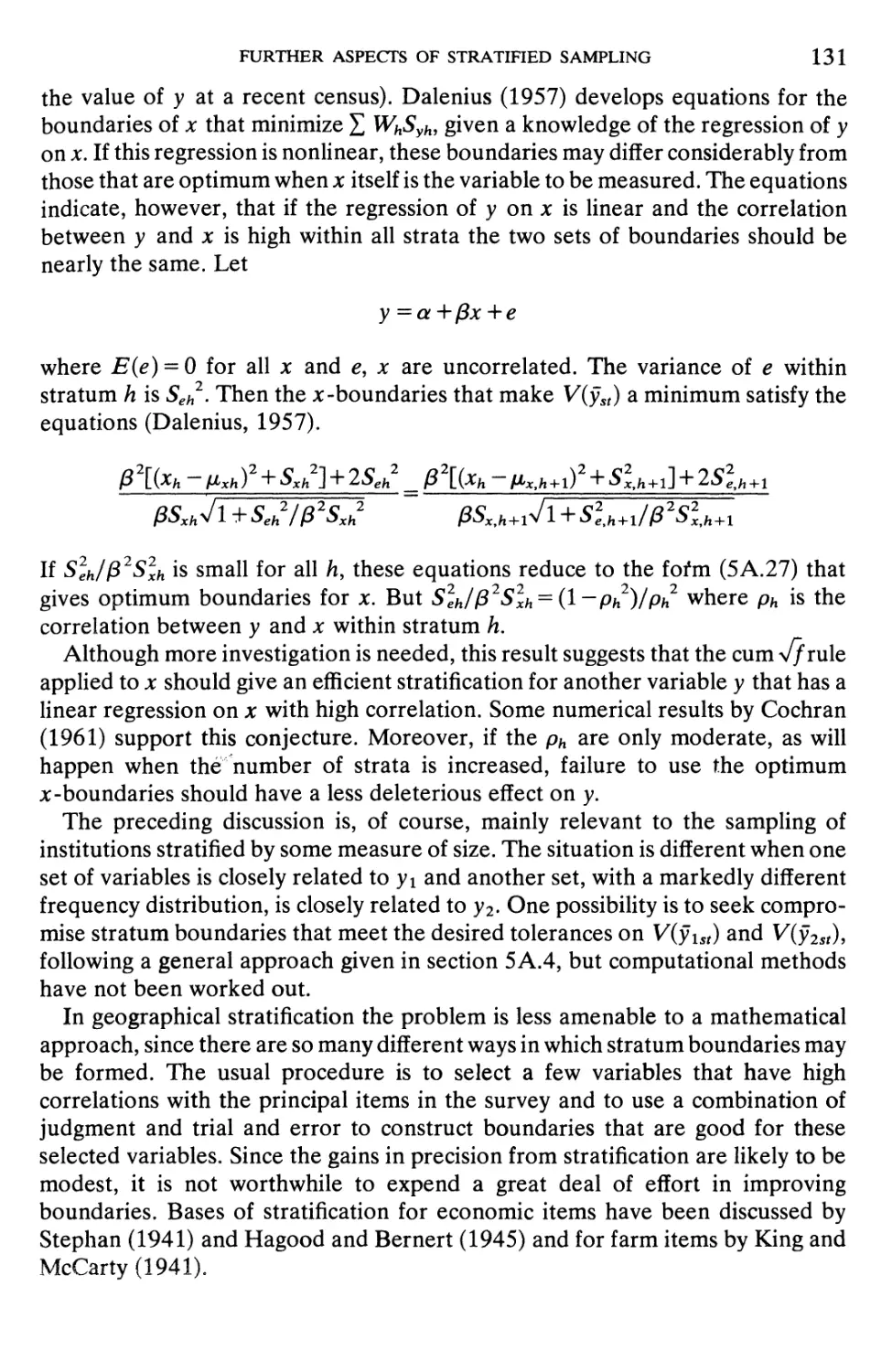


Текст
third edition
WILLIAM G. COCHRAN
Professor of Statistics, Emeritus
Harvard University
JOHN WILEY & SONS
New York • Chichester • Brisbane • Toronto • Singapore
Copyright © 1977, by John Wiley & Sons, Inc.
All rights reserved. Published simultaneously in Canada.
Reproduction or translation of any part of this work beyond that
permitted by Sections 107 or 108 of the 1976 United States
Copyright Act without the permission of the copyright owner is
unlawful. Requests for permission or further information should be
addressed to the Permissions Department, John Wiley & Sons, Inc
Library of Congress Cataloging in Publication Data
Cochran, William Gemmell, 1909
Sampling techniques.
(Wiley series in probability and mathematical statistics)
Includes bibliographical references and index.
1. Sampling (Statistics) I. Title.
QA276.6.C6 1977 001.4'222 77-728
ISBN 0-471-16240-X
Printed in the United States of America
40 39 38 37 36
to Betty
Preface
As did the previous editions, this textbook presents a comprehensive account of
sampUng theory as it has been developed for use in sample surveys. It contains
illustrations to show how the theory is appHed in practice, and exercises to be
worked by the student. The book will be useful both as a text for a course on
sample surveys in which the major emphasis is on theory and for individual
reading by the student.
The minimum mathematical equipment necessary to follow the great bulk of
the material is a familiarity with algebra, especially relatively compUcated
algebraic expressions, plus a knowledge of probability for finite sample spaces,
including combinatorial probabilities. The book presupposes an introductory statistics
course that covers means and standard deviations, the normal, binomial,
hypergeometric, and multinomial distributions, the central Hmit theorem, linear
regression, and the simpler types of analyses of variance. Since much of classical
sample survey theory deals with the distributions of estimators over the set of
randomizations provided by the sampHng plan, some knowledge of nonparamet-
ric methods is helpful.
The topics in this edition are presented in essentially the same order as in earher
editions. New sections have been included, or sections rewritten, primarily for one
of three reasons: A) to present introductions to topics (sampUng plans or methods
of estimation) relatively new in the field; B) to cover further work done during the
last 15 years on older methods, intended either to improve them or to learn more
about the performance of rival methods; and C) to shorten, clarify, or simpHfy
proofs given in previous editions.
New topics in this edition include the approximate methods developed for the
difficult problem of attaching standard errors or confidence Umits to nonlinear
estimates made from the results of surveys with complex plans. These methods
will be more and more needed as statistical analyses (e.g., regressions) are
performed on the results. For surveys containing sensitive questions that some
respondents are unlikely to be willing to answer truthfully, a new device is to
present the respondent with either the sensitive question or an innocuous
question; the specific choice, made by randomization, is unknown to the interviewer.
In some sampHng problems it may seem economically attractive, or essential in
countries without full sampHng resources, to use two overlapping Hsts (or frames,
as they are called) to cover the complete population. The method of double
sampHng has been extended to cases where the objective is to compare the means
Vll
Vlll PREFACE
of a number of subgroups within the population. There has been interesting
work on the attractive properties that the ratio and regression estimators have if it
can be assumed that the finite population is itself a random sample from an infinite
superpopulation in which a mathematical model appropriate to the ratio or
regression estimator holds. This kind of assumption is not new—I noticed
recently that Laplace used it around 1800 in a sampling problem—but it clarifies
the relation between sample survey theory and standard statistical theory.
An example of further work on topics included in previous editions is Chapter
9A, which has been written partly from material previously in Chapter 9; this was
done mainly to give a more adequate account of what seem to me the principal
methods produced for sampHng with unequal probabilities without replacement.
These include the similar methods given independently by Brewer, J. N. K. Ra,o,
and Durbin, Murthy's method, the Rao, Hartley, Cochran method, and Madow's
method related to systematic sampUng, with comparisons of the performances of
the methods on natural populations. New studies have been done of the sizes of
components of errors of measurement in surveys by repeat measurements by
different interviewers, by interpenetrating subsamples, and by a combination of
the two approaches. For the ratio estimator, data from natural populations have
been used to appraise the small-sample biases in the standard large-sample
formulas for the variance and the estimated variance. Attempts have also been
made to create less biased variants of the ratio estimator itself and of the formula
for estimating its sampHng variance. In stratified sampHng there has been
additional work on allocating sample sizes to strata when more than one item is of
importance and on estimating sample errors when only one unit is to be selected
per stratum. Some new systematic sampling methods for handling populations
having linear trends are also of interest.
Alva L. Finkner and Emil H. Jebe prepared a large part of the lecture notes
from which the first edition of this book was written. Some investigations that
provided background material were supported by the Office of Naval Research,
Navy Department. From discussions of recent developments in sampling or
suggestions about this edition, I have been greatly helped by Tore Dalenius,
David J. Finney, Daniel G. Horvitz, Leslie Kish, P. S. R. Sambasiva Rao, Martin
Sandelius, Joseph Sedransk, Amode R. Sen, and especially Jon N. K. Rao, whose
painstaking reading of the new and revised sections of this edition resulted in
many constructive suggestions about gaps, weaknesses, obscurities, and selection
of topics. For typing and other work involved in production of a typescript I am
indebted to Rowena Foss, Holly Grano, and Edith Klotz. My thanks to all.
William G. Cochran
South Orleans, Massachusetts
February, 1977
Contents
CHAPTER PAGE
1 INTRODUCTION i
1.1 Advantages of the SampUng Method 1
1.2 Some Uses of Sample Surveys 2
1.3 The Principal Steps in a Sample Survey 4
1.4 The Role of SampUng Theory 8
1.5 Probability Sampling 9
1.6 Alternatives to Probability SampHng 10
1.7 Use of the Normal Distribution 11
1.8 Bias and Its Effects 12
1.9 The Mean Square Error 15
Exercises 16
CHAPTER
2 SIMPLE RANDOM SAMPLING 18
2.1 Simple Random SampUng 18
2.2 Selection of a Simple Random Sample 19
2.3 Definitions and Notation 20
2.4 Properties of the Estimates 21
2.5 Variances of the Estimates . 23
2.6 The Finite Population Correction 24
2.7 Estimation of the Standard Error from a Sample 25
2.8 Confidence Limits 27
2.9 An Alternative Method of Proof 28
2.10 Random SampUng with Replacement 29
2.11 Estimation of a Ratio 30
2.12 Estimates of Means Over Subpopuiations 34
2.13 Estimates of Totals Over Subpopuiations 35
2.14 Comparisons Between Domain Means 39
2.15 Validity of the Normal Approximation 39
2.16 Linear Estimators of the Population Mean 44
Exercises 45
ix
X CONTENTS
CHAPTER
3 SAMPLING PROPORTIONS
AND PERCENTAGES so
3.1 Qualitative Characteristics 50
3.2 Variances of the Sample Estimates 50
3.3 The Effect of Pon the Standard Errors 53
3.4 The Binomial Distribution 55
3.5 The Hypergeometric Distribution 55
3.6 Confidence Limits 57
3.7 Classification into More than Two Classes 60
3.8 Confidence Limits with More than Two Classes 60
3.9 The Conditional Distribution of/? 61
3.10 Proportions and Totals Over Subpopulations 63
3.11 Comparisons Between Different Domains 64
3.12 Estimation of Proportions in Cluster Sampling 64
Exercises 68
CHAPTER
4 THE ESTIMATION OF SAMPLE SIZE 72
4.1 A Hypothetical Example 72
4.2 Analysis of the Problem 73
4.3 The Specification of Precision . 74
4.4 The Formula for n in Sampling for Proportions 75
4.5 Rare Items—Inverse Sampling 76
4.6 The Formula for/I with Continuous Data 77
4.7 Advance Estimates of Population Variances 78
4.8 Sample Size with More than One Item 81
4.9 Sample Size when Estimates Are Wanted for Subdivisions of the
Population 82
4.10 Sample Size in Decision Problems 83
4.11 The Design Effect (D£j90 85
Exercises 86
CHAPTER
5 STRATIFIED RANDOM SAMPLING 89
5.1 Description 89
5.2 Notation 90
5.3 Properties of the Estimates 91
5.4 The Estimated Variance and Confidence Limits 95
5.5 Optimum Allocation 96
CONTENTS XI
5.6 Relative Precision of Stratified Random and Simple Random
Sampling 99
5.7 When Does Stratification Produce Large Gains in Precision? . . . 101
5.8 Allocation Requiring More than 100 Per Cent SampHng 104
5.9 Estimation of Sample Size with Continuous Data 105
5.10 Stratified SampHng for Proportions 107
5.11 Gains in Precision in Stratified Sampling for Proportions .... 109
5.12 Estimation of Sample Size with Proportions 110
Exercises 111
CHAPTER
5 A FURTHER ASPECTS OF
STRATIFIED SAMPLING lis
5A.1 Effects of Deviations from the Optimum Allocation 115
5A.2 Effects of Errors in the Stratum Sizes 117
5 A.3 The Problem of Allocation with More than One Item ....... 119
5 A.4 Other Methods of Allocation with More than One Item 121
5 A.5 Two-Way Stratification with Small Samples 124
5A.6 Controlled Selection 126
5 A.7 The Construction of Strata 127
5A.8 Number of Strata 132
5 A.9 Stratification After Selection of the Sample (Poststratification) . . 134
5 A. 10 Quota Sampling 135
5A.11 Estimation from a Sample of the Gain Due to Stratification . . . 136
5 A. 12 Estimation of Variance with One Unit per Stratum 138
5 A. 13 Strata as Domains of Study 140
5 A. 14 Estimating Totals and Means Over Subpopulations 142
5 A. 15 Sampling from Two Frames 144
Exercises 146
CHAPTER
6 RATIO ESTIMATORS 150
6.1 Methods of Estimation 150
6.2 The Ratio Estimate 150
6.3 Approximate Variance of the Ratio Estimate 153
6.4 Estimation of the Variance from a Sample 155
6.5 Confidence Limits 156
6.6 Comparison of the Ratio Estimate with Mean per Unit 157
6.7 Conditions Under Which the Ratio Estimate Is a Best Linear
Unbiased Estimator 158
6.8 Bias of the Ratio Estimate 160
Xll CONTENTS
6.9 Accuracy of the Formulas for the Variance and Estimated
Variance 162
6.10 Ratio Estimates in Stratified Random Sampling 164
6.11 The Combined Ratio Estimate 165
6.12 Comparison of the Combined and Separate Estimates ..... 167
6.13 Short-Cut Computation of the Estimated Variance 169
6.14 Optimum Allocation with a Ratio Estimate 172
6.15 Unbiased Ratio-type Estimates 174
6.16 Comparison of the Methods 177
6.17 Improved Estimation of Variance . .^ 178
6.18 Comparison of Two Ratios 180
6.19 Ratio of Two Ratios 183
6.20 Multivariate Ratio Estimates 184
6.21 Product Estimators 186
Exercises 186
CHAPTER
7 REGRESSION ESTIMATORS 189
7.1 The Linear Regression Estimate 189
7.2 Regression Estimates with Preassigned Z? 190
7.3 Regression Estimates when ^ Is Computed from the Sample . . . 193
7.4 Sample Estimate of Variance 195
7.5 Large-Sample Comparison with the Ratio Estimate and the Mean
per Unit 195
7.6 Accuracy of the Large-Sample Formulas for V(y/r) and i;(yJ . ... 197
7.7 Bias of the Linear Regression Estimate 198
7.8 The Linear Regression Estimator Under a Linear Regression
Model 199
7.9 Regression Estimates in Stratified Sampling 200
7.10 Regression Coefficients Estimated from the Sample 201
7.11 Comparison of the Two Types of Regression Estimate 203
Exercises 203
CHAPTER
8 SYSTEMATIC SAMPLING 205
8.1 Description 205
8.2 Relation to Cluster Sampling 207
8.3 Variance of the Estimated Mean 207
8.4 Comparison of Systematic with Stratified Random SampHng ... 212
8.5 Populations in "Random" Order 212
CONTENTS Xlll
8.6 Populations with Linear Trend 214
8.7 Methods for Populations with Linear Trends 216
8.8 Populations with Periodic Variation 217
8.9 Autocorrelated Populations 219
8.10 Natural Populations 221
8.11 Estimation of the Variance from a Single Sample 223
8.12 Stratified Systematic Sampling 226
8.13 Systematic Sampling in Two Dimensions 227
8.14 Summary 229
Exercises^, 231
CHAPTER
9 SINGLE-STAGE CLUSTER SAMPLING:
CLUSTERS OF EQUAL SIZES 233
9.1 Reasons for Cluster Sampling 233
9.2 ASimpleRule 234
9.3 Comparisons of Precision Made from Survey Data 238
9.4 Variance in Terms of Intracluster Correlation 240
9.5 Variance Functions 243
9.6 A Cost Function 244
9.7 Cluster Sampling for Proportions . 246
Exercises 2 47
CHAPTER
9A SINGLE-STAGE CLUSTER SAMPLING:
CLUSTERS OF UNEQUAL SIZES 249
9A.1 Cluster Units of Unequal Sizes 249
9A.2 Sampling with Probability Proportional to Size . 250
9 A.3 Selection with Unequal Probabilities with Replacement .... 252
9A.4 The Optimum Measure of Size 255
9A.5 Relative Accuracies of Three Techniques 255
9A.6 Sampling with Unequal Probabihties Without Replacement . . . 258
9A.7 The Horvitz-Thompson Estimator 259
9A.8 Brewer's Method 261
9A.9 Murthy's Method 263
9 A. 10 Methods Related to Systematic SampHng 265
9A.11 The Rao, Hartley, Cochran Method 266
9 A. 12 Numerical Comparisons 267
9A.13 Stratified and Ratio Estimates 270
Exercises 272
Xiv CONTENTS
CHAPTER
10 SUBSAMPLING WITH UNITS OF EQUAL SIZE 274
10.1 Two-Stage Sampling 274
10.2 Finding Means and Variances in Two-Stage Sampling 275
10.3 Variance of the Estimated Mean in Two-Stage Sampling .... 276
10.4 Sample Estimation of the Variance 278
10.5 The Estimation of Proportions 279
10.6 Optimum Sampling and Subsampling Fractions 280
10.7 Estimation of m^p, from a Pilot Survey 283
10.8 Three-Stage Sampling 285
10.9 Stratified Sampling of the Units 288
10.10 Optimum Allocation with Stratified Sampling 289
Exercises 290
CHAPTER
11 SUBSAMPLING WITH UNITS OF UNEQUAL
SIZES 292
11.1 Introduction 292
11.2 SampHng Methods when n = 1 293
11.3 SampHng with Probability Proportional to Estimated Size .... 297
11.4 Summary of Methods forn = 1 299
11.5 Sampling Methods When n > 1 300
11.6 Two Useful Results 300
11.7 Units Selected with Equal Probabilities: Unbiased Estimator . . . 303
11.8 Units Selected with Equal Probabilities: Ratio to Size Estimate . . 303
11.9 Units Selected with Unequal Probabilities with Replacement:
Unbiased Estimator 306
11.10 Units Selected Without Replacement 308
11.11 Comparison of the Methods 310
11.12 Ratios to Another Variable 311
11.13 Choice of Sampling and Subsampling Fractions. Equal Prob-
abihties 313
11.14 Optimum Selection Probabilities and Sampling and Subsampling
Rates 314
11.15 Stratified SampHng. Unbiased Estimators 316
11.16 Stratified Sampling. Ratio Estimates 317
11.17 Nonlinear Estimators in Complex Surveys 318
11.18 Taylor Series Expansion 319
11.19 Balanced Repeated Replications 320
11.20 The Jackknife Method 321
11.21 Comparison of the Three Approaches . 322
Exercises 324
CONTENTS XV
CHAPTER
12 DOUBLE SAMPLING 327
12.1 Description of the Technique 327
12.2 Double Sampling for Stratification 327
12.3 Optimum Allocation 331
12.4 Estimated Variance in Double Sampling for Stratification .... 333
12.5 Double Sampling for Analytical Comparisons 335
12.6 Regression Estimators .^ 338
12.7 Optimum Allocation and Comparison with Single Sampling . . . 341
12.8 Estimated Variance in Double Sampling for Regression 343
12.9 Ratio Estimators 343
12.10 Repeated Sampling of the Same Population 344
12.11 Sampling on Two Occasions 346
12.12 Sampling on More than Two Occasions 348
12.13 Simplifications and Further Developments 351
Exercises 355
CHAPTER
13 SOURCES OF ERROR IN SURVEYS 359
13.1 Introduction 359
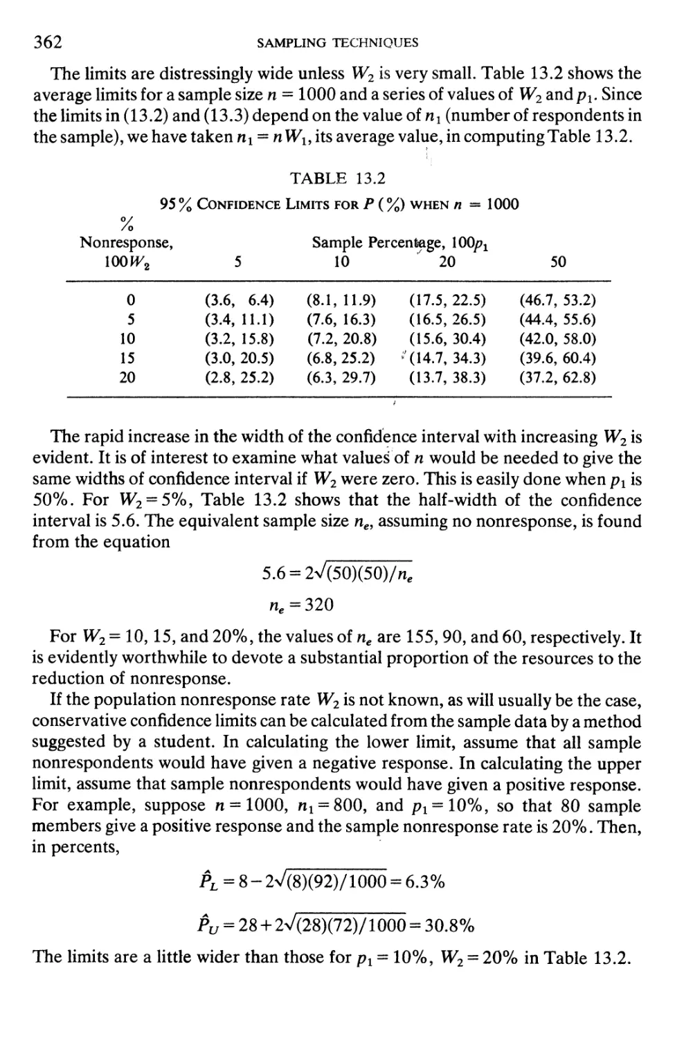
13.2 Effects of Nonresponse 359
13.3 Types of Nonresponse 364
13.4 Call-backs 365
13.5 A Mathematical Model of the Effects of Call-backs 367
13.6 Optimum Sampling Fraction Among the Nonrespondents .... 370
13.7 Adjustments for Bias Without Call-backs 374
13.8 A Mathematical Model for Errors of Measurement 377
13.9 Effects of Constant Bias 379
13.10 Effects of Errors that Are Uncorrelated Within the Sample ... 380
13.11 Effects of Intrasample Correlation Between Errors of
Measurement 383
13.12 Summary of the Effects of Errors of Measurement 384
13.13 The Study of Errors of Measurement 384
13.14 Repeated Measurement of Subsamples . . ; 386
13.15 Interpenetrating Subsamples 388
13.16 Combination of Interpenetration and Repeated Measurement . . 391
13.17 Sensitive Questions: Randomized Responses ......... 392
13.18 The Unrelated Second Question 393
13.19 Summary 395
Exercises 396
XVI CONTENTS
References 400
Answers to Exercises 412
Author Index 419
Subject Index 422
CHAPTER 1
Introduction
1.1 ADVANTAGES OF THE SAMPLING METHOD
Our knowledge, our attitudes, and our actions are based to a very large extent
on samples. This is equally true in everyday life and in scientific research. A
person's opinion of an institution that conducts thousands of transactions every
day is often determined by the one or two encounters he has had with the
institution in the course of several years. Travelers who spend 10 days in a foreign
country and then proceed to write a book telling the inhabitants how to revive
their industries, reform their political system, balance their budget, and improve
the food in their hotels are a famiUar figure of fun. But in a real sense they differ
from the political scientist who devotes 20 years to living and studying in the
country only in that they base their conclusions on a much smaller sample of
experience and are less likely to be aware of the extent of their ignorance. In
science and human affairs alike we lack the resources to study more than a
fragment of the phenomena that might advance our knowledge.
This book contains an account of the body of theory that has been built up to
provide a background for good sampling methods. In most of the applications for
which this theory was constructed, the aggregate about which information is
desired is finite and delimited—the inhabitants of a town, the machines in a
factory, the fish in a lake. In some cases it may seem feasible to obtain the
information by taking a complete enumeration or census of the aggregate.
Administrators accustomed to dealing with censuses were at first inclined to be
suspicious of samples and reluctant to use them in place of censuses. Although this
attitude no longer persists, it may be well to list the principal advantages of
sampling as compared with complete enumeration.
Reduced Cost
If data are secured from only a small fraction of the aggregate, expenditures are
smaller than if a complete census is attempted. With large populations, results
accurate enough to be useful can be obtained from samples that represent only a
small fraction of the population. In the United States the m^st important
recurrent surveys taken by the government use samples of around 105,000
1
2 SAMPLING TECHNIQUES
persons, or about one person in 1240. Surveys used to provide facts bearing on
sales and advertising policy in market research may employ samples of only a few
thousand.
Greater Speed
For the same reason, the data can be collected and summarized more quickly
with a sample than with a complete count. This is a vital consideration when the
information is urgently needed.
Greater Scope c
In certain types of inquiry highly trained personnel or specialized equipment,
Umited in availability, must be used to obtain the data. A complete census is
impracticable: the choice lies between obtaining the information by sampling or
not at all. Thus surveys that rely on sampling have more scope and flexibility
regarding the types of information that can be obtained. On the other hand, if
accurate information is wanted for many subdivisions of the population, the size of
sample needed to do the job is sometimes so large that a complete enumeration
offers the best solution.
Greater Accuracy
Because personnel of higher quality can be employed and given intensive
training and because more careful supervision of the field work and processing of
results becomes feasible when the volume of work is reduced, a sample may
produce more accurate results than the kind of complete enumeration that can be
taken.
1.2 SOME USES OF SAMPLE SURVEYS
To an observer of developments in sampling over the last 25 years the most
striking feature is the rapid increase in the number and types of surveys taken by
sampling. The Statistical Office of the United Nations publishes reports from time
to time on "Sample Surveys of Current Interest" conducted by member countries.
The 1968 report lists surveys from 46 countries. Many of these surveys seek
information of obvious importance to national planning on topics such as
agricultural production and land use, unemployment and the size of the labor force,
industrial production, wholesale and retail prices, health status of the people, and
family incomes and expenditures. But more specialized inquiries can also be
found: for example, annual leave arrangements (Australia), causes of divorce
(Hungary), rural debt and investment (India), household water consumption
(Israel), radio listening (Malaysia), holiday spending (Netherlands), age structure
of cows (Czechoslovakia), and job vacancies (United States).
Sampling has come to play a prominent part in national decennial censuses. In
the United States a 5% sample was introduced into the 1940 Census by asking
INTRODUCTION 3
extra questions about occupation, parentage, fertility, and the Uke, of those
persons whose names fell on two of the 40 lines on each page of the schedule. The
use of sampling was greatly extended in 1950. From a 20% sample (every fifth
line) information was obtained on items such as income, years in school,
migration, and service in armed forces. By taking every sixth person in the 20% sample,
a further sample of 3|% was created to give information on marriage and fertility.
A series of questions dealing with the condition and age of housing was split into
five sets, each set being filled in at every fifth house. Sampling was also employed
to speed up pubHcation of the results. Preliminary tabulations for many important
items, made on a sample basis, appeared more than a year and half before the final
reports.
This process continued in the 1960 and 1970 Censuses. Except for certain basic
information required from every person for constitutional or legal reasons, the
whole census was shifted to a sample basis. This change, accompanied by greatly
increased mechanization, resulted in much earlier pubHcation and substantial
savings.
In addition to their use in censuses, continuing samples are employed by
government bureaus to obtain current information. In the United States,
examples are the Current Population Survey, which provides monthly data on the size
and composition of the labor force and on the number of unemployed, the
National Health Survey, and the series of samples needed for the calculation of
the monthly Consumer Price Index.
On a smaller scale, local governments—city, state, and county—are making
increased use of sample surveys to obtain information needed for future planning
and for meeting pressing problems. In the United States most large cities have
commercial agencies that make a business of planning and conducting sample
surveys for clients.
Market research is heavily dependent on the sampling approach. Estimates of
the sizes of television and radio audiences for different programs and of
newspaper and magazine readership (including the advertisements) are kept
continually under scrutiny. Manufacturers and retailers want to know the reactions of
people to new products or new methods of packaging, their complaints about old
products, and their reasons for preferring one product to another.
Business and industry have many uses for sampling in attempting to increase the
efficiency of their internal operations. The important areas of quality control and
acceptance sampling are outside the scope of this book. But, obviously, decisions
taken with respect to level or change of quality or to acceptance or rejection of
batches are well grounded only if results obtained from the sample data are valid
(within a reasonable tolerance) for the whole batch. The sampling of records of
business transactions (accounts, payrolls, stock, personnel)—usually much easier
than the sampling of people—can provide serviceable information quickly and
economically. Savings can also be made through sampHng in the estimation of
inventories, in studies of the condition and length of the life of equipment, in the
4 SAMPLING TECHNIQUES
inspection of the accuracy and rate of output of clerical work, in investigating how
key personnel distribute their working time among different tasks, and, more
generally, in the field known as operations research. The books by Deming A960)
and Slonim A960) contain many interesting examples showing the range of
appUcations of the sampling method in business.
Opinion, attitude, and election polls, which did much to bring the technique of
sampHng before the public eye, continue to be a popular feature of newspapers. In
the field of accounting and auditing, which has employed sampling for many years,
a new interest has arisen in adapting modern developments to the particular
problems of this field. Thus, Neter A972) describes how airlines and railways save
money by using samples of records to apportion income from freight and
passenger service. The status of sample surveys as evidence in lawsuits has also
been subject to lively discussion. Gallup A972) has noted the major contribution
that sample surveys can make to the process of informed government by
determining quickly people's opinions on proposed or new government programs and
has stressed their role as sources of information in social science.
Sample surveys can be classified broadly into two types—descriptive and
analytical. In a descriptive survey the objective is simply to obtain certain
information about large groups: for example, the numbers of men, women, and
children who view a television program. In an analytical survey, comparisons are
made between different subgroups of the population, in order to discover whether
differences exist among them and to form or to verify hypotheses about the
reasons for these differences. The Indianapolis fertility survey, for instance, was
an attempt to determine the extent to which married couples plan the number and
spacing of children, the husband's and wife's attitudes toward this planning, the
reasons for these attitudes, and the degree of success attained (Kiser and Whelp-
ton, 1953).
The distinction between descriptive and analytical surveys is not, of course,
clear-cut. Many surveys provide data that serve both purposes. Along with the rise
in the number of descriptive surveys, there has, however, been a noticeable
increase in surveys taken primarily for analytical purposes, particularly in the
study of human behavior and health. Surveys of the teeth of school children before
and after fluoridation of water, of the death rates and causes of death of people
who smoke different amounts, and the huge study of the effectiveness of the Salk
poUo vaccine may be cited. The study by Coleman A966) on equality of
educational opportunity, conducted on a national sample of schools, contained
many regression analyses that estimated the relative contributions of school
characteristics, home background, and the child's outlook to variations in exam
results.
1.3 THE PRINCIPAL STEPS IN A SAMPLE SURVEY
As a preliminary to a discussion of the role that theory plays in a sample survey,
it is useful to describe briefly the steps involved in the planning and execution of a
INTRODUCTION 5
survey. Surveys vary greatly in their complexity. To take a sample from 5000
cards, neatly arranged and numbered in a file, is an easy task. It is another matter
to sample the inhabitants of a region where transport is by water through the
forests, where there are no maps, where 15 different dialects are spoken, and
where the inhabitants are very suspicious of an inquisitve stranger. Problems that
are baffling in one survey may be trivial or nonexistent in another.
The principal steps in a survey are grouped somewhat arbitrarily under 11
headings.
Objectives of the Survey
A lucid statement of the objectives is most helpful. Without this, it is easy in a
complex survey to forget the objectives when engrossed in the details of planning,
and to make decisions that are at variance with the objectives.
Population to be Sampled
The word population is used to denote the aggregate from which the sample is
chosen. The definition of the population may present no problem, as when
sampling a batch of electric light bulbs in order to estimate the average length of
life of a bulb. In sampling a population of farms, on the other hand, rules must be
set up to define a farm, and borderhne cases arise. These rules must be usable in
practice: the enumerator must be able to decide in the field, without much
hesitation, whether or not a doubtful case belongs to the population.
The population to be sampled (the sampled population) should coincide with
the population about which information is wanted (the target population).
Sometimes, for reasons of practicability or convenience, the sampled population is
more restricted than the target population. If so, it should be remembered that
conclusions drawn from the sample apply to the sampled population. Judgment
about the extent to which these conclusions will also apply to the target population
must depend on other sources of information. Any supplementary information
that can be gathered about the nature of the differences between sampled and
target population may be helpful.
Data to be Collected
It is well to verify that all the data are relevant to the purposes of the survey and
that no essential data are omitted. There is frequently a tendency, particularly
with human populations, to ask too many questions, some of which are never
subsequently analyzed. An overlong questionnaire lowers the quaUty of the
answers to important as well as unimportant questions.
Degree of Precision Desired
The results of sample surveys are always subject to some uncertainty because
only part of the population has been measured and because of errors of
measurement. This uncertainty can be reduced by taking larger samples and by using
6 SAMPLING TECHNIQUES
superior instruments of measurement. But this usually costs time and money.
Consequently, the specification of the degree of precision wanted in the results is
an important step. This step is the responsibility of the person who is going to use
the data. It may present difficulties, since many administrators are unaccustomed
to thinking in terms of the amount of error that can be tolerated in estimates,
consistent with making good decisions. The statistician can often help at this stage.
Methods of Measurement
There may be a choice of measuring instrument aiid of method of approach to
the population. Data about a person's state of health may be obtained from
statements that he or she makes or from a medical examination. The survey may
employ a self-administered questionnaire, an interviewer who reads a standard
set of questions with no discretion, or an interviewing process that allows much
latitude in the form and ordering of the questions. The approach may be by mail,
by telephone, by personal visit, or by a combination of the three. Much study has
been made of interviewing methods and problems (see, e.g., Hyman, 1954 and
Payne, 1951).
A major part of the preliminary work is the construction of record forms on
which the questions and answers are to be entered. With simple questionnaires,
the answers can sometimes be precoded—that is, entered in a manner in which
they can be routinely transferred to mechanical equipment. In fact, for the
construction of good record forms, it is necessary to visualize the structure of the
final summary tables that will be used for drawing conclusions.
The Frame
Before selecting the sample, the population must be divided into parts that are
called sampling units, or units. These units must cover the whole of the population
and they must not overlap, in the sense that every element in the population
belongs to one and only one unit. Sometimes the appropriate unit is obvious, as in
a population of light bulbs, in which the unit is the single bulb. Sometimes there is
a choice of unit. In sampling the people in a town, the unit might be an individual
person, the members of a family, or all persons living in the same city block. In
sampling an agricultural crop, the unit might be a field, a farm, or an area of land
whose shape and dimensions are at our disposal.
The construction of this list of sampling units, called di frame, is often one of the
major practical problems. From bitter experience, samplers have acquired a
critical attitude toward lists that have been routinely collected for some purpose.
Despite assurances to the contrary, such lists are often found to be incomplete, or
partly illegible, or to contain an unknown amount of duplication. A good frame
may be hard to come by when the population is specialized, as in populations of
bookmakers or of people who keep turkeys. Jessen A955) presents an interesting
method of constructing a frame from the branches of a fruit tree.
INTRODUCTION 7
Selection of the Sample
There is now a variety of plans by which the sample may be selected. For each
plan that is considered, rough estimates of the size of sample can be made from a
knowledge of the degree of precision desired. The relative costs and time involved
for each plan are also compared before making a decision.
The Pretest
It has been found useful to try out the questionnaire and the field methods on a
small scale. This nearly always results in improvements in the questionnaire and
may reveal other troubles that will be serious on a large scale, for example, that the
cost will be much greater than expected.
Organization of the Field Work
In extensive surveys many problems of business administration are met. The
personnel must receive training in the purpose of the survey and in the methods of
measurement to be employed and must be adequately supervised in their work. A
procedure for early checking of the quality of the returns is invaluable. Plans must
be made for handling nonresponse, that is, the failure of the enumerator to obtain
information from certain of the units in the sample.
Summary and Analysis of the Data
The first step is to edit the completed questionnaires, in the hope of amending
recording errors, or at least of deleting data that are obviously erroneous.
Decisions about computing procedure are needed in cases in which answers to
certain questions were omitted by some respondents or were deleted in the editing
process. Thereafter, the computations that lead to the estimates are performed.
Different methods of estimation may be available for the same data.
In the presentation of results it is good practice to report the amount of error to
be expected in the most important estimates. One of the advantages of probabihty
sampling is that such statements can be made, although they have to be severely
qualified if the amount of nonresponse is substantial.
Information Gained for Future Surveys
The more information we have initially about a population, the easier it is to
devise a sample that will give accurate estimates. Any completed sample is
potentially a guide to improved future sampling, in the data that it supplies about
the means, standard deviations, and nature of the variability of the principal
measurements and about the costs involved in getting the data. Sampling practice
advances more rapidly when provisions are made to assemble and record
information of this type.
There is another important respect in which any completed sample f acihtates
future samples. Things never go exactly as planned in a complex survey. The alert
8 SAMPLING TECHNIQUES
sampler learns to recognize mistakes in execution and to see that they do not occur
in future surveys.
1.4 THE ROLE OF SAMPLING THEORY
This list of the steps in a sample survey has been given in order to emphasize that
sampling is a practical business, which calls for several different types of skill. In
some of the steps—the definition of the population, the determination of the data
to be collected and of the methods of measurement, and the organization of the
field work—sampling theory plays at most a minor role. Although these topics are
not discussed further in this book, their importance should be realized. SampUng
demands attention to all phases of the activity: poor work in one phase may ruin a
survey in which everything else is done well.
The purpose of sampling theory is to make sampling more efficient. It attempts
to develop methods of sample selection and of estimation that provide, at the
lowest possible cost, estimates that are precise enough for our purpose. This
principle of specified precision at minimum cost recurs repeatedly in the
presentation of theory.
In order to apply this principle, we must be able to predict, for any sampling
procedure that is under consideration, the precision and the cost to be expected.
So far as precision is concerned, we cannot foretell exactly how large an error will
be present in an estimate in any specific situation, for this would require a
knowledge of the true value for the population. Instead, the precision of a
sampling procedure is judged by examining the frequency distribution generated
for the estimate if the procedure is applied again and again to the same population.
This is, of course, the standard technique by which precision is judged in statistical
theory.
A further simplification is introduced. With samples of the sizes that are
common in practice, there is often good reason to suppose that the sample
estimates are approximately normally distributed. With a normally distributed
estimate, the whole shape of the frequency distribution is known if we know the
mean and the standard deviation (or the variance). A considerable part of sample
survey theory is concerned with finding formulas for these means and variances.
There are two differences between standard sample survey theory and the
classical sampling theory as taught in books on mathematical statistics. In classical
theory the measurements that are made on the sampling units in the population
are usually assumed to follow a frequency distribution, for example, the normal
distribution, of known mathematical form apart from certain population
parameters such as the mean and variance whose values have to be estimated from the
sample data. In sample survey theory, on the other hand, the attitude has been to
assume only very limited information about this frequency distribution. In
particular, its mathematical form is not assumed known, so that the approach
might be described as model-free or distribution-free. This attitude is natural for
INTRODUCTION 9
large surveys in which many different measurements with differing frequency
distributions are made on the units. In surveys in which only a few measurements
per unit are made, studies of their frequency distributions may justify the
assumption of known mathematical forms, permitting the results from classical
theory to be appUed.
A second difference is that the populations in survey work contain a finite
number of units. Results are slightly more complicated when sampling is from a
finite instead of an infinite population. For practical purposes these differences in
results for finite and infinite populations can often be ignored. Cases in which this
is not so will be pointed out.
1.5 PROBABILITY SAMPLING
The sampling procedures considered in this book have the following
mathematical properties in common.
1. We are able to define the set of distinct samples, Si, ^2, • • • , 5^;, which the
procedure is capable of selecting if applied to a specific population. This means
that we can say precisely what samphng units belong to 5i, to 52, and so on. For
example, suppose that the population contains six units, numbered 1 to 6. A
common procedure for choosing a sample of size 2 gives three possible
candidates—Si ~ A,4); S2~B, 5); S3~C, 6). Note that not all possible samples
of size 2 need be included.
2. Each possible sample S, has assigned to it a known probabihty of selection
3. We select one of the S, by a random process in which each S, receives its
appropriate probability ttj of being selected. In the example we might assign equal
probabilities to the three samples. Then the draw itself can be made by choosing a
random number between 1 and 3. If this number is/, Sy is the sample that is taken.
4. The method for computing the estimate from the sample must be stated and
must lead to a unique estimate for any specific sample. We may declare, for
example, that the estimate is to be the average of the measurements on the
individual units in the sample.
For any sampling procedure that satisfies these properties, we are in a position
to calculate the frequency distribution of the estimates it generates if repeatedly
applied to the same population. We know how frequently any particular sample S,
will be selected, and we know how to calculate the estimate from the data in S/. It is
clear, therefore, that a sampling theory can be developed for any procedure of this
type, although the details of the development may be intricate. The term
probability sampling refers to a method of this type.
In practice we seldom draw a probability sample by writing down the S, and tt,
as outhned above. This is intolerably laborious with a large population, where a
sampling procedure may produce billions of possible samples. The draw is most
10 SAMPLING TECHNIQUES
commonly made by specifying probabilities of inclusion for the individual units
and drawing units, one by one or in groups until the sample of desired size and type
is constructed. For the purposes of a theory it is sufficient to know that we could
write down the 5, and tt, if we wanted to and had unlimited time.
1.6 ALTERNATIVES TO PROBABILITY SAMPLING
The following are some common types of nonprobability sampling.
1. The sample is restricted to a-part of th6'population that is readily accessible.
A sample of coal from an open wagon may be taken from the top 6 to 9 in.
2. The sample is selected haphazardly. In picking 10 rabbits from a large cage
in a laboratory, the investigator may take those that his hands rest on, without
conscious planning.
3. With a small but heterogeneous population, the sampler inspects the whole
of it and selects a small sample of "typical" units—that is, units that are close to his
impression of the average of the population.
4. The sample consists essentially of volunteers, in studies in which the
measuring process is unpleasant or troublesome to the person being measured.
Under the right conditions, any of these methods can give useful results. They
are not, however, amenable to the development of a sampHng theory that is
model-free, since no element of random selection is involved. About the only way
of examining how good one of them may be is to find a situation in which the
results are known, either for the whole population or for a probabiHty sample, and
make comparisons. Even if a method appears to do well in one such comparison,
this does not guarantee that it will do well under different circumstances.
In this connection, some of the earliest uses of sampling by country and city
governments from 1850 onward were intended to save money in making
estimates from the results of a Census. For the most important items in the Census,
the country or city totals were calculated from the complete Census data. For
other items a sample of say 15 or 25% of the Census returns was selected in order
to lighten the work of estimating country or city totals for these items. Two rival
methods of sample selection came into use. One, called random selection, was an
application of probability sampling in which each unit in the population (e.g., each
Census return) had an equal chance of being included in the sample. For this
method it was realized that by use of sampling theory and the normal distribution,
as noted previously, the sampler could predict approximately from the sample
data the amount of error to be expected in the estimates made from the sample.
Moreover, for the most important items for which complete Census data were
available, he could check to some extent the accuracy of the predictions.
The other method was purposive selection. This was not specifically defined in
detail but usually had two common features. The sampling unit consisted of
groups of returns, often relatively large groups. For example, in the 1921 Italian
INTRODUCTION 11
Census the country consisted of 8354 communes grouped into 214 districts. In
drawing a 14% sample, the Italian statisticians Gini and Galvani selected 29
districts purposively rather than 1250 communes. Second, the 29 districts were
chosen so that the sample gave accurate estimates for 7 important control
variables for which results were known for the whole country. The hope was that
this sample would give good estimates for other variables highly correlated with
the control variables.
In the 1920s the International Statistical Institute appointed a commission to
report on the advantages and disadvantages of the two methods. The report, by
Jensen A926), seemed on balance to favor purposive selection. However,
purposive selection was abandoned relatively soon as a method of sampling for
obtaining national estimates in surveys in which many items were measured. It
lacked the flexibility that later developments of probability sampling produced, it
was unable to predict from the sample the accuracy to be expected in the
estimates, and it used sampling units that were too large. Gini and Galvani
concluded that the probability method called stratified random sampling (Chapter
5), with the commune as a sampHng unit, would have given better results than
their method.
1.7 USE OF THE NORMAL DISTRIBUTION
It is sometimes useful to employ the word estimator to denote the rule by which
an estimate of some population characteristic /jl is calculated from the sample
results, the word estimate being applied to the value obtained from a specific
sample. An estimator fl of /jl given by a sampling plan is called unbiased if the
mean value of /x, taken over all possible samples provided by the plan, is equal to
/JL. In the notation of section 1.5, this condition may be written
V
Ei/1)= S 7Tiili = /L
i = \
where /Ij is the estimate given by the /th sample. The symbol E, which stands for
"the expected value of," is used frequently.
As mentioned in section 1.4, the samples in surveys are often large enough so
that estimates made from them are approximately normally distributed.
Furthermore, with probability sampling, we have formulas that give the mean and
variance of the estimates. Suppose that we have taken a sample by a procedure
known to give an unbiased estimator and have computed the sample estimate /2
and its standard deviation ap, (often called, alternatively, its standard error). How
good is the estimate? We cannot know the exact value of the error of estimate
(/1—/jl) but, from the properties of the normal curve, the chances are
0.32 (about 1 in 3) that the absolute error |/x -/x| exceeds (x^
0.05 A in 20) that the absolute error |/x -/x| exceeds 1.960-^ = 20-^
0.01 A in 100) that the absolute error |/2 -/x| exceeds 2.580-^
12 SAMPLING TECHNIQUES
For example, if a probability sample of the records of batteries in routine use in
a large factory shows an average life /x = 394 days, with a standard error cr^ = 4.6
days, the chances are 99 in 100 that the average life in the population of batteries
lies between
/I = 394-B.58)D.6) = 382 days
and
flu = 394 + B.58)D.6) = 406 days
The limits, 382 days and 406 days, are called|ower and upper confidence limits.
With a single estimate from a single survey, the statement "/x lies between 382 and
406 days" is not certain to be correct. The "99% confidence" figure implies that if
the same sampling plan were used many times in a population, a confidence
statement being made from each sample, about 99% of these statements would be
correct and 1% wrong. When sampling is being introduced into an operation in
which complete censuses have previously been used, a demonstration of this
property is sometimes made by drawing repeated samples of the type proposed
from a population for which complete records exist, so that jjl is known (see, e.g.,
Trueblood and Cyert, 1957). The practical verification that approximately the
stated proportion of statements is correct does much to educate and reassure
administrators about the nature of sampling. Similarly, when a single sample is
taken from each of a series of different populations, about 95% of the 95%
confidence statements are correct.
The preceding discussion assumes that a^^, as computed from the sample, is
known exactly. Actually, o-^, like /x, is subject to a sampling error. With a normally
distributed variable, tables of Student's / distribution are used instead of the
normal tables to calculate confidence limits for fi when the sample is small.
Replacement of the normal table by the t table makes almost no difference if the
number of degrees of freedom in o-fX exceeds 50. With certain types of stratified
sampling and with the method of replicated sampling (section 11.19) the degrees
of freedom are small and the t table is needed.
1.8 BIAS AND ITS EFFECTS
In sample survey theory it is necessary to consider biased estimators for two
reasons.
1. In some of the most common problems, particularly in the estimation of
ratios, estimators that are otherwise convenient and suitable are found to be
biased.
2. Even with estimators that are unbiased in probability sampling, errors of
measurement and nonreponse may produce biases in the numbers that we are able
to compute from the data. This happens, for instance, if the persons who refuse
to be interviewed are almost all opposed to some expenditure of public funds,
whereas those who are interviewed are split evenly for and against.
INTRODUCnON
13
0.4
0.3
0.2
0.1 -
0
-30- P -2G
-ic M 0
m
icr Q 2cr
Fig. 1.1 Effect of bias on errors of estimation.
To examine the effect of bias, suppose that the estimate /x is normally
distributed about a mean m that is a distance B from the true population value ^l,
as shown in Fig. 1.1. The amount of bias is B = m —/x. Suppose that we do not
know that any bias is present. We compute the standard deviation a of the
frequency distribution of the estimate—this will, of course, be the standard
deviation about the mean m of the distribution, not about the true mean fi. We are
using (T in place of or^. As a statement about the accuracy of the estimate, we
declare that the probability is 0.05 that the estimate /x is in error by more than
1.96C7-.
We will consider how the presence of bias distorts this probability. To do this,
we calculate the true probability that the estimate is in error by more than 1.96cr,
where error is measured from the true mean /x. The two tails of the distribution
must be examined separately. For the upper tail, the probability of an error of
more than +1.96cr is the shaded area above Q in Fig. 1.1. This area is given by
1
^
a
r oo
J/Lt + 1
-(/ii—mJ/2cr2 i a
96o-
d/1
Put (L — m = at, The lower limit of the range of integration for t is
+1.96=1.96
a
cr
Thus the area is
1
f
oo
-t^/2
V^Jl.96-(B/o-)
dt
14 SAMPLING TECHNIQUES
Similarly, the lower tail, that is, the shaded area below P, has an area
H /•-1.96-(B/o-)
yfZTrJ-oo
I
e-''/^ dt
From the form of the integrals it is clear that the amount of disturbance depends
solely on the ratio of the bias to the standard deviation. The results are shown in
Table 1.1.
TABLE 1.1
Effect of a Bias B on the Probability of an Error
Greater than 1.96 cr
Probability of Error
BJG
0.02
0.04
0.06
0.08
0.10
0.20
0.40
0.60
0.80
1.00
1.50
< -1.96G
0.0238
0.0228
0.0217
0.0207
0.0197
0.0154
0.0091
0.0052
0.0029
0.0015
0.0003
> 1.96G
0.0262
0.0274
0.0287
0.0301
0.0314
0.0392
0.0594
0.0869
0.1230
0.1685
0.3228
Total
0.0500
0.0502
0.0504
0.0508
0.0511
0.0546
0.0685
0.0921
0.1259
0.1700
0.3231
For the total probability of an error of more than 1.96cr, the bias has little effect
provided that it is less than one tenth of the standard deviation. At this point the
total probability is 0.0511 instead of the 0.05 that we think it is. As the bias
increases further, the disturbance becomes more serious. At B = o; the total
probability of error is 0.17, more than three times the presumed value.
The two tails are affected differently. With a positive bias, as in this example, the
probability of an underestimate by more than 1.96G shrinks rapidly from the
presumed 0.025 to become negUgible when B = cr. The probability of the
corresponding overestimate mounts steadily. In most applications the total error is the
primary interest, but occasionally we are particularly interested in errors in one
direction.
As a working rule, the effect of bias on the accuracy of an estimate is negligible if
the bias is less than one tenth of the standard deviation of the estimate. If we have
a biased method of estimation for which B/or < 0.1, where B is the absolute value
of the bias, it can be claimed that the bias is not an appreciable disadvantage of the
INTRODUCTION 15
method. Even with B/or = 0.2, the disturbance in the probability of the total error
is modest.
In using these results, a distinction must be made between the two sources of
bias mentioned at the beginning of this section. With biases of the type that arise in
estimating ratios, an upper limit to the ratio B/a can be found mathematically. If
the sample is large enough, we can be confident that B/cr will not exceed 0.1. With
biases caused by errors of measurement or nonresponse, on the other hand, it is
usually impossible to find a guaranteed upper limit to B/or that is small. This
troublesome problem is discussed in Chapter 13.
1.9 THE MEAN SQUARE ERROR
In order to compare a biased estimator with an unbiased estimator, or two
estimators with different amounts of bias, a useful criterion is the mean square
error (MSE) of the estimate, measured from the population value that is being
estimated. Formally,
MSE(/2) = £(/2-M)^ = £[(/x-m) + (m-/Lt)]^
= E{(i — m)^ + 2(m — iJi)E(fl — m)-^{m — /jl)^
= (variance of /2) + (bias)^
the cross-product term vanishing since E{fl - m) = 0.
Use of the MSE as a criterion of the accuracy of an estimator amounts to
regarding two estimates that have the same MSE as equivalent. This is not strictly
correct because the frequency distributions of errors (/2 -/it) of different sizes will
not be the same for the two estimates if they have different amounts of bias. It has
been shown, however, by Hansen, Hurwitz, and Madow A953) that if B/ar is less
than about one half, the two frequency distributions are almost identical in regard
to absolute errors l/x -/il of different sizes. Table 1.2 illustrates this result.
TABLE 1.2
Probability of an Absolute Error ^ 1 VmSE,
1.96VMSE AND 2,576 VMSE
Probability
Bja
0
0.2
0.4
0.6
1 VmSE
0.317
0.317
0.319
0.324
I.96VMSE
0.0500
0.0499
0.0495
0.0479
2.576 VmSE
0.0100
0.0100
0.0095
0.0083
16 SAMPLING TECHNIQUES
Even at Bja = 0.6, the changes in the probabilities as compared with those for
Bja = 0 are slight.
Because of the difficulty of ensuring that no unsuspected bias enters into
estimates, we will usually speak of the precision of an estimate instead of its
accuracy. Accuracy refers to the size of deviations from the true mean /i, whereas
precision refers to the size of deviations from the mean m obtained by repeated
application of the sampling procedure.
EXERCISES
1.1 Suppose that you were using sampling to estimate the total number of words in a
book that contains illustrations.
[a) Is there any problem of definition of the population? (lb) What are the pros and cons
of A) the page, B) the line, as a sampling unit?
1.2 A sample is to be taken from a list of names that are on cards (one name to a card)
numbered consecutively in a file. Each name is to have an equal chance of being drawn in
the sample. What problems arise in the following common situations? [a) Some of the
names do not belong to the target population, although this fact cannot be verified for any
name until it has been drawn, (loi) Some names appear on more than one card. All cards with
the same name bear consecutive numbers and therefore appear together in the file, (c)
Some names appear on more than one card, but cards bearing the same name may be
scattered anywhere about the file.
1.3 The problem of finding a frame that is complete and enables the sample to be drawn
is often an obstacle. What kinds of frames might be tried for the following surveys? Have
the frames any serious weaknesses? [a) A survey of stores that sell luggage in a large city.
(Jo) A survey of the kinds of articles left behind in subways or buses, (c) A survey of persons
bitten by snakes during the last year, (d) A survey to estimate the number of hours per week
spent by family members in watching television.
1.4 A city directory, 4 years old, fists the addresses in order along each street, and gives
the names of the persons living at each address. For a current interview survey of the people
in the city, what are the deficiencies of this frame? Can they be remedied by the
interviewers during the course of the field work? In using the directory, would you draw a
list of addresses (dwelling places) or a list of persons?
1.5 In estimating by samphng the actual value of the small items in the inventory of a
large firm, the actual and the book value were recorded for each item in the sample. For the
total sample, the ratio of actual to book value was 1.021, this estimate being approximately
normally distributed with a standard error of 0.0082. If the book value of the inventory is
$80,000, compute 95% confidence limits for the actual value..
1.6 Frequently data must be treated as a sample, although at first sight they appear to
be a complete enumeration. A proprietor of a parking lot finds that business is poor on
Sunday mornings. After 26 Sundays in operation, his average receipts per Sunday morning
are exactly $ 10. The standard error of this figure, computed from week-to-week variations,
is $ 1.2. The attendant costs $7 each Sunday. The proprietor is willing to keep the lot open at
this time if his expected future profit is $5 per Sunday morning. What is the confidence
probability that the long-term profit rate will be at least $5? What assumption must be
made in order to answer this question?
INTRODUCTION 17
1.7 In Table 1.2, what happens to the probability of exceeding IVmSE. 1.96VMSE,
and 2.576>/MSE when Bjcr tends to infinity, that is, when the MSE is due entirely to bias?
Do your results agree with the directions of the changes noted in Table 1.2 as Bjcr moves
from 0 to 0.6?
1.8 When it is necessary to compare two estimates that have different frequency
distributions of errors (/x—^t), it is occasionally possible, in specialized problems, to
compute the cost or loss that will result from an error (/2 - /li) of any given size. The estimate
that gives the smaller expected loss is preferred, other things being equal. Show that if the
loss is a quadratic function A(/x -/x,)^ of the error, we should choose the estimate with the
smaller mean square error.
CHAPTER 2
Simple Random Sampling
2.1 SIMPLE RANDOM SAMPLING
Simple random sampling is a method of selecting n units out of the N such that
-¦J
every one of the ^C„ distinct samples has an equal chance of being drawn. In
practice a simpfle random sample is drawn unit by unit. The units in the population
are numbered from 1 to N. A series of randoni numbers between 1 and N is then
drawn, either by means of a table of random numbers or by means of a computer
program that produces such a table. At any draw the process used must give an
equal chance of selection to any number in the population not already drawn. The
units that bear these n numbers constitute the sample.
It is easily verified that all ^C„ distinct samples have an equal chance of being
selected by this method. Consider one distinct sample, that is, one set of n
specified units. At the first draw the probability that some one of the n specified
units is selected is n/N. At the second draw the probability that some one of the
remaining (n — 1) specified units is drawn is (n — 1)/(N— 1), and so on. Hence the
the probability that all n specified units are selected in n draws is
n (n-1) (n-2) 1 n\{N-n)l 1 ^^ i)
• • •
N (N-1) {N-2) (N-n + 1) (AT)! ^C,
Since a number that has been drawn is removed from the population for all
subsequent draws, this method is also called random samphng without
replacement. Random sampling with replacement is entirely feasible: at any draw, all
N members of the population are given an equal chance of being drawn, no matter
how often they have already been drawn. The formulas for the variances and
estimated variances of estimates made from the sample are often simpler when
sampling is with replacement than when it is without replacement. For this reason
sampling with replacement is sometimes used in the more complex sampHng
plans, although at first sight there seems little point in having the same unit two or
more times in the sample.
18
SIMPLE RANDOM SAMPLING 19
2.2 SELECTION OF A SIMPLE RANDOM SAMPLE
Tables of random numbers are tables of the digits 0,1, 2,... 9, each digit
having an equal chance of selection at any draw. Among the larger tables are those
published by the Rand Corporation A955)—1 million digits—and by Kendall and
Smith A938)—100,000 digits. Numerous tables are available, many in standard
statistical texts. Table 2.1 shows 1000 random digits for illustration, from
Snedecor and Cochran A967).
TABLE 2.1
One Thousand Random Digits
00-04 05-09 10-14 15-19 20-24 25-29 30-34 35-39 40-44 45-49
00 54463 22662 65905 70639 79365 67382 29085 69831 47058^ 08186
01 15389 85205 18850 39226 42249 90669 96325 23248 60933 26927
02 85941 40756 82414 02015 13858 78030 16269 65978 01385 15345
03 61149 69440 11286 88218 58925 03638 52862 62733 33451 77455
04 05219 81619 10651 67079 92511 59888 84502 72095 83463 75577
05 41417 98326 87719 92294 46614 50948 64886 20002 97365 30976
06 28357 94070 20652 35774 16249 75019 21145 05217 47286 76305
07 17783 00015 10806 83091 91530 36466 39981 62481 49177 75779
08 40950 84820 29881 85966 62800 70326 84740 62660 77379 90279
09 82995 64157 66164 41180 10089 41757 78258 96488 88629 37231
10 96754 17676 55659 44105 47361 34833 86679 23930 .53249 27083
11 34357 88040 53364 71726 45690 66334 60332 22554 90600 71113
12 06318 37403 49927 57715 50423 67372 63116 48888 21505 80182
13 62111 52820 07243 79931 89292 84767 85693 73947 22278 11551
14 47534 09243 67879 00544 23410 12740 02540 54440 32949 13491
15 98614 75993 84460 62846 59844 14922 48730 73443 48167 34770
16 24856 03648 44898 09351 98795 18644 39765 71058 90368 44104
17 96887 12479 80621 66223 86085 78285 02432 53342 42846 94771
18 90801 21472 42815 77408 37390 76766 52615 32141 30268 18106
19 55165 77312 83666 36028 28420 70219 81369 41943 47366 41067
In using these tables to select a simple random sample, the first step is to number
the units in the population from 1 to N. If the first digit of AT is a number between 5
and 9, the following method of selection is adequate. Suppose N= 528, and we
want n = 10. Select three columns from Table 2.1, say columns 25 to 27. Go down
the three columns, selecting the first 10 distinct numbers between 001 and 528.
These are 36, 509, 364, 417, 348, 127, 149, 186, 290, and 162. For the last two
numbers we jumped to columns 30 to 32. In repeated selections it is advisable to
vary the starting point in the table.
20 SAMPLING TECHNIQUES
The disadvantage of this method is that the three-digit numbers 000 and 529 to
999 are not used, although skipping numbers does not waste much time. When the
first digit of N is less than 5, some may still prefer this method if n is small and a
large table of random digits is available.
With N= 128, for example, a second method that involves less rejection and is
easily applied is as follows. In a series of three-digit numbers, subtract 200 from all
numbers between 201 and 400, 400 from all numbers between 401 and 600, 600
from all numbers between 601 and 800, 800 from all numbers between 801 and
999 and, of course, 000 from all numbers between 000 and 200. All remainders
greater than 129 and the numbers 000, 2^0, and so forth, are rejected. Using
columns 05 to 07 in Table 2.1, we get 26, 52,7,94,16,48,41,80,128, and 92, the
draw requiring 15 three-digit numbers for n = 10. In this sample the rejection rate
5/15 = 33% is close to the probability of rejection 72/200 = 36% for this method.
In using this method with a number N like 384, note that one subtracts 400 from a
number between 401 and 800, but automatically rejects all numbers greater than
800. Subtraction of 800 from numbers between 801 and 999 would give a higher
probability of acceptance to remainders between 001 and 199 than to remainders
between 200 and 384.
Other methods of sampling are often preferable to simple random sampling on
the grounds of convenience or of increased precision. Simple random sampling
serves best to introduce sampling theory.
2.3 DEFINITIONS AND NOTATION
In a sample survey we decide on certain properties that we attempt to measure
and record for every unit that comes into the sample. These properties of the units
are referred to as characteristics or, more simply, as items.
The values obtained for any specific item in the N units that comprise the
population are denoted by yi, y2> ••> yN- The corresponding values for the units
in the sample are denoted by yi, y2» • • ? ym or, if we wish to refer to a typical
sample member, by y, (/ = 1, 2,..., n). Note that the sample will not consist of the
first n units in the population, except in the instance, usually rare, in which these
units happen to be drawn. If this point is kept in mind, my experience has been that
no confusion need result.
Capital letters refer to characteristics of the population and lowercase letters to
those of the sample. For totals and means we have the following definitions.
Population Sample
¦ ^—¦ ¦ ¦¦¦ ¦ ¦¦ I MM ¦¦ I — — . ¦¦¦ ¦ ^^^—»¦¦ 11 LIMIII — M^-l ¦— ¦ ¦ I ¦¦ ¦— ¦!»¦ IM ¦¦¦ ¦ —I ..—¦ | ¦¦ H M — ¦ 11 1—^—^1 ¦¦¦¦ ¦¦¦¦¦¦ ¦ ¦¦¦¦ ¦¦¦¦—¦¦¦ I ¦ ¦¦
N "
Total: y=Zy, = yi + y2+- • '-^yN Iy/ = yi+y2+- • -^yn
., ^ yi + y2+ '•• +yN ly.- - yi+y2 + ---+yn ly.
Mean: Y = — ^TT y= = —
N N n n
SIMPLE RANDOM SAMPLING 21
Although sampling is undertaken for many purposes, interest centers most
frequently on four characteristics of the population.
1. Mean = Y (e.g., the average number of children per school).
2. Total = Y (e.g., the total number of acrespf wheat in a region).
3. Ratio of two totals or means R = Y/X= Y/X (e.g., ratio of liquid assets to
total assets in a group of famiUes).
4. Proportion of units that fall into some defined class (e.g., proportion of
people with false teeth).
Estimation of the first three quantities is discussed in this chapter.
The symbol ^ denotes an estimate of a population characteristic made from a
sample. In this chapter only the simplest estimators are considered.
Estimator
Population mean Y Y=y = sample mean
n
Population total Y Y=Ny=N'Z yjn
n
Population ratio R R = y/x = X yi/ Z ^i
In Y the factor N/n by which the sample total is multiplied is sometimes called
the expansion or raising or inflation factor. Its inverse n/N, the ratio of the size of
the sample to that of the population, is called the sampling fraction and is denoted
by the letter /.
2.4 PROPERTIES OF THE ESTIMATES
The precision of any estimate made from a sample depends both on the method
by which the estimate is calculated from the sample data and on the plan of
sampling. To save space we sometimes write of "the precision of the sample
mean" or "the precision of simple random sampling," without specifically
mentioning the other fundamental factor. This has been done, we hope, only in
instances in which it is clear from the context what the missing factor is. When
studying any formula that is presented, the reader should make sure that he or she
knows the specific method of sampling and method of estimation for which the
formula has been established.
In this book a method of estimation is called consistent if the estimate becomes
exactly equal to the population value when n = N, that is, when the sample
consists of the whole population. For simple random sampling it is obvious that y
and Ny are consistent estimates of the population mean and total, respectively.
Consistency is a desirable property of estimators. On the other hand, an
inconsistent estimator is not necessarily useless, since it may give satisfactory precision
when n is small compared to N, Its utility is likely to be confined to this situation.
22 SAMPLING TECHNIQUES
Hansen, Hurwitz, and Madow A953) and Murthy A967) give an alternative
definition of consistency, similar to that in classical statistics. An estimator is
consistent if the probability that it is in error by more than any given amount tends
to zero as the sample becomes large. Exact statement of this definition requires
care with complex survey plans.
As we have seen, a method of estimation is unbiased if the average value of the
estimate, taken over all possible samples of given size n, is exactly equal to the true
population value. If the method is to be unbiased without qualification, this result
must hold for any population of finite values y, and for any n. To investigate
whether y is unbiased with simple random sanipUng, we calculate the value of y
for all j^Cn samples and find the average of the estimates. The symbol E denotes
this average over all possible samples.
Theorem 2.1. The sample mean y is an unbiased estimate of Y.
Proof. By its definition
r7^^Iy^I(yi+y2+-"+yn) ,^^.
NCn n[Nl/nm-n)\] ^ ^ ^
where the sum extends over all /^„ samples. To evaluate this sum, we find out in
how many samples any specific value y, appears. Since there are (N-1) other
units available for the rest of the sample and (n-1) other places to fill in the
sample, the number of samples containing y^ is
(N-l)!
(n-iyXN-nV.
N-lCn-l— y -iM/xr M B.3)
Hence
V/ N (N-1)! ,
I(yi+y2 4- • -^yn)=(^,i)!(^_^)!(yi+y2+- • -^y^)
From B.2) this gives
(N-1)! nl(N-n)\,
^>' = (n-l)!(N-n)! nNl (>'' + >'^+-"-^y-)
Jll±yi±-LLtyHl=Y B.4)
Corollary. Y=Ny is an unbiased estimate of the population total Y,
A less cumbersome proof of theorem 2.1 is obtained as follows. Since every unit
appears in the same number of samples, it is clear that
^(y 1 + y2 + • • • + yn) must be some multiple of yi + y2 + • • • + y^^ B.5)
The multiplier must be n/N, since the expression on the left has n terms and that
on the right has N terms. This leads to the result.
SIMPLE RANDOM SAMPLING 23
2.5 VARIANCES OF THE ESTIMATES
The variance of the y, in a finite population is usually defined as
As a matter of notation, results are presented in terms of a slightly different
expression, in which the divisor (N-1) is used instead of N. We take
5'=n^rr- B-7)
This convention has been used by those who approach sampling theory by means
of the analysis of variance. Its advantage is that most results take a slightly simpler
form. Provided that the same notation is maintained consistently, all results are
equivalent in either notation.
We now consider the variance of y. By this we mean E{y - Yf taken over all
;vC„ samples.
Theorem 2.2. The variance of the mean y from a simple random sample is
V{y)^E{y-Yf--^^^--(\-f) B.8)
n N n
where / = n/N is the sampling fraction.
Proof.
«(y-iO = (yi-iO+(y2-?) + ---+(yn-y) B.9)
By the argument of symmetry used in relation B.5), it follows that
E[iy,-Y)^+- ¦¦+{y„-m=-^[iyi-Y)'+- ¦ ¦ + (y^-Yr] B.10)
and also that
E[iy^-Y)(y2- Y)^iy,-Y)(y,- Y)+ • • • +(yn-i- iO(yn" ?)]
+ ...+(y^_i~y)(y^-Y)] B.11)
In B.11) the sums of products extend over all pairs of units in the sample and
population, respectively. The sum on the left contains n(n-1)/2 terms and that
on the right contains N{N-1)/2 terms.
24
SAMPLING TECHNIQUES
Now square B.9) and average over all simple random samples. Using B.10) and
B.11), we obtain
n'E{y-Yf = ^\
<y\2
(yi-Y)'+---+(yN-n
+2^^[(yi - y)(y2 - f) + • • • + (y;v-i - y)(y,^ - ?)]
N-1
Completing the square on the cross-product term, we have
The second term inside the curly bracket vanishes, since the sum of the y, equals
NY, Division by n^ gives
V(y) = £(y-Y) = ^./^r '.x L^yi-y) =
niV(iV-l)A
This completes the proof,
CoroOary 1. The standard error of y is
n N
ay = -W(iV- n)/N= '-F^>n--f
vn vrt
B.12)
Corollary 2. The variance of Y = Ny, as an estimate of the population total Y, is
r2o2
2r.2
V(Y) = E(Y-'Y)^ =
N^S^iN-n) N'-S
n N
Corollary 3. The standard error of Y is
NS, NS
-^iN-n)/N=-j=
V/1 V«
n
A-/)
B.13)
o-y =-^-v (iV-n)/Ar= ^:rVl-/
B.14)
2.6 THE FINITE POPULATION CORRECTION
For a random sample of size n from an infinite population, it is well known that
the variance of the mean is or^/n. The only change in this result when the
population is finite is the introduction of the factor {N-n)/N. The factors
{N- n)/N for the variance and V(N-n)/Nfor the standard error are called the
finite population corrections (fpc). They are given with a divisor (iV— 1) in place of
N by writers who present results in terms of cr. Provided that the sampling fraction
n/N remains low, these factors are close to unity, and the size of the population as
SIMPLE RANDOM SAMPLING 25
such has no direct effect on the standard error of the sample mean. For instance, if
5 is the same in the two populations, a sample of 500 from a population of 200,000
gives almost as precise an estimate of the population mean as a sample of 500 from
a population of 10,000. Persons unfamiliar with sampling often find this result
difficult to believe and, indeed, it is remarkable. To them it seems intuitively
obvious that if information has been obtained about only a very small fraction of
the population, the sample mean cannot be accurate. It is instructive for the reader
to consider why this point of view is erroneous.
In practice the fpc can be ignored whenever the sampling fraction does not
exceed 5% and for many purposes even if it is as high as 10%. The effect of
ignoring the correction is to overestimate the standard error of the estimate y.
The following theorem, which is an extension of theorem 2.2, is not required for
the discussion in this chapter, but it is proved here for later reference.
Theorem 2.3. If y,, Xi are a pair of variates defined on every unit in the
population and y, x are the corresponding means from a simple random sample of
size n, then their covariance
Eiy -Y){x-X) = ^ -i- I (y, - Y)(x, -X) B.15)
This theorem reduces to theorem 2.2 if the variates y„ jc, are equal on every unit.
Proof. Apply theorem 2.2 to the variate Ui = y^ + x,. The population mean of w,
is U= F+X, and theorem 2.2 gives
nN TV—l,=i
that is
£[(y--Y) + (jc-X)f = ^-^ l[(yi-Y) + ix,-X)f B.16)
Expand the quadratic terms on both sides. By theorem 2.2,
with a similar relation for E{x - X) . Hence these two terms cancel on the left and
right sides of B.16). The result of the theorem (equation 2.15) follows from the
cross-product terms.
2.7 ESTIMATION OF THE STANDARD ERROR
FROM A SAMPLE
The formulas for the standard errors of the estimated population mean and
total are used primarily for three purposes: A) to compare the precision obtained
by simple random sampling with that given by other methods of sampling, B) to
26 SAMPLING TECHNIQUES
estimate the size of the sample needed in a survey that is being planned, and C) to
estimate the precision actually attained in a survey that has been completed. The
formulas involve 5^, the population variance. In practice this will not be known,
but it can be estimated from the sample data. The relevant result is stated in
theorem 2.4.
Theorem 2.4. For a simple random sample
n
liyt-yy
s' = ^
n-l
is an unbiased estimate of
I (y,- - Y)'
s'=^
Nt-l
Proof. We may write
s^=-^i[(y>-Y)-iy-Y)f B.17)
n-l,=i
1 r"
n-l
liyi-Y)^-niy-W] B.18)
1 = 1 J
Now average over all simple random samples of size n. By the argument of
symmetry used in theorem 2.2,
4l(y.-i0i=^I(y,-y)^=^^5^
_i = V J iV , = 1 IS
by the definition of S . Furthermore, by theorem 2.2,
Hence
Eis') = -^~^n(N-l)-iN-n)]^S' B.19)
Corollary. Unbiased estimates of the variances of y and Y=Ny aie
viy-) = s/=-(^)=-{l-f) B.20)
n \ N / n
„(y) = ,/ = __(_-j=__(l-;) B.21)
SIMPLE RANDOM SAMPLING 27
For the standard errors we take
s , Ns ,
5y=-Wl-/, 5^ = _Vl-/ B.22)
These estimates are slightly biased: for most applications the bias ijs unimportant.
The reader should note the symbols employed for true and estimated variances
of the estimates. Thus, for y, we write
2
True variance: V(y) = o-y
Estimated variance: v{y) = s^
2.8 CONFIDENCE LIMITS
It is usually assumed that the estimates y and Y are normally distributed about
the corresponding population values. The reasons for this assumption and its
limitations are considered in section 2.15. If the assumption holds, lower and
upper confidence limits for the population mean and total are as follows:
Mean:
?L = y-7=Vw, yt, = y+^Vi-/ B.23)
vn sn
Total:
tNs . ^ tNs I
y^ = iVy-^>/l-/, y^ = Ny+^Vl-/ B.24)
The symbol t is the value of the normal deviate corresponding to the desired
confidence probability. The most common values are
Confidence probability (%) 50 80 90 95 99
0.67 1.28 1.64 1.96 2.58
If the sample size is less than 50, the percentage points may be taken from
Student's t table with (n-l) degrees of freedom, these being the degrees of
freedom in the estimated variance s^. The t distribution holds exactly only if the
observations y, are themselves normally distributed and N is infinite. Moderate
departures from normality do not affect it greatly. For small samples with very
skew distributions, special methods are needed.
Example, Signatures to a petition were collected on 676 sheets. Each sheet had enough
space for 42 signatures, but on many sheets a smaller number of signatures had been
collected. The numbers of signatures per sheet were counted on a random sample of 50
sheets (about a 7% sample), with the results shown in Table 2.2.
Estimate the total number of signatures to the petition and the 80% confidence limits.
28
SAMPLING TECHNIQUES
The sampling unit is a sheet, and the observations y^ are the numbers of signatures per
sheet. Since about half the sheets had the maximum number of signatures, 42, the data are
presented as a frequency distribution. Note that the original distribution appears to be far
from normal, the greatest frequency being at the upper end. Nevertheless, there is reason to
believe from experience that the means of samples of 50 are approximately normally
distributed.
We find
n=I/; = 50, y = I/;y, = 1471, I/,y,^ = 54,497
Hence the estimated total number of signatures is
F76)A471) ^
Y = Ny=- ^-zz ^=19,888
50
For the sample variance 5^ we have
1
n-1
491
54,497
A471)n_
49L' ' 50 J
From B.22) the 80% confidence limits are
= 229.0
tNs , A.28)F76)A5.13)Vl-0.0740
19,888±-7=rVl-/=19,888± -=
Vn V50
This gives 18,107 and 21,669 for the 80% limits. A complete count showed 21,045
signatures.
TABLE 2.2
Results for a Sample of 50 Petition Sheets y^ = Number of Signatures: fi =
Frequency
yi
fi
yt
fi
42
23
14
1
41
4
11
1
36
1
10
1
32
1
9
1
29
1
7
1
27
2
6
3
23
1
5
2
19
1
4
1
16
2
3
1
15
2
Total
50
2.9 AN ALTERNATIVE METHOD OF PROOF
Cornfield A944) suggested a method of proving the principal results for simple
random sampling without replacement that enables us to use standard results
from infinite population theory. Let a, be a random variate that takes the value 1 if
the ith unit is in the sample and the value 0 otherwise. The sample mean y may be
written
1 ^
y=- Z ^iyi
B.25)
SIMPLE RANDOM SAMPLING 29
where the sum extends over all N units in the population. In this expression the a,
are random variables and the y, are a set of fixed numbers.
Clearly
Pr(a, = l) = ^, Pr(a, = 0) = l~^
Thus Ui is distributed as a binomial variate in a single trial, with P = n/N, Hence
Eia,) = P = ^, V(a,) = PO = ^[l-^ B.26)
To find V(y) we need also the covariance of a, and Uj. The product aiUj is 1 if the
ith and /th unit are both in the sample and is zero otherwise. The probabihty that
two specific units are both in the sample is easily found to he n{n — 1)/N{N— 1).
Hence
Cov (a,ay) = EiaiUj)—E{ai)E{aj)
NiN-1) \N/ N{N-1)\ NJ ^ ¦"
Applying this approach to find V(y), we have, from B.25),
Viy) = Af I yi" Via,)+2 I y,yj Cov (a^aj)] B.28)
using B.26) and B.27). Completing the square on the cross-product term gives
- ^'^ Z(y.-y)^=^i^=^ B.31)
n(Af-l)^'-" ' n
The method gives easy proofs of theorems 2.3 and 2.4. It may be used to find
higher moments of the distribution of y, although for this purpose a method given
by Tukey A950), with further development by Wishart A952), is more powerful.
2.10 RANDOM SAMPLING WITH REPLACEMENT
A similar approach applies when sampling is with replacement. In this event the
Ith unit may appear 0,1, 2,..., n times in the sample. Let /, be the number of
times that the fth unit appears in the sample. Then
y=-iuy, B.32)
=1
30 SAMPLING TECHNIQUES
Since the probability that the ith unit is drawn is 1/N at each draw, the variate
ti distributed as a binomial number of successes out of n trials with p = l/N.
Hence
E(,) = ^^ V(t.) = n{j^)(l-j^) B.33)
Jointly, the variates r, follow a multinomial distribution. For this,
n.
Cow (titj) = -j^^ B.34)
Using B.32), B.33), and B.34), we have, for sampling with replacement.
v(y) = ^
^ 2n{N~l) ^ n
n%=i'' AT ^ -i-^r^'N^J
1 ^ . ,-v^ ' cr^ N-1 S
B.35)
^Z (y.-y)' = - = -rr- B.36)
nN i=i n N n
Consequently, V(y) in sampHng without replacement is only (N-n)/{N—l)
times its value in sampling with replacement. If instead of y the mean ya of the
different or distinct units in the sample is used as an estimate when sampling is with
replacement, Murthy A967) has shown that the leading term in the average
variance of yd is (l-//2M^/n, following work by Basu A958) and Des Raj and
Khamis A958). In some applications the cost of measuring the distinct units in the
sample may be predominating, so that the cost of the sample is proportional to the
number of distinct units. In this situation, Seth and J. N. K. Rao A964) showed
that for given average cost, V{y) in sampling without replacement is less than
V(yd) in sampling with replacement. They also prove the more general result that
if y^' = f{v)yd/Ef{v), where v is the number of jdistinct units in the sample and/(^)
is a function of v, then V{y) < V{yd) if 5^ < NY^, a condition satisfied by nearly all
populations encountered in sample surveys.
2.11 ESTIMATION OF A RATIO
Frequently the quantity that is to be estimated from a simple random sample
is the ratio of two variables both of which vary from unit to unit. In a household
survey examples are the average number of suits of clothes per adult male, the
average expenditure on cosmetics per adult female, and the average number of
hours per week spent watching television per child aged 10 to 15. In order to
estimate the first of these items, we would record for the /th household (/ =
1, 2,..., n) the number of adult males jc, who live there and the total number of
SIMPLE RANDOM SAMPLING 31
suits yt that they possess. The population parameter to be estimated is the ratio
N
Yy.
_ total number of suits _ j [
total number of adult males ^
LXi
1
The corresponding sample estimate is
n
R=j;— = t B.38)
1
Examples of this kind occur frequently when the sampling unit (the household)
comprises a group or cluster of elements (adult males) and our interest is in the
population mean per element. Ratios also appear in many other applications, for
example, the ratio of loans for building purposes to total loans in a bank or the
ratio of acres of wheat to total acres on a farm.
The sampling distribution of jR is more complicated than that of y because both
the numerator y and the denominator x vary from sample to sample. In small
samples the distribution of R is skew and R is usually a slightly biased estimate of
R, In large samples the distribution of jR tends to normality and the bias becomes
negligible. The following approximate result will serve for most purposes: the
distribution of R is studied in more detail in Chapter 6.
Theorem 2.5. If variates y„ Xt are measured on each unit of a simple random
sample of size «, assumed large, the MSB and variance of J? = y/x are each
approximately
..iiy-Rxif
MSE(^) = V{R) = -^ '^' B.39)
nX N-\
where R = Y/X is the ratio of the population means and / = n/N.
Proof.
A ^ y ^ y—Rx ,^ ,^^
R-R=--R--- B.40)
X X
If n is large, x should not differ greatly from X. In order to avoid having to work
out the distribution of the ratio of two random variables (y-Rx) and jc, we replace
JC by X in the denominator of B.40) as an approximation. This gives
R-R^^^ B.41)
32 SAMPLING TECHNIQUES
Now average over all simple random samples of size n,
^.A r,x E{y-Rx) Y-RX ^
E{R-^R)= ^^^ ^ = —^— = 0
since R = Y/X This shows that to the order of approximation used here R is an
unbiased estimate of R.
From B.41) we also obtain the result
MSE,«,=^(^-«,'.^^„-«fl' B.43)
The quantity y-^Rx is the sample mean of the variate di = yi—Rxi, whose
population mean D = Y—RX = 0. Hence we can find V{R) by applying theorem
2.2 for the variance of the mean of a simple random sample to the variate di and
dividing by X . This gives
V{R) = l-^E{y-Rxf = i — A -/) B.44)
1-//=! = lzLizL
nX^ (N-1) ~nX^ N-l
B.45)
This completes the proof.
The way in which theorem 2.5 was proved is worth noting. It was shown that the
formula in theorem 2.2 for the variance of the sample mean y gives the formula for
the approximate variance of the ratio y/x, if the variate y, is replaced by the
variate (y^ —Rxi)/X. The same result, or its natural extension, holds also in more
complex sampling situations and is used frequently later in this book.
As a sample estimate of
iiVi-Rxif
i = \
N-l
it is customary to take
iiyi-Rx<f
1 = 1
n-l
This estimate can be shown to have a bias of order 1/n.
For the estimated standard error of R, this gives
.(^..^/^SiEM ,2.46)
SIMPLE RANDOM SAMPLING 33
If X is not known, the sample estimate x is substituted in the denominator.
One way to compute siR) is to express it as
VnAT^ n-1
Example. Table 2.3 shows the number of persons (xi), the weekly family income (jcj),
and the weekly expenditure on food (y) in a simple random sample of 33 low-income
families. Since the sample is small, the data are intended only to illustrate the calculations.
Estimate from the sample (a) the mean weekly expenditure on food per family, (b) the
mean weekly expenditure on food per person, and (c) the percentage of the income that is
spent on food. Compute the standard errors of these estimates.
Weekly Expenditure on Food per Family. This is the ordinary sample mean
907.2 ^^^ ^^
By theorem 2.2 (ignoring the fpc), its standard error is
Sy--
_ 1
n -
1
-yf
-1
/7.8.?;
Jn
7.4-
1
{n-
rQO'
-1)^
i.-yy
kv?-
/33 = i
(E y,?
n
U.76
VC3)C2)
(The uncorrected sum of squares 28,224 is given underneath Table 2.3.)
Weekly Expenditure on Food per Person. Since the size of family varies, the estimate is a
ratio of two variables,
. ly 907.2
i<i=z;— = ——— = S7.38perperson
2-^1 123
The sums of squares and products needed to compute S{R) by B.47) are found under
Table 2.3. We need in addition
^ 2_
2i?i = 14.7512, i?/ = 54.3996, x^ = 3.7273
^ 2
Extra decimals are carried in Ru 2Ri, R^ to preserve accuracy.
Hence, from B.47),
5(i?i) =
/_B8,224) - A4.7512)C595.5) 4- E4.3996)E33)
>/33C.7273) ^ 32
= $0,534
Percentage of Income Spent on Food. This again is a ratio of two variables
Iy^A00)(907.2)
Ijc2 2394
By B.47) the reader may verify that the standard error is 2.38%.
i?2 = 100£^ = ^—:^^T- = 37.9%
34
SAMPLING TECHNIQUES
TABLE 2.3
Size, Weekly Income, and Food Cost of 33 Families
Family
Number
1
2
3
4
5
6
7
8
9
10
11
12
13
14
15
16
17
Size
^1
2
3
3
5
4
7
2
4
2
5
3
6
4
4
2
5
3
Income
^2
62
62
87
65
58
92
88
79
83
62
63
62
60
75
90
75
69
Food
Cost
y
14.3
20.8
11,1
30.5
41.2
28.2
24.2
30.0
24.2
44.4
13.4
19.8
29.4
27.1
22.2
31.1
22.6
Family
Number
18
19
20 ,
21 '
11
23
24
25
26
27
28
29
30
31
32
33
Total
Size
^1
4
2
4
2
5
3
4
7
3
3
6
2
2
6
4
2
123
Income
X2
83
85
73
66
58
11
69
65
11
69
95
11
69
69
67
63
2394
Food
Cost
2/
36.0
20.6
11,1
25.9
23.3
39.8
16.8
37.8
34.8
28.7
63.0
19.5
21.6
18.2
20.1
20.7
907.2
Ijci^ = 533, 1^:2^=177,254, Sy^ = 28,224
I Xiy = 3595.5, I X2y = 66,618
2.12 ESTIMATES OF MEANS OVER SUBPOPULATIONS
In many surveys, estimates are made for each of a number of classes into which
the population is subdivided. In a household survey separate estimates might be
wanted for families with 0,1, 2,... children, for owners and renters, or for
families in different occupation groups. The term domains of study has been given
to these subpopulations by the U.N. Subcommission on Sampling A950).
In the simplest situation each unit in the population falls into one of the
domains. Let the /th domain contain A/, units, and let«/ be the number of units in a
simple random sample of size n that happen to fall in this domain. If yy^
(fc = 1, 2,..., «;) are the measurements on these units, the population mean Yj
for the /th domain is estimated by
n.
y,= I —
fc=i ftj
B.48)
SIMPLE RANDOM SAMPLING 35
At first sight yy seems to be a ratio estimate as in section 2.11. Although n is
fixed, Hj will vary from one sample of size n to another. The complication of a ratio
estimate can be avoided by considering the distribution of y, over samples in
which both n and /ly are fixed. We assume ny >0.
In the totaUty of samples with given n and rij the probability that any specific set
of rij units from the Nj units in domain / is drawn is
N-NjCn-rij _ 1
Since each specific set of rtj units from domain/ can appear with all selections of
{n — rij) units from the (N—rij) that are not in domain/, the numerator above is the
number of samples containing a specified set of rij, and the denominator is the total
number of samples. It follows that theorems 2.1, 2.2, and 2.4 apply to the yjk if we
put rij for n and Nj for N.
From theorem 2.1: yj is an unbiased estimate of Yj B.49)
S ^
From theorem 2.2: the standard error of yj is -7=vl - (rij/Nj) B.50)
Vrty
where
Sj'=l ^^t 7 B.51)
fc = l /Vy — i
From theorem 2.4: An estimate of the standard error of yj is
^l-irij/Nj) B.52)
yJrij
where
2^ 2 OViZ^ B.53)
If the value of Nj is not known, the quantity n/N may be used in place of rij/Nj
when computing the fpc. (With simple random sampling, rij/Nj is an unbiased
estimate of n/N)
2.13 ESTIMATES OF TOTALS OVER SUBPOPULATIONS
In a firm's list of accounts receivable, in which some accounts have been paid
and some not, we might wish to estimate by a sample the total dollar amount of
unpaid bills. If Nj (the number of unpaid bills in the population) is known, there is
no problem. The sample estimate is Njyj and its conditional standard error is Nj
times expression B.50).
36 SAMPLING TECHNIQUES
Alternatively, if the total amount receivable in the list is known, a ratio estimate
can be used. The sample gives an estimate of the ratio (total amount of unpaid
bills)/(total amount of all bills). This is multiplied by the known total amount
receivable in the list.
If neither Nj nor the total receivables is known, these estimates cannot be made.
Instead, we multiply the sample total of the y's over units falling in the/th domain
by the raising factor N/n. This gives the estimate
- N "'¦
yj=-l yjk . B.54)
We will show that Yj is unbiased and obtain its standard error over repeated
samples of size n. The device of keeping rij fixed as well as n does not help in this
problem.
In presenting the proof we revert to the original notation, in which y, is the
measurement on the /th unit in the population. Define for every unit in the
population a new variate y/, where
(yi if the unit is in the /th domain,
lo otherwise
The population total of the y/ is
Zy/= Z yi = Yj B.55)
1 = 1 /th dom
In a simple random sample of size n, y/ = y, for each of the rij units that lie in the
/th domain; y/' = 0 for each of the remaining n-rij units. If y' is the ordinary
sample mean of the y,', the quantity
A/" " N "^'
iVy' = -Zy/ = - I yj, = Yj B.56)
n 1=1 n k=i
This result shows that the estimate Yj as defined in equation B.54) is N times
the sample mean of the y/.
In repeated samples of size n we can clearly apply theorems 2.1,2.2, and 2.4 to
the variates y,'. These show that Yj is an unbiased estimate of Yj with standard
error
NS'
cr(Yj) = -j=-Jl-(n/N) B.57)
wliere 5' is the population standard deviation of the y/. In order to compute S\ we
regard the population as consisting of the Nj values y, that are in the /th domain
SIMPLE RANDOM SAMPLING 37
and of N—Nj zero values. Thus
From theorem 2.4 a sample estimate of the standard error of Yj is
s(Yj) = -j=ry/l^{n/N) B.59)
In computing s', any unit not in the yth domain is given a zero value. Some students
seem to have a psychological objection to doing this, but the method is sound.
The methods of this and the preceding section also apply to surveys in which the
frame used contains units that do not belong to the population as it has been
defined. An example illustrates this application.
Example. From a list of 2422 minor household expenditures a simple random sample
of 18.0 items was drawn in order to estimate the total spent for operation of the household.
Certain types of expenditure (on clothing and car upkeep) were not considered relevant. Of
the 180 sample items, 152 were relevant. The sum and uncorrected sum of squares of the
relevant amounts (in dollars) were as follows.
Zy/ = 343.5, Zy,'2= 1491.38
Estimate the total expenditure for household operation and give the standard error of the
estimate.
From B.59)
. N" , B422)C43.5)
Yj=- ly. = — = $4622
n i=i 180
Ns'
s{Y,) = —^l-{n/N)
y/n
In computing s' we regard our sample of 180 items as having 28 zeros. Hence
79) L^^' 180 J
s'^ =
A79) r
= ^[1491.38-^1 = 4.670
A79R 180 J
A79)L 180
Finally,
The estimate is not precise, its coefficient of variation 375/4622 being about 8%.
In this example expenditures on car upkeep and clothing were excluded as not
relevant and therefore were scored as zeros in the sample. In some applications it
38 SAMPLING TECHNIQUES
is known in advance that certain units in the population contribute nothing to the
total that is being estimated. For instance, in a survey of stores to estimate total
sales of luggage, some stores do not handle luggage; certain area sampling units
for farm studies contain no farms. Sometimes it is possible, by expenditure of
effort, to identify and count the units that contribute nothing, so that in our
notation (N-Nj), hence N,, is known.
Consequently it is worth examining by how much V{Yj) is reduced when Nj is
known. If TV, is not known, B.57) gives
If Yj and 5, are the mean and standard deviation in the domain of interest (i.e.,
among the nonzero units) the reader may verify that
(N- l)S'^ = (Nj - l)Sf+NjYfl^l-^) B.60)
Since terms in 1/Nj and 1/N are nearly always negligible,
S'^ = PjSl+PjQjY^ B.61)
where Pj - Nj/N and Oy = 1 - Pj. This gives
v(y;.) ^^(p,5^^+p,•0,y;.^)(l-^) B.62)
If nonzero units are identified, we draw a sample of size rij from them. The
estimate of the domain total is A/}y/ with variance
my,)-f5»(.-^).^P,'5/(l-i) ,2.63)
The comparable variances are B.62) and B.63). In B.62) the average number of
nonzero units in the sample of size n is nPj. If we take rij = nPj in B.63), so that the
number of nonzeros to be measured is about the same with both methods, B.63)
becomes
VGV,.y,) = ^/>,5/(l-^) B.64)
The ratio of the variances B.64) to B.62) is
V{Nj known) 5/ Cj
V{Nj not known) Sf + Q Yf Cf 4- Oy
B.65)
where Cy = 5y/ Yj is the coefficient of variation among the nonzeros. As might be
expected, the reduction in variance due to a knowledge of A^ is greater when the
proportion of zero units is large and when yy varies relatively little among the
nonzero units. For further study of this problem, see lessen and Houseman
A944).
SIMPLE RANDOM SAMPLING 39
2.14 COMPARISONS BETWEEN DOMAIN MEANS
Let yj, yk be the sample means in the yth and kth of a set of domains into which
the units in a simple random sample are classified. The variance of their difference
is
V(yi-yk)=V(yj)-^V(yk) B.66)
This formula applies also to the difference between two ratios Rj and R^.
^ One point should be noted. It is seldom of scientific interest to ask whether
Yj = Yic, because these means would not be exactly equal in a finite population,
except by a rare chance, even if the data in both domains were drawn at random
from the same infinite population. Instead, we test the null hypothesis that the two
domains were drawn from infinite populations having the same mean.
Consequently we omit the fpc when computing V(y/) and V{yk), using the formula
Kyy-y.)=—+— B.67)
rij nk
A formula similar to B.67) is obtained for tests of significance if one frames the
question: Could the samples from the two domains have been drawn at random
from the same finite population?
Under this null hypothesis it may be proved (see exercise 2.16) that
m-n)-si{^;j-)
where S% is the variance of the finite population consisting of the combined
domains.
2.15 VALIDITY OF THE NORMAL APPROXIMATION
Confidence that the normal approximation is adequate in most practical
situations comes from a variety of sources. In the theory of probability much study
has been made of the distribution of means of random samples. It has been proved
that for any population that has a finite standard deviation the distribution of the
sample mean tends to normality as n increases (see, e.g.. Feller, 1957). This work
relates to infinite populations.
For sampling without replacement from finite populations, Hajek A960) has
given necessary and sufficient conditions under which the distribution of the
sample mean tends to normality, following work by Erdos and Renyi A959) and
Madow A948). Hajek assumes a sequence of values az^, N^ tending to infinity in
such a way that {N^ — n^) also tends to infinity. The measurements in the vth
population are denoted by y»,„ (/ = 1, 2,..., N^). For this population, let S^ be the
set of units in the population for which
\yvi -Yj\> rVn^ A-/^5^
40
SAMPLING TECHNIQUES
where Y^, 5^, /^ are the population mean, s.d., and fpc, and r is a number >0. Then
the Lindeberg-type condition
= 0
is necessary and sufficient to ensure that y^ tends to normality with the mean and
variance given in theorems 2.1 and 2.2.
This imposing body of knowledge leaves something to be desired. It is not easy
to answer the direct question: "For this population, how large must n be so that
the normal approximation is accurate enough?" Non-normal distributions vary
greatly both in the nature and in the degree of their departure from normality. The
dis^ibutions of many types of economic enterprise (stores, chicken farms, towns)
exhibit a marked positive skewness, with a few large units and many small units.
The same kind of skewness is displayed by some biological populations (e.g., the
number of rats or flies per city block).
140
130
120
1101
100
90
>. 80
o
c
S 70
cr
a>
"^ 60
50
40
30
20
10
0
AMiMMMiMAi^MMMi^
* mil I 1 r- * KvX-XvXvXva
¦JSSSS^ffi*iliiihiii'fi-'V''iiiViii
0 100 200 300 400 500 600 700 800 900 1000 1100
City size (thousands)
Fig. 2.1. Frequency distribution of sizes of 196 United States Cities in 1920.
SIMPLE RANDOM SAMPLING
41
As an illustration of a positively skewed distribution, Fig. 2.1 shows the
frequency distribution of the numbers of inhabitants in 196 large United States
cities in 1920. (The four largest cities, New York, Chicago, Philadelphia, and
Detroit, were omitted. Their inclusion would extend the horizontal scale to more
than five times the length shown and would, of course, greatly accentuate the
skewness.) Figure 2.2 shows the frequency distribution of the total number of
50
40
1^30
<u
cr
^20
10
0
¦
;
:
;
:
L. js«
5 6
Millions
8
Fig. 2.2 Frequency distribution of totals of 200 simple random samples with n=49.
inhabitants in each of 200 simple random samples, with n = 49, drawn from this
population. The distribution of the sample totals, and likewise of the means, is
much more similar to a normal curve but still displays some positive skewness.
From statistical theory and from the results of sampling experiments on skewed
populations, some statements can be made about what usually happens to
confidence probabilities when we sample from positively skew populations, as
follows:
1. The frequency with which the assertion
y-1.965y<f<y + 1.965y
is wrong is usually higher than 5%.
2. The frequency with which
is greater than 2.5%.
3. The frequency with which
is less than 2.5%.
y>y + 1.965y
Y<y-l.96sy
As an illustration, consider a variate y that is essentially binomially distributed,
so that the exact distribution of y can be read from the binomial tables. The variate
42 SAMPLING TECHNIQUES
y takes only two values—the value h with probability P and the value 0 with
probability Q. The population mean is Y = PL A simple random sample of size n
shows a units that have the value h and n—a units that have the value 0. For the
sample,
I,y = ah, y =
n
-2
2» 2
(n-l)s =Sy -ny =a^
a'h
n
n n n — \
2
Hence 95% normal confidence limits for Y are estimated as
y±l,96sy^-\a ± ImJ^^^^—^] B.68)
Let n = 400, P = 0.1. Then f = 0. l/i. By trial we find that it a = 29 in expression
B.68) the upper confidence limit is 39.18/i/400 = 0.098/i, whereas a =30 gives
40.34/i/400 = O.lOl/i. Hence any value of a < 29 gives an upper confidence limit
that is too low. Similarly we find that if a ^ 54 the lower limit is too high.
The variate a follows the binomial distribution with n=400, P = 0.1. The
tables (Harvard Computation Laboratory, 1955) show that
Pr (stated upper limit too low) = Pr (a < 29) = 0.0357
Pr (stated lower limit too high = Pr (a > 54) = 0.0217
Pr (confidence statement wrong) = 0.0574
The total probability of being wrong is not far from 0.05. In more than 60% of
the wrong statements, the true mean is higher than the stated upper limit.
There is no safe general rule as to how large n must be for use of the normal
approximation in computing confidence limits. For populations in which the
principal deviation from normality consists of marked positive skewness, a crude
rule that I have occasionally found useful is
n>25Gi^ B.69)
where Gi is Fisher's measure of skewness (Fisher, 1932).
Eiyj-f)^^ 1 ^
G, = ^^^V^ = Tf3 S (y. - Y)' B.70)
This rule is designed so that a 95% confidence probability statement will be
wrong not more than 6% of the time. It is derived mathematically by assuming
SIMPLE RANDOM SAMPLING
43
that any disturbance due to moments of the distribution of y higher than the third
is negligible. The rule attempts to eontrol only the total frequency of wrong
statements, ignoring the direction of the error of estimate.
By calculating Gu or an estimate, for a specific population, we can obtain a
rough idea of the sample size needed for application of the normal approximation
to compute confidence limits. The result should be checked by sampling
experiments whenever possible.
TABLE 2.4
Frequency Distribution of Acres in Crops on 556 Farms
Class Coded
Intervals Scale Frequency fiVi fiV^ fiV?
(acres)
Vi
fi
0-29
30-63
64-97
98-131
132-165
166-199
200-233
234-267
268-301
302-335
336-369
370-403
404^37
438-471
472-505
Totals
-0.9
0
1
2
3
4
5
6
7
8
9
10
11
12
13
47
143
154
82
62
33
13
6
4
6
2
0
2
0
2
556
-42.3
0
154
164
186
132
65
36
28
48
18
0
22
0
26
836.7
38.1
0
154
328
558
528
325
216
196
384
162
0
242
0
338
3,469.1
-34.3
0
154
656
1,674
2,112
1,625
1,296
1,372
3,072
1,458
0
2,662
0
4,394
20,440.7
-E(y,)= y = -^3^ =1.50486
E{y?) =
556
3469.1
E{yn =
556
20,440.7
= 6.23939
= 36.76385
cr
2 _
C7i=-^ =
556
Eiy,^)-Y^ = 3.97479
E(y, - y)^ = E{yn-?>E{y?)Y+2Y'
15.411
fC3 15.411
cr^ 7.925
= 1.9
44 SAMPLING TECHNIQUES
Example. The data in Table 2.4 show the numbers of acres devoted to crops on 556
farms in Seneca County, New York. The data come from a series of studies by West A951),
who drew repeated samples of size 100 from this population and examined the frequency
distributions of y, s, and Student's t for several items of interest in farm management
surveys.
The computation of Gi is shown under the table. The computations are made on a coded
scale, and, since G^ is a pure number, there is no need to return to the original scale. Note
that the first class-interval was slightly different from the others.
Since Gx = 1.9, we take as a suggested minimum n
« = B5)A.9r = 90 ^
For samples of size 100, West found with this item (acres in crops) that neither the
distribution of y nor that of Student's t differed significantly from the corresponding
theoretical normal distributions.
Good sampling practice tends to make the normal approximation more valid.
Failure of the normal approximation occurs mostly when the population contains
some extreme individuals who dominate the sample average when they are
present. However, these extremes also have a much more serious effect of
increasing the variance of the sample and decreasing the precision. Consequently,
it is wise to segregate them and make separate plans for coping with them, perhaps
by taking a complete enumeration of them if they are not numerous. This removal
of the extremes from the main body of the population reduces the skewness and
improves the normal approximation. This technique is an example of stratified
sampling, which is discussed in Chapter 5.
2.16 LINEAR ESTIMATORS OF THE POPULATION MEAN
Under simple random sampling, is the sample mean y the best estimator of Y?
This question has naturally attracted a good deal of work. The answer depends on
the set of competitors to y that are allowed and on the definition of "best." For
sampling, the units in the population are usually numbered in some way from 1 to
N, These numbers that identify the units are often called the labels attached to the
units.
Early results proved by Horvitz and Thompson A952) for linear estimators in
simple random sampling are as follows. If any y, always receives the same weight
w, whenever unit labeled / is drawn, the sample mean y is the only unbiased
_ n
estimator of Y of the form X W/y,. Since every unit appears in a fraction n/N of
simple random samples, E\Y Wiyij = n\T WiyA/N^ y only if every w, = l//t. If,
alternatively, the weight depends only on the order in which the unit is drawn into
the sample, then y has minimum variance among unbiased linear estimators of the
n
form ^ Wdy(d), where y(d) is the y -value on the unit that turns up at the dth draw.
d
SIMPLE RANDOM SAMPLING 45
n
A wider class of competitors is the set X Wtsyi, where Wis may depend on the
other units that fall into the sample as well as on /. Godambe A955) showed that in
this class no unbiased estimate of Y exists with minimum variance for all
populations.
Further properties of y have been developed by Hartley and J. N. K. Rao A968,
1969), Royall A968), and C. R. Rao A971). In any finite population there will be
at most Ti^A^ distinct values of the y^. In the sample, let there be rtt values equal to
yt, where Y^rit — n. Hartley and Rao A968) show that y has minimum variance
among unbiased estimators of Y that are functions only of the n, and y^ For
random sampling with replacement, they show that thejnean of the distinct values
in the sample is the maximum likelihood estimator of Y, although it does not have
minimum variance in all populations.
C. R. Rao^A971), following work by Kempthorne A969), considered unbiased
estimators y = X Wisyi discussed by Godambe. In order to represent the case in
which the labe|s / supply no information about the values y/, he calculated the
average of V{ Y) over all A^! permutations of the labels attached to the values, and
showed that over these permutations, y has minimum average variance. Royall
A970b) has given a more general result.
Godambe's A955) work has stimulated numerous investigations on sampling
design and estimation, including topics such as criteria by which to judge
estimators, the role of maximum likelihood, the use of auxiliary information that
the labels may carry about the y^, Bayesian estimators, and methods of estimation
when assumptions can be made about the frequency distribution of the y,. The
influence of this work on sampling practice has been limited thus far, but should
steadily increase. Some reference to it will be made from time tg time. For
reviews, see J. N. K. Rao* A975a) and Smith A976).
EXERCISES
2.1 In a population with iV = 6 the values of y, are 8, 3, 1, 11, 4, and 7. Calculate the
sample meanj' for all possible simple random samples of size 2. Verify that y is an unbiased
estimate of Y and that its variance is as given in theorem 2.2.
2.2 For the same population, calculate s^ for all simple random samples of size 3 and
verify that E{s^) = S^.
2.3 If random samples of size 2 are drawn with replacement from this population, show
by finding all possible samples that V{y) satifies the equation
o-^ 5MN-1)
V(y) = - = -i—^
n n N
2.4 A simple random sample of 30 households was drawn from a city area containing
14,848 households. The numbers of persons per household in the sample were as follows.
5,6,3,3,2,3,3,3,4,4,3,2,7,4,3,5,4,4,3,3,4,3,3,1,2,4,3,4,2,4
* Henceforth in this book the surname Rao will refer to J. N. K. Rao unless otherwise noted.
46 SAMPLING TECHNIQUES
Estimate the total number of people in the area and compute the probability that this
estimate is within ±10% of the true value.
2.5 In a study of the possible use of sampling to cut down the work in taking inventory
in a stock room, a count is made of the value of the articles on each of 36 shelves in the
room. The values to the nearest dollar are as follows.
29,38,42,44,45,47,51,53,53,54,56,56,56,58,58,59,60,60,
60,60,61,61,61,62,64,65,65,67,67,68,69,71,74,77,82,85.
The estimate of total value made from a sample is to be correct within $200, apart from a
1 in 20 chance. An advisor suggests that a simple random^sample of 12 shelves will meet the
requirements. Do you agree?
Zy = 2138, Zy' = 131,682
2.6 After the sample in Table 2.2 (p. 28) was taken, the number of completely filled
sheets (with 42 signatures each) was counted and found to be 326. Use this information to
make an improved estimate of the total number of signatures and find the standard error of
your estimate.
2.7 From a list of 468 small 2-year colleges a simple random sample of 100 colleges was
drawn. The sample contained 54 public and 46 private colleges. Data for number of
students (y) and number of teachers (x) are shown below.
n liy) I ix)
Public
Private
Public
Private
54
46
Z(y')
29,881,219
6,366,785
31,281
13,707
1,729,349
431,041
2,024
1,075
lix')
111,090
33,119
(a) For each type of college in the population, estimate the ratio (number of
students)/(number of teachers), (b) Compute the standard errors of your estimates, (c) For
the public colleges, find 90% confidence limits for the student/teacher ratio in the whole
population.
2.8 In the preceding example test at the 5% level whether the student/teacher ratio is
significantly different in the two types of colleges.
2.9 For the public colleges, estimate the total number of teachers (a) given that the
total number of public colleges in the population is 251, (b) without knowing this figure. In
each case compute the standard error of your estimate.
2.10 The table below shows the numbers of inhabitants in each of the 197 United
States cities that had populations over 50,000 in 1940. Calculate the standard error of the
estimated total number of inhabitants in all 197 cities for the following methods of
sampling: (a) a simple random sample of size 50, (b) a sample that includes the five largest
cities and is a simple random sample of size 45 from the remaining 192 cities (c) a sample
that includes'the nine largest cities and is a simple random sample of size 41 from the
remaining cities.
SIMPLE RANDOM SAMPLING
47
Size Class
(lOOO's)
Frequency Distribution of City Sizes
Size Class Size Class
/ (lOOO's) / (lOOO's)
Gaps in the intervals are indicated by
/
50-100
100-150
150-200
200-250
250-300
300-350
350-400
400-450
450-500
500-550
105
36
13
6
7
8
4
1
3
0
550-600
600-650
650-700
700-750
750-800
800-850
850-900
900-950
950-1000
1000-1050
2
1
2
0
1
1
2
0
0
0
• • • •
1500-1550
• • • •
1600-1650
• • • •
1900-1950
• • • •
3350-3400
• • • •
7450-7500
• • • •
1
• • • •
1
• • • •
1
• • • •
1
• • • •
1
2.11 Calculate the coefficient of skewness Gi for the original population and the
population remaining after removing (a) the five largest cities, (b) the nine largest cities.
2.12 A small survey is to be taken to compare home-owners with renters. In the
population about 75% are owners, 25% are renters. For one item the variance is thought to
be about 15 for both owners and renters. The standard error of the difference between the
two domain means is not to exceed 1. How large a sample is needed (a) if owners and
renters can be identified in advance of drawing the sample, (b) if not? (An approximate
answer will do in (b); an exact discussion requires binomial tables.)
2.13 A simple random sample of size 3 is drawn from a population of size N with
replacement. Show that the probabilities that the sample contains 1,2, and 3 different units
(for example, aaa, aab, abc, respectively) are
^1 ~ » r2'
1_
Po =
3(iV-l)
P.=
{N-l){N-2)
As an estimate of Y we take y', the unweighted mean over the different units in the
sample. Show that the average variance of y' is
v(y')
i2N-l)(N-l)S'
6A^
= A-//2MV3
One way to do this is to show that
V(y') = 5^
1 7V-2 N-3
-Pi+-irzrP2-^-z7rP3
2N
3N
)
Hence show that V{y') < V(y), where y is the ordinary mean of the n observations
in the sample. The result that Viy")< V{y) for any n>2 was proved by Des Raj and
Khamis A958).
2.14 Two dentists A and B make a survey of the state of the teeth of 200 children in a
village. Dr. A selects a simple random sample of 20 children and counts the number of
decayed teeth for each child, with the following results.
48 SAMPLING TECHNIQUES
Number of decayed 012345678910
teeth/child
Number of children 8 4 2 2 110 0 0 11
Dr. B, using the same dental techniques, examines all 200 children, recording merely
those who have no decayed teeth. He finds 60 children with no decayed teeth.
Estimate the total number of decayed teeth in the village children, {a) using A*s results
only, {b) using both A's and B's results, (c) Are the estimates unbiased? {d) Which
estimate do you expect to be more precise?
2.15 A company intends to interview a simple random sample of employees who have
been with it more than 5 years. The company has $1000 to spend, and each interview costs
$10. There is no separate list of employees with more than 5 years service, but a list can be
compiled from the files at a cost of $200. The company can either (a) compile the list and
interview a simple random sample drawn from the eligible employees or {b) draw a simple
random sample of all employees, interviewing only those eligible. The cost of rejecting
those not eligible in the sample is assumed negligible.
Show that for estimating a total over the population of eligible employees, plan {a) gives
a smaller variance than plan {b) only if Q < 2-JQ-, where Cj is the coefficient of variation of
the item among eligible employees and Q is the proportion of noneligibles in the company.
Ignore the fpc.
2.16 A simple random sample of size n = rti + /i2 with mean y is drawn from a finite
population, and a simple random subsample of size Wi is drawn from it with mean yi. Show
that {a) V(y 1 - y2) = S\{\/n^ + (l/n2)]- where y2 is the mean of the remaining ^2 units in
the sample, \b) V(yi-y) = 5^[(l/ni)-(l/n)], (c) Cov{y, yi —y} = 0. Repeated sampling
implies repetition of the dra>ying of both the sample and the subsample.
2.17 The number of distinct simple random samples of size n is of course N\/n \{N^ —
n)\. There has been some interest in finding smaller sets of samples of size n that have the
same properties as the set of simple random saniples. One set is that of balanced incomplete
block {bib) designs. These are samples of n distinct units out of N such that (i) every unit
appears in the same number (r) of samples, (ii) every pair of units appears together in A
samples.
Verify that A = r(n - 1)/(N— 1) and that the number of distinct samples in the set is rN/n,
Over the set of bib samples, prove in the usual notation that if y is the mean of a sample, (a)
n
V{y) = it'^f)S^/n and (b) v(y) = {l—f)'Z{yi—yy/n(n-l) is an unbiased estimate of
V(y).
Note, There is no general method for finding the smallest r for which a bib can be
constructed. Sometimes the smallest known r provides N\/n !(N- «)! samples, bringing us
back to simple random samples. But for N = 91, n == 10, the smallest bib set has 91 samples
as against over 6 United States trillion SRS. Avadhani and Sukhatme A973) have shown
how bib designs may be used in attempting to reduce travel costs between sampling units.
2.18 The following is an illustration by Roy all A968) of the fact that in simple random
sampling the sample mean y does not have uniformly minimum variance in the class of
n
estimators of the form X ^isyi considered by Godambe A955), where the weight Wis may
depend on the other units that fall in the sample. For N = 3, n = 2, consider the estimator
A. ^ ^
I^i2 = 2yi+ly2; >^i3 = 2yi+3y3; i^23 = 2y2+3y3
where Vjy is the estimator for the sample that has units (i, /). Prove Royall's results that Y^y
is unbiased and that V( V^y) < Viy) if y3Cy2 - 3yi - y^) > 0. The illustration is taken from an
earlier example by Roy and Chakravarti (I960).
SIMPLE RANDOM SAMPLING 49
2.19 This exercise is another example of estimators geared to particular features of
populations. After the decision to take a simple random sample had been made, it was
realized that yi would be unusually low and y^v would be unusually high. For this situation,
Sarndal A972) examined the following unbiased estimator of Y.
A
Ys = y 4- c if the sample contains yi but not y^^
= y—c if the sample contains y^^ but not y i
= y for all other samples
where c is a constant. Prove Sarndal's result that Ys is unbiased with
V(?.) = (l-/)[^-^(y.-y.-nc)]
so that V(ys)< V(y) if 0<c <(y^-yi)/n.
2.20 For a population with A^= 8 and values y^ = 1, 4, 5, 5, 6, 6, 8, 13, show that with
„ = 4, V{y) = 1.5, while V{Ys) = 0.214 when c = 1.5 (its best value), and 0.357 when c = 1
or 2.
Given the information in exercise 2.19, an alternative sampling plan is to include both yi
and ys in every sample, drawing a simple random sample of size 2 from y2,..., y7, with
mean y2. The estimate of y is
nr = (yi + 6y2 + y8)/8
Shojv that Yst is unbiased, with variance 9V(y2)/16. For this population, show that
V(Tst) = 0.350. This estimator is an example of stratified sampling (Chapter 5) with three
strata: yi;y2.. • y?; and yg.
CHAPTER 3
Sampling Proportions
and Percentages
J.
3.1 QUALITATIVE CHARACTERISTICS
Sometimes we wish to estimate the total number, the proportion, or the
percentage of units in the population that possess some characteristic or attribute
or fall into some defined class. Many of the results regularly published from
censuses or surveys are of this form, for example, numbers of unemployed
persons, the percentage of the population that is native-born. The classification
may be introduced directly into the questionnaire, as in questions that are
answered by a simple ''yes" or "no." In other cases the original measurements are
more or less continuous, and the classification is introduced in the tabulation of
results. Thus we may record the respondents' ages to the nearest year but publish
the percentage of the population aged 60 and over.
Notation. We suppose that every unit in the population falls into one of the
two classes C and C. The notation is as follows:
Number of units in C in Proportion of units in C in
Population Sample Population Sample
A a P = A/N p = a/n
The sample estimate of P is p, and the sample estimate of A is Np or Na/n.
In statistical work the binomial distribution is often applied to estimates like a
and p. As will be seen, the correct distribution for finite populations is the
hyper geometric, although the binomial is usually a satisfactory approximation.
3.2 VARIANCES OF THE SAMPLE ESTIMATES
By means of a simple device it is possible to apply the theorems established in
Chapter 2 to this situation. For any unit in the sample or population, define y, as 1
if the unit is in C and as 0 if it is in C, For this population of values y,, it is clear that
Y^iy^^A C.1)
1
50
SAMPLING PROPORTIONS AND PERCENTAGES 51
Also, for the sample,
N
N
n
Zy,-
1
y =
n
=^=p
N
a
n
C.2)
C.3)
Consequently the problem of estimating A and P can be regarded as that of
estimating the total and mean of a population in which every y, is either 1 or 0. In
order to use the theorems in Chapter 2, we first express 5 and s in terms of P and
p. Note that
iy? = A=NP, ty^ = a=np
1 1
Hence
N N
liVi-Y)' i:yl-NY'
S' = ^
N-l N-1
(NP-NP^) = -^PQ C.4)
N-V ' N-l
where Q = l—P. Similarly
i (yt - yf
s^ = - — = -pq C.5)
n—1 n—l
Application of theorems 2.1, 2.2, and 2.4 to this population gives the following
results for simple random sampling of the units that are being classified.
Theorem 3.1. The sample proportion p = a/n is an unbiased estimate of the
population proportion P = A/N.
Theorem 3.2. The variance of p is
T// ^ r^/ m2 S^/N-n\ PQ(N-n\
Vip)=Eip-Pf = -[-^y-[^ C.6)
using C.4).
CoroUary 1. If p and P are the sample and population percentages,
respectively, falling into class C, C.6) continues to hold for the variance of p.
52 SAMPLING TECHNIQUES
Corollary 2. The variance oi A= Np, the estimated total number of units in
class C, is
Theorem 3.3. An unbiased estimate of the variance of p, derived from the
sample, is
Proof. In the corollary of theorem 2.4 it was shown that for a variate y, an
unbiased estimate of the variance of the sample mean y is
s'{N-n)
viy) = 77— C.9)
n N
For proportions, P takes the place of y, and in C.5) we showed that
5' = -^W C.10)
n — 1
Hence
It follows that if N is very large relative to n, so that the fpc is negligible, an
unbiased estimate of the variance of p is
«-l
The result nxay appear puzzling to some readers, since the expression pq/n is
almost invariably used in practice for the estimated variance. The fact is that pq/n
is not unbiased even with an infinite population.
Corollary. An unbiased estimate of the variance of A = Np, the estimated
total number of units in class C in the population, is
v{A) = s^/ = ^^^^pq C.12)
ft' Jl.
Example, From a list of 3042 names and addresses, a simple random sample of 200
names showed on investigation 38 wrong addresses. Estimate the total number of
addresses needing correction in the list and find the standard error of this estimate. We have
iV=3042, n = 200, a =38, p = 0.19
SAMPLING PROPORTIONS AND PERCENTAGES 53
The estimated total number of wrong addresses is
A=Arp = C042)@.19) = 578
S^ =^/[C042)B842)@.19)@.81)/199] = ^/6686 = 81.8
.Since the sampling ratio is under 7%, the fpc makes little difference. To remove it, replace
the term AT-n by N. If, in addition, we replace n — 1 by n, we have the simpler formula
s^p = Nsfpq/^ = C042)V@.19)@.81)/200 = 84.4
This is in fairly close agreement with the previous result, 81.8.
The preceding formulas for the variance and the estimated variance of p hold
only if the units are classified into C or C so that p is the ratio of the number of
units in C in the sample to the total number of units in the sample. In many surveys
each unit is composed of a group of elements, and it is the elements that are
classified. A few examples are as follows:
Sampling Unit Elements
Family Members of the family
Restaurant Employees
Crate of eggs Individual eggs
Peach tree Individual peaches
If a simple random sample of units is drawn in order to estimate*the proportion P
of elements in the population that belong to class C, the preceding formulas do not
apply. Appropriate methods are given in section 3.12.
3.3 THE EFFECT OF P ON THE STANDARD ERRORS
Equation C.6) shows how the variance of the estimated percentage changes
with P, for fixed n and N. If the fpc is ignored, we have
n
The function PQ and its square root are shown in Table 3.1. These functions
may be regarded as the variance and standard deviation, respectively, for a sample
of size 1.
The functions have their greatest values when the population is equally divided
between the two classes, and are symmetrical about this point. The standard error
of p changes relatively little when P Hes anywhere between 30 and 70%. At the
maximum value of vPO, 50, a sample size of 100 is needed to reduce the standard
54
SAMPLING TECHNIQUES
TABLE 3.1
p =
Values of PQ and Vpg
Population percentage in class C
p
PQ
^PQ
0
0
0
10
900
30
20
1600
40
30
2100
46
40
2400
49
50
2500
50
60
2400
49
—ef
70
2100
46
80
1600
40
90
900
30
100
0
0
error of the estimate to 5%. To attain a 1% standard error requires a sample size
of 2500.
This approach is not appropriate when interest lies in the total number of units
in the population that are in class C. In this event it is more natural to ask: Is the
estimate likely to be correct to within, say, 7% of the true total? Thus we tend to
think of the standard error expressed as a fraction or percentage of the true value,
NP, The fraction is
oj^^nJpQ iN-n^ 1 [Q iN-n
NP sfriNP^N-l yJn^ py N-1
C.13)
This quantity is called the coefficient of variation of the estimate. If the fpc is
ignored, the coefficient is ylQ/nP. The ratio Vo/P, which might be considered the
coefficient of variation for a sample of size 1, is shown in Table 3.2.
TABLE 3.2
Values of Vq/p for Different Values of P
P = Population percentage in class C
P
Vqip
p
Vqip
0
CX)
30
1.5
0.1
31.6
40
1.2
0.5
14.1
50
1.0
1
9.9
60
0.8
5
4.4
70
0.7
10
3.0
80
0.5
20
2.0
90
0.3
For a fixed sample size, the coefficient of variation of the estimated total in class
C decreases steadily as the true percentage in C increases. The coefficient is high
when P is less than 5%. Very large samples are needed for precise estimates of the
total number possessing any attribute that is rare in the population. For P=l%,
we must have vn = 99 in order to reduce the coefficient of variation of the estimate
SAMPLING PROPORTIONS AND PERCENTAGES 55
to 0.1 or 10%. This gives a sample size of 9801. Simple random sampling, or any
method of sampling that is adapted for general purposes, is an expensive method
of estimating the total number of units of a scarce type.
3.4 THE BINOMIAL DISTRIBUTION
Since the population is of a particularly simple type, in which the y, are either 1
or 0, we can find the actual frequency distribution of the estimate p and not merely
its mean and variance.
The population contains A units that are in cAss C and A^-A units in C, where
P = A/N. If the first unit that is drawn happens to be in C, there will remain in the
population A — 1 units in C and N—AinC. Thus the proportion of units in C,
after the first draw, changes slightly to {A - 1)/{N-1). Alternatively, if the first
unit drawn is in C, the proportion in C changes to A/(N-1). In sampling without
replacement, the proportion keeps changing in this way throughout the draw. In
the present section these variations are ignored, that is, P is assumed constant.
This amounts to assuming that A and N-A are both large relative to the sample
size n, or that sampling is with replacement.
With this assumption, the process of drawing the sample consists of a series of n
trials, in each of which the probability that th| unit drawn is in C is P. This
situation gives rise to the familiar binomial frequency distribution for the number
of units in C in the sample. The probability that the sample contains a units in C is
Pr(a)= ,."' . P-Q"-" C.14)
From this expression we may tabulate the frequency distribution of a, of
p = a/n, or of the estimated total Np.
There are three comprehensive sets of tables. All give P by intervals of 0.01.
The ranges for n are as follows.
U.S. Bureau of Standards A950):
n = 1AL9, {i.e., goes from 1 to 49 by intervals of 1).
RomigA952): n = 50EI00.
Harvard Computation Laboratory A955):
n = 1AM0BI00A0J00B0M00E0I000
3.5 THE HYPERGEOMETRIC DISTRIBUTION
The distribution ofp can be found without the assumption that the population is
large in relation to the sample. The numbers of units in the two classes C and C in
the population are A and A', respectively. We will calculate the probability that
56 SAMPLING TECHNIQUES
the corresponding numbers in the sample are a and a\ where
In simple random sampling each of the ( J different selections of n units out of
N has an equal chance of being drawn. To find the probability wanted, we count
how many of these samples contain exactly a units from C and a' from C The
number of different selections of ^ units among iht-A that are in C is I ),
IA\ ^^^
whereas the number of different selections of a' among A' is I , I. Each selection
of the first type can be combined with any one of the second to give a different
sample of the required type. The total number of samples of the required type is
therefore
a)\a') .
Hence, if a simple random sample of size n is drawn, the probability that it is of
the required type is
P.(a.a'iA.Al-{'^yQ/0 <)
This is the frequency distribution of a or np, from which that of p is immediately
derivable. The distribution is called the hypergeometric distribution.
For computing purposes the hypergeometric probability C.15) may be written
as follows.
n\ A{A-\)...{A-a-^\){A'){A'-\).;.{A'-a'->rl)
a\{n-a)\ NiN-1).. .{N-n-^1)
C.16)
Example. A family of eight contains three males and five females. Find the frequency
distribution of the number of males in a simple random sample of size 4. In this case
A=3; A' = 5, N=8; n=4
From C.16) the distribution of the number of males, a, is as follows:
a Probability
0
1
4! 5.4.3.2
0!4! 8.7.6.5 14
4! 3.5.4.3 6
1!3! 8.7.6.5 14
4! 3.2.5.4 _ 6
2!2!*8.7.6.5~14
4! 3.2.1.5 _ 1
3!1!*8.7.6.5~14
Impossible = 0
SAMPLING PROPORTIONS AND PERCENTAGES 57
The reader may verify that the mean number of males is § and the variance is If. These
results agree with the formulas previously established in section 3.2, which give
nA D)C) 3
Einp) = nP = — = -^^-
rrr x r.^^^ ^ 3 5 4 15
^ ^^ iV-1 88 7 28
3.6 CONFIDENCE LIMITS
We first discuss the meaning of confidence Hmits in the case of quaUtative
characteristics. In the sample, a out of n fall in class C. Suppose that inferences are
to be made about the number A in the population that fall in class C For an
upper confidence Umit to A, we compute a value Au such that for this value the
probabiHty of getting a or less f aUing in C in the sample is some small quantity a^,
for example, 0.025. Formally, Au satisfies the equation
t Pr(/, n -j'\Au, N-Au) ^ auU C.17)
7=0
where Pr is the probability term for the hypergeometric distribution, as defined in
C.15).
When au is chosen in advance, C.17) requires in general a nonintegral value of
Au to satisfy it, whereas conceptually Au should be a whole number. In practice
,we choose A(/ as the smallest integral value of A such that the left side of C.17) is
less than or equal to aw Similarly, the lower confidence Hmit Al is the largest
integral value such that
n
lMj\n-j\AL,N-AL)^aL C.18)
j = a
Confidence limits for P are then found by taking Pu = Au/N, Pl =Al/N.
Numerous methods are available for computing confidence limits.
Exact Methods
Chung and DeLury A950) present charts of the 90,95, and 99% limits for P for
N=500, 2500, and 10,000. Values for intermediate population sizes are
obtainable by interpolation. Lieberman and Owen A961) give tables of individual and
cumulative terms of the hypergeometric distribution, but N extends only to 100.
The Normal Approximation
From C.8) for the estimated variance of p, one form of the normal
approximation to the confidence limits for P is
p±[rVwVp^/(n-l) + —j C.19)
58 SAMPLING TECHNIQUES
where / = n/N and t is the normal deviate corresponding to the confidence
probabiUty. Use of the more famiUar term yipq/n seldom makes an appreciable
difference. The last term on the right is a correction for continuity. This produces
only a shght improvement in the approximation. However, without the
correction, the normal approximation usually gives too narrow a confidence interval.
TABLE 3.3
Smallest Values of np for Use of the Normal
Approximation
np = Number Observed n =
p in the Smaller Class Sample Size
30
t 50
80
200
600
1400
00
* This means that p is extremely small, so that np follows
the Poisson distribution.
0.5
0.4
0.3
0.2
0.1
0.05
M)*
15
20
24
40
60
70
80
The error in the normal approximation depends on all the quantities n, p, N, au,
and aL. The quantity to which the error is most sensitive is np or more specifically
the number observed in the smaller class. Table 3.3 gives working rules for
deciding when the normal approximation C.19) may be used.
The rules in Table 3.3 are constructed so that with 95% confidence Umits the
true frequency with which the Umits fail to enclose P is not greater than 5.5%.
Furthermore, the probabiUty that the upper Umit is below P is between 2.5 and
3.5%, and the probabiUty that the lower Umit exceeds P is between 2.5 and 1.5%.
Example 1. In a simple random sample of size 100, from a population of size 500, there
are 37 units in class C. Find the 95% confidence Umits for the proportion and for the total
number in class C in the population. In this example
n = 100, ^^=500, p = 0.37
The example lies in the range in which the normal approximation is recommended. The
estimated standard error of p is
V(l -f)pq/{n -1) = >/@.8)@.37)@.63)/99 = 0.0434
The correction for continuity, l/2rt, equals 0.005. Hence the 95% limits for P are
SAMPLING PROPORTIONS AND PERCENTAGES 59
estimated as
0.37 ±A.96x0.0434 +0.005) = 0.37 ±0.090
Pl = 0.280, Pjj = 0.460
The limits as read from the charts by Ghung and DeLury are 0.285 and 0.462, respectively.
To find limits for the total number in class C in the population, we multiply by N,
obtaining 140 and 230, respectively.
Binomial Approximations
When the normal approximation does not apply, limits for P may be found from
the binomial tables (section 3.4) and adjusted, if necessary, to take account of the
fpc. Table Villi in Fisher and Yates' Statistical Tables A957) gives binomial
confidence limits for P for any value of n, and is a useful alternative to the ordinary
binomial tables. Example 2 shows how the binomial approximation is computed.
Example i^ For another item in the sample in example 1, nine of the 100 units fall in
class C. From ^lomig's table for n = 100 the 95% limits for P are found to be 0.041 and
0.165. (The Fisher-YateS tables give 0.042 and 0.164.) If/, the sampling fraction, is less
than 5%, limits found in this way are close enough for most purposes. In this example,
/ = 0.2 and adjustment is needed.
To apply the adjustment, we shorten the interval between p and each limit by the factor
Vl -/= >/0^ = 0.894. The adjusted limits are as follows:
A, = 0.090-@.894)@.090-0.041) = 0.046
Pt/= 0.090+ @.894)@.165-0.090) = 0.157
The limits read from the charts by Chung and DeLury are 0.045 and 0.157,respectively.
Burstein A975) has produced a variant of this calculation that is slightly more accurate.
Suppose that a units out of n are in class C (in this example, a = 9, n = 100). In Pl, replace
a/« =0.090 by (a-0.5)/n =0.085. In Pjj, replace a/n by («+«/«)/« = 0.0909. Also,
A —/) is taken as (N—n)/(N— 1). Thus, by Burstein's method,
A = 0.085 - @.895)@.085 - 0.041) = 0.046
Pa = 0.0909 + @.895)@.165 - 0.0909) = 0.157
there^ being no change in the limits in this example.
Example 3. In auditing records in which a very low error rate is demanded, the upper
confidence limit for A is primarily of interest. Suppose that 200 of 1000 records are verified
and that the batch of 1000 is accepted if no errors are found. Special tables have been
constructed to give the upper confidence limit for the number of errors in the batch. A good
approximation results from the following relation. The probability that no errors are found
in n when A errors are present in N is, from the hypergeometric distribution,
iN-A)(N-A-l).. .(N-A-n + 1) . IN-A-u
N{N-l)...{N-n + l)
^ (N-A-uy
~V N-u I
60 SAMPLING TECHNIQUES
where w = (n -1)/2. For exaipple, with n == 200, A = 10, N= 1000, the approximation
gives (890.5/900.5)^°°, which is found by logs to be 0.107. Thus A = 10 (a 1% error rate) is
approximately the 90% upper confidence limit for the number of errors in the batch.
3.7 CLASSIFICATION INTO MORE THAN TWO CLASSES
Frequently, in the presentation of results, the units are classified into more than
two classes. Thus a sample from a human population may be arranged in 15
five-year age groups. Even when a question is^supposed to be answered by a
simple "yes" or *'no," the results actually obtained may fall into four classes:
"yes," "no," "don't know," and "no answer." The extension of the theory to such
cases is illustrated by the situation in which there are three classes.
We suppose that the number falling in the /th class is A, in the population and a,
in the sample, where
N = l,Ai, n=Y,cii, ^i^j}' Pi""'^
When the sample size n is small in relation to all the A,, the probabilities P, may
be considered effectively constant throughout the drawing of the sampte. The
probability of drawing the observed sample is given by the multinomial expression
Pr(a,) =—-^Pi^^P2"^P3"^ C.20)
This is the appropriate extension of the binomial distribution and is a good
approximation when the sampling fraction is small.
The correct expression for the probability of drawing the observed sample is
-<^.i-.'=(::)e:)(t)/o
This expression is the natural extension of C.15), section 3.5, for the
hypergeometric distribution. The numerator is the number of distinct samples of
size n that can be formed with ai units in class 1, ^2 in class 2, and a^ in class 3.
3.8 CONFIDENCE LIMITS WITH MORE THAN TWO CLASSES
Two different cases must be distinguished.
Case 1. We calculate
_ number in any one class in sample _ ai
n n
or
total number in a group of classes ai + a2 + as
P =
n n
SAMPLING PROPORTIONS AND PERCENTAGES 61
In either of these situations, although the original classification contains more
than two classes, p itself is obtained from a subdivision of the n units into only two
classes. The theory already presented applies to this case. Confidence limits are
calculated as described in section 3.6.
Case 2. Sometimes certain classes are omitted, p being computed from a
breakdown of the remaining classes into two parts. For example, we might omit
persons who did not know or gave no answer and consider the ratio of number
of'yes" answers to "yes" plus *'no" answers. Ratios that are structurally of this
type are often of interest in sample surveys. The denominator of such a ratio is not
n but some smaller number n'.
Although n' varies from sample to sample, previous results can still be used by
considering the conditional distribution of p in samples in which both n and «' are
fixed. This device was already employed in section 2.12. Suppose that
p= , n =^i4-B2, n=fll + t22 + ^3
so that a 3 is the number in the sample falling in classes in which we are not at the
moment interested. Then, as shown in the next section, the conditional
distribution of Ui and ^2 is the hypergeometric distribution obtained when the sample is of
size n' and the population of size N' = Ai-\-A2. Hence, from C.19), the normal
approximations to conditional confidence limits for P = Ai/(Ai4-A2) are
If the value of N' is not known, n/N may be substituted for n'/N' in the fpc term
in C.22).
3.9 THE CONDITIONAL DISTRIBUTION OF p
To find this distribution, we restrict our attention to samples of size n in which
n' = ai + a2 fall in classes 1 and 2. The number of distinct samples of this type is
\n /\n-n / \ ^1 + ^2/^^3/
Among these samples, the number that have Ui in class 1 and a2 in class 2 has
already been given as the numerator in C.21), section 3.7. Dividing this
numerator by C.23), we have
'"'¦.i^-.^-«')=G;)(t)/(t:t) '"*'
This is an ordinary hypergeometric distribution for a sample of size n' from a
population of size AT' = Ai 4- A2.
62 SAMPLING TECHNIQUES
Example. Consider a population that consists of the five units, b, c, d, e, /, that fall in
three classes.
Class A, Units Denoted By
1
2
3
1
2
2
h
c, d
e,f
With random samples of size 3, we wish to estimate P = Ai/(Ai + A2) or, in this case, 5.
ThusN = 5andN' = 3.
There are 10 possible samples of size 3, all with equal initial probabilities. These are
grouped according to the value of n'.
n'=l
Conditional
Sample
bef
cef or def
ai
1
0
^2
0
1
P
1
0
Probability
1
;. 3
2
3
(p-
-p)
2
3
1
~3
If samples are specified by the values of fli, a2, only two types are obtainable: fli = 1,
a2 = 0; fli == 0, ^2 = 1- Their conditional probabilities, 5 and |, respectively, agree with the
general expression C.24). Furthermore,
E{p) = ^
The estimate p is unbiased, and its variance agrees with the general formula
^p \M'-l))n' V3-1A3A3>' 9
For n' = 2 there are six possible samples, which give only two sets of values of ^i, ^2.
n' = 2
Conditional
Sample Aj ^2 P Probability (p — P)
bee, bcf, bde, or bdf 1 1 5
cdeoxcdf 0 2 0
12 1
3 6
i i
3 3
The estimate is again unbiased and its variance is
SAMPLING PROPORTIONS AND PERCENTAGES 63
which may be verified from the general formula. Note that the variance is only one fourth of
that obtained when n' = \. In a conditional approach the variance changes with the
configuration of the sample that was drawn.
For n' = 3, there is only one possible sample, bed. This gives the correct population
fraction, 5. The conditional variance of p is zero, as indicated by the general formula, which
reduces to zero when N' — n'.
3.10 PROPORTIONS AND TOTALS OVER SUBPOPULATIONS
If separate estimates are to be made for each of a number of subpopulations or
domains of study to which the units in the sample are allotted, the results in
sections 3.8 and 3.9 are appHcable. The sample data may be presented as follows.
Class
Number of units
Domain 1 Domain 2 ... Domain k Total
c c c c ... c a
Ui ai ^2 ^2 • • • ^k ^k ^
Of the n units, («i + a/) are found to fall in domain 1 and of these Ui fall in class
C The proportion falling in class Cin domain 1 is estimated by pi = aJiui + a/).
The frequency distribution and confidence hmits for pi were discussed under Case
2 in sections 3.8 and 3.9.
For estimating the total number A i of units in class C in domain 1, there are two
possibihties. If A^i, the total number of units in domain 1 in the population, is
known, we may use the conditional estimate
Ai = 7ViPi = ^^ C.25)
a\-\-ai
Its standard error is computed as
^(Ai) = MVl-(«i/iVi)V/7iGi/(AZi-l) C.26)
where ni = ai + ai'.
If Ni is not known, the estimate is
Ai' = ^ C.27)
n
with estimated standard error
s(A,') = iVVl - (n/NWpq/(n -1) C.28)
where p = ai/n.
64 SAMPLING TECHNIQUES
3.11 COMPARISONS BETWEEN DIFFERENT DOMAINS
Since proportions are estimated independently in different domains,
comparisons between such proportions are made by standard elementary methods. For
example, to test whether the proportion Pi = aJ{ai-\-ai) differs significantly
from the proportionp2 = ^2/(^2 + 0.2), we form the usual 2x2 table.
Domain
c
a
Total
1
Ml
2
«2
n,'
The ordinary x" test (Fisher, 1958) or the normal approximation to the
distribution of (pi —P2) is appropriate. Similarly, comparisons among proportions
for more than two domains are made by the methods for a 2 x A: contingency table.
Occasionally it is desired to test whether Ui differs significantly from ^2; for
example, whether the number of Republicans who favor some proposal is greater
than the number of Democrats in favor. On the null hypothesis that these two
numbers are equal in the population, the total n' = ai + a2in the two classes in
question should divide with equal probability between the two classes.
Consequently we may regard ai as a binomial number of successes in n' trials, with
probability of success § on the null hypothesis. It may be verified that the normal
deviate (corrected for continuity) is
2{\a^-W\-b
3.12 ESTIMATION OF PROPORTIONS IN CLUSTER
SAMPLING
As mentioned in section 3.2, the preceding methods are not valid if each unit is a
cluster of elements and we are estimating the proportion of elements that fall into
class C.
If each unit contains the same number m of elements, let /?, = ajm be the
proportion of elements in the /th unit that fall into class C. The proportion falling
in C in the sample is
la, In
nm n
that is, the estimate p is the unweighted mean of the quantities p,. Consequently, if
y, is replaced by p„ the formulas in Chapter 2 may be applied directly to give the
SAMPLING PROPORTIONS AND PERCENTAGES 65
true and estimated variance of p,
n N—1
An unbiased sample estimate of this variance is
„(p) = iz/i(EC_P)! . C.30)
n n — 1
Example L A group of 61 leprosy patients were treated with a drug for 48 weeks. To
measure the effect of the drug on the leprosy bacilli, the presence of bacilli at six sites on the
body of each patient was tested bacteriologically. Among the 366 sites, 153, or 41.8%,
were negative. What is the standard error of this percentage?
This example comes from a controlled experiment rather than a survey, but it illustrates
how erroneous the binomial formula may be. By the binomial formula, we have n = 366,
and
s.e. (p) = y/pq/(n -1) = VD1.8)E8.2)/365 = 2.58%
Each patient is a cluster unit with m = 6 elements (sites). To find the standard error by the
correct formula, we need the frequency distribution of the 61 values of p,. It is more
convenient to tabulate the distribution of y„ the number of negative sites per patient. With
Pi expressed in percents, p, = 100y,/6. From the distribution in Table 3.4 we find Z/v^ =
669 and
Hence
,., ^pLfiiVi-yf /669-[A53O61]
'•^•(^^=V „(„_!) =V Fi)F0) =0-27^
S.e. (p)=——s.e. (y) = 4.65%
This figure is about 1.8 times the value given by the binomial formula. The binomial
formula requires the assumption that results at different sites on the same patient are
independent, although actually they have a strong positive correlation. The last line of
Table 3.4 shows the expected number of patients with 0,1, 2,... negative sites, computed
from the binomial @.58 + 0.42)^. Note the marked excesses of observed frequencies / of
patients with zero negatives and with five and six negatives.
TABLE 3.4
Number of Negative Sites per Patient
3/, = 6/>,/100
/
fVi
Jexip
0
17
0
2.3
1
11
11
10.1
2
4
8
18.3
3
4
12
17.6
4
7
28
9.6
5
14
70
2.8
6
4
24
0.3
Total
61
153
61.0
66 SAMPLING TECHNIQUES
If the size of cluster is not constant, let m, be the number of elements in the /th
cluster unit and let Pi = «,/mj. The proportion of units falling in class C in the
sample is
n
P=~- C.31)
I mi
Structurally, this is a typical ratio estimate, discussed in section 2.11 and later in
Chapter 6. It is slightly biased, although the bias is seldom Ukely to be of practical
importance.
If we put Ui for y, and m, for jc, in B.39), the approximate variance of p is
where P is the proportion of elements in C in the population and M = X milN is
the average number of elements per cluster. An alternative expression is
This form shows that the approximate variance involves a weighted sum of
squares of deviations of the /?, from the population value P.
For the estimated variance we have
v{p)=—zrj z C.34)
nm n — \
where m = Z nii/n is the average number of elements per cluster in the sample.
Example 2, A simple random 3ample of 30 households was drawn from a census taken
in 1947 in wards 6 and 7 of the Eastern Health District of Baltimore. The population
contains about 15,000 households. In Table 3.5 the persons in each household are classified
{a) according to whether they had consulted a doctor in the last 12 months, {b) according
to sex.
Our purpose is to contrast the ratio formula with the inappropriate binomial formula.
Consider first the proportion of people who had consulted a doctor. For the binomial
formula, we would take
30
n = 104, p=-—= 0.2885
^ 104
Hence
, , pq @.2885)@.7115) ^^^,^^
v,in(p)=^- = - :^^ ^ = 0.00197
n 104
SAMPLING PROPORTIONS AND PERCENTAGES
67
TABLE 3.5
Data for a Simple Random Sample of 30 Households
Doctor Seen in
Number of Last Year
Household
Number
1
2
3
4
5
6
7
8
9
10
11
12
13
14
15
16
17
18
19
20
21
22
23
24
25
26
27
28
29
30
Totals
Persons
rrii
5
6
3
3
2
3
3
3
4
4
3
2
7
4
3
5
4
4
3
3
4
3
3
1
2
4
3
4
2
4
104
Males
I
1
3
2
3
2
1
3
3
2
3
3
3
2
1
1
2
2
0
1
3
1
2
1
2
53
Females
2z
4
3
2
2
1
2
2
2
2
1
1
1
4
1
1
2
1
1
1
2
3
1
1
1
1
1
2
2
1
2
51
Yes
a
5
0
2
3
0
0
0
0
0
0
0
0
0
4
1
2
0
0
1
3
2
0
0
0
2
2
0
2
0
1
30
No
i
0
6
1
0
2
3
3
3
4
4
3
2
7
0
2
3
4
4
2
0
2
3
3
1
0
2
3
2
2
3
74
68 SAMPLING TECHNIQUES
For the ratio formula, we note that there are 30 clusters and take
n = 30
m, = total number in /th household
Ui = number in /th household who had seen a doctor
p = 0.2885, as before
104
m = -—- = 3.4667
30
Z«.' = 86;Zm," = 404;Za,m, = 113
The fpc may be ignored. Hence, from C.34),
, , (86) -2@.2885)A13) + @.2885)^D04) „ „„„„
^^^= C0)B9)C.4667)^ = ^-°°'''
The variance given by the ratio method, 0.00520, is much larger than that given by the
binomial formula, 0.00197. For various reasons, families differ in the frequency with which
their members consult a doctor. For the sample as a whole, the proportion who consult a
doctor is only a little more than one in four, but there are several families in which every
member has seen a doctor. Similar results would be obtained for any characteristic in which
the members of the same family tend to act in the same way.
In estimating the proportion of males in the population, the results are different. By the
same type of calculation, we find
binomial formula: v{p) = 0.00240
ratio formula v(p) = 0.00114
Here the binomial formula overestimates the variance. The reason is interesting. Most
households are set up as a result of a marriage, hence contain at least one male and one
female. Consequently the proportion of males per family varies less from one half than
would be expected from the binomial formula. None of the 30 families, except one with
only one member, is composed entirely of males, or entirely of females. If the binomial
distribution were applicable, with a true P of approximately one half, households with all
members of the same sex would constitute one quarter of the households of size 3 and one
eighth of the households of size 4. This property of the sex ratio has been discussed by
Hansen and Hurwitz A942). Other illustrations of the error committed by improper use of
the binomial formula in sociological investigations have been given by Kish A957).
EXERCISES
3.1 For a population with N = 6, A=4,A' = 2, work out the value of a for all possible
simple random samples of size 3. Verify the theorems given for the mean and variance of
p = a/n. Verify that
N-n
(n - \)M
is an unbiased estimate of the variance of p.
3.2 In a simple random sample of 200 from a population of 2000 colleges, 120 colleges
were in favor of a proposal, 57 were opposed, and 23 had no opinion. Estimate 95%
SAMPLING PROPORTIONS AND PERCENTAGES 69
confidence limits for the number of colleges in the population that favored the
proposal.
3.3 Do the results of the previous sample furnish conclusive evidence that the majority
of the colleges in the population favored this proposal?
3.4 A population with N = 7 consists of the elements J5i, Ci, C2, C3, £>i, JD2, and D3. A
simple random sample of size 4 is taken in order to estimate the proportion of Cs to
Cs + D's. Work out the conditional distributions of this proportion, p, and verify the
formula for its conditional variance.
3.5 In the preceding exercise, what is the probability that a sample of size 4 contains
Bi? Find the average variance of p in exercise 3.4 over all simple random samples of size 4.
This is 0.0393 as against 0.025 with iV = 6, n = 4, and Bi absent.
3.6 A simple random sample of 290 households was chosen from a city area containing
14,828 households. Each family was asked whether it owned or rented the house and also
whether it had the exclusive use of an indoor toilet. Results were as follows.
Owned Rented Total
Exclusive use of toilet Yes No Yes No
141 6 109 34 290
(a) For families who rent, estimate the percentage in the area with exclusive use of an
indoor toilet and give the standard error of your estimate; (b) estimate the total number of
renting families in the area who do not have exclusive indoor toilet facilities and give the
standard error of this estimate.
3.7 If, in example 3.6, the total number of renting families in the city area is 7526, make
a new estimate of the number of renters without exclusive toilet facilities and give the
standard error of this estimate.
3.8 For estimating the total number of units in class C in domain 1 (section 3.10), the
estimate A1 = NiPi was recommended if Ni were known, as against A/ = Najn if Ni were
not kno>yn. Ignoring the fpc, show that in large samples the ratio of the variance of A1 to
that of Ai' is approximately Oi/(Oi+Pi7r), where tt is the proportion of the population
that is not in domain 1, and Pi, as in section 3.10, is the proportion of the units in domain 1
that fall in class C State the conditions under which knowledge of Ni produces large
reductions in variance.
3.9 In a simple random sample of size 5 from a population of size 30, no units in the
sample were in class C. By the hypergeometric distribution, find the upper limit to the
number A of units in class C in the population, corresponding to a one-tailed confidence
probability of 95%. Find also the approximation to Ajj obtained by computing the upper
95% binomial limit P^ and shortening the interval as described in section 3.6. Try also the
method on p. 59, Example 3.
3.10 A student health service has a record of the total number of eligible students N
and of the total number of visits Y made by students during a year. Some students made no
visits. The service wishes to estimate the mean number of visits Y/Ni for the Ni students
who made at least one visit, but does not know the value of Ni. A simple random sample of
n eligible students is taken. In it Wi students out of the n made at least one visit and their
total number of visits was y. Ignore the fpc in this question, (a) Show that y/rii is an
unbiased estimate of Y/Ni and that its conditional variance is S^/rii, where S^ is the
variance of the number of visits among students making at least one visit, (b) A second
method of estimating Y/N^ is to use Ni - Nrii/n as an estimate of Ni and hence Yn/Nrti as
an estimate of Y/Ni. Show that this estimate is biased and that the ratio of the bias to the
70
SAMPLING TECHNIQUES
true value Y/Ni is approximately {N-N^/nN^. Find an approximate expression for the
variance of the estimate YJNrii and show that the estimate in (a) has a higher variance if
^^^{N-N,)nJYY
N^n
¦
Hint. If p is a binomial estimate of P, based on n trials, then approximately
m
+
Q
P nP
2'
Q
ph nP~
3.11 Which of the two previous estimates seems more precise in the following
circumstances? N = 2004, y = 3011. The sample with n = 100 showed that 73 students
made at least one visit. Their total number of visits was 152 and the estimated variance s^
was 1.55.
3.12 A simple random sample of n cluster units, qach with m elements, is taken from a
population in which the proportion of elements in class C is P. As the intracluster
correlation varies, what are the highest and lowest possible values of the true variance of p
(the sample estimate of P) and how do they compare with the binomial variance? Ignore the
fpc.
3.13 For the sample of 30 households in Table 3-5, the data shown below refer to visits
to the dentist in the last year. Estimate the variance of the proportion of persons who saw a
dentist, and compare this with the binomial estimate of the variance.
3.14 In sampling for a rare attribute, one method is to continue drawing a simple
random sample until m units that possess the rare attribute have been found (Haldane,
1945) where m is chosen in advance. If the fpc is ignored, prove that the probability that the
Number
of
Persons
5
6
3
3
2
3
3
3
4
4
3
2
7
4
3
Dentist Seen
Yes
1
0
1
2
0
0
1
1
1
0
1
0
2
1
0
No
4
6
2
1
2
3
2
2
3
4
2
2
5
3
3
Number
of
Persons
5
4
4
3
3
4
3
3
I
2
4
3
4
2
4
Dentist Seen
Yes
1
4
1
1
0
1
0
1
0
0
0
1
1
0
0
No
4
0
3
2
3
3
3
2
1
2
4
2
3
2
4
SAMPLING PROPORTIONS AND PERCENTAGES 71
total sample required is of size n is
(n-l)\
(m — l)\(n — m)\
pmQn-m (^ ^ ttl)
where P is the frequency of the rare attribute. Find the average size of the total sample and
show that if m > 1, p = (m — l)/(n — 1) is an unbiased estimate of P. (For further discussion,
see Finney, 1949, and Sandelius, 1951, who considers a plan in which sampling continues
until either m have been found or the total sample size has reached a preassigned limit Mq.)
See also section 4.5.
CHAPTER 4
The Estimation of Sample Size
4.1 A HYPOTHETICAL EXAMPLE
In the planning of a sample survey, a stage is always reached at which a decision
must be made about the size of the sample. The decision is important. Too large a
sample implies a waste of resources, and too small a sample diminishes the utility
of the results. The decision cannot always be made satisfactorily; often we do not
possess enough information to be sure that our choice of sample size is the best
one. Sampling theory provides a framework within which to think inteUigently
about the problem.
A hypothetical example brings out the steps involved in reaching a solution. An
anthropologist is preparing to study the inhabitants of some island. Among other
things, he wishes to estimate the percentage of inhabitants belonging to blood
group O. Cooperation has been secured so that it is feasible to take a simple
random sample. How large should the sample be?
This equation cannot be discussed without first receiving an answer to another
question. How accurately does the anthropologist wish to know the percentage of
people with blood group O? In reply he states that he will be content if the
percentage is correct within ±5% in the sense that, if the sample shows 43% to
have blood group O, the percentage for the whole island is sure to lie between 38
and 48.
To avoid misunderstanding, it may be advisable to point out to the
anthropologist that we cannot absolutely guarantee accuracy within 5% except by measuring
everyone. However large n is taken, there is a chance of a very unlucky sample
that is in error by more than the desired 5%. The anthropologist repHes coldly that
he is aware of this, that he is willing to take a 1 in 20 chance of getting an unlucky
sample, and that all he asks for is the value of n instead of a lecture on statistics.
We are now in a position to make a rough estimate of n. To simplify matters, the
fpc is ignored, and the sample percentage p is assumed to be normally distributed.
Whether these assumptions are reasonable can be verified when the initial n is
known.
In technical terms, p is to lie in the range (P±5), except for a 1 in 20 chance.
Since p is assumed normally distributed about P, it will lie in the range (P±2ap),
72
THE ESTIMATION OF SAMPLE SIZE 73
apart from a 1 in 20 chance. Furthermore,
Hence, we may put
; 4P0
l^PQIn = 5 or n =
25
At this point a difficulty appears that is common to all problems in the
estimation of sample size. A formula for n has been obtained, but n depends on
some property of the population that is to be sampled. In this instance the
property is the quantity P that we would like to measure. We therefore ask the
anthropologist if he can give us some idea of the Hkely value of P. He replies that
from previous data on other ethnic groups, and from his speculations about the
racial history of this island, he will be surprised if P lies outside the range 30 to
60%.
This information is sufficient to provide a usable answer. For any value of P
between 30 and 60, the product PQ lies between 2100 and a maximum of 2500 at
P = 50. The corresponding n lies between 336 and 400. To be on the safe side, 400
is taken as the initial estimate of n.
The assumptions made in this analysis can now be reexamined. With n = 400
and a P between 30 aifd 60, the distribution of p should be close to normal.
Whether the fpc is required depends on the number of people on the island. If the
population exceeds 8000, the sampling fraction is less than 5% and no adjustment
for fpc is called for. The method of applying the readjustment, if it is needed, is
discussed in section 4.4.
4.2 ANALYSIS OF THE PROBLEM
The principal steps involved in the choice of a sample size are as follows.
1. There must be some statement concerning what is expected of the sample.
This statement may be in terms of desired limits of error, as in the previous
example, or in terms of some decision that is to be made or action that is to be
taken when the sample results are known. The responsibility for framing the
statement rests primarily with the persons who wish to use the results of the
survey, although they frequently need guidance in putting their wishes into
numerical terms.
2. Some equation that connects n with the desired precision of the sample must
be found. The equation will vary with the content of the statement of precision and
with the kind of sampling that is contemplated. One of the advantages of
probability sampling is that it enables this equation to be constructed.
3. This equation will contain, as parameters, certain unknown properties of the
population. These must be estimated in order to give specific results.
74 SAMPLING TECHNIQUES
4. It often happens that data are to be published for certain major subdivisions
of the population and that desired limits of error are set up for each subdivision. A
separate calculation is made for the n in each subdivision, and the total n is found
by addition.
5. More than one item or characteristic is usually measured in a sample survey:
sometimes the number of items is large. If a desired degree of precision is
prescribed for each item, the calculations lead to a series of conflicting values of n,
one for each item. Some method must be found for reconciling these values.
6. Finally, the chosen value of n must be appraised to see whether it is
consistent with the resources available to take thfe sample. This demands an
estimation of the cost, labor, time, and materials required to obtain the proposed
size of sample. It sometimes becomes apparent that n will have to be drastically
reduced. A hard decision must then be faced—whether to proceed with a much
smaller sample size, thus reducing precision, or to abandon efforts until more
resources can be found.
In succeeding sections some of these questions are examined in more detail.
4.3 THE SPECIFICATION OF PRECISION
The statement of precision desired may be made by giving the amount of error
that we are willing to tolerate in the sample estimates. This amount is determined,
as best we can, in the light of the uses to which the sample results are to be put.
Sometimes it is difficult to decide how much error should be tolerated, particularly
when the results have several different uses. Suppose that we asked the
anthropologist why he wished the percentage with blood group O to be correct to
5% instead of, say, 4 or 6%. He might reply that the blood group data are to be
used primarily for racial classification. He strongly suspects that the islanders
belong either to a racial type with a P of about 35% or to one with a P of about
50%. An error limit of 5% in the estimate seemed to him small enough to permit
classification into one of these types. He would, however, have no violent
objection to 4 or 6% limits of error.
Thus the choice of a 5% limit of error by the anthropologist was to some extent
arbitrary. In this respect the example is typical of the way in which a limit of error
is often decided on. In fact, the anthropologist was more certain of what he wanted
than many other scientists and administrators will be found to be. When the
question of desired degree of precision is first raised, such persons may confess
that they have never thought about it and have no idea of the answer. My
experience has been, however, that after discussion they can frequently indicate at
least roughly the size of a Umit of error that appears reasonable to them.
Further than this we may not be able to go in many practical situations. Part of
the difficulty is that not enough is known about the consequences of errors of
different sizes as they affect the wisdom of practical decisions that are made from
THE ESTIMATION OF SAMPLE SIZE 75
survey results. Even when these consequences are known, however, the results of
many important surveys are used by different people for different purposes, and
some of the purposes are not foreseen at the time when the survey is planned.
Therefore, an element of guesswork is likely to be prominent in the specification
of precision for some time to come.
If the sample is taken for a very specific purpose, (e.g., for making a single "yes"
or "no" decision or for deciding how much money to spend on a certain venture),
the precision needed can usually be stated in a more definite manner, in terms of
the consequences of errors in the decision. A general approach to problems of this
type is given in section 4.10, which, although in need of amplification, offers a
logical start on a solution.
4.4 THE FORMULA FOR n IN SAMPLING FOR PROPORTIONS
The units are classified into two classes, C and C Some margin of error d in the
estimated proportion p of units in class C has been agreed on, and there is a small
risk a that we are willing to incur that the actual error is larger than d; that is, we
want
?T{\p-P\^d) = a
Simple random sampling is assumed, and p is taken as normally distributed.
From theorem 3.2, section 3.2,
o-p
iN-n fPQ
Hence the formula that connects n with the desired degree of precision is
JN-n fFc
where t is the abscissa of the normal curve that cuts off an area of a at the tails.
Solving for n, we find
For practical use, an advance estimate p of Pis substituted in this formula. If N is
large, a first approximation is
^^~d^^'v
76 SAMPLING TECHNIQUES
where
V = — = desired variance of the sample proportion
no
In practice we first calculate no. If no/N is negligible, no is a satisfactory
approximation to the n of D.1). If not, it is apparent on comparison of D.1) and
D.2) that n is obtained as
^ _^ no ^
" l + {no-l)/N 1+ino/I^ ^ '
Example. In the hypothetical blood groups example we had
^ = 0.05, p = 0.5, a = 0.05, t = 2
Thus
D)@.5)(Q.5) . ^
"°= @.0025) ='"'
Let us assume that there are only 3200 people on the island. The fpc is needed, and we
find
_ no ^ 400 ^
" l + (no-l)/N 1+^
The formula for Hq holds also if d, p, and q are all expressed as percentages instead of
proportions. Since the product pq increases as p moves toward \, or 50%, a conservative
estimate of n is obtained by choosing for p the value nearest to \ in the range in which p is
thought likely to lie. If p seems likely to lie between 5 and 9%, for instance, we assume 9%
for the estimation of n.
Sometimes, particularly when estimating the total number NP of units in class
C, we wish to control the relative error r instead of the absolute error in Np; for
example, we may wish to estimate NP with an error not exceeding 10%. That is,
we want
For this specification, we substitute rP or rp for d in formulas D.1) and D.2). From
D.2) we get
«o = -^-T = -2-' D.2)
r p r p
Formula D.3) is unchanged.
4.5 RARE ITEMS—INVERSE SAMPLING
In estimating n from formulas D.1), D.2) and D.2)', the sampler inserts his best
advance estimate of the population proportion P. If P is known to be between 30
THE ESTIMATION OF SAMPLE SIZE
77
and 70%, as in the example in Section 4.1, accurate estimation of P is not crucial.
But with a rare item (e.g., P < 10%), the necessary n for a specified relative error r
is 11 times as large when P = 1% as when P = 10%. In this situation (P small but
not well known in advance), Haldane's A945) method of continuing sampling
until m of the rare items have been found in the sample has one important
advantage. The method is usually called inverse sampling.
If n is the sample size at which the mth rare item appears, (m > 1), an unbiased
estimate of P is p = (m - l)/(n — 1). For iV.very large, P small, and m >: 10, a good
approximation to V{p) may be shown to be mP^Q/{m -1)^. Hence,
cv(p) — {mOy^^/im — 1) <vm/(m — 1), which will be a close upper limit if P is
small. Thus, by fixing m in advance, we can control the value of cw(p) without
advance knowledge of P. The value m = 27 gives cw(p)<20%, but m = 102 is
needed for cv(p) < 10%. The value of n with this method is a random variable, but
will be large if P is small.
4.6 THE FORMULA FOR n WITH CONTINUOUS DATA
Most commonly, we wish to control the relative error r in the estimated
population total or mean. With a simple random sample having mean y, we want
Pr
y-Y
Y
Pr
Ny-NY
NY
>T) = Pr(|y-y|>/'y) = a
where a is a small probability. We assume that y is normally distributed: from
theorem 2.2, corollary 1, its standard error is
/
N-n S
N -Jn
Hence
V /
N-n S
N -Jn
D.4)
Solving for n gives
(tSV
1+
1 (tS
N
\
jSV'
rf) .
Note that the population characteristic on which n depends is its coefficient of
variation 5/ Y. This is often more stable and easier to guess in advance than S
itself.
As a first approximation we take
"°=Grr==c(l)
D.5)
78 SAMPLING TECHNIQUES
substituting an advance estimate of (S/Y). The quantity C is the desired (cv)^ of
the sample estimate.
If no/N is appreciable we compute n as in D.3)
1 + (no/N)
If instead of the relative error r we wish to control the absolute error d in y, we
take no = t^S^/d^ = S^/ V, where V is the desired variance of Y.
Example. In nurseries that produce young trees for sale it is advisable to estimate, in
late winter or early spring, how many healthy young trees are likely to be on hand, since this
determines policy toward the solicitation and acceptance of orders. A study of sampling
methods for the estimation of the total numbers of seedlings was undertaken by Johnson
A943). The data that follow were obtained from a bed of silver maple seedlings 1 ft wide
and 430 ft long. The sampling unit was 1 ft of the length of the bed, so that N = 430. By
complete enumeration of the bed if was found that y =^ 19, 5^ = 85.6, these being the true
population values.
With simple random sampling, how many units must be taken to estimate y within 10%,
apart from a chance of 1 in 20? From D.5) we obtain
^0— 2^~rO~ /f r^\2 ~^^
/^5"^D)(85.6)
y^~ A.9)
Since rio/N is not negligible, we take
-•¦''30
Almost 20% of the bed has to be counted in order to attain the precision desired.
The formulas for n given here apply only to simple random sampling in which
the sample mean is used as the estimate of Y. The appropriate formulas for other
methods of sampling and estimation are presented with the discussion of these
techniques.
4.7 ADVANCE ESTIMATES OF POPULATION VARIANCES
The nursery example is atypical in that the population variance S^ was kn6wn.
In practice, there are four ways of estimating population variances for sample size
determinations: A) by taking the sample in two steps, the first being a simple
random sample of size rii from which estimates Si^ or pi of 5^ or P and the
required n will be obtained; B) by the results of a pilot survey; C) by previous
sampling of the same or a similar population; and D) by guesswork about the
structure of the population, assisted by some mathematical results.
Method 1 gives the most reliable estimates of S^ or P, but it is not often used,
since it slows up the completion of the survey. When the method is feasible, Cox
A952), following work by Stein A945), shows how to compute n from A i^ orpi so
that the final estimate y or p will have a preassigned variance V, a preassigned
THE ESTIMATION OF SAMPLE SIZE 79
0
limit of error d, or a preassigned coefficient of variation. The first sample is
assumed large enough to neglect terms of order l//t ^. A few results are quoted.
The results given here assume «i < ai, the size of the final sample. When this is
not so, see Cox A952).
Estimation of Y with given cv =
The results assume y, normally distributed. If ^i is the estimated variance from
the first sample, take additional units to make the final sample size
n=7^(l + 8C+-^+-) D.6)
Qi \ «iyi nil
The mean y of the final sample is slightly biased. Take y = y(l -2C).
Estimation of Fwith Variance V
Take additional units to make the total sample size
If S were known exactly, the required sample size would be S^/ V. The effect of
not knowing S is to increase the average size by the factor A + 2/ni).
Estimation of P with Variance V
Let pi be the estimate of P from the first sample. The combined size of the first
two samples should be
„=Ml+^=^ + ir^ D.8)
V piqi Vfti
The first term on the right is the size required if P is known to be equal to pi. With
this method, the ordinary binomial estimate p made from the complete sample of
size n is slightly biased. To correct for bias, take
Estimation of P with given cv = y/c
Take
n = :^ + — + r^ D.9)
CPl Pl^l CpiHi
The estimate is P = p — Cp/q, In all results given above the fpc is ignored.
Example. A sampler wishes to estimate P with a coefficient of variation of 0.1A0%).
He guesses that P will lie somewhere between 5 and 20%. This range is too wide to give a
80 SAMPLING TECHNIQUES
good initial estimate of the required n. Since the cv of P is ^jQ/nP, it is easily verified that
n = 400 is adequate for P = 20%, but n = 1900 will be needed if P is only 5%.
Accordingly, he takes an initial sample with ni = 396 and finds pi = 0.101. Since
VC=0.1, C = 0.01, Equation 4.9 gives
@-899) 3 ^ 1 ^
^ @.01)@.101) @.0908) @.0l)D0)
The combined sample gives np = 88; p = 88/926 = 0.0950. The correction for bias, Cp/q,
amounts to 0.0011, giving a final estimate of 0.094 or 9.4%.
The second method, a small pilot survey, serves many purposes, especially if the
feasibility of the main survey is in doubt. If the pilot survey it itself a simple
random sample, the preceding methods apply. But often the pilot work is
restricted to a part of the population that is convenient to handle or that will reveal
the magnitude of certain problems. Allowance' must be made for the selective
nature of the pilot when using its results to estimate S^ or P. For instance, a
common practice is to confine the pilot work to a few clusters of units. Thus the
computed s measures mostly the variation within a cluster and may be an
underestimate of the relevant 5^. The relation between intra- and intercluster
variation is discussed in Chapter 9. The same problem arises in cluster sampling
for proportions, in which the formula pq/n may underestimate the effect of
variation among clusters. Cornfield A951) gives a good illustration of the
estimation of sample size in cluster sampHng for proportions.
Method 3—the use of results from previous surveys—points to the value of
making available, or at least keeping accessible, any data on standard deviations
obtained in previous surveys. Unfortunately, the cost of computing standard
deviations in complex surveys is high, even with electronic machines, and
frequently only those s.d.'s needed to give a rough idea of the precision of the
principal estimates are computed and recorded. If suitable past data are found, the
value of S may require adjustment for time changes. With skew data in which y is
changing with time, 5 is often found to chanje at a rate lying somewhere between
/cy and kY^, where A: is a constant. Thus, if y is thought to have increased by 10%
in the time interval since the previous survey, we might increase our initial
estimate of 5^ by 10 to 20%.
Finally, a serviceable estimate of S^ can sometimes be made from relatively
little information about the nature of the population. In early studies of the
numbers of wireworms in soils, a tool was used to take a sample (9x9x5 in.) of
the topsoil. For estimating /i, the sampler needed to know the standard deviation
of the number of wireworms found in a boring with the tool. If wireworms were
distributed at random over the topsoil, the numberJound in a small volume would
follow the Poisson distribution, for which S^ = Y. Since there might be some
tendency for wireworms to congregate, it was decided to assume S =l.2Y, the
factor 1.2 being an arbitrary safety factor. Although Y was not known, the values
THE ESTIMATION OF SAMPLE SIZE 81
of Y that are of economic importance with respect to crop damage could be
delineated. These two pieces of information made it possible to determine sample
sizes that proved satisfactory.
Deming A960) shows how some simple mathematical distributions may be
used to estimate S from a knowledge of the range and a general idea of the shape
of the distribution. If the distribution is like a binomial, with a proportion p of the
observations at one end of the range and a proportion q at the other end,
5^ = pqh^, where h is the range. Whenp = q=2, the value of S^ = 0.25h^ is the
maximum possible for a given range h. Other useful relations are that 5^ =
0.083/z for a rectangular distribution, 5 =0.056/i for a distribution shaped like
a right triangle, and 5^ = 0.042/i^ for an isosceles triangle.
These relations do not help much if h is large or poorly known. However, if h is
large, good sampling practice is to stratify the population (Chapter 5) so that
within any stratum the range is much reduced. Usually the shape also becomes
simpler (closer to rectangular) within a stratum. Consequently, these relations are
effective in predicting S^, hence n, within individual strata.
4,8 SAMPLE SIZE WITH MORE THAN ONE ITEM
In most surveys information is collected on more than one item. One method of
determining sample size is to specify margins of error for the items that are
regarded as most vital to the survey. An estimation of the sample size needed is
first made separately for each of these important items.
When the single item estimations of n have been completed, it is time to take
stock of the situation. It may happen that the n 's required are all reasonably close.
If the largest of the n 's falls within the limits of the budget, this n is selected. More
commonly, there is a sufficient variation among the n 's so that we are reluctant to
choose the largest, either from budgetary considerations or because this will give
an over-all standard of precision substantially higher than originally
contemplated. In this event the desired standard of precision may be relaxed for certain of
the items, in order to permit the use of a smaller value of n.
In some cases the n 's required for different items are so discordant that certain
of them must be dropped from the inquiry; with the resources available the
precision expected for these items is totally inadequate. The difficulty may not be
merely one of sample size. Some items call for a different type of sampling from
others. With populations that are sampled repeatedly, it is useful to amass
information about those items that can be combined economically in a general
survey and those that necessitate special methods. As an example, a classification
of items into four types, suggested by experience in regional agricultural surveys,
is shown in Table 4.1. In this classification, a general survey means one in which
the units are fairly evenly distributed over some region as, for example, by a
simple random sample.
82
SAMPLING TECHNIQUES
TABLE 4.1
An Example of Different Types of Item in
Regional Surveys
Type
Characteristics of Item
Type of Sampling Needed
2
3
Widespread throughout the region,
occurring with reasonable frequency in all
parts.
Widespread throughout the region but with
low frequency.
Occurring with reasonable frequency in
most parts of the region, but with more
sporadic distribution, being absent in
some parts and highly concentrated in
others.
Distribution very sporadic or concentrated
in a small part of the region.
A general survey with low
sampling ratio.
A general survey, but with
a higher sampling ratio.
For best results, a stratified
sample with different
intensities in different parts
of the region (Chapter 5).
Can sometimes be in-
eluded in a general survey
with supplementary
sampling.
Not suitable for a
general survey. Requires a
sample geared to its
distribution.
4.9 SAMPLE SIZE WHEN ESTIMATES ARE WANTEI>
FOR SUBDIVISIONS OF THE POPULATION
It is often planned to present estimates not only for the population as a whole
but for certain subdivisions. If these can be identified in advance, as with different
geographical regions, a separate calculation of n is made for each region. Suppose
that the mean of each subdivision is to be estimated with a specified variance V,
For the /th subdivision, we have n, = 5/^/ V, so that the total sample size n =
X Si IV. The individual 5, will, on the average, be smaller than S , the population
variance, but often they are only slightly smaller. Thus, if there are k subdivisions,
n = kS^I V, whereas if only the estimate for the population as a whole were
wanted we would take n = S^/ V.
Thus if estimates with variance V are wanted for each of k subdivisions the
sample size may approach k times the n needed for an over-all estimate of the
same precision. This point tends to be overlooked in calculations of sample size by
persons inexperienced in survey methods.
If the subdivisions represent classifications by variables such as age, sex,
income, and years of schooling, the subdivision to which a person belongs is not
known until the sampk has been taken. Advance sample size estimates can still be
THE ESTIMATION OF SAMPLE SIZE 83
made if the proportions tt, of the units that belong to the various subdivisions are
known. If a simple random sample of size n is selected, the expected size of sample
from the rth subdivision is wtt,. The average variance of the mean from this
subdivision is
Ky-)=£(-)=^— D.10)
if HTTi is large. Hence we require n =^ 5,^/77/V in order to make V(y,) = V. If this is
to hold for every subdivision.
n = max
;) D.11)
If the subdivisions are into classes like age, income, Sf/TTi may be less than 5^ for
central classes, but may be large for an extreme class with small tt,. In this event,
we may either have to increase the value qf V in this subdivision or find some way
of identifying units in this subdivision in advance so that they can be
sampled at a higher rate. The method of double sampling (Chapter 12) is
sometimes useful for this purpose.
The demands on sample size are still greater in analytical studies in which the
specifications are
V(y,-yj)^V D.12)
for every pair of subdivisions (domains). In this case
n=maxf-p-+^) D.13)
If the Si^ are not very different from 5^, n will be 2kS^/ V when the k domains are
of equal size, and still greater otherwise. The effect of fpc terms, neglected in this
discussion, is to reduce the required n 's to some extent.
4.10 SAMPLE SIZE IN DECISION PROBLEMS
A more logical approach to the determination of sample size can sometimes be
developed when a practical decision is to be made from the results of the sample.
The decision will presumably be more soundly based if the sample estimate has a
low error than if it has a high error. We may be able to calculate, in monetary
terms, the loss /(z) that will be incurred in a decision through an error-of amount z
in the estimate. Although the actual value of z is not predictable in advance,
sampling theory enables us to find the frequency distribution/(z, n) oi z which,
for a specified sampling method will depend on the sample size n. Hence the
expected loss for a given size of sample is
L{n) = ^l{2)f{z,n)dz D.14)
84 SAMPLING TECHNIQUES
The purpose in taking the sample is to diminish this loss. If C(n) is the cost of a
sample of size n, a reasonable procedure is to choose n to minimize
C{n)+L(n) D.15)
since this is the total cost involved in taking the sample and in making decisions
from its results. The choice of n determines both the optimum size of sample and
the most advantageous degree of precision.
Alternatively, the same approach can be presented in terms of the monetary
gain that accrues from having the sample information, instead of in terms of the
loss that arises from errors in the sample information. If monetary gain is used, we
construct an expected gain G(n) from a sample of size n, where G(n) is zero if no
sample is taken. We maximize
G(n)-C(n)
In this form the principle is equivalent to the rule in classical economics that profit
is to be maximized.
The simplest application occurs when the loss function, l(z), is Az^, where A is a
constant. It follows that
L{n) = XE{z^) D.16)
For instance, if Y is the sample estimate of Y, and z =^Y-Y,
L(«) = AHy)=—-^ D.17)
n N
if simple random sampling is used.
The simplest type of cost function for the sample is
C(n) = Co-^Cin D.18)
where Co is the overhead cost. By differentiation, the value of n that minimizes
cost plus loss is
n=y/\S^/ci D.19)
A more general form of this result is given by Yates A960). The same analysis
applies to any method of sampling and estimation in which the variance of the
estimate is inversely proportional to n and the cost is a Unear function of n.
Blythe A945) describes the application of this principle to the estimation of the
volume of timber in a lot for selling purposes (see exercise 4.11). Nordin A944)
discusses the optimum size of sample for estimating potential sales in a market
that a manufacturer intends to enter. If the sales can be forecast accurately, the
amount of fixed equipment and the production per unit period can be allocated to
maximize the manufacturer's expected profit. Grundy et al. A954,1956) consider
the optimum size of a second sample when the results of a first sample are already
known.
THE ESTIMATION OF SAMPLE SIZE 85
This approach has received substantial further development from workers on
statistical decision theory. Generalizations include the substitution of utility for
money value as a scale on which to measure costs and losses, the explicit use of
subjective prior information about unknown parameters by expressing this
information as "prior" probability distributions of the unknown parameters, and the
investigation of different types of cost and loss functions and of qualitative as well
as quantitative data. For a comprehensive account of the method, see Raiffa and
Schlaifer A961). Although it is still not evident how frequently decision
problems will be amenable to complete solution by this approach, the method has
value in stimulating clear thinking about the important factors in a good decision.
One area that appears suitable for applications is the sampling of lots of articles in
a mass-production process in order to decide whether to accept or reject the lot on
the basis of its estimated quality. Sittig A951) considers the economics of
sample-size determination, taking account of costs of inspection and the costs
incurred through defective articles in accepted lots and good articles in rejected
lots.
4.11 THE DESIGN EFFECT {Deff)
With the more complex sampling plans described later in this book, a useful
quantity is the design effect {deff) of the plan (Kish, 1965). He describes this as the
ratio of the variance of the estimate obtained from the (more complex) sample to
the variance of the estimate obtained from a simple random sample of the same
number of units. The design effect has two primary uses—in sample-size
estimation and in appraising the efficiency of more complex plans. For instance, in
estimating the proportion of people who possess some attribute, it is often
convenient to use the household instead of the person as a sampling unit. As noted
in Chapter 3, the formula PQ/n cannot be used with these plans. For estimating
the proportion who had seen a doctor (section 3.12), a simple random sample of
households gave t;(p) = 0.00520 as against pq/n =0.00197 for an equal-sized
simple random sample of persons. An estimate of the deff for this cluster sample
and this variate is 520/197 = 2.6. When the sampling fractions are small, we can
therefore estimate sample size by calculating the n (number of persons) needed
with a simple random sample of persons and multiplying by 2.6. By noting deff
ratios in this way for the important variates with a complex plan, we can use the
simple formulas in this chapter for estimating the sample size with the complex
plan and also judge whether the complex plan is advantageous in efficiency
relative to its cost and complexity.
Estimating the deff from the results of a complex sample may require some
algebra. We need to show how these results provide, if possible, unbiased
estimates of 5^ or of PQ, Examples of these calculations are given for stratified
random sampling in section 5A.11 and for cluster sampling with clusters of equal
sizes in section 9.3.
86 SAMPLING TECHNIQUES
EXERCISES
4.1 In a district containing 4000 houses the percentage of owned houses is to be
estimated with a s.e. of not more than 2% and the percentage of two-car households with a
s.e. of not more than 1%. (The figures 2 and 1% are the absolute values, not the cv's.) The
true percentage of owners is thought to lie between 45 and 65% and the percentage of
two-car households between 5 and 10%. How large a sample is necessary to satisfy both
aims?
4.2 In the population of 676 petition sheets (Table 2.2, page 28) how large must the
sample be if the total number of signatures is to be estimated with a margin of error of 1000,
apart from a 1 in 20 chance? Assume that the value of s^ given on page 28 is the population
5^
4.3 A survey is to be made of the prevalence of the common diseases in a large
population. For any disease that affects at least 1% of the individuals in the population, it is
desired to estimate the total number of cases, with a coefficient of variaton of not more than
20%. (a) What size of simple random sample is needed, assuming that the presence of the
disease can be recognized without mistakes? (b) What size is needed if total cases are
wanted separately for males and females, with the same precision?
4.4 In a wireworm survey the number of wireworms per acre is to be estimated with
a limit of error of 30%, at the 95% probability level, in any field in which wireworm
density exceeds 200,000 per acre in the top 5 in. of soil. The sampling tool measures
9x9x5 in. deep. Assuming that the number of wireworms in a single sample follows a
distribution slighdy more variable than the Poisson, we take 5^ = 1.2 Y. What size of simple
random sample is needed? A acre = 43,560 sq ft.)
4.5 The following coefficients of variation per unit were obtained in a farm survey in
Iowa, the unit being an area 1 mile square (data of R. J. lessen):
Item
Acres in farms
Acres in corn
Acres in oats
Number of family workers
Number of hired workers
Number of unemployed
Estimated cv
(%)
38
39
44
100
110
317
A survey is planned to estimate acreage items with a cv of 2j% and numbers of workers
(excluding unemployed) with a cv of 5%. With simple random sampling, how many units
are needed? How well would this sample be expected to estimate the number of
unemployed?
4.6 By experimental sampling, the mean value of a random variate is to be estimated
with variance V= 0.0005. The values of the random variate for the first 20 samples drawn
are shown on p. 87. How many more samples are needed? (Use equation 4.7.)
4.7 A household survey is designed to estimate the proportion of families possessing
certain attributes. For the principal items of interest, the value of P is expected to lie
between 30 and 70%. With simple random sampling, how large are the values of n
necessary to estimate the following means with a standard error not exceeding 3% ? (a) The
THE ESTIMATION OF SAMPLE SIZE
87
Sample
Number
1
2
3
4
5
6
7
8
9
10
Value of
Random Variate
0.0725
0.0755
0.0759
0.0739
0.0732
0.0843
0.0727
0.0769
0.0730
0.0727
Sample
Number
11
12
13
14
15
16
17
18
19
20
Value of
Random Variate
0.0712
0.0748
0.0878
0.0710
0.0754
0.0712
0.0757
0.0737
0.0704
0.0723
over-all mean P? (b) The individual means P, for the income classes—under $5000; $5000
to $10,000; over $10,000. (/ = 1, 2, 3)? (c) The differences between the means (P, -Py) for
every pair of the classes in (b)? Give a separate answer for (a), (b), and (c). Income statistics
indicate that the proportions of families witli incomes in the three classes above are 50, 38,
and 12%.
4.8 The 4-year colleges in the United States were divided into classes of four different
sizes according to their 1952-1953 enrollments. The standard deviations within each class
are shown below.
Class
1
Number of students < 1000
Si 236
1000-3000
625
3000-10,000
2008
over 10,000
10,023
If you know the/:lass boundaries but not the values of S„ how well can you guess the 5,
values by using simple mathematical figures (section 4.7)? No college has less than 200
students and the largest has about 50,000 students.
4.9 With a quadratic loss function and a linear cost function, as in section 4.10, S^ is
reduced to 5'^ by a superior sampling plan, Cq, Cu and A remaining unchanged. If n\ V
denote the new optimum sample size and the accompanying V{Y), show that n'<n and
that V < V.
4.10 If the loss function due to an error in y is A |y - y| and if the cost C = Cq + c in, show
that with simple random sampling, ignoring the fpc, the most economical value of n is
XS \
,>/2^>'
2/3
4.11 (Adapted from Blythe, 1945). The selling price of a lot of standing timber is UW,
where U is the price per unit volume and W is the volume of timber on the lot. The number
/V of logs on the lot is counted, and the average volume per log is estimated from a simple
random sample of n logs. The estimate is made and paid for by the seller and is
88
SAMPLING TECHNIQUES
provisionally accepted by the buyer. Later, the buyer finds out the exact volume purchased,
and the seller reimburses him if he has paid for more than was delivered. If he has paid for
less than was delivered, the buyer does not mention the fact.
Construct the seller's loss function. Assuming that the cost of measuring n logs is en, find
the optimum value of n. The standard deviation of the volume per log may be denoted by S
and the fpc ignored.
4.12 (a) The presence or absence of each of two characteristics is to be measured on
each unit in a simple random sample from a large population. If Pi, P2 are the percentages
of units in the population that possess characteristics 1 and 2, a client wishes to estimate
(P1-P2) with a standard error not exceeding two percentage points. What sample size do
you suggest if the client thinks that Pj and P2 both lie between 40 and 60% and that the
characteristics are independently distributed on the units?
(b) Suppose that in (a) the client thinks that the characteristics are positively correlated,
but does not know the correlation. You suggest an initial sample of 200, with the following
results.
Characteristics
1 2
Yes Yes
Yes No
No Yes
No No
-?
Number of unit^
72
44
14
70
200
What sample size do you now recommend to estimate (Pi — P2) with a standard error <2% ?
4.13 (a) Suppose you are estimating the sex ratio, which is close to equality, and could
sample households of four persons father, mother, two children. Ignoring the small
proportion of families with identical twins, find the deff factor for a simple random sample
of n households versus one of the 4n persons.
(b) Would identical twin families lower or raise the deff factor?
CHAPTER 5
Stratified Random Sampling
5.1 DESCRIPTION
In stratified sampling the population of N units is first divided into subpopula-
tions of Ni, N2,..., Nl units, respectively. These subpopulations are nonover-
lapping, and together they comprise the whole of the population, so that
The subpopulations are called strata. To obtain the full benefit from stratification,
the values of the N^, must be known. When the strata have been determined, a
sample is drawn from each, the drawings being made independently in different
strata. The sample sizes within the strata are denoted by ni, ^2,..., n^,
respectively.
If a simple random sample is taken in each stratum, the whole procedure is
described as stratified random sampling.
Stratification is a common technique. There are many reasons for this; the
principal ones are the following.
1. If data of known precision are wanted for certain subdivisions of the
population, it is advisable to treat each subdivision as a ''population" in its own
right.
2. Administrative convenience may dictate the use of stratification; for
example, the agency conducting the survey may have field offices, each of which can
supervise the survey for a part of the population.
3. Sampling problems may differ markedly in different parts of the population.
With human populations, people living in institutions (e.g., hotels, hospitals,
prisons) are often placed in a different stratum from people living in ordinary
homes because a different approach to the sampling is appropriate for the two
situations. In sampling businesses we may possess a list of the large firms, which
are placed in a separate stratum. Some type of area sampling may have to be used
for the smaller firms.
4. Stratification may produce a gain in precision in the estimates of
characteristics of the whole population. It may possible to divide a heterogeneous population
89
90 SAMPLING TECHNIQUES
into subpopulations, each of which is internally homogeneous. This is suggested
by the name strata, with its implication of a division into layers. If each stratum is
homogeneous, in that the measurements vary httle from one unit to another, a
precise estimate of any stratum mean can be obtained from a small sample in that
stratum. These estimates can then be combined into a precise estimate for the
whole population.
The theory of stratified sampling deals with the properties of the estimates from
a stratified sample and with the best choice of the sample sizes rih to obtain
maximum precision. In this development it is taken for granted that the strata
have already been constructed. The problems of how to construct strata and of
how many strata there should be are postponed to a later stage (section 5A.7).
5.2 NOTATION
The suffix h denotes the stratum and / the unit within the stratum. The notation
is a natural extension of that previously used. The following symbols all refer to
stratum h.
Nh total number of units
rih number of units in sample
y^i value obtained for the /th unit
W^^i = — stratum weight
riu
fh~~ZT sampling fraction in the stratum
Y.yhi
h
Yu = ^——— true mean
M
"h
I yhi
% = ^-- sample mean
rih
^H
2
.1 (y.,-n)
Sh^ — ^ true variance
Note that the divisor for the variance is (N;, — 1).
STRATIFIED RANDOM SAMPLING 91
5.3 PROPERTIES OF THE ESTIMATES
For the population mean per unit, the estimate used in stratified sampling is y^,
(st for stratified), where
L
yst=^^^r—= I Whh E.1)
where N = Ni+N2 + ' • •+Nl-
The estimate y,^ is not in general the same as the sample mean. The sample
mean, y, can be written as
L
Z nnyh
y=—— E.2)
n
The difference is that in y^t the estimates from the individual strata receive their
correct weights Nh/N. It is evident that y coincides with y^^ provided that in every
stratum
This means that the sampling fraction is the same in all strata. This stratification is
described as stratification with proportional allocation of the nh. It gives a
self-weighting sample. If numerous estimates have to be made, a self-weighting
sample is time-saving.
The principal properties of the estimate y^^ are outlined in the following
theorems. The first two theorems apply to stratified sampling in general and are
not restricted to stratified random sampling; that is, the sample from any stratum
need not be a simple random sample.
Theorem 5.1. If in every stratum the sample estimate yh is unbiased, then y^, is
an unbiased estimate of the population mean Y.
Proof
£(%,) = E i W,y,= iw,Y,
/t = l h = l
since the estimates are unbiased in the individual strata. But the population mean
Y may be written
L J^H L _
This completes the proof.
92 SAMPLING TECHNIQUES
Theorem 5.2, If the samples are drawn independently in different strata,
V(y.,)= i W^Mh) E.3)
/i=i
where V(yh) is the variance of yn over repeated samples from stratum h.
Proof. Since
yst = i W,y, E.4)
/i=i
yst is a linear function of the y^ with fixed weights^ Wh. Hence we may quote the
result in statistics for the variance of a linear function.
V(y„)= i W,Myh) + 2 i I W.WjCoviMj) E.5)
fi = l h = l j>h
But since samples are drawn independently in different strata, all covariance
terms vanish. This gives the result E.3).
To summarize theorems 5.1 and 5.2: if y;, is an unbiased estimate of Y^ in every
stratum, and sample selection is independent in different strata, then y^^ is an
unbiased estimate of Y with variance X Wi^V{yh).
The important point about this result is that the variance of y^^ depends only on
the variances of the estimates of the individual stratum means Yh. If it were
possible to divide a highly variable population intb^strata such that all items had
the same value within a stratum, we could estimate y without any error. Equation
E.4) shows that it is the use of the correct stratum weights NJN in making the
estimate yst that leads to this result.
Theorem 5,3. For stratified random sampling, the variance of the estimate y^,
is
V(yJ = ^ Z iV,(iV,-n,)^= S W^.'—A-A) E.6)
N h = \ rih h=i rih
Proof. Since y^ is an unbiased estimate of Y^, theorem 5.2 can be applied.
Furthermore, by theorem 2.2, applied to an individual stratum.
By substitution into the result of theorem 5.2, we obtain
Viys,) = ^ I iV,^V(y-ft) = -^ I N,iN,-n,)^ = lW,^^i\-f,)
IS h=i ly h^i rih rih
Some particular cases of this formula are given in the following corollaries.
STRAllFIED RANDOM SAMPLING 93
CoroUary 1. If the sampling fractions njNh are negligible in all strata,
V(yJ = ^I^=I^ E.7)
IS rih fth
This is the appropriate formula when finite population corrections can be ignored.
Corollary 2. With proportional allocation, we substitute
nNh
in E.6)» The variance reduces to
V{%) = I ^ ^(^) = i^ I W,S^ E.8)
Corollary 3. If sampling is proportional and the variances in all strata have the
same value, Sj^, we obtain the simple result
nieorem 5.4. If Y,, = Ny,, is the estimate of the population total Y, then
V(t,) = lNH(NH-n,)^ E.10)
This follows at once from theorem 5.3.
Example, Table 5.1 shows the 1920 and 1930 number of inhabitants, in thousands, of
64 large cities in the United States. The data were obtained by taking the cities which
ranked fifth to sixty-eighth in the United States in total number of inhabitants in 1920. The
cities are arranged in two strata, the first containing the 16 largest cities and the second the
remaining 48 cities.
The total number of inhabitants in all 64 cities in 1930 is to be estimated from a sample of
size 24. Find the standard error of the estimated total for A) a simple random sample, B) a
stratified random sample with proportional allocation, C) a stratified random sample with
12 units drawn from each stratum.
This population resembles the populations of many types of business enterprise in that
some units—the large cities—contribute very substantially to the total and display much
greater variability than the remainder.
The stratum totals and sums of squares are given under Table 5.1. Only the 1930 data are
used in this example: the 1920 data appear in a later example.
For the complete population in 1930, we find
y= 19,568, 5^ = 52,448
The three estimates of Y are denoted by Y,an^ Yprop^ and Y^guai-
1. For simple random sampling
V(f )^j^ jV:^ J64)-E2.448)/40\ ^
^""' n N 24 W/ ^'^^^'^^^
94
SAMPLING TECHNIQUES
TABLE 5.1
Sizes of 64 Cities (in lOOO's) in 1920 and 1930
1920 Size (x^^) 1930 Size B/^,)
h = 1
797
773
748
734
588
577
507
507
457
438
415
401
387
381
324
315
Stratum
314
298
296
258
256
243
238
237
235
235
216
208
201
192
180
179
2
172
172
163
162
161
159
153
144
138
138
138
138
136
132
130
126
121
120
119
118
118
116
116
113
113
110
110
108
106
104
101
100
1
900
822
781
805
670
1238
573
634
578
487
442
451
459
464
400
366
Stratum
364
317;
328
302
288
291
25,3
2^1
308
272
284
255
270
214
195
260
2
209
n83
163
253
232
260
201
147
292
164
143
169
139
170
150
143
113
115
123
154
140
119
130
127
100
107
114
111
163
116
122
134
Note. Cities are arranged in the same order in both years.
Totals and sums of squares
1920 1930
Stratum
1
2
8,349
7,941
4,756,619
1,474,871
2 (yhi)
10,070
9,498
2 B/M-')
7,145,450
2,141,720
from theorem 2.2, corollary 2. The standard error is
cr(Y;,J = 2365
2. For the individual strata the variances are
V== 53,843, 52'= 5581
Note that the stratum with the largest cities has a variance nearly 10 times that of the other
stratum.
STRATIFIED RANDOM SAMPLING 95
In proportional allocation, we have n^ = 6, n2 = 18. From E.7), multiplying by N^, we
have
2
n
= |5[A6)E3,843) + D8)E581)] = 1,882,293
o-(f^p)=1372
3. For «i = rt2 = 12 we use the general formula E.9):
«h
A6)D)E3,843) ^ D8)C6)E581) ^ ^^^ ^^7
12 12 ' '
o-(t,^/)=1044
In this example equal sample sizes in the two strata are more precise than proportional
allocation. Both are greatly superior to simple random sampUng.
5.4 THE ESTIMATED VARIANCE AND
CONFIDENCE LIMITS
/
If a simple random sample is taken within each stratum, an unbiased estimate of
Sh^ (from theorem 2.4) is
5ft'=-^ I (yki-hf E.11)
Hence we obtain the following.
Theorem 5.5. With stratified random sampling, an unbiased estimate of the
variance of fst is
viyu) = sHys.) = ^iNH{N,-n,)^ E.12)
An alternative form for computing purposes is
s\y.)= i ^^^- i ^ E.13)
The second term on the right represents the reduction due to the fpc.
In order to compute this estimate, there must be at least two units drawn from
every stratum. Estimation of the variance when stratification is carried to the point
at which only one unit is chosen per stratum is discussed in section 5A. 12.
The formulas for confidence limits are as follows.
Population mean: yst ± ts (yst) E.14)
Pop-^^iian ..^al: N%t^tNs{yst) E.15)
96 SAMPLING TECHNIQUES
These formulas assume that y^, is normally distributed and that siy^t) is well
determined, so that the multiplier t can be read from tables of the normal
distribution.
If only a few degrees of freedom are provided by each stratum, the usual
procedure for taking account of the sampling error attached to a quantity like
s(yst) is to read the r-value from the tables of Student's t instead of from the
normal table. The distribution of s(yst) is in general too complex to allow a strict
application of this method. An approximate method of assigning an effective
number of degrees of freedom to s(yst) is as follows (Satterthwaite, 1946).
We may write I
s (yst) = T^ I ShSh , where g^ =
The effective number of degrees of freedom n^ is
Z ghShJ
ne= 2~T- E.16)
ygh Sh
rih -1
The value of n^ always lies between the smallest of the values (n^ — 1) and their
sum. The approximation takes account of the fact that 5^ may vary from stratum
to stratum. It requires the assumption that the ynt are normal, since it depends on
the result that the variance of s^^ is 2ai^/{nh — 1). If the distribution of yhi has
positive kurtosis, the variance of s^ will be larger than this and formula 5.16
overestimates the effective degrees of freedom.
5.5 OPTIMUM ALLOCATION
In stratified sampling the values of the sample sizes n^ in the respective strata
are chosen by the sampler. They may be selected to minimize V{yst) for a specified
cost of taking the sample or to minimize the cost for a specified value of Viyst)-
The simplest cost function is of the form
cost=C = Co+Zc^n;, E.17)
Within any stratum the cost is proportional to the size of sample, but the cost per
unit Ch may vary from stratum to stratum. The term Cq represents an overhead
cost. This cost function is appropriate when the major item of cost is that of taking
the measurements on each unit. If travel costs between units are substantial,
empirical and mathematical studies suggest that travel costs are better
represented by the expression 2^;, Vn/^ where th is the travel cost per unit (Beardwood
et al., 1959). Only the linear cost function E.17) is considered here.
STRATIFIED RANDOM SAMPLING 97
Theorem 5.6, In stratified random sampling with a linear cost function of the
form E.17), the variance of the estimated mean y,, is a minimum for a specified
cost C, and the cost is a minimum for a specified variance ^(y,,), when n^ is
proportional to WhSJ^h-
Proof, We have
L
C = Co+ Z Chfih E.17)
h = l
y= V(yJ= I ^ri^(l-/,)= I '^^^^^- I i^ E.18)
Our problems are either A) to choose the rih so as to minimize Vfor specified C, or
B) to choose the n^, so as to minimize C for specified V. It happens that apart from
their final steps, the problems have the same solution. Choosing the Uh to
minimize V for fixed C or C for fixed V are both equivalent to minimizing the
product
= (l^)(lc.n.) E.19)
Stuart A954) has noted that E.19) may be minimized neatly by use of the
Cauchy-Schwarz inequality. If a^, b^ are two sets of L positive numbers, this
inequality comes from the identity
(l a^^ (z h^ - (l a,b,y = I I {a,bj - Ujbf E.20)
It follows from E.20) that
{la,^)[lb^')>:{la,b^y E.21)
equality occurring if and only if bjah is constant for all h. In E.19) take
WhSh I yr—
Uh = —j=^, bh=ychnh, Uhbh = W^Sh v Cy,
yJrih
The inequality E.21) gives
rih
Thus, no choice of the n^ can make V'C smaller than \Y W/i5;,Vc^j . The
VC = (l^^)(l c,n,) = (l a/)[l b,') > (l W,S,^^
98 SAMPLING TECHNIQUES
minimum value occurs when
^ = constant E.22)
Uh WhSh
as stated in the theorem.
In terms of the total sample size n^ in a stratum, we have
nh_ WhSJ\fch ^ NnShZ/c'h
E.23)
This theorem leads to the following rules of conduct. In a given stratum, take a
larger sample if
1. The stratum is larger.
2. The stratum is more variable internally.
3. Sampling is cheaper in the stratum.
One further step is needed to complete the allocation. Equation E.23) gives the
i^h. in terms of n, but we do not yet know what value n has. The solution depends on
whether the sample is chosen to meet a specified total cost C or to give a specified
variance V for y^^. If cost is fixed, substitute the optimum values of n^ in the cost
function E.17) and solve for n. This gives
(C-Co)I(N,5,/>/^) ^. _ .^
n = 7= E.24)
I (iV,5, V^)
If V is fixed, substitute the optimum rih in the formula for V(yst). We find
(l W,Sh^^I W^SJVTh
where W^ = NJN.
An important special case arises if Ch = c, that is, if the cost per unit is the same in
all strata. The cost becomes C = Co + cn, and optimum allocation for fixed cost
reduces to optimum allocation for fixed sample size. The result in this special case
is as follows.
Tlieorem 5.7. In stratified random sampling V{yst) is minimized for a fixed
total size of sample n if
STRATIHED RANDOM SAMPLING 99
This allocation is sometimes called Neyman allocation, after Neyman A934),
whose proof gave the result prominence. An earlier proof by Tschuprow A923)
was later discovered.
A formula for the minimum variance with fixed n is obtained by substituting the
value of Kh in E.26) into the general formula for ^(y,,). The result is
V..(yJ = ^-^-^^ E.27)
The second term on the right represents the fpc.
5.6 RELATIVE PRECISION OF STRATIFIED
RANDOM AND SIMPLE RANDOM SAMPLING
If inljelligently used, stratification nearly always results in a smaller variance for
the estimated mean or total than is given by a comparable simple random sample.
It is not true, however, that any stratified random sample gives a smaller variance
than a simple random sample. If the values of the nh are far from optimum,
stratified sampling may have a higher variance. In fact, even stratification with
optimum allocation for fixed total sample size may give a higher variance,
although this result is ^n academic curiosity rather than something likely to
happen in practice.
In this section a comparison is made between simple i:andom sampling and
stratified random sampling with proportional and optimum allocation. This
comparison shows how the gain due to stratification is achieved.
The variances of the estimated means are denoted by Vran, Vprop^ and V^pt,
respectively.
Theorem 5.8. If terms in l/Ny, are ignored relative to unity,
V . < V < V f5 28)
^ opt— ^prop— ^ ran \^,^l}j
where the optimum allocation is for fixed n, that is, with n/, ocN/,5/,.
Proof.
K.„ = (l-/)~- E.29)
V^^-'^IWA'-^-'^ E.30,
n n N
[from equation E.8), section 5.3]
(:
n N
2
K;« : ^^TT^ E.31)
[from equation E.27), s.;ction 5.5]
100 SAMPLING TECHNIQUES
From the standard algebraic identity for the analysis of variance of a stratified
population, we have
h i
=II(yw-n)'+Iw,(n-Y)'
h i h
= I(N,-lMh'+lN,(n-y)' E.32)
h h
If terms in l/Nh are negligible and hence also in 1/N, E.32) gives
S^ = lWy,S^^ + lW^{Y^-yf E.33)
Hence
V™„ = (l-/)- = ^i^I W'A^+^^-^I W^{%-Yf E.34)
n n n
= V,r„, + ^^-^1 W,(n - Yf E.35)
n
By the definition of V^pt, we must have Vprop ^ Vopt. By E.30) and E.31) their
difference is
V,rop - Kp, = -[I W,S,^ - (I W,Sh) ']
ft'
= -[lWH{SH-Sf] E.36)
n
where 5 = X WhS^ is a weighted mean of the 5;,.
From E.35) and E.36), with terms in 1/Nh negligible,
Vran = ^,,+^1 V^;E, )^+^^^I W,{Y, - Y)^ E.37)
n n
To summarize, in equation E.37) there are two components of the decrease in
variance as we change from simple random sampling to optimum allocation. The
first component (term on the extreme right) comes from the elimination of
differences among the stratum means; the second (middle term on the right)
comes from elimination of the effect of differences among the stratum standard
deviations. The second component represents the difference in variance between
optimum and proportional allocation.
If terms in l/N^ are not negligible, substitution for 5^ from E.32) leads to
Vran = Vprop + ^[^^^^^^ ^^^^^ "^^'^^^ (^-^h)Sh'] E.38)
instead of to E.35).
STRATIFIED RANDOM SAMPLING 101
It follows that proportional stratification gives a higher variance than simple
random sampling if
I JV,(n - ^'<^I iN-N,)SH^ E.39)
Mathematically, this can happen. Suppose that the S^^ are all equal to 5^,^, so that
proportional allocation is optimum in the sense of Neytnan. Then E.39) becomes
IiV,(n~Y)^<(L~lM^^
or
D\2
L-1
2
<5/ E.40)
Those familiar with the analysis of variance will recognize this relation as implying
that the mean square among strata is smaller than the mean square within strata,
that is, that the F-ratio is less than 1.
5.7 WHEN DOES STRATIFICATION PRODUCE
LARGE GAINS IN PRECISION?
The ideal variate for stratification is the value of y itself—the quantity to be
measured in the survey. If we could stratify by the values of y, there would be no
overlap between strata, and the variance within strata would be much smaller than
the over-all variance, particularly if there were many strata. This situation is
illustrated by the example in section 5.3, page 94. The population consisted of the
sizes (numbers of inhabitants) of 64 cities in 1930, stratified by size. Although
there were only two strata, proportional stratification reduced the s.e. (Y) from
2365 to 1372. Stratification with ni = n2= 12, which is optimum under Neyman
allocation, produced a further reduction to 1044.
In practice, of course, we cannot stratify by the values of y. But some important
applications come close to this situation, and therefore give large gains in
precision, by satisfying the following three conditions.
1. The population is composed of institutions varying widel^ in size.
2. The principal variables to be measured are closely related to the sizes of the
institutions. I
3. A good measure of size is available for setting up the ;^trata.
/
Examples are businesses of a specific kind, for example, groceries (in surveys
deaUng with the volume of business or number of employees), schools (in surveys
related to numbers of pupils), hospitals (in studies of patient load), and income tax
returns (for items highly correlated with taxable income). In the United States
farms also vary greatly in size as measured by total acreage or gross income, but
102
SAMPLING TECHNIQUES
common farm items, such as the production of particular crops or types of
livestock, often exhibit only a moderate correlation with farm size, so that the
gains from stratification by farm size are not huge.
If the size of the institution remains stable through time, at least for short
periods, then its best practical measure is usually the size of the institution on some
recent occasion when a census was taken. The example in section 5.3 illustrates
the situation in which good previous data are available. Table 5.2 shows the 5;, and
the resulting optimum Hh^NhSh, when the allocation is made from 1920 and
1930 data, respectively.
The 1920 data indicate an rii of 11.56, as against a "true" optimum of 12.21 for
the 1930 data. When rounded to integers, both sets of data give the same
allocation—a sample size of 12 from each stratum.
TABLE 5.2
Calculation of the ObTimum Allocation
Stratum
1
2
Totals
Nn
16
48
64
Sn
163.30
58.55
1920 Data
NA
2612.80
2810.40
5423.20
rih
11,56
12.44
24.00
Sh
232.04
74.71
1930 Data
NhS^
3712.64
3586.08
7298.72
rih
12.21
11.79
24.00
Note that the optimum saippling fraction is 75% in stratum 1 but only 25% in
stratum 2. It is often found that because of the high variability of the stratum
consisting of the largest institutions, the formula calls for 100% sampHng in this
stratum. Indeed, the allocation may call for more than 100% sampling (see section
5.8). Note also that the S^ are smaller in 1920 than in 1930. The 1920 data give an
overoptimistic impression of the precision to be obtained in a 1930 survey. As
mentioned in section 4.7, the possibility of a change in the levels of the S^ should
always be considered when using past data, even though an allowance for change
may have to be something of a guess.
Geographic stratification, in which the strata are compact areas such as counties
or neighbourhoods in a city, is common—often for administrative convenience or
because separate data are wanted for each stratum. It is usually accompanied by
some increase in precision because many factors operate to make people living or
crops growing in the same area sho^ similarities in their principal characteristics.
The gains from geographic stratification, however, are generally modest. For
example. Table 5.3 shows data published by lessen A942) and lessen and
Houseman A944) on the effectiveness of geographic stratification for a number of
typical farm economic items.
STRATIFIED RANDOM SAMPLING
103
Four sizes of stratum are represented—the township, the county, the "type of
farming" area, and the state. To give some idea of the relative sizes of the strata,
there are about 1600 townships, 100 counties, and 5 areas in Iowa.
In the table the precision of a method of stratification is taken as inversely
proportional to the value of V{yst) given by the method. Thus the relative
precision of method 1 to method 2 is the ratio V2iyst)/Vi(yst), expressed as a
percentage. The data shown are averages over the numbers of items given in the
second column. The county is taken as a standard in each case. As indicated, the
gains in precision are moderate. In Iowa the use of 1600 strata (townships)
compared with no stratification (state) increases the precision by about 30%; that
is, it reduces the variance by about 25%.
TABLE 5.3
Relative Precision of Different Kinds of Geographic
Stratification (in per cent)
Stratum
State
Type of
No. of Farming
Items Township County Area
State
Iowa, 1938
Iowa, 1939
Florida, 1942
Citrus fruit area
Truck farming area
California, 1942
18
19
14
15
17
115
121
144
111
113
100
100
100
100
100
96
97
• •
• •
97
91
91
As regards proportional versus optimum stratification, there are two situations
in which optimum stratification wins handsomely. The first is the case, already
discussed, in which the population consists of large and small institutions,
stratified by some measure of size. The variances Sh^ are usually much greater for
the large institutions than for the small, making proportional stratification
inefficient. The second situation is found in surveys in which some strata are much more
expensive to sample than others. The influence of the factors vc^ may make
proportional allocation poor.
When planning an allocation in which the estimated rih do not differ greatly
from proportionality, it is worthwhile to estimate how much larger V{yst) or
V(Yst) become if proportional allocation is used. The optima in the allocation
problem are rather flat (see section 5A.2) and the increase in variance may turn
out surprisingly small. Moreover, the superiority of the optimum, as computed
from estimated values of the Sh, is always exaggerated because of the errors in the
estimated 5^,. The simplicity and the self-weighting feature of proportional
allocation ai'e probably worth a 10 to 20% increase in variance.
104 SAMPLING TECHNIQUES
5.8 ALLOCATION REQUIRING MORE THAN 100
PER CENT SAMPLING
As mentioned in section 5.7, the formula for the optimum may produce an tth in
some stratum that is larger than the corresponding N^. Consider the example on
city sizes in section 5.3. A sample of 24 cities, distributed between two strata,
called for 12 cities out of 16 in the first stratum and 12 out of 48 in the second. Had
the sample size been 48, the allocation would demand 24 cities out of 16 in the first
stratum. The best that can be done is to take all cities in the stratum, leaving 32
cities for the second stratum instead of the 24 postulated by the formula. This
problem arises only when the over-all sampling fraction is substantial and some
strata are much more variable than others. It has occurred in practice on several
occasions.
If the original allocation gives ni>Ni when there are more than two strata, the
optimum revised allocation is:
n^ = Nu n, = (n-N^)j-^^^, (h^2) E.41)
2
provided that n^ <Ni, for ft >:2. If it should happen that n2>N2, we change the
allocation to
n, = N,; n2 = N2; nH = {n-N,-N2)-^^^^^, (/i>3) E.41)'
3
provided that rih :^ N^ for h> 3. We continue this process until every fih ^ iV^. The
resulting allocation may be shown to be optimum for given n, as would be
expected.
Care must be taken to use the correct formula for V(yst)' The general formula
E.6) in section 5.3 is correct if the fih given by the revised optimum allocation
are substituted. Formula E.27) for Kn/„(y5f),
V.,.&) = <M-£^ E.27)
no longer holds. If X' denotes summation over the strata in which fih <Nh, an
alternative correct formula is
V^0.)-^^-£^ E.42)
n N
where n' is the revised total sample size in these strata.
STRATIFIED RANDOM SAMPLING 105
5.9 ESTIMATION OF SAMPLE SIZE WITH
CONTINUOUS DATA
Formulas for the determination of n under an estimated optimum allocation
were given in section 5.5. The present section presents formulas for any
allocation, with some useful special cases. It is assumed that the estimate has a specified
variance V. If, instead, the margin of error d (section 4.4) has been specified,
V= (d/t) , where t is the normal deviate corresponding to the allowable
probability that the error will exceed the desired margin.
Estimation of the Population Mean Y
Let Sh be the estimate of Sh and let rih = WhU where the Wh have been chosen. In
these terms the anticipated V{yst) (from theorem 5.3, section 5.3) is
V=-l^^~lW,s^ E.43)
n Wh N
with Wh = Nh/N. This gives, as a general formula for n,
y WhW
V+-1 WhSh
If the fpc is ignored, we have, as a first approximation,
n= T-^ E.44)
1 r^ .-. 2
If Hq/N is not negUgible, we may calculate n as
n= p2 E.46)
In particular cases the formulas take various forms that may be more
convenient for computation. A few are given.
Presumed optimum allocation (for fixed n): W;, oc WhS^.
„,_!I«5a1^ E,47)
V+fjl Bis/
Proportional allocation: W/, = W;, = ^h/^-
«p = ———, n = E.48)
N
106 SAMPLING TECHNIQUES
Estimation of the Population Total
If V is the desired V{Yst), the principal formulas are as follows
General:
^ NhW
«=TT-TrT7-2 E.49)
Presumed optimum (for fixed n):
V-h^NhSh
Proportional:
1+—
N
Example. This example comes from a paper by Cornell A947), which describes a
sample of United States colleges and universities drawn in 1946 by the U.S. Office of
Education in order to estimate enrollments for the 1946-1947 academic year. The
illustration is for the population of 196 teachers' colleges and normal schools. These were
arranged in seven strata, of which one small stratum will be ignored. The first five strata
were constructed by size of institution: the sixth contained colleges for women only.
Estimates s^ of the 5;, were computed from results for the 1943-1944 academic year. An
"optimum," stratification based on these 5;, was employed.
The objective was a coefficient of variation of 5% in the estimated total enrollment. In
1943 the total enrollment for this group of colleges was 56,472. Thus the desired standard
error is
@.05)E6,472) = 2824
so that the desired variance is
V= B824)^ = 7,974,976
It may be objected that enrollments will be greater in 1946 than in 1943 and that
allowance should be made for this increase. Actually, the calculation assumes only that the
cv per college remains the same in 1943 and 1946—an assumption that may not be
unreasonable.
Table 5.4 shows the values of N^, s^^, and Nf,Sh, which were known before determining n.
The appropriate formula for n is E.50), which applies to an "optimum" allocation for
estimating a total. With only 196 units in this population, it is improbable that the fpc will be
negligible. However, for purposes of illustration, a first approximation ignoring the fpc will
be sought. This is
° V 7,974,976
STRATIFIED RANDOM SAMPLING 107
TABLE 5.4
Data for Estimating Sample Size
Stratum N^ Sh N^s^ n^
1
2
3
4
5
6
Totals
13
18
26
42
73
24
196
325
190
189
82
86
190
4,225
3,420
4,914
3,444
6,278
4,560
26,841
9
7
10
7
13
10
56
Adjustment is obviously needed. For the correct n in E.50), we have
«o 90.34
"'i+IyNs^ 4,640387 '
A sample size of 56 was chosen.* The n^ for individual strata appear in the right-hand
column of Table 5.4.
5.10 STRATIFIED SAMPLING FOR PROPORTIONS
If we wish to estimate the proportion of units in the population that fall into
some defined class C, the ideal stratification is attained if we can place in the first
stratum every unit that falls in C, and in the second every unit that does not.
Failing this, we try to construct strata such that the proportion in class C varies as
much as possible from stratum to stratum.
Let
be the proportions of units in C in the hth stratum and in the sample from that
stratum, respectively. For the proportion in the whole population, the estimate
appropriate to stratified random sampling is
Ps. = l^ E.52)
Theorem 5.9. With stratified random sampUng, the variance of Pst is
^^p^^^=W^-j^i—;;r E.53)
* The arithmetical results differ slightly from those given by Cornell A947).
108 SAMPLING TECHNIQUES
Proof. This is a particular case of the general theorem for the variance of the
estimated mean. From theorem 5.3
V(yJ = il N,(N, -n,)^ E.54)
N rih
Let yhi be a variate which has the value 1 when the unit is in Q and zero otherwise.
In section 3.2, equation 3.4, it was shown that for this variate
Sh' = i^PhQh . E.55)
Nh-1
This gives the result.
Note. In nearly all applications, even if the fpc is not negligible, terms in 1/A/^
will be negUgible, and the slightly simpler formula
V(Ps.) = -^2lN,{N,-n,)^^^ = l^^^^^ E.56)
can be used.
Corollary 1. When the fpc can be ignored,
l^hOh
V(pJ = ZW^^ E.57)
rih
Corollary 2. With proportional allocation,
= — 1WhPhQh E.59)
n
For the sample estimate of the variance, substitute p^qj{11^ — 1) for the
unknown PhQJrih in any of the formulas above.
The best choice of the n^ in order to minimize V{pst) follows from the general
theory in section 5.5.
Minimum Variance for Fixed Total Sample Size.
n, ccnJnJ{N^-\)^KQ^ = N^^KQ,
Thus
rih = ^ / E.60)
STRATIFIED RANDOM SAMPLING 109
Minimum Variance for Fixed Cost, where Cost — Cq-^Y^ c^nh.
nu = n / E.61)
The value of n is found as in section 5.5.
5.11 GAINS IN PRECISION IN STRATIFIED
SAMPLING FOR PROPORTIONS
If the costs per unit are the same in all strata, two useful working rules are that
(a) the gain in precision from stratified random over simple random sampling is
small or modest unless the P^ vary greatly from stratum to stratum, and (b)
optimum allocation for fixed n gains little over proportional allocation if all P^ lie
between 0.1 and 0.9.
TABLE 5.5
Relative Precision of Stratified and Simple Random Sampling
Simple Stratified
nV(p)l(\ -/) nV(pJK\ -/) Relative
Ph =PQ -^^iPkQk Precision (%)
0.4,0.5,0.6 2500 2433 103
0.3,0.5,0.7 2500 2233 112
0.2,0.5,0.8 2500 1900 132
0.1, 0.5, 0.9 2500 1433 174
To illustrate the first result, Table 5.5 compares stratified random sampling
(proportional allocation) with simple random sampling for three strata of equal
sizes (W/i = 3). Four cases are included, the first having Ph = 0.4,0.5, and 0.6 in the
three strata and the last (and most extreme) having F^^ = 0.1,0.5, and 0.9. The next
two columns show the variances of the estimated proportion, multiplied by
n/(l -/), and the last gives the relative precisions of stratified to simple random
sampling. The gain in precision is large only in the last two cases.
To compare proportional with optimum allocation for fixed n, it will be found
that apart from the multiplier A —/),
n ^ ^ n
110 SAMPLING TECHNIQUES
The relative precision of proportional to optimum allocation is therefore
Vqp, .. (I w^^Jpj^h)
If all P}, Ue between the two values Pq and A-Pq), we are interested in the
smallest value the relative precision will take. For simplicity, we consider two
strata of equal size {W^ = ^2)- The minimum relative precision is attained when
Pi = 5 and P2 = Po' The relative precision then becomes
V,rop 2@.25+ P0O0) ^ * ^
Some values of this function are given in table 5.6. Even with Pq equal to 0.1, or as
high as 0.9, the relative precision is 94%. In most cases the simpUcity and the
self-weighting feature of proportional stratification more than compensate for this
slight loss in precision.
The limitations of the example should be noted. It does not take account of
differential costs of sampling in different strata. In some surveys the P^ are very
small, but they range from, say, 0.001 to 0.05 in different strata. Here there would
be a more substantial gain from optimum stratification.
TABLE 5.6
Relative Precision of Proportional to Optimum Allocation
Pr
RP(%)
0.4 or 0.6 0.3 or 0.7 0.2 or 0.8 0.1 or 0.9 0.05 or 0.95
100.0 99.8 98.8 94.1 86.6
5.12 ESTIMATION OF SAMPLE SIZE WITH
^PROPORTIONS
Formulas can be deduced from the more general formulas in section 5.9. Let V
be the desired variance in the estimate of the proportion P for the whole
population. The formulas for the two principal types of allocation are as follows:
Proportional:
I "^hPhqh .. _ no
no = , n= E.65)
14
N
Presumed optimum:
^ _(lW^nVp^)' no
Hq- -J , n r p.boj
STRATIFIED RANDOM SAMPLING 111
i
where Hq ik the first approximation, which ignores the fpc, and n is the corrected
value taking account of the fpc. In the development of these formulas, the factors
NjiNh -1) have been taken as unity.
These results apply to the estimate of a proportion. If it is preferable to think in
terms of percentages, the same formulas apply if p^, q^, V, and so forth, are
expressed as percentages. For the estimation of the total number in the population
in class C, that is, of NP, all variances are multiplied by N^,
EXERCISES
5.1 In a population with N=6 and L = 2 the values of y^^ are 0,1, 2 in stratum 1 and 4,
6,11 in stratum 2. A sample with n = 4 is to be taken, (a) Show that the optimum n^ under
Neyman allocation, when rounded to integers, are n^ = 1 in stratum 1 and n;, = 3 in stratum
2. (b) Compute the estimate y^t for every possible sample that can be drawn under
optimum allocation and under proportional allocation. Verify that the estimates are
unbiased. Hence find V^p^yst)^^^ V'p.^pCy^f) directly, (c) Verify that V^p,(y^,) agrees with the
formula given in equation E.6) and that Vpropiyst) agrees with the formula given in equation
E.8), page 93. (d) Use of formula E.27), page 99, to compute V^pfiyst) is slightly incorrect
because it does not allow for the fact that the n^ were rounded to integers. How well does it
agree with the corrected value?
5.2 The households in a town are to be sampled in order to estimate the average
amount of assets per household that are readily convertible into cash. The households are
stratified into a high-rent and a low-rent stratum. A house in the high-rent stratum is
thought to have about nine times as much assets as one in the low-rent stratum, and Sh is
expected to be proportional to the square root of the stratum mean.
There are 4000 households in the high-rent stratum and 20,000 in the low-rent stratum.
(a) How would you distribute a sample of 1000 households between the two strata? (b) If
the object is to estimate the difference between assets per household in the two strata, how
should the sample be distributed?
5.3 The following data show the stratification of all the farms in a county by farm size
and the average acres of corn (maize) per farm in each stratum. For a sample of 100 farms,
compute the same sizes in each stratum under (a) proportional allocation, (b) optimum
allocation. Compare the precisions of these methods with that of simple random sampling.
Farm Size
(acres)
0-40
41-80
81-120
121-160
161-200
201-^240
241-
Total or mean
Number of
Farms
Nn
394
461
391
334
169
113
148
2010
Average
Corn Acres
n
5.4
16.3
24.3
34.5
42.1
50.1
63.8
26.3
Standard
Deviation
Sn
8.3
13.3
15.1
19.8
24.5
26.0
35.2
112 SAMPLING TECHNIQUES
5.4 Prove the result stated in formula E.38), section 5.6:
5.5 A sampler has two strata with relative sizes Wi, ^2' ^^ believes that Si, S2 can be
taken as equal but thinks that Cj may be between 2c 1 and 4c 1. He would prefer to use
proportional allocation but does not wish to incur a substantial increase in variance
compared with optimum allocation. For a given cost C = Ci«i 4- C2«2> ignoring the fpc, show
that
If Wi= W2, compute the relative increases in variance from using proportional
allocation when C2/C1 = 2, 4.
5.6 A sampler proposes to take a stratified random sample. He expects that his field
costs will be of the form J] Chttf^. His advance estimates of relevant quantities for the two
strata are as follows.
Stratum VK 5^ C,
1 0.4 10
2 0.6 20 $9
(a) Find the values of rii/n and 112/n that minimize the total field cost for a given value of
yiyst)' (b) Find the sample size required, under this optimum allocation, to make
V(yst) = 1. Ignore the fpc. (c) How much will the total field cost be?
5.7 After the sample in exercise 5.6 is taken, the sampler finds that his field costs were
actually $2 per unit in stratum 1 and $ 12 in stratum 2. (a) How much greater is the field cost
than anticipated? (b) If he had known the correct field costs in advance, could he have
attained Viy^t) -1 for the original estimated field cost in exercise 5.6? (Hint. The
Cauchy-Schwarz inequality, page 97, with V =1, gives the answer to this question without
finding the new allocation.)
5.8 In a stratification with two strata, the values of the W^ and Sh are as follows.
Stratum W. S.
1 0.8 2
2 0.2 4
Compute the sample sizes Mj, /Xj ii^ the two strata needed to satisfy the following conditions.
Each cise requires a separate computation. (Ignore the fpc.) (a) The standard error of the
estimated population mean y^t is to be 0.1 and the total sample size n = ni + n2 is to be
minimized, (b) The standard error of the estimated mean of each stratum is to be 0.1. (c)
The standard error of the difference between the two estimated stratum means is to be 0.1,
again minimizing tjie total size of sample.
5.9 With two strata, a sampler would like to have ni = nj for administrative
convenience, instead of using the values given by the Neyman allocation. If V(y,,), V^ptiy^f) denote
STRATIFIED RANDOM SAMPLING 113
the variances given by the aii = Wj ^^^ the Neyman allocations, respectively, show that the
fractional increase in variance
^optKyst)
(—
where r = ni/n2 as given by Neyman allocation. For the strata in.exercise 5.8, case a, what
would the fractional increase in variance be by using Wi = ^2 instead of the optimum?
5.10 If the cost function is of the form C = Cq+Y. t^^h, where Cq and the t^ are known
numbers, show that in order to minimize Viy^t) for fixed total cost n^ must be proportional
to
m
2/3
Find the n^ for a sample of size 1000 under the following conditions.
Stratum W^ S^ t^
1
2
3
0.4
0.3
0.2
4
5
6
1
2
4
5.11 If Vp^op iyst) is the variance of the estimated mean from a stratified random sample
of size n with proportional allocation and V(y) is the variance of the mean of a simple
random sample of size n, show that the ratio
^ propKyst)
Viy)
does not depend on the size of sample but that the ratio
' propK/st)
decreases as n increases. (This implies that optimum allocation for fixed n becomes more
effective in relation to proportional allocation as n increases.) [Use formulas E.8 and
5.27).]
5.12 Compare the values obtained for V{pst) under proportional allocation and
optimum allocation for fixed sample size in the following two populations. Each stratum is
of equal size. The fpc may be ignored.
Population 1
Stratum
1
2
3
P.
0.1
0.5
0.9
Population 2
Stratum P^
1 0.01
2 0.05
3 0.10
What general result is illustrated by these two populations?
114 SAMPLING TECHNIQUES
5.13 Show that in the estimation of proportions the results corresponding to theorem
5.8 are as follows.
n
V = V +
' prop ' opt
1 w,{sfKdH-Vp;^,f.
n
where
5.14 In a firm, 62% of the employees are skilled or unskilled males, 31% are clerical
females, and 7% are supervisory. From a sample of 400 employees the firm wishes to
estimate the proportion that uses certain recreational facilities. Rough guesses are that the
facilities are used by 40 to 50% of the males, 20 to 30% gf the females, and 5 to 10% of the
supervisors, (a) How would you allocate the sample amohg the three groups? {b) If the true
proportions of users were 48,21, and 4%, respectively, what would the s.e. of the estimated
proportion p,t be? (c) What would the s.e. of p be from a simple random sample with
n = 400?
5.15 Formula E.27) for the minimum variance of y^t under Neyman allocation reads as
follows.
n N
A student comments: "Since X l^/,5'/,^>(Z ^a»^ai)^ unless all the Sf, are equal, the formula
must be wrong because as n approaches N it will give a negative value for VCy^J." Is the
formula or the student wrong?
5.16 By formula E.26) for Neyman allocation, the sampling fraction in stratum h is
fh - ^h/^h - nSjN Z ^jSj. The situations in which this formula calls for more than 100%
sampling in a stratum (/;, > 1) are therefore likely to be those in which the overall sampling
fraction n/N is fairly substantial and one stratum has unusually high variability. The
following is an example for a small population, with N= 100, n = 40.
Stratum
1
2
3
Nh
60
30
10
100
Sh
2
4
15
Optimum
rih
15
15
10
40
(a) Verify that the optimum n^ are as shown in the right column, (b) Calculate V(y^J by
formula E.6) and by formula E.42) and show that both give V(y,,) = 0.12.
CHAPTER 5A
Further Aspects
of Stratified Sampling
5A.1 EFFECTS OF DEVIATIONS FROM THE OPTIMUM
ALLOCATION
This chapter discusses a number of special topics in the practical use of stratified
sampling. Sections 5A.1 to 5A.8, 5 A. 10, and 5A. 15 deal with problems that may
come up in the planning of the sample; the remaining sections deal with
techniques of analysis of results. The present section considers the loss in precision by
failure to achieve an optimum allocation of the sample.
Suppose that it is intended to use optimum allocation for given n. The sample
size n^ in stratum h should be
, njWhSh) ... ..
^h = V Tl/ C EA.1)
From equation E.27), page 99, the resulting minimum variance is
Vmin(yst) = ^{i: W^S^y-j^l W^Sh^ EA.2)
In practice, since the Sh are not known, we can only approximate this allocation.
If Hh is the sample size used in stratum h, the variance actually attained, from
equation E.6), page 92, is
V(yJ = Z^%^-~I W,S,' EA.3)
The increase in variance caused by the imperfect allocation is
V(yJ-V^,„(yJ = Z^%^--(I W,S,y EA.4)
In the first term on the right substitute for W^Sh in terms of n^' from EA.1). This
115
116 SAMPLING TECHNIQUES
gives the interesting result
y(yst) - Vmin (yst) = ^ 2-^i I.— ^j
n \ Hh /
= - 2 L—^ EA.5)
n rih
Reverting to equation E A.2), if the fpc (last term on the right) is negligible, we see
that
n n
Hence the proportional increase in variance resulting from deviations from the
optimum allocation is
7}—73-7 = - L —j-^ EA.7)
Vminiyst) nH=i rih
where rih is the actual and rih the optimum sample size in stratum h. If the fpc is
not neghgible, the = sign in EA.7) becomes >.
Let gh = [rih — nh'l/rih be the absolute difference in the sample sizes in stratum h,
expressed as a fraction of the actual sample size rih. Then EA.7) becomes
V- Vrnin i rih 9
min \^ n 2 /^ao\
—i7 = 1—gh EA.8)
a weighted mean of the gh . A conservative upper limit to (V— Vmin)/ymin is
therefore g , where g is the largest proportional difference in any stratum. Thus, if
g = 0.2 or 20%, the proportional increase in variance cannot exceed @.2)^ or 4%.
If g = 30% the proportional increase in variance is at most 9%. In this sense the
optimum can be described as flat.
TABLE 5A.1
Effects of Deviations from Optimum allocation
rih' n^ |4 - rih\ {nj, - tih'f
Stratum
(opt) (act) rih ^?
1
2
3
Total
200
100
40
340
150
120
70
340
0.33
0.17
0.43
—
16.7
3.3
12.9
32.9
FURTHER ASPECTS OF STRATIFIED SAMPLING 117
Furthermore, EA.8) suggests that the upper Umit g will often overestimate the
proportional increase in variance by a substantial amount. Table 5A.1 gives an
example with three strata for n = 340. Optimum allocation requires sample sizes
of 200, 100, and 40, whereas the sizes actually used are 150, 120, and 70.
Since the value of g is 0.43 (stratum 3), the rough rule gives 18% as the
proportional increase in variance. From the column on the right, the actual
increase is seen to be 32.9/340 = 9.7%.
Evans A951) examined the same question in terms of the effects of errors in the
estimated 5^, and developed an approximate rule showing whether an estimated
optimum is likely to be more precise than proportional allocation. He supposes
that the coefficient of variation of the estimated Sh is the same in all strata. This
assumption is appropriate when the Sh have been estimated from a preliminary
sample of the same size in each stratum. He shows how to compute the size of a
preliminary sample needed to make an "optimum" allocation better, on the
average, than proportional allocation. Previously, Sukhatme A953) showed that a
small initial sample usually gives a high probability that "optimum" allocation will
be superior to proportional stratification. See Sukhatme and Sukhatme A970), p.
88.
5A.2 EFFECTS OF ERRORS IN THE STRATUM SIZES
For a desirable type of stratification, the stratum totals Nh may not be known
exactly, being derived from census data that are out of date. Instead of the tjue
stratum proportions Wh, we have estimates Wh. The sample estimate of Y is
In general terms, the consequences of using weights that are in error are as
follows.
1. The sample estimate is biased. Because of the bias, we measure the accuracy
of the estimate by its mean square error about Y rather than by its variance about
its own mean (see section 1.9).
2. The bias remains constant as the sample size increases. Consequently, a size
of sample is always reached for which the estimate is less accurate than simple
random samphng, and all the gain in precision from stratification is lost.
3. The usual estimate s (y^J underestimates the true error of y^^, since it does not
contain the contribution of the bias to the error.
To justify these statements, note that in repeated sampling the mean value of
the estimate is X ^hYh- The bias therefore amounts to
Z(w,-W,)Y,
It is independent of the size of the sample. In finding the mean square error (MSE)
of the estimate, it is easy to verify that the variance term is given by the usual
118 SAMPLING TECHNIQUES
formula, with Wh in place of Wh, Hence
MSE(y„) = Z "^^^^{1 -/,) + [I {w^ - Wft) nf EA.9)
This expression was given by Stephan A941). Finally, the usual formula for
s (yst) is clearly an unbiased estimate of the first term in EA.9) but takes no
account of the second term.
Example. This illustrates the loss of precision from incorrect weights when
stratification is (a) slightly effective, (b) highly effective. Consifler a large population with 5^= 1,
divisible into two strata with Wi = 0.9, W2 = 0.1. We will assume 5i = 52 = 5;,. Then,
neglecting terms in l/N^,
S' = l W,S,^+1 W; (n - ?)' EA. 10)
if
that is.
In (a) take ¥^-¥2= 1. Then 5,,^ = 0.91, and proportional stratification with correct
weights reduces thevariance by 9%, compared with simple random sampHng.
In {b) take Yi-Y2 = 3, giving 5;,^ = 0.19, a reduction in variance of more than 80%.
With two strata and incorrect weights, the bias may be written
(w,-W,)iY,-Y2)
since (vvj-W^i) = —(wj—^^2)- Suppose that the estimated weights are >Vi = 0.92 and
W2 = 0.08. The bias amounts to @.02)A) = 0.02 in (a) and to 0.06 in (b). Hence we have the
following comparable MSE's for a sample of size n.
Simple random sampling: V{y) = —
n
Stratified random sampling:
0 91
(a): MSE(yJ = ^—+0.0004
n
0 19
(b): MSE(yJ = ^+0.0036
n
As Table 5A.2 shows, simple random sampUng begins to win relative to (a) at n = 300.
There is little to choose between the two methods, however, up to n = 1000.
In (b), with more at stake, stratification is superior up to n = 200, although most of the
potential gain has already been lost at this sample size. Beyond n = 300 stratification
becomes markedly inferior to simple random sampling. Accurate estimation of the W^ is
particularly important when stratification is highly effective or when the sample size is
large.
In some surveys a large preliminary sample of size n' can be taken in order to
estimate the Wh. This technique, known as double sampling or two-phase
sampling, has numerous applications and is discussed in Chapter 12. It will be shown
FURTHER ASPECTS OF STRATIFIED SAMPLING
TABLE 5A.2
Comparable Values of MSE(y)
Stratified Random
119
n
50
100
200
300
400
1000
Random
0.0200
0.0100
0.0050
0.0033
0.0025
0.0010
{a)
0.0186
0.0095
0.0049
0.0034
0.0027
0.0013
W
0.0074
0.0055
0.0045
0.0042
0.0041
0.0038
that with double sampling the mean square error of y^^ is approximately
1 .
n
n
EA.11)
By comparing this MSE with 5 /n, as given by equation E A. 10), we see that most
of the gain from stratification is retained provided that n' is much greater than n.
To put it more generally, a set of estimated weights preserves most of the potential
gain from stratification if the weights are much more accurately estimated than
they would be from a simple random sample of size n.
5A.3 THE PROBLEM OF ALLOCATION WITH MORE
THAN ONE ITEM
Since the best allocation for one item will not in general be best for another,
some compromise must be reached in a survey with numerous items. The first step
is to reduce the items considered in the allocation to a relatively small number
thought to be most important. If good previous data are available, we can then
compute the optimum allocation for each item separately and see to what extent
there is disagreement. In a survey of a specialized type the correlations among the
items may be high and the allocations may differ relatively little.
Example. Data given by Jessen A942) illustrate a farm survey of this kind. The state of
Iowa was divided into five geographic regions, each denoted by its major agricultural
enterprise. Suppose that these regions are to be used as strata in a survey on dairy farming.
The three items of most interest are the number of cows milked per day, the number of
gallons of milk per day, and the total annual cash receipts from dairy products. From a
survey made in 1938, the estimated standard deviations Sy^ within strata are shown in table
5A.3. In Table 5A.4 the optimum Neyman allocations based on these s^ are given for the
individual items in a sample of 1000 farms.
120
SAMPLING TECHNIQUES
Stratum
TABLE 5A.3
Standard Deviations within Strata
Wk =
N
Cows
Milked
Qallons
of Milk
Receipts
for Dairy
Products
(S)
Northeast dairy
Cash grain
Western livejtock
Southern pasture
Eastern livestock
0.197
0.191
0.219
0.184
0.208
4.6
3.4
3.3
2.8
3.7
11.7
I 9.8
7.0
6.5
9.8
332
357
246
173
279
Stratum
TABLE 5A.4
Sample Sizes within Strata (n = 1000)
Allocation
Optimum for
Proportional Cows Gallons Receipts
Average
Northeast dairy
Cash grain
Western livestock
Southern pasture
Eastern livestock
197
191
219
184
208
254
182
203
145
216
258
209
171
134
228
236
246
194
115
209
250
212
189
131
218
TABLE 5A.5
Expected Variances of the Estimated Mean
Type of allocation Cows Gallons Receipts
Optimum
Compromise
Proportional
0.0127
0.0128
0.0131
0.0800
0.0802
0.0837
76.9
77.6
80.9
The individual optimum allocations differ only moderately from each other. With one
exception, all three deviate in the same direction from a proportional allocation. Thus, in
the first stratum, proportional allocation suggests 197 farms, and the individual allocations
lead to numbers between 236 and 258. The average of the optimum sample sizes for the
three items, shown in the right-hand column, provides a satisfactory compromise
allocation.
FURTHER ASPECTS OF STRATIFIED SAMPLING 121
Table 5A. 5 shows the expected sampling variances of y^„ as given by the individual
optima, the compromise, and the proportional allocations. The formulas are as follows.
opt > ^comp i-i 5 ^prop
n nih n
The compromise allocation gives results almost as precise as if it were possible to use
separate optimum allocations for each item. What is more noteworthy is that proportional
allocation is only slightly less precise than the compromise or the individual optima.
Furthermore, Table 5A.5 overestimates the precision of the optima and of the
compromise, since these allocations were made from estimated variances. This result is another
illustration of the flatness of the optimum mentioned in section 5A.1.
5A.4 OTHER METHODS OF ALLOCATION WITH
MORE THAN ONE ITEM
An alternative compromise allocation suggested by Chatterjee A967) is to
choose the rih that minimize the average of the proportional increases in variance
from EA.7), taken over the variables. If / denotes a variable this amounts to
choosing
fth
= nJlnjH'^/lJlnj,'^ EA.12)
7 'hi
where n'jh is the optimum sample size in stratum h for variable /. For the data in
Table 5A.4, where the individual optima differ only slightly, Chatterjee's n^ vary
from the average m^ in Table 5A.4 by, at most, one unit in any stratum.
In some surveys the optimum allocations for individual variates differ so much
that there is no obvious compromise. Some principle is needed to determine the
allocation to be used. Two useful ones suggested by Yates A960) are presented.
The first applies to surveys with a specialized objective, in which the loss due to
an error of given size in an estimate can be measured in terms of money or utility,
as discussed in section 4.10. With k variates and quadratic loss functions, it may be
reasonable to express the total expected loss as a linear function of the variances of
the estimated population means or totals. For the means,
L=ia^V{%,) = ia^i ^hS%(--^ EA.13)
where Sjh is the variance of the/th variate in stratum h. Interchange of the order of
summation gives
L = I-^(Z a^Sji)~l wJl ajSl) EA. 14)
With a linear function for the costs of sampling, we have
C = Co+Xcanf, EA.15)
122 SAMPLING TECHNIQUES
Minimizing the product of (C-Cq) and the first term in L (the term depending on
the Kh) gives, by the Cauchy-Schwarz inequality,
u/ .
nH<^-A^lajS% EA.16)
The constant of proportionality is found by satisfying the constraint given for L or
C. For instance, suppose that the value of L is specified and that the fpc term may
be ignored. We have
n
nh= F=" EA.17)
where Ah = V^ ajS%. The required total sample size is, from EA. 14),
n =-(z-^)(z W4A,v^) EA. 18)
In the second approach we specify the desired variance Vj for each variate. For
population means this implies that
2r.2 r tt/ c^2
^yyH2jh_Y.^^Vj (/ = i,2,...,fc) EA.19)
h = l nil h = l ^
Inequality signs are used because the most economical allocation may supply
variances smaller than the desired Vj for some items.
In this approach the cost C [equation EA. 15)] is minimized subject to the
tolerances Vj and the conditions 0 < n^, < N^. The problem is one in nonlinear
programming. Algorithms for its solution have been given by Hartley and
Hocking A963), Chatterjee A966), Zukhovitsky and Avdeyeva A966), and
Huddleston et al. A970). Earlier, Dalenius A957) gave an ingenious graphical
solution, while Yates A960) and Kokan A963) developed methods of successive
approximation, illustrated in the second edition of this book.
A useful first step is, of course, to work out the optimum allocation for each
variate separately and find the cost of satisfying its tolerance. Take the variate, say
yi, for which the cost Ci is highest and examine whether the optimum n^ values
for yi satisfy all the other (k — 1) tolerances. If so, we use this allocation and the
problem is solved, because no other allocation will satisfy the tolerance V^ for y^
at a cost as low as Ci.
By working a series of examples in a related problem. Booth and Sedransk
A969) have pointed out that in default of a computer program a good
approximation to the solution of Yates' second problem can often be obtained by solving the
easier first problem. Specify that L in EA.13) shall have the value V* = 1! <2yVJ,
where the V^ are the desired individual tolerances and the a^ are made inversely
FURTHER ASPECTS OF STRATIFIED SAMPLING
123
proportional to the Vj.
Vi/(Vi+V2),and
Thus with two variates, cii= V2/(Vi+V2), a2 =
y* =
2V,V
1 ^2
(Vi+V^)
EA.20)
Example. (Four strata, two variates.) The data and the application of the approximate
method are shown in columns A) to F) of Table 5A.6. The problem is to find the smallest n
for which
V{y,J^0.04, V(y,J<0.01
TABLE 5A.6
Artificial Data for Four Strata, Two Variates
Column
A)
B)
C)
D)
E)
F)
G)
Stratum
1
2
3
4
w.
0.4
0.3
0.2
0.1
<?2
25
25
25
25
<?2
1
4
16
64
A ^
J
5.8
8.2
17.8
56.2
pjh
Totals
W^A^
0.963
0.859
0.844
0.750
3.416
riH
206
183
180
160
729
194
180
187
171
732
By working out the optimum allocation for each variate separately it is easily verified that
n = 625 is needed to satisfy the first constraint and n = 676 is needed to satisfy the second.
However, n = 676 with its allocation does not satisfy the first constraint giving 0.0589
instead of 0.04 for Vj. An iterative solution to satisfy both constraints (presented in the
second edition) gave n = 732, with the rih shown in column G) of Table 5 A.6.
To use the Booth and Sedransk approach with V^ = 0.04, V2 = 0.01, we specify
L=0.2V(,.,) + 0.8V(,.,)=?B:^^(?:21) = o.016
@.05)
From E A. 18), with c^ = 1, we have
1W,A
.)
n =
C.416)^
0.016
= 729
using column E) of Table 5A.6. From EA. 17), column E) also leads to the rih values,
shown in column F) of Table 5A.6. As columns F) and G) show, the two solutions n^ and
rih agree well.
As Booth and Sedransk note, n<n in all problems of this type, since n satisfies the single
constraint L = V*, but it need not satisfy the constraint on every variate, whereas the n
allocation satisfies L as well as the individual constraints.
124
SAMPLING TECHNIQUES
5A.5 TWO-WAY STRATIFICATION WITH SMALL SAMPLES
Suppose that there are two criteria of stratification, say by R rows and C
columns, making RC cells. If n > RQ every cell can be represented in the sample.
A problem arises when n<RC, and we would like the sample to give proportional
representation to each criterion of stratification. In a simple method developed by
Bryant, Hartley, and lessen A960) the technique requires only that n exceed the
greater of R and C.
To illustrate this method, suppose that a small population of 165 schools has
been stratified by size of city into five classes and b|^ average expenditure per pupil
into four classes. The numbers of schools m/y and the proportions of schools
Pij= m/y/165 in each of the 20 cells are shown in Table 5A.7.
TABLE 5A.7
Number and Proportion of Schools in Each Cell
Size
of
City
I
II
III
IV
V
Totals
m^j
Pu
p2o
^3i
Psj
^5;
Ps^
m j
Pj
n.i
Expenditure per Pupil
A
15
0.091
10
0.061
6
0.036
4
0.024
3
0.018
38
0.230
2
B
21
0.127
8
0.049
9
0.055
3
0.018
2
0.012
43
0.261
3
C
17
0.103
13
0.079
5
0.030
6
0.036
5
0.030
46
0.278
3
D
9
0.055
7
0.041
8
0.049
6
0.036
8
0.049
38
0.231
2
Totals
m^ 62
Pi. 0.376
/722. 38
^2. 0.231
/W3 28
P3. 0.170
/W4. 19
P4. 0.114
7725 18
P5. 0.109
165
1.000
«z.
4
2
2
1
1
The objective is to give each school an approximately equal chance of selection
while giving each marginal class its proportional representation. In this illustration
« = 10. Compute the numbers riu = nP^ and n.y = nPy, where these products are
rounded to the nearest integers (with a further minor adjustment, if needed, so
that the rii and the n,j both add to n). These numbers are shown in Table 5A.7.
FURTHER ASPECTS OF STRATIFIED SAMPLING
125
The next step is to draw n = 10 cells with probability ntnjn^ for the //th cell.
This is done by constructing an /t x /t square (Table 5A.8). In row 1 one column is
drawn at random. In row 2 one of the remaining columns is drawn at random, and
so on. At the end, each row and column contains one unit. (This draw is most
quickly made by a random permutation of the numbers 1 to 10.) The results of one
draw are indicated by x's in Table 5A.8.
TABLE 5A. 8
10 X 10 Square for Drawing the Sample
Column
Row
1
2
3
4
5
6
7
8
9
10
I
II
III
IV
V
1 2
A
X
X
3
X
4
B
X
5
X
6
X
7
C
X
8
X
9 10
D
X
X
Note that columns 1 and 2 are assigned to marginal stratum A, since n.i = 2.
Similarly, rows 1 through 4 are assigned to marginal stratum I, since azi. = 4, and so
on. This completes the allocation of the sample to the 20 cells. The allocation
appears in more compact form in Table 5A.9. Two schools are drawn at random
from the 15 schools in cell I A, and so on. The probability that a school in row /,
column/ is drawn is proportional to Ai,.n.//Piy. Thus the probabilities are not equal,
although they will be approximately so if Pij = riinjn^.
An unbiased estimate of the mean per school is
yij
where y^ is the sample total in the //th cell. If, however, Pij = riinjn^, the sample
mean y is probably preferable, since its bias should be negligible. A sample
estimate of variance is available for both the unbiased and biased estimates.
126
SAMPLING TECHNIQUES
TABLE 5A.9
Allocation of the Sample to the 20 Cells
I
II
III
IV
V
Total
A
2
0
0
0
0
2
B
1
0
1
1
0
3
C
1
2
0
0
0
3
D
0
0
1
0
2
Total
4
2
2
1
1
10
provided that n is at least twice the greater of R and C and that at least two units
are drawn in every row and column.
If Pij differs markedly from ni.njn in some cells, an extra step keeps the
probabilities of selection of schools more nearly constant. After computing the rit
and /t.y, examine the quantities A; = nPij-hinJn, after rounding them to
integers. If, in any cell, Ay is a positive integer, automatically assign Ay units to this
cell. Reduce n, the n,., and the n,j by the amounts required by this fixed allocation
and carry out the remaining allocation as before.
5A.6 CONTROLLED SELECTION
Another technique for this problem with small samples was named controlled
selection by Goodman and Kish A950). A simple illustration given by Hess,
Riedel, and Fitzpatrick A976), who applied the method for sampling hospitals,
shows the basic idea. The principal stratification is by size of hospital (two strata).
Representation of each of two types of ownership of the hospitals is also desirable,
but only one unit (hospital) is to be drawn from each principal stratum. In
TABLE 5A. 10
Ordering of Units Within Strata for Controlled Selection
Revised Order
Stratum
Original Order
Stratum
I-Large Hospital Il-Small Hospital
Large Hospital
Small Hospital
1
2
y
4'
1
2
3'
4'
5'
1
2
3'
4'
3'
4'
5'
1
2
FURTHER ASPECTS OF STRATIFIED SAMPLING 127
numbering the units within strata, a prime C) indicates one ownership type, and
absence of a prime indicates the other type. Table 5 A. 10 (left side) shows the units
in the two strata.
If unit 1 or 2 is drawn from stratum I, we would like to draw units 3', 4', or 5'
from stratum II, so that both types of stratification are present with n = 2.
Similarly, 3' or 4' (stratum I) is desired with 1 or 2 (stratum II). Controlled
selection makes the probability of these desired combinations as high as is
mathematically possible, while retaining equal probability selection within strata
and therefore unbiased estimates by the usual formulas for stratified sampling.
The purpose is either increased accuracy for given n or a saving in field costs.
With stratified random sampling the probability of a desired combination is
(.5)(.6L-(.5)(.4) = .5. This probability can be increased to .9 by two simple
changes in sample selection. Rearrange the units in stratum II so that the desired
combinations C', 4', 5') with 1 and 2 in stratum I come first, as on the right in Table
5A. 10. Then draw a random number r between 1 and 100 and use it to select the
units from both strata. In stratum I, l</'<25 selects unit 1, 26</'<50 selects
unit 2, and so on, so as to give each unit the desired one fourth probability of being
chosen. Similarly, in stratum II, 1 < r < 20 selects 3', 21 < r < 40 selects 4', and so
on. Hence, if 1 < r < 20, we select A, 3'), if 20 < r < 25, we select A, 4') and so on.
The joint selections and their probabilities are as follows.
Pair: A,30 A,4') B,4') B,5') C', 5') CM) DM) D', 2)
Probability .20 .05 .15 .10 .10 .15 .05 .20
The only nondesired combination is C', 5'). Thus the total probability of the
desired combinations is .90.
Since sampling is not independent in the two strata, the formulas for V(yst) and
v(yst) do not apply. Hess, Riedel, and Fitzpatrick A976), give approximate
formulas. This monograph also gives an algorithm for the application of
controlled selection in problems with more strata, larger n, and more complex controls.
For another approach using balanced incomplete block designs, see Avadhani
and Sukhatme A973).
5A.7 THE CONSTRUCTION OF STRATA
This topic raises several questions. What is the best characteristic for the
construction of strata? How should the boundaries between the strata be
determined? How many strata should there be? For a single item or variable y the best
characteristic is clearly the frequency distribution of y itself. The next best is
presumably the frequency distribution of some other quantity highly correlated
with y. Given the number of strata, the equations for determining the best stratum
boundaries under proportional and Neyman allocation have been worked out by
Dalenius A957), and quicker approximate methods by several workers. We will
consider Neyman allocation, since it is usually superior to proportional allocation
128 SAMPLING TECHNIQUES
in populations in which gains from stratification are greatest. It is assumed at first
that the strata are set up by using the value of y itself.
Let yo, y^ be the smallest and largest values of y in the population. The problem
is to find intermediate stratum boundaries yi, y2, * * •, yjL-i such that
V{yst) = -{i Wy^sX-^ I WhSh^ EA.21)
is a minimum. If the fpc is ignored, it is sufficient to minimize Y^ WhSh. Since yh
appears in this sum only in the terms WhS^ and Wh^\Sh+u we have
,<
dyh dyh dyn
Now if /(y) is the frequency function of y,
Wh=\ mdU -^=f(yH) EA.22)
'Vh-l
Further,
W^Sh^
= 1 t^mdt ff^ EA.23)
J mdt
Differentiation of EA.23) gives
5,^^+2 W,Sh^ = y,V(yJ - 2yHfiHf(yH) + HH^fiyn) E A.24)
dyh dyh
where /Lt^ is the mean of y in stratum h. Add S}^ dWjbyh to the left side, and the
equal quantity Si^f(yh) to the right side. This gives, on dividing by 25;,,
d{WhSh) ^dWh^^,dSh I.. ,{yH-iJ^Hf+Sh^ ... ._^
dyh dyh dyh 2 Sh
Similarly we find
diWh+iSh+i) 1-, >.(y;»~M;i-f-i) "^Sh+i ,-. ^,.
7 = —:^f{yh) ^ EA.26)
Hence the calculus equations for yh are
t; = (/i = l,2, ...,L-1) EA.27)
^h ^h+l
Unfortunately, these equations are ill adapted to practical computation, since
both fi'h and 5;, depend on y^,. A quick approximate method, due to Dalenius and
FURTHER ASPECTS OF STRATIFIED SAMPLING
Hodges A959), is presented for minimizing X WhSh- Let
129
Ziy)=\ JW)dt
EA.28)
If the strata are numerous and narrow, /(y) should be approximately constant
(rectangular) within a given stratum. Hence,
W;, = j"' f{t)dt=fH{yH-yh-i)
5.=
I
12
{yh-yh-i)
r
Zh-Zh-,= \ 4m dt = VA(yh - y^-i)
•'yh-1
EA.29)
EA.30)
EA.31)
where fh is the "constant" value of /(y) in stratum h. By substituting these
approximations, we find
L
I
h = l
Vl2 I ^^,5;,= E fHiyH-yh-if= I (Zft-Z,_i)' EA.32)
h = l
h = l
Since (Zi^ — Zq) is fixed, it is easy to verify that the sum on the right is minimized by
making (Z^ —Zh-i) constant.
Given/(y), the rule is to form the cumulative of >//(y) and choose the yn so that
they create equal intervals on the cum V/(y) scale. Table 5 A. 11 illustrates the use
of the rule.
TABLE
5A.11
Calculation of Stratum Boundaries by the cum
Industrial Loans
o/
Total Loans ^°
0-5
5-10
10-15
15-20
20-25
25-30
30-35
35-40
40-45
45-50
f(y)
3464
2516
2157
1581
1142
746
512
376
265
207
Cum
58.9
109.1
155.5
195.3
229.1
256.4
279.0
298.4
314.7
329.1
Industrial Loans
Total Loans '
50-55
55-60
60-65
65-70
70-75
75-80
80-85
85-90
90-95
95-100
V/B/) Rule
^o m
126
107
82
50
39
25
16
19
2
3
Cum
340.3
350.6
359.7
366.8
373.0
378.0
382.0
386.4
387.8
389.5
130 SAMPLING TECHNIQUES
Example. The data show the frequency distribution of the percentage of bank loans
devoted to industrial loans in a population of 13,435 banks of the United States
(McEvoy, 1956). The distribution is skew, with its mode at the lower end. In the cum yff
column, 58.9 = \/3436, 109.1 =>/3464+V2516, and so on.
Suppose that we want five strata. Since the total of cum >//"is 389.5, the division points
should be at 77.9,155.8, 233.7, and 311.6 on this scale. The nearest available points are as
follows:
Stratum
Boundaries _ 0-5% 5-15% 15-25% 25-45% 45-100%
Interval on cum Vj 58.9 96.6 73.6 85.6 74.8
The first two intervals, 58.9 and 96.6, are rather unequal, but cannot be improved on
without a finer subdivision of the original classes.
If the class intervals in the original distribution of y are of unequal length, a
slight change is needed. When the interval changes from one of length d to one of
length ud, the value of V/"for the second interval is multiplied by V^ when forming
cumV/".
Another method, proposed by Sethi A963), is to w^ork out the boundaries given
by the calculus equations EA. 27) for a standard continuous distribution resem-
bUng the study population. For the normal and various x^ distributions, Sethi has
tabulated the optimum boundaries for Neyman, equal, and proportional
allocation for L < 6. If one of these distributions seems to approximate that in the study
population, the boundaries can be read from Sethi's tables.
Two further approximate methods require some trial and error. From relations
EA.32), the Dalenius-Hodges rule is roughly equivalent to making WhSh
constant, as conjectured earlier by Dalenius and Gurney A951). A similar rule is that
of Ekman A959), who makes Wh{yh~yh-\) constant.
In comparisons on some theoretical and eight study populations, Cochran
A961) found that the cum. \7rule and the Ekman rule worked consistently well
(the Sethi method was not tried). In a study of United States hospital bed capacity,
whose distribution resembles x with 1 degree of freedom, Hess, Sethi, and
Balakrishnan A966) found the Ekman method slightly superior to cum. y/fcind
Sethi's for L > 2, while Murthy A967) also reports good performance by Ekman's
method.
The relations EA.32) have an interesting consequence. If WhSh is constant,
Neyman allocation gives a constant sample size nn = n/L in all strata. For the
approximate methods, the comparisons that have been made suggest that the
simple rule nh = n/L is satisfactory.
Thus far we have made the unrealistic assumption that stratification can be
based on the values of y itself. In practice, some other variable x is used (perhaps
FURTHER ASPECTS OF STRATIFIED SAMPLING 131
the value of y at a recent census). Dalenius A957) develops equations for the
boundaries of x that minimize X WhSyh, given a knowledge of the regression of y
on X. If this regression is nonlinear, these boundaries may differ considerably from
those that are optimum when x itself is the variable to be measured. The equations
indicate, however, that if the regression of y on a: is linear and the correlation
between y and x is high within all strata the two sets of boundaries should be
nearly the same. Let
y =a-^Px-\-e
where E(e) = 0 for all x and e, x are uncorrelated. The variance of e within
stratum h is Seh • Then the jc-boundaries that make V(yst) a minimum satisfy the
equations (Dalenius, 1957).
If S^h/P^Slh is small for all h, these equations reduce to the fofm EA.27) that
gives optimum boundaries for x. But Seh/P Sxh = i^~Ph )/Ph where ph is the
correlation between y and x within stratum h.
Although more investigation is needed, this result suggests that the cum y/frulQ
applied to x should give an efficient stratification for another variable y that has a
linear regression on x with high correlation. Some numerical results by Cochran
A961) support this conjecture. Moreover, if the Ph are only moderate, as will
happen when the number of strata is increased, failure to use the optimum
X-boundaries should have a less deleterious effect on y.
The preceding discussion is, of course, mainly relevant to the sampling of
institutions stratified by some measure of size. The situation is different when one
set of variables is closely related to yi and another set, with a markedly different
frequency distribution, is closely related to y2. One possibility is to seek
compromise stratum boundaries that meet the desired tolerances on Viyut) and V{y2st),
following a general approach given in section 5A.4, but computational methods
have not been worked out.
In geographical stratification the problem is less amenable to a mathematical
approach, since there are so many different ways in which stratum boundaries may
be formed. The usual procedure is to select a few variables that have high
correlations with the principal items in the survey and to use a combination of
judgment and trial and error to construct boundaries that are good for these
selected variables. Since the gains in precision from stratification are likely to be
modest, it is not worthwhile to expend a great deal of effort in improving
boundaries. Bases of stratification for economic items have been discussed by
Stephan A941) and Hagood and Bernert A945) and for farm items by King and
McCarty A941).
132 SAMPLING TECHNIQUES
5A.8 NUMBER OF STRATA
The two questions relevant to a decision about the number of strata L are {a) at
what rate does the variance of yst decrease as L is increased? {b) How is the cost of
the survey affected by an increase in L?
As regards {a), suppose first that strata are constructed by the values of y. To
take the simplest case, let the distribution of y be rectangular in the interval
(<2, a-\-d). Then 5y^, before stratification, is d^/12, so that with a simple random
sample of size n, V{y) = d^/12n. If L strata of equal size are created, the variance
within any stratum is 5y;, = rf^/12L^. Hence, for a Slratified sample, with Wh =
1/L and Hh = n/L,
= ^ EA.33)
Thus with a rectangular distribution the variance of y^, decreases inversely as the
square of the number of strata. Rather remarkably, this relation continues to hold,
roughly, when actual skew distributions with finite range are stratified with the
optimum choice of boundaries for Neyman allocation. In eight distributions of
data of the type likely to occur in. practice, Cochran A961) found that the average
values of V(y,,)/ V{y) were 0.232, 0.098, and 0.053 for L = 2, 3, 4, as compared
with 0.250, 0.111, and 0.062 for the rectangular distribution.
These results, which suggest that multiplicaton of strata is profitable, give a
misleading picture of what happens when some other variable x is used to
construct the strata. If (l>{x) = E{y\x) is the regression of y on jc, we may write
y = <^(;c)H-^ EA.34)
where 4> and e are uncorrected. Hence
5/= 5/+ 5/ EA.35)
By the preceding results, creation of L optimal strata for x may reduce Sj" to
S^ /L if cf>(x) is linear or at a smaller rate if <^(jc) is nonlinear. But the term Se is
not reduced by stratification on x. As L increases, a value is reached sooner or
later at which the term Se^ dominates. Further increases in L will produce only a
trivial proportional reduction in V{yst).
How quickly the point of diminishing returns is reached depends on a number of
factors—particularly the relative sizes of 5/ and S^^ and the nature of <^(jc). Only
a few examples from actual data are available in the literature. To supplement
them, a simple theoretical approach is used. Suppose that the optimum choice of
stratum boundaries by means of x, with samples of equal size n/L in each stratum,
reduces V{Xst) at a rate proportional to 1/L^. Thus
V(xst) = - t W^^Sl,^-^ EA.36)
n h=i nL
FURTHER ASPECTS OF STRATIFIED SAMPLING
133
Suppose also that the regression of y on jc is linear, that is,
y — a+^x + e
where 5/ is constant. Then,
EA.37)
n h=i n h=i
2.2 ^^H ^ W^Sl,+^^ Z W,'
n h=i
EA.38)
1
For any set of L strata, S W4 >—. Using EA.36), we have
L
let 2
2 r 2
^<,„,.i(g^.,,=).^fe,a-p',]
EA.39)
where p is the correlation between y and x in the unstratified population.
With this model, Table 5A.12 shows V(y,,)/ V(y) for p = 0.99, 0.95, 0.90, and
0.85 and L = 2 to 6, assuming that relation EA.39) is an equality. The right-hand
columns of the table give y{yst)ly{y) for three sets of actual data, described
under the table, in which x is the value'of y at some earlier time.
The results for the regression model indicate that unless p exceeds 0.95, little
reduction in variance is to be expected byond L = 6. Data sets 2 and 3 support this
conclusion, although some further increase in L might be profitable with the
TABLE 5A. 12
y^Vit^l y{y) AS A Function of L for the Linear Regression Model and for
Some Actual Data
L
2
3
4
5
6
00
Linear Regression Mode]
0.99
0.265
0.129
0.081
0.059
0.047
0.020
P =
0.95 0.90
0.323 0.392
0.198 0.280
0.154 0.241
0.134 0.222
0.123 0.212
0.098 0.190
I
0.85
0.458
0.358
0.323
0.306
0.298
0.277
1
0.197
0.108
0.075
0.065
0.050
—
Data, Set
2
0.295
0.178
0.142
0.105
0.104
—
3
0.500
0.375
0.244
0.241
0.212
—
Set
Data
Type of Data
X y
Source
1 College enrollments 1952
2 City sizes 1940
3 Family incomes 1929
1958 Cochran A961)
1950 Cochran A961)
1933 Dalenius and Gurney A951)
134 SAMPLING TECHNIQUES
college enrollment data (set 1). In two comparisons on survey data, Hess, Sethi,
and Balakrishnan A966) found that V(yst) decreased faster with L than EA.39)
predicts, which suggests that model EA.37) is oversimplified.
To complete this analysis, we require a cost function that shows how the cost
depends on L. Dalenius A957) suggests the relation C = LC + «d. The cost ratio
Cs/Cn will vary with the type of survey. An increase in the number of strata
involves extra work in planning and drawing the sample and increases the number
of weights used in computing the estimates, unless they are self-weighting. In
some surveys almost no change is required in the organization of the field work; in
others a separate field unit is set up in each stratum. Whatever the form of the cost
function, the results in Table 5A. 12 suggest that if an increase in L beyond 6
necessitates any substantial decrease in n in order to keep the cost constant the
increase will seldom be profitable.
The discussion in this section is confined to surveys in which only over-all
estimates are to be made. If estimates are wanted also for geographic subdivisions
of the population, the argument for a larger number of strata is stronger.
5A.9 STRATIFICATION AFTER SELECTION OF THE SAMPLE
(POSTSTRATIFICATION)
With some variables that are suitable for stratification, the stratum to which a
unit belongs is not known until the data have been collected. Personal
characteristics such as age, sex, race, and educational level are common examples. The
stratum sizes Nh may be obtainable fairly accurately from official statistics, but the
units can be classified into the strata only after the sample data are known. We
assume here that Wh, Nh are known.
One procedure is to take a simple random sample of size n and classify the units.
Instead of the sample mean y, we use the estimate y w = Z ^hyh, where fh is the
mean of the sample units that fall in stratum h, and Wh = NJN. This method is
almost as precise as proportional stratified sampling, provided that {a) the sample
is reasonably large, say >20, in every stratum, and {b) the effects of errors in the
weights Wh can be ignored (see section 5A.2).
To show this, let rrih be the number of units in the sample that fall in stratum h,
where nih will vary from sample to sample. For samples in which the rrih are fixed
and all rrih exceed zero,
wJ- ^J- 1
V{yw) = I^^^^-^-j-jl W^,S^^ EA.40)
rrih N
The average value of V(yw) in repeated samples of size n must now be
calculated. This requires a little care, since one or more of the nih could be zero. If
this happened, two or more strata would have to be combined before making the
estimate, and a less precise estimate would be produced. With increasing n, the
FURTHER ASPECTS OF STRATIFIED SAMPLING 135
probability that any m^ is zero becomes so small that the contribution to the
variance from this source is negligible.
If the case in which nth is zero is ignored, Stephan A945) has shown that to
terms of order n~^
\mhl nWh n Wyf
Hence
^[ny»] = —I Wy,S^^+\l^(l-WH)SH^ EA.42)
n n
The first term is the value of V{yst) for proportional stratification. The second
represents the increase in variance that arises because the rrih do not distribute
themselves proportionally. But
Aid-W/.M.' = -(-M,^-Al W,S,^ = 4-5,'-Al WhSh^ EA.43)
n n \n/ n nrih n
where 5^^ is the average of the 5;, and Rh — n/L is the average number of units per
stratum. Thus, if the 5;, do not differ greatly, the increase is about (L - 1)/Lnh
times the variance for proportional stratification, ignoring the fpc. The increase
will be small if fih is reasonably large.
This method can also be applied to a sample that is already stratified by another
factor, for example, into five geographic regions, provided that the W^ are known
separately within each region. This twofold stratification is widely employed in
U.S. National Surveys: see Bean A970) for a description of the estimation
formulas in the Health Interview Survey of the National Center for Health
Statistics.
5A.10 QUOTA SAMPLING
In another method that has been used in opinion and market research surveys
the Hh required in each stratum is computed in advance so that stratification is
proportional. The enumerator is instructed to continue sampling until the
necessary "quota" has been obtained in each stratum. The most common variables for
stratification are geographic area, age, sex, race, and some measure of economic
level. If the enumerator were to choose persons at random within the geographic
areas and assign each to his appropriate stratum, the method would be identical
with stratified random sampling. A considerable amount of field work would be
required to fill all quotas, however, since in the later stages most of the persons
approached would fall in quotas already filled.
To expedite the filling of quotas, some latitude is allowed to the enumerator
regarding the persons or households to be included. The amount of latitude varies
136 SAMPLING TECHNIQUES
with the agency but, in general, quota sampling may be described as stratified
sampling with a more or less nonrandom selection of units within strata. For this
reason, sampling-error formulas cannot be applied with confidence to the results
of quota samples. A number of comparisons between the results of quota and
probability samples are summarized by Stephan and McCarthy A958), who give
an excellent critique of the performance of both types of survey. The quota
method seems likely to produce samples that are biased on characteristics such as
income, education, and occupation, although it often agrees well with the
probability samples on questions of opinion and attitude.
.<
5A.11 ESTIMATION FROM A SAMPLE OF THE GAIN DUE
TO STRATIFICATION
When a stratified random sample has been taken, it may be of interest, as a
guide to the conduct of future surveys, to appraise the gain in precision relative to
simple random sampling.
The data available from the sample are the values of Nh, rih, yh, and Sh^. From
section 5.4, the estimated variance of the weighted mean from the stratified
sample is, by formula E.13),
v{yst)='L L
rih N
The problem is to compare this variance with an estimate of the variance of the
mean that would have been obtained from a simple random sample. One
procedure sometimes used calculates the familiar mean square deviation from the
sample mean.
where the strata are ignored. This is taken as an estimate of 5^, so that Vran =
{N—n)s^/Nn for the mean of a simple random sample. This method works well
enough if the allocation is proportional, since a simple random sample distributes
itself approximately proportionally among strata. But if an allocation far from
proportional has been adopted, the sample actually taken does not resemble a
simple random sample, and this s^ may be a poor estimator. A general procedure
is given, the proof being due to J. N. K. Rao A962).
Theorem 5A.1. Given the results of a stratified random sample, an unbiased
estimator of Vran, the variance of the mean of a simple random sample from the
same population is
^ran = , .j , J T".Z — I y ^;-y.r + ^^(y J EA.44)
n{N-\)lN h Hh j J
where v{yst) is the usual unbiased estimator of V{yst).
FURTHER ASPECTS OF STRATIFIED SAMPLING 137
Proof.
V =
^ ran
{N-n)^2 {N-n)[l^'^
nN
''-^[hliy«-f'] <'^-^«
Now
^E(l^ly%)=^lly% EA.46)
N \h rih i / N h j
Also, since viyst) and y,, are unbiased estimators of V(y«) and Y, respectively,
Ev (y«) = V(y«) = £(y?,) - f ' EA.47)
and hence an unbiased estimator of Y^ in EA.45) is
y',-t^(y«) EA.48)
From E A.46) and EA.48) it follows that an unbiased sample estimator of V„„ in
EA.45) is
^(N-n)[l^NH"^
r rnrt
ran
niN-1)
r 1 i A/^L "<• 1
T71—I ylj- yl+v{ys.) EA.44)
ll\ h rih j -I
This proves Theorem 5A.1.
With proportional allocation, {Njrih =N/n), the first two terms inside the
square brackets become (l/n) times the within-sample sum of squares =
{n - l)s^/n. Formula EA.44) then reduces to
.™„=-^[^^^.^ + .(y-.)l EA.49)
n(N—\)L n J
If n is large, (n-l) = n, (N-1) = N, and the term in v(yst) is of order l/n
relative to the term in s in EA.49). Hence
t^ran=^^^^5" EA.50)
nN
for proportional allocation. In the general case the corresponding simpUfication (n
large) is
. (N-n)ll^NH'^
Vran =
[h^fiyi.-4 EA.51)
nN IN rih
Example, The calculations are illustrated from the first three strata in the sample of
teachers' colleges (section 5.9). The data in Table 5 A. 13 are for the later 1946 sample. The
means represent enrollment per college in thousands. The Si^ values are slightly higher than
in the second edition, owing to a correction.
138 SAMPLING TECHNIQUES
TABLE 5A. 13
Basic Data from a Stratified Sample of Teachers'
Colleges
Stratum Nh n^ n s^ —\Lyli]
1
2
3
13
18
26
57
9
7
10
26 *
2.200
1.638
0.992
1.8173
0.0735
0.0859
83.920
49.429
27.596
160.945
With n small we use formula EA.44). We find %, = 1.4715. The values of the y^, for the
sample were not reported, but the figures in the right-hand column can be obtained from
preceding columns of Table 5A.13. The formulas work out as follows.
1 N,(JV,-n,)
f(yJ=TT5S^^^^^ -s,^ =0.00497
Stratification appears to have reduced the variance to about one third of the value for a
simple random sample, the estimated dejf factor (section 4.11) being 0.00497/0.01412 =
0.35.
5A.12 ESTIMATION OF VARIANCE WITH ONE UNIT
PER STRATUM
If the population is highly variable and many effective criteria for stratification
are know^n, stratification may be carried to the point at which the sample contains
only one unit in each stratum. In this event the formulas previously given for
estimating V{Yst) and V{yst) cannot be used. With L even, an estimate may be
attempted by grouping the strata in pairs thought beforehand to have roughly
equal true stratum totals. The allocation into pairs should be made before seeing
the sample results, for reasons that will become evident.
Let the sample observations in a typical pair be yyi, yy2, where / goes from 1 to
L/2. Let Yji = Njiyji, Yj2 = Nj2yj2 be the estimated stratum totals. Now
Yj,-t-2 = iY,i-Yj2)^(ti-yji)-(yj2-Yj2) EA.52)
Hence, averaging over all samples from this pair,
EiYn-t2f = (Yn-Yj2f+Nj^(Nj,-l)S%+Nj2(Nj2-l)Sf2 EA.53)
FURTHER ASPECTS OF STRATIFIED SAMPLING 139
For V(Yst) consider the estimate
L/2
vi(Yj=i (ryi-yyzr EA.54)
7 = 1
By EA.53) the expected value of this quantity is
L L/2
EviiYJ = Z NhiNn -1M^'+ I (l^i- Y,-2f EA.55)
h=l 7=1
The first term on the right is the correct variance (by theorem 5.4 with ith = 1).
The second term represents a positive bias, whose size depends on the success
attained in selecting pairs of strata whose true totals differ little. The form of the
estimate E A. 54) warns that construction of pairs by making the sample estimated
totals differ as little as possible can give a serious underestimate. The technique is
called the method of "collapsed strata."
With L odd, at least one group must of course, be of size different from 2. The
extension of the estimate EA.54) to G groups of any chosen sizes Ly >2 is
Q Y L.
viit,) = I -f-h t (Yj, - Y,/L,f EA.56)
where Y, is the estimated total for group /. For Lj = 2, when Yj = Yji + Yj2, this
form agrees with EA.54). As with EA.54), the expectation of this Vi(Yst) gives
the correct variance V(Yst), plus a positive bias found by substituting Yjk and YJ
for Yjk and Yj in EA.56).
When an auxiliary variate Ah is known for each stratum that predicts the
stratum total Y^, Hansen, Hurwitz, and Madow A953) suggested the alternative
variance estimator
V2(tt)= i 7^ i; (%-AkYMjY EA.57)
If Ah is a good predictor, the positive bias term in V2, coming from the
deviations (Yjk — Ajk Yj/Aj) , is likely to be smaller than the corresponding term in
Vi, although unlike i;i, 1^2 also gives a biased estimate of the term in the S^^ in
V{Yst). Hartley, Rao, and G. Kiefer A969) found V2 less biased than Vi in two of
three populations, with little difference in the third.
These authors developed a method that does not involve the collapsing of
strata. This method uses one or__more auxiliary variates Xih, X2h, and so forth, on
which the true stratum means Y^ are thought to have a linear regression. If yh is
the sample value in stratum h, the method uses the deviations
dh=yh-y-I. biixih -Xi) EA.58)
The variance-covariance matrix of the dh can be expressed as a linear function
of the ah^, plus certain bias terms. By inverting this relation, estimates ah^ are
140 SAMPLING TECHNIQUES
obtained, where d^ = (Nh - l)Sh^/Nh, giving
L
2^2
v^(Jst)= I N^W EA.59)
The method appears promising and extends to ratio estimates, but the authors
warn that additional comparisons with "collapsed strata" methods are needed.
Using a different approach, Fuller A970) developed a method of stratum
construction that provides an unbiased sample estimate of V{ Yst) with one unit
per stratum. For simplicity suppose that N/n =N/L = k (an integer). Select a
random number r between 1 and k. The first stratum consists of the units
numbered from (r +1) up to (r + /:), the second those numbered from (/ + A: +1) up
to (r + 2k), and so on, the last (Lth and nth stratum) those numbered from
r -\- (n - l)k -\-1 to N = nk and those from 1 to r. At first sight, this last stratum may
look a poor choice. As Fuller notes, however, this method can work well in
geographic stratification with areal units. Here, stratification usually leans on the
notion that units near one another tend to be similar. By numbering units in
serpentine fashion, one can have y^/ near yi, so that the stratum that includes both
y^ and yi an also be internally homogeneous. The estimate v(Yst) is a weighted
sum of the differences (y^i — y^i+i)^.
The circular method would be less effective for a population showing a rising
trend from yi to y^, in which the stratum including both yi and y^v would have
large internal variability. For this situation Fuller gives a second plan, slightly
more complex, which should give good precision with a rising trend and also
furnishes an unbiased estimate of V(Yst)'
5A.13 STRATA AS DOMAINS OF STUDY
This section deals with surveys in which the primary purpose is to make
comparisons between different strata, assumed to be identifiable in advance. The
rules for allocating the sample sizes to the strata are different from those that apply
when the objective is to make over-all population estimates. If there are only two
strata, we might choose /ii, ^2 to minimize the variance of the difference (yi — y2)
between the estimated strata means. Omitting the fpc's for reasons given in
section 2.14, we have
Viyi-y2)=—+— EA.60)
All «2
With a linear cost function
V is minimized when
C = Co-\-Cini-^C2n2 EA.61)
nSi nS:
^1 ^2 .^. ^^s
/ll = 7= T=, ^2= ' I— 7= (jA.OZJ
FURTHER ASPECTS OF STRATIFIED SAMPLING 141
With L strata, L > 2, the optimum allocation depends on the amounts bf precision
desired for different comparisons. For instance, the cost might be minimized
subject to the set of L{L —1)/2 conditions that V(y^ - y,) < Vht, where the values
of Vhi are chosen according to the precision considered necessary for a
satisfactory comparison of strata h and /.
Frequently a simpler method of allocation is adequate, especially if the Sh and
Ch do not differ greatly. One approach is to minimize the average variance of the
difference between all L{L —1)/2 pairs of strata, that is, to minimize
V = l(^+il+...+il) EA.63)
V is minimized, for fixed C, by the rule in EA.62),
rihoc^ EA.64)
This rule may result in certain pairs of strata being more precisely compared and
others less precisely than is felt appropriate. An alternative is to select the rih so
that the s.e. of the difference is the same, say vV, for every pair of strata. This
amounts to making Sh /n^ = V/2 for every stratum. For a fixed cost this method
gives less over-all precision than the first method. The reader may verify that the
two optimum allocations give
""^ UC-Co) ' ""^IC^^ ^'^-''^
It follows from the Cauchy-Schwarz inequality that V is always greater than V
unless 5;iVC^ = constant. If V is substantially greater than V, a compromise
allocation can sometimes be found, after a little trial and error, that will give an
average variance close to V and also keep V(yh — yi) reasonably constant.
Sometimes the objective is to obtain estimates for each stratum as well as
over-all estimates for the whole population. In planning the survey, we might
specify the following conditions.
V(y,) = —A-/.)^V„ V(yJ=I^^^^(l-A)<V
rih rih
The fpc terms are now included, since the purpose is to specify the precision with
which the means in the finite population are to be estimated. The conditions on the
V{yh) determine lower limits to the values of the rih. K these lower limits are found
to satisfy the condition on V(yst)^ the allocation problem is solved. When the
condition on V{yst) is not satisfied, Dalenius A957) has indicated a graphical
approach.
More complex problems arise when the L = 2^ strata represent all
combinations of k factors each at two levels, and the objective is to estimate the average
effects of the factors. If the stratum or cell to which any member of the population
142 SAMPLING TECHNIQUES
belongs is known in advance of sampling, a sample of desired size rih can be
drawn from stratum h. For 2, 3, or 4 factors Sedransk A967) has given methods
for finding the rih that minimize the cost under different specifications about the
variances of the estimated average effects of the factors and the desired power of a
test for interactions.
5A.14 ESTIMATING TOTALS AND MEANS OVER
SUBPOPULATIONS
Frequently the subpopulations or domains of study are represented in all strata.
If stratification is geographic, for example, separate estimates may be wanted,
over the whole population, for males and females, for different age groups, for
users and nonusers of Blank's toothpaste, and the Uke. The problem presents
some complications. The basic formulas were given by Yates A953) with further
discussion and proofs by Durbin A958) and Hartley A959). Methods applicable
to a single stratum are discussed in sections 2.10 and 2.11.
The following notation applies to the units in stratum h that lie in domain /.
Notation.
Number of units: Nhj, Z Nhj = Nh
i
Number in sample: rihj, Yjf^hj — f^h
j
Measurement on individual unit: yhn
Sample mean: yhj = X -^
^N y
Domain mean: yhj= Z ~rf~
The population total and mean for domain / over all strata are, respectively,
- Yj
Yj = X NhjYhj, ^^"^Tf.
where Nj=Y, Nhj.
h
The complication arises because the rihj are random variables. If the Nhj were
known, the problem would be simple. As estimates of Yj and Y,, we could use
h rsj
By the method in section 2.12, the ordinary formula for V{yhi) is still valid,
provided all nhj>0. Thus
FURTHER ASPECTS OF STRATIFIED SAMPLING 143
V(Y/) = l^^^^^(l--^) (SAM)
where 5% is the variance among units in domain / within stratum h. In
applications, however, the Nhj are rarely known.
Estimating Domain Totals
In default of the Nhj, each stratum total of the domain is estimated as in section
2.13. These totals are added to obtain an estimated domain total, that is,
Nu "^>
Yj=l—lyHij EA.67)
h nh i
The true and estimated variance of Yj are found by the device used in section
2.13. A variate y'hi is introduced that equals yhn for all units in domain/ and equals
zero for all other units in the population. As shown in section 2.13 this gives for the
estimated variance
v{Yj) = 'L ^'' ,,(l-A)[?yLy-^^^1 EA.68)
Estimating Domain Means
In order to estimate the domain mean Yj/Nj, a sample estimate of Nj is
required. An unbiased estimate is
Nj=I.—nHj EA.69)
h rih
Hence we take
^ Z {Nh/rih) I yhij
Ij h
Yj=^ = ^^———^ E A.70)
^- L iNh/nh)nhj
With proportional stratification, Yj reduces to the ordinary sample mean of the
units that fall in domain/. In the general case, this estimate is known as a combined
ratio estimate, discussed later in section 6.11. To show it, introduce another
dummy variate x'hi which equals 1 for every unit in domain / and 0 for all other
units, where / now goes from 1 to A^^. Clearly,
Z ^hi' l^yhi 2- yhij
Xh = =—^, yh = = =—yhf EA.71)
rih rih rih nn nn
144 SAMPLING TECHNIQUES
so that the estimated domain mean may be written
X {Nh/rih) Z yhii Z Nhyh' .
h h
This is the formula for the combined ratio estimate for the two variables yh/ and
jc/j/. From section 6.11, the estimated variance may be expressed approximately
as
t^(y;) = 4z^V^"^\^£[y,/- ^J^Hi'-iyn- t-Xklf EA.73)
^j h nh{nh-i) i
The second summation may be written
I (y/..'- Yjx,/f-n,iy,'- YjX,f = l(y,,i-Yf-^iy,j-Yjf EA.74)
using EA.71). Furthermore, the first term in EA.74) can be expressed
alternatively as
I (yhij - yhj f + riHj (yhj - Yj)
Inserting these results in EA.73) gives, finally, for the estimated variance,
vih^^.l^^^^^^ EA.75)
Nj h nh{nh-l)li \ rihJ J
The term on the right represents a between-stratum contribution to the
variance. Differences among strata means are not entirely eliminated from the
variance of the estimated mean of any subpopulation. The between-stratum
contribution is small if the terms l — nhj/rih are small, that is, if the subpopulation
is almost as large as the complete population.
As Durbin A958) has pointed out, EA.75) applies also to means estimated for
the whole population, if the sample ^s incomplete for any reason such as npn-
response, provided, of course, that Yj is the estimate used. In this event Yj is
interpreted as the estimated mean for the part of the population that would give a
response under the methods of data collection employed. There is, however, an
additional compUcation, in that the "nonreponse" p^rt of the population often has
a different mean from the "response" part. Thus Yj is a biased estimate of the
mean of the whole population, and this bias contribution is not included in
EA.75).
5A.15 SAMPLING FROM TWO FRAMES
An early example of the use of a sample from a list B of large businesses in
combination with a sample from an areal frame A that covers the complete
population is the 1949 sample survey of retail stores taken by the Census Bureau
FURTHER ASPECTS OF STRATIFIED SAMPLING 145
and described in Hansen, Hurwitz, and Madow A953, p. 516 S.). The objectives
in this combined use of an incomplete list frame and a complete areal frame were
to gain increased accuracy and save money. Large businesses can sometimes be
sampled cheaply by a combination of mail and telephone; moreover, being large,
they are often the businesses that have the largest variance for the y variables
being measured. Placing them in a separate stratum with optimum allocation (or
100 per cent sampling if this seems close to optimum) can produce substantial
increases in accuracy. In the retail stores survey, businesses in the Hst frame that
were present in the area sample were identified and removed from the area
sample, so that the population being sampled fell into two distinct strata. This
process, called unduplication, was performed by the field supervisor in advance of
sampling. Unduplication is sometimes complicated and subject to errors. Some of
the practical difficulties are discussed by Hansen, Hurwitz and Jabine A963), as
well as various ways in which incomplete lists can be helpful.
Identification of the sample members from the frame A sample that belong to
the list frame B sometimes requires measurement of the y variables for these
members. The sampler then has three samples at his disposal in which y has been
measured—a sample from stratum a (the part of A that does not belong to B) and
two independent samples from stratum B. One, denoted by the suffix ab, is the
sample obtained from A and identified as belonging to B, and one is obtained by
direct sampling of frame B. With frame A complete and simple random sampling
from both frames. Hartley A962) proposed that both B samples be used in the
poststratified estimate
Y^Naya -^Nabipyab +^^5) EA.76)
where y^, yab, ys denote the respective sample means. The weighting factors p and
q for the two samples that belong to frame B, with p + q = l, are chosen to
minimize V{ Y) under a cost function of the form
C = Ca^a + CsriB E A.77)
In EA.76) the stratum sizes Nab =Nb and Na = (Na -Nb) will, of course, be
known.
With S^>S^ and Cb <Ca, Hartley showed that this method can give large
reductions in V{Y) as compared with sampling from frame A only, even if the
frame A sample is poststratified into the two strata a and B = ab.
The problem becomes more difficult if frame A is also incomplete, two frames
A and S, with some duplication, being required to obtain complete coverage of
the population. For poststratification, there are three distinct strata: a (units in A
alone); ab (units in both A and B)\ and b (units in B alone). The three strata
cannot be sampled directly, samples of sizes Ha, ns having to be drawn from
frames A and B. Furthermore, the strata sizes Na, Nab, Nb will not usually be
known. For simple random sampling from frames A and B, Hartley A962)
146
suggested the estimate
A.
Y
SAMPLING TECHNIQUES
AU AU ^B Nb
—ya +p—yab ^q—yba +—yb
riA riA fiB ris
EA.78)
where, as before, p + q = \ and the y's are sample totals in the strata, the suffixes
ab and ba denoting the samples in the duplicate stratum found in n^ and Hb.
Hartley determined p and q to minimize V{Y) for fixed cost. Improvements in
Hartley's estimate EA.78) have been given by Lund A968) and Fuller and
Burmeister A972), essentially by using better estimates of Na, Nab, Nb than are
implied in Hartley's estimate. Fuller and Burmeister A972) also dealt with the
case in which frame A is areal, with subsampling of the areal units. Hartley A974)
gives a general approach to two-frame sampling, appHcable to any sample design
in the two frames.
EXERCISES
5A.1 In planning a survey of sales in a certain type of store, with n = 550, good
estimates of S^ are available from a previous survey in two of the three strata. The third
stratum consists of new stores and stores that had no sales in the previous survey, so that a
value for ^3 has to be guessed. If 5*3 is actually 10, compute ^(y^,) as given by an estimated
Neyman allocation when ^3 is guessed as (a) 5, (b) 20. Show that in both cases the
proportional increase in variance over the true optimum is slightly over 2%.
Stratum
1
2
3
^n
0.3
0.6
0.1
True
Sn
30
20
10
Estimated S^
(a)
30
20
5
(b)
30
20
20
^ 5A. 2 Show that if all Sh, except S^, are correctly estimated and Si^ is estimated as
Si^ = 5i^(l+A), the proportional increase in Voptiyst), using Si^ instead of the true S^ for
Neyman allocation, is
A^nl(n-nO
where ni. is the sample size in stratum L under true Neyman allocation. Verify that this
formula agrees with the results in exercise 5 A. 1. (The agreement is not exact because of the
rounding of the rih to integers.) Hence show that a 50% underestimation of S^ has the same
effect as 100% overestimation.
5A.3 If there are two strata and if <^ is the ratio of the actual rti/n2 to the Neyman
optimum riling, show that whatever the values of N^, A/2, 5i, and ^2, the ratio
V^m(ysf)/ V^(ysr) is never less than 4<^A + <\>f when the fpc's are negligible.
5 A.4 The results of a simple random sample with n = 1000 can be classified into three
"strata," with y^, = 10.2, 12.6, and 17.1, 5;,^ =10.82 (the same in each stratum), and
5^ = 17.66. The estimated stratum weights are w^=0.5, 0.3, 0.2, respectively. These
FURTHER ASPECTS OF STRATIFIED SAMPLING 147
weights are known to be inexact, but it is thought that all are correct within 5%, so that the
worst cases are either V^; =0.525, 0.285,and 0.190 or W;, =0.475, 0.315, and 0.210. By
the methods of section 5 A.2, would you recommend stratification? (Where needed, assume
that yh = Yh and 5^^ = 5^^)
5A.5 In a stratified random sample with two variates the objective is to satisfy the
specifications
for minimum cost C = X ChJth. The fpc's can be ignored, (a) Prove the result by Chatterjee
A972) that a compromise allocation is necessary if
(b) If V2/Vi equals or exceeds the upper limit, the optimum allocation for yi satisfies
both tolerances, with a corresponding result about the lower limit.
5A. 6 A survey with three strata is planned to estimate the percentage of families who
have accounts in savings banks and the average amount invested per family. Advance
estimates of the percentages P^ and the within-stratum Sh for the amount invested are as
follows.
Stratum W^ P^{%) Sf,($)
1
2
3
0.6
0.3
0.1
20
40
70
90
180
520
Compute the smallest sample sizes n and the rih that satisfy the following requirements: (a)
The percentage of families is to be estimated with s.e. = 2 and the average amount invested
with s.e. = $5. (b) The percentage of families is to be estimated with s.e. = 1.5 and the
average amount invested with s.e. = $5.
Part (b) requires a compromise allocation, either by a computer program or the method
in the second edition, p. 123. The allocation rih = 371,344,315, with n = 1030 satisfies both
tolerances. Show that the Booth-Sedransk method (section 5A.4) gives nJn=OA?>\,
0.326, 0.243! This allocation would require n = 1073 to meet both tolerances.
5A.7 The table at top of p. 148 shows the frequency distribution of a population of 911
city sizes for cities from 10,000 to 60,000, arranged in classes of 2000. To shorten the
calculations, a coded y' and values of V/, cum. V/", cum. /, fy\ and Z/y'^ are given. Apply the
Dalenius-Hodges rule to create two strata for optimum allocation in the sense of Neyman.
Find the values of Wh and Sh for each of your strata. Verify (a) that the optimum sample
sizes are almost the same in the two strata and {b) by finding 5*^ for the whole population,
that
^^^^^ = 4.8
Voptiyst)
5A.8 The right triangular distribution /(y) = 2(l-y), 0<y<l, is divided into two
strata at the point a. (a) Show that
W^ = a{2-a), W2 = (l-ar
ISil-aY ' - 18
148 SAMPLING TECHNIQUES
(b) Show that under the cum V^rule the best choice of« is 1 -1/\^ = 0.37 and that with
this boundary the optimum ni/n2 is about §1 and V(y^,) is about 27% of the value given by
simple random sampling.
5A.9 In both exercises 5A.7 and 5A.8, show that the Ekman rule W^(yh~yh-i) =
constant agrees very closely with the cum. y/fvule in determining the stratum boundaries.
/ y' Vf Cum/ Cum Vf fy'
10-
12-
14-
16-
18-
20-
22-
24-
26-
28-
30-
32-
34-
36-
38-
40-
42-
44-
46-
48-
50-
52-
54-
56-
58-
Totals
205
135
106
82
61
42
32
30
27
18
22
21
19
16
14
17
9
8
11
9
7
4
5
5
6
911
0
1
2
3
4
5
6
7
8
9
10
11
12
13
14
15
16
17
18
19
20
21
22
23
24
Ify^'
14.3
11.6
10.3
9.1
7.8
6.5
5.7 '
5.5
5.2 y
4.2
4.7,
4.6
4.4
4.0
3.7
4.1
3.0
2.8
3.3
3.0
2.6
2.0
2.2
2.2
2.4
129.2
= 50,395
<r 205
340
446
528
589
631
663
693
720
738
760
781
800
816
830
847
856
864
875
884
891
895
900
905
911
14.3
25.9
36.2
45.3
53.1
59.6
65.3
70.8
76.0
80.2
84.9
89.5
93.9
97.9
•101.6
105.7
108.7
111.5
114.8
117.8
120.4
122.4
124.6
126.8
129.2
0
135
212
246
244
210
192
210
216
162
220
231
228
208
196
255
144
136
198
171
140
84
110
115
144
4407
5A. 10 A sum of $5000 is available for a stratified sample. In the notation of section
5A.8 the cost function is thought to be, roughly, C = 200L -f lOn and
S
2
n IL
r ^2
''hi-p^)]
where p is the correlation between the variate used to construct the strata and the variate to
be measured in the survey. Compute the optimum L for p = 0.95, 0.9, and 0.8. What is a
good compromise number of strata to use for all three values of p?
5A. 11 The following data are derived from a stratified sample of tire dealers taken in
March 1945 (Deming and Simmons, 1946). The dealers were assigned to strata according
FURTHER ASPECTS OF STRATIFIED SAMPLING 149
to the number of new tires held at a previous census. The sample means yh are the mean
numbers of new tires per dealer, (a) Estimate the gain in precision due to the stratification.
{b) Compare this result with the gain that would have been attained from proportional
allocation.
Stratum
Boundaries A^;^ Wf, Vh Sf? n^
1-9
10-19
20-29
30-39
Totals
19,850
3,250
1,007
606
24,713
0.8032
0.1315
0.0407
0.0245
0.9999
4.1
13.0
25.0
38.2
34.8
92.2
174.2
320.4
3000
600
340
230
4170
5A. 12 A population has two strata of relative sizes Wi = 0.8, W2 = 0.2. and within-
stratum variances Si^ = 100, 82^ = 400. A stratified random sample is to be taken to satisfy
the following requirements: (/) the means of each stratum are to be estimated with variance
<1; (/7) V(y^,)<0.5. Ignoring the fpc, find the values of ni, ^2 that satisfy all three
requirements for minimum n = Wi + n2.
Hint, Note that -dV(yst)/dn^ >-5V(y,,)/an2 if ni<2n2. Fuller A966) has discussed
various methods of handling this problem.
5 A. 13 In an example due to Nordbotten A956) and worked by Kokan A963), a survey
is planned to estimate total employment Yi and the value of production Y2 in
establishments manufacturing furniture. When establishments are stratified by size, the N^ and
rough estimates of the Sfh are as follows.
Stratum Nh Sjh SIh
Large 600 200 500,000
Small 1,000 10 4,000
1,600
The requirement that estimates of Yi and Y2 not be in error by more than 6% (P = 0.95)
amounts to tolerances
Vi= V(yiJ< 0.0351: ^2= V(y2j^56.25
Show that the optimum allocation for yi with ni = 450, ^2 = 167, n -617 satisfies both
tolerances. Note that in this problem the fpc cannot be ignored.
5 A. 14 In stratified random sampling with one unit per stratum, assume that the strata
can be grouped into pairs with N,i = A/,2 = A^/ (/ = 1, 2, • • •, L/2). An alternative sampling
method draws two units at random from each pair of strata. Show that for this method
(N- -1) ^/2 r 2 -1
^(^.2) = ;^^; , Z 2N,(N,--1) I Si^iY,.,-Y,.2r\
Hence show that the expected value of the "collapsed strata" estimate ViiY^t) in formula
E A. 54), section 5 A. 12, overestimates ViYsfi), the variance that would apply if strata twice
as large were used.
CHAPTER 6
Ratio Estimators
X
6.1 METHODS OF ESTIMATION
One feature of theoretical statistics is the creation of a large body of theory that
discusses how to make good estimates from data. In the development of theory
specifically for sample surveys, relatively little use has been made of this
knowledge. I think there are two principal reasons. First, in surveys that contain a large
number of items, there is a great advantage,'even with computers, in estimation
procedures that require little more than simple addition, whereas the superior
methods of estimation in statistical theoryy such as maximum likelihood, may
necessitate a series of successive approximations before the estimate can be
found. Second, as noted in section 1.4, there has been a difference in attitude in
the two lines of research. Most of the estimation methods in theoretical statistics
assume that we know the functional form of the frequency distribution followed
by the data in the sample, and the method of estimation is carefully geared to this
type of distribution. The preference in sample survey theory has been to make, at
most, limited assumptions about this frequency distribution (that it is very skew or
rather symmetrical) and to leave its specific functional form out of the discussion.
This preference leads to the use of simple methods of estimation that work well
under a range of types of frequency distributions. This attitude is a reasonable one
for handling surveys in which the type of distribution may change from one item to
another and when we do not wish to stop and examine all of them before deciding
how to make each estimate.
Consequently, estimation techniques for sample survey work are at present
restricted in scope. Two techniques will now be considered—the ratio method in
this chapter and the linear regression method in Chapter 7.
6.2 THE RATIO ESTIMATOR
In the ratio method an auxiliary variate jcj, correlated with yi, is obtained for
each unit in the sample. The population total X of the jc, must be known. In
practice, jc, is often the value of y, at some previous time when a complete census
was taken. The aim in this method is to obtain increased precision by taking
150
RATIO ESTIMATORS 151
advantage of the correlation between y, and jc,. At present we assume simple
random sampling.
The ratio estimate of y, the population total of the y,, is
Yr=^X = ^X F.1)
X X
where y, x are the sample totals of the y, and jc„ respectively.
If Xi is the value of y, at some previous time the ratio method uses the sample to
estimate the relative change Y/X that has occurred since that time. The estimated
relative change y/x is multiplied by the known population total X on the previous
occasion to provide an estimate of the current population total. If the ratio yjxi is
nearly the same on all sampling units, the values of y/x vary Uttle from one sample
to another, and the ratio estimate is of high precision. In another appUcation Xf
may be the total acreage of a farm and y, the number of acres sown to some crop.
The ratio estimate will be successful in this case if all farmers devote about the
same percentage of their total acreage to this crop.
If the quantity to be estimated is Y, the population mean value of y,, the ratio
estimate is
± y -
X
Frequently we wish to estimate a ratio rather than a total or mean, for example,
the ratio of corn acres to wheat acres, the ratio of expenditures on labor to total
expenditures, or the ratio of Uquid assets to total assets. The sample estimate is
R = y/x. In this case X need not be known. The use of ratio estimates for this
purpose has already been discussed in sections 2.11 and (with cluster sampling for
proportions) 3.12.
Example. Table 6.1 shows the number of inhabitants (in lOOO's) in each of a simple
random sample of 49 cities drawn from the population of 196 large cities discussed in
section 2.15. The problem is to estimate the total number of inhabitants in the 196 cities in
1930. The true 1920 total, X, is assumed to be known. Its value is 22,919.
The example is a suitable one for the ratio estimate. The majority of the cities in the
sample show an increase in size from 1920 to 1930 of the order of 20%. From the sample
data we have
y = I y. = 6262, ;c = X x, = 5054
Consequently the ratio estimate of the 1930 total for all 196 cities is
/» V 6262
Yr=^-X = —-B2,919) = 28,391
X 5054
The corresponding estimate based on the sample mean per city is
A96)F262)
Y = Ny=- ^ = 25,048
^ 49
The correct total in 1930 is 29,351.
a
era
tn
X
n>
•-I
3
0)
3
o
o
3
O
D
O
3*
•1
3
CO
CO
«-?
o
cr
(A
a
o
0)
3
L/1
to
Frequency
Frequency
o
r-t-
¦c
o
T3
C^
O)
r-»-
o'
3
o
CO
H-« ro CO -P* en ON -vj
oooo oooo
)
1
:
ililMM
,!
X
Q.
n
o
ft)
in
¦o
O
¦o
c_
O)
o
3
^^
O
Si.
ro
o
o
Q>
6
n
t/>
3'
0)
<.?
4i>'ON0N--J--4vO000NtOU)bO00K)ONU)-^
ONOONOOK)U)--J'-*0"^'-^>—'NO-^OOON
^L^OOOOOO<-^ON^--ON4:ii.ONL*»ON4i^OO
<-^-JONONULi»'NONOV-rtUH0^0--4UH
•-*?-- H-k H- V^
4Si.t—*U)UJ^^LhONON~J4^L/»tO-~JO
ON<^ONOOOOON^4^^J:kO*— NO'-JN)
L^ UJ LO v-^ On On
U) O NO N) 45«' O
H- H- to ON
-P>'-OONOOL^ON»-*ONU)Lrt
N>-4U)VO00^U>O-t^O
•-" K> to bs)
4::^L/iU>^^0\U>vO-(a>>voK>4::h.<^<^U>004^
00OOnL^4^^— ON00U>4;i.L/iU)ON^— O-OOJ
•-4 L^ L/» L^ NO U> 4i». •— L^OOV-^OnOO^h-OVO
L^004ik.UJU)N)ON-^0^<^--J»— OOVOt— Vyi>-*
C/5
'^
«».
^
t>>.
N
m
O
NO
r
>
0
m
c
z
H
m
D
C/3
H
>
H
W
n
H
c/a
1—*
o
o
o
CA
H
>
r
w
ON
h-^
C/3
>
o
n
^
o
c
m
CO
NO
O
1?
>
z
a
VO
o
CO
RATIO ESTIMATORS
153
Figure 6.1 shows the ratio estimate and the estimate based on the sample mean per city
for each of 200 simple random samples of size 49 drawn from this population. A substantial
improvement in precision from the ratio method is apparent.
6.3 APPROXIMATE VARIANCE OF THE RATIO
ESTIMATE
The distribution of the ratio estimate has proved annoyingly intractable
because both y and x vary from sample to sample. The known theoretical results
fall short of what we would like to know for practical appUcations. The principal
results are stated first without proof.
The ratio estimate is consistent (this is obvious). It is biased, except for some
special types of population, although the bias is neglible in large samples. The
limiting distribution of the ratio estimate, as n becomes very large, is normal,
subject to some mild restrictions of the type of population from which we are
sampUng. In samples of moderate size the distribution shows a tendency to
positive skewness in the kinds of populations for which the method is most often
used. We have an exact formula for the bias but for the sampling variance of the
estimate only an approximation valid in large samples.
These results amount to saying that there is no difficulty if the sample is large
enough so that (a) the ratio is nearly normally distributed and (b) the large-sample
formula for its variance is valid. As working rule, the large-sample results may be
used if the sample size exceeds 30 and is also large enough so that the coefficients
of variation of x and y are both less than 10%.
Theorem 6.1. The ratio estimates of the population total F, the population
mean, Y, and the population ratio Y/X are, respectively,
A. y A y _ '^ y
j^R^~X, Yr=—X^ R—~
J\f ^C •V
In a simple random sample of size n (n large)
ViYj,)
. N^a -f)
n
N
1 (yi-Rxi)-
1=1
N-1
F.2)
n
N
I (yi-Rxi)-
1=1
N-l
F.3)
y(R)=—.2
nX
N
Z (yi-Rxi)-
1=1
N-l
F.4)
where / = n/N is the sampUng fraction. The method used in theorem 2.5 shows
154 SAMPLING TECHNIQUES
that F.2), F.3), and F.4) are also approximations to the mean square errors of the
estimator in these formulas.
The argument leading to the approximate result F.4) was given in theorem 2.5.
Since Yr = XR, Yr = NXR, the other two results follow immediately.
CoroOary !• There are various alternative forms of the result. Since Y-RX,
we may write
N\\-f) ^
r2
nYR)= rlr i\ I [iyi-Y)-Ri$,-X)f
-2Rl(y,-Y)(xi-X)] *
The correlation coefficient p between y, and x, in the finite population is defined
by the equation
_ E(y,-Y)(xt-X) _I(y.-y)te-X)
This leads to the result
V{Yr)= ^\s/+R '5,' - IRpSyS,) F.5)
WW
An equivalent form is
nf,)^a-f>^(pp'^) F.6)
where Syx = pSyS^ is the covariance between y, and Xt, This relation may also be
written as
V{Yr) = A -f)—iCyy + a. -2Cyx) F.7)
n
where Cyy,Cxx are the squares of the coefficients of variation (cv) of y, and jc,
respectively, and Cyx is the relative covariance.
^ ^
Corollary 2. Since Yr, Yr, and R differ only by known multipliers, the
coefficient of variation (i.e., the standard error divided by the quantity being
estimated) is the same for all three estimates. From F.7) the square of this cv is
._v(y«)^i-/^
(cv)' = -^r^ = —^ (Cyy + Cxx -2Cyx) F.8)
I ft
RATIO ESTIMATORS 155
The quantity (cv) has been called the relative variance by Hansen et al. A953). Its
use avoids repetition of variance formulas for related quantities like the estimated
population total and mean.
6.4 ESTIMATION OF THE VARIANCE FROM A SAMPLE
From equation F.2),
As already mentioned in section 2.11, we take
(«-l)
as a sample estimate of the population variance. This estimate has a bias of
order 1/n.
For the estimated variance, v{Yr), this gives
N\\-f) ^ ,_. ^
n{n-\) f=i
t^(y/.)= ; ;: i iyr-Rx^f F.9)
This result may be expressed in several different ways. For example,
v{Yi,) = ^^^P^{l y.'+R'lx.'-lJR I y,xd F.10)
n{n — l)
= ^^^^ ^(sy'+RW-2Rsy,) F.11)
r2
n
where Syx ='Liyi^y)(Xi'-x)/in — l)is the sample covariance between y, and jc,.
There are twg alternative formula^ for the sample estimate of the variance.
Sjince Yr = NXR, one form for R is
v^iR) = ^^^(Sy^¦¥RW-2RSy,) F.12)
Since, however, R = y/x, the quantity X need not be known and is sometimes
not known when estimating R. This suggests the alternative form
t;2(^) = ^^E/+^V-2i?5yJ F.13)
nx
This form could also be used for 1^A^), taking t;2(^R) = -^^^2(^)-
This raises the question: If X is known, is Vi preferable to i?2? The answer is not
at present clear. P. S. R. S. Rao and J. N. K. Rao A971) studied the biases in Vi and
156 SAMPLING TECHNIQUES
V2 analytically in an infinite population with the linear regression model
y, =a-\-l3Xi-^ei
with
E(ei\xi) = 0, V(ei\xi) = Sx/, E(eiej\xiXj) = 0,
where 0 < ^ < 2 and jc, has a gamma distribution ax^'^e'"". The range 0 :^ / ^ 2 was
studied because in applications the residual variance of y, is thought to increase
with Xi at different rates in different populations. TJiey found V2 less biased for
0 < / < 3/2, but also less stable for r = 0 or / = 1.
6.5 CONFIDENCE LIMITS
If the sample is large enough so that the nf)rmal approximation applies,
confidence limits for Y and R may be obtained.
Y:Yr±z^v(Yr) F.14)
R:R±zyf^) F.15)
where z is the normal deviate corresponding to the chosen confidence probability.
In section 6.3 it was suggested that the normal approximation holds reasonably
well if the sample size is at least 30 and is large enough so that the cv's of y and x
are both less than 0.1. When these conditions do not apply, the formula for viR)
tends to give values that are too low and the positive skewness in the distribution
of R may become noticeable.
An alternative method of computing confidence limits, which takes some
account of the skewness of the distribution of R, has been used in biological assay
(Fieller, 1932; Paulson, 1942). The method requires that y and x follow a
bivariate normal distribution, so that (y-Rx) is normally distributed. It follows
that in simple random samples the quantity
'¦"¦''"" F.16)
y/[{N-n)/Nn]y/sy'+R^s,'' - 2Rsy^
is approximately normally distributed with mean zero and unit standard
deviation.
The value of R is unknown, but any contemplated value of R which makes this
normal deviate large enough may be regarded as rejected by the sample data.
Consequently, confidence limits for R are found by setting F.16) equal to ± z and
solving the resulting quadratic equation for R. The confidence limits are
approximate since the two roots of the quadratic are imaginary with some samples. Such
cases become rare if the cv's of y and x are less than 0.3.
RATIO ESTIMATORS 157
After some manipulation, the two roots may be expressed as
where
is the square of the estimated cv of y, with analogous definitions of Cyx and Cxx- If
z^Cyy, 2^Cjcjc, and z^Cyx are all small relative to 1, the limits reduce to
R — XV it ZV Cyy T" Cxx —ZCyx
This expression is the same as the normal approximation F.15).
Even with bivariate normality, the Fieller limits have been criticized as not
conservative enough. James, Wilkinson, and Venables A975) explain the nature
of the difficulty and present an alternative method.
6.6 COMPARISON OF THE RATIO ESTIMATE WITH
THE MEAN PER UNIT
The type of estimate of Y that was studied in preceding chapters is Ny, where y
is the mean per unit for the sample (in simple random sampling) or a weighted
mean per unit (in stratified random sampling). Estimates of this kind are called
estimates based on the mean per unit or estimates obtained by simple expansion.
Theorem 6.2 In large samples, with simple random sampling, the ratio
estimate Yr has a smaller variance than the estimate Y = Ny obtained by simple
expansion, if
1 (Sx\ /(Sy\ _ coefficient of variation of jc,
^ ^2\x)/ \y) " 2(coefficient of variation of y,)
Proof. For Y we have
n
For the ratio estimate we have from F.5)
V{YR)^—^—^{Sy'^R^Sx^-2RpSySx)
n
Hence the ratio estimate has the smaller variance if
2 , r>2r« 2 r^n^a c ^ a 2
Sy 4- R "-Sx - IRpSySx < Sy
158 SAMPLING TECHNIQUES
If JR = YjX is positive, this condition becomes
i?5.__l/5A //5,\ IcvW
6.7 CONDITIONS UNDER WHICH THE RATIO ESTIMATOR
IS A BEST LINEAR UNBIASED ESTIMATOR
A well-known result in regression theory indicates the type of population under
which the ratio estimate may be called the best among a wide class of estimates.
The result was first proved for infinite populations. Brewer A963Z>) and Royall
A970a) extended the result to finite populations. The result holds if two
conditions are satisfied.
1. The relation between y, and x, is a straight line through the origin.
2. The variance of y, about this line is proportional to Xi.
A ''best linear unbiased estimator" is defined as follows. Consider all estimators
y of y that are linear functions of the sample values y,, that is, that are of the form
/iyi + /2y2+' • '-^Inyn
where the /'s do not depend on the y„ although they may be functions of the jc,. The
choice of /'s is restricted to those that give unbiased estimation of K The
estimator with the smallest variance is called the best linear unbiased estimator
(BLUE).
Formally, Brewer and Royall assume that the A^ population values (y„ jc,) are a
random sample from a superpopulation in which
y^^^Xi^Ei F.19)
where the e, are independent of the Xi and Xi > 0. In arrays in which jc, is fixed, e,
has mean 0 and variance Aa:,. The a:,(/ = 1, 2,..., N) are known.
In the randomization theory used thus far in this book, the finite population
total Y has been regarded as a fixed quantity. Under model F.19), on the other
TV
hand, Y = /SA"+X St is a random variable. In defining an unbiased estimator under
this model. Brewer and Royall use a concept of unbiasedness which differs from
that in randomization theory. They regard an estimator Y as unbiased itE{Y) =
E{Y) in repeated selections of the finite population and sample under the model.
Such an estimator might be called model-unbiased.
Theorem 6.3. Under model F.19) the ratio estimator Yr =Xy/x is a best
linear unbiased estimator for any sample, random or not, selected solely according
to the values of the Xi.
RATIO ESTIMATORS 159
Proof. Since E(ei\xi) = 0 in repeated sampling, it follows from F.19) that
y = i8X+Ie,:£(y) = /3X F.20)
Furthermore, with the model F.19) any linear estimator Y is of the form
^ n n n
>' = I/,y,=)8 I te+!/(£. F.21)
If we keep the n sample values x, fixed in repeated sampling under the model
F.19),
E{f) = ^t liXi: V( y) = A I li'xi F.22)
n
From F.20) and F.22), Y is clearly model-unbiased if Xte=^- Minimizing
V(Y) under this condition by a Lagrange multiplier gives
2//JC, = cXi: /, = constant = X/nx F.23)
The constant must have the value X/nx in order to satisfy the model-unbiased
condition / X Xi =X. Hence the BLUE estimator Y is nyX/nx=Xy/x = Yr, the
usual ratio estimator. This completes the proof.
Furthermore, from F.20) and F.21), with I = X/nx,
Yr - Y = tliSi -i Ei = {X/nx){t ed-i Si F.24)
(X-nx):^ ^-«
= =—LEi- I Bi F.25)
nx
N-n
where X denotes the sum over the (N—n) population values that are not in the
sample. Hence
^ XjX-nxfjnx) , ^ ,^ \(X-nx)X
yiYR)= ——2 -\-A{X-nx) = = F.26)
(nx) nx
A model-unbiased estimator of A from this sample is easily shown to be
^^=t-(yi-Rxf/{n-l) F.27)
Xi
where R — y/x, as usual. This value may be substituted in F.26) to give a
model-unbiased sample estimate of V{Yr).
The practical relevance of these results is that they suggest the conditions under
which the ratio estimator is superior not only to y but is the best of a whole class of
estimators. When we are trying to decide what kind of estimate to use, a graph in
160 SAMPLING TECHNIQUES
which the sample values of y, are plotted against those of Xi is helpful. If this graph
shows a straight line relation passing through the origin and if the variance of the
points y, about the line seems roughly proportional to jc,, the ratio estimator will be
hard to beat.
Sometimes the variance of the y, in arrays in which a:, is fixed is not proportional
to Xi. If this residual variance is of the form \v(Xi), where v(Xi) is known. Brewer
and Royall showed that the BLUE estimator becomes
n
Y = ^^^ , F.28)
Z WiXi
where w, = l/v(Xi). In a population sample of Greece, lessen et al. A947) judged
that the residual variance increased roughly as x, . This suggests a weighted
regression with w, = 1/a:,^, which gives ;
r=4 =-t{^) F.29)
For a given population and given n, V{Yr) in F.26) is clearly minimized, given
every X/ >0, when the sample consists of the n largest Xt in the population. In 16
small natural populations of the type to which ratio estimates have been applied,
Royall A970) found for samples having /i = 2 to 12 that selection of the n largest
Xi usually increased the accuracy of Yr.
In summary, the Brewer-Royall results show that the assumption of a certain
type of model leads to an unbiased ratio estimator and formulas for V(Yr) and
v(Yr) that are simple and exact for any n>l. The results might be used in
practice in cases where examination of the y, x pairs from the available data
suggests that the model is reasonably correct. The variance formulas F.26) and
F.27) appear to be sensitive to inaccuracy in the model, although this issue needs
further study.
Further work by Royall and Herson A973) discusses the type of sample
distribution needed with respect to the Xi in order that Yr remains unbiased when
there is a polynomial regression of y, on Xi.
6.8 BIAS OF THE RATIO ESTIMATE
In general, the ratio estimate has a bias of order 1/n. Since the s.e. of the
estimate is of order 1/vn, the quantity (bias/s.e.) is also of order 1/vn and
becomes negligible as n becomes large. In practice, this quantity is usually
unimportant in samples of moderate size. Its value in small samples is of interest,
RATIO ESTIMATORS 161
however, in stratified sampling with many strata, where we may wish to compute
and examine ratio estimates in individual strata with small samples in the strata.
Two useful results about the bias are presented.
The first gives the leading term in the bias when it is expanded in a^^Taylor's
series.
A ^ y ^ y—Rx
R-R=--R=-
^^^
^
Write
1 1 1/, i-X\"' \l x-X\ ,^ ,
X X+(x-X)
Hence,
R-R^t:^(xJ-^ F.31)
Now
E{y-Rx)=Y-RX^Q
so that the leading term in the bias comes from the second term inside the
brackets. Furthermore,
^y(x-^)=^(y-y)(jc-X) = —/95A F.32)
n
by theorem 2.3 (p. 25) and the definition of p. Also,
2 1-/.2
£x(f-X) = £(jc-Ar)^ =
n
Hence the leading term in the bias is
E(R-R)^^{RS^--pS,S,) F.33)
= ^(C.-QJi? F.34)
n
For a rigorous justification of F.34), see David and Sukhatme A974).
Now the leading term in V(R) is
y{R) = —M-{SJ'-^R^S^-lRpSS^) F.35)
>% A,
from F.5), substituting R = Yr/NX,
162 SAMPLING TECHNIQUES
From F.33) and F.25) the leading term in the quantity (bias/s.e.), which is the
same for R, Yr, and Yr, may be expressed as
(bias) _ (RS.-pSy) ., _.
s.e. ""'^''^''V'5/-2i2p5A+5v')''' ^ ^ ^
where cv (x) = Vl -fSjVnX. By substituting sample estimates of the terms in
F.36), Kish, Namboodiri, and Pillai A962) computed the (bias/s.e.) values for
numerous items in various national and more localized studies. In the national
studies nearly all the (bias/s.e.) values were <0.03 and almost the only values
>0.10 in their studies occurred for a single stratum with nh = 6 small hospitals.
The second result, due to Hartley and Ross A954), gives an exact result for the
bias and an upper bound to the ratio of the bias to the standard error. Consider the
covariance, in simple random samples of size n, of the quantities R and x. We have
cov
(R, x) = e(^'x) -iE{R) e(x) F.37)
= Y-XE{R) F.38)
Hence
^(^) =^-^cov {R, x) = R-^cow (R, x) F.39)
Thus the bias in R is -cov (R, x)/X. Unlike the Taylor approximation F.33) to
the bias, this expression is exact.
Furthermore,
biasmi? = —
X
X
since R and x cannot have a correlation > 1. Hence
CTx
jbias in R
_^ = cvofjc F.40)
ctr X
The same bound applies, of course, to the bias in Yr and Yr, Thus, if the cv of x is
less than 0.1, the bias may safely be regarded as negligible in relation to the s.e.
6.9 ACCURACY OF THE FORMULAS FOR THE
VARIANCE AND ESTIMATED VARIANCE
With small samples, say n < 30 and C^^ large, it has long been suspected that the
large-sample formulas given for V(R) and v{R) are underestimates. By a Taylor
RATIO ESTIMATORS 163
series expansion, Sukhatme A954) expressed the error in V(R) in terms of the
bivariate moments of y and x. Unfortunately, the result is too complicated to lead
to a useful guide for practical applications.
If y and X follow a bivariate normal distribution, Sukhatme's result simplifies
considerably. Let
Vl = {Cyy + C^ - 2Cy:c)/n
denote the first approximation to the relative variance of R, ignoring the fpc. To
terms of order l/n^
JR-RV . ,J, 3C;, 6C^^P^Cyy-\-Q^-2CyA ,, ,,,
Since the right-hand term inside the parentheses is less than 6Cxx/n, this gives
to terms of order 1/n^. Now Cxx/n is the square of the coefficient of variation of x.
Thus, if n is large enough so that the cv of x is less, than 0.1, use of Vi should not
underestimate by more than 9%. In practice, the multiplier 9 in F.42) appears to
be unduly high as compared with F.41). For instance, if Cxx = Cyy, F.41) reduces
to
Since p is almost always positive in appUcations of the ratio method, a multipUer
between 3 and 6 is more representative. However, the effects of nonnormality in y
and X also enter into the term of order 1/n^.
From a Monte Carlo study by Rao A968) of small natural populations, some
illustrative results on the biases of the large-sample formulas for ViR) and Vi{R)
will be quoted for simple random samples from eight populations each with
N>30. The populations are described in Rao A969). The formulas for V{R) and
Vi{R), given in F.4) and F.12), will be appraised as estimators of the true
MSE(jR).
For ^ given population the quantities 100[MSE(i?)-V(^)]/MSE(J?) and
100[MSE(i?)-£'i;i(jR)]/MSE(^) are the percent underestimates of the true
MSE(jR). The averages of these percents in the eight populations were as shown in
Table 6.2.
In these data the percent underestimation in V(R) scarcely declines at all with
increasing n. This is explained in part by the circumstance that in one population
V(R) gave an overestimate which declined with n. The indications from these
results are that the biases in i;i(JR) are much more serious in small samples than
those in R itself, and are unsatisfactory at least up to ?2 = 12. For « =4, Koop
164 SAMPLING TECHNIQUES
TABLE
6.2
Average percent
underestimation of MSE(i?)
Estimator
ViR) in
Vi(R)in
F.4)
F.12)
4
14
31
n
6
14
23
8
14
21
12
12
18
A968) found underestimations in Vi{R) averaging 25% in three populations with
A^ = 20.
An alternative estimator to ViiR)that looks promising as regards bias reduction
is presented in section 6.17.
if
6.10 RATIO ESTIMATES IN STRATIFIED RANDOM
SAMPLING
There are two ways in which a ratio estimate of the population total Y can be
made. One is to make a separate ratio estimate of the total of each stratum and add
these totals. If yh, Xn are the sample totals in the hth stratum and X^ is the stratum
total of the Xht, this estimate Yrs [s for separate) is
yR.=I-X,=Z^X, F.44)
h Xh h Xh
No assumption is made that the true ratio remains constant from stratum to
stratum. The estimate requires a knowledge of the separate totals Xh.
Theorem 6.4. If an independent simple random sample is drawn in each
stratum and sample sizes are large in all strata,
V{Yj,s)-^l^^^^^—{Syh^+RHSj-2RhPhSyhS.h) F.45)
h rih
where Rh ~ YjXh is the true ratio in stratum h, and ph is defined as before in each
stratum.
Proof. Apply formula F.2), section 6.3, for a simple random sample to give in
stratum h,
V{Yrh) = ^'' ^^ ^^'\Syh^+Rh'Sj-2RhPhSyhS.h) F.46)
rih
Since Yrs=T, YRh and sam^pling is independent in each stratum, V{Yrs)-
h
Z y{YRh) and the result F.45) follows.
RATIO ESTIMATORS 165
This formula is vaHd only if the sample in each stratum is large enough so that
the approximate variance formula applies to each stratum. This limitation should
be noted in practical applications.
Moreover, when the rih are small and the number of strata L is large, the bias in
Yrs niay not be negligible in relation to its standard error, as the following crude
argument suggests.
In a single stratum we have seen (section 6.8) that
IbiasinY^;,!
o-{yRh)
If the bias has the same sign in all strata, as may happen, the bias in Yrs will be
roughly L times that in Yrh. But the standard error of Yrs is only of the order of
y/Z times that of Yrh. Hence the ratio
jbiasin Yrs\
ct{Yr,)
is of order
s/L(cv of Xh)
For example, with 50 strata and the cv of Xh about 0.1 in each stratum, the bias
in Yrs might be as large as 0.7 times its standard error. The contribution of the
bias to the mean square error of Yrs would then be about one third.
Although in practice the bias is usually much smaller than its upper bound, the
danger of bias with the separate ratio estimate should be kept in mind if
VL(cv of Xh) ejKeeds, say, 0.3.
6,11 THE COMBINED RATIO ESTIMATE
An alternative estimate is derived from a single combined ratio (Hansen,
Hurwitz, and Gurney, 1946). From the sample data we compute
Yst^lN^yn, Xs,=lNhX, F.47)
h h
These are the standard estimates of the population totals Y and X, respectively,
made from a stratified sample. The combined ratio estimate, Yrc (c for combined)
is
-A
n.=^X = ^X F.48)
where yst = YsJ'N, Xst - XJN are the estimated population means from a
stratified sample.
166 SAMPLING TECHNIQUES
The estimate Yrc does not require a knowledge of the Xh, but only of X,
The combined estimate is much less subject to the risk of bias than the separate
estimate. Using the approach of Hartley and Ross in section 6.8, we have, writing
¦^c ~ yst/Xsh
cov (Re, Xst) = eI~xJ --E{Rc)E{Xst)
= Y-XE{R,) F.49)
Hence
E{Rc)^R-^co\{Rc,Xst)
and
|biasini<c| IpAx'O'x,, . ,, ^^^
I ci_iK/<e.x,, ^^^cvofxst. F.50)
o-A. X
Thus the biases in jR^, Yrc are negligible relative to their standard errors, provided
only that the cv of x^t is less than 0.1.
Theorem 6.5. If the total sample size n is large,
V(yKc) = I^'^^^^'\V+-R'-gx;.'-2igp,5,,5,,) F.51)
h rih
Proof. This follows the same argument as theorem 2.5. In the present case the
key equation is
MX
iYj,c-Y) = ^-{y„-RxJ=Niy„-Rx„) F.52)
Xst
Now consider the variate Um = yht —Rxhi- The right side of F.52) is NUst, where Ust
is the weighted mean of the variate Uhi in a stratified sample. Furthermore, the
population mean U of Uhi is zero, since R = Y/X
Hence we may apply to ilst theorem 5,3 for the variance of the estimated mean
from a stratified random sample. This gives
h rih
V( yJ = N' Via,,) = I '"'•'''"• ""'Sj F.53)
where
1 ^^
^ , I l(yHi-YH)-R(x^,-X^)]
When the quadratic is expanded, result F.51) is obtained.
2
RATIO ESTIMATORS 167
From equations F.45) and F.51) it is interesting to note that the approximate
variances of 1^^ and Yrc assume the same general form, the difference being that
the population ratios Rh in the individual strata in F.45) are all replaced by R in
F.51).
6.12 COMPARISON OF THE COMBINED AND
SEPARATE ESTIMATES
We may write
= 2] i(R —Rh)Sxh —2{R — Rh)phSyhSxh]
h rih
^^N,(l-A)^^^ _^^fSxH^ + 2{RH -R)(pHSyHSxH -RhSJ)]
rih
In situations in which the ratio estimate is appropriate the last term on the right
is usually small (It vanishes if within each stratum the relation between y^, and Xni
is a straight line through the origin.) Thus, unless Rh is constant from stratum to
stratum, the use of a separate ratio estimate in each stratum is likely to be more
precise if the sample in each stratum is large enough so that the approximate
formula for V(Yrs) is valid, and the cumulative bias that can affect Yrs (section
6.10) is negligible. With only a small sample in each stratum, the combined
estimate is to be recommended unless there is good empirical evidence to the
contrary.
For sample estimates of these variances we substitute sample estimates of Rh
and R in the appropriate places. The sample mean squares Sy}^ and Sxh" are
substituted for the corresponding variances and the sample covariance for the
term phSyhSxh- The sample mean square and covariance must be calculated
separately for each stratum.
Example, The data come from a census of all farms in Jefferson County, Iowa. In this
example y^ represents acres in corn and Xhi acres in the farm. The population is divided
into two strata, the first stratum containing farms of as many as 160 acres. We assume a
sample of 100 farms. When stratified sampling is used, we will suppose that 70 farms are
taken from stratum 1 and 30 from stratum 2, this being roughly the optimum allocation.
The data are given in Table 6.3. The last three quantities, C?;,, Vh\ and Vh", are auxiliary
quantities to be used in the computations, the last two being defined later.
We consider five methods of estimating the population mean corn acres per farm. The fpc
are ignored.
1. Simple random sample: mean per farm estimate.
V.=^ = ^ = 6.20
n 100
168
SAMPLING TECHNIQUES
Strata
1
2
For complete
Strata
1
2
For complete
pop.
pop.
TABLE 6.3
Data from Jefferson County,
Size
(farm acres) A^;^ Syf^^
0-160
More than 160
n
19.40
51.63
26.30
A
82.56
244.85
117.28
1580 312
430 922
2010 620
^h ' Qh ¦•
Iowa
494
858
1453
= ^H^K
70 0.008828
30 0.001525
100
c 2
2055
7357
7619
Vn
193
887
I^k
0.2350
0.2109
0.2242
Vn
194
907
2. Simple random sample: ratio estimate.
Vi - -(Sy" + R ^5/ - 2RS,,)
n
100
[620 + @.2242)^G619) - 2@.2242)A453)]
= 3.51
3. Stratified random sample: mean per farm estimate.
V3 = Z-^V = lO.V = 4.16
4. Stratified random sample: ratio estimate using a separate ratio in each stratum.
V4 = ZO.(V + ^A.'5x.'-2i?.5,,J = lO,n' = 3.06
5. Stratified random sampling: ratio estimate using a combined ratio.
The relative precisions of the various methods can be summarized as follows.
Sampling method
1. Simple random
2. Simple random
3. Stratified random
4. Stratified random
5. Stratified random
Method of
Estimation
Mean per farm
Ratio
Mean per farm
Separate ratio
Combined ratio
Relative
Precision
100
177
149
203
200
RATIO ESTIMATORS 169
The results bring out an interesting point of wide application. Stratification by size of
farm accomplishes the same general purpose as a ratio estimate in which the denominator is
farm size. Both devices diminish the effect of variations in farm size on the sampling error of
the estimated mean corn acres per farm. For instance, the gain in precision from a ratio
estimate is 77% when simple random sampHng is used, but it is only 36% B03 against 149)
when stratified samphng is used.
In the design of surveys there may be a choice between introducing a factor into the
stratification or utilizing it in the method of estimation. The best decision depends on the
circumstances. Relevant points are: (a) some factors, for example, geographical location,
are more easily introduced into the stratification than into the method of estimation; {b) the
issue depends on the nature of the relation between y, and Xi. All simple methods of
estimation work most effectively with a Unear relation. With a complex or discontinuous
relation, stratification may be more effective, since, if there are enough strata, stratification
will eliminate the effects of almost any kind of relation between y, and x,. (c) If some
important variates are roughly proportional to jc„ but others are roughly proportional to
another variate z„ it is better to use jc, and z, as denominators in ratio estimates than to
stratify by one of them.
6.13 SHORT-CUT COMPUTATION OF
THE ESTIMATED VARIANCE
If n^i = 2 in all strata, Keyfitz A957) has given simple methods for computing the
approximations to the estimated variances of Yrc or Re or, more generally, of
functions of one or more variables of the form Yst- For Re we have
Z ^/i Z^(yw+y;z2)
r^=^ = ±-^ = Jl1 F.54)
h ^
The Keyfitz method uses the identity that for rih — 2,
25,,' = 2|; {yHi-yHf^{yHi-yH2f = {dyHf F.55)
i = l
where dyn = {yhi - yhi)- Hence
f(n) = (Y) 2(l-AK,^ = (l-A)(yM'-y,2')' = (l-//.)(^yh')' F.56)
where yu = Nhyhijl. Similarly, for the sample estimate of the covariance,
cov (y,X,) = A -U)idyH'){dxt:) F.57)
Now
R^ -R _^-R ___ ^[y"X
) F.58)
170 SAMPLING TECHNIQUES
Since sampling is independent in different strata,
f\ 2
= (D'l(i-A.(^-f)
Keyfitz A957) has extended this method to cover poststratified estimators and
multistage sampHng, and to give variances of differences of estimates from
successive surveys in periodic samples. Woodruff A971) gives a general approach
that handles nonlinear estimators, unequal probabilities of selection, and samples
of size rih in the strata. As an illustration of Woodruff's approach, consider a
A A ' A ^
function/(Y) where Y represents the vector or set of m variables Yj=i^ Yjh. With
h
A -
simple random sampling in stratum h, the Yjh are of the form {Njnh) I, ym, the
sum extending over the Hh sample units in stratum h. By Taylor's approximation,
/(F)-/(F)=^I-^(Y;--i^):=ZI-^(y;-.-i^-.) F.6I)
/ oYj i h dYj
The trick is to reverse the order of summation, writing
f(Y)-fiY)=ll^(Yj,-Yj,) = l {Uh-U,) F.62)
h j Olj h
where
Uh = L-777 Yjh =-^ L(LT77yjhi] = L Uhi F.63)
j 01 j rth i \j olj / ,•
A
By evaluating the (df/d Yj) at the estimates Yj, the Uht can be calculated from F.63)
for each sample unit in stratum h. With simple random sampling in the strata, the
usual formula for the estimated variance of the sum Uh applies. Hence, from
F.62), an approximate sample estimate of the variance of/(Y) is
.-. \2
V [/(Y)] = Z -— F.64)
h Nh (rih -1)
A
The advantage of this approach is that the covariances of the Yjh need not be
calculated.
To illustrate the Uhi for the estimator Re = Y/X, it helps to write Re = Yi/ Y2, so
that
f^"^—' ^=Y^ wr-y? ^'-''^
/ riL Yo
RATIO ESTIMATORS 171
Hence, from F.63), with n^ = 2,
_NJyihi Yi \ Nhiyihi-Rcyihi)
In terms of the original y/,„ Xhi,
w/ii = :^ F.67)
Its estimated variance is approximated as in F.64).
The Keyfitz method is used, for instance, in the Health Interview Survey of the
National Center for Health Statistics. The sampHng unit is a cluster unit—a county
or group of contiguous counties. Each unit is divided into segments of about 9
households, an average of 13 segments being chosen from a sampled unit. The
variables ynu yhi might be the numbers of persons with a specific illness and Xhi,
Xh2 the total numbers of persons in the samples from the two units in stratum h.
In addition to the initial geographic stratification of the counties, the persons in
the sample are poststratified by age, sex, and color. Thus, instead of the estimator
Yrc =XRc of the total number ill, the estimator is
yps=lXaRa=lX,^ F.68)
a
where a represents an age-sex-color class and Xa is the known total population in
this class. Here we have a function of two sets of random variables - Ya and Xa.
Furthermore, for many reasons, yahi and ya'hi for two different classes a and a' in a
cluster unit may be correlated; for example with an infectious disease the number
of cases may be high for all classes in the unit. Applying F.63) and ignoring the
fpc's, we have with riu — 2,
f(i^P.)=l[zxi%^-^^)]' F.69)
^a ^ a -^ *-fl
where dyah' = Nh {yahi - yahi)/^-
In this appHcation the Keyfitz method also handles further complexities of the
survey—selection of primary units with unequal probabiUties, adjustments for
nonresponse, and use of the method of collapsed strata. Furthermore, since
computer time even with this simple method permits variance calculations for
only a Umited number of items, charts of the relation between s.d. (F)/ ^ and Y
are given for different types of item to help in predicting s.d. (Y) for items for
which the s.d. has not been computed. Bean A970) gives a clear presentation of
these methods and results.
172 SAMPLING TECHNIQUES
6.14 OPTIMUM ALLOCATION WITH A RATIO ESTIMATE
The optimum allocation of the rih may be different with a ratio estimate than
with a mean per unit. Consider first the variate 1^^. From theorem 6.4 its variance
is
h^yh^xh)
h fth
^ iV,(N.^n.)^^^,^ witl,5,,^ = -^I^,,^ F.71)
where dht = yht -Rh^hi is the deviation of yni from RhXhi- By the methods given in
Chapter 5 for finding optimum allocation, it follows that F.71) is minimized
subject to a total cost of the form X Chrih, when
nh^—j=—
With a mean per unit it will be recalled that for minimum variance rih is chosen
proportional to NhSyJyfch.
In the planning of a sample, the allocation with a ratio estimate may appear
a little perplexing, because it seems difficult to speculate about likely values of
Sdh- Two rules are helpful. With a population in which the ratio estimate is a best
Unear unbiased estimate, 5^;^ will be roughly proportional to \fXh (by theorem
6.3). In this case the rih should be proportional to Nhy/Xh/\/ch. Sometimes the
variance of dht may be more nearly proportional to Xh^. This leads to the
allocation of rih proportional to NhXh/sfFh, that is, to the stratum total of Xhi,
divided by the square root of the cost per unit. An example of this type is discussed
by Hansen, Hurwitz, and Gurney A946) for a sample designed to estimate sales of
retail stores.
If the estimate Yrc is to be used, the same general argument appHes.
Example. The different methods of allocation can be compared from data collected in a
complete enumeration of 257 commercial peach orchards in North Carolina in June 1946
(Finkner, 1950). The purpose was to determine the most efficient sampling procedure for
estimating commercial peach production in this area. Information was obtained on the
number of peach trees and the estimated total peach production in each orchard. The high
correlation between these two variables suggested the use of a ratio estimate. One very
large orchard was omitted.
For this illustration, the area is divided geographically into three strata. The number of
peach trees in an orchard is denoted by Xht^ and the estimated production in bushels of
peaches by y^,. Only the first ratio estimate Yrs (based on a separate ratio in each stratum)
will be considered, since the principle is the same for both types of stratified ratio estimate.
Four methods of allocation are compared: (a) n^ proportional to Nh, (b) rih
proportional to NhSyhf (c) rih proportional to Nh^fXh, and (d) rih proportional to NhXh =Xh-
The sample size is 100. The data for these comparisons are summarized in Table 6.4.
RATIO ESTIMATORS
173
Strata
C 2
TABLE 6.4
Data from the North Carolina Peach Survey
Syxh Syh Sxh Syh A\ Y^
R.
C 2
*dh
1
2
3
5186
2367
4877
6462
3100
4817
8699
4614
7311
72.01
48.65
69.83
93.27
67.93
85.51
53.80
31.07
56.97
69.48
43.64
66.39
1.29133
1.40475
1.16547
658
573
2706
Pop.
3898 4434 6409 62.43 80.06 44.45 56.47 1.27053 1433
Strata N^ {a) NA, (b) Vx^ N,V X, {c) N,X,
id)
1
2
3
Pop.
47
118
91
256
18
46
36
100
4384
8016
7781
20181
22
40
38
100
7.33
5.57
7.55
20.45
344.5
657.3
687.1
1688.9
20
39
41
100
2529
3666
5184
11379
22
32
46
100
The upper part of the table shows the basic data. The method employed to calculate the
four variances was first to find the n^ for each type of allocation. These values are shown in
the columns headed {a) through {d) in the lower part of the table. Thus, with allocation («),
Hh = nNjN, so that in the first stratum
A00)D7)
256
= 18
When the rih have been obtained, the corresponding V{Yrs) is found by substituting in
the formula
where
Sdh ~ Syh "^ Rh ^xh ^-^h^yxh
The quantities Sdh^ are given on the extreme right of the top half of Table 6.4.
Method of
Allocation: n^
Proportional
to
1. Nn
2. NhSyh
3. Nn^Xr,
4. N^Xj,
Comparison
1
49,824
35,144
41,750
35,144
TABLE 6.5
OF Four Methods of Allocation
Variance
Strata
2
105,833
131,847
136,964
181,710
3
376,215
343,446
300,312
240,888
Total
531,872
510,437
479,026
457,742
Relative
Precision
100
104
111
116
174 SAMPLING TECHNIQUES
The variances and relative precisions are shown in Table 6.5.
There is not much to choose among the different allocations, as would be expected, since
the rih do not differ greatly in the four methods. Method 4, in which alloe^ti\)n is
proportional to the total number of peach trees in the stratum, appears a trifle superior to
the others.
6.15 UNBIASED RATIO-TYPE ESTIMATES
As we have noted, estimates of the ratio type that are unbiased or subject to a
smaller bias than R or Yr may be useful in surveys with many strata and small
samples in each stratum if the separate ratio estimate seems appropriate. Three
methods that give unbiased estimates and three methods that remove the term of
order 1/n in the bias [see F.33)] will be discussed briefly.
In comparing these methods, relevant questiQns are: (a) Does the MSE of the
method compare favorably with that of the ordinary ratio estimate? (b) Does the
method provide a satisfactory sample estimate of variance? This is a difficulty with
R, as we have seen. We first describe the methods. The unbiased methods require
knowledge of X
Unbiased Methods
One estimate, due to Hartley and Ross A954), can be derived by starting with
the mean f of the ratios yjxi and correcting it for bias.
- 1 ^ 1 ^ y.
r = -Lri=-L —
n n Xi
Now
- Z r,{x,-x)=- I ^%-^ I n)x
Ni=i Ni=iXi \Ni=i I
= Y-XE[r,)=X\R-E(r,)'\ {6.12)
But in simple random sampling E{r)=E(ri). Hence
biasinr=£(f)-i? = -J-- f r,{Xi-X) F.73)
XJS i=i
By theorem 2.3, an unbiased sample estimate of
1 ^
I r,{x,-X)
is
1 " _ w
Z ri{Xi-x) = 7(y-rf)
n — li = i' ' rt — l
RATIO ESTIMATORS 175
On substituting into F.73), the estimate r, corrected for bias, becomes
The corresponding unbiased estimate of the population total Y is
n(N-l)
RhrX^FX^ ^ , \y-Fx) F.75)
n —1
By similar arguments, another unbiased estimate (Mickey, 1959) is derived
from the n ratios Rt obtained by removing each unit in turn from the sample, so
that Ri = Z y/S X over the remaining (n -1) members. If JR_ denotes the mean of
the Ri, Mickey's estimate is
Rm = R-+ ^^ -(y-R-x). F.76)
As a third method, Lahiri A951) showed that the ordinary ratio estimate R is
unbiased if the sample is drawn with probability proportional to 2] ^i- Perhaps the
simplest method of doing this (Midzuno, 1951) is to draw the jfirst member of the
sample with probability proportional to JC/. The remaining {n — 1) members of the
sample are drawn with equal probability. It is easy to prove (exercise 6.10) that
with this method the probability that a specific sample is drawn is proportional to
^ n n
Xjc/, and that R=Y, yJ Z Xi is unbiased for this method of sample selection.
Methods with bias of order l//i
These methods consist of an adjustment to R. The first, due to Quenouille
A956), is applicable to a broad class of statistical problems in which the proposed
estimate has a bias of order \/n. It has been given the name of the jackknife
method, to denote a tool with many uses. The utility of this method for ratio
estimates was pointed out by Durbin A959).
Ignoring the fpc for the moment, the bias of estimates like R may be expanded
in a series of the form
£(i?) = i?+^+-^ + --- F.77)
n n
lin = mg, let the sample be divided at random into g groups of size m. From F.77)
£(g^) = gi?+^+-^+... F.78)
m gm
Now let Kj be the ordinary ratio Sy/Z-^> computed from the sample after
omitting the ;th group. Since Rj is obtained from a simple random sample of size
176 SAMPLING TECHNIQUES
'^(^")> we have
Hence
E{R,) = R-^ ^; + % ,+ • • • F.79)
(g-l)m (g-1) m
^[(g~l)^/] = (g-l)i?+-+/^' 2+'" F.80)
m (g-l)m
Subtraction from F.78) gives, to order n
-2
E[gR-(g-l)Rj] = R- ^\ , = R-^-\ ^
g(g-l)m n (g-1)
TTie bias is now of order 1/n^. We can construct g estimates of this type, one for
each group. Quenouille's estimator (the jackknife) is the average of these g
estimates, that is,
Ro==gR-{g-m- F.81)
where R- is the average of the g quantities Rj. As Quenouille showed, the
variance of Rq differs from that of R by terms of order 1/n^. Any increase in
variance due to this adjustment for bias should therefore be negligible in
moderately large samples. The choice m = 1, g = n seems best with the jackknife in small
samples.
If the fpc cannot be ignored, the leading term in the bias of R, as in F.33), is of
the form bi{l ~f)/n. It can be shown (exercise 6.10) that in order to remove both
the terms in l/n and 1/N, we need
Ro = wR-(w-l)R^ F.82)
where w = g[l — (n — m)/N], or with m = l, g = n, w = n[l — (n — l)/N].
Beale's A962) estimator is
yHa-f)/n](SyJx)^^ lHa-f)/n]Cy,
xHa-f)/n]{s^Vx) lHa-f)/n]c
A _ y-ri\L-jj/nj\^yx/xj _^ x-rLVX-y;/rtjCy;c ,, ^^.
while Tin's A965) is the closely related quantity
Rr = R[lJ^{^-?^)]=R[lJ-^ic..-^ F.84)
n n
where Sy^ = I (y, - y){Xi -x)/in -1), s^ =Y. (xt -x) /(n -1), so that Cy^, c^^ are
the sample relative covariance and relative variance of x.
The structure of Rr may be seen by noting that from F.34) the leading term in
the expected value of R may be written
R[i+^-^(a.'Cyx)]
RATIO ESTIMATORS 177
Evidently, Rt is adjusting i? by a sample estimate of the needed bias correction.
Rq and Rt are identical to terms of order Xjn and in general perform very
similarly.
6.16 COMPARISON OF THE METHODS
Example. The artificial population in Table 6.6 contains three strata with N;, = 4, n^ =
2 in each stratum. The population was deliberately constructed so that^(B) R^ varies
markedly from stratum to stratum, thus favoring a separate ratio estimate Y^^, and (Jb) R^
overestimates in each stratum, with the threat of a serious cumulative bias in Yr^- The
' TABLE 6.6
A Small Artificial Population
Stratum
Totals
Rn
y
2
3
4
11
20
I
X
2
4
6
20
32
0.625
y
2
5
9
24
40
11
X
1
4
8
23
36
1.111
III
y ^
3 1
7 3
9 4
25 12
44 20
2.200
following methods of estimating the population total Y were compared.
Simple expansion: X Nnyh
Combined ratio: (ysJ^st)^
Separate ratio: X (yJ^x )Xh = Z Rh^h
The remaining estimates, the separate Hartley-Ross, Lahiri, and Quenouille^ Beale,^and
Tin methods, have the same form as the separate ratio estimate, except that R(HR)hi R(L)hi
and so on, replace Rh- (For rih — 2, the Hartley-Ross and Mickey methods are identical.)
There are 6^ = 216 possible samples. Results are exact apart from rounding errors. For help
in some computations I am indebted to Dr. Joseph Sedransk.
The results in Table 6.7 show some interesting features. For the combined ratio estimate,
the contribution of the (bias)^ to the mean square error is trivial, despite the extreme
conditions, but this estimate does poorly as regards variance because of the wide variation
in the Rh. As judged by the MSE, the separate ratio estimate is much more accurate than
the combined estimate, but it is badly biased. Of the unbiased methods, Hartley-Ross
shows relatively high variance, as it has been found to do for «;, = 2 in some studies on
natural populations. The Lahiri method does particularly well. This population suits the
Lahiri method because one unit in each stratum has unusually high values of both y, and jc„
178 SAMPLING TECHNIQUES
TABLE 6.7
Results for Different Estimates of Y
Method Variance (Bias)^ MSE
Simple expansion
Combined ratio
Separate ratio
Separate Hartley-Ross
Separate Lahiri
Separate Quenouille
Separate Beale
Separate Tin
820.3
262.8
35.9
153.6
19.6
42.9
28.9
28.6
0.0
6.5
24.1
0.0
, 0.0
' 1.1
8.0
5.7
820.3
269.3
60.0
153.6
19.6
44.0
36.9
34.3
with the consequences that this unit has a high probability of being drawn and that samples
containing this unit give good estimates of Rh.
The Quenouille, Beale, and Tin methods all produced substantial decreases in bias as
compared with the separate ratio estimate, and all had smaller MSE's, so that in this
example they achieved their principal purposes.
The study by J. N. K. Rao A969) of natural populations cited in section 6.9
compared the Quenouille, Beale, and Tin methods for n=2, 4, 6, 8, on 15 such
populations. For /i = 2, the most severe test, the medians and the upper quartiles
of the quantities | bias|/VMSE were as follows: Rq, 3%, 7%; Rb, 8%, 12%; Rt,
8%, 19%; as against 15%, 20% for ^. The more complex methods appear to help
materially as regards bias in these tiny samples.
The same study compared the MSB's of five of the estimates in this section with
that of R. (Lahiri's method was omitted, since the study was confined to simple
random samples.) For each method the ratio 100 MSE(Rq)/MSE(R), and so
forth, was calculated for each population.
For « = 4, Quenouille's and Mickey's estimates were slightly inferior to R in
these populations but, for n >6, all methods had average MSB's very close to
those of R, For a very small sample from a single population, this study suggests
that these more complex methods have no material advantage in accuracy over R.
But the fact that they reduce bias with little or no increase in MSB in a single
stratum should give them an advantage in a separate ratio estimate with numerous
strata having small samples.
Under a linear regression model, comparisons of the MSB's of these methods
for small n by P.S.R.S. Rao and J. N. K. Rao A971), Hutchinson A971), and J. N.
K. Rao and Kuzik A974) gave results in general agreeing with those from the
natural populations.
6.17 IMPROVED ESTIMATION OF VARIANCE
One estimator worth consideration for moderate or small samples was
suggested by Tukey A958) for the jackknife (Quenouille's) estimate Rq. With g
RATIO ESTIMATORS 179
groups, n = mg, and / negligible, Rq is the average of the g quantities
R'j^gR-(g-l)Rj
where ^y = Z y/S -^j computed after omitting group/. If the R'j could be regarded
as g independent estimates of R then, with simple random sampling, an unbiased
estimate of V(Rq) would be
v(Ro) = -Y- (^^^) F.85)
Since Rj-Rq = -{g - l)(Rj -R-), F.85) is more easily calculated as
v{Ro) = ^—^^ -liRj-R-f F.86)
o
where R^is the mean of the g quantities Rj.
The Rj or R; for different/ are, of course, not independent, and formula F.86)
is an approximation. So far, the analytical properties of v{Rq) have been
established only for large samples. Arvesen A969) showed that for a broad
class of estimates including Rq that are symmetrical in the elements of the sample
[estimates known as Hoeffding's [/-Statistics A948)], the formula v{Rq)
becomes unbiased either for fixed g or for g = n as n becomes large.
From Rao's A969) study of eight natural populations, small-sample average
percent underestimations in the standard Vi(Ry as an estimate of the true
MSE(R) were reported in section 6.9 for n = 4, 6, 8, 12. The corresponding
average percent biases in v{Rq) are shown for comparison in Table 6.8; these are
the averages of the eight numbers: 100[i;(Rq) -MSE(i?o)]/MSE(^o).
Table 6.8 also gives the averages of the quantities 100 [v(Rq)~
MSE(^)]/MSE(i^). These averages are of interest to the investigator who
uses R but is willing to replace v^(R) by v^Rq) as an estimator of V(R) if it seems
less biased. In view of the biases in R and Rq, the comparisons of V(Rq) are made
with the MSE's as more appropriate.
TABLE 6.8
Average Percent Bias in Estimators of Variance
n =
Average of 4 6 8 12
100[t;(^o)-MSE(^o)]/MSE(^o) +11% +10% +6% +1%
100[t;(i?o)-MSE(^)]/MSE(^) +11% +10% +6% +1%
100[t;i(iR)-MSE(i?)]/MSE(J$) -31% -23% -21% -18%
In these populations v(Rq) is a slight overestimate of both MSE(J?o) and
MSE(jR), while Vi{R) has substantial negative biases in these small samples.
180 SAMPLING TECHNIQUES
The stability of v{Rq) relative to that of ViiR), as judged by the squares of the
coefficients of variation of these variance estimates, was poor in these samples. In
studies by Rao and Beegle A968) of v(Rq) and Vi(R)und&T a linear regression
model of y on jc in an infinite population with x normal, however, v{Rq) and
vi(R) appeared about equally stable for n=4to n = 12.
With a separate ratio estimate and numerous strata these results suggest that
X Xh^viRoh) is superior to 2] Xh^Vi(Rh) as an estimator of V(Yrs). The former is
likely to be freer from bias and both should have adequate stability. But with only
a few strata the issue is questionable until further coi|iparisons appear.
6.18 COMPARISON OF TWO RATIOS
/* A.
In analytical surveys it is frequently necessary to estimate the difference R—R'
between two ratios and to compute the standard eiror oi R-R', The formulas
given here are for the estimated variance of R-R', since these are the ones most
commonly required. The fpc terms are omitted for reasons presented in section
2.14.
Simple random sampling is assumed at first. Three cases can be distinguished.
The Two Ratios Are Independent
This occurs when the units are classified into two distinct classes and we wish to
compare ratios estimated separately in the two classes. For instance, in a study of
household expenditures, a simple random sample of households might be
subdivided into owned and rented houses in order to compare the proportions of
income spent on upkeep of the house in the two classes. If the estimated ratios are
denoted by ^ = y/x, R'= y'/x', then
v(R-R) = v(R)'\-v{R') 6.87)
The Two Ratios Have the Same Denominator
When the unit is a cluster of families, we might wish to compare the proportion
of adult males who use electric shavers with the proportion who use razors. In any
unit, y =!= number of adult males using electric shavers, y' = number of adult males
using razors, and x = total number of adult males.
R-R' = y-=^
If di = yt^y/, the estimated variance of ^ -jR' may be computed as
v(R-R')= . \. 2 I id,-(R-Rlx,f F.88)
n{n — l)x /=i
RATIO ESTIMATORS 181
The Two Ratios Have Different Denominators But May Be Correlated
An example is the comparison of the proportion of men who smoke with the
proportion of women who smoke, in a survey in which the unit is a cluster of
houses. Mathematically, this is the most general case.
A A
v{R-R') = v{R) + v{R')-2coviRR') F.89)
The only unfamiUar term is cov (RR'). Writing, in the usual way,
^ „ y-Rx ^, -, f-R'x'
we have
A. A.
COV (RR')--^^^, cov (y, -RXi){yi'-R'x/)
A sample estimate may be computed as follows:
1 n
COV {RR')=- 7—;! (y,y/-i?y/Jc, -i?'y,jc/+i^i?'x,jc/) F.90)
n{n — l)xx
Example. The 1954 field trial of the Salk polio vaccine was conducted among children
in the first three grades in all schools in a number of counties. The counties were not
randomly selected, since those with a history of previous polio attacks were favored, but for
this illustration, it will be assumed that they are a random sample from some population.
Children whose parents did not give permission to participate in the trial were called the
"not inoculated" group and, of course, received no shots. Half of the children who received
permission were given three shots of an inert liquid and were called the "placebo" group.
From the data in Table 6.9, compare the frequencies .R, ^' of paralytic polio in the "not
inoculated" and "placebo" groups. To reduce the amount of data, the comparison is
restricted to 34 counties, each having more than 4000 children in the two groups combined.
In these data any variation in^the polio attack rate from county to county would produce a
positive correlation between R and R'.
The following quantities are derived from the totals.
88 167.4
Placebo: i? =-—— = 0.525687, x=--— = 4.9235
167.4 34
Not inoculated: ^' = -—— = 0.347857, jc' = -—^ = 8.3706
284.6 34
For v{R),v{R') and cov {RR'), all uncorrected sums of squares and products among the
four variates are required.
n(n — l)x
= ^[E64) - A.05137)(822.2) + @.27635)A661.92)]
C4)C3)D.9235)
= 0.00584
182 SAMPLING TECHNIQUES
TABLE 6.9
Number of Children (x, x') and of Paralytic Cases (y, y') per County
X*
4.1
3.5
4.1
2.6
2.4
2.2
1.1
1.6
5.7
3.3
1.0
2.0
8.3
1.0
1.1
2.3
1.9
x'
2.4
8.0
6.1
4.6
1.5
1.9
4.0
4.0
7.8
11.0
3.8
5.2
19.0
3.7
4.2
6.8
3.5
2/t
0
1
7
2
2
0
1
1
1
3
0
1
4
1
0
1
0
y'
0
6
2
1
1
0
1
2
4
7
1
0
4
5
1
2
2
a;
13.8 ;
10.5
21.6
3.5
6.8
2.3 .
2.6'
6.0
11.0
19.4
6.8
1.2
5.4
1.7
2.1
1.5
3.0
x'
25.6
8.1
25.9
6.7
7.3
3.7
2.9
11.1
14.8
42.5
13.7
4.0
9.3
2.6
2.3
2.6
4.0
y
3
2
10
2
3
0
2
3
7
11
6
3
11
0
0
0
0
y'
3
0
7
2
8
1
0
1
11
14
2
1
6
2
0
0
2
Totals
167.4 284.6
88 99
* x^ x'
¦¦ numbers of "placebo" and "not inoculated" children (in lOOO's)
"f y^y' = numbers of paralytic polio cases in the placebo and not inoculated
groups
Similarly, we find viR') = 0.00240.
1
cow (RR') =
. ,,—ilyy'-Rly'x-R'lyx'+RR'l^xx')
n(n — l)xx
D97) - @.52569)(844.6) - @.34786)A397.4)
4- @.52569)@.34786)B690.8)
C4)C3)D.9235)(8.3706)
= 0.00127
Hence
s.e.(^ -R') = 7000584 + 0.00240-0.00254 = 0.0754
-A >*
Since R-R = 0.1778, the difference approaches significance at the 5% level (the distribu-
tion of R—R may be somewhat skew for this size of sample). A possible explanation is that
the not-inoculated children may have had more natural protection against polio than the
placebo children.
RATIO ESTIMATORS 183
The same problem may arise in stratified samples in which the domains of study
cut across strata. If R^i, Rh' appear to vary from stratum to stratum, the
comparison will probably be based on an examination of the values of Rh—Rh' in
individual strata. By finding the standard errors of Rh^Rh it is possible to
determine whether these differences vary from stratum to stratum and, if not, to
compute an efficient over-all difference.
If the Rh, Rh exhibit no real variation from stratum to stratum, it may be
sufficient to compare the combined estimates Re and Re . As before,
v{Re -Re') = v{Re) + v{Re')-2cov {rA') F.91)
where, putting dni = {yhi-yh)-Rc{Xhi -Xh),
1 ^ TV;
2
h
v(Rc) = — l , " ..Idnt F.92)
Xst h nhirih-l) i
cov(^,J?/) = -r4-7Z ,^'' .JLdy^du F.93)
A more thorough discussion of the comparison of ratios, including shortcut
computing formulas when the sample permits them, has been given by Kish and
HessA959Z?).
6.19 RATIO OF TWO RATIOS
In some appUcations we want to estimate the ratio R/R' of two ratios. Thus, in
the preceding example (section 6.18), we might be interested in the ratio R/R' of
the paralytic poHo case rates for "placebo" and "not inoculated" children, or the
ratio of the proportions of males and females in the labor force from a cluster
sample. If data on (y,x) are available in the same sample for two time periods, the
quantity might be the ratio of the weekly expenditures on food per household at
the two times.
With a simple random sample (e.g., of clusters) the sample estimate of R/R' is
R/R' = {y/x)/y'/x'), sometimes called a double ratio estimate. As with the single
ratio the leading term in the bias of R/R is of order 1/n, but is more complex than
for R OT R . We may write
R/R' = (R/R 0A + 8y){\ + 8x')/{l + 5f )A + 8y') F.94)
where 8y denotes (y — Y)/Y, and so forth. When this expression is expanded,
there are six quadratic terms of order 1/n that enter into the bias of R/R'. Rao
and Pereira A968) give an exact expression for the bias.
Formula F.8) for the relative variance V(R)/R^ = Crr of a ratio can be
written
C ^JR = Cyy 4- CjcJC "f" 2 Gyx
184 SAMPLING TECHNIQUES
From this, the leading term in V{R/R') is
\/(^/i?')=(^) (Car -^Ca'r'-2Caa') F.95)
where
CrR ' = Cyy' 4- Cxx' — Cyi' — Cy'jf F.96)
,A . ^
For the corresponding sample estimate v{R/R') we substitute sample estimates of
the terms in F.95).
Example. For the ratio of placebo and not inoculated case rates, R/R =
0.52569/0.34786 = 1.511. Estimate the s.e. of this ratio. The computations in the
preceding example give
. 0.00584 ^^^,, ^ 0.00240 ^^,^^
^ 0.00127 ^^^,^,
Q^' = = 0.00694
^^ @.5257)@.3479)
^ - ^ " ,2i
i;(i?/i?') = A.5im0.0211+ 0.0198)-0.0139) = 0.0617
s.e. (^/iR 0 = 0.248
The double ratio estimate has occasionally been used in place of Yr — RXto estimate a
population total Y, as suggested by Keyfitz (Yates, 1960). Suppose that R' = iy'/x') is
known for the same sample from a previous period and that R' = Y'/X' is ajso known. If
R'/R'has been found, say, to be slightly > 1, we might argue intuitively that ^ is also likely
to give an overestimate of R that should be adjusted downward by dividing it by the ratio
R'/R'. This leads to the double ratio estimate Ydr-
A.
roR=|;(^ = |;(i?'AO F.97)
A. A
Since the relative variance of Yr is C^^, while that of Yur is
Qj^ + Q'i$'^2Qjj. F.98)
the double ratio will give a more precise estimate in large samples if the correlation between
R and K is high enough.
6.20 MULTIVARIATE RATIO ESTIMATES
Olkin A958) has extended the ratio estimate to the situation in which p
auxiliary jc-variables (jci^ JC2,... Xp) are available. For the population total, the
proposed estimate, say Ymr for multivariate ratio, is
Ymr = W,4-X^-^W2^X2-^' "-hW^^X,
Xi X2 Xp
= WiYi,^+W2Yi,^ + - • • + W,Yi,
A.
P
RATIO ESTIMATORS 185
where the Wt are weights to be determined to maximize the precision of Ymr,
subject to X ^ = 1- This type of estimate appears appropriate when the
regression of y on Xi, JC2,... Xp is linear and passes through the origin. The population
totals Xi must be known.
The method is described for two x-variates, since this should be the most
frequent application. We have
Ymr - Y= W^(Yj,,-Y)'^W2(Yj,^ - Y)
Hence, assuming negligible bias,
v(yM/.) = v^i'v(Y^j+2\yi\y2 cov (y^,y^j+v^2'v(y^,)
= W^^V^^-^2W^W2V^2+W2^V22 F.99)
where Vii= V(YrX etc. The values of Wi, W2, that minimize the variance,
subject to Wi-hW2 = l, are found to be
»^i ~T7—rT3^ ^X7 > ^2 —
Vn+V22-2Vi2' Vn+V22-2Vi2
and the minimum variance is
K,.>,(y-Mi.) = J'^y^~ \'l F.100)
With p variates, it is necessary to compute the inverse V'^ of the matrix VJy. Then
the optimum Wi=Y, //Z ? where X / is the sum of the elements in the /th column of
V and X is the sum of all the/7^ elements of V\ The minimum variance is l/J.
In practice, the weights are determined from estimated variances and
covariances %. From F.7) in section 6.3,
^2
_a-f)Y\ ^ . ^
n
_(i-/)y^
1^22 — (<^yy + ^22 "~ 2Cy 2)
where Cyy =Sy /y , etc. The covariance can be expressed as
1^12 — V^yy ¦T'C:i2~Cyi—Cy2;
n
A convenient method of computation is first to obtain the matrix
yy ^yl ^y2
C = | Cy\ Cii C12
Cy2 C\2 C22
^2
If Vij' = nVij/(l -/) y , the matrix Vi/ is easily obtained by taking diagonal contrasts
186
SAMPLING TECHNIQUES
in C, that is.
^11 —Cyy-^Cll—Cyl—Cyl
V\2 "~^yy"^^12 ^yl ^y2 etC.
The factor A —/) Y^/n is not needed when computing the w,, but it must be
inserted when computing the minimum variance. Thus
(l-/)y' A^1/1^22'-t;i2'')
'Omin ( YmR ) ~
F.101)
n A^11' +1^22'-2i;i2')
In view of the amount of computation involved^this estimate will probably be
restricted to smaller surveys of specialized scope. The method is capable of giving
a marked increase in precision over Yr^ or Yr^ alone.
6.21 PRODUCT ESTIMATORS
V?
If an auxiHary variate x has a negative correlation with y where x and y are
variates that take only positive values, a natural analogue of the ratio estimator is
the product estimator, for which
:ii X
Y =iv-
y.-Njy
F.102)
By the usual Taylor series expansion, the analogue of F.8) for the product
estimator in a large simple random sample is
/ ,2 A-/)
{cv) =
n
v^yy "•" ^xx ' -^^yx/
F.103)
^ Jk.
where {cv) is the square of the coefficient of variation of either Yp of Yp. P.S.R.S.
Rao and Mudholkar A967) have extended Olkin's multivariate ratio estimator to
a weighted combination of ratio estimators (for jc, positively correlated with y)
and product estimators (for Xi negatively correlated with y).
EXERCISES
6.1 A pilot survey of 21 households gave the following data for numbers of members
{x), children (yi), cars (yz), and TV sets (ya).
X
5
2
4
4
6
3
5
2/1
3
0
1
2
4
1
3
2/2
1
1
2
1
1
1
1
2/3
3
1
0
1
1
2
1
X
2
3
2
6
3
4
5
2/1
0
1
0
4
1
2
3
2/2
0
1
2
2
0
1
1
2/3
1
1
0
1
0
1
1
X
6
4
4
3
2
4
3
2/1
3
2
2
1
0
2
1
2/2
2
1
1
0
2
1
1
2/3
0
RATIO ESTIMATORS 187
Assuming that the total population X is known, would you recommend that ratio
estimates be used instead of simple expansions for estimating total numbers of children,
cars, and TV sets?
6.2 In a field of barley the grain, y^, and the grain plus straw, jc,, were weighted for each
of a large number of sampling units located at random over the field. The total produce
(grain plus straw) of the whole field was also weighed. The following data were obtained:
c = 1.13, Cyx = OJS, c^x = 1.11. Compute the gain in precision obtained by estimating the
grain yield of the field from the ratio of grain to total produce instead of from the mean yield
of grain per unit.
It requires 20 min to cut, thresh, and weigh the grain on each unit, 2 min to weigh the
straw on each unit, and 2 hr to collect and weigh the total produce of the field. How many
units must be taken per field in order that the ratio estimate may be more economical than
the mean per unit?
6.3 For the data in Table 6.1, yj,= 28,367 and Cy-y =0.0142068, Cy-^-= 0.0146541,
^._ = 0.0156830. Compute the 95% quadratic confidence limits for Y and compare them
with the limits found by the normal approximation.
6.4 The values of y and x are measured for each unit in a simple random sample from a
population. If X, the population mean of jc, is known, whichof the following procedures do
you recommend for estimating Y/X? (a) Always use y/X. (b) Sometimes use y/X and
sometimes y/x. (c) Always use y/x. Give reasons for your answer.
6.5 The following data are for a small artificial population with N = S and two strata of
equal size.
Stratum 1
^li
2
5
9
15
yii
0
3
7
10
Stratum 2
^2i
10
18
21
25
2/2Z
7
15
10
16
For a stratified random sample in which «i = n2 = 2, compare the MSE's of Yrs and Yrc by
working out the results for all possible samples. To what extent is the difference in MSE's
due to biases in the estimates?
6.6. In exercise 6.5 compute the variance given by using Lahiri's method of sample
selection within each stratum and a separate ratio estimate.
6.7 Forty-five states of the United States (excluding the five largest) were arranged in
nine strata with five states each, states in the same stratum having roughly the same ratio of
1950 to 1940 population. A stratified random sample with «/, = 2 gave the following results
for 1960 population (y) and 1950 population (x), in millions.
Stratum
1 2 3 45 6 78 9
Vhi
^hl
Vhi
^h2
0.23
0.13
4.95
2.78
0.63
0.50
2.85
2.38
0.97
0.91
0.61
0.53
2.54
2.01
6.07
4.84
4.67
3.93
3.96
3.44
4.32
3.96
1.41
1.33
4.56
4.06
3.57
3.29
1.79
1.91
1.86
2.01
2.18
1.90
1.75
1.32
188 SAMPLING TECHNIQUES
Given that the 1950 population total X is 97.94, estimate the 1960 population by the
combined ratio estimate. Find the standard error of your estimate by Keyfitz' short-cut
method (section 6.13). The correct 1960 total was 114.99. Does your estimate agree with
this figure within sampHng errors?
6.8 In the example of a bivariate ratio estimate given by Olkin, a sample of 50 cities was
drawn from a population of 200 large cities. The variates y, Xu x^ are the nujnbers of
inhabitants ger city in 1950, 1940, and 1930, respectively. For the population, Y= 1699,
Xi = 1482, X2 = 1420 (in lOO's) and, for the sample, y = 1896, x^ = 1693, f 2 = 1643. The C
matrix as defined in section 6.20 is
y
Xi
X2
y
1.213
1.241
1.256
Xi
1.24i
1.302
1.335
X2
1.256
1.335
1.381
Estimate F by (a) the sample mean, (^) the ratio of 1950 to 1940 numbers of inhabitants,
and (c) the bivariate ratio estimate. Compute the estimated standard error of each
estimate.
6.9 Prove that with Midzuno's method of sample selection (section 6.15) the
probability that any specific sample will be drawn is
{n-mN-n)\tiXi)
(N-l)l X
6.10 In small populations the leading term in the bias of R in simple random samples of
size n is of the form
. ^1A-/) b, b,
EiR-R) = ——— = ——rr
n n N
where bi does not depend on n, N. If n = mg and the sample is divided at random
into g groups of size m, let Rj = Y. y/Z x taken over the remaining (n — m) sample members
when group / is omitted from the sample. Show that in the bias of the estimate
wR-{w-l)Rj
both terms in b^ vanish if w = g[l — (n —m)/N].
CHAPTER 7
Regression Estimators
7.1 THE LINEAR REGRESSION ESTIMATE
Like the ratio estimate, the linear regression estimate is designed to increase
precision by the use of an auxiliary variate jc, that is correlated with y,. When the
relation between y, and Xf is examined, it may be found that although the relation
is approximately Hnear, the line does not go through the origin. This suggests an
estimate based on the linear regression of y, on jc, rather thad on the ratio of the
two variables. <
We suppose that y, and Xj are each obtained for every unit in the sample and
that the population mean X of the jc, is known. The linear regression estimate of
Y, the population mean of the y,, is
yir = y-^b(X-x) G.1)
where the subscript Ir denotes linear regression and b is an estimate of the change
in y when x is increased by unity. The rationale of this estimate is that if x is below
average we should expect y also to be below average by an amount b{X-x)
because of the regression of y, on jc,. For an estimate of the population total Y, we
take Yir = Nyir.
Watson A937) used a regression of leaf area on leaf weight to estimate the
average area of the leaves on a plant. The procedure was to weigh all the leaves on
the plant. For a small sample of leaves, the area and the weight of each leaf were
determined. The sample mean leaf area was then adjusted by means of the
regression on leaf weight. The point of the application is, of course, that the weight
of a leaf can be found quickly but determination of its area is more time
consuming.
This example illustrates a general situation in which regression estimates are
helpful. Suppose that we can make a rapid estimate jc, of some characteristic for
every unit and can also, by some more costly method, determine the correct value
y, of the characteristic for a simple random sample of the units. A rat expert might
make a quick eye estimate of the number of rats in each block in a city area and
then determine, by trapping, the actual number of rats in each of a simple random
sample of the blocks. In another application described by Yates A960), an eye
189
190 SAMPLING TECHNIQUES
estimate of the volume of timber was made on each of a population of i^-acre
plots, and the actual timber volume was measured for a sample of the plots. The
regression estimate
y + biX-x)
adjusts the sample mean of the actual measurements by the regression of the
actual measurements on the rapid estimates. The rapid estimates need not be free
from bias. If jc, - y, = D, so that the rapid estiniate is perfect except for a constant
bias D, then with fc = 1 the regression estimate becomes
y + (^-f) = X+(y-f)
= (pop. mean of rapid estimate) + (adjustment for bias)
If no linear regression model is assumed, oiir knowledge of the properties of the
regression estimate is of the same scope as pur knowledge for the ratio estimate.
The regression estimate is consistent^ in the trivial sense that when the sample
comprises the whole population, x = X, and the regression estimate reduces to Y.
As will be shown, the estimate is in general biased, but the ratio of the bias to the
standard error becomes small when the sample is large. We possess a large-sample
formula for the variance of the estimate, but more information is needed about the
distribution of the estimate in small samples and about the value of n required for
the practical use of large-sample results.
By a suitable choice of b, the regression estimate includes as particular cases
both the mean per unit and the ratio estimate. Obviously if b is taken as zero, y/^
reduces to y. If 6 = y/jc,
y;, = y+^(X-jc) = ^X=y^ G.2)
X X
7.2 REGRESSION ESTIMATES WITH PREASSIGNED b
Although, in most appHcations, b is estimated from the results of the sample, it
is sometimes reasonable to choose the value of b in advance. In repeated surveys,
previous calculations may have been shown that the sample values of b remain
fairly constant; or, if x is the value of y at a recent census, general knowledge of
the population may suggest that b is not far from unity, so that b = lis chosen.
Since the sampling theory of regression estimates when b is preassigned is both
simple and informative, this case is considered first.
Theorem 7.1. In simple random sampling, in which bo is a preassigned
constant, the linear regression estimate
yir^y-^boiX-x)
REGRESSION ESTIMATORS 191
is unbiased, with variance
._fi[.iyi-Y)-boiXi-X)r
^(y^=^- }^ri G.3)
= — E/ - IboSy, + 6o'S/) G.4)
Note that no assumption is required about the relation between y and x in the
finite population.
Proof. Since bo is constant in repeated sampling,
Eiytr) = Eiy) + boE(x-X) = Y G.5)
by theorem 2.1. Furthermore, yir is _the sample mean of the quantities y,-
boixi -X)j whose population mean is Y. Hence, by theorem 2.2,
. . l[iyi-Y)-bo(Xi-X)f
=—E/ - 2boSy, 4- fto'Sx') G.7)
Corollary. An unbiased sample estimate of V(yir) is
._fi [iyi-y)-boixi-x)f
v(y,r) = —^— : G.8)
n n — 1
=—isy" - IboSy, + 6o'^/) G.9)
n
This follows at once by applying theorem 2.4 to the variate y, — 6o(^i ^-^)-
A natural question at this point is: What is the best value of Z>o? The answer is
given in theorem 7.2.
Theorem 7.2. The value of bo that minimizes V{yir) is
. I {yi-Y){x,-X)
bo = BA^'-^ G.10)
I {X, -Xf
1=1
which may be called the linear regression coefficient of y on x in the finite
population. Note that B does not depend on the properties of any sample that is
192
SAMPLING TECHNIQUES
drawn, and therefore could theoretically be preassigned. The resulting minimum
variance is
Vmin(yir)=—SyM-p^)
n
where p is the population correlation coefficient between y and x.
Proof. In expression G.4), for Viyir), put
G.11)
bo = B-^d=-^-^d
G.12)
This gives
V(yir) = — \Sy^-2S,
n L
y*\ r» 2
5.
"^+^1 + 5."'^""
5;
:^
+ 2d^+d
''-^W'SV'''-]
G.13)
Clearly, this is minimized when d = 0. Since p = Syx /Sy S^ ,
Vminiyir)
1 -/.
n
V(i-pO
G.14)
The same analysis may be used to show how far bo can depart from B without
incurring a substantial loss of precision. From G.13) and G.14),
1-/
V(y/r) = —^[5/A -p') + ibo-Brs/]
n
= V.
min
iy,r) [
1-H
(bo-BfS.,
2o 2
X
5/A-p^)
]
G.15)
G.16)
Since BS^ = pSy, this may be written
V((y-.)=V™.„(y-.)[l + (|-l)^-^]
G.17)
Thus, if the proportional increase in variance is to be less than a, we must have
B
<Va(l-p^)/p'
G.18)
For example, if p = 0.7, the increase in variance is less than 10%, (a = 0.1),
provided that
bo
B
-1
<V@.1)@.51)/@.49) = 0.32
REGRESSION ESTIMATORS 193
Expression G.18) makes it clear that in order to ensure a small proportional
increase in variance bo/B must be close to 1 if p is very high but can depart
substantially from 1 if p is only moderate.
7.3 REGRESSION ESTIMATES WHEN b IS COMPUTED FROM
THE SAMPLE
Theorem 7.2 suggests that if b must be computed from the sample an effective
estimate is likely to be the familiar least squares estimate of B, that is,
n
X {yi-y){xi-x)
i=i
b=-^^ G.19)
I ixt-xf
i = l
The theory of linear regression plays a prominent part in statistical
methodology. The standard results of this theory are not entirely suitable for sample surveys
because they require the assumptions that the population regression of y on jc is
linear, that the residual variance of y about the regression line is constant, and that
the population is infinite. If the first two assumptions are violently wrong, a linear
regression estimate will probably not be used. However, in surveys in which the
regression of y on x is thought to be approximately linear, it is helpful to be able to
use yir without having to assume exact Unearity or constant residual variance.
Consequently we present an approach that makes no assumption of any specific
relation between y^ and jc,. As in the analogous theory for the ratio estimate, only
large-sample results are obtained.
With b as in G.19), the Hnear regression estimator of Y in simple random
samples is
yir = y-^biX-x) = y-b{x-X) G.20)
The estimator y/„ like y^, will be shown in section 7.7 to have a bias of order l/n.
In finding the sampUng error of y/^, replace the sample b in G.20) by the
population regression coeificient 5 in G.10). In Theorem 7.3 the error committed
in this approximation will be shown to be of order 1/vn relative to the terms
retained. We first examine the relation between b and B.
Introduce the variate Ct defined by the relation
ei = yi-Y'-B(xi--X) G.21)
N
Two properties of the Ct are that L ^i = 0 and
I e,{x, -X) = I (y, - Y)(x, -X) -SI (;c, -X)' = 0 G.22)
194 SAMPLING TECHNIQUES
by definition of B. Now
n n
b=Y.yi {Xi - x)/Y. {xi - xf
= B+tei{Xi-x)/t{Xi-xf G.23)
A result needed in Theorem 7.3 is that {b - jB) is of order 1/vn. By theorem 2.3,
X^xfc--^)/(«-l) is an unbiased estimate of X^/fe~^/(^""l) which, by
n
G.22), is zero. Thus I]^/fe~~^)/(^~l) is distributed about a zero mean in
repeated samples. Since the standard error of a.sample covariance is known to be
of order 1/vax, £^,(jc, -x)/(n -1) is of order l/\/n. But X (a:, -x)^/{n -1) = 5/ is
of order unity. Hence (b—B), which from G.23) is the ratio of these two
quantities, is of order 1/vn.
Theorem 7.3. If b is the least squares estimate of B and
yir^y^b{X-x) G.24)
then in simple random samples of size n, with n large,
V(y,.)=^i^5/(l-p') G.25)
n
where p = SyJSyS^ is the population correlation between y and jc.
jRr(?f?/. The sampUng error of yir arises from the quantity
yir-Y=^y-Y-^b(X-x) G.26)
As an approximation, replace yir by
yir = y+B(X-x) G.27)
where B is the population linear regression coefficient of y on jc. The error
committed in this approximation is (B — b){X—x), This quantity is of order 1/n in
a simple random sample of size n, since (b — jB ) and (x—X) are both of order 1 / vn.
But the sampling error in yir is of order 1/vn, since it is the erroj in the sample
mean of the variate (y, -Bxt). Hence the leading term in E{yir - Yf' is V{yir), By
G.11), in large samples,
E{% -Yf= V{y,r) = ^i^5/(l -p^) G.28)
n
REGRESSION ESTIMATORS 195
7.4 SAMPLE ESTIMATE OF VARIANCE
As a sample estimate of V{yir), valid in large samples, we may use
V(y,r) = -^-^ I l(yt -y)-bfe -x)f G.29)
n(n-2),=i
n(n—2)V
-.2 \I(yi-y)(xi-x)f
G.30)
the latter being the usual short-cut computing formula. The derivation is as
follows.
In theorem 7.3, equation G.28), v^e had, since 5y^(l -p^) = 5/
'e 9
vm^^-f'
n
From theorem 2.4, an Unbiased estimate of 5/ is
Now, from equation G.21), it follows that
^/-^ = (y/-y)-S(^i-:^) = [(y/-y)-*(Xi-:^)]+(*-5)(:c,-x) G.31)
The second term on the right, of order 1/>/az, may be neglected in relation to the
first term, which is of order unity. Hence in large samples we may use
-^ Z [(y/ -y)-h{x, -x)f G.32)
as an estimate oi S^ . The divisor (n-2) instead of (n —1) is suggested in
G.29) and G.30) because it is used in standard regression theory and is known to
give an unbiased estimate of S^ if the population is infinite and the regression
is linear.
7,5 LARGE-SAMPLE COMPARISON WITH THE RATIO
ESTIMATE AND THE MEAN PER UNIT
For these comparisons the sample size n must be large enough so that the
approximate formulas for the variances of the ratio and regression estimates are
valid. The.three comparable variances for the estimated population mean Y are as
follows.
196 SAMPLING TECHNIQUES
N—n
Viyir) = -^'^y^(l ~/^^) (regression)
V(yK) = ^^E/ + i?/-2i?p5A) (ratio)
Ky) = -TT— SJ^ (mean per unit)
Nn
It is apparent that the variance of the regression estiijiate is smaller than that of
the mean per unit unless p = 0, in which case the two variances are equal.
The variance of the regression estimate is less than that of the ratio estimate if
-p^Sy^<R^S,^-2RpSyS, G.33)
This is equivalent to the inequahties ,
(pSy-RS,f>0 or iB-Rf>0 G.34)
Thus the regression estimate is more precise than the ratio estimate unless
B =R. This occurs when the relation between y, and Xi is a straight Hne through
the origin.
Example. The precision of the regression, ratio, and mean per unit estimates from a
simple random sample can be compared by using data collected in the complete
enumeration of peach orchards described on p. 172. In this example, y, is the estimated peach
production in an orchard and x, the number of peach trees in the orchard. We will compare
the estimates of the total production of the 256 orchards, made from a sample of 100
orchards. It is doubtful whether the sample is large enough to make the variance formulas
fully valid, since the cv's of y and x are both somewhat higher than 10%, but the example
will serve to illustrate the computations. The basic data are as follows.
5/ = 6409 Sy, = 4434 5,^ = 3898
i? = 1.270 p = 0.887 « = 100 7V = 256
S'il-p')
F409)A - 0.787) = 545,000
V(Yu)-
V{Yn)-
_N{N-n)^
n
B56)A56)
100
_N{N-n)
n
B56)A56)
(S,^+R^S,^-2RS„)
[6409 + A.613)C898)-2A.270)D434)]
= 573,000
^^^ ^MN-n) 2 ^ 2,559,000
n
REGRESSION ESTIMATORS 197
There is little to choose between the regression and the ratio estimates, as might be
expected from the nature of the variables. Both techniques are greatly superior to the mean
per unit.
The preceding result on the superiority of the linear regression estimate is
strictly a large-sample result. In small samples on natural populations the
regression estimate appears disappointing in performance. In eight natural populations
of the type in which the ratio estimate has been used. Rao A969) found in a Monte
Carlo study that the average of the ratios MSE(y/;.)/MSE(Yi?) was 1.15 for
n = 12,1.36 for n=8, and 1.51 for n = 6. These lower efficiencies of Yir were not
due to greater biases in the regression estimates, the corresponding variance ratios
being almost the same.
7.6 ACCURACY OF THE LARGE-SAMPLE FORMULAS FOR
VOir) AND vOir)
No general analytical results are available on the accuracy of the approximate
formulas G.25) for V(yir) and G.29) for v(yir) in moderate or small samples. The
approximate estimators in G.25) and G.29) are
V(yir) = ^^—^SyM-p^) G.25)
n
v{y,r)=^^ Z [(y, - y) -b(x, -x)f G.29)
n{n—2)i
Suppose that the y, for / = 1, 2,... N are a random sample from an infinite
population under the model
yi =a-hfiXi-i-€i G.35)
where for fixed x,, the e, are independently distributed with mean 0, variance
o-e^ = cr/(l -p^). With this model, Cochran A942) gave the result that to terms of
order 1/n^.
EViy,)J^^aAl-p') (l +^+^) G.36)
n \ n—3 n /
where Gi = k^jaj' is Fisher's measure of relative skewness of the distribution of
X, Since Sy^{\-p^) in G.25) is an unbiased estimate of or/(l-p^) under this
model, G.36) suggests that with x symmetrically distributed the percent
underestimation by V{yir) is 100/(n -2) with this model.
From Monte Carlo studies on eight small natural populations, (Rao, 1968),
Table 7.1 shows for n = 6, 8, 12, the average percent underestimation of the
variance of yir by the approximations V{yir) and viyw).
198 SAMPLING TECHNIQUES
TABLE 7.1
Average Percent Underestimation of the Variance OFy^,
Estimator
V(yJ in G.25)
viy^r) in G.29)
n
8 12
38 34 28
48 42 33
For Xi symmetrical, formula G.36) suggests percent lihderestimations by V(yir)
of 25, 17, and 10% for n=6, 8, 12. The percents for V{yir) in Table 7.1 are
substantially higher, by amounts judged unlikely to be accounted for by skewness
in X in these populations—more likely by deficiencies in the linear model. The
underestimations are still greater for the sample estimates of variance v{yir).
Furthermore, comparison with Table 6.2, page 164, which applies to the ratio
estimate in the same eight populations, shows that the percent underestimations
in V and v for yir are at least twice those for yR in samples of the same size.
7.7 BIAS OF THE LINEAR REGRESSION ESTIMATE
The estimator yir has a bias of order 1/n in simple random sampling. We have
E(yir)=Y-Eb(x-X) G.37)
Thus one expression for the bias is -Eb{x—X) = —cov (b, x). The leading term in
the bias turns out to be
n
'X
This term represents a contribution from the quadratic component of the
regression of y on X. Thus, if a sample plot of y, against Xt appears approximately linear,
there should be little risk of major bias in yir.
To show G.38) requires some algebraic development. By G.23), page 194,
n
b=B+- G.39)
iixi-xf
n
~\2
Replace X (xt —x) by its leading term, nS^ . Also write
n n
le,- {x, - f) = I c, {Xi -X) + ne{X - x) G.40)
REGRESSION ESTIMATORS 199
Hence the leading term in the bias -Eb(x-X) of yir is the average of
-teiix,-X){x-X) ^e(x-X)^ .^
Let Ui = CiiXi -X). By G.22) its population mean [7=0. The average value of the
first term in G.41) may therefore be written.
-Eiu-LTjix-X) il-f)E(Ui-U)(Xi-X)
i^ n S^
G.42)
by theorem B.3) (p. 25) for the average value of a sample covariance in simple
random sampling. This in turn equals G.38), namely
{l-f)Ee,{x,-Xf
n S^
In the second term in G.41), e is 0(l/vn) and {x—Xf is 0(l/n), so that this term
is of smaller order than G.38). Thus G.38) is the leading term in the bias of yir.
7.8 THE LINEAR REGRESSION ESTIMATOR
UNDER A LINEAR REGRESSION MODEL
Suppose that the finite population values y, (/ = 1, 2,... AO are randomly
drawn from an infinite superpopulation in which
y=a+px+e G.43)
where the e are independent, with means 0 and variance cr^ for fixed jc. By direct
substitution from the model we find that
n
yi,-Y={en-e,,) + {X-x)^p^^^^ G.45)
lixi-xf
where e„ and sj^ are means over the sample and the finite population. It follows
from G.45) that under this model, E{yir - y) = 0, so that y^ is model-unbiased for
any size of sample.
As regards variance, it follows from G.45) that for a given set of x's,
V(y,)=£(y,-y)^ = c..4(l-l)+^^^"^'^' 1. G.46)
LiXi-x)
200 SAMPLING TECHNIQUES
This result holds for any n > 1 and any sample selected solely by the values of x.
This approach and its generalization to the case of unequal residual variances
were given by Royall A970). Under this model a purposive sampling plan that
succeeded in making x=X would minimize V{yir) for given n.
Also, for any sample selected solely according to the values of the jc„ the usual
least squares estimator
n
^/ = 1 [(y- -y)-*te-x)f/{n-2) G.47)
is a model-unbiased estimator of a^ for n > 2. «
Thus, in problems in which this model applies, simple exact results about the
mean and variance of yir can be established, valid for any sample size > 2 and
requiring only sample selection according to the values of the Xi, the random
element being supplied gratis by the distribution of the e 's assumed in the model.
7.9 REGRESSION ESTIMATES IN STRATIFIED SAMPLING
As with the ratio estimate, two types of regression estimate can be made in
stratified random sampling. In the first estimate y/„ {s for separate), a separate
regression estimate is computed for each stratum mean, that is.
yirh = yh+K{Xh -Xh) G.48)
Then, with Wh = NJN,
yirs^lWhyuH G.49)
h
This estimate is appropriate when it is thought that the true regression coefficients
Bh vary from stratum to stratum.
The second regression estimate, yirc {c for combined), is appropriate when the
Bh are presumed to be the same in all strata. To compute yirc, we first find
yst = I Whyh Xst = Z WhXh
h h
Then
yirc=yst^b{x-x,,) G.50)
The two estimates will be considered first in the case in which the bh and b are
chosen in advance, since their properties are unusually simple in this situation.
From section^ 7.2, yirh is an unbiased estimate of Yh, so that y/„ is an unbiased
estimate of Y. Since sampling is independent in different strata, it follows from
theorem 7.1 that
V{(yirs) = I ^'^^"^'^(V-26,5,,, + bh^Sj) G.51)
h rih
REGRESSION ESTIMATORS 201
Theorem 7.2 shows that Viyirs) is minimized when bh =Bh, the true regression
coefficient in stratum h. The minimum value of the variance may be written
V„<„iy,rs)-l^''^^~^''Us,^-§4) G.52)
Turning to the combined estimate with preassigned b, G.50) shows that yirc is
also an unbiased estimate of Y in this case. Since yirc is the usual estimate from a
stratified sample for the variate yhi -\-b{X-Xhi), we may apply theorem 5.3 to this
variate, giving the result
V(yirc)=i:-^^^-^(SyH^-2bSyx, +b^Sj) G.53)
h rih
The value of b that minimizes this variance is
D ^y ^Ai (^-fh)Syxh /y Wh (l-fh)Sxh .^ ]-..
h nh ' h nh
The quantity Be is a weighted mean of the stratum regression coefficients
Bh = Syxh/Sxh. If v^e write
rih
then Bc=^ ahBj^ an.
From G.52) and G.53), with Be in place of b, we find
Vmin (yirc ) " Vmin (firs ) = I ^hBh^ " (Z «h ) K^
= lah(Bh-Bef G.55)
This result shows that with the optimum choices the separate estimate has a
smaller variance than the combined estimate unless Bh is the same in all strata.
These optimum choices would, of course, require advance knowledge of the Syxh
and Sxh^ values.
7.10 REGRESSION COEFFICENTS ESTIMATED
FROM THE SAMPLE
The preceding analysis is helpful in indicating the type of sample estimates bh
and b that may be efficient when used in regression estimates. With the separate
estimate, the analysis suggests that we take
I.(yhi-yh)(xhi-Xh)
bH=^-^—-—^- G.56)
i
the within-stratum least squares estimate of Bh.
202 SAMPLING TECHNIQUES
Applying theorem 7.3 to each stratum, we have
V{%,)^l^'^^~f''^ Sy,\\-p,^) G.57)
h nh
provided that the sample size rih is large in all strata. To obtain a sample estimate
of variance, substitute
^2
'^ y 'xh
rih
= r X(yhi-yhf-bh^Z(xhi-Xhf
nu-2l i i J
G.58)
in place of Syy^{\-pi^) in G.57). S
The estimate yirs suffers from the same difficulty as the corresponding ratio
estimate, in that the ratio of the bias to the standard error may become
appreciable. It follows from section 7.7 that the regression estimates yirh in the individual
strata may have biases of order l/rih and the biases may be of the same sign in all
strata, so that the over-all bias in yirs may also be of order l/rih. Since the leading
term in the bias comes from the quadratic regression of yhi on Xhh as shown in
section 7.7, this danger is most acute when thp relation between the variates
approximates the quadratic rather than the linear type.
With the combined estimate, we saw that the variance is minimized when
b =Bc, as defined in G.54). This suggests that we take
bc=L—} TrL{yhi-yh){Xhi-Xh)/L—} TrliXhi-Xh)
h rihinh-l) i I h rihinh-l) t
as a sample estimate of Be. If the stratification is proportional and if we may
replace the (rih — 1) in be by rih, be reduces to the familiar pooled least squares
estimate
bc' = lI.(yhi-yh)(xhi-Xh)/l.Hxhi-Xhf
hi 'hi
In certain circumstances other estimates may be preferable to be or be'. For
instance, if the true regression coefficients B^ are the same in all strata but the
residual variances about the regression line differ substantially from one stratum
to another, a different weighted mean of the bh, weighting inversely as the
estimated variance, may be more precise. However, the gain in precision as it
affects yirc is Ukely to be small.
Since
yirc - Y=yst - Y+be{X-Xst)
^[ys,-Y^Be{X-Xst)'] + {be-Be){X-Xst) G.59)
it follows that if sampHng errors of be are negligible
V{yirc) = I ^'^^~f'^ (S,h^ - IBeSy^h + Be^Sj) G.60)
h rih
REGRESSION ESTIMATORS 203
As an estimate of V{yirc), we may take
v(yirc) = ll—^. 7rI.[(yhi-yh)-bc(xhc-Xh)f G.61)
h nhKrih-^) i
7.11 COMPARISON OF THE TWO TYPES OF
REGRESSION ESTIMATE
Hard and fast rules cannot be given to decide whether the separate or the
combined estimate is better in any specific situation. The defects of the separate
estimate are that it is more liable to bias when samples are small within the
individual strata and that its variance has a larger contribution from sampHng
errors in the regression coefficients. The defect of the combined estimate is that its
varialice is inflated if the population regression coefficients differ from stratum to
stratum.
If we are confident that the regressions are Unear and if Bh appears to be
roughly the same in all strata, the combined estimate is to be preferred. If the
regressions appear Unear (so that the danger of bias seems small) but Bh seems to
vary markedly from stratum to stratum, the separate estimate is advisable. If there
is some curvilinearity in the regressions when a Hnear regression estimate is used,
the combined estimate is probably safer unless the samples are large in all strata.
Estimators of the regression type that are unbiased have been developed by
Mickey A959) and WilKams A963), but have not yet been extensively tried. Rao
A969) found Mickey's estimator usually inferior to the standard regression and
ratio estimators in natural populations. A jackknifed version can also be
constructed. With n = mg, let y[ir)j be the standard regression estimate, computed
from the sample with group; omitted, (/ = 1, 2,..., g). Then the jackknifed form
is
yuDQ = gyir-(g- 1)(Zy[ir)i\ g G.62)
EXERCISES
7.1 An experienced farmer makes an eye estimate of the weight of peaches jc, on each
tree in an orchard of N = 200 trees. He finds a total weight oiX= 11,600 lb. The peaches
are picked and weighed on a simple random sample of 10 trees, with the following results.
Tree Number
123456789 10 Total
Actual wt.
Est.
wt.
Vi
^i
61
59
42
47
50
52
58
60
67
67
45
48
39
44
57
58
71
76
53
58
543
569
204 SAMPLING TECHNIQUES
As an estimate of the total actual weight y, we take
'Y = N[X-^(y-x)]
Compute the estimate and find its standard error.
7.2 Does it appear that the linear regression estimate, with the sample least squares b,
would give a more precise estimate in 7.1?
7.3 From the sample data in Table 6.1 (p. 152) compute the regression estimate of the
1930 total number of inhabitants in the 196 large cities. Find the approximate standard
error of this estimate and compare its precision with that of the ratio estimate.
7.4 In exercise 7.3 find the estimated total number of inhabitants and its standard error
if b is taken as 1. ^
7.5 In the following population with N = 5, verify (a) that the regression of y on a: is
linear and (b) that the linear regression estimate is unbiased in simple random samples with
n=3. The (y, x) pairs are C, 0), E, 0), (8, 2), (8, 3), A2, 3).
7.6 A rough measurement x, made on each unit, is related to the true measurement y
on the unit by the equation
X = y + e-\-d
where ^ is a constant bias and e is an error of measurement, uncorrected with y, which has
mean zero and variance Sj^ in the population, assumed infinite. In simple random samples
of size n compare the variances of (a) the "difference" estimate [y + (X-x)] of the mean Y
and (b) the linear regression estimate, using the value of b that gives minimum variance.
(The variances may depend on Sj^.)
7.7 By working out all possible cases, compare the MSB's of the separate and
combined regression estimates of the total Y of the following population, when simple
random samples of size 2 are drawn from each stratum. For each estimate, how much does
its bias contribute to the MSB?
Stratum 1
4 0
6 3
7 5
Stratum 2
^2i 2/2t
5 7
6 12
8 13
Use the ordinary least squares estimates of the B's, bh and be on pp. 201-2.
7.8 In the population of exercise 7.7, show that if the optimum preassigned B could be
used in each case, V{ Yirs) = 4.39, V{ Yirc) = 4.43, both estimates being, of course, unbiased.
7.9 By the same method, compare the MSB's of the separate and combined ratio
estimates in the population in exercise 7.7. Since the ratio Y/X is 8/17 = 0.47 in stratum 1
and 32/19=^1.68 in stratum 2, large sample theory would suggest that Yrs would be
superior to Yr^. You will find, however, that in these^tiny samples, Yrc has the smaller
MSB. Its superiority is not due to smaller bias, neither Yrs nor Yr^ being materially biased.
As another disagreement with large-sample theory, you will find that Yr^ and Yr^ have
smaller MSB's than the corresponding regression estimates.
CHAPTER 8
Systematic Sampling
8.1 DESCRIPTION
This method of sampling is at first sight quite different from simple random
sampling. Suppose that the N units in the population are numbered 1 to N in some
order. To select a sample of n units, we take a unit at random from the first k units
and every fcth unit thereafter. For instance, if A: is 15 and if the first unit drawn is
number 13, the subsequent units are numbers 28,43, 58, and so on. The selection
of the first unit determines the whole sample. This type is called an every kth
systematic sample.
The apparent advantages of this method over simple random sampling are as
follows.
1. It is easier to draw a sample and often easier to execute without mistakes.
This is a particular advantage when the drawing is done in the field. Even when
drawing is done in an office there may be a substantial saving in time. For instance,
if the units are described on cards that are all of the same size and lie in a file
drawer, a card can be drawn out every inch along the file as measured by a ruler.
This operation is speedy, whereas simple random sampling would be slow. Of
course, this method departs slightly from the strict ''every Ath" rule.
2. Intuitively, systematic sampling seems likely to be more precise than simple
random sampling. In effect, it stratifies the population into n strata, which consist
of the first k units, the second k units, and so on. We might therefore expect the
systematic sample to be about as precise as the corresponding stratified random
sample with one unit per stratum. The difference is that with the systematic sample
the units occur at the same relative position in the stratum, whereas with the
stratified random sample the position in the stratum is determined separately by
randomization within each stratum (see Fig. 8.1). The systematic sample is spread
more evenly over the population, and this fact has sometimes made systematic
sampling considerably more precise than stratified random sampling.
One variant of the systematic sample is to choose each unit at or near the center
of the stratum; that is, instead of starting the sequence by a random number
chosen between 1 and fc, we take the starting number as {k +1)/2 if k is odd and
205
206 SAMPLING TECHNIQUES
SYSTEMATIC SAMPLING
X = systematic sample o = stratified random sample
l—x O—LxO
k 2k 3k
Unit number
Fig. 8.1 Systematic and stratified random sampling.
either k/2 or (k + 2)/2 if k is even (Madow, 1953). This procedure carries the idea
of systematic sampling to its logical conclusion, if y, can be considered a
continuous function of a continuous variable /, there are grounds for expecting
that this centrally located sample will be more precise than one randomly located.
Limited investigation on some natural populations supports this opinion,
although centrally located samples tend to behave erratically. Attention here will
be confined to samples with some random element.
TABLE 8.1 ;
The Possible Systematic Samples for N = 23, k = 5
Systematic sample number
I
1
6
11
16
21
II
2
7
12
17
22
III
3
8
13
18
23
IV
4
9
14
19
V
5
10
15
20
Since N is not in general an integral multiple of k, different systematic samples
from the same finite population may vary by one unit in size. Thus, with N = 23,
k = 5, the numbers of the units in the five systematic samples are shown in Table
8.1. The first three samples have n = 5 and the last two have n = 4. This fact
introduces a disturbance into the theory of systematic sampling. The disturbance
is probably negligible if n exceeds 50 and will be ignored, for simplicity, in the
presentation of theory. It is unhkely to be large even when n is small.
Another method, suggested by Lahiri in 1952 (see Murthy, 1967, p. 139)
provides both a constant sample size and an unbiased sample mean. Regard the N
units as arranged round a circle and let k now be the integer nearest to N/n. Select
a random number between 1 and N and take every fcth unit thereafter, going
round the circle until the desired n units have been chosen. Suppose we want n = 5
with TV =23. Then fc = 5. If the random number is 19 we take units 19,1,6,11,16.
It is easily verified that every unit has an equal probability of selection with this
method. If n = 4 units are wanted with N = 23 we take k = 6.
SYSTEMATIC SAMPLING
207
8.2 RELATION TO CLUSTER SAMPLING
There is another way of looking at systematic sampling. With N= nk, the k
possible systematic samples are shown in the columns of Table 8.2. It is evident
from this table that the population has been divided into A: large sampling units,
each of which contains n of the original units. The operation of choosing a
randomly located systematic sample is just the operation of choosing one of these
large sampling units at random. Thus systematic sampling amounts to the
selection of a single complex sampling unit that constitutes the whole sample. A
systematic sample is a simple random sample of one cluster unit from a population
of k cluster units.
Means
Composition
1
Vi
Vk+l
• • •
y{n~l)k+l
Vi
TABLE 8.2
OF THE k Systematic Samples
Sample number
2
2/2
2/^'+2
2/(n_l)A-+2
^2
/ • • •
Vi
Vk-^i
y(n-l)k^i
Vi
k
Vk
y2k
Vnk
Vk
8.3 VARIANCE OF THE ESTIMATED MEAN
Several formulas have been developed for the variance of y^y, the mean of a
systematic sample. The three given below apply to any kind of cluster sampling in
which the clusters contain n elements and the sample consists of one cluster. In
these formulas we assume N = nk.
l(N= nk, it is easy to verify that y^y is an unbiased estimate of Y for a randomly
located systematic sample.
In the following analysis the symbol y^y denotes the /th member of the ith
systematic sample, so that / = 1, 2,..., n, / = 1, 2,..., A:. The mean of the ith
sample is denoted by y,.
Theorem 8.1. The variance of the mean of a systematic sample is
Viysy) =
N-1 . k{n-l)
where
^wsy
N
1
5 -
N
wsy
(8.1)
n
- \2
Jk(n-l)iL?/^'' ^"'-^
208 SAMPLING TECHNIQUES
is the variance among units that lie within the same systematic sample. The
denominator of this variance, fc(n-l), is constructed by the usual rules in the
analysis of variance: each of the k samples contributes (n -1) degrees of freedom
to the sum of squares in the numerator.
Proof. By the usual identity of the analysis of variance
i J
.2,xr\r /.. - \2
I I J
But the variance of y^y is by definition
1 ^
k /=i
Hence
V(ysy) = Tl (yt-n
(N-1M' = nkV(y,y)-^k{n -1M^, (8.2)
The result follows.
Corollary. The mean of a systematic sample is more precise than the mean of a
simple random sample if and only if
^2 ^ ^2
Proof. If y is the mean of a simple random sample of size n,
N n
From (8.1), V(y,y) < V{y) if and only if
N-1 2 A:(n-1) 2 N-nS^
N ^ N '^"^^^ TV n ^^'^^
that is, if
kin-l)Slsy>[N-l-^^—!^)s^ = k{n-l)S^ (8.4)
This important result, which applies to cluster sampling in general, states that
systematic sampling is more precise than simple random sampling if the variance
within the systematic samples is larger than the population variance as a whole.
Systematic sampling is precise when units within the same sample are
heterogeneous and is imprecise when they are homogeneous. The result is obvious intuitively.
If there is little variation within a systematic sample relative to that in the
population, the successive units in the sample are repeating more or less the same
information.
Another form for the variance is given in theorem 8.2.
SYSTEMATIC SAMPLING 209
Theorem 8.2.
Viysy) = 7(^)[1 + (« -1 )Pw] (8.5)
where pw is the correlation coefficient between pairs of units that are in the same
systematic sample. It is defined as
.. -E(y.7 - y)(y.» - Y)
where the numerator is averaged over all kn(n — l)/2 distinct pairs, and the
denominator over all N values of y^. Since the denominator is {N— 1)S^/N, this
gives
P- = ?—ivL nc2 i 2 (ytj-y)(yiu-Y) (8.7)
Proof.
n^kV(y,y) = n'i iy,-Y)'
i = l
= i [iyn-Y) + {yn-Y) + --- + {y,„-Y)f
i = l
The squared terms amount to the total sum of squares of deviations from Y, that
is, to (iV-lM^ This gives
n^kV{%y) = {N-l)S' + 2l I (y;;- y(y,„- y) (8.8)
i j<u
2
= (N-1M^+ (n - 1)(N-1M Ph. (8.9)
Hence
n\ N
yiysy) = -{-^r-ll^ + (n-l)p^] (8.10)
This result shows that positive correlation between units in the same sample
inflates the variance of the sample mean. Even a small positive correlation may
have a large effect, because of the multiplier (n — 1).
The two preceding theorems express V{ysy) in terms of S , hence relate it to the
variance for a simple random sample. Yhere is an analogue of theorem 8.2 that
expresses V(ysy) in terms of the variance for a stratified random sample in which
the strata are composed of the first k units, the second k units, and so on. In our
notation the subscript; in y^ denotes the stratum. The stratum mean is written y y.
Theorem 8.3.
210 SAMPLING TECHNIQUES
where
slst= ,j} ,. i i (ytj-yjf (8.12)
This is the variance among units that He in the same strktum. The divisor n{k — l)
is used because each of the n strata contributes (k — l) degrees of freedom.
Furthermore,
E{yij-y.jy
'wst~ r?/.. - \2 ^r (8.13)
This quantity is the correlation between the deviations from the stratum means of
pairs of items that are in the same systematic sample.
j^^iytj y^)(yiu y.J ^g,^^^
n(n-l)(k-l)i=ij<u S
The proof is similar to that of theorem 8.2.
CoroUary. A systematic sample has the same precision as the
corresponding stratified random sample, with one unit per stratum, if p^vsr = 0- This
follows because for this type of stratified random sample V{yst) is (theorem 5.3,
corollary 3)
Other formulas for Viy^y), appropriate to an autocorrelated population, have
been given by W. G. and L. H. Madow A944), who made the first theoretical study
of the precision of systematic sampling.
Example. The data in Table 8.3 are for a small artificial population that exhibits a fairly
steady rising trend. We have N = 40, A: = 10, n = 4. Each column represents a systematic
sample, and the rows are the strata. The example illustrates the situation in which the
"within-stratum" correlation is positive. For instance, in the first sample each of the four
numbers 0, 6, 18, and 26 lies below the mean of the stratum to which it belongs. This is
consistently true, with a few exceptions, in the first five systematic samples. In the last five
samples, deviations from the strata means are mostly positive. Thus the cross-product
terms in p^^t are predominantly positive. From theorem 8.3 we expect systematic sampling
to be less precise than stratified random sampling with one unit per stratum.
The variance V{ysy) is found directly from the systematic sample totals as
k i=i n k , = 1
= Y^[E0)^ + E8)^ + -•- + (88)^-^^] = 11.63
For random and stratified random sampling, we need an analysis of variance of the
population into "between rows" and "within rows." This is presented in Table 8.4. hence
SYSTEMATIC SAMPLING
211
TABLE 8.3
Data for 10 Systematic Samples with n = A, N = kn
= 40
Strata
1
Systematic sample numbers
23456789
10
Strata
means
I
II
III
IV
Totals
-
Between
0
6
18
26
50
rows (
Within strata
Totals
1
8
19
30
58
1
9
20
31
61
2
10
20
31
63
5
13
24
33
75
4 7 7
12 15 16
23 25 28
32 35 37
71 82 88
TABLE 8.4
Analysis of
Strata)
df
3
36
39
Variance
ss
4828.3
485.5
5313.8
8
16
29
38
91
6
17
27
38
88
ms
13.49 =
136.25 =
52
4.1
12.2
23.3
33.1
72.7
the variances of the estimated means from simple random and stratified random samples
are as follows.
V =
^ ran
v.=
'N-ny_ 9 136.25
N / n 0* 4
'N-n\St,
N
n
9_ 13.49
10' 4
30.66
= 3.04
Both stratified random sampling and systematic samphng are much more
effective than simple random sampling but, as anticipated, systematic sampling is
less precise than stratified random sampling.
Table 8.5 shows the same data, with the order of the observations reversed in
the second and fourth strata. This has the effect of making py^,st negative, because it
makes the majority of the cross products between deviations from the strata
means negative for pairs of observations that He in the same systematic sample. In
the first systematic sample, for instance, the deviations from the strata means are
now -4.1, +4.8, -5.3, +4.9. Of the six products of pairs of deviations, four are
negative. Roughly the same situation applies in every systematic sample.
This change does not affect Vran and V^^. With systematic sampling, it brings
about a dramatic increase in precision, as is seen when the systematic sample totals
in Table 8.5 are compared with those in Table 8.3. We now have
V.
sy
^[G3)^ + G4f+ • • - + F5^-^—^] = 0.46
212 SAMPLING TECHNIQUES
TABLE 8.5
Data in Table 8.3, with the Order Reversed in Strata ii and iv
Systematic sample numbers Strata
Strata 1 2 3 4 5 6 78 910 means
I 0112547786 4.1
II 17 16 16 15 12 13 10 9 8 6 12.2
III 18 19 20 20 24 23 25 28 29 27 23.3
IV 38 38 37 35 32 33 31^^31 30 26 33.1
Totals 73 74 74 72 73 73 73 75 75 65 72.7
It is sometimes possible to exploit this result.by numbering the units to create
negative correlations within strata. Accurate knowledge of the trends within the
population is required. However, as will be seen later, the situation in Table 8.5 is
one in which it is difficult to obtain from tlie sample a good estimate of the
standard error of y^y.
8.4 COMPARISON OF SYSTEMATIC WITH STRATIFIED
RANDOM SAMPLING
The performance of systematic sampling in relation to that of stratified or
simple random sampling is greatly dependent on the properties of the population.
There are populations for which systematic sampling is extremely precise and
others for which it it is less precise than simple random sampling. For some
populations and some values of n, V(ysy) may even increase when a larger sample
is taken—a startling departure from good behavior. Thus it is difficult to give
general advice about the situations in which systematic sampling is to be
recommended. A knowledge of the structure of the population is necessary for its most
effective use.
Two lines of research on this problem have been followed. One is to compare
the different types of sampling on artificial populations in which y, is some simple
function of /. The other is to make the comparisons for natural populations. Some
of the principal results are presented in the succeeding sections.
8,5 POPULATIONS IN "RANDOM" ORDER
Systematic sampling is sometimes used, for its convenience, in populations in
which the numbering of the units is effectively random. This is so in sampling from
a file arranged alphabetically by surnames, if the item that is being measured has
no relation to the surname of the individual. There will then be no trend or
SYSTEMATIC SAMPLING 213
stratification in y, as we proceed along the file and no correlation between
neighboring values.
In this situation we would expect systematic sampling to be essentially
equivalent to simple random sampling and to have the same variance. For any single finite
population, with given values of n and k, this is not exactly true, because Vgy,
which is based on only k degrees of freedom, is rather erratic when k is small and
may turn out to be either greater or smaller than Vran- There are two results which
show that on the average the two variances are equal.
Theorem 8.4. Consider all Nl finite populations that are formed by the N\
permutations of any set of numbers yi, y2, • • • ? y^v- Then, on the average over
these finite populations,
E(Vsy)=Vran (8.16)
Note that Vran is the same for all permutations.
This result, proved by W. G. and L. H. Madow A944), shows that if the order of
the items in a specific finite population can be regarded as drawn at random from
the N\ permutations, systematic sampling is on the average equivalent to simple
random sampling.
The second approach is to regard the finite population as drawn at random from
an infinite superpopulation which has certain properties. The result that is proved
does not apply to any single finite population (i.e., to any specific set of values
yij yiy' • • ¦> y^v) but to the average of all finite populations that can be drawn from
the infinite population.
The symbol ^ denotes averages over all finite populations that can be drawn
from this superpopulation.
Theorem 8.5. If the variates y, (/ = 1, 2,..., N) are drawn at random from a
superpopulation in which
%, = M, ^(y,-/x)(yy-M) = 0 (/^y), ^{y,-,jLf = (T,^
Then
The crucial conditions are that all y, have the same mean /x, that is, there is no
trend, and that no linear correlation exists between the values y, and yy at two
different points. The variance cr,^ may change from point to point in the series.
Proof. For any specific finite population,
"^ Nn N-1
214 SAMPLING TECHNIQUES
Now
i=l 1=1
1 = 1
Since y, and yj are uncorrected (/ t^/),
Hence
nY-fif = -^l^,^ (8.17)
^''--i^^d'"'-^^) <«¦'«)
This gives
N—n ^
^Ka„ = ^^^ .1 Or<^ (8.19)
Turning to Vsy, let y^, denote the mean of the wth systematic sample. For any
specific finite population,
Vsy=l i(yu-W (8.20)
= l[hyu-nf-kiY-nf] (8.21)
By the theorem for the variance of the mean of an uncorrected sample from an
infinite population,
(N N
I (Ti^ k I (Ti^
'-^2 ^1 (8.22)
= ^^ i (T? = ^Vran (8.23)
8.6 POPULATIONS WITH LINEAR TREND
If the population consists solely of a Hnear trend, as illustrated in Fig. 8.2, it is
fairly easy to guess the nature of the results. From Fig. 8.2, it looks as if Vsy and Vst
(with one unit per stratum) will both be smaller than Vran- Furthermore, Vsy will be
larger than Vst, for if the systematic sample is too low in one stratum it is too low in
SYSTEMATIC SAMPLING
215
X = systematic sample
o = stratified random sample
Fig. 8.2 Systematic sampling in a population with linear trend.
all Strata, whereas stratified random sampling gives an opportunity for within-
stratum errors to cancel.
To examine the effects mathematically, we may assume that y, = /. We have
^. N(N+1)
Li= ::5 :
^.2^A^(N+l)BAr+l)
iW 6
The population variance S^ is given by
1 rN(N+l)BiV+1) NjN+lfrNjN+l)
N-ll 6 4 J~ 12
Hence the variance of the mean of a simple random sample is
N-n S^ n(k-l) NiN+1) ik-l){N+l)
(8.24)
V =
^ ran
N n N Un 12
2
(8.25)
To find the variance within strata, 5^, , we need only replace N by kin (8.24).
This gives
^^' N
N-n Sj n(k-l) A:(A: + 1) (k^-1)
n
nk
I2n
12n
(8.26)
For systematic sampling, the mean of the second sample exceeds that of the first
by 1; the mean of the third exceeds that of the second by 1, and so on. Thus the
means y^, may be replaced by the numbers 1, 2,..., fe. Hence, by a further
apphcation of (8.24),
u = l
12
216 SAMPLING TECHNIQUES
This gives
2
1^. .-.. A:-l
V.,=-I(y.-y)^ = -^^ (8.27)
From the formulas (8.25), (8.26), and (8.27) we deduce, as anticipated.
12n ~ '' 12 " ^"" 12
ysr = -T:^^ V;, =-^^< V,,„ =^ ':^ '- (8.28)
Equality occurs only when n = 1. Thus, for removing the effect of a linear trend,
suspected or unsuspected, the systematic sample is much more effective than the
simple random sample but less effective than the stratified random sample.
8.7 METHODS FOR POPULATIONS WITH LINEAR TRENDS
if
y
The performance of systematic sampling in the presence of a linear trend can be
improved in several ways. One is to use a centrally located sample. Another is to
change the estimate from an unweighted to a weighted mean in which all internal
members of the sample have weight unity (before division by n) but different
weights are given to the first and last members. If the random number drawn
between 1 and k is /, these weights are
^ nBi — k — l) ,^ ^ ,
the -f sign being used for the first member, the - sign for the last. For any /, the two
weights obviously add to 2. The reader may verify that if the population consists of
a Hnear trend and N=nk the weighted sample mean gives the correct population
mean. The performance of these end corrections has been examined by Yates
A948), to whom they are due.
Bellhouse and Rao A975) have extended the Yates corrections to the case
N^nk when the systematic sample is drawn by Lahiri's circular method (section
8.1), which guarantees constant n. As before, the weights different from 1 are
applied to the first and last sample numbers in the original serial order of the
population. For example, if the starting random number in drawing the sample is
19 with iV= 23, n = 5, units 19, 1, 6, 11,16 constituting the sample, the first and
last members are yi and yig. Two cases arise.
Case 1. Small / for which / + (n-l)fc<7V, so that the n units are obtained
without passing over y^. The weights for the first (+) and last (—) members are
n[2/ + (n-l)fc-(N+l)]
l=t — — (».3Uj
2{n — \)k
Case 2. i-\-{n — \)k> N. Let ^2 be the number of sample units obtained after
passing over y^v- Thus, with / = 19, n2 = 4. The weights for the first (+) and last (-)
SYSTEMATIC SAMPLING 217
members are
In both cases the internal sample members receive weight 1 in the sample total.
With N= 23, n = A: = 5, / = 19, ^2 = 4, the first and last weights are 1 ±(-7/18).
Hence yi receives a weight 11/18, while yig receives 25/18.
Two alternative methods attempt to change the method of sample selection so
that the sample mean is unaffected by a Hnear trend. With N=nk and n even, a
method suggested by Sethi A965) divides the population into n/2 strata of size 2k,
choosing two units equidistant from the end of each stratum. With starting
random number /, the n/2 pairs of units are those numbered
[/ + 2yA:,2(/ + l)fc-/ + l], / = 0, 1, 2,.. .^n-l (8.32)
This selection removes the effect of a linear trend in any stratum of 2k units,
even if the linear slope varies from stratum to stratum. Murthy A967) has called
the method balanced systematic sampling.
The modified method of Singh et al. A968) chooses pairs of units equidistant
from the ends of the population. With n even, the n/2 equidistant pairs that start
with unit / (/ = 1, 2,..., k) are
[/ +jk, (N-jk)- i + 1], / = 0,1, 2,... in -1 (8.33)
With n odd in these methods, / goes up to \(n — 1) -1 in (8.32) and (8.33). The
balanced method (8.32) adds the remaining sample member near the end at
[/ + (n - \)k\, the modified method near the middle at [/ +|(n - \)k\ The effect of
a linear trend is not completely eliminated in y for n odd.
Comparisons of the performances of these two methods with Yates' corrections
and with ordinary systematic sampling have been made on superpopulation
models representing linear and parabolic trends, periodic and autocorrelated
variation (Bellhouse and Rao, 1975), and on a few small natural populations by
these authors and by Singh (personal communication). In general the three
methods (Yates, balanced, modified) performed similarly, being superior to
ordinary systematic sampHng in the presence of a linear or parabolic trend.
The population in Table 8.3, p. 211, for example, is one on which these methods
should perform very well. Ordinary systematic sampling gave V^y — 11.63.
Comparable variances for the other methods (n =4, /c = 10) are: Yates, 1.29; Sethi
(balanced), 0.46; Singh (modified), 0.34. The balanced method happens to be that
obtained in Table 8.5 by reversal of strata II and IV in Table 8.3.
8.8 POPULATIONS WITH PERIODIC VARIATION
If the population consists of a periodic trend, for example, a simple sine curve,
the effectiveness of the systematic sample depends on the value of k. This may be
218 SAMPLING TECHNIQUES
seen pictorially in Fig. 8.3. In this representation the height of the curve is the
observation y,. The sample points A represent the case least favorable to the
systematic sample. This case holds whenever k is equal to the period of the sine
curve or is an integral multiple of the period. Every observation within the
systematic sample is exactly the same, so that the sample!is no more precise than a
single observation taken at random from the population.
Fig. 8.3 Periodic variation.
The most favorable case (sample B) occurs when' k is an odd multiple of the
half-period. Every systematic sample has a mean exactly equal to the true
population mean, since successive deviations above and below the middle line
cancel. The sampling variance of the mean is therefore zero. Between these two
cases the sample has various degrees of effectiveness, depending on the relation
between k and the wavelength.
Populations that exhibit an exact sine curve are not Ukely to be encountered in
practice. Populations with a more or less definite periodic trend are, however, not
uncommon. Examples are the flow of road traffic past a point on a road over 24
hours of the day and store sales over seven days of the week. For estimating an
average over a time period, a systematic sample daily at 4 p.m. or every Tuesday
would obviously be unwise. Instead, the strategy is to stagger the sample over the
periodic curve, for example, by seeing that every weekday is equally represented
in the case of store sales.
Some populations have a kind of periodic effect that is less obvious. A series of
weekly payrolls in a small sector of a factory may always list the workers in the
same order and may contain between 19 and 23 names every week. A systematic
sample of 1 in 20 names over a period of weeks might consist mainly of the records
of one worker or of the records of two or three workers. Similarly, a systematic
sample of names from a city directory might contain too many heads of
households, or too many children. If there is time to study the periodic structure, a
systematic sample can usually be designed to capitalize on it. Failing this, a simple
or stratified random sample is preferable when a periodic effect is suspected but
not well known.
In some natural populations quasiperiodic variation may be present that would
be difficult to anticipate. L. H. Madow A946) found evidence pointing this way in
a bed of hardwood seedling stock in a rather small population (AT = 420). Finney
A950) discussed a similar phenomenon in timber volume per strip in the Dehra
Dun forest, although in a reexamination of the data Milne A959) suggested that
SYSTEMATIC SAMPLING 219
the apparent periodicity might have been produced by the process of
measurement. The effect of quasiperiodicity is that systematic sampling performs poorly at
some values of n and particularly well for others. Whether this effect occurs
frequently is not known. Matern A960) cites examples in which natural forces
(e.g., tides) might produce a spatial periodic variation, but he is of the opinion that
no clear case has been found in forest surveys.
8.9 AUTOCORRELATED POPULATIONS
With many natural f)opulationSj there is reason to expect that two observations
y., yj will be more nearly alike when / and / are close together in the series than
when they are distant. This happens whenever natural forces induce a slow change
as we proceed along the series. In a mathematical model for this effect we may
suppose that y, and yj are positively correlated, the correlation between them
being a function solely of their distance apart, / -/, and diminishing as this distance
increases. Although this model is oversimplified, it may represent one of the
salient features of many natural populations.
In order to investigate whether this model does apply to a population, we can
calculate the set of correlations p^ for pairs of items that are u units apart and plot
this correlation against w. This curve, or the function it represents, is called a
correlogram. Even if the model is valid, the correlogram will not be a smooth
function for any finite population because irregularities are introduced by the
finite nature of the population. In a comparison of systematic with stratified
random sampling for this model these irregularities make it difficult to derive
results for any single finite population. The comparison can be made over the
average of a whole series of finite populations, which are drawn at random from ah
infinite superpopulation to which the model applies. This technique has already
been appHed in theorem 8.5 and in sections 6.7, 7.8.
Thus we assume that the observations y, (/ = 1, 2,..., N) are drawn from a
superpopulation in which
^(y,) = M, ^iyi-^f = (T^ ^(yi-fi)iyi^u-fJi) = PuO'^ (8.34)
where
Pj^>:p^>: 0, whenever u<v
The drawing of one set of y, from this superpopulation creates a single finite
population of size N.
The average variance for systematic sampling is denoted by
For this class of populations it is easy to show that stratified random sampling is
superior to simple random sampling, but no general result can be established
about systematic sampling. Within the class there are superpopulations in which
220 SAMPLING TECHNIQUES
systematic sampling is superior to stratified random sampling, but there are also
superpopulations in which systematic sampling is inferior to simple random
sampling for certain values of k.
A general theorem can be obtained if it is further assumed that the correlogram
is concave upwards.
Theorem 8.6. If, in addition to conditions (8.34), we have
5«^ = P«+i+P«-i~2p^ >0 [m = 2, 3,..., {kn-2)] (8.35)
then '
^V,y^^Vs,^^Vran (8.36)
for any size of sample. Furthermore, unless 5„ = 0, m = 2, 3,..., (kn — 2),
^K,<^V„ , (8.37)
A proof has been given by Cochran A946).
A sketch of the argument forn = 2 illustrates the role played by the "concave
upwards" condition. In the systematic sample the members of the pair are always
k units apart. Hence
^V(y,,) = i(or' + or^-f-2p,G') = Ml+pJ (8.38)
With the stratified sample, there are k possible positions for the unit drawn from
each stratum, making k combinations of positions. The numbers of combinations
1,2,... Bfc --1) units apart are as follows.
Distance
Number
1 2...(A:-1) k (A: + l)...B/:-l)
1 2...(fc-l) k (/:-!)... 1
Total
e
Hence the average value of ^(y^,), taken over the k combinations, may be
written
^ r k—i I
^^(yst) = fp[ I^wB+p,+p2fc-u) + fc(l+pjJ (8.39)
Similarly, '^Viy^y) may be expressed as
'sy
2
hence
^Viy,y) = jp['luB + 2p,) + k(l+p,)] (8.40)
^V{yJ-^V{%y) = jp[l M(p„+P2.-u-2pfc)] (8.41)
But if
Pu+i+Pu-i^2p„ (m = 2, 3,...)
SYSTEMATIC SAMPLING 221
it is easy to show that every term inside the brackets is positive. This completes
the proof. In short, the average distance apart is k for both the systematic
and the stratified sample, but because of the concavity the stratified sample
loses more in precision when the distance is less than k than it gains when the
distance exceeds k.
Quenouille A949) has shown that the inequahties in theorem 8.6 remain vahd
when two of the conditions are relaxed so that
^(yi) = Mi, ^{yi-iJLf = cT,^ (8.42)
In this event each of the three average variances is increased by the same amount.
As far as practical applications are concerned, correlograms that are concave
upward have been proposed by several writers as models for specific natural
populations. The function p^ = tanh (m~^^^) was suggested by Fisher and
Mackenzie A922) for the correlation between the weekly rainfall at two weather stations
that are a distance u apart; the function p^ = ^~'^" by Osborne A942) and Matern
A947) for forestry and land use surveys; and the function p„ = {l-u)/l by Wold
A938) for certain types of economic time series.
8.10 NATURAL POPULATIONS
Investigations have been made on a variety of natural populations. The data are
described in Table 8.6. The first three studies were made from maps. In the first
study the finite population consists of 288 altitudes at successive distances of 0.1
mile in indulating country. In the next two the data are the fractions of the lengths
of Hues drawn on a cover-type map that lie in a certain type of cover (e.g., grass).
These examples might be considered the closest to continuous variation in the
mathematical sense.
The next three studies are based on temperatures for 192 consecutive days: {a)
12 in. under the soil, {b) 4 in. under the soil, (c) in air. This trio represents a
gradation in the direction of greater influence of erratic day-to-day changes in the
weather compared with slow seasonal influences.
The remaining studies deal with plant or tree yields in sequences that lie along a
line. In the study on potatoes, which is typical of the group, the finite population
consists of the total yields of 96 rows in a field. Since no exhaustive search of the
literature has been made, further data may be available.
In some of the studies Vsy is compared with the variance Vsti for a stratified
random sample with strata of size 2k and two units per stratum. This comparison
is of interest because an unbiased estimate of Vst2 can be obtained from the sample
data. This cannot be done for Vsn (with strata of size k and 1 unit per stratum) or
for Vsy. Other writers report comparisons of Vsy with both Vsn and Vsti- The
majority of the sources do not present comparisons with V^an in readily usable
form, but it appears that in general Vst2 gave gains in precision over V^an-
222
SAMPLING TECHNIQUES
TABLE 8.6
Natural Populations Used in Studies of Systematic Sampling
Reference A'^ Type of Data
Altitudes read at intervals of 0.1 mile from
ordnance survey map.
Per cent of area in (a) cultivated land, (b) shrub,
(c) grass, (cf) woodland on parallel lines drawn
on a cover-type map.
Per cent of area in Douglas^fir on parallel lines
drawn on a cover-type map^.
Soil temperature A2 in. under grass) for 192
consecutive days.
Soil temperature D in. under bare soil) for 192 days.
Air temperature for 192 days.
Yields of 96 rows of potatoes.
Volume of saleable timber per strip, 3 chains
wide and of varying length (Mt. Stuart forest).
Volume of virgin timber per strip, 2.5 chains wide,
80 chains long (Black's Mountain forest).
Volume of timber per strip, 2 chains wide and of
varying length (Dehra Dun forest).
Number of seedlings per 1-ft-bed-width in 4 beds
of hardwood seedbed stock.
Number of seedlings per 1-ft-bed-width in 3 beds
of coniferous seedbed stock.
Number of seedlings per 1-ft-bed-width in 6 beds
of coniferous transplant stock.
* Theoretically, A^ is infinite, if lines that are infinitely thin can be envisaged.
t Approximately. The number varied from bed to bed.
Yates A948),
table 13
Osborne A942)
Osborne A942)
Yates A948)
Yates A948)
Yates A948)
Yates A948)
Finney A948)
Finney A948)
Finney A^50)
Johnson A943)
Johnson A943)
Johnson A943)
288
*
*
192
192
192
96
160
288
292
400t
400t
400t
In the papers by Yates and Finney comparisons are given for a range of values of
n and k within each finite population. In these cases the data in Table 8.7 are the
geometric means of the variance ratios for the individual values of k. The other
writers make computations for only one value of k per population but may give
data for different items or for several populations of the same natural type. Here,
again, geometric means of the variance ratios were taken.
Although the data are limited in extent, the results are impressive. In the studies
that permit comparison with Vsti systematic sampling shows a consistent gain in
precision which, although modest, is worth having. The median of the ratios
Vsti/ Vsy is 1.4. The gains in comparison with Vg^j are substantial, the median ratio
being 1.9.
SYSTEMATIC SAMPLING
223
TABLE 8.7
Relative Precision of Systematic and Stratified Random Sampling
Relative Precision of
Systematic to Stratified
Range —
Data
Altitudes
per cent area D cover types)
Per cent area (Douglas fir)
Soil temperature A2 in.)
Soil temperature D in.)
Air temperature
Potatoes
Timber volume (Mt. Stuart)
Timber volume (Black's Mt.)
Timber volume (Dehra Dun)
Hardwood seedlings
Coniferous seedlings
Coniferous transplant
of A:
2-20
2-24
4-24
4-24
3-16
2-32
2-24
2-32
14
14-24
12-22
V JV
^ stll ^sy
2.99
2.42
1.45
1.26
1.37
1.07
1.19
1.39
—
—
—
^stll ^sy
5.68
4.42
1.83
4.23
2.07
1.65
1.90
1.35
1.44
1.89
1.89
2.22
0.93
The internal trend of the results agrees with expectations, although not too
much should be made of this in view of the small number of studies. The gains are
largest for the types of data in which we would guess that variation would be
nearest to continuous. The decline in Vsn/ ^sy from soil to air temperatures would
also be anticipated from this viewpoint. In the last three items (forest nursery
data), the only one showing no gain is coniferous transplant stock, which is older
and more uniform than seedling stock.
8.11 ESTIMATION OF THE VARIANCE FROM A
SINGLE SAMPLE
From the results of a simple random sample with n > 1, we can calculate an
unbiased estimate of the variance of the sample mean, the estimate being
unbiased whatever the form of the population. Since a systematic sample can be
regarded as a simple random sample with n = 1, this useful property does not hold
for the systematic sample. As an illustration, consider the "sine curve" example.
Let
yi = m + a sm —
224 SAMPLING TECHNIQUES
where k = 4 and / = 1, 2,..., 4n. The successive observations in the population
are
(m + a), m, (m — a), m, (m + a), m, (m —a),m,...
If / = 1 is chosen as the first member, all members of the systematic sample have
the value (m-\-a). For the other three possible choices of /, all members have the
values m, (m — a), or m, respectively. Thus from a single sample we have no means
of estimating the value of a. But the true sampling variance of the mean of the
systematic sample is a /2. The illustration shows that it is impossible to construct
an estimated variance that is unbiased if periodic variation is present.
These results do not mean that nothing can be done. Excluding the case of
periodic variation, we might know enough about the structure of the population to
be able to develop a mathematical model that adequately represents the type of
variation present. We might then be able to manufacture a formula for the
estimated variance that is approximately unbiased for this model, although it may
be badly biased for other models. The decision to use one of these models must
rest on the judgment of the sampler.
Some simple models with their corresponding estimated variances are
presented below. No proofs are given.
The simplest models apply to populations in which y, is composed of a trend
plus a "random" component. Thus
y, = /x, 4- Ci
where /z, is some function of /. For the random component, we assume that there is
a superpopulation in which
^(e,) = 0, ^te') = a^ %{e,e,) = 0 (/ ^/)
A proposed formula Ssy^ for the estimated variance is called unbiased if
that is, if it is unbiased over all finite populations that can be drawn from the
superpopulation.
Population in ^^Random" Order
fjii = constant (/ = 1, 2,..., N)
^N-nY.{yi-ysy)
''' Nn n-\
,l-i2-l^^^y^ y^y^ (8.43)
This case applies when we are confident that the order is essentially random with
respect to the items being measured. The variance formula is the same as that for a
simple random sample and is unbiased if the model is correct.
SYSTEMATIC SAMPLING 225
Stratification Effects Only
fjii constant (rfc +1 < / < rA: + /:)
2 ^N-nY.{yi-yi+kf
''^ Nn 2(n-l)
42 = ^T7^^X^ '':r (8.44)
In this case the mean is constant within each stratum of k units. The estimate s^y2,
which is based on the mean square successive difference, is not unbiased. It
contains an unwanted contribution from the difference between /jl's in
neighboring strata, and the first and last strata carry too little weight in estimating the
random component of the variance. With a reasonably large sample, this estimate
would in general be too high, assuming that the model is correct.
Linear Trend
N n 6(n —2)
The estimate is based on successive quadratic terms in the sequence y,. The sum of
squares contains {n - 2) terms. With a linear trend we have seen (section 8.7) that
the trend can be eliminated by the use of end corrections. The term n'/n^ is the
sum of squares of the weights in y^sy. Unless n is small, n'/n^ can be replaced by
the usual factor 1/n. Because the strata at the ends receive too little weight, the
estimate is biased unless cr,^ is constant, but it should be satisfactory if n is large
and the model is correct.
If continuous variation of a more complex type is present, the preceding
formulas may give poor results. In Table 8.8 the second and third formulas are
applied to six forest nursery beds (Johnson, 1943). The quadratic formula is
slightly better than that based on successive differences, but both give consistently
serious overestimates.
TABLE 8.8
Variances of Sample Mean Numbers of Seedlings (Johnson's data)
Actual
dCQ. Vgy ^sy2 ^syZ
Silver maple
American elm
White spruce
White pine
1
2
1
2
1
2
1
0.91
0.74
4.8
15.5
5.5
2.0
8.2
2.8
3,6
28.4
22.6
17.2
11.6
21.0
2.5
2.9
12.6
18.6
11.2
6.4
21.9
226 SAMPLING TECHNIQUES
Formulas developed from simple assumptions about the nature of the
correlogram have been given by Osborne A942), Cochran A946), and Matern
A947). If the successive observations in the systematic sample are denoted by y j',
y-l, and so forth, Yates A949) suggested an estimator based on differences d^ of
which the first is
rfi = (^y/+y3'+y5'+y7'+5y90-(y2'+y4'+y6'+y80 (8.46)
The next difference, ^2? nmay start with y^, and so on. For the estimated variance of
y^y we take
N-n ^ d^ '
Nn ,ti7.5g
y^ysy)=-T7r Ittt (8.47)
The factor 7.5 is the sum of squares of the coefficients in any d^, and g is the
number of differences that the sample provides (g = n/9). In natural populations
that Yates examined, a formula of this type wa's superior to s\y2 based on
successive differences but still overestimated V(y5y).
In summary, there is no dearth of formulas for the estimated variance, but all
appear to have limited applicability.
With N= nk, suppose that n is divisible by an integer m (say 10). The following
method uses systematic sampling in part and provides an unbiased sample
estimate of Viysy) based on (m — 1) degrees of freedom. Draw a simple random
sample of size m from the units numbered 1 to mk. For every unit in this sample,
take also every (mfc)th thereafter. In effect, this method divides the population
into mk clusters each of size N/mk — n/m, and chooses m clusters at random, so
that we have a simple random sample of m clusters. For instance, suppose that we
want a 20% sample from a population with TV = 2400, so that n = 480, k = 5. Take
a simple random sample of size m = 10 from units numbered 1 to mk = 50, and
take every 50th unit thereafter. We then have 10 cluster samples each of size
2400/50 = 48.
Gautschi A957) has examined the accuracy of this method under the
population structures considered in this chapter. As might be anticipated, the accuracy
Ues between those of simple random sampling and of systematic sampling with
m = 1.
8.12 STRATIFIED SYSTEMATIC SAMPLING
We have seen that if the units are ordered appropriately, systematic sampling
provides a kind of stratification with equal sampling fractions. If we stratify by
some other criterion, we may draw a separate systematic sample within each
stratum with starting points independently determined. This is suitable if separate
estimates are wanted for each stratum or if unequal sampling fractions are to be
used. This method will, of course, be more precise than stratified random sampling
SYSTEMATIC SAMPLING 227
if systematic sampling within strata is more precise than simple random sampling
within strata.
If y^y^ is the mean of the systematic sample in stratum h, the estimate of the
population mean Y and its variance are
With only a few strata, the problem of finding a sample estimate of this quantity
amounts to that already discussed of finding a satisfactory sample estimate of
V(ysyh) iri each stratum.
When the strata are more numerous, an estimate based on the method of
"collapsed strata" (section 5A. 12) may be preferable. From the results in that
section, it follows that the estimate
viystsy) = r W,'(%y, -y,yjf (8.48)
where the sum extends over the pairs of strata, is on the average an overestimate,
even if periodic variation is present within the strata.
An unbiased estimate of the error variance can be obtained if two systematic
samples, with a different random start and an interval 2k, are drawn within each
stratum, one df being provided by each stratum. There will be some loss in
precision if systematic sampling is effective. If there are many strata, one
systematic sample can be used in most of them, drawing two in a random subsample of
strata for the purposes of estimating the error.
8.13 SYSTEMATIC SAMPLING IN TWO DIMENSIONS
In sampling an area, the simplest extension of the one-dimensional systematic
sample is the "square grid" pattern shown in Fig. 8.4a. The sample is completely
determined by the choice of a pair of random numbers to fix the coordinates of the
upper left unit. The performance of the square grid has been studied both on
theoretical and natural populations. Matern A960) has investigated the best type
of sample when the correlation between any two points in the area is a monotone
decreasing concave upward function of their distance apart d. For correlograms
like e"''^ the square grid does well, being superior to simple or stratified random
sampling with one unit per stratum, although Matern gives reasons for expecting
that the best pattern for this situation is a triangular network in which the points lie
at the vertices of equilateral triangles.
In 14 agricultural uniformity trials, Haynes A948) found that the square grid
had about the same precision as simple random sampling in two dimensions.
Milne A959) examined the central square grid, in which the point hes at the center
of the square, in 50 uniformity trials. It performed better than simple random
sampling and perhaps slightly better than stratified random sampling, although
this difference was not statistically significant. These results suggest that, at least
for data of this type, autocorrelation effects are weak. For estimating the area
228
SAMPLING TECHNIQUES
covered by forest or by water on a map, Matern found the square grid superior to
the random method in two examples.
Figure 8.46 shows an alternative systematic sample, called an unaligned
sample. The coordinates of the upper left unit are selected first by a pair of random
numbers. Two additional random numbers determine the horizontal coordinates
¦-f
"T
I X
1
(a) Aligned or "square grid"
sampie
F) Unaligned sample
Fig. 8.4 Two types of two-dimensional systematic sample.
of the remaining two units in the first column of strata. Another two are needed to
fix the vertical coordinates of the remaining units in the first row of strata. The
constant interval k (equal to the sides of the squares) then fixes the locations of all
points. Investigations by Quenouille A949) and Das A950) for simple two-
dimensional correlograms indicate that the unaligned pattern will often be
superior both to the square grid and to stratified random sampling.
Further evidence of the superiority of an unaligned sample is obtained from
experience in experimental design, in which the latin square has been found a
precise method for arranging treatments in a rectangular field. The 5x5 latin
square in Fig. 8.5a may be regarded as a division of the field into five systematic
samples, one for each letter. There is some evidence that this particular square,
which is called the "knight's move" latin square, is slightly more precise than a
randomly chosen 5x5 square, probably because alignment is absent in the
diagonals as well as in rows and columns.
The principle of the latin square has been used by Homeyer and Black A946) in
sampling rectangular fields of oats. Each field contained 21 plots. The three
possible systematic samples are denoted by the letters A, B, and C, respectively, in
Fig. 8.5ft. This arrangement, with one of the letters chosen at random in each field,
gave an increase in precision of around 25% over stratified random sampling with
rows as strata. The arrangement does not quite satisfy the latin square property
because each letter appears three times in one column and twice in the other
columns, but it approaches this property as nearly as possible.
Yates A960), who terms arrangements of this type lattice sampling, discusses
their use in two- and three-dimensional sampUng. In three dimensions each row,
SYSTEMATIC SAMPLING
229
A B C D E
D E A B C
B C D E A
E A B C D
C D E A B
(a) "Knight's move** latin square
A
B
C
A
B
C
A
B
C
A
B
C
A
B
(b) Systematic design
tangular field
C
A
B
C
A
B
C
for a
3x7 rec
Fig. 8.5 Two systematic designs based on the latin square.
column, and vertical level can be represented in the sample by choosing p units out
of the p^ in the population. With p^ units in the sample, each of the p^
combinations of levels of rows and columns, of rows and vertical heights, and of
columns and vertical heights can be represented. Patterson A954) has
investigated the arrangements that provide an unbiased estimate of error.
8.14 SUMMARY
Systematic samples are convenient to draw and to execute. In most of the
studies reported in this chapter, both on artificial and on natural populations, they
compared favorably in precision with stratified random samples. Their
disadvantages are that they may give poor precision when unsuspected periodicity is
present and that no trustworthy method for estimating V(ysy) from the sample
data is known.
In the light of these results systematic sampling can safely be recommended in
the following situations.
1. Where the ordering of the population is essentially random or contains at
most a mild stratification. Here systematic sampUng is used for convenience, with
little expectation of a gain in precision. Sample estimates of error that are
reasonably unbiased are available (section 8.11).
2. Where a stratification with numerous strata is employed and an independent
systematic sample is drawn from each stratum. The effects of hidden periodicities
tend to cancel out in this situation, and an estimate of error that is known to be an
overestimate can be obtained (section 8.12). Alternatively, we can use half the
number of strata and draw two systematic samples, with independent random
starts, from each stratum. This method gives an unbiased estimate of error.
3. For subsampling cluster units (Chapter 10). In this case an unbiased or
almost unbiased estimate of the sampling error can be obtained in most practical
situations. This is a common use of systematic sampling.
4. For sampling populations with variation of a continuous type, provided that
an estimate of the sampling error is not regularly required. If a series of surveys of
CO
o
z
Q
ui
w
(^
O
CO
w
CQ
C/3 CO H
o
o
oo
o
oo
O
I OO
o
<N
1—H
o
o
o
00
O
oo
^O
«r>
O
I m
O
O -H
fNOOOOO^'—''*^<N«oa^'-«^nvOr^OTt¦0^a^(N^r>m
o«or-aN<^t*-v^Ttr^«oooTtTtONooooONO
«o m
voooONmTt-mooOfnrfO>oo*>00'Ou^rtooooO
vO(Nooo<Nor^<Nt^r«.i—ivo^oo'—"
'—< r—i 1-H 1—< (NJ 1—t »—1 1—( fSj fNJ '"^ r-H 1—H
ON r- o> "-^ CN
•^ (N CN rn fN
00 CO r- On ^-^
TfONOoooaNTfror^rNvovoofor^O'-ooaNrfo
m (NJ Tt »-H ^ CN rsj
T-H m Tt «o '-^
On >n vo m <N oo On
fN '—H »—I (N 1—I
Tt'-Hr^»r)<Nrnro«omr^r-~TtTtTtoor^Ttoo^aN
vovoO'-<o»o'^vooN'-Hr^o«oOTf<oooTf»oaN
oa>«/->i-4'-^voosaNr--oovoasfNvor-aN^Ttoo
oovo^Oro'O'OoO'-^rvloovooo
V£> r- (N n- ^ —. VO
^ (N Tf fN m rj
o
OO
ro
O
CO
00
ON
o
C/3
230
SYSTEMATIC SAMPLING 231
this type is being made, an occasional check on the sampling errors may be
sufficient. Yates A948) has shown how this may be done by taking supplementary
observations.
EXERCISES
8.1 The data in the table (p.230) are the numbers of seedlings for each foot of bed in a
bed 200 ft long.
Find the variance of the mean of a systematic sample consisting of every twentieth foot.
Compare this with the variances for (a) a simple random sample, (b) a stratified random
sample with two units per stratum, (c) a stratified random sample with one unit per stratum.
All samples have n = 10. [I (y,- - Y)^ = 23,601.]
8.2 A population of 360 households (numbered 1 to 360) in Baltimore is arranged
alphabetically in a file by the surname of the head of the household. Households in which
the head is nonwhite occur at the following numbers: 28, 31-33, 36-41,44,45,47, 55, 56,
58,68,69, 82, 83,85, 86, 89-94,98,99,101,107-110,114,154,156,178,223,224,296,
298-300, 302-304, 306-323, 325-331, 333, 335-339, 341, 342. (The nonwhite
households show some "clumping" because of an association between surname and color.)
Compare the precision of a l-in-8 systematic sample with a simple random sample of the
same size for estimating the proportion of households in which the head is nonwhite.
8.3 A neighborhood contains three compact communities, consisting, respectively, of
people of Anglo-Saxon, Polish, and Italian descent. There is an up-to-date directory. In it
the persons in a house are listed in the following order: husband, wife, children (by age),
others. Houses are listed in order along streets. The average number of persons per house is
five.
The choice is between a systematic sample of every fifth person in the directory and a
20% simple random sample. For which of the following variables do you expect the
systematic sample to be more precise? (a) Proportion of people of Polish descent, (b)
proportion of males, (c) proportion of children. Give reasons.
8.4 In a directory of 13 houses on a street the persons are listed as follows: M = male
adult, F = female adult, m = male child, / = female child.
Household
1
M
F
f
m
f
2
M
F
f
m
f
3
M
F
m
f
4
M
F
5
M
F
m
m
f
6
M
F
f
m
7
M
F
f
f
m
8
M
F
m
f
9
M
F
m
10
M
F
m
f
11
M
F
f
m
12
M
F
f
13
M
F
Compare the variances given by a systematic sample of one in five persons and a 20%
simple random sample for estimating (a) the proportion of males, (b) the proportion of
children, (c) the proportion of persons living in professional households (households 1,2,3,
12, and 13 are described as professional). Do the results support your answers to exercise
8.3? For the systematic sample, number down each column, then go to the top of the next
column.
8.5 In exercise 8.1 we might estimate Viy^y) by (a) regarding each systematic sample as
a simple random sample, {b) pretending that each l-in-20 systematic sample is composed
232 SAMPLING TECHNIQUES
of two l-in-40 systematic samples with a separate random start. For each method, compare
the average of the estimated variances with the actual variance of y^y.
8.6 In a population consisting of a Unear trend (section 8.6) show that a systematic
sample is less precise than a stratified random sample with strata of size 2k and two units
per stratum if n > DA: + 2)/(A: -1-1).
8.7 A two-dimensional population with a linear trend may be represented by the
relation
yij = i+j (/,/=l,2,,. ..,nA:)
2 7.2
where y^ is the value in the /th row and/th column. The population contains N =n k
units. J
A systematic square grid sample is selected by drawing at random two independent
starting coordinates io, /o, each between 1 and k. The sample, of size n^, contains all units
whose coordinates are of the form
^0 + yk, io + 8k
where % 8 are any two integers between 0 and {n — ,1), inclusive.
Show that the mean of this sample has the same precision as the mean of a simple random
sample of size n^.
8.8 If the comparison in exercise 8.7 were made for a three-dimensional population
with Unear trend, what result would you expect?
8.9 In a population with y, = i^ (i = 1,2,... ,;i6), compare the values of E{Y— Y)^
given by every kth systematic sampling and by the Yates, Sethi, and Singh et al. methods for
n=4, ^=4,N=16.
CHAPTER 9
Single-Stage Cluster Sampling:
clusters of Equal Sizes
9.1 REASONS FOR CLUSTER SAMPLING
Several references have been made in preceding chapters to surveys in which
the sampUng unit consists of a group or cluster of smaller units that we have called
elements or subunits. There are two main reasons for the widespread application
of cluster sampling. Although the first intention may be to use the elements as
sampling units, it is found in many surveys that no reliable list of the elements in
the population is available and that it would be prohibitively expensive to
construct such a list. In many countries there are no complete and up-to-date lists
of the people, the houses, or the farms in any large geographic region. From maps
of the region, however, it can be divided into areal units such as blocks in the cities
and segments of land with readily identifiable boundaries in the rural parts. In the
United States these clusters are often chosen because they solve the problem of
constructing a list of sampling units.
Even when a list of individual houses is available, economic considerations may
point to the choice of a larger cluster unit. For a given size of sample, a small unit
usually gives more precise results than a large unit. For example, a simple random
sample of 600 houses covers a town more evenly than 20 city blocks containing an
average of 30 houses apiece. But greater field costs are incurred in locating 600
houses and in travel between them than in locating 20 blocks and visiting all the
houses in these blocks. When cost is balanced against precision, the larger unit
may prove superior.
A rational choice between two types or sizes of unit may be made by the familiar
principle of selecting the unit that gives the smaller variance for a given cost or the
smaller cost for a prescribed variance. As in many practical decisions, there may
be imponderable factors: one type of unit may have some special convenience or
disadvantage that is difficult to include in a calculation of costs. In sampling a
growing crop, some experiences suggest that a small unit may give biased
estimates because of uncertainty about the exact boundaries of the unit. Homeyer
and Black A946) found that units 2 x 2 ft gave yields of oats about 8% higher than
233
234 SAMPLING TECHNIQUES
units 3 X 3 ft, possibly because samplers tend to place boundary plants inside the
unit when there is doubt. Sukhatme A947) cities similar results for wheat and rice.
This Chapter deals with the case in which every cluster unit contains the same
number of elements or subunits.
9.2 A SIMPLE RULE
When the problem is to compare a few specific sizes or types of unit, the
following result is helpful.
Theorem 9.1. This apphes to simple random sampHng in which the fpc is
negligible. The quantity to be estimated is the population total. For the wth type of
unit, let
M. = relative size of unit
2
5i, = variance among the unit totals
C„ = relative cost of measuring one unit
Then relative cost for specified variance or relative variance for specified cost
Proof. Suppose V is the specified variance of the estimated population total.
For the wth type of unit the estimate is N^yu with variance
y=—--' ^u=—Tf- (9.1
The cost of taking n^ units is Cji^ = CuNJ'SJ'/ V, Since NJA^ = constant for
different types of unit, the cost is proportional to C^S^ /M^ . On the other hand, if
the cost C is specified, riu = CjC^ and, in (9.1), VocC^Sm /Mj, . This completes
the proof.
Corollary 1. If we define the relative net precision of a unit as inversely
proportional to the variance obtained for fixed cost, theorem 9.1 may be stated as
relative net precision oc—^ (9.2)
'W^U
CoroDary 2. In the analysis of variance, the variances for units of different
sizes are often computed on what is called a common basis—usually that
applicable to the smallest unit. To put the variances on a common basis, the variance S«^
among the totals of units of size M^ is divided by M„. Let
SJ^ = —^ = variance among unit totals (on a common basis)
Cu
Cm'oc-—p- = relative cost of taking a given bulk of sample
SINGLE-STAGE CLUSTER SAMPLING 235
Then theorem 9.1 and corollary 1 may be stated as follows.
C S^
relative cost for equal precision oc " 2 ^ CJSJ^ (9.3)
lyiu
1
relative net precisionoc—y—2 (9.4)
If differences in the costs of taking the sample are ignored (i.e., if CJ is
constant), the relative net precision with the wth unit ^1/SJ . Kish's dejf factors
for the different units (section 4.11) are therefore proportional to the SJ^ =
Example. Johnson's data A941) for a bed of white pine seedlings provide a simple
example. The bed contained six rows, each 434 ft long. There are many ways in which the
bed can be divided into sampling units. Data for four types of unit are shown in Table 9.1.
Since the bed was completely counted, the data are correct population values.
TABLE 9.1
Data for Four Types of Sampling Unit
Type of Unit
Preliminary Data
M„ = relative size of unit
N^ = number of units in pop.
5^2 __ pQp variance per unit
Number of feet of row that can
be counted in 15 min. 44 62 78 108
1-ft
row
1
2604
2.537
2-ft
row
2
1302
6.746
1-ft
bed
6
434
23.094
2-ft
bed
12
217
68.558
The units were
1 ft of a single row
2 ft of a single row
1 ft of the width of the bed
2 ft of the width of the bed
With the first two units it was assumed that sampling would be stratified by rows, so that
the Sj" represent variances within rows. Simple random sampling was assumed for the last
two units.
Since the principal cost is that of locating and counting the units, costs were estimated by
a time study (last row of Table 9.1). With the larger units, a greater bulk of sample can be
counted in 15 min, less time being spent in moving from one unit to another.
The quantity to be estimated is the total number of seedlings in the bed. In the notation of
theorem 9.1^Table 9.1 gives the value of M„ and Sj". The relative values of C„, expressed as
the time required to count one unit, are as follows.
236
SAMPLING TECHNIQUES
C„ (in 15-min times)
1-ft
row
1
44
2-ft
row
2
62
1-ft
bed
6
78
2-ft
bed
12
108
By theorem 9.1, corollary 1, the relative net precisions are worked out in Table 9.2.
The last line of Table 9.2 gives the relative precisions when that of the smallest unit is
taken as 100. The 1-ft bed appears to be the best unit.
TABLE 9.2
Relative Net Precisions of The Four Units
/- C 2
1-ft row
44
= 17.34
2.537
100
2-ft row
^''''^\ = 18.38
B)F.746)
106
1-ft bed
C6)G8)
. = 20.27
F)B3.094j
117
2-ft bed
A44)A08)
-^^ ~ = 18.90
A2X68.558)
109
The variances among units, expressed on a common basis, are also worth looking at. The
values of SJ^ = S^jM^,, applicable to a single foot of row, are, respectively, 2.537, 3.373,
3.849, 5.713. Note that these variances increase steadily with increasing size of unit. This
result is commonly found (although exceptions may occur). Since the relative net precision
ocl/C„'5„'^, the cost of taking a given bulk of sample must decrease with the larger units if
they are to prove economical.
Theorem 9.1 and its corollaries remain valid for stratified sampling with
proportional allocation if all strata are of the same size and if S^, SJ^ represent
average variances within strata. This is so, under the conditions stated, because
the variance of the estimated population total, ignoring the fpc, is AT 5^ /n, and
therefore assumes the same form as in simple random sampling. Theorem 9.1
does not hold for more complex types of sampling.
The preceding results are intended merely as an illustration of the general
procedure. Comparisons among units should always be made for the kind of
sampling that is to be used in practice or, if this has not been decided, for the kinds
that are under consideration. Changes in the method of sampling or of estimation
will alter the relative net precisions of the different units. Even with a fixed method
of sampling and estimation, relative net precisions vary with size of sample if the
cost is not a linear function of size or if the size is large enough so that the fpc must
be taken into account.
There is usually more than one item to consider. One approach is to fix the total
cost and work out the relative net precisions for each type of unit and each item.
Unless one type is uniformly superior, some compromise decision is made, giving
principal weight to the most important items.
SINGLE-STAGE CLUSTER SAMPLING
TABLE 9.3
Estimated Standard Errors (%) for Four Sizes of Unit, with Simple
Random Sampling
Best
Items 5/4 5/2 5 25 Unit
237
Number of swine
Number of horses
Number of sheep
Number of chickens
Number of eggs yesterday
Number of cattle
Number of cows milked
Number of gallons of milk
Dairy products receipts
Number of farm acres
Number of corn acres
Number of oat acres
Corn yield
Oat yield
Commercial feed expenditures
Total expenditures, operator
Total receipts, operator
Net cash income, operator
5.0
3.4
17.4
3.0
5.7
4.7
3.7
4.4
5.5
2.9
3.7
4.6
1.6
1.6
12.6
7.8
6.2
6,8
4.9
3.3
15.7
3,0
5.2
4,6
3.6
4.2
5.2
2.8
3.5
4.8
1.7
1.5
13.6
8.1
6.5
6.9
5.3
3.6
14.9
3.3
4.9
4.8
3.8
4.4
5.4
3.0
3.8
5.6
2.0
1.6
16.7
9.6
7.7
7.8
6.2
4.2
14.3
3.8
4.7
5,5
4,4
4,9
6.0
3.5
4.4
7.0
2.5
1.8
21.8
12.0
9.8
9.5
5/2
5/2
25
5/4, 5/2
25
5/2
5/2
5/2
5/2
5/2
5/2
SIAr
^/4
5/2
5/4
5/4
5/4
5/4
In view of the numerous factors that influence the results, a study of optimum
size of unit in an extensive survey is a large task. A good example for farm
sampling is described by lessen A942). An excerpt from his results is given in
Table 9.3. This compares four sizes of unit—a quarter-section, a half-section, a
section, and a block consisting of two contiguous sections. The section is an area 1
mile square, containing on the average slightly under four farms. In this
comparison the total field cost ($1000), the length of questionnaire F0 min to complete),
and the travel cost E cents per mile) are all specified, because relative net
precisions change if any of these variables is altered. Costs are at a 1939 level.
The data in the table are the relative standard errors (in per cent) of the
estimated means per farm for 18 items. No unit is best for all items. The
half-section and the quarter-section are, however, superior to the larger units for
all except two items, with Httle to choose between the half- and quarter-sections.
The half-section would probably be preferred, because the problem of identifying
the boundaries accurately is easier.
238
SAMPLING TECHNIQUES
9.3 COMPARISONS OF PRECISION MADE FROM
SURVEY DATA
In the nursery seedling example the variances for the different types of unit
were obtained from a complete count of the population. Except with small
populations, however, it is seldom feasible to conduct a survey solely for the
purpose of comparison. Information about the optimum unit is more usually
procured as an ingenious by-product of a survey whose main purpose is. to make
estimates.
Suppose that in a survey each unit can be divided irito M smaller units. Instead
of recording only the totals for each "large" unit in the sample, we record data
separately for each of the M small units. A comparison can then be made of the
precision of the large and small units. A simple random sample of size n will be
assumed at first.
The analysis of variance in Table 9.4 can be conlputed from the sample.
TABLE 9.4
Analysis of Variance of the Sample Data (on a small-unit basis)
Between large units
Between small units within large
Between small units in sample
df
n{M - 1)
ms
nM - 1
Sb'
*w
.2 __
nM - 1
The estimated variance of a large unit (on a small-unit basis) is s^ . It might be
thought that an appropriate estimate of the variance of a small unit would be the
mean square between all small units in the sample; that is,
{n-l)Sb^^n{M-\)s^'
nM-1
(9.5)
This estimate, although often satisfactory, is slightly biased because the sample is
not a simple random sample of small units, since these are sampled in contiguous
groups of M units.
An unbiased estimate is obtained from the sample by constructing an analysis of
variance, as in Table 9.5, for the whole population, which contains N large units
and NM small units.
By its definition, the population variance among small units is given by the last
line of the table, that is.
2 {N-l)Sb^-\-N(M-l)S,^
S' =
'W
NM-1
(9.6)
SINGLE-STAGE CLUSTER SAMPLING 239
TABLE 9.5
Analysis of Variance for the Whole Population (on a small-unit basis)
Between large units
Between small units within
large units
Between small units in the
population
df
A^ - 1
N{M - 1)
NM - 1
52
(;v-
ms
c 2
1M^2 + N{M -
NM - 1
^)SJ
With simple random sampling, 5^^ in Table 9.4 is an unbiased estimate of Sb^ (this
follows from section 2.3). It may be shown easily that sj^ is an unbiased estimate of
5,^^. Hence an unbiased estimate of the variance 5^ among all small units in the
population is
^, (N-lM,^ + iV(M--lW
NM-1
(9.7)
Clearly, this expression is almost the same as the simpler expression
M
(9.8)
If n > 50, (9.5) for s also reduces to (9.8), so that 5 is a satisfactory
approximation to 5^ for Az > 50.
The two estimates s^^ (for the large unit) and 5^ (for the small unit) are on a
common basis and may be substituted in theorem 9.1, corollary 2.
If the sample is large, the small units may be measured for a random subsample
of the large units (say 100 out of 600). Alternatively, two small units, chosen at
random from each large unit, might be measured. More than one size of small unit
may be investigated simultaneously, provided that we take data that give an
unbiased estimate of Sj^ for each small unit.
With stratified sampling, the variances for the large and small units can be
estimated by these methods separately in each stratum and then substituted in the
appropriate formula for the variance of the estimate from a stratified sample.
Example, The data come from a farm sample taken in North Carolina in 1942 in order
to estimate farm employment (Finkner, Morgan, and Monroe, 1943). The method of
drawing the sample was to locate points at random on the map and to choose as sampling
units the three farms that were nearest to each point. This method is not recommended
because a large farm has a greater chance of inclusion in the sample than a small farm, and
an isolated farm has a greater chance than another in a densely farmed area. Any effects of
this bias will be ignored.
240 SAMPLING TECHNIQUES
TABLE 9.6
Sample Analysis of Variance (number of paid workers)
(single-farm basis)
df ; ms
Between units within strata 825 6.218
Between farms within units 2768 2.918
Between farms within strata 3593 3.676
From the sample data for individual farms, the group of three farms can be compared
with the individual farm as a sampling unit. The item chosen is the number of paid workers.
The sample was stratified, the stratum being a group of townships similar in density of farm
population and in ratio of cropland to farmland. Since the sampling fraction was 1.9%, the
fpc can be ignored.
'fi
The correct procedure is to compute Nf^Si^/rih separately within each stratum for the two
types of unit, using an analysis of variance and expression (9.8). We will use a simpler
procedure as an approximation.
The strata contained in general between 300 and 450 farms, and either two or three
3-farm units were taken in each stratum to make the sampling approximately proportional.
Assuming proportionality, that is, nJNh = n/N, we may write
V(YJ = -IN,S,'^—S,'
n n
if we assume further that the S^^ do not vary greatly among strata, so that they may be
replaced by their average, Sf,^.
Estimates of Sh^ are obtained from the analysis of variance in Table 9.6, which is on a
single-farm basis.
For the group of three farms, the mean square 5^3^ = 6.218 serves as the estimate of S^^
on a single-farm basis. For the individual farm, using (9.8), we have
^2 6.218 + 2B.918) , ^,„
5^ = -^ ^ = 4.018
3
By theorem 9.1, corollary 2, the two figures, 6.218 for the group of three farms and 4.018
for the individual farm, indicate the relative variances obtained for a fixed total size of
sample. The group of farms gives about two thirds the precision of the single farm.
Consideration of costs would presumably make the result more favorable to the three-farm
unit.
9.4 VARIANCE IN TERMS OF INTRACLUSTER CORRELATION
Variance formulas are sometimes expressed in terms of the correlation
coefficient p between elements in the same cluster. This approach has already been used
for systematic sampling (section 8.3).
SINGLE-STAGE CLUSTER SAMPLING 241
Let yij be the observed value for the /th element within the /th unit, and let y, be
the unit total. In cluster sampling we need to distinguish between two kinds of
average: the mean per unit F = Z yt/N and the mean per element ^=X yjNM -
ylM. The variance among elements is
I (y,7 - ft
NM-l
The intracluster correlation coefficient p was defined (section 8.3) as
E(, -Wv -^ 2Zi:(y,-f)(y,,-^
^ E{yij-f)^ {M-l)(NM-l)S^ ^^
The number of terms (cross products) in the numerator E is NM{M—1)/2, and in
the denominator E is (NM- l)S^/NM.
Theorem 9.2. A simple random sample of n clusters, each containing M
elements, is drawn from the N clusters in the population. Then the sample mean
per element y is an unbiased estimate of Y with variance
= ^5'[l + (M-l)p] (9.10)
tiM
where p is the intracluster correlation coefficient. „
Proof. Let y, denote the total for the /th cluster and y = £ yjn. By theorems
2.1 and 2.2, y is an unbiased estimate of Y with variance
^'^' n N-\
But y = My and Y=MY. Hence y is an unbiased estimate of Y with variance
V(y) = ^ SiyilJl (9.11)
^^' nM^ N-1
But
iyi-Y) = {yn-t)+iyi2-t)+- ¦ ¦+iyu^-Y}
Square and sum over all JV clusters,
N _ NM _ N M _
I (y,- - ?)'=11 (y*/ - ^'+21 Z (y,; - Y){y,^ - Y)
/¦ i j i }<k
= {NM-l)S^ + iM-l){NM-l)pS^
= (NM-l)S\l + iM-l)p] (9.12)
242 SAMPLING TECHNIQUES
using the definition of p in (9.9). Substitute in (9.11) for V(y). This gives
This completes the proof.
If a simple random sample of nM elements is taken, the formula for V(y) is the
same as (9.10) except for the term in brackets. The factor
H-(M-l)p S
shows by how much the variance is changed by the use of a cluster instead of an
element as samphng unit. This factor is therefore Kish's (deff) for clusters of size M
(section 4.11). If p >0, the cluster is less precise for a given bulk of sample. If
p <0, as sometimes happens, the cluster is more precise. Theorem 9.2 is a simple
extension of theorem 8.2, p. 209.
An alternative expression can be given for p, Let S^^ denote the variance among
cluster totals, on a single unit basis. Then
Equation 9.12 can be written as
(TV- l)MSi,^ = (NM- l)S\l + (M- l)p]
so that
_(Ar-l)M5/-GVM-lM^^ S,^-S^
^ {NM-1)(M-1)S^ (M-lM^ ^ ^ ^
when terms inl/N are negligible.
The value of the within-cluster mean square
N M
5.' = 11 iyij - yf/NiM-1) (9.14)
is worth noting. By the one-way analysis of variance,
N __ N M
(NM-1M' = I (y,- - mM+l I {y>i - y,f
(NM-l)
M
by (9.12). Hence,
5'[1 + (M- l)p]+N(M-1M^'
Sj' = ~^SHl-p) = SHl-p) (9.15)
SINGLE-STAGE CLUSTER SAMPLING 243
A good discussion of the numerical values of p for different items and different
sizes of cluster is given by Hansen, Hurwitz, and Madow A953), who regard p as a
"measure of homogeneity" of the cluster.
9.5 VARIANCE FUNCTIONS
In some types of surveys, for example, soil sampling, crop cutting, and surveys
of farming that utiHze an areal sampling unit, the size of the cluster unit may be
capable of almost continuous variation. In the search for the best unit the problem
is not that of choosing between two or three specific sizes that have been tried but
of finding the optimum value of M regarded as a continuous variable. This
problem requires a method of predicting the variance 5^ between units in the
population as a function of M By the analysis of variance, 5/ can be found if we
know (a) the variance 5^ between all elements-in the population and {b) the
variance 5^ between elements that lie in the same unit. Our approach is to predict
5w.^ and S^ and to find S^ by the analysis of variance.
The sample data produce estimates of 5^ and 5^^ for the size of unit actually
used. Since 5^ is the variance among elements, it is not affected by the size of the
unit. However, 5^ will be affected. It might be expected to increase as the size
of the large unit increases. If the large units to be examined differ little in size from
the unit actually used, a first approximation is to regard 5^ as constant, using the
estimate given by the sample data. An investigation by McVay A947) suggests
that this approximation may often be satisfactory.
As a better approximation, attempts have been made (lessen, 1942;
Mahalanobis, 1944; Hendricks, 1944) to develop a general law to predict how 5^^
changes with the size of unit. In several agricultural surveys, 5^^ appeared to be
related to M by the empirical formula
Sj^AM^ (g>0) (9.16)
where A and g are constants that do not depend on M. In this formula 5^^
increases steadily as M increases. Usually g is small. A curve of this type might be
expected when there are forces that exert a similar influence on elements close
together. CUmate, soil type, topography, and access to markets tend to give
neighboring farms similar features.
Theoretically, the formula is open to objection, since it makes 5^ increase
without bound as M increases. If we assume, as seem reasonable, that there is no
correlation between elements that are far apart, a formula in which 5^^
approaches an upper bound with large M would be more appropriate. However, a
formula will suffice if it gives a good fit over the range of M that is under
investigation.
If this formula fits, log Sj should plot as a straight line against log M. Values of
S^ for at least two values of M are needed in order to estimate the constants log A
and g. At least three values of M are necessary for any appraisal of the linearity of
the fit.
244 SAMPLING TECHNIQUES
From the analysis of variance in Table 9.5 (p. 239) we find
,2..(iVM-lM^-N(M~lM^^
^' " N-1
_ (NM- l)S^-N{M- 1)AM^
N-1
= MS^-(M-1)AM^ (9.17)
Hendricks A944) has pointed out that the complete population might be
regarded as a single large sampling unit containing NM elements. If (9.16) holds,
then S^ = A (NM)^. The advantage of this device is that the values of A and g can
now be estimated from the data for a survey in which only one value of M was
used. The two equations that lead to the estimates are
log5^^ = logA + glog'M (9.18)
log 5^ = log A + g log (NAf) (9.19)
The formula for 5^,^ becomes [from (9.17)]
5^,^ = AM^IMN^ - (M-1)] (9.20)
This method furnishes no check on the correctness of (9.16), which might hold
well enough for small values of M but fail for a value as large as NM.
Formula 9.16 is presented as an example of the methodology rather than as a
general law. The reader who faces a similar problem should construct and test
whatever type of formula seems most appropriate to his material. In some cases
log Sb^ might be a linear function of M, as Fairfield Smith A938) suggested for
yield data.
9.6 A COST FUNCTION
In an extensive survey the nature of the field costs plays a large part in
determining the optimum unit. As an illustration of the role of cost factors, we will
describe a cost function developed by lessen A942) for farm surveys in which the
large units are clusters of neighboring farms.
Two components of field cost are distinguished. The component CiMn
comprises costs that vary directly with the total number of elements (farms). Thus Ci
contains the cost of the interview and the cost of travel from farm to farm within
the cluster.
The second component, C2Vn, measures the cost of travel between the clusters.
Tests on a map showed that this cost, for a fixed population, varies approximately
as the square root of the number of clusters. Total field cost is therefore
C = CiMn-fc2Vn (9.21)
SINGLE-STAGE CLUSTER SAMPLING 245
Assuming simple random sampling and ignoring the fpc, the variance of the mean
per element y is S^/nM, From (9.17), this equals
V(y).'-!^M=W^t^ (9.22)
ft
To determine the optimum size of unit, we find M, and incidentally n, to
minimize V for fixed C The general solution is complicated, although its
application in a numerical problem presents no great difficulty.
By some manipulation we can obtain the equation that gives the optimum M
First solve the cost equation (9.21) as a quadratic in Vn. This gives
= (:,l^"_i ,,.23,
The equation to be minimized is
C+AV=CiMn + C2Vn+AV
Differentiating, and noting that dV/dn = ~ V/n, we obtain the equations
n: CiM+|c2n ^ = = — (9.24)
dn n
M: ^1" = -^ (9-25)
dm
Divide (9.25) by (9.24) to eliminate A. This leads to
n BV cifi
(9.26)
V BM CiM+\c2n~^'^
or
MdV_^ 1
V BM l + C2/2ciM>/n
If we substitute for sn from (9.23), we obtain, after some simplification,
M BV / 4CciAf\-i/2
By writing out the left side of this equation in full and changing signs on both
sides, we find
AM^"'[gM~(g~l)] ^ (^ ACci}"^-'^^
= l_(l^4a^-^'^ (9.28)
This equation gives the optimum M. The l^ft side does not involve any of the cost
246 SAMPLING TECHNIQUES
factors, being dependent only on the shape of the variance function. Both sides
can be seen to be increasing functions of M, for g > 0, M> 1, within the region of
interest. Suppose that the solution has been found for specified values of C, Ci, and
C2, and we wish to examine the effect of an increase in Ci on this solution. The left
side does not depend on Ci, but the right side increases as c^ increases. However,
the optimum M is found to decrease because of the term CiM on the right. A
decrease in C2 produces a similar effect.
Now Ci increases if the length of interview increases, whereas C2 decreases if
travel becomes cheaper or if the farms in a given arpa become denser. These facts
lead to the conclusion that the optimum size of unit becomes smaller when
length of interview increases
travel becomes cheaper
the elements (farms) become more dense
total amount of money used (C) increases
This conclusion is a consequence of the type of cost function and would require
reexamination with a different function. It illustrates the fact that the optimum
unit is not a fixed characteristic of the population, but depends also on the type of
survey and on the levels of prices and wages. .
Hansen, Hurwitz, and Madow A953) give an excellent discussion of the
construction of cost functions for surveys involving cluster sampling.
9.7 CLUSTER SAMPLING FOR PROPORTIONS
The same techniques apply to cluster sampling for proportions. Suppose that
the M elements in any cluster can be classified into two classes and that p, = ajM
is the proportion in class C in the ith cluster. A simple random sample of n clusters
is taken, and the average p of the observed p, in the sample is used as the estimate
of the population proportion P.
It will be recalled (section 3.12) that we cannot use binomial theory to find V{p)
but must apply the formula for continuous variates to the p,. This gives
Alternatively, if we take a simple random sample of nM elements, the variance of
p is obtained by binomial theory (theorem 3.2) as
(NM-nM) PQ . N-n PQ
if N is large. Consequently the factor, the deff,
J^PL^MliPizH (^large) (9 31)
SINGLE-STAGE CLUSTER SAMPLING 247
shows the relative change in the variance caused by the use of clusters. Numerical
values of this factor are helpful in making preliminary estimates of sample size
with cluster sampling. The required sample size is first estimated by the binomial
formula and then multiplied by the factor to indicate the size that will be necessary
with cluster sampUng. For an illustration, see Cornfield A951).
If the cluster sizes Ai, are variable, the estimate p = S ^//Z M is a ratio estimate.
Its variance is given approximately by the formula (section 3.12)
where M = Yj MJN is the average size of cluster.
If this sample is compared with a simple random sample of nM elements, we
find, as a generalization of (9.31),
V,,^{p) NMPO ^^'^^^
As with continuous variates, the relationship of size of cluster to between-
cluster variance can be investigated, either by expressing the factor in (9.31) and
(9.33) as a function of M, or by seeking a relation between the within-cluster
variance and M If we assign the value 1 to any unit that falls in class C and 0 to any
other unit, the fundamental analysis of variance equation for fixed M is
NMPH -P) = Mlip,-Pf+MlMl -p,)
total ss - ss between clusters + ss within clusters * ^
From this relation the mean square within clusters can be computed and plotted as
a function of M. McVay A947) describes how this analysis can be used to
investigate optimum cluster size.
EXERCISES
9.1 For the data in Table 9.1 compare the relative net precisions of the four types of
unit when the object is to estimate the total number of seedlings in the bed with a standard
error of 200 seedlings. (Note that the fpc is involved.)
9.2 For the data in Table 3.5 (p. 67) estimate the relative precision of the household to
the individual for estimating the sex ratio and the proportion of people who had seen a
doctor in the past 12 months, assuming simple random sampling.
9.3 A population consisting of 2500 elements is divided into 10 strata, each containing
50 large units composed of five elements. The analysis of variance of the population for an
item is as follows, on an element basis.
df ms
Between strata 9 30.6
Between large units within strata 490 3.0
Between elements within large units 2000 1.6
248 SAMPLING TECHNIQUES
Ignoring the fpc, is the relative precision of the large to the small unit greater with simple
random sampling than with stratified random sampling (proportional allocation)?
9.4 A population containing LNM elements is divided into L strata, each having iV
large units, each of which contains M small units. The following quantities come from the
analysis of variance of the population, on an element basis.
5i^ = mean square between strata
S'^ = mean square between large units within strata
53^ = mean square between elements within strata
If N is large and the fpc is ignored, show that the relative precision of the large to the small
unit (element) is improved by stratification if
(M-1) M 1
52 C 2 c 2
1 »^2 ^3
9.5 In a rural survey in which the sampling unit is a cluster of Mfarms, the cost of taking
a sample of n units is ^
C = 4tMn+60>/n
where t is the time in hours spent getting the answers from a single farmer. If $2000 is spent
on the survey, the values of n for M = 1, 5, 10; t = \, 2; work out as follows.
M "
1 5 10
r = |hr 400 131 74
r = 2hr 156 40 21
Verify two of these values to ensure that you understand the use of the formula.
The variance of the sample mean (ignoring the fpc) is
-^[l + (M-l)p]
Mn
If p = 0.1 for all M between 1 and 10, which size of unit is most precise for (a) r = 5 hr, {b)
t — 1 hr? How do you explain the difference in results?
9.6 If $5000 were available for the survey, would you expect the optimum size of unit
to decrease or increase (relative to that for $2000)? Give reasons. You may, if you wish,
find the optimum size in order to check your argument.
CHAPTER 9A
Single-Stage Cluster Sampling:
Clusters of Unequal Sizes
9A.1 CLUSTER UNITS OF UNEQUAL SIZES
In most applications the cluster units (e.g., counties, cities, city blocks) contain
different numbers of elements or subunits (areal units, households, persons). This
chapter deals w^ith some of the numerous methods of sample selection and
estimation that have been produced for cluster units of unequal sizes. Let Mi be
the number of elements in the ith unit. For the estimation of the population total Y
of the yij, two methods are already familiar to us.
Simple random sample of clusters: unbiased estimate
As before, let
yt = I yij = M-y/
1=1
denote the item total for the ith cluster unit. Given a simple random sample of n of
the iVpopulation units, an unbiased estimate of y is (by theorem 2.1, corollary)
^ N "
Y=- Z yi (9A.1)
n /=i
By theorem 2.2, its variance is
a.. ^ I iVi - Y}'
V(y)=.^(l-^-' (9A.2)
n N-1
where Y= Y/N is the population mean per cluster unit.
The estimate Y is often found to be of poor precision. This occurs when the y,
(means per element) vary little from unit to unit and the Mi vary greatly. In this
event the y, = M^yi also vary greatly from unit to unit and the variance (9A.2) is
large.
249
250 SAMPLING TECHNIQUES
Simple Random Sample of Ousters: Ratio-to-Size Estimate
Let
N
M) = Yj Mi = total number of elements in the population.
1=1
If the Mi and hence Mq are all known, an alternative is a ratio estimate in which
Mi is taken as the auxihary variate jc,.
n
Yr = Mq- = Mo (sample mean per element)
1=1
In the notation of the ratio estimate the population ratio R = Y/X = Y/Mq = F,
the population mean per element. By theorem 6.1, assuming that the number of
clusters in the sample is large,
n N-\ ^ '
As (9 A.4) shows, the variance of Yr depends on the variability among the means
per element and is often found to be much smaller than V{Y).
Note that Yr requires a knowledge of the total Mq of all the M,, while Y does
not. The reverse is true when we are estimating the population mean per element.
In this case the corresponding estimates are
n
A A
Y=-— = ——- y v., Yd = -—- = = sample mean per element
Mo nMo"^' ^0 ^,.
A
Thus, Yr requires knowledge of only the M, that fall in the selected sample.
9A.2 SAMPLING WITH PROBABILITY PROPORTIONAL TO SIZE
If all the Mi are known, another technique, developed by Hansen and Hurwitz
A943), is to select the units with probabiHties proportional to their sizes Mi. One
SINGLE-STAGE CLUSTER SAMPLING 251
method of selecting a single unit is illustrated in the following small population of
jV=7 units.
Unit
1
2
3
4
5
6
7
Size
M,
3
1
11
6
4
2
3
IM,
3
4
15
21
25
27
30
Assigned
Range
1-3
4
5-15
16-21
22-25
26-27
28-30
The cumulative sums of the Mi are formed. To select a unit, draw a random
number between 1 and Mq = 30. Suppose that this is 19. In the sum, number 19
falls in unit 4, which covers the range from numbers 16 to 21, inclusive. With this
method of drawing, the probability that any unit another is selected is
proportional to its size.
This method of selecting a unit is convenient when N is only moderate, or in
stratified sampling when the Nh are moderate or small, but the cumulation of the
Mi can be time-consuming with N large (e.g., N= 20,000). For this case, Lahiri
A951) has given an alternative method that avoids the cumulation. Let M^ax
be the largest of the Ai,. Draw a random number between 1 and N',
suppose this is /. Now draw another random number m between 1 and Mmax- If ^
is less than or equal to Mi, the /th unit is selected. If not, try another pair of random
number's. Naturally, this method involves the fewest rejections when the Mi do
not differ too much in size.
Now consider n > 1. Assume at present that sampling is with replacement. To
select a second unit by the cumulative method, draw a new random number
between 1 and 30. However, unlike sampling without replacement, we do not
forbid the selection of unit 4 a second time. With this rule, the probabilities of
selection remain proportional to the sizes at each draw. An advantage of selection
with replacement is that the formulas for the true and estimated variances of the
estimates are simple.
In samphng without replacement, on the other hand (section 9 A.6), keeping the
selection probabihties proportional to the chosen sizes is more diflScult and sooner
or later becomes impossible as n increases. This may be seen in the extreme
(although impractical) case n = 7 in the preceding example. If selection were made
without replacement, every unit would be certain to be chosen, irrespective of the
original sizes Mi. However, for stratified sampling in which the Nh are small, much
research has been done (section 9A.6 jf) to develop practical methods of samphng
with unequal probabihties without replacement.
252 SAMPLING TECHNIQUES
9A.3 SELECTION WITH UNEQUAL PROBABILITIES
WITH REPLACEMENT
Let the /th unit be selected with probability MjMo and with replacement,
where Mo = 'Z A^- We will show that an unbiased estimate of the population 'total
yis
^^^ Mo,, , , .
- Mq (mean of the unit means per ejement) (9A. 5)
For comparison with subsequent methods, this estimate will be denoted by Ypp,.
Furthermore,
V{Y,^) = ^lM,{y,-yf (9A.6)
n ,=1
so that the variance of Ypps, like that of Yr, depends on the variability of the unit
means per element.
In some applications the sizes Mi are known only approximately. In others the
''size" is not the number of elements in the unit but a measure of its bigness that is
thought to be highly correlated with the unit total y,. For instance, the "size" of a
hospital might be measured by the total number of beds or by the average number
of occupied beds over some time period. Similarly, various measures of the ''size"
of a restaurant, a bank, or an agricultural district can be devised. Consequently,
we will consider a measure of size Mi and a corresponding probability of selection
N
Zi = Mi/Mo, where Mq = X M'- As far as the theoretical results are concerned,
the Zi can be any set of positive numbers that add to 1 over the population. It will
be shown that
tppz=^lf^ (9A.7)
n ,=1 Zi
is an unbiased estimate of Y with variance
ni;pz) = -I 4~"^r (9A.8)
fZ / = 1 \Zi /
The proofs utilize a method introduced in section 2.10. Let ti be the number of
times that the /th unit appears in a specific sample of size, n, where U may have any
of the values 0,1,2,... ,n. Consider the joint frequency distribution of the U for
all N units in the population.
The method of drawing the sample is equivalent to the standard probability
problem in which n balls are thrown into N boxes, the probability that a ball goes
SINGLE-STAGE CLUSTER SAMPLING 253
into the rth box being 2, at every throw. Consequently the joint distribution of the
^. is the multinomial expression
n! ,^ ^ ^
• t i -2^ 1 ^2 • • • '^N
For the multinomial, the following properties of the distribution of the r, are well
known.
E{ti) = nzi, V{tj) = nZiil - z,), Cov (^O = -nziZj (9A.9)
Theorem 9A.1. If a sample of n units is drawn with probabilities 2/ and with
replacement, then
V=^l7 (9A.10)
n /=i 2|
is an unbiased estimate of Y with variance
V(^pp.) = ^Iz/^-y)' (9A.11)
n /=i \2/ /
/Voo/. We may write
^^ n\ Zi 22 2jv>' n,-=:i Zi
where the sum extends over all units in the population. In repeated sampling the
fs are the random variables, whereas the y^ and the 2, are a set of fixed numbers.
Hence, since J5(^) = nzi by (9A.9),
1 ^ V- ^
E(yp,J = ^ S(n2,)f =Sy, = y
n i=i 2/ /=i
so that K«^ is unbiased. Also,
ppz
V{Y,,,)
Ui (jfvitd + l I l^^Covm)] (9A.12)
= ^l (j)%(l-2,)-2 I I ^^2J (9A.13)
since Z ^< = 1- This completes the proof.
Taking 2, = Mi/Mo in theorem 9A. 1 gives the corresponding results for
sampling with probability proportional to size.
254 SAMPLING TECHNIQUES
An alternative expression for V{Ypp^) can be given. From (9A.13),
nViYpp,) = I ^ ^-2 I I y,yj (9A.14)
/ = 1 Zj i = lj>i
Since A -z,) equals the sum of all other z's in the population, the coefficient of
yt^/Zi in (9A. 14) contains a term Zj for any/ 9^ i. Similarly, the coefficient of y//zy
contains a term z,. Hence,
'^ / = 1 />/ ^ Z,- Zf >
= ^I I ^.-^.(f-?)' (9A.15)
n i = \ j>i VZj Zy/
Theorem 9A.2. If a sample of n units is drawn with probability proportional
to 2, with replacement, an unbiased sample estimate of V( YppJ is, for any n > 1,
Jl /y.- . ^2
i'(i;pJ=Z l^-y^p, 7n(n-l) (9A.16)
i = l ^Z/
Proo/. By the usual algebraic identity,
t (-- 0'= i (-- 5^)'-«(tp. - >0' (9A.17)
i = l VZj / , = 1 VZ; /
Hence, from (9A. 16)
E[nin~l)viYpp,)] = E f (^-Y)'-nV(y,,J {9A.18)
/ = 1 ^Z
by definition of ViYpp^). Introducing the variables ti, we get
nin-l)E[viYpp,)] = E I ti^-YY-nViYpp,)
1 = 1 ^-Zi '
n ,y. ^2
= « I 2,1--Y) -nViYpp,)
i = l ^Zj /
= n(n-l)V(yppJ (9A.19)
using (9A.11) in theorem 9A.1. This completes the proof.
Since Ypp^ is the mean of the n values yt/Zi, formula (9A. 16) has a very simple
form.
When selection is strictly proportional to size (i.e., z, = Mi/Mq), theorems 9 A. 1,
9A.2 are expressed as follows.
Theorem 9 A.3. If a sample of n units is drawn with probabilities proportional
to size, Z/ = MJMq and, with replacement,
n i=i \MiJ n i=i
tp. = — I G7) = ,^ Z (y.) = Moy (9A.20)
SINGLE-STAGE CLUSTER SAMPLING 255
where y is the unweighted mean of the unit means, is an unbiased estimate of Y
vvith variance
- - Mo ^ ,...- .=^2
V(Y,,,) = -^ I M,(y,-Y)' (9A,21)
n ,=1
These results follow from theorem 9A.1, since y, = y,/M and Y= Y/Mq.
Theorem 9A.4. Under the conditions of theorem 9A.3, an unbiased sample
estimate of V(Ypps) is
^ 2 V- /- =\2
viY,,s) = Mo' i (y,-yOn(n-l) (9A.22)
1 = 1
The result follows by substituting Zt ^MJMq in (9A. 16), since y, =yi/Mi and
Ypp, = Moy.
9A.4 THE OPTIMUM MEASURE OF SIZE
In cases in which the measure of size M/ is some estimate .of the bigness of the
unit, a question of interest is: what measure of size minimizes the variance of Ypp^ ?
Now,
This expression becomes zero if z, oc y.: that is, z, = y,/ Y. If the y^ are all positive,
this set of z, is an acceptable set of probabiUties. Consequently, the best measures
of size are numbers proportional to the item totals y, for the units.
This result is not of direct practical application; if the y^ were known in advance
for the whole population the sample would be unnecessary. The result suggests
that if the y^ are relatively stable through time, the most recently available
previous values of the y, may be the best measures of size for this item. In practice,
of course, a single measure of size must be used for all items in selecting the
sample. If there is a choice between different measures of size, the measure most
nearly proportional to the unit totals of the principal items is likely to be best.
9A.5 RELATIVE ACCURACIES OF THREE TECHNIQUES
In this section we compare the accuracies of three preceding techniques for
estimating the population total with cluster units of unequal sizes (assuming that
the Mi are known if the technique requires them).
1. Selection: equal probabilities. Estimate; Y^.
2. Selection: equal probabiHties. Estimate; Yr.
3. Selection: probability oc size. Estimate; Ypps.
256 SAMPLING TECHNIQUES
There is no simple rule for deciding which is most accurate. The issue depends
on the relation between y, and Ai, and on the variance of y, as a function of Mi. The
situation favorable to the ratio and pps estimates is that in which y, is unrelated to
Mi. The situation favorable to Y^ is that in which the unit total yi is unrelated to M,.
Some guidance can be obtained by expressing the variances of the three
estimates in a (S)mparable form. We assume that (N-l) = N and write E(yi -
Y)^ = 1] (y, - Yf/N. We also assume that the bias of Yr is negligible.
For Y„ we have, from (9A.2),
nV{ YJ = N\\ -f)E{yi - Y)' = A -/)£(Ny, - Yf (9A.23)
For Yr, from (9A.4),
nV{YR) = N\l -f)EM^yi -ff = {\ -f)E{^\M,yi - Yf
; (9A.24)
where M = IMJN = MJN.
From (9A.21), for Y^p^,
r7\2
nV(J,,s) = NMoEMiiyi ~t)^ = Mo^^)(y, - t)
= E[^)(Moyi-Y)' (9A.25)
From (9A.23), (9A.24), (9A.25), we see that V( Y„) depends on the accuracy of
the quantities Ny/ = NMiyi as estimates of Y, while V{Yr) and V{Ypps) depend on
the accuracy of the quantities Moyi = M^yi/Mi as estimates of Y. If y, is unrelated
to Mi, we expect the Moy, to be more accurate than the NMiyi, ^^^ the reverse if y,
is unrelated to Mi.
As regards Yr and Ypps, note from (9A.24)^and (9A.25) that V{Yr) gives
relatively greater weight to large units than V{Ypps). Note also that Y„ and Yr
benefit from the fpc term, which can become substantial in small strata (e.g., with
nh = 2, Nh = lG). This point stimulated the development of unequal probability
selection without replacement. Formula (9A.24) for Yr, of course, holds only in
large samples.
Further comparisons among the methods have been made from an infinite
population model by Cochran, 2nd ed., Des Raj A954, 1958), Yates A960),
Zarcovic A960), and Foreman and Brewer A971). Most writers assume that the
finite population is a random sample from an infinite superpopulation in which
y, -= a + ^Mi + d; E(ei \Mi) = 0 (9 A.26)
which is hoped to approximate the relation that holds in many surveys. Some
assumption must also be made about the variance of e, in clusters of given size.
SINGLE-STAGE CLUSTER SAMPLING 257
From (9.12) in Section 9.4, we get on dividing by (N-1) = N,
V(e,) = V(y,|M) = M,S\M,p + A -p)]
As an approximation this suggests V(ei) = cMi^ where 1 < g < 2 in most
applications. From the model (9A. 26) we get
Y=a+pM+er,: ^ = ^+)8+S (9A.27)
M M
We assume here that ejsi is negligible; this amounts to ignoring the fpc.
It follows that,
^^^|^ = B(y,-Y)^ = £[j8(M-M) + e<f
= /3^V(Ai,) + c£(M*) (9A.28)
N'
= E[ail-MJM)+e^f = " ^j^'^ + cE(Mn (9A.29)
M
,^'J<MiZglh„ME(Mr)^^^^+cME(Mr) (9A.30)
L MiM J M
Hence, approximately comparable variances under this model are
^ = /3^V(M) + c£(M/) (9A.31)
-Tp- = « jTfi +cE(Mn (9A.32)
n^ = ^^^+cME{MD (9A.33)
Consider first a = 0, the case in which y, is unrelated to Mi, Clearly,
If )8 (which in this case becomes ?) is large, the superiority of the ratio estimate
may be great. With a = 0,
ypps<Vu for g>l
This holds because the covariance of M, and M,^~^ is positive if g > 1 and zero if
258 SAMPLING TECHNIQUES
g = 1, so that with g ^ 1,
E{Mi^) = E[(Mi){Mr')] ^ ME(Mr^)
If /8 = 0 and a 9^0, so that the unit total y, is unrelated to Mf, Y^ always beats y^
and beats Ypps except possibly in the unlikely case g = 2 with /3 = 0.
When neither a nor /3 vanishes, the relative performances of Y^ and Yr, Yp^^
depend on the relative sizes of \a\ and 1/81. For instance, Yr beats y^ if
P >a /M , as noted by Foreman and Brewer A971).
As regards Vr versus Vpps, the coefficients of a^ are approximately the same in
Vr and Vpps. From the terms in c, Vpps < Vr in the caSe g > 1 expected to apply to
most applications that have P^Q, while Vpps > Vr if g < 1.
The results from this model agree with the conclusions suggested earlier in this
section. If y, shows no trend or only a moderate trend as Mi increases, the ratio
method with equal probabilities and the pps method are more precise than
unbiased estimation with equal probabilities and may be much more precise. Y^ is
superior if the unit total y, is unrelated to Mi. There is less to choose between the
ratio and the pps estimates. Since g is expected to lie between 1 and 2, the pps
estimate is usually more precise and its results are not restricted to large samples.
The estimates yj, and Yr are helped by the fpc term when this is appreciable.
To anticipate later work (section 9A.12), the evidence suggests that the best pps
methods without replacement benefit from about the same size of fpc term as in
equal-probabiUty sampling.
9A.6 SAMPLING WITH UNEQUAL PROBABILITIES WITHOUT
REPLACEMENT
Much of this work was produced for extensive surveys in which the cluster units
had first been stratified by some other principle (e.g., geographic location) into a
substantial number of relatively small strata, only a small number of cluster units
being drawn from each stratum. The case n^ = 2, which provides one degree of
freedom from each stratum for estimating sampling errors, is of particular
interest.
Suppose that two units are to be drawn from a stratum. The first unit is drawn
with probabilities Zy, proportional to some measure of size. Let the /th unit be
selected. If we follow the most natural method, at the second draw one of the
remaining units is selected with assigned probabihties Zy/A — z,). Hence the total
probability tt, that the /th unit will be selected at either the first or the second draw
is
(9A.34)
(9A.35)
1-z,/
where A = X -2^y/(l"~ Zj) taken over all N units.
SINGLE-STAGE CLUSTER SAMPLING 259
Suppose that tt, = 2z/, the relative probabilities of selection of the units
remaining proportional to the measure of size z,. The simple estimator introduced by
Horvitz and Thompson A952),
^HT — L ~ ^L
i TTi L i Zi
will then have zero variance if the z, are proportional to the y,, since z, = yj Y and
every selected unit will give the correct estimate yjzi = Y. However, in (9A.35),
the quantities z/ = 7r,/2 are always closer to equality than the original z, because
of the second factor in (9A.35). In the example given by Yates and Grundy A953),
with JV = 4, n = 2, z, = 0.1, 0.2, 0.3, and 0.4, the z/ are found to be 0.1173,
0.2206, 0.3042, and 0.3579.
Three approaches have been used to cope with this distortion of the intended
probabilities of selection. One is to retain the preceding natural method of sample
selection, but make appropriate changes in the method of estimating the
population total. One is to use a different method of sample selection that keeps tt, = nz,
subject to certain restrictions on the values of the nz,. One is to accept some
distortion of the probabilities if this has compensating advantages (e.g. in
simplicity or generality). Examples of the three methods will be given in section 9A.8 and
following sections.
First, we present the best-known general estimate of the population total for
unequal probability sampling without replacement.
9A.7 THE HORVITZ-THOMPSON ESTIMATOR
A sample of n units is selected, without replacement, by some method. Let
TT, = probability that the /th unit is in the sample
TTij = probability that the /th and /th units are both in the sample
The following relations hold:
(9A.36)
To establish the second relation, let P(s) denote the probabihty of a sample
consisting of n specified units. Then ttij = ^Pis) over all samples containing the /th
and /th units, and tt, = ^P{s) over all samples containing the /th unit. When we
take l^TTij for/ 9^ /, every P{s) for a sample containing the /th unit is counted (n -1)
times in the sum, since there are (n — 1) other values of/ in the sample. This proves
the second relation. The third relation follows from the second.
The Horvitz-Thompson A952) estimator of the population total is
YHT = t- (9A.37)
i ^i
where y, is the measurement for the /th unit.
iV
S -^i = n,
i
N
I 'TTy =
i^i
Hn-
- Dtt,,
N
Z I '"¦//• =
i ;•>/
¦=^\n(n-
-1)
260 SAMPLING TECHNIQUES
Theorem 9A.5. If tt, > 0, (/ = 1, 2, • • •, N),
/ m
is an unbiased estimator of Y, with variance
ViY^)= I ^i-^y,^ + 2 I I ^^'^ "^'^^%.y, (9A.38)
i = l 'TTj 1 = 1 ;>i TTfTTy
where tt^ is the probability that units / and ; both are in the sample.
Proof. Let r, (/ = 1, 2,..., N) be a random variable that takes the value 1 if the
/th unit is drawn and zero otherwise. Then tf follows the binomial distribution for a
sample of size 1, with probability tt,. Thus
E(td = TT,, Va) = 77,A - TT,) (9A.39)
The value of Cov (titj) is also required. Since tftj is 1 only if both units appear in the
sample, .
Cov (titj) = E{titj)-E{ti)E{tj) = 7Tij - TTfTTy (9A.40)
Hence, regarding the y, as fixed and the ti as random variables,
\j = l TT,/ / = i
)
^f^lZllly^^^lliElLZZEily^^ (9A.41)
This proves the theorem.
This variance may be expressed in another form by using the first two of the
relations in (9A.36). These give
I (tT^- - TTfTTy) = (n " 1O7, ~ TT/CaX - TT,) = -77,A - 77,)
Substituting for A — 77,) in the first term in (9A.41),
L yt =1.1 (^i^;~'?r^)l —) =11 ('^/^y—TTy) I —I +|-^!
i 77, , ;Vi ' \77,/ , y>, 'L\77,/ \77y/J
Hence,
v(iW)=I I Gr,.^r-^</)f(-)'+(^)'-2-^l
/ ;•>, L\77,/ \77y/ 77, 77yJ
-lli^i^j-^A--^^) (9A.42)
, j>i \77, 77y/
SINGLE-STAGE CLUSTER SAMPLING 261
Corollary. From (9A.41), using the ^ method, an unbiased sample estimator
of V( Yht) is seen to be
Vi{Yht) = Z 2—y/ +211 —^. ^ytyj (9A.43)
provided that none of the TTy in the population vanishes.
A different sample estimator has been given by Yates and Grundy A953) and
by Sen A953). From (9A.42), this estimator is
i J>i '^ij ^'^i "^j^
with the same restriction on the tt/,.
Since the terms G7^77; - tt^,) often vary widely, being sometimes negative, Vi and
\J tend to be unstable quantities. Both estimators can assume negative values for
some sample selection methods. Rao and Singh A973) compared the coefficients
of variation of Vi and V2 in samples of n = 2 from 34 small natural populations
found in books and papers on sample surveys, using Brewer's sample selection
method (section 9A.8), for which tt, = 2z, as desired. The estimator V2 was
considerably more stable as well as being always ^0 for this method, while Vi
frequently took negative values.
We turn now to methods of sample selection. The bibliography by Brewer and
Hanif A969) mentions over 30 methods, of which 4 methods will be described.
Most methods become steadily more complex as n increases beyond 2, a few
extend fairly easily. The presentation will give most attention first to n = 2, both
for simplicity and because this is a common situation in nationwide samples using
many small strata with n;, = 2.
9A.8 BREWER'S METHOD
For n = 2 this method of sample selection keeps tt, = 2z, and uses the Horvitz-
Thompson estimator
Using different approaches, methods produced by Brewer A963), Rao A965),
and Durbin A967) all gave the same tt, and TTy values. We assume every z, < 1/2.
Brewer draws the first unit with what he calls revised probabilities proportional
to Z/(l - Z/)/(l - 2z,), and the second unit with probabilities z,/(l - Zj), where j is
the unit drawn first. The divisor needed to convert the Zi(l-z,)/(l-2z,) into
actual probabilities is their sum
^~h l-2z, ik l-2z, 21^^1-1-22,/ ^^^-^^^
262 SAMPLING TECHNIQUES
With n = 2 the probability that the /th unit is drawn is the sum of the
probabilities that it was drawn first and drawn second. Thus
Z,(l-Z,) 1 ^Zj(l-Zj) Z,
D{\-2zd D^i{\-2zj) (l-zj)
noting (9A.45) for D. Similarly,
^ZjZjl 1 1 \ 2z,zy (l-Zj-Zj)
""^ dV1-2z,. l-2z/ D (l-2z,)(l-2zy) ^^'^^^
Since this method uses the //T estimate, theorem 9A.5 and its corollary provide
formulas for the variance and estimated variance of Xb-.
The method has two desirable properties. Brewer A963) has shown that its
variance is always less than that of the estimate Ypp^ in sampling with replacement.
Second, sbme algebra shows (Rao, 1965) that (TT/TTy -7r^)>0 for all / #/, so that
the Yates-Grundy estimate ^2 of the variance is always positive.
Durbin's A967) approach draws the first unit (/) with probabiHty z,. If unit / was
drawn first, the probability that unit / is drawn second is made proportional to
In this case the divisor of the proportions is
y [1,1 l-^^"-''^ f ^' 1 I y
,4 4(l-2z,) (l-2z,)J l-2z, A A-2-^ ^
IL
{\-2Zj) y=il-2Zy
(9A.49)
Thus the divisor is equal to 2D in Brewer's (9A.45). The probability that the fth
unit was drawn first and the /th unit second is, therefore,
By symmetry, this equals P(j)P(i\j), so that Durbin's ttij is the same as Brewer's in
(9A.47).
Sampford A967) has extended this method to samples of size n, provided
nZi < 1 for all units in the population. With his method of sample selection, the
probability that the sample consists, for example, of units 1, 2,..., /i is a natural
extension of (9A.47), being proportional to
n \ n / n
l-l Zi Uzi/na-nzd (9A.51)
1 = 1 / 1 = 1 / i = l
SINGLE-STAGE CLUSTER SAMPLING 263
For this method it can be shown that tt, = nZi. A formula for ttj, is given, with
advice on its calculation by computer. The HT estimator of Y is used, so that
formulas are available for its variance and estimated variance. The Yates-Grundy
estimator V2 in (9 A.44) is always positive. Several methods of actually drawing the
sample so as to satisfy (9A.51) are suggested by Sampford. One is to draw the first
unit with probabilities z, and all subsequent units with probabilities proportional
to Zj/il — nZj) with replacement. If a sample with n distinct units is obtained, this is
accepted. An attempt at a sample is rejected as soon as a unit appears twice. This
method can be seen to lead to (9A.51). As a guide to its speed, a formula is given
for the expected number of attempts required to obtain a sample.
For rt = 2 Durbin's A967) method of drawing the sample, unHke the Brewer
method, has the property that the unconditional probability of drawing unit i is z,
at both the first and the second draws. In multistage sampling in surveys repeated
at regular intervals, Fellegi A963) pointed out earlier that it is necessary or
advisable to drop units and replace them from time to time on some regular
pattern called a rotation scheme, because of the undesirability of long-continued
questioning of the same persons. He produced a method of selection of successive
units that also has the Durbin property. His method, based on iterative
calculations, is similar to the Brewer-Durbin method, but has slightly different Try.
9A.9 MURTHY'S METHOD
This method uses the first selection technique suggested (section 9A.6), the
successive units being drawn with probabilities z^, Zy/A -Z/), Zfc/A -z, -Zy), and
so on. Murthy's estimator A957) follows earlier work by Des Raj A956a),
who produced ingenious unbiased estimates based on the specific order in which
the n units in the sample were drawn. Murthy showed that corresponding to any
ordered estimate of this class we can construct an unordered estimate that is also
unbiased and has smaller variance.
His proposed estimator is
n
where
P{s\i) = conditional probability of getting the set of units that was drawn, given
that the rth unit was drawn first
P(s) = unconditional probability of getting the set of units that was drawn
We now prove that the estimate Ym is unbiased. For any unit / in the
population, X Pis\i) = 1, taken over all samples having unit / drawn first. To show
264 SAMPLING TECHNIQUES
this for n = 2, where / is the other unit in the sample,
N
P(s\i) = -^; lP(s\i) = f^=l
For n = 3, with / and k the second and third units,
lPis\i)=l I zjzja-zd{l-z,-zj)=lzj/il-z,)=l
and so on forn > 3. Hence, when we sum 2 P{s) Ym over all samples of size n, the
coefficient of y, in the sum is 1, so that
E{ Y^) = Z P(s) YM = lyi=Y (9 A.53)
General expressions for V(Ym) and v(Ym) for any n have been given by
Murthy A957).
When n = 2, the sample consisting of units / and)*,
P{s\i) = -^^; P(s\ j) =--^ (9A.54)
P{s) = 77^ = z,P{s\i) + ZjP{s\j) = z,Zj{2-z,-Zj)/(l-Zi){l-Zj) (9A.55)
The estimate is therefore, using (9A.52), (9A.54), (9A.55),
YM~':r~
2-z
^[(l-z,)^+(l-z,)^] (9A.56)
By definition, VCYm) is (for « = 2)
IP(.)n.^- y^ = I I ';''^^~y;~''l Ym - Y^ (9A.57)
^ ,¦ />,¦ A-Zj)(l-Zy)
After substituting for Y^ from (9A.56) and for Y^ and rearranging, we find
V(Yju) = I I ^''^^1~ !i~ ^^'^ (^-^)' (9A.58)
i j>i Z Zj Zy ^Zj Zy/
By comparison with ViYpp^^ for sampling with replacement, formula (9A. 15),
clearly V(yM)<ni^^pz).
Since for any proposed v(Yi^ its average is X P{s)v(Yf^, an unbiased sample
estimate of variance f or n = 2 is
.(yM)-^^"^f:^-l^^y"^^Y^-^)^ (9A.59)
which is always positive.
SINGLE-STAGE CLUSTER SAMPLING 265
The corresponding formula for samples of size n is
f(VM) = f^fl I [Pis)P{s\i,j)-P{s\i)Pis\j)]zJ^-^y} (9A.60)
ir\S)j ^ i j>i \Zi Zj/ J
where P(s\ij) is the conditional probability of getting the sample given that units /
and / were selected (in either order) in the first two draws. A computer program
for calculating the P(s\i), and P{s\ij) has been given by Bayless A968).
9A,10 METHODS RELATED TO SYSTEMATIC SAMPLING
A method suggested by Madow A949), which Murthy A967) notes has been
used in Indian surveys, is an extension of systematic sampling. Its advantages are
that the sample is easy to draw for any n, the method keeps tt, = nZi, and it
provides an unbiased estimate of Y. Furthermore, the sampler may sometimes
have enough advance knowledge to arrange the units at least roughly in an order
under which this systematic sampling performs well. A drawback of the systematic
method is, as usual, the absence of an unbiased t?( Ysys)-
A sample of size n may be drawn using either the z, or the measures of size M/
from which the z, = M/VZ Ai,' = M/fMo were derived. If the Mi' are used, form a
column of the cumulative totals T] of the quantities nM/. From this column,
within the interval 1 to hMq assign a range of size nM/ to unit /. For sample
selection, draw a random number r between 1 and Mq and select the n units for
which the assigned range includes the numbers r, t+Mq, ... , r + (n — 1)Mq.
This method is illustrated by the data used in Section 9A.2 with N=7. We
suppose n = 3. Having formed the T) and the assigned ranges, draw a random
number between 1 and Mq = 30, say r = 17. The units selected are those whose
ranges assigned include the numbers 17, 47, 77, that is, units 3, 4, 6.
Unit
1
2
3
4
5
6
7
Mo' =
Size
m:
3
1
11
6
4
2
3
30
t;=3Im/
9
12
45
63
75
81
90
Assigned
Range
1-9
10-12
13-45
46-63
64-75
76-81
82-90
Units
Selected
17 (unit 3)
47 (unit 4)
77 (unit 6)
If nzi<l (i.e., nMi'^^Mo) for all /, any unit has a probability nZi of being
selected, and no unit is selected more than once. For instance, unit 5 is selected if
4<r< 15, giving probability 12/30 = 3z5. If nz, > 1 for one or more units, such
266 SAMPLING TECHNIQUES
units may be selected more than once in the sample, but the average frequency of
selection is tt, = nZf. This happens in the example for unit 3, since 3M3' = 33 >
30 = Mq. Unit 3 is chosen once if 1 < r < 12 or 16 ^ r < 30 (in all 27 choices), and
twice ifl3<r<15C choices). The average frequency of selection is A x 27 + 2 x
3)/30 = 33/30 = 323.
It follows that
tys = I- = -f- (9A.61)
/ TTi n i Zi
is an unbiased estimate of Y.
Of
Hartley and Rao A962) examined this method With the units first arranged in
random order. With the restriction nz,<l, (all /), they obtained approximate
expressions for V{Y^y^ and v{Y^y^.
9A.11 THE RAO, HARTLEY, COCHRAN METHOD
ft
For a sample of size n, this method first forms n random groups of units, one unit
to be drawn from each group. The numbers .of units Ni, N2, •. •, N„ in the
respective groups may be chosen in advance: we will see that it is advantageous to
make the A/g as equal as possible. If Zg is the total measure of size for group g, the
/th unit in the group is given probability of selection zJZg. The estimate of the
population total, Rao, Hartley, and Cochran A962), is
Yrhc^ t z/^=t Y, (9A.62)
where y^, Zg refer to the unit drawn from group g.
Since the Zg will not be equal, this method does not keep the probabilities of
selection proportional to the sizes, and there is some evidence that its estimator
sufi[ers a slight loss in precision. Its advantages are its simplicity and generality.
In developing V(Yrhc) we average over two stages. Stage 1 is the
randomization into groups, stage 2 the selection of a unit within each group. For any specific
spHt into groups, Yg in (9A.62) is an unbiased estimator of the group total Yg, and
hence E2{Yrhc)- ^- A well-known formula for finding a variance over two
stages of sampling, proved in Chapter 10, is
V{Y^Hc) = E,iV2{YnHc)'\+ ViiE^iY^Hc)] A0.2)
Since £'2( Yrhc) = ^ and is a constant, it has zero variance and the second term in
A0.2) disappears in this application.
For V2{Yrhc) we can use, within a group, the variance formula for sampUng
with replacement, since only one unit is selected from each group. Within a group
the probabihties of selection are zJZg. By (9A. 15) in section 9A.3 we get, for any
specific spht (with /tg = 1),
V{Yg)=tzd^-^^ (9A.63)
/<;• '\Zi Zj)
SINGLE-STAGE CLUSTER SAMPLING 267
taken over the pairs of units in group g. Over the set of random subdivisions into
groups, the probability that any pair of units falls in group g is Ng(Ng — l)/
I^(N-1). Hence the average value of V2(Yg) over the randomization is
EtV2(Y,) MiN-l)ik %> zj) N{N-l)\hz, ^) ^^^¦^^'
from (9A.63). Since Yi,hc = I K
Emf.nc)>^^]^^^_,^ (l|-y?)= -;^_,) V(Y^.) (9A.65)
Thus V( Yrhc) is simply a multiple of the variance of the estimate Ypp^ in sampling
with replacement. If N/n is integral, the choice Ng = N/n minimizes the
multiplier. In this case
n-1
N-t
V(%Hc) = A -T7-t) y^yppz) (9A.66)
ltN=nR-^k, with R integral and k < n, the best choice is to make k groups of
size (jR +1), the remaining (n - k) of size jR. This gives
V(Y.Hc) = [l~;^+^|^ (9A.67)
It N/n is integral, (9A.66) gives V{YRHc)/y(Ypp,) = {N-n)/(N-1), the same
ratio as obtained in simple random sampling.
An unbiased variance estimator can be shown to be
n
2
viYj,„c) = T=^ T S ZP-^- Y^hA (9A.68)
With TV = ni? + A;, and k groups of size (R +1), formula (9A.68) becomes
N^ + fc(n-fc)-Nn n /y^ y
v(yRHc) ^\n-\)-k(n-k)Y\zg ^^^^i ^^^'^^^
9A.12 NUMERICAL COMPARISONS
In the literature, comparisons of the performances of some of the methods have
been made, particularly by Rao and Bayless A969,1970), in three situations: (a)
on small artificial populations [e.g., the populations with N= 4, n = 2 constructed
by Yates and Grundy A953)], (fe) under the hnear regression model used in
section 9A.5, and (c) on 20 natural populations.
268 SAMPLING TECHNIQUES
Seven methods are compared here on three artificial populations with N=s^
n^2. The relative sizes z, of the units are the same in all three populations
(A, B, C) (Table 9A.1). In A the mean per element, which is proportional to yjzi,
is uncorrelated with z,. In B the mean per element rises as the sizes increase. In C
the unit totals have little relation to the sizes.
TABLE 9A.1
Three Small Artificial Populations
Relative sizes (z,) 0.1 0.1 , 0.2 0.3 0.3
Population A
Population B
Population C
yi
yjzi
y.-
yjzi
yi
yjzi
0.3
3
0.3
3
0.7
7
0.5
5
0.3
3
0.6 ^
6
0.8
4
0.8
4
0.4
2
0.9
3
1.5
5
0.9
3
1.5
5
1.5
5
0.6
2
The plans compared are as follows.
1. Simple random sampUng of the units (equal probability). Estimate: Ysrs -
Ny.
2. Simple random sampling of the units. Estimate: Ratio to size, Yr =
3. Sampling with probabiUty proportional to size with replacement. Estimate:
ypp. = {l/n)Uyi/Zi).
4. Brewer's method, sampling without replacement. Estimate: Yb =
a/n)UyJzd.
5. Murthy's method. Estimate: Ym = A -Zj)—+{\ -Zi)^ /B-z, -Zy).
6. The RHC method with one group of three units, one of two units. Estimate:
yRHc = Y.Zg{yJZg).
7. Madow's systematic method, with units arranged in increasing order of y,/z,.
Estimate: Ysys = (l/«)Z {yjzi).
To obtain a rough idea of what to expect in the relative performances of
methods like B, M, and RHC versus simple random sampling with equal
probabiHties, note that the relative variances of the newer methods to V{Ysrs)
are approximately the relative coefficients of variation of the quantities yt/zi and
yi. The ratios cv{yi/Zi)/cv(yi) are 0.19 in population A, 0.11 in B, and 6.7 in C
Thus the unequal probability methods should have a relative efficiency of around
5 in A, 9 in B, but only 0.15 in C. This comparison is somewhat unfair to the
unequal-probabiUty methods, which weight the squared errors in yjzi by the
SINGLE-STAGE CLUSTER SAMPLING 269
measures of size. The MSB's of Yr should be fairly close to the variances of the
unequal-probability methods.
In a choice of a method in practice, major considerations are the ease with
which the sample can be drawn, the simplicity of the estimate, the accuracy of the
estimate, and the availability of an estimator of the variance of the estimate. With
n = 2, all methods are simple. As regards accuracy, the systematic method is
shown here only in its most favorable case, which the sampler rarely has the
knowledge to use. All methods except Fsys ^md Yr provide unbiased sample
estimates of error variance. Table 9A.2 presents the variances (with the MSB
for Yr).
TABLE 9A.2
Variances of The Estimated Population
Totals
Population
Estimate
YsRS
YAMSE)
Y
Ys
A
A
^RHC
A
Y
¦*¦ sys
A
1.575
0.344
0.400
0.246
0.267
0.320
0.150
B
2.715
0.351
0.320
0.248
0.237
0.256
0.140
C
0.248
1.421
1.480
1.251
1.130
1.184
0.760
In equal-probability selection, the ratio of V{Y) in sampling without
replacement to V(Y) in sampling with replacement is {N—n)/(N-l) = 0.75 for
these populations. For Yrhc^ the ratio V(Y'/?hc)/^(^pz)) where Ypp^ denotes
sampling with replacement is 0.8 in Table 9A.2. For the other unequal-
probabiUty methods, the ratio varies from population to population. The average
of the three ratios in A, B, and C is 0.74 for Brewer's method and 0.73 for
Murthy's method, about the same ratio as for equal-probability methods. Results
for n = 3, 4 on small natural populations by Bayless and Rao A970) agree in
general with (N-n)/(N— 1).
In populations A and B, all other methods are much more accurate than Ysrs
with simple random sampling. The ratio-to-size estimate with SRS performs
roughly similarly to the unequal probability methods, although not quite as well.
In the latter, there is little to choose among the Brewer, Murthy, or RHC
methods. The systematic method at its best performs very well.
In population C, in which the unit totals bear little relation to the sizes, simple
random sampling with equal probabilities is much the best. As noted at the end of
270 SAMPLING TECHNIQUES
section 9A.13, this superiority is probably due to the estimator Ny, not the SRS
feature.
Rao and Bayless A969) compared 10 unequal-probabiHty methods in 20
natural populations found in books and papers on sampling, with N ranging from
9 to 35. They confined themselves to methods (a) kndwn to have smaller variances
than Ypp^: and (b) providing a positive unbiased variance estimator. Among the
methods presented here, they compared the efficiencies of Ym> yRHc^ and Yp ^
with that of Yb. For n = 2, there was little to choose among the three "without
replacement" methods, with Y^ sHghtly ahead, beating Yrhc whenever the two
methods differed in precision. Also, we have noted (section 9A.7) that the
variance estimator may be unstable for methods using the Horvitz-Thompson
estimate. The Rao-Bayless results compare the coefficients of variation of v{Yj^)^
v(Yrhc), and v(Yb) in the Yates-Grundy form with that of v{Yppz), as measures
of the stabiHties of the variance estimators. Relative to v{Yb) as 100%, the
median efficiencies of the other variance estimators were: y(li?Hc) = 109%
i^CPm) = 104%, v{Ypp^) = 97%, the three methods all showing a few large
individual gains.
Bayless and Rao A970) give similar comparisons torn = 3 A4 populations) and
n=4 A0 populations). Sampford's extension of the Brewer method was used. For
n much beyond 2, both Sampford's and Murthy's methods require computer aid
in calculating the needed probabiHties. The variances of Y^ and Ys agreed closely
in nearly all populations, with Yrhc slightly behind, its median efficiency relative
to Ys dropping to 92% for n = 4. In stability of the variance estimators, on
the other hand, the superiority of Yrhc and Y^ increased, the median relative
efficiencies being 118% {n = 3) and 129% (n = 4) for v{Yrhc) and 110% (n = 3)
and 120% (n-4) for v{Ym) relative to 100% for v(Ys).
A. A
Rao and Bayless also compared the efficiencies of Y and v{Y)iox some of the
estimators under the linear regression model of section 9A.5 with a = 0. While
comparative results depended on the power g, the general trend was similar to that
in the natural populations.
9A.13 STRATIFIED AND RATIO ESTIMATES
The preceding formulas have been presented as they would apply to a single
stratum, although the concentration on small n implied previous stratification by
another principle (e.g., geographic location, urban-rural). The extension of the
formulas to this stratification is as usual. For any method, if az^, Zhi, tthu yhi, and so
forth, refer to stratum /z,
Y = IY,: Vif) = tviY,y.vit) = lviY,) (9A.70)
h h
Ratio estimates enter either when the variable of interest is a ratio (e.g.,
unemployed females/females eligible for work), or when they are used to increase
SINGLE-STAGE CLUSTER SAMPLING 271
precision. In unequal-probability sampling a single choice of the Zj or Zhi must be
made for all variables for which estimates are required. For instance, the z, or Zhi
may be proportional to the total recent sales of a type of business, where the
survey has to estimate current sales of individual classes of items as well as current
total sales. For some classes, sales may not be closely proportional to the z,. In
such cases, use of the famiUar "ratio to the same variable last time" estimate may
bring substantial increases in precision.
With unequal-probability sampling the change in formulas to those for ratio
estimators is easily made. In an unstratified population, replace y for any method
by XY/X. For instance, with the HT estimator, we use X(Y, yil^i)IY. i^i/TTi) for
the ratio form instead of X [yil'^i)' For the standard approximations to the MSE
A
and estimated MSE of a ratio estimate, replace y, by d, = (y, — Rxi) in V( Y) and by
d^'^iyi^Rx,) in v{Y).
For instance, with the ratio form of the Horvitz-Thompson estimator, the
approximation to V2, the estimated variance in the Yates-Grundy form, is from
(9A.44), p. 261,
..[WJ-II^SS^(^-^)' (9A.71,
i j>l "^ij ^"^i '^j^
In a stratified population it is likely with small n^ that the combined ratio
estimate (section 6.11) will be used [i.e., Y=X{Yj Yh)/[Y.Xh)\ For approximate
variance formulas, replace y^i by dhi = ym ~ ^^hi in V and by dht' = yni ~ R^hi ^^ ^•
When the y, for an item are not related to the z, and no suitable ratio estimate is
feasible for such an item, Rao A966) has investigated alternative estimators.
These are produced from any of the unequal-probability estimators {HT, M,
RHC, etc.) by replacing yi/Zi by Ny,, wherever y, appears in the estimator. Thus,
for the Horvitz-Thompson estimator, the alternative form is
Y%r=-tyi (9A.72)
n i
while for the RHC method
Y%HC=NlZ,y, (9A.73)
g
The estimators are biased but intuition suggests that if the y, have no relation to
the z„ the biases should be relatively small. By the same method as used in finding
V(yHT) in (9A.42), we get
V[YfrT] = ^l Z Gr,-7r,--7r^)(y,-y,.)' (9A.74)
n i j>i
Thus V[y^7'] depends on the amount of variation in the unit totals, as with
V{YsRs)' In population C, Table 9A.2, this method gave 0.266 and 0.280 for the
272
SAMPLING TECHNIQUES
MSB's of the alternative forms of Yht and Y^, these forms doing almost as well as
YsRS' For both methods the (Bias)^ term was about 4% of the MSE.
EXERCISES
9A. 1 Horvitz and Thompson A952) give the following data for eye estimates Mi of the
numbers of households and for the actual numbers y, in 20 city blocks in Ames, Iowa. To
assist in the calculations, values of y, and y^jM^ are also given. A sample of n - 1 block is
chosen. Compute the variances of the total number of households y, as obtained by (a) the
unbiased estimate in sampling with equal probabilities!^ {b) the ratio estimate in sampling
with equal probabilities, (c) sampling with probability'proportional to A^. (For the ratio
estimate, compute the true mean square error, not the approximate formula.)
M,
9
9
12
12
12
14
14
17
18
18
Vi
9
13
12
12
14
17
15
20
19
18
Vi
1.0000
1.4444
1.0000
1.0000
1.1667
1.2143
1.0714
1.1765
1.0556
1.0000
y^l^fi
9.000
18.778
12.000
12.000
16.333
20.643
16.071
23.529
20.056
18.000
Mi
19 ,
21
23
24^
24
25
26
27
30
40
Vi
19
25
27
21
35
22
25
27
47
37
Vi
1.0000
1.1905
1.1739
0.8750
1.4583
0.8800
0.9615
1.0000
1.5667
0.9250
y^^|Mi
19.0P0
29.762
31.696
18.375
51.042
19.360
24.038
27.000
73.633
34.225
Do the results agree with the discussion in section 9A.5?
9A.2 A questionnaire is to be sent to a sample of high schools to find out which schools
provide certain facilities, for example, a course in Russian or a swimming pool. If A^ is the
number of students in the fth school, the quantity to be estimated for any given facility is the
proportion P of high-school students who are in schools having the facihty, that is,
IM
i' =
w
N
i = l
where X is a sum over those schools with the facility.
w
A sample of n schools is drawn with probability proportional to M, with replacement.
For one facility, a schools out of n are found to possess it. (a) Show that P = a/n is an
unbiased estimate of P and that its true variance is P{l-P)/n, {Hint. In the corollary to
theorem 9.4 let y, -Mi if the school has the facility and 0 otherwise.) {b) Show that an
unbiased estimate of V(P) is v{P) = P(l -P)/(n -1).
9A. 3 The large units in a population arrange themselves into a finite number of size
classes: all units in class h contain M^ small units, (a) Under what conditions does sampling
with pps give, on the average, the same distribution of the size classes in the sample as
stratification by size of unit, with optimum allocation for fixed sample size? (b) If the
variance among large units in class h is kM^, where /c is a constant for all classes, what
SINGLE-STAGE CLUSTER SAMPLING 273
system of probabilities of selection of the units gives a sample in which the sizes have
approximately the same distribution as a stratified random sample with optimum allocation
for fixed sample size?
9/^.4 For a population with TV =3, 2,=i, |, s and y, = 7, 5, 2, two units are drawn
without replacement, the first with probability proportional to 2„ the second with
probability proportional to the remaining sizes, (a) Verify that 7ri = f5. ttj-w^ ''^^-^ and that
= |g, TT^n = si, TTjs = z6'i}>) For this method of sample selection, compare the variances of
-^^ and Ym and also compare them with the variance of Yr„c using its method of sample
selection. You may either construct ^all three j30ssible estimates or use the variance
formulas, (c) Show that the ratio of V{ Yj^) to V{ Ypp^) in sampling with replacement is close
to the value ^ that applies for equal probability sampling.
9A.5 For the population in exercise 9A.4, a second variable had values y2i = 8,5,9, not
at all closely related to the z„ so that with the sampling method used in exercise 9 A.4, Yj^
and y would be expected to perform poorly for this variable. For Rao's estimator
y^= 1.5(y2,+y2;), compare its MSE with the variance of Is/^s = 1.5(y21+y2/)
in equal-probability sampling. How much does bias contribute to the MSE?
9A.6 For Brewer's method with n = 2, section 9A.8 showed that
¦/Ht^)
""' (l-22,)(l-2z,)y
{a) Show that if every z, <\,
0<7rij< ^^i^i (every / 5^ j)
(b) Show that this result makes the Yates-Grundy estimator of variance always positive
for this method.
Hint. For (a) it is sufficient to show that
,) = (l-2z,)(l-24l+^+^]
9A.7 (a) For Durbin's method with n = 2, verify directly that the probability that the
/th unit is drawn second is Zj as stated on p. 263.
(b) With N = 4, z,=0.1, 0.2, 0.3, 0.4, calculate the probabiHty that with Brewer's
method unit 1 is drawn first and the probability that it is drawn second. Verify that the two
probabilities add to 0.2 = 2Zi.
9A.8 In Madow's systematic method, a unit may be chosen more than once in the
sample if nz, > 1 (i.e., nM/ > Mq). Show (as stated on p. 266) that for such units the average
frequency of selection is nZi, so that the Horvitz-Thompson estimator of Y remains
unbiased for nZi > 1.
CHAPTER 10
Subsampling with Units
of Equal Size
10.1 TWO-STAGE SAMPLING
Suppose that each unit in the population can be divided into a number of
smaller units, or subunits. A sample of n uiiits has been selected. If subunits within
a selected unit give similar results, it seems uneconomical to measure them all. A
common practice is to select and measure a sample of the subunits in any chosen
unit. This technique is called subsampling, since the unit is not measured
completely but is itself sampled. Another name, due to Mahalanobis, is two-stage
sampling, because the sample is taken in two steps. The first is to select a sample of
units, often called the primary units, and the second is to select a sample of
second-stage units or subunits from each chosen primary unit.
Subsampling has a great variety of applications, which go far beyond the
immediate scope of sample surveys. Whenever any process involves chemical,
physical, or biological tests that can be performed on a small amount of
material, it is likely to be drawn as a subsample from a larger amount that is itself
a sample.
In this chapter we consider the simplest case in which every unit contains the
same number M of subunits, of which m are chosen when any unit is subsampled.
A schematic representation of a two-stage sample, in which M= 9 and m = 2, is
shown in Fig. 10.1.
The principal advantage of two-sta^e sampling is that it is more^flexibJe than
one-stage sampling. It reduces to one-stage sampling when m=M but, unless this
is the best choice for m, we have the opportunity of taking some smaller value that
appears more efficient. As usual, the issue reduces to a balance between statistical
precision and cost. When subunits in the same unit agree very closely,
considerations of precision suggest a small value of m. On the other hand, it is sometimes
almost as cheap to measure the whole of a unit as to subsample it, for example,
when the unit is a household and a single respondent can give accurate data about
all members of the household.
274
SUBSAMPLING WITH UNITS OF EQUAL SIZE
275
^ denotes an element in the sample
Fig. 10.1 Schematic representation of two-stage sampling (N=81,n = 5,M=9, m = 2).
10.2 FINDING MEANS AND VARIANCES IN
TWO-STAGE SAMPLING
In two-stage sampling the sampUng plan gives first a method for selecting n
units. Then, for each selected unit, a method is given for selecting the specified
number of subunits from it. In finding the mean and variance of a«i estimate,
averages must be taken over all samples that can be generated by this two-stage
process. One way of calculating this average is first to average the estimate over all
second-stage selections that can be drawn from a fixed set of n units that the plan
selects. Then we average over all possible selections of n units by the plan. For an
estimate 0, this method can be expressed as
E(e) = E,[E2{e)]
A0.1)
where E denotes expected or average value over all samples, E2 denotes
averaging over all possible second-stage selections from a fixed set of units, and Ei
denotes averaging over all first-stage selections.
276 SAMPLING TECHNIQUES
For Vid) this method gives the following easily remembered result.
v(e) = v,[E2(S)]^E,[V2(e)] A0.2)
where ¥2@) is the variance over all possible subsample selections for a given set of
units. To show this, let 0 = E@) (where 6 is not necessarily the quantity that 0 is
designed to estimate, since 0 may be biased). By definition,
Vi0) = Ei0-0f = EiE2{S-ef A0.3)
But
E2iS-ef = E2ie^)-2dE2id)+e^ ' A0.4)
= [E2id)f+ V2{e)-2dE2(e)+e^ A0.5)
.A
Average now over first-stage selections. Since EiE2i6) - 6,
v{e) = E,{E2{e)f-e^+Eiy,2{e)-\ A0.6)
= Vi[E2{e)]-^E,[V2m A0.7)
Formula A0.7) extends naturally to three or niore stages. For three-stage
sampling,
v{e) = vAE2[E,{e)]}-vE,{V2[EM'\)^E,{E2[v,{e)]} A0.7')
10.3 VARIANCE OF THE ESTIMATED MEAN IN
TWO-STAGE SAMPLING
The following notation is used.
yij = value obtained for the yth subunit in the /th primary unit
" yiy_
y, = X] -^ = sample mean per subunit in the /th primary unit
y = Y. — = over-all sample mean per subunit
Si^ = -——— = variance among primary unit means
N M
S-^ ='-—^ _ . = variance among subunits within primary units
Note that Y; denotes the total over-all subunits in the /th unit (denoted by y, in
Chapters 9 and 9A).
SUBSAMPLING WITH UNITS OF EQUAL SIZE 277
Theorem 10.1. If the n units and the m subunits from each chosen unit are
selected by simple random sampling, y is an unbiased estimate of Y with
variance
V(„.(~^)i!+(«^)^ A0.8)
\ N / n \ M / mn
Proof. With simple random sampling at both stages,
E{y) = £,[£2(y)] = ^1 (^ i y) = (^ I ^j = ^ A0.9)
For V{y), we use formula A0.2).
V{y)=VlE2m+E,[V2m A0.10)
n
Since £'2(y) = 2 YJn, the first term on the right is the variance of the mean per
subunit for a one-stage simple random sample of n units. Hence, by
Theorem 2.2,
v.[E,{m={^)^ A0.11)
n
Furthermore, with y = Z yt/n and simple random sampling used at the second
stage,
n
^2(y) = —TT~2 A0.12)
Mn m
M _
where S2i^ = Y.(yij-Yi)^/(M-l) is the variance among subunits for the zth
/ n
primary unit. When we average over tlie first-stage samples, X S2, /n averages to
i
Hence
2
_^T /M—m\S2 z.,^ ^^x
-^^-'-——)-^ A0.13)
M /
\[V2m={
mn
The theorem follows from formula A0.10), on adding A0.11) and A0.13).
If /i = n/N and /2 = m/M are the sampling fractions in ;Le first and second
stages, an alternative form of the result is
V(y) = i^5i'+^^S2' A0.14)
n mn
278 SAMPLING TECHNIQUES
10.4 SAMPLE ESTIMATION OF THE VARIANCE
Theorem 10.2. Under the conditions of theorem 10.1, an unbiased estimate
of V(y) is
n mn
where /i = n/N, /2 = m/M, and ^
rr\2
n —1 n(m-l)
Proof.
n n
2 _ V- / - .^\2 _ v^ -2 „/?2
(n-i)v=l(y,-yr=ir-"r (io.i7>
Hence
{n-\)E^{s^) = tV+t^^^^S^?-nV--t^^^^S^^ A0.18)
m n m
n
where y„ = Z ^Z'^- The last term on the right holds because subsampling is
independent in different units and y = Z yjn. Thus,
(n-l)EAs^^) = i{Y,- ^j2^(n-l)(l-/2)|. 2 ^q j^)
nm
Multiplying by (l~/i)/n(n-l) and averaging over the first stage of simple
random sampling,
E^kdA,2jlzfAs^^^^^f^^^-I^S^ A0.20)
n n mn
By comparison with A0.14) for V(y), note that the term in S-^ is too small by the
amount/i(l--/2M2 /mn. Since EiE2is2 ) = S2 , an unbiased estimate of V{y) is
therefore
t,(y=)=lz/lj^2^/l(L:/^,^2 A0 21)
n mn
Corollary. A result used later is that from A0.20).
£Ei^) = Si^4-^i^^52' = S,^+^-^ A0.22)
m m M
SUBSAMPLING WITH UNITS OF EQUAL SIZE 279
2
It follows that an unbiased estimate of 5i is
2 V(l-/2)
Si
m
Notes on Theorem 10.2. If m = M, that is, /2 = 1, formula A0.15) becomes that
appropriate to simple random sampling of the units. ltn=N, the formula is that
for proportional stratified random sampling, since primary units may then be
regarded as strata, all of which are sampled. In this connection, two-stage
sampling is a kind of incomplete stratification, with the units as strata.
When /i = n/N is negligible, we obtain the simple result,
v{y)=—='^—rr A0.23)
n n(n — l)
Thus the estimated variance can be computed from a knowledge of the unit means
only. This result is helpful when subsampling is systematic, because in this event
we cannot compute an unbiased estimate of 82^. But A0.23) still applies, provided
that n/N is small. If n/N is not small, A0.23) overestimates by the amount
fiSi^/n, as seen from A0.20) and A0.14).
10.5 THE ESTIMATION OF PROPORTIONS
If the subunits are classified into two classes and we estimate the proportion that
falls in the first class, the preceding formulas can be applied by the usual device of
defining yij as 1 if the corresponding subunit falls into this class and as zero
otherwise. Let pi = Uf/m be the proportion falling in the first class in the subsample
from the ith unit. The two estimated variances Si^ and 52^ required for theorem
10.2 work out as follows:
n-l
2 rn "
^2 =-7 IT L Pi^i
n{m-l)i=i
where p = 2p//n. Consequently, by theorem 10.2,
v(p) = -^^liPi-p?+^r^lp,qi A0.24)
n(n — l) i n (m —1) /
Example. In a study of plant disease the plants were grown in 160 small plots
containing nine plants each. A random sample of 40 plots was chosen and three random
plants in each sampled plot were examined for the presence of disease. It was found that 22
280 SAMPLING TECHNIQUES
plots had no diseased plants (out of three), 11 had one, 4 had two, and 3 had three. Estimate
the proportion of diseased plants and its s.e. The symbol (f) denotes the frequencies 22 H
4, 3.
We have N = 160, M = 9, n = 40, m = 3. In finding Si^ and 52^, it is convenient to work at
first with the numbers of diseased plants Cp,) and the numbers of healthy plants C^,). The
calculations are set out as follows.
Frequency
3pi <t> 9piq, 9cl>piq, 3</>/7, 9(/>/?/
0
1
2
3
22
11
4
3
40
0
2
2
0
0 S
22
8
0
30
*;
0
11
8
9
28
0
11
16
27
54
31 Spi 28
I<^(A-p)^=(^E4-^) = 3.822
30
I0A^,=y = 3.333
Hence, from the formula immediately before this example,
, , C)C.822) B)C.333) ^ _^
The proportion diseased is 0.233 with s.e. 0.045. The approximate formula sj^fn, from
A0.23), gives 0.049, a reasonably good estimate considering that/i =\.
10.6 OPTIMUM SAMPLING AND SUBSAMPLING FRACTIONS
These depend on the type of cost function. If travel costs between units are
unimportant, one form that has proved useful is
The first component of cost, Cin, is proportional to the number of primary
units in the sample; the second, C2nm, is proportional to the total number of
second-stage units or elements. From theorem 10.1, V(y) may be written
y(y)=-W-^y—S^~S^' A0.25)
n\ M/ mn N
The last term on the right does not depend on the choice of n and m. Minimizing V
SUBSAMPLING WITH UNITS OF EQUAL SIZE 281
for fixed C, or C for fixed V, is equivalent to minimizing the product
(v.is,')c.[(s.=-^L](c,+c,„)
By the Cauchy-Schwarz inequality,
provided 5i^ > S-^ jM, Round m^pr to the nearest integer. If m is an integer such
that m <mopt<m-\-l, a slightly better rule for niopt small is (Cameron, 1951):
round up if mlpt> m{m-^ 1), otherwise round down. If niopt >Mor if Si^ < S^ IM^
take m=M, using one-stage sampling. (The product {V-^Si^/N)C is a strictly
decreasing function of m when 5i < 52 /M)
The value of n is found by solving either the cost equation or the variance
equation, depending on which has been preassigned.
In most practical situations the optimum is relatively flat. An error of a few units
in the choice of m produces only a small loss of precision, as the following example
illustrates. Write
'S«^ = 5i^~~T A0.27)
M
Example. Let
Ci=10C2, 52=1.35^
then
m
opt
= 1.3>/l0 = 4.1
We will regard total cost as fixed and see how the variance of y changes with m. N is
assumed large. From A0.14).
^2 r^ 2
2
n nm
^ + mc-
m
V m /
eliminating n by means of the cost equation. This gives
'u ' ^«-2
Omitting the constant factor, the relative variance can be calculated for different values of
m. Table 10.1 shows these variances and the relative precisions (with the maximum
precision for m = 4 taken as the standard).
For any value of m between 2 and 9, the loss of precision relative to the optimum is less
than 12%.
282 SAMPLING TECHNIQUES
TABLE 10.1
Relative Variances and Precisions for Different Values of m
w= 123456789 10
Rel. variance
Rel. precision
29.59 22.14 20.32 19.92 20.07 20.51 21.10 21.80 22.56 23.38
0.67 0.90 0.98 1.00 0.99 0.97 0.94 0.91 0.88 0.85
In practice, the choice of m requires estimates of Ci/c2 and S2/S1 or equival-
ently 82/8^ Because of the flatness of the optimum, these ratios need not be
obtained with high accuracy. If C1/C2 is known reasonably well and a value of m,
say mo, has been selected, a useful table (Brooks, 1955) shows the range of values
of 82^/5J" within which this mo gives a precision at least 90% of the optimum.
The table was obtained as follows. For given cost^^assuming N large, the relative
precision of mo to niopt is found to be
V(y|mo) Sj^Ci + 52^C2 + rnoC2Sj' + €182 Im^
The set of values of 52/5^ for which this expression exceeds some assigned level L
are those lying between the two roots
52^,y±VL(l-L)(V^+yVv^)
S. (LyVmo)-(l-L) ^'""'^^^
where y^ - C1/C2.
Table 10.2, adapted from Brooks A955), shows the lower and upper limits of
S'^/Sj' for L = 0.9. The wide interval between the lower and upper hmits is
striking in nearly all cases. Note that the range of mo changes in different parts of
the table.
If we have a rough idea about the values of S'^/Sj' for the principal items in a
survey, Table 10.2 may be used to select a value m©. Note that if p is the
correlation between elements in the same primary unit, as defined in section 9.4,
the ratio S-^IS^ is nearly equal to (l--p)/p. A value of S2IS.]' as low as 1
corresponds to p = 0.5. This would be an unusually high degree of intraunit
correlation. Similarly, p = 0.1 gives S2ISU = 9, whereas p = 0.01 gives S'^/Sj' =
99.
Example. Suppose that Ci/cj is about 1 and that 82^/8J is expected to lie between 5
and 100 for the principal items. The columns C1/C2 = 1 give /Wq = 4 as a satisfactory choice,
since this covers ratios from 4 to more than 100 (actually to 196). With C1/C2 =16 and the
same desired range, the table suggests a value of Wq somewhere between 15 and 20.
Further calculation from A0.29) shows that m© = 18 is best. This covers the range from 5.2
to 84—not quite so wide as desired.
SUBSAMPLING WITH UNITS OF EQUAL SIZE
283
TABLE 10.2
Limits FOR S^jS^ within which m^ Gives at Least 90% of the Maximum
Precision
CllC2 =
rriQ
1
2
3
4
5
6
7
8
CllC2 =
mo
6
7
8
9
10
15
20
25
L
0.0
2.0
4.1
6.6
9.5
13
16
20
L
1.0
1.5
2.0
2.6
3.3
7.6
13.3
20.4
\
U
11
98
>*
>
>
>
>
>
8
U
17
24
32
42
53
>
>
>
1
L
0.0
1.1
2.4
4.0
5.9
8.1
11
13
16
L
0.3
0.5
0.7
1.0
1.3
3.5
6.6
10.5
U
4
22
72
>
>
>
>
>
U
8
11
15
19
23
55
>
>
Cilc^ =
/Wo
2
3
4
5
6
7
8
9
Cilc^ =
rriQ
5
10
15
20
25
30
35
40
2
L
0.5
1.2
2.2
3.3
4.7
6.3
8.0
10
32
L
0.1
0.4
1.2
in
4.5
6.9
9.7
13
U
8
21
44
82
>
>
>
>
U
3
12
26
46
74
>
>
>
4
L U
0.2 4
0.5 8
1.0 16
1.6 27
2.4 42
3.3 61
4.3 87
5.4 >
64
L U
0.0 2
0.1 7
0.3 14
0.7 24
1.5 37
2.5 52
3.7 71
5.2 93
? > denotes "> 100."
When the cost of travel between primary units is substantial, a more accurate
cost function may be
C = Cin + CfSn+C2nm A0.30)
since travel costs tend to be proportional to Vn. If a desired value of V{y) has been
specified, pairs of values of (n, m) that give this variance are easily computed from
A0.25) for V{y). The costs for different combinations are then computed from
A0.30) and the combination giving the smallest cost is found. When cost is fixed in
advance, Hansen, Hurwitz, and Madow A953) give a method for determining the
(n, m) combination that minimizes the variance and a table that facilitates a rapid
choice. Note that their n is our m and vice versa.
10.7 ESTIMATION OF m«„, FROM A PILOT SURVEY
^opt
Sometimes estimates of 52 and Si are obtained from a pilot survey in which n
primary units are chosen, with m' elements taken from each unit. This section
284 SAMPLING TECHNIQUES
deals with the choice of n' and m'.Ifsi is the variance between unit means and ^2^
is the variance between subunits within units, as defined in section 10.4, A0.22)
gives
Eis^) = (s^-^)+^-S^'+^ A0.31)
\ M/ mm '
For the simple cost function CxU-^c^nm^ we had
52
m„„, =
^CJC2
"" ^s^-s^Vm ,
As an estimate of mopt from the pilot survey, A0.31) suggests that we take
^opt-
Si I——- vm
-^^i-^-TTT,, ,. .>/^I7^ A0.32)
^s^^-s^lm' ^{m's,^ls2^)-l
The estimate mopt is subject to a sampling error that depends on the sampling error
of the ratio s^/s^^. From the analysis of variance it is known that m's-^js^ is
distributed as
where F has (n'-1) and n\m' — 1) degrees of freedom, provided that the y^ are
normally distributed. This result leads to the sampling distribution of rhopt for
given values of n* and m\ that is.
Example. For the example in section 10.6, in which
Ci = 10c2, 52=1.35„, m^p, = 1.3>/l0 = 4.1
consider how well niopt is estimated from a pilot sample with n'= 10 and m' = 4. From
A0.33),
6.324 6.324
t^opt-
Vf[H-D/1.69I-1 V3.367F-1
where F has 9 and 30 df. To find the limits within which thopt will lie 80% of the time, we
have, from the 10% one-tailed significance levels of F,
Fio (9,30) = 1.8490, F^o (9,30) = 1/F ioC0,9) = 1/2.2547 = 0.4435
Substitution of these values of F gives
lower limit, niopt - 2.8; upper limit, thopt - 9.0
SUBSAMPLING WITH UNITS OF EQUAL SIZE
285
As shown in Table 10.1, any m in this range gives a degree of precision close to the
optimum. Thus, with n'= 10, m' = 4, the chances are 8 in 10 that the loss of precision is
small with normal data.
The 80 and 95% limits forn' = 5,10, 20 and m' = 4 appear in Table 10.3. With n' = 20,
we are almost certain to estimate m^p, with precision close to the optimum. This is not so
with n' = 5.
TABLE 10.3
Lower and Upper Limits for /Wo^^
n' 80% 90%
5
10
20
2.5, 00 L8, cx)
2.8, 9.0 2.3, 00
3.1,6.4 2.7,9.1
If the ratio Ci/c2 is the same in the pilot survey as in the main survey, the cost of
the pilot survey will be proportional to Cin'-hc2n'm'. Brooks A955) gives a table
of the values of (n', m') in the most economical pilot survey that provides an
expected relative precision of 90% in the estimation of mopt- Table 10.4 shows part
of this table.
TABLE 10.4
Pilot Sample Designs Having an Expected Relative Precision of 90%
CllC2
02 l^u
1
2
4
8
16
32
64
<1
n' m'
7 3
8 5
9 9
10 14
10 25
10 46
10 92
n'
6
7
8
10
10
10
10
2
m'
4
7
11
15
27
47
93
n'
6
6
8
9
10
10
10
4
m'
5
9
12
17
27
48
96
n'
5
6
7
9
10
10
10
8
m'
6
9
14
18
28
49
100
n'
5
5
1
8
8
9
10
16
m'
1
13
15
22
37
58
104
n'
4
5
5
6
7
8
8
32
m'
10
14
25
32
46
69
137
64
n' m'
4 12
4 20
5 27
5 44
6 60
6 102
7 169
The computations assume that TV and M are large: the designs are conservative
if fpc terms are taken into account. Note that no more than 10 primary units are
required and that the designs are relatively insensitive to the ratio Ci/c2.
10.8 THREE-STAGE SAMPLING
The process of subsampling can be carried to a third stage by sampling the
subunits instead of enumerating them completely. For instance, in surveys to
286 SAMPLING TECHNIQUES
estimate crop production in India (Sukhatme, 1947), the village is a convenient
sampling unit. Within a village, only some of the fields growing the crop in
question are selected, so that the field is a subunit. When a field is selected, only
certain parts of it are cut for the determination of yield per acre; thus, the subunit
itself is sampled. If physical or chemical analyses of the crop are involved, an
additional subsampling may be used, since these determinations are often made
on a part of the sample cut from a field.
The results are a straightforward extension of those for two-stage sampling and
are given briefly. The population contains N first-stage units, each with M
second-stage units, each of which has K third-s|age units. The corresponding
numbers for the sample are n, m, and k, respectively. Let yy^, be the value obtained
for the w th third-stage unit in the/th second-stage unit drawn from the ith primary
unit. The relevant population means per third-stage unit are as follows.
K M K N M K
Zj yiju La Ld jiju V _ Li L* Li Jiju
" K ' ' MK ' NMK
The following population variances are required.
N M
2_.±J_
' N{M-1)
NMK
2
r? \2
III (yijk - Y,j)
' NM(K-l)
Theorem 10.3. If simple random sampling is used at all tjiree stages, the
sample mean y per third-stage unit is an unbiased estimate of Y with variance
V(y) = ^—^Si^+^—^52^^—^53^ A0.34)
n nm nmk
where/i = n/N, /2 = m/M, f^ = k/K are the sampling fractions at the three stages.
Proof. Only the principal steps are indicated. Write
y-f={f-fnJ + {fnm-fn) + ifn-t) A0.35)
where Ynm is the population mean of the nm second-stage units that were selected
and Yn is the population mean of the n primary units that were selected. When we
square and take the average, the cross-product terms vanish. The contributions of
SUBSAMPLING WITH UNITS OF EQUAL SIZE 287
the squared terms turn out to be as follows.
nmk
_ ^ ^ o -I- "^ T'y o
E{Ynm~-yn) = ^2
nm
n
When these three terms are added, the theorem is obtained.
Theorem 10.4. An unbiased estimate of V(y) from the sample is
^\y)- -Si + 52 + 53 A0.36)
n nm nmk
where Sx, s^, s^ are the sample analogues of 5i^, S-^, S^^i respectively.
Proof, This may be proved by the methods in section 10.4 or alternatively by
showing that
jBEi') = 5i'+^—^52^+^—^53' A0.37)
m mk
and i5'E3 ) = 53 .To obtain the first result, let fiK denote the mean over the m
second-stage units in the ith primary unit, given that all K elements were
enumerated at the third stage. Let y^ be the mean of the n values fiK- Then, from
A0.22) for two-stage sampling, it follows that
n
= \2
JliyiK h)ls^2^LJis^^ A0.38)
L n—1 J m
Now, if fi is the sample mean for the /th primary unit, write
(yi-9) = (yiK-9K)H(yi-yiK)-iy-yK)] A0.39)
By first averaging over samples in which the first-stage and second-stage units
are fixed, it may be shown that
~ EI [(y, - y,^) - if - p^)f = iiz/2)^ A0.40)
(n-1)"^^^'' •""' '' ""' mk
and that the cross-product terms from A0.39) contribute nothing. This establishes
288 SAMPLING TECHNIQUES
the result for E{si ). That for E{s2 ) is found similarly. Hence
E[vm = ^S^'+^^S^+^sA
n \ m mk /
nm \ k / nmk
= i^5i^+^^52^+^53'=V(y) A0.41)
n nm nmk
9
As with two-stage sampling, it is clear from A0.36) that if /i is negligible
y(y)reduces to
2 ^,=. j,,2
t^(y) = ^ = ^fcf A0.42)
n n{n-^l)
This estimate is conservative if /i is not negligible.
With a cost function of the form
C=Cin + C2nm + C3nmk A0.43)
the optimum values of k and m are
^opt = /^ 2 ^ ? . =^^2/^3. ^Wopr = /^o ^o,-=y^l/^2 A0.44)
The extension of the results in this section to additional stages of sampling should
be clear from the structure of the formulas.
10.9 STRATIFIED SAMPLING OF THE UNflTS
SubsampUng may be combined with any type of sampling of the primary units.
The subsampHng itself may employ stratification or systematic sampling. Variance
formulas for these modifications can be built up from the formulas for the simpler
methods.
Results are given for stratified sampling of the primary units in a two-stage
sample. The primary unit sizes are assumed constant for a given stratum but may
vary from stratum to stratum. This situation occurs when primary units are
stratified by size so that sizes within a stratum become constant or nearly so.
The /ith stratum contains N^, primary units, each with M^ second-stage units;
the corresponding sample numbers are n^ and m;,. The estimated population
mean per second-stage unit is
I NhMhyh
yst=\^^ =1W^% A0.45)
h
SUBSAMPLING WITH UNITS OF EQUAL SIZE 289
where W^ = NhMJ^N^Mh is the relative size of the stratum in terms of second-
stage units and % is the sample mean in the stratum. By applying theorem 10.1
within each stratum, we have
V(yJ = I wA^-i^S,,^ + ^^^^sA A0.46)
h \ nh n^nin /
where fin = nJNh, f2h = rnjMh.
From theorem 10.2, an unbiased sample estimate is
v(y.) = l wA^^^s,^J"'^^~^''\,A A0.47)
h ^' rih nhnih J
Corresponding variances for the estimated population total are obtained by
multiplying formulas A0.46) and A0.47) by (LNnM^f.
10.10 OPTIMUM ALLOCATION WITH STRATIFIED SAMPLING
This deals with the best choice of the nji and the nih. If travel costs between units
are not a major factor, the cost may be represented adequately by the formula
C = "Lc^hnh +Z C2hnhmh A0.48)
h h
h \-nu\ Mu/ numu Nu J
From A0.46), the variance may be rewritten as
i_
nh^^^^ Mh^^nhirih
The quantity
y(yst) + Ml Ci^rih +Z C2hnhnih -c)
where A is a Lagrange multiplier, is a function of the variables n^, and (nhnih).
Hence, to minimize V for fixed C, or vice versa, we have
n^yf\ = ^=V5i,'-52,VM, A0.49)
Ih
/c
nhnih-/\= I— A0.50)
These give
^•Sih -52h /Mfc
290 SAMPLING TECHNIQUES
The formula for optimum rrih is exactly the same as in unstratified sampling
[A0.26) in section 10.6].
From A0.49), since W^ oc N^Mh
NhMhSuh , . . o 2 o 2 S
2
rih oc—— where 5„|» = Si;, A0.52)
y/cih Mh
Since self-weighting estimates are convenient, we consider under what
circumstances the optimum allocation leads to a self-weighting estimate. From
A0.45), it follows that y^^ is self-weighting if rthnih/NhMh =/o = constant since, in
this event,
UNhMJnhnth)!, I yhij III yhij
s h t ;' h i J
mi yhij
^h i i _ «
InnmH '
The condition is, as might be expected, that the probability/o of selecting a subunit
be the same in all strata.
From A0.50), the optimum allocation gives
U=^^^oc^ A0.53)
Frequently C2h, the cost per second-stage unit, will be approximately the same
in large and small primary units; but 52;, may be greater in large units than in
small. However, since the optimum is flat, a self-weighting sample will often be
almost as precise as the optimum. Note that this result holds even if the optimum
sampling of primary units is far from proportional.
EXERCISES
10.1 A set of 20,000 records are stored in 400 file drawers, each containing 50 records.
In a two-stage sample, five records are drawn at random from each of 80 randomly selected
drawers. For one item, the estimates of variance were 5i^ = 362, ^2^ = 805, as defined in
section 10.4. {a) Compute the standard error of the mean per record from this sample, {b)
Compare this with the standard error given by the approximate formula A0.23) in section
10.4.
10.2 From the results of a pilot two-stage sample, in which m' subunits were chosen
from each of n' units, it is useful to be able to estimate the value of V{y) that would be given
by a subsequent sample having m subunits from each of n units. Show that an unbiased
estimate of V{y) is
^ \ N ) n mn\ m' m'N Mn)
SUBSAMPLING WITH UNITS OF EQUAL SIZE 291
where Si^ and S2^ are computed from the preliminary sample. Hint, Use theorem 10.1 and
the resuh A0.22):
o 2 o 2
M m
10.3 In sampHng wheat fields in Kansas, with the field as a primary unit. King and
McCarty A941) report the following mean squares for yield in bushels per acre: s-^^ — 165,
52^ = 66. Two subsamples were taken per field. For a sample of n fields, compare the
variances of the sample mean as given by {a) the sample as actually taken, {b) four
subsamples per field from n fields, (c) completely harvesting n fields.
N and M may be assumed large and constant. In (c) assume that complete harvesting is
equivalent to single-stage sampling (i.e., to having m =M).
10.4 In the same survey, with two subsamples per field, the mean squares for the
percentage of protein were s^^ = 7.73, s-^ =1.43. How many fields are required to estimate
the mean yield to within ± 1 bushel and the mean protein percentage to within ±\, apart
from a l-in-20 chance in each case? Perform the calculations (a) assuming that two
subsamples per field are taken in the main survey, {b) assuming complete harvesting of a
field in the main survey.
10.5 For the wheat-yield data in exercise 10.3, what is the value of cjc2 in a Unear cost
function if the estimated optimum m is 2?
10.6 If m/M and n/N are both small and the cost function is linear, show that m = 2
gives a smaller value of V{y) than m = 1 if
~>2-~
10.7 A large department store handles about 20,000 accounts receivable per month. A
2% sample (m = 400) was verified each month over a 2-year period (n = 24). The numbers
of accounts found to be in error per month (out of 400) were (in order of magnitude) 0,0,1,
1, 2, 4, 4, 5, 5, 5, 5, 6, 6, 6, 7, 7, 8, 9, 9, 10, 10, 13, 14, 17, the time pattern being erratic.
From the results in section 10.5, compute Si^ and s-^. Hence compute the standard error of
p, as an estimate of the percentage of accounts that are in error over a period of a year, that
would be obtained from verifying (a) 1200 accounts from a single month, chosen at
random, {b) 300 accounts from each of four random months, (c) 100 accounts each month.
Hint, Either use the formula in exercise 10.2 with m' = 400 or obtain unbiased estimates of
Si^ and S-^ and use theorem 10.1.
10.8 In planning a two-stage survey it was expected that cjc2 would be about 4 and
that S-^/S^ would lie between 5 and 50. (a) What value of m would you choose from Table
10.2? {b) Suppose that after the survey was completed it was found that cjc2 was close to 8
and S'^/S^^ was about 25. Compute the relative precision given by your m to that given by
the optimum m, (c) Make the same computation for cjc2 = 4, S-^/Sj" = 100.
10.9 If p is the correlation coefficient between second-stage units in the same primary
unit, prove that
1-p^ S2^ J2'
p [iN-l)/N]S,'-S2VM 5„^
(This establishes a result used in section 10.6.)
10.10 Show that if 5„^ > 0, in the notation of section 10.6, a simple random sample of n
primary units, with 1 element chosen per unit, is more precise than a simple random sample
of n elements (n >1, M> 1). Show that the precision of the two methods is equal if n/N is
neghgible. Would you expect this intuitively?
CHAPTER 11
Subsampling with Units of
Unequal Sizes
11.1 INTRODUCTION
In sampling extensive populations, primary units that vary in size are
encountered frequently. Moreover, considerations ofi cost often dictate the use of
multistage sampling, so that the problems discussed in this chapter are of common
occurrence. If the sizes do not vary greatly, one method is to stratify by size of
primary unit, so that the units within a stratum become equal, or nearly so. The
formulas in section 10.9 may then be an adequate approximation. Often,
however, substantial differences in size remain within some strata, and sometimes it is
advisable to base the stratification on other variables. In a review of the British
Social Surveys, which are nationwide samples with districts as primary units. Gray
and Corlett A950) point out that size was at first included as one of the variables
for stratification but that another factor was found more desirable when the
characteristics of the population became better known.
Some concentrated effort is required in order to obtain a good working
knowledge of multistage sampling when the units vary in size, because the
technique is flexible. The units may be chosen either with equal probabilities or
with probabilities proportional to size or to some estimate of size. Various rules
can be devised to determine the sampling and subsampling fractions, and various
methods of estimation are available. The advantages of the different methods
depend on the nature of the population, on the field costs, and on the
supplementary data that are at our disposal.
The first part of this chapter is devoted to a description of the principal methods
that are in use. We will begin with a population that consists of a single stratum.
The extension to stratified sampling can be made, as in preceding chapters, by
summing the appropriate variance formulas over the strata. For simplicity, we
assume at first that only a single primary unit is chosen, that is, that n = \. This case
is not so impractical as it might appear at first sight, because when there is a large
number of strata we may achieve satisfactory precision in estimation even though
nh = l. In the monthly surveys taken by the U.S. Census Bureau to estimate
292
SUBSAMPLING WITH UNITS OF UNEQUAL SIZES 293
numbers of employed people, the primary unit is a county or a group of
neighboring counties. This is a large unit, but it has administrative advantages that
decrease costs. Since counties are far from uniform in their characteristics,
stratification is extended to the point at which only one is selected from each
stratum. Consequently, the theory to be discussed is applicable to a single stratum
in this sampling plan.
As in preceding chapters, the quantities to be estimated may be the population
total Y, the population mean (usually the mean per subunit f), or a ratio of two
variates.
Notation. The observation for the /th subunit within the ith unit is denoted by
yij. The following symbols refer to the /th unit.
Population Sample
Number of subunits M^ m^
Mean per subunit Yi y,
Total Y,=M,Y, yi^m.^,
The following symbols refer to the whole population or sample.
Population Sample
Number of subunits
Total
Mean per subunit
Mean per primary unit
Mo = ZM-
N
V=I Y,
f= Y/Mo
Y=Y/N
y
y
n
1^1
n
Ey,-
= I y,/I m(
=Iy,/n
11.2 SAMPLING METHODS WHEN n = 1
Suppose that the /th unit is selected and that it contains Mi subunits, of which m,
are sampled at random. We consider three methods of estimating Y, the mean per
subunit, or second-stage unit, as it is often called.
I. Units Chosen with Equal Probability
Estimate ^ y i = y,.
The estimate is the sample mean per subunit. It is biased, for in repeated sampling
from the same unit the average of y^ is Y|, and, since every unit has an equal chance
of being selected, the average of Yi is
^lYi^f, (say)
i\ ,-=1
294 SAMPLING TECHNIQUES
But the population mean is
y='~ , ^—, whereM=y'M
Hence the bias equals (^^ - F). Since the method is biased, vye will compute the
mean square error (MSE) about Y. Write
(?
Square and take the expectation over all possible samples. All contributions from
cross-product terms vanish. The expectations of the squared terms follow easily
by the methods given in Chapter 10. We fiind
MSE(y,) = i I ^^^7^—+i/I (%-Y^fHYa + Yr (ill)
Ni^i Mi rrii N^r
1
where
So-^=—=— y (v--y)^
is the variance among subunits in the ith unit.
The MSE of yi contains three components: one arising from variation within
units, one from variation between the true means of the units, and one from the
bias.
The values of the m, have not been specified. The most common choice is either
to take all m, equal or to take m, proportional to Mf, that is, to subsample a fixed
proportion of whatever unit is selected. The choice of the m, affects only the first
of the three components of the variance—the component that arises from
variation within units.
II. Units Chosen with Equal Probability,
Estimate = yu
Mo
This estimate is unbiased. Since y, is an unbiased estimate of YJ, the product
Miyi is an unbiased estimate of the unit total 1^. Hence iV?kf;y,>is an unbiased
estimate of the population total Y. Dividing by Mq, the total number of subunits in
the population, we obtain an unbiased estimate of F.
To find V(yii) which, of course, equals its MSE, we have
yn-Y= ^
Mo
SUBSAMPLING WITH UNITS OF UNEQUAL SIZES 295
Now MYi = Yi, the total for the unit, and Y = NY/Mq, where Y is the population
mean per unit. This gives
= NM- - N
Mo Mo
Hence
N ^ 82^ N ^
rri lMiiMi-mi)—^+-—i _
Mo /=i rrii Mo /=i
^(yii) = T7^ ZM(M-m,)-^ + —^ Z {Y,-Yf A1.2)
The between-units component of this variance (second term on the right)
represents the variation among the unit totals Yf. This component is affected both
by variations in the Mi from unit to unit by variations in the means Yj per element.
If the units vary considerably in size, this component is large, even though the
means per element Yj are almost constant from unit to unit. Frequently this
component is so large that yu has a much higher MSE than the biased estimate yi.
Thus neither method I nor method II is fully satisfactory.
III. Units Chosen with Probability Proportional to Size
Estimate = yni = y, = sample mean
This technique is due to Hansen and Hurwitz A943). It gives a sample mean
that is unbiased and is not subject to the inflation of the variance in method II.
In repeated sampling, the zth unit appears with relative frequency MJMq.
Hence
^ M- -
E{yiu)-l-ryYi = Y
/=iMo
Furthermore,
Average first over samples in which the /th unit is selected.
i \ Mi / nii
Now average over all possible selections of the unit. Since the rth unit is selected
with relative frequency Mi/Mo,
2
V(yiii)= ^
Mo
I(M-m,)^+lM<(y;.-f)^l A1.3)
1 = 1 ffli 1 = 1 -»
Note that, as in method I, the between-units component arises from differences
among the means per subunit Yi in the successive units. If these means per subunit
are nearly equal, this component is small.
296
SAMPLING TECHNIQUES
TABLE 11.1
Artificial.Population with Units of Unequal Sizes
Unit
yi.
M,
9 2
^2t
Fv
Y
1
2
3
0,1
1,2,2,3
»^ • ^5 ^^) ^^9 9
Totals
2
4
6
12
1
8
24
33
0.500
0.667
0.800
1? —
0.5
2.0
4.0
-2.25
-0.75
+ 1.25
j:
Example. Let us apply these results to a small population, artificially constructed. The
data are presented in Table 11.1. There are three units, with 2, 4,_and 6 elements,
respectively. The reader may verify the figures given for Yf, 82^, and Yj. The population
mean ? is fl, or 2.75. The unweighted mean of the Yi is 2.167 = Y^^, so that the bias in
method I is -0.583. Its square, the contribution tq the MSE, is 0.340.
One unit is to be selected and two subunits sampled from it. We consider four methods,
two of which are variants of method L
Method la.
Selection: unit with equal probability, m, = 2.
Estimate: y, (biased).
Method lb.
Selection: unit with equal probability, m, = ^M^.
Estimate: y, (biased).
Method II.
Selection: unit with equal probability, m, = 2.
Estimate: NMiyjMQ (unbiased).
Method in.
Selection: unit with probability MJMq, m, = 2.
Estimate: yi (unbiased).
Method lb (proportional subsampling) does not guarantee a sample size of 2 (it may be 1,
2, or 3), but the average sample size is 2.
By application of the sampling error formulas A1.1), A1.2), and A1.3), we obtain the
results in Table 11.2.
Method
la
lb
II
III
MSE'
S OF
TABLE 11.2
Sample Estimates of Y
Contribution to MSE from
Within Units
0.144
0.183
0.256
0.189
Between Units
2.056
2.056
5.792
1.813
Bias
0.340
0.340
0.000
0.000
Total
MSE
2.540
2.579
6.048
2.002
Although the example is artificial, the results are typical of those found in
comparisons made on many populations. Method III gives the smallest MSE
SUBSAMPLING WITH UNITS OF UNEQUAL SIZES 297
because it has the smallest contribution from variation between units. Method II,
although unbiased, is very inferior. Method la (equal size of subsample) is slightly
better than method lb (proportional subsampling).
Some comparisons of these methods have also been made on actual
populations. For six items (total workers, total agricultural workers, total nonagricultural
workers, estimated separately for males and females), Hansen and Hurwitz
A943) found that method III produced large reductions in the contribution from
variation between units as compared with the unbiased method II, and reductions
that averaged 30% as compared with method I. (They assumed the contribution
from variation within units to be negligible.) In estimating typical farm items for
the state of North Carolina, Jebe A952) reported reductions in the total variance
of the order of 15% as compared with methods of type I. In both studies the
primary unit was a county.
11.3 SAMPLING WITH PROBABILITY PROPORTIONAL
TO ESTIMATED SIZE
As mentioned in Chapter 9, the sizes Mi of the units are sometimes known only
approximately from previous data, and in other surveys several possible measures
of the size of a unit may be available. Let z, be the probability or relative size
assigned to the ith unit, where the z, are any set of positive numbers that add to
unity. We still assume n = 1.
Method IV. An unbiased estimate of F is
yiv=~TT- A1.4)
ZiMo
This follows because, in repeated sampling, the /th unit appears with relative
frequency z„ so that
E{yiv) = I z\--rr) = 1-77"= Y
The variance of yiv is obtained in the usual way. Write
y^^-f = ^-f [by A1.4)]
1 r^v-
U>'-M^''-^'^n
Mo
In the variance, each square receives a weight 2,. Hence
V(M-^ f *«<M^ ^+ f J^-M^fY] A1.5)
Mo L,=i Zi rrii i=i \ z,- /J
298
SAMPLING TECHNIQUES
If Zi^^Mi/Mo, A1.5) reduces to A1.3) for V(yiii). If Zt = l/N (initial prob-
abiUties equal), A1.5) reduces to A1.2) for the variance of the unbiased estimate
when probabiUties are equal.
Unless Zi^MJMo, the between-units component in A1.5) is affected to some
extent by variations in the sizes Mi as well as by variations in the means per
element %.
TABLE 11.3
_?
Unit Mi MJMq z
Computation of Vivj^)
Mi(Mi - nii)
m.
Zitrii
T, Yi
S2i^ Yi - — - r
1
2
3
2
4
6
0.17
0.33
0.50
0.2
0.4
0.4
2
2
2
0
10 '
30
0.500
0.667
0.800
1 5
8 20
24 60
-28
-13
+27
Example. Table 11.3 shows the computatioils for finding V{yiy) in the artificial
population in Table 11.1. The z^ have been taken as 0.2, 0.4, and 0.4, and the m, = 2.
From A1.5), the variance comes out as follows:
within-units contribution = I Mi!^!kl!!h}^/i^2 == o.213
between-units contribution = X ^i~~ y\ /Mq = 3.583
Comparison with Table 11.2 shows that method IV has a lower variance than
the unbiased method II in which the primary unit is chosen with equal
probabilities, but method IV is decidedly inferior to method I or method III. In this
example method IV pays too high a price in order to obtain an unbiased estimate.
Consequently, it is natural to consider whether the sample mean (as in method
I) would be better than the estimate adopted in method IV.
V. Units Chosen with Probability Proportional To Estimated Size
Estimate = y v = y, = sample mean
The estimate is biased since, for example.
If the Zi are good estimates, F^ is close to the correct mean^=X MiYJMQ and
the bias is small.
If we write
yv-^= (y,-- Vi)+(l^--'?z)+(n - F)
SUBSAMPLING WITH UNITS OF UNEQUAL SIZES
299
the three components of the MSE work out as follows.
MSE(y-v) = I ^'^ ' "^'^ ^+ I z,iY, - Y,r+iZ - r)'
(=1 Mi m,- ,=1
A1.6)
Example. If the values of z^ and m, are chosen as in Table 11.3, the reader may verify
that the components of the variance of yv are as shown in Table 11.4.
TABLE 11.4
Contributions to the MSE in Method v
Within
Units
Between
Units
Bias
Total
MSE
0.173
1.800
0.062
2.035
This is superior to all methods except method III (pps) and is almost as good as
method III.
11.4 SUMMARY OF METHODS FOR n = 1
The five methods of estimating the mean per element Y and their MSB's in the
numerical example are summarized in Table 11.5.
For estimating the population total Y^MqY, the preceding estimates are
multiplied by Mq and their MSB's in Table 11.5 by Mq^ = 144. Their relative
performances remain the same.
Method
TABLE 11.5
Two-Stage Sampling Methods (m = 1)
Probabilities in Estimate Bias
Selecting Units of Y Status
MSE
in Example
I
II
III
IV
V
Equal
Equal
—- oc size
Zi oc estimated
Zi cc estimated
size
size
Vi
M
Vi
z^Mq
Vi
Biased
Unbiased
Unbiased
Unbiased
Biased
la: 2.541
lb: 2.579
6.048
2.002
3.796
2.035
300 SAMPLING TECHNIQUES
11,5 SAMPLING METHODS WHEN n > 1
For n > 1 the principal sampling methods are natural extensions both of the
preceding methods I to IV and of the methods discussed in Chapter 9A for
one-stage sampling with cluster units of unequal sizes. The quantities most
commonly estimated are population totals, population means per subunit, and
means or proportions that have the structure of ratio estimates.
In many applications the quantity Mq, the total number of subunits in the
population, is not known, but only the Mi for th@ sample primary units that are
drawn, since these Ai, can be counted by hsting. It is worth noting, therefore, that
methods II and IV and their extensions to n > 1 do not require knowledge of Mq
for estimation of the population total. Method I and its extensions do not require
knowledge of Mq for estimating the mean per subunit. Method III, probability
proportional to size, requires knowledge of Mq.,
Estimates are called self-weighting when they are simply a multiple of the total
over all subunits in the sample. In view of the practical convenience of self-
weighting estimates in large-scale surveys, the condition under which each
estimate becomes self-weighting will be noted. For unbiased estimates the
condition is, as will be seen, that every second-stage unit in the population or,
more generally, every unit of the final stage of sampling, has an equal chance of
being drawn.
11.6 TWO USEFUL RESULTS
In finding variances and sample estimates, two general results are useful. They
show how to extend one-stage sampling results to two-stage or more generally
multistage sampling. They were first proved by Durbin A953) for estimators that
are sums of estimators for the sample primary units, extended by Des Raj A966)
to linear functions of the primary unit estimators, and extended to still more
complex cases by Rao A975/?). We will follow the approach used by Des Raj.
Primary units are chosen without replacement, with equal or unequal
probabilities. In the ith primary unit, let YJ be an unbiased estimator of the unit total
Yi, with second-stage variance 0-2, . SubsampUng is independent in different
primary units. Consider an unbiased estimator of the population total Y of the
form
n
Y= I w^Y, A1.7)
i = l
where the weight Wts is known for every sample 5, and may depend on other
primary units that are in the sample as well as on unit /.
We will adopt the device used in section 2.9 of letting Wi/ be a random variable
that equals w^s if unit / appears in the sample and equals zero otherwise. This gives
y=i>v,s'y;- (ii.s)
i = l
SUBSAMPLING WITH UNITS OF UNEQUAL SIZES 301
How
E{t) = E,E2(Y) = EJlw^'Y) = Y A1.9)
if and only if Ei(wis') = 1 for every /.
Theorem 11.1.
V{Y)= v( t w,,y) = v(t w,,y) + I £i(w,/^)cr2,^ A1.10)
Proof. By formula A0.2),
ViY)=VriE2it)]+ElV2(Y)]
= y{iwisY)+EJlw,,"V2iYd
A1.11)
since the second-stage covariance between Yj and YJ (/t^/) is zero, because
subsampling is independent. Hence
v(y) = v( f w,;y\ + I \EMJ'-)<T2h A1-12)
This completes the proof.
The first term in A1.12) is the variance of the corresponding estimator when
every primary sample unit is completely enumerated, and it is obtained from
results in single-stage sampHng.
Example. For the two-stage analogue of the Horvitz-Thompson estimator, Yht~
Y.yj'^h the weight wJ-X/TTi if imit i is in the sample and zero otherwise. Hence,
Ei{WiJ^) = 'tt-j/tt,^ = V-TT,, where tt, is the probability that primary unit / is drawn.
Furthermore, if nii subunits are drawn from the Mi by simple random sampling whenever unit i is
drawn,
^^^^y^^f^)^^^^BzJ!hls,^ A1.13)
Hence, by theorem 11.1, using formula (9A.42) for the single-stage analogue of V{Yf„),
we have
T/rv ^ vv/ ^^^- ^V, ^Mi{Mi-mi)S^?
» = l/>i ^TTi TTj/ , = 1 mfTTf
Theorem 11.2. Suppose that we have an unbiased estimate 0-21^ of the
second-stage variance 0-21^ of Yi, and an unbiased sample estimate of V(X w,, Yi) =
N
m ^is^Yi) from one-stage sampling. The latter will be a quadratic of the form
t^(l>v^^)=i; a,, 1^-^21 tbijsY.Yj A1.15)
302 SAMPLING TECHNIQUES
n
Then an unbiased sample estimator of V{Z ^tsYi) is
v[l w,,y) = (l a,,t^ + 2t ikjsY^Y^ +1! m^.^2/' A1.16)
Thus the rule for constructing the sample estimator of V(X WisYi) is: In an
h ^
unbiased estimator of V(£ Wi^Yi) from one-stage sampling, insert Xi wherever Y
n " >^ >» '
appears. To this add the term Z(^i5^2i^)j where S^w^^ Y, and &2i^ is an
unbiased estimator of V2(Yi). 5
Proof.
v(i w,/y)=^i 1^'v(>v,;)+2Z 11^-1^. COY (w,/h^;) (n.n)
Introduce the random variable, a,/, where ai/ = a,, if linit / is in the sample
and a^^' = 0 otherwise. Similarly, let bljs = bijs if units / and / are in the sample and
b'ijs = 0 otherwise. From A1.15) for one-stage sampling,
vllwts'Y)=la,/Y,'A-2llbljsY,Yj A1.18)
If this is to be unbiased, comparison of A1.18) and A1.17) shows that we must
have EiiUis') = V(w,/). Now for our variance estimator A1.16)
E,E2{ia^'y;V211fe^,y;.i>-) +£,£2A wj&2r
= -Ei(lai/Y;-V2l l6;;.l^l})+I[Hw,,')+£V^')W A1-19)
^ i i i>i ^ i
In A1.19) we have used the results that E{ais)= V{Wis) and that for any /,
Ei{Wis')=l =Ei^{wis'). Continuing,
E[vi^ w,,y)\ = v(l w,sl^)+S£i(w,;V2.'= v(l w,,y) A1.20)
by A1.12). This completes the proof.
We consider now some specific estimators of the population total Y. In
extensive surveys, selection of primary units with unequal probabilities has
become the most commonly used technique. Sections 11.9 (sampling with
replacement) and 11.10 (sampUng without replacement) deal with these methods;
section 11.13 presents the ratio estimator in ppz sampUng. Other sections A1.7
and 11.8) give the corresponding methods when primary units are chosen with
equal probabilities.
SUBSAMPLING WITH UNITS OF UNEQUAL SIZES 303
11,7 UNITS SELECTED WITH EQUAL PROBABILITIES:
UNBIASED ESTIMATOR
Except where noted otherwise, the m, sample subunits in the ith unit are chosen
by simple random sampling. The unbiased estimator of the population total is
>'«=-lMyi=-Iv; A1.21)
n n
To apply theorem 11.1, note that
n N n N n n
Hence, by theorem 11.1 and earlier results,
V(y.) = ^»-/,)£azg.^I^'"-^">^'- A1.22)
n (N—l) n nii
where /i, = mi/Mi. The estimator becomes self-weighting if f2i is constant, (=/2,
say). We then have
Yu=-rltyii A1.23)
The quantity n/2/Ar is, of course, the probabihty that any second-stage unit is
drawn.
For an unbiased sample estimate of variance, theorem 11.2 gives, from A1.16),
n n — l « ; m,
11.8 UNITS SELECTED WITH EQUAL PROBABILITIES:
RATIO TO SIZE ESTIMATE
This estimator of the population total Y is
y.=Mo£^ = Mof^ A1.25)
This is a typical ratio estimator, since both numerator and denominator vary
from sample to sample. It is used mainly for estimating means per subunit, for
which knowledge of Mq is not required, and for which it is an extension of method
Iwithn = l.
304 SAMPLING TECHNIQUES
To find its approximate MSE, write
n
^n-Y=Mfi^-Y=-iM^{y,-f) A1.26)
EM-
where Y = Y/Mq.
Since Y^ = {N/n)Y,Miyi, we can obtain the approximate MSE(Y^) from for-
mula A1.22) for V(Yu) by substituting M(yi - r) for A^y, or, more generally,
{ytj - t) for yij. Now A1.22) is
V{Y)-^\l .)I(^-y)',^yM'(l-/2.M2.-'
" n ^ N-l n m,
In the substitution, Yi^^^MiYi becomes MCV;-?) while Y^Y^yJ^ is
replaced by 0. Also 52, = Y. (yij"" ^) /iMi ~ 1) remains unchanged when (y^y - F)
replaces y/y. This gives the result
MSE(Yr)-=—(l-/i) zj—. +-I A1.27)
As with Yu, this estimator becomes self-weighting if
m, . m Nm
/2/= — = constant =/2 =-r-= ^rr
Mi M Mq
In this event the within-units contribution may be expressed more simply by
putting m, = NmMi/Mo, giving
MSE( Yr) = —A ~/i) +- 1—-2, [TT]S2i
A1.28)
The resemblance to the corresponding formula when primary units are of equal
sizes may be noted. From A0.14) section 10.3, multiplying by Mq since Y=Mop,
we have
n (N-1) nm \N/
The difference is that in A1.28) the contributions to the MSE from the primary
units are weighted, larger units receiving greater weight.
SUBSAMPLING WITH UNITS OF UNEQUAL SIZES 305
By theorem 11.2 an approximate sample estimate of MSE(yi^) in A1.27) is
given by
„(y,).«;„.^jiMAy,-^.)%jy^M.'(l-/.W
n n — 1 n nii
n n
where Yj,=l^M.yJlM, = Y^/Mo.
When this estimator is used to estimate the population mean per subunit, we
A M ^ n A ^
have Yr=Y. Yi/Y,Mi and v{'Yr) = v{Yr)/M^. When Mq is not known, we
n
substitute Mq = N(^ Mt/n) for Mo in calculating v{Yr).
When primary units are selected with equal probabilities, an alternative
estimate of the population mean per subunit (another extension of method I) is
1/- -
-(yi+y2+---+yn)
This estimate is self-weighting if m, = constant, as in the following example. When
m, and % are uncorrelated, this estimate may be satisfactory, but it is liable to a
bias that does not vanish even with n large.
Example. From the volume American Men of Science, 20 pages were selected at
random. On each page the ages of two scientists, from two biographies also selected at
random, were recorded. The total number of biographies per page varies in general from
about 14 to 21. Estimate the average age and its standard error from the data in Table 11.6,
using the ratio estimate.
From the extreme right column,
^ lM,y, 17,121.5
Since n/N is negligible, we have from A1.30), dividing by M^,
n A
2
t^(y«) = —7>i
nM\n -1)
The numerator is computed as
= 15,375,020 - (95.3844)C09,747.5) + B274.55)F481) = 571,300
Since M„ = 359/20, as estimated from the sample, this gives
B0)E71,300)
A9)C59)'
A
5(^1?) = 2.16 years
306 SAMPLING TECHNIQUES
Ages of 40 Scientists
Unit
No.
1
2
3
4
5
6
7
8
9
10
11
12
13
14
15
16
17
18
19
20
Totals
Mi
15
19
19
16
16
19
18
18
18
18
20
18
19
19
18
16
16
19
19
19
359
TABLE 11.6
IN American Men (
Ages
Vii
47
38
43
55
59
39
43
49
45
46
71
35
61
45
31
64
63
36
61
54
2/t2
30
51
45
41
45
38
43
51
35
59
64
46
54
87
38
39
47
33
39
34
of Science {n
Total
Vi
11
89
88
%
10^
11
86
100
80
405
135
; 81
115
132
69
103
110
69
100
88
1,904
= 20, /w = 2)
f^iVi
511.5
845.5
836.0
768.0
832.0
731.5
774.0
900.0
720.0
945.0
1,350.0
729.0
1,092.5
1,254.0
621.0
824.0
880.0
655.5
950.0
836.0
17,121.5
11.9 UNITS SELECTED WITH UNEQUAL PROBABILITIES WITH
REPLACEMENT: UNBIASED ESTIMATOR
Primary units are selected with probabilities proportional to z, with
replacement. Results for z, = M/Mq (probability proportional to size) follow as a special
case.
The subsample of m, subunits from the /th unit is assumed to be randomly
drawn without replacement. If the ith unit is selected more than once, we suppose
that on each selection the whole subsample is replaced, a new independent
drawing of m, units being made without replacement from the complete unit.
An unbiased estimate of the population total is
1"" Mv- 1" y-
i;p.=-I^^ = -I- A1.31)
n Zi n Zi
SUBSAMPLING WITH UNITS OF UNEQUAL SIZES 307
For n = 1, it was shown in section 11.3 that this estimator, Moyiv= Yiv, is
unbiased. Its variance is obtained from formula A1.5) on multiplying by Mq^ as
v(i>,„).!z,(i-y)%fM<Mziaa! („.32,
, = 1 \Zi f 1 = 1 ZiTYii
With this method of sampling, the estimator Y^p^ is the mean of n independent
estimates of the form Y^y. Consequently, from classical sampling theory Ypp^ is
unbiased and
v(yppj=-v(yiv)=-" IM—^/ ^^ 2 ^ A1.33)
Furthermore, given n independent estimates Yiv = Yjzi^ an unbiased sample
estimator of V(yiv) is, of course,
2
,=i\z,- /
t;(yiv) = '"^ / ,, A1.34)
(n-1)
Consequently, an unbiased sample estimator of V{Ypp^ is the very simple
expression
; = 1 Vz^
n(n —1)
t;(yppj= ..;.. .. A1.35)
These results hold also for multistage samphng, provided that YJ is an unbiased
estimator of YJ and that subsampling is independent whenever a primary unit is
drawn.
To discover when Ypp^ becomes self-weighting in two-stage sampling, write
1 " M; ^i
Yppz=-I—^Zy, A1.36)
The condition is therefore
nztnii
—^ = constant=/o A1.37)
This expression is the probabihty that any specific second-stage unit is drawn.
From A1.37), rrii/Mi ^fo/nzi. If the probabihty/o is chosen in advance, the field
worker can be told in advance what second-stage fraction rrii/Mi to take from any
primary unit that has been chosen^ For instance, suppose /o = 1/50 = 0.02 and
n = 60 primary units have been chosen. If z, = 0.0026 for one selected unit, we
must have m,/M = 0.02/F0)@.0026), or 1 in 7.8.
308 SAMPLING TECHNIQUES
With a self-weighting sample, the variance estimator A1.35) takes the simples
form
n
n
-\2
^(^PP^)=7—TTTiliyi-y) A1.38)
{It — i)fo i
where y, = X yij is the sample total in the ith unit. The simplicity of the estimated
J
variances A1.35) and A1.38) is an attractive feature of with-replacement
sampling.
With this method there are other ways in which the subsamples may be drawn.
If the ith unit is selected ti times, one variant is to draw% single subsample of size
titfii without replacement, provided that Mi>miti. Sukhatme A954) has shown
that with this method, ViYpp^) is reduced by (« -1) X M^z/ /n. Another method
is to draw a single subsample of size m, no matter how many times the ith unit is
selected. The estimate Miyi/zi from this unit receivers a weight U (the number of
times that the unit has been drawn) with either method. The effect is to increase
v(iWz)by ^
''(l-/2/M2/
. n I
rrii
For the same cost, the differences in precision among these methods are seldom
Ukely to be substantial.
If Zi = A^/Mo the unbiased estimate A1.31) reduces to
A/f n
Y,,s=~lyi A1.39)
n i
Clearly this estimate becomes self-weighting when m, = m, so that Ypps = M^f.
An unbiased sample estimator is
11.10 UNITS SELECTED WITHOUT REPLACEMENT
For any of the "without-replacement" methods studied in Chapter 9A, the
formulas for the variance and estimated variance in two-stage sampling are
obtained from theorems 11.1, 11.2. With the Brewer or Durbin methods.
with variance
t3=f^af^=if2j A1.41)
TTi n Zi n Zi
SUBSAMPLING WITH UNITS OF UNEQUAL SIZES 309
For the corresponding estimator Y^p^ in sampling with replacement, we have,
from A1.33), with tt, = nzt,
2 ^M'(l-/2iM2,-'
V(yppz) = -l4--^) +Z-- — A1.43)
Since the "within-units" contributions to the variance are the same in A1.33)
and A1.43), any relative gain in precision from selecting units without
replacement is watered down in two-stage samples by the within-units contribution to the
variance. For instance, in a stratified multistage sample of n = 44 provinces out of
N=147 provinces, Des Raj A964) found that the ratio ViYwoR)/yiYwR)
averaged about 0.79 over seven items for the between-units component, but the
average ratio over both components was 0.92.
With n = 2 an unbiased sample estimate of V{Yb) is
v{YB) = {^i7r27Ti2 -1)\— ) ^L A1.44)
where suffixes 1, 2 denote the chosen units.
The extension to the Sampford estimator for n > 2 is straightforward. The
alternative RHC estimator
= 1^^-^^ A1.45)
Yi
RHC
8 ^8
where Zg = X ^i over the gth group and Mg, yg, and Zg refer to the unit drawn from
the group. For a sample of n units an unbiased estimator of V{Yrhc) is
(N'-lNg')^-^\ Zg ^--^7 '^-^Zg m,
A1.46)
Formulas A1.44) and A1.46) require separate calculation of the between-units
and the within-units contributions to the estimated variance. In extensive surveys
with many strata and numerous items, the complexity of such formulas makes the
estimation of variances a task requiring more computer time than can be devoted
to it in practice, recall the much simpler form of the variance formula A1.35) when
units are drawn with replacement; that is.
"<^«">=^^(f-*--)
where y"-Miy-Jzi, This result makes with-replacement sampling appealing if it
does not involve too much loss of precision.
Among without-replacement methods, Platek and Singh A972), in planning
the redesign of the Canadian Labor Force Survey for strata in which w;, = 6 or a
310 SAMPLING TECHNIQUES
multiple of 6, point out the advantages of Yr^c and the Hartley-Rao version of
systematic sampling (section 9A. 10) in simplicity and variance estimation.
For many small strata with rih = 2, Durbin A967) has produced methods that
give simple variance estimation when units are selected without replacement. He
uses Yht and seeks methods for which tt, = 2zj. Within a stratum, the strategy is to
use selection methods that make (Tr/TryTTf/"^ - 1) either 1 or 0. These choices enable
v{Yht) in A1.44) to reduce either to the term
2 ^
---
or to the second term in A1.44). Brewer and Hanif A969) have improved and
extended the methods to estimators other than Yfrr-
11.11 COMPARISON OF TME METHODS
In one-stage sampling (section 9A.12), equal-probabihty sampling with the
unbiased estimate Y^ was compared with the corresponding ratio estimates and
with various unequal-probability sampling methods. Roughly, the ratio of the
variance of Yy to that of another method that sampled without replacement was
equal to the ratio of the coefficient of variation of the unit total 1^ to that of Yjzi.
As regards unequal-probability sampling with and without replacement, the ratio
y{YwoR)/y(YwR) roughly equaled (N-n)/(N-1), the same figure as in equal-
probability selection.
In two-stage and multistage sampling the net effect of the within-units
contribution to the variance is to dilute the differences created by the between-units
contributions. With the subsampHng methods used in practice, the within-units
contribution is often approximately the same for different methods. The net effect
is that the overall relative precisions of different methods move toward equality.
In practice the within-units component is often at least as large as the between-
units component.
Even with large computers the self-weighting forms of the estimates are a
convenience and are widely used. Use of a self-weighting plan should incur only
minor loss of precision, since the choice of the m^ affects only the within-units
contribution to the variance. The self-weighting form requires m, ocMt/zi, while
the m, that minimizes V2 for a given expected total number of subunits is
mi<^MiS2i/Zi. These two allocations differ little unless the 52, vary over a wide
range.
In surveys with many items we also noted (section 9A.13) that the z, used for
sample selection may not be a good choice for some items, Y; having little relation
to Zj. If an auxiliary variate x, cart be found such that yjxi is reasonably constant,
one possibility is to switch to a ratio estimate (section 11.13). If no such jc, is
SUBSAMPLING WITH UNITS OF UNEQUAL SIZES 311
available, the alternative estimate suggested by Rao A966) is of the form
v^pz = ~lMy/ A1.47)
n i
Preliminary evidence by Rao suggests that if Yi and z, are unrelated, Y^p^ may
perform about as well as Y^ would if sampling were with equal probabilities (as
illustrated in section 9A. 13). If primary units are chosen with replacement, an
unbiased sample estimate of V{Y^p^ is
f(y?pz)=^^l(My,-y?p/ A1.48)
nyn — i)
where Y^p^ = Y^pz/N- This expression does not include the contribution of the
bias in this estimate to its MSE, which it is hoped will be small if Yi and z, are
unrelated.
11.12 RATIOS TO ANOTHER VARIABLE
In two-stage sampling the quantity to be estimated is often a ratio Y/X. This
happens for two different reasons. As mentioned previously, if x is the value of y
at a recent census, the ratio y/x may be relatively stable. An estimate of the
population total or mean of y that is based on this ratio may be more precise than
the estimates considered thus far in this chapter.
Ratio estimates of this type are encountered also in the estimation of
proportions or means over parts of the population. In an urban survey with the city block
as primary unit, an example of a proportion of this type is
number of employed males over 16 years
total number of males over 16 years
If y^ = 1 for any employed male over 16 and y^ = 0 otherwise, and jc/y = 1 for any
male over 14 and jc/y = 0 otherwise, the population proportion is Y/X. Other
examples for this type of survey are the average income of famiUes that subscribe
to a certain magazine or the average amount of pocket money per teen-aged child.
With any of the preceding methods of selection of the units (equal or unequal
probabilities, with or without replacement), the standard approximate formula for
the MSE or variance of Yr and R is easily obtained from the formula for V{ Y) for
the same method of sample selection by the technique which we have used
repeatedly.
To obtain V( Y^), replace y^y by dy = y^ - JRjc^y in V( Y) for the sampling method
used. For V{R), also divide by X^.
For the estimated MSE or variance v{Yji), replace y^ by dt/ = yij-Rxij 'mv{Y).
For 1^2(^M divide also by X^.
312 SAMPLING TECHNIQUES
This follows by the method used in Theorem 2.5. For
Yr - Y^xZ- Y=^iY-RX) = {Y-RX) = D A1.49)
X X
where dij = yij-RXfj. Since E{D) = 0 with any sampUn^ plan for which Y and X
are unbiased, we find E( Yr - Yf by taking the formula for V{ Y) for this plan and
substituting dij = yij —RXij in place of y^.
For example, consider Y^ = (iV/n) X Myi = (N/n) X^^ in sampling with equal
probabilities. From formula A1.22) in section 11.7,
V(t).^(l-/.)^g^.^I^'<'-^-'"'' (.1.50)
n N—1 n rUi
A A A
Hence, with equal-probability sampling and Yr = X^JX,
v(yR) =—(i-/i)—77—^—+-I — A1.51)
n N—1 n nii
where
sl2i=Tr-^ I [(y,-i?Jt,,)-(Y;-i?;^)f
The conditions under which Yr reduces to a multiple of the ratio of the sample
totals J^liyij/lsJ^Xij are always those under which the corresponding Y becomes
self-weighting; in this case f2i = mjMi = constant.
For the estimated variance, substitution of di/ = yij—Rxij for y^y in A1.24) for
viYJ gives
v{Yr) = +--L A1.52)
n n — 1 n rrii
Similarly, with ppz selection with replacement we had for
1 "
Yppz = -1 Miyi/Zi
n
(from A1.33) in section 11.9)
v,y^L^,(f-r)%if^^»^ (U.53)
A . A
Hence, for Yr = XY/X in sampling with replacement,
V(%)^-l-{Y,-RX,r+-l^'^^^~^"^^''' A1.54)
n Zi n Zitrii
SUBSAMPLING WITH UNITS OF UNEQUAL SIZES 313
From A1.35) a sample estimate v(Yr) that is slightly biased is
X A^ /<
With Brewer's method of sampling without replacement, Yrb ~ ^ys/^By
where Ib = Z ^tyt/'^i' For « = 2, formulas A1.42) and A1.44) give, for the ratio
estimate,
y{yRB)=L L {TTiTTj - 7rij)[- ^1 + ^ ' = A1.56)
i j>i ^TTi TTj/ i = i miTTi
where D, = Yi—RXi and units / and/ are the two selected.
v{YRB) = {'rri7rj^ij -1)[ j^L A1.57)
11,13 CHOICE OF SAMPLING AND SUBSAMPLING
FRACTIONS. EQUAL PROBABILITIES
This problem is discussed first for the ratio-to-size estimate when units are chosen
with equal probabilities. The subsampling fraction /2 = m,/A^ is assumed
constant, so that the estimate is the sample mean per subunit.
The simplest cost function contains three terms.
Cj, = fixed cost per primary unit
C2 = cost per subunit
C/ = cost of listing per subunit in a selected unit
The third term is included because the sampler must usually list the elements in
any selected unit and verify their number in order to draw a subsample. Hence
n n
cost = c^n + C2 S nii •^CiY.Mi
This formula is not usable as it stands, since the cost depends on the particular set
of units that is chosen. Instead, consider the average cost over n units, which
equals
E(C) = Cult-\-C2nm-^ CihM — (c^ + C/Af)n ^-€2^1171 = Cin-^C2nm A1.58)
where Ci now includes the average cost of listing a unit.
We determine n and m =/2M so as to minimize V(f) for given cost or vice
versa. From A1.28) in section 11.8, dividing by Mo^ = (MN)^,
n M (N— 1) nm Mq
314 SAMPLING TECHNIQUES
Write
' M\N-\)
This is a weighted variance among unit means per element. It is analogous to the
variance 5i^ in section 10.3 and reduces to S^ if all Mi are equal. We may also
write
o 2 ^ M- ^ 2
Mo J
This is a weighted mean of the within-unit variances. It reduces to the 82^ of
section 10.3 if all M, are equal.
In this notation, since /2 = m/M,
MSE(y) = -(s,^-%:) +-^52^'-f S,^ A1.59)
n\ MJ nm N
Applying the Cauchy-Schwarz inequality as usual to A1.58) and A1.59) we get
The methods given in section 10.8 for utilizing knowledge about the ratios ^2/5^
and C1/C2 to guide the selection of m^p/ are applicable here. The unbiased estimate
when units are drawn with equal probabiHties can be handled similarly.
The next section presents a more general analysis of this problem.
11.14 OPTIMUM SELECTION PROBABILITIES AND
SAMPLING AND SUBSAMPLING RATES
An important early analysis by Hansen and Hurwitz A949) determines at the
same time the optimum z, as functions of the A^ and the optimum sampling and
subsampling fractions. Selection of units is with replacement. The analysis is
presented for Yr in the self-weighting form, so that m, =foMi/nZi =foMi/7ri.
As in Section 11.13, the cost function is
n n
C = Cun + C2 Z ^i + Q Z M-
Although the M, are known, a listing cost is included for those units that are in the
sample, since listing may be needed to provide a frame for subsampling.
The average cost of sampling n units is
EiC) = c,n-^C2foMo + Cil^7riMi A1.61)
SUBSAMPLING WITH UNITS OF UNEQUAL SIZES 315
By A1.54) in section 11.12,
nl Zi Zifrii J
Since dtj = yij-RXij, we may write (Yi-RXi) = MfDi, Noting that 7ri'=nZi,
Mi/nZiirii = I//0, and combining the first and third terms in A1.62), we get
V=V(y,,.f[^(A'-|i) + ^5k] A1.63,
The problem is to choose n, /o, and the tt, = nz, to minimize V subject to fixed
average cost and to the restriction
N N
Take A and /i as Lagrangian multipliers and minimize
V+ a[ c^n + C2/0M0 + Q I TTiMi - E{C)
+ /xl«-Z^/) A1.64)
Differentiation gives
n: Ac„H-/x = 0; /i, = -ACi, A1.65)
77,: =^(a—^)+AqM-M=0 A1.66)
Relations A1.65) and A1.66) lead to
z,=^c^M{A'~^)''y(c.4-cMy/' A1.67)
Since the individual values of (D, — Sd2i/M) will not be known, we consider
how the average value may depend on the size of unit Mj, using the following
rough argument. Suppose a population were divided into units of size M Since
E{Di) = 0, formula (9.10) on p. 241 gives
£(A') = V(A) = ^[1 + (M- Dpm]
where S/ is the population variance of the rfy and p^ is the intraunit correlation
for units of size M. Also, from (9.15), p. 242,
E{s\2i)=s/a-PM)
hence
s.'
{Di'-j^)^j^[l + (M-l)pM-(l-PM)]=^PMS/
316 sampling techniques
From A1.67) this gives as an approximation
,,.oc^^ A1.68)
V c„ + CiMi
With p positive, p^t may be expected to decrease as Mi increases, since subunits
far apart are less subject to common influences, but this decrease may be only
slight for Vp^. Deductions from A1.68) are as follows.
1. If the cost of listing C/M, is unimportant, z, ocAi, (i.Q., pps selection) is best if
vp^ changes little over the range of sizes in the population. If V^ decreases
noticeably, optimum probabilities lies between z, ocM, and Z/ oc vM;.
2. If listing cost predominates, z^ should lie between vA^ and constant (equal
probabihties).
3. If listing costs and fixed costs are of the same orcjer of magnitude, z, oc
may be a good compromise.
Differentiation of A1.64) with respect to the overall sampling fraction/o gives
AT
To == . .. : A1.69)
AC2M0
The value of A is found in terms of the known tt's by adding A1.66) over all units.
This step leads to the result
/o =
(c„ + c,M)I(M,/MoML,-
TTi \ Mi J ,
1/2
A1.70)
Comparison with A1.60) will show that /o has the same structure as in sampling
with equal probabilities, remembering that in A1.60), fo = nmopt/Mo and Ci =
Ct, 4- CiM,
The optimum n is found from the average cost equation A1.61).
11.15 STRATIFIED SAMPLING. UNBIASED ESTIMATORS
A /\ A.
For the unbiased methods (Yj,, Ypp^, Yg, etc.) the extension to stratified
sampling is straightforward. The subscript h denotes the stratum.
The estimated population total is Y^, = X Y^> with
nfj'inU .(y-.,)=i»(n) (h.td
h h
These variances are obtainable from the formulas already given.
SUBSAMPLING WITH UNITS OF UNEQUAL SIZES 317
We may note the conditions under which the estimates become self-weighting.
For Yppz (section 11.9) or Y^ (section 11.10),
tA-l'^^ A1.72)
h ^h i ^hi^hi
where y^i is the total over the m/,/ subunits from the /th unit in stratum h. These
estimates are seen to be self-weigh ting within strata if the probabihty foh —
nhZhirrihi/Mhi of selecting any subunit in the stratum is constant within the stratum.
In this event, the estimate becomes
^ 1 "^
Yst = lj-lyHi A1.73)
h J Oh i
which is completely self-weighting if /o/, is the same in all strata, as might be
anticipated intuitively.
If units are of the same size within a given stratum (i.e., M^, = Mh), it was shown
(section 10.10) that sample allocation leading to a completely self-weighting
estimate is close to optimum, provided that S^J^^^h is reasonably constant.
When the M^j vary within strata, a corresponding result for estimators like Yp^^
and Yb is as follows. Suppose that the cost function is linear as in sections 11.13
and 11.14, and that the estimator is self-weighting within strata (i.e., /o^ =
rihZhimhi/Mhi). Then the optimum/o/i for given expected cost may be shown to be
of the form
1
/o.^7=>/Z(A4,/Mo,)SL A1-74)
where Mq^ = ^^hi- Thus, choice of /o/, = /o, which makes these estimators
completely self-weighting, will be near-optimal as regards precision unless either the
S2hi or the C2h vary widely from stratum to stratum, especially since this choice
affects only the second-stage contribution to the variance.
11.16 STRATIFIED SAMPLING. RATIO ESTIMATES
The formulas for the separate estimate Yr^ follow from those in section 11.12
for a single stratum, assuming a large sample in each stratum and independent
sampling in different strata.
For the combined estimate, Yrc = ^^stl^st,
=^i(n-i^h)=i(n-i?^/,)
Hence, we substitute dy^^^ - yhij-RXhij for y^tj to obtain the approximate formulas
318 SAMPLING TECHNIQUES
for V{Yrc) from those for V(Yst) by the sampling plan used. For v{Yrc) we
substitute dlij = y^y - K^hij in i; (Y,,).
For example, with unequal probabiUties with replacement (section 11.9),
formula A1.33) leads to
V(y.L-^£-[zigi^-D.)%""'"-/-'"-"] (.1.75)
h rih i I \Zhi / Zhirrihi J
where
^dihi — jr} 77 S \.iyhij~'^^hij)~{yhi~f^hiy\
For the estimated variance, formula A1.35) gives, after the substitution,
v.
v{Yj,,) = ^ 7T- A1.76)
where
"/t
^'" — , l>'h ~ J ^hi ~ yhi ^c^hi
'hi
^hi ^h
ll.n NONLINEAR ESTIMATORS IN COMPLEX SURVEYS
In addition to the estimation of totals, means, ratios and differences among
them, analyses of survey data may involve estimates of more complex
mathematical structure (e.g. simple and partial correlation coefficients, medians, and other
percentiles). The objectives of the analyses may include attaching a confidence
interval to the quantity estimated or performing a test of significance.
Given a random sample from an infinite population, statistical theory has
produced a variety of methods for meeting these objectives—exact small-sample
methods based on assumptions about the nature of the distributions followed by
the observations, and approximate large-sample methods requiring fewer
assumptions. With the more complex types of sample studied in this book, on the
other hand, we have been able to give methods for computing unbiased estimators
of the variances of unbiased linear estimators like Y^t-, Ypp2, or Yj-fp, Assuming the
sample large enough so that these estimators have distributions close to normality,
the normal tables supply confidence limits and tests of significance. There remain
many problems with nonlinear estimators in complex surveys.
SUBSAMPLING WITH UNITS OF UNEQUAL SIZES 319
Three approximate methods for estimating the standard errors of nonlinear
estimators have been produced. They will be described for stratified random
samples with «;, = 2 in all strata, the case for which they have received the most
study. All methods give the usual unbiased variance estimates when the estimator
is linear. The sample can be a multistage sample, primary units being drawn either
with equal probabilities or with unequal probabilities with replacement.
11.18 TAYLOR SERIES EXPANSION
This is the method that produced the approximate formulas for the estimated
variances of R, and R^ Rs in stratified sampling. The function to be estimated,
/(Yi, Y2y..., yic)=/(Y) is expressed as a function of the population totals of
certain variables, the estimate /(Y) being the corresponding function of unbiased
sample estimates of Y. For variable / with M;, = 2, when units are chosen with ppz
with replacement, the population total and its linear estimator are
5^-= iS 5^f.,-; Yj=li^ = iiy;,, + y},2) A1.77)
hi hi ^Zhi h
where y'j^i = Yjhil^Zhi and YJt,, is an unbiased sample estimate of Y^hi from the
subsample in this unit.
From A1.35) an unbiased estimate of V{Yj) works out as
«(i;)=ii2(y;w-y;,f^i(y;M-y;„2)' A1.78)
h i h
Hence, by Woodruff's A971) extension in section F.13) of the Keyfitz short-cut
method for n^, = 2, a Taylor series approximation to the variance of /(Y) is
J^[/(Y)] = l[i(^)(y,;,-y;-,2)]' A1.79)
Expression of a nonlinear function of the measured variables in the form /(Y)
may require some work and care and is not possible with some functions of
interest. Consider a simple example—simple random single-stage sampling with
primary units of equal sizes, where the correlation between the unit totals of two
variables f/i and U2 is to be estimated. The population value /(Y) is
(l I t/lM.) (l I f/2w)
L Z UihiU2hi r;
h i N
p= .
U^l^^lhi] -.1/2 r (IZf^2/t/) Ti/2
320 SAMPLING TECHNIQUES
In terms of our variables Yjhi, this is a function of five such variables.
with y'lhi'^ UihiU2hi/2zhi, i = 1, 2, z,,,- = 1/N;, in this case.
11.19 BALANCED REPEATED REPLICATIONS
We consider this method first for a linear functioii of a single variable. Let
f{Y)^Y, with its estimate /(y) = y = I(yM' + yiz2'), where y;,/= n,/2z^,-. An
h
unbiased variance estimate v{Y) is, from A1.78),
t^(y)=Z(yM'-y;,20' A1.80)
Select a half-sample H by choosing one unit from each stratum. The estimate of
f{Y)=Y from this half-sample is f{H) = 2 X y^,/, vyhere hi is the unit chosen in
h
stratum h. Hence, if f{S) denotes the estimate of f{Y) made from the whole
sample,
/(//)-/(S) = 2Iy,,'-I(yM' + yft2') = I±(yM'-y/.2') A1-81)
h h h
the signs depending on whether unit 1 or unit 2 was selected in stratum h.
Comparison of A1.81) and A1.80) shows that for any of the 2^ possible
selections, if{H)—f{S)'f contains the correct squared terms {yh\~'yh2f' in v{Y^
in every stratum. However, for any specific half-sample every pair of strata
contributes a cross-product term with a ± sign to [/(H) -/(S)]^. McCarthy A966)
noted that a set of balanced half-samples can be found in which, for every pair of
strata, half the cross-product signs in the set are 4- and half -. If this set contains g
different half-samples, the unwanted cross-product terms cancel when we sum
over the set giving
^t[f{Hd-mf^i{yur'-yH2f = v{Y) A1.82)
g / h
If Q is the complementary half-sample to Hi, second and third forms are
t;(Y)--i[/(q)-/(S)]^-^I[/(H,)-/(q)]^ A1.83)
A fourth estimator is the average of the first two above.
Balanced sets of this type were given earlier by Plackett and Burman A946) for
use in experimental design for g any multiple of 4. For L strata the smallest
balanced set has g equal to the smallest multiple of 4 that is >L. With L = 5 strata,
g = 8. Table 11.7 shows a balanced set for L = 5, + denoting unit 1, - denoting
unit 2 in a stratum.
SUBSAMPLING WITH UNITS OF UNEQUAL SIZES 321
TABLE 11.7
Balanced Half-Samples for L = 5 Strata
Half-Sample
Stratum 12 3 4 5 6 7 8
1
2
3
4
5
+
—
—
+
—
-f
+
—
—
+
+
+
+
—
—
—
4-
+
+
—
+
—
+
4-
+
—
+
—
+
-f-
— —
— —
+ -
— —
+ -
When this balanced repeated replication (BRR) method is applied to a
nonlinear function /(Y) of several variables, the four estimators
-hf(Hd-f{S)f; -t[fiQ)-fiS)f; ^tUim-fiQ)f
A
and the average of the first two, all differ to some extent. Also, /E)=/(Y) is
biased, and the variance estimates do not include the correct bias contribution to
MSE[/(Y)]. However, note that if we drew m independent samples S„ each with a
complementary Hi, Q, the quantity
1 ^ ..^.,,
m
2m
l[f{Hi)-f(Q)f A1.84)
would be an unbiased estimate of V[/(H)]. Thus, roughly speaking, the BRR
method amounts to assuming, for /(S), that (a) its bias is negligible, (b)
V[/(S)] = il/2)V[f(H)l and (c) calculation of v[f{S)] from BRR for a single
stratified 5 agrees well enough with its calculation from independent samples S, to
be useful.
The repeated replications method has been extensively used both for sample
selection and variance estimation by the U.S. Census Bureau in the 1950s and by
Deming A956, 1960). The idea goes back to the Mahalanobis technique of
interpenetrating subsamples (Mahalanobis, 1944). McCarthy A969) reviews the
properties of the BRR method, with further discussion by Kish and Frankel
A974).
11.20 THE JACKNIFE METHOD
For R in simple random samples this method was described in section 6.17. It
was proposed as a means of estimating V{Rq), but could also be tried for
estimating ViR). Omit unity from the sample and calculate Rj, the ratio estimate
from the rest of the sample. Ignoring the fpc, an approximate estimator of ViR)
can be obtained from F.86) with g = n. If we assume ^=^_, the mean of the Rj,
322 SAMPLING TECHNIQUES
this estimator becomes
v{R)=^^^^l(Rj-RrJ-^^^[fiSj)-fiS)f A1.85)
the expression on the extreme right indicating how the method might be applied to
other nonlinear estimation.
For a linear estimator like y it is easily verified that formula A1.85) reduces to
the usual v(y) = Y, (yt ~y)^/n(n — 1).
In extending this method to stratified samples with nh = 2, Frankel A971)
suggests omitting one unit at random from stratum /i for /i = 1, 2,... L in turn,
calculating/E/j) from the remaining sample of size BL-1). One form of the
Jacknife estimate of V[f(S)] is then
vU(S)] = t[f{SH)-f{S)f A1.86)
h
For a linear estimator / (Y), this variance estimator reduces to the usual unbiased
estimator in ppz sampling with replacement.
As with BRR, there are four analogous version^ of the Jacknife estimator of
v[f{S)l
11.21 COMPARISON OF THE THREE APPROACHES
The Taylor, BRR, and / methods have had very limited rigorous theoretical
justification. Appraisal of their performance with different estimators and types of
surveys has relied thus far primarily on Monte Carlo studies. One study is
described by Frankel A971) and Kish and Frankel A974).
The sample was a single-stage sample of cluster units of slightly differing sizes, a
unit having on the average 14.1 households. The population ofN= 3240 units or
45,737 households was divided in turn into 6, 12, and 30 equal-sized strata, with
nh = 2 in each stratum. Simple random sampling within strata was used. The data
were taken from the Current Population Survey (U.S. Census Bureau). The eight
original variables for a household were the number of persons, number under 18,
number in labor force, income, age, sex, and years of schooling of household head,
and total income. Various means (ratios), differences of means, and simple, partial
and multiple regression or correlation coefficients (three independent variables)
were computed. In numbers of primary units the samples were quite small, 12,24,
and 60, being about 170, 340, and 850 in numbers of households.
In computing variance estimators, all four forms of the BRR and the / methods
were compared. The Taylor method was not used for partial and multiple
regressions, because of difficulty in expressing the partial derivatives df/dYj in
manageable form. Since the sampling method was proportional stratification
without replacement, the fpc A—/) was included in all variance estimates, with
f=n/N, although scarcely needed with these small samples.
Except for the multiple correlation coefficients, the estimators /(Y) had
relatively unimportant biases for all three sample sizes, the ratios |Bias|/s.e. being
SUBSAMPLING WITH UNITS OF UNEQUAL SIZES 323
<0.1 for ratios, differences of ratios, and simple regression coefficients, and
around 0.2 for simple and partial correlation coefficients. When the approximate
v(Y) are regarded as estimators of MSE(Y), all three methods—^Taylor, BRR, and
/—performed well for ratios and differences of ratios, the average |Bias in
t;(Y)|/MSE(Y) being under 5%. For simple correlation coefficients, the BRR
variance estimators had substantially smaller biases than the T or J estimators.
The reverse was true for simple regression coefficients. With both BRR and / the
best of the four v{Y) methods was the average of the Hand Cestimates (i.e. with
BRR)
^[t U{Hd-mf+t [f{Q)-f{S)f] A1.87)
In confidence interval statements and tests of significance, the important issue is
how well the tail probabihties of the variate [/(Y)-/(Y)]/s.e.[/(Y)] agree with
those of Student's t with L d.f. For selected ^-values Frankel A971) gives the
Monte Carlo estimates of the tail frequencies for the related variate [/(Y) —
£/(Y)]/s.e.[/(Y)]. Some results for 6 and 30 strata are shown in Table 11.8 for the
^-values that Frankel presents nearest to the 5 and 10% two-tailed levels. Version
A1.87) of the BRR and / methods is the one shown.
TABLE 11.8
Average Tail Probabilities of [/ (Y) - Ef (Y)]/s.e.[/ (Y)]
Compared with those of Students' t
6 strata
P{t) = .042, t = 2.576 P@ = .^98, t= 1.960
BRR J Taylor BRR J Taylor
Ratios
^V
r's''
Partial r's
Multiple JR 's
Ratios
b'%
r's
Partial r's
Multiple i?'s
.044
.034
.052
.043
.065
Pit)-
BRR
.056
.062
.089
.103
.175
.049
.048
.069
.063
.088
.052
.058
.084
—
—
30 strata
= .059, r =
/
.057
.067
.098
.121
.207
= 1.960
Taylor
.057
.068
.102
—
—
.096
.085
.114
.092
.105
Pit) =
BRR
.109
.110
.138
.156
.265
.106
All
.137
.132
.160
= .110, r =
/
.111
.116
.153
.181
.297
All
All
.163
—
—
= 1.645
Taylor
.112
.116
.164
—
—
"^ b — simple regression coefficient.
* r = simple correlation coefficient.
324 SAMPLING TECHNIQUES
To summarize, BRR consistently performs best in Table 11.8. Except for
multiple jR's, it can be regarded as adequate for practical use if one has the view
that in data analysis a tabular 5% tail value represents an actual tail value
somewhere between 3 and 8%. / does slightly better than Taylor. Except for BRR
with ratios and simple regressions, all methods give actual tail frequencies higher
than the r-tables, so that confidence probabilities are overstated. A puzzling
feature is that for correlation coefficients the increase in sample size from 12 to 60
has not brought a corresponding improvement in the closeness of the actual to the
t tail frequencies. J
This study opens up a wide area for investigation of the methods with different
survey plans and different types of estimator /(Y).
In a Monte Carlo study of a larger, more complex sample (two-stage pps
sampling with replacement, including both stratification and poststratification)
Bean A975) compared the Taylor and BRR methods for estimators of the ratio
type. Both methods gave satisfactory variance estimates and adequate two-sided
confidence probabilities calculated from the normal distribution. Sufficient skew-
ness remained, however, so that one-sided confidence intervals could not be
trusted.
EXERCISES
11.1 By working out the estimates for all possible samples that can be drawn from the
artificial population in Table 11.1, by methods la, lb, II, and III, verify the total MSE's
given in Table 11.2.
11.2 For methods II (eq^al probabilities, unbiased estimate) and III( pps selection),
recompute the variances of f for the example in Table 11.1 when m, = 1. Show that the
precision of method III in relation to method II is lower for m, = 1 than for m, = 2. What
general result does this illustrate?
11.3 For the population in Table 11.1, if the estimated sizes z, are 0.1,0.3 and 0.6, with
m^ = 2, show that the unbiased estimate (method IV) gives a smaller variance than pps
sampling. What is the explanation of this result?
11.4 The elements in a population with three primary units are classified into two
classes. The unit sizes A^ and the proportions P, of elements that belong to the first class are
as follows.
Ml = 100, M2 = 200, M3 = 300, Pi = 0.40, P2 = 0.45, P3 = 0.35
For a sample consisting of 50 elements from one primary unit, compare the MSE's of
methods la, II, and III for estimating the proportion of elements in the first class in the
population. (In the variance formulas in section 11.2, 5,^ is approximately PiOt.)
11.5 A sample of n primary units is selected with equal probabilities. From each chosen
unit, a constant fraction /j of the subunits is taken. If a^ out of the m, subunits in the ith unit
fall in class C, show that the ratio-to-size estimate (section 11.8) of the population
proportion in class C is p^^aj^nii. From formula A1.36), show that an estimate of
MSE(p) is
l-hiM^(p,-pf . /id-A) " M,m,
nM n~\ n mM mj-l
where p, = ajnii.
SUBSAMPUNG WITH UNITS OF UNEQUAL SIZES
325
11.6 A firm with 36 factories decides to check the condition of some equipment of
which Mo = 25,012 pieces are in use. A random sample of 12 factories is taken, a 10%
subsample being checked in each selected factory. The numbers of pieces checked (m,) and
the numbers found with signs of deterioration (a,) are as follows.
Factory
1
2
3
4
5
6
rrii
65
82
52
91
62
69
Qi
8
21
4
12
1
3
rrii
0.123
0.256
0.077
0.132
0.016
0.043
Factory
7
8
9
10
11
12
rrti
85
73
50
76
64
50
^i
18
11
7
9
20
2
Pi = —
0.212
0.151
0.140
0.118
0.312
0.040
Estimate the percentage and the total number of defective pieces in use and give
estimates of their standard errors.
Note. Since MJM = nii/m, the between-units component of v (p) may be computed as
nm (n — l)
(la.'-2pla,m,+p'lm,')
and, since the m, are fairly large, the within-units component as
z.\2
(nm)
Z «i4i
11.7 If primary units are selected with equal probabilities and /2 is constant, show that
in the notation of exercise 11.5 the unbiased estimate of a population proportion is
p = N2a,/nMo/2 and that, if terms in 1/m, are negligible, its variance may be computed as
v(p) =
l-/i
n
-.liai-d?^
/id-A)^
Z ^i^i
n(n — l)m^^^^' ' (rimf
Calculate p and its standard error for the data in exercise 11.6.
11.8 A sample of n primary units is chosen with probabilities proportional to estimated
sizes z, (with replacement) and with a constant expected over-all sampling fraction/q. Show
that the unbiased and the ratio-to-size estimates of the population total are, respectively.
n
T/foemd TMJY, nii, where T is the sample total. (It follows that if Mq is not known the
unbiased estimate can be used, but not the ratio to size. For estimating the population mean
per subunit, the situation is reversed.)
11.9 In a study of overcrowding in a large city one stratum contained 100 blocks of
which 10 were chosen with probabiUties proportional to estimated size (with replacement).
An expected over-all sampling fraction /„ = 2% was used. Estimate the total number of
persons and the average persons per room and their s.e.'s from the data below.
Block 123456789 10
Rooms 60 52 58 56 62 51 72 48 71 58
Persons 115 80 82 93 105 109 130 93 109 95
11.10 For Durbin's method (section 11.10) of simplifying variance estimation in ppz
sampling without replacement, a simple method of sample selection, due essentially to Kish
326 SAMPLING TECHNIQUES
A965), is as follows. The subscript h to denote the stratum will be omitted and the number
of primary units is assumed to be even.
Arrange the units in order of increasing z, and mark them off in pairs. The method is
exact only if z, = Zj for members of the same pair; this will be assumed here. Select two units
ppz with replacement. If two different units are drawn, accept both. If the same unit is drawn
twice, let the sample consist of the two members of the pair to which this unit belongs. Show
that for this method: {a) tt, = 2z„ {b) for units not in the same pair, ttj, = 2z,Zy = 7r,7ry/2, so
that 7r,7ry77iy~^-l = 1, and (c) for units in the same pair, tt^ = 4z,Zy = Tr.TTy, so that
7r,7ry7r^--'-l = 0.
11.11 In section 11.9, formula A1.33) for V{ Ypp^) in samphng with replacement was
proved under the plan that whenever the rth unit was selected, an independent simple
random subsample of size m, was drawn from the whole of the unit. Prove the following
results for two alternative plans.
(a) When the /th unit is selected r, times, a simple random subsample of size m,r, is
drawn from it (assume m,^,:^M,). Under this plan, ViYpp^) in A1.41) is reduced by
(n -1I M,S2iVn (Sukhatme, 1954).
(b) When the^ /th unit is selected ^, times, a simple tandom subsample of size m, is
drawn. Then ViYpp^) in A1.41) is increased by
(n-1)^ '
-lMM-f,,)S,,ym,
n
^ TV
In both {a) and {b), Ypp^ =X U^iyJ^^h the /th unit receiving weight /,.
CHAPTER 12
Double Sampling
12.1 DESCRIPTION OF THE TECHNIQUE
As we have seen, a number of sampling techniques depend on the possession of
advance information about an auxiliary variate jc,. Ratio and regression estimates
require a knowledge of the population mean X. If it is desired to stratify the
population according to the values of the jc„ their frequency distribution must be
known.
When such information is lacking, it is sometimes relatively cheap to take a
large preliminary sample in which Xj alone is measured. The purpose of this
sample is to furnish a good estimate of X or of the frequency distribution of x,. In a
survey whose function is to make estimates for some other variate y„ it may pay to
devote part of the resources to this preliminary sample, although this means that
the size of the sample in the main survey on y, must be decreased. This technique is
known as double sampling or two-phase sampling. As the discussion implies, the
technique is profitable only if the gain in precision from ratio or regression
estimates or stratification more than offsets the loss in precision due to the
reduction in the size of the main sample.
Double sampling may be appropriate when the information about jc, is on file
cards that have not been tabulated. For instance, in surveys of the German civilian
population in 1945, the sample from any town was usually drawn from rationing
registration lists. In addition to geographic stratification within the town, for
which data were usually already available, stratification by sex and age was
proposed. Since the sample had to be drawn in a hurry and since the lists were in
constant use, tabulation of the complete age and sex distribution was not feasible.
A moderately large systematic sample could, however, be drawn quickly. Each
person drawn was classified into the appropriate age-sex class. From these data
the much smaller list of persons to be interviewed was selected.
12,2 DOUBLE SAMPLING FOR STRATIFICATION
The theory was first given by Neyman A938), The population is to be stratified
into L classes (strata). The first sample is a simple random sample of size n'.
327
328 SAMPLING TECHNIQUES
Let
Wh = Nh/N = proportion of population falling in stratum h
^h^^h/n'- proportion of first sample falling in stratum h
Then Wh is an unbiased estimate of W^. ,
The second sample is a stratified random sample 6f size n in which the y^i are
measured: n^ units are drawn from stratum h. Usually the second sample in
stratum /i is a random subsample from the n^' in the stratum. The objective of the
first sample is to estimate the strata weights; that of the second sample is to
estimate the strata means Yij. _ ^
The population mean Y = J^ "^h^h- As an estimate we use
L
yst= Z ^hh A2.1)
h = \
The problem is to choose n' and the rih to minimize V{yst) for given cost.
We must then verify whether the minimum variance is smaller than can be
attained by a single simple random sample in which y, alone is measured. In
presenting the theory, we assume that the n^ are a random subsample of the 1%^.
Thus, rih - ^h^h\ where 0< i^^ ^ 1 and the p^ are chosen in advance. Repeated
sampling implies a fresh drawing of both the first and the second samples, so that
the Wh, rih, and fh are all random variables. The problem is therefore one of
stratification in which the strata sizes are not known exactly (section 5A.2).
Two approximations will be made for simplicity. The first sample size n' is
assumed large enough so that every Wh>0. Second, when we come to discuss
optimum strategy, every optimum Ph as found by the formula is assumed < 1.
Theorem 12.1. The estimate y^, is unbiased.
Proof. Average first over samples in which the Wh are fixed. Since yh is the
mean of a simple random sample from the stratum, E{yh)= Yh. Furthermore,
when we average over different selections of the first sample, E{Wh) = Wh, since
the first sample is itself a simple random sample. Hence
E(ys,) = E[E{l Whyh\wh)] = E{l >v,n) =1 W.f, = Y A2.2)
Theorem 12.2. If the first sample is random and of size n\ the second sample
is a random subsample of the first, of size rih = i^h^h\ where 0 < i^;, < 1, and the Ph
are fixed,
V(y.)..'(i-i).i^(l-:) A2.3,
where S^ is the population variance.
Proof. The proof is easily obtained by the following device. Siippose that the
yhi were measured on all tih first-sample units in stratum h, not just on the random
DOUBLE SAMPLING 329
subsample of rih. Then, since Wh — n^ ln\
L
ly^hyh=f
h
is the mean of a simple random sample of size n' from the population. Hence,
averaging over repeated selections of the sample of size «/,
V(|>v.y.') = 5^A-1) A2.4)
But
L L L
ysr = Z H';*}^/* = 1 vt^hy^'+Z y^h{yh-yh) A2.5)
h h h
Let the subscript 2 refer to an average over all random subsamples of n^ units that
can be drawn from a given rih units. Clearly, E2iyh) = yh'' Results that follow
immediately are (see exercise 2.16):
cov[yh',iyh-yh')] = 0:
A2.6)
cov (y,^ yh) = V(y,0: V(y. -y,') = V(y,)- V(y,0
Hence, for fixed Wh,
V,
= Zw,^S,^(-~^)-Z^(--l) A2.7)
\nh riu J n \vu /
Ivv/.(y/i-yh')] =
since rih = VhTih ~ Vh^h^ -
Averaging over the distribution of the Wh obtained by repeated selections of the
first sample, we have, from A2.4), A2.5) and A2.7),
V(yJ = S^(A-^)+I^(--l) A2.8)
\n NJ h n \vh f
Corollary 1. The result can be expressed in a number of different forms. By
the analysis of variance,
(Ar-l)S' = I(N,-l)S,'+lN,( n-Y)^ A2.9)
Hence, if g' = (N— n')/(N— 1), multiplying by g'/n'N gives
^^~"J^' = sH^-^)=^,l{W,-N-')S^+^,lW,iY,-W
n N \n NJ n n
A2.10)
From A2.3) this gives
v(yj=i-^^--i)+^i(vn-7vrw+^iw.(n-y)'
h n \Vh / n h n h
A2.11)
330 SAMPLING TECHNIQUES
Furthermore, by the definition of g' = (N-n')/(N-1), it follows that
-A+^=-^+4r; A2.12)
n n N n N
Hence, in A2.11), the second and third terms inY, W^Sh^, which have coefficients
- 1/n' and g'/n', may be written alternatively, giving
A2.13)
If classification is cheap, it may not be reasonable to assume n'/N negligible, since
a sizable proportion of the population may be classified. For most applications,
however, the term in g'/nN in A2.13) can be neglected. In this event A2.13)
simplifies to
V(yJ = I W^^i^-^^^i W^{Y^-Yf A2.14)
The results in theorem A2.2) were given by Rao A973).
Corollary 2. If a proportion is being estimated in the second sample, the
expressions: S =^NPO/{N—l) and
2 ^hPhOh /V> v>^2
are substituted in A2.3), A2.11), and A2.13). In A2.14) we have, for n'ViV
also negligible,
V(Pst)^t^^^^ A2.15)
h nvh n h
Corollary 3. Results for the case where the second sample is drawn
independently of the first, so that the n^ do not depend on the n^' (except for the
assumption nh^n^'), were given in the second edition, p. 329. For nJNh
negligible, the leading term in the variance has the same structure as A2.14),
being,
Viys,) = l-^^-^+^,lW,iY,-W A2.16)
h nh n h
Papers by Robson A952) and Robson and King A953) extend the stratification
theory to two-stage sampling, applying it to the estimation of magazine
readership.
DOUBLE SAMPLING 331
12.3 OPTIMUM ALLOCATION
The objective is to choose the n' and v^ so as to minimize V(yst) for specified
cost. Let c' be the cost of classification per unit and c^ the cost of measuring a unit
in stratum h. For a specific sample,
C = c'n'+lchnH A2.17)
h
Since the n^ are random variables, we minimize the expected cost for chosen n'
and Ph.
E(C) = C* = c'n'-i-n' S Ch^hWh A2.18)
For V= V{yst), formula A2.3) leads to
n'(V+SVN) = E'-I W4S;,')+I-^^^ A2.19)
h Vh
The product C*(V+5^/N) does not involve n'. Application of the Cauchy-
Schwarz inequality to this product shows that the product is minimized if, for
every /i.
This gives
vh = S,[c7c,E'-2 W,5,')r/' A2.21)
The value of n' is obtained from the expected cost equation A2.18).
By substitution of the optimum v^ in the formula for C*(V+5^/A/'), the
minimum variance is found to be
ymin{yst) = -^\l W.5,V^+E^-I W^S^Y^^'f-^ A2.22)
Use of formula A2.21) for sample allocation in practice demands more
knowledge of the population than the sampler is likely to have. Fortunately, errors
in guessing have compensating features. Thus, if the v^ in A2.21) are too high, n'
from A2.18) will be too low and the stratum weights will not be determined as well
as they should be. However, in partial compensation, the stratum means % will be
determined more precisely than under the optimum solution. When there is little
advance knowledge of the stratum weights Wh, Srinath A971) and Rao A973)
suggest a slightly different method of choosing the Uh, thought to be more robust
against poor guesses at the W^.
The case that presents the easiest allocation problem is that in which C/, and 5/,
are constant. Then A2.21) becomes
Vh
l\cl{S'-S,')J
'"-[{jii^r ""''
332 SAMPLING TECHNIQUES
where (f) = S /S^ is the relative efficiency of proportional stratification to simple
random sampling. Thus, if we guessed that stratification would reduce V(y) in half
so that (^ = 2, then Ph = (c'/cY^^.
Example. This example did not arise from a double sampling problem, but illustrates
some features of the solution. We use the Jefferson data from p. 168. In estimating corn
acres, assume that we could either take a simple random sample of farms or devote some
resources to classifying farms into two strata by farm size. Relevant population data are for
corn acres.
Strata
1
2
Population
w.
0.786
0.214
<? 2
^h
312
922
620
Sh
17.7
30.4
u
Yh
19.404
51.626
26.300
Suppose that C* = 100, c^ = 1 = c, and that S^/N is negligible. This implies that if double
sampling is not used, we can afford to take a sample of « = 100 farms, giving V(y) = 6.20.
Let c' be the cost per farm of classifying farms into stratum 1 (< 160 acres) and stratum 2
(> 160 acres). Consider the questions:
1. For what values of c'/c does double sampling bring an increase in precision?
2. What is the optimum double sampling plan if <:' = c/100, and what is the resulting
V(y..)?
3. In problem 2, how do the plan and the value of V(yst) change if the r^, are guessed as
twice the optimum fractions?
1. Fromthepopulationdata,2W;.S;. =20.4,(S^-i:WA^)= 177.HencefromA2.22)
K,i„(yJ = 0.01 B0.4+13.3Vcr
If this is to be less than 6.20 for simple random sampling, c' < 0.11; that is, c'/c <l/9.
2. If c'/c = 1/100, then with the optimum plan, A2.22) gives
K.,„(yJ = 0.01B0.4+1.3)^ = 4.71
Note that if classification by farm size cost nothing, we would have
V^in(yJ = 0.01B0.4)^ = 4.16
As regards the details of the plan with c'/c = 1/100, from A2.21), we get
^;, =5^/133; ^1 = 0.133; 1^2 = 0.229
Since 2W;,!',, = 0.1535, we find, from A2.18), that n' = 612. In return this gives
expected values of 64, 30 for nj, nj. Thus nearly all the money is spent on
measurement: only 6% on classification.
3. If we guess ^i = 0.266, V2 = 0.458, then 2 W^v,, = 0.307 and from A2.18), n' = 315,
leading to an expected nj = 66, n2 = 31. From A2.3), V(yst) for this plan will be found
to be 4.85, only a 3% increase over the optimum 4.71 in problem 2.
DOUBLE SAMPLING 333
12.4 ESTIMATED VARIANCE IN DOUBLE SAMPLING FOR
STRATIFICATION
If Ifn' and 1/N are both negligible with respect to 1 (e.g., <0.02), an almost
unbiased sample estimate of V{yst) in A2.14) is simply the sample copy of this
formula.
h \nvh N/ n h
= 1 L—rr^'~iLy^hiyh-yst) A2.24)
where g' = (N—n')/{N— 1). This formula will suffice for almost all applications.
With \/N and \/n' not negligible a more complex algebraic expression is needed.
Theorem 12.3. An unbiased sample estimate of V{yst) in double sampling is
n\N-l)
v{yst) = ri
(n'-l)N
.7 \2
St,
A2.25)
Proof, From A2.13) the general form of the variance to be estimated is
;. \n Vh N/ n N h n u
A2.26)
By averaging first for fixed n' and Wh and then over variations in the Wh, the
average of WhS^^ in A2.25) is WhS^^, while that of Sh^ is 5/,^. These results will be
used after equation A2.31).
In the last term in A2.25)
I ^hiyh~ystf=l ^hyh'-yl A2,27)
Averaging first for fixed w^,
Ed, w,y,^) = S w, ?,'+1 w,5,'(—i-7 ^—) A2^8)
Furthermore,
E^E(Zw,y,^) = l W.n^I sA—-^) A2.29)
Also,
E{yl) = Y^-^ V{y,,) A2.30)
334 SAMPLING TECHNIQUES
Subtracting A2.30) from A2.29) and multiplying by g'In' gives
n n I Vv/jn N/ J
A2.31)
Substitute A2.31) in finding in'-l)NEv(ys,)/n'(N-1) from A2.25). We get
(n'-l)N^ ,. , / g'\,,,., (n'-l)N,,,_ ,
This proves the result. Note that the two middle terms in A2.25) are of order
l/n'N and \/n' v^ and are negligible relative to terms retained if \JN and 1/n'
are negligible. This supports the simpler form A2.24).
Rao A973) has given the result A2.25) in terms pi the rih and n^' as follows.
t^(yJ=-^Zi^^7rr-]^7::TJ-7r^M^
A2.32)
Corollary. To use A2.24) in the estimation of a proportion, put Ph for yf, and
nhPhqJinh ~ 1) for Sh^.
Example. In a simple random sample of 374 households from a large district, 292 were
occupied by white families and 82 by nonwhite families. A sample of about one in four
households gave the following data on ownership.
Owned Rented Total
White 31 43 74
Nonwhite 4 14 18
Estimate the proportion of rented households in the area from which the sample was drawn
an# its standard error.
If the first stratum consists of the white-occupied households.
292 82
374 374
43 14
p, = - = 0.5S, P, = - = 0.78
Ps. = H'iPi + H'2P2 = 0.624
n' = 374, ni = 74, ^2=18
DOUBLE SAMPLING 335
It is readily found that only the first term in A2.24) is of importance. Hence
n, w^,q, ^ w,^p,q, ^ @.78)^@.2436) @.22)^@.1716)
""^^"^ Hin,-1) v,n' t(n,-l) 73 17
= 0.00252
5(p„) = 0.050
The estimated proportion of rented households is 0.62 ± 0.050.
12.5 DOUBLE SAMPLING FOR ANALYHCAL
COMPARISONS
Section 5A.13 dealt with the determination of sample sizes in subgroups of the
population for certain analytical comparisons among L subgroup means. If the
objective is to have the variances of the differences between the means of every
pair of subgroups all equal to V, it was noted that a simple compromise allocation,
often adequate, is to specify or minimize only the average variance of the
L{L —1)/2 differences.
-rl —=V A2.33)
L i Hi
In another application. Booth and Sedransk A969), the subgroups formed a
2x2 factorial classification, the problem being to estimate row and column effects
with equal precision. In this case the variance to be specified or minimized took
the form
^iiie>^+ef)^=v A2.34)
where the 0^ and 0j are weights chosen by the investigator, the symbols (//)
denoting the 4 subgroups.
In the discussion in section 5A. 13, subgroups could be sampled directly. The
problem becomes one of double sampling when members of the subgroups cannot
be identified in advance but units can be classified relatively cheaply into the
subgroups from an initial simple random sample of size n'. If n/ of the initial
sample fall in subgroup /, the n, for the final sample that is measured to provide the
desired comparisons are drawn from the n/. The simplest cost function is
C = c'n'-^cY.ni = c'n'-\-cn A2.35)
where we assume c'«c.
For fixed n,, both relations A2.33) and A2.34) are of the form
l — =V A2.36)
where we assume that the S,^, 5/ and hence the a,^ are known in advance.
336 SAMPLING TECHNIQUES
When the objective is to minimize V for given C, Sedransk A965) and Booth
and Sedransk A969) try different values of n' in turn. For given n\ the value of n is
then known from A2.35). For given n, the n, that minimize V are /i, = nai/(J^ a,).
Difficulty may arise in using these n,, however, because the n/ provided by the
initial sample are random variables. In some subgroups we may find /i,'<
naJiX, cii) so that the minimizing n, exceeds the available n/. Allocation rules to
handle this situation will be illustrated for L = 3 groups, from Sedransk A965).
Number the subgroups in increasing order of m/(X! a,)/na„ and let (X dt) denote
the sum over all classes except the first. Take ^
^¦
nUx .„ . na
n^—-=,—- if n
dad '~ilad
ni = n^ if ni<——r
. ilai)
w
_(n-ni)a2 .. , (/2-Wi)fl2
"'" (!«,) "''- (la,) A2.37)
1 1
(L ^/)
1
where X ^/ — Z ^i ¦"^i-
1
These rules are not complete, but will cover most n' likely to be near optimal.
The principle is to keep close to the n, oc a, allocation. See Booth and Sedransk
A969) for more detail.
Example. An example in which double sampling should perform well is as follows:
C= 2,000, c' = 1, c = 10. The three subgroups are of relative sizes W^ = 0.05, W2 = 0.25,
W3 = 0.70, ^,^ = 5,^=10 (/ = 1,2, 3). Consider first single sampling. Since it costs 11
monetary units to select, classify, and measure a sampling unit, we can afford « = 182 with
single sampling.
Optimum allocation would require equal n^, but on the average the values of n, from
single sampling with n = 182 are 9.1,45.5,127.4. Assuming£'(l/n,)=l/£(n,), the average
V from single sampling is approximately
E(V)= 10( —+ + ) = 1.40
^ ^ V9.I 45.5 127.4/
With double sampling, calculations for different n' show that the optimum n' is close to
620, giving n = 138. With n = 138 the optimal n, is 46 in each class. However, n' = 620
provides only an expected 31 in class 1. Hence, on the average, the allocation rule A2.37)
DOUBLE SAMPLING 337
for double sampling gives rii = E{ni) = @.05)F20) = 31, n2 = ^3 = 53.5, leading to
a 50% reduction from E{V) with single sampling.
Rao A973) handles these problems by the method used with stratified
sampling: this method specifies the fraction Vi of the n/ in the ith subgroup that are to
be measured. An advantage is that the optimum n' can be determined analytically.
With C = c'n'-\'cn as before, the expected cost is
C* = c'n'-^cn'lriW, A2.38)
where W^ is the relative size of subgroup /. Assuming as before that
E(l/ni)=l/E(ni), the average Vis
E{V) = l-^ A2.39)
By the Cauchy-Schwarz inequality, the optimal Vi for fixed n' is given by
„.W...-^^^.^^Z^ A2.40)
provided all i^, < 1. Substitution of n'WiVi from A2.40) into A2.39) gives, for the
minimal EiV),
C*-n'c'
EiV) = i^^, A2.41)
Since E{ V) in A2.41) decreases as n' decreases, the optimum n' will decrease at
least until it reaches the value mi, say, at which one of the Vi, say vi, becomes 1. At
this point A2.40) and A2.41) no longer apply. From A2.40), vi becomes 1 when
„.„,. = aiE^ (.2.42,
CKL «i)
Solving A2.42) for mi, the value of n' at which Vi = 1, we get
^i"r ^-L Ti//v^\/ -1 A2.43)
[c+cW^i(Ia,)/aiJ
To examine values of n' smaller than mi, set ^'i = 1 and use the Cauchy-
Schwarz inequality to obtain the remaining Vi. We find, for / > 1,
1
338 SAMPLING TECHNIQUES
where Z ^i ==1 ^z ~^i- Th^ resulting minimal E(V) is now
1
From this £{V) the derivative dE{V)/dn' vanishes at
(I a,)
1
«1
n'^C*
(L ^/) .
(c' + cH^i)+~^ [cl^i(c' + cWi)r/^ A2.46)
The value m2 at which i^i and V2 are both 1, so that A2.45) ceases to hold, is
ma = C'
cW2(la,)
(c' + cW^i)+ ' A2.47)
. «2 -1
Thus expressions A2.45) and A2.46) apply only over the range mi > n'> m2. If
dE{V)/dn' does not vanish for n'>m2, we need to set v^, V2, and so forth, = 1 in
turn until the turning point of £( V) is found. In many situations for which double
sampling is economical, however, the turning value of £"( V) occurs for mi > n'>
m2.
Example. For the worked example in this section, C* = 2000, c' = 1, c = 10, a^ = 5,^ =
10, \^. = 0.05, 0.25, 0.70. We have, from A2.43) and A2.47),
2000
^^"[14-A0)@.05)C)"^^^
m2 = .. - . = 308
2000
[1.5 + A0)(.25J]
Furthermore, dE{V)/dn' in formula A2.46) vanishes at
,^ 2000
"" ~{1.5 + B)[@.5)A.5)]^/^}' ^
Since this value lies between 800 and 308, it gives the required minimum. Formula A2.44)
gives V2 = .346, v^ = . 124. Numerically this solution is essentially the same as that found by
Sedransk's method, which had n' = 620 and similar values of n, in the three subgroups.
Both methods extend easily to the case of differential costs of measurement in
different subgroups. Suggestions are also given (Rao, 1973) for the case where
E{\/ni) is substantially larger than l/£'(n,).
12.6 REGRESSION ESTIMATORS
In some applications of double sampling the auxiliary variate Xi has been used
to make a regression estimate of Y. In the first (large) sample of size n\ we
DOUBLE SAMPLING 339
measure only jc,; in the second, a random subsample of size n = vn' = n'/k where
the fraction v is chosen in advance, we measure both x, and y,. The estimate of yis
yir = y^b{x'-x) A2.48)
where x\ x are the means of the jc, in the first and second samples and b is the least
squares regression coefficient of y, on jc,-, computed from the second sample.
If no assumption is made about the presence of a linear regression in the
population, yi^. will be biased, just as in one-stage sampling (Chapter 7). An
approximation to V{yir) can be given, assuming random sampling and \/n and
\/n' negligible with respect to 1.
o 2/-* 2\ 2^2 Q^
V(y-.)^^^^' P^g^L,^ A2.49)
n n N
Proof. In finding the sampling error of y/^ in simple random sampling, we
showed that if b in y/^ is replaced by the finite population regression coefficient
B = SyJSx^, the error in the approximation is of order 1/vn relative to that in y/^.
The same device applies here. We therefore examine the variance of the
approximation
yir = y-^Bix'-x)
The subscripts 1, 2 will denote variations over the first and second phases of
sampling. Let w, = y, -Bx,. In the second phase, regard the large sample as a finite
population. Then, since the small sample was drawn at random from the large
sample.
n n
i2
where sj is the variance of u within the large sample. It follows that
V{%}=V{y,r)=V^{y') + EJ---)sj' A2.50)
\n n /
^n N/ \n n /
since sj is an unbiased estimate of S„ = Sy A -p ). Hence
, Sy A-p ) p Sy S
n n N
2
V{y,r)= ' ' y ,^y_^_-^_y_ ^2.49)
This completes the proof.
As in section 7.8, suppose we assume, following Royall A970), that the finite
population is itself a random sample from an infinite superpopulation in which a
linear regression model holds. Then y/^. becomes model-unbiased and exact
340 SAMPLING TECHNIQUES
small-sample results for its variance can be obtained. Let the regression model in
the superpopulation be
y = ck:+/8jc + e A2.52)
where, for given x's, the e's are independent with means 0 and variance o-y A-
p^), where ay and p are now parameters of the superpopulation.
On substituting for y, Y, and b from A2.52), straightforward algebra gives
n
y,-Y=e„-e^+P(x'-X) + ^^' p^''^""' ^^ A2.53)
By averaging over the distribution of the e's, it follows from A2.53) that yi, is
model-unbiased for fixed x's in the finite population and the two samples.
Furthermore, from A2.53),
E[{y,r - Y)^\X] = CT,H1 -P^){~j^) +/3 V-^' + Or/d -p')
-\2
(x'-x)
lix,-xf
A2.54)
The last term on the right in A2.54) arises from the sampling error of b and is of
order 1/n relative to the first two terms on the right. Averaging the first two terms
on the right over the distribution of the x 's created by repeated random selections
of the finite population and the two samples, we get
£V(y,)=^.r/(l-p^)(i-l)+pV/(^-l) A2.55)
2/1 2\ 2 2 2
^a,Jl^p_)^pa^_5^ A2.56)
n n N
This expression has the same form as A2.49) except that in A2.56) ay^ and p
refer to the superpopulation.
Double sampling with regression has been extended by Khan and Tripathi
A967) to the case where p auxiliary x variables are measured in the second
sample, Y being estimated by the multiple Unear regression of y on these
variables. With the second sample a random subsample of the first and with
multivariate normality assumed for y and the jc's, the extension of A2.54) for
p > 1 gives for the average variance
V(W.Sfc^f,.<^—^l+«!S!4 (,2.57)
n I n (n-p — 2)j n N
where R is the multiple correlation coefficient between y and the jc's.
The case where the second sample is drawn independently of the first was
considered by Chameli Bose A943).
DOUBLE SAMPLING
341
12.7 OPTIMUM ALLOCATION AND COMPARISON WITH
SINGLE SAMPLING
From the variance formula A2.49), which assumes 1/n negligible, double
sampling with a regression estimate can be compared with a single simple random
sample with no regression adjustment. We have
V+
Sy\_Sy\l-p^) ^P%\
f.^f
N
C= cn^-c n
n
n
A2.58)
By the Cauchy-Schwarz inequality, the product VC is minimized when
en
c'n'^
2/1 _2\ _2a 2
SyM-p') P%
Substitution in VC gives
so that
n' L
2\n
c'(l-p^)
1/2
A2.59)
(VC)„,„ = S/(Vc(l-p')+Vcy)
2 ^"^y
N
A2.60)
Thus, for a specified cost C,
V =S
' min *^\
(Vc(l-p^) + v^J 5/
C
N
A2.61)
If all resources are devoted instead to a single sample with no regression
adjustment, this sample has size C/c and the variance of its mean is
^^' C N
Hence, optimum use of double sampling gives a smaller variance if
A2.62)
c>(Vc(l-p^)+Vcy)-
This inequality may be expressed in two ways.
A2.63)
or
c_ (l+Vl-pY
c'^ p'
, 4(c/c')
P >
l\2
A + c/c')
A2.64)
A2.65)
Equations A2.64) and A2.65) give the critical ranges of c/c' for given p and of p
for given c/c' that make double sampling profitable.
Figure 12.1 plots the values of the ratio c/c' (on a log scale) against p. Curve I is
the relationship when double and single sampling are equally precise; curve II
342
SAMPLING TECHNIQUES
holds when Vopt = 0.8 V(y), that is, when double sampling gives a 25% increase
in precision; and curve III refers to a 50% increase in precision. For example,
when p = 0.8, double sampling equals single sampling in precision if c/c' is 4,
gives a 25% increase in precision if c/c' is about 7|, and a 50% increase if c/c' is
about 13.
100
E
to
(A
1 50
c 40
c
3
o
o
E
Si
C
o
c
3
o
u
o
o
'¦S
(O
30
20
10
8
6
5
4
rv
m\
n\
3
< \
\ 1
\
\
<}
K
J ;
X
«'X
X X
\ \
X^
L \
""S. 3
< V
X \
0.4
0.5
0.6 0.7 0.8 0.9
p s correlation between yi and xi
1.0
Fig. 12.1 Relation between c/c' and p for three fixed values of the relative precision of double and
single sampling.
Curve I: double and single sampling equally precise.
Curve II: double sampling gives 25 per cent increase in precision.
Curve III: double sampling gives 50 per cent increase in precision.
For practical use, the curves overestimate the gains to be achieved from double
sampling, because the best values of n and n' must either be estimated from
previous data or be guessed. Some allowance for errors in these estimations
should be made before deciding to adopt double sampling.
For any p, there is an upper limit to the gain in precision from double sampling.
This occurs when information on x' is obtained free {c' = 0). The upper limit to the
relative precision is 1/A-p^).
DOUBLE SAMPLING 343
12.8 ESTIMATED VARIANCE IN DOUBLE SAMPLING
FOR REGRESSION
If terms in 1/n are negligible, V{y,r) is given by A2.49):
n n N
With a linear regression model, the quantity
^2
= ^[l (yi-yf-b^ i iXi-xf] A2.66)
2/1 2>
is an unbiased estimate of 5y A -p ). Since
-\2
_2_liyi-y)
is an unbiased estimate of 5v^, it follows that
2_ 2
is an unbiased estimate of p 5y .
Thus a sample estimate of V{yir) is
v(y,) = '^-^-'^—^-ij A2.67)
n n N
If the second sample is small and terms in 1/n are not negligible relative to 1, an
estimate of variance suggested for simple random samples from A2.54) is
This is a hybrid of the conditional variance and the average variance.
12.9 RATIO ESTIMATORS
If the first sample is used to obtain x' as an estimate of X in a ratio estimate of Y,
the estimator of Y is
VrAx' A2.69)
X
To find the approximate variance, write
X
= (^X-^y\+^x'-X)
\x / X
X X
344 SAMPLING TECHNIQUES
The first component is the error of the ordinary ratio estimate (section 2.11). In
obtaining the appropriate error variance in section 2.11, we replaced the factor
XIX by unity in this term. To the same order of approximation, we replace the
factor yjx in the second component by the population ratio R — Y/X, Thus
yR-Y=(y-R5c)-^R(x'^X) A2.70)
If the second sample is a random subsample of the first,
E2{yR - Y)^y'- Y: V2{yR - f) - (--^)^/' A2.71)
where s/ is the variance within the second sample of the variate dj = y, —RXf.
Averaging now over repeated random selections of the first sample,
ViyR)=V,E2-^E,V2
/2
since s^' is an unbiased estimate of 5^ = Sy —IRSyj,. -\-R Sx .
Separating the terms in 1/n and 1/n' we get
V{yR)^-^ ^ ^4- ^ --^ A2.72')
n n N
12.10 REPEATED SAMPLING OF THE SAME POPULATION
The practice of relying on samples for the collection of important series of data
that are pubhshed at regular intervals has become common. In part, this is due to a
realization that with a dynamic population a census at infrequent intervals is of
limited use. Highly precise information about the characteristics of a population in
July 1960 and July 1970 may not help much in planning that demands a
knowledge of the population in 1976. A series of small samples at annual or even
shorter intervals may be more serviceable.
When the same population (apart from the changes that the passage of time
introduces) is sampled repeatedly, the sampler is in an ideal position to make
realistic estimates both of costs and of variances and to apply the techniques that
lead to optimum efficiency of sampling. One important question is how frequently
and in what manner the sample should be changed as time progresses. Many
considerations affect the decision. People may be unwilling to give the same type
of information time after time. The respondents may be influenced by information
which they receive at the interviews, and this may make them progressively less
representative as time proceeds. Sometimes, however, cooperation is better in a
second interview than in the first, and when the information is technical or
confidential the second visit may produce more accurate data than the first.
DOUBLE SAMPLING 345
The remainder of this chapter considers the question of replacement of the
sample and the related question of making estimates from the series of repeated
samples. The topic is appropriate to the present chapter because double sampling
techniques can be utilized.
Given the data from a series of samples, there are three kinds of quantity for
which we may wish estimates.
1. The change in Y frompne occasion to the next.
2. The average value of Y over all occasions.
3. The average value of Y for the most recent occasion.
In most surveys, interest centers on the current average C), particularly if the
characteristics of the population are likely to change rapidly with time. With a
population in which time changes are slow, on the other hand, an annual average
B) taken over 12 monthly samples or four quarterly samples may be adequate for
the major uses. This would be the situation in a study of the prevalence of chronic
diseases of long duration. With a disease whose prevalence shows marked
seasonal variation, the current data are of major interest, but annual averages are
also useful for comparisons between different regions and different years.
Estimates of change A) are wanted mainly in attempts to study the effects of forces
that are known to have acted on the population. For instance, if a bill is passed that
is supposed to stimulate the building of houses, it is interesting to know whether
the building rate of new houses has increased in the succeeding year (with a
realization that an increase may not be entirely due to the bill).
Suppose that we are free to alter or retain the composition of the sample and
that the total size of sample is to be the same on all occasions. If we wish to
maximize precision, the following statements can be made about replacement
policy:
1. For estimating change, it is best to retain the same sample throughout all
occasions.
2. For each estimating the average over all occasions, it is best to draw a new
sample on each occasion.
3. For current estimates, equal precision is obtained either by keeping the same
sample or by changing it on every occasion. Replacement of part of the sample on
each occasion may be better than these alternatives.
Statements 1 and 2 hold because there is nearly always a positive correlation
between the measurements on the same unit on two successive occasions. The
estimated change on a unit has variance Si +52 -2pSiS2, where the subscripts
refer to the occasions. If the change is estimated from two different units, the
variance is 5i + 52 . In estimating the over-all mean for the two occasions, the
variance is Ei^ + 52^ + 2p5i52)/4 if the same unit is retained and Ei^ + S'^)/A if a
new unit is t:hosen.
Statement 3, which is less obvious, is investigated in succeeding sections.
346
SAMPLING TECHNIQUES
12.11 SAMPLING ON TWO OCCASIONS
or
J-
Suppose that the samples are of the same size n on both occasions and that the
current estimates are of primary interest. Replacement policy has been examined
by lessen A942). For simplicity, we assume that simple random sampling is used.
The mean of the first sample has varience 5i^//i, there being no previous
information to utilize. In selecting the second sample, m of the units in the first
sample are retained (m for matched). The remaining u units {u for unmatched)
are discarded and replaced by a new selection from the units not previously
selected.
Notation,
yhu = mean of unmatched portion on occasion h
yhm — mean of matched portion on occasion h
% = mean of whole sample on occasion h
The unmatched and matched portions of the secQnd sample provide
independent estimates y2u'j y^m ^^ ?2> as shown in Table 12.1. In the matched portion we
use a double-sampling regression estimate, where the "large'' sample is the first
sample and the auxiliary variate jc, is the value of y, on the first occasion. The
variance of y2m' comes from A2.49), p. 339: note that our m and n correspond to
n and n\ respectively, in A2.49). The fpc is ignored.
TABLE 12.1
Estimates from the Unmatched and Matched Portions
Unmatched:
Matched:
y^>
yim'--
Estimate
'-yiu
= y2m+^(yi-yim)
Variance
5^' 1
u W^^
5/A-p^) ,S^ 1
-\- p =
m n W2m
The best combined estimate of Y2 is found by weighting the two independent
estimates inversely as their variances. If W2U, ^im are the inverse variances, this
estimate is
y2' = <^2k' + (l-<^2)y2m' A2.73)
where
By least squares theory, the variance of ^2' is
1
m
vih')=
W^2„ + W2„
DOUBLE SAMPLING
347
From Table 12.1, this works out after simplification as
S2^{n-up^)
viyi)
2 2 2
n -u p
A2.74)
Note that if w = 0 (complete matching) or if w = n (no matching) this variance
has the same value, S2 jn.
The optimum value of u is found by minimizing A2.74) with respect to variation
in u. This gives
u
n
1
m
Vi^
i+vT^'
n 1+Vl-p^
A2.75)
When the optimum u is substituted in A2.74), the minimum variance works
out as
5^
V„p,(y2') = :;-(!+vrV)
2/1
A2.76)
Table 12.2 shows for a series of values of p the optimum percent that should be
matched and the relative gain in precision compared with no matching. The best
TABLE 12.2
Optimum % Matched
p
0.5
0.6
0.7
0.8
0.9
0.95
1.0
Optimum
% matched
46
44
42
38
30
24
0
% gain in
precision
7
11
17
25
39
52
100
%gain
rn 1
1
11
17
25
39
50
67
with
m 1
6
9
15
23
39
52
75
percentage to match never exceeds 50% and decreases steadily as p increases.
When p = 1, the formula suggests m = 0, which lies outside the range of our
assumptions, since m has been assumed reasonably large. iTie correct procedure
in this case is to take m-2. The two matched units are sufficient to determine the
regression line exactly.
The greatest attainable gain in precision is 100% when p = 1. Unless p is high,
the gains are modest.
348 SAMPLING TECHNIQUES
Although the optimum percentage to match varies with p, only a single
percentage can be used in practice for all items in a survey. The right-hand
columns of Table 12.2 show the percent gains in precision when one third and one
fourth of the units are matched. Both are good compromises, except for iteihs in
which p exceeds 0.95.
KuUdorff A963) gives an extensive discussion of this model. He considers the
case where on the second occasion the cost of measuring a matched unit (i.e., one
previously measured) may differ from that of measuring a new unmatched unit
and does not assume equal sample sizes on two occasions. Thus, apart from fixed
costs, his cost on the second occasion is ^
C2 = rnc^ + uCu'' —=m8-^u A2.77)
where 8 = Cm/Cu' If sample sizes are the same on the two occasions so that
m-^u = n, the optimum unmatched proportion on the second occasion is found by
minimizing
CuSi (n -u p ) A-/X, p )
where ^t = w/n and V comes from A2.74). If 5 < 1, matching being cheaper, the
optimum proportion matched is, of course, greater than the values in Table 12.2.
He also deals with the case where the costs are to be the same on the two
occasions.
In some applications the data for occasion 1 provide several auxiliary variables
correlated with y2, one of which will, of course, usually be yi. For example, in
estimating the kill y2 of waterfowl per hunter in Ontario from 1968 to 1969, Sen
A973a) found that the kill per hunter and the number of days hunted in 1967 and
1968 were both correlated with y2- In this paper he extended the preceding
analysis to the case where y2m is adjusted by its multiple linear regression on the
auxiliary variables and where the samples on the two occasions are of unequal
sizes. With large samples of equal size the only change in A2.76) for Voptiyi) is to
replace p by the square R of the multiple correlation coefficient between y2 and
the auxihary variables (assuming multivariate normality). The corresponding
theory for the case where y2m is adjusted by the multivariate ratio estimate is
given in Sen A972) for equal sample sizes and in Sen A973b) for unequal sample
sizes.
12.12 SAMPLING ON MORE THAN TWO OCCASIONS
The general problem of replacement has been studied by Yates A960) and
Patterson A950), with respect to both current estimates and estimates of change.
When there are more than two occasions, the opportunities for a flexible use of the
data are increased. On occasion h we may have parts of the sample that are
DOUBLE SAMPLING
349
matched with occasion h — 1, parts that are matched with both occasions h — 1 and
h — 2, and so on. In attempting to improve the current estimate, we might try a
multiple regression involving all matchings to previous occasions. It is also
possible to revise the current estimate for occasion h — 1 after the data for occasion
/i are known. In the revised estimate the regression of occasion h-1 on both
occasion h — 2 and occasion h could be utilized, assuming that suitably matched
portions of the sample were available.
TABLE 12.3
Estimates ofY;, on the hth Occasion
Unmatched:
Matched:
Estimate
yhm' = yhm'^b{yh-i-yh-i,m)
Variance
S^ 1
+P V(y;_i) =
The present section contains an introduction to the subject. Attention will be
restricted to current estimates in which only the regression on the sample
immediately preceding is used. This results in some loss of precision but, since the
correlation p usually decreases as the time interval between the occasions is
increased, the loss of precision will seldom be great. The variance S^ and the
correlation coefficient p between the item values on the same unit on two
successive occasions are assumed constant throughout.
On the hth occasion let nth and u^ be the numbers of units that are matched and
unmatched, respectively, with the (h — l)th occasion. The two estimates of Y^ that
can be made are given in Table 12.3. The only change in procedure from the
second occasion (Table 12.1) is that in the regression adjustment of the estimate
from the matched portion we use the improved estimate y'h-i instead of the
sample mean y^^-i.
The variance of the matched estimate y^^' in Table 12.3 is derived from A2.49)
on page 339. Note that (a) our m corresponds to the n in A2.49) and (b) the term
p^Sy^/n' in A2.49), which equals B^V(x'), is replaced by p^V(yJ,_i), since B =p
when 5 is constant on successive occasions and yj,_i corresponds to x' in the
earlier analysis.
We now examine the precision obtained if the optimum ruh and Uh and the
optimum weights are used on every occasion. It will be found that the optimum
rrih/n increases steadily on successive occasions, rapidly approaching a limiting
value of ^.
350 SAMPLING TECHNIQUES
Weighting inversely as the variance, the best estimate of yh is
yh' = cf>hyhu'+(i-<l>h)yhm' A2.79)
where (^^ = W^JiWhu + W^J. This gives
1 gkS' ¦
Vih')
Wf,^ + Wh„ n
where gh denotes the ratio of the variance on occasion h to that on the first
occasion. Substituting for W^u, W^m from Table 12.3, we have
S^ n ^2,— — - ' 1
.,,.,. S\Wh^^WhJ = Uh+- 5- 2 A2.80)
nyh) gh (y-p) pgh-i
— 1
nih n
We now choose nth and u^ to maximize this quantity and therefore to minimize
V(yh)- Writing Uh^^n-rrih and differentiating the right side of A2.80) with
respect to nih we obtain
l-p^_/l--p^^pV;^^
nih^ \ ruh
gh-i\
n 7
This gives, on solving for the optimum m^j, say,
vr=v
— = ' ''r . A2.81)
n g;,_i(l+Vl-p^)
When this value is substituted in A2.80), the relation becomes, after some
algebraic manipulation.
1 1-VT-V
-=1+ J—— A2.82)
gH g;,_i(l+Vl-p2)
This relation may be written
where rh = l/gh and ri = 1/gi = 1. Repeated use of this recurrence relation gives
— = r^ = l+ & + />"+•• •+6'*-' = V^
gh l-b
where, from A2.82), b = {l--Jl-p^)/{l-^>Jl-p^). Since 0<6< 1, the limiting
variance factor goo is
goo=l-*= 7= A2.83)
1+Vl-p^
DOUBLE SAMPLING
351
SV 2Vl-p'
Hence the variance of y^' tends to
Finally, the limiting value of rhh is obtained from A2.81) as
A2.84)
m
oo
VTV
1
n goo(l+VT-7) 2
irrespective of the value of p.
Table 12.4 shows the optimum percentage to match—V^^mjn, as found from
A2.81)—and the resulting variances for p = 0.7,0.8,0.9 and 0.95 and for a series
of values of h.
TABLE 12.4
Optimum % Matched and Variances
h
2
3
4
5
00
% matched lOOmJn
0.7
42
49
50
50
50
P =
0.8 0.9
38 30
47 42
49 47
50 49
50 50
0.95
24
36
43
46
50
0.7
0.857
0.837
0,834
0.833
0.833
gn - nV{y^^)lS^
0.8
0.800
0.762
0.753
0.751
0.750
0 =
0.9
0.718
0.646
0.622
0.613
0.607
0.95
0.656
0.556
0.515
0.495
0.476
By the fourth occasion, the optimum percent matched is close to 50 for all the
values of p shown, although a smaller amount of matching is indicated for the
second and third occasions. The reductions in variance, A ~ g/,), are modest if p is
less than 0.8.
12.13 SIMPLIFICATIONS AND FURTHER DEVELOPMENTS
In practical application the preceding analysis may need modification. We
assumed that all replacement policies cost the same and are equally feasible. With
human populations, field costs are Ukely to be lower if the same units are retained
for a number of occasions. If estimates of the change in the population total or
mean are of interest, this factor also points toward matching more than half the
units from one occasion to the next.
It is convenient also to keep the weights and the proportion matched constant,
instead of changing them on every occasion. Consequently, we will investigate the
352 SAMPLING TECHNIQUES
variances of yh and of the estimated change {%' — y'h-i) when m, w, and <^ are held
constant. We continue to write V{yh) = ghS^/n, although the actual value of g^
will be different from that in the preceding section.
The estimate is now
Substituting the expressions for the two variances (from Table 12.3), we have
Vih') = ^ = </. V(y,„') + A - <^)' V(y,„')
n y-
2 /-t i\2/i _2\-\ c2^2,
L w m J
(i-<^ni-pOi 5V(i-<^m-i
n
Hence
\<t>^ . (l-</>)^(l-p^I . 2/1 .x2^ /10QC\
gh = Y—+ -^ J+P A-<A) gh-\ A2.85)
where /x = u/n, A = m/n. Write this relation as
gh=a-hbgh-i
By repeated appHcation, we have, since gi = 1,
a(l-Z)'-') ,_i
Since b=p {l~(f>) is less than 1, the limiting value is
The value of the weight cf) that minimizes the limiting variance may be found by
differentiating A2.86). This leads to a quadratic equation whose appropriate root
is
_Vl-pVl-p^ + 4A/xp^-Vl-p']
'^^^'" 2Ap^
In practice, the value of p will not be known exactly and will differ from item to
item. A compromise value can usually be chosen. Clearly, (^^pr will be less than
ix = u/n, since the matched part of the sample gives higher precision per unit than
the unmatched part. For example, with jjl = 0.25, that is, I of the sample
unmatched, (/>^p, turns out to be 0.216, 0.198, and 0.164 for p = 0.7, 0.8, 0.9. The
choice of <^ = 0.2 would be adequate for this range of p.
For the estimate of change, we have
V(yH'-yh-i)=V(yHl-^V(y'H-i)-2coviy,'yl_,) A2.87)
DOUBLE SAMPLING 353
To find the covariance term, note that if y;,/, yh-i,i are the values for the ith unit
in the matched set on occasions h and (h — l), our model is
yhi = Yh -^piyh-u - Yh.i)-^ehi
where the e^i are independent of the y's. From this model it is found by
substitution that
Hence the covariance of yhJ and y'h^i is pV(yJ,_i). But
cov(y,'y^0 = cov{[(Ay,„ + (l-</>)y,^1y;_i} = p(l-(A)H
since yh^^ is independent of y'h-i. From A2.87), this gives
y{yH-yH-i)=-{gH^gH-i[i-2p{\-<t>)']} A2.88)
n
From A2.85) and A2.87), the variances of y^ and {yn "y'h-i) niay be
computed for any values of m, 0, and p. Table 12.5 shows the resulting percent gains in
efficiency for these estimates relative to the estimates obtained from independent
TABLE 12.5
Percent Gains in Efficiency for the Current Estimate yh and the
Estimate of Change (y/,'-yi_i). Proportions Matched: \ and |
Current estimate: percent gain = 100A - gh)/gh
h
2
3
4
00
RC"
h
2
3
4
00
RG
P =
1
2
14
16
17
17
15
106
113
115
115
101
0.7
3
4
10
14
15
15
10
P =
1
2
22
30
32
33
27
Estimate of (
153
160
160
163
163
156
170
174
178
166
0.8
3
4
14
20
24
26
18
P =
1
2
33
52
59
62
56
0.9
3
4
19
32
40
50
40
change: percent gain =
233
245
251
251
269
245
277
285
292
381
399
415
424
440
605
p = (
1
2
41
67
79
89
—
= 100B
326
365
388
397
—
0.95
3
4
22
39
52
74
—
-gnVgH
565
588
603
624
—
""Described on p. 355.
354 SAMPLING TECHNIQUES
samples on each occasion. The proportions matched are A = m/n = 5 and 4. The
weight (f> was taken as 0.35 for A = 5 and 0.2 for A = |.
Not surprisingly, the major features of Table 12.5 are the large gains in
efficiency for the estimates of change when p is at least 0.7. Moreover, increase in
the proportion matched from 2 to 4 produces substantial gains in efficiency for the
estimates of change at the expense of smaller losses in efficiency for the current
estimates. The results suggest that retention of 3, 4 or 5 from one occasion to the
next may be a good practical policy if current estimates and estimates of change
are both important.
Comparison of the gains in efficiency for the current estimate y^ in Table 12.5
with the optimum gains from Table 12.4 suggests that after the second occasion
little precision is lost by using a constant weight and a fixed proportion matched,
unless p> 0.95.
If p exceeds 0.8, the regression coefficient b = p may be replaced by 1 with only
a small additional loss of precision. This gives an estimate yh" of the form
yH' = cl>yhu^(l-<t>)(yH-l + yHrn-yH-l,rn) A2.89)
In the important Current Population Survey taken monthly by the U.S. Bureau
of the Census, one quarter of the second-stage units are replaced each month, so
that an individual household remains in the sample during four consecutive
months. The household is omitted for the eight succeeding months but is then
brought back for another four months, thus increasing slightly the precision of
year-to-year comparisons.
The composite estimate used in this survey is of a form related to A2.89) but
sUghtly different.
yH" = a-K)yh+K{rh-i + yhm-h-i,m) A2.90)
where i^ is a constant weighting factor. The difference is that yh, the current
estimate for the whole sample, takes the place of the yhu in A2.89). The quantities
yhm, y/i-i,m> yh in A2.90) are ratio estimates of a fairly complex type.
The variance of y^' (due to Bershad) is given in Hansen, Hurwitz, and Madow
A953); see also the Appendix in Hansen et al. A955). The estimator of the
month-to-month change is
4 = y/."=y7-i
Since the primary units remain unchanged, only the within-units components of
V(yh") and V(dh) are affected by the sample rotation policy.
Rao and Graham A964) have examined the performance of composite
estimators in rotation poUcies of this type, in which a respondent remains in the
sample for r months and then drops out for m months. They used as models an
exponential correlogram and a linear correlogram in time, descending to zero. A
more complex correlogram, needed if there is a high correlation between months
h and {h -12), has been studied by Graham A973).
DOUBLE SAMPLING 355
Their gains in efficiency for r = 2, 4 and m = oo correspond to the results for
A =i, I in Table 12.5. For an exponential correlogram in which the correlation
between results on the same unit on occasions h,h — i isp\ the lines labeled RG in
Table 12.5 show for p = 0.7, 0.8, 0.9, their percent gains in efficiency. For each p
they use in A2.90) the optimum K for the current estimates as /i ->oo. As Table
12.5 shows, they also find that the gains in efficiency from the composite
estimators are much greater in estimating change than current level.
In a more general framework, Scott and Smith A974) have discussed the role of
time series methods in making estimates in repeated surveys of various types.
In another rotation policy a new sample is drawn on each occasion, with no
matching. With weekly or monthly sampling, this plan is appropriate when annual
estimates, and to a lesser extent semiannual or quarterly estimates, are of primary
importance, for example, in an illness survey with emphasis on chronic diseases. If
the questionnaire obtains for any unit the results for the preceding month as well
as for the current month, we can consider composite estimates of the form
yh=yh-^<f>h(yLi-'yh-i,h) (i2.9i)
where y^ - estimate made from current data in the current sample
yh-\M — estimate made from previous month's data in the current sample
y'h-\- composite estimate for the previous month
The theory is discussed by Hansen, Hurwitz, and Madow A953) and Woodruff
A959), who apply it to a survey of retail sales, and by Eckler A955). In the Retail
Trade Survey the composite estimate involves a ratio estimate, being of the form
y,"-(l-W)y,4-w(-z-^^)y;'.
where W is a weighting factor. Since month-to-month correlations are very high,
averaging around 0.98, the gains in precision are substantial. One month later a
revised composite estimate for month h is computed, using the results for month h
from the new sample taken in month (ft +1).
With this method, it is essential that the data obtained for the preceding month
from the current sample be accurate. This may not be so when the data depend on
the unrecorded memory of the respondent, although the method may work
successfully if the data are of a type that the respondent records carefully as a
routine matter.
EXERCISES
12.1 $3000 is allocated for a survey to estimate a proportion. The main survey will cost
$10 per sampling unit. Information is available in files, at a cost of $0.25 per sampling unit,
that enables the units to be classified into two strata of about equal si:^es. If the true
proportion is 0.2 in stratum 1 and 0.8 in stratum 2, estimate the optimum n, n\ and the
resulting value of ViPs^- Does double sampling produce a gain in precision over single
sampling? (The ratios n'/N, n^^/N^ may be ignored.)
356 SAMPLING TECHNIQUES
12.2 For the W),, P^ in exercise 12.1, find the cost ratios cjc^' for which double
sampling is more economical than single sampling.
12.3 A population contains L strata of equal size. If V^an denotes the variance of the
mean of a simple random sample and V,„ V^ are the corresponding variances for stratified
random sampling with proportional allocation and for double sampling with stratification,
show that, approximately,
nV„„-5fc^ +
nV,, = S^
nV^ = S^ +
n
n
L
8f
UYh-Y)^
h
L
where S^^ is the average variance within strata. (N and^'n' may both be assumed large
relative to L, and the n^ in double sampling may be assumed equal to n/L.)
Hence, if (RP)^, denotes the relative precision of the? stratified sample to the simple
random sample, with a corresponding definition for (RP)^^, show that
. X (RPL
(RPL =
l + (n/n')[(RPL-l]
For (RF)st = 2, plot (RP)^^ against n/n'. How small must this ratio be in order that
(RP)^ = 1.9?
12.4 If p = 0.8 in double sampUng for regression, how large must n' be relative to n, if
the loss in precision due to sampling errors in the mean of the large sample is to be less than
10%.
12.5 In an application of double sampling for regression, the small sample was of size
87 and the large sample of size 300. The following computations apply to the small sample.
Z(y,-y)^= 17,283, I (y,-y)(jc,-jc) = 5114, Z (x,-jc)^ = 3248
Compute the standard error of the regression estimate of Y.
12.6 For p = 0.95, verify the data given in Table 12.4 for the optimum percentage that
should be matched and for the gain in precision relative to no matching. Compute the
corresponding percent gains in precision if one third of the units are retained from the first
to the second occasion and one half of the units are retained on each subsequent occasion.
12.7 In simple random sampling on two occasions, suppose that the estimate on the
second occasion is, in the notation of section 12.11,
yi" = A - </>)(y 1+yim - yim)+</>y2«
(a) Ignoring the fpc, show that
V(y2)
s
2
n
2'
A fJL
where A = m/n, /jl = u/n. (b) For given p. A, /x, find the value of 0 that minimizes Viy2")-
Show that if p exceeds ^ the best weight (f) lies between /u, and /x/(l 4- /x).
DOUBLE SAMPLING 357
12.8 For iJL=i, /jL=i, p = 0.8, and p = 0.9, compare VCy/) in the preceding exercise
with the variance of the optimum composite regression estimate yj', as given by equation
12.74. (In y2" take <^ = 0.2 when /a = :| and 0 = 0.4 when fx = |.) Verify that for these values
of p the estimate yj" is almost as precise as y2 for both fi=l and /x. = 5.
12.9 An independent sample of size n is drawn each month. From the sample taken in
any month, data are obtained for the current and the preceding month. A composite
estimate y^' is made as in A2.91), section 12.13.
yh' = yh-^(t>hiyh-i-yh-i,h)
The model is
yhi = Yh -^piyh-u - ?/,-i) + ^/xi
where e^, is independent of the y's and has variance A -p^). Show that (a)
(b) If V(y^') - g^S^/n, where S^ is constant on all occasions,
(c) The optimum (f>^ = p/(l + g;,_i) and the resulting optimum g^ is
(d) The limiting g^ is g„ p . These results were given by Eckler A955).
12.10 If Ei^ = V(y)/V(y,^) and Er = V'(y)/V(y^) are the relative efficiencies of the
linear regression and ratio estimates of the sample mean of a simple random sample, show
that for both y^^ and y^ the corresponding relative eificiency to y in double sampling with
optimum choice of n/n' is (ignore 1/N),
-ds
¦/(i + f-VW^)
Hence note that with either of these estimators, double sampling will not be highly effective
unless c'/c is small (e.g., < 1/10). For example, with c'/c - 1/10, E = 6 gives E^ = 2.1.
12.11 In sampling on two occasions, suppose that 5i = Sj = S and that the samples are
large, so that the regression coefficients of yj, on y^ and of y^ on yj, in the matched part of
the samples on the two occasions are both effectively equal to p. The estimate y2 in section
12.10 is constructed and an analogous estimate y/ using the regression of yj, on y2,. Show
that
(«) V(y,' + y,')
(n — up)
2S\l+p)
(n + up)
(One way of doing this is to express (y2'±yi') as linear functions of (y2m^yim) and
(y2„ ±yi„), which are uncorrelated).
Note that, as intuition suggests, (i) is minimized when m = 0, while (ii) is minimized when
u — n.
12.12 The most favorable case for the application of the method in exercise 12.1 occurs
when the true proportion is 0 in stratum 1. In estimating the total number of units Y^ in the
358 SAMPLING TECHNIQUES
population that possess an attribute costly to measure, this happens when there is a second
attribute, cheap to measure, such that only units having the second attribute can possess the
first attribute. In a simple random sample of size n\ count the number m' who have
attribute 2. Draw ^ subsample of size ym' = m'/k from these, and count the number r who
have attribute 1. ^ ,
(a) From theorems 12.1 and 12.2, show that Y^ = Nkr/n is an unbiased estimate of Y^
with variance
-<^.>=?[°.('-^)^^]
where Pj, (Pj + P2) are the population proportions having attributes 1,2. Assume l/NiP^ +
P2) negligible.
{b) With c = 10, c'=l, the investigator guesses that Pi=0.25, P2—0.15. Is double
sampling profitable in this case?
CHAPTER 13
Sources of Error in Surveys
13,1 INTRODUCTION
The theory presented in preceding chapters assumes throughout that some kind
of probability sampling is used and that the observation y, on the ith unit is the
correct value for that unit. The error of estimate arises solely from the random
sampling variation that is present when n of the units are measured instead of the
complete population of N units.
These assumptions hold reasonably well in the simpler types of surveys in which
the measuring devices are accurate and the quality of work is high. In complex
surveys, particularly when difficult problems of measurement are involved, the
assumptions may be far from true. Three additional sources of error that may be
present are as follows.
1. Failure to measure some of the units in the chosen sample. This may occur by
oversight or, with human populations, because of failure to locate some
individuals or their refusal to answer the questions when located.
2. Errors of measurement on a unit. The measuring device may be biased or
imprecise. With human populations the respondents may not possess accurate
information or they may give biased answers.
3. Errors introduced in editing, coding and tabulating the results.
These sources of error necessitate a modification of the standard theory of
sampling. The principal aims of such a modification are to provide guidance about
the allocation of resources between the reduction of random sampling errors and
the reduction of the other errors and to develop methods for computing standard
errors and confidence limits that remain valid when the other errors are present.
13.2 EFFECTS OF NONRESPONSE
We will use the term nonresponse to refer to the failure to measure some of the
units in the selected sample. In the study of nonresponse it is convienient to think
of the population as divided into two "strata", the first consisting of all units for
359
360
SAMPLING TECHNIQUES
which measurements would be obtained if the units happened to fall in the sample,
the second of the units for which no measurements would be obtained. The
compositions of the two strata depend intimately on the methods used to find the
units and obtain the data. A survey in which at least three calls are niade, if
necessary, on every house and in which a supervisor with exceptional powers of
persuasion calls on all persons who refuse to give data will have a much smaller
"nonresponse" stratum than one in which only a single attempt is made for every
house.
/¦
TABLE 13.1
Responses to Three Requests in a
Response to first mailing
Response to second mailing
Response to third mailing
Nonrespondents after 3 mailings
Total population
Number of
Growers
300
543
434
1839
3116
Mailed Inquiry
7oOf
P'opulation
; 10
17
14
59
100
Average Number
of Fruit Trees
per
' Grower
456
382
340
290
329
This division into two distinct strata is, of course, an oversimplification. Chance
plays a part in determining whether a unit is found and measured in a given
number of attempts. In a more complete specification of the problem we would
attach to each unit a probability representing the chance that it would be
measured by a given field method if it fell in the sample.
The sample provides no information about the nonresponse stratum 2. This
would not matter if it could be assumed that the characteristics of stratum 2 are the
same as those of stratum 1. Where checks have been made, however, it has often
been found that units in the "nonresponse" stratum differ from units that are
measurable. An illustration appears in Table 13.1. The data come from an
experimental sampling of fruit orchards in North Carolina in 1946. Three
successive maiUngs of the same questionnaire were sent to growers. For one of the
questions—number of fruit trees—complete data were available for the
population (Finkner, 1950).
The steady decline in the number of fruit trees per grower in the successive
responses is evident, these numbers being 456 for respondents to the first mailing,
382 in the second maiUng, 340 in the third, and 290 for the refusals to all three
letters. The total response was poor, more than half the population failing to give
data even after three attempts.
SOURCES OF ERROR IN SURVEYS 361
We now consider the effects of nonresponse on the sample estimate. Let Ni, N2
be the numbers of units in the two strata and let Wi = Ni/N, W2 = N2/N, so that
W2 is the proportion of nonresponse in the population. Assume that a simple
random sample is drawn from the population. When the field work is completed,
we have data for a simple random sample from stratum 1 but no data from stratum
2. Hence the amount of bias in the sample mean is
E(y,)-Y==Y,-Y=Y,-(W,Y,^W2Y2)
= W2iY,-Y2) A3.1)
The amount of bias is the product of the proportion of nonresponse and the
difference betweenthe means in the two strata. Since the sample provides no
information about Y2? the size of the bias is unknown unless bounds can be placed
on Y2 from some source other than the sample data. With a continuous variate,
the only bounds that can be assigned with certainty are often so wide as to be
useless.
Consequently, with continuous data, any sizable proportion of nonresponse
usually makes it impossible to assign useful confidence limits to Y from the sample
results. We are left in the position of relying on some guess about the size of the
bias, without data to substantiate the guess.
In sampling for proportions the situation is a little easier, since the unknown
proportion P2 in stratum 2 must lie between 0 and 1. If W2 is known, these bounds
for P2 enable us to construct confidence limits for the population proportion P.
Suppose that a simple random sample of n units is drawn and that measurements
are obtained for rii of the units in the sample. Assuming rii large enough, 95%
confidence limits for Pi are given by
Pi±2y/piqjni
where pi is the sample proportion and the fpc is ignored.
When we try to derive a confidence statement about P, we are on safe ground if
we assume P2 = 0 when finding P^ and P2 = 1 when finding Pjj. Thus we might
take, for 95% limits,
PL = Wl{p,-2^/plqJn,)+W2iO) A3.2)
Pu=Wi{pi-¥2>JpiqJn,)^W2{l) A3.3)
It is easy to verify that these limits are conservative, that is, that
Pr(PL:<P^Pu)>0.95
The limits can be narrowed a little by a more careful argument (Cochran,
Mosteller, and Tukey, 1954, p. 280), since P2 cannot be 0 and 1 simultaneously, as
assumed above.
362 SAMPLING TECHNIQUES
The limits are distressingly wide unless W2 is very small. Table 13.2 shows the
average limits for a sample size n = 1000 and a series of values of W2 and pi. Since
the limits in A3.2) and A3.3) depend on the value of nj (number of respondents in
the sample), we have taken ni = nWi, its average value, in computing Table 13.2.
TABLE 13.2
95% Confidence Limits for P (%) when n = 1000
/o
Nonresponse,
100^2
0
5
10
15
20
t
C.6,
C.4,
C.2,
5
6.4)
11.1)
15.8)
C.0, 20.5)
B.8,
25.2)
Sample Percentage, lOOpi
10
(8.1, 11.9)
G.6, 16.3)
G.2, 20.8)
F.8, 25.2)
F.3, 29.7)
20
A7.5,
A6.5,
A5.6,
^A4.7,
A3.7,
22.5)
26.5)
30.4)
34.3)
38.3)
50
D6.7, 53.2)
D4.4, 55.6)
D2.0, 58.0)
C9.6, 60.4)
C7.2, 62.8)
The rapid increase in the width of the confidence interval with increasing W2 is
evident. It is of interest to examine what values of n would be needed to give the
same widths of confidence interval if W2 were zero. This is easily done when pi is
50%. For ^^2 = 5%, Table 13.2 shows that the half-width of the confidence
interval is 5.6. The equivalent sample size n^, assuming no nonresponse, is found
from the equation
5.6 = 2VE0)E0)/ne
n, = 320
For W2 = 10,15, and 20%, the values of n^ are 155, 90, and 60, respectively. It
is evidently worthwhile to devote a substantial proportion of the resources to the
reduction of nonresponse.
If the population nonresponse rate W2 is not known, as will usually be the case,
conservative confidence limits can be calculated from the sample data by a method
suggested by a student. In calculating the lower limit, assume that all sample
nonrespondents would have given a negative response. In calculating the upper
limit, assume that sample nonrespondents would have given a positive response.
For example, suppose n = 1000, ni = 800, and pi = 10%, so that 80 sample
members give a positive response and the sample nonresponse rate is 20%. Then,
in percents,
Pj, = 8-2V(8)(92)/1000 = 6.3%
P(^ = 28 + 2VB8)G2)/1000 = 30.8%
The limits are a little wider than those for pi = 10%, W2 = 20% in Table 13.2.
SOURCES OF ERROR IN SURVEYS 363
If W2 is known from previous experience in the particular type of survey,
Birnbaum and Sirken A950a, 1950b) give a method of finding the sample size n
that guarantees with risk a an absolute error in the sample proportion less than a
specified amount d. No advance knowledge of Pi,P2, or P is assumed. If there
were no nonresponse, we would take (by section 4.4),
n = CPQ/d^ A3.4)
where 4 is the normal deviate corresponding to the risk that the error exceeds d.
With no advance information about P, the least favorable case is P = 0,5, giving
n=^ A3.5)
By taking the least favorable combination of the bias W2(A "^2) and the value
of Pi, Birnbaum and Sirken show that a value of n that still guarantees an error
less than d, with risk a, is approximately
Note that no value of n suffices if W2 > d. If W2 = 0, this equation reduces to A3.5)
apart from the term -1, which comes from an approximation in the analysis. Some
values of n given by Birnbaum and Sirken's method are shown in Table 13.3.
This table tells the same sad story as Table 13.2. If we are content with a crude
estimate (d = 20), amounts of nonresponse up to 10% can be handled by doubling
the sample size. However, any sizable percentage of nonresponse makes it
impossible or very costly to attain a highly guaranteed precision by increasing the
sample size among the respondents. 1
TABLE 13.3
Smallest Value of n for Given Limit \o¥ Error d, with Risk a = 0.05
/o ^
Nonresponse, ' ^ (%)
100^2 20 15 10 5
0
2
4
6
8
10
15
24
27
31
36
43
53
112
43
50
60
^ 75
99
142
• • •
96
122
166
255
521
• • •
. • • •
384
653
2000
• • • •
• • • •
• • • •
• • • •
364 SAMPLING TECHNIQUES
13.3 TYPES OF NONRESPONSE
Some methods for handling the nonresponse problem are described in
succeeding sections. A rough classification of the types of nonresponse is as follows.
1. Noncoverage. This is failure to locate or to visit some units in the sample.
This is a problem with areal sampling units, in which the interviewer must find
and list all dweUings (according to some definition) in a city block. It arises also
from the use of incomplete lists. Sometimes weather or poor transportation
facilities make it impossible to reach certain units during the period of the survey.
2. Not-at'homes. This group contains persons who reside at home but are
temporarily away from the house. Families in which both parents work and
families without children are harder to reach than famihes with very young
children or with old people confined to the house.
3. Unable to answer. The respondent may n4t have the information wanted in
certain questions or may be unwilling to give it. Skillful wording and pretesting of
the questionnaire are a safeguard. ¦;
4. The "hard core.'' Persons who adamantly refuse to be interviewed, who
are incapacitated, or who are far from home during the whole time available for
field work constitute this sector. It represents a source of bias that persists no
matter how much effort is put into completeness of returns.
The detection and measurement of noncoverage are difficult. With areal
samphng, one method is to revisit the primary units, making a careful listing that
serves as a check. Comparisons of counts of numbers of people or dwellings with
those in another survey sometimes give a warning that some have been missed.
When the principal frame is a directory of street addresses, it may be
supplemented by an area sample, the purpose of which is to sample parts of the town
(new building) not adequately covered by the directory and, in parts in which the
directory seems accurate, to search for addresses missing from the directory.
Surveys using these methods, with a discussion of the problem of noncoverage, are
described by Kish and Hess A958) and Woolsey A956).
In regard to the not-at-homes, the problem is easier in surveys in which any
adult in the home is capable of answering the questions than in those in which a
single adult, chosen at random, is to be interviewed. A single adult is usually
preferred if the survey is one of individuals in which one person cannot report
accurately for another or if intrahousehold correlations are expected to be high, so
that the measurement of more than one person per family is uneconomical. In this
connection, a useful method of selecting a single person from a household was
developed by Kish A949). The original plan was intended for households that
may contain as many as six eligible persons, but the procedure can be adapted for
smaller or larger households.
The interviewer lists on the schedule the eligible persons in the household and
then numbers them: males first in order of decreasing age, then females in order of
SOURCES OF ERROR IN SURVEYS
365
decreasing age. Each schedule has printed on it one of the sets of instructions in
Table 13.4.
Each eligible person in a household of a given size has an equal chance of being
selected, except that adults 3 and 5 in households of size 5 are slightly overrep-
resented. Since male respondents are concentrated in Tables A, B, and C, the
interviewer can devote evening calls to households so designated.
TABLE 13.4
Instructions for Selecting a Single Respondent
Relative
Frequency
of Use
1/6
1/12
1/12
1/6
1/6
1/12
1/12
1/6
Table
Number
A
Bl
B2
C
D
El
E2
F
If Number of Adults in
Household is
1
2
3
4
5
Select Adult Numbered
1
1
1
1
2
2
2
2
1
1
1
2
2
3
3
3
1
1
2
2
3
3
4
4
1
2
2
3
4
3
5
5
6
1
2
2
3
4
5
5
6
13.4 CALL-BACKS
A standard technique is to specify the number of call-backs, or a minimum
number, that must be made on any unit before abandoning it as "unable to
contact." Stephan and McCarthy A958) give data from a number of surveys on
the percentage of the total sample obtained at each call. Average results are
shown in Table 13.5.
TABLE 13.5
Number of Calls Required for Completed Interviews
% of Sample contacted on
First Second Third or Later Per Cent
Respondent Call Call Call Nonresponse
Any adult* 70
Random adult 37
17
32
8
23
5
8
Total
100
100
*Two surveys in which the respondent was a housewife and a farm operator, respectively,
have been included in the ''any adult*' group.
366 SAMPLING TECHNIQUES
In surveys in which any adult in the house could answer the questions, the first
call obtained about 70% of the sample and the first two calls, 87%. The increased
cost of sampling when a randomly chosen adult is to be interviewed is evident, the
first call producing only 37% of the required interviews. The marked success of
the second call reflects the work of the interviewer in finding out in advance when
the desired respondent would be at home and available.
Little has been published on the relative costs of later calls to the first call. Later
calls would be expected to be more expensive per completed interview, since the
houses are more sparsely located in the area assigned to the interviewer and since
the occupants are presumably people who spend moye than an average amount of
time away from home. From British experience, Durbin A954) suggests that later
calls may be less expensive than would be anticipated. The following figures
(Table 13.6) show estimated relative costs per completed interview (i.e., money
spent on ith calls divided by number of new interviews obtained) for each call up
to the fifth in a special study reported by Durbin ^and Stuart A954).
TABLE 13.6 .
Relative Costs per New Completed Interview at the /th call
Call 1 2 ,; 3 4 5
Relative cost 100 112 127 151 250
The estimation of these costs requires care. If the desired respondent is not at
home at the first call, the interviewer may spend time inquiring when this person
will be at home and making a tentative appointment. In the costing such time
should be assigned to the second call instead of to an unsuccessful first call.
A more useful measure is the average cost per completed interview over all
interviews obtained up to the ith call. These figures give the relative costs of
obtaining n completed interviews when we insist on / calls before the interviewer
gives up. In order to compute these figures, we must know how many interviews
are obtained at each call. In Table 13.7 these calculations are made under two sets
of assumptions. The first simulates surveys in which any adult can answer the
questions, the second those demanding a random adult. The data on numbers of
interviews obtained were taken from Table 13.5.
The details o^ the calculation are shown only for the first assumption, the
method being exactly the same for the second. The symbol n^ denotes the original
sample size.
Insistence on up to three calls costs only 4% more per completed interview than
single calls if any adult is a satisfactory respondent, and only 10% more if a
random adult must be interviewed. How typical these results are is not known, but
the method provides realistic estimates of the cost of insisting on call-backs if the
necessary cost and sample size data have been collected. There is also the time
factor: call-backs delay the final results.
SOURCES OF ERROR IN SURVEYS
TABLE 13.7
Relative Costs per Completed Interview up to the /th Call
Respondent = Any Adult
367
Call
1
2
3
4
5
Relative
Cost
100
112
127
151
250
At ith Call
No.
of
Ints.*
OJOrto
OMrio
O.Olno
0.04no
O.Olno
Cost
of
Ints.
lOrio
19.04/20
S.S9no
6Mno
S.OOrio
Up
Total
No. of
Ints.
OJOrio
O.Slno
0.94no
0.98/2^
1 .OOno
to /th Call
Total
Cost
lOrio
89.04/2o
97.93«o
\03,91no
108.97//^
Cost
per
Int.
100
102
104
106
109
"Random"
Adult
No. Cost
of per
Ints. Int.
0.31 no 100
0.32no 106
O.l6no 110
0.09^0 114
0.06no 122
* Interviews
13.5 A MATHEMATICAL MODEL OF THE EFFECTS
OF CALL-BACKS
Deming A953) developed a useful and flexible mathematical model for
examining in more detail the coii^equences of different call-back policies. The
population is divided into r classes, according to the probability that the
respondent will be found at home. Let
Wij = probability that a respondent in the y th class will be reached on or before the
/th call
Pj = proportion of the population f aUing in the /th class
/jbj = item mean for the /th class
a-/ = item variance for the /th class
For simplicity we assume Wy>0 for all classes, although the method is
easily adapted to include persons impossible to reach. If y^ is the mean for those
in class / who were reached on or before the /th call, it is also assumed that
The true population mean for the item is
/^
j
A3.7)
Consider the composition of the sample after / calls. The persons in the sample can
be classified into (r +1) classes as follows: in the first class and interviewed; in the
second class and interviewed; and so on. The (r + l)th class consists of all those not
yet interviewed after / calls. If the fpc is ignored, the numbers falling in these
368 SAMPLING TECHNIQUES
(r+1) classes are distributed according to the multinomial
where n^ is the initial size of the sample
It follows that the number n, who have been interviewed in the course of / calls
is binomially distributed with number of trials = no and probability of success
X WijPj. Hence
r
Eirij) = expected number of interviews in / calls = n^ Z ^ijPj A3.8)
/¦
For fixed n„ the numbers of interviews n^y obtained (/ = 1, 2,..., /•) follow a
multinomial with probabilities WifPj/Y, ^ijPr It follows that
E{nij\ni) = :=.—^
Hence, if y, is the sample mean obtained after / calls,
E(y:[nd = Ei^^^^^^^ A3.9)
Since this result does not depend on n„ the unconditional mean of y, is also /I,. The
bias in the estimate y is therefore (/I, -/i).
The conditional variance of y, for given n, is found similarly to be
r
I>VyPy[cr/ + (/Xy-/Ii)^]
Viyi\nd = ^ ; A3.10)
rii I WijPj
J
The unconditional variance, ignoring terms of order l/n,^, is given approximately
by replacing n, in A3.10) by its expected value form A3.8).
Finally, the mean square error of the estimate obtained after / calls is
MSE(y,|/)= V(y,|/) + (/Z,-/Z)' A3.11)
The cost of making / calls must also be considered. The expected number of new
interviews obtained in the kth call is X i^kj ~ ^k-ij)Pj' Hence, if q is the cost per
completed interview at the kth call, the expected total cost of making / calls is
noCii), where
C{i) = Ci I WyPj + C2I {W2j- Wij)pj +• • • + c- X! (y^ij-^i~ij)Pj
Example. A population with three classes is shown in Table 13.8. The Pj and w^y are
intended to represent surveys in which a random adult is interviewed. At the first call the
probabilities Wy of obtaining an interview are taken as 0.6,0.3, and 0.1 in the three classes.
At the second and subsequent calls, the conditional probabilities of interviewing a person
SOURCES OF ERROR IN SURVEYS
369
missed previously are 0.9, 0.5, and 0.2. These figures were made higher than the
corresponding probabilities at the first call in order to represent the effect of intelligent
inquiry by the interviewer.
Pi
Hi";
TABLE 13.8
Characteristics of the Three Classes
Class
1
0.45
0.6 -h @.4)[1 - {O.iy-']
55
60
2
0.50
0.3 + @.7)[1 -@.5)»-i]
50
50
3
0.05
0.1 + @.9)[1 -@.8)*-^]
45
40
TABLE 13.9
Number of Interviews, Costs per Interview and Biases
Number of Calls
Required
1
2
3
4
5
Number of
Interviews
Obtained
0.425//O
OJlXrio
OMlfto
0.933/2^
0.960no
Average
Cost per
Interview
100
105
108
110
114
I
Bias
+ 1.118
+0.711
+0.421
+0.266
+0.180
II
Bias
+2.235
+ 1.421
+0.842
+0.532
+0.360
The item being estimated is a binomial percentage close to 50%. Two sets of fXf are
considered (I, II). For simplicity, the within-class variances cr/ == /xy A00 - fij) were all taken
as 2500. The relative costs per completed interview at successive calls were those given in
Table 13.6.
Table 13.9 shows (a) expected total number of interviews obtained for a total of i calls^
(b) the average cost of these calls per interview, and (c) the bias {fLi-jl) in the estimate y
under assumptions I and II about the iXj.
In II, for example, the true population mean (l is 54%. The mean /Ij obtained from first
calls is 56.235%, giving the bias of +2.235% shown in the table. A policy that requires
three calls reduces this bias to +0.842%.
The values of MSE(y) obtained from a given expenditure of money were compared for
the different call-back policies. In the first comparisons the amount of money is sufficient to
take n^ = 500 if only one call is made. From Table 13.9 the expected number of interviews
obtained in the first call is E{n^) = E00)@.425) = 212.5. If two calls are made, this expected
number must be reduced to E{n^ = 212.5/1.05 = 202.4. to maintain the same cost, and
similarly for 3, 4, and 5 call-backs. These values of i5(n,) were substituted in equation
A3.10) to give V{y) and hence MSE(y).
370 SAMPLING TECHNIQUES
TABLE 13.10
Values of MSE(§) for Different Call-Back Policies
Costing the Same Amount
Number of
Calls
Required
1
2
3
4
5
(for
No
Bias
11.8
12.4
12.7
13.0
13.5
Ho = 500
first calls
I*
13.0
12.9
12.9
13.1
13.5
1
only)
II*
16.9
14.6
13.6
13.4
13.8
no =
I
7.1
6.7
6.5
6.6
6.8
1000
II
10.9
8.3
7.1
6.9
6.9
no =
I
4.2
3.6
3.4
3.3
3.4
= 2000
II
8.0
5.2
3.9
3.6
3.5
* These represent populations with smaller (I) and greater (II) amounts of
bias, as defined in Table 13.8.
Table 13.10 presents the resulting MSE's for three amounts of expenditure,
corresponding to n^ = 500, 1000, 2000 for a single call. When n^ = 500, the values of
MSE(y) are also given for the "no bias" situation in which every fjij = 50. This column
shows the effect of call-backs when they are unnecessary, since no bias results from
confining the survey to a single call.
The policies giving the lowest MSE's are shown in boldface type. Consider first the
smallest sample size, n^ = 500. If call-backs are unnecessary, a poHcy demanding as many
as four call-backs results in only a modest increase in the MSE. In I, involving the smaller
amount of bias, the different policies produce about the same accuracy, although three is
the optimum. In II, three to five call-backs are satisfactory, a single call giving a MSE about
25% above the minimum.
For the larger sample sizes the optimum number of call-backs increases to four or five,
and the use of a single call results in more substantial losses of accuracy.
This is, of course, only an illustration. The importance of the method is that as
information accumulates about costs and relative biases an economical policy can
be worked out for any specific type of survey.
13.6 OPTIMUM SAMPLING FRACTION AMONG THE
NONRESPONDENTS
After the first attempt to reach the persons in the sample has been made,
another approach, due to Hansen and Hurwitz A946), is to take a random
subsample of the persons who have not been reached and make a major effort to
interview everyone in the subsample. This technique was first developed for
surveys in which the initial attempt was made by mail, a subsample of persons who
did not return the completed questionnaire being approached by the more
expensive method of a personal interview.
SOURCES OF ERROR IN SURVEYS 371
This method can be regarded as an appHcation of the technique of double
sampling for stratification presented in section 12.2 We first take a simple random
sample of n' units. Let n/ be the number of units in the sample that provide the
data sought and n2 the number in the nonresponse group. By intensive efforts, the
data are later obtained from a random subsample 112 = ^2^2' out of the n2» Hansen
and Hurwitz use the notation V2 = 1/k, so that ^2 = n2/k.
In the framework of section 12.2 there are two strata. Stratum 1 consists of
those who would respond to a first attempt, with a measured sample of size
All = f^i\ so that vi = 1. Stratum 2 consists of those who would respond to the
second attempt, with «2 = n2/k.
The cost of taking the sample is
Con' + Cin/+^ A3.12)
k
where the c's are the costs per unit: Cq is the cost of making the first attempt, Ci is
the cost of processing the results from the first attempt, and C2 is the cost of getting
and processing the data in the second stratum. If Wi, W2 are the population
proportions in the two strata, the expected cost is
C = Con'-\-c^W,n'+^^^^ A3.13)
k
As an estimate of Y, we take
y =Wiyi + W2y2 = ; A3.14)
n
where yi, y2 are the means of the samples of sizes rii = n/ and 1x2 = n-^Ik. By
theorem 12.1, the estimate y' will be unbiased if responses are obtained from all
the selected random subsample of size ^2 = n-^jk.
By formula A2.3), the variance of y' is
v(,,=(i-i)s=.i&S!(i.,)
\n N/ n \V2 ^
S^^^lZ^r^ A3.15)
n
n' n)
The quantities n' and k are then chosen to minimize the product C( V+ S^/N).
From A3.15) and A3.13) we have
n n
C = {co + c,W^)n'+^ ,^ A3.17)
372 SAMPLING TECHNIQUES
By Cauchy's inequality, the optimum k is
The initial sample size n' may be chosen either to minimize C for specified V or
V for specified C by solving for n' from A3.16) or A3.17). If V is specified,
.^
where Vis the value specified for the variance of the estimated population mean.
The solutions require a knowledge of W2: this can often be estimated from
previous experience. In addition to S^, whose value must be estimated in advance
in any "sample size" problem, the solutions also involve S-^, the variance in the
nonresponse stratum. The value of S'^ may be harjder to predict; it will probably
not be the same as 5^. For instance, in surveys made by mail of most kinds of
economic enterprise, the respondents tend to be larger operators, with larger
between-unit variances than the nonrespondents.
If W2 is not well known, a satisfactory approxihiation is to work out the value of
n'opt from a provisional A3.18) and A3.19) for a range of assumed values of W2
between 0 and a safe upper limit. The maximum n'opt'ivi this series is adopted as the
initial sample size n'. When the replies to the mail survey have been received, the
value of n2 is known. In seeking the value of k to be used with this method, we use
the variance vdy') conditional on the known values of /Z2 ^r^d n'. This can be
obtained from A2.4) and 12.7) as
Equation A3.20) is solved to find the k that gives the desired conditional
variance. The cost for this method is usually only sHghtly higher than the optimum
cost for known W2.
Example, This example is condensed from the paper by Hansen and Hurwitz A946).
The first sample is taken by mail and the response rate W^ is expected to be 50%. The
precision desired is that which would be given by a simple random sample^^of size 1000 if
there were no nonresponse. The cost of mailing a questionnaire is 10 cents, knd the cost of
processing the completed questionnaire is 40 cents. To carry out a personal interview costs
$4.10.
How many questionnaires should be sent out and what percentage of the
nonrespondents should be interviewed?
In terms of the cost function A3.12) the unit costs in dollars are as follows.
Cq = cost of first attempt =0.1
Cj = cost of processing data for a respondent = 0.4
C2 = cost of obtaining and processing data
for a nonrespondent =4.5
SOURCES OF ERROR IN SURVEYS 373
The optimum n' and k can be found from A3.19) and A3.18). If the variances S^ and ^2^
are assumed equal and N is assumed to be large, then
^ Jc^jl -^2) J D.5)(Q.5)"
"^ Co + CjWi ~^0.l4-@.4)@.;
Kt-\ . . . „. = v.. ....wn 5) = ^^ = 2-739
5^[1+ (^1I^2]
n'opt = —^^ \, ^ "-* = 1000{1 + A.739)@.5)}
= 1870
Note that we have put S^/V= 1000, or V= 5V1000, since this is the variance that the
sample mean would have if a sample of 1000 were taken and complete response were
obtained.
Consequently, 1870 questionnaires should be mailed. Of the 935 that are not returned,
we interview a random subsample of 935/2.739, or 341. The cost is $2095.
As Durbin A954) has pointed out, subsampling is unhkely to show a marked
profit unless C2 is large in relation to (cq + Ci M^i). The two quantities are
comparable, since (cq + Ci Wi) is the expected cost per unit of making the first attempt and
processing the results and C2 has the same meaning for the second attempt. From
the equations it can be shown that the ratio of the cost of obtaining a prescribed V
with k = \ (no subsampling) to the minimum cost for optimum k is
S\co^C^W^-^C2W2) Co + CiW^l + C2W2
[V(S'- W2S2^){Co + C,W,) + sf72W2S2f yW,{c,+C,W,)-\-^2W2f
if S and 52 are approximately equal. If r is the ratio of C2 to (cq + Ci W^J, the cost
ratio becomes
l + rW2
(v^+v^W2)^
For instance, the cost ratio is 1.029 for Wi = 0.5 if r = 4, 1.146 if / =
10, and 1.228 if r = 16. If, however, S^ is substantially greater than 82^, there is
more to be gained from subsampling.
With stratified sampling, the optimum values of the rih and the k^ in the
individual strata are rather complex. A good approximation is to estimate first, by
the methods in sections 5.5 and 5.9, the sample sizes rioh that would be required in
the strata if there were no nonresponse. Now, from A3.19), if W2 = 0, we have
Hence A3.19) can be written as
{k-\)W2S2^^
n'op, = n„\
1 +
A3.22)
374 SAMPLING TECHNIQUES
This equation, applied separately to each stratum, gives an approximation to
the optimum rih'. The values of kh are found by applying A3.18) in each stratum.
These techniques can be used with ratio or regression estimates. With the ratio
estimate, the quantities S^ and 82^ are replaced by S/ and S2/, where df =
yi-RXi. With a regression estimate, 5 becomes S (l—p ) and S2 becomes
S2Hi-p\
13.7 ADJUSTMENTS FOR BIAS WTTHOUT CALL-BACKS
An ingenious method of diminishing the biases present in the results of the first
call was suggested by Hartley A946) and developed by Politz and Simmons A949,
1950) and Simmons A954). Suppose that all calls are made during the evening on
the six week-nights. The respondent is asked whether he was at home, at the time
of the interview, on each of the five preceding weeknights. If the respondent states
that he was at home t nights out of five, the ratio (t +1)/6 is taken as an estimate of
the frequency tt with which he is at home during interviewing hours.
The results from the first call are sorted intd six groups according to the value of
t, @,1, 2,3,4, 5). In the fth group let rit be the number of interviews obtained and
yt, the item mean. The Pohtz-Simmons estimate of the population mean /x is
i 6n,yJ(t+l)
yps=—, A3.23)
I 6n,/(r + l)
This approach recognizes that the first call results are unduly weighted with
persons who are at home most of the time. Since a person who is at home, on the
average, a proportion tt of the time has a relative chance tt of appearing in the
sample, his response should receive a weight I/tt. The quantity 6/(t +1) is used as
an estimate of I/tt. Thus yps is less biased than the sample mean y from the first
call, but its variance is greater, because an unweighted mean is replaced by a
weighted mean with estimated weights.
In presenting the mean and variance of yps, we use the notation of section 13.5.
The population is divided into classes, people in the /th class being at home a
fraction ttj of the time. Note that the rth group (i.e., persons at home t nights out of
the preceding five) will contain persons from various classes. Let rijt, yjt be the
number and the item mean for those in class / and group t. Then yps may be
written as follows.
- II6n,y-,/(r + l) N
^'^ II6n,,/(r + l) D ^'^y^ ^^^•^^'
This is a ratio type of estimate. In large samples its mean is approximately
E{N)/E{D).
SOURCES OF ERROR IN SURVEYS 375
If Ho is the initial size of sample (responses plus not-at-homes) and rij is the
number from class / who are interviewed, the following assumptions are made.
(i) -^ is a binomial estimate of p.Tr,
n
(ii) E(nj,\nj) = nj^^^^^^^^^7r;{l-7rjy-'
(iii) E(yjt) = /jlj, for any / and t
Assumption (ii) is open to question. Without giving a detailed discussion, it
assumes that people report correctly whether they were at home.
For given /, using assumption (ii),
4, "'(tTt) = "-1 (FTTOi(lbi'"'<'-'">'"' "'•^=>
^ri-n—\6
^i
[l-a-TTyn A3.26)
Hence
E{D)= i ^^[l-(l-7r/] = n, I Py[l-(l-7r/] A3.27)
using assumption (i). Furthermore, since E(yjt) = /jlj for any/ and t, this gives the
result
Eiyps) = flps =—, A3.28)
I Pjii-a-TTjf]
Since the true mean /I = E p/^ty, some bias remains in yps. In a certain sense, this
estimate has the same bias as y^, the sample mean given by the call-back method
with a requirement that as many as six calls be made if necessary. In section 13.5,
equation A3.9), it was shown that the call-back method, with a total of / calls,
gives an unbiased estimate of /xy,=X WijPjfjLj/Y, y^tjPp where Wy is the probability
that a person in class / who falls in the sample will be interviewed. Now Wij - ttj. If
at subsequent calls the probability of finding at home a person not previously
reached remains at ttj, then
H;,^ = [l-(l-7r;I
so that /Ips-fie' However, with the call-back method the probability of an
interview at a later call may be greater than vj as a result of information obtained
376 SAMPLING TECHNIQUES
by the interviewer at the first or earlier calls. In this event the call-back method has
less bias after six calls.
The variance of yps is rather complicated. With the usual approximation for a
ratio estimate, it may be expressed, following Deming A953), as
V(yps)^-^{L7rjPjBj[a;'-^{lxj-flpsf]
ttoU
+ (no " 1) I imf(Bj - Ai'Xfjij - Upsf}
where «
U=l-lpj(l-7Tjf
A--[l~(l-7r,.n
5
r=0
5!
^7=2 ttt:^ .u^ ' Ai^/(^~^y)
.5-t
L(l + r)J t\{5-t)\
Although this expression is difficult to appraise without applying it to specific
populations, two comments can be made. If the ^y do not differ greatly, that is, if
the bias from first calls is moderate, the dominating term is the first.
rioU
This expression tends to be 25 to 35% higher than the variance of the unweighted
mean of the first calls. Also, V{yps) contains a term that does not decrease as rio
increases and becomes important in very large samples.
To summarize, comparisons made on simulated populations by Deming A953),
Durbin A954), and myself suggest that this method shows to best advantage, in
relation to call-backs, when the biases from early calls are substantial and the
sample is large. The reductions in MSE for the same outlay are small, however,
unless call-backs cost substantially more than postulated here. The Politz-
Simmons technique has the advantage of saving time. Errors and incompleteness
in the values of t, not considered in the analysis, are a disadvantage. The method
may also be apphed, as suggested by Simmons A954), in conjunction with several
call-backs.
Several other methods for mitigating the '*not-at-home" bias have been
proposed. Bartholomew's A961) applies to a survey with two calls. He supposes
that, for those not at home on the first call, the interviewer, by careful inquiry, can
make the probability of finding them on the second call approximately equal. If
this is so, the /I2 persons interviewed at the second call are a random subsample of
the (/lo —Ml) persons missed at the first call. Hence [niyi + (no~ni)y2]/no is an
unbiased estimate of the mean of the initial target sample. The method worked
well on some British surveys to which Bartholomew applied it. In repeated
SOURCES OF ERROR IN SURVEYS 377
surveys Kish and Hess A959a) suggest that nonresponses from recent surveys
may serve as a replacement for nonresponses in a current survey. Wherever the
bias from early calls shows a systematic pattern, as in Table 13.1, Hendricks
A949) has outlined extrapolation methods to estimate the average results that
would be given by nonrespondents.
13.8 A MATHEMATICAL MODEL FOR ERRORS OF
MEASUREMENT
Conceptually, we can imagine that a large number of independent repetitions
of the measurement on the /th unit are possible. Let y/« be the value obtained in
the ath repetition. Then
la
fJii-^e,^ A3.29)
where /x, = correct value
e,vv = error of measurement.
'lor
The idea of a "correct value" requires a little discussion. With some items the
concept is simple and concrete. For instance, in an inventory taken by sampling,
the correct value may be the number of fan belts lying on a shelf at 12 noon on a
specified day. In some cases the correct value can be defined operationally. A
person's correct diastolic blood pressure at a specified time might be defined as the
value obtained when it is measured by a certain standard instrument under
carefully prescribed conditions. We may realize, however, that our standard
instrument is itself subject to errors of measurement, and we may expect that in
course of time a more precise instrument will be developed. With other items, for
instance, some aspect of an employee's attitude toward his employer or of a
person's feelings of ability to cope with his day-to-day problems, nobody may
claim to have a satisfactory method of measuring the "correct value."
Nevertheless, the concept is useful even in such cases.
Under repeated measurements of the same unit, the errors Ci^ will follow a
frequency distribution. For the rth unit, let e,« have mean jS, and variance cr,^. The
term /3, represents a bias in the measurements. The magnitudes of j8, and cr,^ will,
of course, depend on the nature of the item being measured and on the measuring
instrument. They may depend also on numerous other factors. With human
populations the prevaiHng economic and political climate and the amount and
type of advance publicity received by the survey may influence the responses to
the questionnaire.
The next step is to consider how the errors of measurement change when we
move from one unit to another. Various complications can arise.
For the bias component /S^, there may be a constant bias, say, £'(ft) =/S, that
affects all units in the population. There will also be a component (/?, -/8) that
follows a frequency distribution over the population. This component may be
378 SAMPLING TECHNIQUES
correlated with the correct value /x,; for instance, the measuring device may
consistently underestimate high values of /x, and overestimate low values.
There may be a correlation between the values of e,« on different units in the
same sample. The simplest example is the "interviewer bias." Dramatic
differences are sometimes found in the mean values of y/« obtained by different
interviewers who are sampling comparable parts of the same population (see
Lienau, 1941, Mahalanobis, 1946, and Barr, 1957).
A similar effect has appeared when samples of a growing crop are cut by
different teams and when chemical or biological analyses are done in different
laboratories. The human factor is not the only cause i&r correlations among units
that are measured at about the same time. Many measuring processes are affected
by the weather; some use raw materials whose quality varies from batch to batch.
In estimating the current sale price of homes built some years ago, Hansen,
Hurwitz, and Bershad A961) point out that if some houses in the sample have
been sold recently their prices establish a level that gliides the interviewer and the
householder in assigning values to houses that have not been sold for many years.
In fact, the average price recorded for the sample may depend on the order in
which the recently sold houses appear in the sample.
In order to handle these intrasample correlations in their most general terms, a
more complex model than that presented here is required. In particular, the
notation for e,^ and /S, would have to indicate that their values may depend on the
other units present in the sample However, the types of correlation that are
believed to be most common in practice can be represented by the present model
or by simple extensions of it.
The components of the error of measurement are summarized in Table 13.11.
We have noted further that values of ft and di^ on different units in the same
sample may be correlated with one another, where d/„ = e,« — )8,.
TABLE 13.11
Components of the Error of Measurement on the /th Unit
Symbol Nature of Component
Constant bias over all units
Variable component of bias, which follows some frequency
distribution with mean zero as / varies and may be
correlated with the correct value ju^
- Pi Fluctuating component of error, which follows some
frequency distribution with mean zero and variance
o^ as a varies for fixed /
^
^i-
^ia
-|S
~ ^ia
Models in general similar to the preceding have been developed by Hansen
et al. A951), Sukhatme and Seth A952), Hansen, Hurwitz, and Bershad A961),
SOURCES OF ERROR IN SURVEYS 379
and Hansen, Hurwitz, and Pritzker A965). Fellegi A964) has given a more
extensive model that includes numerous cross correlations that may exist between
different sources of measurement error in practical situations.
In their 1961 and 1965 papers, Hansen et al. expressed our model in sHghtly
different terminology, including adding a subscript G to all variables as a reminder
that the errors and their sizes may depend on the general (G) conditions of the
survey. They express results in terms of the di^ and of
/^/ = ^(y/JO = M/+A A3.30)
The quantity /x/ (which they denote by Y^, or Pj with a proportion) is
conceptually the average obtained from many repetitions of the measuring
process on unit /. Hence
dia = ^ia - A = y/« - A^/ A3.31)
They call di^ the response deviation on unit /, whereas we have called it the
fluctuating component of the measurement error. Thus
yia-fi = di^-^{lJLi'-fi')-\-{fjL'-/ji) A3.32)
where /x' is the population mean of the /jl/.
Averaging over the sample, we have
y.-fJL^d^+ifl'-fJLl-^ifJi'-fJi) A3.33)
This gives the formula
MSE(yJ = V(Jj-f V(/I0 + (m'-/x)' + 2 cov (J,, /!') A3.34)
For the sample mean y«, the terms on the right are called, respectively, the
response variance, the sampling variance, the square of the overall bias, and twice
the CO variance between the sample's average response deviation and sampling
error. Since E(dia\i) = 0 under our model, this covariance vanishes under
repetitions of the measuring process on the same set of sample units in the same order. It
might not vanish under repetitions over different samples or different orders if the
dia are affected by the other units in the sample. Although this term will be ignored
here for simplicity, Fellegi A964) has shown in a Canadian study that it may
materially bias some methods of estimating components of the response variance
V(JJ.
Using Cornfield's approach, as described in section 2.9, Koch A973) has given a
general decomposition of the MSE of the estimator in multivariate sample
surveys, with applications to subclass means.
13.9 EFFECTS OF CONSTANT BIAS
Suppose that the measurements y, on all units are subject to a constant bias j8
whose magnitude is unknown. Then the mean y of a simple random sample is also
380 SAMPLING TECHNIQUES
subject to bias j8. In the estimated error variance, which we attach to the sample
mean, the bias cancels out, since this estimate is derived from a sum of squares of
terms (yi-^y)^- Consequently,, the usual computation of confidence Umits for Y
from the sample data takes no account of the bias. The same results hold in
stratified random sampling.
The situation is essentially the same with regression and ratio estimates.
Consider the regression estimate
where both the y, and the Xi may be subject to 3:onstant biases )8y and p^,
respectively. Since the least squares estimate b remains unchanged and since the
bias Px cancels out of the term (X—x), it follows that y/^ is subject to a bias Py. It is
easy to verify that the sample estimate of V(yir) contains no contribution due to
the biases.
With the ratio estimate ^
the bias is also Py, to a first approximation, since in large samples E(X/x) is
approximately 1 even if the jc, are subject to a constant bias. In large samples the
sample estimate of variance
iN-n)l{y,-Rxf
viyR) = —r: A3.35)
Nn n-1
will be almost free from bias as an estimate of
E(yR - Yf
that is, as an estimate of the variance about the biased mean Y.
To summarize, a constant bias passes undetected by the sample data. As we
have seen (section 1.8), the 95% confidence probabilities are almost unaffected if
the ratio of /3y to the standard error of the estimated mean is less than 0.1 but, as
the ratio increases beyond this value, the computation of confidence limits
becomes misleading. Estimates of change from one time period to another, or
from one stratum to another, remain unbiased, provided that the bias is constant
throughout.
J3.10 EFFECTS OF ERRORS THAT ARE
UNCORRELATED WITHIN THE SAMPLE
In this section a few results about V(y«) and viy^) are given for simple random
sampling in the simplest situation in which errors of measurement are uncorre-
lated within the sample. This situation may apply in surveys taken from records, in
SOURCES OF ERROR IN SURVEYS 381
self-filled questionnaires (as in mail surveys) in which members of the same
sample do not consult one another, and in some surveys of inanimate populations
in which the measurement is objective. The assumption of no correlation cannot
be made lightly: intrasample correlation may enter, for example, in interviewing,
editing, coding, and transferring the data to the computer if the same person
handles a number of elements in the sample.
From A3.34) we get, for the variance,
V(yJ=V(Jj+V(/iO A3.36)
In finding variances we average first over repetitions of the measuring process
on a specific sample and then over different simple random samples. Now
yidia) = o-i and errors are uncorrelated on different units within the sample.
Hence, for simple random sampling, where 5 denotes a specific sample,
E(d^'\S) = \t<ri' A3.37)
n i
When we average subsequently over all simple random samples, we have
N
V(y-J = —Zcr,^ + ^^^——— A3.38)
nN i n N-1
= -(r/-^- ^-S^>^ A3.39)
n n
where a^ denotes the population average of the. variances of the errors of
measurement. In the Hansen et al. terminology, a^ /n is the response variance of
the sample estimate y«.
With uncorrelated errors the same model can be applied in estimating a
population proportion P (Hansen, Hurwitz, and Bershad, 1961). For any unit, let
the correct value jii be 1 if the unit is in class C and zero otherwise. If errors of
measurement occur, this implies that units are sometimes incorrectly classified.
For the /th unit, the recorded value y/« is sometimes 1, sometimes 0. Let Pi denote
the proportion of measurements on the rth unit for which y/« = 1. Then, for given /,
y,^ is a binomial variate in repeated measurement, with mean /x/ = P, while the
variance of (i,« is P/O,. Hence, if p« = y« is the sample estimate, A3.38) becomes
N
VipJ= V(yJ = 4;Ii^.0.+^^-^-^l^^' A3.40)
nN n N— 1
1 /N N N \
= ^^P0 A3-41)
n{N-l)
382 SAMPLING TECHNIQUES
where
N
N
As A3.41) shows, the sum of the response variance and the sampling variance
has an upper limit NPQ/n{N— 1). This upper limit is also the variance of the
sample mean of the correct measurements on the units if the fpc is ignored and
there is no overall bias. For the correct measurement /x, on any unit is then a
binomial variate with mean P, so that
~= tM u^O^VipJ A3.42)
n n{N—l)
This rather puzzling result holds because (i) the sampling variance entering into
A3.39) and A3.40) is that of /jii' = {fjLi+Pi) and (ii) in the estimation of a
proportion, fii and j8/ are always negatively correlated. When /x/ = 1, /3/ < 0, since
Pi - i/^i + ft) — 1? and similarly when /x, = 0, ft > 0. Thus the term
in A3.39) is always less than
n
S ^
/
•^,
n
by just about the response variance of y^.
With uncorrelated errors, a useful result is that the usual formula for viy^) in
simple random sampling remains unbiased if the fpc is negligible. From theorem
2,4 corollary, this formula, developed by assuming no errors of measurement, is
n
.- \2
v{ya) = s = ^— —— A3.43)
n n (n — l)
Now
yia-ya = (di^-dJ-^ifjLi'-fl') A3.44)
Squaring and averaging first over repeated measurements and then over
repeated sample selections, we obtain
Ev(yJ = ^a/ + ^S^>^ A3.45)
n n
while, from A3.39)
1 9 A-/) 0
V(yJ = -a/+^-^S^^^ A3.46)
n n
Thus Ev{y^) = V{y^) if / is neghgible.
SOURCES OF ERROR IN SURVEYS 383
In the same way the formulas in preceding chapters for the sample estimates of
sampling error variances can be shown to remain valid in stratified and multistage
sampling, as do the large-sample formulas applicable to ratio and regression
estimates, provided that errors of measurement in y,^ and jc,c, are uncorrelated
within the sample and that the fpc's are negligible.
13.11 EFFECTS OF INTRASAMFLE CORRELATION
BETWEEN ERRORS OF MEASUREMENT
Suppose that some or all of the values of di^ for units in the same sample are
correlated. The term dj^ can be written
dJ = -2ltdi^^ + 2 I d^^dj^ A3.47)
Hence, averaging over repeated measurements and simple random samples.
9, 1 9 2n(n — l)
n In
VidJ = E{dJ) = -a-/+ \ , 'E{d,^ dj A3.48)
where the products are averaged over all pairs of units in the same sample. By
analogy with cluster sampling, the average intrasample correlation coefficient p^
may be defined by the equation
Eidi^djJ = p^a/ A3.49)
This gives, from A3.48),
V(Jj = ^[l + (n-l)pJ A3.50)
n
Hansen, Hurwitz, and Bershad A961) have called V(d«) the total response
variance as it affects the sample mean. Its component (r//n is called the simple
response variance, while the term (n — l)py^a//n is the correlated component of
the total response variance.
From A3.34) we get, assuming cov (J«, /i') = 0,
V(yJ = ^[l + (n-l)pJ+i^S^^^ A3.51)
n ft
The average value of the usual viy^) in A3.43) is found in the same way to be
J5t^(yJ = ^^-^[a-/(l-pJ + S/] A3.52)
n
Since Pn, is likely to be positive for many types of measurement error, the standard
formula for viy^t) is usually an underestimate in this case and makes the sample
estimate appear more precise than it is. This is true even when the fpc is negligible.
384 SAMPLING TECHNIQUES
Perhaps the most frequent example of intrasample correlation between errors
of measurement is the intrainterviewer correlation previously mentioned,
particularly on questions involving opinions and judgment. Suppose that n = mk, and
that each of the k interviewers obtains data from m respondents. If we can assume
that there is no correlation between the errors of measurement of different
interviewers,
V(Jj = ^[l-f(m-l)pJ A3.53)
n
where Pn, is the average intrainterviewer correlatjon coefficient.
Even a small p^ may make a major contribution to Viy^,), since it is multiplied by
roughly the size m of the interviewer's assignment. There may also be some
correlation between errors of measurement for different interviewers (e.g., if they
have been trained or directed by the same supervisor).
This model represents only the simplest type of intrasample correlation. With
stratified sampling, for instance, a coder may process results from several strata
and through a misunderstanding of instructions may introduce correlated errors
that extend over the strata. The mathematical model can be adapted to apply to
situations of this type.
13.12 SUMMARY OF THE EFFECTS OF ERRORS
OF MEASUREMENT
In terms of the model, the mean y of a simple random sample would be
unbiased, with variance Sj^/n (ignoring the fpc), if all measurements were fully
accurate. As a result of the types of errors of measurement discussed here, the
mean may be subject to a bias of amount )8, and its mean square error is
MSE(yJ = -{5^.' + a-/[l + (n - I)p^]} + I3^ A3.54)
n
where /jl/= jXi-^ Pi,
Formula 13.54 contains two terms^ 5^' /n and o-^ A -py^)/n, that decrease as
1/n. The remaining two terms, Py^o-/ and /8^, appear at first sight to be
independent of n. This is probably an oversimplification. Any material change in the size
of sample may require a change in the field methods of measurement, and this may
affect Pw and C^. However, these two terms should change relatively slowly, if at
all, with n. Thus, in large samples, the MSE is likely to be dominated by these two
terms, the ordinary sampling variance becoming unimportant and misleading as a
guide to the real accuracy of the results.
13.13 THE STUDY OF ERRORS OF MEASUREMENT
In recent years much of the research on sampling practice has been devoted to
the study of errors of measurement. The objectives are to discover the compo-
SOURCES OF ERROR IN SURVEYS 385
nents that make a large contribution to the MSE and to find ways of decreasing
these contributions. Some of the principal methods are described in this and the
following sections. It is already clear that progress will be slow and expensive. One
reason is that, as already mentioned, the measurement errors depend intimately
both on the items and on the measuring process. Results about measurement
errors found in one survey can seldom be assumed to apply to other surveys.
Ideally, the best method of studying errors of measurement is to obtain the
correct values /x,. In practice, this approach is limited to items for which a feasible
method of finding ^t, exists and by problems of expense and execution. Examples
are given by Belloc A954), who compared data on hospitalization as reported in
household interviews with the hospital records for the individual, and by Gray
A955), who compared employees' statements of sick leave with the personnel
office records. Checks of this type—sometimes called "record-checks"—are
possible with items such as age, occupation, number of years of schooling, and
price paid for car. One difficulty is that sometimes the records contain no exact
match of the person interviewed.
Failing a method of determining the correct value, an alternative is to remeas-
ure by an independent method that is considered more accurate. Kish and Lansing
A954) engaged professional appraisers to estimate the selling prices of homes that
had already been reported by the home owners. In surveys of illness respondents'
replies have been compared either with doctors' records on the respondents or
with the results of a complete medical examination [Sagen, Dunham, and
Simmons, 1959, Trussell and EUnson, 1959). The results of such comparisons are not
easy to interpret in terms of the model, since the superior instrument is itself
subject to measurement errors, but the comparisons will at least indicate the items
for which the routine instrument agrees well with the superior instrument and
those for which it does not.
In household interview surveys, a method with a similar purpose is to reinter-
view a subsample of the respondents by more expert interviewers, the
questionnaire being more detailed and probing. After the reinterview, the expert discusses
with the respondent any discrepancies between the original and the repeat
answers, the objectives being to determine the most accurate answer and the
reason for the discrepancy. Much useful information may be gained. In
presenting some devices for the measurement of response errors, Madow A965) has
discussed the use of double sampling, with a difference estimator of the form
[y' —(y —/I)] as a means of reducing response bias. Here, /I is the mean of
unbiased or less biased measurements made on the subsample, while y' and y are
means of the original measurements on the sample and subsample.
Occasionally, overall comparisons between the results of two different surveys
are feasible. For a number of items, the results of the U.S. Census can be
compared with those given by the Current Population Survey taken at the same
time. Since the Survey is considered more accurate, particularly for items difficult
to measure, rough estimates of the measurement bias ^ in the Census data can be
386 SAMPLING TECHNIQUES
made (Hansen, Hurwitz, and Bershad, 1961). A number of comparisons between
the results of quota samples and probability samples are discussed by Stephan and
McCarthy A958).
In the following sections we consider some methods designed to produce
quantitative estimates of the components of the total variance (response variance
plus sampling variance) of a sample estimate.
13.14 REPEATED MEASUREMENT OF SUBSAMPLES
In recent studies, interest has centered on estimating: (a) the total response
variance and the relative sizes of the simple response variance and the correlated
component as contributors to it, and (b) the relative sizes of the total response
variance and the sampling variance. For (a) a common method is to select a
subsample of the measuring agents (interviewers, coders, etc.) and remeasure
their assignments by second agents presumabfy of the same skill. Suppose mk is
the size of the subsample, m being the size of an agent's assignment and k the
number of agents chosen from the original sdmple.
Let yn, y,2 be the two measurements on the rth unit of an agent's assignment.
If A3.31) holds,
yia = dia-^ fii' A3.55)
Hence, averaging over the assignment,
m
_L^ = ^kl_^_cov {dn da) A3.56)
2m 2
This expression estimates cr^i^, the simple response variance for agent 1 in the
survey, if two conditions (A) hold: no correlation between response errors dn, di2
on the same unit; and o-^i =cr^2 • Equation A3.56) applies to a single pair of
agents and is averaged over the subsample of k pairs of agents.
Conditions A may hold when the measurement is coding, the agents being
coders of similar skill trained by different supervisors, neither coder seeing the
other's work. With interviewing, a positive cov {dn di^) is to be expected because
some respondents repeat a first incorrect response from memory. In this event
m
Z (yii~yi2)^/2m underestimates cr^i^. It also underestimates a^^ if the second
agent is more skilled than the first, as shown for a @,1) measurement by Hansen,
Hurwitz, and Pritzker A965). Moreover, Z(ya~yi2)^/2m has been found to
decline if the second interviewer is given the responses obtained by the first
interviewer, even if told not to look at them until the repeat interview is completed
(Koons, 1973). These complexities illustrate why the realistic study of errors of
measurement is difficult.
SOURCES OF ERROR IN SURVEYS
387
For the total response variance the relevant estimate from A3.55) for a single
pair of agents is (y i — y 2) /2, where y 1,3/2 are the means of the m first and second
measurements. Under conditions (A).
- \2
EiyA-y.i) cTd
m
[l-f-(m-l)p^]
A3.57)
where p^ is the correlation between response errors on different units by the same
agent. Equation A3.57) provides only a single degree of freedom, but is averaged
over the k pairs of agents. Having an estimate of a^ from A3.56), we can estimate
the relative sizes of the simple response variance and the correlated component.
In interview surveys the correlated component is usually found much larger than
the simple response variance except for basic items such as age, sex, and marital
status (Fellegi, 1964). Partly for this reason the 1970 U.S. Census used self-
enumeration by mail extensively (Hansen and Waksberg, 1970).
If A3.55) holds, we can also study the ratio of the simple response variance to
the sampling variance that applies to the sample in an agent's assignment. For
under conditions A,
2 m
^ 11 (yi« - y. J72(m -1) = <r/( 1 -p J+5^.
A3.58)
a I
Pritzker and Hanson A962) have called the ratio
2
o-d
(o-d +S^' )
A3.58)'
the index of inconsistency. It is analogous to the quantity A — <^), where <p is the
coefficient of reliability used in studying errors of measurement in psychology. If
p^ is negligible, / can be estimated from the ratio of A3.56) to A3.58).
With a @,1) variate, equations A3.40) and 13.41) in section 13,10, putting
n = 1, show that for a single measurement of a single unit, the sum of the simple
response variance and the sampling variance is V(yi«) = PO, where P = Y.Pi/N,
assuming/ negligible. The set of joint values (y^, y,2) obtained by the two agents
can be summarized in the following 2 x 2 frequency table.
Number of responses
First
agent
1
0
Second
1
a
c
a + c
agent
0
b
d
b-i-d
Total
a + b
c + d
m
Thus, b is the number of units on which the first agent records 1, the second
388 SAMPLING TECHNIQUES
agent 0. Under conditions A
m
l{yn-yi2f
^d=-^—^ = (* + c)/2m A3.59)
As an estimate of / from the subsample, one choice is
I = ~^r^ — Z 777 7^ '/ 77i TT A3.60)
PQ ia-^b)(c + d)-\-ia-^c)ib + d)
•which averages the PQ estimates from the two sets of measurements. Estimates of
the index have been published for both Census and sample survey items by
Pritzker and Hanson A962), Fellegi A964), and Koons A973). These estimates
are useful in comparing the relative unreliabilities of measurement for different
items, in successive censuses, or as between different methods of measurement,
thus providing some appraisal of new methods of measurement.
The interpretation of these comparisons is, of cpurse, often clouded by doubts
as to whether conditions A apply. More complex estimates based on more
realistic assumptions are given by Fellegi A964).
13.15 INTERPENETRATING SUBSAMPLES
This technique, particularly useful for the study of correlated errors, was
proposed by Mahalanobis A946). To present is in the simplest terms, a random
sample of n units is divided at random into k subsamples, each subsample
containing m = n/k units. The field work and processing of the sample are
planned so that there is no correlation between the errors of measurement of any
two units in different subsamples. For instance, suppose that the correlation with
which we have to deal arises solely from biases of the interviewers. If each of k
interviewers is assigned to a different subsample and if there is no correlation
between errors of measurement for different interviewers, we have an example of
the technique.
With the same mathematical model, it is convenient to label the units by double
subscripts. Let
yija=f^'ij-^dij^ A3.61)
where / denotes the subsample (interviewer) and / the member within the
subsample. The fpc is ignored.
Since the ith subsample is a random subsample, it is itself a simple random
sample of size m. Hence, by A3.51), the variance of its mean is
V(y,J = -{5^'' + a-Al + (m-l)p^]} A3.62)
m
where p^ is the correlation between the dy« obtained by the same interviewer.
SOURCES OF ERROR IN SURVEYS
389
Since errors are independent in the different subsamples,
ViVa) = I V(y, J = i{5^^' + cr/[l + (m - l)p,]}
A3.63)
From the sample results we can compute an analysis of variance of the km
observations into the components "Between interviewers (subsamples)" with
{k — 1) degrees of freedom and "Within interviewers" with k(m — l) degrees of
freedom. It is easy to verify that the expected values of the mean squares,
averaged over selections of the interviewers and of the random samples and
subsamples, work out as in Table 13.12.
TABLE 13.12
Expectations of the Mean Squares (on a single-unit basis)
df
ms
jB(ms)
Between
interviewers
(subsamples)
Within
interviewers
k-1
k(m-l)
.T \2
s ^ =
ml(y,-a-y^)
k-l
fc(w-l)
V+<^/[i+('"-i)pJ
SJ+<r/{\-p„)
Table 13.12 contains two important results. By comparison with A3.63) we see
that Sb In is an unbiased estimate of V(y«), ignoring the fpc. Thus
interpenetrating subsamples provide an estimate of V(ya) that takes proper account of both the
simple response variance and the correlated component.
The analysis also enables us to estimate the correlated component, since
m
A3.64)
Consequently, comparison of (m -1) {s^-sj')/m with s^ estimates the
relative amount which the correlated component of the response variance contributes
to the total variance of %. With measurements in which the correlated component
is much larger than the simple response variance, the ratio (m - l){s^-sj^)/ms^
has been used alternatively as a measure of the relative contribution of the total
response variance to the total variance of y«. Tepping and Boland A972) present
estimates of this ratio for items in the Current Population Survey.
When the interpenetration method is applied in a multistage sample covering a
wide geographic area, the most common practice is to have pairs of interviewers
390 SAMPLING TECHNIQUES
measure interpenetrating subsamples drawn from the smallest clusters among the
successive stages. In this way the number of ultimate units in an interviewer's
assignment is kept at its customary level in the survey, although the interviewer
has to travel over twice the usual area. For a single cluster, Table 13.12 provides
1 df between interviewers and 2(m — 1) df within interviewers: the corresponding
mean squares are averaged over the c clusters chosen for the study. The samphng
variance that is measured is, of course, only that within the last stage of clustering.
As a reminder of this fact, the sampUng variance term in E{ms) is sometimes
written 5^' (l—ps) instead of 5^' , where p, is the injtracluster correlation among
the sampling errors for different subunits. "^
The interpenetration method was used in this form in Response Variance Study
I by the U.S. Census Bureau A968), designed to estimate the correlated
components of the total response variances of items in the 1960 Census. The areas in this
study were compact clusters of households, the clusters being scattered all over
the U.S.A. In any sample cluster, two interpenetrating subsamples were formed,
each subsample being assigned to a different interviewer.
In half the clusters the two interviewers had different crew leaders. In this half it
was assumed, as seems reasonable,.that the response errors of the two
interviewers were uncorrected. Thus {s^ — sj^)/m estimates p^^o'd'^ where s^, is now the
average mean square between interviewers in the same cluster. In the other half of
the clusters the two interviewers had the same crew leader. The objective here
was to measure the extent to which ''crew leader effect" induced a covariance
between d i and J2 for the two interviewers in a cluster. If so, s^^ in Table 13.12
now estimates
5^'^A -ps) + ^/[l + (m - l)p^]-mE cov (J 1J2)
and {Sb -5h; )/m estimates
PwO"/~E{cow J.i J2) A3.65)
Comparison of the two sets of values of (Sf, -5^ )/m reveals the presence of a
"crew leader effect." Since differences between estimates of variance like Sb nad
sj^ are unstable, large numbers of clusters in the two halves of this type of study
are necessary to measure "crew leader effect" with any precision.
The interpenetration technique extends to stratified and multistage sampling. If
the primary interest is in an unbiased estimate of V(ya) that takes proper account
of the effects of errors of measurement, all that is necessary is that the sample
consist of a number of subsamples of the same structure in which we are sure that
errors of measurement are independent in different subsamples. Strictly, this
requires that different interviewing teams, supervisors, and data processors be
used in different subsamples. If y^^ is the mean of the ith subsamp)le, the quantity
Z(yia ~ ya)^/k{k -1) is an unbiased estimate of V{y^), with (k -1) df. This result
holds because the subsample can be regarded as a single complex sampling unit,
the sample being in effect a simple random sample of these complex units, with
SOURCES OF ERROR IN SURVEYS 391
uncorrelated errors of measurement between different complex units.
Consequently, the results in section 13.10 apply.
Numerous applications of this method, sometimes called replicated sampling,
are described by Deming A960), who has used the method extensively. For other
discussions of its advantages, see Jones A955) and Koop A960). Travel costs of
interviewers are increased by interpenetration, but this can be mitigated if the
sample is stratified into compact areas. For instance, each stratum might contain
two random samples, assigned to a different interviewer. Each interviewer is
required to travel over the whole stratum instead of over only half the stratum.
Every stratum provides 1 df for the estimate of V(y^).
13.16 COMBINATION OF INTERPENETRATION
AND REPEATED MEASUREMENT
As we have seen (Section 13.14), repeated measurement of the units in an
agent's assignment by another agent of similar quality provides estimates of the
simple response variance and the total response variance if conditions A apply,
although it may underestimate in interview surveys if the respondent's errors on
the two occasions are positively correlated. The interpenetration scheme (section
13.15) provides estimates of the correlated component of the response variance
and its contribution to the total variance, response variance plus sampling
variance.
Much more may be learned from an ingenious combination of interpenetration
and repetition, as used by Fellegi A964) in a study of response errors in the 1961
Canadian Census of Population. The study was conducted in 134 Enumeration
Areas (E.A.'s), each containing about 150 households, the size of an interviewer's
assignment. Contiguous E. A.'s were grouped into 67 pairs. Two interviewers
were assigned to each pair, each interviewing a random half of the households in
the pair. Thus each enumerator had the regular workload, but spread over twice
the area. Then the assignments of the two interviewers were switched, giving the
desired combination of interpenetration and repeated measurement.
If 5i,S2 denote the two interpenetrating subsamples and /i, I2, the two
interviewers, comparison of (/i5i) with {I2S1) or (/i52) with {I2S2) gives the
"repeated measurement" analysis, while comparison of (JiSi) with (/2S2) or (/i52)
with {I2S1) gives the ''interpenetration" analysis. These comparisons lead to
estimates of the simple response variance, the correlated component, the total
response variance, and the index of inconsistency. The sampling variance involved
is that between households within pairs of E,A,'s. More extensive analysis by
Fellegi also estimates the covariance between sampling.and response deviations
for the same interviewer. This term has been neglected in the model presented
here, but Fellegi shows that it may create sizable biases in the estimates of pa/.
A good exposition of the strengths and weaknesses of different variants of the
repeated measurement and the interpenetration approaches has been given by
392 SAMPLING TECHNIQUES
Bailar and Dalenius A969). Hansen and Waksberg A970) review the research
work of the U.S. Census Bureau on measurement errors as they affect the Census
and some of the most important sample surveys taken by the Census Bureau.
Resulting changes in the 1970 Census included more widespread use of self-
enumeration (omitting interviewer biases) in a Census by mail, further use of
sampling as distinct from a complete Census, and advance computer selection of
the sample to avoid some biases that had been detected in selection of the
final-stage sample by the interviewer. Disturbing errors found in data on
occupation, industry, and housing quality as well as recall problems in expenditure data
are under continuing study.
13.17 SENSITIVE QUESTIONS: RANDOMIZED RESPONSES
A situation likely to lead either to refusals to answer or to evasive answers
occurs when a question in a survey is sensitive or highly personal (e.g. does the
respondent regularly engage in shoplifting or use drugs?). Consider first the
estimation of a binomial proportion—the proportion tt^ of respondents who
belong to a certain class A or have committed a certain act. By ingenious use of a
randomizing device, Warner A965) showed that it is possible to estimate this
proportion without the respondent revealing his or her personal status with
respect to this question. The objective is to encourage truthful answers while fully
preserving confidentiality.
The randomizing device, such as a spinning arrow or a box with red and white
balls, selects one of two statements or questions, each requiring a "yes" or "no"
response, to be presented to the respondent. The interviewer does not know
which question any respondent has answered, but does know the relative
probabilities P and (l — P) with which the two statements are presented. The success of
the method depends, of course, on the respondent's being convinced that by
participating he or she will not be revealing personal status with regard to the
sensitive issue.
In Warner's original proposal the two statements are:
I am a member of class A." (presented with probability P)
I am not a member of class A."
With a random sample of n respondents the interviewer records a binomial
estimate 0 = m/n of the proportion (f) of "yes" answers. If the questions are
answered truthfully, the relation between (f) and tta in the population is
<P=P7r^-hil-P)(l-7r^) = BP-lOr^-h(l-P) A3.66)
With known P, this relation suggests the estimate
tJ'aw
BP-1) \ 2
[P^fj A3.67)
SOURCES OF ERROR IN SURVEYS 393
This estimate turns out to be the maximum likelihood estimate of tta- (The sufBx
W denotes "Warner".) The estimate is unbiased, with variance
VG7^w) = ;^^^^ A3.68)
Writing A — </>) in the form
(l-(^) = BP-l)(l-7r^)-f(l-P) A3.69)
we find easily
y{'TrAw) = + .^p -.^2 A3.70)
n n{2P—l)
The first term in VGfAvv) is the variance that VGr^) would have if all n
respondents answered truthfully a direct question about class A membership.
1
Except for tt^ near - and P > 0.85, the second term is greater than the first, often
much greater. The method is thus quite imprecise in general. This might be
expected, since the interviewer does not know whether a "yes" answer implies
membership in class A or the opposite. As Warner showed, however, his method
may give a smaller MSE than a direct sensitive question would, if the latter
produced numerous refusals or false answers.
13.18 THE UNRELATED SECOND QUESTION
As an alternative to the Warner method, Simmons suggested (Horvitz, Shah,
and Simmons, 1967) that respondent cooperation might improve if the second
statement was not in any way sensitive, being unrelated to the first. For example,
"I was born in the month of May."
The first statement remains unchanged. If all respond truthfully, the population
proportion of "yes" answers is now
(t)=P7rA-^(l-POru A3.71)
where ttu is the proportion in^the sampled population who were born in May. If
TTu is known, the obvious (and maximum likelihood) estimate of rr^ is
[$-(l-POru] nrin^\
^Au = —7^ A3.72)
with variance
V(^..) = ^^ A3.73)
nP
394 SAMPLING TECHNIQUES
Morton (Greenberg et al., 1969, p. 532) has suggested how the case, wu known
can always be achieved. A box contains red, white, and blue balls in known
proportions Pi, P2, P3. Drawing a red ball produces the sensitive statement.
Drawing a white or a blue ball produces the statement: "The color of this ball is
white." Thus, nu = Pi/(Pi + P3)' 1
Dowling and Shachtman A975) have shown that VGrAu) < Vi'^Aw) for all
"""a^ '"¦[/, provided that P exceeds about 5. (The variance of ttaw is symmetrical
about P = § but that of ^n-Au is not, a small P providing few responses on the
sensitive question with this method.)
If it is necessary to estimate both tta and ttu vfe can have two random samples
of sizes rti, n2, with different proportions Pi, P2 for the sensitive question. With
(f)i, <^2 denoting the proportions of "Yes" answers in the populations defined by
the choices Pi and P2,
<f>i = Pi^A^a-Pi)^u A3.74)
<f>2 = P27TA-^a-P2)^U A3.75)
These relations suggest the estimate
[<Pia-P2)-$ii-Pi)] ,,. ^.,
^.u = (^^-^) A3.76)
with
V(^..)-^^^[^-"-^-'"-^''%^'"-^''"-^-'1 (.3.77,
(P1-P2) L Ml ^2 J
IfPi>\. Greenberg et al. A969) showed that this variance is minimized when
P2 = 0, that is, when all in the second (^2) sample are asked the unrelated ttu
question. Moors A971) has recommended this procedure, but Greenberg et al.
A969) suggest Pi+P2= 1 as a working rule, in case the choice P2-O might
weaken cooperation by respondents. When Pi = 0.8, for example, 80% of sample
1 and 20% of sample 2 would be asked the sensitive question on the average.
With the optimum ni, n2 for given n = ni + n2, the Cauchy-Schwarz inequality
shows that the resulting minimum variance of Tr^t/ is
1
Vn.iA^Au)= ,p p ,2[(l-i^2)^/<Al(l-0l) + (l-/^l)^/<^2(l-</>2)]' A3.78)
The minimizing ni/n2 ratio is
(l-P2).Ml(l-<^l)
n2 A-Fi) " <l>2{l-<l>2)
^'-.
A3.79)
This choice requires advance estimates of tt^ and tt^/, but the optimum is fairly
flat. Greenberg et al. A969) give recommendations about the choices of Pi, P2, ni.
SOURCES OF ERROR IN SURVEYS 395
and ^2. For preservation of confidentiality it helps to have ttu approximately
equal to tt^.
Numerous variants of these methods have been studied (e.g., use of two
unrelated questions), as well as the biases produced in ttaw and ir^u if a fraction
of the respondents answer the question falsely. Greenberg et al. A971) have
applied the two-sample technique to estimate the mean /x^ for a sensitive discrete
or continuous variable by methods analogous to those leading to equations
A3.74) and A3.75). The unrelated question estimates the mean ixjj for a
nonsensitive variable. Random subgroups of rii subjects (/ = 1,2) receive the
sensitive question with probability F,, the nonsensitive with probability A —P,).
The recorded variable z, for a subject therefore follows a mixture of two
distributions in proportions Pj, A -Pj), one distribution with mean /i^, variance
cr^ , the other with mean /t^y, variance (Tu . Hence
E(zd = PifiA + a-Pi)fJiu A3.80)
V(z,) = P,cT^^-^(l-P,)au' + m-P,)i^iA-fiuf A3.81)
Analogous to A3.76), the estimate of /jl^ is
[(l-P2)Zi-(l-Pi)Z2] .. . ^..
f^Au = .p px A3.82)
For maximum efficiency the conditions ixu = /z^, crif — 0 are required, while for
preservation of anonymity, jxu = /i^, di^ — cr^ are best.
Warner A971) has given a theoretical framework for a broad class of
randomized response models. As A3.74) and A3.75) suggest, the trick is to estimate
certain linear functions of the sensitive and unrelated tt's or /x's with as many
equations as there are parameters to be estimated.
The method has been applied to obtain estimates of the proportions of
illegitimate births, of induced abortions, of users of heroin, of persons having
contact with organized crime, and of mean income and number of abortions as
continuous-discrete applications. Since the method has attracted widespr^ead
attention, further applications are likely to appear. An excellent review is given by
Horvitz, Greenberg, and Abernathy A975).
There have recently been discussions of the degree of privacy that the
respondents have in different versions of randomized interviewing. In some versions the
interviewer may be able to guess the status of some respondents with regard to the
sensitive issue with a fairly high probability of being correct—an undesirable
feature for this method.
13.19 SUMMARY
In regard to their effects on the formulas given in preceding chapters, nonsam-
pling errors may be classified as follows.
396 SAMPLING TECHNIQUES
1. With noncoverage and nonresponse, the most important consequence is that
estimates may become biased, because the part of the population that is not
reached may differ from the part that is sampled. There is now ample evidence
that these biases vary considerably from item to item and from survey to survey,
being sometimes negligible and sometimes large. A second consequence is, of
course, that the variances of estimates are increased because the sample actually
obtained is smaller than the target sample. This factor can be allowed for, at least
approximately, in selecting the size of the target sample.
2. Errors of measurement that are indepenc^nt from unit to unit within the
sample and average to zero over the whole population are properly taken into
account in the usual formulas for computing the standard errors of the estimates,
provided that fpc terms are negligible. Such errors decrease the precision of the
estimates, and it is worthwhile to find out whether this decrease is serious.
3. If errors of measurement on different units in the sample are correlated, the
usual formulas for the standard errors are biased. The standard errors are likely to
be too small, since the correlations are mostly positive in practice. This type of
disturbance is easily overlooked and may often have passed unnoticed.
4. A constant bias that affects all units alike is hardest of all to detect. No
manipulations of the sample data will reveal this bias.
As this chapter has indicated, the study of these problems is slow and difficult.
Nevertheless, a good beginning has been made. Much ingenuity has been shown in
devising techniques for the assessment and control of nonsampling errors.
Although this is a field in which broad generalizations are hard to attain,
information is accumulating about the nature and magnitudes of errors of
measurement in different types of survey. More is being learned also about what
can be accomplished with good training and supervision of the interviewers, with
pretesting, with mechanisms to control the quality of the field work, and with a
postsurvey appraisal of the successes and weaknesses in the operation.
Under certain assumptions, a second measurement of a subsample of the units
by another interviewer of similar skill provides estimates of the simple response
variance and its ratio to the total response variance, as well as an approximate
estimate of its ratio to the samphng variance to which this subsample is subject. A
second device—interpenetrating subsamples—furnishes estimates of the total
variance (samphng variance plus response variance) and an estimate of the
correlated component of the response variance. Combination of interpenetration
and repeat measurement is particularly fruitful.
EXERCISES
13.1 Suppose that, by field methods of different intensities, it is possible to make the
"response" stratum consist of 60,80,90, or 95% of the whole population. For a percentage
that is to be estimated, the true "response" stratum means are: 60% stratum, 40.7; 80%
stratum, 43.5; 90% stratum, 44.8; 95% stratum, 45.4; last 5%, 59.0. (a) For a method that
SOURCES OF ERROR IN SURVEYS 397
samples only,the 60% stratum, show that the root mean square error of the estimated
percentage for the whole population is
VB414/rt) +28.94
where n is the number of completed questionnaires obtained, (b) Show that a root mean
square error of 5% cannot be achieved by a method with 60% response but can be obtained
with slightly over 100 completed questionnaires for the methods that have a response of
80% or better, (c) If a root mean square error of 2% is prescribed, what methods can
achieve it and what sample sizes are needed?
13.2 In 13.1 (c) suppose that it costs $5 per completed questionnaire for the field
method that has a 90% response. To obtain a completed questionnaire from the next 5% of
the population costs $20. For a root mean square error of 2%, is it cheaper to use the
method with 90% response rate or that with 95% response rate?
13.3 A population consists of two strata of equal sizes. The probability of finding the
respondent at home and willing to be interviewed at any call is 0.9 for persons in stratum 1
and 0.4 for persons in stratum 2. {a) In the notation of section 13.5 show that
w,i=l-@.1)', w,2=l-@.6y
(b) If the original sample size is n^, compute the total expected number of interviews
obtained for 1, 2, 3,4 and 5 calls, (c) If the relative costs per completed interview at the ith
call are 100, 120,150, 200, and 300 for / = 1, 2, 3,4, 5, respectively, compute the average
cost per interview for all interviews obtained up to the ith call, (d) The money available for
the survey is enough to pay for 300 completed first calls. If the policy is to insist on i calls,
what are the expected total numbers of completed interviews that can be obtained for the
same amount of money when / = 1, 2, 3, 4, 5?
13.4 In exercise 13.3 persons in stratum 1 have a mean of 40% for some binomial
percentage that is being estimated and persons in stratum 2 have a mean of 60%. (a)
Compute the bias in the sample mean for i* = 1, 2, 3,4,5 calls, (b) Compute the variances of
the sample means for the cost situation in part (d) of exercise 13.3. (To save computing, the
variance may be taken as 2600/n„ where /i, is the expected total number of interviews
obtained.) (c) Which policy gives the lowest MSE?
13.5 In section 13.6 (subsampling of the nonrespondents) verify the formula (p. 373)
for the ratio of the expected cost of obtaining a specified V with no subsampling to the
minimum expected cost.
Ratio
where F = 8^/82^. Let Co = Ci = 1, ^2= 16. (a) If F= 1, show that the cost ratio has a
maximum 1.25 when W2 — O.2 or 0.25. (b) If F= 1.5, show that the maximum is 1.41 for
1^2 = 0.3 or 0.35.
13.6 In a survey on poultry and pigs kept in gardens and certain small holdings (Gray,
1957) a postal inquiry with several reminders was followed by interviews of a subsample of
nonrespondents. By advance judgment, k = 2 was chosen (i.e., a 50% subsample). The
following data were available after the survey for one important item, in the notation of
exercise 13.5.
£1 = 0.15, ~=9.5, H^,=0.8, 5^ = 52^
Cq Cq
398 SAMPLING TECHNIQUES
By finding VC for /c =2 and for the optimum k, determine whether k = 2 was a good
choice.
13.7 In a,survey by the Politz-Simmons method 390 respondents in an initial sample of
660 were found at home on the first call. Th^ numbers who stated that they were at home on
0, 1, • • •, 5 of the five previous nights and the number answering yes to a question in the
survey were as follows.
0/5 1/5 2/5 3/5 4/5 5/5
Number 14 35 55 74 94 118
Yes answers 4 13 lo 30 42 156
Compute the Politz-Simmons estimate of the proportion of "yes" answers in the
population and compare it with the simple binomial estimate.
13.8 A population with N = 6 contains three units for which the correct answer to a
question is yes and three for which it is no. Owing td errors of measurement, the probability
of obtaining a "yes" response on a yes unit is 0.9. and the probability of obtaining a "no"
response on a no unit is also 0.9. (a) By worl^ing out the distribution of all possible
responses for samples of size 2, show that the probabilities are 0.218,0.564, and 0.218 that
the sample gives 0, 1, 2 "yes" responses. (^) Show that the variance of the estimated
proportion of "yes" responses is 0.1090. Verify results A3.40) and A3.41) in section
13.10. (c) What would be the variance of the estimated proportion of "yes" responses if
there were no errors of measurement?
13.9 In part of the 1942 Bengal Labour Enquiry (Mahalanobis, 1946) a random
sample of about 175 families was taken in each of three strata. The sample in each stratum
was divided into five random subsamples, each assigned to a different interviewer. The five
interviewers worked in all three strata. For expenditure on food, the relevant part of the
analysis of variance (on a single-family basis) is as follows.
df ms £'(ms)
Between interviewers
Interviews x strata
Within subsamples
4
8
510
22.3 a-^.^ + c7-/ + 35a-^5^ + 105a-/
9.6 a^>^ + (r/ + 35ajs^
9.9 a^>^-¥cr/
W gh ^hi represent biases of interviewer /, the model for a single family is
yhija = Mm + gi + y^hi + (/A 'hij ^ /if.) + dhija
Variances: cr/ ajs^ a^'^ cr^
Verify the expressions given for £'(m5) and estimate the proportion of the total variance
of the mean that may be ascribed to enumerator biases.
13.10 Consider an illegal act that 10% of the population have committed (tt^ = 0.1). If
all respondents answer truthfully, compare the Virr^) for n =500 given by {a) a direct
sensitive question, {b) the Warner method with P = 0.8, (c) the unrelated question method
with TTy = 0.2 known, {d) the two-sample unrelated question method with 7r„ actually 0.2
but unknown, when P, = 0.8, P2 = ^ as recommended by Moors, {e) the same method when
Pi = 0.8, P2= I-Pi' Assume that you can use the optimal njn2 in (d) and (e). Some
decimals are avoided by calculating VA007r^) = 10"^ VGr^) for the methods.
SOURCES OF ERROR IN SURVEYS 399
13.11 In exercise 13.10, suppose that all respondents answer truthfully with any of the
randomized response methods {b),(c), (d), or (e), but that under a single direct sensitive
question, method (a), some respondents who have committed the act deny this. For
n = 500, which of the randomized response methods give a smaller MSEGf^) than method
(a) if (/) 15%, (ii) 20%, (in) 25% of those who have committed the act deny it under
method (a)?
References
Armitage, P. A947). A comparison of stratified with unrestricted random sampling from a finite
population. Biometrika, 34, 273-280.
Arvesen, J. N. A969). Jackknifing U-Statistics. Ann. Math. Stat., 40, 2076-2100.
Avadhani, M. S. and Sukhatme, B. V. A973). Controlled sampling with equal probabilities and
without replacement. Int. Stat. Rev., 41, 175-183.
Bailar, B. A. A975). The effects of rotation group bias on estimates from panel surveys. Jour. Amer.
Stat. Assoc, 70,23-30.
Bailar, B. A., and Dalenius, T. A969). Estimating response variance components of the U.S. Bureau
of the Census Survey Model. Sankhya, B31, 341-360.
Barr, A. A957). Differences between experienced interviewers. App. Stat., 6, 180-188.
Bartholomew, D. J. A961). A method of allowing for "not-at-home" bias in sample surveys, App.
Stat., 10, 52-59.
Bartlett, M. S. A949). Fitting a straight line when both variables are subject to error. Biometrics, 5,
207-212.
Basu, D. A958). On sampling with and without replacement. Sankhya, 20, 287-294.
Bayless, D. L. A968). Variance estimation in sampling from finite populations. Ph.D. Thesis, Texas A
& M University.
Bayless, D. L., and Rao, J. N. K. A970). An empirical study of stabiHties of estimators and variance
estimators in unequal probability sampling (n = 3 or 4). Jour. Amer. Stat. Assoc, 65,1645-1667.
Beale, E. M. L. A962). Some uses of computers in operational research. Industrielle Organisation, 31,
51-2.
Bean, J. A. A970). Estimation and sampling variance in the health interview survey. National Center
for Health Statistics, Washington, D.C., Series 2, 38.
Bean, J. A. A975). Distribution and properties of variance estimators for complex multistage
probability samples. National Center for Health Statistics, Washington, D.C., Series 2, 65.
Beardwood, J., Halton, J. H., and Hammersley, J. M. A959). The shortest path through many points,
I^oc Cambridge Phil. Soc, 55, 299-327.
Bellhouse, D. R. and Rao, J. N. K. A975). Systematic sampling in the presence of a trend. Biometrika,
62, 694-697.
Belloc, N. B. A954). Validation of morbidity survey data by comparison with hospital records. Jour.
Amer. Stat. Assoc, 49, 832-846.
Birnbaum, Z. W., and Sirken, M. G. A950a). Bias due to nonavailability in sampling surveys. Jour.
Amer. Stat. Assoc, 45, 98-111.
Birnbaum, Z. W., and Sirken, M. G. A950b). On the total error due to noninterview and to random
sampling. Int. Jour. Opinion and Attitude Res., 4, 179-191.
Blythe, R; H. A945). The economics of sample size applied to the scaling of saw-logs. Biom. Bull., 1,
67-70.
400
REFERENCES 401
Booth, G., and Sedransk, J. A969). Planning some two-factor comparative surveys. Jour. Amer. Stat.
Assoc, 64, 560-573.
Bose, Chameli A943). Note on the sampling error in the method of double sampling. Sankhya, 6,330.
Brewer, K. W. R. A963a). A model of systematic sampling with unequal probabihties. Australian
Jour. Stat., 5, 5-13.
Brewer, K. W. R. A963b). Ratio estimation in finite populations: Some results deducible from the
assumption of an underlying stochastic process. Australian Jour. Stat., 5, 93-105.
Brewer, K. W. R., and Hanif, M. A969). Sampling without replacement and probability of inclusion
proportional to size. I Methods using the Horvitz and Thompson estimator. II Methods using
special estimators. Unpublished manuscript.
Brewer, K. W. R., and Hanif, M. A970). Durbin's new multistage variance estimator. Jour. Roy. Stat.
5oc.,B32, 302-311.
Brooks, S. A955). The estimation of an optimum subsampling number. Jour. Amer. Stat. Assoc, 50,
398-415.
Bryant, E. C, Hartley, H. O., and Jessen, R. J. A960). Design and estimation in two-way stratification.
Jour. Amer. Stat. Assoc, 55, 105-124.
Buckland, W. R. A951). A review of the literature of systematic sampling. Jour. Roy. Stat. Soc, B13,
208-215.
Burstein, H. A975). Finite population correction for binomial confidence limits. Jour. Amer. Stat.
Assoc, 70, 67-69.
Cameron, J. M. A951). Use of variance components in preparing schedules for the samphng of baled
wool. Biomerics, 7, 83-96.
Chatterjee, S. A966). A programming algorithm and its statistical applications. O.N.R. Tech. Rept. 1,
Department of Statistics, Harvard University, Cambridge.
Chatterjee, S. A967). A note on optimum stratification. Skand. Akt., 50, 40-44.
Chatterjee, S. A968). Multivariate stratified surveys. Jour. Amer. Stat. Assoc, 63, 530-534.
Chatterjee, S. A972). A study of optimum allocation in multivariate stratified surveys. Skand. Akt.,
55, 73-80.
Chung, J. H., and DeLury, D. B. A950). Confidence Limits for the Hypergeometric Distribution.
University of Toronto Press, Toronto, Canada.
Cochran, W. G. A942). Sampling theory when the sampling units are of unequal sizes. Jour. Amer.
Stat. Assoc, 37, 199-212.
Cochran, W. G. A946). Relative accuracy of systematic and stratified random samples for a certain
class of populations. Ann. Math. Stat., 17, 164-177.
Cochran, W. G. A961). Comparison of methods for determining stratum boundaries. Bull. Int. Stat
Inst., 38, 2, 345-358.
Cochran, W. G., Mostelier, F., and Tukey, J. W. A954). Statistical Problems of the Kinsey Report.
American Statistical Association, Washington, D.C., p. 280.
Coleman, J. S. A966), Equality of Educational Opportunity, U.S. Government Printing Office,
Washington, D.C.
Cornell, F. G. A947). A stratified random sample of a small finite population. Jour. Amer. Stat. Assoc,
42, 523-532.
Cornfield, J. A944). On samples from finite populations. Jour. Amer. Stat. Assoc, 39, 236-239.
Cornfield, J. A951). The determination of sample size. Amer. Jour. Pub. Health, 41, 654-661.
Cox, D. R. A952). Estimation by double samphng. Biometrika, 39, 217-227.
Daienius, T. A957). Sampling in Sv^eden. Contributions to the methods and theories of sample survey
practice. Almqvist and Wicksell, Stockholm.
Daienius, T., and Gurney, M A951). The problem of optimum stratification, li. Skand. Akt., 34,
133-148.
402 SAMPLING TECHNIQUES
Dalenius, T., and Hodges, J. L., Jr. A959). Minimum variance stratification. Jour. Amer. Stat. Assoc,
54,88-101.
Das, A. C. A950). Two-dimensional systematic sampling and the associated stratified and random
sampling. Sankhya, 10, 95-108.
David, F. N., and Neyman, J. A938). Extension of the Markoff theorem of least squares. Stat. Res.
Mem., 2, 105. '
David, I. P., and Sukhatme, B. V. A974). On the bias and niean square error of the ratio estimator.
Jour. Amer. Stat. Assoc, 69, 464-466.
Deming, W. E. A953). On a probabiHty mechanism to attain an economic balance between the
resultant error of non-response and the bias of non-response. Jour. Amer. Stat. Assoc, 48,
743-772.
Deming, W. E. A956). On simplifications of sampling design through replication with equal
probabilities and without stages. Jour. Amer. Stat. Assoc, 51, 24-53.
Deming, W. E. A960). Sample Design in Business Research. John Wiley and Sons, New York.
Deming, W. E., and Simmons, W. R. A946). On the design of a sample for dealer inventories. Jour.
Amer. Stat. Assoc, 41, 16-33.
Des Raj A954). On sampling with probabilities proportional to size. Ganita, 5, 175-182.
Des Raj A956a). Some estimators in sampling with varying probabilities without replacement. Jour.
Amer. Stat. Assoc, 51, 269-284.
Des Raj A956b). A note on the determination of optimum probabilities in sampling without
replacement. Sankhya, 17, 197-200.
Des Raj A958). On the relative accuracy of some sampling techniques. Jour. Amer. Stat. Assoc, 53,
98-101. :!
Des Raj A964). The use of systematic sampling with probability proportional to size in a large-scale
survey. Jour. Amer. Stat. Assoc, 59, 251-255.
Des Raj A966). Some remarks on a simple procedure of sampHng without replacement. Jour. Amer.
Stat. Assoc, 61, 391-396.
Des Raj, and Khamis, S. H. A958). Some remarks on sampHng with replacement. Ann. Math. Stat.,
29, 550-557.
Dowling, T. A., and Shachtman, R. H. A975). On the relative efficiency of randomized response
models. Jour. Amer. Stat. Assoc, 70, 84-87.
Durbin, J. A953). Some results in sampling theory when the units are selected with unequal
probabilities. Jour. Roy. Stat. Soc, B15, 262-269.
Durbin, J. A954). Non-response and call-backs in surveys. Bull. Jnt. Stat. Inst., 34, 72-86.
Durbin, J, A958). Sampling theory for estimates based on fewer individuals than the number selected.
Bull. Int. Stat. Inst., 36, 3, 113-119.
Durbin, J. A959). A note on the application of Quenouille's method of bias reduction to the estimation
of ratios. Biometrika, 46, 477-480.
Durbin, J. A967). Design of multi-stage surveys for the estimation of sampling errors App. Stat., 16,
152-164.
Durbin, J., and Stuart, A. A954). Callbacks and clustering in sample surveys: an experimental study.
Jour. Roy. Stat. Soc, A117, 387-428.
Eckler, A. R. A955). Rotation sampling. Ann. Math. Stat., 26, 664-685.
Ekman, G. A959). An approximation useful in univariate stratification. Ann. Math. Stat., 30,
219-229.
Erdos, P., and Renyi, A. A959). On the central limit theorem for samples from a finite population.
Pub. Math. Inst. Hungarian Acad. ScL, 4, 49-57.
Ericson, W. A. A969). Subjective Bayesian models in sampling finite populations. Jour. Roy. Stat.
Soc, B31, 195-233.
Evans, W. D. A951). On stratification and optimum allocations. Jour. Amer. Stat. Assoc, 46,
95-104.
REFERENCES 403
Fellegi, I. A963). Sampling with varying probabilities without replacement: rotating and non-rotating
samples. Jour. Amer. Stat. Assoc, 58,183-201.
Fellegi, I. A964). Response variance and its estimation. Jour. Amer. Stat. Assoc., 59, 1016-1041.
Feller, W. A957). An Introduction to Probability Theory and Its Applications, John Wiley and Sons,
New York, second edition.
Fieller, E. C. A932). The distribution of the index in a normal bivariate population. Biometrika, 24,
428-440.
Finkner, A. L. A950). Methods of sampling for estimating commercial peach production in North
Carolina. North Carolina Agr. Exp. Stat. Tech. Bull., 91.
Finkner, A. L., Morgan, J. J., and Monroe, R. J. A943). Methods of estimating farm employment from
sample data in North Carolina. N. C. Agr. Exp. Sta. Tech. Bull, 75.
Finney, D. J. A948). Random and systematic sampling in timber surveys. Forestry, 22, 1-36.
Finney, D. J. A949). On a method of estimating frequencies. Biometrika, 36, 233-234.
Finney, D. J. A950). An example of periodic variation in forest sampling. Forestry, 23, 96-111.
Fisher, R. A. A958). Statistical Methods for Research Workers. Oliver and Boyd, Edinburgh,
thirteenth edition, section 21, fourth ed. A932).
Fisher, R. A., and Mackenzie, W. A. A922). The correlation of weekly rainfall. Quart. Jour. Roy. Met.
Soc, 48, 234-245.
Fisher, R. A., and Yates, F. A957). Statistical Tables for Biological, Agricultural and Medical
Research. Oliver and Boyd, Edinburgh, fifth edition.
Foreman, E. K., and Brewer, K. W. R. A971). The efficient use of supplementary information in
standard sampling procedures. Jour. Roy. Stat. Soc. B33, 391-400.
Frankel, M. R. A971). Inference from survey samples. Institute for Social Research, Ann Arbor,
Mich.
Fuller, W. A. A966). Estimation employing post strata. Jour. Amer. Stat. Assoc, 61, 1172-1183.
Fuller, W. A. A970). Sampling with random stratum boundaries. Jour. Roy. Stat. Soc, B32,209-226.
Fuller, W. A., and Burmeister, L. F. A972). Estimators for samples selected from two overlapping
frames. Proc Soc. Stat. Sect. Amer. Stat. Assoc, 245-249.
Gallup, G. A972). Opinion polling in a democracy. Statistics, a Guide to the Unknown. J. M. Tanur et
al. (eds.), Holden-Day, Inc., San Francisco, 146-152.
Gautschi, W. A957). Some remarks on systematic sampling. Ann. Math. Stat., 28, 385-394.
Godambe, V. P. A955). A unified theory of sampling from finite populations. Jour. Roy. Stat. Soc,
B17, 269-278.
Goodman, L. A., and Hartley, H. O. A958). The precision of unbiased ratio-type estimators. Jour.
Amer. Stat. Assoc, 53, 491-508.
Goodman, R., and Kish, L. A950). Controlled selection—a technique in probabiUty sampling. Jour.
Amer. Stat. Assoc, 45, 350-372.
Graham, J. E. A973). Composite estimation in two cycle rotation sampling designs. Comm. in Stat., 1,
419-431.
Gray, P. G. A955). The memory factor in social surveys. Jour. Amer. Stat. Assoc, 50, 344-363.
Gray, P. G. A957). A sample survey with both a postal and an interview stage. App. Stat., 6,139-153.
Gray, P. G., and Corlett, T. A950). Sampling for the social survey. Jour. Roy. Stat. Soc, A113,
150-206.
Greenberg, B. G., et al. A969). The unrelated question randomized response model: Theoretical
framework. Jour. Amer. Stat. Assoc, 64, 520-539.
Greenberg, B. G. et al. A971). Application of the randomized response technique in obtaining
quantitative data. Jour. Amer. Stat. Assoc, 66, 243-250.
Grundy, P. M., Healy, M. J. R., and Rees, D. H. A954). Decision between two alternatives—how
many experiments? Biometrics, 10, 317-323.
Grundy, P. M., Healy, M. J. R., and Rees, D. H. A956). Economic choice of the amount of
experimentation. Jour. Roy. Stat. Soc, B18, 32-55.
404 SAMPLING TECHNIQUES
Hagood, M. J., and Bernert, E. H. A945). Component indexes as a basis for stratification. Jour. Amer.
Stat. Assoc, 40, 330-341.
Hajek, J. A958). Some contributions to the theory of probability sampling. Bull. Int. Stat. Inst., 36, 3,
127-134.
Hajek, J. A960). Limiting distributions in simple random sampling from a finite population. Pub.
Math. Inst. Hungarian Acad. Sci., 5, 361-374. ;
Haldane, J. B. S. A945). On a method of estimating frequencies. Biometrika, 33, 222-225.
Hansen, M. H., et al. A951). Response errors in surveys. Jour. Amer. Stat. Assoc, 46, 147-190.
Hansen, M. H., and Hurwitz, W. N. A942). Relative efficiencies of various sampling units in
population inquiries. Jour. Amer. Stat. Assoc, 37, 89-94.
Hansen, M. H., and Hurwitz, W. N. A943). On the theory of sampling from finite populations. Ann.
Math. Stat., 14, 333-362. ^
Hansen, M. H., and Hurwitz, W. N. A946). The problem of nonresponse in sample surveys. Jour.
Amer. Stat. Assoc, 41, 517-529.
Hansen, M. H., and Hurwitz, W. N. A949). On the determination of the optimum probabilities in
sampUng. Ann. Math. Stat., 20, 426-432.
Hansen, M. H., Hurwitz, W. N., and Bershad, M. A961). Measurement errors in censuses and surveys.
Bull. Int. Stat. Inst., 38, 2, 359-374. '
Hansen, M. H., Hurwitz, W. N., and Gurney, M. A946). Problems and methods of the sample survey
of business. Jour. Amer. Stat. Assoc, 41, 173-189. ;
Hansen, M. H., Hurwitz, W. N., and Jabine, T. B. A963). The use of imperfect fists for probability
sampling at the U.S. Bureau of the Census. Bull. Int. Stat. Inst., 40, 1, 497-517.
Hansen, M. H., Hurwitz, W. N., and Madow, W. G. A953). Sample Survey Methods and Theory. John
Wiley and Sons, New York, Vols. I and II.
Hansen, M. H., Hurwitz, W. N., Nisselson, H., and Steinberg, J. A955). The redesign of the census
current population survey. Jour. Amer. Stat. Assoc, 50, 701-719.
Hansen, M. H., Hurwitz, W. N., and Pritzker, L. A965). The estimation and interpretation of gross
differences and the simple response variance. Contributions to statistics presented to Professor P. C.
Mahalanobis. Pergamon Press, Oxford, and Statistical PubHshing Society, Calcutta, 111-136.
Hansen, M. H., and Waksberg, J. A970). Research on non-sampling errors in censuses and surveys.
Rev. Int. Stat. Inst., 38, 318-332.
Hanson, R. H., and Marks, E. S. A958). Influence of the interviewer on the accuracy of survey results.
Jour. Amer. Stat. Assoc, 53, 635-655.
Hartley, H. O. A946). Discussion of paper by F. Yates. Jour. Roy. Stat. Soc, 109, 37.
Hartley, H. O. A959). Analytic Studies of Survey Data. Istituto di Statistica, Rome, volume in honor of
Corrado Gini.
Hartley, H. O. A962). Multiple frame surveys. Proc Soc. Stat. Sect. Amer. Stat. Assoc, 203-206.
Hartley, H. O. A974). Multiple frame methodology and selected applications. Sankhya, C36,99-118.
Hartley, H. O., and Hocking, R. A963). Convexing programming by tangential approximation.
Management Science, 9, 600-612.
Hartley, H. O., and Rao, J. N. K. A962). Sampling with unequal probabifities and without
replacement. Ann. Math. Stat., 33, 350-374.
Hartley, H. O., and Rao, J. N. K. A968). A new estimation theory for sample surveys. Biometrika, 55,
547-557.
Hartley, H. O., and Rao, J. N. K. A969). A nevv estimation theory for sample surveys, II. In New
Developments in Survey Sampling, N. L. Johnson and H. Smith (eds.), Wiiey-Interscience, New
York, 147-169.
Hartley, H. O., Rao, J. N. K., and Kiefer, G. A969). Variance estimation with one unit per stratum.
Jour. Amer. Stat. Assoc, 64, 841-851.
Hartley, H. O., and Ross, A. A954). Unbiased ratio estimates. Nature, 174, 270-271.
Harvard Computation Laboratory A955). Tables of the Cumulative Binomial Probability Distribution.
Harvard University Press, Cambridge, Mass.
REFERENCES 405
Haynes, J. D. A948). An empirical investigation of sampHng methods for an area. M. S. thesis,
University of North Carolina.
Hendricks, W. A. A944). The relative efficiencies of groups of farms as sampling units. Jour. Amer.
Stat. Assoc, 39, 367-376.
Hendricks, W. A. A949). Adjustment for bias by non-response in mailed surveys. Agr. Econ. Res., 1,
52-56.
Hendricks, W. A. A956). The Mathematical Theory of Sampling. Scarecrow Press, New Brunswick,
N.J.
Hess, I., Riedel, D. C, and Fitzpatrick, T. B. A976). Probability Sampling of Hospitals and Patients.
University of Michigan, Ann Arbor, Mich., second edition.
Hess, I., Sethi, V. K., and Balakrishnan, T. R. A966). Stratification: A practical investigation. Jour.
Amer. Stat. Assoc, 61, 74-90.
Hoeffding, W. A948). A class of statistics with asymptotically normal distribution. Ann. Math. Stat.,
19, 293-325.
Homeyer, P. G., and Black, C. A. A946). Samphng replicated field experiments on oats for yield
determinations. Proc Soil Sci. Soc America, 11, 341-344.
Horvitz, D. G. A952). Sampling and field procedures of the Pittsburgh morbidity survey. Pub. Health
Reports, 67, 1003-1012.
Horvitz, D. G., Greenberg, B. G., and Abernathy, J. R. A975). Recent developments in randomized
response designs. A survey of statistical design and linear models. J. N. Srivastava (ed.), American
Elsevier Publishing Co., New York, 271-285.
Horvitz, D. G., Shah, B. V., and Simmons, W. R. A967). The unrelated randomized response model.
Proc Soc. Stat. Sect. Amer. Stat. Assoc, 65-72.
Horvitz, D. G., and Thompson, D. J. A952). A generalization of sampling without replacement from a
finite universe. Jour. Amer. Stat. Assoc, 47, 663-685.
Huddleston, H. F., Claypool, P. L., and Hocking, R. R. A970). Optimum sample allocation to strata
using convex programming. App. Stat. 19, 273-278.
Hutchinson, M. C. A971). A Monte Carlo comparison of some ratio estimators. Biometrika, 58,
313-321.
Hyman, H. H. A954). Interviewing in Social Research, University of Chicago Press, Chicago, 111.
James, A. T., Wilkinson, G. N., and Venables, W. N. A975). Interval estimates for a ratio of means.
Sankhya (in press).
Jebe, E. H. A952). Estimation for sub-sampling designs employing the county as a primary sampling
unit. Jour. Amer. Stat. Assoc, 47, 49-70.
Jensen, A. A926). Report on the representative method in statistics. Bull. Int. Stat. Inst., 22,359-377.
Jessen, R. J. A942). Statistical investigation of a sample survey for obtaining farm facts. Iowa Agr.
Exp. Sta. Res. Bull., 304.
Jessen, R. J. A955). Determining the fruit count on a tree by randomized branch sampling. Biometrics,
11, 99-109.
Jessen, R. J., et al. A947). On a population sample for Greece. Jour. Amer. Stat. Assoc, 42,357-384.
Jessen, R. J., and Houseman, E. E. A944). Statistical investigations of farm sample surveys taken in
Iowa, Florida and California. Iowa Agr. Exp. Sta. Res. Bull., 329.
Johnson, F. A. A941). A statistical study of sampling methods for tree nursery inventories. M. S.
thesis, Iowa State College.
Johnson, F. A. A943). A statistical study of sampling methods for tree nursery inventories. Jour.
Forestry, 41, 674-689.
Jones, H. W. A955). Investigating the properties of a sample mean by employing random subsample
means. Jour. Amer. Stat. Assoc, 51, 54-83.
Kempthorne, O. A969). Some remarks on inference in finite sampling. New Developments in Survey
Sampling, N. L. Johnson and H. Smith, Jr. (eds.), John Wiley & Sons, New York, 671-695.
406 SAMPLING TECHNIQUES
Kendall, M. G., and Smith, B. B. A938). Randomness and random sampHng numbers. Jour. Roy. Stat.
Soc,101, 147-166.
Keyfitz, N. A957). Estimates of sampling variance where two units are selected from each stratum.
Jour. Amer. Stat. Assoc, 52, 503-510.
Khan, S., and Tripathi, T. P. A967). The use of multivariate auxiliary information in double-sampling.
/. Ind. Stat. Assoc, 5, 42-48.
King, A. J., and McCarty, D. E. A941). Application of sampling to agricultural statistics with emphasis
on stratified samples. Jour. Marketing, April, 462-474.
Kiser, C. V., and Whelpton, P. K. A953). Resume of the Indianapolis study of social and psychological
factors affecting fertility. Population Studies, 7, 95-110.
Kish, L. A949). A procedure for objective respondent selection within the household. Jour. Amer.
Stat. Assoc, 44, 380-387.
Kish, L. A957). Confidence limits for clustered samples. Amer. Soc Rev., 22, 154-165.
Kish, L. A965). Survey Sampling. John Wiley & Sons, New York.
Kish, L., and Frankel, M. R. A974). Inference from complex samples. Jour. Roy. Stat. Soc, B36,1-37.
Kish, L., and Hess, I. A958). On noncoverage of sample dwellings. Jour. Amer. Stat. Assoc, 53,
509-524.
Kish, L., and Hess, I. A959a). A "replacement" procedure'for reducing the bias of nonresponse.
Amer. Statistician, 13, 4, 17-19.
Kish, L., and Hess, I. A959b). On variances of ratios and their differences in multistage samples. Jour.
Amer. Stat. Assoc, 54, 416-446.
Kish, L., and Lansing, J. B. A954). Response errors in estimating the value of homes. Jour. Amer. Stat.
Assoc, 49, 520-538.
Kish, L., Namboodiri, N. K., and Pillai, R. K. A962). The ratio bias in surveys, Jour. Amer. Stat.
Assoc, 57, 863-876.
Koch, G. A973). An alternative approach to multivariate response error models for sample survey
data with applications to estimators involving subclass means. Jour. Amer. Stat. Ass., 68,
906-913.
Kokan, A. R. A963). Optimum allocation in multivariate surveys. Jour. Roy. Stat. Soc, A126,
557-565.
Koons, D. A. A973). Quality control and measurement of nonsampling error in the Health Interview
Survey. Nat. Center for Health Stat., Series 2, 54.
Koop, J. C. A960). On theoretical questions underlying the technique of replicated or interpenetrating
samples. iVoc. Soc. Stat. Sect. Amer. Stat. Assoc, 196-205.
Koop, J. C. A968). An exercise in ratio estimation. Amer. Statistician, 22, 1, 29-30.
Kulldorff, G. A963). Some problems of optimum allocation for sampling on two occasions. Rev. Int.
Stat. Inst., 31, 24-57.
Lahiri, D. B. A951). A method for sample selection providing unbiased ratio estimates. Bull. Int. Stat.
Inst., 33, 2, 133-140.
Lieberman, G. J., and Owen, D. B. A961). Tables of the Hypergeometric Probability Distribution.
Stanford University Press, Stanford, Calif.
Lienau, C. C. A941). Selection, training and performance of the National Health Survey field staff.
Amer. Jour. Hygiene, 34, 110-132.
Lund, R. E. A968). Estimators in multiple frame surveys. Proc Soc. Sci. Sect. Amer. Stat. Assoc,
282-288.
McCarthy, P. J. A966). Replication: An approach to the analysis of data from complex surveys.
National Center for Health Statistics, Washington, D. C, Series, 2, 14.
McCarthy, P. J. A969). Pseudo-replication: Half-samples. Rev. Int. Stat. Inst., 37, 239-264.
McVay, F. E. A947). Sampling methods applied to estimating numbers of commercial orchards in a
commercial peach area. Jour. Amer. Stat. Assoc, 42, 533-540.
Madow, L. H. A946). Systematic sampling and its relation to other sampling designs. Jour. Amer. Stat.
Assoc, 41, 207-214.
REFERENCES 407
Madow, L. H. A950). On the use of the county as a primary sampling unit for state estimates. Jour.
Amer. Stat. Assoc, 45, 30-47.
Madow, W. G. A948). On the limiting distributions of estimates based on samples from finite
universes. A/in. Math. Stat., 19, 535-545.
Madow, W. G. A949). On the theory of systematic sampling, II. Ann Math. Stat., 20, 333-354.
Madow, W. G. A953). On the theory of systematic sampling, III. Ann. Math. Stat., 24, 101-106.
Madow, W. G., and Madow, L. H. A944). On the theory of systematic sampling. Ann. Math. Stat., 15,
1-24.
Madow, W. G. A965). On some aspects of response error measurement. Proc. Soc. Stat. Soc. Amer.
Stat. Assoc, 182-192.
Mahalanobis, P. C A944). On large-scale sample surveys. Phil. Trans. Roy. Soc. London, B231,
329-451.
Mahalanobis, P. C. A946). Recent experiments in statistical sampling in the Indian Statistical
Institute. Jour. Roy. Stat. Soc, 109, 325-370.
Matern, B. A947). Methods of estimating the accuracy of line and sample plot surveys. Medd. fr.
Statens Skogsforsknings Institut., 36, 1-138.
Matern, B. A960). Spatial variation. Medd. fr. Stateris Skogsforsknings Institut., 49, 5, 1-144.
Mickey, M. R. A959). Some finite population unbiased ratio and regression estimators. Jour. Amer.
Stat. Assoc, 54, 594-612.
Midzuno, H. A951). On the sampling system with probability proportionate to sum of sizes Ann. Inst.
Stat. Math., 2, 99-108.
Milne, A. A959). The centric systematic area sample treated as a random sample. Biometrics, 15,
270-297.
Moors, J. J. A. A971). Optimization of the unrelated question randomized response model. Jour.
Amer. Stat. Assoc, 66, 627-629.
Murthy, M. N. A957). Ordered and unordered estimators in sampling without replacement. Sankhya,
18, 379-390.
Murthy, M. N. A967). Sampling Theory and Methods. Statistical Publishing Society, Calcutta, India.
Narain, R. D. A951). On sampling without replacement with varying probabiHties. Jour. Ind. Soc.
Agric Stat., 3, 169-174.
National Bureau of Standards A950). Tables of the Binomial Probability Distribution. U.S.
Government Printing Office, Washington, D.C.
Neter, J. A972). How accountants save money by sampling. Statistics, A Guide to the Unknown, J. M.
Tanur et al. (eds.), Holden-Day, Inc., San Francisco, 203-211.
Neyman, J. A934). On the two different aspects of the representative method: The method of stratified
sampling and the method of purposive selection. Jour. Roy. Stat. Soc, 97, 558-606.
Neyman, J. A938). Contribution to the theory of sampling human populations. Jour. Amer. Stat.
Assoc, 33, 101-116.
Nordbotten, S. A956). Allocation in stratified sampling by means of linear programming. Skand. Akt.
Tidskr., 39, 1-6.
Nordin, J. A. A944). Determining sample size. Jour. Amer. Stat. Assoc, 39, 497-506.
Olkin, I. A958). Multivariate ratio estimation for finite populations. Biometrika, 45, 154-165.
Osborne, J. G. A942). Sampling errors of systematic and random surveys of cover-type areas. Jour.
Amer. Stat. Assoc, 37, 256-264.
Patterson, H. D. A950). Sampling on successive occasions with partial replacement of units. Jour. Roy.
Stat. 5oc., 812,241-255.
Patterson, H. D. A954). The errors of lattice sampHng. Jour. Roy. Stat. Soc, B16, 140-149.
Paulson, E. A942). A note on the estimation of some mean values for a bivariate distribution. Ann.
Math. Stat., 13, 440-444.
408 SAMPLING TECHNIQUES
Payne, S. L. A951). The Art of Asking Questions. Princeton University Press, Princeton, N.J.
Plackett, R. L., and Burman, J. P. A946). The design of optimum multifactorial experiments.
Biometrika, 33, 305-325.
Platek, R., and Singh, M. P. A972). Some aspects of redesign of the Canadian Labor Force Survey.
Proc. Soc, Stat. Sect. Amer. Stat. Assoc, 397-402. ;
Politz, A. N., and Simmons, W. R. A949,1950). An attempt to get the "not at homes" into the sample
without callbacks. Jour. Amer. Stat. Assoc, 44, 9-31, and 45, 136-137.
Pritzker, L., and Hanson, R. A962). Measurement errors in the 1960 Census of Population. Proc. Soc
Stat. Sect. Amer. Stat. Assoc, 80-89.
Quenouille, M. H. A949). Problems in plane samphng. Atfn. Math. Stat., 20, 355-375.
Quenouille, M. H. A956). Notes on bias in estimation. Biometrika, 43, 353-360.
Raiffa, H., and Schlaifer, R. A961). Applied Statistical Decision Theory. Harvard Business School,
Cambridge, Mass.
Rand Corporation A955). A Million Random Digits. Free Press, Glencoe, 111.
Rao, C. R. A971). Some aspects of statistical inference in problems of sampling from finite
populations. Foundations of Statistical Inference. V. P. Godambe and D. A. Sprott, (eds.). Holt,
Rinehart, and Winston, Toronto, Canada 177-202,
Rao, J. N. K. A962). On the estimation of the relative bfficiency of sampling procedures. Ann. Inst.
Stat. Math., 14, 143-150.
Rao, J. N. K. A965). On two simple schemes of unequal probability sampling without replacement.
Jour. Ind. Stat. Assoc, 3, 173-180.
Rao, J. N. K. A966). Alternative estimators in pps sampling for multiple characteristics. Sankhya,
A23, 47-60.
Rao, J. N. K. A968). Some small sample results in ratio and regression estimation. Jour. Ind. Stat.
Assoc, 6, 160-168.
Rao, J. N. K. A969). Ratio and regression estimators. New Developments in Survey Sampling, N. L.
Johnson and H. Smith, Jr. (eds.), John Wiley & Sons, New York, 213-234.
Rao, J. N. K. A973). On double sampling for stratification and analytical surveys. Biometrika, 60,
125-133.
Rao, J. N. K. A975a). On the foundations of survey sampling. In A Survey of Statistical Design
and Linear Models, J. N. Srivastava (ed.), American Elsevier Publishing Co, New York,
489-505.
Rao, J. N. K. A975b). Unbiased variance estimation for multistage designs. Sankhya (in press).
Rao, J. N. K., and Bayless, D. L. A969). An empirical study of the stabiHties of estimators and variance
estimators in unequal probability sampling of two units per stratum. Jour. Amer. Stat. Assoc, 64,
540-559.
Rao, J. N. K., and Beegle, L. D. A967). A Monte Carlo study of some ratio estimators. Sankhya, B29,
47-56.
Rao, J. N. K., and Graham, J. E. A964). Rotation designs for sampling on repeated occasions. Jour.
Amer. Stat. Assoc, 59, 492-509.
Rao, J. N. K., and Kuzik, R. A. A974). Sampling errors in ratio estimation. Indian Jour. Stat. 36, C,
43-58.
Rao, J. N. K., Hartley, H. O., and Cochran, W. G. A962). A simple procedure of unequal probabiHty
sampling without replacement. Jour. Roy. Stat. Soc. B24, 482-491.
Rao, J. N. K., and Pereira, N. P. A968). On double ratio estimators. Sankhya, A30, 83-90.
Rao, J. N. K., and Singh, M. P. A973). On the choice of estimator in survey sampling. Australian Jour.
Stat., 15, 95-104.
Rao, P. S. R. S., and Mudholkar, G. S. A967). Generalized multivariate estimations for the mean of
finite populations. Jour. Amer. Stat. Assoc, 62, 1008-1012.
REFERENCES 409
Rao, P. S. R. S., and Rao, J. N. K. A971). Small sample results for ratio estimators. Biometrika, 58,
625-630.
Robson, D. S. A952). Multiple sampling of attributes. Jour. Amer. Stat. Assoc, 41, 203-215.
Robson, D. S. A957). Applications of multivariate polykays to the theory'of unbiased ratio type
estimation. Jour. Amer. Stat. Assoc, 52, 511-522.
Robson, D. S., and King, A. J. A953). Double sampling and the Curtis impact survey. Cornell Univ.
Agr. Exp. Sta. Mem., 231.
Romig, H. G. A952). 50-100 Binomial Tables. John Wiley & Sons, New York.
Roy, J., and Chakravarti, I. M. A960). Estimating the mean of a finite population. Ann. Math. Stat.,
31, 392-398.
Royall, R. M. A968). An old approach to finite population sanfpling theory. Jour. Amer. Stat. Assoc,
63,1269-1279.
Royall, R. M. A970a). On finite population sampling theory under certain linear regression models.
Biometrika, 57, 377-387.
Royall, R. M. A970b). Finite population sampling—on labels in estimation., Ann. Math. Stat., 41,
1774-1779.
Royall, R. M. A971). Linear regression models in fihite population sampling theory. Foundations of
Statistical Inference, V. P. Godambe, and D. A. Sprott (eds.). Holt, Rinehart, & Winston,
Toronto, Canada, 259-279.
Royall, R. M., and Herson, J. A973). Robust estimation in finite populations, I. Jour. Amer. Stat.
Assoc, 68, 880-889.
Sagen, O. K., Dunham, R. E., and Simmons, W. R. A959). Health statistics from record sources and
household interviews compared. fVoc. Soc Stat. Sect. Amer. Stat. Assoc, 6-15.
Sampford, M. R. A967). On sampUng without replacement with unequal probabilities of selection.
Biometrika, 54, 499-513.
Sandelius, M. A951). Truncated inverse binomial sampling. Skandinavisk Aktuarietidskrift, 34,
41-44.
Sarndal, C. E. A972). Sample survey theory vs. general statistical theory: Estimation of the population
mean. Rev. Int. Stat. Inst., 40, 1-12.
Satterthwaite, F. E. A946). An approximate distribution of estimates of variance components.
Biometrics,!, 110-114.
Scott, A. J., and Smith, T. M. F. A974). Analysis of repeated surveys using time series methods. Jour.
Amer. Stat. Assoc, 69, 674-678.
Sedransk, J. A965). A double sampling scheme for analytical surveys. Jour. Amer. Stat. Assoc, 60,
985-1004.
Sedransk, J. A967). Designing some multi-factor analytical studies. Jour. Amer. Stat. Assoc, 62,
1121-1139.
Sen, A. R. A953). On the estimate of variance in sampling with varying probabilities. Jour. Ind. Soc.
AgricStat.,S, 119-127.
Sen, A. R. A972). Successive sampling with p (p ^ 1) auxihary variables. Ann. Math. Stat., 43,
2031-2034.
Sen, A. R. A973a). Theory and application of sampling on repeated occasions with several auxihary
variables. Biometrics, 29, 383-385.
Sen, A. R. A973b). Some theory of sampling on successive occasions. Australian Jour. Stat., 15,
105-110.
Seth, G. R., and Rao, J. N. K. A964). On the comparison between simple random sampling with and
without replacement. Sankhya, A26, 85-86.
Sethi, V. K. A963). A note on optimum stratification for estimating the population means. Australian
Jour. Stat., 5, 20-33.
Sethi, V. K. A965). On optimum pairing of units. Sankhya, B27, 315-320.
410 SAMPLING TECHNIQUES
Simmons, W. R. A954). A plan to account for "not-at-homes" by combining weighting and callbacks.
Jour, of Marketing, 11, 42-53.
Singh, D., Jindal, K. K., and Garg, J. N., A968). On modified systematic sampling. Biometrika, 55,
541-546.
Sittig, J. A951). The economic choice of sampling system in acceptance sampling. Bull. Int. Stat. Inst.,
33, V, 51-84.
Slonim, M. J. A960). Sampling in a Nutshell. Simon & Schuster, New York.
Smith, H. F. A938). An empirical law describing heterogeneity in the yields of agricultural crops. Jour.
Agric. Sci., 28, 1-23.
Smith, T. M. F. A976). The foundations of survey sampling: A Review. Jour. Roy. Stat. Soc, A139,
183-204.
Snedecor, G. W., and Cochran, W. G. A967). Statistical Methods. Iowa State University Press, Ames,
Iowa, sixth edition.
Srinath, K. P. A971). Multiphase sampling in nonresponse problems. Jour. Amer. Stat. Assoc, 16,
583-586.
Stein, C. A945). A two-sample test for a linear hypothesis whose power is independent of the variance.
Ann. Math. Stat., 16, 243-258.
Stephan, F. F. A941). Stratification in representative sampling. Jour. Marketing, 6, 38-46.
Stephan, F. F. A945). The expected value and variance of the reciprocal and other negative powers of
a positive Bernoulli variate. Ann. Math. Stat., 16, 50-^61.
Stephan, F., and McCarthy, P. J. A958). Sampling Opinions. John Wiley and Sons, New York, p. 243.
Stuart, A. A954). A simple presentation of optimum sampling results. Jour. Roy. Stat. Soc, B16,
239-241. ;¦
Sukhatme, P. V. A935). Contrii^ution to the theory of the representative method. Supp. Jour. Roy.
Stat. Soc, 2, 253-268.
Sukhatme, P. V. A947). The problem of plot size in large-scale yield surveys. Jour. Amer. Stat. Assoc,
42,297-310.
Sukhatme, P. V. A954). Sampling Theory of Surveys, With Applications. Iowa State College Press,
Ames, Iowa.
Sukhatme, P. V., and Seth, G. R. A952). Non-sampling errors in surveys. Jour. Ind. Soc. Agr. Stat., 4,
5-41.
Sukhatme, P. V., and Sukhatme, B. V. A970). Sampling Theory of Surveys With Applications. Food
and Agriculture Organization, Rome, second edition.
Tepping, B. J., and Boland, K. L. A972). Response variance in the Current Population Survey. U.S.
Bureau of the Census Working Paper No. 36, U. S. Government Printing Office, Washington,
D.C.
Tin, M. A965). Comparison of some ratio estimators. Jour. Amer. Stat. Assoc, 60, 294-307.
Trueblood, R. M., and Cyert, R. M. A957). Sampling Techniques in Accounting, Prentice-Hall,
Englewood Cliffs, N.J.
Trussell, R. E., and EUnson, J. A959). Chronic Illness in a Large City. Harvard University Press,
Cambridge, Mass., pp. 339-370.
Tschuprow, A. A. A923). On the mathematical expectation of the moments of frequency distributions
in the case of correlated observations. Metron, 2, 461-493, 646-683.
Tukey, J. W. A950). Some sampling simplified. Jour. Amer. Stat. Assoc, 45, 501-519.
Tukey, J. W. A958). Bias and confidence in not-quite large samples. Ann. Math. Stat., 29, 614.
U. N. Statistical Office A950). The preparation of sample survey reports. Stat. Papers Series C, No. 1.
U. N. Statistical Office A960). Sample Surveys of Current Interest. Eighth Report.
U. S. Bureau of the Census. A968). Evaluation and Research Program of the U.S. Census of Population
and Housing, 1960: Effects of Interviews and Crew Leaders. Series ER 60, No. 7, Washington,
D.C.
REFERENCES 411
Warner, S. L. A965). Randomized response: A survey technique for eliminating evasive answer bias.
Jour. Amer. Stat. Assoc, 60, 63-69.
Warner, S. L. A971). The linear randomized response model. Jour. Amer. Stat. Assoc, 66,884-888.
Watson, D. J. A937). The estimation of leaf areas. Jour. Agr. Sci., 27, 474.
West, 0. M. A951). The Results of Applying a Simple Random Sampling Process to Farm Management
Data. Agricultural Experiment Station, Cornell University.
Williams, W. H. A963). The precision of some unbiased regression estimators. Biometrika, 17,
267-274.
Wishart, J. A952). Moment-coefficients of the /c-statistics in samples from a finite population.
Biometrika, 39, 1-13.
Wold, H. O. A. A954). A Study in the Analysis of Stationary Time Series. Almqvist and Wicksell,
Stockholm, second edition.
Woodruff, R. S. A959). The use of rotating samples in the Census Bureau's Monthly Surveys. /Voc.
Soc Stat. Sect. Amer. Stat. Assoc, 130-138.
Woodruff, R. S. A971). A simple method for approximating the variance of a complicated estimate.
Jour. Amer. Stat. Assoc, 66, 411-414.
Woolsey, T. D. A956). Sampling methods for a small household survey. Pub. Health Monographs, No.
40.
Yates, F. A948). Systematic samphng. Phil. Trans. Roy. Soc. London, A241, 345-377.
Yates, F. A960). Sampling Methods for Censuses and Surveys. Charles Griffin and Co., London, third
edition.
Yates, F., and Grundy, P. M. A953). Selection without replacement from withinstrata with probability
proportional to size. Jour. Roy. Stat. Soc, B15, 253-261.
Zarkovic, S. S. A960). On the efficiency of sampling with various probabilities and the selection of
units with replacement. Metrika, 3, 53-60.
Zukhovitsky, S. I., and Avdeyeva, L. I. A966). Linear and Convex Programming. W. B. Saunders,
Philadelphia.
Answers to Exercises
1.1 (a) Examples of problems of definition are decisions whether to count words in a preface or
index and how mathematical symbols are treated as "words." In a book such as this one with many
If
mathematical symbols, however, it seems unHkely that a coujit of words, either including or omitting
symbols, would be wanted, (b) A) The pages constitute a convenient frame. A disadvantage of the
page as a sampling unit in which we count all words on any sample page is that with numerous
illustrations the number of words per page may be quite variable because of the incomplete pages. It
may be worthwhile first to Hst all the incomplete pages, forming two subpopulations or strata, one of
incomplete pages and one of complete pages, that are sampled separately by the method of stratified
sampling described in Chapter 5. B) A problem with the lihe is that obtaining a listing of lines so that
lines can be sampled directly is time-consuming. Also, there are incomplete lines at the end of
paragraphs. Since words per line should be fairly stable, however, the solution may be to use two-stage
sampling (Chapter 11), first drawing a sample of pages and then counting the number of lines on each
selected page and drawing a subsample of Ijnes on thesie pages.
1.2 This question supposes that we first draw a sample of cards with equal probability, (a) If
sample names not in the target population are discarded, the only problem is thatjthe size of the sample
of names from the target population will generally be less than the number of cards and will be a
random variable, depending on the cards that happen to be chosen, (b) The problem is that names
appearing on several cards have higher probabilities of selection. One way of handling this is to count
the number of cards on which a selected name appears and use this number in making the estimate by
methods appropriate to selection with unequal probabiHties (Chapter 9A). Another way that gives
each name an equal chance but may involve many rejections is to retain a card only if it is the first of the
set on which this name appears, (c) As in (b), names are being selected with unequal probabilities. I
know of no easy method of giving each name an equal chance. If the number of cards on which each
name appears has been recorded somewhere, an unequal-probability method can be used, as in (^).
1.3 Suggestions are: (a) a recent directory of department and luggage stores, (b) the repositories
for lost articles maintained by the subway and bus companies, and (c) hospitals and private physicians
in the geographical area in which snake bites occur, plus any public health organization to which
reporting of bites is compulsory. Weaknesses in all three frames are likely to be incompleteness, plus
high costs in (c) if snake bites are rare and not centrally reported, (d) A list of households is often used
as a frame for selecting a sample of families. Although there will be some incompleteness (families who
cannot be reached), the major problem may be errors in measurement.
1.4 A problem is incompleteness because of new construction. In a sample of addresses, new
dwellings can usually be handled by the interviewer, who checks, for any sample address, whether
there are new dwellings between this address and the next address in the directory and, if so, includes
these new dwellings in the sample. Whole areas of new construction may not be mentioned in the
directory and require development of a separate frame. Drawing a list of addresses is preferable to
drawing a list of persons, since addresses are more permanent. For reasons of travel expense, however,
the sampling unit may be a city block from which a subsample of dwellings is selected.
1.5 $80,390 and $82,970.
1.6 The confidence probability is about 0.054 (found from t= -1.61 with 25 degrees of
freedom). This assumes that future receipts follow the same frequency distribution as the sample of 26
receipts, and that this distribution is normal.
412
ANSWERS TO EXERCISES 413
1.7 When the MSE is due entirely to bias, the estimate is always wrong by IVMSE. The
probability of an error ^ 1 vMSE is therefore unity and the probability of an error >1.96VMSE or
>2.576VMSE is zero.
2.4 y= 51,473. Probability about 0.9.
2.5 Yes. o-(y)is98.4.
2.6 y= 20,238, 5(y) = 849.
2.7 (a) Public: R = 15.46. Private: R = 12.75. (b) Public: s(R) = 0.761. Private: siR) = 0.727.
For the fpc we take/=100/468. (c) 14.2<R<16.7.
2.8 Diff./s.e.diff = 2.71/1.186 = 2.28. P about 0.023. Note that the fpc is not used in computing
S-C«difi'
2.9 (a) 9408, s.e. = 780; (b) 9472, s.e. = 1104.
2.10 S.e. (in 1000's) = (a) 14,800; (b) 3900; (c) 3140.
2.11 9.2. (a) 2.7; (b) 2.4.
2.12 (a) n = 60, with 30 from each domain; (b) n = 80 will do if the number of owners in the
sample lies anywhere between 20 and 60. With n = 80, the probability that this happens is only about
0.54 (from the binomial tables). With n = 100, any sample number of owners between 19 and 81 will
suffice, the probability that this happens being about 0.94.
2.14 (a) 420; (b) 490; (c) both are unbiased; (d) estimate (b).
3.2 1066, 1334 as given by the normal approximation, equation 3.19.
3.3 Nearly conclusive.
3.6 (a) 76.2±3.6%; (b) 1738±280 families.
3.7 1789 ± 268 families.
3.8 As an exact result.
ViA,) N^\Q,
V(Ai') iV^«i(l-7r)(Oi + Pi7r)
Now Ni = N(l - tt), and in large samples rii = n(l- tt). These substitutions give the stated result. In
order that V{Ai)V{Ai) be small, we must have 7r(l —Oi)/Oi large. This means that Oi must be
small: in other words, the proportion of domain 1 that Hes in class C must be large. For given d, w
should be large.
3.9 All give A^y = 13. By the hypergeometric, the probability of no units in C in the sample is
0.0601 ioT Au = 12 and 0.0434 for A^/ = 13. By the binomial, Pu = 0.4507 and y/l-fPu = 0.4114,
giving Au = 12.3. Page 59, Ex. 3 gives 0.061 for Ajj = 12 and 0.044 for Au = 13.
3.11 Estimate (b) seems more precise.
3.12 The highest value is PQ/n as compared with PQ/mn by the binomial formula. This occurs
when every cluster consists entirely of I's or entirely of O's. The lowest value can be zero if every cluster
gives the same proportion P. (This is possible only for certain values of P and m).
3.13 Variance is 0.00184 by the ratio method and 0.00160 by the binomial formula.
3.14 Average size of sample = m/P.
4.1 735 houses. This sample size is needed for two-car households if F = 10%.
4.2 About 260 sheets.
4.3 (a) 2475; (^>) 4950.
4.4 n = 21 (taking r = 2).
4.5 n = 484. For number of unemployed, the cv would be about 15%.
414 SAMPLING TECHNIQUES
4.6 62 more.
4.7 (a) n = 278; (b) n = 2315; (c) n = 3046.
4.8 If a rectangular distribution is assumed within each class, we take S^ = 0.083^1^ or S = 0.29h.
This gives estimates of 230, 580, 2030, and 11,600 in the four classes. If the right-triangular
distribution is used in the fourth class, we take 5* = 0.24h, giving 9600 for this class.
/ UNS \2/3
4.12 (a) n = 1250; (b) n = 679. In this part, we can give a dummy variate y, the value +100 for a
(Yes, No) answer, —100 for a (No, Yes) answer, and 0 otherwise. Then Y=Pi- P2'\n percentages.
With an advance sample of /ii = 200, formula D.7) in Section 4.7 can be used, giving n = 679.
4.13 (a) The probabiHty that a family of four persons has 1,2, and 3 females is approximately 1/4,
1/2, and 1/4, respectively. For estimating the proportion P of females, a simple random sample of n
families gives V{P) = 0.03125/n, as against 0.0625/n for a sample of 4n persons. The deff factor is
about 1/2. In the corresponding example in Table 3.5 with 30 households of unequal sizes, the
estimated deff factor was 0.475. (b) The deff factor would be slightly raised by families with identical
twins, since the proportions of families with 1 and 3 females would be slightly increased.
5.1 (a) Neyman allocation gives rti = 0.87, n2 = 3.13. (b) There are three possible estimates
under optimum allocation and nine under proportional ^allocation. Vop,(ys,) = 6 = 0.167: Vpropifst) —
TI = 0.583. (d) Formula 5.27 gives V^pti9st) = 0.159.
5.2 (a) ni = 375, ^2 = 625; {b) rii = 750, ^2 = 250.,
5.3 RP =181% for proportional allocation and 214% for optimum allocation.
5.5 When Wi = W2 the relative increases equal 0.029 for C2/C1 = 2 and 0.111 for C2/C1 = 4.
5.6 (a) njn = \, 112/n = |, {b) n = 264, Wi = 88, ^2 = 176; (c) $1936.
5.7 {a) $2288 against $1936. {b) No. The minimum field cost to reduce V to 1 is $2230.
5.8 {a) Hi = 384, n2 = 192; (b) n^ = 400, /I2 = 1600; (c) n^ = 1200, Mj = 2400.
5.9 Fractional increase = 9.
5.10 Hi = 541, ^2 = 313, ^3 = 146.
5.12 In population 1, Vprop = 0.143/n; Vopt = 0.134/n. In population 2, Vj^^p = 0.0491/n, V;,pf =
0.0423/«. The reduction in variance from optimum allocation is about 6% in population 1 as against
14% in population 2.
5.14 {a) If we guess Pi = 45%, P2 = 25%, ^3 = 7.5% as a compromise, this gives «i = 268,
n2 = 116, 713 = 16; (b) s.e. = 0.0225; (c) s.e. = 0.0241.
5.15 As n approaches N, a stage is reached in which the standard formula W/, oc NhSh for Neyman
optimum allocation is no longer applicable, since it would require n/, > Nh in at least one stratum. As
noted in Section 5.8, formula E.27) then ceases to hold. The student is in error if he claims that E.27) is
always wrong; the formula has a limited range which, however, covers nearly all appHcations.
5A.4 No. In each of the worst cases [l{wh - Wh)YHf is @.105)^ = 0.0110. Thus, with
stratification, MSE(y,,), as given by formula EA.6), is 0.0108 + 0.0110 = 0.0218. With simple random
sampling, V(y) = 0.0177.
5A.6 (a) n = 1024. The optimum allocation for the second variate (average amount invested)
satisfies both requirements.
5A.7 H^i = 0.728, 1^2 = 0.272, 5i = 1.806, ^2 = 4.698 (in the coded scale), (a) The optimum
sample sizes are nj = 0.507n, ^2 = 0.493n. (b) V(y) = 31.95/n, Vopr(y5r) = 6.72/n.
5A.8 (b) rVAy)fify= [ V2(l-.y) Jr = 2V2[l-(l-fl)'/2]/3. Hence we want [l-(l-a)'/2] = i
•'0 •'0
5A.9 In Exercise 5A.7, Wi = 0.728, as in the Dalenius-Hodges rule, comes closest to satisfying
the Ekman rule. In Exercise 5A.8, the Ekman rule gives a = C - V5)/2 = 0.38.
ANSWERS TO EXERCISES 415
5A.10 The optima are L = 7 for p = 0.95, L = 5 for p = 0.9, and L = 4 for p = 0.8. Either L = 5 or
L = 6 is a good compromise.
5A.11 (a) Gain in precision is about 110%. (b) Gain from proportional stratification over simple
random sampUng is about 90%.
5A.12 Increase «i as the hint suggests, leave n2 - 400. We require rii = 140, giving n = 5^'0.
6.1 For the ratio estimate V{Yr) = N^(l—f)S//n and for simple expansion V(Y) =
TV (l-/My /rt, where rf = (y—/?jc). For the sample of 21 households the estimates of S^ and^y areas
^ o 0 0
follows. Number of children, s^i = 0.49, Sy = 1.61; number of cars, s^ = 0.41, Sy = 0.39; number of
TV sets, Sd = 0.51, Sy = 0.45. The ratio estimate appears superior for children.
6.2 Gain = 66%. At leat 11 units by the ratio method.
6.3 Quadratic Hmits B7,100, 29,870); normal limits B7,030, 29,700).
6.4 Apply theorem 6.3 to the estimation of R = Y/X. With large samples, use y/X if r < (cv of
a:)/2(cv of y), and use y/x otherwise, where r and the cv's are sample estimates.
6.5 The MSE's are 46.5 for the separate ratio estimate and 40.6 for the combined ratio estimate.
In both cases the contribution of bias to the MSE is negligible.
6.6 For Lahiri's method, V(y';^,) = 40.1.
6.7 Estimated population total = 116.21 milHons. The relative variance is 0.00111, so that the
s.e. is @.0333)A16.21) = 3.87 millions. The estimate is within 1 s.e. of the true total.
6.8 The estimates are (a) 1896, (b) 1660, (c) 1689. In (c) we find wi = 2.38, W2 = -1.38.
Estimated s.e.'s are (a) 256, (b) 36.9, (c) 18.6. For the s.e. in (b) I used the formula s.e. =
Yji\/(l—f)(Cyy + Cii — 2Cyi)/n, whcrc Yr is the ratio estimate of Y, that is, 1660. For the s.e. in (c) I
MR
yy
used Ya^d = 1689
7.1 Estimate = 11,080; s.e. = 152 (including the fpc).
7.2 No, since b is very close to 1.
7.3 Yir = 28,177±570. The relative precision is 113%.
7.4 27,751 ±694.
7.6 For the difference estimate, V(y) = 5^ /«, for the linear regression estimate, V(yir) =
0 0 O O _
Sg Sy /n(Se +Sy ). The regression estimate has the smaller variance, but its superiority is unimportant
if Sg^/Sy^ is small.
7.7 MSE(y,„) = 34.5, Bias^ = 9.7; MSE(y/,J = 11.9, Bias^= 1.2.
7.9 MSB(Yrs) = 8.9, MSE(y^c) = 6.7.
8.1 Variances are 8.19 (systematic), 11.27 (simple random), 8.25 (stratified, 2), 7.46
(stratified, 1).
8.2 Vsys = 0.00141, V,an = 0.00340.
8.3 The systematic sample should be superior for the proportion of people of Polish descent,
since this variable exhibit.^ geographical stratification. It is likely to be inferior for proportion of
children because the sampling interval, 1 in 5, coincides with the average size of a household. The same
is true, though to a smaller extent, for proportion of males.
8.4 The variances are as follows. Males, V,„ = 0.0204, V,y^ = 0.0216; children, V^^„ = 0.0204,
V,y^ = 0.0776; professional, Vj„ = 0.0192, V,y^ = 0.0016.
8.5 Actual variance = 8.19. Method (a) gives 11.29. For method (b) the estimated variance from
O ¦ •
a single sample is A -/)(y,i - y,2) /4, where y,i, y,2>are the means of the two halves. The average is
3.24. The serious underestimation is unfexpected.
8.7 Both variances are (fc^- l)/6.
416 SAMPLING TECHNIQUES
8.8 Simple random sampling is better unless n = 1 or fc = 1.
8.9 Every kth unit, V(fo = 362.2; Yates, MSE(y) = 7.3; Sethi, V(f) = 21.0; Singh et al.,
V(Y) = 81.0. The last two estimators are unbiased in this example.
9.1 Relative costs of using the four types of unit are as lOQ, 90.1, 79.7, and 77.8 (taking the first
unit as a standard).
9.2 Relative precision of the household is 211 % for the sex ratio and 3 8 % for the proportion who
had seen a doctor.
9.3 Relative precision of the large unit is 0.566 with simple random sampHng and 0.625 with
stratified random sampling.
9.5 (a)M=5;(^)M=l. •"
9.6 The optimum M should decrease because travel cost, which varies as vn, becomes relatively
less important when n increases.
9A.1 (a) 34,242; (b) 5534; (c) 6493.
9A.3 (a) If the s.d. among large units in class h <^Mh. ip) If probability ocVa^.
9A.4 {b) V{Yht) = 1.75, V{Ym) = 0.27, V{Yrhc) = 0.33. In this problem yjzi varies little, but
yHT performs relatively poorly because with the method of sample selection tt, 5^ 2z,. Murthy's
estimator is devised for this method of sample selection having V(y^) = 0 if yt/zi is constant, as
(9A.60) shows, (c) V^(Fm)/V(^ppz) = 0.54, while {N-n)/{N-\) = \.
9A.5 MSE(y3T(^)) = 7.06, (Bias)VMSE = 0.065, K(;i^sKs) = 6.5.
10.1 {a) 2.00; {b) 2.13.
10.3 {a) 165/«; {b) 148.5/n; (c) 132/n.
10.4 {a) n = 660 fields; (b) n = 530 fields. Protein requires fewer fields than yield.
10.5 Ci/c2 = 8.
10.7 (a) 0.93%; (b) 0.51%; (c) 0.36%.
10.8 (a) Either mo = 7 or mo = 8 is suitable; (b) 89% for mo = 7 and 93% for mo = 8; (c) 86% for
mo = 7 and 89% for mo = 8.
11.2 The relative precision of III to II drops from 3.02 to 2.75. If two sampHng plans differ
primarily in their between-units contribution to the variance, the relative precision of the superior plan
will in general decrease as the ratio of the within-units variance to the total variance increases.
11.3 The explanation is, roughly speaking, that with these data the y,/z, are more stable than the
YjMi. If we took Zi — ^, ^, and H, the between-units contribution in method IV would vanish.
11.4 Total variance: 0.00504 (Ia), 0.02358 (II), 0.00554 (III).
11.6 Estimated percentage 14.2 ±2.16. Estimated number 3540 ±540.
11.7 Estimated percentage 13.9±2.49.
11.9 Total rooms, 29,400, total persons, 50,550, persons per room, 1.72; s.e.'s: total persons,
2,440, persons per room 0.066.
12.1 n = 261 y n' = 1320 orn = 268, n' = 1280. V{pst) with optimum allocation is 6.67 when p^t is
in %'s. With single sampling, V{p) = 8.33.
12.2 cjcn>9.
12.3 n/n'=l/\9.
12.4 «'>16«.
12.5 By formula A2.67), s.e. = 1.25, ignoring l/N.
12.6 Per cent gains from the second to the sixth occasion are 50,75,91,100, and 105, respectively.
ANSWERS TO EXERCISES 417
12.8 The values of n VCyz")/'^^ and « V(y2')/5^ are as follows: fi=ip = 0.8: 0.885, 0.875; /x = J;
p = 0.9: 0.843, 0.840; /x = i p = 0.8: 0.824, 0.810; yu = i P = 0.9: 0.752, 0.746.
12.12 (a) Let y, = 1 for any unit that has the first attriukite and y, = 0 otherwise and let stratum 1 be
the stratum in which every unit has the second attribute. In the notation of theorems 12.1, 12.2, with
1/N negligible, S^ = Fid and Si^ = ^1^2/(^1 + Pif- Results in (a) follow from the theorems; (b) if
C* is the expected cost, double sampling with 1^1 = 1/2, k = 2 (the optimum) gives ViYst) =
N"@.844)/C , while a simple random sample gives ViY) = N"A.875)/C*, over twice as large.
13.1 (c) 90% response with 1047 completed questionnaires or 95% response with 701 completed
questionnaires.
13.2 The method with 90% response costs $5235. That with 95% response costs $5.7895 per
completed questionnaire, or $4058 total cost.
13.3 (b) 0.65^0, 0.815no, 0.8915«o, 0.9351no, 0.9611mo; (c) 100, 104, 108, 112, 117; (d) 300,
288, 277, 267, 256.
13.4 (a) Bias (in %) = -3.85, -2.15,-1.21,-0.69, -0.40; (b) variances are 8.67, 9.03, 9.39, 9.74,
10.16; (c) four calls.
13.6 Yes. VC for A: = 2 is only about 2% over the minimum VC.
13.7 Politz-Simmons estimate, 39.7%; binomial, 42.3%.
13.8 (c) Variance = 0.1.
13.9 If each enumerator's error of measurement were independent from family to family, the
variance of the sample mean would be (cr^- +cr^ +cris +cri )/525 instead of (o-^- +o-^ +35crjs +
105(Ti )/525. Enumerator biases contribute about 55% of the total variance.
13.10 10VGf^)= VA0077A) = (fl) 1.80 (Direct); (b) 10.69 (Warner); (c) 3.30 (tt^ known); (d)
5.12 (Moors); (e) 6.30 iP2=l-Pi).
13.11 (a) 10 MSEGfyv) = 3.81; itau is superior if ttu is known, (b) 10 MSEGf^) = 5.47; the
two-question tt^u is also superior if P2 = 0. (c) 10 MSEGf^) = 7.64. All methods are superior except
Warner's original method.
Author Index
Aberaathy, J.R., 395
Arvesen, J.N., 179
Avadhani, M.S., 48, 127
Avdeyeva, L.I., 122
Bailar, B.A., 392
Balakrishnan, T.R., 130, 134
Barr, A., 378
Bartholomew, D.J., 376
Basu, D., 30
Bayless, D.L., 265, 267, 269, 270
Beale, E.M.L., 176, 178
Bean, J.A., 135, 171, 324
Beard wood, J., 96
Beegle, L.D., 180
Bellhouse, D.R., 216, 217
Belloc, N.B., 385
Bemert, E.H., 131
Bershad, M., 354, 378, 381, 383, 386
Bimbaum, Z.W., 363
Black, C.A., 228, 233
Blythe, R.H., 84, 88
Boland, K.L., 389
Booth, G., 122, 123, 335, 336
Bose, Chameli, 340
Brewer, K.W.R., 158, 256, 261, 310
Brooks, S., 282, 285
Bryant, E.G., 124
Burman, J.P., 320
Burmeister, L.F., 146
Burstein, H., 59
Gameron, J.M., 281
Ghakravarti, I.M., 48
Ghatterjee, S., 121, 122, 147
Ghung, J.H., 57, 59
Gochran, W.G., 19, 130, 131, 132, 197, 220,
226, 256, 266, 361
Goleman, J.S., 4
Gomel!, E.G., 106
Gomfield, J., 28, 80, 247, 379
Corlett, T., 292
Gox, D.R., 79
Gyert, R.M., 12
Dalenius, T., 122, 127, 129, 130, 131, 134, 140,
392
Das, A.G., 228
David, LP., 161
DeLury, D.B., 57, 59
Deming, W.E., 4, 81, 148, 321, 367, 376, 391
Des Raj, 30, 256, 263, 300, 309
Dowling, T.A., 394
Dunham, R.E., 385
Durbin, J., 142, 144, 175, 261, 262, 263, 300,
310, 325, 366, 373, 376
Eckler, A.R., 355
Ekman, G., 130
Elinson J., 385
Erdos, P., 39
Evans, W.D., 117
Fellegi, I., 263, 279, 387, 388, 391
Feller, W., 39
Fieller, E.G., 156
Finkner, A.L., 172, 239, 360
Finney, D.J., 71, 222
Fisher, R.A., 42, 59, 221
Fitzpatrick, T.B., 126, 127
Foreman, E.K., 256
Frankel, M.R., 321, 322
Fuller, W.A., 140, 146, 149
Gallup, G., 4
Garg, J.N., 217
Gautschi, W., 226
Godambe, V.P., 45, 48
Goodman, R., 126
Graham, J.E., 354
Gray, P.G., :^85
Greenberg, B.G., 394, 395
Grundy, P.M., 84
Gumey, M., 130, 165, 172, 261
419
420
AUTHOR INDEX
Hagood, M., 131
Hajek, J., 39
Haldane, J.B.S., 77
Halton, J.H., 400
Hammersley, J.M., 400
Hanif, M., 261, 310
Hansen, M.H., 22, 68, 139, 145, 155, 165, 172,
243, 246, 250, 283, 297, 314, 354, 355, 370,
372, 378, 381, 383, 386, 392
Hanson, R., 387, 388
Hartley, H.0.,45, 122, 124, 139, 142, 145, 146,
162, 174, 266, 374
Haynes, J.D., 227
Hendricks, W.E., 243, 244, 377
Herson, J., 160
Hess, I., 126, 127, 134, 183, 364, 377
Hocking, R.R., 122
Hodges, J.L., 129
Hoeffding, W., 179
Homeyer, P.G., 228, 233
Horvitz, D.G., 44, 259, 272, 393, 395
Houseman, E.E., 38, 102
Huddleston, H.F., 122
Hurwitz, W.N., 22, 68, 139, 145, 165, 172, 243,
246, 250, 283, 297, 314, 354, 355, 370, 372,
378, 381, 383, 386
Hutchinson, M.C., 178
Hyman, H.H., 6
Jabine, T.B., 145
James, A.T., 157
Jebe, E.H., 297
Jensen, A., 11
Jessen, R.J.,6,38, 102, 119, 124, 160,237,243,
244, 346
Jindal, K.K., 217
Johnson, F.A., 222, 225, 235
Jones, H.W., 391
Kempthorne, O., 45
Kendall, M.G., 19
Keyfitz, N., 169, 170, 184
Khamis, S.H., 30
Khan, S.; 340
Kiefer, G., 139
King, A.J., 131, 330
Kiser, C.V., 4
Kish, L., 68, 126, 162, 183, 242, 321, 322, 325,
364, 377, 383
Koch, G., 379
Kokan, A.R., 122, 149
Koons, D.A., 386, 388
Koop, J.C., 163, 391
Kulldorf, G., 348
Kuzik, R.A., 178
Lahiri, D.B., 175, 206, 251
Lansing, J.B., 383
Lieberman, G.J., 57
Lienau, C.C., 378
Lund, R.E., 146
McCarthy,S'.J., 136, 320, 321, 365, 386
McCarty, D.E., 131
McVay, F.E., 243, 247
Mackenzie, W.A., 221
Madow, L.H., 210, 213, 218
Madow, W.G., 39, 139, 145, 206, 210, 213,
243, 2^6, 265, 283, 354, 355, 385
Mahalanobis, P.C., 243, 274, 321, 378, 388
Matem, B., 219, 221, 226, 227
Mickey, M.R., 175, 203
Midzuno, H., 175
Milne,: A., 218, 227
Monroe, R.J., 239
Moors, J.J.A., 394
Morgan, J.J., 239
Morton, R., 394
Mosteller, P., 361
Mudholkar, G.S., 186
Murthy, M.N., 22, 30, 130, 206, 217, 263, 265
Namboodiri, N.K., 162
Neter, J., 4
Neyman, J., 99, 101, 327
Nordbotten, S., 149
Nordin, J.A., 84
Olkin, I., 184, 186
Osborne, J.G., 221, 222, 226
Owen, D. B., 57
Patterson, H.D., 348
Paulson, E., 156
Payne, S.L., 6
Pereira, P., 183
Pillai, R.K., 162
Plackett, R.L., 320
Platek, R., 309
Politz, A.N., 374
Pritzker, L., 379, 386, 387, 388
Quenouille, M.H., 175, 178, 221, 228
AUTHOR INDEX
421
Raiffa, H., 85
Rao, C.R., 45
Rao, J.N.K.,45, 136, 139, 155, 163, 178, 179,
180, 183, 197, 203, 216, 217, 261, 262, 266,
267, 269, 270, 300, 311, 330, 337, 338, 354
Rao, P.S.R.S., 155, 178, 186
Renyi, A., 39
Riedel, D.C., 126, 127
Robson, D.S., 330
Romig, H.G., 55, 59
Ross, A., 162, 174
Roy, J., 48
Royall, R.M., 45, 48, 158, 160, 200, 339
Sagen, O.K., 385
Sampford, M.R., 262, 263
Sandelius, M., 71
Sarndal, C.E., 49
Satterthwaite, F.E., 96
Schlaifer, R., 85
Scott, A.J., 355
Sedransk, J., 122, 123, 335, 336
Sen, A.R., 261, 348
Seth, G.R., 30, 378
Sethi, V.K., 130, 134, 217
Shachtman, R.H., 394
Shah, B.V., 393
Simmons, W.R., 148, 374, 385, 393
Singh, D., 217
Singh, M.P., 261, 309
Sirken, M.G., 363
Sittig, J., 85
Slonim, M.J., 4
Smith, B.B., 19
Smith, H.F., 244
Smith, T.M.F., 45, 355
Snedecor, G.W., 19
Srinath, K.P., 330
Stein, C., 78
Stephan, F., 118, 131, 135, 136, 365, 386
Stuart, A., 97, 366
Sukhatme, B.V., 48, 117, 127, 161
Sukhatme, P.V., 117, 163, 308, 326, 378
Tepping, B.J., 389
Thompson, D.J., 44, 259, 272
Tin, M., 176, 178
Tripathi, T.P., 340'
Trueblood, R.M., 12
Trussell, R.E., 385
Tschuprow, A.A., 99
Tukey, J.W., 29, 178, 361
Venables, W.N., 157
Waksberg, J., 387, 392
Warner, S.L., 392, 393, 395
Watson, D.J., 189
West, Q.M., 44
Whelpton, P.K., 4
Wilkinson, G., 157
Williams, W.A., 203
Wishart, J., 29
Wold, H.O.A., 221
Woodruff, R.S., 170, 319, 355
Woolsey, T.D., 364
Yates, F., 59, 84, 121, 122, 142, 184, 189, 216,
217, 222, 226, 228, 256, 261, 348
Zarcovic, S.S., 256
Zukhovitskay, S.L., 122
Subject Index
Acceptance sampling, 3
Advantages of sampling, 1-2
Aligned systematic sample, 228
Analytical surveys, 4. See also Domains of study
Area sample, 89
Attributes, see Proportions
Autocorrelated populations, 219
Balanced repeated replications, 320
Best linear unbiased estimate, 158
Bias:
definition, 13
deliberate use of biased procedures, 12, 15
due to errors in stratum weights. 117
due to nonresponse, 359-361
of interviewer, 378
of ratio estimator, 160
of regression estimator, 198
in small areal units, 233
Binomial distribution, 59
confidence limits, 59
erroneous use in cluster sampling, 64-68 (
references to tables, 55
for sample proportions, 55
Boundaries of strata, rule for determining,
127-130
Call-backs, 365
effects on response ratio, 365
mathematical model, 367
optimum policy, 369-370
relative cost, 366-367
Cauchy-Schwarz inequality, 97
Census, use of sampling, 2
Centrally-located systematic samples, 205
Change, estimates of, 345, 352-353
Cluster sampling (single-stage):
clusters of eqiial sizes, 233
compared with SRS of elements, 242
estimation of proportions, 64-65, 246
optimum size and shape of cluster, 234-240,
246
variance as function of size of cluster, 243
variance of mean per element, 240
cluster* of unequal sizes, 249
comparison of ^u, Yr, ^pps, 255-258
equal-probability selection, unbiased*
estimator Yu, 249
ratio estimator Y r, 250
Horvitz-Thompson estimator, 259-261
optimum selection probabilities, 255
I-
ratio estimators, 271
selection:
} methods related to systematic sampling,
265
without replacement (WOR), 258-259
' selection WOR, Brewer's method, 261
comparison of methods, 270
Murthy's method, 263
Rao, Hartley, Cochran method, 266
in stratified sampling, 270
unequal-probability selection with
replacement (WR), Yppz, 251-255
Cluster sampling (with subsampling), see
Two-stage sampling
Coefficient of variation(cv), 54
Collapsed strata method, 139, 227
Combined ratio estimate, 165
compared with separate ratio estimate, 167
estimated variance, 167
in estimating domain means, 143
optimum allocation for, 172
in stratified two-stage sampling, 318
upper bound to relative bias, 166
variance, 166
Combined regression estimate, 202
compared with separate regression estimate, 203
estimated variance, 203
variance, 202
Composite estimate, in repeated sampling, 354
Conditional distribution, of proportions, 61
Confidence limits, 12
conditional, 60
definition for attributes, 57
effect of bias on, 14
effect of nonresponse on, 361-363
422
SUBJECT INDEX
423
for means in simple random sampling, 27
for proportions or percentages, 57-60
for ratio estimates, 156
in stratified random sampling, 95
validity of normal approximation, 39-44
Consistency:
definition, 21
of mean of simple random sample, 21
of ratio estimate, 153
of regression estimate, 190
Controlled selection, 124
Correction for continuity, 58, 64
"Correct value," 377
Correlation coefficient:
in finite populations, 154
intracluster, 209
within a systematic sample, 209
Correlogram, 219
Cost function:
for number of strata, 134
in determining optimum probabilities of
selecting primary units, 311-318
in determining optimum sampling fraction
for nonrespondents, 371
in determining optimum size of cluster unit,
244
in determining optimum subsampling
fraction, 280, 313-316
in determining sample size, 84
in double sampling:
for analytical comparisons, 335
for regression estimates, 341
with stratification, 331
in stratified random sampling, 96
in two-frame sampling, 145
Covariance of sample means, 25
Cumulative V f rule, 129
Degrees of freedom, effective number in stratified
sampling, 96
Descriptive surveys, 4
Design effect (Deff), 21
Domains of study (subpopulations), 34
comparisons between means, 39
comparisons between proportions and totals, 64
domains cutting across strata, 142-144
estimates of means and totals (continuous
variate), 34-35
estimates of proportions and totals @-1 variate),
63
sample size needed, 82-83
strata as domains, 140
Double sampling, 327
ratio estimates, 343-344
Double sampling with regression estimates, 335
comparison with simple random sampling, 341
estimated variance, 343
optimum sample sizes, 341
variance, 339-340
Double sampling with stratification, 327
comparison with simple random sampling, 362
estimated variance, 333
estimation of proportions, 330
optimum sample sizes, 331
variance, 328
E, average over all possible samples, 11
El, E2, averages over first and second stages, 275
Elements, 31
End corrections, 216
Errors in surveys, types of, 359
Errors of measurement, 377
effects of constant bias, 379
effects of correlation between errors, 383
effects of errors uncorrelated within sample,
380
mathematical model, 377-379
summary of effects, 384
techniques for studying, 384—392
use of interpenetrating subsamples, 389, 391
Estimates of population variances:
effects of errors in Sh on precision of stratified
sampling, 115
for determining sample size, 78
Expansion factor, 21
Eye estimates, 189
Finite population correction (fpc), 24
rule for ignoring, 25
in stratified random sampling, 92
in two-stage sampling, 277
Frame, 6
estimates when frame has units not in target
population, 37-38
sampling from two frames, 144-146
Geographic stratification, 102
construction of strata, 131
gains in precision, 102-103
Hard core in nonresponse, 364
Horvitz-Thompson estimator, 259-261
Hypergeometric distribution, 55
as conditional distribution, 61
424
SUBJECT INDEX
confidence limits, 57
reference to charts and tables, 57
Index of inconsistency, 387
Inflation factor, 21
Interpenetrating subsamples, 388-392
Interviewer bias, 378, 384
mathematical models, 377-379
Intracluster correlation, 209
Inverse sample (Haldane's method), 77
Item, definition, 20
Jacknife method, 174
for estimating variance of a ratio, 178
for variance of nonlinear function, 321
Keyfitz, short-cut method of variance estimation,
169-171
Knight's move latin square, 229
Labels, 44
Lattice sampling, 228
Linear regression estimator, see Regression
estimator
Listing of primary units, effect of cost on
optimum selection probability, 316
Loss function, 83, 121
Mail surveys, 145, 360^ 370
Matching in repeated sampling of same
population, 364—365
Mean of sample, optimum properties, 44—45
Mean square error, definition, 15
justification for use of, 15
relation to variance and bias, 15
Measure of homogeneity, 248
Model-unbiased, 158
Multivariate ratio estimate, 185
Neyman allocation, 99
best stratum boundaries for, 127
Noncoverage, 364
Nonnormality:
effect of stratification on, 44
effect on confidence limits, 41
frequentiy encountered in sampling practice, 40
Nonresponse, 359
bias produced by, 359-361
effect of call-backs, 365-370
effect on confidence limits, 361-363
effect on variance in stratified sampling, 144
optimum sampling fraction among
nonrespondents, 370-374
Politz and Simmons' method, 374-377
reasons for, 364
Normal distribution, 8
as approximation to hypergeometric, 57
as limiting distribution of sample means, 39
use in surveys, 11
validity,with means from continuous data,
39^^W
Notation:
for errors of measurement, 377-379
for proportions, 50, 63
for ratit) estimates, 151
for simple random sampling, 20
for stratified sampling, 90
for two-stage sampling, 276
for variances of estimates, 27
Optimlim allocation in stratified sampling:
comparison with proportional allocation, 99,
109
comparison with simple random sampling, 99,
109
with double sampling, 330
effect of deviations from the optimum, 115
effect of errors:
inSh, 115-117
in stratum sizes, 117
estimation from previous data, 102, 131
for fixed sample size, 98-99
for fixed total cost, 96-98
with more than one item, 119-123
with ratio estimates, 172
requiring more than 100% sampling, 104
in sampling for proportions, 108
Optimum allocation in stratified two-stage
sampling, 280
Optimum per cent matched, in repeated sampling,
347, 350
Optimum size of subsample:
primary units of equal size, 280
primary units of unequal size, 313-316
Percentages, estimation of, see Proportions,
estimation of
Periodic variation, effect on systematic sampling,
217
Pilot survey:
use in estimating optimum sampling and
subsampling fractions, 283-285
use in estimating sample size, 78
Politz and Simmons' method for handling
nonresponse, 374—377
SUBJECT INDEX
425
Population, 5
sampled, 5
target, 5
Poststratification, 134
compared with proportional allocation, 134
Precision contrasted with accuracy, 16
relative, 99
Pretest, 7
Primary sampling units (primary units), 274
Probability proportional to size, pps, (one-stage
sampling), 250
compared with equal probabilities, 255-258
method of drawing sample, 250
selection without replacement, 258
Pps (two-stage sampling), 295, 308
compared with equal probabilities, 299, 310.
selection without replacement, 308
Probability sampling, definition and properties, 9
alternatives to, 10
Product estimator, 186
Proportional allocation in stratified sampling, 91
advice on use, 103, 110
comparison with optimum allocation, 99, 103,
109
comparison with poststratification, 134
comparison with simple random sampling, 99,
109
in estimating proportions, 109
sample self-weighting, 91
variance formulas, 92-95
Proportions, estimation of, 50
in cluster sampling, 64—68, 246
in double sampling, 330
effect of nonresponse, 361
effect of population P on precision, 53
with more than two classes, 60, 61
in simple random sampling, 50-68
size of sample for, 74
in stratified random sampling, 107-111
in two-stage sampling (units of equal size), 279
in two-stage sampling (units of unequal size),
311
Purposive selection, 10
Quadratic confidence limits for ratio estimate, 156
Qualitative characteristics, 50. See also
Proportions, estimation of
Quota sampling, 135
Raising factor, 21
Random member of household, method of
selecting, 365
Random numbers, 19
Randomized response method, 392
other variants, 395
unrelated second question, 393
Warner's original method, 392
Random sampling, see Simple random sampling
Rare items, Haldane's method, 77
Ratio estimator, 30, 150
accuracy of approximate variance, 162
adjustments to decrease bias, 174
bias, 160-162
in cluster sampling, 31, 66
compared with mean per unit, 157
compared with regression estimate, 195
compared with stratified sampling, 169
conditions under which unbiased, 158
confidence limits, 156
consistency, 153
in double sampling, 343
estimated variance, 32, 155, 178
Hartley-Ross estimate, 174
jackknife estimate of variance, 178
Lahiri's method, 175
multivariate, 185
optimum allocation in stratified sampling, 172
optimum conditions for, 160
as special case of regression estimate, 190
standard error for comparison of two ratios, 180
in stratified random sampling, 164
in stratified two-stage sampling, 317
unbiased ratio-type estimates, 174
upper bound to relative bias, 162
variance in large samples, 30, 153
see also Combined ratio estimate; Separate ratio
estimate
Ratio of two ratio estimators, 183
Record checks, 385
Regression coefficient in finite populations, 191
Regression estimator, 189
accuracy of large-sample variance, 197
bias, 198
compared with mean per unit, 195
compared with ratio estimate, 195
conditions under which unbiased, 199
in double sampling, 338
effect of error in slope, 192
estimated variance, 195
with preassigned slope, 190
in repeated sampling of same population
346-355
in stratified random sampling, 201, 202
uses, 189
426
SUBJECT INDEX
variance in large samples, 194
see also Combined regression estimate;
Separate regression estimate
Reinterviews in study of errors of measurement,
385, 386
Relative precision, 99
method of calculating, 103
Repeated measurements, 386, 391
Repeated sampling of population, 344
composite estimate, 354
current estimates, 346-355
estimates of change, 345, 352
optimum percent matched, 347, 350
rotation policies, 354
use of nonrespondents from previous surveys,
377
Resfionse deviation, 379
Response variance, 379
correlated component, 383
simple, 383
total, 383
Sampled population, 5
Sampling fraction, 21
first-stage, 277
second-stage, 277
oampling unit, definition, 6
Sampling with replacement (WR), 18, 29
Sampling without replacement (WOR), 18
Satterthwaite's approximation to number of df, 96
Self-weighting estimate, 91
in two-stage sampling, 303, 304, 307, 317
Sensitive questions, 392
randomized response method, 392-395
Separate ratio estimate, 164
compared with combined ratio estimate, 167
estimated variance, 167
liability to bias, 165
optimum allocation, 172
variance, 164
Separate regression estimate, 201
compared with combined regression estimate,
203
estimated variance, 202
liability to bias, 202
variance, 202
Short-cuts, in computation of variance of ratio
estimate, 173
Simple expansion, 169
Simple random sampling, 18
for classification into more than two classes, 60
confidence limits:
for sample mean, 27
for sample proportion, 57
distribution of sample proportion, 55-57
estimated variance, 202
of sample mean, 26
of sample proportion, 52
method of drawing, 19
optimum linear estimator of population mean,
44
sample size:
» needed for means, 77
sample size needed for proportions, 75
Simple response variance, 383
Size of sample for specified limits of error:
analysis of problem, 73
for comparisons between domains, 83
with continuous data, 77
Cox's method of two-step sampling, 78-80
for means over domains, 82
by minimizing cost plus loss due to errors, 83
with m^re than one item, 81
for normal approximation to confidence limits
for continuous data, 41-44
for normal approximation to confidence limits of
proportions, 58
with proportions, 75
with rare items, 76
in stratified random sampling, 105, 110
Skewness:
coefficient of, 42, 197
effect of stratification on, 44
effect on confidence limits, 41
Square grid sample, 227
Standard deviation in finite population, 23
Standard error:
of difference between domain means, 39
of difference between two ratios, 180
of domain mean, 33-34
in stratified sampling, 145-147
of domain total, 35
in stratified sampling, 143
of estimated population total from simple
random sample, 24
of mean:
in cluster sampling, 240
of simple random sample, 24, 25-27
in stratified sampling, 91-98
of systematic sample, 207-212
in three-stage sampling, 286-287
of proportion:
in cluster sampling, 64-68
in simple random sampling, 51-55
SUBJECT INDEX
427
in stratified sampling, 107-109
in two-stage sampling, 279
over a domain, 62-63
of ratio estimate, 31-32, 153-156
in stratified sampling, 164-167
of ratio in two-stage sampling, 311
of regression estimate, 190, 194, 195
of regression in stratified sampling, 200-203
of sample standard deviation, 43
of total in population possessing some attribute,
52
Standard error (approximate) of nonlinear
estimators, 318
balanced repeated replications, 320
comparison of methods, 322-324
jackknife method, 321
Taylor series method, 319
Steps in a sample survey, 4
Strata, 89
construction, 127-131
optimum number, 132-134
Stratification, 89
best variable for, 101
effect of number of strata on precision, 132
effect on normality of variate, 44
two-way, 124
Stratified random sampling, 89
compared with simple random sampling,
99-101
compared with ratio estimate, 169
compared with systematic sampling, 209-223
construction of strata, 127-131
estimate p St, 107-108
estimate yst, 91-92
estimate of gain in precision, 136
estimated variance of ypt, 95
estimated variance of pst, 108
estimates for domains of study, 142-144
Neyman allocation, 98-99
with one unit per stratum, 138
optimum allocation for fixed cost, 96-98
with ratio estimates, 164
with regression estimates, 200
size of sample, 105, llOl
type of population giving large gains, 101
Subpopulations, see Domains of study
Subunits (elements), 233
Superpopulation, 158
Systematic sampling, 205
in autocorrelatQd populations, 219
compared with simple random sampling,
208-221
compared with stratified sampling, 209-223
effect of periodic variation, 217
end corrections, 216
estimation of variance, 223-226
method of drawing, 206
in natural populations, 221
in populations:
in "random" order, 212
with linear trend, 214-217
in single-stage cluster sampling, 265
stratified systematic sampling, 226
in two dimensions, 227
in two-stage sampling, 279
recommendations about use, 229
relation to cluster sampling, 207
variance of mean, 207-212
Target population, 5
Taylor series method, 319
Theory, in sample surveys, 8
Three-stage sampling, 285
optimum sampling and subsampling fractions,
288
variance of mean per third-stage unit, 286-287
Total response variance, 383
Travel costs, formula, 96
Two-phase sampling, see Double sampling
Two-stage sampling (units of equal size):
advantage, 274
optimum sampling and subsampling fractions,
280
stratified sampling of the primary units,
288-289
table for selecting optimum size of subsample,
283
use of pilot survey, 283
variance:
of estimated mean, 276
of estimated proportions, 279
Two-stage sampling (units of unequal size), 292
comparison of methods, 310
methods with one unit per stratum, 293-299
optimum sampling and subsampling fractions,
313-316
ratio estimators, 311
units chosen:
with equal probabilities, 293-295, 303-305
with unequal probabilities WOR, 308-310
with unequal probabilities WR, 306^308
Unaligned systematic sample, 228
Unbiased estimate, definition, 11
428
SUBJECT INDEX
Unit (sampling unit), definition, 6
United States Census, use of sampling, 2-3
Uses of sample surveys, 2-4
by business and industry, 3
in decennial censuses, 2-3
in market research, 3
by members of United Nations, 2
in opinion polls, 4
Variance, definition of S^2 and sigma^2, 22, 25
Variance function, 243
Variance of population, advance estimates, 78-81
Variance of sample estimates, see Standard error