RANKAR
hysics of

Statistical Physics of Particles
Statistical physics has its origins in attempts to describe the thermal properties
of matter in terms of its constituent particles, and has played a fundamental
role in the development of quantum mechanics. It describes how new behavior
emerges from interactions of many degrees of freedom, and as such has found
applications outside physics in engineering, social sciences, and, increasingly,
in biological sciences. This textbook introduces the central concepts and tools
of statistical physics. It includes a chapter on probability and related issues
such as the central limit theorem and information theory, not usually covered
in existing texts. The book also covers interacting particles, and includes an
extensive description of the van der Waals equation and its derivation by
mean-field approximation. A companion volume. Statistical Physics of Fields*
discusses non-mean field aspects of scaling and critical phenomena, through
the perspective of renormalization group.
Based on lectures for a course in statistical mechanics taught by Professor
Kardar at Massachusetts Institute of Technology (MIT), this textbook contains
an integrated set of problems, with solutions to selected problems at the end
of the book. It will be invaluable for graduate and advanced undergraduate
courses in statistical physics. Additional solutions are available to lecturers on
a password protected website at www.cambridge.org/9780521873420.
Mehkan Kardar is Professor of Physics at MIT. where he has taught and
researched in the field of statistical physics for the past 20 years. He received
his B.A. at Cambridge, and gained his Ph.D. at MIT. Professor Kardar has
held research and visiting positions as a junior Fellow at Harvard, a
Guggenheim Fellow at Oxford, UCSB, and at Berkeley as a Miller
Fellow.

In this much-needed modern text. Kardar presents a remarkably clear view of statistical
mechanics as a whole, revealing the relationships between different parts of this diverse subject.
In two volumes, the classical beginnings of thermodynamics are connected smoothly to a
thoroughly modern view of fluctuation effects, stochastic dynamics, and renormalization and
scaling theory. Students will appreciate the precision and clarity in which difficult concepts are
presented in generality and by example. I particularly like the wealth of interesting and
instructive problems inspired by diverse phenomena throughout physics (and beyond!), which
illustrate the power and broad applicability of statistical mechanics.
Statistical Physics of Particles includes a concise introduction to the mathematics of probability
for physicists, an essential prerequisite to a true understanding of statistical mechanics, but which
is unfortunately missing from most statistical mechanics texts. The old subject of kinetic theory
of gases is given an updated treatment which emphasizes the connections to hydrodynamics.
As a graduate student at Harvard. I was one of many students making the trip to MIT from across
the Boston area to attend Kardar's advanced statistical mechanics class. Finally, in Statistical
Physics of Fields Kardar makes his fantastic course available to the physics community as a
whole' The book provides an intuitive yet rigorous introduction to field-theoretic and related
methods in statistical physics. The treatment of renormalization group is the best and most
physical I've seen, and is extended to cover the often-neglected (or not properly explained") but
beautiful problems involving topological defects in two dimensions The diversity of lattice
models and techniques are also well-illustrated and complement these continuum approaches. The
final two chapters provide revealing demonstrations of the applicability of renormalization and
fluctuation concepts beyond equilibrium, one of the frontier areas of statistical mechanics.
Leon Balents, Department of Physics, University of California, Santa Barbara
Statistical Physics of Particles is the welcome result of an innovative and popular graduate
course Kardar has been teaching at MIT for almost twenty years. It is a masterful account of the
essentials of a subject which played a vital role in the development of twentieth century physics,
not only surviving, but enriching the development of quantum mechanics. Its importance to
science in the future can only increase with the rise of subjects such as quantitative biology.
Statistical Physics 'of Fields builds on the foundation laid by the Statistical Physics of Particles,
with an account- of the revolutionary developments of the past 35 years, many of which were
facilitated by renormalization group ideas. Much of the subject matter is inspired by problems in
condensed matter physics, with a number of pioneering contributions originally due to Kardar
himself. This lucid exposition should be of particular interest to theorists with backgrounds in
field theory and statistical mechanics.
David R Nelson, Arthur K Solomon Professor of Biophysics, Harvard University
If Landau and Lifshitz were to prepare a new edition of their classic Statistical Physics text they
might produce a book not unlike this gem by Mehran Kardar. Indeed, Kardar is an extremely rare
scientist, being both brilliant in formalism and an astoundingly careful and thorough teacher. He
demonstrates both aspects of his range of talents in this pair of books, which belong on the
bookshelf of every serious student of theoretical statistical physics.
Kardar does a particularly thorough job of explaining the subtleties of theoretical topics too new
to have been included even in Landau and Lifshitz's most recent Third Edition A980), such as
directed paths in random media and the dynamics of growing surfaces, which are not in any text
to my knowledge He also provides careful discussion of topics that do appear in most modern
texts on theoretical statistical physics, such as scaling and renormalization group.
H Eugene Stanley, Director, Center for Polymer Studies, Boston University
This is one of the most valuable textbooks I have seen in a long time. Written by a leader in the
field, it provides a crystal clear, elegant and comprehensive coverage of the field of statistical
physics I'm sure this book will become "the" reference for the next generation of researchers,
students and practitioners in statistical physics. I wish I had this book when I was a student but I
will have the privilege to rely on it for my teaching.
Alessandro Vespignani, Center for Biocomplexity, Indiana University

Statistical Physics of Particles
Mehran Kardar
Department of Physics
Massachusetts Institute of Technology
| Cambridge
UNIVERSITY PRESS

CAMBRIDGE UNIVERSITY PRESS
Cambridge, New York, Melbourne, Madrid, Cape Town, Singapore, Sao Paulo
Cambridge University Press
The Edinburgh Building, Cambridge CB2 8RU, UK
Published in the United States of America by Cambridge University Press, New York
www.cambridge.org
Information on this title: www.cambridge.org/9780521873420
© M. Kardar 2007
This publication is in copyright. Subject to statutory exception
and to the provisions of relevant collective licensing agreements,
no reproduction of any part may take place without
the written permission of Cambridge University Press.
First published 2007
Printed in the United Kingdom at the University Press, Cambridge
A catalog record for this publication is available from the British Library
ISBN 978-0-521-87342-0 hardback
Cambridge University Press has no responsibility for the persistence or accuracy of URLs
for external or third-party internet websites referred to in this publication, and does not
guarantee that any content on such websites is. or will remain, accurate or appropriate.

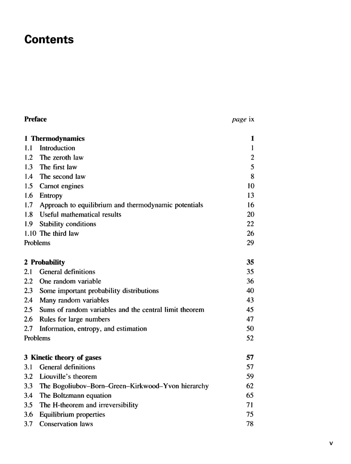
Contents
Preface page ix
1 Thermodynamics 1
1.1 Introduction 1
1.2 The zeroth law 2
1.3 The first law 5
1.4 The second law 8
1.5 Carnot engines 10
1.6 Entropy 13
1.7 Approach to equilibrium and thermodynamic potentials 16
1.8 Useful mathematical results 20
1.9 Stability conditions 22
1.10 The third law 26
Problems 29
2 Probability 35
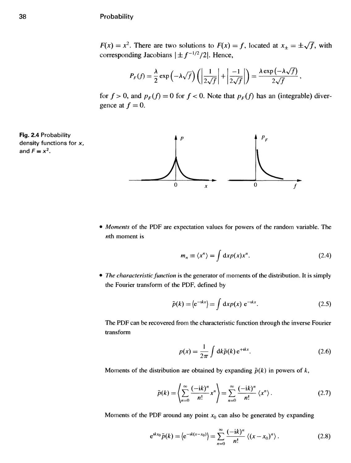
2.1 General definitions 35
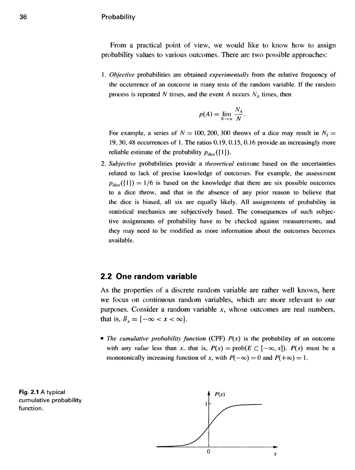
2.2 One random variable 36
2.3 Some important probability distributions 40
2.4 Many random variables 43
2.5 Sums of random variables and the central limit theorem 45
2.6 Rules for large numbers 47
2.7 Information, entropy, and estimation 50
Problems 52
3 Kinetic theory of gases 57
3.1 General definitions 57
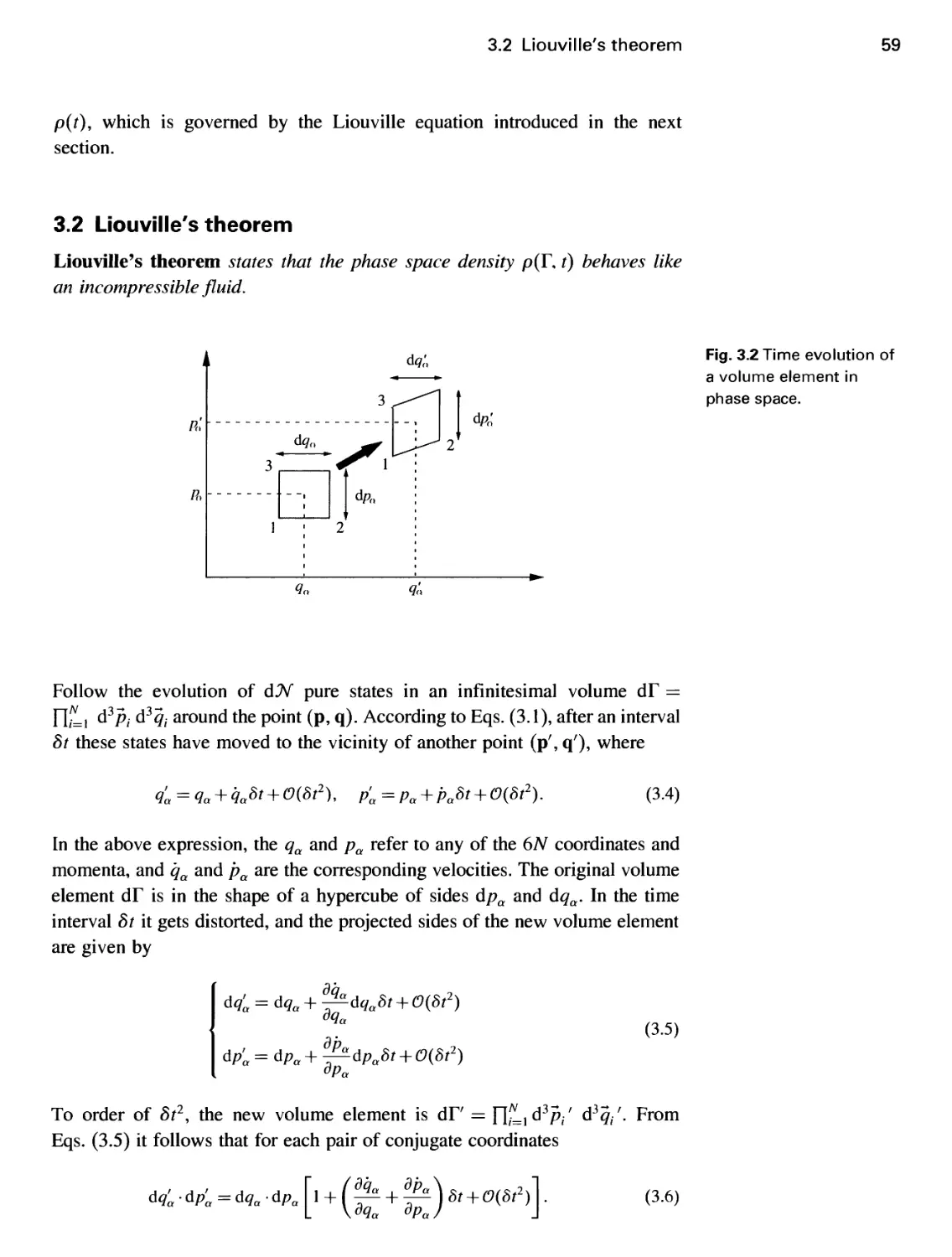
3.2 Liouville's theorem 59
3.3 The Bogoliubov-Born-Green-Kirkwood-Yvon hierarchy 62
3.4 The Boltzmann equation 65
3.5 The H-theorem and irreversibility 71
3.6 Equilibrium properties 75
3.7 Conservation laws 78

Contents
3.8 Zeroth-order hydrodynamics 82
3.9 First-order hydrodynamics 84
Problems 87
4 Classical statistical mechanics 98
4.1 General definitions 98
4.2 The microcanonical ensemble 98
4.3 Two-level systems 102
4.4 The ideal gas 105
4.5 Mixing entropy and the Gibbs paradox 107
4.6 The canonical ensemble 110
4.7 Canonical examples 113
4.8 The Gibbs canonical ensemble 115
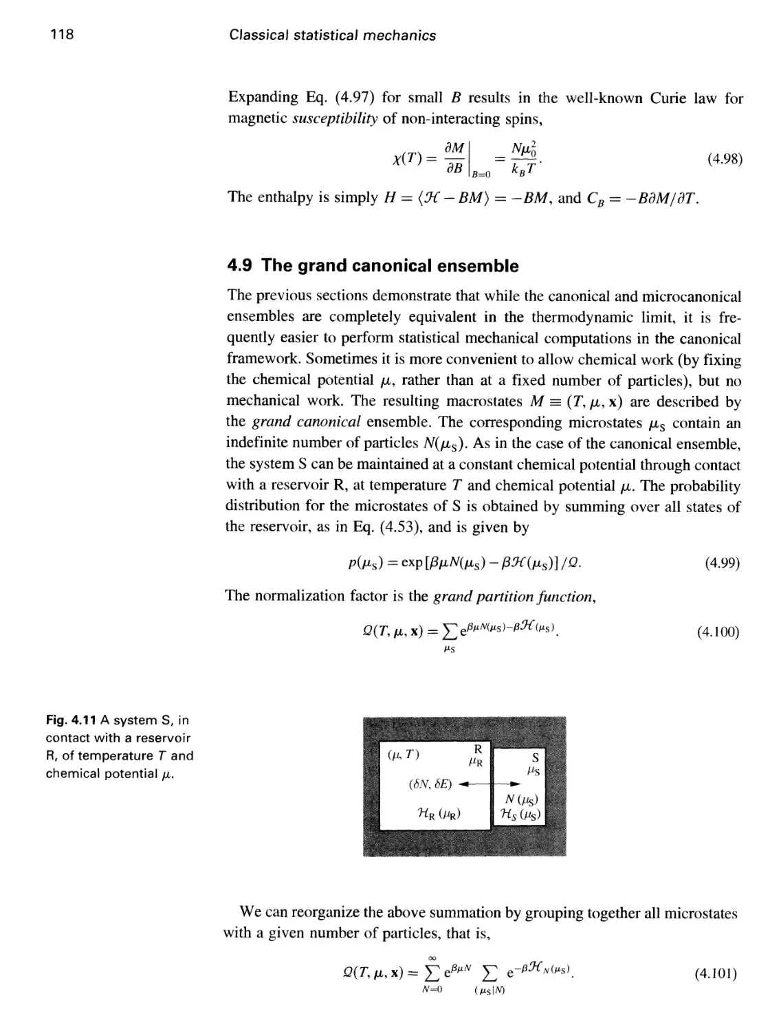
4.9 The grand canonical ensemble 118
Problems 120
5 Interacting particles 126
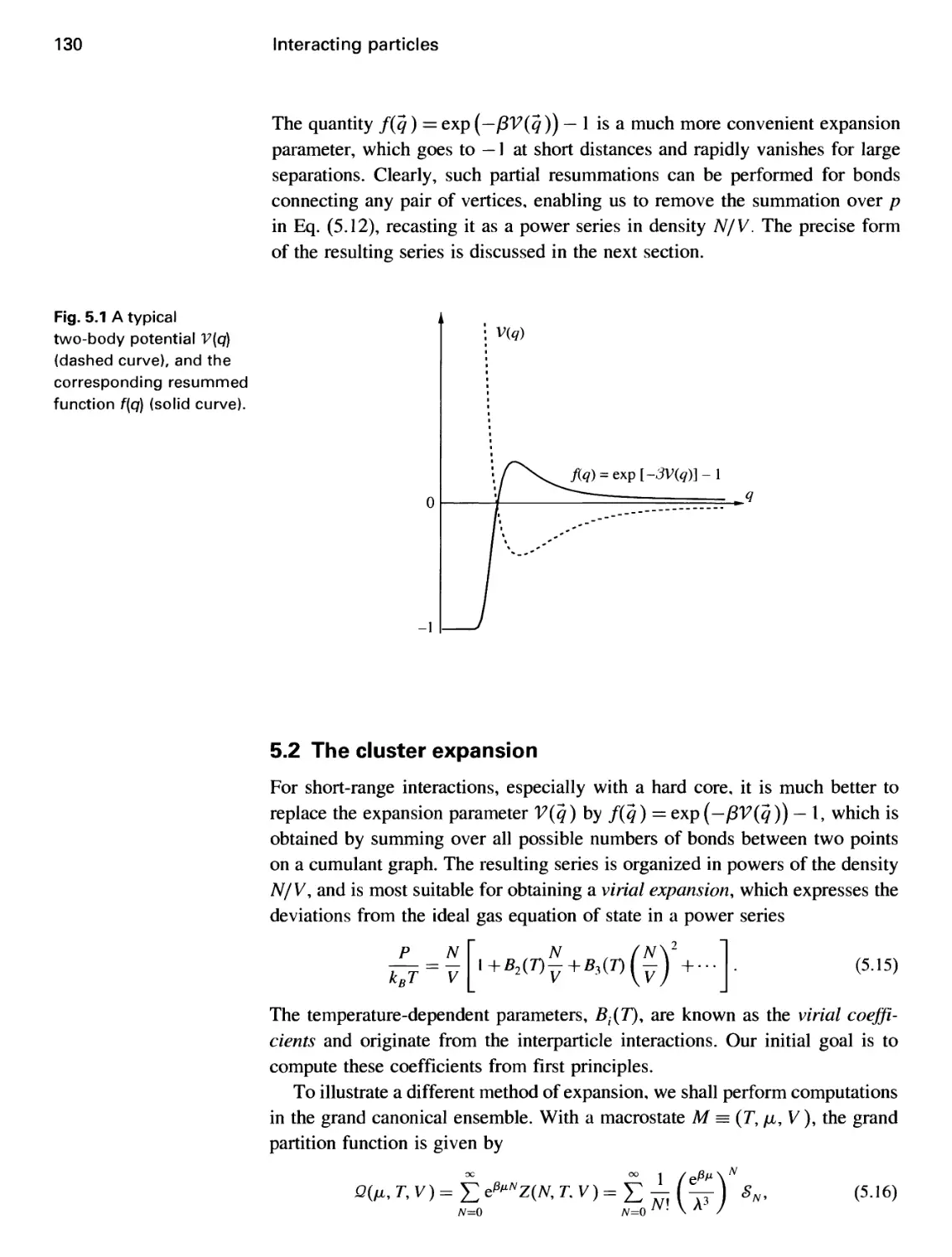
5.1 The cumulant expansion 126
5.2 The cluster expansion 130
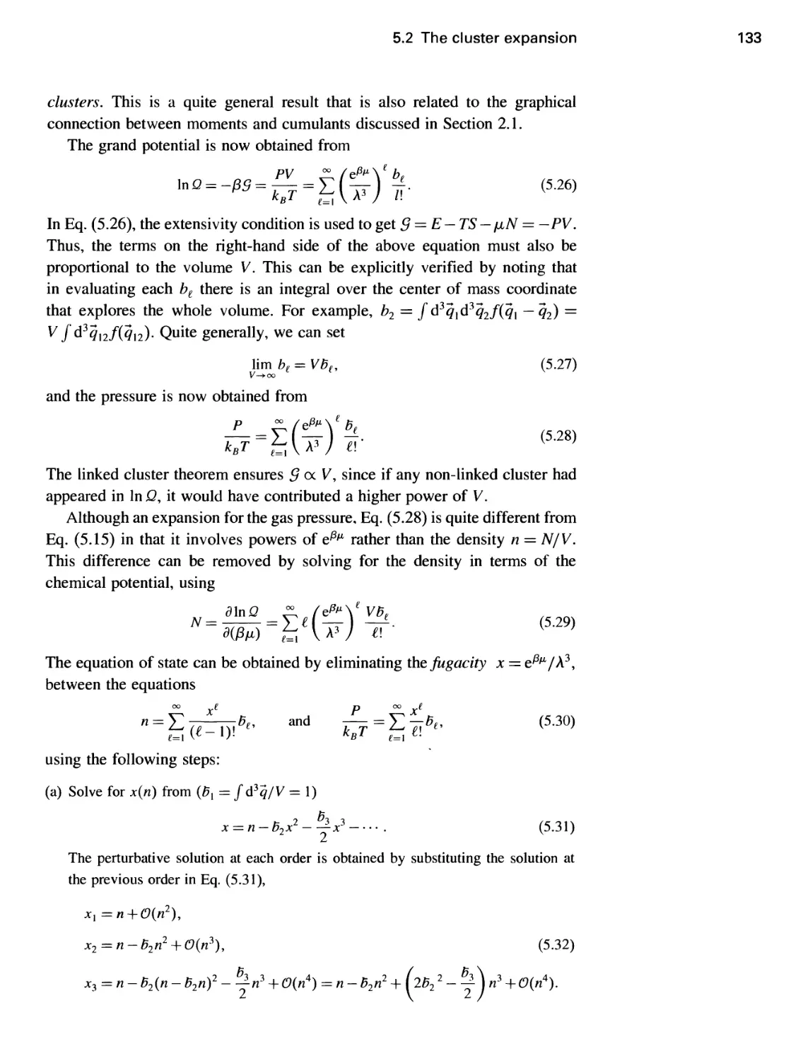
5.3 The second virial coefficient and van der Waals equation 135
5.4 Breakdown of the van der Waals equation 139
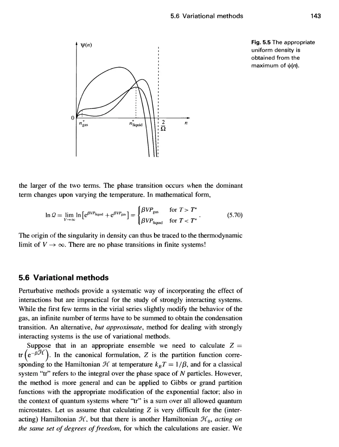
5.5 Mean-field theory of condensation 141
5.6 Variational methods 143
5.7 Corresponding states 145
5.8 Critical point behavior 146
Problems 148
6 Quantum statistical mechanics 156
6.1 Dilute polyatomic gases 156
6.2 Vibrations of a solid 161
6.3 Black-body radiation 167
6.4 Quantum microstates 170
6.5 Quantum macrostates 172
Problems 175
7 Ideal quantum gases 181
7.1 Hilbert space of identical particles 181
7.2 Canonical formulation 184
7.3 Grand canonical formulation 187
7.4 Non-relativistic gas 188
7.5 The degenerate fermi gas 190

Contents
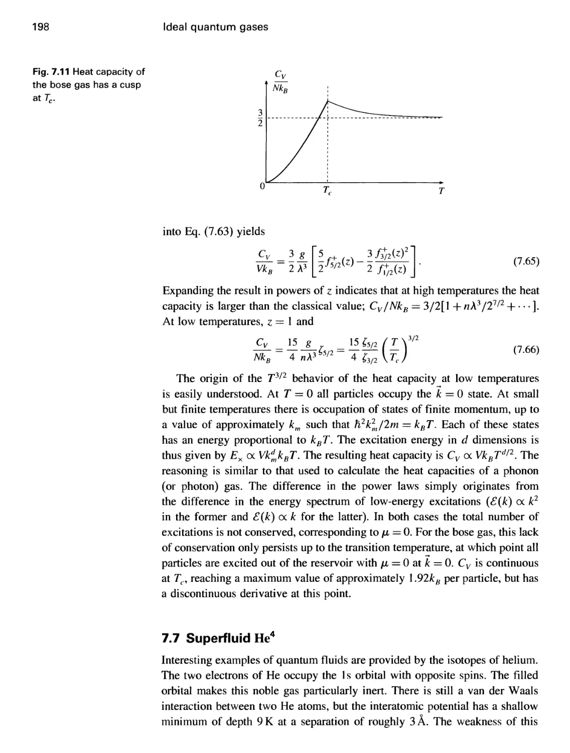
7.6 The degenerate bose gas 194
7.7 Superfluid He4 198
Problems 202
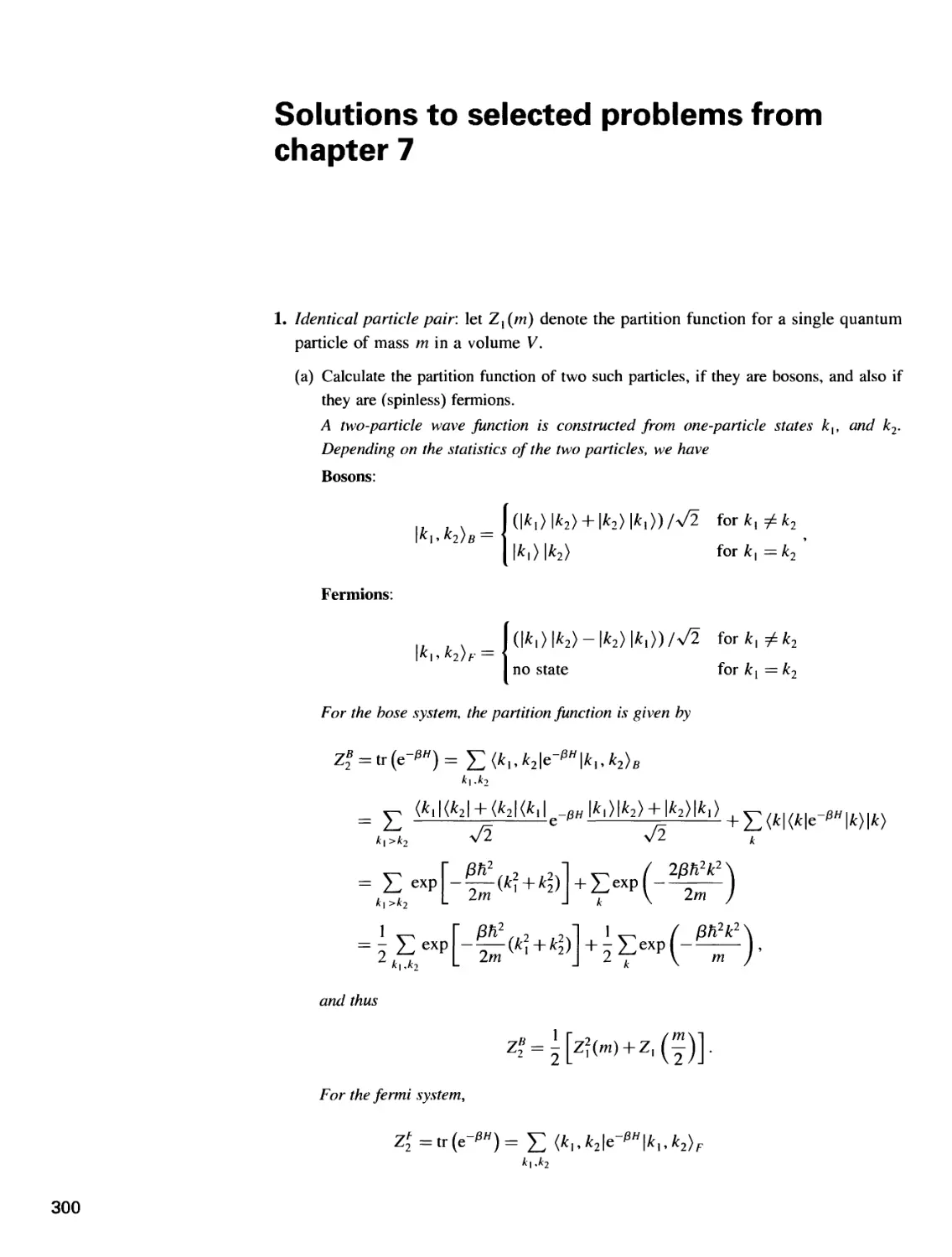
Solutions to selected problems 211
Chapter 1 211
Chapter 2 224
Chapter 3 235
Chapter 4 256
Chapter 5 268
Chapter 6 285
Chapter 7 300
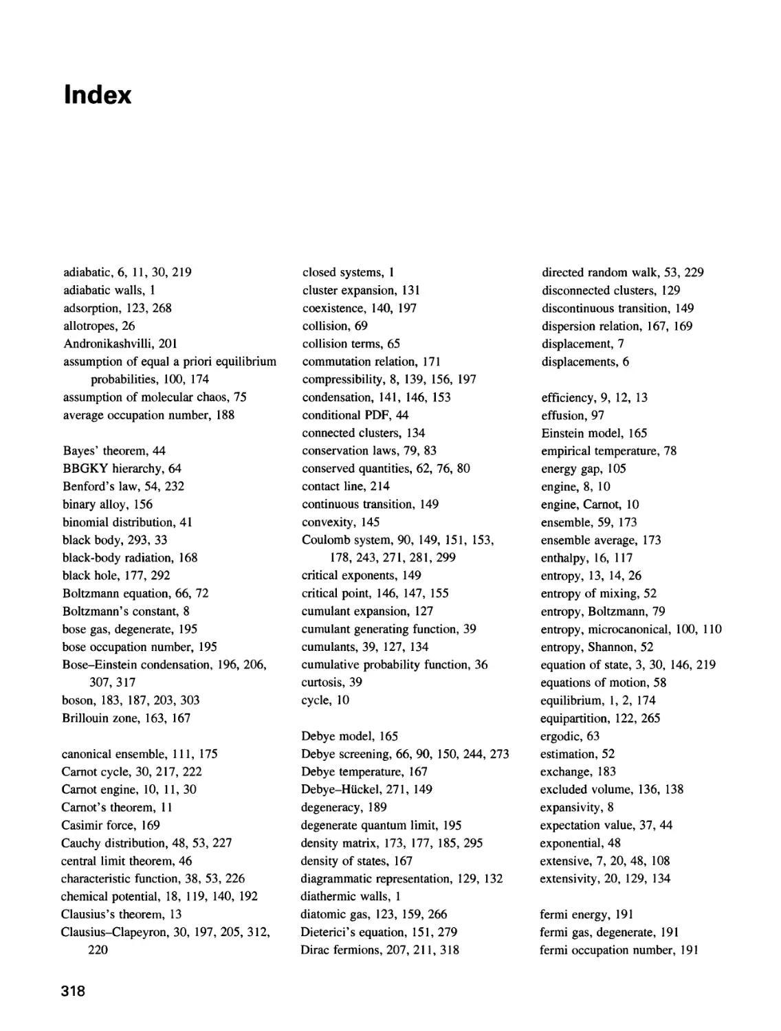
Index 318

Preface
Historically, the discipline of statistical physics originated in attempts to
describe thermal properties of matter in terms of its constituent particles, but
also played a fundamental role in the development of quantum mechanics.
More generally, the formalism describes how new behavior emerges from
interactions of many degrees of freedom, and as such has found applications
in engineering, social sciences, and increasingly in biological sciences. This
book introduces the central concepts and tools of this subject, and guides
the reader to their applications through an integrated set of problems and
solutions.
The material covered is directly based on my lectures for the first semester
of an MIT graduate course on statistical mechanics, which I have been teaching
on and off since 1988. (The material pertaining to the second semester is
presented in a companion volume.) While the primary audience is physics
graduate students in their first semester, the course has typically also attracted
enterprising undergraduates, as well as students from a range of science and
engineering departments. While the material is reasonably standard for books
on statistical physics, students taking the course have found my exposition
more useful, and have strongly encouraged me to publish this material. Aspects
that make this book somewhat distinct are the chapters on probability and
interacting particles. Probability is an integral part of statistical physics, which
is not sufficiently emphasized in most textbooks. Devoting an entire chapter to
this topic (and related issues such as the central limit theorem and information
theory) provides valuable tools to the reader. In the context of interacting
particles, I provide an extensive description of the van der Waals equation,
including its derivation by mean-field approximation.
An essential part of learning the material is doing problems; an interesting
selection of problems (and solutions) has been designed and integrated into
the text. Following each chapter there are two sets of problems: solutions to
the first set are included at the end of the book, and are intended to introduce
additional topics and to reinforce technical tools. Pursuing these problems
should also prove useful for students studying for qualifying exams. There

Preface
are no solutions provided for a second set of problems, which can be used in
assignments.
I am most grateful to my many former students for their help in formulating
the material, problems, and solutions, typesetting the text and figures, and
pointing out various typos and errors. The support of the National Science
Foundation through research grants is also acknowledged.

1
Thermodynamics
1.1 Introduction
Thermodynamics is a phenomenological description of properties of
macroscopic systems in thermal equilibrium.
Imagine yourself as a post-Newtonian physicist intent on understanding the
behavior of such a simple system as a container of gas. How would you
proceed? The prototype of a successful physical theory is classical mechanics,
which describes the intricate motions of particles starting from simple basic
laws and employing the mathematical machinery of calculus. By analogy, you
may proceed as follows:
• Idealize the system under study as much as possible (as is the case of a point
particle). The concept of mechanical work on the system is certainly familiar, yet
there appear to be complications due to exchange of heat. The solution is first to
examine closed systems, insulated by adiabatic walls that don't allow any exchange
of heat with the surroundings. Of course, it is ultimately also necessary to study
open systems, which may exchange heat with the outside world through diathermic
walls.
• As the state of a point particle is quantified by its coordinates (and momenta),
properties of the macroscopic system can also be described by a number of thermodynamic
coordinates or state functions. The most familiar coordinates are those that relate
to mechanical work, such as pressure and volume (for a fluid), surface tension and
area (for a film), tension and length (for a wire), electric field and polarization (for
a dielectric), etc. As we shall see, there are additional state functions not related to
mechanical work. The state functions are well defined only when the system is in
equilibrium, that is, when its properties do not change appreciably with time over
the intervals of interest (observation times). The dependence on the observation time
makes the concept of equilibrium subjective. For example, window glass is in
equilibrium as a solid over many decades, but flows like a fluid over time scales of
millennia. At the other extreme, it is perfectly legitimate to consider the equilibrium
between matter and radiation in the early universe during the first minutes of the
Big Bang.

2
Thermodynamics
• Finally, the relationship between the state functions is described by the laws of
thermodynamics. As a phenomenological description, these laws are based on a
number of empirical observations. A coherent logical and mathematical structure
is then constructed on the basis of these observations, which leads to a variety of
useful concepts, and to testable relationships among various quantities. The laws of
thermodynamics can only be justified by a more fundamental (microscopic) theory
of nature. For example, statistical mechanics attempts to obtain these laws starting
from classical or quantum mechanical equations for the evolution of collections of
particles.
1.2 The zeroth law
The zeroth law of thermodynamics describes the transitive nature of thermal
equilibrium. It states:
//* two systems, A and B, are separately in equilibrium with a third system, C,
then they are also in equilibrium with one another.
Despite its apparent simplicity, the zeroth law has the consequence of implying
the existence of an important state function, the empirical temperature (H), such
that systems in equilibrium are at the same temperature.
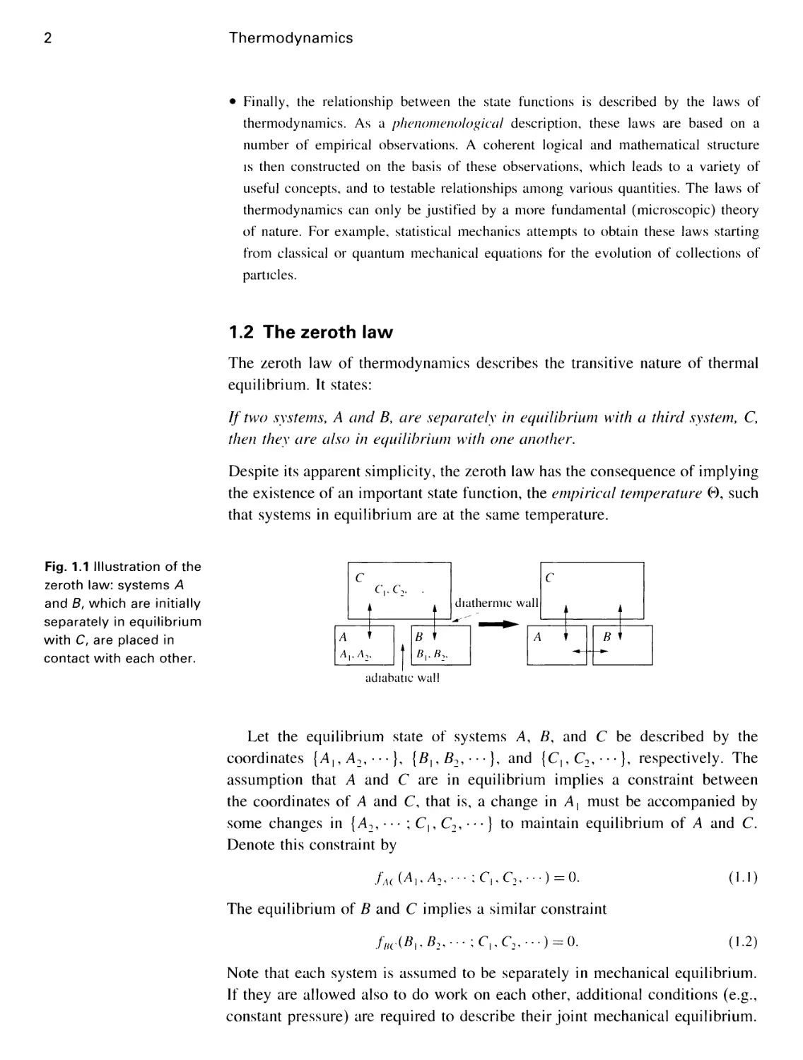
Fig. 1.1 Illustration of the
zeroth law: systems A
and B, which are initially
separately in equilibrium
with C, are placed in
contact with each other.
c
c\,c2. .
I
A I
/\,,/l2.
I
dia
-
B I
B,,«2,
diathermic wall
A 1 \\ B
adiabatic wall
Let the equilibrium state of systems A, B, and C be described by the
coordinates {A,, A2, • • •}, {B\,B2,- ••}, and {C|,C2,---}, respectively. The
assumption that A and C are in equilibrium implies a constraint between
the coordinates of A and C, that is, a change in A, must be accompanied by
some changes in {A2, • • • ; C,, C2, • • •} to maintain equilibrium of A and C.
Denote this constraint by
/^(^1M2,---;C„C2,...) = 0.
The equilibrium of B and C implies a similar constraint
/wr(flI,fl2,.--;C,,C2,...) = 0.
A.1)
A.2)
Note that each system is assumed to be separately in mechanical equilibrium.
If they are allowed also to do work on each other, additional conditions (e.g.,
constant pressure) are required to describe their joint mechanical equilibrium.

1.2 The zeroth law
Clearly we can state the above constraint in many different ways. For example,
we can study the variations of C, as all of the other parameters are changed.
This is equivalent to solving each of the above equations for C, to yield '
A.3)
Thus if C is separately in equilibrium with A and B. we must have
FAC(Al.A2,---xC2.---) = FBC(Bl.B2....;C2,..-). A.4)
However, according to the zeroth law there is also equilibrium between
A and B, implying the constraint
fAB(Ax,A2.-.-:Bx.B2,--.)=Q. A.5)
We can select any set of parameters [A. B] that satisfy the above equation, and
substitute them in Eq. A.4). The resulting equality must hold quite
independently of any set of variables (C) in this equation. We can then change these
parameters, moving along the manifold constrained by Eq. A.5), and Eq. A.4)
will remain valid irrespective of the state of C. Therefore, it must be possible
to simplify Eq. A.4) by canceling the coordinates of C. Alternatively, we can
select any fixed set of parameters C, and ignore them henceforth, reducing the
condition A.5) for equilibrium of A and B to
B,(V^--) = <HMfl.^-'), A.6)
that is, equilibrium is characterized by a function f) of thermodynamic
coordinates. This function specifies the equation of state, and isotherms of A are
described by the condition &A(A}. A2,---) = ®. While at this point there are
many potential choices of (H), the key point is the existence of a function that
constrains the parameters of each system in thermal equilibrium.
There is a similarity between CH) and the force in a mechanical system.
Consider two one-dimensional systems that can do work on each other as
in the case of two springs connected together. Equilibrium is achieved when
the forces exerted by each body on the other are equal. (Of course, unlike
the scalar temperature, the vectorial force has a direction; a complication that
we have ignored. The pressure of a gas piston provides a more apt analogy.)
The mechanical equilibrium between several such bodies is also transitive, and
the latter could have been used as a starting point for deducing the existence
of a mechanical force.
1 From a purely mathematical perspective, it is not necessarily possible to solve an arbitrary
constraint condition for C, However, the requirement that the constraint describes real physical
parameters clearly implies that we can obtain C, as a function of the remaining parameters.

4
Thermodynamics
As an example, let us consider the following three systems: (A) a wire of
length L with tension F, (B) a paramagnet of magnetization M in a magnetic
field B, and (C) a gas of volume V at pressure P.
Fig. 1.2 Equilibria of a gas
(A) and a magnet (B), and
a gas (A) and a wire <C).
—¦
V,P
\
It
L
u
'F
(A)&(C)
(A)&(B)
Observations indicate that when these systems are in equilibrium, the
following constraints are satisfied between their coordinates:
(P+ ~^_) (V ~ b)(L- L{))-c[F - K(L- L{))]=0,
(p+^){V-b)M-dB = Q.
A.7)
The two conditions can be organized into three empirical temperature
functions as
Hoc
('+?)<
V-b):
L-U
K
,1.
M
A.8)
Note that the zeroth law severely constrains the form of the constraint
equation describing the equilibrium between two bodies. Any arbitrary function
cannot necessarily be organized into an equality of two empirical temperature
functions.
The constraints used in the above example were in fact chosen to reproduce
three well-known equations of state that will be encountered and discussed
later in this book. In their more familiar forms they are written as
f {P + a/V2){V-b) = NkBT
M = (NMB)/{3kBT)
F = (K + DT)(L-L0)
(van der Waals gas)
(Curie paramagnet)
(Hooke's law for rubber)
A.9)
Note that we have employed the symbol for Kelvin temperature T, in place of
the more general empirical temperature (H). This concrete temperature scale can
be constructed using the properties of the ideal gas.
The ideal gas temperature scale: while the zeroth law merely states the
presence of isotherms, to set up a practical temperature scale at this stage, a
reference system is necessary. The ideal gas occupies an important place in
thermodynamics and provides the necessary reference. Empirical observations
indicate that the product of pressure and volume is constant along the isotherms
of any gas that is sufficiently dilute. The ideal gas refers to this dilute limit of

1.3 The first law
5
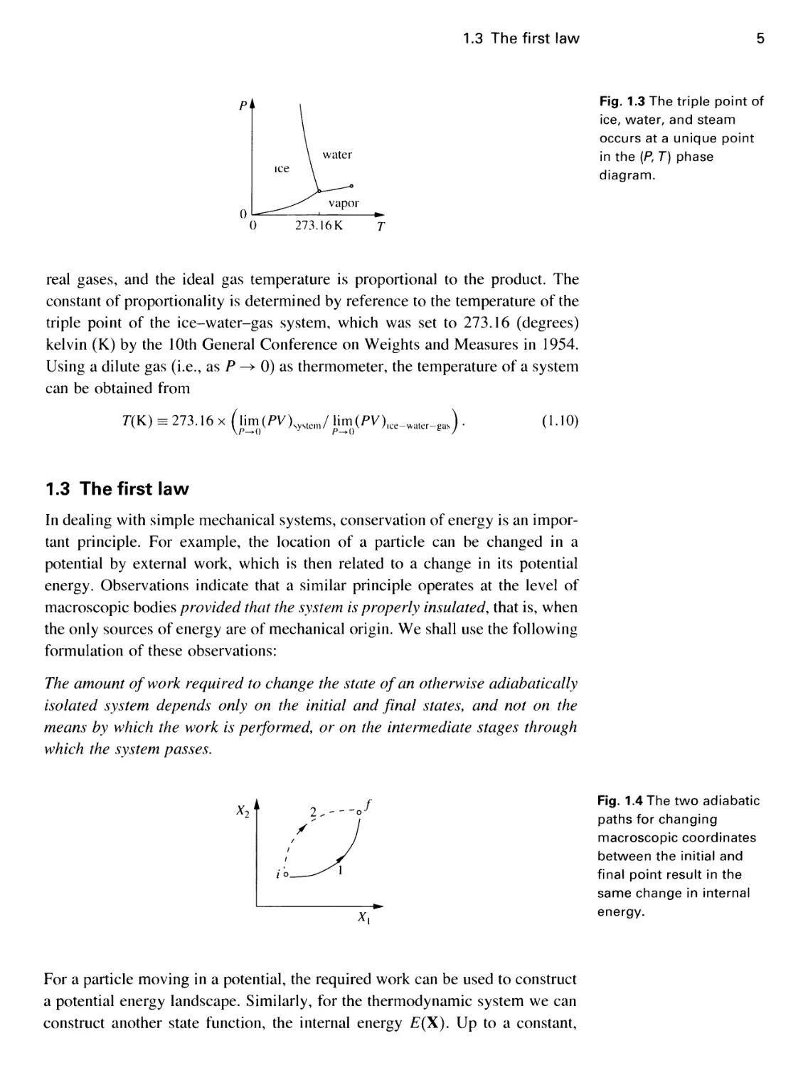
Fig. 1.3 The triple point of
ice, water, and steam
occurs at a unique point
in the (P, 7") phase
diagram.
0 273.16 K T
real gases, and the ideal gas temperature is proportional to the product. The
constant of proportionality is determined by reference to the temperature of the
triple point of the ice-water-gas system, which was set to 273.16 (degrees)
kelvin (K) by the 10th General Conference on Weights and Measures in 1954.
Using a dilute gas (i.e., as P —> 0) as thermometer, the temperature of a system
can be obtained from
T(K) ee 273.16 x (lim(W)syslcm/ \im(PV)lce_^_gas) .
A.10)
1.3 The first law
In dealing with simple mechanical systems, conservation of energy is an
important principle. For example, the location of a particle can be changed in a
potential by external work, which is then related to a change in its potential
energy. Observations indicate that a similar principle operates at the level of
macroscopic bodies provided that the system is properly insulated, that is, when
the only sources of energy are of mechanical origin. We shall use the following
formulation of these observations:
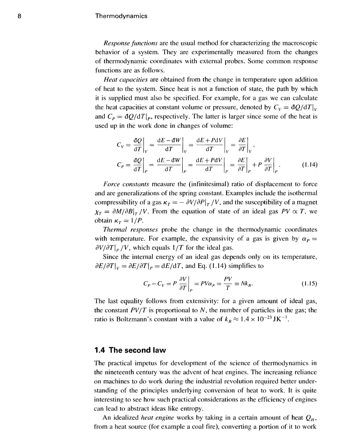
The amount of work required to change the state of an otherwise adiabatically
isolated system depends only on the initial and final states, and not on the
means by which the work is performed, or on the intermediate stages through
which the system passes.
1 2,--
,L_^
-J
Fig. 1.4 The two adiabatic
paths for changing
macroscopic coordinates
between the initial and
final point result in the
same change in internal
energy.
For a particle moving in a potential, the required work can be used to construct
a potential energy landscape. Similarly, for the thermodynamic system we can
construct another state function, the internal energy E(X). Up to a constant,

Thermodynamics
E(X) can be obtained from the amount of work AW needed for an adiabatic
transformation from an initial state Xj to a final state Xf, using
AW = ?(Xf)-E(Xl). A.11)
Another set of observations indicate that once the adiabatic constraint is
removed, the amount of work is no longer equal to the change in the internal
energy. The difference AQ = AE — AW is defined as the heat intake of the
system from its surroundings. Clearly, in such transformations, AQ and AW
are not separately functions of state in that they depend on external factors such
as the means of applying work, and not only on the final states. To emphasize
this, for a differential transformation we write
dQ = dE-dW, A.12)
where dE = YLi djEdXj can be obtained by differentiation, while dQ and dW
generally cannot. Also note that our convention is such that the signs of work
and heat indicate the energy added to the system, and not vice versa. The first
law of thermodynamics thus states that to change the state of a system we
need a fixed amount of energy, which can be in the form of mechanical work
or heat. This can also be regarded as a way of defining and quantifying the
exchanged heat.
A quasi-static transformation is one that is performed sufficiently slowly
so that the system is always in equilibrium. Thus, at any stage of the process,
the thermodynamic coordinates of the system exist and can in principle be
computed. For such transformations, the work done on the system (equal in
magnitude but opposite in sign to the work done by the system) can be related to
changes in these coordinates. As a mechanical example, consider the stretching
of a spring or rubber band. To construct the potential energy of the system
as a function of its length L, we can pull the spring sufficiently slowly so
that at each stage the external force is matched by the internal force F from
the spring. For such a quasi-static process, the change in the potential energy
of the spring is f FdL. If the spring is pulled abruptly, some of the external
work is converted into kinetic energy and eventually lost as the spring comes
to rest.
Generalizing from the above example, one can typically divide the state
functions {X} into a set of generalized displacements {x}, and their conjugate
generalized forces {J}, such that for an infinitesimal quasi-static transformation2
dW = ^Jidxi. A.13)
2 I denote force by the symbol J rather than F, to reserve the latter for the free energy. I hope the
reader is not confused with currents (sometimes also denoted by J), which rarely appear in this
book.

1.3 The first law
Table l.l Generalized forces and displacements
System
Wire
Film
Fluid
Magnet
Dielectric
Chemical reaction
Force
tension
surface tension
pressure
magnetic field
electric field
chemical potential
F
S
-P
H
E
M
Displacement
length
area
volume
magnetization
polarization
particle number
L
A
V
M
P
N
Table 1.1 provides some common examples of such conjugate coordinates.
Note that pressure P is by convention calculated from the force exerted by the
system on the walls, as opposed to the force on a spring, which is exerted in
the opposite direction. This is the origin of the negative sign that accompanies
hydrostatic work.
The displacements are usually extensive quantities, that is, proportional to
system size, while the forces are intensive and independent of size. The latter
are indicators of equilibrium; for example, the pressure is uniform in a gas in
equilibrium (in the absence of external potentials) and equal for two equilibrated
gases in contact. As discussed in connection with the zeroth law. temperature
plays a similar role when heat exchanges are involved. Is there a corresponding
displacement, and if so what is it? This question will be answered in the
following sections.
The ideal gas: we noted in connection with the zeroth law that the equation
of state of the ideal gas takes a particularly simple form, PV oc T. The internal
energy of the ideal gas also takes a very simple form, as observed for example
by Joule's free expansion experiment: measurements indicate that if an ideal
gas expands adiabatically (but not necessarily quasi-statically), from a volume
V,- to Vf, the initial and final temperatures are the same. As the transformation
is adiabatic (AQ = 0) and there is no external work done on the system (AW =
0), the internal energy of the gas is unchanged. Since the pressure and volume
of the gas change in the process, but its temperature does not, we conclude that
the internal energy depends only on temperature, that is, ?(V, T) = E(T). This
property of the ideal gas is in fact a consequence of the form of its equation of
state, as will be proved in one of the problems at the end of this chapter.
Fig. 1.5 A gas initially
confined in the left
chamber is allowed to
expand rapidly to both
chambers.

Thermodynamics
Response functions are the usual method for characterizing the macroscopic
behavior of a system. They are experimentally measured from the changes
of thermodynamic coordinates with external probes. Some common response
functions are as follows.
Heat capacities are obtained from the change in temperature upon addition
of heat to the system. Since heat is not a function of state, the path by which
it is supplied must also be specified. For example, for a gas we can calculate
the heat capacities at constant volume or pressure, denoted by Cv = 6Q/dT\v
and CP = 6Q/dT\p, respectively. The latter is larger since some of the heat is
used up in the work done in changes of volume:
Cv =
dQ
dT
dE-dW
Lp~ dT
dT
dE-dW
d? + /W
dT
dT
dT
dE
~df
dE
~df
dV
+ P —
dT
A.14)
Force constants measure the (infinitesimal) ratio of displacement to force
and are generalizations of the spring constant. Examples include the isothermal
compressibility of a gas kt = — dV/dP\T /V, and the susceptibility of a magnet
%T = 3M/dB\T /V. From the equation of state of an ideal gas PV oc 7\ we
obtain kt = 1 /P.
Thermal responses probe the change in the thermodynamic coordinates
with temperature. For example, the expansivity of a gas is given by aP =
dV/dT\p/V, which equals \/T for the ideal gas.
Since the internal energy of an ideal gas depends only on its temperature,
3E/dT\v = 3E/dT\P = dE/dT, and Eq. A.14) simplifies to
Cp Ci/ — /
dV
:PVaP=
PV
A.15)
The last equality follows from extensivity: for a given amount of ideal gas,
the constant PV/T is proportional to N, the number of particles in the gas; the
ratio is Boltzmann's constant with a value of kB& 1.4 x 10~23 JK_I.
1.4 The second law
The practical impetus for development of the science of thermodynamics in
the nineteenth century was the advent of heat engines. The increasing reliance
on machines to do work during the industrial revolution required better
understanding of the principles underlying conversion of heat to work. It is quite
interesting to see how such practical considerations as the efficiency of engines
can lead to abstract ideas like entropy.
An idealized heat engine works by taking in a certain amount of heat QH,
from a heat source (for example a coal fire), converting a portion of it to work

1.4 The second law
9
< I.
A.16)
W, and dumping the remaining heat Qc into a heat sink (e.g., atmosphere).
The efficiency of the engine is calculated from
= _^ = Qh-Qc
V Qh Qh
An idealized refrigerator is like an engine running backward, that is, using
work W to extract heat Qc from a cold system, and dumping heat QH at a higher
temperature. We can similarly define a figure of merit for the performance of
a refrigerator as
w=^ = _^?_. (U7)
W QH-QC
Source
JQh
Engine
TeT
Sink
Exhaust
-$—W
W—>-
~JQh_
Refrigerator
\Qc
Ice-box
Fig. 1.6 The idealized
engine and refrigerator.
The first law rules out so-called "perpetual motion machines of the first
kind," that is, engines that produce work without consuming any energy.
However, the conservation of energy is not violated by an engine that produces
work by converting water to ice. Such a "perpetual motion machine of the
second kind" would certainly solve the world's energy problems, but is ruled
out by the second law of thermodynamics. The observation that the natural
direction for the flow of heat is from hotter to colder bodies is the essence of
the second law of thermodynamics. There is a number of different formulations
of the second law, such as the following two statements:
Kelvin's statement. No process is possible whose sole result is the complete
conversion of heat into work.
Clausius's statement. No process is possible whose sole result is the transfer
of heat from a colder to a hotter body.
A perfect engine is ruled out by the first statement, a perfect refrigerator by
the second. Since we shall use both statements, we first show that they are
equivalent. Proof of the equivalence of the Kelvin and Clausius statements
proceeds by showing that if one is violated, so is the other.
(a) Let us assume that there is a machine that violates Clausius's statement by taking
heat Q from a cooler region to a hotter one. Now consider an engine operating
between these two regions, taking heat QH from the hotter one and dumping Qc at
the colder sink. The combined system takes QH — Q from the hot source, produces
work equal to QH — Qc, and dumps Qc — Q at the cold sink. If we adjust the engine

10
Thermodynamics
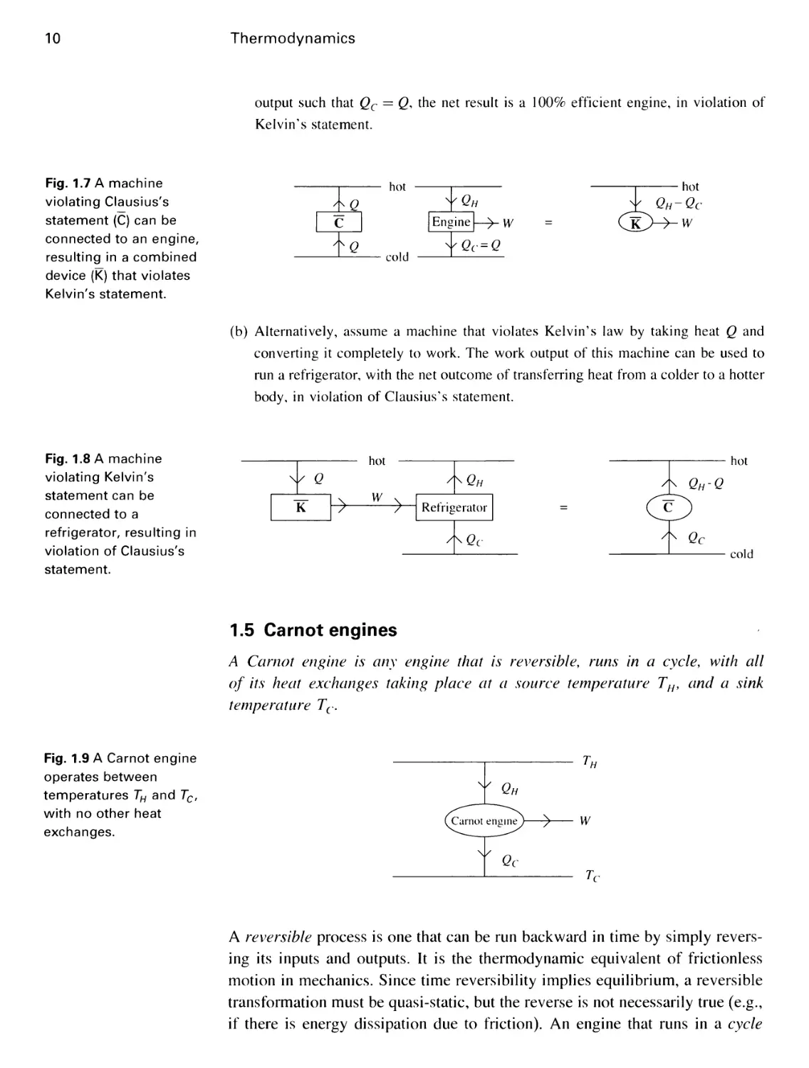
output such that Qc = Q, the net result is a 100% efficient engine, in violation of
Kelvin's statement.
Fig. 1.7 A machine
violating Clausius's
statement (C) can be
connected to an engine,
resulting in a combined
device (K) that violates
Kelvin's statement.
hot
cold
ta,
Engine
¦ W
Qc = Q
hot
Qh-Qc
KJ-^W
(b) Alternatively, assume a machine that violates Kelvin's law by taking heat Q and
converting it completely to work. The work output of this machine can be used to
run a refrigerator, with the net outcome of transferring heat from a colder to a hotter
body, in violation of Clausius's statement.
Fig. 1.8 A machine
violating Kelvin's
statement can be
connected to a
refrigerator, resulting in
violation of Clausius's
statement.
\k Q
hot
W
A^Qh
Refrigerator
/KQC
hot
^ Qh-Q
c
Qc
- cold
1.5 Carnot engines
A Carnot engine is any engine that is reversible, runs in a cycle, with all
of its heat exchanges taking place at a source temperature TH, and a sink
temperature Tc.
Fig. 1.9 A Carnot engine
operates between
temperatures TH and Tc,
with no other heat
exchanges.
Carnot engine/ —> W
Tr
A reversible process is one that can be run backward in time by simply
reversing its inputs and outputs. It is the thermodynamic equivalent of frictionless
motion in mechanics. Since time reversibility implies equilibrium, a reversible
transformation must be quasi-static, but the reverse is not necessarily true (e.g.,
if there is energy dissipation due to friction). An engine that runs in a cycle

1.5 Carnot engines
11
returns to its original internal state at the end of the process. The distinguishing
characteristic of the Carnot engine is that heat exchanges with the surroundings
are carried out only at two temperatures.
The zeroth law allows us to select two isotherms at temperatures TH and
Tc for these heat exchanges. To complete the Carnot cycle we have to connect
these isotherms by reversible adiabatic paths in the coordinate space. Since
heat is not a function of state, we don't know how to construct such paths in
general. Fortunately, we have sufficient information at this point to construct
a Carnot engine using an ideal gas as its internal working substance. For the
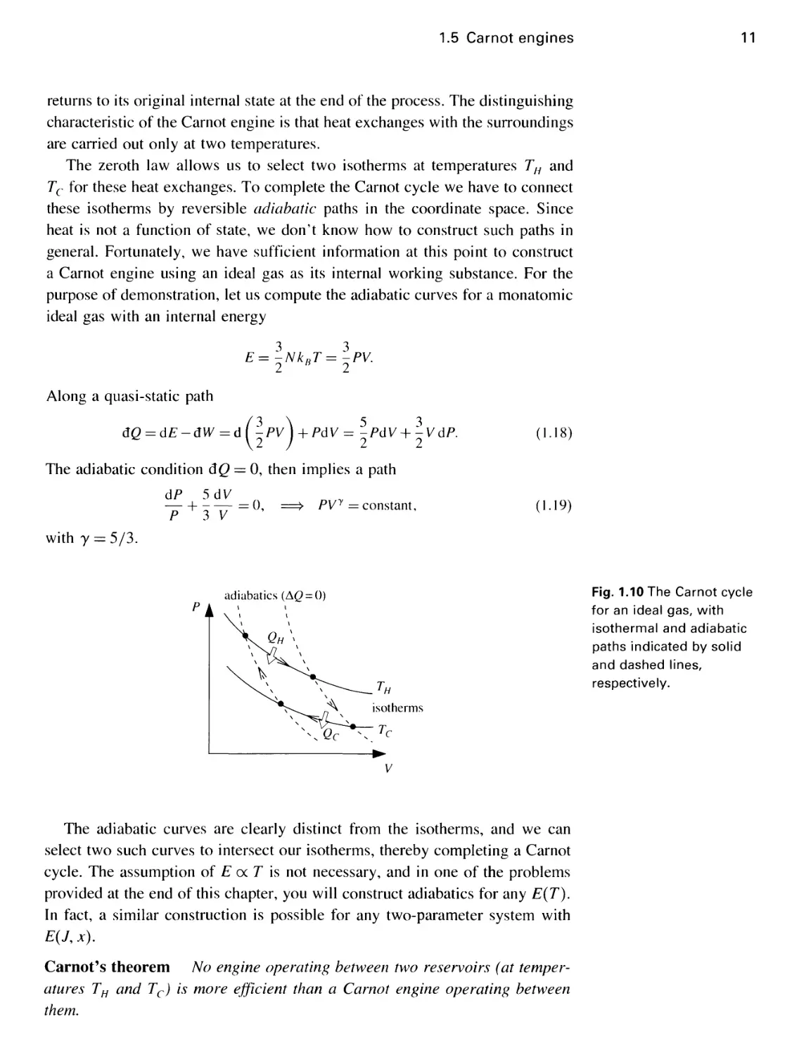
purpose of demonstration, let us compute the adiabatic curves for a monatomic
ideal gas with an internal energy
3 3
E=-NkBT=-PV.
2 B 2
Along a quasi-static path
dQ = dE-dW =d(-PV)
5 3
+ PdV= -PdV+-VdP.
2 2
The adiabatic condition dQ = 0, then implies a path
dP 5dV
P+3V=°-
PVy = constant,
(I-18)
A.19)
with y = 5/3.
adiabatics(A<2 = 0)
Fig. 1.10 The Carnot cycle
for an ideal gas, with
isothermal and adiabatic
paths indicated by solid
and dashed lines,
respectively.
The adiabatic curves are clearly distinct from the isotherms, and we can
select two such curves to intersect our isotherms, thereby completing a Carnot
cycle. The assumption of E oc T is not necessary, and in one of the problems
provided at the end of this chapter, you will construct adiabatics for any E(T).
In fact, a similar construction is possible for any two-parameter system with
E(J, x).
Carnot's theorem No engine operating between two reservoirs (at
temperatures TH and Tc) is more efficient than a Carnot engine operating between
them.

12
Thermodynamics
Since a Carnot engine is reversible, it can be run backward as a refrigerator.
Use the non-Carnot engine to run the Carnot engine backward. Let us denote
the heat exchanges of the non-Carnot and Carnot engines by QH, Qc, and Q'H,
Q'c, respectively. The net effect of the two engines is to transfer heat equal to
Qh ~ Q'h ~ Qc ~ Qc fr°m TH to Tc. According to Clausius's statement, the
quantity of transferred heat cannot be negative, that is, QH > Q'H. Since the
same quantity of work W is involved in this process, we conclude that
W W
~Qh~~Qh
^Ca:
'/non-Carnot •
A.20)
Fig. 1.11 A generic engine
is used to run a Carnot
engine in reverse.
Y Qh
CE \^WM CE
Y Qc
±Qh
Qc
Corollary All reversible (Carnot) engines have the same universal efficiency
r](TH,Tc), since each can be used to run any other one backward.
The thermodynamic temperature scale: as shown earlier, it is at least
theoretically possible to construct a Carnot engine using an ideal gas (or any other
two-parameter system) as working substance. We now find that independent of
the material used, and design and construction, all such cyclic and reversible
engines have the same maximum theoretical efficiency. Since this maximum
efficiency is only dependent on the two temperatures, it can be used to
construct a temperature scale. Such a temperature scale has the attractive property
Fig. 1.12 Two Carnot
engines connected in
series are equivalent to a
third.
7\-
7V
YGi
CE>^:
4-2:
CE B-w23
CE
^_ W^=Wi2 + w23
-h
of being independent of the properties of any material (e.g., the ideal gas). To
construct such a scale we first obtain a constraint on the form of y){TH,Tc).
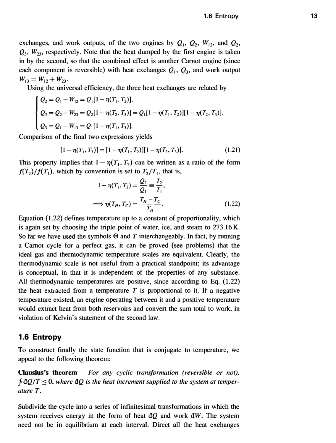
Consider two Carnot engines running in series, one between temperatures 7,
and r2, and the other between T2 and 73 G, > T2 > 7^). Denote the heat

1.6 Entropy
exchanges, and work outputs, of the two engines by 0,, Q2, Wl2, and Q2,
g3, W23, respectively. Note that the heat dumped by the first engine is taken
in by the second, so that the combined effect is another Carnot engine (since
each component is reversible) with heat exchanges Q,, Q3, and work output
W.3 = W.2
+Mousing the universal efficiency, the three heat exchanges are related by
lQ2 = Ql-Wl2 = Ql[\-V(T],T2)l
JG3 = G2-^23 = e2[i~^2,r3)] = G1[i-r7(r1,r2)][i-7?(r2,r3)],
Comparison of the final two expressions yields
[i-ij(rI,r3)] = [i-i,(rIfr2)][i-i7(r2fr3)]. A.21)
This property implies that 1 — r)(Tx, T2) can be written as a ratio of the form
/(r2)//(r,), which by convention is set to T2/T}, that is,
i-i7(r„r2) = f = ?,
=> v(TH, Tc) = -^-^. A.22)
1 H
Equation A.22) defines temperature up to a constant of proportionality, which
is again set by choosing the triple point of water, ice, and steam to 273.16 K.
So far we have used the symbols & and T interchangeably. In fact, by running
a Carnot cycle for a perfect gas, it can be proved (see problems) that the
ideal gas and thermodynamic temperature scales are equivalent. Clearly, the
thermodynamic scale is not useful from a practical standpoint; its advantage
is conceptual, in that it is independent of the properties of any substance.
All thermodynamic temperatures are positive, since according to Eq. A.22)
the heat extracted from a temperature T is proportional to it. If a negative
temperature existed, an engine operating between it and a positive temperature
would extract heat from both reservoirs and convert the sum total to work, in
violation of Kelvin's statement of the second law.
1.6 Entropy
To construct finally the state function that is conjugate to temperature, we
appeal to the following theorem:
Clausius's theorem For any cyclic transformation (reversible or not),
(f&Q/T < 0, where &Q is the heat increment supplied to the system at
temperature T.
Subdivide the cycle into a series of infinitesimal transformations in which the
system receives energy in the form of heat &Q and work dW. The system
need not be in equilibrium at each interval. Direct all the heat exchanges

14
Thermodynamics
Fig. 1.13 The heat
exchanges of the system
are directed to a Carnot
engine with a
reservoir at 7.
efW
l+awt
of the system to one port of a Carnot engine, which has another reservoir at a
fixed temperature T0. (There can be more than one Carnot engine as long as
they all have one end connected to T{).) Since the sign of dQ is not specified, the
Carnot engine must operate a series of infinitesimal cycles in either direction.
To deliver heat dQ to the system at some stage, the engine has to extract heat
dQR from the fixed reservoir. If the heat is delivered to a part of the system
that is locally at a temperature 7\ then according to Eq. A.22),
*Qr = T{
dQ
A.23)
After the cycle is completed, the system and the Carnot engine return to
their original states. The net effect of the combined process is extracting heat
QR = <f)dQK from the reservoir and converting it to external work W. The work
W = QR is the sum total of the work elements done by the Carnot engine, and
the work performed by the system in the complete cycle. By Kelvin's statement
of the second law, QK = W < 0, that is,
r<>^<o,
dQ
<0,
A.24)
since T{) > 0. Note that T in Eq. (l .24) refers to the temperature of the whole
system only for quasi-static processes in which it can be uniquely defined
throughout the cycle. Otherwise, it is just a local temperature (say at a boundary
of the system) at which the Carnot engine deposits the element of heat.
Consequences of Clausius's theorem:
l. For a reversible cycle fdQlcv/T = 0, since by running the cycle in the opposite direction
dBrev _> — d&ev' and by the above theorem dBlcv /T is both non-negative and non-positive,
hence zero. This result implies that the integral of dQTCV/T between any two points A and
B is independent of path, since for two paths (l) and B)
•*de^.
¦m T, hi
A dfiS
r,
= o,
J A I i J A
A.25)
2. Using Eq. A.25) we can construct yet another function of state, the entropy S. Since the
integral is independent of path, and only depends on the two end-points, we can set
S(B)
¦5M)-/
11 aelc»
A.26)

1.6 Entropy
15
(c)
Fig. 1.14 (a) A reversible
cycle, (b) Two reversible
paths between A and B.
(c) The cycle formed from
a generic path between A
and B, and a reversible
one.
For reversible processes, we can now compute the heat from dQKX = TdS. This allows us to
construct adiabatic curves for a general (multi variable) system from the condition of constant
S. Note that Eq. A.26) only defines the entropy up to an overall constant.
For a reversible (hence quasi-static) transformation, dQ = TdS and dW = ]?, 7,dx,, and
the first law implies
dE = dQ + dW = TdS + J2J>dxl-
A.27)
We can see that in this equation S and T appear as conjugate variables, with S
playing the role of a displacement, and T as the corresponding force. This identification
allows us to make the correspondence between mechanical and thermal exchanges more
precise, although we should keep in mind that unlike its mechanical analog,
temperature is always positive. While to obtain Eq. (l .27) we had to appeal to reversible
transformations, it is important to emphasize that it is a relation between functions of state.
Equation (l .27) is likely the most fundamental and useful identity in thermodynamics.
4. The number of independent variables necessary to describe a thermodynamic system also
follows from Eq. (l .27). If there are n methods of doing work on a system, represented
by n conjugate pairs G,, a,), then /?+ I independent coordinates are necessary to describe
the system. (We shall ignore possible constraints between the mechanical coordinates.)
For example, choosing (E, {x,}) as coordinates, it follows from Eq. A.27) that
3S_
Je
l
= — and
T
dS_
~dx,
J,
T'
A.28)
(x and J are shorthand notations for the parameter sets {a,} and [J,].)
I H-2
4—r-3
Fig. 1.15 The initially
isolated subsystems are
allowed to interact,
resulting in an increase of
entropy.
5. Consider an irreversible change from A to B. Make a complete cycle by returning from
B to A along a reversible path. Then
"dQ t*&Qin
rn ay r
J A I JB
<o,
/.
BdQ
<S(B)-S(A).
A.29)
JA 1 JB T
In differential form, this implies that dS > dQ/T for any transformation. In particular,
consider adiabatically isolating a number of subsystems, each initially separately in equi-

16
Thermodynamics
librium. As they come to a state of joint equilibrium, since the net dQ = 0, we must have
8S > 0. Thus an adiabatic system attains a maximum value of entropy in equilibrium since
spontaneous internal changes can only increase S. The direction of increasing entropy
thus points out the arrow of time, and the path to equilibrium. The mechanical analog is
a point mass placed on a surface, with gravity providing a downward force. As various
constraints are removed, the particle will settle down at locations of decreasing height. The
statement about the increase of entropy is thus no more mysterious than the observation
that objects tend to fall down under gravity!
1.7 Approach to equilibrium and thermodynamic
potentials
The time evolution of systems toward equilibrium is governed by the second
law of thermodynamics. For example, in the previous section we showed that
for an adiabatically isolated system entropy must increase in any spontaneous
change and reaches a maximum in equilibrium. What about out-of-equilibrium
systems that are not adiabatically isolated, and may also be subject to
external mechanical work? It is usually possible to define other thermodynamic
potentials that are extremized when the system is in equilibrium.
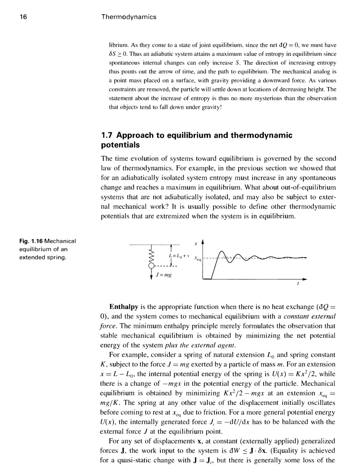
Fig. 1.16 Mechanical
equilibrium of an
extended spring.
Enthalpy is the appropriate function when there is no heat exchange (dQ =
0), and the system comes to mechanical equilibrium with a constant external
force. The minimum enthalpy principle merely formulates the observation that
stable mechanical equilibrium is obtained by minimizing the net potential
energy of the system plus the external agent.
For example, consider a spring of natural extension L0 and spring constant
K, subject to the force J = mg exerted by a particle of mass m. For an extension
x = L — L0, the internal potential energy of the spring is U(x) = Kx2/2, while
there is a change of —mgx in the potential energy of the particle. Mechanical
equilibrium is obtained by minimizing Kx2/2 — mgx at an extension xeq =
mg/K. The spring at any other value of the displacement initially oscillates
before coming to rest at xe due to friction. For a more general potential energy
U(x), the internally generated force /, = — dU/dx has to be balanced with the
external force J at the equilibrium point.
For any set of displacements x, at constant (externally applied) generalized
forces J, the work input to the system is dW < J • 8x. (Equality is achieved
for a quasi-static change with J = J,, but there is generally some loss of the

1.7 Approach to equilibrium and thermodynamic potentials
17
external work to dissipation.) Since dQ = 0, using the first law, 8E < J • 8x,
and
5//<0, where // = ?-Jx A.30)
is the enthalpy. The variations of H in equilibrium are given by
d// = d? - d(J • x) = TdS + J • dx - x • dj - J • dx = TdS - x • dj. A.31)
The equality in Eq. A.31), and the inequality in Eq. A.30), are a possible
source of confusion. Equation A.30) refers to variations of H on approaching
equilibrium as some parameter that is not a function of state is varied (e.g., the
velocity of the particle joined to the spring in the above example). By contrast,
Eq. A.31) describes a relation between equilibrium coordinates. To differentiate
the two cases, I will denote the former (non-equilibrium) variations by 8.
The coordinate set E, J) is the natural choice for describing the enthalpy,
and it follows from Eq. A.31) that
3H\
dJ,
A-32)
Variations of the enthalpy with temperature are related to heat capacities at
constant force, for example
CP =
dQ
dT
d? + /W
dr
d(E + PV)
dT
dH
dT
A.33)
Note, however, that a change of variables is necessary to express H in terms
of 7\ rather than the more natural variable 5.
Helmholtz free energy is useful for isothermal transformations in the
absence of mechanical work (dW = 0). It is rather similar to enthalpy, with
T taking the place of /. From Clausius's theorem, the heat intake of a system
at a constant temperature T satisfies dQ < T8S. Hence 8E = dQ + dW < T8S,
and
8F<0, where F = E-TS A.34)
is the Helmholtz free energy. Since
dF = dE - d(TS) = TdS + J • dx - SdT - TdS = -SdT + J • dx, A.35)
the coordinate set (T, x) (the quantities kept constant during an isothermal
transformation with no work) is most suitable for describing the free energy.
The equilibrium forces and entropy can be obtained from
1 =
dF
dx.
S = -
dF
The internal energy can also be calculated from F using
E = F+TS = F-T
dF\
~df\
= -T
2 diF/T) I
dT
A.36)
A.37)

18 Thermodynamics
Table 1.2 Inequalities satisfied by thermodynamic potentials
dQ = 0 constant T
dW = 0 8S>0 8F<0
constant J 8H < 0 8G < 0
Gibbs free energy applies to isothermal transformations involving
mechanical work at constant external force. The natural inequalities for work and
heat input into the system are given by dW < J • 8x and dQ < T8S. Hence
8E < T8S + J- Sx, leading to
SG<0, where G = E-TS-Jx A.38)
is the Gibbs free energy. Variations of G are given by
dG = dE-d(TS)-d(Jx) = TdS + Jdx-SdT-TdS-xdJ-Jdx
= -Sdr-x-dJ, A.39)
and most easily expressed in terms of (T, J).
Table 1.2 summarizes the above results on thermodynamic functions.
Equations A.30), A.34), and A.38) are examples of Legendre transformations, used
to change variables to the most natural set of coordinates for describing a
particular situation.
So far, we have implicitly assumed a constant number of particles in the
system. In chemical reactions, and in equilibrium between two phases, the number
of particles in a given constituent may change. The change in the number of
particles necessarily involves changes in the internal energy, which is expressed
in terms of a chemical work dW = jjl • dN. Here N = {N,, N2, • • •} lists the
number of particles of each species, and /x = {/x,, /x2, ¦ • •} the associated
chemical potentials that measure the work necessary to add additional particles to
the system. Traditionally, chemical work is treated differently from mechanical
work and is not subtracted from E in the Gibbs free energy of Eq. A.38). For
chemical equilibrium in circumstances that involve no mechanical work, the
appropriate state function is the grand potential given by
S = E-TS-n-N. A.40)
S(T,jji,x) is minimized in chemical equilibrium, and its variations in general
satisfy
dS = -Sdr + J.dx-N-dAi. A.41)
Example. To illustrate the concepts of this section, consider N particles of
supersaturated steam in a container of volume V at a temperature T. How can
we describe the approach of steam to an equilibrium mixture with Nw; particles

1.7 Approach to equilibrium and thermodynamic potentials
19
in the liquid and Ns particles in the gas phase? The fixed coordinates describing
this system are V, T, and N. The appropriate thermodynamic function from
Table 1.2 is the Helmholtz free energy F(V, T, /V), whose variations satisfy
dF = d(? - TS) = -SdT - PdV + jud/V.
A.42)
V,N
"s =
\m?
N-
-Nw
T
I
fe
v?-
Fig. 1.17 Condensation of
water from
supersaturated steam.
Before the system reaches equilibrium at a particular value of Nw, it goes
through a series of non-equilibrium states with smaller amounts of water. If
the process is sufficiently slow, we can construct an out-of-equilibrium value
for F as
F{ V, 7, N\NW) = FW(T, Nw) + Fs( V, 7, N - /V,,.),
(I-43)
which depends on an additional variable Nw. (It is assumed that the volume
occupied by water is small and irrelevant.) According to Eq. A.34), the
equilibrium point is obtained by minimizing F with respect to this variable. Since
8F =
Mw-
3FS
In,
SAL
A.44)
and 3F/dN\rv = /x from Eq. A.42), the equilibrium condition can be obtained
by equating the chemical potentials, that is, from ^M,(V, T) = fis(V, T).
f\
Fig. 1.18 The net free
energy has a minimum
as a function of the
amount of water.
N»,
The identity of chemical potentials is the condition for chemical equilibrium.
Naturally, to proceed further we need expressions for /xu, and /xv.

20
Thermodynamics
1.8 Useful mathematical results
In the preceding sections we introduced a number of state functions. However,
if there are n ways of doing mechanical work, n + 1 independent parameters
suffice to characterize an equilibrium state. There must thus be various
constraints and relations between the thermodynamic parameters, some of which
are explored in this section.
A) Extensivity: including chemical work, variations of the extensive
coordinates of the system are related by (generalizing Eq. A.27))
d? = 7US + J.dx + /i,-dN. A.45)
For fixed intensive coordinates, the extensive quantities are simply
proportional to size or to the number of particles. This proportionality is expressed
mathematically by
?(AS, Ax, AN) = A?E, x, N). A.46)
Evaluating the derivative of the above equation with respect to A at A = 1
results in
dE
~dS
^ dE
^ dE
N„ = ?(S, x, N). A.47)
The partial derivatives in the above equation can be identified from Eq. A.45)
as 7\ /,, and [Aa, respectively. Substituting these values into Eq. A.47) leads to
E = TS + J-x + /jl-N. A.48)
Combining the variations of Eq. A.48) with Eq. A.45) leads to a constraint
between the variations of intensive coordinates
Sdr + x-dJ + N-d^ = 0, A.49)
known as the Gibbs-Duhem relation. While Eq. A.48) is sometimes referred
to as the "fundamental equation of thermodynamics," I regard Eq. A.45) as the
more fundamental. The reason is that extensivity is an additional assumption,
and in fact relies on short-range interactions between constituents of the system.
It is violated for a large system controlled by gravity, such as a galaxy, while
Eq. A.45) remains valid.
Example. For a fixed amount of gas, variations of the chemical potential
along an isotherm can be calculated as follows. Since dT = 0, the Gibbs-Duhem
relation gives — VdP + Ndfi = 0, and
V dP
dfi=-dP = kHT — , A.50)

1.8 Useful mathematical results
21
where we have used the ideal gas equation of state PV = NkBT. Integrating
the above equation gives
P V
/jL — /jL() + kHT\n — = fjb() — knT\n ¦
(l.5l)
V<>
where (P{), V(), /x()) refer to the coordinates of a reference point.
B) Maxwell relations. Combining the mathematical rules of differentiation
with thermodynamic relationships leads to several useful results. The most
important of these are Maxwell's relations, which follow from the commutative
property [dxd^f (x,y) = dxdxf (x, v)] of derivatives. For example, it follows
from Eq. A.45) that
BE
~dS
— T, and
dE
57
= J,.
The joint second derivative of E is then given by
32E
dSdx,
d2E
dx,dS
dT
57
dJ,
3S
Since (dy/dx) = (dx/dy) ', the above equation can be inverted to give
3S
57
dx,
57
A.52)
A.53)
A.54)
Similar identities can be obtained from the variations of other state functions.
Supposing that we are interested in finding an identity involving dS/dx\T. We
would like to find a state function whose variations include SdT and Jdx.
The correct choice is dF = d(E — TS) = —SdT + Jdx. Looking at the second
derivative of F yields the Maxwell relation
A.55)
~ 57
sj
\T~ 57
To calculate dS/dJ\T, consider d(E — TS
the identity
dS\
57
dx\
- Jx) = — SdT — xdJ\ which leads to
A.56)
There is a variety of mnemonics that are supposed to help you remember and
construct Maxwell relations, such as magic squares, Jacobians, etc. I personally
don't find any of these methods worth learning. The most logical approach
is to remember the laws of thermodynamics and hence Eq. A.27), and then
to manipulate it so as to find the appropriate derivative using the rules of
differentiation.
Example. To obtain d[i/dP\N T for an ideal gas, start with d(E — TS + PV) =
-SdT+ VdP + fidN. Clearly
3/jl I
57
dV\
5am
v
A.57)

Thermodynamics
as in Eq. A.50). From Eq. A.27) it also follows that
dS
dv
P dE/3V\SN
1 lSM A.58)
T dE/dS\VmN
where we have used Eq. A.45) for the final identity. The above equation can
be rearranged into
dV
dE
~ds
dv
~dE
= -1, A.59)
S.N
which is an illustration of the chain rule of differentiation.
C) The Gibbs phase rule. In constructing a scale for temperature, we
used the triple point of steam-water-ice in Fig. 1.3 as a reference standard.
How can we be sure that there is indeed a unique coexistence point, and
how robust is it? The phase diagram in Fig. 1.3 depicts the states of the
system in terms of the two intensive parameters P and T. Quite generally,
if there are n ways of performing work on a system that can also change
its internal energy by transformations between c chemical constituents, the
number of independent intensive parameters is n + c. Of course, including
thermal exchanges there are n + c+ 1 displacement-like variables in Eq. A.45),
but the intensive variables are constrained by Eq. A.49); at least one of the
parameters characterizing the system must be extensive. The system depicted in
Fig. 1.3 corresponds to a one-component system (water) with only one means
of doing work (hydrostatic), and is thus described by two independent intensive
coordinates, for example, (f\ T) or (/x, T). In a situation such as depicted in
Fig. 1.17, where two phases (liquid and gas) coexist, there is an additional
constraint on the intensive parameters, as the chemical potentials must be equal
in the two phases. This constraint reduces the number of independent parameters
by 1, and the corresponding manifold for coexisting phases in Fig. 1.3 is one-
dimensional. At the triple point, where three phases coexist, we have to impose
another constraint so that all three chemical potentials are equal. The Gibbs
phase rule states that quite generally, if there are p phases in coexistence, the
dimensionality (number of degrees of freedom) of the corresponding loci in
the space of intensive parameters is
f = n + c+\-p. A.60)
The triple point of pure water thus occurs at a single point (f =1 + 1 + 1—3 = 0)
in the space of intensive parameters. If there are additional constituents, for
example, a concentration of salt in the solution, the number of intensive
quantities increases and the triple point can drift along a corresponding manifold.
1.9 Stability conditions
As noted earlier, the conditions derived in Section 1.7 are similar to the well-
known requirements for mechanical stability: a particle moving freely in an

1.9 Stability conditions
23
metastable
stable
Fig. 1.19 Possible types of
mechanical equilibrium
for a particle in a
potential. The convex
portions (solid line) of the
potential can be explored
with a finite force J, while
the concave (dashed line)
portion around the
unstable point is not
accessible.
external potential U(x) dissipates energy and settles to equilibrium at a
minimum value of U. The vanishing of the force 7, = — dU/dx is not by itself
sufficient to ensure stability, as we must check that it occurs at a minimum
of the potential energy, such that d2U/dx2 > 0. In the presence of an
external force 7, we must minimize the "enthalpy" H = U — Jx, which amounts
to tilting the potential. At the new equilibrium point xcq(J), we must require
d2H/dx2 = d2U/dx2 > 0. Thus only the convex portions of the potential U(x)
are physically accessible.
With more than one mechanical coordinate, the requirement that any change
8x results in an increase in energy (or enthalpy) can be written as
?
fiU * * n
oxfix > 0.
dx, dx, J
A.61)
We can express the above equation in more symmetric form, by noting that
the corresponding change in forces is given by
\dx,J y dx,dxj '
Thus Eq. A.61) is equivalent to
?57,5*,->0.
A.62)
A.63)
When dealing with a thermodynamic system, we should allow for thermal and
chemical inputs to the internal energy of the system. Including the
corresponding pairs of conjugate coordinates, the condition for mechanical stability should
generalize to
SrSS + ?S7,SA:f + ?S/i,ttSWa >0.
A.64)
Before examining the consequences of the above condition, I shall provide a
more standard derivation that is based on the uniformity of an extended
thermodynamic body. Consider a homogeneous system at equilibrium, characterized

24
Thermodynamics
Fig. 1.20 Spontaneous
change between two
halves of a homogeneous
system.
by intensive state functions G, J, ju), and extensive variables (?, x,N). Now
imagine that the system is arbitrarily divided into two equal parts, and that
one part spontaneously transfers some energy to the other part in the form of
work or heat. The two subsystems, A and B, initially have the same values for
the intensive variables, while their extensive coordinates satisfy EA + EB = E,
xA+xB = x, and N^ + N# = N. After the exchange of energy between the two
subsystems, the coordinates of A change to
{EA+8E, x/A + Sx, N^+SN) and (TA + 8TA, J^ + SJ^, fiA+8fiA),
and those of B to
A.65)
(EB-8E, xB-8x, Nfi-5N) and (TB-\-8TB, 5B + 85B, jjlb-\-8jjlb). A.66)
Note that the overall system is maintained at constant E, x, and N. Since the
intensive variables are themselves functions of the extensive coordinates, to
first order in the variations of (?, x, N), we have
8TA
-8TB = 57, 6J-
-83B = 5J, 8/jla = —8fjLB = 8/jL.
A.67)
A.68)
Using Eq. A.48), the entropy of the system can be written as
S = SA+SB=(^-^.xA-^.NA) + (^ -i« ^ .N V
\TA TA A TA A) \TB TB B TB B)
Since, by assumption, we are expanding about the equilibrium point, the first-
order changes vanish, and to second order
dS = dSA + dSB = 2]d(^BE^^ (L69)
(We have used Eq. A.67) to note that the second-order contribution of B is the
same as A.) Equation A.69) can be rearranged to
8S
-zH
8EA-JA-8xA-iiA-8NA
\+8JA-8xA+8nA-8NA
A.70)
= -—[8TA8SA+8JA-8xA+8pA-8NA].

1.9 Stability conditions
The condition for stable equilibrium is that any change should lead to a decrease
in entropy, and hence we must have
S7SS + SJSx + S/^SN>0.
A.71)
We have now removed the subscript A, as Eq. A.71) must apply to the whole
system as well as to any part of it.
The above condition was obtained assuming that the overall system is kept
at constant E, x, and N. In fact, since all coordinates appear symmetrically in
this expression, the same result is obtained for any other set of constraints. For
example, variations in 8T and 8\ with SN = 0, lead to
8S =
dS_
dT
57 +
ds
dX;
' dT
dxj
8X;
8x;
Substituting these variations into Eq. A.71) leads to
as
~df
E7J +
a/.
8xj8xj > 0.
A.72)
A.73)
Note that the cross terms proportional to STSx, cancel due to the Maxwell
relation in Eq. A.56). Equation A.73) is a quadratic form, and must be positive
for all choices of 8T and 8x. The resulting constraints on the coefficients are
independent of how the system was initially partitioned into subsystems A and
B, and represent the conditions for stable equilibrium. If only 8T is non-zero,
Eq. A.71) requires dS/dT\x > 0, implying a positive heat capacity, since
x dT
T —
dT
>0.
A.74)
If only one of the 8x{ in Eq. AJ1) is non-zero, the corresponding response
function dxJdJ^j^, must be positive. However, a more general requirement
exists since all 8x values may be chosen non-zero. The general requirement is
that the matrix of coefficients dJ(/dXj\ must be positive definite. A matrix is
positive definite if all of its eigenvalues are positive. It is necessary, but not
sufficient, that all the diagonal elements of such a matrix (the inverse response
functions) be positive, leading to further constraints between the response
functions. Including chemical work for a gas, the appropriate matrix is
8P_
" dV
dfi
W
T.N
dp
M
T,V
A.75)
In addition to the positivity of the response functions ktn = — V ] dV/dP\TN
and dN/d/x\TV, the determinant of the matrix must be positive, requiring
dp
M
3fJL
TVdV
T.N
dP
w
dfji
TN dN
>o.
A.76)

26
Thermodynamics
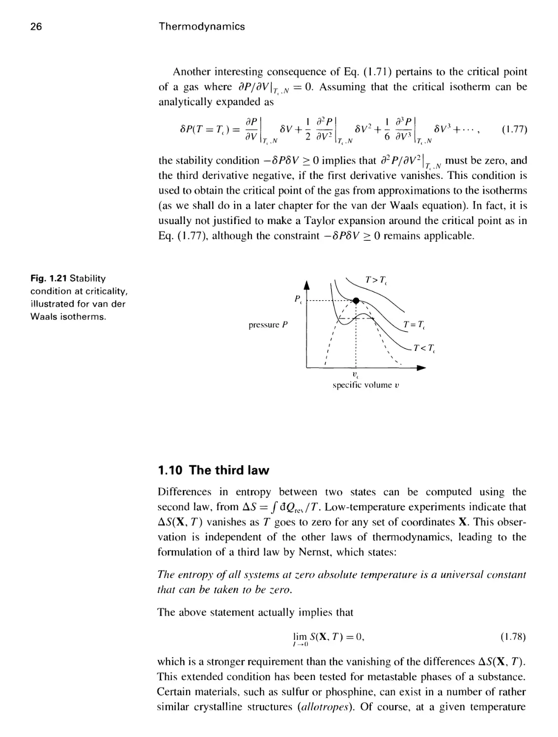
Fig. 1.21 Stability
condition at criticality,
illustrated for van der
Waals isotherms.
Another interesting consequence of Eq. A.71) pertains to the critical point
of a gas where 8P/dV\T N — 0. Assuming that the critical isotherm can be
analytically expanded as
SP(T = Tt)= —
1 d2P
8V +
2 dV2
5V3 + «-
A.77)
the stability condition — 8P8V > 0 implies that d2P/dV2\ must be zero, and
the third derivative negative, if the first derivative vanishes. This condition is
used to obtain the critical point of the gas from approximations to the isotherms
(as we shall do in a later chapter for the van der Waals equation). In fact, it is
usually not justified to make a Taylor expansion around the critical point as in
Eq. A.77), although the constraint — 8P8V > 0 remains applicable.
pressure P
T>T,
specific volume v
1.10 The third law
Differences in entropy between two states can be computed using the
second law, from AS — f dQrcJT. Low-temperature experiments indicate that
AS(X, T) vanishes as T goes to zero for any set of coordinates X. This
observation is independent of the other laws of thermodynamics, leading to the
formulation of a third law by Nernst, which states:
The entropy of all systems at zero absolute temperature is a universal constant
that can be taken to be zero.
The above statement actually implies that
lim5(X,7)=0,
A.78)
which is a stronger requirement than the vanishing of the differences AS(X, T).
This extended condition has been tested for metastable phases of a substance.
Certain materials, such as sulfur or phosphine, can exist in a number of rather
similar crystalline structures (allotropes). Of course, at a given temperature

1.10 The third law
27
only one of these structures is truly stable. Let us imagine that, as the high-
temperature equilibrium phase A is cooled slowly, it makes a transition at a
temperature T* to phase B, releasing latent heat L. Under more rapid cooling
conditions the transition is avoided, and phase A persists in metastable
equilibrium. The entropies in the two phases can be calculated by measuring the heat
capacities CA(T) and CB(T). Starting from 7 = 0, the entropy at a temperature
slightly above T* can be computed along the two possible paths as
•r* ,W)
s(t*+€) = sa(o)+[ dr-*L-L = sB(o)+[ dr-^ + —. A.79)
Jo I Jo II*
By such measurements we can indeed verify that SA@) = SB@) = 0.
metastable A
*f
,>•"" B
latent heat L
Fig. 1.22 Heat capacity
measurements on
allotropes of the same
material.
Consequences of the third law:
1. Since S(T = 0, X) = 0 for all coordinates X,
r dS
lim —
7-0 dX
2. Heat capacities must vanish as T -> 0 since
'T^CX(T)
s(r,x)-s(o,x)= f &r x ,
•A) T'
and the integral diverges as T -> 0 unless
A.80)
A.81)
limCxG) = 0.
3. Thermal expansivities also vanish as T —> 0 since
1 dx
x ~df
1 dS
x ~dJ
A.82)
A.83)
The second equality follows from the Maxwell relation in Eq. A.56). The vanishing of
the latter is guaranteed by Eq. A.80).

28
Thermodynamics
It is impossible to cool any system to absolute zero temperature in a finite number of steps.
For example, we can cool a gas by an adiabatic reduction in pressure. Since the curves of
S versus T for different pressures must join at T = 0, successive steps involve progressively
smaller changes, in S and in 7\ on approaching zero temperature. Alternatively, the
unattainability of zero temperatures implies that S(T = 0, P) is independent of P. This is
a weaker statement of the third law, which also implies the equality of zero temperature
entropy for different substances.
Fig. 1.23 An infinite
number of steps is
required to cool a gas to
7" = 0 by a series of
isothermal
decompressions.
In the following chapters, we shall attempt to justify the laws of
thermodynamics from a microscopic point of view. The first law is clearly a reflection
of the conservation of energy, which also operates at the microscopic level.
The zeroth and second laws suggest an irreversible approach to equilibrium,
a concept that has no analog at the particulate level. It is justified as reflecting
the collective tendencies of large numbers of degrees of freedom. In statistical
mechanics the entropy per particle is calculated as S/N = kB\n(gN)/N, where
gN is the degeneracy of the states (number of configurations with the same
energy) of a system of N particles. The third law of thermodynamics thus
requires that lim^^ \n(gN)/N —> 0 at T = 0, limiting the possible number of
ground states for a many-body system.
The above condition does not hold within the framework of classical
statistical mechanics, as there are examples of both non-interacting (such as an
ideal gas) and interacting (the frustrated spins in a triangular antiferromagnet)
systems with a large number of (degenerate) ground states, and a finite zero-
temperature entropy. However, classical mechanics is inapplicable at very low
temperatures and energies where quantum effects become important. The third
law is then equivalent to a restriction on the degeneracy of ground states of a
quantum mechanical system.3 While this can be proved for a non-interacting
1 For any spin system with rotational symmetry, such as a ferromagnet, there are of course many
possible ground states related by rotations. However, the number of such states does not grow
with the number of spins N. thus such degeneracy does not affect the absence of a
thermodynamic entropy at /ero temperature.

Problems
system of identical particles (as we shall demonstrate in the final chapter), there
is no general proof of its validity with interactions. Unfortunately, the onset of
quantum effects (and other possible origins of the breaking of classical
degeneracy) is system-specific. Hence it is not a priori clear how low the temperature
must be before the predictions of the third law can be observed. Another
deficiency of the law is its inapplicability to glassy phases. Glasses result from
the freezing of supercooled liquids into configurations with extremely slow
dynamics. While not truly equilibrium phases (and hence subject to all the
laws of thermodynamics), they are effectively so due to the slowness of the
dynamics. A possible test of the applicability of the third law to glasses is
discussed in the problems.
Problems for chapter 1
1. Surface tension: thermodynamic properties of the interface between two phases are
described by a state function called the surface tension S. It is defined in terms of the
work required to increase the surface area by an amount &A through SW = SdA.
(a) By considering the work done against surface tension in an infinitesimal change in
radius, show that the pressure inside a spherical drop of water of radius R is larger
than outside pressure by 2S/R. What is the air pressure inside a soap bubble of
radius Rl
(b) A water droplet condenses on a solid surface. There are three surface tensions
involved, Saw, Ssw, and Ssa, where a, s, and w refer to air, solid, and water,
respectively. Calculate the angle of contact, and find the condition for the appearance of a
water film (complete wetting).
(c) In the realm of "large** bodies gravity is the dominant force, while at "small" distances
surface tension effects are all important. At room temperature, the surface tension
of water is S0 % 7 x 10~2N m. Estimate the typical length scale that separates
"large" and "small" behaviors. Give a couple of examples for where this length scale
is important.
2. Surfactants: surfactant molecules such as those in soap or shampoo prefer to spread on
the air-water surface rather than dissolve in water. To see this, float a hair on the surface
of water and gently touch the water in its vicinity with a piece of soap. (This is also why
a piece of soap can power a toy paper boat.)
(a) The air-water surface tension Sn (assumed to be temperature-independent) is reduced
roughly by N kBT/A, where N is the number of surfactant particles, and A is the
area. Explain this result qualitatively.
(b) Place a drop of water on a clean surface. Observe what happens to the air-water
surface contact angle as you gently touch the droplet surface with a small piece of
soap, and explain the observation.

30
Thermodynamics
(c) More careful observations show that at higher surfactant densities
A-Nb
dS
NkBT la /NV 8T
T~ (A-NbJ~ A \a) ' an ~dS
NkR
where a and b are constants. Obtain the expression for S(A, T) and explain
qualitatively the origin of the corrections described by a and b.
(d) Find an expression for C§ - CA in terms of ff\T = ff \§y S, ff |r, and § |^.
3. Temperature scales: prove the equivalence of the ideal gas temperature scale 0, and the
thermodynamic scale 7\ by performing a Carnot cycle on an ideal gas. The ideal gas
satisfies PV = N kB®, and its internal energy ? is a function of 6 only. However, you
may not assume that E oc 6. You may wish to proceed as follows:
(a) Calculate the heat exchanges QH and Qc as a function of 6^, Bc, and the volume
expansion factors.
(b) Calculate the volume expansion factor in an adiabatic process as a function of O.
(c) Show that QH/QC = ®///Br.
4. Equations of state: the equation of state constrains the form of internal energy as in the
following examples.
(a) Starting from d? = TdS - PdV, show that the equation of state PV = NkBT in fact
implies that E can only depend on T.
(b) What is the most general equation of state consistent with an internal energy that
depends only on temperature?
(c) Show that for a van der Waals gas Cv is a function of temperature alone.
jje 3}: 3}: 3}: sje 3}: 3:3):
5. The Clausius-Clapeyron equation describes the variation of boiling point with pressure.
It is usually derived from the condition that the chemical potentials of the gas and liquid
phases are the same at coexistence. For an alternative derivation, consider a Carnot
engine using one mole of water. At the source (P, 7) the latent heat L is supplied
converting water to steam. There is a volume increase V associated with this process.
The pressure is adiabatically decreased to P — dP. At the sink (P — dP, T — dT) steam
is condensed back to water.
(a) Show that the work output of the engine is W = VdP + 0{dP2). Hence obtain the
Clausius-Clapeyron equation
^1 =^. (i)

Problems
(b) What is wrong with the following argument: "The heat QH supplied at the source to
convert one mole of water to steam is L(T). At the sink L(T — d7) is supplied to
condense one mole of steam to water. The difference dTdL/dT must equal the work
W = VdPy equal to LdT/T from Eq. A). Hence dL/dT = L/T, implying that L is
proportional to TV*
(c) Assume that L is approximately temperature-independent, and that the volume change
is dominated by the volume of steam treated as an ideal gas, that is, V = NkBT/P.
Integrate Eq. A) to obtain P(T).
(d) A hurricane works somewhat like the engine described above. Water evaporates
at the warm surface of the ocean, steam rises up in the atmosphere, and
condenses to water at the higher and cooler altitudes. The Coriolis force converts
the upward suction of the air to spiral motion. (Using ice and boiling water,
you can create a little storm in a tea cup.) Typical values of warm ocean
surface and high altitude temperatures are 80° F and — 120°F, respectively. The warm
water surface layer must be at least 200 feet thick to provide sufficient water
vapor, as the hurricane needs to condense about 90 million tons of water vapor
per hour to maintain itself. Estimate the maximum possible efficiency, and power
output, of such a hurricane. (The latent heat of vaporization of water is about
2.3 x 106Jkg_1.)
(e) Due to gravity, atmospheric pressure P(h) drops with the height h. By balancing the
forces acting on a slab of air (behaving like a perfect gas) of thickness dh, show that
P(h) = P0exp(—mgh/kT), where m is the average mass of a molecule in air.
(f) Use the above results to estimate the boiling temperature of water on top of
Mount Everest (h % 9 km). The latent heat of vaporization of water is about
2.3xl06Jkg-'.
6. Glass: liquid quartz, if cooled slowly, crystallizes at a temperature Tmt and releases latent
heat L. Under more rapid cooling conditions, the liquid is supercooled and becomes
glassy.
(a) As both phases of quartz are almost incompressible, there is no work input, and
changes in internal energy satisfy d? = TdS 4- fidN. Use the extensivity condition
to obtain the expression for /x in terms of E, T, 5, and N.
(b) The heat capacity of crystalline quartz is approximately Cx = aT*, while that of
glassy quartz is roughly CG = CT, where a and C are constants.
Assuming that the third law of thermodynamics applies to both crystalline and glass
phases, calculate the entropies of the two phases at temperatures T < Tm.
(c) At zero temperature the local bonding structure is similar in glass and
crystalline quartz, so that they have approximately the same internal
energy E0. Calculate the internal energies of both phases at temperatures
T < Tm.
(d) Use the condition of thermal equilibrium between two phases to compute the
equilibrium melting temperature Tm in terms of a and /3.
(e) Compute the latent heat L in terms of a and f$.

Thermodynamics
(f) Is the result in the previous part correct? If not, which of the steps leading to it is
most likely to be incorrect?
** ** ****
7. Filament: for an elastic filament it is found that, at a finite range in temperature, a
displacement x requires a force
J = ax — bT+ cTx,
where a, by and c are constants. Furthermore, its heat capacity at constant displacement
is proportional to temperature, that is, Cx = A(x)T.
(a) Use an appropriate Maxwell relation to calculate dS/dx\T.
(b) Show that A has to in fact be independent of x, that is, dA/dx = 0.
(c) Give the expression for 5G, x) assuming 5@,0) = S0.
(d) Calculate the heat capacity at constant tension, that is, C, = T dS/dT\j as a function
of T and J.
8. Hard core gas: a gas obeys the equation of state P(V — Nb) = NkBT, and has a heat
capacity Cv independent of temperature. (N is kept fixed in the following.)
(a) Find the Maxwell relation involving 8S/dV\TN.
(b) By calculating dE(T, V), show that E is a function of T (and N) only.
(c) Show that y = CP/CV = 1 +NkB/Cv (independent of T and V).
(d) By writing an expression for E(P, V), or otherwise, show that an adiabatic change
satisfies the equation P(V — Nb)y = constant.
9. Superconducting transition: many metals become superconductors at low temperatures
7\ and magnetic fields B. The heat capacities of the two phases at zero magnetic field
are approximately given by
I CS(T) = VaT3 in the superconducting phase
| Cn(T) = V [PT3 + yT] in the normal phase
where V is the volume, and {a, j8, y] are constants. (There is no appreciable change in
volume at this transition, and mechanical work can be ignored throughout this problem.)
(a) Calculate the entropies SS(T) and Sn(T) of the two phases at zero field, using the
third law of thermodynamics.
(b) Experiments indicate that there is no latent heat (L = 0) for the transition between
the normal and superconducting phases at zero field. Use this information to obtain
the transition temperature Tc, as a function of a, j8, and y.

Problems
(c) At zero temperature, the electrons in the superconductor form bound Cooper pairs.
As a result, the internal energy of the superconductor is reduced by an amount
VA, that is, En(T = 0) = EQ and ES(T = 0) = E{) - V& for the metal and
superconductor, respectively. Calculate the internal energies of both phases at finite
temperatures.
(d) By comparing the Gibbs free energies (or chemical potentials) in the two phases,
obtain an expression for the energy gap A in terms of a, j8, and y.
(e) In the presence of a magnetic field B, inclusion of magnetic work results in dE =
TdS + BdM + fidN, where M is the magnetization. The superconducting phase is
a perfect diamagnet, expelling the magnetic field from its interior, such that Ms —
— VB/Dtt) in appropriate units. The normal metal can be regarded as approximately
non-magnetic, with Mn = 0. Use this information, in conjunction with previous
results, to show that the superconducting phase becomes normal for magnetic fields
larger than
Be(T) = Bo(l~y
giving an expression for BQ.
10. Photon gas Carnot cycle: the aim of this problem is to obtain the black-body radiation
relation, E(T, V) oc VT4, starting from the equation of state, by performing an infinitesimal
Carnot cycle on the photon gas.
P
A
P + dP
T
V+dV
(a) Express the work done, W, in the above cycle, in terms of dV and dP.
(b) Express the heat absorbed, g, in expanding the gas along an isotherm, in terms of
P, dV, and an appropriate derivative of E(T, V).
(c) Using the efficiency of the Carnot cycle, relate the above expressions for W and Q
to T and d7\
(d) Observations indicate that the pressure of the photon gas is given by P = AT4, where
A = 7r2k4B/45 (heK is a constant. Use this information to obtain E(T, V), assuming
E@, V) = 0.
(e) Find the relation describing the adiabatic paths in the above cycle.

Thermodynamics
11. Irreversible processes
(a) Consider two substances, initially at temperatures 71,0 and 7^, coming to equilibrium
at a final temperature Tf through heat exchange. By relating the direction of heat
flow to the temperature difference, show that the change in the total entropy, which
can be written as
fTf do. fTt aOo r Tt-T?
Jt? Tx Jt* T2 J TJ2
must be positive. This is an example of the more general condition that "m a closed
system, equilibrium is characterized by the maximum value of entropy S."
(b) Now consider a gas with adjustable volume V, and diathermal walls, embedded in a
heat bath of constant temperature 7\ and fixed pressure P. The change in the entropy
of the bath is given by
A5baIh = ^=-^=-i(A?gas + PAVgas).
By considering the change in entropy of the combined system establish that "the
equilibrium of a gas at fixed T and P is characterized by the minimum of the Gibbs
free energy G = E + PV- TS."
12. The Solar System originated from a dilute gas of particles, sufficiently separated from
other such clouds to be regarded as an isolated system. Under the action of gravity the
particles coalesced to form the Sun and planets.
(a) The motion and organization of planets is much more ordered than the original dust
cloud. Why does this not violate the second law of thermodynamics?
(b) The nuclear processes of the Sun convert protons to heavier elements such as carbon.
Does this further organization lead to a reduction in entropy?
(c) The evolution of life and intelligence requires even further levels of organization.
How is this achieved on Earth without violating the second law?

2
Probability
2.1 General definitions
The laws of thermodynamics are based on observations of macroscopic bodies¦,
and encapsulate their thermal properties. On the other hand, matter is composed
of atoms and molecules whose motions are governed by more fundamental
laws (classical or quantum mechanics). It should be possible, in principle, to
derive the behavior of a macroscopic body from the knowledge of its
components. This is the problem addressed by kinetic theory in the following
chapter. Actually, describing the full dynamics of the enormous number of
particles involved is quite a daunting task. As we shall demonstrate, for
discussing equilibrium properties of a macroscopic system, full knowledge of the
behavior of its constituent particles is not necessary. All that is required is
the likelihood that the particles are in a particular microscopic state. Statistical
mechanics is thus an inherently probabilistic description of the system, and
familiarity with manipulations of probabilities is an important prerequisite. The
purpose of this chapter is to review some important results in the theory of
probability, and to introduce the notations that will be used in the following
chapters.
The entity under investigation is a random variable x, which has a set of
possible outcomes S == {x{, jc2, • •}. The outcomes may be discrete as in the case of
a coin toss, Scoin = {head, tail), or a dice throw, ?dice = {1,2,3,4,5,6}, or
continuous as for the velocity of a particle in a gas, S~ = {—oo < vx, vy, vz < oo},
or the energy of an electron in a metal at zero temperature, Se = {0 < e < eF}.
An event is any subset of outcomes E c <S, and is assigned a probability p(E),
for example, pdice({l}) = 1/6, or pdice({l, 3}) = 1/3. From an axiomatic point
of view, the probabilities must satisfy the following conditions:
(i) Positivity. p(E) > 0, that is, all probabilities must be real and non-negative,
(ii) Additivity. p(A or B) = p(A) + p(B), if A and B are disconnected events,
(iii) Normalization. p(S) = 1, that is, the random variable must have some outcome
in S.

36
Probability
From a practical point of view, we would like to know how to assign
probability values to various outcomes. There are two possible approaches:
1. Objective probabilities are obtained experimentally from the relative frequency of
the occurrence of an outcome in many tests of the random variable. If the random
process is repeated TV times, and the event A occurs NA times, then
p(A)= lim ^-.
For example, a series of TV = 100, 200, 300 throws of a dice may result in TV, =
19, 30,48 occurrences of 1. The ratios 0.19, 0.15, 0.16 provide an increasingly more
reliable estimate of the probability Pd\ce({^})-
2. Subjective probabilities provide a Theoretical estimate based on the uncertainties
related to lack of precise knowledge of outcomes. For example, the assessment
Pdice({l}) — 1/6 is based on the knowledge that there are six possible outcomes
to a dice throw, and that in the absence of any prior reason to believe that
the dice is biased, all six are equally likely. All assignments of probability in
statistical mechanics are subjectively based. The consequences of such
subjective assignments of probability have to be checked against measurements, and
they may need to be modified as more information about the outcomes becomes
available.
2.2 One random variable
As the properties of a discrete random variable are rather well known, here
we focus on continuous random variables, which are more relevant to our
purposes. Consider a random variable x, whose outcomes are real numbers,
that is, Sx = {—oo < x < oo}.
• The cumulative probability function (CPF) P(x) is the probability of an outcome
with any value less than x, that is, P{x) = prob(? C [—oo, x]). P(x) must be a
monotonically increasing function of x, with P(—oo) = 0 and P(+oo) = 1.
Fig. 2.1 A typical
cumulative probability
function.

2.2 One random variable
37
P(x) =
dP_
Fig. 2.2 A typical
probability density
function.
• The probability density function (PDF) is defined by p{x) = dP{x)/dx. Hence,
p(x)dx = prob(? e [x, x + dx]). As a probability density, it is positive, and normalized
such that
prob(S)= / dx p(x) = 1.
J — oo
B.1)
Note that since p(x) is a probability density, it has dimensions of [x]~\ and changes
its value if the units measuring x are modified. Unlike P(x), the PDF has no upper
bound, that is, 0 < p(x) < oo, and may contain divergences as long as they are
integrable.
The expectation value of any function, F(x), of the random variable is
<fU)>=/ dxp(x)F(x).
B.2)
Fig. 2.3 Obtaining the
PDF for the function
F(x).
The function F(x) is itself a random variable, with an associated PDF of
pF(f)df = prob(F(jc) e [/, f-\-df\). There may be multiple solutions jc, to the
equation F(x) = f, and
M/W = I>(*/)d*M
M/) = E/to)
djc
dF
B.3)
The factors of |dx/dF| are the Jacobians associated with the change of variables
from x to F. For example, consider p(x) = Aexp(—A|jc|)/2, and the function

38
Probability
F(x) = x2. There are two solutions to F(x) = /, located at x± = ±V7\ with
corresponding Jacobians |±//2/2|. Hence,
PF(f) = -exp
(->Ml7?\+\w\h
Aexp(-AV7)
2VT
for / > 0, and pF(f) = 0 for / < 0. Note that pF(f) has an (integrable)
divergence at / = 0.
Fig. 2.4 Probability
density functions for x,
and F = x2.
4 Pc
• Moments of the PDF are expectation values for powers of the random variable. The
/ith moment is
% = {xn) = j dxp(x)xn
B.4)
The characteristic function is the generator of moments of the distribution. It is simply
the Fourier transform of the PDF, defined by
p(k) = (e~lkx) = f dxp(x) e~,/cx.
B.5)
The PDF can be recovered from the characteristic function through the inverse Fourier
transform
p(x)=—jdkp(k)e+'k*. B-6)
Moments of the distribution are obtained by expanding p(k) in powers of k,
«*> = <?^ =?^?V>. B.7)
Moments of the PDF around any point x0 can also be generated by expanding
00 i—'ikY7
e^/K*) = (e-*<*-*<')) = ? ^—- ((x -XoY).
B.8)

2.2 One random variable
39
• The cumulant generating function is the logarithm of the characteristic function. Its
expansion generates the cumulants of the distribution defined through
lnp(*) = E
(-!*)"
<*">, •
B.9)
Relations between moments and cumulants can be obtained by expanding the
logarithm of p(k) in Eq. B.7), and using
ln(l+e) = ?(-0"
B.10)
The first four cumulants are called the mean, variance, skewness, and curtosis (or
kurtosis) of the distribution, respectively, and are obtained from the moments as
B.11)
(X\={X*)-4(x>){x)-3(Xif + l2(Xi){Xf-6{X)\
The cumulants provide a useful and compact way of describing a PDF.
An important theorem allows easy computation of moments in terms of the
cumulants: represent the nth cumulant graphically as a connected cluster of n
points. The rath moment is then obtained by summing all possible subdivisions
of ra points into groupings of smaller (connected or disconnected) clusters. The
contribution of each subdivision to the sum is the product of the connected
cumulants that it represents. Using this result, the first four moments are
computed graphically.
.&..+3.*V +
:••: +4.iV + 3 *? +6
Fig. 2.5 Graphical
computation of the first
four moments.
The corresponding algebraic expressions are
{Xi)={x\+3{X2)c{x)c + {X)l
(x*) = (x*)( +4(*3), <*>,+ 3(*t+6^ (tf + ix)!.
B.12)

Probability
This theorem, which is the starting point for various diagrammatic computations
in statistical mechanics and field theory, is easily proved by equating the
expressions in Eqs B.7) and B.9) for p(k):
00 (—\1Am
EL-T-<^)=exp
?^<*->.
»=1
n\
=nz[t^m-\ <,„
Matching the powers of (—ik)m on the two sides of the above expression leads to
{Pn)
<^) = ^m!n-ir|r-<xB>f-. B.14)
The sum is restricted such that J2 nPn — m> anc* leads to the graphical
interpretation given above, as the numerical factor is simply the number of ways of
breaking m points into {pn} clusters of n points.
2.3 Some important probability distributions
The properties of three commonly encountered probability distributions are
examined in this section.
A) The normal (Gaussian) distribution describes a continuous real random
variable jc, with
^-^•"[-^l B,5)
The corresponding characteristic function also has a Gaussian form,
*W>^^[-^H=^[_i*A-nr|- B'16)
Cumulants of the distribution can be identified from \np(k) = —ik\ — k2crT/2,
using Eq. B.9), as
<*>t=A, (x\ = cr\ (x\=(x\ = ... = 0. B.17)
The normal distribution is thus completely specified by its two first
cumulants. This makes the computation of moments using the cluster expansion
(Eqs. B.12)) particularly simple, and
<*> =A,
(JC2)=I72 + A2,
(x3)=3<72A + A3, B-18)
(jc4)=3o-4 + 6o-2A2 + A4,

2.3 Some important probability distributions
The normal distribution serves as the starting point for most perturbative
computations in field theory. The vanishing of higher cumulants implies that
all graphical computations involve only products of one-point, and two-point
(known as propagators), clusters.
B) The binomial distribution: consider a random variable with two outcomes
A and B (e.g., a coin toss) of relative probabilities pA and pB = 1 — pA. The
probability that in TV trials the event A occurs exactly NA times (e.g., 5 heads
in 12 coin tosses) is given by the binomial distribution
(;>
pANa)=\::)Pa*PNb-Na- B-19)
The prefactor,
-, r-, B-20)
is just the coefficient obtained in the binomial expansion of (pA + pB)N\ and
gives the number of possible orderings of NA events A and NB = N — NA events
B. The characteristic function for this discrete distribution is given by
Mk) = ( e"^> = ?u ^1^, nN/nNB-N* e-™< = (p*-* +pBf . B.21)
The resulting cumulant generating function is
lnpN(k) = N\n(pAe-ik+pB) = N]npl(k), B.22)
where \np{ (k) is the cumulant generating function for a single trial. Hence, the
cumulants after N trials are simply N times the cumulants in a single trial. In
each trial, the allowed values of NA are 0 and 1 with respective probabilities pB
and pA, leading to (NA) = pA, for all L After TV trials the first two cumulants
are
<NA)c = NpA9 {N2A)c = N(pA-p2A) = NpApB. B.23)
A measure of fluctuations around the mean is provided by the standard
deviation, which is the square root of the variance. While the mean of the binomial
distribution scales as N, its standard deviation only grows as «/N. Hence, the
relative uncertainty becomes smaller for large N.
The binomial distribution is straightforwardly generalized to a multinomial
distribution, when the several outcomes {A, B, • • • , M} occur with probabilities
{pA, pB,-" , pM}. The probability of finding outcomes {NA,NB,-- , NM} in a
total of N = NA + NB H h NM trials is
pA{Na*Nb*-*Nm))=n"\ n /aAPNbB"-PNmM- B.24)

42
Probability
C) The Poisson distribution: the classical example of a Poisson process
is radioactive decay. Observing a piece of radioactive material over a time
interval T shows that:
(a) The probability of one and only one event (decay) in the interval [t, t + dt] is
proportional to dt as dt —> 0.
(b) The probabilities of events at different intervals are independent of each other.
Fig. 2.6 Subdividing the
time interval into small
segments of size df.
dt
H—I—I—I—I—I—I—I—I—I—h
The probability of observing exactly M decays in the interval T is given by
the Poisson distribution. It is obtained as a limit of the binomial distribution
by subdividing the interval into N = T/dt ^> 1 segments of size dt. In each
segment, an event occurs with probability p = adt, and there is no event with
probability q=\— adt. As the probability of more than one event in dt is too
small to consider, the process is equivalent to a binomial one. Using Eq. B.21),
the characteristic function is given by
p(k) = (pe-lk + q)" = lim [1 -{-adt (e* - \)]T/dt = exp[a(e~lk -\)T]. B.25)
The Poisson PDF is obtained from the inverse Fourier transform in Eq. B.6)
as
dk
p(x)=f ^exp[a(e^-l)r + i^] = e-^f f-e*< ?
J-oo Z7T J-oo LIT .. „
^^e-'kM, B.26)
, M!
using the power series for the exponential. The integral over k is
dk
leading to
J-oo 2tt
00 (aT\M
B.27)
B.28)
This answer clearly realizes that the only possible values of x are integers M.
The probability of M events is thus paT{M) = e~aT(aT)M/Ml. The cumulants
of the distribution are obtained from the expansion
In paT{k) = aT(e~ik - 1) = aT ?
(-i*)"
(M")c = aT. B.29)

2.4 Many random variables
All cumulants have the same value, and the moments are obtained from
Eqs. B.12) as
<M> = (a7), (M2) = (aTJ + (a7), (M3) = (a7K + 3(aTJ + («7). B.30)
Example. Assuming that stars are randomly distributed in the Galaxy
(clearly unjustified) with a density n, what is the probability that the nearest
star is at a distance /?? Since the probability of finding a star in a small volume
dV is ndV, and they are assumed to be independent, the number of stars in a
volume V is described by a Poisson process as in Eq. B.28), with a = n. The
probability p(R) of encountering the first star at a distance R is the product of
the probabilities pnV@) of finding zero stars in the volume V = 4ttR3/3 around
the origin, and pndv(\) of finding one star in the shell of volume dV = AirR2dR
at a distance R. Both pnV@) and pndv(l) can be calculated from Eq. B.28),
and
p(R)dR = pnV@) PndvV) =e-47r*3"/3 e-47r*2"d/? 4irR2ndR,
(Air
——R3n
2.4 Many random variables
With more than one random variable, the set of outcomes is an Af-dimensional
space, Sx = {—oo < x{, x2, • • • ,xN < oo}. For example, describing the location
and velocity of a gas particle requires six coordinates.
• The joint PDF p(x) is the probability density of an outcome in a volume element
d^x = njli dXj around the point x = {*,, jc2, • • • , -%}• The joint PDF is normalized
such that
Py(S) = fd"xp(x)=l. B.32)
If, and only if, the Af random variables are independent, the joint PDF is the product
of individual PDFs,
p(x) = Y\Pi(Xi). B.33)
1=1
• The unconditional PDF describes the behavior of a subset of random variables,
independent of the values of the others. For example, if we are interested only in the
location of a gas particle, an unconditional PDF can be constructed by integrating
over all velocities at a given location, p(x) = f d3vp(x, v)\ more generally,
c N
p(xi>~'>xj=j n d*//**.'•••'•%)• B-34)
i=m+1
•

Probability
• The conditional PDF describes the behavior of a subset of random variables, for
specified values of the others. For example, the PDF for the velocity of a particle at
a particular location 3c, denoted by p(v\x), is proportional to the joint PDF p(v\x) =
p(x, v)/N. The constant of proportionality, obtained by normalizing p(v\x), is
N
= j tfvp{x,v)=p(x), B.35)
the unconditional PDF for a particle at x. In general, the unconditional PDFs are
obtained from Bayes' theorem as
P(*\, • • • , xm\xm+l, • • • , xN) = — -. B.36)
P\xm+l> " ' ¦> XN)
Note that if the random variables are independent, the unconditional PDF is equal to
the conditional PDF.
• The expectation value of a function F(x) is obtained as before from
<F(x)) = /d"xp(x)F(x). B.37)
• The joint characteristic function is obtained from the TV-dimensional Fourier
transformation of the joint PDF,
¦D4
p(k) = Uxpl-iJ2kJxJ\j. B.38)
The joint moments and joint cumulants are generated by p(k) and lnp(k),
respectively, as
B.39)
The previously described graphical relation between joint moments (all clusters
of labeled points) and joint cumulant (connected clusters) is still applicable. For
example, from
11 11 12 11
we obtain
<*1*2> = C*l>< (*2>< +<*1 **2>c • and
(x2lx2) = (xlJl (x2)t + (**) (X2)c +2(Xl *x2)c <jc,>c + (^**2)t..
B.40)

2.5 Sums of random variables and the central limit theorem
The connected correlation (xa*Xp) is zero if xa and Xp are independent random
variables.
• The joint Gaussian distribution is the generalization of Eq. B.15) to TV random
variables, as
1
p(x) = —===== exp
JB<n)Ndet[C]
-^E^-'L^-aj^-aj
B.41)
where C is a symmetric matrix, and C_1 is its inverse. The simplest way to get
the normalization factor is to make a linear transformation from the variables
yy = Xj — Ay, using the unitary matrix that diagonalizes C. This reduces the
normalization to that of the product of N Gaussians whose variances are determined
by the eigenvalues of C. The product of the eigenvalues is the determinant det[C].
(This also indicates that the matrix C must be positive definite.) The corresponding
joint characteristic function is obtained by similar manipulations, and is given by
p(k) = exp I-i*wAm - -C„J/?/;,AJ , B-42)
where the summation convention (implicit summation over a repeated index) is used.
The joint cumulants of the Gaussian are then obtained from lnp(k) as
{xm)c = A„„ (xm *x„)t = Cm„, B.43)
with all higher cumulants equal to zero. In the special case of {\m} = 0, all odd
moments of the distribution are zero, while the general rules for relating moments to
cumulants indicate that any even moment is obtained by summing over all ways of
grouping the involved random variables into pairs, for example,
(xaxbxcxd) = CahCcd + CacCM + CadCbc. B.44)
In the context of field theories, this result is referred to as Wick's theorem.
2.5 Sums of random variables and the central
limit theorem
Consider the sum X — J2h=\ xn where xt are random variables with a joint PDF
of p(x). The PDF for X is
/ N-l
J i=l
B.45)
and the corresponding characteristic function (using Eq. B.38)) is given by
'H'')
px(k) = exp -ikj^xj ) = p(k1=k2 = ... = kN = k). B.46)

Probability
Cumulants of the sum are obtained by expanding Inpx{k),
N (-ikJ N
as
W,=EWc {x2)c = x>,*,-)c,-.- B-48)
If the random variables are independent, p(x) = Y\Pi(xi)> anc* Px(k) = Y\Pi(k),
the cross cumulants in Eq. B.48) vanish, and the nth cumulant of X is simply
the sum of the individual cumulants, (Xn)c = ?*, (jc?)c. When all the N
random variables are independently taken from the same distribution p{x),
this implies (Xn)c = N (x")c, generalizing the result obtained previously for
the binomial distribution. For large values of N, the average value of the
sum is proportional to N, while fluctuations around the mean, as measured
by the standard deviation, grow only as y/N. The random variable y = (X —
zero mean, and cumulants that scale as (yn)c<xNl n/2. As
N -» oo, only the second cumulant survives, and the PDF for v converges to
the normal distribution,
lim P (y = &^m = -* exp (?) . B.49)
(Note that the Gaussian distribution is the only distribution with only first and
second cumulants.)
The convergence of the PDF for the sum of many random variables to a
normal distribution is an essential result in the context of statistical mechanics
where such sums are frequently encountered. The central limit theorem states a
more general form of this result: it is not necessary for the random variables to
be independent, as the condition J2",..yl (*,, '"xim) <^0(Nm/2) is sufficient
for the validity of Eq. B.49).
Note that the above discussion implicitly assumes that the cumulants of the
individual random variables (appearing in Eq. B.48)) are finite. What happens if
this is not the case, that is, when the variables are taken from a very wide PDF?
The sum may still converge to a so-called Levy distribution. Consider a sum
of N independent, identically distributed random variables, with the mean set
to zero for convenience. The variance does not exist if the individual PDF falls
off slowly at large values as /?,-(*) = px (x) oc l/|jc|1+a, with 0 < a < 2. (a > 0
is required to make sure that the distribution is normalizable; while for a > 2
the variance is finite.) The behavior of /?, (x) at large x determines the behavior
of /?, (k) at small k, and simple power counting indicates that the expansion of
px(k) is singular, starting with \k\a. Based on this argument we conclude that
\npx(k) = N\npi(k) = N[-a\k|a + higher order terms]. B.50)

2.6 Rules for large numbers
As before we can define a rescaled variable y = X/Nx/a to get rid of the N
dependence of the leading term in the above equation, resulting in
lim px(k) = -a\k\a. B.51)
N—>-oo
The higher-order terms appearing in Eq. B.50) scale with negative powers of N
and vanish as N -» oo. The simplest example of a Levy distribution is obtained
for a = 1, and corresponds to pY = a/[7r(y2 + a2)]. (This is the Cauchy
distribution discussed in the problems section.) For other values of a the distribution
does not have a simple closed form, but can be written as the asymptotic series
p (y) = — > ( — 1) sinl—a) ; . B.52)
Such distributions describe phenomena with large rare events, characterized
here by a tail that falls off slowly as pa (y -» oo) ~ y~l~a.
2.6 Rules for large numbers
To describe equilibrium properties of macroscopic bodies, statistical mechanics
has to deal with the very large number N of microscopic degrees of freedom.
Actually, taking the thermodynamic limit of N -> oo leads to a number of
simplifications, some of which are described in this section.
There are typically three types of N dependence encountered in the
thermodynamic limit:
(a) Intensive quantities, such as temperature 7, and generalized forces, for example,
pressure f\ and magnetic field B, are independent of N, that is, 0(N°).
(b) Extensive quantities, such as energy E, entropy S, and generalized displacements,
for example, volume V, and magnetization M, are proportional to TV, that is,
(c) Exponential dependence, that is, 0(expGV</>)), is encountered in enumerating
discrete micro-states, or computing available volumes in phase space.
Other asymptotic dependencies are certainly not ruled out a priori. For
example, the Coulomb energy of N ions at fixed density scales as Q2/R ~ N5/3.
Such dependencies are rarely encountered in everyday physics. The Coulomb
interaction of ions is quickly screened by counter-ions, resulting in an
extensive overall energy. (This is not the case in astrophysical problems since the
gravitational energy is not screened. For example, the entropy of a black hole
is proportional to the square of its mass.)

48
Probability
In statistical mechanics we frequently encounter sums or integrals of
exponential variables. Performing such sums in the thermodynamic limit is
considerably simplified due to the following results.
A) Summation of exponential quantities: consider the sum
N
B.53)
where each term is positive, with an exponential dependence on N, that is,
0 < ?t ~ G(exp(N4>i))9 B.54)
and the number of terms N is proportional to some power of N.
Fig. 2.7 A sum over N
exponentially large
quantities is dominated
by the largest term.
123456789
N
Such a sum can be approximated by its largest term ?max, in the following
sense. Since for each term in the sum, 0 < ?t < ?max,
Smax<S<N?max.
B.55)
An intensive quantity can be constructed from In S/N, which is bounded by
B.56)
N ~ N ~ N N
For N oc Np, the ratio \nN/N vanishes in the large N limit, and
In S ln^
^max i
»7 at at ^max-
lim
B) Saddle point integration: similarly, an integral of the form
J= f dxexp(N<f)(x))
B.57)
B.58)
can be approximated by the maximum value of the integrand, obtained at a
point jcmax that maximizes the exponent (f){x). Expanding the exponent around
this point gives
r= /djtexpjjvl
<H*max) - 2 l<?"(-*max)IC* ~ *maxJ + '
¦I
B.59)

2.6 Rules for large numbers
49
Note that at the maximum, the first derivative </>'(*max) *s zero> while the second
derivative <l>"(xmax) is negative. Terminating the series at the quadratic order
results in
j % e"</>(w) j djcexp |"-y | </>"(-
^max /1 \X -*rnax /
¦]-/
2tt
pW(w)
W"(*max)l
, B.60)
where the range of integration has been extended to [—00,00]. The latter
is justified since the integrand is negligibly small outside the neighborhood
of x^y.
yv<p(.v)
Fig. 2.8 Saddle point
evaluation of an
"exponential" integral.
There are two types of correction to the above result. Firstly, there are
higher-order terms in the expansion of <f)(x) around xmax. These corrections can
be looked at perturbatively, and lead to a series in powers of \/N. Secondly,
there may be additional local maxima for the function. A maximum at x'max
leads to a similar Gaussian integral that can be added to Eq. B.60). Clearly
such contributions are smaller by #(exp{—N[cj)(xmax) — $0x'max)]}). Since all
these corrections vanish in the thermodynamic limit,
lim
N-+00
- lim
[^-^(^^(i)]-^ <261)
The saddle point method for evaluating integrals is the extension of the above
result to more general integrands, and integration paths in the complex plane.
(The appropriate extremum in the complex plane is a saddle point.) The
simplified version presented above is sufficient for our needs.
Stirling's approximation for N! at large N can be obtained by saddle point
integration. In order to get an integral representation of N!, start with the result
dxe-ax = -.
a
B.62)
Repeated differentiation of both sides of the above equation with respect to a
leads to
dxxNc~ax =
N\
B.63)

Probability
Although the above derivation only applies to integer N, it is possible to define
by analytical continuation a function
I\N + 1) = N\ = [°°dxxNe-\ B.64)
for all N. While the integral in Eq. B.64) is not exactly in the form of Eq. B.58),
it can still be evaluated by a similar method. The integrand can be written
as cxp(N(f)(x)), with (f>(x) = \nx — x/N. The exponent has a maximum at
*max = N, with <f>(xmax) = \nN- 1, and (/>"(*max) = -1/N2. Expanding the
integrand in Eq. B.64) around this point yields
N\^ [ dx exp|^/ln N-N-—(x -A/J1 * NN e~N JlirN, B.65)
where the integral is evaluated by extending its limits to [—oo, oo]. Stirling's
formula is obtained by taking the logarithm of Eq. B.65) as
\nN\ = N\nN-N+-\nB7rN) + o(-Y B.66)
2.7 Information, entropy, and estimation
Information: consider a random variable with a discrete set of outcomes S =
{xt}, occurring with probabilities {/?(/)}, for * = 1, • • • , Af. In the context of
information theory there is a precise meaning to the information content of
a probability distribution. Let us construct a message from N independent
outcomes of the random variable. Since there are M possibilities for each
character in this message, it has an apparent information content of N ln2 M
bits; that is, this many binary bits of information have to be transmitted to
convey the message precisely. On the other hand, the probabilities {/?(/)} limit
the types of messages that are likely. For example, if p2^> P\, it is very unlikely
to construct a message with more xx than x2. In particular, in the limit of
large N, we expect the message to contain "roughly" {N( = Npt} occurrences
of each symbol.1 The number of typical messages thus corresponds to the
number of ways of rearranging the {Af} occurrences of {xj, and is given by
the multinomial coefficient
AM
8=^1 • B.67)
n?,w
This is much smaller than the total number of messages Mn. To specify one
out of g possible sequences requires
M
ln2 g « -N J2 Pi ln2 Pi (for N -> oo) B.68)
i=i
1 More precisely, the probability of finding any N{ that is different from Npj by more than
0(y/N) becomes exponentially small in N, as N —> oo.

2.7 Information, entropy, and estimation
bits of information. The last result is obtained by applying Stirling's
approximation for In N\. It can also be obtained by noting that
= Y.^X\Pir^sX\^\ B.69)
where the sum has been replaced by its largest term, as justified in the previous
section.
Shannon's theorem proves more rigorously that the minimum number of
bits necessary to ensure that the percentage of errors in N trials vanishes in the
N —> oo limit is ln2 g. For any non-uniform distribution, this is less than the
Nln2 M bits needed in the absence of any information on relative probabilities.
The difference per trial is thus attributed to the information content of the
probability distribution, and is given by
M
/[{/>,}] = ln2M + 2>ln2p,. B.70)
Entropy: Eq. B.67) is encountered frequently in statistical mechanics in
the context of mixing M distinct components; its natural logarithm is related
to the entropy of mixing. More generally, we can define an entropy for any
probability distribution as
M
S = -!>(') Inp(i) = - (lnp(O) - B.71)
The above entropy takes a minimum value of zero for the delta function
distribution p{i) = 8- •, and a maximum value of In M for the uniform distribution
p(i) = \/M. S is thus a measure of dispersity (disorder) of the distribution, and
does not depend on the values of the random variables {jcf-}. A one-to-one
mapping to /) = F(xi) leaves the entropy unchanged, while a many-to-one mapping
makes the distribution more ordered and decreases S. For example, if the two
values, xx and jc2, are mapped onto the same /, the change in entropy is
A5(jcI,jc2^/) = Lln—g—+ftln—g—]<0. B.72)
Estimation: the entropy S can also be used to quantify subjective estimates
of probabilities. In the absence of any information, the best unbiased estimate
is that all M outcomes are equally likely. This is the distribution of
maximum entropy. If additional information is available, the unbiased estimate is
obtained by maximizing the entropy subject to the constraints imposed by this
information. For example, if it is known that (F(x)) =/, we can maximize
S(a,MP/}) = -?p@1np@-a[?M^ B.73)
-z>

Probability
where the Lagrange multipliers a and j8 are introduced to impose the constraints
of normalization, and (F(x)) = /, respectively. The result of the optimization
is a distribution pt oc exp( —j8F(jcf-)), where the value of j8 is fixed by the
constraint. This process can be generalized to an arbitrary number of conditions.
It is easy to see that if the first n — 2k moments (and hence n cumulants)
of a distribution are specified, the unbiased estimate is the exponential of an
nth-order polynomial.
In analogy with Eq. B.71), we can define an entropy for a continuous
random variable {Sx = {—oo<jc<oo})as
S = -jdx p(x) lnp(jr) = - (In p(x)). B.74)
There are, however, problems with this definition, as for example S is not
invariant under a one-to-one mapping. (After a change of variable to / = F(x),
the entropy is changed by (|F'C*)|).) As discussed in the following chapter,
canonically conjugate pairs offer a suitable choice of coordinates in classical
statistical mechanics, since the Jacobian of a canonical transformation is unity.
The ambiguities are also removed if the continuous variable is discretized. This
happens quite naturally in quantum statistical mechanics where it is usually
possible to work with a discrete ladder of states. The appropriate volume for
discretization of phase space is then set by Planck's constant h.
Problems for chapter 2
1. Characteristic functions: calculate the characteristic function, the mean, and the
variance of the following probability density functions:
(a) Uniform p(x) = ^ for —a < x < a, and p(x) = 0 otherwise.
(b) Laplace p{x) = JLexp(-?).
(c) Cauchy p(x) = ^J'^y
The following two probability density functions are defined for x > 0. Compute
only the mean and variance for each.
(d) Rayleigh p(x) = 4 exp(- ^).
(e) Maxwell p(x) = ^^ exp(-^).
2. Directed random walk: the motion of a particle in three dimensions is a series of
independent steps of length i. Each step makes an angle 6 with the z axis, with a
probability density p{6) = 2cos2@/2)/7r; while the angle 4> is uniformly distributed
between 0 and 2tt. (Note that the solid angle factor of sin 6 is already included in
the definition of p{6), which is correctly normalized to unity.) The particle (walker)
starts at the origin and makes a large number of steps TV.
(a) Calculate the expectation values (z), (x), (y), (z2), (x2), and (y2), and the covariances
(xy), (xz), and (vz).

Problems
53
(b) Use the central limit theorem to estimate the probability density p(x, y, z) for the
particle to end up at the point (xy y, z).
3. Tchebycheff inequality: consider any probability density p(x) for (-00 < x < 00),
with mean A, and variance a2. Show that the total probability of outcomes that are
more than na away from A is less than I//12, that is,
/ dxp(x)<—.
Hint. Start with the integral defining cr2, and break it up into parts corresponding
to |jc — A| > na, and |jc — A| < na.
4. Optimal selection: in many specialized populations, there is little variability among
the members. Is this a natural consequence of optimal selection?
(a) Let {ra} be n random numbers, each independently chosen from a probability density
p(r), with r e [0, 1]. Calculate the probability density p„(x) for the largest value of
this set, that is, for jc = max{r,, • • , rn}.
(b) If each ra is uniformly distributed between 0 and 1, calculate the mean and variance
of jc as a function of n, and comment on their behavior at large n.
5. Benford's law describes the observed probabilities of the first digit in a great variety
of data sets, such as stock prices. Rather counter-intuitively, the digits 1 through 9
occur with probabilities 0.301,0.176,0.125,0.097,0.079,0.067,0.058,0.051,0.046,
respectively. The key observation is that this distribution is invariant under a change
of scale, for example, if the stock prices were converted from dollars to Persian rials!
Find a formula that fits the above probabilities on the basis of this observation.
6. Information: consider the velocity of a gas particle in one dimension (—00 < v < 00).
(a) Find the unbiased probability density p] (v), subject only to the constraint that the
average speed is c, that is, (|v|) = c.
(b) Now find the probability density p2(v), given only the constraint of average kinetic
energy, (mf2/2) = mc2/2.
(c) Which of the above statements provides more information on the velocity? Quantify
the difference in information in terms of /2 — /, = ((lnp2) — (lnp,)) /In2.

54
Probability
7. Dice: a dice is loaded such that 6 occurs twice as often as 1.
(a) Calculate the unbiased probabilities for the six faces of the dice.
(b) What is the information content (in bits) of the above statement regarding the dice?
8. Random matrices: as a model for energy levels of complex nuclei, Wigner
considered N x N symmetric matrices whose elements are random. Let us assume that
each element Ml} (for i > j) is an independent random variable taken from the
probability density function
p(MlJ) = — for —a<MlJ<a, and p(MIJ)=0 otherwise.
(a) Calculate the characteristic function for each element Mty
(b) Calculate the characteristic function for the trace of the matrix, T = tr M = ?,. Mir
(c) What does the central limit theorem imply about the probability density function of
the trace at large N?
(d) For large N, each eigenvalue Aa (a = 1,2, • • • , N) of the matrix M is distributed
according to a probability density function
p(\) = —— /1 j f°r — A0 < A < A0, and p(\) = 0 otherwise
7rA0 y A0
(known as the Wigner semicircle rule). Find the variance of A.
(Hint. Changing variables to A = A0 sin 0 simplifies the integrals.)
(e) If, in the previous result, we have A^ = 4Na2/3. can the eigenvalues be independent
of each other?
9. Random deposition: a mirror is plated by evaporating a gold electrode in vac-
cum by passing an electric current. The gold atoms fly off in all directions,
and a portion of them sticks to the glass (or to other gold atoms already on
the glass plate). Assume that each column of deposited atoms is independent
of neighboring columns, and that the average deposition rate is d layers per
second.
(a) What is the probability of m atoms deposited at a site after a time tl What fraction
of the glass is not covered by any gold atoms?
(b) What is the variance in the thickness?
10. Diode: the current / across a diode is related to the applied voltage V via / =
/0 [exp(eV/kT) — 1]. The diode is subject to a random potential V of zero mean and
variance cr2, which is Gaussian distributed. Find the probability density /?(/) for the

Problems
current / flowing through the diode. Find the most probable value for /, the mean
value of /, and indicate them on a sketch of p(f).
11. Mutual information: consider random variables x and v, distributed according to
a joint probability p(x, y). The mutual information between the two variables is
defined by
tT \Px(x)Py(y)J
where px and px denote the unconditional probabilities for x and y.
(a) Relate M(x, y) to the entropies S(x, y), S(x), and S(y) obtained from the
corresponding probabilities.
(b) Calculate the mutual information for the joint Gaussian form
/ax2 by2 \
p(x9 y) oc exp I— — - cxyj .
12. Semi-flexible polymer in two dimensions: configurations of a model polymer can
be described by either a set of vectors {t,} of length a in two dimensions (for
i = 1, • • • , N)y or alternatively by the angles {(/>,} between successive vectors, as
indicated in the figure below.
t2^
¦--!>
The polymer is at a temperature 7\ and subject to an energy
N-\ N-l
!K = —K^tr t/+1 = — Ka2 ^ cos 4>;
2
i=l
where k is related to the bending rigidity, such that the probability of any
configuration is proportional to exp(—J{/kBT).
(a) Show that (tm • tM) a exp (—\n — m\/^), and obtain an expression for the persistence
length tp = at;. (You can leave the answer as the ratio of simple integrals )
(b) Consider the end-to-end distance R as illustrated in the figure. Obtain an expression
for (R2) in the limit of N > 1.
(c) Find the probability p(R) in the limit of N ^> 1.

56
Probability
(d) If the ends of the polymer are pulled apart by a force F, the probabilities for polymer
configurations are modified by the Boltzmann weight exp f f^y)- By expanding this
weight, or otherwise, show that
(R) = K-lF + 0(F3),
and give an expression for the Hookian constant K in terms of quantities calculated
before.

3
Kinetic theory of gases
3.1 General definitions
Kinetic theory studies the macroscopic properties of large numbers of
particles, starting from their (classical) equations of motion.
Thermodynamics describes the equilibrium behavior of macroscopic objects
in terms of concepts such as work, heat, and entropy. The phenomenological
laws of thermodynamics tell us how these quantities are constrained as a
system approaches its equilibrium. At the microscopic level, we know that
these systems are composed of particles (atoms, molecules), whose interactions
and dynamics are reasonably well understood in terms of more fundamental
theories. If these microscopic descriptions are complete, we should be able to
account for the macroscopic behavior, that is, derive the laws governing the
macroscopic state functions in equilibrium. Kinetic theory attempts to achieve
this objective. In particular, we shall try to answer the following questions:
1. How can we define "equilibrium" for a system of moving particles?
2. Do all systems naturally evolve towards an equilibrium state?
3. What is the time evolution of a system that is not quite in equilibrium?
The simplest system to study, the veritable workhorse of thermodynamics, is the
dilute (nearly ideal) gas. A typical volume of gas contains of the order of 1023
particles, and in kinetic theory we try to deduce the macroscopic properties of
the gas from the time evolution of the set of atomic coordinates. At any time t,
the microstate of a system of N particles is described by specifying the positions
§,¦(*)» and momenta /?,-(*)» of all particles. The microstate thus corresponds to
a point fi(t), in the 6N-dimensional phase space T = ni=i{$i» A-}- The time
evolution of this point is governed by the canonical equations
dg, _ d!K
dt ~ dp(
C.1)
dpt _ dM
dt ~~ dqt
where the Hamiltonian ^"(p, q) describes the total energy in terms of the
set of coordinates q = [qx, q2, • • • , qN}, and momenta p = {px, p2, • • • , pN}.
57

58
Kinetic theory of gases
The microscopic equations of motion have time reversal symmetry, that is, if
all the momenta are suddenly reversed, p -> —p, at t = 0, the particles retrace
their previous trajectory, q(t) — q(—t). This follows from the invariance of !K
under the transformation 7(p, q) -> (—p, q).
Fig. 3.1 The phase space
density is proportional to
the number of
representative points in
an infinitesimal volume.
As formulated within thermodynamics, the macrostate M of an ideal gas
in equilibrium is described by a small number of state functions such as E,
T, P9 and N. The space of macrostates is considerably smaller than the phase
space spanned by microstates. Therefore, there must be a very large number of
microstates fi corresponding to the same macrostate M.
This many-to-one correspondence suggests the introduction of a
statistical ensemble of microstates. Consider N copies of a particular macrostate,
each described by a different representative point fi(t) in the phase space T.
Let dJV(p, q, t) equal the number of representative points in an infinitesimal
volume dT = ]~[?Li d3p,d35, around the point (p, q). A phase space density
p(p, q, t) is then defined by
p(p, q
r)dr= lim
d*T(p,q,Q
C.2)
This quantity can be compared with the objective probability introduced in the
previous section. Clearly, f dVp = 1 and p is a properly normalized probability
density function in phase space. To compute macroscopic values for various
functions (9(p, q), we shall use the ensemble averages
<0> = /drP(pfq,O0(p,q).
C.3)
When the exact microstate p, is specified, the system is said to be in a
pure state. On the other hand, when our knowledge of the system is
probabilistic, in the sense of its being taken from an ensemble with density
p(T), it is said to belong to a mixed state. It is difficult to describe
equilibrium in the context of a pure state, since pi(t) is constantly changing in
time according to Eqs. C.1). Equilibrium is more conveniently described for
mixed states by examining the time evolution of the phase space density

3.2 Liouville's theorem
59
p(t), which is governed by the Liouville equation introduced in the next
section.
3.2 Liouville's theorem
Liouville's theorem states that the phase space density p(r, t) behaves like
an incompressible fluid.
Fig. 3.2 Time evolution of
a volume element in
phase space.
Follow the evolution of dN pure states in an infinitesimal volume dr =
ll/Ii d3Pj d3#7 around the point (p, q). According to Eqs. C.1), after an interval
8t these states have moved to the vicinity of another point (p', q'), where
q'a = qa + qjt + 0(8t2), p'a = pa +pa8t + 0(8t2).
C.4)
In the above expression, the qa and pa refer to any of the 6N coordinates and
momenta, and qa and pa are the corresponding velocities. The original volume
element dr is in the shape of a hypercube of sides dpa and dqa. In the time
interval 8t it gets distorted, and the projected sides of the new volume element
are given by
dq'a = dqa+d-^dqa8t + 0{8t2)
dp'a = dpa+d-^dpa8t + 0{8t2)
dPa
C.5)
To order of 8t2, the new volume element is dV — fl/Li d3/V d3#,\ From
Eqs. C.5) it follows that for each pair of conjugate coordinates
d,;-d^=d,a.dpa[.+(^+^Mf+^)]. 0.6)

Kinetic theory of gases
But since the time evolution of coordinates and momenta are governed by the
canonical Eqs. C.1), we have
dqa d dM d2M dpa d ( dM\ d2J{
dQa dPa dPad<la
and |* >(_»_** C.7)
Thus the projected area in Eq. C.6) is unchanged for any pair of coordinates,
and hence the volume element is unaffected, dV = dr. All the pure states
dN originally in the vicinity of (p, q) are transported to the neighborhood
of (p', q'), but occupy exactly the same volume. The ratio dN/dT is left
unchanged, and p behaves like the density of an incompressible fluid.
The incompressibility condition p(p\ q\ t + Si) = p(p, q, i) can be written
in differential form as
^J + yfi.^^.^Uo. C.8)
dt * tAdPa dr dqa dt ) y }
Note the distinction between dp/dt and dp/dt: the former partial derivative
refers to the changes in p at a particular location in phase space, while the
latter total derivative follows the evolution of a volume of fluid as it moves in
phase space. Substituting from Eq. C.1) into Eq. C.8) leads to
?E = l(^..aJL-±.aJi) = .{p,X). C.9)
dt a=l\dPa d<la dQa dPa )
where we have introduced the Poisson bracket of two functions in phase space
as
{A,B]^?(^.^-^.^)=-{B,A]. C.10)
Consequences of Liouville's theorem:
1. Under the action of time reversal, (p, q, t) -> (—p, q, — t), the Poisson bracket {p, CK)
changes sign, and Eq. C.9) implies that the density reverses its evolution, that is,
p(p,q,f) = p(-p,q,-f).
2. The time evolution of the ensemble average in Eq. C.3) is given by (using Eq. C.9))
m.f dr*fc4J>0<M)_?/ tmM.j±."L-f..»?).
dt J dt ^J \dpa dqa dqa dpaJ
C.11)
The partial derivatives of p in the above equation can be removed by using the method
of integration by parts, that is, f fp' = — f pf since p vanishes on the boundaries of the
integrations, leading to
d(O) _ ^ r r/fl9_ cW_dO_ <wr\ ( d2M d2M \"|
dt a=J PL\dPa dqa dqa dp J \dpadqa dqadpa J J
= -/ dTp{M,0} = {{0,M}).
C.12)

3.2 Liouville's theorem
Note that the total time derivative cannot be taken inside the integral sign, that is,
dM^/dr^iH(p,q). C,3)
This common mistake yields d (O) /At = 0.
3. If the members of the ensemble correspond to an equilibrium macroscopic state, the
ensemble averages must be independent of time. This can be achieved by a stationary
density dpeq/dt = 0, that is, by requiring
{Peq,H}=0. C.14)
A possible solution to the above equation is for peq to be a function of J-Cy that is, peq (p, q) =
p(^"(p, q)). It is then easy to verify that {p(^"), ft] = p'(J{){J{, J{} = 0. This solution
implies that the value of p is constant on surfaces of constant energy J-C, in phase space. This
is indeed the basic assumption of statistical mechanics. For example, in the microcanonical
ensemble, the total energy E of an isolated system is specified. All members of the ensemble
must then be located on the surface #"(p, q) = E in phase space. Equation C.9) implies
that a uniform density of points on this surface is stationary in time. The assumption of
statistical mechanics is that the macrostate is indeed represented by such a uniform density of
microstates. This is equivalent to replacing the objective measure of probability in Eq. C.2)
with a subjective one.
There may be additional conserved quantities associated with the Hamiltonian that
satisfy {L„, !K] = 0. In the presence of such quantities, a stationary density exists for any
function of the form peq(p, q) = p(^"(p, q), L, (p, q), L2(p, q), • •). Clearly, the value
of Ln is not changed during the evolution of the system, since
dI,.(p,q)_LB(p(f + dr),q(r + dO)-L.(p@,q(f))
At At
™(8L„ dp dLn dqa\
tAdP« dqa 8qa dp J X "' '
Hence, the functional dependence of peq on these quantities merely indicates that all
accessible states, that is, those that can be connected without violating any conservation
law, are equally likely.
4. The above postulate for peq answers the first question posed at the beginning of this chapter.
However, in order to answer the second question, and to justify the basic assumption of
statistical mechanics, we need to show that non-stationary densities converge onto the
stationary solution peq. This contradicts the time reversal symmetry noted in point A)
above: for any solution p(t) converging to peq, there is a time-reversed solution that
diverges from it. The best that can be hoped for is to show that the solutions p(t) are in
the neighborhood of peq the majority of the time, so that time averages are dominated by
the stationary solution. This brings us to the problem of ergodicity, which is whether it is
justified to replace time averages with ensemble averages. In measuring the properties of
any system, we deal with only one representative of the equilibrium ensemble. However,
most macroscopic properties do not have instantaneous values and require some form

Kinetic theory of gases
of averaging. For example, the pressure P exerted by a gas results from the impact of
particles on the walls of the container. The number and momenta of these particles vary
at different times and different locations. The measured pressure reflects an average over
many characteristic microscopic times. If over this time scale the representative point of
the system moves around and uniformly samples the accessible points in phase space, we
may replace the time average with the ensemble average. For a few systems it is possible
to prove an ergodic theorem, which states that the representative point comes arbitrarily
close to all accessible points in phase space after a sufficiently long time. However, the
proof usually works for time intervals that grow exponentially with the number of particles
N, and thus exceed by far any reasonable time scale over which the pressure of a gas is
typically measured. As such the proofs of the ergodic theorem have so far little to do with
the reality of macroscopic equilibrium.
3.3 The Bogoliubov-Born-Green-Kirkwood-Yvon
hierarchy
The full phase space density contains much more information than
necessary for description of equilibrium properties. For example, knowledge of the
one-particle distribution is sufficient for computing the pressure of a gas. A
one-particle density refers to the expectation value of finding any of the N
particles at location $, with momentum /?, at time t, which is computed from
the full density p as
/i(?.5,0=(E«3(?-?/)«3E-5i)
r N
J i=2
To obtain the second identity above, we used the first pair of delta functions
to perform one set of integrals, and then assumed that the density is symmetric
with respect to permuting the particles. Similarly, a two-particle density can be
computed from
f N
/2(?1.3l.?2.52.0 = W(W-l) / El <WiP(?1.3l.?2.32.--- ,PN^N,t), C-17)
J i=3
where dV7 = d3pt d3g, is the contribution of particle i to phase space volume.
The general s-particle density is defined by
N} r N N}
¦ttP" •"•*•'>= (AT^/JJ, d^P(P.«.0 = ^f^P.(P..-.5,.0. C-18)
where ps is a standard unconditional PDF for the coordinates of s particles,
and pN = p. While ps is properly normalized to unity when integrated over
all its variables, the s-particle density has a normalization of N\/(N — s)\. We
shall use the two quantities interchangeably.

3.3 The Bogoliubov-Born-Green-Kirkwood-Yvon hierarchy 63
The evolution of the few-body densities is governed by the BBGKY
hierarchy of equations attributed to Bogoliubov, Born, Green, Kirkwood, and Yvon.
The simplest non-trivial Hamiltonian studied in kinetic theory is
^(P.q)==E[7- + ^Ei)l + ^ E n^-qj). C-19)
This Hamiltonian provides an adequate description of a weakly interacting gas.
In addition to the classical kinetic energy of particles of mass m, it contains
an external potential U9 and a two-body interaction V, between the particles.
In principle, three- and higher-body interactions should also be included for a
complete description, but they are not very important in the dilute gas (nearly
ideal) limit.
For evaluating the time evolution of fs9 it is convenient to divide the
Hamiltonian into
M = Ms + !KN_S + M\ C.20)
where CK\ and CKN_S include only interactions among each group of particles,
^ = e[^ + w1 + ^ E vfa-SJ,
n=l L J {n,m)=\
N Xv 2 1 1 N
-=.? &+H+2(.F,v(?'-*)'
i=s+\ L J (i,j)=s+l
C.21)
while the interparticle interactions are contained in
^" = E ?n§„-<?,)• C-22)
fl=l f=A+l
From Eq. C.18), the time evolution of fs (or pj is obtained as
ir=f n dv-f=-/ n dv^p, #,+#•„_,+$n, C.23)
/=.V+ I f=.s + 1
where Eq. C.9) is used for the evolution of p. The three Poisson brackets in
Eq. C.23) will now be evaluated in turn. Since the first s coordinates are not
integrated, the order of integrations and differentiations for the Poisson bracket
may be reversed in the first term, and
/ n dv, {p. *,}=((/ ft
dViP).tt-,
= {p„tt,}. C.24)
Writing the Poisson brackets explicitly, the second term of Eq. C.23) takes the
form
-/ n ivlta*,j-/ ft -v, ?f* .^=_ * .•^1

Kinetic theory of gases
(using Eq. C.21))
r N
=/n.
dV;
N
?
7=4+1
[dp IdU
[dp j \dqj
f WGj-qkV
dp_
= 0. C.25)
i=s+1 j=5+1 |_»Hj \»Hj - k=5+1 &<Ij
The last equality is obtained after performing the integrations by part: the term
multiplying dp/dpj has no dependence on pp while Pj/m does not depend on
qr The final term in Eq. C.23), involving the Poisson bracket with !K\ is
-/n
dH'
dp_
\_n=\dPn j=s+]
dJC'
dqn
+ " dp j^dV(qj-qn)
J=s+ldPj n=X fy
where the sum over all particles has been subdivided into the two groups.
(Note that Di' in Eq. C.22) has no dependence on the momenta.) Integration
by parts shows that the second term in the above expression is zero. The first
term involves the sum of (N — s) expressions that are equal by symmetry and
simplifies to
=4+1 n=l
(N-S)f n
¦ i
dV(qn-qs+i)
dp_
dPn
dQn
d
dPn
r N
J U WiP
C.26)
Note that the quantity in the above square brackets is ps+l. Thus, adding up
Eqs. C.24), C.25), and C.26),
dt
{xs,Ps}=(n-s)j:] dvs+l-
dqtl
dpn
C.27)
or in terms of the densities fs9
di-{x,fs)=±l
dK,
^Qn-gs+l) *f*X
C.28)
In the absence of interactions with other particles, the density ps for a group
of s particles evolves as the density of an incompressible fluid (as required
by Liouville's theorem), and is described by the streaming terms on the left-
hand side of Eq. C.27). However, because of interactions with the remaining
N — s particles, the flow is modified by the collision terms on the right-hand
side. The collision integral is the sum of terms corresponding to a potential
collision of any of the particles in the group of s, with any of the remaining
N — s particles. To describe the probability of finding the additional particle
that collides with a member of this group, the result must depend on the
joint PDF of 5+ 1 particles described by ps+l. This results in a hierarchy of
equations in which dpjdt depends on p2, dp2/dt depends on p3, etc., which is
at least as complicated as the original equation for the full phase space density.

3.4 The Boltzmann equation
To proceed further, a physically motivated approximation for terminating the
hierarchy is needed.
3.4 The Boltzmann equation
To estimate the relative importance of the different terms appearing in
Eqs. C.28), let us examine the first two equations in the hierarchy,
\d 8L! j \h j I/,-/" dV2dVi\-^ 8{\ C.29)
\_dt dqx dpx m dqx\ J dqx dp^
and
d 8U d dU d p, d p2 d dV(qx-q2)
' H * t^—H
h
........ . -(±-Vi\
dt dqx dpx dq2 dp2 m dqx m dq2 dqx \dp\ dPi)\
= r dv3 r^,-^),4_+^fe-^),4_i/3
J l dqx dp{ dq2 dp2]
Note that two of the streaming terms in Eq. C.30) have been combined by
using dV(q{ —q2)/dq\ = —dVfa — q^/d^ which is valid for a symmetric
potential such that V(ql — q2) = V(q2 — qx).
Time scales: all terms within square brackets in the above equations have
dimensions of inverse time, and we estimate their relative magnitudes by
dimensional analysis, using typical velocities and length scales. The typical
speed of a gas particle at room temperature is v ^ 102 m s. For terms involving
the external potential U, or the interatomic potential V, an appropriate length
scale can be extracted from the range of variations of the potential.
(a) The terms proportional to
1 _ dU d
Tu dq dp
involve spatial variations of the external potential U(q), which take place over
macroscopic distances L. We shall refer to the associated time % as an extrinsic time scale,
as it can be made arbitrarily long by increasing system size. For a typical value of
L % 10~3 m, we get tu % L/v % 10-5 s.
(b) From the terms involving the interatomic potential V, we can extract two additional time
scales, which are intrinsic to the gas under study. In particular, the collision duration
}__d_V_ d_
Tc dq dp
is the typical time over which two particles are within the effective range d of their
interaction. For short-range interactions (including van der Waals and Lennard-Jones,
despite their power law decaying tails), d % 10~10m is of the order of a typical atomic
size, resulting in rc *v 10~12 s. This is usually the shortest time scale in the problem. The
analysis is somewhat more complicated for long-range interactions, such as the Coulomb
gas in a plasma. For a neutral plasma, the Debye screening length A replaces d in the
above equation, as discussed in the problems.

66
Kinetic theory of gases
(c) There are also collision terms on the right-hand side of Eqs. C.28), which depend on
/5+1, and lead to an inverse time scale
1
/
dV
dq dP fs
J dq dp ps
The integrals are only non-zero over the volume of the interparticle potential d3. The
term fs+Jfs is related to the probability of finding another particle per unit volume,
which is roughly the particle density n = N/V ~ 1026 m-3. We thus obtain the mean free
time
1
nd3 nvd2'
C.31)
which is the typical distance a particle travels between collisions. For short-range
interactions, rx % 10_8s is much longer than rt, and the collision terms on the right-hand
side of Eqs. C.28) are smaller by a factor of nd3 « A026m-3)A0-,0mK « 1(T4.
Fig. 3.3 The mean free
time between collisions is
estimated by requiring
that there is only one
other particle in the
volume swept in time rx.
vt*
d2vT„.n~0{\)
The Boltzmann equation is obtained for short-range interactions in the dilute
regime by exploiting tc/tx % nd3 <$: 1. (By contrast, for long-range interactions
such that nd3 ^> 1, the Vlasov equation is obtained by dropping the collision
terms on the left-hand side, as discussed in the problems.) From the above
discussion, it is apparent that Eq. C.29) is different from the rest of the
hierarchy: it is the only one in which the collision terms are absent from the
left-hand side. For all other equations, the right-hand side is smaller by a factor
of nd3, while in Eq. C.29) it may indeed dominate the left-hand side. Thus a
possible approximation scheme is to truncate the equations after the first two,
by setting the right-hand side of Eq. C.30) to zero.
Setting the right-hand side of the equation for f2 to zero implies that the
two-body density evolves as in an isolated two-particle system. The relatively
simple mechanical processes that govern this evolution result in streaming
terms for f2 that are proportional to both r^1 and T. The two sets of terms
can be more or less treated independently: the former describe the evolution of
the center of mass of the two particles, while the latter govern the dependence
on relative coordinates.
The density f2 is proportional to the joint PDF p2 for finding one particle at
(/?,, 5i), and another at (p2, q2), at the same time t. It is reasonable to expect
that at distances much larger than the range of the potential V, the particles are
independent, that is,

3.4 The Boltzmann equation
67
P2(?1.5l.P2.52»0-
/2(?1.5l.?2»52>0-
•Pl(?l,§l,0Pl(?2»52»0. 0r
/l (?1. 5l> O/l (?2, §2. 0. f°r I§2 ~ 5l I » <*•
C.32)
Fig. 3.4 Particles escaping
into an initially empty
container through a hole.
The above statement should be true even for situations out of equilibrium. For
example, imagine that the gas particles in a chamber are suddenly allowed
to invade an empty volume after the removal of a barrier. The density fx
will undergo a complicated evolution, and its relaxation time will be at least
comparable to ru. The two-particle density f2 will also reach its final value at
a comparable time interval. However, it is expected to relax to a form similar
to Eq. C.32) over a much shorter time of the order of rc.
Si
Mii.t)-M<i2,t)
h-^l
Fig. 3.5 The schematic
behavior of a two-body
density as a function of
relative coordinates.
For the collision term on the right-hand side of Eq. C.29), we actually
need the precise dependence of f2 on the relative coordinates and momenta
at separations comparable to d. At time intervals longer than rc (but possibly
shorter than tv), the "steady state" behavior of f2 at small relative distances is
obtained by equating the largest streaming terms in Eq. C.30), that is,
P\ d Pi d WiVi-Vi)
m dqx m dq2 dq{
\dp] dp2J\

68
Kinetic theory of gases
We expect f2{qx,q2) t0 have slow variations over the center of mass
coordinate Q = (§1 + q2)/2, and large variations over the relative coordinate
q = q2 - 51# Therefore, df2/dq » df2/dQ, and df2/q2 % -df2/dqx % d/2/d§,
leading to
^5i
•f4--4-)/2 = -f^^)-4/, C.34)
V^, ^2/ \ m J dq
The above equation provides a precise mathematical expression for how f2
is constrained along the trajectories that describe the collision of the two
particles.
The collision term on the right-hand side of Eq. C.29) can now be written as
dt
= f d3?2d3§2
- W{qx-q2)
dqx
\dpl dp2J
fi
if d3fed35 (E^)^f2{P^qirP2,qu).
C.35)
The first identity is obtained from Eq. C.29) by noting that the added term
proportional to df2/dp2 is a complete derivative and integrates to zero, while
the second equality follows from Eq. C.34), after the change of variables to
q = q2 — qx. (Since it relies on establishing the "steady state" in the relative
coordinates, this approximation is valid as long as we examine events in time
with a resolution longer than tc.)
Kinematics of collision and scattering: the integrand in Eq. C.35) is a
derivative of f2 with respect to q along the direction of relative motion p =
p2—Px of the colliding particles. To perform this integration we introduce a
convenient coordinate system for q, guided by the formalism used to describe
the scattering of particles. Naturally, we choose one axis to be parallel to
p2 — P\, with the corresponding coordinate a that is negative before a collision,
and positive afterwards. The other two coordinates of q are represented by an
Fig. 3.6 The parameters
used to describe the
collision of two particles
in their center of mass (at
3 = 0) frame, which
moves with a conserved
momentum
^ = Pi+P2=P/+p2'. In
an elastic collision, the
relative momentum p is
rotated by solid angle H.
-P
\ 0
~:~W»
p = (px-p2)ll
p=(p{-p2')l2

3.4 The Boltzmann equation
impact vector b that is 0 for a head-on collision ([px — p2] || [§i — $2])- We can
now integrate over a to get
-^ =/ d3?2d22|5i-w2l[/2(?i.5i.?2.^+;0-/2(?i.5i.?2.^-;0].
C.36)
where |5] — u2| = \px — p2 | /m is the relative speed of the two particles, with (b, —)
and (b, +) referring to relative coordinates before and after the collision. Note
that d2b I vx — v2 | is just the flux of particles impinging on the element of area d2b.
In principle, the integration over a is from —00 to +00, but as the variations
of f2 are only significant over the interaction range d, we can evaluate the
above quantities at separations of a few d from the collision point. This is a
good compromise, allowing us to evaluate f2 away from the collisions, but
at small enough separations so that we can ignore the difference between qx
and q2. This amounts to a coarse graining in space that eliminates variations
on scales finer than d. With these provisos, it is tempting to close the
equation for /,, by using the assumption of uncorrected particles in Eq. C.32).
Clearly some care is necessary as a naive substitution gives zero! The key
observation is that the densities f2 for situations corresponding to before and
after the collision have to be treated differently. For example, soon after
opening of the slot separating empty and full gas containers, the momenta of
the gas particles are likely to point away from the slot. Collisions will tend
to randomize momenta, yielding a more isotropic distribution. However, the
densities f2 before and after the collision are related by streaming,
implying that f2(px,ql,p2,b, +; t) = f2(px', qx, p2', 6, -; f), where px' and p2' are
momenta whose collision at an impact vector b results in production of
outgoing particles with momenta px and p2. They can be obtained using time
reversal symmetry, by integrating the equations of motion for incoming
colliding particles of momenta —px and — p2. In terms of these momenta, we can
write
—M = f d3p2d2b \vx - v2\ \f2(px', 3,, p2', b9 -; 0 -/2(p,, ql9p2, b, -; t) 1.
dt Icon. J L J
C.37)
[t is sometimes more convenient to describe the scattering of two
particles in terms of the relative momenta p — P\—p2 and p' =px'—p2\ before
and after the collision. For a given b, the initial momentum p is determin-
istically transformed to the final momentum p'. To find the functional form
p'(\p\,b), one must integrate the equations of motion. However, it is
possible to make some general statements based on conservation laws: in elastic
collisions, the magnitude of p is preserved, and it merely rotates to a final
direction indicated by the angles F, </>) = tl(b) (a unit vector) in spherical
coordinates. Since there is a one-to-one correspondence between the impact

70
Kinetic theory of gases
vector b and the solid angle ft, we make a change of variables between the two,
resulting in
d/,
dt
= j d3p2d2n ^ l^-i^lJ/aO/,?,,^',^-;/)
-/2(?i.5i.?2.^-;0j-
C.38)
The Jacobian of this transformation, |dcr/dft|, has dimensions of area, and is
known as the differential cross-section. It is equal to the area presented to an
incoming beam that scatters into the solid angle ft. The outgoing momenta
px' and p2' in Eq. C.38) are now obtained from the two conditions px' +
p2r = P\+p2 (conservation of momentum), and /?,' — p2' = \f>\ -p2\&(b)
(conservation of energy), as
Pi
(?l+?2 + l?l-?2|ti(S))/2,
[P2' = (P\+P2- \P\-P2Mh) /2-
C.39)
For the scattering of two hard spheres of diameter Z), it is easy to show that
the scattering angle is related to the impact parameter b by cos@/2) = b/D for
all </>. The differential cross-section is then obtained from
@\ (B\ dO D2 D2 0
d2a = bdbdcj) = Dcos I- j Dsinl - j — d<b = —sin0d0d0= —d2ft.
(Note that the solid angle in three dimensions is given by d2ft = sin0 dddcf).)
Integrating over all angles leads to the total cross-section of a = ttD2, which is
evidently correct. The differential cross-section for hard spheres is independent
of both 6 and \P\. This is not the case for soft potentials. For example, the
Coulomb potential V = e2/\Q\ leads to
do-
dft
_ / me2 V
\2\P\ism2(e/2)J
Fig. 3.7 The scattering of
two hard spheres of
diameter D, at an impact
parameter b — |?|.

3.5 The H-theorem and irreversibility
(The dependence on |P| can be justified by obtaining a distance of closest
approach from \P\2/m + e2/b ^ 0.)
The Boltzmann equation is obtained from Eq. C.38) after the substitution
/2(?i. §i. ?2. *>, -; 0 = /i(?!, 5i. 0 '/i(?2. 5i. 0. C-4°)
known as the assumption of molecular chaos. Note that even if one starts
with an uncorrected initial probability distribution for particles, there is no
guarantee that correlations are not generated as a result of collisions. The final
result is the following closed form equation for /,:
\_dt dqx dpx m dqx J
I da I
- / d3?2d2n
da
l^i-^l [/i(?i. 5i. 0/i(?2. Si. 0 -f\(p\'. 5i. 0/i(?2'. 5i. 0] •
C.41)
Given the complexity of the above "derivation" of the Boltzmann
equation, it is appropriate to provide a heuristic explanation. The streaming terms
on the left-hand side of the equation describe the motion of a single
particle in the external potential U. The collision terms on the right-hand side
have a simple physical interpretation: the probability of finding a particle of
momentum px at qx is suddenly altered if it undergoes a collision with another
particle of momentum p2. The probability of such a collision is the product
of kinematic factors described by the differential cross-section |do/dft|, the
"flux" of incident particles proportional to \v2 — vx |, and the joint probability
of finding the two particles, approximated by f\{p\)fx(p2)- The first term on
the right-hand side of Eq. C.41) subtracts this probability and integrates over
all possible momenta and solid angles describing the collision. The second
term represents an addition to the probability that results from the inverse
process: a particle can suddenly appear with coordinates (px,qx) as a result
of a collision between two particles initially with momenta p{' and p2'. The
cross-section, and the momenta (px\ p2 ')» m&y have a complicated dependence
on (pi,p2) and fl, determined by the specific form of the potential V.
Remarkably, various equilibrium properties of the gas are quite independent of this
potential.
3.5 The H-theorem and irreversibility
The second question posed at the beginning of this chapter was whether a
collection of particles naturally evolves toward an equilibrium state. While it
is possible to obtain steady state solutions for the full phase space density pN,
because of time reversal symmetry these solutions are not attractors of generic
non-equilibrium densities. Does the unconditional one-particle PDF px suffer
the same problem? While the exact density px must necessarily reflect this
property of pN, the H-theorem proves that an approximate p,, governed by the

Kinetic theory of gases
Boltzmann equation, does in fact non-reversibly approach an equilibrium form.
This theorem states that:
V f\ (/>» #> 0 satisfies the Boltzmann equation, then dH/df < 0, where
H(r) = j d3pd3? /,(?, §, 01n/,(p, 5. 0- C-42)
The function H(t) is related to the information content of the one-particle PDF.
Up to an overall constant, the information content of p, = fJN is given by
/[pjj = (lnpj), which is clearly similar to H(f).
Proof. The time derivative of H is
^=/d3?, d% ^(ln/1 + l) = /d3p1 d35, ln/,^, C.43)
dH
d7
since f dV{f{ = N f dTp — N is time-independent. Using Eq. C.41), we obtain
= / d-p, tfqx In/, I —- • — — I
-/d3?, d3§, d3p2d2o-l^,-^| [/!(?!, 5i)/,(?2. 5i)
-/itfi'^O/i^'.?!)]^/,^,?,), C.44)
where we shall interchangeably use d2cr, d2?, or d2fl|dcr/dn| for the
differential cross-section. The streaming terms in the above expression are zero, as
shown through successive integrations by parts,
[ A^ A^ 1 * 8U dfl I A^ A^ * 3U l 6fl
/ d3/>, d3?, In/, -—.-—=- / d>, dsqxf -7^'T^=r-
J dqx dPl J dq{ /, dP]
r ^ ^ d dU
= /d3pId3^1/1—•—=0,
J dPl dqx
and
/tfpItf5Iln/I^.^ = -/d'pI^I/ia >Vl=|d3?ldJ?l/*.?L=o.
./ m dq{ J m /, d^ J c^ m
The collision term in Eq. C.44) involves integrations over dummy variables
px and /?2. The labels A) and B) can thus be exchanged without any change
in the value of the integral. Averaging the resulting two expressions gives
^ =- \ f d3q d% d?Pl d2b\v{ -v2\ [f{Px)f{Pi)
dt 2J C.45)
-/i (Pi ')/i (?2')] In (/! (P, )/i (P2)) -
(The arguments, q and t, of f are suppressed for ease of notation.) We
would now like to change the variables of integration from the coordinates
describing the initiators of the collision, (p}, p2, b), to those of their products,

3.5 The H-theorem and irreversibility
(/?!', /?2', ?')• The explicit functional forms describing this transformation are
complicated because of the dependence of the solid angle tl in Eq. C.39) on b
and \p2—P\\- However, we are assured that the Jacobian of the transformation
is unity because of time reversal symmetry; since for every collision there is
an inverse one obtained by reversing the momenta of the products. In terms of
the new coordinates
^ =- I f d35 d3?,' d3p2' #b'\vx -v2\ [/,(?,)/,(p2)
-/i(?i,)/,(?2,)]ln(/1(?1)/,(?2)),
where we should now regard ipx,p2) in the above equation as functions of
the integration variables {px \p2\ ^') as m ^q. C.39). As noted earlier, \vx —
v2\ = \vx' — v2'\ for any elastic collision, and we can use these quantities
interchangeably. Finally, we relabel the dummy integration variables such that
the primes are removed. Noting that the functional dependence of (px,p2,b)
on (p\\p2\bf) is exactly the same as its inverse, we obtain
^ =- i f d3$ d3?, d3p2 d2b\v{ -v2\ [fx(p, ')/i(ft')
dt 2 J C47)
-fx(?i)/i(ft)]^ (/,(?, ')fi(Pi')) ¦
Averaging Eqs. C.45) and C.47) results in
^^-l/d^d^d^d^l^-^I^^O/.^-Zi^^feO]
dt 4J C>48)
[In (/, (?,)/, (p2)) ~ In (/, (?, ')/i (A'))] •
The integrand of the above expression is always positive. If f\{P\)f\(p2) >
fi(Pi )/i(/V)> both terms in square brackets are positive, while both are
negative if /, if>i)fiip2) < f\(pi ')/iiPi ')• m either case, their product is positive.
The positivity of the integrand establishes the validity of the H-theorem,
— < 0. C.49)
dt
Irreversibility: the second law is an empirical formulation of the vast number
of everyday observations that support the existence of an arrow of time.
Reconciling the reversibility of laws of physics governing the microscopic domain
with the observed irreversibility of macroscopic phenomena is a fundamental
problem. Of course, not all microscopic laws of physics are reversible: weak
nuclear interactions violate time reversal symmetry, and the collapse of the
quantum wave function in the act of observation is irreversible. The former
interactions in fact do not play any significant role in everyday observations
that lead to the second law. The irreversible collapse of the wave function may

Kinetic theory of gases
itself be an artifact of treating macroscopic observers and microscopic observ-
ables distinctly.1 There are proponents of the view that the reversibility of the
currently accepted microscopic equations of motion (classical or quantum) is
indicative of their inadequacy. However, the advent of powerful computers
has made it possible to simulate the evolution of collections of large numbers
of particles, governed by classical reversible equations of motion. Although
simulations are currently limited to relatively small numbers of particles A06),
they do exhibit the irreversible macroscopic behaviors similar to those observed
in nature (typically involving 1023 particles). For example, particles initially
occupying one half of a box proceed to irreversibly, and uniformly, occupy
the whole box. (This has nothing to do with limitations of computational
accuracy; the same macroscopic irreversibility is observed in exactly reversible
integer-based simulations, such as with cellular automata.) Thus the origin of
the observed irreversibilities should be sought in the classical evolution of large
collections of particles.
The Boltzmann equation is the first formula we have encountered that
is clearly not time reversible, as indicated by Eq. C.49). We can thus ask
the question of how we obtained this result from the Hamiltonian equations
of motion. The key to this, of course, resides in the physically motivated
approximations used to obtain Eq. C.41). The first steps of the approximation
were dropping the three-body collision term on the right-hand side of Eq. C.30),
and the implicit coarse graining of the resolution in the spatial and temporal
scales. Neither of these steps explicitly violates time reversal symmetry, and
the collision term in Eq. C.37) retains this property. The next step in getting
to Eq. C.41) is to replace the two-body density f2(—), evaluated before the
collision, with the product of two one-body densities according to Eq. C.32).
This treats the two-body densities before and after the collision differently.
We could alternatively have expressed Eq. C.37) in terms of the two-body
densities /2(+) evaluated after the collision. Replacing /2(+) wim tne product
of two one-particle densities would then lead to the opposite conclusion, with
dH/df > 0! For a system in equilibrium, it is hard to justify one choice over
the other. However, once the system is out of equilibrium, for example, as
in the situation of Fig. 3.4, the coordinates after the collision are more likely
to be correlated, and hence the substitution of Eq. C.32) for /2(+) does not
make sense. Time reversal symmetry implies that there should also be subtle
correlations in f2{—) that are ignored in the so-called assumption of molecular
chaos.
While the assumption of molecular chaos before (but not after) collisions is
the key to the irreversibility of the Boltzmann equation, the resulting loss of
1 The time-dependent Schrodinger equation is fully time reversible. If it is possible to write a
complicated wave function that includes the observing apparatus (possibly the whole Universe),
it is hard to see how any irreversibility may occur.

3.6 Equilibrium properties
information is best justified in terms of the coarse graining of space and time:
the Liouville equation and its descendants contain precise information about the
evolution of a pure state. This information, however, is inevitably transported
to shorter scales. A useful image is that of mixing two immiscible fluids. While
the two fluids remain distinct at each point, the transitions in space from one
to the next occur at finer resolution on subsequent mixing. At some point, a
finite resolution in any measuring apparatus will prevent keeping track of the
two components. In the Boltzmann equation, the precise information of the
pure state is lost at the scale of collisions. The resulting one-body density only
describes space and time resolutions longer than those of a two-body collision,
becoming more and more probabilistic as further information is lost.
3.6 Equilibrium properties
What is the nature of the equilibrium state described by /,, for a homogeneous
gas?
A) The equilibrium distribution: after the gas has reached equilibrium,
the function H should no longer decrease with time. Since the integrand in
Eq. C.48) is always positive, a necessary condition for dH/df = 0 is that
/i(?i.5i)/i(?2.5i)-/i(?i'.5i)/i(?i,.5i) = 0, C.50)
that is, at each point q we must have
ln/1(?1,§) + ln/1(p2,$) = ln/1(p,',^) + ln/1(p2,,5). C.51)
The left-hand side of the above equation refers to the momenta before a two-
body collision, and the right-hand side to those after the collision. The equality
is thus satisfied by any additive quantity that is conserved during the collision.
There are five such conserved quantities for an elastic collision: the particle
number, the three components of the net momentum, and the kinetic energy.
Hence, a general solution for /, is
ln/1=flE)-5E).?-i8E)(^). C.52)
We can easily accommodate the potential energy U(q) in the above form, and
set
/i(?.5) = ^E)exp[-5E).p-j8E)^ + t/E))j. C.53)
We shall refer to the above distribution as describing local equilibrium. While
this form is preserved during collisions, it will evolve in time away from
collisions, due to the streaming terms, unless {!KX, fx} = 0. The latter condition
is satisfied for any function fx that depends only on Jf,, or any other quantity
that is conserved by it. Clearly, the above density satisfies this requirement as
long as N and /3 are independent of q, and a = 0.

Kinetic theory of gases
According to Eq. C.16), the appropriate normalization for f{ is
fd3pd3qfl(p,q) = N. C.54)
For particles in a box of volume V, the potential U(q) is zero inside the
box, and infinite on the outside. The normalization factor in Eq. C.53) can be
obtained from Eq. C.54) as
,. *v [/_>.(-„,, .?)]¦- OT (^r «P(f). **>
Hence, the properly normalized Gaussian distribution for momenta is
fAhq)-
\27rmJ
3/2
exp
r pcp-poJ]
C.56)
where p0 = (/?) = ma/ft is the mean value for the momentum of the gas, which
is zero for a stationary box, and n = N/V is the particle density. From the
Gaussian form of the distribution it can be easily concluded that the variance
of each component of the momentum is (/??) = m//3, and
3m
(pi) = (pI+pI+p3=J
C.57)
B) Equilibrium between two gases: consider two different gases (a) and
(b), moving in the same potential U, and subject to a two-body interaction
Vah [q ^ — q(h^). We can define one-particle densities, f\ and f[ , for the
two gases, respectively. In terms of a generalized collision integral
co.0 = -/ d3A d2n 1^1 is, -v2\ [/i(a)(?„ $i)/r(?2,50
-f\a\Krqi)f\"\p2,rq^)\
C.58)
the evolution of these densities is governed by a simple generalization of the
Boltzmann equation to
Aa)
+ ca^a + ca^
d/l~"' [ Aa) nr(a)\
dt
(*)
C.59)
Stationary distributions can be obtained if all six terms on the right-hand
side of Eqs. C.59) are zero. In the absence of interspecies collisions, that is,
for Cab = Cha = 0, we can obtain independent stationary distributions f{ oc
exp(-/3aJ{[a)) and f[b) oc exp (-fib?c[b)). Requiring the vanishing of Cah
leads to the additional constraint,
f\a\h)fr\h)-f\a\h')fr{P2') = o, =>
PaX^Qd+foxTfa) = Pax\a)(A')+fax™ fa').
C.60)

3.6 Equilibrium properties
77
Since the total energy Jty + !K\ is conserved in a collision, the above
equation can be satisfied for fia = fib = /3. From Eq. C.57) this condition
implies the equality of the kinetic energies of the two species,
\2mJ \2rnJ 2/3
The parameter /3 thus plays the role of an empirical temperature describing the
equilibrium of gases.
C.61)
Fig. 3.8 The pressure
exerted on the wall due
to impact of particles.
C) The equation of state: to complete the identification of /3 with temperature
7\ consider a gas of TV particles confined to a box of volume V. The gas
pressure results from the force exerted by the particles colliding with the walls
of the container. Consider a wall element of area A perpendicular to the x
direction. The number of particles impacting this area, with momenta in the
interval [/?, p + dp], over a time period 8t, is
dN(p) = (fl(p)d3p)(Avx8t).
C.62)
The final factor in the above expression is the volume of a cylinder of height
vx8t perpendicular to the area element A. Only particles within this cylinder
are close enough to impact the wall during 8t. As each collision imparts a
momentum 2px to the wall, the net force exerted is
F=i/-0ocd^/-ld/7>7-ld^/l(?)(A m 8t)Bp^' C'63)
As only particles with velocities directed toward the wall will hit it, the first
integral is over half of the range of px. Since the integrand is even in px, this
restriction can be removed by dividing the full integral by 2. The pressure P
is then obtained from the force per unit area as

Kinetic theory of gases
where Eq. C.56) is used for the equilibrium form of fx. Comparing with
the standard equation of state, PV = NkBT, for an ideal gas, leads to the
identification, j8 = \/kBT.
D) Entropy: as discussed earlier, the Boltzmann H-function is closely related
to the information content of the one-particle PDF px. We can also define a
corresponding Boltzmann entropy,
SB(t) = -kBH(t), C.65)
where the constant kB reflects the historical origins of entropy. The H-theorem
implies that SB can only increase with time in approaching equilibrium. It has
the further advantage of being defined through Eq. C.42) for situations that
are clearly out of equilibrium. For a gas in equilibrium in a box of volume V,
from Eq. C.56), we compute
H = v/d3pfl(p)lnfl(p)
-"Kcssb*)-!]- <"»
The entropy is now identified as
5B = -^H = MJ^ + ^lnB77m^r)-ln^^l. C.67)
The thermodynamic relation, TdSB = dE + PdV9 implies
dE dS„\ 3
7 = -NkB,
dT\„ dT \v 2 B
V
T
= 1
= /
dSB
dT
dSD
dV
BE\ _rrdSB\ _NkBT
dV\
C.68)
lr v
The usual properties of a monatomic ideal gas, PV = NkBT, and E = 3NkBT/2,
can now be obtained from the above equations. Also note that for this classical
gas, the zero temperature limit of the entropy in Eq. C.67) is not independent
of the density n, in violation of the third law of thermodynamics.
3.7 Conservation laws
Approach to equilibrium: we now address the third question posed in the
introduction, of how the gas reaches its final equilibrium. Consider a situation
in which the gas is perturbed from the equilibrium form described by Eq. C.56),
and follow its relaxation to equilibrium. There is a hierarchy of mechanisms
that operate at different time scales.
(i) The fastest processes are the two-body collisions of particles in immediate vicinity. Over
a time scale of the order of tc, /2Ei » $2* 0 relaxes to fx (qx, i)fx (q2, t) for separations
I5i ~~ §21 ^ d. Similar relaxations occur for the higher-order densities fs.

3.7 Conservation laws
(ii) At the next stage, fx relaxes to a local equilibrium form, as in Eq. C.53), over the time
scale of the mean free time rx. This is the intrinsic scale set by the collision term on the
right-hand side of the Boltzmann equation. After this time interval, quantities conserved
in collisions achieve a state of local equilibrium. We can then define at each point a
(time-dependent) local density by integrating over all momenta as
n(q,t) = fd3pfl(p,q,t), C.69)
as well as a local expectation value for any operator 0(p,q,t),
{OQ. t)) = -^-^ j d3p/, (p, q, tH(p, q, t). C.70)
(iii) After the densities and expectation values have relaxed to their local equilibrium forms
in the intrinsic time scales tc and tx , there is a subsequent slower relaxation to global
equilibrium over extrinsic time and length scales. This final stage is governed by the
smaller streaming terms on the left-hand side of the Boltzmann equation. It is most
conveniently expressed in terms of the time evolution of conserved quantities according
to hydrodynamic equations.
Conserved quantities are left unchanged by the two-body collisions, that is,
they satisfy
x(?i. 5. t)+x(P2> 5> 0 = x(h \ 5, t)+x(j>2\ 5,0. C.7i)
where (p\,p2) and (/?,', p2') refer to the momenta before and after a collision,
respectively. For such quantities, we have
(?.5,0 = 0. C.72)
coll
JxG,t) = fd3px(p,q,t)-?
Proof. Using the form of the collision integral, we have
y^ = -/d3?1d3?2d^|^-^2|[/1(pO/,(?2)-/i(?i0/,(?2,)]^(?i). C-73)
(The implicit arguments (§, t) are left out for ease of notation.) We now
perform the same set of changes of variables that were used in the proof of the
H-theorem. The first step is averaging after exchange of the dummy variables
px and p2, leading to
Jx = ~\S d3?i d"P2 d^l"! -v2\ [/,(?,)/, (ft) -/,(?, ')/i(ft')] [X©l) + X(?2)] •
C.74)
Next, change variables from the originators (Pi,p2,b) to the products
(Pi'tPi'ib') °f the collision. After relabeling the integration variables, the
above equation is transformed to
Jx=-\j d3?, d3p2 d2b\v, -v2\ [/,(?, ')/i(/V)
2; C.75)
-fl(Pl)fl(P2)][xG>l')+X(P2')].

Kinetic theory of gases
Averaging the last two equations leads to
J =-Ud3p, d^d^l^-Salf/,©,)/,^)-/,©/)/,^')]
4-/ C.76)
[x(Pi)+X(Pi)-x(Pi') -xiPi')}.
which is zero from Eq. C.71).
Let us explore the consequences of this result for the evolution of
expectation values involving \- Substituting for the collision term in Eq. C.72) the
streaming terms on the left-hand side of the Boltzmann equation lead to
7,E, t) = f d3pX(p, q, t) [dt + ^3tt +Ftt JL] /,(p, §, t) = 0, C.77)
where we have introduced the notations dt = d/dt, da = d/dqa, and Fa =
—dU/dqa. We can manipulate the above equation into the form
/d3?{[,,+ ^a + FA](^])_/i[5, + ^5a + Fa_?_],}=o. C.78)
The third term is zero, as it is a complete derivative. Using the definition of
expectation values in Eq. C.70), the remaining terms can be rearranged into
*,("<*>) + *« ("(^*))-^^^ C-79)
As discussed earlier, for elastic collisions, there are five conserved quantities:
particle number, the three components of momentum, and kinetic energy. Each
leads to a corresponding hydrodynamic equation, as constructed below.
(a) Particle number, setting ^ = 1 in Eq. C.79) leads to
dtn + da(nua)=0, C.80)
where we have introduced the local velocity
C.81)
¦¦(?)¦
This equation simply states that the time variation of the local particle density
is due to a particle current Jn = nu.
(b) Momentum: any linear function of the momentum p is conserved in the
collision, and we shall explore the consequences of the conservation of
c = - - u. C.82)
m
Substituting ca into Eq. C.79) leads to
dp (n {{up + cp) ca)) + ndtua + ndpUa [u^ + Cp) - n — = 0. C.83)
Taking advantage of (ca) = 0, from Eqs. C.81) and C.82), leads to
dtua + updpua = -± dpPap , C.84)

3.7 Conservation laws
where we have introduced the pressure tensor,
Pap = mn(caCp). C.85)
The left-hand side of the equation is the acceleration of an element of the fluid
du/dt, which should equal Fnet/m according to Newton's equation. The net
force includes an additional component due to the variations in the pressure
tensor across the fluid.
(c) Kinetic energy: we first introduce an average local kinetic energy
(mc2\ In2 _> _> mu2\ ,„ „,x
— ) = \in~PU+— )• C86)
and then examine the conservation law obtained by setting \ equal to mc2/2
in Eq. C.79). Since for space and time derivatives de = mcpdcp = —mcpdup,
we obtain
d,(we)+da(w((«a + 0^)K
-nFa(ca)=0.
Taking advantage of (ca) = 0, the above equation is simplified to
dt(ns) + da (nuas) + da (n (^ ^)) + Kffl*"* = 0. C.88)
We next take out the dependence on n in the first two terms of the above
equation, finding
edtn + ndtE + sda (nua) + nuadas + daha + PapUaf3 = 0, C.89)
where we have also introduced the local heat flux
h=™(cac2), C.90)
and the rate of strain tensor
UaP=2(d«UP + dPUa)- C-91)
Eliminating the first and third terms in Eq. C.89) with the aid of Eq. C.80)
leads to
dte + uadae = daha - -PaaUaQ. C.92)
n n H H
Clearly, to solve the hydrodynamic equations for n, w, and e, we need
expressions for PaC and h, which are either given phenomenologically, or calculated
from the density /,, as in the next sections.

Kinetic theory of gases
3.8 Zeroth-order hydrodynamics
As a first approximation, we shall assume that in local equilibrium, the density
/, at each point in space can be represented as in Eq. C.56), that is,
fx (p, g, t) = — __ 3/2 exp
(p-mu(q9t))
2 "I
2mkBT(q, t)
C.93)
"E. t)
BrnnkBnq,t)Y
The choice of parameters clearly enforces f d3pf® = n, and (p/m) = u, as
required. Average values are easily calculated from this Gaussian weight; in
particular,
/ \0 kBT.
H m
¦««/B. C.94)
leading to
Pl^nkBT8a^ and s = ^kBT. C.95)
Since the density f® is even in c, all odd expectation values vanish, and in
particular
h° = 0. C.96)
The conservation laws in this approximation take the simple forms
Dtn = —ndaua
mDtua = Fa--da(nkBT) C.97)
DtT = ~Tdaua
In the above expression, we have introduced the material derivative
Dt = [dt + updp]t C.98)
which measures the time variations of any quantity as it moves along the
stream-lines set up by the average velocity field u. By combining the first and
third equations, it is easy to get
Dt\n(nT-3/2)=0. C.99)
The quantity In (nT~3/2) is like a local entropy for the gas (see Eq. C.67)),
which according to the above equation is not changed along stream-lines. The
zeroth-order hydrodynamics thus predicts that the gas flow is adiabatic. This
prevents the local equilibrium solution of Eq. C.93) from reaching a true global
equilibrium form, which necessitates an increase in entropy.
To demonstrate that Eqs. C.97) do not describe a satisfactory approach to
equilibrium, examine the evolution of small deformations about a stationary
(u0 = 0) state, in a uniform box (F = 0), by setting
I/iE,r) = w + K5.0
C.100)
7X5.0= r+0E.')

3.8 Zeroth-order hydrodynamics
We shall next expand Eqs. C.97) to first order in the deviations (y, 6, u).
Note that to lowest order, Dt = dt + O(u), leading to the linearized zeroth-order
hydrodynamic equations
kBT
mdtua = —
n
dnv-
C.101)
dte = --Tdaua
Normal modes of the system are obtained by Fourier transformations,
A (it, o>\ = f d3qdt exp [i (it • q - cot\] A E, t) , C.102)
where A stands for any of the three fields (y, 0, u). The natural vibration
frequencies are solutions to the matrix equation
0 nkp 0
0
iTkn
f8<*pkp
0
C.103)
It is easy to check that this equation has the following modes, the first three
with zero frequency:
(a) Two modes describe shear flows in a uniform (n = n) and isothermal (T =T) fluid, in
which the velocity varies along a direction normal to its orientation (e.g., u = f(x, t)y).
In terms of Fourier modes k ¦ uT(k) = 0, indicating transverse flows that are not relaxed
in this zeroth-order approximation.
(b) A third zero-frequency mode describes a stationary fluid with uniform pressure P =
nkBT. While n and T may vary across space, their product is constant, insuring that the
fluid will not start moving due to pressure variations. The corresponding eigenvector of
Eq. C.103) is
C.104)
(c) Finally, the longitudinal velocity (ue || k) combines with density and temperature
variations in eigenmodes of the form
with co(k) = ±ve\k\>
where
3 m
C.105)
C.106)
is the longitudinal sound velocity. Note that the density and temperature variations in
this mode are adiabatic, that is, the local entropy (proportional to In (nT~3/2)) is left
unchanged.

Kinetic theory of gases
We thus find that none of the conserved quantities relaxes to equilibrium in
the zeroth-order approximation. Shear flow and entropy modes persist forever,
while the two sound modes have undamped oscillations. This is a deficiency
of the zeroth-order approximation that is removed by finding a better solution
to the Boltzmann equation.
3.9 First-order hydrodynamics
While f®(p, q, i) of Eq. C.93) does set the right-hand side of the Boltzmann
equation to zero, it is not a full solution, as the left-hand side causes its form
to vary. The left-hand side is a linear differential operator, which using the
various notations introduced in the previous sections, can be written as
L[f]^\dt + ^da + Fa^]f=\Dt + cada + ^^]f. C.107)
It is simpler to examine the effect of C on In/,0, which can be written as
ln/f = In (nT-) - ~ - ^ In {2irmkB). C.108)
Using the relation d(c2/2) = c^dc^ = —c^dup, we get
C [in/?] = Dt In (nT-i'2) + ^DtT + {^caDtua
B B C.109)
(dan 3 d„T\ mc2 m „ Faca
~^r- + ^, ^oc<Ar+- cacBdauB- -——.
n 2 T ) 2kBT2 a a kBT a p a p kBT
If the fields n, T, and ua, satisfy the zeroth-order hydrodynamic Eqs. C.97),
we can simplify the above equation to
mc2 m
m ( 8<*n i\ , (mcl 5V»3T
The characteristic time scale tv for C is extrinsic, and can be made much
larger than rx. The zeroth-order result is thus exact in the limit (^/r^) —> 0;
and corrections can be constructed in a perturbation series in (tx/tu). To this
purpose, we set /, = f®(l +g), and linearize the collision operator as
= -fi(Pi)CL\g\. C.111)

3.9 First-order hydrodynamics
While linear, the above integral operator is still difficult to manipulate in
general. As a first approximation, and noting its characteristic magnitude, we
set
Q[g]«-. C.H2)
This is known as the single collision time approximation, and from the
linearized Boltzmann equation ?[/i] = —f\CL[g\ we obtain
g = -Tx^^[/1]^-rx>C[ln/10], C.113)
J\
where we have kept only the leading term. Thus the first-order solution is given
by (using Eq. C.110))
// (?, 5, t) = /{>(?, §, t) [l - g (cacfi - ^c2) uap
C.114)
where t^ = tk = tx in the single collision time approximation. However, in
writing the above equation, we have anticipated the possibility of r^ ^ tk,
which arises in more sophisticated treatments (although both times are still of
order of rx).
It is easy to check that f d3/?// = / d3/?/,0 = n, and thus various local
expectation values are calculated to first order as
(O)l = ±[d3pOfl(l+g) = (OH + (gO)°. C-115)
n J
The calculation of averages over products of ca's, distributed according to the
Gaussian weight of /}*, is greatly simplified by the use of Wick's theorem,
which states that expectation value of the product is the sum over all possible
products of paired expectation values, for example
(k T\2
-^-j {8afi8y8 + Say8fi8 + Sa88fiy)- C.116)
(Expectation values involving a product of an odd number of cft's are zero by
symmetry.) Using this result, it is easy to verify that
The pressure tensor at first order is given by
nm[cac^ = nm (cacpf - -±j \cac^ (c^ - -j-<?\\ u>
nksTd^-lnksTr^ (uap - -yuyy) •
P] ¦
C.118)

Kinetic theory of gases
(Using the above result, we can further verify that e1 = (mc2/2) = 3kBT/2, as
before.) Finally, the heat flux is given by
,, / mc2\ nmrK doT l( mc2 5\ 9\
5 nk2DTT,
C.119)
B1 4K
2 m
d„T.
At this order, we find that spatial variations in temperature generate a heat
flow that tends to smooth them out, while shear flows are opposed by the
off-diagonal terms in the pressure tensor. These effects are sufficient to cause
relaxation to equilibrium, as can be seen by examining the modified behavior
of the modes discussed previously.
(a) The pressure tensor now has an off-diagonal term
pUf3 = ~2nkBTrtluaB = -ix (dauB + dBua) , C.120)
where jjl = nkBTT^ is the viscosity coefficient. A shearing of the fluid (e.g., described by
a velocity uy(x, t)) now leads to a viscous force that opposes it (proportional to iid2xux),
causing its diffusive relaxation as discussed below.
(b) Similarly, a temperature gradient leads to a heat flux
h = -KVT, C.121)
where K = Enk2BTTK)/Bm) is the coefficient of thermal conductivity of the gas. If the
gas is at rest (u = 0, and uniform P = nkBT), variations in temperature now satisfy
3 2K
ndts = -nkBdtT = -da (-KdaT) , => dtT = —V2I C.122)
2 3nkB
This is the Fourier equation and shows that temperature variations relax by diffusion.
We can discuss the behavior of all the modes by linearizing the equations
of motion. The first-order contribution to Dtua ^ dtua is
81 {d'Ua) = ~Ldf>8lPa/i ** ~rih (\d»dP + S«>dydy) u^ BU23)
where /jl = nkBTT^. Similarly, the correction for DtT ^ dt6 is given by
2 2K
8'(d,0) = --—daha*--—dadae, C.124)
3kBn 3kBn
with K = Enk2BTTK)/Bm). After Fourier transformation, the matrix
equation C.103) is modified to
n8aBkB 0 \
«i«.i = i*2f
**h "^(*2^ + ^) k^aBkB
2Tfl h ;2Kk2 .
uB
C.125)

Problems
We can ask how the normal mode frequencies calculated in the zeroth-order
approximation are modified at this order. It is simple to verify that the transverse
(shear) normal models (k • uT = 0) now have a frequency
wT = -i-^k2. C.126)
mn
The imaginary frequency implies that these modes are damped over a
characteristic time TT(k) ~ l/|a>r| ~ M2/(T/^2)» where A is the corresponding
wavelength, and i; ~ y/kBT/m is a typical gas particle velocity. We see that
the characteristic time scales grow as the square of the wavelength, which is
the signature of diffusive processes.
In the remaining normal modes the velocity is parallel to ?, and Eq. C.125)
reduces to
C.127)
The determinant of the dynamical matrix is the product of the three eigenfre-
quencies, and to lowest order is given by
det(M) = i^.^.^+(9(Tj). C.128)
3kBn mn
At zeroth order the two sound modes have a)±(k) = ±vek, and hence the
frequency of the isobaric mode is
At first order, the longitudinal sound modes also turn into damped oscillations
with frequencies a>±(k) = ±vek — iy. The simplest way to obtain the decay
rates is to note that the trace of the dynamical matrix is equal to the sum of
the eigenvalues, and hence
a>l(k) = ±vek-ik2(^ + -^)+0(rl). C.130)
\3mn \5kBnJ
The damping of all normal modes guarantees the, albeit slow, approach of the
gas to its final uniform and stationary equilibrium state.
Problems for chapter 3
1. One-dimensional gas: a thermalized gas particle is suddenly confined to a one-
dimensional trap. The corresponding mixed state is described by an initial density
function p(q, p,t = 0) = 8(q)f(p), where f(p) = exp(-p2/2mkBT)/y/27rmkBT.
(a) Starting from Liouville's equation, derive p(q, p, t) and sketch it in the (q, p) plane.
(b) Derive the expressions for the averages [q2) and (p2) at t > 0.
(c) Suppose that hard walls are placed at q = ±Q. Describe p(q, p,t^> t), where t is
an appropriately large relaxation time.

Kinetic theory of gases
(d) A "coarse-grained" density p is obtained by ignoring variations of p below some
small resolution in the (q, p) plane; for example, by averaging p over cells of the
resolution area. Find p(q, p) for the situation in part (c), and show that it is stationary.
2. Evolution of entropy, the normalized ensemble density is a probability in the phase space
T. This probability has an associated entropy S(t) = — fdTp(T, t) lnp(r, t).
(a) Show that if p(Y, t) satisfies Liouville's equation for a Hamiltonian J{, dS/dt = 0.
(b) Using the method of Lagrange multipliers, find the function pmax(T) that
maximizes the functional S[p], subject to the constraint of fixed average energy, (PC) =
fdTp!K = E.
(c) Show that the solution to part (b) is stationary, that is, dpmax/dt = 0.
(d) How can one reconcile the result in (a) with the observed increase in entropy as
the system approaches the equilibrium density in (b)? (Hint. Think of the situation
encountered in the previous problem.)
3. The Vlasov equation is obtained in the limit of high particle density n = N/V, or large
interparticle interaction range A, such that wA3 ^> 1. In this limit, the collision terms are
dropped from the left-hand side of the equations in the BBGKY hierarchy.
The BBGKY hierarchy
\d IJ2?" dU f (dU i y-dV^-qi)\ *1
fs
¦if
dV„
<w(§„-§s+i) dfs-,
(In
dp„
has the characteristic time scales
1
\_
1
dU d
dq dp
dV d
dq dp
v
Z'
V
J q p fs
-nX*
where n\3 is the number of particles within the interaction range A, and v is a typical
velocity. The Boltzmann equation is obtained in the dilute limit, nA3 <^C 1, by disregarding
terms of order l/rx <C 1/tc. The Vlasov equation is obtained in the dense limit of
n A3 » 1 by ignoring terms of order \/t( <& 1 /rx.
(a) Assume that the TV-body density is a product of one-particle densities, that is, p =
n?Li Pi (x/, t), where x, = (pf, qt). Calculate the densities fs, and their normalizations.

Problems
(b) Show that once the collision terms are eliminated, all the equations in the BBGKY
hierarchy are equivalent to the single equation
I" d p d dUef{ dl
\_dt m dq dq dp]
where
C/eff{q, t) = U{q) + f dx'VQ-$')/i(*'> 0-
(c) Now consider N particles confined to a box of volume V, with no
additional potential. Show that f\(q,p) = g(p)/V is a stationary solution to the
Vlasov equation for any g(p). Why is there no relaxation toward equilibrium for
4. Two-component plasma: consider a neutral mixture of N ions of charge +e and mass
m+, and N electrons of charge —e and mass m_, in a volume V = N/n0.
(a) Show that the Vlasov equations for this two-component system are
{[ d p d d®eff d 1 _ _ x
I L^ m4 dq dq dp J
Ira p 8 <90>eff d i _
[ \_dt m_ dq dq dp]
where the effective Coulomb potential is given by
^ffE,0 = *ex((§) + ^/dx'CE-5')[/+(x',0-/-(x',0]-
Here, <?ext is the potential set up by the external charges, and the Coulomb potential
C(q) satisfies the differential equation V2C = 47r83(q).
(b) Assume that the one-particle densities have the stationary forms f± = g±(p)n±(q).
Show that the effective potential satisfies the equation
V20>eff = 47rpext +47TC (n+(q) - n_(q)) ,
where pext is the external charge density.
(c) Further assuming that the densities relax to the equilibrium Boltzmann weights
n±(q) = «0exp[±/3e<I>eff(§)] leads to the self-consistency condition
V2«*>eff = 477 [peu + n0e (e*«* - e"^«)],
known as the Poisson-Boltzmann equation. Due to its non-linear form, it is generally
not possible to solve the Poisson-Boltzmann equation. By linearizing the
exponentials, one obtains the simpler Debye equation
Vz*eff=477-pext + 4)eff/A2.
Give the expression for the Debye screening length A.

Kinetic theory of gases
(d) Show that the Debye equation has the general solution
<*>effE) = / d35'GE " 5')PextE').
where G(q) = exp(— \q |/A)/|51 is the screened Coulomb potential.
(e) Give the condition for the self-consistency of the Vlasov approximation, and interpret
it in terms of the interparticle spacing.
(f) Show that the characteristic relaxation time (r % \/v) is temperature-independent.
What property of the plasma is it related to?
5. Two-dimensional electron gas in a magnetic field: when donor atoms (such as
P or As) are added to a semiconductor (e.g., Si or Ge), their conduction
electrons can be thermally excited to move freely in the host lattice. By growing
layers of different materials, it is possible to generate a spatially varying potential
(work-function) that traps electrons at the boundaries between layers. In the
following, we shall treat the trapped electrons as a gas of classical particles in two
dimensions.
If the layer of electrons is sufficiently separated from the donors, the main source of
scattering is from electron-electron collisions.
(a) The Hamiltonian for non-interacting free electrons in a magnetic field has the form
(h-eA)
V ' ±Hb\B\
2m
(The two signs correspond to electron spins parallel or anti-parallel to the field.)
The vector potential A = Bx q/2 describes a uniform magnetic field B. Obtain the
classical equations of motion, and show that they describe rotation of electrons in
cyclotron orbits in a plane orthogonal to B.
(b) Write down heuristically (i.e., not through a step-by-step derivation) the Boltzmann
equations for the densities /T(/?, q, t) and f±(p, q, t) of electrons with up and down
spins, in terms of the two cross-sections a = crn = cru, and crx = crn, of spin
conserving collisions.
(c) Show that dH/df < 0, where H = Ht + H^ is the sum of the corresponding
H-functions.
(d) Show that dH/df = 0 for any In/ that is, at each location, a linear combination of
quantities conserved in the collisions.
(e) Show that the streaming terms in the Boltzmann equation are zero for any function
that depends only on the quantities conserved by the one-body Hamiltonians.
(f) Show that angular momentum L = q x p is conserved during, and away from,
collisions.
(g) Write down the most general form for the equilibrium distribution functions for
particles confined to a circularly symmetric potential.

Problems
(h) How is the result in part (g) modified by including scattering from magnetic and
non-magnetic impurities?
(i) Do conservation of spin and angular momentum lead to new hydrodynamic equations?
6. The Lorentz gas describes non-interacting particles colliding with a fixed set of
scattered. It is a good model for scattering of electrons from donor impurities. Consider
a uniform two-dimensional density n0 of fixed impurities, which are hard circles of
radius a.
(a) Show that the differential cross-section of a hard circle scattering through an angle
0is
a 6 „
da = — sin — d0,
2 2
and calculate the total cross-section.
(b) Write down the Boltzmann equation for the one-particle density f(q, p, t) of the
Lorentz gas (including only collisions with the fixed impurities). (Ignore the electron
spin.)
(c) Find the eigenfunctions and eigenvalues of the collision operator.
(d) Using the definitions F = —dU/dq, and
n(q, t) = f d2pf{q, p, t), and (g(q, t)) = —— j d2pf(q, p, t)g(q, r),
show that for any function ^(|?|), we have
(e) Derive the conservation equation for local density p = mn(q, t), in terms of the local
velocity u = (p/m).
(f) Since the magnitude of particle momentum is unchanged by impurity scattering, the
Lorentz gas has an infinity of conserved quantities |p|m. This unrealistic feature is
removed upon inclusion of particle-particle collisions. For the rest of this problem
focus only on p2 /2m as a conserved quantity. Derive the conservation equation for
the energy density
e(q, t) = - [c ), where c = u,
in terms of the energy flux h = p(cc2)/2, and the pressure tensor Pa/3 = p[cac^).
(g) Starting with a one-particle density
/«(?.3,0-«G.0exp[-5S^]
1
2mkBT(q, t) J 27rmkBT(q, t)'
reflecting local equilibrium conditions, calculate w, h, and Pa/3. Hence obtain the
zeroth-order hydrodynamic equations.

Kinetic theory of gases
(h) Show that in the single collision time approximation to the collision term in the
Boltzmann equation, the first-order solution is
fl(p,q,t)=f(p,q,t)
1-T
p (d\np d\nT p2 dT F Y
m \ dq dq 2mkBT2 dq kBT I
(i) Show that using the first-order expression for /, we obtain
pu = ht\f-kBTVIn(pT)] .
(j) From the above equation, calculate the velocity response function xafi = dUa/dFp.
(k) Calculate Pa/3, and h, and hence write down the first-order hydrodynamic
equations.
7. Thermal conductivity: consider a classical gas between two plates separated by a distance
w. One plate at y = 0 is maintained at a temperature Tx, while the other plate at y = w
is at a different temperature T2. The gas velocity is zero, so that the initial zeroth-order
approximation to the one-particle density is
[2nmkBT(y)f2
(a) What is the necessary relation between n(y) and T(y) to ensure that the gas velocity
u remains zero? (Use this relation between n(y) and T(y) in the remainder of this
problem.)
(b) Using Wick's theorem, or otherwise, show that
{P2f = (PaPaf = 3 (mkBT) , and (p4f s (paPappppf = 15 (mkBTJ ,
where @)° indicates local averages with the Gaussian weight /,0. Use the result
(p6) = \05(mkBTK in conjunction with symmetry arguments to conclude
{Pyf = 35 (mkBT)K
(c) The zeroth-order approximation does not lead to relaxation of temperature/density
variations related as in part (a). Find a better (time-independent) approximation
// (?> y), by linearizing the Boltzmann equation in the single collision time
approximation to
wHt+H]*-*?-
where tk is of the order of the mean time between collisions,
(d) Use //, along with the averages obtained in part (b), to calculate hY, the y
component of the heat transfer vector, and hence find K, the coefficient of thermal
conductivity.

Problems
(e) What is the temperature profile, T(y), of the gas in steady state?
8. Zeroth-order hydrodynamics: the hydrodynamic equations resulting from the
conservation of particle number, momentum, and energy in collisions are (in a uniform box):
dtn + da(nua) = Q
dtua + UpdpUa = dnPap
H H mn H H
dte + uadae
— dnh„ PnaUn
n n
where n is the local density, u = (p/m), uap = (daUp -\-dpUa) /2, and e = (mc2/2), with
c = p/m — u.
(a) For the zeroth-order density
/?(?.5.0 = -
w($, 0
rexp
(/? — mu(q, r))
2mkBT(q, t)
BTrmkBT{q, t))'
calculate the pressure tensor P^ = mn(caCp) , and the heat flux h°a = nm(cac2/2) .
(b) Obtain the zeroth-order hydrodynamic equations governing the evolution of n(q, t),
u(q,t), and T(q,t).
(c) Show that the above equations imply Dt In (nT~3/2) = 0, where Dt = dt + u^d^ is the
material derivative along stream-lines.
(d) Write down the expression for the function H°(r) = f d3qd3pfy(p, q, t) \nf^(p, q, t),
after performing the integrations over p, in terms of n(q, t), u(q, f), and T(q, t).
(e) Using the hydrodynamic equations in (b), calculate dH°/df.
(f) Discuss the implications of the result in (e) for approach to equilibrium.
9. Viscosity: consider a classical gas between two plates separated by a distance w. One
plate at y = 0 is stationary, while the other at y = w moves with a constant velocity
vx = u. A zeroth-order approximation to the one-particle density is
/?(?.?) = ¦
;exp
[-db^*-
mayJ+p2+p:
']¦
B7rmkBTK/2
obtained from the uniform Maxwell-Boltzmann distribution by substituting the average
value of the velocity at each point, (a = u/w is the velocity gradient.)
(a) The above approximation does not satisfy the Boltzmann equation as the collision
term vanishes, while d/,°/df ^ 0. Find a better approximation, fj (p), by linearizing
the Boltzmann equation, in the single collision time approximation, to
fl-f!
'wi-[H-?]/f
where rx is a characteristic mean time between collisions

Kinetic theory of gases
(b) Calculate the net transfer n^ of the x component of the momentum, of particles
passing through a plane at y, per unit area and in unit time.
(c) Note that the answer to (b) is independent of y, indicating a uniform transverse
force Fx = —UXY, exerted by the gas on each plate. Find the coefficient of viscosity,
defined by 17 = Fx/a.
10. Light and matter, in this problem we use kinetic theory to explore the equilibrium
between atoms and radiation.
(a) The atoms are assumed to be either in their ground state a0, or in an excited state
«,, which has a higher energy e. By considering the atoms as a collection of N
fixed two-state systems of energy E (i.e., ignoring their coordinates and momenta),
calculate the ratio n}/n0 of densities of atoms in the two states as a function of
temperature T.
Consider photons y of frequency w = e/h and momentum \p \ = hw/c, which can
interact with the atoms through the following processes:
(i) Spontaneous emission: ax —> aQ + y.
(ii) Adsorption: aQ + y —> ax.
(iii) Stimulated emission: ax+y —> aQ + y+y.
Assume that spontaneous emission occurs with a probability crsp, and that adsorption
and stimulated emission have constant (angle-independent) differential cross-sections
of (Tad/47r and (Tst/477\ respectively.
(b) Write down the Boltzmann equation governing the density / of the photon gas,
treating the atoms as fixed scatterers of densities n0 and «,.
(c) Find the equilibrium density feq for the photons of the above frequency.
(d) According to Planck's law, the density of photons at a temperature T depends on
their frequency co as / = [exp(hco/kBT) — 1]_1 /h3. What does this imply about
the above cross-sections?
(e) Consider a situation in which light shines along the x axis on a collection of atoms
whose boundary coincides with the x = 0 plane, as illustrated in the figure.
Y
^-
^-
^-
^~
vacuum
^
\
^
X
matter (n0,n{)
Clearly, / will depend on x (and px), but will be independent of y and z. Adapt the
Boltzmann equation you propose in part (b) to the case of a uniform incoming flux

Problems
of photons with momentum p = hcox/c. What is the penetration length across which
the incnminp flux Hecavs?
the incoming flux decays
11. Equilibrium density: consider a gas of N particles of mass m, in an external potential
U(q). Assume that the one-body density p, (p, q, t) satisfies the Boltzmann equation.
For a stationary solution, dpjdt = 0, it is sufficient from Liouville's theorem for p, to
satisfy px oc exp[—f3(p2/2m-\- (/($))]. Prove that this condition is also necessary by
using the H-theorem as follows.
(a) Find p, (p, q) that minimizes H = N f d3pd3qpl (p,q)\npl(p,q), subject to the
constraint that the total energy E = (!K) is constant. (Hint. Use the method of
Lagrange multipliers to impose the constraint.)
(b) For a mixture of two gases (particles of masses ma and mh) find the distributions
p, and p, that minimize H = H{a) +H{b) subject to the constraint of constant total
energy. Hence show that the kinetic energy per particle can serve as an empirical
temperature.
12. Moments of momentum: consider a gas of N classical particles of mass m in thermal
equilibrium at a temperature T, in a box of volume V.
(a) Write down the equilibrium one-particle density /eq (p, q), for coordinate q, and
momentum p.
(b) Calculate the joint characteristic function, (exp f — ik • p)), for momentum.
(c) Find all the joint cumulants (plxPyP") .
(d) Calculate the joint moment (paPp (p-p)).
13. Generalized ideal gas: consider a gas of N particles confined to a box of volume V in
d dimensions. The energy, 6. and momentum, p, of each particle are related by 6 = ps,
where p = |p|. (For classical particles s = 2, while for highly relativistic ones s = 1.)
Let f(v)dv denote the probability of finding particles with speeds between v and v + dv,
and n = N/V.
(a) Calculate the number of impacts of gas molecules per unit area of the wall of the
box, and per unit time as follows:
(i) Show that the number of particles hitting area A in a time dt arriving from a
specific direction ft, with a speed v, is proportional to A ¦ vdtcosO • nf(v)dv,
where 0 is the angle between the direction fl and the normal to the wall,
(ii) Summing over all directions ?1 with the same polar angle 6, demonstrate that
S, .sin^fldfl
dN@,v) = A udfcosfl • nf(v)dv • -^ ,
where Sd = 27TlI/2/(d/2 — 1)! is the total solid angle in d dimensions.

Kinetic theory of gases
(iii) By averaging over v and 6 show that
= -——— • riv , where v= j vf(v)dv is the average speed.
A dt (a — \)Sd J
(b) Each (elastic) collision transfers a momentum 2/?cos 6 to the wall. By examining the
net force on an element of area prove that the pressure P equals ^ - f, where E is
the average (kinetic) energy. (Note that the velocity v is not p/ra but de/dp.) (Hint.
Clearly, upon averaging over all directions (cos2 0) = \/d.)
(c) Using thermodynamics and the result in (b), show that along an adiabatic curve PVy
is constant, and calculate y.
(d) According to the equipartition theorem, each degree of freedom that appears quadrat-
ically in the energy has an energy kBT/2. Calculate the value of y if each gas particle
has I such quadratic degrees of freedom in addition to its translational motion. What
values of y are expected for helium and hydrogen at room temperature?
(e) Consider the following experiment to test whether the motion of ants is random. 250
ants are placed inside a 10 cm x 10 cm box. They cannot climb the wall, but can
escape through an opening of size 5 mm in the wall. If the motion of ants is indeed
random, and they move with an average speed of 2 mm s_1, how many are expected
to escape the box in the first 30 seconds?
14. Effusion: a box contains a perfect gas at temperature T and density n.
(a) What is the one-particle density, px(v), for particles with velocity vl
A small hole is opened in the wall of the box for a short time to allow some particles
to escape into a previously empty container.
(b) During the time that the hole is open what is the flux (number of particles per unit
time and per unit area) of particles into the container? (Ignore the possibility of any
particles returning to the box.)
(c) Show that the average kinetic energy of escaping particles is 2kBT. (Hint. Calculate
contributions to kinetic energy of velocity components parallel and perpendicular to
the wall separately.)
(d) The hole is closed and the container (now thermally insulated) is allowed to reach
equilibrium. What is the final temperature of the gas in the container?
(e) A vessel partially filled with mercury (atomic weight 201), and closed except for
a hole of area 0.1 mm2 above the liquid level, is kept at 0° C in a continuously
evacuated enclosure. After 30 days it is found that 24 mg of mercury has been lost.
What is the vapor pressure of mercury at 0° C?
15. Adsorbed particles: consider a gas of classical particles of mass m in thermal equilibrium
at a temperature 7\ and with a density n. A clean metal surface is introduced into the
gas. Particles hitting this surface with normal velocity less than vt are reflected back into
the gas, while particles with normal velocity greater than vt are absorbed by it.
(a) Find the average number of particles hitting one side of the surface per unit area and
per unit time.

Problems
97
(b) Find the average number of particles absorbed by one side of the surface per unit
area and per unit time.
16. Electron emission: when a metal is heated in vacuum, electrons are emitted from its
surface. The metal is modeled as a classical gas of non-interacting electrons held in the
solid by an abrupt potential well of depth <f> (the work-function) relative to the vacuum.
(a) What is the relationship between the initial and final velocities of an escaping
electron?
(b) In thermal equilibrium at temperature T, what is the probability density function for
the velocity of electrons?
(c) If the number density of electrons is «, calculate the current density of thermally
emitted electrons.

4
Classical statistical mechanics
4.1 General definitions
Statistical mechanics is a probabilistic approach to equilibrium macroscopic
properties of large numbers of degrees of freedom.
As discussed in chapter 1, equilibrium properties of macroscopic bodies are
phenomenologically described by the laws of thermodynamics. The macrostate
M depends on a relatively small number of thermodynamic coordinates. To
provide a more fundamental derivation of these properties, we can examine
the dynamics of the many degrees of freedom comprising a macroscopic body.
Description of each microstate /x requires an enormous amount of information,
and the corresponding time evolution, governed by the Hamiltonian equations
discussed in chapter 3, is usually quite complicated. Rather than following the
evolution of an individual (pure) microstate, statistical mechanics examines an
ensemble of microstates corresponding to a given (mixed) macrostate. It aims
to provide the probabilities pM(/x) for the equilibrium ensemble. Liouville's
theorem justifies the assumption that all accessible microstates are equally likely
in an equilibrium ensemble. As explained in chapter 2, such assignment of
probabilities is subjective. In this chapter we shall provide unbiased estimates of
pM(li) for a number of different equilibrium ensembles. A central conclusion is
that in the thermodynamic limit, with large numbers of degrees of freedom, all
these ensembles are in fact equivalent. In contrast to kinetic theory, equilibrium
statistical mechanics leaves out the question of how various systems evolve to
a state of equilibrium.
4.2 The microcanonical ensemble
Our starting point in thermodynamics is a mechanically and adiabatically
isolated system. In the absence of heat or work input to the system, the
internal energy E, and the generalized coordinates x, are fixed, specifying a
macrostate M = (?, x). The corresponding set of mixed microstates form the
microcanonical ensemble. In classical statistical mechanics, these microstates
98

4.2 The microcanonical ensemble
are defined by points in phase space, their time evolution governed by a Hamil-
tonian J{(jjl), as discussed in chapter 3. Since the Hamiltonian equations C.1)
conserve the total energy of a given system, all microstates are confined to
the surface J?(jjl) = E in phase space. Let us assume that there are no other
conserved quantities, so that all points on this surface are mutually accessible.
The central postulate of statistical mechanics is that the equilibrium probability
distribution is given by
1 f 1 for JC(jl) = E
v il(E,x) yo otherwise
Some remarks and clarification are in order:
A) Boltzmann's assumption of equal a priori equilibrium probabilities refers to the
above postulate, which is in fact the unbiased probability estimate in phase
space subject to the constraint of constant energy. This assignment is
consistent with, but not required by, Liouville's theorem. Note that the phase space
specifying the microstates fi must be composed of canonically conjugate pairs.
Under a canonical change of variables, \x —> ///, volumes in phase space are
left invariant. The Jacobian of such transformations is unity, and the transformed
probability, p(/jl') = p(fi) \d/jb/d/jL'\9 is again uniform on the surface of constant
energy.
B) The normalization factor fl(E, x) is the area of the surface of constant energy
E in phase space. To avoid subtleties associated with densities that are non-zero
only on a surface, it is sometimes more convenient to define the microcanonical
ensemble by requiring E — A < !K{ix) < E + A, that is, constraining the energy of
the ensemble up to an uncertainty of A. In this case, the accessible phase space
forms a shell of thickness 2A around the surface of energy E. The normalization is
now the volume of the shell, ft' ^ 2Aft. Since ft typically depends exponentially
on E, as long as A ~ 0(E°) (or even 0(El)\ the difference between the surface
and volume of the shell is negligible in the E <x N —> oo limit, and we can use ft
and ft' interchangeably.
C) The entropy of this uniform probability distribution is given by
S(E, x) = kB In ft(?, x). D.2)
An additional factor of kB is introduced compared with the definition of Eq. B.70),
so that the entropy has the correct dimensions of energy per degree Kelvin, used
in thermodynamics. O and S are not changed by a canonical change of coordinates
in phase space. For a collection of independent systems, the overall allowed phase
space is the product of individual ones, that is, 0Tota, = ]~[, ^V The resulting entropy
is thus additive, as expected for an extensive quantity.
Various results in thermodynamics now follow from Eq. D.1), provided that
we consider macroscopic systems with many degrees of freedom.

100
Classical statistical mechanics
Fig. 4.1 The exchange of
energy between two
isolated systems.
The zeroth law. equilibrium properties are discussed in thermodynamics
by placing two previously isolated systems in contact, and allowing them to
exchange heat. We can similarly bring together two microcanonical systems,
and allow them to exchange energy, but not work. If the original systems have
energies Ex and E2, respectively, the combined system has energy E = Ex-\-E2.
Assuming that interactions between the two parts are small, each microstate of
the joint system corresponds to a pair of microstates of the two components,
that is, jjl = jjlx (g)/A2, and ^K(fix <8>fJL2) = -^i(/xi) + ^2(/x2)- As the joint system
is in a microcanonical ensemble of energy E = Ex + E2, in equilibrium
1 fl for Jf,(fix)-\-!K2(fi2) = E
0 otherwise
Pe(/*i®/a2):
D.3)
a(E)
Since only the overall energy is fixed, the total allowed phase space is computed
from
-Sl(El) + S2(E-El)
?l(E)= f dExnx(Ex)?l2(E-
¦ Ex) = / dEx exp
D.4)
Fig. 4.2 The joint number
of states of two systems
in contact is
overwhelmingly larger at
the "equilibrium"
energies E* and E\.
The properties of the two systems in the new joint equilibrium state are implicit
in Eq. D.3). We can make them explicit by examining the entropy that follows
from Eq. D.4). Extensivity of entropy suggests that Sx and S2 are proportional
to the numbers of particles in each system, making the integrand in Eq. D.4) an
exponentially large quantity. Hence the integral can be equated by the saddle
point method to the maximum value of the integrand, obtained for energies E*
and E2= E — E*9 that is,
S(E) = kB\nn(E)
'.SX(E*X) + S2(E*2).
D.5)

4.2 The microcanonical ensemble
The position of the maximum is obtained by extremizing the exponent in
Eq. D.4) with respect to ?,, resulting in the condition
D.6)
Although all joint microstates are equally likely, the above results indicate
that there is an exponentially larger number of states in the vicinity of (E*, ??).
Originally, the joint system starts in the vicinity of some point (E®, E®). After
the exchange of energy takes place, the combined system explores a whole
set of new microstates. The probabilistic arguments provide no information
on the dynamics of evolution amongst these microstates, or on the amount
of time needed to establish equilibrium. However, once sufficient time has
elapsed so that the assumption of equal a priori probabilities is again valid, the
system is overwhelmingly likely to be at a state with internal energies (?*, ?J).
At this equilibrium point, condition D.6) is satisfied, specifying a relation
between two functions of state. These state functions are thus equivalent to
empirical temperatures, and, indeed, consistent with the fundamental result of
thermodynamics, we have
dS\\
dE\x~ T' ( ' '
The first law: we next inquire about the variations of S(E, x) with x, by
changing the coordinates reversibly by 8x. This results in doing work on
the system by an amount 6W = J • 8x, which changes the internal energy to
E + J • 8x. The first-order change in entropy is given by
5S = S(E + J-Sx,x + 5x)-S(E,x) = ( — J+ — )Sx.
\dEL dx\J
D.8)
This change will occur spontaneously, taking the system into a more probable
state, unless the quantity in brackets is zero. Using Eq. D.7), this allows us to
identify the derivatives
as
T'
D.9)
Having thus identified all variations of S, we have
d? J dx
dS(E,x) = , => d? = 7US + J-dx, D.10)
allowing us to identify the heat input 6Q = TdS.
The second law: clearly, the above statistical definition of equilibrium rests
on the presence of many degrees of freedom N ^> 1, which make it
exponentially unlikely in TV that the combined systems are found with component
energies different from {E\,E^). By this construction, the equilibrium point
has a larger number of accessible states than any starting point, that is,
ft1(?j,x1)ft2(?j,x2)>ft1(?1,x,)ft2(E2,x2). D.11)

Classical statistical mechanics
In the process of evolving to the more likely (and more densely populated)
regions, there is an irreversible loss of information, accompanied by an increase
in entropy,
8S = Sl(E*l) + S2(El)-Sl(El)-S2(E2)>0, D.12)
as required by the second law of thermodynamics. When the two bodies are
first brought into contact, the equality in Eq. D.6) does not hold. The change
in entropy is such that
/55,i _8_s1\ \ n_j_\SE D13)
that is, heat (energy) flows from the hotter to the colder body, as in Clausius's
statement of the second law.
Stability conditions: since the point (E*,E2) is a maximum, the second
derivative of SX(EX) + S2(E2) must be negative at this point, that is,
d2Sy
~dEf
d2S2
~dEl
<0. D.14)
x2

Applying the above condition to two parts of the same system, the condition of
thermal stability, Cx > 0, as discussed in Section 1.9, is regained. Similarly, the
second-order changes in Eq. D.8) must be negative, requiring that the matrtix
d2S/dxidxj\E be positive definite.
4.3 Two-level systems
Consider N impurity atoms trapped in a solid matrix. Each impurity can be
in one of two states, with energies 0 and 6, respectively. This example is
somewhat different from the situations considered so far, in that the allowed
microstates are discrete. Liouville's theorem applies to Hamiltonian evolution
in a continuous phase space. Although there is less ambiguity in enumeration
of discrete states, the dynamics that ensures that all allowed microstates are
equally accessed will remain unspecified for the moment. (An example from
quantum mechanical evolution will be presented later on.)
The microstates of the two-level system are specified by the set of occupation
numbers {«,}, where nt = 0 or 1 depending on whether the /th impurity is in
its ground state or excited. The overall energy is
X({ni}) = cY,ni = cNl9 D.15)
where N, is the total number of excited impurities. The macrostate is specified
by the total energy E, and the number of impurities N. The microcanonical
probability is thus
p«n'])=m»8*-'-< D-,6)

4.3 Two-level systems
103
As there are N, = E/e excited impurities, the normalization H is the number
of ways of choosing Nx excited levels among the available N, and given by
the binomial coefficient
a(E, n) =
W,!(W-W,)!
The entropy
S(E,N) = kB\n
N\
W,!(W-W,)!
can be simplified by Stirling's formula in the limit of N{, TV ^> 1 to
[Ni N\ N-N.N-Ml
S(E, N) % -NkB — In — + - In -
The equilibrium temperature can now be calculated from Eq. D.7) as
1
f
dS
~dE
€ \Ne-Ej
D.17)
D.18)
D.19)
D.20)
E
eN
eN/2\-
(negative temperatures)
-dk T
Fig. 4.3 The internal
energy of a two-level
system, as a function of
its temperature 7".
Alternatively, the internal energy at a temperature T is given by
Ne
E(T) =
exp
te)+1'
D.21)
The internal energy is a monotonic function of temperature, increasing from
a minimum value of 0 at T = 0 to a maximum value of Ne/2 at infinite
temperature. It is, however, possible to start with energies larger than Ne/2,
which correspond to negative temperatures from Eq. D.20). The origin of
the negative temperature is the decrease in the number of microstates with
increasing energy, the opposite of what happens in most systems. Two-level
systems have an upper bound on their energy, and very few microstates close to
this maximal energy. Hence, increased energy leads to more order in the system.
However, once a negative temperature system is brought into contact with the

104
Classical statistical mechanics
rest of the Universe (or any portion of it without an upper bound in energy), it
loses its excess energy and comes to equilibrium at a positive temperature. The
world of negative temperatures is quite unusual in that systems can be cooled by
adding heat, and heated by removing it. There are physical examples of systems
temporarily prepared at a metastable equilibrium of negative temperature in
lasers, and for magnetic spins.
The heat capacity of the system, given by
C
-?-»-(?M?)hGir)+'r- <«»
Fig. 4.4 The heat capacity
of a two-1 eve I system
goes to zero at both high
and low temperatures 7".
vanishes at both low and high temperatures. The vanishing of C as
exp(—e/kBT) at low temperatures is characteristic of all systems with an
energy gap separating the ground state and lowest excited states. The vanishing
of C at high temperatures is a saturation effect, common to systems with a
maximum in the number of states as a function of energy. In between, the heat
capacity exhibits a peak at a characteristic temperature of Te <x e/kB.
Fig. 4.5 The probabilities
for finding a single
impurity in its ground
state (top), or excited
state (bottom), as a
function of
temperature T.
Statistical mechanics provides much more than just macroscopic information
for quantities such as energy and heat capacity. Equation D.16) is a complete
joint probability distribution with considerable information on the microstates.
For example, the unconditional probability for exciting a particular impurity is
obtained from
n(E-H,6,;V-l)
p(*i)= ? p(K-}) = -
il(E,N)
D.23)

4.4 The ideal gas
The second equality is obtained by noting that once the energy taken by the
first impurity is specified, the remaining energy must be distributed among the
other TV— 1 impurities. Using Eq. D.17),
FV ' ft(?,/V) W,!(W-W,-1)! N\ N K
and p(n] = 1) = 1 -/?(«, = 0) = NJN. Using /V, = E/e, and Eq. D.21), the
occupation probabilities at a temperature T are
i exp (— -jf^)
P@) = t r, and p(l) = V ' 7 D.25)
4.4 The ideal gas
As discussed in chapter 3, microstates of a gas of N particles correspond to
points /i = {/?,, 5,} in the 6N-dimensional phase space. Ignoring the potential
energy of interactions, the particles are subject to a Hamiltonian
^ = E[f^ + ^($/)]> D-26)
where U(q) describes the potential imposed by a box of volume V. A micro-
canonical ensemble is specified by its energy, volume, and number of particles,
M = (E,V,N). The joint PDF for a microstate is
1 } 1 for ?,. G box, and ?,- p, 2/2m = E (±A?)
ft(E, V,W) l0 otherwise
In the allowed microstates, coordinates of the particles must be within the
box, while the momenta are constrained to the surface of the (hyper-)sphere
J2?=\ Pi2 = 2mE. The allowed phase space is thus the product of a contribution
VN from the coordinates, with the surface area of a 3N-dimensional sphere of
radius y/2mE from the momenta. (If the microstate energies are accepted in
the energy interval E±A?, the corresponding volume in momentum space is
that of a (hyper-)spherical shell of thickness A^ = oJ2m/EAE.) The area of a
^-dimensional sphere is Ad = SdRd~\ where Sd is the generalized solid angle.
A simple way to calculate the ^-dimensional solid angle is to consider the
product of d Gaussian integrals,
'-(/>-)
Id = [] dxe~x \ =7Td/2. D.28)
Alternatively, we may consider Id as an integral over the entire ^-dimensional
space, that is,
ld = ) lid**exp(-*?). D.29)

Classical statistical mechanics
The integrand is spherically symmetric, and we can change coordinates to
R2 = Yli x2- Noting that the corresponding volume element in these coordinates
isdVd = SdRd-ldR,
Id = Td/ttX-'e-*2 = % /"dy/^-'e- = ^ (J/2-1)!, D.30)
•>o 2 Jo 2
where we have first made a change of variables to y = R2, and then used the
integral representation of n! in Eq. B.63). Equating expressions D.28) and
D.30) for Id gives the final result for the solid angle,
27Td'2 , x
The volume of the available phase space is thus given by
2773yV/2
ft(E, V, N) = VN- -BmE)CN-l)/2AR. D.32)
v ' CN/2-\)r ' R J
The entropy is obtained from the logarithm of the above expression. Using
Stirling's formula, and neglecting terms of order of 1 or ln? ~ \nN in the
large N limit, results in
T 3/V 3N 3N 3 AH
S(E, V,N) = kB\N\nV+ — lnB7rmE) In — 4- —
D.33)
= M.ln V
r 3n
Properties of the ideal gas can now be recovered from TdS — dE 4- Pd V — judN,
1 _ dS
T~ ~dE
§*.
The internal energy E = 3NkBT/2 is only a function of T, and the heat capacity
Cv = 3NkB/2 is a constant. The equation of state is obtained from
P _ dS
T~dV
Nk
—-, => PV = NkBT. D.35)
The unconditional probability of finding a particle of momentum px in the
gas can be calculated from the joint PDF in Eq. D.27), by integrating over all
other variables,
p(Pi)=/d35ind35l-d3P/P({5/.P/})
i=1 D.36)
_Vft(?-p,2/2m, V, 7V-1)
~ fl(?, V, AO '

4.5 Mixing entropy and the Gibbs paradox
The final expression indicates that once the kinetic energy of one particle is
specified, the remaining energy must be shared amongst the other N—\. Using
Eq. D.32),
VN7T^N-^2BmE-px 2)(™-4>/2 CN/2-\)\
PKPi)=-
C(N- l)/2- 1)! VN7r™/2BmE)VN-^2
= ({_ ^.2YW2 1 C7V/2-1)! DJ7)
V 2mEJ (lirmEyi2 C(N - l)/2- l)! '
From Stirling's formula, the ratio of CN/2- 1)! to C(N- l)/2- 1)! is
approximately CN/2K/2, and in the large ? limit,
/ 3/V \3/2 ( 3N p2\
This is a properly normalized Maxwell-Boltzmann distribution, which can be
displayed in its more familiar form after the substitution E = 3NkBT/2,
4.5 Mixing entropy and the Gibbs paradox
The expression in Eq. D.33) for the entropy of the ideal gas has a major
shortcoming in that it is not extensive. Under the transformation (E, V, N) —>
(A?, AV, AN), the entropy changes to A(S + NkB\nA). The additional term
comes from the contribution VN of the coordinates to the available phase
space. This difficulty is intimately related to the mixing entropy of two gases.
Consider two distinct gases, initially occupying volumes Vx and V2 at the same
temperature T. The partition between them is removed, and they are allowed
to expand and occupy the combined volume V = V, 4- V2. The mixing process
is clearly irreversible, and must be accompanied by an increase in entropy,
calculated as follows. According to Eq. D.33), the initial entropy is
St = S, +S2 = NikB(\nVi+al) + N2kB(\nV2 + a2), D.40)
where
is the momentum contribution to the entropy of the ath gas. Since Ea/Na =
3kBT/2 for a monotonic gas,
aa(T)=3-\nB7TtmakBT). D.42)
The temperature of the gas is unchanged by mixing, since
3 Et+E? E, E9 3
-kBTf = ' 2 = — = — = -kBT. D.43)
2 B f N{+N2 Nx N2 2 B y '

108
Classical statistical mechanics
The final entropy of the mixed gas is
SJ=NlkB\n(Vl + V2) + N2kB\n(Vl + V2) + kB(Nl<rl+N2<r2).
D.44)
There is no change in the contribution from the momenta, which depends only
on temperature. The mixing entropy,
AS^^-^A^^^+A^/^ D.45)
is solely from the contribution of the coordinates. The above expression
is easily generalized to the mixing of many components, with A5Mix =
-NkBZa(NJN)ln(Va/V).
Fig. 4.6 A mixing entropy
results from removing
the partition separating
two gases.
The Gibbs paradox is related to what happens when the two gases, initially
on the two sides of the partition, are identical with the same density, n =
Nx/Vx = N2/V2. Since removing or inserting the partition does not change the
state of the system, there should be no entropy of mixing, while Eq. D.45) does
predict such a change. For the resolution of this paradox, note that while after
removing and reinserting the partition, the macroscopic system does return to its
initial configuration, the actual particles that occupy the two chambers are not
the same. But as the particles are by assumption identical, these configurations
cannot be distinguished. In other words, while the exchange of distinct particles
leads to two configurations
and
A \ B A \ B
a similar exchange has no effect on identical particles, as in
B
and
B
Therefore, we have over-counted the phase space associated with TV identical
particles by the number of possible permutations. As there are TV! permutations
leading to indistinguishable microstates, Eq. D.32) should be corrected to
yN 27T3N/2
n(N, E, V) =
N\ CN/2-1)
BmE)CA/-1)/2A*,
D.46)

4.5 Mixing entropy and the Gibbs paradox 109
resulting in a modified entropy,
S = kB\nn = kB[N\nV-N\nN + N\ne] + mBa = NkB\\n — + a\. D.47)
As the argument of the logarithm has changed from V to V/N, the final
expression is now properly extensive. The mixing entropies can be recalculated
using Eq. D.47). For the mixing of distinct gases,
V V V, v2
ASMix = S, -S: = N,kRIn — + N2kBIn NxkB\n — -N2kBIn —
Mix ./ / 1 B ^ T 2 B ^ 1 B ^ 2 B N2
( V N, \ ( V N2 \
B[N V N V]
exactly as obtained before in Eq. D.45). For the "mixing" of two identical
gases, with NJVy = N2/V2 = (N{ +N2)/(V} + V2),
A5Mix = Sf- Sf = (N, + N2)kB In ^^ -NlkB[nXL- NlkBIn ^ = 0. D.49)
Note that after taking the permutations of identical particles into account, the
available coordinate volume in the final state is VNl+N2/N]\N2\ for distinct
particles, and VNl+N^/(Nl +N2)l for identical particles.
Additional comments on the microcanonical entropy:
1. In the example of two-level impurities in a solid matrix (Section 4.3), there is no
need for the additional factor of N\, as the defects can be distinguished by their
locations.
2. The corrected formula for the ideal gas entropy in Eq. D.47) does not affect the
computations of energy and pressure in Eqs. D.34) and D.35). It is essential to
obtaining an intensive chemical potential,
jjl dS
T~~~dN
3/2
-*+2*'=*-ta[kiirJ i- D-50)
S 5, f , [V /47rmE\
- + -kB = kB\n\ - I—— )
3. The above treatment of identical particles is somewhat artificial. This is because the
concept of identical particles does not easily fit within the framework of classical
mechanics. To implement the Hamiltonian equations of motion on a computer,
one has to keep track of the coordinates of the TV particles. The computer will
have no difficulty in distinguishing exchanged particles. The indistinguishability
of their phase spaces is in a sense an additional postulate of classical statistical
mechanics. This problem is elegantly resolved within the framework of quantum
statistical mechanics. Description of identical particles in quantum mechanics requires
proper symmetrization of the wave function. The corresponding quantum microstates
naturally yield the TV! factor, as will be shown later on.

110
Classical statistical mechanics
4. Yet another difficulty with the expression D.47), resolved in quantum statistical
mechanics, is the arbitrary constant that appears in changing the units of measurement
for q and p. The volume of phase space involves products pq, of coordinates and
conjugate momenta, and hence has dimensions of (action)^. Quantum mechanics
provides the appropriate measure of action in Planck's constant h. Anticipating these
quantum results, we shall henceforth set the measure of phase space for identical
particles to
drw = -
1
h3NN\
nw?,-
D.51)
4.6 The canonical ensemble
In the microcanonical ensemble, the energy E of a large macroscopic system is
precisely specified, and its equilibrium temperature T emerges as a consequence
(Eq. D.7)). However, from a thermodynamic perspective, E and T are both
functions of state and on the same footing. It is possible to construct a statistical
mechanical formulation in which the temperature of the system is specified
and its internal energy is then deduced. This is achieved in the canonical
ensemble where the macrostates, specified by M = (T, x), allow the input of
heat into the system, but no external work. The system S is maintained at
a constant temperature through contact with a reservoir R. The reservoir is
another macroscopic system that is sufficiently large so that its temperature
is not changed due to interactions with S. To find the probabilities p(rx)(/x)
of the various microstates of S, note that the combined system R0S belongs
to a microcanonical ensemble of energy ?Tot > Es. As in Eq. D.3), the joint
probability of microstates (/jls ®/xr) is
1 f 1 f°r^s(/*s) + ^R(MR) = ?Tot
iZ,S0R 0 otherwise
/K^s®Mr):
D.52)
Fig. 4.7 The system S can
be maintained at a
temperature T through
heat exchanges with the
reservoir R.
IT
^r Or)
R
1 Sl
^s Os) |
The unconditional probability for microstates of S is now obtained from
P(^s) = E p(^s®Vr) • D.53)
{Mr}

4.6 The canonical ensemble 111
Once jjls is specified, the above sum is restricted to microstates of the reservoir
with energy FTot — ^sC^s)- The number of such states is related to the entropy
of the reservoir, and leads to
pO*s) = nR(oT°l~JS(rS)) « exp \±SR(ETot - ^s))l . D.54)
Since, by assumption, the energy of the system is insignificant compared with
that of the reservoir,
SR{ETot - tts(/*s)) * SR(ETot) - ^s(Ms) ^ = SR(ETot) - ^^ . D.55)
Dropping the subscript S, the normalized probabilities are given by
e-/8#V)
W^) = ^r^. D.56)
The normalization
Z(r,x) = X]e"^(/l) D.57)
is known as the partition function, and j8 = \/kBT. (Note that probabilities
similar to Eq. D.56) were already obtained in Eqs. D.25) and D.39), when
considering a portion of the system in equilibrium with the rest of it.)
Is the internal energy E of the system S well defined? Unlike in a micro-
canonical ensemble, the energy of a system exchanging heat with a reservoir
is a random variable. Its probability distribution p(?) is obtained by changing
variables from /jl to !K(/jl) in p(j±), resulting in
P(?) = ? P (AO 5 W(jl) -?) = ?—? 5 (#•(/*)-?) . D.58)
Since the restricted sum is just the number 0(?) of microstates of appropriate
energy,
,„, n(?)e-f>? 1 [S(?) ? 1 1 [ F(?)l /A ^
^=-4-=z^L4r-M:J=z^l-^fJ- D59)
where we have set F = ? — TS(?), in anticipation of its relation to the Helmholtz
free energy. The probability p(?) is sharply peaked at a most probable energy
E*, which minimizes F(?). Using the result in Section 3.6 for sums over
exponentials,
Z = J2c-fiH™ = J2*~m8) *z~mE*] • D-6°)
{m} ?
The average energy computed from the distribution in Eq. D.59) is
m=zx(»f—=-~Y = ~ • D-61)

112
Classical statistical mechanics
Fig. 4.8 The probability
distribution of the internal
energy for a system in a
canonical ensemble at a
temperature T.
P(?)\
fe~VkRT2Cx
In thermodynamics, a similar expression was encountered for the energy
(Eq. A.37)),
E = F + TS = F-T
dF
'df
= -Tz
dT
(?)-
difiF)
Equations D.60) and D.61) both suggest identifying
F(T,x) = -kBT\nZ(T,x).
D.62)
D.63)
However, note that Eq. D.60) refers to the most likely energy, while the average
energy appears in Eq. D.61). How close are these two values of the energy? We
can get an idea of the width of the probability distribution p(?), by computing
the variance (Jt2)c. This is most easily accomplished by noting that Z(/3) is
related to the characteristic function for !K (with /3 replacing \k) and
dp ^
d2Z
and — = YW2
w2 r
-pJC
Cumulants of !K are generated by lnZ(/3),
Wc = iE^e-^ = -I^ = -^;
zdfi
a/3
and
Z^
ir-eX.
z2 \r ) ^
More generally, the nth cumulant of J{ is given by
,d"lnZ
<tt">c = (-l)"-
dp1
From Eq. D.66),
dT
(X2)c = kBT2Cx,
D.64)
D.65)
D.66)
D.67)
D.68)
where we have identified the heat capacity with the thermal derivative of the
average energy (!K). Equation D.68) shows that it is justified to treat the mean
and most likely energies interchangeably, since the width of the distribution

4.7 Canonical examples
113
Table 4.1 Comparison of canonical and microcanonical ensembles
Ensemble
Macrostate
P(^)
Normalization
Microcanonical {E, x) 8a(J{(ijl) — E)/?l
Canonical G, x) exp (- /3^(^))/Z
S(E,x) = kB\nn
F(T,x) = -kBT\nZ
p{8) only grows as yj(tt2)c oc Nx/1. The relative error, yj'{tt2)c/'(JC)c,
vanishes in the thermodynamic limit as l/VN. (In fact, Eq. D.67) shows that all
cumulants of !K are proportional to N.) The PDF for energy in a canonical
ensemble can thus be approximated by
(?-<tt»2\ 1
p(?) = ie-^>:
*exp
V 2kBT>Cx J
D.69)
y/27rkBT2Cx
The above distribution is sufficiently sharp to make the internal energy in a
canonical ensemble unambiguous in the N —> oo limit. Some care is necessary
if the heat capacity Cx is divergent, as is the case in some continuous phase
transitions.
The canonical probabilities in Eq. D.56) are unbiased estimates obtained
(as in Section 2.7) by constraining the average energy. The entropy of the
canonical ensemble can also be calculated directly from Eq. D.56) (using
Eq. B.68)) as
E-F
S = -kB (Inp(fji)) = -kB <H3tt-lnZ)> =
D.70)
again using the identification of InZ with the free energy from Eq. D.63).
For any finite system, the canonical and microcanonical properties are
distinct. However, in the so-called thermodynamic limit of N —> oo, the
canonical energy probability is so sharply peaked around the average energy that
the ensemble becomes essentially indistinguishable from the microcanonical
ensemble at that energy. Table 4.1 compares the prescriptions used in the two
ensembles.
4.7 Canonical examples
The two examples of Sections 4.3 and 4.4 are now re-examined in the canonical
ensemble.
A) Two-level systems: the N impurities are described by a macrostate M =
(T, N). Subject to the Hamiltonian !K = e^Xi nn tne canonical probabilities
of the microstates fi = {nt} are given by
P (K-})= ^ exp
-06?"/
D.71)

114
Classical statistical mechanics
From the partition function,
Z(T, N) = ?exp I-j3€l>, 1 = ( ? e"^-) ( ?
= (l+e-*)\
we obtain the free energy
F(Ty N) = -kBT\nZ = -NkBT\n [l +e-e/(*«7')].
The entropy is now given by
p-^rt/v
dF
The internal energy,
-F/7-
can also be obtained from
E = -
Ne
\+Ge/(kBT) '
dlnZ Nee-?'
D.72)
D.73)
D.74)
D.75)
D.76)
d/3 l+e-^e
Since the joint probability in Eq. D.71) is in the form of a product, p = fl, Pi,
the excitations of different impurities are independent of each other, with the
unconditional probabilities
Pi("i)z
D.77)
This result coincides with Eqs. D.25), obtained through a more elaborate
analysis in the microcanonical ensemble. As expected, in the large N limit, the
canonical and microcanonical ensembles describe exactly the same physics,
both at the macroscopic and microscopic levels.
B) The ideal gas: for the canonical macrostate M = (T, V, N), the joint PDF
for the microstates jjl = {/?,-, qt} is
1 for {§,} € box
P({?;. $,-}) = ^exP
N p2
0 otherwise
D.78)
Including the modifications to the phase space of identical particles in
Eq. D.51), the dimensionless partition function is computed as
D.79)
_ V^ B7TmkBT\iN/2 _ J_ / V \N
where
AG") =
y/27rmkBT
D.80)

4.8 The Gibbs canonical ensemble 115
is a characteristic length associated with the action h. It shall be demonstrated
later on that this length scale controls the onset of quantum mechanical effects
in an ideal gas.
The free energy is given by
Q it /a ^^ 1 rrt \
F = -kBT\nZ = -McBT\nV + NkBT\nN-NkBT kBT\n ( 7™2 B \
T /Ve\ 3 BirmkBTy\ / n x
=-Minu)+2,n(^)J- D8i)
Various thermodynamic properties of the ideal gas can now be obtained from
dF = — SdT — PdV + /jidN. For example, from the entropy
dF\ I" Ve 3 BirmkBTy\ 3 F-E
-s=Mv,r-NkBr^+2ln{-^)\-NkBT^=^' D-82)
we obtain the internal energy E = 3NkBT/2. The equation of state is obtained
from
dF\ NkRT
P
and the chemical potential is given by
PV = NkBT, D.83)
_ dF_
^ = ^+kBT=E TSN+PV=kBT\n(n\>). D.84)
Also, according to Eq. D.78), the momenta of the /V particles are taken from
independent Maxwell-Boltzmann distributions, consistent with Eq. D.39).
4.8 The Gibbs canonical ensemble
We can also define a generalized canonical ensemble in which the internal
energy changes by the addition of both heat and work. The macrostates M =
(T, J) are specified in terms of the external temperature and forces acting
on the system; the thermodynamic coordinates x appear as additional random
variables. The system is maintained at constant force through external elements
(e.g., pistons or magnets). Including the work done against the forces, the energy
of the combined system that includes these elements is J{ — J • x. Note that
while the work done on the system is + J • x, the energy change associated with
the external elements with coordinates x has the opposite sign. The microstates
of this combined system occur with the (canonical) probabilities
p(/its, x) - exp [-j3#(/*s) + i8J • x] /Z(T, tf, J), D.85)
with the Gibbs partition function
Z(N9 T,J) = J2 ^ x~^{,xs). D.86)
(Note that we have explicitly included the particle number N to emphasize that
there is no chemical work. Chemical work is considered in the grand canonical
ensemble, which is discussed next.)

116
Classical statistical mechanics
Fig. 4.9 A system in
contact with a reservoir
at temperature 7", and
maintained at a fixed
force J.
(*,?)
/A Tid*)
(J,T)
wv|—
In this ensemble, the expectation value of the coordinates is obtained from
d\nZ
(x) = kBT-
dj
D.87)
which together with the thermodynamic identity x = —dG/dJ, suggests the
identification
G(N, T, J) = -kBThiZ, D.88)
where G = E — TS — x • J is the Gibbsfree energy. (The same conclusion can be
reached by equating Z in Eq. D.86) to the term that maximizes the probability
with respect to x.) The enthalpy H = E — x • J is easily obtained in this ensemble
from
d\nZ
dp
= (M-x-J) = H.
D.89)
Note that heat capacities at constant force (which include work done against
the external forces) are obtained from the enthalpy as Cj = dH/dT.
The following examples illustrate the use of the Gibbs canonical ensemble.
A) The ideal gas in the isobaric ensemble is described by the macrostate
M = (N, T,P). A microstate /jl = [pn g,}, with a volume V, occurs with the
probability
11 for {§,} e box of volume V
0 otherwise
P({Pi.3/}.^)= ^exp
N P2
,=>2m
D.90)
The normalization factor is now
1
N v2
.=12m
1
D.91)
N\\{TfN (pp)N+l \(ryN'
Ignoring non-extensive contributions, the Gibbs free energy is given by
G = -^71nZ^MfirLp-^ln(^7) + ^ln('^')l.
D.92)
Starting from dG = — SdT+ VdP + jjidN, the volume of the gas is obtained as
D.93)
dG
V= —
dP
T,N

4.8 The Gibbs canonical ensemble
117
(P.T)
(V,E)
Fig. 4.10 In the isobaric
ensemble, the gas in the
piston is maintained at a
pressure P.
The enthalpy //=(? + PV) is easily calculated from
d\nZ 5
H = = -NkBT,
d/3 2 B
from which we get CP = dH/dT = 5/2NkB.
B) Spins in an external magnetic field B provide a common example for
usage of the Gibbs canonical ensemble. Adding the work done against the
magnetic field to the internal Hamiltonian !K results in the Gibbs partition
function
Z(M 7, B) = tr Texp (-fiW + PB • M\\,
where M is the net magnetization. The symbol "tr" is used to indicate the sum
over all spin degrees of freedom, which in a quantum mechanical formulation
are restricted to discrete values. The simplest case is spin of 1/2, with two
possible projections of the spin along the magnetic field. A microstate of N spins
is now described by the set of Ising variables {at = ±1}. The corresponding
magnetization along the field direction is given by M = /jl0 Ylf=i °"h where /jl0
is a microscopic magnetic moment. Assuming that there are no interactions
between spins (!K = 0), the probability of a microstate is
P(fo})= ^exp
pBn0J2<Ti
D.94)
Clearly, this is closely related to the example of two-level systems discussed in
the canonical ensemble, and we can easily obtain the Gibbs partition function
Z(N, T, B) = [2cosh(PfjL0B)]N ,
and the Gibbs free energy
G = -kBT\nZ = -NkBT\n [2cosh(/3^0^)] •
The average magnetization is given by
M = -—= Nfi0tmh(l3fi0B).
SB
D.95)
D.96)
D.97)

118
Classical statistical mechanics
Expanding Eq. D.97) for small B results in the well-known Curie law for
magnetic susceptibility of non-interacting spins,
X(T) =
dM
~dB
Nf4
kBT'
D.98)
The enthalpy is simply H = {M - BM) = -BM, and CB = -BdM/dT.
4.9 The grand canonical ensemble
The previous sections demonstrate that while the canonical and microcanonical
ensembles are completely equivalent in the thermodynamic limit, it is
frequently easier to perform statistical mechanical computations in the canonical
framework. Sometimes it is more convenient to allow chemical work (by fixing
the chemical potential /jl, rather than at a fixed number of particles), but no
mechanical work. The resulting macrostates M = (T, /jl, x) are described by
the grand canonical ensemble. The corresponding microstates ^s contain an
indefinite number of particles N(jjls). As in the case of the canonical ensemble,
the system S can be maintained at a constant chemical potential through contact
with a reservoir R, at temperature T and chemical potential \x. The probability
distribution for the microstates of S is obtained by summing over all states of
the reservoir, as in Eq. D.53), and is given by
pQis) = exp WfiN(fis) - ptK(jLs)] /Q.
The normalization factor is the grand partition function,
Q(T, \x, x) = ^e^^-^^.
D.99)
D.100)
Fig. 4.11 A system S, in
contact with a reservoir
R, of temperature T and
chemical potential /x.
H K
\
]H
We can reorganize the above summation by grouping together all microstates
with a given number of particles, that is,
Q(T, fi, x) = f; e^" ? G-fiH»tes)m
N=0 (Ms|A0
D.101)

4.9 The grand canonical ensemble
119
The restricted sums in Eq. D.101) are just the N-particle partition functions.
As each term in Q is the total weight of all microstates of N particles, the
unconditional probability of finding N particles in the system is
e^ZG,Mx)
Q(Ty ijl, x)
The average number of particles in the system is
(N) =
1
-Q =
ln?,
Q 308/1) d(PfjL)
while the number fluctuations are related to the variance
2
(N2)C = {N2)-(NJ =
1
a d{faf
-lnQ-
hk)lnQ) =
d2
d(M:
\nQ =
D.102)
D.103)
D.104)
The variance is thus proportional to N, and the relative number fluctuations
vanish in the thermodynamic limit, establishing the equivalence of this
ensemble to the previous ones.
Because of the sharpness of the distribution for Af, the sum in Eq. D.101)
can be approximated by its largest term at N = N* ^ (N), that is,
Q{T, /x, x) = lim Y, ^NZ(T, N, x) = e^N*Z(T, N\ x) = e^N*~^F
D.105)
where
S(Ty^x) = E-TS-fjLN--
-kBT\nQ
D.106)
is the grand potential. Thermodynamic information is obtained by using dS =
-SdT-Ndfji + Jdx, as
dT
djJL
T,x
8X:
D.107)
T,ul
As a final example, we compute the properties of the ideal gas of non-
interacting particles in the grand canonical ensemble. The macrostate is M =
(T, fi, V), and the corresponding microstates {?i, 5i» ?2» #2>'' *) nave indefinite
particle number. The grand partition function is given by
Q(T,p,V)=Ye>
jBjdV.
= ?
~~m~
(p) (
exp
-'?&
with A =
yj27rmk
mmkBT I
D.108)
= exPp^],

Classical statistical mechanics
and the grand potential is
S(T,/x, V) = -kBT\nQ = -kBT^^ . D.109)
But, since S = E — TS — fiN = —PV, the gas pressure can be obtained directly
as
V dV
= kBT—. D.110)
*T A
The particle number and the chemical potential are related by
N = - —
d/JL
A3
T,V A
D.111)
The equation of state is obtained by comparing Eqs. D.110) and D.111), as
P = kBTN/V. Finally, the chemical potential is given by
li = kBT\n(\^=kBTln(^y D.112)
Problems for chapter 4
1. Classical harmonic oscillators: consider TV harmonic oscillators with coordinates
and momenta {qh /?,-}, and subject to a Hamiltonian
*«-»-5[? + =7*]-
(a) Calculate the entropy S, as a function of the total energy E.
(Hint. By appropriate change of scale, the surface of constant energy can be deformed
into a sphere. You may then ignore the difference between the surface area and
volume for N^>1. A more elegant method is to implement this deformation through
a canonical transformation.)
(b) Calculate the energy E, and heat capacity C, as functions of temperature 7\ and N.
(c) Find the joint probability density P(p, q) for a single oscillator. Hence calculate the
mean kinetic energy, and mean potential energy for each oscillator.
2. Quantum harmonic oscillators: consider Af independent quantum oscillators subject
to a Hamiltonian
*¦({«,•}) = E ft* (»i+^)-
where nt¦,= 0, 1,2, • • • is the quantum occupation number for the ith oscillator.
(a) Calculate the entropy 5, as a function of the total energy E.
(Hint. Cl(E) can be regarded as the number of ways of rearranging M = ?,. n{ balls,
and N — 1 partitions along a line.)

Problems
(b) Calculate the energy ?, and heat capacity C, as functions of temperature T, and N.
(c) Find the probability p{n) that a particular oscillator is in its nth quantum level.
(d) Comment on the difference between heat capacities for classical and quantum
oscillators.
3. Relativistic particles: N indistinguishable relativistic particles move in one
dimension subject to a Hamiltonian
^((p,%)) = EWaI+%)].
1=1
with U{qi) = 0 for 0 < q{ < L, and ?/(#,) = oo otherwise. Consider a microcanonical
ensemble of total energy E.
(a) Compute the contribution of the coordinates ql to the available volume in phase
space Cl{E,L,N).
(b) Compute the contribution of the momenta pt to Cl(E, L, N).
{Hint. The volume of the hyperpyramid defined by Yl1=i xi — ^> anc* *,- > 0, in d
dimensions is Rd/d\.)
(c) Compute the entropy S(E, L.N).
(d) Calculate the one-dimensional pressure P.
(e) Obtain the heat capacities CL and CP.
(f) What is the probability p{p{) of finding a particle with momentum pxl
4. Hard sphere gas: consider a gas of N hard spheres in a box. A single sphere
excludes a volume to around it, while its center of mass can explore a volume V (if
the box is otherwise empty). There are no other interactions between the spheres,
except for the constraints of hard-core exclusion.
(a) Calculate the entropy 5, as a function of the total energy E.
{Hint. (V-aoj)(V-{N-a)oj)^(V-No)/2J.)
(b) Calculate the equation of state of this gas.
(c) Show that the isothermal compressibility, kt = — V~x dV/dP\T, is always positive.
5. Non-harmonic gas: let us re-examine the generalized ideal gas introduced in the
previous section, using statistical mechanics rather than kinetic theory. Consider
a gas of N non-interacting atoms in a d-dimensional box of "volume" V, with a
kinetic energy
#-=x>ip,r,
where px is the momentum of the ith particle.

Classical statistical mechanics
(a) Calculate the classical partition function Z(N, T) at a temperature T. (You don't
have to keep track of numerical constants in the integration.)
(b) Calculate the pressure and the internal energy of this gas. (Note how the usual
equipartition theorem is modified for non-quadratic degrees of freedom.)
(c) Now consider a diatomic gas of TV molecules, each with energy
^0) ~<2>r
^ = ^(|pi(,)|, + |p,B)|>«r|5.(,)-ft
where the superscripts refer to the two particles in the molecule. (Note that this
unrealistic potential allows the two atoms to occupy the same point.) Calculate the
expectation value ( §,-A) — 5/B) /» at temperature T.
(d) Calculate the heat capacity ratio y = CP/CV, for the above diatomic gas.
6. Surfactant adsorption: a dilute solution of surfactants can be regarded as an ideal
three-dimensional gas. As surfactant molecules can reduce their energy by contact
with air, a fraction of them migrate to the surface where they can be treated as
a two-dimensional ideal gas. Surfactants are similarly adsorbed by other porous
media such as polymers and gels with an affinity for them.
(a) Consider an ideal gas of classical particles of mass m in d dimensions, moving in a
uniform attractive potential of strength ed. By calculating the partition function, or
otherwise, show that the chemical potential at a temperature T and particle density
nd is given by
h
Vd = ~?c! + kBT\n [nd\{T)d], where \(T) =
y/27rmkBT
(b) If a surfactant lowers its energy by e0 in moving from the solution to the surface,
calculate the concentration of floating surfactants as a function of the solution
concentration n (= rc3), at a temperature T.
(c) Gels are formed by cross-linking linear polymers. It has been suggested that the
porous gel should be regarded as fractal, and the surfactants adsorbed on its surface
treated as a gas in df-dimensional space, with a non-integer df. Can this assertion
be tested by comparing the relative adsorption of surfactants to a gel, and to the
individual polymers (presumably one-dimensional) before cross-linking, as a function
of temperature?
7. Molecular adsorption: N diatomic molecules are stuck on a metal surface of square
symmetry. Each molecule can either lie flat on the surface, in which case it must be
aligned to one of two directions, x and v, or it can stand up along the z direction.
There is an energy cost of s > 0 associated with a molecule standing up, and zero
energy for molecules lying flat along x or v directions.

Problems 123
(a) How many microstates have the smallest value of energy? What is the largest
microstate energy?
(b) For microcanonical macrostates of energy E, calculate the number of states Q(E* N),
and the entropy S(E,N).
(c) Calculate the heat capacity C(T) and sketch it.
(d) What is the probability that a specific molecule is standing up?
(e) What is the largest possible value of the internal energy at any positive temperature?
8. Curie susceptibility: consider N non-interacting quantized spins in a magnetic field
B = Bz, and at a temperature T. The work done by the field is given by BMZ, with
a magnetization Mz = /J>Ylh=i mi- F°r eacn sPm> mi takes only the 2s + 1 values
—5, — s+ 1, • •• ,s — 1,5.
(a) Calculate the Gibbs partition function Z(T, B). (Note that the ensemble
corresponding to the macrostate (T, B) includes magnetic work.)
(b) Calculate the Gibbs free energy G(T, B), and show that for small B,
G(B)=G(o)-^;(;V)fiW).
6k BT
(c) Calculate the zero field susceptibility \ — dM:/dB\B=0, and show that it satisfies
Curie's law
X = c/T.
(d) Show that CB — CM = cB2/T2, where CB and CM are heat capacities at constant B
and M, respectively.
9. Langmuir isotherms: an ideal gas of particles is in contact with the surface of a
catalyst.
(a) Show that the chemical potential of the gas particles is related to their temperature
and pressure via fi = kBT [in (P/T5/2) + A0], where A0 is a constant.
(b) If there are N distinct adsorption sites on the surface, and each adsorbed particle
gains an energy e upon adsorption, calculate the grand partition function for the
two-dimensional gas with a chemical potential /x.
(c) In equilibrium, the gas and surface particles are at the same temperature and chemical
potential. Show that the fraction of occupied surface sites is then given by f(T, P) =
PI(P + P0(T)). Find Pn(T).
(d) In the grand canonical ensemble, the particle number TV is a random variable.
Calculate its characteristic function (exp(-ikN)) in terms of <2(/3/x), and hence show
that
dm Q I
(AT), =-(kBT)m-] — ,
where S is the grand potential.

Classical statistical mechanics
(e) Using the characteristic function, show that
d{N)
(N\ = kBT
d/JL
(f) Show that fluctuations in the number of adsorbed particles satisfy
in =izz
(NJr *f ¦
10. Molecular oxygen has a net magnetic spin S of unity, that is, Sz is quantized to
— 1, 0, or +1 • The Hamiltonian for an ideal gas of N such molecules in a magnetic
field B || z is
iV r- 2
*=?[lf-H'
where {/?,} are the center of mass momenta of the molecules. The
corresponding coordinates {§,} are confined to a volume V. (Ignore all other degrees
of freedom.)
(a) Treating {/?,, 5,} classically, but the spin degrees of freedom as quantized, calculate
the partition function, Z(T, N. V, B).
(b) What are the probabilities for Sj of a specific molecule to take on values of — 1, 0,
+1 at a temperature Tl
(c) Find the average magnetic dipole moment. (M) /V, where M = /x^/Li $1-
(d) Calculate the zero field susceptibility x — d(M)/dB\B=0.
11. One-dimensional polymer: consider a polymer formed by connecting N disc-shaped
molecules into a one-dimensional chain. Each molecule can align along either its
long axis (of length 2a) or short axis (length a). The energy of the monomer aligned
along its shorter axis is higher by e, that is, the total energy is 3i = sU, where U is
the number of monomers standing up.
(a) Calculate the partition function, Z(T, A/), of the polymer.
(b) Find the relative probabilities for a monomer to be aligned along its short or long
axis.
(c) Calculate the average length, (L(T, N)), of the polymer.
(d) Obtain the variance, (L(T. NJ)r
(e) What does the central limit theorem say about the probability distribution for the
length L(T, N)*!

Problems 125
12. Polar rods: consider rod-shaped molecules with moment of inertia /, and a dipole
moment jx. The contribution of the rotational degrees of freedom to the Hamiltonian
is given by
= h(f
^"rot =^7 \p28+—T-a )-/!,? COS 0,
sin 6
where E is an external electric field. (<? e [0, 2 77], 6 e [0, 77] are the azimuthal and
polar angles, and p^, pe are their conjugate momenta.)
(a) Calculate the contribution of the rotational degrees of freedom of each dipole to the
classical partition function.
(b) Obtain the mean polarization P = {fi cos 0) of each dipole.
(c) Find the zero-field polarizability
_ dP
Xt~ ~dE
(d) Calculate the rotational energy per particle (at finite E), and comment on its
highland low-temperature limits.
(e) Sketch the rotational heat capacity per dipole.

Interacting particles
5.1 The cumulant expansion
The examples studied in the previous chapter involve non-interacting particles.
It is precisely the lack of interactions that renders these problems exactly
solvable. Interactions, however, are responsible for the wealth of interesting
materials and phases observed in nature. We would thus like to understand the
role of interactions amongst particles, and learn how to treat them in statistical
mechanics. For a general Hamiltonian,
** = ?|? + tfEi."-.3*).
E.1)
the partition function can be written as
= Z0(r, V, N) (exp [-pUfa, • • • , qN)]f,
exp[H8tfBi. ¦•-.$*)]
E.2)
where Z0(T, V, N) = (V/A3)' /N\ is the partition function of the ideal gas
(Eq. D.73)), and @)° denotes the expectation value of 0 computed with the
probability distribution of the non-interacting system. In terms of the cumulants
of the random variable Z/, Eq. E.2) can be recast as
lnZ = lnZ0 + E^«
E.3)
The cumulants are related to the moments by the relations in Section 2.2. Since
U depends only on [qi}9 which are uniformly and independently distributed
within the box of volume V, the moments are given by
[W
t-i{0)
tf(?i.-.$*)'-
E.4)
126

5.1 The cumulant expansion 127
Various expectation values can also be calculated perturbatively, from
@L^/^(^^)exp["^?K]exp[~w'l,'•',^)]xC,
(exp[-HU]H dk
E.5)
The final expectation value generates the joint cumulants of the random
variables 0 and U, as
ln(exp[-i^-^]H^ ? t^t&Llpe*u<)\ E'6)
in terms of which1
?=0 l'
The simplest system for treating interactions is again the dilute gas. As
discussed in chapter 3, for a weakly interacting gas we can specialize to
U{q{,---rqN) = T.nqi-qj), E-8)
where V(qt — q^) is a pairwise interaction between particles. The first correction
in Eq. E.3) is
i<J E.9)
N(N-\) /•.,.„,-,.
The final result is obtained by performing the integrals over the relative and
center of mass coordinates of qt and ^ separately. (Each of the N(N — l)/2
pairs makes an identical contribution.)
The second-order correction,
[u2fc = ? [(nil -3;)n5* -5i))° -(n* - gj)f (n$* -5#))°] > E.io)
i<j,k<l
is the sum of [N(N — l)/2]2 terms that can be grouped as follows:
(i) There is no contribution from terms in which the four indices {i\y, ?./} are
different. This is because the different {$,-} are independently distributed, and
[V{qi - qjWGt - %)f equals {V(q, - qj)f {V(qk - q,)f.
(ii) There is one common index between the two pairs, for example, {(/, j), (i, /)}.
By changing coordinates to qu = q{ — qj and qn = q{ — qh it again follows that
[VGi-qjWG,-*)H equals {V(q,-qj)f{V{q,-q,)H. The vanishing of these
1 While this compact norarion is convenient, it may be confusing. The joint cumulants are
defined through Eq. E.6), and for example A *Ue)c = 0 (/ {Ul)t\ while (l*Z/°>t = 1!

Interacting particles
terms is a consequence of the translational symmetry of the problem in the absence
of an external potential,
(iii) In the remaining N(N — l)/2 terms the pairs are identical, resulting in
<<=^
/?„,,_(/Srr,,)'
E.11)
The second term in the above equation is smaller by a factor of d3/V, where d is
a characteristic range for the potential V. For any reasonable potential that decays
with distance, this term vanishes in the thermodynamic limit.
Similar groupings occur for higher-order terms in this cumulant expansion.
It is helpful to visualize the terms in the expansion diagrammatically as follows:
(a) For a term of order p, draw p pairs of points (representing qt and $•) connected
by bonds, representing the interaction V;j = V(q{ — §•). An overall factor of \/p\
accompanies such graphs. At the third order, we have
i E ••-• ••-• ••-• .
3! . . . | i j k I m n
(b) By multiple selections of the same index i, two or more bonds can be joined together
forming a diagram of interconnected points. There is a factor Sp associated with the
number of ways of assigning labels 1 through N to the different points of the graph.
Ignoring the differences between N, N —\, etc., a diagram with s points makes
a contribution proportional to Ns. There is typically also division by a symmetry
factor that takes into account the number of equivalent assignments. For example,
the diagrams involving a pair of points, calculated in Eqs. E.9) and E.11), have a
symmetry factor of 1/2. A potential pairing at the third order is
1 N5 •....• •....•....•
3! 2^2 12 3 4 5
(c) Apart from these numerical prefactors, the contribution of a diagram is an integral
over all the s coordinates §;, of products of corresponding —fiVi}. If the graph
has nc disconnected clusters, integration over the center of mass coordinates of the
clusters gives a factor of V"<. Thus, the contribution of the above diagram is
^P- ^ ^(/d35,2^12))(/d3534d3^45n$34)VE45))-
Fortunately, many cancellations occur in calculating cumulants. In particular:
• When calculating the moment (?/p)°, the contribution of a disconnected diagram
is simply the product of its disjoint clusters. The coordinates of these clusters are
independent random variables, and make no contribution to the joint cumulant (Up)®.
This result also ensures the extensivity of In Z, as the surviving connected diagrams
give a factor of V from their center of mass integration. (Disconnected clusters have
more factors of V, and are non-extensive.)

5.1 The cumulant expansion
• There are also one-particle reducible clusters, which are fully connected, yet fall to
disjoint fragments if a single coordinate point is removed. By measuring all other
coordinates relative to this special point, we observe that (in a translationally invariant
system) the value of such a diagram is the product of its disjoint fragments. It can
be shown that such diagrams are also canceled out in calculating the cumulant. Thus
only one-particle irreducible clusters survive in this cumulant expansion. A cluster
with s sites and p bonds makes a contribution of order of V(N/Vy(CV)p to InZ.
These results are summarized in the expansion
XnZ = \nZ0 + vY,{~®P {N'VJD(p,s), E.12)
P,s P'- S\
where D(p, s) indicates the sum over the contributions of all one-particle irreducible
clusters of s sites and p bonds. (The factor of \/s\, reflecting the symmetry of
permuting the vertices of clusters, is included for later ease of comparison with the
cluster expansion.)
At the second order in (f3V), the perturbative series for the free energy is
E.13)
+<
From this expression we can proceed to calculate other modified state functions,
for example, P = — 3F/dV\TN. Unfortunately, the expansion in powers of f5V
is not particularly useful. The interatomic potential V(r) for most particles has
an attractive tail due to van der Waals interaction that decays as — 1/r6 at large
separations r = \r |. At short distances the overlap of the electron clouds makes
the potential strongly repulsive. Typically there is a minimum of depth a few
hundred Kelvin, at a distance of a few angstroms. The infinity in V(r) due to
the hard core at short distances makes it an unsuitable expansion parameter.
This problem can be alleviated by a partial resummation of diagrams. For
example, to get the correction at order of N2/V, we need to sum over all
two-point clusters, independent of the number of bonds. The resulting sum is
actually quite trivial, and leads to
= lnZ0 +
p=\
N{N-\)
E.14)
The resummation can be expressed diagrammatically by introducing a new
bond
1 1
• —• = •....• -\— •::::• -|— •::::• H
2! 3!

130
Interacting particles
The quantity f(g) = exp(—f3V(q)) — 1 is a much more convenient expansion
parameter, which goes to — 1 at short distances and rapidly vanishes for large
separations. Clearly, such partial resummations can be performed for bonds
connecting any pair of vertices, enabling us to remove the summation over p
in Eq. E.12), recasting it as a power series in density N/V. The precise form
of the resulting series is discussed in the next section.
Fig. 5.1 A typical
two-body potential V(q)
(dashed curve), and the
corresponding resummed
function f(q) (solid curve).
5.2 The cluster expansion
For short-range interactions, especially with a hard core, it is much better to
replace the expansion parameter V(q) by f(q) = exp(—f3V(q)) — 1, which is
obtained by summing over all possible numbers of bonds between two points
on a cumulant graph. The resulting series is organized in powers of the density
N/V, and is most suitable for obtaining a virial expansion, which expresses the
deviations from the ideal gas equation of state in a power series
kBT
\+B2(T)^+B,(T)
(?)'
E.15)
The temperature-dependent parameters, #,G), are known as the virial
coefficients and originate from the interparticle interactions. Our initial goal is to
compute these coefficients from first principles.
To illustrate a different method of expansion, we shall perform computations
in the grand canonical ensemble. With a macrostate M = (T, jn, V), the grand
partition function is given by
Q(>l,T,V):
N=0
00 1 /ep^\N
E.16)

5.2 The cluster expansion 131
where
SN = jf\*3«iW+fij)> E-17)
i=l i<j
The 2N{N~l)/2 terms in SN can now be ordered in powers of f{j as
^ = /f[d35i(l+E///+ E fijfki + -). E-18)
i'=l \ /"</ /</.*</ J
An efficient method for organizing the perturbation series is to represent the
various contributions diagrammatically. In particular, we shall apply the
following conventions:
(a) Draw N dots labeled by i — 1, • • • , N to represent the coordinates qx through qN,
• • •
\ 2 '" N
(b) Each term in Eq. E.18) corresponds to a product of /)-, represented by drawing
lines connecting i and j for each /)¦. For example, the graph
• •—• •—•—• •
1 2 3 4 5 6'" AT
represents the integral
(/ d%) (/ d352d353/23) (/ d354d355d35jw*) • • • (/ d35w)
As the above example indicates, the value of each graph is the product
of the contributions from its linked clusters. Since these clusters are more
fundamental, we reformulate the sum in terms of them by defining a quantity
be, equal to the sum over all l-particle linked clusters (one-particle irreducible
or not). For example,
bx = . = jd3q=V, E.19)
and
b2 = .~. = f d3qxd%f(qx - q2). E.20)
There are four diagrams contributing to b3, leading to
• • • •
/ \ / \ / \
b^= • - • + •-• + • • + •-•
= / d35,d352d353[/E, - q2)f(q2 - 53)+/(?2 - h)f(h - 5i)+/fe - 5i)/Ei - $2)
+/Ei-§2)/E2-^)/E3-§i)]- E.2i)
A given TV-particle graph can be decomposed into nx 1-clusters, n2 2-clusters,
• • •, nt ^-clusters, etc. Hence,
S*=E]K'W(K}). E-22)

132 Interacting particles
where the restricted sum is over all distinct divisions of N points into a set of
clusters {ne}, such that J2t^ne — N- The coefficients W({ng}) are the number
of ways of assigning N particle labels to groups of nt ^-clusters. For example,
the divisions of three particles into a 1-cluster and a 2-cluster are
• • —• • • —• • • —•
1 2 3 ' 2 1 3 ' and 3 2 1
All the above graphs have n, = 1 and n2 = 1, and contribute a factor of b{b2
to S3; thus, W(\, 1) = 3. Other possible divisions of a three-particle system are
to three 1-point clusters, or one 3-point cluster, leading to
( • • • • \
• • / • • •
53=. • +3
= b] + 3bib2 + bs.
In general, W({ng}) is the number of distinct ways of grouping the labels
1, • • • ,N into bins of ne ^-clusters. It can be obtained from the total number
of permutations, N\, after dividing by the number of equivalent assignments.
Within each bin of lne particles, equivalent assignments are obtained by:
(i) permuting the I labels in each subgroup in l\ ways, for a total of (?!)"'
permutations; and (ii) the ne\ rearrangements of the ne subgroups. Hence,
¦"'""-idjiflF- <523)
(We can indeed check that W(l, 1) = 3!/(l!)B!) = 3 as obtained above.)
Using the above value of W, the expression for SN in Eq. E.22) can be
evaluated. However, the restriction of the sum to configurations such that
J2e lne — N complicates the calculation. Fortunately, this restriction disappears
in the expression for the grand partition function in Eq. E.17),
00 1 /e^\N /V'
The restriction in the second sum is now removed by noting that
T,N=oT,{nf} sj:eent,N = E{„,}- Therefore,
_ \- / e^ \Zt ^ n b"' _ v- n l (^bt
?, v*) n ^(^7=? n -< {-j^i)
-ns^syar-HG)'*] «
The above result has the simple geometrical interpretation that the sum over
all graphs, connected or not, equals the exponential of the sum over connected

5.2 The cluster expansion 133
clusters. This is a quite general result that is also related to the graphical
connection between moments and cumulants discussed in Section 2.1.
The grand potential is now obtained from
In Eq. E.26), the extensivity condition is used to get S = E — TS — jjlN = —PV.
Thus, the terms on the right-hand side of the above equation must also be
proportional to the volume V. This can be explicitly verified by noting that
in evaluating each be there is an integral over the center of mass coordinate
that explores the whole volume. For example, b2 = /d35id3<72/Ei ~~ #2) =
^ f^^nfQn)- Quite generally, we can set
lim bt = VBt, E.27)
and the pressure is now obtained from
P
SUV a
E.28)
The linked cluster theorem ensures 9 oc V, since if any non-linked cluster had
appeared in In Q, it would have contributed a higher power of V.
Although an expansion for the gas pressure, Eq. E.28) is quite different from
Eq. E.15) in that it involves powers of e^M rather than the density n = N/V.
This difference can be removed by solving for the density in terms of the
chemical potential, using
N=™=Yl(*L)t™L E29)
The equation of state can be obtained by eliminating the fugacity x = e^/A3,
between the equations
E.30)
xe P
n = Y^ —&p, and :
using the following steps:
(a) Solve for x(n) from F, = fd3q/V = 1)
fc 2 ^3 i
1 2
00 1
e=i °*
E.31)
The perturbative solution at each order is obtained by substituting the solution at
the previous order in Eq. E.31),
x2 = n-&2n2 + 0(n3), E.32)

134 Interacting particles
(b) Substitute the perturbative result for x(n) into Eq. E.30), yielding
= n- B2n2 + (lB2 2 - | ) n3 + ^n2 - B2 V + ^n3 + ¦ ¦ • E.33)
= n_!„2 + (y-!)„3+cV).
The final result is in the form of the virial expansion of Eq. E.15),
pP = n + f:Bt(T)nt.
The first term in the series reproduces the ideal gas result. The next two
corrections are
fi2 = -| = -I/d^(e-^»-l), E.34)
and
= [/d>?(e-»"«>-,)f
~ 3 L / d35l2d35l3/El2)/El3) + / d35,2d35,3/E12)/Ei3)/El2 - 5l3>]
= ~\j d%2d3ql3f(ql2)f(qu)f(^2 ~ 5i3). E-35)
1
3-
The above example demonstrates the cancellation of the one-particle reducible
clusters that appear in b3. While all clusters (reducible or not) appear in the
sum for b€, as demonstrated in the previous section, only the one-particle
irreducible ones can appear in an expansion in powers of density. The final
expression for the ?th virial coefficient is thus
Bt(T) = -^P-dt9 E.36)
where d? is defined as the sum over all one-particle irreducible clusters of I
points.
This result can also be obtained from the expansion of the partition function
in Eq. E.12). The key observation is that the summation over all powers of
f5V (leading to multiple connections between pairs of sites) in the diagrams
considered in the previous section, results in precisely the clusters introduced in
this section (with pairs of sites connected by /). Thus, J2P(—P)p/(p]-)D(Pi ?) —
de, and
lnZ = lnZ0 + vf;^f E.37)
reproducing the above virial expansion from f3P = dlnZ/dV.

5.3 The second virial coefficient and van der Waals equation
135
5.3 The second virial coefficient and van der Waals
equation
Let us study the second virial coefficient B2 for a typical gas using Eq. E.34).
As discussed before, the two-body potential is characterized by a hard core
repulsion at short distances and a van der Waals attraction at large distances.
To make the computations easier, we shall use the following approximation
for the potential:
V{r) =
\+oo
for r < rn
-"o (ro/06 for r > r0
E.38)
which combines both features. The contributions of the two portions can then
be calculated separately, as
62 = f°°d3r (*-&<'*-\)
= j r° 477r2dr(-1) + / °° 477T2dr re+^o(ro/rN - 11.
E.39)
V(r)
Fig. 5.2 The continuous
two-body potential (solid
curve) is replaced by a
hard core and an
attractive tail (dashed
curve).
The second integrand can be approximated by j8w0(r0/rN in the high-
temperature limit, Cu0 )$> 1, and leads to
B7 =
47772
-—r^+47Tj&
«A (~)
= ^0-*«o).
E.40)
We can define an excluded volume of O = 4wrl/3, which is 8 times the atomic
volume (since the distance of minimum approach r0 is twice an atomic radius),
to get
B2(T).
2 V kBTj ¦
E.41)

136 Interacting particles
Remarks and observations:
A) The tail of the attractive van der Waals interaction (oc r-6) extends to very long
separations. Yet, its integral in Eq. E.40) is dominated by contributions from the
short scales r0. In this limited context, the van der Waals potential is short-ranged,
and results in corrections to the ideal gas behavior that are analytical in density n,
leading to the virial series.
B) By contrast, potentials that fall off with separation as 1/r3 or slower are long-
ranged. The integral appearing in calculation of the second virial coefficient is
then dominated by long distances, and is divergent. As a result, corrections to the
ideal gas behavior cannot be written in the form of a virial series, and are in fact
non-analytic. A good example is provided by the Coulomb plasma discussed in the
problem section. The non-analytic corrections can be obtained by summing all the
ring diagrams in the cumulant (or cluster) expansions.2
C) The second virial coefficient has dimensions of volume and (for short-range
potentials) is proportional to the atomic volume ft. In the high-temperature limit, the
importance of corrections to ideal gas behavior can be estimated by comparing the
first two terms of Eq. E.15),
B?n2 Bn atomic volume gas density
—-— = —— ~~ ~~ — —. E-42)
n n~l volume per particle in gas liquid density
This ratio is roughly 10~3 for air at room temperature and pressure. The corrections
to ideal gas behavior are thus small at low densities. On dimensional grounds, a
similar ratio is expected for the higher-order terms, Z??rt€/^€-iw*-,» in the virial
series. We should thus be wary of the convergence of the series at high densities
(when the gas may liquify).
D) The virial expansion breaks down not only at high densities, but also at low
temperatures. This is suggested by the divergences in Eqs. E.41) and E.39) as T —> 0,
and reflects the fact that in the presence of attractive interactions the particles can
lower their energy at low temperatures by condensing into a liquid state.
E) The truncated virial expansion,
?-¦+?('-?)"¦¦•-
can be rearranged as
1 / w0ft ?\ / ft \ n N ,
P+-2— n2 )=n[ 1+w— + ... % —- = . E.44)
kBT\ 2 ) \ 2 / l-rcft/2 V-Nft/2 V ;
2 Consider a potential with typical strength u, and range A. Each bond in the cumulant expansion
contributes a factor of jSV, while each node contributes N fd3q/V. Dimensional arguments
then suggest that a diagram with b bonds and s nodes is proportional to (Cu)b(N\3/V)s. At a
given order in Cu, the factor of «A3 thus discriminates between weakly and strongly interacting
systems. For wA3 <$C 1 (dilute gas, or short-range interactions) the diagrams with the fewest
nodes should be included. For «A3 ^> 1 (dense gas, or long-range interactions) the ring
diagrams, which have the most nodes, dominate.

5.3 The second virial coefficient and van der Waals equation
This is precisely in the form of the van der Waals equation
P+JL
(?)*
V-™]=NkBT. E.45)
and we can identify the van der Waals parameters, a = uQQ/2 and b = ft/2.
Physical interpretation of the van der Waals equation: historically, van der
Waals suggested Eq. E.45) on the basis of experimental results for the equation
of state of various gases, toward the end of the nineteenth century. At that
time the microscopic interactions between gas particles were not known, and
van der Waals postulated the necessity of an attractive interaction between gas
atoms based on the observed decreases in pressure. It was only later on that
such interactions were observed directly, and then attributed to the induced
dipole-dipole forces by London. The physical justification of the correction
terms is as follows.
(a) There is a correction to the gas volume V due to the exclusions. At first
sight, it may appear surprising that the excluded volume b in Eq. E.45) is one
half of the volume that is excluded around each particle. This is because this
factor measures a. joint excluded volume involving all particles in phase space.
In fact, the contribution of coordinates to the partition function of the hard-core
gas can be estimated at low densities, from
sN = f^^=^v(v-n)(v-2ii).:(v-(N-m)
(,_»)•
•Sil"-^! ¦ <M6)
The above result is obtained by adding particles one at a time, and noting that
the available volume for the (m + l)th particle is (V — mil). At low densities,
the overall effect is a reduction of the volume available to each particle by
approximately ft/2. Of course, the above result is only approximate since the
effects of excluded volume involving more than two particles are not correctly
taken into account. The relatively simple form of Eq. E.46) is only exact for
spatial dimensions d = 1, and at infinity. As proved in the problems, the exact
excluded volume at d = 1 is in fact ft.
(b) The decrease in P, due to attractive interactions, is somewhat harder to
quantify. In Section 3.6, the gas pressure was related to the impacts of particles
on a wall via
P= (nvx)Bmvx)\ = nmv2x, E.47)
where the first term is the number of collisions per unit time and area, while
the second is the momentum imparted by each particle. For the ideal gas, the
usual equation of state is recovered by noting that the average kinetic energy is
mv2x/2 = kBT/2. Attractive interactions lead to a reduction in pressure given by
8P = 8n (mvl) + n8 [rmA . E.48)

138 Interacting particles
While the pressure of a gas is a bulk equilibrium property, in Eq. E.48)
it is related to behavior of the particles close to a surface. The following
interpretations of the result depend on distinct assumptions about the relaxation
of particles at the surface.
In a canonical ensemble, the gas density is reduced at the walls. This
is because the particles in the middle of the box experience an attractive
potential U from all sides, while at the edge only an attractive energy of
U/2 is available from half of the space. The resulting change in density is
approximately
8n % n (e-^/2 - e^u) % pnU/2. E.49)
Integrating the interaction of one particle in the bulk with the rest gives
U = f d3 r V.dm (r) n = -nilu0. E.50)
The change in density thus gives the pressure correction of 8P = — n2flu0/2
calculated in Eq. E.45). There is no correction to the kinetic energy of the
particles impinging on the wall, since in the canonical formulation the
probabilities for momentum and location of the particles are independent variables. The
probability distribution for momentum is uniform in space, giving the average
kinetic energy of kBT/2 for each direction of motion.
The range of decreased density close to the wall in the above description may
be quite small; of the order of the range of the interaction between particles.
If this length is smaller than the mean free path between collisions, we may
well question the assumption that the surface particles can be described by an
equilibrium ensemble. An alternative explanation can then be formulated in
which particles close to the surface simply follow deterministic Hamiltonian
equations in an effective potential, without undergoing any collisions. In this
formulation, the impinging particles lose kinetic energy in approaching the
wall, since they have to climb out of the potential well set up by the attractions
of the bulk particles. The reduction in kinetic energy is given by
jd'rVamir)n = -[-nnu0. E.51)
The reduced velocities lead to an increase in the surface density in this case,
as the slower particles spend a longer time r in the vicinity of the wall! The
relative change in density is given by
8n 8t 8vr 1 8vl „ ,
— = — = x- = ^, => 8n = -/3nU/2. E.52)
n t vx 2 v2x
The increase in density is precisely the opposite of the result of Eq. E.49)
in the equilibrium formulation. However, with the decrease in kinetic energy
calculated in Eq. E.51), it again leads to the correct reduction in pressure.

5.4 Breakdown of the van der Waals equation
5.4 Breakdown of the van der Waals equation
As discussed in Section 1.9, mechanical stability of a gas requires the positivity
of the isothermal compressibility, kt = — V~l dV/dP\T. This condition can be
obtained by examining density fluctuations in a grand canonical ensemble. The
probability of finding N particles in a volume V is given by
c^NZ(T,N,V)
P(N,V):
Q
E.53)
Since for a gas In Q = ¦
to
(N)c = N
fig — py/kBT, the mean and variance of N simplify
d(\nQ)
<N2)c =
d2(\nQ) d{N)c
dfx,
dN
= kRT —
E.54)
dip^y d(M ""' dpi
Dividing the two equations, and using the chain rule, results in
<*2)<
N
kBT dN
~V~ ~dP
kBT dN
~~V~ ~dV
dV
!)P
= nkBTKT.
E.55)
The positivity of kt is thus tied to that of the variance of N. A stable value
of TV corresponds to a maximum of the probability p(N, V), that is, a positive
compressibility. A negative kt actually corresponds to a minimum in p(N9 V),
implying that the system is least likely to be found at such densities. Fluctuations
in density will then occur spontaneously and change the density to a stable
value.
Any approximate equation of state, such as the van der Waals equation, must
at least satisfy the stability requirements. However, the van der Waals isotherms
contain a portion with — 3P/dV\T < 0, for temperatures less than a critical
value Tc. The negative compressibility implies an instability toward forming
domains of lower and higher density, that is, phase separation. The attractive
interactions in real gases do indeed result in a liquid-gas phase separation at
low temperatures. The isotherms then include a flat portion, 3P/dV\T = 0, at
the coexistence of the two phases. Can the (unstable) van der Waals isotherms
be used to construct the phase diagram of a real gas?
One way of doing so is by the following Maxwell construction: the variations
of the chemical potential /jl(T, P) along an isotherm are obtained by integrating
Eq. E.54), as
"p ,V(T,P')
V
li{T,F) = p(T,PA)+[ dP'
N
E.56)
Since the van der Waals isotherms for T < Tc are non-monotonic, there is a
range of pressures that correspond to three different values, {/Aa}, of the
chemical potential. The possibility of several values of /i at a given temperature and
pressure indicates phase coexistence. In equilibrium, the number of particles in
each phase Afa adjusts so as to minimize the Gibbs free energy G = J^a^a^a-

140
Interacting particles
Fig. 5.3 Isotherms of the
van der Waals equation
have an unphysical
portion at low
temperature. By contrast,
a real gas (inset) has a
coexistence region
(indicated in gray) with
flat isotherms.
P
k
T>T^
Nb
Clearly, the phase with lowest fia will acquire all the particles. A phase
transition occurs when two branches of allowed chemical potentials intersect. From
Eq. E.56), the critical pressure Pc for this intersection is obtained from the
condition
' dP'V(T9P')=0.
E.57)
A geometrical interpretation of the above result is that Pc corresponds to a
pressure that encloses equal areas of the non-monotonic isotherm on each
side. The Maxwell construction approach to phase separation is somewhat
unsatisfactory, as it relies on integrating a clearly unphysical portion of the van
der Waals isotherm. A better approach that makes the approximations involved
more apparent is presented in the next section.
Fig. 5.4 Using the
Maxwell equal-area
construction, the
unstable portion of the
isotherm from C to D is
replaced with the
"tie-line" BE. The
regions BCO and EDO
have equal area. The
isothermal portions BC
and DE are metastable.
KP)

5.5 Mean-field theory of condensation
5.5 Mean-field theory of condensation
In principle, all properties of the interacting system, including phase
separation, are contained within the thermodynamic potentials that can be obtained
by evaluating Z(T9N) or Q(T*/jl). Phase transitions, however, are
characterized by discontinuities in various state functions and must correspond to
the appearance of singularities in the partition functions. At first glance, it is
somewhat surprising that any singular behavior should emerge from computing
such well-behaved integrals (for short-ranged interactions) as
v ' J N\h3N
mv» exp
E.58)
Instead of evaluating the integrals perturbatively, we shall now set up a
reasonable approximation scheme. The.contributions of the hard core and attractive
portions of the potential are again treated separately, and the partition function
approximated by
Z(r,Af,V)^i--L v(V-Cl)...(V-{N-l)Sl)exp{-pU). E.59)
N\ A3yv s.
Excluded volume effects
Here U represents an average attraction energy, obtained by assuming a uniform
density n — N/V, as
U = 2 E ^attr C/ - ?;) = 5 / d3?id3?2"(?i )"Cr2)Vanr (r, - r2)
E.60)
n2 f ^ A^2
~-VJ#rVAK(r) = --u.
The key approximation is replacing the variable local density n(f) with the
uniform density n. The parameter u describes the net effect of the attractive
interactions. Substituting into Eq. E.59) leads to the following approximation
for the partition function:
From the resulting free energy,
uN2
F = -kBT\nZ = -mBT\n(V-Nn/2) + mBT\n(N/e) + 3NkBT\n\-—,
E.62)
we obtain the expression for the pressure in the canonical ensemble as
NkBT uN2
dF
P =
dV
E.63)
TN V-Ml/2 2V2
Remarkably, the uniform density approximation reproduces the van der
Waals equation of state. However, the self-consistency of this approximation
can now be checked. As long as kt is positive, Eq. E.55) implies that the

Interacting particles
variance of density vanishes for large volumes as (w2) = kBTn2KT/V, But kt
diverges at Tc9 and at lower temperatures its negativity implies an instability
toward density fluctuations as discussed in the previous section. When
condensation occurs, there is phase separation into high (liquid) and low (gas) density
states, and the uniform density assumption becomes manifestly incorrect. This
difficulty is circumvented in the grand canonical ensemble. Once the chemical
potential is fixed, the number of particles (and hence density) in this ensemble
is automatically adjusted to that of the appropriate phase.
As the assumption of a uniform density is correct for both the liquid and gas
phases, we can use the approximations of Eqs. E.60) and E.61) to estimate
the grand partition function
2(r.M,v) = ?>^z(r^
E.64)
where A = 1 + f3fi — ln(A3). As in any sum over exponentials in N9 the above
expression is dominated by a particular value of particle number (hence
density), and given by
fl^/i.VJ^expJmaxpA + NlnQ-y^ + ^-l J. E.65)
Hence, the grand canonical expression for the gas pressure is obtained from
j3Pgc=^=max[>P(n)]II> E.66)
where
^#0 = "A + n In (iT1- —J+ — n2. E.67)
The possible values of density are obtained from d*$?/dn\n = 0, and satisfy
A = -.n(„-'-f) + Tr^-^a. E.68)
The above equation in fact admits multiple solutions na for the density.
Substituting the resulting A into Eq. E.66) leads after some manipulation to
r naicBT u o
= max[PcanK)]Q, E.69)
that is, the grand canonical and canonical values of pressure are identical at a
particular density. However, if Eq. E.68) admits multiple solutions for the
density at a particular chemical potential, the correct density is uniquely determined
as the one that maximizes the canonical expression for pressure (or for ^(w)).
The mechanism for the liquid-gas phase transition is therefore the following.
The sum in Eq. E.64) is dominated by two large terms at the liquid and gas
densities. At a particular chemical potential, the stable phase is determined by

5.6 Variational methods
143
t ?(«)
Fig. 5.5 The appropriate
uniform density is
obtained from the
maximum of i|i(n).
the larger of the two terms. The phase transition occurs when the dominant
term changes upon varying the temperature. In mathematical form,
In
]8VPgas
/3VPliquid
for T> T*
for T< T*
E.70)
The origin of the singularity in density can thus be traced to the thermodynamic
limit of V —> oo. There are no phase transitions in finite systems!
5.6 Variational methods
Perturbative methods provide a systematic way of incorporating the effect of
interactions but are impractical for the study of strongly interacting systems.
While the first few terms in the virial series slightly modify the behavior of the
gas, an infinite number of terms have to be summed to obtain the condensation
transition. An alternative, but approximate, method for dealing with strongly
interacting systems is the use of variational methods.
Suppose that in an appropriate ensemble we need to calculate Z =
In the canonical formulation, Z is the partition function
corresponding to the Hamiltonian J{ at temperature kBT = 1//3, and for a classical
system "tr" refers to the integral over the phase space of N particles. However,
the method is more general and can be applied to Gibbs or grand partition
functions with the appropriate modification of the exponential factor; also in
the context of quantum systems where "tr" is a sum over all allowed quantum
microstates. Let us assume that calculating Z is very difficult for the
(interacting) Hamiltonian 9i% but that there is another Hamiltonian ^*0, acting on
the same set of degrees of freedom, for which the calculations are easier. We

144
Interacting particles
then introduce a Hamiltonian J{(\) = !K0 + A (J{ — !K0), and a corresponding
partition function
Z(A) = tr{exp [-j8^0 - A|B (#" - #)]},
E.71)
which interpolates between the two as A changes from zero to one. It is then
easy to prove the convexity condition
d2lnZ(A)
dA2
:/32((^-^0J)>0,
E.72)
where () is an expectation value with the appropriately normalized probability.
Fig. 5.6 A convex curve is
always above a tangent
line to the curve at any
point.
From the convexity of the function, it immediately follows that
lnZ(A)>lnZ@) + A d
dA
E.73)
But it is easy to see that dlnZ/dA|A=0 = j8 {CKQ — CK)Q, where the superscript
indicates expectation values with respect to !H0. Setting A = I, we obtain
In Z > In Z@) + p (ft0)° - p (JC)°.
E.74)
Equation E.74), known as the Gibbs inequality, is the basis for most
variational estimates. Typically, the "simpler" Hamiltonian CKQ (and hence the
right-hand side of Eq. E.74)) includes several parameters {na}. The best
estimate for In Z is obtained by finding the maximum of the right-hand side with
respect to these parameters. It can now be checked that the approximate
evaluation of the grand partition function Q in the preceding section is equivalent to
a variational treatment with J{0 corresponding to a gas of hard-core particles
of density w, for which (after replacing the sum by its dominant term)
In <20 = jfy/JV + lnZ = V \n (l +)8^-ln(A3)) + nln (n~] j
E.75)

5.7 Corresponding states
The difference J{ — J{0 contains the attractive portion of the two-body
interactions. In the regions of phase space not excluded by the hard-core interactions,
the gas in Jf0 is described by a uniform density n. Hence,
P(X0-X)° = pvl-u,
E.76)
and
/3P=^>|^l+/^-ln(A3^ E-77)
which is the same as Eq. E.67). The density n is now a parameter on the right-
hand side of Eq. E.77). Obtaining the best variational estimate by maximizing
with respect to n is then equivalent to Eq. E.66).
5.7 Corresponding states
We now have a good perturbative understanding of the behavior of a
dilute interacting gas at high temperatures. At lower temperatures, attractive
interactions lead to condensation into the liquid state. The qualitative behavior
of the phase diagram is the same for most simple gases. There is a line of
transitions in the coordinates (P, T) (corresponding to the coexistence of liquid
and gas in the (V, T) plane) that terminates at a so-called critical point. It is
thus possible to transform a liquid to a gas without encountering any
singularities. Since the ideal gas law is universal, that is, independent of material, we
may hope that there is also a generalized universal equation of state
(presumably more complicated) that describes interacting gases, including liquid/gas
condensation phenomena. This hope motivated the search for a law of
corresponding states^ obtained by appropriate rescalings of state functions. The most
natural choice of scales for pressure, volume, and temperature are those of the
critical point, (Pc, Vc, Tc).
The van der Waals equation is an example of a generalized equation of
state. Its critical point is found by setting dP/dV\T and fiP/dV2\ to zero.
The former is the limit of the flat coexistence portion of liquid/gas isotherms;
the latter follows from the stability requirement kt > 0 (see the discussion
in Section 1.9). The coordinates of the critical point are thus obtained from
solving the following coupled equations:
P =
v-b
vL
dP
d2p
~dvJ
kBT 2a
1 =0
(v-bJ 
vJ
E.78)
2k bt 6a =Q
(v-bK v4 ~

146 Interacting particles
*
pc
vc
STt
a
= 3b
Sa
~27b
where v = V/N is the volume per particle. The solution to these equations is
E.79)
Naturally, the critical point depends on the microscopic Hamiltonian (e.g.,
on the two-body interaction) via the parameters a and b. However, we can
scale out such dependencies by measuring P, T, and i; in units of Pc9 Tc9 and
vc. Setting Pr = P/Pc9 vr = v/vc9 and Tr = T/Tc9 a reduced version of the van
der Waals equation is obtained as
Pr*-l^-l. E.80)
3 vr — 1 /3 v2r
We have thus constructed a universal (material-independent) equation of state.
Since the original van der Waals equation depends only on two parameters,
Eqs. E.79) predict a universal dimensionless ratio,
P v 3
^^ = -=0.375. E.81)
kBTc 8 V ;
Experimentally, this ratio is found to be in the range of 0.28 to 0.33. The
van der Waals equation is thus not a good candidate for the putative universal
equation of state.
We can attempt to construct a generalized equation empirically by using
three independent critical coordinates, and finding Pr = pr(vr, Tr) from the
collapse of experimental data. Such an approach has some limited success in
describing similar gases, for example, the sequence of noble gases Ne, Xe, Kr,
etc. However, different types of gases (e.g., diatomic, ionic, etc.) show rather
different behaviors. This is not particularly surprising given the differences in
the underlying Hamiltonians. We know rigorously from the virial expansion
that perturbative treatment of the interacting gas does depend on the details of
the microscopic potential. Thus the hope of finding a universal equation of state
for all liquids and gases has no theoretical or experimental justification; each
case has to be studied separately starting from its microscopic Hamiltonian.
It is thus quite surprising that the collapse of experimental data does in fact
work very well in the vicinity of the critical point, as described in the next
section.
5.8 Critical point behavior
To account for the universal behavior of gases close to their critical point, let
us examine the isotherms in the vicinity of (Pc, v(, Tc). For T > Tc, a Taylor
expansion of P(T, v) in the vicinity of vc9 for any T9 gives

5.8 Critical point behavior
P(T,v) = P(T,vr)+~
ov
, 1 d2p
^2 [ d'P
(v-vcK + ---
E.82)
Since dP/dv\T and d2P/dv2\T are both zero at Tc, the expansion of the
derivatives around the critical point gives
P(Tivc) = Pl+a(T-Tc) + 0[(T-TJ],
dP\
dv
d2P
Jv2
d3p
7><
= -a(T - Tc) + O [{T - TcJ],
= b(T -Tt) + G[(T -TJ],
= -c + 0[{T-Tc)},
E.83)
where a, b, and c are material-dependent constants. The stability condition,
8P8v < 0, requires a > 0 (for T> Tc) and c > 0 (for T =TC), but provides
no information on the sign of b. If an analytical expansion is possible, the
isotherms of any gas in the vicinity of its critical point must have the general
form,
P(T,v)=Pl+a(T-Tc)-a(T-Tl)(v-vc) + ^(T-Tj(v-vcJ-^(v-vcK + .-.
E.84)
Note that the third and fifth terms are of comparable magnitude for (T — Tc) ~
(v — vcJ. The fourth (and higher-order) terms can then be neglected when this
condition is satisfied.
The analytic expansion of Eq. E.84) results in the following predictions for
behavior close to the critical point:
(a) The gas compressibility diverges on approaching the critical point from the high-
temperature side, along the critical isochore (v = vc), as
I
E.85)
1 dP
hm *cG>,) = —
T^T? V( OV
vca{T-Tc)
(b) The critical isotherm (T =TC) behaves as
P = P.
¦-(i>-i;cK + -"
E.86)
(c) Equation E.84) is manifestly inapplicable to T< T(. However, we can try to extract
information for the low-temperature side by applying the Maxwell construction to the
unstable isotherms (see the problem section). Actually, dimensional considerations
are sufficient to show that on approaching T( from the low-temperature side, the
specific volumes of the coexisting liquid and gas phases approach each other as
^lim_(i;gas - uHquid) a (r( - 7)
1/2
E.87)

Interacting particles
The liquid-gas transition for T < Tc is accompanied by a discontinuity in
density, and the release of latent heat L. This kind of transition is usually
referred to as first order or discontinuous. The difference between the two
phases disappears as the sequence of first-order transitions terminates at the
critical point. The singular behavior at this point is attributed to a second-order
or continuous transition. Equation E.84) follows from no more than the
constraints of mechanical stability, and the assumption of analytical isotherms.
Although there are some unknown coefficients, Eqs. E.86)-E.87) predict
universal forms for the singularities close to the critical point and can be compared
to experimental data. The experimental results do indeed confirm the general
expectations of singular behavior, and there is universality in the results for
different gases that can be summarized as:
(a) The compressibility diverges on approaching the critical point as
\\m K(T9vc)oL{T-Ttyy> with y^l.3. E.88)
(b) The critical isotherm behaves as
{P-Pc)(x{v-vc)\ with 5^5.0. E.89)
(c) The difference between liquid and gas densities vanishes close to the critical point
as
7hm (pliquid - pgas) a Tlim (vgas - vliquid) a (Tc - 7/, with /3 % 0.3. E.90)
These results clearly indicate that the assumption of analyticity of the
isotherms, leading to Eq. E.84), is not correct. The exponents 5, y, and j8
appearing in Eqs. E.89)-E.90) are known as critical exponents. Understanding
the origin, universality, and numerical values of these exponents is a fascinating
subject covered by the modern theory of critical phenomena, which is explored
in a companion volume.
Problems for chapter 5
1. Debye-Hiickel theory and ring diagrams: the virial expansion gives the gas pressure
as an analytic expansion in the density n = N/V. Long-range interactions can result
in non-analytic corrections to the ideal gas equation of state. A classic example is
the Coulomb interaction in plasmas, whose treatment by Debye-Huckel theory is
equivalent to summing all the ring diagrams in a cumulant expansion.
For simplicity consider a gas of N electrons moving in a uniform background
of positive charge density Ne/V to ensure overall charge neutrality. The Coulomb
interaction takes the form
UQ = T.nqi-qj), with V{q) = -±—-c.
i<j 47T\q\
The constant c results from the background and ensures that the first-order correction
vanishes, that is, fd3qV(q) =0.

Problems 149
(a) Show that the Fourier transform of V(q) takes the form
- , x \e2/co2 for w^O
[0 for?> = 0
(b) In the cumulant expansion for (Uq) , we shall retain only the diagrams forming a
ring, which are proportional to
R'= f ^v1"' 1? V{7lx ~ "qi)V^2" 5s)'''V(* |)-
Use properties of Fourier transforms to show that
d3w - ..
Rt~v^l
B77)^
¦VE)'
(c) Show that the number of ring graphs generated in (lteQ) is
Nl (€-!)!(€-!)!
A<"(N-€)! 2 ~—2~"•
(d) Show that the contribution of the ring diagrams can be summed as
In Zrings = In Z0 + J2 —jr~ seRe
y -oo 477^2^ r/Kv2 / K2\-|
ilnZ«+2/o l2^-[0-'n(I + ^)J'
where k = y/pe2N/V is the inverse Debye screening length,
(//inf. Use ln(l+;c) = - ??li(-*O^)
(e) The integral in the previous part can be simplified by changing variables to x = k/w,
and performing integration by parts. Show that the final result is
V ,
toZrings = In Z0 + — /c.
(f) Calculate the correction to pressure from the above ring diagrams.
(g) We can introduce an effective potential V(q — q') between two particles by
integrating over the coordinates of all the other particles. This is equivalent to an expectation
value that can be calculated perturbatively in a cumulant expansion. If we include
only the loopiess diagrams (the analog of the rings) between the particles, we have
vE-5')=vE-5') + E(-i8A0e/ ~i-- -j^n*-§!)?($¦-*)•••
V(qe-q').
Show that this sum leads to the screened Coulomb interaction V(q) =
e2exp(-K\q\)/Dir\q\).

150 Interacting particles
2, Virial coefficients: consider a gas of particles in d-dimensional space interacting
through a pairwise central potential, V(r), where
V(r) =
+00 for 0 < r < a,
—s for a < r < b,
0 for b < r < 00.
(a) Calculate the second virial coefficient B2(T), and comment on its high- and low-
temperature behaviors.
(b) Calculate the first correction to isothermal compressibility
1 dV
T V dP
(c) In the high-temperature limit, reorganize the equation of state into the van der Waals
form, and identify the van der Waals parameters.
(d) For b = a (a hard sphere), and d = 1, calculate the third virial coefficient B3(T).
3. DietericVs equation: a gas obeys Dieterici's equation of state:
where v = V/N.
(a) Find the ratio Pv/kBT at the critical point.
(b) Calculate the isothermal compressibility kt for v = vt as a function of T — Tc.
(c) On the critical isotherm expand the pressure to the lowest non-zero order in (v — vc).
4. Two-dimensional Coulomb gas: consider a classical mixture of N positive and
N negative charged particles in a two-dimensional box of area A = L x L. The
Hamiltonian is
2N -» 2 27V
*- = E§r-?^H5,-$y|.
7=1 /</•
where c, = +cc for / = 1, • • • , N, and c, = — c0 for / = N 4-1, ¦ • • , 2N, denote the
charges of the particles; {<?,} and {/?,} their coordinates and momenta, respectively.
(a) Note that in the interaction term each pair appears only once, and there is no self-
interaction 1 = j. How many pairs have repulsive interactions, and how many have
attractive interactions?
(b) Write down the expression for the partition function Z(N, T, A) in terms of integrals
over {5,} and {/?,). Perform the integrals over the momenta, and rewrite the
contribution of the coordinates as a product involving powers of {§,}, using the identity

Problems
(c) Although it is not possible to perform the integrals over {§,-} exactly, the dependence
of Z on A can be obtained by the simple rescaling of coordinates, qf' = qJL. Use
the results in pans (a) and (b) to show that Z oc a2N~Pcon/2.
(d) Calculate the two-dimensional pressure of this gas, and comment on its behavior at
high and low temperatures.
(e) The unphysical behavior at low temperatures is avoided by adding a hard core that
prevents the coordinates of any two particles from coming closer than a distance a.
The appearance of two length scales, a and L, makes the scaling analysis of part
(c) questionable. By examining the partition function for N = 1, obtain an estimate
for the temperature Tc at which the short distance scale a becomes important in
calculating the partition function, invalidating the result of the previous part. What
are the phases of this system at low and high temperatures?
5. Exact solutions for a one-dimensional gas: in statistical mechanics, there are very
few systems of interacting particles that can be solved exactly. Such exact solutions
are very important as they provide a check for the reliability of various
approximations. A one-dimensional gas with short-range interactions is one such solvable
case.
(a) Show that for a potential with a hard core that screens the interactions from further
neighbors, the Hamiltonian for N particles can be written as
N 2 N
i=l 2m i=2
The (indistinguishable) particles are labeled with coordinates {*,} such that
0 < x{ < x2 < • • • < xN < L,
where L is the length of the box confining the particles.
(b) Write the expression for the partition function Z(T, N, L). Change variables to 5, =
jc,, 82 = x2 — jc,, • • • , 8N = xN — xN_{, and carefully indicate the allowed ranges of
integration and the constraints.
(c) Consider the Gibbs partition function obtained from the Laplace transformation
Z(T, N,P)= f dLexp(-/3PL)Z(r, TV, L),
and by extremizing the integrand find the standard formula for P in the canonical
ensemble.
(d) Change variables from L to 8N+] = L — Y^L\ ?,, and find the expression for
Z(T, N, P) as a product over one-dimensional integrals over each 5,.
(e) At a fixed pressure P, find expressions for the mean length L(T,N,P), and the density
n = N/L(T, N, P) (involving ratios of integrals that should be easy to interpret).
Since the expression for n(T, P) in part (e) is continuous and non-singular for
any choice of potential, there is in fact no condensation transition for the one-
dimensional gas. By contrast, the approximate van der Waals equation (or the mean-
field treatment) incorrectly predicts such a transition.

Interacting particles
(f) For a hard-sphere gas, with minimum separation a between particles, calculate the
equation of state P(T, n). Compare the excluded volume factor with the approximate
result obtained in earlier problems, and also obtain the general virial coefficient
6. The Manning transition: when ionic polymer (polelectrolytes) such as DNA are
immersed in water, the negatively charged counter-ions go into solution, leaving
behind a positively charged polymer. Because of the electrostatic repulsion of
the charges left behind, the polymer stretches out into a cylinder of radius a, as
illustrated in the figure. While thermal fluctuations tend to make the ions wander
about in the solvent, electrostatic attractions favor their return and condensation on
the polymer. If the number of counter-ions is N, they interact with the TV positive
charges left behind on the rod through the potential U (r) = —2 (Ne/L) In (r/L),
where r is the radial coordinate in a cylindrical geometry. If we ignore the Coulomb
repulsion between counter-ions, they can be described by the classical Hamiltonian
*=U&+2e2nin&}'
where n = N/L.
1--J i *

Problems
(a) For a cylindrical container of radius /?, calculate the canonical partition function Z
in terms of temperature 7\ density n. and radii R and a.
(b) Calculate the probability distribution function p(r) for the radial position of a
counter-ion, and its first moment (r), the average radial position of a counter-ion.
(c) The behavior of the results calculated above in the limit R ^> a is very different at high
and low temperatures. Identify the transition temperature, and characterize the nature
of the two phases. In particular, how does (r) depend on R and a in each case?
(d) Calculate the pressure exerted by the counter-ions on the wall of the container, at
r = R, in the limit R ^> a, at all temperatures.
(e) The character of the transition examined in part (d) is modified if the Coulomb
interactions between counter-ions are taken into account. An approximate approach
to the interacting problem is to allow a fraction Nl of counter-ions to condense
along the polymer rod, while the remaining N2 = N — N{ fluctuate in the solvent.
The free counter-ions are again treated as non-interacting particles, governed by the
Hamiltonian
^=|[fi+2e2w2,n©]'
where n2 = N2/L. Guess the equilibrium number of non-interacting ions, N2*, and
justify your guess by discussing the response of the system to slight deviations from
Af2*. (This is a qualitative question for which no new calculations are needed.)
7. Hard rods: a collection of TV asymmetric molecules in two dimensions may be
modeled as a gas of rods, each of length 2/ and lying in a plane. A rod can move
by translation of its center of mass and rotation about the latter, as long as it does
not encounter another rod. Without treating the hard-core interaction exactly, we
can incorporate it approximately by assuming that the rotational motion of each
rod is restricted (by the other rods) to an angle 0, which in turn introduces an
excluded volume ?1 F) (associated with each rod). The value of 6 is then calculated
self-consistently by maximizing the entropy at a given density n = N/V, where V
is the total accessible area.
excluded/
volume /

Interacting particles
(a) Write down the entropy of such a collection of rods in terms of N, n, Cl, and A @),
the phase space volume associated with the rotational freedom of a single rod. (You
may ignore the momentum contributions throughout, and consider the large N limit.)
(b) Extremizing the entropy as a function of 0, relate the density to ft, A, and their
derivatives ft', A'; express your result in the form n = f (ft, A, ft', A').
(c) Express the excluded volume ft in terms of 6 and sketch / as a function of 6 e [0, 7r],
assuming Aon 6.
(d) Describe the equilibrium state at high densities. Can you identify a phase transition
as the density is decreased? Draw the corresponding critical density nc on your
sketch. What is the critical angle 6C at the transition? You don't need to calculate
6C explicitly, but give an (implicit) relation defining it. What value does 6 adopt at
n < nc?
8. Surfactant condensation: N surfactant molecules are added to the surface of water
over an area A. They are subject to a Hamiltonian
where r{ and /?, are two-dimensional vectors indicating the position and momentum
of particle i. (This simple form ignores the couplings to the fluid itself. The actual
kinetic and potential energies are more complicated.)
(a) Write down the expression for the partition function Z(N, T, A) in terms of integrals
over r, and /?,, and perform the integrals over the momenta.
The interparticle potential V(r) is infinite for separations \r\ < a, and attractive
for \r | > a such that f™ 27rrdrV(r) = —u0.
(b) Estimate the total non-excluded area available in the positional phase space of the
system of N particles.
(c) Estimate the total potential energy of the system, within a uniform density
approximation n = N/A. Using this potential energy for all configurations allowed in the
previous part, write down an approximation for Z.
(d) The surface tension of water without surfactants is cr0, approximately independent
of temperature. Calculate the surface tension a(n7 T) in the presence of surfactants.
(e) Show that below a certain temperature, Tc, the expression for a is manifestly
incorrect. What do you think happens at low temperatures?
(f) Compute the heat capacities, CA, and write down an expression for Ca without
explicit evaluation, due to the surfactants.
9. Critical point behavior: the pressure P of a gas is related to its density n — N/V9
and temperature T by the truncated expansion
b n c ,
P = kBTn--n2 + -n\
where b and c are assumed to be positive temperature-independent constants.

Problems
(a) Locate the critical temperature Tc below which this equation must be invalid, and
the corresponding density nc and pressure Pc of the critical point. Hence find the
ratio kBTcnc/Pc.
(b) Calculate the isothermal compressibility kt = — ^ fjsL, and sketch its behavior as
a function of T for n = nc.
(c) On the critical isotherm give an expression for (P — Pc) as a function of (n — nr).
(d) The instability in the isotherms for T < Tc is avoided by phase separation into a
liquid of density n+ and a gas of density n_. For temperatures close to Tc, these
densities behave as n± ~ nc A ±8). Using a Maxwell construction, or otherwise,
find an implicit equation for §G), and indicate its behavior for (Tc — T) —> 0. (//inf.
Along an isotherm, variations of chemical potential obey dfi = dP/n.)
10. The binary alloy: a binary alloy (as in /3 brass) consists of NA atoms of type A, and
7Vfl atoms of type B. The atoms form a simple cubic lattice, each interacting only
with its six nearest neighbors. Assume an attractive energy of —J (/ > 0) between
like neighbors A — A and B — B, but a repulsive energy of +/ for an A — B pair.
(a) What is the minimum energy configuration, or the state of the system at zero
temperature?
(b) Estimate the total interaction energy assuming that the atoms are randomly
distributed among the N sites; that is, each site is occupied independently with
probabilities pA = NA/N and pB = NB/N.
(c) Estimate the mixing entropy of the alloy with the same approximation. Assume
NA,NB^>L
(d) Using the above, obtain a free energy function F(x), where x = (NA — NB)/N.
Expand F(x) to the fourth order in x, and show that the requirement of convexity of
F breaks down below a critical temperature Tc. For the remainder of this problem
use the expansion obtained in (d) in place of the full function F(x).
(e) Sketch F(x) for T > Tc, T = Tc, and T < Tc. For T <TC there is a range of
compositions x < |xip(r)|, where F(x) is not convex and hence the composition is locally
unstable. Find xsp(T).
(f) The alloy globally minimizes its free energy by separating into A-rich and 5-rich
phases of compositions ±xeq(T), where xeq{T) minimizes the function F{x). Find
*«(T).
(g) In the (T, x) plane sketch the phase separation boundary ±xeg(T), and the so-
called spinodal line ±xsp(T). (The spinodal line indicates onset of metastability and
hysteresis effects.)

6
Quantum statistical mechanics
There are limitations to the applicability of classical statistical mechanics. The
need to include quantum mechanical effects becomes especially apparent at
low temperatures. In this chapter we shall first demonstrate the failure of
the classical results in the contexts of heat capacities of molecular gases and
solids, and the ultraviolet catastrophe in black-body radiation. We shall then
reformulate statistical mechanics using quantum concepts.
6.1 Dilute polyatomic gases
Consider a dilute gas of polyatomic molecules. The Hamiltonian for each
molecule of n atoms is
*i=E|?+n5i... -,$„). F.1)
where the potential energy V contains all the information on molecular bonds.
For simplicity, we have assumed that all atoms in the molecule have the
same mass. If the masses are different, the Hamiltonian can be brought into
the above form by rescaling the coordinates qt by yjmjm (and the momenta
by y/m/rrii), where mt is the mass of the /th atom. Ignoring the interactions
between molecules, the partition function of a dilute gas is
^f^|/n^H-4;S-^ «]}"•<«.
The chemical bonds that keep the molecule together are usually quite
strong (energies of the order of electron volts). At typical accessible
temperatures, which are much smaller than the corresponding dissociation temperatures
(^ 104K), the molecule has a well-defined shape and only undergoes small
deformations. The contribution of these deformations to the one-particle
partition function Zx can be computed as follows:
(a) The first step is to find the equilibrium positions, (§*,..., q*)9 by minimizing the
potential V.
156

6.1 Dilute polyatomic gases 157
(b) The energy cost of small deformations about equilibrium is then obtained by setting
qi = q* + uh and making an expansion in powers of «,
1 " 3 d2V
V = V* + - ? ? ——— uitaujtfi + 0(u3). F.3)
2ij=laf3=]dqLadql(i
(Here i9j= 1, • • • , n identify the atoms, and a, /3 = 1, 2, 3 label a particular
component.) Since the expansion is around a stable equilibrium configuration, the first
derivatives are absent in Eq. F.3), and the matrix of second derivatives is positive
definite, that is, it has only non-negative eigenvalues.
(c) The normal modes of the molecule are obtained by diagonalizing the 3n x 3n
matrix d2V/dql adqj B. The resulting 3n eigenvalues, {Ks}, indicate the stiffness of
each mode. We can change variables from the original deformations {«,} to the
amplitudes {us} of the eigenmodes. The corresponding conjugate momenta are [ps =
mus}. Since the transformation from {«,} to [us] is unitary (preserving the length
of a vector), J^iPi2 = JlsP^ an^ me quadratic part of the resulting deformation
Hamiltonian is
^=K+|[2^ + f4 F4)
(Such transformations are also canonical, preserving the measure of integration in
phase space, Y\i,aduiMdpLa = Tldusdps.)
The average energy of each molecule is the expectation value of the above
Hamiltonian. Since each quadratic degree of freedom classically contributes a
factor of kBT/2 to the energy,
<#I>=V* + ^pV. F.5)
Only modes with a finite stiffness can store potential energy, and m is defined
as the number of such modes with non-zero Ks. The following symmetries of
the potential force some eigenvalues to be zero:
(a) Translation symmetry: since V(qx + c, • • • ,qn + c) = V(ql9 • • • , qn), no energy is
stored in the center of mass coordinate Q = J^a Qa/n^ mat is- V(Q) = V{Q + c),
and the corresponding three values of A^trans are zero.
(b) Rotation symmetry: there is also no potential energy associated with rotations of the
molecule, and ATrot = 0 for the corresponding stiffnesses. The number of rotational
modes, 0 < r < 3, depends on the shape of the molecule. Generally r = 3, except
for a single atom that has r = 0 (no rotations are possible), and any rod-shaped
molecule, which has r — 2 as a rotation parallel to its axis does not result in a new
configuration.
The remaining m — 3n — 3 — r eigenvectors of the matrix have non-zero
stiffness, and correspond to the vibrational normal modes. The energy per
molecule, from Eq. F.5), is thus
(Xl) = 6n~*~rkBT. F.6)

158
Quantum statistical mechanics
The corresponding heat capacities,
Fn-3-r),
and CP = Cv + kB =
Fn-\-r)
F.7)
are temperature-independent. The ratio y=CP/Cv is easily measured in adia-
batic processes. Values of 7, expected on the basis of the above argument, are
listed below for a number of different molecules.
Monatomic
Diatomic
Linear triatomic
Planar triatomic
Tetra-atomic
He
02 or CO
O-C-O
H/°\H
NH3
n=\
n — 2
n = 3
n = 3
n=A
r = 0
r = 2
r = 2
r = 3
r = 3
7 = 5/3
7 = 9/7
7=15/13
7=14/12 = 7/6
7 = 20/18= 10/9
Fig. 6.1 Temperature
dependence of the heat
capacity for a typical gas
of diatomic molecules.
iCv/NkB
T(K)
Measurements of the heat capacity of dilute gases do not agree with the
above predictions. For example, the value Cv/kB = 7/2, for a diatomic gas such
as oxygen, is only observed at temperatures higher than a few thousand Kelvin.
At room temperatures, a lower value of 5/2 is observed, while at even lower
temperatures of around 10K, it is further reduced to 3/2. The low-temperature
value is similar to that of a monatomic gas, and suggests that no energy is
stored in the rotational and vibrational degrees of freedom. These observations
can be explained if the allowed energy levels are quantized, as follows.
Vibrational modes: a diatomic molecule has one vibrational mode with
stiffness K = maJ, where a) is the frequency of oscillations. The classical
partition function for this mode is
7l
¦/
dpdq
exp
M?+=?)]

6.1 Dilute polyatomic gases
159
where h = h/lir. The corresponding energy stored in this mode,
dlnZ d\n(Bha>) 1 , x
comes from kBT/2 per kinetic and potential degrees of freedom. In quantum
mechanics, the allowed values of energy are quantized such that
nrq
^vib
= ha)\n+-y
F.10)
with n = 0,1, 2, • • •. Assuming that the probability of each discrete level is
proportional to its Boltzmann weight (as will be justified later on), there is a
normalization factor
-phto/2
Zq- — ^ eH8A«(#H-l/2) _
J Q-Chu) '
F.11)
The high-temperature limit,
™o Vib"/^~7k«7'
coincides with Eq. F.8) (due in part to the choice of h as the measure of
classical phase space).
The expectation value of vibrational energy is
F.12)
The first term is the energy due to quantum fluctuations that are present even
in the zero-temperature ground state. The second term describes the additional
energy due to thermal fluctuations. The resulting heat capacity,
Cq —
vib~ AT
-<¦(?)
(J _e-pfto.J'
F.13)
Fig. 6.2 The contribution
of (quantized) vibrations
to the heat capacity.
achieves the classical value of kB only at temperatures T ^> 0vib, where 0vib =
ha)/kB is a characteristic temperature associated with the quanta of vibrational

Quantum statistical mechanics
energy. For T <? 0vib, C^ib goes to zero as exp(-0vib/r). Typical values of 0vib
are in the range of 103 to 104K, explaining why the classical value of heat
capacity is observed only at higher temperatures.
Rotational modes: to account for the low-temperature anomaly in the
heat capacity of diatomic molecules, we have to study the quantization of
the rotational degrees of freedom. Classically, the orientation of a diatomic
molecule is specified by two angles 0 and </>, and its Lagrangian (equal to the
kinetic energy) is
C=LF2 + sm2ej>2),
where / is the moment of inertia. In terms of the conjugate momenta,
Pe-
d0
10, /v
d</>
:/sin20</>,
F.14)
F.15)
the Hamiltonian for rotations is
l( 2M 4 \_i2
2/^+sin20/ = 2/'
sin20
where L is the angular momentum. From the classical partition function,
J rTT r2TT
F.16)
_ BtI\ [4it\ _ 2IkBT
F.17)
the stored energy is
, v dlnZ d
(Em) = -_ = _!„
m-
kRT,
F.18)
as expected for two degrees of freedom. In quantum mechanics, the allowed
values of angular momentum are quantized to Z2 = h2t(l +1) with I = 0, 1, 2, • • •,
and each state has a degeneracy of 21 + 1 (along a selected direction, Lz =
—I, • ¦ , +1). A partition function is now obtained for these levels as
zt.f«p[-S*S±I>](«+i,.f«,[-4^±I>](a+.). F,,)
where 0rot = h2/BIkB) is a characteristic temperature associated with quanta
of rotational energy. While the sum cannot be analytically evaluated in general,
we can study its high- and low-temperature limits.
(a) For T ^> 0rot, the terms in Eq. F.19) vary slowly, and the sum can be replaced by
the integral
Jjim Z*. = jf°° d*B*+l) exp[-9ro'*(r*+1)]
J0 Ore,
F.20)
that is, the classical result of Eq. F.17) is recovered.

6.2 Vibrations of a solid
161
(b) For T <3C 0rot> tne first few terms dominate the sum, and
lim Z?ot = 1 +3e-2^'/r + (9(e-6*ro'/:r),
T—>oo
leading to an energy
HnZ d
AFq
dT
-—In [1 +3e-20-/r] % 6kB6rot e~2e^T.
les at low t
The resulting heat capacity vanishes at low temperatures as
q-IQxov/T _|_ . .
F.21)
F.22)
F.23)
4 Wot'%
Fig. 6.3 The contribution
of (quantized) rotations to
the heat capacity of a
rod-shaped molecule.
Typical values of 0rot are between 1 and 10 K, explaining the lower temperature
shoulder in the heat capacity measurements. At very low temperatures, the only contributions
come from the kinetic energy of the center of mass, and the molecule behaves as a
monatomic particle. (The heat capacity vanishes at even lower temperatures due to
quantum statistics, as will be discussed in the context of identical particles.)
6.2 Vibrations of a solid
Attractive interactions between particles first lead to condensation from a gas
to liquid at low temperatures, and finally cause freezing into a solid state at
even lower temperatures. For the purpose of discussing its thermodynamics,
the solid can be regarded as a very large molecule subject to a Hamiltonian
similar to Eq. F.1), with n = N ^> 1 atoms. We can then proceed with the
steps outlined in the previous section.
(a) The classical ground state configuration of the solid is obtained by
minimizing the potential V. In almost all cases, the minimum energy corresponds
to a periodic arrangement of atoms forming a lattice. In terms of the three basis
vectors, a, b, and c, the locations of atoms in a simple crystal are given by
q*(l,m,n) = \la + mb + nc] =r, F.24)
where {I, m, n] is a triplet of integers.

162
Quantum statistical mechanics
(b) At finite temperatures, the atoms may undergo small deformations
5- = r + 5(r), F.25)
with a cost in potential energy of
-ua{r)up(r') + 0{u3). F.26)
1 d2V
V = V* + -J] — » ^ » (^\^n(^\
2 -rV dq?,adK>,p
(c) Finding the normal modes of a crystal is considerably simplified by its
translational symmetry. In particular, the matrix of second derivatives only
depends on the relative separation of two points,
d2V
= KaB(r-r).
F.27)
d4r,ad4r',p
It is always possible to take advantage of such a symmetry to at least partially
diagonalize the matrix by using a Fourier basis,
i Sk~r
z V N
F.28)
The sum is restricted to wavevectors k inside a Brillouin zone. For example, in
a cubic lattice of spacing a, each component of k is restricted to the interval
[—it I a, tt/o\. This is because wavevectors outside this interval carry no
additional information as (kx + 27rm/a)(na) = kx(na) + 2mmr, and any phase that
is a multiple of 277 does not affect the sum in Eq. F.28).
Fig. 6.4 The Brillouin zone
of a square lattice of
spacing a.
A ^v
-ir/a
7i7 a
ir/a
-ir/a
In terms of the Fourier modes, the potential energy of deformations is
1
v = v* + ^ E M?-?)err«fl(*)eu?a^).
F.29)
We can change variables to relative and center of mass coordinates,
r + r'
p = r — r\ and R = ,

6.2 Vibrations of a solid
163
by setting
P P
r = R+-, and r =/?--.
2 2
Equation F.29) now simplifies to
V--
2N ~ \2
(P) ei(
!(*-*') p/2-
««W^(n - F-30)
As the sum in the first brackets is NS^, 0,
V = V* + - V
?*«*(?) e*j
««(*)"/}(-*)
= V* + - ? k^{k)ua{k)ueCk)\
F.31)
where Kap(k) = ^2-Kaf3(p)exp(ik'p), and Up(k)* = Up(—k) is the complex
conjugate of Up(k).
The different Fourier modes are thus decoupled at the quadratic order, and
the task of diagonalizing the 3N x3N matrix of second derivatives is reduced
to diagonalizing the 3 x 3 matrix Ka^{k), separately for each k. The form of
Kap is further restricted by the point group symmetries of the crystal. The
discussion of such constraints is beyond the intent of this section and for
simplicity we shall assume that Kap(k) = 8apK(k) is already diagonal. (For
an isotropic material, this implies a specific relation between bulk and shear
moduli.)
The kinetic energy of deformations is
N i
F.32)
k, a
k,a
where
PM= . - =mua(k)
dua(k)
is the momentum conjugate to ua{k). The resulting deformation Hamiltonian,
J{ = V* + Y1
2m I I 2 1 I
F.33)
describes 3N independent harmonic oscillators of frequencies coa(k) =
yjk(k)/m.
In a classical treatment, each harmonic oscillator of non-zero stiffness
contributes kBT to the internal energy of the solid. At most, six of the 3N oscillators
are expected to have zero stiffness (corresponding to uniform translations and

164 Quantum statistical mechanics
rotations of the crystal). Thus, up to non-extensive corrections of order 1/N,
the classical internal energy associated with the Hamiltonian F.33) is 3NkBT,
leading to a temperature-independent heat capacity of 3kB per atom. In fact,
the measured heat capacity vanishes at low temperatures. We can again relate
this observation to the quantization of the energy levels of each oscillator, as
discussed in the previous section. Quantizing each harmonic mode separately
gives the allowed values of the Hamiltonian as
W = V* + ?*««(*) Ua + ± Y F.34)
k,a
where the set of integers [n-k a} describes the quantum microstate of the
oscillators. Since the oscillators are independent, their partition function
Z« = ? e ¦&* = e-^° n ? e^"*"*"." = e"^ U \ ? ^1 F.35)
is the product of single oscillator partition functions such as Eq. F.11). (E0
includes the ground state energies of all oscillators in addition to V*.)
The internal energy is
E(T) = {W) = E0 + E *<»a(h (njty. F-36)
k,a
where the average occupation numbers are given by
L{k))=^i^ „ d—^\n( ! ^)
* ' E"=o e-^"-f«" d(phoa(k)) V1 -e-^«W /
F.37)
e-ph(oa(k) j
1 -C-Ph<oa{k) QPh(oa(k) _ l
As a first attempt at including quantum mechanical effects, we may adopt
the Einstein model in which all the oscillators are assumed to have the same
frequency wE. This model corresponds to atoms that are pinned to their ideal
location by springs of stiffness K = d2V/dq2 = m<oE. The resulting internal
energy,
E = E0 + 3N *Rh, F.38)
and heat capacity,
C= — =3NkBl-?) r, F.39)
are simply proportional to that of a single oscillator (Eqs. F.12) and F.13)). In
particular, there is an exponential decay of the heat capacity to zero with a
characteristic temperature TE = hwE/kB. However, the experimentally measured
heat capacity decays to zero much more slowly, as T3.
The discrepancy is resolved through the Debye model, which emphasizes
that at low temperatures the main contribution to heat capacity is from the

6.2 Vibrations of a solid
165
I Qolid/^B
Fig. 6.5 The heat capacity
of a solid (gray line) goes
to zero more slowly than
in the Einstein model
(solid line).
oscillators of lowest frequency that are the most easily excited. The lowest
energy modes in turn correspond to the smallest wave vectors k = \k\, or
the longest wavelengths A = 27r/k. Indeed, the modes with k = 0 simply
describe pure translations of the lattice and have zero stiffness. By continuity,
we expect lim^0 K(k) = 0, and ignoring considerations of crystal symmetry,
the expansion of K(k) at small wave vectors takes the form
K{k) = Bk2 + Q{kA).
The odd terms are absent in the expansion, since K(k) = K(—k) follows from
K(r — r') = K(rf — r) in real space. The corresponding frequencies at long
wavelengths are
Bk2
o)(k) = J = vk*
V m
F.40)
where v = y/B/m is the speed of sound in the crystal. (In a real material, Kap
is not proportional to 5ajS, and different polarizations of sound have different
velocities.)
Fig. 6.6 The dispersion of
phonons in an isotropic
crystal has different
branches for longitudinal
and transverse waves.
n/a k

Quantum statistical mechanics
The quanta of vibrational modes are usually referred to as phonons. Using
the dispersion relation in Eq. F.40), the contribution of low-energy phonons
to the internal energy is
{W) = Eo + Y.J?-x. F.41)
k, a
With periodic boundary conditions in a box of dimensions Lx x Ly x Lv the
allowed wavevectors are
where nx, ny9 and nz are integers. In the large size limit, these modes are very
densely packed, and the number of modes in a volume element d3k is
(W = J^_^_^_ = _!Ld3Jk» pdBfc. F.43)
2tt/Lx 2ir/Ly 2tt/Lz BttK h k '
Using the density of states p, any sum over allowed wavevectors can be replaced
by an integral as
lim ?/(*)=/ d3kpf(k). F.44)
k
Hence, Eq. F.41) can be rewritten as
*-*+» I" m*2=\-
where the integral is performed over the volume of the Brillouin zone, and
the factor of 3 comes from assuming the same sound velocity for the three
polarizations.
Due to its dependence on the shape of the Brillouin zone, it is not possible
to give a simple closed form expression for the energy in Eq. F.45). However,
we can examine its high- and low-temperature limits. The characteristic Debye
temperature separating the two limits,
r ^n-x^ f F46)
kB kB a
corresponds to the high-frequency modes at the edge of the zone. For T ^> TD,
all modes behave classically. The integrand of Eq. F.45) is just kBT, and since
the total number of modes is 3N = 3V f "d3fc/B7rK, the classical results
of E(T) = E0 + 3NkBT and C = 3NkB are recovered. For T <?C TD, the factor
exp(fihvk) in the denominator of Eq. F.45) is very large at the Brillouin zone
edge. The most important contribution to the integral comes from small k, and
the error in extending the integration range to infinity is small. After changing

6.3 Black-body radiation
variables to x = /3hv\k\, and using d3k = 4ttx2 dx/(phvK due to spherical
symmetry, Eq. F.45) gives
lim E(T)*E0 + ^(^) 4irkBT f°° dx-^—
~«td v y ° 8tt3 \ hv J B Jo ev - ]
7T2 (kT\\
F-47)
(The value of the definite integral, 774/15 % 6.5, can be found in standard
tables.) The resulting heat capacity,
dr
¦>¦*%(%)'¦
has the form C ocNkB(T/TD)~ in agreement with observations. The physical
interpretation of this result is the following: at temperatures T <^TD, only a
fraction of the phonon modes can be thermally excited. These are the low-
frequency phonons with energy quanta ho)(k) <? kBT. The excited phonons
have wavevectors \k\ < k*(T) ^ (kBT/hv). Quite generally, in d space
dimensions, the number of these modes is approximately Vk*(T)d ~ V(kBT/hv)d.
Each excited mode can be treated classically, and contributes roughly kBT to the
internal energy, which thus scales as E ~ V(kBT/hv)dkBT. The corresponding
heat capacity, C ~ VkB(kBT/hv)d, vanishes as Td.
6.3 Black-body radiation
Phonons correspond to vibrations of a solid medium. There are also
(longitudinal) sound modes in liquid and gas states. However, even "empty" vacuum
can support fluctuations of the electromagnetic (EM) field, photons, which can
be thermally excited at finite temperatures. The normal modes of this field
are EM waves, characterized by a wavenumber k, and two possible
polarizations a. (Since V • E = 0 in free space, the electric field must be normal to k,
and only transverse modes exist.) With appropriate choice of coordinates, the
Hamiltonian for the EM field can be written as a sum of harmonic oscillators,
^=^E[|«,a|2 + Wa(*J|fi«(*)|2]. F-49)
k,a *~ ¦"
with coa(k) = ck, where c is the speed of light.
With periodic boundary conditions, the allowed wavevectors in a box of size
L are k = 2ir(nx, n 9 nz)/L, where [nx9 n 9 n.} are integers. However, unlike
phonons, there is no Brillouin zone limiting the size of k, and these integers
can be arbitrarily large. The lack of such a restriction leads to the ultraviolet
catastrophe in a classical treatment: as there is no limit to the wavevector,
assigning kBT per mode leads to an infinite energy stored in the high-frequency
modes. (The low frequencies are cut off by the finite size of the box.) It was

Quantum statistical mechanics
indeed to resolve this difficulty that Planck suggested the allowed values of
EM energy must be quantized according to the Hamiltonian
F.50)
JC« = J2hck(na(k) + -), with na(k) = 0, 1,2,-.. .
k,a
As for phonons, the internal energy is calculated from
(i „-phck \ 2V r hck
K,a
The zero-point energy is actually infinite, but as only energy differences are
measured, it is usually ignored. The change of variables to x = fihck allows
us to calculate the excitation energy,
V~7r2 \~hc~) Jo er-;
~ 15 { he) ksT'
F.52)
F.54)
The EM radiation also exerts a pressure on the walls of the container. From
the partition function of the Hamiltonian F.50),
Z= E nexp\-Hh<o(k)(na(k) + -\ \=Yl—^-k, F.53)
the free energy is
F = -*FrinZ = *FrE[^+ta(l-e-*")]
k,a
-w/<^[~«."-0-.-n].
The pressure due to the photon gas is
= -j-0p[hck + 2kBT\n()-t-l»")]
= P0 - "V / dk kl ln 0 -e~*R'*) (integrate by parts)
7T2 Jo
kBT /•« fc3 Chce-Phck
8F
P =
<9V
F.55)
¦ Po + -V / d* T 7 ^T (compare with Eq. F.51))
7Tl JO 3 1 —Q-Pnik
1 ?
= Pu+3V-
Note that there is also an infinite zero-point pressure P0. Differences in this
pressure lead to the Casimir force between conducting plates, which is measurable.
The extra pressure of 1/3 times the energy density can be compared with
that of a gas of relativistic particles. (As shown in the problem sets, a dispersion
relation, 8 oc |/?|\ leads to a pressure, P = (s/d)(E/V) in d dimensions.)

6.3 Black-body radiation
169
Continuing with the analogy to a gas of particles, if a hole is opened in the
container wall, the escaping energy flux per unit area and per unit time is
E
4> = (cA}
F.56)
All photons have speed c, and the average of the component of the velocity
perpendicular to the hole can be calculated as
1
(c±)=cx
477
f7T/2 c
/ 27rsin0d0cos0= -,
Jo 4
resulting in
I E _ 7T2 k4BT4
^~4C V ~ 60 ~h?c1'
F.57)
F.58)
The result, <f) = o~T4, is the Stefan-Boltzmann law for black-body radiation,
and
<r= — —^ ^5.67 x l(T8Wm-2K-4
60 n?c2
F.59)
is Stefan's constant. Black-body radiation has a characteristic frequency
dependence: let E(T)/V = fdk?(k, t), where
*3
?(*, T) =
he
F.60)
7T2 e^* - 1
is the energy density in wavevector k. The flux of emitted radiation in the
interval [k, k + dk] is I(k, T)dk, where
r he1 k3
/(*, T) = -?(k, T) = ^- -f-
ckBTk2/47T
for k<?k*(T)
hc2k3e-Chck/47T2 for k >> ^(T)
F.61)
The characteristic wavevector k*(T) % kBT/hc separates quantum and classical
regimes. It provides the upper cutoff that eliminates the ultraviolet catastrophe.
Fig. 6.7 The spectrum of
black-body radiation from
a system at
temperature 7".

Quantum statistical mechanics
6.4 Quantum microstates
In the previous sections we indicated several failures of classical statistical
mechanics, which were heuristically remedied by assuming quantized energy
levels, while still calculating thermodynamic quantities from a partition sum
Z = J2n exP (~PEn)- This implicitly assumes that the microstates of a quantum
system are specified by its discretized energy levels, and governed by a
probability distribution similar to a Boltzmann weight. This "analogy" to classical
statistical mechanics needs to be justified. Furthermore, quantum mechanics
is itself inherently probabilistic, with uncertainties unrelated to those that lead
to probabilities in statistical mechanics. Here, we shall construct a quantum
formulation of statistical mechanics by closely following the steps that lead to
the classical formulation.
Microstates of a classical system of particles are described by the set of
coordinates and conjugate momenta {/?/,$,¦}; that is, by a point in the 6N-
dimensional phase space. In quantum mechanics {#,} and {/?,} are not
independent observables. Instead:
• The (micro-)state of a quantum system is completely specified by a unit vector |^),
which belongs to an infinite-dimensional Hilbert space. The vector |^) can be written
in terms of its components (w|^), which are complex numbers, along a suitable set
of orthonormal basis vectors \n). In the convenient notation introduced by Dirac, this
decomposition is written as
l*> =?<«!*> I«>- F-62)
n
The most familiar basis is that of coordinates | {<7,}), and ({?,¦} |M0 = ^(<?i> ¦ ¦ > §/v)
is the wave function. The normalization condition is
{y\r\y\r) =?(?|n) <n|?) = l, where (^\n) =(n\^)\ F.63)
For example, in the coordinate basis, we must require
<?|?> = /" [I <*% W5i Vn)\2 = 1. F.64)
J 1=1
• Classically, various observables are functions 0({ph §,}), defined in phase space. In
quantum mechanics, these functions are replaced by Hermitian matrices (operators)
in Hilbert space, obtained by substituting operators for {$,-} and {/?,} in the classical
expression (after proper symmetrization of products, e.g., pq -> (pq + qp)/2). These
basic operators satisfy the commutation relations,
[Pj> Rk ] = PjQk ~ QkPj = t S,-,*. F.65)
For example, in the coordinate basis | {$,-}), the momentum operators are

6.4 Quantum microstates
(Note that classical Poisson brackets satisfy [pjy qk\ = —8jk. Quite generally,
quantum commutation relations are obtained by multiplying the corresponding classical
Poisson brackets by ih.)
• Unlike in classical mechanics, the value of an operator O is not uniquely determined
for a particular microstate. It is instead a random variable, whose average in a state
|*P) is given by
(o) = (v\o\v) = J2Wm)(m\°\n)(n\v)- F-67)
For example,
n
Wlq})) = f ]1 d35/*'Ci. • • • rqN)U{{q}mqx, . . .,?„), and
J 1=1
<*({?})>=/ft d3?/**Ei.--..5*)k(jy^})^5i 5a.)-
To ensure that the expectation value {(9) is real in all states, the operators O
must be Hermitian, that is, satisfy
Ol = O, where (m\Of\n) = (n\0\m)\ F.68)
When replacing p and q in a classical operator #({/?,, 5,}) by corresponding
matrices, proper symmetrization of various products is necessary to ensure the
above hermiticity.
Time evolution of microstates is governed by the Hamiltonian 9<{{ph #/})•
A classical microstate evolves according to Hamilton's equations of motion,
while in quantum mechanics the state vector changes in time according to
ihy \V(t)) = W@>- F-69)
at
A convenient basis is one that diagonalizes the matrix !K. The energy
eigenstates satisfy !K\n) = ?n\n)9 where ?n are the eigenenergies. Substituting
WO) = E«("WO)!") in Eq- F.69), and taking advantage of the orthonor-
mality condition (m\n) = 8m ,?, yields
i^H*(o>=?A*m)h => <* wo)=exp (-^) <« wo».
F.70)
The quantum states at two different times can be related by a time evolution
operator, as
W0) = tf('.'o)W'o)). F.71)
which satisfies \hdtU{t, t0) = !KU(t, *0), with the boundary condition
U(t0, t0) = 1. If !K is independent of t, we can solve these equations to yield
U{u t0) = exp Ll^r- r0)l • F.72)

Quantum statistical mechanics
6.5 Quantum macrostates
Macrostates of the system depend on only a few thermodynamic functions. We
can form an ensemble of a large number N9 of microstates p,a, corresponding
to a given macrostate. The different microstates occur with probabilities pa.
(For example, pa = l/N for an unbiased estimate in the absence of any other
information.) When we no longer have exact knowledge of the microstate of a
system, the system is said to be in a mixed state.
Classically, ensemble averages are calculated from
0({pt^})t = Ep«0(m«(O) = / n<W5.-0 ({?,-. 3,-}) p ({?,-• 5,-}. 0. F-73)
where
p ({?„ 5/}, 0 = ?p« IIfi3 E/ - 5/Ma) «3 (?/ - ?/(')«) F-74)
is the phase space density.
Similarly, a mixed quantum state is obtained from a set of possible states
{|*Aa)}> wim probabilities {pa}. The ensemble average of the quantum
mechanical expectation value in Eq. F.67) is then given by
W) = EPa(%\0\%)= E Pa{%\m){n\%)(m\0\n)
a a.m.n
F.75)
= J2{n\p\m){m\0\n)=tr(pO),
where we have introduced a basis {\n)}> and defined the density matrix
(n\p(t)\m) ss EPa(n\%(t))(%(t)\m). F.76)
a
Classically, the probability (density) p(t) is a function defined on phase space.
As all operators in phase space, it is replaced by a matrix in quantum mechanics.
Stripped of the choice of basis, the density matrix is
pW = Ep«I^«WX%WI. F.77)
a
Clearly, p corresponds to a pure state if and only if p2 = p.
The density matrix satisfies the following properties:
(i) Normalization. Since each \Wa) is normalized to unity,
<l>=tr(p) = ?<n|pl»>=?paK"l*«>l2 = ?/>« = !• F.78)
n a,n a
(ii) Hermiticity. The density matrix is Hermitian, that is, pf = p, since
Hp» = <»|ph>* = Ep«<*«I»X»I*«> = <»IpI»>. F-79)
ensuring that the averages in Eq. F.75) are real numbers.

6.5 Quantum macrostates
(iii) Positivity. For any |<l>),
<*IpI*> = Ep-<*I*«X*«I*> = Ep«K*I,»,->I2^0- F-8°)
a a
Thus, p is positive definite, implying that all its eigenvalues must be positive.
Liouville 's theorem gives the time evolution of the classical density as
It is most convenient to examine the evolution of the quantum density matrix
in the basis of energy eigenstates, where according to Eq. F.70)
ih^{n\p(t)\m) = ihjtZPa(n\%(t))(%(t)\m)
= Zpa[(?»-?J(n\%)(%\m)] F.82)
a
= (n\(ftp-pX)\m).
The final result is a tensorial identity, and hence, independent of the choice of
basis
ihytp = [!K9p]. F.83)
Equilibrium requires time-independent averages, and suggests dp/dt = 0.
This condition is satisfied in both Eqs. F.81) and F.83) by choosing p = p{J().
(As discussed in chapter 3, p may also depend on conserved quantities {La}
such that [!K, La] = 0.) Various equilibrium quantum density matrices can now
be constructed in analogy with classical statistical mechanics.
Microcanonical ensemble: as the internal energy has a fixed value E, a
density matrix that includes this constraint is
In particular, in the basis of energy eigenstates,
I A if ?„ = E, and m = n,
F.85)
0 if ?n ^ ?, or m ^ n.
The first condition states that only eigenstates of the correct energy can appear
in the quantum wave function, and that (for pa = l/N) such states on average
have the same amplitude, K^l^)!2 = 1/ft. This is equivalent to the classical
assumption of equal a priori equilibrium probabilities. The second (additional)
condition states that the fl eigenstates of energy E are combined in a typical
microstate with independent random phases. (Note that the normalization
condition tr p = 1 implies that ?l(E) = J2n 5(? — En) is the number of eigenstates
of !K with energy E.)

174
Quantum statistical mechanics
Canonical ensemble: a fixed temperature T = 1 /kBf3 can be achieved by
putting the system in contact with a reservoir. By considering the combined
system, the canonical density matrix is obtained as
The normalization condition tr(p) = 1 leads to the quantum partition function
Z = tr(e-^)=X:e-^». F.87)
n
The final sum is over the (discrete) energy levels of !K, and justifies the
calculations performed in the previous sections.
Grand canonical ensemble: the number of particles N is no longer fixed.
Quantum microstates with indefinite particle number span a so-called Fock
space. The corresponding density matrix is
p03, M) = s , where 0@, M) = tr U-W+w) = ? ^NZN{fi).
F.88)
Example. Consider a single particle in a quantum canonical ensemble in a
box of volume V. The energy eigenstates of the Hamiltonian
p2 h2
J{l = — = V2 (in coordinate basis), F.89)
2m 2m
obtained from !KX\k) = ?(k)\k), are
e'*,J - h2k2
(x\k) = —=, with ?(k) = . F.90)
y/V 2m
With periodic boundary conditions in a box of size L, the allowed values of
k are Btt/L)(?x, ly, lz), where (lx, ly, lz) are integers. A particular vector in
this one-particle Hilbert space is specified by its components along each of
these basis states (infinite in number). The space of quantum microstates is
thus much larger than the corresponding 6-dimensional classical phase space.
The partition function for L —> oo,
/ x v- ( Ph2k2\ f d3k ( Ch2k2\
V ( 27rmkBT\ _ V
~ {2ttY \V h2 J ~A^

Problems 175
coincides with the classical result, and A = h/y/27rmkBT (justifying the use of
d3p d3q/h3 as the correct dimensionless measure of phase space). Elements of
the density matrix in a coordinate representation are
* F.92)
I T m(x-x'Jl 1 T ttOc -x'J1
= VeXPL 2^^J=VeXPL A^—J'
The diagonal elements, (x\p\x) = 1/V, are just the probabilities for finding
a particle at 3c. The off-diagonal elements have no classical analog. They
suggest that the appropriate way to think of the particle is as a wave packet
of size A = h/y/27TmkBT, the thermal wavelength. As T —> oo, A goes to
zero, and the classical analysis is valid. As T —> 0, A diverges and quantum
mechanical effects take over when A becomes comparable with the size of
the box.
Alternatively, we could have obtained Eq. F.92), by noting that Eq. F.86)
implies
l-Zp = -XZp=?-V2Zp. F.93)
dp 2m
This is just the diffusion equation (for the free particle), which can be solved
subject to the initial condition p(/3 = 0) = 1 (i.e., (J'|p(j3 = 0)|J) = 83(x —
x')/V) to yield the result of Eq. F.92).
Problems for chapter 6
1. One-dimensional chain: a chain of N + \ particles of mass m is connected by
Af massless springs of spring constant K and relaxed length a. The first and last
particles are held fixed at the equilibrium separation of Na. Let us denote the
longitudinal displacements of the particles from their equilibrium positions by {«,},
with uQ = uN = 0 since the end particles are fixed. The Hamiltonian governing {«,},
and the conjugate momenta {/?,}, is
t^2m 2
w? + E(m/+i-m/J+m?/-i
(a) Using the appropriate (sine) Fourier transforms, find the normal modes {uk}, and
the corresponding frequencies {cok}.
(b) Express the Hamiltonian in terms of the amplitudes of normal modes {uk}, and
evaluate the classical partition function. (You may integrate the {«,-} from — oo to
+oo.)
(c) First evaluate (|wj2), and use the result to calculate («¦). Plot the resulting squared
displacement of each particle as a function of its equilibrium position.

Quantum statistical mechanics
(d) How are the results modified if only the first particle is fixed (u0 = 0), while the
other end is free (uN ^ 0)? (Note that this is a much simpler problem as the partition
function can be evaluated by changing variables to the N — 1 spring extensions.)
2. Black-hole thermodynamics: according to Bekenstein and Hawking, the entropy of
a black hole is proportional to its area A, and given by
kHc3
s=<kA-
(a) Calculate the escape velocity at a radius R from a mass M using classical mechanics.
Find the relationship between the radius and mass of a black hole by setting this
escape velocity to the speed of light c. (Relativistic calculations do not modify this
result, which was originally obtained by Laplace.)
(b) Does entropy increase or decrease when two black holes collapse into one? What is
the entropy change for the Universe (in equivalent number of bits of information)
when two solar mass black holes (M0 % 2 x 1030kg) coalesce?
(c) The internal energy of the black hole is given by the Einstein relation, E = Mc2.
Find the temperature of the black hole in terms of its mass.
(d) A "black hole" actually emits thermal radiation due to pair creation processes on its
event horizon. Find the rate of energy loss due to such radiation.
(e) Find the amount of time it takes an isolated black hole to evaporate. How long is
this time for a black hole of solar mass?
(f) What is the mass of a black hole that is in thermal equilibrium with the current
cosmic background radiation at T = 2.7 K?
(g) Consider a spherical volume of space of radius R. According to the recently
formulated Holographic Principle there is a maximum to the amount of entropy that
this volume of space can have, independent of its contents! What is this maximal
entropy?
^c ^c ^c ^c ^c ^c jJcjJc
3. Quantum harmonic oscillator: consider a single harmonic oscillator with the Hamil-
tonian
p2 mat2a2 . , h d
K=?- + „ » Wlth P=-T~-
2m 2 l dq
(a) Find the partition function Z, at a temperature 7\ and calculate the energy {CK).
(b) Write down the formal expression for the canonical density matrix p in terms of the
eigenstates ({|«)}), and energy levels ({e„}) of CK.
(c) Show that for a general operator A(jc),
— exp [A(x)] ^ — exp [A(x)], unless A, — = 0,
while in all cases
— tr {exp [A(x)]} = tr I — exp [A(x)]
ox ox

Problems
(d) Note that the partition function calculated in part (a) does not depend on the mass
m, that is, dZ/dm = 0. Use this information, along with the result in part (c), to
show that
p2 \ I ma>2q2\
2mj~\ 2 /"
(e) Using the results in parts (d) and (a), or otherwise, calculate (q2). How are the results
in Problem 1 modified at low temperatures by inclusion of quantum mechanical
effects?
(f) In a coordinate representation, calculate {q'\p\q) in the high-temperature limit. One
approach is to use the result
exp(jSA) exp(j3fl) = exp [p(A + B)+ 02[A, B]/2 + 0(jS3)] -
(g) At low temperatures, p is dominated by low-energy states. Use the ground state
wave function to evaluate the limiting behavior of (q'\p\q) as T -> 0.
(h) Calculate the exact expression for (q'\p\q).
4. Relativistic Coulomb gas: consider a quantum system of TV positive, and TV negative
charged relativistic particles in a box of volume V = L3. The Hamiltonian is
2/V IN p p
x = Y.c\p,\+Y.tt±-v
'=1 i<j \r' rj\
where e{ — +eQ for i = 1, • • • , TV, and ex — —eQ for i = N + 1, • • • , 27V, denote the
charges of the particles; {r,} and {/?,} their coordinates and momenta, respectively.
While this is too complicated a system to solve, we can nonetheless obtain some
exact results.
(a) Write down the Schrodinger equation for the eigenvalues e„(L), and (in coordinate
space) eigenfunctions ^({?,-}). State the constraints imposed on ^({?,-}) if the
particles are bosons or fermions.
(b) By a change of scale r,' = r,/L, show that the eigenvalues satisfy a scaling relation
8n(L) = 8n{\)/L.
(c) Using the formal expression for the partition function Z(N, V, 7), in terms of the
eigenvalues {en(L)}, show that Z does not depend on T and V separately, but only
on a specific scaling combination of them.
(d) Relate the energy ?, and pressure P of the gas to variations of the partition function.
Prove the exact result E = 3PV.
(e) The Coulomb interaction between charges in d-dimensional space falls off with
separation as eie)l^-l—~r^ . (In d = 2 there is a logarithmic interaction.) In
what dimension d can you construct an exact relation between E and P for non-
relativistic particles (kinetic energy J^,p2/2m)? What is the corresponding exact
relation between energy and pressure?

Quantum statistical mechanics
(f) Why are the above "exact" scaling laws not expected to hold in dense (liquid or
solid) Coulomb mixtures?
5. The virial theorem is a consequence of the invariance of the phase space for a
system of N (classical or quantum) particles under canonical transformations, such
as a change of scale. In the following, consider N particles with coordinates {$,},
and conjugate momenta {/?,} (with i = 1,«- , N), and subject to a Hamiltonian
*({?.}. ft-})-
(a) Classical version: write down the expression for the classical partition function,
Z = Z[!K\. Show that it is invariant under the rescaling ql —> \qly pl —> /?,/A of
a pair of conjugate variables, that is, Z[J{X] is independent of A, where 3i\ is the
Hamiltonian obtained after the above rescaling.
(b) Quantum mechanical version: write down the expression for the quantum partition
function. Show that it is also invariant under the rescalings qx —> A§,, /?, —> px/K
where pt and q{ are now quantum mechanical operators. (Hint. Start with the time-
independent Schrodinger equation.)
(c) Now assume a Hamiltonian of the form
^ = ?fb + v({5,}).
2m
Use the result that Z\tHA] is independent of A to prove the virial relation
m-(wA
where the brackets denote thermal averages,
(d) The above relation is sometimes used to estimate the mass of distant galaxies. The
stars on the outer boundary of the G-8.333 galaxy have been measured to move with
velocity v % 200kms_l. Give a numerical estimate of the ratio of the G-8.333's
mass to its size.
6. Electron spin: the Hamiltonian for an electron in a magnetic field B is
- o /0l\ /0 -i\ , (\ 0 \
Jl = —uRa.B, where a,.= I 1 , o\, = I I, and a~ = \ I
*B A \I0/ y \\ o) - \0 -\)
are the Pauli spin operators, and fjuB is the Bohr magneton.
(a) In the quantum canonical ensemble evaluate the density matrix if B is along the z
direction.
(b) Repeat the calculation assuming that B points along the jc direction.
(c) Calculate the average energy in each of the above cases.
^c ^c ^c ^c ^c ^c jJcjJc

Problems
7. Quantum rotor: consider a rotor in two dimensions with
*-2 a2
J? = -, and 0 < 6 < 2tt.
2/ d02
(a) Find the eigenstates and energy levels of the system.
(b) Write the expression for the density matrix F'\p\6) in a canonical ensemble of
temperature 7\ and evaluate its low- and high-temperature limits.
8. Quantum mechanical entropy: a quantum mechanical system (defined by a Hamil-
tonian J{), at temperature T, is described by a density matrix p(t), which has an
associated entropy S(t) = —trp(f) In p(f).
(a) Write down the time evolution equation for the density matrix, and calculate dS/dt.
(b) Using the method of Lagrange multipliers, find the density operator pmax that
maximizes the functional S[p], subject to the constraint of fixed average energy {J{) =
XxpH = E.
(c) Show that the solution to part (b) is stationary, that is, dpmay,/dt = 0.
9. Ortho/para-hydrogen: hydrogen molecules can exist in ortho and para states.
(a) The two electrons of H2 in para-hydrogen form a singlet (antisymmetric) state. The
orbital angular momentum can thus only take even values; that is,
where € = 0, 2,4, • • •. Calculate the rotational partition function of para-hydrogen,
and evaluate its low- and high-temperature limits.
(b) In ortho-hydrogen the electrons are in a triply degenerate symmetric state, hence
h2
with € = 1,3,5,---. Calculate the rotational partition function of ortho-hydrogen,
and evaluate its low- and high-temperature limits.
(c) For an equilibrium gas of N hydrogen molecules calculate the partition function.
(Hint. Sum over contributions from mixtures of Np para- and Na = N — Np ortho-
hydrogen particles. Ignore vibrational degrees of freedom.)
(d) Write down the expression for the rotational contribution to the internal energy
(Erot), and comment on its low- and high-temperature limits.
Actually, due to small transition rates between ortho- and para-hydrogen, in most
circumstances the mixture is not in equilibrium.

180
Quantum statistical mechanics
10. van Leeuwen 's theorem: Consider a gas of charged particles subject to a general
Hamiltonian of the form
In an external magnetic field, B, the canonical momenta, pn, are replaced with
pn — eA, where A is the vector potential, B = VxA. Show that if quantum effects
are ignored, the thermodynamics of the problem is independent of B.

7
Ideal quantum gases
7.1 Hilbert space of identical particles
In chapter 4, we discussed the Gibbs paradox for the mixing entropy of gases
of identical particles. This difficulty was overcome by postulating that the
phase space for N identical particles must be divided by N\, the number
of permutations. This is not quite satisfactory as the classical equations of
motion implicitly treat the particles as distinct. In quantum mechanics, by
contrast, the identity of particles appears at the level of allowed states in
Hilbert space. For example, the probability of finding two identical particles at
positions x{ and x2, obtained from the expectation value of position operators,
is given by |^Cc,, 3c2)|2, where *PCc,, x2) is the state vector in the coordinate
representation (i.e., the wave function). Since the exchange of particles 1 and
2 leads to the same configuration, we must have 1^E,, 3c2)|2 = |^Cc2,3c,)|2.
For a single-valued function, this leads to two possibilities1
10A,2)) = +|<K2,1)>. or |<AA,2)) = -|<K2,1)>- G.1)
The Hilbert space used to describe identical particles is thus restricted to obey
certain symmetries.
For a system of N identical particles, there are N\ permutations P, forming a
group SN. There are several ways for representing a permutation; for example,
P(l 2 3 4) = C 2 4 1) for N = 4 can alternatively be indicated by
A 2 3 A
3 2 4 \)
1 A complex phase is ruled out by considering the action of the operator ?J2, which exchanges
the labels 1 and 2. Since E\2 = /, the identity operator, its squared eigenvalue must be unity,
ruling out e1^ unless </> = 0 or it. This constraint is circumvented by anyons, which are
described by multivalued wave functions with so-called fractional statistics.
181

182
Ideal quantum gases
Any permutation can be obtained from a sequence of two particle exchanges.
For example, the above permutation is obtained by the exchanges A,3) and
A,4) performed in sequence. The parity of a permutation is defined as
p I +1 if P involves an even number of exchanges, e.g. A 2 3)^ B 3 1)
1—1 if P involves an odd number of exchanges, e.g. A 2 3) —> B 1 3)
(Note that if lines are drawn connecting the initial and final locations of each
integer in the above representation of P, the parity is (— 1) raised to the number
of intersections of these lines; four in the above example.)
The action of permutations on an TV-particle quantum state leads to a
representation of the permutation group in Hilbert space. Requiring the wave
function to be single-valued, and to give equal probabilities under particle exchange,
restricts the representation to be either fully symmetric or anti-symmetric. This
allows for two types of identical particles in nature:
A) Bosons correspond to the fully symmetric representation such that
B) Fermions correspond to the fully anti-symmetric representation such that
pm\,-..,N)) = (-\ym\,---,N)).
Of course, the Hamiltonian for identical particles must itself be symmetric,
that is, P!K = !K. However, for a given !K, there are many eigenstates with
different symmetries under permutations. To select the correct set of eigenstates,
in quantum mechanics the statistics of the particles (bosons or fermions) is
specified independently. For example, consider N non-interacting particles in
a box of volume V, with a Hamiltonian
N N , h2 x
*=e*.=i:(-^4 a2)
a=l a=l \ /
Each !Ka can be separately diagonalized, with plane wave states {\k)} and
corresponding energies ?(k) = h2k2/2m. Using sums and products of these
one-particle states, we can construct the following TV-particle states:
A) The product Hilbert space is obtained by simple multiplication of the one-body
states, that is,
l*i."-.*tf>® = l*i>"-|**>. G-3)

7.1 Hilbert space of identical particles
and
the coordinate representation.
(*,, • •• ,xN\kx,- — ,kN}^ = T^jexP (
/ N h2 \ -
*'* »^N/®-
G.4)
G.5)
But the product states do not satisfy the symmetry requirements for identical
particles, and we must find the appropriate subspaces of correct symmetry.
B) The fermionic subspace is constructed as
|*„---.*w>_ = -7jFE(-D,>|ti."-,*jv>®. G.6)
where the sum is over all N\ permutations. If any one-particle label k appears more
than once in the above list, the result is zero and there is no anti-symmetrized state.
Anti-symmetrization is possible only when all the N values of ka are different. In
this case, there are AM terms in the above sum, and N_ = N\ is necessary to ensure
normalization. For example, a two-particle anti-symmetrized state is
,r rN (M2)-lM!»
(If not otherwise indicated, |&,, • • • ,kN) refers to the product state.)
C) Similarly, the bosonic subspace is constructed as
|*„ •¦-.**>+= -7j=I>l*i'¦•••**>«• G.7)
V + P
In this case, there are no restrictions on the allowed values of k. A particular one-
particle state may be repeated n~k times in the list, with J^ n-k = N. As we shall prove
shortly, proper normalization requires N+ = N\]~[-knkl. For example, a correctly
normalized three-particle bosonic state is constructed from two one-particle states
|a), and one one-particle state |/3) as (na = 2, rip = 1, and N+ = 3!2!1! = 12)
\a)\a)\P) + \a)\0)\a) + \0)\a)\a) + \a)\a)\p) + \p)\a)\a) + \a)\P)\a)
\aa/3)+ =
712
= ^(\a)\a)\p) + \a)\p)\a) + \p)\a)\a)).
It is convenient to discuss bosons and fermions simultaneously by defining
1 _ „ - I +1 for bosons
|{*}>„=—Er/PK*}), withr,= , G.8)
y/^-q p 1—1 for fermions
with (+l)/> = 1, and (— l)p used to indicate the parity of P as before. Each
state is uniquely specified by a set of occupation numbers {«/•}, such that
J2i Wji = N, and

Ideal quantum gases
A) For fermions, \{k})_ = 0, unless n-k = 0 or I, and N_ = N\ Yik nl}- = ^!.
B) For bosons, any k may be repeated n-k times, and the normalization is calculated
from
+<{*}im>+ = ±- EcwiHi)) = ? E(fk}\p{k})
Iy+ p,p> /v+ p
G.9)
wrw
u+
= 1, => N+=N\\\nl\.
(The term ({?}|/*{&}) is zero unless the permuted fc's are identical to the original
set, which happens \\i ni}- times.)
7.2 Canonical formulation
Using the states constructed in the previous section, we can calculate the
canonical density matrix for non-interacting identical particles. In the coordinate
representation we have
<{*>!{*}>, = ??VV\{*'^ G.io)
where p({k}) = exp[-j8(E^i fi2*»]Izn- The sum E',^..^ is
restricted to ensure that each identical particle state appears once and only once.
In both the bosonic and fermionic subspaces the set of occupation numbers
{nk} uniquely identifies a state. We can, however, remove this restriction from
Eq. G.10) if we divide by the resulting over-counting factor (for bosons) of
M/(n^!),thatis,
4" ^ N\
{*} 1*1
(Note that for fermions, the (—\)p factors cancel out the contributions from
cases where any nk is larger than one.) Therefore,
G.H)
?
nPnP' 1 N fc2ir2\
;^_exPf-pi;1^J<{i'}|P'{t}></'{*}|{J}>.
In the limit of large volume, the sums over {k} can be replaced by integrals,
and using the plane wave representation of wave functions, we have
\ex.p\-i'EZ=,(kPa-xa-kP,a-x'a)]
G.12)
Ka kpfa'xa)\ I

7.2 Canonical formulation
We can order the sum in the exponent by focusing on a particular /c-vector.
Since Eaf(p<x)g(a) = Y.pAP)g{P~XP), where j8 = Pa and a = P~lp, we
obtain
<{*'}|p|{*}> =
^v?Er?Vn
&ka -i*0 (xp.la-x' Y^klllm
e v P a/
J B77:
B77K
G.13)
The Gaussian integrals in the square brackets are equal to
Setting C = P~la in Eq. G.13) gives
<{*'}|p|{*}> =
I
ZN\*N(N\J
Y, VPVP exp
A 0=1
A2
P' '/>/3.
)!
G.14)
Finally, we set Q — P' lP, and use the results rjp = rjp , and rjQ = rjp p ¦
rfrf, to get (after performing J2p = N!)
<{5'}|p|{*}> =
Z„A™M Q
T?>Gexp
'T2 S(X/3_XB/3)
A /3=1
G.15)
The canonical partition function, Zw, is obtained from the normalization
condition
tr(p)=l, => /fl«i3*.<Wlp|{S}> = l.
as
Z/v " MA*"
/n^E^exp
A2
EP
*G/3
G.16)
a=\ Q
The quantum partition function thus involves a sum over TV! possible
permutations. The classical result ZN = (V/A3) /Af! is obtained from the term
corresponding to no particle exchange, 2=1. The division by TV! finally
justifies the factor that was (somewhat artificially) introduced in classical statistical
mechanics to deal with the phase space of identical particles. However, this
classical result is only valid at very high temperatures and is modified by the
quantum corrections coming from the remaining permutations. As any
permutation involves a product of factors exp[—tt(xx — i2J/A2], its contributions
vanish as A —> 0 for T —> oo.
The lowest order correction comes from the simplest permutation, which is
the exchange of two particles. The exchange of particles 1 and 2 is accompanied
by a factor of rjexp[—27r(xl — 3c2J/A2]. As each of the possible N(N — l)/2
pairwise exchanges gives the same contribution to ZN, we get
1 H 7) exp
[-™r(i.-*2J] + -}- G-17)

186
Ideal quantum gases
For any a > 3, f d3xa = V; in the remaining two integrations we can use the
relative, r12 = x2 — xu and center of mass coordinates to gel
1
N\\™
VN 1 +
-m'
N(N-\)
2V
2V
1,/d3?
2ttA2
477
V + '
G.18)
From the corresponding free energy,
F = -kBT\nZN = -NkBT\n^-^j-
the gas pressure is computed as
kBTN2 A3
2V "W*
T)+-
G.19)
dF
NkBT N2kBT
lkBT A3 T ^?A3 1
Note that the first quantum correction is equivalent to a second virial
coefficient of
* = -|?. G-2.)
The resulting correction to pressure is negative for bosons, and positive for
fermions. In the classical formulation, a second virial coefficient was obtained
from a two-body interaction. The classical potential V(f) that leads to a virial
series for the partition function as in Eq. G.17) is obtained from
-2tt7~/\~
V{7) = -kBT\n [l +r?e-27r?2/A2l % -kBT^-2
lirr-fA1
G.22)
(The final approximation corresponds to high temperatures, where only the first
correction is important.) Thus the effects of quantum statistics at high
temperatures are approximately equivalent to introducing an interaction between
particles. The interaction is attractive for bosons, repulsive for fermions, and
operates over distances of the order of the thermal wavelength A.
Fig. 7.1 The effective
classical potential that
mimicks quantum
correlations at high
temperatures is attractive
for bosons, and repulsive
for fermions.
V(r)
fermions
-!¦¦¦¦¦¦¦¦¦¦¦'
bosons

7.3 Grand canonical formulation
7.3 Grand canonical formulation
Calculating the partition function by performing all the sums in Eq. G.16) is a
formidable task. Alternatively, we can compute ZN in the energy basis as
-??«*«)
EexP
K-l
-PY,?(k)n(k)
G.23)
These sums are still difficult to perform due to the restrictions of symmetry on
the allowed values of k or {n-k}: the occupation numbers {nk} are restricted to
J2% n-k — N, and n-k: = 0, 1, 2, • ¦ • for bosons, while nk = 0 or 1 for fermions.
As before, the first constraint can be removed by looking at the grand partition
function,
W/^Ec^Eexp
N=Q [n
-PE *(*)**
G.24)
EI1^p[-^W-mK]-
l«rl k
The sums over {nk} can now be performed independently for each k, subject
to the restrictions on occupation numbers imposed by particle symmetry.
For fermions, nr = 0 or 1, and
Q. = n [l+exp {fin -0? (*))].
G.25)
• For bosons, nk =0, 1, 2, • • •, and summing the geometric series gives
0+ = n[1-«P(/3M-i8?(*))]~1
The results for both cases can be presented simultaneously as
G.26)
G.27)
with rj = — 1 for fermions, and rj = +1 for bosons.
In the grand canonical formulation, different one-particle states are occupied
independently, with a joint probability
1
pi,((»w|) = 5-n«p[-^w-/*)»*]¦
G.28)
The average occupation number of a state of energy ?{k) is given by
<"*>,=
d\nQn
d(p?(k)) z-^W-ij'
G.29)

Ideal quantum gases
where z = exp(/3/z). The average values of the particle number and internal
energy are then given by
",=?<**>, = ?
i
71 iz-]e^~k)-v
E,=Y,m(n-k), = z
?{k)
G.30)
"z-'e^-r/
7.4 Non-relativistic gas
Quantum particles are further characterized by a spin s. In the absence of
a magnetic field, different spin states have the same energy, and a spin
degeneracy factor, g = 2s+\, multiplies Eqs. G.27)-G.30). In particular,
for a non-relativistic gas in three dimensions (?(k) = h2k2/2m, and J^l ~*
V fd3k/B7rK) these equations reduce to
ln?„ , d3k T ( 0ft2?2\
= NJ__ r d3ft
"*" V 8J BttK
BttK (phW\
» -Ejl- f d3* hlkl
^=Y~8I BttK ~2^~ ~
G.31)
1
/ph2k2\
Z~,eXV{-2^)-V
To simplify these equations, we change variables tojc = j3h2k2/Bm), so that
JlmkBT _ 2ttx'1 2
k~ h X " A X '
Substituting into Eqs. G.31) gives
p 47T3/2 z*00
g 4 r00 dxjc3/2
77
1/2
-f
A3 lypn Jo z~lex — T]
_ g 2 r™ 6xx]/1
nri=^7^Jo z-le*-n*
g 2 r°° dxxy2
(integration by parts),
G.32)
a g Z f
A3 Jtt h)
z~lex — r]'

7.4 Non-relativistic gas
We now define two sets of functions by
1 f°° dxxm~]
fZ(z) =
-f
Wo
G.33)
(m-\)\JQ z~lex-r)
For non-integer arguments, the function ml = Y(m+ I) is defined by the integral
f™ dxxm e~x. In particular, from this definition it follows that A/2)! = y/7r/2,
and C/2)! = C/2)^/77/2. Equations G.32) now take the simple forms
s =3-P
G.34)
These results completely describe the thermodynamics of ideal quantum gases
as a function of z. To find the equation of state explicitly in the form P^n^, T)
requires solving for z in terms of density. To this end, we need to understand
the behavior of the functions f%(z).
The high-temperature, low-density (non-degenerate) limit will be examined
first. In this limit, z is small and
= 1-^ -^n— = r-Lr^/ d^-V-Hi-i,*-*)-'
(m-\)\J{> z'e' — T] (m—\)\Jo
1 r°° °°
(m-1I Jo ~
1
Pm(z)
Eva
= ZV
(m-1)
¦d
,z" z2 z3 z4
= z + f) 1 h 77 1 .
G.35)
We thus find (self-consistently) that f%(z), and hence nv(z) and Pv(z), are
indeed small as z -> 0. Equations G.34) in this limit give
n A3 z2 z3 z4
0V3
G.36)
= fs/2k) = Z + V^ + X77T + V^ +•
g -.,,- — '25/2 ' 35/2 '45/2
The first of the above equations can be solved perturbatively, by the recursive
procedure of substituting the solution up to a lower order, as
Z g 7?23/2 33/2
\ s ) v>2\ s ) \4 y»)\ g )
G.37)

Ideal quantum gases
Substituting this solution into the second leads to
? \ 8 ) 2W\ g ) + \4 V*)\ g
The pressure of the quantum gas can thus be expressed in the form of a virial
expansion, as
Pr] = nr]kBT
'-M^H-M^h-
G.38)
The second virial coefficient B2 = —rj\3/B5/2g) agrees with Eq. G.21)
computed in the canonical ensemble for g = 1. The natural (dimensionless)
expansion parameter is nv\3/g, and quantum mechanical effects become important
when w A3 > g; in the so-called quantum degenerate limit. The behavior of
fermi and bose gases is very different in this degenerate limit of low
temperatures and high densities, and the two cases will be discussed separately in the
following sections.
7.5 The degenerate fermi gas
At zero temperature, the fermi occupation number,
("*>- = (P * v—, G-39)
is one for 8(k) < fi, and zero otherwise. The limiting value of jjl at zero
temperature is called the fermi energy, 8F, and all one-particle states of energy
less than ?F are occupied, forming a. fermi sea. For the ideal gas with ?{k) =
h2k2/Bm), there is a corresponding fermi wavenumber kF, calculated from
»=E&+i) = *v {"'$?=*?*¦ G-40)
l*l<*F
In terms of the density n = N/V,
*' = (—) • => ?fM = ^ = ^{—) G4,)
Note that while in a classical treatment the ideal gas has a large density of
states at T = 0 (from ftaassicaI <xVN/N\),thc quantum fermi gas has a unique
ground state with ft = 1. Once the one-particle momenta are specified (all k for
|A:| < kF), there is only one anti-symmetrized state, as constructed in Eq. G.6).

7.5 The degenerate fermi gas
191
Fig. 7.2 The fermi
distribution for
occupation numbers, at
zero (dotted), and finite
(solid) temperatures.
To see how the fermi sea is modified at small temperatures, we need the
behavior of f~(z) for large z, which, after integration by parts, is
1 ,oc d / —1 \
fm(z) = —f djcjc"—( , ).
ml Jq dx \z_,eA + 1/
Since the fermi occupation number changes abruptly from one to zero, its
derivative in the above equation is sharply peaked. We can expand around
this peak by setting x = In z +1, and extending the range of integration to
—oo < t < H-oo, as
'-"<*>* = /> ('"<+'>"iK?T7)
^/>?C)'"<'"^(^) <-)
Using the (anti-)symmetry of the integrand under t —> — f, and undoing the
integration by parts, yields
a\J-oc df\e' + iy
0
for a odd,
— / dt —— = 2/"(l) for a even.
a- \)\ Jq e' + l
Inserting the above into Eq. G.42), and using tabulated values for the integrals
/~A), leads to the Sommerfeld expansion,
/i \m even j
lim/-(z)=i-^- E2/;(l) t -T7 (lnz)-
'"¦ a=0
_(lnz)"'(" tt1 m(m-\) 7tt4 m(m-\)(m-2)(m-3) 1
m! [ ~6 (lnzJ + 360 (lnzL +""J-
G.43)
In the degenerate limit, the density and chemical potential are related by
^1 _<•-,, _ (|n^3/2
-/3/2UJ- C/2)!
r tt:
6 2 2
(lnz)+-. »1.
G.44)

192
Ideal quantum gases
Fig. 7.3 The function
fz/2(z) determines the
chemical potential /a.
k fll2<V
The lowest-order result reproduces the expression in Eq. G.40) for the fermi
energy,
[3 >zA3f/3 ph2 /67r2n\2/3 no
limlnz= —— =tM =Psf-
Inserting the zero-temperature limit into Eq. G.44) gives the first-order correction,
$m'+-]-*'[-m)
. G.45)
Fig. 7.4 Temperature
dependence of the
chemical potential for a
fermi gas.
The appropriate dimensionless expansion parameter is (kBT/?F). Note that the
fermion chemical potential jjl = kBT\nz is positive at low temperatures, and
negative at high temperatures (from Eq. G.37)). It changes sign at a temperature
of the order of ?F/kB, set by the fermi energy.
The low-temperature expansion for the pressure is
(lnzM/2
Pp- vfwte)- k3 E/2)!
11 l\ ^
=ppF
> S(P?FM/2 [ 5 tt2 /^r\
3 15^ [ 2 12 UJ
5 «2(k*T\\
5 3
2 2
2
flnz)"
1 +
t(?)'
+ •
G.46)
where PF = B/5)n?F is the fermi pressure. Unlike its classical counterpart,
the fermi gas at zero temperature has finite pressure and internal energy.

7.5 The degenerate fermi gas
193
P/PF
Fig. 7.5 Temperature
dependence of the
pressure of a fermi gas.
The low-temperature expansion for the internal energy is obtained easily
from Eq. G.46) using
E 3 3
— = -P= -nkRTF
V 2 5 B F
1 +
M0
G.47)
where we have introduced the fermi temperature TF = ?F/kB. Equation G.47)
leads to a low-temperature heat capacity,
L 3
G.48)
d? tt2 ( T \ ( T y
Fig. 7.6 Temperature
dependence of the heat
capacity of a fermi gas.
The linear scaling of the heat capacity as T —> 0 is a general feature of
a fermi gas, valid in all dimensions. It has the following simple physical
interpretation: the probability of occupying single-particle states, Eq. G.39),
is very close to a step function at small temperatures. Only particles within a
distance of approximately kBT of the fermi energy can be thermally excited.
This represents only a small fraction, 777^, of the total number of fermions.
Each excited particle gains an energy of the order of kBT, leading to a change
in the internal energy of approximately kBTN(T/TF). Hence the heat capacity
is given by Cv = dE/dT ~ NkBT/TF. This conclusion is also valid for an
interacting fermi gas.

Ideal quantum gases
The fact that only a small number, N(T/TF). of fermions are excited at small
temperatures accounts for many interesting properties of fermi gases. For
example, the magnetic susceptibility of a classical gas of N non-interacting particles
of magnetic moment fiB follows the Curie law, \ ^ N/jt|/(fcBjT). Since
quantum mechanically, only a fraction of spins contributes at low-temperatures, the
low-temperature susceptibility saturates to a (Pauli) value of ^ a Nfjb2B/(kBTF).
(See the problems for details of this calculation.)
7.6 The degenerate bose gas
The average bose occupation number,
<**>+ = r / I—vi-• G'49)
must certainly be positive. This requires 8(h) — fx to be positive for all k, and
hence fi < min \S(k) I = 0 (for ?(k) = h2k2/2m). At high temperatures
(classical limit), jjl is large and negative, and increases toward zero like kBT\n(n\3/g)
as temperature is reduced. In the degenerate quantum limit, fi approaches its
limiting value of zero. To see how this limit is achieved, and to find out
about the behavior of the degenerate bose gas, we have to examine the
limiting behavior of the functions f+(z) in Eqs. G.34) as z = exp(/3/i) goes to
unity.
The functions f*(z) are monotonically increasing with z in the interval
0 < z < 1. The maximum value attained at z = 1 is given by
1 r°° dx x'"_1
The integrand has a pole as x -> 0, where it behaves as fdxxm~2. Therefore,
t,m is finite for m > 1 and infinite for m < 1. A useful recursive property of
these functions is (for m > 1)
d
dz
r°° xm~] d / 1 \
(use ^(^.-'/..-I*/,^)
r00 xm~] d ( 1 \
/ dx — — —^—- (integrate by pans)
Jq (m— 1)! dx \z ]ex— 1 /
1
z ¦
_1 f°° x'"-2 1 _ 1 +
~~zh dx (m-2)\z-^*-\-~zL-l{z)'
G.51)
(m-2)! z~]ex-\ zJ
Hence, a sufficiently high derivative of f*(z) will be divergent at z = 1 for
all m.

7.6 The degenerate bose gas
195
Fig. 7.7 Graphical
calculation of the
fugacity of a
three-dimensional ideal
bose gas.
The density of excited states for the non-relativistic bose gas in three
dimensions is thus bounded by
?/?(*)<»* = ??
3/2-
At sufficiently high temperatures, such that
n\3 _n /
8 ~ 8 \
y/27rmkBT
< f3/2% 2.612--
G.52)
G.53)
this bound is not relevant, and nx = n. However, on lowering temperature, the
limiting density of excited states is achieved at
Tc{n) =
lirmk
B \ 8^/2 J
2/3
G.54)
For T <TC, z gets stuck to unity (fi = 0). The limiting density of excited states,
n* = g^3/2/A3 a r3/2, is then less than the total particle density (and independent
of it). The remaining gas particles, with density n0 = n — n*, occupy the lowest
energy state with k = 0. This phenomenon, of a macroscopic occupation of a
single one-particle state, is a consequence of quantum statistics, and known as
Bose-Einstein condensation.
7,
Fig. 7.8 Temperature
dependence of the
thermally excited bose
particle density (solid
line). For T< Tc(n), the
remaining density
occupies the ground
state (dashed line).

196
Ideal quantum gases
Fig. 7.9 Temperature
dependence of the
pressure of the bose gas,
at two densities n<\ < n2.
Tc(nx) Tc(n2)
The bose condensate has some unusual properties. The gas pressure for
T<TC,
Pp=p^(l) = Y^'
= 1.341 J.
G.55)
vanishes as T5/2 and is independent of density. This is because only the excited
fraction n* has finite momentum and contributes to the pressure. Alternatively,
bose condensation can be achieved at a fixed temperature by increasing density
(reducing volume). From Eq. G.53), the transition occurs at a specific volume
G.56)
3/2
For v < v*, the pressure-volume isotherm is flat, since dP/dv oc dP/dn = 0 from
Eq. G.55). The flat portion of isotherms is reminiscent of coexisting liquid
and gas phases. We can similarly regard bose condensation as the coexistence
of a "normal gas" of specific volume t>*, and a "liquid" of volume 0. The
vanishing of the "liquid" volume is an unrealistic feature due to the absence of
any interaction potential between the particles.
Bose condensation combines features of discontinuous (first-order), and
continuous (second-order) transitions; there is a finite latent heat while the
compressibility diverges. The latent heat of the transition can be obtained from
the Clausius-Clapeyron equation, which gives the change of the transition
temperature with pressure as
dr
dP
Ay^rc(u*-u0)
AS L
I Coexistence
Since Eq. G.55) gives the gas pressure right up to the transition point,
dPl
5 P
IT'
G.57)
G.58)

7.6 The degenerate bose gas
197
Fig. 7.10 Isotherms of
the bose gas at two
temperatures 7", < T2.
v= \/n
Using the above equations we find a latent heat,
5_ . 5 g
dP
c dT
L=^kBTc*1.28kBTc.
G.59)
To find the compressibility kt = dn/dP\T /n, take derivatives of Eqs. G.34),
and take advantage of the identity in Eq. G.51) to get
f dP = gkBT 1 J+
dz A' zJ
zfiab)
I dz ~ A^ z/l/2U;
The ratio of these equations leads to
ftaiz)
G.60)
G.61)
**a7y3+2(z)'
which diverges at the transition since lim^! f^2{z) —> oo, that is, the isotherms
approach the flat coexistence portion tangentially.
From the expression for energy in the grand canonical ensemble,
E=\pV= \v^kBTf+a(z) a r5/2/+2(z),
and using Eq. G.51), the heat capacity is obtained as
Cv,n —
dE
V,N
\vfc.T
5 f+nj.l/+n^i
V,N
G.62)
G.63)
The derivative dz/dT\VN is found from the condition of fixed particle number,
using
dN
dT
= o = ±v
^,fUz)+\fUz)%
G.64)
Substituting the solution
T dzl
z AT\
3/3+/2(z)
/,-J(z)

198
Ideal quantum gases
Fig. 7.11 Heat capacity of
the bose gas has a cusp
at 71.
into Eq. G.63) yields
Cy =3 8
VkB 2 A3
fiito-
3/^UJ
2 fUz)
G.65)
Expanding the result in powers of z indicates that at high temperatures the heat
capacity is larger than the classical value; Cv/NhB — 3/2[l + nX3/27/2 H ].
At low temperatures, z — 1 and
Cv 15 z to \5Csr /rrxV2
NkR
8_
4 n\3
?s/2 —
4 ?
b5/2
3/2
@
G.66)
The origin of the T3/2 behavior of the heat capacity at low temperatures
is easily understood. At T = 0 all particles occupy the k = 0 state. At small
but finite temperatures there is occupation of states of finite momentum, up to
a value of approximately km such that h2k2m/2 m — kBT. Each of these states
has an energy proportional to kBT. The excitation energy in d dimensions is
thus given by Ex oc VkdmkBT. The resulting heat capacity is Cv a VkBTd/2. The
reasoning is similar to that used to calculate the heat capacities of a phonon
(or photon) gas. The difference in the power laws simply originates from
the difference in the energy spectrum of low-energy excitations (?(k) a k2
in the former and 8{k) ex k for the latter). In both cases the total number of
excitations is not conserved, corresponding to jjl = 0. For the bose gas, this lack
of conservation only persists up to the transition temperature, at which point all
particles are excited out of the reservoir with jjl = 0 at k = 0. Cv is continuous
at Tc, reaching a maximum value of approximately \.92kB per particle, but has
a discontinuous derivative at this point.
7.7 Superfluid He4
Interesting examples of quantum fluids are provided by the isotopes of helium.
The two electrons of He occupy the 1 s orbital with opposite spins. The filled
orbital makes this noble gas particularly inert. There is still a van der Waals
interaction between two He atoms, but the interatomic potential has a shallow
minimum of depth 9 K at a separation of roughly 3 A. The weakness of this

7.7 Superfluid He4
199
Fig. 7.12 Schematic
phase diagram of He4
with a phase transition
between normal and
superfluid forms of the
liquid.
2.18K 5.2K T
interaction makes He a universal wetting agent. As the He atoms have a stronger
attraction for practically all other molecules, they easily spread over the surface
of any substance. Due to its light mass, the He atom undergoes large zero-point
fluctuations at T = 0. These fluctuations are sufficient to melt a solid phase,
and thus He remains in a liquid state at ordinary pressures. Pressures of over
25 atmospheres are required to sufficiently localize the He atoms to result in
a solid phase at T = 0. A remarkable property of the quantum liquid at zero
temperature is that, unlike its classical counterpart, it has zero entropy.
Fig. 7.13 Evaporative
Pump vapor out cooling of helium by
pumping out vapor.
The lighter isotope of He3 has three nucleons and obeys fermi statistics.
The liquid phase is very well described by a fermi gas of the type discussed
in Section 7.5. The interactions between atoms do not significantly change
the non-interacting picture described earlier. By contrast, the heavier isotope
of He4 is a boson. Helium can be cooled down by a process of evaporation:
liquid helium is placed in an isolated container, in equilibrium with the gas
phase at a finite vapor density. As the helium gas is pumped out, part of the
liquid evaporates to take its place. The evaporation process is accompanied by
the release of latent heat, which cools the liquid. The boiling liquid is quite
active and turbulent, just as a boiling pot of water. However, when the liquid is
cooled down to below 2.2 K, it suddenly becomes quiescent and the turbulence
disappears. The liquids on the two sides of this phase transition are usually
referred to as Hel and Hell.
26atm
2.3 atm

200
Ideal quantum gases
Fig. 7.14 Pushing
superfluld helium
through a (super-)leak
can be achieved for
P, -> P2, and leads to
cooling of the intake
chamber.
Fig. 7.15 Helium spurts
out of the (resistively)
heated chamber in the
"fountain effect/'
Hell has unusual hydrodynamic properties. It flows through the finest
capillaries without any resistance. Consider an experiment that pushes Hell from
one container to another through a small tube packed with powder. For
ordinary fluids a finite pressure difference between the containers, proportional to
viscosity, is necessary to maintain the flow. Hell flows even in the limit of
zero pressure difference and acts as if it has zero viscosity. For this reason
it is referred to as a superfluid. The superflow is accompanied by heating of
the container that loses Hell and cooling of the container that accepts it; the
mechano-caloric effect. Conversely, Hell acts to remove temperature
differences by flowing from hot regions. This is demonstrated dramatically by the
fountain effect, in which the superfluid spontaneously moves up a tube from a
heated container.
In some other circumstances Hell behaves as a viscous fluid. A classical
method for measuring the viscosity of a liquid is via torsional oscillators: a
collection of closely spaced disks connected to a shaft is immersed in the fluid
and made to oscillate. The period of oscillations is proportional to the moment
of inertia, which is modified by the quantity of fluid that is dragged by the
oscillator. This experiment was performed on Hell by Andronikashvilli, who
indeed found a finite viscous drag. Furthermore, the changes in the frequency
of the oscillator with temperature indicate that the quantity of fluid that is
dragged by the oscillator starts to decrease below the transition temperature.
The measured normal density vanishes as T —> 0, approximately as T4.
In 1938, Fritz London suggested that a good starting hypothesis is that the
transition to the superfluid state is related to the Bose-Einstein condensation.
This hypothesis can account for a number of observations:

7.7 Superfluid He4
201
Fig. 7.16 A torsional
oscillator can be used to
measure the "normal
fraction" in a superfluid.
A) The critical temperature of an ideal bose gas of volume v = 46.2 A3 per particle is
obtained from Eq. G.54) as
T =
h2
27rmHekB
(^3/2)
-2/31
J3.14K.
G.67)
The actual transition temperature of Tc. % 2.18K is not far from this value.
B) The origin of the transition has to be related to quantum statistics as He3, which
is atomically similar, but a fermion, does not have a similar transition. (Actually
He3 does become superfluid but at temperatures of only a few milli-Kelvin. This
follows a pairing of He3 atoms, which changes their statistics.)
C) A bose condensate can account for the observed thermo-mechanical properties of
Hell. The expression for pressure in Eq. G.55) is only a function of temperature,
and not density. As such, variations in pressure are accompanied by changes in
temperature. This is also the reason for the absence of boiling activity in Hell.
Bubbles nucleate and grow in a boiling liquid at local hot spots. In an ordinary fluid,
variations in temperature relax to equilibrium only through the slow process of heat
diffusion. By contrast, if the local pressure is a function of temperature only, there
will be increased pressure at a hot spot. The fluid flows in response to pressure
gradients and removes them very rapidly (at the speed of sound in the medium).
D) Hydrodynamic behavior of Hell can be explained by Tisza's two-fluid model, which
postulates the coexistence of two components for T < Tc:
(a) A normal component of density pn, moving with velocity vn, and having a finite
entropy density sn.
(b) A superfluid component of density ps, which flows without viscosity and with no
vorticity (V x us = 0), and has zero entropy density, ss = 0.
In the super-leak experiments, it is the superfluid component that passes through,
reducing the entropy and hence temperature. In the Andronikashvilli experiment,
the normal component sticks to the torsional oscillator and gets dragged by it. This
experiment thus gives the ratio of pn to ps.
There are, however, many important differences between superfluid helium
and the ideal bose condensate:

Ideal quantum gases
A) Interactions certainly play an important role in the liquid state. The Bose-Einstein
condensate has infinite compressibility, while Hell has a finite density, related to
atomic volume, and is essentially incompressible.
B) It can be shown that, even at T = 0, the ideal bose condensate is not superfluid. This
is because the low-energy spectrum, ?(k) = h2k2/2m* admits too many excitations.
Any external body moving through such a fluid can easily lose energy to it by
exciting these modes, leading to a finite viscosity.
C) The detailed functional forms of the heat capacity and superfluid density are very
different from their counterparts in the ideal bose condensate. The measured heat
capacity diverges at the transition with a characteristic shape similar to A, and
vanishes at low temperatures as T3 (compared with T3/2 for the ideal bose gas). The
superfluid density obtained in the Andronikashvilli experiment vanishes as (Tc —
TJ/3 at the transition, while the normal component vanishes as approximately T4 as
T —> 0 (compared with T3/2 for the condensate density in Eq. G.52)). Understanding
the nature of the singular behavior close to T{ is beyond the scope of this discussion,
and will be taken up in the accompanying volume. The behavior close to zero
temperature, however, suggests a different spectrum of low-energy excitations.
Based on the shape of the experimentally measured heat capacity, Landau
suggested that the spectrum of low-energy excitations is actually similar to that
of phonons. This is a consequence of the interactions between the particles.
The low-energy excitations of a classical liquid are longitudinal sound waves.
(In comparison, a solid admits three such excitations, two transverse and one
longitudinal.) The correspondence principle suggests that quantized versions
of such modes should also be present in a quantum liquid. As in the case of
phonons, a linear spectrum of excitations leads to a heat capacity that vanishes
as T3. The speed of sound waves can be computed from the coefficient of
the T3 dependence (see problems) as v % 240 m s_1. A further anomaly in heat
capacity can be explained by assuming that the spectrum of excitations bends
down and has a minimum in the vicinity of a wavenumber k0 % 2A_1. The
excitations in the vicinity of this minimum are referred to as rotons, and have
an energy
?roton(*) = A+|^(/:-/:0J, G.68)
with A % 8.6 K, and fi ~ 0.16raHe. The spectrum postulated by Landau was
confirmed directly by neutron scattering measurements in the 1950s.
Problems for chapter 7
1. Identical particle pair: let Z, (m) denote the partition function for a single quantum
particle of mass m in a volume V.
(a) Calculate the partition function of two such particles, if they are bosons, and also if
they are (spinless) fermions.

Problems
(b) Use the classical approximation Z, (m) = V/A3 with A = h/y/27rmkBT. Calculate the
corrections to the energy E, and the heat capacity C, due to bose or fermi statistics.
(c) At what temperature does the approximation used above break down?
2. Generalized ideal gas: consider a gas of non-interacting identical (spinless) quantum
particles with an energy spectrum e = \p/h |\ contained in a box of "volume" V in
d dimensions.
(a) Calculate the grand potential Sv = —kBT\nQv, and the density n = N/V, at a
chemical potential p. Express your answers in terms of s, d, and /,JJ(z), where
z = efr\ and
1 p dx*-'
JmKJ r(m)A) z-'^-v
(Hint. Use integration by parts on the expression for In Q .)
(b) Find the ratio PV/E, and compare it with the classical result obtained previously.
(c) For fermions, calculate the dependence of E/N, and P, on the density n = N/Vy at
zero temperature. (Hint. fm(z) —> (\nz)m/m\ as z —> oo.)
(d) Fr?r bosons, find the dimension df (.9), below which there is no bose condensation.
Is there condensation for s = 2 at d = 2?
3. Paw// paramagnetism: calculate the contribution of electron spin to its magnetic
susceptibility as follows. Consider non-interacting electrons, each subject to a
Hamiltonian
2m
where /^0 = eh/lmc, and the eigenvalues of cr • B are ±5.
(The orbital effect, p^p — eA, has been ignored.)
(a) Calculate the grand potential ?}_ = —kBT\r\Q_, at a chemical potential p.
(b) Calculate the densities n+ = N+/V, and n_ = N_/V, of electrons pointing parallel
and anti-parallel to the field.
(c) Obtain the expression for the magnetization M = p{)(N+ —N_), and expand the result
for small B.
(d) Sketch the zero-field susceptibility xiX) = dM/<9Z?|g=(), and indicate its behavior at
low and high temperatures.
(e) Estimate the magnitude of \/N for a typical metal at room temperature.

Ideal quantum gases
4. Freezing ofHc: at low temperatures He can be converted from liquid to solid by
application of pressure. A peculiar feature of its phase boundary is that (dP/d7)meltlng
is negative at temperatures below 0.3K [(dP/dT)m % -30atm K at T % 0.1 K].
We will use a simple model of liquid and solid phases of He3 to account for this
feature.
(a) In the solid phase, the He3 atoms form a crystal lattice. Each atom has nuclear spin
of 1/2. Ignoring the interaction between spins, what is the entropy per particle ss,
due to the spin degrees of freedom?
(b) Liquid He3 is modeled as an ideal fermi gas, with a volume of 46 A3 per atom. What
is its fermi temperature TF, in degrees Kelvin?
(c) How does the heat capacity of liquid He3 behave at low temperatures? Write down
an expression for Cv in terms of TV, T, kB,TF, up to a numerical constant, that is
valid for T<&TF.
(d) Using the result in (c), calculate the entropy per particle st, in the liquid at low
temperatures. For T <$C 7>, which phase (solid or liquid) has the higher entropy?
(e) By equating chemical potentials, or by any other technique, prove the Clausius-
Clapeyron equation (dP/d7)melting = (st — ss)/(ve — vs), where vt and vs are the
volumes per particle in the liquid and solid phases, respectively.
(f) It is found experimentally that vt — vs = 3 A3 per atom. Using this information, plus
the results obtained in previous parts, estimate (dP/d7)melnng at T <&TF.
5. Non-interacting fermions: consider a grand canonical ensemble of non-interacting
fermions with chemical potential /jl. The one-particle states are labeled by a wave
vector k, and have energies ?(k).
(a) What is the joint probability f>({/i^}) of finding a set of occupation numbers {nj.} of
the one-particle states?
(b) Express your answer to part (a) in terms of the average occupation numbers {(«*)_}.
(c) A random variable has a set of ? discrete outcomes with probabilities pn, where
n = 1,2, ¦ • • , l. What is the entropy of this probability distribution? What is the
maximum possible entropy?
(d) Calculate the entropy of the probability distribution for fermion occupation numbers
in part (b), and comment on its zero-temperature limit.
(e) Calculate the variance of the total number of particles (TV2) , and comment on its
zero-temperature behavior.
(f) The number fluctuations of a gas are related to its compressibility Kr, and number
density n = N/V, by
(N2)( =NnkBTKT.
Give a numerical estimate of the compressibility of the fermi gas in a metal at T = 0
in units of A3eV_i.

Problems
6. Stoner ferromagnetism: the conduction electrons in a metal can be treated as a
gas of fermions of spin 1/2 (with up/down degeneracy), and density n = N/V.
The Coulomb repulsion favors wave functions that are anti-symmetric in position
coordinates, thus keeping the electrons apart. Because of the full (position and spin)
anti-symmetry of fermionic wave functions, this interaction may be approximated
by an effective spin-spin coupling that favors states with parallel spins. In this
simple approximation, the net effect is described by an interaction energy
where N+ and N_ = N — N+ are the numbers of electrons with up and down spins,
and V is the volume. (The parameter a is related to the scattering length a by
a = 47rh2a/m.)
(a) The ground state has two fermi seas filled by the spin-up and spin-down electrons.
Express the corresponding fermi wavevectors kF± in terms of the densities n± = N±/V.
(b) Calculate the kinetic energy density of the ground state as a function of the densities
n±, and fundamental constants.
(c) Assuming small deviations n± = n/2±8 from the symmetric state, expand the
kinetic energy to fourth order in 8.
(d) Express the spin-spin interaction density U/V in terms of n and 8. Find the critical
value of ac, such that for a > ac the electron gas can lower its total energy by
spontaneously developing a magnetization. (This is known as the Stoner instability.)
(e) Explain qualitatively, and sketch the behavior of, the spontaneous magnetization as
a function of a.
7. Boson magnetism: consider a gas of non-interacting spin 1 bosons, each subject to
a Hamiltonian
P2
where jjl0 = eh/mc, and sz takes three possible values of (—1,0, +1). (The orbital
effect, /? —> p — eA, has been ignored.)
(a) In a grand canonical ensemble of chemical potential fi, what are the average
occupation numbers | (n+(k)), (n0(k)), (n_(k)) } of one-particle states of wavenumber
k = p/hl
(b) Calculate the average total numbers {N+, NQ, N_] of bosons with the three possible
values of sz in terms of the functions f+(z).
(c) Write down the expression for the magnetization M(T, fi) = /jl0(N+ — N_), and
by expanding the result for small B find the zero-field susceptibility #(r, fi) =
dM/dB\B=0.
To find the behavior of x{T, n), where n = N/V is the total density, proceed as
follows:
(d) For B = 0, find the high-temperature expansion for z(f3,n) = e^\ correct to second
order in n. Hence obtain the first correction from quantum statistics to #(r, n) at
high temperatures.

Ideal quantum gases
(e) Find the temperature Tc(n, B = 0) of Bose-Einstein condensation. What happens to
X(T, n) on approaching Tc(n) from the high-temperature side?
(f) What is the chemical potential fi for T < Tc (n), at a small but finite value of Bl
Which one-particle state has a macroscopic occupation number?
(g) Using the result in (f), find the spontaneous magnetization
M(T,n) = \imM(T,n,B).
8. Dirac fermions are non-interacting particles of spin 1/2. The one-particle states
come in pairs of positive and negative energies,
E±(k) = ±y/m2cA + h2k2c2,
independent of spin.
(a) For any fermionic system of chemical potential /jl, show that the probability of finding
an occupied state of energy /jl + 8 is the same as that of finding an unoccupied state
of energy /jl — 8. (8 is any constant energy.)
(b) At zero temperature all negative energy Dirac states are occupied and all positive
energy ones are empty, that is, /jl(T = 0) = 0. Using the result in (a) find the chemical
potential at finite temperature T.
(c) Show that the mean excitation energy of this system at finite temperature satisfies
E(T)-E@)=4V f
tfk ?+(k)
B77Kexp^+w) + l
(d) Evaluate the integral in part (c) for massless Dirac particles (i.e., for m = 0).
(e) Calculate the heat capacity, Cv, of such massless Dirac particles.
(f) Describe the qualitative dependence of the heat capacity at low temperature if the
particles are massive.
9. Numerical estimates: the following table provides typical values for the fermi energy
and fermi temperature for (i) electrons in a typical metal; (ii) nucleons in a heavy
nucleus; and (iii) He3 atoms in liquid He3 (atomic volume — 46.2 A3 per atom).
(a) Estimate the ratio of the electron and phonon heat capacities at room temperature
for a typical metal.
(b) Compare the thermal wavelength of a neutron at room temperature to the minimum
wavelength of a phonon in a typical crystal.
(c) Estimate the degeneracy discriminant, wA3, for hydrogen, helium, and oxygen gases
at room temperature and pressure. At what temperatures do quantum mechanical
effects become important for these gases?

Problems
Electron
Nucleons
Liquid He3
n(l/m3)
1029
1044
2.6 x 1028
m (kg)
9x 10-31
1.6 x 1(T27
4.6 xlO-27
eF (eV)
4.4
1.0 x 108
io-3
TF(K)
5xl04
1.1 x 1012
101
(d) Experiments on He4 indicate that at temperatures below 1 K, the heat capacity is
given by Cv = 20AT3 J kg-1 K_1. Find the low-energy excitation spectrum, ?{k),
of He4.
{Hint. There is only one non-degenerate branch of such excitations.)
10. Solar interior: according to astrophysical data, the plasma at the center of the Sun
has the following properties:
Temperature: T = 1.6 x 107 K
Hydrogen density: pH = 6 x 104 kg m 3
Helium density: pHe = 1 x 105kg m-3.
(a) Obtain the thermal wavelengths for electrons, protons, and a-particles (nuclei of He).
(b) Assuming that the gas is ideal, determine whether the electron, proton, or a-particle
gases are degenerate in the quantum mechanical sense.
(c) Estimate the total gas pressure due to these gas particles near the center of the Sun.
(d) Estimate the total radiation pressure close to the center of the Sun. Is it matter, or
radiation pressure, that prevents the gravitational collapse of the Sun?
11. Bose condensation in d dimensions', consider a gas of non-interacting (spinless)
bosons with an energy spectrum e = p2/2m, contained in a box of "volume" V = Ld
in d dimensions.
(a) Calculate the grand potential S = —kBT\n Q, and the density n = N/ V, at a chemical
potential fi. Express your answers in terms of d and /+ (z), where z = e^, and
T(m)A) z_,el-l
(Hint. Use integration by parts on the expression for In Q.)
(b) Calculate the ratio PV/E, and compare it with the classical value.
(c) Find the critical temperature, T( (n), for Bose-Einstein condensation.
(d) Calculate the heat capacity C(T) for T< Tt (n).
(e) Sketch the heat capacity at all temperatures.
(f) Find the ratio, Cmax/C (T ->- oo), of the maximum heat capacity to its classical limit,
and evaluate it in d = 3.

Ideal quantum gases
(g) How does the above calculated ratio behave as d —> 2? In what dimensions are your
results valid? Explain.
12. Exciton dissociation in a semiconductor: shining an intense laser beam on a
semiconductor can create a metastable collection of electrons (charge —e, and effective
mass me) and holes (charge +e, and effective mass mh) in the bulk. The oppositely
charged particles may pair up (as in a hydrogen atom) to form a gas of excitons. or
they may dissociate into a plasma. We shall examine a much simplified model of
this process.
(a) Calculate the free energy of a gas composed of Ne electrons and Nh holes, at temperature
T, treating them as classical non-interacting particles of masses rae and rah.
(b) By pairing into an excition, the electron hole pair lowers its energy by e. (The binding
energy of a hydrogen-like exciton is e ~ meA/{2h2e2), where e is the dielectric
constant, and m_i = m~x H-ra^1.) Calculate the free energy of a gas of Np excitons,
treating them as classical non-interacting particles of mass m = rae + mh.
(c) Calculate the chemical potentials fie, fih, and fip of the electron, hole, and exciton
states, respectively.
(d) Express the equilibrium condition between excitons and electrons/holes in terms of
their chemical potentials.
(e) At a high temperature T, find the density np of excitons, as a function of the total
density of excitations n ~ ne + nh.
13. Freezing of He4: at low temperatures He4 can be converted from liquid to solid
by application of pressure. An interesting feature of the phase boundary is that
the melting pressure is reduced slightly from its T = 0 K value, by approximately
20N m at its minimum at T = 0.8 K. We will use a simple model of liquid and
solid phases of He4 to account for this feature.
(a) The important excitations in liquid He4 at T < 1 K are phonons of velocity c.
Calculate the contribution of these modes to the heat capacity per particle, Cy/N,
of the liquid.
(b) Calculate the low-temperature heat capacity per particle, Csv/N, of solid He4 in
terms of longitudinal and transverse sound velocities cL and cT.
(c) Using the above results calculate the entropy difference (st —ss), assuming a single
sound velocity c % cL % cT, and approximately equal volumes per particle vt ~ vs ~
v. Which phase (solid or liquid) has the higher entropy?
(d) Assuming a small (temperature-independent) volume difference 8v = vf — vs,
calculate the form of the melting curve. To explain the anomaly described at the beginning,
which phase (solid or liquid) must have the higher density?

Problems 209
14. Neutron star core: Professor Rajagopal's group at MIT has proposed that a new
phase of QCD matter may exist in the core of neutron stars. This phase can be viewed
as a condensate of quarks in which the low-energy excitations are approximately
7(l^|-^J
v }± ± 2M
The excitations are fermionic, with a degeneracy of g = 2 from spin.
(a) At zero temperature all negative energy states are occupied and all positive energy
ones are empty, that is, fi(T = 0) = 0. By relating occupation numbers of states
of energies fi + 8 and \x — 8. or otherwise, find the chemical potential at finite
temperatures 7\
(b) Assuming a constant density of states near k = kF, that is, setting d3k ~ Airkp&q
with q = \k | — kF, show that the mean excitation energy of this system at finite
temperature is
W W * Wo V exp (/??+(<?))+ 1
(c) Give a closed form answer for the excitation energy by evaluating the above integral.
(d) Calculate the heat capacity, Cv, of this system, and comment on its behavior at low
temperature.
15. Non-interacting bosons: consider a grand canonical ensemble of non-interacting
bosons with chemical potential fx. The one-particle states are labeled by a wave
vector q, and have energies ?(q).
(a) What is the joint probability ^({/i-}) of finding a set of occupation numbers [n^\
of the one-particle states, in terms of the fugacities z- = exp [/3(/jl — ?(<?))]?
(b) For a particular q, calculate the characteristic function (exp [i&fl^]).
(c) Using the result of part (b), or otherwise, give expressions for the mean and variance
of n- occupation number (/i-).
(d) Express the variance in part (c) in terms of the mean occupation number (/i-).
(e) Express your answer to part (a) in terms of the occupation numbers {(n^)}.
(f) Calculate the entropy of the probability distribution for bosons, in terms of {(w^)},
and comment on its zero-temperature limit.
16. Relativistic bose gas in d dimensions: consider a gas of non-interacting (spin-
less) bosons with energy e = c \p |, contained in a box of "volume" V = Ld in d
dimensions.
(a) Calculate the grand potential S = —kB T In Q, and the density n = N/ V, at a chemical
potential jjl. Express your answers in terms of d and /+ (z), where z = e^M, and
1 c °° xm~'

210 Ideal quantum gases
(Hint. Use integration by parts on the expression for In Q.)
(b) Calculate the gas pressure P, its energy E, and compare the ratio E/(PV) to the
classical value.
(c) Find the critical temperature, Tc (n), for Bose-Einstein condensation, indicating the
dimensions where there is a transition.
(d) What is the temperature dependence of the heat capacity C (T) for T < Tc (n)l
(e) Evaluate the dimensionless heat capacity C(T)/(NkB) at the critical temperature
T = Tt, and compare its value to the classical (high-temperature) limit.
17. Graphene is a single sheet of carbon atoms bonded into a two-dimensional hexagonal
lattice. It can be obtained by exfoliation (repeated peeling) of graphite. The band
structure of graphene is such that the single-particle excitations behave as relativistic
Dirac fermions, with a spectrum that at low energies can be approximated by
?±(k) = ±hv\k\.
There is spin degeneracy of g = 2, and v ^ 106m s_1. Experiments on unusual
transport properties of graphene were reported in Nature 438, 197 B005). In this
problem, you shall calculate the heat capacity of this material.
(a) If at zero temperature all negative energy states are occupied and all positive energy
ones are empty, find the chemical potential /jl(T).
(b) Show that the mean excitation energy of this system at finite temperature satisfies
E(T)-E@)=4AJ
d2k ?+(k)
B77Jexp(^+(^)) + r
(c) Give a closed form answer for the excitation energy by evaluating the above integral.
(d) Calculate the heat capacity, Cv, of such massless Dirac particles.
(e) Explain qualitatively the contribution of phonons (lattice vibrations) to the heat
capacity of graphene. The typical sound velocity in graphite is of the order of
2 x 104 m s_I. Is the low temperature heat capacity of graphene controlled by phonon
or electron contributions?

Solutions to selected problems from
chapter 1
Surface tension: thermodynamic properties of the interface between two phases are
described by a state function called the surface tension S. It is defined in terms of
the work required to increase the surface area by an amount dA through dW = SdA.
(a) By considering the work done against surface tension in an infinitesimal change
in radius, show that the pressure inside a spherical drop of water of radius R
is larger than outside pressure by 2S/R. What is the air pressure inside a soap
bubble of radius /??
The work done by a water droplet on the outside world, needed to increase
the radius from R to R + AR, is
AW = (P - P0) 4ttR2 A/?,
where P is the pressure inside the drop and P0 is the atmospheric pressure.
In equilibrium, this should be equal to the increase in the surface energy
SAA = S - SttR • AR, where S is the surface tension, and
A Wtotal =0, => A Wpressure = -AWsurface,
resulting in
2S
(P-P0) 4irR2 • AR = S SirR- AR, => (P-P0) = —.
In a soap bubble, there are two air-soap surfaces with almost equal radii
of curvatures, and
2S
P _ p _ p _ p —
1 film * o l interior *¦ film p '
leading to
P — P = —
* interior * o p •
Hence, the air pressure inside the bubble is larger than atmospheric pressure
by 48/R.
(b) A water droplet condenses on a solid surface. There are three surface tensions
involved, Saw, Ssw, and Ssa, where a, s, and w refer to air, solid, and water,
211

Solutions to selected problems from chapter 1
respectively. Calculate the angle of contact, and find the condition for the
appearance of a water film (complete wetting).
When steam condenses on a solid surface, water either forms a droplet, or
spreads on the surface. There are two ways to consider this problem:
Method I. Energy associated with the interfaces.
In equilibrium, the total energy associated with the three interfaces should
be at a minimum, and therefore
dE = Saw dAaw + Sas dAas + Sm dAws = 0.
Since the total surface area of the solid is constant,
dAas + dAws = 0.
From geometrical considerations (see proof below), we obtain
dAwscosd = dAaw.
From these equations, we obtain
dE = (Saw cos 0 - Sas + Sws) dAws = 0, =
cos 0 = — .
Proof of d^ cos 0 = dAaw: consider a droplet that is part of a sphere of radius R,
which is cut by the substrate at an angle 0. The areas of the involved surfaces are
tt(R sin0J
and
Aflu; = 27r/?2(l-cos0).
Let us consider a small change in shape, accompanied by changes in R and 6.
These variations should preserve the volume of water, that is, constrained by
7T/?3
V = —(cos30-3cos0 + 2).
Introducing x = cos 0, we can rewrite the above results as
Aws = ttR2A-x2),
Aaw = 2TrR2(l-x),
V=^f(x*-3x + 2).
The variations of these quantities are then obtained from
dAws = 2<ttR J ^A -x2) -Rx\dx,
dAflu; = 277/?r2^(l-jc)-/?ldjc,
dV = irR2 | j^(*3 -3x + 2) + R(x2 -x)l dx = 0.

Solutions to selected problems from chapter 1
From the last equation, we conclude
1 dR x2-x jc-f-1
Rdx jc3-3jc + 2 (jc-1)(jc + 2)'
Substituting for dR/dx gives
dx x'dx
dAws = 2ttR2 , and dAaw = 2ttR2 ,
jc-f-2 au jc + 2
resulting in the required result of
dAaw = x • dAws = dAws cos 0.
Method 2. Balancing forces on the contact line.
Another way to interpret the result is to consider the force balance of the
equilibrium surface tension on the contact line. There are four forces acting
on the line: A) the surface tension at the water-gas interface, B) the surface
tension at the solid-water interface, C) the surface tension at the gas-solid
interface, and D) the force downward by solid-contact line interaction. The last
force ensures that the contact line stays on the solid surface, and is downward
since the contact line is allowed to move only horizontally without friction.
These forces should cancel along both the y and x directions. The latter gives
the condition for the contact angle known as Young *s equation,
Sas = Saw • COS 0 + §ws , =» COS e =
§aw
The critical condition for the complete wetting occurs when 6 = 0, or cos 0=1,
that is, for
S -S
~ „ a as ^ws i
COS 6C = = 1.
Complete wetting of the substrate thus occurs whenever
(c) In the realm of "large" bodies gravity is the dominant force, while at "small"
distances surface tension effects are all important. At room temperature, the
surface tension of water is S0 ^ 7 x 10~2N m_1. Estimate the typical length
scale that separates "large" and "small" behaviors. Give a couple of examples
for where this length scale is important.
Typical length scales at which the surface tension effects become significant
are given by the condition that the forces exerted by surface tension and
relevant pressures become comparable, or by the condition that the surface
energy is comparable to the other energy changes of interest.
Example 1. Size of water drops not much deformed on a non-wetting surface.
This is given by equalizing the surface energy and the gravitational energy,
A-7T
S ¦ 4ttR2 % mgR = pVgR= —R4g,

Solutions to selected problems from chapter 1
leading to
3S / 3x7x 10-2N/m ,
V pg V 103kg/m3x 10m/s2
Example 2. Swelling of spherical gels in a saturated vapor: osmotic pressure
of the gel (about 1 atm) = surface tension of water, gives
N IS
Vs R
"gel *7 KB* ~ D »
w/zere TV is the number of counter-ions within the gel Thus,
/2x7xlO-2N/m\
Surfactants: surfactant molecules such as those in soap or shampoo prefer to spread
on the air-water surface rather than dissolve in water. To see this, float a hair on
the surface of water and gently touch the water in its vicinity with a piece of soap.
(This is also why a piece of soap can power a toy paper boat.)
(a) The air-water surface tension S„ (assumed to be temperature-independent) is reduced
roughly by NkBT/A, where N is the number of surfactant particles, and A is the area.
Explain this result qualitatively.
Typical surfactant molecules have a hydrophilic (water-soluble) head and a
hydrophobic (oil-soluble) tail, and prefer to go to the interface between water and
air, or water and oil. Some examples are,
CH3-(CH2)u-SO^-Na+,
CH3-(CH2)n-N+(CH3K-Cr,
CH3 - (CH2)n -O- (CH2 -CH2 -0)I2 -H.
The surfactant molecules spread over the surface of water and behave as a two-
dimensional gas. The gas has a pressure proportional to the density and the
absolute temperature, which comes from the two-dimensional degrees of freedom of the
molecules. Thus the surfactants lower the free energy of the surface when the surface
area is increased.
A^surfacan, = jkBTAA = (S- 5„) • AA, => S = S„ - jkBT.
(Note that surface tension is defined with a sign opposite to that of hydrostatic-
pressure.)
(b) Place a drop of water on a clean surface. Observe what happens to the air-water-
surface contact angle as you gently touch the droplet surface with a small piece of
soap, and explain the observation.

Solutions to selected problems from chapter 1
215
As shown in the previous problem, the contact angle satisfies
cos 6 =
Touching the surface of the droplet with a small piece of soap reduces Saw, hence
cos 6 increases, or equivalently, the angle 6 decreases.
(c) More careful observations show that at higher surfactant densities
2
dS
NkBT 2a (NY dT
T~ (A-NbJ~~A \a) ' an ~d§
A-Nb
NkR '
where a and b are constants. Obtain the expression for S(A, T) and explain
qualitatively the origin of the corrections described by a and b.
When the surfactant molecules are dense their interaction becomes important,
resulting in
and
Integrating the first equation gives
dS
~dA
T (A
dT
NkBT 2a
i-NbJ ~~A
A-Nb
~~~Nks~
(?)¦•
WM-gk+W
where f(T) is a function of only T, while integrating the second equation yields
with g(A) a function of only A. By comparing these two equations we get
™---Zk+<$
where Sa represents the surface tension in the absence of surfactants and is
independent of A and T. The equation resembles the van der Waals equation of state for
gas-liquid systems. The factor Nb in the second term represents the excluded volume
effect due to the finite size of the surfactant molecules. The last term represents the
binary interaction between two surfactant molecules If surfactant molecules attract
each other, the coefficient a is positive and the surface tension increases.
(d) Find an expression for Cs — CA in terms of ff |r = ff \s, S,
Taking A and T as independent variables, we obtain
and zL\
dA\T> an° dS\A'
and
dQ = dE-SdA,
8Q
dQ =
dE
~dA
dA+ —
dT-SdA,
\dA\T J
dA-h
BE\
~df\
dT.

216
Solutions to selected problems from chapter 1
From the above result, the heat capacities are obtained as
resulting in
A~ ST
s ST
dE
A~Jf
s U
Using the chain rule
we obtain
dE\ \ dA\ dE
\dA\j ) dT\§ dT
c--c-(iL-')
dA\
~df\
dT
Is
dS_
dA
dA
~df
= -1,
Cs ~ Ca :
( Ja\ ~S)'\^r\ ^T/'
\dAW / \3s\A'3a\t/
3. Temperature scales: prove the equivalence of the ideal gas temperature scale 0,
and the thermodynamic scale T, by performing a Carnot cycle on an ideal gas. The
ideal gas satisfies PV = NkB®, and its internal energy ? is a function of 0 only.
However, you may not assume that E oc 0. You may wish to proceed as follows:
(a) Calculate the heat exchanges QH and Qc as a function of 0W, 0C, and the volume
expansion factors.
The ideal gas temperature is defined through the equation of state
6 =
PV
The thermodynamic temperature is defined for a reversible Carnot cycle by
'hot
a.
^cold Gcold
For an ideal gas, the internal energy is a function only of 6, that is, E = EF), and
dE
dQ = dE-dW = -—-d6 + PdV.
du
Consider the Carnot cycle indicated in the figure. For the segment 1 to 2, which
undergoes an isothermal expansion, we have
d6> = 0, => dQhot = PdV, and P =
NkBeh(

Solutions to selected problems from chapter 1
adiabatics (AQ = 0)
0cold 3 s >
volume V
nee, ine neat input of the cycle is related to the expansion factor by
Co.
¦jv NkBehM— = mBebat\n^y
>v, v
similar calculation along the low-temperature isotherm yields
Ccoid = J NksOcM -y = MBecM In I ^ J,
Qho, _ flho, ln(V2/V,)
Gcoid e^lniVj/V^'
) calculate the volume expansion factor in an adiabatic process as a function of @.
Next, we calculate the volume expansion/compression ratios in the adiabatic
processes. Along an adiabatic segment
dQ = 0, :
dE n NkB6 dV
1 dE
d0.
dd V V
Integrating the above between the two temperatures, we obtain
f /V3\ 1 /^ot 1 d?
ln(-M = / - — -A0, and
I \v2J NkBhcoXA ode
\VJ NkBJecM Odd
While we cannot explicitly evaluate the integral (since EF) is arbitrary), we can
nonetheless conclude that
V,
Yi
;) Show that QH/QC = ®H/SC.
Combining the results of parts (a) and (b), we observe that
Qhot _ flhot
Gcold ^cold

218
Solutions to selected problems from chapter 1
Since the thermodynamic temperature scale is defined by
Qhol _ ^hot
Gcold 'cold
we conclude that 6 and T are proportional. If we further define ^(triple pointH^0) =
r(triple pointHi0) = 273.16, 6 and T become identical.
4. Equations of state: the equation of state constrains the form of internal energy as in
the following examples.
(a) Starting from dE = TdS - PdV, show that the equation of state PV = NkBT in fact
implies that E can only depend on T.
Since there is only one form of work, we can choose any two parameters as
independent variables. For example, selecting T and V, such that E = E(T, V). and
S = S(T,V), we obtain
3C
dE = TdS-PdV = T —
dT
dS
dT + T —
, dV
dV-PdV,
resulting in
dE
~dV
Using Maxwell's relation^
we obtain
dS
~dV
T —
dV
dP
-P.
dT
dE
~dV
= T
dP
~d?
P.
Since T |? | = T^f- = P, for an ideal gas, || | = 0. Thus E depends only on T,
that is, E = E(T).
(b) What is the most general equation of state consistent with an internal energy that
depends only on temperature?
IfE = E(T).
dE
= 0,
dP
~df
= P.
The solution for this equation is P = /(VO\ where f(V) is any function of only V.
(c) Show that for a van der Waals gas Cv is a function of temperature alone.
The van der Waals equation of state is given by
H?)l
(V-Nb) = NkBT,
dL = Xdx+Ydy+-

Solutions to selected problems from chapter 1
NkBT
' (V-Nb) ' "\vj
From these equations, we conclude that
Cv~ dT
9Cy
d2E d f dP
T ~ dVdT ~ df J ~df
P\ = T
d2P
= o.
5. The Clausius-Clapeyron equation describes the variation of boiling point with
pressure. It is usually derived from the condition that the chemical potentials of the
gas and liquid phases are the same at coexistence.
From the equations
and
M]iqu,d(^)=AVs(^)>
MnqUid(^+dP,r-hdr) = Atgas(p+dP,r+dr),
we conclude that along the coexistence line
dP
df
fa*
dfX,\
d±L\ .
dP \T
fan
The variations of the Gibbs free energy, G — Nfx{P, T), from the extensivity
condition are given by
V =
dG
~dP
S =
dG
~df
In terms of intensive quantities
_ V _ dfi
V~N~~dP
S
dfx
Of
where s and v are molar entropy and volume, respectively. Thus, the coexistence
line satisfies the condition
dP
df
sg~si _ sg~si
V-V, v-vt'
For an alternative derivation, consider a Carnot engine using one mole of water.
At the source (f\ T) the latent heat L is supplied converting water to steam. There
is a volume increase V associated with this process. The pressure is adiabatically
decreased to P — dP. At the sink (P — dP, T — dT) steam is condensed back to water.

Solutions to selected problems from chapter 1
(a) Show that the work output of the engine is W = VdP + 0(dP2). Hence obtain the
Clausius-Clapeyron equation
dP
df
boiling
L
TV'
A)
If we approximate the adiabatic processes as taking place at constant volume V
(vertical lines in the P —V diagram), we find
W = j> Pd V = PV - (P - dP) V = VdP.
P-dP
volume
Here, we have neglected the volume of the liquid state, which is much smaller
than that of the gas state. As the error is of the order of
dV
~dP
dPdP = 0(dP2),
we have
W=VdP+0(dP2).
The efficiency of any Carnot cycle is given by
= Z. = i_Zk
v QH V
and in the present case,
QH = L, W = VdP, TH = T, Tc = T-dT
Substituting these values in the universal formula for efficiency, we obtain the
Clausius-Clapeyron equation
VdP _ dT dP
~T~Y' °r df
L
TV'

Solutions to selected problems from chapter 1
(b) What is wrong with the following argument: "The heat QH supplied at the source to
convert one mole of water to steam is L(T). At the sink L(T — dT) is supplied to
condense one mole of steam to water. The difference dTdL/dT must equal the work
W = VdP, equal to LdT/T from Eq. A). Hence dL/dT = L/T, implying that L is
proportional to 7T'
The statement "At the sink L(T — dT) is supplied to condense one mole of water"
is incorrect. In the P—V diagram shown, the state at " corresponds to pure water,
" corresponds to pure vapor, but the states " and " have two phases coexisting.
In going from the state 3 to 4 less than one mole of steam is converted to water. Part
of the steam has already been converted into water during the adiabatic expansion
2—^3, and the remaining portion is converted in the adiabatic compression 4 —>¦ 1.
Thus the actual latent heat should be less than the contribution by one mole of water.
(c) Assume that L is approximately temperature-independent, and that the volume change
is dominated by the volume of steam treated as an ideal gas, that is, V = NkBT/P.
Integrate Eq. A) to obtain P(T).
For an ideal gas
_ NkBT dP_
P ,=> df
LP dP L
-dT.
Nk.T2' P NkRT2
Integrating this equation, the boiling temperature is obtained as a function of the
pressure P, as
P = C-exp(-F^—).
\ KB L Boiling /
(d) A hurricane works somewhat like the engine described above. Water evaporates at
the warm surface of the ocean, steam rises up in the atmosphere, and condenses
to water at the higher and cooler altitudes. The Coriolis force converts the upward
suction of the air to spiral motion. (Using ice and boiling water, you can create a
little storm in a tea cup.) Typical values of warm ocean surface and high altitude
temperatures are 80° F and —120° F, respectively. The warm water surface layer must
be at least 200 feet thick to provide sufficient water vapor, as the hurricane needs to
condense about 90 million tons of water vapor per hour to maintain itself. Estimate
the maximum possible efficiency, and power output, of such a hurricane. (The latent
heat of vaporization of water is about 2.3 x 106 J kg-1.)
For Tc = -120° F = 189° K, and TH = 80° F = 300° K, the limiting efficiency, as
that of a Carnot engine, is
„ TH — TC
1 H
The output power, equal to (input power) x (efficiency), is
90xl06tons lhr 1000kg 2.3 x 106J _ ^ ,,
power output = x 0.37 = 2x10 watts.
F F hr 3600 sec ton kg

Solutions to selected problems from chapter 1
6. Glass: liquid quartz, if cooled slowly, crystallizes at a temperature Tm, and releases
latent heat L. Under more rapid cooling conditions, the liquid is supercooled and
becomes glassy.
(a) As both phases of quartz are almost incompressible, there is no work input, and
changes in internal energy satisfy &E = TdS + fJidN. Use the extensivity condition to
obtain the expression for fi in terms of E, 7\ 5, and N.
Since in the present context we are considering only chemical work, we can regard
entropy as a function of two independent variables, for example, E and N, which
appear naturally from dS = dE/T — p,dN/T. Since entropy is an extensive variable,
\S = S(XE, AA/). Differentiating this with respect to A and evaluating the resulting
expression at \ = J gives
S(E, N) :
dS
~dE
E
N = --
T
Npi
leading to
fi =
E-TS
N
(b) The heat capacity of crystalline quartz is approximately Cx = aT3, while that of
glassy quartz is roughly CG = f3T, where a and /3 are constants.
Assuming that the third law of thermodynamics applies to both crystalline and
glass phases, calculate the entropies of the two phases at temperatures T <Tm.
Finite-temperature entropies can be obtained by integrating dQ/T, starting from
S(T = 0) = 0. Using the heat capacities to obtain the heat inputs, we find
C - n.T3 - T dtScry-stal
^crystal — UL1 — w
cglM = i3r =
TdS,
dT
'glass
N dT
. c _
'-'crystal
NaT3
Jglass
-f3NT.
(c) At zero temperature the local bonding structure is similar in glass and crystalline
quartz, so that they have approximately the same internal energy E(). Calculate the
internal energies of both phases at temperatures T <Tm.
Since dE = TdS + pidN, for dN = 0, we have
IdE = TdS = aNT3 dT (crystal),
dE = TdS = CNTdT (glass).
Integrating these expressions, starting with the same internal energy E0 at T = 0,
yields
aN
E = E0 + T4 (crystal),
E = E0 + ^T2 (glass).

Solutions to selected problems from chapter 1
(d) Use the condition of thermal equilibrium between two phases to compute the
equilibrium melting temperature Tm in terms of a and j8
From the condition of chemical equilibrium between the two phases, fJLcrystal = Mgiass'
we obtain
(K^-H)-**-
aT4 ^ pT2
resulting in a transition temperature
T — /
' melt — A/
V a
(e) Compute the latent heat L in terms of a and /3.
From the assumptions of the previous parts, we obtain the latent heats for the
glass to crystal transition as
( a^melt\
^ = -'melt (^glass — ^crystal) = ^melt I P* melt ^ I
= A^e„ (P ~ ^) = NTllt(/3- 2/3) = -N/BT2^ < 0.
(f) Is the result in the previous part correct? If not, which of the steps leading to it is
most likely to be incorrect?
The above result implies that the entropy of the crystal phase is larger than that
of the glass phase. This is clearly unphysical, and one of the assumptions must be
wrong. The questionable step is the assumption that the glass phase is subject to
the third law of thermodynamics, and has zero entropy at T = 0. In fact, glass is a
non-ergodic state of matter that does not have a unique ground state, and violates
the third law.

Solutions to selected problems from
chapter 2
1. Characteristic functions: calculate the characteristic function, the mean, and the
variance of the following probability density functions:
(a) Uniform p(x) = ^ for — a < x < a, and p(x) — 0 otherwise.
A uniform probability distribution ,
|;f- for — a < x < a
0 otherwise
for which there exist many examples, gives
1 ra 11
f{k) = — / exp(-ikx) dx= exp(-ikx)
2a J-a 2a —\k
= 4sin(^)=E(-ir (akJm
ak ^ B/n+l)!
Therefore,
mx = (x) = 0, and m2 = (x2) = -a2.
(b) Laplace p(x) = JLexp(-W).
The Laplace PDF,
p(x) = — exp
(-?)•
/or example describing light absorption through a turbid medium, gives
f(k) = ^ /" d*exp (-\kx-^\
1 r°° 1 r°
= — / dxexp(—\kx — x/a)-\ / dxexp(—ikx + x/a)
2a Jo 2a J-oo
=ir_i !—1=-^—
2a\_-ik + \/a -ik-\/a\ \ + (akJ
= \-(akJ + (akL .
Therefore,
m, = (x) = 0, and m2 = (x2) = 2a2.

Solutions to selected problems from chapter 2
(c) Cauchy p(x) = ^J^y
The Cauchy, or Lorentz, PDF describes the spectrum of light scattered by diffusive
modes, and is given by
P(X):
For this distribution,
ir(x2 + a2)'
/°° a
exp(-ikx) dx
7r(xz + az)
1 r°°
= —: / exp(—ikx)
ZTTl J-oo
x — ia x +
-U
x + \a\
dx.
The easiest method for evaluating the above integrals is to close the integration
contours in the complex plane, and evaluate the residue. The vanishing of the integrand
at infinity determines whether the contour has to be closed in the upper or lower half
of the complex plane, and leads to
f(k) =
1 r exp(—ikx)
2iri Jc x-\-ia
exp(-ikx)
llT\ Jr
dx = exp(-ka) fork > 0
dx = exp(ka) for?<0
:exp(—\ka\).
2iri Jb x — ia
Note that f(k) is not an analytic function in this case, and hence does not have
a Taylor expansion. The moments have to be determined by another method, for
example, by direct evaluation, as
v-2
mx = (x) =0,
and
J a xz +az
The first moment vanishes by symmetry, while the second (and higher) moments
diverge, explaining the non-analytic nature of f(k).
The following two probability density functions are defined for x >0. Compute
only the mean and variance for each,
(d) Rayleigh p(x) = ± exp(-^).
The Rayleigh distribution,
M*) = ^expf-^J, for x>0,
can be used for the length of a random walk in two dimensions. Its characteristic
function is
r°° x ( x2 \
f(k) = J exp(-ikx) — exp I - — J dx
f°° x ( x2 \
= / [cos(/:jc) — i sin(A:x)] —- exp ( I dx.
Jo a2 \ 2a2/
The integrals are not simple, but can be evaluated as
/ cos(kx)— exp -- dx = ^ Ba k) ,
Jo a2 \ 2a2) ^ B/i)!

226 Solutions to selected problems from chapter 2
and
/o"sin(^)^exp(-^)d,= l?sin(^)^exp(-^)d,
= J — ka exp | J,
V2 V\ 2 )'
resulting in
77ze moments can also be calculated directly, from
m>=<*>=c j exp {-h)dx=c hexp (-&)dx=yf °-
/. oo
= 2a2 y cxp(-y) dy = 2a2.
(e) Maxwell p(x) = ^\ ? exp(-gr).
It is difficult to calculate the characteristic function for the Maxwell distribution
2x2 ( x2\
V it a5 \ 2al)
say describing the speed of a gas particle. However, we can directly evaluate the
mean and variance, as
mx = (x)
~~ x2
2 r°° x3 / x2 \
7T Jo a3 \ 2a2)
/2 c°° [2
— a\ yexp(—y)dy = 2J—a,
IT h V 77
:2J
\2
and
/2 r°° x4 ( x2 \
«h ^exp(-2^JdJC=3a2-

Solutions to selected problems from chapter 2
2. Directed random walk: the motion of a particle in three dimensions is a series of
independent steps of length L Each step makes an angle 6 with the z axis, with a
probability density pF) = 2cos2@/2)/7r, while the angle <j) is uniformly distributed
between 0 and 2tt. (Note that the solid angle factor of sin 6 is already included in
the definition of pF), which is correctly normalized to unity.) The particle (walker)
starts at the origin and makes a large number of steps N.
(a) Calculate the expectation values (z), (x), (y), (z2), (x2), and (y2), and the covariances
(xy), (xz), and (yz).
From symmetry arguments,
(x) = (y)=0,
while along the z axis,
Na
(z) = ?<*,¦> = ^fc> = Na (cosfl,.) = —.
The last equality follows from
(cos 0t) = f p{6) cos 6d6 = f - cos 6 • (cos 6 + 1) d0
J Jo 77"
f77 1 1
= / — (cos20+l)d0=-.
Jo 2tt 2
The second moment of z is given by
M=EW=EEM+EK)
i,j i &j i
= EEfe>y+E(^>
= N(N-l)(z,.J+iV^).
qJ = /^-cos^cosfl+Odfl^ C — (cos20+l)d0 =
a2 Jo tt Jo 2tt
Noting that
2
we find
The second moments in the x and y directions are equal, and given by
M=Em=EEW+EW)=^).
Using the result
_ = (sin20cos2<?)
= —- f d<pcos2<f) f d0sin20(cos0+l):
27T2 Jq JQ

Solutions to selected problems from chapter 2
we obtain
Nn2
(*2) = (y2)=^-
While the variables jc, y, and z are not independent because of the constraint of
unit length, simple symmetry considerations suffice to show that the three covariances
are in fact zero, that is,
(xy) = (xz) = (yz)=0.
(b) Use the central limit theorem to estimate the probability density p(x, y, z) for the
particle to end up at the point (x, y, z).
From the central limit theorem, the probability density should be Gaussian,
However, for correlated random variables we may expect cross terms that describe their
covariance. However, we showed above that the covariances between x, y, and z are
all zero Hence we can treat them as three independent Gaussian variables, and write
p(x, y, z) oc exp
(x-{x)f (y-(y)J (z-{z)J
2a2
2*1
2a}
(There will be correlations between x, y, and z appearing in higher cumulants, but
all such cumulants become irrelevant in the N —> oo limit.) Using the moments
(x) = {y)=0,
and
(z) = N-,
and
we obtain
:N-
P(
w)=GJ^) exp
x2+y2 + (z-Na/2f
Na2/2
3. Tchebychejf inequality: consider any probability density p{x) for (—oo < x < oo),
with mean A, and variance <r2. Show that the total probability of outcomes that are
more than na away from A is less than 1/n2, that is,
L
\x—\\>ncr
dxp(x) <
1
Hint. Start with the integral defining <r2, and break it up into parts corresponding to
\x — A| > na, and \x — A| < na.
By definition, for a system with a PDF p(x), and average A, the variance is
a2 = f(x-XJp(x)dx.

Solutions to selected problems from chapter 2
Let us break the integral into two parts as
a2 = f (x- XJp{x) dx + f (x- \Jp(x) dx,
•*\x—\\>ncr J\x—\\<ncr
resulting in
a2- ( 0-XJp(x)dx = f (x-XJp{x)dx.
Now since
we obtain
and
f (x - AJp(x) dx > f (naJp(x)dx,
/ (naJp{x)dx<a2- j (x - AJp(x) dx < a2,
J\x-\\>no- J\x-\\<no-
f 1
/ p(x)dx<—.
J\x-\\>no- n?
4. Optimal selection', in many specialized populations, there is little variability among
the members. Is this a natural consequence of optimal selection?
(a) Let {ra} be n random numbers, each independently chosen from a probability density
p(r), with r e [0,1]. Calculate the probability density pn(x) for the largest value of
this set, that is, for x = maxf^, • • • , rn}.
The probability that the maximum ofn random numbers falls between x and x-\-dx
is equal to the probability that one outcome is in this interval, while all the others
are smaller than x, that is,
pn(x) = p(rx = x, r2 < x, r3 < x, • • • , rn < x) x j
where the second factor corresponds to the number of ways of choosing ra = x.
As these events are independent,
Pn(x) = P(ri = x)'P(r2 < x)'P(r3 <x)'~P(ra<x)x(^
= p(r = x)[p(r<x)rlx(").
The probability of r < x is just a cumulative probability function, and
-in-l
pn(x) = n-p(x)-
x -in—1
l0 P(r)dr\ •

Solutions to selected problems from chapter 2
(b) If each ra is uniformly distributed between 0 and I, calculate the mean and variance
of x as a function of n, and comment on their behavior at large n.
If each ra is uniformly distributed between 0 and 1, p(r) = 1 (/n p(r) dr = fQ
dr = 1). With this PDF, we find
pn(x) = n-p(x)Aj p{r)dr\ =n\] <H = nxn \
and the mean is now given by
(x) = / xpn (x) dx = n I xn dx= .
Jo Jo n + \
The second moment of the maximum is
2) = nf x"
Jo
+ldx =
n + 2'
resulting in a variance
cr2-{x2) W2-n + 2 yn+1) -(B+1J(B + 2)-
Note that for large n the mean approaches the limiting value of unity, while the
variance vanishes as \/n2. There is too little space at the top of the distribution for
a wide variance.
5. Benford's law describes the observed probabilities of the first digit in a great variety
of data sets, such as stock prices. Rather counter-intuitively, the digits 1 through 9
occur with probabilities 0.301, 0.176, 0.125, 0.097, 0.079, 0.067, 0.058, 0.051, 0.046,
respectively. The key observation is that this distribution is invariant under a change
of scale, for example, if the stock prices were converted from dollars to Persian rials!
Find a formula that fits the above probabilities on the basis of this observation.
Let us consider the observation that the probability distribution for first integers
is unchanged under multiplication by any (i.e., a random) number. Presumably we
can repeat such multiplications many times, and it is thus suggestive that we should
consider the properties of the product of random numbers. (Why this should be a
good model for stock prices is not entirely clear, but it seems to be as good an
explanation as anything else!)
Consider the x = Ylh=\ rv ^here rt are positive, random variables taken from some
reasonably well-behaved probability distribution. The random variable I = In x =
Ylh=] m ri is tne sum °f many random contributions, and according to the central
limit theorem should have a Gaussian distribution in the limit of large N, that is,
lim p(l) = exp
N—>oo
(l-Nl)
2Na2
1
J2ttN(t2 '

Solutions to selected problems from chapter 2
where I and a2 are the mean and variance of In r, respectively. The product x is
distributed according to the log-normal distribution
\2"
dl 1
p(x)=p(l)— = -exp
dx x
(\n(x)-N?)
2Na2
1
y/27TNa2 '
The probability that the first integer of x in a decimal representation is i is now
obtained approximately as follows:
.109(/+1)
„ J\Wi
dxp(x).
The integral considers cases in which x is a number of magnitude \0q (i.e., has q-\-l
digits before the decimal point). Since the number is quite widely distributed, we
then have to sum over possible magnitudes q. The range of the sum actually need
not be specified! The next stage is to change variables from x to I = In x, leading to
Pi
q+\n(i+\)
dip(l) :
:? /,
Jq+\m
<7+ln(/+l)
dlcxp
2Na2
1
y/2irNa2'
We shall now make the approximation that over the range of integration {q + In i to
# + ln(/+ 1)), the integrand is approximately constant. (The approximation works
best for q ~ Nl where the integral is largest.) This leads to
EexP
2Na2
1
sI2itN(j2
[ln(i + l)-lni]alnn + TJ,
where we have ignored the constants of proportionality that come from the sum
over q. We thus find that the distribution of the first digit is not uniform, and
the properly normalized proportions of \n(l + 1/0 indeed reproduce the
probabilities /?!,••• ,p9 of 0.301, 0.176, 0.125, 0.097, 0.079, 0.067, 0.058, 0.051, 0.046
according to Benford's law. (For further information check http://www.treasure-
troves.com/math/Benf ordsLaw.html; and for an alternative view the article by
T P. Hill, American Scientist 86, 358 A998).)
6. Information: consider the velocity of a gas particle in one dimension (—oo < v < oo).
(a) Find the unbiased probability density P\{v), subject only to the constraint that the
average speed is c, that is, (|t>|) = c.
For an unbiased probability estimation, we need to maximize entropy subject to
the two constraints of normalization, and of given average speed ((|f|) — c). Using
Lagrange multipliers a and fi to impose these constraints, we need to maximize
S = -{\np)=- f p(v)\np(v)dv + a(\- f p(v)dv)
J—oo \ •'— oo J
+ fi(c-fj{v)\v\A^.

Solutions to selected problems from chapter 2
Extremizing the above expression yields
dS
dp(v)
= -\np(v)-l-a-p\v\=09
which is solved for
\np(v) = — 1 — a — j8|v|,
p(v) = Ce"m, with C = e-1-".
The constraints can now be used to fix the parameters C and /3:
/OO pOO /.OO 1
p(v)dv= / Ct~Mdv = 2C e-pvdv= 2C-—
-oo •'— OO •'O jt
which implies
-/8w
_2C
o" P'
From the second constraint, we have
/OO p oo
-oo ^0
which when integrated by parts yields
? = -•
c
The unbiased PDF is then given by
*w) = Ce-™ = ^exp(-^).
(b) Now find the probability density p2(v), given only the constraint of average kinetic
energy, (mv2/2) = mc2/2.
When the second constraint is on the average kinetic energy, (mt>2/2) = mc2/2, we
have
/°° / f°° \ /mc2 f°° mv2 \
^p(v)lnp(v)dv+ail -J^p(v)dv\+p I — - Jj(v)— dv J .
The corresponding extremization,
dS , x „mv2
—— = -lnp(u)-l-a-|8—=0.
dp{v) 2

Solutions to selected problems from chapter 2
results in
, , „ / pmv2\
p(v) = Cexpl —J.
The normalization constraint implies
/OO p oo
p(v) dv = C / e-^w,r/2 = Cy/27r/pn
-oo ^ —oo
C = y/pm/lir.
The second constraint,
J-
mc2 „oo mt;2 m /jSra z-00 / Bmv2\ ,
-r=Lp{v)—dv=2^Lexp{-—)v dv
m I f3m y/ir / 2 \
3/2
1
20'
gives
1
0= —
for a full PDF of
, , „ / jSmv2\
p(u) = Cexp^-^y-J = -
/^TT?
exp
(-?)•
(c) Which of the above statements provides more information on the velocity? Quantify
the difference in information in terms of I2—I\ = ((ln/?2) — (mPi))/In2.
77ze entropy of the first PDF is given by
51=-(.nPl) = -?leXp(=M)[_lnBc)_M]d„
lnBc)
/ exp (— ) dv + - / exp (— ) - dv
Jo \ c/ c Jo V c/ c
= -lnBc) exp(-v/cC + - [-c exp(-v/c)|~]
= lnBc) + l = l+ln2 + lnc.
For the second distribution, we obtain
1
-{inpi}=-^jy*{-i)[-l2in{2nc2)-&}
exp (-«2/2c2) dv + -== / — exp (- f/2c2)
-oo *. Ittc1 j-oo Z.C
In Bttc2)
2V2ttc2
dv
1
In Bttc2) + -
2V^
V2ttc2c2
= - In Bttc2) + - = i + - lnBir) + In c.

234
Solutions to selected problems from chapter 2
For a discrete probability, the information content is
Ia = \n2M-Sa/\n2,
where M denotes the number of possible outcomes. While M, and also the proper
measure of probability, are not well defined for a continuous PDF, the ambiguities
disappear when we consider the difference
I2-Ix=(-S2 + Sx)/\ii2
= -(S2-Sl)/\n2
(In7r-ln2-1) __
= =t-^ % 0.3956.
21n2
Hence the constraint of constant energy provides 0.3956 more bits of information.
(This is partly due to the larger variance of the distribution with constant speed.)

Solutions to selected problems from
chapter 3
.dp .dp
dq dp
dj{ dp dJ{ dp
dp dq dq dp
-{p.*-}.
1. One-dimensional gas: a thermalized gas particle is suddenly confined to a one-
dimensional trap. The corresponding mixed state is described by an initial density
function p(q, p,t = 0) = 8(q)f(p), where f(p) = cxp(—p2/2mkBT)/y/27rmkBT.
(a) Starting from Liouville's equation, derive p(q, p, t) and sketch it in the (q, p) plane.
Liouville's equation, describing the incompressible nature of phase space density,
is
dp
dt
For the gas particle confined to a one-dimensional trap, the Hamiltonian can be
written as
P2 P2
since V = 0, and there is no motion in the y and z directions. With this Hamiltonian,
Liouville 's equation becomes
dp p dp
dt m dq'
whose solution, subject to the specified initial conditions, is
p(q, p.t) = p(q-^-t.p,o)=s(q-^-t) ftp).
V m / \ m /
235

236
Solutions to selected problems from chapter 3
(b) Derive the expressions for the averages (q2) and (p2) at t > 0.
The expectation value for any observable O is
<o> = /drop(r,o,
and hence
[p2) = j P2AP)S (g-^t)dpdq = f p2 f(P)dp
yflmnk^r \ 2mkBT J
Likewise, we obtain
[q2) = / q2Kp)8(q-^t)&pAq = j (?;)' f(p)dp
kBT t2
(c) Suppose that hard walls are placed at q = ±Q. Describe p(q, p,t^> r), where r is an
appropriately large relaxation time.
With hard walls placed at q = ±Q, the appropriate relaxation time r is the
characteristic length between the containing walls divided by the characteristic velocity
of the particle, that is,
2Q 2Qm
Initially p(q, p, t) resembles the distribution shown in part (a), but each time the
particle hits the barrier, reflection changes p to —p. As time goes on, the slopes
become less, and p(q, p, t) becomes a set of closely spaced lines whose separation
vanishes as 2mQ/t.
(d) A "coarse-grained" density p is obtained by ignoring variations of p below some
small resolution in the (q, p) plane; for example, by averaging p over cells of the
resolution area. Find p{q, p) for the situation in part (c), and show that it is stationary.

Solutions to selected problems from chapter 3
We can choose any resolution e in (p, q) space, subdividing the plane into an
array of pixels of this area. For any e, after sufficiently long time many lines will
pass through this area. Averaging over them leads to
p(^,p,r»r) = —/(p),
as (i) the density f(p) at each p is always the same, and (ii) all points along q e
[—Q,+Q] are equally likely. For the time variation of this coarse-grained density,
we find
dp p dp . _ .
— = =0, that is, p is stationary.
dt m dq
2. Evolution of entropy: the normalized ensemble density is a probability in the phase
space F. This probability has an associated entropy S(t) = —/drp(T, f)lnp(T, t).
(a) Show that if p(T, t) satisfies Liouville's equation for a Hamiltonian !K, dS/dt = 0.
The entropy associated with the phase space probability is
s(t) = -j drP(r, t) in P(r, t) = - (in P(r, 0) •
Taking the derivative with respect to time gives
-/-r(**,+,ift)~/-r*o.,+ „.
Substituting the expression for dp/dt obtained from Liouville's theorem gives
— = - dr? IJL-—-JL-—) (lnp-
dS
dt
>+l).
(Here the index i is used to label the three coordinates, as well as the N particles,
and hence runs from 1 to 3N.) Integrating the above expression by parts yields1
This is standard integration by parts, that is, f? FdG = FG\ab — f? GdF. Looking explicitly at
one term in the expression to be integrated in this problem,
fit dp dtt r dp d!K
/ \ldViJ-^—= / d<2\dP\ " 'd<lidPi- ' -d<l3NdP3Nj-^-.
J /=1 dqt dPi J dqt dPi
we identify dG = dq^, and F with the remainder of the expression. Noting that p(#,) = 0 at
the boundaries of the box, we get
r™ dp d?{ r™ d d!K
3 iJx tyi dPi J J=\ tyi dPi

Solutions to selected problems from chapter 3
f^^T &M „ ,x M 1 dp d2H /t 1X bJi l dpi
3 ;=iL dP'Mi dQipdPi fyidPi dPipfyi]
' i=\Ld<Ii dPi dPi d<li\'
=i
Integrating the final expression by parts gives
dS
d7
/"drvT- ^ d2!K I -Q
(b) Using the method of Lagrange multipliers, find the function pmax(T) that maximizes the
functional 5[p], subject to the constraint of fixed average energy, (9C) = f dTp!K = E.
There are two constraints, normalization and constant average energy, written
respectively as
f dTp(T) = l, and (H) = j &Yp{Y)X = E.
Rewriting the expression for entropy,
S(t) = f drP@ [-Inp(T) -a-/3ft] + a + /3E,
where a and j8 are Lagrange multipliers used to enforce the two constraints. Extrem-
izing the above expression with respect to the function p(T) results in
dS
= -lnpmax(r)-a-/^(r)-l=0.
P=Pmax
dp(F)
The solution to this equation is
rnPnm = -(a+l)-px,
which can be rewritten as
p„,„ = CexpHWO, where C = e-(a+".
(c) Show that the solution to part (b) is stationary, that is, dpmdX/dt = 0.
The density obtained in part (b) is stationary, as can easily be checked from
dPm
dt
= -{pmax^} = -|Ce-^,^|
= -—C{-P)—e-fi" - —C(-j6)—e~^ =0.
dp dq dq dp
(d) How can one reconcile the result in (a) with the observed increase in entropy as
the system approaches the equilibrium density in (b)? (Hint. Think of the situation
encountered in the previous problem.)
Liouville's equation preserves the information content of the PDF p(T,t), and
hence S(t) does not increase in time. However, as illustrated in the example in
Problem 1, the density becomes more finely dispersed in phase space. In the presence
of any coarse graining of phase space, information disappears. The maximum entropy,
corresponding to p, describes equilibrium in this sense.

Solutions to selected problems from chapter 3
3. The Vlasov equation is obtained in the limit of high particle density n = N/V, or
large interparticle interaction range A, such that wA3 ^> 1. In this limit, the collision
terms are dropped from the left-hand side of the equations in the BBGKY hierarchy.
The BBGKY hierarchy
dt ~ m dqn ~x\dqH y
dV(qn-qs+l)
d
fs
%
dqn
dPn
has the characteristic time scales
1 dU
1
rc
1
d
dq dp
dV d
dq dp
dV
v
V
V
A'
tv J dq dp fs tc
where n\3 is the number of particles within the interaction range A, and v is a
typical velocity. The Boltzmann equation is obtained in the dilute limit, n\3 <$C 1,
by disregarding terms of order l/rx <$C 1/t, . The Vlasov equation is obtained in the
dense limit of n\3 ^> 1 by ignoring terms of order \/tc <$C 1/tx.
(a) Assume that the A/-body density is a product of one-particle densities, that is, p =
nJL Pi (xf-» i), where x, = (/?,, $,)• Calculate the densities fs, and their normalizations.
Let x, denote the coordinates and momenta for particle i. Starting from the joint
probability pN = Yl^Li P\ (x;> 0» for independent particles, we find
fs=-
N\
-J n dv«p*
M
The normalizations follow from
/dTp=l. -
and
\ npi(x«'0-
/dVlPl(x,0 = l.
ftlWnfs
M
(N-s)\
-<NS
for
s<?N.
(b) Show that once the collision terms are eliminated, all the equations in the BBGKY
hierarchy are equivalent to the single equation
/,(?,§, 0 = o,
where
r * , p a w/«ff * 1
|_cfr m dq dq dp y
UM(q, t) = U(q) + fd*V(q-q')M*, t).

240
Solutions to selected problems from chapter 3
Noting that
fs+l (N-sy.
L ~ (,v-,-l)!MX*+l)'
the reduced BBGKY hierarchy is
dt „=|\ffl dq„ dq„ dp J
f,
%!
dVr.
$<ln dPn
where we have used the approximation (N — s) ^ N for N ^> s. Rewriting the above
expression,
dt
n=Am dQn dQn dPn)
fs=0,
where
Ue([ = U(q) + N f dV'V(q-q')Pt(x\t).
(c) Now consider TV particles confined to a box of volume V, with no additional potential.
Show that /j E, p) = g(p)/V is a stationary solution to the Vlasov equation for any
g(p). Why is there no relaxation toward equilibrium for g(p)?
Starting from
P,=g(p)/V,
we obtain
with
UM = 0 + NfdV'V(q-q')^g(p) = ^f d3qV(q).
(We have taken advantage of the normalization f d3pg(p) = 1.) Substituting into the
Vlasov equation yields
( b p d \
—+ -•— p,=0.
\dt m dq J
There is no relaxation toward equilibrium because there are no collisions that
allow g(p) to relax. The momentum of each particle is conserved by 0-C^f; that is,
{p,, J-Ctff] = 0, preventing its change.

Solutions to selected problems from chapter 3
4. Two-component plasma: consider a neutral mixture of N ions of charge +e and mass
ra+, and N electrons of charge — e and mass ra_, in a volume V = N/n0.
(a) Show that the Vlasov equations for this two-component system are
r d p d d®eff 8 1 ^ _ x
[
+ — - — -«-^-^ !/-(?. 9. 0 = 0
_dr ra_ $5 d$ d/?_
where the effective Coulomb potential is given by
*effE. 0 = *„,(§) + «/ dx'CE - q') [/+(x', 0 -/_(x', /)] ¦
Here, Oext is the potential set up by the external charges, and the Coulomb potential
C(q) satisfies the differential equation V2C = 47r63E).
The Hamiltonian for the two-component mixture is
N r -2 ? 2 "I 2N { IN
where C{qt — qj) = 1/15; ~ 5./1> resulting in
dH d<?ext ^ d _ _ x
55/ ' dq,
Substituting this into the Vlasov equation, we obtain
[5/ ra+ d# dq dp]
I [_d/ m_ d# dg dp]
(b) Assume that the one-particle densities have the stationary forms f± = g±(p)n±(q).
Show that the effective potential satisfies the equation
V23>eff = 47rpext + Aire (n+(q ) - n_(q )) ,
where pext is the external charge density.
Setting f±(p, q) = g±(p)n±(q), and using fd3pg±(p) = 1, the integrals in the
effective potential simplify to
OeirE. 0 = ^extE) + ej dVcE - 5') KE') - «-E')] •
Ap/?fy V2 to the above equation, and use V2Oext = 47rpext and V2C{q — q ') = 47r63
(q — q'),to obtain
V24>e{{ = 47TPext+47re[n+(q) - n_(q)].

Solutions to selected problems from chapter 3
(c) Further assuming that the densities relax to the equilibrium Boltzmann weights
n±(q) = n()exp[±/3e<?>ett(q)] leads to the self-consistency condition
V24>eff = 477 [pexl + n0e (e**» - e"***)],
known as the Poisson-Boltzmann equation. Due to its non-linear form, it is generally
not possible to solve the Poisson-Boltzmann equation. By linearizing the exponentials,
one obtains the simpler Debye equation
V24)eff = 47rpext + 4>eff/A2.
Give the expression for the Debye screening length A.
Linearizing the Boltzmann weights gives
n± = rt„exp[=F/3eOeffE)] - n0 [1 Tpe^],
resulting in
V24>etT = 47rpext + — Oeff,
with the screening length given by
$im0e2
(d) Show that the Debye equation has the general solution
*effE) = /d35'G($-5')pext($').
where G(q) = exp(— \q \/\)/\q | is the screened Coulomb potential.
We want to show that the Debye equation has the general solution
*effE)=/d35GE-5>ex,E')-
where
cflj.SfclsW).
Effectively, we want to show that V2G = G/A2 for q ^ 0. In spherical coordinates,
G = exp(—r/A)/r. Evaluating V2 in spherical coordinates gives
V2G--—f 2^_ii 2[" le~r/A e-^1
r2 dr \ dr) r2 dr [_ A r r2 \
r2|_A2 A +A J A2 r A2
(e) Give the condition for the self-consistency of the Vlasov approximation, and interpret
it in terms of the interparticle spacing.

Solutions to selected problems from chapter 3
The Vlasov equation assumes the limit nf)\3 ^> 1, which requires that
n)l2e*
»1,
kBT
««
-1/3 ,
¦L
where I is the interparticle spacing. In terms of the interparticle spacing, the self-
consistency condition is
j<kBT,
that is, the interaction energy is much less than the kinetic (thermal) energy.
(f) Show that the characteristic relaxation time (r % X/v) is temperature-independent.
What property of the plasma is it related to?
A characteristic time is obtained from
1
where O) is the plasma frequency.
5. Two-dimensional electron gas in a magnetic field: when donor atoms (such as P or
As) are added to a semiconductor (e.g., Si or Ge), their conduction electrons can be
thermally excited to move freely in the host lattice. By growing layers of different
materials, it is possible to generate a spatially varying potential (work-function) that
traps electrons at the boundaries between layers. In the following, we shall treat the
trapped electrons as a gas of classical particles in two dimensions.
If the layer of electrons is sufficiently separated from the donors, the main source
of scattering is from electron-electron collisions.
(a) The Hamiltonian for non-interacting free electrons in a magnetic field has the form
# = ?
(-
-eX\
2m
±fiB\B\
(The two signs correspond to electron spins parallel or anti-parallel to the field.) The
vector potential A = Bx q/2 describes a uniform magnetic field B. Obtain the classical
equations of motion, and show that they describe rotation of electrons in cyclotron
orbits in a plane orthogonal to B.
The Hamiltonian for non-interacting free electrons in a magnetic field has the form
x = Y.
(pi + eA)
2m
±fxB\B\
or in expanded form
X=^- + -p-A + ~A2±fiB\B\.
2m m 2m

Solutions to selected problems from chapter 3
Substituting A = Bx q/2, results in
r.2
2m 2m
r.2
e2
= ? + ^X^5+?(fiV-^-5J)±^l-
Using the canonical equations, q = dCK/p and p = —d^K/q, we find
a dM p e - _
p = mq--Bxq,
e _
2m
pxB-
Am
B2q +
Am
E.5M.
Differentiating the first expression obtained for p, and setting it equal to the second
expression for p above, gives
«9-5*^ = -i(«9-5«x5)x5-^|5|a5+^E.?M.
Simplifying the above expression, using B xq xB = B2q— (Bq)B, leads to
mq = eB xq.
This describes the rotation of electrons in cyclotron orbits,
q = wcxq,
where ojc = eB/m; that is, rotations are in the plane perpendicular to B.
(b) Write down heuristically (i.e., not through a step-by-step derivation) the Boltzmann
equations for the densities /t(/?, q, t) and f^(p, q, t) of electrons with up and down
spins, in terms of the two cross-sections <x = <xtt = <xu, and <rx = <rn, of spin-
conserving collisions.
Consider the classes of collisions described by cross-sections a = <xtt = <xu, and
<rx = <r^. We can write the Boltzmann equations for the densities as
^ - {#•«., /t} =/ d2P2dn\V] - v2\ J ^ [/t(p,')/t(ft) -/t (p, )/t(ft)]
+7fn [A(Pi')/i(ft)-/t(Pi)/i(ft)]J.
^-{^./il =/d2ftdnk, -v2|{^[/;(p, ViiPi ')-fM)fM)]
+^f [A(p. ')/t(ft ')-A(pi)/t(ft)]} •

Solutions to selected problems from chapter 3
(c) Show that dH/dt < 0, where H = Ht +H^ is the sum of the corresponding H-functions.
The usual Boltzmann H-theorem states that dH/d? < 0, where
H = / d2qd2pf(q,p,t)\nf(q,p,t).
For the electron gas in a magnetic field, the H-function can be generalized to
H = /dV2p[/tln/t+/iln/J,
where the condition dH/dr < 0 is proved as follows:
=/dVp[(i„/, + i)((/t,^)+ctt+ctl)
+ (ta/i + 0({/i.^i}+cu + cit)],
with C||, etc., defined via the right-hand side of the equations in part (b). Hence
dH c
— =] d2qd2pOn/t + 1) (Ctt + Cu) + (In/, + 1) (Cu + Cit)
= f d2qd2p (ln/t + 1) Ctt + (In/; + 1) Cu
+ (ln/t + l)Cn + (ln/4 + l)Cn
= -T1 + "T1 + T- (HH +H!t) >
dt dt dt v u u/
where the H 's are in correspondence to the integrals for the collisions. We have also
made use of the fact that f d2pd2q {/t, 0-Ct} = / d2pd2q {/^, 0-C^} = 0. Dealing with
each of the terms in the final equation individually,
^ii =/ d2*d2p,d2ftdnh - v2\ (in/t +1) ^ [MhWh')
-/t(?l)/t(ft)]-
After symmetrizing this equation, as done in the text,
^hi=-lf dVpi^ftdnh - Vl\^ [in/t(?,)/t(ft)-in/t(p;)/t(pi)]
•[/t(Pi)/t(?i)-/t(?i)/t(K)]^0.
Similarly, dHu/dr < 0. Dealing with the two remaining terms,
dH
n;
d/
dcrx
dfl
j d2qd2pxd2p2d?l\v, -v2\ [111/^?,) +1]
[/t(?i)/i(?2)-/t(?i)/i(ft)]
= / dV'Pid'ftcinii;, -»2| [ln/t(p;) + 1]
^[/t(Pi)/|(ft)-/t(Pl)/i(Pi)].

Solutions to selected problems from chapter 3
where we have exchanged (p,, p2 ** p\, p'2). Averaging these two expressions together,
^ = -]-/d2gd2P]d2p2dn\v] -v2\^ [ln/t(p,)-ln/t(p',)]
¦[/t(?i)A(ft)-/t(?;)/|(^)]-
Likewise,
^ =-l-fd2qd2pld2p2dil\vl -Wzl^-pn/^^-ln/^)]
¦[/i(ft)/t(?i)-/i(K)/t(?i)]-
Combining these two expressions,
±(Hn+Hlt) = -yd2qd2pld2p2dn\vl-v2\^
[In /t(p, )/4 (ft) - In/t (p',)/; (K)] [/t (p, )/t (p2) - /t (p', )/4 (ft)] < 0.
Swce each contribution is separately negative, we have
dH dHn dH,, d , x „
dt dt dt dt v n u/
(d) Show that dH/dt = 0 for any In/ that is, af eac/z location, a linear combination of
quantities conserved in the collisions.
For dH/dt = 0 we need each of the three square brackets in the previous derivation
to be zero. The first two contributions, from dH^^/dt and dHu/df, are similar to
those discussed in the notes for a single particle, and vanish for any In / that is a
linear combination of quantities conserved in collisions
ln/„ = E «?(§)*(?).
where a = (f or I). Clearly at each location §, for such /a,
ln/„(p,) + ln/a(p2) = ln/tt(p',) + ln/a(pi).
If we consider only the first two terms of dH/dt = 0, the coefficients af(q) can vary
with both q and a = (f or I). This changes when we consider the third term
d(Hn +H|t)/d/. The conservations of momentum and kinetic energy constrain the
corresponding four functions to be the same, that is, they require aj(q) = aj(q).
There is, however, no similar constraint for the overall constant that comes from
particle number conservation, as the numbers of spin-up and spin-down particles are
separately conserved. This implies that the densities of up and down spins can be
different in the final equilibrium, while the two systems must share the same velocity
and temperature.
(e) Show that the streaming terms in the Boltzmann equation are zero for any function
that depends only on the quantities conserved by the one-body Hamiltonians.
The Boltzmann equation is
dt
3. — \Ja- Jtal + ^aa + ^a/3>

Solutions to selected problems from chapter 3 247
where the right-hand side consists of streaming terms {fa, J€a], and collision terms C.
Let /, denote any quantity conserved by the one-body Hamiltonian, that is, {/,, J-Ca} =
0. Consider fa, which is a function only of the Ij's
Then
(f) Show that angular momentum L = q x p is conserved during, and away from,
collisions.
Conservation of momentum for a collision at q
(?l+?2) = (Pl+?2)»
implies
5x(?i+?2) = 5x(?i+?2).
or
Ly -r L,2 — L,\ -\- L<2-,
where we have used L, = q x ~pr Hence angular momentum L is conserved during
collisions. Note that only the z component L, is present for electrons moving in two
dimensions, q = (x,, x2), as is the case for the electron gas studied in this problem.
Consider the Hamiltonian discussed in (a)
2 2
9{=h+^x~B^+h(B2q2~(i^J)±'JiBlil-
Let us evaluate the Poisson brackets of the individual terms with Lz=qxp | . The
first term is
- [\P I2, 5 x P} = eiJk {p(ph xjPk) = Eijk2Pl — (xjpk) = 2EilkPlpk = 0,
where we have used ?ijkPjPk = 0 since p}pk = pkpj is symmetric. The second term is
proportional to L,,
p x B ¦ 5, Lz} = {B.L., L.} = 0.
The final terms are proportional to q2, and [q1, q x p} = 0 for the same reason that
[p2, q x p} =0. leading to
{K.qxp} =0.
Hence angular momentum is conserved away from collisions as well.

Solutions to selected problems from chapter 3
(g) Write down the most general form for the equilibrium distribution functions for
particles confined to a circularly symmetric potential.
The most general form of the equilibrium distribution functions must set both the
collision terms, and the streaming terms, to zero. Based on the results of the previous
parts, we thus obtain
fa = Aaexp[-pXa-yLz].
The collision terms allow for the possibility of a term —u-pin the exponent,
corresponding to an average velocity. Such a term will not commute with the potential set up by a
stationary box, and is thus ruled out by the streaming terms. On the other hand, the
angular momentum does commute with a circular potential {V(q), L} = 0, and is allowed by
the streaming terms. A non-zero y describes the electron gas rotating in a circular box.
(h) How is the result in part (g) modified by including scattering from magnetic and
non-magnetic impurities?
Scattering from any impurity removes the conservation ofp, and hence L, in
collisions. The y term will no longer be needed. Scattering from magnetic impurities mixes
populations of up and down spins, necessitating A^ = A±', non-magnetic impurities do
not have this effect.
(i) Do conservation of spin and angular momentum lead to new hydrodynamic equations?
Conservation of angular momentum is related to conservation of p, as shown in
(f), and hence does not lead to any new equation. In contrast, conservation of spin
leads to an additional hydrodynamic equation involving the magnetization, which is
proportional to (n^—n^).
6. The Lorentz gas describes non-interacting particles colliding with a fixed set of
scatterers. It is a good model for scattering of electrons from donor impurities.
Consider a uniform two-dimensional density n0 of fixed impurities, which are hard
circles of radius a.
(a) Show that the differential cross-section of a hard circle scattering through an angle 6 is
da = - sin - d0,
2 2
and calculate the total cross-section.
Let b denote the impact parameter, which (see figure) is related to the angle 6
between p' and p by

Solutions to selected problems from chapter 3
. ir-0 0
b(d) — a sin = a cos -.
2 2
The differential cross-section is then given by
do- = 2|dfc| = tfsin-d0.
Hence the total cross-section
rv o [ ey
atot = / dda sin - = 2a — cos - = 2a.
Jo 2 L 2J0
(b) Write down the Boltzmann equation for the one-particle density f(q, p, t) of the
Lorentz gas (including only collisions with the fixed impurities). (Ignore the electron
spin.)
The corresponding Boltzmann equation is
d± + lL.d± + f.dl
dt m dq dp
ae m
= ^/d^[/(?')-/(p)]-C[/(?)].
=/<^%N?)+/(?)]
J da m
m J d6
(c) Find the eigenfunctions and eigenvalues of the collision operator.
(d) Using the definitions F = —dU/dq, and
«($, i) = j d2pf{q, p, t), and (g(q, t)) = —— j d2pf{q, p9 t)g(q, t),
show that for any function ;r(l?l)» we have
dt
Using the above definitions we can write
^(»M?l))) = /dWl?l)[-?|-?|
Rewriting this final expression gives the hydrodynamic equation
(e) Derive the conservation equation for local density p ee mn(q, r), in terms of the local
velocity u = (p/m).
Using x — 1 in tne above expression
dt dq \ \mlJ

Solutions to selected problems from chapter 3
In terms of the local density p = mn> and velocity u = (p/m), we have
-P+w(pu)=0.
(f) Since the magnitude of particle momentum is unchanged by impurity scattering, the
Lorentz gas has an infinity of conserved quantities \p\m. This unrealistic feature is
removed upon inclusion of particle-particle collisions. For the rest of this problem
focus only on p2/2m as a conserved quantity. Derive the conservation equation for
the energy density
P / ?\ P
e(q,t) = —lc ), where c= u,
2 x ' m
in terms of the energy flux h = p(cc2)/2, and the pressure tensor Paf3 = p(cacB).
With the kinetic energy x — p2 /2m as a conserved quantity, the general
conservation equation reduces to
dt\2m^*'/ dq \2\mml) \ m)
Substituting p/m = u-\-c, where {c) = 0, and using p = nm,
From the definition s = p(c2)/2, we have
i[^u2+e]+^{^("u2+^c2)+^c2)+ru-(rc))] = ^F-Ji-
Finally, by substituting h = p(cc2)/2 and Pap = p(cacB), we get
(g) Starting with a one-particle density
/>0.?,O = »G,o«p[-2^^]
27rmkBT(q, t)'
reflecting local equilibrium conditions, calculate w, h, and PaB. Hence obtain the
zeroth-order hydrodynamic equations.
There are only two quantities, 1 and p2/2m, conserved in collisions. Let us start
with the one-particle density
/°(p, §, t) = n{q, f)exp [ ^——1
1
27rtnkBT(q, t)
Then
\mj0 \mmj02

Solutions to selected problems from chapter 3
since both are odd functions ofp, while f° is an even function ofp, while
Substituting these expressions into the results for (c) and (d), we obtain the zeroth-
order hydrodynamic equations
dt
d d p , 9,
dt dtlx '
The above equations imply that p and s are independent of time, that is,
p = n(q),
and
e = kBT(q),
f° = :
n(q)
—— exp
L 2mkBT{q)\
2irmkBT(q)
(h) Show that in the single collision time approximation to the collision term in the
Boltzmann equation, the first-order solution is
fx<J>,q,t)=f(p,q,t)
p (d\r\p d\r\T p2 8T
1 -T— ( ~—h — + r— -
m \ dq dq 2mkBT2 dq
The single collision time approximation is
f°-f
kBT)l
The first-order solution to the Boltzmann equation
/=/°o+*)
is obtained from
Noting that
v2
ln/° = -7 +ln«-ln7-lnB7rm^),
where n and T are independent oft, we have d\nf°/dt = 0, and
. . r . r , - dn 1 dT p
{-TfYL\l
\mkBT) m \_n
A dp_J_<97
\pdq f dq
p2 8T
2mkBT2 dq
2 dTl)

Solutions to selected problems from chapter 3
(i) Show that using the first-order expression for /, we obtain
pu = nr \f - kBTVIn (p7)l.
Clearly fd2qf° A +g) = fd2qf = n, and
"- = (-) = i/^-/,o+«)
\ m I n J m
nJ m \_ m \ oq^ oq^ kBT 2mkBTz oq^J J
Wick's theorem can be used to check that
{PaPpH = ^a^m/cB7,
{p2PaPpH = {*nkBTJ [2Sa/3 + 28a(i] = 48ap(mkBT)\
resulting in
u°=-7 [s^t D,n © - ^fFp)+2kewM ¦
Rearranging these terms yields
pua = «t Fa - kBT— In (pT) .
(j) From the above equation, calculate the velocity response function xap — dua/dFB.
The velocity response function is now calculated easily as
_du?L _ nr
Xafi ~dFp~ p daf>'
(k) Calculate PaB, and h, and hence write down the first-order hydrodynamic equations.
The first-order expressions for pressure tensor and heat flux are
p*p = ~i {PaPp) = 8apnkBT, and 8lPaj3 = 0,
The latter is calculated from Wick's theorem results
{PiPaP2) = 4$ai (mkBTJ, and
{PiPaP2p2) = (mkBTK [5tt/D + 2) + 4 x 28ai + 4 x 28ai] = 228ah
as
, dT
= -[\nk2BTr .
B dqa

Solutions to selected problems from chapter 3
253
Substitute these expressions for PaB and ha into the equation obtained in (e)
7. Thermal conductivity: consider a classical gas between two plates separated by a
distance w. One plate at y — 0 is maintained at a temperature T{, while the other
plate at y — w is at a different temperature T2. The gas velocity is zero, so that the
initial zeroth-order approximation to the one-particle density is
[27rmkBT(y)Y/2 |_ 2mkBT(y)j
(a) What is the necessary relation between n(y) and T(y) to ensure that the gas velocity
u remains zero? (Use this relation between n(y) and T(y) in the remainder of this
problem.)
Since there is no external force acting on the gas between plates, the gas can
only flow locally if there are variations in pressure. Since the local pressure is
P(y) = n(y)kBT(y), the condition for the fluid to be stationary is
n(y)T(y) = constant.
(b) Using Wick's theorem, or otherwise, show that
{P2f = (PaPaf = 3 (mkBT), and (p4f = {papaPpPp)° = 15 (mkBTJ ,
where {0)° indicates local averages with the Gaussian weight /j°. Use the result
{p6} = W5(mkBTK in conjunction with symmetry arguments to conclude
(Py>° = 35(^srK.
The Gaussian weight has a covariance (paPp) — ^a/3(m^B^)- Using Wick's theorem
gives
{P2f = {PaPaf = {mkBT) Saa = 3 (mkBT).
Similarly
{p4f = {PaPaPpPpf = (mkBTJ (8aa + 28ap8a(i) = 15 (mkBTJ.
The symmetry along the three directions implies
(p2yf=(Pyf=(Pyf=\ {P2Pi=\ x ios {mkBT?=35 («*flD3 •

Solutions to selected problems from chapter 3
(c) The zeroth-order approximation does not lead to relaxation of temperature/density
variations related as in part (a). Find a better (time-independent) approximation
ft(p,y), by linearizing the Boltzmann equation in the single collision time
approximation to
w[i+H]f
yT
where tk is of the order of the mean time between collisions.
Since there are only variations in v, we have
\l + ElJL]fO=foEldlnf° =f°Zldy \\nn--\nT--^- - - \n B7rmkB)]
Idt mdy\U Jl m y Jl Jlm'l 2 2mkBT 2 V B)J
= f0PvK" 3dyT P2 an oP>r 5 P2 y:
Jl m L n 2 7 2mkBT T \ J] m [ 2 2mkBT \ '.
where in the last equality we have used nT = constant to get dYn/n = —dxT/T. Hence
the first-order result is
flCP,y)=fXP,y)[-TA(^4)d4].
(d) Use //, along with the averages obtained in part (b), to calculate hv, the y
component of the heat transfer vector, and hence find K, the coefficient of thermal
conductivity.
Since the velocity u is zero, the heat transfer vector is
I mc2\] n . 2.i
K = n[c—) =2^(P,P).
In the zeroth-order Gaussian weight all odd moments of p have zero average. The
corrections in f\, however, give a non-zero heat transfer
Note that we need the Gaussian averages of (pip4) and (pip2) . From the results of
part (b), these averages are equal to 35(mkBTK and 5(mkBTJy respectively. Hence
u n dj . _2/35 5x5\ 5 nr^T
The coefficient of thermal conductivity relates the heat transferred to the temperature
gradient by h = —KVT, and hence we can identify
5 nrKk2BT
K = .
2 m
(e) What is the temperature profile, T(y), of the gas in steady state?
Since dtT is proportional to —dt/^, there will be no time variation if hx is a
constant. But h^ = —KdYT, where K, which is proportional to the product nT, is

Solutions to selected problems from chapter 3
255
a constant in the situation under investigation. Hence d^T must be constant, and
T(y) varies linearly between the two plates. Subject to the boundary conditions of
7@) = Tj, and T(w) = T2, this gives
T —T
T{y) = Ti + -± l-y.
w

Solutions to selected problems from
chapter 4
1. Classical harmonic oscillators: consider N harmonic oscillators with coordinates and
momenta {qh /?,}, and subject to a Hamiltonian
*«-»-5[?^]-
(a) Calculate the entropy S, as a function of the total energy E.
(Hint. By appropriate change of scale, the surface of constant energy can be deformed
into a sphere. You may then ignore the difference between the surface area and
volume for N » 1. A more elegant method is to implement this deformation through
a canonical transformation.)
The volume of accessible phase space for a given total energy is proportional to
n=~h"J'K- d^d^"-d^dp1dp2---d/V,
where the integration is carried out under the condition of constant energy,
*-*«**»-?[? + =?]¦
Note that Planck's constant h is included as a measure of phase space volume, so as
to make the final result dimensionless.
The surface of constant energy is an ellipsoid in 2N dimensions, whose area is
difficult to calculate. However, for N —> oo the difference between volume and area is
subleading in Ny and we shall instead calculate the volume of the ellipsoid, replacing
the constraint !K = E by !K < E. The ellipsoid can be distorted into a sphere by a
canonical transformation, changing coordinates to
q. = y/ma>qiy and p = .
y/mo)
The Hamiltonian in this coordinate system is
Since the canonical transformation preserves volume in phase space (the Jacobian is
unity), we have
^ ^ ~h» i^C<EdqX ' "^^ * "dP'Ny

Solutions to selected problems from chapter 4
where the integral is now over the 2N-dimensional (hyper-)sphere of radius
R — y/2E/co. As the volume of a d-dimensional sphere of radius R is SdRd/d, we
obtain
2ttn 1 (}E\N ^/IttEV 1
The entropy is now given by
2ttn 1 /2Ey BttEY
~ (N-\)\ ' 2N \h(o) ~\ hw )
.B.nn.MB.„(^).
(b) Calculate the energy E, and heat capacity C, as functions of temperature T, and N.
From the expression for temperature,
1 _ 9S I ^NkB
we obtain the energy
and the heat capacity
E = NkBT,
C = NkR.
(c) Find the joint probability density P(p, q) for a single oscillator. Hence calculate the
mean kinetic energy, and mean potential energy for each oscillator.
The single-particle distribution function is calculated by summing over the unde-
sired coordinates and momenta of the other N — 1 particles. Keeping track of the
units of h used to make phase space dimensionless gives
p(px, qx) &p{ dg, = -r1—=-yJ x ,
lift <?) W d#l ^ * • ' d<?/V dP\ dp2-~ dPN h
where EN_X = E — p\ /2m — maI q\ /2. Using the results from part (a),
?1{N-\,EN_X)
p(P\><li) =
hCl(N. E)
\hio) (N-iy {^ 2m 2 li\)
P\ , WW2 Jl \
Using the approximation (N — 1) ~ Nyfor N ^> 1, and setting E = NkBT, we have
5^„p _S±i&i
2irkRT

Solutions to selected problems from chapter 4
Let us denote (/?,, q^) by (p, q), then
w / p2 moJq2\
P{P>q)=2^^{-2^-^F)
is a properly normalized product of two Gaussians. The mean kinetic energy is
{^)=I^^dp=
kj_
2 '
while the mean potential energy is also
(^)=/i<P.«)^d,dp=*?
2. Quantum harmonic oscillators: consider N independent quantum oscillators subject
to a Hamiltonian
*({«,}) = E a* (»i+^).
where ntr = 0, 1, 2, • • • is the quantum occupation number for the ith oscillator.
(a) Calculate the entropy 5, as a function of the total energy E.
(Hint. fl(E) can be regarded as the number of ways of rearranging M = J^in, balls,
and N — 1 partitions along a line.)
The total energy of the set of oscillators is
( N N\
Let us set the sum over the individual quantum numbers to
M ? E N
The number of configurations {«,} for a given energy (thus for a given value of M) is
equal to the possible number of ways of distributing M energy units into N slots, or of
partitioning M particles using N — 1 walls. This argument gives the number of states as
(M + N-l)\
M\ (N-\)\ '
and a corresponding entropy
S = kB\nn^kB \(M-\-N-\)\n( —- ]-Mln
M
e
(N-l)\

Solutions to selected problems from chapter 4
(b) Calculate the energy E, and heat capacity C, as functions of temperature 7, and N.
The temperature is calculated by
1 _ dS
f= ~dE
N ha> \ M J ha> \ ?-* ) ha, \E - *
rting this equation, we get the energy
E=fLha«p^r)+i=Nh r.+ i_l,
2 exp(h(o/kBT)— 1 \_2 exp(ha)/kBT) — 1J
ha)
ho)
and a corresponding heat capacity
exp(ha)/kBT)
_ dE
= ~df
[exp(ho)/kBT)-\]2'
(c) Find the probability p(n) that a particular oscillator is in its nth quantum level.
The probability that a particular oscillator is in its nth quantum level is given by
summing the joint probability over states for all the other oscillators, that is,
_ [(M-n) + N-2]\ M\-(N-\)[
~ (M-n)\-(N-2)\ ' (M + N- 1)!
M(M-l)--'(M-n+\)'N
~ (M + N-l)(M + N-2)--(M + N-n-\)
*> N(M + N)-n~] Mny
where the approximations used are of the form (/ — 1) ^ /, for I ^> 1. Hence,
( E N Yn~l ( E N\"
hw T 2 \ fiw T 2 /
which using
1 A:
- = -^-ln
leads to the probability
y
p(n) = exp(-„0)[.-exp(-0)].
(d) Comment on the difference between heat capacities for classical and quantum
oscillators.
As found in part (b),
c,
/ hoj\
exp
( ha>\
quantum iin*B \ b T I V / \ n2 "
hte)-1]

Solutions to selected problems from chapter 4
In the high-temperature limit, hw/(kBT) <K 1. using the approximation ex ^ 1 -\-xfor
x <C 1, gives
^-quantum = NkB = ^classical •
At low temperatures, the quantized nature of the energy levels of the quantum
oscillators becomes noticeable. In the limit 7 —» 0, there is an energy gap between the
ground state and the first excited state. This results in a heat capacity that goes to
zero exponentially, as can be seen from the limit hw/(kBT) ^> 1,
,„ (ho>\2 ( h<o\
3. Relativistic particles: N indistinguishable relativistic particles move in one dimension
subject to a Hamiltonian
5f((ft.ft)) = EW+%)].
i=\
with U(q{) = 0 for 0 < qt < L, and U(qt) = oo otherwise. Consider a microcanonical
ensemble of total energy E.
(a) Compute the contribution of the coordinates qt to the available volume in phase space
n(?,L,7V).
Each of N coordinates explores a length L,for an overall contribution of LN/N\.
Division by N\ ensures no over-counting of phase space for indistinguishable particles.
(b) Compute the contribution of the momenta /?, to fl(E.L,N).
(Hint. The volume of the hyper pyramid defined by ?f=, xt < R, and x{ > 0, in d
dimensions is Rd/d\.)
The N momenta satisfy the constraint J2h=\ \Pi\ = E/c. For a particular choice
of the signs of {/?,}, this constraint describes the surface of a hyper pyramid in N
dimensions. If we ignore the difference between the surface area and volume in the
large N limit, we can calculate the volume in momentum space from the expression
given in the hint as
p M \c)
The factor of2N takes into account the two possible signs for each pr The surface
area of the pyramid is given by \TdRd~x /(d — 1)!; the additional factor of \fd with
respect to dvolume/dR is the ratio of the normal to the base to the side of the pyramid.
Thus, the volume of a shell of energy uncertainty A?, is
a- -2".-^-.(*)N~\^
"p-2 GV-1)! \c)
We can use the two expressions interchangeably, as their difference is subleading
in N.

Solutions to selected problems from chapter 4
(c) Compute the entropy S(E, L. N).
Taking into account quantum modifications due to indistinguishability, and phase
space measure, we have
1 L»_ 7N _^N "-"-"
M
fl(?, L,N) = -
hN M (N-\)\ \cj c
Ignoring subleading terms in the large N limit, the entropy is given by
'2e2 L
S(E, L, N)
= NkBin(
he N
(?)
ropy is
¦-I
n)
(d) Calculate the one-dimensional pressure P.
From dE = TdS — PdV -\-jJidN, the pressure is given by
P=T —
dL
(e) Obtain the heat capacities CL and CP.
Temperature and energy are related by
1 _ dS\ NkR
T~ ~dE
dE
L dT
L,N
Including the work done against external pressure, and using the equation of state,
= 2Nkn.
dE
CP= —
P dT
P,N
dL
+ P8f
(f) What is the probability p{p\) of finding a particle with momentum pxl
Having fixed px for the first particle, the remaining N — 1 particles are left to share
an energy of (E — c\p} |). Since we are not interested in the coordinates, we can get
the probability from the ratio of phase spaces for the momenta, that is,
Clp{E-c\Pl\,N-l)
P(P\)=~
np(z*,A0
2N~l (E-c\p
(N-i)
2E
c
N
cN\Pi\\
y normalh
( c\Pl\\
\ kBTj
IE r\ E
Substituting E = NkBT, we obtain the (properly normalized) Boltzmann weight
c
P(Pi) =
•exp
4. Hard sphere gas: consider a gas of N hard spheres in a box. A single sphere excludes
a volume o) around it, while its center of mass can explore a volume V (if the box
is otherwise empty). There are no other interactions between the spheres, except for
the constraints of hard-core exclusion.

262 Solutions to selected problems from chapter 4
(a) Calculate the entropy 5, as a function of the total energy E.
(Hint. (V - aw) (V-(N- a)w) ^ (V - Nw/2J.)
The available phase space for N identical particles is given by
where the integration is carried out under the condition
E = *•($,-, Pi) = E f". ™ Erf = 2mE'
77ze momentum integrals are now performed as in an ideal gas, yielding
ft=Sife--(fTT)j7d^---«13^
77ic y'oiw!" integral over the spatial coordinates with excluded volume constraints is
best performed by introducing particles one at a time. The first particle can explore
a volume V, the second V — w, the third V — 2w, etc., resulting in
j d3ql..-d3qN = V(V-(o)(V-2a))--.(V-(N-\)a)).
(V - aw)(V -(N- a)w) » (V
/d>3l...d^~(v-^)
ystem is
[e / N(o\ /47rmEc\
(b) Calculate the equation of state of this gas.
We can obtain the equation of state by calculating the expression for the pressure
of the gas,
Using the approximation (V — aw)(V — (N — a)w) ~ (V — Nw/2J, we obtain
N
Thus the entropy of the system is
k 3/2
P _ dS
T~ ~8V
NkR
T/ Nw ,
V 2
which is easily rearranged to
p(v-f)=NkBT.
Note that the joint effective excluded volume that appears in the above expressions is
one half of the total volume excluded by N particles.
(c) Show that the isothermal compressibility, kt = — V~] dV/dP\T, is always positive.
The isothermal compressibility is calculated from
_ 1 dV
Kt~~vw
P2V
T,N r v
NknT
>0,
and is explicitly positive, as required by stability constraints.

Solutions to selected problems from chapter 4
5. Non-harmonic gas: let us re-examine the generalized ideal gas introduced in the
previous section, using statistical mechanics rather than kinetic theory. Consider a
gas of N non-interacting atoms in a d-dimensional box of "volume" V, with a kinetic
energy
*"=2>i?,r.
where p( is the momentum of the ith particle.
(a) Calculate the classical partition function Z(N, T) at a temperature T. {You don't have
to keep track of numerical constants in the integration.)
The partition function is given by
Z(N,T,V) = -^j^f---fd%--ddqNddpr--ddpNexp
1=1
Ignoring hard-core exclusion, each atom contributes a d-dimensional volume V to
the integral over the spatial degrees of freedom, and
Z{N- T-V)=w^ U d*pexp(-^ \p\')]N
Observing that the integrand depends only on the magnitude \p\=p,we can evaluate
the integral in spherical coordinates using f ddp = Sd f dppd~], where Sd denotes
the surface area of a unit sphere in d dimensions, as
vN r r°° ~lN
Z{N'T'V)=NU^[S"I0 dp/-'«P(-P^)J
Introducing the variable x = (fiA)llsp, we have
VN SN / A \ ~dN/s r r °° 1^
1 'N\ \ h" ) \kBT)
where C denotes the numerical value of the integral. (We assume that A and s are
both real and positive. These conditions ensure that energy increases with increasing
\p\.) The integral is in fact equal to
C(d, s) = / dx^ exp(-jc9) dx = -r - ),
Jo s \ s J
and the partition function is
-dN/s

Solutions to selected problems from chapter 4
(b) Calculate the pressure and the internal energy of this gas. (Note how the usual
equipartition theorem is modified for non-quadratic degrees of freedom.)
To calculate the pressure and internal energy, note that the Helmholtzfree energy is
and that
dV
First calculating the pressure:
dF
while
E = -
dlnZ
dp
= kRT
d\nZ
dV
NkBT
V
Now calculating the internal energy:
d\nZ\ d
E =
dp
dp
r dN / A \] </
Note that for each degree of freedom with energy A\p;\s, we have the average value,
(A\pi\s) = i^BT. This evaluates to \kBT for the three-dimensional ideal gas.
(c) Now consider a diatomic gas of TV molecules, each with energy
Jii — Ay\Pi | +\Pi | ) + K\4i -Qi | '
where the superscripts refer to the two particles in the molecule. (Note that this
unrealistic potential allows the two atoms to occupy the same point.) Calculate the
expectation value ( 5-1} — 5,-2) ), at temperature T.
Now consider N diatomic molecules, with
*- = ?>,, where X, = A (|^f + |/ff) +k\^ ~^\ ¦
The expectation value
(i^-^r)-
/nr=, d,0> d"§,B) d"p?} d*/f |§J'> - §f>I exp[-ft E, *,]
h f TIL d"?,(I) A"q?) d"p^ d"?f> exp [-0 E, X,]
is easily calculated by changing variables to
5(D + 5B)
x = q^-qV\
and
y=-
as (note that the Jacobian of the transformation is unity)
/dJxdJHx|'-expH6A:|x|']
/d^d^-exp[-/3*:|x|']
/dJ5c.|3c|'.exp[-/3/qx|']
fd*x-exp[-pK\x\<]
(|5A)-5B)f) =

Solutions to selected problems from chapter 4
Further simplifying the algebra by introducing the variable z = (/3K)]/tx, leads to
(i5(i)-5B)r)=
{pK)-«'fddz.\z\''Cxp[-\z\']_d kBT
/d.exp[-|z|']
K
Here we have assumed that the volume is large enough, so that the range of integration
over the relative coordinate can be extended from 0 to oo.
Alternatively, note that for the degree of freedom x = 5(l) — $B\ the energy is
K\x\*. Thus, from part (b) we know that
(AT|S|') =
d kBT
7'T"'
that is,
And yet another way of calculating the expectation value is from
g(|3}"-5}a|') = -),a,nZ-AW*'r
P dK
t K
(note that the relevant part of Z is calculated in part (d) below).
(d) Calculate the heat capacity ratio y = CP/CV, for the above diatomic gas.
For the ideal gas, the internal energy depends only on temperature T. The gas
in part (c) is ideal in the sense that there are no molecule-molecule interactions.
Therefore,
and
CP =
Cv =
<*Q
dQ
dT
dE + PdV
dT
dE(T)
dT '
dT
d? + PdV
dT
dE{T) +pdV{T)
Since PV = NkBT,
dE(T)
dT
dT
+ NkB.
dT
We now calculate the partition function
i -N
Z=A^/nd^',d^2)d''?'(',d^2)eXP
-PE^i
i
N\hdN
where
z, =/d"$<"d'2,d''p"M'/p<2,exp[-)8-(^|?(l,|1+A|pB)|s + /f|§,1)-5B)|')]
= [/ d(l) dV2) exp (-pK |§(,) - $<2>|')] • [/ d"p"> exp (-/3A |p<'>|*)]2 .

Solutions to selected problems from chapter 4
Introducing the variables, jc, y, ond z, as in part (c),
p?-lexp(-pAif)dp\
Now we can calculate the internal energy as
, v d\nZ d 2d (\ 2\
(E) = -—- = -NkBT+—NkBT = dNkBT [- + -).
dp t s \t s)
From this result, the heat capacities are obtained as
CP
dE
~df
dE
~df
dV
-\-P —
dT
:Nk}
Bd d \
¦¦dNk'(-,+\Y
resulting in the ratio
_CP _ 2d/s + d/t+\ _ st
y~~Cy~ 2d/s + d/t + dBt + s)'
6. Surfactant adsorption: a dilute solution of surfactants can be regarded as an ideal
three-dimensional gas. As surfactant molecules can reduce their energy by contact
with air, a fraction of them migrate to the surface where they can be treated as a
two-dimensional ideal gas. Surfactants are similarly adsorbed by other porous media
such as polymers and gels with an affinity for them.
(a) Consider an ideal gas of classical particles of mass m in d dimensions, moving in a
uniform attractive potential of strength ed. By calculating the partition function, or
otherwise, show that the chemical potential at a temperature 7\ and particle density
nd, is given by
h
fid = -ed + kBTln[nd\{T)d], where \(T) =
y/27TmkBT
The partition function of a d-dimensional ideal gas is given by
i /. Nd f r Nd / ??¦
Z,=
Nd\hdN<i
/.••/rid^d^exp -^U^ + E^)
Nd\\\'J
where
-?Nded
A =
y/27rmkBT

Solutions to selected problems from chapter 4 267
The chemical potential is calculated from the Helmholtz free energy as
_ dF
= -kRT
dlnZ.
v,t dNd
(b) If a surfactant lowers its energy by e0 in moving from the solution to the surface,
calculate the concentration of floating surfactants as a function of the solution
concentration n(= n3), at a temperature T.
The density of particles can also be calculated from the grand canonical partition
function, which for particles in a d-dimensional space is
oo
?(^Vd,T) = J2Z(N(hV{hT)e^
Nd=0
- Vs — (?±\ d e-PNd*d ePNap _ exn | (YjL\ .^W--^) 1
-N%Nd>w) -expLU"J J-
The average number of particles absorbed in the space is
{N"}- /s^ln— pd„lW)e \-U*)e
We are interested in the coexistence of surfactants between a d = 3 dimensional
solution, and its d = 2 dimensional surface. Dividing the expressions for (N3) and
(N2), and taking into account e() = e3 — e2, gives
(N3) V '
which implies that
A
(c) Gels are formed by cross-linking linear polymers. It has been suggested that the
porous gel should be regarded as fractal, and the surfactants adsorbed on its surface
treated as a gas in ^-dimensional space, with a non-integer df. Can this assertion
be tested by comparing the relative adsorption of surfactants to a gel, and to the
individual polymers (presumably one-dimensional) before cross-linking, as a function
of temperature?
Using the result found in part (b), but regarding the gel as a d^-dimensional
container, the adsorbed particle density is
{ngel) = n\3-dfexp[l3(e,-ege])].
Thus by studying the adsorption of particles as a function of temperature one can
determine the fractal dimensionality, df, of the surface. The largest contribution
comes from the difference in energies. If this leading part is accurately determined,
there is a subleading dependence via A3-^, which depends on df.

Solutions to selected problems from
chapter 5
1. Debye-Huckel theory and ring diagrams: the virial expansion gives the gas pressure
as an analytic expansion in the density n = N/V. Long-range interactions can result
in non-analytic corrections to the ideal gas equation of state. A classic example is
the Coulomb interaction in plasmas, whose treatment by Debye-Huckel theory is
equivalent to summing all the ring diagrams in a cumulant expansion.
For simplicity, consider a gas of N electrons moving in a uniform background
of positive charge density Ne/V to ensure overall charge neutrality. The Coulomb
interaction takes the form
HG = En5/-5;), with V(q) = -^—-c.
The constant c results from the background and ensures that the first-order correction
vanishes, that is, / d?qV{q) =0.
(a) Show that the Fourier transform of V(q) takes the form
~ _x \e2/ar forw^O
[0 forw = 0
The Fourier transform ofV(q) is singular at the origin, and can be defined explicitly
as
V(a>) = lim / d3qV(q) ei5*"c«.
The result at o) = 0 follows immediately from the definition of c. For o) ^ 0,
V(a>) = lim f d3§ ( — c] e1" q~eq = lim f d3q (—} ^'~q~eq
e^oJ \4irq J e-*oJ ^\47rqJ
= liiJ[2»/;»i„»d»/oVd,(ji)e'-»-.]
f
-dq

Solutions to selected problems from chapter 5
(b) In the cumulant expansion for (UeQ) , we shall retain only the diagrams forming a
ring, which are proportional to
*« = /^L-^vCl-ft)V(fe-ft).-vE,-?l).
Use properties of Fourier transforms to show that
In the cumulant expansion for (UeQ) , we retain only the diagrams forming a ring.
The contribution of these diagrams to the partition function is
= VJ'"I d3*' d^2 '''d3^"' d3«<V<*')V{xJ '"' V(^-'}V (~S*•') •
where we introduced the new set of variables {3c, = ~q{ — qi+x },for i = I, 2, • • • , I — 1.
Afote ?/*tff fi/ice f/*? integrand is independent ofqe,
Rl = V^i
f ¦¦¦/ tPx1tPx2-.-d%_lV(x1)V(x2)---vl-'?xiY
Using the inverse Fourier transform
V®=B^/d3"-i>(")e"'"'
B77)
the integral becomes
••• V(a^)exp
Since
>( -j E sr **)
Rl=Biryv'-*I"'I (n8&'-&<W@k)d3&kJ d3a>„
resulting finally in
1 /* d3it> ~ ,

Solutions to selected problems from chapter 5
(c) Show that the number of ring graphs generated in (Uq) is
s m V-w^v-w
1 {N-?)\ 2 2
The number of ring graphs generated in (Uq) is given by the product of the number
of ways to choose ? particles out of a total of N,
M
(N-?)\'
multiplied by the number of ways to arrange the ? particles in a ring,
?\
2?'
The numerator is the number of ways of distributing the ? labels on the ? points
of the ring. This over-counts by the number of equivalent arrangements that appear
in the denominator. The factor of 1 /2 comes from the equivalence of clockwise and
counter-clockwise arrangements (reflection), and there are ? equivalent choices for
the starting point of the ring (rotations). Hence
N\ ?\ N\ (€-1)!
1 (N-?)\ 2? (N-?)\ 2
For N ~S> ?,we can approximate N(N — \) ¦ ¦ (N — ?+\)^N*, and
Another way to justify this result is by induction: a ring of length ?+1 can be created
from a ring of ? links by inserting an additional point in between any of the existing ?
nodes. Hence Se+] = Se x (N — ? — \) x ?, leading to the above result, when starting
withS2=N(N-l)/2.
(d) Show that the contribution of the ring diagrams can be summed as
lnZrings=lnZ0 + ?^-^S^
V f°°47roD2doD I-/k\2 , /\ *2M
ilnZo+y/0 i2^[fc)-lnA+^)J'
where k = y/fie2N/V is the inverse Debye screening length.
(Hint. Use ln(l +*) = -T?=l(-xY/Z-)
The contribution of the ring diagrams is summed as
lnZn^ = lnZ0 + ?^-S,K€
H3)'(l-1)! 1 r d36
l\ 2 V* J Btt
0 2 Jo Biry f^l\ V y ')
° + S~^ ~ V^J B^V(W)
' Attco2 dw ,

Solutions to selected problems from chapter 5
V r0047rco2daj [ fiNe2 ( fiNe2\l
where we have used ln(l + jc) = — Y17=\ (~XY/^- Finally, substituting k = y/fie2N/V
leads to
lnZrings = .nZ0 + I/o _^(_) -,„(| + _jj.
(e) The integral in the previous part can be simplified by changing variables to x = k/oj,
and performing integration by parts. Show that the final result is
InZ,
rings ¦
:lnZ„ + — K>.
Changing variables to x = k/w, and integrating the integrand by parts, gives
_ k3 f°° dx I* 2x "I _ 2k3 /*°° dx _
TTKJ
resulting in
lnZnngs = lnZ0 + ^^ - — = lnZ0 + y^k
V 7TKJ
4^2*~ "~~u " 12tt"
(f) Calculate the correction to pressure from the above ring diagrams.
The correction to the ideal gas pressure due to the Debye-Huckel approximation
is
' d\nZ„
P = kBT
dV
T,N/
n , „ d /Vk3\
T,N
24tt
_p kBT(e2N\
0 24tt \kBTV)
3/2
Afote fto f/*e correction to the ideal gas behavior is non-analytic, and cannot be
expressed by a virial series. This is due to the long-range nature of the Coulomb
interaction.
(g) We can introduce an effective potential V(q — q') between two particles by integrating
over the coordinates of all the other particles. This is equivalent to an expectation
value that can be calculated perturbatively in a cumulant expansion. If we include
only the loopless diagrams (the analog of the rings) between the particles, we have
V(q-q') = V(q-q') + Y.(-^)Cjd^---d^V{q-qi)V{q,-q2).--
VGi-?)-

Solutions to selected problems from chapter 5
Show that this sum leads to the screened Coulomb interaction V(q) =
e2exp(-K\q\)/DTT\q\).
Introducing the effective potential V(q — q'), and summing over the loopless
diagrams, gives
— °° r d3<7 d3#
e=i v v
= V(q-q')-PN j ^V(q-qi)V(qi-q')
+ (PN J / ^ ~nq ~ <7, )V(§, - q2)V(q2 -§')--••.
Using the changes of notation
xx=q, x2 = q, x3 = ql9 x4 = q2, ••• xt = qt9
VI2 = V(Jc,-Jc2), and n = N/V9
we can write
Vii = V12-Pnf d3Jt,VaV32 + (M2 f d% d334V13V34V42 - • • • .
Using the inverse Fourier transform (as in part (a)), and the notation xtj = xt — Xj,
Vl2 = Vl2-/3nf ^^(S.jJVfe) e-«i'3s'3+^a«)d35I3d3532 + ... ,
and employing the delta function, as in part (a)
= Va-Pnf -^ [V(S>)] exp[a> • *,2] + • ¦ ¦ .
Generalizing this result and dropping the subscript such that x = x]2,
Vn = Vl2 + l^/[v^r^^
Finally, including the Fourier transform of the direct potential (first term), gives
00 r d3(h p2l+2 ~~ °° r d3o) (-\Yp2ku
Jo ~ 2tt2 W /-1
^0 27TZ XO) jzQ \0)/

Solutions to selected problems from chapter 5
Setting y = w/K gives
v l
c>lXKX _— \XKX
1 r°° e e
2J-oc2^K~
e, 1
(p. — KX p>-KX \
2x 2x )
-1
¦dy.
2\XKy y2 4-1
Intergrating in the complex plane, via the residue theorem, gives
— e2 /e KX e KX\ e2t
12 ~ 4tt2 l"zST"h 2x
4ttx
Recalling our original notation, x = \q — q'\ = \q\, we obtain the screened Coulomb
potential
_ J- tx-*\q\
vE) =
4tt |$|
2. Virial coefficients: consider a gas of particles in ^/-dimensional space interacting
through a pairwise central potential, V(r), where
V{r)
-hoo for 0 < r < a,
—€ for a < r < ?,
0 for b < r < oo.
(a) Calculate the second virial coefficient B2(T), and comment on its high- and low-
temperature behaviors.
The second virial coefficient is obtained from
1
Z?2 =--/ d% {exph6V(r12)] - 1},
where r,? = |r, — r2|, as
/fldrfr12(-l)+/*d"r12(e<te-l)
 (K,(«)(-l) + [V„(A) - V»] • [exp(j8?) - 1]},
where
d ji .
Vd(r) = ^ =
2ird/2
d' d(d/2-l)\ '
is the volume of a d-dimensional sphere of radius r. Thus,
BiiX) = ]- Vd(b) - I exp(/3e) [Vd(b) - Vd(a)] ¦
For high temperatures exp(jSfi) % 1 -fjSfi, arcd
52(r) * iK,(fl) - ^ [V/*) - V,(a)].

Solutions to selected problems from chapter 5
At the highest temperatures, j8fi <§C 1, the hard-core part of the potential is dominant,
and
B2(T)^~Vd(a).
For low temperatures j8 ^> 1, the attractive component takes over, and
B2 = ~\ {V„(fl)(-1) + [Vd(b) ~ Vrf(a)] • [expGSe) - 1]}
1
[Vd(b)-Vd(a)]eKP(Ps),
resulting in B2 < 0.
(b) Calculate the first correction to isothermal compressibility
_ 1 dV\
T ~ V ~dP\
v ur \t,n
The isothermal compressibility is defined by
1 dV\
KT = ~V~dP\ *
v ur \t,n
From the expansion
P N N2
kBT V V2 2
for constant temperature and particle number, we get
1 N N2
dP = - — dV-2B2 — dV.
kRT
V2
V3
Thus
and
dV
~dP
1
T,N
kBT N/V2+2B2N2/V3
NkBT \l+2B2N/VJ
NkBT
\l+2B2N/Vj NkBT\ 2VJ
(c) In the high-temperature limit, reorganize the equation of state into the van der Waals
form, and identify the van der Waals parameters.
Including the correction introduced by the second virial coefficient, the equation
of state becomes
NkBT V 2
Using the expression for B2 in the high-temperature limit,
and
N2 N ( N \
P+WAV^b)-VAa)] = kBT-^\ + — Vd{a)y

Solutions to selected problems from chapter 5
Using the variable n = N/V, and noting that for low concentrations
n / n \-' / N \_1
l + 2W^(l--V>)) =v\V--Vd(a)) .
2flW \ 2
the equation of state becomes
(p+ ^ [VAb) - Vd(a)]) ¦ (v ~ y V^)) = MBr.
77hs can be recast in the usual van der Waals form
(P - an2) • (V - Nb) = NkBT,
with
fl = |[Vrf(fc)-V»], and b=l-Vd(a).
(d) For b = a (a hard sphere), and d = \, calculate the third virial coefficient B3(T).
By definition, the third virial coefficient is
B3 = ~f ddrddr'f(r)f(r')f(r-r%
where, for a hard-core gas
fif) = exp
(-m-<=
— 1 for 0 < r < a,
0 for a < r < oo
In one dimension, the only contributions come from 0 < r, and r' < a, where
f(r) = f(r') = — 1. Using the notations \x\ = r, \y\ = r' {i.e., —a < x, and y < a),
1 ca ra \ r r 16
B3 = -- dx dyf(x-y) = - (-1) = --BaJ = a2,
j J—a J—a -J J J —a<x,x<a,—a<x—y<a -J o
where the relevant integration area is plotted below.

Solutions to selected problems from chapter 5
3. DietericVs equation: a gas obeys Dieterici's equation of state:
P(v-b) = kBTcxV(--^r\
where v=V/N.
(a) Find the ratio Pv/kBT at the critical point.
The critical point is the point of inflection, described by
d2P\
dP
Jv
= 0, and
Tt,N
dv2
= 0.
Tt,N
Pc
pressure P
T>T
specific volume v
The first derivative of P is
dP
~dv
t n dv\_v — b \ kBTv)\ v — b \ kBTv) \kBTv2 v — bj
=P\kBTv2 ~ v-b)'
while a second derivative gives
d2P
dv2
T(N dvl \kBTv2 v-b J
_dP / a 1 \ /2a 1
~~ ~dv \kBTv2 ~ ~v~^b) ~P \kBTv3 ~ (v-bJ
)•
Therefore vc and Tc are determined by
a 1
= 0, and
2a
kBTcv2c vc-b
kBTcVl (vc-bf
= 0,
with the solutions
The critical pressure is
vc = 2b, and kBTc =
4b'
kRTc ( a \ a 9

Solutions to selected problems from chapter 5
resulting in the ratio
P,v,.
kBTt
Note that for the van der Waals gas
Ptvc _ 3
while for some actual gases
: 2e-2 « 0.27.
: 0.375,
(kr) =am and (kr) =°-29L
\KBIc / water \KBJi / argon
(b) Calculate the isothermal compressibility kt for v = vt as a function of T — Tt.
The isothermal compressibility is defined by
1 dv
v ~dP
T,N
and from part (a), given by
dP
~dv
;JV \kBTv2 v-bj'
Expanding this expression, at v — vc, in terms oft = kBT — kBTt (for T> Tc), yields
dP
Jv
( a ] \^ Pc 4bt _ 2Pc
T N*Pc \(a/4b + tLb2 lj%T7" ~v(kBTcl
and thus
be2
' 2PC t 2kB(T-Tt)
Note that expanding any analytic equation of state will yield the same simple pole for
the divergence of the compressibility.
(c) On the critical isotherm expand the pressure to the lowest non-zero order in (v — vt).
Perform a Taylor series expansion along the critical isotherm T = TC, as
P(v,Tj = Pc +
dP
Jv
(V-Vc) +
1 d2P
2! 'dv2'
x2 1 d'P
(i;-03 + -
Tt,vt
The first two terms are zero at the critical point, and
d3P
Jo*
d / 2a 1 \
t^ " ~Pc ^ Ivy " (v-by)
( 6a 2 \
p(
'2b1'

Solutions to selected problems from chapter 5
Substituting this into the Taylor expansion for P{vy Tc) results in
\3^
which is equivalent to
P. 3 \vt J
4. Two-dimensional Coulomb gas: consider a classical mixture of TV positive and N
negative charged particles in a two-dimensional box of area A = Lx L. The Hamiltonian
is
2N jl 2 IN
^=H— - y>:C:lll 1$; -5/1 ,
^2m tj'J ' ' *'
where c, = -|-c0 for i = 1, • • • , N, and ct¦ = -cQ for / = N + 1, • • • , 27V, denote the
charges of the particles; {§,} and {/?,} their coordinates and momenta, respectively.
(a) Note that in the interaction term each pair appears only once, and that there is no
self-interaction /" = j. How many pairs have repulsive interactions, and how many
have attractive interactions?
There are N positively charged particles, and N negatively charged particles.
Hence there are N • N = N2 pairs of opposite charges, and "attractive = N2. For like
charges, we can choose pairs from the N particles of positive charge, or from the N
particles with negative charges. Hence the number of pairs of like pairs is
(n\ N\
"revive = 2 X ^ j = 2 X ^ _ ^ = N(N - 1).
(b) Write down the expression for the partition function Z(N, Ty A) in terms of integrals
over {5,} and {/?,}. Perform the integrals over the momenta, and rewrite the
contribution of the coordinates as a product involving powers of {5,}, using the identity
The partition function is
z(Mr'A)=7]v^/n^
(N\Jh4N
1
2N
-PZ%i+fiZclcJ\n\ql-qJ\
—| nd25.-«p[0in is*-?/"¦'] •
where A = h/y/2irmkBT. Further simplifying the expression for the partition function
l f 2N 2N
Z(N- T' A) = A^W / ,0 d% 0 VC" ~ "if"''
where we have used the fact that eln x = x.

Solutions to selected problems from chapter 5
(c) Although it is not possible to perform the integrals over {~q{} exactly, the dependence
of Z on A can be obtained by the simple rescaling of coordinates, qt' = qJL. Use the
results in parts (a) and (b) to show that Z ex a2n~Pc»n/2.
The only length scale appearing in the problem is set by the system size L. Rescaling
the expression using 5,' = qj/L tnen yields
x IN IN
z(MrM) = j^^/n(LM25/)nt^i5,-'-5/l^.
Note that there are N2 terms for which the interaction is attractive (j3c,-Cy = — jScjj),
and N(N — 1) terms for which the interaction is repulsive (j3c,-Cy = ficfy. Thus
i 2N IN
z(n, t, a)=l™ . /**«"-'>. L-rt»2 ^J^ / n d%' n I?/' - q,r,i>
= L4N~^Z0(N, T,A' = L'2=l)cx A2"-*2*2,
since A = L2.
(d) Calculate the two-dimensional pressure of this gas, and comment on its behavior at
high and low temperatures.
The pressure is then calculated from
1ainZl =kT±_Xn(A2N-^NI2z\
jS dA \NT B dA \ °J
9 x d 2NkRT Nek
= kBTBN-PclN/2)-inA = ^-^.
At high temperatures,
2NkBT
P= —,
A
which is the ideal gas behavior for 2N particles. The pressure becomes negative at
temperatures below
r2
j{) _ co
' 4A:fi'
which is unphysical, indicating the collapse of the particles due to their attractions.
(e) The unphysical behavior at low temperatures is avoided by adding a hard core that
prevents the coordinates of any two particles from coming closer than a distance a.
The appearance of two length scales, a and L, makes the scaling analysis of part (c)
questionable. By examining the partition function for N = 1, obtain an estimate for the
temperature Tc at which the short distance scale a becomes important in calculating
the partition function, invalidating the result of the previous part. What are the phases
of this system at low and high temperatures?
A complete collapse of the system (to a single point) can be avoided by adding
a hard-core repulsion that prevents any two particles from coming closer than a
distance a. The partition function for two particles (i.e., N = 1) is now given by
Z(N=\,T,A) = ^f d% d% ¦ |5, - q2\~rt.

Solutions to selected problems from chapter 5
To evaluate this integral, first change to center of mass and relative coordinates
G = 5Ei+32)»
5 = $i-32-
Integrating over the center of mass gives
Z(N=l,T,A) = ±f d^.T'MU^jf'd,V-**
lit A L2-*Z-a2-*i
_2ttA q2'K
//2-/3cjj<0,<wL-yoo,
A4 2-Pc2
A4 2-fie2
^ 2ttA a2'^
Z*1^2~p?0
is controlled by the short distance cutoff a; while if 2 — pel > 0, the integral is
controlled by the system size L, as assumed in part (c). Hence the critical temperature
can be estimated by jScq = 2, giving
T. =
2kB
which is larger than T® by a factor of 2. Thus the unphysical collapse at low
temperatures is pre-empted at the higher temperature where the hard cores become
important. The high-temperature phase (T > Tc) is a dissociated plasma; while the
low-temperature phase is a gas of paired dipoles.
5. Exact solutions for a one-dimensional gas: in statistical mechanics, there are very few
systems of interacting particles that can be solved exactly. Such exact solutions are
very important as they provide a check for the reliability of various approximations.
A one-dimensional gas with short-range interactions is one such solvable case.
(a) Show that for a potential with a hard core that screens the interactions from further
neighbors, the Hamiltonian for N particles can be written as
N 2 N
,= 1 zm ,=2
The (indistinguishable) particles are labeled with coordinates {jc,} such that
0 < JCj < x2 < ¦ - < xN < L,
where L is the length of the box confining the particles.
Each particle i interacts only with adjacent particles i — 1 and i + 1, as the hard
cores from these nearest neighbors screen the interactions with any other particle.
Thus we need only consider nearest-neighbor interactions, and, including the kinetic
energies, the Hamiltonian is given by
N ? "
M = ^ —+?'V7(jt,-jt,_1), for 0<jt, <x2<---xN <L.
;=1 2W2 /=2

Solutions to selected problems from chapter 5
(b) Write the expression for the partition function ZG, N, L). Change variables to
8] = jc, , 82 = x2 — jc,, • • • , 8N = xN — xN_x, and carefully indicate the allowed ranges
of integration and the constraints.
The partition function is
\ n L p L p L,
Z(TyN,L) = -— dxx\ dx2-- d^exp
-pE^i-'i-i)
/OO /. oo
dpi ¦¦ ¦ / dpN
-OO J — oo
exp
-PEN
EL
2m
1 p Li p L C
A™ Jo JX{ JxN_{
-P? v(*,.-*,._,)
where A = h/y/27rmkBT. (Note that there is no N\ factor, as the ordering of the
particles is specified.) Introducing a new set of variables
Oj — JC| , 02 — %2 — X\ <
or equivalently
xl = 5|, x2 = 8\ +52,
r/ze integration becomes
„L-S.
„L-(S,+62)
"« — XN XN-\*
-El-
rL-i:?=l*i
Z(T,N,L) = —f dSj A82 AS,--- dS„ e"^1^.
A™ Jq ->o Jo Jo
-PEm)
i=2
This integration can also be expressed as
Z(T, N,L) = ± [f dS, dS2 ¦ • -dsj'exp
with the constraint
0<?8,<L.
7%w constraint can be put into the equation explicitly with the use of the step function
|0 forjc<0
®w =
1 for jc > 0
1 r°° r°° r™ r N ~\ / N \
Z(T,N,L) = — ]q d^jf d^...^ dS^exp -jS^V^-) efL-^Sj.
(c) Consider the Gibbs partition function obtained from the Laplace transformation
-00
Z(T, N,P)= dLexp(-j3PL)Z(r, N, L),

Solutions to selected problems from chapter 5
and by extremizing the integrand find the standard formula for P in the canonical
ensemble.
The Gibbs partition function is
-OO
Z(T, N,P)= dLexp(-/3PL)Z(T, N, L).
Jq
The saddle point is obtained by extremizing the integrand with respect to L,
— exp(-pPL)Z(T,N,L)
= 0,
T,N
which implies that
pP= —\nZ(T,N,L)
oL
P = kRT
dlnZ
dL
From thermodynamics, for a one-dimensional gas we have
dF = -SdT-PdL,
Further noting that
P=-d-l
dL
T,N
again results in
F = -kRT\nZ
dlnZ
dL
T,N
(d) Change variables from L to 8N+] =L — Y^=\ ?/» and find the expression for Z(Ty N, P)
as a product over one-dimensional integrals over each 5,-.
The expression for the partition function given above is
I p OO p OO p ou
Z(T,N,L) = — ddY d52.../ d^exp
A™ Jq Jo Jo
The Laplace transform of this equation is
1
i=2
.(,-?*).
I p OO p OO p OO p OO
Z(T, N,P) = — dLexp(-pPL) / d«, / dS2 • • • / dS„
A/v Jo Jo Jo Jq
•exp -jSEVCfi,) eU-?s-)
1/.00 p OO p oo I "
= A*j?p/o d6'/, ^-/o ^exp|^?V(S,
exp -J8pfefii)
1 f°° f°° \ N 1

Solutions to selected problems from chapter 5
Since the integrals for different 8f's are equivalent, we obtain
Z(T9 N, P) ¦¦
1
\N(PP)- [Jo
d8exp[-p(V(8) + P8)]
This expression can also be obtained directly, without use of the step function as
follows.
J /. L p L—8\ * L—(8\+8->) p
Z{T,N,P)=— d«, / dS2 ' dS,--/
A/v Jo Jo Jo Jo
^-E?,s,
d8K
p oo
• / dLexp
-PPL-P\
1 .i .L-s, rL-^lis' rx ( N \
•expj-pp|f:«I.+ fL-?8jjl-pf?v(81)j|.
Change variables to 8N+] = L — Ylh=\ 8t, and note tnat eacn °ftne ^s indicates the
distance between neighboring particles. The size of the gas L has been extended to
any value, hence each 8 can be varied independently from 0 to oo Thus the Gibbs
partition function is
1/.00 pOO pOO /.OO
Z(T,N,P)=— 08, dS2- dSN dSN+l
A/v Jo Jq Jo Jo
=^ (jT d8.exp[-pV(8)-pP8]j jT dS.expC-jSPS.)
¦ / d8N+lexp(-pP8N+l)
•'o
!N-\
xN(ppy
(e) At a fixed pressure P, find expressions for the mean length L(TyNyP), and the density
n = N/L(T, Ny P) (involving ratios of integrals that should be easy to interpret).
The mean length is
L(T, N, P) = -kBT
8(PP)
In Z(T,N,P)
T,N
= 2 rd8-8-exp[-ffl?E)-j8F6]
PP ( ' J^dS.exp[-pV(S)-pPS\ '
and the density n is given by
N
L(T, N, P)
= N
2kBT [ f~ d8-8.ay[-P(V(8)-P8)]
f~d8-exp[-P(V(8)-P8)]

284 Solutions to selected problems from chapter 5
Note that for an ideal gas Vig (8) = 0, and
leading to
N P
n(Phg =
N+\ kBT
Since the expression for n(T, P) in part (e) is continuous and non-singular for any
choice of potential, there is in fact no condensation transition for the one-dimensional
gas. By contrast, the approximate van der Waals equation (or the mean-field treatment)
incorrectly predicts such a transition,
(f) For a hard-sphere gas, with minimum separation a between particles, calculate the
equation of state P(T, n). Compare the excluded volume factor with the approximate
result obtained in earlier problems, and also obtain the general virial coefficient Bt(T).
For a hard-sphere gas
8t > a, for i = 2, 3, • • • , N,
the Gibbs partition function is
Z(T, N, P)
\N(PP)
J" d8exp(-j3VE) - j3P5) 1
IT/0 T
d8exp(-flP8)\
\N(PPJ
A" \PP
^ exp(-pPa)"
From the partition function, we can calculate the mean length
d\nZ
(N+l}k°T+(N-l)a.
dP
which after rearrangement yields
PP=,{N<v{)U =1 /+'wM ~{n+\/l){\ + (n-\/L)aHn-l/L?a1 + ...)
L — (N—\)a 1 —{n — \/L)a
For N» 1, w» \/L, and
f$P^n(\+na + n2a2 + ...) = n + an2 + a2n3 + • • • ,
which gives the virial coefficients
Be(T) = at-'.
The value of B3 = a2 agrees with the result obtained in an earlier problem Also note
that the exact "excluded volume" is (N — \)a, as opposed to the estimate of Na/2
used in deriving the van der Waals equation.

Solutions to selected problems from
chapter 6
1. One-dimensional chain: a chain of N + 1 particles of mass m is connected by N
massless springs of spring constant K and relaxed length a. The first and last particles
are held fixed at the equilibrium separation of Na. Let us denote the longitudinal
displacements of the particles from their equilibrium positions by {«,}, with w() =
uN = 0 since the end particles are fixed. The Hamiltonian governing {«,}, and the
conjugate momenta {/?,}, is
N~l »2 is
m? + E(m/+i-m/J+m^-i
(a) Using the appropriate (sine) Fourier transforms, find the normal modes {uk}> and the
corresponding frequencies [o)k\.
From the Hamiltonian
f-T 2m 2
mi + E(m/-m/-iJ+4-i
/=2
the classical equations of motion are obtained as
d2«,
'» ^ = ~K(Uj - Uj-\)~ K(Uj - Uj+\) = K(Uj-l - 2uj + "y+l).
for j = 1, 2, • • • , N — 1, and with u0 = uN = 0. In a normal mode, the particles
oscillate in phase. The usual procedure is to obtain the modes, and corresponding
frequencies, by diagonalizing the matrix of coefficients coupling the displacements
on the right-hand side of the equation of motion. For any linear system, we have
mtfuj/dt2 = JCfjUj, and we must diagonalize %i}. In the above example, X{j is only
a function of the difference i — j. This is a consequence of translational symmetry,
and allows us to diagonalize the matrix using Fourier modes. Due to the boundary
conditions in this case, the sine transformation is appropriate, and the motion of the
jth particle in a normal mode is given by
The origin of time is arbitrary, and to ensure that uN = 0, we must set
k(n) = —, for n = l,2, ••• ,N-[.
285

Solutions to selected problems from chapter 6
Larger values of n give wavevectors that are simply shifted by a multiple of 7T, and
hence coincide with one of the above normal modes. The number of normal modes
thus equals the number of original displacement variables, as required. Furthermore,
the amplitudes are chosen such that the normal modes are also orthonormal, that isy
N-\
12Uk(n)U)'»kim)U)=8„,m'
7=1
By substituting the normal modes into the equations of motion we obtain the dispersion
relation
^ = 2^[l-cos(^)]=^sin2(^
where oH = y/K/m.
The potential energy for each normal mode is given by
«.-!D*-"^-?EM2')-*[?<<-'>]r
1=1 1=1
N V2N/~ L N V 2/J
Noting that
we have
(b) Express the Hamiltonian in terms of the amplitudes of normal modes {uk}, and
evaluate the classical partition function. (You may integrate the {«,} from — oo to
+oo.)
Before evaluating the classical partition function, let's evaluate the potential energy
by first expanding the displacement using the basis of normal modes, as
N-l
Uj= ?*»» •"*<»)(/)•
n=l
The expression for the total potential energy is
K N is N (n-i l2
V = -r ?("/ - w,_iJ = -r E | E an ["*<„)(/) - uk(n)U- 0] }
Z i=l Z /=! [n=\ J
Since
N-\ I N-\
E "ft(«HV"t(m)C/- 0 =x8n.,n E {-cos [*(w)B./- 1)]+ cos*(w)}
7=1 /=1
= 8njn cos k(n),

Solutions to selected problems from chapter 6
the total potential energy has the equivalent forms
ts N N-l
f = xE(«,-«/-iJ = K ? a\ A -cos*(«)),
z ;=i n=i
/ = i /= l
The next step is to change the coordinates of phase space from u- to an. The Jacobian
associated with this change of variables is unity, and the classical partition function
is now obtained from
] /. oo p oo I " * / W 7T \
where A = h/y/27rmkBT corresponds to the contribution to the partition function
from each momentum coordinate. Performing the Gaussian integrals, we obtain
Z =
1
A"-
n(/_>.»p[-2^^rf(ff)]}.
>(?)*n[*S)]''
(c) First evaluate (iw/J /, and use the result to calculate (uj). Plot the resulting squared
displacement of each particle as a function of its equilibrium position.
The average squared amplitude of each normal mode is
(°D-
/ld«„(^,)eXp[-2^^sin2(ff)]
/r.dfl,,exp[-2j8jrfl;sin2(§=)]
'tiir\-\-1 kBT 1
:[~4j3tfsin2(
2N)\ 4/^sin2(ff)'
The variation of the displacement is then given by
K2)=
N-l
X^AO)
2 "-1
N
EK)^(i)
-?EKK(=>)
kKT
E-
!(^)
«=1
2^^sin2(f=)'
The evaluation of the above sum is considerably simplified by considering the
combination
(,? \UJ \ ?M\ k°T y2cos[^j]-cos[^0-+l)]-oos[^Q--l)]
(V.J + K-l) 2(»y)-5^E l-cos(^)
/tBr^2cos(^;)[l-co8(f)] *fi7
2KN
l-cos(^)
tf/V

288
Solutions to selected problems from chapter 6
NkBT/K
-a
3
a*
in
3
a,
<
0
'
free end ,.-''
..--''
.,¦'""
'^^^ fixed end ^^"
/
X'
s
N/2
Position j
N
where we have used Y^=i cos(iTn/N) = — 1. It is easy to check that subject to the
boundary conditions of[u§ = (u2N) = 0, the solution to the above recursion relation is
{«}) =
kBTj(N-j)
K
N
(d) How are the results modified if only the first particle is fixed (uQ = 0), while the
other end is free (uN ^ 0)? (Note that this is a much simpler problem as the partition
function can be evaluated by changing variables to the N — 1 spring extensions.)
When the last particle is free, the overall potential energy is the sum of the
contributions of each spring, that is, U = A^Z^T,1 (Uj — uj_lJ/2. Thus each extension
can be treated independently, and we introduce a new set of independent variables
Auj = Uj — Uj_x. (In the previous case, where the two ends are fixed, these variables
were not independent.) The partition function can be calculated separately for each
spring as
1 r°° r™
A J— OO •'— oo
K
~2k7f
?(«;-
1
/OO p oo
dAw, • ¦• / dAwyv_, exp
-oo J—oo
Ayv-i
For each spring extension, we have
K
'ikTr
The displacement
(Auj) = ((uJ-uJ_lf) =
uj = 12Aui
7=1
k^T
K
2^fi7N(A'-,)/2
is a sum of independent random variables, leading to the variance

Solutions to selected problems from chapter 6
The results for displacements of open and closed chains are compared in the above
figure.
2. Black hole thermodynamics: according to Bekenstein and Hawking, the entropy of a
black hole is proportional to its area A, and given by
kBc3
s = ?rnA-
(a) Calculate the escape velocity at a radius R from a mass M using classical mechanics.
Find the relationship between the radius and mass of a black hole by setting this
escape velocity to the speed of light c. (Relativistic calculations do not modify this
result, which was originally obtained by Laplace.)
The classical escape velocity is obtained by equating the gravitational energy and
the kinetic energy on the surface, as
Mm mv\
G = —-,
R 2
leading to
\2GM
VE" V r
Setting the escape velocity to the speed of light, we find
2G
R=-rM.
cl
For a mass larger than given by this ratio (i.e., M > c2R/2G), nothing will escape
from distances closer than R.
(b) Does entropy increase or decrease when two black holes collapse into one? What is
the entropy change for the Universe (in equivalent number of bits of information)
when two solar mass black holes (A/0 %2x 1030 kg) coalesce?
When two black holes of mass M collapse into one, the entropy change is
AS = S2-2Sl = ^(A2-2Al) = ^47r(Rl-2R])
?TkBc3
Gh
(!H-*(W")'
SiTGkBM2
ch
Thus the merging of black holes increases the entropy of the universe.
Consider the coalescence of two solar mass black holes. The entropy change is
%irGkBMl
A5= 2_o
ch
87r.6.7xlO-11(N.m2kg).1.38xlO-23(JK-,).Bxl030Jkg2
3x lO^ms-O-l.OSx io-34(j.s)
<3xl054(J/K).

Solutions to selected problems from chapter 6
In units of bits, the information lost is
AS In 2 77
N{ = = 1.5x 1077-
kB
(c) The internal energy of the black hole is given by the Einstein relation, E = Mc2. Find
the temperature of the black hole in terms of its mass.
Using the thermodynamic definition of temperature ^ = f§, and the Einstein
relation E = Mc2,
1 _ l d
T~ c^~dM
kBc3 2G \2
-J— 477" (-— M)
AGh \c2 J
SirknG „ he3 1
-M,
he3 ' SirkRGM'
(d) A "black hole" actually emits thermal radiation due to pair creation processes on its
event horizon. Find the rate of energy loss due to such radiation.
The (quantum) vacuum undergoes fluctuations in which particle-anti-particle pairs
are constantly created and destroyed. Near the boundary of a black hole, sometimes
one member of a pair falls into the black hole while the other escapes. This is a hand-
waving explanation for the emission of radiation from black holes. The decrease in
energy E of a black body of area A at temperature T is given by the Stefan-Boltzmann
law,
IdE _4 7T2k%
= —aT, where a =
A dt ' 60h3c2'
(e) Find the amount of time it takes an isolated black hole to evaporate. How long is this
time for a black hole of solar mass?
Using the result in part (d) we can calculate the time it takes a black hole to
evaporate. For a black hole
~ , ^w v2 1677-G2 , , , he3 1
A = 4tt7?2 = 4tt [ — M) = ^M2, E = Mc2< and T--
BG Y
d, 2x *r2*i /1677-G2 A/ he3 1 \4
c4 S7rkBG M
Hence
which implies that
2dM_ he4 _
~df~~ 15360G2 '
This can be solved to give
M(t) = (M3-3bt)l/3
The mass goes to zero, and the black hole evaporates after a time
3b he4
which is considerably longer than the current age of the Universe (approximately
xlO,8s).

Solutions to selected problems from chapter 6
(f) What is the mass of a black hole that is in thermal equilibrium with the current cosmic
background radiation at T = 2.7 K?
The temperature and mass of a black hole are related by M = hc3/($irkBGT). For
a black hole in thermal equilibrium with the current cosmic background radiation at
T = 2.1K,
M~ 1.05xlO-34(J.s)CxlO^(ms-K ^45xl022kg.
8tt• 1.38 x 10-23(JK-»)-6.7 x 10-N(N-m2kg)-2.7K
(g) Consider a spherical volume of space of radius R. According to the recently formulated
Holographic Principle there is a maximum to the amount of entropy that this volume
of space can have, independent of its contents! What is this maximal entropy?
The mass inside the spherical volume of radius R must be less than the mass that
would make a black hole that fills this volume. Bring in additional mass (from infinity)
inside the volume, so as to make a volume-filling black hole. Clearly the entropy of
the system will increase in the process, and the final entropy, which is the entropy
of the black hole, is larger than the initial entropy in the volume, leading to the
inequality
where A = AttR2 is the area enclosing the volume. The surprising observation is that
the upper bound on the entropy is proportional to area, whereas for any system of
particles we expect the entropy to be proportional to N. This should remain valid
even at very high temperatures when interactions are unimportant. The "holographic
principle " is an allusion to the observation that it appears as if the degrees of freedom
are living on the surface of the system, rather than its volume. It was formulated in the
context of string theory, which attempts to construct a consistent theory of quantum
gravity, which replaces particles as degrees of freedom, with strings.
* * * * * * * *
3. Quantum harmonic oscillator: consider a single harmonic oscillator with the
Hamiltonian
p2 moJq2 ., H d
^=f- + —-^-, with p=T-.
2m 2 i aq
(a) Find the partition function Z, at a temperature 7\ and calculate the energy (Jf).
The partition function Z, at a temperature T, is given by
Z = trp = ?>-"*¦.
n
As the energy levels for a harmonic oscillator are given by
€n = ha)(n + -y

Solutions to selected problems from chapter 6
the partition function is
Z = ?exp \-P*<» (n + -I = e-^/2 -he-3/3^/2 + -
1 1
cCha>/2 _ c-pha>/2 2 SlTih (pHoj/2) '
The expectation value of the energy is
dlnZ _/hco\ cosh(l3ho)/2) _ /
( )_ dJ3~ ~ V~2~; smh(pha>/2) ~ V
ho)\ 1
2 / tanh(j3^w/2)
(b) Write down the formal expression for the canonical density matrix p in terms of the
eigenstates ({|«)}), and energy levels ({en}) of CK.
Using the formal representation of the energy eigenstates, the density matrix p is
p = 2sinh(^Hi:i»>exp[-/3ftft.(n + ^j<«|J.
In the coordinate representation, the eigenfunctions are in fact given by
Wft/ y/2^. \ 2)
where
with
mat
V fi
//„(?) = (-irexp(?2)(^) exp(-?2)
exp(?2)
^^ f (-2ii/)"exp(-w2 + 2i^)dM.
7T J-oo
For example,
H0(€) = 1, and Hx @ = - exp(?2) A exp(-?2) = 2?
res^/? m ?/ze eigenstates
Lfring ?/*e above expressions, the matrix elements are obtained as
<<? IP9> = ? <9 I" > <" IpI"> <«l9> = F r a*, i . m
= 2sinh (^) ¦ ?exp [-K/ia> (n + I) J ¦ (9» <«|9>.

Solutions to selected problems from chapter 6
(c) Show that for a general operator A(x),
exp \A(x)] ^ — exp [A(x)], unless A, — =0,
3~ [ &xJ
ox ox
while in all cases
By definition
— tr {exp [AW]} = tr I — exp[A(x)]}.
OO J
and
dtA _ ~ 1 dA"
dx „ n! dx
/i=0
But for a product of n operators,
d , dA dA dA
— (A.A-..A)=— .A..-A + A. — ...A + .-. + AM-..—
ax ax ax ax
77ie |? can be moved through the A's surrounding it only if [A, |?] = 0, m w/mc/i
dA dA . de* aA ,
— = w—A", and = —e*.
dx dx dx dx
However, as we can always reorder operators inside a trace, that is, tr(BC) =
tr(Cfl),
'(*¦¦¦* -s-)-(S-^)-
and the identity
5-M-(Sv)
can always be satisfied, independent of any constraint on [A, |?].
(d) Note that the partition function calculated in pan (a) does not depend on the mass ra,
that is, dZ/dm = 0. Use this information, along with the result in part (c), to show
that
m-m
The expectation values of the kinetic and potential energy are given by
\p_
\2m
)-&)¦ - (=?)-(=?')•

Solutions to selected problems from chapter 6
Noting that the expression for the partition function derived in part (a) is independent
of mass, we know that dZ/dm = 0. Starting with Z = tr (e-/3*^ J, and differentiating
dZ
dm
^»K)-[i«1=«
where we have used the result in part (c). Differentiating the Hamiltonian, we find
that
Equivalently,
which shows that the expectation values of kinetic and potential energies are equal.
(e) Using the results in parts (d) and (a), or otherwise, calculate [q2]. How are the results in
Problem 1 modified at low temperatures by inclusion of quantum mechanical effects?
In part (a) it was found that (M) = (hw/2) (tanh(jSnw/2))"'. Note that (#*) =
(/?2/2m) + (mct>2g2/2), and that in part (d) it was determined that the contribution
from the kinetic and potential energy terms are equal Hence,
(mco2q2/2) = - (hco/2) (tanh(j3^w/2))_I.
Solving for (g2),
(<72) = ^ (tanh03ftft>/2)r' = ^ coth(j8fi*i/2).
While the classical result (q2) = kBT/mw2 vanishes as T —> 0, the quantum result
saturates at T = 0 to a constant value of [q1) = h/Bmco). The amplitudes of the
displacement curves in Problem 1 are affected by exactly the same saturation factors.
(f) In a coordinate representation, calculate (q'\p\q) in the high-temperature limit. One
approach is to use the result
exp(jM)exp(j8fl) = exp [&(A + B) + 0*[A, B]/2 + 0{P3)].
Using the general operator identity
exp(j3,4) exp(j3?) = exp [p(A + ?) + p2[A, B]/2 + 0(fi3)],
the Boltzmann operator can be decomposed in the high-temperature limit into those
for kinetic and potential energy; to the lowest order as
exp (~P^ ~P^1) * exp(-/3p72m) • exp(-j3mo>y/2).

Solutions to selected problems from chapter 6
The first term is the Boltzmann operator for an ideal gas. The second term contains
an operator diagonalized by \q). The density matrix element
W\P\«) = <«'|exp(-|8p2/2m)exp(-/3m«V/2)k>
= f dp'(q'\exp(-pp2/2m)\p')(p'\exp(-pm<o2q2/2)\q)
= f dp'W\p'){p'\q)exP(-l3p'2/2m)exP(-l3<]2m<o2/2).
Using the free particle basis {q'\p') = 7f=fe_1</ p/h*
(q'\p\q) = / dpfep'{cJ-cn/he-pp'2/2me-pq2
— /dp'
-p<]2maJ/2
-p<]2m(o2/2 '
exp
, P i 2m
-lPJ2m- + 2hiT(q~q)
exp
/ 1 2m
where we completed the square. Hence
1
{q'\p\q) = 2^*~* ™ "Jl^mTJTexp . ^
77ie proper normalization in the high-temperature limit is
¦[¦
mkRT
{q-q'f
-. = j Aqiq]^'2"' ¦^""¦'1"ll2\q)
= / d9| dp'<?|e-'"'/2m|//><p'|e-'b-'*J/2|9>
= / d9 / dp |<9|p>|2e-'"/2/2-e-P-l«J/2 = k-f-
J J ho)
Hence the properly normalized matrix element in the high-temperature limit is
/MIX / m(°2 ( m(°2 2\ [ mkBT , /x2l
(?|pk)li-- = V2^^eXPiM:VeXP["^2"(9"9)J-
(g) At low temperatures, p is dominated by low energy states. Use the ground state wave
function to evaluate the limiting behavior of {q'\p\q) as T —>• 0.
In the low-temperature limit, we retain only the first terms in the summation
Plimr^O ''
|O)e-0W2 <0| + 11 )e-3^/2 A1 + • • •
e-ph(o/2 _|_ e-3iSfto;/2
Retaining only the term for the ground state in the numerator, but evaluating the
geometric series in the denominator,
te'lpk),™ * (^'|0)@k)e-^2 • (e<^2 -e"^2).
Using the expression for {q\0) given in part (b),

Solutions to selected problems from chapter 6
4. Relativistic Coulomb gas: consider a quantum system of TV positive, and N negative
charged relativistic particles in box of volume V — L3. The Hamiltonian is
* = I>lp/l+?-
where e{ = +eQ for / = 1, • • • , N, and e{ — —e0 for / = N +1, • • • , 2N, denote the
charges of the particles; {r,} and {/?,} their coordinates and momenta, respectively.
While this is too complicated a system to solve, we can nonetheless obtain some
exact results.
(a) Write down the Schrodinger equation for the eigenvalues sn(L), and (in coordinate
space) eigenfunctions ^({r,}). State the constraints imposed on ^ ({?,-}) if the
particles are bosons or fermions.
In the coordinate representation ~px is replaced by —ihVh leading to the Schrodinger
equation
?c|-mv,|+?-
%({n\) = e„(L)%({ri\).
There are N identical particles of charge -\-e0, and N identical particles of charge
—e0. We can examine the effect of permutation operators P+ and P_ on these two
sets. The symmetry constraints can be written compactly as
P+P-%{\rt)) = yfc v--%({n}),
where r\ = +1 for bosons, r\ — — 1 for fermions, and ( — \)p denotes the parity of the
permutation. Note that there is no constraint associated with exchange of particles
with opposite charge.
(b) By a change of scale r,' = rJL, show that the eigenvalues satisfy a scaling relation
en(L) = en(\)/L.
After the change of scale ?,' = ~r-JL {and corresponding change in the derivative
V,' = LVf), the above Schrodinger equation becomes
2N
V-'
L
IN
+E
w^v-my^-m-
The coordinates in the above equation are confined to a box of unit size. We can
regard it as the Schrodinger equation in such a box, with wave functions ^ ({?,¦}) =
^({r-'/L}). The corresponding eigenvalues are en{\) = Le„{L) (obtained after
multiplying both sides of the above equation by L). We thus obtain the scaling relation
e„(L) :
e„(l)
(c) Using the formal expression for the partition function Z(N. V, 7), in terms of the
eigenvalues {ew(L)}, show that Z does not depend on T and V separately, but only
on a specific scaling combination of them.

Solutions to selected problems from chapter 6
The formal expression for the partition function is
Z(MK7) = ,r(e-^) = Eexp(-^)
where we have used the scaling form of the energy levels. Clearly, in the above sum
T and L always occur in the combination TL. Since V = L3, the appropriate scaling
variable is VT3, and
Z(N, V,T) = Z(N, VT3).
(d) Relate the energy E, and pressure P. of the gas to variations of the partition function.
Prove the exact result E = 3PV.
The average energy in the canonical ensemble is given by
d\r\Z nd\nZ ~, - d\nZ A dln?
E = = kBT2 = kBT2CVT2) = 3kBVT4
d/3 b dT b v Jd(VT3) * d(VT3)'
The free energy is F = —kBT\nZ, and its variations are dF = — SdT — PdV -\-fidN.
Hence the gas pressure is given by
dF d\r\Z A d\nZ
P = -—=kRT-
~dV B dV B ^(VT3)'
The ratio of the above expressions gives the exact identity E = 3PV.
(e) The Coulomb interaction between charges in d-dimensional space falls off with sep-
aration as eiej/\ri — ry-| '. (In d = 2 there is a logarithmic interaction.) In what
dimension d can you construct an exact relation between E and P for non-relativistic
particles (kinetic energy ?. pj/2m)? What is the corresponding exact relation between
energy and pressure?
The above exact result is a consequence of the simple scaling law relating the
energy eigenvalues en (L) to the system size. We could obtain the scaling form in
part (b) since the kinetic and potential energies scaled in the same way. The kinetic
energy for non-relativistic particles Y^i p] /2m = — ?,- h2Vf/2m scales as 1 /L2 under
the change of scale r,' = rJL, while the interaction energy Y^<j eiej/ | ?,¦ — 01 *'w d
space dimensions scales as \/Ld~2. The two forms will scale the same way in d = 4
dimensions, leading to
n\ e"A)
e.(i) = -Zl-
The partition function now has the scaling form
Z(M V = L\ T) = Z (K (TL2J) = Z (M VT2).
Following steps in the previous part, we obtain the exact relationship E = 2PV.

Solutions to selected problems from chapter 6
(f) Why are the above "exact" scaling laws not expected to hold in dense (liquid or solid)
Coulomb mixtures?
The scaling results were obtained based on the assumption of the existence of a
single scaling length L, relevant to the statistical mechanics of the problem. This is
a good approximation in a gas phase. In a dense (liquid or solid) phase, the short-
range repulsion between particles is expected to be important, and the particle size
a is another relevant length scale that will enter in the solution to the Schrodinger
equation, and invalidate the scaling results.
5. The virial theorem is a consequence of the invariance of the phase space for a
system of N (classical or quantum) particles under canonical transformations, such
as a change of scale. In the following, consider N particles with coordinates {§,},
and conjugate momenta {/?,} (with i = l,-- , N), and subject to a Hamiltonian
(a) Classical version: write down the expression for the classical partition function,
Z = Z[CK]. Show that it is invariant under the rescaling qx —> \q]? p{ —> P\/X of
a pair of conjugate variables, that is, Z [CKK] is independent of A, where CH\ is the
Hamiltonian obtained after the above rescaling.
The classical partition function is obtained by appropriate integrations over phase
space as
:=^/(nd3^-)
e"^.
The rescaled Hamiltonian J-C\ = CK (J>JX, \pt^ }, A^i, {§,^1}) leads to a rescaled
partition function
which reduces to
under the change of variables §,' = A$i, /?,' =p]/\.
(b) Quantum mechanical version: write down the expression for the quantum partition
function. Show that it is also invariant under the rescalings qx -> \qx, /?, -> pJK
where /?, and qt are now quantum mechanical operators. (Hint. Start with the time-
independent Schrodinger equation.)
Using the energy basis
Z = tr(e-^) = ^e-'3?»,
n
where En are the energy eigenstates of the system, obtained from the Schrodinger
equation
*({?,}. {5/})l*„> = ?J0„>.

Solutions to selected problems from chapter 6
where \ipn) are the eigenstates. After the reseating transformation, the corresponding
equation is
tt(p,/A, {?,„,}, A§,. |5?I}) |^»> = #» M»).
In the coordinate representation, the momentum operator is /?,. = —ihd/dqh and
therefore \pK ({5,}) = *P {{^Qi}) ™ a solution of the re scaled equation with eigenvalue
E\^ = En. Since the eigenenergies are invariant under the transformation, so is the
partition function, which is simply the sum of corresponding exponentials.
(c) Now assume a Hamiltonian of the form
*=Ef?+ "({*,})•
Use the result that Z [CKK] is independent of A to prove the virial relation
(?)-(*4
where the brackets denote thermal averages.
Differentiating the free energy with respect to A at \= \, we obtain
that is
(?)-(«4
(d) The above relation is sometimes used to estimate the mass of distant galaxies. The
stars on the outer boundary of the G-8.333 galaxy have been measured to move with
velocity v ^ 200 km s_1. Give a numerical estimate of the ratio of the G-8 333's mass
to its size.
The virial relation applied to a gravitational system gives
, 2. lGMm\
Assuming that the kinetic and potential energies of the stars in the galaxy have
reached some form of equilibrium gives
M v2 on ,
— % — %6x lO^kgnT1.
R G B

Solutions to selected problems from
chapter 7
1. Identical particle pair, let Z,(m) denote the partition function for a single quantum
particle of mass m in a volume V.
(a) Calculate the partition function of two such particles, if they are bosons, and also if
they are (spinless) fermions.
A two-particle wave function is constructed from one-particle states kt, and k2.
Depending on the statistics of the two particles, we have
Bosons:
„ , . f(l*i>l*2> + l*2>l*i»A/2 fork^k2
[l*i>l*2> for kl=k2
Fermions:
,, , , f(l*,>l*2>-!*2>IM)A/2 for k^k2
I no state for kx = k2
For the hose system, the partition function is given by
ZB2=tr(e-^)=j:(kl,k2\e-^\kl,k2)B
= (t,l<t,K(t,l<t,le_„|t,>fe>-Ht,>|t,)+E(t|(t|e_„|t)|t)
:^[-^+*]+?«p(-^) "
and thus
z»=i[z»+z,(^)].
For the fermi system,
Z2"=tr(e-V»)=j:(k],k2\e-e»\kl,k2)F
*|.*2
300

Solutions to selected problems from chapter 7
'*|.*2
1
z[ = ^[z?(w)-z,(f)].
Afote r/zar classical Boltztnann particles have a partition function
Zclassical = IZ,(mJ.
(b) Use the classical approximation Z, (m) = V/A3 with A = h/y/27rmkBT. Calculate the
corrections to the energy ?, and the heat capacity C, due to bose or fermi statistics.
If the system is non-degenerate, the correction term is much smaller than the
classical term, and
\nZf =\n{[Zl{mJ±Zl{m/2)]/2}
Z,(m/2)
= 21nZ1(m)+ln|l± 1\ ' ' -ln2
-Ol V / x, Zl(™/2) , 0
%21nZ1(m)±——--lnl
Z,(mJ
Using
can write
ZAm\ —
lW A(mK'
/i
y/27TmkBT
lnZ± ^^assica, ± M^ / _A^V = lasslcal 3/2 A^l! ,
2 2 V \X(m/2)J 2 V
. \\nZ± = +2~3/2 — = + 2_3/2
2 VB7rmkBT)V2 VB7rm)V2'
Thus the energy differences are
A^ = --AlnZ2^-^^=T-^r(y),
resulting in heat capacity differences of
3 hsk
v dT
= ±
27/2 v{2<rrmk
i =±J_ife /^
fl7K/2 27/2 B\VJ'
This approximation holds only when the thermal volume is much smaller than the
volume of the gas where the ratio constitutes a small correction.

Solutions to selected problems from chapter 7
(c) At what temperature does the approximation used above break down?
The approximation is invalid if the correction terms are comparable to the first term.
This occurs when the thermal wavelength becomes comparable to the size of the box,
that is, for
A= , =>L-Vl/\ or T<
y/27rmkBT ' 27TmkBL2'
2. Generalized ideal gas: consider a gas of non-interacting identical (spinless) quantum
particles with an energy spectrum e = \p/h\\ contained in a box of "volume" V in
d dimensions.
(a) Calculate the grand potential Sv = —kBT\n Qv, and the density n = N/V, at a chemical
potential /x. Express your answers in terms of s, d, and f?(z), where z = e^S and
1 r°° dxxm~l
1 (m) Jo
z~]e* — rj'
(Hint. Use integration by parts on the expression for \nQv.)
The grand partition function is given by
Fermions:
oo 1
Qf = E ^N E e-^«»*> = Y\ E e^-e'>" = f] [1 + e^-^].
N=0 {#!„} v n„=0 v
Bosons:
N=0 \n„} v {nt,} v
Hence we obtain
InG^-ijEKl-^].
where rj = +1 for bosons, and r) = — 1 for fermions.
Changing the summation into an integration in d dimensions yields
? .+ ttfn _> V[d'k=™^[k<'-idk9
~ J BirY J Bir)d J
where
Then
s,=
BirY J BnY
2tt"I2
InQv = -r,^ / *'"'d* In [1 - ^->]

Solutions to selected problems from chapter 7
where
z = e*\
Introducing a new variable
x = flks, -* k
results in
In (?„ = -»?
1/v-l
dx
-G)--*-Ki) ,
V5rf ^/dx^-'lnfl-^).
B7T)rf 5
Integrating by parts,
vsd p~d/K
ln^=B^^/d^rf/!
Ydh
1 - i?ze-A B?r)<y J J z~lex-r}
Finally,
where
T(n) J z~xtx-r]
Using similar notation, the total particle number is obtained as
N:
and thus
d(PfJL)
lnGr
VSd p^_ d
-v
f dxxd/s~l ln(l-7?ze-A)
d/s-l
VSd Cd/< r xd/s-lzG~x _ VSd Pd/S r
Bir)d s J X 1 -T?ze-V ~ Bv)d s ZJ *-r-i^-x
z 'e~A — 7]
N
V BttYs
(^7)^r^)./;A(z).
(b) Find the ratio PV/E, and compare it to the classical result obtained previously.
The gas pressure is given by
PV = -kBTIn &, = •
8 ^ {IttY d
Note that since In Qv oc fj~d/'.
vs„ W"*1 id \
ri- + ] l-/,//,+i(z)-
?=-aptafi'
d\r\Q7L__d
s
s p
which is the same result obtained classically.
l = — kBT\nQv,
PV _ s
~E ~dJ

Solutions to selected problems from chapter 7
(c) For fermions, calculate the dependence of E/N, and P, on the density n = N/V, at
zero temperature. (Hint. fm(z) —> (lnz)m/m! as z —> oo.)
For fermions at low 7\
resulting in
eP(e-eF) + i ^ '" -""^ „r(„)
VSrf 4/s+1 _.. VS,, ef9+I * od/s
E^ — — , PV - .. -
(IttY d {IttY s {IttY s
Hence, we obtain
F 1 S Pd/s+l s:
- ** - • -\:^— « -^ a *"", and
N n Btt)^ d d F
P oc *#*+1 a n"d+l.
(d) For bosons, find the dimension <^(V), below which there is no Bose condensation. Is
there condensation for s = 2 at d = 2?
7b see i/ Bose-Einstein condensation occurs, check whether a density n can be
found such that z = zmax = 1. Since fj/s(z) is a monotonic function of z for 0 < z < 1,
the maximum value for the right-hand side of the equation for n = N/V, given in part
(a) is
If this value is larger than n, we can always find z < 1 that satisfies the above
equation. If this value is smaller than n, then the remaining portion of the particles
should condense into the ground state. Thus the question is whether /<JVA) diverges
at z = 1, where
1 r xd!s~]
tf/,(z-™ = i) = Tjjj-j J d* -rrj-
The integrand may diverge near x = 0; the contribution for x ~ 0 is
f dx* ~ / djCJC^,
A) e* -1 Jo
which converges for d/s — 2 > — 1, or d > s. Therefore, Bose-Einstein
condensation occurs for d > s. For a two-dimensional gas, d = s = 2, the integral diverges
logarithmically, and hence Bose-Einstein condensation does not occur.
3. Pauli paramagnetism: calculate the contribution of electron spin to its magnetic
susceptibility as follows. Consider non-interacting electrons, each subject to a Hamil-
tonian
P2 - -
H\ = ~ V>o<r-B9
2m
where /x{) = eh/2mc, and the eigenvalues of a • B are ±B
(The orbital effect, p —> p — eA, has been ignored.)

Solutions to selected problems from chapter 7
(a) Calculate the grand potential S_ = —kBT\r\Q_, at a chemical potential jjl.
The energy of the electron gas is given by
P
where n^(= 0 or 1) denotes the number of particles having ± spins and momentum
p, and
Tfe grand partition function of the system is
N=-?("i-L.)
Q=^exp(-CixN)
? exp[-/3?„(<,np]
«2
n E_i«p{^[("-mo*-^)<+(m+m.i»-^)»;]}
KM-M°B-^)]lli+expKM+^^)]l
=n[,+exp
= Go (M + Mo^) • Go (M - Mo^)
where
eo(M) = nj'+exp[p(/*-^)]|.
Thus
In G = In {CoO* + Mo*)) + •" {G«(M - Mo^)}•
Eac7i contribution is given by
lnG„(M) = Eln(>+exP[«M-^)]) = ^^/dVln(l+Ze-^)
V Airm 2m
a/td integrating by parts yields
-^ /" dxy/x\n(\+ze~x), where z = e^,
In
, x B7TmkBT\vl 2 2 r t jc3/2 V r , x

Solutions to selected problems from chapter 7
The total grand free energy is obtained from
In G(M) = ^ [fv2 («*°B) +/T/2 (ze-*011)] •
G = -*Brin GO*) = -*BrI [/^ (ze^B) +/5-/2 (ze-^»B)].
(b) Calculate the densities n+ = N+/V, and n_ = N_/V, of electrons pointing parallel
and anti-parallel to the field.
The number densities of electrons with up or down spins are given by
where we used
Z — fn(z)=fn-\(z)-
The total number of electrons is the sum of these, that is,
(c) Obtain the expression for the magnetization M = /jl0(N+ _ N_), and expand the result
for small B.
The magnetization is related to the difference between numbers of spin-up and
spin-down electrons as
M = k(N+ -N_) = ^L [f-2 (ze^fi) _/-2 (ze-^8)] .
Expanding the results for small B gives
fv2 (ze±fti«B) « fy2[z(\±Pn0B)] « /:T/2(z)±Z-^()b|/3-/2(z),
which results in
<<B
M = Mo-B^MoB)-/r/2(Z) = J^-.B-fTpiz).
(d) Sketch the zero-field susceptibility x(T) = dM/dB\B=Q, and indicate its behavior at
low and high temperatures.
The magnetic susceptibility is
_ dM
X=~dB
with z given by
-Ml.r.)
N=2^-fy2(z)-

Solutions to selected problems from chapter 7
n the low-temperature limit (lru = j8/x —»> oo),
1 rln(:)
"u; IX#.)/o l+e*-'»<0 r^o r(«)/0 «ix«) *
N = 2X_ 4(\nzK'2
A3 ' 3V^ '
"<-(^'f-
X~ yfTrkBTX} V 8V / ~ kBT\2 \irv) ~ h1 ' \irV)
"he ratio of the last two expressions gives
Mo /1/2 _ 3/ig 1 3/x2 1 3/x2
N|r_0 *flr/3/2 2*fl7Mn(z) 2kBTpsF 2kBTF
n the high-temperature limit (z —> 0),
#zd r/zws
-> 2V
—>> 7 r°°
^N_ X3_N_ ( h2 \3/2
v/iic/i w consistent with ^8 —> 0. Using this result,
X~kBT\* kBT'
The result
\NJt-*oo
s known as the Curie susceptibility.
Mo
X/^Mo'
X/Nfi02~VkBT
3/2kBTF
\lkRT

Solutions to selected problems from chapter 7
(e) Estimate the magnitude of x/N for a typical metal at room temperature.
Since Txoom <^C TF ~ 104K, we can take the low T limit for \ (see (d)), and
X_ 3/ig Jx (9.3xlO-MJ M 2
N 2kBTF 2x1.38x10-23 ^X1U
where we used
/x0 = — 2^9.3 xlO^JT-1.
2rac
4. Freezing of He3: at low temperatures He3 can be converted from liquid to solid by
application of pressure. A peculiar feature of its phase boundary is that (dP/d7)melting
is negative at temperatures below 0.3 K [(dP/dT)m « -30atm K_l at T « 0.1 K].
We will use a simple model of liquid and solid phases of He3 to account for this
feature.
(a) In the solid phase, the He3 atoms form a crystal lattice. Each atom has nuclear spin
of 1/2. Ignoring the interaction between spins, what is the entropy per particle ss, due
to the spin degrees of freedom?
Entropy of solid He3 comes from the nuclear spin degeneracies, and is given by
Ss kBlnBN)
sc = — = = kR In 2.
n n
Bl
(b) Liquid He3 is modeled as an ideal fermi gas, with a volume of 46 A3 per atom. What
is its fermi temperature TF, in degrees Kelvin?
The fermi temperature for liquid He1 may be obtained from its density as
T = *" = hl (M\V3
F kB 2mkB \Sttv)
F.7 xlO4J / 3 \2/3
2-F.8x 10-27)A.38x 103) \8^x46x 100/
(c) How does the heat capacity of liquid He3 behave at low temperatures? Write down an
expression for Cv in terms of N, T, kB, TF, up to a numerical constant, that is valid
for T<?TF.
The heat capacity comes from the excited states at the fermi surface, and is given
by
it2 , it1 7 3N n2 T
Cv = kB — kBT D(eF) = —k2RT = —NkR —.
V B 6 B V F) 6 B 2JcbTf 4 BT^
(d) Using the result in (c), calculate the entropy per particle se, in the liquid at low
temperatures. For T «7f, which phase (solid or liquid) has the higher entropy?
The entropy can be obtained from the heat capacity as
TdS _ 1 rT CvdT _tt2 T
"V
dT ' N
Jo T

Solutions to selected problems from chapter 7
As T —> 0, se —> 0, w/h/? ss remains finite. This is an unusual situation in which
the solid has more entropy than the liquid! (The finite entropy is due to treating the
nuclear spins as independent. There is actually a weak coupling between spins, which
causes magnetic ordering at a much lower temperature, removing the finite entropy.)
(e) By equating chemical potentials, or by any other technique, prove the Clausius-
Clapeyron equation (dP/d7)melting = (st — ss)/(vf —1\), where ve and vs are the
volumes per particle in the liquid and solid phases, respectively.
The Clausius-Clapeyron equation can be obtained by equating the chemical
potentials at the phase boundary,
tLe(T9P) = tLs(T9P), and jjl?(T+ AT, P + AP) = }is(T + AT, P + AP).
Expanding the second equation, and using the thermodynamic identities
(?),-*-(S)r~"-
results in
/dP\ = se-ss
\dT)melting ^ - u/
(f) It is found experimentally that ve — vs=3 A3 per atom. Using this information, plus
the results obtained in previous parts, estimate (dP/dr)me]ting at T <? TF.
The negative slope of the phase boundary results from the solid having more entropy
than the liquid, and can be calculated from the Clausius-Clapeyron relation
\\ =*<-*> ~k ^W~]
'BP\ _ Se-Ss ^ -r(-)-ln2
AT I ~ ^fi
K01 / melting
Using the values, T = 0.1 K, TF = 9.2 K, and ve — vs = 3 A3, we estimate
i^r) ~-2.7xl06PaK-\
V °* J melting
in reasonable agreement with the observations.
5. Non-interacting fermions: consider a grand canonical ensemble of non-interacting
fermions with chemical potential /x. The one-particle states are labeled by a wave
vector k, and have energies ?(k).
(a) What is the joint probability P({n-k}) of finding a set of occupation numbers {n-k} of
the one-particle states?
In the grand canonical ensemble with chemical potential /x, the joint probability of
finding a set of occupation numbers [n-k\ for one-particle states of energies 8(k) is
given by the fermi distribution
expf/3(M-?(*))«»]
P({n-j}) = ]"[ ^-= 4- where n-k=0or\, for each ?.
I l+exp[0(/*-?(*))J

Solutions to selected problems from chapter 7
(b) Express your answer to part (a) in terms of the average occupation numbers {(«*)_}•
The average occupation numbers are given by
exp[/30i-?(*))]
l+exp[pO*-?(*))]'
from which we obtain
L J '-("*)_
This enables us to write the joint probability as
/>({^})=n[(k>-)"i(i-kul""i]-
k
(c) A random variable has a set of ? discrete outcomes with probabilities pn, where
n = 1,2, • • • , I. What is the entropy of this probability distribution? What is the
maximum possible entropy?
A random variable has a set of ? discrete outcomes with probabilities pn. The
entropy of this probability distribution is calculated from
t
S = -kB?p„\npn.
n=\
The maximum entropy is obtained if all probabilities are equal, pn= \/?, and given
bySmx = kB\nl.
(d) Calculate the entropy of the probability distribution for fermion occupation numbers
in part (b), and comment on its zero-temperature limit.
Since the occupation numbers of different one-particle states are independent, the
corresponding entropies are additive, and given by
S = -*«E[(»*)Jn(»*)_ + (l-(«i)_)ln(l-(«iE)_)].
it
In the zero-temperature limit all occupation numbers are either 0 or 1. In either case
the contribution to entropy is zero, and the fermi system at T = 0 has zero entropy.
(e) Calculate the variance of the total number of particles (N2) , and comment on its
zero-temperature behavior.
The total number of particles is given by N = Yli n-j-. Since the occupation numbers
are independent,
<n=eD=E(H)_-w_)=Ek)_(i-k)j>
k k k
since In2.) = (^)_. Again, since at T = 0, (nj:)_ = 0 or 1, the variance (N2)c vanishes.
(f) The number fluctuations of a gas are related to its compressibility kt, and number
density n = N/V, by
(N2)f =NnkBTKT.

Solutions to selected problems from chapter 7 311
Give a numerical estimate of the compressibility of the fermi gas in a metal at T = 0
in units of A3eV_l.
To obtain the compressibility from (N2^ = NnkBTKT, we need to examine the
behavior at small but finite temperatures. At small but finite T, a small fraction of
states around the fermi energy have occupation numbers around 1/2. The number of
such states is roughly NkBT/sF, and hence we can estimate the variance as
{N\=NnkBTKT 4
The compressibility is then approximated as
1
4neF
where n = N/V is the density. For electrons in a typical metal n % 1029 m-3 ^ 0.1 A3,
and Et ^ 5 eV % 5 x 104 K, resulting in
KT^0.5A3eV~l.
6. Stoner ferromagnetism: the conduction electrons in a metal can be treated as a gas of
fermions of spin 1/2 (with up/down degeneracy), and density n — N/V. The Coulomb
repulsion favors wave functions that are anti-symmetric in position coordinates, thus
keeping the electrons apart. Because of the full (position and spin) anti-symmetry
of fermionic wave functions, this interaction may be approximated by an effective
spin-spin coupling that favors states with parallel spins. In this simple approximation,
the net effect is described by an interaction energy
N.N
V
where 7V+ and N_ = N — N+ are the numbers of electrons with up and down spins,
and V is the volume. (The parameter a is related to the scattering length a by
a = 47rh2a/m.)
(a) The ground state has two fermi seas filled by the spin-up and spin-down electrons.
Express the corresponding fermi wavevectors kF± in terms of the densities n± = N±/V.
In the ground state, all available wavevectors are filled up in a sphere. Using the
appropriate density of states, the corresponding radii of kF± are calculated as
N,=V / T = V/ ~k2dk = —%
A<*F± BttK A) BttK 6tt2
leading to
kF± = F7T2n±)y

Solutions to selected problems from chapter 7
(b) Calculate the kinetic energy density of the ground state as a function of the densities
«±, and fundamental constants.
For each fermi sea. the kinetic energy is given by
r h2k2 d3k „h2 4tt kl
V- ' "F±
A<*F± 2m BttK 2mB7TK 5
where m is the mass of the electron. The total kinetic energy density is thus equal to
Ek\n & ] /, 5 , ,5 \ ^ 3 //w2\2/3 / 5/3 5/3\
(c) Assuming small deviations n± = n/2±8 from the symmetric state, expand the kinetic
energy to fourth order in 8.
Using the expansion
the kinetic energy calculated in the previous part can be written as
(d) Express the spin-spin interaction density U/V in terms of n and 8. Find the critical
value of ac, such that for a > ac the electron gas can lower its total energy by
spontaneously developing a magnetization. (This is known as the Stoner instability.)
The interaction energy density is
U /n \ /n \ n2 _2
— = an, n = ai - + o ) ( o) = a ao .
The total energy density has the form
E E0 + an2/4 r^ .... *2
V
[^37r2J/3?n_l/3-a]62+(9F4)-
When the second-order term in 8 is negative, the electron gas has lower energy for
finite 8, that is, it acquires a spontaneous magnetization. This occurs for
a>ac = -C7T2J/3—n-1/3.
c 3 v ) 2m
(e) Explain qualitatively, and sketch the behavior of, the spontaneous magnetization as a
function of a.
For a > ac, the optimal value of 8 is obtained by minimizing the energy density.
Since the coefficient of the fourth-order term is positive, and the optimal 8 goes to zero
continuously as a—> at, the minimum energy is obtained for a value of 82 oc (a —a().
The magnetization is proportional to 6, and hence grows in the vicinity of ac as
^/a — at, as sketched below.

Solutions to selected problems from chapter 7
A Mocd
7. Boson magnetism: consider a gas of non-interacting spin 1 bosons, each subject to a
Hamiltonian
— 2
2m
where ju() = eh/mc, and sz takes three possible values of (—1,0, +1). (The orbital
effect, p -> p — eA, has been ignored.)
(a) In a grand canonical ensemble of chemical potential fi, what are the average
occupation numbers ](«+(&)), (nQ(k)), (n_(k))\ of one-particle states of wavenumber
k = p/hl
Average occupation numbers of the one-particle states in the grand canonical
ensemble of chemical potential jjl are given by the Bose-Einstein distribution
",(*)=
1
e^M - 1
(for s = -1,0, 1)
exp[j8(?-/M*)-ft*]-
1
(b) Calculate the average total numbers {N+, N0, N_] of bosons with the three possible
values of sz in terms of the functions f*(z).
The total numbers of particles with spin s are given by
V f
ITT)* J '
1
N' B^id3"exp^(Z_Alo5B)_^]_
After a change of variables, k = xl/2 y/2mkBT/h, we get
V
"s = ^(*e^"),
where
fi(z)->
T(m)
f
dxxm
z~'eA —i
yJlirmkgT
z = e
fo

Solutions to selected problems from chapter 7
(c) Write down the expression for the magnetization M(T, jjl) = fiQ{N+ — N_), and by
expanding the result for small B find the zero-field susceptibility \(T, /jl) = dM/dB\B=0.
The magnetization is obtained from
M(T,,x)=ix0(N+-N_)
Expanding the result for small B gives
fyziz^") * /^(z[l±/W*]) * ftl2(z)±Z-H^Bjjtl2(z).
Using zdf+(z)/dz = /*_, (z), we obtain
V 2u? V
and
_ dM
x= Jb
2f4V_
kBTV
¦fUz)-
To find the behavior of x(T, n), where n = N/V is the total density, proceed as
follows,
(d) For B = 0, find the high-temperature expansion for z(jS, n) = e^\ correct to second
order in n. Hence obtain the first correction from quantum statistics to ^G, n) at high
temperatures.
In the high-temperature limit, z is small. Use the Taylor expansion for /+ (z) to
write the total density n(B = 0), as
n(B = 0)= + ° =
B=0 A
A3 J3/2\Z)
\^z+23/2 + 33/2 ¦• y
Inverting the above equation gives
13x2
:" V 3 ) 23/2 V 3 )
+ •
7%e susceptibility is then calculated as
X~kBT\> hllKZh

Solutions to selected problems from chapter 7
(e) Find the temperature T( (n, B = 0) of Bose-Einstein condensation. What happens to
x(T, n) on approaching Tc (n) from the high-temperature side?
Bose-Einstein condensation occurs when z = 1, at a density
or a temperature
Tc(n) =
h
2 / „ \2/3
27TmkR \ J 4,3/2
vv/zere f3/2 = /3+2(l) ~ 2.61. Smce lim,_^, f*/2(z) = oo, f/ze susceptibility x(T,ri)
diverges on approaching Tt (n) from the high-temperature side.
(f) What is the chemical potential \± for T < 7t («), at a small but finite value of Bl
Which one-particle state has a macroscopic occupation number?
Since ns(k, B) = ^-1e/3<-*(*<fi) _ ij (s a positive number for all k and sz, jjl is
bounded above by the minimum possible energy, that is,
for T<Tt, and ? finite, zep^B = l, => fx = -fiQB.
Hence the macroscopically occupied one-particle state has k = 0, and s. = +1.
(g) Using the result in (f), find the spontaneous magnetization,
M(T,n) = \imM(T,n,B).
The contribution of the excited states to the magnetization vanishes as B —> 0.
Therefore the total magnetization for T < T( is due to the macroscopic occupation of
the (k = 0, sz = +1) state, and
M(T,n)=fjL0Vn+(k = 0)
= Mo V(n- nexcited) =h()(n-— ?3/2 J.
8. Dime fermions are non-interacting particles of spin 1/2. The one-particle states come
in pairs of positive and negative energies,
8±(k) = ±Jm2c4 + h2k2c2,
independent of spin.
(a) For any fermionic system of chemical potential jjl, show that the probability of finding
an occupied state of energy fi + 8 is the same as that of finding an unoccupied state
of energy /jl — 8. (8 is any constant energy.)
According tofermi statistics, the probability of occupation of a state of energy S is
eP(ti-?)n
P["(€)] = - TT-a:* for #i = 0,l.
1+ePifi-c)

Solutions to selected problems from chapter 7
For a state of energy jjl-\-8.
e/88#i e/36 j
pbfc+ $)] = ——, => p[n(n + 8): -
1+e/35' ^L V^ / J j+e/35 1+e-/36-
Similarly, for a state of energy /x — 8,
r/zar /s, the probability of finding an occupied state of energy /a+ 8 is the same as
that of finding an unoccupied state of energy fx — 8.
(b) At zero temperature all negative energy Dirac states are occupied and all positive
energy ones are empty, that is, jjl{T = 0) = 0. Using the result in (a) find the chemical
potential at finite temperature T.
The above result implies that for fi = 0, (n(?)) + («(—?)) is unchanged for any
temperature; any particle leaving an occupied negative energy state goes to the
corresponding unoccupied positive energy state. Adding up all such energies, we
conclude that the total particle number is unchanged if fi stays at zero. Thus, the
particle-hole symmetry enforces ju,(T) = 0.
(c) Show that the mean excitation energy of this system at finite temperature satisfies
E{T) - E@) = 4V f ?L —7^-
¦' B7r>~ exph3?+(*)j
+ 1
Using the label +(—) for the positive (energy) states, the excitation energy is
calculated as
EG) -E@) = ?|>+(*)>?+W + 0-<"-(*)>)<U*)]
k,s-
d3k ?+(k)
k J B77> exp(j3?+(*)) + l
(d) Evaluate the integral in part (c) for massless Dirac particles (i.e., for m = 0).
For m = 0, ?+(k) = hc\k\, and
= ™k T(k"T\3 fix X"
= w-vk°T{-t)-
For the final expression, we have noted that the needed integral is 3!/4"(l), and used
the value qff-(\) = 7tt4/720.
(e) Calculate the heat capacity, Cv, of such massless Dirac particles.
The heat capacity can now be evaluated as
7772
dE
-Vk
15
•(?)'•

Solutions to selected problems from chapter 7 317
(f) Describe the qualitative dependence of the heat capacity at low temperature if the
particles are massive.
When m^O, there is an energy gap between occupied and empty states, and we
thus expect an exponentially activated energy, and hence heat capacity. For the low
energy excitations,
h2k2
8+(k)^mc2 + — + ..-,
and thus
E(T)-E@) * ^mcV3"^^ r<taV
772 A3 Jq
—=—mc*e pm
y/7T A3
The corresponding heat capacity, to leading order thus behaves as
V
C(T)<xkB-(Cmc2) e
,2\2--Pm<2

Index
adiabatic , 6 , 11 , 30 , 219
adiabatic walls , 1
adsorption , 123 , 268
allotropes , 26
Andronikashvilli , 201
assumption of equal a priori equilibrium
probabilities , 100 , 174
assumption of molecular chaos , 75
average occupation number , 188
Bayes' theorem , 44
BBGKY hierarchy , 64
Benford's law , 54 , 232
binary alloy , 156
binomial distribution , 41
black body , 293 , 33
black-body radiation , 168
black hole , 177 , 292
Boltzmann equation , 66 , 72
Boltzmann's constant , 8
bose gas , degenerate , 195
bose occupation number , 195
Bose-Einstein condensation , 196 , 206 ,
307 , 317
boson , 183 , 187 , 203 , 303
Brillouin zone , 163 , 167
canonical ensemble , 111 , 175
Carnot cycle , 30 , 217 , 222
Carnot engine , 10 , 11 , 30
Carnot's theorem , 11
Casimir force , 169
Cauchy distribution , 48 , 53 , 227
central limit theorem , 46
characteristic function , 38 , 53 , 226
chemical potential , 18 , 119 , 140 , 192
Clausius's theorem , 13
Clausius-Clapeyron , 30 , 197 , 205 , 312 ,
220
closed systems , 1
cluster expansion , 131
coexistence , 140 , 197
collision , 69
collision terms , 65
commutation relation , 171
compressibility , 8 , 139 , 156 , 197
condensation , 141 , 146 , 153
conditional PDF , 44
connected clusters , 134
conservation laws , 79 , 83
conserved quantities , 62 , 76 , 80
contact line , 214
continuous transition , 149
convexity , 145
Coulomb system , 90 , 149 , 151 , 153 ,
178 , 243 , 271 , 281 , 299
critical exponents , 149
critical point , 146 , 147 , 155
cumulant expansion , 127
cumulant generating function , 39
cumulants , 39 , 127 , 134
cumulative probability function , 36
curtosis , 39
cycle , 10
Debye model , 165
Debye screening , 66 , 90 , 150 , 244 , 273
Debye temperature , 167
Debye-Huckel , 271 , 149
degeneracy , 189
degenerate quantum limit , 195
density matrix , 173 , 177 , 185 , 295
density of states , 167
diagrammatic representation , 129 , 132
diathermic walls , 1
diatomic gas , 123 , 159 , 266
Dieterici's equation , 151 , 279
Dirac fermions , 207 , 211 , 318
directed random walk , 53 , 229
disconnected clusters , 129
discontinuous transition , 149
dispersion relation , 167 , 169
displacement , 7
displacements , 6
efficiency , 9 , 12 , 13
effusion , 97
Einstein model , 165
empirical temperature , 78
energy gap , 105
engine , 8 , 10
engine , Carnot , 10
ensemble , 59 , 173
ensemble average , 173
enthalpy , 16 , 117
entropy , 13 , 14 , 26
entropy of mixing , 52
entropy , Boltzmann , 79
entropy , microcanonical , 100 , 110
entropy , Shannon , 52
equation of state , 3 , 30 , 146 , 219
equations of motion , 58
equilibrium , 1 , 2 , 174
equipartition , 122 , 265
ergodic , 63
estimation , 52
exchange , 183
excluded volume , 136 , 138
expansivity , 8
expectation value , 37 , 44
exponential , 48
extensive , 7 , 20 , 48 , 108
extensivity , 20 , 129 , 134
fermi energy , 191
fermi gas , degenerate , 191
fermi occupation number , 191
318

Index
319
fermi sea , 191 , 206 , 314
fermi temperature , 194
fermion , 183 , 187 , 203 , 205 , 303 , 312
first law , 5 , 6 , 102
Fock space , 175
force , 7
forces , 6
fountain effect , 201
Fourier equation , 87
fractal , 123 , 269
free energy , Gibbs , 18
free energy , Helmholtz , 17
fugacity , 134
Gaussian distribution , 40
Gibbs canonical ensemble , 116
Gibbs free energy , 18 , 117
Gibbs inequality , 145
Gibbs paradox , 108 , 182
Gibbs partition function , 116 , 152 , 285
Gibbs phase rule , 22
Gibbs-Duhem relation , 20
glass , 31 , 223
grand canonical ensemble , 119 , 140 , 175
grand partition function , 119 , 133 ,
188 , 305
grand potential , 18 , 120 , 134
H-theorem , 72
Hamiltonian , 58
hardcore , 130 , 131 , 136 , 138 , 142
hard rods , 154
hard sphere , 71 , 122 , 263
harmonic oscillator , 121 , 164 , 168 , 177 ,
258 , 294
heat , 6 , 102
heat capacity , 8 , 25 , 105 , 113 , 159 , 166 ,
168 , 194 , 198 , 205 , 311
heat flux , 82 , 87
helium , 199 , 204 , 209 , 311
Helmholtz free energy , 17 , 112
Hermitian , 174 , 171
Hilbert space , 171 , 175 , 182
hurricane , 31 , 223
hydrodynamic equations , 80
hydrodynamics , first order , 85
hydrodynamics , zeroth order , 83 , 94
hydrophilic , 215
hydrophobic , 215
ideal gas , 4 , 7 , 106 , 115 , 117 , 120 ,
204 , 305
ideal gas , free expansion , 7
ideal gas , quantum , 182 , 189 , 204 , 305
identical particles , 109 , 111 , 182 , 186
information , 51 , 54 , 73 , 76 , 79 , 233
intensive , 7 , 20 , 48
internal energy , 5
irreversibility , 74
irreversible , 15
Ising , 118
isobaric , 117
isotherm , 3 , 4 , 140
isothermal , 17
joint characteristic function , 44
joint cumulants , 44
joint Gaussian distribution , 46
joint moments , 44
joint PDF , 43
kinetic theory , 58
kurtosis , 39
Lagrange multipliers , 53
Langmuir isotherm , 124
Laplace distribution , 53 , 226
latent heat , 27 , 31 , 197 , 200 , 224
lattice , 162
law of corresponding states , 146
Levy distribution , 47
linked clusters , 132
Liouville's theorem , 60 , 100 , 174
liquid , 142 , 146
local density , 80
local equilibrium , 76 , 80 , 83
local expectation value , 80
local velocity , 81
log-normal distribution , 232
longitudinal , 166 , 209
Lorentz gas , 92 , 250
macrostate , 59 , 173
magnetization , 118
Manning transition , 153
Maxwell construction , 140
Maxwell distribution , 53 , 228
Maxwell relations , 21
mean , 39
mean-field theory , 141
mean free time , 67
mechano-caloric effect , 201
microcanonical ensemble , 99 , 174
microstate , 58 , 171
mixed state , 59 , 173
mixing entropy , 108 , 182
moments , 38 , 127 , 134
mutual information , 56
negative temperature , 104
Nernst , 26
normal distribution , 40
normal modes , 158 , 163 , 168 , 176 , 288
occupation number , 165 , 205 , 312
occupation numbers , 103 , 184 , 188
one-dimensional gas , 152 , 283
one-particle density , 63
one-particle irreducible , 130 , 135
open systems , 1
optimal selection , 54 , 231
parity , 183
partition function , 112 , 175 , 186
Pauli paramagnetism , 204 , 307
periodic boundary conditions , 167 ,
168 , 175
permutation , 182
perpetual motion machine , 9
phase diagram , 146
phase separation , 140 - 141
phase space , 58 , 111 , 171 , 175 , 186
phase space density , 59 , 60 , 173
phase transition , 142 , 144
phonons , 167 , 203 , 209
photons , 168
Planck , 169
Poisson bracket , 61 , 172
Poisson distribution , 42
Poisson-Boltzmann equation , 90 , 244
polarization , 166 , 168
polyatomic molecules , 157
polyelectrolyte , 153
polymer , 123 , 125 , 153 , 269
pressure , 78 , 138
pressure tensor , 82 , 87
probability , 35
probability density function , 37
pure state , 59 , 173
quantum degenerate limit , 191
quantum observable , 171
quasi-static , 6

320
Index
random matrix , 55
random variable , 35 , 36
Rayleigh distribution , 53 , 227
refrigerator , 9
reservoir , 111 , 175
response function , 25
response functions , 8
reversible , 10 , 14
ring diagrams , 149 , 271
rotational modes , 161
rotons , 203
saddle point integration , 49
second law , 8 , 74 , 102
second law , Clausius , 9
second law , Kelvin , 9
second virial coefficient , 136 , 137 , 151 ,
187 , 276
Shannon , 52
single collision time , 86
skewness , 39
solid angle , 106
solid , heat capacity , 162
solid , vibrations , 162
Sommerfeld expansion , 191
sound , 84 , 203 , 209
sound speed , 166
spin , 118 , 124 , 125 , 179 , 189
stability , 22 , 103 , 139 , 146
standard deviation , 41
state functions , 1
statistical mechanics , classical , 99
statistical mechanics , quantum , 157
Stefan-Boltzmann law , 293 , 170
Stirling's approximation , 50
Stoner ferromagnetism , 205 , 314
streaming terms , 65 , 67
superconductor , 32
superfluid , 199
surface tension , 7 , 29 , 155
surfactant , 29 , 123 , 155 , 215 , 268
susceptibility , 8 , 119 , 124 , 195 , 204 , 307
Tchebycheff inequality , 54 , 230
temperature , empirical , 2
temperature , ideal gas , 4 , 30 , 217
temperature , Kelvin , 4 , 30 , 217
temperature , thermodynamic , 12
thermal conductivity , 87 , 93 , 255
thermal equilibrium , 1
thermal wavelength , 176 , 187
thermodynamic coordinates , 1
thermodynamic limit , 114 , 144
thermodynamics , 1
third law , 26 , 31 , 224
time reversal , 61 , 62 , 70 , 74
torsional oscillator , 202
translational symmetry , 163
transverse , 166 , 168 , 209
triple point , 5 , 22
two-particle density , 63 , 68
two-body interaction , 64
ultraviolet catastrophe , 168
unbiased estimate , 52
unconditional PDF , 43
uniform density approximation , 155
uniform density assumption , 142
uniform distribution , 53 , 226
universality , 149
van der Waals equation , 136 , 137 , 142
van der Waals interaction , 130 , 136 ,
137 , 199
variance , 39
variational approximation , 144
vibrational modes , 159
virial coefficient , 131 , 135
virial coefficients , 151 , 276
virial expansion , 131 , 135 , 149 , 271
virial theorem , 179 , 301
viscosity , 87. 94
Vlasov equation , 67 , 89 , 90 , 241 , 243
wavelength , 166
wavevector , 166 , 168 , 163
wetting , 200
Wick's theorem , 46 , 86 , 93 , 255
Wigner , 55
work , 5 , 102
Young's equation , 214
zeroth law , 2 , 101

Statistical physics has its origins in attempts to describe the thermal properties of matter in terms of
its constituent particles , and has played a fundamental role in the development of quantum
mechanics. It describes how new behavior emerges from interactions of many degrees of freedom ,
and as such has found applications outside physics in engineering , social sciences , and , increasingly ,
in biological sciences. This textbook introduces the central concepts and tools of statistical physics.
It includes a chapter on probability and related issues such as the central limit theorem and information
theory not usually covered in existing texts. The book also covers interacting particles , and includes an
extensive description of the van der Waals equation and its
derivation by mean-field approximation. A companion volume ,
Statistical Physics of Fields , discusses non-mean-fleld aspects of
scaling and critical phenomena , through the perspective of
the renormalization group.
Based on lectures for a course in statistical mechanics taught by
Professor Kardar at Massachusetts Institute of Technology (MIT) ,
this textbook contains an integrated set of problems , with solutions
to selected problems at the end of the book. It will be invaluable for
graduate and advanced undergraduate courses in statistical
physics. Additional solutions are available to lecturers on a password-protected website at
www.cambridge.org/9780521873420.
In this much-needed modern text , Kardar presents a
remarkably clear view of statistical mechanics as a
whole , revealing the relationships between different
parts of this diverse subject. In two volumes , the
classical beginnings of thermodynamics are connected
smoothly to a thoroughly modern view of fluctuation
effects , stochastic dynamics , and renormalization and
scaling theory. Students will appreciate the precision
and clarity in which difficult concepts are presented in
generality and by example. I particularly like the
wealth of interesting and instructive problems inspired
by diverse phenomena throughout physics (and
beyond!) , which illustrate the power and broad
applicability of statistical mechanics. Leon Balents ,
Department of Physics , University of California , Santa
Barbara
... Statistical Physics of Particles is the welcome result of
an innovative and popular graduate course Kardar has
been teaching at MIT for almost 20 years. It is a
masterful account of the essentials of a subject which
played a vital role in the development of twentieth-
century physics ... Statistical Physics of Fields builds on
the foundation laid by the Statistical Physics of Particles ,
with an account of the revolutionary developments of
the past 35 years , many of which were facilitated by
renormalization group ideas. Much of the subject
matter is inspired by problems in condensed matter
physics , with a number of pioneering contributions
originally due to Kardar himself. David R. Nelson ,
Arthur K. Solomon Professor of Biophysics , Harvard
University
If Landau and Lifshitz were to prepare a new edition of
their classic statistical physics text they might produce
a book not unlike this gem by Mehran Kardar. Indeed ,
Kardar is an extremely rare scientist , being both
brilliant in formalism and an astoundingly careful and
thorough teacher. He demonstrates both aspects of
his range of talents in this pair of books , which belong
on the bookshelf of every serious student of theoretical
statistical physics. H. Eugene Stanley , Director , Center
for Polymer Studies , Boston University
This is one of the most valuable textbooks I have seen in
a long time. Written by a leader in the field , it provides
a crystal clear , elegant and comprehensive coverage of
the field of statistical physics. I'm sure this book will
become the reference for the next generation of
researchers , students and practitioners in statistical
physics. I wish I had this book when I was a student ,
but I will have the privilege to rely on it for my teaching.
Alessandro Vespignani , Center for Biocomplexity ,
Indiana University
CAMBRIDGE
UNIVERSITY
www.cambridge ,
PRESS
org
-87342-0
8734;